Knowing the right person in the right place: political connections and resistance to change

NOTA DILAVORO107.2009

Knowing the Right Person in the Right Place: Political Connections and Economic Growth

By Giorgio Bellettini, University of Bologna, CHILD and CESifo Carlotta Berti Ceroni, University of Bologna and CHILD Giovanni Prarolo, University of Bologna and FEEM

The opinions expressed in this paper do not necessarily reflect the position of Fondazione Eni Enrico Mattei

Corso Magenta, 63, 20123 Milano (I), web site: www.feem.it, e-mail: [email protected]

GLOBAL CHALLENGES Series Editor: Gianmarco I.P. Ottaviano Knowing the Right Person in the Right Place: Political Connections and Economic Growth By Giorgio Bellettini, University of Bologna, CHILD and CESifo Carlotta Berti Ceroni, University of Bologna and CHILD Giovanni Prarolo, University of Bologna and FEEM Summary We develop a model of Schumpeterian growth where political connections with long-term politicians can be exploited by low-quality producers to defend their monopoly position and prevent innovation and entry of high-quality competitors. Through personal relationships developed with the incumbent politicians, connected firms are able to reduce bureaucratic costs that are set by the politicians in order to affect their chances of re-election. We focus on the stationary Markov perfect equilibria that are generated by the strategic interaction between politicians, firms and voters and show the dependence of the equilibrium on technological and political parameters. Under certain configurations, a political equilibrium arises where the politician secures re-election by setting high bureaucratic costs and firms invest in network blocking innovation and entry. Though inefficient, this equilibrium is supported by voters who prefer the status quo. Thus, the model provides a possible explanation for the persistence of inefficient democracies where these reflect shared rather than conflicting interests. Keywords: Political Connections, Growth, Innovation JEL Classification: O43 A previous version of the paper circulated with the title “Political persistence, connections and economic growth” We would like to thank Giacomo Calzolari, Matteo Cervellati, Allan Drazen, Vincenzo Denicolò, Margherita Fort, Hubert Kempf, Luca Lambertini, Antonio Merlo, and Chiara Monfardini for helpful suggestions. We also benefited from comments and discussions with participants at seminars at Bologna, Lausanne, LUISS, Milan, Padua, Paris and conference presentations at 2008 EEA Meeting, 2008 ASSET Meeting, 8th Journées Louis-André Gérard Varet, 2009 APET Conference and 2009 CESifo Conference on Public Sector Economics. All remaining errors are ours alone.

Address for correspondence: Giorgio Bellettini Department of Economics University of Bologna Piazza Scaravilli 2 40126 Bologna Italy E-mail: [email protected]

Knowing the right person in the right place: political

connections and economic growth�

Giorgio Bellettini

University of Bologna, CHILD and CESifo

Carlotta Berti Ceroni

University of Bologna and CHILD

Giovanni Prarolo

University of Bologna and FEEM

JANUARY 2010

Abstract

We develop a model of Schumpeterian growth where political connections with

long-term politicians can be exploited by low-quality producers to defend their monopoly

position and prevent innovation and entry of high-quality competitors. Through per-

sonal relationship developed with the incumbent politicians, connected �rms are able

to reduce bureaucratic costs that are set by the politicians in order to a¤ect their

chances of re-election. We focus on the stationary Markov perfect equilibria that are

generated by the strategic interaction between politicians, �rms and voters and show

the dependence of the equilibrium on technological and political parameters. Un-

der certain con�gurations, a political equilibrium arises where the politician secures

re-election by setting high bureaucratic costs and �rms invest in network blocking

innovation and entry. Though ine¢ cient, this equilibrium is supported by voters who

prefer the status quo. Thus, the model provides a possible explanation for the per-

sistence of ine¢ cient democracies where these re�ect shared rather than con�icting

interests.

�A previous version of the paper circulated with the title �Political persistence, connections and eco-

nomic growth�. We would like to thank Giacomo Calzolari, Matteo Cervellati, Allan Drazen, Vincenzo

Denicolò, Margherita Fort, Hubert Kempf, Luca Lambertini, Antonio Merlo, and Chiara Monfardini for

helpful suggestions. We also bene�ted from comments and discussions with participants at seminars at

Bologna, Lausanne, LUISS, Milan, Padua, Paris and conference presentations at 2008 EEA Meeting, 2008

ASSET Meeting, 8th Journées Louis-André Gérard Varet, 2009 APET Conference and 2009 CESifo Con-

ference on Public Sector Economics. All remaining errors are ours alone.

1 Introduction

In several countries the existence of long-lived political and economic elites is often blamed

for the low rate of technological innovation, economic growth and social mobility. Politi-

cians and major economic actors are perceived as an inaccessible and self-su¢ cient core

that rules the country by means of long-lasting personal relations, contacts and acquain-

tances, preventing access to power by more dynamic (and young) individuals and creating

a relationship-based system where economic outcomes tend to be driven by �knowing the

right person in the right place�more than by the market. This relationship-based system

is likely to oppose technological innovation, especially when innovation implies radical

changes in the status quo and destruction of incumbent (political and economic) rents.

To capture how connections between politicians and �rms can explain political persis-

tence and hinder economic growth, in this paper we use a simple dynamic model of growth

with quality improvements à la Aghion and Howitt [5]. In the intermediate good sector,

the leading-edge quality is exogenously available in each period and is used by �nal-good

producers to generate output. Firms in the intermediate good sector engage in Bertrand

price competition and the quality leader employs a limit-pricing strategy to make it un-

pro�table for the next best quality to be produced. A signi�cant departure from this

literature comes from the political side of the model. We assume that production costs

are a¤ected by the extent of red tape and bureaucracy which is strategically chosen by

the politician in o¢ ce at the beginning of each period, seeking re-election. The incumbent

monopolist chooses whether to invest in a network with the incumbent politician or to

invest in the adoption of a more advanced technology. Investment in network allows the

�rm to reduce the production costs of the current vintage and pays o¤ provided that the

incumbent politician is con�rmed in o¢ ce. Although the connected �rm faces competition

from outsiders that may enter the market with a leading-edge technology, it might succeed

in keeping competitors out of the market as the latter cannot bene�t from cost reductions

generated by the network with the politician.

Focusing on the stationary Markov Perfect Equilibria of an in�nitely-repeated dynamic

game, we show that the strategic interaction between politician, monopolist and voters

(that is, workers) yields two possible equilibrium outcomes, depending on structural pa-

rameters. In the �bad�equilibrium, which emerges when quality improvements are low,

the politician introduces distortionary red-tape costs, the monopolist invests in network

and the economy is locked in a stagnant equilibrium with no innovation and no growth.

The incumbent politician never loses elections and the incumbent monopolist never loses

1

its market. When quality improvements are large the �good� equilibrium arises, where

red tape costs are negligible, new technologies are always adopted and there is sustained

growth. Moreover, there is turnover of politicians and �rms.

Rather than being imposed on the society by the political-economic elite (as, for in-

stance, in Acemoglu, Ticchi and Vindigni [3]), our �bad�equilibrium, where the level of

bureaucracy is ine¢ ciently high and innovation is low, is supported by voters who value

the static gains of cost reductions delivered by the political network more than the dy-

namic loss of blocked innovation. Although new and more advanced technology is freely

available, all economic agents prefer to keep the status quo and the current technology in

order to exploit the advantages of the network in the presence of high bureaucratic costs.1

Our model describes a world in which ine¢ cient democracies are particularly di¢ cult

to reform and persist over time as they re�ect shared rather than con�icting interests.

By moving �rst, politicians have the opportunity to gain political support for an inef-

�cient policy which is a (welfare reducing) second-best policy but increases chances of

re-election. When called upon to decide in a democratic way whether to con�rm the

incumbent politician or not, voters choose the �ine¢ cient�incumbent. This strategic in-

terpretation of the use of bureaucracy to gain electoral advantage is reminiscent of the one

put forward by Golden [14] in a political-science analysis of postwar Italian politics, �bu-

reaucratic ine¢ ciency, excessive legislation and widespread bureaucratic corruption were

features of Italian public administration that were deliberately designed by legislators and

intended to enhance re-election prospects for incumbents [our italics] by providing them

with opportunities for extensive constituency service�(p. 189).

Our framework allows to solve for the equilibrium level of red-tape costs and to study

how the Markov equilibrium depends on the structural parameters of our economy. Specif-

ically, the �bad�equilibrium is more likely to emerge the higher is the responsiveness of

voters to economic policies and the lower is the probability that the incumbent �rm is

successful in innovation, which we interpret as a proxy for economic competition in the

intermediate sector. However, when economic competition increases, the equilibrium level

of ine¢ cient bureaucracy, which is chosen by the politician to increase the chances of

remaining in power, decreases.

These results yield some interesting political economy implications. On the one hand,

when responsiveness of voters is low, the good equilibrium can arise even in cases where

1Acemoglu, Ticchi and Vindigni [3] provide a di¤erent explanation for the emergence and persistence

of ine¢ cient states based on the strategic use of patronage politics by the elite of the rich who try to limit

provision of public goods and redistribution.

2

voters would support the bad equilibrium since, once bureaucratic costs are in place, they

are better o¤ by supporting the network between the politician and the �rm. However,

in this situation the incumbent politician internalizes the cost of bureaucracy and prefers

to implement the �rst best. On the other hand, when responsiveness of voters is high,

the good equilibrium emerges even in cases where the politician would rather set high

bureaucratic costs and prevent innovation. Political accountability through elections is a

credible threat which induces the politician to reform bureaucracy.

The rest of the paper is organized as follows. Section 2 presents some motivating

evidence and discusses the related literature. Section 3 introduces the theoretical model

and Section 4 analyzes the politico-economic equilibrium. Section 5 concludes.

2 Motivating evidence and related literature

2.1 Motivating evidence

According to the theoretical framework developed in the Introduction, as political con-

nections are lost when the incumbent politician is removed from o¢ ce, low turnover of

politicians should be associated to low growth in heavily regulated economies (e.g. Italy),

as political persistence implies the perpetuation of the network and the blocking of in-

novation in these countries, while it would be less relevant for growth in countries where

regulation is low (e.g. the US).

As it is well known, there are large cross-country di¤erences in the extent and e¢ ciency

of bureaucracy, even considering democratic countries at similar levels of development.

According to Doing Business 2009, dealing with licenses (in the construction industry)

takes on average 257 days in Italy and 40 days in the US, with a cost of 136.4% of income

per capita in Italy and 13.1% in the US. Starting a business requires a cost of 18.5% of

income per capita in Italy compared to only 0.7% in the US.

In this Section, we investigate empirically the relationship between political persistence

and growth in democracies and provide evidence of a negative association between political

persistence and economic growth in countries with high red tape costs. Consistently with

our idea, we �nd weaker or no evidence of a relationship between persistence and growth

in countries where these costs are low.

Using information from the Database of Political Institutions (DPI), we measure polit-

ical persistence as the percentage of main political entities (�veto players�) who remain in

place in the government in any given year, relative to the previous one.2 In line with our2Veto players are de�ned as the chief executive (counted twice if she�s competitively elected) and the

3

theoretical framework, we restrict our investigation to democracies, and focus on political

turnover that takes place through democratic institutions.3

We use the index of Bureaucratic Quality (BQ) constructed in the International Coun-

try Risk Guide (ICRG) as a proxy for red-tape costs4. As the within country variation of

BQ is very low, we consider it a country-speci�c �xed e¤ect and de�ne a dummy variable

dHi for high red-tape costs. In particular, we consider a country having high (low) red-tape

costs, and set dHi = 1 (dHi = 0), if the value of BQ in 1984 (the �rst available observation

for most countries) is below (above) 3.5 (the OECD average is 3.56).

Observations for political persistence are available starting in 1975. We construct six 5-

year periods between 1975 and 2004. Since we will regress growth on lagged persistence and

always include country �xed e¤ects, observations are included if a country is democratic

for at least three consecutive periods between 1975 and 2004, giving rise to an unbalanced

panel of 205 observations for 56 countries. For 51 of these countries we have information

on BQ starting in 1984 (see the Data Appendix for the list of countries). The growth rate

(GROWTH ) is de�ned as the average annual per capita GDP growth rate at constant 2005

PPP USD over 5-year periods using data from World Development Indicators (WDI) and

PERS is average persistence over 5-year periods.

We begin by estimating the following equation:

GROWTHit = �1PERSit�1 + �i + �t + "it (1)

where i denotes country, t the time period, PERSit�1 is lagged persistence, �i are country

�xed e¤ects, �t are time �xed e¤ects and "it is the error term. Column (1) in Table 1

opposition if it controls the legislature. In addition, each chamber (unless the chief executive controls the

lower house through a closed list system) and each of the party allied with the president is a veto player

in presidential systems. In parliamentary systems, veto players are those parties that are necessary for the

winning coalition to keep the absolute majority in the government and those parties in the government

coalition that are ideologically nearer to opposition parties. It is worth emphasizing that, di¤erently from

widely used de�nitions of political stability, our measure captures political changes not only in electoral

years but also during the legislature.3According to DPI, country i is de�ned democratic in year t if legislative and executive competitiveness

both take their maximum value in country i in year t.4The BQ index takes values between 0 and 4, with 0 denoting lowest quality. This variable captures

one determinant of red-tape costs, that is a weak and ine¢ cient bureaucracy. We prefer this measure

to alternative proxies of red-tape costs - such as measures of government e¤ectiveness from the World

Bank�s Worldwide Governance Indicators (Kaufman et al.[16]) and indicators of the cost of setting up

and operating a business (Doing Business: Measuring Business Regulations [19])- since it is available for a

longer time span.

4

(see the Data Appendix) reports results obtained by LSDV estimation. The coe¢ cient for

lagged PERS is negative and marginally signi�cant.

Notice that �nding a negative association between political persistence and economic

growth contrasts with the results of the existing literature on political instability and

growth, as surveyed in Carmignani [8]. In fact, by using measures of political instability

based on data on revolutions, coups and assassinations, these studies �nd a positive e¤ect

of stability on growth. On the contrary, we �nd that when government change occurs

through democratic institutions, political turnover (i.e. instability) is positively associated

with growth.

We now turn to explore the possibility that the relationship between political per-

sistence and growth may be di¤erent when red-tape costs are high, that is when the

administrative burden imposed on �rms is high and/or the bureaucracy is ine¢ cient, and

when these costs are low. As discussed above, our idea is that when red-tape costs are

high, political persistence should hinder innovation and growth, as it implies perpetua-

tion of the network. Instead, political persistence should not be related to growth when

red-tape costs are low.

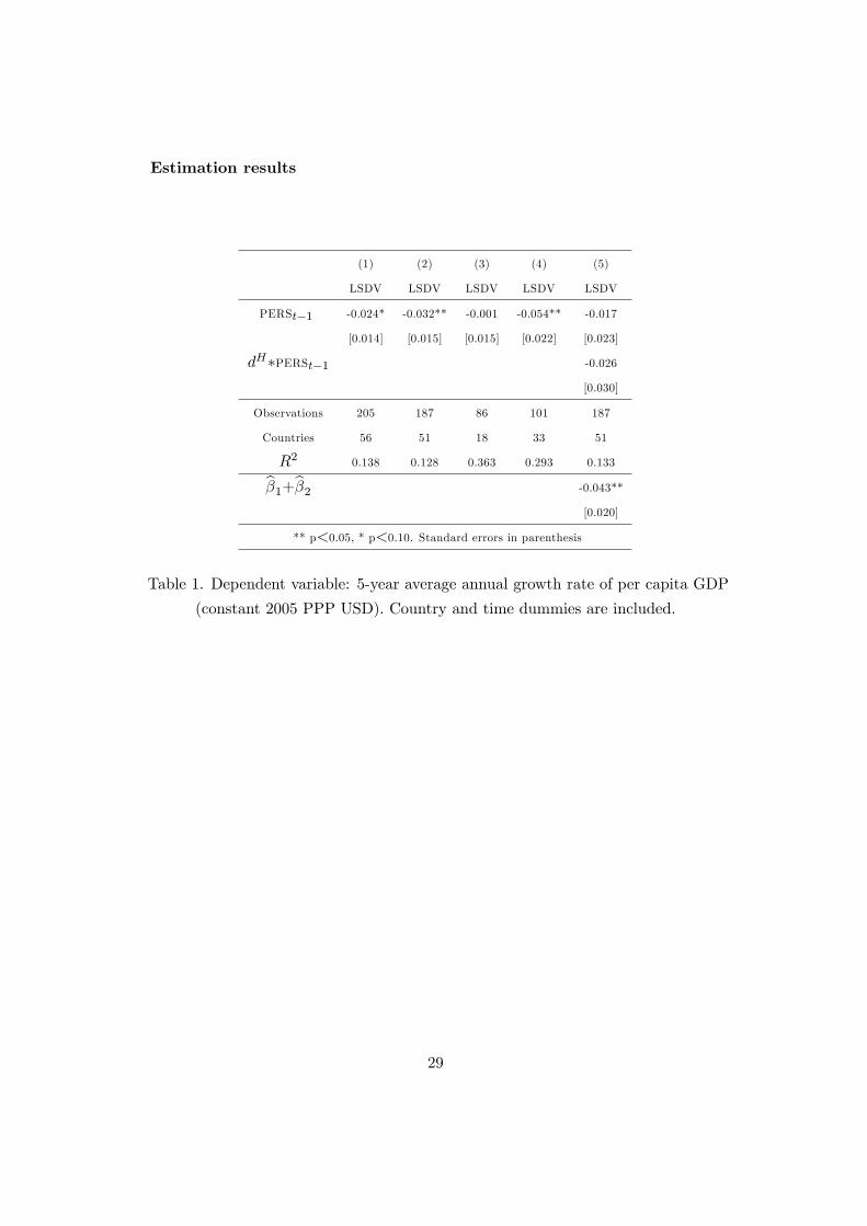
Column (2) in Table 1 replicates the baseline regression of column (1) considering the

51 countries for which data on BQ are available since 1984. The coe¢ cient for lagged

PERS is again negative and signi�cant at 5% level. In columns (3) and (4) we split the

sample into low and high red-tape cost countries, respectively5. Consistently with our

view, the negative correlation is present only in the group of countries with high red-tape

costs, while it disappears in the other group. Conditional distributions and �tting lines of

PERS and GROWTH for low and high cost countries are reported in panel (a) and (b)

of Figure 1, respectively.

Column (5) reports estimation results for the equation:

GROWTHit = �1PERSit�1 + �2�dHi � PERSit�1

�+ �i + �t + "it (2)

where dHi � PERSit�1 is the interaction between the dummy variable for high red-tapecosts and lagged persistence. The null hypothesis �1 = 0 and (�1 + �2) < 0 cannot be

rejected at 5% con�dence level, again indicating that political persistence is negatively

correlated with growth in high cost countries but is uncorrelated with growth in low cost

countries. Note that the correlation between PERS and GROWTH is not only statistically

signi�cant, but also sizeable: in fact the point estimates for the high cost countries indicate

5Approximately 54% of the observations in our sample belong to the group of countries with high

red-tape costs using our threshold.

5

that a one standard deviation increase in political persistence is associated with roughly

0.5% decrease in the growth rate.

In order to verify the robustness of these results, we run again our estimates including

the initial (log of) GDP per capita as well as several standard controls in growth re-

gressions, such as investment/GDP and government expenditure/GDP (from Penn World

Tables 6.1), average schooling years in total population (from Barro and Lee), fertility rate

(from WDI) and a proxy for corruption (from ICRG)6. Estimation of equations (1) and

(2) including these controls yields similar estimated coe¢ cients for our variables of interest

(estimation results not shown).7 We also tried di¤erent thresholds to classify countries

into high and low cost, with threshold values ranging between 3.1 and 3.9. Estimation

results are qualitatively similar (not shown), as very few countries are a¤ected by these

changes.

As estimation results of equation (2) are particularly relevant for our purposes, we

proceed further to deal with possible sources of bias due to omitted variables and endo-

geneity.

We start by performing 2SLS instrumental variable estimation of equation (2). To this

end, in order to gain information, we rely on yearly observations in the period 1984-2004.

As PERS is very irregular when observed on a yearly basis (recall that we used 5-years

averages in the previous exercises), we de�ne a new measure of political persistence in

year t, which we call �smooth�persistence (SPERS ), using the moving average of PERS

calculated between t� 1 and t� 4. More precisely:

SPERSit =MXm=1

PERSi(t�m)

with M = 3. To minimize missing information, we include all yearly data for countries

that show an average degree of democracy over the sample period higher than 0.7, where

country i in year t receives value 1 if democratic or 0 if not democratic. As before, we

classify a country as having high (low) red-tape costs and set dHi = 1 (dHi = 0) if the

initial value of BQ (that is the value of BQ in 1984 or the �rst available observation) is

6This variable, named control of corruption, is an index ranging from 0 to 6 (where 0 corresponds to

low control of corruption) that measures mainly actual or potential corruption in the form of excessive

patronage, nepotism, job reservations, favor exchange, secret party funding, and suspiciously close ties

between politics and business.7 In order to alleviate estimation bias due to measurement error and reverse causation, all these controls

are taken at the beginning of each period, with the exception of EDU which is the average over the current

and previous 5-year periods.

6

below (above) 3:5. Our new sample includes 55 countries8.

Using additional data from DPI, we construct two variables that will be used as instru-

ments for SPERS. The �rst is a dummy variable, LAG_LEG, taking value one (zero) when

legislative elections took (did not take) place in the previous year. The second variable,

PAST_EL, counts the number of years since the last legislative or executive election.

As the empirical literature on political business cycles �nds no evidence of a system-

atic association between growth and election dates, we expect the timing of elections to

be uncorrelated with growth. Instead, we expect LAG_LEG to be positively related

and PAST_EL to be negatively related with SPERS. As most changes in veto players

take place in elections years, persistence should be high in the subsequent year. Instead,

the longer the time span between the last election and the year in which persistence is

measured, the more likely that some veto players have changed.

We start by estimating the reduced form equation:

GROWTHit = �1SPERSit + �2(dHi � SPERSit) + it+ �i + �t + "it (3)

where GROWTH is the yearly per capita GDP growth rate at constant 2005 PPP USD

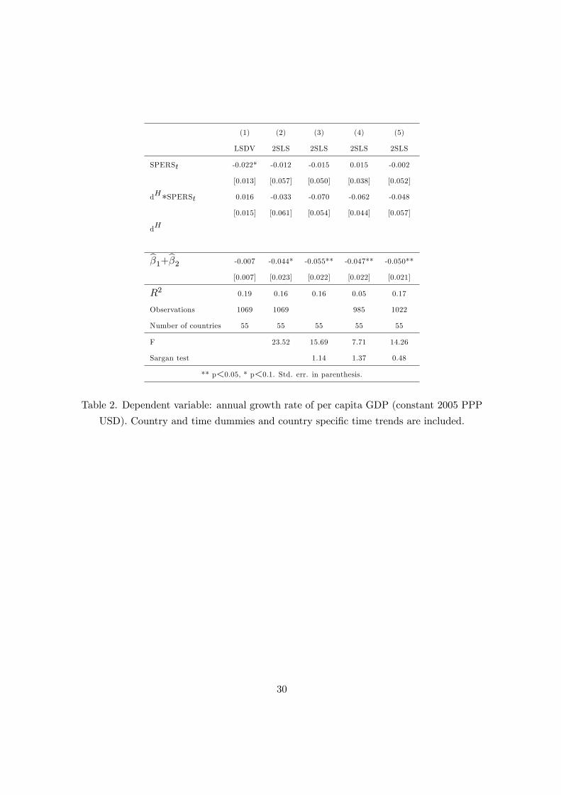
and it denotes country-speci�c trends. Column (1), Table 2, reports estimation results

by LSDV. Here, contrary to our previous �ndings, political persistence appears to be neg-

atively associated with growth only in countries with low red-tape costs, though the coef-

�cient is only marginally signi�cant. However, as shown in column (2), once LAG_LEG

and dHi �LAG_LEG are used as instruments for SPERS and dHi �SPERS, we recover theresult that political persistence is negatively associated with growth in countries with high

red-tape costs, while it is uncorrelated with growth in countries with low red-tape costs. In

fact, as in column (5), Table 1, the null hypothesis �1 = 0 and (�1+�2) < 0 cannot be re-

jected (at 10% con�dence level). In column (3) we add PAST_EL and dHi �PAST_EL inthe set of instruments: this improves signi�cance of the estimated coe¢ cient of (�1+ �2).

The F- test and Sargan test suggest that our instruments are relevant and there is no

overidenti�cation. In column (4) we use lagged (rather than smooth) persistence with the

same set of instruments as in column (3): results are very stable in terms of estimated

coe¢ cients and statistical signi�cance. However, the R2 is sensibly smaller and the power

of the instruments is not as evident as before. In column (4), dH is de�ned as the av-

erage level for each country: estimation results are unchanged. In order to estimate the

8This new sample is very similar to the one used to estimate equation (2). In particular 49 out of the

51 original countries are still present. New entries are Bahamas, Germany, Czech Republic, Papua New

Guinea, Slovakia and Slovenia. Instead, Poland and Senegal are no longer present.

7

coe¢ cient of red-tape costs, we also run regressions allowing dH to vary over time, setting

dHit = 1 (dHit = 0) when BQ < 3:5 (BQ > 3:5) in country i in year t: dHit is not signi�cant

in the second stage (estimation results not shown) and its estimated coe¢ cient is very

close to zero.

Finally, we take into account the possible source of bias related to the LSDV estimation

of growth regressions which include country �xed e¤ects. To tackle this issue, we rewrite

(3) as follows:

GDPit = �1GDPit�1 + �1SPERSit + �2(dHi � SPERSit) + it+ �i + �t + "it (4)

and estimate equation (4) using Arellano-Bond GMM estimator that is precisely designed

for dynamic panels of this sort. Among the excluded instruments we add LAG_LEG

and PAST_EL as in speci�cations (3) - (5) of Table 2. Column (1), Table 3, reports the

benchmark case in which we estimate (4) by means of 2SLS, where only SPERS (and

its interaction) are instrumented. As before, the hypothesis �1 = 0 and (�1 + �2) < 0

cannot be rejected (at 5% con�dence level). The autoregressive term is strongly signi�cant

and smaller than one. The �rst stage is reliable (F = 33:73) and overidenti�cation is

not an issue. Column (2) presents results for Arellano-Bond GMM estimations, where

the lagged di¤erences used as instruments are of second order. Since with yearly data

autocorrelation is usually large and the AR(2) test in column (2) rejects the hypothesis of

no serial correlation of second order, in column (3) we also add the (t�3) lag of di¤erencesamong instruments. Both columns show that, if any, the estimation bias induced by the

omission of the correlation between lagged GDP and the error term is small. Again, we

cannot reject the null hypotheses �1 = 0 and (�1 + �2) < 0 (at 5% and 1% con�dence

level, respectively). However, some concerns arise about the overidenti�cation of our

regressions.9

To summarize, our empirical analysis provides evidence that political persistence is

negatively associated with growth in high red-tape costs countries, while we �nd weaker

or no evidence of a relationship between persistence and growth in low costs countries.

This result, which is robust to several sources of estimation bias, provides motivation for

the theoretical analysis that we will develop in the following section.

9Adding lags up to the (t � 5) order does not qualitatively change results, although the number ofdegrees of freedom decreases when we add further lags.

8

2.2 Related literature

Besides contributions already cited in the Introduction, our paper is related to several

strands of literature. First, Acemoglu and Robinson [2] analyze ine¢ cient institutions by

developing a political economy model where political elites may block innovation for fear

of losing political power, as innovation reduces the cost of replacing the incumbent. Their

main result is a non-monotonic relationship between a measure of political competition

and the incentive to block innovation. Our model emphasizes the strategic interaction

between the politician (political elite), the �rm (economic elite, absent in AR model) and

voters, showing the conditions under which a �blocked�society with persistent networks

of politicians and entrepreneurs can be supported by a vast majority of forward-looking

voters. Moreover, we endogenously determine the level of ine¢ cient bureaucracy that

the politicians use to perpetuate their power and highlight the (static) costs versus the

(dynamic) gains of breaking up the status quo.

Second, in a Schumpeterian framework with innovation and technology adoption, Ace-

moglu, Aghion and Zilibotti [1] and Aghion, Alesina and Trebbi [4] incorporate a political-

economy model where �rms lobby the government to reduce economic competition (AAZ)

and entry threat (AAT). Our analysis di¤ers in many respects as we consider the �rm�s

choice between network and innovation, and focus on the strategic interaction between

politicians, �rms and voters in democracies where political accountability through voting

constrains the policy choices of the politician.

Third, recent empirical contributions investigate the relevance of political connections

on �rms�performance. From a cross-country perspective, Faccio [10] documents the wide-

spread existence of political connections and that these connections signi�cantly add to

company values. Faccio et al. [11] �nd that politically-connected �rms are signi�cantly

more likely to be bailed out than similar non-connected �rms. More importantly for our

contribution, in a recent paper Desai and Olofsgard [9] investigate the consequences of

political connections on about 10.0000 �rms surveyed in 40 developing countries and �nd

that in�uential �rms face fewer administrative and regulatory burdens and invest and

innovate less.

Finally, our empirical results are related to the existing literature on political insta-

bility and economic growth. Almost all contributions use data on revolutions, coups and

assassinations to construct a measure of political instability (see, for instance Alesina et

al. [6] and the survey of the literature in Carmignani [8]). Not surprisingly, these studies

�nd a positive e¤ect of stability on growth.10 On the contrary, our �ndings suggest that,10An exception is the paper by Feng [12], who distinguishes between irregular and regular government

9

when government change occurs through democratic institutions, political turnover (i.e.

instability) rather than political persistence (i.e. stability) is positively associated with

growth in countries where red-tape costs are high, while no robust correlation emerges

when red-tape costs are low.

3 The model

3.1 The environment

Consider a two-sector economy populated by a continuous mass of in�nitely-lived agents.

Time is discrete with t = 0; 1; :::;1: Utility is linear in consumption and future consump-tion is discounted at the subjective discount factor � = 1=(1 + r) where r is the interest

rate. This implies that, in each period, consumption is equal to income.

The intermediate good is produced using the �nal good by means of a one-to-one linear

technology. At time 0 there exists an incumbent �rm which produces as a monopolist in

the intermediate sector.

In each period t output in the �nal good sector is given by:

Yt = ex�t Lt1�� (5)

where Lt is labor, ext =PQtq=0

qxq is a quality-adjusted intermediate input, with q denoting

quality rung of intermediate good xq that has quality q: Qt denotes the highest quality

level in use at time t. We will take the �nal good as numeraire and normalize its price

to one. We assume no population growth and normalize L = 1. The �nal good sector is

perfectly competitive.

To keep the economic side of the model simple and focus on the relationship between

innovation, growth and political persistence, we abstract from endogenous innovation de-

termined by R&D and from the potential catching up associated to distance to frontier.

Speci�cally, we assume that in each period exogenous technological progress makes a

higher quality version of the intermediate good available. Technological upgrade is limited

to the next higher quality good (step-by-step innovation). Thus, if technology Q is the

highest quality adopted in the previous period, only technology Q+ 1 can be adopted in

changes and �nds that stability enhances growth in the case of irregular changes, but is negatively associated

with growth in the case of regular changes. Our empirical analysis, using a completely di¤erent dataset and

exploiting the time dimension, shows that the negative relation between political persistence (stability)

and growth is robust solely in countries that we classify as having high red-tape costs.

10

the current period, although other superior technologies may be available. For reasons

that will become clear later, technology adoption will be related to political outcomes.

At the beginning of period t; there is an incumbent monopolist who owns technology

Qt�1 and an incumbent politician who was appointed at t� 1. The incumbent politiciansets the level of red-tape costs �t � 1 that are related to norms and regulations to carryout production in the intermediate good sector. Bureaucracy and excessive regulation

impose external costs on �rms as information on bureaucratic requirements are costly to

acquire and bureaucratic processes are time consuming. In our model, these costs will

proportionally a¤ect marginal costs of production. Speci�cally, given our technology in

the intermediate good sector, marginal cost of production is constant and equal to one.

Due to bureaucratic requirements, e¤ective production costs become equal to �t. Note

that we are assuming that, in order to a¤ect production in period t; the level of red-tape

costs must be chosen at the beginning of the period. This assumption is meant to capture

the idea that reforms of bureaucracy take time to be designed and implemented.

The incumbent monopolist and politician are potentially connected. We have in mind

a system of personal relationships between the operating �rm and the politician in o¢ ce

whereby the politician serves as facilitator by providing information on how to approach

the bureaucracy or directly intervening in bureaucratic processes. By knowing the right

person in the right place (�a rolodex e¤ect�), the �rm can more easily deal with bureau-

cratic requirements and acquires a competitive advantage over the outsiders.

We model the bene�t of being politically connected by assuming that connected �rms

can enjoy lower marginal costs of production relative to unconnected �rms. Speci�cally,

the marginal cost of production can be reduced to the minimum level equal to 1 for the

connected �rm, if it exploits the network (thus acquiring a cost advantage �t � 1 overunconnected �rms). Notice that, if the politician sets �t = 1; there is nothing to gain from

a network with the politician.

In period t; in order to exploit the network advantage, two conditions must be satis�ed.

First, the incumbent politician must win period-t election and be re-elected. Second, the

incumbent �rm must devote resources (in particular, spend time) to maintain its network.

In this case, the incumbent will face competition from an unconnected �rm with superior

technology, but it might still be able to keep its monopoly by exploiting the network

advantage. The alternative option for the incumbent �rm is to spend time to adopt the

new technology. In this case, the existing network is lost and the �rm survives in the market

(that is, it becomes the sole owner of the leading-edge technology) with probability �. If

the incumbent monopolist is unsuccessful, a new unconnected leader enters the market

11

with probability one.

In other words, the incumbent �rm faces a trade-o¤ between �learning-by-knowing�

and innovation. In the former case, the �rm exploits the repeated interaction and rela-

tionship with the politician to produce with the current technology at lower costs; in the

latter case, the investment in innovation might lead the �rm to adopt the leading-edge

technology and reach the technological frontier. Notice that the �learning-by-knowing�

option is available only to the incumbent �rm and can be e¤ective only if the incumbent

politician is con�rmed in o¢ ce. This captures the idea that it takes time to build rela-

tionships and makes the incumbent politician intrinsically di¤erent from the opponent in

the eyes of economic agents.11

According to a standard assumption in the literature on Schumpeterian models of

growth (see Grossman and Helpman [15]), in the intermediate good sector owners of

di¤erent vintages compete à la Bertrand. Since intermediate inputs are perfect substitutes

in the production of the �nal good, if all producers faced the same marginal costs of

production �t, the technological leader would become monopolist by setting a limit price

pt = �t. In this case, output would be given by:

Yt = �(Qt�1+1)

1��

"��

�t

� �1��

� �t��

�t

� 11��#

(6)

and the monopolist would earn pro�ts equal to:

�t = �1

1�� �(Qt�1+1)

1�� ( �t)1

��1 ( �t � �t) (7)

In our model, however, the incumbent producer, if politically connected, can prevent

entry of more advanced but unconnected competitors by setting a limit price equal to

pt = �t= where �t > 1 is the marginal cost of production of the competitor (recall that in

this case the marginal cost for the incumbent is equal to 1).12 Notice that the incumbent

11Our description of the speci�c role of the incumbent politician in aiding �rms to deal with bureaucracy

is reminiscent of political-science contributions on excessive bureaucracy in representative democracies. For

instance, Fiorina and Noll [13] argue that �As the public bureaucracy grows larger, the importance of the

performance of facilitation will grow, and a legislator who is a good facilitator will be increasingly likely

to be reelected. ...Because part of facilitation is the possession and use of information which is acquired

through experience, and because seniority enhances the in�uence of a legislator in determining the fate of

an agency, incumbents can be more e¤ective facilitators than their challengers�(p. 257).12Limit pricing requires that �� < < 1=�. The �rst inequality ensures that the connected �rm cannot

keep the leading-edge competitor out of the market by setting the monopoly price 1=�: Similarly, the second

inequality ensures that the technological leader cannot keep competitors out of the market by setting the

monopoly price �=�:

12

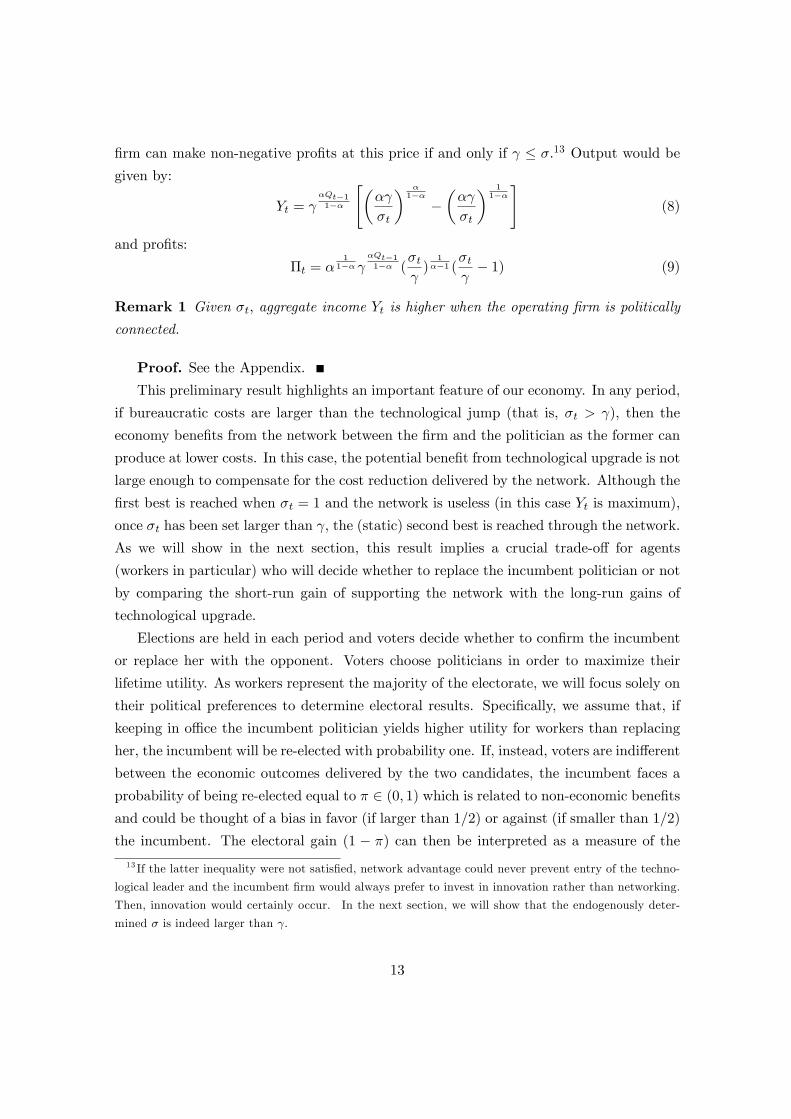
�rm can make non-negative pro�ts at this price if and only if � �:13 Output would be

given by:

Yt = �Qt�11��

"��

�t

� �1��

���

�t

� 11��#

(8)

and pro�ts:

�t = �1

1�� �Qt�11�� (

�t )

1��1 (

�t � 1) (9)

Remark 1 Given �t; aggregate income Yt is higher when the operating �rm is politically

connected.

Proof. See the Appendix.

This preliminary result highlights an important feature of our economy. In any period,

if bureaucratic costs are larger than the technological jump (that is, �t > ), then the

economy bene�ts from the network between the �rm and the politician as the former can

produce at lower costs. In this case, the potential bene�t from technological upgrade is not

large enough to compensate for the cost reduction delivered by the network. Although the

�rst best is reached when �t = 1 and the network is useless (in this case Yt is maximum),

once �t has been set larger than , the (static) second best is reached through the network.

As we will show in the next section, this result implies a crucial trade-o¤ for agents

(workers in particular) who will decide whether to replace the incumbent politician or not

by comparing the short-run gain of supporting the network with the long-run gains of

technological upgrade.

Elections are held in each period and voters decide whether to con�rm the incumbent

or replace her with the opponent. Voters choose politicians in order to maximize their

lifetime utility. As workers represent the majority of the electorate, we will focus solely on

their political preferences to determine electoral results. Speci�cally, we assume that, if

keeping in o¢ ce the incumbent politician yields higher utility for workers than replacing

her, the incumbent will be re-elected with probability one. If, instead, voters are indi¤erent

between the economic outcomes delivered by the two candidates, the incumbent faces a

probability of being re-elected equal to � 2 (0; 1) which is related to non-economic bene�tsand could be thought of a bias in favor (if larger than 1/2) or against (if smaller than 1/2)

the incumbent. The electoral gain (1 � �) can then be interpreted as a measure of the

13 If the latter inequality were not satis�ed, network advantage could never prevent entry of the techno-

logical leader and the incumbent �rm would always prefer to invest in innovation rather than networking.

Then, innovation would certainly occur. In the next section, we will show that the endogenously deter-

mined � is indeed larger than :

13

responsiveness of voters to economic policies. When (1 � �) gets higher, voters become

more responsive and the incumbent can capture more additional votes with an economic

platform that provides higher utility for workers than the opponent�s platform.14

Taking into account the last two paragraphs, let us consider a one-period version of

our model. It should be clear that, in this case, if � < and the network is useless, the

two candidates deliver exactly the same economic bene�ts to workers, aggregate income

is maximized and the probability of re-election for the incumbent is equal to �. If instead

� > , the incumbent politician guarantees higher economic bene�ts than the opponent

and is re-elected with probability one, although aggregate income would be lower than in

the previous case. The illustration of this static case will be useful to better understand

the results of the following section.

3.2 The game

Each period t starts with technology Qt�1 inherited from period t� 1. The timing of theevents is the following. (1) At the beginning of period t, the incumbent politician sets

red tape costs �t 2 � = [1;1). (2) The incumbent �rm decides whether to invest in

networking or innovation by choosing zt 2 Z = fN; Ig. (3) Elections are held and voters(workers) decide whether to con�rm the incumbent in o¢ ce or replace her by choosing

vt 2 V = fM;Rg where M denotes voting for the incumbent and R replacing her. (4)

Production and consumption take place.

The history of the game in period t is a vector

ht � (t; Q�1; ::; Qt�1; �1::; �t�1; z1::; zt�1; v1::; vt�1)

The set of all possible history is denoted by Ht. The future in period t is the sequence

of future actions and states (t+ 1; ::::; Qt; ::::; �t+1; ::::; zt+1; ::::::; vt+1; :::::). We denote by

14We are assuming a simple voting model, where probability of politician i to be elected is equal to:

�it = 1 if uwit > uwjt

�it = � if uwit = uwjt

�it = 0 if uwit < uwjt

where j is the opponent politician, uw is the utility of workers (voters) and �jt = 1��it: The model couldbe easily generalized to �it = 1 > �0 > � if uwit > u

wjt: The simplifying assumption here is that �it is a step

function which will reduce the optimal choice of the politician to two possible levels of �: In the Appendix

we show how our voting model can be obtained using a probabilistic voting model à la Persson-Tabellini

([18], ch. 3).

14

H(ht; �t; zt; vt) the set of all possible histories ht+1 generated by ht; �t; zt; and vt: Finally,

h0 � (0; Q�1) and time 0 begins with an incumbent politician and an incumbent �rm.A strategy for the politician is a sequence of actions � : Ht ! � which depends on

history at time t. A strategy for the �rm is a sequence of actions z : Ht x � ! Z which

depends on history and the action of the politician. Finally, a strategy for voters is a

sequence of actions v : Ht x � x Z ! V which depends on history, the action of the

politician and the choice of the �rm.

With history ht, the expected pay-o¤ for the politician of an action �t is given by:

up(ht; �t; zt; vt) = Et

1Xs=0

�sRt+s (10)

where Et is the expectations operator conditional on information available at time t and

Rt+s is a variable which takes value Yt+s = �(Qt+s)

1��

���pt+s

� �1�� � ct+s

��pt+s

� 11���when

the incumbent is elected (where ct+s is the marginal cost of production for the active �rm)

and 0 otherwise. In other words, we assume that the politician is benevolent and cares

about aggregate welfare provided that she remains in o¢ ce.15 To simplify the analysis,

we will assume that when is not re-elected, the politician no longer runs for o¢ ce.

The expected pay-o¤ for the �rm of an action zt is given by:

uf (ht; �t; zt; vt) = Et

1Xs=0

�s�t+s (11)

where �t+s = �1

1�� �(Qt+s)

1�� p1

��1t+s (pt+s� ct+s) if the incumbent monopolist is still active at

time t + s and 0 otherwise. Finally, the expected pay-o¤ for the voter of an action vt is

given by:

uw(ht; �t; zt; vt) = Et

1Xs=0

�swt+s (12)

where wt+s = (1� �)��

1�� �(Qt+s)

1�� p�

��1t+s denotes the wage rate at time t+ s:

16

4 The politico-economic equilibrium

We will now characterize the equilibrium of our in�nitely repeated game. We limit the

analysis to stationary Markov perfect equilibria (SMPE). Given the structure of our15 In general, we need politicians�preferences to be de�ned over Yt and �t. In our simple speci�cation,

politician�s istantaneous utility is linear in income.16Notice that, from an economic point of view, the only feature that distinguishes the two politicians in

the eyes of the voters is the potential connection with the operating �rm. If this connection is absent, the

two politicians would necessarily deliver the same economic outcome.

15

in�nite-horizon model, time is not part of the payo¤ relevant state so that it seems nat-

ural to focus on stationary strategies that do not depend on calendar time (see Maskin

and Tirole [17]). Moreover, given the economics of the model, the state of technology at

the end of the previous period Qt�1 is the appropriate state variable since current pay-

o¤s (and therefore current actions) depend crucially on the inherited level of technology.

Accordingly:

De�nition 1 (Stationary Markov Perfect Equilibrium) The Markov strategies

��(Qt�1); z�(Qt�1; �t(�)); v�(Qt�1; �t(�); zt(�))

form a Stationary Markov Perfect Equilibrium (SMPE) if and only if:

(i) for all Qt�1 and all �t(�) and zt(�), v�(Qt�1; �t(�); zt(�)) is a solution to:

argmaxvt2fM;Rg

uw(Qt�1; vt)

(ii) for all Qt�1 and �t(�):

uf (Qt�1; z�t ; v

�t ) > uf (Qt�1; bzt; bvt)

for any bzt 6= z�t ; where v� and bv are best response actions to z� and bz respectively.

(iii) for all Qt�1:

up(Qt�1; ��t ; z

�t ; v

�t ) > up(Qt�1; �t; zt; vt)

for any �t 6= ��t , where z�; v� and z; v are best response actions to �� and � respectively:

We are now ready to characterize the SPME of our dynamic game. Before stating our

main proposition, let us de�ne a threshold level of the technological jump:

1 ��1� ��

� 1���

which will be crucial for our next result. Then, we can write the following:

Proposition 1 (Equilibrium) The SMPE exists, is unique and entails constant actions.

Speci�cally, there exists � > 1 independent of Q such that:

(i) if < min[ 1; �] the only SMPE is (�0; N), where:

�0 =

1� �(1��)( �1)

11�� (1���

�1�� )

>

and the incumbent politician is re-elected with probability one.

(ii) if > min[ 1; �], the only SMPE is (1; I) and the incumbent politician is re-elected

with probability �:

16

Proof. See the Appendix.

As this Proposition shows, the economy can follow two equilibrium trajectories. In the

�rst one, red-tape costs are high, the incumbent politician is always in power, and tech-

nology is never upgraded as the incumbent �rm exploits the network with the politician.

In the second one, red-tape costs are lowest, the incumbent is re-elected with a probability

smaller than one, and technology is upgraded in every period.

In the �rst equilibrium (henceforth called �bad�), the politician deliberately chooses

to maintain a high level of bureaucratic costs to maximize the probability of being re-

elected, thus creating an incumbency advantage, at the cost of economic stagnation. When

the politician sets �0 > , the incumbent monopolist �nds it pro�table to exploit the

network thereby preventing entry of technologically advanced competitors. In turn, voters

(workers) con�rm the incumbent politician and bene�t from lower prices generated by the

cost reduction enjoyed by the connected �rm. In the second equilibrium (henceforth called

�good�), the politician does not introduce bureaucratic distortions (� = 1) as she �nds it

worthwhile to maximize growth despite the lower chances of being re-elected. As already

discussed, the good equilibrium represents the �rst best of our economy, where aggregate

income is maximized: the deviation from the �rst best is ultimately due to the re-election

strategy of the politician.

Several comments are in order here. First, the Proposition highlights the crucial role

of two threshold levels, 1 and �. The former is related to the indi¤erence condition

of voters between choosing the incumbent and supporting the status quo or electing the

opponent and breaking the network. Note that, for the bad equilibrium to be sustained,

the subjective discount factor of voters must be su¢ ciently low so that the short-run

bene�t of the network outweighs the long-run cost of stagnation. In other words, voters

cannot be excessively forward-looking.17 The latter threshold � is instead related to

the indi¤erence condition of the incumbent politician between setting �0 and maximize

probability of re-election or implementing the �rst best and the high-growth path.

Whenever is lower than both thresholds, voters and politician are better o¤ in the

bad equilibrium which is, in this case, the only SMPE of the game. However, as soon as

is larger than either of the two thresholds, the good equilibrium emerges. Speci�cally, if

� < < 1, the good equilibrium emerges as the politician does not �nd it worthwhile to

set high red-tape costs although the voters would support them. If 1 < < � the good

17Note that < 1 can be written as � � 1=(1 + �

1�� ) where �

1�� is the rate of growth of wages in

the �good� equilibrium. A necessary condition for the latter to hold is that � �

1�� < 1; which ensures

that the discounted utility of workers in the good equilibrium is bounded.

17

equilibrium emerges as the voters would vote against an incumbent who set high costs.

Second, our model allows us to fully characterize the level of distortion �0 that emerges

in the �bad�equilibrium as a function of the structural parameters of the economy. This

turns out to be the minimum level necessary to induce the incumbent �rm to invest in the

network so that re-election is achieved at the minimum cost in terms of welfare. Third,

as we discussed in the Introduction, it is worthwhile to emphasize again that our �bad�

equilibrium is voluntarily supported by voters: once the politician has opted for a high

level of red-tape costs, and the �rm has not invested in innovation, it is optimal for voters

to con�rm thr incumbent. In this case, the status quo is unanimously preferred by all

agents and therefore particularly hard to break up.

To conclude this section, let us discuss how the equilibrium outcome depends on the

main parameters of our model, and in particular on parameters related to economic com-

petition and electoral results. By simple inspection of �0 it is easy to verify that higher

� (that is, lower economic competition) implies higher �0: The intuition is pretty simple.

The higher is the expected return from innovation for the incumbent �rm (which depends

positively on �), the higher is the network advantage �0 � 1 that the �rm must enjoy to

be induced to invest in networking rather than innovation. We can also prove (see the

Appendix) that higher � implies lower � so that the good equilibrium becomes more

likely to emerge.18 As the politician takes into account the higher welfare loss that has to

be imposed on the society to induce the �rm to invest in networking, she will be willing to

set higher red-tape costs and prevent innovation only if the increase in aggregate income

associated to technological upgrade is lower. Turning to elections, if responsiveness of vot-

ers to economic policies decreases (that is, � increases) the electoral gain of the network

for the incumbent politician decreases and she will be more willing to lower bureaucratic

costs and reform the ine¢ cient state. Again, � decreases and the good equilibrium is

more likely to occur.

To summarize, we can write the following:

Proposition 2 (Comparative statics) The good equilibrium is more (less) likely to

emerge the higher (lower) is � and the higher (lower) is �.

Proof. See the Appendix.

Further elaborating on the previous results, we can prove (see the Appendix) that

there always exists b� 2 (0; 1) such that � = 1. This result has interesting implications

18Clearly, as � increases, the set of such that > � enlarges when � < 1. In the opposite case,

changes in � have no e¤ect on the set of for which either equilibrium can occur.

18

in terms of political economy. Consider Figure 2a. When 2 ( �A; 1), although voterswould support the second-best equilibrium and vote for the incumbent politician, the latter

is benevolent enough to internalize the cost of ine¢ cient bureaucracy and to implement the

�rst-best. This occurs as the share of additional voters that could be captured through the

network is low and it is not worthwhile for the politician to distort the economy. Consider

now Figure 2b. Here, when 2 ( �A; 1), the incumbent politician sets high bureaucraticcosts to ensure re-election and is supported by voters. Thus, the set of for which the

second-best equilibrium arises is larger. Interestingly, for 2 ( 1; �B), the �rst best isachieved through elections: although the politician would be better o¤ by setting �0, in

this case voters would overthrow the incumbent and elect the opponent to bene�t from

technological innovation. Notice that this outcome could not occur in political economy

models (such as Acemoglu, Aghion and Zilibotti [1] and Aghion, Alesina and Trebbi [4])

where the politician responds only to �rms� interests and is not constrained by voters�

actions.

5 Conclusions

Excessive regulatory and administrative burdens due to cumbersome regulatory and ad-

ministrative requirements and/or ine¢ cient bureaucracy are often pointed out as a major

hindrance to growth as they subtract resources to investment and innovation and might

represent a barrier to entry for new �rms and superior technologies.

In this paper, we consider red-tape as a production cost for �rms that can be mitigated

through political connections in a relationship-based system (�knowing the right person

in the right place�). As establishing connections requires time but no extra resources,

connected �rms face lower marginal costs than potential competitors. Thus, incumbent

�rms may be able to prevent entry of competitors with superior technology if they can

exploit their political connections, that is, if politicians do not change too frequently. For

the society as a whole, this creates a trade-o¤ between the short-run bene�ts of enjoying

low production prices by keeping the status quo and the long-run costs of retarding and

preventing technological upgrade.

Our model shows that the interaction between politicians, �rms and voters gener-

ates political equilibria that involve either perpetual innovation and replacement of the

incumbent politician or stagnation and political persistence. By keeping an ine¢ cient

bureaucracy, the incumbent politician can induce the incumbent �rm to spend time in

establishing connections with the politician (which help to deal with bureaucracy, a sort

19

of �learning-by-knowing�) rather than innovating. As a result, voters may support the

incumbent politician and the status quo to enjoy the lower production prices delivered by

the connected �rm. In this stagnation trap, a unanimous socioeconomic block emerges,

which prevents the adoption of new technologies and leads to economic backwardness.

Ceteris paribus, when facing similar technological opportunities (same ), countries

are more likely to end up in the stagnation trap the more responsive to economic policies

are voters (lower �) and the lower is the probability of success for the incumbent �rm

when it invests in innovation (lower �). However, the welfare loss associated to stagnation

is lower (lower �0) for lower �.

The results of our model are consistent with a negative association between political

persistence and economic growth in presence of high red-tape costs that we documented

in the �rst part of the paper. In the bad equilibrium, a change in the politician in o¢ ce

breaks the network between politicians and �rms and ensures that an outside �rm endowed

with the leading-edge technology enters the market. In this case, there is technological

upgrade and high growth. In the good equilibrium, technological upgrade occurs regardless

of electoral results: even if the incumbent wins the elections, an e¢ cient bureaucracy

guarantees that the quality leader enters the market.

Our theoretical analysis could be extended in di¤erent ways. First, we could extend

the analysis of voters� behavior, in order to provide a fully-�edged probabilistic voting

model (along the lines of Persson and Tabellini [18], ch. 3) which could allow us to enlarge

the set of structural parameters of our model and to incorporate additional political-

economy issues. Second, an overlapping-generations version of our model could highlight

interesting political and economic con�icts between short-sighted and long-sighted agents,

which would give rise to intergenerational con�icts between the young (more inclined to

political turnover and economic change) and the old (supporting the status quo). We

could then use the model to shed light on important policy aspects, such as the issue of

gerontocracy, low socioeconomic mobility and economic backwardness.

20

APPENDIX

A1. A probabilistic voting model (see Persson and Tabellini [18], ch. 3).

Suppose that individual worker i has the following preferences:

eui(P; �) = ui(P; �) + �i(P ) (13)

when politician P 2 fI;Og is elected and the policy � is implemented (by the incumbentpolitician at the beginning of the period).

The term �i(P ) captures the non-economic related bene�ts that individual i enjoys

if politician P is elected (for instance, related to ideology). Let us normalize �i(I) = 0

so that �i > 0 implies that individual i has a bias in favor of politician O while �i = 0

denotes an ideologically neutral voter. Moreover, let us assume that the parameter � is

distributed uniformly on the interval [a; b] with a < 0 and b > 0.

Individual i prefers politician I if

ui(�I) > ui(�O) + �i + � (14)

where � measures the average relative popularity of O in the population. Assume that �

has a uniform distribution on �� 1

2 ;1

2

�: (15)

It can be easily veri�ed that the total vote share for the incumbent is given by:

v =1

2+2e� � (a+ b)

b� a (16)

where e� = ui(�I)� ui(�O)� �: The probability that the incumbent is elected is thereforegiven by:

� = Pr�[v � 1

2] =

1

2+

�ui(�I)� ui(�O)�

a+ b

2

�(17)

Note whenever ui(�I) = ui(�O) (as for instance in the good equilibrium where � = 1), the

probability that the incumbent is re-elected is

� =1

2� (a+ b)

2(18)

which is larger (smaller) than 1/2 if a+b is smaller (larger) than 0. If instead the incumbent

sets � > 1, we have

ui(�I)� ui(�O) = (1� �)��

1�� �(Q+1)1�� �

���1

"�

�1�� � 11� � �

���1

#(19)

21

which is positive whenever < 1. Clearly, in this case, � is decreasing with �. Thus, the

incumbent will choose between �0 and 1 by computing the probability of being elected

when � = �0 in equation (19). For the sake of simplicity, in our model we assume that

� = �0 implies � = 1, that is:

(1� �)��

1�� �(Q+1)1�� �

���10

"�

�1�� � 11� � �

���1

#� 1= + a+ b

2: (20)

A2. Proof of Remark 1

Equation (6) can be written as:

Yt = �Qt�11��

"��

�t

� �1��

� �t

��

�t

� 11��#

Comparing this expression with equation (8), it can be easily noted that the latter is larger

as �t > :

A3. Proof of Proposition 1.

The proof is divided into three parts. First, we show that there are only two possible

equilibria, characterized by constant actions of all players. Second, we show that the

equilibrium exists and is unique for given con�gurations of parameters. Third, we prove

that �0 > :

1) (i) Any equilibrium strategy pro�le must have zt = I when �t = 1: Given �t = 1,

best response for �rm is to play I. (ii) Any equilibrium strategy pro�le must have zt = N

when �t > 1: If the strategy pro�le of the �rm had zt = I when �t > 1; then the politician

would be better o¤ by deviating and playing 1 to which the �rm would respond by playing

I (see i). There is no incentive for the politician to keep high red tape costs when the �rm

is not investing in networking. When the incumbent �rm invests in innovation, voters

are indi¤erent between the two politicians, the probability of being re-elected is � and

cannot be a¤ected by an increase in �: (iii) Any equilibrium strategy pro�le must have

vt = M when zt = N: If the strategy pro�le of the voters had vt = R when zt = N , then

the �rm would be better of by deviating and playing I as the network would be broken

anyway. In this case, there is no reason for the �rm to invest in networking as there is no

network advantage. (iv) We are left with equilibrium strategies pro�les that yield either

(�t; N;M) or (1; I) and voters con�rm the incumbent with probability �, 8t. (v) Supposethat at time 0 the politician chooses �0 > 1. Then, we know that players�actions are

given by (�0; N;M) and Q does not change. By stationarity, from time 0 onwards players

will always play (�0; N;M). (vi) Suppose instead that at time 0 the politician chooses

22

�0 = 1. Then, players�actions are given by (1; I) and the incumbent wins elections with

probability �. In period 1; Q has changed and two possibilities arise. Either the politician

chooses �1 > 1 and actions are given by (�1; N;M) or she chooses �1 = 1 and actions are

given by (1; I). The �rst possibility cannot be an equilibrium action as it would imply:

�

Y H0 +

1Xt=1

�tY L1

!>

1Xt=0

�tY L0 (21)

�

Y H1 +

1Xt=1

�tY L2

!<

1Xt=0

�tY L1 (22)

where Y Lt denotes the low level of aggregate income in period t when � = �1 and Y Htdenotes the high level of aggregate income in period t when � = 1. The �rst inequality

follows from 1 being preferred to �1 in period 0. The second follows from �1 being preferred

to 1 in period 1. Since Y Lt+1 = �

1��Y Lt and Y Ht+1 = �

1��Y Ht , the two inequalities cannot

hold together. Thus, if equilibrium actions are (1; I) in period 0 it must also be the case

that equilibrium actions are (1; I) in period 1 and in all subsequent periods. In all periods

the incumbent will be re-elected with probability �.

2) Consider the following Markov strategy pro�le for the voters, the �rm and the

politician: v�(Q; �;N j � > 1) = M; z�(Q; � j � � �0) = N; z�(Q; � j � < �0) = I , and

��(Q) = �0. Moreover, recall that, whenever voters are indi¤erent between the economic

outcomes delivered by the two politicians (that is, whenever z = I and/or � = 1), we

assumed that they will vote for the incumbent with probability �. To prove that these are

Markov equilibrium strategies, we apply the one-stage deviation principle. (i) For voters

not to deviate when politician plays �0 and �rm plays N it must be true that:

wR(Q; �0; N) +1Xs=1

�t+swM (Q0; �0; N) �1Xs=0

�t+swM (Q; �0; N)

where Q0 = Q + 1, wR is the wage rate when the voters choose the opponent and a new

unconnected entrant with high production costs replaces the incumbent �rm, and wM is

the wage rate when the voters choose the incumbent and the connected �rm produces at

low production costs. The LHS represents voters�utility if they vote for the opponent in

period t and then vote for the incumbent for all subsequent period. The RHS represents

voters�utility if they vote for the incumbent in all periods. After some algebra the latter

inequality reduces to:

�

1�� � 1� �1� �

�1��

(23)

23

The left-hand side represents the ratio wM=wR: Given �0; this term measures the static

e¢ ciency gain from the network. The right-hand side represents the dynamic loss of the

network, related to the blocking of innovation that leads to stagnant wages and income. If

the latter inequality does not hold, workers would value the long-run gain of technological

upgrades more than the short-run bene�t of reducing production costs through the political

network. Inequality (23) can be easily rewritten as:

<

�1� ��

� 1���

� 1 (24)

(ii) Consider now the �rm. The �rm would not deviate by playing I when the politician

sets �0 if and only if:

�

"�I(Q; �0) +

1Xs=1

�t+s�N (Q0; �0)

#�

1Xs=0

�t+s�N (Q; �0) (25)

where �N is the pro�t when the �rm invests in networking and �I is the pro�t when the

�rm invests in innovation. The LHS represents �rm�s utility if it invests in innovation

in period t (and survives with probability �) and invests in networking in all subsequent

periods. The RHS represents �rm�s utility if it invests in networking in all periods. After

some algebra, the above inequality can be rewritten as:

� �

1� �(1��)( �1)

11�� (1���

�1�� )

� �0 (26)

To prove that �0 > it is su¢ cient to show that

�(1� �)( � 1)

11�� (1� ��

�1�� )

< 1 (27)

We will prove that this inequality holds for all � 1 (which is a necessary condition for

the bad equilibrium to exist). Recall that 1 � �� �

1�� > 0 by previous assumption (see

footnote 21), so that the above inequality can be written as:

� 1 + 1

1�� (1� �� �

1�� )

�(1� �) (28)

The second term on the RHS is strictly concave and positive for <�1��

� 1���. Moreover,

the second term reaches its maximum at =�

1��(1+�)

� 1���. Thus, there exists 1 < b

<�1��

� 1���such that b = 1 + b 1

1�� (1���b �1�� )

�(1��) and < 1 + 1

1�� (1��� �

1�� )�(1��) when < b .

24

Notice also that �0 ! 1 when ! b . Now consider = 1. It is easy to verify that

�(1 � �)( 1 � 1) < 1

1��1 (1 � ��

�1��1 ). Thus 1 < b which ensures that �0 > . Finally,

when the politician sets � = 1, the �rm certainly chooses I (the alternative N would imply

zero pro�ts). (iii) The politician will not deviate by setting � = 1 for any Q if and only if:

�

"Y H(Q; 1) +

1Xs=1

�t+sY L(Q0; �0)

#<

1Xs=0

�t+sY L(Q; �0) (29)

where Y H(Q; 1) is the high level of income when � = 1 and there is innovation (given by

eq. 6 with � = 1) and Y L(Q; �0) is the low level of income when � = �0 and innovation

is blocked (given by eq. 8 with � = �0). The latter inequality can be rewritten as:

Y L(Q; �0)

Y H(Q; 1)� �(1� �)1� ��

�1��

(30)

Notice that:

Y L(Q; �0) =

��

�0

� �1��

���

�0

� 11��

(31)

has a unique maximum for �0= = 1 (that is, for = 1) and, as it can be easily veri�ed,

�0= is monotonically increasing with . Also:

Y H(Q; 1) = ��

1�� � �1

1��

(32)

is monotonically increasing with : Thus, the LHS is strictly decreasing with and LHS

= 1 for = 1, LHS ! 0 when ! b : Moreover, the RHS is monotonically increasingwith , and 0 <RHS < 1 when = 1. Thus, there exists a unique � 2 (1; b ) such thatinequality (30) holds if and only if � �. Clearly, Y L(Q; �0)=Y H(Q; 1) does not depend

on Q so that � also cannot depend on Q: It remains to show that no other deviation can

be pro�table for the politician. Clearly, the politician would not set � > �0 as there would

be no electoral gain but only an e¢ ciency loss. Finally, any � 2 (1; �0) is dominated by� = 1 as the network would be broken in any case, the probability of re-election would be

� and the politician would be better o¤ by minimizing the distortionary costs.

A4. Proof of Proposition 2.

(i) Consider equation (26). It can be easily veri�ed that @�0=@� > 0: Then, for any

; Y L(Q; �0) decreases and the LHS of equation (30) shifts upward so that � decreases.

(ii) If � increases, the RHS of (30) decreases and � decreases.

A5. Proof of the existence of b�:25

Let � = 1. Then, the RHS of (23) and (30) are equal. Consider the LHS. We can show

that LHS of (30) < LHS of (23). This inequality can be written as:�� �

� �1�� �

�� �

� 11��

��

1�� � �1

1��

< �

1�� ,���

� �1�� �

���

� 11��

< ��

1�� � �1

1��

(33)

which holds since���

� �1�� �

���

� 11�� < �

�1�� � �

11�� . Thus, � < 1. Let now � = 0.

Then, from eq. (30) we get � !1. By @ �

@� < 0 and continuity, it yields that there existsb� 2 (0; 1) such that � = 1:

26

DATA APPENDIX

List of variables

BQ : bureaucratic quality index (0-4 scale).

CORR: control of corruption index (0-6 scale).

EDU : average schooling years in total population.

FERT : log of total fertility rate (births per woman).

GDP : log of gross domestic product per capita (constant 2005 PPP USD).

GOV : government expenditure as share of GDP.

GROWTH : average annual growth rate of gross domestic product per capita (constant

2005 PPP USD).

INV : investment as share of GDP.

PERS : 1- share of veto players that drop from the government in any given year.

Countries

Our basic sample includes 56 democratic countries for which data are available for

PERS and GROWTH in the 1975-2004 period. Countries are listed below, together with

the number of observations available in the 1980-2004 period (in parentheses). Information

for BQ is available for 51 countries since 1984.

Low red-tape costs countries: Australia (5), Austria (5), Belgium (5), Canada (5),

Denmark (5), Finland (5), France (5), Iceland (5), Ireland (5), Japan (4), Netherlands

(5), New Zealand (5), Norway (5), South Africa (2), Sweden (5), Switzerland (5), UK (5),

USA (5).

High red-tape costs countries: Argentina (3), Bolivia (2), Brazil (3), Chile (2), Colom-

bia (5), Costa Rica (5), Cyprus (2), Ecuador (4), El Salvador (3), Greece (4), Guatemala

(2), Honduras (3), India (3), Israel (5), Italy (4), Korea (3), Malaysia (2), Mexico (3),

Nicaragua (3), Panama (3), Paraguay (2), Peru (3), Poland (2), Portugal (4), Senegal (2),

Spain (4), Sri Lanka (3), Thailand (2), Trinidad and Tobago (2), Turkey (3), Uruguay (3),

Venezuela (4).

Remaining countries for which we have no information on BQ in 1984 are: Bahamas

(3), Germany (5), Luxembourg (5), Madagascar (2), Malta (5).

27

Descriptive Statistics

Tables A and B report descriptive statistics and pairwise correlations for the 5-year

periods dataset.

Full Sample Low Cost Countries High Cost Countries

Variable Obs. Mean Std.Dev. Obs. Mean Std.Dev. Obs. Mean Std.Dev.

PERS 187 0.84 0.12 86 0.85 0.12 101 0.83 0.12

GROWTH 187 1.88 2.00 86 1.84 1.45 101 1.91 2.37

GDP 187 9.43 0.87 86 10.10 0.28 101 8.87 0.81

EDU 187 7.54 2.47 86 9.44 1.37 101 5.92 2.01

GOV 185 15.34 8.01 86 11.91 6.10 99 18.32 8.31

INV 187 20.14 6.65 86 23.37 4.49 99 17.34 6.97

FERT 187 0.79 0.38 86 0.58 0.16 101 0.98 0.41

CORR 181 4.61 1.92 83 5.98 1.81 98 3.45 1.05

BQ 187 2.83 1.28 86 3.94 0.16 101 1.89 1.04

Table A: Descriptive statistics

PERS GROWTH GDP EDU GOV INV FERT CORR

GROWTH -0.06 1.00

GDP 0.10 -0.06 1.00

EDU 0.20** 0.07 0.80** 1.00

GOV -0.20** -0.11 -0.54** -0.41** 1.00

INV 0.04 -0.04 0.69** 0.58** -0.41** 1.00

FERT -0.06 -0.18* -0.82** -0.65** 0.52** -0.64** 1.00

CORR -0.01 -0.05 0.51** 0.50** -0.11 0.37** -0.43** 1.00

BQ 0.06 0.01 0.73** 0.63** -0.39** 0.54** -0.63** 0.59**

Table B. Pairwise correlations; * signi�cant at 5% level; ** signi�cant at 1% level

28

Estimation results

(1) (2) (3) (4) (5)

LSDV LSDV LSDV LSDV LSDV

PERSt�1 -0.024* -0.032** -0.001 -0.054** -0.017

[0.014] [0.015] [0.015] [0.022] [0.023]

dH�PERSt�1 -0.026

[0.030]

Observations 205 187 86 101 187

Countries 56 51 18 33 51

R2 0.138 0.128 0.363 0.293 0.133b�1+b�2 -0.043**

[0.020]

** p<0.05, * p<0.10. Standard errors in parenthesis

Table 1. Dependent variable: 5-year average annual growth rate of per capita GDP

(constant 2005 PPP USD). Country and time dummies are included.

29

(1) (2) (3) (4) (5)

LSDV 2SLS 2SLS 2SLS 2SLS

SPERSt -0.022* -0.012 -0.015 0.015 -0.002

[0.013] [0.057] [0.050] [0.038] [0.052]

dH�SPERSt 0.016 -0.033 -0.070 -0.062 -0.048

[0.015] [0.061] [0.054] [0.044] [0.057]

dH

b�1+b�2 -0.007 -0.044* -0.055** -0.047** -0.050**

[0.007] [0.023] [0.022] [0.022] [0.021]

R2 0.19 0.16 0.16 0.05 0.17

Observations 1069 1069 985 1022

Number of countries 55 55 55 55 55

F 23.52 15.69 7.71 14.26

Sargan test 1.14 1.37 0.48

** p<0.05, * p<0.1. Std. err. in parenthesis.

Table 2. Dependent variable: annual growth rate of per capita GDP (constant 2005 PPP

USD). Country and time dummies and country speci�c time trends are included.

30

(1) (2) (3)

2SLS Arellano Bond GMM (L2) Arellano Bond GMM (L3)

GDPt�1 0.8239*** 0.8121*** 0.6676***

[0.0196] [0.0457] [0.0294]

SPERSt 0.0131 -0.0209 0.0023

[0.0493] [0.0244] [0.0184]

dH�SPERSt -0.0604 -0.0183 -0.0432*

[0.0493] [0.0339] [0.0253]b�1+b�2 -0.0473** -0.0392** -0.0409***

[0.0217] [0.0171] [0.0119]

R2 0.96

Observations 1022 1022 1022

Number of countries 55 55 55

F 33.73

Sargan test 0.61 0.00 0.00

AR(2) test 0.00 0.00

*** p<0.01, ** p<0.05, * p<0.10. Standard errors in parenthesis

Table 3. Dependent variable: log of per capita GDP (constant 2005 PPP USD). Country

and time dummies and country speci�c time trends are included.

31

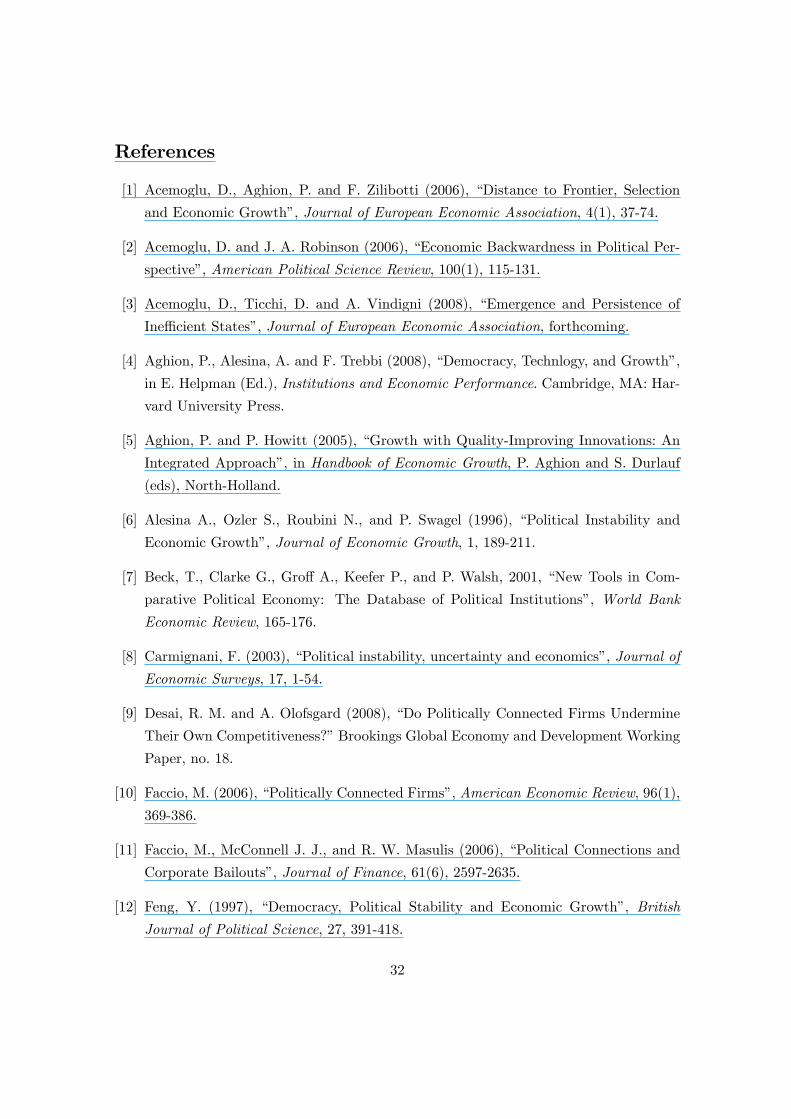
References

[1] Acemoglu, D., Aghion, P. and F. Zilibotti (2006), �Distance to Frontier, Selection

and Economic Growth�, Journal of European Economic Association, 4(1), 37-74.

[2] Acemoglu, D. and J. A. Robinson (2006), �Economic Backwardness in Political Per-

spective�, American Political Science Review, 100(1), 115-131.

[3] Acemoglu, D., Ticchi, D. and A. Vindigni (2008), �Emergence and Persistence of

Ine¢ cient States�, Journal of European Economic Association, forthcoming.

[4] Aghion, P., Alesina, A. and F. Trebbi (2008), �Democracy, Technlogy, and Growth�,

in E. Helpman (Ed.), Institutions and Economic Performance. Cambridge, MA: Har-

vard University Press.

[5] Aghion, P. and P. Howitt (2005), �Growth with Quality-Improving Innovations: An

Integrated Approach�, in Handbook of Economic Growth, P. Aghion and S. Durlauf

(eds), North-Holland.

[6] Alesina A., Ozler S., Roubini N., and P. Swagel (1996), �Political Instability and

Economic Growth�, Journal of Economic Growth, 1, 189-211.

[7] Beck, T., Clarke G., Gro¤ A., Keefer P., and P. Walsh, 2001, �New Tools in Com-

parative Political Economy: The Database of Political Institutions�, World Bank

Economic Review, 165-176.

[8] Carmignani, F. (2003), �Political instability, uncertainty and economics�, Journal of

Economic Surveys, 17, 1-54.

[9] Desai, R. M. and A. Olofsgard (2008), �Do Politically Connected Firms Undermine

Their Own Competitiveness?�Brookings Global Economy and Development Working

Paper, no. 18.

[10] Faccio, M. (2006), �Politically Connected Firms�, American Economic Review, 96(1),

369-386.

[11] Faccio, M., McConnell J. J., and R. W. Masulis (2006), �Political Connections and

Corporate Bailouts�, Journal of Finance, 61(6), 2597-2635.

[12] Feng, Y. (1997), �Democracy, Political Stability and Economic Growth�, British

Journal of Political Science, 27, 391-418.

32

[13] Fiorina, M. P. and R. G. Noll (1978), �Voters, Legislators and Bureaucracy: In-

stitutional Design in the Public Sector�, American Economic Review Papers and

Proceedings, 68(2), 256-260.

[14] Golden, A. M. (2003), �Electoral Connections: The E¤ects of the Personal Vote on

Political Patronage, Bureaucracy and Legislation in Postwar Italy�, British Journal

of Political Science, 33, 189-212.

[15] Grossman, G. and E. Helpman (1991), Innovation and Growth in the Global Economy,

MIT Press.

[16] Kaufmann D., Kraay A. and M. Mastruzzi (2008), �Governance Matters VII: Aggre-

gate and Individual Governance Indicators, 1996-2007�, World Bank Policy Research

Working Paper No. 4654

[17] Maskin, E. and J. Tirole (2001), �Markov Perfect Equilibrium I. Observable Actions�,

Journal of Economic Theory, 100, 191-219.

[18] Persson, T. and G. Tabellini (2000), �Political Economics: Explaining Economic

Policy�, Cambridge, MA: MIT Press.

[19] World Bank and International Finance Corporation, �Doing Business: Measuring

Business Regulations�, Washington D.C.

33

Figure 1. Conditional plots of PERS and GROWTH for low (panel (a)) and high costs

countries (panel (b)).

34

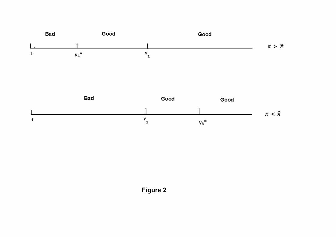
NOTE DI LAVORO DELLA FONDAZIONE ENI ENRICO MATTEI

Fondazione Eni Enrico Mattei Working Paper Series

Our Note di Lavoro are available on the Internet at the following addresses: http://www.feem.it/Feem/Pub/Publications/WPapers/default.htm

http://www.ssrn.com/link/feem.html http://www.repec.org

http://agecon.lib.umn.edu http://www.bepress.com/feem/

NOTE DI LAVORO PUBLISHED IN 2009 SD 1.2009 Michael Hoel: Bush Meets Hotelling: Effects of Improved Renewable Energy Technology on Greenhouse Gas

Emissions SD 2.2009 Abay Mulatu, Reyer Gerlagh, Dan Rigby and Ada Wossink: Environmental Regulation and Industry LocationSD 3.2009 Anna Alberini, Stefania Tonin and Margherita Turvani: Rates of Time Preferences for Saving Lives in the

Hazardous Waste Site Context SD 4.2009 Elena Ojea, Paulo A.L.D. Nunes and Maria Loureiro: Mapping of Forest Biodiversity Values: A Plural

Perspective SD 5.2009 Xavier Pautrel: Macroeconomic Implications of Demography for the Environment: A Life-Cycle Perspective IM 6.2009 Andrew Ellul, Marco Pagano and Fausto Panunzi: Inheritance Law and Investment in Family Firms IM 7.2009 Luigi Zingales: The Future of Securities Regulation SD 8.2009 Carlo Carraro, Emanuele Massetti and Lea Nicita: How Does Climate Policy Affect Technical Change? An

Analysis of the Direction and Pace of Technical Progress in a Climate-Economy Model SD 9.2009 William K. Jaeger: The Welfare Effects of Environmental Taxation SD 10.2009 Aude Pommeret and Fabien Prieur: Double Irreversibility and Environmental Policy Design SD 11.2009 Massimiliano Mazzanti and Anna Montini: Regional and Sector Environmental Efficiency Empirical Evidence

from Structural Shift-share Analysis of NAMEA data SD 12.2009 A. Chiabai, C. M. Travisi, H. Ding, A. Markandya and P.A.L.D Nunes: Economic Valuation of Forest

Ecosystem Services: Methodology and Monetary Estimates SD 13.2009 Andrea Bigano, Mariaester Cassinelli, Fabio Sferra, Lisa Guarrera, Sohbet Karbuz, Manfred Hafner, Anil

Markandya and Ståle Navrud: The External Cost of European Crude Oil Imports SD 14.2009 Valentina Bosetti, Carlo Carraro, Romain Duval, Alessandra Sgobbi and Massimo Tavoni: The Role of R&D

and Technology Diffusion in Climate Change Mitigation: New Perspectives Using the Witch Model IM 15.2009 Andrea Beltratti, Marianna Caccavaio and Bernardo Bortolotti: Stock Prices in a Speculative Market: The

Chinese Split-Share Reform GC 16.2009 Angelo Antoci, Fabio Sabatini and Mauro Sodini: The Fragility of Social Capital SD 17.2009 Alexander Golub, Sabine Fuss, Jana Szolgayova and Michael Obersteiner: Effects of Low-cost Offsets on

Energy Investment – New Perspectives on REDD – SD 18.2009 Enrica De Cian: Factor-Augmenting Technical Change: An Empirical Assessment SD 19.2009 Irene Valsecchi: Non-Uniqueness of Equilibria in One-Shot Games of Strategic Communication SD 20.2009 Dimitra Vouvaki and Anastasios Xeapapadeas: Total Factor Productivity Growth when Factors of Production

Generate Environmental Externalities SD 21.2009 Giulia Macagno, Maria Loureiro, Paulo A.L.D. Nunes and Richard Tol: Assessing the Impact of Biodiversity

on Tourism Flows: A model for Tourist Behaviour and its Policy Implications IM 22.2009 Bernardo Bortolotti, Veljko Fotak, William Megginson and William Miracky: Sovereign Wealth Fund

Investment Patterns and Performance IM 23.2009 Cesare Dosi and Michele Moretto: Auctioning Monopoly Franchises: Award Criteria and Service Launch

Requirements SD 24.2009 Andrea Bastianin: Modelling Asymmetric Dependence Using Copula Functions: An application to Value-at-

Risk in the Energy Sector IM 25.2009 Shai Bernstein, Josh Lerner and Antoinette Schoar: The Investment Strategies of Sovereign Wealth Funds SD 26.2009 Marc Germain, Henry Tulkens and Alphonse Magnus: Dynamic Core-Theoretic Cooperation in a Two-

Dimensional International Environmental Model IM 27.2009 Frank Partnoy: Overdependence on Credit Ratings Was a Primary Cause of the Crisis SD 28.2009 Frank H. Page Jr and Myrna H. Wooders (lxxxv): Endogenous Network Dynamics SD 29.2009 Caterina Calsamiglia, Guillaume Haeringer and Flip Klijnb (lxxxv): Constrained School Choice: An

Experimental Study SD 30.2009 Gilles Grandjean, Ana Mauleon and Vincent Vannetelbosch (lxxxv): Connections Among Farsighted Agents SD 31.2009 Antonio Nicoló and Carmelo Rodríguez Álvarez (lxxxv): Feasibility Constraints and Protective Behavior in

Efficient Kidney Exchange SD 32.2009 Rahmi İlkiliç (lxxxv): Cournot Competition on a Network of Markets and Firms SD 33.2009 Luca Dall'Asta, Paolo Pin and Abolfazl Ramezanpour (lxxxv): Optimal Equilibria of the Best Shot Game SD 34.2009 Edoardo Gallo (lxxxv): Small World Networks with Segregation Patterns and Brokers SD 35.2009 Benjamin Golub and Matthew O. Jackson (lxxxv): How Homophily Affects Learning and Diffusion in

Networks SD 36.2009 Markus Kinateder (lxxxv): Team Formation in a Network SD 37.2009 Constanza Fosco and Friederike Mengel (lxxxv): Cooperation through Imitation and Exclusion in Networks SD 38.2009 Berno Buechel and Tim Hellmann (lxxxv): Under-connected and Over-connected Networks

SD 39.2009 Alexey Kushnir (lxxxv): Matching Markets with Signals SD 40.2009 Alessandro Tavoni (lxxxv): Incorporating Fairness Motives into the Impulse Balance Equilibrium and Quantal

Response Equilibrium Concepts: An Application to 2x2 Games SD 41.2009 Steven J. Brams and D. Marc Kilgour (lxxxv): Kingmakers and Leaders in Coalition Formation SD 42.2009 Dotan Persitz (lxxxv): Power in the Heterogeneous Connections Model: The Emergence of Core-Periphery

Networks SD 43.2009 Fabio Eboli, Ramiro Parrado, Roberto Roson: Climate Change Feedback on Economic Growth: Explorations

with a Dynamic General Equilibrium Mode GC 44.2009 Fabio Sabatini: Does Social Capital Create Trust? Evidence from a Community of Entrepreneurs SD 45.2009 ZhongXiang Zhang: Is it Fair to Treat China as a Christmas Tree to Hang Everybody’s Complaints? Putting

its Own Energy Saving into Perspective SD 46.2009 Eftichios S. Sartzetakis, Anastasios Xepapadeas and Emmanuel Petrakis: The Role of Information Provision

as a Policy Instrument to Supplement Environmental Taxes: Empowering Consumers to Choose Optimally SD 47.2009 Jean-François Caulier, Ana Mauleon and Vincent Vannetelbosch: Contractually Stable Networks GC 48.2009 Massimiliano Mazzanti, Susanna Mancinelli, Giovanni Ponti and Nora Piva: Education, Reputation or

Network? Evidence from Italy on Migrant Workers Employability SD 49.2009 William Brock and Anastasios Xepapadeas: General Pattern Formation in Recursive Dynamical Systems

Models in Economics SD 50.2009 Giovanni Marin and Massimiliano Mazzanti: Emissions Trends and Labour Productivity Dynamics Sector

Analyses of De-coupling/Recoupling on a 1990-2005 Namea SD 51.2009 Yoshio Kamijo and Ryo Kawasaki (lxxxv): Dynamics, Stability, and Foresight in the Shapley-Scarf Housing

Market IM 52.2009 Laura Poddi and Sergio Vergalli: Does Corporate Social Responsibility Affect the Performance of Firms? SD 53.2009 Valentina Bosetti, Carlo Carraro and Massimo Tavoni: Climate Change Mitigation Strategies in Fast-

Growing Countries: The Benefits of Early Action GC 54.2009 Alireza Naghavi and Gianmarco I.P. Ottaviano: Firm Heterogeneity, Contract Enforcement, and the Industry

Dynamics of Offshoring IM 55.2009 Giacomo Calzolari and Carlo Scarpa: On Regulation and Competition: Pros and Cons of a Diversified

Monopolist SD 56.2009 Valentina Bosetti, Ruben Lubowski and Alexander Golub and Anil Markandya: Linking Reduced

Deforestation and a Global Carbon Market: Impacts on Costs, Financial Flows, and Technological Innovation

IM 57.2009 Emmanuel Farhi and Jean Tirole: Collective Moral Hazard, Maturity Mismatch and Systemic Bailouts SD 58.2009 Kelly C. de Bruin and Rob B. Dellink: How Harmful are Adaptation Restrictions SD 59.2009 Rob Dellink, Michel den Elzen, Harry Aiking, Emmy Bergsma, Frans Berkhout, Thijs Dekker, Joyeeta Gupta:

Sharing the Burden of Adaptation Financing: An Assessment of the Contributions of Countries SD 60.2009 Stefania Tonin, Anna Alberini and Margherita Turvani: The Value of Reducing Cancer Risks at Contaminated

Sites: Are More Heavily Exposed People Willing to Pay More? SD 61.2009 Clara Costa Duarte, Maria A. Cunha-e-Sá and Renato Rosa: The Role of Forests as Carbon Sinks: Land-Use

and Carbon Accounting GC 62.2009 Carlo Altomonte and Gabor Békés: Trade Complexity and Productivity GC 63.2009 Elena Bellini, Gianmarco I.P. Ottaviano, Dino Pinelli and Giovanni Prarolo: Cultural Diversity and Economic

Performance: Evidence from European Regions SD 64.2009 Valentina Bosetti, Carlo Carraro, Enrica De Cian, Romain Duval, Emanuele Massetti and Massimo Tavoni:

The Incentives to Participate in, and the Stability of, International Climate Coalitions: A Game-theoretic Analysis Using the Witch Model

IM 65.2009 John Temple Lang: Article 82 EC – The Problems and The Solution SD 66.2009 P. Dumas and S. Hallegatte: Think Again: Higher Elasticity of Substitution Increases Economic Resilience SD 67.2009 Ruslana Rachel Palatnik and Roberto Roson: Climate Change Assessment and Agriculture in General

Equilibrium Models: Alternative Modeling Strategies SD 68.2009 Paulo A.L.D. Nunes, Helen Ding and Anil Markandya: The Economic Valuation of Marine Ecosystems IM 69.2009 Andreas Madestam: Informal Finance: A Theory of Moneylenders SD 70.2009 Efthymia Kyriakopoulou and Anastasios Xepapadeas: Environmental Policy, Spatial Spillovers and the

Emergence of Economic Agglomerations SD 71.2009 A. Markandya, S. Arnold, M. Cassinelli and T. Taylor: Coastal Zone Management in the Mediterranean:

Legal and Economic Perspectives GC 72.2009 Gianmarco I.P. Ottaviano and Giovanni Prarolo: Cultural Identity and Knowledge Creation in Cosmopolitan

Cities SD 73.2009 Erik Ansink: Self-enforcing Agreements on Water allocation GC 74.2009 Mario A. Maggioni, Francesca Gambarotto and T. Erika Uberti: Mapping the Evolution of "Clusters": A

Meta-analysis SD 75.2009 Nektarios Aslanidis: Environmental Kuznets Curves for Carbon Emissions: A Critical Survey SD 76.2009 Joan Canton: Environmentalists' Behaviour and Environmental Policies SD 77.2009 Christoph M. Rheinberger: Paying for Safety: Preferences for Mortality Risk Reductions on Alpine Roads IM 78.2009 Chiara D’Alpaos, Michele Moretto, Paola Valbonesi and Sergio Vergalli: "It Is Never too late": Optimal

Penalty for Investment Delay in Public Procurement Contracts SD 79.2009 Henry Tulkens and Vincent van Steenberghe: “Mitigation, Adaptation, Suffering”: In Search of the Right Mix

in the Face of Climate Change

SD 80.2009 Giovanni Bella: A Search Model for Joint Implementation SD 81.2009 ZhongXiang Zhang: Multilateral Trade Measures in a Post-2012 Climate Change Regime?: What Can Be

Taken from the Montreal Protocol and the WTO? SD 82.2009 Antoine Dechezleprêtre, Matthieu Glachant, Ivan Hascic, Nick Johnstone and Yann Ménière: Invention and

Transfer of Climate Change Mitigation Technologies on a Global Scale: A Study Drawing on Patent Data SD 83.2009 László Á. Kóczy: Stationary Consistent Equilibrium Coalition Structures Constitute the Recursive Core SD 84.2009 Luca Di Corato and Michele Moretto: Investing in Biogas: Timing, Technological Choice and the Value of

Flexibility from Inputs Mix SD 85.2009 Valentina Bosetti, Enrica De Cian, Alessandra Sgobbi, and Massimo Tavoni: The 2008 WITCH Model: New

Model Features and Baseline IM 86.2009 Rocco Macchiavello: Vertical Integration and Investor Protection in Developing Countries SD 87.2009 Massimiliano Mazzanti and Antonio Musolesi: Carbon Kuznets Curves: Long-run Structural Dynamics and

Policy Events GC 88.2009 Gianmarco I.P. Ottaviano and Christian Volpe Martincus: SMEs in Argentina: Who are the Exporters GC 89.2009 Gianpaolo Rossini and Cecilia Vergari: Input Production Joint Venture SD 90.2009 Angelo Antoci, Simone Borghesi and Marcello Galeotti: Environmental Options and Technological

Innovation: An Evolutionary Game Model GC 91.2009 Cristina Cattaneo: The Decision to Migrate and Social Capital: Evidence from Albania SD 92.2009 Valentina Bosetti and Jeffrey Frankel: Global Climate Policy Architecture and Political Feasibility: Specific

Formulas and Emission Targets to Attain 460 ppm CO2 Concentrations IM 93.2009 Benno Bühler: Do International Roaming Alliances Harm Consumers? GC 94.2009 Elena Fumagalli and Laura Fumagalli: Like Oil and Water or Chocolate and Peanut Butter? Ethnic Diversity

and Social Participation of Young People in England GC 95.2009 Olga Shurchkov: Gender Differences in Output Quality and Quantity under Competition and Time

Constraints: Evidence from a Pilot Study GC 96.2009 Benedicte Apouey and Andrew E. Clark: Winning Big but Feeling no Better? The Effect of Lottery Prizes on

Physical and Mental Health GC 97.2009 Giovanni Gallipoli and Laura Turner: Household Responses to Individual Shocks: Disability and Labor SupplyIM 98.2009 Felix Bierbrauer: On the Legitimacy of Coercion for the Financing of Public Goods IM 99.2009 Ángel L. López and Patrick Rey: Foreclosing Competition through Access Charges and Price Discrimination SD 100.2009 Massimo Tavoni and Bob van der Zwaan: Nuclear versus Coal plus CCS: A Comparison of Two Competitive

Base-load Climate Control Options SD 101.2009 Dinko Dimitrov and Clemens Puppe: Non-bossy Social Classification GC 102.2009 Ngo Van Long, Antoine Soubeyran and Raphael Soubeyran: Joint Venture Breakup and the Exploration-

Exploitation Trade-off IM 103.2009 Mariassunta Giannetti and Andrei Simonov: On the Real Effects of Bank Bailouts: Micro-Evidence from

Japan SD 104.2009 Xavier Pautrel: Time-separable Utility, Leisure and Human Capital Accumulation: What New Implications for

the Environment-Growth Nexus? SD 105.2009 Johannes Bollen, Sebastiaan Hers and Bob van der Zwaan: An Integrated Assessment of Climate Change, Air

Pollution, and Energy Security Policy SD

106.2009

Nicholas Stern: Imperfections in the Economics of Public Policy, Imperfections in Markets, and Climate Change

GC

107.2009

Giorgio Bellettini, Carlotta Berti Ceroni and Giovanni Prarolo: Knowing the Right Person in the Right Place: Political Connections and Economic Growth

(lxxxv) This paper has been presented at the 14th Coalition Theory Network Workshop held in Maastricht, The Netherlands, on 23-24 January 2009 and organised by the Maastricht University CTN group (Department of Economics, http://www.feem-web.it/ctn/12d_maa.php).