Kinetic simulation of living carbocationic polymerizations. II. Simulation of living isobutylene polymerization using a mechanistic model Judit E. Puskas a, * , Sohel Shaikh b , Kevin Z. Yao c , Kim B. McAuley c , Gabor Kaszas d a Macromolecular Engineering Research, Department of Polymer Science, The University of Akron, Akron, OH 44325-3909, USA b Department of Chemical and Biochemical Engineering, The University of Western Ontario, London, ON, Canada N6A c Department of Chemical Engineering, Queen’s University, Kingston, ON, Canada K7L 3N6 d Lanxess Inc., 1265 Vidal St. South, Sarnia, ON, Canada N7T 7M2 Received 14 July 2004; received in revised form 30 July 2004; accepted 2 August 2004 Available online 25 September 2004 Abstract This paper discusses the kinetic simulation of TiCl 4 ––coinitiated living carbocationic isobutylene (IB) polymeriza- tions governed by dormant-active equilibria, using a mechanistic model. Two kinetic models were constructed from the same underlying mechanism: one using a commercial simulation software package (Predici Ò ), and the other using the method of moments. Parameter estimation from experimental batch reactor data with Predici yielded a rate con- stant of propagation k p = 4.64 · 10 8 ± 2.75 · 10 8 L/mol s, with no constraints imposed. This agrees with k p data meas- ured with diffusion clock and competition methods, but disagrees with kinetically obtained k p values. Estimation of rate constants with Predici Ò and the GREG parameter estimation software packages revealed that it was difficult to estimate the complete set of kinetic parameters, due to correlated effects of the parameters on model predictions. Estimability analysis confirmed that some of the strongly correlating parameters could not be estimated simultaneously using the available experimental data. Using k p =6 · 10 8 ± 2.75 · 10 8 L/mol s measured by Mayr, and using starting estimates of other rate constants defined by experimentally observed correlations, yielded the set of rate constants required for the simulations. Both kinetic models yielded good agreement with experimental data, with the exception of M w values that slightly diverged from the theoretically predicted ÔM w M n = constantÕ relationship. This may indicate the occur- rence of a minor side reaction. However, the k p /k 1 = 17.5 L/mol average run length calculated from measured and sim- ulated MWD data agrees well with earlier literature values. Ó 2004 Published by Elsevier Ltd. Keywords: Living carbocationic polymerization; Isobutylene; Modeling; Kinetics; Mechanism; Run length 0014-3057/$ - see front matter Ó 2004 Published by Elsevier Ltd. doi:10.1016/j.eurpolymj.2004.08.006 * Corresponding author. Tel.: +1 330 972 6203; fax: +1 330 972 5290. E-mail address: [email protected] (J.E. Puskas). European Polymer Journal 41 (2005) 1–14 www.elsevier.com/locate/europolj EUROPEAN POLYMER JOURNAL

Welcome message from author
This document is posted to help you gain knowledge. Please leave a comment to let me know what you think about it! Share it to your friends and learn new things together.
Transcript
EUROPEAN
European Polymer Journal 41 (2005) 1–14
www.elsevier.com/locate/europolj
POLYMERJOURNAL
Kinetic simulation of living carbocationic polymerizations.II. Simulation of living isobutylene polymerization
using a mechanistic model
Judit E. Puskas a,*, Sohel Shaikh b, Kevin Z. Yao c,Kim B. McAuley c, Gabor Kaszas d
a Macromolecular Engineering Research, Department of Polymer Science, The University of Akron, Akron,
OH 44325-3909, USAb Department of Chemical and Biochemical Engineering, The University of Western Ontario, London, ON, Canada N6A
c Department of Chemical Engineering, Queen’s University, Kingston, ON, Canada K7L 3N6d Lanxess Inc., 1265 Vidal St. South, Sarnia, ON, Canada N7T 7M2
Received 14 July 2004; received in revised form 30 July 2004; accepted 2 August 2004
Available online 25 September 2004
Abstract
This paper discusses the kinetic simulation of TiCl4––coinitiated living carbocationic isobutylene (IB) polymeriza-
tions governed by dormant-active equilibria, using a mechanistic model. Two kinetic models were constructed from
the same underlying mechanism: one using a commercial simulation software package (Predici�), and the other using
the method of moments. Parameter estimation from experimental batch reactor data with Predici yielded a rate con-
stant of propagation kp = 4.64 · 108 ± 2.75 · 108L/mols, with no constraints imposed. This agrees with kp data meas-
ured with diffusion clock and competition methods, but disagrees with kinetically obtained kp values. Estimation of rate
constants with Predici� and the GREG parameter estimation software packages revealed that it was difficult to estimate
the complete set of kinetic parameters, due to correlated effects of the parameters on model predictions. Estimability
analysis confirmed that some of the strongly correlating parameters could not be estimated simultaneously using the
available experimental data. Using kp = 6 · 108 ± 2.75 · 108L/mols measured by Mayr, and using starting estimatesof other rate constants defined by experimentally observed correlations, yielded the set of rate constants required for
the simulations. Both kinetic models yielded good agreement with experimental data, with the exception of Mw values
that slightly diverged from the theoretically predicted �Mw�Mn = constant� relationship. This may indicate the occur-rence of a minor side reaction. However, the kp/k�1 = 17.5L/mol average run length calculated from measured and sim-
ulated MWD data agrees well with earlier literature values.
� 2004 Published by Elsevier Ltd.
Keywords: Living carbocationic polymerization; Isobutylene; Modeling; Kinetics; Mechanism; Run length
0014-3057/$ - see front matter � 2004 Published by Elsevier Ltd.
doi:10.1016/j.eurpolymj.2004.08.006
* Corresponding author. Tel.: +1 330 972 6203; fax: +1 330 972 5290.
E-mail address: [email protected] (J.E. Puskas).
Nomenclature
I initiator, 2-chloro-2,4,4-trimethyl-pentane
(TMPCl)
IB isobutylene
LA Lewis acid (TiCl4––titanium tetrachloride)
M monomer, isobutylene (IB)
PIB polyisobutylene
MeCl methyl chloride
MeCHx methylcyclohexane
Hx hexane
DtBP di-tert-butylpyridine, proton trap
ED electron pair donor
[ ] concentrations of individual species, mol/L
[ ]0 initial concentrations of individual species,
mol/L
MW molecular weight
Mn number average molecular weight
Mw weight average molecular weight
DPn number average chain length
DPw weight average chain length
MWD Mw=Mn, molecular weight distribution
I * LA initiator/Lewis acid intermediate
I+LA� active initiator with monomeric gegenion
IþLA�2 active initiator with dimeric gegenion
PIB-Cl dormant tertiary chloride capped polyiso-
butylene chain
Pn * LA polymer/Lewis acid intermediate with chain
of n, n P 3
Pn-Cl dormant, tert-chloride capped polymer
chain of length n, where n P 3
Pþn LA
� active growing chain of length n, with mono-
meric Lewis acid gegenions n P 3
Pþn LA
�2 active growing chain of length n, with dimer
Lewis acid gegenions n P 3
kp propagation rate constant of polymeriza-
tion, L/mols
k00p overall propagation rate constant of polym-
erization, L3/mol3 s
k0 rate constant of intermediate formation, L/
mols
k�0 rate constant of intermediate dissociation,
s�1
K0 k0/k�0, equilibrium constant of intermediate
formation, L/mol
k1 ionization rate constant of form active spe-
cies with monomeric gegenion, s�1
k�1 deactivation rate constant of active species
with monomeric gegenion, s�1
K1 k1/k�1, equilibrium constant of the forma-
tion of active species with monomeric
gegenion
k2 ionization rate constant of form active spe-
cies with dimeric gegenion, L/mols
k�2 deactivation rate constant of active species
with dimeric gegenion, s�1
K2 k2/k�2, equilibrium constant of the forma-
tion of active species with dimeric gegenion,
L/mol
u0 zeroth moment of dormant polymer chains
uc0 zeroth moment of intermediate complex
ud0 zeroth moment of polymer chains with
dimeric counterions
um0 zeroth moment of polymer chains with
monomeric counterions
ut0 total zeroth moment (u0 + uc0 + ud0 + um0)
u1 first moment of dormant polymer chains
uc1 first moment of intermediate complex
ud1 first moment of polymer chains with dimeric
counterions
um1 first moment of polymer chains with mono-
meric counterions
ut1 total first moment (u1 + uc1 + ud1 + um1)
u2 second moment of dormant polymer chains
uc2 second moment of intermediate complex
ud2 second moment of polymer chains with
dimeric counterions
um2 second moment of polymer chains with
monomeric counterions
ut2 total second moment (u2 + uc2 + ud2 + um2)
2 J.E. Puskas et al. / European Polymer Journal 41 (2005) 1–14
1. Introduction
Living polymerization is characterized by the ab-
sence of significant chain transfer or irreversible chain
termination reactions. Living conditions were first
achieved in anionic polymerization [1]. Essentially liv-
ing conditions in carbocationic systems had been
achieved experimentally as early as 1974 [2]. Systematic
research in Kennedy�s group in the 1980s led to the suc-cessful production of high molecular weight and nearly
uniform polymers with living/controlled carbocationic
polymerization [3]. By the mid-1990s, living/controlled
radical polymerization was also a reality [4]. Living
polymerization provides control over the molecular
weight (MW) and the architecture of the polymer
produced, and therefore is a preferred method of
macromolecular engineering [5–7]. In both living carbo-
cationic and radical polymerizations there is a reversi-
ble equilibrium between dormant and active chain
ends [7–10].

I + LA
I*LA
I+LA- I+LA2-
Pn+LA- Pn
+LA2-
Pn*LA
Pn + LA
k0k-0
k1
k-1
k-2
k2+ LA
kp kp+ M+ M
k-1k1
k-0k0
kp
+ Mkp
+ M
k2k-2
+ LA
Path A Path B
Scheme 1. Comprehensive mechanism proposed for living IB
polymerization.
I + LA I*Pn + LAPn
*k1
k-1
k-1
k1
kp
+ M
+ M
kp
K1,eq=k1/k-1
Scheme 2. Simplified model of living IB polymerization.
J.E. Puskas et al. / European Polymer Journal 41 (2005) 1–14 3
Pn P�n
In the living carbocationic polymerization of isobutylene
(IB), it has been demonstrated that the active initiating
and propagating centers are paired ions [9,11].
PIB-Clþ LA PIB�==�LA
where PIB-Cl is the dormant PIB chain capped with a
tertiary chloride group, and LA denotes the Lewis acid
coinitiator. The polymerization rate of IB is first-order
in monomer, but under certain conditions apparent zero
order has also been reported [12,13]. The rate is first-
order in initiator for a variety of initiating systems
[14–16]. This implies that the propagation is a simple
bimolecular reaction between active chains and mono-
mer. However, the polymerization rate has shown both
first-order and second-order dependence on Lewis acid
(TiCl4) [15–26]. This close to second-order behavior
was attributed to the fact that TiCl4 may form bimolec-
ular complex gegenions [25,26]. It was also suggested
that the propagation involves both monomeric and
dimeric counterions [27]. The rate of polymerization
decreases with increasing temperature. This phenome-
non manifests itself as an ‘‘apparent negative activation
energy’’ [14,22,28,29]. These facts indicate that the
polymerization rate is a complicated function of all
the factors during a polymerization. When interpreting
the influences of these factors on the polymerization
rate, the equilibrium between active and dormant chains
plays a key role. The shift of the equilibrium is governed
by many factors, including concentrations of initiator,
Lewis acid, monomer, additives, such as proton trap
and electron pair donors (EDs), as well as temperature
and solvent polarity [14–26].
The comprehensive mechanistic model, shown in
Scheme 1, was conceived by Puskas� group [15,25,26]
for 2-chloro-2,4,4-trimethylpentane (TMPCl)/TiCl4 ini-
tiated living IB polymerization. In this model system,
the structure of the TMPCl initiator mimics that of the
growing polymer chains. It has been demonstrated that
if ki � kp is assumed for this system, it greatly simplifies
the kinetic derivations [17]. Subsequently this assump-
tion was verified experimentally; kp = 6 ± 4 · 108L/molswas measured by the diffusion clock method [30] and
with kp/k�1 = 16.5, kp � 3ki [17,23]. In previous papers,
a Predici� simulation of a simplified version of the ki-
netic model, as shown in Scheme 2, was described
[25,26]. The rate constants that were used in the simple
model were combinations of the true kinetic constants
in the proposed comprehensive model. The current pa-
per is particularly aimed at deconvoluting appropriate
values for the true constants, regardless of the different
experimental conditions (e.g., different initiator and
Lewis acid concentrations), and using them in the com-
prehensive mechanistic model to simulate living IB
polymerization.
2. Kinetic background
2.1. The proposed scheme
The proposed comprehensive mechanism [15] in-
volves a series of consecutive and competitive reactions.
Firstly, the initiator and Lewis acid form an intermedi-
ate, I * LA, through an equilibrium involving rate con-
stants k0 and k�0. This intermediate species can
undergo two reactions as shown by the Paths A and
B. In Path A, this intermediate species becomes a mono-
meric active initiator through an equilibrium involving
rate constants k1 and k�1. The monomeric active initia-
tor can polymerize monomers, leading to growth of the
active chain. An active growing chain of any length, n,
can transform back to a polymer/Lewis acid intermedi-
ate through an equilibrium involving k�1 and k1. In Path
B, the initiator/Lewis acid intermediate can incorporate
an additional Lewis acid to form a dimeric active initia-
tor through an equilibrium involving rate constants k2and k�2. The dimeric active initiator can then propagate

4 J.E. Puskas et al. / European Polymer Journal 41 (2005) 1–14
by adding monomer. It has been shown that the dimeric
gegenion must form by a two-step process [11,24,31].
Halogenated titanium compounds are known to form
neutral dimers in a variety of crystal structures and
also under cryogenic conditions, but with a very lim-
ited stability range [32,33]. The existence of neutral
dimeric Ti2Cl8 under dilute polymerization conditions
([TiCl4]0 � 10�2–10�1mol/L) has never been demon-
strated experimentally. In Scheme 1, the dimer forma-
tion follows a two-step course as suggested earlier
[11,24,31]. In the first step, the initiator/Lewis acid or
polymer/Lewis acid intermediate dissociate forming
monomeric counteranions, which in turn can react with
additional Lewis acid to form dimeric counteranions.
The species with dimeric counteranion can propagate
with monomer, or can also release Lewis acid and trans-
form back to an initiator/Lewis acid or polymer/Lewis
acid intermediate by an equilibrium reaction involving
k�2 and k2. The polymer/Lewis acid intermediate,
Pn * LA, formed from both Paths A and B can undergo
equilibrium reactions to produce dormant chains, Pn,
and free Lewis acid.
The mechanism in Scheme 1 accounts for a number
of important experimental observations: the depend-
ence of polymerization rate on Lewis acid can be either
first or second order, or in between, depending on the
actual Lewis acid concentration and other experimental
conditions [17–26]; the true propagation rate constant
kp, can be as high as 109L/mols as determined by dif-
fusion clock methods [30,34–36] while the kinetically-
determined rate constant (a combination of K0K1kpand K0K2kp in Scheme 1) can be as low as 104L/mols.
Table 1 lists the high and low values of kp obtained by
various research groups using different experimental
techniques. The inconsistency in reported kp values
has been discussed by Plesch [41,43] and still remains
unresolved [44]. While the mechanistic model shown
in Scheme 1 provides a plausible solution to this appar-
ent discrepancy, as yet there has been no direct experi-
mental confirmation of the existence and the chemical
Table 1
kp values in carbocationic IB polymerizations obtained by various m
kp (L/mols) Initiating system Solvent
6 · 103 AlBr3/TiCl4 Heptane
7.9 · 105 Light/VCl4 In bulk
1.2 · 104 Et2AlCl/Cl2 CH3Cl
9.1 · 103 Ionizing radiation CH2Cl21.5 · 108 Ionizing radiation In bulk
6 · 108 R-Cl/TiCl4 CH2Cl27 · 108 IB n-mer/TiCl4 Hexanes/CH
4.7 · 108 TMP-Cl/TiCl4 Hexanes/CH
1.7 · 109 TMP-Cl/BCl3 Hexanes/CH
a Diffusion clock/competition experiments.
nature of the proposed intermediates, I * LA and
Pn * LA. Several investigators have suggested the exist-
ence of various intermediates and suggested pathways
for their formation. For example, the formation of
polarized (stretched or activated, more-covalent-than-
ionic) dipole intermediates in the reaction of TMPCl
or PIB-Cl with TiCl4 (Winstein spectrum) was sug-
gested by various researchers [17,45]. Plesch suggested
the formation of a monomer-solvated carbocation
intermediate [43] and in this case high monomer con-
centration would result in first-order propagation with
the intermediate. Sigwalt argued that this suggestion
was not convincing since low kp values were also ob-
served at low monomer concentrations [46,47], and in
turn he suggested a two-step propagation with the
formation of solvated carbocationic intermediates
[48]. With this, the apparent second-order rate con-
stant obtained in kinetic experiments would be
kp,app = KSM * kp where KSM is the constant for the
equilibrium between solvated carbocation and mono-
mer-complexed solvated carbocation, this latter pro-
pagating by unimolecular rearrangement. Scheme 1
proposes the formation of polymerization-active carbo-
cations via intermediates involving the initiator and/or
the dormant polymer chain and the Lewis acid. It
may be reasonable to assume that these intermediates
are polarized species. Following the formation of
Pþn ==
�LA or Pþ
n ==�LA2 propagation could proceed
via a collision of these species with monomer as shown
in Scheme 1, or via a two-step reaction as suggested by
Sigwalt: first by monomer solvation, followed by prop-
agation via rearrangement. In this latter case the kp in
Scheme 1 would also represent a composite rate con-
stant involving the monomer solvation equilibrium
constant and the true rate constant of propagation
(KSM * kp). Scheme 1 and Sigwalt�s model show similar-
ities in terms of reasoning that the discrepancy between
kinetically obtained rate constants and those measured
by the diffusion clock method could be due to various
pre-equilibria.
ethods
T/�C Reference
�14 [37]
�20 [38]
�48 [39]
�78 [40,41]
�78 [42]
�78 [30]a
3Cl �80 [34]a
3Cl �80 to �40 [35]a
3Cl �80 to �40 [36]a
Table 2
Reactions
I + LAM I * LA k0, k�0I * LAM I+LA� k1, k�1I � LAþ LA$ IþLA�
2 k2, k�2IþLA� þM! Pþ
n LA� ki � kp
IþLA�2 þM! Pþ
n LA�2 ki � kp
Pþn LA� þM! Pþ
nþ1LA� kp
Pþn LA�2 þM! Pþ
nþ1LA�2 kp
Pþn LA� ! Pn � LA k�1
Pn � LA! Pþn LA
� k1Pþn LA
�2 ! Pn � LAþ LA k�2
Pn � LAþ LA! Pþn LA
�2 k2
Pn * LA! Pn + LA k�0Pn + LA! Pn * LA k0
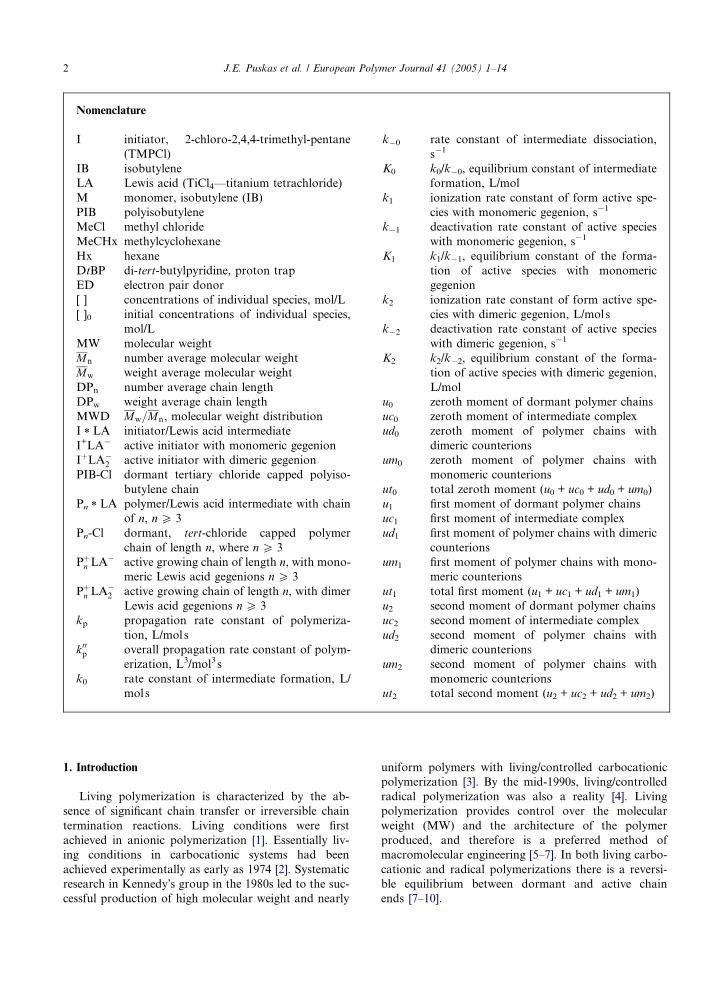
J.E. Puskas et al. / European Polymer Journal 41 (2005) 1–14 5
As mentioned earlier, this paper discusses the decon-
volution of kinetically obtained rate constants using the
mechanistic model of Scheme 1.
2.2. Kinetic modeling
Based on Scheme 1, a kinetic model was developed
using Predici�, an open-ended integrated polymerization
software that is based on the discrete Galerkin h-p
Method [49]. It allows unrestricted input of reaction rate
constants, different types of polymer species, monomers
and reactants, reaction steps and polymerization condi-
tions such as temperature and pressure [50]. During a
typical dynamic simulation, the formation or consump-
tion of any of the individual species can be followed
either with respect to time or conversion. It also has
parameter estimation capabilities; based on a given
kinetic model and sufficient experimental data, rate con-
stants can be estimated. Within the Predici environment,
the series of reactions shown in Table 2, was written.
Independently, a set of ordinary differential equa-
tions (ODEs) were derived as shown in Table 3 [51].
The model equations are composed of a set of dynamic
Table 3
Material balance equations for the comprehensive model
Low molecular weight species:d½I�dt
¼ �k0½I�½LA� þ k�0½I � LA�
d½I � LA�dt
¼ k0½I�½LA� � k2½LA�½I � LA� � ðk�0 þ k1Þ½I � LA� þ k�1½IþL
d½IþLA��dt
¼ k1½I � LA� � ðk�1 þ kp½M�Þ½IþLA��
d½IþLA�2 �
dt¼ k2½I � LA�½LA� � ðk�2 þ kp½M�Þ½IþLA�
2 �
d½M�dt
¼ �kp½M�ð½IþLA�� þX1
i¼3½Pþi LA
�� þ ½IþLA�2 � þ
X1i¼3½P
þi LA
�2
d½LA�dt
¼ k�0ð½I � LA� þX1
i¼3½Pi � LA�Þ � k0½LA�ð½I� þX1
i¼3PiÞ � k2½þP1
i¼3½Pi � LA�Þ þ k�2ð½Iþ LA�2 � þ
P1i¼3½Pþ
i LA�2 �Þ
High molecular weight species:
d½Pþ3 LA
��dt
¼ kp½M�ð½IþLA�� � ½Pþ3 LA��Þ � k�1½Pþ
3 LA�� þ k1½P3 � LA�
d½Pþi LA
��dt
¼ kpð½Pþi�1LA
�� � ½Pþi LA
��Þ � k�1½Pþi LA
�� þ k1½Pi � LA� i
d½Pþ3 LA
�2 �
dt¼ kp½M�ð½IþLA�
2 � � ½Pþ3 LA�2 �Þ � k�2½Pþ
3 LA�2 � þ k2½P3 � LA�
d½Pþi LA
�2 �
dt¼ kp½M�ð½Pþi�1LA
�2 � � ½Pþ
i LA�2 �Þ � k�2½Pþi LA
�2 � þ k2½P3 � LA
d½P3 � LA�dt
¼ k�1½Pþ3 LA
�� � ðk�0 þ k1 þ k2½LA�Þ½P3 � LA� þ k�2½Pþ3 LA
d½Pi � LA�dt
¼ k�1½Pþi LA�� � ðk�0 þ k1 þ k2½LA�Þ½Pi � LA� þ k�2½Pþi LA
d½P3�dt
¼ k�0½P3 � LA� � k0½P3�½LA�
d½Pi�dt
¼ k�0½Pi � LA� � k0½Pi�½LA� i ¼ 4 � � �1
material balance equations for each individual species.
Because we have used TMPCl, essentially a dimer PIB,
as the initiator in the experiments, we refer to the first
polymeric species formed by propagation as P3 (Table
3: Eqs. (g), (i) and (m)).
The method of moments was used to determine the
weight and number average molecular weights of the
(a)
A�� þ k�2½IþLA�2 � (b)
(c)
(d)
�Þ (e)
LA�ð½I � LA�(f)
(g)
¼ 4 � � �1 (h)
½LA� (i)
�½LA� i ¼ 4 � � �1 (j)
�2 � þ k0½P3�½LA� (k)
�2 � þ k0½Pi�½LA� i ¼ 4 � � �1 (l)
(m)
(n)
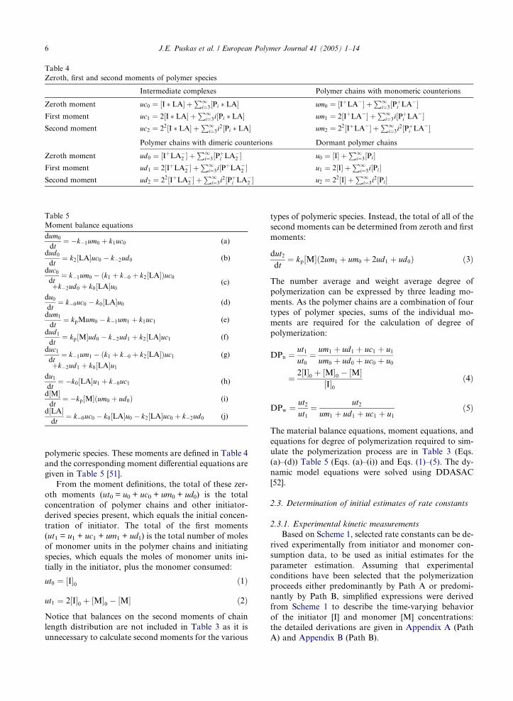
Table 4
Zeroth, first and second moments of polymer species
Intermediate complexes Polymer chains with monomeric counterions
Zeroth moment uc0 ¼ ½I � LA� þP1
i¼3½Pi � LA� um0 ¼ ½IþLA�� þP1
i¼3½Pþi LA
��First moment uc1 ¼ 2½I � LA� þ
P1i¼3i½Pi � LA� um1 ¼ 2½IþLA�� þ
P1i¼3i½Pþi LA
��Second moment uc2 ¼ 22½I � LA� þ
P1i¼3i
2½Pi � LA� um2 ¼ 22½IþLA�� þP1
i¼3i2½Pþ
i LA��
Polymer chains with dimeric counterions Dormant polymer chains
Zeroth moment ud0 ¼ ½IþLA�2 � þ
P1i¼3½Pþ
i LA�2 � u0 ¼ ½I� þ
P1i¼3½Pi�
First moment ud1 ¼ 2½IþLA�2 � þ
P1i¼3i½PþLA�
2 � u1 ¼ 2½I� þP1
i¼3i½Pi�Second moment ud2 ¼ 22½IþLA�
2 � þP1
i¼3i2½Pþ
i LA�2 � u2 ¼ 22½I� þ
P1i¼3i
2½Pi�
Table 5
Moment balance equations
dum0
dt¼ �k�1um0 þ k1uc0 (a)
dud0dt
¼ k2½LA�uc0 � k�2ud0 (b)
duc0dt
¼ k�1um0 � ðk1 þ k�0 þ k2½LA�Þuc0þk�2ud0 þ k0½LA�u0
(c)
du0dt
¼ k�0uc0 � k0½LA�u0 (d)
dum1
dt¼ kpMum0 � k�1um1 þ k1uc1 (e)
dud1dt
¼ kp½M�ud0 � k�2ud1 þ k2½LA�uc1 (f)
duc1dt
¼ k�1um1 � ðk1 þ k�0 þ k2½LA�Þuc1þk�2ud1 þ k0½LA�u1
(g)
du1dt
¼ �k0½LA�u1 þ k�0uc1 (h)
d½M�dt
¼ �kp½M�ðum0 þ ud0Þ (i)
d½LA�dt
¼ k�0uc0 � k0½LA�u0 � k2½LA�uc0 þ k�2ud0 (j)
6 J.E. Puskas et al. / European Polymer Journal 41 (2005) 1–14
polymeric species. These moments are defined in Table 4
and the corresponding moment differential equations are
given in Table 5 [51].
From the moment definitions, the total of these zer-
oth moments (ut0 = u0 + uc0 + um0 + ud0) is the total
concentration of polymer chains and other initiator-
derived species present, which equals the initial concen-
tration of initiator. The total of the first moments
(ut1 = u1 + uc1 + um1 + ud1) is the total number of moles
of monomer units in the polymer chains and initiating
species, which equals the moles of monomer units ini-
tially in the initiator, plus the monomer consumed:
ut0 ¼ ½I�0 ð1Þ
ut1 ¼ 2½I�0 þ ½M�0 � ½M� ð2Þ
Notice that balances on the second moments of chain
length distribution are not included in Table 3 as it is
unnecessary to calculate second moments for the various
types of polymeric species. Instead, the total of all of the
second moments can be determined from zeroth and first
moments:
dut2dt
¼ kp½M�ð2um1 þ um0 þ 2ud1 þ ud0Þ ð3Þ
The number average and weight average degree of
polymerization can be expressed by three leading mo-
ments. As the polymer chains are a combination of four
types of polymer species, sums of the individual mo-
ments are required for the calculation of degree of
polymerization:
DPn ¼ut1ut0
¼ um1 þ ud1 þ uc1 þ u1um0 þ ud0 þ uc0 þ u0
¼ 2½I�0 þ ½M�0 � ½M�½I�0
ð4Þ
DPw ¼ ut2ut1
¼ ut2um1 þ ud1 þ uc1 þ u1
ð5Þ
The material balance equations, moment equations, and
equations for degree of polymerization required to sim-
ulate the polymerization process are in Table 3 (Eqs.
(a)–(d)) Table 5 (Eqs. (a)–(i)) and Eqs. (1)–(5). The dy-
namic model equations were solved using DDASAC
[52].
2.3. Determination of initial estimates of rate constants
2.3.1. Experimental kinetic measurements
Based on Scheme 1, selected rate constants can be de-
rived experimentally from initiator and monomer con-
sumption data, to be used as initial estimates for the
parameter estimation. Assuming that experimental
conditions have been selected that the polymerization
proceeds either predominantly by Path A or predomi-
nantly by Path B, simplified expressions were derived
from Scheme 1 to describe the time-varying behavior
of the initiator [I] and monomer [M] concentrations:
the detailed derivations are given in Appendix A (Path
A) and Appendix B (Path B).

J.E. Puskas et al. / European Polymer Journal 41 (2005) 1–14 7
Path A
ln½I�0½I� ¼ K0k1½LA�0t ð6Þ
ln½M�0½M� ¼ kpK0K1½I�0½LA�0t ð7Þ
Employing Eqs. (6) and (7), K0k1 = 0.22L/mol s and
K0K1kp = 3.4L2/mol2 s were calculated from previously
published experimental initiator and monomer con-
sumption data in Path A [15].
Path B
ln½M�0½M� ¼ K0K2kp½I�0½LA�
2
0t ð8Þ
In Path B, that is, under conditions normally used in liv-
ing IB polymerizations, initiation is nearly instantaneous
and initiator consumption cannot be followed experi-
mentally. After a very fast initiation period, [Pn] = [I]0.
In classical living polymerization this simplification is
routinely used in formulating rate equations for mono-
mer consumption. Also, in case of instantaneous ini-
tiation the monomer consumed during initiation is
neglected. In contrast, in Path A, initiation and propa-
gation was found to proceed simultaneously, so these
simplifications cannot be considered. In Path B, experi-
mental data have revealed a fractional order of 1.76 in
TiCl4 [15], which is in good agreement with the range
of 1.7–2.2 reported by other researchers [11,16,19,24].
ln½M�0½M� ¼ k00p½I�0½LA�
1:76 ð9Þ
Here k00p is the experimentally measured apparent rate
constant. This indicates that in reality, both Paths A
and B proceed simultaneously, with Path B dominating.
Using Eq. (9), constant k00p ¼ 52L3/mol3 s was obtained
from experimental monomer consumption data [15].
With the interpretation in Eq. (8), K0K2kp = 52L3/
mol3 s. Eqs. (6)–(8) were derived with several assump-
tions and should be viewed as simplified rate expres-
sions, but they provide means to establish initial
estimates for the simulations.
Selected rate constants in IB polymerizations have
been measured or derived independently. For instance,
‘‘diffusion clock’’ and competition experiments methods
yielded kp � 108L/mols [30,35,36]. As discussed earlier,
this high value is contradicting earlier data, presented
in Table 1, with the exception of kp obtained from irra-
diation-initiated IB polymerization. Industrial experi-
ence supports the close to diffusion-limited high value
[53], therefore we accepted this value. Later it will be
shown that parameter estimation also supports a high
kp value. Published capping rate constants, although de-
rived from differing interpretations, were in the range of
3–5 · 107s�1 (Puskas and Peng [26]: k�1 = 3.9 · 107 s�1
(TMPCl); Kim and Faust [55]: k�1 = 5.0 · 107s�1
(TMPCl) and k�1 = 3.4 · 107 s�1 (PIB-36mer). Using
kp = 6 · 108L/mols we get K0K1 = 5.7 · 10�9L/mol andK0K2 = 8.7 · 10�8L2/mol2, which confirms that both
equilibria are dramatically shifted toward the dormant
polymer chains Pn-Cl. From K0k1 = 0.22L/mols and
K0K1 = 5.7 · 10�9L/mol we get k�1 = 3.9 · 107 s�1. Thisagrees very well with published capping rate coefficients,
thus we assumed this value for k�2 and determined
K0k2 = (k0/k�0) Æ k2 = 3.38L2/mol2 s.
As a result, the following correlations have been
established:
C1 : k1K0 ¼ k1 � ðk0=k�0Þ ¼ 0:22L=mols ð10Þ
C2 : k2K0 ¼ k2 � ðk0=k�0Þ ¼ 3:38L2=mol2 s ð11Þ
The correlation between the parameters will influence
the estimability of individual parameters.
2.4. PREDICI parameter estimation
For the PREDICI parameter estimation, the reaction
scheme in Table 2 was used. Table 6 lists initial rate con-
stant values and sets of estimated parameters. The initial
values for k0, k�0, k1 and k2 were established from the
correlations given in (10) and (11) by trial and error, fit-
ting experimental data [54]. The parameter estimation
routine in PREDICI is based on the damped Gauss–
Newton method [56,57] and has the ability to converge
well even with bad starting values. Seven experimental
data sets were used in the simulation [15]. First, all
parameters were estimated simultaneously. The simula-
tion did converge with kp = 6 * 108L/mols as a starting
estimate without any constraints imposed, although with
high error within the 90% confidence intervals; the data
are listed as Set 1 in Table 6. It is interesting to note that
kp converged to a value of 4.64 * 108 ± 2.75 * 10
8L/mol s.
In contrast, the simulation was unable to converge with
kp = 104L/mols as a starting estimate. This further sup-
ports the high kp values obtained in diffusion clock and
competition experiments [30,35,36]. The values for k�1and k�2 converged to 1.77 and 2.75 * 10
7 s�1, close to
the initial values. However, k0, k�0, k1 and k2 carried very
large errors and did not satisfy the correlations estab-
lished in (10) and (11). Next we fixed kp = 6 * 108L/mols
and k�1 = k�2 = 3.9 * 107 s�1, and estimated k0, k1 and
k2. Set 2 shows that the error is still high. In the next step
we enforced the correlations defined in Eqs. (10) and (11)
using interpreter functions in Predici [57]. Set 3 shows
that k0 and k�0 still carry very high error. As was deter-
mined from the estimability analysis, these parameters
were correlated and hence could not be estimated simul-
taneously. Therefore in Set 4, we fixed the value of k�0 to
3.9 * 107s�1. Set 4 shows the estimated k0 with low error
within the 90% confidence interval. The parameters in
Set 4 were used for the simulations with Predici. It should
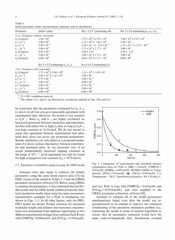
Table 6
Initial parameter values and parameter estimates used in simulations
Parameter Initial values Set 1 ± CIa (estimating all) Set 2 ± CI (estimating k0, k1, k2)
1(a): Estimates without constraints
k0 (L/mols) 1.56 * 108 2.75 * 10
8 ± 2.79 * 108 7.96 * 107 ± 3.97 * 10
7
k�0 (s�1) 3.90 * 10
7 1.13 * 108 ± 7.62 * 10
8 3.90 * 107
k1 (s�1) 5.50 * 10
�2 1.20 * 10�2 ± 1.23 * 10
�2 1.72 * 10�2 ± 1.23 * 10�2
k�1 (s�1) 3.90 * 10
7 1.71 * 107 ± 1.77 * 107 3.90 * 10
7
k2 (L/mols) 8.45 * 10�1 5.88 ± 3.93 3.50 ± 1.47
k�2 (s�1) 3.90 * 10
7 5.90 * 107 ± 2.75 * 107 3.90 * 10
7
kp (L/mols) 6.00 * 108 4.64 * 10
8 ± 2.75 * 108 6.00 * 108
Set 3 ± CI (estimating k0, k�0) Set 4 ± CI (estimating k0)
1(b): Estimates with constraints
k0 (L/mols) 1.72 * 108 ± 3.84 * 10
8 1.51 * 108 ± 2.03 * 10
7
k�0 (s�1) 4.48 * 10
7 ± 1.16 * 108 3.90 * 10
7
k1b (s�1) 5.73 * 10
�2 5.68 * 10�2
k�1 (s�1) 3.90 * 10
7 3.90 * 107
k2b (L/mols) 8.80 * 10
�1 8.73 * 10�1
k�2 (s�1) 3.90 * 10
7 3.90 * 107
kp (L/mols) 6.00 * 108 6.00 * 10
8
a CI = 90% confidence interval.b The values of k1 and k2 are dictated by correlations defined in Eqs. (10) and (11).
0 200 400 600 8000.00
0.01
0.02
0.03
0.04
0.05 Predici ODE
[TM
PCl],
mol
/L
time (s)
Fig. 1. Comparison of experimental and simulated initiator
consumption plots for Path A: [IB]0 = 2.0mol/L, [TMPCl]0 =
0.05mol/L, [DtBP]0 = 0.007mol/L. Hx/MeCl=60/40 v/v; Exper-
imental: [TiCl4] = 0.05mol/L (m), [TiCl4] = 0.025mol/L (s);
Temperature: �80�C; Simulation parameters: Set 4 (Table 1).
8 J.E. Puskas et al. / European Polymer Journal 41 (2005) 1–14
be noted here that the parameters estimated for k0, k�0,k1 and k2 in all four sets gave reasonable agreement with
experimental data. However, the model is very sensitive
to kp/k�1. Since kp and k�1 are highly correlated we
had good agreement between simulation and experimen-
tal data with either low or high kp data as long as kp/k�1was kept constant at 16.5L/mol. We do not intend to
argue that agreement between experimental and simu-
lated data alone can prove any proposed mechanisms.
Kinetic simulation can only disprove a proposed mecha-
nism if it shows serious discrepancy between experimen-
tal and simulated plots. In our particular case, if we
accept independently measured capping constants in
the range of 107s�1, good agreement can only be found
for high propagation rate constant (kp � 108L/mols).
2.5. Parameter estimability analysis using the ODE model
Attempts were also made to estimate the kinetic
parameters using the same batch reactor data [15] the
ODE version of the model in Tables 3–5 and the GREG
parameter estimation software [52]. Before using GREG
to estimate the parameters, it was confirmed that the Pre-
dici model and the ODE model yielded practically iden-
tical simulation results when using the same parameters;
representative examples for a Path A simulations are
shown in Figs. 1–3. In all other figures, only the PRE-
DICI results are shown. Pooled variances for measured
molecular weight and initiator and monomer concentra-
tions were determined from replicate experiments at two
different experimental settings (four replicate Path B runs
with [TMPCl]0 =0.004mol/L and [TiCl4]0 = 0.032mol/L,
and two Path A runs with [TMPCl]0 = 0.05mol/L and
[TiCl4]0 = 0.0125mol/L), and were supplied to the
GREG parameter estimation software [58].
Attempts to estimate all of the model parameters
simultaneously failed, even after the model was re-
parameterized in an attempt to improve the numerical
conditioning of the parameter estimation problem (i.e.,
expressing the model in terms of natural logarithms to
ensure that all parameters estimated would have the
same order-of-magnitude size). Simulations revealed
0 200 400 600 8000.0
0.5
1.0
1.5
2.0
[M],
mol
/L
time (s)
Predici ODE
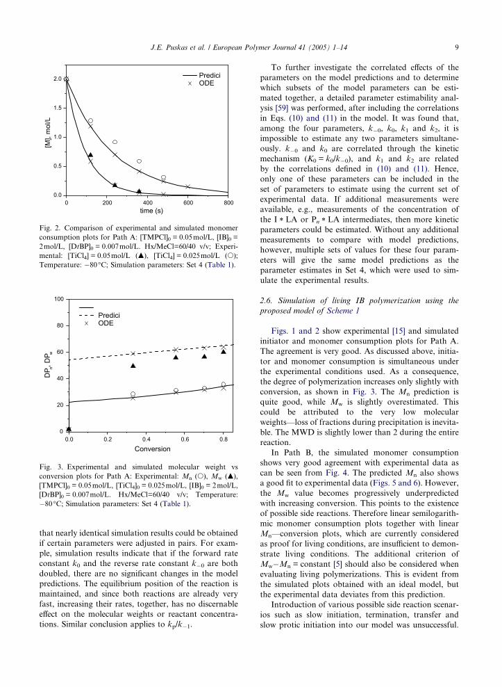
Fig. 2. Comparison of experimental and simulated monomer
consumption plots for Path A: [TMPCl]0 = 0.05mol/L, [IB]0 =
2mol/L, [DtBP]0 = 0.007mol/L. Hx/MeCl=60/40 v/v; Experi-
mental: [TiCl4] = 0.05mol/L (m), [TiCl4] = 0.025mol/L (s);
Temperature: �80�C; Simulation parameters: Set 4 (Table 1).
0.0 0.2 0.4 0.6 0.80
20
40
60
80
100
Predici ODE
DP n,
DP w
Conversion
Fig. 3. Experimental and simulated molecular weight vs
conversion plots for Path A: Experimental: Mn (s), Mw (m),
[TMPCl]0 = 0.05mol/L, [TiCl4]0 = 0.025mol/L, [IB]0 = 2mol/L,
[DtBP]0 = 0.007mol/L. Hx/MeCl=60/40 v/v; Temperature:
�80�C; Simulation parameters: Set 4 (Table 1).
J.E. Puskas et al. / European Polymer Journal 41 (2005) 1–14 9
that nearly identical simulation results could be obtained
if certain parameters were adjusted in pairs. For exam-
ple, simulation results indicate that if the forward rate
constant k0 and the reverse rate constant k�0 are both
doubled, there are no significant changes in the model
predictions. The equilibrium position of the reaction is
maintained, and since both reactions are already very
fast, increasing their rates, together, has no discernable
effect on the molecular weights or reactant concentra-
tions. Similar conclusion applies to kp/k�1.
To further investigate the correlated effects of the
parameters on the model predictions and to determine
which subsets of the model parameters can be esti-
mated together, a detailed parameter estimability anal-
ysis [59] was performed, after including the correlations
in Eqs. (10) and (11) in the model. It was found that,
among the four parameters, k�0, k0, k1 and k2, it is
impossible to estimate any two parameters simultane-
ously. k�0 and k0 are correlated through the kinetic
mechanism (K0 = k0/k�0), and k1 and k2 are related
by the correlations defined in (10) and (11). Hence,
only one of these parameters can be included in the
set of parameters to estimate using the current set of
experimental data. If additional measurements were
available, e.g., measurements of the concentration of
the I * LA or Pn * LA intermediates, then more kinetic
parameters could be estimated. Without any additional
measurements to compare with model predictions,
however, multiple sets of values for these four param-
eters will give the same model predictions as the
parameter estimates in Set 4, which were used to sim-
ulate the experimental results.
2.6. Simulation of living IB polymerization using the
proposed model of Scheme 1
Figs. 1 and 2 show experimental [15] and simulated
initiator and monomer consumption plots for Path A.
The agreement is very good. As discussed above, initia-
tor and monomer consumption is simultaneous under
the experimental conditions used. As a consequence,
the degree of polymerization increases only slightly with
conversion, as shown in Fig. 3. The Mn prediction is
quite good, while Mw is slightly overestimated. This
could be attributed to the very low molecular
weights––loss of fractions during precipitation is inevita-
ble. The MWD is slightly lower than 2 during the entire
reaction.
In Path B, the simulated monomer consumption
shows very good agreement with experimental data as
can be seen from Fig. 4. The predicted Mn also shows
a good fit to experimental data (Figs. 5 and 6). However,
the Mw value becomes progressively underpredicted
with increasing conversion. This points to the existence
of possible side reactions. Therefore linear semilogarith-
mic monomer consumption plots together with linear
Mn––conversion plots, which are currently considered
as proof for living conditions, are insufficient to demon-
strate living conditions. The additional criterion of
Mw�Mn = constant [5] should also be considered when
evaluating living polymerizations. This is evident from
the simulated plots obtained with an ideal model, but
the experimental data deviates from this prediction.
Introduction of various possible side reaction scenar-
ios such as slow initiation, termination, transfer and
slow protic initiation into our model was unsuccessful.

0 2000 4000 6000 80000.0
0.5
1.0
1.5
2.0
[M],
mol
/L
time (s)
Predici
Fig. 4. Comparison of experimental and simulated monomer
consumption plots for Path B: [TMPCl]0 = 0.004mol/L, [IB]0 =
2mol/L, [DtBP]0 = 0.007mol/L. Hx/MeCl=60/40 v/v; Experi-
mental: [TiCl4] = 0.064mol/L (m), [TiCl4] = 0.04mol/L (s);
Temperature: �80�C; Simulation parameters: Set 4 (Table 1).
0.0 0.2 0.4 0.6 0.80
100
200
300
400
500
600
Predici
DP n,
DP w
Conversion
Fig. 5. Experimental and simulated molecular weight vs
conversion plots for Path B: Experimental: Mn (s), Mw (m),
[TMPCl]0 = 0.004mol/L, [TiCl4]0 = 0.04mol/L, [IB]0 = 2mol/L,
[DtBP]0 = 0.007mol/L, Hx/MeCl=60/40 v/v; Temperature:
�80�C; Simulation parameters: Set 4 (Table 1).
0.0 0.2 0.4 0.6 0.80
100
200
300
400
500
600
Predici
DP n,
DP w
Conversion
Fig. 6. Experimental and simulated molecular weight vs
conversion plots for Path B: Experimental: Mn (s), Mw (m),
[TMPCl]0 = 0.004mol/L, [TiCl4]0 = 0.064mol/L, [IB]0 = 2mol/
L, [DtBP]0 = 0.007mol/L. Hx/MeCl=60/40 v/v; Temperature:
�80�C; Simulation parameters: Set 4 (Table 1).
10 J.E. Puskas et al. / European Polymer Journal 41 (2005) 1–14
When TMP-Cl and PIB 36-mer were used as initiators, it
was found that kp � 3 * ki [23], but simulations con-
ducted using a ki value of 1–2 * 108L/mols did not show
any noticeable difference when compared to simulations
with kp = ki. When slow irreversible termination was
introduced, a better fit was obtained for Mw in certain
experiments [54], but in others led to discrepancies in
the monomer consumption and Mn data. Introducing
chain transfer caused a simultaneous reduction in both
Mn and Mw values. More detailed studies are necessary
to find the cause of the Mw divergence.
2.7. Calculating the average run length �l0 from Path A
Puskas et al. [9] introduced a method to calculate the
average run length �l0, defined as the average number ofmonomer units incorporating in one active ionization
period, from MWD data using Eq. (12)
DPw
DPn¼ 1þ l0
ðDPnÞð12Þ
where �l0 ¼ ðkp=k�1Þ½M�0. Eq. (13) shows the form for
intermediate conversion.
�l ¼ 1þ l0 � 1
21þ ½M�
½M�0
� �ð13Þ
Subsequently Muller et al. [60] introduced another
method:
DPw
DPn¼ 1þ 1
b2
X� 1
� �ð14Þ
where X = conversion and b = k�1/kp[I]0.
Storey recently showed that average run length num-
bers could also be obtained from ‘‘rapid monomer con-
sumption’’ (RCM) data [28]. We now will show that �l0can also be obtained from Path A in IB polymerization.
At the end of the reaction in Path A, when the initiator
is consumed, polydispersity of 1.84 was obtained exper-
imentally and simulation yielded a polydispersity of 1.88
(Fig. 3). The conditions in Path A experiments, when
initiator and monomer consumption is simultaneous,

J.E. Puskas et al. / European Polymer Journal 41 (2005) 1–14 11
can be considered as the first ‘‘run’’ of a living polymer-
ization; initiation is complete only at the end of the reac-
tion. Using DPw/DPn = 1.88 and the DPn value of 40 at
full initiator conversion, �l0 ¼ 35 was obtained from Eq.
(13). Using �l0 ¼ ðkp=k�1Þ½M�0 [8], kp/k�1 = 17.5L/mol iscalculated. This is in excellent agreement with that pub-
lished by Kaszas and Puskas [17] (kp/k�1 = 16.5L/mol)
and Schlaad et al. [23] (kp/k�1 = 16.4L/mol). Thus �l0can be obtained experimentally under Path A condi-
tions, where initiation will compete with propagation.
Under these conditionsMn andMw will remain approx-
imately constant, with the polydispersity for the most
probable distribution of MWD = 2. The MWD will start
to narrow only after initiation is complete.
3. Conclusions
In conclusion, we can state that the reaction mecha-
nism proposed in Scheme 1 reconciles seemingly contra-
dictory experimental findings (e.g., shifting TiCl4 order
and discrepancy in rate constant values obtained with
diffusion clock methods and kinetic measurements)
and can be used to simulate experimental results with
rate constants that satisfy the correlations imposed by
the mechanism and/or independently measured rate con-
stants. This by no means can be considered as proof of
the proposed mechanism. The existence and chemical
nature of the proposed intermediates must be proven
independently. However, in the absence of another
model that satisfies all the contradictory requirements
this model does not seem to be unreasonable. In addi-
tion, large-scale production data (confidential) demon-
strates that the rate constant of propagation must be
very high.
Acknowledgment
Financial support of Bayer Inc., Canada and
NSERC Canada is gratefully acknowledged.
Appendix A. Path A
Initiator consumption rate. From material balances
on the initiator and the intermediates, we have:
d½I�dt
¼ �k0½I�½LA� þ k�0½I � LA� ðA:1Þ
d½I � LA�dt
¼ k0½I�½LA� � k�0½I � LA� � k1½I � LA�
þ k�1½IþLA�� ðA:2Þ
To obtain the net rate of consumption of both of these
initiator-derived species together to form ionized species
that can polymerize, Eqs. (A.1) and (A.2) may be added
together to get:
d½I�dt
þ d½I � LA�dt
¼ dð½I� þ ½I � LA�Þdt
¼ �k1½I � LA� þ k�1½IþLA�� ðA:3Þ
[I] + [I * LA] = [I]u, where [I]u is the concentration of
unreacted initiator, thus Eq. (A.4) defines the rate of
initiator consumption and polymer formation:
� d½I�udt
¼ d½Pn�dt
ðA:4Þ
If the reactions involving k0 and k�0 are very fast,
then we will have an initial rapid equilibration, after
which:
½I � LA� ¼ k0k�0
½I�½LA� ðA:5Þ
so that Eq. (A.3) becomes:
d½I�udt
¼ �k1K0½I�½LA� þ k�1½IþLA�� ðA:6Þ
Now, if [I+LA�] is small due to the fast propagation
reaction of the ionized species, and [LA] � [LA]0, we
have:
d½I�udt
¼ �k1K0½I�½LA�0 ðA:7Þ
Expanding (A.7) with 1/[I]u on both sides and substitut-
ing (A.5) gives:
1
ð½I�uÞ� d½I�udt
¼ �k1K0½I�½LA�0ð½I� þ ½I � LA�Þ ¼
�k1K0½LA�0ð1þ K0½LA�0Þ
ðA:8Þ
Assuming K0[I]0 � 1 (A.8) can be simplified to give
(A.9):
1
ð½I�uÞ� d½I�udt
¼ �k1K0½I�½LA�0 ðA:9Þ
Integrating (A.9) between the limits of [I]u,0 = [I]0 and
[I]u,t = [I]t + [I * LA]tZ ½I�u;t
½I�u;0
d½I�u½I�u
¼ �k1K0½LA�0Z t
t¼0dt ðA:10Þ
we get the simplified rate Eq. (A.10)
ln½I�0½I�u;t
¼ k1K0½LA�0t ðA:11Þ
This is equivalent to Eq. (6) in the text.
Propagation rate. For Path A, the rate of propaga-
tion is described by Eq. (A.12):
Rp ¼ � d½M�dt
¼ kp½M�ð½IþLA�� þ ½Pþn LA
��Þ ðA:12Þ
The consumption rate of the active propagating species
is given in Eq. (A.13):
12 J.E. Puskas et al. / European Polymer Journal 41 (2005) 1–14
dð½IþLA�� þ ½Pþn LA
��Þdt
¼ k1½I � LA� � k�1½IþLA��
þ k1½Pn � LA� � k�1½Pþn LA
��ðA:13Þ
The combined change in initiator and polymer concen-
trations with time can be written as follows:
dð½I� þ ½Pn�Þdt
¼ �k0½I�½LA� þ k�0½I � LA�
� k0½Pn�½LA� þ k�0½Pn � LA� ðA:14Þ
Since the reactivities of the initiator and the growing
chains are about equal, the sums of the concentrations
of the active cationic species and also the dormant spe-
cies are constant and the quasi-steady state assumption
(QSSA) can be applied:
dð½IþLA�� þ ½Pþn LA
��Þdt
ffi 0 ðA:15Þ
dð½I� þ ½Pn�Þdt
ffi 0 ðA:16Þ
With this and assuming fast equilibria, the concentration
of active cationic species is derived as follows:
½IþLA�� þ ½Pþn LA
�� ¼ K1ð½I � LA� þ ½Pn � LA�Þ ðA:17Þ
½I � LA� þ ½Pn � LA� ¼ K0ð½I� þ ½Pn�Þ½LA� ðA:18Þ
Substituting (A.18) into (A.17), we have
½IþLA�� þ ½Pþn LA
�� ¼ K1K0ð½I� þ ½Pn�Þ½LA� ðA:19Þ
where K1 = k1/k�1 and K0 = k0/k�0.
Substituting (A.18) into (A.12) yields
Rp ¼ � d½M�dt
¼ kpK1K0½M�ð½I� þ ½Pn�Þ½LA� ðA:20Þ
Since the concentration of active cationic species
([I+LA�] and ½Pþn LA
��) is very small, simplified mass
balances for the initiator and Lewis acid can be written
as follows:
½I�0 ¼ ½I� þ ½Pn� þ ½I � LA� þ ½Pn � LA� ðA:21Þ
½LA�0 ¼ ½LA� þ ½I � LA� þ ½Pn � LA� ðA:22Þ
Substituting (A.17) into (A.20) and (A.21) yields:
½I� þ ½Pn� ¼½I�0
1þ K0½LA�ðA:23Þ
and
½LA� ¼ ½LA�01þ K0
½I�01þ K0½LA�
ðA:24Þ
If the concentration of free Lewis acid is small, i.e.,
K0[LA]� 1, (A.23) and (A.24) can be simplified:
½I� þ ½Pn� � ½I�0 ðA:25Þ
½LA� � ½LA�01þ K0½I�0
ðA:26Þ
With K0[I]0 � 1, [LA] � [LA]0.
Substituting (A.25) and (A.26)into Eq. (A.20) gives
the general form of the differential polymerization rate
equation:
Rp ¼ � d½M�dt
¼ kpK1K0½M� ½I�0½LA�01þ K0½LA�0
ðA:27Þ
Assuming K0[LA]0 � 1 again, we can simplify and inte-
grate the rate equation to get (A.28):
ln½M�0½M� ¼ kpK0K1½I�0½LA�0t ðA:28Þ
(A.28) is equivalent to Eq. (7) in the text.
Appendix B. Path B
Propagation rate. The rate of polymerization for Path
B can be derived similarly to Path A:
Rp ¼ � d½M�dt
¼ kp½M�ð½IþLA�2 � þ ½Pþ
n LA�2 �Þ ðB:1Þ
dð½IþLA�2 � þ ½Pþ
n LA�2 �Þ
dt¼ k2½I � LA�½LA�
� k�2½IþLA�2 �
þ k2½Pn � LA�½LA�� k�2½Pþ
n LA�2 � ðB:2Þ
dð½I� þ ½Pn�Þdt
¼ �k0½I�½LA� þ k�0½I � LA�
� k0½Pn�½LA� þ k�0½Pn � LA� ðB:3Þ
dð½IþLA�2 � þ ½Pþ
n LA�2 �Þ
dtffi 0 ðB:4Þ
dð½I� þ ½Pn�Þdt
ffi 0 ðB:5Þ
Since the reactivities of the initiator and the polymer are
close to equivalent, the rate of consumption of the initi-
ating species is equal to the rate of the formation of the
growing species.
½IþLA�2 � þ ½Pþ
n LA�2 � ¼ K2ð½I � LA� þ ½Pn � LA�Þ½LA�
ðB:6Þ
½I � LA� þ ½Pn � LA� ¼ K0ð½I� þ ½Pn�Þ½LA� ðB7 ¼ A7Þ
½IþLA�2 � þ ½Pþ
n LA�2 � ¼ K2K0ð½I� þ ½Pn�Þ½LA�2 ðB:8Þ

J.E. Puskas et al. / European Polymer Journal 41 (2005) 1–14 13
where K2 = k2/k�2.
Substituting (B.8) into (B.1) yields:
Rp ¼ � d½M�dt
¼ kpK1K0½M�ð½I� þ ½Pn�Þ½LA�2 ðB:9Þ
The concentrations of the ionic species are very small,
thus the simplified mass balances established in Eqs.
(A.20) and (A.21) and Eqs. (A.22)–(A.25) will apply.
With these we get the form given below:
Rp ¼ � d½M�dt
¼ kpK1K0½M� ½I�0½LA�2
0
ð1þ K0½I�0Þ2
ðB:10Þ
Assuming K0[LA]0 � 1 again and integrating, we get
(B.11):
ln½M�0½M� ¼ kpK0K1½I�0½LA�
2
0t ðB:11Þ
Eq. (B.11) is equivalent to Eq. (9) in the text.
References
[1] Szwarc M. Carbanions, living polymers and electron
transfer processes. New York: Wiley; 1968.
[2] (a) Pepper DC. Makromol Chem 1974;175:1077;
(b) Johnson AF, Young RN. J Polym Sci Polym Symp
1976;56:211.
[3] Kennedy JP, Kelen T, Tudos FJ. J Macromol Sci Chem A
1982;18(9):1189;
Faust R, Fehervari A, Kennedy JP. J Macromol Sci A
1982;18(9):1209;
Puskas JE, Kaszas G, Kennedy JP, Kelen T, Tudos FJ. J
Macromol Sci Chem A 1982;18(9):1245;
Puskas JE, Kaszas G, Kennedy JP, Kelen T, Tudos FJ. J
Macromol Sci Chem A 1982;18(9):1229;
Kennedy JP. J Polym Sci Polym Chem 1999;37:2285.
[4] Georges MK, Veregin RP, Kazmaier PM, Hamer GK.
Macromolecules 1993;26:2987;
Wang JS, Matyjaszewski K. Macromolecules 1995;28:
7901;
Kato M, Kamigaito M, Sawamoto M, Higashimura T.
Macromolecules 1995;28:1721.
[5] Puskas JE, Kaszas G. Carbocationic polymerization. En-
cyclopedia of polymer science and technology, V5. Wiley-
Interscience; 2003. p. 382.
[6] Puskas JE, Kaszas G. Prog Polym Sci 2000;25:403.
[7] Matyjaszewski K, Sawamoto M. In: Matyjaszewski K,
editor. Cationic polymerizations: mechanisms, synthesis and
applications. New York: Marcel Dekker; 1996. p. 265.
[8] Kaszas G, Puskas JE, Kennedy JP, Chen CC. J Macromol
Sci Chem A 1989;26(8):1099.
[9] Puskas JE, Kaszas G, Litt M. Macromolecules 1991;
24:5278.
[10] Sigwalt P. Makromol Chem Makromol Symp 1991;47:179.
[11] Storey RF, Choate Jr KR. Macromolecules 1997;30:4799.
[12] Kaszas G, Puskas JE, Kennedy JP. J Makromol Chem
Makromol Symp 1988;13/14:473.
[13] Roth M, Patz M, Preter H, Mayr H. Macromolecules
1997;30:722.
[14] Storey RF, Maggio TL. Macromolecules 2000;33:681.
[15] Puskas JE, Lanzendorfer MG. Macromolecules 1998;31:
8684.
[16] Wu Y, Tan Y, Wu G. Macromolecules 2002;35:3801.
[17] Kaszas G, Puskas JE. Polym React Eng 1994;2(3):251.
[18] Kennedy JP, Majoros I, Nagy A. Adv Polym Sci 1994;
112:1.
[19] Gyor M, Wang HC, Faust R. J Macromol Sci Chem A
1992:639.
[20] Storey RF, Chisholm BJ, Brister LB. Macromolecules
1995;28(12)4055.
[21] Puskas JE et al. In: Puskas JE, Long TE, Storey RF,
editors. In situ monitoring of monomer and polymer
synthesis. New York: Kluwer Academic/Plenum Publish-
ers; 2003. p. 37.
[22] Paulo C, Puskas JE, Angepat S. Macromolecules 2000;33:
4634.
[23] Schlaad H, Kwon Y, Faust R, Mayr H. Macromolecules
2000;33:743.
[24] Storey RF, Donnalley AB. Macromolecules 2000;33:53.
[25] Puskas JE, Lanzendorfer MG, Peng H, Michel AJ, Brister
LB, Paulo C. In: Puskas JE, editor. Ionic polymerizations
and related processes. Netherlands: Kluwer Academic/
Plenum Publishers; 1999. p. 143.
[26] Puskas JE, Peng H. Polym React Eng 1999;7(4):553.
[27] Hadjikyriacou S, Faust R. Macromolecules 1995;28:
7893.
[28] Storey RF, Thomas QA. Macromolecules 2003;36:5065.
[29] Fodor Z, Bae YC, Faust R. Macromolecules 1998;31:4439.
[30] Roth M, Mayr H. Macromolecules 1996;29:6104.
[31] Moreau M. IP �97. In: Proceedings of the InternationalSymposium on Ionic Polymerization and Related Proc-
esses, Paris, 1997. p. 135.
[32] Kistenmacher TJ, Stucky GD. Inorg Chem 1971;10:122.
[33] Rytter E, Kvisle S. Inorg Chem 1985;24:640.
[34] Schlaad H, Kwon Y, Sipos L, Faust R, Charleaux B.
Macromolecules 2000;33:8225.
[35] Sipos L, De P, Faust R. Macromolecules 2003;36:8282.
[36] Mayr H, Schimmel H, Kobayashi S, Kotani M, Praba-
rakaran TR, Sipos L, et al. Macromolecules 2002;35:4611.
[37] Marek M, Chmelir M. J Polym Sci 1967;22:177.
[38] Toman L, Marek M. Makromol Chem 1976;22:3325.
[39] Magagnini PL, Cesca S, Giusti P, Priola A, Di Maina M.
Makromol Chem 1977;178:2235.
[40] Ueno K, Yamaoka H, Hayashi K, Okamura S. Int J Appl
Radiat Isotopes 1966;17:595.
[41] Plesch PH. Prog Reaction Kinetics 1993;18:1.
[42] Taylor RB, Williams F. J Am Chem Soc C 1969;22:177.
[43] Plesch PH. Macromolecules 2001;34:1143.
[44] Puskas JE, Shaikh S. Macromol Symp [in press].
[45] Majoros I, Nagy A, Kennedy JP. Adv Polym Sci 1994;
112:1.
[46] Lorimer JP, Pepper DC. Prod R Soc Lond A 1976;351:551.
[47] Vairon JP, Charleaux B, Moreau M. In: Puskas JE, editor.
Ionic polymerizations and related processes. Nether-
lands: Kluwer Academic/Plenum Publishers; 1999. p. 177.
[48] Sigwalt P, Moreau M, Polton A. Makromol Chem
Macromol Symp 2002;183:35.
[49] Wulkow M. PREDICI� Simulation Package for Poly-
reactions, CiT, GmbH, 1996.
[50] Wulkow M. Chem Eng Technol 1996;5:393.

14 J.E. Puskas et al. / European Polymer Journal 41 (2005) 1–14
[51] Liu Q. MSc (Eng) thesis, Queen�s University, 2001.[52] Stewart WE, Caracotsios M, Sorensen JP. DDASAC
Software Package Documentation, University of Wiscon-
sin, 1994.
[53] Puskas JE, Schmidt J, Collart P, Verhelst M. Kautsch
Gummi Kunst 1995;12:866.
[54] Shaikh S, Peng H, Puskas JE. Polym Prepr 2002;35:
5320.
[55] Kim MS, Faust R. Macromolecules 2002;36:8282.
[56] Wulkow M. Macromol Theory Simul 1996;5:393.
[57] Wulkow M. PREDICI� Simulation Package for Poly-
reactions: Users Manual Ver.5.18.5, CiT GmbH, 2001.
[58] Stewart WE, Caracotsios M, Sorensen JP. GREG: Gen-
eralized REGression Package for Non-linear Parameter
Estimation 1994, University of Wisconsin.
[59] Yao KZ, Shaw B, Kou B, McAuley KB, Bacon D. Polym
React Eng 2003;11(3):563.
[60] Muller AHE, Litvinenko G, Yan D. Macromolecules
1996;29:2339.
Related Documents


![2008 Fall Natl ACS meeting · 2018. 5. 18. · 2008 Fall Meeting 10:50 —13. Controlled carbocationic polymerization of bicyclo[2,2,1]hepta-2,5-diene. N. Mijid Taylor, R. M. Peetz](https://static.cupdf.com/doc/110x72/5fe1538b0340fd06db7ce441/2008-fall-natl-acs-meeting-2018-5-18-2008-fall-meeting-1050-a13-controlled.jpg)