Kinematic self-identification of a redundantly actuated parallel manipulator using differential evolution

Proceedings of the 8th

World Congress on Intelligent Control and Automation July 6-9 2010, Jinan, China

978-1-4244-6712-9/10/$26.00 ©2010 IEEE

Kinematic Self-Identification of a Redundantly Actuated Parallel Manipulator using Differential Evolution*

Weiwei Shang, Shuang Cong, and Yuan Ge Department of Automation, University of Science and Technology of China, Hefei, Anhui, 230027, P. R. China

{wwshang & scong}@ustc.edu.cn, [email protected]

* This work was supported by the National Natural Science Foundation of China with Grant No. 50905172, the Anhui Provincial Natural Science Foundation with Grant No.090412040, Youth Innovation Foundation of University of Science and Technology of China, and the K. C. Wong Education Foundation of Hong Kong.

Abstract - The self-identification of a redundantly actuated parallel manipulator is transformed into an optimization problem, and then differential evolution algorithm is used to obtain a globally optimal solution of the kinematic parameters. Based on the kinematic equations of the parallel manipulator, a new optimization function is formulated by eliminating the passive joint angles and decoupling the kinematic parameters. In order to obtain the global optimum, differential evolution algorithm is applied to minimize the optimization function. The proposed self-identification method is realized on an actual parallel manipulator, and the comparison on the actuated joint errors indicates that the identified kinematic parameters are much more accurate than the nominal parameters. Finally, the kinematic control experiments are carried out, and then the tracking accuracy of the end-effector based on the identified kinematic model is compared with the results by using the nominal kinematic model.

Index Terms – parallel manipulator, redundant actuation, differential evolution, self-identification, kinematic

I. INTRODUCTION

Parallel manipulators are commonly claimed as appealing solutions in many industrial applications for their inherent advantages such as good stiffness, large load capacity, high speed and high accuracy [1]. However, in actual applications, due to the inevitable manufacturing tolerances and assembling errors in numerous links and joints, the actual model parameters of parallel manipulators are always unequal to the values provided by the manufacturers [2]. Thus the performances of parallel manipulators highly rely on accurate model parameters, including kinematic parameters and dynamic parameters.

The kinematic parameters of parallel manipulators have to be identified by the so-called kinematic identification (or kinematic calibration). According to the measurement devices adopted to get redundant information, kinematic identification methods of parallel manipulators can be classified into three categories[3], [4]: external identification methods, self-identification methods by applying mechanical constraints, and self-identification methods by using redundant sensors. External identification methods rely on the precise measuring devices, such as laser tracking devices [5], [6], mechanical devices [7], [8], and vision systems [9]. With these external devices, the position and pose of moving platform can be measured, and then the kinematic parameters can be identified by minimizing the kinematic errors. The first self-

identification methods are realized by applying the mechanical constraints on the moving platform or mechanism legs [10], [11]. This class of methods only needs joint measurements, but it reduces the workspace size and therefore the identification efficiency [12]. The second self-identification methods depend on the redundant joint sensors of parallel manipulators, which can be achieved by adding extra sensors on moving platform or some joints [13], [14]. The extra information can be obtained without employing external measuring devices, and then self-identification are usually implemented by minimizing a function of closed-loop constraint errors. It is more convenient to measure the sampled configurations by the redundant joint sensors than the external measuring devices, especially for the redundantly actuated parallel manipulator with inherent redundant joint sensors. The parameter identification results of the self-identification are usually dependent on the error functions defined and the optimization methods adopted. The error functions can be simplified to decrease the optimization calculation to get better self-identification results. Although the error functions were studied in detail [15], [16], the optimization algorithms applied in above articles were all local optimization methods, and the solutions obtained by these methods would inevitably be local solutions of the error functions [6], [17]. As a result, not all the kinematic parameters can be identified, and the identification results are not reliable. Therefore, the kinematic parameters of parallel manipulators can not be identified accurately by using the local optimization methods.

Differential evolution (DE) is a real-valued number encoded evolutionary strategy for global optimization. It has been shown to be an efficient and robust optimization algorithm, especially for problems containing continuous variables [18], [19]. We have applied a DE algorithm to solve the kinematic self-identification problem of a redundantly actuated parallel manipulator. On the basis of the closed-loop constrained equations of the parallel manipulator, a new optimization function is formulated. In the optimization function, the passive joint angles are eliminated, and the product items of kinematic parameters are decoupled completely to reduce the search process of optimization. The formulated optimization function is very complex both in the number of variables and its multimodal features; thus it is very hard to converge to a global minimum using local optimization methods. In order to obtain the globally optimal solution, the DE algorithm is applied to minimize the optimization function.

6654

The proposed self-identification method is realized on an actual parallel manipulator, and the comparison on the actuated joint errors indicates that the identified kinematic parameters are much more accurate than the nominal parameters. At last, the kinematic control experiments with the PD algorithm are implemented on an actual 2-DOF redundantly actuated parallel manipulator. The experiment results indicate that, the kinematic control based on the identified kinematic model can get better tracking accuracy than that with the nominal model. Thus, the developed kinematic self-identification method is effective for redundantly actuated parallel manipulator.

This paper is organized as follows. In section II, the kinematic model is formulated. In section III, an optimization function about the actuated joint angles is derived, and the self-identification is developed by using the DE algorithm. In section IV, the self-identification method is implemented and validated by actual experiments. In section V, the kinematic control experiments of a 2-DOF redundantly actuated parallel manipulator are carried out, and the experiment results are compared between the identified model and the nominal model. In section VI, several remarks are concluded.

II. KINEMATIC MODELING

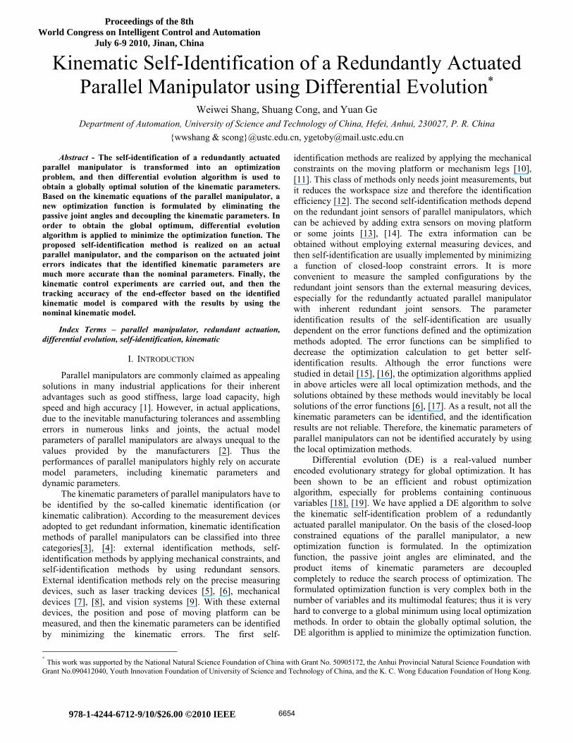
The experiment platform is a 2-DOF redundantly actuated parallel manipulator [20]. As shown in Fig.1, a reference frame is established in the workspace of the parallel manipulator. The parallel manipulator is actuated by three servo motors located at the base ( )1 1 1,a aA x y , ( )2 2 2a aA x y , and ( )3 3 3,a aA x y . The end-effector is mounted at the common joint point ( ),o oO x y , where three sub-chains meet. The definitions of the joints and links are as follows: , 1,2,3aiq i = refer to the actuated joint angles; , 1,2,3biq i = refer to the passive joint angles; , 1,2,3ail i = refer to the length of the actuated joint links; , 1,2,3bil i = refer to the length of the passive joint links.

From Fig.1, one can get ( ) ( )( ) ( )

cos cos, 1,2,3

sin sino ai ai ai bi bi

o ai ai ai bi bi

x x l q l qi

y y l q l q= + ⋅ + ⋅

== + ⋅ + ⋅

. (1)

Let the coordinates of the passive joints be ( ), , 1, 2,3i bi biB x y i = , then one can have

( ) ( )cos , sin , 1,2,3bi ai ai ai bi ai ai aix x l q y y l q i= + ⋅ = + ⋅ = (2) Substituting (2) into Eq. (1), one can get an equation group with three equations as

( ) ( )2 2 2 , 1,2,3o bi o bi bix x y y l i− + − = = . (3) Eliminating the secondary items in (3), one can have an equation group as

( ) ( )( ) ( )

2 1 2 1 2 1

3 1 3 1 3 1

2 2

2 2b b o b b o

b b o b b o

x x x y y y d d

x x x y y y d d

− + − = −

− + − = −, (4)

b3

A2

A3

A1

B1

B2

B3

Oa1q

a2qb2q

q

Y a3qb1q

X

l a1 l b1

lb2

la2

a3l

b3l

Fig. 1. Coordinates of the 2-DOF redundantly actuated parallel manipulator. where 2 2 2 , 1, 2,3i bi bi bid x y l i= + − = . Solve (4) yields the end-

effector coordinates as [21] ( ) ( ) ( )( ) ( ) ( )( )( ) ( ) ( )( ) ( ) ( )( )213132321

123312231

213132321

213132321

2

2

bbbbbbbbb

bbbbbbo

bbbbbbbbb

bbbbbbo

yyxyyxyyxxxdxxdxxd

y

yyxyyxyyxyydyydyyd

x

−+−+−−⋅+−⋅+−⋅

=

−+−+−−⋅+−⋅+−⋅

=. (5)

By applying the Cosine theorem to the triangle OBA ii in Fig. 1, the actuated joint angles can be expressed as

( )2 2 2arccos ( ) / (2 ) , 1,2,3i iai ai A O bi ai A o iq l l l l l iα= + − + = , (6)

where ( ) ( )2 2

iA O o ai o ail x x y y= − + − , and the angle

( )( ) / ( )i o ai o aiarctg y y x xα = − − is the angle between the line OAi and coordinate axis X . The passive joint angles can be

calculated as ( )tan 2 sin( ), cos( )bi o ai ai ai o ai ai aiq a y y l q x x l q= − − ⋅ − − ⋅ . (7)

III. KINEMATIC SELF-IDENTIFICATION WITH DIFFERENTIAL EVOLUTION

For the parallel manipulator studied in this paper, only three actuated joint angles can be measured by three absolute optical-electrical encoders, and the passive joint angles are unknown. As the parallel manipulator has two degrees-of-freedom, one joint sensor is redundant over the degree-of-freedom. The redundancy of the sensor information makes self-calibration possible by using the three inner encoders only, without applying any extra sensor. To determine the values of the actuated joint angles, the positive direction of the X axis in Fig.1 is defined as the zero positions and the anticlockwise direction is defined as the positive direction of the joint angles. Due to the assembly errors, there is always a bias angle between the sensor zero position and the zero position of the actuated joint.

Besides six link lengths ail , bil , 1, 2,3i = and six base coordinates ( ),ai aix y , 1, 2,3i = , three bias angles between the zero positions of the sensors and the zero positions of the actuated joints should be identified. Denote the bias angles by aiqΔ , 1, 2,3i = and the readings of the encoders by aiq , then the actuated joint angles can be expressed as

6655

ai ai aiq q q= + Δ (8) Among the six base coordinates, three of them must be set

to their nominal values to establish the coordinate frame before kinematic identification. Otherwise, the parallel manipulator can move freely in the workspace, and infinite solutions can be obtained through identification. Thus it is impossible to distinguish which solution is the actual one. Considering three coordinates must be predefined, there are altogether twelve kinematic parameters to be identified. Without losing generality, suppose that the base coordinate 1 1 2, ,a a ax y x are equal to their nominal values and regard them as constants. Therefore, three base coordinates 2 3 3, ,a a ay x y , six link lengths

, , 1, 2,3ai bil l i = , and three bias angles 1 2 3, ,a a aq q qΔ Δ Δ should be identified in the kinematic self-identification.

In order to realize the self-identification of the parallel manipulator, the kinematic parameter errors can be formulated by the closed-loop constrained equations as [17]

1 1 1 1 1 1

1 1 1 1 1 1

2 2 2 2 2 21

2 2 2 2 2 2

3 3 3 3 3 3

3 3

cos( ) cos( )sin( ) sin( )

cos( ) cos( )sin( ) sin( )cos( ) cos( )sin(

o a a a a b b

o a a a a b b

o a a a a b b

o a a a a b b

o a a a a b b

o a a a

x x l q q l qy y l q q l q

x x l q q l qE

y y l q q l qx x l q q l qy y l q

− − + Δ −− − + Δ −

− − + Δ −=

− − + Δ −− − + Δ −− − 3 3 3 3) sin( )a b bq l q

⎡ ⎤⎢ ⎥⎢ ⎥⎢ ⎥⎢ ⎥⎢ ⎥⎢ ⎥⎢ ⎥

+ Δ −⎢ ⎥⎣ ⎦

. (9)

Considering the passive joint angles biq can not be measured directly, by eliminating the terms respect to biq , (9) can be expressed as

( ) ( )( ) ( )( ) ( )

2 2 21 1 1 1 1 1 1 1 1

2 2 22 2 2 2 2 2 2 2 2 2

2 2 23 3 3 3 3 3 3 3 3

cos( ) sin( )

cos( ) sin( )

cos( ) sin( )

o a a a a o a a a a b

o a a a a o a a a a b

o a a a a o a a a a b

x x l q q y y l q q l

E x x l q q y y l q q l

x x l q q y y l q q l

⎡ ⎤− − + Δ + − − + Δ −⎢ ⎥⎢ ⎥= − − + Δ + − − + Δ −⎢ ⎥

− − + Δ + − − + Δ −⎢ ⎥⎣ ⎦(10)

In (10), the coupled products terms make the calculation of the self-identification difficult. To decouple these products, the coupled products terms can be expressed as

cos( ) cos( )cos( ) sin( )sin( )sin( ) sin( )cos( ) cos( )sin( )

ai ai ai ai ai ai ai ai ai

ai ai ai ai ai ai ai ai ai

l q q l q q l q ql q q l q q l q q

+ Δ = Δ − Δ+ Δ = Δ + Δ

(11)

In (11), cos( )ai ail qΔ and sin( )ai ail qΔ can be used instead of

ail and aiqΔ as parameters to be identified. Let cos( )ai ai il q lacΔ = and sin( )ai ai il q lasΔ = , then (11) can be

written by ( )

( )( )

( )( )

21 1 1 1 1

2 21 1 1 1 1 1

22 2 2 2 2

3 2 22 2 2 2 2 2

23 3 3 3 3

3

cos( ) sin( )

sin( ) cos( )

cos( ) sin( )

sin( ) cos( )

cos( ) sin( )

o a a a

o a a a b

o a a a

o a a a b

o a a a

o a

x x lac q las q

y y lac q las q l

x x lac q las qE

y y lac q las q l

x x lac q las q

y y la

− − +

+ − − − −

− − +=

+ − − − −

− − +

+ − −( )2 23 3 3 3 3sin( ) cos( )a a bc q las q l

⎡ ⎤⎢ ⎥⎢ ⎥⎢ ⎥⎢ ⎥⎢ ⎥⎢ ⎥⎢ ⎥⎢ ⎥⎢ ⎥⎢ ⎥− −⎣ ⎦

. (12)

For M sampled configurations, the kinematic parameters can be identified by minimizing the following optimization function

23 3 3

1 1( ) ( ) ( )

M MT

m mJ E m E m E m

= =

= =∑ ∑ . (13)

By using (13), the kinematic self-identification problem is now transformed into an optimization problem. When the self-identification finishes, parameters ail , 1,2,3i = and

aiqΔ , 1,2,3i = can be calculated as 2 2 , ( / ), 1,2,3ai i i ai i il lac las q arctg las lac i= + Δ = = . (14)

One can find that the error function 3E in Eq.(13) is continuous, nonlinear, no-convex, multi-dimensional, and it has a lot of local minima. Differential evolution (DE) has been shown to be an efficient and robust optimization algorithm, especially for problems containing continuous variables. Therefore, the DE algorithm is a good choice to the self-identification of the parallel manipulator [17]. DE is a population-based optimization algorithm, in which a candidate solution is called an individual and individuals constitute a population. The individuals evolution mainly through mutation, crossover, and selection operation. In an n variables problem, the individual in DE is represented by vector ( )1 2 , , nX x x x= . And the population for each generation G can be represented as iGX , 1,2, ,i N= , in which N is the population size. In mutation,

( ), 1 1, 2, 3,i G r G r G r GV X F X X+ = + ⋅ − , (15)

where random indexes 1 2 3, , { , [1, ]}r r r j j i j N∈ ≠ ∈ and the step size F is usually in the range of [0,2] . And in crossover,

( ), 1 1 , 1 2 , 1 , 1

, 1, 1

,

, , ,

if rand ( ) or ( )if rand ( ) or ( )

1,2, , ; 1,2, ,

i G i G i G ni G

ji Gji G

ji G

U U U U

V b j CR j rnbr iU

X b j CR j rnbr i

j n i N

+ + + +

++

=

≤ =⎧⎪= ⎨ > ≠⎪⎩= =

(16)

where rand ( ) [0,1]b j ∈ is the j th evaluation of a norm random number, [0,1]CR ∈ is the crossover constant set by the user, and ( )rnbr i is a randomly chosen index from n dimensions to ensure that at least one dimension parameter from , 1i GV + can be attained by , 1i GU + . In selection stage,

, 1 , 1 ,, 1

,

, if ( ) ( ), else

i G i G i Gi G

i G

U J U J XX

X+ +

+

<⎧⎪= ⎨⎪⎩

(17)

In the kinematic self-identification based on DE, the initial population is randomly generated. In every generation, mutation is employed according to (15) and crossover operation is implemented according to (16),. After mutation and crossover, check whether the individuals are still in the search range [ ]min max,X X . If any parameter is out of this range, this parameter is randomly regenerated. When this checking is finished, evaluate ,i GX and , 1i GU + . On the basis of the quality of ,i GX and , 1i GU + , selection operation is carried out according to (17) and the selected individuals constitute the new population of the next generation.

Based on the DE algorithm, the procedures of the kinematic self-identification can be designed as follows.

6656

(1) Select M different configurations of the end-effector for the parallel manipulator, then write down the readings of the actuated joint angles , 1,2,3aiq i = .

(2) Determine the values of the parameters in DE, such as population size N, step size F, and crossover constant CR.

(3) The initial population is initialized randomly in the search space according to the range of the variables, and then let the iterative number 1k = .

(4) Calculate the fitness function based on (13), and update the global optimizing individual if the global fitness function is improved.

(5) Execute the mutation, crossover, and selection operation according to (15)-(17) respectively to update individuals. If the end conditions are satisfied, then finish the optimization, else set the iterative number 1k k= + and return to step (4).

IV. KINEMATIC SELF-IDENTIFICATION EXPERIMENT

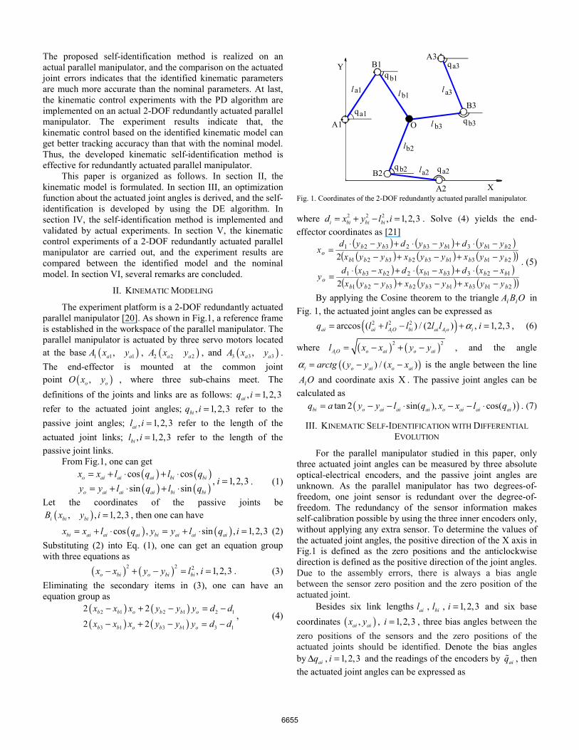
As shown in Fig.2, the actual experiment platform is a 2-DOF redundantly actuated parallel manipulator. It is equipped with three permanent magnet synchronous motors with harmonic gear drives. The actuated joint angles are measured with absolute optical-electrical encoders.

In the kinematic self-identification experiment, 100 positions of the end-effector are sampled on a circle. The center of the circle is (290, 250) which is the geometric center of the workspace of the parallel manipulator, and the radius of the circle is 40 mm. By this selection, all the kinematic parameters of the parallel manipulator can be excited sufficiently and the sensor errors can be balanced completely. In the actual kinematic self-identification, the parameters of the DE are tuned as follows: the population size is often set as

10N n= × , where n represents the dimensions of the optimization variables. In this problem, 12n = , thus 120N = . In order to make the differential parts of the algorithm not be too large or too small, one can set 0.5F = . In crossover, the constant is usually set between 0.8 and 1, and here we set

0.8CR = . By using the DE method, all the twelve kinematic

parameters are identified under the optimization function J . The best solution found is regarded as the final identification result of the kinematic parameters shown in Table 1. Also, the nominal values of the kinematic parameters are shown in Table 1 as comparison. Without losing generality, suppose that the base coordinate 1 1 2, ,a a ax y x are equal to their nominal values as 1 1 20, 250, 433a a ax y x= = = .

To see whether the self-identification results are more accurate than the nominal values provided by the producer, comparisons can be made between the identified parameters and the nominal parameters. The actuated joint angles can be measured directly by the encoders, then the coordinates of the end-effector can be calculated based on the forward kinematic (5). And with the forward kinematic solution, the actuated

Fig.2. The prototype of the 2-DOF redundantly actuated parallel manipulator.

TABLE I IDENTIFIED RESULTS AND NOMINAL VALUES OF THE KINEMATIC PARAMETERS

Parameters Nominal value Identified value

2ay (mm) 0 2.1571

3ax (mm) 433 436.5436

3ay (mm) 500 500.4123

1al (mm) 244 243.4827

2al (mm) 244 243.5634

3al (mm) 244 242.3579

1bl (mm) 244 243.8194

2bl (mm) 244 243.9168

3bl (mm) 244 246.7952

1aqΔ (rad) 0 2.2215e-3

2aqΔ (rad) 0 1.2223e-3

3aqΔ (rad) 0 2.7343e-3

joint angles can be calculated based on the inverse kinematic (6). If the kinematic parameters were accurate enough, then the calculated joint angles would be the same as the joint angles measured by encoders. On the contrary, if the kinematic parameters are not accurate, then the errors between the calculated joint angles and the measured angles will be large.

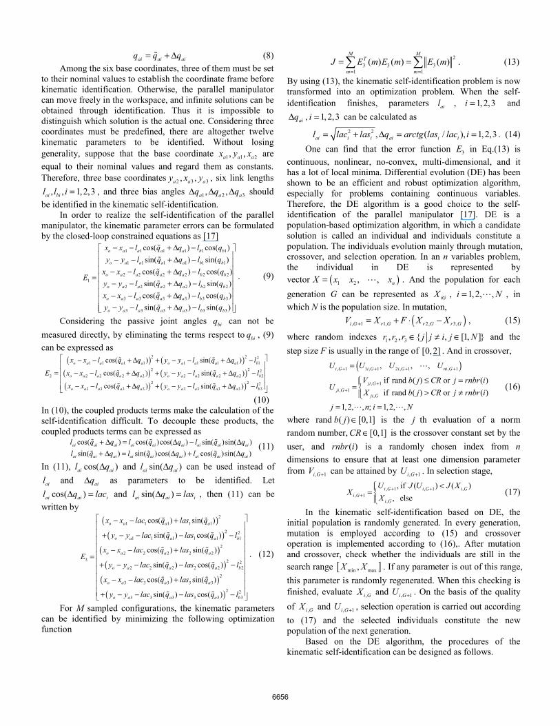
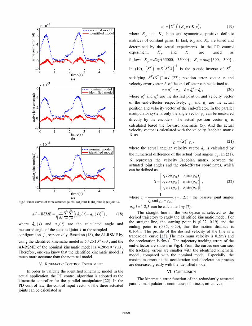
In order to validate the identified kinematic model, the errors between the measured joint angles and the calculated joint angles are studied. In our experiment, the actual test trajectory of the end-effector of the parallel manipulator is a circle repeated for two times. The center of the circle is (216.5, 250), and the radius is 70mm. The error curves of the three actuated joints are shown in Fig.3. In Fig.3, the red curves are the actuated joint errors based on the identified kinematic model, and the blue curves are the errors based on the nominal kinematic model. From these error curves, one can find that, the identified kinematic model is much more accurate than the nominal model.

Furthermore, in order to compare the identified kinematic model with the nominal kinematic model, the actuated joint root mean square error (AJ-RSME) can be defined by

6657

activ

e joi

nt er

ror(r

ad)

-2

0

2

4

6

8

0 1 2 3 4 5time(s)

identified modelnominal model

x 10-3

(a)

identified modelnominal model

-2

0

2

4

6

0 1 2 3 4 5time(s)

x 10-3

activ

e joi

nt er

ror(r

ad)

(b)

identified modelnominal model

-2

0

2

4

6

0 1 2 3 4 5time(s)

x 10-3

activ

e joi

nt er

ror(r

ad)

(c)

Fig.3. Error curves of three actuated joints: (a) joint 1; (b) joint 2; (c) joint 3.

( )( )32

1 1

1 ˆ ( ) ( )M

ai aii j

AJ RSME q j q jM = =

− = −∑∑ , (18)

where ˆ ( )aiq j and ( )aiq j are the calculated angle and measured angle of the actuated joint i at the sampled configuration j , respectively. Based on (18), the AJ-RSME by using the identified kinematic model is 45.42 10 rad−× , and the AJ-RSME of the nominal kinematic model is 34.20 10 rad−× . Therefore, one can know that the identified kinematic model is much more accurate than the nominal model.

V. KINEMATIC CONTROL EXPERIMENT

In order to validate the identified kinematic model in the actual application, the PD control algorithm is adopted as the kinematic controller for the parallel manipulator [22]. In the PD control law, the control input vector of the three actuated joints can be calculated as

( ) ( )Ta p vS K e K eτ

+= + , (19)

where pK and vK both are symmetric, positive definite matrices of constant gains. In fact, pK and vK are tuned and determined by the actual experiments. In the PD control experiment, pK and vK are tuned as

follows: ( )35000, 35000pK diag= , ( )300, 300vK diag= .

In (19), ( ) ( ) 1T TS S S S+ −

= is the pseudo-inverse of TS ,

satisfying ( )T TS S I+ = [22]; position error vector e and velocity error vector e of the end-effector can be defined as

,d de e e ee q q e q q= − = − , (20)

where deq and d

eq are the desired position and velocity vector of the end-effector respectively; eq and eq are the actual position and velocity vector of the end-effector. In the parallel manipulator system, only the angle vector aq can be measured directly by the encoders. The actual position vector eq is calculated based the forward kinematic (5). And the actual velocity vector is calculated with the velocity Jacobian matrix S as

( )e aq S q+= , (21) where the actual angular velocity vector aq is calculated by the numerical difference of the actual joint angles aq . In (21), S represents the velocity Jacobian matrix between the actuated joint angles and the end-effector coordinates, which can be defined as

1 1 1 1

2 2 2 2

3 3 3 3

cos( ) sin( )cos( ) sin( )cos( ) sin( )

b b

b b

b b

r q r qS r q r q

r q r q

⎡ ⎤⎢ ⎥= ⎢ ⎥⎢ ⎥⎣ ⎦

, (22)

where 1 , 1,2,3sin( )i

ai bi ai

r il q q

= =−

; the passive joint angles

, 1,2,3biq i = can be calculated by (7). The straight line in the workspace is selected as the

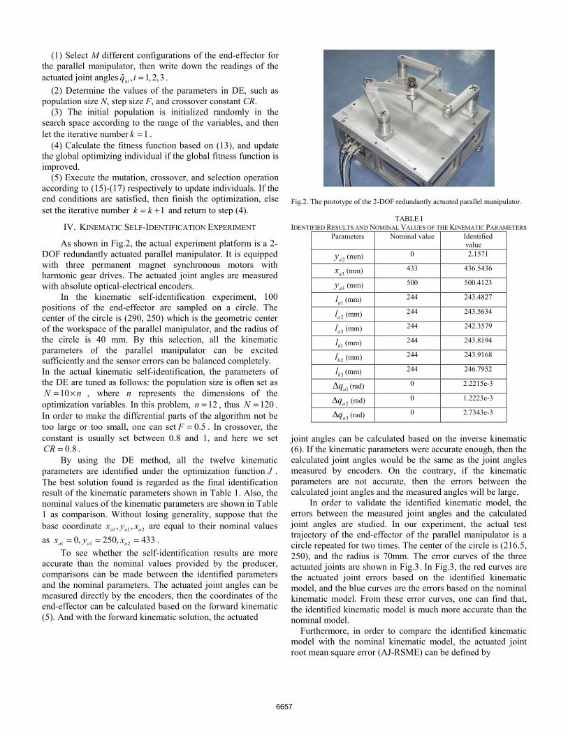
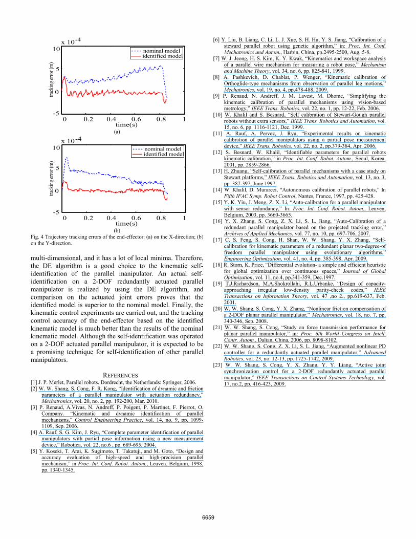
desired trajectory to study the identified kinematic model. For the straight line, the starting point is (0.22, 0.19) and the ending point is (0.35, 0.29), thus the motion distance is 0.164m. The profile of the desired velocity of the line is a trapezoidal curve [23]. The maximum velocity is 0.2m/s and the acceleration is 5m/s2. The trajectory tracking errors of the end-effector are shown in Fig.4. From the curves one can see, the tracking, errors are smaller with the identified kinematic model, compared with the nominal model. Especially, the maximum errors at the acceleration and deceleration process are decreased greatly with the identified model.

VI. CONCLUSION

The kinematic error function of the redundantly actuated parallel manipulator is continuous, nonlinear, no-convex,

6658

0 0.2 0.4 0.6 0.8 1-5

0

5

10x 10-4

track

ing er

ror (

m)

time(s)

identified modelnominal model

(a)

identified modelnominal model

0 0.2 0.4 0.6 0.8 1-5

0

5

10x 10-4

track

ing er

ror (

m)

time(s) (b)

Fig. 4 Trajectory tracking errors of the end-effector: (a) on the X-direction; (b) on the Y-direction. multi-dimensional, and it has a lot of local minima. Therefore, the DE algorithm is a good choice to the kinematic self-identification of the parallel manipulator. An actual self- identification on a 2-DOF redundantly actuated parallel manipulator is realized by using the DE algorithm, and comparison on the actuated joint errors proves that the identified model is superior to the nominal model. Finally, the kinematic control experiments are carried out, and the tracking control accuracy of the end-effector based on the identified kinematic model is much better than the results of the nominal kinematic model. Although the self-identification was operated on a 2-DOF actuated parallel manipulator, it is expected to be a promising technique for self-identification of other parallel manipulators.

REFERENCES [1] J. P. Merlet, Parallel robots. Dordrecht, the Netherlands: Springer, 2006. [2] W. W. Shang, S. Cong, F. R. Kong, “Identification of dynamic and friction

parameters of a parallel manipulator with actuation redundancy,” Mechatronics, vol. 20, no. 2, pp. 192-200, Mar. 2010.

[3] P. Renaud, A.Vivas, N. Andreff, P. Poigent, P. Martinet, F. Pierrot, O. Company. “Kinematic and dynamic identification of parallel mechanisms,” Control Engineering Practice, vol. 14, no. 9, pp. 1099-1109, Sep. 2006.

[4] A. Rauf, S. G. Kim, J. Ryu, “Complete parameter identification of parallel manipulators with partial pose information using a new measurement device,” Robotica, vol. 22, no.6 , pp. 689-695, 2004.

[5] Y. Koseki, T. Arai, K. Sugimoto, T. Takatuji, and M. Goto, “Design and accuracy evaluation of high-speed and high-precision parallel mechanism,” in Proc. Int. Conf. Robot. Autom., Leuven, Belgium, 1998, pp. 1340-1345.

[6] Y. Liu, B. Liang, C. Li, L. J. Xue, S. H. Hu, Y. S. Jiang, “Calibration of a steward parallel robot using genetic algorithm,” in: Proc. Int. Conf. Mechatronics and Autom., Harbin, China, pp.2495-2500, Aug. 5-8.

[7] W. J. Jeong, H. S. Kim, K. Y. Kwak, “Kinematics and workspace analysis of a parallel wire mechanism for measuring a robot pose,” Mechanism and Machine Theory, vol. 34, no. 6, pp. 825-841, 1999.

[8] A. Pashkevich, D. Chablat, P. Wenger, “Kinematic calibration of Orthoglide-type mechanisms from observation of parallel leg motions,” Mechatronics, vol. 19, no. 4, pp.478-488, 2009.

[9] P. Renaud, N. Andreff, J. M. Lavest, M. Dhome, “Simplifying the kinematic calibration of parallel mechanisms using vision-based metrology,” IEEE Trans. Robotics, vol. 22, no. 1, pp. 12-22, Feb. 2006.

[10] W. Khalil and S. Besnard, “Self calibration of Stewart-Gough parallel robots without extra sensors,” IEEE Trans. Robotics and Automation, vol. 15, no. 6, pp. 1116-1121, Dec. 1999.

[11] A. Rauf, A. Pervez, J. Ryu, “Experimental results on kinematic calibration of parallel manipulators using a partial pose measurement device,” IEEE Trans. Robotics, vol. 22, no. 2, pp.379-384, Apr. 2006.

[12] S. Besnard, W. Khalil, “Identifiable parameters for parallel robots kinematic calibration,” in Proc. Int. Conf. Robot. Autom., Seoul, Korea, 2001, pp. 2859-2866.

[13] H. Zhuang, “Self-calibration of parallel mechanisms with a case study on Stewart platforms,” IEEE Trans. Robotics and Automation, vol. 13, no. 3, pp. 387-397, June 1997.

[14] W. Khalil, D. Murareci, “Autonomous calibration of parallel robots,” In Fifth IFAC Symp. Robot Control, Nantes, France, 1997, pp. 425-428.

[15] Y. K. Yiu, J. Meng, Z. X. Li, “Auto-calibration for a parallel manipulator with sensor redundancy,” In: Proc. Int. Conf. Robot. Autom., Leuven, Belgium, 2003, pp. 3660-3665.

[16] Y. X. Zhang, S. Cong, Z. X. Li, S. L. Jiang, “Auto-Calibration of a redundant parallel manipulator based on the projected tracking error,” Archives of Applied Mechanics, vol. 77, no. 10, pp. 697-706, 2007.

[17] C. S. Feng, S. Cong, H. Shan, W. W. Shang, Y. X. Zhang, “Self-calibration for kinematic parameters of a redundant planar two-degree-of freedom parallel manipulator using evolutionary algorithms,” Engineering Optimization, vol. 41, no. 4, pp. 385-398, Apr. 2009.

[18] R. Storn, K. Price, “Differential evolution- a simple and efficient heuristic for global optimization over continuous spaces,” Journal of Global Optimization, vol. 11, no.4, pp.341-359, Dec.1997.

[19] T.J.Richardson, M.A.Shokrollahi, R.L.Urbanke, “Design of capacity-approaching irregular low-density parity-check codes,” IEEE Transactions on Information Theory, vol. 47 ,no 2., pp.619-637, Feb. 2001.

[20] W. W. Shang, S. Cong, Y. X. Zhang, “Nonlinear friction compensation of a 2-DOF planar parallel manipulator,” Mechatronics, vol. 18, no. 7, pp. 340-346, Sep. 2008.

[21] W. W. Shang, S. Cong, “Study on force transmission performance for planar parallel manipulator,” in: Proc. 6th World Congress on Intell. Contr. Autom., Dalian, China, 2006, pp. 8098-8102.

[22] W. W. Shang, S. Cong, Z. X. Li, S. L. Jiang, “Augmented nonlinear PD controller for a redundantly actuated parallel manipulator,” Advanced Robotics, vol. 23, no. 12-13, pp. 1725-1742, 2009.

[23] W. W. Shang, S. Cong, Y. X. Zhang, Y. Y. Liang, “Active joint synchronization control for a 2-DOF redundantly actuated parallel manipulator,” IEEE Transactions on Control Systems Technology, vol. 17, no.2, pp. 416-423, 2009.

6659