Killer Sudoku Solver - Dissertation Tools · This report describes the design and development of the Killer Sudoku Solver, which ... Figure 6.5: Comparison of solved and unsolved

1

Killer Sudoku Solver

Student: Mohammed Rizwan

[email protected]

Supervisor: Dr. Andrea Schalk

[email protected]

Date: 29th April 2008

2

Killer Sudoku Solver

Student: Mohammed Rizwan

Supervisor: Dr. Andrea Schalk

Date: 29th April 2008

Abstract

Killer Sudoku is a puzzle game which combines elements of two other puzzle games,

Sudoku and Kakuro. However, when compared to original Sudoku, there has been relatively

little research conducted into the logic and techniques required to complete Killer Sudoku

puzzles.

This report describes the design and development of the Killer Sudoku Solver, which

solves Killer Sudoku puzzles by employing human-like reasoning. To prove its success, the

solver is able to explain its decisions and works with user-inputted puzzles. The results of

how the solver performs are discussed in detail, which are then used to evaluate the success

of this project. Possible extensions to the solver are also discussed.

3

Acknowledgements

Firstly, I would like to like to thank Dr. Andrea Schalk, for her invaluable support

and guidance throughout the course of the project.

Thanks also go to the Killer Sudoku community, my friends and of course, my

family.

4

Table of Contents Chapter 1: Introduction ...............................................................................9

1.1. Sudoku and Killer Sudoku in the United Kingdom............................................................ 9 1.2. The Project..............................................................................................................................11

1.2.1. Project Objectives ..........................................................................................................11 1.2.2. Functional Requirements...............................................................................................11 1.2.3. Non-Functional Requirements.....................................................................................13

Chapter 2: Background ............................................................................. 14

2.1. Sudoku .....................................................................................................................................14 2.1.1. Solving Techniques ........................................................................................................14 2.1.2. Measuring Difficulty.......................................................................................................18

2.2. Kakuro .....................................................................................................................................19 2.2.1. Solving Techniques ........................................................................................................20 2.2.2. Measuring Difficulty.......................................................................................................24

2.3. Killer Sudoku ..........................................................................................................................24 2.3.1. Solving Techniques ........................................................................................................25 2.3.2. Measuring Difficulty.......................................................................................................27

2.4. Software Development Methodology.................................................................................28 2.4.1. Waterfall Methodology ..................................................................................................28 2.4.2. Spiral Methodology ........................................................................................................28 2.4.3. The Unified Process.......................................................................................................29

Chapter 3: Design......................................................................................30

3.1. Design Overview....................................................................................................................30 3.1.1. Development Methodology Decision .........................................................................30 3.1.2. Program Architecture.....................................................................................................30

3.2. Internal Representation .........................................................................................................31 3.2.1. Grid...................................................................................................................................32 3.2.2. Game................................................................................................................................32 3.2.3. Puzzle ...............................................................................................................................33 3.2.4. State ..................................................................................................................................33 3.2.5. Puzzle History .................................................................................................................33 3.2.6. Grid Restriction ..............................................................................................................33

3.3. User Interface .........................................................................................................................34 3.3.1. Eight Golden Rules of Interface Design ....................................................................34 3.3.2. Use Case 1: Play and Solve a Puzzle ............................................................................34 3.3.3. Use Case 2: Input a Puzzle............................................................................................35 3.3.4. Solver Input Designs......................................................................................................36 3.3.5. Solver GUI Designs .......................................................................................................37 3.3.6. Puzzle Input GUI Design .............................................................................................40

3.4. Solving Techniques................................................................................................................41 Chapter 4: Implementation and Solving Techniques ..............................43

4.1. Development Tools ...............................................................................................................43

5

4.2. Internal Representation .........................................................................................................43 4.2.1. Puzzle ...............................................................................................................................44 4.2.2. Grid Initialisation............................................................................................................46 4.2.3. Puzzle History .................................................................................................................47

4.3. User Interface .........................................................................................................................49 4.3.1. Solver Grid ......................................................................................................................49 4.3.2. Puzzle Input Grid...........................................................................................................50 4.3.3. Puzzle Input Error Prevention.....................................................................................50 4.3.4. Cell Colours.....................................................................................................................51 4.3.5. User Input........................................................................................................................52 4.3.6. Help Documents ............................................................................................................52

4.4. Solving Techniques................................................................................................................52 4.4.1. Evaluators ........................................................................................................................53 4.4.2. Grid Manipulator............................................................................................................53 4.4.3. Rule Interface..................................................................................................................53 4.4.4. One and Two Solution Cages Technique ...................................................................54 4.4.5. Row and Column Value Checker Technique.............................................................55 4.4.6. Holes and Stubs Techniques.........................................................................................55 4.4.7. Sum Checker Technique................................................................................................56 4.4.8. Cage Possible Finder Technique ..................................................................................56 4.4.9. Eight Cell Technique .....................................................................................................57 4.4.10. Cell Impossible Count Technique .............................................................................58 4.4.11. Cage Completion Technique ......................................................................................58

Chapter 5: User-Software Interaction .......................................................59

5.1. Use Cases.................................................................................................................................59 5.1.1. Play and Solve Puzzle Use Case ...................................................................................59 5.1.2. Input Puzzle Use Case ...................................................................................................62

5.2. Puzzle History Usage.............................................................................................................64 5.2.1. One Solution Technique ...............................................................................................64 5.2.2. Holes Technique.............................................................................................................64 5.2.3. Sum Checker Technique................................................................................................66 5.2.4. Value Checker Technique .............................................................................................66

Chapter 6: Results .....................................................................................68

6.1. Solver Success.........................................................................................................................68 6.2. Effectiveness of the Solving Techniques............................................................................70 6.3. Puzzle Difficulty .....................................................................................................................71

Chapter 7: Conclusion ...............................................................................75

7.1. Project Summary ....................................................................................................................75 7.2. Conclusion...............................................................................................................................75 7.3. Future Work............................................................................................................................77

References .................................................................................................79

6

Glossary .....................................................................................................82 Appendix A: Eight Golden Rules of Interface Design.............................83 Appendix B: XML Puzzle .........................................................................85 Appendix C: User Help Documents.........................................................88 Appendix D: Killer Sudoku Questionnaire...............................................93

7

Table of Figures Figure 1.1: Dr. Kawashima’s Brain Training screenshot......................................................................9 Figure 2.1: A Sudoku puzzle from The Times. ................................................................................15 Figure 2.2: The result of cross-hatch scanning. .............................................................................16 Figure 2.3: Sudoku puzzle showing the use of the candidate lines technique...........................17 Figure 2.4: An X-Wing. .....................................................................................................................18 Figure 2.5: An empty Kakuro puzzle. .............................................................................................20 Figure 2.6: A solved Kakuro puzzle. ...............................................................................................20 Figure 2.7: Cross referencing............................................................................................................22 Figure 2.8: Criss-cross arithmetic.....................................................................................................23 Figure 2.9: Criss-cross arithmetic with multiple cells....................................................................23 Figure 2.10: A typical Killer Sudoku puzzle...................................................................................25 Figure 2.11: Stub technique with two columns. ............................................................................27 Figure 3.1: Input method one. .........................................................................................................37 Figure 3.2: Input method two. .........................................................................................................37 Figure 3.3: Design 1 for the solver interface..................................................................................38 Figure 3.4: Design 2 for the solver interface..................................................................................39 Figure 3.5: Design for the puzzle input screen. .............................................................................41 Figure 4.1: Overview of the internal representation of the software. ........................................44 Figure 4.2: XML representation for a puzzle in its initial state. ..................................................45 Figure 4.3: XML representation for a puzzle in its second state.................................................45 Figure 4.4: Code extract from the parseCell() method. ................................................................47 Figure 4.5: Code extract from the parseCage() method. ..............................................................47 Figure 4.6: An example puzzle history window.............................................................................48 Figure 4.7: A grid showing a half-completed puzzle.....................................................................50 Figure 4.8: Error message displayed when user inputs an erroneous cage................................51 Figure 4.9: Grids displaying the default colours and the max colours. ......................................52 Figure 4.10: Code implemented for the ‘Rule’ interface. .............................................................54 Figure 5.1: Puzzle selection...............................................................................................................59 Figure 5.2: User attempt at the puzzle. ...........................................................................................60 Figure 5.3: The action history...........................................................................................................60 Figure 5.4: Text-free history. ............................................................................................................61 Figure 5.5: The states of the puzzle; from a fully incomplete puzzle to a complete one.......61 Figure 5.6: Message notifying the user that the solver could not solve the puzzle. ................62 Figure 5.7: Input of pre-filled cells. .................................................................................................62 Figure 5.8: Input of the cages...........................................................................................................63 Figure 5.9: Edit Cage and Delete Cage options.............................................................................63 Figure 5.10: Invalid puzzle notification. .........................................................................................63 Figure 5.11: A ‘one solution’ cage....................................................................................................64 Figure 5.12: One Solution Cage explanation..................................................................................64 Figure 5.13: A screenshot of a two cell hole. .................................................................................65 Figure 5.14: ‘One Region Hole’ possible set. .................................................................................65 Figure 5.15: Effect of the hole technique.......................................................................................65 Figure 5.16: Sum Checker technique screenshot...........................................................................66 Figure 5.17: Sum Checker explanation. ..........................................................................................66 Figure 5.18: Value Checker screenshot...........................................................................................67 Figure 5.19: Value Checker rule explanation. ................................................................................67

8

Figure 6.1: Success rate histogram for the Killer Sudoku Online website. ....................................69 Figure 6.2: Success rate histogram for the The Times book. .........................................................69 Figure 6.3: Success rate histogram for the The Big Book of Killer Su Doku book........................70 Figure 6.4: Solving technique analysis.............................................................................................71 Figure 6.5: Comparison of solved and unsolved puzzles. ............................................................72 Figure 6.6: Average states histogram for the Killer Sudoku Online website. ................................73 Figure 6.7: Average states histogram for the The Times book. .....................................................73 Figure 6.8: Average states histogram for the The Big Book of Killer Su Doku book....................74 Figure 7.1: A puzzle which could not be further solved by the solver. .....................................76

9

Chapter 1: Introduction

1.1. Sudoku and Killer Sudoku in the United Kingdom

Over the last 3 years, the popularity of Sudoku in the United Kingdom has risen

considerably [1]. Sudoku is a number placement game played on (typically) a 9 x 9 grid. The

grid is empty, except a few cells, for which values are provided. These pre-filled cells are

expected to provide enough clues to help the user fill in the rest of the grid. The grid must

then be completed such that every row, column and nonet 1 contains every digit from 1-9

(depending on the grid size) exactly once. A certain degree of logic is required to solve the

various Sudoku puzzles.

British newspapers have done much to promote Sudoku by publishing daily puzzles

and even producing books containing many Sudoku puzzles. In recent years, Sudoku has

also found a home in our computers, appearing on many Sudoku-dedicated websites and

even in video games (Figure 1.1). This has led to a wider range of players having access to

Sudoku puzzles, and has also meant that such puzzle games are no longer restricted to just

being played with a pen and paper.

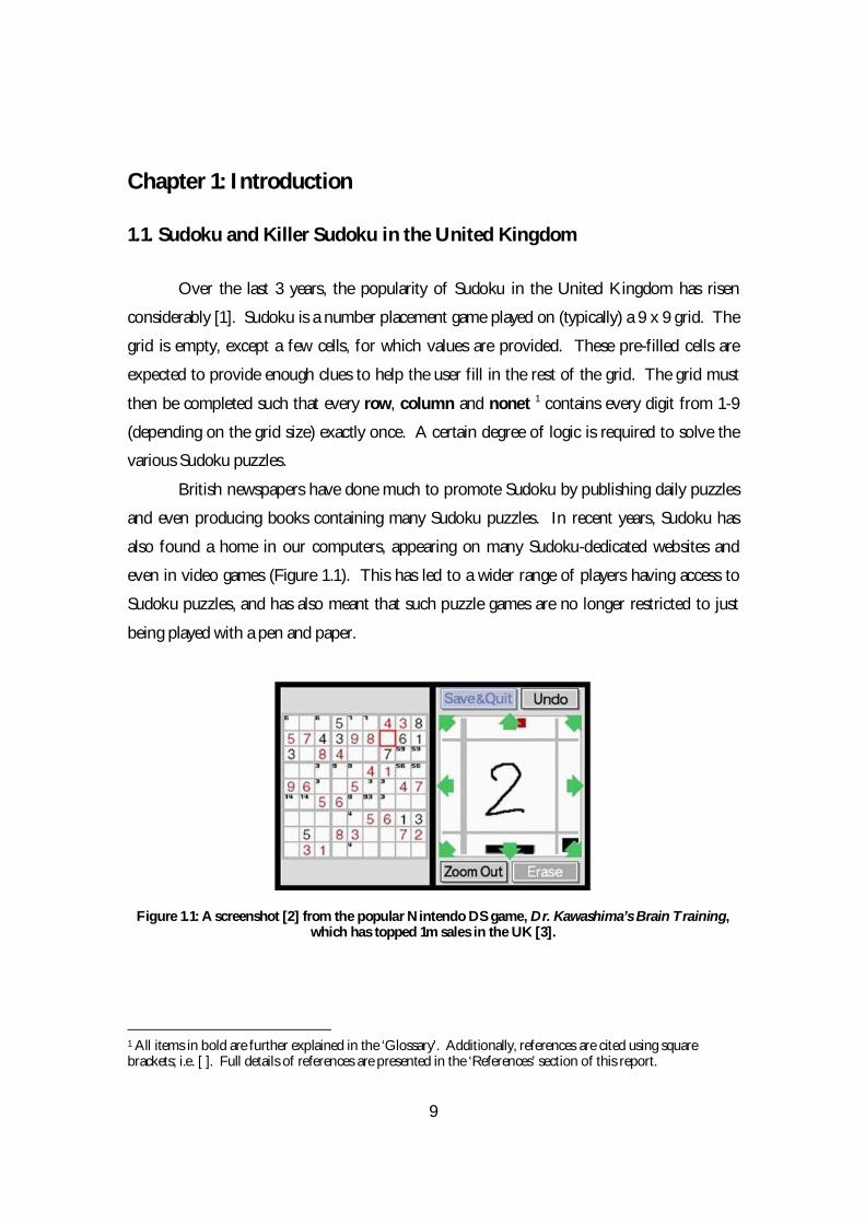
Figure 1.1: A screenshot [2] from the popular Nintendo DS game, Dr. Kawashima’s Brain Training, which has topped 1m sales in the UK [3].

1 All items in bold are further explained in the ‘Glossary’. Additionally, references are cited using square brackets; i.e. [ ]. Full details of references are presented in the ‘References’ section of this report.

10

The increased levels of interest have resulted in extensive research being conducted

into Sudoku. Techniques for both solving and creating puzzles have been the subject for

much of this study. The research has largely been successful, with highly advanced solvers

available freely over the Internet.

However, the focus of this project is not Sudoku, but is in fact a variant called ‘Killer

Sudoku’. The premise of Killer Sudoku is the same as that of Sudoku; namely to complete

the grid with every row, column and nonet containing the digits from 1-9 exactly once2. The

fundamental difference is that, unlike Sudoku, the grid does not have any pre-filled cells.

Rather, the player is faced with an empty grid made up of cages. Each cage has a value

attached to it and is made up of an indeterminate number of cells. The sum of the cell

values in the cage must be equal to the cage value. This additional mathematical aspect

comes from a puzzle game called ‘Kakuro’. These cages are the only hints the player has in

order to complete the puzzle.

There is much to suggest that Killer Sudoku will find popularity in the United

Kingdom, and indeed, in the western world. Much like Sudoku before it, Killer Sudoku

became popular in Japan first, where Killer Sudoku (or ‘Samunamupure’ as it is known in

Japan; Killer Sudoku is a phrase coined by The Times [4]) became the choice game for those

who had grown weary of Sudoku, or indeed for those who were simply looking for a puzzle

game to complement Sudoku. One could propose that we are witnessing this already in the

United Kingdom. National newspapers, such as The Times and Guardian, have already started

printing daily Killer Sudoku puzzles on their games pages, and many bookshops now stock

Killer Sudoku puzzle compilations alongside original Sudoku books.

Despite the growing popularity of Killer Sudoku, there has been relatively little study

expended into the formulation of Killer Sudoku solving techniques. Whilst various websites

contain some tips for players, they are not particularly exhaustive, and certainly would not

help players tackle the harder Killer Sudoku puzzles. Most importantly however, a logical

Killer Sudoku solver does not yet exist.

2 Unless stated otherwise, I will assume that the Sudoku and Killer Sudoku puzzles under discussion are being played on 9x9 grids.

11

1.2. The Project

1.2.1. Project Objectives

The aim of the project was to produce a solver for Killer Sudoku. Unlike many of

the Sudoku solvers out there, this solver aimed to use human-like reasoning and behaviour

to solve Killer Sudoku puzzles. This would mean that each puzzle would be approached

differently, with the solving policy being adapted for each puzzle. The alternative to this

approach would be to create a solver which employs a brute-force solving strategy. This

would involve trying out every possible value at every cell, and iterating until the solution

was reached. While this would invariably solve puzzles, it would not provide us with any

useful analyses on Killer Sudoku. We would not be able to find the most effective solving

techniques or even attempt to surmise the factors which contribute towards the difficulty of

Killer Sudoku puzzles.

By imitating a human player however, the solver would be able to explain its

decisions to the user, to show exactly how a puzzle was solved. This would then provide the

opportunity for the solver to be used as a learning aid, for players who wish to become more

proficient Killer Sudoku players. Furthermore, it was hoped that analysis of the

performance and behaviour of the solver would reveal effective solving techniques, how to

measure the difficulty of Killer Sudoku puzzles and more.

Thus, the objectives identified for the project were:

Objective 1: To develop a program which solves Killer Sudoku puzzles by employing

human-like logic and reasoning.

Objective 2: To assess the effectiveness of the various solving techniques.

Objective 3: To investigate the means by which the difficulty of Killer Sudoku puzzles can

be measured.

1.2.2. Functional Requirements The following functional requirements were identified:

12

1.2.2a: The software should be able to solve medium-rated difficulty puzzles from the Killer

Sudoku Online [5] website.

In order to test the capabilities of the solver, it is imperative that the puzzles used are

challenging. Additionally, they should come from a source which regularly publishes an

array of puzzles; ranging from easy to difficult puzzles, with a level of consistency between

the various difficulties. Upon discussion with Dr. Andrea Schalk, it was agreed that the

puzzles from the Killer Sudoku Online website will be used. This does not mean that testing is

limited to just this source.

1.2.2b: Users should be able to input puzzles into the software.

In order to provide the solver with puzzles to solve, a mechanism to allow users to input

their own puzzles should exist.

1.2.2c: The software should allow users to play Killer Sudoku.

To effectively fulfil the software’s role as a learning aid, it is essential that the users are first

allowed to attempt the puzzle.

1.2.2d: The solver should provide the user with feedback, explaining the steps it took in order to

solve a puzzle.

Upon solving a puzzle, the solver must offer a detailed explanation of how the puzzle was

solved. The user should be able to step through the solution, viewing the result of the

decisions the solver made.

1.2.2e: If the solver cannot successfully solve a puzzle, it should notify the user of this and

subsequently present the user with the half-completed puzzle.

It is likely that the solver will have to attempt a puzzle it cannot solve. In such cases, the

solver must be able to make available its progress to the user. The user will then be able to

attempt to complete the rest of the puzzle.

13

1.2.3. Non-Functional Requirements

The following non-functional requirements have been identified:

1.2.3a: Help documentation should be provided.

Due to the fact that the solver is aimed at all types of users, help documentation is required

to cater for those who are unfamiliar with Killer Sudoku, or who simply need help operating

the software.

1.2.3b: The solver should be able to solve puzzles quicker than a human player.

While the main priority is for the software to solve Killer Sudoku puzzles, it should do so in

less time than it would take for a human player to solve the puzzle.

1.2.3c: The software should be platform independent.

The program must work on various operating systems.

14

Chapter 2: Background

2.1. Sudoku

As discussed, Sudoku is a number placement game typically played on a 9 by 9 grid. The

aim of the game is to fill the grid, ensuring that every row, column and nonet contains the

digits 1-9 exactly once. Originally created in New York in 1979 where it was named Number

Place, Sudoku found widespread popularity in Japan during the late 1980s and throughout the

1990s [6]. In recent years, Sudoku has become a household name in the UK, with regular

puzzles being published in newspapers and on dedicated websites.

2.1.1. Solving Techniques

The techniques needed for solving Sudoku puzzles are well documented, to the

extent that the many techniques now have an agreed name within the Sudoku community.

In general, there are two types of solving techniques; one type which results in the

assignment of a value to a cell, and the second type which helps to reduce the possible values

a cell might be. Some techniques for solving Sudoku puzzles are examined:

Sudoku Technique 1: Naked Single

Cells which have only one possible value are known as ‘Naked Singles’. Such cells

may not be obvious naked singles from the outset, and as a result, need to be checked for

regularly. Furthermore, naked singles can become apparent in a number of ways. For

example, when a row, column or nonet has had 8 of its cells filled in, the remaining cell in

the region will only have one possible value, thus becoming a naked single.

Sudoku Technique 2: Hidden Single

Hidden singles are cells which seemingly have many different possible values, but

upon closer inspection, can actually only contain a certain value. Unlike naked singles where

15

a cell is marked with only one possibility, hidden single cells may be marked with many

possibilities. However, by examining the region the cell belongs to, one may notice that a

value appears only in that cell as a possibility. As all values must appear exactly once in a

region, the other possible values for the cell must therefore be discarded.

Sudoku Technique 3: Cross Hatch Scanning

Cross hatch scanning [7] is a technique used to eliminate possible values from cells

and can lead to some cells being assigned values. The technique involves looking at each

numeral from 1 to 9, and drawing a line through any rows and columns in which they

appear. In general, those numerals which have the most occurrences in the grid are targeted

first. The result of this process is a grid in which one can visually see where the numeral can

and can not occur. Consider the example Sudoku puzzle given in Figure 2.1.

Figure 2.1: A Sudoku puzzle [8] from The Times. This particular puzzle was rated as ‘Difficult’.

The puzzle shown in this figure has not had any cells solved yet (i.e. the cell values shown

are the pre-filled ones). By employing the cross-hatching technique on this grid we find that

16

the value 1 must go into the cells R1C2 and R4C73 (Figure 2.2). Further cross-hatch

scanning reveals that cell R6C7 must contain a 3.

Figure 2.2: The result of cross-hatch scanning with the numeral 1.

Sudoku Technique 4: Candidate Lines

The candidate lines technique is one which helps minimise the possible values a cell

can contain. Whereas the cross-hatch scanning relied on looking primarily along rows and

columns, the candidate lines strategy examines the possible values in each nonet first. Upon

doing so, the player can identify which possible values lie within the same row or column. If

they lie in just one of these horizontal or vertical regions, the value under scrutiny can be

removed as a possible value from the rest of the row or column. The example in Figure 2.3

shows clearly the use of this technique. Looking at the bottom-right nonet4, the value 4 is

only possible in column eight. Therefore, the rest of this column can not contain a 4,

meaning that any cells with the possible value of 4 are amended accordingly. This allows the

player to deduce that cell R7C8 must hold the value 2.

3 Cell coordinates will be given in the form RpCq, where p and q are the row and column numbers respectively. Figure 2.1 displays the row and column numbers. 4 Nonets, like rows and columns, will also be numbered, and will be presented in the form Nr, where r is a number from 1 to 9. The numbering will start from left to right, advancing from bottom to top. Hence, the bottom-right nonet is given by N3.

17

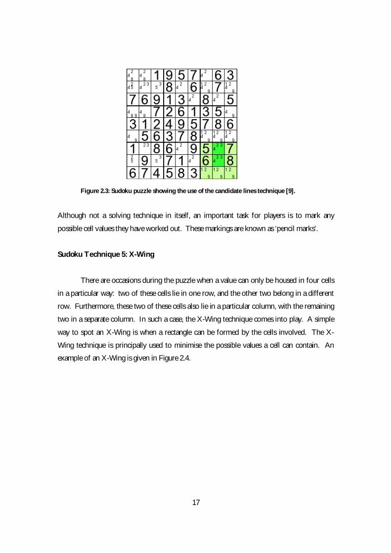
Figure 2.3: Sudoku puzzle showing the use of the candidate lines technique [9].

Although not a solving technique in itself, an important task for players is to mark any

possible cell values they have worked out. These markings are known as ‘pencil marks’.

Sudoku Technique 5: X-Wing

There are occasions during the puzzle when a value can only be housed in four cells

in a particular way: two of these cells lie in one row, and the other two belong in a different

row. Furthermore, these two of these cells also lie in a particular column, with the remaining

two in a separate column. In such a case, the X-Wing technique comes into play. A simple

way to spot an X-Wing is when a rectangle can be formed by the cells involved. The X-

Wing technique is principally used to minimise the possible values a cell can contain. An

example of an X-Wing is given in Figure 2.4.

18

Figure 2.4: An X-Wing with the value 1 [10].

As is visible, an X-Wing has been formed with the highlighted cells: R2C4, R2C7, R6C4 and

R6C7. The value 1 must be present in column 4 and in column 7. Thus, if cell R2C4

contains a 1, then R2C7 can not contain it, meaning that R6C7 will therefore contain 1. The

reverse case is also true. This allows for the value 1 to be removed from the possible values

of all other cells in rows 2 and 6. In this particular example, the result is that cell R6C9 is

assigned the value 9.

2.1.2. Measuring Difficulty

Although Sudoku puzzles vary in difficulty, there is still much debate as to how to

measure this. It was initially felt that the number of given values could be used as a

barometer of difficulty. However, Helmut Simonis’ research into Sudoku [11] suggests that

there are actually three main factors which influence the difficulty of a puzzle:

The number of pre-filled cells.

The placement of the pre-filled cells.

19

The value of the pre-filled cells.

The combination of these three determines the techniques required to solve a given puzzle.

The more complex the solving strategy required (such as X-Wing compared to cross-hatch

scanning), the more difficult the puzzle is. This idea has been incorporated by many puzzle

setters, and as a result the difficulty of puzzles is now rated on the solving strategies needed

to complete the puzzle.

2.2. Kakuro

Kakuro is a puzzle game which requires the user to employ simple arithmetic and logic

to solve it. It is often referred to as the “mathematical transliteration of the crossword” [12]

due to the grid appearance and the fact that the entries of white cells are filled horizontally

(from left to right) and vertically (from top to bottom). Similar to a crossword, the aim is to

completely fill in the white cells. In Kakuro however, the black cells provide the clues

needed to complete the game. Every white cell should be filled such that the values in each

entry sum to equal the number in the corresponding black cell. It must be noted that a cell

can not contain a value less than 1 or greater than 9. Of course, puzzle setters are free to

choose their own colours, and are not forced to use black or white. An example of an empty

(Figure 2.5) and solved (Figure 2.6) Kakuro puzzle is provided. As one can see, none of the

cells are pre-filled.

Like Sudoku, its origins lie in New York, where it was first published by Dell Puzzle

Magazines (the same magazine to first print Sudoku). Kakuro has been hugely successful in

Japan, and has started to emerge in Britain [13], with some newspapers providing daily

puzzles for their readers.

20

Figure 2.5: An empty Kakuro puzzle [14].

Figure 2.6: A solved Kakuro puzzle [14].

2.2.1. Solving Techniques

In comparison to Sudoku, techniques for completing Kakuro puzzles are not as well

documented. While tips can be found, the names given to each solving strategy varies from

source to source. It is interesting to note that many sources do not make a clear distinction

between simple techniques and more advanced ones. This suggests that all techniques are

used, irrespective of the puzzle’s difficulty.

21

Kakuro Technique 1: Lone Square

When there is only one cell remaining in an entry, its value must be equal to the

required sum of the entry, minus the sum of the filled in values. For example, if an entry has

three cells, two of which are filled with value 5 and 6, and its total must be equal to 12, the

remaining cell must contain the value 1, as 12 – (5 + 6) is equal to 1.

Kakuro Technique 2: Single Solution Entries

A technique for generating useful possible cell values quickly is to target those entries

which only have a single value combination. An example would be to create the sum of 17

using only two cells. There is only one solution for this and that is 9 + 8. With this

information the user can further reduce the possible values of any adjacent entries. Entries

which have two possible value combinations are also considered as they can often provide

hints as to which values are definitely required in the entry. An example is an entry of sum 8

with three cells; it can be filled with 1+2+5 or 1+3+4. We can see that the value 1 is

definitely going to appear in the entry.

Kakuro Technique 3: Cross Referencing

Cross referencing works by recognising where vertical and horizontal entries cross.

The sum combinations for both entries are calculated; any values which appear in all

combinations for both entries are candidates for being placed in the cell where the entries

cross.

22

Figure 2.7: Cross referencing performed on the highlighted cell.

While initially it seems that this technique only helps reduce the possible values for the cell in

question, in some cases, it can result in a value being assigned. The example in Figure 2.7

presents such a case. The highlighted cell shows where the horizontal 12 sum entry and the

vertical 6 sum entry cross. Although there are various ways create the sum of 12 using two

numerals, there is only one combination which allows 6 to be created from three numerals; 1

+ 2 + 3. This means that the highlighted cell must hold the value 1, 2 or 3. By reviewing

the combinations for the 12 entry, we can see that 12 can not be created by using a 1 or a 2.

It can however be created by using a 3 (and adding 9). Therefore, the value of the

highlighted cell must be 3.

Kakuro Technique 4: Criss-Cross Arithmetic

The criss-cross arithmetic technique focuses on those cells which appear at ‘turning

points’ on the grid, and are often referred to as corner-squares. They can be recognised as

they often provide links from a cluster of entries to another cluster. As a result, there are

only ever a few of these types of cells in a grid. The criss-cross strategy adds and subtracts

the sums of the entries to determine the value of the corner-square. An example is shown in

Figure 2.8.

23

Figure 2.8: Criss-cross arithmetic performed on the highlighted cell. This cell is often referred to as a corner-square.

The value for the highlighted cell is deduced by taking the sum of the vertical entries,

11+7+3, and subtracting the sum of the horizontal entries, 6+6+7. Therefore, the value of

the highlighted cell is equal to 21 minus 19; which is 2. It must be noted that this technique

can work for multiple connected corner-squares (Figure 2.9). In such cases, the technique

will not necessarily assign values to the cells, but will reduce the possible values the cells can

contain.

Figure 2.9: Criss-cross arithmetic with multiple cells [15].

24

2.2.2. Measuring Difficulty

As pre-filled values are generally not provided (though they can be included by the

puzzle setter to make the puzzles very easy), the factors which determine the difficulty of

Kakuro puzzles differ from those of Sudoku. One of the obvious ways to determine

difficulty is by examining the provided clues. If there are many entries whose clues indicate

that there are only one or two possible combinations, the puzzle will be easier than those

with fewer single combination entries.

However, there is no agreed means of measuring and setting difficulty for Kakuro,

and as a result, difficulty is often set depending upon how long it takes an average skilled

player to complete the puzzle. In order to make Kakuro puzzles more difficult, some puzzle

setters have started to add twists to the rules, such as using multiplication instead of addition

and decimal numbers in place of integer values.

2.3. Killer Sudoku

Killer Sudoku is a variant of Sudoku which incorporates the mathematical elements

of Kakuro. The grids have rows, columns and nonets indistinguishable from Sudoku, and

additionally contain cages made up of numerous cells. These cages have the same purpose

as entries do in Kakuro. The aim of the game is to complete the grid ensuring that every

region contains the values from 1 to 9 exactly once, and that the sums of the cages are met

exactly by the values in the cage cells. Other constraints imposed are that cages can not

contain duplicate values, and thus, can not contain more than nine cells. An example puzzle

can be seen below (Figure 2.10).

Its reputation in Japan has garnered much attention from the Western world.

Although its popularity has not quite reached those levels achieved by Sudoku, it has

certainly proven to be more popular than Kakuro, with many Killer Sudoku puzzle books

now available. Additionally, dedicated Killer Sudoku websites and newspapers have begun

to publish daily Killer Sudoku puzzles.

25

Figure 2.10: A typical Killer Sudoku puzzle [5].

2.3.1. Solving Techniques

Killer Sudoku Technique 1: Single and Double Solution Cages

Similar to Kakuro technique 2, this technique inspects those cages which have only

one possible value combination. In doing so, the possible values for the cells in that cage

can be drastically reduced. In some cases, any cells which lie in the same region as the cage

cells can also be affected. This also works by looking at cages which have multiple possible

value combinations and spotting those values which appear in all combinations. However, it

is very time consuming to examine all cages in this way, so often only those cages which

have one or two possible solutions are considered. This technique is normally employed at

the start of a puzzle, and provides some initial values to work with.

26

A cage which has three cells and a sum value of 23 is an example of a single solution

cage. It can only be created using 9+8+6. However, if the cage had a sum value of 22, it

would be a double solution cage as the possible value combinations are 9+8+5 and 9+7+6.

Killer Sudoku Technique 2: Sub-Cage Analysis

With every cell that is completed, the number of unsolved cells in the cage it belongs

to is reduced. Thus, the remaining cells can be thought of as a sub-cage of the original cage.

If the number of cells in the sub-cage is one, then the value for the cell must be equal to the

cage sum minus the sum of the cell values in the cage. However, if the number of the cells

in the sub-cage is greater than one, then the sub-cage can be checked to see if it is a single or

double solution cage. This can further reduce the possible values of the remaining cells in

the cage, and those which share the same regions as the cells.

Killer Sudoku Technique 3: Stubs and Holes

There are often cases when nearly all of a region’s cells belong to cages which do not

span into other regions. For example, there may be a row which has eight of its cells

belonging to cages which do not span any other rows. However the ninth cell may be a part

of a cage which does span multiple rows. In this case, this cell is a hole. With the

knowledge that the total sum of the row must be 45, the value of the ninth cell can be

worked out. This is done by subtracting the sum of the cage sums from 45.

If one considers the cells of a cage which spans into other regions, a stub may be

found. This occurs when the cage in question has only one cell which belongs to a different

region. The stub cell can be worked out by totalling the cage sums and subtracting 45.

While the above examples illustrate that stubs and holes can be used to assign values

to cells, it is often helpful to consider stubs and holes which may be made up of multiple

cells. Although this technique may not allocate any values to the cells, the possible values of

the cells may still be reduced further.

An advanced holes and stubs technique is one which treats multiple bordering

regions as one region. Figure 2.11 shows an example of a two column stub. In the example,

the cages in columns eight and nine are almost all contained wholly in those two columns.

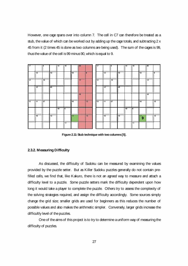
27

However, one cage spans over into column 7. The cell in C7 can therefore be treated as a

stub, the value of which can be worked out by adding up the cage totals, and subtracting 2 x

45 from it (2 times 45 is done as two columns are being used). The sum of the cages is 99,

thus the value of the cell is 99 minus 90, which is equal to 9.

Figure 2.11: Stub technique with two columns [5].

2.3.2. Measuring Difficulty

As discussed, the difficulty of Sudoku can be measured by examining the values

provided by the puzzle setter. But as Killer Sudoku puzzles generally do not contain pre-

filled cells, we find that, like Kakuro, there is not an agreed way to measure and attach a

difficulty level to a puzzle. Some puzzle setters mark the difficulty dependent upon how

long it would take a player to complete the puzzle. Others try to assess the complexity of

the solving strategies required, and assign the difficulty accordingly. Some sources simply

change the grid size; smaller grids are used for beginners as this reduces the number of

possible values and also makes the arithmetic simpler. Conversely, larger grids increase the

difficultly level of the puzzles.

One of the aims of this project is to try to determine a uniform way of measuring the

difficulty of puzzles.

28

2.4. Software Development Methodology

A key decision in the software development process is the choice of software

development methodology to be used. The methodology chosen determines the order in

which the various modules of software are developed and can also specify how much time is

to be spent on the various phases of software development (such as requirements analysis,

design, implementation etc). I will briefly consider three possible methodologies.

2.4.1. Waterfall Methodology

When using the waterfall methodology, the phases of the development process do

not overlap. As a result, once one phase ends, the next one begins. This sequential nature

of the waterfall model means that it is often used in projects where the requirements of the

system are well understood.

This has resulted in criticism of the waterfall model. David L. Parnas, the developer

of the concept of modular design, has stated that the constantly changing nature of software

development requires backtracking to the earlier phases regularly [16]. Further studies

confirm Parnas’ beliefs, with one source claiming that 87% out of over a thousand projects

using the waterfall model failed, before continuing to state that “waterfall-style scope

management was the ‘single largest contributing factor for failure, being cited in 82% of the

projects as the number one problem.’” [17].

2.4.2. Spiral Methodology

The spiral methodology can be thought of as an iterative version of the waterfall

methodology. The project is broken up into spirals, with each spiral containing every phase

(from requirements through to system integration). Early spirals are often used to produce

29

prototypes of the final program. Analysis of the prototypes can lead to new requirements

and designs for the following spirals [18].

The tentative make-up of the spiral model means that it can often be a long time

before usable components are available to the end-user.

2.4.3. The Unified Process

The Unified Process is a methodology designed to be as flexible as the project

requires. As a result, there exist many different adaptations of it and it is applicable to

projects of varying size.

The main idea behind the Unified Process is that everything produced at any given

point is developed to a standard such that it can be included in the final system. This means

that prototypes are not explicitly created. Additionally, it avoids the pitfalls of the waterfall

cycle by being an iterative process. Iterations are referred to as timeboxes. Within each

timebox, a component of the final system is completely developed, from design to testing,

and is integrated into the partially developed system. Furthermore, the most important units

of the system are developed first [19].

30

Chapter 3: Design

3.1. Design Overview

3.1.1. Development Methodology Decision

Before work on a software development project can begin, a development

methodology must be chosen. As noted earlier, the selected methodology determines how

the project is developed. The advantages and disadvantages of three different

methodologies were discussed; waterfall, spiral and the Unified Process.

Upon consideration, the Unified Process methodology was chosen. The timescale of

the project suggested that there simply was not enough time to develop prototypes as

suggested by the spiral methodology. The sequential nature and failure rate of the waterfall

model suggest that it is not suited to this project, where the requirements are not fully

known before the design and implementation.

The flexibility of the Unified Process was appealing, as it allowed for the riskiest

elements of the system to be built first. The knowledge gained of the domain and

technology would then be available for use to aid the development of the subsequent system

components.

3.1.2. Program Architecture

Upon entering the design phase, the architecture of the system was divided into three

parts using the Model, View and Controller (MVC) architectural pattern. The MVC pattern is

used to divide the system logic from the visual interface the user sees. This allows the logic

components to be changed without requiring a change in the user interface components

(and vice versa). Although this separation of system units is not an explicit requirement, it is

a desirable feature to have in a software project.

The three components as identified by the MVC pattern are:

Model: The model refers to the internal representation of the system. The grid, cells, cages

etc. are presented to the other system components for modification.

31

View: The view refers to the visual interface of the system. This allows users to understand

the state of the system. In particular, the interface informs the user of the status of the

puzzle, as well as presenting the various options available to the user.

Controller: The controller refers to the components of the system that alter the state of the

model. The model can be altered in two ways: by the solving techniques and by user events

(e.g. key presses, mouse clicks).

3.2. Internal Representation

When following the style of a Unified Process guided project, system components

are built in timeboxes. Additionally, those components which are the riskiest or most

important are developed first.

Although it could be argued that the collection of solving techniques the solver

employs is the most important component, a framework needed to be designed,

implemented and tested first. As a result, the first timebox was allocated to creating the

model for the solver.

The model provides the internal representation for the Killer Sudoku game. In order

for a Killer Sudoku game to be modelled, a representation was needed for the grid, and for

the game itself.

It must be noted that the system was designed to be implemented as an object-

oriented software project. In order to better support the MVC pattern in an object-oriented

program, two sets of design patterns were used; ‘GRASP’ patterns and ‘Gang of Four’

Patterns [19]. These patterns helped to decide upon the objects needed, and the

responsibilities to be assigned to each object.

A Killer Sudoku grid is made up of many parts; cells, regions (rows, columns and

nonets) and cages. The ‘high cohesion’ design pattern suggests that objects should be

focused and manageable. This results in objects which have a precise meaning and role

within the software. By applying this pattern, it can be seen that the components which

make up the grid (the cells, regions and cages), should be contained within individual objects.

32

3.2.1. Grid

Cells, regions and cages are represented as individual objects. The grid is an object

which contains the cell, region and cage objects, as well as information on its current state.

For example, it is aware of how many of its cells have had a value assigned to them. Due to

the separation of the components in the grid, the grid object is the only one which has

exclusive access to them all. For example, as cell can not access information belonging to its

row directly, the grid object provides the information.

This form of object separation supports another design pattern; ‘low coupling’. The

low coupling pattern proposes that the impact of change can be reduced if the

responsibilities between objects is minimised. This can be seen in the case above, where the

grid is the only object with the responsibility of holding the information of all the other

components. As a result, if the information in one of the components changes, the only

other object affected is the grid. It must be made clear, that whilst the grid is highly coupled

to the other types of objects, it still remains highly cohesive. The low impact of change

provided by the use of the design patterns further supports the aims of an MVC

architectural system.

3.2.2. Game

While the grid contains the information that the user is concerned with (i.e. cell

values, cage sums and lengths etc.), the game is responsible for handling the execution of the

solving techniques to be applied to the grid. In addition to these responsibilities, the game

also monitors the state of the grid, and deduces whether progress is being made. If not,

subsequent solving techniques are applied accordingly.

Additionally, the game is responsible for holding the information regarding the

various states the grid has been in. This information is then relayed onto the user as part of

the feedback (as specified by functional requirement 1.2.2d).

33

3.2.3. Puzzle

The puzzle is responsible for providing the data required to initialise the grid. In

particular, the puzzle describes the cages. The descriptions include the sum of the cage, as

well as the cells included in the cage. As some puzzles help the user by providing a number

of pre-filled cells, the puzzle must also provide these cell values to the grid. The initialising

information held by the puzzle is regarded as the first state of the game.

3.2.4. State

In essence, states are used as a measurement of time in the puzzle. Each state

provides a snapshot of the grid at a particular time. The puzzle moves onto the next state

upon each cycle of its solving techniques. The state holds the values of each cell, as well as

any possible and impossible values the cells have. By storing the details of each state in the

game, the progress of the puzzle can be viewed from the beginning to the end.

3.2.5. Puzzle History

The system is able to provide the user with an account of how the puzzle was solved.

In particular, this account describes the history of actions performed on each individual cell.

These details include what sort of action was performed (set the actual value, updated the list

of possible values or updated the list of impossible values) on that cell, as well explaining the

technique used to perform the action.

3.2.6. Grid Restriction

Due to the fact that an aim of the project was to investigate the techniques required

to solve Killer Sudoku puzzles, a decision to work only with 9 x 9 grids was made. This

decision was further supported by the fact that, as discussed, smaller grids (e.g. 6 x 6) are

34

generally easier and larger grids (e.g. 12 x 12) are more difficult. As I was aiming to solve

medium difficulty rated puzzles from Killer Sudoku Online, which primarily publishes 9 x 9

grid puzzles, the decision to limit the size makes sense.

3.3. User Interface

The user interface serves many purposes. As well as allowing the user to take

control of the underlying model, it also presents the user with a visual representation of the

model. Despite the purposes it serves, it was considered to be the least risky component in

the system, and was thus assigned to be created during the third (and last) timebox.

In order to design an effective user interface, interface design principles were

considered along with system use cases. Use cases are often examined in order to discover

the requirements of a system and its components. The two main tasks that users of the

software face are:

Play and solve a puzzle.

Input a puzzle.

The resulting interface requirements were used to evaluate the various potential designs.

3.3.1. Eight Golden Rules of Interface Design

Shneiderman’s Eight Golden Rules of Interface Design [20] were considered when

designing the user interface. These design principles are guidelines to ensure that the

interface is as user friendly as possible, as well as fulfilling its purpose. A detailed description

of these guidelines is provided in Appendix A.

3.3.2. Use Case 1: Play and Solve a Puzzle

35

The proposed set of actions required for the user to successfully play and solve a

puzzle was:

“The user loads the software and opens a puzzle he wants to play. The system subsequently

displays the puzzle grid to the user. He is then able to key in values and possible values into

any cell he chooses. The system updates the grid display accordingly. At any time during

the game, the user can ask the solver to complete the puzzle. Upon this request, the system

tries to solve the puzzle, updates the grid with its progress and notifies the user whether or

not the solving process was successful. If the process was successful the user can choose to

view the puzzle history. Furthermore, he can cycle through the puzzle states, from start to

finish, viewing how the puzzle was completed. At the end of the desired session, the user

exits from the system.”

Thus, the main interface requirements that were taken from this use case were:

There are three cases when the numerals in the grid update; when the user inputs a

value, when the solver has finished solving a puzzle and when the different states are

displayed.

The options to view the puzzle history and traverse through the puzzle states are

made available after the solver has successfully solved the puzzle under review.

3.3.3. Use Case 2: Input a Puzzle

The proposed set of actions required for the user to successfully input a puzzle into

the system was:

“The user loads the software and chooses to input a puzzle. She inputs any given cell values

and defines the cages required. The user can only request to store the puzzle when every cell

in the grid has been allocated to a cage or assigned a value. If the total of the cage sums and

cell values is equal to 405, the puzzle is saved. Otherwise it is an invalid puzzle and the user

is notified. Throughout the process, the software notifies the user of any errors which exist

in the puzzle.”

36

Thus, the main interface requirements that were taken from this use case were:

Pre-filled cells must be input before defining the cages.

Errors are clearly highlighted as and when they occur.

3.3.4. Solver Input Designs

After deciding upon the interface requirements, various interface designs for the

solver were considered. In particular, the grid input was considered separately to the overall

graphical user interface (GUI).

Two possible input methods were considered:

1. Before inputting a value, the user defines the input mode to use. The mode in use

defines whether entered values are to be considered as actual values or possible

values.

2. The user inputs values into the cell. If the value is the only numeral to be entered

into the cell, it is viewed as being the actual cell value. Otherwise, it is considered as

a possible value.

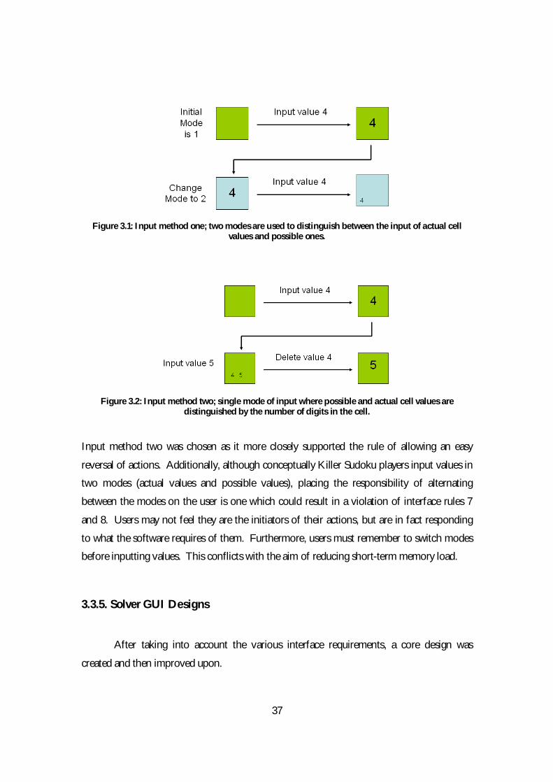
The first input method is illustrated in Figure 3.1. In the diagram, mode 1 refers to the input

mode where actual values are placed in cells. Input mode 2 allows for possible values to be

entered. The initial mode is set to 1 and is changed by the user.

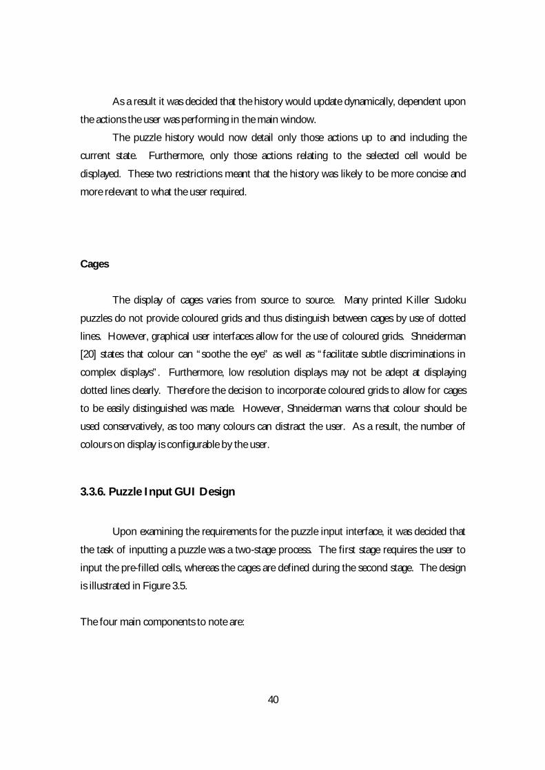
The second input method is shown in Figure 3.2. There is only a single mode of input. In

order to identify actual cell values from possible cells values, the number of values in a cell is

examined. If there is only one value in the cell, it is displayed as being the actual cell value.

Otherwise, the values are presented as possible values for that cell.

37

Figure 3.1: Input method one; two modes are used to distinguish between the input of actual cell values and possible ones.

Figure 3.2: Input method two; single mode of input where possible and actual cell values are distinguished by the number of digits in the cell.

Input method two was chosen as it more closely supported the rule of allowing an easy

reversal of actions. Additionally, although conceptually Killer Sudoku players input values in

two modes (actual values and possible values), placing the responsibility of alternating

between the modes on the user is one which could result in a violation of interface rules 7

and 8. Users may not feel they are the initiators of their actions, but are in fact responding

to what the software requires of them. Furthermore, users must remember to switch modes

before inputting values. This conflicts with the aim of reducing short-term memory load.

3.3.5. Solver GUI Designs

After taking into account the various interface requirements, a core design was

created and then improved upon.

38

Design 1 (Figure 3.3) was the first attempt at designing an interface for the solver. It

was created such that it met the identified requirements and that it did not infringe upon

Shneiderman’s interface principles. Design 1 has four main components:

Component A: The grid.

Component B: The puzzle history box.

Component C: A button allows the user to automatically solve the puzzle. A drop-down

box allows the user to choose which state to view.

Component D: The menu bar to provide options to do various tasks, such as load a puzzle,

create a puzzle, exit the system etc.

Although all the components are on screen at all times, not all of them are required all the

time. For example, the puzzle history box is only needed after the solver has successfully

solved a puzzle. Additionally, the drop down box does not allow incremental traversal

through the states to be achieved easily.

Figure 3.3: Design 1 for the solver interface.

39

The main changes from design 1 to design 2 (Figure 3.4) was to separate out the

puzzle history box into a separate window. Also, the drop-down box for state traversal was

replaced with two buttons. The components to note in this design are:

Component A: The grid.

Component B: The menu bar to provide options to do various tasks, such as load a puzzle,

create a puzzle, exit the system etc.

Component C: Three buttons; one to initiate the automatic solving process, another to

cycle to the next state and the last button to cycle to the previous state.

Component D: The puzzle history box contained in a separate window. The box contains

the log of the solving process.

Component E: A button to allow the puzzle history window to be closed.

Figure 3.4: Design 2 for the solver interface.

Puzzle History Box

The solver is designed to log actions where it assigns an actual value to a cell, or a

possible or impossible value. When one considers that the solver will do this for eighty-one

cells, the log could be too long to be readable.

40

As a result it was decided that the history would update dynamically, dependent upon

the actions the user was performing in the main window.

The puzzle history would now detail only those actions up to and including the

current state. Furthermore, only those actions relating to the selected cell would be

displayed. These two restrictions meant that the history was likely to be more concise and

more relevant to what the user required.

Cages

The display of cages varies from source to source. Many printed Killer Sudoku

puzzles do not provide coloured grids and thus distinguish between cages by use of dotted

lines. However, graphical user interfaces allow for the use of coloured grids. Shneiderman

[20] states that colour can “soothe the eye” as well as “facilitate subtle discriminations in

complex displays”. Furthermore, low resolution displays may not be adept at displaying

dotted lines clearly. Therefore the decision to incorporate coloured grids to allow for cages

to be easily distinguished was made. However, Shneiderman warns that colour should be

used conservatively, as too many colours can distract the user. As a result, the number of

colours on display is configurable by the user.

3.3.6. Puzzle Input GUI Design

Upon examining the requirements for the puzzle input interface, it was decided that

the task of inputting a puzzle was a two-stage process. The first stage requires the user to

input the pre-filled cells, whereas the cages are defined during the second stage. The design

is illustrated in Figure 3.5.

The four main components to note are:

41

Component A: The grid in stage 1. The cages are not yet defined, and instead just show

any pre-filled cells.

Component B: A button allows the user to move to stage 2. As many Killer Sudoku

puzzles do not contain any pre-filled cells, this button is available at all times.

Component C: The grid in stage 2. The pre-filled cells have been defined and at this stage,

the cages can be defined.

Component D: The button which allows the user to go to stage 2 is replaced with buttons

which allow cage actions to be performed. These actions are to add, edit or delete a cage.

Additionally, a text box is provided to allow the cage sum to be entered.

Figure 3.5: Design for the puzzle input screen.

3.4. Solving Techniques

In conjunction with the user actions, the solving strategies play the role of controller

in the MVC architecture. The techniques manipulate the model. The state of the model is

then displayed by the view.

Examination of the solving techniques detailed earlier in this report shows that all

techniques have one thing in common. That is that before the technique can be applied, the

player needs to be at a certain ‘position’ in the game. For example, the X-Wing can only be

applied if the cells in question create a rectangle upon their common possible values.

42

Similarly, the stubs and holes technique is rendered useless if the gird does not contain any

stubs or holes.

A primary objective of the project was to develop a program which solves Killer

Sudoku puzzles by employing human-like logic and reasoning. Thus, the solver needs to be

able to first evaluate the position of the grid at a given time, and then decide whether or not

a technique can be applied. This realisation led to the design that every technique is split

into two parts; evaluate and apply.

Furthermore, each solving strategy needs to be named. This allows for a clear

distinction between the techniques. Additionally, the naming of techniques facilitates

communication between the system and the user.

The solving techniques were created during the second timebox. Specific solving

techniques are discussed in the ‘Implementation and Solving Techniques’ section of this

report.

43

Chapter 4: Implementation and Solving Techniques

4.1. Development Tools

Before implementation can begin on a project, the development tools to be used

must first be decided upon.

The time constraints of the project meant that Java was used, as it is the only object-

oriented programming language I had sufficient experience in. The portability of Java, as

well as the wide support and availability of open source libraries meant that Java would have

been a good development choice for this project, regardless of my development experience.

While the internal representation was implemented using Java, the user interface was

developed using the Java ‘Swing’ toolkit and ‘Java2D’.

Swing is an API provided by Sun Microsystems which allows developers to create

graphical user interfaces. The API provides Java developers with methods to create

windows and populate them with buttons, textboxes, menus and many other components.

An attractive feature of the API is that it is extensible; therefore the provided classes can be

built upon to suit the needs of the project under development.

Java2D is an API which provides developers with a means to draw and render

graphics to the application window. Such graphics include images, shapes and colours.

4.2. Internal Representation

A simplified overview of the internal representation is provided in Figure 4.1. The

boxes in the figure relate to the objects described in the design section. A class for each

object was developed to hold information specific only to that object. Each object was

developed with methods to access and manipulate the instance variables of each class.

These methods were primarily used by the grid. The grid is then used by game for

manipulation.

44

A way to provide the puzzle history feedback to the user was also discussed and

designed. Due to the complex nature of generating the feedback, it was not included in the

figure shown.

Figure 4.1: Overview of the internal representation of the software.

However, in order to initialise the grid with the required information, the grid needs

to be provided with the puzzle.

4.2.1. Puzzle

The representation of the puzzle must contain a list of all cages present and a clear

way to identify which cells belong to which cage. In order to accommodate those Killer

Sudoku puzzles which contain pre-filled cells, the puzzle representation would also have to

contain the value information for each cell. Furthermore, the puzzle is responsible for

representing the changes it goes through as the solver solves it.

With the above requirements in place, it was decided that the puzzle was to be

represented using XML. XML is an extensible language which allows developers to describe

their own elements. Many open source Java libraries are available for the parsing of XML

data. ‘NanoXML’ [21] was used to parse the XML puzzle files. Figure 4.2 shows the puzzle

in its initial state. Figure 4.3 shows how the puzzle is represented when it is in its second

state.

45

Figure 4.2: XML representation for a puzzle in its initial state.

Figure 4.3: XML representation for a puzzle in its second state.

A puzzle contains one ‘cages’ element and multiple ‘cells’ elements. The ‘cages’

element contains many ‘cage’ elements, each of which describe the sum and length of the

cage as well as attaching a number to each cage. This number is then used as a unique

identifier.

The ‘cells’ elements contain eighty-one ‘cell’ elements each and these are

distinguishable by their ‘state’ attribute. Thus, if one needs to know the cell values of a

46

puzzle at state three, the ‘cells’ element with a state value of three will hold the cells that can

provide the required information. The ‘cell’ element then contains attributes to detail which

row, column and cage the cell belongs to, as well as its value. The nonet is not recorded as it

can be inferred from the row and column. A complete XML puzzle is included (Appendix

B).

4.2.2. Grid Initialisation

In order for the grid to be initialised, the information stored in the XML needs to be

extracted. By parsing the XML elements which describe the cells and cages, the rows,

columns and nonets can then be deduced. Figures 4.4 and 4.5 show the salient code extracts

used.

Upon initialising the grid, its solved status is set to false and state is set to one.

When this initialisation is complete, the grid is ready to have solving techniques applied to it.

The initialisation of individual cells affects the way the solving techniques work.

Upon the initialisation of the puzzle, one can view every cell as having a possible value of

one to nine, and thus has nine possible values. Alternatively, one can argue that until the

cells have been evaluated by the solving techniques, the number of possible values for a cell

start off as zero. Dependent upon the initialisation strategy used, solver needs to do one of

two things:

Minimise the possible values a cell can be from nine to one.

Build up the impossible values of a cell from zero to eight.

The decision to initialise the cells with zero possible values was made due to the fact that

it fits more closely with how Killer Sudoku is played. Cages instantly limit the possible

values of a cell, and thus very few cells actually contain one to nine as possible values.

Furthermore, if all cells were initialised with one to nine, every cage would have to be

analysed to reduce the possible values. Such evaluation would not accurately reflect how a

human player would approach a Killer Sudoku puzzle.

47

if ( cellXml.getProperty( "row") != null ) { row = cellXml.getProperty( "row" ); } if ( cellXml.getProperty( "column") != null ) { column = cellXml.getProperty( "column" ); } if ( ( cellXml.getProperty( "value") != null ) && ( ! cellXml.getProperty( "value" ).equals( "" ) ) ) {

value = Integer.parseInt( cellXml.getProperty( "value" ) ); } if ( cellXml.getProperty( "cage") != null ) { cage = cellXml.getProperty( "cage" ); }

Figure 4.4: Code extract from the parseCell() method.

if ( cageXml.getProperty( "number" ) != null ) {

number = cageXml.getProperty( "number" ); } if ( cageXml.getProperty( "length" ) != null ) { length = cageXml.getProperty( "length" ); } if ( cageXml.getProperty( "sum" ) != null ) { sum = cageXml.getProperty( "sum" ); } // work out which cells belong to this cage if ( cells != null ) { for ( Cell cell : cells) { if ( cell.getCage( ).equals( number ) ) { cageCells.add( cell.getId( ) ); } } }

Figure 4.5: Code extract from the parseCage() method.

4.2.3. Puzzle History

One of the main requirements of the program was that upon solving a puzzle, it

would be able to provide the user with a history of the actions and techniques it employed.

In order to compile this history, two pieces of information need to be collected; the actions

performed on the cell and the state number when they were performed.

However, the actions performed on the cells are recorded by each individual cell, yet

the state number is known only to the game. Introducing a direct link between game objects

and cell object would violate the ‘low coupling’ design pattern. As a result, the grid was

amended to include the state information. As grid objects are directly coupled to cell

48

objects, when the action on the cell is recorded, the state information can be passed from

the grid to the cell.

In order to create a highly cohesive way to represent history in the model, two

additional classes were implemented; ‘CellHistory’ and ‘CellHistoryItem’. Every cell has its

own CellHistory object, which is initialised at the same time as the cell. For every action that

occurs on a cell, a CellHistoryItem object is created and stored in the cell’s CellHistory

object.

The CellHistoryItem records the type of action that occurred (actual value set,

possible value set or impossible value set) along with the state number, solving technique

used and a message for the user to read. Additionally, the CellHistoryItem receives a list of

the cells which contributed in the decision to perform that particular action. The message

then includes this list of cells for the user to view. An example of the cell history can be

seen in Figure 4.6.

Figure 4.6: An example puzzle history window, detailing two actions on a cell.

In addition to the history described above, a text-free version was also implemented.

By choosing to view this alternative history, the user can view the cells which contributed to

a cell being set a value. This provides a quick way to view how a puzzle was solved without

having to read any text. Of course, this option is ideal for experienced Killer Sudoku

players, or those who only require the information of a particular cell.

An alternative was to include the puzzle history details in the XML puzzle file. This

would have meant that the CellHistory and CellHistoryItem objects would not be needed,

resulting in reduced memory usage. However, having to write to and read from the XML

would affect the performance and in turn, affect the user experience.

49

4.3. User Interface

4.3.1. Solver Grid

There were two implementation options available for the grid. The first option was

to take advantage of the extensibility of the Swing toolkit, and create custom components to

model the cells and grid. Alternatively, Java2D could be used to draw the cells and grid

directly to a single component.

Upon consideration of both approaches, the option to use Java2D was chosen.

Utilising a custom component per cell would have resulted in having eighty-one different

components to manage. This would have risked reducing performance of the software and

would therefore potentially affect user satisfaction. As Java2D draws directly to

components, only one component needed to be managed.

Thus, in order to implement the grid, a custom JPanel was created. A JPanel is a

component provided by Swing. The custom panel, named GridPanel, overrode the

‘paintComponent()’ method of the JPanel. This method is responsible for updating the

appearance of Swing components.

The grid drawing process is as follows:

1. Calculate the height and width of each cell by dividing the current panel height and

width by 9.

2. Draw a coloured box for each cell. The colour is dependent upon the cage the cell

belongs to. If the text-free history is selected and the puzzle has been solved, colour the

cell a different colour to all others. Otherwise, if the cell is the currently selected one, fill

it with a unique colour.

3. The grid lines are then drawn onto the GridPanel.

4. The sum for each cage is drawn into the highest, leftmost cell of the cage.

5. The values for each cell are painted into the matching cell. If the cell has an actual value

assigned to it, the digit is represented using a large, bold font. Otherwise, any assigned

possible values are illustrated using a smaller font.

50

Whenever the model is changed in some way; user inputs a cell value, solver solves the

puzzle or a new puzzle is loaded, the grid is repainted to reflect the new state of the model.

A sample grid is provided below (Figure 4.7).

Figure 4.7: A grid showing a half-completed puzzle.

4.3.2. Puzzle Input Grid

The grid used for inputting a puzzle is slightly different to the grid used for the main

solver. Although it is still implemented using Java2D and a customised JPanel, the process

for drawing the grid differs. This is because the model used is built up by the user. Cages

which have been entered are coloured using the same colouring scheme employed in the

solver grid.

4.3.3. Puzzle Input Error Prevention

Preventing user error is a golden rule in interface design. By its very nature, the task

of inputting a puzzle into the system provides many opportunities for errors to occur. The

errors handled and their solutions are:

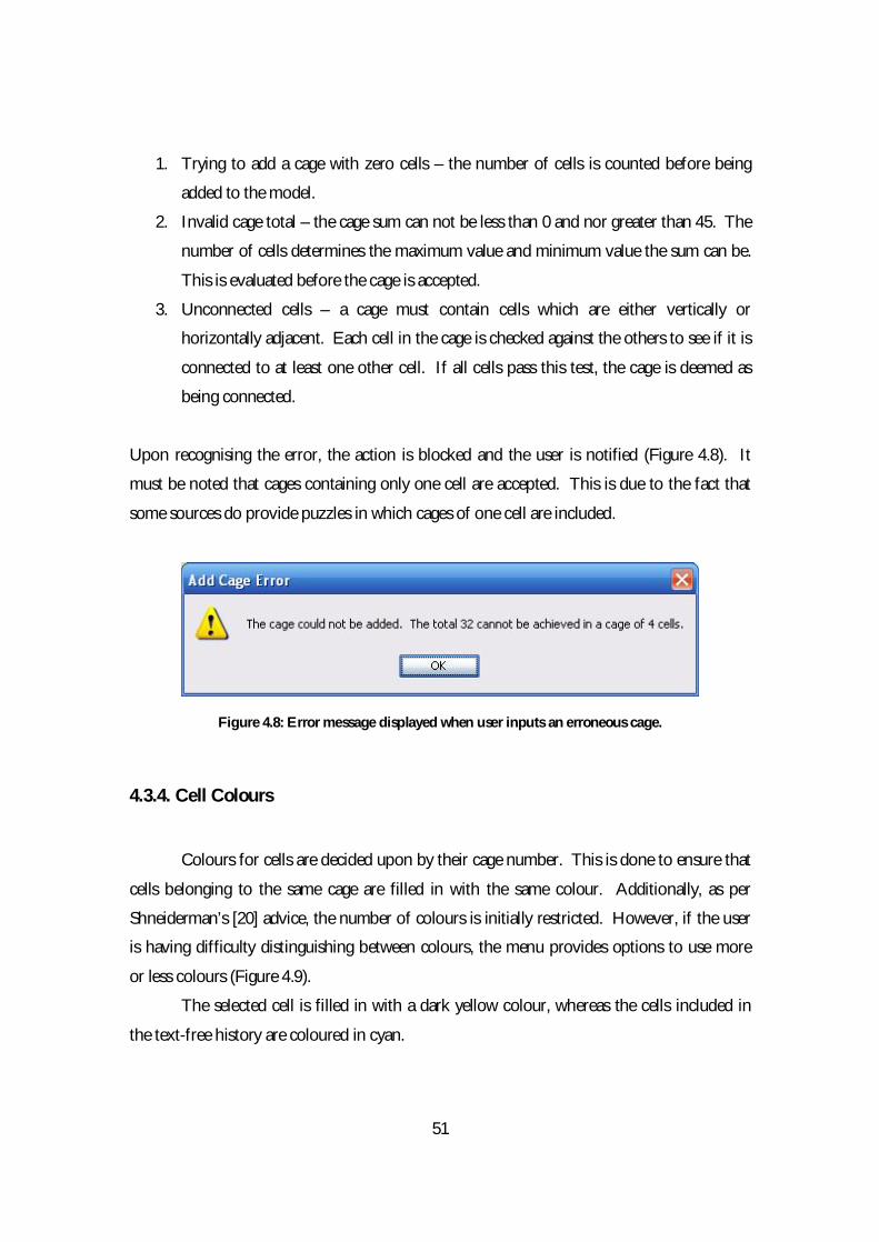
51

1. Trying to add a cage with zero cells – the number of cells is counted before being

added to the model.

2. Invalid cage total – the cage sum can not be less than 0 and nor greater than 45. The

number of cells determines the maximum value and minimum value the sum can be.

This is evaluated before the cage is accepted.

3. Unconnected cells – a cage must contain cells which are either vertically or

horizontally adjacent. Each cell in the cage is checked against the others to see if it is

connected to at least one other cell. If all cells pass this test, the cage is deemed as

being connected.

Upon recognising the error, the action is blocked and the user is notified (Figure 4.8). It

must be noted that cages containing only one cell are accepted. This is due to the fact that

some sources do provide puzzles in which cages of one cell are included.

Figure 4.8: Error message displayed when user inputs an erroneous cage.

4.3.4. Cell Colours

Colours for cells are decided upon by their cage number. This is done to ensure that

cells belonging to the same cage are filled in with the same colour. Additionally, as per

Shneiderman’s [20] advice, the number of colours is initially restricted. However, if the user

is having difficulty distinguishing between colours, the menu provides options to use more

or less colours (Figure 4.9).

The selected cell is filled in with a dark yellow colour, whereas the cells included in

the text-free history are coloured in cyan.

52

Figure 4.9: The same grid, displayed with the default colours on the left, and the max colours on the right.

4.3.5. User Input

Support for both keyboard and mouse input was implemented. Although a mouse

can not be used to enter digits, it can be used to select cells. In the puzzle input grid, mouse

clicks are used to select the cells to be added to the cage.

The keyboard can be used to navigate around the grid, as well as inputting the values

into the cells.

4.3.6. Help Documents

In order to help novice users operate the software, help documents were provided.

The documents were created as web pages (Appendix C). The JDesktop [22] library was

used to allow web pages to be opened from the application.

4.4. Solving Techniques

53

4.4.1. Evaluators

As discussed, in order for the solver to behave like a human, it must first evaluate the

position of the grid before it can apply the solving techniques. This was achieved by creating

a family of evaluator classes; ‘RuleEvaluation’, ‘GridEvaluator’ and ‘GridEvaluation’.

An instance of the RuleEvaluation class is the object returned after a technique has

evaluated a grid. It must be noted that the techniques are referred to as ‘rules’ in the

software. A reason for this is that conceptually, they are rules by which the solver must

behave by. A RuleEvaluation object contains information stating whether or not a particular

rule can be applied, and if it can, the cells it will affect.

The GridEvaluator class can be viewed as the nucleus of the solver. The role of the

GridEvaluator is to evaluate the grid using the evaluation methods defined by each solving

technique.

The results of the GridEvaluator are presented to the game as a GridEvaluation

object. The GridEvaluation stores a list of RuleEvaluation objects, collected by the

GridEvaluator.

4.4.2. Grid Manipulator

A utility class used by all the solving techniques, the main role for the

‘GridManipulator’ class is to provide grid maintenance. Whenever a technique sets the value

of a cell, the GridManipulator makes sure that the value is deemed as impossible for any cells

which are in the same row, column and nonet as the cell having its value set. The inclusion

of this utility class means that code blocks are not repeated unnecessarily.

4.4.3. Rule Interface

All techniques are viewed by the solver as rules by which it must behave by.

Furthermore, it was decided that the rules are split into two parts; a part which evaluates the

grid and a part which applies the technique. In order to make sure all techniques worked like

54

this, an interface, ‘Rule’, was implemented. The code used to implement the interface can be

seen in Figure 4.10.

public interface Rule {

public Grid apply( Grid grid, RuleEvaluation evaluation ); public RuleEvaluation evaluate( Grid grid );

}

Figure 4.10: Code implemented for the ‘Rule’ interface.

The interface defines the template for every technique employed by the solver.

Additionally, it provides a way for new techniques to be added with ease. As long as the

desired technique implements the interface and is added to the GridEvaluator, no other

classes need amending.

4.4.4. One and Two Solution Cages Technique

The ‘OneSolutionRule’ and ‘TwoSolutionRule’ rules locate cages which have only

one or two possible value combinations. Upon discovering such cages, the possible values

are allocated to the cells.

Subsequently, a check is done to see how many rows, columns and nonets the cage

under evaluation spans. This potentially helps reduce the possible values of those cells

which share the same region. For example, if a cage with a sum of 6 is composed of three

horizontal cells and is placed in the top left corner of the grid, we know that all cells belong

in the same row and the same nonet. As we know that the cage is a single solution cage that

can only contain the values 1, 2 and 3, we can surmise that any other cells in the row and

nonet can not possibly contain 1, 2 or 3.

Updating the impossible values of those cells which share the same region is

performed slightly differently in the TwoSolutionRule rule. If the above example is changed

so that the sum of the cage is 8 instead of 6, we see that the cage now has two possible

combinations; 1+2+5 and 1+3+4. The TwoSolutionRule identifies those values which are

common across the two possible combinations. Such values are viewed as vital values, as

they are vital to the cage. In this case, the vital value is 1. This then allows the solver to set

the value 1 as an impossible value for the other cells in the row and nonet.

55

These two techniques are the only ones which are not held by the GridEvaluator. A

simple reason for this is that they only need to be performed once at the start of the puzzle.

4.4.5. Row and Column Value Checker Technique

Many documented Killer Sudoku techniques are based upon looking at the grid to

deduce possible values for the cells. The group of value checker techniques however, takes

each numeral from 1 to 9 in turn, and attempts to see where the value can fit inside the

region.

In order to do this, the numeral is checked against every cell in the region to see if it

has been set as an actual value for a cell. If it has, the solving technique moves on to the

next numeral. If not, the impossible values for each cell are considered. If eight of the cells

contain the current numeral as an impossible value, the value for the remaining cell is set as

the current numeral.

These techniques are only useful after other techniques have evaluated the cages and

updated the impossible values for the cells sufficiently.

4.4.6. Holes and Stubs Techniques

As detailed in the ‘Background’ chapter of this report, the holes and stubs techniques

focus on those cages which deviate away from a specific region, unlike other cages in that

region. The cells which remain in the region can be seen as holes, whereas the cells which

extend out from the region are viewed as stubs.

If the hole or stub comprises of only one cell, the value can be easily calculated; 45

minus the other cages sums for a hole, or the sum of all cages in the region minus 45 for a

stub.

This notion is extended to include those holes and stubs which are made up of more

than one cell. By working out the total value of the cells in the same way as described for a

single cell, the solver finds itself with a sub-cage. The sum combinations for the sub-cage

can then be evaluated. Values which occur in every combination are deemed as the vital

56

values for this sub-cage. If this sub-cage spans only one row, column or nonet, then any

vital values are instantly marked as impossible values for the rest of the cells in the same

region.

4.4.7. Sum Checker Technique

Often knowing the possible values a cell can contain is only half the task. Evaluating

the various permutations of values within a cage, and the consequences of each, is another

task. This technique examines those cages which have been analysed and amended in some

way by other rules.

Upon looking at a cage, it works out the possible sums that can fit in the cage. The

technique then tries to fit various sum combinations into the cage. This is done by trying

out each value in each cell, and seeing if any of the cell impossible values are violated. If not,

then the permutation is considered to be good. The result of this check yields one of three

cases:

Only one sum permutation fits without error.

Many sum permutations fit without error, but one cell contains the same value in

each.

Many sum permutations fit without error.

Depending on the case, all cell values, or one value or none are set. This rule can be viewed

as a sophisticated maintenance technique, which helps refine the possible values that have

been set by other techniques.

4.4.8. Cage Possible Finder Technique

Given a particular grid position, there is potential that none of the techniques will be

able to progress the puzzle. In such a case, the solver is deemed as being stuck. This

situation is recognised when the puzzle has remained the same for a number of states. The

‘CagePossibleFinderRule’ helps the solver by mimicking what a human player would do

57

when stuck; it looks at a cage it has not looked at yet. Although this seems obvious, one

must remember that the techniques discussed so far primarily focus on those which have

only one or two solutions. Any other cages looked at are those which have been affected by

the one and two solution cages, or those which contribute to the presence of holes and

stubs.

As the name suggests, this technique finds possible values for cages. Upon finding

the possible values, it checks for vital values and the number of regions the cage spans.

Based on this, other cells lying within the same region as the cage can have their impossible

cell values updated. After completing this analysis, the cage is marked as having been

checked. This means that the next time the CagePossibleFinderRule is fired; the same cage

will not be examined again.

Before any of this can be performed, the rule must first pick a cage to find possible

values for. There were three options available for how this could be done:

1. Stochastic – Randomly choose a cage to examine.

2. Smallest Cage First – Target those cages which have the least number of cells.

3. Largest Cage First – Target those cages which have the most number of cells.

The option to randomly choose a cage was rejected due to its imprecise nature. The

puzzle history log would not be able to give a suitable explanation for how the cage was

chosen. Similarly, the time taken to solve the same puzzle could vary, dependent upon

which cages were chosen.

Out of the remaining two choices, option two was selected. There were two reasons for

this. Firstly, a human player is more likely to look at the smaller cages first, as the arithmetic

is easier and thus less effort. Secondly, using a smaller cage means that there is more chance

that the cage spans one column, row and/or nonet. This means that if vital values are

found, they are likely to be more useful than if found in a larger cage.

4.4.9. Eight Cell Technique

58

This technique is a very simple rule in comparison to some of the ones discussed; it

simply examines each region to see if eight of the cells have been allocated a value. If this is

the case, the value of ninth cell is deduced and set.

4.4.10. Cell Impossible Count Technique

Every cell is checked to see how many impossible values it has; if it has eight

impossible values, the actual value of the cell can be inferred.

4.4.11. Cage Completion Technique

If only one cell in a cage is empty (i.e. has not had its value set) then the value is

calculated by summing the values of the other cells in the cage cell and subtracting from the

cage total.

59

Chapter 5: User-Software Interaction

5.1. Use Cases

5.1.1. Play and Solve Puzzle Use Case

An attempt to gain user feedback was made by distributing the solver and a

questionnaire (Appendix D) to close family and friends. However, after sending out 25

questionnaires, only 2 were returned.

Thus, in order to ascertain whether or not the software operates as required, the two

use cases described in the ‘Design’ chapter were carried out.

The first use case models how the user would go about playing and solving a puzzle.

The user navigates to and opens the puzzle he wants to play (Figure 5.1).

Figure 5.1: Puzzle selection.

The system displays the grid. The user can enter any values into the grid (Figure 5.2) until he

either completes the puzzle, or requests that the solver complete the puzzle by clicking on

the ‘Solve’ button.

60

Figure 5.2: User attempt at the puzzle.

If the solver was successful, the user can view the puzzle history in text (Figure 5.3) or

without text (Figure 5.4).

Figure 5.3: The action history for a particular cell in the puzzle.

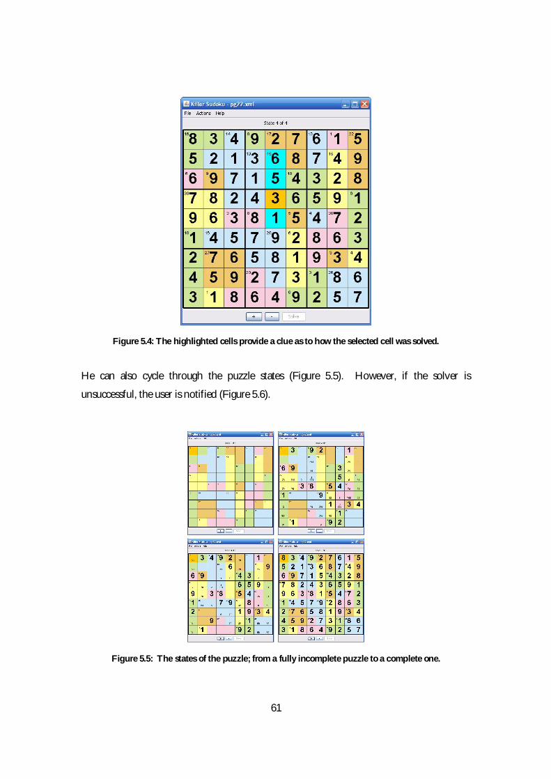
61

Figure 5.4: The highlighted cells provide a clue as to how the selected cell was solved.

He can also cycle through the puzzle states (Figure 5.5). However, if the solver is

unsuccessful, the user is notified (Figure 5.6).

Figure 5.5: The states of the puzzle; from a fully incomplete puzzle to a complete one.

62

Figure 5.6: Message notifying the user that the solver could not solve the puzzle.

5.1.2. Input Puzzle Use Case

The second use case details how the user would input a puzzle. If any cells have

been pre-filled, the values for those cells are entered (Figure 5.7).

Figure 5.7: Input of pre-filled cells.

The user then enters the cages (Figure 5.8). The cages can be edited or deleted at any time

(Figure 5.9). The user is notified of any errors during the process.

63

Figure 5.8: Input of the cages.

Figure 5.9: Edit Cage and Delete Cage options.

The user then saves the puzzle. If the total of the cage sums was not equal to 405, the user

is notified of this and the puzzle is not saved (Figure 5.10).

Figure 5.10: Invalid puzzle notification.

64

5.2. Puzzle History Usage

Upon solving a puzzle, the user is able to view the history of actions performed by

the solver (as illustrated by Figure 5.3 above). Each action performed is explained in full

sentences. This means that users can read the explanation and understand the reasoning

employed by the solver.

Some of the rules, and their explanations in the puzzle history, are presented below.

5.2.1. One Solution Technique

A cage with only one possible value combination is regarded as a ‘one solution’ cage

and is picked up by the ‘OneSolutionRule’. Figure 5.11 shows such a cage.

Figure 5.11: A ‘one solution’ cage.

As one can see, the cage can only possibly be made up of 1 and 2. Figure 5.12 displays how

the system explains this to the user (the explanation of how the cell might also contain the

value 1 has been omitted).

HOLE

Figure 5.12: ‘One Solution Cage’ explanation.

5.2.2. Holes Technique

State 1

Event Type: POSSIBLE_SET Rule Name: ONE_SOLUTION_CAGE

Message: This cage has only one possible solution, and 2 is one of the values allowed in

this cage. Thus, it is possible that the value of this cell may be 2.

Contributing Cells: 25, 15

65

As described in section 4.4.6, holes can be found when a region contains only one or

two multiple-region spanning cages. Figure 5.13 shows a hole in the top row. The hole is

made up of the two leftmost cells. This means that although the solver can not assign a

value to the cell, it can reduce the possible values those cells might be.

Figure 5.13: A screenshot displaying a two-cell hole.

The solver makes clear to the user that the rule was used to set two possible values to the

cell (Figure 5.14).

Figure 5.14: ‘One Region Hole’ possible set.

Furthermore, as the hole must be equal to 16, the solver recognises that 16 can only be made

up of 7 and 9. As a result, no other cells in the row can contain a 7 or a 9. The solver also

presents this to the user (Figure 5.15)

Figure 5.15: Effect of the hole technique.

State 2

Event Type: POSSIBLE_SET Rule Name: RULE_ONE_REGION_HOLE

Message: This cell is a hole in this row. As a result, this cell may be 7

Contributing Cells: 59, 89, 79, 69, 19, 29, 99, 39, 49

State 2

Event Type: IMPOSSIBLE_SET Rule Name: RULE_ONE_REGION_HOLE

Message: The hole(s) in the row all lie on the same row. The sums that can be used to

complete the hole(s) all contain value 9. Which means this cell can't be that value.

Contributing Cells: 59, 89, 79, 69, 19, 29, 99, 39, 49

66

5.2.3. Sum Checker Technique

The SumCheckerRule5 simply looks at cages which have had possible and impossible

values assigned to them, and tries to refine these values by checking to see if the various sum

permutations would actually fit in. Figure 5.16 shows an example of this.

Figure 5.16: Sum Checker technique screenshot.

The solver explanation is displayed below (Figure 5.17).

Figure 5.17: Sum Checker explanation.

5.2.4. Value Checker Technique

This technique simply checks a region to determine where a value may go. Figure

5.18 presents a case where this is used.

5 For more information on the SumCheckerRule, please refer to section 4.4.7.

Event Type: VALUE_SET Rule Name: RULE_SUM_CHECKER_RULE

Message: This cell must be value 2. With the current possible and impossible values

considered, this cage can only have a certain sum combination. And a value needed to

make that sum can only be placed in this cell

Contributing Cells: 76, 75

67

Figure 5.18: Value Checker screenshot.

The explanation provided to the user is shown below (Figure 5.19).

Figure 5.19: Value Checker rule explanation.

Figure 5.18 also shows an example of the text-free history report. When the user selects a

cell, the cells which contributed towards the decision to set its value are highlighted. This

allows a player to get a quick grasp of how a particular cell was solved, without having to

read through the system’s explanation.

State 9

Event Type: VALUE_SET Rule Name: RULE_ROW_VALUE_CHECKER

Message: After checking the rest of the row, it turns out that this value can only go in

this cell.

Contributing Cells: 19, 29, 39, 49, 59, 69, 79, 89, 99

68

Chapter 6: Results

The main aim of the project was to create a program which solves Killer Sudoku

puzzles by employing human-like logic and reasoning. This would then allow us to assess

the effectiveness of the various solving techniques. Additionally, it was hoped that we would

be able to identify the factors which alter the difficulty of a puzzle.

In order to test the solving abilities of the software, a sample of 100 puzzles was

created and provided to the solver to attempt. A quarter of the test puzzles were medium-

rated difficulty puzzles from the Killer Sudoku. A clear functional requirement was that the

software should be able to solve such puzzles. A further 15 puzzles were taken from the

Killer Sudoku Online website (10 easy puzzles and 5 hard puzzles). The remaining 60 puzzles

were taken evenly from two different sources: The Times - Killer Su Doku [23] and The Big Book

of Killer Su Doku [24]. Both publications contain puzzles split into 5 difficulty categories.

It must be noted that all puzzles were chosen randomly, with only the puzzle

difficulty and source predetermined.

6.1. Solver Success

Before the various solving techniques and the puzzle difficulty were investigated, the

solver was first tested to see how effective it was. The results of these tests are shown in

Figures 6.1, 6.2 and 6.3.

Overall, the solver successfully solved 83% of the puzzles put to it. As one can see,

the solver was particularly adept at solving the puzzles provided by the two books, and failed

only when confronted with the most challenging puzzles.

However, the solver did not fare as well against the puzzles from the Killer Sudoku

Online website. Although the easy puzzles were all solved without fail, the medium puzzles

were only successfully completed 60% of the time. Furthermore, the hard puzzles proved

very difficult for the solver, solving only 1 out of 5.

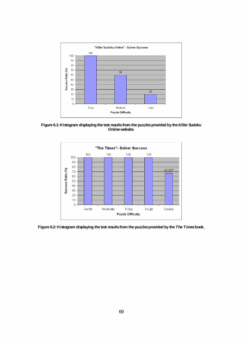
69

Figure 6.1: Histogram displaying the test results from the puzzles provided by the Killer Sudoku Online website.

Figure 6.2: Histogram displaying the test results from the puzzles provided by the The Times book.

70

Figure 6.3: Histogram displaying the test results from the puzzles provided by the The Big Book of Killer Su Doku book.

6.2. Effectiveness of the Solving Techniques

To test the effectiveness of each solving technique, the same test was performed

repeatedly. The difference between iterations was that the technique being reviewed was

disabled to see what effect (if any) this would have on the software’s solving capabilities.

The results are shown in Figure 6.4.

Disabling most techniques did not make too much difference to the solving ability of

the solver. However, a result of this was an increased number of states for each puzzle. For

example, disabling the one and two solution cage techniques did not affect the eventual

outcome but resulted in many more puzzle states. A reason for this was that the

CagePossibleFinder rule eventually examined the all empty cages, meaning that disabling the

OneSolutionRule and TwoSolutionRule rules did not make a difference to the end result.

Disabling the SumCheckerRule led to the most striking result; only 18% of the

puzzles were successfully solved without it. Furthermore, out of the 40 puzzles from the

Killer Sudoku Online website, only 2 easy puzzles were completed.

71

Figure 6.4: Histogram showing the success rate of the solver without various groups of solving techniques.

6.3. Puzzle Difficulty

As noted in the ‘Background’ chapter of this report, there were various hypotheses

relating to how the difficulty of Killer Sudoku puzzles should be measured. However, an

agreed meaning of the best model for performing this measurement did not exist. Thus, an

aim of this project was to ascertain the factors which contribute to the difficulty of a Killer

Sudoku puzzle.

The results illustrating the success rate of the solver show that even puzzle setters do

not use a common method to measure and set the difficulty of puzzles. For example, the

medium rated puzzles on from the Killer Sudoku Online website were more challenging than

even the hardest ones in the printed books.

The analysis of the solving techniques shows that reducing the solving techniques

one employs makes either very little difference or a large difference. This is not greatly

useful when assessing the difficulty of a puzzle.

As a result, a comparison was made between those puzzles which were successfully

solved, and those which were not. Various factors were considered. The results are

presented in Figure 6.5.

72

Average Per Puzzle Solved Unsolved Number of Cages 29.06 26.53 Number of One Cell Cages 1.12 0 Number of One Solution Cages 7.52 4.53 Number of Two Solution Cages 3.77 3.35 Number of Rows Spanned Per Cage 1.42 1.41 Number of Columns Spanned Per Cage 1.24 1.53 Number of Nonets Spanned Per Cage 1 1

Figure 6.5: Comparison of solved and unsolved puzzles.

These results suggest that puzzles which provide more one and two solution cages

are more likely to be solved, and are thus easier. Additionally, the number of cell cages was

zero in every puzzle that was not solved. The results also hint that the more cages that are

present in the puzzle, the easier the puzzle is. This is only a slight hint and thus can not be

deemed as particularly valuable.

A possible way of measuring the difficulty of puzzles with the software is to look at

the number of states a puzzle goes through before it is solved. Figures 6.6, 6.7 and 6.8 show

the average number of states required for the puzzles to be solved.

The results display a positive correlation between the difficulty of the puzzle and the

number of states resulting from the puzzle. This method of measuring difficulty could also

be used to compare puzzles from different sources. For example, the results suggest that the

toughest puzzles from the two books (The Times… and The Big Book…) are only slightly

easier than the medium-rated difficulty puzzles from the Killer Sudoku Online website. This

supports exactly the results found when testing the success rate of the solver.

73

Figure 6.6: Histogram displaying the average states required per puzzle for puzzles from the Killer Sudoku Online website.

Figure 6.7: Histogram displaying the average states required per puzzle for puzzles from The Times book.

74

Figure 6.8: Histogram displaying the average states required per puzzle for puzzles from The Big Book of Killer Su Doku book.

75

Chapter 7: Conclusion

7.1. Project Summary

The main aim of the project was to create a Killer Sudoku solver. Rather than using

a brute-force solving strategy, it was decided that the solver would behave and reason in a

human-like way. This would then allow the software to report a history of its actions to the

user. It was hoped that the user would then be able to use this information to learn how the

puzzle was solved.

The solver was successfully implemented. By modelling the internal representation,

the interface and the solving techniques separately from each other, the software was built in

a way that modifications to the program could be easily made at any time.

The solving techniques were broken up into two parts: evaluation and application.

The evaluation element was responsible for evaluating the grid to see if the technique could

be used. The application part applied the technique to the grid.

A usable GUI was developed upon following well-known interface design principles.

7.2. Conclusion

The fact that the solver was not quite as strong as hoped suggests that more time

should have been spent on the solving techniques. It also suggests that I should have spent

more time improving my own Killer Sudoku playing skills.

An aspect of the techniques I misjudged was deciding how specific/general each

technique should be. More general solving strategies would allow for a wider range of

techniques to be represented by just one ‘rule’. An example of this could be a rule which

holds all holes and stubs variations in one rule. This would be acceptable, as the techniques

required to find and solve the holes and stubs are very similar. However, the result of this

would mean that the explanation the system provides to the user would in turn be general.

76

I decided that the puzzle history provided for the user was an important aspect of

the project and was thus prompted to make the techniques as specific as possible. For

example, stubs and holes were represented separately. Furthermore, the variations within

the holes and stubs were again represented by different rules (single region holes compared

to multiple region holes). This resulted in very precise explanations, but meant that for every

variation of similar techniques, a new software class had to be developed.

It must be noted that the in the puzzles the solver could not solve, substantial

progress often was made (Figure 7.1).

Figure 7.1: A puzzle which could not be further solved by the solver.

In addition, the only other aspect of the final program I believe could be improved is

the puzzle input. The task of inputting every puzzle the user wants to play is a laborious

one. I attempted to include a feature to allow for puzzles to be syndicated from websites.

An obvious candidate for this was the Killer Sudoku Online website. This would allow users to

download puzzles from the website directly to the software. However, I did not receive a

reply from my email in which I enquired about the syndication services available.

A particularly interesting aspect of the solver was the inclusion of states6, due to the

fact that it provided the strongest hint yet as to how one can measure the difficulty of a

6 For more information on states, please refer to section 3.2.4.

77

puzzle. This revealed that it is not necessarily the complexity of the techniques that

determine the difficulty, but the number of techniques that can be successfully applied at any

given time. The fewer the techniques one can effectively apply, the more difficult the

puzzle.

Determining the effectiveness of each technique did not provide the insight I was

looking for. However, the results revealed that there are actually three, not two, types of

solving technique; ones which reduce the possible values of cells, ones which set the actual

values and those which manipulate the existing possible values. Many Sudoku and Killer

Sudoku techniques focus on minimising the number of values a cell can be. The player is

then expected to deduce the cell values. In the solver, this deduction was performed by the

SumCheckerRule, which proved to be the most effective technique. The only limitation of

the rule is that it only evaluates one cage at a time. Therefore, creating a technique which

behaves in a similar way to SumCheckerRule, but also explores the relationship between cells

in unconnected cages, would be an interesting one.

Overall, I am confident that a good framework for solving Killer Sudoku puzzles has

been developed. This framework allows for developers to easily create new solving

techniques and a new interface, should they desire it. The solver is also especially good at

solving printed puzzles, which would suggest that it would be practical to a user who is

tackling puzzles from newspapers or books. Apart from failing to fully meet the

requirement to solve medium-rated puzzles 100% of the time, the rest of the requirements

were met. As a result, I feel the project has been a success.

7.3. Future Work

There are many ways in which the project could be extended. A flaw of the current

system was that the techniques were not general enough. Implementing techniques which

address this problem would be an obvious step forward. If successful, cases as illustrated by

Figure 7.1 (above) would not occur as often.

78

Another way to combat cases like the one in Figure 7.1 would be to accept aid from

the user. The user would attempt complete the next step of the puzzle, and then allow the

solver to carry on from this new position.

The strength of the solver is not the only way the project could be expanded. By

further investigating the puzzle syndication feature, the user experience could be improved.

Different sized grids could also be considered along with incorporating a complete set of

Sudoku and Kakuro rules.

As the investigation into how the difficulty rating of puzzles is determined proved to

be slightly inconclusive, my final suggestion would be to research this topic further.

79

References

[1] A. Turpin. The rise and rise of Sudoku.

http://www.independent.co.uk/news/uk/this-britain/the-rise-and-rise-of-sudoku-473598.html Accessed: 23rd March 2008.

[2] Screenshot of Dr. Kawashima’s Brain Training taken from

http://www.blueunplugged.com/p.aspx?p=118926 [3] W. Yin-Poole. DS Tops 4 million sales in the UK.

http://www.videogamer.com/news/30-10-2007-6785.html Accessed: 21st March 2008.

[4] L. Lewis. Too good for fiendish? Then try Killer Su Doku. http://www.timesonline.co.uk/tol/life_and_style/article560581.ece Accessed: 23rd March 2008. [5] http://www.killersudokuonline.com Accessed: 13th April 2008 [6] D. Smith. So you thought Sudoku came from the Land of the Rising Sun…

http://www.guardian.co.uk/media/2005/may/15/pressandpublishing. usnews

Accessed: 13th April 2008 [7] B. Hanson. Solving Techniques. http://www.stolaf.edu/people/hansonr/sudoku/explain.htm Accessed: 3rd April 2008 [8] Sudoku puzzle number 1827 taken from

http://entertainment.timesonline.co.uk/tol/arts_and_entertainment/games_and_puzzles/sudoku/

[9] Solving Sudoku. http://www.sudokuoftheday.com Accessed: 3rd April 2008 [10] Picture of X-Wing position taken from http://www.djape.net/sudoku/wp/?p=98 [11] H. Simonis. Sudoku as a Constraint Problem. http://homes.ieu.edu.tr/~bhnich/mod-proc.pdf#page=21

80

Accessed: 12th March 2008 [12] Wikipedia. Kakuro. http://en.wikipedia.org/wiki/Kakuro Accessed: 4th April 2008 [13] J. McCurry. The new grid on the block. http://www.guardian.co.uk/g2/story/0,,1569223,00.html Accessed: 4th April 2008 [14] Puzzle taken from DoKakuro. http://www.dokakuro.com/index.php Accessed: 7th April 2008 [15] J. Bumgardner. The Kakuro Kraze. www.coverpop.com/sfiles/kakuro/HowToSolveKakuro.pdf Accessed: 11th April 2008 [16] D. Parnas. A Rational Design Process: How and Why to Fake it http://web.cs.wpi.edu/~gpollice/cs3733-b05/Readings/FAKE-IT.pdf [17] Benefits of Agile Development. http://versionone.com/Resources/AgileBenefits.asp Accessed: 13th April 2008 [18] R. Sorensen. A Comparison of Software Development Methodologies http://www.stsc.hill.af.mil/crosstalk/1995/01/Comparis.asp Accessed: 13th April 2008 [19] C. Larman. Applying UML and Patterns: An Introduction to Object-Oriented Analysis and

Design and Iterative Development (3rd Edition) Pearson Education (2005) Pages: 31-40, 53-57, 61-67, 271-319, 413-472. ISBN: 0131489062

[20] B. Shneiderman, C. Plaisant. Designing the User Interface (4th Edition) Pearson Education (2005) Pages: 64-65, 74-76, 510-514. ISBN: 0321268780 [21] M. Scheemaecker. NanoXML. http://nanoxml.sourceforge.net/orig/ [22] JDesktop Integration Components. https://jdic.dev.java.net/ [23] The Times. The Times - Killer Su Doku. Times Books (2005)

81

ISBN-13: 9780007223633 [24] M. Huckvale. The Big Book of Killer Su Doku. Orion Publishing Group (2006) ISBN-13: 9870752880938

82

Glossary API: ‘Application Programming Interface’ – A source code interface which grants

programmers access to methods and classes defined in pre-built software modules.

Architectural Pattern: Defines the structural organisation of a software system and its sub-

systems.

Cage: A group of cells which only appears in Killer Sudoku. Each cage has a value

attributed to it. The total sum of the cells in the cage must be equal to the cage value.

Column: A group of vertically aligned cells, spanning the height of the grid.

Design Patterns: Guidelines which advise developers on how to design and implement

software. There are many patterns, all of which have come about through best practice.

Such patterns are general enough to be applied to many software projects, but precise

enough to tackle specific development problems.

Entry: In Kakuro, an entry is a group of horizontal or vertical cells which belong to the

same black cell.

Gang of Four Patterns: See Design Patterns (above). More code driven than GRASP

patterns, and thus are more geared to use during the implementation phase.

GRASP Patterns: ‘General Responsibility Assignment Software Principles’ – See Design

Patterns (above). More basic than ‘Gang of Four’ patterns, and thus are more driven to being

used during the design phase.

Nonet: A block of cells, which, in a 9 x 9 grid, span 3 rows and 3 columns.

Region: A region is a general term to describe a column, row or nonet.

Row: A group of horizontally aligned cells, spanning the width of the grid.

Samunamupure: Japanese name for ‘Killer Sudoku’. Directly translates to ‘Sum Number

Place’, which describes concept of the game.

Timebox: An iteration in the Unified Process in which at least one module of the final

system is designed, implemented and integrated.

83

Appendix A: Eight Golden Rules of Interface Design Rule 1: Strive For Consistency

Consistent sequences of actions should be required in similar situations; identical

terminology should be used in prompts, menus, and help screens; and consistent colour,

layout, capitalisation, fonts, and so on should be employed throughout.

Rule 2: Cater To Universal Usability

Recognise the diversity of the users and their needs. Novice users should be

provided with explanations whereas shortcuts and faster pacing may be relevant for expert

users.

Rule 3: Offer Informative Feedback

Whenever a user performs an action, the system should respond in some way. By

doing so, the user is informed that the system has received/processed the user’s request.

Rule 4: Design Dialogs to Yield Closure

Upon completion of a set of actions, the user must be notified that the actions have

been successfully completed (e.g. through use of a dialog box). Not only does this give users

the satisfaction of successfully completing a multiple action task, this rule also helps support

rules 3 and 7.

Rule 5: Prevent Errors

Wherever possible, the user must be presented from being able to perform actions

which result in errors. This can be done in two ways. Firstly, the action can be disabled; this

84

is often enforced by the greying out buttons or items in a menu. Secondly, the action can be

processed and the software can calculate whether or not the current state of the software is

valid.

Rule 6: Permit Easy Reversal of Actions

As much as possible, actions should be reversible. This feature relieves anxiety, since

the user knows that errors can be undone, thus encouraging the exploration of unfamiliar

options.

Rule 7: Support Internal Locus of Control

One of the most important rules is to make sure that the user feels in control of the

interface. This means minimising unexpected interface actions and long, drawn out

sequences of actions. Failure to enforce this rule can lead to user dissatisfaction and anxiety.

Rule 8: Reduce Short-Term Memory Load

The rule of thumb is that humans can remember “seven plus or minus two chunks”

of information. This requires that displays be kept simple, multiple-page displays to be

consolidated, window-motion frequency be reduced, and sufficient training time be allotted

for codes, mnemonics, and sequences of actions.

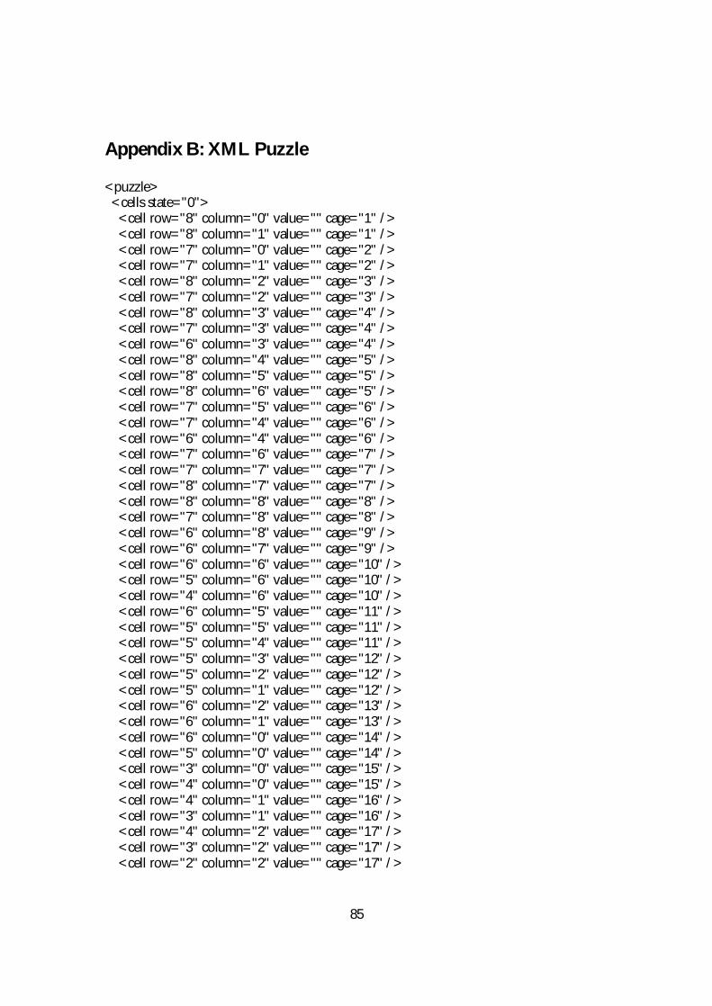
85

Appendix B: XML Puzzle <puzzle> <cells state="0"> <cell row="8" column="0" value="" cage="1" /> <cell row="8" column="1" value="" cage="1" /> <cell row="7" column="0" value="" cage="2" /> <cell row="7" column="1" value="" cage="2" /> <cell row="8" column="2" value="" cage="3" /> <cell row="7" column="2" value="" cage="3" /> <cell row="8" column="3" value="" cage="4" /> <cell row="7" column="3" value="" cage="4" /> <cell row="6" column="3" value="" cage="4" /> <cell row="8" column="4" value="" cage="5" /> <cell row="8" column="5" value="" cage="5" /> <cell row="8" column="6" value="" cage="5" /> <cell row="7" column="5" value="" cage="6" /> <cell row="7" column="4" value="" cage="6" /> <cell row="6" column="4" value="" cage="6" /> <cell row="7" column="6" value="" cage="7" /> <cell row="7" column="7" value="" cage="7" /> <cell row="8" column="7" value="" cage="7" /> <cell row="8" column="8" value="" cage="8" /> <cell row="7" column="8" value="" cage="8" /> <cell row="6" column="8" value="" cage="9" /> <cell row="6" column="7" value="" cage="9" /> <cell row="6" column="6" value="" cage="10" /> <cell row="5" column="6" value="" cage="10" /> <cell row="4" column="6" value="" cage="10" /> <cell row="6" column="5" value="" cage="11" /> <cell row="5" column="5" value="" cage="11" /> <cell row="5" column="4" value="" cage="11" /> <cell row="5" column="3" value="" cage="12" /> <cell row="5" column="2" value="" cage="12" /> <cell row="5" column="1" value="" cage="12" /> <cell row="6" column="2" value="" cage="13" /> <cell row="6" column="1" value="" cage="13" /> <cell row="6" column="0" value="" cage="14" /> <cell row="5" column="0" value="" cage="14" /> <cell row="3" column="0" value="" cage="15" /> <cell row="4" column="0" value="" cage="15" /> <cell row="4" column="1" value="" cage="16" /> <cell row="3" column="1" value="" cage="16" /> <cell row="4" column="2" value="" cage="17" /> <cell row="3" column="2" value="" cage="17" /> <cell row="2" column="2" value="" cage="17" />

86

<cell row="4" column="3" value="" cage="18" /> <cell row="4" column="4" value="" cage="18" /> <cell row="4" column="5" value="" cage="18" /> <cell row="3" column="4" value="" cage="19" /> <cell row="3" column="3" value="" cage="19" /> <cell row="2" column="3" value="" cage="19" /> <cell row="3" column="5" value="" cage="20" /> <cell row="3" column="6" value="" cage="20" /> <cell row="3" column="7" value="" cage="20" /> <cell row="5" column="7" value="" cage="21" /> <cell row="4" column="7" value="" cage="21" /> <cell row="5" column="8" value="" cage="22" /> <cell row="4" column="8" value="" cage="22" /> <cell row="3" column="8" value="" cage="23" /> <cell row="2" column="8" value="" cage="23" /> <cell row="2" column="7" value="" cage="24" /> <cell row="2" column="6" value="" cage="24" /> <cell row="2" column="5" value="" cage="25" /> <cell row="1" column="5" value="" cage="25" /> <cell row="0" column="5" value="" cage="25" /> <cell row="2" column="4" value="" cage="26" /> <cell row="1" column="4" value="" cage="26" /> <cell row="1" column="3" value="" cage="26" /> <cell row="1" column="2" value="" cage="27" /> <cell row="1" column="1" value="" cage="27" /> <cell row="0" column="1" value="" cage="27" /> <cell row="2" column="1" value="" cage="28" /> <cell row="2" column="0" value="" cage="28" /> <cell row="1" column="0" value="" cage="29" /> <cell row="0" column="0" value="" cage="29" /> <cell row="0" column="2" value="" cage="30" /> <cell row="0" column="3" value="" cage="30" /> <cell row="0" column="4" value="" cage="30" /> <cell row="1" column="6" value="" cage="31" /> <cell row="0" column="6" value="" cage="31" /> <cell row="1" column="8" value="" cage="32" /> <cell row="1" column="7" value="" cage="32" /> <cell row="0" column="8" value="" cage="33" /> <cell row="0" column="7" value="" cage="33" /> </cells> <cages> <cage number="1" sum="7" length="2" /> <cage number="2" sum="8" length="2" /> <cage number="3" sum="10" length="2" /> <cage number="4" sum="17" length="3" /> <cage number="5" sum="17" length="3" /> <cage number="6" sum="10" length="3" /> <cage number="7" sum="18" length="3" />

87

<cage number="8" sum="10" length="2" /> <cage number="9" sum="4" length="2" /> <cage number="10" sum="18" length="3" /> <cage number="11" sum="13" length="3" /> <cage number="12" sum="15" length="3" /> <cage number="13" sum="16" length="2" /> <cage number="14" sum="13" length="2" /> <cage number="15" sum="9" length="2" /> <cage number="16" sum="4" length="2" /> <cage number="17" sum="12" length="3" /> <cage number="18" sum="14" length="3" /> <cage number="19" sum="17" length="3" /> <cage number="20" sum="14" length="3" /> <cage number="21" sum="11" length="2" /> <cage number="22" sum="16" length="2" /> <cage number="23" sum="3" length="2" /> <cage number="24" sum="13" length="2" /> <cage number="25" sum="12" length="3" /> <cage number="26" sum="24" length="3" /> <cage number="27" sum="7" length="3" /> <cage number="28" sum="14" length="2" /> <cage number="29" sum="14" length="2" /> <cage number="30" sum="14" length="3" /> <cage number="31" sum="5" length="2" /> <cage number="32" sum="12" length="2" /> <cage number="33" sum="14" length="2" /> </cages> </puzzle>

88

Appendix C: User Help Documents

Index Page

89

How to… Page

90

How To Input A Puzzle (NOTE: Images have been omitted)

91

Killer Sudoku Tips Page

92

About the Solver Page

93

Appendix D: Killer Sudoku Questionnaire

Killer Sudoku Questionnaire By Mohammed Rizwan

Please complete the following questionnaire AFTER you have used the ‘Killer Sudoku

Solver’ software. All answers will remain anonymous. Thank you!

1. Before using the software, had you ever… (please delete as appropriate)

a) … heard of Sudoku? YES / NO

b) … played Sudoku? YES / NO

c) … heard of Kakuro? YES / NO

d) … played Kakuro? YES / NO

e) … heard of Killer Sudoku? YES / NO

f) … played Killer Sudoku? YES / NO

2. If you have ever played Sudoku, Kakuro or Killer Sudoku before, have you played

using a pen and paper? If so…

a) … what was the source of the puzzle (newspaper, puzzle book etc.)?

………………………………………………………………………………………………

b) … did you complete the puzzle? YES / NO / NA

c) … did you enjoy playing using a pen and paper? YES / NO / NA

3. If you have ever played Sudoku, Kakuro or Killer Sudoku before, have you played

using a computer? If so…

a) … what was the source of the puzzle (website, computer game etc.)?

………………………………………………………………………………………………

b) … did you complete the puzzle? YES / NO / NA

c) … did you enjoy playing using a computer? YES / NO / NA

94

3. Approximately, for what length of time have you used the software?

(Please choose ONE option.)

Time Range (in minutes) Yes/No (please type into

the appropriate box)

0-15

15-30

30-60

60-120

120+

4. What was the first thing you did when you loaded up the software?

………………………………………………………………………………………………

………………………………………………………………………………………………

………………………………………………………………………………………………

………………………………………………………………………………………………

5. Did you input a puzzle using the create puzzle option? YES / NO

6. Did you successfully complete one puzzle (using the software) without the help of

the solver? YES / NO

7. Did the solver successfully solve a puzzle for you? YES / NO

8. If so, was the available feedback (through the ‘View Cell Activity’ option) useful?

YES/ NO / NA

9. Was the solver ever unsuccessful in solving a puzzle? YES / NO

10. If so, what was the difficulty of the puzzle (easy, medium, hard etc.)?

YES / NO / NA

11. Did you manage to complete the puzzle nevertheless? YES / NO / NA

95

12. Please rate the following aspects of the software from 1 to 5, where:

1 = strongly agree

3 = neither agree nor disagree

5 = strongly disagree

Statement Rating

(please type into the box)

I found the help pages to be useful.

I feel the software was easy to use and well

presented.

Playing Killer Sudoku using the software is

preferable to playing using a pen and paper.

The feedback the solver gives after solving

a puzzle is clear.

I am a better Killer Sudoku player as a

direct result of using the software.

13. Are you male or female? MALE / FEMALE

14. How old are you? Under 18 / 18 – 25 / 26 – 30 / 31 – 40 / Over 40

There are no more questions. Thank you for using the software and completing the

questionnaire!