CH>t Of'-I Cranfield University, Silsoe Campus National Soil Resources Institute (NSRI) - Engineering This thesis is submitted in fulfilment of the requirements for the award of degree of Doctor of Engineering (EngD) By Kieron Eatough Academic year - 2002 Tractive performance o f 4x4 tyre treads on pure sand Supervisor - Dr. James L. Brighton Presented on 3 1st December 2002

Welcome message from author
This document is posted to help you gain knowledge. Please leave a comment to let me know what you think about it! Share it to your friends and learn new things together.
Transcript
CH>t Of'-I
Cranfield University, Silsoe Campus
National Soil Resources Institute (NSRI) - Engineering
This thesis is submitted in fulfilment of the requirements for the
award of degree of Doctor of Engineering (EngD)
By
Kieron Eatough
Academic year - 2002
Tractive performance o f 4x4 tyre treads on pure sand
Supervisor - Dr. James L. Brighton
Presented on 3 1st December 2002
ProQuest Number: 10832281
All rights reserved
INFORMATION TO ALL USERS The quality of this reproduction is dependent upon the quality of the copy submitted.
In the unlikely event that the author did not send a com p le te manuscript and there are missing pages, these will be noted. Also, if material had to be removed,
a note will indicate the deletion.
uestProQuest 10832281
Published by ProQuest LLC(2018). Copyright of the Dissertation is held by Cranfield University.
All rights reserved.This work is protected against unauthorized copying under Title 17, United States C ode
Microform Edition © ProQuest LLC.
ProQuest LLC.789 East Eisenhower Parkway
P.O. Box 1346 Ann Arbor, Ml 48106- 1346
Abstract
School: Cranfield University, Silsoe Campus, NSRI
Student: KieronEatough
Degree: Engineering Doctorate
Title: Tractive performance o f 4x4 tyre treads on pure sand
This thesis examined the difficulties of generating traction from 4x4 (light truck) tyres
in pure sand conditions. Investigations conducted in the Cranfield University Soil
Dynamics Laboratory measured the tractive performance of a range of production and
prototype 4x4 tyre tread patterns to quantify the effect of tread features upon tractive
performance. The investigation also quantified the amount of sand displacement
instantaneously occurring beneath the tyre, by a novel application of radio frequency
identification (RFID) technology, which determined sand displacements to an accuracy
of ±5.5 mm. A limited number of normal contact stress measurements were recorded
using a TekScan normal pressure mapping system. This technology was employed in a
new manner that allowed pressure distributions to be dynamically recorded on a
deformable soil surface.
Models were developed or adapted to predict rolling resistance, gross thrust of a tyre
and the gross thrust effect due to its tread. Net thrust was predicted from refined
versions of equations developed by Bekker to predict gross thrust and rolling resistance.
These were modified to account for dynamic tractive conditions. A new tread model
proposed by the author produced a numerical representation of the gross thrust
capability of a tread based on factors hypothesised to influence traction on loose sand.
This allowed the development of a relationship between the features of the tread and its
measured gross thrust improvement (relative to a plain tread tyre), from which a total
relationship was developed. The tread features were also, in combination with the wheel
slip, related to the sand displacements and net thrusts simultaneously achieved.
The sand displacement results indicated that the majority of the variation in
displacement between the different treads occurred in the longitudinal (rearward)
direction. This effect was influenced by the wheel slip, as increased slip caused greater
displacements, so the differences between the treads were greater at higher slips. The
treads that generated the highest relative displacements also derived the higher gross
thrusts (up to +5% extra gross thrust compared to a plain tread), although at the higher
slips this also caused increased sinkage. As sinkage increased, the rolling resistance
increased at a fester rate then the gross thrust, and thus the net thrust reduced. To
prevent this effect the wheel slip should be limited to a maximum of 20% at low
forward speeds (approximately 5 km/h).
Current market forces dictate that the biggest benefit that tyre manufacturers could offer
in desert market regions would be to optimise road-biased tyres to suit loose sand
conditions. The modelling developed indicated that this could be achieved by
maximising the number of lateral grooves (and thus lateral edges) featured on a tread,
however care would have to be exercised so as not to compromise the necessaiy on-road
capability. The models could also be used to quantifiably determine from a choice of
possible tyre treads, the tread that would offer most traction on pure loose sand.
\J

Acknowledgements
The author would like to thank the sponsors, in particular EPSRC, for their financial
support, which enabled this work to be undertaken. The technical assistance and advice
received from numerous people at Land Rover, Dunlop and Goodyear was important in
the research achieving a successful outcome. Thanks are particularly due to John Kellett
and Eddie Franklin of Land Rover who supported the project throughout and Ian Kemp
of Dunlop who made a positive impact during uncertain times.
The support and guidance received from John Kilgour, Prof. Dick Godwin and Dr.
Mike Hann and other academic staff at the Silsoe Campus has been very useful and
welcome throughout the project. Particular thanks go to Dr. James Brighton for his
thoughtful supervision, continuous support and considerable effort over the whole
project.
Thanks are also due to the technical staff at the Silsoe Campus, especially Roy Newland
and Tony Reynolds who assisted in conducting much of the experimental work, and
who provided the benefit of their expertise on many instances. I am also grateful to the
workshop staff for their support in producing, or repairing, numerous components, often
at short notice, whilst always providing a sense of humour.
This research would not have been achieved without the assistance of Marcus Oliver.
This came on many levels, from conducting experiments and manufacturing test
equipment, to processing data and scrutinising results and ideas, all of this was
appreciated. Thank you also for a continued friendship outside of work.
The most thanks must go to my fiancee Frances Tubb, who has provided continuous
support and encouragement from the outset of the project, particularly during the most
frustrating and challenging stages. A special thank you is also necessary for the
continued support and understanding shown over most evenings and weekends during
the final six months, which made this thesis possible.
Table of Contents
TABLE OF FIGURES............................................................................................... VII
TABLE OF PLATES................................................................................................ XIV
TABLE OF TABLES................................................................................................ XVI
LIST OF SYMBOLS................................................................................................XVH
LIST OF ABBREVIATIONS.................................. XX
1 INTRODUCTION...................................................................................................1
2 AIM AND OB JECTIVES...................................................................................... 52.1 AIM.......................................... 52.2 OBJECTIVES.................................................................................................. 52.3 PROJECT METHODOLOGY ................................................................ 6
3 LITERATURE REVIEW...................................................................................... 73.1 INTRODUCTION............................................ 7
3.2 BASIC TYRE EVALUATION.......................................................................... 83.2.1 Basic Tyre Relationships............................................................................ 83.2.2 Features of a Sand Tyre............................................................................ 103.2.3 Implications of the Engineering Features of Desert Sand.........................133.2.4 Tyre Evaluation Using Slip-Pull Curves...................................................143.2.5 Indications from a Simple Off-Road Tyre Field Investigation................. 16
3.3 MEASUREMENT OF SOIL (SAND) DISTURBANCE................................. 163.3.1 Glass Sided Tanks and Visible Markers...................................................17
3.3.1.1 Paints, dyes, films and layers.....................................................................................193.3.2 Particles Inserted in a Soil Profile ................................................... 19
3.3.2.1 Metal detection........................................................................................................... 213.3.3 RFID Technology....................................................................................223.3.4 The Implications of Other Sand Flow Investigations.............................. 23
3.4 PRESSURE/ STRESS SENSING....................................................................243.4.1 Pressure/ Stress Sensing from the Sand (Soil)....................................... 243.4.2 Pressure/ Stress Sensing from the Tyre ......................................... 25
3.4.2.1 Pressure cells in/ on the tyre tread............................................................................ 253.4.2.2 Conductive rubber...................................................................................................... 293.4.2.3 TekScanpressure sensing system................................................................................30
3.4.3 Findings of Oida etal...............................................................................31
3.5 TRACTION MODELS....................................................................................343.5.1 Analytical Models....................................................................................343.5.2 Empirical Models................................. 343.5.3 Semi-Empirical Models............................................................................37
Silsoe Campus, Kieron Eatough, 2002
3.5.3.1 Prediction of tractive pull.................. 393.5.3.2 Derivation of the soil deformation modulus (K).......................................................... 403.5.3.3 Contact area prediction............................................................................................... 423.5.3.4 Other thrust prediction methods................................................................................ 453.5.3.5 Prediction of rolling resistance................................................................................... 463.5.3.6 An analysis of 4x4performance on sand.................................................................... 473.5.3.7 Bekker ’s prediction for wheeled and tracked vehicles (from Wong)...........................50
3.5.4 Finite Element Mathematical Models............................... 53
3.6 TYRE TEST RIGS...........................................................................................553.6.1 Fixed Slip Test Rigs................................................................................. 553.6.2 Variable Slip Test Rigs............................................................................ 55
3.7 SUMMARY OF LITERATURE REVIEW......................................................57
4 MARKET SURVEY AND REVIEW ................................................... 594.1 MARKET SURVEY METHODOLOGY.........................................................59
4.2 MARKET SURVEY RESULTS...................................................................... 604.2.1 The Profile of Prospective Purchasers of Off-road Tyres.........................614.2.2 Properties Identified as Important for Off-road Tyres..............................624.2.3 Respondents’ Perceptions of Tyre Brands............................................... 644.2.4 Likelihood of Purchasing Secondary Performance Off-Road Tyres 654.2.5 Interest in Automatic Central Tyre Inflation Systems (CTIS)................65
4.3 IMPLICATIONS OF THE MARKET SURVEY RESULTS........................ 65
5 TRACTION SURFACE EVALUATION.............................................................685.1 SOIL ASSESSMENT...................................................................................... 68
5.1.1 Determination of K (Soil Deformation Modulus).....................................705.1.2 Determination of Bekker Plate Sinkage Values.......................................715.1.3 Comparison of the Experimental Soil Preparations ....................... 72
5.2 SAND COMPARISON ANALYSIS...............................................................78
5.3 ANALYSIS OF THE DA80F SAND...............................................................845.3.1 Determination of K (Sand Deformation Modulus)...................................855.3.2 Determination of Bekker Plate Sinkage Values.......................................86
6 TYRE EVALUATION APPARATUS AND METHODOLOGY...................... 876.1 THE SOIL DYNAMICS LABORATORY (SDL)...........................................87
6.2 TEST TYRES...................................................................................................88
6.3 FIXED SLIP TEST RIG............................................................ 906.3.1 Design of the Fixed Slip System............................................................. 906.3.2 Derivation of Tractive Forces.................................................................. 94
6.3.2.1 Free-rolling rolling resistance....................................................................................946.3.2.2 Gross thrust, net thrust and rolling resistance............................................................94
6.3.3 Test Rig Instrumentation..........................................................................956.3.3.1 EORT calibration....................................................................................................... 97
Silsoe Campus, Kieron Eatough, 2002
6.3.3.2 Tension link calibration.............................................................................................. 986.3.3.3 L VDT (sinkage) calibration........................................................................................996.3.3.4 Tacho-generator (fifth wheel) calibration.................................................................996.3.3.5 Rotary encoder (wheel speed) calibration...............................................................100
6.4 FIXED SLIP TESTS ON SOIL......................................................................1026.4.1 Treatments Investigated......................................................................... 1026.4.2 Experimental Results............................................................................. 103
6.4.2.1 Effect of inflation pressure....................................................................... 1046.4.2.2 Effect of soil bulk density........................................................................ 1056.4.2.3 Effect of tread pattern...........................................................................109
6.4.3 Summary of Results................. .........................................110
6.5 FIXED SLIP TESTS ON SAND.................................................................. 1116.5.1 Experimental Results............................................................................. 1126.5.2 Fluctuations within the Traction Results................................................ 1156.5.3 Limitations of the Fixed Slip System..................................................... 118
6.6 THE VARIABLE SLIP TEST RIG................................................................1196.6.1 Operating Characteristics of the Variable Slip R ig................................121
6.7 COMPARISON (VERIFICATION) TESTS ON SOIL.................................1236.7.1 Variable Slip Test Results......................................................................1246.7.2 Methodology for Test Rig Performance Comparisons.......................... 1266.7.3 Test Rig Comparison Results.................................................................128
6.8 COMPARISON (VERIFICATION) TESTS ON SAND...............................1306.8.1 Variable Slip Test Results......................................................................1306.8.2 Test Rig Comparison Results.................................................................132
6.9 A FULL VEHICLE TEST ON SAND............................. 134
7 SAND FLOW MEASUREMENT APPARATUS AND METHODOLOGY. 1377.1 SAND AND RFID TAG DISPLACEMENT ASSESSMENT...................... 137
7.1.1 Bench Sand Flow Evaluations................................................................1377.1.1.1 RFID Tag and sand flow assessment methodology....................................................1377.1.1.2 Tag/ sandflow assessment results................................................................. 139
1.2 FULL SIZE SAND DISPLACEMENT MEASUREMENT RIGS...................... 1417.2.1 Tag Position Placement..........................................................................1417.2.2 Tag Position Location............................................................................1477.2.3 Tag Position Measurement Apparatus................................................... 1477.2.4 Accuracy and Repeatability of Tag Placement and Measurement 153
7.3 POSITION OF THE TAG GRID IN THE THRUST (SLIP) CYCLE 1577.4 VERIFICATION OF THE SUITABILITY OF THE TEKSCAN SYSTEM158
7.4.1 6911 mat.................................................................................................1597.4.2 5051 mat.................................................................................................1607.4.3 6300 mat.................................................................................................162
Silsoe Campus, Kieron Eatough, 2002
7.4.4 TekScan Measurement Capabilities........................................................ 1637.4.5 Attachment of the TekScan Mats to the Tyres........................................163
8 INVESTIGATION OF NORMAL STRESSES UNDER TYRES..................1678.1 EXPERIMENTAL TREATMENTS..............................................................1678.2 PRESSURE MEASUREMENT RESULTS ........................................ 167
8.2.1 Pressure Map Construction Procedure.................................................... 1678.2.2 Experimental Results..............................................................................169
8.2.2.1 Plain tread (PT).........................................................................................................1698.2.2.2 Lateral tread (LA T)................. 1708.2.2.3 Longitudinal tread (LON)..........................................................................................1718.2.2.4 45 °Backwardfacing tread (45B).............................................................................. 171
8.3 DISCUSSION OF THE RESULTS...............................................................172
9 SAND DISPLACEMENT INVESTIGATION.................................................1749.1 TEST TREATMENTS....................................................................................174
9.2 SAND DISPLACEMENT TEST RESULTS..................................................1759.2.1 Horizontal Net Thrust Results................................................................ 1769.2.2 Wheel Slip and Wheel Sinkage Results.................................................. 1789.2.3 Longitudinal (X-axis) Displacements..................................................... 1809.2.4 Lateral (Y -axis) Displacements.............................................................. 1859.2.5 Vertical (Z-axis) Displacements............................................................. 1899.2.6 Peak Net Thrusts..................................................................................... 193
9.3 ROLLING RESISTANCE TESTS....................... 194
9.4 SUMMARY OF THE RESULTS.................................................................. 1959.4.1 Combined Sand Displacements.............................................................. 1959.4.2 Tread Effects........................................................................................... 1989.4.3 Tyre Body (Carcass) Effects.................................................................. 199
10 MODELLING OF SAND - TYRE INTERACTION...................................... 20110.1 VARIABLES REQUIRING TRACTION MODELLING............................ 201
10.2 MODEL FORMATION.................................................................................20210.2.1 Gross Thrust................................... 20210.2.2 Rolling Resistance................................................................................. 20610.2.3 Mathematical Description of the Tyre Treads............... 20810.2.4 Calculation of the Volume of Sand Flow............................................... 210
10.3 PROOF OF THE MODEL COMPONENTS.................................................21110.3.1 Rolling Resistance................................................................................. 21110.3.2 Gross Thrust - Tyre Effects................................................................... 21310.3.3 Gross Thrust - Tread Effects..................................................................21410.3.4 Volume of Displaced Sand.....................................................................219
10.4 THRUST COMPONENTS DURING THE SAND DISPLACEMENTS.... 220
Silsoe Campus, Kieron Eatough, 2002

V
10.5 APPLICATION OF THE NET THRUST MODEL..................................... 22210.6 RELATIONSHIP OF THE NET THRUST MODEL COMPONENTS 226
10.6.1 Thrust - Slip Relationships and Sand Displacement Results................22910.7 TREAD EFFECTS, GROSS THRUSTS AND DISPLACEMENTS 23010.8 APPLICATION OF THE MODELLING TO PRODUCTION TREADS... 232
10.8.1 235/70 R16 Treads................................................................................ 23210.8.2 255/55 R19 Treads................................................................................237
10.9 IMPROVEMENT OF THE TREAD FACTOR MODEL............................ 24110.10 PERFORMANCE INDICATED BY THE MODELLING.......................... 242
11 DISCUSSION OF THE PROJECT FINDINGS............................................. 24511.1 TEST EQUIPMENT AND METHODOLOGIES............................ 245
11.1.1 Traction Test Rigs.................................................................................24511.1.2 Sand Displacement Assessment Methodology..................................... 246
11.2 MODELLING CAPABILITIES................................................................. 24711.3 TYRE PERFORMANCE........................................................................ 248
11.3.1 Cyclical Slip and Thrust Behaviour...................................................... 24811.3.2 Sand Displacements..............................................................................24911.3.3 Tread Effects......................................................................................... 25011.3.4 Contact Patch Pressure Distributions.................................................... 25211.3.5 Combination of the Effects Upon Performance.....................................253
11.4 TYRE RECOMMENDATIONS AND IMPLICATIONS........................... 255
12 CONCLUSION...................................................................................................25912.1 TRACTION MODELLING............................................................. 259
12.2 TYRE PERFORMANCE AND DESIGN IMPLICATIONS......................26012.3 NOVEL INVESTIGATIVE TECHNIQUES................................... 261
13 FUTURE RECOMMENDATIONS..................................................................262
14 REFERENCES.................................................................................................. 264
APPENDIX 1 - RFID TECHNOLOGY AND PRODUCTS...................................273
APPENDIX 2 - TEKSCAN SYSTEM DATA AND INFORMATION.................. 277
APPENDIX 3 - MOTOR SHOW QUESTIONNAIRE - OCT. 1998..................... 280
APPENDIX 4 - TRANSLATIONAL SOIL SHEAR TEST RESULTS................. 285
APPENDIX 5 - CALCULATION OF K (SOIL DEF. MODULUS)...................... 286
APPENDIX 6 - PLATE SINKAGE TESTS ON SOIL............................................292
APPENDIX 7 - DENSITY AND MOISTURE CONTENT STATISTICS............300
Silsoe Campus, Kieron Eatough, 2002
APPENDIX 8 - CONE INDEX STATISTICS (SOIL)............................................309
APPENDIX 9 - SLED FRICTION ANOVA RESULTS.........................................314
APPENDIX 10 - TRANSLATIONAL SAND SHEAR RESULTS........................ 317
APPENDIX 11 - SAND DENSITY RESULTS........................................................ 318
APPENDIX 12 - CONE INDEX STATISTICS (REPLICATE SAND)................319
APPENDIX 13 - CALCULATION OF K (SAND DEF. MODULUS)...................322
APPENDIX 14 - PLATE SINKAGE TESTS ON SAND........................................328
APPENDIX 15 - TEST RIG DRAWINGS.......................................... 337
APPENDIX 16 - TEST RIG INSTRUMENTATION.............................................340
APPENDIX 17 - PULSE COUNTER CIRCUIT (WHEEL SPEED).................... 341
APPENDIX 18 - VARIABLE SLIP RIG PERFORMANCE................................. 342
APPENDIX 19 - MATHEMATICS OF THE MEASURING FRAME.................344
APPENDIX 20 - TRIAL COLUMN INSERTION RESULTS.............................. 346
APPENDIX 21 - TRIAL GRID INSERTION RESULTS....................... 349
APPENDIX 22 - TEKSCAN DATA SHEETS AND RESULTS............................ 353
APPENDIX 23 - SAND DISPLACEMENT STATISTICS.....................................357
APPENDIX 24 - MODELLING SPREADSHEETS............................................. 358
APPENDIX 25 - CALCULATION OF TREAD COEFFICIENTS....................... 359
APPENDIX 26 - DISPLACED SAND VOLUMES................................................. 367
APPENDIX 27 - MODELLING NET THRUST RESULTS................................. 368
Silsoe Campus, Kieron Eatough, 2002
Table of Figures
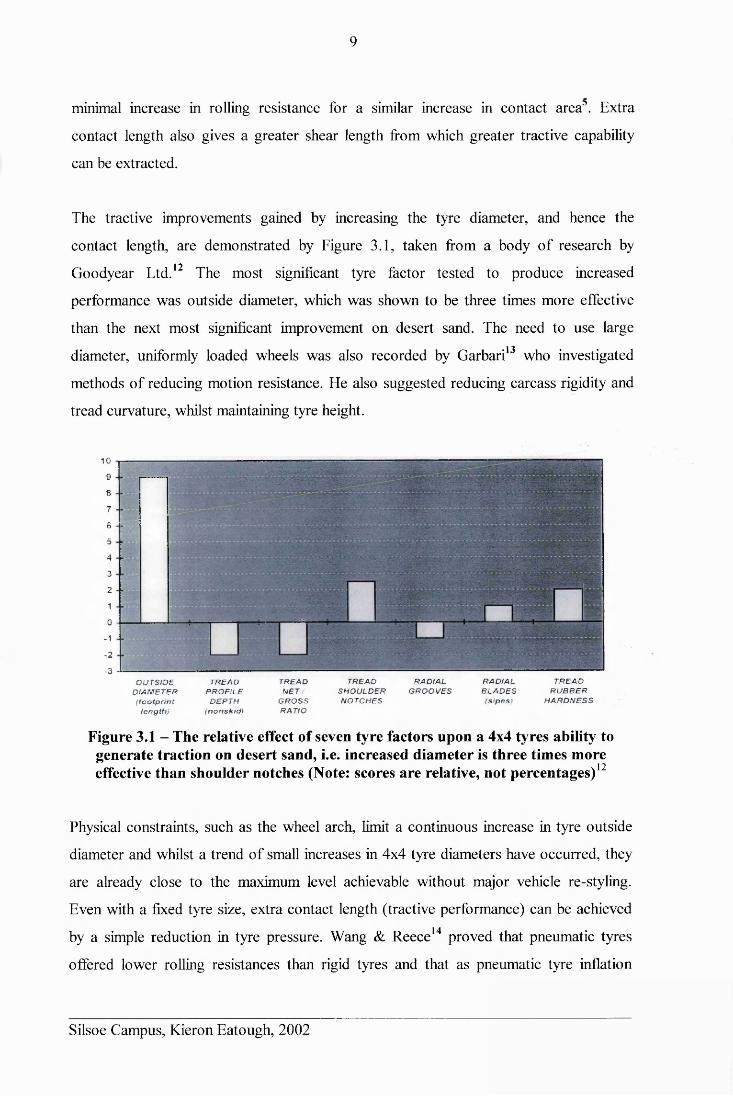
Figure 3.1 - The relative effect of seven tyre factors upon a 4x4 tyres ability to generate traction on desert sand, i.e. increased diameter is three times more effective than shoulder notches (Note: scores are relative, not percentages).............. 9
Figure 3.2 - Tyre performance requirements for 4x4 vehicles in five worldwide markets 11
Figure 3.3 - Tyres demonstrating sipes and shoulder notches....................................... 12Figure 3.4 - Typical slip-pull curves generated by Goodyear from full vehicle tests of
off-road tyres.............................................................................................. 14Figure 3.5 - General slip-pull curves for illustration, from Wismer & Luth..................15Figure 3.6 - A circular three-axis stress transducer................................................. 27Figure 3.7 - A normal pressure transducer.................................................................... 28Figure 3.8 - A schematic of the combination stress transducer with sonic emitters 28Figure 3.9 - Stress distributions along the tyre-soil contact surface at a sideslip angle of
20°; at 3 slips:------ -29.7%,------- = 12.2%, = 66.8%...................32Figure 3.10 - Distribution of thrust (+ ve) and rolling resistance (- ve) components
along the contact surface at slips of 8.2% (left) and 53.5% (right) at 10° sideslip........................................................................................................ 33
Figure 3.11 - Variations in dynamic weight (W), thrust/ weight ratio (H/W) and rolling resistance/ weight ratio (R/W) with slip......................................................33
Figure 3.12 - A typical plot of pressure (p) against sinkage (z) for 3 plate widths (b)from plate sinkage tests.............................................................................. 38
Figure 3.13 - A diagram illustrating how soil deformation modulus, K, is determined.40Figure 3.14 - A diagram of the position of the forces acting on a driven wheel operating
on soft terrain....................................................................................... 43Figure 3.15 - Forces, torque and stresses acting on a driven rigid wheel.......................45Figure 3.16 - A graph of contact stress characteristics beneath a tyre on sand 48Figure 3.17 - A diagram of the forces acting on a tractive tyre in sand.........................49Figure 3.18 - A method for measuring compressive sand fracture................................49Figure 4.1 - The relative importance of five off-road tyre factors as indicated by off-
road drivers.................................................................................................62Figure 4.2 - The relative importance of five off-road tyre performance factors as
indicated by off-road drivers...................................................................... 63Figure 4.3 - Typical smooth (left) and chunky (right) treaded tyres..............................64Figure 5.1 - Particle size distribution graphs for a number of global and local sand
samples and a sandy loam soil.................................................................... 69Figure 5.2 - The relationships between the contact area and Kj for the sandy loam soil
under different normal tyre loads................................................................ 70Figure 5.3 - The soil densities achieved for the 1170 kg/m3 soil preparations created
during the fixed slip tests.............................................. 73
Silsoe Campus, Kieron Eatough, 2002
Figure 5.4 - The soil densities achieved for the 1270 kg/m3 soil preparations createdduring the fixed slip tests............................................................................ 73
Figure 5.5 - The soil densities achieved for the 1400 kg/m3 soil preparations createdduring the fixed slip tests............................................................................ 74
Figure 5.6 - The moisture contents achieved for the 1170 kg/m3 soil preparationscreated during the fixed slip tests...............................................................74
Figure 5.7 - The moisture contents achieved for the 1270 kg/m3 soil preparationscreated during the fixed slip tests...............................................................75
Figure 5.8 - The moisture contents achieved for the 1400 kg/m3 soil preparationscreated during the fixed slip tests............................................................... 75
Figure 5.9 - Cone index readings recorded for different 1170 kg/m3 soil binpreparations over the duration of all testing.......................................... .....77
Figure 5.10 - Cone index readings recorded for different 1270 kg/m3 soil binpreparations over the duration of all testing................................................77
Figure 5.11 - Cone index readings recorded for different sand preparations in the soilbin over the duration of all testing.............................................................. 85
Figure 5.12 - The relationships between contact area and Kj for the DA80F sand underdifferent normal tyre loads.................. 86
Figure 6.1 - A schematic diagram of the layout of the fixed slip test rig.......................91Figure 6.2 - The deflected sinkage of a wheel..................................................... 96Figure 6.3 - EORT calibration graph..............................................................................97Figure 6.4 - Tension link calibration graph................................................................... 98Figure 6.5 - LVDT calibration graph............................................................................ 99Figure 6.6 - Tacho-generator calibration graph........................................................... 100Figure 6.7 - Rotary encoder calibration graph.............................. 101Figure 6.8 - Gross and net forces generated by the plain tread tyre on 1170 kg/m3 soil
across a range of discrete slips and inflation pressures............. 104Figure 6.9 - Rolling resistances and depths of sinkage generated by the plain tread tyre
on 1170 kg/m3 soil across a range of discrete slips and inflation pressures .................................................................................................................. 105
Figure 6.10 - Gross and net forces generated by the plain tread tyre inflated to 1.10 bar across a range of discrete slips and soil preparations.............................. 106
Figure 6.11 - Rolling resistances and sinkage generated by the plain tread tyre inflatedto 1.10 bar across a range of discrete slips and soil preparations..............106
Figure 6.12 - Gross and net forces generated by the plain tread tyre inflated to 3.10 bar across a range of discrete slips and soil preparations................................ 107
Figure 6.13 - Rolling resistances and sinkage generated by the plain tread tyre inflatedto 3.10 bar across a range of discrete slips and soil preparations..............108
Figure 6.14 - Gross and net forces generated on 1170 kg/m3 soil across a range ofdiscrete slips by six different tread pattern tyres inflated to 1.10 bar 109
Figure 6.15 - Rolling resistances and sinkage generated on 1170 kg/m3 soil across arange of discrete slips by six different tread pattern tyres inflated to 1.10 bar 110
Silsoe Campus, Kieron Eatough, 2002
Figure 6.16 - Gross and net thrusts, rolling resistances and deflected sinkages generated by the PT tyre operating at 1.10 bar on sand ...................................... 113
Figure 6.17 - Gross and net thrusts, rolling resistances and deflected sinkages generated by the G82 tyre operating at 1.10 bar on sand..........................................114
Figure 6.18 - The PT tyre tractive performance when operated at an intended 10% slip (inflation pressure 1.10 bar and static normal load 632 kg) on sand 115
Figure 6.19 - PT tyre tractive performance when operated at a nominal 50% slip(inflation pressure 1.10 bar and static normal load 632 kg) on sand 116
Figure 6.20 - G82 tyre tractive performance when operated at a nominal 50% slip(inflation pressure 1.10 bar and static normal load 632 kg) on sand 116
Figure 6.21 - Two cycles of data generated by the G82 tread inflated to 1.10 bar with a 650 kg static normal load (as described in section 1.1.1)......................... 122
Figure 6.22 - Typical results generated by the variable slip test rig operating the PT tyre inflated to 3.10 bar on 1170 kg/m3 soil.....................................................125
Figure 6.23 - Typical regions of decreasing slip (indicated by lengths ‘X’) ................127Figure 6.24 - Comparative results for the net thrusts and sinkages generated by a PT
tyre inflated to 3.10 bar operated on both the fixed and variable slip rigs across a slip range on 1170 kg/m3 soil......................................................129
Figure 6.25 - Comparative results for the net thrusts and sinkages generated by a PT tyre inflated to 3.10 bar operated on both the fixed and variable slip rigs across a slip range on 1270 kg/m3 soil......................................................129
Figure 6.26 - Traction data produced using the PT tread inflated to 1.10 bar and a static normal load o f650 kg on the variable slip test rig on sand....................... 131
Figure 6.27 - Traction data produced using the G82 tread inflated to 1.10 bar and astatic normal load o f650 kg on the variable slip test rig on sand 131
Figure 6.28 - Tractive performance traces from a full 4x4 vehicle test where thevehicle’s right side was operated on the sand surface.............................. 135
Figure 7.1 - The chosen tag grid positions in the sand profile (in mm)....................... 142Figure 7.2 - A schematic plan view of the tag placement equipment showing the
location of the zero point...........................................................................145Figure 7.3 - The calibration graphs for the three drawstring transducers.....................149Figure 7.4 - A schematic plan view of the tag location measurement equipment
showing the location of the zero point (as per the placement frame) and the positive measurement axes........................................................................149
Figure 7.5 - A schematic plan and side view of the measuring frame showing the three drawstrings and the two triangles these created (soil bin and sand omitted) .............................................................................................. 151
Figure 7.6 - A schematic plan and side view of the measuring frame and the distancesinto which the drawstring lengths were transformed................................ 151
Figure 7.7 - The positions of some of the tags during the assessment of the accuracy of the combined system.................................................................................156
Figure 7.8 - The typical slips within the thrust/ slip cycle at which the three tag gridswere positioned so as to be struck at three different slips......................... 157
Silsoe Campus, Kieron Eatough, 2002
Figure 7.9 - The relationship between the contact area (white) and the 3 mm band of contact length (blue) over which the 6911 TekScan mat could potentially measure stress...........................................................................................159
Figure 7.10 - Mean normal stress distributions along the contact length as measured by the 6911 TekScan mat.............................................................................. 160
Figure 7.11 - The relationship between the contact area (white) and the 112 mm band of contact length (blue) over which the 5051 mat measured stress...............161
Figure 7.12 - Mean normal stress distributions along the contact length as measured by the 5051 TekScan mat...............................................................................161
Figure 7.13 - Mean normal stress distributions along the contact length as measured by the 6300 TekScan mat...............................................................................162
Figure 7.14 - The TekScan mat bonded to the LAT tread prior to rubber encapsulation ..................................................................................................................165
Figure 7.15 - The relative location of each TekScan mat in the 180 mm wide treadregion of each of the six different treads ...........................................166
Figure 8.1 - Normal stresses recorded through the contact patch of the PT tread 169Figure 8.2 - Normal stresses recorded through the contact patch of the LAT tread.... 170Figure 8.3 - Normal stresses recorded through the contact patch of the LON tread.... 171Figure 8.4 - Normal stresses recorded through the contact patch of the 45B tread 172Figure 9.1 - An illustration of typical tag displacements that occurred as the tag grids
were struck at the three different slips (Note: the three positive axes of tag displacement, shown as X, Y and Z )........................................................ 174
Figure 9.2 - Mean values of net thrust recorded at the three slip treatments for the sixdifferent treads.......................................................................................... 177
Figure 9.3 - Mean values of wheel slip recorded at the three slip treatments for the sixdifferent treads.......................................................................................... 178
Figure 9.4 - Mean values of deflected wheel sinkage recorded at the three sliptreatments for the six different treads....................................................... 179
Figure 9.5 - Mean tag displacements in the X direction across the grid for all tyre treads and slips (as viewed from beneath a tyre along the line of travel)............181
Figure 9.6 - Mean tag displacements in the X direction for tag positions across the grid for all treads at the three levels of slip (again viewed from beneath a tyre along the line of travel).............................................................................182
Figure 9.7 - Mean tag displacements in the X direction for tag depth levels down thegrid for all treads at the three levels of slip (side view)............................ 183
Figure 9.8 - Smoothed mean tag displacements in the X direction for all the grid locations and slips to allow comparison between the six treads (same viewpoint as previous figures)...................................................................184
Figure 9.9 - A two-dimensional plot of mean tag displacements in the Y direction for all grid locations, treads and slips (viewed along the direction of wheel travel)........................................................................................... 186
Figure 9.10 - Two-dimensional plots of mean tag displacements in the Y direction for all grid locations and treads at the three slips (viewed along direction of travel)........................................................................................................187
Silsoe Campus, Kieron Eatough, 2002
Figure 9.11 - Two-dimensional plots of mean tag displacements in the Y direction for all grid locations and slips for the six treads (viewed along direction of travel)........................ 188
Figure 9.12 - A two-dimensional plot of mean tag displacements in the Z direction for all grid locations, treads and slips (viewed along the direction of wheel travel)........................................................................................................190
Figure 9.13 - Two-dimensional plots of mean tag displacements in the Z direction for all grid locations and treads at the three slips (viewed along direction of travel).................................................................................................. 191
Figure 9.14 - Two-dimensional plots of mean tag displacements in the Z direction for all grid locations and slips for the six treads (viewed along direction of travel)........................................................................................................192
Figure 9.15 - Mean net thrusts derived from the three replicate tests of each tread, and associated mean values of slip and sinkage that occurred simultaneously 193
Figure 9.16 - The relationship between deflected wheel sinkage and rolling resistanceacross all treatments on sand.................................................................... 195
Figure 9.17 - The different sand profile displacement patterns that occurred..............196Figure 9.18 - A diagram showing how slip governed the void size left by the tyre and
hence the sand’s Y displacement as it re-filled the void............................197Figure 10.1 - The derivation of the dynamic deflected wheel sinkage........................203Figure 10.2 - The relationship between contact length and vertical tyre acceleration. 204Figure 10.3 - The relationship between contact width and vertical tyre acceleration.. 205Figure 10.4 - The relationship between tyre contact width and rut width....................207Figure 10.5 - A typical tread pattern identified with the variables used to determine its
tread coefficient........................................................................................209Figure 10.6 - A representation of the methodology used to determine the volume of
sand displacement....................................................................................211Figure 10.7 - A comparison of experimental rolling resistance results and predicted
rolling resistance results................................................................... 212Figure 10.8 - A comparison between experimental and predicted gross thrust results for
the plain tread tyre inflated to 1.10 bar operated on 1170 kg/m3 soil 213Figure 10.9 - Gross thrusts achieved by the PT tread during the displacement
experiments........................................ 215Figure 10.10 - Gross thrusts achieved by the LON tread during the displacement
experiments............................................................................................... 215Figure 10.11 - Gross thrusts achieved by the 45F tread during the displacement
experiments............................................................................................... 216Figure 10.12 - Gross thrusts achieved by the 45B tread during the displacement
experiments............................................................................................... 216Figure 10.13 - Gross thrusts achieved by the LAT tread during the displacement
experiments............................................................................................... 217Figure 10.14 - The relationship between tread coefficients and the percentage extra
thrust that each tread was capable of generating over a plain tread tyre... 218
Silsoe Campus, Kieron Eatough, 2002
Figure 10.15 - Mean volumes of sand displaced at the eighteen slip and tyre treatments plotted with corresponding values of net thrust........................................ 219
Figure 10.16 - Gross thrust and rolling resistance data from the sand displacementexperiments; treatments ordered by the magnitude of gross thrust.......... 221
Figure 10.17 - Experimental net thrust results plotted against predicted net thrustscalculated for the PT tread............................................................ 222
Figure 10.18 - Experimental net thrust results plotted against predicted net thrustscalculated for the LON tread.................................................................... 223
Figure 10.19 - Experimental net thrust results plotted against predicted net thrustscalculated for the 45F tread...................................................................... 223
Figure 10.20 - Experimental net thrust results plotted against predicted net thrustscalculated for the 45B tread...................................................................... 224
Figure 10.21 - Experimental net thrust results plotted against predicted net thrustscalculated for the LAT tread..................................................................... 224
Figure 10.22 - A comparison plot of experimental and predicted net thrust results.... 225Figure 10.23 - A plot of experimental and predicted net thrusts for the PT tyre inflated
to 1.10 bar operating on the 1170 kg/m3 soil............................................ 226Figure 10.24 - The components of the gross thrust prediction, based upon PT results
recorded during the sand displacement experiments................................ 227Figure 10.25 - The relationships between sinkage and predictions of both the gross
thrust and rolling resistance made using the PT experimental results 228Figure 10.26 - Net thrusts produced by the combination of gross thrusts and rolling
resistances, based upon PT results from the sand displacement experiments ..................................................................................................................229
Figure 10.27 - The relationship between the volume of sand displacement caused by the treads and the gross thrusts achieved....................................................... 231
Figure 10.28 - The relationships between the tyre treads and the sand displacements 232Figure 10.29 - Experimental net thrust results plotted against predicted net thrusts
calculated for the G82 tread..................................................................... 234Figure 10.30 - Experimental net thrust results plotted against predicted net thrusts
calculated for the Wrangler HP tread........................................................234Figure 10.31 - Experimental net thrust results plotted against predicted net thrusts
calculated for the Wrangler UG tread.......................................................235Figure 10.32 - A comparison plot of experimental and predicted net thrust results for
the production treads.................................................................................236Figure 10.33 - The relationships between the tyre treads and the sand displacements for
all the treads.............................................................................................. 237Figure 10.34 - Experimental net thrust results plotted against predicted net thrusts
calculated for the Diamaris tread.............................................................. 238Figure 10.35 - Experimental net thrust results plotted against predicted net thrusts
calculated for the Wrangler HP (255) tread..............................................239Figure 10.36 - Experimental net thrust results plotted against predicted net thrusts
calculated for the TG31 tread................................................................... 239
Silsoe Campus, Kieron Eatough, 2002

Figure 10.37 - A comparison plot of experimental and predicted net thrust results forthe production treads................................................................................ 240
Figure 10.38 - The relationship between tread coefficient and percentage extra grossthrust relative to a PT tyre for all the tyres............................................... 242
Silsoe Campus, Kieron Eatough, 2002
xiv
Table of Plates
Plate 1.1 - A photograph of an immobilised Land Rover Discovery in Dubai desert sandconditions.....................................................................................................2
Plate 3.1 - The Goodyear G82 sand tyre........................................................................ 10Plate 3.2 - Typical forward and rearward sand failure patterns beneath a narrow plain
rigid wheel.................................................................................................. 17Plate 3.3 - A soil profile with paint markers developed by Trein..................................20Plate 3.4 - The handheld RFID scanner (a Pocket Reader) and a data tag used for the
experiments (the tag’s code is visible on the scanner’s screen)................. 22Plate 3.5 - A fully assembled SST................................................................................. 24Plate 3.6 - Stress sensors mounted to the outside of a plain tread tyre...........................25Plate 3.7 - An agricultural tyre mounted with diaphragm type pressure cells............... 26Plate 3.8 - A TekScan pressure sensing system.............................................................30Plate 3.9 - One side of a 5101 TekScan pressure sensitive mat showing the parallel
horizontal piezo-electric gel lines...............................................................31Plate 5.1 - The rubber bases of the sliding friction test sleds........................................ 81Plate 6.1 - A rear view of the soil bin and processor unit (mounted with the variable slip
single wheel tester).....................................................................................87Plate 6.2 - The three standard production tyres supplied.............................................. 89Plate 6.3 - Left: A comparison in diameter between the two G82 tyres supplied; Right:
the laser cut 235/70 R16 G82 tread and a 235/70 R16 plain tread blank.... 89Plate 6.4 - The symmetrical hand cut tread designs; the forward (F) and backward (B)
facing nomenclature was applied as if the tyres were rolling towards the reader............................................................................ 90
Plate 6.5 - The fixed slip test rig mounted to the soil processor operating on a firmsandy loam soil............................................. 92
Plate 6.6 - A view of the opposite side of the fixed slip test rig .................................... 93Plate 6.7 - The rotary encoder, signal cables and cable storage drum mounted to the test
rig............................................................................................................... 96Plate 6.8 - A front view of the soil processor, diesel engine and sub-frame................120Plate 6.9 - The new components fitted to create the hydraulically driven variable slip
test rig........................................................................................................120Plate 7.1 - The tank of sand to which dyed sand strips and then twenty data tags were
added, together with a 012 mm tine that was used to disturb the sand.... 138Plate 7.2 - The flow patterns of dyed sand strips and tags after disturbance................139Plate 7.3 - The flow patterns of dyed sand and tags after further excavation...............140Plate 7.4 - The location of the remaining tags and dyed sand......................................140Plate 7.5 - The data tag placement frame.....................................................................143Plate 7.6 - The placement frame insertion bracket.................................................... 144Plate 7.7 - A plan view of the frame zero point on the tag measurement frame 145
Silsoe Campus, Kieron Eatough, 2002

XV
Plate 7.8 - The data tag insertion process.................................................................... 146Plate 7.9 - The tag position measurement frame positioned over a sand tank..............148Plate 7.10 - The three drawstring transducers mounted to the measuring frame..........150
Silsoe Campus, Kieron Eatough, 2002
xvi
Table of Tables
Table 2.1 - The stages of the project methodology..........................................................6Table 5.1 - Particle size analysis of the sandy loam soil............................................... 68Table 5.2 - Average soil densities produced for the three soil preparations during the
plate sinkage tests and appropriate dry base moisture contents................. 71Table 5.3 - Bekker pressure sinkage coefficients for the three soil preparations.......... 72Table 5.4 - Mean soil density preparations and moisture contents................................76Table 5.5 - Descriptions of the assessed sand samples..................................................79Table 5.6 - Weightings used for sand ranking analysis..................................................79Table 5.7 - Results from the translational shear box tests............................................. 80Table 5.8 - Results from the sliding sand-rubber friction tests...................................... 82Table 5.9 - The weighted percentage differences of the local sand sample scores
(relative to the Dubai sand)........................................................................ 83Table 5.10 - Bekker pressure sinkage coefficients for the sand preparation................. 86Table 6.1 - Fixed slip tests treatments investigated on the sandy loam soil (note: colour
coding indicates the different groups of variables investigated)...............102Table 6.2 - The variables investigated in the fixed slip tests on the sand....................112Table 6.3 - The bands of slip that were used to produce mean values......................... 127Table 7.1 - The results from the carpenters square calibration measurements 154Table 9.1 - The test variables for the sand displacement investigation for the prototype
treads inflated to 1.10 bar..........................................................................175Table 9.2 - A sample section of the overall results table showing the experimental data
and headings that were entered into Genstat.............................................176Table 9.3 - The treads grouped by the tractive performance variations they caused... 180Table 9.4 - The tractive performance trends produced by the different treads.............199Table 10.1 - Tread coefficients for the five prototype treads tested during the sand
displacement experiment.......................................................................... 210Table 10.2 - Percentage extra gross thrust outputs that were achieved by the five
prototype treads at 100mm sinkage..........................................................217Table 10.3 - Tread factors determined for the five prototype treads............................219Table 10.4 - Tread coefficients and factors determined for the production treads......233Table 10.5 - Tread coefficients and percentage extra gross thrusts achieved by the
255/55 R19 production treads................................................................... 238Table 10.6 - Tread coefficients and gross thrust benefits of the production treads.....241
Silsoe Campus, Kieron Eatough, 2002

List of Symbols
This list details commonly used symbols used throughout the whole text. It does not
include specific symbols from several equations detailed only in the literature review,
which are listed with a frill explanation of the relevant symbols, because different
authors use conflicting symbols to represent the same set of variables.
Symbol Full DescriDtion
0 Diameter
a Gradient of tangent to shear stress / shear displacement curve
a Terms from Bekker resistance prediction equations
ae Angle of the groove edge
d Tyre deflection
s Terms from Bekker resistance prediction equations
<1> Angle of internal shearing resistance
7 Soil density
P Normal pressure (stress) typically below a sinkage plate
Pgcr Critical ground pressure
r Shear stress
10 Angular velocity of the wheel
A Contact area
a Acceleration
Ad Dynamic contact areas (w° x 1D)
b Contact patch width
b Minimum sinkage plate width
btr Deflected tyre width
c Cohesion
C Cone Index
d Tyre diameter
D Undeflected tyre diameter
En Edge number
Silsoe Campus, Kieron Eatough, 2002
XV111
Symbol Full Description
G Sand penetration resistance gradient
g Acceleration due to gravity (9.81 m/s )
g ’ Dynamic vertical load adjustment factor
Gey Revised sand penetration resistance gradient
G„ Groove number
H Thrust
h Tyre section height (unloaded)
Hmax Maximum thrust
i Slip
j Shear deformation (displacement)
K Soil deformation modulus
k<h Empirically measured Bekker soil deformation coefficient
kc Empirically measured Bekker soil deformation coefficient
Ke Representation number for tyre carcass
Kpy Terms from Bekker resistance prediction equations
Kpc Terms from Bekker resistance prediction equations
/ Contact patch (shear) length
lD Dynamic contact length
Le Length of groove edge
Lfu Fraction of tread unit length
Lg Length of a groove type
M Mobility number
m Mass
n Empirically measured Bekker soil deformation coefficient
n Number of different groove types
Ny Terzaghi soil coefficient
Nc Tyre numeric for clay
Nc Terzaghi soil coefficient
Nq Terzaghi soil coefficient
Ns Tyre numeric for sand
Nsey Revised tyre numeric for sand
Silsoe Campus, Kieron Eatough, 2002
Symbol Full Description
P Pull
Q Normal load on axle
Qg Quantity of grooves of each particular groove type
Qte Total number of groove edges
r Rolling radius of wheel
R Resistance
Rb Bulldozing resistance
Rc Compaction resistance
Rf Tyre carcass flexing resistance
RR Rolling Resistance
Tc Tread coefficient
Tf Tread factor
Tn Tread number
TVr Tread: void ratio
Va Actual travel speed
Vt Theoretical travel speed (roi)
W Normal load on axle
mP Dynamic contact width
Wff Fraction of full tread width
wg Width of a grove type
z Plate (or wheel) sinkage
Zdef Deflected wheel sinkage
Zr Tyre sinkage
Silsoe Campus, Kieron Eatough, 2002
XX
List of Abbreviations
Abbreviation Full Description
A-D Analogue to Digital
CCD Charge Couple Device
CFD Computational Fluid Dynamics
CTIS Central Tyre Inflation System
DA80F Product code for the replicate sand
DAC Digital / Analogue Conversion
DC Direct Current
EORT Extended Octagonal Ring Transducer
EPSRC Engineering and Physical Sciences Research Council
FE / FEA Finite Element / Finite Element Analysis
FPS Frames per second
GTC*L Goodyear Technical Centre in Luxembourg
IPOT Image Processing and Optical Technology
LVDT Linear Variable Displacement Transducer
NIAE National Institute of Agricultural Engineering
OEM Original Equipment Manufacturer
RDC Region of Direct Contact
RF / RFID Radio Frequency / Radio Frequency Identification
RHS Rectangular Hollow Section
RS Radio Spares
SDL Soil Dynamics Laboratory (Cranfield University Silsoe)
SIMS School of Industrial Manufacturing Science
SST Soil Stress State Transducer
SUV Sports Utility Vehicle
Tread G82 Goodyear Sand Tread
Tread G90 Goodyear Off-road Military Mud Tread
Tread HP Goodyear Wrangler HP Tread
Tread LAT Lateral Prototype Tread
Tread LON Longitudinal Prototype Tread
Silsoe Campus, Kieron Eatough, 2002

Abbreviation
Tread PT
Tread UG
Tread xxB
Tread xxF
U.A.E.
WES
xxi
Full Description
Plain Tread (Slick or Blank)
Goodyear Wrangler Ultra-Grip Tread
Prototype Tread (xx degrees rearward)
Prototype Tread (xx degrees forward)
United Arab Emirates
Waterways Engineering Station
Silsoe Campus, Kieron Eatough, 2002

1
1 INTRODUCTION
It is no longer sufficient, nor economically sustainable, for well developed automotive
markets to produce a basic car to just get people from A to B. Across the consumer
vehicle range the automotive industry is becoming ever-increasingly competitive as the
market becomes more demanding. This is especially true in ‘newer’ market segments,
such as the SUV (Sports Utility Vehicle) sector, also termed the 4x4, or light truck,
market. To maintain sales in this premium brand environment, vital customer value
must be added by delivering high performance, high specification vehicles. The desires
of several motor vehicle and tyre manufacturing companies to maintain their
commercial positions as leading manufacturers of high performance off-road products
led to this project’s sponsorship.
Alongside EPSRC, who provided much of the fimding for this study, Land Rover
(BMW) provided the initial company sponsorship, whilst Goodyear Technical Centre in
Luxembourg (GTC*L) provided technical assistance. Both companies wished to
develop a greater understanding of the factors that contribute to 4x4 tyres offering good
mobility on loose desert sands, which cover approximately one-seventh of the world’s
land mass1, and more importantly, which are commonly located adjacent to the potential
future growth markets for motor vehicles in the developing world2. The sponsors also
wished to identify modifications that could be made to existing tyre designs and/ or
vehicle systems to further improve the mobility of Land Rover vehicles.
In desert conditions it is a tyre’s limited ability to develop net positive traction that
limits vehicle performance. For Land Rover to maintain its brand and market position as
the manufacturer of “the best 4x4 by far” its products must be capable of achieving
superior off-road performance over competitor vehicles, as once mobility is lost then
any vehicle becomes of little use, whatever its brand. Whilst limits to a vehicle’s ability
will always exist, such circumstances are potentially very damaging for a brand image
built on its product’s off-road capabilities.
As the tyre is the limiting factor in these conditions, Land Rover only has indirect
control over the main component governing its product (and brand) performance,
Silsoe Campus, Kieron Eatough, 2002
2
makes it difficult to ensure that the premium performance tyre that is desired is always
available to Land Rover. To help address this situation Land Rover wished to
collaborate with both a tyre manufacturer and a University. Their aim was to develop a
clearer understanding of sand traction mechanics for 4x4 vehicles, whilst allowing
closer integration of tyre and vehicle development.
Goodyear’s participation was driven by their brand image being enhanced when their
products are fitted to high-performance vehicles. Closer involvement with an OEM
(original equipment manufacturer) also provided increased opportunities to understand
the OEM requirements and market their products. Increased OEM custom also
generates more secondary purchases from end-users. Additionally, in recent years no
tyre manufacturer has conducted any significant quantity of research on off-road desert
tyres3, thus the project offered Goodyear an opportunity to develop a competitive
advantage.
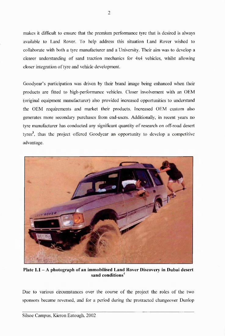
Plate 1.1 - A photograph of an immobilised Land Rover Discovery in Dubai desertsand conditions4
Due to various circumstances over the course of the project the roles of the two
sponsors became reversed, and for a period during the protracted changeover Dunlop
Silsoe Campus, Kieron Eatough, 2002
3
Tyres Ltd, Fort Dunlop, Erdington, UK, replaced GTC*L as sponsors. Despite these
changes, the project’s focus remained on identifying the interactions between a tyre
(tread) and sand surface that enable useful traction to be generated, and determining if,
and how, the governing factors in the interaction could be altered to reduce the
likelihood of vehicle immobility occurring in the manner shown in Plate 1.1.
Generating net positive traction on pure sand can be difficult, especially if the sand is in
a loose state. Desert sand conditions can vary from firm to weak depending upon the
local conditions. Often the sand medium results from the deposition of large quantities
of loose sand by aeolian processes over many years. The extreme diurnal temperature
fluctuations (and associated evaporation/ dew formation) encountered in desert regions
cause the top sand layer to form a stronger crust that overlies weak structured, loose
sand5. The stronger crust is more capable of bearing vehicle weight and thus allowing
vehicle mobility, however once the crust is breached the vehicle is then forced to
operate in weaker sand conditions. It is these weaker conditions that are most likely to
immobilise the vehicle, and hence the conditions that warrant the most study.
In these conditions it is important to extend the barriers of mobility as far as possible.
Through its many years of off roading experience Land Rover has learnt that tyre choice
is vital to maximising mobility. However, whilst both sponsors can identify good
performing tyres for sand environments through extensive field-testing, they have not
identified exactly which tyre features actually generate the high tractive performance .
This is sometimes highlighted when end-users fit different replacement tyres that did
not demonstrate impressive performance during company testing6, but which the user
either know, feel or believe, enable the vehicle to deliver greater performance over the
standard fitment. These choices are particularly important, as end-user experience in its
totality far exceeds that of the manufacturers, whose test programmes are operated
under cost and time constraints. The manufactures are therefore often unable to identify
when particular tyre (and vehicle) features are suited to specific local conditions.
If the factors governing a tyre’s performance, in particular the tread, which is often the
biggest difference between different manufacturers’ tyres, were modelled then the
Silsoe Campus, Kieron Eatough, 2002

4
potential performance of different tyre designs could be evaluated from the design
office by the manufacturers, who are increasingly relying upon FEA (finite element
analysis), CFD (computational fluid dynamics) and dynamic analysis software packages
to fully model vehicle behaviour in the virtual environment. This type of evaluation is
used because it removes some field-testing costs, whilst also reducing the development
time scale, which achieves further indirect cost savings. Developing a tyre performance
model necessitated both a model and actual test results against which the model’s
predictions could be benchmarked, thus physical traction experiments were required.
These provided a basis for the understanding of the contact interactions, which enabled
the tyre and tread performance prediction models to be developed, and test data for
validation purposes.
Silsoe Campus, Kieron Eatough, 2002

5
2 AIM AND OBJECTIVES
2.1 AIM
To determine the relationships between tractive force, sand displacement and tread
pattern for light truck (4x4) tyres generating traction from pure sand.
2.2 OBJECTIVES
1. Develop instrumentation and methodologies for the measurement of tyre tractive
performance and three-dimensional sand particle movement underneath tyres.
2. Determine the effect of tread pattern upon the three-dimensional sand disturbance
and tractive performance generated at low forward speeds across a slip range.
3. Develop empirical or computational models of the relationships between tread
pattern features, sand flow and traction.
4. To identify developments for 4x4 tread designs for desert conditions to improve
traction and determine the commercial implications of the proposed changes.
Silsoe Campus, Kieron Eatough, 2002

6
2.3 PROJECT METHODOLOGY
Project management procedures were adopted for the study to ensure that it was
delivered within the time, budget and quality constraints that were fixed at the outset.
Seven key project phases were defined, as listed in Table 2.1.
Table 2.1 - The stages of the project methodology
No. Component Deliverable
1 Literature review. A critical review of current applicable traction knowledge and applicable tyre test methodologies.
2 Traction surface analysis. Quantification of the differences in the traction (engineering) properties of a range of sand and soil traction mediums.
3 Design and development of instrumentation.
Instrumentation systems and test methodologies to allow the measurement of three-dimensional sand displacements and normal stresses beneath 4x4 tyres.
4 Tyre test rig construction. An instrumented test rig suitable for the tractive evaluation of 4x4 tyres in the soil bin environment to enable slip-pull graphs to be generated.
5 Measurement of tyre tractive performance and associated sand displacement.
Tyre traction and sand displacement results from the range of treatments tested, which were suitable for the development and validation of the models.
6 Modelling of tractive force and sand displacement relationship.
A prediction model for tyre tractive performance and sand displacement, based on both tyre and tread characteristics, which was capable of predicting traction on loose sand for a given tread and other treatments.
7 Evaluate the commercial implications of the findings.
An evaluation of the recommendations for sand tyre design from a commercial viewpoint.
Silsoe Campus, Kieron Eatough, 2002
7
3 LITERATURE REVIEW
3.1 INTRODUCTION
The need for the research arose because both tyres and sand have complex
characteristics. A tyre is a heterogeneous, discontinuous composite, made from cords,
wires and elastomers, with complex elastic, plastic and viscous properties, which under
operates under mechanical and thermal stress7. No test equipment capable of measuring
all tyre properties in a satisfactoiy and reproducible way is currently available and no
theoretical model exists to predict all tyre properties, whilst the partial models that do
exist are very complex and mathematically demanding7. In short, whilst tyre
manufacturers have a very good knowledge of on-road tyre mechanics, they do not
completely understand how a tyre functions in all environments.
The complexity of sand arises because in its naturally occurring state it too is a
heterogeneous material, comprised of quartz particles and other minerals of varying size
combined with varying sizes of air pores, depending upon its compaction. As many
different sand types exist in comparison to the quantity of different road pavements,
thus modelling tyre performance and surface interaction is considerably more
complicated for sand surfaces than for road pavements. Until recently 4x4 tyre/ soil
interaction represented only a small and complex part of the tyre market, thus
comparatively less money and effort was expended on understanding its mechanics, in
comparison to the resources spent upon understanding tyre behaviour on wet tarmac3.
Therefore a gap in knowledge exists in this subject area.
Both sponsors wished to address the general lack of test procedures, apparatus or
models that could simply and universally describe the performance capabilities of new,
or development, tyres in sand. Any partial substitutes for the extensive subjective
handling tests necessarily conducted at present to determine the optimum vehicle and
tyre combinations have the potential to generate significant cost savings. Additionally,
the automotive industry has a growing need for greater statistical information to more
accurately model the effects of different tyres within the totality of vehicle simulation
and modelling8. Additional comments by Williams9 confirmed both those needs. Hence,
Silsoe Campus, Kieron Eatough, 2002
8
as computing capability develops so too will the requirement; to model tyre behaviour,
and to have raw test data to use when validating computer prediction models.
3.2 BASIC TYRE EVALUATION
3.2.1 Basic Tyre Relationships
At the base level it is well known that to generate increased traction from a vehicle on
cohesionless soils then further normal load, should be added as predicted by
Micklethwaite’s10 development of Coulomb’s soil equation shown below.
Thrust = H max = blc + Qtan<f> (1)
Where: b = contact patch width / = contact patch length
c = cohesion Q = normal load on axle
(j) = angle of internal shearing resistance
This applies until the soil bearing capacity is exceeded, at which point the tyre, (or
track), will sink into the surface forming a rut. If further load is applied to increase the
gross thrust potential, then a further level of sinkage (rutting) will occur. As sinkage
increases so does the rolling resistance faced by the tyre, thus the overall net thrust
output is reduced. The only way to reduce sinkage is to reduce the normal stress for a
given load, which necessitates increasing the contact area11.
Physical and mechanical limitations govern the magnitude by which the contact patch
can be increased, for instance, track width and suspension performance requirements
both limit the tyre width. Within these limits, either widening the tyre or increasing its
diameter will increase the contact area. However on loose sand the effect of these
changes upon rolling resistance is important. The mechanism by which rolling
resistance is generated is complicated, but its magnitude directly increases with wheel
sinkage, whether the sinkage is caused by a lack of soil bearing capacity, or slip-sinkage
of the wheel. Once a tyre is partially sunk it produces rolling resistance by acting like a
backward raked, convex, bulldozer blade, hence resistance increases with tyre width.
Contrastingly, increasing contact patch length by increasing tyre diameter produces a
Silsoe Campus, Kieron Eatough, 2002
9
minimal increase in rolling resistance for a similar increase in contact area3. Extra
contact length also gives a greater shear length from which greater tractive capability
can be extracted.
The tractive improvements gained by increasing the tyre diameter, and hence the
contact length, are demonstrated by Figure 3.1, taken from a body of research by
Goodyear Ltd.12 The most significant tyre factor tested to produce increased
performance was outside diameter, which was shown to be three times more effective
than the next most significant improvement on desert sand. The need to use large
diameter, uniformly loaded wheels was also recorded by Garbari13 who investigated
methods of reducing motion resistance. He also suggested reducing carcass rigidity and
tread curvature, whilst maintaining tyre height.
10
9 8
7
6
5
4
3
2
1
0 -1
-2
-3
Figure 3.1 - The relative effect of seven tyre factors upon a 4x4 tyres ability to generate traction on desert sand, i.e. increased diameter is three times more effective than shoulder notches (Note: scores are relative, not percentages)12
Physical constraints, such as the wheel arch, limit a continuous increase in tyre outside
diameter and whilst a trend of small increases in 4x4 tyre diameters have occurred, they
are already close to the maximum level achievable without major vehicle re-styling.
Even with a fixed tyre size, extra contact length (tractive performance) can be achieved
by a simple reduction in tyre pressure. Wang & Reece14 proved that pneumatic tyres
offered lower rolling resistances than rigid tyres and that as pneumatic tyre inflation
OUTSIDE TREAD TREAD TREAD RADIAL RADIAL TREADDIAM ETER PROFILE N E T / SH OU LDER G RO O V E S B L A D E S R U B B E R(fo o tp rin t DEPTH G R O S S NO TCH ES (s ip e s ) H A R D N E SS
leng th ) (n o n sk id ) RATIO
Silsoe Campus, Kieron Eatough, 2002
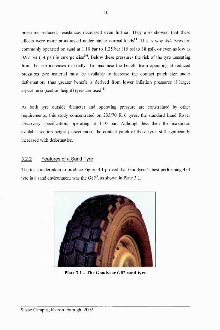
10
pressures reduced, resistances decreased even further. They also showed that these
effects were more pronounced under higher normal loads14. This is why 4x4 tyres are
commonly operated on sand at 1.10 bar to 1.25 bar (16 psi to 18 psi), or even as low as
0.97 bar (14 psi) in emergencies ’ . Below these pressures the risk of the tyre unseating
from the rim increases markedly. To maximise the benefit from operating at reduced
pressures tyre material must be available to increase the contact patch size under
deformation, thus greater benefit is derived from lower inflation pressures if larger
aspect ratio (section height) tyres are used15.
As both tyre outside diameter and operating pressure are constrained by other
requirements, this study concentrated on 235/70 R16 tyres, the standard Land Rover
Discovery specification, operating at 1.10 bar. Although less then the maximum
available section height (aspect ratio) the contact patch of these tyres still significantly
increased with deformation.
3.2.2 Features of a Sand Tyre
The tests undertaken to produce Figure 3.1 proved that Goodyear’s best performing 4x4
tyre in a sand environment was the G82 , as shown in Plate 3.1.
Plate 3.1 - The Goodyear G82 sand tyre
Silsoe Campus, Kieron Eatough, 2002
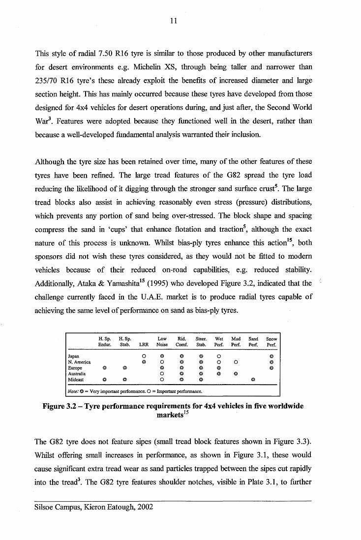
11
This style of radial 7.50 R16 tyre is similar to those produced by other manufacturers
for desert environments e.g. Michelin XS, through being taller and narrower than
235/70 R16 tyre’s these already exploit the benefits of increased diameter and large
section height. This has mainly occurred because these tyres have developed from those
designed for 4x4 vehicles for desert operations during, and just after, the Second World
War3. Features were adopted because they functioned well in the desert, rather than
because a well-developed fundamental analysis warranted their inclusion.
Although the tyre size has been retained over time, many of the other features of these
tyres have been refined. The large tread features of the G82 spread the tyre load
reducing the likelihood of it digging through the stronger sand surface crust5. The large
tread blocks also assist in achieving reasonably even stress (pressure) distributions,
which prevents any portion of sand being over-stressed. The block shape and spacing
compress the sand in ‘cups’ that enhance flotation and traction5, although the exact
nature of this process is unknown. Whilst bias-ply tyres enhance this action15, both
sponsors did not wish these tyres considered, as they would not be fitted to modem
vehicles because of their reduced on-road capabilities, e.g. reduced stability.
Additionally, Ataka & Yamashita15 (1995) who developed Figure 3.2, indicated that the
challenge currently faced in the U.A.E. market is to produce radial tyres capable of
achieving the same level of performance on sand as bias-ply tyres.
H. Sp. Endur.
H. Sp. Stab. LRR
LowNoise
Rid.Comf.
Steer.Stab.
WetPerf.
MudPerf.
SandPerf.
SnowPerf.
Japan O © © © O ©N. America © O © © O 0 ©Europe © © © © © © ©Australia o © © © ©Mideast © © 0 © © ©Note: © = Very important performance. O = Important performance.
Figure 3.2 - Tyre performance requirements for 4x4 vehicles in five worldwidemarkets15
The G82 tyre does not feature sipes (small tread block features shown in Figure 3.3).
Whilst offering small increases in performance, as shown in Figure 3.1, these would
cause significant extra tread wear as sand particles trapped between the sipes cut rapidly
into the tread3. The G82 tyre features shoulder notches, visible in Plate 3.1, to further
Silsoe Campus, Kieron Eatough, 2002
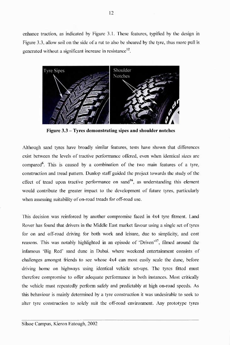
12
enhance traction, as indicated by Figure 3.1. These features, typified by the design in
Figure 3.3, allow soil on the side of a rut to also be sheared by the tyre, thus more pull is• • • 12 generated without a significant increase in resistance .
Figure 3.3 - Tyres demonstrating sipes and shoulder notches
Although sand tyres have broadly similar features, tests have shown that dilferences
exist between the levels of tractive performance offered, even when identical sizes are
compared6. This is caused by a combination of the two main features of a tyre,
construction and tread pattern. Dunlop staff guided the project towards the study of the
effect of tread upon tractive performance on sand16, as understanding this element
would contribute the greater impact to the development of future tyres, particularly
when assessing suitability of on-road treads for off-road use.
This decision was reinforced by another compromise faced in 4x4 tyre fitment. Land
Rover has found that drivers in the Middle East market favour using a single set of tyres
for on and off-road driving for both work and leisure, due to simplicity, and cost
reasons. This was notably highlighted in an episode of ‘Driven’17, filmed around the
infamous ‘Big Red’ sand dune in Dubai, where weekend entertainment consists of
challenges amongst friends to see whose 4x4 can most easily scale the dune, before
driving home on highways using identical vehicle set-ups. The tyres fitted must
therefore compromise to offer adequate performance in both instances. Most critically
the vehicle must repeatedly perform safely and predictably at high on-road speeds. As
this behaviour is mainly determined by a tyre construction it was undesirable to seek to
alter tyre construction to solely suit the off-road environment. Any prototype tyres
Silsoe Campus, Kieron Eatough, 2002
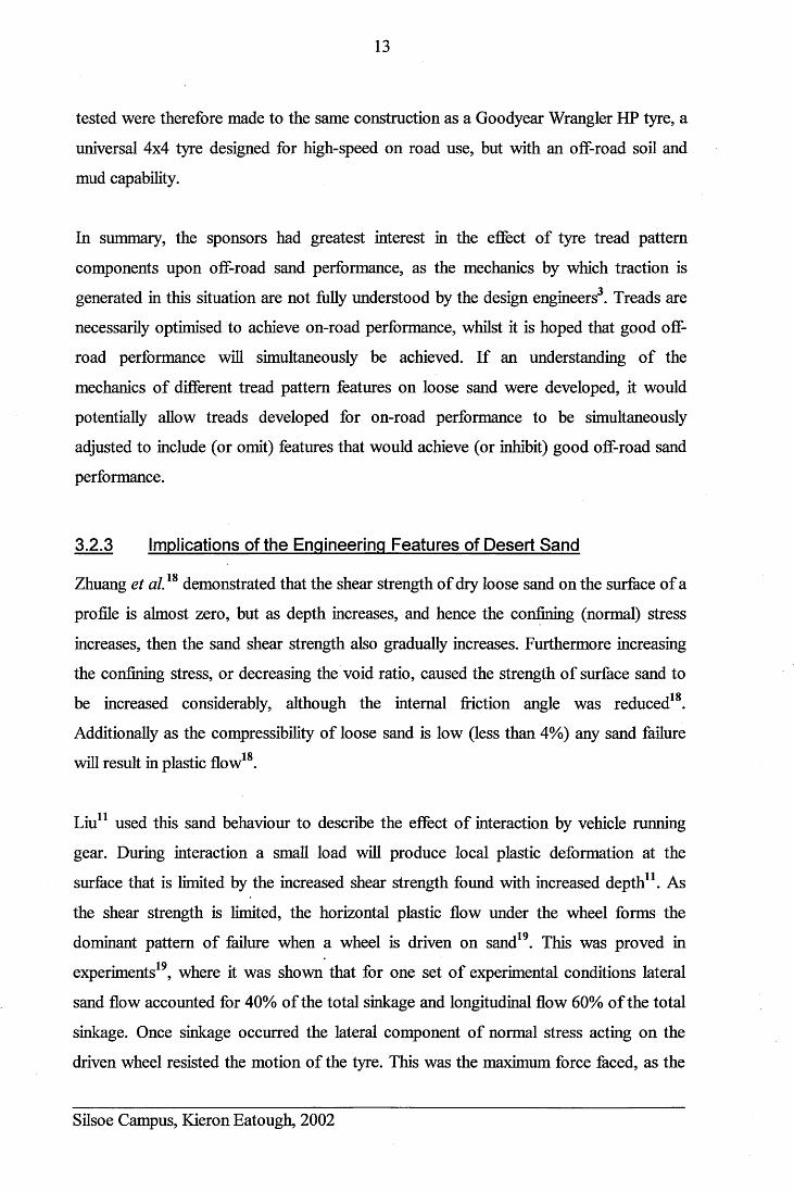
13
tested were therefore made to the same construction as a Goodyear Wrangler HP tyre, a
universal 4x4 tyre designed for high-speed on road use, but with an ofif-road soil and
mud capability.
In summary, the sponsors had greatest interest in the effect of tyre tread pattern
components upon off-road sand performance, as the mechanics by which traction is
generated in this situation are not fully understood by the design engineers3. Treads are
necessarily optimised to achieve on-road performance, whilst it is hoped that good off-
road performance will simultaneously be achieved. If an understanding of the
mechanics of different tread pattern features on loose sand were developed, it would
potentially allow treads developed for on-road performance to be simultaneously
adjusted to include (or omit) features that would achieve (or inhibit) good off-road sand
performance.
3.2.3 Implications of the Engineering Features of Desert Sand152Zhuang et al demonstrated that the shear strength of dry loose sand on the surface of a
profile is almost zero, but as depth increases, and hence the confining (normal) stress
increases, then the sand shear strength also gradually increases. Furthermore increasing
the confining stress, or decreasing the void ratio, caused the strength of surface sand to• 1 5 2be increased considerably, although the internal friction angle was reduced .
Additionally as the compressibility of loose sand is low (less than 4%) any sand failure1 5 2will result in plastic flow .
Liu11 used this sand behaviour to describe the effect of interaction by vehicle running
gear. During interaction a small load will produce local plastic deformation at the
surface that is limited by the increased shear strength found with increased depth11. As
the shear strength is limited, the horizontal plastic flow under the wheel forms the
dominant pattern of failure when a wheel is driven on sand19. This was proved in
experiments19, where it was shown that for one set of experimental conditions lateral
sand flow accounted for 40% of the total sinkage and longitudinal flow 60% of the total
sinkage. Once sinkage occurred the lateral component of normal stress acting on the
driven wheel resisted the motion of the tyre. This was the maximum force faced, as the
Silsoe Campus, Kieron Eatough, 2002
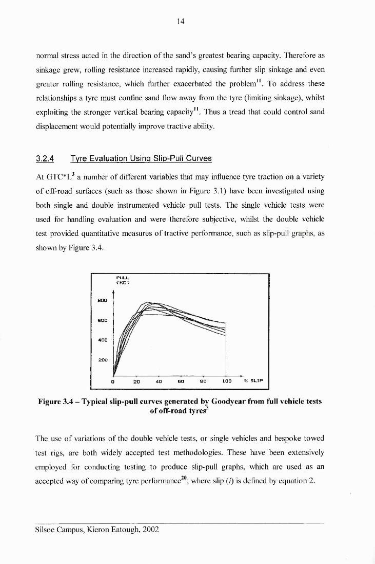
14
normal stress acted in the direction of the sand’s greatest bearing capacity. Therefore as
sinkage grew, rolling resistance increased rapidly, causing further slip sinkage and even
greater rolling resistance, which further exacerbated the problem11. To address these
relationships a tyre must confine sand flow away from the tyre (limiting sinkage), whilst
exploiting the stronger vertical bearing capacity11. Thus a tread that could control sand
displacement would potentially improve tractive ability.
3.2.4 Tyre Evaluation Using Slip-Puil Curves
At GTC*L3 a number of different variables that may influence tyre traction on a variety
of off-road surfaces (such as those shown in Figure 3.1) have been investigated using
both single and double instrumented vehicle pull tests. The single vehicle tests were
used for handling evaluation and were therefore subjective, whilst the double vehicle
test provided quantitative measures of tractive performance, such as siip-puli graphs, as
shown by Figure 3.4.
PULLC KG >
8 0 0
600
400
200
% S L IP1008 0SO20 4 0
Figure 3.4 - Typical slip-pull curves generated by Goodyear from full vehicle testsof off-road tyres3
The use of variations of the double vehicle tests, or single vehicles and bespoke towed
test rigs, are both widely accepted test methodologies. These have been extensively
employed for conducting testing to produce slip-pull graphs, which are used as an
accepted way of comparing tyre performance ; where slip (/) is defined by equation 2.
Silsoe Campus, Kieron Eatough, 2002
15
(2)
Where: Va = actual travel speed
r = rolling radius of wheel
Vt = theoretical travel speed = rco
(o= angular velocity of the wheel
A slip-pull curve describes a tyre’s performance envelope. Typically a graph will show
the pull (thrust) of a vehicle (tyre) across the full range of slips (0-100%) for any set of
tyre and soil treatments. As no useful traction is achieved at 0% or 100%, graphs more
commonly describe traction from about 5% to 80% slip. However, the frill range of skid
and slip can be plotted for completeness, as shown by Figure 3.5.
Results can either be generated for a whole vehicle, or if a single wheel tester is used,
for an individual wheel. In both instances vehicles separate from those being tested are
required to provide a resistance to enable slip to be generated. Thrust results are
single test run conducted with a varied slip sweep range. Gross, or net, thrust results
may be plotted for tyre analysis and comparison.
Silsoe Campus, Kieron Eatough, 2002
TOWEDWHEEL D RIV IN G WHEEL TORQUE, Q
GIVEN S O IL STRENGTH, T IR E S IZ E AND LOAD
TOWEDFORCE
/ / \ SElF-PROPELLED W/ / I WHEEL ^
Figure 3.5 - General slip-pull curves for illustration, from Wismer & Luth21
recorded for either several passes testing at a range of discrete wheel slips, or for a
16
3.2.5 Indications from a Simple Off-Road Tyre Field Investigation
Piper22 conducted an investigation examining the tractive performance of a variety of
tyres, both production and experimental, operating on sand at Cainhoe sand quarry, near
Silsoe, UK, at discrete inflation pressures ranging from 1.10 bar to 2.76 bar. This work
involved the development and testing of an experimental methodology for outdoor tyre
evaluation with 4x4 vehicles. This author gave assistance during the testing, and thus
observed first hand the processes of sand traction for a Land Rover vehicle and a range
of different treaded tyres. Piper’s work showed that his methodology was effective, but
the experimental results were not extensive enough to support dependable conclusions,
although the following trends were shown :
1. Different treads influenced the rate of wheel sinkage.
2. The relationship between pull and tyre inflation pressure was not consistent with
the typically accepted theory that lower pressure equals greater pull.
If, as was indicated, tread pattern influences the rate of sinkage by influencing slip
sinkage, then the potential exists to optimise tread to reduce sinkage, and hence rolling
resistance. Perara23 proposed a possible explanation why, in contrary to accepted
wisdom, the measured pulls were not necessarily increased with reduced inflation
pressure. When operating at very low inflation pressures the tyre carcass may become• • • 23squarer, and hence act more like a bulldozer blade with increased rolling resistance .
However, this conclusion contradicts a vast body of anecdotal evidence from
experienced 4x4 desert drivers5 and must therefore remain doubtful.
3.3 MEASUREMENT OF SOIL (SAND) DISTURBANCE
If soil deformation can be measured then it can be directly related to the traction
generated by a tyre. Strain is a more direct measurement than stress, being directly
related to the deformation experienced. Several authors have investigated both variables
on soil, with early methods documented by Gill & Vanden Berg24. During tyre
immobilisation sand flow occurs in every plane so to measure the tread effect upon sand
displacement an ability to identify, mark and measure sand displacements in three-
dimensions was required. The options examined were:
Silsoe Campus, Kieron Eatough, 2002
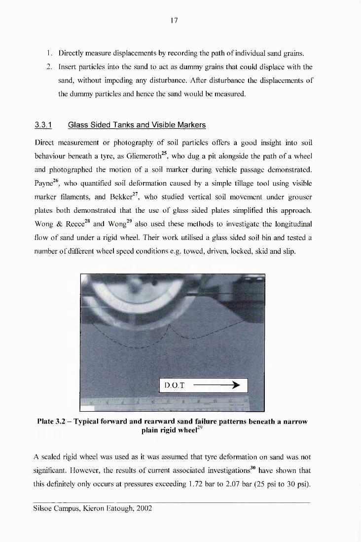
17
1. Directly measure displacements by recording the path of individual sand grains.
2. Insert particles into the sand to act as dummy grains that could displace with the
sand, without impeding any disturbance. After disturbance the displacements of
the dummy particles and hence the sand would be measured.
3.3.1 Glass Sided Tanks and Visible Markers
Direct measurement or photography of soil particles offers a good insight into soil
behaviour beneath a tyre, as Gliemeroth25, who dug a pit alongside the path of a wheel
and photographed the motion of a soil marker during vehicle passage demonstrated.
Payne26, who quantified soil deformation caused by a simple tillage tool using visible
marker filaments, and Bekker27, who studied vertical soil movement under grouser
plates both demonstrated that the use of glass sided plates simplified this approach.
Wong & Reece^° and Wong29 also used these methods to investigate the longitudinal
flow of sand under a rigid wheel. Their work utilised a glass sided soil bin and tested a
number of different wheel speed conditions e.g. towed, driven, locked, skid and slip.
v
. ;
D O T
Plate 3.2 - Typical forward and rearward sand failure patterns beneath a narrowplain rigid wheel29
A scaled rigid wheel was used as it was assumed that tyre deformation on sand was not
significant. However, the results of current associated investigations30 have shown that
this definitely only occurs at pressures exceeding 1.72 bar to 2.07 bar (25 psi to 30 psi).
Silsoe Campus, Kieron Eatough, 2002
18
The failure patterns produced by the various treatments were filmed through a glass
plate, as Plate 3.2 demonstrates. Using these techniques the authors28’29 investigated and
measured forward and rearward failure patterns beneath wheels. Their findings are
further discussed in section 3.3.4.
More recently new technology has allowed this technique to be further developed.
Shikanai et a l31 used a photographic technique to measure deformation beneath scaled
rigid wheels in a 2 m long, glass sided, soil tank, previously used for the assessment of
tractive performance32,33. Their technique used 0 5 mm markers made from 25 jam thick
polyester film with fine crosshairs printed on their surface. Sand grains were glued to
one face, which forced the markers to displace with any sand deformations, whilst the
opposite faces were attached to the glass plate with 15 mm spacings using a moisture
film. Between 200 and 300 markers were placed whilst the tank was filled with sand.
The side of the tank was photographed before, during, and after passage by the rigid
wheel. The photographs were analysed using a two-axis table and a microscopic CCD
camera, which allowed accurate measurement of the markers’ positions. This system
allowed the marker (and assumedly the sand) displacement to be accurately and reliably
measured, although no proof that the markers truly followed the sand flow was stated.
The data they gathered was used to improve the accuracy of several FEA analyses31.
Applications of these techniques were investigated in discussions between Marantz34
and the author, and at the Image Processing and Optical Technology (IPOT) Exhibition
2000 and Machine Vision 2000. These investigations confirmed that camera technology
with frame per second (fps) speeds capable of recording particle displacements, was
potentially available to the author through the EPSRC instrumentation hire pool.
Hardware existed that was capable of capturing and digitising such photographs in real
time for interpretation on a PC. However, although some generic software packages
were available that could translate these into tracks of particle displacements these
would require a significant level of custom programming to make them suitable for this
particular application. Also two other problems rendered the use of glass-sided bins
inappropriate:
Silsoe Campus, Kieron Eatough, 2002
19
1. Assumptions concerning friction losses of the soil against the glass, and soil
containment by the glass must always be made24.
2. Soil displacement is limited to only the vertical or longitudinal directions. For
the purposes of this research project the effect of lateral movement was very
important, because of the lateral flow effect upon sinkage noted by Liu11.
Thus other methods of measuring deformation using in-situ particles were investigated.
3.3.1.1 Paints, dyes, films and layers
The use of different materials and/ or colours to differentiate between different sand
layers was considered. Plastic or foil films were discounted, as they would severely
impede any sand flow. Also Cranfield University experience35 had shown that pressure
film, as manufactured by Pressurex, yielded poor results in a soil profile because
localised stress differentials between soil particles were below the film’s sensitivity.
Attempts were made to paint sand particles, but even aerosol paints caused the particles
to agglomerate, which was unacceptable. On a small-scale sand could be dyed using a
solution of potassium permanganate to produce coloured sand with matching physical
properties. Consideration was given to using coloured sand regions throughout the
profile, but whilst these would have produced good visual patterns, it would have been
very difficult to measure grain displacements in a repeatable manner. Furthermore the
test sand would gradually have been contaminated with coloured sand making
measurements after each test repetition more difficult.
3.3.2 Particles inserted in a Soil Profile
To measure sand disturbance in three-dimensions insertion of identifiable and
retrievable particles into the sand mass would be required instead. Previous Cranfield
University experience35 indicated that any particles used would have to be less than 0 7
mm to be carried by the sand flow. For disturbance to be characterised throughout a
portion of sand then the insertion of some form of numbered grid pattern with
individually identifiable particles would be necessary.
Silsoe Campus, Kieron Eatough, 2002
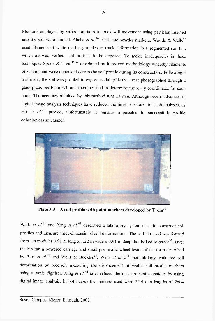
20
Methods employed by various authors to track soil movement using particles inserted
into the soil were studied. Abebe et a l36 used lime powder markers. Woods & Wells37
used filaments of white marble granules to track deformation in a segmented soil bin,
which allowed vertical soil profiles to be exposed. To tackle inadequacies in these
techniques Spoor & Trein3839 developed an improved methodology whereby filaments
of white paint were deposited across the soil profile during its construction. Following a
treatment, the soil was profiled to expose nodal grids that were photographed through a
glass plate, see Plate 3.3, and then digitised to determine the x - y coordinates for each
node. The accuracy obtained by this method was ±3 mm. Although recent advances in
digital image analysis techniques have reduced the time necessary for such analyses, as
Yu et al,40 proved, unfortunately it remains impossible to successfully profile
cohesionless soil (sand).
Plate 3.3 - A soil profile with paint markers developed by Trein39
Wells et a l41 and Xing et a l42 described a laboratory system used to construct soil
profiles and measure three-dimensional soil deformations. The soil bin used was formed
from ten modules 0.91 m long x 1.22 m wide x 0.91 m deep that bolted together37. Over
the bin ran a powered carriage and small pneumatic wheel tester of the form described
by Burt et al.43 and Wells & Buckles44. Wells et al. s41 methodology evaluated soil
deformation by precisely measuring the displacement of visible soil profile markers
using a sonic digitiser. Xing et a l42 later refined the measurement technique by using
digital image analysis. In both cases the markers used were 25.4 mm lengths of 06.4
Silsoe Campus, Kieron Eatough, 2002
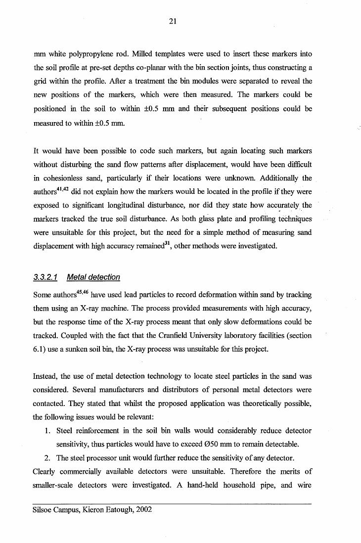
21
mm white polypropylene rod. Milled templates were used to insert these markers into
the soil profile at pre-set depths co-planar with the bin section joints, thus constructing a
grid within the profile. After a treatment the bin modules were separated to reveal the
new positions of the markers, which were then measured. The markers could be
positioned in the soil to within ±0.5 mm and their subsequent positions could be
measured to within ±0.5 mm.
It would have been possible to code such markers, but again locating such markers
without disturbing the sand flow patterns after displacement, would have been difficult
in cohesionless sand, particularly if their locations were unknown. Additionally the
authors41,42 did not explain how the markers would be located in the profile if they were
exposed to significant longitudinal disturbance, nor did they state how accurately the
markers tracked the true soil disturbance. As both glass plate and profiling techniques
were unsuitable for this project, but the need for a simple method of measuring sand
displacement with high accuracy remained , other methods were investigated.
3.3.2.1 Metal detection
Some authors45,46 have used lead particles to record deformation within sand by tracking
them using an X-ray machine. The process provided measurements with high accuracy,
but the response time of the X-ray process meant that only slow deformations could be
tracked. Coupled with the fact that the Cranfield University laboratory facilities (section
6.1) use a sunken soil bin, the X-ray process was unsuitable for this project.
Instead, the use of metal detection technology to locate steel particles in the sand was
considered. Several manufacturers and distributors of personal metal detectors were
contacted. They stated that whilst the proposed application was theoretically possible,
the following issues would be relevant:
1. Steel reinforcement in the soil bin walls would considerably reduce detector
sensitivity, thus particles would have to exceed 050 mm to remain detectable.
2. The steel processor unit would further reduce the sensitivity of any detector.
Clearly commercially available detectors were unsuitable. Therefore the merits of
smaller-scale detectors were investigated. A hand-held household pipe, and wire
Silsoe Campus, Kieron Eatough, 2002
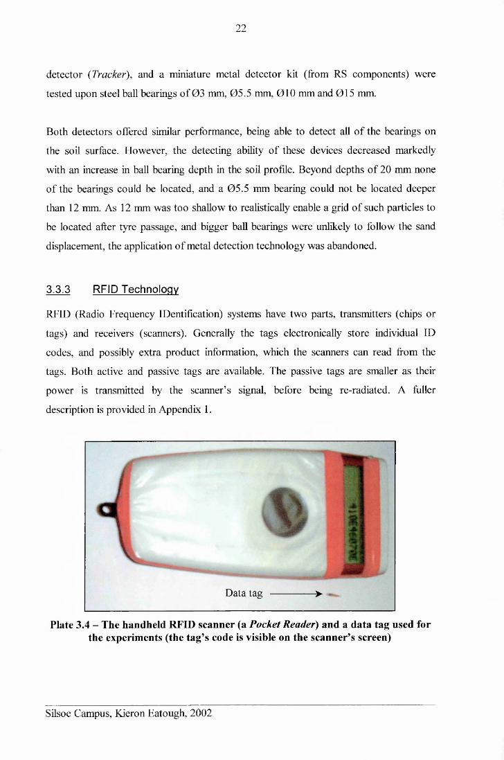
22
detector {Tracker), and a miniature metal detector kit (from RS components) were
tested upon steel ball bearings of 03 mm, 05.5 mm, 010 mm and 015 mm.
Both detectors offered similar performance, being able to detect all of the bearings on
the soil surface. However, the detecting ability of these devices decreased markedly
with an increase in ball bearing depth in the soil profile. Beyond depths of 20 mm none
of the bearings could be located, and a 05.5 mm bearing could not be located deeper
than 12 mm. As 12 mm was too shallow to realistically enable a grid of such particles to
be located after tyre passage, and bigger ball bearings were unlikely to follow the sand
displacement, the application of metal detection technology was abandoned.
3.3.3 RFID Technology
RFID (Radio Frequency IDentification) systems have two parts, transmitters (chips or
tags) and receivers (scanners). Generally the tags electronically store individual ID
codes, and possibly extra product information, which the scanners can read from the
tags. Both active and passive tags are available. The passive tags are smaller as their
power is transmitted by the scanner’s signal, before being re-radiated. A fuller
description is provided in Appendix 1.
Data tag ------------ >
Plate 3.4 - The handheld RFID scanner (a Pocket Reader) and a data tag used for the experiments (the tag’s code is visible on the scanner’s screen)
Silsoe Campus, Kieron Eatough, 2002
23
Destron-Fearing manufacture the smallest commercially available coded tags. These are
supplied in glass capsules 0 2 mm by 12 mm long, with each tag containing a unique 10
to 16 digit alphanumeric code, see Plate 3.4 and Appendix 1. Predominantly they are
used for the tagging of wildlife and pets. Both the size and construction made these
potentially suitable particles, so their performance was investigated (section 7.1).
3.3.4 The Implications of Other Sand Flow Investigations
From their investigations, which were initially upon dry sand, but later on clay, Reece &
Wong28 and Wong29 drew the following conclusions. Soil failure was a three-
dimensional phenomenon, rather than a two-dimensional occurrence, upon which
contemporary theory was based. Their studies demonstrated that soil was displaced
partly sideways and partly longitudinally. Unless the wheel was operating at 100% slip
or 100% skid, then forward and rearward longitudinal failure, and flow, planes existed
beneath the wheel, see Plate 3.2, with the changeover in direction occurring at the point
of maximum radial (normal) stress. The location of this point was dependent upon both
the wheel width and slip, and increased slip caused the point to move forwards. The
formation and location of these failure planes conformed to the basic principles of soil
mechanics, being bounded by logarithmic spirals and straight lines such that the soil
ahead of the tyre failed forwards and outwards, whilst that soil failing rearwards was
simply driven backwards by the stresses formed at the sand-tyre interface.
Whilst a tyre on sand would have an initial sinkage due to a bearing capacity failure,
tyre slippage would increase this sinkage further by driving sand rearwards. The
authors28’29 termed this phenomenon ‘slip sinkage’ and showed that it increased as
wheel slip increased. As well as causing extra wheel sinkage this event also caused 4rut
recovery \ whereby the sand being forced rearwards filled the rut left behind the tyre.
Zhuang et al.19 also noted forward and rearward failure zones under tyres. Additionally
they also showed that the magnitude of the forward zone increased with increased
sinkage, and that the backward zone enlarged with increased slip. This led the authors19
to investigate methods of confining both side and longitudinal sand flows by using rigid
paddle-type plates fitted to the outside of tyres. These consisted of two flanges to stop
Silsoe Campus, Kieron Eatough, 2002
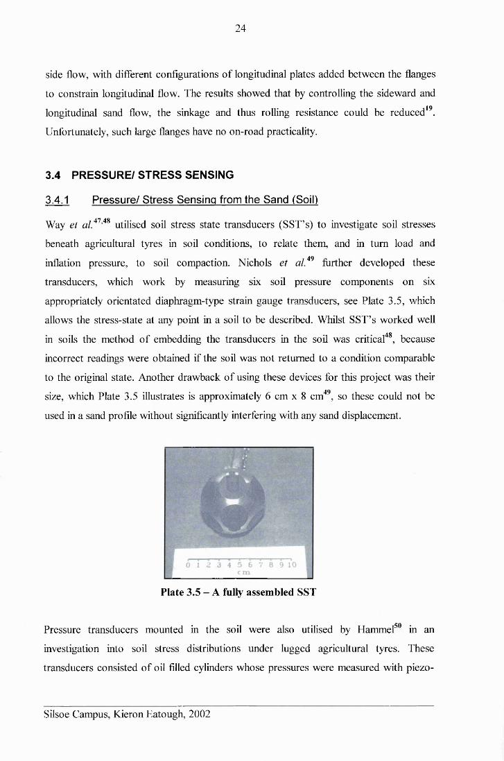
24
side flow, with different configurations of longitudinal plates added between the flanges
to constrain longitudinal flow. The results showed that by controlling the sideward and
longitudinal sand flow, the sinkage and thus rolling resistance could be reduced19.
Unfortunately, such large flanges have no on-road practicality.
3.4 PRESSURE/ STRESS SENSING
3.4.1 Pressure/ Stress Sensing from the Sand (Soil)
Way et a l47,48 utilised soil stress state transducers (SST’s) to investigate soil stresses
beneath agricultural tyres in soil conditions, to relate them, and in turn load and
inflation pressure, to soil compaction. Nichols et a l49 further developed these
transducers, which work by measuring six soil pressure components on six
appropriately orientated diaphragm-type strain gauge transducers, see Plate 3.5, which
allows the stress-state at any point in a soil to be described. Whilst SST’s worked well
in soils the method of embedding the transducers in the soil was critical48, because
incorrect readings were obtained if the soil was not returned to a condition comparable
to the original state. Another drawback of using these devices for this project was their
size, which Plate 3.5 illustrates is approximately 6 cm x 8 cm49, so these could not be
used in a sand profile without significantly interfering with any sand displacement.
Plate 3.5 - A fully assembled SST
Pressure transducers mounted in the soil were also utilised by Hammel50 in an
investigation into soil stress distributions under lugged agricultural tyres. These
transducers consisted of oil filled cylinders whose pressures were measured with piezo-
Silsoe Campus, Kieron Eatough, 2002
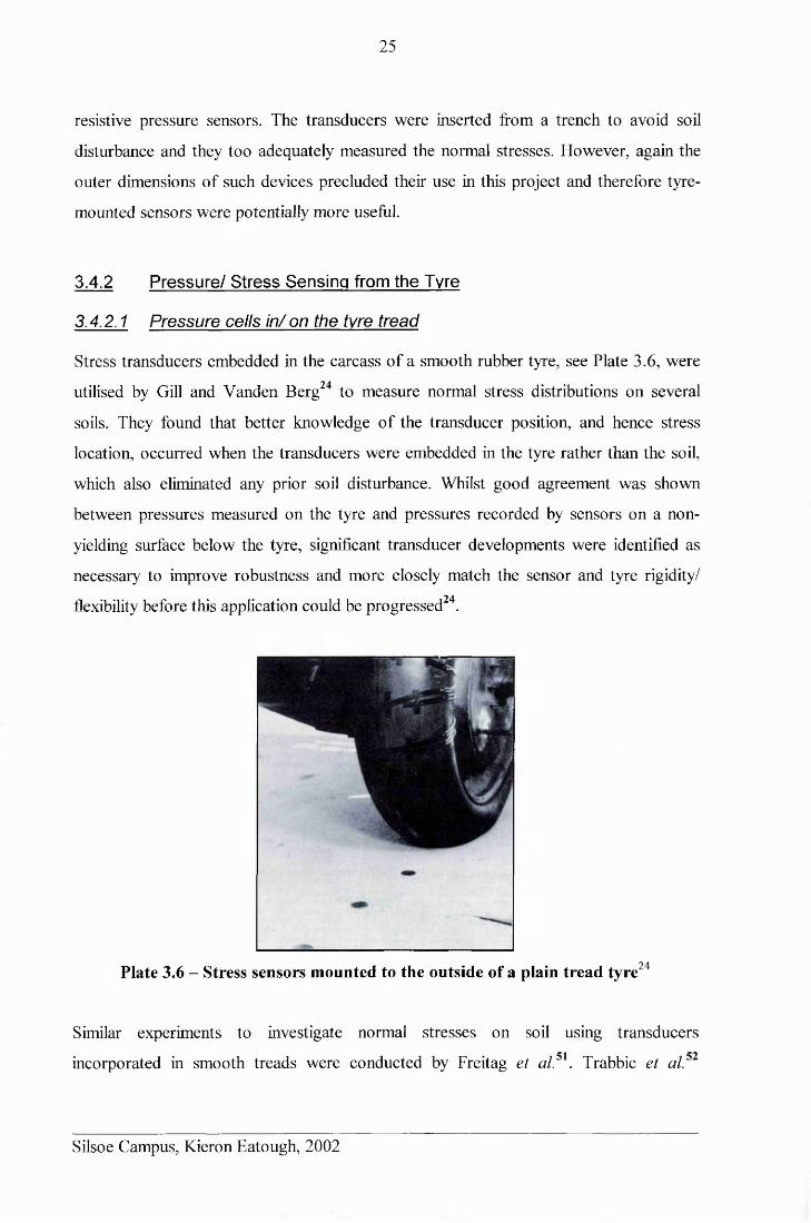
25
resistive pressure sensors. The transducers were inserted from a trench to avoid soil
disturbance and they too adequately measured the normal stresses. However, again the
outer dimensions of such devices precluded their use in this project and therefore tyre-
mounted sensors were potentially more useful.
3.4.2 Pressure/ Stress Sensing from the Tyre
3.4.2.1 Pressure cells in/ on the tyre tread
Stress transducers embedded in the carcass of a smooth rubber tyre, see Plate 3.6, were
utilised by Gill and Vanden Berg24 to measure normal stress distributions on several
soils. They found that better knowledge of the transducer position, and hence stress
location, occurred when the transducers were embedded in the tyre rather than the soil,
which also eliminated any prior soil disturbance. Whilst good agreement was shown
between pressures measured on the tyre and pressures recorded by sensors on a non
yielding surface below the tyre, significant transducer developments were identified as
necessary to improve robustness and more closely match the sensor and tyre rigidity/
flexibility before this application could be progressed24.
Plate 3.6 - Stress sensors mounted to the outside of a plain tread tyre24
Similar experiments to investigate normal stresses on soil using transducers
incorporated in smooth treads were conducted by Freitag et al. . Trabbic et al.
Silsoe Campus, Kieron Eatough, 2002
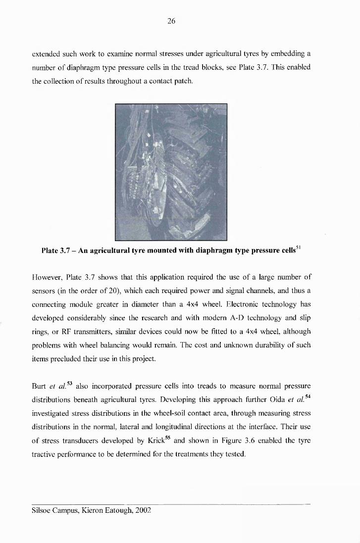
26
extended such work to examine normal stresses under agricultural tyres by embedding a
number of diaphragm type pressure cells in the tread blocks, see Plate 3.7. This enabled
the collection of results throughout a contact patch.
Plate 3.7 - An agricultural tyre mounted with diaphragm type pressure cells31
However, Plate 3.7 shows that this application required the use of a large number of
sensors (in the order of 20), which each required power and signal channels, and thus a
connecting module greater in diameter than a 4x4 wheel. Electronic technology has
developed considerably since the research and with modem A-D technology and slip
rings, or RF transmitters, similar devices could now be fitted to a 4x4 wheel, although
problems with wheel balancing would remain. The cost and unknown durability of such
items precluded their use in this project.
Burt et al*3 also incorporated pressure cells into treads to measure normal pressure
distributions beneath agricultural tyres. Developing this approach further Oida et a l54
investigated stress distributions in the wheel-soil contact area, through measuring stress
distributions in the normal, lateral and longitudinal directions at the interface. Their use
of stress transducers developed by Krick 5 and shown in Figure 3.6 enabled the tyre
tractive performance to be determined for the treatments they tested.
Silsoe Campus, Kieron Eatough, 2002
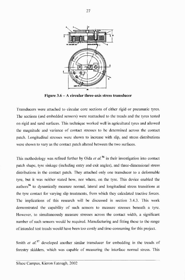
27
W jF^TT
Figure 3.6 - A circular three-axis stress transducer
Transducers were attached to circular core sections of either rigid or pneumatic tyres.
The sections (and embedded sensors) were reattached to the treads and the tyres tested
on rigid and sand surfaces. This technique worked well in agricultural tyres and allowed
the magnitude and variance of contact stresses to be determined across the contact
patch. Longitudinal stresses were shown to increase with slip, and stress distributions
were shown to vary as the contact patch altered between the two surfaces.
This methodology was refined further by Oida et al.*6 in their investigation into contact
patch shape, tyre sinkage (including entry and exit angles), and three-dimensional stress
distributions in the contact patch. They attached only one transducer to a deformable
tyre, but it was neither stated how, nor where, on the tyre. This device enabled the
authors56 to dynamically measure normal, lateral and longitudinal stress transitions at
the tyre contact for varying slip treatments, from which they calculated tractive forces.
The implications of this research will be discussed in section 3.4.3. This work
demonstrated the capability of such sensors to measure stresses beneath a tyre.
However, to simultaneously measure stresses across the contact width, a significant
number of such sensors would be required. Manufacturing and fitting these to the range
of intended test treads would have been too costly and time-consuming for this project.
Smith et al.51 developed another similar transducer for embedding in the treads of
forestry skidders, which was capable of measuring the interface normal stress. This
Silsoe Campus, Kieron Eatough, 2002
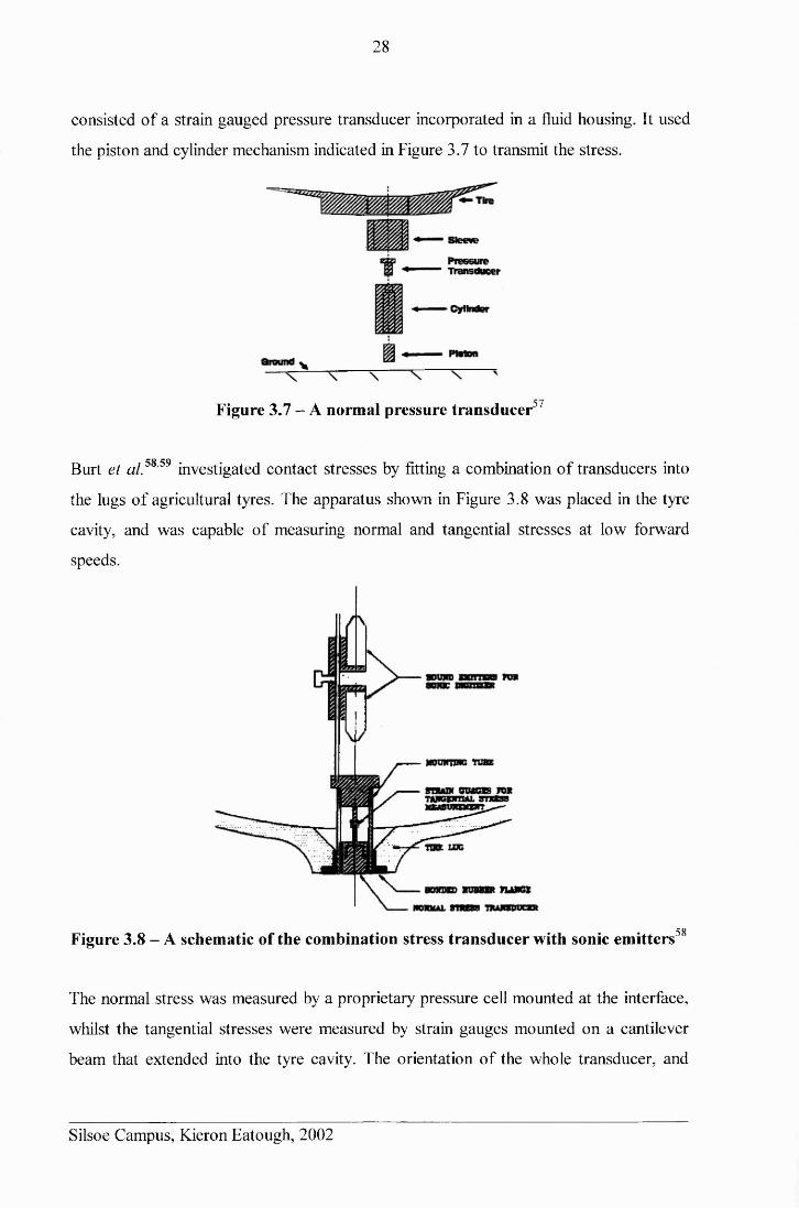
28
consisted of a strain gauged pressure transducer incorporated in a fluid housing. It used
the piston and cylinder mechanism indicated in Figure 3.7 to transmit the stress.
Figure 3.7 - A normal pressure transducer37
Burt et a l58,59 investigated contact stresses by fitting a combination of transducers into
the lugs of agricultural tyres. The apparatus shown in Figure 3.8 was placed in the tyre
cavity, and was capable of measuring normal and tangential stresses at low forward
speeds.
• • 58Figure 3.8 - A schematic of the combination stress transducer with sonic emitters
The normal stress was measured by a proprietary pressure cell mounted at the interface,
whilst the tangential stresses were measured by strain gauges mounted on a cantilever
beam that extended into the tyre cavity. The orientation of the whole transducer, and
Silsoe Campus, Kieron Eatough, 2002
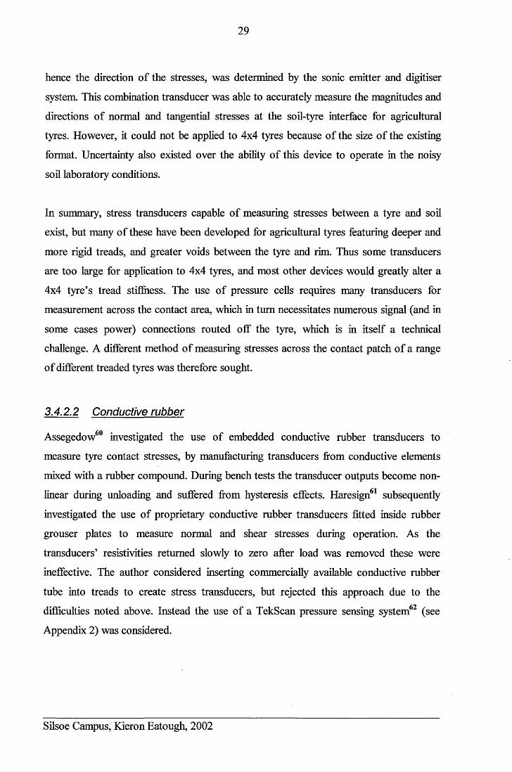
29
hence the direction of the stresses, was determined by the sonic emitter and digitiser
system. This combination transducer was able to accurately measure the magnitudes and
directions of normal and tangential stresses at the soil-tyre interface for agricultural
tyres. However, it could not be applied to 4x4 tyres because of the size of the existing
format. Uncertainty also existed over the ability of this device to operate in the noisy
soil laboratory conditions.
In summary, stress transducers capable of measuring stresses between a tyre and soil
exist, but many of these have been developed for agricultural tyres featuring deeper and
more rigid treads, and greater voids between the tyre and rim. Thus some transducers
are too large for application to 4x4 tyres, and most other devices would greatly alter a
4x4 tyre’s tread stififiiess. The use of pressure cells requires many transducers for
measurement across the contact area, which in turn necessitates numerous signal (and in
some cases power) connections routed off the tyre, which is in itself a technical
challenge. A different method of measuring stresses across the contact patch of a range
of different treaded tyres was therefore sought.
3.4.2.2 Conductive rubber
Assegedow60 investigated the use of embedded conductive rubber transducers to
measure tyre contact stresses, by manufacturing transducers from conductive elements
mixed with a rubber compound. During bench tests the transducer outputs become non
linear during unloading and suffered from hysteresis effects. Haresign61 subsequently
investigated the use of proprietary conductive rubber transducers fitted inside rubber
grouser plates to measure normal and shear stresses during operation. As the
transducers’ resistivities returned slowly to zero after load was removed these were
ineffective. The author considered inserting commercially available conductive rubber
tube into treads to create stress transducers, but rejected this approach due to the
difficulties noted above. Instead the use of a TekScan pressure sensing system62 (see
Appendix 2) was considered.
Silsoe Campus, Kieron Eatough, 2002
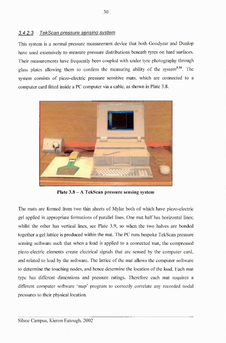
30
3.4.2.3 TekScan pressure sensing system
This system is a normal pressure measurement device that both Goodyear and Dunlop
have used extensively to measure pressure distributions beneath tyres on hard surfaces.
Their measurements have frequently been coupled with under tyre photography through
glass plates allowing them to confirm the measuring ability of the system3,16. The
system consists of piezo-electric pressure sensitive mats, which are connected to a
computer card fitted inside a PC computer via a cable, as shown in Plate 3.8.
■ ■ ■■ ■
Plate 3.8 - A TekScan pressure sensing system
The mats are formed from two thin sheets of Mylar both of which have piezo-electric
gel applied in appropriate formations of parallel lines. One mat half has horizontal lines;
whilst the other has vertical lines, see Plate 3.9, so when the two halves are bonded
together a gel lattice is produced within the mat. The PC runs bespoke TekScan pressure
sensing software such that when a load is applied to a connected mat, the compressed
piezo-electric elements create electrical signals that are sensed by the computer card,
and related to load by the software. The lattice of the mat allows the computer software
to determine the touching nodes, and hence determine the location of the load. Each mat
type has different dimensions and pressure ratings. Therefore each mat requires a
different computer software ‘map’ program to correctly correlate any recorded nodal
pressures to their physical location.
Silsoe Campus, Kieron Eatough, 2002
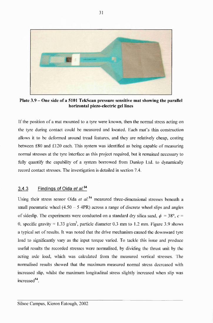
31
Plate 3.9 - One side of a 5101 TekScan pressure sensitive mat showing the parallelhorizontal piezo-electric gel lines
If the position of a mat mounted to a tyre were known, then the normal stress acting on
the tyre during contact could be measured and located. Each mat’s thin construction
allows it to be deformed around tread features, and they are relatively cheap, costing
between £80 and £120 each. This system was identified as being capable of measuring
normal stresses at the tyre interface as this project required, but it remained necessary to
fully quantify the capability of a system borrowed from Dunlop Ltd. to dynamically
record contact stresses. The investigation is detailed in section 7.4.
3.4.3 Findings of Oida et a lM
Using their stress sensor Oida et al.54 measured three-dimensional stresses beneath a
small pneumatic wheel (4.50 - 5 4PR) across a range of discrete wheel slips and angles
of sideslip. The experiments were conducted on a standard dry silica sand, $ =38°, c =
0, specific gravity = 1.33 g/cm3, particle diameter 0.3 mm to 1.2 mm. Figure 3.9 shows
a typical set of results. It was noted that the drive mechanism caused the downward tyre
load to significantly vary as the input torque varied. To tackle this issue and produce
useful results the recorded stresses were normalised, by dividing the thrust unit by the
acting axle load, which was calculated from the measured vertical stresses. The
normalised results showed that the maximum measured normal stress decreased with
increased slip, whilst the maximum longitudinal stress slightly increased when slip was
increased54.
Silsoe Campus, Kieron Eatough, 2002
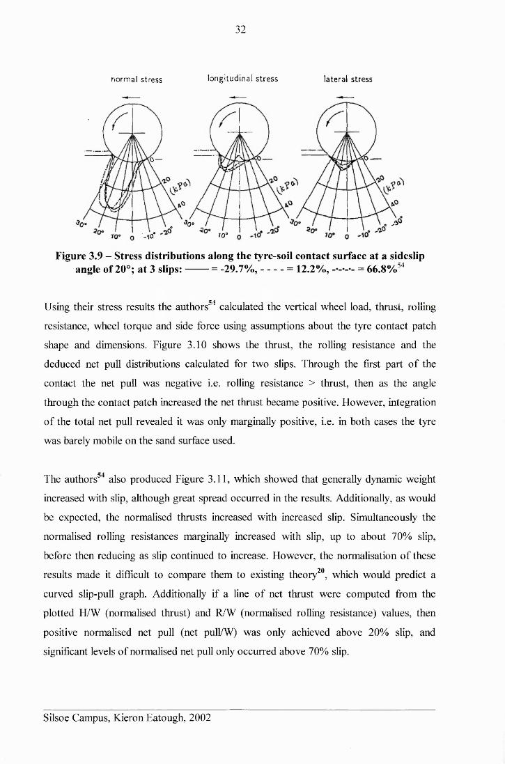
32
n o r m a l s t r e s s l o n g i t u d i n a l s t r e s s l a t e r a l s t r e s s
.0—
’0 °\ « -AO" 10 "
Figure 3.9 - Stress distributions along the tyre-soil contact surface at a sideslip angle of 20°; at 3 slips:------ = -29.7%,-------= 12.2%, = 66.8%34
Using their stress results the authors54 calculated the vertical wheel load, thrust, rolling
resistance, wheel torque and side force using assumptions about the tyre contact patch
shape and dimensions. Figure 3.10 shows the thrust, the rolling resistance and the
deduced net pull distributions calculated for two slips. Through the first part of the
contact the net pull was negative i.e. rolling resistance > thrust, then as the angle
through the contact patch increased the net thrust became positive. However, integration
of the total net pull revealed it was only marginally positive, i.e. in both cases the tyre
was barely mobile on the sand surface used.
The authors34 also produced Figure 3.11, which showed that generally dynamic weight
increased with slip, although great spread occurred in the results. Additionally, as would
be expected, the normalised thrusts increased with increased slip. Simultaneously the
normalised rolling resistances marginally increased with slip, up to about 70% slip,
before then reducing as slip continued to increase. However, the normalisation of these
results made it difficult to compare them to existing theory20, which would predict a
curved slip-pull graph. Additionally if a line of net thrust were computed from the
plotted H/W (normalised thrust) and R/W (normalised rolling resistance) values, then
positive normalised net pull (net pull/W) was only achieved above 20% slip, and
significant levels of normalised net pull only occurred above 70% slip.
Silsoe Campus, Kieron Eatough, 2002
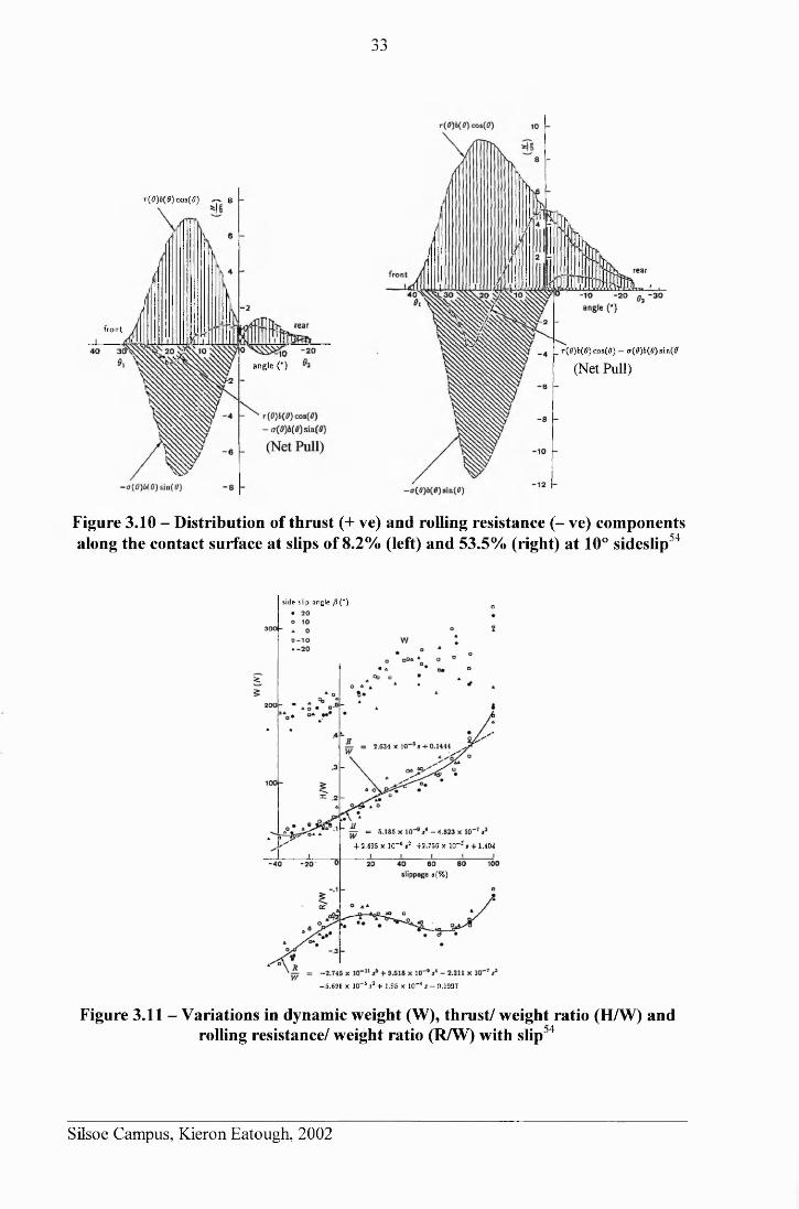
33
r(0)b(0) cos(fl) ^ 8
- 2
front
a n g le ( ' )
Figure 3.10 - Distribution of thrust (+ ve) and rolling resistance (- ve) components along the contact surface at slips of 8.2% (left) and 53.5% (right) at 10° sideslip34
s id e s lip a n g le f l ( " )
+ 2.195 X I0 ~ s »3 +2 .755 X H T J < + 1.401
»(%)
-5.656 X 10~5J3 + 1.35 X 10“' s - 0.1997
Figure 3.11 - Variations in dynamic weight (W), thrust/ weight ratio (H/W) and rolling resistance/ weight ratio (R/W) with slip34
r(fl)i(fl)eos(0) - tr(9)b(B)sin{6
(Net Pull)
Silsoe Campus, Kieron Eatough, 2002
^
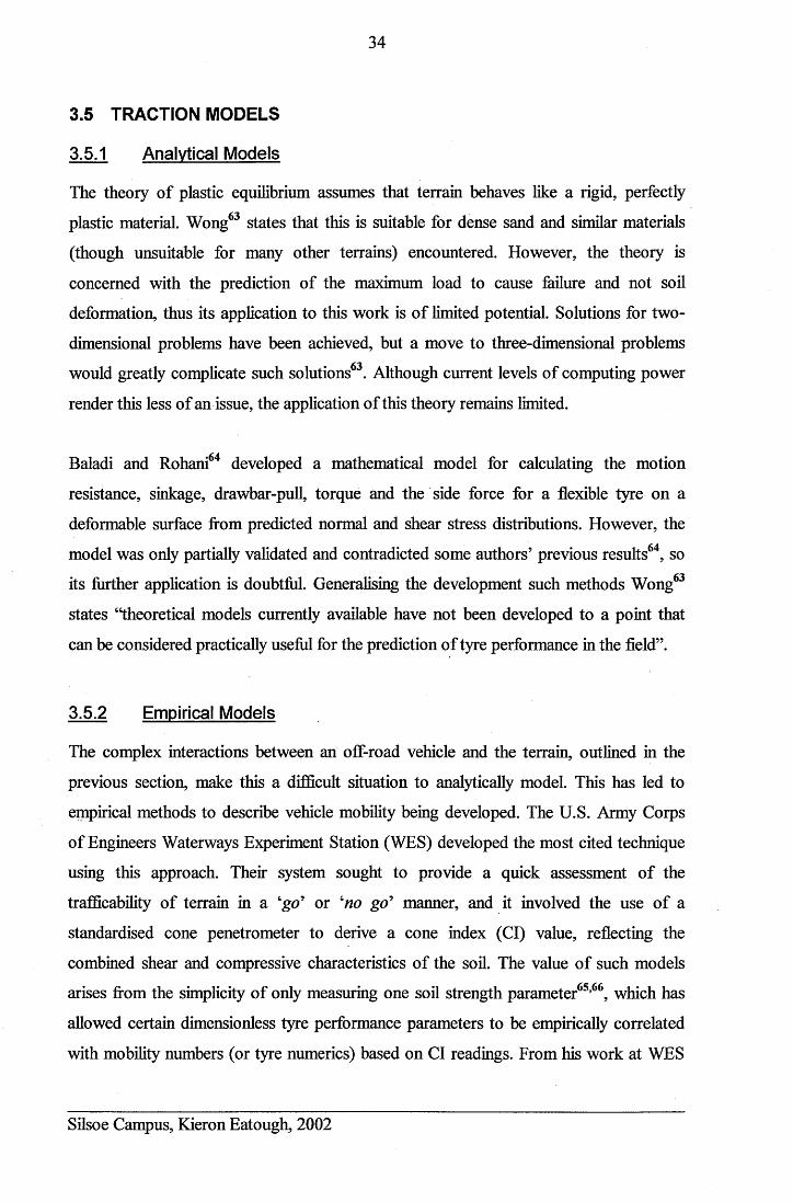
34
3.5 TRACTION MODELS
3.5.1 Analytical Models
The theory of plastic equilibrium assumes that terrain behaves like a rigid, perfectly
plastic material. Wong63 states that this is suitable for dense sand and similar materials
(though unsuitable for many other terrains) encountered. However, the theory is
concerned with the prediction of the maximum load to cause failure and not soil
deformation, thus its application to this work is of limited potential. Solutions for two-
dimensional problems have been achieved, but a move to three-dimensional problems
would greatly complicate such solutions . Although current levels of computing power
render this less of an issue, the application of this theory remains limited.
Baladi and Rohani64 developed a mathematical model for calculating the motion
resistance, sinkage, drawbar-pull, torque and the side force for a flexible tyre on a
deformable surface from predicted normal and shear stress distributions. However, the
model was only partially validated and contradicted some authors’ previous results64, so
its further application is doubtful. Generalising the development such methods Wong63
states “theoretical models currently available have not been developed to a point that
can be considered practically useful for the prediction of tyre performance in the field”.
3.5.2 Empirical Models
The complex interactions between an off-road vehicle and the terrain, outlined in the
previous section, make this a difficult situation to analytically model. This has led to
empirical methods to describe vehicle mobility being developed. The U.S. Army Corps
of Engineers Waterways Experiment Station (WES) developed the most cited technique
using this approach. Their system sought to provide a quick assessment of the
trafficability of terrain in a ‘go’ or ‘no go’ manner, and it involved the use of a
standardised cone penetrometer to derive a cone index (Cl) value, reflecting the
combined shear and compressive characteristics of the soil. The value of such models
arises from the simplicity of only measuring one soil strength parameter65,66, which has
allowed certain dimensionless tyre performance parameters to be empirically correlated
with mobility numbers (or tyre numerics) based on Cl readings. From his work at WES
Silsoe Campus, Kieron Eatough, 2002
35
Freitag67 developed the following tyre numerics for clay (Nc) and sand (Ns) for
operation on purely cohesive or frictional soil, equations 3 and 4 respectively.
=C(bd)
WX-t —
v h
TV
Where:
^ Gjbd)W
sx —h
C = cone index
b = tyre width
W= tyre load
5= tyre deflection
(3)
(4)
G = sand penetration resistance gradient
d= tyre diameter
h = tyre section height (unloaded)
Tumage68 (1972) produced a tyre mobility number, M, (equation 5) that enhanced
equation 3 to more accurately consider the wheel properties.
Cbd S 1M = ------1 — XY— -W \h (l + b (5)
2dJ
Dwyer et al. developed this equation fiirther69 during their investigation of the
performance of a range of tractor drive tyres operated in a range of field conditions.
Wismer and Luth21,70 used equation 3, to formulate equation 6, which predicted the net
pull of off-road wheeled vehicles on agricultural (not pure frictional) soils, and Cn
became a wheel numeric that was a function of tyre diameter and section width, as well
as the Cl value, which represented topsoil strength.
W
Where:
= 0.75(1 - e - ° 3c» ' ) -1.2C\ N
\+ 0.04 (6)
P = pull W = dynamic wheel load Cn = CIbd/W
CI= cone index averaged over top 150 mm (6 in.) of soil
b = tyre width d = tyre diameter z = wheel slip
Silsoe Campus, Kieron Eatough, 2002
36
Whilst Cl values can easily be obtained, the adequacy of empirical models to fully and
accurately predict mobility remains controversial. As with any empirical method,
predictions cannot be accurately extrapolated beyond the conditions from which results
were derived. Additionally cone penetrometer resistance depends greatly upon the cone71 77design and its method of use . For instance, Reece & Peca indicated that whilst the
methodology is useful for remoulded frictionless clay soil, it is inadequate for
characterising sand mobility properties. Wang & Reece14 also showed that performance
prediction using Ns was inadequate for free-rolling tyres on a variety of sands.
Following this publication14, Tumage73 re-examined a sizeable portion of the WES
experimental data. He concluded that for better accuracy in predicting tyre performance
upon any given sand of given moisture content, additional laboratory testing alongside
penetrometer readings was required. Therefore the original concept of a single test to
determine the properties of coarse-grained soils became insufficient. Gee-Clough74 had
also reported that predictions of certain tyre performance parameters on sand from the
cone penetrometer/ mobility number approach were insufficiently accurate. In response
to all of these issues Tumage73 proposed a revised numeric Nsey, shown on equation 7,
where the variables remained common to equations 4, except for Gey, which replaced G
and introduced the effects of sand grain median diameter and sand compactibility,
which and to be quantified by laboratory investigations.
G j b d i sN sev =------------x — (7)
sey W h
This gave improved prediction over a broader range of sand types, however, the
surrounding debate meant that extensive geo-technical testing and analysis, including
in-situ measurement, sample acquisition and laboratory testing were necessary to
accurately define the properties of any sand75. This all renders the philosophy of a single
measurement inadequate and questions the usefulness of this empirical method for
sand63. Additionally the action of the cone penetrometer bears little analogy to that of a
traction wheel, a fact investigated by Dwyer et al.16 who compared the ability of a cone
penetrometer and a soil shear meter to measure soil parameters. They concluded that the
Silsoe Campus, Kieron Eatough, 2002
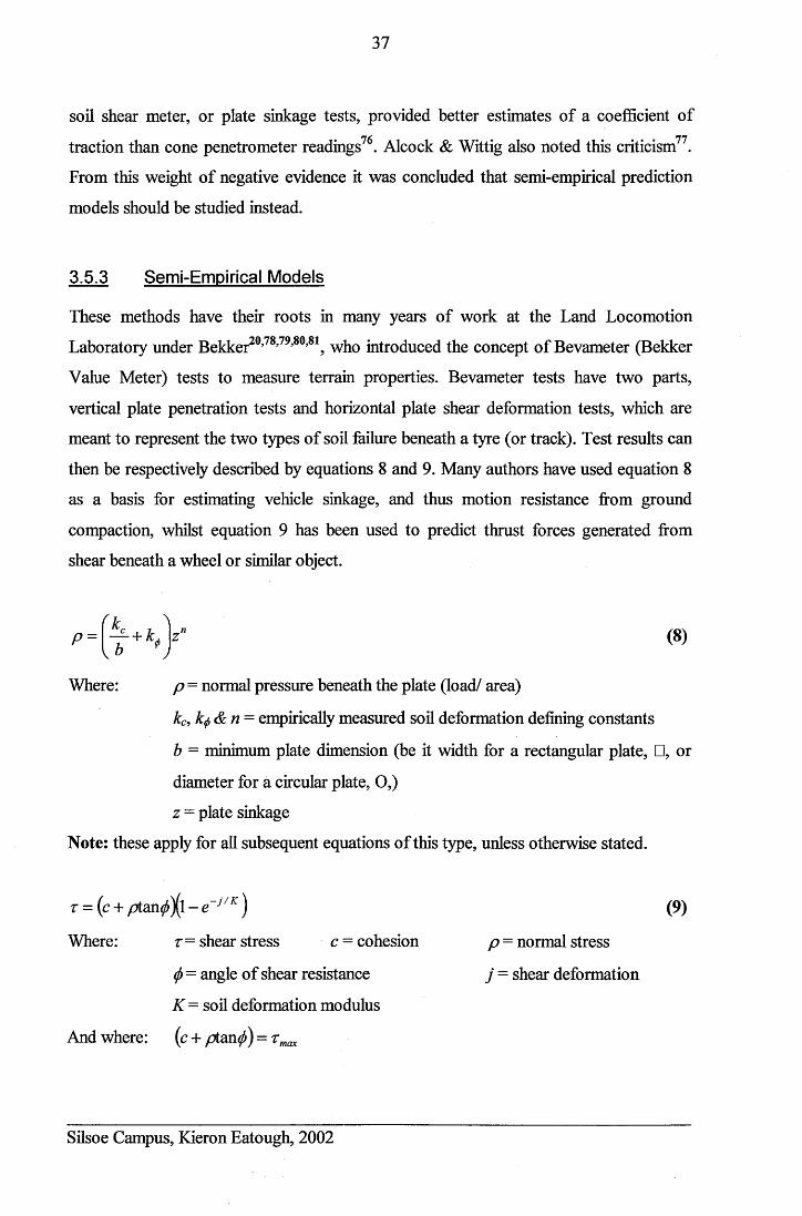
37
soil shear meter, or plate sinkage tests, provided better estimates of a coefficient ofH(\ 77traction than cone penetrometer readings . Alcock & Wittig also noted this criticism .
From this weight of negative evidence it was concluded that semi-empirical prediction
models should be studied instead.
3.5.3 Semi-Empirical Models
These methods have their roots in many years of work at the Land LocomotionOTA OTQ AA Qj
Laboratory under Bekker ’ ’ ’ ’ , who introduced the concept of Bevameter (Bekker
Value Meter) tests to measure terrain properties. Bevameter tests have two parts,
vertical plate penetration tests and horizontal plate shear deformation tests, which are
meant to represent the two types of soil failure beneath a tyre (or track). Test results can
then be respectively described by equations 8 and 9. Many authors have used equation 8
as a basis for estimating vehicle sinkage, and thus motion resistance from ground
compaction, whilst equation 9 has been used to predict thrust forces generated from
shear beneath a wheel or similar object.
P = f + k t f (8)
Where: p = normal pressure beneath the plate (load/ area)
kc, k(f)&n = empirically measured soil deformation defining constants
b = minimum plate dimension (be it width for a rectangular plate, □, or
diameter for a circular plate, O,)
z = plate sinkage
Note: these apply for all subsequent equations of this type, unless otherwise stated.
t = (c + /7tan^)(l - e~j/K ) (9)
Where: r= shear stress c = cohesion p = normal stress
(j> = angle of shear resistance j = shear deformation
K - soil deformation modulus
And where: (c + ptan^) = t max
Silsoe Campus, Kieron Eatough, 2002
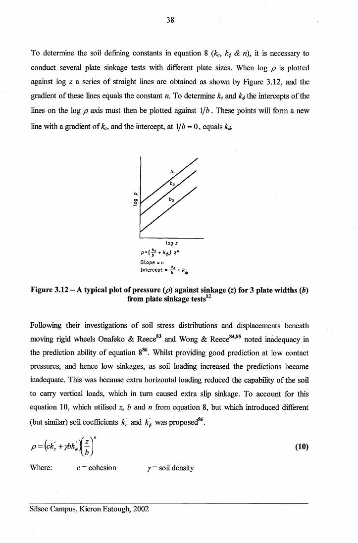
38
To determine the soil defining constants in equation 8 (kc, k# & n), it is necessary to
conduct several plate sinkage tests with different plate sizes. When log p is plotted
against log z a series of straight lines are obtained as shown by Figure 3.12, and the
gradient of these lines equals the constant n. To determine kc and k$ the intercepts of the
lines on the log p axis must then be plotted against \ jb . These points will form a new
line with a gradient of kc, and the intercept, at 1/6 = 0, equals k#.
Q.
o
log z
+ z° Slope = n *cIntercept = — +
Figure 3.12 - A typical plot of pressure (p) against sinkage (z) for 3 plate widths (6)from plate sinkage tests82
Following their investigations of soil stress distributions and displacements beneathO'* O/l O f
moving rigid wheels Onafeko & Reece and Wong & Reece ’ noted inadequacy in
the prediction ability of equation 886. Whilst providing good prediction at low contact
pressures, and hence low sinkages, as soil loading increased the predictions became
inadequate. This was because extra horizontal loading reduced the capability of the soil
to carry vertical loads, which in turn caused extra slip sinkage. To account for this
equation 10, which utilised z, b and n from equation 8, but which introduced different
(but similar) soil coefficients k'c and k\ was proposed86.
f V p = (ck'+fik’, ] j (10)
Where: c = cohesion y= soil density
Silsoe Campus, Kieron Eatough, 2002

39
Although improved prediction was achieved from equation 10, Wong63, who has
considerable experience of using both prediction equations for a range of mineral soil
types (including sand), stated that “both the Bekker and Reece equations may be used to
characterise the pressure sinkage relationships of mineral terrains” and that “both
equations can provide an acceptable fit to measured data”. Therefore the simpler, and
more universally employed, Bekker equation was utilised as a basis for prediction
within this project. Further evidence for the use of the Bekker equation comes from
Ziani & Biarez’s investigation of pressure sinkage on loose sand87. They showed that
for very loose, to average density sand, bearing capacity prediction using equation 11 (a
simplified version of Bekker’s equation) gave suitably representative results.
p = kzn (11)
Where: k = constant
• • « o oA modified version of Equation 11 was utilised by Ji et al. to describe the effect of
different loading patterns upon plate sinkages in dry sand. They found that the use of
both inclined loads, and inclined plates, affected pressure sinkage relationships88. They
modified equation 11 to account for the angled loading by including extra terms and
presented a single set of traction results to prove their new theory. Unfortunately a
single set of results did not provide a sufficiently rigorous assessment of the
methodology to justify its utilisation. Therefore the more accepted equation 8 was used.
3.5.3.1 Prediction of tractive pullOQ
Based upon Bekker’s work (equation 9), Janosi & Hanamoto proposed equation 12,
where thrust, P, is assumed to act similarly to the shear force, F, in a horizontal plane
under the traction device, where F is dependant upon the slip and soil deformation
relationships. This methodology gave good estimations of the tractive effort/ slip
characteristics and the maximum traction achievable for both tracked and wheeled
vehicles89. “Although many other researchers have subsequently developed a wide
variety of differing models, this approach has remained both popular and durable
because it is based upon related mechanical principles”90.
Silsoe Campus, Kieron Eatough, 2002
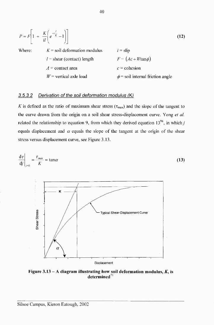
40
P = F 1 +
Where:
K_il
( .1-1
K= soil deformation modulus
/ = shear (contact) length
A = contact area
W= vertical axle load
(12)
i - slip
F= ( 4c + JFtan^)
c = cohesion
(j) = soil internal friction angle
3.5.3.2 Derivation of the soil deformation modulus (K)
K is defined as the ratio of maximum shear stress (T max) and the slope of the tangent to
the curve drawn from the origin on a soil shear stress-displacement curve. Yong et al.
related the relationship to equation 9, from which they derived equation 1391, in which j
equals displacement and a equals the slope of the tangent at the origin of the shear
stress versus displacement curve, see Figure 3.13.
dr
4/ j = 0K
= tan a (13)
V)V) Typical Shear-Displacement Curve
coi—ra0JZCO
Displacement
Figure 3.13 - A diagram illustrating how soil deformation modulus, K, isdetermined 71
Silsoe Campus, Kieron Eatough, 2002
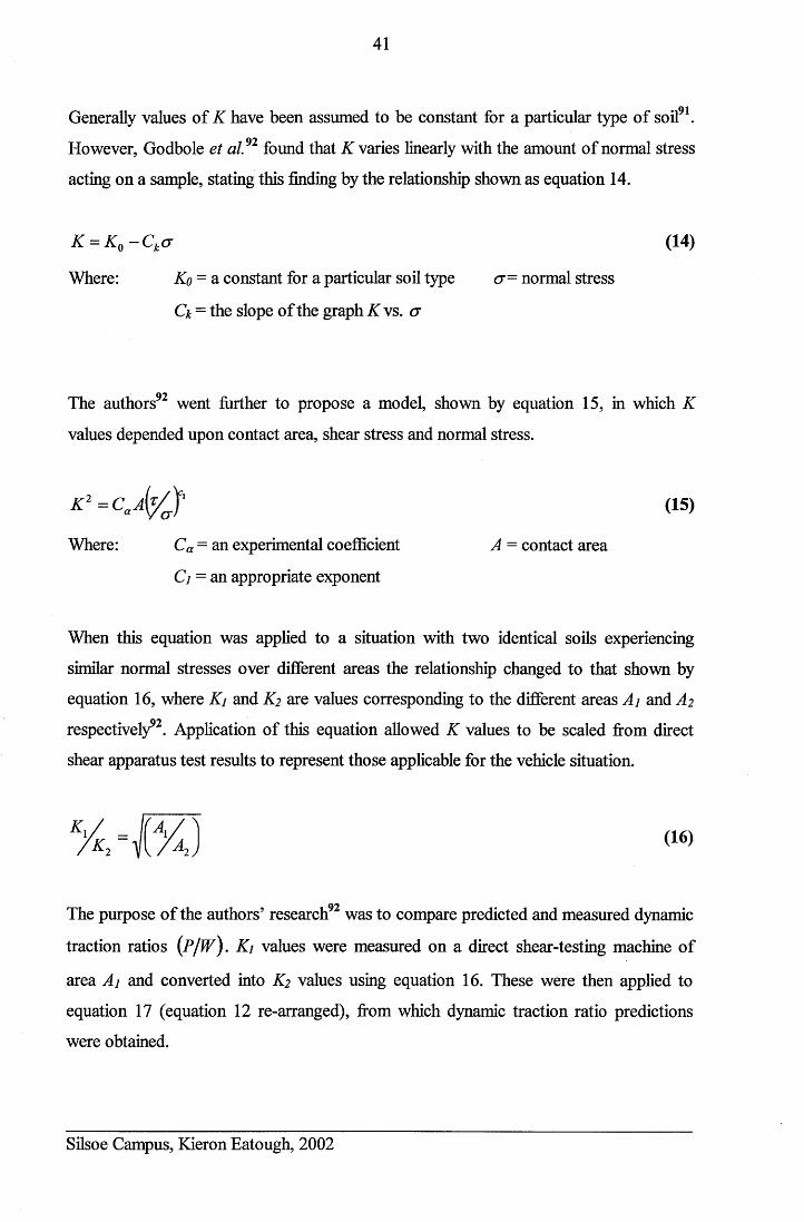
41
Generally values of K have been assumed to be constant for a particular type of soil91.
However, Godbole et al.92 found that K varies linearly with the amount of normal stress
acting on a sample, stating this finding by the relationship shown as equation 14.
K = K0- Ckcr (14)
Where: Ko = a constant for a particular soil type <r= normal stress
Ck = the slope of the graph K vs. a
The authors92 went further to propose a model, shown by equation 15, in which K
values depended upon contact area, shear stress and normal stress.
K 2 = C « a { /J ' (15)
Where: Ca= an experimental coefficient A = contact area
Ci = an appropriate exponent
When this equation was applied to a situation with two identical soils experiencing
similar normal stresses over different areas the relationship changed to that shown by
equation 16, where Ki and K2 are values corresponding to the different areas A 1 and A2
respectively92. Application of this equation allowed K values to be scaled from direct
shear apparatus test results to represent those applicable for the vehicle situation.
O'?The purpose of the authors’ research was to compare predicted and measured dynamic
traction ratios (P/W). Kj values were measured on a direct shear-testing machine of
area Ai and converted into K2 values using equation 16. These were then applied to
equation 17 (equation 12 re-arranged), from which dynamic traction ratio predictions
were obtained.
Silsoe Campus, Kieron Eatough, 2002
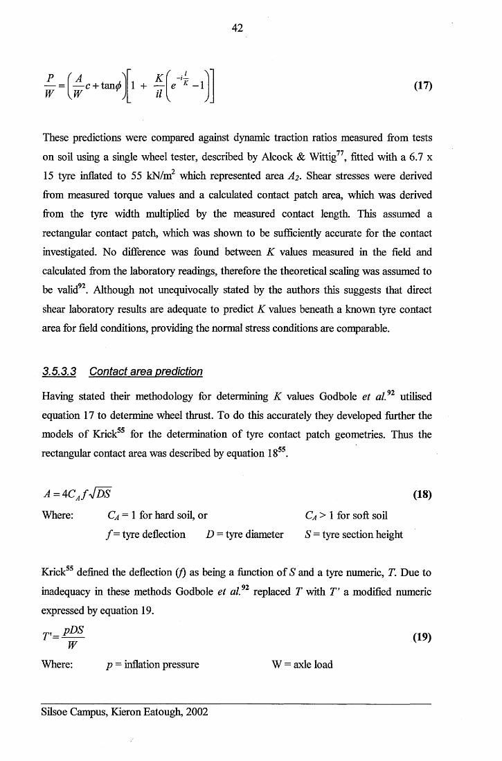
42
(17)
These predictions were compared against dynamic traction ratios measured from tests
from measured torque values and a calculated contact patch area, which was derived
from the tyre width multiplied by the measured contact length. This assumed a
rectangular contact patch, which was shown to be sufficiently accurate for the contact
investigated. No difference was found between K values measured in the field and
calculated from the laboratory readings, therefore the theoretical scaling was assumed to
be valid92. Although not unequivocally stated by the authors this suggests that direct
shear laboratory results are adequate to predict K values beneath a known tyre contact
area for field conditions, providing the normal stress conditions are comparable.
3.5.3.3 Contact area prediction
Having stated their methodology for determining K values Godbole et al.92 utilised
equation 17 to determine wheel thrust. To do this accurately they developed further the
models of Krick55 for the determination of tyre contact patch geometries. Thus the
rectangular contact area was described by equation 1855.
on soil using a single wheel tester, described by Alcock & Wittig77, fitted with a 6.7 x
15 tyre inflated to 55 kN/m2 which represented area A2 . Shear stresses were derived
a = a c j 4 d s (18)
Where: C a = 1 for hard soil, or C a > 1 for soft soil
/ = tyre deflection D = tyre diameter S = tyre section height
Krick55 defined the deflection if) as being a function of S and a tyre numeric, T. Due to
inadequacy in these methods Godbole et al replaced T with T ’ a modified numeric
expressed by equation 19.
r _ pDS (19)W
Where: p = inflation pressure W = axle load
Silsoe Campus, Kieron Eatough, 2002
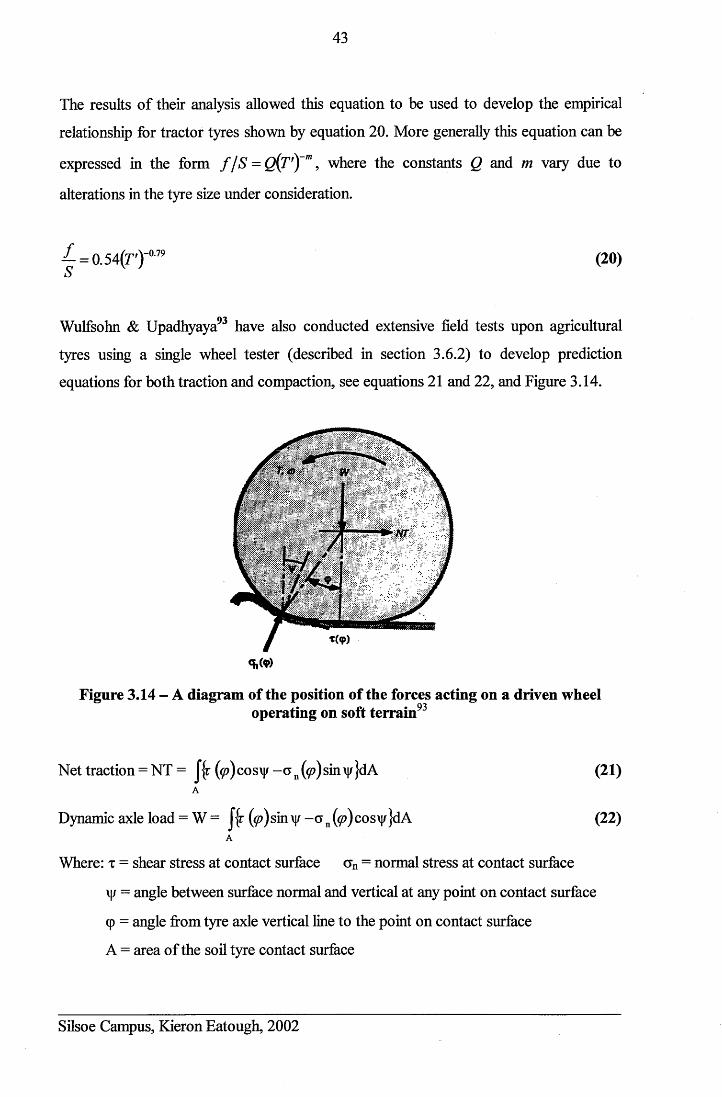
43
The results of their analysis allowed this equation to be used to develop the empirical
relationship for tractor tyres shown by equation 20. More generally this equation can be
expressed in the form f / S = Q(T') m, where the constants Q and m vary due to
alterations in the tyre size under consideration.
^ = 0.54(r')"a79 (20)
Wulfsohn & Upadhyaya93 have also conducted extensive field tests upon agricultural
tyres using a single wheel tester (described in section 3.6.2) to develop prediction
equations for both traction and compaction, see equations 21 and 22, and Figure 3.14.
<*.(*>
Figure 3.14 - A diagram of the position of the forces acting on a driven wheeloperating on soft terrain93
Net traction = NT = J{r (<p) cosy - o n (<p) sin y }dAA
Dynamic axle load = W = J* { r (^)siny - a n(<p)cosy}dA
(21)
(22)
Where: t = shear stress at contact surface an = normal stress at contact surface
y = angle between surface normal and vertical at any point on contact surface
y = angle from tyre axle vertical line to the point on contact surface
A = area of the soil tyre contact surface
Silsoe Campus, Kieron Eatough, 2002
44
To fully utilise these equations the contact patch dimensions were required. This led
Upadhyaya & Wulfsohn94 to develop mathematical expressions for two-dimensional
agricultural tyre contact patch areas on rigid surfaces. Later these were enhanced to
determine three-dimensional soil-tyre contact profiles for agricultural tyres operating on
deformable soil95,96, which were related to the tyres’ tractive performances97. The three-
dimensional prediction method involved the measurement of incremental arc lengths at
discrete locations along the contact length95. This prediction was derived from
measurements made using wire and cable potentiometers placed in the soil to measure
the soil deformation at the interface. As would be expected the three-dimensional
representation produced the best traction predictions, achieving a correlation coefficient
value of 0.7, when compared against actual measured net traction values96.
From their testing Upadhyaya et al.98 determined traction equations capable of defining
gross and net thrust coefficients produced by agricultural tyres, based on five semi-
empirical coefficients. However, these were related to cone index readings and proved
inadequate. Thus a device was developed to measure soil sinkage and shear
parameters99, allowing the five coefficients to be related to directly measured soil
characteristics100. Latterly Upadhyaya et al.m developed simplified equations. Whilst
these theories are important in terramechanics their suitability for application to this
situation was unknown because only agricultural (tractor) tyres were evaluated when
operating on typical agricultural soils (clays and loams). In contrast Bekker’s equations
have been validated for tyre sizes and soil conditions appropriate to this study.
Although knowledge of contact area dimensions is important for traction prediction this
project overlooked the methods outlined above and instead used the more relevant
results recorded by a contemporary Cranfield University EngD student30. His research
investigated the dynamic behaviour of 4x4 contact patches for identical tyres and related
them to tyre performances. He did thus by fitting drawstring potentiometer
measurement devices inside the tested tyres to allow dynamic measurement of contact
patch areas on sand30. To hasten both researcher’s test programmes the investigations
were conducted jointly where possible, so identical tyre and soil treatments were
investigated. Thus, for the purposes of traction prediction, contact patch dimensions
Silsoe Campus, Kieron Eatough, 2002

45
relevant to this project were drawn directly from Oliver’s measurements30 and a
separate contact area prediction model was not required.
3.5.3.4 Other thrust prediction methods
Reece86 postulated that developments of Bekker’s models were needed to account for
bow wave effects, which altered both the contact patch dimensions and thus the points
of action of forces between the soil and the tyre. He therefore proposed the following
theory to predict both the radial (normal) stresses and tangential (shear) stresses beneath
a rigid wheel86. The radial stresses in the forward region of failure cry, were predicted by
equation 23, whilst the radial stresses in the rearward region of failure <72, were
predicted by equation 24. Plate 3.2 shows typical forward and rearward failure zones,
whilst Figure 3.15 shows the nomenclature for equations 23 and 24. Equation 25 was
proposed to predict the shear stresses around the rim86.
ri(^) = ( i + (cos0 —COS60”
cr2 (6) = (frj + k2b)f \ n 1 r ' cos ex-e 1 (cl + c2i)
(c, +c2i)
Wcos 6
(23)
(24)
Figure 3.15 - Forces, torque and stresses acting on a driven rigid wheel86
■(0) = (c + cr(#)tan^)^l - e 6>)-(l -i Xsin -s in 0 )](25)
Silsoe Campus, Kieron Eatough, 2002
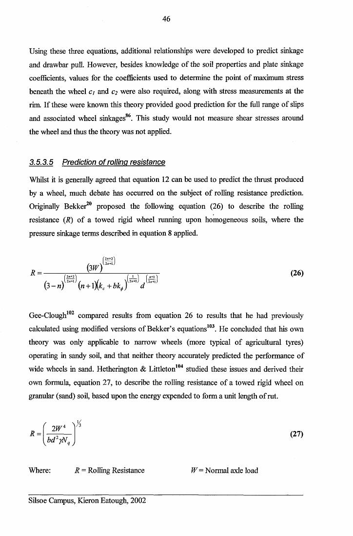
46
Using these three equations, additional relationships were developed to predict sinkage
and drawbar pull. However, besides knowledge of the soil properties and plate sinkage
coefficients, values for the coefficients used to determine the point of maximum stress
beneath the wheel ci and C2 were also required, along with stress measurements at the
rim. If these were known this theory provided good prediction for the full range of slips
and associated wheel sinkages86. This study would not measure shear stresses around
the wheel and thus the theory was not applied.
3.5.3.5 Prediction of rolling resistance
Whilst it is generally agreed that equation 12 can be used to predict the thrust produced
by a wheel, much debate has occurred on the subject of rolling resistance prediction.
Originally Bekker20 proposed the following equation (26) to describe the rolling
resistance (R) of a towed rigid wheel running upon homogeneous soils, where the
pressure sinkage terms described in equation 8 applied.
R = (M _________________ (26)f2n+ 21 ( 1 'j ( „+l 'j
/ _ \ 12n+l J / \ l 2 n + l j U n + lJ(3- n ) {n + \ \k c + b k j d
Gee-Clough102 compared results from equation 26 to results that he had previously
calculated using modified versions of Bekker’s equations103. He concluded that his own
theory was only applicable to narrow wheels (more typical of agricultural tyres)
operating in sandy soil, and that neither theory accurately predicted the performance of
wide wheels in sand. Hetherington & Littleton104 studied these issues and derived their
own formula, equation 27, to describe the rolling resistance of a towed rigid wheel on
granular (sand) soil, based upon the energy expended to form a unit length of rut.
R =xK 2 W 4 '
bd yNq
Where: R = Rolling Resistance W= Normal axle load
(27)
Silsoe Campus, Kieron Eatough, 2002
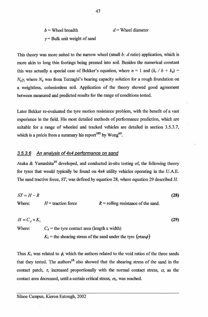
47
b - Wheel breadth d = Wheel diameter
y= Bulk unit weight of sand
This theory was more suited to the narrow wheel (small b: d ratio) application, which is
more akin to long thin footings being pressed into soil. Besides the numerical constant
this was actually a special case of Bekker’s equation, where n = 1 and (kc / b + =
Nqy, where Nq was from Terzaghi’s bearing capacity solution for a rough foundation on
a weightless, cohesionless soil. Application of the theory showed good agreement
between measured and predicted results for the range of conditions tested.
Later Bekker re-evaluated the tyre motion resistance problem, with the benefit of a vast
experience in the field. His most detailed methods of performance prediction, which are
suitable for a range of wheeled and tracked vehicles are detailed in section 3.5.3.7,
which is a precis from a summary his report105 by Wong63.
3.5.3.6 An analysis of 4x4 performance on sand
Ataka & Yamashita15 developed, and conducted in-situ testing of, the following theory
for tyres that would typically be found on 4x4 utility vehicles operating in the U.A.E.
The sand tractive force, ST, was defined by equation 28, where equation 29 described H.
ST = H - R (28)
Where: H= traction force R = rolling resistance of the sand.
H = CAx K l (29)
Where: C a = the tyre contact area (length x width)
K\ = the shearing stress of the sand under the tyre (otan^)
Thus K\ was related to $, which the authors related to the void ratios of the three sands
that they tested. The authors15 also showed that the shearing stress of the sand in the
contact patch, r, increased proportionally with the normal contact stress, cr, as the
contact area decreased, until a certain critical stress, o\, was reached.
Silsoe Campus, Kieron Eatough, 2002

48
o
Figure 3.16 - A graph of contact stress characteristics beneath a tyre on sand15
Once <j\ was exceeded then the sand beneath the tyre could not support the excessive
load, and hence moved aside and rose ahead of the tyre. Thus the shearing stress
achieved a constant critical value of T\, whilst the sand rising ahead of the tyre increased
the resistance force R. Figure 3.16 represents this conceptual analysis, from which
equation 29 was developed into equations 30 and 31, to describe the two possible stress
states beneath the wheel15.
If (<r< oi) then: H = CA x otan0 (30)
Else if (<7> <j\) then: H = Catx (31)
R was described as the force required to compressively fracture the sand in front of the
tyre. This was translated into a mathematical expression equation 32.
R - K 2C wLr {0l - 9 V) (32)
Where: K2 = compressive fracture force of sand ahead of the tyre
Cw — contact width
L r = static loaded radius measured in laboratory on sand
6l & Oy = Angles from the horizontal to the sand, see Figure 3.17 and
equations 33 and 34 (measured statically in the laboratory)
Silsoe Campus, Kieron Eatough, 2002
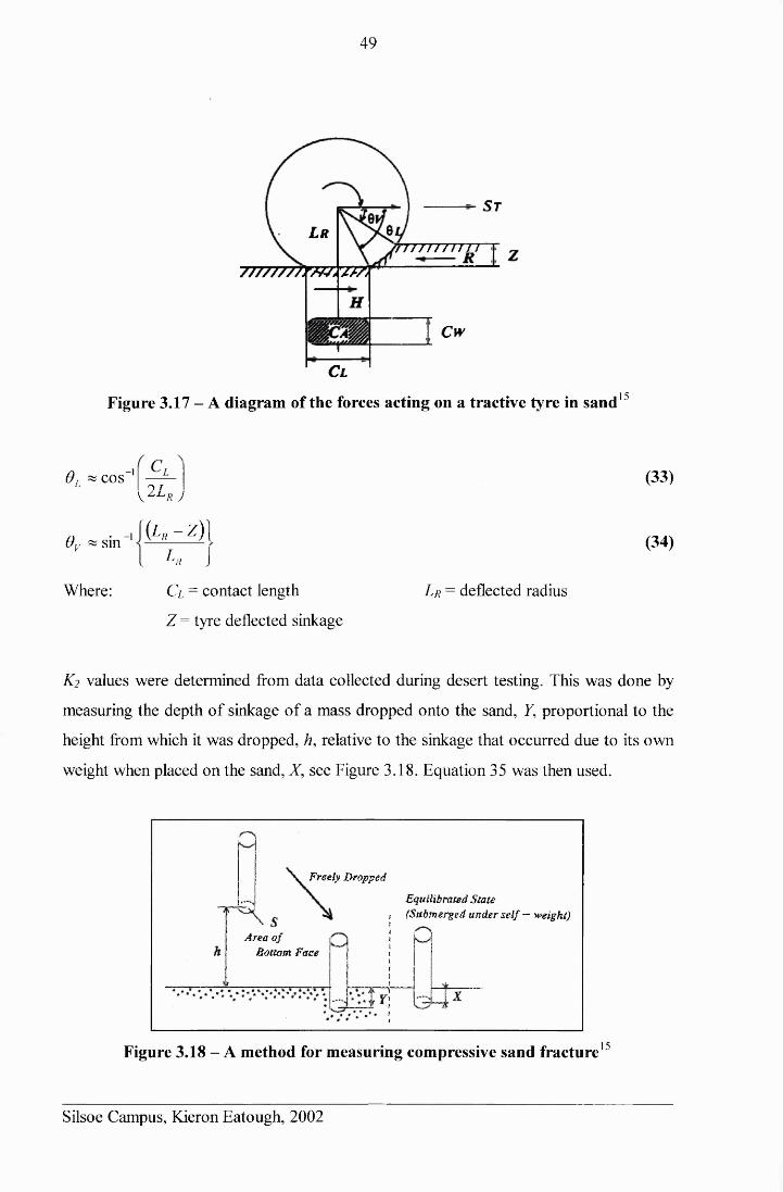
49
S t
LrT T T T T T T T T T
777777777777.Tm
Cw
Cl
Figure 3.17 - A diagram of the forces acting on a tractive tyre in sand 15
6j « cos 1
Gv « sin
Where:
\2 L r j
\ l s - z ) 1
. A. J
Ci = contact length
Z = tyre deflected sinkage
(33)
(34)
Z/? = deflected radius
K2 values were determined from data collected during desert testing. This was done by
measuring the depth of sinkage of a mass dropped onto the sand, Y, proportional to the
height from which it was dropped, h, relative to the sinkage that occurred due to its own
weight when placed on the sand, X, see Figure 3.18. Equation 35 was then used.
Freely Dropped
Equilibrated State (Submerged under self — weight)
Area o fBottom Face
Figure 3.18 - A method for measuring compressive sand fracture13
Silsoe Campus, Kieron Eatough, 2002
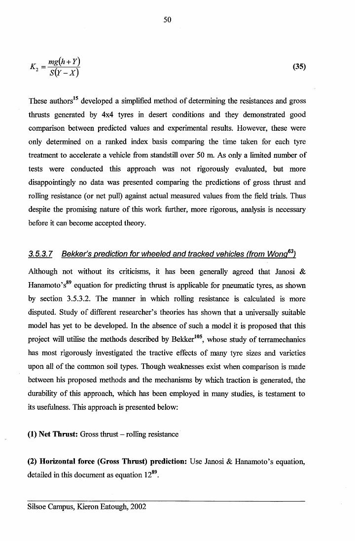
50
mg(h + Y)K l ~ W ^ J ( )
These authors15 developed a simplified method of determining the resistances and gross
thrusts generated by 4x4 tyres in desert conditions and they demonstrated good
comparison between predicted values and experimental results. However, these were
only determined on a ranked index basis comparing the time taken for each tyre
treatment to accelerate a vehicle from standstill over 50 m. As only a limited number of
tests were conducted this approach was not rigorously evaluated, but more
disappointingly no data was presented comparing the predictions of gross thrust and
rolling resistance (or net pull) against actual measured values from the field trials. Thus
despite the promising nature of this work further, more rigorous, analysis is necessary
before it can become accepted theory.
3.5.3.7 Bekker’s prediction for wheeled and tracked vehicles (from Wong63)
Although not without its criticisms, it has been generally agreed that Janosi &OQ
Hanamoto’s equation for predicting thrust is applicable for pneumatic tyres, as shown
by section 3.5.3.2. The manner in which rolling resistance is calculated is more
disputed. Study of different researcher’s theories has shown that a universally suitable
model has yet to be developed. In the absence of such a model it is proposed that this
project will utilise the methods described by Bekker105, whose study of terramechanics
has most rigorously investigated the tractive effects of many tyre sizes and varieties
upon all of the common soil types. Though weaknesses exist when comparison is made
between his proposed methods and the mechanisms by which traction is generated, the
durability of this approach, which has been employed in many studies, is testament to
its usefulness. This approach is presented below:
(1) Net Thrust: Gross thrust - rolling resistance
(2) Horizontal force (Gross Thrust) prediction: Use Janosi & Hanamoto’s equation,
detailed in this document as equation 1289.
Silsoe Campus, Kieron Eatough, 2002
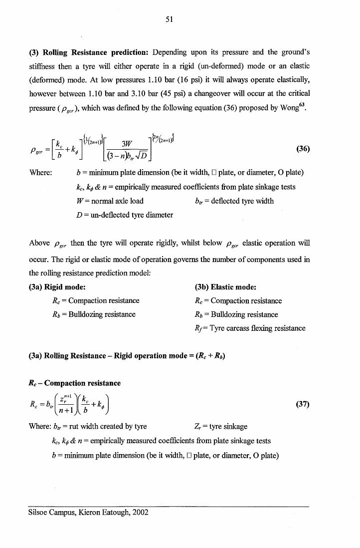
51
(3) Rolling Resistance prediction: Depending upon its pressure and the ground’s
stiffness then a tyre will either operate in a rigid (un-deformed) mode or an elastic
(deformed) mode. At low pressures 1.10 bar (16 psi) it will always operate elastically,
however between 1.10 bar and 3.10 bar (45 psi) a changeover will occur at the critical63pressure ( p ), which was defined by the following equation (36) proposed by Wong .
Pgcr
Where:
+ kk (2n+l). 3 W
(3 - n \ 4 B
b = minimum plate dimension (be it width, □ plate, or diameter, O plate)
kc, k$&n = empirically measured coefficients from plate sinkage tests
W= normal axle load btr = deflected tyre width
D = un-deflected tyre diameter
(36)
Above PgCr then the tyre will operate rigidly, whilst below p gcr elastic operation will
occur. The rigid or elastic mode of operation governs the number of components used in
the rolling resistance prediction model:
(3a) Rigid mode: (3b) Elastic mode:
Rc = Compaction resistance Rc = Compaction resistance
Rb = Bulldozing resistance Rb = Bulldozing resistance
R/= Tyre carcass flexing resistance
(3a) Rolling Resistance - Rigid operation mode = (Rc + Rb)
Rc - Compaction resistance
R, = b,f _«+1 V fc
v " + 1A— + k d b 4
(37)
Where: btr = rut width created by tyre Zr = tyre sinkage
kc, k(/)&n = empirically measured coefficients from plate sinkage tests
b = minimum plate dimension (be it width, □ plate, or diameter, O plate)
Silsoe Campus, Kieron Eatough, 2002
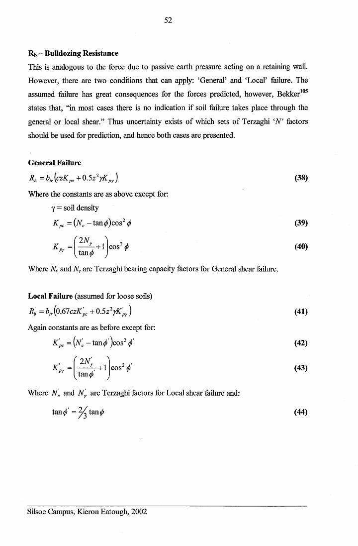
52
Rb - Bulldozing Resistance
This is analogous to the force due to passive earth pressure acting on a retaining wall.
However, there are two conditions that can apply: ‘General’ and ‘Local’ failure. The
assumed failure has great consequences for the forces predicted, however, Bekker105
states that, “in most cases there is no indication if soil failure takes place through the
general or local shear.” Thus uncertainty exists of which sets of Terzaghi W ' factors
should be used for prediction, and hence both cases are presented.
General Failure
R„=blr{czKpc+0.5z2rKpr) (38)
Where the constants are as above except for:
y = soil density
K pc = (Nc - tan )cos2 $ (39)'pcf O A7- A
KPr = 2N>. + 1 cos (f> (40)vtan^ j
Where Nc and Ny are Terzaghi bearing capacity factors for General shear failure.
Local Failure (assumed for loose soils)
K = K (0.67czKpc + 0.5z2jK „ ) (41)
Again constants are as before except for:
K 'pc = iN 'c - tan^ ')c°s2 $ (42)
X Pr = tan^cos2 (ft (43)
V r JWhere N'c and N'y are Terzaghi factors for Local shear failure and:
tan (ft' - ^ tan (j) (44)
Silsoe Campus, Kieron Eatough, 2002

53
(3b) Rolling Resistance - Elastic operating mode = (Rc + Rb+ Rj)
Rc - Compaction resistance
R = b ,f z * « \
n + 1rK , N — +k
b 1(45)
Where: btr — rut width created by tyre Ze = Tyre sinkage
kc, k(f)&n = empirically measured coefficients from plate sinkage tests
b = minimum plate dimension (be it width, □ plate, or diameter, O plate)
Rb - Bulldozing Resistance
This prediction is common to both operating modes and therefore the equations
presented for rigid operation should be used.
R f - Tyre Carcass Flexing Resistance
Rf = [3.5816,rD2 p ge({iM 49a-sm 2a)\/ a {D -2d )
Where: D = tyre diameter 3 = tyre deflection
X.2n+i) '1JJ7 "1 /f2n+1)
b *3W
(3 - n \ 4 D
a = cos-1 [(/) - 25)/Z>]
s = l - e y J
Where: h = Section height Ke = l for radial tyres
(46)
(47)
(48)
(49)
3.5.4 Finite Element Mathematical Models
More recently as computing performance and capability has increased some authors
have pursued the use of FE models to predict tractive tyre performance and tyre effects
on the soil, i.e. compaction. Yong & Fattah106 (1976) were amongst the first authors to
apply the finite element method to terramechanics using energy calculations to predict
soil deformation beneath, and drawbar pull of, a rigid wheel but the descriptions of soil
material properties and boundary conditions were inherently limited.
Silsoe Campus, Kieron Eatough, 2002
54
Oida107 (1984) developed FE methods further to better account for soil properties,
which were not well described by off-the-shelf products, thereby addressing some of the
weaknesses in Yong & Fattah’s106 model. Oida’s107 model showed good prediction of
wheel sinkage on a sandy loam soil and Regli et al.108 developed an FE model to predict
the tractive performance for, and soil deformation beneath, lugged agricultural tyres for
limited conditions. Whilst model predictions correlated well to measured values at low
slips (up to 20%) considerable error occurred above 30% slip. The authors stated this as
being due to “big deformations causing significant inaccuracies in the FE program”108.
A more recent FE sand-tyre interaction model by Liu et al109 produced useful prediction
of tyre traction, but only for a specialised set of conditions. Particular limitations were
the use of two-dimensional solid wheels (discs) and poor representation of the contact
pressure and friction force along the tyre-soil interface. More significantly “local failure
and significant amounts of sand flow under moving tyres cannot be modelled
adequately by the conventional finite element method”109. Thus the model’s
performance deteriorated with increased slip, indicating that such methods would be
inappropriate to provide predictions at the high slips of approximately 75% that would
form part of this investigation.
Despite all the advances, the modelling of tyres and soil by the FE approach remains
complex. It is possible to produce models to predict performance where small soil
strains occur, but FE methods struggle to solve problems involving large soil
displacements. There is also the issue of developing models that are suitably complex to
accurately model a given situation. At the initiation of this project (1998) Goodyear
were developing a dynamic FE tyre model capable of replicating low speed revolutions
on a non-deformable surface with an accuracy suitable for their purposes. This required
a supercomputer for its solution. In the light of this evidence it was beyond this
project’s capabilities to deliver an FE type model capable of providing useful
predictions for a tyre operating at high slips on loose deformable sand.
Silsoe Campus, Kieron Eatough, 2002
55
3.6 TYRE TEST RIGS
3.6.1 Fixed Slip Test Rigs
Publications by Uffelman110 and Reece & Wills111 detailed systems developed for their
experimental tyre investigations and the generation of slip-pull curves. Both systems
operated with a similar principle, whereby fixed wheel (or track) slips were generated
using anchored cables that wrapped around variable sized drums (or chain drives),
which in turn connected to the wheel. The test tyre was mounted on a framework that
was driven away from the anchor point using either a tractor or a towed trolley, thereby
inducing wheel slip. Measuring the forces within the system allowed the tyre thrust and
rolling resistance to be determined. These machines offered the researchers versatility
and simplicity at a low cost. Latterly Del Rosario112 designed a system that generated
good experimental results by adapting these principles for use in a soil bin situation.
The one drawback of these systems was that, either the slip (drum size) had to be
changed before each test run to generate results across the full slip range, or else a
variable diameter drum had to be utilised. Variable size drums were achievable as
Soehne113 demonstrates, however, it was difficult and costly to manufacture such items,
especially if a large diameter was required. Thus, more commonly, a number of discrete
drum sizes or gear ratios were utilised to overcome this issue.
3.6.2 Variable Slip Test Rigs
Truly adequate variable slip tyre traction test rigs were not developed until around the
1940’s114, when the N.I.A.E. were simultaneously developing a single wheel tester115.
This device was structured around a tractor that underwent a bespoke re-design to
include an electric motor to apply a controlled torque to the separate test wheel mounted
behind the tractor. The wheel frame mounting used parallel linkages and Hooke’s joints
to avoid weight transfer between the two sections, a criticism of earlier devices.
The advantages of this device115 were that it was able to quickly measure thrusts across
a range of slips for a given tyre, and because it was mounted on a tractor it was
extremely mobile and could be used on any surface. The experiments conducted with
Silsoe Campus, Kieron Eatough, 2002
56
the device showed that it worked well, however, the design was complex, expensive and
had been time consuming to perfect. Despite this, the advantages that could be achieved
in the timely completion of a test programme by being able to speedily change the tyre
slip, through a separately controllable wheel drive, were clearly apparent.
Billington116 described the further development of this apparatus as it was improved to
form the N.I.A.E. Mark II single wheel tester. 52 kW (70 hp) hydrostatic transmissions
were fitted as they best provided the high power and controllable drives necessary for
both the tractor and test wheels. Again the test frame was connected to the tractor by
parallel linkages to avoid weight transfer between the two units, whilst strain gauged
units were fitted appropriately to measure the thrust produced by the wheel. Wheel
speeds were measured by tacho-generators, whilst wheel torque was measured using a
strain-gauged transducer. This equipment was successfully used to investigate the
tractive performance of a range of agricultural tyres on a variety of agricultural surfaces.
Upadhyaya e t «/.117,118 described the development of another type of single wheel tester
undertaken by staff at the University of California, Davis to allow the investigation of
soil-tyre interaction. This took the form of a mobile soil bin with a drive unit that could
be operated in either a draft, or slip control mode. It consisted of two 12 m tracks
mounted on either side of a front and rear trailer, which allowed easy location of the
device in a field. A carriage with a test wheel, powered by a hydrostatic drive, ran along
the tracks. Changing the pressure in a load cylinder controlled the vertical tyre load.
Variation to the hydrostatic controls allowed a tyre to be tested across the full slip
range, although this required several test runs. A range of instrumentation was fitted to
the device to measure the carriage and wheel speeds and sinkages, thereby allowing a
full picture of the traction interactions to be developed.
Keen 119120121 described various traction investigations that were undertaken using a
single wheel tester that was developed at Harper Adams University College, Shropshire,
UK. This single wheel device was designed to mimic a quarter of a high-speed tractor
through the inclusion of a suspension between the wheel and the supported mass. It was
mounted to a tractor three-point linkage and driven through a 44 kW diesel Land Rover
Silsoe Campus, Kieron Eatough, 2002
57
engine and gearbox. The tractor forward speed controlled ground speed, and varying the
Land Rover engine speed controlled the wheel slip. This worked well across the low
slip range that was investigated (up to 25%). The tester was instrumented to measure
thrust, through a strain gauged parallel linkage, thus allowing slip-pull curves and wheel
sinkages to be determined. Good agreement was shown119 between thrust values
measured by this device and the prediction equations proposed by Janosi and
Hanamoto89. Accelerometers were also fitted to the test rig and used to measure the
vertical accelerations that were incorporated into Keen’s later research120,121.
The most capable of the single wheel testers discussed have a high mobility allowing
them to operate upon a range of soil surfaces. However, even the most basic systems
using cable drums are very capable of producing results from which slip-pull curves can
be constructed. Although more costly, variable hydrostatic transmissions allow much
greater experimental flexibility, as a full range of wheel slips can be quickly tested.
Study of all of these devices indicated that instrumentation and data recording systems
should be fitted to allow the determination of the following tractive variables:
1. Tractive Force (Thrust) and (or) Rolling Resistance.
2. Test wheel rotational speed
3. Drive unit ground speed.
4. Wheel sinkage.
5. Wheel slip (derived from measurements 2 and 3).
6. Angular wheel position
7. Tyre deflection
8. Normal and longitudinal stress at the interface
3.7 SUMMARY OF LITERATURE REVIEW
The completed literature review enabled the required stages of the project to be more
clearly identified and planned. Initially it was necessary to understand the market
requirements for performance off-road tyre products, which would necessitate a market
survey. Then to enable the tyre performance to be modelled using adaptations of
Bekker’s predictive methodologies outlined above it would be necessary to collect raw
data that could be used to develop and validate the models. A further model would have
Silsoe Campus, Kieron Eatough, 2002
58
to be developed to allow the required tread pattern to be related to the tyre performance.
The development of this would also require experimental results.
To enable experimental results to be collected it was necessary to develop an
instrumented test-rig and experimental methodology capable of measuring the tractive
performance data outlined in section 3.6 in the Cranfield University Soil Dynamics
Laboratory. Additionally the performance of both the TekScan stress measuring system
and the RFID tag sensing system required evaluation in terms of their new intended
applications before they could be adopted for the main investigations into pressure
distributions and particularly sand displacements beneath the tyres. Tractive
performance data was also recorded during these investigations so that the prediction
capabilities of the proposed tyre performance models could be assessed for the dynamic
sand traction environment created in the SDL.
Silsoe Campus, Kieron Eatough, 2002
59
4 MARKET SURVEY AND REVIEW
Before any tyre performance investigations were conducted, it was necessary to
investigate the implications of optimising 4x4 tyre treads to suit off-road environments
from the perspective of 4x4 end-users (drivers). If the tyre (and vehicle) products
currently available to them already delivered capabilities that exceeded their
requirements, then further tread developments and enhanced modelling techniques
would be unnecessary and unwarranted. A customer questionnaire was identified as
being the most effective way to evaluate the market’s views upon a range of tyre issues
related to off-road and on-road performance. When this was jointly designed and
undertaken with Marcus Oliver30, during the early stages of both projects, the author
was considering conducting tyre traction investigations on a range of off-road surfaces.
Therefore a set of results from which the implications of off-road tyre requirements
could be assessed for a range of off-road surfaces, not just sand environments, was
required. These implications were considered for both of the sponsoring manufacturers.
4.1 MARKET SURVEY METHODOLOGY
The requirement to understand a range of views of end-users meant that the
questionnaire had to be universally applicable to a range of 4x4 drivers and it had to
sample an audience with a wide range of driving habits, skills etc. This meant that it
could not be conducted at a specialised off-roading event, so instead it was undertaken
at the 1998 International Motor Show, held in October at the NEC, Birmingham, UK,
for the following reasons:
• It would attract large numbers of prospective 4x4 tyre customers, from diverse
backgrounds, including overseas visitors.
• The event is the UK’s premier car show.
• Its proximity to the Land Rover Solihull site, allowed use of their Driving
Experience site (a dedicated off-road promotional training track). This greatly
assisted identifying existing, and potential, Land Rover customers, and therefore
prospective performance 4x4 tyre purchasers, as guests invited to the Driving
Experience were either existing Land Rover customers, or had a strong interest in
owning a Land Rover.
Silsoe Campus, Kieron Eatough, 2002
60
The questionnaire used, see Appendix 3, was designed to survey people who drove a
variety of vehicles upon a range of on-road and off-road surfaces, from ice to desert
sand, for a range of purposes. A significant number of the questions were designed to be
open-ended, so that a range of individual views could be sampled from respondents. In
particular the questionnaire was intended to determine:
1. The market’s perception of the performance of existing 4x4 tyres.
2. What would be the important factors if respondents were considering
purchasing high performance off-road tyres?
3. The likelihood of respondents to purchase a second set of dedicated off-road
tyres for their 4x4 vehicles if they offered extra performance over existing tyres
on a particular surface.
The questionnaire was also designed to record:
1. People’s personal profiles, to determine the sex, age, geographical location,
socio-economic group and vehicles driven both on and off-road by respondents.
2. Data questions, to determine opinions, particularly those related to cost, value
and relative importance, for a range of tyre related issues.
3. Response triangulation, for analysis of the truthfulness and/or bias of answers.
The questionnaire was conducted at the Driving Experience for the show’s duration
whilst the respondents waited for their promotional trip around the track. The wait could
take up to 30 minutes, which allowed time for people to fully participate with the
questionnaire. Respondent’s participation was sought on a purely random basis as they
entered the waiting area. A total of 369 questionnaires were fully completed, however,
the results of respondents whose replies contained three or more contradictory answers
(about 3%) were not included in the analysis.
4.2 MARKET SURVEY RESULTS
The questionnaires were individually examined and the responses entered into an Excel
spreadsheet, which allowed the results to be easily sorted and grouped. The results were
then analysed to find trends and factors contained within the replies. The respondents
were segmented into separate groups of purely on-road drivers, on and off-road drivers
Silsoe Campus, Kieron Eatough, 2002
61
and ‘serious’ off-road drivers by employing recognised methods122,123. ‘Serious’ off-
road drivers were those people who were the most frequent and knowledgeable off-road
drivers, be it through work or leisure, for example Land Rover enthusiasts, hill farmers
and landowners. This last segment were of most interest because they owned the greater
quantity of 4x4 vehicles, had the most valid opinions based upon their real experience,
and because they were the drivers most likely to purchase second sets of dedicated 4x4
off-road tyres to supplement existing road biased tyres. This group accounted for 12%
of all respondents, and 46% of the respondents who partook in some form off-road
driving. Analysis of the replies from the off-road drivers and ‘serious’ off-road drivers
produced the following results.
4.2.1 The Profile of Prospective Purchasers of Off-road Tyres
Within the UK these drivers were concentrated in Yorkshire and Humberside, the East
and West Midlands, and the South East. However, these results were biased by the
proximity of these locations to the Motor Show. Typically these people drove off-road
in muddy environments, although some people drove on beach sand. The off-road
drivers from overseas accounted for 7% of respondents, but this quantity was too small
to identify patterns in their geographical locations. 65% of these drivers did their off-
roading in rocky (semi-desert) or sand environments, though often off-roading only
involved driving on dirt tracks and trails, for which universal (compromise) treads were
generally fitted.
The respondents in the ‘serious’ group were either in the Middle or Skilled working
classes and exclusively male drivers (as no women questioned undertook any form off-
road driving, although this cannot be representative of the whole off-roading
population). The ages of likely purchasers ranged from 26-50 Predominantly these
respondents drove off-road for recreation and leisure and they were well informed about
the importance of tyre choice for such ventures. Both the respondents from the UK and
overseas stated that they were keen that their vehicles should be fitted with high-
performing tyres when they were undertaking off-roading, although 80% of tyre
fitments were actually compromises that offered an adequate level of on-road
performance. These statements were confused by the respondents’ relative perceptions
Silsoe Campus, Kieron Eatough, 2002
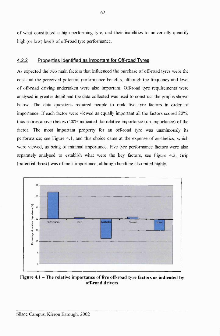
62
of what constituted a high-performing tyre, and their inabilities to universally quantify
high (or low) levels of off-road tyre performance.
4.2.2 Properties Identified as Important for Off-road Tyres
As expected the two main factors that influenced the purchase of off-road tyres were the
cost and the perceived potential performance benefits, although the frequency and level
of off-road driving undertaken were also important. Off-road tyre requirements were
analysed in greater detail and the data collected was used to construct the graphs shown
below. The data questions required people to rank five tyre factors in order of
importance. If each factor were viewed as equally important all the factors scored 20%,
thus scores above (below) 20% indicated the relative importance (un-importance) of the
factor. The most important property for an off-road tyre was unanimously its
performance; see Figure 4.1, and this choice came at the expense of aesthetics, which
were viewed, as being of minimal importance. Five tyre performance factors were also
separately analysed to establish what were the key factors, see Figure 4.2. Grip
(potential thrust) was of most importance, although handling also rated highly.
| 20
0
,---------------. 1 " 1
F erform anc e C ost C omfort N oise
Figure 4.1 - The relative importance of five off-road tyre factors as indicated byoff-road drivers
Silsoe Campus, Kieron Eatough, 2002
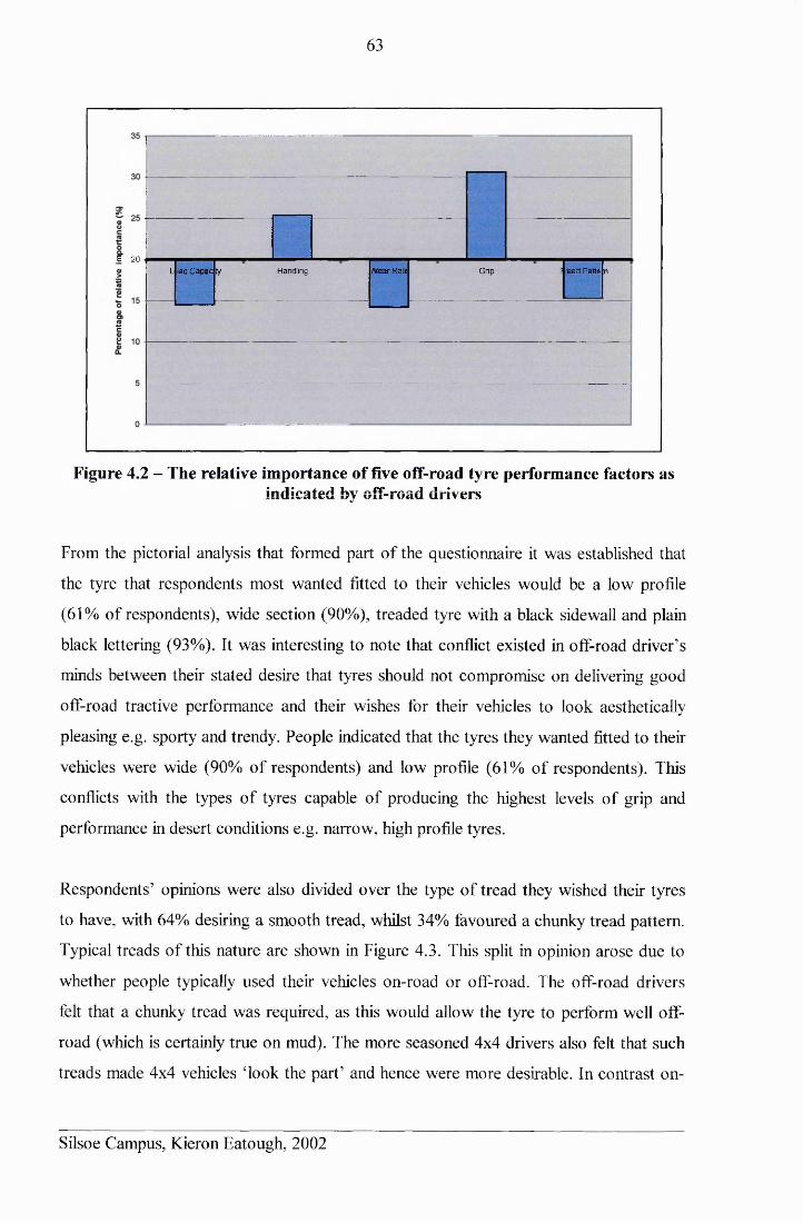
63
E 20
L iad C ap ac ty Handling Ale a r Rate Grip 1 'ea d Patte n
Figure 4.2 - The relative importance of five off-road tyre performance factors asindicated by off-road drivers
From the pictorial analysis that formed part of the questionnaire it was established that
the tyre that respondents most wanted fitted to their vehicles would be a low profile
(61% of respondents), wide section (90%), treaded tyre with a black sidewall and plain
black lettering (93%). It was interesting to note that conflict existed in off-road driver’s
minds between their stated desire that tyres should not compromise on delivering good
off-road tractive performance and their wishes for their vehicles to look aesthetically
pleasing e.g. sporty and trendy. People indicated that the tyres they wanted fitted to their
vehicles were wide (90% of respondents) and low profile (61% of respondents). This
conflicts with the types of tyres capable of producing the highest levels of grip and
performance in desert conditions e.g. narrow, high profile tyres.
Respondents’ opinions were also divided over the type of tread they wished their tyres
to have, with 64% desiring a smooth tread, whilst 34% favoured a chunky tread pattern.
Typical treads of this nature are shown in Figure 4.3. This split in opinion arose due to
whether people typically used their vehicles on-road or off-road. The off-road drivers
felt that a chunky tread was required, as this would allow the tyre to perform well off-
road (which is certainly true on mud). The more seasoned 4x4 drivers also felt that such
treads made 4x4 vehicles Took the part’ and hence were more desirable. In contrast on-
Silsoe Campus, Kieron Eatough, 2002
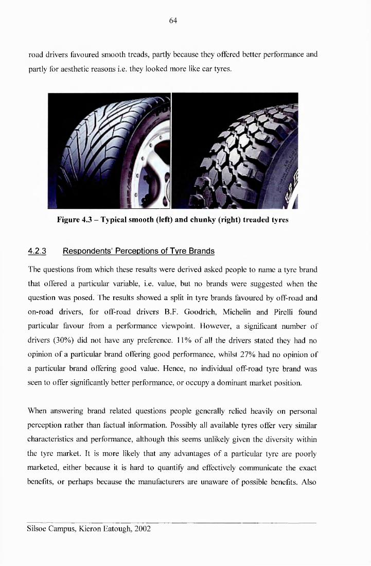
64
road drivers favoured smooth treads, partly because they offered better performance and
partly for aesthetic reasons i.e. they looked more like car tyres.
Figure 4.3 - Typical smooth (left) and chunky (right) treaded tyres
4.2.3 Respondents’ Perceptions of Tyre Brands
The questions from which these results were derived asked people to name a tyre brand
that offered a particular variable, i.e. value, but no brands were suggested when the
question was posed. The results showed a split in tyre brands favoured by off-road and
on-road drivers, for off-road drivers B.F. Goodrich, Michelin and Pirelli found
particular favour from a performance viewpoint. However, a significant number of
drivers (30%) did not have any preference. 11% of all the drivers stated they had no
opinion of a particular brand offering good performance, whilst 27% had no opinion of
a particular brand offering good value. Hence, no individual off-road tyre brand was
seen to offer significantly better performance, or occupy a dominant market position.
When answering brand related questions people generally relied heavily on personal
perception rather than factual information. Possibly all available tyres offer very similar
characteristics and performance, although this seems unlikely given the diversity within
the tyre market. It is more likely that any advantages of a particular tyre are poorly
marketed, either because it is hard to quantify and effectively communicate the exact
benefits, or perhaps because the manufacturers are unaware of possible benefits. Also
Silsoe Campus, Kieron Eatough, 2002
65
each tyre probably only performs well in particular circumstances, thus different tyres
will better suit different driving habits.
4.2.4 Likelihood of Purchasing Secondary Performance Off-Road Tyres
For infrequent off-road driving, one set of tyres offering an off' on-road compromise
was considered adequate. Only the most ‘serious’ (frequent and skilled) off-road drivers
would consider purchasing a second set of dedicated off-road tyres, for example 81% of
the overseas off-road drivers stated that they would seriously consider purchasing a
second set of dedicated tyres. Respondents would generally not be willing to pay more
for a set of high performance, dedicated 4x4 off-road tyres than sets of currently
available 4x4 tyres cost; approximately £400 a set (excluding the rims).
Offers put to respondents were considered much more in terms of cost, than extra tyre
performance. However, most respondents stated that if significant measurable
performance advantages of a high performance off-road tyre could be demonstrated
over and above the performance levels of existing tyres, then they would consider
justifying the purchase of a second set of tyres for use purely off-road. When choosing
secondary specialist off-road tyres the ease of interchange between the two sets of tyres
was also important. Whereas noise would only become a deterring issue (inhibitor) if
off-road tyres had to be driven at high-speed on-road, for example, getting to and from
the off-roading locations in Dubai17.
4.2.5 Interest in Automatic Central Tyre Inflation Systems (CT1S)
Interest existed in the fitment of a self-sensing tyre inflation system as an extra vehicle
feature, providing its cost did not exceed £1000. Respondents indicated that a
specification of such a system and its merits would be required before a true value of its
worth could be estimated (such a specification was not supplied with the questionnaire).
4.3 IMPLICATIONS OF THE MARKET SURVEY RESULTS
A market interested in purchasing off-road tyres offering better tractive performance
was identified. However, consumers are quite ignorant about the relative performance
Silsoe Campus, Kieron Eatough, 2002
66
abilities of different tyre makes and brands. Individual views are predominantly based
upon subjective personal experience, influenced by opinions expressed in the motoring
press. This is understandable given that no simple and effective means of tyre
comparison is publicly available, however, it can lead to conflicting opinions
developing between manufacturers and drivers. Franklin6 commented that in the Middle
Eastern market the Dunlop TG35 tyre was perceived to offer performance advantages,
which may be true in a particular driver’s circumstances, however, Land Rover’s
official off-road testing had not shown this tyre to significantly outperform any other
products on the market. These findings demonstrated that the lack of a unified measure
of tyre performance across a range of conditions, and no simple way of communicating
tyre test data to the general public, prevents them knowing which tyres offer the “best”
performance.
The serious off-road drivers were capable of picking a tyre that would offer good off-
road performance if fitted to their vehicles. However, this statement was contradicted by
a desire to purchase and fit tyres that “looked good” on their vehicles. Low profile tyres,
which are typically considered to ‘look good’, do not allow a vehicle to achieve its
maximum potential traction, as tyre deformation, and hence the contact patch length is
limited. This conflict is seen in the Middle Eastern market where 4x4 vehicle image is
viewed as very important by the wealthy 4x4 owning classes6’17. Land Rover has
traditionally erred towards fitting tyres able to generate high levels of off-road (and
where possible on-road) performance ahead of those that ‘look good’6. However,
recently competitor 4x4 vehicles, e.g. BMW X5, have been optimised for the on-road
situation, which has partially been achieved by the fitment of lower profile, wider tyres,
which also happen to ‘look good’. The success of such vehicles has placed increased
pressure upon Land Rover to justify (compromise) its tyre fitments, so that sales are not
jepordaised6. Tyre tread was also shown to govern the vehicle aesthetics, but the exact
patterns were unclear as different customers favour different treads. However, if
significantly greater tyre performance could be generated then most consumers would
disregard the style of the treads, and be satisfied with the performance gain.
Silsoe Campus, Kieron Eatough, 2002

67
Currently Land Rover’s tyre testing mainly involves large quantities of subjectively
marked, and loosely controlled, field trials9. This process could be improved if a more
objective test method capable of speedily determining a single measure of a tyre’s
potential tractive performance were developed. It would not be cost-effective to develop
a significantly better performing tyre if this ability cannot be clearly demonstrated to the
market, to justify a premium price tag. The development of a model to relate tyre (and
tread) parameters to vehicle performance could allow potential performance
improvements to be directly communicated to the public. The results indicated that 21%
of the 4x4 vehicle owning/ driving market would seriously consider purchasing a
second set of dedicated high performance 4x4 off-road tyres. However, any interest was
highly cost dependant and to justify any extra cost over the price of existing tyres then
significant performance gains would have to be demonstrated.
Silsoe Campus, Kieron Eatough, 2002
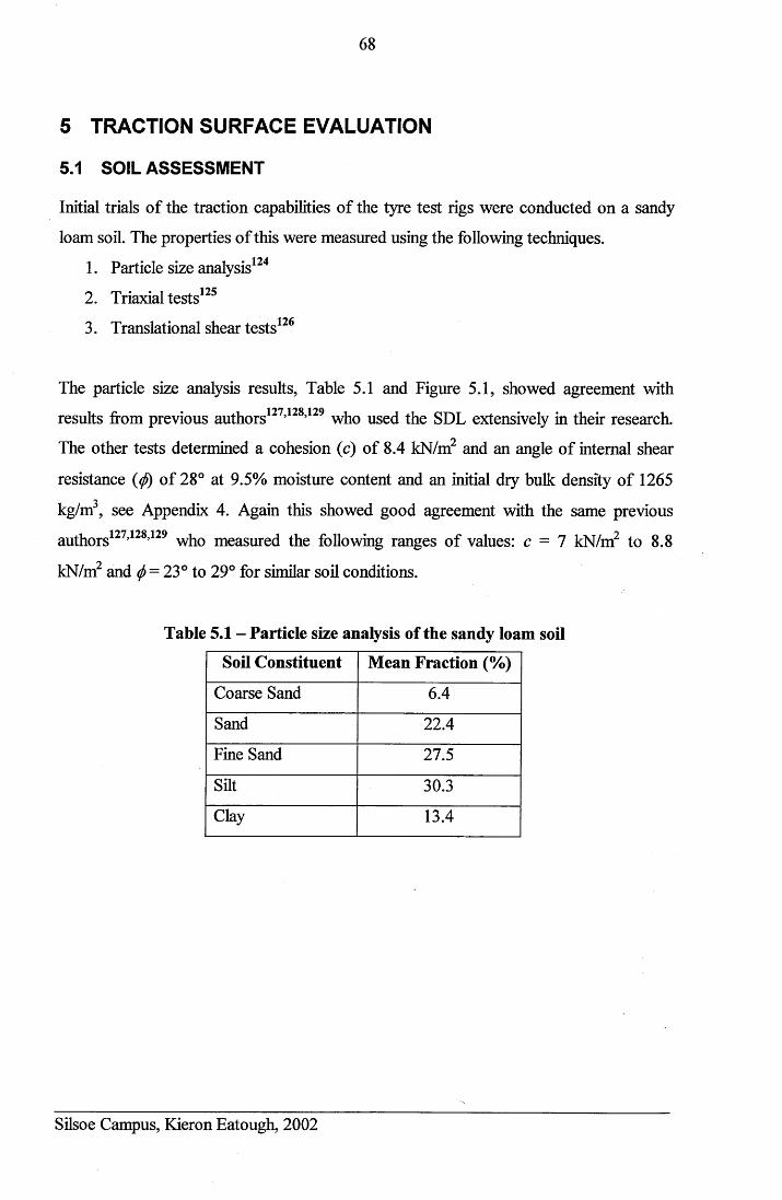
68
5 TRACTION SURFACE EVALUATION
5.1 SOIL ASSESSMENT
Initial trials of the traction capabilities of the tyre test rigs were conducted on a sandy
loam soil. The properties of this were measured using the following techniques.
1. Particle size analysis124
2. Triaxial tests125
3. Translational shear tests126
The particle size analysis results, Table 5.1 and Figure 5.1, showed agreement with
results from previous authors ’ ’ who used the SDL extensively in their research.
The other tests determined a cohesion (c) of 8.4 kN/m2 and an angle of internal shear
resistance ($) of 28° at 9.5% moisture content and an initial dry bulk density of 1265
kg/m3, see Appendix 4. Again this showed good agreement with the same previous1 7 7 17ft 1 7 0 Oauthors ’ ’ who measured the following ranges of values: c = 7 kN/m to 8.8
kN/m2 and ^ = 23° to 29° for similar soil conditions.
Table 5.1 - Particle size analysis of the sandy loam soil
Soil Constituent Mean Fraction (%)
Coarse Sand 6.4
Sand 22.4
Fine Sand 27.5
Silt 30.3
Clay 13.4
Silsoe Campus, Kieron Eatough, 2002
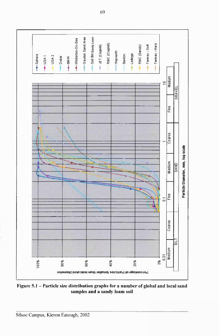
69
jajauieia paieojpui uein janeuis sappjBd jo aBepiaojad
Figure 5.1 - Particle size distribution graphs for a number of global and local sandsamples and a sandy loam soil
Silsoe Campus, Kieron Eatough, 2002
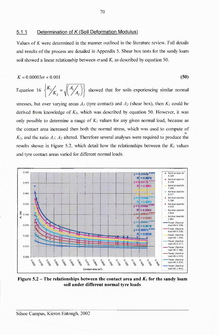
70
5.1.1 Determination of K (Soil Deformation Modulus)
Values of K were determined in the manner outlined in the literature review. Full details
and results of the process are detailed in Appendix 5. Shear box tests for the sandy loam
soil showed a linear relationship between crand K, as described by equation 50.
K = 0.00003cr + 0.001 (50)
Equation 16 ~ s^owe< ^ at or so^s exPeriencing similar normal
stresses, but over varying areas Ai (tyre contact) and A 2 (shear box), then Ki could be
derived from knowledge of K2, which was described by equation 50. However, it was
only possible to determine a range of K/ values for any given normal load, because as
the contact area increased then both the normal stress, which was used to compute of%
K2, and the ratio Aj: A 2 altered. Therefore several analyses were required to produce the
results shown in Figure 5.2, which detail how the relationships between the Kj values
and tyre contact areas varied for different normal loads.
♦ Norm al load kN 9 .320
■ Norm al load kN 8 .339
Norm al load kN 7.358
x Norm al load kN 6.377
x Norm al load kN 5.396
• Norm al load kN 4.415
+ Norm al load kN 3.434
- Norm al load kN 2.453
— P o w er (N orm al load kN 9 .320)
— P o w er (N orm al load kN 8 .339)
P ow er (N orm al load kN 7 .358)
— P ow er (N orm al load kN 6 .377)
— P ow er (N orm al load kN 5 .396)
— P o w er (N orm al load kN 4.415)
— P ow er (N orm al load kN 3 .434)
P o w er (N orm al load kN 2 .453)
0 .080 1
0.070
0.060
0.050
~ 0 .0 4 0 - 5C0 .030
0.020
0.010
°o % <C on tact area (m 2)
.0082y =■0.3724QQZZ
= 0.9
•0 .3419 ;.0069= 0.9
.0065:= 0,9659
yjssU :,O O S l
Ry=C
= 0.9*98 .0059 n-0-2515
Figure 5.2 - The relationships between the contact area and Kj for the sandy loamsoil under different normal tyre loads
Silsoe Campus, Kieron Eatough, 2002
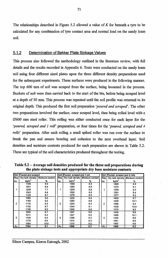
71
The relationships described in Figure 5.2 allowed a value of K for beneath a tyre to be
calculated for any combination of tyre contact area and normal load on the sandy loam
soil.
5.1.2 Determination of Bekker Plate Sinkaae Values
This process also followed the methodology outlined in the literature review, with full
details and the results recorded in Appendix 6. Tests were conducted on the sandy loam
soil using four different sized plates upon the three different density preparations used
for the subsequent experiments. These surfaces were produced in the following manner.
The top 600 mm of soil was scraped from the surface, being loosened in the process.
Buckets of soil were then carried back to the start of the bin, before being scraped level
at a depth of 50 mm. This process was repeated until the soil profile was returned to its
original depth. This produced the first soil preparation *poured and scraped\ The other
two preparations involved the surface, once scraped level, then being rolled level with a
0600 mm steel roller. This rolling was either conducted once for each layer for the
‘poured, scraped and 1 roll9 preparation, or four times for the ‘poured, scraped and 4
rolls’ preparation. After each rolling a small spiked roller was run over the surface to
break the pan and ensure bonding and cohesion to the next overhead layer. Soil
densities and moisture contents produced for each preparation are shown in Table 5.2.
These are typical of the soil characteristics produced throughout the testing.
Table 5.2 - Average soil densities produced for the three soil preparations during the plate sinkage tests and appropriate dry base moisture contents
Soil Poured and scraped Soil Poured, scraped and 1 roll Soil Poured, scraped and 4 rollsRep Dry bulk density Moisture content Rep Dry bulk density Moisture content Rep Dry bulk density Moisture contentno. kg/m3 % no. kg/m3 % no. kg/m3 %
1185 9.3 1309 8.5 1408 8.91201 8.4 1280 8.6 1372 8.1
1 1239 7.7 1 1239 8.8 1 1358 8.01243 8.4 1320 8.8 1391 8.41129 8.7 1276 8.9 1377 9.21090 9.0 1229 8.8 1402 9.71163 9.2 1268 8.8 1425 10.1
2 1176 9.4 2 1234 9.4 2 1386 9.41132 8.7 1240 9.1 1430 10.41190 9.0 1248 9.8 1370 9.01092 9.7 1267 9.6 1408 9.61211 9.3 1247 9.5 1400 10.1
3 1148 9.4 3 1295 9.4 3 1433 9.61179 9.6 1314 9.3 1361 9.61080 10.0 1219 9.2 1402 9.6
Av. 1164 9.1 Av. 1266 9.1 Av. 1395 9.3
Silsoe Campus, Kieron Eatough, 2002
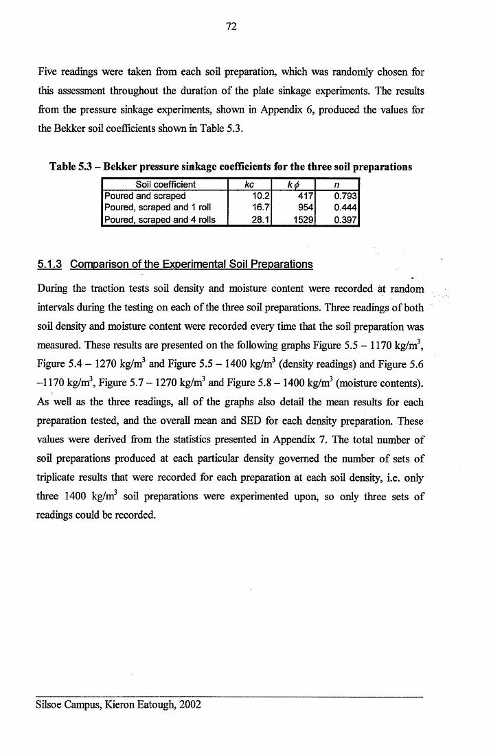
72
Five readings were taken from each soil preparation, which was randomly chosen for
this assessment throughout the duration of the plate sinkage experiments. The results
from the pressure sinkage experiments, shown in Appendix 6, produced the values for
the Bekker soil coefficients shown in Table 5.3.
Table 5.3 - Bekker pressure sinkage coefficients for the three soil preparationsSoil coefficient kc k<l> n
Poured and scraped Poured, scraped and 1 roll Poured, scraped and 4 rolls
10.216.728.1
417954
1529
0.7930.4440.397
5.1.3 Comparison of the Experimental Soil Preparations
During the traction tests soil density and moisture content were recorded at random
intervals during the testing on each of the three soil preparations. Three readings of both
soil density and moisture content were recorded every time that the soil preparation was
measured. These results are presented on the following graphs Figure 5.5 - 1170 kg/m3,
Figure 5.4 - 1270 kg/m3 and Figure 5.5 - 1400 kg/m3 (density readings) and Figure 5.6
-1170 kg/m3, Figure 5.7 - 1270 kg/m3 and Figure 5.8 - 1400 kg/m3 (moisture contents).
As well as the three readings, all of the graphs also detail the mean results for each
preparation tested, and the overall mean and SED for each density preparation. These
values were derived from the statistics presented in Appendix 7. The total number of
soil preparations produced at each particular density governed the number of sets of
triplicate results that were recorded for each preparation at each soil density, i.e. only
three 1400 kg/m3 soil preparations were experimented upon, so only three sets of
readings could be recorded.
Silsoe Campus, Kieron Eatough, 2002
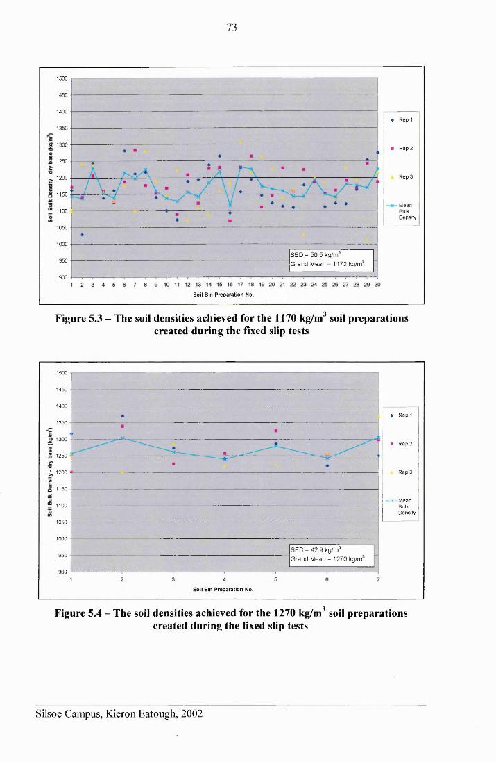
73
1500 -ip-
1450
1400
♦ R ep 1
1350
o> 1300■ R ep 2
1250
R ep 3' 1200
1150
M eanBulkDensity
1100 -
1050
1000
SED = 50.5 kg/m3 Grand Mean = 1172 kg/m:950
900
S o il Bin P reparation No.
Figure 5.3 - The soil densities achieved for the 1170 kg/m3 soil preparations created during the fixed slip tests
1500
1450
1400
♦ R ep 1
1350
■ R ep 2
1250
R ep 3■ 1200
1150
-x— M ean Bulk D ensity
1100
1050
1000
SED = 42.9 kg/m3 Grand Mean = 1270 kg/m'950
900
S o il Bin Preparation No.
Figure 5.4 - The soil densities achieved for the 1270 kg/m3 soil preparations created during the fixed slip tests
Silsoe Campus, Kieron Eatough, 2002
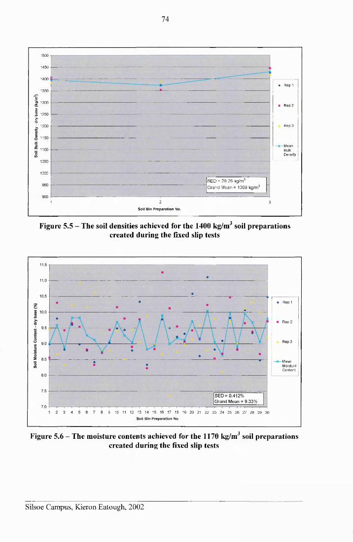
74
♦ R ep 1
■ R ep 2
R ep 3
—x — M ean Bulk Density
1 2 3
S o il B in Preparation No.
TOUU1450
1400
1350
"E|> 1300
v«5 1250 £I 1200’5>
g 1150 £“ 1100o05
1050
1000
SED = 28.28 kg/m3 Grand Mean = 1398 kg/m3
1Figure 5.5 - The soil densities achieved for the 1400 kg/m soil preparations
created during the fixed slip tests
SED =0.412%Grand Mean = 9.33%
9 10 11 12 13 14 15 16 17 18 19 2 0 21 22 2 3 2 4 2 5 2 6 2 7 2 8 2 9 30
S o il Bin Preparation No.
♦ R ep 1
R ep 2
M eanM oistureC o n te n t
Figure 5.6 - The moisture contents achieved for the 1170 kg/m3 soil preparationscreated during the fixed slip tests
Silsoe Campus, Kieron Eatough, 2002
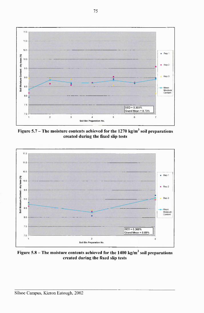
75
11.5
11.0
10.5
♦ R ep 1
10.0
■ R ep 2
9 .5
R ep 39 .0 -
M eanM oistureC o n te n t
7 .5SED = 0.303%Grand Mean = 8.73%
7.0
S oil Bin P reparation No.
Figure 5.7 - The moisture contents achieved for the 1270 kg/m3 soil preparationscreated during the fixed slip tests
11.5
10.5
« R ep 1
10.0
■ R ep 2
R ep 39 .0
M eanM oistureC o n te n t
7 .5SED = 0.368%Grand Mean = 8.69%
7 .0
S o il Bin Preparation No.
Figure 5.8 - The moisture contents achieved for the 1400 kg/m3 soil preparationscreated during the fixed slip tests
Silsoe Campus, Kieron Eatough, 2002
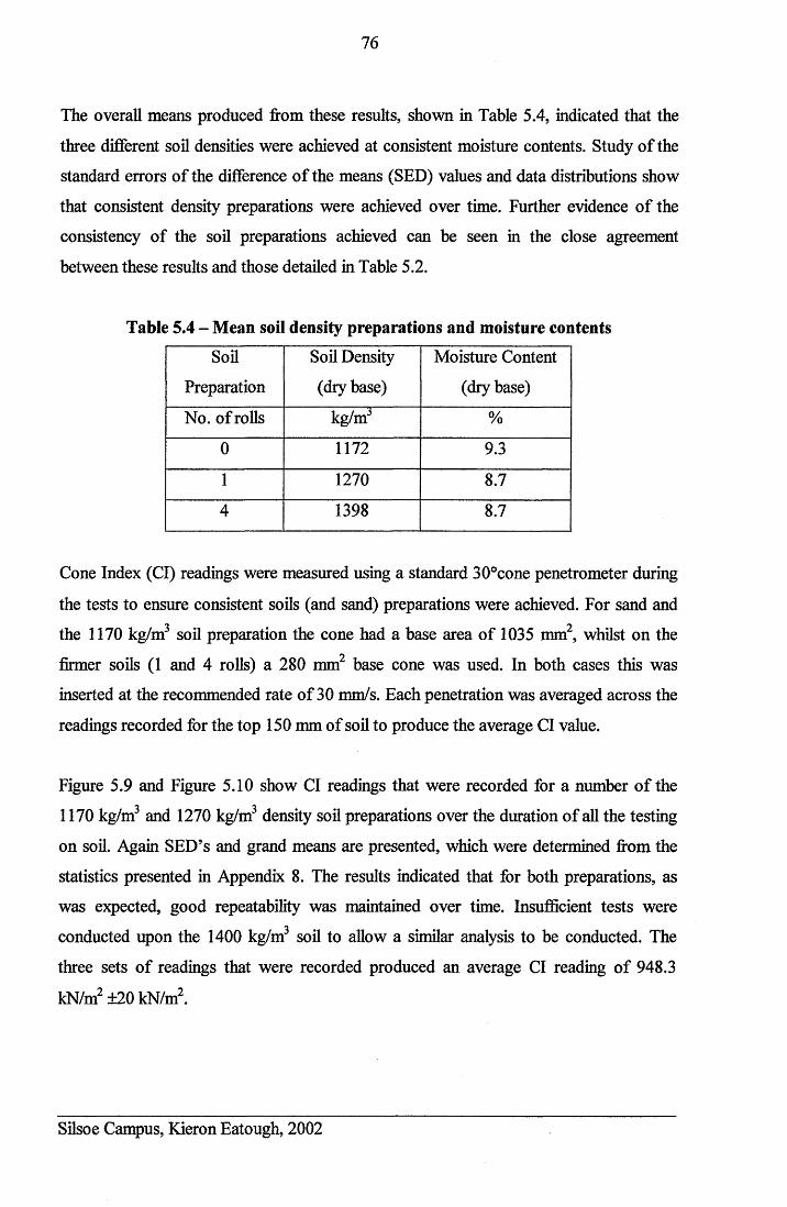
76
The overall means produced from these results, shown in Table 5.4, indicated that the
three different soil densities were achieved at consistent moisture contents. Study of the
standard errors of the difference of the means (SED) values and data distributions show
that consistent density preparations were achieved over time. Further evidence of the
consistency of the soil preparations achieved can be seen in the close agreement
between these results and those detailed in Table 5.2.
Table 5.4 - Mean soil density preparations and moisture contents
Soil
Preparation
Soil Density
(dry base)
Moisture Content
(dry base)
No. of rolls kg/m3 %
0 1172 9.3
1 1270 8.7
4 1398 8.7
Cone Index (Cl) readings were measured using a standard 30°cone penetrometer during
the tests to ensure consistent soils (and sand) preparations were achieved. For sand and
the 1170 kg/m soil preparation the cone had a base area of 1035 mm , whilst on the
firmer soils (1 and 4 rolls) a 280 mm2 base cone was used. In both cases this was
inserted at the recommended rate of 30 mm/s. Each penetration was averaged across the
readings recorded for the top 150 mm of soil to produce the average Cl value.
Figure 5.9 and Figure 5.10 show Cl readings that were recorded for a number of the
1170 kg/m and 1270 kg/m density soil preparations over the duration of all the testing
on soil. Again SED’s and grand means are presented, which were determined from the
statistics presented in Appendix 8. The results indicated that for both preparations, as
was expected, good repeatability was maintained over time. Insufficient tests were
conducted upon the 1400 kg/m3 soil to allow a similar analysis to be conducted. The
three sets of readings that were recorded produced an average Cl reading of 948.3
kN/m2 +20 kN/m2.
Silsoe Campus, Kieron Eatough, 2002
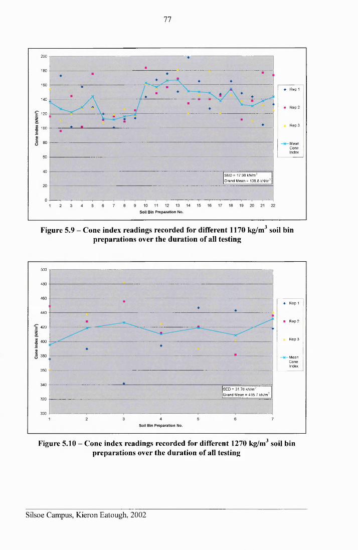
77
200 -
180
160 -♦ R ep 1
140
■ R ep 2
ne 120
R ep 3a> 100
M eanC oneIndex
6 0 -
40SE D = 17.98 kN/m 2
G ran d M ean = 138.8 kN/m'
S o il Bin P reparation No.
Figure 5.9 - Cone index readings recorded for different 1170 kg/m3 soil binpreparations over the duration of all testing
500 T
480
460♦ R ep 1
440
■ R ep 2
g 420
R ep 3« 400
° 380 M eanC oneIndex
360
340S E D = 3 1 .76 kN /m 2 G ran d M ean = 4 15 .7 kN/m'
320
300
S o il Bin Preparation No.
Figure 5.10 - Cone index readings recorded for different 1270 kg/m3 soil binpreparations over the duration of all testing
Silsoe Campus, Kieron Eatough, 2002
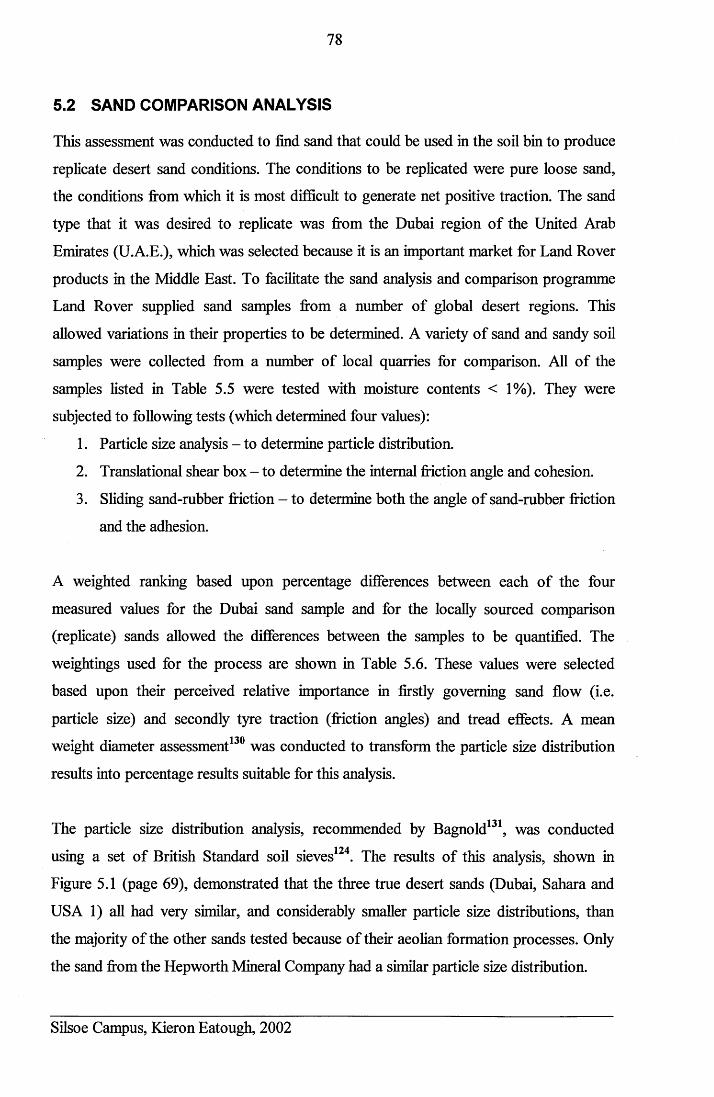
78
5.2 SAND COMPARISON ANALYSIS
This assessment was conducted to find sand that could be used in the soil bin to produce
replicate desert sand conditions. The conditions to be replicated were pure loose sand,
the conditions from which it is most difficult to generate net positive traction. The sand
type that it was desired to replicate was from the Dubai region of the United Arab
Emirates (U.A.E.), which was selected because it is an important market for Land Rover
products in the Middle East. To facilitate the sand analysis and comparison programme
Land Rover supplied sand samples from a number of global desert regions. This
allowed variations in their properties to be determined. A variety of sand and sandy soil
samples were collected from a number of local quarries for comparison. All of the
samples listed in Table 5.5 were tested with moisture contents < 1%). They were
subjected to following tests (which determined four values):
1. Particle size analysis - to determine particle distribution.
2. Translational shear box - to determine the internal friction angle and cohesion.
3. Sliding sand-rubber friction - to determine both the angle of sand-rubber friction
and the adhesion.
A weighted ranking based upon percentage differences between each of the four
measured values for the Dubai sand sample and for the locally sourced comparison
(replicate) sands allowed the differences between the samples to be quantified. The
weightings used for the process are shown in Table 5.6. These values were selected
based upon their perceived relative importance in firstly governing sand flow (i.e.
particle size) and secondly tyre traction (friction angles) and tread effects. A mean
weight diameter assessment130 was conducted to transform the particle size distribution
results into percentage results suitable for this analysis.
The particle size distribution analysis, recommended by Bagnold131, was conducted
using a set of British Standard soil sieves124. The results of this analysis, shown in
Figure 5.1 (page 69), demonstrated that the three true desert sands (Dubai, Sahara and
USA 1) all had very similar, and considerably smaller particle size distributions, than
the majority of the other sands tested because of their aeolian formation processes. Only
the sand from the Hepworth Mineral Company had a similar particle size distribution.
Silsoe Campus, Kieron Eatough, 2002
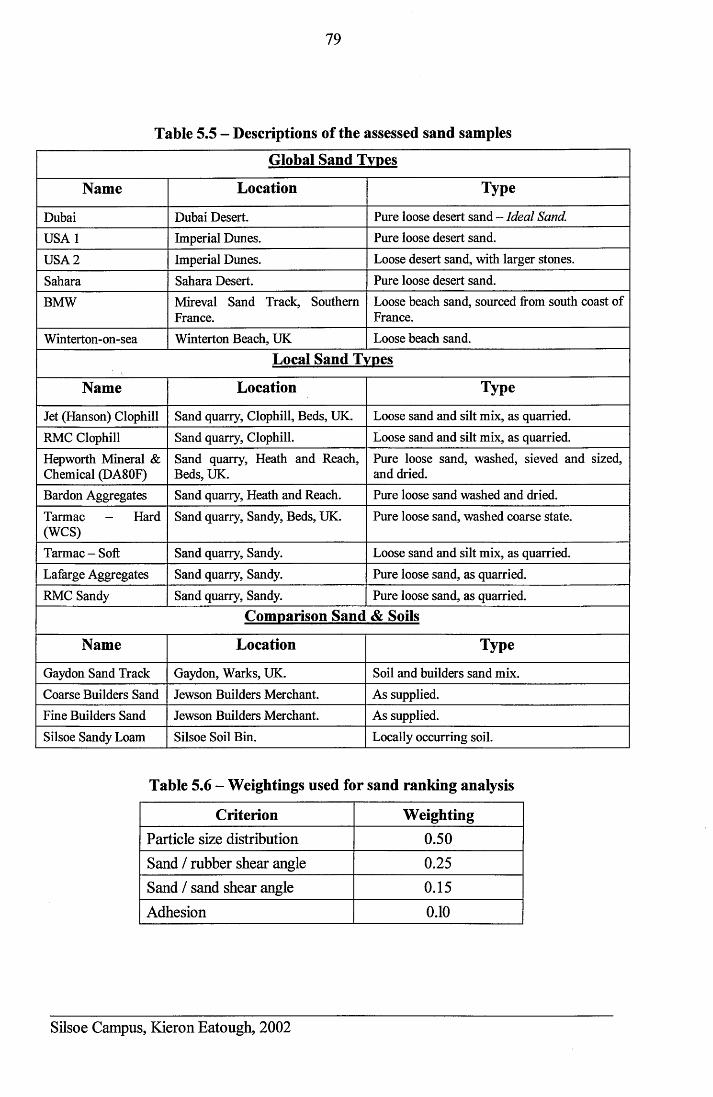
79
Table 5.5 - Descriptions of the assessed sand samples
Global Sand Tvnes
Name Location Type
Dubai Dubai Desert. Pure loose desert sand - Ideal Sand.USA 1 Imperial Dunes. Pure loose desert sand.
USA 2 Imperial Dunes. Loose desert sand, with larger stones.
Sahara Sahara Desert. Pure loose desert sand.
BMW Mireval Sand Track, Southern France.
Loose beach sand, sourced from south coast of France.
Winterton-on-sea Winterton Beach, UK Loose beach sand.
Local Sand Tvnes
Name Location Type
Jet (Hanson) Clophill Sand quarry, Clophill, Beds, UK. Loose sand and silt mix, as quarried.
RMC Clophill Sand quarry, Clophill. Loose sand and silt mix, as quarried.
Hepworth Mineral & Chemical (DA80F)
Sand quarry, Heath and Reach, Beds, UK.
Pure loose sand, washed, sieved and sized, and dried.
Bardon Aggregates Sand quarry, Heath and Reach. Pure loose sand washed and dried.
Tarmac - Hard (WCS)
Sand quarry, Sandy, Beds, UK. Pure loose sand, washed coarse state.
Tarmac-Soft Sand quarry, Sandy. Loose sand and silt mix, as quarried.
Lafarge Aggregates Sand quarry, Sandy. Pure loose sand, as quarried.
RMC Sandy Sand quarry, Sandy. Pure loose sand, as quarried.Comparison Sand & Soils
Name Location Type
Gaydon Sand Track Gaydon, Warks, UK. Soil and builders sand mix.
Coarse Builders Sand Jewson Builders Merchant. As supplied.
Fine Builders Sand Jewson Builders Merchant. As supplied.
Silsoe Sandy Loam Silsoe Soil Bin. Locally occurring soil.
Table 5.6 - Weightings used for sand ranking analysis
Criterion WeightingParticle size distribution 0.50Sand / rubber shear angle 0.25Sand / sand shear angle 0.15Adhesion 0.10
Silsoe Campus, Kieron Eatough, 2002
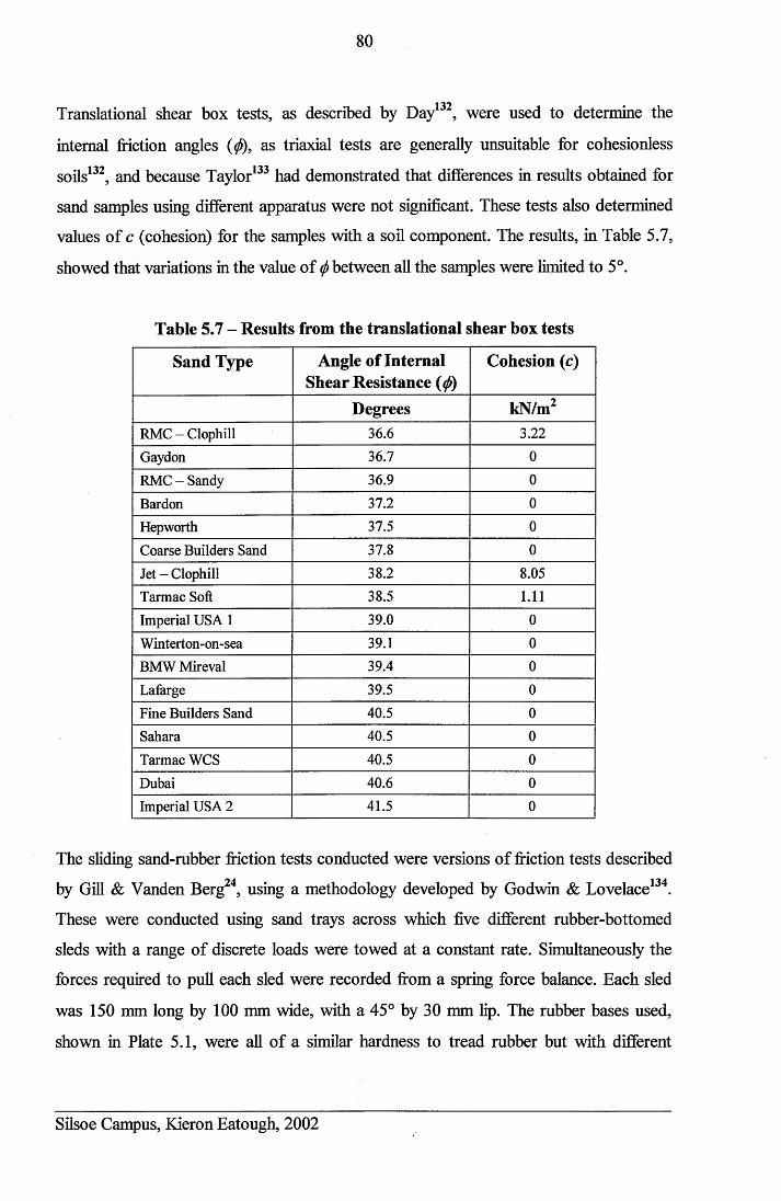
80
Translational shear box tests, as described by Day132, were used to determine the
internal friction angles (<f>), as triaxial tests are generally unsuitable for cohesionless
soils132, and because Taylor133 had demonstrated that differences in results obtained for
sand samples using different apparatus were not significant. These tests also determined
values of c (cohesion) for the samples with a soil component. The results, in Table 5.7,
showed that variations in the value of <j) between all the samples were limited to 5°.
Table 5.7 - Results from the translational shear box tests
Sand Type Angle of Internal Shear Resistance (</>)
Cohesion (c)
Degrees kN/m2RMC-Clophill 36.6 3.22
Gaydon 36.7 0
RMC-Sandy 36.9 0
Bardon 37.2 0
Hepworth 37.5 0
Coarse Builders Sand 37.8 0
Jet - Clophill 38.2 8.05
Tarmac Soft 38.5 1.11
Imperial USA 1 39.0 0
Winterton-on-sea 39.1 0
BMW Mireval 39.4 0
Lafarge 39.5 0
Fine Builders Sand 40.5 0
Sahara 40.5 0
Tarmac WCS 40.5 0
Dubai 40.6 0
Imperial USA 2 41.5 0
The sliding sand-rubber friction tests conducted were versions of friction tests described
by Gill & Vanden Berg24, using a methodology developed by Godwin & Lovelace134.
These were conducted using sand trays across which five different rubber-bottomed
sleds with a range of discrete loads were towed at a constant rate. Simultaneously the
forces required to pull each sled were recorded from a spring force balance. Each sled
was 150 mm long by 100 mm wide, with a 45° by 30 mm lip. The rubber bases used,
shown in Plate 5.1, were all of a similar hardness to tread rubber but with different
Silsoe Campus, Kieron Eatough, 2002
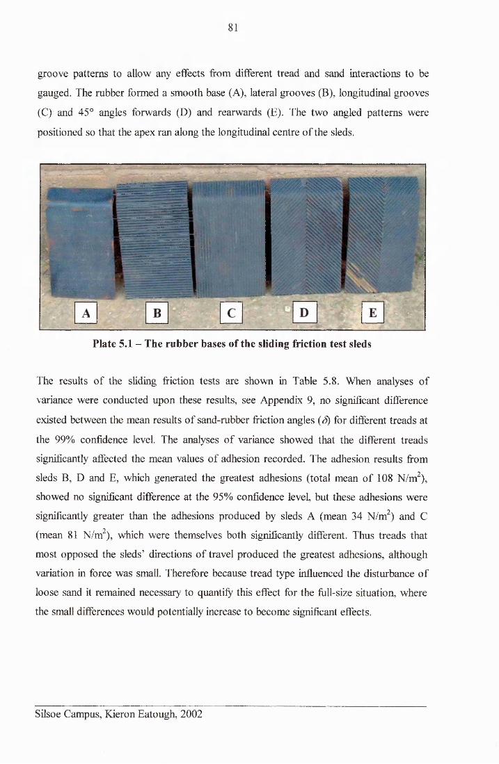
81
groove patterns to allow any effects from different tread and sand interactions to be
gauged. The rubber formed a smooth base (A), lateral grooves (B), longitudinal grooves
(C) and 45° angles forwards (D) and rearwards (E). The two angled patterns were
positioned so that the apex ran along the longitudinal centre of the sleds.
Plate 5.1 - The rubber bases of the sliding friction test sleds
The results of the sliding friction tests are shown in Table 5.8. When analyses of
variance were conducted upon these results, see Appendix 9, no significant difference
existed between the mean results of sand-rubber friction angles (S) for different treads at
the 99% confidence level. The analyses of variance showed that the different treads
significantly affected the mean values of adhesion recorded. The adhesion results from
sleds B, D and E, which generated the greatest adhesions (total mean of 108 N/m2),
showed no significant difference at the 95% confidence level, but these adhesions were
significantly greater than the adhesions produced by sleds A (mean 34 N/m2) and C
(mean 81 N/m2), which were themselves both significantly different. Thus treads that
most opposed the sleds’ directions of travel produced the greatest adhesions, although
variation in force was small. Therefore because tread type influenced the disturbance of
loose sand it remained necessary to quantify this effect for the full-size situation, where
the small differences would potentially increase to become significant effects.
Silsoe Campus, Kieron Eatough, 2002
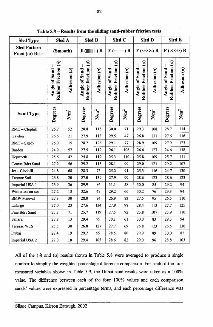
82
Table 5.8 - Results from the sliding sand-rubber friction tests
Sled Type Sled A Sled B Sled C Sled D Sled ESled Pattern
Front (to) Rear (Smooth) F(IIIIIIIIII)R U1 / \ r» F ( « « ) R F ( » » ) R* ( ) KAn
gle
of Sa
nd
- Ru
bber
Fric
tion
(8)
Adhe
sion
(a)
Angle
of
Sand
-
Rubb
er F
rictio
n (8
)
Adhe
sion
(a)
Angle
of
Sand
-
Rubb
er F
rictio
n (8
)
Adhe
sion
(a)
Angle
of
Sand
-
Rubb
er F
rictio
n (8
)
Adhe
sion
(a)
Angle
of
Sand
-
Rubb
er F
rictio
n (8
)
Adhe
sion
(a)
Sand Type
Deg
rees <s
SsS D
egre
es
£D
egre
es£ D
egre
es
£ Deg
rees n
E
RMC-Clophill 26.7 52 28.8 115 30.0 71 29.3 108 28.7 114
Gaydon 26.6 21 27.9 113 29.5 47 26.8 131 27.6 116
RMC-Sandy 26.9 15 28.2 126 29.1 77 28.9 109 27.9 123
Bardon 24.9 57 27.5 112 26.1 106 26.4 127 24.6 118
Hepworth 25.6 42 24.8 119 25.3 110 25.8 109 25.7 111
Coarse Bdrs Sand 27.2 56 29.2 115 28.1 99 29.0 121 29.2 107
Jet - Clophill 24.8 68 28.3 75 25.2 91 25.3 116 24.7 130
Tarmac Soft 26.8 20 27.0 139 27.9 99 28.6 123 28.6 123
Imperial USA 1 26.9 36 29.9 86 31.1 58 30.0 85 29.2 94
Winterton-on-sea 27.2 13 32.6 49 29.2 66 30.2 76 29.3 94
BMW Mireval 27.3 30 28.0 84 26.9 83 27.5 95 26.5 110
Lafarge 27.0 23 27.6 134 27.9 98 28.4 113 27.7 125
Fine Bdrs Sand 25.3 71 25.7 119 27.5 72 25.8 107 25.9 110
Sahara 27.8 13 29.4 99 30.1 61 30.0 83 29.3 94
Tarmac WCS 25.5 30 26.8 127 27.7 69 26.8 123 26.5 130
Dubai 27.4 19 29.2 99 28.5 80 29.9 89 30.0 82
Imperial USA 2 27.0 18 29.4 105 28.6 82 29.0 96 28.8 103
All of the (8) and (a) results shown in Table 5.8 were averaged to produce a single
number to simplify the weighted percentage difference comparison. For each of the four
measured variables shown in Table 5.9, the Dubai sand results were taken as a 100%
value. The difference between each of the four 100% values and each comparison
sands’ values were expressed in percentage terms, and each percentage difference was
Silsoe Campus, Kieron Eatough, 2002
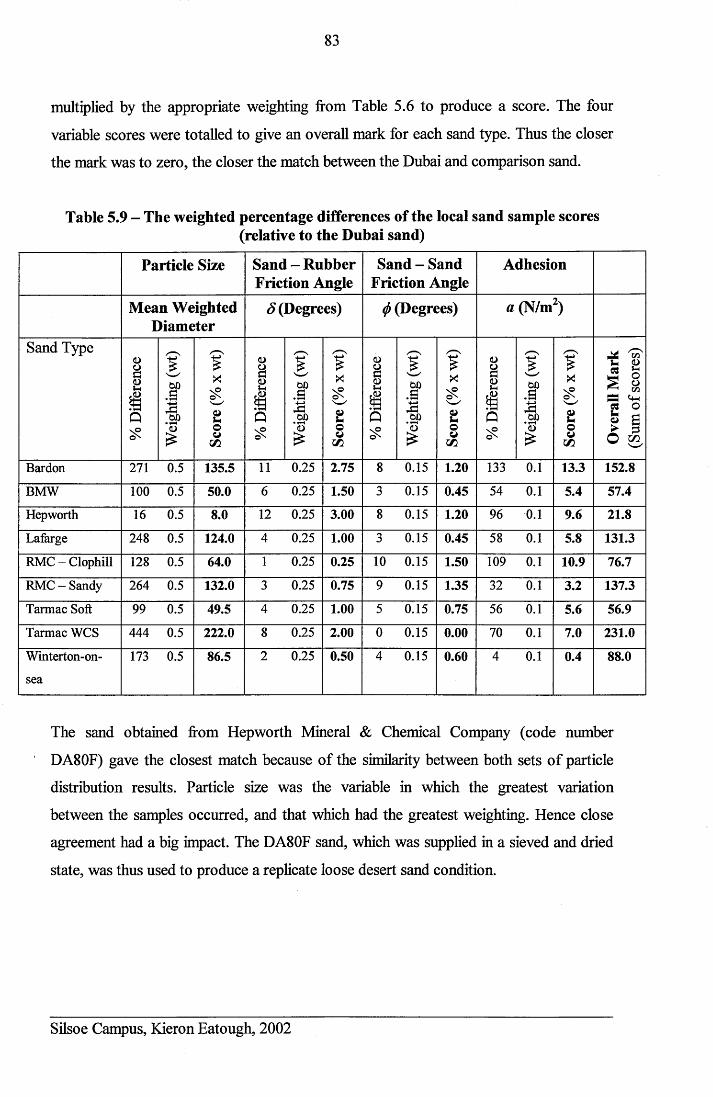
83
multiplied by the appropriate weighting from Table 5.6 to produce a score. The four
variable scores were totalled to give an overall mark for each sand type. Thus the closer
the mark was to zero, the closer the match between the Dubai and comparison sand.
Table 5.9 - The weighted percentage differences of the local sand sample scores(relative to the Dubai sand)
Particle Size Sand - Rubber Friction Angle
Sand - Sand Friction Angle
Adhesion
Mean Weighted Diameter
5 (Degrees) <j> (Degrees) a (N/m2)
Sand Type
% D
iffer
ence
Weig
htin
g (w
t)
Scor
e (%
x w
t)
% D
iffer
ence
Weig
htin
g (w
t)
Scor
e (%
x w
t)
% D
iffer
ence
Weig
htin
g (w
t)
Scor
e (%
x w
t)
% D
iffer
ence
Weig
htin
g (w
t)
Scor
e (%
x w
t)
Ove
rall
Mar
k(Su
m of
scor
es)
Bardon 271 0.5 135.5 11 0.25 2.75 8 0.15 1.20 133 0.1 13.3 152.8
BMW 100 0.5 50.0 6 0.25 1.50 3 0.15 0.45 54 0.1 5.4 57.4
Hepworth 16 0.5 8.0 12 0.25 3.00 8 0.15 1.20 96 0.1 9.6 21.8
Lafarge 248 0.5 124.0 4 0.25 1.00 3 0.15 0.45 58 0.1 5.8 131.3
RMC-Clophill 128 0.5 64.0 1 0.25 0.25 10 0.15 1.50 109 0.1 10.9 76.7
RMC - Sandy 264 0.5 132.0 3 0.25 0.75 9 0.15 1.35 32 0.1 3.2 137.3
Tarmac Soft 99 0.5 49.5 4 0.25 1.00 5 0.15 0.75 56 0.1 5.6 56.9
Tarmac WCS 444 0.5 222.0 8 0.25 2.00 0 0.15 0.00 70 0.1 7.0 231.0
Winterton-on- 173 0.5 86.5 2 0.25 0.50 4 0.15 0.60 4 0.1 0.4 88.0
sea
The sand obtained from Hepworth Mineral & Chemical Company (code number
DA80F) gave the closest match because of the similarity between both sets of particle
distribution results. Particle size was the variable in which the greatest variation
between the samples occurred, and that which had the greatest weighting. Hence close
agreement had a big impact. The DA80F sand, which was supplied in a sieved and dried
state, was thus used to produce a replicate loose desert sand condition.
Silsoe Campus, Kieron Eatough, 2002
84
5.3 ANALYSIS OF THE DA80F SAND
The previous section showed that the DA80F sand had the following properties:
• Particle size ~ 0.1 mm < over 97% of grains > 0.4 mm.
• Angle of internal resistance (</>) (sand-sand shear) ~ 37.5° (Appendix 10).
• Cohesion (c) ~ 0 kN/m2 (as would be expected for frictional sand).
• Angle of sand-rubber friction ~ «25.5° (mean value).
• Adhesion (a) ~ 98 N/m2 (mean value).
Further properties of this sand, which was always used at a moisture content of less than
1%, were also measured. The density of the sand was measured as 1485 kg/m3 ±12
kg/m3 by weighing the mass of a tin of a known volume (approximately 0.015 m3) filled
with loosely poured sand. To mimic the manner in which the sand was prepared in the
soil bin {poured and scraped), and therefore its experimental density, excess sand was
added to the tin before being levelled. This was repeated three times. The small density
variation occurred because of the low compactibility of a material with similar particle
sizes. To ensure that the sand was not being compacted during the traction tests, density
readings were taken from the top sand layers using density rings at random intervals
over the duration of all the testing. These results (see Appendix 11) showed that a mean
sand density of 1482 kg/m ±21 kg/m was recorded, which agreed closely with the
bench test value.
The torsional shear strength of the sand mass was measured in-situ in the soil bin using
two different shear vane devices, both of which were used to test the surface strength.
Five different sand preparations were tested and ten readings were recorded each time.
These devices recorded the surface sand torsional shear strength as being 1.25 kPa
±0.25 kPa. Cone Index (Cl) readings were also recorded at random intervals during all
the testing on sand to further investigate any variation in the sand strength properties
between different preparations. This provided a simple comparison between the sand
preparations to ensure the expected levels of repeatability were maintained. The results
from these tests can be seen in Figure 5.11, and the associated statistics are presented in
Appendix 12. The first eight preparations were tested when the sand was used in the
sand tank, whilst the other results were recorded when the full soil bin was used. These
Silsoe Campus, Kieron Eatough, 2002
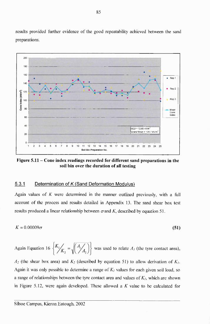
85
results provided further evidence of the good repeatability achieved between the sand
preparations.
200
180
160» R ep 1
140
■ R ep 2
T= 120
R ep 3a> 100
M eanC oneIndex
SE D = 12.65 kN /m 2
G ran d M ean = 128 .7 kN/rrr
S o il B in P reparation No.
Figure 5.11 - Cone index readings recorded for different sand preparations in thesoil bin over the duration of all testing
5.3.1 Determination of K (Sand Deformation Modulus)
Again values of K were determined in the manner outlined previously, with a full
account of the process and results detailed in Appendix 13. The sand shear box test
results produced a linear relationship between cr and K , described by equation 51.
£ = 0.00009cr (51)
Again Equation 16 A was used to relate A j (the tyre contact area),
A 2 (the shear box area) and K2 (described by equation 51) to allow derivation of K/.
Again it was only possible to determine a range of Kj values for each given soil load, so
a range of relationships between the tyre contact area and values of Ki, which are shown
in Figure 5.12, were again developed. These allowed a K value to be calculated for
Silsoe Campus, Kieron Eatough, 2002
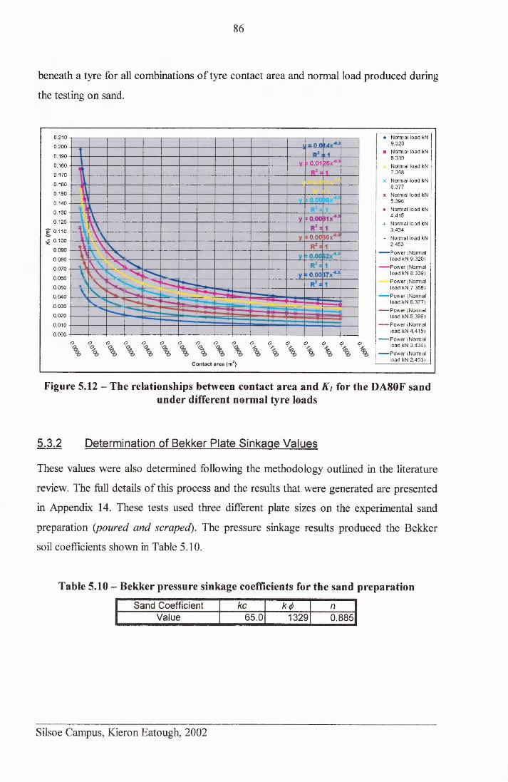
86
beneath a tyre for all combinations of tyre contact area and normal load produced during
the testing on sand.
♦ Norm al load kN 9.320
■ Norm al load kN 8.339
Normal load kN 7 .358
x Norm al load kN 6 .377
x Norm al load kN 5.396
• Norm al load kN 4 .415
+ Norm al load kN 3 .434
- Normal load kN 2 .453
— P ow er (N orm al load kN 9 .3 2 0 )
— P ow er (Norm al load kN 8 .339)
P ow er (N orm al load kN 7 .358)
— P ow er (N orm al load kN 6 .3 7 7 )
— P ow er (N orm al load kN 5 .396)
— P ow er (N orm al load kN 4 .415)
— P ow er (N orm al load kN 3 .434)
— P ow er (N orm al load kN 2 .453)
Figure 5.12 - The relationships between contact area and Ki for the DA80F sandunder different normal tyre loads
5.3.2 Determination of Bekker Plate Sinkaae Values
These values were also determined following the methodology outlined in the literature
review. The full details of this process and the results that were generated are presented
in Appendix 14. These tests used three different plate sizes on the experimental sand
preparation {poured and scraped). The pressure sinkage results produced the Bekker
soil coefficients shown in Table 5.10.
Table 5.10 - Bekker pressure sinkage coefficients for the sand preparationSand Coefficient kc k(f) n
Value 65.0 1329 0.885
0.210
0.200
0.190= 0.01 25x'0.180
0.170
0.160
0.150
0.140
0.130
0.120
E 0.110
£ 0.100 0.00 J6x‘
0.080
0.0700.00 J7x‘0.060
0.050
0.040
0.030
0.020
0.010
0.000O O o o o o o o o o o oo o o o o
C on tact area (m 2)
Silsoe Campus, Kieron Eatough, 2002
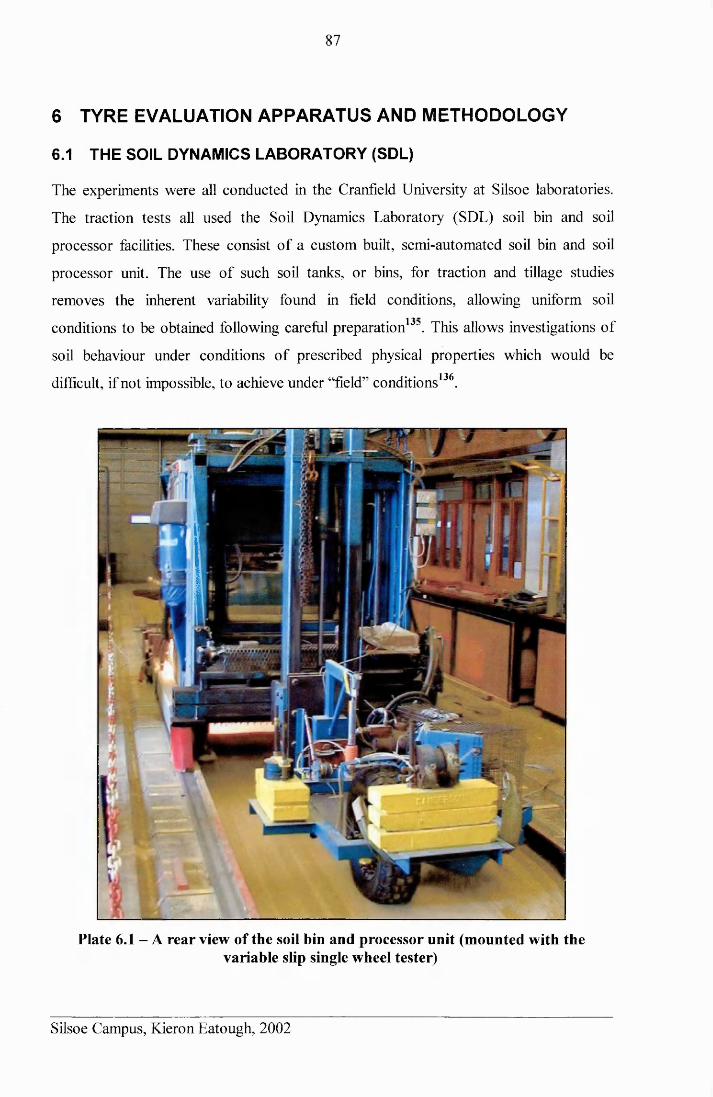
87
6 TYRE EVALUATION APPARATUS AND METHODOLOGY
6.1 THE SOIL DYNAMICS LABORATORY (SDL)
The experiments were all conducted in the Cranfield University at Silsoe laboratories.
The traction tests all used the Soil Dynamics Laboratory (SDL) soil bin and soil
processor facilities. These consist of a custom built, semi-automated soil bin and soil
processor unit. The use of such soil tanks, or bins, for traction and tillage studies
removes the inherent variability found in field conditions, allowing uniform soil
conditions to be obtained following careful preparation133. This allows investigations of
soil behaviour under conditions of prescribed physical properties which would be
difficult, if not impossible, to achieve under “field” conditions136.
Plate 6.1 - A rear view of the soil bin and processor unit (mounted with thevariable slip single wheel tester)
Silsoe Campus, Kieron Eatough, 2002
88
• 117The soil bin is a sub-surface concrete tank 20 m long, 1.7 m wide and 1 m deep . On
top of this tank run the rails that guide the main processor unit, see Plate 6.1, which
contains the hydraulically operated soil engaging blades, bucket and grabs, and rollers
to enable a variety of soil preparations to be produced. To the rear of this unit is fitted
an adjustable mounting plate for attaching test equipment. The whole unit is moved by a
cable drive system, which is operated by an electro-hydraulically controlled winch
drum138. The maximum forward velocity of the processor unit is approximately 8 km/h.
Attached to the mounting plate was an Extended Octagonal Ring Transducer
(EORT)139, which was used to measure horizontal and vertical forces applied between
the processor unit and any attached drive systems. Each of the three channel outputs
from the EORT was passed through an individual strain gauge conditioning module
(Strainstall Model 91C), which produced a stabilised 9.2 V supply for each particular
wheatstone-bridge circuit on the EORT. The strain gauge module amplified the pV
return output from each circuit, such that a voltage output proportional to load could be
determined. The strain gauge module also allowed any offsets, from gauge
inconsistency or static load to be removed.
6.2 TEST TYRES
To investigate the effect of tread pattern upon tractive performance a range of different
treaded tyres were used. The production tyres selected were standard Goodyear
products, which are shown in Plate 6.2. These were a Goodyear HP Wrangler (HP), an
on-road/ mud biased tyre and a Goodyear Wrangler Ultra-Grip (UG), a winter on-road/
mud biased tyre, both of which were supplied in the 235/ 70 R16 size, and a G82, as
described in section 3.2.2, which was supplied as a 7.50 R16 (its only manufactured
size). The differences in section width and outside diameter of these two sizes can be
clearly seen in Plate 6.2 and Plate 6.3. To ensure comparable results between the G82
tread and the 235/70 R16 treads, a 235/70 R16 G82 tread was required. This tyre was a
bespoke prototype produced by Goodyear by being laser cut on to a plain tread blank
(slick), which produced the tyre shown in Plate 6.3. The blank used was of the same
rubber, construction and size as the 235/70 R16 Goodyear Wrangler HP.
Silsoe Campus, Kieron Eatough, 2002
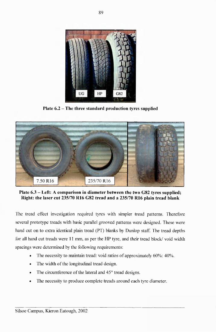
89
Plate 6.2 - The three standard production tyres supplied
235/70 R16
Plate 6.3 - Left: A comparison in diameter between the two G82 tyres supplied; Right: the laser cut 235/70 R16 G82 tread and a 235/70 R16 plain tread blank
The tread effect investigation required tyres with simpler tread patterns. Therefore
several prototype treads with basic parallel grooved patterns were designed. These were
hand cut on to extra identical plain tread (PT) blanks by Dunlop staff. The tread depths
for all hand cut treads were 11 mm, as per the HP tyre, and their tread block/ void width
spacings were determined by the following requirements:
• The necessity to maintain tread: void ratios of approximately 60%: 40%.
• The width of the longitudinal tread design.
• The circumference of the lateral and 45° tread designs.
• The necessity to produce complete treads around each tyre diameter.
Silsoe Campus, Kieron Eatough, 2002
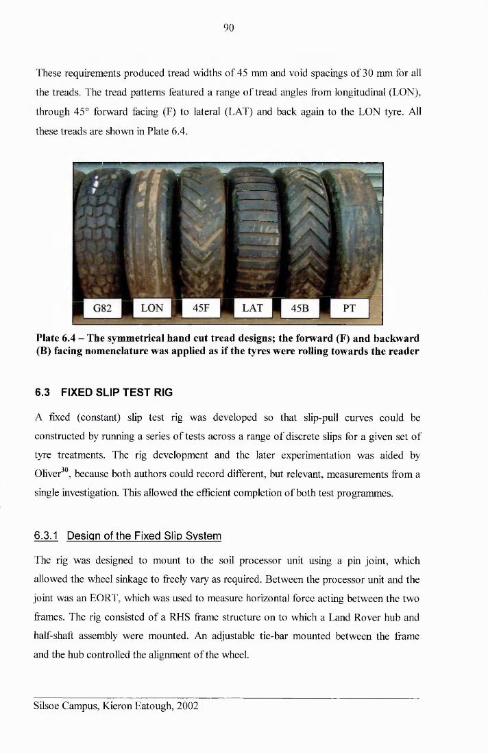
90
These requirements produced tread widths of 45 mm and void spacings of 30 mm for all
the treads. The tread patterns featured a range of tread angles from longitudinal (LON),
through 45° forward facing (F) to lateral (LAT) and back again to the LON tyre. All
these treads are shown in Plate 6.4.
Plate 6.4 - The symmetrical hand cut tread designs; the forward (F) and backward (B) facing nomenclature was applied as if the tyres were rolling towards the reader
6.3 FIXED SLIP TEST RIG
A fixed (constant) slip test rig was developed so that slip-pull curves could be
constructed by running a series of tests across a range of discrete slips for a given set of
tyre treatments. The rig development and the later experimentation was aided by
Oliver30, because both authors could record different, but relevant, measurements from a
single investigation. This allowed the efficient completion of both test programmes.
6.3.1 Design of the Fixed Slip System
The rig was designed to mount to the soil processor unit using a pin joint, which
allowed the wheel sinkage to freely vary as required. Between the processor unit and the
joint was an EORT, which was used to measure horizontal force acting between the two
frames. The rig consisted of a RHS frame structure on to which a Land Rover hub and
half-shaft assembly were mounted. An adjustable tie-bar mounted between the frame
and the hub controlled the alignment of the wheel.
Silsoe Campus, Kieron Eatough, 2002
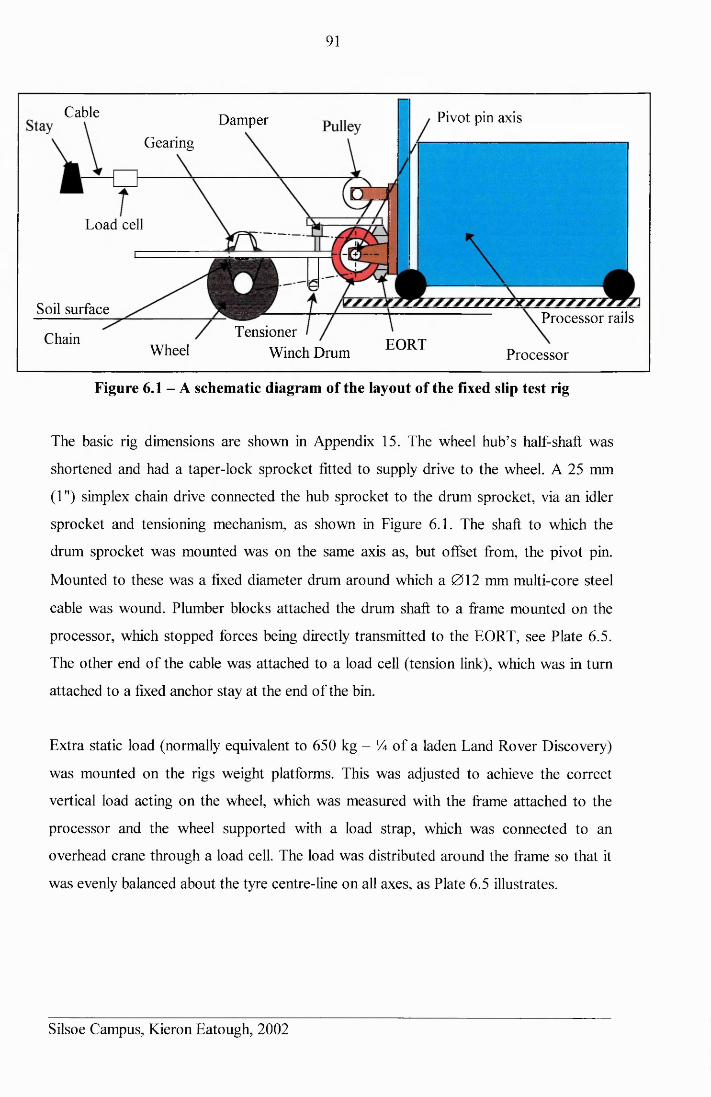
91
Cable DamperGearing
Load cell
Tensioner
Pivot pin axis
Soil surface
ChainWheel Winch Drum EORT
Processor rails
Processor
Figure 6.1 - A schematic diagram of the layout of the fixed slip test rig
The basic rig dimensions are shown in Appendix 15. The wheel hub’s half-shaft was
shortened and had a taper-lock sprocket fitted to supply drive to the wheel. A 25 mm
(1") simplex chain drive connected the hub sprocket to the drum sprocket, via an idler
sprocket and tensioning mechanism, as shown in Figure 6.1. The shaft to which the
drum sprocket was mounted was on the same axis as, but offset from, the pivot pin.
Mounted to these was a fixed diameter drum around which a 012 mm multi-core steel
cable was wound. Plumber blocks attached the drum shaft to a frame mounted on the
processor, which stopped forces being directly transmitted to the EORT, see Plate 6.5.
The other end of the cable was attached to a load cell (tension link), which was in turn
attached to a fixed anchor stay at the end of the bin.
Extra static load (normally equivalent to 650 kg - !4 of a laden Land Rover Discovery)
was mounted on the rigs weight platforms. This was adjusted to achieve the correct
vertical load acting on the wheel, which was measured with the frame attached to the
processor and the wheel supported with a load strap, which was connected to an
overhead crane through a load cell. The load was distributed around the frame so that it
was evenly balanced about the tyre centre-line on all axes, as Plate 6.5 illustrates.
Silsoe Campus, Kieron Eatough, 2002
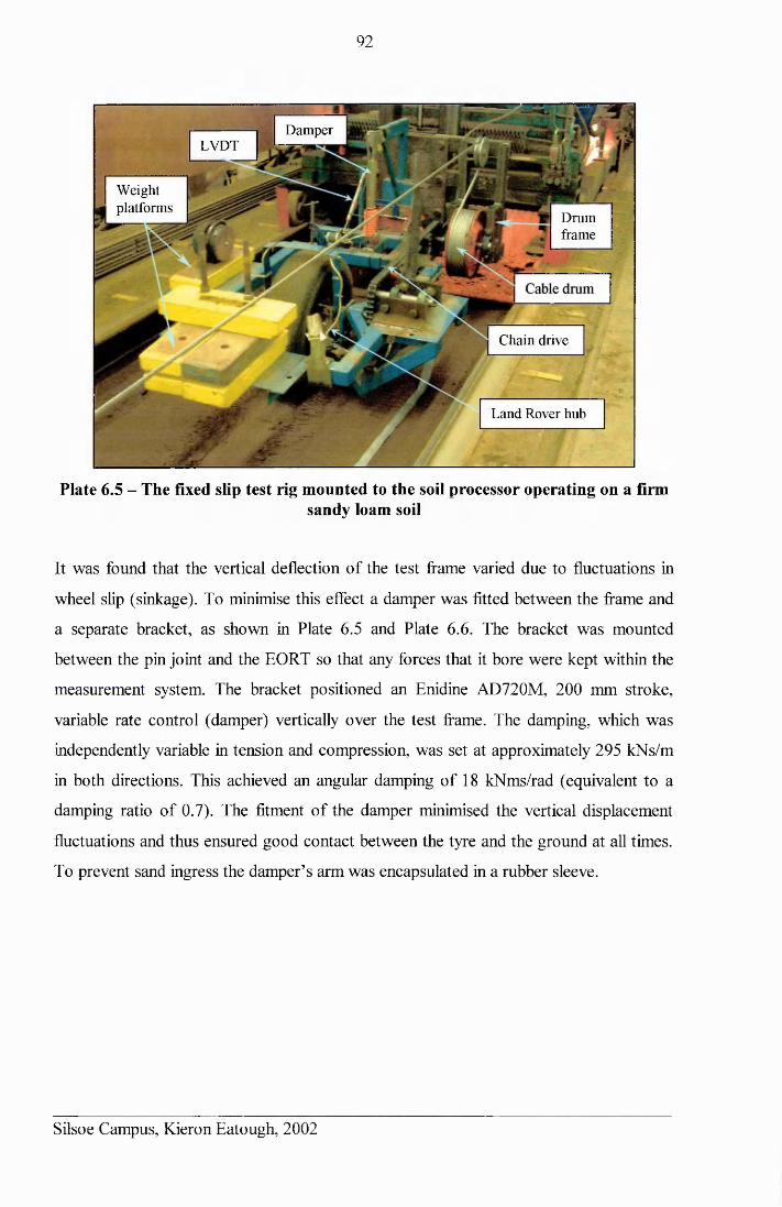
92
DamperLVDT
Weightplatforms
Drumframe
Chain drive
Land Rover hub
Plate 6.5 - The fixed slip test rig mounted to the soil processor operating on a firmsandy loam soil
It was found that the vertical deflection of the test frame varied due to fluctuations in
wheel slip (sinkage). To minimise this effect a damper was fitted between the frame and
a separate bracket, as shown in Plate 6.5 and Plate 6.6. The bracket was mounted
between the pin joint and the EORT so that any forces that it bore were kept within the
measurement system. The bracket positioned an Enidine AD720M, 200 mm stroke,
variable rate control (damper) vertically over the test frame. The damping, which was
independently variable in tension and compression, was set at approximately 295 kNs/m
in both directions. This achieved an angular damping of 18 kNms/rad (equivalent to a
damping ratio of 0.7). The fitment of the damper minimised the vertical displacement
fluctuations and thus ensured good contact between the tyre and the ground at all times.
To prevent sand ingress the damper’s arm was encapsulated in a rubber sleeve.
Silsoe Campus, Kieron Eatough, 2002
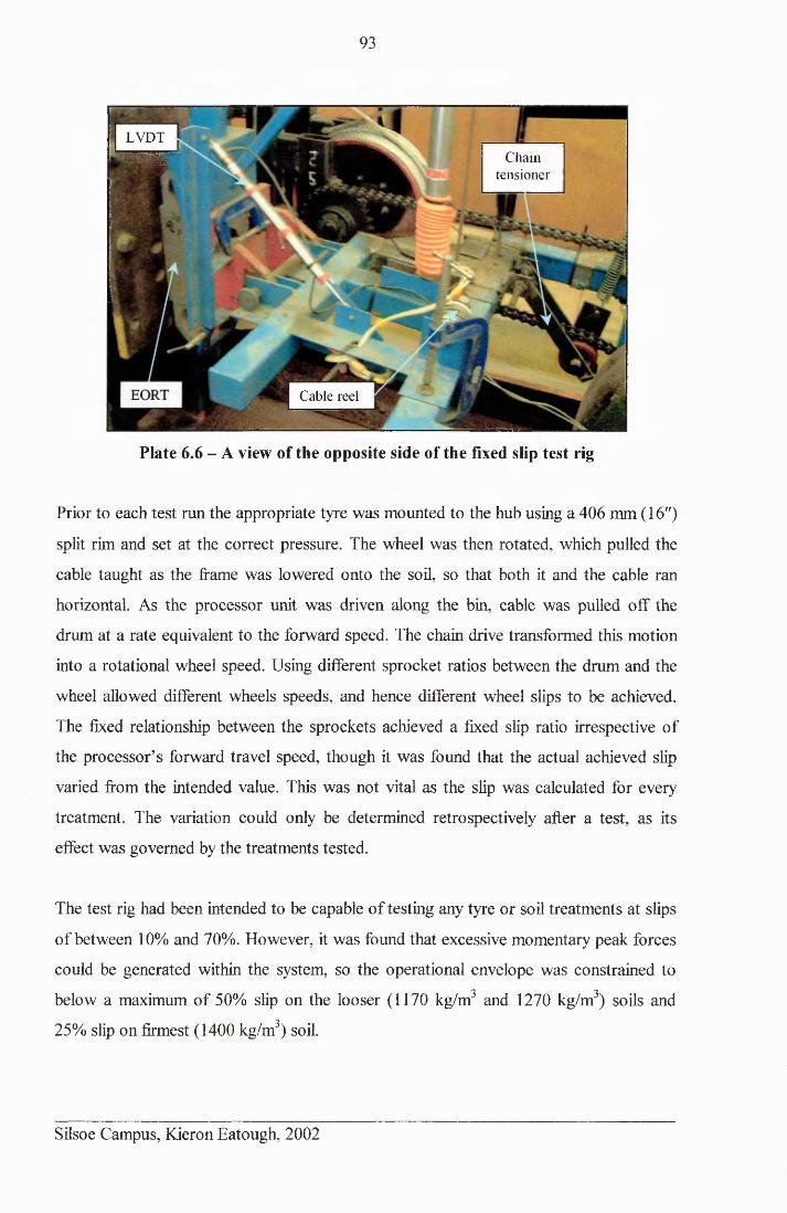
93
LVDTm m g Chain
tensioner
Cable reel
Plate 6.6 - A view of the opposite side of the fixed slip test rig
Prior to each test run the appropriate tyre was mounted to the hub using a 406 mm (16")
split rim and set at the correct pressure. The wheel was then rotated, which pulled the
cable taught as the frame was lowered onto the soil, so that both it and the cable ran
horizontal. As the processor unit was driven along the bin, cable was pulled off the
drum at a rate equivalent to the forward speed. The chain drive transformed this motion
into a rotational wheel speed. Using different sprocket ratios between the drum and the
wheel allowed different wheels speeds, and hence different wheel slips to be achieved.
The fixed relationship between the sprockets achieved a fixed slip ratio irrespective of
the processor’s forward travel speed, though it was found that the actual achieved slip
varied from the intended value. This was not vital as the slip was calculated for every
treatment. The variation could only be determined retrospectively after a test, as its
effect was governed by the treatments tested.
The test rig had been intended to be capable of testing any tyre or soil treatments at slips
of between 10% and 70%. However, it was found that excessive momentary peak forces
could be generated within the system, so the operational envelope was constrained to
below a maximum of 50% slip on the looser (1170 kg/m3 and 1270 kg/m3) soils and
25% slip on firmest (1400 kg/m3) soil.
Silsoe Campus, Kieron Eatough, 2002
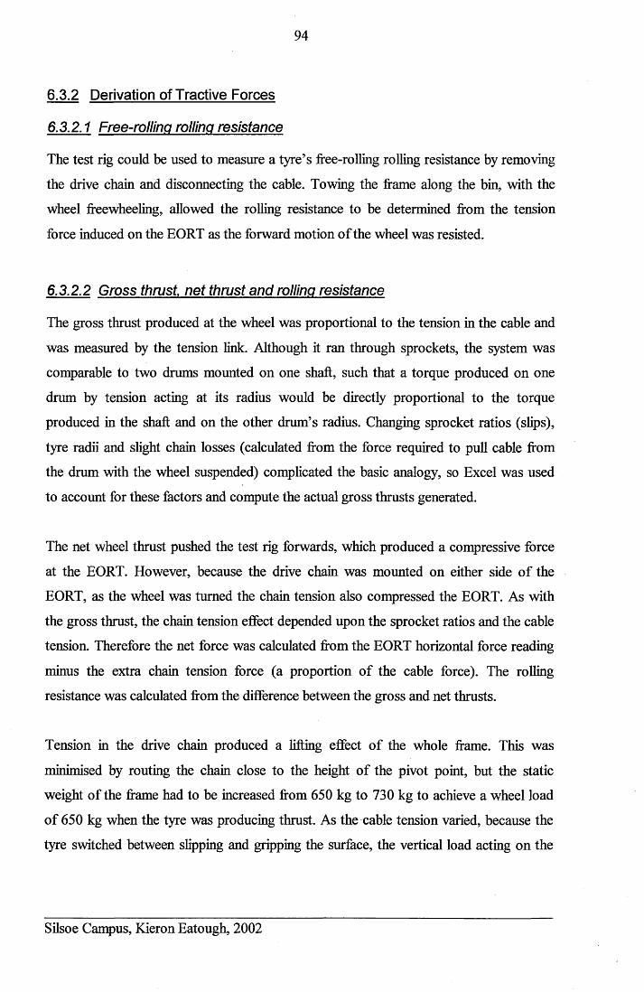
94
6.3.2 Derivation of Tractive Forces
6.3.2.1 Free-rolling rolling resistance
The test rig could be used to measure a tyre’s free-rolling rolling resistance by removing
the drive chain and disconnecting the cable. Towing the frame along the bin, with the
wheel freewheeling, allowed the rolling resistance to be determined from the tension
force induced on the EORT as the forward motion of the wheel was resisted.
6.3.2.2 Gross thrust net thrust and rolling resistance
The gross thrust produced at the wheel was proportional to the tension in the cable and
was measured by the tension link. Although it ran through sprockets, the system was
comparable to two drums mounted on one shaft, such that a torque produced on one
drum by tension acting at its radius would be directly proportional to the torque
produced in the shaft and on the other drum’s radius. Changing sprocket ratios (slips),
tyre radii and slight chain losses (calculated from the force required to pull cable from
the drum with the wheel suspended) complicated the basic analogy, so Excel was used
to account for these factors and compute the actual gross thrusts generated.
The net wheel thrust pushed the test rig forwards, which produced a compressive force
at the EORT. However, because the drive chain was mounted on either side of the
EORT, as the wheel was turned the chain tension also compressed the EORT. As with
the gross thrust, the chain tension effect depended upon the sprocket ratios and the cable
tension. Therefore the net force was calculated from the EORT horizontal force reading
minus the extra chain tension force (a proportion of the cable force). The rolling
resistance was calculated from the difference between the gross and net thrusts.
Tension in the drive chain produced a lifting effect of the whole frame. This was
minimised by routing the chain close to the height of the pivot point, but the static
weight of the frame had to be increased from 650 kg to 730 kg to achieve a wheel load
of 650 kg when the tyre was producing thrust. As the cable tension varied, because the
tyre switched between slipping and gripping the surface, the vertical load acting on the
Silsoe Campus, Kieron Eatough, 2002
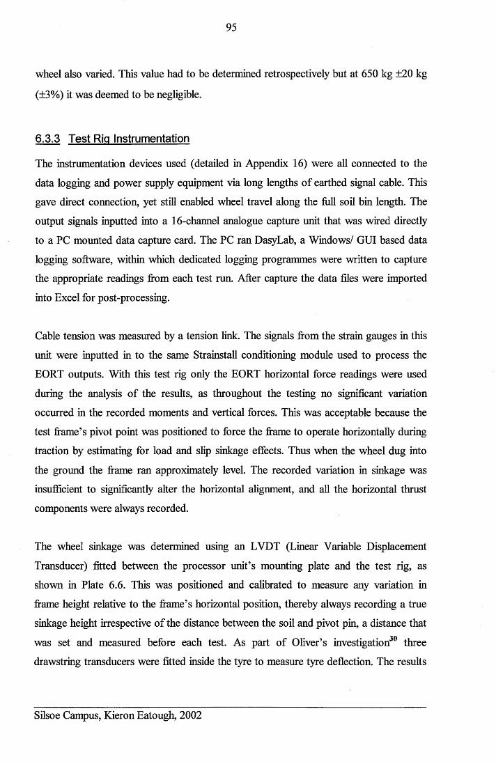
95
wheel also varied. This value had to be determined retrospectively but at 650 kg ±20 kg
(±3%) it was deemed to be negligible.
6.3.3 Test Rig Instrumentation
The instrumentation devices used (detailed in Appendix 16) were all connected to the
data logging and power supply equipment via long lengths of earthed signal cable. This
gave direct connection, yet still enabled wheel travel along the full soil bin length. The
output signals inputted into a 16-channel analogue capture unit that was wired directly
to a PC mounted data capture card. The PC ran DasyLab, a Windows/ GUI based data
logging software, within which dedicated logging programmes were written to capture
the appropriate readings from each test run. After capture the data files were imported
into Excel for post-processing.
Cable tension was measured by a tension link. The signals from the strain gauges in this
unit were inputted in to the same Strainstall conditioning module used to process the
EORT outputs. With this test rig only the EORT horizontal force readings were used
during the analysis of the results, as throughout the testing no significant variation
occurred in the recorded moments and vertical forces. This was acceptable because the
test frame’s pivot point was positioned to force the frame to operate horizontally during
traction by estimating for load and slip sinkage effects. Thus when the wheel dug into
the ground the frame ran approximately level. The recorded variation in sinkage was
insufficient to significantly alter the horizontal alignment, and all the horizontal thrust
components were always recorded.
The wheel sinkage was determined using an LVDT (Linear Variable Displacement
Transducer) fitted between the processor unit’s mounting plate and the test rig, as
shown in Plate 6.6. This was positioned and calibrated to measure any variation in
frame height relative to the frame’s horizontal position, thereby always recording a true
sinkage height irrespective of the distance between the soil and pivot pin, a distance that
was set and measured before each test. As part of Oliver’s investigation30 three
drawstring transducers were fitted inside the tyre to measure tyre deflection. The results
Silsoe Campus, Kieron Eatough, 2002
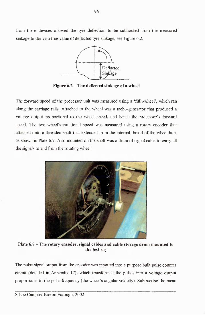
96
from these devices allowed the tyre deflection to be subtracted from the measured
sinkage to derive a true value of deflected tyre sinkage, see Figure 6.2.
DeflectedSinkage
Figure 6.2 - The deflected sinkage of a wheel
The forward speed of the processor unit was measured using a ‘fifth-wheel’, which ran
along the carriage rails. Attached to the wheel was a tacho-generator that produced a
voltage output proportional to the wheel speed, and hence the processor’s forward
speed. The test wheel’s rotational speed was measured using a rotary encoder that
attached onto a threaded shaft that extended from the internal thread of the wheel hub,
as shown in Plate 6.7. Also mounted on the shaft was a drum of signal cable to carry all
the signals to and from the rotating wheel.
Plate 6.7 - The rotary encoder, signal cables and cable storage drum mounted tothe test rig
The pulse signal output from the encoder was inputted into a purpose built pulse counter
circuit (detailed in Appendix 17), which transformed the pulses into a voltage output
proportional to the pulse frequency (the wheel’s angular velocity). Subtracting the mean
Silsoe Campus, Kieron Eatough, 2002
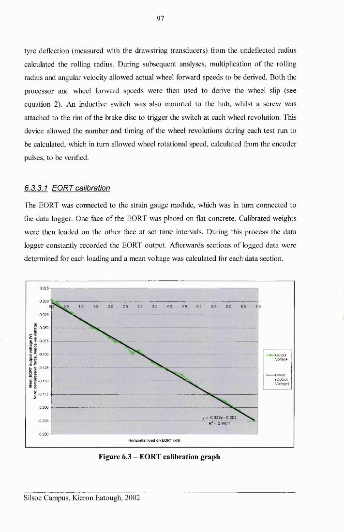
97
tyre deflection (measured with the drawstring transducers) from the undeflected radius
calculated the rolling radius. During subsequent analyses, multiplication of the rolling
radius and angular velocity allowed actual wheel forward speeds to be derived. Both the
processor and wheel forward speeds were then used to derive the wheel slip (see
equation 2). An inductive switch was also mounted to the hub, whilst a screw was
attached to the rim of the brake disc to trigger the switch at each wheel revolution. This
device allowed the number and timing of the wheel revolutions during each test run to
be calculated, which in turn allowed wheel rotational speed, calculated from the encoder
pulses, to be verified.
6.3.3.1 EORT calibration
The EORT was connected to the strain gauge module, which was in turn connected to
the data logger. One face of the EORT was placed on flat concrete. Calibrated weights
were then loaded on the other face at set time intervals. During this process the data
logger constantly recorded the EORT output. Afterwards sections of logged data were
determined for each loading and a mean voltage was calculated for each data section.
0.025
0.0003.5 4 .0 4 .50 .5 2.0 2 .5 3 .0 5 .0 5 .5 6.0
-0 .025
SP -0 .050
o -0 .075
= - 0.100 O utpu tV oltage
h « -0 .125
— Linear(O utputV oltage)
-0 .150
X -0 .175
-0.200 -
y = -0.032x- 0.002-0 .225
R7 = 0.9977
-0 .250
H orizontal load o n EORT (kN)
Figure 6.3 - EORT calibration graph
Silsoe Campus, Kieron Eatough, 2002
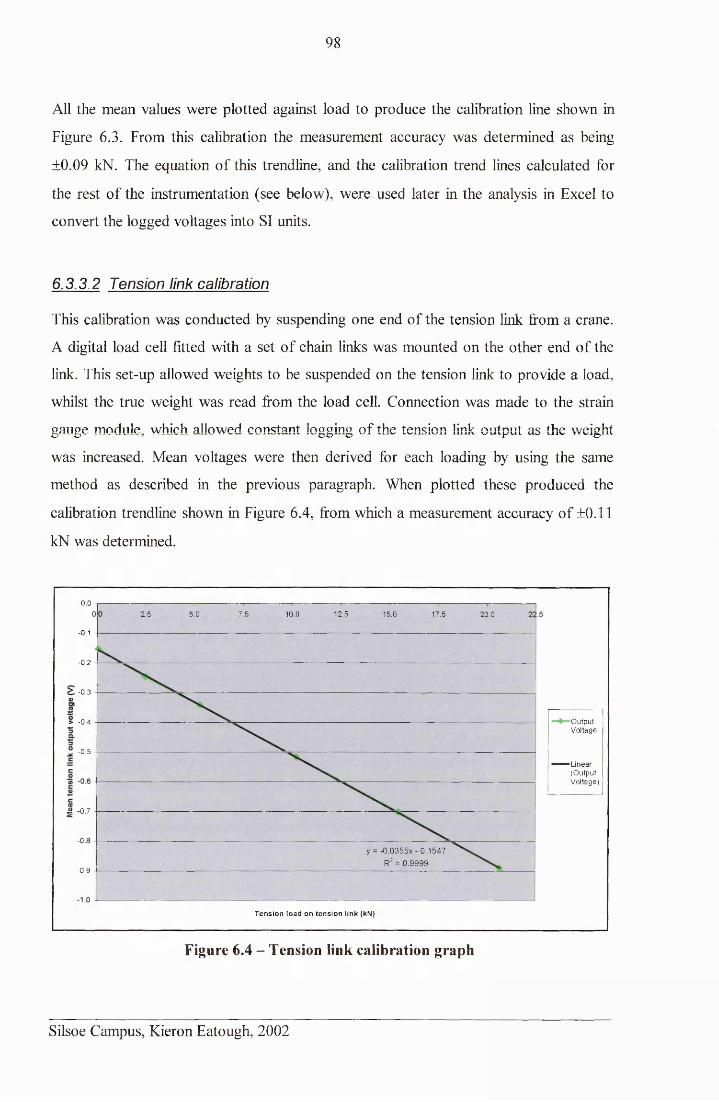
98
All the mean values were plotted against load to produce the calibration line shown in
Figure 6.3. From this calibration the measurement accuracy was determined as being
±0.09 kN. The equation of this trendline, and the calibration trend lines calculated for
the rest of the instrumentation (see below), were used later in the analysis in Excel to
convert the logged voltages into SI units.
6.3.3.2 Tension link calibration
This calibration was conducted by suspending one end of the tension link from a crane.
A digital load cell fitted with a set of chain links was mounted on the other end of the
link. This set-up allowed weights to be suspended on the tension link to provide a load,
whilst the true weight was read from the load cell. Connection was made to the strain
gauge module, which allowed constant logging of the tension link output as the weight
was increased. Mean voltages were then derived for each loading by using the same
method as described in the previous paragraph. When plotted these produced the
calibration trendline shown in Figure 6.4, from which a measurement accuracy of ±0.11
kN was determined.
0.010.0 12.5 15.02 .5 5 .0 7 .5 17.5 20.0
- 0.1
- 0.2
> -0.3
O utpu tV oltage
> -0.4
-0.5
Linear(O utputV oltage)
S -0 .7
-Ofy = -0.0355x - 0.1547
R2 = 0.9999-0 .9
T en sio n load o n te n s io n link (kN)
Figure 6.4 - Tension link calibration graph
Silsoe Campus, Kieron Eatough, 2002
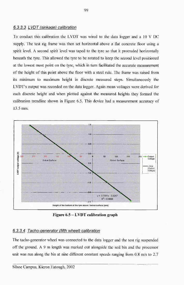
99
6.3.3.3 LVDT (sinkage) calibration
To conduct this calibration the LVDT was wired to the data logger and a 10 V DC
supply. The test rig frame was then set horizontal above a flat concrete floor using a
spirit level. A second spirit level was taped to the tyre so that it protruded horizontally
beneath the tyre. This allowed the tyre to be rotated to keep the second level positioned
at the lowest most point on the tyre, which in turn facilitated the accurate measurement
of the height of this point above the floor with a steel rule. The frame was raised from
its minimum to maximum height in discrete measured steps. Simultaneously the
LVDT’s output was recorded on the data logger. Again mean voltages were derived for
each discrete height and when plotted against the measured heights they formed the
calibration trendline shown in Figure 6.5. This device had a measurement accuracy of
±3.5 mm.
250 200 150 200100 150
Below Surface Above Surface
Linear(O u tpu tV oltage)
y = -0.0091x-0.9287
I --- —----- 2-1------------H eight o f th e b o tto m o f th e tyre a b o v e / b e lo w su r fa c e (m m )
Figure 6.5 - LVDT calibration graph
6.3.3.4 Tacho-generator (fifth wheel) calibration
The tacho-generator wheel was connected to the data logger and the test rig suspended
off the ground. A 9 m length was marked out alongside the soil bin and the processor
unit was run along the bin at nine different constant speeds ranging from 0.8 m/s to 2.7
Silsoe Campus, Kieron Eatough, 2002
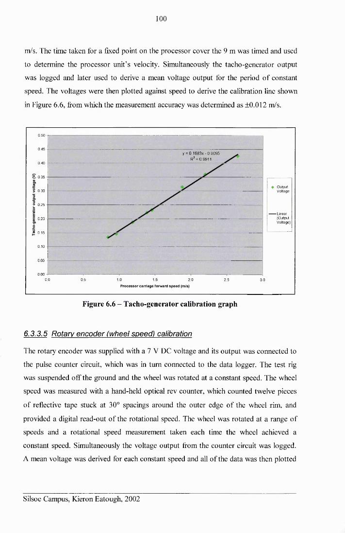
100
m/s. The time taken for a fixed point on the processor cover the 9 m was timed and used
to determine the processor unit’s velocity. Simultaneously the tacho-generator output
was logged and later used to derive a mean voltage output for the period of constant
speed. The voltages were then plotted against speed to derive the calibration line shown
in Figure 6.6, from which the measurement accuracy was determined as ±0.012 m/s.
0.50 |—
0.45y = 0.1683x-0.0095
R2= 0.99110.40
> 0 .35 -
♦ O u tpu t V oltage0.30
° 0.25
— Linear(O utputV oltage)
1.20
« 0.15
0.10
0.05
0.000.0 0.5 2.0 2 .5 3 .0
P r o c e s s o r carriage forw ard s p e e d (m /s)
Figure 6.6 - Tacho-generator calibration graph
6.3.3.5 Rotary encoder (wheel speed) calibration
The rotary encoder was supplied with a 7 V DC voltage and its output was connected to
the pulse counter circuit, which was in turn connected to the data logger. The test rig
was suspended off the ground and the wheel was rotated at a constant speed. The wheel
speed was measured with a hand-held optical rev counter, which counted twelve pieces
of reflective tape stuck at 30° spacings around the outer edge of the wheel rim, and
provided a digital read-out of the rotational speed. The wheel was rotated at a range of
speeds and a rotational speed measurement taken each time the wheel achieved a
constant speed. Simultaneously the voltage output from the counter circuit was logged.
A mean voltage was derived for each constant speed and all of the data was then plotted
Silsoe Campus, Kieron Eatough, 2002
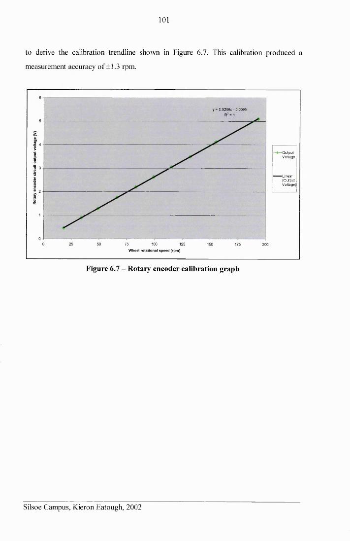
101
to derive the calibration trendline shown in Figure 6.7. This calibration produced a
measurement accuracy of ±1.3 rpm.
0.0266X - 0 .0095
—♦ —O utpu tV oltage
Linear(O utputV oltage)
75 100 125
W heel rotational s p e e d (rpm )
Figure 6.7 - Rotary encoder calibration graph
Silsoe Campus, Kieron Eatough, 2002
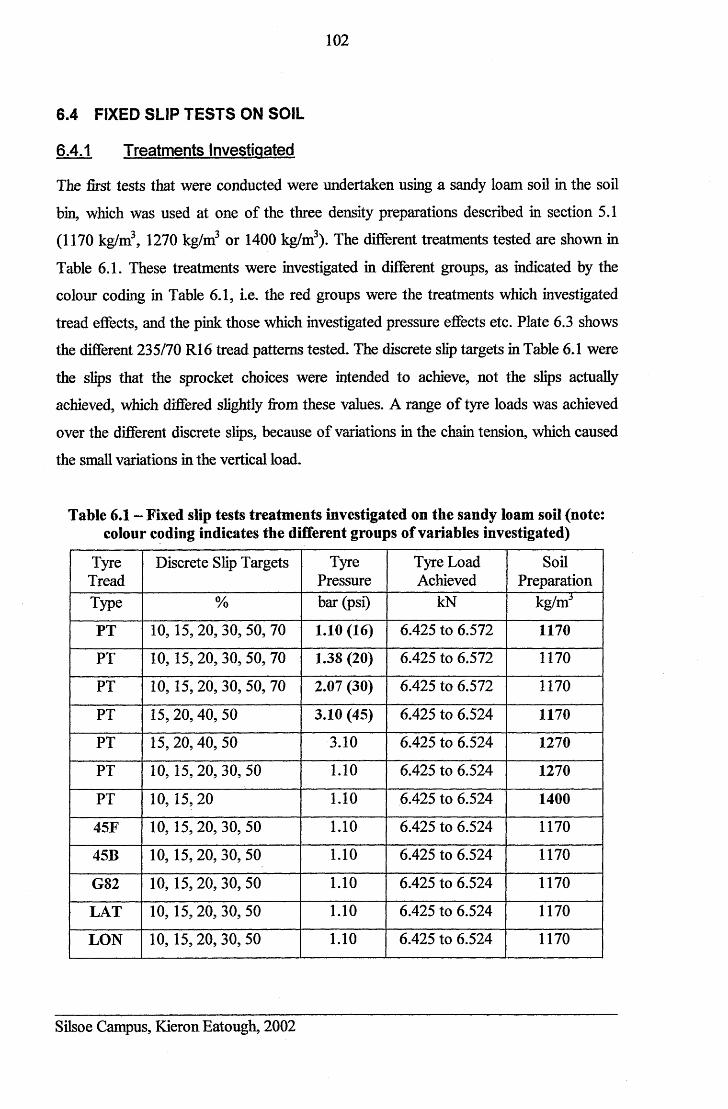
1 0 2
6.4 FIXED SLIP TESTS ON SOIL
6.4.1 Treatments Investigated
The first tests that were conducted were undertaken using a sandy loam soil in the soil
bin, which was used at one of the three density preparations described in section 5.1
(1170 kg/m3, 1270 kg/m3 or 1400 kg/m3). The different treatments tested are shown in
Table 6.1. These treatments were investigated in different groups, as indicated by the
colour coding in Table 6.1, i.e. the red groups were the treatments which investigated
tread effects, and the pink those which investigated pressure effects etc. Plate 6.3 shows
the different 235/70 R16 tread patterns tested. The discrete slip targets in Table 6.1 were
the slips that the sprocket choices were intended to achieve, not the slips actually
achieved, which differed slightly from these values. A range of tyre loads was achieved
over the different discrete slips, because of variations in the chain tension, which caused
the small variations in the vertical load.
Table 6.1 - Fixed slip tests treatments investigated on the sandy loam soil (note: colour coding indicates the different groups of variables investigated)
TyreTread
Discrete Slip Targets TyrePressure
Tyre Load Achieved
SoilPreparation
Type % bar (psi) kN kg/m3
PT 10,15, 20, 30, 50, 70 1.10 (16) 6.425 to 6.572 1170
PT 10, 15,20, 30, 50, 70 1.38 (20) 6.425 to 6.572 1170
PT 10,15, 20, 30, 50, 70 2.07 (30) 6.425 to 6.572 1170
PT 15, 20, 40, 50 3.10 (45) 6.425 to 6.524 1170
PT 15, 20,40, 50 3.10 6.425 to 6.524 1270
PT 10, 15, 20, 30, 50 1.10 6.425 to 6.524 1270
PT 10, 15, 20 1.10 6.425 to 6.524 1400
45F 10,15, 20, 30, 50 1.10 6.425 to 6.524 1170
45B 10,15, 20, 30, 50 1.10 6.425 to 6.524 1170
G82 10,15,20, 30, 50 1.10 6.425 to 6.524 1170
LAT 10,15, 20, 30, 50 1.10 6.425 to 6.524 1170
LON 10,15, 20, 30, 50 1.10 6.425 to 6.524 1170
Silsoe Campus, Kieron Eatough, 2002
103
These tests were not thoroughly replicated, as some replication of the results was
achieved during each test-run and because this was a pilot experiment that was
conducted to:
1. Confirm the operation of the test rig.
2. Check that the slip-pull results generated agreed with accepted theory20, thus
validating the methodology used with the fixed-slip test rig.
3. Determine if variations in slip-pull performance occurred between different tyre
treatments, and if they were measurable.
6.4.2 Experimental Results
Slip-pull curves were used for tyre comparisons. These were constructed from
measurements recorded over a series of test runs conducted across a range of discrete
fixed slips. The following variables were plotted on the slip-pull graphs:
1. Gross thrust
2. Rolling resistance
3. Net thrust (calculated from 1 & 2)
4. Deflected sinkage (accounting for both tyre and ground deformation)
Thus four values (one for each variable) were plotted at each discrete slip value
generated by each different test run, i.e. five test runs would produce five discrete sets
of data on each curve. Results were only calculated from the central periods of each
test-run, when the rig operated at a constant forward speed, mechanically set at 1.4 m/s
(« 5 km/h), and hence when it achieved a consistent wheel slip. The value plotted for
each variable was a mean value of all the data recorded for that variable during the
period of constant speed during the test-run. This process was undertaken for all four
variables for all of the test-runs conducted. The results for each treatment effect
presented in the following sub-sections are shown on two pairs of graphs, which use the
following coding system to identify the results; i.e. TREAD, PRESSURE, SOIL
DENSITY, i.e. PT 1.38 1170, would indicate a plain tread tyre inflated to 1.38 bar
operating on 1170 kg/m3 soil.
Silsoe Campus, Kieron Eatough, 2002
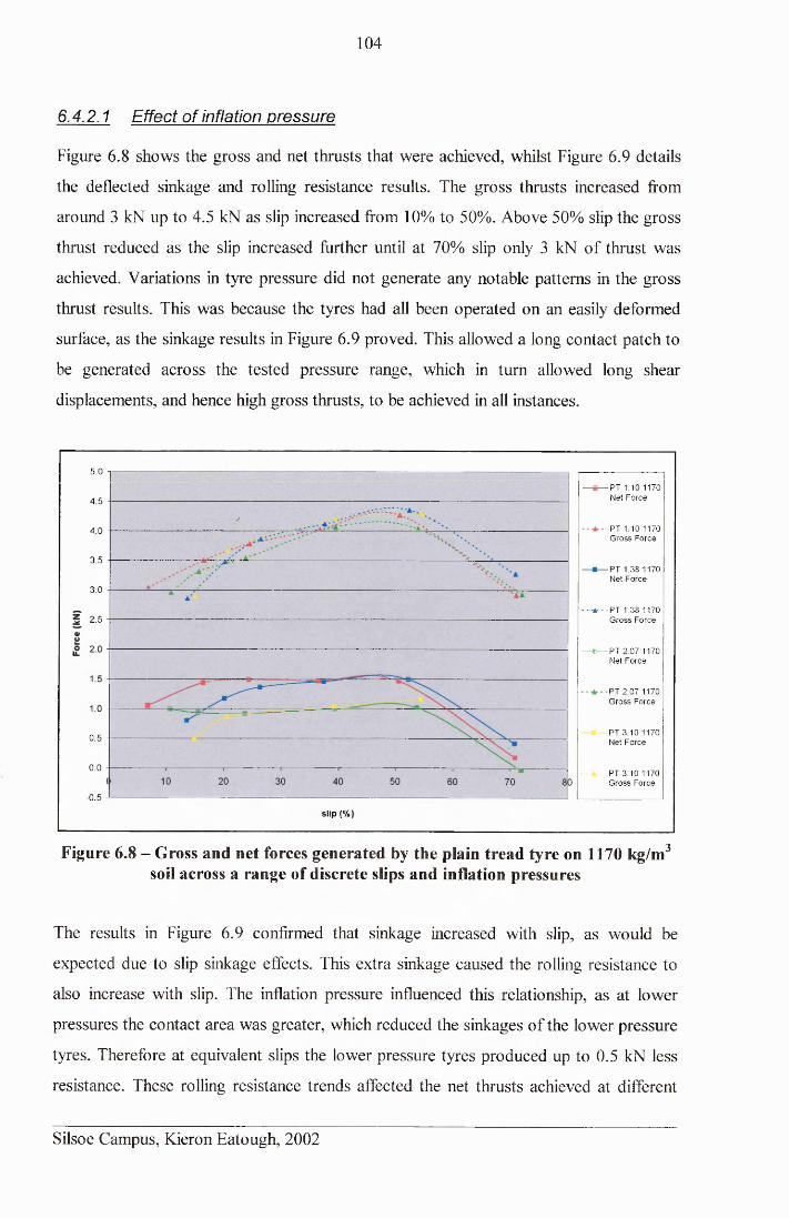
104
6.4.2.1 Effect of inflation pressure
Figure 6.8 shows the gross and net thrusts that were achieved, whilst Figure 6.9 details
the deflected sinkage and rolling resistance results. The gross thrusts increased from
around 3 kN up to 4.5 kN as slip increased from 10% to 50%. Above 50% slip the gross
thrust reduced as the slip increased further until at 70% slip only 3 kN of thrust was
achieved. Variations in tyre pressure did not generate any notable patterns in the gross
thrust results. This was because the tyres had all been operated on an easily deformed
surface, as the sinkage results in Figure 6.9 proved. This allowed a long contact patch to
be generated across the tested pressure range, which in turn allowed long shear
displacements, and hence high gross thrusts, to be achieved in all instances.
5 .0 -r
PT 1.10 1170 Net F orce4 .5
-P T 1.10 1170 G ro ss F orce
4 .0
3 .5PT 1.38 1170 Net F o rce
3 .0
- - • * - - P T 1.38 1170 G ro ss F o rce2 .5
—m— PT 2 .0 7 1170 N et F orce
PT 2 .0 7 1 1 7 0 G ro ss F orce
PT 3 .10 1170 N et F o rce0 .5
0.0PT 3 .10 1170 G ro ss F orce
-0 .5 J
s l ip (%
Figure 6.8 - Gross and net forces generated by the plain tread tyre on 1170 kg/m3soil across a range of discrete slips and inflation pressures
The results in Figure 6.9 confirmed that sinkage increased with slip, as would be
expected due to slip sinkage effects. This extra sinkage caused the rolling resistance to
also increase with slip. The inflation pressure influenced this relationship, as at lower
pressures the contact area was greater, which reduced the sinkages of the lower pressure
tyres. Therefore at equivalent slips the lower pressure tyres produced up to 0.5 kN less
resistance. These rolling resistance trends affected the net thrusts achieved at different
Silsoe Campus, Kieron Eatough, 2002
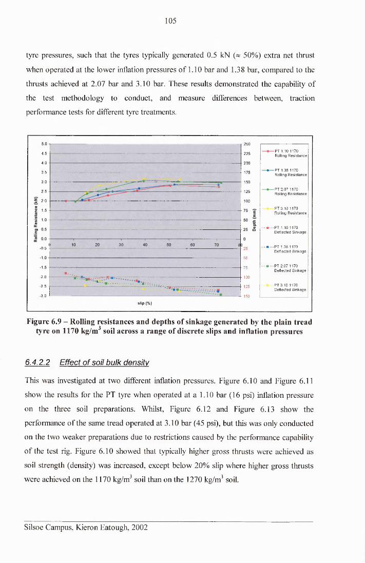
105
tyre pressures, such that the tyres typically generated 0.5 kN (« 50%) extra net thrust
when operated at the lower inflation pressures of 1.10 bar and 1.38 bar, compared to the
thrusts achieved at 2.07 bar and 3.10 bar. These results demonstrated the capability of
the test methodology to conduct, and measure differences between, traction
performance tests for different tyre treatments.
- r 250
PT 1.10 1170 Rolling R e s is ta n c e4 .5 22 5
4 .0 200
PT 1.38 1170 Rolling R e s is ta n c e
3.5 175
3.0 150
PT 2 .07 1170 Rolling R e s is ta n c e
2 .5 125
2.0 100PT 3 .1 0 1170 Rolling R e s is ta n c e
- - * - - P T 1.10 1170D eflected S in k a g e
30 80 - - * ■ - PT 1.38 1170D eflected S in k a g e
-0 .5
50
- - * - - PT 2 .0 7 1170D eflected S in k a g e
7 5
-2.0 100
PT 3 .1 0 1170 D eflected S in k a g e
-2.5 125
-3.0 — 150
s l ip (%)
Figure 6.9 - Rolling resistances and depths of sinkage generated by the plain tread tyre on 1170 kg/m3 soil across a range of discrete slips and inflation pressures
6.4.2.2 Effect o f soil bulk density
This was investigated at two different inflation pressures. Figure 6.10 and Figure 6.11
show the results for the PT tyre when operated at a 1.10 bar (16 psi) inflation pressure
on the three soil preparations. Whilst, Figure 6.12 and Figure 6.13 show the
performance of the same tread operated at 3.10 bar (45 psi), but this was only conducted
on the two weaker preparations due to restrictions caused by the performance capability
of the test rig. Figure 6.10 showed that typically higher gross thrusts were achieved as
soil strength (density) was increased, except below 20% slip where higher gross thrusts
were achieved on the 1170 kg/m3 soil than on the 1270 kg/m3 soil.
Silsoe Campus, Kieron Eatough, 2002
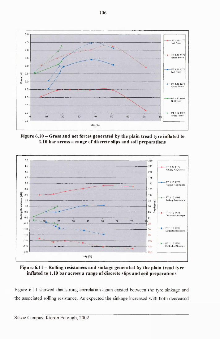
106
P T 1 .1 0 1 1 7 0 Net Force4 .5
4 .0
- - ★ - -P T 1.10 1170 G ross Force3 .5
PT 1.10 1270 Net Force
i 2 .5
• - -A- - - PT 1.10 1270 G ross Force
PT 1.10 1400 Net Force
0 .5
0.0 - - * - - P T 1 . 1 0 1400 G ross Force3 0 4 020 50 7 0
-0 .5
slip (%)
Figure 6.10 - Gross and net forces generated by the plain tread tyre inflated to 1.10 bar across a range of discrete slips and soil preparations
5.0 t—
4 .5 22 5 PT 1.10 1170 Rolling R e s is ta n c e
4 .0 200
3.5 175
PT 1 .10 1270 Rolling R e s is ta n c e
3 .0 150
125
2.0 100PT 1.10 1400 Rolling R e s is ta n c e
- - * - - P T 1.10 1170D eflected S in k a g e
40 60-0 .5
- ■ * - - PT 1.10 1270D eflected S in k a g e
50
-2.0 100- - * - - P T 1.10 1400
D eflected S in k a g e-2.5 125
-3 .0 -1 — 150
slip (%)
Figure 6.11 - Rolling resistances and sinkage generated by the plain tread tyre inflated to 1.10 bar across a range of discrete slips and soil preparations
Figure 6.11 showed that strong correlation again existed between the tyre sinkage and
the associated rolling resistance. As expected the sinkage increased with both decreased
Silsoe Campus, Kieron Eatough, 2002
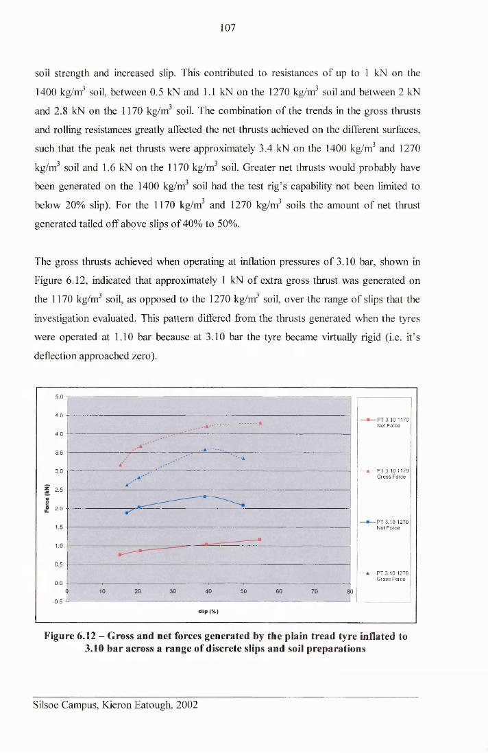
107
soil strength and increased slip. This contributed to resistances of up to 1 kN on the
1400 kg/m3 soil, between 0.5 kN and 1.1 kN on the 1270 kg/m3 soil and between 2 kN
and 2.8 kN on the 1170 kg/m soil. The combmation of the trends in the gross thrusts
and rolling resistances greatly affected the net thrusts achieved on the different surfaces,
such that the peak net thrusts were approximately 3.4 kN on the 1400 kg/m3 and 1270
kg/m soil and 1.6 kN on the 1170 kg/m soil. Greater net thrusts would probably have
been generated on the 1400 kg/m soil had the test rig’s capability not been limited to
below 20% slip). For the 1170 kg/m3 and 1270 kg/m3 soils the amount of net thrust
generated tailed off above slips of 40% to 50%.
The gross thrusts achieved when operating at inflation pressures of 3.10 bar, shown in
Figure 6.12, indicated that approximately 1 kN of extra gross thrust was generated on
the 1170 kg/m3 soil, as opposed to the 1270 kg/m3 soil, over the range of slips that the
investigation evaluated. This pattern differed from the thrusts generated when the tyres
were operated at 1.10 bar because at 3.10 bar the tyre became virtually rigid (i.e. it’s
deflection approached zero).
5 .0
4 .5PT 3 .1 0 1170 N e t F orce
4 .0
3 .5
- - * - - P T 3 .1 0 1 1 7 0 G ro ss F o rce
3 .0
2 .5
2.0
PT 3 .10 1270 N et F o rce
0 .5
--■ * - - P T 3 .1 0 1270 G ro ss F o rce
0.05 0
-0 .5
s l ip (% )
Figure 6.12 - Gross and net forces generated by the plain tread tyre inflated to 3.10 bar across a range of discrete slips and soil preparations
Silsoe Campus, Kieron Eatough, 2002
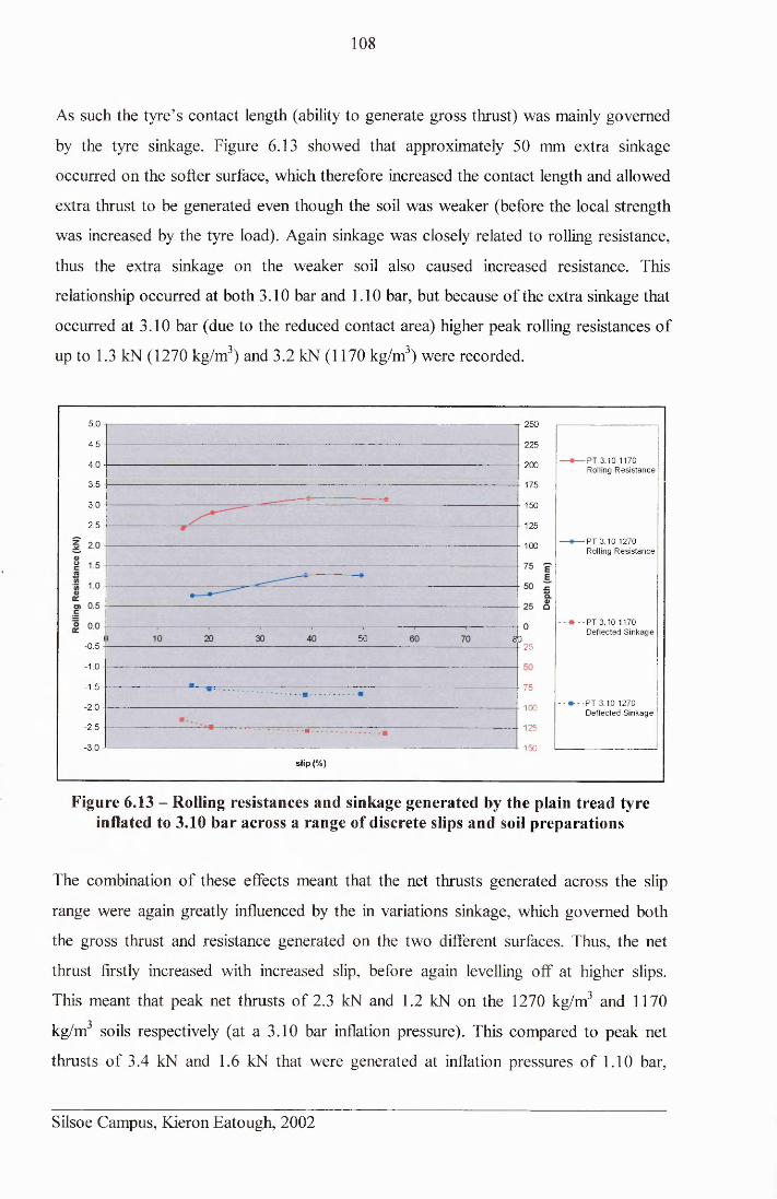
108
As such the tyre’s contact length (ability to generate gross thrust) was mainly governed
by the tyre sinkage. Figure 6.13 showed that approximately 50 mm extra sinkage
occurred on the softer surface, which therefore increased the contact length and allowed
extra thrust to be generated even though the soil was weaker (before the local strength
was increased by the tyre load). Again sinkage was closely related to rolling resistance,
thus the extra sinkage on the weaker soil also caused increased resistance. This
relationship occurred at both 3.10 bar and 1.10 bar, but because of the extra sinkage that
occurred at 3.10 bar (due to the reduced contact area) higher peak rolling resistances of
up to 1.3 kN (1270 kg/m3) and 3.2 kN (1170 kg/m3) were recorded.
5 .0 2 5 0
4 .5 2 2 5
PT 3 .1 0 1170 Rolling R e s is ta n c e
4 .0 200
3 .5 175
3 .0 150
2 .5 125
PT 3 .10 1270 Rolling R e s is ta n c e
100
- - * - - PT 3 .10 1170D eflected S in k a g e
5 0 8 0-0 .5 2 5
- 1.0
-1 .5 7 5
-■ * - - P T 3 .10 1270D eflected S in k a g e
- 2.0 100
-2 .5 1 25
-3 .0 J 1 50
s l ip (%)
Figure 6.13 - Rolling resistances and sinkage generated by the plain tread tyre inflated to 3.10 bar across a range of discrete slips and soil preparations
The combination of these effects meant that the net thrusts generated across the slip
range were again greatly influenced by the in variations sinkage, which governed both
the gross thrust and resistance generated on the two different surfaces. Thus, the net
thrust firstly increased with increased slip, before again levelling off at higher slips.
This meant that peak net thrusts of 2.3 kN and 1.2 kN on the 1270 kg/m3 and 1170
kg/m soils respectively (at a 3.10 bar inflation pressure). This compared to peak net
thrusts of 3.4 kN and 1.6 kN that were generated at inflation pressures of 1.10 bar,
Silsoe Campus, Kieron Eatough, 2002
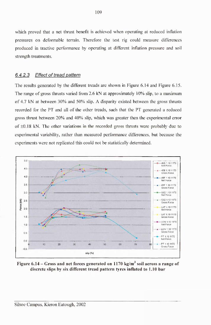
109
which proved that a net thrust benefit is achieved when operating at reduced inflation
pressures on deformable terrain. Therefore the test rig could measure differences
produced in tractive performance by operating at different inflation pressure and soil
strength treatments.
6.4.2.3 Effect of tread pattern
The results generated by the different treads are shown in Figure 6.14 and Figure 6.15.
The range of gross thrusts varied from 2.6 kN at approximately 10% slip, to a maximum
of 4.7 kN at between 30% and 50% slip. A disparity existed between the gross thrusts
recorded for the PT and all of the other treads, such that the PT generated a reduced
gross thrust between 20% and 40% slip, which was greater then the experimental error
of ±0.18 kN. The other variations in the recorded gross thrusts were probably due to
experimental variability, rather than measured performance differences, but because the
experiments were not replicated this could not be statistically determined.
5 .045B 1.10 1170 Net F orce
4 .5- - A - -45B 1.10 1170
G ro ss F orce
45F 1 .10 1170 N et F orce
3 .5 - - A - -45F 1.10 1170 G ro ss F orce
G 8 2 1 .10 1170 Net F o rce
3 .0
- - -A- - - G 8 2 1.10 1170 G ro ss F o rce
LAT 1 .10 1170 N et F o rce
LAT 1.10 1170 G ro ss F o rce
LON 1.10 1170 N et F o rce
- • a - -LON 1.10 1170 G ro ss F o rce0 .5
— PT 1.10 1170 N et F o rce
0.0- a - PT 1.10 1170
G ro ss F o rce4 0 50 7010 3 0 6 0
-0 .5
s l ip (%)
Figure 6.14 - Gross and net forces generated on 1170 kg/m3 soil across a range ofdiscrete slips by six different tread pattern tyres inflated to 1.10 bar
Silsoe Campus, Kieron Eatough, 2002
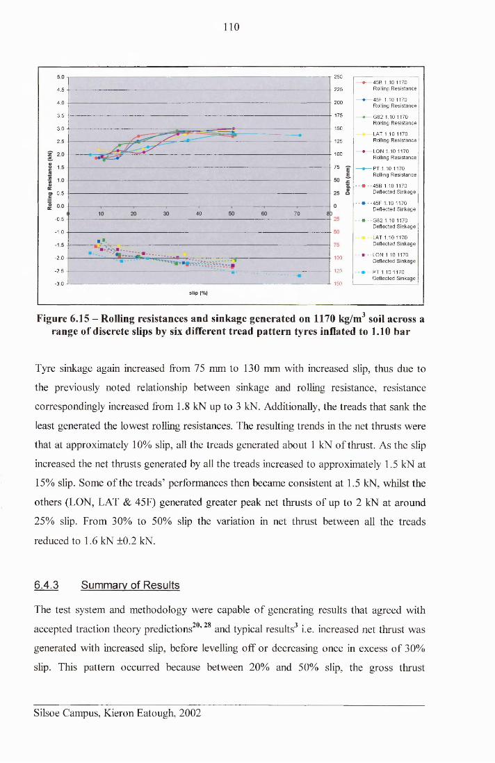
110
250
2254 .5
2004 .0
1753.5
1503.0
1252 .5
100
75
o> 0.5
40 7 0-0.5
- 1.0
■ »100- 2.0
125-2.5
150-3 .0 J-
s lip (%)
— • — 45B 1.10 1170Rolling R e s is ta n c e
— • — 45F 1.10 1170Rolling R es is ta n ce
— • — G 8 2 1.10 1170Rolling R es is ta n ce
LAT 1 .10 1170 Rolling R e s is ta n c e
— • — LON 1.10 1170Rolling R e s is ta n c e
— • — PT 1.10 1170Rolling R e s is ta n c e
- - * - -45B 1.10 1170D eflected S in k ag e
- - -4 5 F 1.10 1170D eflected S in k a g e
- - * - -G 8 2 1.10 1170D eflected S in k a g e
LAT 1.10 1170 D eflected S in k a g e
• - * -LO N 1.10 1170D eflected S in k ag e
- - - PT 1.10 1170D eflected S in k a g e
Figure 6.15 - Rolling resistances and sinkage generated on 1170 kg/m3 soil across a range of discrete slips by six different tread pattern tyres inflated to 1.10 bar
Tyre sinkage again increased from 75 mm to 130 mm with increased slip, thus due to
the previously noted relationship between sinkage and rolling resistance, resistance
correspondingly increased from 1.8 kN up to 3 kN. Additionally, the treads that sank the
least generated the lowest rolling resistances. The resulting trends in the net thrusts were
that at approximately 10% slip, all the treads generated about 1 kN of thrust. As the slip
increased the net thrusts generated by all the treads increased to approximately 1.5 kN at
15% slip. Some of the treads’ performances then became consistent at 1.5 kN, whilst the
others (LON, LAT & 45F) generated greater peak net thrusts of up to 2 kN at around
25% slip. From 30% to 50% slip the variation in net thrust between all the treads
reduced to 1.6 kN ±0.2 kN.
6.4.3 Summary of Results
The test system and methodology were capable of generating results that agreed with20 28 • 3accepted traction theory predictions ’ and typical results i.e. increased net thrust was
generated with increased slip, before levelling off or decreasing once in excess of 30%
slip. This pattern occurred because between 20% and 50% slip, the gross thrust
Silsoe Campus, Kieron Eatough, 2002
I l l
increased asymptotically with extra slip, whilst the increase in rolling resistance with
increased wheel slip (extra slip sinkage) was approximately linear. Between 55% and
70% slip the gross thrust decreased markedly, whilst the rolling resistance continued to
increase, thus considerably less net thrust was achieved. Also more net thrust was
generated with reduced tyre inflation pressure, or increased soil density. In both cases
this occurred because the sinkage was reduced, as the gross thrust potential increased.
The trends between the tread patterns were insufficiently clear for detailed conclusions
to be drawn. However, notable differences existed between the net thrusts generated by
the different treads across the range of slips. Even though the variations caused between
the treads were at their maximum 0.45 kN, this was important. For instance, a potential
difference of 0.2 kN acting at each comer of a vehicle would equate to 0.8 kN of extra
thrust, which could potentially change a ‘no-go’ situation into a ‘go’ situation. Thus
further study of the effects of tread pattern on tyre performance on sand was justified, to
enable the potential benefits of different tread features to be understood.
6.5 FIXED SLIP TESTS ON SAND
In addition to the verification (rig comparison) tests conducted on the sandy loam,
similar tests were conducted upon the replicate sand to act as a pilot study to enable the
sand displacement boundaries to be quantified prior to their attempted measurement and
to investigate the tyre performance on sand. These tests investigated the treatments
detailed in Table 6.2. Again these tests were not thoroughly replicated because it was a
pilot study, but a limited replication of the results was derived from the repetitive results
that occurred over the course of each test-run. Instead the available experimental time
was devoted to investigating the maximum possible range of variables.
These tests were conducted using a sand tank that was 6 m long x 1 m wide x 0.6 m
deep. This was sufficiently large to prevent any significant edge effects occurring
during the testing, which was confirmed as none of the sand displacements reached
either the base or the sides of the tank.
Silsoe Campus, Kieron Eatough, 2002
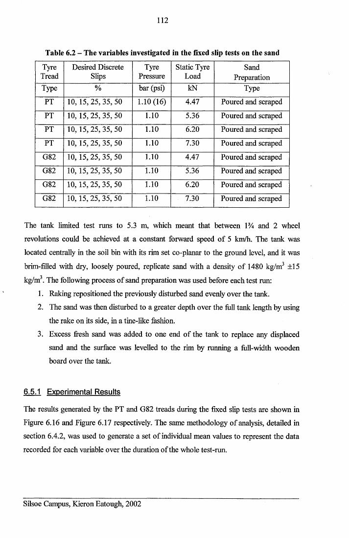
1 1 2
Table 6.2 - The variables investigated in the fixed slip tests on the sand
TyreTread
Desired Discrete Slips
TyrePressure
Static Tyre Load
SandPreparation
Type % bar (psi) kN Type
PT 10, 15, 25, 35, 50 1.10(16) 4.47 Poured and scraped
PT 10, 15, 25, 35, 50 1.10 5.36 Poured and scraped
PT 10, 15, 25, 35, 50 1.10 6.20 Poured and scraped
PT 10, 15, 25, 35, 50 1.10 7.30 Poured and scraped
G82 10, 15, 25, 35, 50 1.10 4.47 Poured and scraped
G82 10,15, 25, 35, 50 1.10 5.36 Poured and scraped
G82 10, 15, 25,35, 50 1.10 6.20 Poured and scraped
G82 10, 15, 25, 35, 50 1.10 7.30 Poured and scraped
The tank limited test runs to 5.3 m, which meant that between 1% and 2 wheel
revolutions could be achieved at a constant forward speed of 5 km/h. The tank was
located centrally in the soil bin with its rim set co-planar to the ground level, and it was
brim-filled with dry, loosely poured, replicate sand with a density of 1480 kg/m3 ±15
kg/m . The following process of sand preparation was used before each test run:
1. Raking repositioned the previously disturbed sand evenly over the tank.
2. The sand was then disturbed to a greater depth over the full tank length by using
the rake on its side, in a tine-like fashion.
3. Excess fresh sand was added to one end of the tank to replace any displaced
sand and the surface was levelled to the rim by running a full-width wooden
board over the tank.
6.5.1 Experimental Results
The results generated by the PT and G82 treads during the fixed slip tests are shown in
Figure 6.16 and Figure 6.17 respectively. The same methodology of analysis, detailed in
section 6.4.2, was used to generate a set of individual mean values to represent the data
recorded for each variable over the duration of the whole test-run.
Silsoe Campus, Kieron Eatough, 2002
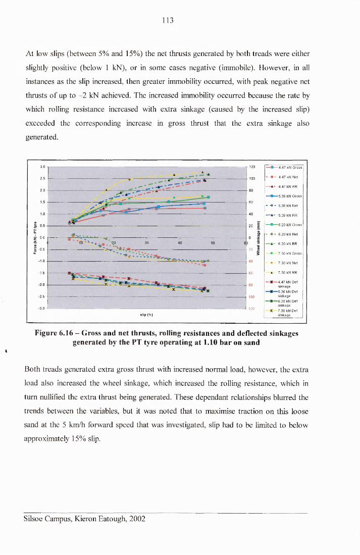
113
At low slips (between 5% and 15%) the net thrusts generated by both treads were either
slightly positive (below 1 kN), or in some cases negative (immobile). However, in all
instances as the slip increased, then greater immobility occurred, with peak negative net
thrusts of up to -2 kN achieved. The increased immobility occurred because the rate by
which rolling resistance increased with extra sinkage (caused by the increased slip)
exceeded the corresponding increase in gross thrust that the extra sinkage also
generated.
3.0 1202.5 1002.0
6 0
20HCL
0.0z.x >20 30
u .- 0.5 20
-1.5 60
-2.5
- 3.0 120slip <%)
D — 4.47 kN G ross
• - 4.47 kN Net
— A - 4.47 kN RR
- 0 — 5.36 kN G ross
& - 5.36 kN Net
- A - 5.36 kN RR
- » — 6.20 kN G ross
•* - 6.20 kN Net
- A - '6.20 kN RR
■ 7.30 kN G ross
• 7.30 kN Net
• 7.30 kN RR
-W — 4.47 kN Def sinkage 5.36 kN Def sinkage
- * ” - 6 .2 0 kN Def sinkage
X 7.30 kN Def sinkage
Figure 6.16 - Gross and net thrusts, rolling resistances and deflected sinkages generated by the PT tyre operating at 1.10 bar on sand
Both treads generated extra gross thrust with increased normal load, however, the extra
load also increased the wheel sinkage, which increased the rolling resistance, which in
turn nullified the extra thrust being generated. These dependant relationships blurred the
trends between the variables, but it was noted that to maximise traction on this loose
sand at the 5 km/h forward speed that was investigated, slip had to be limited to below
approximately 15% slip.
Silsoe Campus, Kieron Eatough, 2002
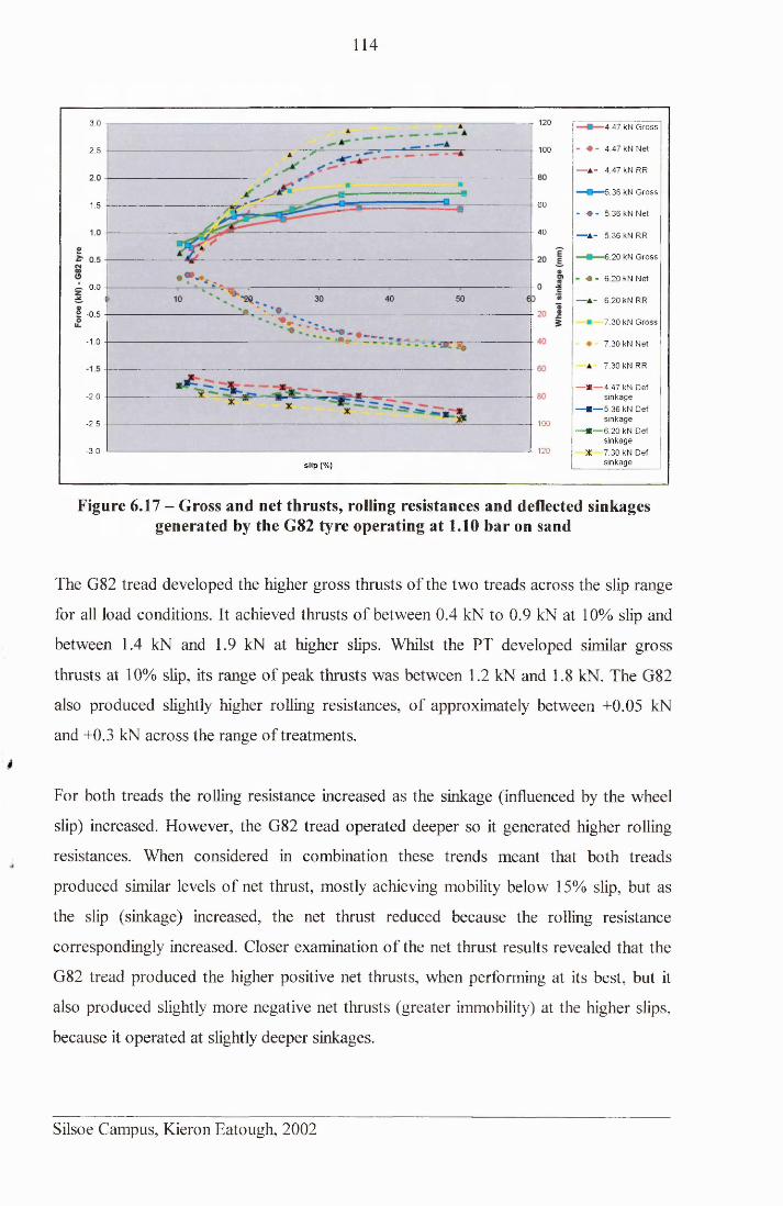
114
r 1203.0 T 4.47 kN G ro ss
* - 4 .47 kN Net1002 .5 -
— A - 4 .47 k N R R
■5.36 kN G ro ss
601.5- « - 5 .3 6 kN N et
40 — A - 5 .3 6 kN RR
■6.20 kN G ro ss
« « 6 .20 kN N et~ 0.0
— -A - 6 .2 0 k N R R
a -o.57 .3 0 kN G ro ss
- 1.0 7.3 0 kN N et
7 .3 0 kN RR
— * — 4.4 7 kN Def sin k ag e
— ■ — 5.36 kN D ef sin k ag e
~~rn—6 .2 0 kN D ef sin k ag e
X 7 .3 0 kN D ef sin k ag e
-2.0
100-2 .5
-3 .0 -I -J- 120slip (%)
Figure 6.17 - Gross and net thrusts, rolling resistances and deflected sinkages generated by the G82 tyre operating at 1.10 bar on sand
The G82 tread developed the higher gross thrusts of the two treads across the slip range
for all load conditions. It achieved thrusts of between 0.4 kN to 0.9 kN at 10% slip and
between 1.4 kN and 1.9 kN at higher slips. Whilst the PT developed similar gross
thrusts at 10% slip, its range of peak thrusts was between 1.2 kN and 1.8 kN. The G82
also produced slightly higher rolling resistances, of approximately between +0.05 kN
and +0.3 kN across the range of treatments.
For both treads the rolling resistance increased as the sinkage (influenced by the wheel
slip) increased. However, the G82 tread operated deeper so it generated higher rolling
resistances. When considered in combination these trends meant that both treads
produced similar levels of net thrust, mostly achieving mobility below 15% slip, but as
the slip (sinkage) increased, the net thrust reduced because the rolling resistance
correspondingly increased. Closer examination of the net thrust results revealed that the
G82 tread produced the higher positive net thrusts, when performing at its best, but it
also produced slightly more negative net thrusts (greater immobility) at the higher slips,
because it operated at slightly deeper sinkages.
Silsoe Campus, Kieron Eatough, 2002
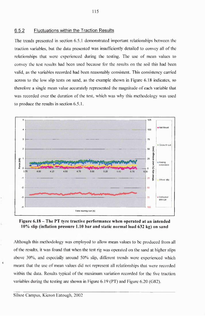
115
6.5.2 Fluctuations within the Traction Results
The trends presented in section 6.5.1 demonstrated important relationships between the
traction variables, but the data presented was insufficiently detailed to convey all of the
relationships that were experienced during the testing. The use of mean values to
convey the test results had been used because for the results on the soil this had been
valid, as the variables recorded had been reasonably consistent. This consistency carried
across to the low slip tests on sand, as the example shown in Figure 6.18 indicates, so
therefore a single mean value accurately represented the magnitude of each variable that
was recorded over the duration of the test, which was why this methodology was used
to produce the results in section 6.5.1.
4.25 5.50
• G ro ss th ru st
x Rolling re s is ta n c e
W heel slip
♦ D eflected sin k ag e
T im e during run (s)
Figure 6.18 - The PT tyre tractive performance when operated at an intended 10% slip (inflation pressure 1.10 bar and static normal load 632 kg) on sand
Although this methodology was employed to allow mean values to be produced from all
of the results, it was found that when the test rig was operated on the sand at higher slips
above 30%, and especially around 50% slip, different trends were experienced which
meant that the use of mean values did not represent all relationships that were recorded
within the data. Results typical of the maximum variation recorded for the five traction
variables during the testing are shown in Figure 6.19 (PT) and Figure 6.20 (G82).
Silsoe Campus, Kieron Eatough, 2002
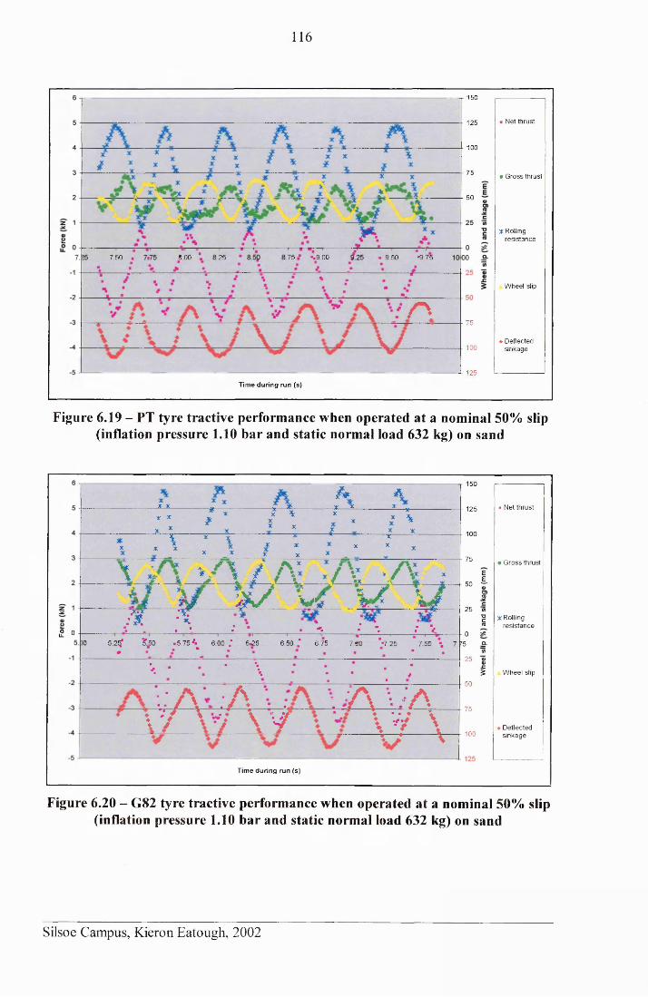
116
~r 150
Net thrust125
100
75 a G ro ss th ru st
50
x Rolling re s is tan c e
8.00 -.9 .0 0I.25 1.75 9.50 “9 .7 57.50
W heel slip
/ - \75
♦ D eflected sin k ag e100
~L 125
T im e d ur in g run (s)
Figure 6.19 - PT tyre tractive performance when operated at a nominal 50% slip (inflation pressure 1.10 bar and static normal load 632 kg) on sand
S. o
£ *- - ..... X J X ....... ...- . * - .... * . * --------- X
X X * * * * * & *
X * X * * £
- * -------------------* - » --------------------------
X « \X X
1 * * X X
* . * _ * * J * * x *
— XX X x
X v'X t A ’ /V . A *JT \ \ * f %. / a x
m ’$ % / VS v n rM ;e : k * .■ * • '■ »" % : V
)0 5 .2 C K .50 . 5 . 7 5 ^ 6 .0 0 .* 6 .2 5 6 .5 0 ' 6 .75 7 .6 0 “7 .2 5 7 .5 0 7 .^5
V- ' ‘ \ " # ■
/ \ A \;/\ A * A\ 7 X "7 \ ^■ ■ \ vy \
— \ / — V
150
-- 125 • N et th ru st
-■ 100
- 75 • G ro ss th ru st
EE
-- 50 ~atac
2 5 «13C x Rollingre re s is ta n c e
0
75 £■tn
■ 25 jc.5 W h e el slip
- 50
- 75
♦ D eflected■ 100 s in k ag e
T im e during run (s)
Figure 6.20 - G82 tyre tractive performance when operated at a nominal 50% slip (inflation pressure 1.10 bar and static normal load 632 kg) on sand
Silsoe Campus, Kieron Eatough, 2002
117
When these are compared to Figure 6.18 (note: both sets of data are presented on
identical Y-axes), the wide variation between the sets of results becomes evident. The
changes in the rig performance occurred because large variations in the performance of
the test wheel were caused at the higher slips. These occurred because of the varying
wheel slip, which caused the sand displacement to vary, which in turn altered the slip
sinkage of the wheel (note: increased slip caused increased sinkage and vice versa). As
the sinkage varied, it produced vertical accelerations of the test rig, which altered the
normal load acting on the wheel and thus the gross thrust potential. The varying sinkage
of the wheel also increased (or reduced) the contact length, further influencing its gross
thrust potential. Although the rig behaviour fluctuated, strong positive correlations were
still experienced between wheel sinkage and the associated rolling resistance. These
relationships made the mean value approach insufficient to represent and study these
results, so a more thorough explanation was required.
The mechanics of the fixed slip system meant that gross thrust was always directly
proportional to the chain tension. As the sand was sheared, the torque within the system,
which was caused by friction at the interface, was rapidly translated into rotational
momentum. If more torque was created in the system, then more gross thrust was
achieved, hence why the gross thrust was directly proportional to the sinkage and
normal load. As the sinkage reduced, the torque contained within the system was
rapidly released causing the wheel speed to increase. As the cycle progressed this
caused wheel slips in excess of the intended setting to be produced, as the minimum
sinkage was reached. This in turn caused high levels of sand displacement to occur,
which consequently once again increased the wheel sinkage. As the sinkage (and
torque) once again increased, due to reduced slip, the net effect was that the maximum
wheel sinkage (and tyre immobility) was achieved. Normally tyre immobilisation would
have occurred, but instead the combination of continued wheel torque and the test rig’s
(processor’s) forward motion drove the tyre up the opposing sand ridge. This action
increased the cable tension and subsequently the wheel slip, which forced the thrust
cycle to become a repetitive cyclical event.
Silsoe Campus, Kieron Eatough, 2002
118
The combination of the wide variations in the gross thrusts and rolling resistances
greatly influenced the net thrust results. Whilst the mean results had recorded the tyres
producing approximately -1 kN of net thrust, the true net thrusts varied from between 1
kN to -3 kN over a test run. Peak net thrust was achieved where both minimum gross
thrust and rolling resistance occurred, as then the gross thrust exceeded the resistance.
Thereafter as sinkage increased, the rate of increase in resistance with increased
sinkage, exceeded the rate of increase in gross thrust, and thus the net thrust became
increasingly worse.
Comparison of the relative performance of the two treads operating at 50% slip showed
that the peak sinkage of the G82 was deeper than the PT, which resulted in it generating
higher rolling resistances, and therefore achieving the peak negative net thrusts of either
tread. The G82 also generated higher gross thrusts when operating at the minimum
sinkages, which caused this tread to also generate the higher peak positive net thrusts as
well. Therefore again the G82 showed that it would achieve either the peak positive, or
peak negative, net thrusts (mobility, or immobility) depending upon at which point in
the thrust-slip cycle it was operating
The changeover from steady behaviour (at low slips), to the fluctuating behaviour (at
higher slips) was driven by increased slip altering the tyre sinkage. These events were
confidently related to the shear interactions between the tyres and sand, as the same
fluctuating behaviour had only been experienced to a minor extent at high slips during
the soil tests, which tested similar tyre treatments (except the surface). These tests
indicated that wheel sinkage, which was caused by sand displacement that was driven
by the magnitude of slip, governed the mobility of the tyre. Therefore for mobility to be
increased it was necessary to understand what type of sand displacements were caused
by the wheel slip, before any possible methods to address them could be considered.
6.5.3 Limitations of the Fixed Slip System
These results demonstrated the capability of the fixed slip system to conduct traction
experiments, but the key drawback of the system’s operation was that to produce one
useful slip-pull curve for each treatment, at least five test runs were required. Whilst
Silsoe Campus, Kieron Eatough, 2002
119
each run took about ten seconds, the soil preparation and all of the subsequent
measurements meant that theoretically approximately five hours of testing were
required to produce one curve (depending upon the soil preparation tested). However,
the initial test programme had progressed at a slower rate because the necessity to
change the test tyres, deflection transducers, or sprocket ratios to achieve the necessary
treatments took longer than planned. Also the time-consuming necessity to check that
the sprockets were correctly aligned prior to each test-run had wasted a considerable
amount of testing. These time losses meant that the drive system needed to be altered
prior to the main experiments.
It had also been discovered that some of the drive system components failed when the
rig was operated above certain slip limits on the firm soils, when the maximum gross
thrusts were achieved. Thus before a more detailed, replicated test programme to
examine the tractive effects of tread on sand across a wide range of slip treatments
could be efficiently conducted the rig required re-designing. This necessity presented an
opportunity to re-evaluate the operation of the whole system. As the instrumentation
and the logging hardware and software had proved capable of accurately and repeatedly
measuring the required traction variables these systems were not altered. Instead the re
design concentrated on the drive system with the following two priorities in mind:
1. To provide a quicker method of slip variation, thus allowing greater flexibility
and efficiency in the experimental work.
2. To reduce the stresses on the drive components in the system.
6.6 THE VARIABLE SLIP TEST RIG
As well as the instrumentation systems, the main framework, hub unit, load platforms
and damper were all carried over to the new rig. The most obvious solution to providing
a flexible, and easily adjustable, method of changing the wheel slip was the adoption of
a hydraulic drive system. A variable flow system allowed easy adjustment of the motor
speed, and hence the wheel speed, and mounting the motor on the test frame closer to
the hub reduced the stresses generated in the system, whilst higher input drive speeds
reduced the torques transmitted by some of the components.
Silsoe Campus, Kieron Eatough, 2002
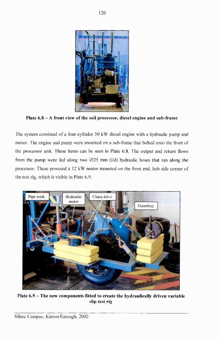
120
Plate 6.8 - A front view of the soil processor, diesel engine and sub-frame
The system consisted of a four-cylinder 50 kW diesel engine with a hydraulic pump and
motor. The engine and pump were mounted on a sub-frame that bolted onto the front of
the processor unit. These items can be seen in Plate 6.8. The output and return flows
from the pump were fed along two 025 mm (i/d) hydraulic hoses that ran along the
processor. These powered a 12 kW motor mounted on the front end, hub side comer of
the test rig, which is visible in Plate 6.9.
m j Hydraulic v * motor
Chain drive
Guarding
Plate 6.9 - The new components fitted to create the hydraulically driven variableslip test rig
Silsoe Campus, Kieron Eatough, 2002
121
A manually operated flow divider was mounted on the processor between the pump and
the motor. This enabled oil to be directed away from the motor and thus, to a degree,
allowed its speed to be controlled and easily adjusted. Some speed control could also
have been achieved by changing the engine (pump) speed, but test runs were always
conducted at full throttle to maximise the system pressure. The location of the divider
meant that a desired slip could be manually selected prior to each test run, but it could
not be adjusted during a test run. At a processor forward speed of 5 km/h the new
design could theoretically achieve a wheel slip range of 10% to 80%. This capability
was confirmed by static tests, which are described in Appendix 18.
Mounting the motor on the test rig meant the rig’s sinkage (and that of the test wheel)
was unrestricted. It also removed the necessity to deduct the chain tension readings
from the EORT readings, which now solely represented the net thrust generated by the
tyre (tread). However, this change removed the ability to determine both the gross thrust
and rolling resistance produced during each test run. Instead, to derive a gross thrust
from the wheel it was necessary to separately measure the rolling resistance (using the
procedure outlined in section 6.3.2) and add it to the net thrust. The net thrust remained
the most useful value to use for tyre comparison as it described the overall mobility.
6.6.1 Operating Characteristics of the Variable Slip Rig
When it was used for traction tests this test rig produced a fluctuating range of the slip,
sinkage and net thrust results. It was easiest to understand the relationships between the
slip, the sinkage and net thrust by considering a single cycle from a test run. Figure 6.21
presents such a section of data, with numbered dashed lines that relate to the stages
through the cycle and the following explanation:
1. At this position the wheel slip was at its lowest, whilst the wheel was rising above
its median depth. The low wheel slip, and thus low rearward sand displacements
meant that the wheel continued to rise up the sand ahead of it. This reduced the
negativity of the net thrust because the reducing sinkage reduced the rolling
resistance.
Silsoe Campus, Kieron Eatough, 2002
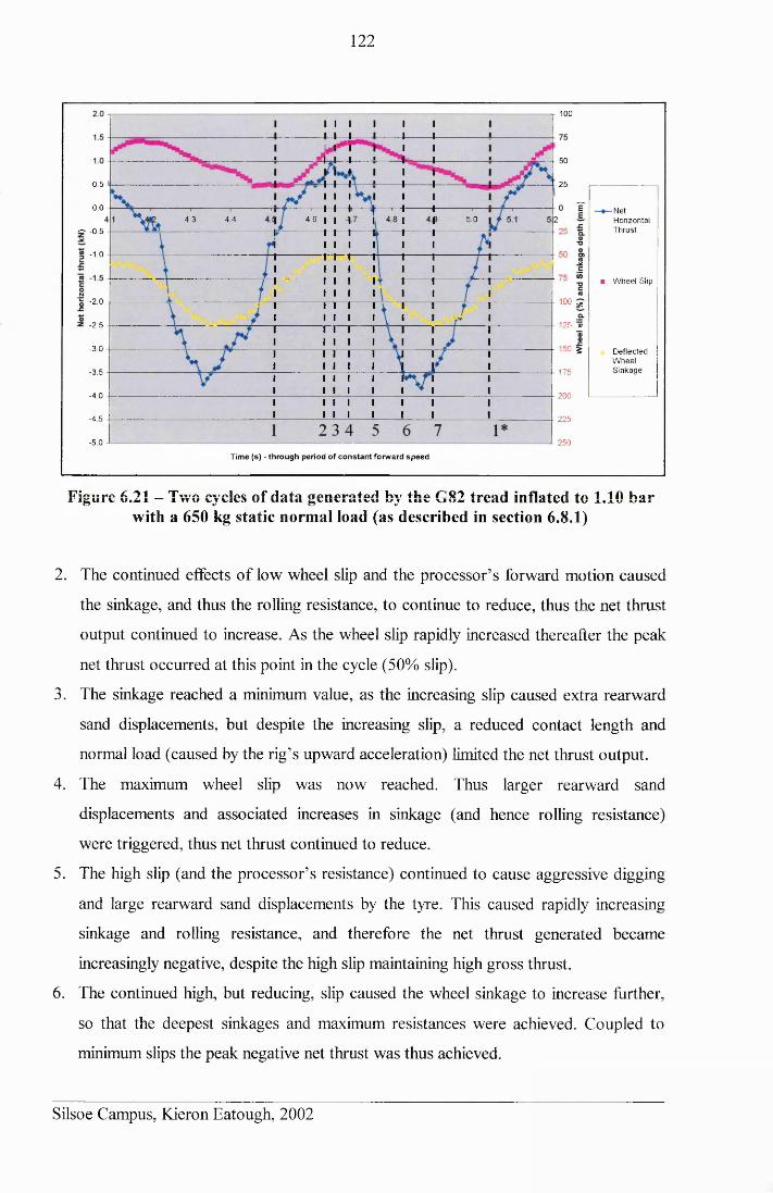
122
- r 100
50
0.5 25
0.0 - NetHorizontalT hrust
4.3 4.4 4 .6 5 .0~ -0.5
- 1.0
■ W heel Slip
1005 -2.0
z -2.5 125 »
-3 .0 150 g D eflectedW heelS in k ag e-3 .5 175
-4.0 200
-4.5 225
-5.0 — J- 250
Tim e (s) - through period o f c o n sta n t forw ard s p e e d
Figure 6.21 - Two cycles of data generated by the G82 tread inflated to 1.10 bar with a 650 kg static normal load (as described in section 6.8.1)
2. The continued effects of low wheel slip and the processor’s forward motion caused
the sinkage, and thus the rolling resistance, to continue to reduce, thus the net thrust
output continued to increase. As the wheel slip rapidly increased thereafter the peak
net thrust occurred at this point in the cycle (50% slip).
3. The sinkage reached a minimum value, as the increasing slip caused extra rearward
sand displacements, but despite the increasing slip, a reduced contact length and
normal load (caused by the rig’s upward acceleration) limited the net thrust output.
4. The maximum wheel slip was now reached. Thus larger rearward sand
displacements and associated increases in sinkage (and hence rolling resistance)
were triggered, thus net thrust continued to reduce.
5. The high slip (and the processor’s resistance) continued to cause aggressive digging
and large rearward sand displacements by the tyre. This caused rapidly increasing
sinkage and rolling resistance, and therefore the net thrust generated became
increasingly negative, despite the high slip maintaining high gross thrust.
6. The continued high, but reducing, slip caused the wheel sinkage to increase further,
so that the deepest sinkages and maximum resistances were achieved. Coupled to
minimum slips the peak negative net thrust was thus achieved.
Silsoe Campus, Kieron Eatough, 2002
123
7. The peak sinkage was quickly reached as the low slip reduced the rearward sand
movements, so continued tyre rotation and forward displacement of the processor
forced the tyre to begin climbing out of the sand. The reducing sinkage (rolling
resistance) allowed the net horizontal thrust to increase and the tyre returned to stage
1*. Thereafter the cycle of passing from mobility to immobility due to high slips
was once again repeated.
This understanding related both the drivers of, and the responses to, the relationships
between the wheel slip, sinkage and net thrust. It also allowed the effect upon the net
thrust of both, the variations in dynamic normal loading, and the positive relationship
between tyre sinkage and the associated rolling resistance to be understood. This
understanding allowed the importance of the effect of sand displacement (sinkage) upon
tyre mobility to be realised. This enabled the sections of the thrust cycle where sand
displacement measurements were required to enable the quantification of this effect to
be identified (see section 7.3).
6.7 COMPARISON (VERIFICATION) TESTS ON SOIL
The re-design meant that the effectiveness and suitability of the variable slip rig had to
be evaluated against the performance of the fixed slip test rig. It was particularly
important to compare net thrusts and sinkages produced across a slip range when using
the variable slip rig, against those that had been produced at discrete slips (within the
same slip range) by the fixed slip rig. If agreement occurred between the two sets of
results (for the same treatments), then the variable slip test rig could be confidently used
for the future tests. Tests were conducted using the variable slip rig to obtain results for
the following treatments:
• PT tread inflated to 3.10 bar (thereby minimising any tyre deflection effects),
• 1170 kg/m and 1270 kg/m soil density preparations,
• A static normal load of 650 kg,
• A variable slip range that encompassed discrete slips of 15%, 20%, 40% and
50%, i.e. the discrete slips tested by the fixed slip tests.
Silsoe Campus, Kieron Eatough, 2002
124
The results from these tests were compared to results generated when testing the
following treatments with the fixed slip rig (before its modification):
• PT inflated to 3.10 bar,
• 1170 kg/m and 1270 kg/m soil density preparations,
• Static normal loads of 350 kg, 450 kg, 550 kg, 650 kg, 750 kg and 850 kg,
• Target discrete slips of 15%, 20%, 40% and 50%.
6.7.1 Variable Slip Test Results
It was found that when the variable slip test rig was set to achieve a nominal slip of 50%
it produced results that were comparable to the results that the fixed slip rig had
produced on the sand when operated at high slips, i.e. a variable thrust-slip cycle was
produced, which created vertical accelerations of the rig. Therefore the flow divider did
not make the test rig produce a constant slip value, but rather a consistent range of
wheel slips, which would typically fluctuate from 15% to 70% wheel slip, as the typical
results presented in Figure 6.22 for an intended 50% slip setting indicate.
As well as fluctuating slips and sinkages, the results showed that the net thrusts also
altered considerably over the course of a test-run. The wheel slip fluctuations caused the
significant variations in wheel sinkage that were experienced, and thus (due to the
relationships noted in section 6.4) they indirectly controlled the rolling resistance.
Silsoe Campus, Kieron Eatough, 2002
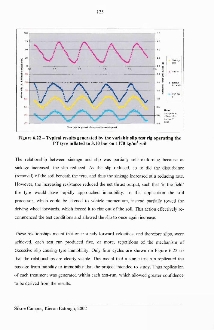
125
100 r 5.0
75 4.5
4.0
3.5S in k a g e
3.00.5 2.0
a Slip
2.0 ♦ Net hz fo rce kN
Vert acc
100 1.0
125 0.5Note:Z ero point is differen t for th e two Y
150 -0.0
175 J------- -L -0.5
Tim e (s ) - for period o f c o n sta n t forw ard s p e e d
Figure 6.22 — Typical results generated by the variable slip test rig operating the PT tyre inflated to 3.10 bar on 1170 kg/m3 soil
The relationship between sinkage and slip was partially self-reinforcing because as
sinkage increased, the slip reduced. As the slip reduced, so to did the disturbance
(removal) of the soil beneath the tyre, and thus the sinkage increased at a reducing rate.
However, the increasing resistance reduced the net thrust output, such that ‘in the field’
the tyre would have rapidly approached immobility. In this application the soil
processor, which could be likened to vehicle momentum, instead partially towed the
driving wheel forwards, which forced it to rise out of the soil. This action effectively re
commenced the test conditions and allowed the slip to once again increase.
These relationships meant that once steady forward velocities, and therefore slips, were
achieved, each test run produced five, or more, repetitions of the mechanism of
excessive slip causing tyre immobility. Only four cycles are shown on Figure 6.22 so
that the relationships are clearly visible. This meant that a single test run replicated the
passage from mobility to immobility that the project intended to study. Thus replication
of each treatment was generated within each test-run, which allowed greater confidence
to be derived from the results.
Silsoe Campus, Kieron Eatough, 2002
126
This methodology introduced a drawback, as the frame’s height constantly varied due to
the fluctuating sinkage. This caused vertical acceleration of the test rig, such that the
static normal tyre load of 6.377 kN was either increased, or decreased, depending upon
the location in the thrust cycle. However, the adjustment to the normal load could be
derived by using the equation F = ma, where a (gravitational acceleration) was
increased (or reduced) by a factor, g \ to represent the acting acceleration. The acting
acceleration a ’ (in m/s2) was derived from the displacement, s, by using the relationship
d2sa '= —- . Dividing a ’ by 9.81 produced the acting g ’ factor. This was applied as d r
follows; if the g ’ factor was calculated as +0 .2 , then the dynamic normal tyre load
would equal; 650 x (9.81 x (1 + 0.2)) = 7.652 kN. Dynamic normal load fluctuations
were experienced up to ±0.5#, over all the testing, which equated to a range of mass
from 325 kg to 975 kg. Figure 6.22 shows the typical cyclical nature of these variations.
Quantifying this effect allowed the rigs to be compared when the same normal loads
were acting upon the tyres.
6.7.2 Methodology for Test Rig Performance Comparisons
Useful suitable comparisons could only be made between results taken when similar
treatments were tested on both rigs. As only the normal load and wheel slip were
deliberately varied, achieving this need was simplified. The results from the variable
slip test runs used for comparison with those from the fixed slip tests were taken over
the period of decreasing wheel slip, as the high slip caused the wheel to dig into the soil,
which generated gross thrust, but which also increased the rolling resistance, causing
immobility to be approached. Typical data regions used for the comparison are shown
in Figure 6.23. Data outside these regions was ignored for this comparison.
The variable slip test rig produced results similar to those shown by Figure 6.23 on both
soil preparations. From these results five or six consecutive regions of decreasing slip
were selected from each test run’s period of constant forward speed and all of the net
thrusts, sinkages, slips and g ’ factors that occurred in those regions were noted. The
selected results for each test run were grouped and ordered by ascending slip value.
Silsoe Campus, Kieron Eatough, 2002
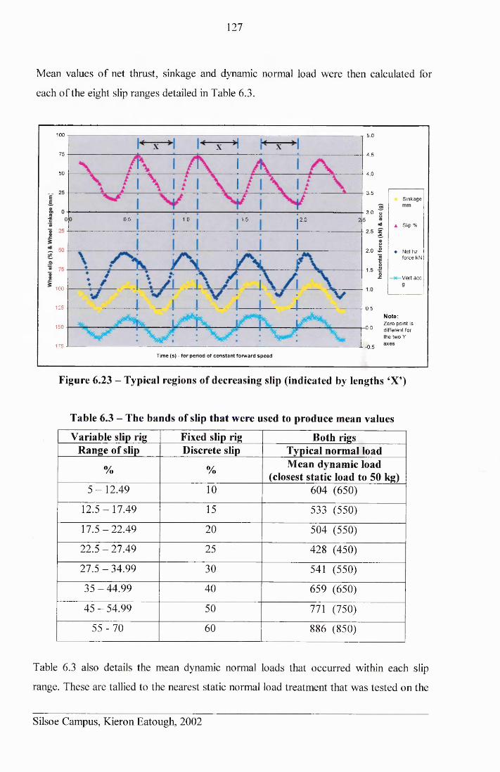
127
Mean values of net thrust, sinkage and dynamic normal load were then calculated for
each of the eight slip ranges detailed in Table 6.3.
100 r 5 .0
75 4.5
5 0 4.0
3.5S in k ag e
3 .01.00.5 1.5 2.0
A Slip %
2.0 ♦ N et hz fo rce kN
Vert acc
100
125 0.5
N o te :Z ero point is d ifferen t for th e tw o Y
150 -0.0
175 i -0 .5
Tim e (s) - for period o f c o n sta n t forw ard s p e e d
Figure 6.23 - Typical regions of decreasing slip (indicated by lengths ‘X’)
Table 6.3 - The bands of slip that were used to produce mean values
Variable slip rig Fixed slip rig Both rigsRange of slip Discrete slip Typical normal load
% % Mean dynamic load (closest static load to 50 kg)
5-12.49 10 604 (650)
12.5-17.49 15 533 (550)
17.5-22.49 20 504 (550)
22.5 - 27.49 25 428 (450)
27.5-34.99 30 541 (550)
35-44.99 40 659 (650)
45 - 54.99 50 771 (750)
55-70 60 886 (850)
Table 6.3 also details the mean dynamic normal loads that occurred within each slip
range. These are tallied to the nearest static normal load treatment that was tested on the
Silsoe Campus, Kieron Eatough, 2002
128
fixed slip rig, i.e. for a mean dynamic load of 604 kg (variable slip), the nearest static
load tested using the fixed slip rig was 650 kg. The mean net thrusts and sinkages
measured using the variable slip rig were plotted against appropriate sets of results
recorded with the fixed slip rig. Appropriate results were selected by using mean results
from the constant speed sections of the tests (section 6.4) with normal load and discrete
slip conditions that matched the data presented in Table 6.3, e.g. at a discrete slip of
40% results recorded with a 750 kg normal load were used. Undeflected tyre sinkages
were used for the comparison, as the drawstring transducers were not fitted for the
variable slip runs.
6.7.3 Test Riq Comparison Results*3
The results for the tests on the 1170 kg/m soil are presented in Figure 6.24, and those
for the 1270 kg/m3 soil in Figure 6.25. Generally, agreement existed between the results
from the two test rigs with all the results being of comparable magnitudes. The closest
agreement occurred in the net thrust results. Agreement occurred between the sinkages,
but more variation occurred between results across the slip range. Broadly both test rigs
extracted similar tractive performances from the same treatments and in both cases the
tyres operating on the firmer surface generated lower sinkages, and thus higher net
thrusts, as traction theory would predict20.
When the results were more closely examined to determine the cause of the variations,
it was noted that the fixed slip rig results displayed the classical trends of small
increases in net thrust with increased slip, whereas the variable slip rigs’ results
displayed some differing trends, with all the results having slightly ‘U’ shaped profiles.
Initially the sinkage increased with slip, as would be expected, but above 40% slip it
then decreased with increased slip. Differences also occurred in the associated net thrust
results, such that higher net thrusts were achieved at the higher and lower slips.
Silsoe Campus, Kieron Eatough, 2002
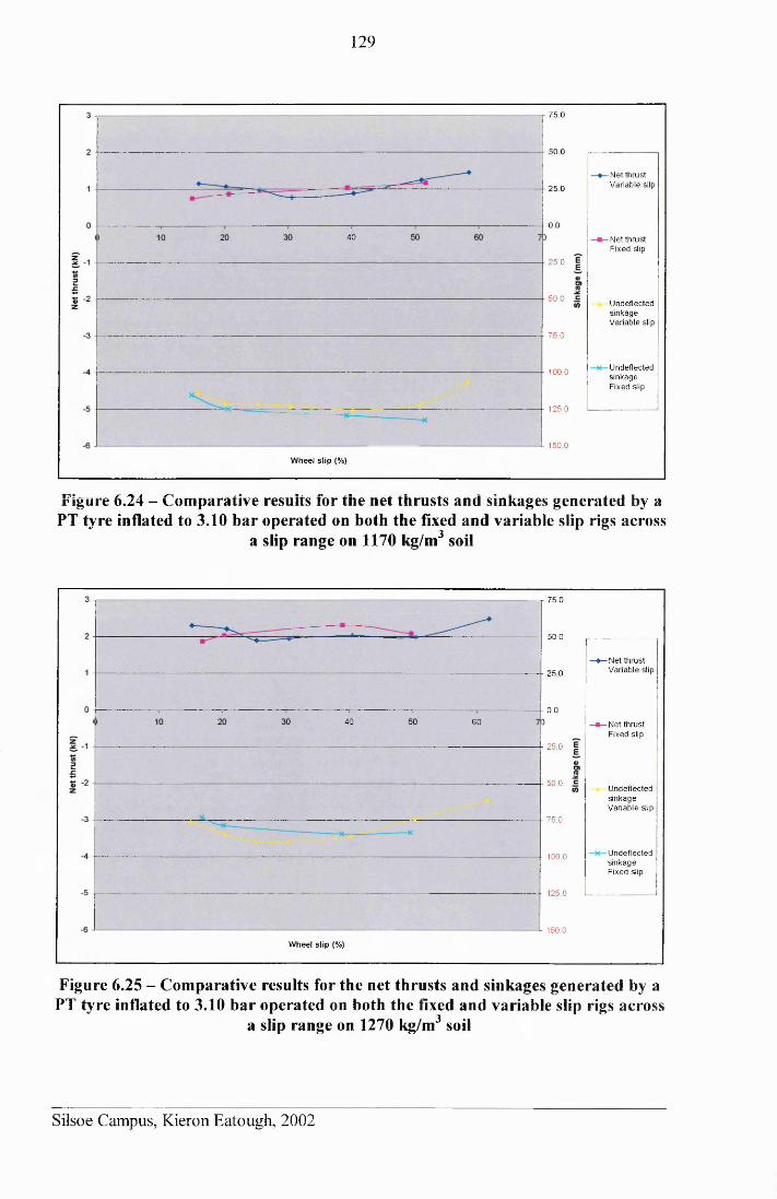
129
75.0
50.0
■Net th ru st V ariab le slip25.0
0.040 N et th ru st
Fixed slip
2 5 .0
50 .0 U ndeflected s in k ag e V ariab le slip
7 5 .0
U ndeflected s in k ag e F ixed slip
100.0
125.0
150.0
W heel s lip (%)
Figure 6.24 - Comparative resuits for the net thrusts and sinkages generated by a PT tyre inflated to 3.10 bar operated on both the fixed and variable slip rigs across
a slip range on 1170 kg/m3 soil
r 75.0
50.0
N et th rust V ariab le slip25 .0
0.040 6 0 —■— N et th ru st
F ixed slip
25 .0
50 .0U ndeflected s in k ag e V ariab le slip
7 5 .0
U ndeflected s in k ag e F ixed slip
100.0
125.0
L 150.0
W heel s lip (%)
Figure 6.25 - Comparative results for the net thrusts and sinkages generated by a PT tyre inflated to 3.10 bar operated on both the fixed and variable slip rigs across
a slip range on 1270 kg/m3 soil
Silsoe Campus, Kieron Eatough, 2002
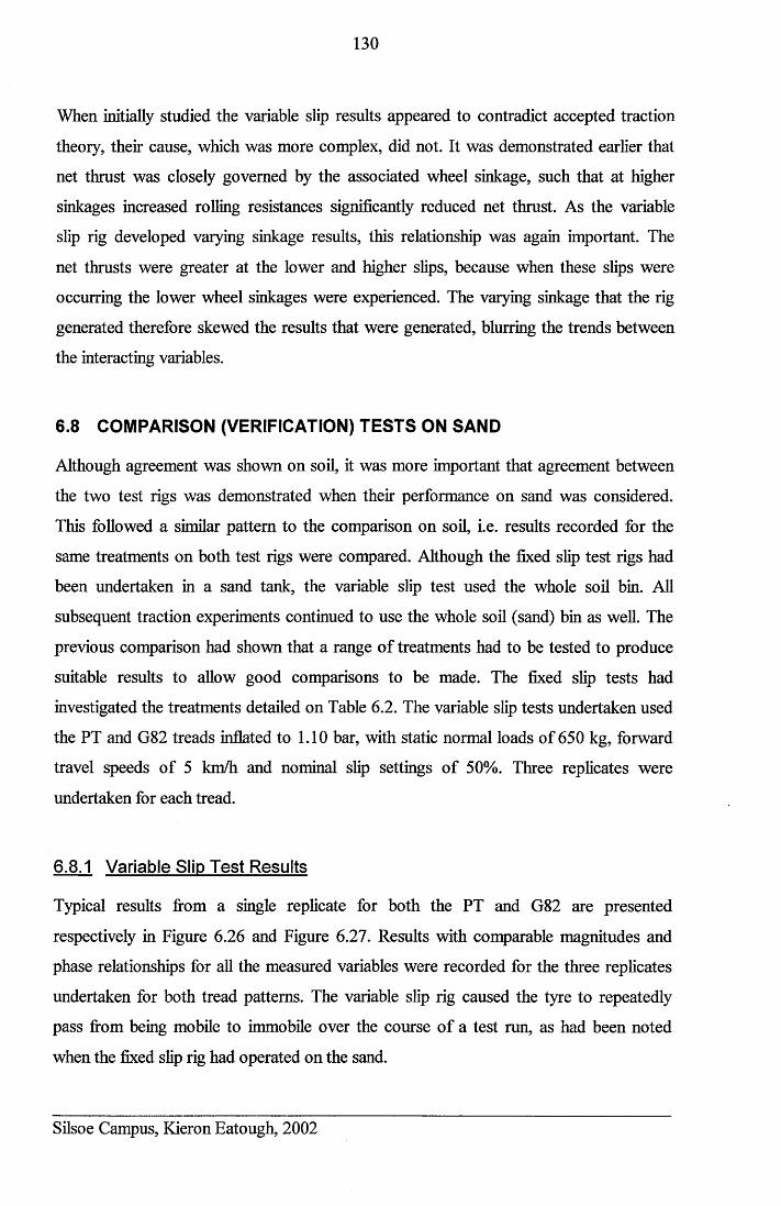
130
When initially studied the variable slip results appeared to contradict accepted traction
theory, their cause, which was more complex, did not. It was demonstrated earlier that
net thrust was closely governed by the associated wheel sinkage, such that at higher
sinkages increased rolling resistances significantly reduced net thrust. As the variable
slip rig developed varying sinkage results, this relationship was again important. The
net thrusts were greater at the lower and higher slips, because when these slips were
occurring the lower wheel sinkages were experienced. The varying sinkage that the rig
generated therefore skewed the results that were generated, blurring the trends between
the interacting variables.
6.8 COMPARISON (VERIFICATION) TESTS ON SAND
Although agreement was shown on soil, it was more important that agreement between
the two test rigs was demonstrated when their performance on sand was considered.
This followed a similar pattern to the comparison on soil, i.e. results recorded for the
same treatments on both test rigs were compared. Although the fixed slip test rigs had
been undertaken in a sand tank, the variable slip test used the whole soil bin. All
subsequent traction experiments continued to use the whole soil (sand) bin as well. The
previous comparison had shown that a range of treatments had to be tested to produce
suitable results to allow good comparisons to be made. The fixed slip tests had
investigated the treatments detailed on Table 6.2. The variable slip tests undertaken used
the PT and G82 treads inflated to 1.10 bar, with static normal loads of 650 kg, forward
travel speeds of 5 km/h and nominal slip settings of 50%. Three replicates were
undertaken for each tread.
6.8.1 Variable Slip Test Results
Typical results from a single replicate for both the PT and G82 are presented
respectively in Figure 6.26 and Figure 6.27. Results with comparable magnitudes and
phase relationships for all the measured variables were recorded for the three replicates
undertaken for both tread patterns. The variable slip rig caused the tyre to repeatedly
pass from being mobile to immobile over the course of a test run, as had been noted
when the fixed slip rig had operated on the sand.
Silsoe Campus, Kieron Eatough, 2002
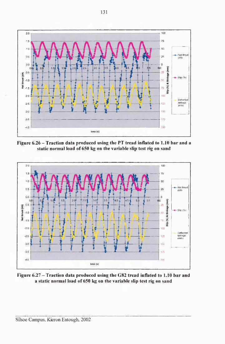
131
- r 1 0 0
1.5
5 01.0
N et th ru st (kN)2 50 .5
0.03 .52.0 ,2 .5 3 .01 .0 .
^ -0 .5
Slip (% )5 0
z -1 .5
100-2.0D eflectedsin k ag e(m m )
12 5-2 .5
150-3 .0
175-3 .5
-J- 2 0 0-4 .0 J
t im e (s )
Figure 6.26 - Traction data produced using the PT tread inflated to 1.10 bar and a static normal load of 650 kg on the variable slip test rig on sand
2.0 ~ r 1 0 0
7 5
1.0 5 0
N et th ru st(kN)0 .5
0.03 .52.0" 2 5 5 .53 .0 ” 4 .5
— -0 .5
Slip (% )5 0
z -1 .5 7 5
-2.0 100
D eflec teds inkage(m m )
-2 .5 125
-3 .0 1 50
-3 .5 1 75
-4 .0 -1 -J- 200
t im e (s )
Figure 6.27 - Traction data produced using the G82 tread inflated to 1.10 bar and a static normal load of 650 kg on the variable slip test rig on sand
Silsoe Campus, Kieron Eatough, 2002
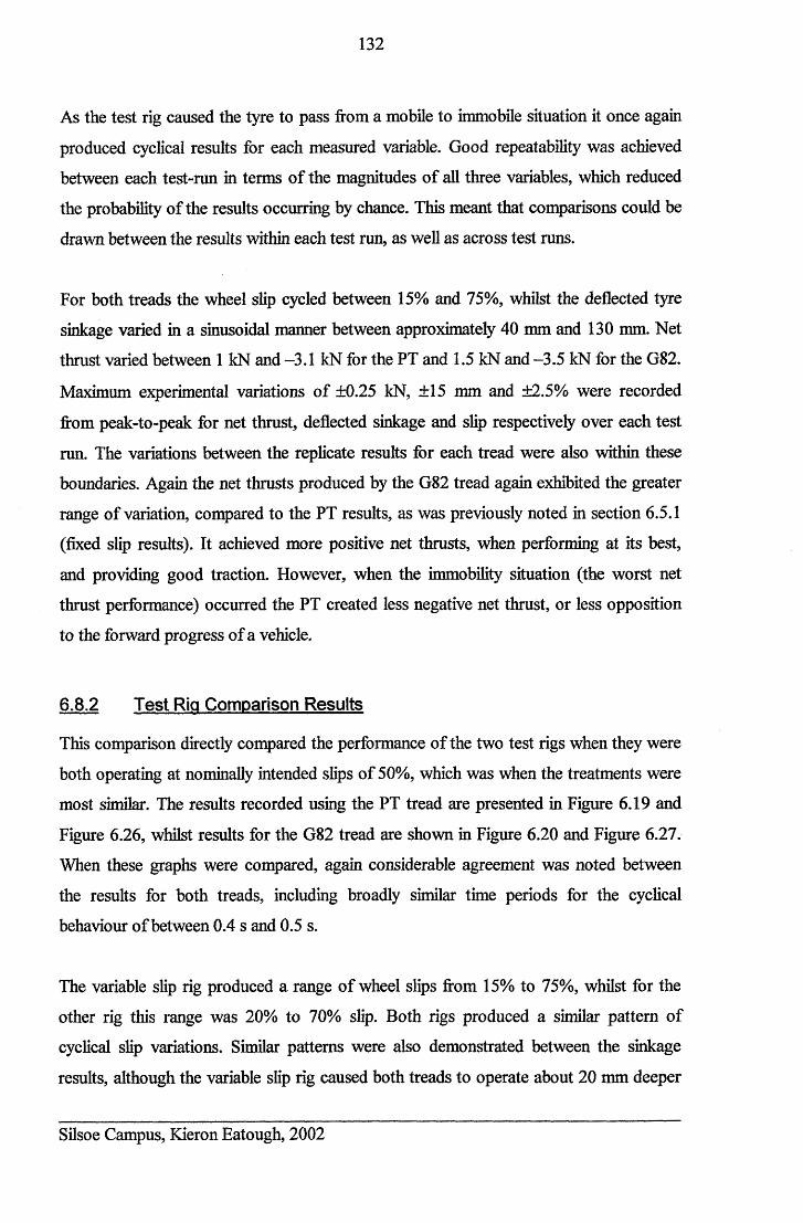
132
As the test rig caused the tyre to pass from a mobile to immobile situation it once again
produced cyclical results for each measured variable. Good repeatability was achieved
between each test-run in terms of the magnitudes of all three variables, which reduced
the probability of the results occurring by chance. This meant that comparisons could be
drawn between the results within each test run, as well as across test runs.
For both treads the wheel slip cycled between 15% and 75%, whilst the deflected tyre
sinkage varied in a sinusoidal manner between approximately 40 mm and 130 mm. Net
thrust varied between 1 kN and -3.1 kN for the PT and 1.5 kN and -3.5 kN for the G82.
Maximum experimental variations of ±0.25 kN, ±15 mm and ±2.5% were recorded
from peak-to-peak for net thrust, deflected sinkage and slip respectively over each test
run. The variations between the replicate results for each tread were also within these
boundaries. Again the net thrusts produced by the G82 tread again exhibited the greater
range of variation, compared to the PT results, as was previously noted in section 6.5.1
(fixed slip results). It achieved more positive net thrusts, when performing at its best,
and providing good traction. However, when the immobility situation (the worst net
thrust performance) occurred the PT created less negative net thrust, or less opposition
to the forward progress of a vehicle.
6.8.2 Test Riq Comparison Results
This comparison directly compared the performance of the two test rigs when they were
both operating at nominally intended slips of 50%, which was when the treatments were
most similar. The results recorded using the PT tread are presented in Figure 6.19 and
Figure 6.26, whilst results for the G82 tread are shown in Figure 6.20 and Figure 6.27.
When these graphs were compared, again considerable agreement was noted between
the results for both treads, including broadly similar time periods for the cyclical
behaviour of between 0.4 s and 0.5 s.
The variable slip rig produced a range of wheel slips from 15% to 75%, whilst for the
other rig this range was 20% to 70% slip. Both rigs produced a similar pattern of
cyclical slip variations. Similar patterns were also demonstrated between the sinkage
results, although the variable slip rig caused both treads to operate about 20 mm deeper
Silsoe Campus, Kieron Eatough, 2002
133
when maximum sinkage was produced. At the minimum sinkages produced both rigs
caused sinkages of approximately 55 mm. The variation in depth at maximum sinkage
may have been caused by the difference in the test tanks, or because of the difference in
the length of the test runs, as when the foil bin was used the rig had longer to settle into
its rhythm, which possibly allowed greater sinkages to develop.
Each tread developed different net thrusts, as described previously, but when these were
compared between the two rigs, it was noted that the ranges of net thrusts were again
similar. Thus both rigs were capable of deriving similar levels of tractive performance
from the tyres under investigation. Although small differences were achieved between
each oscillation effects for both test rigs, it was concluded that overall the oscillation
effects were similar for both systems. Generally the individual differences were not
significant, as where practicable, mean data from a number of oscillations or test-runs
would be considered when comparing the tyre (tread) tractive performance. The
similarities between the results for both tyre treatments indicated that the consistently
fluctuating results were not generated solely by a particular drive mechanism, and were
instead mainly the result of the sand/ tyre interaction and sand displacement. The use of
the processor to provide a fixed resistance influenced this behaviour, but it was not the
main driver in the relationships.
For a completely accurate comparison to have been achieved, in the manner attempted,
it would have been necessary to design and develop a methodology to prevent wheel
sinkage, whilst still allowing complete tyre-soil contact to be maintained, irrespective of
the wheel slip. Whilst such a design may have been possible, to produce suitable
apparatus would have been a major distraction from the project’s objectives. Instead, it
was more beneficial to take the agreement demonstrated between the sets of results
from the two rigs as sufficient proof that the variable slip rig was capable of conducting
realistic and useful tractive performance tests. Additionally, as the operation of the
variable slip rig produced a number of immobilisation events over a single test run, the
effect of tread upon mobility (or immobility) on sand could be more thoroughly
investigated.
Silsoe Campus, Kieron Eatough, 2002
134
As the effect of these relationships upon the tyre mobility remained of interest, further
testing was continued with the variable slip rig because of its ability to produce greater
consistency in the results, due to its ability to more smoothly apply the variations in
torque that occurred, and because it allowed a particular test schedule to be completed
faster. Improvements to the design of the variable slip rig also meant that an unlimited
range of tyre and surface treatments could be studied during the further investigations.
Using this rig meant that it was impossible to produce traditional slip-pull curves from
the results, as the slip-pull inter-relationship was always complicated by the varying
sinkage, which controlled both the rolling resistance and the contact length. This
complication was tackled by the modelling that was developed, which allowed the
performance of the treads to be compared, so it was not an obstacle to the
investigations.
6.9 A FULL VEHICLE TEST ON SAND
A separate project undertaken by Cranfield University staff and Land Rover140
generated some limited traction test data for a full vehicle operating on the replicate
sand in the soil bin. The testing used a V8 Land Rover Discovery Series 2 fitted with
235/70 R16 Goodyear HP Wrangler tyres inflated to 1.24 bar. The right side of the
vehicle drove on the sand, whilst the left side operated on sealed concrete. A full vehicle
width beam was mounted to the rear chassis. Tension links attached at either end of the
beam allowed independent net thrust measurement along each side of the vehicle.
Wheel speed was measured from pulses off the ABS sensors and the true forward speed
was measured with ground radar. The wheel slip was derived from these two readings.
The tension links were connected to a beam that attached to a winch drum mounted on a
static tractor, via a winch cable. As the Discovery was driven forwards the tension
began to retard the vehicle, the throttle was incrementally increased until it was frilly
open, which gave an increasing slip profile. As the tyres on the sand became buried, the
throttle was released and so the slip declined. A plot of the net thrusts achieved by the
right side tyres, with both the differential locks and the traction control disengaged, is
shown in Figure 6.28.
Silsoe Campus, Kieron Eatough, 2002
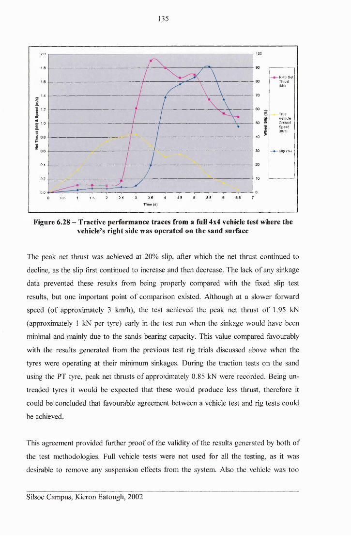
135
— 1002.0 T
RHS NetT hrust(kN)
1.4
1.2T rueV ehicleG roundS p eed(m /s)
~ 1.0
40
Slip (% )
0 .4
100.2
0.05.53 .5
T im e (s)
4 .52 .50.5 1.5
Figure 6.28 - Tractive performance traces from a full 4x4 vehicle test where the vehicle’s right side was operated on the sand surface
The peak net thrust was achieved at 20% slip, after which the net thrust continued to
decline, as the slip first continued to increase and then decrease. The lack of any sinkage
data prevented these results from being properly compared with the fixed slip test
results, but one important point of comparison existed. Although at a slower forward
speed (of approximately 3 km/h), the test achieved the peak net thrust of 1.95 kN
(approximately 1 kN per tyre) early in the test run when the sinkage would have been
minimal and mainly due to the sands bearing capacity. This value compared favourably
with the results generated from the previous test rig trials discussed above when the
tyres were operating at their minimum sinkages. During the traction tests on the sand
using the PT tyre, peak net thrusts of approximately 0.85 kN were recorded. Being un-
treaded tyres it would be expected that these would produce less thrust, therefore it
could be concluded that favourable agreement between a vehicle test and rig tests could
be achieved.
This agreement provided further proof of the validity of the results generated by both of
the test methodologies. Full vehicle tests were not used for all the testing, as it was
desirable to remove any suspension effects from the system. Also the vehicle was too
Silsoe Campus, Kieron Eatough, 2002

136
wide to fully operate in the soil bin, so variations in the heights of the bin and sand
caused the vehicle tilt. Additionally it would not have been possible to operate safely on
the dissimilar surfaces without the requirement for steering inputs, which would have
added another dimension to the complex interactions experienced. Further testing was
therefore conducted with the variable slip test rig for the pressure and sand displacement
investigations as this had proved to be the most useful test device.
Silsoe Campus, Kieron Eatough, 2002
137
7 SAND FLOW MEASUREMENT APPARATUS AND
METHODOLOGY
7.1 SAND AND RFID TAG DISPLACEMENT ASSESSMENT
7.1.1 Bench Sand Flow Evaluations
The initial investigations into the suitability of the RFID system were conducted in
small sand masses. The first trial investigated the abilities of the two available RFID
scanners (Appendix 1) to detect the 0 2 mm x 12 mm long tags in a sand mass. The
more powerful scanner detected tags up to 150 mm deep, but this greater range became
a hindrance when trying to locate several closely spaced tags, because interfering
signals from the tags ‘confused’ the scanner, and so it would not register any of the tags.
Hence the smaller scanner, see Plate 3.4, which could locate tags up to 100 mm to 125
mm deep was more suitable. The variance in the range of detection occurred because
variations in the orientations of the tags affected the scanner’s sensitivity.
The tags were entered into a small sand mass (approximate size 400 mm x 300 mm x
300 mm), which was then disturbed laterally. The small size of the tags appeared to
allow them to flow with the sand mass, although this was not definitely confirmed at
this stage. It was established that by scanning over a buried tag from several directions
its location in plan view could be closely determined, such that the tag would lie
centrally in the region over which it could be detected. It was also found that because
the mass of a tag was greater than that of a sand grain, the overlaying sand layers could
be gently sucked off a tag (using a vacuum tube) to reveal the tag’s location without
disturbing its position, which could then be measured. These promising results made it
necessary to evaluate the flow relationship between the tags and the sand, to check that
the tags would flow exactly with surrounding sand grains, thus making them suitable as
markers for tracking sand flow.
7.1.1.1 RFID Tag and sand flow assessment methodology
The aim of this experiment was to quantify if the tags would flow with the sand. For
this assessment a quantity of dyed replicate sand (achieved using potassium
Silsoe Campus, Kieron Eatough, 2002
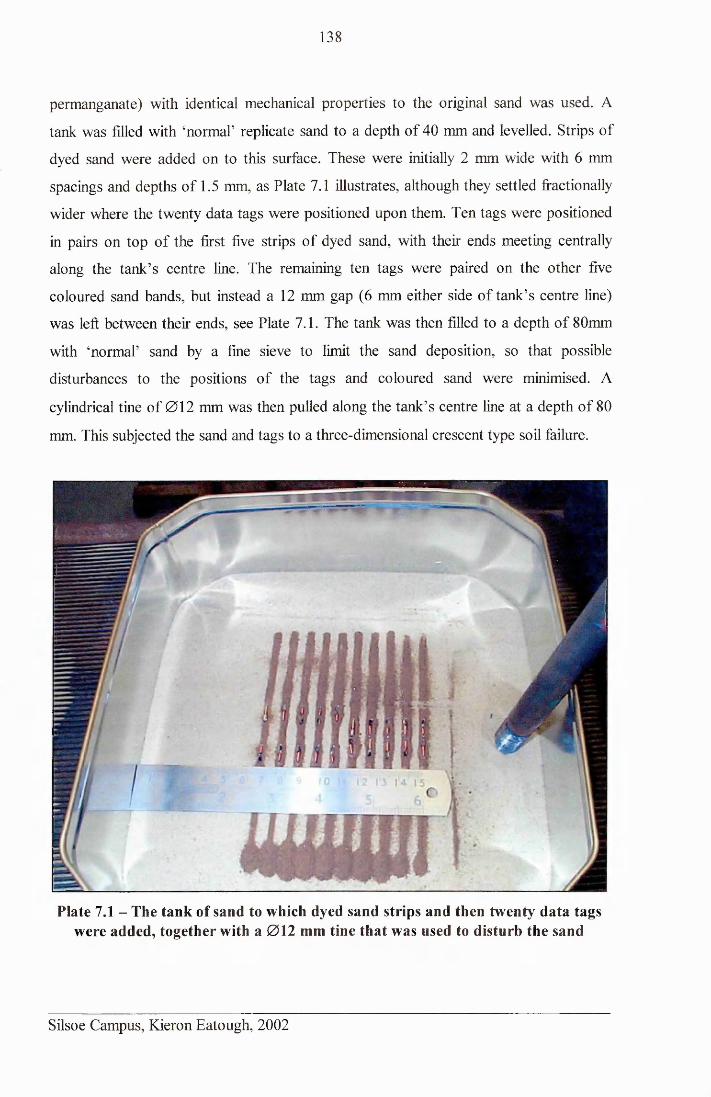
138
permanganate) with identical mechanical properties to the original sand was used. A
tank was filled with ‘normal’ replicate sand to a depth of 40 mm and levelled. Strips of
dyed sand were added on to this surface. These were initially 2 mm wide with 6 mm
spacings and depths of 1.5 mm, as Plate 7.1 illustrates, although they settled fractionally
wider where the twenty data tags were positioned upon them. Ten tags were positioned
in pairs on top of the first five strips of dyed sand, with their ends meeting centrally
along the tank’s centre line. The remaining ten tags were paired on the other five
coloured sand bands, but instead a 12 mm gap (6 mm either side of tank’s centre line)
was left between their ends, see Plate 7.1. The tank was then filled to a depth of 80mm
with ‘normal’ sand by a fine sieve to limit the sand deposition, so that possible
disturbances to the positions of the tags and coloured sand were minimised. A
cylindrical tine of 012 mm was then pulled along the tank’s centre line at a depth of 80
mm. This subjected the sand and tags to a three-dimensional crescent type soil failure.
Plate 7.1 - The tank of sand to which dyed sand strips and then twenty data tags were added, together with a 0 1 2 mm tine that was used to disturb the sand
Silsoe Campus, Kieron Eatough, 2002
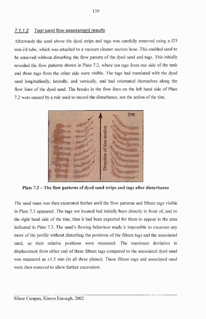
139
7.1.1.2 Tag/sand flow assessment results
Afterwards the sand above the dyed strips and tags was carefully removed using a 03
mm i/d tube, which was attached to a vacuum cleaner suction hose. This enabled sand to
be removed without disturbing the flow pattern of the dyed sand and tags. This initially
revealed the flow patterns shown in Plate 7.2, where ten tags from one side of the tank
and three tags from the other side were visible. The tags had translated with the dyed
sand longitudinally, laterally, and vertically, and had orientated themselves along the
flow lines of the dyed sand. The breaks in the flow lines on the left hand side of Plate
7.2 were caused by a rule used to record the disturbance, not the action of the tine.
Plate 7.2 - The flow patterns of dyed sand strips and tags after disturbance
The sand mass was then excavated further until the flow patterns and fifteen tags visible
in Plate 7.3 appeared. The tags not located had initially been directly in front of, and to
the right hand side of the tine, thus it had been expected for them to appear in the area
indicated in Plate 7.3. The sand’s flowing behaviour made it impossible to excavate any
more of the profile without disturbing the positions of the fifteen tags and the associated
sand, so their relative positions were measured. The maximum deviation in
displacement from either end of these fifteen tags compared to the associated dyed sand
was measured as ±1.5 mm (in all three planes). These fifteen tags and associated sand
were then removed to allow further excavation.
Silsoe Campus, Kieron Eatough, 2002
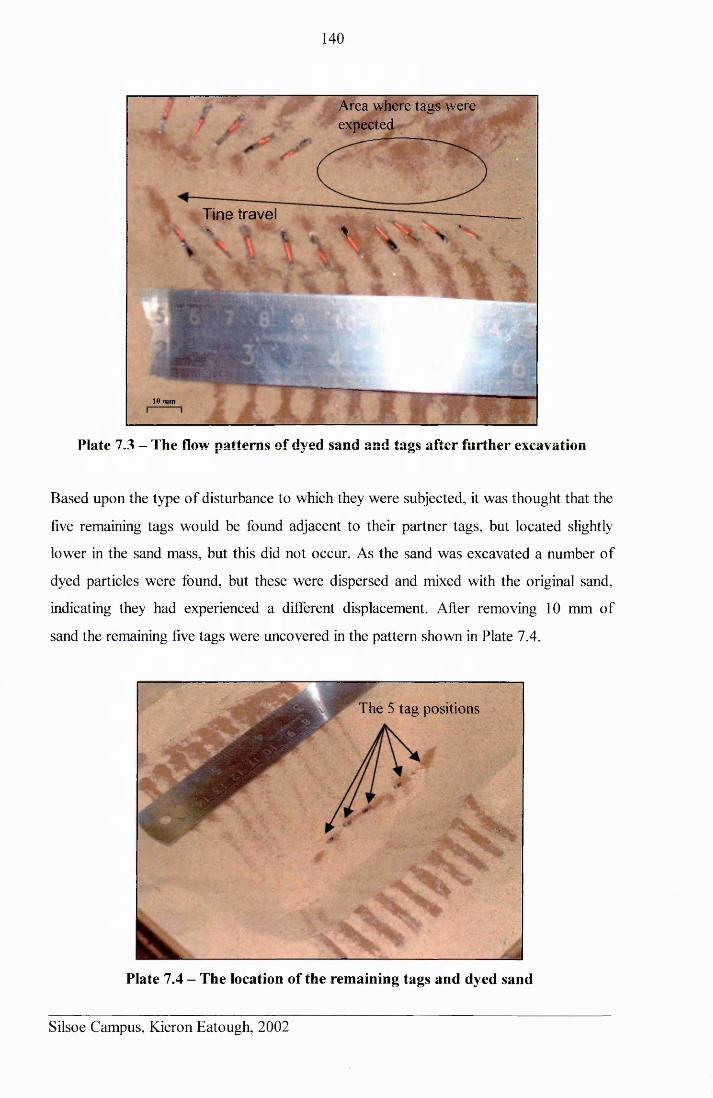
140
Area where tags were expected
Tine travel% V'.%
£
10 mm
Plate 7,3 - The flow patterns of dyed sand and tags after further excavation
Based upon the type of disturbance to which they were subjected, it was thought that the
five remaining tags would be found adjacent to their partner tags, but located slightly
lower in the sand mass, but this did not occur. As the sand was excavated a number of
dyed particles were found, but these were dispersed and mixed with the original sand,
indicating they had experienced a different displacement. After removing 10 mm of
sand the remaining five tags were uncovered in the pattern shown in Plate 7.4.
The 5 tag positions
Plate 7.4 - The location of the remaining tags and dyed sand
Silsoe Campus, Kieron Eatough, 2002
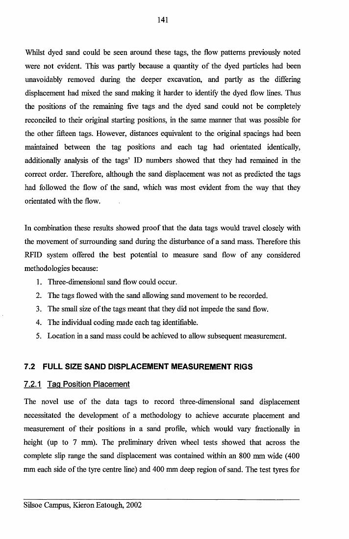
141
Whilst dyed sand could be seen around these tags, the flow patterns previously noted
were not evident. This was partly because a quantity of the dyed particles had been
unavoidably removed during the deeper excavation, and partly as the differing
displacement had mixed the sand making it harder to identify the dyed flow lines. Thus
the positions of the remaining five tags and the dyed sand could not be completely
reconciled to their original starting positions, in the same manner that was possible for
the other fifteen tags. However, distances equivalent to the original spacings had been
maintained between the tag positions and each tag had orientated identically,
additionally analysis of the tags’ ID numbers showed that they had remained in the
correct order. Therefore, although the sand displacement was not as predicted the tags
had followed the flow of the sand, which was most evident from the way that they
orientated with the flow.
In combination these results showed proof that the data tags would travel closely with
the movement of surrounding sand during the disturbance of a sand mass. Therefore this
RFID system offered the best potential to measure sand flow of any considered
methodologies because:
1. Three-dimensional sand flow could occur.
2. The tags flowed with the sand allowing sand movement to be recorded.
3. The small size of the tags meant that they did not impede the sand flow.
4. The individual coding made each tag identifiable.
5. Location in a sand mass could be achieved to allow subsequent measurement.
7.2 FULL SIZE SAND DISPLACEMENT MEASUREMENT RIGS
7.2.1 Tag Position Placement
The novel use of the data tags to record three-dimensional sand displacement
necessitated the development of a methodology to achieve accurate placement and
measurement of their positions in a sand profile, which would vary fractionally in
height (up to 7 mm). The preliminary driven wheel tests showed that across the
complete slip range the sand displacement was contained within an 800 mm wide (400
mm each side of the tyre centre line) and 400 mm deep region of sand. The test tyres for
Silsoe Campus, Kieron Eatough, 2002
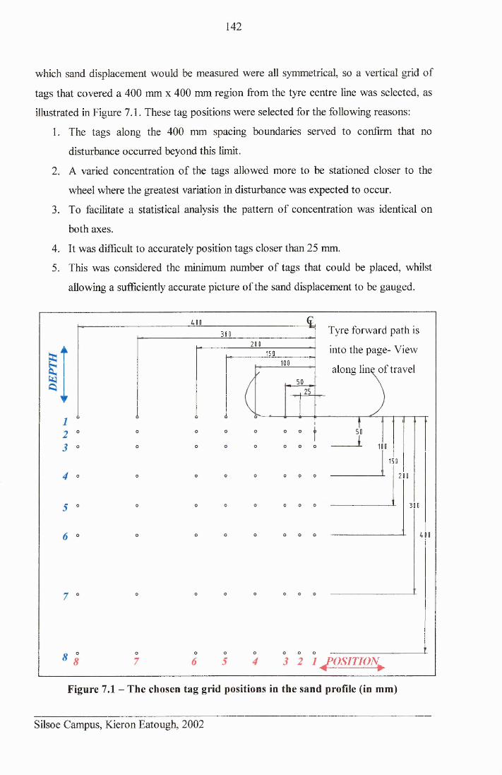
142
which sand displacement would be measured were all symmetrical, so a vertical grid of
tags that covered a 400 mm x 400 mm region from the tyre centre line was selected, as
illustrated in Figure 7.1. These tag positions were selected for the following reasons:
1. The tags along the 400 mm spacing boundaries served to confirm that no
disturbance occurred beyond this limit.
2. A varied concentration of the tags allowed more to be stationed closer to the
wheel where the greatest variation in disturbance was expected to occur.
3. To facilitate a statistical analysis the pattern of concentration was identical on
both axes.
4. It was difficult to accurately position tags closer than 25 mm.
5. This was considered the minimum number of tags that could be placed, whilst
allowing a sufficiently accurate picture of the sand displacement to be gauged.
Tyre forward path is
into the page- View
along line of travel
381
150
100
158
2 0 0
310
fosrriQNFigure 7.1 - The chosen tag grid positions in the sand profile (in mm)
Silsoe Campus, Kieron Eatough, 2002
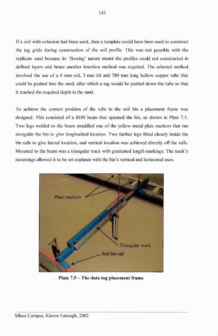
143
If a soil with cohesion had been used, then a template could have been used to construct
the tag grids during construction of the soil profile. This was not possible with the
replicate sand because its ‘flowing’ nature meant the profiles could not constructed in
defined layers and hence another insertion method was required. The selected method
involved the use of a 6 mm o/d, 3 mm i/d and 780 mm long hollow copper tube that
could be pushed into the sand, after which a tag would be pushed down the tube so that
it reached the required depth in the sand.
To achieve the correct position of the tube in the soil bin a placement frame was
designed. This consisted of a RHS beam that spanned the bin, as shown in Plate 7.5.
Two legs welded to the beam straddled one of the yellow metal plate markers that ran
alongside the bin to give longitudinal location. Two further legs fitted closely inside the
bin rails to give lateral location, and vertical location was achieved directly off the rails.
Mounted to the beam was a triangular track with graduated length markings. The track’s
mountings allowed it to be set coplanar with the bin’s vertical and horizontal axes.
Plate markers
Triangular track
Plate 7.5 - The data tag placement frame
Silsoe Campus, Kieron Eatough, 2002
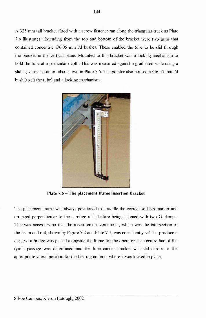
144
A 325 mm tall bracket fitted with a screw fastener ran along the triangular track as Plate
7.6 illustrates. Extending from the top and bottom of the bracket were two arms that
contained concentric 06.05 mm i/d bushes. These enabled the tube to be slid through
the bracket in the vertical plane. Mounted to this bracket was a locking mechanism to
hold the tube at a particular depth. This was measured against a graduated scale using a
sliding vernier pointer, also shown in Plate 7.6. The pointer also housed a 06.05 mm i/d
bush (to fit the tube) and a locking mechanism.
Plate 7.6 - The placement frame insertion bracket
The placement frame was always positioned to straddle the correct soil bin marker and
arranged perpendicular to the carriage rails, before being fastened with two G-clamps.
This was necessary so that the measurement zero point, which was the intersection of
the beam and rail, shown by Figure 7.2 and Plate 7.7, was consistently set. To produce a
tag grid a bridge was placed alongside the frame for the operator. The centre line of the
tyre’s passage was determined and the tube carrier bracket was slid across to the
appropriate lateral position for the first tag column, where it was locked in place.
Silsoe Campus, Kieron Eatough, 2002
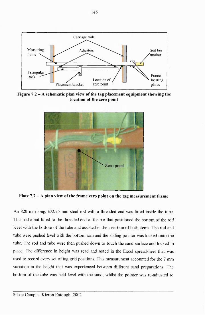
145
Carriage rails
Measuring frame \
Soil bin marker
Adjusters
Triangulartrack Frame
locatingplates
Location of zero pointPlacement bracket
Figure 7.2 - A schematic plan view of the tag placement equipment showing thelocation of the zero point
Plate 7.7 - A plan view of the frame zero point on the tag measurement frame
An 820 mm long, 02.75 mm steel rod with a threaded end was fitted inside the tube.
This had a nut fitted to the threaded end of the bar that positioned the bottom of the rod
level with the bottom of the tube and assisted in the insertion of both items. The rod and
tube were pushed level with the bottom arm and the sliding pointer was locked onto the
tube. The rod and tube were then pushed down to touch the sand surface and locked in
place. The difference in height was read and noted in the Excel spreadsheet that was
used to record every set of tag grid positions. This measurement accounted for the 7 mm
variation in the height that was experienced between different sand preparations. The
bottom of the tube was held level with the sand, whilst the pointer was re-adjusted to
Silsoe Campus, Kieron Eatough, 2002
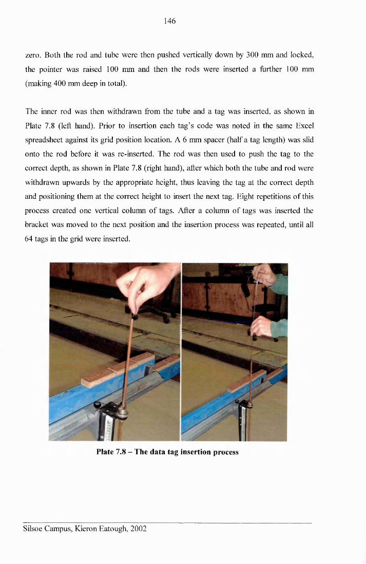
146
zero. Both the rod and tube were then pushed vertically down by 300 mm and locked,
the pointer was raised 100 mm and then the rods were inserted a further 100 mm
(making 400 mm deep in total).
The inner rod was then withdrawn from the tube and a tag was inserted, as shown in
Plate 7.8 (left hand). Prior to insertion each tag’s code was noted in the same Excel
spreadsheet against its grid position location. A 6 mm spacer (half a tag length) was slid
onto the rod before it was re-inserted. The rod was then used to push the tag to the
correct depth, as shown in Plate 7.8 (right hand), after which both the tube and rod were
withdrawn upwards by the appropriate height, thus leaving the tag at the correct depth
and positioning them at the correct height to insert the next tag. Eight repetitions of this
process created one vertical column of tags. After a column of tags was inserted the
bracket was moved to the next position and the insertion process was repeated, until all
64 tags in the grid were inserted.
Plate 7.8 - The data tag insertion process
Silsoe Campus, Kieron Eatough, 2002
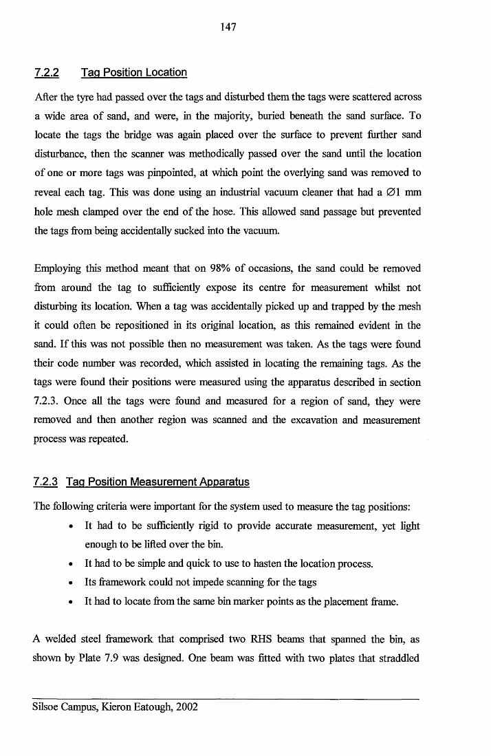
147
7.2.2 Tag Position Location
After the tyre had passed over the tags and disturbed them the tags were scattered across
a wide area of sand, and were, in the majority, buried beneath the sand surface. To
locate the tags the bridge was again placed over the surface to prevent further sand
disturbance, then the scanner was methodically passed over the sand until the location
of one or more tags was pinpointed, at which point the overlying sand was removed to
reveal each tag. This was done using an industrial vacuum cleaner that had a 01 mm
hole mesh clamped over the end of the hose. This allowed sand passage but prevented
the tags from being accidentally sucked into the vacuum.
Employing this method meant that on 98% of occasions, the sand could be removed
from around the tag to sufficiently expose its centre for measurement whilst not
disturbing its location. When a tag was accidentally picked up and trapped by the mesh
it could often be repositioned in its original location, as this remained evident in the
sand. If this was not possible then no measurement was taken. As the tags were found
their code number was recorded, which assisted in locating the remaining tags. As the
tags were found their positions were measured using the apparatus described in section
7.2.3. Once all the tags were found and measured for a region of sand, they were
removed and then another region was scanned and the excavation and measurement
process was repeated.
7.2.3 Tag Position Measurement Apparatus
The following criteria were important for the system used to measure the tag positions:
• It had to be sufficiently rigid to provide accurate measurement, yet light
enough to be lifted over the bin.
• It had to be simple and quick to use to hasten the location process.
• Its framework could not impede scanning for the tags
• It had to locate from the same bin marker points as the placement frame.
A welded steel framework that comprised two RHS beams that spanned the bin, as
shown by Plate 7.9 was designed. One beam was fitted with two plates that straddled
Silsoe Campus, Kieron Eatough, 2002
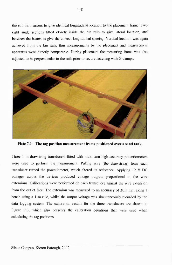
148
the soil bin markers to give identical longitudinal location to the placement frame. Two
right angle sections fitted closely inside the bin rails to give lateral location, and
between the beams to give the correct longitudinal spacing. Vertical location was again
achieved from the bin rails; thus measurements by the placement and measurement
apparatus were directly comparable. During placement the measuring frame was also
adjusted to be perpendicular to the rails prior to secure fastening with G-clamps.
Plate 7.9 - The tag position measurement frame positioned over a sand tank
Three 1 m drawstring transducers fitted with multi-turn high accuracy potentiometers
were used to perform the measurement. Pulling wire (the drawstring) from each
transducer turned the potentiometer, which altered its resistance. Applying 12 V DC
voltages across the devices produced voltage outputs proportional to the wire
extensions. Calibrations were performed on each transducer against the wire extension
from the outlet face. The extension was measured to an accuracy of ±0.5 mm along a
bench using a 1 m rule, whilst the output voltage was simultaneously recorded by the
data logging system. The calibration results for the three transducers are shown in
Figure 7.3, which also presents the calibration equations that were used when
calculating the tag positions.
Silsoe Campus, Kieron Eatough, 2002
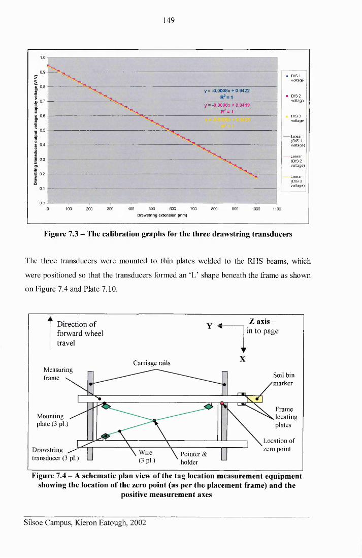
149
« D/S 1 vo ltage
y=-0.0008x + 0.9422■ D /S 2
v o ltage>, 0.7y = -0.0008x + 0.9449
R2 = 1D/S 3 v o ltage
Z 0 .5
L inear(D /S 1 vo ltage)
Linear(D /S 2 vo ltage)
0.3
tr> 0.2Linear (D /S 3 v o ltage)
0.0100 5 00 600
D raw string e x te n s io n (m m )
700 900200 300 400 800 1000 1100
Figure 7.3 - The calibration graphs for the three drawstring transducers
The three transducers were mounted to thin plates welded to the RHS beams, which
were positioned so that the transducers formed an ‘L’ shape beneath the frame as shown
on Figure 7.4 and Plate 7.10.
Z axis -in to page
Direction of forward wheel travel
Carriage railsMeasuring frame \ Soil bin
marker
Framelocatingplates
Mounting plate (3 pi.)
Location of zero pointDrawstring /
transducer (3 pi.)Wire (3 pi)
Pointer & holder
Figure 7.4 - A schematic plan view of the tag location measurement equipmentshowing the location of the zero point (as per the placement frame) and the
positive measurement axes
Silsoe Campus, Kieron Eatough, 2002
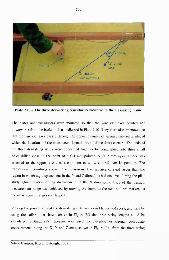
150
Orientation
Pointer
(down)
Wire exit axis
ofwire exit axes
Plate 7.10 - The three drawstring transducers mounted to the measuring frame
The plates and transducers were mounted so that the wire exit axes pointed 45°
downwards from the horizontal, as indicated in Plate 7.10. They were also orientated so
that the wire exit axes passed through the opposite comer of an imaginary rectangle, of
which the locations of the transducers formed three (of the four) comers. The ends of
the three drawstring wires were connected together by being glued into three small
holes drilled close to the point of a 0 4 mm pointer. A 012 mm nylon holder was
attached to the opposite end of the pointer to allow control over its position. The
transducers’ mountings allowed the measurement of an area of sand larger than the
region in which tag displacement in the Y and Z directions had occurred during the pilot
study. Quantification of tag displacement in the X direction outside of the frame’s
measurement range was achieved by moving the frame to the next soil bin marker, as
the measurement ranges overlapped.
Moving the pointer altered the drawstring extensions (and hence voltages), and thus by
using the calibrations shown above in Figure 7.3 the three string lengths could be
calculated. Pythagoras’s theorem was used to calculate orthogonal coordinate
measurements along the X, Y and Z-axes, shown in Figure 7.4, from the three string
Silsoe Campus, Kieron Eatough, 2002
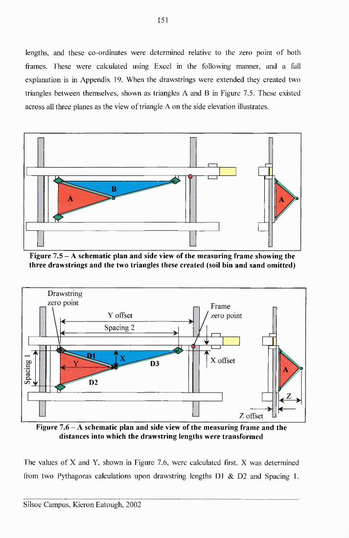
151
lengths, and these co-ordinates were determined relative to the zero point of both
frames. These were calculated using Excel in the following manner, and a lull
explanation is in Appendix 19. When the drawstrings were extended they created two
triangles between themselves, shown as triangles A and B in Figure 7.5. These existed
across all three planes as the view of triangle A on the side elevation illustrates.
Figure 7.5 - A schematic plan and side view of the measuring frame showing the three drawstrings and the two triangles these created (soil bin and sand omitted)
Drawstring zero point Frame
zero pointY offsetSpacing 2
X offsetD3
D2
Z offsetFigure 7.6 - A schematic plan and side view of the measuring frame and the
distances into which the drawstring lengths were transformed
The values of X and Y, shown in Figure 7.6, were calculated first. X was determined
from two Pythagoras calculations upon drawstring lengths D1 & D2 and Spacing 1.
Silsoe Campus, Kieron Eatough, 2002
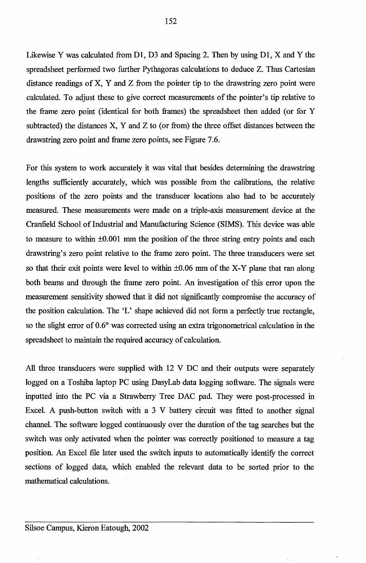
152
Likewise Y was calculated from Dl, D3 and Spacing 2. Then by using Dl, X and Y the
spreadsheet performed two further Pythagoras calculations to deduce Z. Thus Cartesian
distance readings of X, Y and Z from the pointer tip to the drawstring zero point were
calculated. To adjust these to give correct measurements of the pointer’s tip relative to
the frame zero point (identical for both frames) the spreadsheet then added (or for Y
subtracted) the distances X, Y and Z to (or from) the three offset distances between the
drawstring zero point and frame zero points, see Figure 7.6.
For this system to work accurately it was vital that besides determining the drawstring
lengths sufficiently accurately, which was possible from the calibrations, the relative
positions of the zero points and the transducer locations also had to be accurately
measured. These measurements were made on a triple-axis measurement device at the
Cranfield School of Industrial and Manufacturing Science (SIMS). This device was able
to measure to within ±0.001 mm the position of the three string entry points and each
drawstring’s zero point relative to the frame zero point. The three transducers were set
so that their exit points were level to within ±0.06 mm of the X-Y plane that ran along
both beams and through the frame zero point. An investigation of this error upon the
measurement sensitivity showed that it did not significantly compromise the accuracy of
the position calculation. The ‘L’ shape achieved did not form a perfectly true rectangle,
so the slight error of 0.6° was corrected using an extra trigonometrical calculation in the
spreadsheet to maintain the required accuracy of calculation.
All three transducers were supplied with 12 V DC and their outputs were separately
logged on a Toshiba laptop PC using DasyLab data logging software. The signals were
inputted into the PC via a Strawberry Tree DAC pad. They were post-processed in
Excel. A push-button switch with a 3 V battery circuit was fitted to another signal
channel. The software logged continuously over the duration of the tag searches but the
switch was only activated when the pointer was correctly positioned to measure a tag
position. An Excel file later used the switch inputs to automatically identify the correct
sections of logged data, which enabled the relevant data to be sorted prior to the
mathematical calculations.
Silsoe Campus, Kieron Eatough, 2002
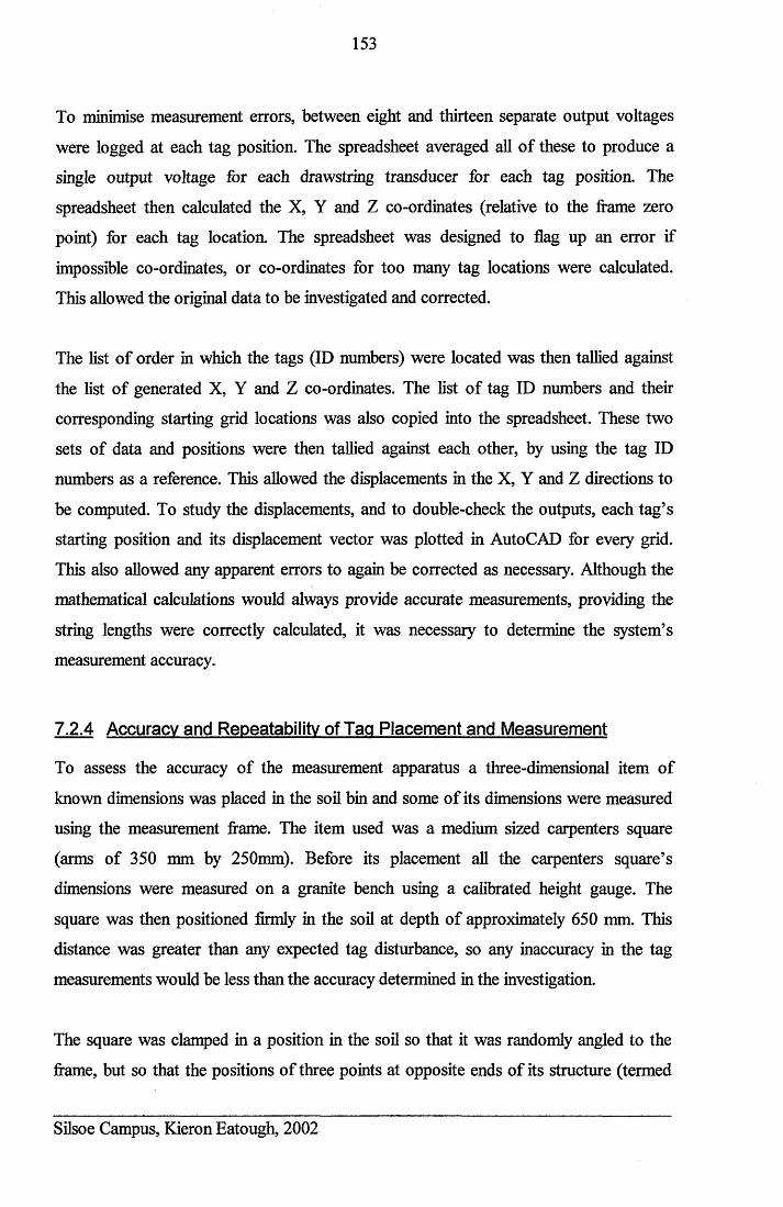
153
To minimise measurement errors, between eight and thirteen separate output voltages
were logged at each tag position. The spreadsheet averaged all of these to produce a
single output voltage for each drawstring transducer for each tag position. The
spreadsheet then calculated the X, Y and Z co-ordinates (relative to the frame zero
point) for each tag location. The spreadsheet was designed to flag up an error if
impossible co-ordinates, or co-ordinates for too many tag locations were calculated.
This allowed the original data to be investigated and corrected.
The list of order in which the tags (ID numbers) were located was then tallied against
the list of generated X, Y and Z co-ordinates. The list of tag ID numbers and their
corresponding starting grid locations was also copied into the spreadsheet. These two
sets of data and positions were then tallied against each other, by using the tag ID
numbers as a reference. This allowed the displacements in the X, Y and Z directions to
be computed. To study the displacements, and to double-check the outputs, each tag’s
starting position and its displacement vector was plotted in AutoCAD for every grid.
This also allowed any apparent errors to again be corrected as necessary. Although the
mathematical calculations would always provide accurate measurements, providing the
string lengths were correctly calculated, it was necessary to determine the system’s
measurement accuracy.
7.2.4 Accuracy and Repeatability of Tag Placement and Measurement
To assess the accuracy of the measurement apparatus a three-dimensional item of
known dimensions was placed in the soil bin and some of its dimensions were measured
using the measurement frame. The item used was a medium sized carpenters square
(arms of 350 mm by 250mm). Before its placement all the carpenters square’s
dimensions were measured on a granite bench using a calibrated height gauge. The
square was then positioned firmly in the soil at depth of approximately 650 mm. This
distance was greater than any expected tag disturbance, so any inaccuracy in the tag
measurements would be less than the accuracy determined in the investigation.
The square was clamped in a position in the soil so that it was randomly angled to the
frame, but so that the positions of three points at opposite ends of its structure (termed
Silsoe Campus, Kieron Eatough, 2002
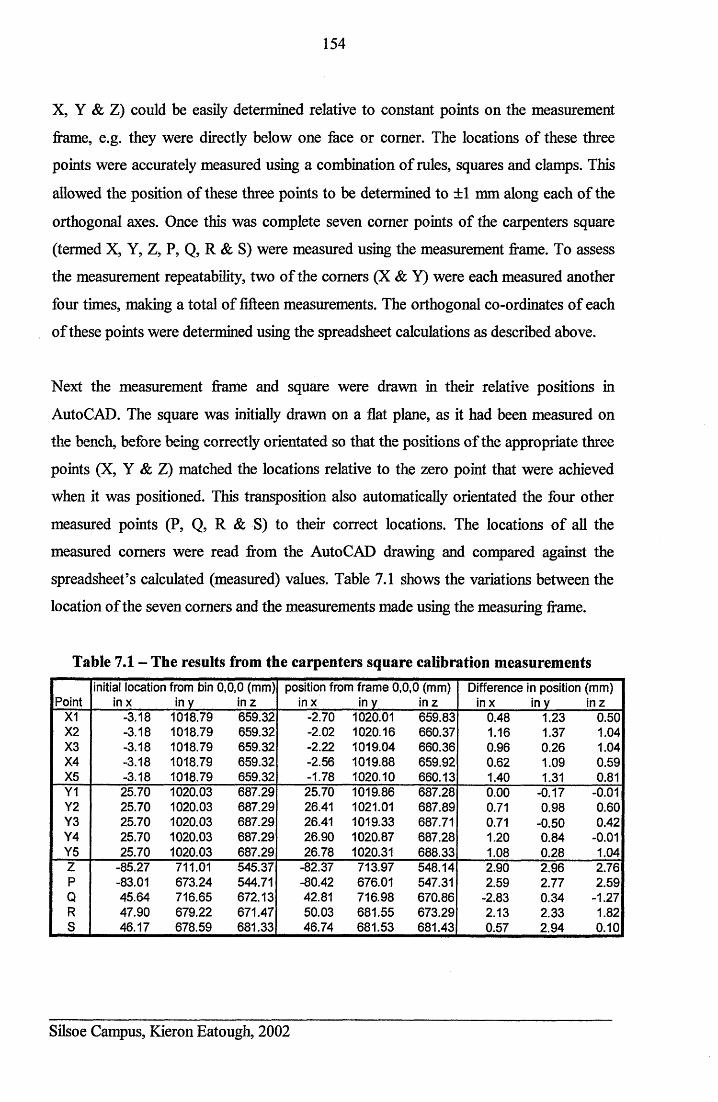
154
X, Y & Z) could be easily determined relative to constant points on the measurement
frame, e.g. they were directly below one face or comer. The locations of these three
points were accurately measured using a combination of rules, squares and clamps. This
allowed the position of these three points to be determined to ±1 mm along each of the
orthogonal axes. Once this was complete seven comer points of the carpenters square
(termed X, Y, Z, P, Q, R & S) were measured using the measurement frame. To assess
the measurement repeatability, two of the comers (X & Y) were each measured another
four times, making a total of fifteen measurements. The orthogonal co-ordinates of each
of these points were determined using the spreadsheet calculations as described above.
Next the measurement frame and square were drawn in their relative positions in
AutoCAD. The square was initially drawn on a flat plane, as it had been measured on
the bench, before being correctly orientated so that the positions of the appropriate three
points (X, Y & Z) matched the locations relative to the zero point that were achieved
when it was positioned. This transposition also automatically orientated the four other
measured points (P, Q, R & S) to their correct locations. The locations of all the
measured comers were read from the AutoCAD drawing and compared against the
spreadsheet’s calculated (measured) values. Table 7.1 shows the variations between the
location of the seven comers and the measurements made using the measuring frame.
Table 7.1 - The results from the carpenters square calibration measurementsinitial location from bin 0,0,0 (mm) position from frame 0,0,0 (mm) Difference in position (mm)
Point in x in y in z inx in y in z in x in y inzX1 -3.18 1018.79 659.32 -2.70 1020.01 659.83 0.48 1.23 0.50X2 -3.18 1018.79 659.32 -2.02 1020.16 660.37 1.16 1.37 1.04X3 -3.18 1018.79 659.32 -2.22 1019.04 660.36 0.96 0.26 1.04X4 -3.18 1018.79 659.32 -2.56 1019.88 659.92 0.62 1.09 0.59X5 -3.18 1018.79 659.32 -1.78 1020.10 660.13 1.40 1.31 0.81Y1 25.70 1020.03 687.29 25.70 1019.86 687.28 0.00 -0.17 -0.01Y2 25.70 1020.03 687.29 26.41 1021.01 687.89 0.71 0.98 0.60Y3 25.70 1020.03 687.29 26.41 1019.33 687.71 0.71 -0.50 0.42Y4 25.70 1020.03 687.29 26.90 1020.87 687.28 1.20 0.84 -0.01Y5 25.70 1020.03 687.29 26.78 1020.31 688.33 1.08 0.28 1.04Z -85.27 711.01 545.37 -82.37 713.97 548.14 2.90 2.96 2.76P -83.01 673.24 544.71 -80.42 676.01 547.31 2.59 2.77 2.59Q 45.64 716.65 672.13 42.81 716.98 670.86 -2.83 0.34 -1.27R 47.90 679.22 671.47 50.03 681.55 673.29 2.13 2.33 1.82S 46.17 678.59 681.33 46.74 681.53 681.43 0.57 2.94 0.10
Silsoe Campus, Kieron Eatough, 2002
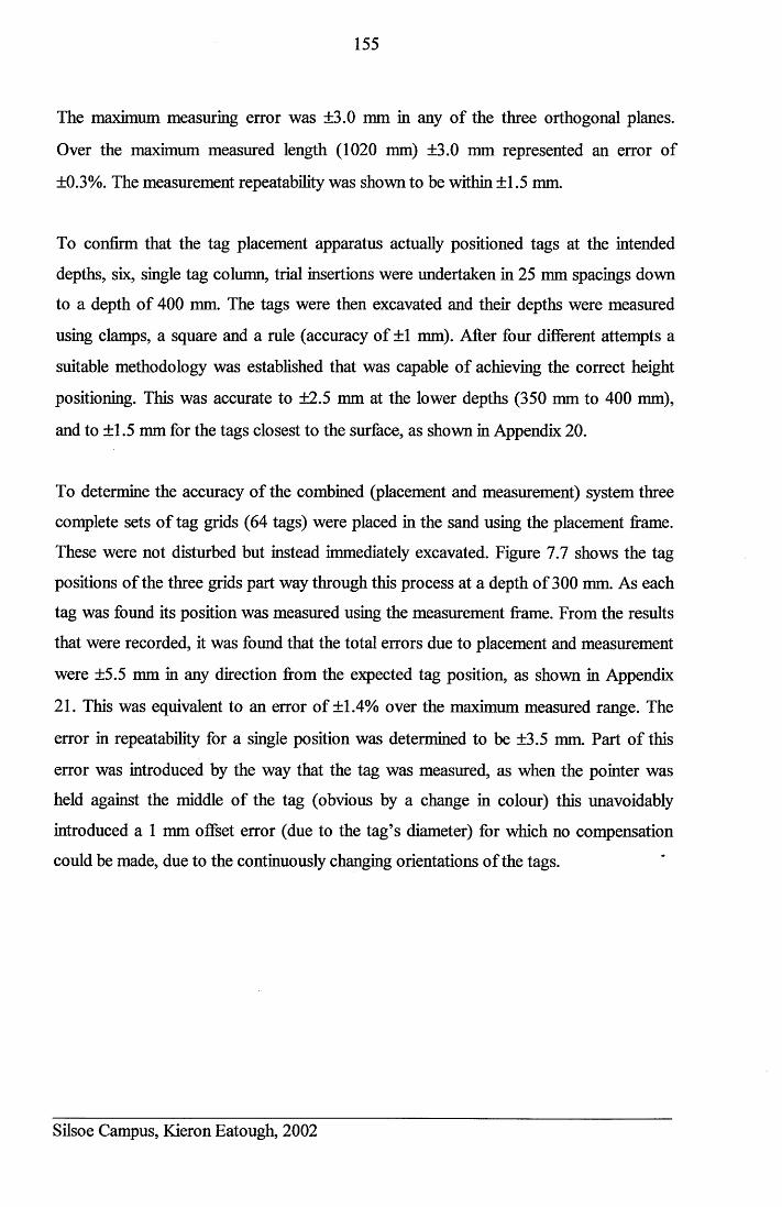
155
The maximum measuring error was ±3.0 mm in any of the three orthogonal planes.
Over the maximum measured length (1020 mm) ±3.0 mm represented an error of
±0.3%. The measurement repeatability was shown to be within ±1.5 mm.
To confirm that the tag placement apparatus actually positioned tags at the intended
depths, six, single tag column, trial insertions were undertaken in 25 mm spacings down
to a depth of 400 mm. The tags were then excavated and their depths were measured
using clamps, a square and a rule (accuracy of ±1 mm). After four different attempts a
suitable methodology was established that was capable of achieving the correct height
positioning. This was accurate to ±2.5 mm at the lower depths (350 mm to 400 mm),
and to ±1.5 mm for the tags closest to the surface, as shown in Appendix 20.
To determine the accuracy of the combined (placement and measurement) system three
complete sets of tag grids (64 tags) were placed in the sand using the placement frame.
These were not disturbed but instead immediately excavated. Figure 7.7 shows the tag
positions of the three grids part way through this process at a depth of 300 mm. As each
tag was found its position was measured using the measurement frame. From the results
that were recorded, it was found that the total errors due to placement and measurement
were ±5.5 mm in any direction from the expected tag position, as shown in Appendix
21. This was equivalent to an error of ±1.4% over the maximum measured range. The
error in repeatability for a single position was determined to be ±3.5 mm. Part of this
error was introduced by the way that the tag was measured, as when the pointer was
held against the middle of the tag (obvious by a change in colour) this unavoidably
introduced a 1 mm offset error (due to the tag’s diameter) for which no compensation
could be made, due to the continuously changing orientations of the tags.
Silsoe Campus, Kieron Eatough, 2002
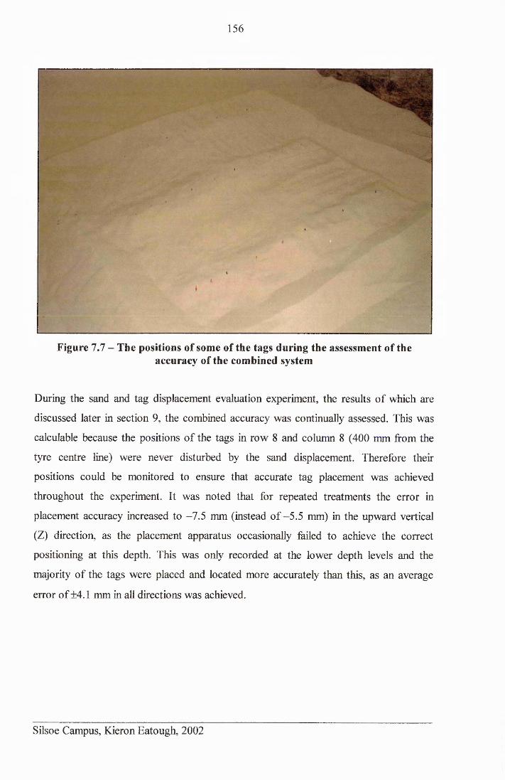
156
Figure 7.7 - The positions of some of the tags during the assessment of the accuracy of the combined system
During the sand and tag displacement evaluation experiment, the results of which are
discussed later in section 9, the combined accuracy was continually assessed. This was
calculable because the positions of the tags in row 8 and column 8 (400 mm from the
tyre centre line) were never disturbed by the sand displacement. Therefore their
positions could be monitored to ensure that accurate tag placement was achieved
throughout the experiment. It was noted that for repeated treatments the error in
placement accuracy increased to -7.5 mm (instead of -5.5 mm) in the upward vertical
(Z) direction, as the placement apparatus occasionally failed to achieve the correct
positioning at this depth. This was only recorded at the lower depth levels and the
majority of the tags were placed and located more accurately than this, as an average
error of ±4.1 mm in all directions was achieved.
Silsoe Campus, Kieron Eatough, 2002
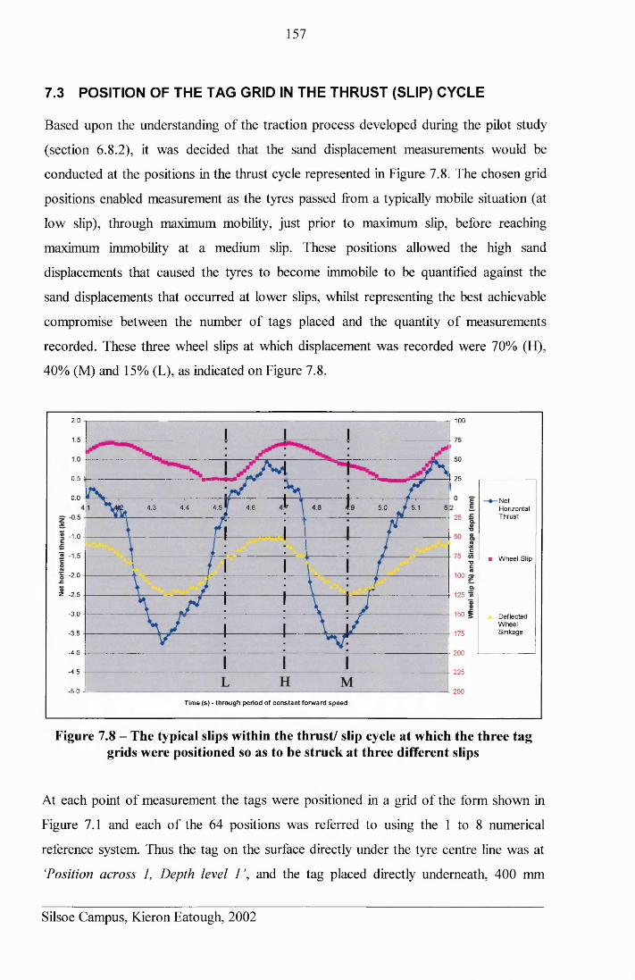
157
7.3 POSITION OF THE TAG GRID IN THE THRUST (SLIP) CYCLE
Based upon the understanding of the traction process developed during the pilot study
(section 6.8.2), it was decided that the sand displacement measurements would be
conducted at the positions in the thrust cycle represented in Figure 7.8. The chosen grid
positions enabled measurement as the tyres passed from a typically mobile situation (at
low slip), through maximum mobility, just prior to maximum slip, before reaching
maximum immobility at a medium slip. These positions allowed the high sand
displacements that caused the tyres to become immobile to be quantified against the
sand displacements that occurred at lower slips, whilst representing the best achievable
compromise between the number of tags placed and the quantity of measurements
recorded. These three wheel slips at which displacement was recorded were 70% (H),
40% (M) and 15% (L), as indicated on Figure 7.8.
2.0 -r 100
0.5 25
0.0 ■NetHorizontalT h ru s t
4 .3 4.4 4 .5 4.6 5 .0 5.1
- 1.0
■ W h e e l S lip
-2.0 100
z -2.5 125 »
-3.0 150 g D eflectedW heelS in k a g e-3 .5 175
-4.0 200
-4.5 225
-5.0 -L— 250
Tim e (s ) - through period o f co n sta n t forw ard s p e e d
Figure 7.8 - The typical slips within the thrust/ slip cycle at which the three tag grids were positioned so as to be struck at three different slips
At each point of measurement the tags were positioned in a grid of the form shown in
Figure 7.1 and each of the 64 positions was referred to using the 1 to 8 numerical
reference system. Thus the tag on the surface directly under the tyre centre line was at
‘Position across 1, Depth level 1 ’, and the tag placed directly underneath, 400 mm
Silsoe Campus, Kieron Eatough, 2002
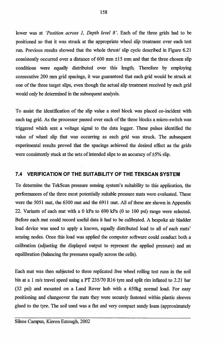
158
lower was at ‘Position across 1, Depth level 8 ’. Each of the three grids had to be
positioned so that it was struck at the appropriate wheel slip treatment over each test
run. Previous results showed that the whole thrust/ slip cycle described in Figure 6.21
consistently occurred over a distance of 600 mm ±15 mm and that the three chosen slip
conditions were equally distributed over this length. Therefore by employing
consecutive 200 mm grid spacings, it was guaranteed that each grid would be struck at
one of the three target slips, even though the actual slip treatment received by each grid
would only be determined in the subsequent analysis.
To assist the identification of the slip value a steel block was placed co-incident with
each tag grid. As the processor passed over each of the three blocks a micro-switch was
triggered which sent a voltage signal to the data logger. These pulses identified the
value of wheel slip that was occurring as each grid was struck. The subsequent
experimental results proved that the spacings achieved the desired effect as the grids
were consistently stuck at the sets of intended slips to an accuracy of ±5% slip.
7.4 VERIFICATION OF THE SUITABILITY OF THE TEKSCAN SYSTEM
To determine the TekScan pressure sensing system’s suitability to this application, the
performances of the three most potentially suitable pressure mats were evaluated. These
were the 5051 mat, the 6300 mat and the 6911 mat. All of these are shown in Appendix
22. Variants of each mat with a 0 kPa to 690 kPa (0 to 100 psi) range were selected.
Before each mat could record useful data it had to be calibrated. A bespoke air bladder
load device was used to apply a known, equally distributed load to all of each mats’
sensing nodes. Once this load was applied the computer software could conduct both a
calibration (adjusting the displayed output to represent the applied pressure) and an
equilibration (balancing the pressures equally across the cells).
Each mat was then subjected to three replicated free wheel rolling test runs in the soil
bin at a 1 m/s travel speed using a PT 235/70 R16 tyre and split rim inflated to 2.21 bar
(32 psi) and mounted on a Land Rover hub with a 650kg normal load. For easy
positioning and changeover the mats they were securely fastened within plastic sleeves
glued to the tyre. The soil used was a flat and very compact sandy loam (approximately
Silsoe Campus, Kieron Eatough, 2002
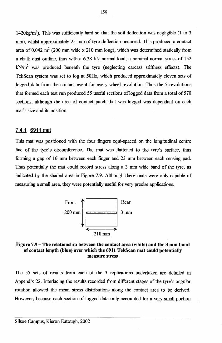
159
1420kg/m3). This was sufficiently hard so that the soil deflection was negligible (1 to 3
mm), whilst approximately 25 mm of tyre deflection occurred. This produced a contact
area of 0.042 m2 (200 mm wide x 210 mm long), which was determined statically from
a chalk dust outline, thus with a 6.38 kN normal load, a nominal normal stress of 152
kN/m2 was produced beneath the tyre (neglecting carcass stiffness effects). The
TekScan system was set to log at 50Hz, which produced approximately eleven sets of
logged data from the contact event for every wheel revolution. Thus the 5 revolutions
that formed each test run produced 55 useful sections of logged data from a total of 570
sections, although the area of contact patch that was logged was dependant on each
mat’s size and its position.
7.4.1 6911 mat
This mat was positioned with the four fingers equi-spaced on the longitudinal centre
line of the tyre’s circumference. The mat was flattened to the tyre’s surface, thus
forming a gap of 16 mm between each finger and 23 mm between each sensing pad.
Thus potentially the mat could record stress along a 3 mm wide band of the tyre, as
indicated by the shaded area in Figure 7.9. Although these mats were only capable of
measuring a small area, they were potentially useful for very precise applications.
Front
200 mm
Rear
3 mm
210 mm
Figure 7.9 - The relationship between the contact area (white) and the 3 mm band of contact length (blue) over which the 6911 TekScan mat could potentially
measure stress
The 55 sets of results from each of the 3 replications undertaken are detailed in
Appendix 22. Interlacing the results recorded from different stages of the tyre’s angular
rotation allowed the mean stress distributions along the contact area to be derived.
However, because each section of logged data only accounted for a very small portion
Silsoe Campus, Kieron Eatough, 2002
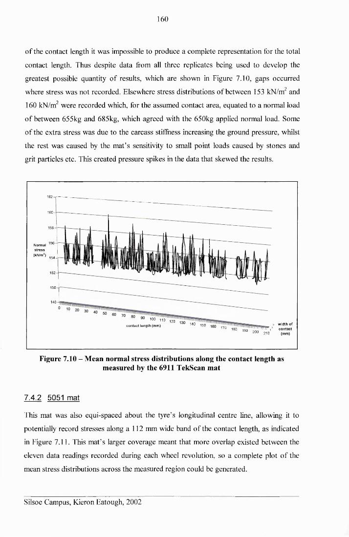
160
of the contact length it was impossible to produce a complete representation for the total
contact length. Thus despite data from all three replicates being used to develop the
greatest possible quantity of results, which are shown in Figure 7.10, gaps occurred
where stress was not recorded. Elsewhere stress distributions of between 153 kN/m2 and
160 kN/m2 were recorded which, for the assumed contact area, equated to a normal load
of between 655kg and 685kg, which agreed with the 650kg applied normal load. Some
of the extra stress was due to the carcass stiflness increasing the ground pressure, whilst
the rest was caused by the mat’s sensitivity to small point loads caused by stones and
grit particles etc. This created pressure spikes in the data that skewed the results.
162
160
158
156Normals tr e s s
(kN/m2)154
152
150
148
100 110 120' ' ' 140 iso170 180 lq o ' " ' TrTTTTrr
190 200 210
3 w id th o f 2 co n ta c t
(m m )
co n ta c t len gth (m m)
Figure 7.10 - Mean normal stress distributions along the contact length as measured by the 6911 TekScan mat
7.4.2 5051 mat
This mat was also equi-spaced about the tyre’s longitudinal centre line, allowing it to
potentially record stresses along a 112 mm wide band of the contact length, as indicated
in Figure 7.11. This mat’s larger coverage meant that more overlap existed between the
eleven data readings recorded during each wheel revolution, so a complete plot of the
mean stress distributions across the measured region could be generated.
Silsoe Campus, Kieron Eatough, 2002
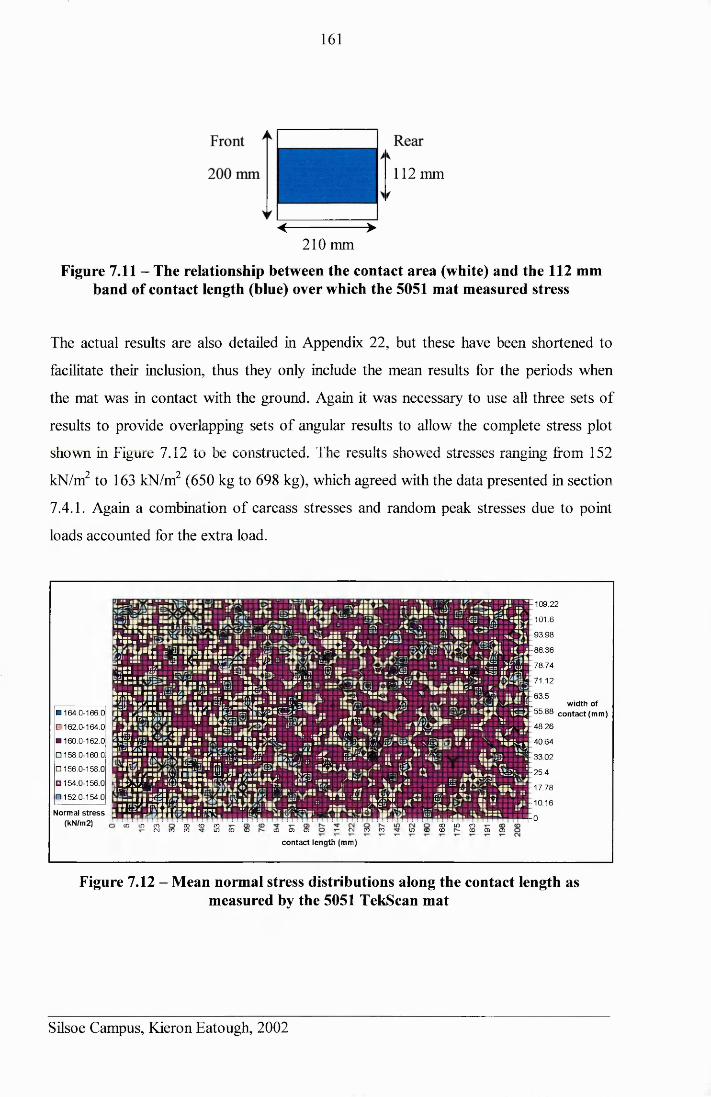
161
112 mm
< >210 mm
Figure 7.11 - The relationship between the contact area (white) and the 112 mm band of contact length (blue) over which the 5051 mat measured stress
The actual results are also detailed in Appendix 22, but these have been shortened to
facilitate their inclusion, thus they only include the mean results for the periods when
the mat was in contact with the ground. Again it was necessary to use all three sets of
results to provide overlapping sets of angular results to allow the complete stress plot
shown in Figure 7.12 to be constructed. The results showed stresses ranging from 152
kN/m2 to 163 kN/m2 (650 kg to 698 kg), which agreed with the data presented in section
7.4.1. Again a combination of carcass stresses and random peak stresses due to point
loads accounted for the extra load.
□ 164.0-166.0□ 162.0-164.0 ■ 160.0-162.0□ 158.0-160.0□ 156.0-158.0□ 154.0-156.0□ 152.0-154.0
Normal stress (kN/m 2)
» ■ iB iv ■ 11 i t ! ’%«r . cj r«af a l r r T r c . i ■■ ■ » r;.i ~ a &i_____ a w
I L r V >■■ .■ !> eu r * iI%.1 I I II <1 ^ ^ 1 1 1 |« | iiSJ V3P“ .. ^■ ■•*« ■■ ■ Uzmmmmrn* i f ■■ it ■■ ,£«*. HIM. %. II !>*■=■* n ^ r \ .
> i > ■ > 3 P % # - # * # k » . ^ B c R s t / J f t \ * S 7 ? v l l l P 'W B ag .W ■%#■!•« r DHI^ilUil lOII aliii I V>I R <1. If ./ l**VJ Uii I p * t7)K mK -JW l a ll ■■ Li 1 l^afllll^liM ' -Jn* .. i l i lh ^ l k . S-■ ■— mm L J iw>i m iinF .aai ’I'S* Uii#- II r n ~ ' ma IPta \ W T -7>mmw r.7>■ i l i l l 1 l£ -J r 3 . ■ ■ ! ! IP ■■ r.7\ ■ ■ . > ^ B r i ■ » " "C'sr .# ■ Uil
' A M m il’A — u i l i ■ i p r > . n i v j ip- — \ * * r . - ^ a .. *■» mm\ ± * = : : i I I .til ■■■ i i .■■ ■!! .. l j uu ■« ■■ ■<>*« --r&afcii*” I l n v i *■ Bf ■%. «« k « F “ r-i . . r i r^rVJV
■ fol • « . t i l i I R / j4< w . IV J ■" U i r i l l ^ J nn r — \i:£I f l B . U P M . ^ > ^ 1 * i ^ ' BI I I . ■ ! ! » '%■ ■■ - W W . . . l i IF — — — Uil- H . . .# 1f r o l l i III 11 ( V f J ■■ f77; ■%F"Ca>l ■ > , II » . r , r ■ I k ■ ■ - ■ # * 4 " " S 4 ' I k i i a * . » / r 7 4 IkJlf,■ rJll 1l« O H ■■ ■« •« ti l . Cfeatuija* ■■ ■■ IV ? ■ ■ /- r.»7 r * / B i r t■Si* lri ln i i ■■ HIM |^B«a^fea r<iB7^«Slll ./>li ./ <k P«l .--mfl» i Ob I I ^ H 11 i | | l i . ’ K a " ^ l l l ^ a ^ 1 « ■■ IP " ' ! ■ I l lriAi I I ri>V!JHI I II » - * « ■ ,*■ —#r:i rsi 'V ■■ I#* W aI ■■ HV«^ II ■»!!»/« .{£»'*■ _/ll 14 ii'- ./1'IVWP?1 ..#■ ■“ 1■ .#■ i b . i I. ii^.1 rnm ” II ■■ IP II ih . r i ,B l l ^ " ' B-V «. , / .#■#ni ■■•',^»o i i i i i .i a m i i ip ■*. .«#■ i i . f/fl _ /• w u p ii ik*B —*i»LfJ m tt ■«•< ■ ■!»>■ iO<1 *BI frTP IF k / \ an « .■ > W P f c i J »*■ » ■ « ■■■ >«l n-i ■■ lk/7 L * P f» l. \ii5BHJ IP II BBF^«fl■ f r u p a t f i i i i » i « n i v i i w'ai •%. »■ . . i i ik r?■■ ■ ■ ■ ■ ■ ! BJIH. ■■ ■OaS=o'V,"« rn“ . r nJr;4ir P . . .# JP .<L:V71 Jl livnRSl i i a i ii*m r.7iXw f r ^ . l l BB .IZ&mrn.-Ll* ■■'S3' Jl .. T ^ i Ufii ’•c II BB .# BBLiiJ I I a ' ^ *U ^«n*l LS t i l l n •* ■»— *' .m 'X 'm mm m . ■* r . 2 \ ,m 'm W K w t m■■ 1! " ■■•(ill ■■ nil ■■ ■> HUM ‘IIMMii. 15-P PI ,B H. 11 \ln. B■ I f/B « | >V»'JI1I|B« UJ i ^ I i ^ I i i .. ■O'sn ~ BV *4 la /U # B. •C&v', .I H ^ l l l i # 1 . r / O I - « A B | k ( T ? ^ l . I M - I P I / 1 M fih 'J .m m u / * * * I . V i s i l i i R . t I P k # ^ / ^ ’l,V«IVvi “■ "liM. '!■ PILiJil. r >Bi ,B 't*s ■■■ -Try* a /• lk .^^B .. tan —r j f ? 7 l« B u J BB . . B* » fc f P 'vM. .. .«■ *rf~ H I » 1 1 1 , „
mT/AW I ' J a ' J * 1 1 1 1 l l i l r i f ! f / B . F l l i i i ^ r - . ” I f B"iB B B llll liS ir /T A . .#P^k>B. I'k'l I I ISSli?? ■■ BB ll«»7^P .# V W Ik u II i;?0« Rnll[i£lll<f1 III ri ■■■> _/li5a IL II '■ I#!
i i f l ^ i i t ' l i i i f S M i i m ■■ Bf f/' a r/i0«5^». il!V BB■ BB . . r 5 i r .F l 11 11 I/T.l' i iiS'B « U IP B VJm uy :
109.22
101.6
93.98
86.36
78.74
71.12
63.5width of
55.88 contact (mm)48.26
40.64
33.02
25.4
17.78
10.16
CO LO COCN CO CO
CO CD COin CD CD CO 0 ) 0 CM CO CO in CD CDco in co
n-oCO 0 CD
contact length (mm)
Figure 7.12 - Mean normal stress distributions along the contact length as measured by the 5051 TekScan mat
Silsoe Campus, Kieron Eatough, 2002
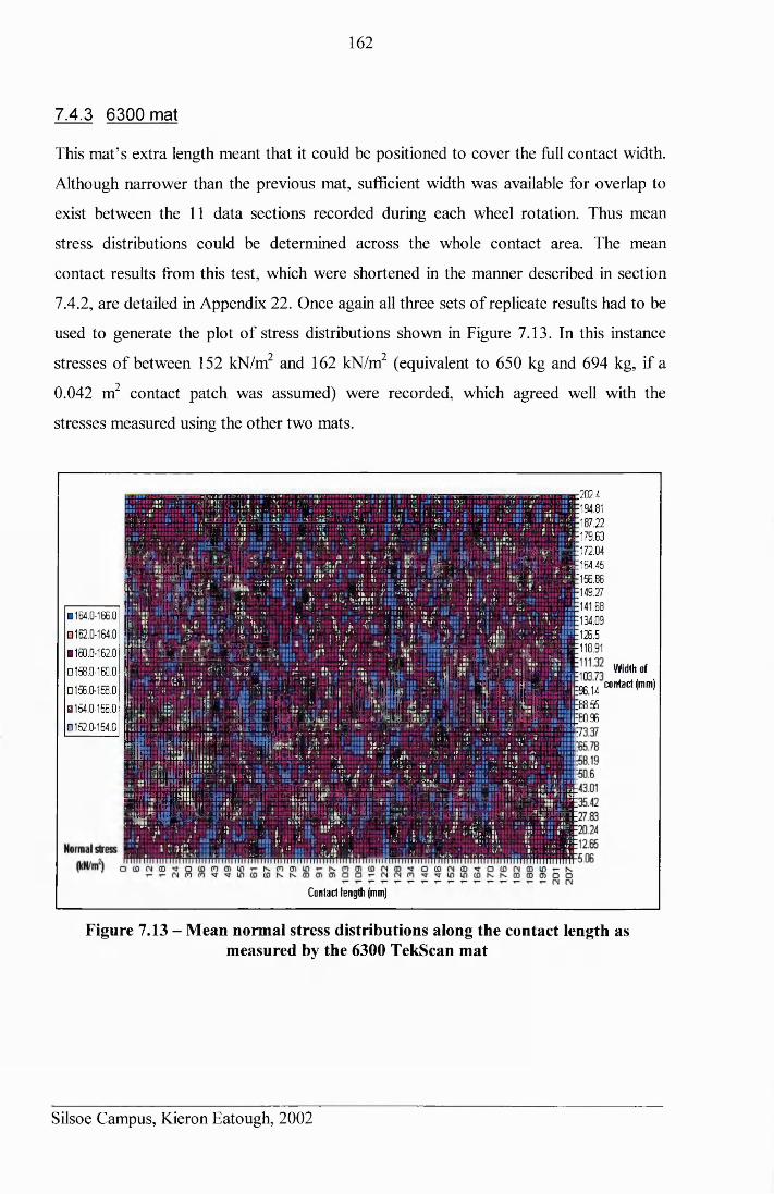
162
7.4.3 6300 mat
This mat’s extra length meant that it could be positioned to cover the full contact width.
Although narrower than the previous mat, sufficient width was available for overlap to
exist between the 11 data sections recorded during each wheel rotation. Thus mean
stress distributions could be determined across the whole contact area. The mean
contact results from this test, which were shortened in the manner described in section
7.4.2, are detailed in Appendix 22. Once again all three sets of replicate results had to be
used to generate the plot of stress distributions shown in Figure 7.13. In this instance
stresses of between 152 kN/m2 and 162 kN/m2 (equivalent to 650 kg and 694 kg, if a
0.042 m2 contact patch was assumed) were recorded, which agreed well with the
stresses measured using the other two mats.
«r i ■ ii i \ 1 ? i ’ V.* ' . r\ '■ i i i> t ,n\ is* * o >ft» i * / I. '■ r . "V. ■- r t i | l P ' i r '■ “ *i I I*.- 1 ■’
< ii n *' Mi?a» i p» i« ■. i >f , • o ir s. j > t rn, v a . j - ,-sb « . *« u i a *:•>• «• •* . i »-.••: .1.0 *. ?• • 'Kii*- ... • n u . i <r
■II .5> ■ Sili'fjB s i r ’ll H I. n-'1 I 'I s. B: I . /I «|«(3" I - ^111 ':<■ , / ' I t . * ' II. I,.-/* L * i *#••• -. If ' . / I S l i ' S VI 8 th - 'I I ■ If •»il lP!l • 1 : 15f ?
V0 « | A " • • •• /‘ I i- . r ‘ fft -r f>! I *• - T I /• > n • ’f t v ...■ ♦ . iT/a l i ’V* —. >.5fl 0B31M - - V i . :l«5«-■ . ' .I ! . I'Jl • i.» I I . i l l I— It . k II Ik j, . i j . p•1 i f w i ■ ai i . . . . 'ft. .11 Y i — fill ‘ ! 4ft V M
i / l i W / • i f k/tw U i .m r i i I 'Ik • tr 4 iP. V'f . . . . . .z< /■ irp ■■ M f k i • iktfi »- “i --iif i i n - i.*' .. t ~ <.-?• »' :
l i i- V 14 ,'J- ' a ll . W»0’ ' I f *' BIO Vi ' /• : . 11 * 4?i P.ISVt i l l v '• <■«_ *1 .» ’ * • ft Bi M !! ** • '■ fill s I n ’l . .. , .fa'I I V •••: M l.'n fc< .. I. h> ' ■ ' I Ii 0 .* . lM--.fi* 1* I ■* 85 I I "I■r . . ' ' 1 n r u . <*" .v, ,.ji; . ' i f / i > • v « i n ;Pi U /lif - : -» ii 'It |' ik J i ’VI o*- v 3 W ll 3 v • V . V. fi Ik T . i / | » |fi1 >•?* it . iv us i*i - . - i i ' i v *u i. ii _ v _ir<i f
.ria -I* O : ■ ’• Wi i i ■■■ v; I i; If 41 f i l l | I « ' MllMil «, !. .1 U5Hi' .4 ■*- a#< • u : * : r i '• ir ' o p i i ikM "I. if \u‘ *- < m . <i • vi' 4' - v « ‘ ■ i . • ik ki.kavi i a -t-.j ...
~ vp '• n . i i r . f.i /«-»-. *■ . . ik r ^ u r i r .» n • i w •>pi .-.i'll; t i i • ' «r ’ k. • n 'v. d i i - ■ . v- n * • - «/v. i.»i ■' '»r -- i: . - . > ! ’ < • ' ft,. 41 -i- »l i I t "• . . . 1 i_ . •,««. 8o -.-7 . 1 i' -■ ; •< . it 1 ' ' /■' »' « ,. ti ' i l l - ip- I P J i l l i sr ■SFM : ft .i
. . VI' -i. I < v tilf » •• *'M -S P i-71 .. /p . '1 S • -a3«,J£5f.»MI**W
r — 8 If V2| fi ii IJ ■ '1. ,| ,T . -. A,- I<1 v '• k'lt r 4 £<■ ■<■
ik « Bk.
f ' 4 •• . 'tk.jl r 17 ' - o Cm- A t 4 A • i .* <‘1 ■ 1i. / : • m i • -s ji i ■- f - i <r.> -• ■» ... i
. . Si : t i , U :! i* v. %!• . C i ' Si*' p 1H k iP ' • ; f 14 ■ 7 H V a 1r 1j* ir* ii i ;n i t*+v ,■ ' • i» - i.. -> ,. o ■ -.a -1 r ii - "■ eg i i t - i■ .. r-s ir 11 «i» : ,?■ _ • sssasi
r w ’ i- n ■ ■ ' «. . j f p i* >■ s. , i ii i i . ir n r 1.1 1,1 ■: •P. I'JSi. ■</>>.’ . . . "V l l i r 1 J"| I7I .. I
v •••-. -V -^41 ii - 1>. £■} ■*» «r<4 'IP IN "171 I ir « * J. V _ I
tiiT ki ssi ii r n i -1 :• 4 iF ji i\ i v v, i i»■ i-*a* i-.t ;.as3: - avB.i, -ii ,-.55 ;r.,fc hi ',i- .ii.r.i b .* '•jo = 'VPp/; *n» ir n • n.-..-.- m -::b rn .aaen
i?4ii«i»»*ns«....: B7r-n" n i p m - ii, i iiin .v 1 /t . . *i , «■ - c.-ii/i 4 i -it, • i i n fttif'w *1 * *.. ' i ik. • • z ■ - 1 '• 1 - ‘I ’ -.SB ;■■■■■ F \ « at r r,» - ? . iki p. c: ipn~
• aft - ' • • !' *i -I .i • >- L .4, ii ^ ’ i; 1'»1« : II iV *' ft <..« Y • k P’ *J IV ■ f * i. *• •■ . •! ' ... P. ’ W V *■<11.
12 If * i V 553 ■ ill S . T * ' .I m i > i» - 7 ■ ifSI I l f 11 II • l l 'fii SfW. TOf* . ? «>k i; 17k i l l .. iu ■ ■ *• .i JPi • Y-. . . /• wi * r- - s :-'.fc i i <i n -*r
■ in - i . tl ■ . 1 " Ji JIT U tH ,. ' . . . W V I, , .> I
1 i |I M
■ 164.0-166.0□ 162.0-164.0■ 160.0-162.0□ 158.0-160.0□ 156.0-158.0□ 154.0-156.0□ 152.0-154.0
Contact length (mm)
:202.4 E194.81 E187.22 -179.63 :172.04 :164.45 : 156.86 ;149.27 1141.68 1134.09 : 126.5 118.91
Wid,h0f ^ ^ contact (mm)
88.5580.96
Figure 7.13 - Mean normal stress distributions along the contact length as measured by the 6300 TekScan mat
Silsoe Campus, Kieron Eatough, 2002
163
7.4.4 TekScan Measurement Capabilities
The dynamic normal stress results calculated from this trial showed good agreement
with the expected stress of 152 kN/m2 in all instances. Some slightly higher stresses
were also recorded, but these were caused by a combination of the tyre carcass stress
and extreme point loads. As the surface tested upon was comparatively rigid and the
forward speed was relatively low, no significant pressure distribution variations due to
tyre and surface interactions were recorded across the contact areas of any of the mats.
Instead the results that were derived were more closely related to the static situation as
approximately consistent pressure distributions were recorded, although slight pressure
reductions were noted at the rear of the patches, where contact with the ground reduced
as the tyre lifted off.
It was concluded that the TekScan system could be used for normal stress
measurements when attached to a tyre. The 6300 strip-sensor achieved the best results
because it covered the biggest contact width and it enabled the closest location of the
connection block to the axle, which reduced the likelihood of large sinkages causing the
mats to tear. Additionally the 6300 mat could be successfully moulded around the
prototype treads’ linear tread features. A caveat remained over the manufacturer’s
advice that sensing performance would deteriorate under high shear stresses, as these
were not examined in this investigation. This could potentially be addressed if the mats
were protected with a thin covering capable of bearing the shear stresses. This would
also have to be flexible to match the tyre deformation so as not to distort the normal
stress patterns.
7.4.5 Attachment of the TekScan Mats to the Tyres
Six 6300 4L’ shaped strip sensors, rated for pressures up to 690 kPa (100 psi) were
attached to six differently treaded prototype tyres using the following procedure:
1. Each mat was individually calibrated and equilibrated (prior to attachment).
2. The appropriate section of each tyre was sanded to produce a flat, but roughened,
surface and then cleaned with a spirit fluid.
Silsoe Campus, Kieron Eatough, 2002
164
3. The underside of the each mat was bonded to the appropriate tread using an
activated cyanoacrylate.
4. Thin patches produced from a two-pack self-curing (vulcanising) rubber compound
purchased from Pang Rubber Ltd. were attached over the mat to provide mechanical
protectioa This compound was designed for repairing tyre cuts and punctures so its
deformation properties matched those of tread rubber.
5. Prior to curing the compound was very malleable, which allowed the patches to be
shaped around the tread features and pressed firmly into the tread rubber, which had
been painted with the appropriate chemical activator solution, which chemically
bonded them to the tread rubber.
The symmetry of the treads enabled only half of each tread face to be covered, yet the
correct orientation had to be achieved so that each mat also reached the connection
block on the wheel rim. Figure 7.14 demonstrates the necessary orientation of the
connecting leg towards the rim so that a metal bracket mounted on the wheel studs
could be used to securely retain the TekScan connecting block. Each mat’s exact
position varied slightly to accommodate each tread’s individual features, as Figure 7.15,
which illustrates flattened versions of each tread and the mat position demonstrates.
Approximately 90 mm from the centre line the tread merged into the tyre shoulder so
the mats were bent around the tyre contours at this point, as Figure 7.14 demonstrates.
This transition was omitted from Figure 7.15 as only poor results were recorded from
these regions, so they were ignored.
Silsoe Campus, Kieron Eatough, 2002
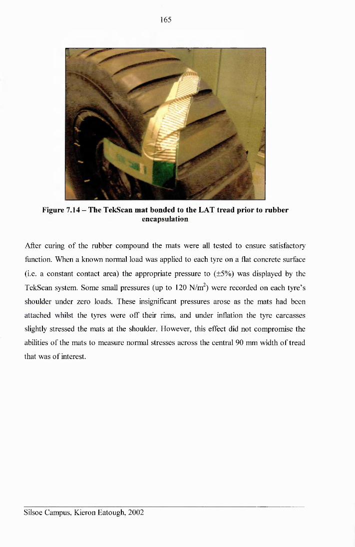
165
Figure 7.14 - The TekScan mat bonded to the LAT tread prior to rubberencapsulation
After curing of the rubber compound the mats were all tested to ensure satisfactory
function. When a known normal load was applied to each tyre on a flat concrete surface
(i.e. a constant contact area) the appropriate pressure to (±5%) was displayed by the
TekScan system. Some small pressures (up to 120 N/m2) were recorded on each tyre’s
shoulder under zero loads. These insignificant pressures arose as the mats had been
attached whilst the tyres were off their rims, and under inflation the tyre carcasses
slightly stressed the mats at the shoulder. However, this effect did not compromise the
abilities of the mats to measure normal stresses across the central 90 mm width of tread
that was of interest.
Silsoe Campus, Kieron Eatough, 2002
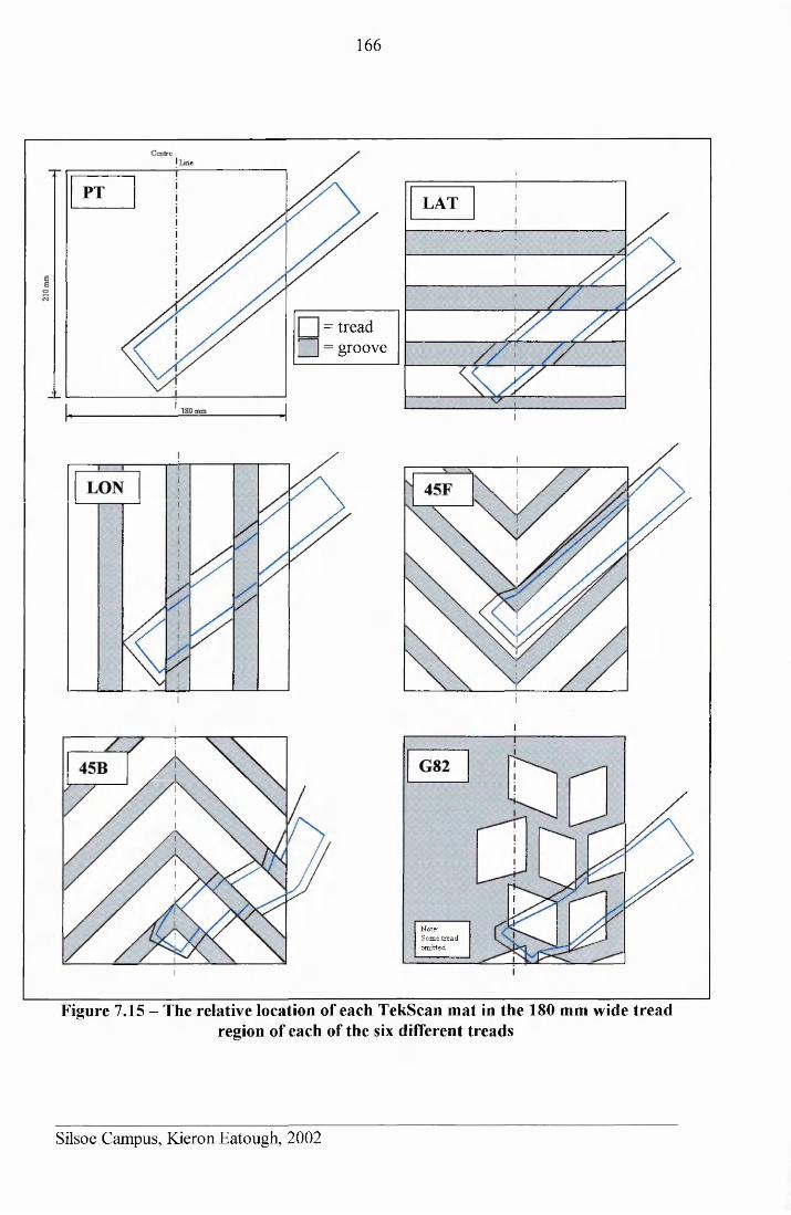
166
Note:Some tread omitted.
LAT
= tread ; J = groove
Figure 7.15 - The relative location of each TekScan mat in the 180 mm wide tread region of each of the six different treads
Silsoe Campus, Kieron Eatough, 2002
167
8 INVESTIGATION OF NORMAL STRESSES UNDER TYRES
8.1 EXPERIMENTAL TREATMENTS
The test runs were all conducted upon the previously described poured and rolled sand
preparation over the full soil bin length at a constant 5 km/h forward speed. A nominal
50% slip was selected, which achieved the same cyclical thrust - slip fluctuations
described in section 6.9. The other treatments were as previously detailed for other
experiments, i.e. 1.10 bar inflation pressure and the five prototype treads (PT, LON,
LAT, 45B & 45F shown in Plate 6.4), except for the TekScan system’s logging speed,
which was increased to its 100 Hz maximum setting.
It had been intended to record three test-run replications of the pressure distributions
beneath each of the six tread patterns. Unfortunately the quality of the outputs from the
mats on the prototype tyres deteriorated much quicker than had been expected. The
constant flexing and high strains quickly damaged the mats’ electrical connections, so
that large holes appeared in the data. The poor longevity of the mats limited the amount
of useful results that could be collected, and thus data was only collected for the LON
tread (over 1XA test runs), and the PT, LAT and 45B treads (over 2 complete test runs).
8.2 PRESSURE MEASUREMENT RESULTS
8.2.1 Pressure Map Construction Procedure
The poor mat longevity meant that sufficient data was only available to produce detailed
results for a single region of the thrust cycle. The position in the thrust cycle chosen for
the pressure distribution analysis was the period of maximum slip (maximum potential
sand displacement), which was of greatest interest because this was where the most
excessive tyre sinkage and resulting immobility was caused. Oliver’s30 drawstrings
measured an approximately rectangular contact area with a length of 390 mm ±10 mm
for this part of the thrust cycle.
The recorded results were used to produce pressure maps of the form shown in Figure
8.1, which described the variations in pressure on the contact patch at a single moment
Silsoe Campus, Kieron Eatough, 2002
168
in the thrust cycle. Each pressure mat was derived through a lengthy analysis procedure
conducted using Excel. The TekScan system recorded all the test results in long data
streams. Each stream had to be individually analysed to isolate the sections of data
where the mat had experienced an applied pressure (ground contact). These readings (in
psi) were then translated from pressures at isolated mat locations angled across the tyre
(due to the mat positions - see Figure 7.14) into pressures (in kPa) at appropriately
defined grid locations around the tyre circumference that were square (perpendicular) to
the longitudinal axis.
The sections of contact data appropriate to the high slip region of the thrust cycle were
then identified and isolated by considering the micro-switch outputs. All of the isolated
sections (bands) of data were appropriately positioned along a single timeline to
represent each angular position through the contact event, which allowed overlaps
between the results to be identified. Any overlapping pressure readings were spliced
together by calculating a mean value. Thus a single pressure value was determined for
each grid location (angular position) by combining readings from different wheel
revolutions at the correct cyclical position to cover all of the angular positions. As only
small sections of data were recorded during each wheel revolution, all the recorded data
had to be combined to enable continuous snapshots of the pressure distributions beneath
each tread for a single moment in the thrust cycle to be produced. Thus as each map was
the product of data from six or more wheel revolutions only a small likelihood of any
chance influence skewing the results was small
The contact region was considered flat, as this was simpler to represent than the true
complex curved profile. Each tread was featured on the plots, but it was only possible to
derive sufficient data to accurately record the pressures experienced on the normal tread
faces and not those on the groove sides (faces). The mapping was confined to the 180
mm tread width because of the measurement inconsistencies on the tyre shoulder. The
position of all the mats only allowed pressures to be recorded for just over half of the
tread, as the pink boxes indicate, however, maps of the whole contact area were easier
to interpret, so the recorded pressures were reflected about the tyre centre line for the
regions where stress was not measured. The estimated errors created by the process used
Silsoe Campus, Kieron Eatough, 2002
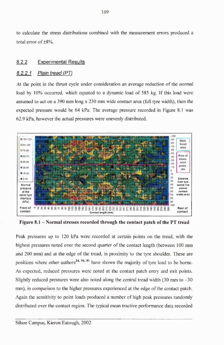
169
to calculate the stress distributions combined with the measurement errors produced a
total error of ±8%.
8.2.2 Experimental Results
8.2.2.1 Plain tread (PT)
At the point in the thrust cycle under consideration an average reduction of the normal
load by 10% occurred, which equated to a dynamic load of 585 kg. If this load were
assumed to act on a 390 mm long x 230 mm wide contact area (full tyre width), then the
expected pressure would be 64 kPa. The average pressure recorded in Figure 8.1 was
62.9 kPa, however the actual pressures were unevenly distributed.
0105-120
□ 90-105
□ 75-90
B 60-75
0 45-60
O 30-45
0 1 5 - 3 0
■ 0-15
Normal pressure
at the sand/ tyre interface
(kPa)
Front of contact
_ ’>« v/ / k i <kires tm t i i v ~ - .* r : A r . i i s s f v r 1 , t m v \ r \ . > t o
. »*»■- — H i.* liih'kJk »RS» •* i.
• a B U 8 0 S a ih = S * r« f l lS=i.\.4r. < jBLV. k ' l k « immr : I ' l a u 'S i i i s R s s / ' • ’ .. v* t r vit- ifs? ' t ' w X -.S W " ■■■». ■ • '{ •B r '.w v sa ik u b s * U r • ' ' - - = s s / * ,-ss»i:’3
ik u * • , i » n , * n ; u » « a B r x a ! »*./<*■..iE ia»" ' r ; r m u--
k E S k k i e % r » — tiii / » ' "K « a s is r.w i . r e s * -- - * r a n n a u k T i B f i t
"*• ...'..rj-i.Kteff*9SSS?«eBSH*«»i?» f !» .^ = a a 0 -S » l5 « « f.r%r.rt '• -IRS? > -*! ..r.n ^ s b » « ! 5 » « u s i : d i R s a « : S a l u w j a t i
r ( » M r i t - .» . . « » . ik .1 , . . .■ /" s a c k » • •» * ................ ................................ .. %.j -
tk ■-./ ? r t ^ ~ . . s - : s i t r i B n R t : » a 8 H ^ M ¥ i 9 ( / i i » i M a a B i i B a « H R n u v « a v M M S .iH * « k :s i iR % s * k < r . M i a > 7 c s ■s < f 2 M S K S I I I I B « K S B > lS S a : :H ’a V X K W M B r i i« a '2 ! 3 f f * * a S S W 2 = V B & I k > S 3 l l i r k 9 E r : . ' .
S. IMfck . ■ ■„ — *■ ' , B S « 'W / V ! I *--> •• B / ? k - r <--•=i*(R 4 3 H ■ W -a f iS S C •:.•>• * X r tt i r i r • ■••••'*•=!!>•-Wt7 ■ / a t f f \ 7 Ii’ > < k . kf
n iM w m m zw sm iK X H isa x m s s « i• i s »»ii ;•«& . " , i : s s s i .• • \tiu u * is» is s « ss s i -JuaBikaBiwctA ‘.wt-SMaik. I’ssa'iRi’sniiaaiB^sdsuK j u b p w
X f '/X t- ' 'n x . - ,li~ - » < -i k r n i l l k W T t r , . KtiS»;a<SiI M *» ' K G n ' 1 ' «*V .,/S ’T j . i *r\U"
■ n i ‘ i . , « , » i -iia^aw . . y . S L . ’* / ! : ? t t - = ^ = « w » s s s t »,:»■-«« -s2aB!*BBii»ie«<*a*i2»Br/s*aR!«*=«ii»*iMis» a«aii=?ss' aaBimniBBssiMisnBivaflif&ftBwzz r-
=-«» i r - - r<»v '^ii=^w =3ii ii 'ir/i' r»iM>r.- ' i - ._4Bv.H J S M I r > < « B 4 I ' iO B I V .» !* > . /■✓ s 'S k -k B 'k . " i f - '
. * ¥ ~ ~ -V > J5I Si'BXr I S S V >■»Bl> S ■( / uv>«v -■««»«■-' Wll' 'ii . ■■'■'«WSaB/V «Jk tkri I V 4 'kr kS'IUaXBBkiJt'BI f - — ‘ aik«v-lli/ I
■■ /irs i . a r Mh^wsfiwSKiKSoeM'itx ■ ■-v n - i • *r i
' » «>>tI I I I I
o o o or - (N COo o o o o o^ If) © S CO CD o o o o o o o If) (D N CO O) o
C o n ta c t len g th (m m )
O O O O O O O O O O O O O ^ - ^ ^ ^ ^ ^ T - C N C O ^ t f ) ( O N C O O ) O T - O I ( O ^ l f ) 0 N C O O ) C MC MC MC Mf NC NC MMMC OC OC OC OC OC OC OCO CO CO
p-100-9 0 Main—80 tread-7 0 area—60-5 0-4 0 Area of
--30 meas
—20 ured
-10 press
-0 ure
: 10-20 D is ta n c e-30 from tyre-40 ce n tr e lin e-50 a c r o s s-60 c o n ta c t
o w id th (m m )
F80p90Moo
Rear of contact
Figure 8.1 - Normal stresses recorded through the contact patch of the PT tread
Peak pressures up to 120 kPa were recorded at certain points on the tread, with the
highest pressures noted over the second quarter of the contact length (between 100 mm
and 200 mm) and at the edge of the tread, in proximity to the tyre shoulder. These are
positions where other authors24’54’81 have shown the majority of tyre load to be borne.
As expected, reduced pressures were noted at the contact patch entry and exit points.
Slightly reduced pressures were also noted along the central tread width (30 mm to -30
mm), in comparison to the higher pressures experienced at the edge of the contact patch.
Again the sensitivity to point loads produced a number of high peak pressures randomly
distributed over the contact region. The typical mean tractive performance data recorded
Silsoe Campus, Kieron Eatough, 2002
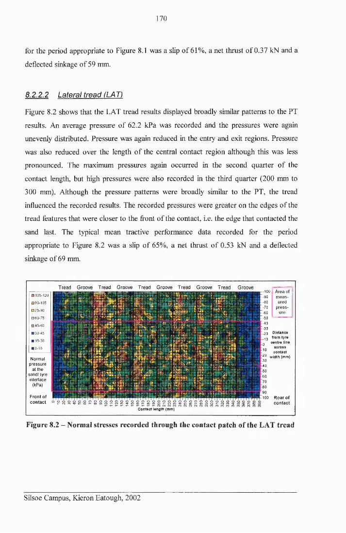
170
for the period appropriate to Figure 8.1 was a slip of 61%, a net thrust of 0.37 kN and a
deflected sinkage of 59 mm.
8.2.22 Lateral tread (LAT)
Figure 8.2 shows that the LAT tread results displayed broadly similar patterns to the PT
results. An average pressure of 62.2 kPa was recorded and the pressures were again
unevenly distributed. Pressure was again reduced in the entry and exit regions. Pressure
was also reduced over the length of the central contact region although this was less
pronounced. The maximum pressures again occurred in the second quarter of the
contact length, but high pressures were also recorded in the third quarter (200 mm to
300 mm). Although the pressure patterns were broadly similar to the PT, the tread
influenced the recorded results. The recorded pressures were greater on the edges of the
tread features that were closer to the front of the contact, i.e. the edge that contacted the
sand last. The typical mean tractive performance data recorded for the period
appropriate to Figure 8.2 was a slip of 65%, a net thrust of 0.53 kN and a deflected
sinkage of 69 mm.
Tread Groove Tread Groove Tread Groove Tread Groove Tread Groove0 1 0 5 -1 2 0
0 9 0 -1 0 5
□ 75-90
0 6 0 - 7 5
0 45-60
0 3 0 -4 5
0 1 5 - 3 0
■ 0 -15
Normal pressure
at the sand/ tyre interface
(kPa)
Front of contact
( a e t 'B / X 'B B
... t.'Mt+mv. r.M KilSBiT
.B C S B M IB S S--jjk; ■ -.
* a r u u M ' i a'.H lil.'v ifM r. B B B / f . l i t M l S f cmmf '■•rnnms*.*■> f lB B fcT B
b i b s f r . r -■rikx tr: ■>w!!iTjar.--.v * i*\'t *:mi: s ifcsv iv B B B s
a a ' f s a k i s i i ar. ■ » n s ’r u r s i it t v r r i
i r n H i i y s n. i B v . i r v
b s b s v i w t • s s - n s i ■ i z i K x x m m t iBBkTBlik.y;riB*W4Vfi,*
w a m e a » « f e s a « 6 « fea .r/v ta i» « s 'MHHB'r.a-MB*B.V HIBBS IB . '
if?; . a i * * a r? sc i.» v R » B> I J r,MI- 111 IB
nakM B '. - s r a i . ra s i u r s i i n v / s B i s i K r ; . " :».»,as"5ri p i i f ia k , r i a r * •' .n w z s s i i u i ' f L X ! * ' ii i i v ' i i / s a . -
-1. \ *\m m i}9 x a b p ' t . i r a r '* « r 3 » B 'S * * ^ 2 :i B i s i i u . " ! , a / ' . . j h » - v « aw r e s « •( K iif f i! a a s i « » i i > n « a m s n.lr./i- m I m!M Tit,BIT '» «« II.UBIIAt
'■ W • w y l l fl u s a ^ K l' w » - . i k t a a ^ w a M B i ia a i s e mS!1C5?SW ««air„r,.?> S » a WfG&im 'I»- ip,' r Raii«»t55.«a
, . 7 r s r .' itkJk rvr,' tt ■ ru siB titttY B B r .y * .//«;. u v s u i i / iB a i ’ r ." V'S A P B ' IB I W T ia S i 'i r ,v v i .u i a i ir- tr .;r ,
i i t a r i , ! U 2 L . r S T T T " . # /- . M B * » ! !.1!I H * » - J I K s 'V l \U I■■ tta-ies ^ s iJ K r-
B r a i -■••ss«sa5iiSB*i»-■ n.t . i» r » y : , _ .'i 1yk i n r . * : v « a , n i i'.M ./.tp
b^ p s -s i i a n c a i 'B B . i i • s r s - y n y ■ 1 r \ i - . 2 / IT
e i i s a r . ^ ■ ra n % - .'. r ikM ii. M i a v c , .».yT/ i r
PS»!iiy,«,M K«liiB!5i«isr.»i Jk»ir,M2 ( ■ ■ » « i ( i i » a HHM BV* o « P V , B B . IB"- IB*:S!>Ti1H?/a:: ,.T O T a ir ' 4 B am aitrT n a t f / f i i 1*p * P B k . .- a s a s . ' T e a t s s t f B ^ a B B . i
. • d«*a :S# " ■ H I M I / I — . : r .
: //• i . - ~'t.r > > h » * ' • >k.fflllKKJIS'ks i'.: ■ .1 - l M . a . ,• S S I k l l l l • iy U / i l iM tM il1 « .«■ « :•«■ »% > Tl".Ss:-f ' »«IK-|?!«B»l*M-llfiMWKISBB’4 VV~’ t ‘■IT. -
r iT > .. ' i ^ n i yU is ib .a ii .»=:'PT ” 'IB •K SCS'^--:. I ■.? »»S* < . ?(■ ItS R
1 } * S ^ K f f i R S f i P S ' S a | ! i a 5 - W B B
2 1 7. ii i \5 k l » .ISi'MUS 1,1 l<‘i - s=s :s T? tut.i'm b i x '-, " s y - ip s i
' l U . S . 'T I S 't r iB i i r - ' l« S I» '. '-TB IkTTi'# I I 1=4»H . . y SS73I iT -' , . ,
•BBWiT V lM ISk'JS '/.PJSSI l i B T / - - " : i I I / MB ' i l i i►isif'-iir . . . . i * j . . . i r . . i k - r
. :•! «* — ii i ••yTtii r/rrrv iu« im <91■ m 'J tK G tt -5 fsg g jg 5VK IIKMM » i l ,B B i* i,\.S JM I iM SMiff kl IB ‘B I-'.'W r r i B k O k - ^ l . l a w . , f 1> I k .ik > y iib r i R a i ' ; b - .o i \ * b b . : i < b r « bb T /T IklTl* >■— ■ »B ." ' \»>' -
", / . « • ' \ l '• = ■' I J I• B % S 1 C 1 V 'I S « I i B S ! » - « a * 5 l n f i U B k i a i S l R S ^ S ' / i B K nSiiBB W S S f .B S U k /ii ua'it«?jaf7iir VB'k -.’ ^ 2 t - ^ s B w i i if . S i X I M i T i i n . I - < > ’ :l . B t • - . . J s » « « • • | ’< i » - . i * S B B k J i t n B ' f i a M I l i a B U W I E SIB ■n.%'5. Ik* i .41 S*TSVnrilB'B’IWWir »3'1BB1 cVkt?<s»iaia» ..< in i;»9« isa i.' isea»ia« xae%*'W!9'4 nssia. M B B I a . 1 ' i P ' J l V B ' M B B T ' ' V ' r i . i ■:X E .T P im i!H!r«,VITSi»!:5lll. M i a . -liaiUKIHI S-IIX' !! SCI ii I I B r S B ! / ! , , : -J P B B IW . . - i . - . j ; -J ,1
SPAM WWTiBBSSI&'yT'a ■ ' ” S S S « £ i ' « - 8 9 » S a » * J l i B <1 M l i M
o o o o o o o o o o o o o o o o o o o o o o o o o o o o o o o o o o o o o o o oT - M f O ^ i f i C D N C O O J O T - M C O ^ l O f D N c O O i O T - C i i r O ^ l O C D N c O O O T - i M r O T t i o O N - -
C o n ta c t len g th (m m )
— 100 Area of— 90 meas— 80 ured— 70 press- 6 0 ure—50- 4 0- 3 01-20 D is ta n c e: 10 from tyre- n ce n tr e lin e
a c r o s sc o n ta c t
I^ u w id th (m m )-3 0
-40
-5 0
-60-70-80
- 9 0-1 0 0 Rear of
contact
Figure 8.2 - Normal stresses recorded through the contact patch of the LAT tread
Silsoe Campus, Kieron Eatough, 2002
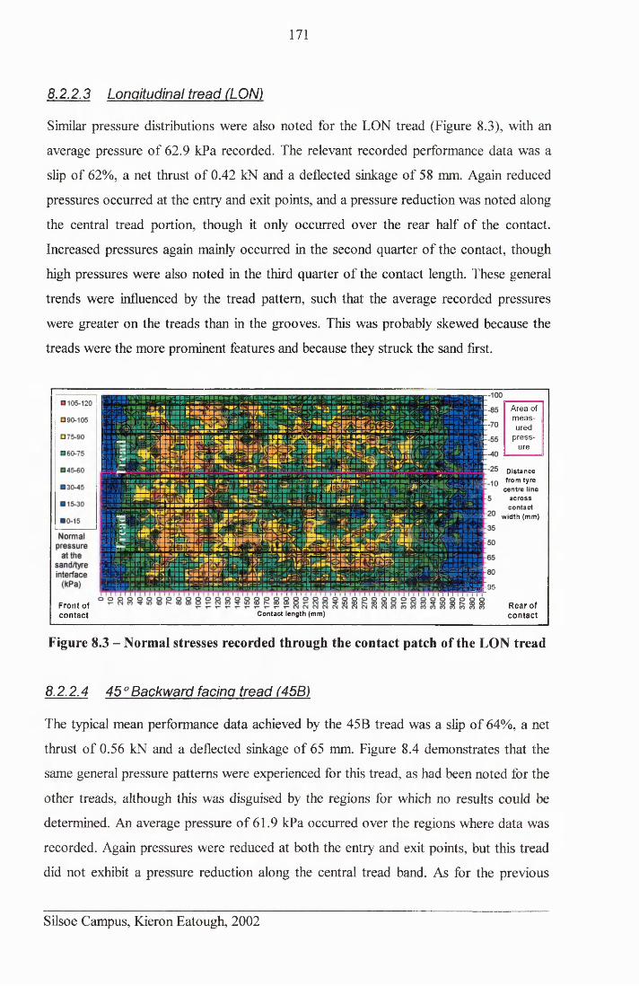
171
8.2.2.3 Longitudinal tread (LON)
Similar pressure distributions were also noted for the LON tread (Figure 8.3), with an
average pressure of 62.9 kPa recorded. The relevant recorded performance data was a
slip of 62%, a net thrust of 0.42 kN and a deflected sinkage of 58 mm. Again reduced
pressures occurred at the entry and exit points, and a pressure reduction was noted along
the central tread portion, though it only occurred over the rear half of the contact.
Increased pressures again mainly occurred in the second quarter of the contact, though
high pressures were also noted in the third quarter of the contact length. These general
trends were influenced by the tread pattern, such that the average recorded pressures
were greater on the treads than in the grooves. This was probably skewed because the
treads were the more prominent features and because they struck the sand first.
-SSX.
a »3 is’s •« n n c n * tpVSSKjaKSBHKtfaJPS’i
w n r3BBfi*’BMiiki«kLK
i
nr.z.zm9\tipifwaiiiilM li!
- i W M W X ii idB fear
i'Mmn ikJZfcdli \ N £ f S I
i hw%v.A .« nsH;a|K*KSSBite53£#JlNH A IlM
■.-t
A B K fe iftB H
utMrjtmnmaw viid \i% * J l . ‘ 1 * * 6 « * f l f c gl»!££S'?SfK«5Mf|:BB«7
■.»& * - J
ar J5»EM2S«i she J!s %t I Mi&S>BP P BUS» m
■ p 95
Area of measured
pressure
Rear of contact
Front of contact C o n ta c t len g th (m m )
D is ta n c e from tyre
ce n tr e lin e a c r o s s
c o n ta c t w id th (m m )
Figure 8.3 - Normal stresses recorded through the contact patch of the LON tread
8.2.2.4 45° Backward facing tread (45B)
The typical mean performance data achieved by the 45B tread was a slip of 64%, a net
thrust of 0.56 kN and a deflected sinkage of 65 mm. Figure 8.4 demonstrates that the
same general pressure patterns were experienced for this tread, as had been noted for the
other treads, although this was disguised by the regions for which no results could be
determined. An average pressure of 61.9 kPa occurred over the regions where data was
recorded. Again pressures were reduced at both the entry and exit points, but this tread
did not exhibit a pressure reduction along the central tread band. As for the previous
Silsoe Campus, Kieron Eatough, 2002
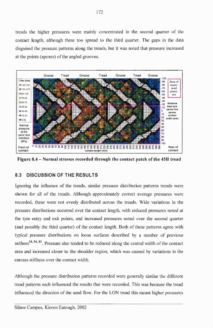
172
treads the higher pressures were mainly concentrated in the second quarter of the
contact length, although these too spread to the third quarter. The gaps in the data
disguised the pressure patterns along the treads, but it was noted that pressure increased
at the points (apexes) of the angled grooves.
'B B B k U i !M:
;^»nrA‘IBP^BBk i i \
V .B B L i^ '.-^ B B B k .
xw'immii w w:■>*>'/Z'AWjk* i t- * <i,vv. ■ s '
i 1 I '* V 'a 11 £ *J \
I k I 2 S H B V UI l klllL iK'illk JI
1ST ^ B B B k ie a ' 'B B B k
1 B B B Iwuu w m kS '/ y>5. -
V'. 1 ■ *.:IkIB t B J l l i^ vnr ssssss?ir '.:iivisa&«
k ' . - - *1 i B k '
; s^ s* j b b b i\r/,*\ jmmmr
Area of measured
pressure
Groove□ N o Data
□ 120-135
□ 105-120
□ 90-105
□ 75-90
□ 60-75
□ 45-60
□ 30-45
□ 15-30
□ 0-15
Tread Groove Tread
c o n ta c t len g th (m m )
Groove Tread Groove
Rear of contact
Normal pressure
at the sand / tyre interface
(kPa)
Front of contact
D ista n c e from tyre
c e n tr e lin e a c r o s s
c o n ta c t w id th (m m )
Figure 8.4 - Normal stresses recorded through the contact patch of the 45B tread
8.3 DISCUSSION OF THE RESULTS
Ignoring the influence of the treads, similar pressure distribution patterns trends were
shown for all of the treads. Although approximately correct average pressures were
recorded, these were not evenly distributed across the treads. Wide variations in the
pressure distributions occurred over the contact length, with reduced pressures noted at
the tyre entry and exit points, and increased pressures noted over the second quarter
(and possibly the third quarter) of the contact length. Both of these patterns agree with
typical pressure distributions on loose surfaces described by a number of previous
authors24,54,81. Pressure also tended to be reduced along the central width of the contact
area and increased closer to the shoulder region, which was caused by variations in the
carcass stiffness over the contact width.
Although the pressure distribution patterns recorded were generally similar the different
tread patterns each influenced the results that were recorded. This was because the tread
influenced the direction of the sand flow. For the LON tread this meant higher pressures
Silsoe Campus, Kieron Eatough, 2002
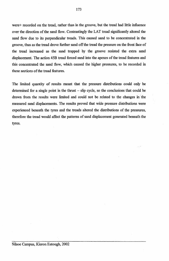
173
were+ recorded on the tread, rather than in the groove, but the tread had little influence
over the direction of the sand flow. Contrastingly the LAT tread significantly altered the
sand flow due to its perpendicular treads. This caused sand to be concentrated in the
groove, thus as the tread drove further sand off the tread the pressure on the front face of
the tread increased as the sand trapped by the groove resisted the extra sand
displacement. The action 45B tread forced sand into the apexes of the tread features and
this concentrated the sand flow, which caused the higher pressures, to be recorded in
these sections of the tread features.
The limited quantity of results meant that the pressure distributions could only be
determined for a single point in the thrust - slip cycle, so the conclusions that could be
drawn from the results were limited and could not be related to the changes in the
measured sand displacements. The results proved that wide pressure distributions Were
experienced beneath the tyres and the treads altered the distributions of the pressures,
therefore the tread would affect the patterns of sand displacement generated beneath the
tyres.
Silsoe Campus, Kieron Eatough, 2002
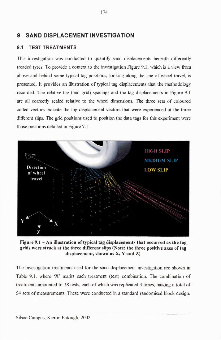
174
9 SAND DISPLACEMENT INVESTIGATION
9.1 TEST TREATMENTS
This investigation was conducted to quantify sand displacements beneath differently
treaded tyres. To provide a context to the investigation Figure 9.1, which is a view from
above and behind some typical tag positions, looking along the line of wheel travel, is
presented. It provides an illustration of typical tag displacements that the methodology
recorded. The relative tag (and grid) spacings and the tag displacements in Figure 9.1
are all correctly scaled relative to the wheel dimensions. The three sets of coloured
coded vectors indicate the tag displacement vectors that were experienced at the three
different slips. The grid positions used to position the data tags for this experiment were
those positions detailed in Figure 7.1.
HIGH SLIP
MEDIUM SLIPDirection of wheel
travel
Figure 9.1 - An illustration of typical tag displacements that occurred as the tag grids were struck at the three different slips (Note: the three positive axes of tag
displacement, shown as X, Y and Z)
The investigation treatments used for the sand displacement investigation are shown in
Table 9.1, where ‘X’ marks each treatment (test) combination. The combination of
treatments amounted to 18 tests, each of which was replicated 3 times, making a total of
54 sets of measurements. These were conducted in a standard randomised block design.
Silsoe Campus, Kieron Eatough, 2002
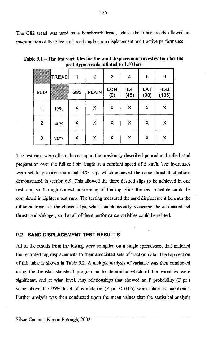
175
The G82 tread was used as a benchmark tread, whilst the other treads allowed an
investigation of the effects of tread angle upon displacement and tractive performance.
Table 9.1 - The test variables for the sand displacement investigation for the prototype treads inflated to 1.10 bar
'""111TREAD 1 2 3 4 5 6
SLIPI i
G82 PLAIN LON(0)
45F(45)
LAT(90)
45B(135)
1 15% X X X X X X
2 40% X X X X X X
3 70% X X X X X X
The test runs were all conducted upon the previously described poured and rolled sand
preparation over the full soil bin length at a constant speed of 5 km/h. The hydraulics
were set to provide a nominal 50% slip, which achieved the same thrust fluctuations
demonstrated in section 6.9. This allowed the three desired slips to be achieved in one
test run, so through correct positioning of the tag grids the test schedule could be
completed in eighteen test runs. The testing measured the sand displacement beneath the
different treads at the chosen slips, whilst simultaneously recording the associated net
thrusts and sinkages, so that all of these performance variables could be related.
9.2 SAND DISPLACEMENT TEST RESULTS
All of the results from the testing were compiled on a single spreadsheet that matched
the recorded tag displacements to their associated sets of traction data. The top section
of this table is shown in Table 9.2. A multiple analysis of variance was then conducted
using the Genstat statistical programme to determine which of the variables were
significant, and at what level. Any relationships that showed an F probability (F pr.)
value above the 95% level of confidence (F pr. < 0.05) were taken as significant.
Further analysis was then conducted upon the mean values that the statistical analysis
Silsoe Campus, Kieron Eatough, 2002
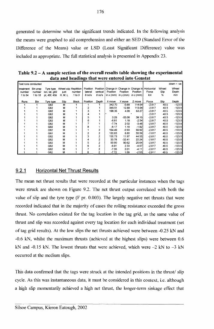
176
generated to determine what the significant trends indicated. In the following analysis
the means were graphed to aid comprehension and either an SED (Standard Error of the
Difference of the Means) value or LSD (Least Significant Difference) value was
included as appropriate. The full statistical analysis is presented in Appendix 23.
Table 9.2 - A sample section of the overall results table showing the experimental _____________ data and headings that were entered into Genstat_____________Test runs conducted down = -ve
treatment Bin prep Tyre type Wheel slip Repitition Position Position Change in Change in Change in Horizontal Wheel Wheelnumber number Ion, lat, g82 just number lateral vertical Position Position Position Force Slip Depth1 to 54 1 to 18 pt, 45f, 45b H, M, L 1 to 3 8 no's 8 no's in x (mm) in y (mm) in z (mm) k N % mm
Runs Bin Tyre type Slip Block Position Depth X move Y move Z move Force Slip Depth1 1 G82 M 1 1 1 342.70 -0.88 114.64 -2.817 40.5 -123.51 1 G82 M 1 2 1 345.51 12.88 113.04 -2.817 40.5 -123.51 1 G82 M 1 3 1 198.35 4.08 63.27 -2.817 40.5 -123.51 1 G82 M 1 4 1 * * * -2.817 40.5 -123.51 1 G82 M 1 5 1 3.25 -53.06 39.15 -2.817 40.5 -123.51 1 G82 M 1 6 1 -6.81 1.18 -2.54 -2.817 40.5 -123.51 1 G82 M 1 7 1 -7.74 2.02 -3.48 -2.817 40.5 -123.51 1 G82 M 1 8 1 -8.17 1.19 -1.82 -2.817 40.5 -123.51 1 G82 M 1 1 2 154.40 -0.93 56.92 -2.817 40.5 -123.51 1 G82 M 1 2 O 150.83 8.80 58.59 -2.817 40.5 -123.51 1 G82 M 1 3 2 155.73 11.97 44.55 -2.817 40.5 -123.51 1 G82 M 1 4 2 33.78 -32.41 22.24 -2.817 40.5 -123.51 1 G82 M 1 5 2 50.90 90.62 25.64 -2.817 40.5 -123.51 1 G82 M 1 6 2 -6.91 2.33 -4.57 -2.817 40.5 -123.51 1 G82 M 1 7 2 -7.35 2.01 -4.11 -2.817 40.5 -123.51 1 G82 M 1 8 2 -7.72 1.09 -2.53 -2.817 40.5 -123.5
9.2.1 Horizontal Net Thrust Results
The mean net thrust results that were recorded at the particular instances when the tags
were struck are shown on Figure 9.2. The net thrust output correlated with both the
value of slip and the tyre type (F pr. 0.003). The largely negative net thrusts that were
recorded indicated that in the majority of cases the rolling resistance exceeded the gross
thrust. No correlation existed for the tag location in the tag grid, as the same value of
thrust and slip was recorded against every tag location for each individual treatment (set
of tag grid results). At the low slips the net thrusts achieved were between -0.25 kN and
-0.6 kN, whilst the maximum thrusts (achieved at the highest slips) were between 0.6
kN and -0.15 kN. The lowest thrusts that were achieved, which were -2 kN to -3 kN
occurred at the medium slips.
This data confirmed that the tags were struck at the intended positions in the thrust/ slip
cycle. As this was instantaneous data, it must be considered in this context, i.e. although
a high slip momentarily achieved a high net thrust, the longer-term sinkage effect that
Silsoe Campus, Kieron Eatough, 2002
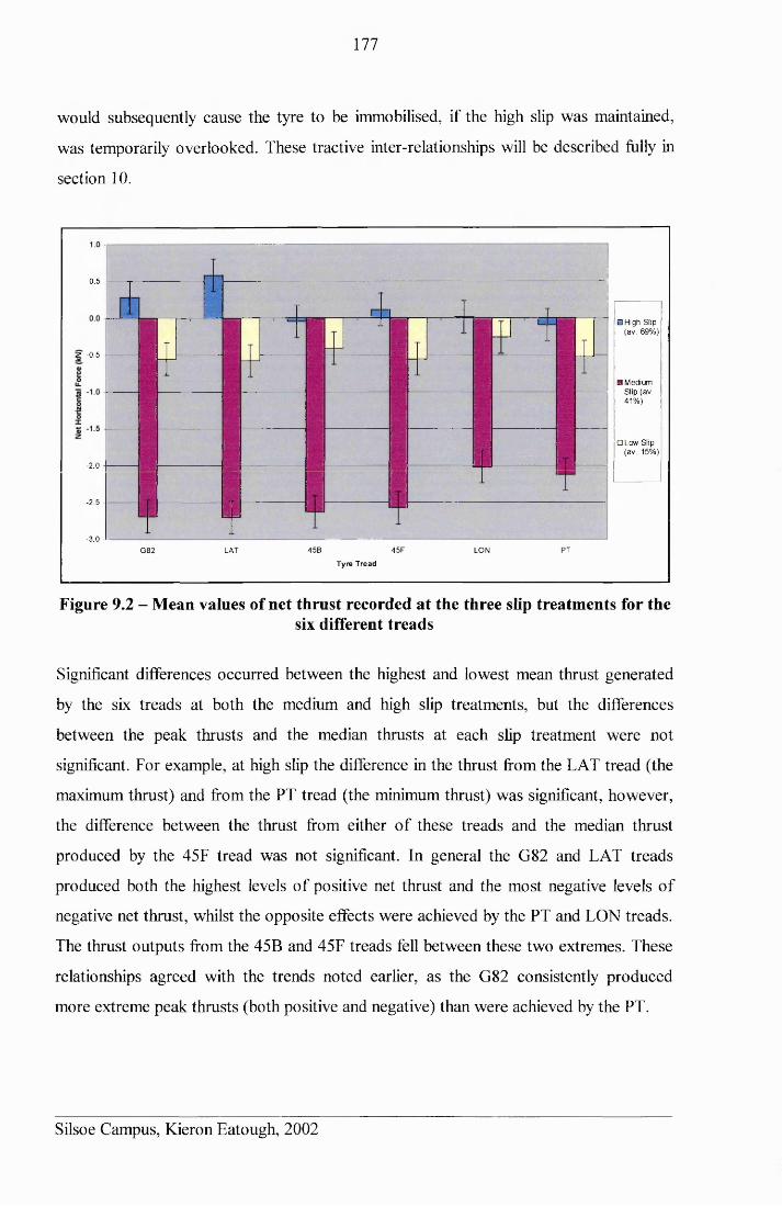
177
would subsequently cause the tyre to be immobilised, if the high slip was maintained,
was temporarily overlooked. These tractive inter-relationships will be described fully in
section 10.
0.5
□ High Slip (av. 69% )
z -0.5
E3 Medium Slip (av. 41% )
□ Low Slip (av. 15%)
- 2.0
-2.5
-3.0 -L45B 45F PTG82 LAT LON
Tyre T read
Figure 9.2 - Mean values of net thrust recorded at the three slip treatments for thesix different treads
Significant differences occurred between the highest and lowest mean thrust generated
by the six treads at both the medium and high slip treatments, but the differences
between the peak thrusts and the median thrusts at each slip treatment were not
significant. For example, at high slip the difference in the thrust from the LAT tread (the
maximum thrust) and from the PT tread (the minimum thrust) was significant, however,
the difference between the thrust from either of these treads and the median thrust
produced by the 45F tread was not significant. In general the G82 and LAT treads
produced both the highest levels of positive net thrust and the most negative levels of
negative net thrust, whilst the opposite effects were achieved by the PT and LON treads.
The thrust outputs from the 45B and 45F treads fell between these two extremes. These
relationships agreed with the trends noted earlier, as the G82 consistently produced
more extreme peak thrusts (both positive and negative) than were achieved by the PT.
Silsoe Campus, Kieron Eatough, 2002
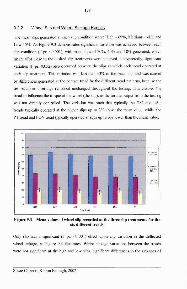
178
9.2.2 Wheel Slip and Wheel Sinkage Results
The mean slips generated at each slip condition were: High - 69%, Medium - 41% and
Low 15%. As Figure 9.3 demonstrates significant variation was achieved between each
slip condition (F pr. <0.001), with mean slips of 70%, 40% and 18% generated, which
meant slips close to the desired slip treatments were achieved. Unexpectedly, significant
variation (F pr. 0.052) also occurred between the slips at which each tread operated at
each slip treatment. This variation was less than ±3% of the mean slip and was caused
by differences generated at the contact tread by the different tread patterns, because the
test equipment settings remained unchanged throughout the testing. This enabled the
tread to influence the torque at the wheel (the slip), as the torque output from the test rig
was not directly controlled. The variation was such that typically the G82 and LAT
treads typically operated at the higher slips up to 3% above the mean value, whilst the
PT tread and LON tread typically operated at slips up to 3% lower than the mean value.
1 0 0 - r -
□ High Slip (av. 69%)
□ Medium Slip (av. 41% )
40
□ Low Slip (av. 15%)
45F LONG82 LAT 45B PT
T yre Tread
Figure 9.3 - Mean values of wheel slip recorded at the three slip treatments for thesix different treads
Only slip had a significant (F pr. <0.001) effect upon any variation in the deflected
wheel sinkage, as Figure 9.4 illustrates. Whilst sinkage variations between the treads
were not significant at the high and low slips, significant differences in the sinkages of
Silsoe Campus, Kieron Eatough, 2002
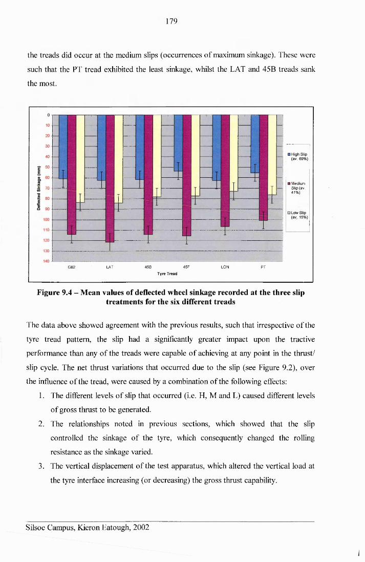
179
the treads did occur at the medium slips (occurrences of maximum sinkage). These were
such that the PT tread exhibited the least sinkage, whilst the LAT and 45B treads sank
the most.
E3 M ediumSlip (av . 41% )
G 82 LAT 45B 45F LON PT
Tyre Tread
Figure 9.4 - Mean values of deflected wheel sinkage recorded at the three slip treatments for the six different treads
The data above showed agreement with the previous results, such that irrespective of the
tyre tread pattern, the slip had a significantly greater impact upon the tractive
performance than any of the treads were capable of achieving at any point in the thrust/
slip cycle. The net thrust variations that occurred due to the slip (see Figure 9.2), over
the influence of the tread, were caused by a combination of the following effects:
1. The different levels of slip that occurred (i.e. H, M and L) caused different levels
of gross thrust to be generated.
2. The relationships noted in previous sections, which showed that the slip
controlled the sinkage of the tyre, which consequently changed the rolling
resistance as the sinkage varied.
3. The vertical displacement of the test apparatus, which altered the vertical load at
the tyre interface increasing (or decreasing) the gross thrust capability.
Silsoe Campus, Kieron Eatough, 2002
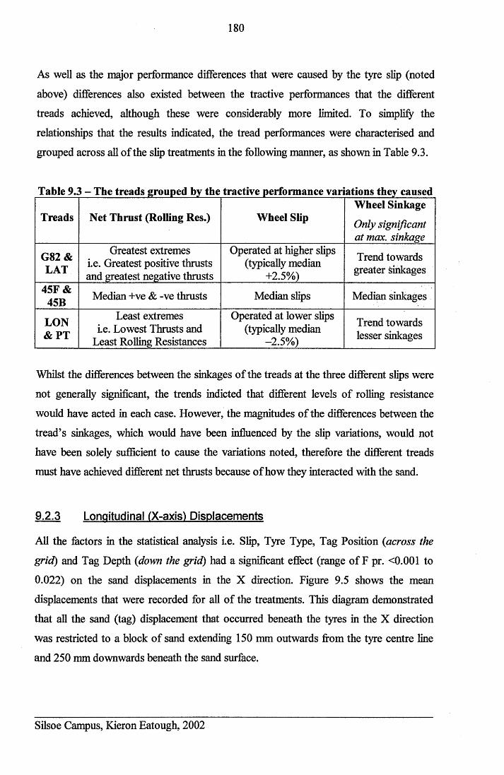
180
As well as the major performance differences that were caused by the tyre slip (noted
above) differences also existed between the tractive performances that the different
treads achieved, although these were considerably more limited. To simplify the
relationships that the results indicated, the tread performances were characterised and
grouped across all of the slip treatments in the following manner, as shown in Table 9.3.
Table 9.3 - The treads grouped by the tractive performance variations they caused
Treads Net Thrust (Rolling Res.) Wheel SlipWheel Sinkage
Only significant at max. sinkage
G82&LAT
Greatest extremes i.e. Greatest positive thrusts and greatest negative thrusts
Operated at higher slips (typically median
+2.5%)
Trend towards greater sinkages
45F&45B Median +ve & -ve thrusts Median slips Median sinkages
LON & PT
Least extremes i.e. Lowest Thrusts and
Least Rolling Resistances
Operated at lower slips (typically median
-2.5%)
Trend towards lesser sinkages
Whilst the differences between the sinkages of the treads at the three different slips were
not generally significant, the trends indicted that different levels of rolling resistance
would have acted in each case. However, the magnitudes of the differences between the
tread’s sinkages, which would have been influenced by the slip variations, would not
have been solely sufficient to cause the variations noted, therefore the different treads
must have achieved different net thrusts because of how they interacted with the sand.
9.2.3 Longitudinal (X-axis) Displacements
All the factors in the statistical analysis i.e. Slip, Tyre Type, Tag Position (across the
grid) and Tag Depth (down the grid) had a significant effect (range of F pr. <0.001 to
0.022) on the sand displacements in the X direction. Figure 9.5 shows the mean
displacements that were recorded for all of the treatments. This diagram demonstrated
that all the sand (tag) displacement that occurred beneath the tyres in the X direction
was restricted to a block of sand extending 150 mm outwards from the tyre centre line
and 250 mm downwards beneath the sand surface.
Silsoe Campus, Kieron Eatough, 2002
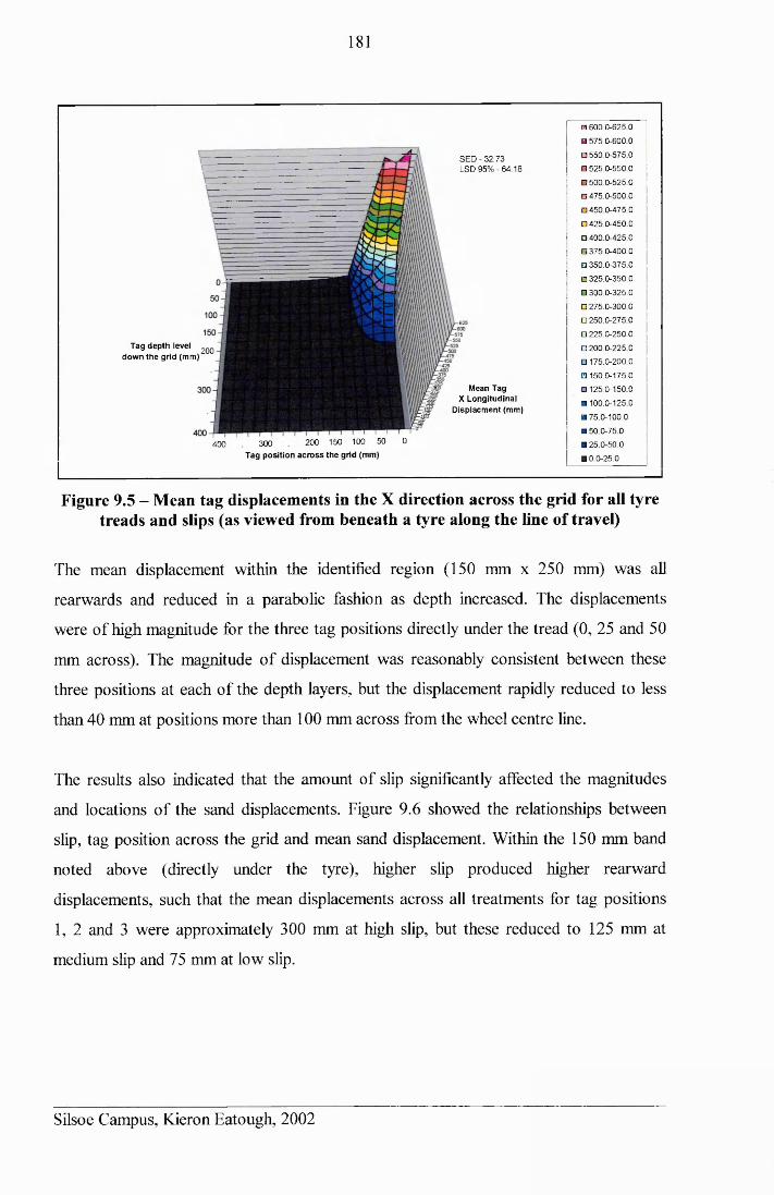
181
□ 600 .0 -625 .0
□ 5 7 5 .0 -600 .0
□ 5 5 0 .0 -575 .0
□ 5 2 5 .0 -550 .0
□ 5 00 .0 -5 2 5 .0
□ 4 7 5 .0 -500 .0
□ 4 50 .0 -4 7 5 .0
□ 4 2 5 .0 -450 .0
□ 400 0 -425 .0
□ 3 7 5 .0 -400 .0
□ 350 .0 -3 7 5 .0
□ 3 2 5 .0 -350 .0
□ 3 0 0 .0 -325 .0
□ 2 7 5 .0 -300 .0
□ 2 5 0 .0 -275 .0
□ 225 .0 -2 5 0 .0
□ 2 0 0 .0 -225 .0
□ 175.0-200.0
□ 150.0-175.0
□ 125 .0-150.0
□ 100.0-125.0
□ 75 .0-100.0
□ 50 .0-75 .0
■ 25 .0-50 .0
■ 0 .0-25 .0
S E D - 32 .73 LSD 95% - 64 .18
4 00 30 0 2 00 150 100 50 0
T ag p o s it io n a c r o s s th e grid (m m )
Mean Tag X L ongitud inal
D isp la cm en t (m m )
T ag d ep th leve l 2QQ
d o w n th e grid (m m )
Figure 9.5 - Mean tag displacements in the X direction across the grid for all tyre treads and slips (as viewed from beneath a tyre along the line of travel)
The mean displacement within the identified region (150 mm x 250 mm) was all
rearwards and reduced in a parabolic fashion as depth increased. The displacements
were of high magnitude for the three tag positions directly under the tread (0, 25 and 50
mm across). The magnitude of displacement was reasonably consistent between these
three positions at each of the depth layers, but the displacement rapidly reduced to less
than 40 mm at positions more than 100 mm across from the wheel centre line.
The results also indicated that the amount of slip significantly affected the magnitudes
and locations of the sand displacements. Figure 9.6 showed the relationships between
slip, tag position across the grid and mean sand displacement. Within the 150 mm band
noted above (directly under the tyre), higher slip produced higher rearward
displacements, such that the mean displacements across all treatments for tag positions
1, 2 and 3 were approximately 300 mm at high slip, but these reduced to 125 mm at
medium slip and 75 mm at low slip.
Silsoe Campus, Kieron Eatough, 2002
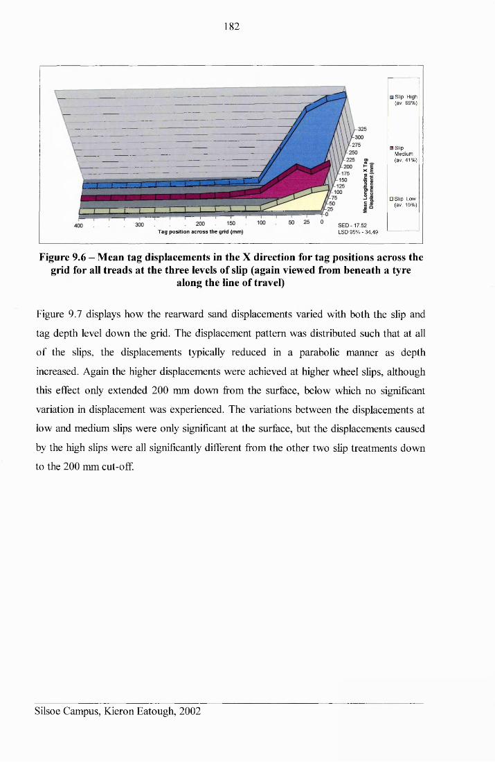
182
□ Slip High (av. 69% )
□ Slip M edium (av. 41% )
□ S lip Low (av. 15%)
T ag p o s it io n a c r o s s th e grid (m m ) LSD 95% - 34 .49
Figure 9.6 - Mean tag displacements in the X direction for tag positions across the grid for all treads at the three levels of slip (again viewed from beneath a tyre
along the line of travel)
Figure 9.7 displays how the rearward sand displacements varied with both the slip and
tag depth level down the grid. The displacement pattern was distributed such that at all
of the slips, the displacements typically reduced in a parabolic manner as depth
increased. Again the higher displacements were achieved at higher wheel slips, although
this effect only extended 200 mm down from the surface, below which no significant
variation in displacement was experienced. The variations between the displacements at
low and medium slips were only significant at the surface, but the displacements caused
by the high slips were all significantly different from the other two slip treatments down
to the 200 mm cut-off.
Silsoe Campus, Kieron Eatough, 2002
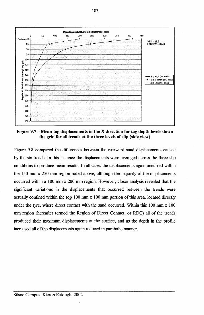
183
Mean longitudinal X tag displacem ent (mm)
150 200 250 300 400350 45010050Surface • 0
SED —23.6 LSD 95% -46.4625
100
125
150
175 —• —Slip High (av. 69%) - b— Slip Medium (av. 41%) - -Slip Low (av. 15%)
200
S» 225
£ 250
■° 275
300
325
350
375 -
400 r '
Figure 9.7 - Mean tag displacements in the X direction for tag depth levels down the grid for all treads at the three levels of slip (side view)
Figure 9.8 compared the differences between the rearward sand displacements caused
by the six treads. In this instance the displacements were averaged across the three slip
conditions to produce mean results. In all cases the displacements again occurred within
the 150 mm x 250 mm region noted above, although the majority of the displacements
occurred within a 100 mm x 200 mm region. However, closer analysis revealed that the
significant variations in the displacements that occurred between the treads were
actually confined within the top 100 mm x 100 mm portion of this area, located directly
under the tyre, where direct contact with the sand occurred. Within this 100 mm x 100
mm region (hereafter termed the Region of Direct Contact, or RDC) all of the treads
produced their maximum displacements at the surface, and as the depth in the profile
increased all of the displacements again reduced in parabolic manner.
Silsoe Campus, Kieron Eatough, 2002
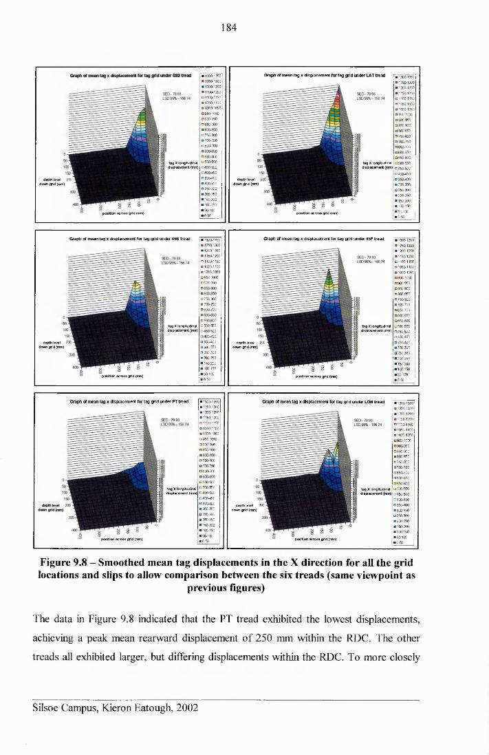
184
Graph of mean tag x displacement for tag grid inder LAT tread■ 1300-1350■ 1250-1300■ 1200-1250 B 1150-1200□ 1100-1150□ 1050-1100■ 1000-1050□ 950-1000□ 900-950□ 850-900
0 750-800 ■ 700-750 □ 650-700
□ 550-600□ 500-550□ 450-500□ 400-450□ 350-400■ 300-350 0 250-300■ 200-250■ 150-200■ 100-150■ 50-100■ 0-50
tag X longitudinal displacement (mm)
tag X longitudinal displacement (mm)
depth level 200 dovMi grid (mm)
depth level 200 dowm g ld (mm)
position across y id (mm)position across grid (mm)
Graph of mean tag x displacement for tag grid under 45B tread Graph of mean tag x displacement for tag grid under 45F tread■ 1300-1350 0 1250-1300■ 1200-1250■ 1150-1200□ 1100-1150□ 1050-1100■ 1000-1050□ 950-1000□ 900-950
□ 750-800 ■ 700-750□ 650-700
□ 550-600□ 500-550□ 450-500□ 400-450□ 350-400 B 300-350□ 250-300■ 200-250■ 150-200■ 100-150■ 50-100■ 0-50
tag X longitudinal displacement (mm)
tag X longitudinal displacement (mm)
depth level 200 down grid (mm)
depth level 200 down grid (mm)
position across grid (mm) position across grid (mm)
Graph of mean tag x displacement for tag grid under PT tread Graph of mean tag x displacement for tag grid under LON tread■ 1300-1350■ 1250-1300■ 1200-1250■ 1150-1200□ 1100-1150□ 1050-1100□ 1000-1050□ 950-1000□ 900-950□ 850-900
□ 750-800 IB 700-750□ 650-700
□ 550-600□ 500-550□ 450-500□ 400-450□ 350-400■ 300-350□ 250-300■ 200-250■ 150-200■ 100-150■ 50-100■ 0-50
tag X longitudinal displacement (mm)
tag X longitudinal displacement (mm)
depth level 200 down grid (mm)
position across grid (mm) position across grid (mm)
■ 1300-1350■ 1250-1300■ 1200-1250■ 1150-1200□ 1100-1150□ 1050-1100□ 1000-1050□ 950-1000□ 900-950□ 850-900 B 800-850□ 750-800■ 700-750□ 650-700□ 600-650□ 550-600□ 500-550□ 450-500□ 400-450□ 350-400■ 300-350■ 250-300■ 200-250■ 150-200■ 100-150■ 50-100■ 0-50
■ 1300-1350■ 1250-1300■ 1200-1250■ 1150-1200□ 1100-1150□ 1050-1100□ 1000-1050□ 950-1000□ 900-950□ 850-900■ 800-850□ 750-800■ 700-750□ 650-700□ 600-650□ 550-600□ 500-550 □450-500 □400-450□ 350-400■ 300-350□ 250-300■ 200-250■ 150-200■ 100-150■ 50-100■ 0-50
■ 1300-1350 01250-1300■ 1200-1250■ 1150-1200□ 1100-1150□ 1050-1100■ 1000-1050□ 950-1000□ 900-950□ 850-900■ 800-850□ 750-800 B 700-750□ 650-700□ 600-650□ 550-600□ 500-550 □450-500 □400-450□ 350-400■ 300-350 0250-300■ 200-250■ 150-200■ 100-150■ 50-100■ 0-50
Figure 9.8 - Smoothed mean tag displacements in the X direction for all the grid locations and slips to allow comparison between the six treads (same viewpoint as
previous figures)
The data in Figure 9.8 indicated that the PT tread exhibited the lowest displacements,
achieving a peak mean rearward displacement of 250 mm within the RDC. The other
treads all exhibited larger, but differing displacements within the RDC. To more closely
Silsoe Campus, Kieron Eatough, 2002
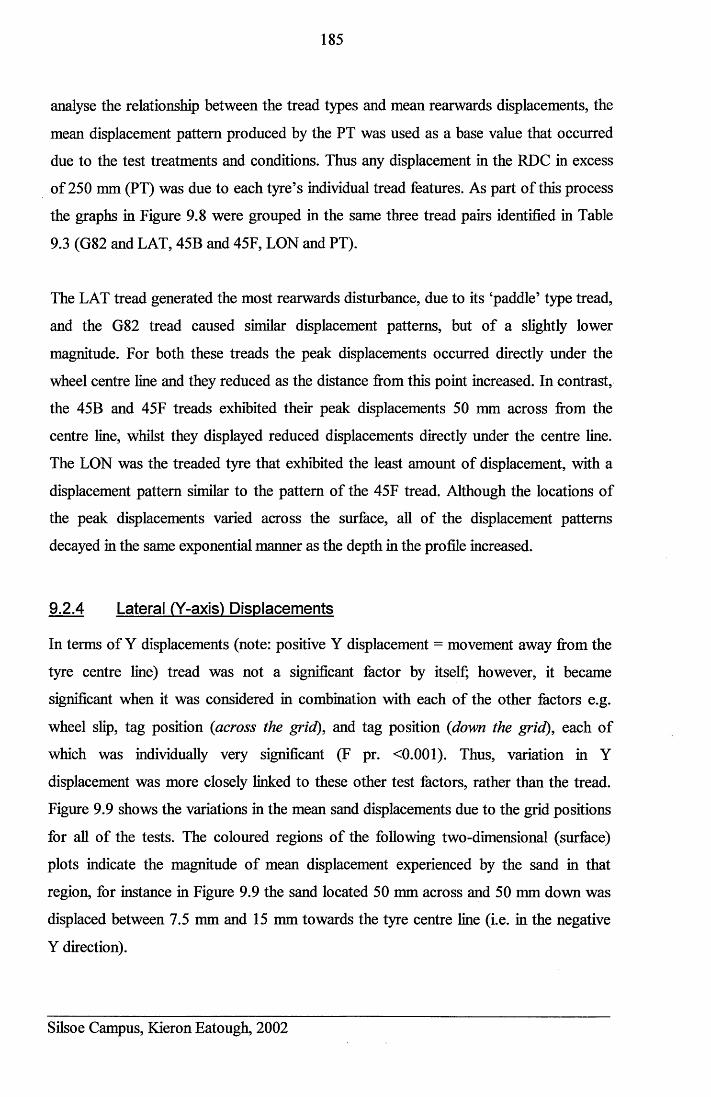
185
analyse the relationship between the tread types and mean rearwards displacements, the
mean displacement pattern produced by the PT was used as a base value that occurred
due to the test treatments and conditions. Thus any displacement in the RDC in excess
of 250 mm (PT) was due to each tyre’s individual tread features. As part of this process
the graphs in Figure 9.8 were grouped in the same three tread pairs identified in Table
9.3 (G82 and LAT, 45B and 45F, LON and PT).
The LAT tread generated the most rearwards disturbance, due to its ‘paddle’ type tread,
and the G82 tread caused similar displacement patterns, but of a slightly lower
magnitude. For both these treads the peak displacements occurred directly under the
wheel centre line and they reduced as the distance from this point increased. In contrast,
the 45B and 45F treads exhibited their peak displacements 50 mm across from the
centre line, whilst they displayed reduced displacements directly under the centre line.
The LON was the treaded tyre that exhibited the least amount of displacement, with a
displacement pattern similar to the pattern of the 45F tread. Although the locations of
the peak displacements varied across the surface, all of the displacement patterns
decayed in the same exponential manner as the depth in the profile increased.
9.2.4 Lateral (Y-axis) Displacements
In terms of Y displacements (note: positive Y displacement = movement away from the
tyre centre line) tread was not a significant factor by itself; however, it became
significant when it was considered in combination with each of the other factors e.g.
wheel slip, tag position {across the grid), and tag position {down the grid), each of
which was individually very significant (F pr. <0.001). Thus, variation in Y
displacement was more closely linked to these other test factors, rather than the tread.
Figure 9.9 shows the variations in the mean sand displacements due to the grid positions
for all of the tests. The coloured regions of the following two-dimensional (surface)
plots indicate the magnitude of mean displacement experienced by the sand in that
region, for instance in Figure 9.9 the sand located 50 mm across and 50 mm down was
displaced between 7.5 mm and 15 mm towards the tyre centre line (i.e. in the negative
Y direction).
Silsoe Campus, Kieron Eatough, 2002
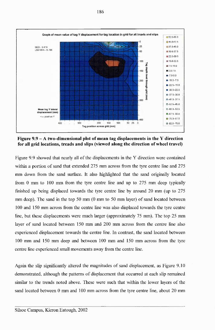
186
□ 52.5 -60 .0
□ 45.0 -52 .5
□ 3 7 .5 -45 .0
□ 3 0 .0 -37 .5
□ 2 2 .5 -30 .0
ES 15.0-22.5
□ 7.5 -15 .0
■ 0.0 -7 .5
61 -7 .5-0 .0
□ -1 5 .0 -7 .5
□ -2 2 .5 -1 5 .0
□ -3 0 .0 -2 2 .5
□ -3 7 .5 -3 0 .0
□ -4 5 .0 -3 7 .5
□ -5 2 .5 -4 5 0
□ -6 0 .0 -5 2 .5
□ -6 7 .5 -6 0 .0
□ -7 5 .0 -6 7 .5
□ -8 2 .5 -7 5 .0
Graph of mean value of tag Y displacement for tag location in grid for all treads and slips
S E D - 3 .419 LSD 95% - 6 .706
M ean tag Y lateral d isp la c e m e n t (m m )
<— positive Y
400 . . 3 00 . . 20 0 . 150 . 100 . 50 2 5 0T a g p o s i t io n a c r o s s g rid (m m )
Figure 9.9 - A two-dimensional plot of mean tag displacements in the Y direction for all grid locations, treads and slips (viewed along the direction of wheel travel)
Figure 9.9 showed that nearly all of the displacements in the Y direction were contained
within a portion of sand that extended 275 mm across from the tyre centre line and 275
mm down from the sand surface. It also highlighted that the sand originally located
from 0 mm to 100 mm from the tyre centre line and up to 275 mm deep typically
finished up being displaced towards the tyre centre line by around 20 mm (up to 275
mm deep). The sand in the top 50 mm (0 mm to 50 mm layer) of sand located between
100 and 150 mm across from the centre line was also displaced towards the tyre centre
line, but these displacements were much larger (approximately 75 mm). The top 25 mm
layer of sand located between 150 mm and 200 mm across from the centre line also
experienced displacement towards the centre line. In contrast, the sand located between
100 mm and 150 mm deep and between 100 mm and 150 mm across from the tyre
centre line experienced small movements away from the centre line.
Again the slip significantly altered the magnitudes of sand displacement, as Figure 9.10
demonstrated, although the patterns of displacement that occurred at each slip remained
similar to the trends noted above. These were such that within the lower layers of the
sand located between 0 mm and 100 mm across from the tyre centre line, about 20 mm
Silsoe Campus, Kieron Eatough, 2002
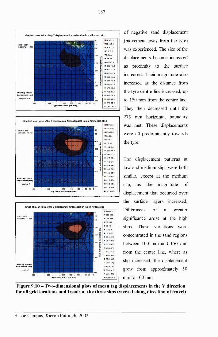
of negative sand displacement
(movement away from the tyre)
was experienced. The size of the
displacements became increased
as proximity to the surface
increased. Their magnitude also
increased as the distance from
the tyre centre line increased, up
to 150 mm from the centre line.
They then decreased until the
275 mm horizontal boundary
was met. These displacements
were all predominantly towards
the tyre.
The displacement patterns at
low and medium slips were both
similar, except at the medium
slip, as the magnitude of
displacement that occurred over
the surface layers increased.
Differences of a greater
significance arose at the high
slips. These variations were
concentrated in the sand regions
between 100 mm and 150 mm
from the centre line, where as
slip increased, the displacement
grew from approximately 50
mm to 100 mm.
Figure 9.10 - Two-dimensional plots of mean tag displacements in the Y direction for all grid locations and treads at the three slips (viewed along direction of travel)
187
G raph of m ean value of ta g Y d isp lacem en t for tag location in grid for high s lip s
Mean tag Y lateral displacement (mm)
I I I ! ‘ I
T T T T T l r a W T i \ L Jj i 7 y \ j
j j1 I [NvJ
Tag position across grid (mm)
□ 30.0-37.5
□ 22.5-30.0
□ 15.0-22.5
□ 7.5-15.0
B 0.0-7.5
□ -7.5-0.0
0-15.0—7.5
■-22.5-15.0
□-30.0-22.5
□-37.5-30.0
□-45.0-37.5
□-52.5-45.0
□-60.0-52.5
□-67.5-60.0
□-75.0-67.5
B-82.5-75.0
□-90.0-82.5
□-97.5-90.0
H-105.0-97.5
G raph of m ean value of ta g Y d isp lacem en t for tag loca tion in grid fo r m edium slip s
9PS SOS SSEfe 2% *35$ 1 £ 3 9
BSSBBBSf^B B B B B B l
m m m a M n h i i m mBBBBfiflBBBBBBBBBB
Mean tag Y lateral displacement (mm)
<— positive YIlilllllilRlE HI
■300 . . 200 . 150 . 4
Tag position across grid (mm)
□ 30.0-37.5
□ 22.5-30.0
□ 15.0-22.5
□ 7.5-15.0
■ 0.0-7.5
H-7.5-0.0
B-15.0-7.5
□ -22.5—15.0
□-30.0-22.5
□-37.5-30.0
□-45.0-37.5
□-52.5-45.0
□-60.0-52.5
□-67.5-60.0
□-75.0—67.5
□ -82.5—75.0
□-90.0-82.5
□-97.5-90.0
B-105.0-97.5
G raph of m ean value of ta g Y d isp lacem en t for tag location in grid fo r low slips
Mean tag Y lateral displacement (mm)
<— positive Y
■SB 33 BBSS ESS 39' 'Wm8m
W MfiBBBBBBB^ S’MM
■ ^ i s n BBflflBBBBBfettiiflftHiB BBBBBBBBBBBBBKBSI B B B B B B B B B B I 2 B 3 & .I B
—
Tag position across grid (mm)
□ 30.0-37.5
□ 22.5-30.0
□ 15.0-22.5
□ 7.5-15.0
B0.0-7.5
B-7.5-0.0
B-15.0-7.5
□-22.5-15.0
B -30.0-22.5
□-37.5-30.0
□-45.0-37.5
□ -52.5-45.0
□-60.0—52.5
□-67.5-60.0
□-75.0-67.5
H-82.5-75.0
□-90.0-82.5
B-97.5-90.0
B-105.0—97.5
Silsoe Campus, Kieron Eatough, 2002
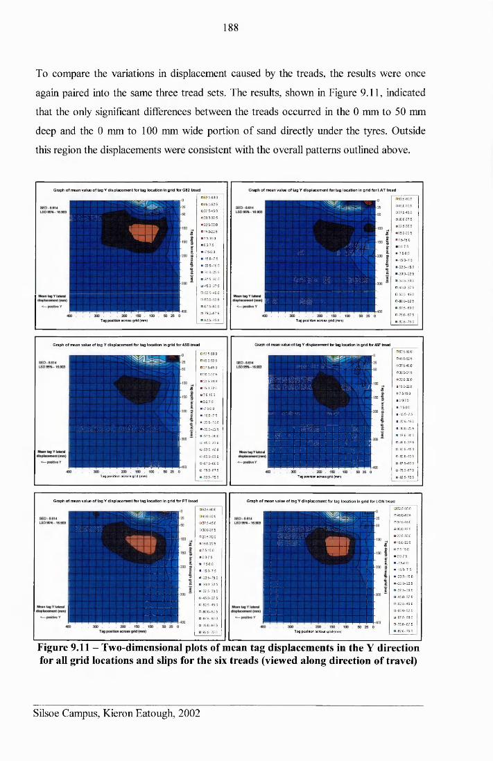
188
To compare the variations in displacement caused by the treads, the results were once
again paired into the same three tread sets. The results, shown in Figure 9.11, indicated
that the only significant differences between the treads occurred in the 0 mm to 50 mm
deep and the 0 mm to 100 mm wide portion of sand directly under the tyres. Outside
this region the displacements were consistent with the overall patterns outlined above.
Graph of mean value of tag Y displacement for tag location in grid for G82 tread
Him pmmwm
in r*mwr"
n across grid (mm)
□ 52.5-60.0
□45.0-52.5
□ 37.5-45.0
□ 30.0-37.5
B22.5-30.0
■ 15.0-22.5
07.5-15.0
■ 0.0-7.5
■-7.5-0.0
■ -15.0-7.5
■-22.5-15.0
■-30.0-22.5
■-37.5-30.0
□-45.0-37.5
□-52.5-45.0
□-60.0-52.5
0-67.5-60.0
□-75.0-67.5
■-82.5-75.0
Graph of mean value of tag Y displacement for tag location in grid for LAT tread
a C B H III * i' iBBB
imm-< it ■ jfei; ______________________Z M - IS M $-
Tag position across grid (mm)
□ 525-600
□45.0-52.5
□ 37.5-45.0
■ 30 0-37 5
■ 22.5-30 0
n 15.0-22.5
075-15.0
■ 0 0-7 5
■ -7 5-0.0
■ -15.0-7.5
■-22.5—15.0
■-30.0-22.5
■-37.5-30.0
□-45.0-37.5
□-52 5-45.0
□-60.0-52.5
0-67 5-60.0
0-75.0-67.5
■-82 5-75.0
Graph of mean value of tag Y displacement for tag location in grid for 45B tread
BBBBBBBBBBBBI
IBBflfTag position across grid (mm)
□ 52.5-60.0
□ 45.0-52 5
□ 37.5-45.0
□ 30.0-37.5
■ 22.5-30 0
a 15.0-22.5
■ 7.5-15.0
■ 00-7.5
■ -7.5-0.0
s -15.0-7.5
a -22.5-15.0
■ -30 0-22.5
■ -37.5-30.0
□ -45.0-37.5
□ -52 5-45.0
□ -60 0-52.5
□ -67 5-60.0
□ -75.0-67.5
■ -82.5-75.0
Graph of mean value of tag Y displacement for tag location in grid for 45F tread
W--V; •.>®S5SBP¥iB■b b h m s tIB B IH II -., 18UIH
m a s W. 155 SS '4f$ 31
r _ r □— j— —
r
n - V:.i——; _ |
_ ,*S— i r~ ; i S
J ' ;• i__
__L_ ___
■ __ _~~f
- . _ _ g
Tag position across grid (mm)
□ 52.5-60.0
□ 45 0-52.5
□ 37.5-45.0
□ 30 0-37.5
■ 225-30.0
B 15 0-22.5
□ 7.5-15.0
10.0-7.5
a-7.5-0.0
a -15.0-7.5
1-22.5-15.0
■ -30.0-22.5
B -37.5-30.0
□-45.0-37.5
□-52.5-45.0
□ -60 0-52.5
□-67 5-60.0
□-75.0-67.5
1-82 5-75.0
Graph of mean value of tag Y displacement for tag location in grid for PT tread
BHBiT
□ 52.5-60.0
□ 45 0-52.5
□ 37 5-45.0
□ 30.0-37.5
■ 22.5-30.0
□ 15.0-22.5
0 7.5-15.0
■ 0.0-7.5
■ -7.5-0.0
1-15.0-7.5
■ -22.5-15.0
■ -30 0-22.5
■ -37 5-30.0
□ -45 0-37 5
□ -52 5-45 0
□ -60 0-52 5
0-67 5-60.0
□ -75 0-87.5
■ -82 5-75 0
Graph of mean value of tag Y displacement for tag location in grid for LON tread
BBaBBr^&SSBB■BBBr:’mmmt- j b b b i ' ■■■!
~
Tag position across grid (mm)
□ 52.5-60.0
□ 45.0-52 5
□ 37 5-45 0
□ 30.0-37.5
■ 22.5-30 0
0 15.0-22.5
a 7.5-15.0
■ 0.0-7.5
a -7.5-0.0
a -15.0-7.5
0-22.5-15.0
■ -30.0-22.5
■ -37 5-30 .0
□ -45.0-37.5
□-52.5-45.0
□ -60 0-52 5
■-67 5-60 0
□ -75 0-67.5
■ -82 5-75.0
Figure 9.11 - Two-dimensional plots of mean tag displacements in the Y direction for all grid locations and slips for the six treads (viewed along direction of travel)
Silsoe Campus, Kieron Eatough, 2002
189
Again the treads only caused differing disturbances over the portions of sand with
which they had direct contact. Although the different treads caused different
displacements within the 50 mm wide x 100 mm deep region of sand, the limited
number of results recorded within this region did not allow any patterns to be
determined. Also, in reality the differences in the displacements were only of small
magnitudes (being between 20 mm and 30 mm). Thus it was the tyre carcass that was
responsible for most of the Y displacements, i.e. those that were common between
treads, whilst the tread only had a minor influence over the variations in the Y
displacement and these were concentrated in the sand closest to the tyre.
9.2.5 Vertical (Z-axis) Displacements
The same factors were significant for the Z (vertical movement) analysis as had been for
the Y analysis, i.e. wheel slip, and tag vertical and horizontal tag position (all F pr.
<0.001). Again tread was only significant when considered in combination with the
other factors (F pr. <0.001 to 0.034). Figure 9.12 indicated that the displacements in the
X direction were also limited within the same 275 mm x 275 mm region of sand. The
downward displacements from the surface in the sand located between 125 mm and 200
mm across from the tyre centre line occurred because of the sand flow effects explained
in section 9.2.4, where the most significant sand flows were those from this region
which moved back towards the tyre. Contrastingly the sand in the lower layers of this
band of sand was forced to rise slightly as the tyre load caused a crescent shear failure
across the cross-section of sand. This upward displacement added further impetus to the
later failure of the sand back into the void left by the tyre, which was highlighted the Y
and Z displacement results.
Silsoe Campus, Kieron Eatough, 2002
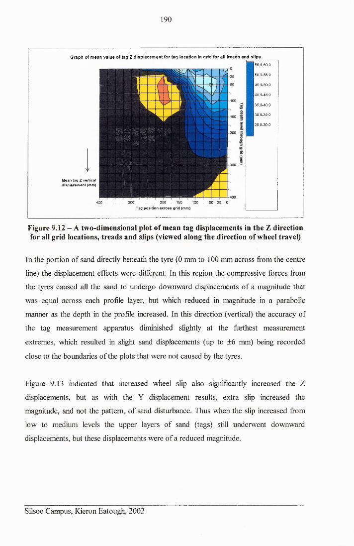
190
'M m W m M M MSpjj J . S’; $$$ P?$*' *%; ; ? %&&
MM ■ MM.:m . ■ ■ ,. •■■
5 5 .0 -60 .0
5 0 .0 -55 .0
4 5 .0 -5 0 .0
4 0 .0 -4 5 .0
35 .0 -4 0 .0
30 .0 -35 .0
25 .0 -3 0 .0
Graph of mean value of tag Z displacement for tag location in grid for all treads and slips
M ean tag Z vertical d isp la c e m e n t (m m )
400 . . 3 0 0 . . 200 . 150 . 100 . 5 0 25 0
T ag p o s it io n a c r o s s grid (m m )
Figure 9.12 - A two-dimensional plot of mean tag displacements in the Z direction for all grid locations, treads and slips (viewed along the direction of wheel travel)
In the portion of sand directly beneath the tyre (0 mm to 100 mm across from the centre
line) the displacement effects were different. In this region the compressive forces from
the tyres caused all the sand to undergo downward displacements of a magnitude that
was equal across each profile layer, but which reduced in magnitude in a parabolic
manner as the depth in the profile increased. In this direction (vertical) the accuracy of
the tag measurement apparatus diminished slightly at the furthest measurement
extremes, which resulted in slight sand displacements (up to ±6 mm) being recorded
close to the boundaries of the plots that were not caused by the tyres.
Figure 9.13 indicated that increased wheel slip also significantly increased the Z
displacements, but as with the Y displacement results, extra slip increased the
magnitude, and not the pattern, of sand disturbance. Thus when the slip increased from
low to medium levels the upper layers of sand (tags) still underwent downward
displacements, but these displacements were of a reduced magnitude.
Silsoe Campus, Kieron Eatough, 2002
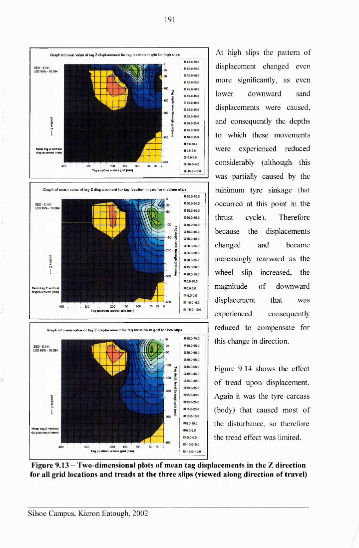
191
1 H K Ll i i i i m w ' l l l l K ^ s<MBi ATmmmmt
^ '*•I l I K t ^ \% 4 K ^m u m m m m n m i i B — w m ^ ■ i i r " m msasa
1111! UlASIiSii
3200 5
Mean tag Z vertical displacement (mm)
•1 -1 300 . . 200 . 150 . 100 . 50 25
Tag position across grid (mm)
G rap h o f m e a n v a lu e o f ta g Z d is p la c e m e n t fo r ta g lo ca tio n in g rid fo r low s lip s
Mean tag Z vertical displacement (mm)
~ /////&$& i w i i B w mmwm
■Ksiw m m s iimmw 'x s m'v r n u n
’ 1 IL IM I!I B S l B S g® I-1
300 . . 200 . 150 . 100 . 50 25Tag position across grid (mm)
G rap h o f m e a n v a lu e o f ta g Z d is p la c e m e n t fo r ta g lo ca tio n in g rid fo r m ed ium s lip s
G raph o f m ean value o f tag Z d isp lacem ent fo r ta g location in grid for h igh s lip s
400 . . 300 . . 200 . 150 . 100 . 50 25 0Tag position across grid (mm)
Mean tag Z vertical displacement (mm)
At high slips the pattern of
displacement changed even
more significantly, as even
lower downward sand
displacements were caused,
and consequently the depths
to which these movements
were experienced reduced
considerably (although this
was partially caused by the
minimum tyre sinkage that
occurred at this point in the
thrust cycle). Therefore
because the displacements
changed and became
increasingly rearward as the
wheel slip increased, the
magnitude of downward
displacement that was
experienced consequently
reduced to compensate for
this change in direction.
Figure 9.14 shows the effect
of tread upon displacement.
Again it was the tyre carcass
(body) that caused most of
the disturbance, so therefore
the tread effect was limited.
Figure 9.13 - Two-dimensional plots of mean tag displacements in the Z direction for all grid locations and treads at the three slips (viewed along direction of travel)
Silsoe Campus, Kieron Eatough, 2002
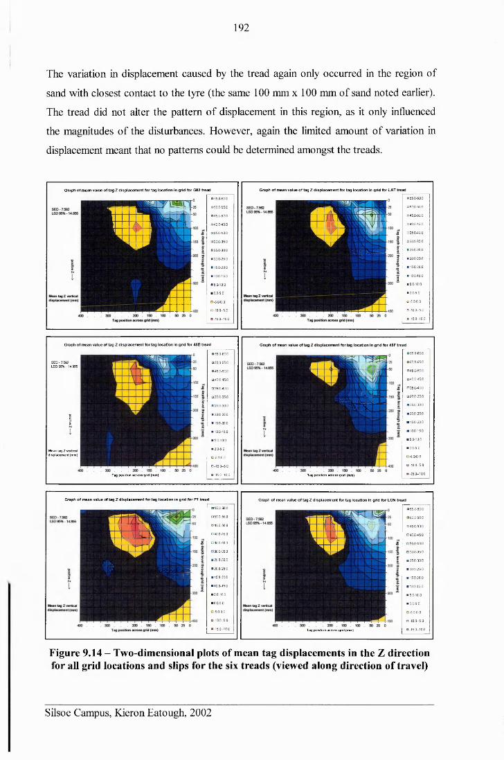
192
The variation in displacement caused by the tread again only occurred in the region of
sand with closest contact to the tyre (the same 100 mm x 100 mm of sand noted earlier).
The tread did not alter the pattern of displacement in this region, as it only influenced
the magnitudes of the disturbances. However, again the limited amount of variation in
displacement meant that no patterns could be determined amongst the treads.
Graph of mean value of tag 2 displacement for tag location in grid for G82 tread
1 1 1 ! S M Iman ;asu »M 1 S IIL '<11111 ■■k<JW
"WW*
a 55 0-80.0
0 50 0-55.0
045 0-50.0
□ 40.0-45.0
0 35.0-40.0
0 30.0-35.0
B 25.0-30.0
■ 20.0-25.0
■ 15.0-20.0
■ 10.0-15.0
a 5.0-10.0
■ 0.0-5.0
□ -5.0-0.0
O-10.0-5.0
□ -15.0-10.0
Graph of mean value of tag Z displacement for tag location in grid for LAT tread
IAmmv
link 1HISSW w r ^U9r
?$■■■■
a 55 0-60 0
□ 50 0-55 0
□ 450-50.0
□ 40.0-450
□ 35.0-40 0
□ 30 0-35.0
B 25.0-30.0
B 20.0-25.0
B 15.0-20.0
B 10.0-15.0
a 5 0-10.0
a 0.0-5.0
□ -5.0-0.0
□ -10 0-5.0
a-15.0-100
Graph of mean value of tag Z displacement for tag location in grid for 45B tread
SED - 7.562 LSD 95% - 14.855
■8
tI
Mean tag Z verticaldisplacement (mm)
Tag position across grid (mm)
■ 55 0-60.0
Q 50.0-55 0
045 0-50 0
O40.0-45.0
□ 35.0-40.0
□ 30.0-35.0
B 25.0-30.0
■ 20.0-25.0
B 15.0-20.0
■ 10.0-15.0
■ 5.0-10.0
■ 0.0-5.0
□ -5.0-0.0
0-10.0-5.0
0-15.0-10 0
Graph of mean value of tag Z displacement for tag location in grid for 45F tread
i h l i i s r ir wmuw mmitmxsmmmwmwwmm,iwmmum
Tag position across grid (mm)
■ 55.0-60 0
□ 50 0-55 0
045 0-50.0
□40 0-450
□ 35.0-40.0
□ 30.0-35.0
■ 25.0-30.0
■ 20.0-25.0
■ 15.0-20 0
■ 10.0-15.0
■ 5.0-100
■ 0 0-5 0
□-5 0-00
0-10.0-5.0
□ -15 0-10.0
Graph of mean value of tag Z displacement for tag location in grid for PT tread
■km! «■ ^ ao n■IIKIlMkY■■■HIT
-yw'H im ' ' USSHS
il
■ 55 0-60 0
□ 50 0-55.0
□45 0-50.0
□40.0-45.0
□ 35.0-40.0
□ 30.0-35.0
■ 25.0-30 0
■ 20.0-25.0
■ 15 0-20 0
■ 10.0-15.0
■ 50-100
■ 0 0-5 0
□-5 0-0.0
0 -100-5 0
□ -15.0-10 0
Graph of mean value of tag Z displacement for tag location in grid for LON tread
_____I B W lL l ^ H S i l'■■■ilk mwmw■■I «: V'w iaw
''W W W
Tag position across grid (mm)
■ 55.0-60.0
□ 50.0-55 0
□ 45 0-50.0
□ 40.0-45.0
□ 35.0-40.0
□ 30.0-35 0
■ 25.0-30.0
■ 20.0-25.0
■ 15.0-20.0
■ 10.0-15.0
■ 5.0-10.0
■ 0 0-5.0
0 -5 .0-0.0
0-10 0-5.0
0-15.0-10.0
Figure 9.14 - Two-dimensional plots of mean tag displacements in the Z direction for all grid locations and slips for the six treads (viewed along direction of travel)
Silsoe Campus, Kieron Eatough, 2002
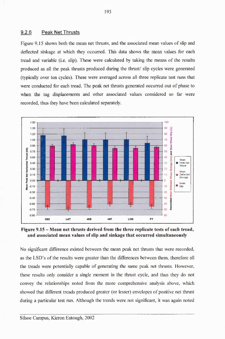
193
9.2.6 Peak Net Thrusts
Figure 9.15 shows both the mean net thrusts, and the associated mean values of slip and
deflected sinkage at which they occurred. This data shows the mean values for each
tread and variable (i.e. slip). These were calculated by taking the means of the results
produced as all the peak thrusts produced during the thrust/ slip cycles were generated
(typically over ten cycles). These were averaged across all three replicate test runs that
were conducted for each tread. The peak net thrusts generated occurred out of phase to
when the tag displacements and other associated values considered so far were
recorded, thus they have been calculated separately.
40 ? -------------------f= Mean
30 B Peak Net Thrust
20 Bif Mean
10 S □ Deflected Sinkage
M eanSlip
Figure 9.15 - Mean net thrusts derived from the three replicate tests of each tread, and associated mean values of slip and sinkage that occurred simultaneously
No significant difference existed between the mean peak net thrusts that were recorded,
as the LSD’s of the results were greater than the differences between them, therefore all
the treads were potentially capable of generating the same peak net thrusts. However,
these results only consider a single moment in the thrust cycle, and thus they do not
convey the relationships noted from the more comprehensive analysis above, which
showed that different treads produced greater (or lesser) envelopes of positive net thrust
during a particular test run. Although the trends were not significant, it was again noted
Silsoe Campus, Kieron Eatough, 2002
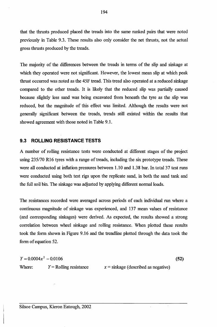
194
that the thrusts produced placed the treads into the same ranked pairs that were noted
previously in Table 9.3. These results also only consider the net thrusts, not the actual
gross thrusts produced by the treads.
The majority of the differences between the treads in terms of the slip and sinkage at
which they operated were not significant. However, the lowest mean slip at which peak
thrust occurred was noted as the 45F tread. This tread also operated at a reduced sinkage
compared to the other treads. It is likely that the reduced slip was partially caused
because slightly less sand was being excavated from beneath the tyre as the slip was
reduced, but the magnitude of this effect was limited. Although the results were not
generally significant between the treads, trends still existed within the results that
showed agreement with those noted in Table 9.1.
9.3 ROLLING RESISTANCE TESTS
A number of rolling resistance tests were conducted at different stages of the project
using 235/70 R16 tyres with a range of treads, including the six prototype treads. These
were all conducted at inflation pressures between 1.10 and 1.38 bar. In total 37 test runs
were conducted using both test rigs upon the replicate sand, in both the sand tank and
the full soil bin. The sinkage was adjusted by applying different normal loads.
The resistances recorded were averaged across periods of each individual run where a
continuous magnitude of sinkage was experienced, and 137 mean values of resistance
(and corresponding sinkages) were derived. As expected, the results showed a strong
correlation between wheel sinkage and rolling resistance. When plotted these results
took the form shown in Figure 9.16 and the trendline plotted through the data took the
form of equation 52.
7 = 0.0004x2 -0.0106 (52)Where: Y= Rolling resistance x = sinkage (described as negative)
Silsoe Campus, Kieron Eatough, 2002
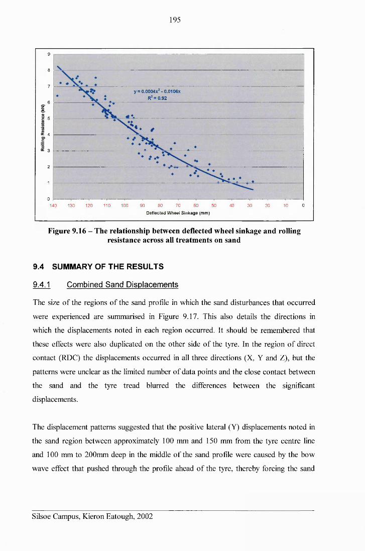
195
9
8
7y = 0.0004x2 - 0.0106x
R2 = 0.926
zJ£<DC O <00?10ffiDC 4 O)C
2
1
070 60 50 40 0140 120 110 100 90 80 30 20 10130
D e f l e c t e d W h e e l S in k a g e (m m )
Figure 9.16 - The relationship between deflected wheel sinkage and rolling resistance across all treatments on sand
9.4 SUMMARY OF THE RESULTS
9.4.1 Combined Sand Displacements
The size of the regions of the sand profile in which the sand disturbances that occurred
were experienced are summarised in Figure 9.17. This also details the directions in
which the displacements noted in each region occurred. It should be remembered that
these effects were also duplicated on the other side of the tyre. In the region of direct
contact (RDC) the displacements occurred in all three directions (X, Y and Z), but the
patterns were unclear as the limited number of data points and the close contact between
the sand and the tyre tread blurred the differences between the significant
displacements.
The displacement patterns suggested that the positive lateral (Y) displacements noted in
the sand region between approximately 100 mm and 150 mm from the tyre centre line
and 100 mm to 200mm deep in the middle of the sand profile were caused by the bow
wave effect that pushed through the profile ahead of the tyre, thereby forcing the sand
Silsoe Campus, Kieron Eatough, 2002
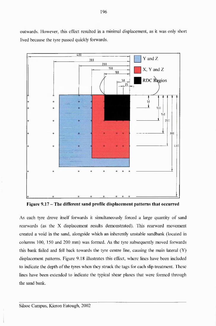
196
outwards. However, this effect resulted in a minimal displacement, as it was only short
lived because the tyre passed quickly forwards.
Y and Z
X,Y and Z
RDC ion
5D
1 1 0
1 5 0
*- 2 0 0
---------------------------- *- 30 0
--------------- !L Ufl
Figure 9.17 - The different sand profile displacement patterns that occurred
As each tyre drove itself forwards it simultaneously forced a large quantity of sand
rearwards (as the X displacement results demonstrated). This rearward movement
created a void in the sand, alongside which an inherently unstable sandbank (located in
columns 100, 150 and 200 mm) was formed. As the tyre subsequently moved forwards
this bank failed and fell back towards the tyre centre line, causing the main lateral (Y)
displacement patterns. Figure 9.18 illustrates this effect, where lines have been included
to indicate the depth of the tyres when they struck the tags for each slip treatment. These
lines have been extended to indicate the typical shear planes that were formed through
the sand bank.
Silsoe Campus, Kieron Eatough, 2002
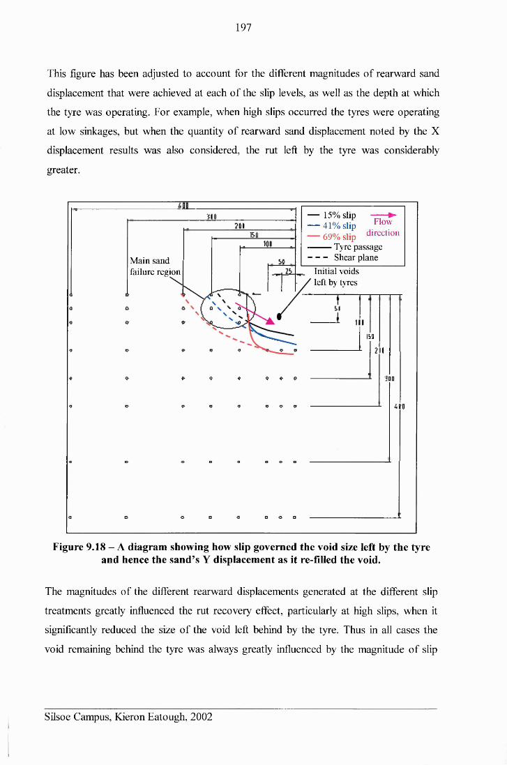
197
This figure has been adjusted to account for the different magnitudes of rearward sand
displacement that were achieved at each of the slip levels, as well as the depth at which
the tyre was operating. For example, when high slips occurred the tyres were operating
at low sinkages, but when the quantity of rearward sand displacement noted by the X
displacement results was also considered, the rut left by the tyre was considerably
greater.
— 15% slip— 41% slip— 69% slip Tyre passage Shear plane
FlowdirectionIS O
Main sand failure region Initial voids
left by tyres
IH
3DD
Figure 9.18 - A diagram showing how slip governed the void size left by the tyre and hence the sand’s Y displacement as it re-filled the void.
The magnitudes of the different rearward displacements generated at the different slip
treatments greatly influenced the rut recovery effect, particularly at high slips, when it
significantly reduced the size of the void left behind by the tyre. Thus in all cases the
void remaining behind the tyre was always greatly influenced by the magnitude of slip
Silsoe Campus, Kieron Eatough, 2002
198
(rut recovery) occurring directly ahead of it. These effects were also considered when
Figure 9.18 was constructed.
Additionally the vertical (Z) displacement results indicated that the mean depths at
which the sand was left after traction were higher than the sinkages at which the tyres
operated at each considered point in the thrust cycle. This was partially due to the rut
recoveiy effect that occurred, due to sand displacement in the longitudinal (X) direction,
which replaced some of the sand in the void left behind the slipping (excavating) tyre. It
was also partially due to sand moving into the tyre void as the sand alongside the rut
failed. These combined effects meant that the sand from the top layers of the profile (0
mm to 50 mm deep) became mixed as it moved either rearward or sideward and the
volume increased, which meant that the surface layers finished their displacement at a
position that was above the lower sinkage to which they had been forced whilst
producing traction.
9.4.2 Tread Effects
The tread effect in both the lateral (Y) and vertical (Z) displacement directions all
occurred within the RDC region. Whilst differences did occur between the treads these
affected only small quantities of sand, such that in both directions the effects of any
variations were small, and the limited number of tags located in this region produced
insufficient data to allow any precise trends to be determined. Contrastingly the tread
pattern significantly affected the mean longitudinal (X) displacements across all the
treads and with a much greater magnitude. The PT produced the minimum displacement
in this direction, which was taken as the ‘base’ displacement caused by the tyre. The
other treads all produced similar patterns of displacement, although the magnitude of
these varied significantly depending upon the tread pattern, whilst all of the variation in
magnitude occurred in the RDC.
As the tyre tread only very significantly affected both the net thrusts that were produced
by the treads and the longitudinal (X) displacements noted in the RDC, then the net
thrust variations produced by the treads must be dependant upon the magnitude of
rearward sand displacement. This could have affected either (or both) the gross thrust or
Silsoe Campus, Kieron Eatough, 2002i
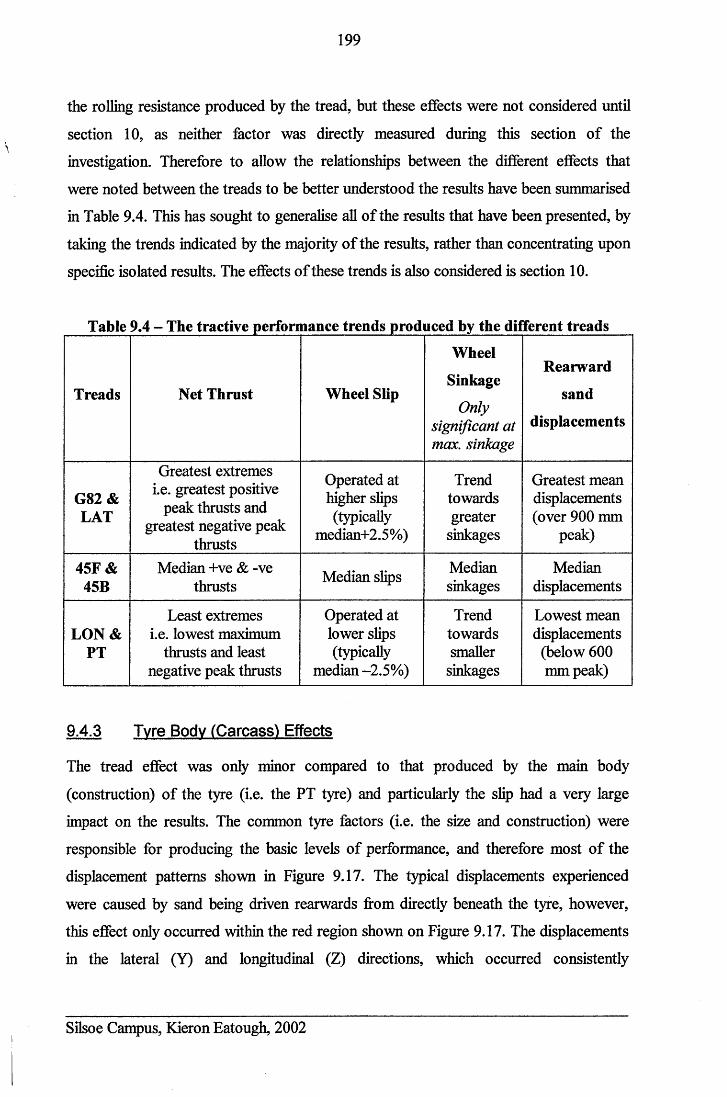
199
the rolling resistance produced by the tread, but these effects were not considered until
section 10, as neither factor was directly measured during this section of the
investigation. Therefore to allow the relationships between the different effects that
were noted between the treads to be better understood the results have been summarised
in Table 9.4. This has sought to generalise all of the results that have been presented, by
taking the trends indicated by the majority of the results, rather than concentrating upon
specific isolated results. The effects of these trends is also considered is section 10.
Table 9.4 - The tractive performance trends produced by the diJferent treads
Treads Net Thrust Wheel Slip
Wheel
Sinkage
Only significant at max. sinkage
Rearward
sand
displacements
G82&LAT
Greatest extremes i.e. greatest positive
peak thrusts and greatest negative peak
thrusts
Operated at higher slips (typically
median+2.5%)
Trendtowardsgreatersinkages
Greatest mean displacements (over 900 mm
peak)
45F&45B
Median +ve & -ve thrusts Median slips Median
sinkagesMedian
displacements
LON & PT
Least extremes i.e. lowest maximum
thrusts and least negative peak thrusts
Operated at lower slips (typically
median -2.5%)
Trendtowardssmaller
sinkages
Lowest mean displacements
(below 600 mm peak)
9.4.3 Tvre Body (Carcass) Effects
The tread effect was only minor compared to that produced by the main body
(construction) of the tyre (i.e. the PT tyre) and particularly the slip had a very large
impact on the results. The common tyre factors (i.e. the size and construction) were
responsible for producing the basic levels of performance, and therefore most of the
displacement patterns shown in Figure 9.17. The typical displacements experienced
were caused by sand being driven rearwards from directly beneath the tyre, however,
this effect only occurred within the red region shown on Figure 9.17. The displacements
in the lateral (Y) and longitudinal (Z) directions, which occurred consistently
Silsoe Campus, Kieron Eatough, 2002
200
irrespective of the tread pattern, affected a much greater region of the sand. In the
central region of the sand profile (between 100 mm and 200 mm on both axes) the sand
was pushed slightly upwards and laterally away from the tyre by a combination of the
bow-wave and shear failure effects. In contrast, directly underneath the tyre, below 150
mm deep, the traction forces simply forced the sand downwards and slightly laterally
inwards toward the tyre centre line as it was sheared to generate traction.
The sand in the surface layers that bordered the tyre rut underwent much greater
magnitudes of lateral flow towards the tyre, with a downwards element, as the sand
failed into the void left by the rearwards, and upwards, displacement of sand from the
RDC by the slipping tyre. The sand displacements along all three axes were shown to be
closely inter-related, such that an increase in displacement in one direction normally
caused a reduction in displacement along a different axis. However, these basic
relationships were greatly influenced by the slip at which the tyre was operated. In
particular, increased slip caused the sand displacement to change from being
downwards and rearwards to being mostly rearwards. Simultaneously the greater slip
disturbed a greater volume of sand, which left greater voids behind each tyre, which
resulted in greater lateral sand flow back into the void due to sand failure.
Silsoe Campus, Kieron Eatough, 2002

201
10 MODELLING OF SAND - TYRE INTERACTION
The modelling was conducted to relate the tyre tread, sand flow and tyre performance,
to produce a predictive performance tool. This process used measured results from the
experimental tests that were undertaken and applied these in combination with Bekker’s
prediction methods. His work, and other useful related work, was outlined in section
3.5.3. Most of the equations listed in section 3.5.3 (8 to 17 and 36 to 49) were used
during this modelling, although they were adapted and developed to improve the
accuracy of prediction for the sand environment.
10.1 VARIABLES REQUIRING TRACTION MODELLING
The modelling sought to relate the quantity of sand flow produced by a tyre to the tread
pattern and from knowledge of the quantity of sand flow produced, as well as the tyre
size, tread pattern and sinkage, predict the net thrust that the tyre (and tread) would
generate. Thus modelling had to account for a number of different variables:
1. Tyre characteristics, particularly size, construction, inflation pressure and most
importantly the tread features.
2. The quantity of sand flow produced by the tyres, which was linked to the tread
features, wheel slip and wheel sinkage.
3. The net thrust produced by the tyres. This was derived by two elements that
required modelling separately:
a. Gross Thrust
b. Rolling Resistance
These elements were determined using Bekker’s prediction methods, although
the author customised these to suit this situation.
4. Gross thrust was modelled using an adaptation of equation 12 (page 40).
5. Rolling resistance was modelled using the methodology detailed in section
3.5.3.9.
Where possible actual values of the relevant variables recorded during the tests were
used in the models to produce more accurate outputs.
Silsoe Campus, Kieron Eatough, 2002
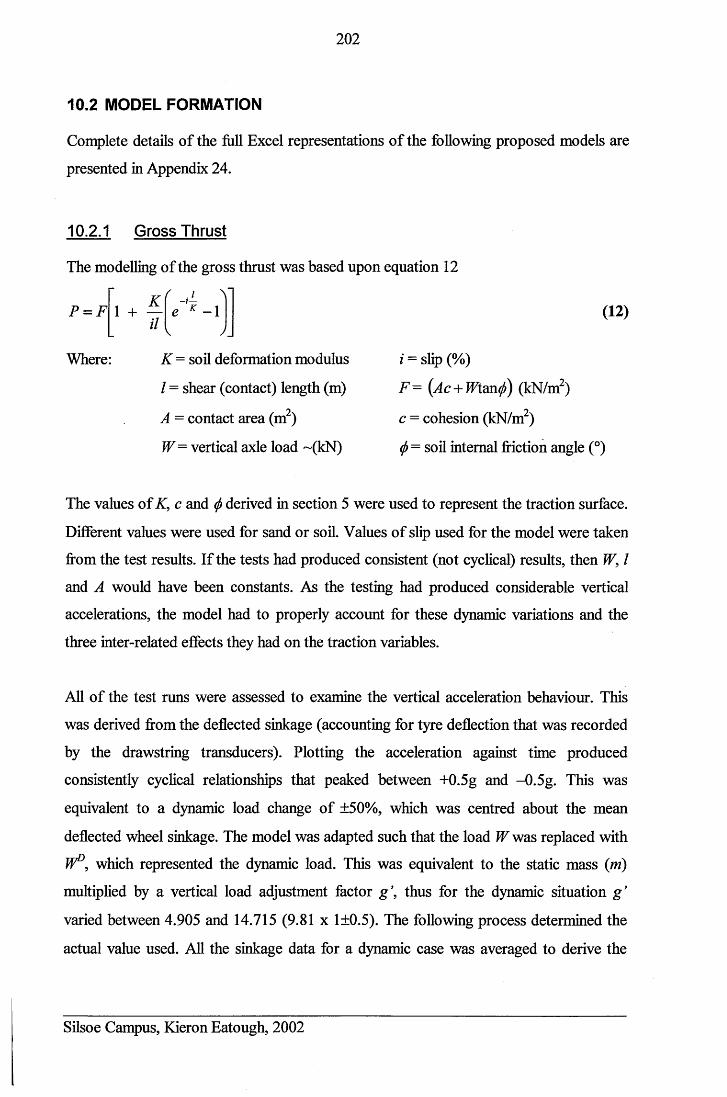
202
10.2 MODEL FORMATION
Complete details of the full Excel representations of the following proposed models are
presented in Appendix 24.
10.2.1 Gross Thrust
The modelling of the gross thrust was based upon equation 12
r . i vP = F i + *
ilK -1
Where: K = soil deformation modulus
/ = shear (contact) length (m)
A = contact area (m2)
W= vertical axle load ~(kN)
(12)
i = slip (%)
F= (Ac + Wtm<f) (kN/m2)
c = cohesion (kN/m )
(j> = soil internal friction angle (°)
The values of K, c and <j) derived in section 5 were used to represent the traction surface.
Different values were used for sand or soil. Values of slip used for the model were taken
from the test results. If the tests had produced consistent (not cyclical) results, then W, I
and A would have been constants. As the testing had produced considerable vertical
accelerations, the model had to properly account for these dynamic variations and the
three inter-related effects they had on the traction variables.
All of the test runs were assessed to examine the vertical acceleration behaviour. This
was derived from the deflected sinkage (accounting for tyre deflection that was recorded
by the drawstring transducers). Plotting the acceleration against time produced
consistently cyclical relationships that peaked between +0.5g and -0.5g. This was
equivalent to a dynamic load change of ±50%, which was centred about the mean
deflected wheel sinkage. The model was adapted such that the load W was replaced with
W°, which represented the dynamic load. This was equivalent to the static mass (m)
multiplied by a vertical load adjustment factor g \ thus for the dynamic situation g ’
varied between 4.905 and 14.715 (9.81 x 1±0.5). The following process determined the
actual value used. All the sinkage data for a dynamic case was averaged to derive the
Silsoe Campus, Kieron Eatough, 2002
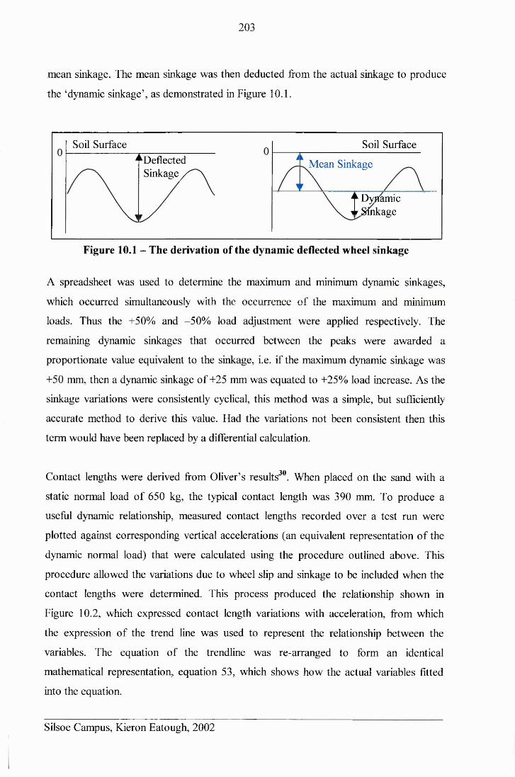
203
mean sinkage. The mean sinkage was then deducted from the actual sinkage to produce
the ‘dynamic sinkage’, as demonstrated in Figure 10.1.
Soil Surface Soil Surface^Deflected
Sinkage /Mean Sinkage
A Dvftamic^Sinkage
Figure 10.1 - The derivation of the dynamic deflected wheel sinkage
A spreadsheet was used to determine the maximum and minimum dynamic sinkages,
which occurred simultaneously with the occurrence of the maximum and minimum
loads. Thus the +50% and -50% load adjustment were applied respectively. The
remaining dynamic sinkages that occurred between the peaks were awarded a
proportionate value equivalent to the sinkage, i.e. if the maximum dynamic sinkage was
+50 mm, then a dynamic sinkage of +25 mm was equated to +25% load increase. As the
sinkage variations were consistently cyclical, this method was a simple, but sufficiently
accurate method to derive this value. Had the variations not been consistent then this
term would have been replaced by a differential calculation.
• • TOContact lengths were derived from Oliver’s results . When placed on the sand with a
static normal load of 650 kg, the typical contact length was 390 mm. To produce a
useful dynamic relationship, measured contact lengths recorded over a test run were
plotted against corresponding vertical accelerations (an equivalent representation of the
dynamic normal load) that were calculated using the procedure outlined above. This
procedure allowed the variations due to wheel slip and sinkage to be included when the
contact lengths were determined. This process produced the relationship shown in
Figure 10.2, which expressed contact length variations with acceleration, from which
the expression of the trend line was used to represent the relationship between the
variables. The equation of the trendline was re-arranged to form an identical
mathematical representation, equation 53, which shows how the actual variables fitted
into the equation.
Silsoe Campus, Kieron Eatough, 2002
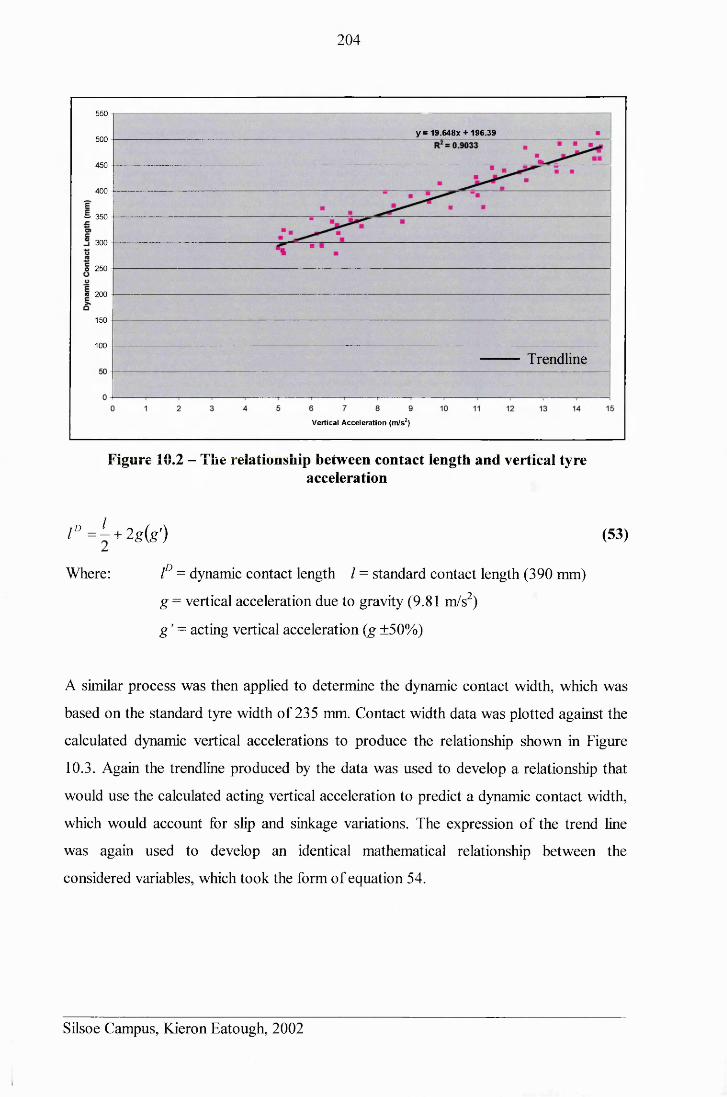
204
550
y = 19.648X + 196.39500
450
400
■=• 350
" 300
o 250
« 200
150
100Trendline
V ertical A c cele ra tio n (m /s2)
Figure 10.2 - The relationship between contact length and vertical tyreacceleration
l D = l- + 2g{g’) (53)
Where: lD = dynamic contact length / = standard contact length (390 mm)
g = vertical acceleration due to gravity (9.81 m/s2)
g ’ = acting vertical acceleration (g ±50%)
A similar process was then applied to determine the dynamic contact width, which was
based on the standard tyre width of 235 mm. Contact width data was plotted against the
calculated dynamic vertical accelerations to produce the relationship shown in Figure
10.3. Again the trendline produced by the data was used to develop a relationship that
would use the calculated acting vertical acceleration to predict a dynamic contact width,
which would account for slip and sinkage variations. The expression of the trend line
was again used to develop an identical mathematical relationship between the
considered variables, which took the form of equation 54.
Silsoe Campus, Kieron Eatough, 2002
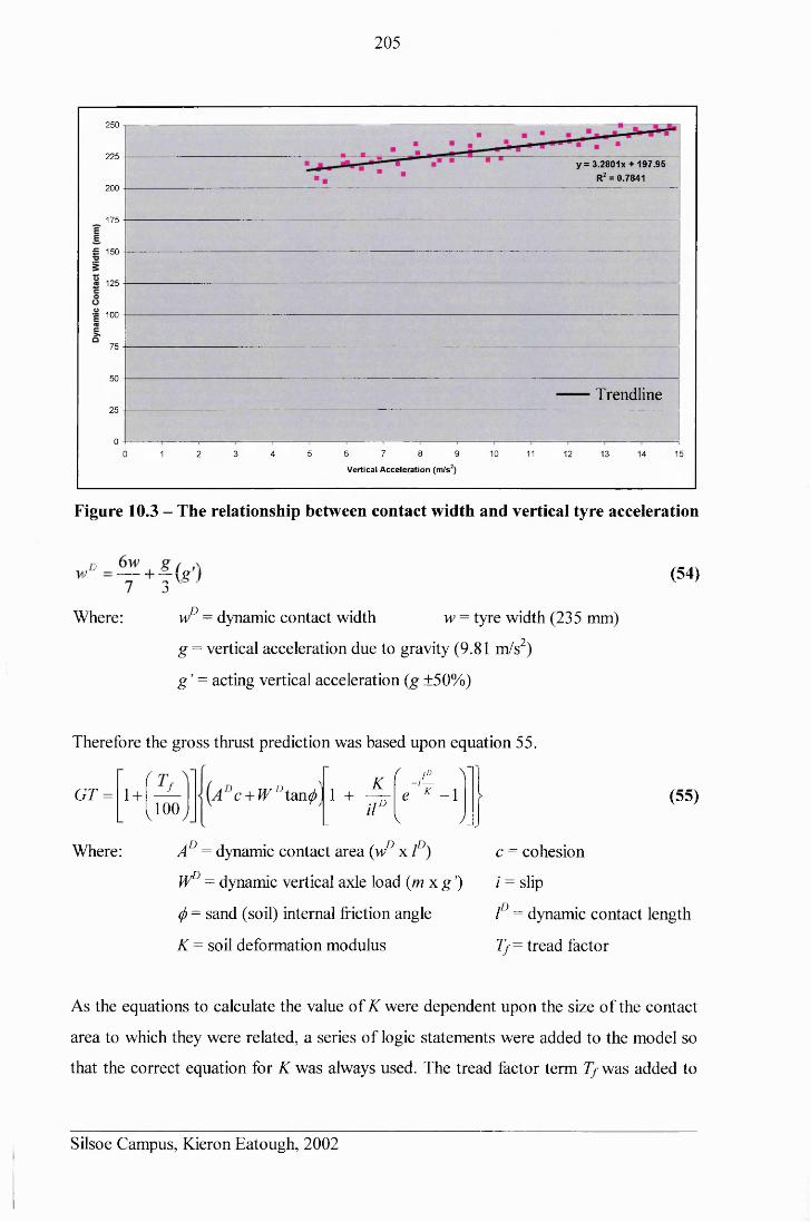
205
250
225y=3.2801x + 197.95
R2 = 0.7841200
175
£ 150
125
100
75
50
Trendline25
073 5 6 8 9 10 11 12 150 1 2 4 13 14
V ertical A c cele ra tio n (m /s2)
Figure 10.3 - The relationship between contact width and vertical tyre acceleration
™D = ~ + f ( g ' ) (54)
Where: wD = dynamic contact width w = tyre width (235 mm)
g = vertical acceleration due to gravity (9.81 m/s2)
g ’ = acting vertical acceleration (g ±50%)
Therefore the gross thrust prediction was based upon equation 55.
GT = 1 +f,100, )c + W D tan^
” ( 1° ^K —i—1 + “ TV e K -1 >
ilD- V / _>
Where: A° = dynamic contact area (wD x lD)
W° = dynamic vertical axle load ( m x g ’)
(j) = sand (soil) internal friction angle
K = soil deformation modulus
(55)
c = cohesion
i = slip
lD = dynamic contact length
Tf— tread factor
As the equations to calculate the value of K were dependent upon the size of the contact
area to which they were related, a series of logic statements were added to the model so
that the correct equation for K was always used. The tread factor term Tf was added to
Silsoe Campus, Kieron Eatough, 2002
206
the equation to allow a percentage increase in the thrust prediction to account for any
variation in thrust produced by the tread designs, as the equation by itself accounted for
a plain tread tyre. The value of this factor depended upon the gross thrust output
produced by the tread. This was determined from the experimental results in a process
that will be detailed subsequently.
10.2.2 Rolling Resistance
The calculation of the rolling resistance of the treads was determined by using the
process detailed in equations 36 to 49 (section 3.5.3.9). The model was designed to
automatically calculate the critical pressure and check the mode of operation (rigid or
elastic). It then included the correct terms for the particular case. When inflated to 1.10
bar the tyre always operated elastically, but the inclusion of all the possible terms
increased the model’s flexibility to be used for other cases. The mode of operation
governed the terms included in the calculation (see below).
Rigid mode: Elastic mode:
Rc = Compaction resistance Rc = Compaction resistance
Rb = Bulldozing resistance Rb = Bulldozing resistance
R/= Tyre carcass flexing resistance
The following equations are based upon Bekker’s work, as noted above. However,
because these were customised to suit this particular application, they are all fully
detailed below, with the source and nature of the new terms that were introduced (or
replaced) identified.
Rc - Compaction resistance
R = w J( „»+i A
d e f — + kA wn + 1v / v
Where: w°= Dynamic contact width (equivalent to rut width)
Zdef= Recorded experimental deflected tyre sinkage
kc, k(j)&n = empirically measured coefficients from plate sinkage tests
w = tyre width (equivalent to minimum plate dimension)
(56)
Silsoe Campus, Kieron Eatough, 2002
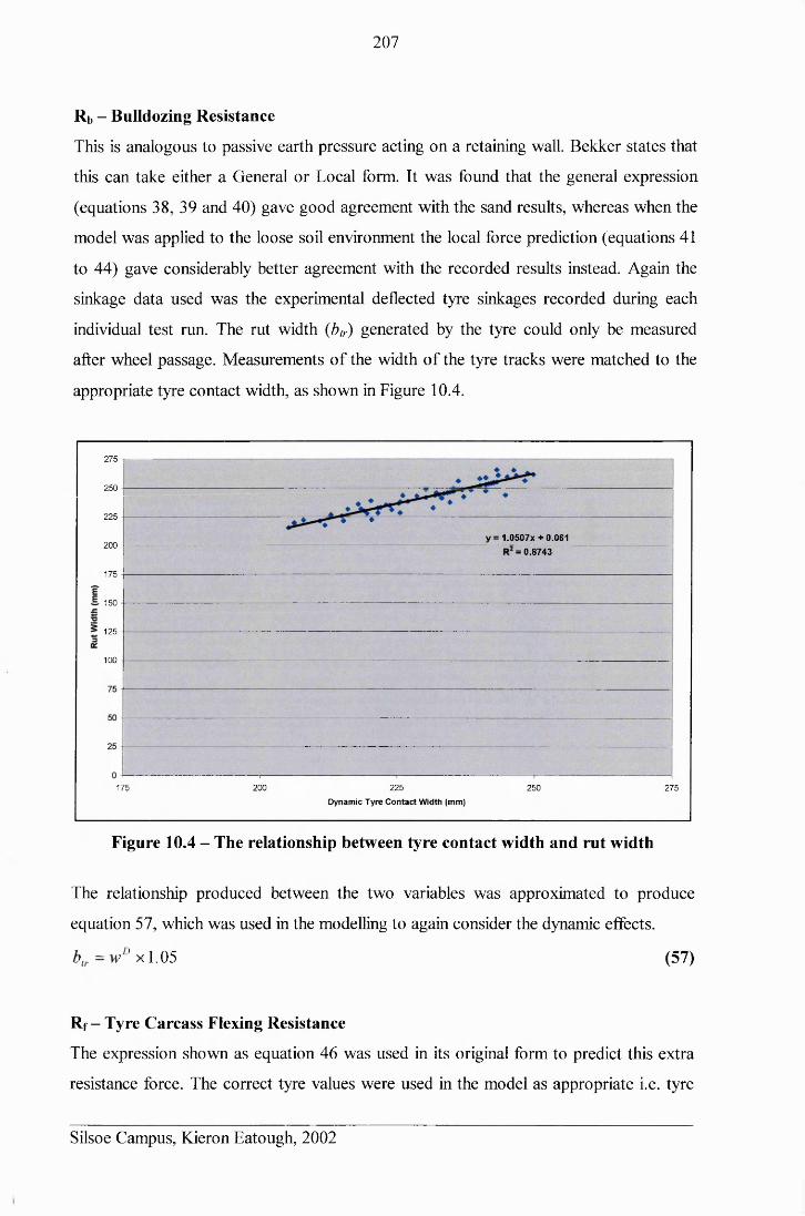
207
Rb - Bulldozing Resistance
This is analogous to passive earth pressure acting on a retaining wall. Bekker states that
this can take either a General or Local form. It was found that the general expression
(equations 38, 39 and 40) gave good agreement with the sand results, whereas when the
model was applied to the loose soil environment the local force prediction (equations 41
to 44) gave considerably better agreement with the recorded results instead. Again the
sinkage data used was the experimental deflected tyre sinkages recorded during each
individual test run. The rut width (btr) generated by the tyre could only be measured
after wheel passage. Measurements of the width of the tyre tracks were matched to the
appropriate tyre contact width, as shown in Figure 10.4.
275
2 50
225
y = 1.0507X + 0.061200
= 0.8743
175
150
125
100
175 200 2 25
D ynam ic Tyre C o n ta c t W idth (m m )
250 275
Figure 10.4 - The relationship between tyre contact width and rut width
The relationship produced between the two variables was approximated to produce
equation 57, which was used in the modelling to again consider the dynamic effects.
blr= wn x1.05 (57)
Rf - Tyre Carcass Flexing Resistance
The expression shown as equation 46 was used in its original form to predict this extra
resistance force. The correct tyre values were used in the model as appropriate i.e. tyre
Silsoe Campus, Kieron Eatough, 2002
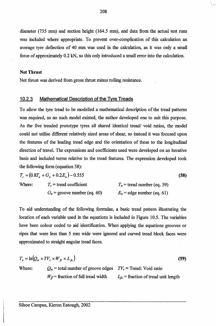
208
diameter (735 mm) and section height (164.5 mm), and data from the actual test runs
was included where appropriate. To prevent over-complication of this calculation an
average tyre deflection of 40 mm was used in the calculation, as it was only a small
force of approximately 0.2 kN, so this only introduced a small error into the calculation.
Net Thrust
Net thrust was derived from gross thrust minus rolling resistance.
10.2.3 Mathematical Description of the Tvre Treads
To allow the tyre tread to be modelled a mathematical description of the tread patterns
was required, as no such model existed, the author developed one to suit this purpose.
As the five treaded prototype tyres all shared identical tread/ void ratios, the model
could not utilise different relatively sized areas of shear, so instead it was focused upon
the features of the leading tread edge and the orientation of these to the longitudinal
direction of travel. The expressions and coefficients used were developed on an iterative
basis and included terms relative to the tread features. The expression developed took
the following form (equation 58):
Tc =(0.87; +G„ + 0 .2 £ „ )-0.555 (58)
Where: Tc = tread coefficient T„ - tread number (eq. 59)
Gn = groove number (eq. 60) E„ = edge number (eq. 61)
To aid understanding of the following formulae, a basic tread pattern illustrating the
location of each variable used in the equations is included in Figure 10.5. The variables
have been colour coded to aid identification. When applying the equations grooves or
sipes that were less than 5 mm wide were ignored and curved tread block faces were
approximated to straight angular tread faces.
T„ = ln(g,e xTV'XWffXLf,) (59)
Where: Qte - total number of groove edges TVr = Tread: Void ratio
Wf= fraction of full tread width L/u = fraction of tread unit length
Silsoe Campus, Kieron Eatough, 2002
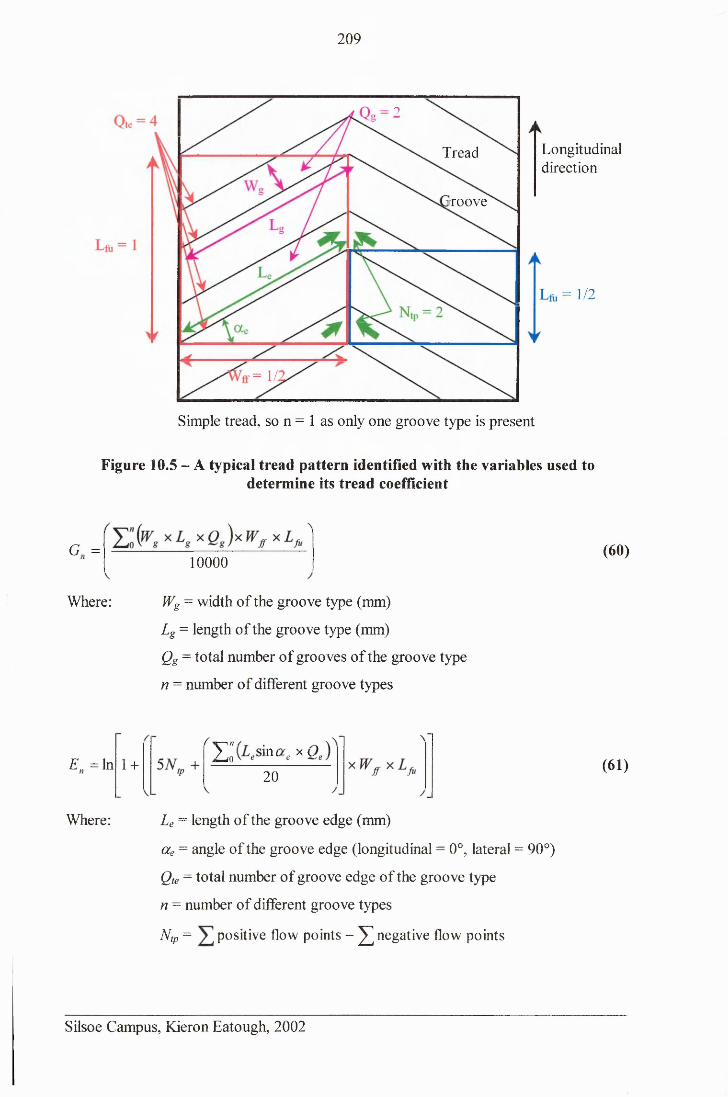
209
- ?
Longitudinaldirection
Tread
rroove
= 1/2
= l/:
Simple tread, so n = 1 as only one groove type is present
Figure 10.5 - A typical tread pattern identified with the variables used todetermine its tread coefficient
G. =
Where:
10000
Wg = width of the groove type (mm)
Lg = length of the groove type (mm)
Qg = total number of grooves of the groove type
n = number of different groove types
(60)
E. =ln
Where:
1 +Y l (Lesma,
20(61)
Le = length of the groove edge (mm)
ae = angle of the groove edge (longitudinal = 0°, lateral = 90°)
Qte = total number of groove edge of the groove type
n = number of different groove types
Ntp = positive flow points - ^ negative flow points
Silsoe Campus, Kieron Eatough, 2002
210
Note for equation 61: A positive flow point is a tread location where sand is forced
together, i.e. the apex of a backward vee, whilst a negative flow point is where the tread
forces sand apart, i.e. from one channel to two channels.
Equation 58 was applied to the five prototype treads used during the sand displacement
experiment and it produced the tread coefficients shown in Table 10.1. Full details of
this calculation are in Appendix 25.
Table 10.1 - Tread coefficients for the five prototype treads tested during the sand
Tread Type Tread CoefficientPT 0.00
LON 2.5045F 4.6445B 5.06LAT 5.62
10.2.4 Calculation of the Volume of Sand Flow
It was necessary to calculate the volume of sand that had been displaced during the sand
flow experiments from the recorded sand displacements. This process was simplified to
include only longitudinal displacements, which had been related to gross thrust output.
These were contained within the region of sand 100 mm across from the tyre centre and
200 mm down from the surface. This region encompassed four tag positions across the
grid and six tag grid positions down the grid. Adjoining tag positions within this region
were linked to form a series of rectangular grids, with a total area of three grids across
by five grids deep. A representative volume of displacement from each grid was
determined from the four displacements that were recorded for the four comer points.
This was done by an adaptation of the trapezium rule, as demonstrated by Figure 10.6.
This was such that the four displacements were averaged to produce a mean
displacement (h), which was then multiplied by the base area of the rectangle (ab) to
produce a value equivalent to the total volume of sand displaced within the region of
interest. This process was repeated for each of the fifteen rectangular grids and these
Silsoe Campus, Kieron Eatough, 2002
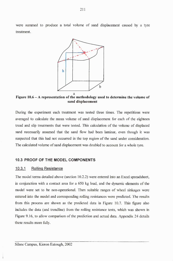
211
were summed to produce a total volume of sand displacement caused by a tyre
treatment.
aFigure 10.6 - A representation of the methodology used to determine the volume of
sand displacement
During the experiment each treatment was tested three times. The repetitions were
averaged to calculate the mean volume of sand displacement for each of the eighteen
tread and slip treatments that were tested. This calculation of the volume of displaced
sand necessarily assumed that the sand flow had been laminar, even though it was
suspected that this had not occurred in the top region of the sand under consideration.
The calculated volume of sand displacement was doubled to account for a whole tyre.
10.3 PROOF OF THE MODEL COMPONENTS
10.3.1 Rolling Resistance
The model terms detailed above (section 10.2.2) were entered into an Excel spreadsheet,
in conjunction with a contact area for a 650 kg load, and the dynamic elements of the
model were set to be non-operational. Then suitable ranges of wheel sinkages were
entered into the model and corresponding rolling resistances were predicted. The results
from this process are shown as the predicted data in Figure 10.7. This figure also
includes the data (and trendline) from the rolling resistance tests, which was shown in
Figure 9.16, to allow comparison of the prediction and actual data. Appendix 24 details
these results more fully.
Silsoe Campus, Kieron Eatough, 2002
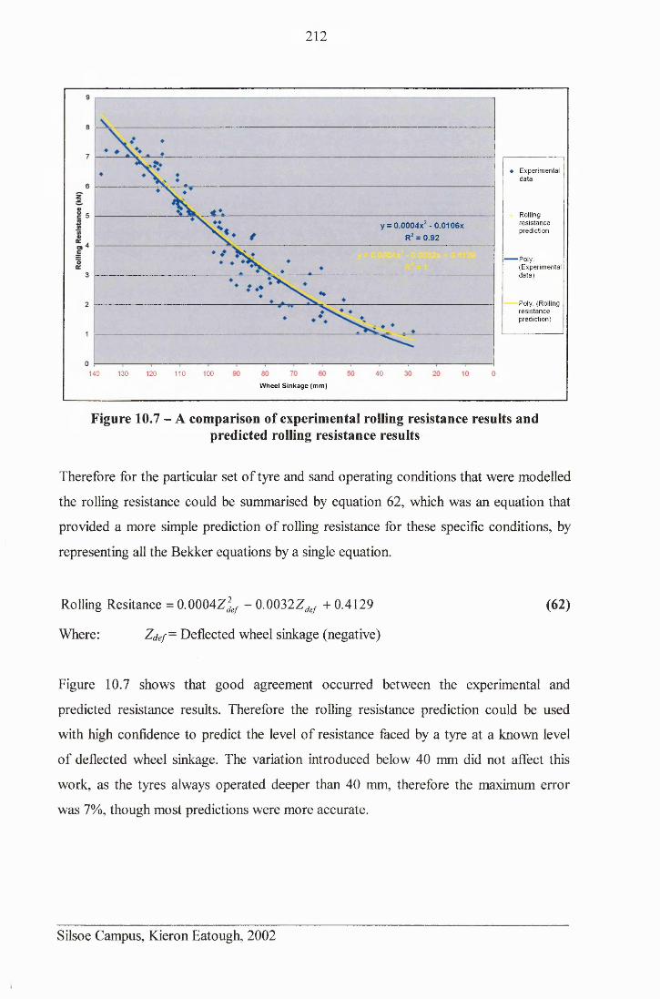
212
♦ E xperim ental d a ta
Rollingre s is ta n c eprediction
y = 0.0004x2 - 0.0106x R2 = 0.92
— Poly.(E xperim entaldata )
Poly. (Rollingre s is ta n c eprediction)
140 130 120 110 100 40W h e el S in k a g e (m m )
Figure 10.7 - A comparison of experimental roiling resistance results and predicted rolling resistance results
Therefore for the particular set of tyre and sand operating conditions that were modelled
the rolling resistance could be summarised by equation 62, which was an equation that
provided a more simple prediction of rolling resistance for these specific conditions, by
representing all the Bekker equations by a single equation.
Rolling Resitance = 0.0004Z 2def - 0.0032Zdef + 0.4129 (62)
Where: Zdef~ Deflected wheel sinkage (negative)
Figure 10.7 shows that good agreement occurred between the experimental and
predicted resistance results. Therefore the rolling resistance prediction could be used
with high confidence to predict the level of resistance faced by a tyre at a known level
of deflected wheel sinkage. The variation introduced below 40 mm did not affect this
work, as the tyres always operated deeper than 40 mm, therefore the maximum error
was 7%, though most predictions were more accurate.
Silsoe Campus, Kieron Eatough, 2002
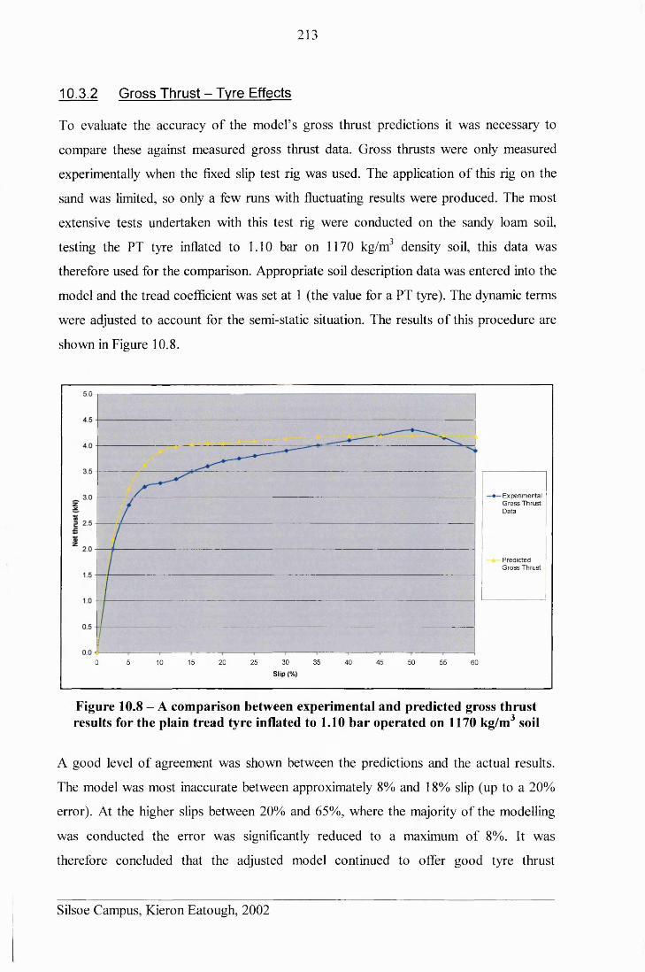
213
10.3.2 Gross Thrust - Tyre Effects
To evaluate the accuracy of the model’s gross thrust predictions it was necessary to
compare these against measured gross thrust data. Gross thrusts were only measured
experimentally when the fixed slip test rig was used. The application of this rig on the
sand was limited, so only a few runs with fluctuating results were produced. The most
extensive tests undertaken with this test rig were conducted on the sandy loam soil,
testing the PT tyre inflated to 1.10 bar on 1170 kg/m3 density soil, this data was
therefore used for the comparison. Appropriate soil description data was entered into the
model and the tread coefficient was set at 1 (the value for a PT tyre). The dynamic terms
were adjusted to account for the semi-static situation. The results of this procedure are
shown in Figure 10.8.
0 5 10 15 2 0 2 5 30 35 4 0 45 50 5 5 60
S lip (%)
♦ E xperim en tal G ro ss T hrust D ata
P red ic te d G ro ss T h ru st
Figure 10.8 - A comparison between experimental and predicted gross thrust results for the plain tread tyre inflated to 1.10 bar operated on 1170 kg/m3 soil
A good level of agreement was shown between the predictions and the actual results.
The model was most inaccurate between approximately 8% and 18% slip (up to a 20%
error). At the higher slips between 20% and 65%, where the majority of the modelling
was conducted the error was significantly reduced to a maximum of 8%. It was
therefore concluded that the adjusted model continued to offer good tyre thrust
Silsoe Campus, Kieron Eatough, 2002
214
predictions. Thus as the original authors of the model validated the model across a wide
range of soil conditions, it was also equally applicable to modelling the gross thrust
output on sand when the appropriate sand engineering values were employed.
10.3.3 Gross Thrust - Tread Effects
The majority of the tests conducted on the sand used the variable slip test rig, therefore
only the wheel slip, wheel sinkage and the net thrust were recorded. To allow the effect
of the tread patterns to be calculated, with reference to the gross thrust outputs, a
method was devised to calculate gross thrusts from the experimental net thrust results.
Rolling resistances calculated from the sinkage data were added to the experimental net
thrust data to produce gross thrust results. The close agreement between the predicted
and actual rolling resistance results allowed this calculation to be conducted with a high
degree of accuracy. This was conducted for all the different experimental tread patterns
for all the thrust slip data that was recorded during the displacement experiments.
To allow these results to be compared, a method of achieving representative comparison
between the treads was required. Due to the inter-related elements that occurred
between the thrust, slip and sinkage during the experiments, a holistic approach was
used. Comparison was achieved by normalising the data in terms of deflected tyre
sinkage. Using wheel sinkage minimised the errors in this process, because the
variations in gross thrust were more sensitive to changes in sinkage, rather than wheel
slip. The calculated (predicted) gross thrust output was plotted against the deflected
wheel sinkage for the five prototype treads.
To calculate the effect of the tread upon the thrust, linear trend lines were fitted through
the data. As zero gross thrust would occur at zero sinkage, as contact with the ground
would cease, these were orientated through the origin. Linear trend lines were used to
provide a simple approximation to the relationships. With any variations in thrust due to
sinkage accounted for, then the difference between the thrusts was due to variations in
the tread. Therefore the relative gradients of the trend lines equated to relative gross
thrust benefits derived from the different treads. The results of this process are shown in
Figure 10.9 to Figure 10.13, for the different tread patterns.
Silsoe Campus, Kieron Eatough, 2002
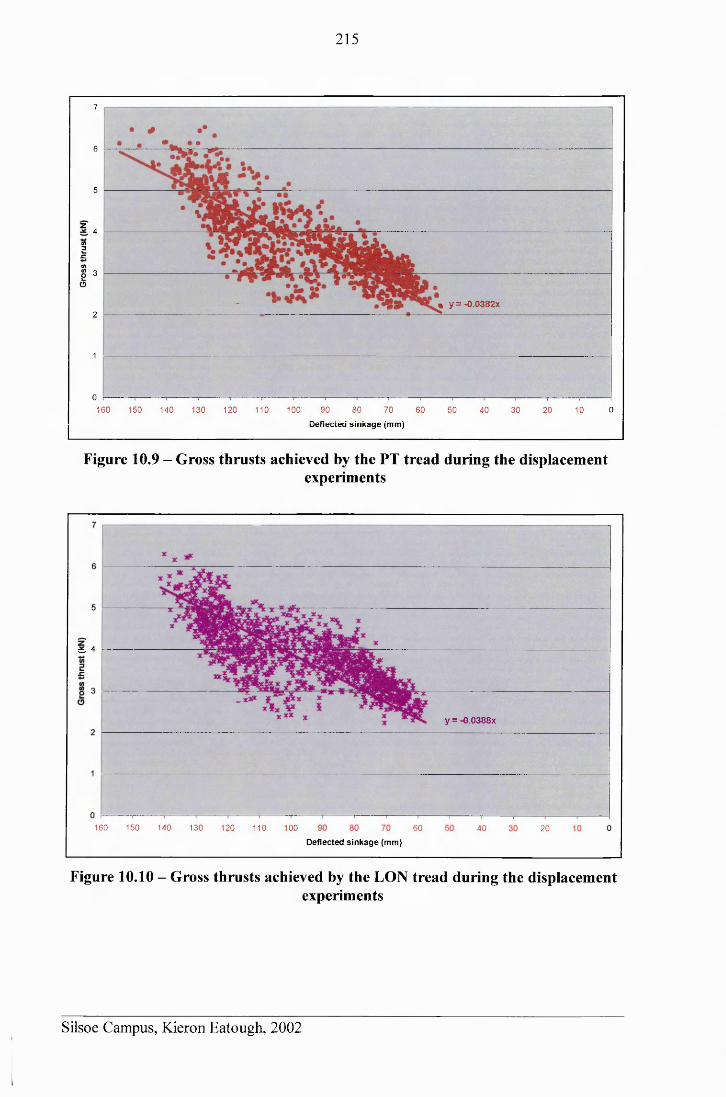
215
7
6
5
Z4
0)□
-CCA2 3ge>
« y = -0.0382x2
1
080160 150 140 130 120 110 100 90 70 60 50 40 30 20 10 0
D e f le c t e d s i n k a g e (m m )
Figure 10.9 - Gross thrusts achieved by the PT tread during the displacementexperiments
i 4
y = -0.0388x
160 150 140 130 120 110 100 60 40 20D e f le c t e d s i n k a g e (m m )
Figure 10.10 - Gross thrusts achieved by the LON tread during the displacementexperiments
Silsoe Campus, Kieron Eatough, 2002
!
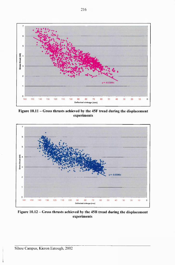
216
■»!
i 4
‘••A■ V
------------
f i
V
y = -0.0394x
150 110 100160 140 130 120 50 30Deflected sinkage (mm)
Figure 10.11 - Gross thrusts achieved by the 45F tread during the displacementexperiments
7
6
5
♦ * ♦---U)«O 3 ♦♦
y = -0.0396X2
1
0160 150 140 130 120 110 100 90 80 70 60 50 40 30 20 010
D e flec te d s in k a g e (m m )
Figure 10.12 - Gross thrusts achieved by the 45B tread during the displacementexperiments
Silsoe Campus, Kieron Eatough, 2002
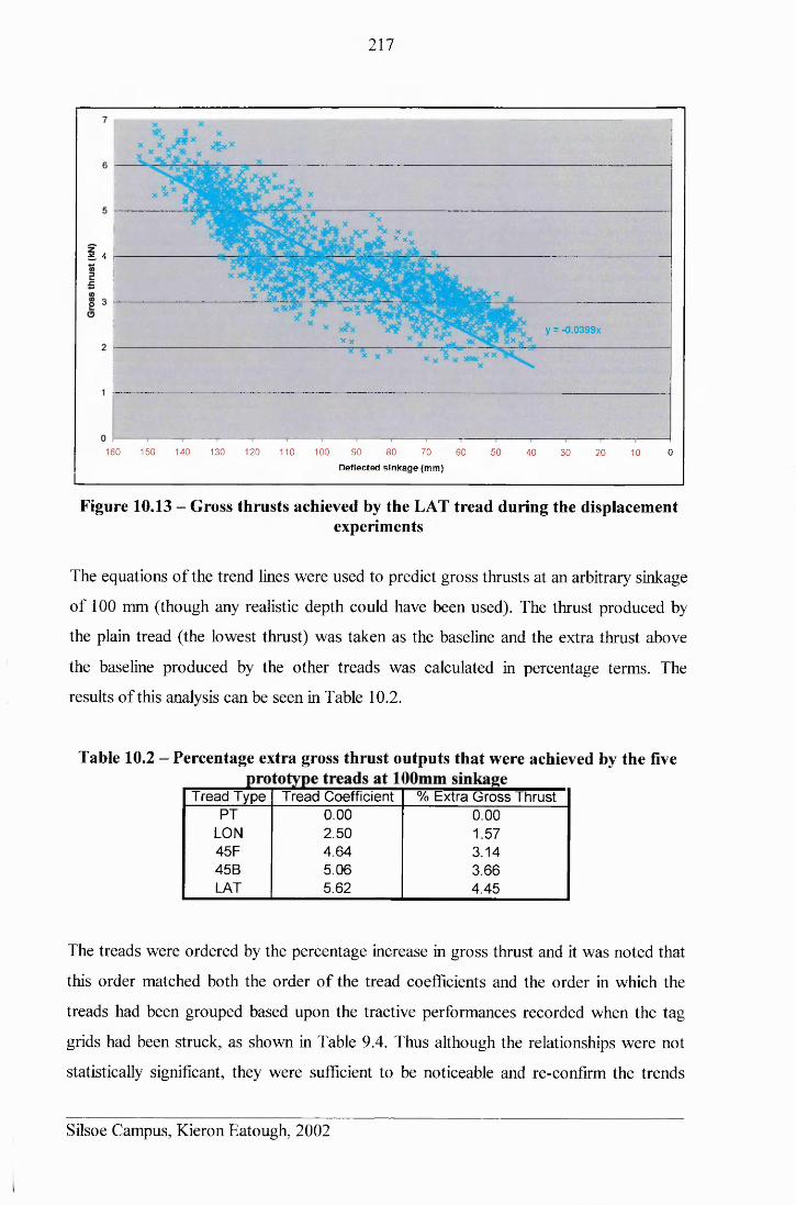
217
* x?«■
£. 4
y = -0.0399xx X
*■£ i-------
160 150 140 130 120 110 100 90 80 70 60 50 40 30 020 10
D e f l e c t e d s i n k a g e (m m )
Figure 10.13 - Gross thrusts achieved by the LAT tread during the displacementexperiments
The equations of the trend lines were used to predict gross thrusts at an arbitrary sinkage
of 100 mm (though any realistic depth could have been used). The thrust produced by
the plain tread (the lowest thrust) was taken as the baseline and the extra thrust above
the baseline produced by the other treads was calculated in percentage terms. The
results of this analysis can be seen in Table 10.2.
Table 10.2 - Percentage extra gross thrust outputs that were achieved by the five
Tread Type Tread Coefficient % Extra Gross ThrustPT 0.00 0.00
LON 2.50 1.5745F 4.64 3.1445B 5.06 3.66LAT 5.62 4.45
The treads were ordered by the percentage increase in gross thrust and it was noted that
this order matched both the order of the tread coefficients and the order in which the
treads had been grouped based upon the tractive performances recorded when the tag
grids had been struck, as shown in Table 9.4. Thus although the relationships were not
statistically significant, they were sufficient to be noticeable and re-confirm the trends
Silsoe Campus, Kieron Eatough, 2002
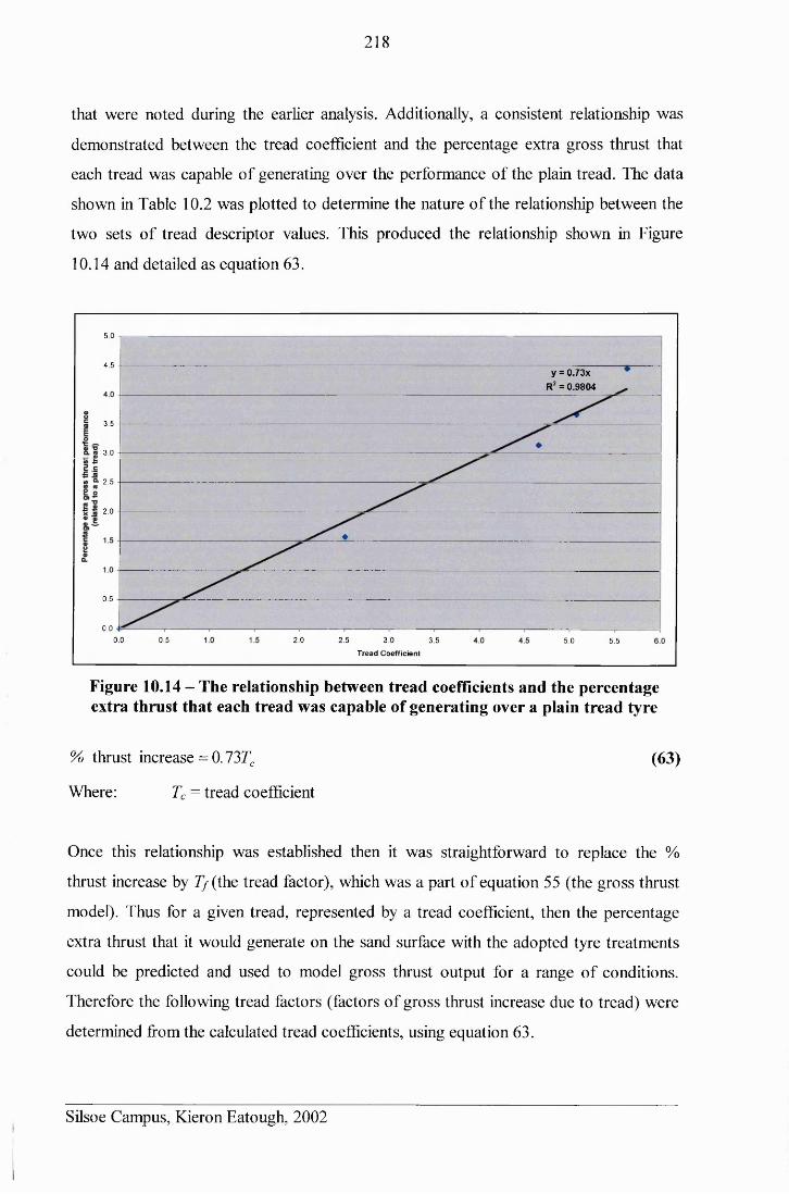
218
that were noted during the earlier analysis. Additionally, a consistent relationship was
demonstrated between the tread coefficient and the percentage extra gross thrust that
each tread was capable of generating over the performance of the plain tread. The data
shown in Table 10.2 was plotted to determine the nature of the relationship between the
two sets of tread descriptor values. This produced the relationship shown in Figure
10.14 and detailed as equation 63.
5.0
4.5y = 0.73x
R2 = 0.9804
3.5
3.0
2.5
2.0
0.5
0.00.0 0.5 2.0 2.5 3.0 3.5 5.0 5.5
T read C oeffic ien t
Figure 10.14 - The relationship between tread coefficients and the percentage extra thrust that each tread was capable of generating over a plain tread tyre
% thrust increase = 0.73Tc (63)
Where: Tc = tread coefficient
Once this relationship was established then it was straightforward to replace the %
thrust increase by 7 /(the tread factor), which was a part of equation 55 (the gross thrust
model). Thus for a given tread, represented by a tread coefficient, then the percentage
extra thrust that it would generate on the sand surface with the adopted tyre treatments
could be predicted and used to model gross thrust output for a range of conditions.
Therefore the following tread factors (factors of gross thrust increase due to tread) were
determined from the calculated tread coefficients, using equation 63.
Silsoe Campus, Kieron Eatough, 2002
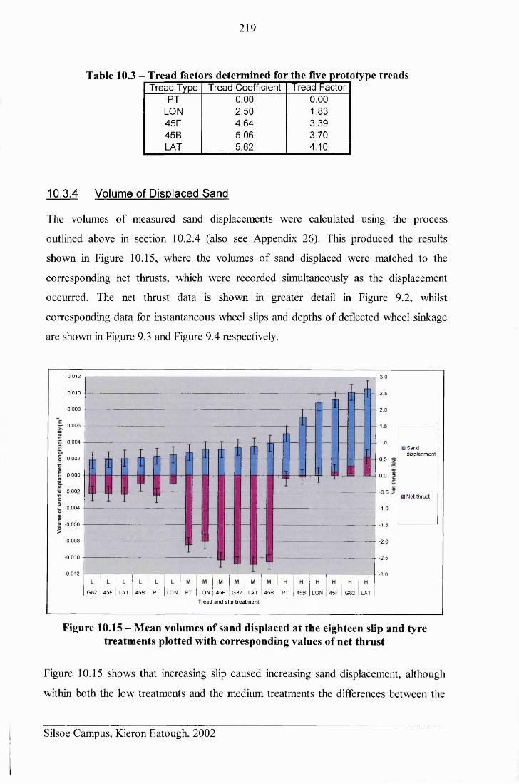
219
Table 10.3 - Tread factors determined for the five prototype treadsTread Type Tread Coefficient Tread Factor
PT 0.00 0.00LON 2.50 1.8345F 4.64 3.3945B 5.06 3.70LAT 5.62 4.10
10.3.4 Volume of Displaced Sand
The volumes of measured sand displacements were calculated using the process
outlined above in section 10.2.4 (also see Appendix 26). This produced the results
shown in Figure 10.15, where the volumes of sand displaced were matched to the
corresponding net thrusts, which were recorded simultaneously as the displacement
occurred. The net thrust data is shown in greater detail in Figure 9.2, whilst
corresponding data for instantaneous wheel slips and depths of deflected wheel sinkage
are shown in Figure 9.3 and Figure 9.4 respectively.
0.012 -r-js — r 3.0
0.010 - - 2 .5
0 .008 I - - 2 . 0
0.006
0.004 - 1.0□ S a n d
d isp la cm en t0.002 - 0 .5 ?■
0.000■■5 . 0.002 — -0 .5 z
■ N et th ru st
" -0 .004 - 1.0
2 -0 .006 -1 .5
-0 .008 - 2.0
- 0.010 -2 .5
-0.012 - - - -3 .0
G 82 45F LAT LON PT LON 45F G 82 LAT
T re ad a n d s lip tre a tm e n t
45B PT 45B PT 45B LON 45F G82 LAT
Figure 10.15 - Mean volumes of sand displaced at the eighteen slip and tyre treatments plotted with corresponding values of net thrust
Figure 10.15 shows that increasing slip caused increasing sand displacement, although
within both the low treatments and the medium treatments the differences between the
Silsoe Campus, Kieron Eatough, 2002
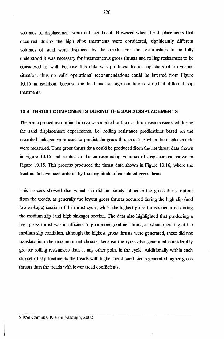
220
volumes of displacement were not significant. However when the displacements that
occurred during the high slips treatments were considered, significantly different
volumes of sand were displaced by the treads. For the relationships to be fully
understood it was necessary for instantaneous gross thrusts and rolling resistances to be
considered as well, because this data was produced from snap shots of a dynamic
situation, thus no valid operational recommendations could be inferred from Figure
10.15 in isolation, because the load and sinkage conditions varied at different slip
treatments.
10.4 THRUST COMPONENTS DURING THE SAND DISPLACEMENTS
The same procedure outlined above was applied to the net thrust results recorded during
the sand displacement experiments, i.e. rolling resistance predications based on the
recorded sinkages were used to predict the gross thrusts acting when the displacements
were measured. Thus gross thrust data could be produced from the net thrust data shown
in Figure 10.15 and related to the corresponding volumes of displacement shown in
Figure 10.15. This process produced the thrust data shown in Figure 10.16, where the
treatments have been ordered by the magnitude of calculated gross thrust.
This process showed that wheel slip did not solely influence the gross thrust output
from the treads, as generally the lowest gross thrusts occurred during the high slip (and
low sinkage) section of the thrust cycle, whilst the highest gross thrusts occurred during
the medium slip (and high sinkage) section. The data also highlighted that producing a
high gross thrust was insufficient to guarantee good net thrust, as when operating at the
medium slip condition, although the highest gross thrusts were generated, these did not
translate into the maximum net thrusts, because the tyres also generated considerably
greater rolling resistances than at any other point in the cycle. Additionally within each
slip set of slip treatments the treads with higher tread coefficients generated higher gross
thrusts than the treads with lower tread coefficients.
Silsoe Campus, Kieron Eatough, 2002
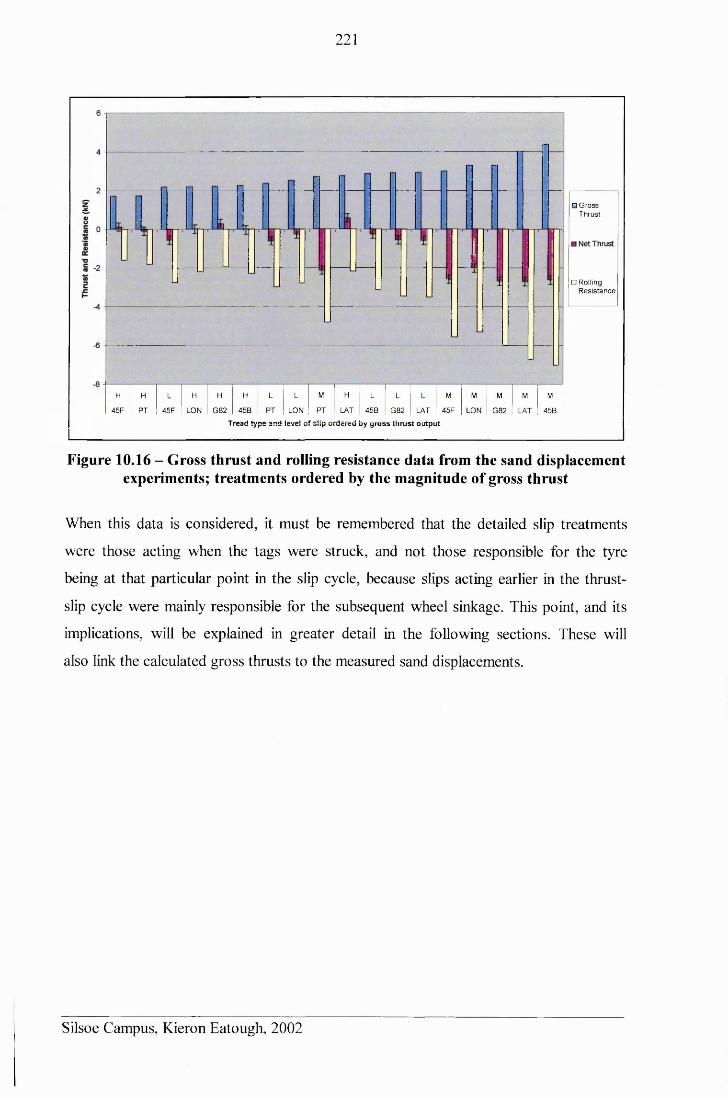
221
□ G ross T h ru st
□ Rolling R e s is ta n c e
H H L H H H L L M H L L L M M M M
45F PT 45F LON G 82 45B PT LON PT LAT 45B G 82 LAT 45F LON G 82 LAT
M
45B
Tread ty p e and lev e l o f s lip ord ered by g r o s s th ru st ou tp u t
Figure 10.16 - Gross thrust and rolling resistance data from the sand displacement experiments; treatments ordered by the magnitude of gross thrust
When this data is considered, it must be remembered that the detailed slip treatments
were those acting when the tags were struck, and not those responsible for the tyre
being at that particular point in the slip cycle, because slips acting earlier in the thrust-
slip cycle were mainly responsible for the subsequent wheel sinkage. This point, and its
implications, will be explained in greater detail in the following sections. These will
also link the calculated gross thrusts to the measured sand displacements.
Silsoe Campus, Kieron Eatough, 2002
222
10.5 APPLICATION OF THE NET THRUST MODEL
To better understand the relationship between the thrust components the elements of the
predictive model were considered. For this to be appropriate the validity of the model
had to be assessed when it was used to predict net thrusts based upon the data recorded
during the sand displacement experiments. Gross thrust and rolling resistance
predictions were used to predict net thrusts, which were then compared against the
recorded net thrusts. For the model to provide a good representation of the results it had
to be able to account for the large variations in wheel slip, sinkage and vertical
acceleration, as well as the tyre tread treatments used during the experiments. To allow
comparison of the differences in performance between each tread one test run was
modelled for each tyre tread, and the tread factor equation (63) was used to introduce
the tread effects into the gross thrust model. This evaluation was conducted for all five
of the prototype treads. The results are shown in Figure 10.17 to Figure 10.21. The
details of the modelling calculations for all similar plots, on the accompanying data CD,
are listed in Appendix 27. These are presented in order of the tread factor rankings,
starting with the lowest scoring tread, the PT tyre.
Exp. N et T h ru sts
P red ic te dN etT h ru sts
Tim e (s)
Figure 10.17 - Experimental net thrust results plotted against predicted net thrustscalculated for the PT tread
Silsoe Campus, Kieron Eatough, 2002
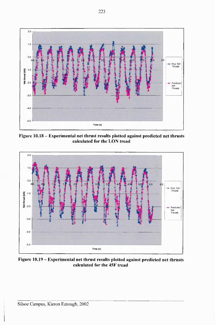
223
6.5
-E x p . N et T h ru sts
- P red ic ted N etT h ru sts
Tim e (s)
Figure 10.38 - Experimental net thrust results plotted against predicted net thrustscalculated for the LON tread
—♦ —Exp. N et T h ru sts
—• — P red ic te d N etT h ru sts
Tim e (s )
Figure 10.19 - Experimental net thrust results plotted against predicted net thrustscalculated for the 45F tread
Silsoe Campus, Kieron Eatough, 2002
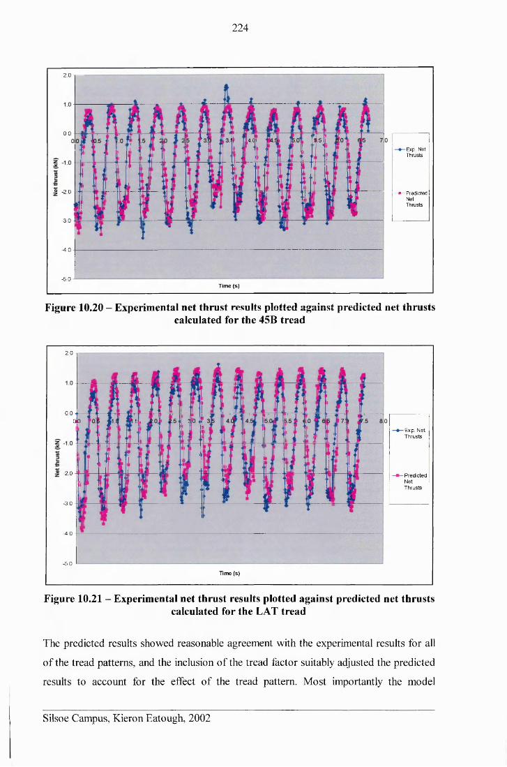
224
2.0 - |-------
0.04.( 5 .5
Exp. Net Thrusts
3 -2.0 - ■ —PredictedNetThrusts
-3.0
-4.0
-5.0T im e (s )
Figure 10.20 - Experimental net thrust results plotted against predicted net thrustscalculated for the 45B tread
2 .0 T«
0.0: bok) ■ 5«
Exp. N e t T h ru sts
-2.0 P red ic te dN etT h ru sts
-3.0
-4 .0
-5.0 -1Tim e (s )
Figure 10.21 - Experimental net thrust results plotted against predicted net thrustscalculated for the LAT tread
The predicted results showed reasonable agreement with the experimental results for all
of the tread patterns, and the inclusion of the tread factor suitably adjusted the predicted
results to account for the effect of the tread pattern. Most importantly the model
Silsoe Campus, Kieron Eatough, 2002
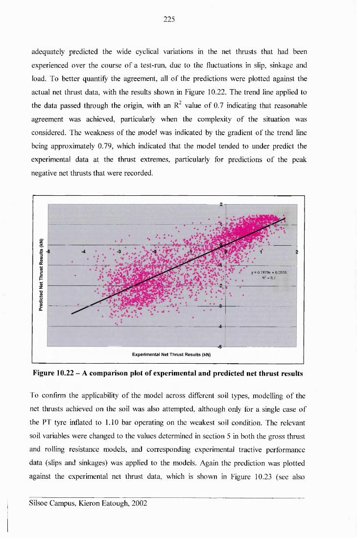
225
adequately predicted the wide cyclical variations in the net thrusts that had been
experienced over the course of a test-run, due to the fluctuations in slip, sinkage and
load. To better quantify the agreement, all of the predictions were plotted against the
actual net thrust data, with the results shown in Figure 10.22. The trend line applied to• • 2 • the data passed through the origin, with an R value of 0.7 indicating that reasonable
agreement was achieved, particularly when the complexity of the situation was
considered. The weakness of the model was indicated by the gradient of the trend line
being approximately 0.79, which indicated that the model tended to under predict the
experimental data at the thrust extremes, particularly for predictions of the peak
negative net thrusts that were recorded.
0.7879X + 0 .0078
R2 = 0 .7
Experimental Net Thrust Results (kN)
Figure 10.22 - A comparison plot of experimental and predicted net thrust results
To confirm the applicability of the model across different soil types, modelling of the
net thrusts achieved on the soil was also attempted, although only for a single case of
the PT tyre inflated to 1.10 bar operating on the weakest soil condition. The relevant
soil variables were changed to the values determined in section 5 in both the gross thrust
and rolling resistance models, and corresponding experimental tractive performance
data (slips and sinkages) was applied to the models. Again the prediction was plotted
against the experimental net thrust data, which is shown in Figure 10.23 (see also
Silsoe Campus, Kieron Eatough, 2002
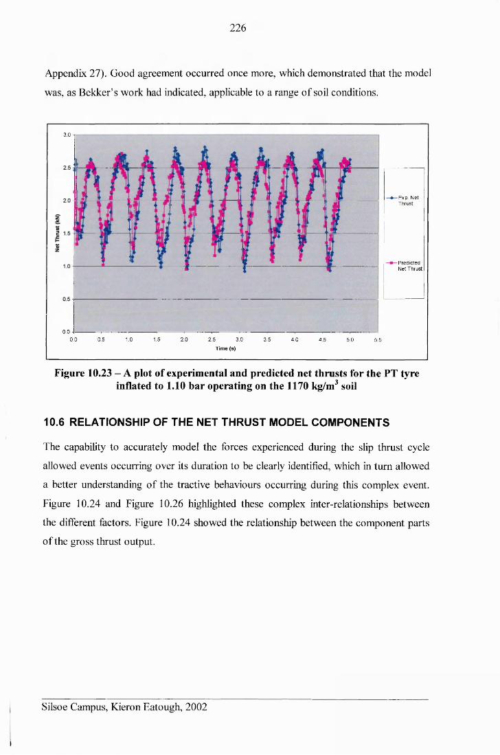
226
Appendix 27). Good agreement occurred once more, which demonstrated that the model
was, as Bekker’s work had indicated, applicable to a range of soil conditions.
3 .0
Exp. N et T h ru st
P red ic ted N et T hrust
0 .0 -I----------------------T---------------------- T---------------------- T----------------------T-----------------------1----------------------T-----------------------T----------------------T----------------------T-----------------------T---------------------- 1
0 .0 0 .5 1 .0 1.5 2 .0 2 .5 3 .0 3 .5 4 .0 4 .5 5 .0 5 .5
T im e (s)
Figure 10.23 - A plot of experimental and predicted net thrusts for the PT tyre inflated to 1.10 bar operating on the 1170 kg/m3 soil
10.6 RELATIONSHIP OF THE NET THRUST MODEL COMPONENTS
The capability to accurately model the forces experienced during the slip thrust cycle
allowed events occurring over its duration to be clearly identified, which in turn allowed
a better understanding of the tractive behaviours occurring during this complex event.
Figure 10.24 and Figure 10.26 highlighted these complex inter-relationships between
the different factors. Figure 10.24 showed the relationship between the component parts
of the gross thrust output.
Silsoe Campus, Kieron Eatough, 2002
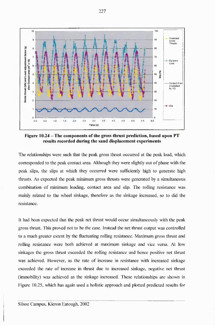
227
- r 100
P red ic tedG ro ssT h ru sts
90
D ynam icLoad
C o n ta c t A rea(m ultiplied by 10)
3 -------
20
Slip
2 .5 3 .0
T im e ( s )
3.5 4 .0 4 .5 5.0 5 .52.00.0 0.5
Figure 10.24 - The components of the gross thrust prediction, based upon PT results recorded during the sand displacement experiments
The relationships were such that the peak gross thrust occurred at the peak load, which
corresponded to the peak contact area. Although they were slightly out of phase with the
peak slips, the slips at which they occurred were sufficiently high to generate high
thrusts. As expected the peak minimum gross thrusts were generated by a simultaneous
combination of minimum loading, contact area and slip. The rolling resistance was
mainly related to the wheel sinkage, therefore as the sinkage increased, so to did the
resistance.
It had been expected that the peak net thrust would occur simultaneously with the peak
gross thrust. This proved not to be the case. Instead the net thrust output was controlled
to a much greater extent by the fluctuating rolling resistance. Maximum gross thrust and
rolling resistance were both achieved at maximum sinkage and vice versa. At low
sinkages the gross thrust exceeded the rolling resistance and hence positive net thrust
was achieved. However, as the rate of increase in resistance with increased sinkage
exceeded the rate of increase in thrust due to increased sinkage, negative net thrust
(immobility) was achieved as the sinkage increased. These relationships are shown in
Figure 10.25, which has again used a holistic approach and plotted predicted results for
Silsoe Campus, Kieron Eatough, 2002
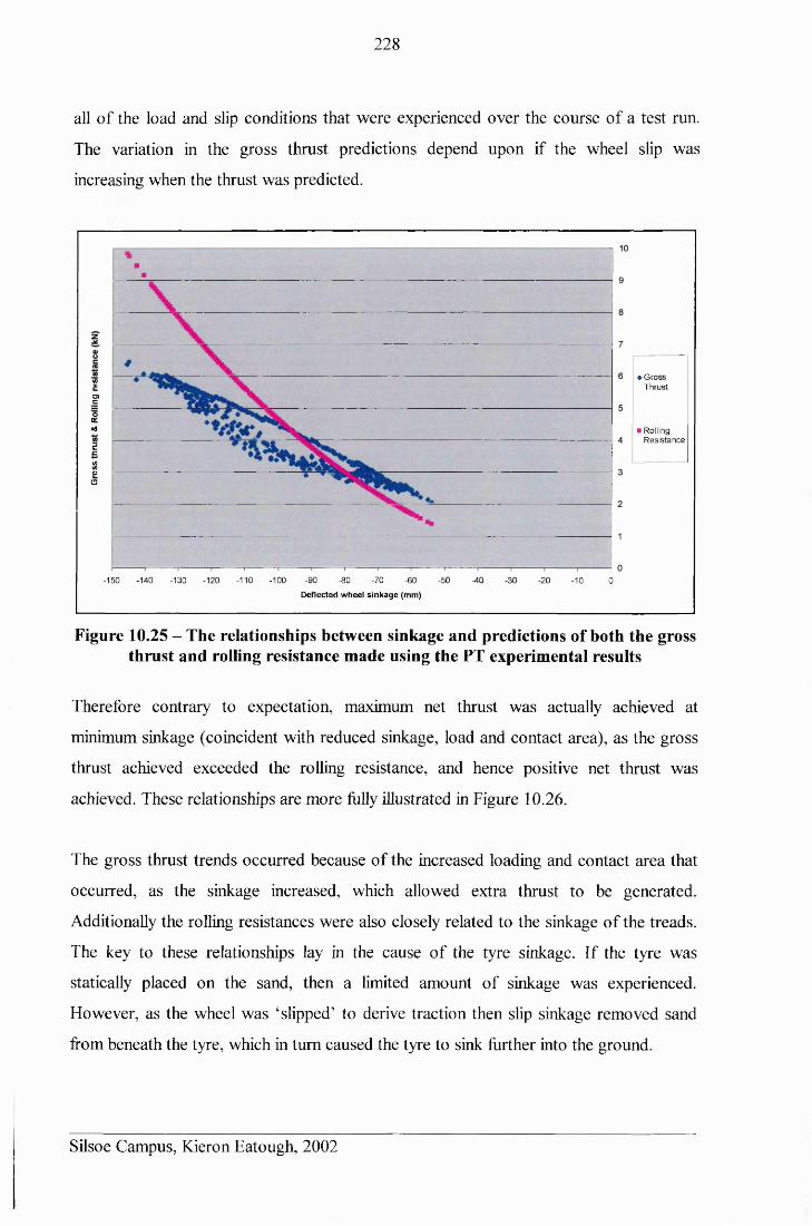
228
all of the load and slip conditions that were experienced over the course of a test run.
The variation in the gross thrust predictions depend upon if the wheel slip was
increasing when the thrust was predicted.
re'atat
a tC
OO '°a
s.cinino«
-150 -140 -130 -120 -110 -100 -90 -80 -70 -50 10-60 -30 -20 -10 0Deflected wheel sinkage (mm)
♦ G ro ss T hrust
■ Rolling R es is ta n ce
Figure 10.25 - The relationships between sinkage and predictions of both the gross thrust and rolling resistance made using the PT experimental results
Therefore contrary to expectation, maximum net thrust was actually achieved at
minimum sinkage (coincident with reduced sinkage, load and contact area), as the gross
thrust achieved exceeded the rolling resistance, and hence positive net thrust was
achieved. These relationships are more fully illustrated in Figure 10.26.
The gross thrust trends occurred because of the increased loading and contact area that
occurred, as the sinkage increased, which allowed extra thrust to be generated.
Additionally the rolling resistances were also closely related to the sinkage of the treads.
The key to these relationships lay in the cause of the tyre sinkage. If the tyre was
statically placed on the sand, then a limited amount of sinkage was experienced.
However, as the wheel was ‘slipped’ to derive traction then slip sinkage removed sand
from beneath the tyre, which in turn caused the tyre to sink further into the ground.
Silsoe Campus, Kieron Eatough, 2002
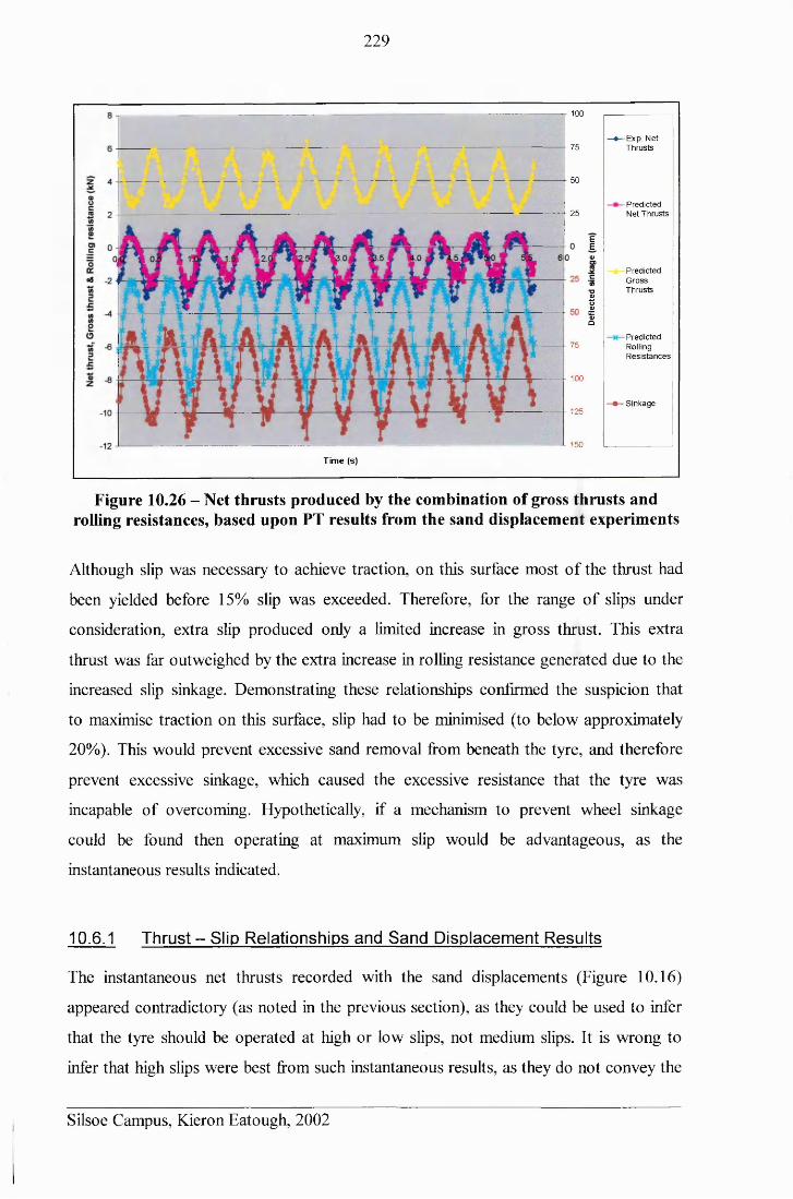
229
-E x p . N et T h ru sts
- P red ic te d N et T h ru sts
P red ic te dG ro ssT h ru s ts
P red ic te dRollingR e s is ta n c e s
-S in k a g e
100
75
50
25
E Eo> o>
C V> TJ (1) t s 01 c 6 Q
75
100
125
150
T im e (s )
Figure 10.26 - Net thrusts produced by the combination of gross thrusts and rolling resistances, based upon PT results from the sand displacement experiments
Although slip was necessary to achieve traction, on this surface most of the thrust had
been yielded before 15% slip was exceeded. Therefore, for the range of slips under
consideration, extra slip produced only a limited increase in gross thrust. This extra
thrust was far outweighed by the extra increase in rolling resistance generated due to the
increased slip sinkage. Demonstrating these relationships confirmed the suspicion that
to maximise traction on this surface, slip had to be minimised (to below approximately
20%). This would prevent excessive sand removal from beneath the tyre, and therefore
prevent excessive sinkage, which caused the excessive resistance that the tyre was
incapable of overcoming. Hypothetically, if a mechanism to prevent wheel sinkage
could be found then operating at maximum slip would be advantageous, as the
instantaneous results indicated.
10.6.1 Thrust - Slip Relationships and Sand Displacement Results
The instantaneous net thrusts recorded with the sand displacements (Figure 10.16)
appeared contradictory (as noted in the previous section), as they could be used to infer
that the tyre should be operated at high or low slips, not medium slips. It is wrong to
infer that high slips were best from such instantaneous results, as they do not convey the
Silsoe Campus, Kieron Eatough, 2002
230
very large sinkages (resistances) that the high slips generated immediately after they
occurred. These effects become obvious once constant streams of data generated over
fall test runs were considered, because as the previous section noted, the instantaneous
data recorded during the displacement experiments neither accounted for the dynamic
nature of the relationships, nor the effect of slip upon the subsequent sinkage.
The instantaneous slip results did not account for the preceding slip (slip sinkage),
though this slip was directly responsible for the sinkage of the wheel when the
instantaneous displacement and tractive measurements were recorded. These effects
were instead considered when the whole test runs were considered. Therefore although
the results indicated that the high slips were potentially capable of generating the
highest net thrusts. They failed to properly demonstrate that this benefit was only
momentary as the slip sinkage that was generated quickly immobilised the tyre, an
effect that was properly explained once the model could be applied to complete sets of
results.
10.7 TREAD EFFECTS, GROSS THRUSTS AND DISPLACEMENTS
The theoretical derivation of gross thrust allowed the sand displacements calculated for
the treads to be related to the derived gross thrusts (i.e. the data shown in Figure 10.16).
This data was plotted as Figure 10.27. This graph indicated that two different types of
displacement had occurred. The two patterns were separated by the slip treatments at
which the treads had operated, such that between the high and medium slip conditions
the sand displacement had changed significantly. At low and medium slips higher net
thrusts were generated, from smaller volumes of sand displacement. At higher slips
significantly greater sand displacements produced lower thrusts, because the dynamic
load (and contact area) were reduced. This allowed the treads to throw the surface layers
of sand rearwards after they were sheared, which resulted in the larger sand
displacements that occurred even though lower gross thrusts were generated.
‘Low’ slips still achieved sufficient slip to release a large proportion of the potential
shear force from the sand and thus good gross thrust was achieved. Despite the
difference in thrust, Figure 10.27 showed that these were altered by the tread pattern,
Silsoe Campus, Kieron Eatough, 2002
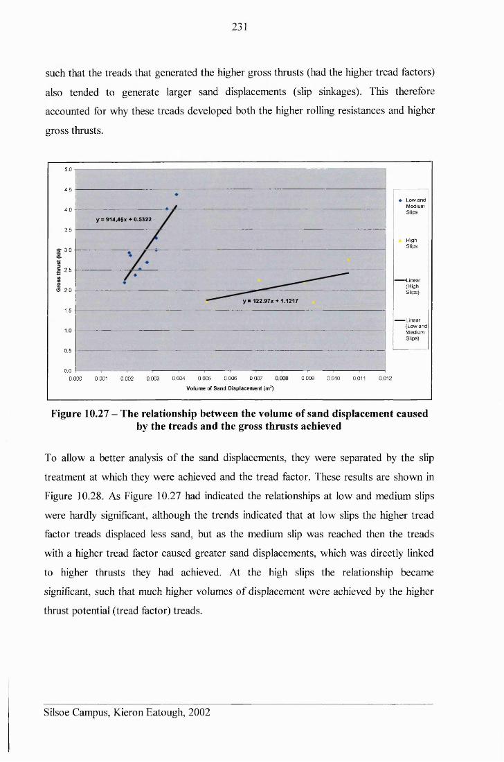
231
such that the treads that generated the higher gross thrusts (had the higher tread factors)
also tended to generate larger sand displacements (slip sinkages). This therefore
accounted for why these treads developed both the higher rolling resistances and higher
gross thrusts.
5.0
4 .5
♦ Low an d M edium S lips4 .0
y = 9 1 4 .4 5 x + 0.5322
3 .5
HighS lips
5 - 3 .0
2 .5
■Linear(HighS lips)e> 2.o
y = 122.97x + 1.1217
1.5
— Linear (Low an d M edium Slips)
0.5
0.00 .005 0 .006 0 .007
Volume of Sand Displacement (m3)
0.009 0.0120.004 0.010 0.0110.001 0.0030.000 0.002
Figure 10.27 - The relationship between the volume of sand displacement caused by the treads and the gross thrusts achieved
To allow a better analysis of the sand displacements, they were separated by the slip
treatment at which they were achieved and the tread factor. These results are shown in
Figure 10.28. As Figure 10.27 had indicated the relationships at low and medium slips
were hardly significant, although the trends indicated that at low slips the higher tread
factor treads displaced less sand, but as the medium slip was reached then the treads
with a higher tread factor caused greater sand displacements, which was directly linked
to higher thrusts they had achieved. At the high slips the relationship became
significant, such that much higher volumes of displacement were achieved by the higher
thrust potential (tread factor) treads.
Silsoe Campus, Kieron Eatough, 2002
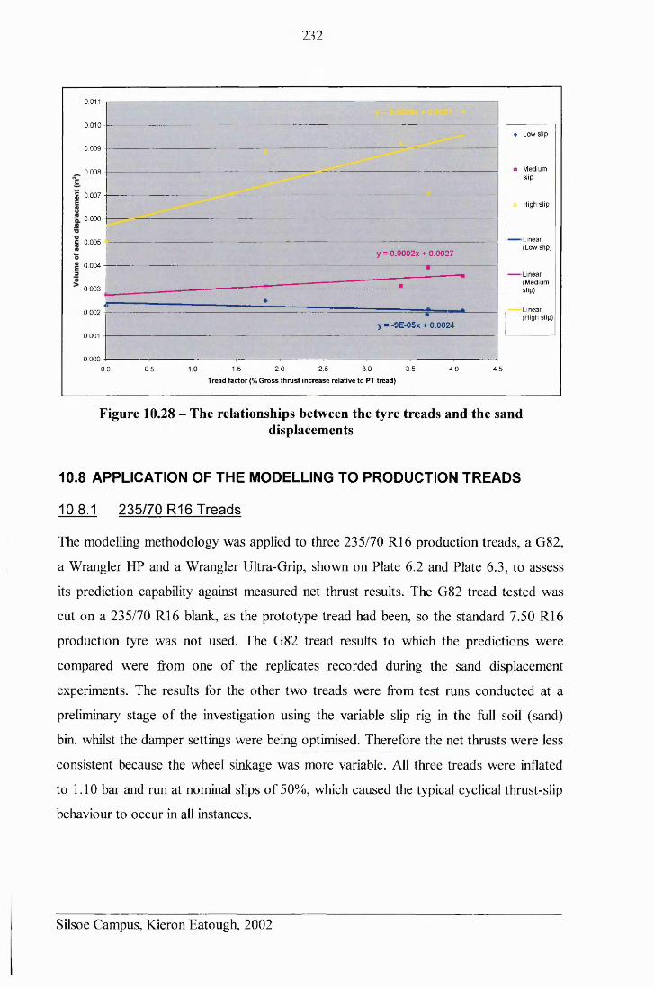
232
0.011 -
0.010♦ Low slip
0.009
■ M edium slip
0.008
g 0.007High slip
0 .006
■Linear (Low slip)
= 0.005
y = 0.0002x + 0.00270.004
■Linear(M ediumslip)0 .003
Linear (H igh slip)
0.002
y = -9E-05X + 0.00240.001
0.0001.5 2 .0 2 .5 3 .0
Tread factor (% Gross thrust increase relative to PT tread)3 .50.5 4 .50.0 4 .0
Figure 10.28 - The relationships between the tyre treads and the sanddisplacements
10.8 APPLICATION OF THE MODELLING TO PRODUCTION TREADS
10.8.1 235/70 R16 Treads
The modelling methodology was applied to three 235/70 R16 production treads, a G82,
a Wrangler HP and a Wrangler Ultra-Grip, shown on Plate 6.2 and Plate 6.3, to assess
its prediction capability against measured net thrust results. The G82 tread tested was
cut on a 235/70 R16 blank, as the prototype tread had been, so the standard 7.50 R16
production tyre was not used. The G82 tread results to which the predictions were
compared were from one of the replicates recorded during the sand displacement
experiments. The results for the other two treads were from test runs conducted at a
preliminary stage of the investigation using the variable slip rig in the full soil (sand)
bin, whilst the damper settings were being optimised. Therefore the net thrusts were less
consistent because the wheel sinkage was more variable. All three treads were inflated
to 1.10 bar and run at nominal slips of 50%, which caused the typical cyclical thrust-slip
behaviour to occur in all instances.
Silsoe Campus, Kieron Eatough, 2002
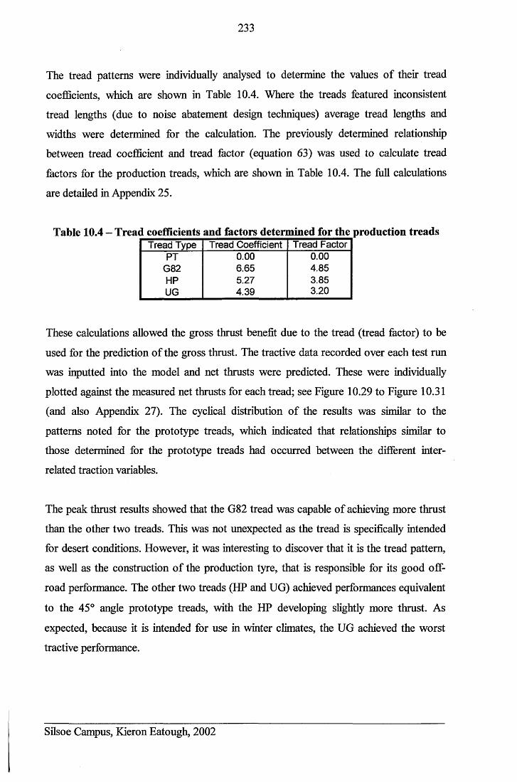
233
The tread patterns were individually analysed to determine the values of their tread
coefficients, which are shown in Table 10.4. Where the treads featured inconsistent
tread lengths (due to noise abatement design techniques) average tread lengths and
widths were determined for the calculation. The previously determined relationship
between tread coefficient and tread factor (equation 63) was used to calculate tread
factors for the production treads, which are shown in Table 10.4. The full calculations
are detailed in Appendix 25.
Table 10.4 - Tread coefficients and factors determined for the production treadsTread Type Tread Coefficient Tread Factor
PT 0.00 0.00G82 6.65 4.85HP 5.27 3.85UG 4.39 3.20
These calculations allowed the gross thrust benefit due to the tread (tread factor) to be
used for the prediction of the gross thrust. The tractive data recorded over each test run
was inputted into the model and net thrusts were predicted. These were individually
plotted against the measured net thrusts for each tread; see Figure 10.29 to Figure 10.31
(and also Appendix 27). The cyclical distribution of the results was similar to the
patterns noted for the prototype treads, which indicated that relationships similar to
those determined for the prototype treads had occurred between the different inter
related traction variables.
The peak thrust results showed that the G82 tread was capable of achieving more thrust
than the other two treads. This was not unexpected as the tread is specifically intended
for desert conditions. However, it was interesting to discover that it is the tread pattern,
as well as the construction of the production tyre, that is responsible for its good off-
road performance. The other two treads (HP and UG) achieved performances equivalent
to the 45° angle prototype treads, with the HP developing slightly more thrust. As
expected, because it is intended for use in winter climates, the UG achieved the worst
tractive performance.
Silsoe Campus, Kieron Eatough, 2002
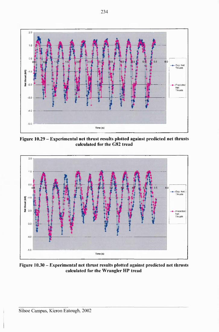
234
2 . 0 -i
0.05 .5*3-02 .5 i1.0
•Exp. N et T hrusts
? -1.0
- 2.0 P red ic tedNetT h ru sts
-3 .0
-4 .0
-5 .0 1Time (s)
Figure 10.29 - Experimental net thrust results plotted against predicted net thrustscalculated for the G82 tread
2.0
1.0
0.05.5
Exp. N et T h ru sts
z -1 .0
-2.0 P red ic te dN etT h ru sts
-3.0
-4.0
-5 .0 J-
Time (s)
Figure 10.30 - Experimental net thrust results plotted against predicted net thrustscalculated for the Wrangler HP tread
Silsoe Campus, Kieron Eatough, 2002
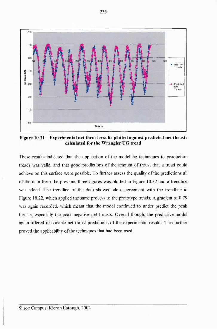
235
2 .0 -r—
Exp. N et T h ru sts
P red ic tedN etT hrusts
-4.0
Time (s)
Figure 10.31 - Experimental net thrust results plotted against predicted net thrustscalculated for the Wrangler UG tread
These results indicated that the application of the modelling techniques to production
treads was valid, and that good predictions of the amount of thrust that a tread could
achieve on this surface were possible. To further assess the quality of the predictions all
of the data from the previous three figures was plotted in Figure 10.32 and a trendline
was added. The trendline of the data showed close agreement with the trendline in
Figure 10.22, which applied the same process to the prototype treads. A gradient of 0.79
was again recorded, which meant that the model continued to under predict the peak
thrusts, especially the peak negative net thrusts. Overall though, the predictive model
again offered reasonable net thrust predictions of the experimental results. This further
proved the applicability of the techniques that had been used.
Silsoe Campus, Kieron Eatough, 2002
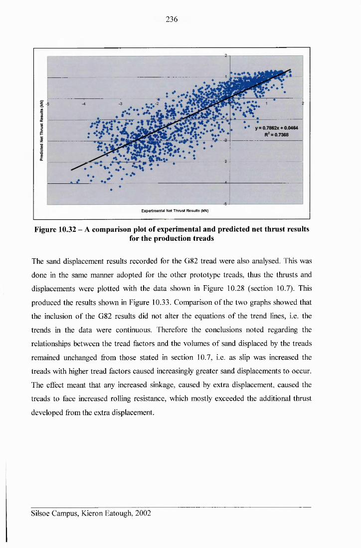
236
Experimental Net Thrust Results (kN)
Figure 10.32 - A comparison plot of experimental and predicted net thrust resultsfor the production treads
The sand displacement results recorded for the G82 tread were also analysed. This was
done in the same manner adopted for the other prototype treads, thus the thrusts and
displacements were plotted with the data shown in Figure 10.28 (section 10.7). This
produced the results shown in Figure 10.33. Comparison of the two graphs showed that
the inclusion of the G82 results did not alter the equations of the trend lines, i.e. the
trends in the data were continuous. Therefore the conclusions noted regarding the
relationships between the tread factors and the volumes of sand displaced by the treads
remained unchanged from those stated in section 10.7, i.e. as slip was increased the
treads with higher tread factors caused increasingly greater sand displacements to occur.
The effect meant that any increased sinkage, caused by extra displacement, caused the
treads to face increased rolling resistance, which mostly exceeded the additional thrust
developed from the extra displacement.
Silsoe Campus, Kieron Eatough, 2002
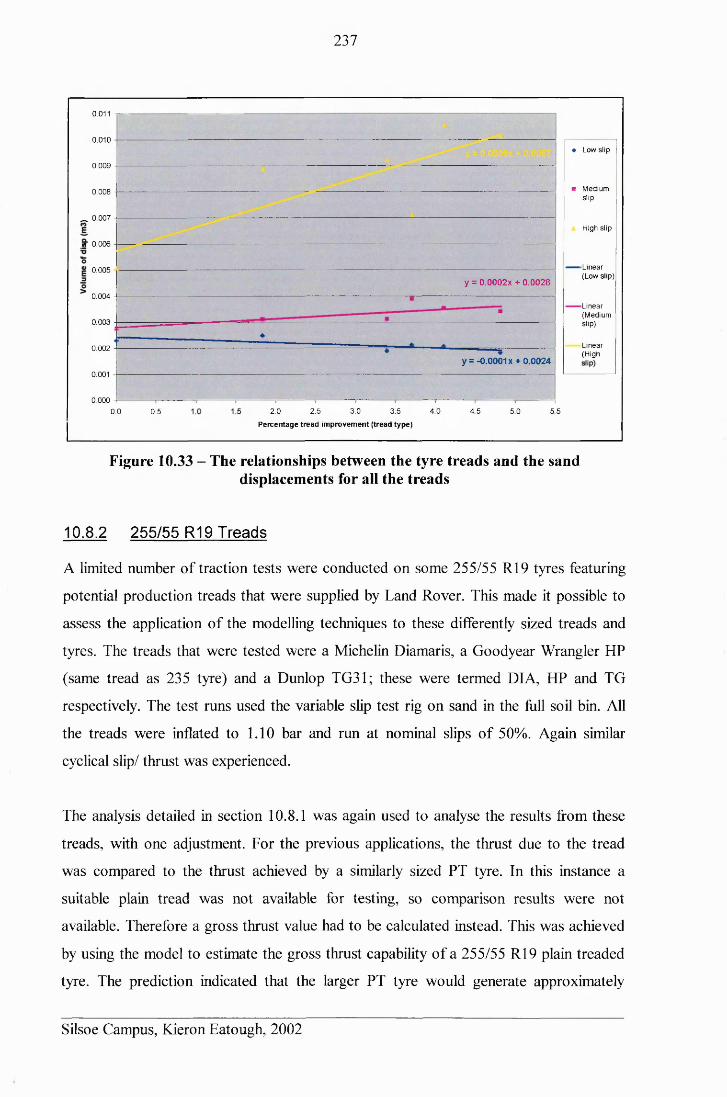
237
0.011 -r
0.010♦ Low slip
0 .009
■ M edium slip
0 .008
_ 0 .007High slip
» 0 .006
■Linear (Low slip)
0 .005
y = 0.0002X + 0.00280.004
•Linear(M ediumslip)0 .003
Linear(High
0.002
y = -0.0001 x + 0.00240.001
0.0002.5 3 .0 4 .02.0
Percentage tread improvement (tread type)
3 .5 4 .5 5 .0 5 .50.0 0.5
Figure 10.33 - The relationships between the tyre treads and the sand displacements for all the treads
10.8.2 255/55 R19 Treads
A limited number of traction tests were conducted on some 255/55 R19 tyres featuring
potential production treads that were supplied by Land Rover. This made it possible to
assess the application of the modelling techniques to these differently sized treads and
tyres. The treads that were tested were a Michelin Diamaris, a Goodyear Wrangler HP
(same tread as 235 tyre) and a Dunlop TG31; these were termed DIA, HP and TG
respectively. The test runs used the variable slip test rig on sand in the hill soil bin. All
the treads were inflated to 1.10 bar and run at nominal slips of 50%. Again similar
cyclical slip/ thrust was experienced.
The analysis detailed in section 10.8.1 was again used to analyse the results from these
treads, with one adjustment. For the previous applications, the thrust due to the tread
was compared to the thrust achieved by a similarly sized PT tyre. In this instance a
suitable plain tread was not available for testing, so comparison results were not
available. Therefore a gross thrust value had to be calculated instead. This was achieved
by using the model to estimate the gross thrust capability of a 255/55 R19 plain treaded
tyre. The prediction indicated that the larger PT tyre would generate approximately
Silsoe Campus, Kieron Eatough, 2002
I
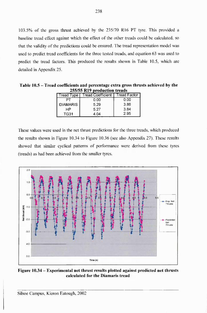
238
103.5% of the gross thrust achieved by the 235/70 R16 PT tyre. This provided a
baseline tread effect against which the effect of the other treads could be calculated, so
that the validity of the predictions could be ensured. The tread representation model was
used to predict tread coefficients for the three tested treads, and equation 63 was used to
predict the tread factors. This produced the results shown in Table 10.5, which are
detailed in Appendix 25.
Table 10.5 - Tread coefficients and percentage extra gross thrusts achieved by the
Tread Type Tread Coefficient Tread FactorPT 0.00 0.00
DIAMARIS 5.29 3.86HP 5.27 3.84
TG31 4.04 2.95
These values were used in the net thrust predictions for the three treads, which produced
the results shown in Figure 10.34 to Figure 10.36 (see also Appendix 27). These results
showed that similar cyclical patterns of performance were derived from these tyres
(treads) as had been achieved from the smaller tyres.
2.0
0.02 to
■Exp. N et T h ru s ts
? -1.0
-2.0 P red ic te dN etT h ru s ts
-3 .0
-4 .0
-5 .0 1Time (s)
Figure 10.34 - Experimental net thrust results plotted against predicted net thrustscalculated for the Diamaris tread
Silsoe Campus, Kieron Eatough, 2002
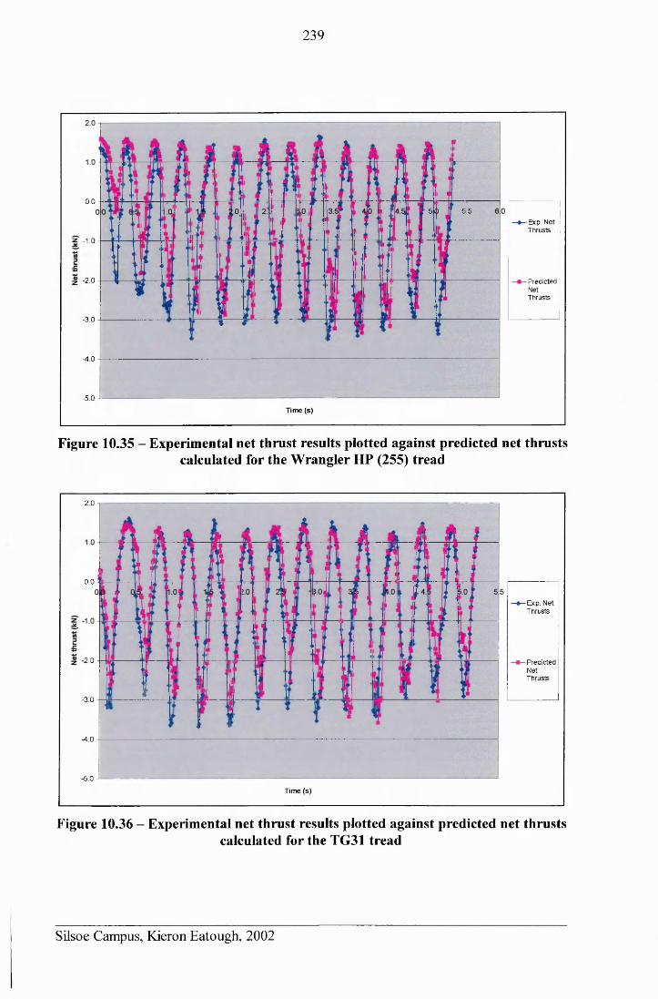
239
0.05<& 5 .5
■Exp. N et T hrusts
? - 1.0
-2.0 P red ictedNetT hrusts
-3 .0
-4 .0
-5 .0 -L
Time (s)
Figure 10.35 - Experimental net thrust results plotted against predicted net thrusts calculated for the Wrangler HP (255) tread
2.0
0.0
Exp. N et T hrusts
-2.0 P red ic te dN etT h ru sts
-3 .0
^ . 0
-5 .0 -L
Time (s)
Figure 10.36 - Experimental net thrust results plotted against predicted net thrustscalculated for the TG31 tread
Silsoe Campus, Kieron Eatough, 2002
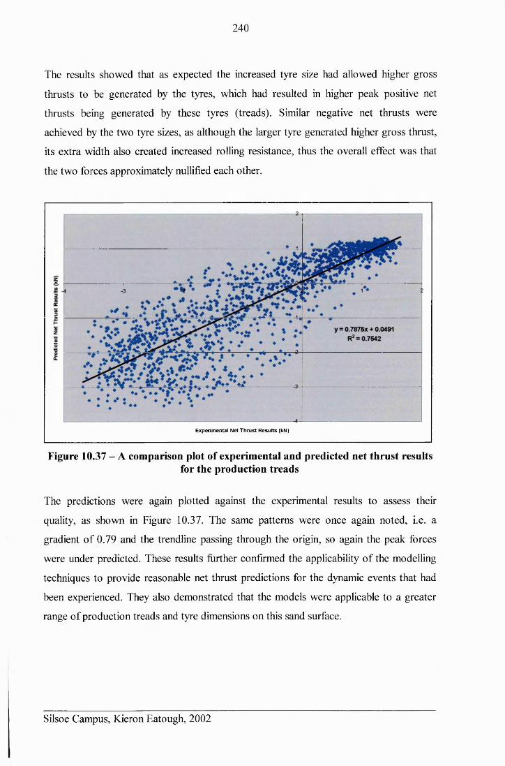
240
The results showed that as expected the increased tyre size had allowed higher gross
thrusts to be generated by the tyres, which had resulted in higher peak positive net
thrusts being generated by these tyres (treads). Similar negative net thrusts were
achieved by the two tyre sizes, as although the larger tyre generated higher gross thrust,
its extra width also created increased rolling resistance, thus the overall effect was that
the two forces approximately nullified each other.
Experimental Net Thrust Results (kN)
Figure 10.37 - A comparison plot of experimental and predicted net thrust resultsfor the production treads
The predictions were again plotted against the experimental results to assess their
quality, as shown in Figure 10.37. The same patterns were once again noted, i.e. a
gradient of 0.79 and the trendline passing through the origin, so again the peak forces
were under predicted. These results further confirmed the applicability of the modelling
techniques to provide reasonable net thrust predictions for the dynamic events that had
been experienced. They also demonstrated that the models were applicable to a greater
range of production treads and tyre dimensions on this sand surface.
Silsoe Campus, Kieron Eatough, 2002
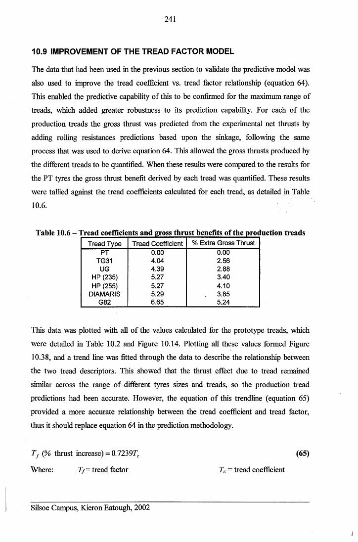
241
10.9 IMPROVEMENT OF THE TREAD FACTOR MODEL
The data that had been used in the previous section to validate the predictive model was
also used to improve the tread coefficient vs. tread factor relationship (equation 64).
This enabled the predictive capability of this to be confirmed for the maximum range of
treads, which added greater robustness to its prediction capability. For each of the
production treads the gross thrust was predicted from the experimental net thrusts by
adding rolling resistances predictions based upon the sinkage, following the same
process that was used to derive equation 64. This allowed the gross thrusts produced by
the different treads to be quantified. When these results were compared to the results for
the PT tyres the gross thrust benefit derived by each tread was quantified. These results
were tallied against the tread coefficients calculated for each tread, as detailed in Table
10.6.
Table 10.6 - Tread coefficients and gross thrust benefits of the production treadsTread Type Tread Coefficient % Extra Gross Thrust
PT 0.00 0.00TG31 4.04 2.56
UG 4.39 2.88HP (235) 5.27 3.40HP (255) 5.27 4.10
DIAMARIS 5.29 3.85G82 6.65 5.24
This data was plotted with all of the values calculated for the prototype treads, which
were detailed in Table 10.2 and Figure 10.14. Plotting all these values formed Figure
10.38, and a trend line was fitted through the data to describe the relationship between
the two tread descriptors. This showed that the thrust effect due to tread remained
similar across the range of different tyres sizes and treads, so the production tread
predictions had been accurate. However, the equation of this trendline (equation 65)
provided a more accurate relationship between the tread coefficient and tread factor,
thus it should replace equation 64 in the prediction methodology.
T f (% thrust increase) = 0.7239TC (65)
Where: T f - tread factor Tc = tread coefficient
Silsoe Campus, Kieron Eatough, 2002
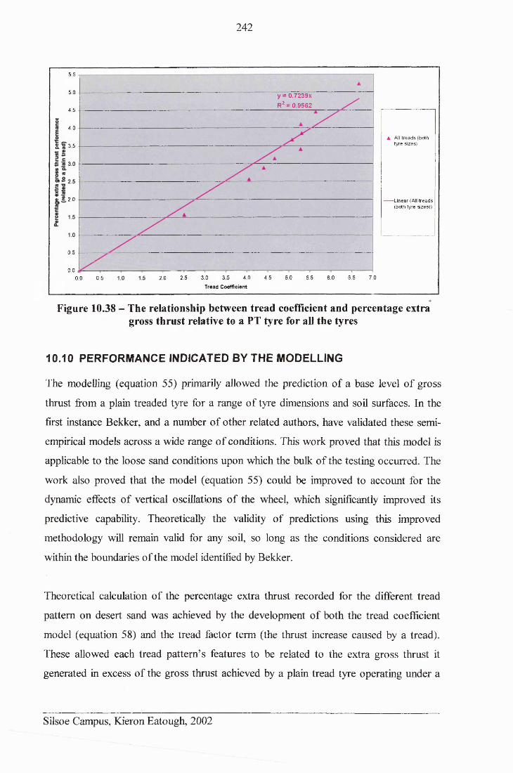
242
5.5
5.0 y = 0.7239x R2 = 0.9562
4.5
4 .0
▲ All trea d s (both tyre sizes)« *o o c
c l m 0 0
• e 2 .o Linear (All tread s(both tyre sizes))
0.5
0.04.5 5.0 5.5 6.0 6.5 7.02.5 3 .0
Tread Coefficient
a o0.5 2.00.0
Figure 10.38 - The relationship between tread coefficient and percentage extragross thrust relative to a PT tyre for all the tyres
10.10 PERFORMANCE INDICATED BY THE MODELLING
The modelling (equation 55) primarily allowed the prediction of a base level of gross
thrust from a plain treaded tyre for a range of tyre dimensions and soil surfaces. In the
first instance Bekker, and a number of other related authors, have validated these semi-
empirical models across a wide range of conditions. This work proved that this model is
applicable to the loose sand conditions upon which the bulk of the testing occurred. The
work also proved that the model (equation 55) could be improved to account for the
dynamic effects of vertical oscillations of the wheel, which significantly improved its
predictive capability. Theoretically the validity of predictions using this improved
methodology will remain valid for any soil, so long as the conditions considered are
within the boundaries of the model identified by Bekker.
Theoretical calculation of the percentage extra thrust recorded for the different tread
pattern on desert sand was achieved by the development of both the tread coefficient
model (equation 58) and the tread factor term (the thrust increase caused by a tread).
These allowed each tread pattern’s features to be related to the extra gross thrust it
generated in excess of the gross thrust achieved by a plain tread tyre operating under a
Silsoe Campus, Kieron Eatough, 2002
243
similar treatment. This model showed good agreement with the recorded results (see
Figure 10.38).
The relationships confirmed by the model (equation 55) showed that within the 15% to
80% slip range the dynamic normal load and related contact area of the tyre had a more
significant impact on the gross thrust generated than the slip. However, the wheel slip
was directly related to the sand displacement, and thus more crucially, the sinkage of the
tyre, because as the slip sinkage increased, so too did the rolling resistance. As high
slips (of approximately 55% to 70%) occurred at small sinkages and loads, the M ure of
the surface layers of sand changed from being purely sheared (as occurred at lower
slips) to being sheared and having the surface layers thrown rearwards. This change in
caused extra sand to be removed from beneath the tyres at high slips, as greater
displacements were achieved, which subsequently left the tyres facing considerably
greater rolling resistances.
The resistance faced due to the resulting high sinkage far exceeded the gross thrust
capabilities of any of the evaluated tyres treads and thus the tyres were placed in an
immobile condition. Thus although operating the tyres at high slips momentarily
yielded high net thrusts, they rapidly became immobilised thereafter. Thus to achieve
maximum tractive performance on this surface at the forward speeds, the slip should be
limited to below 20% slip, so as to prevent excessive sand disturbance. This
requirement is not necessarily valid at higher forward speeds, where vehicle momentum
and the position of the tyre relative to its bow-wave would influence the tyre
performance. This conditions could possible prevent a wheel with limited slip from
achieving maximum thrust, but these conditions were not investigated.
If a volume of sand displacement were known for a particular tread pattern in
combination with its tread factor, and corresponding values of wheel slip, sinkage and
load, then this could be used to predict the gross thrust and rolling resistance produced
by the tread, and thus the net thrust. However, it is very time consuming to quantify
sand displacement and thus it is easier to use the thrust prediction model (equation 55)
and tread factor model (equation 58) to achieve the same prediction, providing the
Silsoe Campus, Kieron Eatough, 2002
244
necessary engineering coefficients for the soil surface that are used in the model are
known.
As it is based on Bekker’s prediction methods, the proposed methodology is also
potentially applicable to other sandy surfaces, but this should be confirmed by
additional traction tests to record data against which model predictions could be judged.
It would be necessary to test a PT tread and at least two other treads on appropriately
sized tyres to establish the tread factor vs. tread coefficient relationship for the new
surface (following section 10.8.1 as a methodology route map). These should be treads
expected to produce average and high levels of performance on that surface. Once the
relationship is established it would be straightforward to develop desk-based
performance predictions for any treads under consideration, by using the tread factors to
predict the gross thrust benefit of the new treads. Such a study would also allow further
confidence to be placed in the tread representation models and confirm the application
of the methodology to a boarder range of situations.
Silsoe Campus, Kieron Eatough, 2002
245
11 DISCUSSION OF THE PROJECT FINDINGS
11.1 TEST EQUIPMENT AND METHODOLOGIES
11.1.1 Traction Test Rias
Two test rigs were developed during the project to allow the completion of the traction
investigations. Two fundamentally different drive mechanisms were used for these, but
both achieved similar patterns of tractive performance on both the soil and sand
surfaces. The similarities between the tractive performances derived from the two rigs
were most striking when they were operated at higher wheel slips. In particular, in terms
of the consistency of the relationships developed between the wheel slip, sinkage, and
contact area. These relationships indicated that the treatments tested had affected both
the gross thrust and rolling resistances generated by the tyres, which in combination
governed the overall net thrust output. The net thrusts generated varied between
approximately +1.2 kN and -4 kN on the sand surface in both instances. The similarities
in the performance (behaviour), and comparative tests conducted on both the soil and
sand, confirmed that the results were related to the thrust interaction between the surface
and the tyre tread and not a particular drive system.
The variable slip (hydrostatic) drive was used for the majority of the testing, as it
provided several replications of a wheel passing from a mobile to immobile situation
due to the large sand displacements. It was also more operationally flexible when
changing the intended band of wheel slip. Typically ranges of slip of approximately
50% to 60% slip were achieved, which enabled the investigation of the tyre behaviour
across a range of conditions (from 15% to 75% wheel slip). The variable sinkage
behaviour that occurred did so because of the combination of the varying wheel slip and
the constant forward motion of the test rig. This was partially self-reinforcing as it
caused the normal load acting on the tyre to vary dynamically, but this allowed a tyre’s
interaction with the sand to be studied across a range of tractive conditions, rather than a
single case, so a greater range of results were collected. Additionally the repetitive
cycles of the test rig allowed more results to be produced from a single test run, so more
significance could be derived from the test results.
Silsoe Campus, Kieron Eatough, 2002
246
The use of the University soil bin facilities enabled the testing to be conducted in a
controlled environment with a degree of consistency that would be impossible to
replicate in any field environment. The repeatability provided by the test methodology
allowed the results to be easily compared to establish their variance. However, the
complex interlinked nature of the results made the production of a simple method of
tyre (tread) performance comparison, such as a slip-pull graph, difficult. Therefore the
modelling techniques developed had to firstly allow the effects of the inter-relationships
between the slip, sinkage, load and tread pattern upon the net thrust that was generated
to be understood. Secondly, they had to allow the tread pattern and its effect upon the
performance to be quantified in a manner that allowed comparative evaluations.
11.1.2 Sand Displacement Assessment Methodology
This measurement methodology was developed specifically for this project. For the tag
movements to be accurately determined, both the tag placement locations and their final
positions (displacements) had to be accurately determined. All the equipment developed
by the author for this purpose was proved to be suitably accurate for the task
(positioning and measurement accuracy ±5.5 mm). The placement equipment was
particularly effective in the X-Y plane, but its accuracy reduced in the vertical plane as
it occasionally failed (approximately 1% of occasions) to release the tags at the correct
depth and instead positioned them up to 5 mm too high. Although adequate for the tests
conducted, this apparatus would need re-designing if significantly deeper tag
placements were required to prevent deflection of the rods during installation.
The key benefit that the tag measurement frame delivered for the investigations, when
used with Excel, was a fast and simple method of transforming the three-dimensional
tag positions into real Cartesian disturbance measurements relative to a fixed reference
point. A more automated insertion process could hasten the overall operation, but this
would not avoid the largest time absorbing factor necessary to produce accurate results,
which was the painstaking tag excavation process.
The data tags proved to be a reliable and accurate method of recording the movement of
particles within a sand mass. The main criticisms of this methodology were threefold.
Silsoe Campus, Kieron Eatough, 2002
247
Firstly, it was not possible to accurately place sufficient tags to comprehensively record
the disturbance patterns that occurred in close proximity to the tyre tread, due to the
complex disturbances that occurred. Secondly, it was very time consuming to accurately
place, uncover and measure the tag positions. Finally, it could not determine the exact
trajectories of the particles, so they were assumed to follow vector paths, even though
this was thought to be unlikely.
The merits of this system do not lie in a large-scale application outside a research
environment, but in its ability to provide otherwise unobtainable data, which allowed a
superior empirical quantification of the magnitude of three-dimensional sand
disturbance caused by a 4x4 tyre, without constraining or interrupting the resulting sand
flow. This in turn allowed the successful development and validation of model
predictions. In the future this approach will be useful to confirm the CFD sand
displacement models that will undoubtedly be developed to replicate traction situations.
11.2 MODELLING CAPABILITIES
To enable the gross thrust effect of the tread (and tyre) to be considered, it had to be
derived from the net thrust results recorded during the sand displacement experiments.
This was achieved by calculating a resistance to add to the net thrusts (NT + RR = GT).
The good agreement that occurred between measured resistances and those predicted by
the rolling resistance model across the range of sinkage experienced (maximum error of
7%) enabled resistances to be predicted for each net thrust result (see Figure 10.7). This
allowed suitably accurate gross thrust data to be derived from the data recorded from the
full duration of each test run, for both the driven and towed-driven conditions. These
were compared against gross thrust predictions produced by the modified equations and
agreement was noted. The combination of the measured net thrusts and the rolling
resistance predictions therefore enabled gross thrusts to be calculated. These were
shown to give close agreement with the predicted gross thrusts (maximum error ±8%).
The tread model (equation 58) developed by the author (in the absence of a recognised
method) produced quantitative representations of the tread patterns, which were termed
tread coefficients. These allowed the theoretical longitudinal gross thrust benefits of the
Silsoe Campus, Kieron Eatough, 2002
248
treads to be calculated for the sand environment, based upon the treads’ features (see
Appendix 25. The evaluations of the differences in the gross thrusts (tread factors) that
the prototype treads were capable of achieving showed the ranked order of treads (by
thrust) matched the ranked hierarchy of the magnitudes of sand displacements, i.e. the
G82 and LAT which typically caused the highest disturbances also produced the highest
extra gross thrusts (the highest tread factors). This thrust benefit was necessarily
determined in a holistic manner from all of the data, as no simple methodology was able
to separate the complex inter-relationships caused by the tyres. A close relationship was
established between the tread factors and coefficients (equation 65) which enabled the
percentage extra gross thrust that a tread with a given tread coefficient would be capable
of achieving over a plain tread tyre on loose desert sand to be calculated.
The tread representation also allowed a relationship between the tread patterns and the
sand displacements they caused to be determined. The significance of the trends was
negligible at low slips, but at higher slips the treads with higher tread coefficients
caused considerably more sand to be displaced, so the relationship was non-linear. As
the treads with higher tread coefficients created more longitudinal sand flow, this
explained why they derived both greater gross thrusts and increased wheel sinkages.
11.3 TYRE PERFORMANCE
11.3.1 Cyclical Slip and Thrust Behaviour
The modelling results confirmed that the gross thrusts achieved were dependent upon
the wheel sinkage, load, contact area and slip, but providing 15% slip was exceeded the
effect of slip on the gross thrust was considerably less significant than other factors.
Instead slip had a much more significant influence on the wheel sinkage, and hence the
rolling resistance, as increased slip sinkage notably increased the depth of operation. As
the slip cyclically changed over the course of each test run, 80 mm to 100 mm
variations in wheel sinkage were generated. These caused significant vertical
accelerations of the test rig, as it drove (dug) itself into or out of the sand mass. These
were equivalent to a 50% increase (or decrease) in dynamic loading (±% g). The
minimum loading occurred at minimum sinkage and vice versa. Therefore as the
Silsoe Campus, Kieron Eatough, 2002
249
sinkage increased the contact area was increased because it was surrounded by extra
sand and because the extra loading caused an increased deflection of the tyre carcass.
The increased contact area (and loading) potentially produced a gross thrust benefit for
the tyre. However, gross thrust was only one part of the relationship. Both the fixed slip
and variable slip test runs that were conducted on the sand found that increased wheel
slip led to extra sinkage, but not increased net thrust. This was because the increased
sinkage also caused the tyre to face a greater mass of sand ahead of itself, which
generated extra rolling resistance. Although the gross thrust output at low sinkages
exceeded the rolling resistance, the rate of increase in resistance with increased sinkage
exceeded the rate of increase in gross thrust as the sinkage increased (Figure 10.25).
Therefore extra sinkage produced greater immobility. As the wheel slip exceeded 20%
(which yielded good sand shear) the variation in the magnitude of the slip at higher slips
did not greatly influence the gross thrust output. However, the slip sinkage governed the
rolling resistance faced by the tyre instead and therefore the slip indirectly controlled
the net thrust.
The combination of the variations in gross thrust and rolling resistance caused the net
thrusts to cyclically vary between approximately +1 kN and -4 kN over a test run (for a
235/70 R16 tyre on sand). The peak net thrust output of +1 kN was authenticated by a
whole vehicle test in which a similar net thrust was achieved on the same sand surface
at a low sinkage. It was found that for both the fixed slip tests and the variable slip tests
the maximum (positive) net thrusts were achieved at the lowest slips, and as the slip was
increased the increased sinkage (resistance) caused the tyre to become immobilised.
When higher slips occurred the transformation from mobility to immobility occurred
more rapidly, as the tyre sank faster.
11.3.2 Sand Displacements
The sand displacement results highlighted that performance differences existed between
the tread patterns. Two elements of the tyres contributed to the sand displacements, and
therefore the recorded thrusts. These were (1) the tyre carcass structure and its
dimensions, and (2) the tread pattern. The carcass was responsible for the main
Silsoe Campus, Kieron Eatough, 2002
250
quantities and patterns of sand displacement experienced, which occurred in all three-
dimensions. The common disturbances due to the carcasses occurred across a 500 mm
wide by 250 mm deep portion of the sand mass. In contrast, the treads only influenced a
region of sand 200 mm wide by 200 mm deep. Within this region only variations in the
displacement in the longitudinal (rearward) direction were significantly related to
variations in the tread pattern, and more importantly the variation in the magnitude of
gross thrust caused by each tread (up to 5% extra thrust over a plain tread tyre).
The directions of the sand displacements were significantly affected by the magnitude
of wheel slip. Increased slip caused increased rearward sand displacements, so the
displacements changed from being both downwards and rearwards, to mostly rearwards.
This change was supported by the modelling results, which indicated that when passing
from medium to high slips a changeover occurred, such that the sand came to be both
sheared and thrown rearwards. The increased volume of displacement at higher slips
that this created caused larger voids beneath the tyres, which in turn increased the lateral
sand flows along the side of the tyre rut, as failure back towards the tyre and into the rut
occurred. Carcass effects upon sand displacement were not investigated as a constant
tyre size was tested, but it is more likely that changes to the tyre dimensions would have
affected the magnitudes of the displacements, rather than their directions.
11.3.3 Tread Effects
The investigation of the effects of tread showed that the PT tread produced the least
rearwards sand displacement. This displacement was used as a base line quantity of
disturbance against which any extra longitudinal displacement produced by the other
treads could be quantified. The treads that created the biggest disturbances (G82 and
LAT) tended to generate the peak positive net thrusts. However, they also generated the
peak negative net thrusts because they operated at slightly higher slips (up to +5%),
which caused them to operate slightly deeper, especially at maximum slip.
When the extra gross thrusts produced by the treads during the displacement
investigations were ranked by magnitude, their order agreed with a ranking based upon
the magnitude of the displacements, i.e. greater displacement equalled a greater gross
Silsoe Campus, Kieron Eatough, 2002
251
thrust capability. The tread model developed by the author (equation 58) linked this
effect to the tread, such that the treads with higher tread coefficients were those that
were able to achieve more thrust. However, the increased thrust came at the expense of
greater sand disturbance (sinkage), particularly at higher slips. This explained why at
low slips and low sinkages the higher tread coefficient treads developed higher net
thrusts (due to higher gross thrusts), yet why at high slips they offered the most negative
net thrusts due to the extra resistance generated by the extra sinkage they caused.
This relationship showed that at the low forward speeds (5 km/h) tested on this poor
mobility surface, continuous positive net traction would only be achieved if the wheel
slip were limited to below 20%. If this setting was exceeded then high thrust would
momentarily be achieved, but the tyre would soon become immobilised by the
excessive sinkage generated by the high slip. At the tested forward speeds the
experiment was comparable to the vehicle situation, as the processor resistance
represented the resistance of the vehicle, which causes a wheel to spin and dig into the
sand if high slips are rapidly applied, rather than drive the vehicle forward. At higher
forward speed conditions (which were not investigated) it is suspected that the test
methodology would become unrepresentative, as the processor would prevent the tyre
rapidly propelling both itself and the vehicle (processor) forward when operating at high
slips. Thus the tyre would be prevented from driving up the bow-wave (operating with
reduced sinkage), in a manner similar to how dune racers operate. Instead, the resistance
of the processor would limit the forward motion and force the tyre to sink into the rut
that it would create beneath itself.
At slips of less than 20% the higher tread coefficient treads produced extra gross thrust.
This was translated into extra net thrust because at low slips all the treads operated at
comparable sinkages, so hence no rolling resistance penalty existed. The thrust results
indicated that the maximum possible gross thrust benefit due to tread pattern would
always be small in comparison to the total gross thrust generated by the rest of the tyre,
but the maximum recorded thrust increase due to tread (+5% over a plain tread) was still
sufficient enough to cause a significant effect.
Silsoe Campus, Kieron Eatough, 2002
252
11.3.4 Contact Patch Pressure Distributions
The pressure distributions were recorded for four of the treads at the point of greatest
interest in the thrust/ slip cycle, when high slip (approx. 70%) was causing high sand
displacement, which was the condition that resulted in tyre immobility. Reduced
pressures were recorded at the tyre entry and exit points, whilst the highest pressures
were recorded across the second quarter of the tread contact length and along the edges
of tread features when the traction process concentrated the sand at these tread faces.
These pressure distributions indicated that wide variations occurred in the pressures
acting across the contact patch in all cases, which agreed with results presented by other
previous authors. Although wide variations occurred within the pressure distributions
experienced beneath all of the treads, in each case the recorded average pressure agreed
with the expected average pressure, which was calculated based upon the measured
contact area and acting normal load at the point in the thrust cycle under consideration.
The uneven pressure distributions meant that the treads did not produce uniform gross
thrusts over their contact lengths. Assuming that the thrust at the tread interface was
proportional to the normal load, then the bulk of thrust would have been generated
where the maximum normal loads occurred. These positions were concentrated across
the second quarter of the contact length, but they also appeared over the third quarter of
the contact length. Less thrust would have been produced from the regions where the
load was reduced, most notably the contact entry and exit points. The pressure also
tended to be increased closer to the shoulder of the treads, rather than along the central
portion. Thus, if lateral tread features were to be included on a tread to boost gross
thrust performance, as indicated by the tread model, then these should be positioned
toward the outer edges of the tyre to achieve the maximum possible thrust benefit.
Towards the end of the contact patch the load (pressure) on the sand reduced and
therefore less effort was required to displace any sand located here that had direct
contact with the treads. Thus the sand that was closest to the surface experienced the
greatest rearward displacements. This effect was especially pronounced at the highest
slips, when the sand tended to be both sheared and thrown rearwards, rather than being
solely sheared rearwards as it was at lower slips. These changing displacement effects
Silsoe Campus, Kieron Eatough, 2002
253
accounted for why much higher sand displacements were recorded at the highest slips,
than the medium or lower slips.
The possible longevity of the TekScan mats under exposure to harsh shear
environments had always been questioned, and whilst the rubber covers offered
mechanical protection, they could not prevent the multi-planar deformations that the
mats endured during the contact event, which led to the connections being severed.
Despite the mats’ failures to withstand these extreme conditions, the preliminary tests
undertaken at zero slip on a firm surface were all conducted satisfactorily, as less
extreme deflection differentials were experienced. This functionality means that
potentially some research applications could change from placing mats on the ground
and driving over them, which still causes some mat damage, to instead encapsulating
them onto experimental tyres. This could allow speedier data collection and enable
greater mobility, as experimentation could occur upon a range of surfaces.
11.3.5 Combination of the Effects Upon Performance
The experimental results and subsequent modelling showed that tread pattern affected
tyre performance in off road sand conditions, but its effect was small in comparison to
the thrust achieved by the overall tyre dimensions and construction, i.e. the considerable
increase in contact patch length that can be generated at low inflation pressures. As the
tyre body, its carcass and dimensions, rather than the tread, generated the majority of
this thrust, then thrust on sand could only be greatly increased by fitting larger tyres. As
the tyre diameter has already been maximised within the bodywork and packaging
constraints, and the width and stiffness are limited by handling and manoeuvrability
constraints, the small thrust contribution (recorded as up to 5% gross thrust) that a tread
can give becomes significant for the low mobility conditions under consideration.
At low slips (below 20%) and therefore low sinkages the tyre’s gross thrust exceeded its
rolling resistance and thus positive net thrust and forward progress ensued. This set of
circumstances was stable until wheel slip was increased, a method which some drivers
use in an attempt to increase thrust. However, extra slip produced extra slip sinkage and
thus extra resistance, which exceeded the actual gross thrust benefit yielded. This
Silsoe Campus, Kieron Eatough, 2002
254
achieved negative net thrust and led to the tyre being immobilised. The only way to
maintain mobility at low forward speeds tested on this surface was to limit the wheel
slip to below 20%. This would not however prevent immobility on significantly softer
sand conditions, where the initial sinkage due to bearing capacity failure would be
significantly increased to the point where the resistance would exceed the maximum
achievable gross thrust.
At higher forward speeds it may not be desirable to limit the slip. In these instances it is
likely that the ability to achieve a large amounts of sand displacement becomes vital to
the vehicle being able to generate sufficient thrust and momentum so that it can
maintain its speed and keep on the crest of the bow-wave (reduced sinkage), leading to
reduced sinkage. Speed (or momentum) effects were not investigated, nor were they
were modelled, so although slip should be controlled at low speeds, the type of control
required at high forward speeds is unknown.
Tread patterns influenced both the amount of gross thrust achieved and the rate at which
sinkage (resistance) increased. The magnitude of the extra sinkage (resistance)
generated by the tread increased as the wheel slip increased. Despite this relationship, if
the slip was limited, then the maximum traction would be derived from a more laterally
treaded (higher tread coefficient) tyre, which featured a high quantity of tread grooves.
The tyres tested were capable of achieving up to 1 kN of net thrust on the sand surface
at the forward speeds that were investigated, providing that the wheel slip was limited.
Although a range of different prototype treads were tested, it was found that the
standard production G82 tread was capable of achieving the greatest percentage extra
thrust (relative to a plain tread). This was not unexpected as this tread was developed for
this purpose, and it achieved the highest tread coefficient score. It was interesting to
prove that the quoted performance benefits achieved by the actual G82 tyre are not only
due to both its shape and size, but also its tread pattern. So although the larger diameter
tyres were able to generate the greatest net thrusts, a larger diameter tyre that featured
the G82 tread pattern would deliver the maximum known performance.
Silsoe Campus, Kieron Eatough, 2002
255
Alternatively the tread model (equation 58) could be used to design a tread with a
higher tread coefficient score (gross thrust potential) than the G82 tread, which would
potentially deliver even higher thrusts. This possibility was not investigated, but such a
tread would require tread grooves sufficiently wide (approximately 5 mm) to allow sand
to enter them, whilst retaining sufficient block width to provide enough mechanical
strength to shear the sand and maintain a typical block: groove ratio of between 60% to
70%. Extra thrust could also be developed by tread features to constrict the sand flow.
Whilst this factors can be adjusted, equation 55 clearly demonstrated that slip exercised
much greater control over the tyre performance than the tread, and thus any optimisation
of tyre tread is of limited use without an adequate traction (slip) control system.
11.4 TYRE RECOMMENDATIONS AND IMPLICATIONS
The outcomes of the work showed that for traction to be maximised, wheel slip must be
controlled. Land Rover has used this knowledge in the production of control strategies
to govern the vehicle drive attributes through slip control and traction control systems
for sand environments, irrespective of the tyre fitment. These allow the vehicle to derive
maximum net thrust from the tyre and surface, by offering faster and more complex
vehicle control than any driver is capable of achieving. These systems will help
maintain Land Rover’s brand value of off-road excellence, which will assist in
justifying the premium price tag of its vehicles.
The current market trends exhibit increased competition in the ‘high performance’
premium sector of the 4x4 market, e.g. the new entrants of Volkswagen Touareg and
Porsche Cayenne, alongside established brands such as Jeep and Toyota. Such vehicles
need to be fitted with high quality, high performance road going tyres that are capable
of delivering the grip necessary to keep these powerful vehicles, which inherently have
a reduced dynamic capability (e.g. high centre of gravity) on the road. In many markets
highways lead to the off-road environment, so the vehicles must be able to perform well
on-road to safely reach an intended off-road destination. These requirements force
OEM’s to fit tyres capable of safely achieving the necessary on-road performance as the
number one priority.
Silsoe Campus, Kieron Eatough, 2002
256
Market opportunities exist for selling dedicated off-road sand tyres in the replacement
(custom) tyre market. These customers would be more likely to select tyres to suit their
personal vehicle usage. Choosing these as a second set of dedicated off-road sand tyres
could be useful for certain global regions and vehicle roles, i.e. expeditions, military
vehicles and serious off-road enthusiasts. However, the size of modem 4x4 tyres
(between 16 and 19 inch rims) make transporting and changing sets of them highly
impractical, so most owners are likely to only fit one set of tyres for use in all instances.
Therefore most tyre purchasers (either OEM or secondary) seek one set of tyres for their
vehicle that will achieve the desired compromise between the levels of on-road versus
off-road performance that they require.
Most manufacturers SUV’s are road-biased, to suit the larger (road-going) market
segments, so tyres that meet the on-road performance criteria are specified as a matter
of priority. Contrastingly Land Rover’s product (brand) targets demand that its vehicles
achieve ‘best in class’ off road performance, which necessities that the tyres fitted
achieve both on-road, and off-road performance goals. In a similar manner, a secondary
tyre purchaser has an opinion regarding the level of performance compromise they wish
their vehicle to achieve. For any tyres to be eligible selections for either customer (an
OEM or an end-user) then some minimum acceptable levels (baseline hygiene
standards) of both on-road and off-road performance must be achieved. Failure to
achieve either baseline will preclude a tyre’s selection, but a tyre that cost effectively
exceeds either, or preferably both, of the entry targets (hygiene standards) becomes
desirable. Increasingly achieving the off-road target becomes more challenging as the
necessary on-road performance levels become more stringent to enable the tyre to be a
competitive fitment.
It is already known that traction on sand can be maximised by fitting the largest possible
diameter tyres. Tyres currently fitted to Land Rover vehicles are already close to the
achievable boundaries, given all the technical constraints and conflicting performance
requirements, so this has already been exploited. Therefore given the necessities to
maintain a given tyre size and construction, the only option remaining to improve the
necessary performance compromise is the adjustment of the tread pattern. ‘Serious’ off-
Silsoe Campus, Kieron Eatough, 2002
257
road drivers were shown to be capable of using their experience to choose tyres that
would offer good off-road performance. However, a desire also existed to fit tyres that
would ‘look good’ on their cars. High performance and ‘good’ looks are not mutually
exclusive, but good off-road performance requires high profile tyres, which are deemed
as less attractive and perform worse on road. Tread patterns can be adjusted for looks,
but if the priority is performance, then a tyre should be designed to achieve the
necessary on-road performance targets, after which the tread should, where possible, be
optimised to give good thrust in the off-road environment.
The current G82 tread pattern from Goodyear was shown to offer the best gross thrust
improvement gains (+5%) on the loose sand conditions that were tested. This was due to
a good combination of lateral edges, a balance between the quantity and the width of the
grooves, and a number of constricting tread features, all of which combined to promote
sand/ sand shear and thus high thrusts. However, such large tread features potentially
make a tyre too noisy and insufficiently capable at high speeds for the level of on-road
performance currently required, so a more refined version would be necessary. Whilst
the other tested treads were less capable, they helped determine important tread features
for the delivery of good thrust performance. Therefore developments that Goodyear
could make for improved off-road capability for on-road/ loose sand biased tyres would
be to incorporate the maximum possible number of lateral tread edges, though these
need not be continuous. Maintaining a groove of sufficient width to allow sand ingress
(i.e. approximately 5 mm) between these edges is also a necessity and constricting tread
features (apexes) can assist in achieving extra thrust.
The main benefit that this work delivered were the models (equation 55, 58 and 65) that
allowed the effect of the interrelating of variables on desert sand to be understood.
These showed that the tread effect was a small, but significant, consideration. Thus
predictions can be made for future tread designs, for example, if Goodyear was
considering two tread designs that offered similar levels of on-road performance for an
SUV, these could be analysed using the models presented to determine which tread
would offer the better performance on desert sand, and therefore warrant selection. The
models and the test results in this thesis also have potential value in the development of
Silsoe Campus, Kieron Eatough, 2002

258
the computational models of vehicle (and terrain) off-road tractive performance models
that will undoubtedly be created in the coming years, as vehicle development becomes
further based in the virtual world to achieve extra cost savings.
Tread design is only one small decision to be made among many necessary tyre design
considerations, and the results showed that the tread gross thrust effect was small (+5%
maximum). For thrust to be maximised most effectively the construction must allow the
tyre to freely deform under reduced inflation pressure so that the contact area is
maximised. A better way to address the issue and improve vehicle performance both on
road and off-road would be to fit a CTIS system to Land Rover vehicles. This would
allow tyre pressure to be adjusted on either surface and would allow tyre pressures to be
reduced when off-roading, in the knowledge that they can be increased again, to make
driving home safe. This would be a relatively straightforward development for Land
Rover, as air inflation systems are already fitted to its products for the air suspension,
whilst hollow axles and rim assemblies have been designed for military applications, so
these would only need refining.
Silsoe Campus, Kieron Eatough, 2002
259
12 CONCLUSION
The conclusions drawn from the study were grouped into three sections:
12.1 TRACTION MODELLING
• The tyre carcass dimensions and construction accounted for approximately 95% of
the gross thrust achieved by a tyre. In contrast the maximum gross thrust benefit
achieved by any of the tested tread patterns was less than 5% (G82). However, if
tyre dimensions and construction are constrained then the potential extra thrust
achieved by a sand-biased tread becomes significant.
• A traction prediction model (equation 55) was developed from adaptations of
Bekker’s105 tyre prediction methodologies. This enabled rolling resistance and gross
thrust to be predicted for typical 4x4 tyres operating on desert sand to within an
error of 7% and 8% respectively. Net thrust could then be derived from these values
for constant or fluctuating conditions.
• The measured gross thrust benefit of a tread pattern was related to the quantity of
tread grooves and lateral tread features on the tyre via the tread coefficient model
developed by the author (equations 58 and 65). In combination these models
enabled the prediction of the gross thrust performance of a tread pattern relative to a
plain treaded tyre of similar properties, i.e. size and construction.
• The tyre tread performance model can be used for the optimisation of on-road tyres
to offer better levels of off-road sand performance, which could enable designers to
better meet the conflicting range of on-road and off-road performance requirements
for desert tyres in markets situated in desert regions.
Silsoe Campus, Kieron Eatough, 2002
260
12.2 TYRE PERFORMANCE AND DESIGN IMPLICATIONS
• The modelling of the results showed that complex inter-relationships existed
between the gross thrust, the wheel slip and the sinkage. Once 15% wheel slip was
exceeded the gross thrusts were mainly dependent upon the applied load and contact
area, which were both governed by the sinkage, rather than being directly affected
by the slip. However, the slip directly governed the wheel sinkage, as increased slip
caused increased sinkage, so it indirectly governed the thrust output.
• Positive net thrust was only achieved at low slip, when minimum sinkage (due to
bearing capacity failure) occurred, which allowed the gross thrust to exceed the
rolling resistance. The modelling proved that the rate of increase in resistance due to
increased slip sinkage exceeded the rate by which the gross thrust increased, and
thus why the net thrust reduced as slip increased. Therefore to prevent
immobilisation on this surface at the 5 km/h (1.4 m/s) forward speed investigated,
the wheel slip should be limited to below 20%, irrespective of the tread pattern.
• The tread patterns that produced the greatest quantities of longitudinal sand
displacement also produced the most positive gross thrusts, and therefore the highest
net traction at low slips. However, at higher slips (in excess of 20% slip) the same
treads also caused the highest wheel sinkages, which resulted in rolling resistances
that exceeded (nullified) the gross thrust benefit and which thus caused these treads
to also be capable of achieving the greatest levels of immobility.
• Consumers indicated that they wanted ‘aesthetically pleasing’ tread patterns, but this
wish was outweighed by their desire for off-road performance. If an ‘unsightly’
tread achieves sufficient off-road performance the market will always favour it over
a more ‘pleasing’ tread that fails to deliver good thrust.
• For improved net thrust on loose desert sand a tread design should maximise the
quantity of lateral tread edges and provide a space between blocks in excess of 5
mm to enable sufficient sand to be captured to maximise sand/ sand shear.
Silsoe Campus, Kieron Eatough, 2002
261
12.3 NOVEL INVESTIGATIVE TECHNIQUES
• A novel sand displacement measurement methodology was developed which
enabled sand displacement occurring beneath driven wheels to be quantified to a
resolution of ±5.5 mm in three-dimensions by the application of RFID data tag
technology.
• A novel application of TekScan pressure measuring hardware and software directly
to the tyre surface enabled maps of the normal stress distributions beneath the tyres
during some of the investigations to be determined for a dynamic situation on a
deformable surface across the fttll contact area of the tyres.
• The methodologies, data and models developed from this study could potentially be
applied when validating the computational models that will inevitably be developed
within the automotive industry to predict off-road vehicle and tyre performance.
Silsoe Campus, Kieron Eatough, 2002
262
13 FUTURE RECOMMENDATIONS
No simple test rig design could deliver a constant torque on a variable soil surface,
particularly under the effect of slip sinkage, as soil does not provide a consistent
resistance. To account for this situation a closed loop torque control system, with a fast
feedback, could be employed which would allow the wheel speed to be far more
consistently controlled than was achieved with the presented test rig design.
The applications of the modelling techniques to different production tyre situations were
outlined in the thesis. It would be useful to conduct further testing on this surface to
widen the boundaries of the model in terms of different sized or shaped wheels and a
wider range of normal loads, as this work only investigated a limited range of
conditions.
The tread coefficient model (equation 58) produced a very useful means of quantifiably
representing tread patterns. The elements of the model were based upon factors that
were believed to be important for pure loose sand. The tread model could be used to
determine an optimum tread for a sand tyre. This would have to be conducted in an
iterative fashion, as the inputs rely on a number of inter-related factors, each of which
has different limits, so it is not possible to adjust each variable individually in isolation
to achieve the maximum tread coefficient. Instead a structured investigation of different
potential tread combinations would be required.
To enable this model to be applied to a greater range of deformable surfaces it may be
necessary to include extra terms to account for the interaction between the tread and
surface, for instance in a very cohesive soil, the cleaning ability of the tread can become
vital, but the representation of this effect was unnecessary for the application to sand
traction and therefore ignored. Although in principle the approach detailed in this work
would be applicable to a range of surfaces, further research will be necessary to
establish what, if any, extra model terms are necessary to improve its representative
capability.
Silsoe Campus, Kieron Eatough, 2002

263
The novel use of the TekScan system in this investigation has developed an
investigative technique. Previously this system has been used statically beneath rolling
tyres on hard surfaces. The new application of the mats directly onto the tyre surface has
improved the flexibility of the system and proved its usefulness for investigating normal
stress distributions beneath tyres on deformable surfaces. Therefore this approach could
now be adopted in similar future investigations on deformable surfaces.
The proven application of the RFID technology to the quantification of sand
displacement within soils is a powerful development. The small size of the tags allows
them to be introduced into the soil surface with a very minimal disturbance to both the
existing conditions and any subsequent soil flow. Whilst it is time consuming to
subsequently locate a large number of such tags, careful choice of the boundaries of any
such investigation can limit this issue. Irrespectively, this issue would be a criticism of
any similar previous methodology, but which have been significantly less capable of
reducing the interference of the additional particles on the soil deformation.
Silsoe Campus, Kieron Eatough, 2002
264
14 REFERENCES
1 Ji, X., Zhuang, J. & Qiu, X. (1996) A new type o f off-road tire - Bionic Camel FootTire. Proceedings of the 12th International Conference of the International Society of Terrain Vehicle Systems (ISTVS), 1, pp. 639-646.
2 Pemberton, M. (2002) Long-term forecasting: World Automotive Forum start-up -31/05/2002. Automotive Online News and Information, www.automotive- online.com/data analvsis/details.asp. 23/08/02.
3 Hitzky, L. & Van Der Meer, A. of GTC*L, Goodyear Ltd. (1999) Personal meetingwith the author. Both light truck/ 4x4 tyre designers/ developers specialising in off- road performance.
4 Rodgerson, C. (1998) Just Desert. Land Rover Owner International, no. 8, July 1998,pp. 34-45.
5 Sheppard, T. (1994) The Land Rover Experience - A user’s guide to four-wheeldriving, 2nd edition. Land Rover Ltd.
6 Franklin, E. of Land Rover Ltd. (Various 1998-2002) Personal communications withthe author. Senior tyre test/ tyre development engineer.
7 Lechtenbohmer, A. of GTC*L, Goodyear Ltd. (1998) Tire technology - a trainingcourse. Unpublished.
8 Robinson, T. (1998) Foreword - Statistically speaking. Tire TechnologyInternational, December 1998.
9 Williams, M. of Land Rover Ltd. (Various 2002) Personal communications with theauthor. Traction and modelling engineer.
10 Mickleth waite, E. W. E. (1944) Soil mechanics in relation to fighting vehicles.Military College of Science, Chertsey, UK.
11 Liu, J. (1994) The mechanism o f sinkage o f running gear on sand. Journal ofTerramechanics, 31 (3), pp. 185-195.
12 Goodyear GTC*L (1996) Basic Tyre Training, June 1996. Unpublished technicalreport.
11 Garbari, F. (1964) Rolling resistance o f wheeled vehicles on deformable terrains. Journal of Terramechanics, 1 (1), pp. 7-30.
14 Wang, Z. & Reece, A. (1984) The performance o f free rolling rigid and flexiblewheels on sand. Journal of Terramechanics, 21 (4), pp. 347-360.
15 Ataka, H & Yamashita, F. (1995) Analysis and prediction o f tire performance onsand. Tire Science and Technology, TSTCA, 23 (1), pp. 52-67.
16 Kemp, I. of Dunlop Tyres Ltd. (Various 2000-2001) Personal communications withthe author. Tyre research manager, Dunlop UK.
17 fUDriven (2002) TV motoring programme screened on Channel 4. Shown at 20.30, 18 April, 2002.
Silsoe Campus, Kieron Eatough, 2002
265
18 Zhuang, J., Wang, Z. & Liu, J. (1990) Study on the dynamic characteristics o fwheeled vehicles on sand. Proceedings of the 2nd ASME Symposium on Transportation systems, ASME Winter Annual Meeting, Dallas, Texas.
19 Zhuang, J., Wang, Z. & Liu, J. (1991) The ways to improve trafficahility o f vehicleson sand. Proceedings of the 5th European Conference of the International Society of Terrain Vehicle Systems (ISTVS), 1, pp. 121-126.
Bekker, M. G. (1960) Off-the-road locomotion; research and developments in terramechanics. University of Michigan Press, Ann Arbor.
21 Wismer, R. D. & Luth, H. J. (1973) Off-road traction prediction for wheeledvehicles. Journal of Terramechanics, 10 (2), pp. 49-62.
22 Piper, E. J. W. (2000) Experimental design for the evaluation o f the tractiveperformance o f tyres in sand. Unpublished BSc. Thesis, Cranfield University at Silsoe.
Perera, R. (1979) The effect o f tread pattern and wheel shape on rolling resistance in sand. Unpublished TEng. Thesis, Cranfield University at Silsoe.
24 Gill, W. R. & Vanden Berg, G E. (1968) Soil dynamics in tillage and traction.Agricultural Handbook No. 316; Agricultural Research Service, United States Department of Agriculture.
25 Gliemeroth, G. (1953) Investigations o f compaction and displacement phenomenon in the soil under wheel and track vehicles. Zeitschrift fur Acker und Pflanzenbau,96, pp. 218-234.
26 Payne, P. C. J. (1956) Relationships between the mechanical properties o f soil and the performance o f simple cultivation implements. Journal of Agricultural Engineering Research, 1, pp. 23-50.
27 Bekker, M. G. (1958) Performance improvement in track-type tractors. Agricultural Engineering, 39, pp. 630-632.
28 Wong, J. Y. & Reece, A. R. (1966) Soil failure beneath rigid wheels. Proceedings of the 2nd International Conference of the International Society for Terrain-Vehicle Systems (ISTVS), pp. 425-445.
29 Wong, J. Y. (1967) Behaviour o f soil beneath rigid wheels. Journal of Agricultural Engineering Research, 12 (4), pp. 257-269.
30 Oliver, M. J. (2002) Contact patch dynamics o f pneumatic tyres in pure sand. Unpublished EngD. Thesis, Cranfield University at Silsoe.
31 Shikanai, T., Hashiguvhi, K., Nohse, Y., Ueno, M. & Okayasu, T. (2000) Precisemeasurement o f soil deformation andfluctuation in drawbar pull for steel and rubber-coated rigid wheels. Journal of Terramechanics, 37 (1), pp. 21-39.
Nohse, Y., Hashiguchi, K., Ueno, M., Shikanai, T., Izuini, H. & Koyama, F.(1991) A measurement o f basic mechanical quantities o f off-the-road travelling performance. Journal of Terramechanics, 28 (4), pp. 359-370.
33 Hashiguchi, K., Nohse, Y., Ueno, M., Sumiyoshi, K., Uchiyama, K. &Yoshimaru, T. (1994) Travelling performance o f a wheel on a finite thickness ground. Journal of Terramechanics, 31 (4), pp. 257-263.
Silsoe Campus, Kieron Eatough, 2002
266
34 Marantz P. of Cranfield University (2000) Personal communication with the author.Expert in image processing and control, School of Industrial Manufacturing Science.
35 Reynolds, A. J. R. of Cranfield University at Silsoe (Various 1998-2002) Personalcommunications with the author. Senior soil bin technician.
36 Abebe, A. T., Tanaka, T. & Yamazaki, M. (1989) Soil compaction by multiplepasses o f a rigid wheel relevant for optimisation o f traffic. Journal of Terramechanics, 26 (2), pp. 139-148.
37 Wood, R. K. & Wells, L. G. (1985) Characterizing soil deformation by directmeasurement within the profile. Transactions of the ASAE, 1985, 28 (6), pp. 1754- 1758.
Spoor, G. & Trein, C. R. (1992) A technique for quantifying soil strain and density change. ASAE. Paper no. 92-1505, St. Joseph, MI.
39 Trein, C. R. (1995) The mechanics o f soil compaction under wheels. UnpublishedPhD. Thesis, Cranfield University at Silsoe.
40 Yu, Qun, Jie, Shen, & Xianbin, Dia. (1996) Camera tracing and image processingsystem for soil deformation. Journal of Terramechanics, 29 (4/5), pp. 423-431.
41 Wells, L. G., Yaping, Jiang, & Xing, Zhang Xiao. (1996) Measuring three-dimensional soil deformation. Journal of Terramechanics, 33 (6), pp. 281-292.
42 Xing, Zhang Xiao, Wells, L. G., Yaping, Jiang & Shearer, S. A. (1997) Usingimage analysis to measure two-dimensional soil deformation. Journal of Terramechanics, 34 (2), pp. 73-82
43 Burt, E. C., Reaves, C. A., Bailey, A. C. & Pickering, W. D. (1980) A machine fortesting tractor tires in soil bins. Transactions of the ASAE, 23 (3), pp. 546-552.
44 Wells, L. G. & Buckles, J. D. (1987) PC-controlled soil/ tire tester. ASAE. Paperno. 87-1014, St. Joseph, MI.
45 Boyd, C. W & Windisch, S. J. (1966) A technique for measuring deformationswithin a sand under controlled wheel loads. Proceedings of the 2nd International Conference of the International Society for Terrain-Vehicle Systems (ISTVS), 1, pp. 183-197.
46 Windisch E. J. & Yong, R. N. (1970) The determination o f soil strain-ratebehaviour beneath a moving wheel. Journal of Terramechanics, 7 (1), pp. 55-67
47 Way, T. R., Bailey, A. C., Raper, R. L. & Burt, E. C. (1993) Tire lug height effecton soil stress measurements. ASAE paper, no. 93-1033.
48 Way, T. R., Johnson, C. E. Bailey, A. C., Raper, R. L. & Burt, E. C. (1996) Soilstress state orientation beneath a tyre at various loads and inflation pressures. Journal of Terramechanics, 33 (4), pp. 185-194.
49 Nichols, T. A., Bailey, A. C. Johnson, C. E. & Grisso, R. D. (1987) A stress statetransducer for the soil. Transactions of the ASAE, 30 (5), pp. 1237-1241.
Hammel, K. (1994) Soil stress distribution under lugged tyres. Soil and tillage research, 32, pp. 163-181.
Silsoe Campus, Kieron Eatough, 2002
267
51 Freitag, D. R., Green, A. J. & Murphy, N. R. (1965) Normal stresses at the tire soilinterface in yielding soils. Highway Research Record, No. 74, pp. 1-18.
52 Trabbic, G. W. Lask, K. V. & Buchele, W. F. (1959) Measurement o f soil-tireinterface pressures. Agricultural Engineering, Nov. 1959, pp. 678-681.
53 Burt, E. C., Wood, R. K. & Bailey, A. C. (1992) Some comparisons o f average topeak soil-tire contact pressures. Transactions of the ASAE, 35 (2), pp. 401-404.
54 Oida, A., Satoh, A., Itoh, H., & Triratanasirihai, K. (1988) Measurement andanalysis o f normal, longitudinal and lateral stresses in the wheel-soil contact area. Proceedings of the 2nd Asia-Pacific Conference of the International Society for Terrain-Vehicle Systems (ISTVS).
55 Krick, G. (1969) Radial and shear stress distribution under rigid wheels andpneumatic tires operating on yielding soils, with considerable tyre deformation. Journal of Terramechanics, 6 (3), pp. 73-98.
56 Oida, A., Satoh, A., Itoh, H., & Triratanasirihai, K. (1991) Three-dimensionalstress distributions on a tire-sand contact surface. Journal of Terramechanics, 28(4), pp. 319-330.
57 Smith, B. E., Burcham, T. N., To, F. S., Van Devender, K. W. & Matthes, R. K.(1994) Mobile soil-tire interface measurement system. Transactions of the ASAE,37 (5), pp. 1633-1637.
58 Burt, E. C., Bailey, A. C. & Wood, R. K. (1987a) Effects o f soil and operationalparameters on soil-tire interface stress vectors. Journal of Terramechanics, 24 (3), pp. 324-327.
59 Burt, E. C., Wood, R. K. & Bailey, A. C. (1987b) A three-dimensional system formeasuring tire deformation and contact stresses. Transactions of the ASAE, 30 (2), pp. 401-404.
60 Assegedow, T. (1991) An investigation into developing a conductive rubbertransducer for tyre contact stress measurement. Unpublished MSc Thesis, Cranfield University at Silsoe.
61 Haresign, S. (1993) Development o f transducers to determine normal and shearforces exerted on a rubber crawler track over the contact area. Unpublished MSc Thesis, Cranfield University at Silsoe.
62 TekScan Inc. Website. (1999) www.tekscan.comWong, J. Y. (1989) Terramechanics and off-road vehicles. Elsevier Science
Publishers, B. V.64 Baladi, G. Y. & Rohani, B. (1984) Development o f a soil-wheel interaction model.
Proceedings of the 4th International Conference of the International Society for Terrain-Vehicle Systems (ISTVS), I, pp. 33-60.
65 Upadhyaya, S. K. & Wulfsohn, D. (1990) Review o f traction prediction equations.ASAE Paper No. 90-1573.
66 Sharma, A. K. & Pandey, K. P. (1996) A review on contact area measurement o fpneumatic tyres on rigid and deformable surfaces. Journal of Terramechanics, 33(5), pp. 253-264.
Silsoe Campus, Kieron Eatough, 2002
268
67 Freitag, D. R. (1965) A dimensional analysis o f the performance o f pneumatic tireson soft soils. Technical Report No. 3-688, U.S. Army Engineer Waterways Experiment Station, Vicksburg, Mississippi.
68 Turnage, G. W. (1972) Performance o f soils under tire loads; application o f testresults to tire selection for off-road vehicles. Technical Report No. 3-666, 8th September, U.S. Army Engineer Waterways Experiment Station, Vicksburg, Mississippi.
69 Dwyer, M. J., Comely, D. R. & Evernden, D. W. (1975) Development o f theN.I.A.E. handbook o f agricultural tyre performance. Proceedings of the 5th International Conference of the International Society for Terrain-Vehicle Systems (ISTVS).
70 Wismer, R. D. & Luth, H. J. (1974) Off-road traction prediction for wheeledvehicles. Transactions of the ASAE, 17 (1), pp. 8-14.
71 Godbole, R. & Alcock, R. (1995) A device for the in situ determination o f soildeformation modulus. Journal of Terramechanics, 32 (4), pp. 199-204.
72 Reece, A. R. & Peca, J. O. (1981) An assessment o f the value o f the conepenetrometer in mobility prediction. Proceedings of the 7th International Conference of the International Society for Terrain-Vehicle Systems (ISTVS), III: A1-A33.
73 Turnage, G. W. (1984) Prediction o f in-sand tire and wheeled vehicle drawbarperformance. Proceedings of the 8 International Conference of the International Society for Terrain-Vehicle Systems (ISTVS), I, pp. 121-150.
74 Gee-CIough D. (1978) A comparison o f the mobility number and the Bekkerapproaches to traction mechanics and recent advances in both methods at N.I.A.E. Proceedings of the 6th International Conference of the International Society for Terrain-Vehicle Systems (ISTVS), II, pp. 735-755.
75 Wong, J. Y. (1984) On the study o f wheel-soil interaction. Journal ofTerramechanics, 21 (2), pp. 117-131.
76 Dwyer, M. J., Comely, D. R. & Evernden, D. W. (1974) The field performance o fsome tractor tyres related to soil mechanical properties. Journal of Agricultural Engineering Research, 19, pp.35-50.
77 Alcock, R. & Wittig, V. (1992) An empirical method o f predicting traction. Journalof Terramechanics, 29 (4/5), pp. 381-394.
mr%
Bekker, M. G. (1956) Theory o f land locomotion; the mechanics o f vehicle mobility. University of Michigan Press, Ann Arbor.
79 Bekker, M. G. (1959) Mobility o f cross-country vehicles, 1; Thrust for propulsion. Machine Design, December 24, pp. 93-98.
OA
Bekker, M. G. (1960) Mobility o f cross-country vehicles, 2; Flotation and motion resistance. Machine Design, January 7, pp. 145-152.
81 Bekker, M. G. (1969) Introduction to terrain-vehicle systems. University of Michigan Press, Ann Arbor.
O'}
Dwyer, M. J. (1984) The tractive performance o f wheeled vehicles. Journal of Terramechanics, 21 (1), pp. 19-34.
Silsoe Campus, Kieron Eatough, 2002
269
83 Onafeko, O. & Reece, A. R. (1967) Soil stresses and deformations beneath rigidwheels. Journal of Terramechanics, 4 (1), pp. 59-80.
84 Wong, J. Y. & Reece, A. R. (1967) Prediction o f rigid wheel performance based onthe analysis o f soil-wheel stresses, Part I. Performance o f driven rigid wheels. Journal of Terramechanics, 4 (1), pp. 81-98.
Wong, J. Y. & Reece, A. R. (1967) Prediction o f rigid wheel performance based on the analysis o f soil-wheel stresses, Part II. Performance o f towed rigid wheels. Journal of Terramechanics, 4 (1), pp. 81-98.
86 Reece, A. R. (1965) Principles o f soil-vehicle mechanics. Proceedings of theInstitution of Mechanical Engineers, Automobile division, 1965-66, vol. 180, part 2a, no. 2, pp. 45-66.
87 Ziani, F. & Biarez, J. (1990) Pressure sinkage relationship for tyres on very loosesand. Journal of Terramechanics, 27 (3), pp. 167-177.
88 Ji, X., Zhuang, J. & Qui, X. (1996) Effects o f loadings patterns on the pressure-sinkage relation o f dry loose sand. Journal of Terramechanics, 33 (1), pp. 13-20.
89 Janosi, Z. & Hanamoto, B. (1961) The analytical determination o f drawbar pull asa function o f slip for tracked vehicles in deformable soil. Proceedings of the 1st International Conference of the Mechanics of Soil-Vehicle Systems, Italy
90 Komandi, G. (1999) An evaluation o f the concept o f rolling resistance. Journal ofTerramechanics, 36 (2), pp. 159-166.
91 Yong, R. N., Fattah, E. A. & Skiadas, N. (1984) Vehicle traction mechanics —developments in agricultural engineering 3. Elsevier Science Publishers B.V.
92 Godbole, R., Alcock, R. & Hettiaratchi, D. (1994) The prediction o f tractiveperformance on soil surfaces. Journal of Terramechanics, 30 (6), pp. 443-459.
Q 1)
Wulfsohn, D. & Upadhyaya, S. K. (1991) Traction o f low-pressure pneumatic tires in deformable soil. Transactions of the SAE, 100 (2), pp. 348-363.
94 Upadhyaya, S. K. & Wulfsohn, D. (1990a) Relationship between tire deflectioncharacteristics and 2D tire contact area. Transactions of the ASAE, 33 (1), pp. 25- 30.
95 Upadhyaya, S. K. & Wulfsohn, D. (1990b) Determination o f the 3D soil-tirecontact profile. ASAE Paper No. 90-1571.
96 Wulfsohn, D. & Upadhyaya, S. K. (1992a) Determination o f dynamic three-dimensional soil-tyre contact profile. Journal of Terramechanics, 29 (4), pp. 433- 464.
Wulfsohn, D. & Upadhyaya, S. K. (1992b) Prediction o f traction and soil compaction using 3D soil-tyre contact profile. Journal of Terramechanics, 29 (5), pp. 541-564.
98 Upadhyaya, S. K., Wulfsohn, D. & Jubbal, G. (1989) Traction predictionequations for radial ply tires. Journal of Terramechanics, 26 (2), pp. 149-175.
99 Upadhyaya, S. K., Wulfsohn, D. & Mehlschau, J. (1993)An instrumented device toobtain traction related parameters. Journal of Terramechanics, 30 (1), pp. 1-20.
Silsoe Campus, Kieron Eatough, 2002
270
100 Upadhyaya, S. K. & Wulfsohn, D. (1993) Traction prediction using soil parameters obtained with an instrumented analogue device. Journal of Terramechanics, 30 (2), pp. 85-100.
101 Upadhyaya, S. K., Sime, M., Raghuwanshi, N. & Adler, B. (1997) Semi-empiricaltraction prediction equations based on relevant soil parameters. Journal of Terramechanics, 34 (3), pp. 141-154.
102 Gee-CIough, D. (1978) A comparison o f the mobility number and Bekker approaches to traction mechanics and recent advances in both methods at the N.I.A.E. Proceedings of the 6th International Conference of the International Society for Terrain-Vehicle Systems (ISTVS), II, pp. 735-755.
103 Gee-CIough D. (1976) The Bekker theory o f rolling resistance to take account o f skid and deep sinkage. Journal of Terramechanics, 13 (2), pp. 87.
104 Hetherington, J. G. & Littleton, I. (1978) The rolling resistance o f towed, rigidwheels in sand. Journal of Terramechanics, 15 (2), pp. 95-105.
105 Bekker, M. G. (1983) Prediction o f design and performance parameters in agro- forestry vehicles. National Research Council of Canada Report No. 22880.
106 Yong, R. N. & Fattah, E. A. (1976) Prediction o f wheel-soil interaction and performance using the finite element method. Journal of Terramechanics, 13 (4), pp. 227-240.
107 Oida, A. (1984) Analysis o f rheological deformation o f soil by means o f the finiteelement method. Journal of Terramechanics, 21 (3), pp. 237-251.
108 Regli, G., Handke, A. & Biitikofer, M. (1993) Material laws as a basis forsimulation models for the calculation o f wheel-soil interaction examination using the finite element method. Journal of Terramechanics, 30 (3), pp. 165-179.
109 Liu, C. H., Wong, J. Y. & Mang, H. A. (2000) Large strain finite element analysiso f sand: model algorithm and application to numerical simulation o f tire-sand interaction. Computers and Structures, 74 (3), pp. 253-265.
ii° uffejman> F. L. (1961) The performance o f rigid cylindrical wheels on clay soil. Proceedings of the 1st International Conference of the Mechanics of Soil-Vehicle Systems, Italy, pp. 111-125.
111 Reece, A. R & Wills, B. M. D. (1961) A Forced-slip wheel and track tester. Proceedings of the 1st International Conference of the Mechanics of Soil-Vehicle Systems, Italy, pp. 387-399.
■i ■*
Del Rosario, C. R. (1980) Lateral force investigations on steered pneumatic tyres operating under soil condition. Unpublished Ph.D. Thesis, Cranfield University at Silsoe.
113 Soehne, W. (1961) Discussion o f Reece & Wills paper, ref. no. in . Proceedings ofthe 1st International Conference of the Mechanics of Soil-Vehicle Systems, Italy.
114 Reed, I. F. & Berry, M. O. (1949) Equipment and procedures for farm tractor tyrestudies under controlled conditions. Agricultural Engineering, 30, pp. 67.
115 Bailey, P. H. (1954) The N.I.A.E. single wheel tester; an apparatus for research onthe performance o f tractor wheels. Report No. 40, N.I.A.E., Silsoe, UK.
Silsoe Campus, Kieron Eatough, 2002
271
116 Billington, W. P. (1973) The N.I.A.E. Mk II single wheel tester. Research Note,Journal of Agricultural Engineering Research, 18, pp 61-IQ.
117 Upadhyaya, S. K., Mehlschau, J., Wulfsohn, D. & Glancey, J. L. (1986)Development o f a unique, mobile, single wheel traction testing machine. Transactions of the ASAE, 29 (5), pp. 1243-1246.
118 Upadhyaya, S. K., Mehlschau, J., Wulfsohn, D. & Glancey, J. L. (1985)Development o f a unique, mobile, single wheel traction testing device. ASAE Paper no. 85-1554, St. Joseph, MI.
119 Keen, A. (1998) Traction prediction on a sandy loam soil for a single wheel tester.Proceedings of the 5th Asia-Pacific Conference of the International Society for Terrain-Vehicle Systems (ISTVS), Seoul, Korea, pp. 393-400.
120 Keen, A. (2001) The effect o f wheel vibration on traction - an investigation using asingle wheel tester. Proceedings of the 6th Asia-Pacific Conference of the International Society for Terrain-Vehicle Systems (ISTVS), Bangkok, Thailand.
121 Keen, A. (2001) The tyre and suspension characteristics o f an off-road vehicledetermined using a single wheel tester. Proceedings of the EAEC European Automotive Congress, Bratislava.
177 The Advertising Association. (1995) Regional marketing pocket book, 1995. NTC Publications Ltd. Oxfordshire.
123 McDonald, M. & Dunbar, I. (1998) Market segmentation, How to do it, How to profit from it. Macmillan Business, Hampshire.
124 British Standards. 1990.1377: Part 2: Classification tests. (1990) Methods o f test for classifying soils andfor determining their basic physical properties. B.S.I. London.
1 7 ^ Terzaghi, K. Peck, R. B. & Mesri G. (1996) Soil mechanics in engineering practice, 3rd Edition. J. Wiley & Sons, Inc. New York.
126 Osman, M. S. (1964) The measurement o f soil shear strength. Journal ofTerramechanics, 1 (3), pp. 54.
127 Moseley, P. (1999) Soil incorporation o f bio-solids into arable cropping.Unpublished EngD. Thesis, Cranfield University at Silsoe.
17fi Desboilles, J. M. A. (1994) Development o f semi-empirical draught force models for tillage implements. Unpublished PhD. Thesis, Cranfield University at Silsoe.
170 Hatherill, D. W. (1993) The design and development o f a rigid tine implement for sub-soil slotting and chemical incorporation. Unpublished PhD. Thesis, Cranfield University at Silsoe.
Van Bavel, C. H. M. (1949) Mean weight-diameter o f soil aggregates as a statistical index o f aggregation. Soil Science Society Proceedings 1949, pp. 20-23.
111 Bagnold, R. A. (1965) The physics o f blown sands and desert dunes. Methuen & Co. Ltd. London.
117 Day, R. W. (2001) Soil testing manual, procedures, classification data, and sampling procedures. McGraw-Hill, Inc. New York.
Silsoe Campus, Kieron Eatough, 2002
272
133 Taylor, D. W. (1948) Fundamentals o f soil mechanics. New York, John Wiley &Sons, Inc. London.
134 Godwin R. J. & Lovelace G. (1992) Soil mechanics laboratory sheet: A measurement o f soil/ metal friction. Unpublished experimental guidance notes, Cranfield University at Silsoe.
135 Siemens, J. C. & Weber, J. A. (1964) Soil bin and model studies on tillage tools and traction devices. Journal of Terramechanics, 1 (2), pp. 56-67.
1 “X U Wismer, R. D. (1984) Soil bin facilities: characteristics and utilization. Proceedings of the 8th International Conference of the International Society for Terrain-Vehicle Systems (ISTVS), Cambridge, UK.
1 ' X l Hann, M. J. & Giessibel, J. (1998) Force measurement on driven discs. Journal of Agricultural Engineering Research, 69 (2), pp. 149-158
138 Smith, D. L. O., Godwin, R. J., Spoor, G. S. & Kilgour, J. (1987) The new soil bin testing facilities at Silsoe College. Internal Engineering Report, Silsoe College, Cranfield University, Beds, UK. Unpublished.
I
'** Godwin, R. J. (1975) An extended octagonal ring transducer for use in tillage studies. Journal of Agricultural Engineering Research, 20, pp. 347-352.
140 Brighton, J. L. & Richards, T. E. (2001) Soil Dynamics Laboratory Whole Vehicle Test. Unpublished Test Data, Cranfield University at Silsoe.
Silsoe Campus, Kieron Eatough, 2002
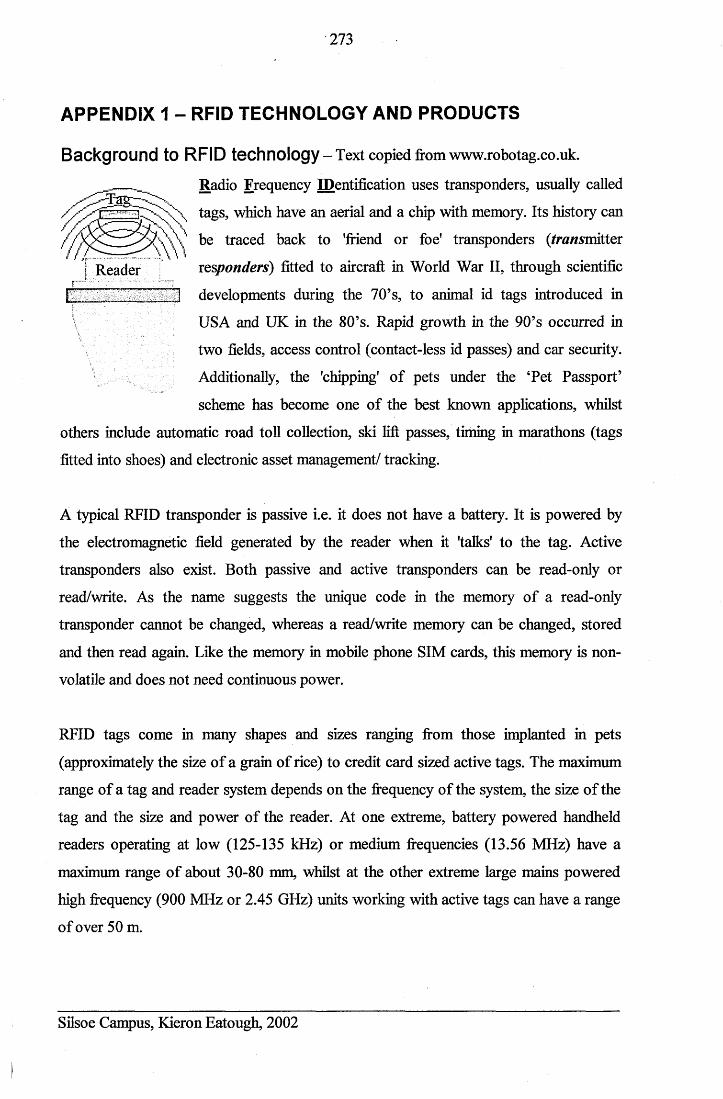
273
APPENDIX 1 - RFID TECHNOLOGY AND PRODUCTS
Background to RFID technology-T extcopiedfrom www.robotag.co.uk.
others include automatic road toll collection, ski lift passes, timing in marathons (tags
fitted into shoes) and electronic asset management/ tracking.
the electromagnetic field generated by the reader when it 'talks' to the tag. Active
transponders also exist. Both passive and active transponders can be read-only or
read/write. As the name suggests the unique code in the memory of a read-only
transponder cannot be changed, whereas a read/write memory can be changed, stored
and then read again. Like the memory in mobile phone SIM cards, this memory is non
volatile and does not need continuous power.
RFID tags come in many shapes and sizes ranging from those implanted in pets
(approximately the size of a grain of rice) to credit card sized active tags. The maximum
range of a tag and reader system depends on the frequency of the system, the size of the
tag and the size and power of the reader. At one extreme, battery powered handheld
readers operating at low (125-135 kHz) or medium frequencies (13.56 MHz) have a
maximum range of about 30-80 mm, whilst at the other extreme large mains powered
high frequency (900 MHz or 2.45 GHz) units working with active tags can have a range
of over 50 m.
Silsoe Campus, Kieron Eatough, 2002
Radio Frequency IDentification uses transponders, usually called
\ tags, which have an aerial and a chip with memory. Its history can
\ be traced back to 'friend or foe' transponders (transmitter
j Reader responders) fitted to aircraft in World War II, through scientific
developments during the 70’s, to animal id tags introduced in
USA and UK in the 80’s. Rapid growth in the 90’s occurred in
two fields, access control (contact-less id passes) and car security.
Additionally, the 'chipping' of pets under the ‘Pet Passport’
scheme has become one of the best known applications, whilst
A typical RFID transponder is passive i.e. it does not have a battery. It is powered by

274
Specific Destron Fearing tag and reader systems used
Information from www.destron-fearing.com
Destron Fearing has pioneered the development of syringe injectable, miniaturized
microchip technology for injection under the skin of animals. The products and
technology Destron Fearing manufactures and markets to the animal identification
industry include a variety of radio frequency microchips or "tags,” portable readers,
stationary readers and microchip injecting devices. Destron microchips have their
identification codes read by magnetic radio frequency signals generated from scanning
devices. The microchip uses the energy from the magnetic field to power itself and
transmit a return signal to the scanner, which is converted to the microchip's
identification code. The alphanumeric identification code is displayed on the reader, or
relayed via computer interface to other equipment. Destron's portable scanners are
battery operated and feature similar electrical components, but differing hardware and
packaging designs. The scanners considered for this project were the Pocket Reader,
and the Pocket Reader EX.
Pocket R e a d e r ™ Pocket Reader EX "
The Destron hand-held "Pocket" type scanners were designed specifically for use with
companion animals in animal shelters or veterinary clinics. Both scanners have a one-
function button for ease of operation and display only the tag’s alphanumeric code. The
Pocket Reader EX™ scanner is a universal scanner so it consistently read microchips
from various manufacturers.
Silsoe Campus, Kieron Eatough, 2002
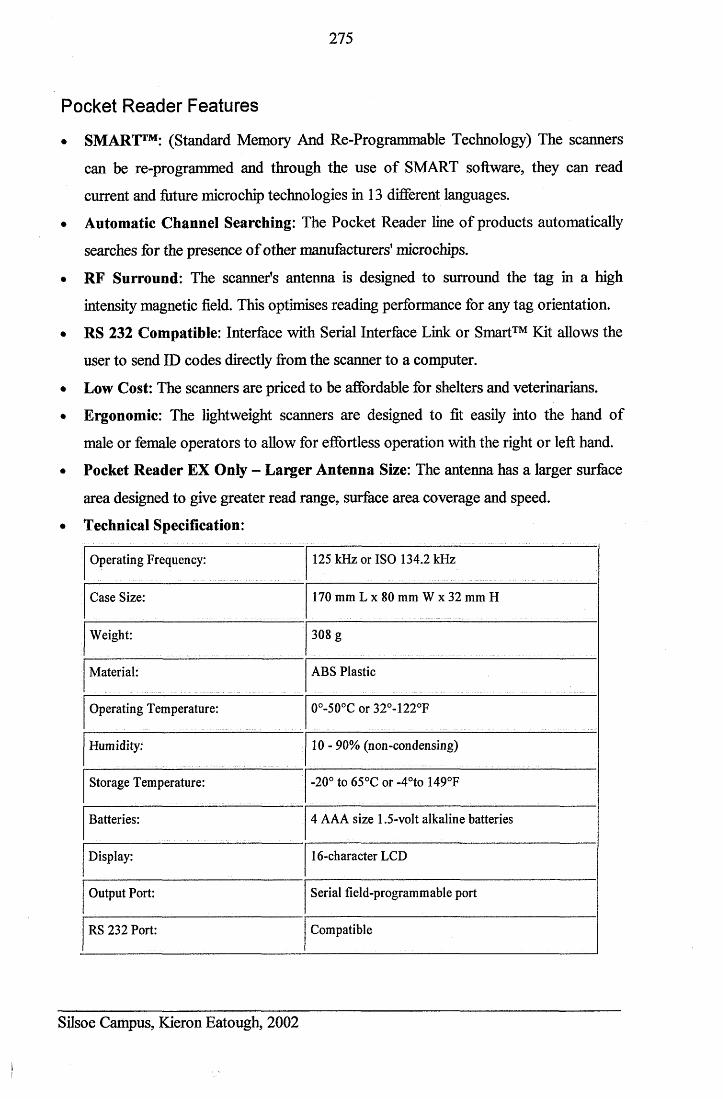
275
Pocket Reader Features
• SMART™: (Standard Memory And Re-Programmable Technology) The scanners
can be re-programmed and through the use of SMART software, they can read
current and future microchip technologies in 13 different languages.
• Automatic Channel Searching: The Pocket Reader line of products automatically
searches for the presence of other manufacturers' microchips.
• RF Surround: The scanner’s antenna is designed to surround the tag in a high
intensity magnetic field. This optimises reading performance for any tag orientation.
• RS 232 Compatible: Interface with Serial Interface Link or Smart™ Kit allows the
user to send ID codes directly from the scanner to a computer.
• Low Cost: The scanners are priced to be affordable for shelters and veterinarians.
• Ergonomic: The lightweight scanners are designed to fit easily into the hand of
male or female operators to allow for effortless operation with the right or left hand.
• Pocket Reader EX Only - Larger Antenna Size: The antenna has a larger surface
area designed to give greater read range, surface area coverage and speed.
• Technical Specification:
Operating Frequency: 125 kHz or ISO 134.2 kHz
Case Size: 170 mm L x 80 mm W x 32 mm H
Weight: 308 g
Material: ABS Plastic
Operating Temperature: 0°-50°C or 32°-122°F
Humidity: 10 - 90% (non-condensing)
Storage Temperature: -20° to 65°C or -4°to 149°F
Batteries: 4 AAA size 1.5-volt alkaline batteries
Display: 16-character LCD
Output Port: Serial field-programmable port
RS 232 Port: Compatible
Silsoe Campus, Kieron Eatough, 2002
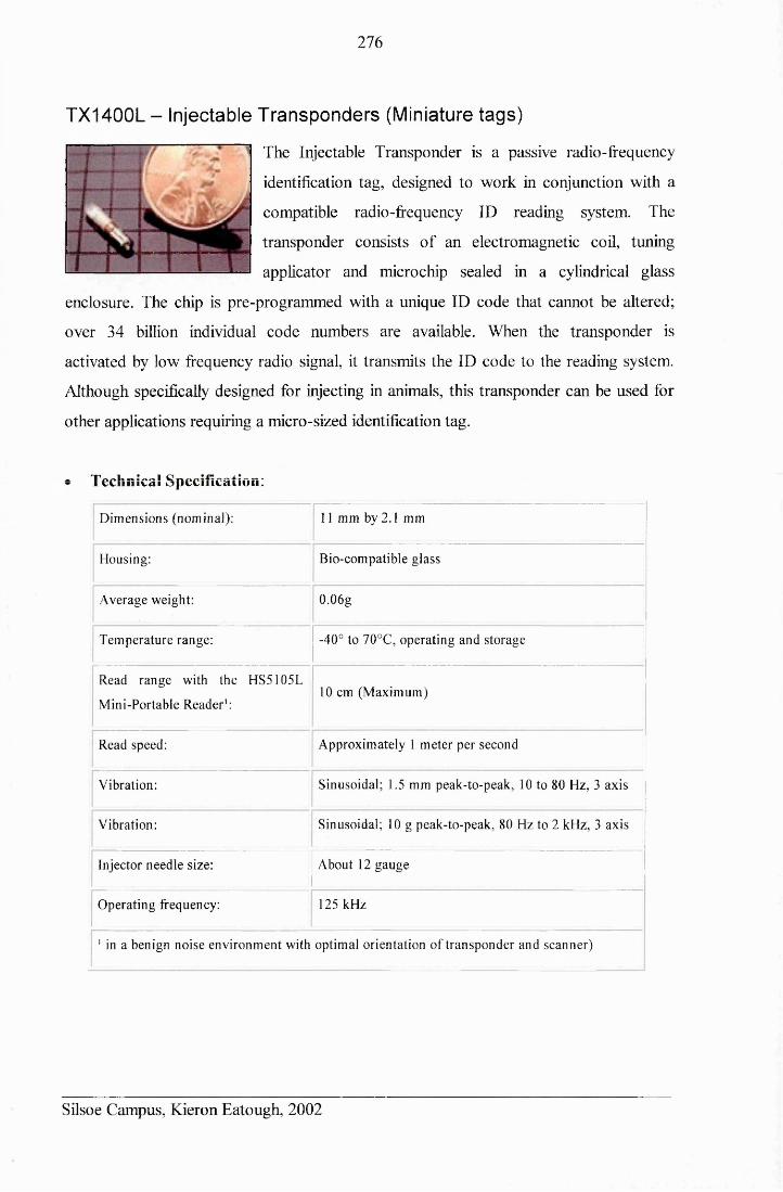
276
TX1400L - Injectable Transponders (Miniature tags)
The Injectable Transponder is a passive radio-frequency
identification tag, designed to work in conjunction with a
compatible radio-frequency ID reading system. The
transponder consists of an electromagnetic coil, tuning
applicator and microchip sealed in a cylindrical glass
enclosure. The chip is pre-programmed with a unique ID code that cannot be altered;
over 34 billion individual code numbers are available. When the transponder is
activated by low frequency radio signal, it transmits the ID code to the reading system.
Although specifically designed for injecting in animals, this transponder can be used for
other applications requiring a micro-sized identification tag.
Technical Specification;
Dimensions (nominal): 11 mm by 2.1 mm
Housing: Bio-compatible glass
Average weight: 0.06g
Temperature range: -40° to 70°C, operating and storage
Read range with the HS5105L
Mini-Portable Reader1:10 cm (Maximum)
Read speed: Approximately 1 meter per second
Vibration: Sinusoidal; 1.5 mm peak-to-peak, 10 to 80 Hz, 3 axis
Vibration: Sinusoidal; 10 g peak-to-peak, 80 Hz to 2 kHz, 3 axis
Injector needle size: About 12 gauge
Operating frequency: 125 kHz
1 in a benign noise environment with optimal orientation of transponder and scanner)
Silsoe Campus, Kieron Eatough, 2002

277
APPENDIX 2 - TEKSCAN SYSTEM DATA AND INFORMATION
aTekscan Text taken from the company website (www.tekscan.com).
The Industrial Sensing (1-Scan) System - Overview
TekScan’s pressure sensing technology is used worldwide to solve the toughest pressure
measurement problems. The Industrial Sensing System (I-Scan) removes many of the
obstacles to studying the pressure distribution between two mating surfaces, and thus
provides insights into dynamic pressure events.
Applications range from soft seal applications with highly
compliant materials at extremely low pressures, to extremely
high-pressure applications such as engine gasket design. For
example TekScan allows design engineers to evaluate fasteners,
gaskets and seals; scientists to measure the force distribution in
granular materials; ergonomicists to develop improved
automotive seating; and production engineers to adjust roller nip
pressure to insure proper materials transport.
Each system is portable and comes with appropriate sensors and unique Windows ™
based software. The software displays the pressure and force information in 'real time'
on a computer screen in coloured 2D or 3D images. Dynamic tests can also be recorded
as a "movie", and played back in a VCR style. Pressure data can be analysed using the
I-Scan software, copied and pasted it into other applications, saved as text (ASCII) files
and imported it into other analysis programs, or printed it out.
The Industrial Sensing (I-Scan) System - Hardware
The TekScan Industrial Sensing (I-Scan) System is a complete kit that converts an IBM-
compatible PC into an advanced pressure distribution measurement system. The I-Scan
system consists of matrix-based sensors of various shapes, sizes, resolutions and
Silsoe Campus, Kieron Eatough, 2002

278
pressure ranges; an 8-bit A/D converter (handle) that connects to the sensors; a specially
designed interface; and Windows™-based software.
For flexibility two hardware interfaces are supported; a
PC Interface Board or a Parallel Interface. The PC
Interface Board is a data acquisition card that inserts into
a 16-bit ISA expansion slot, whilst the Parallel Interface
shares the printer port. The hardware components - the
handle and interface - collect pressure information from
the sensor and make it available to the system software,
which processes, displays, and analyses this data.
The Industrial Sensing (I-Scan) System - Software
The I-Scan system is capable of interfacing with a broad range of
sensors from TekScan. The standard I-Scan sensor is a flexible
printed circuit with up to 2288 individual pressure sensing
locations, which can be close together (0.025'7 0.6 mm) or far
apart (0.57 13 mm).
Due to the nature of the pressure sensitive layer inside the sensor,
it is possible to produce sensors of varying sensitivity. Sensors
with pressure ranges from as low as 0 - 2 PSI (14 kPa) up to as
high as 0 - 25,000 PSI (175 MPa) have been produced.
The system software displays contact pressure or force in real time on the computer
screen in coloured, easy to understand, 2-dimensional or 3-dimensional images. The
software allows multiple windows to be opened and force and pressure information to
be viewed in user-defined focus areas.
Silsoe Campus, Kieron Eatough, 2002
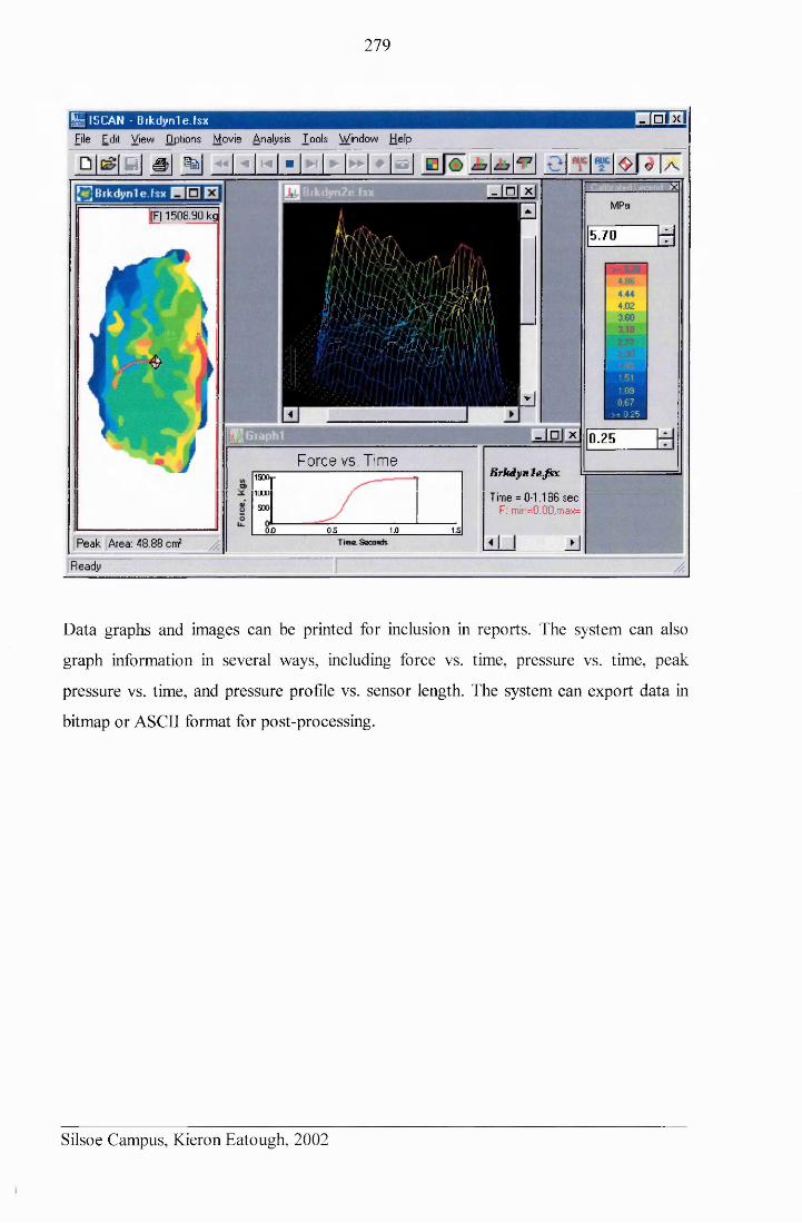
279
|§r ISCAN - B ikdynle.fsxFile Edit View Options Movie Analysis Tools Window Help
rrnDfl
LgI MI JSlI 4 M l I
(F) 1508.90 kg
AT i
$
- n x
.m m H, # , i i A i i \ a ' n■A-J-1-.-1- rtt- -tf-f I'l A ' I I I fl. |,Vt H h. £>/ i j - A 7 - i . i v i ,^5 /J V ••J-rli1.M. 11 'J i v n
E
Peak Area: 48.88 cnrf
Ready
B
- □ X
Force vs. Time130ft
1000
300
0 0 0 3 1 0 13
B r k d y n l e . f c x
Time = 0-1.188 secF: min=0.00,max=
j J
M P a
5.70
0.25
m
Data graphs and images can be printed for inclusion in reports. The system can also
graph information in several ways, including force vs. time, pressure vs. time, peak
pressure vs. time, and pressure profile vs. sensor length. The system can export data in
bitmap or ASCII format for post-processing.
Silsoe Campus, Kieron Eatough, 2002

280
APPENDIX 3 - MOTOR SHOW QUESTIONNAIRE - OCT. 1998
DATE _______________ /LOCATION /INTERVIEWER _____
1. What area of the U.K. do you come from?________________________ Male / Female
2. Age Group? <20 21-25 26-30 31-35 36-40 41-50 51-60 61+
3. What is your occupation?________________________ ____________________ _
4. What is your current vehicle?
Make _______________Model Age Private / Company
5. Rank the following tyre factors in order of importance, for driving on-road. (1-5)
Performance _______ Aesthetics _______
Noise _______ Cost _______
Comfort _______
6. Choose and rank the 4 most important on-road tyre performance factors. (1-4)
Load Capacity _______ Tread Pattern _______
Handling _______ Grip _______
Wear Rate _______ Wet Performance _______
7. Do you prefer wide or narrow tyres on your vehicle? Wide / Narrow
8. Do you prefer low or high profile tyres on your vehicle? Low / High
9. Which of these tyre types would you prefer to see on your vehicle? A / B / C
Why? _____________________________________________
10. Which of these tyre styles would be most aesthetically suited to your vehicle? D / E / F / G
Why? _____________________________________________
11. Do you prefer a chunky or smooth tread pattern on your tyres?Chunky / Smooth
12. Do you prefer plain black or raised white lettering? Plain / White
13. Do you prefer black, white or coloured sidewall? Black / White / Coloured
14. Which of these tyres would grip better on road? H /I
15. Which brand of tvre offers the best performance?
16. Which brand offers the best value for monev?
17. What mileage do you expect from your tvres?
18. Have you ever change a 4x4 wheel and tyre assembly due to a puncture?
If yes - Rate the difficulty 1 - 1 0 (l=easy / 10=v. hard).
Yes / No
19. For a puncture would you use a breakdown organisation or D.I.Y? B.O / D.I.Y
20. How often do vou check your tyre pressures?
Do you also check the spare tyre pressure? Yes / No
21. Do you participate in off-road driving? Yes / No
22. What vehicle do you use? Make Model
Silsoe Campus, Kieron Eatough, 2002

281
23. Is the use recreational or job related? Recreational / Job
24. On what terrain? Mud Sand Rock Snow Ice Wet Grass Other
25. How frequently? Daily Weekly Monthly Annually Other
26. What type / make of tyres do you use? ______________________________
Why? ____________________________________________________
27. Rank the following tyre factors in order of importance, for driving off-road. (1-5)
Noise Comfort_______ _______
Performance Aesthetics_____________
Cost _______
28. Choose and rank the 3 most important off-road tyre performance factors. (1-3)
Handling Load Capacity__________
Wear Rate Grip__________________
Tread Pattern _______
29. Do you use the same tyres for both off-road and on-road driving? Ye s/No
If yes, would you consider using separate off-road tyres if they were available? Yes / No
30. Rank these 3 factors in order of importance when choosing specialist off-road tyres. (1-3)
Extra cost for two sets of tyres _______
Ease of interchange between on and off-road tyres _______
Improved performance over on-road tyres_________________ _______
31. If special off road tyres giving better off-road grip were available but only capable of 55 mph on
road would you consider their purchase? Yes / No
32. If, as an extra, you could purchase a self-sensing tyre inflation system which automatically
adjusted your tyre pressures to give maximum traction, would you be prepared to pay for this
feature? Y es/No How much? £500, £1000, £2000, £4000?
33. Do you expect one set of tyres to exhibit good performance over all terrain’s and conditions?
Yes / No
34. Would you be prepared to purchase one set of tyres for on-road and one for off-road, if the off-
road tyres gave a 30% improved performance for total off-road driving and cost £600 for a
complete set of tyres. Why?
Yes / No - too expensive / No - too little performance / No - don’t go off-road
35. Should off-road tyres be low profile and wide section so they are similar to on-road tyres?
Yes / No ____________________________________________________________
36. When will you next change your vehicle?_________________ ______________________
37. Will your next vehicle be New or Used?__________________ ______________________
38. If private owner will you purchase outright or use finance? Purchase / Finance
Silsoe Campus, Kieron Eatough, 2002
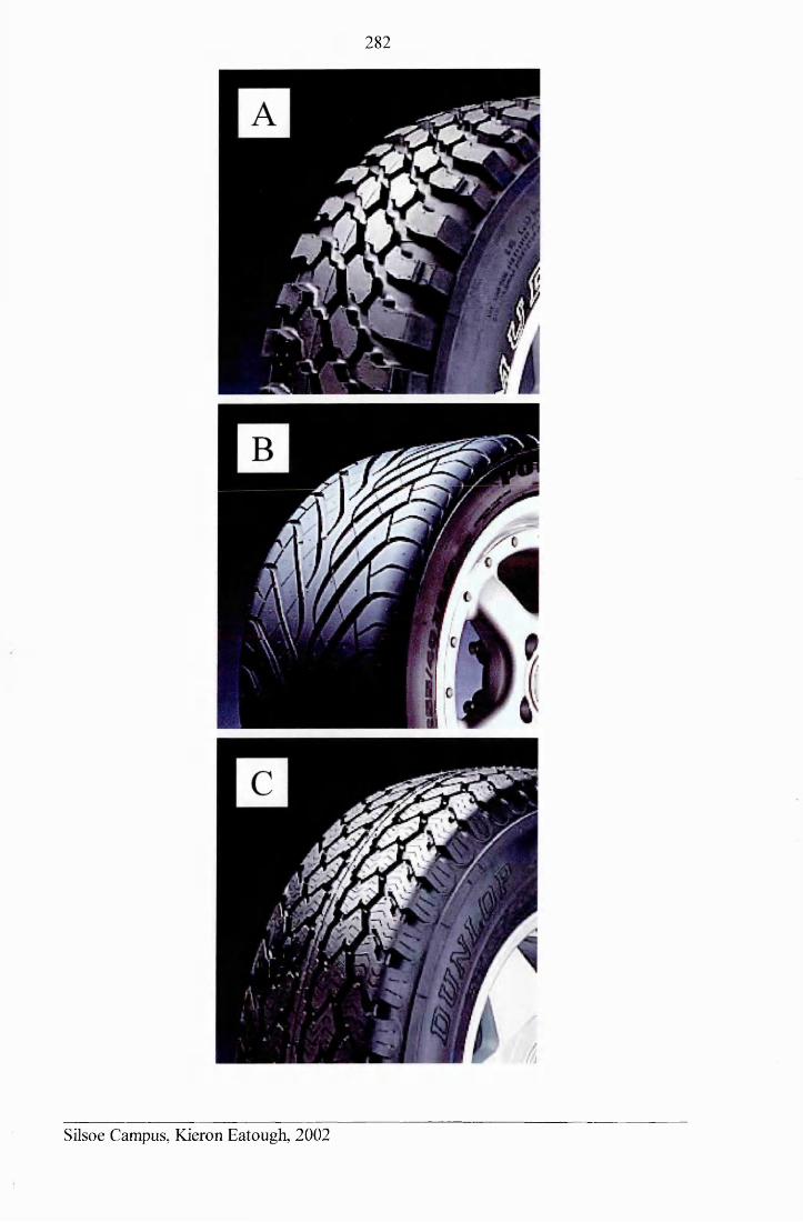
282
Silsoe Campus, Kieron Eatough, 2002
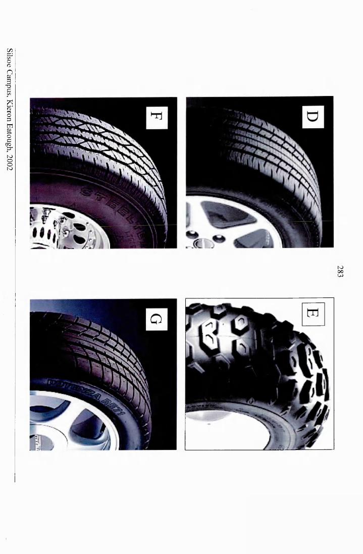
Silsoe Cam
pus, Kieron Eatough, 2002
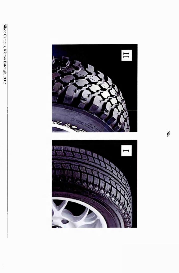
Silsoe Cam
pus, Kieron Eatough, 2002
284
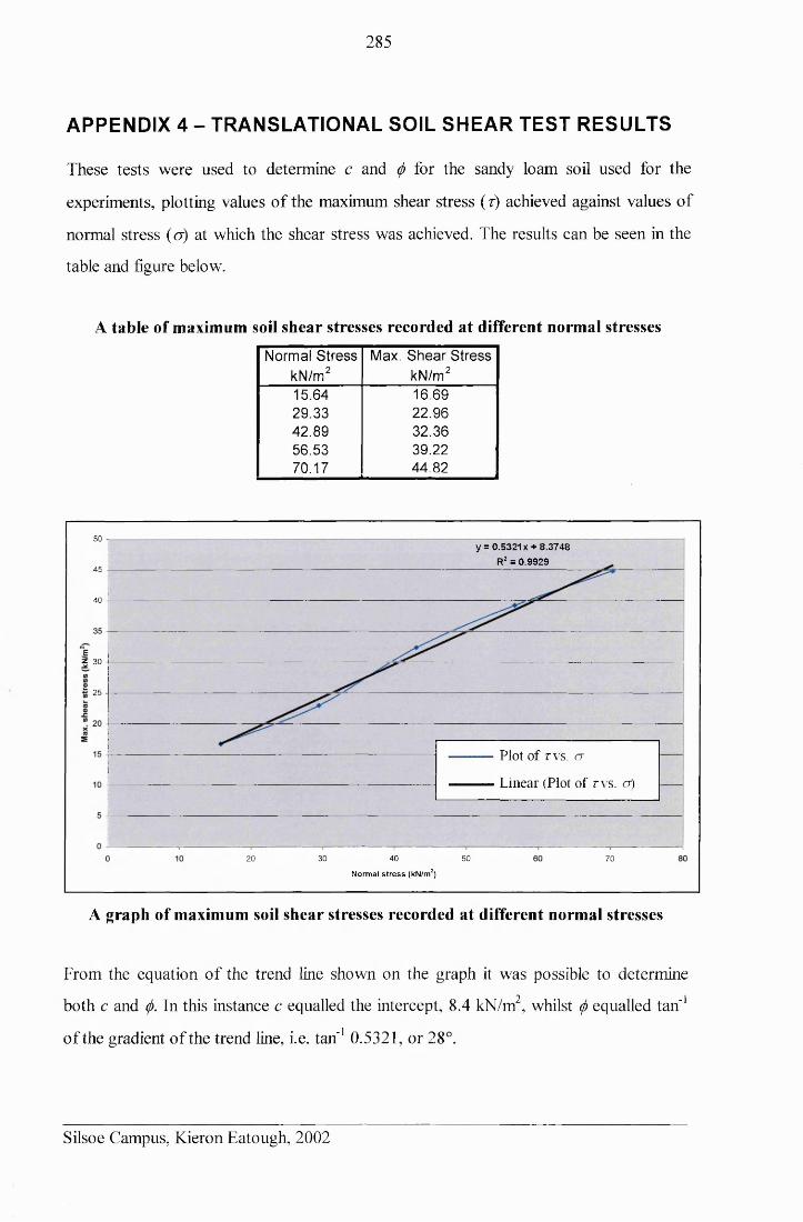
285
APPENDIX 4 - TRANSLATIONAL SOIL SHEAR TEST RESULTS
These tests were used to determine c and (/) for the sandy loam soil used for the
experiments, plotting values of the maximum shear stress (r) achieved against values of
normal stress (a ) at which the shear stress was achieved. The results can be seen in the
table and figure below.
A table of maximum soil shear stresses recorded at different normal stressesNormal Stress
, kN/m2Max. Shear Stress
kN/m215.64 16.6929.33 22.9642.89 32.3656.53 39.2270.17 44.82
50y= 0.5321 x + 8.3748
R2 = 0.992945
40
z 30
25
Plot of TVS. CT
Linear (Plot of rvs. o)
30 40
Normal s tr e s s (kN/m2)
5020 70
A graph of maximum soil shear stresses recorded at different normal stresses
From the equation of the trend line shown on the graph it was possible to determine
both c and (ft. In this instance c equalled the intercept, 8.4 kN/m2, whilst (j) equalled tan'1
of the gradient of the trend line, i.e. tan'1 0.5321, or 28°.
Silsoe Campus, Kieron Eatough, 2002
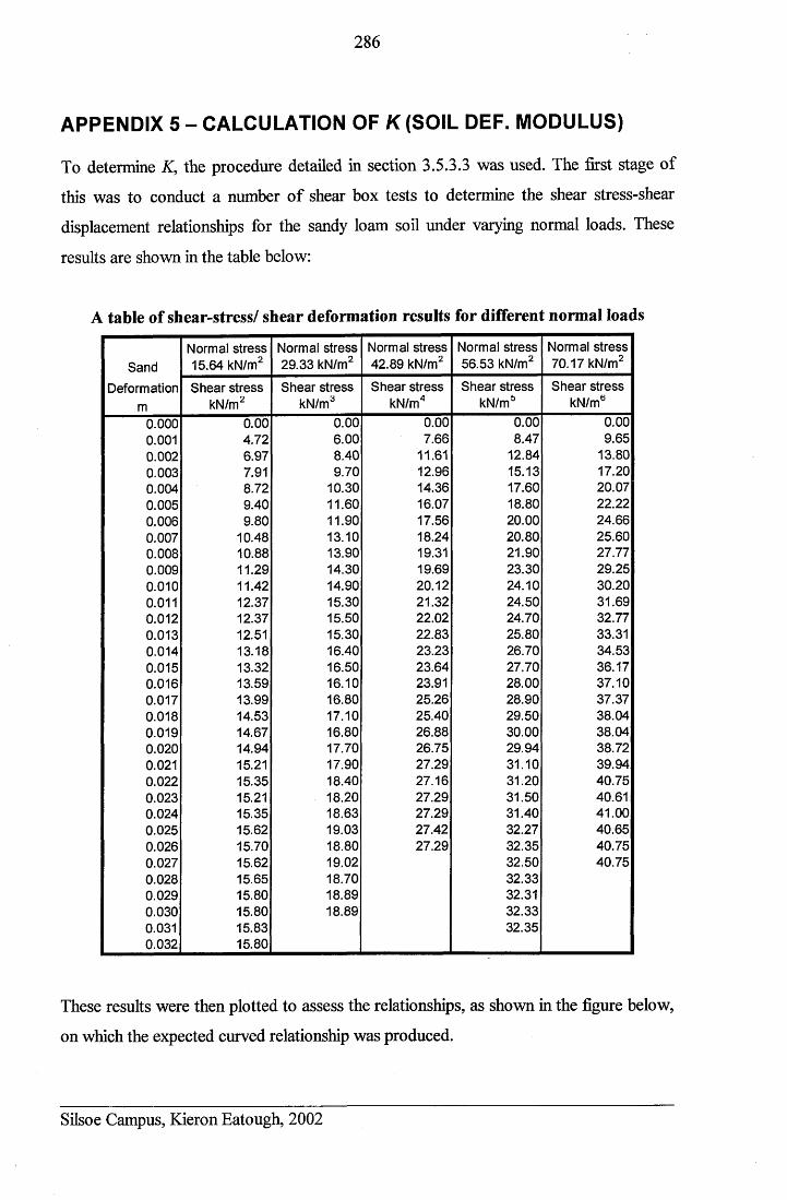
286
APPENDIX 5 - CALCULATION OF K (SOIL DEF. MODULUS)
To determine K, the procedure detailed in section 3.5.3.3 was used. The first stage of
this was to conduct a number of shear box tests to determine the shear stress-shear
displacement relationships for the sandy loam soil under varying normal loads. These
results are shown in the table below:
A table of shear-stress/ shear deformation results for different normal loads
SandDeformation
m
Normal stress 15.64 kN/m2
Normal stress 29.33 kN/m2
Normal stress 42.89 kN/m2
Normal stress 56.53 kN/m2
Normal stress 70.17 kN/m2
Shear stress kN/m2
Shear stress kN/m3
Shear stress kN/m4
Shear stress kN/m 6
Shear stress kN/m6
0.000 0.00 0.00 0.00 0.00 0.000.001 4.72 6.00 7.66 8.47 9.650.002 6.97 8.40 11.61 12.84 13.800.003 7.91 9.70 12.96 15.13 17.200.004 8.72 10.30 14.36 17.60 20.070.005 9.40 11.60 16.07 18.80 22.220.006 9.80 11.90 17.56 20.00 24.660.007 10.48 13.10 18.24 20.80 25.600.008 10.88 13.90 19.31 21.90 27.770.009 11.29 14.30 19.69 23.30 29.250.010 11.42 14.90 20.12 24.10 30.200.011 12.37 15.30 21.32 24.50 31.690.012 12.37 15.50 22.02 24.70 32.770.013 12.51 15.30 22.83 25.80 33.310.014 13.18 16.40 23.23 26.70 34.530.015 13.32 16.50 23.64 27.70 36.170.016 13.59 16.10 23.91 28.00 37.100.017 13.99 16.80 25.26 28.90 37.370.018 14.53 17.10 25.40 29.50 38.040.019 14.67 16.80 26.88 30.00 38.040.020 14.94 17.70 26.75 29.94 38.720.021 15.21 17.90 27.29 31.10 39.940.022 15.35 18.40 27.16 31.20 40.750.023 15.21 18.20 27.29 31.50 40.610.024 15.35 18.63 27.29 31.40 41.000.025 15.62 19.03 27.42 32.27 40.650.026 15.70 18.80 27.29 32.35 40.750.027 15.62 19.02 32.50 40.750.028 15.65 18.70 32.330.029 15.80 18.89 32.310.030 15.80 18.89 32.330.031 15.83 32.350.032 15.80
These results were then plotted to assess the relationships, as shown in the figure below,
on which the expected curved relationship was produced.
Silsoe Campus, Kieron Eatough, 2002
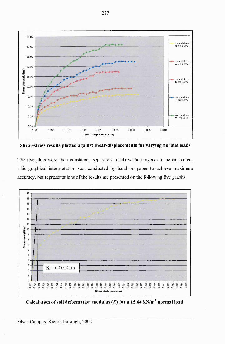
287
45.00 j
N orm al s tre s s 15 .64 kN/m240.00
35.00Norm al s tre s s 2 9 .3 3 kN/m2
30.00
it 25.00■Normal s tre s s 4 2 .8 9 kN/m2
" 20 .0 0
15.00 Norm al s tre s s 5 6 .5 3 kN/m2
10.00
N orm al s tre s s 70 .1 7 kN/m2
5.00
0.000.025 0.035 0.0400.020
S h e a r d is p la c e m e n t (m )
0.0300.010 0.0150.000 0.005
Shear-stress results plotted against shear-displacements for varying normal loads
The five plots were then considered separately to allow the tangents to be calculated.
This graphical interpretation was conducted by hand on paper to achieve maximum
accuracy, but representations of the results are presented on the following five graphs.
17 T
K = 0.00141m
S h e a r d isp la cem en t (m)
Calculation of soil deformation modulus (K) for a 15.64 kN/m2 normal load
Silsoe Campus, Kieron Eatough, 2002
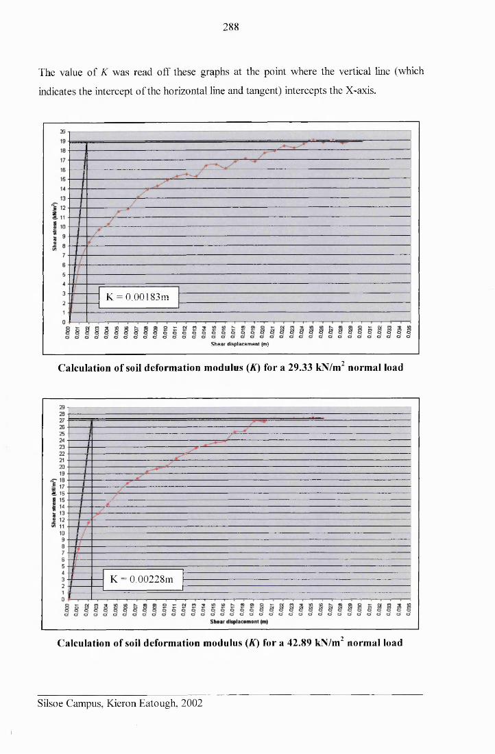
288
The value of K was read off these graphs at the point where the vertical line (which
indicates the intercept of the horizontal line and tangent) intercepts the X-axis.
20
K = 0.00183m
S h ea r d isp la cem en t (m)
Calculation of soil deformation modulus (A) for a 29.33 kN/m2 normal load
5. 16
K = 0.00228m
Calculation of soil deformation modulus (A) for a 42.89 kN/m2 normal load
Silsoe Campus, Kieron Eatough, 2002
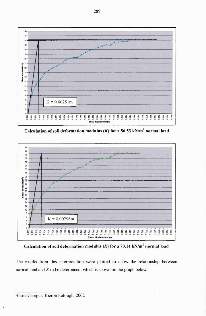
289
K = 0.00251m
Calculation of soil deformation modulus (A) for a 56.53 kN/m2 normal load
K = 0.00296m
S h e a r d isp la cem en t (m)
Calculation of soil deformation modulus (A) for a 70.14 kN/m2 normal load
The results from this interpretation were plotted to allow the relationship between
normal load and K to be determined, which is shown on the graph below.
Silsoe Campus, Kieron Eatough, 2002
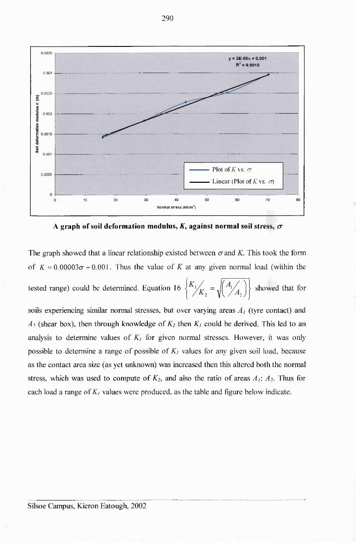
290
0 .0035 T
y = 3E-05x + 0.001 R2 = 0.9915
0.003
0 .0025
0.002
E 0 .0015
0.001
Plot of K vs. a0.0005
Linear (Plot of K vs. a)
7010 20
N orm al s tr e s s (kN/m 2)
A graph of soil deformation modulus, A, against normal soil stress, cr
The graph showed that a linear relationship existed between a and K. This took the form
of K =0.00003cr + 0.001. Thus the value of K at any given normal load (within the
tested range) could be determined. Equation 16 j j showed that for
soils experiencing similar normal stresses, but over varying areas A j (tyre contact) and
A 2 (shear box), then through knowledge of AT? then K\ could be derived. This led to an
analysis to determine values of Ki for given normal stresses. However, it was only
possible to determine a range of possible of K\ values for any given soil load, because
as the contact area size (as yet unknown) was increased then this altered both the normal
stress, which was used to compute of K 2 , and also the ratio of areas A r. A 2 . Thus for
each load a range of K / values were produced, as the table and figure below indicate.
Silsoe Campus, Kieron Eatough, 2002
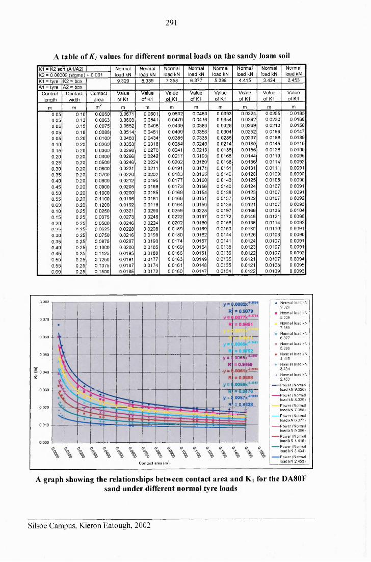
291
A table of K\ values for different normal loads on the sandy loam soilK1 = K2 sqrt (A1/A2) | Normal Normal Normal Normal Normal Normal Normal NormalK2 = 0.00009 (sigma) + 0.001 load kN load kN load kN load kN load kN load kN load kN load kNK1 = tyre K2 = box 9.320 8.339 7.358 6.377 5.396 4.415 3.434 2.453A1 = tyre A2 = box
Contact Contact Contact Value Value Value Value Value Value Value Valuelength width area of K1 of K1 of K1 of K1 of K1 of K1 of K1 of K1
m m rv, 2m m m m m m m m m0.05 0.10 0.0050 0.0671 0.0601 0.0532 0.0463 0.0393 0.0324 0.0255 0.01850.05 0.13 0.0063 0.0603 0.0541 0.0479 0.0416 0.0354 0.0292 0.0230 0.01680.05 0.15 0.0075 0.0552 0.0496 0.0439 0.0383 0.0326 0.0269 0.0213 0.0156
; 0.05 0.18 0.0088 0.0514 0.0461 0.0409 0.0356 0.0304 0.0252 0.0199 0.01470.05 0.20 0.0100 0.0483 0.0434 0.0385 0.0335 0.0286 0.0237 0.0188 0.01390.10 0.20 0.0200 0.0353 0.0318 0.0284 0.0249 0.0214 0.0180 0.0145 0.01100.15 0.20 0.0300 0.0298 0.0270 0.0241 0.0213 0.0185 0.0156 0.0128 0.01000.20 0.20 0.0400 0.0266 0.0242 0.0217 0.0193 0.0168 0.0144 0.0119 0.00950.25 0.20 0.0500 0.0246 0.0224 0.0202 0.0180 0.0158 0.0136 0.0114 0.00920.30 0.20 0.0600 0.0231 0.0211 0.0191 0.0171 0.0151 0.0131 0.0111 0.0091
! 0.35 0.20 0.0700 0.0220 0.0202 0.0183 0.0165 0.0146 0.0128 0.0109 0.00900.40 0.20 0.0800 0.0212 0.0195 0.0177 0.0160 0.0143 0.0125 0.0108 0.00900.45 0.20 0.0900 0.0205 0.0189 0.0173 0.0156 0.0140 0.0124 0.0107 0.00910.50 0.20 0.1000 0.0200 0.0185 0.0169 0.0154 0.0138 0.0123 0.0107 0.00910.55 0.20 0.1100 0.0196 0.0181 0.0166 0.0151 0.0137 0.0122 0.0107 0.00920.60 0.20 0.1200 0.0192 0.0178 0.0164 0.0150 0.0136 0.0121 0.0107 0.00930.10 0.25 0.0250 0.0321 0.0290 0.0259 0.0228 0.0197 0.0166 0.0135 0.01040.15 0.25 0.0375 0.0273 0.0248 0.0222 0.0197 0.0172 0.0146 0.0121 0.0096
j 0.20 0.25 0.0500 0.0246 0.0224 0.0202 0.0180 0.0158 0.0136 0.0114 0.00920.25 0.25 0.0625 0.0228 0.0208 0.0189 0.0169 0.0150 0.0130 0.0110 0.00910.30 0.25 0.0750 0.0216 0.0198 0.0180 0.0162 0.0144 0.0126 0.0108 0.0090
' 0.35 0.25 0.0875 0.0207 0.0190 0.0174 0.0157 0.0141 0.0124 0.0107 0.00910.40 0.25 0.1000 0.0200 0.0185 0.0169 0.0154 0.0138 0.0123 0.0107 0.0091
I 0.45 0.25 0.1125 0.0195 0.0180 0.0166 0.0151 0.0136 0.0122 0.0107 0.00920.50 0.25 0.1250 0.0191 0.0177 0.0163 0.0149 0.0135 0.0121 0.0107 0.00940.55 0.25 0.1375 0.0187 0.0174 0.0161 0.0148 0.0135 0.0121 0.0108 0.00950.60 0.25 0.1500 0.0185 0.0172 0.0160 0.0147 0.0134 0.0122 0.0109 0.0096
q.ooss
= (1.0057 R = 0.8
♦ Norm al load kN9.320
■ Norm al load kN8.339
Norm al load kN7.358
X Norm al load kN6 .377
X Norm al load kN5.396
• Norm al load kN4 .415N orm al load kN3 .434
. Norm al load kN2 .453
------ p o w e r (N orm alload kN 9 .3 2 0 )
P ow er (N orm alload kN 8 .3 3 9 )
P ow er (N orm allo ad kN 7 .3 5 8 )
------ P ow er (N orm alload kN 6 .3 7 7 )
------ P o w er (N orm alload kN 5 .396)
— P ow er (N orm alload kN 4 .4 1 5 )
— P ow er (N orm alload kN 3 .434)
Pow er (N orm alload kN 2 .453)
0.080
0.070
0.060
0.050
0.040sc0.030
0.020
0.010
O O O I
C on tact area (m 2)
A graph showing the relationships between contact area and Ki for the DA80F sand under different normal tyre loads
Silsoe Campus, Kieron Eatough, 2002

292
APPENDIX 6 - PLATE SINKAGE TESTS ON SOIL
These tests were used to determine values of the Bekker soil coefficients n, kc and k^ for-j
the three sandy loam soil preparations used for the experiments, those being 1170 kg/m
(0 rolls), 1270 kg/m3 (1 roll) and 1400 kg/m3 (4 rolls). The coefficients were derived
from knowledge of equation 8, p - i +k*
where: p = normal pressure beneath the plate (load/ area)
b = minimum plate dimension (width □)
z - plate sinkage
kc, k^&n = soil defining constants
This equation can be re-arranged, such that, l n p = « l n z + ln — + k, . Thus if In p isKb )
plotted against In z for several different plate sizes then the gradient of the lines will
equal n, whilst the intercepts will equal In — +K b *
. To determine these k coefficients
then the inverse In’s of intercept values must be plotted against the appropriate 1 lb
values. When trend lines are fitted to this data a new line will be formed, with a gradient
equal to kc, and the intercept at 1/6 = 0 will equal k f
This investigation used four different sized rectangular plates that were hydraulically
forced into the three soil preparations at a constant velocity of 0.025 m/s, and the
resistive force upon each plate and its sinkage were recorded. Each test was replicated
three times. The pressure acting on the soil/ plate and the plate sinkage was determined
and the pressure sinkage relationships achieved from these tests are detailed on the
following sets of tables and graphs.
Silsoe Campus, Kieron Eatough, 2002
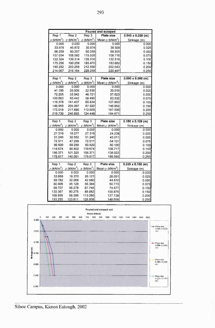
293
Poured and scrapedRep 1 Rep 2 Rep 3 Plate size 0.045 x 0.030 (m)
p (kN/m2) p (kN/m2) p (kN/m2) Mean p (kN/m2) Sinkage (m)0.000 0.000 0.000 0.000 0.000
33.979 45.872 35.678 38.509 0.02566.259 80.257 60.259 68.925 0.050
107.034 106.582 115.528 109.715 0.075122.324 139.314 135.916 132.518 0.100175.258 190.258 185.470 183.662 0.150190.282 203.258 212.590 202.043 0.200214.067 219.164 228.258 220.497 0.250
Rep 1 Rep 2 Rep 3 Plate size 0.090 x 0.060 (m)p (kN/m2) p (kN/m2) p (kN/m2) Mean p (kN/m2) Sinkage (m)
0.000 0.000 0.000 0.000 0.00041.199 25.909 22.936 30.015 0.02572.205 53.942 46.721 57.623 0.050
100.663 93.442 56.490 83.532 0.075116.378 141.437 65.834 107.883 0.100146.959 205.997 87.920 146.959 0.150172.018 217.890 112.609 167.506 0.200218.739 240.826 124.448 194.671 0.250
Rep 1 Rep 2 Rep 3 Plate size 0 .1 8 0 x 0 .1 2 0 (m)p /kN/m21 n I'kN/m2') o /kN/m2'! Mean o /kN/m21 Sinkage (m)
0.000 0.000 0.000 0.000 0.00027.319 18.077 27.319 24.238 0.02551.240 32.552 51.240 45.011 0.05072.511 47.299 72.511 64.107 0.07590.520 59.259 90.520 80.100 0.100
119.674 80.802 119.674 106.717 0.150156.371 101.325 156.371 138.022 0.200179.817 140.061 179.817 166.565 0.250
Rep 1 Rep 2 Rep 3 Plate size 0.225 x 0.150 (m)p (kN/m2) p (kN/m2) p (kN/m2) Mean p (kN/m2) Sinkage (m)
0.000 0.000 0.000 0.000 0.00033.660 18.370 26.121 26.051 0.02559.782 32.068 42.580 44.810 0.05080.806 45.128 56.384 60.773 0.07599.707 56.278 67.745 74.577 0.100
133.367 80.275 88.982 100.875 0.150168.939 99.388 113.086 127.138 0.200193.255 123.811 128.908 148.658 0.250
P o u red and scraped s o i l
Stress (KN/ni2)
0 100 200 300 400 500 600 700 800 900 1000 1100 1200 1300 1400 1500 1600
• Plate size 0.045 x 0.030(m )0.050
Plate sizex 0.060
(m)
c</>
Plate size
<m>
0.250 * — Plate size0.225 x 0.150 (m )
0.300
Silsoe Campus, Kieron Eatough, 2002
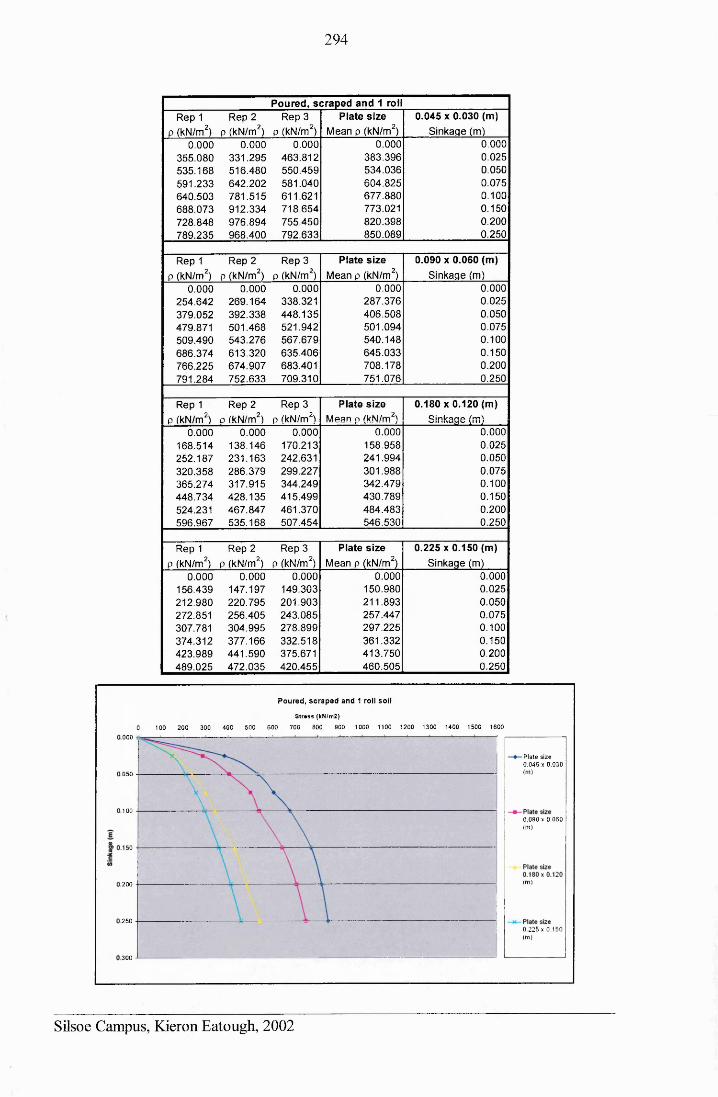
294
Poured, scraped and 1 rollRep 1 Rep 2 Rep 3 Plate size 0.045 x 0.030 (m)
p (kN/m2) p (kN/m2) p (kN/m2) Mean p (kN/m2) Sinkaqe (m)0.000 0.000 0.000 0.000 0.000
355.080 331.295 463.812 383.396 0.025535.168 516.480 550.459 534.036 0.050591.233 642.202 581.040 604.825 0.075640.503 781.515 611.621 677.880 0.100688.073 912.334 718.654 773.021 0.150728.848 976.894 755.450 820.398 0.200789.235 968.400 792.633 850.089 0.250
Rep 1 Rep 2 Rep 3 Plate size 0.090 x 0.060 (m)p (kN/m2) p (kN/m2) p (kN/m2) Mean p (kN/m2) Sinkage (m)
0.000 0.000 0.000 0.000 0.000254.642 269.164 338.321 287.376 0.025379.052 392.338 448.135 406.508 0.050479.871 501.468 521.942 501.094 0.075509.490 543.276 567.679 540.148 0.100686.374 613.320 635.406 645.033 0.150766.225 674.907 683.401 708.178 0.200791.284 752.633 709.310 751.076 0.250
Rep 1 Rep 2 Rep 3 Plate size 0.180x0.120 (m)p (kN/m2) p (kN/m2) p (kN/m2) Mean p (kN/m2) Sinkage (m)
0.000 0.000 0.000 0.000 0.000168.514 138.146 170.213 158.958 0.025252.187 231.163 242.631 241.994 0.050320.358 286.379 299.227 301.988 0.075365.274 317.915 344.249 342.479 0.100448.734 428.135 415.499 430.789 0.150524.231 467.847 461.370 484.483 0.200596.967 535.168 507.454 546.530 0.250
Rep 1 Rep 2 Rep 3 Plate size 0.225x0.150 (m)P (kN/m2) p (kN/m2) P (kN/m2) Mean p (kN/m2) Sinkage (m)
0.000 0.000 0.000 0.000 0.000156.439 147.197 149.303 150.980 0.025212.980 220.795 201.903 211.893 0.050272.851 256.405 243.085 257.447 0.075307.781 304.995 278.899 297.225 0.100374.312 377.166 332.518 361.332 0.150423.989 441.590 375.671 413.750 0.200489.025 472.035 420.455 460.505 0.250
P o u red , s c r a p e d and 1 roll s o i l
Str«ss (kN/m2)
100 200 300 400 500 600 700 800 900 1000 1100 1200 1300 1400 1500 16000.000
Plate size 0.045 x 0.030(m).050
.1000.090 x 0.060(m )
50
(m ).200
.2500.225 x 0.150 (m)
.300
Silsoe Campus, Kieron Eatough, 2002
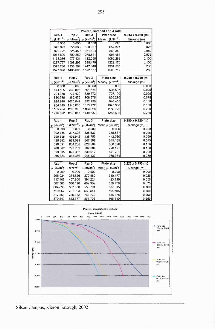
295
Poured, scraped and 4 rollsRep 1 Rep 2 Rep 3 Plate size 0.045 x 0.030 (m)
p (kN/m2) p (kN/m2) p (kN/m2) Mean p (kN/m2) Sinkage (m)0.000 0.000 0.000 0.000 0.000
643.073 655.063 658.977 652.371 0.025872.722 725.450 961.604 853.259 0.050
1013.690 899.850 1078.831 997.457 0.0751138.336 977.431 1182.080 1099.282 0.1001257.757 1098.292 1328.479 1228.176 0.1501373.286 1238.564 1442.846 1351.565 0.2001527.890 1405.685 1592.577 1508.717 0.250
Rep 1 Rep 2 Rep 3 Plate size 0.090 x 0.060 (m)p (kN/m2) p (kN/m2) P (kN/m2) Mean p (kN/m2) Sinkage (m)
0.000 0.000 0.000 0.000 0.000574.105 533.803 501.614 536.507 0.025704.370 727.429 689.772 707.190 0.050830.785 880.479 806.575 839.280 0.075925.926 1020.642 892.796 946.455 0.100934.845 1148.063 1053.772 1045.560 0.150
1105.254 1200.306 1164.628 1156.729 0.2001275.852 1230.887 1149.337 1218.692 0.250
Rep 1 Rep 2 Rep 3 Plate size 0.180x0.120 (m)p (kN/m2) p (kN/m2) p(kN/m2) Mean p (kN/m2) Sinkage (m)
0.000 0.000 0.000 0.000 0.000302.744 397.628 336.537 345.637 0.025390.545 496.942 438.753 442.080 0.050496.942 591.021 547.592 545.185 0.075599.091 664.288 628.504 630.628 0.100768.667 797.762 762.084 776.171 0.150899.805 875.382 839.917 871.701 0.200965.326 985.389 948.437 966.384 0.250
Rep 1 Rep 2 Rep 3 Plate size 0.225x0.150 (m)p (kN/m2) p (kN/m2) p (kN/m2) Mean p (kN/m2) Sinkage (m)
0.000 0.000 0.000 0.000 0.000296.024 364.526 270.880 310.477 0.025417.465 457.900 394.224 423.196 0.050507.305 536.120 482.909 508.778 0.075604.893 597.350 559.701 587.315 0.100719.062 701.393 663.541 694.665 0.150817.261 780.632 768.739 788.878 0.200870.549 863.677 861.706 865.310 0.250
- Plate size 0.045 x 0.030 (m)
- Plate size 0.090 x 0.060(m)
Plate size 0.180 x 0.120<m)
Plate size 0.225 x 0.150(m)
P o u red , s c r a p e d a n d 4 roll s o i l
Stress (kN/m2)0 100 200 300 400 500 600 700 800 900 1000 1100 1200 1300 1400 1500 1600
0.050
0.100
E.
§> 0.150-XcV)
0.200
Silsoe Campus, Kieron Eatough, 2002
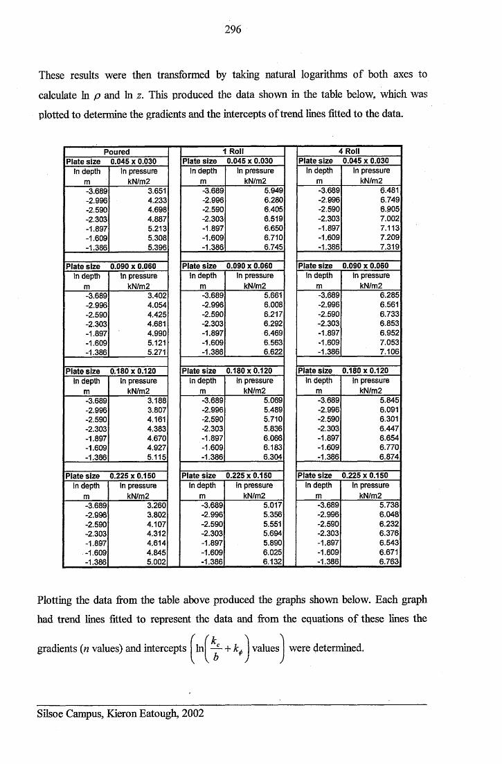
296
These results were then transformed by taking natural logarithms of both axes to
calculate In p and In z. This produced the data shown in the table below, which was
plotted to determine the gradients and the intercepts of trend lines fitted to the data.
Poured 1 Roll 4 RollPlate size 0.045 X 0.030 Plate size 0.045 x 0.030 Plate size 0.045 x 0.030
In depth In pressure In depth In pressure In depth In pressurem kN/m2 m kN/m2 m kN/m2-3.689 3.651 -3.689 5.949 -3.689 6.481-2.996 4.233 -2.996 6.280 -2.996 6.749-2.590 4.698 -2.590 6.405 -2.590 6.905-2.303 4.887 -2.303 6.519 -2.303 7.002-1.897 5.213 -1.897 6.650 -1.897 7.113-1.609 5,308 -1.609 6.710 -1.609 7.209-1.386 5.396 -1.386 6.745 -1.386 7.319
Plate size 0.090 x 0.060 Plate size 0.090 x 0.060 Plate size 0.090 x 0.060In depth In pressure In depth In pressure In depth In pressure
m kN/m2 m kN/m2 m kN/m2-3.689 3.402 -3.689 5.661 -3.689 6.285-2.996 4.054 -2.996 6.008 -2.996 6.561-2.590 4.425 -2.590 6.217 -2.590 6.733-2.303 4.681 -2.303 6.292 -2.303 6.853-1.897 4.990 -1.897 6.469 -1.897 6.952-1.609 5.121 -1.609 6.563 -1.609 7.053-1.386 5.271 -1.386 6.622 -1.386 7.106
Plate size 0.180 x 0.120 Plate size 0.180x0.120 Plate size 0.180 x 0.120In depth In pressure In depth In pressure In depth In pressure
m kN/m2 m kN/m2 m kN/m2-3.689 3.188 -3.689 5.069 -3.689 5.845-2.996 3.807 -2.996 5.489 -2.996 6.091-2.590 4.161 -2.590 5.710 -2.590 6.301-2.303 4.383 -2.303 5.836 -2.303 6.447-1.897 4.670 -1.897 6.066 -1.897 6.654-1.609 4.927 -1.609 6.183 -1.609 6.770-1.386 5.115 -1.386 6.304 -1.386 6.874
Plate size 0.225 x 0.150 Plate size 0.225x0.150 Plate size 0.225x0.150In depth In pressure In depth In pressure In depth In pressure
m kN/m2 m kN/m2 m kN/m2-3.689 3.260 -3.689 5.017 -3.689 5.738-2.996 3.802 -2.996 5.356 -2.996 6.048-2.590 4.107 -2.590 5.551 -2.590 6.232-2.303 4.312 -2.303 5.694 -2.303 6.376-1.897 4.614 -1.897 5.890 -1.897 6.543-1.609 4.845 -1.609 6.025 -1.609 6.671-1.386 5.002 -1.386 6.132 -1.386 6.763
Plotting the data from the table above produced the graphs shown below. Each graph
had trend lines fitted to represent the data and from the equations of these lines the
gradients (n values) and intercepts/ ( k ) \In\ — + k. values
V b *) )were determined.
Silsoe Campus, Kieron Eatough, 2002
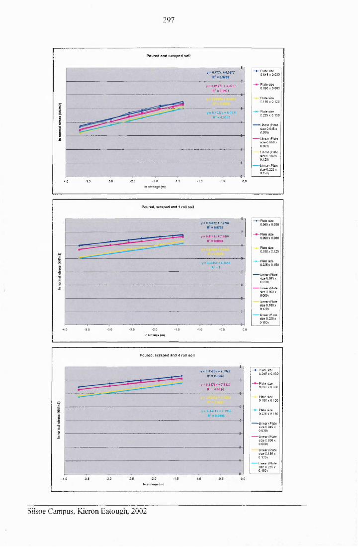
297
P ou red and sc r a p e d so i!
y = 0.777x + 6.5977
y = 0.8127x+ 6.4757 R2 = 0.9901
Ez 0.7547X ♦ 6.0531
R2 = 0.9998£occ
-2.0 -1.5-4.0 -3 5 -3.0 -25 -1 .0 -0.5 0.0
-Plate size 0.045 x 0.030
- Plate size 0.090 x 0.060
Plate size 0 .180x0.120
- Plate size 0.225 x 0.150
-Linear (Plate size 0.045 x 0.030)
-Linear (Plate size 0.090 X 0.060)
Linear (Plate size 0.180 x 0 . 120 )
-Linear (Plate size 0.225 x 0.150)
P o u re d , s c ra p e d an d 1 roll so il
y = 0.3447x + 7.2767
y = 0.4161x + 7.2407
0.180 X 0.120
y= 0.4845X +6.8066
R2 = 1
■Linear (Plate size 0.045 x 0.030)
■Linear (Plate size 0.090 x 0.060)
Linear (Plate
0 .120)
Linear (Plate
0.150)
In sinkage (m)
P oured , s c r a p e d and 4 roll so il
y = 0.3526X + 7.7979 R2 = 0.9963
y = 0.3576x + 7.6332 R2 =0.9914
62 y = 0.4471x+7.3906
iocc
-P la te size 0.045 x 0.030
- Plate size 0.090 x 0.060
Plate size 0.180 x 0.120
- Plate size0.225 x 0.150
-Linear (Plate size 0.045 x 0.030)
-Linear (Plate size 0.090 x 0.060)
Linear (Plate size 0.180 x 0 .120)
-Linear (Plate size 0.225 x 0.150)
In sinkeoe (m)
Silsoe Campus, Kieron Eatough, 2002
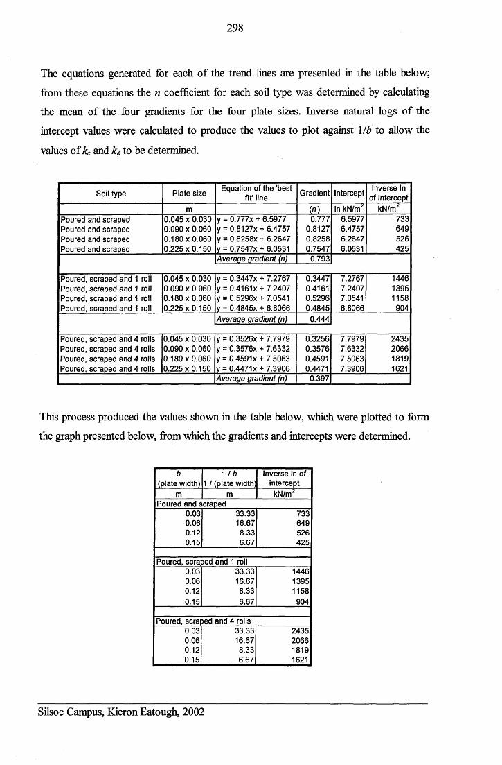
298
The equations generated for each of the trend lines are presented in the table below;
from these equations the n coefficient for each soil type was determined by calculating
the mean of the four gradients for the four plate sizes. Inverse natural logs of the
intercept values were calculated to produce the values to plot against Mb to allow the
values of kc and k<f, to be determined.
Soil type Plate size Equation of the 'best fit' line Gradient Intercept Inverse In
of interceptm (n) In kN/m2 kN/m2
Poured and scraped 0.045 x 0.030 y = 0.777x + 6.5977 0.777 6.5977 733Poured and scraped 0.090 x 0.060 y = 0.8127x + 6.4757 0.8127 6.4757 649Poured and scraped 0.180x0.060 y = 0.8258X + 6.2647 0.8258 6.2647 526Poured and scraped 0.225x0.150 y = 0.7547X + 6.0531 0.7547 6.0531 425
Average gradient (n) 0.793
Poured, scraped and 1 roll 0.045 x 0.030 y = 0.3447X + 7.2767 0.3447 7.2767 1446Poured, scraped and 1 roll 0.090 x 0.060 y = 0.4161X + 7.2407 0.4161 7.2407 1395Poured, scraped and 1 roll 0.180x0.060 y = 0.5296x + 7.0541 0.5296 7.0541 1158Poured, scraped and 1 roll 0.225x0.150 y = 0.4845X + 6.8066 0.4845 6.8066 904
Average gradient (n) 0.444
Poured, scraped and 4 rolls 0.045 x 0.030 y = 0.3526X + 7.7979 0.3256 7.7979 2435Poured, scraped and 4 rolls 0.090 x 0.060 y = 0.3576x + 7.6332 0.3576 7.6332 2066Poured, scraped and 4 rolls 0.180 x 0.060 y = 0.4591X + 7.5063 0.4591 7.5063 1819Poured, scraped and 4 rolls 0.225x0.150 y = 0.4471X + 7.3906 0.4471 7.3906 1621
Average gradient (n) 0.397
This process produced the values shown in the table below, which were plotted to form
the graph presented below, from which the gradients and intercepts were determined.
b M b Inverse In of(plate width) 1 / (plate width] intercept
m m kN/m2Poured and scraped
0.03 33.33 7330.06 16.67 6490.12 8.33 5260.15 6.67 425
Poured, scrajDed and 1 roll0.03 33.33 14460.06 16.67 13950.12 8.33 11580.15 6.67 904
Poured, scraped and 4 rolls0.03 33.33 24350.06 16.67 20660.12 8.33 18190.15 6.67 1621
Silsoe Campus, Kieron Eatough, 2002
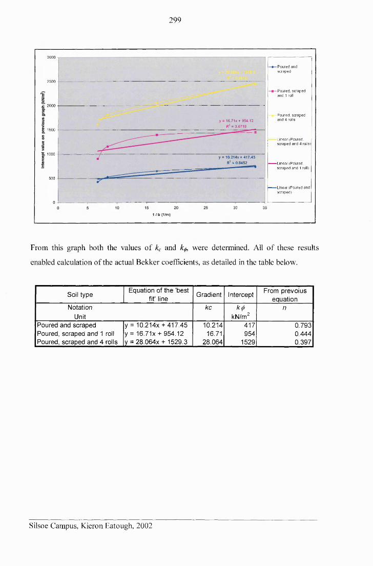
299
3000
P oured and sc rap ed
2500
Po u red , sc rap ed an d 1 roll
2000
Poured , sc rap ed an d 4 rollsy = 1 6 .7 1 x + 954.12
R2 = 0 .67191500
Linear (Poured , sc rap ed an d 4 rolls)
1000y = 10 .214x + 417 .45
R2 = 0 .8452 L inear (Poured .sc rap ed an d 1 roll)
500
— —Linear (P o u re d and sc rap ed )
30 35
1 / b (1/m)
From this graph both the values of kc and were determined. All of these results
enabled calculation of the actual Bekker coefficients, as detailed in the table below.
Soil type Equation of the 'best fit' line Gradient Intercept From prevoius
equationNotation kc kef) n
Unit kN/m2Poured and scraped y = 10.214X + 417.45 10.214 417 0.793Poured, scraped and 1 roll y = 16.71x + 954.12 16.71 954 0.444Poured, scraped and 4 rolls y = 28.064X + 1529.3 28.064 1529 0.397
Silsoe Campus, Kieron Eatough, 2002
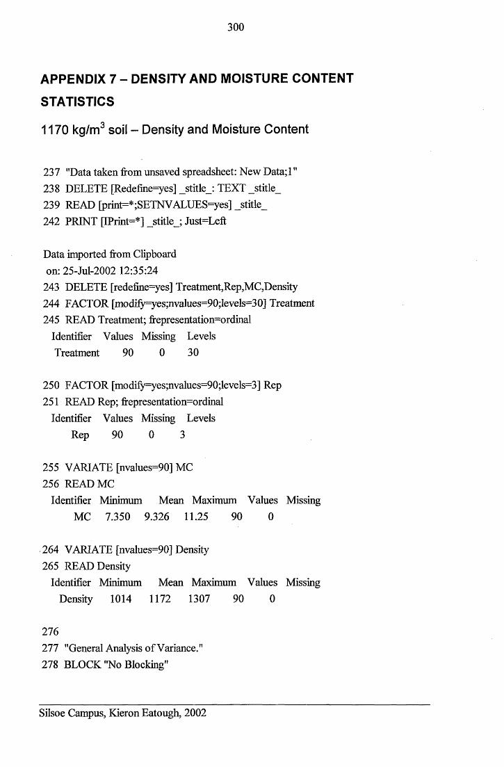
300
APPENDIX 7 - DENSITY AND MOISTURE CONTENT
STATISTICS
1170 kg/m3 soil - Density and Moisture Content
237 "Data taken from unsaved spreadsheet: New Data; 1"238 DELETE [Redefine=yes] _stitle_: TEXT _stitle_239 READ [print=* ;SETNVALUES=yes] _stitle_242 PRINT [IPrint=*] _stitle_; Just=Left
Data imported from Clipboard on: 25-M-2002 12:35:24
243 DELETE [redefine=yes] Treatment,Rep,MC,Density244 FACTOR [modify=yes;nvalues=90;levels=30] Treatment245 READ Treatment; frepresentation=ordinal
Identifier Values Missing Levels Treatment 90 0 30
250 FACTOR [modify=yes;nvalues=90;levels=3] Rep251 READ Rep; frepresentation=ordinal
Identifier Values Missing LevelsRep 90 0 3
255 VARIATE [nvalues=90] MC256 READ MC
Identifier Minimum Mean Maximum Values MissingMC 7.350 9.326 11.25 90 0
264 VARIATE [nvalues=90] Density265 READ Density
Identifier Minimum Mean Maximum Values MissingDensity 1014 1172 1307 90 0
276277 "General Analysis of Variance."278 BLOCK "No Blocking"
Silsoe Campus, Kieron Eatough, 2002
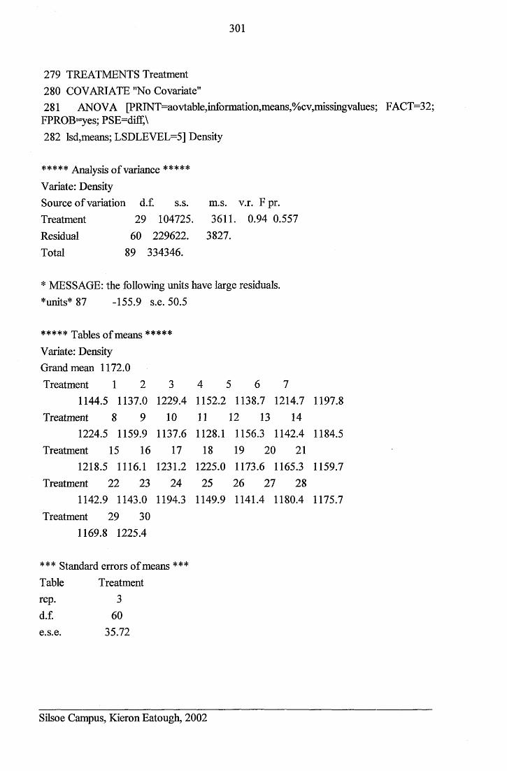
301
279 TREATMENTS Treatment280 COVARIATE "No Covariate"281 ANOVA [PRINT=aovtable,information,means,%cv,missingvalues; FACT=32; FPROB=yes; PSE=diff,\282 lsd,means; LSDLEVEL=5] Density
***** Analysis of variance *****Variate: DensitySource of variation d.f. s. s. m.s. v.r. F pr.Treatment 29 104725. 3611. 0.94 0.557Residual 60 229622. 3827.Total 89 334346.
* MESSAGE: the following units have large residuals. *units* 87 -155.9 s.e. 50.5
***** Tables of means ***** Variate: Density Grand mean 1172.0 Treatment 1 2 3
1144.5 1137.0 1229.4 Treatment 8 9 10
1224.5 1159.9 1137.6 Treatment 15 16 17
1218.5 1116.1 1231.2 Treatment 22 23 24
1142.9 1143.0 1194.3 Treatment 29 30
1169.8 1225.4
4 5 6 71152.2 1138.7 1214.7 1197.8 11 12 13 141128.1 1156.3 1142.4 1184.5
18 19 20 211225.0 1173.6 1165.3 1159.7
25 26 27 281149.9 1141.4 1180.4 1175.7
*** Standard errors of means *** Table Treatment rep. 3d.f. 60e.s.e. 35.72
Silsoe Campus, Kieron Eatough, 2002
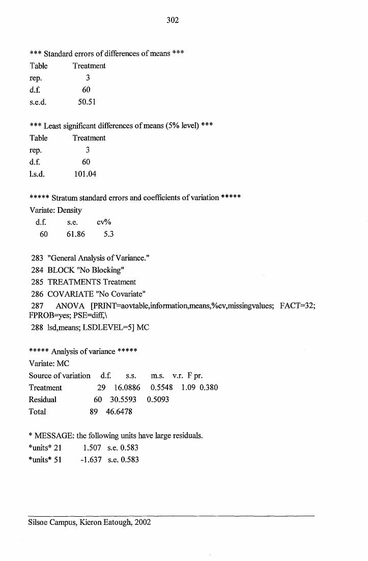
302
*** Standard errors of differences of means ***Table Treatmentrep. 3d.f. 60s.e.d. 50.51
*** Least significant differences of means (5% level) ***Table Treatmentrep. 3d.f. 60l.s.d. 101.04
***** Stratum standard errors and coefficients of variation *****Variate: Density
d.f. s.e. cv%60 61.86 5.3
283 "General Analysis of Variance."284 BLOCK "No Blocking"285 TREATMENTS Treatment286 COVARIATE "No Covariate"287 ANOVA [PRINT=aovtable,information,means,%cv,missingvalues; FACT=32;
FPROB=yes; PSE=diff,\288 lsd,means; LSDLEVEL=5] MC
***** Analysis of variance *****Variate: MCSource of variation d.f. s.s. m.s. v.r. F pr.Treatment 29 16.0886 0.5548 1.09 0.380Residual 60 30.5593 0.5093Total 89 46.6478
* MESSAGE: the following units have large residuals.*units* 21 1.507 s.e. 0.583*units* 51 -1.637 s.e. 0.583
Silsoe Campus, Kieron Eatough, 2002
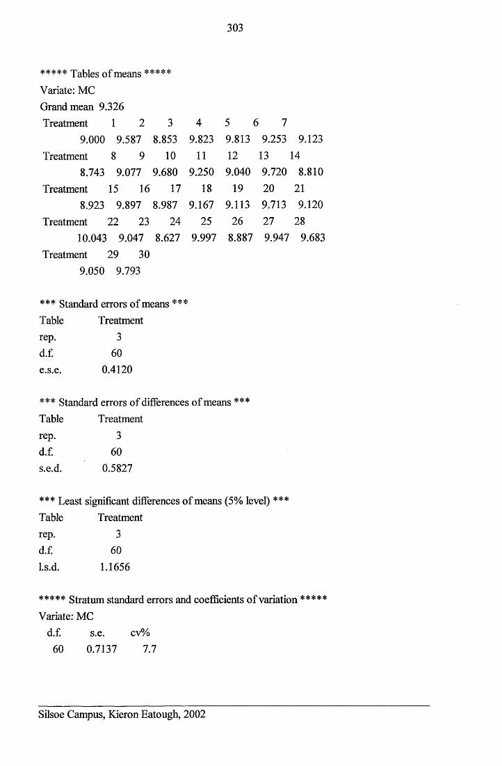
303
***** TableS of means ***** Variate: MC Grand mean 9.326 Treatment 1 2 3
9.000 9.587 8.853Treatment 8 9 10
8.743 9.077 9.680Treatment 15 16 17
8.923 9.897 8.987Treatment 22 23 24
10.043 9.047 8.627Treatment 29 30
9.050 9.793
4 5 6 79.823 9.813 9.253 9.123
11 12 13 149.250 9.040 9.720 8.810
18 19 20 219.167 9.113 9.713 9.120
25 26 27 289.997 8.887 9.947 9.683
*** Standard errors of means ***Table Treatmentrep. 3d.f. 60e.s.e. 0.4120
*** Standard errors of differences of means ***Table Treatmentrep. 3d.f. 60s.e.d. 0.5827
*** Least significant differences of means (5% level) ***Table Treatmentrep. 3d.f. 60Ls.d. 1.1656
***** Stratum standard errors and coefficients of variation ***** Variate: MC
d.f. s.e. cv%60 0.7137 7.7
Silsoe Campus, Kieron Eatough, 2002
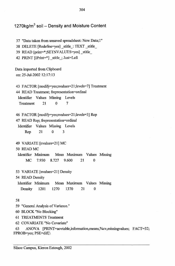
304
1270kg/m3 soil - Density and Moisture Content
37 "Data taken from unsaved spreadsheet: New Data;l"38 DELETE [Redefine=yes] _stitle_: TEXT _stitle_39 READ [print=*;SETNVALUES=yes] _stitle_42 PRINT [IPrint=*] _stitle_; Just=Left
Data imported from Clipboard on: 25-M-2002 12:17:13
43 FACTOR [modify=yes;nvalues=21 ;levels=7] Treatment44 READ Treatment; frepresentation=ordinal
Identifier Values Missing LevelsTreatment 21 0 7
46 FACTOR [modify=yes;nvalues=21 ;levels=3] Rep47 READ Rep; frepresentation=ordinal
Identifier Values Missing LevelsRep 21 0 3
49 VARIATE [nvalues=21] MC50 READ MCIdentifier Minimum Mean Maximum Values Missing
MC 7.930 8.727 9.600 21 0
53 VARIATE [nvalues=21] Density54 READ DensityIdentifier Minimum Mean Maximum Values Missing
Density 1201 1270 1370 21 0
5859 "General Analysis of Variance."60 BLOCK "No Blocking"61 TREATMENTS Treatment62 COVARIATE "No Covariate"63 ANOVA [PRINT=aovtable,information,means,%cv,missingvalues; FACT=32;
FPROB=yes; PSE=diff,\
Silsoe Campus, Kieron Eatough, 2002
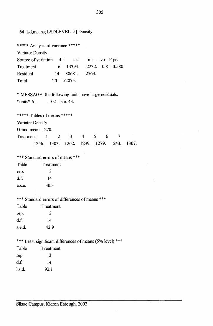
305
64 lsd,means; LSDLEVEL=5] Density
***** Analysis of variance *****Variate: DensitySource of variation d.f. s.s. m.s. v.r. F pr.
* MESSAGE: the following units have large residuals.*units* 6 -102. s.e. 43.
***** Tables of means *****Variate: Density Grand mean 1270.Treatment 1 2 3 4 5 6 7
1256. 1303. 1262. 1239. 1279. 1243. 1307.
*** Standard errors of means ***Table Treatmentrep. 3d.f. 14e.s.e. 30.3
*** Standard errors of differences of means ***Table Treatmentrep. 3d.f. 14s.e.d. 42.9
*** Least significant differences of means (5% level) ***Table Treatmentrep. 3
TreatmentResidualTotal
6 13394. 2232. 0.81 0.58014 38681. 2763.
20 52075.
d.f.l.s.d.
1492.1
Silsoe Campus, Kieron Eatough, 2002
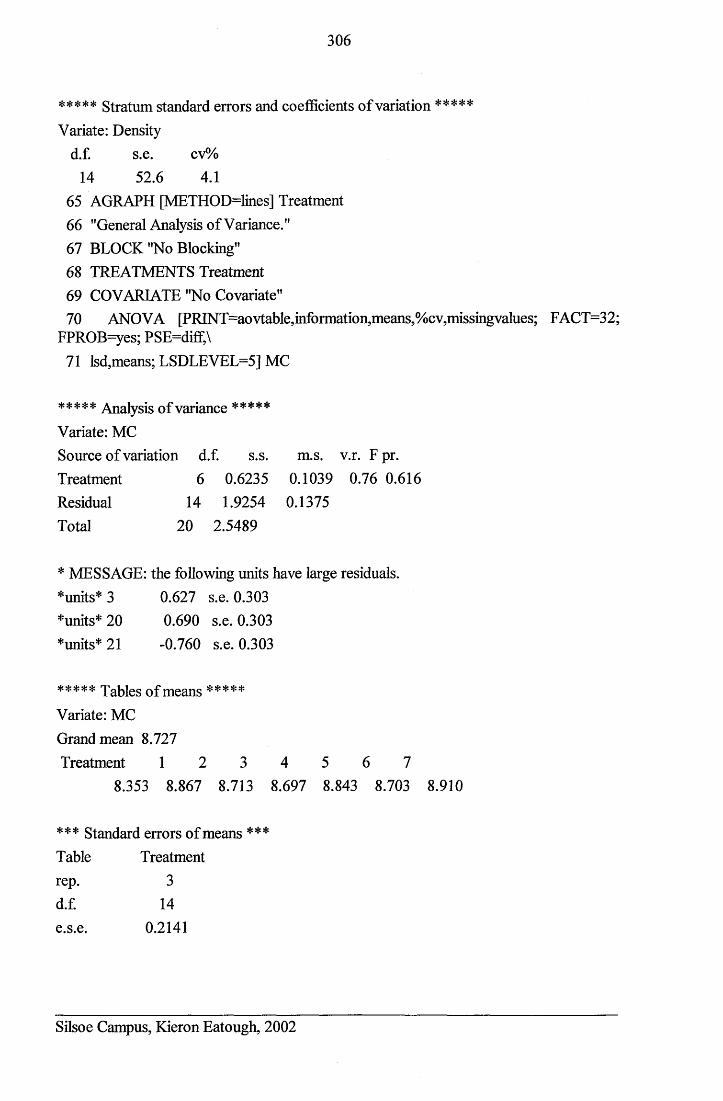
306
***** Stratum standard errors and coefficients of variation *****Variate: Density
d.f. s.e. cv%14 52.6 4.1
65 AGRAPH [METHOD=lines] Treatment66 "General Analysis of Variance."67 BLOCK "No Blocking"68 TREATMENTS Treatment69 COVARIATE "No Covariate"70 ANOVA [PRINT=aovtable,information,means,%cv,missingvalues; FACT=32;
FPROB=yes; PSE=diff,\71 lsd,means; LSDLEVEL=5] MC
***** Analysis of variance *****Variate: MCSource of variation d.f. s.s. m.s. v.r. F pr.Treatment 6 0.6235 0.1039 0.76 0.616Residual 14 1.9254 0.1375Total 20 2.5489
* MESSAGE: the following units have large residuals.*units* 3 0.627 s.e. 0.303*units* 20 0.690 s.e. 0.303*units* 21 -0.760 s.e. 0.303
***** Tables of means *****Variate: MC Grand mean 8.727Treatment 1 2 3 4 5 6 7
8.353 8.867 8.713 8.697 8.843 8.703 8.910
*** Standard errors of means ***Table Treatmentrep. 3d.f. 14e.s.e. 0.2141
Silsoe Campus, Kieron Eatough, 2002
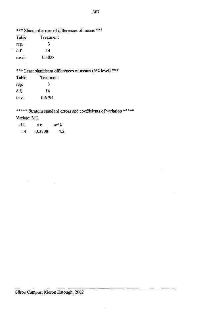
307
*** Standard errors of differences of means ***Table Treatmentrep. 3d.f. 14s.e.d. 0.3028
*** Least significant differences of means (5% level) ***Table Treatmentrep. 3d.f. 14Ls.d. 0.6494
***** Stratum standard errors and coefficients of variation ***** Variate: MC
d.f. s.e. cv%14 0.3708 4.2
Silsoe Campus, Kieron Eatough, 2002
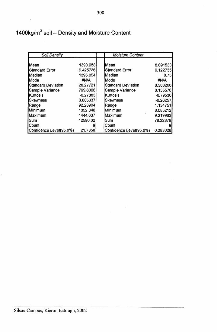
308
1400kg/m3 soil - Density and Moisture Content
Soil Density Moisture Content
Mean 1398.958 Mean 8.691533Standard Error 9.425736 Standard Error 0.122735Median 1395.054 Median 8.75Mode #N/A Mode #N/AStandard Deviation 28.27721 Standard Deviation 0.368206Sample Variance 799.6006 Sample Variance 0.135576Kurtosis -0.27083 Kurtosis -0.79536Skewness 0.005337 Skewness -0.26257Range 92.28904 Range 1.134751Minimum 1352.348 Minimum 8.085212Maximum 1444.637 Maximum 9.219962Sum 12590.62 Sum 78.22379Count 9 Count 9Confidence Level(95.0%) 21.7358 Confidence Level(95.0%) 0.283028
Silsoe Campus, Kieron Eatough, 2002
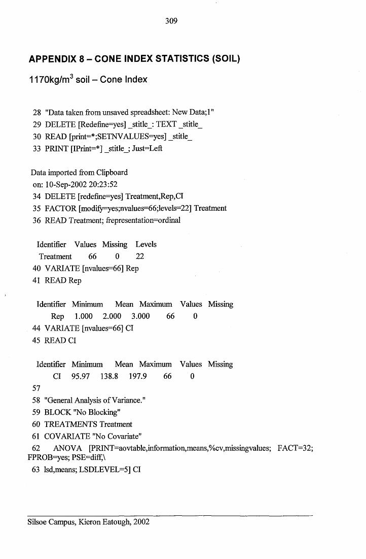
309
APPENDIX 8 - CONE INDEX STATISTICS (SOIL)
1170kg/m3 soil - Cone Index
28 "Data taken from unsaved spreadsheet: New Data;l"29 DELETE [Redefine=yes] _stitle_: TEXT _stitle_30 READ [print=*;SETNVALUES=yes] _stitle_33 PRINT [IPrint=*] _stitle_; Just=Left
Data imported from Clipboard on: 10-Sep-2002 20:23:5234 DELETE [redefine=yes] Treatment,Rep,Cl35 FACTOR [modify=yes;nvalues=66;levels=22] Treatment36 READ Treatment; frepresentation=ordinal
Identifier Values Missing Levels Treatment 66 0 22
40 VARIATE [nvalues=66] Rep41 READ Rep
Identifier Minimum Mean Maximum Values Missing Rep 1.000 2.000 3.000 66 0
44 VARIATE [nvalues=66] Cl45 READ Cl
Identifier Minimum Mean Maximum Values Missing Cl 95.97 138.8 197.9 66 0
5758 "General Analysis of Variance."59 BLOCK "No Blocking"60 TREATMENTS Treatment61 COVARIATE "No Covariate"62 ANOVA [PRINT=aovtable,information,means,%cv,missingvalues; FACT=32;
FPROB=yes; PSE=diff,\63 lsd,means; LSDLEVEL=5] Cl
Silsoe Campus, Kieron Eatough, 2002
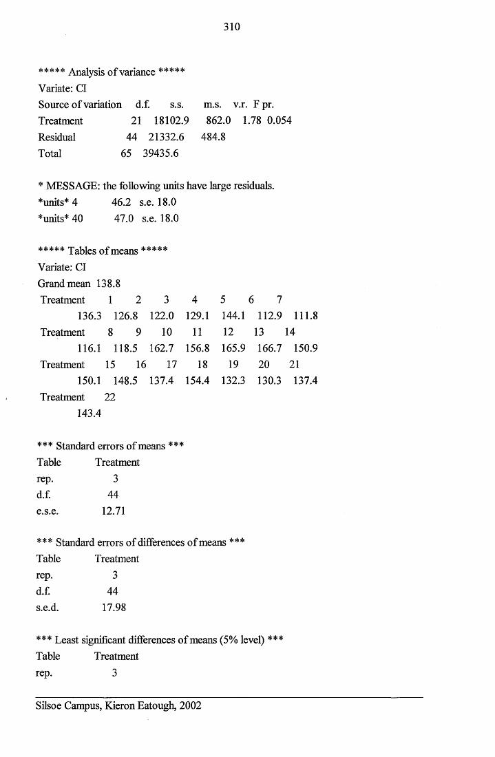
310
***** AnalySiS of variance *****Variate: ClSource of variation d.f. s. s. m.s. v.r. F pr.Treatment 21 18102.9 862.0 1.78 0.054Residual 44 21332.6 484.8Total 65 39435.6
* MESSAGE: the following units have large residuals. *units* 4 46.2 s.e. 18.0*units* 40 47.0 s.e. 18.0
***** Tables of means *****Variate: Cl Grand mean 138.8Treatment 1 2 3 4 5 6 7
136.3 126.8 122.0 129.1 144.1 112.9 111.8Treatment 8 9 10 11 12 13 14
116.1 118.5 162.7 156.8 165.9 166.7 150.9Treatment 15 16 17 18 19 20 21
150.1 148.5 137.4 154.4 132.3 130.3 137.4Treatment 22
143.4
*** Standard errors of means ***Table Treatmentrep. 3d.f. 44e.s.e. 12.71
*** Standard errors of differences of means ***Table Treatmentrep. 3d.f. 44s.e.d. 17.98
*** Least significant differences of means (5% level) *** Table Treatmentrep. 3
Silsoe Campus, Kieron Eatough, 2002

311
d.f. 44l.s.d. 36.23
***** Stratum standard errors and coefficients of variation ***** Variate: Cl
d.f. s.e. cv%44 22.02 15.9
Silsoe Campus, Kieron Eatough, 2002
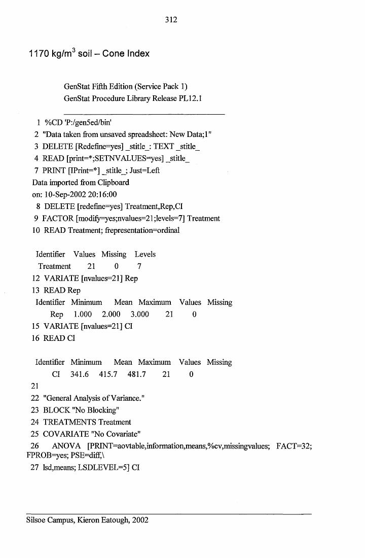
312
1170 kg/m3 soil - Cone Index
GenStat Fifth Edition (Service Pack 1) GenStat Procedure Library Release PL12.1
1 %CD 'P:/gen5ed/binf2 "Data taken from unsaved spreadsheet: New Data;l"3 DELETE [Redefine=yes] _stitle_: TEXT _stitle_4 READ [print=*;SETNVALUES=yes] _stitle_7 PRINT [IPrint=*] _stitle_; Just=Left
Data imported from Clipboardon: 10-Sep-2002 20:16:00
8 DELETE [redefine=yes] Treatment,Rep,Cl9 FACTOR [modify=yes;nvalues=21;levels=7] Treatment10 READ Treatment; frepresentation=ordinal
Identifier Values Missing Levels Treatment 21 0 7
12 VARIATE [nvalues=21] Rep13 READ RepIdentifier Minimum Mean Maximum Values Missing
Rep 1.000 2.000 3.000 21 015 VARIATE [nvalues=21] Cl16 READ Cl
Identifier Minimum Mean Maximum Values Missing Cl 341.6 415.7 481.7 21 0
2122 "General Analysis of Variance."23 BLOCK "No Blocking"24 TREATMENTS Treatment25 COVARIATE "No Covariate"26 ANOVA [PRINT=aovtable,information,means,%cv,missingvalues; FACT=32;
FPROB=yes; PSE=diff,\27 lsd,means; LSDLEVEL=5] Cl
Silsoe Campus, Kieron Eatough, 2002
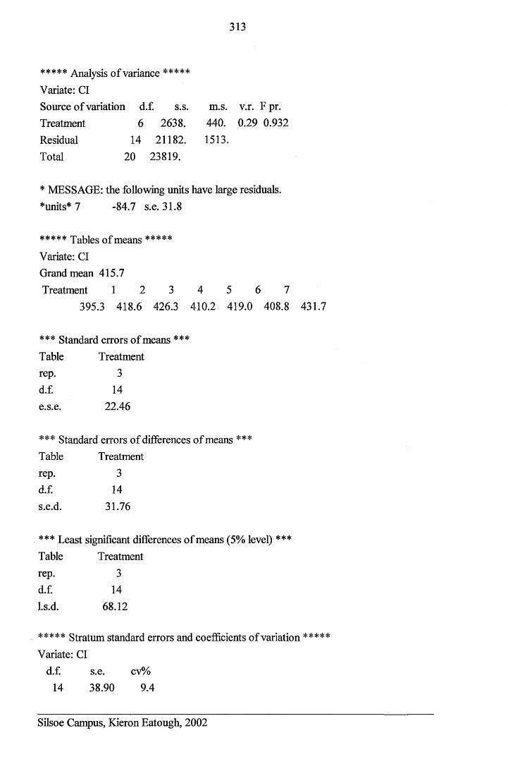
313
***** Analysis of variance *****Variate: ClSource of variation d.f. s.s. m.s. v.r. F pr.
* MESSAGE: the following units have large residuals.*units* 7 -84.7 s.e. 31.8
***** Tables of means *****Variate: Cl Grand mean 415.7Treatment 1 2 3 4 5 6 7
395.3 418.6 426.3 410.2 419.0 408.8 431.7
*** Standard errors of means ***Table Treatment rep. 3d.f. 14e.s.e. 22.46
*** Standard errors of differences of means ***Table Treatmentrep. 3d.f. 14s.e.d. 31.76
*** Least significant differences of means (5% level) ***Table Treatmentrep. 3
***** Stratum standard errors and coefficients of variation ***** Variate: Cl
TreatmentResidualTotal
6 2638. 440. 0.29 0.93214 21182. 1513.
20 23819.
d.f.l.s.d.
1468.12
d.f. s.e. cv% 14 38.90 9.4
Silsoe Campus, Kieron Eatough, 2002
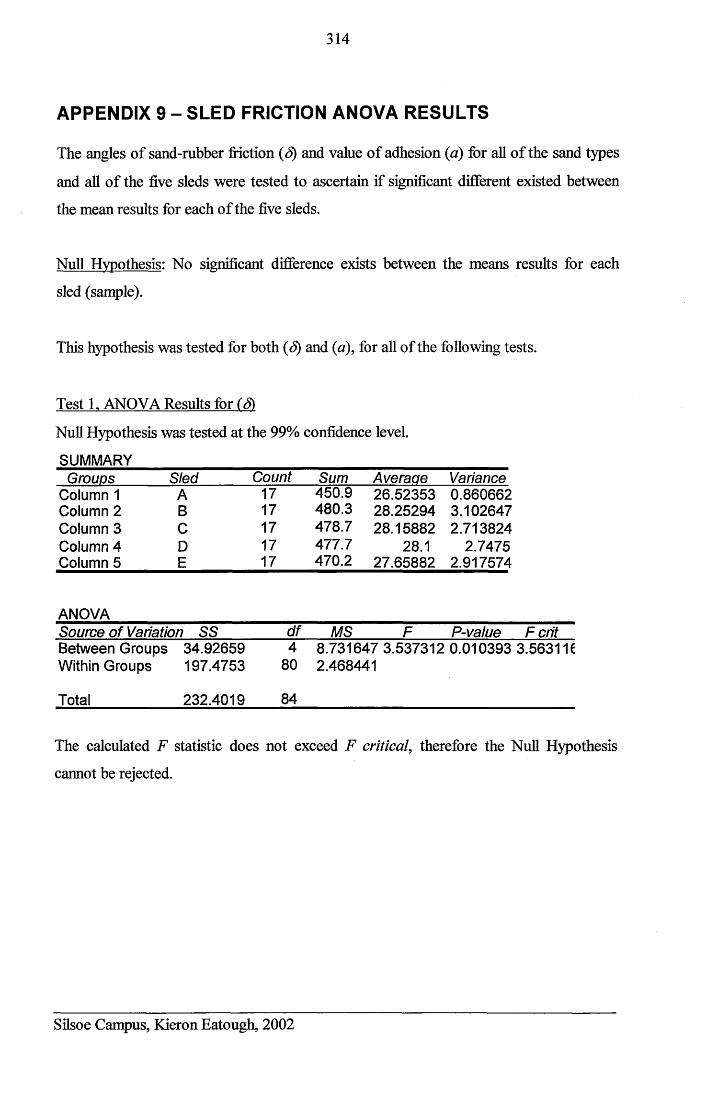
314
APPENDIX 9 - SLED FRICTION ANOVA RESULTS
The angles of sand-rubber friction (S) and value of adhesion (a) for all of the sand types
and all of the five sleds were tested to ascertain if significant different existed between
the mean results for each of the five sleds.
Null Hypothesis: No significant difference exists between the means results for each
sled (sample).
This hypothesis was tested for both (S) and (a), for all of the following tests.
Test 1. ANOVA Results for (S)
Null Hypothesis was tested at the 99% confidence level.
SUMMARYGroups Sled Count Sum Averaae Variance
Column 1 A 17 450.9 26.52353 0.860662Column 2 B 17 480.3 28.25294 3.102647Column 3 C 17 478.7 28.15882 2.713824Column 4 D 17 477.7 28.1 2.7475Column 5 E 17 470.2 27.65882 2.917574
ANOVASource of Variation SS df MS F P-value F critBetween Groups 34.92659 Within Groups 197.4753
480
8.731647 3.537312 0.010393 3.5631 U 2.468441
Total 232.4019 84
The calculated F statistic does not exceed F critical, therefore the Null Hypothesis
cannot be rejected.
Silsoe Campus, Kieron Eatough, 2002
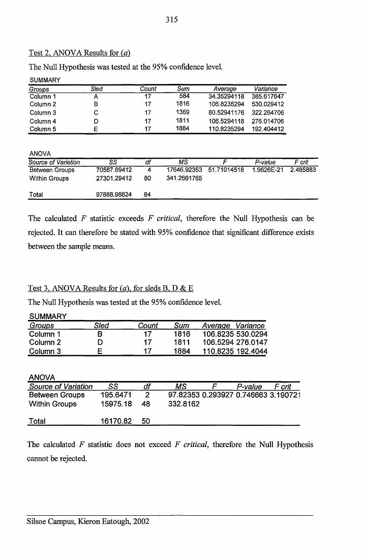
315
Test 2. ANOVA Results for (a)
The Null Hypothesis was tested at the 95% confidence level.SUMMARYGroups Sled Count Sum Average VarianceColumn 1 A 17 584 34.35294118 385.617647Column 2 B 17 1816 106.8235294 530.029412Column 3 C 17 1369 80.52941176 322.264706Column 4 D 17 1811 106.5294118 276.014706Column 5 E 17 1884 110.8235294 192.404412
ANOVASource of Variation SS df MS F P-vaiue F critBetween Groups 70587.69412 4 17646.92353 51.71014518 1.9626E-21 2.485883Within Groups 27301.29412 80 341.2661765
Total 97888.98824 84
The calculated F statistic exceeds F critical, therefore the Null Hypothesis can be
rejected. It can therefore be stated with 95% confidence that significant difference exists
between the sample means.
Test 3. ANOVA Results for (a\ for sleds B. D & E
The Null Hypothesis was tested at the 95% confidence level.
SUMMARYGroups Sled Count Sum Averaae VarianceColumn 1 B 17 1816 106.8235 530.0294Column 2 D 17 1811 106.5294 276.0147Column 3 E 17 1884 110.8235 192.4044
ANOVASource of Variation SS df MS F P-value F critBetween Groups 195.6471 2 97.82353 0.293927 0.746663 3.190721Within Groups 15975.18 48 332.8162
Total 16170.82 50
The calculated F statistic does not exceed F critical, therefore the Null Hypothesis
cannot be rejected.
Silsoe Campus, Kieron Eatough, 2002
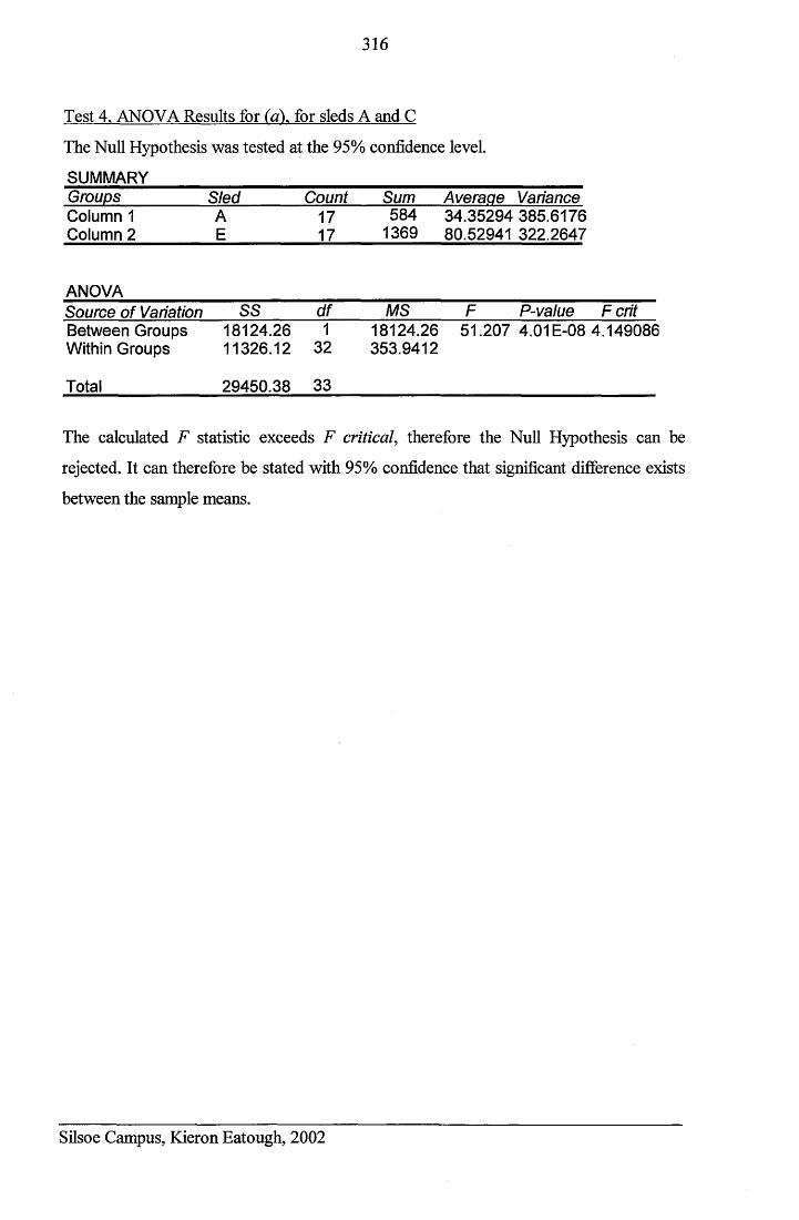
316
Test 4. ANOVA Results for (a), for sleds A and C
The Null Hypothesis was tested at the 95% confidence level.
SUMMARYGroups Sled Count Sum Averaoe VarianceColumn 1 A 17 584 34.35294 385.6176Column 2 E 17 1369 80.52941 322.2647
ANOVASource of Variation SS df MS F P-value F critBetween Groups 18124.26 1 18124.26 51.207 4.01 E-08 4.149086Within Groups 11326.12 32 353.9412
Total 29450.38 33
The calculated F statistic exceeds F critical, therefore the Null Hypothesis can be
rejected. It can therefore be stated with 95% confidence that significant difference exists
between the sample means.
Silsoe Campus, Kieron Eatough, 2002
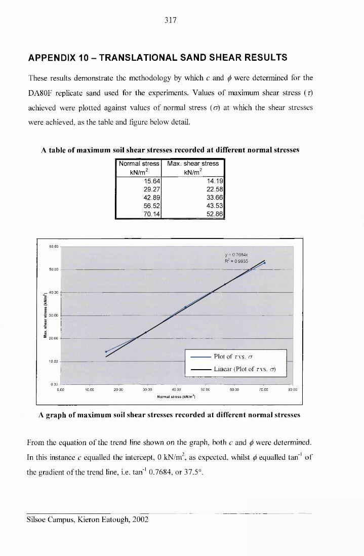
317
APPENDIX 10 - TRANSLATIONAL SAND SHEAR RESULTS
These results demonstrate the methodology by which c and $ were determined for the
DA80F replicate sand used for the experiments. Values of maximum shear stress (r)
achieved were plotted against values of normal stress (<r) at which the shear stresses
were achieved, as the table and figure below detail.
A table of maximum soil shear stresses recorded at different normal stresses
Normal stress ' kN/m2
Max. shear stress kN/m2
15.64 14.1929.27 22.5842.89 33.6656.52 43.5370.14 52.86
60.00
y = 0.7684x R2 = 0.9935
50.00
^ 40.00
30.00
20.00
Plot of r\ s. a10.00
Linear (Plot of r\ s. ct)
0.0020.00 40.00
Norm al s t r e s s (kN/m2)
50.00 80.0030.00 60.00 70.000.00 10.00
A graph of maximum soil shear stresses recorded at different normal stresses
From the equation of the trend line shown on the graph, both c and </> were determined.2 1 r*In this instance c equalled the intercept, 0 kN/m , as expected, whilst (f> equalled tan' of
the gradient of the trend line, i.e. tan'1 0.7684, or 37.5°.
Silsoe Campus, Kieron Eatough, 2002
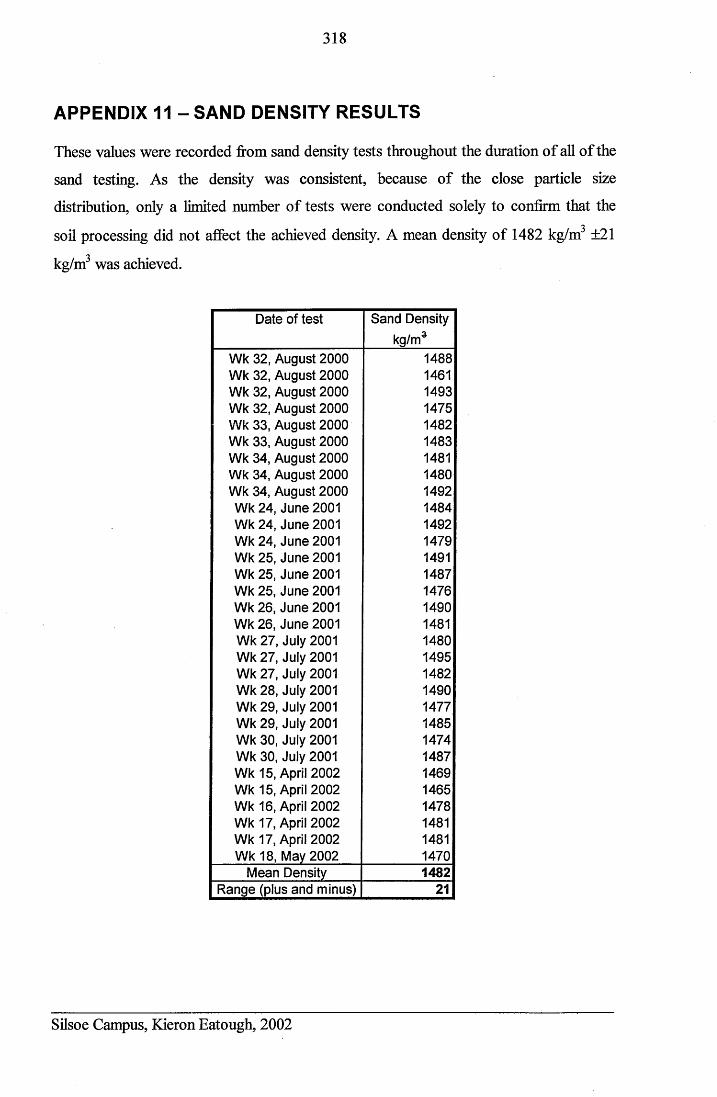
318
APPENDIX 11 - SAND DENSITY RESULTS
These values were recorded from sand density tests throughout the duration of all of the
sand testing. As the density was consistent, because of the close particle size
distribution, only a limited number of tests were conducted solely to confirm that the
soil processing did not affect the achieved density. A mean density of 1482 kg/m ±21
kg/m3 was achieved.
Date of test Sand Density kg/m3
Wk 32, August 2000 1488Wk 32, August 2000 1461Wk 32, August 2000 1493Wk 32, August 2000 1475Wk 33, August 2000 1482Wk 33, August 2000 1483Wk 34, August 2000 1481Wk 34, August 2000 1480Wk 34, August 2000 1492Wk 24, June 2001 1484Wk 24, June 2001 1492Wk 24, June 2001 1479Wk 25, June 2001 1491Wk 25, June 2001 1487Wk 25, June 2001 1476Wk 26, June 2001 1490Wk 26, June 2001 1481Wk 27, July 2001 1480Wk 27, July 2001 1495Wk 27, July 2001 1482Wk 28, July 2001 1490Wk 29, July 2001 1477Wk 29, July 2001 1485Wk 30, July 2001 1474Wk 30, July 2001 1487Wk 15, April 2002 1469Wk 15, April 2002 1465Wk 16, April 2002 1478Wk 17, April 2002 1481Wk 17, April 2002 1481Wk 18, May 2002 1470
Mean Density 1482Range (plus and minus) 21
Silsoe Campus, Kieron Eatough, 2002
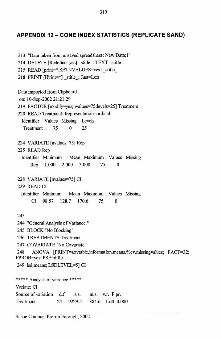
319
APPENDIX 12 - CONE INDEX STATISTICS (REPLICATE SAND)
213 "Data taken from unsaved spreadsheet: New Data; 1"214 DELETE [Redefine=yes] _stitle_: TEXT _stitle_215 READ [print=*;SETNVALUES=yes] _stitle_218 PRINT [IPrint=*] _stitle_; Just=Left
Data imported from Clipboard on: 10-Sep-2002 21:21:29
219 FACTOR [modify=yes;nvalues=75;levels=25] Treatment220 READ Treatment; frepresentation=ordinal
Identifier Values Missing Levels Treatment 75 0 25
224 VARIATE [nvalues=75] Rep225 READ Rep
Identifier Minimum Mean Maximum Values Missing Rep 1.000 2.000 3.000 75 0
228 VARIATE [nvalues=75] Cl229 READ Cl
Identifier Minimum Mean Maximum Values Missing Cl 98.57 128.7 170.6 75 0
243244 "General Analysis of Variance."245 BLOCK "No Blocking"246 TREATMENTS Treatment247 COVARIATE "No Covariate"248 ANOVA [PRINT=aovtable,information,means,%cv,missingvalues; FACT=32;
FPROB=yes; PSE=diff,\249 lsd,means; LSDLEVEL=5] Cl
***** Analysis of variance *****Variate: ClSource of variation d.f. s.s. m.s. v.r. F pr.Treatment 24 9229.5 384.6 1.60 0.080
Silsoe Campus, Kieron Eatough, 2002
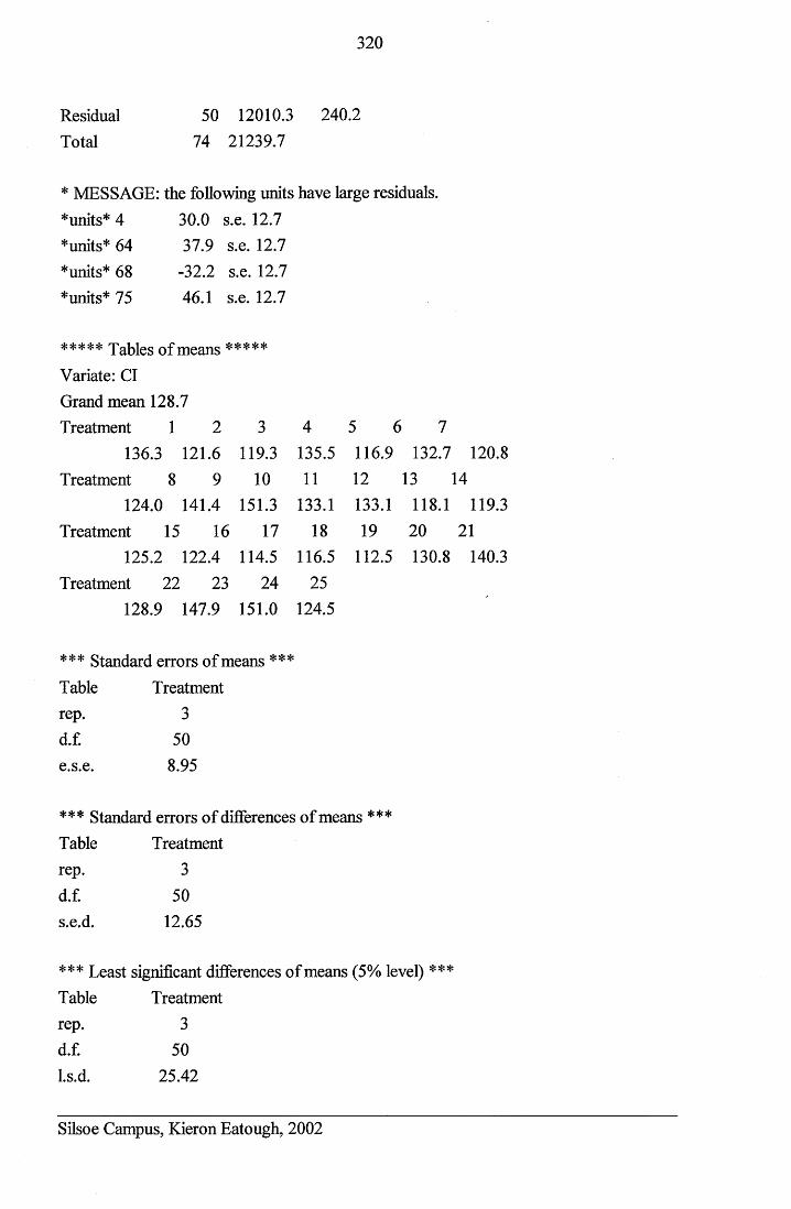
320
Residual 50 12010.3 240.2Total 74 21239.7
* MESSAGE: the following units have large residuals.*units* 4 30.0 s.e. 12.7*units* 64 37.9 s.e. 12.7*units* 68 -32.2 s.e. 12.7*units* 75 46.1 s.e. 12.7
***** Tables of means *****Variate: Cl Grand mean 128.7Treatment 1 2 3 4 5 6 7
136.3 121.6 119.3 135.5 116.9 132.7 120.8Treatment 8 9 10 11 12 13 14
124.0 141.4 151.3 133.1 133.1 118.1 119.3Treatment 15 16 17 18 19 20 21
125.2 122.4 114.5 116.5 112.5 130.8 140.3Treatment 22 23 24 25
128.9 147.9 151.0 124.5
*** Standard errors of means ***Table Treatment rep. 3d.f. 50e.s.e. 8.95
*** Standard errors of differences of means ***Table Treatment rep. 3d.f. 50s.e.d. 12.65
*** Least significant differences of means (5% level) ***Table Treatment rep. 3d.f. 50l.s.d. 25.42
Silsoe Campus, Kieron Eatough, 2002

321
***** stratum standard errors and coefficients of variation ***** Variate: Cl
d.f. s.e. cv%50 15.50 12.0
Silsoe Campus, Kieron Eatough, 2002
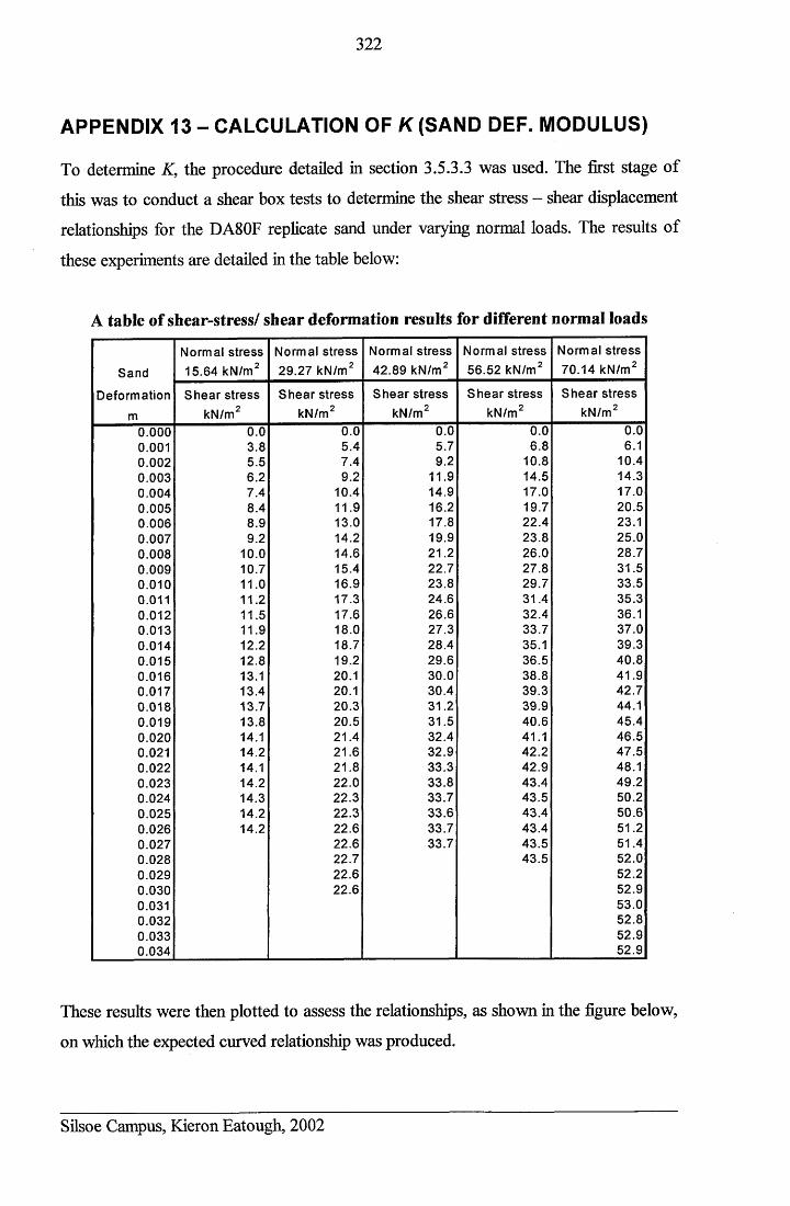
322
APPENDIX 13 - CALCULATION OF K (SAND DEF. MODULUS)
To determine K, the procedure detailed in section 3.5.3.3 was used. The first stage of
this was to conduct a shear box tests to determine the shear stress - shear displacement
relationships for the DA80F replicate sand under varying normal loads. The results of
these experiments are detailed in the table below:
A table of shear-stress/ shear deformation results for different normal loads
Sand
Deformationm
Normal stress 15.64 kN/m2
Normal stress 29.27 kN/m2
Normal stress 42.89 kN/m2
Normal stress 56.52 kN/m2
Normal stress 70.14 kN/m2
Shear stress kN/m2
Shear stress kN/m2
Shear stress kN/m2
Shear stress kN/m2
Shear stress kN/m2
0.000 0.0 0.0 0.0 0.0 0.00.001 3.8 5.4 5.7 6.8 6.10.002 5.5 7.4 9.2 10.8 10.40.003 6.2 9.2 11.9 14.5 14.30.004 7.4 10.4 14.9 17.0 17.00.005 8.4 11.9 16.2 19.7 20.50.006 8.9 13.0 17.8 22.4 23.10.007 9.2 14.2 19.9 23.8 25.00.008 10.0 14.6 21.2 26.0 28.70.009 10.7 15.4 22.7 27.8 31.50.010 11.0 16.9 23.8 29.7 33.50.011 11.2 17.3 24.6 31.4 35.30.012 11.5 17.6 26.6 32.4 36.10.013 11.9 18.0 27.3 33.7 37.00.014 12.2 18.7 28.4 35.1 39.30.015 12.8 19.2 29.6 36.5 40.80.016 13.1 20.1 30.0 38.8 41.90.017 13.4 20.1 30.4 39.3 42.70.018 13.7 20.3 31.2 39.9 44.10.019 13.8 20.5 31.5 40.6 45.40.020 14.1 21.4 32.4 41.1 46.50.021 14.2 21.6 32.9 42.2 47.50.022 14.1 21.8 33.3 42.9 48.10.023 14.2 22.0 33.8 43.4 49.20.024 14.3 22.3 33.7 43.5 50.20.025 14.2 22.3 33.6 43.4 50.60.026 14.2 22.6 33.7 43.4 51.20.027 22.6 33.7 43.5 51.40.028 22.7 43.5 52.00.029 22.6 52.20.030 22.6 52.90.031 53.00.032 52.80.033 52.90.034 52.9
These results were then plotted to assess the relationships, as shown in the figure below,
on which the expected curved relationship was produced.
Silsoe Campus, Kieron Eatough, 2002
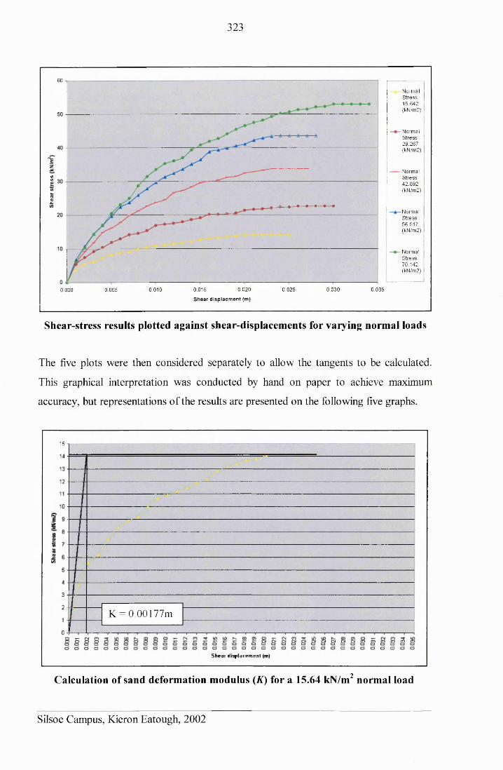
323
60
1z<na)<u»(5vc .W
0.015 0.020 0 .025 0.0350.010 0 .0300.0050.000S h e a r d is o la c m e n t (m )
N orm alS tre s s15.642(kN /m 2)
-N o rm alS tre s s2 9 .267(kN /m 2)
-N orm alS tre s s42 .892(kN /m 2)
-N o rm alS tre s s56 .517(kN /m 2)
-N o rm alS tr e s s7 0 .142(kN /m 2)
Shear-stress results plotted against shear-displacements for varying normal loads
The five plots were then considered separately to allow the tangents to be calculated.
This graphical interpretation was conducted by hand on paper to achieve maximum
accuracy, but representations of the results are presented on the following five graphs.
15
K = 0.00177m
S h e a r d isp la cem en t (m)
Calculation of sand deformation modulus (A) for a 15.64 kN/m2 normal load
Silsoe Campus, Kieron Eatough, 2002
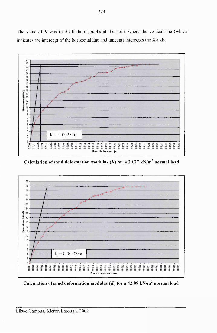
324
The value of K was read off these graphs at the point where the vertical line (which
indicates the intercept of the horizontal line and tangent) intercepts the X-axis.
K = 0.00252m
S h e a r d i s p la c e m e n t (m)
Calculation of sand deformation modulus (A) for a 29.27 kN/m2 normal load
5 20
f 14tSi
K = 0.00409m
S h e a r d isp la cem en t (m)
Calculation of sand deformation modulus (K) for a 42.89 kN/m2 normal load
Silsoe Campus, Kieron Eatough, 2002
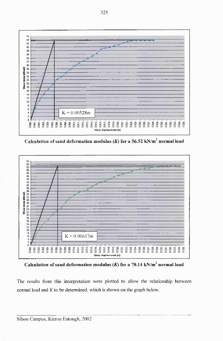
325
46 "i
K = 0.00528m
S h e a r d is p la c e m e n t (m)
Calculation of sand deformation modulus (K) for a 56.52 kN/'m7 normal load
56
z 32
to 26
£ 22
K = 0.00617m
S h e a r d isp la cem en t (m)
Calculation of sand deformation modulus (K) for a 70.14 kN/m2 normal load
The results from this interpretation were plotted to allow the relationship between
normal load and K to be determined, which is shown on the graph below.
Silsoe Campus, Kieron Eatough, 2002
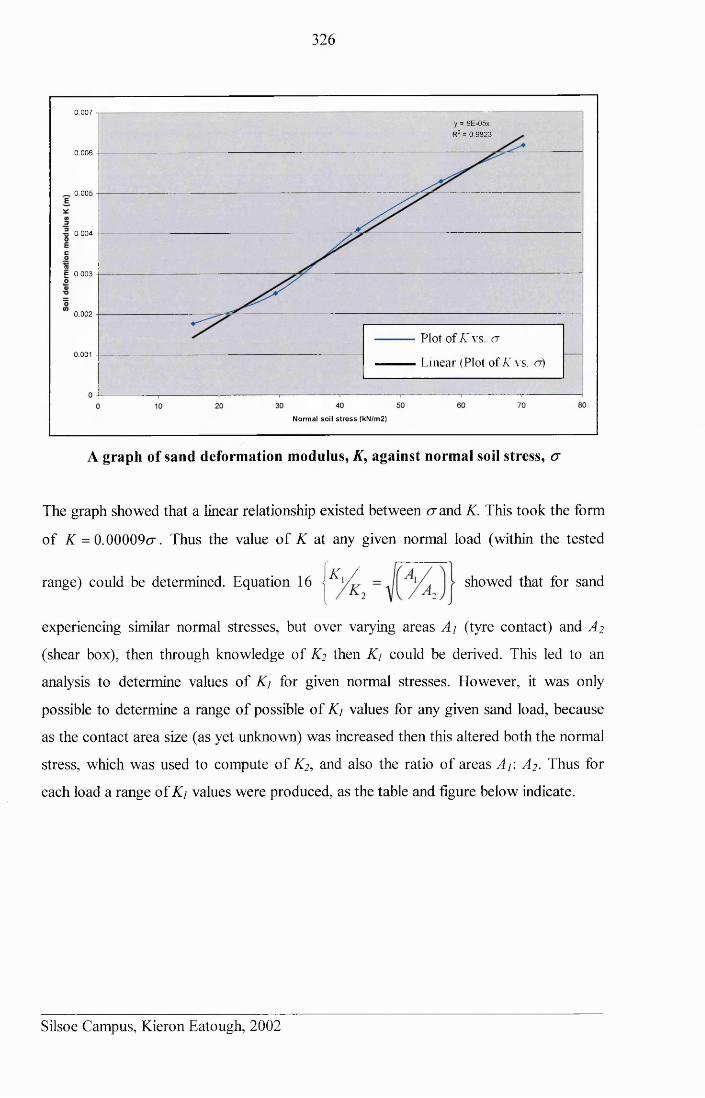
326
0.007y = 9E-05x
R2 = 0 .9823
0.006
0.005
■5 0.004
£ 0 .003
0.002
Plot of K vs. a0.001
Linear (Plot of K vs. a)
Normal so il s t r e s s (kN/m2)
A graph of sand deformation modulus, K, against normal soil stress, cr
The graph showed that a linear relationship existed between cr and K. This took the form
of K = 0.00009cr. Thus the value of K at any given normal load (within the tested
\k /range) could be determined. Equation 16 j
experiencing similar normal stresses, but over varying areas Aj (tyre contact) and A2
(shear box), then through knowledge of K2 then K\ could be derived. This led to an
analysis to determine values of Kj for given normal stresses. However, it was only
possible to determine a range of possible of K\ values for any given sand load, because
as the contact area size (as yet unknown) was increased then this altered both the normal
stress, which was used to compute of K2, and also the ratio of areas Aj: A2 . Thus for
each load a range of K) values were produced, as the table and figure below indicate.
showed that for sand
Silsoe Campus, Kieron Eatough, 2002
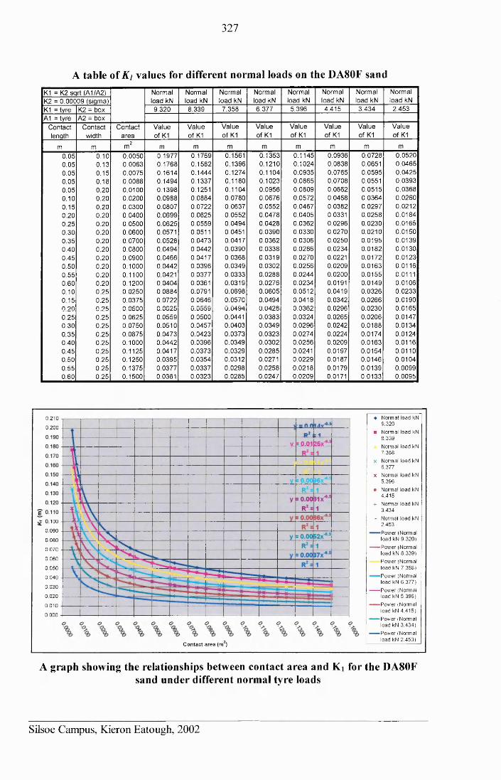
327
A table of Kj values for different normal loads on the DA80F sandK1 = K2 sqrt (A1/A2) Normal Normal Normal Normal Normal Normal Normal NormalK2 = 0.00009 (sigma) load kN load kN load kN load kN load kN load kN load kN load kNK1 = tyre K2= box 9.320 8.339 7.358 6.377 5.396 4.415 3.434 2.453A1 = tyre A2 = box
Contact Contact Contact Value Value Value Value Value Value Value Valuelength width area of K1 of K1 of K1 of K1 of K1 of K1 of K1 of K1
m m r r , 2m m m m m m m m m0.05 0.10 0.0050 0.1977 0.1769 0.1561 0.1353 0.1145 0.0936 0.0728 0.05200.05 0.13 0.0063 0.1768 0.1582 0.1396 0.1210 0.1024 0.0838 0.0651 0.04650.05 0.15 0.0075 0.1614 0.1444 0.1274 0.1104 0.0935 0.0765 0.0595 0.04250.05 0.18 0.0088 0.1494 0.1337 0.1180 0.1023 0.0865 0.0708 0.0551 0.03930.05 0.20 0.0100 0.1398 0.1251 0.1104 0.0956 0.0809 0.0662 0.0515 0.03680.10 0.20 0.0200 0.0988 0.0884 0.0780 0.0676 0.0572 0.0468 0.0364 0.02600.15 0.20 0.0300 0.0807 0.0722 0.0637 0.0552 0.0467 0.0382 0.0297 0.02120.20 0.20 0.0400 0.0699 0.0625 0.0552 0.0478 0.0405 0.0331 0.0258 0.01840.25 0.20 0.0500 0.0625 0.0559 0.0494 0.0428 0.0362 0.0296 0.0230 0.01650.30 0.20 0.0600 0.0571 0.0511 0.0451 0.0390 0.0330 0.0270 0.0210 0.01500.35 0.20 0.0700 0.0528 0.0473 0.0417 0.0362 0.0306 0.0250 0.0195 0.01390.40 0.20 0.0800 0.0494 0.0442 0.0390 0.0338 0.0286 0.0234 0.0182 0.01300.45 0.20 0.0900 0.0466 0.0417 0.0368 0.0319 0.0270 0.0221 0.0172 0.01230.50 0.20 0.1000 0.0442 0.0396 0.0349 0.0302 0.0256 0.0209 0.0163 0.01160.55 0.20 0.1100 0.0421 0.0377 0.0333 0.0288 0.0244 0.0200 0.0155 0.01110.60 0.20 0.1200 0.0404 0.0361 0.0319 0.0276 0.0234 0.0191 0.0149 0.01060.10 0.25 0.0250 0.0884 0.0791 0.0698 0.0605 0.0512 0.0419 0.0326 0.02330.15 0.25 0.0375 0.0722 0.0646 0.0570 0.0494 0.0418 0.0342 0.0266 0.01900.20 0.25 0.0500 0.0625 0.0559 0.0494 0.0428 0.0362 0.0296 0.0230 0.01650.25 0.25 0.0625 0.0559 0.0500 0.0441 0.0383 0.0324 0.0265 0.0206 0.01470.30 0.25 0.0750 0.0510 0.0457 0.0403 0.0349 0.0296 0.0242 0.0188 0.01340.35 0.25 0.0875 0.0473 0.0423 0.0373 0.0323 0.0274 0.0224 0.0174 0.01240.40 0.25 0.1000 0.0442 0.0396 0.0349 0.0302 0.0256 0.0209 0.0163 0.01160.45 0.25 0.1125 0.0417 0.0373 0.0329 0.0285 0.0241 0.0197 0.0154 0.01100.50 0.25 0.1250 0.0395 0.0354 0.0312 0.0271 0.0229 0.0187 0.0146 0.01040.55 0.25 0.1375 0.0377 0.0337 0.0298 0.0258 0.0218 0.0179 0.0139 0.00990.60 0.25 0.1500 0.0361 0.0323 0.0285 0.0247 0.0209 0.0171 0.0133 0.0095
♦ Norm al load kN 9 .320
■ Normal load kN 8 .339
Normal load kN 7 .358
x Norm al load kN 6 .377
x Normal load kN 5.396
• Norm al load kN 4 .415
+ Normal load kN 3.434
- Norm al load kN 2 .453
P ow er (N orm al load kN 9 .3 2 0 )
— P o w er (N orm al load kN 8 .3 3 9 )
P ow er (N orm al load kN 7 .358)
— P o w er (N orm al load kN 6 .3 7 7 )
— P ow er (N orm al load kN 5 .396)
— Pow er (N orm al load kN 4 .4 1 5 )
— P ow er (N orm al load kN 3 .434)
— P ow er (N orm al load kN 2 .453)
0.210
0.200
100
0.090
0 .080
0.070
0.060
0.050
0.040
0.030
0.020
0.010
0.000
C o n ta c t a r e a (m )
A graph showing the relationships between contact area and Kj for the DA80F sand under different normal tyre loads
Silsoe Campus, Kieron Eatough, 2002
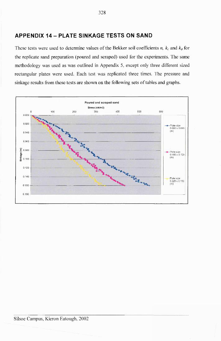
328
APPENDIX 14 - PLATE SINKAGE TESTS ON SAND
These tests were used to determine values of the Bekker soil coefficients n, kc and k# for
the replicate sand preparation (poured and scraped) used for the experiments. The same
methodology was used as was outlined in Appendix 5, except only three different sized
rectangular plates were used. Each test was replicated three times. The pressure and
sinkage results from these tests are shown on the following sets of tables and graphs.
Poured and scraped sand
S tr e s s (kN /m 2)
300 400 500 6002001000.000
0.020■Plate size 0 .090 x 0 .060(m )0.040
0.060
E. 0 080-P la te size 0 .180 x 0 .120 ( m )S 0 .100
0 120
0 .140P la te s ize 0 .2 2 5 x 0 .150 (m )
0.160
0 .180 J
Silsoe Campus, Kieron Eatough, 2002
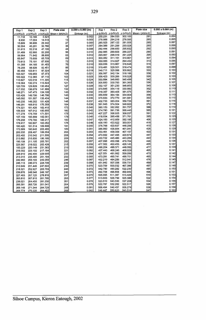
329
Rep 1 p (kN/u2)
Rep 2 p (kN/u2)
Rep 3 p (kN/u2)
Plate sizeMean r (kN/m2)
0.090 x 0.060 (m)Sinkaae (m)
Rep 1 p (kN/u2)
Rep 2 p (kN/u2)
Rep 3 p (kN/u2)
Plate sizeMean r (kN/m2)
0.090 x 0.060 (m)Sinkaae (m)
11.118 10.166 5.624 9 0.002 255.231 284.533 302.100 281 0.0848.930 17.004 14.515 13 0.003 278.988 284.218 276.585 280 0.085
15.699 36.906 29.442 27 0.005 285.923 287.122 281.505 285 0.08730.394 45.201 32.780 36 0.007 284.388 291.299 293.028 290 0.08831.613 52.218 47.100 44 0.008 282.444 298.850 295.832 292 0.09051.469 62.966 52.200 56 0.010 292.885 289.603 286.227 290 0.09156.964 71.842 58.806 63 0.012 293.967 298.519 291.225 295 0.09365.847 75.606 65.709 69 0.013 300.082 311.151 310.801 307 0.09473.613 75.191 67.936 72 0.015 330.083 314.827 294.432 313 0.09661.368 84.165 81.453 76 0.016 309.056 313.867 316.646 313 0.09776.258 88.926 92.451 86 0.018 319.481 329.501 319.474 323 0.09980.468 103.811 97.324 94 0.019 348.711 329.996 309.862 330 0.100
103.327 109.953 97.373 104 0.021 356.997 342.134 319.186 339 0.102100.322 112.383 97.110 103 0.023 358.423 339.266 318.528 339 0.103110.627 122.018 111.305 115 0.024 333.884 346.660 345.456 342 0.105118.384 130.274 113.524 121 0.026 305.850 339.793 361.360 336 0.107120.709 129.829 130.454 127 0.028 332.107 351.230 346.853 343 0.108117.032 136.679 141.999 132 0.030 370.845 354.119 330.980 352 0.110146.271 147.473 134.108 143 0.032 318.357 363.405 381.575 354 0.111133.426 149.796 146.796 143 0.033 355.659 364.184 354.904 358 0.113145.092 151.557 135.434 144 0.035 375.633 372.770 341.681 363 0.115143.235 149.252 151.428 148 0.037 402.733 383.004 358.726 381 0.116146.291 168.810 176.359 164 0.038 391.945 374.504 349.920 372 0.118174.321 181.426 162.415 173 0.040 380.153 392.992 391.757 388 0.119156.333 167.012 156.655 160 0.042 374.780 391.736 388.443 385 0.121177.278 175.759 171.501 175 0.043 407.227 398.905 368.037 391 0.122157.159 185.889 192.001 178 0.045 418.834 395.456 371.761 395 0.123176.298 179.766 183.217 180 0.047 424.183 412.959 382.195 406 0.125178.917 182.607 165.052 176 0.048 438.190 422.622 393.001 418 0.127190.426 181.514 169.808 181 0.050 376.768 420.637 446.299 415 0.128172.589 190.945 203.466 189 0.051 386.860 436.884 461.041 428 0.129200.335 208.407 199.354 203 0.053 453.461 438.358 407.157 433 0.131202.402 210.342 211.556 208 0.054 473.932 447.495 420.674 447 0.133213.882 215.835 196.186 209 0.056 430.722 445.486 443.289 440 0.134190.108 211.105 205.791 202 0.057 407.098 450.098 479.764 446 0.136225.367 218.022 202.428 215 0.059 477.352 460.433 428.143 455 0.137193.229 220.149 231.363 215 0.060 496.204 486.371 448.592 477 0.139219.302 225.102 217.184 221 0.062 457.443 468.245 468.029 465 0.141226.910 242.435 229.655 233 0.064 427.551 481.982 509.056 473 0.142213.315 235.495 251.194 233 0.065 473.291 493.741 488.701 485 0.144242.960 253.193 243.059 246 0.067 432.219 484.256 512.941 476 0.145246.113 246.073 224.706 239 0.068 451.942 507.038 536.731 499 0.147210.949 231.446 247.604 230 0.070 523.709 500.032 467.386 497 0.148218.321 252.927 263.753 245 0.072 442.790 490.282 522.230 485 0.150239.676 248.348 249.197 246 0.073 492.708 496.808 499.943 496 0.151227.463 267.125 276.816 257 0.075 505.095 511.387 513.426 510 0.153265.810 267.815 261.795 265 0.077 513.603 526.799 525.386 522 0.154238.021 264.455 281.230 261 0.078 523.510 540.536 537.208 534 0.156266.391 265.726 261.041 264 0.079 522.787 532.282 522.517 526 0.157268.148 271.344 264.729 268 0.081 568.494 540.437 506.279 538 0.158268.774 270.225 264.482 268 0.082 546.447 550.620 543.516 547 0.160
Silsoe Campus, Kieron Eatough, 2002
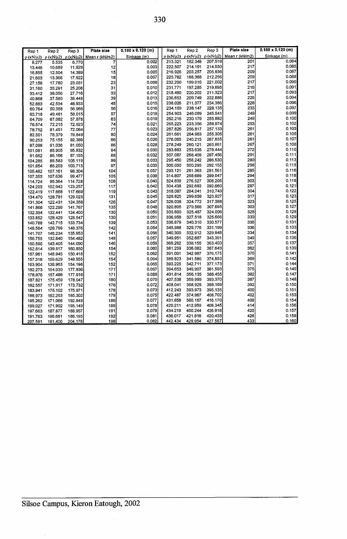
330
Rep 1 p (kN/u2)
Rep 2 p (kN/u2)
Rep 3 p (kN/u2)
Plate sizeMean r (kN/m2)
0.180x0.120 (m)Sinkaae (m)
Rep 1 p (kN/m2)
Rep 2 p (kN/u2)
Rep 3 p (kN/u2)
Plate sizeMean r (kN/m2)
0.180 x 0.120 (m)Sinkaae (m)
8.277 5.535 6.770 7 0.002 213.321 182.348 207.519 201 0.08413.446 10.689 11.829 12 0.003 222.507 214.191 214.030 217 0.08516.855 12.504 14.389 15 0.005 216.926 203.257 205.936 209 0.08721.603 13.366 17.922 18 0.007 225.782 188.368 212.256 209 0.08827.158 17.780 23.031 23 0.008 232.200 199.016 221.002 217 0.09031.160 35.291 25.208 31 0.010 231.771 197.285 219.895 216 0.09133.412 38.056 27.716 33 0.012 218.480 220.202 211.323 217 0.09340.868 37.580 38.448 39 0.013 236.653 209.749 232.886 226 0.09452.883 42.594 48.933 48 0.015 238.026 211.377 234.386 228 0.09660.764 50.388 56.966 56 0.016 234.159 238.147 228.135 233 0.09763.718 49.481 58.015 57 0.018 254.903 246.089 245.541 249 0.09964.709 67.082 57.878 63 0.019 262.216 230.179 255.882 249 0.10076.574 72.215 72.923 74 0.021 265.223 233.356 258.974 253 0.10278.752 81.451 72.084 77 0.023 267.826 256.817 257.133 261 0.10382.501 78.379 78.849 80 0.024 261.661 264.983 255.305 261 0.10590.253 75.155 92.389 86 0.026 276.085 240.215 267.835 261 0.10787.098 91.036 81.050 86 0.028 278.249 260.121 263.861 267 0.108
101.081 85.905 95.832 94 0.030 283.883 253.635 278.444 272 0.11091.662 86.166 87.155 88 0.032 307.087 268.456 297.456 291 0.111
104.285 86.583 105.119 99 0.033 295.450 258.242 286.530 280 0.113101.854 86.203 103.713 97 0.035 300.050 300.295 292.155 298 0.115105.482 107.161 98.304 104 0.037 293.121 281.363 281.561 285 0.116107.353 107.636 99.477 105 0.038 314.807 268.689 299.047 294 0.118114.724 95.364 114.728 108 0.040 324.839 276.527 308.205 303 0.119124.203 102.942 123.257 117 0.042 304.438 292.692 292.660 297 0.121122.419 117.668 117.669 119 0.043 318.087 284.041 310.749 304 0.122134.470 128.781 129.023 131 0.045 328.825 299.659 323.927 317 0.123131.304 122.431 124.358 126 0.047 326.038 324.772 317.388 323 0.125141.866 122.299 141.767 135 0.048 320.805 279.566 307.695 303 0.127132.394 132.441 124.400 130 0.050 335.600 325.487 324.006 328 0.128133.852 128.429 128.547 130 0.051 336.958 327.518 325.666 330 0.129140.788 142.715 133.734 139 0.053 336.879 340.310 330.577 336 0.131148.584 128.799 148.376 142 0.054 345.988 329.776 331.199 336 0.133141.707 146.234 135.953 141 0.056 340.300 332.912 329.948 334 0.134156.755 132.840 154.482 148 0.057 349.951 352.687 343.301 349 0.136150.590 143.405 144.090 146 0.059 369.282 338.155 363.403 357 0.137162.814 139.517 160.850 154 0.060 381.259 336.082 367.643 362 0.139157.961 148.945 150.418 152 0.062 391.001 342.987 376.175 370 0.141157.316 156.629 148.955 154 0.064 389.823 341.586 374.853 369 0.142163.904 136.965 154.198 152 0.065 393.225 342.711 377.173 371 0.144182.273 154.030 177.836 171 0.067 394.653 349.907 381.593 375 0.145178.976 157.486 177.916 171 0.068 401.814 356.135 388.455 382 0.147187.821 175.459 178.047 180 0.070 407.538 359.999 393.370 387 0.148182.557 171.917 173.732 176 0.072 408.041 368.928 398.169 392 0.150183.941 175.102 175.971 178 0.073 412.243 393.973 395.135 400 0.151188.973 162.263 185.302 179 0.075 422.487 374.967 408.702 402 0.153195.262 171.066 192.849 186 0.077 431.858 380.167 416.170 409 0.154199.027 171.902 195.149 189 0.078 420.211 412.959 408.345 414 0.156197.663 187.877 188.957 191 0.079 434.219 400.244 426.916 420 0.157191.763 196.661 186.195 192 0.081 436.017 421.816 420.433 426 0.158207.581 181.406 204.178 198 0.082 442.434 429.954 427.567 433 0.160
Silsoe Campus, Kieron Eatough, 2002
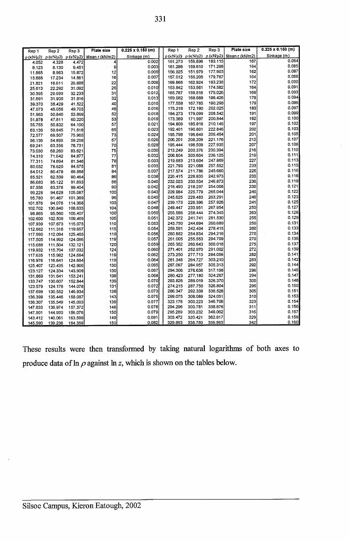
331
Rep 1 Rep 2 o (kN/u2) d (kN/u2)
Rep 3 p (kN/u2)
Plate sizeMean r (kN/m2)
0.225 x 0.150 (m)Sinkaae fm)
Rep 1 p (kN/p2)
Rep 2 p (kN/p2)
Rep 3 p (kN/|x2)
Plate sizeMean r (kN/m2)
0.225x0.160 (m)Sinkaae (m)
4.052 4.328 4.472 4 0.002 161.273 156.896 183.115 167 0.0848.123 8.130 9.451 9 0.003 161.288 159.610 171.268 164 0.085
11.885 8.963 15.872 12 0.005 156.925 151.979 177.903 162 0.08715.688 17.234 14.561 16 0.007 157.012 155.205 179.767 164 0.08821.821 18.611 26.888 22 0.008 169.868 162.924 183.238 172 0.09025.613 22.292 31.092 26 0.010 163.842 153.561 174.582 164 0.09130.395 29.999 32.233 31 0.012 165.787 159.516 179.026 168 0.09331.691 31.905 31.816 32 0.013 169.082 168.688 196.426 178 0.09439.370 38.429 41.522 40 0.015 177.558 167.785 190.298 179 0.09647.073 46.056 49.705 48 0.016 175.218 172.180 202.025 183 0.09751.963 50.840 53.869 52 0.018 184.273 179.099 208.542 191 0.09951.878 47.811 60.220 53 0.019 173.369 171.997 200.844 182 0.10055.755 50.832 64.100 57 0.021 194.809 185.818 210.146 197 0.10263.136 59.845 71.518 65 0.023 192.401 190.801 222.846 202 0.10372.577 69.507 75.965 73 0.024 195.798 196.649 209.454 201 0.10556.136 54.895 59.258 57 0.026 206.201 208.209 221.176 212 0.10769.241 63.356 78.731 70 0.028 195.444 196.509 227.935 207 0.10873.030 68.260 83.621 75 0.030 213.249 203.376 230.394 216 0.11074.310 71.642 84.877 77 0.032 206.804 205.604 236.125 216 0.11177.311 74.694 81.546 78 0.033 219.683 213.604 247.869 227 0.11380.032 78.620 84.675 81 0.035 221.793 221.088 257.552 233 0.11584.012 80.478 88.568 84 0.037 217.574 211.786 245.660 225 0.11685.521 82.339 90.464 86 0.038 226.415 228.835 242.973 233 0.11886.680 85.122 91.693 88 0.040 232.023 230.534 246.873 236 0.11987.556 83.378 99.404 90 0.042 218.490 218.297 254.008 230 0.12199.228 94.628 105.087 100 0.043 229.984 225.779 265.044 240 0.12295.780 91.467 101.369 96 0.045 245.625 229.483 263.291 246 0.123
101.876 94.076 114.368 103 0.047 239.173 226.396 257.926 241 0.125102.702 100.840 108.633 104 0.048 249.447 233.951 267.954 250 0.12798.865 95.560 105.407 100 0.050 •255.586 258.444 274.345 263 0.128
102.600 102.509 109.469 105 0.051 242.372 241.741 281.530 255 0.129107.939 107.673 115.075 110 0.053 243.750 244.694 260.689 250 0.131112.882 111.316 119.657 115 0.054 259.591 242.404 278.415 260 0.133117.990 112.094 125.465 119 0.056 260.852 254.834 294.218 270 0.134117.505 114.992 124.086 119 0.057 261.005 255.553 294.709 270 0.136115.688 111.504 132.121 120 0.059 265.352 260.643 300.018 275 0.137119.932 115.704 137.032 124 0.060 271.401 252.970 291.002 272 0.139117.635 115.982 124.684 119 0.062 273.250 277.713 294.056 282 0.141116.976 116.641 124.684 119 0.064 281.348 264.727 303.210 283 0.142125.407 120.435 142.966 130 0.065 287.097 284.957 305.313 292 0.144123.127 124.334 143.908 130 0.067 294.306 276.636 317.198 296 0.145131.869 131.641 153.241 139 0.068 280.423 277.180 324.267 294 0.147133.747 130.607 152.844 139 0.070 283.826 289.019 326.370 300 0.148123.579 124.176 144.078 131 0.072 274.215 287.750 326.804 296 0.150137.699 130.552 146.934 138 0.073 286.347 292.339 336.528 305 0.151136.398 135.446 158.087 143 0.075 299.075 308.089 324.051 310 0.153136.307 135.549 145.093 139 0.077 323.178 300.223 346.706 323 0.154147.833 138.974 157.372 148 0.078 294.296 300.781 338.876 311 0.156147.501 144.933 156.076 150 0.079 295.289 303.232 348.062 316 0.157143.412 140.061 163.599 149 0.081 303.472 320.421 362.817 329 0.158145.590 139.236 164.359 150 0.082 329.863 338.780 356.863 342 0.160
These results were then transformed by taking natural logarithms of both axes to
produce data of In p against In z, which is shown on the tables below.
Silsoe Campus, Kieron Eatough, 2002
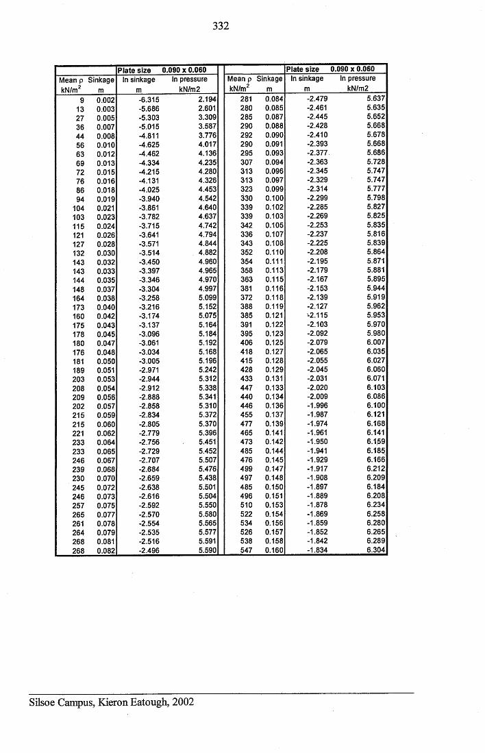
332
Plate size 0.090 x 0.060 Plate size 0.090 x 0.060Mean p Sinkage In sinkage In pressure Mean p Sinkage In sinkage In pressurekN/m2 m m kN/m 2 kN/m2 m m kN/m2
9 0.002 -6.315 2.194 281 0.084 -2.479 5.63713 0.003 -5.686 2.601 280 0.085 -2.461 5.63527 0.005 -5.303 3.309 285 0.087 -2.445 5.65236 0.007 -5.015 3.587 290 0.088 -2.428 5.66844 0.008 -4.811 3.776 292 0.090 -2.410 5.67856 0.010 -4.625 4.017 290 0.091 -2.393 5.66863 0.012 -4.462 4.136 295 0.093 -2.377 5.68669 0.013 -4.334 4.235 307 0.094 -2.363 5.72872 0.015 -4.215 4.280 313 0.096 -2.345 5.74776 0.016 -4.131 4.326 313 0.097 -2.329 5.74786 0.018 -4.025 4.453 323 0.099 -2.314 5.77794 0.019 -3.940 4.542 330 0.100 -2.299 5.798
104 0.021 -3.861 4.640 339 0.102 -2.285 5.827103 0.023 -3.782 4.637 339 0.103 -2.269 5.825115 0.024 -3.715 4.742 342 0.105 -2.253 5.835121 0.026 -3.641 4.794 336 0.107 -2.237 5.816127 0.028 -3.571 4.844 343 0.108 -2.225 5.839132 0.030 -3.514 4.882 352 0.110 -2.208 5.864143 0.032 -3.450 4.960 354 0.111 -2.195 5.871143 0.033 -3.397 4.965 358 0.113 -2.179 5.881144 0.035 -3.346 4.970 363 0.115 -2.167 5.895148 0.037 -3.304 4.997 381 0.116 -2.153 5.944164 0.038 -3.258 5.099 372 0.118 -2.139 5.919173 0.040 -3.216 5.152 388 0.119 -2.127 5.962160 0.042 -3.174 5.075 385 0.121 2.115 5.953175 0.043 -3.137 5.164 391 0.122 -2.103 5.970178 0.045 -3.096 5.184 395 0.123 -2.092 5.980180 0.047 -3.061 5.192 406 0.125 -2.079 6.007176 0.048 -3.034 5.168 418 0.127 -2.065 6.035181 0.050 -3.005 5.196 415 0.128 -2.055 6.027189 0.051 -2.971 5.242 428 0.129 -2.045 6.060203 0.053 -2.944 5.312 433 0.131 -2.031 6.071208 0.054 -2.912 5.338 447 0.133 -2.020 6.103209 0.056 -2.888 5.341 440 0.134 -2.009 6.086202 0.057 -2.858 5.310 446 0.136 -1.996 6.100215 0.059 -2.834 5.372 455 0.137 -1.987 6.121215 0.060 -2.805 5.370 477 0.139 -1.974 6.168221 0.062 -2.779 5.396 465 0.141 -1.961 6.141233 0.064 -2.756 5.451 473 0.142 -1.950 6.159233 0.065 -2.729 5.452 485 0.144 -1.941 6.185246 0.067 -2.707 5.507 476 0.145 -1.929 6.166239 0.068 -2.684 5.476 499 0.147 -1.917 6.212230 0.070 -2.659 5.438 497 0.148 -1.908 6.209245 0.072 -2.638 5.501 485 0.150 -1.897 6.184246 0.073 -2.616 5.504 496 0.151 -1.889 6.208257 0.075 -2.592 5.550 510 0.153 -1.878 6.234265 0.077 -2.570 5.580 522 0.154 -1.869 6.258261 0.078 -2.554 5.565 534 0.156 -1.859 6.280264 0.079 -2.535 5.577 526 0.157 -1.852 6.265268 0.081 -2.516 5.591 538 0.158 -1.842 6.289268 0.082 -2.496 5.590 547 0.160 -1.834 6.304
Silsoe Campus, Kieron Eatough, 2002
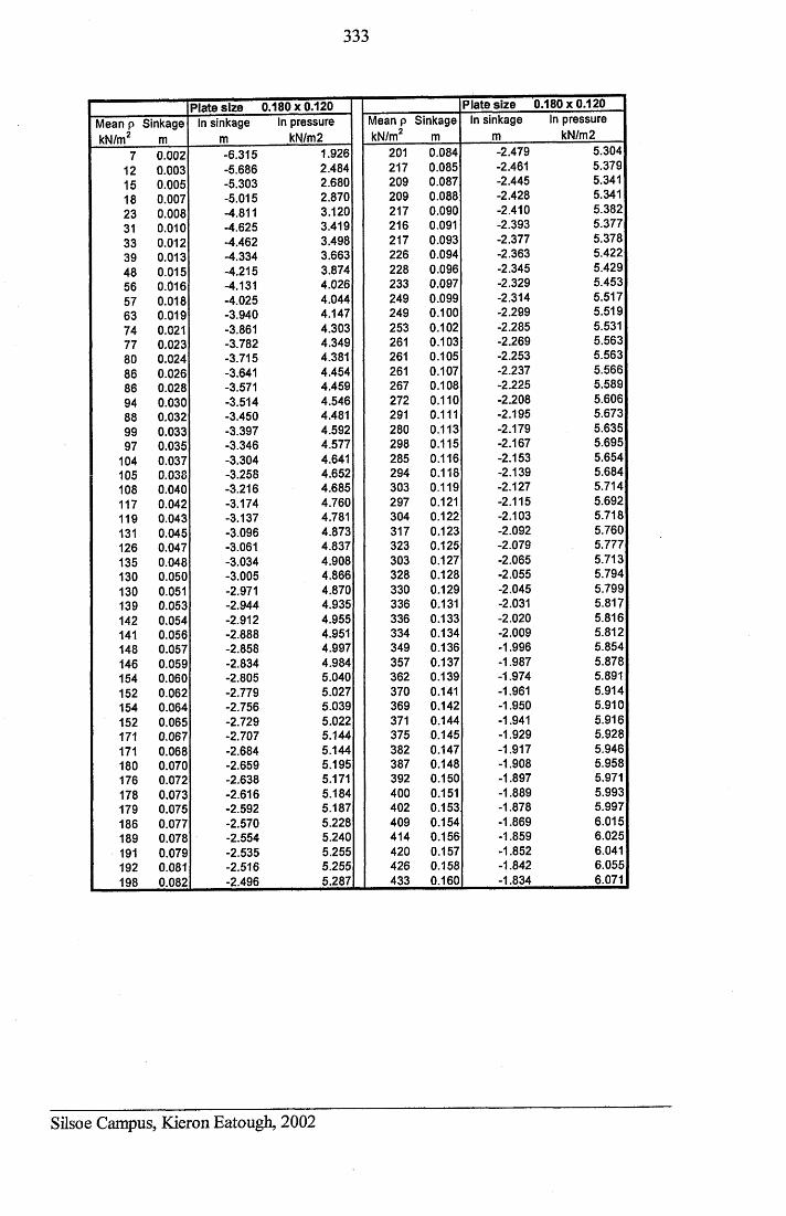
333
Plate size 0.180x0.120 Plate size 0.180x0.120Mean p Sinkage In sinkage In pressure Mean p Sinkage In sinkage In pressurekN/m2 m m kN/m 2 kN/m2 m m kN/m 2
7 0.002 -6.315 1.926 201 0.084 -2.479 5.30412 0.003 -5.686 2.484 217 0.085 -2.461 5.37915 0.005 -5.303 2.680 209 0.087 -2.445 5.34118 0.007 -5.015 2.870 209 0.088 -2.428 5.34123 0.008 -4.811 3.120 217 0.090 -2.410 5.38231 0.010 -4.625 3.419 216 0.091 -2.393 5.37733 0.012 -4.462 3.498 217 0.093 -2.377 5.37839 0.013 -4.334 3.663 226 0.094 -2.363 5.42248 0.015 -4.215 3.874 228 0.096 -2.345 5.42956 0.016 -4.131 4.026 233 0.097 -2.329 5.45357 0.018 -4.025 4.044 249 0.099 -2.314 5.51763 0.019 -3.940 4.147 249 0.100 -2.299 5.51974 0.021 -3.861 4.303 253 0.102 -2.285 5.53177 0.023 -3.782 4.349 261 0.103 -2.269 5.56380 0.024 -3.715 4.381 261 0.105 -2.253 5.56386 0.026 -3.641 4.454 261 0.107 -2.237 5.56686 0.028 -3.571 4.459 267 0.108 -2.225 5.58994 0.030 -3.514 4.546 272 0.110 -2.208 5.60688 0.032 -3.450 4.481 291 0.111 -2.195 5.67399 0.033 -3.397 4.592 280 0.113 -2.179 5.63597 0.035 -3.346 4.577 298 0.115 -2.167 5.695
104 0.037 -3.304 4.641 285 0.116 -2.153 5.654105 0.038 -3.258 4.652 294 0.118 -2.139 5.684108 0.040 -3.216 4.685 303 0.119 -2.127 5.714117 0.042 -3.174 4.760 297 0.121 -2.115 5.692119 0.043 -3.137 4.781 304 0.122 -2.103 5.718131 0.045 -3.096 4.873 317 0.123 -2.092 5.760126 0.047 -3.061 4.837 323 0.125 -2.079 5.777135 0.048 -3.034 4.908 303 0.127 -2.065 5.713130 0.050 -3.005 4.866 328 0.128 -2.055 5.794130 0.051 -2.971 4.870 330 0.129 -2.045 5.799139 0.053 -2.944 4.935 336 0.131 -2.031 5.817142 0.054 -2.912 4.955 336 0.133 -2.020 5.816141 0.056 -2.888 4.951 334 0.134 -2.009 5.812148 0.057 -2.858 4.997 349 0.136 -1.996 5.854146 0.059 -2.834 4.984 357 0.137 -1.987 5.878154 0.060 -2.805 5.040 362 0.139 -1.974 5.891152 0.062 -2.779 5.027 370 0.141 -1.961 5.914154 0.064 -2.756 5.039 369 0.142 -1.950 5.910152 0.065 -2.729 5.022 371 0.144 -1.941 5.916171 0.067 -2.707 5.144 375 0.145 -1.929 5.928171 0.068 -2.684 5.144 382 0.147 -1.917 5.946180 0.070 -2.659 5.195 387 0.148 -1.908 5.958176 0.072 -2.638 5.171 392 0.150 -1.897 5.971178 0.073 -2.616 5.184 400 0.151 -1.889 5.993179 0.075 -2.592 5.187 402 0.153 -1.878 5.997186 0.077 -2.570 5.228 409 0.154 -1.869 6.015189 0.078 -2.554 5.240 414 0.15& -1.859 6.025191 0.079 -2.535 5.255 420 0.157 -1.852 6.041192 0.081 -2.516 5.255 426 0.158 -1.842 6.055198 0.082 -2.496 5.287 433 0.160 -1.834 6.071
Silsoe Campus, Kieron Eatough, 2002
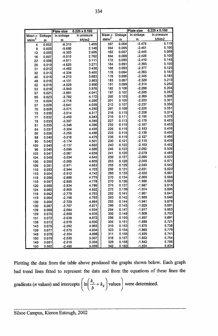
334
Plate size 0.225 x 0.150 Plate size 0.225 x 0.150Mean p Sinkage In sinkage In pressure Mean p Sinkage In sinkage In pressurekN/m2 m m kN/m2 kN/m2 m m kN/m2
4 0.002 -6.315 1.455 167 0.084 -2.479 5.1199 0.003 -5.686 2.148 164 0.085 -2.461 5.100
12 0.005 -5.303 2.505 162 0.087 -2.445 5.08916 0.007 -5.015 2.762 164 0.088 -2.428 5.10022 0.008 -4.811 3.111 172 0.090 -2.410 5.14826 0.010 -4.625 3.271 164 0.091 -2.393 5.10031 0.012 -4.462 3.430 168 0.093 -2.377 5.12532 0.013 -4.334 3.460 178 0.094 -2.363 5.18240 0.015 -4.215 3.683 179 0.096 -2.345 5.18548 0.016 -4.131 3.863 183 0.097 -2.329 5.21052 0.018 -4.Q25 3.956 191 0.099 -2.314 5.25053 0.019 -3.940 3.976 182 0.100 -2.299 5.20457 0.021 -3.861 4.041 197 0.102 -2.285 5.28365 0.023 -3.782 4.172 202 0.103 -2.269 5,30873 0.024 -3.715 4.286 201 0.105 -2.253 5.30157 0.026 -3.641 4.039 212 0.107 -2.237 5.35670 0.028 -3.571 4.255 207 0.108 -2.225 5.33175 0.030 -3.514 4.317 216 0.110 -2.208 5.37477 0.032 -3.450 4.343 216 0.111 -2.195 5.37678 0.033 -3.397 4.355 227 0.113 -2.179 5.425
5.45^81 0.035 -3.346 4.396 233 0.115 -2.16784 0.037 -3.304 4.435 225 0.116 -2.153 5.41686 0.038 -3.258 4.456 233 0.118 -2.139 5.45088 0.040 -3.216 4.475 236 0.119 -2.127 5.46690 0.042 -3.174 4.501 230 0.121 -2.115 5.439
100 0.043 -3.137 4.602 240 0.122 -2.103 5.48296 0.045 -3.096 4.566 246 0.123 -2.092 5.506
103 0.047 -3.061 4.639 241 0.125 -2.079 5.485104 0.048 -3.034 4.645 250 0.127 -2.065 5.523100 0.050 -3.005 4.605 263 0.128 -2.055 5.571105 0.051 -2.971 4.653 255 0.129 -2.045 5.542110 0.053 -2.944 4.703 250 0.131 -2.031 5.520115 0.054 -2.912 4.742 260 0.133 -2.020 5.561119 0.056 -2.888 4.775 270 0.134 -2.009 5.598119 0.057 -2.858 4.778 270 0.136 -1.996 5.600120 0.059 -2.834 4.786 275 0.137 -1.987 5.618124 0.060 -2.805 4.822 272 0.139 -1.974 5.605119 0.062 -2.779 4.783 282 0.141 -1.961 5.641119 0.064 -2.756 4.783 283 0.142 -1.950 5.646130 0.065 -2.729 4.864 292 0.144 -1.941 5.678130 0.067 -2.707 4.871 296 0.145 -1.929 5.691139 0.068 -2.684 4.934 294 0.147 -1.917 5.683139 0.070 -2.659 4.935 300 0.148 -1.908 5.703131 0.072 -2.638 4.872 296 0.150 -1.897 5.691138 0.073 -2.616 4.930 305 0.151 -1.889 5.721143 0.075 -2.592 4.965 310 0.153 -1.878 5.738139 0.077 -2.570 4.934 323 0.154 -1.869 5.779148 0.078 -2.554 4.998 311 0.156 -1.859 5.741150 0.079 -2.535 5.007 316 0.157 -1.852 5.754149 0.081 -2.516 5.004 329 0.158 -1.842 5.796150 0.082 -2.496 5.009 342 0.160 -1.834 5.834
Plotting the data from the table above produced the graphs shown below. Each graph
had trend lines fitted to represent the data and from the equations of these lines the
gradients (n values) and interceptsf ( k 1 \In values
V [ b *) )were determined.
Silsoe Campus, Kieron Eatough, 2002
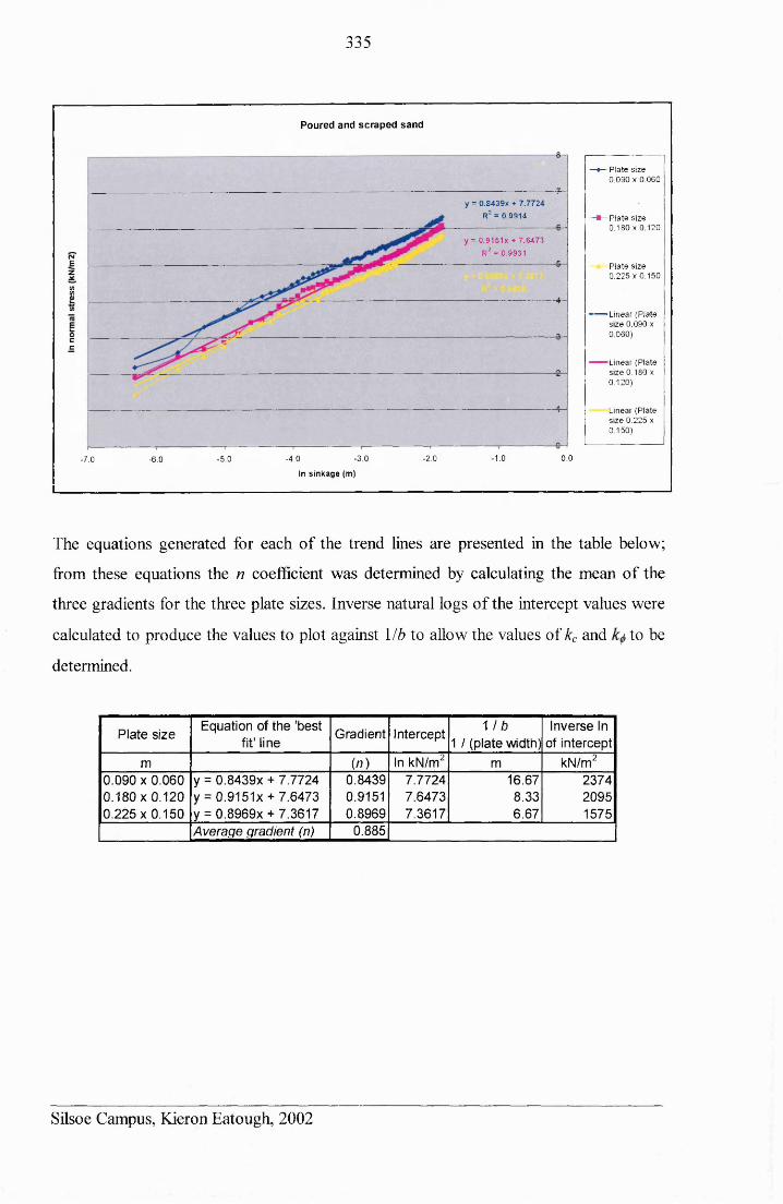
335
Poured and scraped sand
- 7 -y = 0.8439x + 7.7724
R2 = 0.9914
y = 0.9151X + 7.6473 R 2 = 0.9931CM£
zXLVIVIoU>
occ
- 2.0 •1.0 0.0-3 .0-4 .0-5 .0-7 .0 -6.0
In s in k a g e (m )
—♦— P la te s iz e 0 .0 9 0 x 0 .0 6 0
—• — P la te s iz e 0 .1 8 0 x 0 .120
P la te s ize 0 .2 2 5 x 0 .1 5 0
■— L inear (P la te s iz e 0 .0 9 0 x 0 .0 6 0 )
■Linear (P la te s iz e 0 .1 8 0 x 0 . 120)
L inear (P la te s iz e 0 .2 2 5 x 0 .1 5 0 )
The equations generated for each of the trend lines are presented in the table below;
from these equations the n coefficient was determined by calculating the mean of the
three gradients for the three plate sizes. Inverse natural logs of the intercept values were
calculated to produce the values to plot against Mb to allow the values of kc and to be
determined.
Plate size Equation of the 'best fit' line Gradient Intercept M b
1 / (plate width)Inverse In
of interceptm (Ai) In kN/m2 m kN/m2
0.090 x 0.060 y = 0.8439x + 7.7724 0.8439 7.7724 16.67 23740.180x0.120 y = 0.9151x + 7.6473 0.9151 7.6473 8.33 20950.225 x 0.150 y = 0.8969x + 7.3617 0.8969 7.3617 6.67 1575
Average gradient (n) 0.885
Silsoe Campus, Kieron Eatough, 2002
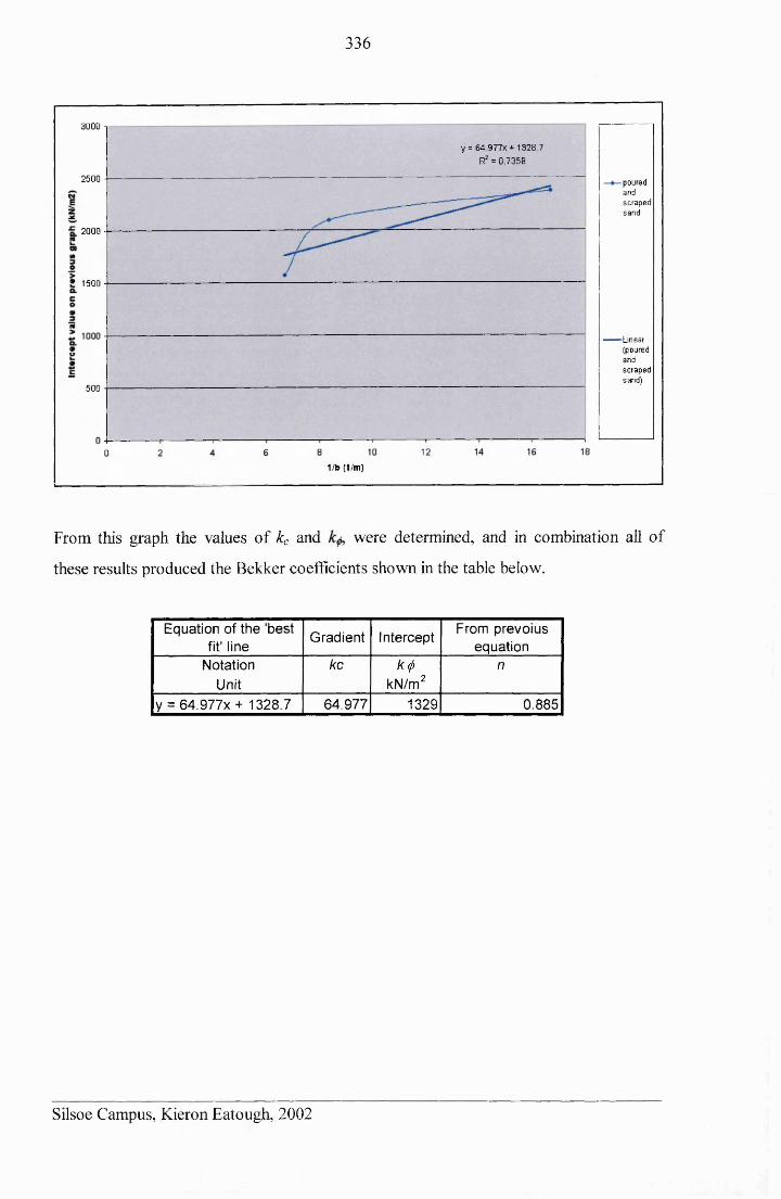
336
3 0 0 0 T
y = 6 4 .9 7 7 x + 1 3 2 8 .7
R2 = 0 .7 3 5 8
2 5 0 0 pouredandscrap edsan d
2000
2 1500
■Linear(pouredandscrap edsand)
5 0 0
1/b (1/m)
From this graph the values of kc and were determined, and in combination all of
these results produced the Bekker coefficients shown in the table below.
Equation of the 'best fit' line
Gradient Intercept From prevoius equation
Notation kc k(j) nUnit kN/m2
y = 64.977x + 1328.7 64.977 1329 0.885
Silsoe Campus, Kieron Eatough, 2002
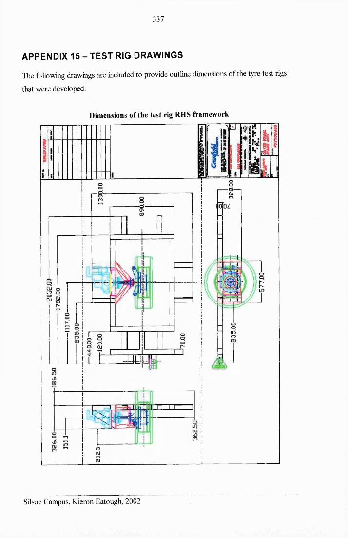
337
APPENDIX 15 - TEST RIG DRAWINGS
The following drawings are included to provide outline dimensions of the tyre test rigs
that were developed.
Dimensions of the test rig RHS framework
Silsoe Campus, Kieron Eatough, 2002
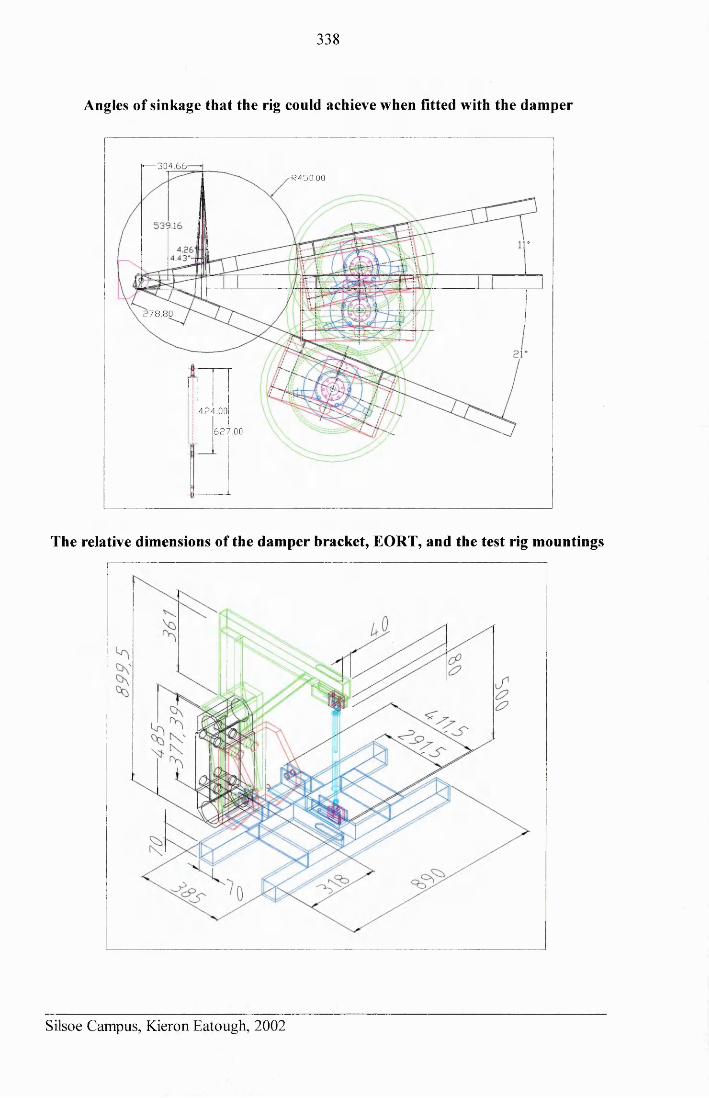
338
Angles of sinkage that the rig could achieve when fitted with the damper
h— 304.66--R450.00
2 78 .80
424.00
627.00
The relative dimensions of the damper bracket, EORT, and the test rig mountings
Silsoe Campus, Kieron Eatough, 2002
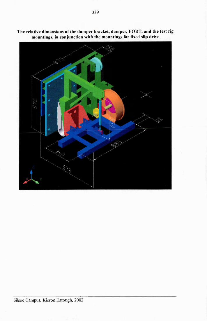
339
The relative dimensions of the damper bracket, damper, EORT, and the test rig mountings, in conjunction with the mountings for fixed slip drive
Silsoe Campus, Kieron Eatough, 2002
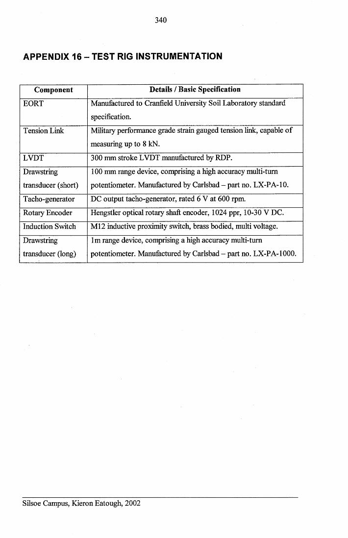
340
APPENDIX 16 - TEST RIG INSTRUMENTATION
Component Details / Basic Specification
EORT Manufactured to Cranfield University Soil Laboratory standard
specification.
Tension Link Military performance grade strain gauged tension link, capable of
measuring up to 8 kN.
LVDT 300 mm stroke LVDT manufactured by RDP.
Drawstring
transducer (short)
100 mm range device, comprising a high accuracy multi-turn
potentiometer. Manufactured by Carlsbad - part no. LX-PA-10.
Tacho-generator DC output tacho-generator, rated 6 V at 600 rpm.
Rotary Encoder Hengstler optical rotary shaft encoder, 1024 ppr, 10-30 V DC.
Induction Switch M l2 inductive proximity switch, brass bodied, multi voltage.
Drawstring
transducer (long)
lm range device, comprising a high accuracy multi-turn
potentiometer. Manufactured by Carlsbad - part no. LX-PA-1000.
Silsoe Campus, Kieron Eatough, 2002

341
APPENDIX 17 - PULSE COUNTER CIRCUIT (WHEEL SPEED)
Encoder Frequency to Voltage Conversion Circuit
The frequency to voltage conversion circuit was based around an LM2917 operational
amplifier. The encoder output was connected to the circuit shown below, which gave a
varying voltage output, which was proportional to the pulse frequency output of the
encoder (or test wheel speed).
Vcc = !5V Q
X
V A R I A B L E
R E L U C T A N C E
M A G N E T I C
P I C K U P
i
i x Tr" 1+ V q u i = 6 7
Silsoe Campus, Kieron Eatough, 2002
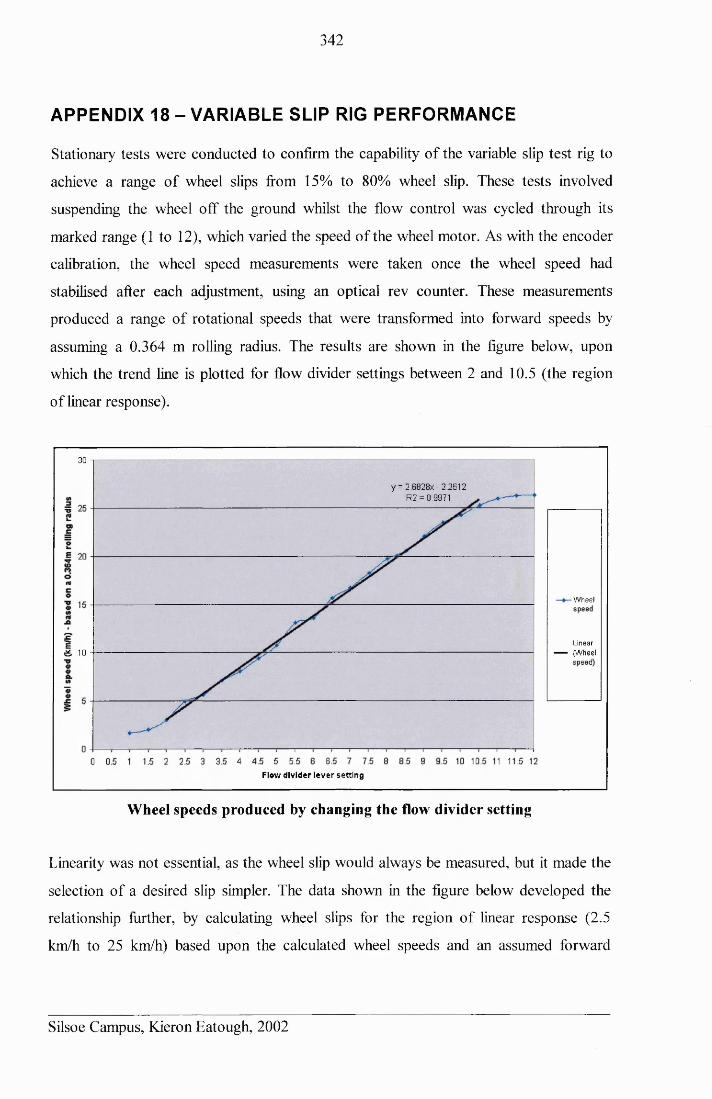
342
APPENDIX 18 - VARIABLE SLIP RIG PERFORMANCE
Stationary tests were conducted to confirm the capability of the variable slip test rig to
achieve a range of wheel slips from 15% to 80% wheel slip. These tests involved
suspending the wheel off the ground whilst the flow control was cycled through its
marked range (1 to 12), which varied the speed of the wheel motor. As with the encoder
calibration, the wheel speed measurements were taken once the wheel speed had
stabilised after each adjustment, using an optical rev counter. These measurements
produced a range of rotational speeds that were transformed into forward speeds by
assuming a 0.364 m rolling radius. The results are shown in the figure below, upon
which the trend line is plotted for flow divider settings between 2 and 10.5 (the region
of linear response).
30 ->
y = 2.6828x- 2.2612 R2 = 0.9971
W heel
Linear (W heel& 10
Flow divider lever setting
Wheel speeds produced by changing the flow divider setting
Linearity was not essential, as the wheel slip would always be measured, but it made the
selection of a desired slip simpler. The data shown in the figure below developed the
relationship further, by calculating wheel slips for the region of linear response (2.5
km/h to 25 km/h) based upon the calculated wheel speeds and an assumed forward
Silsoe Campus, Kieron Eatough, 2002
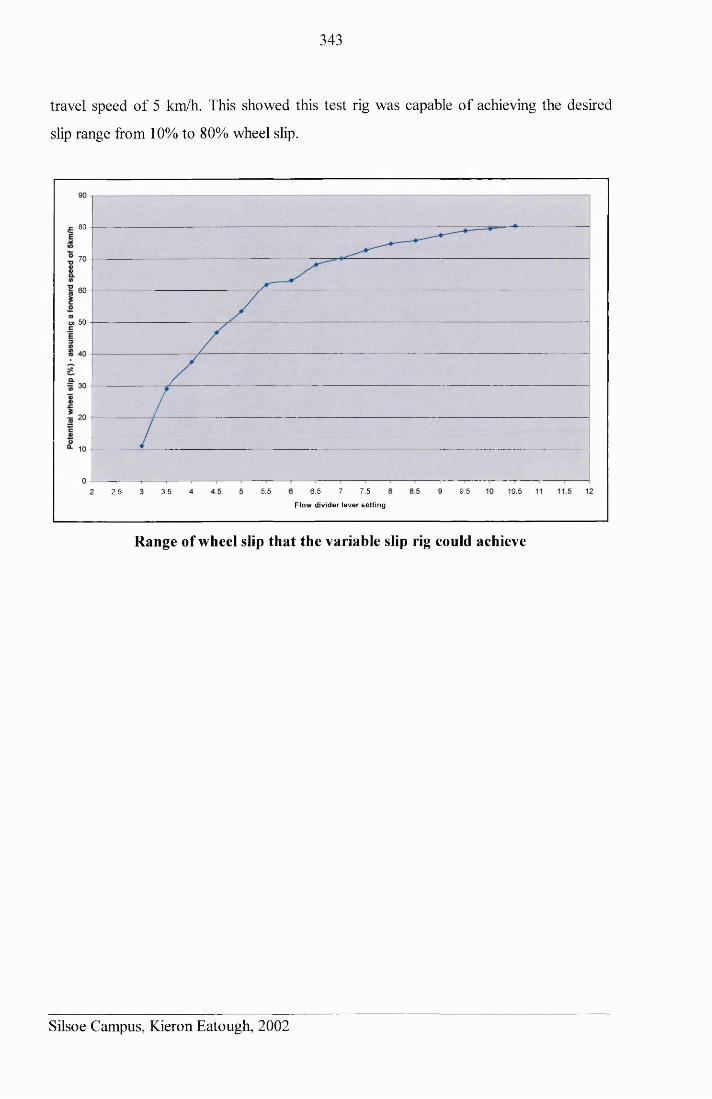
343
travel speed of 5 km/h. This showed this test rig was capable of achieving the desired
slip range from 10% to 80% wheel slip.
x: 80
O) 50
5.5 6 .5 7 7 .5
F low d iv id e r le v e r s e t t in g
9 .5 10.53.52 .5
Range of wheel slip that the variable slip rig could achieve
Silsoe Campus, Kieron Eatough, 2002
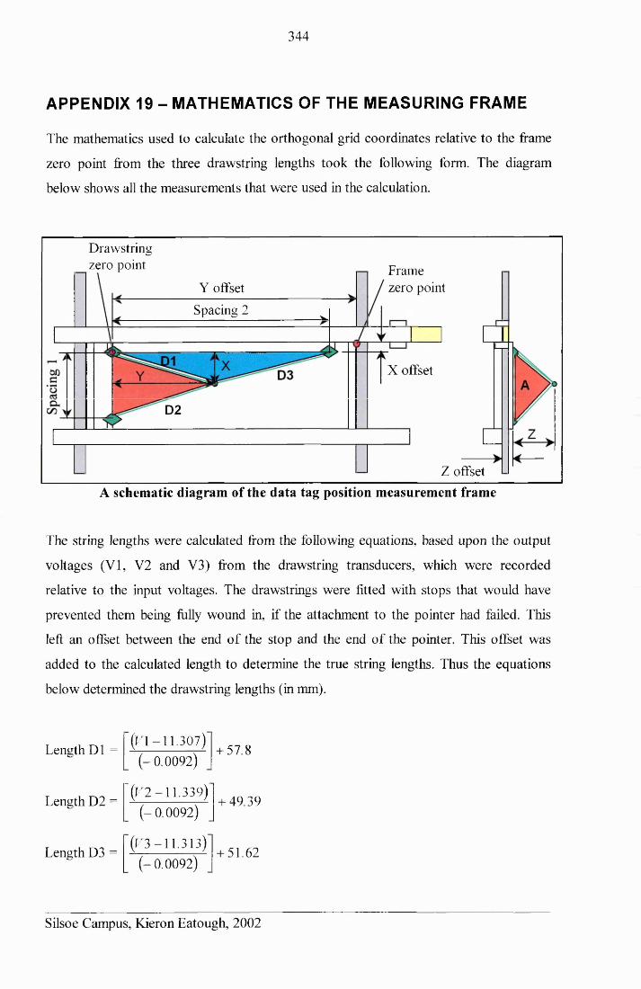
344
APPENDIX 19 - MATHEMATICS OF THE MEASURING FRAME
The mathematics used to calculate the orthogonal grid coordinates relative to the frame
zero point from the three drawstring lengths took the following form. The diagram
below shows all the measurements that were used in the calculation.
Drawstring zero point Frame
zero pointY offsetSpacing 2
X offset
D2
Z offsetA schematic diagram of the data tag position measurement frame
The string lengths were calculated from the following equations, based upon the output
voltages (VI, V2 and V3) from the drawstring transducers, which were recorded
relative to the input voltages. The drawstrings were fitted with stops that would have
prevented them being fully wound in, if the attachment to the pointer had failed. This
left an offset between the end of the stop and the end of the pointer. This offset was
added to the calculated length to determine the true string lengths. Thus the equations
below determined the drawstring lengths (in mm).
Length D1 =
Length D2 =
Length D3 =
( r i - 11.307) (-0.0092)
'( ( ’2-11.339)'(-0.0092)
((’3-11.313)(-0.0092)
+ 57.8
+ 49.39
+ 51.62
Silsoe Campus, Kieron Eatough, 2002
345
The calculation used these string lengths to determine the orthogonal coordinates
relative to the drawstring zero point by applying Pythagoras’s theorem, which was
accounts for the angular offset of 0.0028° from True Square of the three drawstring
positions.
Spacing 1 = 503.8580
Spacing 2 = 497.8555
The offset distances were then included to determine the position relative to the frame
zero point.
X offset = -25.4662
Y offset = 53.7814 + 1032 = 1085.7814
Z offset = 41.696
This methodology is clearer when studied in conjunction with the attached file
Measuring Frame Calculation (on the enclosed data CD), which presents these
equations in the form in which they were applied.
included in the equations presented below. The cosine term in the ‘X’ calculation
Distance X =
J (497.85552 +£>12 -D 3 2) L (2 x 497.8555 x Dl)
cos 0.0028
Distance Y = (-)Dl (s03.8582 + D12 - D 2 1) (2 x 503.858 x Dl)
Distance Z
Silsoe Campus, Kieron Eatough, 2002

346
APPENDIX 20 - TRIAL COLUMN INSERTION RESULTS
These results were used to determine the accuracy of the tag positioning apparatus. A
single column of tags was entered into the sand to a depth of 400 mm using the
positioning apparatus. Tags were placed at 25 mm depth intervals over the full depth.
These were not disturbed, but instead they were immediately excavated and their
positions were measured using rulers, squares and clamps. This process was repeated
six times in total. The measurements recorded are shown in the tables on the following
two pages. These results showed that the accuracy of the placement apparatus was ±1.5
mm to a depth of 300 mm and ± 2.5 mm between a depth of 325 mm and 400 mm,
which are shown at the bottom of the second set of tables (below data from insertion 6).
Silsoe Campus, Kieron Eatough, 2002
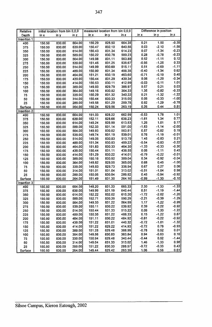
347
RelativeDepth
initial location from bin 0,0,0 inx in v in z
measured location from bin 0,0,0 in x in y in z
Difference in position in x in y in z
Insertion 1400 150.50 830.00 664.00 150.29 828.50 664.35 0.21 1.50 -0.35375 150.50 830.00 639.00 150.47 832.10 640.56 0.03 -2.10 -1.56350 150.50 830.00 614.00 150.43 831.34 614.23 0.07 -1.34 -0.23325 150.50 830.00 589.00 150.22 830.78 589.23 0.28 -0.78 -0.23300 150.50 830.00 564.00 149.98 831.11 563.88 0.52 -1.11 0.12275 150.50 830.00 539.00 151.45 831.25 538.67 -0.95 -1.25 0.33250 150.50 830.00 514.00 149.99 830.69 515.11 0.51 -0.69 -1.11225 150.50 830.00 489.00 150.90 831.34 488.38 -0.40 -1.34 0.62200 150.50 830.00 464.00 151.21 830.19 463.60 -0.71 -0.19 0.40175 150.50 830.00 439.00 150.44 831.29 439.34 0.06 -1.29 -0.34150 150.50 830.00 414.00 150.53 830.11 412.99 -0.03 -0.11 1.01125 150.50 830.00 389.00 149.93 829.79 388.97 0.57 0.21 0.03100 150.50 830.00 364.00 149.15 830.82 364.33 1.35 -0.82 -0.3375 150.50 830.00 339.00 150.29 831.32 340.22 0.21 -1.32 -1.2250 150.50 830.00 314.00 150.44 830.33 315.00 0.06 -0.33 -1.0025 150.50 830.00 289.00 149.58 831.29 289.78 0.92 -1.29 -0.78
Surface 150.50 830.00 264.00 150.24 829.56 263.19 0.26 0.44 0.81Insertion 2
400 150.50 830.00 664.00 151.03 828.22 662.99 -0.53 1.78 1.01375 150.50 830.00 639.00 152.11 828.66 638.23 -1.61 1.34 0.77350 150.50 830.00 614.00 149.24 828.99 613.83 1.26 1.01 0.17325 150.50 830.00 589.00 152.33 831.14 591.00 -1.83 -1.14 -2.00300 150.50 830.00 564.00 149.93 830.82 563.81 0.57 -0.82 0.19275 150.50 830.00 539.00 149.74 831.19 539.01 0.76 -1.19 -0.01250 150.50 830.00 514.00 149.05 830.83 513.79 1.45 -0.83 0.21225 150.50 830.00 489.00 151.04 830.83 489.22 -0.54 -0.83 -0.22200 150.50 830.00 464.00 151.83 830.33 464.30 -1.33 -0.33 -0.30175 150.50 830.00 439.00 150.44 831.11 438.55 0.06 -1.11 0.45150 150.50 830.00 414.00 151.29 830.22 414.01 -0.79 -0.22 -0.01125 150.50 830.00 389.00 150.16 830.92 389.04 0.34 -0.92 -0.04100 150.50 830.00 364.00 149.82 829.55 365.00 0.68 0.45 -1.0075 150.50 830.00 339.00 149.83 829.73 338.94 0.67 0.27 0.0650 150.50 830.00 314.00 151.01 831.04 313.02 -0.51 -1.04 0.9825 150.50 830.00 289.00 150.05 830.94 289.92 0.45 -0.94 -0.92
Surface 150.50 830.00 264.00 151.49 831.30 264.10 -0.99 -1.30 -0.10Insertion 3
400 150.50 830.00 664.00 148.20 831.33 665.33 2.30 -1.33 -1.33375 150.50 830.00 639.00 149.99 831.19 640.44 0.51 -1.19 -1.44350 150.50 830.00 614.00 152.22 832.02 615.20 -1.72 -2.02 -1.20325 150.50 830.00 589.00 152.71 830.39 590.29 -2.21 -0.39 -1.29300 150.50 830.00 564.00 149.33 831.22 564.99 1.17 -1.22 -0.99275 150.50 830.00 539.00 150.11 830.22 539.92 0.39 -0.22 -0.92250 150.50 830.00 514.00 150.44 831.33 515.22 0.06 -1.33 -1.22225 150.50 830.00 489.00 150.35 831.22 488.33 0.15 -1.22 0.67200 150.50 830.00 464.00 151.11 830.22 464.92 -0.61 -0.22 -0.92175 150.50 830.00 439.00 151.22 831.01 440.32 -0.72 -1.01 -1.32150 150.50 830.00 414.00 151.22 829.22 414.93 -0.72 0.78 -0.93125 150.50 830.00 389.00 151.28 829.48 388.99 -0.78 0.52 0.01100 150.50 830.00 364.00 149.56 830.83 363.84 0.94 -0.83 0.1675 150.50 830.00 339.00 150.94 829.48 340.44 -0.44 0.52 -1.4450 150.50 830.00 314.00 149.04 831.33 313.02 1.46 -1.33 0.9825 150.50 830.00 289.00 151.22 830.33 288.57 -0.72 -0.33 0.43
Surface 150.50 830.00 264.00 149.44 829.42 263.39 1.06 0.58 0.61
Silsoe Campus, Kieron Eatough, 2002
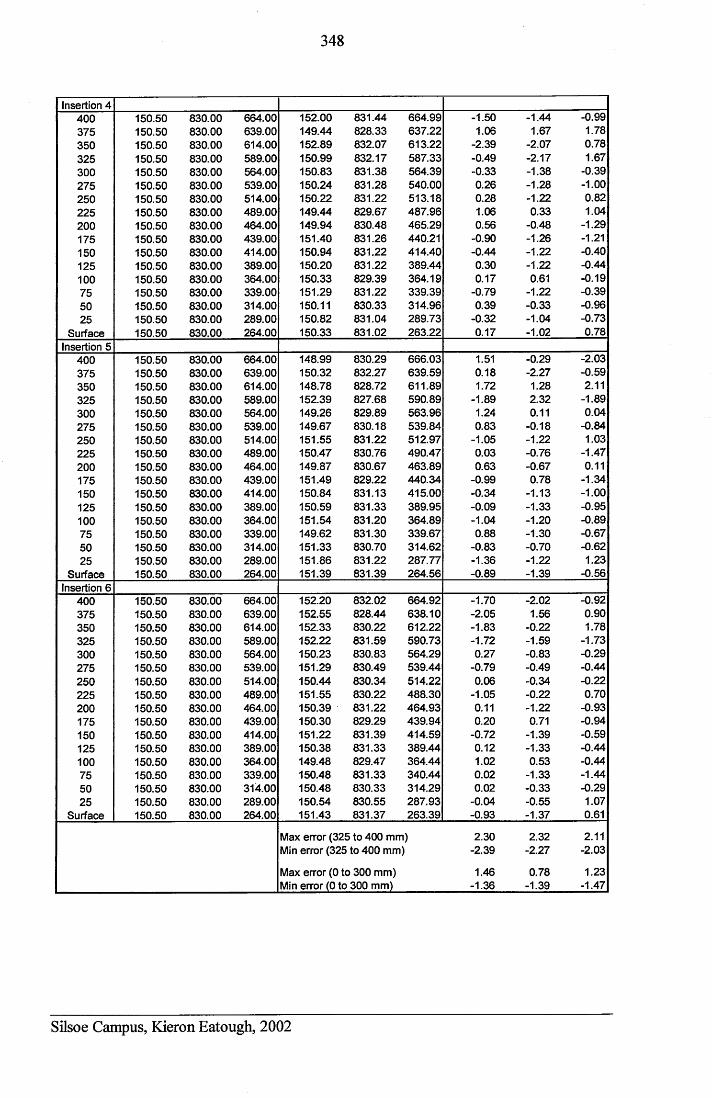
348
Insertion 4400 150.50 830.00 664.00 152.00 831.44 664.99 -1.50 -1.44 -0.99375 150.50 830.00 639.00 149.44 828.33 637.22 1.06 1.67 1.78350 150.50 830.00 614.00 152.89 832.07 613.22 -2.39 -2.07 0.78325 150.50 830.00 589.00 150.99 832.17 587.33 -0.49 -2.17 1.67300 150.50 830.00 564.00 150.83 831.38 564.39 -0.33 -1.38 -0.39275 150.50 830.00 539.00 150.24 831.28 540.00 0.26 -1.28 -1.00250 150.50 830.00 514.00 150.22 831.22 513.18 0.28 -1.22 0.82225 150.50 830.00 489.00 149.44 829.67 487.96 1.06 0.33 1.04200 150.50 830.00 464.00 149.94 830.48 465.29 0.56 -0.48 -1.29175 150.50 830.00 439.00 151.40 831.26 440.21 -0.90 -1.26 -1.21150 150.50 830.00 414.00 150.94 831.22 414.40 -0.44 -1.22 -0.40125 150.50 830.00 389.00 150.20 831.22 389.44 0.30 -1.22 -0.44100 150.50 830.00 364.00 150.33 829.39 364.19 0.17 0.61 -0.1975 150.50 830.00 339.00 151.29 831.22 339.39 -0.79 -1.22 -0.3950 150.50 830.00 314.00 150.11 830.33 314.96 0.39 -0.33 -0.9625 150.50 830.00 289.00 150.82 831.04 289.73 -0.32 -1.04 -0.73
Surface 150.50 830.00 264.00 150.33 831.02 263.22 0.17 -1.02 0.78Insertion 5
400 150.50 830.00 664.00 148.99 830.29 666.03 1.51 -0.29 -2.03375 150.50 830.00 639.00 150.32 832.27 639.59 0.18 -2.27 -0.59350 150.50 830.00 614.00 148.78 828.72 611.89 1.72 1.28 2.11325 150.50 830.00 589.00 15Z39 827.68 590.89 -1.89 2.32 -1.89300 150.50 830.00 564.00 149.26 829.89 563.96 1.24 0.11 0.04275 150.50 830.00 539.00 149.67 830.18 539.84 0.83 -0.18 -0.84250 150.50 830.00 514.00 151.55 831.22 512.97 -1.05 -1.22 1.03225 150.50 830.00 489.00 150.47 830.76 490.47 0.03 -0.76 -1.47200 150.50 830.00 464.00 149.87 830.67 463.89 0.63 -0.67 0.11175 150.50 830.00 439.00 151.49 829.22 440.34 -0.99 0.78 -1.34150 150.50 830.00 414.00 150.84 831.13 415.00 -0.34 -1.13 -1.00125 150.50 830.00 389.00 150.59 831.33 389.95 -0.09 -1.33 -0.95100 150.50 830.00 364.00 151.54 831.20 364.89 -1.04 -1.20 -0.8975 150.50 830.00 339.00 149.62 831.30 339.67 0.88 -1.30 -0.6750 150.50 830.00 314.00 151.33 830.70 314.62 -0.83 -0.70 -0.6225 150.50 830.00 289.00 151.86 831.22 287.77 -1.36 -1.22 1.23
Surface 150.50 830.00 264.00 151.39 831.39 264.56 -0.89 -1.39 -0.56Insertion 6
400 150.50 830.00 664.00 152.20 832.02 664.92 -1.70 -2.02 -0.92375 150.50 830.00 639.00 152.55 828.44 638.10 -2.05 1.56 0.90350 150.50 830.00 614.00 152.33 830.22 612.22 -1.83 -0.22 1.78325 150.50 830.00 589.00 152.22 831.59 590.73 -1.72 -1.59 -1.73300 150.50 830.00 564.00 150.23 830.83 564.29 0.27 -0.83 -0.29275 150.50 830.00 539.00 151.29 830.49 539.44 -0.79 -0.49 -0.44250 150.50 830.00 514.00 150.44 830.34 514.22 0.06 -0.34 -0.22225 150.50 830.00 489.00 151.55 830.22 488.30 -1.05 -0.22 0.70200 150.50 830.00 464.00 150.39 831.22 464.93 0.11 -1.22 -0.93175 150.50 830.00 439.00 150.30 829.29 439.94 0.20 0.71 -0.94150 150.50 830.00 414.00 151.22 831.39 414.59 -0.72 -1.39 -0.59125 150.50 830.00 389.00 150.38 831.33 389.44 0.12 -1.33 -0.44100 150.50 830.00 364.00 149.48 829.47 364.44 1.02 0.53 -0.4475 150.50 830.00 339.00 150.48 831.33 340.44 0.02 -1.33 -1.4450 150.50 830.00 314.00 150.48 830.33 314.29 0.02 -0.33 -0.2925 150.50 830.00 289.00 150.54 830.55 287.93 -0.04 -0.55 1.07
Surface 150.50 830.00 264.00 151.43 831.37 263.39 -0.93 -1.37 0.61
Max error (325 to 400 mm) 2.30 2.32 2.11Min error (325 to 400 mm] -2.39 -2.27 -2.03
Max error (0 to 300 mm) 1.46 0.78 1.23Min error (0 to 300 mm) -1.36 -1.39 -1.47
Silsoe Campus, Kieron Eatough, 2002
349
APPENDIX 21 - TRIAL GRID INSERTION RESULTS
The results from this trail were used to determine the accuracy of the tag positioning
and measurement apparatus as a total package. Three complete grids of tags (64 tags in
each grid) were entered into the sand in the standard grid alignment. These were not
disturbed, but instead they were immediately excavated and their positions were
measured using the measurement frame. This produced the measurements recorded in
the three tables below, which compared the measurements to the tags intended
positions. These results showed that the accuracy of the placement and measurement
apparatus in combination was ±5.5 mm in any direction (as indicated in the top right
comer of first table). The error in repeatability for measurements of the same grid
position over the three grids was ±3.5 mm. The frill results, including the spatial
calculations are copied on the enclosed data CD, see file: 3 trial tag grid insertions.
Silsoe Campus, Kieron Eatough, 2002
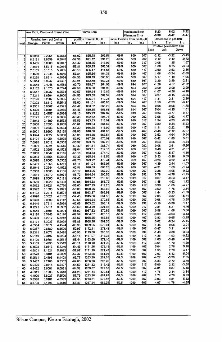
350
use Pexit, Pzero and Frame Zero Frame Zero Maximum Error Minimum Error
5.23-5.38
5.02-5.47
5.22-5.47
Reading from pot (volts) position from bin 0,0,0 initial location from bin 0,0,0 Difference in positionpoint Orange Purple Brown in x in v in z in x in v inz in x in v inz
Positive (viewdown bin)Back Left Down
1 8.5058 9.2054 6.3512 -61.62 865.78 263.51 -59.5 869 267 -2.12 -3.22 -3.492 8.3121 9.0559 6.3048 -57.38 871.12 291.28 -59.5 869 292 2.12 2.12 -0.723 8.1455 8.8586 6.2047 -66.42 870.85 318.97 -59.5 869 317 3.08 1.85 1.974 7.8614 8.5215 6.0014 -57.81 869.75 363.37 -59.5 869 367 1.69 0.75 -3.635 7.5165 8.1018 5.7085 -63.10 866.47 414.84 -59.5 869 417 -3.60 -2.53 -2.166 7.1589 7.7048 5.4845 -57.84 865.66 464.31 -59.5 869 467 1.66 -3.34 -2.697 6.3258 6.8514 4.9054 -54.33 870.19 568.96 -59.5 869 567 5.17 1.19 1.968 5.5014 5.9947 4.2437 -56.21 872.49 669.21 -59.5 869 667 3.29 3.49 2.219 8.2648 9.4048 6.4568 -60.70 898.57 264.08 -59.5 894 267 -1.20 4.57 -2.92
10 8.1132 9.1670 6.3244 -62.59 896.00 294.99 -59.5 894 292 -3.09 2.00 2.9911 8.0547 9.0032 6.2534 -60.57 889.64 312.82 -59.5 894 317 -1.07 -4.36 -4.1812 7.7211 8.6504 6.1000 -54.53 893.85 362.34 -59.5 894 367 4.97 -0.15 -4.6613 7.3196 8.2007 5.8035 -58.19 896.31 419.26 -59.5 894 417 1.31 2.31 2.2614 7.0302 7.8112 5.5543 -58.00 891.01 463.83 -59.5 894 467 1.50 -2.99 -3.1715 6.2501 6.9567 4.9521 -59.42 893.02 565.22 -59.5 894 567 0.08 -0.98 -1.7816 5.4390 6.0501 4.2965 -54.46 889.85 668.61 -59.5 894 667 5.04 -4.15 1.6117 8.1232 9.4757 6.5024 -59.16 915.23 267.67 -59.5 919 267 0.34 -3.77 0.6718 7.9121 9.2912 6.3806 -63.46 922.62 296.77 -59.5 919 292 -3.96 3.62 4.7719 7.8043 9.1509 6.3533 -57.56 923.33 316.01 -59.5 919 317 1.94 4.33 -0.9920 7.5600 8.7690 6.1603 -55.61 919.34 361.67 -59.5 919 367 3.89 0.34 -5.3321 7.2001 8.2833 5.8534 -58.39 916.78 418.99 -59.5 919 417 1.11 -2.22 1.9922 6.9001 7.9200 5.6128 -59.96 916.88 461.93 -59.5 919 467 -0.46 -2.12 -5.0723 6.1324 7.0027 5.0060 -55.98 914.36 567.54 -59.5 919 567 3.52 -4.64 0.5424 5.3121 6.1054 4.3098 -59.92 917.20 670.01 -59.5 919 667 -0.42 -1.80 3.0125 7.6990 9.8012 6.6503 -58.97 973.55 262.26 -59.5 969 267 0.53 4.55 -4.7426 7.6001 9.5921 6.5545 -59.42 971.61 286.74 -59.5 969 292 0.08 2.61 -5.2627 7.4502 9.3696 6.4523 -59.04 973.31 314.13 -59.5 969 317 0.46 4.31 -2.8728 7.2050 8.8547 6.2115 -55.18 963.53 371.10 -59.5 969 367 4.32 -5.47 4.1029 6.9013 8.4554 5.9512 -59.37 965.84 417.59 -59.5 969 417 0.13 -3.16 0.5930 6.5076 8.0065 5.6502 -62.76 973.22 470.41 -59.5 969 467 -3.26 4.22 3.4131 5.8481 7.1555 5.1211 -55.11 971.94 565.97 -59.5 969 567 4.39 2.94 -1.0332 5.1044 6.2544 4.4032 -63.81 970.69 665.26 -59.5 969 667 -4.31 1.69 -1.7433 7.3560 9.9033 6.7155 -56.12 1014.05 267.22 -59.5 1019 267 3.38 -4.95 0.2234 7.2511 9.6970 6.6071 -58.72 1014.24 290.55 -59.5 1019 292 0.78 -4.76 -1.4535 7.1098 9.5006 6.5121 -59.43 1018.37 313.83 -59.5 1019 317 0.07 -0.63 -3.1736 6.8560 9.0020 6.2498 -60.98 1014.38 368.72 -59.5 1019 367 -1.48 -4.62 1.7237 6.5862 8.6221 6.0760 -55.60 1017.95 412.23 -59.5 1019 417 3.90 -1.05 -4.7738 6.2522 8.1590 5.7921 -56.00 1020.76 463.86 -59.5 1019 467 3.50 1.76 -3.1439 5.6122 7.2216 5.1501 -58.06 1013.87 565.91 -59.5 1019 567 1.44 -5.13 -1.0940 4.9096 6.3521 4.5132 -57.45 1015.68 661.56 -59.5 1019 667 2.05 -3.32 -5.4441 6.9320 9.9599 6.7112 -59.58 1064.24 270.65 -59.5 1069 267 -0.08 -4.76 3.6542 6.8440 9.7511 6.5999 -62.69 1063.62 293.17 -59.5 1069 292 -3.19 -5.38 1.1743 6.7221 9.5011 6.5332 -56.69 1063.79 321.46 -59.5 1069 317 2.81 -5.21 4.4644 6.4548 9.0501 6.2904 -58.92 1067.32 370.86 -59.5 1069 367 0.58 -1.68 3.8645 6.2126 8.5948 6.0110 -62.59 1064.07 420.13 -59.5 1069 417 -3.09 -4.93 3.1346 5.9330 8.2017 5.8212 -55.67 1068.35 463.85 -59.5 1069 467 3.83 -0.65 -3.1547 5.3121 7.3037 5.2029 -58.88 1068.76 561.55 -59.5 1069 567 0.62 -0.24 -5.4548 4.5534 6.3072 4.4594 -60.95 1069.96 670.01 -59.5 1069 667 -1.45 0.96 3.0149 6.0287 9.8189 6.6500 -59.97 1172.11 271.41 -59.5 1169 267 -0.47 3.11 4.4150 5.9311 9.6071 6.5498 -60.93 1173.88 295.33 -59.5 1169 292 -1.43 4.88 3.3351 5.9119 9.4492 6.5204 -55.14 1167.07 316.38 -59.5 1169 317 4.36 -1.93 -0.6252 5.7100 8.9701 6.2511 -58.44 1163.60 371.10 -59.5 1169 367 1.06 -5.40 4.1053 5.4139 8.4990 5.9513 -63.11 1170.70 421.79 -59.5 1169 417 -3.61 1.70 4.7954 5.1502 8.0513 5.7340 -54.46 1171.76 472.18 -59.5 1169 467 5.04 2.76 5.1855 4.5801 7.1521 5.1013 -57.97 1171.70 571.47 -59.5 1169 567 1.53 2.70 4.4756 4.0570 6.3401 4.5039 -57.47 1163.58 661.96 -59.5 1169 667 2.03 -5.42 -5.0457 5.2511 9.4195 6.4408 -63.77 1263.70 269.05 -59.5 1269 267 -4.27 -5.30 2.0558 5.1487 9.2108 6.3302 -64.83 1266.28 295.49 -59.5 1269 292 -5.33 -2.72 3.4959 5.0495 9.0514 6.2497 -64.59 1271.12 313.42 -59.5 1269 317 -5.09 2.12 -3.5860 4.8462 8.6001 6.0021 -64.31 1269.87 372.18 -59.5 1269 367 -4.81 0.87 5.1861 4.6311 8.1985 5.7613 -64.26 1271.44 420.84 -59.5 1269 417 -4.76 2.44 3.8462 4.4000 7.8027 5.5500 -57.79 1273.76 467.93 -59.5 1269 467 1.71 4.76 0.9363 3.8598 6.9101 4.8999 -62.53 1273.81 572.12 -59.5 1269 567 -3.03 4.81 5.1264 3.3798 6.1398 4.3610 -55.43 1267.24 662.75 -59.5 1269 667 4.07 -1.76 -4.25
Silsoe Campus, Kieron Eatough, 2002
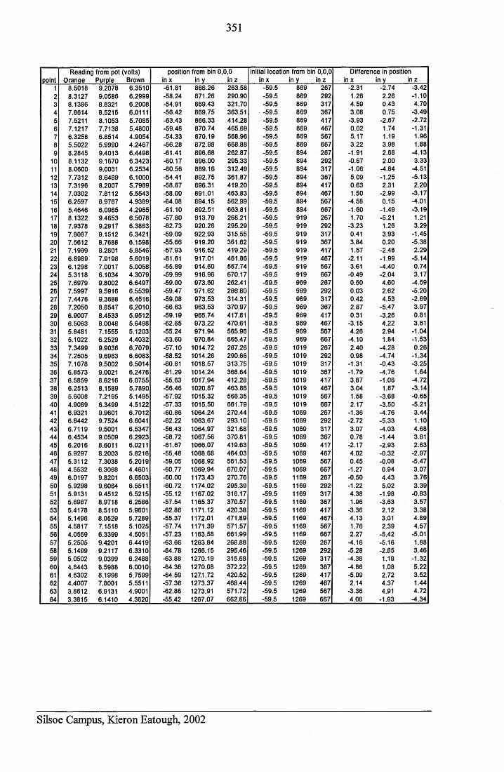
351
pointReading from pot (volts)
Orange Purple Brownposition from bin 0,0,0
in x in y in zinitial location from bin 0,0,0
in x in y in zDifference in position
in x in y in z1 8.5018 9.2078 6.3510 -61.81 866.26 263.58 -59.5 869 267 -2.31 -2.74 -3.422 8.3127 9.0586 6.2999 -58.24 871.26 290.90 -59.5 869 292 1.26 2.26 -1.103 8.1386 8.8321 6.2008 -54.91 869.43 321.70 -59.5 869 317 4.59 0.43 4.704 7.8614 8.5215 6.0111 -56.42 869.75 363.51 -59.5 869 367 3.08 0.75 -3.495 7.5211 8.1053 5.7085 -63.43 866.33 414.28 -59.5 869 417 -3.93 -2.67 -2.726 7.1217 7.7138 5.4800 -59.48 870.74 465.69 -59.5 869 467 0.02 1.74 -1.317 6.3258 6.8514 4.9054 -54.33 870.19 568.96 -59.5 869 567 5.17 1.19 1.968 5.5022 5.9990 4.2467 -56.28 872.98 668.88 -59.5 869 667 3.22 3.98 1.889 8.2845 9.4013 6.4498 -61.41 896.68 262.87 -59.5 894 267 -1.91 2.68 -4.13
10 8.1132 9.1670 6.3423 -60.17 896.00 295.33 -59.5 894 292 -0.67 2.00 3.3311 8.0600 9.0031 6.2534 -60.56 889.16 312.49 -59.5 894 317 -1.06 -4.84 -4.5112 7.7312 8.6489 6.1000 -54.41 892.75 361.87 -59.5 894 367 5.09 -1.25 -5.1313 7.3196 8.2007 5.7989 -58.87 896.31 419.20 -59.5 894 417 0.63 2.31 2.2014 7.0302 7.8112 5.5543 -58.00 891.01 463.83 -59.5 894 467 1.50 -2.99 -3.1715 6.2597 6.9767 4.9389 -64.08 894.15 562.99 -59.5 894 567 -4.58 0.15 -4.0116 5.4646 6.0965 4.2965 -61.10 892.51 663.81 -59.5 894 667 -1.60 -1.49 -3.1917 8.1322 9.4653 6.5078 -57.80 913.79 268.21 -59.5 919 267 1.70 -5.21 1.2118 7.9378 9.2917 6.3863 -62.73 920.26 295.29 -59.5 919 292 -3.23 1.26 3.2919 7.8087 9.1512 6.3421 -59.09 922.93 315.55 -59.5 919 317 0.41 3.93 -1.4520 7.5612 8.7688 6.1598 -55.66 919.20 361.62 -59.5 919 367 3.84 0.20 -5.3821 7.1999 8.2801 5.8546 -57.93 916.52 419.29 -59.5 919 417 1.57 -2.48 2.2922 6.8989 7.9198 5.6019 -61.61 917.01 461.86 -59.5 919 467 -2.11 -1.99 -5.1423 6.1298 7.0017 5.0058 -55.89 914.60 567.74 -59.5 919 567 3.61 -4.40 0.7424 5.3118 6.1034 4.3079 -59.99 916.96 670.17 -59.5 919 667 -0.49 -2.04 3.1725 7.6979 9.8002 6.6497 -59.00 973.60 262.41 -59.5 969 267 0.50 4.60 -4.5926 7.5997 9.5916 6.5539 -59.47 971.62 286.80 -59.5 969 292 0.03 2.62 -5.2027 7.4476 9.3688 6.4516 -59.08 973.53 314.31 -59.5 969 317 0.42 4.53 -2.6928 7.2050 8.8547 6.2010 -56.63 963.53 370.97 -59.5 969 367 2.87 -5.47 3.9729 6.9007 8.4533 5.9512 -59.19 965.74 417.81 -59.5 969 417 0.31 -3.26 0.8130 6.5063 8.0048 5.6498 -62.65 973.22 470.61 -59.5 969 467 -3.15 4.22 3.6131 5.8481 7.1555 5.1203 -55.24 971.94 565.96 -59.5 969 567 4.26 2.94 -1.0432 5.1022 6.2529 4.4032 -63.60 970.84 665.47 -59.5 969 667 -4.10 1.84 -1.5333 7.3499 9.9036 6.7079 -57.10 1014.72 267.26 -59.5 1019 267 2.40 -4.28 0.2634 7.2505 9.6963 6.6083 -58.52 1014.26 290.66 -59.5 1019 292 0.98 -4.74 -1.3435 7.1078 9.5002 6.5014 -60.81 1018.57 313.75 -59.5 1019 317 -1.31 -0.43 -3.2536 6.8573 9.0021 6.2476 -61.29 1014.24 368.64 -59.5 1019 367 -1.79 -4.76 1.6437 6.5859 8.6216 6.0755 -55.63 1017.94 412.28 -59.5 1019 417 3.87 -1.06 -4.7238 6.2513 8.1589 5.7890 -56.46 1020.87 463.86 -59.5 1019 467 3.04 1.87 -3.1439 5.6008 7.2195 5.1495 -57.92 1015.32 566.35 -59.5 1019 567 1.58 -3.68 -0.6540 4.9089 6.3499 4.5122 -57.33 1015.50 661.79 -59.5 1019 667 2.17 -3.50 -5.2141 6.9321 9.9601 6.7012 -60.86 1064.24 270.44 -59.5 1069 267 -1.36 -4.76 3.4442 6.8442 9.7524 6.6041 -62.22 1063.67 293.10 -59.5 1069 292 -2.72 -5.33 1.1043 6.7119 9.5001 6.5347 -56.43 1064.97 321.68 -59.5 1069 317 3.07 -4.03 4.6844 6.4534 9.0509 6.2923 -58.72 1067.56 370.81 -59.5 1069 367 0.78 -1.44 3.8145 6.2016 8.6011 6.0211 -61.67 1066.07 419.63 -59.5 1069 417 -2.17 -2.93 2.6346 5.9297 8.2003 5.8216 -55.48 1068.68 464.03 -59.5 1069 467 4.02 -0.32 -2.9747 5.3112 7.3038 5.2019 -59.05 1068.92 561.53 -59.5 1069 567 0.45 -0.08 -5.4748 4.5532 6.3068 4.4601 -60.77 1069.94 670.07 -59.5 1069 667 -1.27 0.94 3.0749 6.0197 9.8201 6.6503 -60.00 1173.43 270.76 -59.5 1169 267 -0.50 4.43 3.7650 5.9298 9.6064 6.5511 -60.72 1174.02 295.39 -59.5 1169 292 -1.22 5.02 3.3951 5.9131 9.4512 6.5215 -55.12 1167.02 316.17 -59.5 1169 317 4.38 -1.98 -0.8352 5.6987 8.9718 6.2586 -57.54 1165.37 370.57 -59.5 1169 367 1.96 -3.63 3.5753 5.4178 8.5110 5.9601 -62.86 1171.12 420.38 -59.5 1169 417 -3.36 2.12 3.3854 5.1496 8.0529 5.7289 -55.37 1172.01 471.89 -59.5 1169 467 4.13 3.01 4.8955 4.5817 7.1518 5.1025 -57.74 1171.39 571.57 -59.5 1169 567 1.76 2.39 4.5756 4.0569 6.3399 4.5051 -57.23 1163.58 661.99 -59.5 1169 667 2.27 -5.42 -5.0157 5.2505 9.4201 6.4419 -63.66 1263.84 268.88 -59.5 1269 267 -4.16 -5.16 1.8858 5.1499 9.2117 6.3310 -64.78 1266.15 295.46 -59.5 1269 292 -5.28 -2.85 3.4659 5.0502 9.0399 6.2488 -63.88 1270.19 315.68 -59.5 1269 317 -4.38 1.19 -1.3260 4.8443 8.5988 6.0010 -64.36 1270.08 372.22 -59.5 1269 367 -4.86 1.08 5.2261 4.6302 8.1998 5.7599 -64.59 127,1.72 420.52 -59.5 1269 417 -5.09 2.72 3.5262 4.4007 7.8001 5.5511 -57.36 1273.37 468.44 -59.5 1269 467 2.14 4.37 1.4463 3.8612 6.9131 4.9001 -62.86 1273.91 571.72 -59.5 1269 567 -3.36 4.91 4.7264 3.3815 6.1410 4.3620 -55.42 1267.07 662.66 -59.5 1269 667 4.08 -1.93 -4.34
Silsoe Campus, Kieron Eatough, 2002
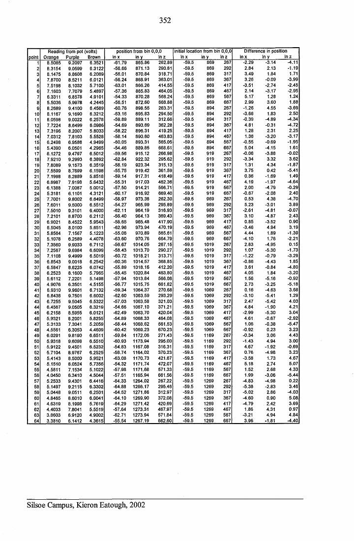
352
pointReading from pot (volts)
Orange Purple Brownposition from bin 0,0,0
in x in v in zinitial location from bin 0,0,0
in x in y in zDifference in position
in x in y in z1 8.5085 9.2097 6.3521 -61.79 865.86 262.89 -59.5 869 267 -2.29 -3.14 -4.112 8.3154 9.0599 6.3122 -56.66 871.13 290.81 -59.5 869 292 2.84 2.13 -1.193 8.1475 8.8608 6.2089 -56.01 870.84 318.71 -59.5 869 317 3.49 1.84 1.714 7.8700 8.5211 6.0121 -56.24 868.91 363.01 -59.5 869 367 3.26 -0.09 -3.995 7.5198 8.1032 5.7100 -63.01 866.26 414.55 -59.5 869 417 -3.51 -2.74 -2.456 7.1603 7.7079 5.4897 -57.36 865.83 464.05 -59.5 869 467 2.14 -3.17 -2.957 6.3311 6.8578 4.9101 -54.33 870.28 568.24 -59.5 869 567 5.17 1.28 1.248 5.5036 5.9978 4.2445 -56.51 872.60 668.88 -59.5 869 667 2.99 3.60 1.889 8.2689 9.4100 6.4589 -60.76 898.55 263.31 -59.5 894 267 -1.26 4.55 -3.69
10 8.1167 9.1690 6.3212 -63.16 895.83 294.50 -59.5 894 292 -3.66 1.83 2.5011 8.0598 9.0022 6.2578 -59.89 889.11 312.66 -59.5 894 317 -0.39 -4.89 -4.3412 7.7224 8.6499 6.0986 -54.69 893.69 362.28 -59.5 894 367 4.81 -0.31 -4.7213 7.3196 8.2007 5.8033 -58.22 896.31 419.25 -59.5 894 417 1.28 2.31 2.2514 7.0312 7.8103 5.5528 -58.14 890.80 463.83 -59.5 894 467 1.36 -3.20 -3.1715 6.2498 6.9588 4.9499 -60.05 893.31 565.05 -59.5 894 567 -0.55 -0.69 -1.9516 5.4390 6.0501 4.2965 -54.46 889.85 668.61 -59.5 894 667 5.04 -4.15 1.6117 8.1272 9.4797 6.5012 -59.56 915.12 266.98 -59.5 919 267 -0.06 -3.88 -0.0218 7.9210 9.2993 6.3892 -62.84 922.32 295.62 -59.5 919 292 -3.34 3.32 3.6219 7.8089 9.1573 6.3519 -58.19 923.34 315.13 -59.5 919 317 1.31 4.34 -1.8720 7.5599 8.7699 6.1598 -55.75 919.42 361.59 -59.5 919 367 3.75 0.42 -5.4121 7.1998 8.2889 5.8518 -59.14 917.31 418.49 -59.5 919 417 0.36 -1.69 1.4922 6.8987 7.9198 5.6432 -55.31 917.03 462.36 -59.5 919 467 4.19 -1.97 -4.6423 6.1388 7.0087 5.0012 -57.50 914.21 566.71 -59.5 919 567 2.00 -4.79 -0.2924 5.3181 6.1101 4.3121 -60.17 916.92 669.40 -59.5 919 667 -0.67 -2.08 2.4025 7.7001 9.8002 6.6499 -58.97 973.38 262.30 -59.5 969 267 0.53 4.38 -4.7026 7.6011 9.5000 6.5512 -54.27 965.99 295.89 -59.5 969 292 5.23 -3.01 3.8927 7.5010 9.3101 6.4000 -62.11 964.19 316.93 -59.5 969 317 -2.61 -4.81 -0.0728 7.2101 8.8700 6.2112 -56.40 964.13 369.43 -59.5 969 367 3.10 -4.87 2.4329 6.9021 8.4522 5.9543 -58.65 965.48 417.90 -59.5 969 417 0.85 -3.52 0.9030 6.5045 8.0100 5.6511 -62.96 973.94 470.19 -59.5 969 467 -3.46 4.94 3.1931 5.8564 7.1567 5.1223 -55.06 970.89 565.61 -59.5 969 567 4.44 1.89 -1.3932 5.1078 6.2589 4.4078 -63.60 970.76 664.79 -59.5 969 667 -4.10 1.76 -2.2133 7.3560 9.9033 6.7112 -56.67 1014.05 267.15 -59.5 1019 267 2.83 -4.95 0.1534 7.2567 9.6984 6.6099 -58.43 1013.70 290.27 -59.5 1019 292 1.07 -5.30 -1.7335 7.1108 9.4999 6.5019 -60.72 1018.21 313.71 -59.5 1019 317 -1.22 -0.79 -3.2936 6.8543 9.0018 6.2542 -60.36 1014.57 368.85 -59.5 1019 367 -0.86 -4.43 1.8537 6.5847 8.6225 6.0742 -55.89 1018.16 412.20 -59.5 1019 417 3.61 -0.84 -4.8038 6.2523 8.1600 5.7965 -55.45 1020.84 463.80 -59.5 1019 467 4.05 1.84 -3.2039 5.6112 7.2201 5.1498 -57.94 1013.84 566.08 -59.5 1019 567 1.56 -5.16 -0.9240 4.9076 6.3501 4.5155 -56.77 1015.75 661.82 -59.5 1019 667 2.73 -3.25 -5.1841 6.9310 9.9601 6.7132 -59.34 1064.37 270.68 -59.5 1069 267 0.16 -4.63 3.6842 6.8438 9.7501 6.6002 -62.60 1063.59 293.29 -59.5 1069 292 -3.10 -5.41 1.2943 6.7255 9.5045 6.5322 -57.03 1063.58 321.03 -59.5 1069 317 2.47 -5.42 4.0344 6.4567 9.0505 6.3219 -54.66 1067.10 371.21 -59.5 1069 367 4.84 -1.90 4.2145 6.2158 8.5955 6.0121 -62.49 1063.70 420.04 -59.5 1069 417 -2.99 -5.30 3.0446 5.9321 8.2001 5.8255 -54.89 1068.33 464.08 -59.5 1069 467 4.61 -0.67 -2.9247 5.3133 7.3041 5.2059 -58.44 1068.62 561.53 -59.5 1069 567 1.06 -0.38 -5.4748 4.5561 6.3053 4.4609 -60.42 1069.23 670.23 -59.5 1069 667 -0.92 0.23 3.2349 6.0291 9.8190 6.6511 -59.84 1172.06 271.43 -59.5 1169 267 -0.34 3.06 4.4350 5.9318 9.6098 6.5510 -60.93 1173.94 295.00 -59.5 1169 292 -1.43 4.94 3.0051 5.9122 9.4501 6.5232 -54.83 1167.08 316.31 -59.5 1169 317 4.67 -1.92 -0.6952 5.7104 8.9767 6.2525 -58.74 1164.02 370.23 -59.5 1169 367 0.76 -4.98 3.2353 5.4143 8.5000 5.9521 -63.08 1170.73 421.67 -59.5 1169 417 -3.58 1.73 4.6754 5.1510 8.0524 5.7356 -54.32 1171.74 472.07 -59.5 1169 467 5.18 2.74 5.0755 4.5811 7.1534 5.1022 -57.98 1171.68 571.33 -59.5 1169 567 1.52 2.68 4.3356 4.0450 6.3410 4.5044 -57.51 1165.94 661.56 -59.5 1169 667 1.99 -3.06 -5.4457 5.2533 9.4301 6.4416 -64.33 1264.02 267.22 -59.5 1269 267 -4.83 -4.98 0.2258 5.1497 9.2115 6.3302 -64.88 1266.17 295.46 -59.5 1269 292 -5.38 -2.83 3.4659 5.0448 9.0511 6.2501 -64.52 1271.86 312.97 -59.5 1269 317 -5.02 2.86 -4.0360 4.8465 8.6010 6.0041 -64.10 1269.90 372.08 -59.5 1269 367 -4.60 0.90 5.0861 4.6319 8.1998 5.7619 -64.29 1271.42 420.69 -59.5 1269 417 -4.79 2.42 3.6962 4.4033 7.8041 5.5519 -57.64 1273.31 467.97 -59.5 1269 467 1.86 4.31 0.9763 3.8603 6.9120 4.9002 -62.71 1273.94 571.84 -59.5 1269 567 -3.21 4.94 4.8464 3.3810 6.1412 4.3615 -55.54 1267.19 662.60 -59.5 1269 667 3.96 -1.81 -4.40
Silsoe Campus, Kieron Eatough, 2002
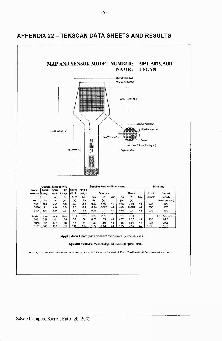
353
APPENDIX 22 - TEKSCAN DATA SHEETS AND RESULTS
MAP AND SENSOR MODEL NUMBER: 5051,5076, 5101NAME: I-SCANOverall Width (W)
Maxtrix Width (MW)
Matrix Height (MH)
Column Width (cw)
Row Spacing (rs)Overall Length (L)
Row Width (rw)
Column Spacing (cs)
Tab Length (A)
General Dimensions _____________ Sensing Region Dimensions_____________ SummaryM odel Overall Overall Tab Matrix Matrix
Number Length Width Length Width Height Columns Rows No. of SenselL W A MW MH CW CS Qty. RW RS Qtv Sensels Density
US (in) (in) (In) (in) (m) (in) (in) (in) (in) (sensel per sqnn)5051 9.9 3.2 6.6 2.2 2.2 0.03 0.05 44 0.03 0.05 44 1936 4005076 12 4.8 6.9 3.3 3.3 0.04 0.075 44 0.04 0.075 44 1936 1785101 13.4 5.9 6.5 4.4 4.4 0.05 0.1 44 0.05 0.1 44 1936 100
Metric (mm) (mm) (mm) (mm) (mm) (mm) (nun) (mm) (mm) (sensel per sq-cm)5051 251 81 168 56 56 0.76 1.27 44 0.76 1.27 44 1936 62.05076 305 122 175 84 84 1.02 1.91 44 1.02 1.91 44 1936 27.65101 340 150 165 112 112 1.27 2.54 44 1.27 2.54 44 1936 15.5
Application Example: Excellent for general purpose uses.
Special Feature: Wide range of available pressures.
Tekscan, Inc., 307 West First Street, South Boston, MA 02127 Phone:617-464-4500 Fax 617-464-4266 Website: www.tekscan.com
Silsoe Campus, Kieron Eatough, 2002
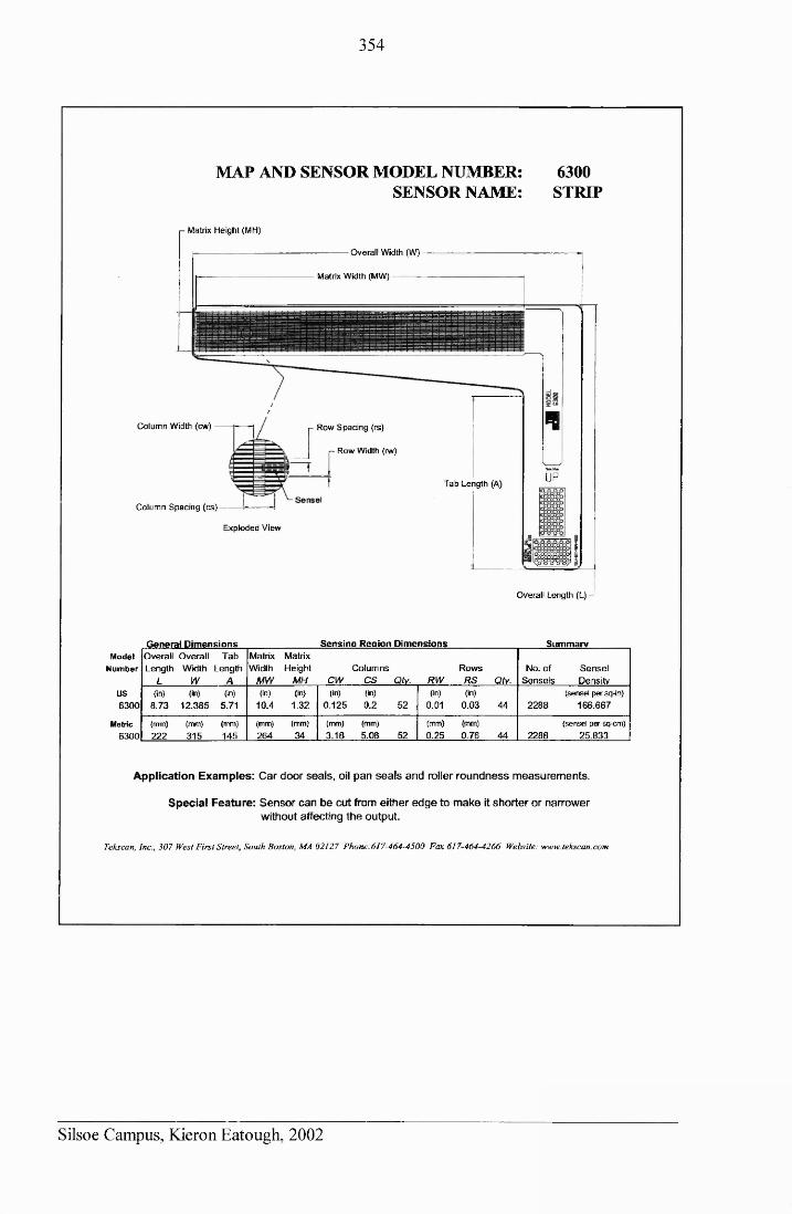
354
MAP AND SENSOR MODEL NUMBER: 6300SENSOR NAME: STRIP
M atrix H e igh t (MH)
- O verall Width (W)
Matrix W idth (MW)
C olum n Width (cw )
C olu m n S p a c in g (c s ) -
r R ow S p a c in g (rs)
R ow Width (rw)
T a b L en g th (A)
E x p lo d ed V iew
UP
oToroTa; ^o°g°o0o"o7
O v erall L eng th (L) - 1
General Dimensions Sensing Region Dimensions SummaryModel
NumberOverallLength
L
OverallWidth
W
TabLength
A
MatrixWidth
MW
MatrixHeight
MH CWColumns
CS Qty. RWRows
RS Qty.No. of
SenselsSenselDensity
US (in) (in) (in) (In) (in) (in) (in) On) (in) (sensel per sq-in)6300 8.73 12.385 5.71 10.4 1.32 0.125 0.2 52 0.01 0.03 44 2288 166.667
Metric (mm) (mm) (mm) (mm) (mm) (mm) (mm) (mm) (mm) (sensel pa- sq-cm)6300 222 315 145 264 34 3.18 5.08 52 0.25 0.76 44 2288 25.833
Application Examples: Car door seals, oil pan seals and roller roundness measurements.
Special Feature: Sensor can be cut from either edge to make it shorter or narrower without affecting the output.
Tekscan, Inc., 307 West First Street, South Boston, MA 02127 Phone:617-464-4500 Fax 617-464-4266 Website: www.tekscan.com
Silsoe Campus, Kieron Eatough, 2002
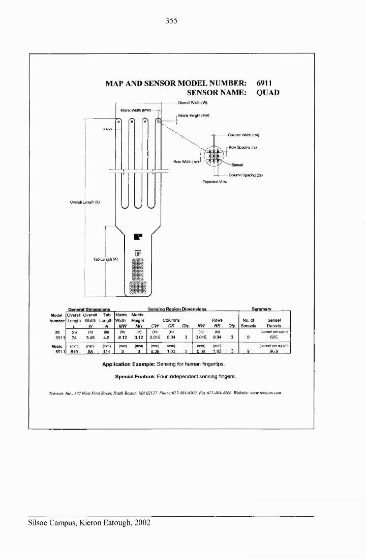
355
MAP AND SENSOR MODEL NUMBER: 6911SENSOR NAME: QUAD
-Overall Width (W)
Matrix Width (MW )—Matrix Height (MH)O
0 .4 5 0 - —
-Column Width (cw)
Row Spacing (rs)
Row Width (rw)
Column S pacing (cs)
Exploded View
Overall Length (L)
T ab Length (A)
Sensing Region Dimensions SummaryModel
NumberOverallLength
L
OverallWidth
W
TabLength
A
MatrixWidth
MW
MatrixHeight
MH CWColumns
CS Qtv. RWRowsRS QfV.
No. of Sensels
SenselDensity
US (in) (In) (in) (in) (in) (in) On) (in) fin) (sensel per sq-in)6911 24 3.45 4.5 0.12 0.12 0.015 0.04 3 0.015 0.04 3 9 625
Metric (mm) (mm) (mm) (mm) (mm) (mm) (mm) (mm) (mm) (sensel per sq-cm)6911 610 88 114 3 3 0.38 1.02 3 0.38 1.02 3 9 96.9
Application Example: Sensing for human fingertips.
Special Feature: Four independent sensing fingers.
Tekscan, Inc., 307 West First Street, South Boston, MA 02127 Phone:617-464^f500 Fax 617-464-4266 Website: www.tekscan.com
Silsoe Campus, Kieron Eatough, 2002

356
The data used to produce the pressure maps for the comparison of the performance of
the three different pressure maps is included on the data CD, in files: TekScan results
6911 (22), TekScan results 5051 (22) and TekScan results 6300 (22). Results are
presented for all three mats, 6911, 5051 and 6300. To allow their inclusion limited
processing has been conducted, as every TekScan test generated a very large quantity of
data. Even these short test runs produced too much data to enable its direct inclusion;
therefore the data corresponding to when the mats were out of ground contact has been
omitted. The 6911 mats had significantly fewer cells on each mat, so it was possible to
present the pure results for this mat, for all three repetitions of the tests. For the other
two mats mean results of the three repetitions were included to reduce the quantity of
data presented.
Silsoe Campus, Kieron Eatough, 2002

357
APPENDIX 23 - SAND DISPLACEMENT STATISTICS
The statistical analysis that was conducted on these results produced a large quantity of
data; therefore copies of the output files have been included on the enclosed data CD.
The files included have been separated by the variable for which they were analysed e.g.
wheel slip. The following files are included:
Sand tag displacement stats - Force
Sand tag displacement stats - Tyre Depth
Sand tag displacement stats - Tyre Slip
Sand tag displacement stats - X Direction
Sand tag displacement stats - Y Direction
Sand tag displacement stats - Z Direction
Silsoe Campus, Kieron Eatough, 2002

358
APPENDIX 24 - MODELLING SPREADSHEETS
All of the modelling (thrust and tread) was completed using models created in Excel.
These have been included on the data CD, to allow their construction and application to
be fully understood. They are located in the files detailed in the table below.
DATA FILENAME
Net Thrust modelling
(derived from Gross Thrust and
Rolling Resistance modelling)
Net thrust model - GT + RR
Rolling Resistance modelling Rolling Resistance model
Tread Coefficient modelling Tread Coefficient model
Silsoe Campus, Kieron Eatough, 2002
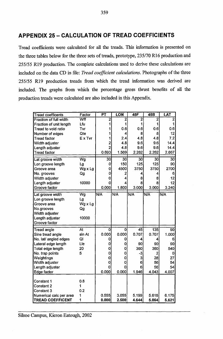
359
APPENDIX 25 - CALCULATION OF TREAD COEFFICIENTS
Tread coefficients were calculated for all the treads. This information is presented on
the three tables below for the three sets of treads, prototype, 235/70 R16 production and
255/55 R19 production. The complete calculations used to derive these calculations are
included on the data CD in file: Tread coefficient calculations. Photographs of the three
255/55 R19 production treads from which the tread information was derived are
included. The graphs from which the percentage gross thrust benefits of all the
production treads were calculated are also included in this Appendix.
Tread coefficents Factor PT LON 45F 45B LATFraction of full width Wff Fraction of unit length Lfu Tread to void ratio Tvr Number of edges Qte Tread factor Ex Tvr Width adjuster Length adjuster Tread factor
2111122
0.693
21
0.64
2.44.84.8
1.569
21
0.68
4.89.69.6
2.262
21
0.68
4.89.69.6
2.262
21
0.612
7.214.414.4
2.667
Lat groove width Wg Lon groove length Lg Groove area Wg x Lg No. grooves Qg Width adjusterLength adjuster 10000 Groove factor
3000000
0.000
30150
4500244
1.800
30125
3750488
3.000
30125
3750488
3.000
3090
27006
1212
3.240
Lat groove width Wg Lon groove length Lg Groove area Wg x Lg No.grooves Qg Width adjusterLength adjuster 10000 Groove factor
N/A N/A N/A N/A N/A
Tread angle At Sine tread angle sin At No. lat/ angled edges Ql Lateral edge length Lie Total edge length 20 No. trap points 5 Weightings Width adjuster Length adjuster Edge factor
00.000
0000000
0.000
00.000
0000000
0.000
450.707
490
360-3366
1.946
1350.707
490
3602
285656
4.043
901.000
690
5400
275454
4.007
Constant 1 0.8 Constant 2 1 Constant 3 0.2 Numerical calc per area 1 TREAD COEFFICENT 1
0.5550.000
3.0552.500
5.1994.644
5.6185.064
6.1755.621
Silsoe Campus, Kieron Eatough, 2002
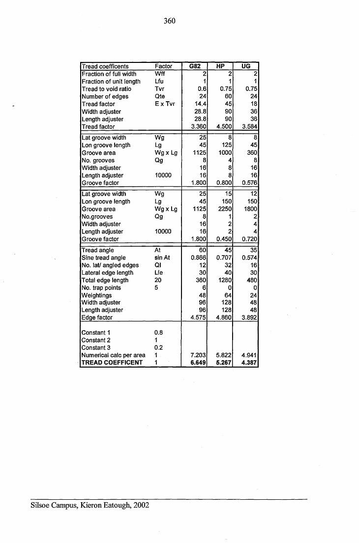
360
Tread coefficents Factor G82 HP UGFraction of full width Wff Fraction of unit length Lfu Tread to void ratio Tvr Number of edges Qte Tread factor Ex Tvr Width adjuster Length adjuster Tread factor
21
0.624
14.428.828.8
3.360
21
0.7560459090
4.500
21
0.7524183636
3.584
Lat groove width Wg Lon groove length Lg Groove area Wg x Lg No. grooves Qg Width adjusterLength adjuster 10000 Groove factor
2545
11258
1616
1.800
8125
1000488
0.800
845
3608
1616
0.576
Lat groove width Wg Lon groove length Lg Groove area Wg x Lg No.grooves Qg Width adjusterLength adjuster 10000 Groove factor
2545
11258
1616
1.800
15150
2250122
0.450
12150
1800244
0.720
Tread angle At Sine tread angle sin At No. lat/ angled edges Ql Lateral edge length Lie Total edge length 20 No. trap points 5 Weightings Width adjuster Length adjuster Edge factor
600.866
1230
3606
489696
4.575
450.707
3240
12800
64128128
4.860
350.574
1630
4800
244848
3.892
Constant 1 0.8 Constant 2 1 Constant 3 0.2 Numerical calc per area 1 TREAD COEFFICENT 1
7.2036.649
5.8225.267
4.9414.387
Silsoe Campus, Kieron Eatough, 2002
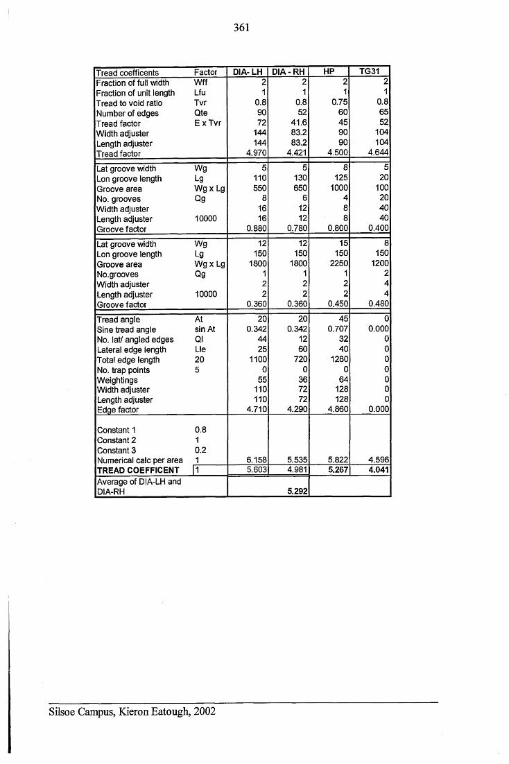
361
Tread coefficents Factor DIA- LH DIA - RH HP TG31Fraction of full width Wff Fraction of unit length Lfu Tread to void ratio Tvr Number of edges Qte Tread factor Ex Tvr Width adjuster Length adjuster Tread factor
21
0.89072
144144
4.970
21
0.852
41.683.283.2
4.421
21
0.7560459090
4.500
21
0.86552
104104
4.644
Lat groove width Wg Lon groove length Lg Groove area Wg x Lg No. grooves Qg Width adjusterLength adjuster 10000 Groove factor
5110550
81616
0.880
5 130 650
6 12 12
0.780
8125
1000488
0.800
520
100204040
0.400
Lat groove width Wg Lon groove length Lg Groove area Wg x Lg No.grooves Qg Width adjusterLength adjuster 10000 Groove factor
12150
1800122
0.360
12150
1800122
0.360
15150
2250122
0.450
8150
1200244
0.480
Tread angle At Sine tread angle sin At No. lat/ angled edges Ql Lateral edge length Lie Total edge length 20 No. trap points 5 Weightings Width adjuster Length adjuster Edge factor
200.342
4425
11000
55110110
4.710
200.342
1260
7200
367272
4.290
450.707
3240
12800
64128128
4.860
00.000
0000000
0.000
Constant 1 0.8 Constant 2 1 Constant 3 0.2 Numerical calc per area 1 6.158 5.535 5.822 4.596TREAD COEFFICENT 1 5.603 4.981 5.267 4.041Average of DIA-LH and DIA-RH 5.292
Silsoe Campus, Kieron Eatough, 2002
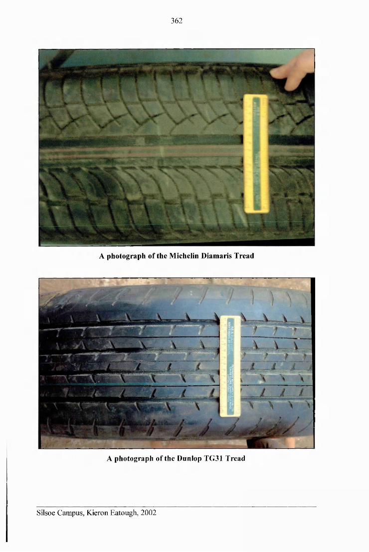
362
A photograph of the Michelin Diamaris Tread
A photograph of the Dunlop TG31 Tread
Silsoe Campus, Kieron Eatough, 2002
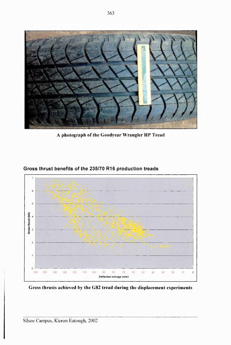
363
A photograph of the Goodyear Wrangler HP Tread
Gross thrust benefits of the 235/70 R16 production treads7
6
5
z4
toE
3O
2
1
0150 80160 140 130 120 110 100 90 70 60 50 40 30 20 10 0
Deflected sinkage (mm)
Gross thrusts achieved by the G82 tread during the displacement experiments
Silsoe Campus, Kieron Eatough, 2002
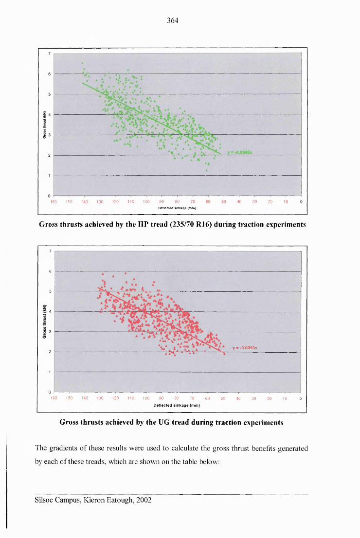
364
150 110 100 90Deflected sinkage (mm)
80 40160 140 130 120 30 20
liross thrusts achieved by the HP tread (235/70 R16) during traction experiments
7
6
5
3
/mV*1 a\ aa a i -A \ A * ****
y = -0.0393X2
1
0160 150 140 130 120 110 100 90 80 70 60 50 40 30 1020 0
Deflected sinkage (mm)
Gross thrusts achieved by the UG tread during traction experiments
The gradients of these results were used to calculate the gross thrust benefits generated
by each of these treads, which are shown on the table below:
Silsoe Campus, Kieron Eatough, 2002
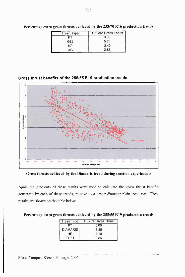
365
Percentage extra gross thrusts achieved by the 235/70 R16 production treadsTread Type % Extra Gross Thrust
PT 0.00G82 5.24HP 3.40UG 2.88
Gross thrust benefits of the 255/55 R19 production treads
y = -0.0405x
Deflected sinkage (mm)
Gross thrusts achieved by the Diamaris tread during traction experiments
Again the gradients of these results were used to calculate the gross thrust benefits
generated by each of these treads, relative to a larger diameter plain tread tyre. These
results are shown on the table below:
Percentage extra gross thrusts achieved by the 255/55 R19 production treadsTread Type % Extra Gross Thrust
PT 0.00DIAMARIS 3.85
HP 4.10TG31 2.56
Silsoe Campus, Kieron Eatough, 2002
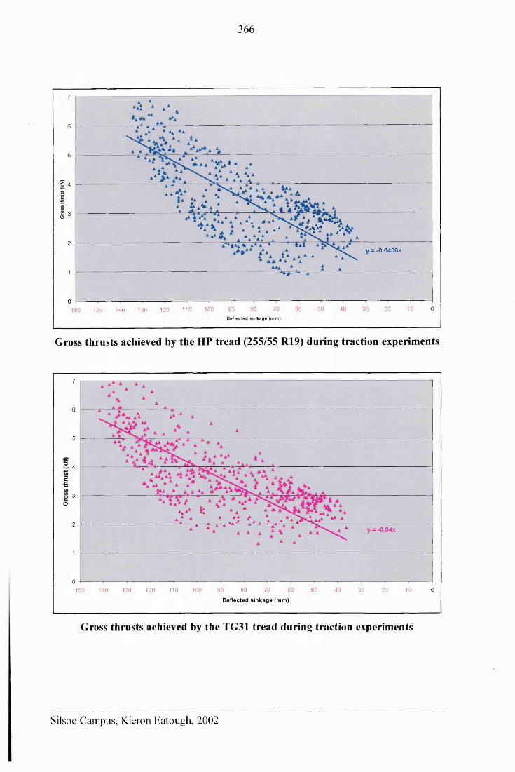
366
7
6
5
z 4w5g
A A A a A
A * A * .A / V * * A
A ! a ‘ ‘ X ' a ' V { a
A A A . 4 '
o 3O
2■0.0406X
1
070 50 30 20 10 080 60 4090110 100150 120160 130140
Deflected sinkage (mm)
Gross thrusts achieved by the HP tread (255/55 R19) during traction experiments
7
6
5
*a*a fe Aa * 4* * A ± A .XAJ * a . ‘ a ‘ 0 < a/ 4
*-----------X-------A a A * * ------ A A--------- j * — J ------ « ----------=>*5----------
zAC4
E£I/IO3O
2
1
070 50110 90 80 60 40 30 20 10 0130 120 100150 140
Deflected sinkage (mm)
Gross thrusts achieved by the TG31 tread during traction experiments
Silsoe Campus, Kieron Eatough, 2002
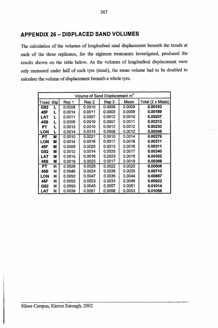
367
APPENDIX 26 - DISPLACED SAND VOLUMES
The calculation of the volumes of longitudinal sand displacement beneath the treads at
each of the three replicates, for the eighteen treatments investigated, produced the
results shown on the table below. As the volumes of longitudinal displacement were
only measured under half of each tyre (tread), the mean volume had to be doubled to
calculate the volume of displacement beneath a whole tyre.
Volume of Sand Displacement m3Tread Slip Rep 1 Rep 2 Rep 3 Mean Total (2 x Mean)G82 L 0.0008 0.0010 0.0009 0.0009 0.0018345F L 0.0014 0.0011 0.0003 0.0009 0.00189LAT L 0.0011 0.0007 0.0012 0.0010 0.0020745B L 0.0006 0.0019 0.0007 0.0011 0.00212PT L 0.0013 0.0010 0.0012 0.0012 0.00230
LON L 0.0014 0.0015 0.0008 0.0012 0.00248PT M 0.0010 0.0021 0.0010 0.0014 0.00276
LON M 0.0014 0.0016 0.0017 0.0016 0.0031145F M 0.0009 0.0025 0.0013 0.0016 0.00311G82 M 0.0012 0.0014 0.0025 0.0017 0.00340LAT M 0.0015 0.0016 0.0023 0.0018 0.0035245B M 0.0016 0.0025 0.0017 0.0019 0.00389PT H 0.0026 0.0028 0.0022 0.0025 0.00508
45B H 0.0045 0.0024 0.0038 0.0035 0.00710LON H 0.0050 0.0047 0.0036 0.0044 0.0088745F H 0.0053 0.0053 0.0033 0.0046 0.00922G82 H 0.0050 0.0045 0.0057 0.0051 0.01014LAT H 0.0039 0.0061 0.0058 0.0053 0.01056
Silsoe Campus, Kieron Eatough, 2002
368
APPENDIX 27 - MODELLING NET THRUST RESULTS
All of the net thrust modelling was completed using models created in Excel. All of the
models that produced the predicted sand performance results used in the thesis for
comparison against net thrust results are included on the data CD in the following files:
235 45F on sand 235 45B on sand
235 G82 on sand 235 HP on sand
235 LAT on sand 235 LON on sand
235 PT on sand 235 UG on sand
255 DIA on sand 255 HP on sand
255 TG on sand
Silsoe Campus, Kieron Eatough, 2002
Related Documents