Keypoint descriptor matching with context-based orientation estimation

Keypoint descriptor matching with

context-based orientation estimation

F. Bellaviaa,∗, D. Tegolob, C. Valentib

aCVG, Universita degli Studi di Firenze, 50139 Firenze, ItalybDMI, Universita degli Studi di Palermo, 90123 Palermo, Italy

Abstract

This paper presents a matching strategy to improve the discriminative power

of histogram-based keypoint descriptors by constraining the range of allow-

able dominant orientations according to the context of the scene under ob-

servation. This can be done when the descriptor uses a circular grid and

quantized orientation steps, by computing or providing a global reference

orientation based on the feature matches.

The proposed matching strategy is compared with the standard approaches

used with the SIFT and GLOH descriptors and the recent rotation invariant

MROGH and LIOP descriptors. A new evaluation protocol based on an ap-

proximated overlap error is presented to provide an effective analysis in the

case of non-planar scenes, thus extending the current state-of-the-art results.

Keywords: image descriptors, local features, dominant orientation,

rotation invariance, keypoint matching, SIFT, LIOP, MROGH.

∗Corresponding authorEmail addresses: [email protected] (F. Bellavia),

[email protected] (D. Tegolo), [email protected] (C. Valenti)

Preprint submitted to Image and Vision Computing May 27, 2014

1. Introduction1

Keypoint extracted from digital images have been adopted with good2

results as primitive parts in many computer vision tasks, such as recogni-3

tion [1], tracking [2] and 3D reconstruction [3]. The detection and extraction4

of meaningful image regions, named keypoints or image features, is usually5

the first step of these methodologies. Numerical vectors that embody the6

image region properties are successively computed to compare the keypoints7

found according to the particular task.8

Different feature detectors have been proposed during the last decades9

invariant to affine transformations or scale and rotation only, including, but10

not limited to, corners and blobs. The reader may refer to [4] for a general11

overview.12

After the keypoint is located, a meaningful descriptor vector to embody13

the characteristic properties of the keypoint support region (i.e. its neigh-14

bourhood) is computed. Different descriptors have been developed, which15

can be divided mainly into two categories: distribution-based descriptors16

and banks of filters. In general, while the former give better results, the17

latter provide more compact descriptors. Banks of filters include complex18

filters, color moments, the local jet of the keypoint, differential operators19

and Haar wavelet coefficients. Refer to [5] for more details.20

Distribution-based descriptors, also named histogram-based descriptors,21

divide the keypoint region, also called feature patch, into different areas22

and compute specific histograms related to some image properties for each23

area. The final descriptor is given by the ordered concatenation of these24

histograms. The rank and the census transforms [6], which consider binary25

2

comparisons of the intensity of central pixel against its neighborhood, are the26

precursors of the histogram-based descriptors. In particular, the CS-LBP [7]27

descriptor can be considered an extension of this kind of approach. The spin28

image descriptor, the shape context and the geometric blur and the more29

recent DAISY, BRIEF, BRISK and FREAK descriptors (see [5, 8]) should30

be mentioned.31

One of the most popular descriptors based on histograms is surely the32

SIFT (Scale Invariant Feature Transform) [9], which is a 3D histogram of33

gradient orientations on a Cartesian grid. SIFT has been extended in vari-34

ous ways since its first introduction. The PCA-SIFT descriptor [10] increases35

the robustness of the descriptor and decreases its length by applying PCA36

(Principal Component Analysis), RIFT (Rotation Invariant Feature Trans-37

form) [11] is a ring-based rotational invariant version, while GLOH (Gradient38

Local Orientation Histogram) [5] combines a log-polar grid with PCA and39

SURF [12] is an efficient discrete SIFT variant. Recently, RootSIFT [13]40

improves upon SIFT by replacing the Euclidean distance with the Bhat-41

tacharyya distance after the normalization of the descriptor vector with the42

Manhattan norm instead of the conventional Euclidean norm. Overlapping43

regions using multiple support regions combined by intensity order pooling44

are used by MROGH (Multi Support Region Order Based Gradient His-45

togram) [14]. Furthermore, LIOP (Local Intensity Order Pattern) [15] uses46

the intensity order pooling and the relative order of neighbor pixels to define47

the histogram.48

Over the last few years, machine learning techniques have been applied49

to remove the correlation between the descriptor elements and to reduce the50

3

dimension [10, 16], as well as, different histogram distances to improve the51

matches [17, 18].52

Different methodologies for evaluating feature descriptors and detectors53

have been proposed [4, 5, 8, 16, 19–23]. In the case of planar images, the54

Oxford dataset benchmark [4, 24] is a well-established set of de facto stan-55

dard, although an extension to non-planar images is not immediate [19].56

Other evaluation methodologies use laser-scanner images [21] or structure57

from motion algorithms [16, 23] or epipolar reprojection on more than two58

images [20], but in general they require a complex and error prone setup.59

1.1. Our Contributions60

This paper presents in Section 2 a matching strategy to improve the61

discriminative power of histogram-based keypoint descriptors by constraining62

the range of allowable orientations according to the scene context.63

We build the proposed matching strategy on the sGLOH (shifting GLOH)64

descriptor described in Section 2, presented in our previous work [25]. It uses65

a circular grid to embed more descriptor instances with different dominant66

discrete orientations of the same feature patch into a single feature vector.67

Each descriptor instance is accessible by an internal shift of the feature vector68

elements without the need to recompute the histograms. The matching dis-69

tance between features is modified to consider the minimum distance among70

all descriptor instances for the possible dominant discrete orientations.71

The sGLOH design can be used to further constrain the allowable domi-72

nant discrete orientations to be considered in the matching distance. A finer73

selection of the range of the dominant discrete orientations to be considered74

can be done a priori by defining a very fast matching strategy, named sCOr75

4

(shifting Constrained Orientation) or alternatively, when no further informa-76

tion is given in advance, by using an adaptive distance measure according77

to a voting strategy to get the sGOr (shifting Global Orientation) matching78

(see Section 2).79

In order to assess the properties of the novel matching strategies, different80

experiments reported in Section 3 were carried out, both on planar and non-81

planar scenes. To provide more insights, we also evaluated the case when82

more than just the first dominant orientation is used in SIFT and GLOH.83

The rotational invariant MROGH [14] and LIOP [15] were also included in the84

evaluation due to the increasing interest towards them in recent works [8, 14].85

In the case of non-planar scenes, a novel dataset was created which86

employs a new evaluation protocol based on the approximated overlap er-87

ror [26, 27]. This evaluation protocol provides an effective analysis in the case88

of non-planar scenes, extending the current state-of-the-art results [20, 22].89

Section 4 reports final comments and conclusions.90

2. The Proposed Matching Strategy91

Patch normalization and orientation methods are presented before defin-92

ing the keypoint matching with sCOr and sGOr, as well as details on the93

sGLOH descriptor [25], which is essential in the matching pipeline since it94

allows constraints on the range of allowable orientations.95

2.1. Patch Normalization96

Given an image I(x), x ∈ R2, the feature patch must be normalized97

before the computation of the descriptor vector. In the general case of affine-98

invariant keypoint detectors, which usually represent a good trade-off be-99

5

tween transformation invariance and discriminative power, an elliptical re-100

gion R ⊂ I is extracted. If the ellipse is given by the equation xTΣ−1x = 1,101

considering the keypoint centre as coordinate origin, the patch is normal-102

ized to a circle of a fixed radius r according to the formula x′ = rAx, where103

A = D−12 RT with Σ = RDRT by the eigenvalue decomposition [5]. The ellipse104

axis lengths and orientations are given by the square root of the eigenval-105

ues and the corresponding eigenvectors of Σ respectively [5]. The symmetric106

matrix Σ ∈ R2×2 is obtained as the covariance matrix for some quantity107

φ(x) ∈ R2 related to the points of the patch R [4]. This is the gradient108

vector in the case of the Harris detector or the coordinates of the boundary109

points for the MSER detector [4].110

The affine illumination invariance is obtained by normalizing the inten-111

sity value I(x) of the points inside the region R through their mean µ and112

standard deviation σ, according to the formula I ′(x) = I(x)−µσ

.113

2.2. Finding the Patch Orientation114

In order to be rotational invariant, most of the histogram-based descrip-115

tors have to be rotated according to a reference dominant orientation and116

different methodologies have been designed for its computation [9, 12, 28–30].117

The common approach was proposed by Lowe [9], where the gradient118

∇I(x) = [dx, dy]T is computed for each point x ∈ R and a histogram of ori-119

entations θ∇I(x) = arctan(dy/dx) is built up. The contribution of each point120

x is given by its gradient magnitude ‖ ∇I(x) ‖, weighted by the Gaussian121

function122

gσ(x) =1

2πσ2e−‖x‖2

2σ2

6

with standard deviation σ. It is assumed that θv = arctan(v), i.e. the123

arctangent of a generic vector v ∈ R2, and the coordinate origins coincide124

with the centre xc of the feature patch. The orientation Θ of the highest125

peak in the histogram, interpolated by a parabolic fitting, is chosen as the126

dominant orientation. More dominant orientations can be assigned to the127

feature, by retaining other peaks above 80% of the highest peak [9].128

Histogram-based descriptors which do not require a dominant orientation129

have also been proposed [14, 15]. The underlying idea, first exploited by130

RIFT [11], consists in the use of the outside direction perpendicular to the131

tangent direction at each point as reference in the bin assignment. This is132

however not sufficient, because patch regions have to be made invariant to133

rotation, too. The RIFT descriptor uses concentric rings which are clearly134

rotational invariant, but less discriminative.135

A last approach, named intensity order pooling [14], defines regions ac-136

cording the intensity value of the feature patch points without spatial con-137

strains, i.e. points with similar intensity values belong to the same region.138

This approach is used by MROGH [14], which computes a gradient histogram139

as for RIFT, and by LIOP [15], where instead the bins represent the rela-140

tive order of the intensities in a neighbourhood of the point. Furthermore,141

MROGH uses multiple support regions, which result in overlapping regions.142

According to [8], both LIOP and MROGH seem to outperform recent state-143

of-the-art descriptors, at least in the case of the Oxford planar scenes. How-144

ever, it must be noted that the MROGH outer support region is 2.5 times145

bigger than the standard elliptic region employed by other descriptors [14]146

in the tests, which lead to better but distorted results, especially in the case147

7

of planar scenes. See the additional material for more details.148

The sGLOH approach [25] uses the RIFT reference orientation for bin149

assignment, but a circular grid is maintained instead of concentric rings. The150

descriptor instances for different dominant discrete orientations obtained by151

shifting the descriptor vector are compared during the matching step and the152

best one is selected. Even if this approach is not a novelty [31], it had never153

been extended and evaluated in the context of histogram-based descriptors.154

Note that a similar descriptor, named RIFF, was introduced by Takacs et155

al. [32], contemporaneously to our preliminary paper concerning sGLOH [25].156

2.3. The sGLOH Descriptor157

The sGLOH descriptor grid is made up of n ×m regions Rr,d with r =158

{0, 1, . . . , n− 1} and d = {0, 1, . . . ,m− 1}, defined by n − 1 circular rings159

centred on the keypoint, plus one small inner circle, all of them containing160

m sectors, equally distributed along m directions (see Fig. 1). Previous161

experiments [25] have shown that not dividing the inner circular region into162

sectors decreases the discriminative power of the descriptor.163

For each region Rr,d, the histogram of m quantized orientations weighted164

by the gradient magnitude is computed. In order to obtain a better estima-165

tion of the gradient distribution, instead of using the trilinear interpolation166

as in SIFT [9], the bin value hi, where i = 0, 1, . . .,m − 1, is computed by167

the Gaussian kernel density estimation for each region168

hir,d =1√2πσ

∑x∈Rr,d

‖ ∇I(x) ‖ e−(M2π(θ∇I(x)−mi))

2

2σ2

where ‖ ∇I(x) ‖ and θ∇I(x) are respectively the gradient magnitude and169

8

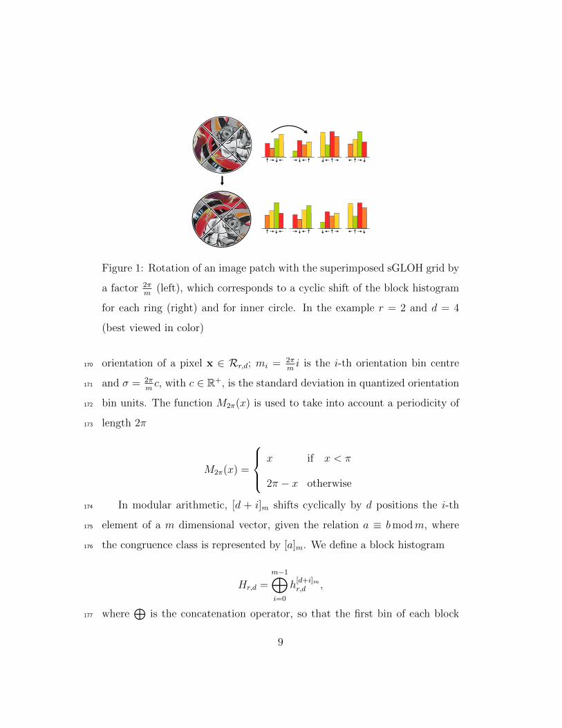
Figure 1: Rotation of an image patch with the superimposed sGLOH grid by

a factor 2πm

(left), which corresponds to a cyclic shift of the block histogram

for each ring (right) and for inner circle. In the example r = 2 and d = 4

(best viewed in color)

orientation of a pixel x ∈ Rr,d; mi = 2πmi is the i-th orientation bin centre170

and σ = 2πmc, with c ∈ R+, is the standard deviation in quantized orientation171

bin units. The function M2π(x) is used to take into account a periodicity of172

length 2π173

M2π(x) =

x if x < π

2π − x otherwise

In modular arithmetic, [d + i]m shifts cyclically by d positions the i-th174

element of a m dimensional vector, given the relation a ≡ bmodm, where175

the congruence class is represented by [a]m. We define a block histogram176

Hr,d =m−1⊕i=0

h[d+i]mr,d ,

where⊕

is the concatenation operator, so that the first bin of each block177

9

has direction d. The final descriptor vector H is obtained by concatenating178

the histograms179

H =n−1⊕i=0

m−1⊕j=0

Hi,j

The length of H = [h1, h2, . . . , hl] is l = m2n. In order to be more tolerant180

to noise and errors, the descriptor vector H is normalized to the unit length181

on the L1 norm instead of the usual normalization through the L2 norm [18].182

Moreover, no threshold is applied [9] (e.g. 0.2 for SIFT) to saturate values183

greater than a given quantity. The values hi are quantized to q levels to184

reduce the total descriptor to b = l log2 q bits [9]. The final descriptor is then185

H? = bwHc where w = q/l∑

i=1

hi. To avoid a complex notation, H will refer186

to both H and H? if it is not specified.187

The rotation of the descriptor by a factor αk, where α = 2πm

, is obtained188

by a cyclic shift of the block histogram for each ring and for the inner circle,189

without recomputing the descriptor vector (see Fig. 1)190

Hαk =n−1⊕i=0

m−1⊕j=0

Hi,[k+j]m

In this sense, the sGLOH descriptor packs m different descriptors of the191

same patch with different dominant orientations. The distance between two192

features H and H is then given by193

D(H,H) = mink=0,...,m−1

D(H,Hαk) (1)

where D(·, ·) is a generic distance measure.194

10

2.4. The sGLOH Implementation Details195

Experimental tests were carried out [25] on the Oxford dataset by using196

the setup described by Mikolajczyk and Schmid [5] in order to find the best197

parameter settings for sGLOH. We found that n = 2 and m = 8, which198

imply that the descriptor dimension is l = 128 and the discrete orientation199

step is 45◦, provide the best compromise between the descriptor length and200

its discriminative power. Moreover, the patch radii of the circular grid are201

set to 12 and 20 so that the patch size is 41× 41.202

For Gaussian kernel density estimation, the standard deviation in bin203

units is set to c = 0.7 and the quantization levels are set to q = 512 as204

for the Mikolajczyk’s SIFT implementation [24]. The normalization of the205

sGLOH vector to L2 unit length with a successive saturation threshold of 0.2206

has been shown to decrease its discriminative power [25]. Furthermore, no207

additional smoothness on the normalized and bilinear interpolated patches208

according to the scale to remove high frequencies is needed by sGLOH.209

2.5. The sCOr and sGOr Matching210

Both sCOr and sGOr reduce the number of wrong matches of sGLOH,211

as all wrong matches outside the correct range of discrete orientations are212

discarded and cannot be selected by chance.213

In the sCOr approach the range of the allowable orientations to be checked214

is constrained up to the first clockwise and counterclockwise discrete rotations215

only, given an a priori fixed reference orientation f ∈ {0, 1, . . . ,m − 1}, i.e.216

k = [f − 1]m, f, [f + 1]m in equation 1. Although the range of sCOr applica-217

tions is limited since high degrees of rotations cannot be handled, the method218

11

is general enough to be employed by setting f = 0 in common practical ap-219

plications, such as SLAM [2] and sparse matching [3], since transformations220

are relatively continuous for close images. Moreover, scenes and objects are221

usually acquired roughly with the same orientations so that this issue can222

be often neglected in the general case, since sCOr handles rotations of up223

to ±67.5◦ (see the experimental section). Note also that sCOr decreases the224

time required for the distance computation with respect to sGLOH.225

The sGOr approach uses the information provided by the scene context226

to provide a global reference orientation, under the reasonable assumption227

that all keypoints of the scene undergo roughly the same approximated dis-228

crete rotation αg, not known a priori. The range of discrete orientations in229

equation 1 is modified to k = [g−1]m, g, [g+1]m, where g ∈ {0, 1, . . . ,m−1}230

can be estimated according to the most probable relative orientation among231

all matches.232

Given two images I1 and I2, the relative orientation k?(H,S) of the best233

match pair containing the feature H and any other feature in the other image234

is considered235

k?(H,S) = ( arg mink=0,1,...,m−1

H∈S

D(H,Hαk))`

where (k,H)` = k and S is the set of feature vectors from the image not236

containing H. We define the histogram of the relative orientations so that237

the bin zk counts the number of the best matches with relative discrete238

orientation αk239

12

zk =∑H1∈S1

t(k = [k?(H1, S2)]m) +∑H2∈S2

t(k = [−k?(H2, S1)]m)

where t(W ) is 0, 1 if W is false, true respectively. S1 and S2 are the sets of240

descriptor vectors associated to features belonging to the images I1 and I2241

respectively. The value of g is finally given by242

g = arg maxk=0,1,...,m−1

zk

We experimentally verified that, consistently to the definition of g, wrong243

matches are distributed uniformly across the bins zk while correct matches244

are distributed according to a Gaussian centred in zg. The computation of245

g is similar to the Hough voting scheme [33] and, with respect to sGLOH, it246

just adds a minimal amount of computation to evaluate the distance D (see247

equation 1), since all required values of D have been computed already.248

3. Experimental Evaluation249

In order to evaluate the proposed matching approaches, comparisons with250

SIFT, GLOH, LIOP, MROGH and the original sGLOH were carried out,251

both in the planar and non-planar cases. The HarrisZ detector [34] which252

selects robust and stable Harris corners in the affine scale-space was used.253

Previous evaluations [34] have shown that it is comparable with the state-of-254

the-art detectors and provides better keypoints than Harris-affine. Moreover,255

although descriptors are influenced by detectors, the relative performances256

of the descriptors among different detectors are consistent [14].257

13

In the planar case, precision/recall curves on correct matches were ex-258

tracted through the overlap error ε for the stereo pairs (I1, I2) in the Oxford259

dataset [24]260

ε(Rw,Rz) = 1− Rw

⋂T2→1(Rz)

Rw

⋃T2→1(Rz)

where Rw ∈ I1, Rz ∈ I2 and T2→1 is the function that reprojects the feature261

Rz from I2 to I1.262

Detectors were also considered in the case of 2D planar rotations, to un-263

derline the effects of the dominant orientation on descriptors and the benefits264

of the rotation invariant descriptors. For the non-planar case, a novel super-265

vised evaluation strategy was adopted. An approximated overlap error εq,266

given a ground-truth fundamental matrix, was extracted according to the267

methodology described in [26, 27], which is based on the epipolar geometry268

and tangency relations. Finally, the time complexity of the descriptors is269

discussed.270

3.1. Planar Images271

As considered in [5], the support region of each keypoint was increased272

by a factor of 3 and normalized to a 41× 41 pixel patch.273

The Mikolajczyk’s GLOH and SIFT implementations were adapted to be274

used with multiple dominant orientations [9], in order to provide a reference275

with previous evaluations [24]. In particular, we considered the case when276

peaks greater by a factor of 0.8 and 0.7 of the maximum peak in the histogram277

of gradient orientations are retained. Differently from Lowe’s implementa-278

tion, these use finer bins, so that the number of descriptors associated to each279

14

keypoint doubles instead of increasing by 15% only [9]. However, as shown280

in the next section, results improve as more peaks were considered, so that281

the number of correct matches obtained by our implementations represent282

an upper bound to Lowe’s original implementation. When multiple domi-283

nant orientations were considered, similarly to sGLOH, the distance between284

two keypoints was computed as the minimum distance among all the pos-285

sible descriptor vectors associated to them. The implementations of LIOP286

and MROGH, provided by respective authors were used, while the code of287

sGLOH, sCOr and sGOr can be downloaded from [35]. The MROGH outer288

support region is 2.5 times bigger than the standard elliptic region employed289

by other descriptor by design [14], so that better results are expected for290

this descriptor since more discriminative data are available. Nevertheless,291

MROGH results were also included as an upper bound to analyze the allow-292

able gain that can be introduced in SIFT-like descriptors by using of a bigger293

feature area. Moreover, note that while the descriptor vector dimension is294

128 for SIFT, GLOH and sGLOH, it is 144 and 192 for LIOP and MROGH,295

respectively.296

The Oxford dataset [24] used in this evaluation contains planar images di-297

vided in two categories: structured images, containing homogeneous regions298

with well defined borders, and textured images. Eight different scenes are299

presented, each one subject to a different transformation across the images:300

viewpoint change, scale and orientation change, blur, lossy compression and301

luminosity. As in [5], the first and the fourth images for each scene were302

used.303

Precision/recall curves for a fixed overlap error ε = 50% were extracted304

15

for increasing distance values by using NN (Nearest-Neighbor) and NNR305

(Nearest-Neighbor Ratio) [9] matching criteria with L1 or Manhattan dis-306

tance and the L2 or Euclidean distance. The more rapidly the precision/recall307

curve grows and becomes stable with high recall, the better the descriptor308

is [5].309

Finally, 2D rotations were tested by artificially rotating 16 different im-310

ages, each by a step of 3◦ until 90◦, to get a quantitative evaluation about the311

possible drawbacks due to a wrong estimation of the dominant orientation312

and to show the tolerance which can be achieved by descriptors under small313

orientations.314

Relatively small rotations are more interesting in common applications315

because objects are almost always depicted in their frontal position. Fur-316

thermore, in 3D cases such as structure from motion [3] or SLAM [2], small317

rotations can aid to approximate admissible perspective distortions. To get318

an extensive analysis in the case of small rotations, the upright SIFT and319

GLOH descriptors, i.e. with no dominant orientation computation, named320

as uSIFT and uGLOH respectively, were included in this test.321

Note that uSIFT, uGLOH and sCOr were not tested on the Oxford322

dataset, since rotation sequences contain high degree rotations, while scenes323

with non-geometric transformations do not contain any rotation. In the for-324

mer case they could not be correctly applied while in the latter case the325

comparison would be unfair.326

Plots in Fig. 2 show precision/recall curves with the best matching strat-327

egy for each descriptor, i.e. L1 distance with NN for sGLOH and sGOr and328

L1 distance with NNR for other descriptors. Results in terms of correct329

16

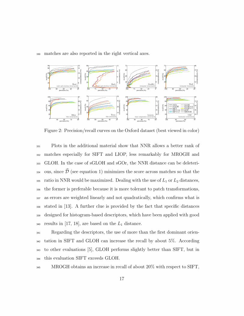
matches are also reported in the right vertical axes.330

204060801000

20

40

60

80

90

precision (%)

reca

ll (%

)

scale and rotation (structured)Boat

0

8

16

24

31

35

corr

espo

nden

ces

(%)

02550751000

20

40

60

80

precision (%)

reca

ll (%

)scale and rotation (textured)

Bark

0

3

6

8

11

corr

espo

nden

ces

(%)

02550751000

20

40

60

75

precision (%)

reca

ll (%

)

viewpoint (structured)Graffiti

0

8

16

23

29

corr

espo

nden

ces

(%)

204060801000

20

40

60

75

precision (%)

reca

ll (%

)

viewpoint (textured)Wall

0

12

24

37

46

corr

espo

nden

ces

(%)

607080900

20

40

60

80

100

precision (%)

reca

ll (%

)

blur (structured)Bikes

0

17

35

52

69

87

corr

espo

nden

ces

(%)

204060801000

20

40

60

75

precision (%)

reca

ll (%

)

blur (textured)Trees

0

14

29

43

54

corr

espo

nden

ces

(%)

607080901000

20

40

60

80

100

precision (%)

reca

ll (%

)

lossy compression (structured)Leuven

0

18

35

53

71

89

corr

espo

nden

ces

(%)

7080901000

20

40

60

80

100

precision (%)

reca

ll (%

)

luminosity (structured)UBC

0

18

36

54

72

90

corr

espo

nden

ces

(%)

Figure 2: Precision/recall curves on the Oxford dataset (best viewed in color)

Plots in the additional material show that NNR allows a better rank of331

matches especially for SIFT and LIOP, less remarkably for MROGH and332

GLOH. In the case of sGLOH and sGOr, the NNR distance can be deleteri-333

ous, since D (see equation 1) minimizes the score across matches so that the334

ratio in NNR would be maximized. Dealing with the use of L1 or L2 distances,335

the former is preferable because it is more tolerant to patch transformations,336

as errors are weighted linearly and not quadratically, which confirms what is337

stated in [13]. A further clue is provided by the fact that specific distances338

designed for histogram-based descriptors, which have been applied with good339

results in [17, 18], are based on the L1 distance.340

Regarding the descriptors, the use of more than the first dominant orien-341

tation in SIFT and GLOH can increase the recall by about 5%. According342

to other evaluations [5], GLOH performs slightly better than SIFT, but in343

this evaluation SIFT exceeds GLOH.344

MROGH obtains an increase in recall of about 20% with respect to SIFT,345

17

which shows the robustness of the new rotational invariant descriptor. Except346

for the textured scale and rotation cases in the Bark sequence, it achieves347

the best results. However, a bigger support region is used, the vector length348

is 50% more than the standard 128 descriptor length and it requires more349

computational time (see Sect. 3.3).350

LIOP provides about 10-15% increase in recall, it is fast and increases351

the descriptor length by 13% only. Apart from the textured Bark sequence352

(see Fig. 2b), for which it achieves the best results, LIOP works better for353

structured scenes than for textured scenes. This implies that the relative354

ordering of pixel intensities is more stable for well defined and homogeneous355

patches.356

The sGOr results are better than sGLOH, which demonstrates the effec-357

tiveness of the adaptive distance in constraining the range of discrete rota-358

tions. Except for Bark, sGOr results are in general quite similar to those359

obtained by LIOP, but sGOr works better with textured scenes. Further-360

more, sGLOH always surpasses the results obtained by SIFT and GLOH for361

a precision which is less than 90%.362

By inspecting the results in the case of no geometrical transformation363

(e.g. for the sequences Bikes, Trees, UBC and Leuven) it can be noted that364

the computation of the dominant orientation could lead to wrong matches.365

If no dominant orientation is used for SIFT and GLOH, results similar to366

other descriptors should be expected. Usually this information is not known367

a priori and needs to be explicitly included for SIFT and GLOH, while it368

is automatically addressed and handled by MROGH, LIOP, sGLOH and369

sGOr. Furthermore, larger support regions in the case of MROGH improve370

18

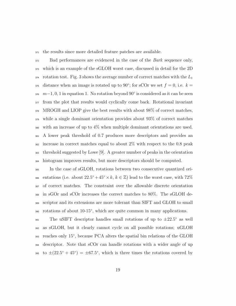
the results since more detailed feature patches are available.371

Bad performances are evidenced in the case of the Bark sequence only,372

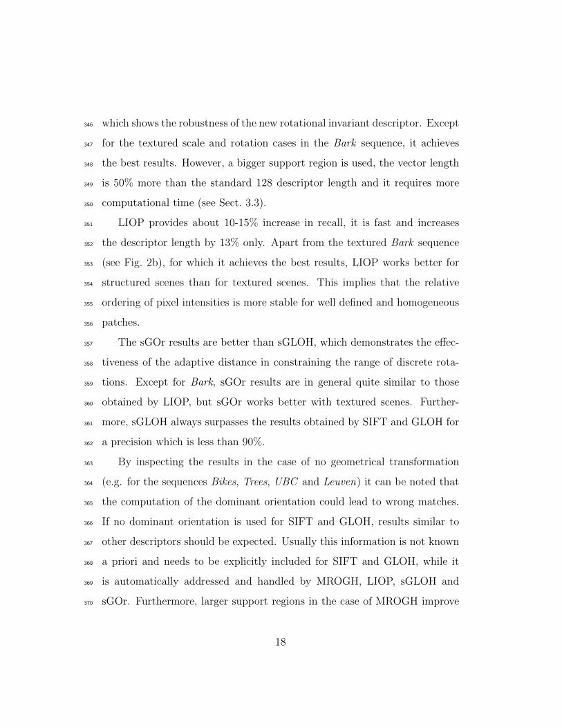
which is an example of the sGLOH worst case, discussed in detail for the 2D373

rotation test. Fig. 3 shows the average number of correct matches with the L1374

distance when an image is rotated up to 90◦; for sCOr we set f = 0, i.e. k =375

m−1, 0, 1 in equation 1. No rotation beyond 90◦ is considered as it can be seen376

from the plot that results would cyclically come back. Rotational invariant377

MROGH and LIOP give the best results with about 98% of correct matches,378

while a single dominant orientation provides about 93% of correct matches379

with an increase of up to 4% when multiple dominant orientations are used.380

A lower peak threshold of 0.7 produces more descriptors and provides an381

increase in correct matches equal to about 2% with respect to the 0.8 peak382

threshold suggested by Lowe [9]. A greater number of peaks in the orientation383

histogram improves results, but more descriptors should be computed.384

In the case of sGLOH, rotations between two consecutive quantized ori-385

entations (i.e. about 22.5◦+45◦×k, k ∈ Z) lead to the worst case, with 72%386

of correct matches. The constraint over the allowable discrete orientation387

in sGOr and sCOr increases the correct matches to 80%. The sGLOH de-388

scriptor and its extensions are more tolerant than SIFT and GLOH to small389

rotations of about 10-15◦, which are quite common in many applications.390

The uSIFT descriptor handles small rotations of up to ±22.5◦ as well391

as sGLOH, but it clearly cannot cycle on all possible rotations; uGLOH392

reaches only 15◦, because PCA alters the spatial bin relations of the GLOH393

descriptor. Note that sCOr can handle rotations with a wider angle of up394

to ±(22.5◦ + 45◦) = ±67.5◦, which is three times the rotations covered by395

19

sCOrsGOrsGLOHSIFTSIFT 0.8SIFT 0.7uSIFTGLOHGLOH 0.8GLOH 0.7uGLOHLIOPMROGH

Figure 3: Average correct L1 matches versus rotation (best viewed in color)

uSIFT and sufficient for a considerable number of tasks.396

3.2. Non-planar Images397

The evaluation on non-planar images was carried out according to the398

dataset reported in the additional material. Both the evaluation scripts and399

the dataset are freely available [35]. The dataset consists of 10 different400

stereo scenes with 3 images for each scene so that a total of 30 stereo pairs401

is obtained. Stereo pairs present rotations of less than 45◦, since we are402

interested in testing sCOr and SGOr, which cycle through this value (see403

Fig. 3).404

With respect to other evaluation methodologies [16, 19–21, 23], this com-405

parison strategy does not require a complex setup, depth maps or camera406

calibration, but only the computation of the ground-truth fundamental ma-407

trix, so that the dataset can be easily extended. For each stereo pair, the408

fundamental matrix was computed with more than 50 hand-taken correspon-409

dences and an average epipolar error of about 1 pixel. The average number410

of keypoints extracted for each image was around 800.411

20

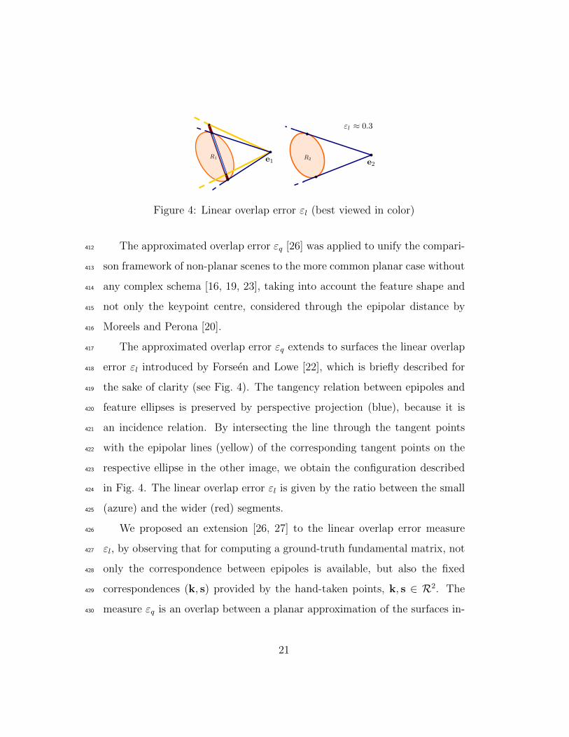
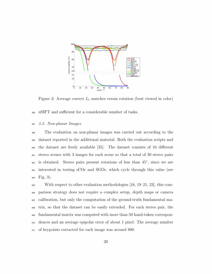
Figure 4: Linear overlap error εl (best viewed in color)

The approximated overlap error εq [26] was applied to unify the compari-412

son framework of non-planar scenes to the more common planar case without413

any complex schema [16, 19, 23], taking into account the feature shape and414

not only the keypoint centre, considered through the epipolar distance by415

Moreels and Perona [20].416

The approximated overlap error εq extends to surfaces the linear overlap417

error εl introduced by Forseen and Lowe [22], which is briefly described for418

the sake of clarity (see Fig. 4). The tangency relation between epipoles and419

feature ellipses is preserved by perspective projection (blue), because it is420

an incidence relation. By intersecting the line through the tangent points421

with the epipolar lines (yellow) of the corresponding tangent points on the422

respective ellipse in the other image, we obtain the configuration described423

in Fig. 4. The linear overlap error εl is given by the ratio between the small424

(azure) and the wider (red) segments.425

We proposed an extension [26, 27] to the linear overlap error measure426

εl, by observing that for computing a ground-truth fundamental matrix, not427

only the correspondence between epipoles is available, but also the fixed428

correspondences (k, s) provided by the hand-taken points, k, s ∈ R2. The429

measure εq is an overlap between a planar approximation of the surfaces in-430

21

side the feature patches. The assumption that the scene can be approximated431

by piecewise planar patches was already used successfully to train and test432

features in [16].433

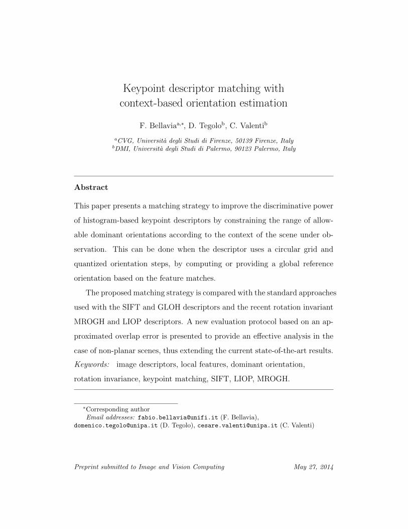
Figure 5: Approximated overlap error εq (best viewed in color)

For an ellipse patchR (orange), tangent points define an inscribed quadri-434

lateral Q? (azure), while tangent lines limit a circumscribed quadrilateral Q435

(blue), as in Fig. 5. The corresponding quadrilaterals P ? (light green) and P436

(dark green) are obtained by projecting from the other images through the437

fundamental matrix as done for εl. The area of the ellipse R can be roughly438

approximated by the average area between Q and Q?439

R ≈ Q+Q?

2

The final approximate overlap error εq is defined as440

εq =ε(Q,P ) + ε(Q?, P ?)

2

The measure εq is not symmetric so the maximal value obtained for the441

ordered stereo pairs (I1, I2) and (I2, I1) is assigned to the match. In the442

22

computation, the best pair (k, s) of correspondences is considered according443

to the heuristic constrains described in [27].444

A match is considered correct with respect to a given threshold value tε445

if εq < tεq . As tεq decreases, the precision increases in same way as in the446

framework by Moreels and Perona [20] and, as for all the methodologies based447

on a ground-truth fundamental matrix, the precision loss depends on the448

transformation applied to the scene, as well as, the uncertainty of the feature449

point on the epipolar line. In particular, wrong matches sharing the same450

epipolar cone can be misclassified. However, this is a stronger constraint than451

to take only into consideration the epipolar distance of the feature center.452

In order to deal with this issue, the error εq was first computed for the453

candidate matches and an initial selection of matches was done automatically454

by thresholding with tεq < 1, removing all matches with no overlap according455

to εq. The reduced subset of matches was then manually refined and only456

the remaining matches with an approximated overlap error less than the457

threshold tεq < 0.5 were retained. This final set of correct matches was used458

in the evaluation as ground-truth.459

In the case of no user inspection, we verified an average error rate equal460

to about 5% without the high recall loss due to the use of three images [20].461

This error rate is sufficiently low and would not alter the results in the case462

of no manual interaction [27].463

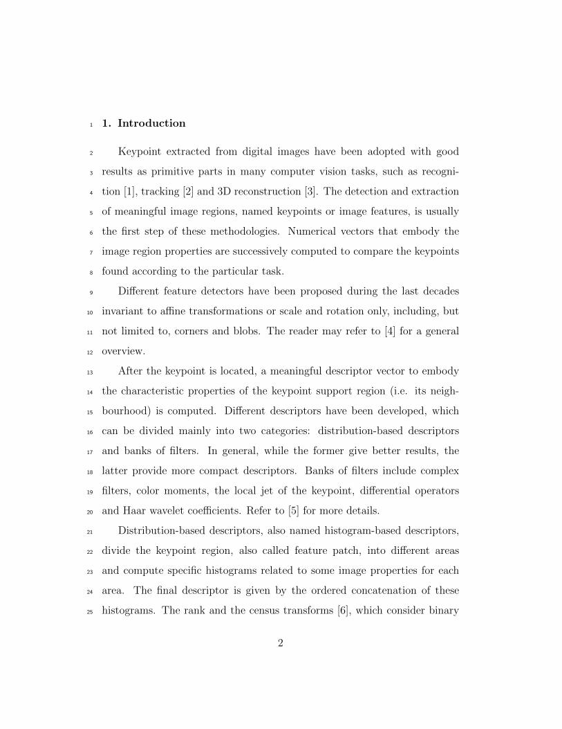
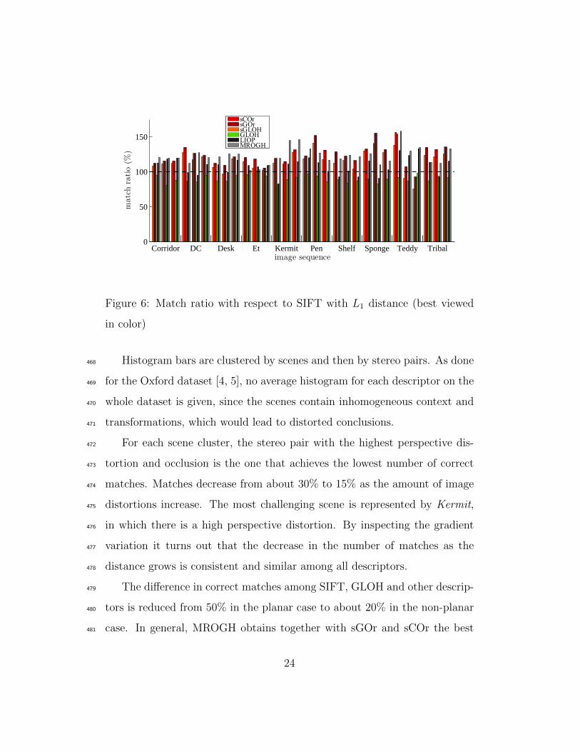
Fig. 6 shows the correct matches for each stereo pair and descriptor,464

considering SIFT as the reference descriptor. Further plots can be found in465

the additional material. The matching strategy and the distance used are466

the same as for the planar test, since the same considerations hold.467

23

Corridor DC Desk Et Kermit Pen Shelf Sponge Teddy Tribal0

50

100

150

image sequence

matchratio(%

)sCOrsGOrsGLOHGLOHLIOPMROGH

Figure 6: Match ratio with respect to SIFT with L1 distance (best viewed

in color)

Histogram bars are clustered by scenes and then by stereo pairs. As done468

for the Oxford dataset [4, 5], no average histogram for each descriptor on the469

whole dataset is given, since the scenes contain inhomogeneous context and470

transformations, which would lead to distorted conclusions.471

For each scene cluster, the stereo pair with the highest perspective dis-472

tortion and occlusion is the one that achieves the lowest number of correct473

matches. Matches decrease from about 30% to 15% as the amount of image474

distortions increase. The most challenging scene is represented by Kermit,475

in which there is a high perspective distortion. By inspecting the gradient476

variation it turns out that the decrease in the number of matches as the477

distance grows is consistent and similar among all descriptors.478

The difference in correct matches among SIFT, GLOH and other descrip-479

tors is reduced from 50% in the planar case to about 20% in the non-planar480

case. In general, MROGH obtains together with sGOr and sCOr the best481

24

results, but none of these approaches clearly outperform the others. The482

advantage of using a bigger support region in the case of non-planar scenes is483

reduced, since bigger patches can introduce also more distortions with respect484

to the planar case, according to the concept of locality of the features [5].485

LIOP improvements over SIFT are more limited than the planar case and486

in some cases obtains a lower number of matches for some image pairs, so487

that the local relative order of pixel intensity seems to suffer due to image488

discontinuities associated with perspective distortions in non-planar images.489

Regarding GLOH, the same considerations obtained for the planar case490

still hold, while the number of matches for sGLOH is greater than SIFT but491

slightly lower than MROGH, sGOr and sCOr. The benefits of sGOr and492

sCOr over sGLOH are more evident than those obtained in the planar case.493

Rotations of the form ±22.5◦ + 45◦ × k, k ∈ Z, correspond to the worst494

case of sGLOH (the third image pair of Teddy). As for the planar case, this495

issue can be alleviated by focusing on an admissible number of quantized496

orientations to remove ambiguities, as done by sGOr and sCOr which return497

similar results to SIFT.498

Table 1 shows the percentage p of correct matches detected by sCOr along499

the orientation of 0◦ so that 1 − p corresponds to the percentage of correct500

matches detected along the orientation of ±45◦, since discrete rotations are501

limited to up to this value. The following weighted average provides a rough502

estimate of the average orientation of the scene503

r(p) = p× 0◦ + (1− p)× 45◦

neglecting the clockwise or counterclockwise direction of the rotation. The504

25

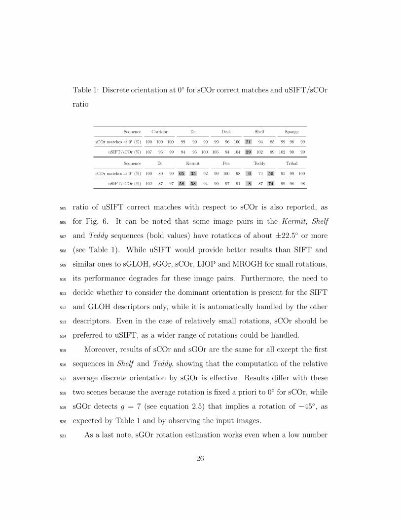
Table 1: Discrete orientation at 0◦ for sCOr correct matches and uSIFT/sCOr

ratio

Sequence Corridor Dc Desk Shelf Sponge

sCOr matches at 0◦ (%) 100 100 100 99 90 99 99 96 100 21 94 88 99 98 99

uSIFT/sCOr (%) 107 95 99 94 95 100 105 94 104 29 102 89 102 90 99

Sequence Et Kermit Pen Teddy Tribal

sCOr matches at 0◦ (%) 100 80 99 65 35 92 99 100 98 6 74 50 95 99 100

uSIFT/sCOr (%) 102 87 97 58 58 94 99 97 91 8 87 74 99 98 98

ratio of uSIFT correct matches with respect to sCOr is also reported, as505

for Fig. 6. It can be noted that some image pairs in the Kermit, Shelf506

and Teddy sequences (bold values) have rotations of about ±22.5◦ or more507

(see Table 1). While uSIFT would provide better results than SIFT and508

similar ones to sGLOH, sGOr, sCOr, LIOP and MROGH for small rotations,509

its performance degrades for these image pairs. Furthermore, the need to510

decide whether to consider the dominant orientation is present for the SIFT511

and GLOH descriptors only, while it is automatically handled by the other512

descriptors. Even in the case of relatively small rotations, sCOr should be513

preferred to uSIFT, as a wider range of rotations could be handled.514

Moreover, results of sCOr and sGOr are the same for all except the first515

sequences in Shelf and Teddy, showing that the computation of the relative516

average discrete orientation by sGOr is effective. Results differ with these517

two scenes because the average rotation is fixed a priori to 0◦ for sCOr, while518

sGOr detects g = 7 (see equation 2.5) that implies a rotation of −45◦, as519

expected by Table 1 and by observing the input images.520

As a last note, sGOr rotation estimation works even when a low number521

26

of correct matches are present so that the corresponding peak in the discrete522

relative rotation histogram (see Section 2.5) is very low, as for the second523

scene with Kermit which has about 10% of correct matches.524

3.3. Time Complexity525

The descriptor matching time depends on the average number n of ex-526

tracted keypoints for each stereo pair. Indeed, the total time required is527

given by the time to compute the descriptors on both images, which is O(n),528

plus the time to compute the distance for each possible match, which grows529

as O(n2). Here it is assumed that the computation of the distance between530

two descriptor requires a constant time and the descriptor length can be531

neglected.532

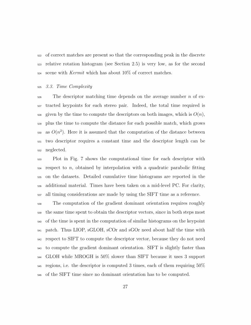
Plot in Fig. 7 shows the computational time for each descriptor with533

respect to n, obtained by interpolation with a quadratic parabolic fitting534

on the datasets. Detailed cumulative time histograms are reported in the535

additional material. Times have been taken on a mid-level PC. For clarity,536

all timing considerations are made by using the SIFT time as a reference.537

The computation of the gradient dominant orientation requires roughly538

the same time spent to obtain the descriptor vectors, since in both steps most539

of the time is spent in the computation of similar histograms on the keypoint540

patch. Thus LIOP, sGLOH, sCOr and sGOr need about half the time with541

respect to SIFT to compute the descriptor vector, because they do not need542

to compute the gradient dominant orientation. SIFT is slightly faster than543

GLOH while MROGH is 50% slower than SIFT because it uses 3 support544

regions, i.e. the descriptor is computed 3 times, each of them requiring 50%545

of the SIFT time since no dominant orientation has to be computed.546

27

0 500 1000 1500 2000 2500 3000 3500 40000

5

10

15

20

average number of keypoints per image

time

(sec

)

sCOrsGOrsGLOHSIFTGLOHLIOPMROGH

Figure 7: Expected running time (best viewed in color)

The quadratic term is comparable and irrelevant for SIFT, GLOH, LIOP547

and MROGH, if we do not consider large scale problems [3]. In these cases,548

MROGH and LIOP descriptor dimensions are respectively increased by 50%549

and 13% with respect to the standard 128 descriptor length of SIFT and this550

implies a similar increasing amount in the matching time. About sGLOH,551

sCOr and sGOr, the minimization of the distance D (see equation 1) adds a552

constant multiplicative factor to the quadratic term. This can be neglected in553

the case of sCOr, comparable to the fast LIOP in terms of running time for a554

value of n used in common applications. In this case, both sGLOH and sGOr555

are still faster than MROGH. The sGLOH, sCOr and sGOr descriptors could556

save space in large scale matching problems with respect to SIFT and GLOH557

when multiple orientations are used, since a single sGLOH feature descriptor558

packs 8 different orientations. Note that SIFT and GLOH can require an559

additional running time proportional to further dominant orientations.560

28

4. Conclusions561

In this paper we have shown how to improve the discriminative power of562

histogram-based keypoint descriptors by constraining the range of allowable563

orientations according to the scene under observation. This is done by com-564

puting a global gradient orientation based on the image matching context in565

the case of sGOr, or can be provided a priori in the case of sCOr.566

We tested the proposed descriptors together with SIFT, GLOH and recent567

rotation invariant descriptors by intensity order pooling, MROGH and LIOP,568

both on planar and non-planar images. In the former case the Oxford dataset569

was used, while in the latter case we proposed a novel supervised strategy,570

based on an approximated overlap error. This method allows to compare571

descriptors in the non-planar case in a similar way to the planar case, by572

taking into account the feature shape and not only the keypoint centre. The573

new evaluation strategy does not require any complex setup to extend the574

dataset and the error rate is sufficiently low not to alter the results in the575

case of unsupervised usage [27]. This new evaluation method adds a valuable576

tool to be joined with the current evaluation methods in order to provide a577

more insightful understanding of the descriptors.578

According to our tests, the L1 distance should be chosen, while NNR579

matching is preferable for most descriptors. All investigated descriptors are580

expected to degrade when passing from the planar to non-planar cases. None581

of the considered descriptors clearly outperforms the others, since results582

depend on the input scene and time and space requirements are different,583

that should be also taken into account.584

SIFT results as a good descriptor, while GLOH gives less correct matches585

29

in our tests. The rotational invariant LIOP descriptor is very fast, and586

achieves a higher number of matches with respect to SIFT, especially in the587

planar case. In non-planar scenes results are less stable, due to the inten-588

sity ordering used by LIOP, affected by eventual image discontinuities or in589

the presence of textured or noisy scenes. MROGH achieves the best results590

together with sGOr and sCOr, but it uses bigger support regions and also591

requires the highest computational time. The sGLOH descriptor returns592

good results on both planar and non-planar images with a time complex-593

ity comparable with SIFT in practical situations. The sGLOH descriptor594

is very tolerant to small rotations, but its results degrade for planar rota-595

tions between two quantized orientations, which limits its usability in general596

applications. The sCOr and the more general sGOr descriptors are very suit-597

able for non-planar scenes and can be applied to common tasks with results598

comparable to MROGH and LIOP. Furthermore, sCOr and LIOP have a599

comparable running time while sGOr is faster than MROGH.600

Results achieved by sGOr, sCOr and sGLOH, considering their similar-601

ity with SIFT, underline how the reference orientation represents a possible602

drawback in the matching process. In the case of small rotations, this issue603

can be removed by uSIFT. However, the need to use the dominant orienta-604

tion has to be explicitly included in SIFT or GLOH, which is automatically605

handled by the other descriptors. For this reason, the sCOr descriptor should606

be preferred to uSIFT, as a wider range of rotations can be handled.607

30

Acknowledgements608

This work was supported partially by grant B71J12001380001, University609

of Palermo FFR 2012/2013.610

References611

[1] S. Lazebnik, C. Schmid, J. Ponce, Beyond bags of features: spatial612

pyramid matching for recognizing natural scene categories, in: Proc.613

of the IEEE Conference on Computer Vision and Pattern Recognition,614

Vol. 2, 2006, pp. 2169–2178.615

[2] A. Gil, O. M. Mozos, M. Ballesta, O. Reinoso, A comparative evalua-616

tion of interest point detectors and local descriptors for visual SLAM,617

Machine Vision and Applications (MVA) 21 (6) (2010) 905–920.618

[3] N. Snavely, S. Seitz, R. Szeliski, Modeling the world from internet photo619

collections, International Journal of Computer Vision 80 (2) (2008) 189–620

210.621

[4] K. Mikolajczyk, T. Tuytelaars, C. Schmid, A. Zisserman, J. Matas,622

F. Schaffalitzky, T. Kadir, L. Van Gool, A comparison of affine region623

detectors, International Journal of Computer Vision 65 (1-2) (2005) 43–624

72.625

[5] K. Mikolajczyk, C. Schmid, A performance evaluation of local descrip-626

tors, IEEE Transactions on Pattern Analysis and Machine Intelligence627

27 (10) (2005) 1615–1630.628

31

[6] R. Zabih, J. Woodfill, Non-parametric local transforms for computing629

visual correspondence, in: Proc. of the European Conference on Com-630

puter Vision, Vol. 2, 1994, pp. 151–158.631

[7] M. Heikkila, M. Pietikainen, C. Schmid, Description of interest regions632

with local binary patterns, Pattern Recognition 42 (3) (2009) 425–436.633

[8] O. Miksik, K. Mikolajczyk, Evaluation of local detectors and descriptors634

for fast feature matching, in: Proc. of the International Conference on635

Pattern Recognition, 2012, pp. 2681–2684.636

[9] D. Lowe, Distinctive image features from scale-invariant keypoints, In-637

ternational Journal of Computer Vision 60 (2) (2004) 91–110.638

[10] Y. Ke, R. Sukthankar, PCA-SIFT: a more distinctive representation for639

local image descriptors, in: Proc. of the IEEE Conference on Computer640

Vision and Pattern Recognition, Vol. 2, 2004, pp. 506–513.641

[11] S. Lazebnik, C. Schmid, J. Ponce, A sparse texture representation using642

local affine regions, IEEE Transactions on Pattern Analysis and Machine643

Intelligence 27 (8) (2005) 1265–1278.644

[12] H. Bay, A. Ess, T. Tuytelaars, L.Van Gool, Speeded-up robust features645

(SURF), Computer Vision and Image Understanding 110 (3) (2008) 346–646

359.647

[13] R. Arandjelovic, A. Zisserman, Three things everyone should know to648

improve object retrieval, in: Proc. of the IEEE Conference on Computer649

Vision and Pattern Recognition, 2012, pp. 2911–2918.650

32

[14] B. Fan, F. Wu, Z. Hu, Rotationally invariant descriptors us-651

ing intensity order pooling, IEEE Transactions on Pattern652

Analysis and Machine Intelligence 34 (10) (2012) 2031–2045,653

http://vision.ia.ac.cn/Students/bfan/mrogh.htm.654

[15] Z. Wang, B. Fan, F. Wu, Local intensity order pattern655

for feature description, in: Proc. of the IEEE Interna-656

tional Conference on Computer Vision, 2011, pp. 603–610,657

http://vision.ia.ac.cn/Students/wzh/publication/liop/index.html.658

[16] M. Brown, G. Hua, S. Winder, Discriminative learning of local image659

descriptors, IEEE Transactions on Pattern Analysis and Machine Intel-660

ligence 33 (1) (2011) 43–57.661

[17] Y. Rubner, C. Tomasi, L. Guibas, The earth mover’s distance as a metric662

for image retrieval, Tech. rep., Stanford University (1998).663

[18] H. Ling, K. Okada, Diffusion distance for histogram comparison, in:664

Proc. of the IEEE Conference on Computer Vision and Pattern Recog-665

nition, 2006, pp. 246–253.666

[19] F. Fraundorfer, H. Bischof, A novel performance evaluation method of667

local detectors on non-planar scenes, in: Proc. of the IEEE Conference668

on Computer Vision and Pattern Recognition, 2005, pp. 33–33.669

[20] P. Moreels, P. Perona, Evaluation of features detectors and descriptors670

based on 3D objects, International Journal of Computer Vision 73 (2007)671

263–284.672

33

[21] C. Strecha, W. von Hansen, L. Van Gool, P. Fua, U. Thoennessen, On673

benchmarking camera calibration and multi-view stereo for high resolu-674

tion imagery, in: Proc. of the Computer Vision and Pattern Recognition,675

2008, pp. 2838–2845.676

[22] P. Forssen, D. Lowe, Shape descriptors for maximally stable extremal677

regions, in: Proc. of the International Conference on Computer Vision,678

2007, pp. 1–8.679

[23] R. Lakemond, C. Fookes, S. Sridharan, Evaluation of two-view geometry680

methods with automatic ground-truth generation, Image Vision Com-681

puting 31 (12) (2013) 921–934.682

[24] K. Mikolajczyk, T. Tuytelaars, et al., Affine covariant features,683

http://www.robots.ox.ac.uk/~vgg/research/affine (2010).684

[25] F. Bellavia, D. Tegolo, E. Trucco, Improving SIFT-based descriptors sta-685

bility to rotations, in: Proc. of the International Conference on Pattern686

Recognition, 2010, pp. 3460–3463.687

[26] F. Bellavia, D. Tegolo, New error measures to evaluate features on three-688

dimensional scenes, in: Proc. of the International Conference on Image689

Analysis and Processing, 2011, pp. 524–533.690

[27] F. Bellavia, C. Valenti, C. A. Lupascu, D. Tegolo, Approximated overlap691

error for the evaluation of feature descriptors on 3D scenes, in: Proc. of692

the International Conference on Image Analysis and Processing, 2013,693

pp. 270–279.694

34

[28] S. Taylor, T. Drummond, Multiple target localisation at over 100 FPS,695

in: Proc. of the British Machine Vision Conference, 2009, pp. 58.1–58.11.696

[29] S. Gauglitz, M. Turk, T. Hollerer, Improving keypoint orientation as-697

signment, in: Proc. of the British Machine Vision Conference, 2011, pp.698

93.1–93.11.699

[30] M. Brown, R. Szeliski, S. Winder, Multi-image matching using multi-700

scale oriented patches, in: Proc. of the IEEE Conference on Computer701

Vision and Pattern Recognition, Vol. 1, 2005, pp. 510–517.702

[31] F. Ullah, S. Kaneko, Using orientation codes for rotation-invariant tem-703

plate matching, Pattern Recognition 37 (2) (2004) 201–209.704

[32] G. Takacs, V. Chandrasekhar, S. Tsai, D. Chen, R. Grzeszczuk,705

B. Girod, Unified real-time tracking and recognition with rotation-706

invariant fast features, in: Proc. of the IEEE Conference on Computer707

Vision and Pattern Recognition, 2010, pp. 934–941.708

[33] D. H. Ballard, Generalizing the Hough transform to detect arbitrary709

shapes, Pattern Recognition 13 (2) (1981) 111–122.710

[34] F. Bellavia, D. Tegolo, C. Valenti, Improving Harris corner selection711

strategy, IET Computer Vision 5 (2) (2011) 86–96.712

[35] http://www.math.unipa.it/fbellavia/htm/research.html.713

35