Rocco Langone, Raghvendra Mall, Carlos Alzate, Johan A. K. Suykens Kernel Spectral Clustering and applications Chapter Contribution to the book: Unsupervised Learning Algorithms May 5, 2015 Springer arXiv:1505.00477v1 [cs.LG] 3 May 2015

Welcome message from author
This document is posted to help you gain knowledge. Please leave a comment to let me know what you think about it! Share it to your friends and learn new things together.
Transcript
Rocco Langone, Raghvendra Mall, CarlosAlzate, Johan A. K. Suykens
Kernel Spectral Clustering andapplications
Chapter Contribution to the book:Unsupervised Learning Algorithms
May 5, 2015
Springer
arX
iv:1
505.
0047
7v1
[cs
.LG
] 3
May
201
5

Contents
1 Kernel Spectral Clustering and applications . . . . . . . . . . . . . . . . . . . . . . . 11.1 Introduction . . . . . . . . . . . . . . . . . . . . . . . . . . . . . . . . . . . . . . . . . . . . . . . 11.2 Notation . . . . . . . . . . . . . . . . . . . . . . . . . . . . . . . . . . . . . . . . . . . . . . . . . . 31.3 Kernel Spectral Clustering (KSC) . . . . . . . . . . . . . . . . . . . . . . . . . . . . . 3
1.3.1 Mathematical formulation . . . . . . . . . . . . . . . . . . . . . . . . . . . . . 31.3.2 Soft Kernel Spectral Clustering (SKSC) . . . . . . . . . . . . . . . . . 71.3.3 Hierarchical Clustering . . . . . . . . . . . . . . . . . . . . . . . . . . . . . . . 81.3.4 Sparse Clustering Models . . . . . . . . . . . . . . . . . . . . . . . . . . . . . 11
1.4 Applications . . . . . . . . . . . . . . . . . . . . . . . . . . . . . . . . . . . . . . . . . . . . . . . 141.4.1 Image Segmentation . . . . . . . . . . . . . . . . . . . . . . . . . . . . . . . . . . 141.4.2 Scientific Journal Clustering . . . . . . . . . . . . . . . . . . . . . . . . . . . 161.4.3 Power Load Clustering . . . . . . . . . . . . . . . . . . . . . . . . . . . . . . . 181.4.4 Big data . . . . . . . . . . . . . . . . . . . . . . . . . . . . . . . . . . . . . . . . . . . . 20
1.5 Conclusions . . . . . . . . . . . . . . . . . . . . . . . . . . . . . . . . . . . . . . . . . . . . . . . 21References . . . . . . . . . . . . . . . . . . . . . . . . . . . . . . . . . . . . . . . . . . . . . . . . . . . . . 23
v

Chapter 1Kernel Spectral Clustering and applications
Abstract In this chapter we review the main literature related to kernel spectralclustering (KSC), an approach to clustering cast within a kernel-based optimizationsetting. KSC represents a least-squares support vector machine based formulationof spectral clustering described by a weighted kernel PCA objective. Just as in theclassifier case, the binary clustering model is expressed by a hyperplane in a highdimensional space induced by a kernel. In addition, the multi-way clustering canbe obtained by combining a set of binary decision functions via an Error Correct-ing Output Codes (ECOC) encoding scheme. Because of its model-based nature,the KSC method encompasses three main steps: training, validation, testing. In thevalidation stage model selection is performed to obtain tuning parameters, like thenumber of clusters present in the data. This is a major advantage compared to clas-sical spectral clustering where the determination of the clustering parameters is un-clear and relies on heuristics. Once a KSC model is trained on a small subset ofthe entire data, it is able to generalize well to unseen test points. Beyond the basicformulation, sparse KSC algorithms based on the Incomplete Cholesky Decompo-sition (ICD) and L0, L1,L0 +L1, Group Lasso regularization are reviewed. In thatrespect, we show how it is possible to handle large scale data. Also, two possibleways to perform hierarchical clustering and a soft clustering method are presented.Finally, real-world applications such as image segmentation, power load time-seriesclustering, document clustering and big data learning are considered.
1.1 Introduction
Spectral clustering (SC) represents the most popular class of algorithms based ongraph theory (Chung 1997). It makes use of the Laplacian’s spectrum to partitiona graph into weakly connected sub-graphs. Moreover, if the graph is constructed
1
2 1 Kernel Spectral Clustering and applications
based on any kind of data (vector, images etc.), data clustering can be performed1.SC began to be popularized when Shi and Malik introduced the Normalized Cutcriterion to handle image segmentation (Shi & Malik 2000). Afterwards, Ng andJordan (Ng et al. 2002) in a theoretical work based on matrix perturbation theoryhave shown conditions under which a good performance of the algorithm is ex-pected. Finally, in the tutorial by Von Luxburg the main literature related to SChas been exhaustively summarized (von Luxburg 2007). Although very success-ful in a number of applications, SC has some limitations. For instance, it can-not handle big data without using approximation methods like the Nystrom algo-rithm (Fowlkes et al. 2004, Williams & Seeger 2001), the power iteration method(Lin & Cohen 2010), or linear algebra based methods (Ning et al. 2010, Dhanjalet al. 2013, Frederix & Van Barel 2013). Furthermore, the generalization to out-of-sample data is only approximate.
These issues have been recently tackled by means of a spectral clustering algo-rithm formulated as weighted kernel PCA (Alzate & Suykens 2010). The technique,named kernel spectral clustering (KSC), is based on solving a constrained opti-mization problem in a primal-dual setting. In other words, KSC is a Least SquaresSupport Vector Machine (LS-SVM (Suykens et al. 2002)) model used for clusteringinstead of classification2. By casting SC in a learning framework, KSC allows torigorously select tuning parameters such as the natural number of clusters which arepresent in the data. Also, an accurate prediction of the cluster memberships for un-seen points can be easily done by projecting test data in the embedding eigenspacelearned during training. Furthermore, the algorithm can be tailored to a given appli-cation by using the most appropriate kernel function. Beyond that, by using sparseformulations and a fixed-size (Suykens et al. 2002, De Brabanter et al. 2010) ap-proach, it is possible to readily handle big data. Finally, by means of adequate adap-tations of the core algorithm, hierarchical clustering and a soft clustering approachhave been proposed.
All these topics will be detailed in the next Sections. Precisely, after present-ing the basic KSC method, the soft KSC algorithm will be summarized. Next,two possible ways to accomplish hierarchical clustering will be explained. After-wards, some sparse formulations based on the Incomplete Cholesky Decompo-sition (ICD) and L0, L1,L0 + L1, Group Lasso regularization will be described.Lastly, various interesting applications in different domains such as computer vi-sion, power-load consumer profiling, information retrieval and big data clusteringwill be illustrated. All these examples assume a static setting. Concerning otherapplications in a dynamic scenario the interested reader can refer to (Langone,Alzate, De Ketelaere & Suykens 2013, Langone et al. 2015) for fault detection,to (Langone, Agudelo, De Moor & Suykens 2014) for incremental time-series clus-tering, to (Langone, Alzate & Suykens 2013, Langone & Suykens 2013, Langone,
1 In this case the given data points represent the node of the graph and their similarity the corre-sponding edges.2 This is a considerable novelty, since SVMs are typically known as classifiers or function approx-imation models rather than clustering techniques.
1.3 Kernel Spectral Clustering (KSC) 3
Mall & Suykens 2014) in case of community detection in evolving networks and(Peluffo et al. 2013) in relation to human motion tracking.
1.2 Notation
xT Transpose of the vector xAT Transpose of the matrix AIN N×N Identity matrix1N N×1 Vector of onesDtr = xiNtr
i=1 Training sample of Ntr data pointsϕ(·) Feature mapF Feature space of dimension dhApk
p=1 Partitioning composed of k clustersG = (V ,E ) Set of N vertices V = viN
i=1 and m edges E of a graph| · | Cardinality of a set
1.3 Kernel Spectral Clustering (KSC)
1.3.1 Mathematical formulation
1.3.1.1 Training problem
The KSC formulation for k clusters is stated as a combination of k− 1 binaryproblems (Alzate & Suykens 2010). In particular, given a set of training dataDtr = xiNtr
i=1, the primal problem is:
minw(l),e(l),bl
12
k−1
∑l=1
w(l)Tw(l)− 1
2
k−1
∑l=1
γle(l)TVe(l)
subject to e(l) = Φw(l)+bl1Ntr , l = 1, . . . ,k−1.
(1.1)
The e(l) = [e(l)1 , . . . ,e(l)i , . . . ,e(l)Ntr]T are the projections of the training data mapped
in the feature space along the direction w(l). For a given point xi, the model in theprimal form is:
e(l)i = w(l)Tϕ(xi)+bl . (1.2)
The primal problem (1.1) expresses the maximization of the weighted variancesof the data given by e(l)
TVe(l) and the contextual minimization of the squared
norm of the vector w(l), ∀l. The regularization constants γl ∈ R+ mediate themodel complexity expressed by w(l) with the correct representation of the train-ing data. V ∈ RNtr×Ntr is the weighting matrix and Φ is the Ntr× dh feature matrix
4 1 Kernel Spectral Clustering and applications
Φ = [ϕ(x1)T ; . . . ;ϕ(xNtr)
T ], where ϕ : Rd → Rdh denotes the mapping to a high-dimensional feature space, bl are bias terms.
The dual problem corresponding to the primal formulation (1.1), by setting V =D−1 becomes3:
D−1MDΩα(l) = λ lα
(l) (1.3)
where Ω is the kernel matrix with i j-th entry Ωi j = K(xi,x j) = ϕ(xi)T ϕ(x j).
K : Rd ×Rd → R means the kernel function. The type of kernel function to utilizeis application-dependent, as it is outlined in Table 1.1. The matrix D is the graphdegree matrix which is diagonal with positive elements Dii = ∑ j Ωi j, MD is a cen-tering matrix defined as MD = INtr − 1
1TNtr
D−11Ntr1Ntr 1
TNtr
D−1, the α(l) are vectors of
dual variables, λ l =Ntrγl
, K : Rd×Rd→R is the kernel function. The dual clusteringmodel for the i-th point can be expressed as follows:
e(l)i =Ntr
∑j=1
α(l)j K(x j,xi)+bl , j = 1, . . . ,Ntr, l = 1, . . . ,k−1. (1.4)
The cluster prototypes can be obtained by binarizing the projections e(l)i as sign(e(l)i ).This step is straightforward because, thanks to presence of the bias term bl , both thee(l) and the α(l) variables get automatically centred around zero. The set of the mostfrequent binary indicators form a code-book C B = cpk
p=1, where each code-wordof length k−1 represents a cluster.
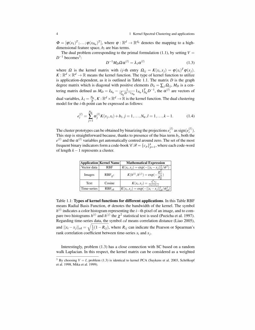
Application Kernel Name Mathematical ExpressionVector data RBF K(xi,x j) = exp(−||xi− x j||22/σ2)
Images RBFχ2 K(h(i),h( j)) = exp(−χ2
i j
σ2χ
)
Text Cosine K(xi,x j) =xT
i x j||xi||||x j ||
Time-series RBFcd K(xi,x j) = exp(−||xi− x j||2cd/σ2cd)
Table 1.1: Types of kernel functions for different applications. In this Table RBFmeans Radial Basis Function, σ denotes the bandwidth of the kernel. The symbolh(i) indicates a color histogram representing the i−th pixel of an image, and to com-pare two histograms h(i) and h( j) the χ2 statistical test is used (Puzicha et al. 1997).Regarding time-series data, the symbol cd means correlation distance (Liao 2005),
and ||xi− x j||cd =√
12 (1−Ri j), where Ri j can indicate the Pearson or Spearman’s
rank correlation coefficient between time-series xi and x j.
Interestingly, problem (1.3) has a close connection with SC based on a randomwalk Laplacian. In this respect, the kernel matrix can be considered as a weighted
3 By choosing V = I, problem (1.3) is identical to kernel PCA (Suykens et al. 2003, Scholkopfet al. 1998, Mika et al. 1999).
1.3 Kernel Spectral Clustering (KSC) 5
graph G = (V ,E ) with the nodes vi ∈ V represented by the data points xi. Thisgraph has a corresponding random walk in which the probability of leaving a ver-tex is distributed among the outgoing edges according to their weight: pt+1 = Ppt ,where P = D−1Ω indicates the transition matrix with the i j-th entry denoting theprobability of moving from node i to node j in one time-step. Moreover, the sta-tionary distribution of the Markov Chain describes the scenario where the randomwalker stays mostly in the same cluster and seldom moves to the other clusters(Meila & Shi 2001b, Meila & Shi 2001b, Meila & Shi 2001a, Delvenne et al. 2010).
1.3.1.2 Generalization
Given the dual model parameters α(l) and bl , it is possible to assign a membershipto unseen points by calculating their projections onto the eigenvectors computed inthe training phase:
e(l)test = Ωtestα(l)+bl1Ntest (1.5)
where Ωtest is the Ntest×N kernel matrix evaluated using the test points with en-tries Ωtest,ri = K(xtest
r ,xi), r = 1, . . . ,Ntest, i = 1, . . . ,Ntr. The cluster indicator for agiven test point can be obtained by using an Error Correcting Output Codes (ECOC)decoding procedure:
• the score variable is binarized• the indicator is compared with the training code-book C B (see previous Sec-
tion), and the point is assigned to the nearest prototype in terms of Hammingdistance.
The KSC method, comprising training and test stage, is summarized in algorithm1, and the related Matlab package is freely available on the Web4.
1.3.1.3 Model selection
In order to select tuning parameters like the number of clusters k and eventuallythe kernel parameters, a model selection procedure based on grid search is adopted.First, a validation set Dval = xiNval
i=1 is sampled from the whole dataset. Then, a gridof possible values of the tuning parameters is constructed. Afterwards, a KSC modelis trained for each combination of parameters and the chosen criterion is evaluatedon the partitioning predicted for the validation data. Finally, the parameters yieldingthe maximum value of the criterion are selected. Depending on the kind of data, avariety of model selection criteria have been proposed:
• Balanced Line Fit (BLF). It indicates the amount of collinearity between vali-dation points belonging to the same cluster, in the space of the projections. It
4 http://www.esat.kuleuven.be/stadius/ADB/alzate/softwareKSClab.php
6 1 Kernel Spectral Clustering and applications
Algorithm 1: KSC algorithm (Alzate & Suykens 2010)Data: Training set Dtr = xiNtr
i=1, test set Dtest = xtestm
Ntestm=1 kernel function
K : Rd ×Rd → R positive definite and localized (K(xi,x j)→ 0 if xi and x j belong todifferent clusters), kernel parameters (if any), number of clusters k.
Result: Clusters A1, . . . ,Ak, codebook C B = cpkp=1 with cp ∈ −1,1k−1.
1 compute the training eigenvectors α(l), l = 1, . . . ,k−1, corresponding to the k−1 largesteigenvalues of problem (1.3)
2 let A ∈ RNtr×(k−1) be the matrix containing the vectors α(1), . . . ,α(k−1) as columns3 binarize A and let the code-book C B = cpk
p=1 be composed by the k encodings ofQ = sign(A) with the most occurrences
4 ∀i, i = 1, . . . ,Ntr, assign xi to Ap∗ where p∗ = argminpdH(sign(αi),cp) and dH(., .) is theHamming distance
5 binarize the test data projections sign(e(l)m ), m = 1, . . . ,Ntest, and let sign(em) ∈ −1,1k−1
be the encoding vector of xtestm
6 ∀m, assign xtestm to Ap∗ , where p∗ = argminpdH(sign(em),cp).
reaches its maximum value 1 in case of well separated clusters, represented aslines in the space of the e(l)val (see for instance the bottom left side of Figure 1.1)
• Balanced Angular Fit or BAF (Mall et al. 2013b). For every cluster, the sumof the cosine similarity between the validation points and the cluster prototype,divided by the cardinality of that cluster, is computed. These similarity values arethen summed up and divided by the total number of clusters.
• Average Membership Strength abbr. AMS (Langone, Mall & Suykens 2013). Themean membership per cluster denoting the mean degree of belonging of the val-idation points to the cluster is computed. These mean cluster memberships arethen averaged over the number of clusters.
• Modularity (Newman 2006). This quality function is well suited for networkdata. In the model selection scheme, the Modularity of the validation sub-graphcorresponding to a given partitioning is computed, and the parameters related tothe highest Modularity are selected (Langone et al. 2011, Langone et al. 2012).
• Fisher Criterion. The classical Fisher criterion (Bishop 2006) used in classifica-tion has been adapted to select the number of clusters k and the kernel parametersin the KSC framework (Alzate & Suykens 2012). The criterion maximizes thedistance between the means of the two clusters while minimizing the variancewithin each cluster, in the space of the projections e(l)val.
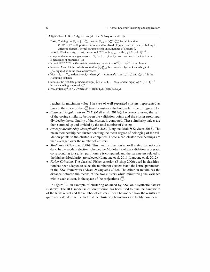
In Figure 1.1 an example of clustering obtained by KSC on a synthetic datasetis shown. The BLF model selection criterion has been used to tune the bandwidthof the RBF kernel and the number of clusters. It can be noticed how the results arequite accurate, despite the fact that the clustering boundaries are highly nonlinear.
1.3 Kernel Spectral Clustering (KSC) 7
Fig. 1.1: KSC partitioning on a toy dataset. (Top) Original dataset consisting of3 clusters (left) and obtained clustering results (right). (Bottom) Points representedin the space of the projections [e(1),e(2)] (left), for an optimal choice of k (and σ2 =4.36 · 10−3) suggested by the BLF criterion (right). We can notice how the pointsbelonging to one cluster tend to lie on the same line. A perfect line structure is notattained due to a certain amount of overlap between the clusters.
1.3.2 Soft Kernel Spectral Clustering (SKSC)
Soft kernel spectral clustering (SKSC) makes use of algorithm 1 in order to com-pute a first hard partitioning of the training data. Next, soft cluster assignments areperformed by computing the cosine distance between each point and some clus-ter prototypes in the space of the projections e(l). In particular, given the projec-tions for the training points ei = [e(1)i , . . . ,e(k−1)
i ], i = 1, . . . ,Ntr and the correspond-ing hard assignments qp
i we can calculate for each cluster the cluster prototypess1, . . . ,sp, . . . ,sk, sp ∈ Rk−1 as:
sp =1np
np
∑i=1
ei (1.6)
where np is the number of points assigned to cluster p during the initialization stepby KSC. Then the cosine distance between the i-th point in the projections space
8 1 Kernel Spectral Clustering and applications
and a prototype sp is calculated by means of the following formula:
dcosip = 1− eT
i sp/(||ei||2||sp||2). (1.7)
The soft membership of point i to cluster q can be finally expressed as:
sm(q)i =
∏ j 6=q dcosi j
∑kp=1 ∏ j 6=p dcos
i j(1.8)
with ∑kp=1 sm(p)
i = 1. As pointed-out in (Ben-Israel & Iyigun 2008), this member-ship represents a subjective probability expressing the belief in the clustering as-signment.
The out-of-sample extension on unseen data consists simply of calculating eq.(1.5) and assigning the test projections to the closest centroid.
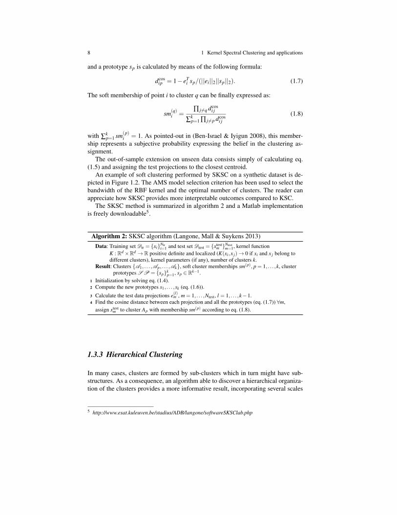
An example of soft clustering performed by SKSC on a synthetic dataset is de-picted in Figure 1.2. The AMS model selection criterion has been used to select thebandwidth of the RBF kernel and the optimal number of clusters. The reader canappreciate how SKSC provides more interpretable outcomes compared to KSC.
The SKSC method is summarized in algorithm 2 and a Matlab implementationis freely downloadable5.
Algorithm 2: SKSC algorithm (Langone, Mall & Suykens 2013)Data: Training set Dtr = xiNtr
i=1 and test set Dtest = xtestm
Ntestm=1, kernel function
K : Rd ×Rd → R positive definite and localized (K(xi,x j)→ 0 if xi and x j belong todifferent clusters), kernel parameters (if any), number of clusters k.
Result: Clusters A1, . . . ,Ap, . . . ,Ak, soft cluster memberships sm(p), p = 1, . . . ,k, clusterprototypes S P = spk
p=1, sp ∈ Rk−1.1 Initialization by solving eq. (1.4).2 Compute the new prototypes s1, . . . ,sk (eq. (1.6)).
3 Calculate the test data projections e(l)m , m = 1, . . . ,Ntest, l = 1, . . . ,k−1.4 Find the cosine distance between each projection and all the prototypes (eq. (1.7)) ∀m,
assign xtestm to cluster Ap with membership sm(p) according to eq. (1.8).
1.3.3 Hierarchical Clustering
In many cases, clusters are formed by sub-clusters which in turn might have sub-structures. As a consequence, an algorithm able to discover a hierarchical organiza-tion of the clusters provides a more informative result, incorporating several scales
5 http://www.esat.kuleuven.be/stadius/ADB/langone/softwareSKSClab.php
1.3 Kernel Spectral Clustering (KSC) 9
Fig. 1.2: SKSC partitioning on a synthetic dataset. (Top) Original dataset consist-ing of 2 clusters (left) and obtained soft clustering results (right). (Bottom) Pointsrepresented in the space of the projection e(1) (left), for an optimal choice of k (andσ2 = 1.53 ·10−3) as detected by the AMS criterion (right).
in the analysis. The flat KSC algorithm has been extended in two ways in order todeal with hierarchical clustering.
1.3.3.1 Approach 1
This approach, named hierarchical kernel spectral clustering (HKSC), was proposedin (Alzate & Suykens 2012) and exploits the information of a multi-scale structurepresent in the data given by the Fisher criterion (see end of Section 1.3.1.3). A gridsearch over different values of k and σ2 is performed to find tuning parameter pairssuch that the criterion is greater than a specified threshold value. The KSC modelis then trained for each pair and evaluated at the test set using the out-of-sampleextension. A specialized linkage criterion determines which clusters are merging
10 1 Kernel Spectral Clustering and applications
based on the evolution of the cluster memberships as the hierarchy goes up. Thewhole procedure is summarized in algorithm 3.
Algorithm 3: HKSC algorithm (Alzate & Suykens 2012)
Data: Training set Dtr = xiNtri=1, Validation set Dval = xiNval
i=1 and test setDtest = xtest
m Ntestm=1, RBF kernel function with parameter σ2, maximum number of
clusters kmax, set of R σ2 values σ21 , . . . ,σ
2R, Fisher threshold θ .
Result: Linkage matrix Z1 For every combination of parameter pairs (k,σ2) train a KSC model using algorithm 1,
predict the cluster memberships for validation points and calculate the related Fishercriterion
2 ∀k, find the maximum value of the Fisher criterion across the given range of σ2 values. If themaximum value is greater than the Fisher threshold θ , create a set of these optimal (k∗,σ2
∗ )pairs.
3 Using the previously found (k∗,σ2∗ ) pairs train a clustering model and compute the cluster
memberships for the test set using the out-of-sample extension.4 Create the linkage matrix Z by identifying which clusters merge starting from the bottom of
the tree which contains max k∗ clusters.
1.3.3.2 Approach 2
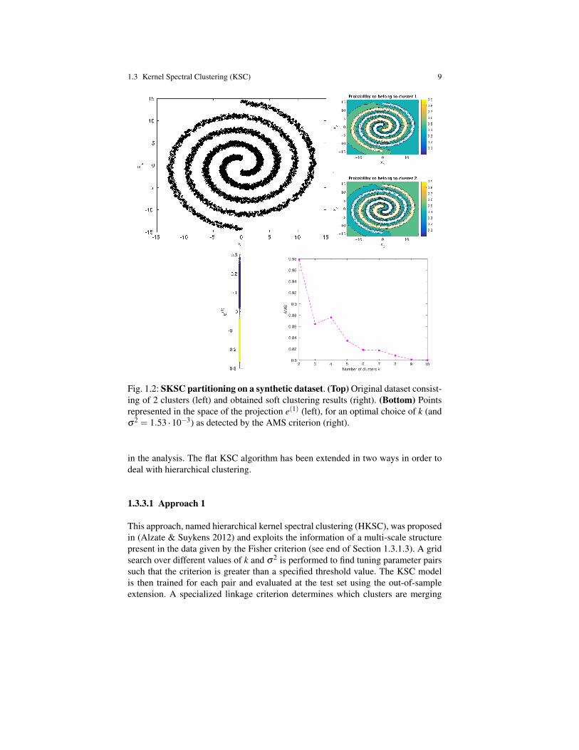
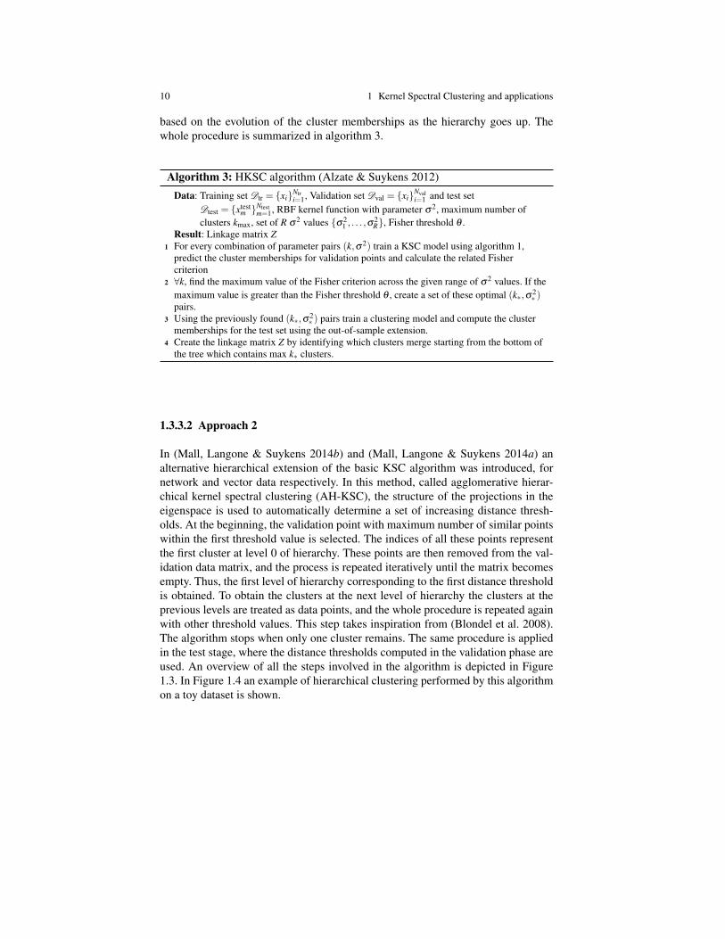
In (Mall, Langone & Suykens 2014b) and (Mall, Langone & Suykens 2014a) analternative hierarchical extension of the basic KSC algorithm was introduced, fornetwork and vector data respectively. In this method, called agglomerative hierar-chical kernel spectral clustering (AH-KSC), the structure of the projections in theeigenspace is used to automatically determine a set of increasing distance thresh-olds. At the beginning, the validation point with maximum number of similar pointswithin the first threshold value is selected. The indices of all these points representthe first cluster at level 0 of hierarchy. These points are then removed from the val-idation data matrix, and the process is repeated iteratively until the matrix becomesempty. Thus, the first level of hierarchy corresponding to the first distance thresholdis obtained. To obtain the clusters at the next level of hierarchy the clusters at theprevious levels are treated as data points, and the whole procedure is repeated againwith other threshold values. This step takes inspiration from (Blondel et al. 2008).The algorithm stops when only one cluster remains. The same procedure is appliedin the test stage, where the distance thresholds computed in the validation phase areused. An overview of all the steps involved in the algorithm is depicted in Figure1.3. In Figure 1.4 an example of hierarchical clustering performed by this algorithmon a toy dataset is shown.
1.3 Kernel Spectral Clustering (KSC) 11
Fig. 1.3: AH-KSC algorithm. Steps of AH-KSC method as described in (Mall,Langone & Suykens 2014b) with addition of the step where the optimal σ and k areestimated.
Fig. 1.4: AH-KSC partitioning on a toy dataset. Cluster memberships for a toydataset at different hierarchical levels obtained by the AH-KSC method.
1.3.4 Sparse Clustering Models
The computational complexity of the KSC algorithm depends on solving the eigen-value problem (1.3) related to the training stage and computing eq. (1.5) whichgives the cluster memberships of the remaining points. Assuming that we have Ntotdata and we use Ntr points for training and Ntest = Ntot−Ntr as test set, the runtimeof algorithm 1 is O(N2
tr)+O(NtrNtest). In order to reduce the computational com-plexity, it is then necessary to find a reduced set of training points, without loosingaccuracy. In the next Sections two different methods to obtain a sparse KSC model,based on the Incomplete Cholesky Decomposition (ICD) and L1 and L0 penaltiesrespectively, are discussed. In particular, thanks to the ICD, the KSC computationalcomplexity for the training problem is decreased to O(R2Ntr) (Novak et al. 2015),where R indicates the reduced set size.
12 1 Kernel Spectral Clustering and applications
1.3.4.1 Incomplete Cholesky Decomposition
One of the KKT optimality conditions characterizing the Lagrangian of problem(1.1) is:
w(l) = ΦT
α(l) =
Ntr
∑i=1
α(l)i ϕ(xi). (1.9)
From eq. (1.9) it is evident that each training data point contributes to the primalvariable w(l), resulting in a non-sparse model. In order to obtain a parsimoniousmodel a reduced set method based on the Incomplete Cholesky Decomposition(ICD) was proposed in (Alzate & Suykens 2011, Novak et al. 2015). The tech-nique is based on finding a small number RNtr of points R = xrR
r=1 and relatedcoefficients ζ (l) with the aim of approximating w(l) as:
w(l) ≈ w(l) =R
∑r=1
ζ(l)r ϕ(xr). (1.10)
As a consequence, the projection of an arbitrary data point x into the training em-bedding is given by:
e(l) ≈ e(l) =R
∑r=1
ζ(l)r K(x, xr)+ bl . (1.11)
The set R of points can be obtained by considering the pivots of the ICD performedon the kernel matrix Ω . In particular, by assuming that Ω has a small numericalrank, the kernel matrix can be approximated by Ω ≈ Ω = GGT , with G ∈ RNtr×R.If we plug in this approximated kernel matrix in problem (1.3), the KSC eigenvalueproblem can be written as:
D−1MDUΨ2UT
α(l) = λlα
(l), l = 1, . . . ,k (1.12)
where U ∈RNtr×R and V ∈RNtr×R denotes the left and right singular vectors derivingfrom the singular value decomposition (SVD) of G, and Ψ ∈ RNtr×Ntr is the matrixof the singular values. If now we pre-multiply both sides of eq. (1.12) by UT andreplace δ (l) =UT α(l), only the following eigenvalue problem of size R×R must besolved:
UT D−1MDUΨ2δ(l) = λl δ
(l), l = 1, . . . ,k. (1.13)
The approximated eigenvectors of the original problem (1.3) can be computed asα(l) =U δ (l), and the sparse parameter vector can be found by solving the followingoptimization problem:
minζ (l) ‖ w(l)− w(l) ‖2
2= minζ (l) ‖Φ
Tα(l)−χ
Tζ(l) ‖2
2 . (1.14)
The corresponding dual problem can be written as follows:
Ωχχ
δ(l) = Ω
χφα(l), (1.15)
1.3 Kernel Spectral Clustering (KSC) 13
where Ωχχrs = K(xr, xs), Ω
χφ
ri = K(xr,xi), r,s = 1, . . . ,R, i = 1, . . . ,Ntr and l =1, . . . ,k−1. Since the size R of problem (1.13) can be much smaller than the size Ntrof the starting problem, the sparse KSC method6 is suitable for big data analytics.
1.3.4.2 Using Additional Penalty terms
In this part we explore sparsity in the KSC technique by using an additional penaltyterm in the objective function (1.14). In (Alzate & Suykens 2011), the authors usedan L1 penalization term in combination with the reconstruction error term to in-troduce sparsity. It is well known that the L1 regularization introduces sparsity asshown in (Zhu et al. 2003). However, the resulting reduced set is neither the spars-est nor the most optimal w.r.t. the quality of clustering for the entire dataset. In(Mall, Mehrkanoon, Langone & Suykens 2014), we introduced alternative penal-ization techniques like Group Lasso (Yuan & Lin 2006) and (Friedman et al. 2010),L0 and L1 + L0 penalizations. The Group Lasso penalty is ideal for clusters as itresults in groups of relevant data points. The L0 regularization calculates the num-ber of non-zero terms in the vector. The L0-norm results in a non-convex and NP-hard optimization problem. We modify the convex relaxation of L0-norm based onan iterative re-weighted L1 formulation introduced in (Candes et al. 2008, Huanget al. 2010). We apply it to obtain the optimal reduced sets for sparse kernel spectralclustering. Below we provide the formulation for Group Lasso penalized objective(1.16) and re-weighted L1-norm penalized objectives (1.17).
The Group Lasso (Yuan & Lin 2006) based formulation for our optimizationproblem is:
minβ∈RNtr×(k−1)
‖Φᵀα−Φ
ᵀβ‖2
2 +λ
Ntr
∑l=1
√ρl‖βl‖2, (1.16)
where Φ = [φ(x1), . . . ,φ(xNtr)], α = [α(1), . . . ,α(k−1)], α ∈ RNtr×(k−1) and β =[β1, . . . ,βNtr ], β ∈ RNtr×(k−1) . Here α(i) ∈ RNtr while β j ∈ Rk−1 and we set
√ρl
as the fraction of training points belonging to the cluster to which the lth trainingpoint belongs. By varying the value of λ we control the amount of sparsity intro-duced in the model as it acts as a regularization parameter. In (Friedman et al. 2010),the authors show that if the initial solutions are β1, β2, . . . , βNtr then if ‖Xᵀ
l (y−∑i6=l Xiβi)‖< λ , then βl is zero otherwise it satisfies: βl = (Xᵀ
l Xl +λ/‖βl‖)−1Xᵀl rl
where rl = y−∑i 6=l Xiβi.Analogous to this, the solution to the group lasso penalization for our problem
can be defined as: ‖φ(xl)(Φᵀα−∑i 6=l φ(xi)βi)‖< λ then βl is zero otherwise it sat-
isfies: βl = (ΦᵀΦ +λ/‖βl‖)−1φ(xl)rl where rl = Φᵀα−∑i 6=l φ(xi)βi. The GroupLasso penalization technique can be solved by a blockwise co-ordinate descent pro-
6 A C implementation of the algorithm can be downloaded at:http://www.esat.kuleuven.be/stadius/ADB/novak/softwareKSCICD.php
14 1 Kernel Spectral Clustering and applications
cedure as shown in (Yuan & Lin 2006). The time complexity of the approach isO(maxiter ∗ k2N2
tr) where maxiter is the maximum number of iterations specifiedfor the co-ordinate descent procedure and k is the number of clusters obtained viaKSC. From our experiments we observed that on an average 10 iterations suffice forconvergence.
Concerning the re-weighted L1 procedure, we modify the algorithm related toclassification as shown in (Huang et al. 2010) and use it for obtaining the reducedset in our clustering setting:
minβ∈RNtr×(k−1)
‖Φᵀα−Φ
ᵀβ‖2
2 +ρ
Ntr
∑i=1
εi +‖Λβ‖22
such that ‖βi‖22 ≤ εi, i = 1, . . . ,Ntr
εi ≥ 0,
(1.17)
where Λ is matrix of the same size as the β matrix i.e. Λ ∈ RNtr×(k−1). The term‖Λβ‖2
2 along with the constraint ‖βi‖22≤ εi corresponds to the L0-norm penalty on β
matrix. Λ matrix is initially defined as a matrix of ones so that it gives equal chanceto each element of β matrix to reduce to zero. The constraints on the optimizationproblem forces each element of βi ∈R(k−1) to reduce to zero. This helps to overcomethe problem of sparsity per component which is explained in (Alzate & Suykens2011). The ρ variable is a regularizer which controls the amount of sparsity that isintroduced by solving this optimization problem.
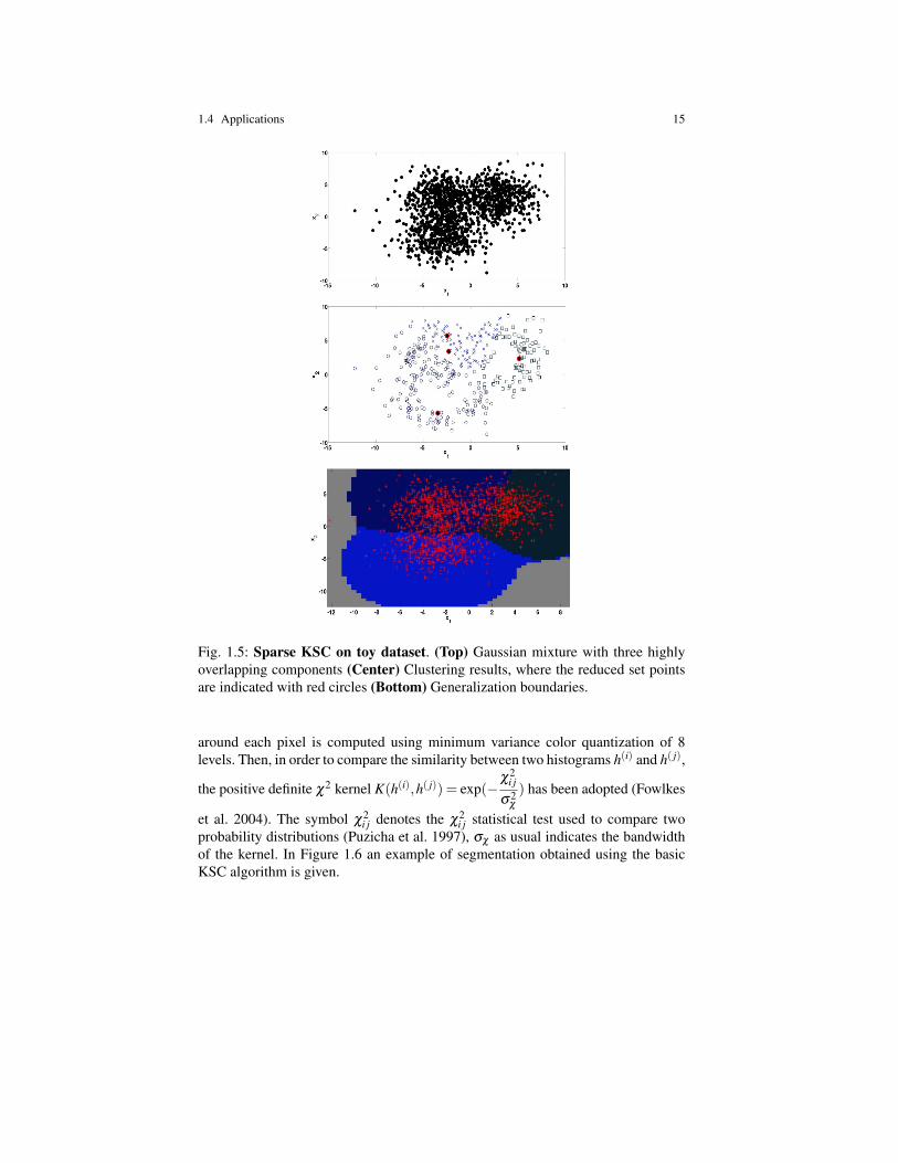
In Figure 1.5 an example of clustering obtained using the group lasso formulation(1.16) on a toy dataset is depicted. We can notice how the sparse KSC model is ableto obtain high quality generalization using only 4 points in the training set.
1.4 Applications
The KSC algorithm has been successfully used in a variety of applications in dif-ferent domains. In the next Sections we will illustrate various results obtained indifferent fields such as computer vision, information retrieval and power load con-sumer segmentation.
1.4.1 Image Segmentation
Image segmentation relates to partitioning a digital image into multiple regions,such that pixels in the same group share a certain visual content. In the experimentsperformed using KSC only the color information is exploited in order to segment thegiven images7. More precisely, a local color histogram with a 5×5 pixels window
7 The images have been extracted from the Berkeley image database (Martin et al. 2001).
1.4 Applications 15
Fig. 1.5: Sparse KSC on toy dataset. (Top) Gaussian mixture with three highlyoverlapping components (Center) Clustering results, where the reduced set pointsare indicated with red circles (Bottom) Generalization boundaries.
around each pixel is computed using minimum variance color quantization of 8levels. Then, in order to compare the similarity between two histograms h(i) and h( j),
the positive definite χ2 kernel K(h(i),h( j)) = exp(−χ2
i j
σ2χ
) has been adopted (Fowlkes
et al. 2004). The symbol χ2i j denotes the χ2
i j statistical test used to compare twoprobability distributions (Puzicha et al. 1997), σχ as usual indicates the bandwidthof the kernel. In Figure 1.6 an example of segmentation obtained using the basicKSC algorithm is given.
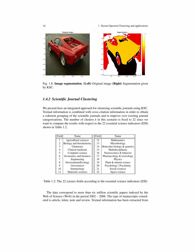
16 1 Kernel Spectral Clustering and applications
Fig. 1.6: Image segmentation. (Left) Original image (Right) Segmentation givenby KSC.
1.4.2 Scientific Journal Clustering
We present here an integrated approach for clustering scientific journals using KSC.Textual information is combined with cross-citation information in order to obtaina coherent grouping of the scientific journals and to improve over existing journalcategorizations. The number of clusters k in this scenario is fixed to 22 since wewant to compare the results with respect to the 22 essential science indicators (ESI)shown in Table 1.2.
Field Name
1 Agricultural sciences2 Biology and biochemistry3 Chemistry4 Clinical medicine5 Computer science6 Economics and business7 Engineering8 Environment/Ecology9 Geosciences10 Immunology11 Materials sciences
Field Name
12 Mathematics13 Microbiology14 Molecular biology & genetics15 Multidisciplinary16 Neuroscience & behavior17 Pharmacology & toxicology18 Physics19 Plant & animal science20 Psychology / Psychiatry21 Social sciences22 Space science
Table 1.2: The 22 science fields according to the essential science indicators (ESI)
The data correspond to more than six million scientific papers indexed by theWeb of Science (WoS) in the period 2002−2006. The type of manuscripts consid-ered is article, letter, note and review. Textual information has been extracted from

1.4 Applications 17
titles, abstracts and keywords of each paper together with citation information. Fromthese data, the resulting number of journals under consideration is 8,305.
The two resulting datasets contain textual and cross-citation information and aredescribed as follows:
• Term/Concept by Journal dataset: The textual information was processed us-ing the term frequency - inverse document frequency (TF-IDF) weighting pro-cedure (Baeza-Yates & Ribeiro-Neto 1999). Terms which occur only in onedocument and stop words were not considered into the analysis. The Porterstemmer was applied to the remaining terms in the abstract, title and key-word fields. This processing leads to a term-by-document matrix of aroundsix million papers and 669,860 term dimensionality. The final journal-by-termdataset is a 8,305×669,860 matrix. Additionally, latent semantic indexing (LSI)(Deerwester et al. 1990) was performed on this dataset to reduce the term dimen-sionality to 200 factors.
• Journal cross-citation dataset: A different form of analyzing cluster informa-tion at the journal level is through a cross-citation graph. This graph containsaggregated citations between papers forming a journal-by-journal cross-citationmatrix. The direction of the citations is not taken into account which leads to anundirected graph and a symmetric cross-citation matrix.
The cross-citation and the text/concept datasets are integrated at the kernel level byconsidering the following linear combination of kernel matrices8:
Ωintegr = ρΩ
cross-cit +(1−ρ)Ω text
where 0 ≤ ρ ≤ 1 is a user-defined integration weight which value can be obtainedfrom internal validation measures for cluster distortion9, Ω cross-cit is the cross-citation kernel matrix with i j-th entry Ω cross-cit
i j = K(xcross-citi ,xcross-cit
j ), xcross-citi is
the i-th journal represented in terms of cross-citation variables, Ω text is the textualkernel matrix with i j-th entry Ω text
i j = K(xtexti ,xtext
j ), xtexti is the i-th journal repre-
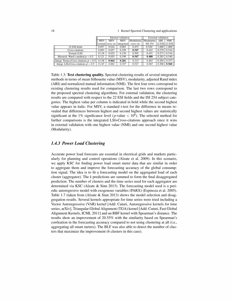
sented in terms of textual variables and i, j = 1, . . . ,N.The KSC outcomes are depicted in Tables 1.3 and 1.4. In particular, Table
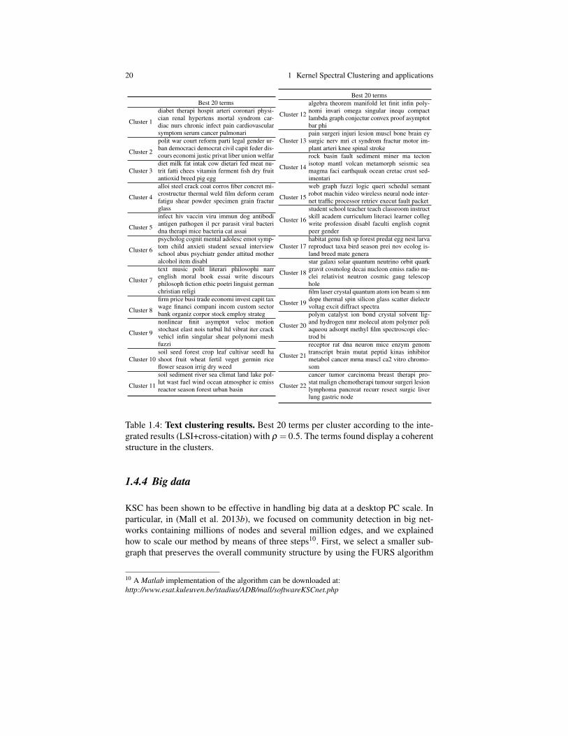
1.3 shows the results in terms of internal validation of cluster quality, namelymean silhouette value (MSV) (Rousseeuw 1987) and Modularity (Newman &Girvan 2004, Newman 2006), and in terms of agreement with existing categoriza-tions (adjusted rand index or ARI (Hubert & Arabie 1985) and normalized mutualinformation (NMI (Strehl & Ghosh 2002)). Finally, Table 1.4 shows the top 20 termsper cluster, which indicate a coherent structure and illustrate that KSC is able to de-tect the text categories present in the corpus.
8 Here we use the cosine kernel described in Table 1.1.9 In our experiments we used the mean silhouette value (MSV) as an internal cluster validationcriterion to select the value of ρ which gives more coherent clusters.
18 1 Kernel Spectral Clustering and applications
Internal validation External validationMSV MSV MSV Modularity Modularity ARI NMI
textual cross-cit. integrated cross-cit. ISI 254 22 ESI 22 ESI22 ESI fields 0.057 0.016 0.063 0.475 0.526? 1.000 1.000
Cross-citations 0.093 0.057 0.189 0.547 0.442 0.278 0.516Textual (LSI) 0.118 0.035 0.130 0.505 0.451 0.273 0.516
Hierarch. Ward’s method ρ = 0.5 0.121 0.055 0.190 0.547 0.488 0.285 0.540
Integr. Terms+Cross-citations ρ = 0.5 0.138 0.064 0.201 0.533 0.465 0.294 0.557Integr. LSI+Cross-citations ρ = 0.5 0.145 0.062 0.197 0.527 0.465 0.308 0.560
Table 1.3: Text clustering quality. Spectral clustering results of several integrationmethods in terms of mean Silhouette value (MSV), modularity, adjusted Rand index(ARI) and normalized mutual information (NMI). The first four rows correspond toexisting clustering results used for comparison. The last two rows correspond tothe proposed spectral clustering algorithms. For external validation, the clusteringresults are compared with respect to the 22 ESI fields and the ISI 254 subject cate-gories. The highest value per column is indicated in bold while the second highestvalue appears in italic. For MSV, a standard t-test for the difference in means re-vealed that differences between highest and second highest values are statisticallysignificant at the 1% significance level (p-value < 108). The selected method forfurther comparisons is the integrated LSI+Cross-citations approach since it winsin external validation with one highest value (NMI) and one second highest value(Modularity).
1.4.3 Power Load Clustering
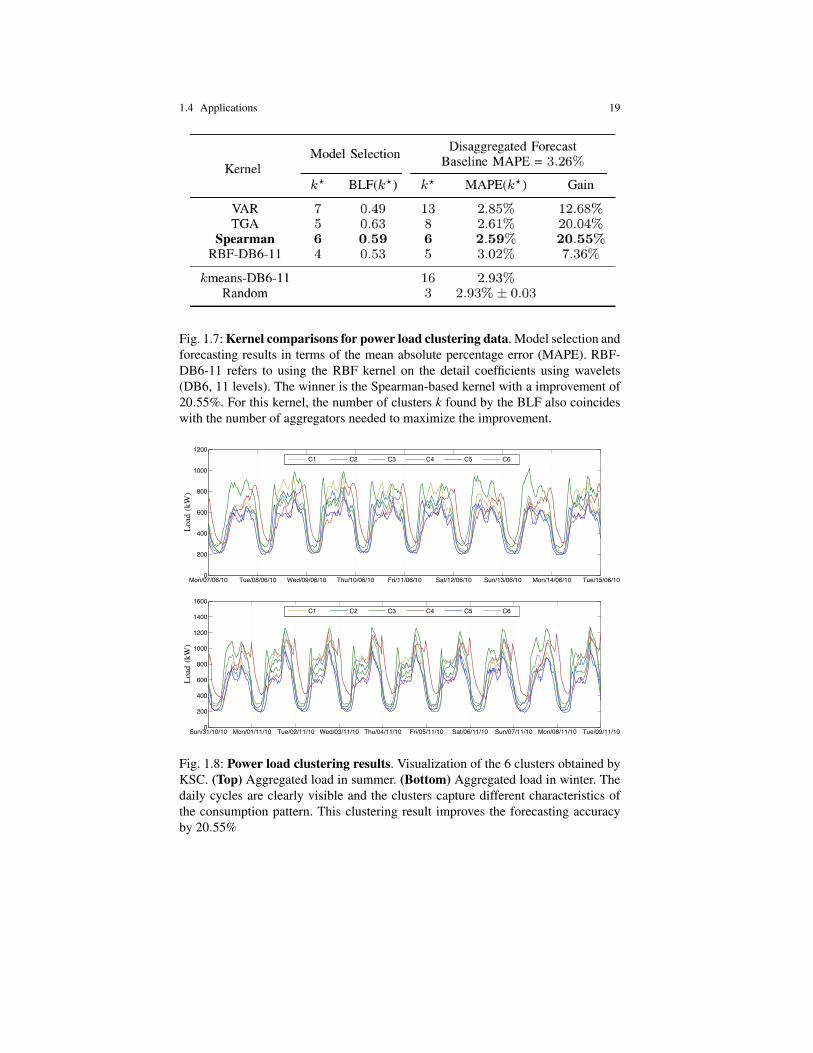
Accurate power load forecasts are essential in electrical grids and markets partic-ularly for planning and control operations (Alzate et al. 2009). In this scenario,we apply KSC for finding power load smart meter data that are similar in orderto aggregate them and improve the forecasting accuracy of the global consump-tion signal. The idea is to fit a forecasting model on the aggregated load of eachcluster (aggregator). The k predictions are summed to form the final disaggregatedprediction. The number of clusters and the time series used for each aggregator aredetermined via KSC (Alzate & Sinn 2013). The forecasting model used is a peri-odic autoregresive model with exogenous variables (PARX) (Espinoza et al. 2005).Table 1.7 (taken from (Alzate & Sinn 2013) shows the model selection and disag-gregation results. Several kernels appropriate for time series were tried including aVector Autoregressive (VAR) kernel [Add: Cuturi, Autoregressive kernels for timeseries, arXiv], Triangular Global Alignment (TGA) kernel [Add: Cuturi, Fast GlobalAlignment Kernels, ICML 2011] and an RBF kernel with Spearman’s distance. Theresults show an improvement of 20.55% with the similarity based on Spearman’scorrleation in the forecasting accuracy compared to not using clustering at all (i.e.,aggregating all smart meters). The BLF was also able to detect the number of clus-ters that maximize the improvement (6 clusters in this case).
1.4 Applications 19
Fig. 1.7: Kernel comparisons for power load clustering data. Model selection andforecasting results in terms of the mean absolute percentage error (MAPE). RBF-DB6-11 refers to using the RBF kernel on the detail coefficients using wavelets(DB6, 11 levels). The winner is the Spearman-based kernel with a improvement of20.55%. For this kernel, the number of clusters k found by the BLF also coincideswith the number of aggregators needed to maximize the improvement.
Mon/07/06/10 Tue/08/06/10 Wed/09/06/10 Thu/10/06/10 Fri/11/06/10 Sat/12/06/10 Sun/13/06/10 Mon/14/06/10 Tue/15/06/100
200
400
600
800
1000
1200
C1 C2 C3 C4 C5 C6
Loa
d(k
W)
Sun/31/10/10 Mon/01/11/10 Tue/02/11/10 Wed/03/11/10 Thu/04/11/10 Fri/05/11/10 Sat/06/11/10 Sun/07/11/10 Mon/08/11/10 Tue/09/11/100
200
400
600
800
1000
1200
1400
1600
C1 C2 C3 C4 C5 C6
Loa
d(k
W)
Fig. 10
Mon/20/12/10 Tue/21/12/10 Wed/22/12/10 Thu/23/12/10 Fri/24/12/10 Sat/25/12/10 Sun/26/12/10 Mon/27/12/10 Tue/28/12/10 Wed/29/12/10 Thu/30/12/10 Fri/31/12/10
2000
3000
4000
5000
6000
7000
8000
9000t
ObservedPredicted − GlobalPredicted − Disaggregation
Adj
uste
dR
and
Inde
x
Fig. 11: Disaggregated forecast for the last 12 days of the time series using the kernel based on the Spearman distance, k = 6and PARX(48) models. The global forecast has a MAPE of 3.26% while the disaggregated forecast has a MAPE of 2.59%leading to an improvement of 20.55%.
Fig. 1.8: Power load clustering results. Visualization of the 6 clusters obtained byKSC. (Top) Aggregated load in summer. (Bottom) Aggregated load in winter. Thedaily cycles are clearly visible and the clusters capture different characteristics ofthe consumption pattern. This clustering result improves the forecasting accuracyby 20.55%
20 1 Kernel Spectral Clustering and applications
Best 20 terms
Cluster 1
diabet therapi hospit arteri coronari physi-cian renal hypertens mortal syndrom car-diac nurs chronic infect pain cardiovascularsymptom serum cancer pulmonari
Cluster 2
polit war court reform parti legal gender ur-ban democraci democrat civil capit feder dis-cours economi justic privat liber union welfar
Cluster 3diet milk fat intak cow dietari fed meat nu-trit fatti chees vitamin ferment fish dry fruitantioxid breed pig egg
Cluster 4
alloi steel crack coat corros fiber concret mi-crostructur thermal weld film deform ceramfatigu shear powder specimen grain fracturglass
Cluster 5
infect hiv vaccin viru immun dog antibodiantigen pathogen il pcr parasit viral bacteridna therapi mice bacteria cat assai
Cluster 6
psycholog cognit mental adolesc emot symp-tom child anxieti student sexual interviewschool abus psychiatr gender attitud motheralcohol item disabl
Cluster 7
text music polit literari philosophi narrenglish moral book essai write discoursphilosoph fiction ethic poetri linguist germanchristian religi
Cluster 8
firm price busi trade economi invest capit taxwage financi compani incom custom sectorbank organiz corpor stock employ strateg
Cluster 9
nonlinear finit asymptot veloc motionstochast elast nois turbul ltd vibrat iter crackvehicl infin singular shear polynomi meshfuzzi
Cluster 10soil seed forest crop leaf cultivar seedl hashoot fruit wheat fertil veget germin riceflower season irrig dry weed
Cluster 11
soil sediment river sea climat land lake pol-lut wast fuel wind ocean atmospher ic emissreactor season forest urban basin
Best 20 terms
Cluster 12
algebra theorem manifold let finit infin poly-nomi invari omega singular inequ compactlambda graph conjectur convex proof asymptotbar phi
Cluster 13pain surgeri injuri lesion muscl bone brain eysurgic nerv mri ct syndrom fractur motor im-plant arteri knee spinal stroke
Cluster 14
rock basin fault sediment miner ma tectonisotop mantl volcan metamorph seismic seamagma faci earthquak ocean cretac crust sed-imentari
Cluster 15
web graph fuzzi logic queri schedul semantrobot machin video wireless neural node inter-net traffic processor retriev execut fault packet
Cluster 16
student school teacher teach classroom instructskill academ curriculum literaci learner collegwrite profession disabl faculti english cognitpeer gender
Cluster 17habitat genu fish sp forest predat egg nest larvareproduct taxa bird season prei nov ecolog is-land breed mate genera
Cluster 18
star galaxi solar quantum neutrino orbit quarkgravit cosmolog decai nucleon emiss radio nu-clei relativist neutron cosmic gaug telescophole
Cluster 19
film laser crystal quantum atom ion beam si nmdope thermal spin silicon glass scatter dielectrvoltag excit diffract spectra
Cluster 20
polym catalyst ion bond crystal solvent lig-and hydrogen nmr molecul atom polymer poliaqueou adsorpt methyl film spectroscopi elec-trod bi
Cluster 21
receptor rat dna neuron mice enzym genomtranscript brain mutat peptid kinas inhibitormetabol cancer mrna muscl ca2 vitro chromo-som
Cluster 22
cancer tumor carcinoma breast therapi pro-stat malign chemotherapi tumour surgeri lesionlymphoma pancreat recurr resect surgic liverlung gastric node
Table 1.4: Text clustering results. Best 20 terms per cluster according to the inte-grated results (LSI+cross-citation) with ρ = 0.5. The terms found display a coherentstructure in the clusters.
1.4.4 Big data
KSC has been shown to be effective in handling big data at a desktop PC scale. Inparticular, in (Mall et al. 2013b), we focused on community detection in big net-works containing millions of nodes and several million edges, and we explainedhow to scale our method by means of three steps10. First, we select a smaller sub-graph that preserves the overall community structure by using the FURS algorithm
10 A Matlab implementation of the algorithm can be downloaded at:http://www.esat.kuleuven.be/stadius/ADB/mall/softwareKSCnet.php
1.5 Conclusions 21
(Mall et al. 2013a), where hubs in dense regions of the original graph are selectedvia a greedy activation-deactivation procedure. In this way the kernel matrix relatedto subgraph fits the main memory and the KSC model can be quickly trained bysolving a smaller eigenvalue problem. Then the BAF criterion described in Section1.3.1.3, which is memory and computationally efficient, is used for model selec-tion11. Finally, the out-of-sample extension is used to infer the cluster membershipsfor the remaining nodes forming the test set (which is divided into chunks due tomemory constraints).
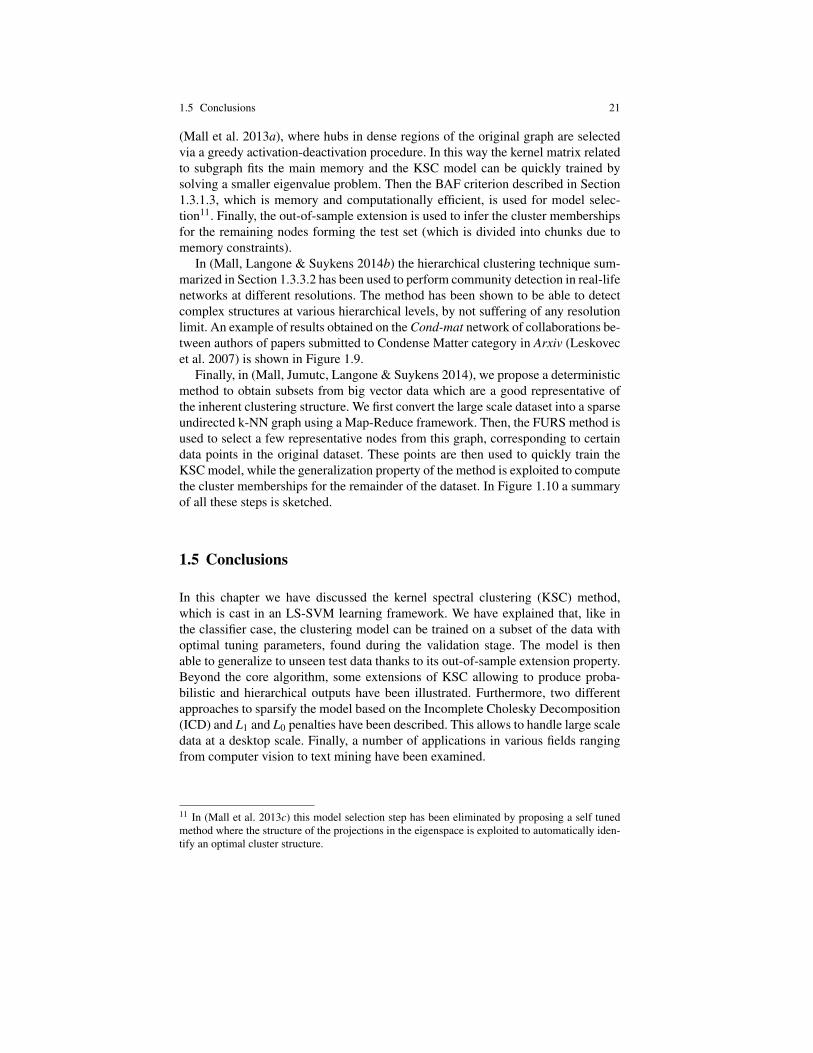
In (Mall, Langone & Suykens 2014b) the hierarchical clustering technique sum-marized in Section 1.3.3.2 has been used to perform community detection in real-lifenetworks at different resolutions. The method has been shown to be able to detectcomplex structures at various hierarchical levels, by not suffering of any resolutionlimit. An example of results obtained on the Cond-mat network of collaborations be-tween authors of papers submitted to Condense Matter category in Arxiv (Leskovecet al. 2007) is shown in Figure 1.9.
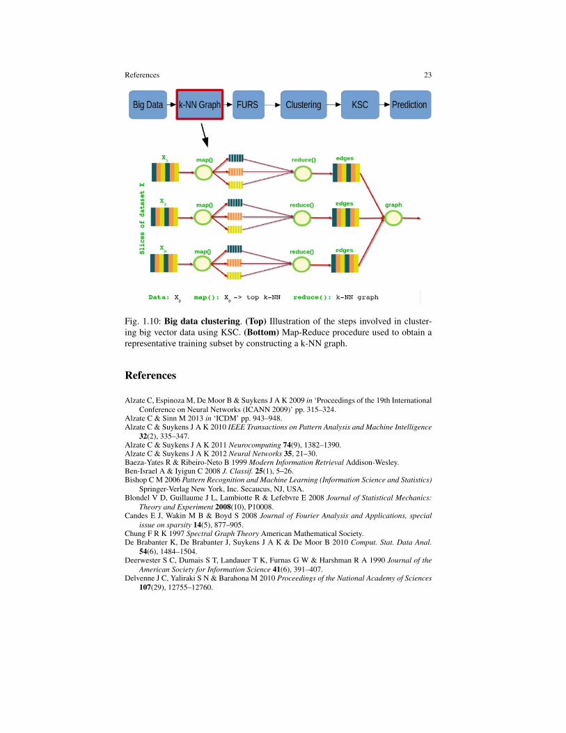
Finally, in (Mall, Jumutc, Langone & Suykens 2014), we propose a deterministicmethod to obtain subsets from big vector data which are a good representative ofthe inherent clustering structure. We first convert the large scale dataset into a sparseundirected k-NN graph using a Map-Reduce framework. Then, the FURS method isused to select a few representative nodes from this graph, corresponding to certaindata points in the original dataset. These points are then used to quickly train theKSC model, while the generalization property of the method is exploited to computethe cluster memberships for the remainder of the dataset. In Figure 1.10 a summaryof all these steps is sketched.
1.5 Conclusions
In this chapter we have discussed the kernel spectral clustering (KSC) method,which is cast in an LS-SVM learning framework. We have explained that, like inthe classifier case, the clustering model can be trained on a subset of the data withoptimal tuning parameters, found during the validation stage. The model is thenable to generalize to unseen test data thanks to its out-of-sample extension property.Beyond the core algorithm, some extensions of KSC allowing to produce proba-bilistic and hierarchical outputs have been illustrated. Furthermore, two differentapproaches to sparsify the model based on the Incomplete Cholesky Decomposition(ICD) and L1 and L0 penalties have been described. This allows to handle large scaledata at a desktop scale. Finally, a number of applications in various fields rangingfrom computer vision to text mining have been examined.
11 In (Mall et al. 2013c) this model selection step has been eliminated by proposing a self tunedmethod where the structure of the projections in the eigenspace is exploited to automatically iden-tify an optimal cluster structure.
22 1 Kernel Spectral Clustering and applications
Fig. 1.9: Large scale community detection. Community structure detected at oneparticular hierarchical level by the AH-KSC method summarized in Section 1.3.3.2,related to the Cond-Mat collaboration network.
Acknowledgements EU: The research leading to these results has received funding from the Eu-ropean Research Council under the European Union’s Seventh Framework Programme (FP7/2007-2013) / ERC AdG A-DATADRIVE-B (290923). This chapter reflects only the authors’ views, theUnion is not liable for any use that may be made of the contained information. Research CouncilKUL: GOA/10/09 MaNet, CoE PFV/10/002 (OPTEC), BIL12/11T; PhD/Postdoc grants. Flem-ish Government: FWO: projects: G.0377.12 (Structured systems), G.088114N (Tensor based datasimilarity); PhD/Postdoc grants. IWT: projects: SBO POM (100031); PhD/Postdoc grants. iMindsMedical Information Technologies SBO 2014. Belgian Federal Science Policy Office: IUAP P7/19(DYSCO, Dynamical systems, control and optimization, 2012-2017.)
References 23
Fig. 1.10: Big data clustering. (Top) Illustration of the steps involved in cluster-ing big vector data using KSC. (Bottom) Map-Reduce procedure used to obtain arepresentative training subset by constructing a k-NN graph.
References
Alzate C, Espinoza M, De Moor B & Suykens J A K 2009 in ‘Proceedings of the 19th InternationalConference on Neural Networks (ICANN 2009)’ pp. 315–324.
Alzate C & Sinn M 2013 in ‘ICDM’ pp. 943–948.Alzate C & Suykens J A K 2010 IEEE Transactions on Pattern Analysis and Machine Intelligence
32(2), 335–347.Alzate C & Suykens J A K 2011 Neurocomputing 74(9), 1382–1390.Alzate C & Suykens J A K 2012 Neural Networks 35, 21–30.Baeza-Yates R & Ribeiro-Neto B 1999 Modern Information Retrieval Addison-Wesley.Ben-Israel A & Iyigun C 2008 J. Classif. 25(1), 5–26.Bishop C M 2006 Pattern Recognition and Machine Learning (Information Science and Statistics)
Springer-Verlag New York, Inc. Secaucus, NJ, USA.Blondel V D, Guillaume J L, Lambiotte R & Lefebvre E 2008 Journal of Statistical Mechanics:
Theory and Experiment 2008(10), P10008.Candes E J, Wakin M B & Boyd S 2008 Journal of Fourier Analysis and Applications, special
issue on sparsity 14(5), 877–905.Chung F R K 1997 Spectral Graph Theory American Mathematical Society.De Brabanter K, De Brabanter J, Suykens J A K & De Moor B 2010 Comput. Stat. Data Anal.
54(6), 1484–1504.Deerwester S C, Dumais S T, Landauer T K, Furnas G W & Harshman R A 1990 Journal of the
American Society for Information Science 41(6), 391–407.Delvenne J C, Yaliraki S N & Barahona M 2010 Proceedings of the National Academy of Sciences
107(29), 12755–12760.
24 1 Kernel Spectral Clustering and applications
Dhanjal C, Gaudel R & Clemenccon S 2013 arXiv/1301.1318 .Espinoza M, Joye C, Belmans R & De Moor B 2005 IEEE Transactions on Power System
20(3), 1622–1630.Fowlkes C, Belongie S, Chung F & Malik J 2004 IEEE Transactions on Pattern Analysis and
Machine Intelligence 26(2), 214–225.Frederix K & Van Barel M 2013 J. Comput. Appl. Math. 237(1), 145–161.Friedman J, Hastie T & Tibshirani R 2010 arXiv:1001.0736 .Huang K, Zheng D, Sun J, Hotta Y, Fujimoto K & Naoi S 2010 Pattern Recognition Letters
31(13), 1944–1951.Hubert L & Arabie P 1985 Journal of Classification 1(2), 193–218.Langone R, Agudelo O M, De Moor B & Suykens J A K 2014 Neurocomputing 139(0), 246–260.Langone R, Alzate C, De Ketelaere B & Suykens J A K 2013 in ‘IEEE Symposium Series on
Computational Intelligence and data mining SSCI (CIDM) 2013’ pp. 39–45.Langone R, Alzate C, De Ketelaere B, Vlasselaer J, Meert W & Suykens J A K 2015 Engineering
Applications of Artificial Intelligence 37, 268–278.Langone R, Alzate C & Suykens J A K 2011 in ‘Proc. of the International Joint Conference on
Neural Networks (IJCNN 2011)’ pp. 1849–1856.Langone R, Alzate C & Suykens J A K 2012 in ‘Proc. of the International Joint Conference on
Neural Networks (IJCNN 2012)’ pp. 2596–2603.Langone R, Alzate C & Suykens J A K 2013 Physica A: Statistical Mechanics and its Applications
392(10), 2588–2606.Langone R, Mall R & Suykens J A K 2013 in ‘Proc. of the International Joint Conference on
Neural Networks (IJCNN 2013)’ pp. 1–8.Langone R, Mall R & Suykens J A K 2014 SSCI (CIDM) 2014 pp. 1–8.Langone R & Suykens J A K 2013 Journal of Physics: Conference Series 410(1), 012100.Leskovec J, Kleinberg J & Faloutsos C 2007 ACM Trans. Knowl. Discov. Data 1(1).Liao T W 2005 Pattern Recognition 38(11), 1857 – 1874.Lin F & Cohen W W 2010 in ‘ICML’ pp. 655–662.Mall R, Jumutc V, Langone R & Suykens J A K 2014 in ‘IEEE International Conference on Big
Data’ pp. 37–42.Mall R, Langone R & Suykens J 2013a Social Network Analysis and Mining 3(4), 1–21.Mall R, Langone R & Suykens J A K 2013b Entropy (Special Issue on Big Data) 15(5), 1567–1586.Mall R, Langone R & Suykens J A K 2013c in ‘IEEE International Conference on Big Data’.Mall R, Langone R & Suykens J A K 2014a in ‘Symposium Series on Computational Intelligence
(SSCI-CIDM)’ pp. 1–8.Mall R, Langone R & Suykens J A K 2014b PLoS ONE 9(6), e99966.Mall R, Mehrkanoon S, Langone R & Suykens J A K 2014 in ‘Proc. of the International Joint
Conference on Neural Networks (IJCNN 2014)’ pp. 2436–2443.Martin D, Fowlkes C, Tal D & Malik J 2001 in ‘Proc. 8th Int’l Conf. Computer Vision’ Vol. 2
pp. 416–423.Meila M & Shi J 2001a in T. K Leen, T. G Dietterich & V Tresp, eds, ‘Advances in Neural Infor-
mation Processing Systems 13’ MIT Press.Meila M & Shi J 2001b in ‘Artificial Intelligence and Statistics AISTATS’.Mika S, Scholkopf B, Smola A J, Muller K R, Scholz M & Ratsch G 1999 in M. S Kearns, S. A
Solla & D. A Cohn, eds, ‘Advances in Neural Information Processing Systems 11’ MIT Press.Newman M E J 2006 Proc. Natl. Acad. Sci. USA 103(23), 8577–8582.Newman M E J & Girvan M 2004 Physical Review E 69(2).Ng A Y, Jordan M I & Weiss Y 2002 in T. G Dietterich, S Becker & Z Ghahramani, eds, ‘Advances
in Neural Information Processing Systems 14’ MIT Press Cambridge, MA pp. 849–856.Ning H, Xu W, Chi Y, Gong Y & Huang T S 2010 Pattern Recogn. 43(1), 113–127.Novak M, Alzate C, langone R & Suykens J A K 2015 Internal Report 14-119, ESAT-SISTA, KU
Leuven (Leuven, Belgium) .Peluffo D, Garcia S, Langone R, Suykens J A K & Castellanos G 2013 in ‘Proc. of the International
Joint Conference on Neural Networks (IJCNN 2013)’ pp. 1085 – 1090.
References 25
Puzicha J, Hofmann T & Buhmann J 1997 in ‘Computer Vision and Pattern Recognition’ pp. 267–272.
Rousseeuw P J 1987 Journal of Computational and Applied Mathematics 20(1), 53–65.Scholkopf B, Smola A J & Muller K R 1998 Neural Computation 10, 1299–1319.Shi J & Malik J 2000 IEEE Trans. Pattern Anal. Machine Intell. 22(8), 888–905.Strehl A & Ghosh J 2002 Journal of Machine Learning Research 3, 583–617.Suykens J A K, Van Gestel T, De Brabanter J, De Moor B & Vandewalle J 2002 Least Squares
Support Vector Machines World Scientific, Singapore.Suykens J A K, Van Gestel T, Vandewalle J & De Moor B 2003 IEEE Transactions on Neural
Networks 14(2), 447–450.von Luxburg U 2007 Statistics and Computing 17(4), 395–416.Williams C K I & Seeger M 2001 in ‘Advances in Neural Information Processing Systems 13’ MIT
Press.Yuan M & Lin Y 2006 Journal of Royal Statistical Society 68(1), 49–67.Zhu J, Rosset S, Hastie T & Tibshirani R 2003 in ‘Neural Information Processing Systems’ Vol. 16.

Related Documents