Kernel density estimates of alongshore home range of Hector's dolphins at Banks Peninsula, New Zealand

MARINE MAMMAL SCIENCE, 25(3): 537–556 (July 2009)C© 2009 by the Society for Marine MammalogyDOI: 10.1111/j.1748-7692.2008.00271.x

Kernel density estimates of alongshore home rangeof Hector’s dolphins at Banks Peninsula, New Zealand

WILLIAM RAYMENT

Department of Marine Science,and

Department of Zoology,University of Otago,

P. O. BOX 56, Dunedin, New ZealandE-mail: [email protected]

STEVE DAWSON

Department of Marine Science,University of Otago,

P. O. BOX 56, Dunedin, New Zealand

ELISABETH SLOOTEN

Department of Zoology,University of Otago,


STEFAN BRAGER


P. O. BOX 56, Dunedin, New Zealandand

German Oceanographic Museum (DMM), Stralsund, Germany

SAM DU FRESNE


P. O. BOX 56, Dunedin, New Zealandand

Du Fresne Ecology Ltd.,P. O. Box 1523, Nelson, New Zealand

TRUDI WEBSTER

Department of Marine Science,and

Department of ZoologyUniversity of Otago,


537

538 MARINE MAMMAL SCIENCE, VOL. 25, NO. 3, 2009

ABSTRACT

Knowledge about home ranges is essential for understanding the resources re-quired by a species, identifying critical habitats, and revealing the overlap withanthropogenic impacts. Ranging behavior of Hector’s dolphins (Cephalorhynchushectori) was studied via coastal photo-ID surveys in the Banks Peninsula MarineMammal Sanctuary (BPMMS) between 1985 and 2006. Univariate kernel densityestimates of alongshore home range were calculated for 20 individuals with 15sightings or more. For each individual, sighting locations were transformed into aunivariate data set by projecting sightings onto a line drawn 1 km from the coastand measuring the distance along this line relative to an origin. Sightings wereweighted by survey effort. Ninety-five percent (K95) of the density estimate wasused as a measure of alongshore home range, and 50% of the estimate (K50) wasused to reveal core portions of coastline where dolphins concentrated their activity.The mean estimates of K95 and K50 were 49.69 km (SE = 5.29) and 17.13 km(SE = 1.89), respectively. Four distinct hubs were apparent where the core areas ofdifferent individuals coincided. Three of the dolphins’ alongshore ranges extendedbeyond the current northern boundary of the BPMMS, raising fresh concerns thatthe sanctuary is not large enough. Proposed changes to gill netting regulations, ifenacted, will result in the alongshore ranges of all the dolphins in our study beingprotected.

Key words: Cephalorhynchus hectori, core areas, Hector’s dolphin, home range, kernelanalysis.

Home range is a fundamental concept in ecology. It is best described as “that areatraversed by the individual in its normal activities of food gathering, mating andcaring for young” (Burt 1943, p. 351). Knowledge about home ranges is essentialfor understanding the resources necessary to a species, identifying critical habitats,and guiding decisions regarding management of threatened populations (Ingram andRogan 2002, Seminoff et al. 2002).

Due to their very nature, the majority of home range estimates are derived frombivariate data sets (i.e., observed locations recorded in two dimensions). How-ever, many species have ranges that conform to relatively linear geographic fea-tures (Blundell et al. 2001). For example, fish in river systems are bounded byland (Vokoun 2003), coastal otters largely restrict their movements to the land–sea interface (Blundell et al. 2001), and many delphinids favor coastal waters(Karczmarski et al. 2000, Dawson 2002). Note that the home ranges are not trulylinear, but the second dimension of variation in space use is small compared to thefirst. In such instances, the home range could be more simply described by a uni-variate data set, with the variable being the distance along the linear feature withreference to some origin (e.g., Vokoun 2003).

There are several examples of alongshore ranges of cetaceans described by univariatedata sets (e.g., Wells et al. 1990, Defran et al. 1999, Brager et al. 2002). All usea simple estimate of range length, namely, the linear distance between the twomost extreme sighting locations. By virtue of its simplicity this method has severalundesirable properties: it gives no measure of space usage, range estimates are highlycorrelated with the number of observations used (especially for small sample sizes)and can include areas of habitat that are never visited (Worton 1987). In contrast,kernel methods (see reviews in Silverman 1986, Worton 1987) assign a level of use

RAYMENT ET AL.: HECTOR’S DOLPHINS 539

Figure 1. Location of survey area and numbered sections to summarize survey effort.

to any given point in the habitat based on the entire sample set of relocations duringthe period of interest (Vokoun 2003). This provides insights into the animal’s use ofspace within its range, as well as allowing estimation of the overall extent of the homerange (Vokoun 2003). There are therefore potential advantages in applying kernelmethodology to univariate estimates of alongshore home range of coastal cetaceans.

Hector’s dolphin (Cephalorhynchus hectori) is a small, coastal delphinid endemic toNew Zealand and is listed as endangered (IUCN 2006). The population around BanksPeninsula (Fig. 1), on the South Island’s east coast, is likely to be decreasing (Slootenet al. 2000, Du Fresne 2004) despite protection by the Banks Peninsula MarineMammal Sanctuary (BPMMS) since 1988 (Dawson and Slooten 1993). Hector’sdolphins have a preference for shallow, nearshore waters (Dawson and Slooten 1988,Brager et al. 2003). Aerial and boat-based surveys have shown that sighting ratesare highest within 1 km of the coast (Dawson and Slooten 1988, Rayment et al.2006, Slooten et al. 2006) and dolphins are frequently seen foraging, socializing,and nurturing young in this habitat (personal observation). Alongshore movementsare therefore likely to constitute an important component of an individual’s homerange. However, Hector’s dolphins are also found outside this narrow coastal strip,typically within 7 km of the coast (Dawson and Slooten 1988, Rayment et al. 2006),but in shallow areas have been sighted up to 35 km offshore (Rayment et al. 2006).Estimates of alongshore range therefore do not fully describe an individual’s homerange, and should be interpreted within this context. There is evidence from someareas of seasonal changes in distribution with dolphins being found further offshorein winter (Brager et al. 2003, Slooten et al. 2006).

To date, there have been two attempts to describe home range characteristicsof Hector’s dolphin. Brager et al. (2002) used photo-ID data to estimate alongshorehome range of Hector’s dolphins photographed on coastal surveys at Banks Peninsula.Ranges were estimated by calculating the shortest linear distances (without crossing


land) between the two most extreme sightings for 32 individuals each seen ≥10times between 1985 and 1997. The mean alongshore home range (excluding oneoutlier) was 31.0 km (SE = 2.43). A second study, by Stone et al. (2005), gatheredlocation data via satellite tags for three Hector’s dolphins at Banks Peninsula. Homeranges were estimated via the mean activity radius (mean = 11.60 km; Stone et al.2005). In combination, the two studies revealed that Hector’s dolphins at BanksPeninsula have small home ranges in comparison to other coastal delphinids andexhibit a remarkable degree of site fidelity.

The objectives of this study were to add detail to what is known about thealongshore range of Hector’s dolphins at Banks Peninsula. Firstly, the method ofBrager et al. (2002) was applied to a larger data set to examine the influence ofextending the study period and increasing the sample size. Secondly, we have usedunivariate kernel density estimation, in an attempt to provide more realistic rangeestimates and new insights into habitat use by Hector’s dolphins.

MATERIALS AND METHODS

Survey Protocol and Effort

Photo-ID surveys of Hector’s dolphins were carried out at Banks Peninsula between1985 and 2006 using small (≤6.6 m) outboard-powered research vessels. Photo-ID surveys on open coasts were conducted by following an alongshore transectapproximately 400 m offshore at speeds of 10–15 km. Within Akaroa Harboursurveys followed a standardized zigzag pattern. Our photo-ID protocols are describedin detail by Slooten et al. (1992) and Brager et al. (2002). To reduce the effects ofautocorrelation in the data set, only the first sighting per day for each individualdolphin is included in the analyses. The coastal start point of surveys varied from dayto day so this introduces no systematic bias. We minimized the chance of resamplingindividuals in two ways: (1) by moving swiftly away from a dolphin group once it hadbeen photographed, and (2) by conducting each day’s photo-ID survey in one directiononly (i.e., dolphins were photographed on the outgoing trip, or the returning trip,but not both). The spatial distribution of survey effort was summarized by dividingthe coastline into sections approximately 6 km in length (Fig. 1) and counting thenumber of times that each section was visited. Each section was visited no more thanonce per day. Survey effort was not uniform throughout the study area (Fig. 2). Upto 1990, fieldwork focused predominantly on Akaroa Harbour. Thereafter, surveyswere conducted mostly between Sumner Head and Birdlings Flat, with the majorityof effort concentrated on the south side of the peninsula between Pompey’s Pillarand Birdlings Flat. Occasional survey trips were extended north as far as Motunauand south to the Rakaia River (Fig. 1). Photo-ID surveys were conducted year round,although the majority of effort took place in summer and autumn.

Observed Range Length

To evaluate the effect of extending the study period and increasing the samplesize, the methods of Brager et al. (2002) were applied to the current data set. Brageret al. estimated alongshore home ranges of 32 individual Hector’s dolphins with 10sightings or more between 1985 and 1997. To increase confidence that individualdolphins would have been resighted if they were present, only individuals with


Figure 2. Spatial distribution of photo-ID survey effort, 1985–2006. Sections are numberedas in Figure 1.

very obvious marks (category one or two in Slooten et al. 1992) were included inthe analysis. Extending the study period to 2006 resulted in 53 individuals meetingBrager et al.’s 10 sighting criterion. Some sightings included in Brager et al.’s analysisdid not have accompanying effort data and have been omitted from this analysis. Theobserved range length (HR) was calculated for each individual by plotting sightingsin program ArcView GIS v. 3.3 (UTM projection, zone 59) and measuring theshortest linear distance between the two most extreme locations without crossingland.

In analyses including age, minimum age for each individual (Amin) was equal tothe number of years that the individual was known to be alive, assuming that it wasat least 1 yr old when first sighted.

Kernel Density Estimates of Alongshore Home Range

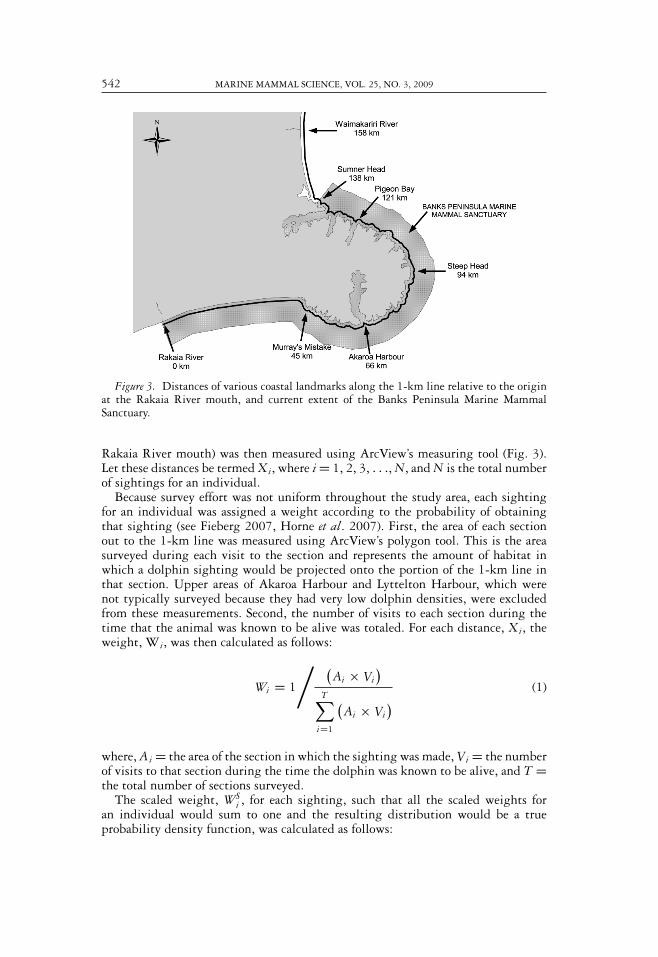
Univariate kernel density estimates of alongshore home range were calculatedfor the 20 Hector’s dolphins with at least 15 sightings between 1985 and 2006.Again, only dolphins with very obvious (category one or two) marks were includedin the analysis. All these marks were nicks out of the dorsal fin (typically the trailingedge) and would not have impaired the swimming abilities of the dolphins. Firstly,sighting locations for each individual were transformed into univariate values fromwhich kernel density estimates could be obtained. Each sighting for an individualwas plotted in ArcView and projected onto the nearest point on a line 1 km fromthe coast. The 1-km line was chosen for two reasons. It represents the approximateouter limit of the transect strip, and hence the vast majority of dolphin sightingswere within 1 km of the coastline. Secondly, the 1-km line effectively “straightensout” the coast so that estimates of home range will not be inflated by the complexnature of the Banks Peninsula shoreline. For each projected point, the distance alongthe 1-km line relative to an origin at the southern most point of the study area (the


Figure 3. Distances of various coastal landmarks along the 1-km line relative to the originat the Rakaia River mouth, and current extent of the Banks Peninsula Marine MammalSanctuary.

Rakaia River mouth) was then measured using ArcView’s measuring tool (Fig. 3).Let these distances be termed Xi, where i = 1, 2, 3, . . ., N, and N is the total numberof sightings for an individual.

Because survey effort was not uniform throughout the study area, each sightingfor an individual was assigned a weight according to the probability of obtainingthat sighting (see Fieberg 2007, Horne et al. 2007). First, the area of each sectionout to the 1-km line was measured using ArcView’s polygon tool. This is the areasurveyed during each visit to the section and represents the amount of habitat inwhich a dolphin sighting would be projected onto the portion of the 1-km line inthat section. Upper areas of Akaroa Harbour and Lyttelton Harbour, which werenot typically surveyed because they had very low dolphin densities, were excludedfrom these measurements. Second, the number of visits to each section during thetime that the animal was known to be alive was totaled. For each distance, Xi, theweight, Wi, was then calculated as follows:

Wi = 1

/ (Ai × Vi

)T∑

i=1

(Ai × Vi

) (1)

where, Ai = the area of the section in which the sighting was made, Vi = the numberof visits to that section during the time the dolphin was known to be alive, and T =the total number of sections surveyed.

The scaled weight, WSi , for each sighting, such that all the scaled weights for

an individual would sum to one and the resulting distribution would be a trueprobability density function, was calculated as follows:


W Si = Wi

N∑i=1

Wi

(2)

where, N = total number of sightings for an individual.The weighting process assigns greater weight to sightings in sections that have

received less survey effort. In sections with very low levels of effort this could resultin very large weights and unrealistic density estimates. Therefore, sightings wereonly included in sections that had received at least 10 survey visits during the timethe dolphin was known to be alive. Two sightings were excluded from the analysisdue to this decision rule. For the majority of animals this effectively limited thestudy area to sections 1–24, a coastline length of 147 km along the 1-km line.

Fixed kernel density estimates were calculated using the “density” function inprogram R v. 2.3.0 (R Development Core Team 2006). Each distance measurement,Xi, was assigned a scaled weight, WS

i , as calculated in Equation (2).The choice of smoothing parameter, or bandwidth, is of crucial importance in

density estimation, although uncertainty remains over which is the most appropriatemethod to use. Simulations have shown that choice of bandwidth using least-squarescross-validation (LSCV) results in the most accurate estimates of home range forbivariate data sets (Worton 1989, Seaman and Powell 1996) and the method hasbeen widely used in cetacean studies (e.g., Heide-Jorgensen et al. 2002, Hobbs et al.2005). However, Horne and Garton (2006) highlight the drawbacks of using LSCV,namely high variability, a tendency to undersmooth, and multiple local minima inthe LSCV function. They recommend the use of likelihood cross-validation (LCV) forchoosing the bandwidth, suggesting that it performs better than LSCV, especially atsmall sample sizes, although the problem of multiple local minima remains. Blundellet al. (2001) also suggested that choice of bandwidth by LSCV does not result in themost accurate home range estimates in all situations. They found that LSCV producedhighly variable estimates of bandwidth, often resulting in excessive fragmentationand underestimation of home ranges, and recommended the use of the referencebandwidth (Worton 1989), especially when estimating linear home ranges. Bowman(1985) showed that in univariate density estimation, the reference bandwidth oftenperformed better than more sophisticated methods of bandwidth selection, althoughnoted that caution should be exercised if the utilization distribution is multi-modal.

We trialed bandwidth selection by LSCV, LCV, and the reference method. LSCVtypically gave small values (<1) for bandwidth resulting in highly fragmenteddensity estimates that we considered unrealistic given what is known about Hector’sdolphin space use. LCV produced highly variable values of bandwidth that wereoccasionally very large, resulting in excessively smoothed density estimates, andwere very sensitive to outliers. For our, relatively small, sample sizes, the referencemethod produced the most consistent values of bandwidth, which resulted in themost believable density estimates.

The bandwidth was therefore selected automatically for each individual by thereference method, weighted according to the amount of sighting effort in the sectioneach sighting was made (Eq. (3)).

href = �w × N−1/6 (3)


where �w is the weighted standard deviation of the sample, calculated via:

�w =

√√√√√√√√√√

N∑i=1

Wi X2i

N∑i=1

Wi−(

N∑i=1

Wi Xi

)2

(N∑

i=1

Wi

)2

−N∑

i=1

W2i

(4)

where Wi is the weight for each distance, Xi, as in Equation (1).Ninety-five percent of the kernel density estimate (K95) was used as a measure

of alongshore home range to truncate the tails of the utility distribution (Bertrandet al. 1996, Flores and Bazzalo 2004). Fifty percent of the kernel density estimate(K50) was used to reveal core portions of coastline where dolphins concentrated theiractivity (Bertrand et al. 1996, Flores and Bazzalo 2004). K95 and K50 were estimatedusing the “hdr” command in the hdrcde library (Hyndman and Einbeck 2006) inprogram R.

The effect of number of sightings on alongshore home range for all individualswas investigated by regressing K95 against N. Additionally, for each individual,the change in K95 via adding successive sightings was plotted to examine whetherthe home range stabilized. The absolute incremental change was then calculated asfollows:

�K 95 =∣∣∣∣ (K 95(n ) − K 95(n−1))

K 95(n )

∣∣∣∣ × 100% (5)

where, �K95 = the absolute incremental percentage change in K95 between the(n − 1)th and nth sightings,

K 95(n ) = K 95 at the n th sighting.

�K95 was then averaged across all individuals between n = 3 and n = 29 (therewas no replication beyond n = 29) and plotted against N. A curve, weighted by thereciprocal of the variance, was fitted to these data.

Annual residence of the 20 dolphins sighted at least 15 times was investigated bydividing the number of years a dolphin was sighted by the number of years it wasknown to be alive in which survey effort had been conducted.

RESULTS

Observed Range Length

For the 53 dolphins sighted ≥10 times the mean number of sightings was 15(SD = 5.07, max. = 34). The mean distance between the two most extreme locations(HR) was 33.01 km (SE = 2.27). Values ranged from 9.34 km, for a dolphin thatwas sighted only around the entrance of Lyttelton Harbour, to 107.38 km, for adolphin that was sighted once at Motunau and on all other occasions around BanksPeninsula. Thirty-two of the 53 dolphins were of known gender. There was no


Table 1. Summary of home range characteristics for the 20 most frequently sighted Hector’sdolphins around Banks Peninsula, 1985–2006. ∗One sighting excluded from kernel densityestimates as there were fewer than 10 trips to that section in the time the animal was knownto be alive.

Individual Sex Amin N HR (km) K95 (km) K50 (km) Mode (km)

FSV.3025 M 17 29 28.92 26.06 7.02 45.97FSL45.0600 M 20 26 25.76 38.27 13.81 45.46FSL45.0550 M 16 20 53.36 59.07 15.22 125.09FSVW.300 M 4 19 12.74 21.02 7.67 124.23FSV.3430 M 20 18 24.76 26.00 14.82 72.41FSV.0240 M 22 17 60.41 101.43 35.38 113.03FL67.1595 M 3 16 27.30 42.24 15.39 119.46FSV.0100 F 12 34 19.88 13.60 5.35 65.95FSL67.0170 F 19 25 28.50 44.55 15.95 50.39FL45.0250∗ F 13 24 107.38 48.07∗ 13.94∗ 123.19∗FSV.3050 F 8 24 39.90 76.19 28.60 50.97FSV.0670 F 14 22 20.88 33.18 11.03 69.19FSL45.0100 F 3 21 28.23 55.94 22.14 87.23FSVW.333 F 14 19 49.72 81.40 28.25 63.85FL13.0400 F 19 18 25.48 30.22 9.80 46.39FS67.8150 F 21 18 42.50 65.41 20.01 43.94FSV.3100 F 5 16 40.10 77.80 28.97 88.34FSVW.265 F 10 15 29.46 26.05 8.61 46.73FSVW.340 Unknown 22 16 38.39 76.55 25.43 50.01FSV.0750 Unknown 4 15 23.65 40.80 15.16 67.44

Mean NA 13.30 21 36.37 49.69 17.13 NASE NA 1.52 1.13 4.61 5.29 1.89 NA

significant difference between HR of male (mean = 29.36, SE = 4.87) and female(mean = 34.28, SE = 4.26) dolphins (t = 0.76, df = 22, P = 0.46).

Among all individuals, there was no significant effect of number of locations onHR (r2 = 0.01, F = 0.55, df = 1, 51, P = 0.46) or of minimum age on HR (r2 =0.02, F = 0.83, df = 1, 51, P = 0.37).

Kernel Density Estimates of Alongshore Home Range

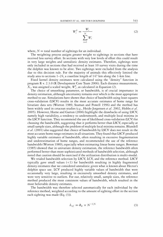
The kernel estimate of alongshore home range, K95, ranged from 13.60 km fora dolphin sighted all but once on Akaroa Harbour, to 101.43 km for a dolphinsighted all around Banks Peninsula (mean = 49.69 km, SE = 5.29; Table 1, Fig. 4).The smallest kernel estimate of alongshore home range (dolphin FSV.0100) appearssomewhat anomalous; the dolphin was sighted only once outside Akaroa Harbour,resulting in a very small value for bandwidth and large relative densities compared toall other individuals. K95 was continuous in 16 of the 20 individuals and fragmentedinto two portions for the others (Fig. 5). The kernel estimate of alongshore homerange exceeded the simple estimate of alongshore home range in all but one individual(FSV.0100). HR also exceeded K95 for dolphin FL45.0250, but one sighting wasexcluded from the kernel density estimate due to the 10 visits per section rule, sothey are not strictly comparable. There was no significant difference between K95 of


Figure 4. Individual kernel density estimates for all Hector’s dolphins with at least 15sightings (excluding FSV.0100). Distance is relative to the origin (0 km) at the Rakaia River.

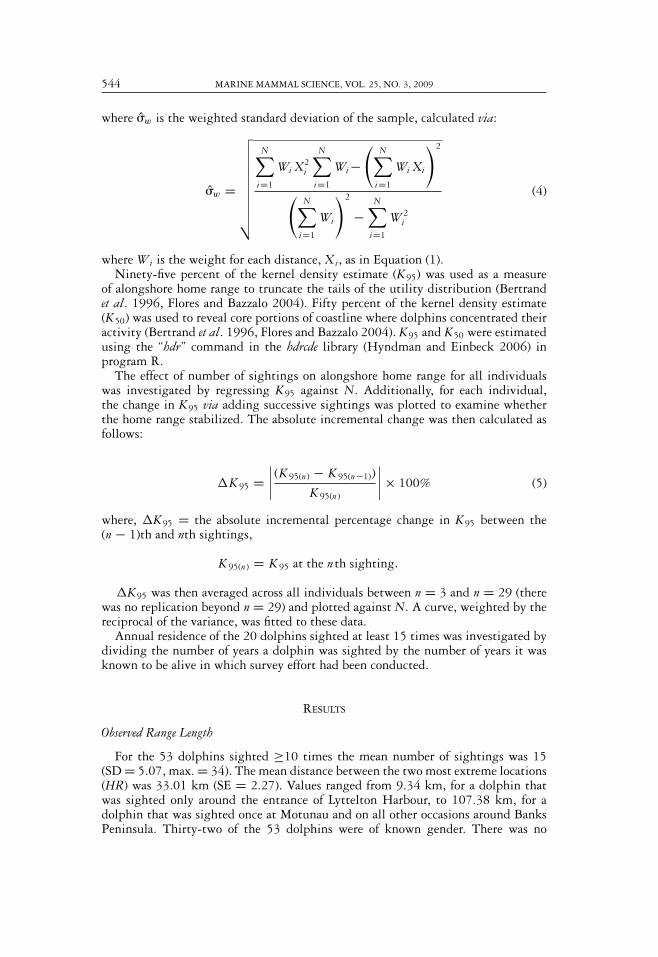
Figure 5. Schematic showing extent of K95 (gray bars) and K50 (black bars) for individualHector’s dolphins. Alongshore boundaries of the Banks Peninsula Marine Mammal Sanctuaryare represented by the dashed lines. Distance is relative to the origin (0 km) at the RakaiaRiver.

male (mean = 46.30, SE = 10.28) and female (mean = 50.22, SE = 6.96) dolphins(t = −0.32, df = 11, P = 0.76).

The kernel estimate of the core portion of coastline used, K50, ranged from 5.35 kmto 35.38 km, with a mean of 17.13 km (SE = 1.89) (Table 1, Fig. 5). K50 wascontinuous in 18 of the 20 individuals and fragmented into two portions for the


Figure 6. Distribution of home range centers throughout the study area. Sections arenumbered as in Figure 1.

others. There was no significant difference between K50 of male (mean = 15.61,SE = 3.56) and female (mean = 17.51, SE = 2.60) dolphins (t = −0.43, df = 12,P = 0.68).

The modal value of the kernel density estimate (Table 1) is the point withthe maximum estimated density, and therefore represents the part of the coast-line where the dolphin is predicted to have spent the greatest amount of time.This could also be described as the “center of activity,” although use of space isnot necessarily symmetrical around the modal value. Centers of activity were notuniformly distributed around Banks Peninsula (goodness of fit test; � 2 = 26.4,df = 15, P < 0.05) with particularly favored areas at section 8 (Murray’s Mistake),section 12 (Akaroa Harbour), section 16 (Steep Head), and section 21 (Pigeon Bay)(Fig. 6).

Among dolphins with ≥15 sightings, there was no significant effect of number ofsightings on K95 (r2 = 0.15, F = 3.23, df = 1, 18, P = 0.09) or of minimum ageon K95 (r2 = 0.03, F = 0.62, df = 1, 18, P = 0.44).

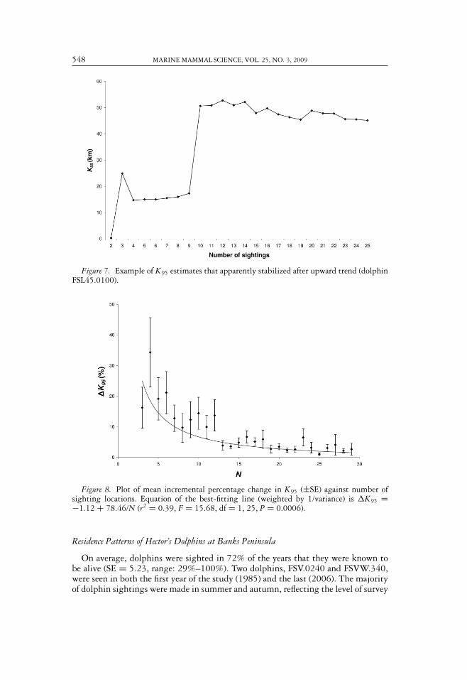
Cumulative curves of change in K95 with successive sightings showed that K95had apparently stabilized in 16 of the 20 individuals. The most common patternobserved was an upward trend in K95 as sightings were recorded in progressivelymore distant locations, with stability reached by 10–15 sightings (Fig. 7). For thefour dolphins whose estimates of alongshore home range had apparently failed tostabilize, either locations late in the sighting history caused large changes in K95,or K95 had not reached its asymptote following very distant locations early in thesighting history.

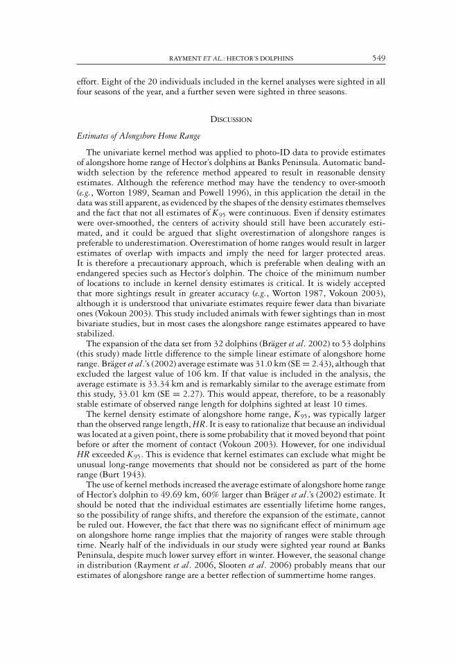
The plot of mean incremental change in home range showed that estimates of K95became more precise as the number of sightings of an individual increased (Fig. 8).There were large gains in precision up to approximately 15 sightings, at which pointthe best-fitting curve levels off toward an asymptote. Average absolute change in K95dropped below 5% beyond 12 sightings per individual.


Figure 7. Example of K95 estimates that apparently stabilized after upward trend (dolphinFSL45.0100).

Figure 8. Plot of mean incremental percentage change in K95 (±SE) against number ofsighting locations. Equation of the best-fitting line (weighted by 1/variance) is �K95 =−1.12 + 78.46/N (r2 = 0.39, F = 15.68, df = 1, 25, P = 0.0006).

Residence Patterns of Hector’s Dolphins at Banks Peninsula

On average, dolphins were sighted in 72% of the years that they were known tobe alive (SE = 5.23, range: 29%–100%). Two dolphins, FSV.0240 and FSVW.340,were seen in both the first year of the study (1985) and the last (2006). The majorityof dolphin sightings were made in summer and autumn, reflecting the level of survey


effort. Eight of the 20 individuals included in the kernel analyses were sighted in allfour seasons of the year, and a further seven were sighted in three seasons.

DISCUSSION

Estimates of Alongshore Home Range

The univariate kernel method was applied to photo-ID data to provide estimatesof alongshore home range of Hector’s dolphins at Banks Peninsula. Automatic band-width selection by the reference method appeared to result in reasonable densityestimates. Although the reference method may have the tendency to over-smooth(e.g., Worton 1989, Seaman and Powell 1996), in this application the detail in thedata was still apparent, as evidenced by the shapes of the density estimates themselvesand the fact that not all estimates of K95 were continuous. Even if density estimateswere over-smoothed, the centers of activity should still have been accurately esti-mated, and it could be argued that slight overestimation of alongshore ranges ispreferable to underestimation. Overestimation of home ranges would result in largerestimates of overlap with impacts and imply the need for larger protected areas.It is therefore a precautionary approach, which is preferable when dealing with anendangered species such as Hector’s dolphin. The choice of the minimum numberof locations to include in kernel density estimates is critical. It is widely acceptedthat more sightings result in greater accuracy (e.g., Worton 1987, Vokoun 2003),although it is understood that univariate estimates require fewer data than bivariateones (Vokoun 2003). This study included animals with fewer sightings than in mostbivariate studies, but in most cases the alongshore range estimates appeared to havestabilized.

The expansion of the data set from 32 dolphins (Brager et al. 2002) to 53 dolphins(this study) made little difference to the simple linear estimate of alongshore homerange. Brager et al.’s (2002) average estimate was 31.0 km (SE = 2.43), although thatexcluded the largest value of 106 km. If that value is included in the analysis, theaverage estimate is 33.34 km and is remarkably similar to the average estimate fromthis study, 33.01 km (SE = 2.27). This would appear, therefore, to be a reasonablystable estimate of observed range length for dolphins sighted at least 10 times.

The kernel density estimate of alongshore home range, K95, was typically largerthan the observed range length, HR. It is easy to rationalize that because an individualwas located at a given point, there is some probability that it moved beyond that pointbefore or after the moment of contact (Vokoun 2003). However, for one individualHR exceeded K95. This is evidence that kernel estimates can exclude what might beunusual long-range movements that should not be considered as part of the homerange (Burt 1943).

The use of kernel methods increased the average estimate of alongshore home rangeof Hector’s dolphin to 49.69 km, 60% larger than Brager et al.’s (2002) estimate. Itshould be noted that the individual estimates are essentially lifetime home ranges,so the possibility of range shifts, and therefore the expansion of the estimate, cannotbe ruled out. However, the fact that there was no significant effect of minimum ageon alongshore home range implies that the majority of ranges were stable throughtime. Nearly half of the individuals in our study were sighted year round at BanksPeninsula, despite much lower survey effort in winter. However, the seasonal changein distribution (Rayment et al. 2006, Slooten et al. 2006) probably means that ourestimates of alongshore range are a better reflection of summertime home ranges.


The estimates of alongshore range are similar to those reported for other membersof the genus. The average observed range length for Chilean dolphins (Cephalorhynchuseutropia) seen five times or more was 23.1 km (Heinrich 2006), whereas the meanalongshore range (measured as 90% of the utilization distribution) of five satellitetagged Heaviside’s dolphins (C. heavisidii) was 36.6 km (Elwen et al. 2006).

Factors Affecting Home Range

The kernel density estimate of alongshore home range of Hector’s dolphin is largerthan the previous estimate but is still remarkably small compared to many othersmall cetaceans. For example, bottlenose dolphins (Tursiops sp.) have been shownto range over 670 km off the California coast (Wells et al. 1990), harbor porpoises(Phocoena phocoena) have coastal ranges exceeding 400 km in the Bay of Fundy (Readand Westgate 1997), and dusky dolphins (Lagenorhynchus obscurus) make seasonal mi-grations over 200 km of coastline in New Zealand (Markowitz et al. 2004). Althoughhome ranges of small cetaceans are likely to be influenced by a number of factors (e.g.,Stern 2002), variation in home range sizes between similar species and populationsis most often attributed to prey distribution (e.g., Defran et al. 1999, Gubbins 2002).This seems likely to be especially so for small cetacean species in cold-water envi-ronments, because these species have relatively high daily energy requirements yetlimited energy stores (Heinrich 2006). In general, within a trophic guild, individ-uals in habitats of high productivity have smaller home ranges than individuals inhabitats of lower productivity (Harestad and Bunnell 1979). Intuitively this makessense, as they should need to move around less to find their food. Gubbins (2002)suggested that the small home range of bottlenose dolphins on the South Carolinacoast reflected a relatively abundant food supply, distributed uniformly in spaceand time. Similarly, Flores and Bazzalo (2004) attributed the small home ranges oftucuxi (Sotalia fluviatilis) in southern Brazil to the high productivity of the area andthe abundance of fish prey. Conversely, the large ranges of bottlenose dolphins onthe Californian coast have been linked to the patchy and ephemeral distribution ofpreferred prey items (Wells et al. 1990, Defran et al. 1999). The remarkably limitedcore and overall alongshore ranges of Hector’s dolphin at Banks Peninsula indicatethat the majority of individuals are capable of finding the resources required for lifein a relatively small area and therefore suggests an adequate and temporally stablesupply of prey. That Hector’s dolphins are generalist feeders (Slooten and Dawson1994) probably helps reduce the area they need to support themselves. Note thatthese estimates of alongshore range are specific to Banks Peninsula. In areas withmore variable habitat quality it is possible that ranging behavior could be quitedifferent.

Within a species, variation in home range size is often a function of reproductivestatus (Greenwood 1980, Dobson 1982). In polygynous species, males are expectedto maximize their reproductive success by dispersing from the natal site and thenmoving among sexually receptive females (Greenwood 1980, Dobson 1982). Thatmales have larger home ranges than females has been demonstrated in a number oftaxa, e.g., salmon (Hutchings and Gerber 2002), bears (Dahle and Swenson 2003),and seals (Austin et al. 2004). Cetaceans have polygynous or polygynandrous matingsystems (Mesnick and Ralls 2002), so males would be expected to have larger homeranges than females. Direct evidence in support of this hypothesis is somewhatscant. No significant gender differences in home range sizes were found in bottlenose


dolphins (Gubbins 2002), tucuxi (Flores and Bazzalo 2004), beluga (Delphinapterusleucas) (Hobbs et al. 2005), or Chilean dolphins (Heinrich 2006), although the powerto detect differences was probably low. However, studies of cetacean home rangemight be confounded by home ranges being age specific as well as sex specific.For example, Wells et al. (1980) found that subadult male bottlenose dolphins andfemales with calves had significantly larger home ranges than other age–sex classes.

In our study the power to detect a sex specific difference in alongshore range wasalso very low, but the means for males and females were very similar. It is not clearwhether the failure to detect differences in home ranges of male and female Hector’sdolphins is due to the absence of such differences or limitations of the method used.Photo-ID of Hector’s dolphins relies on individuals acquiring marks that are bothdistinctive and persistent (Wursig and Jefferson 1990). Therefore older animals aremore likely to be recognizable than young ones. Photo-ID studies will therefore bebiased toward older animals. It is possible therefore that differences in home rangethat are specific to younger animals would not be detected by photo-ID methods.

Core Use Areas

Kernel density estimates showed evidence of well-defined core use areas for allHector’s dolphins in our analysis. The core area or areas for each individual arelikely to contain the most reliable food resources (Macleod et al. 2004, Bailey andThompson 2006) and may provide access to potential mates (Hooker et al. 2002,Ersts and Rosenbaum 2003) or refuge from predators (Heithaus and Dill 2002).

Of particular interest is that there were four distinct areas around Banks Peninsula(termed “hubs” by Gubbins 2002), where the core areas of different individuals co-incided. The hubs are consistent with the summer hotspots of distribution identifiedby Clement (2005) and could therefore be considered critical habitats. It remains un-clear why these areas are consistently favored by Hector’s dolphins. Clement (2005)found a strong positive relationship between the distribution of dolphins and thepresence of seasonally predictable oceanographic frontal zones around Banks Penin-sula. Although this relationship would account for the general pattern of dolphindistribution, it fails to explain why certain individuals retain fidelity to particularhubs year round. Ultimately, Hector’s dolphin distribution is likely to be shapedby the distribution of their prey and predators (Brager et al. 2003, Clement 2005)as well as their conspecifics (Clement 2005). We suggest that further research isrequired on these topics.

Through limiting associations with other individuals, the ranging behavior ofcoastal dolphins can potentially determine the social structure of the community(Wells 1991, Lusseau et al. 2006). For example, it has been shown that bottlenosedolphins (Lusseau et al. 2006) and Chilean dolphins (Heinrich 2006) that tend toassociate together also have overlapping home ranges. As noted by Clement (2005),the four hubs or hotspots for Hector’s dolphins around Banks Peninsula are spacedapproximately 30 km apart. Furthermore, individual density estimates of dolphinsthat had their home ranges centered on the same hub were often remarkably similar,and alongshore home ranges tended to be small. Hence, dolphins with their homeranges centered at one of the four main hubs would only have limited overlap withdolphins of the adjacent hub(s). A community structure of this nature would haveprofound implications for genetic differentiation and management of the population(Brager et al. 2002).


Conservation Implications

Univariate estimation of alongshore home range does not fully describe the homerange of Hector’s dolphins as individuals clearly range offshore as well (e.g., Raymentet al. 2006, Slooten et al. 2006). However, because nearshore areas are among themarine habitats most at risk from human activities, alongshore range is a veryuseful measure for understanding how dolphins might overlap with anthropogenicactivities in the coastal zone (McIntyre 1999, Elwen et al. 2006, Parra et al. 2006).The majority of human impacts on Hector’s dolphin, for example, fisheries bycatch(Dawson 1991), pollution (Baker 1978), and tourism (Bejder et al. 1999), occurwithin the first 1 km from the coast.

The new information on alongshore home ranges helps to assess the overlapwith potential impacts within the BPMMS. Tourist boats have been shown to havebehavioral effects on Hector’s dolphins (Bejder et al. 1999) and boat-strike is aknown cause of mortality (Stone and Yoshinaga 2000). Viewing and swimmingwith Hector’s dolphins is a lucrative industry around Banks Peninsula, concentratedon Akaroa Harbour. Currently there are up to 31 commercial boat trips per dayon Akaroa Harbour targeting Hector’s dolphins1 in addition to the recreationalboating activity. Eighty percent of the dolphins had individual alongshore homeranges including Akaroa Harbour, and for half of these it was a core use area. Thisdemonstrates that a large proportion of the Banks Peninsula dolphin population isexposed to intensive tourism pressure.

Bycatch in gill nets is the major threat facing Hector’s dolphin (Dawson andSlooten 2005) and has been documented immediately to the north and south ofthe BPMMS boundaries (Starr and Langley 2000). Although the new estimate ofalongshore home range is still relatively small, it is larger than previously thoughtand raises concerns that the BPMMS does not protect the Hector’s dolphin populationadequately. For example, 15% of the 20 individuals in our study had alongshore homeranges that extended beyond the northern boundary of the BPMMS (Fig. 5) and aretherefore vulnerable to gill net bycatch. A shortcoming of the current study is therelatively low level of effort outside the BPMMS and in the southern part of the studyarea, largely due to the constraints of using small research vessels. Consequently,dolphins that have home ranges outside the BPMMS or that overlap the southernboundary are under-represented in the sample. Additional research effort in theseareas would provide more information on the proportion of time that dolphins areoutside the protection of the BPMMS.

This study is one example of the science supporting the call to improve protectionmeasures for Hector’s dolphin. That call was heeded in May 2008 by New Zealand’sMinister of Fisheries who proposed banning all gill netting on the majority of theSouth Island’s east coast out to 4 nmi offshore (Ministry of Fisheries 2008). TheMinister of Conservation also proposed extending the BPMMS to 12 nmi fromthe coast and approximately 45 km north, but redefining its regulations so that itrestricts acoustic seismic surveys, but no longer restricts gill netting (Departmentof Conservation 2008). The proposals would place large areas of Hector’s dolphinhabitat under protective management and would be a very positive development fordolphin conservation. For example, the new measures would protect the alongshorehome ranges of all the dolphins in our study. However, the fishing industry has

1Personal communication from Laura Allum, Department of Conservation, Level 4 Torrens House,195 Hereford Street, Christchurch 8011, New Zealand, 22 April 2008.


objected to the Minister of Fisheries’ proposals and the process is currently thesubject of judicial review.

ACKNOWLEDGMENTS

This study was possible thanks to support from the New Zealand Whale and DolphinTrust. Financial assistance was provided by Reckitt-Benckiser Ltd., Whale and DolphinConservation Society, University of Otago, Foundation for Research Science and Technology,Hiking New Zealand, New Zealand Lottery Board, Greenpeace, WWF New Zealand, ProjectJonah, Black Cat Group, Department of Conservation, and Cetacean Society International.We thank numerous volunteers for their assistance with data collection, and Black CatGroup for logistical support. Sincere thanks also to the Fraser family for help and support atBanks Peninsula. Thanks to Murray Efford and Jon Horne for advice on data analysis. Thismanuscript was greatly improved by comments from Roger Powell, Murray Efford, ShannonGowans, Leszek Karczmarski, and three anonymous reviewers.

LITERATURE CITED

AUSTIN, D., W. D. BOWEN AND J. I. MCMILLAN. 2004. Intraspecific variation in movementpatterns: Modelling individual variation in a large marine predator. Oikos 105:15–30.

BAILEY, H., AND P. THOMPSON. 2006. Quantitative analysis of bottlenose dolphin movementpatterns and their relationship with foraging. Journal of Animal Ecology 75:456–465.

BAKER, A. N. 1978. The status of Hector’s dolphin Cephalorhynchus hectori (van Beneden) inNew Zealand waters. Report of the International Whaling Commission 28:331–334.

BEJDER, L., S. M. DAWSON AND J. A. HARRAWAY. 1999. Responses by Hector’s dolphins toboats and swimmers in Porpoise Bay, New Zealand. Marine Mammal Science 15:738–750.

BERTRAND, M. R., A. J. DENICOLA, S. R. BEISSINGER AND R. K. SWIHART. 1996. Effects ofparturition on home ranges and social affiliations of female white tailed deer. Journal ofWildlife Management 60:899–909.

BLUNDELL, G. M., J. A. K. MAIER AND E. M. DEBEVEC. 2001. Linear home ranges: Effects ofsmoothing, sample size and autocorrelation on kernel estimates. Ecological Monographs71:469–489.

BOWMAN, A. W. 1985. A comparative study of some kernel-based nonparametric densityestimators. Journal of Statistical Computation and Simulation 21:313–327.

BRAGER, S., S. M. DAWSON, E. SLOOTEN, S. SMITH, G. S. STONE AND A. YOSHINAGA. 2002.Site fidelity and along-shore range in Hector’s dolphin, an endangered marine dolphinfrom New Zealand. Biological Conservation 108:281–287.

BRAGER, S., J. HARRAWAY AND B. F. J. MANLY. 2003. Habitat selection in a coastal dolphinspecies (Cephalorhynchus hectori). Marine Biology 143:233–244.

BURT, W. H. 1943. Territoriality and home range as applied to mammals. Journal of Mam-malogy 24:346–352.

CLEMENT, D. 2005. Distribution of Hector’s dolphin (Cephalorhynchus hectori) in relation tooceanographic features. Ph.D. dissertation, University of Otago, Dunedin, New Zealand.290 pp.

DAHLE, B., AND J. E. SWENSON. 2003. Home ranges in adult Scandinavian brown bears (Ursusarctos): Effect of mass, sex, reproductive category, population density and habitat type.Journal of Zoology 260:329–335.

DAWSON, S. M. 1991. Incidental catch of Hector’s dolphin in inshore gillnets. Marine MammalScience 7:283–295.

DAWSON, S. M. 2002. Cephalorhynchus dolphins (Cephalorhynchus sp.). Pages 200–203 in W. F.Perrin, B. Wursig, and J. G. M. Thewissen, eds. The encyclopaedia of marine mammals.Academic Press, San Diego, CA.


DAWSON, S. M., AND E. SLOOTEN. 1988. Hector’s Dolphin Cephalorhynchus hectori: Distributionand abundance. Report of the International Whaling Commission (Special Issue 9):315–324.

DAWSON, S. M., AND E. SLOOTEN. 1993. Conservation of Hector’s dolphins: The case and pro-cess which led to the establishment of the Banks Peninsula Marine Mammal Sanctuary.Aquatic Conservation: Marine and Freshwater Ecosystems 3:207–221.

DAWSON, S. M., AND E. SLOOTEN. 2005. Management of gillnet bycatch of cetaceans in NewZealand. Journal of Cetacean Research and Management 7:59–64.

DEFRAN, R. H., D. W. WELLER, D. L. KELLY AND M. A. ESPINOSA. 1999. Range characteristicsof Pacific Coast bottlenose dolphins (Tursiops truncatus) in the Southern California Bight.Marine Mammal Science 15:381–393.

DEPARTMENT OF CONSERVATION. 2008. Hector’s and Maui’s dolphins—marine mam-mal sanctuaries. Available from http://www.doc.govt.nz/templates/page.aspx?id=53584(accessed 25 November 2008).

DOBSON, F. S. 1982. Competition for mates and predominant juvenile dispersal in mammals.Animal Behaviour 30:1183–1192.

DU FRESNE, S. 2004. Conservation biology of Hector’s dolphin. Ph.D. dissertation, Universityof Otago, Dunedin, New Zealand. 166 pp.

ELWEN, S., M. A. MEYER, P. B. BEST, P. G. H. KOTZE, M. THORNTON AND S. SWANSON.2006. Range and movements of female Heaviside’s dolphins (Cephalorhynchus heavisidii),as determined by satellite-linked telemetry. Journal of Mammalogy 87:866–877.

ERSTS, P. J., AND H. C. ROSENBAUM. 2003. Habitat preference reflects social organisationof humpback whales (Megaptera novaeangliae) on a wintering ground. Journal of theZoological Society of London 260:337–345.

FIEBERG, J. 2007. Utilization distribution estimation using weighted kernel density estima-tors. Journal of Wildlife Management 71:1669–1675.

FLORES, P. A. C., AND M. BAZZALO. 2004. Home ranges and movement patterns of the marinetucuxi dolphin, Sotalia fluviatilis, in Baia Norte, southern Brazil. Latin American Journalof Marine Mammals 3:37–52.

GREENWOOD, P. J. 1980. Mating systems, philopatry and dispersal in birds and mammals.Animal Behaviour 28:1140–1162.

GUBBINS, C. 2002. Use of home ranges by resident bottlenose dolphins (Tursiops truncatus) ina South Carolina estuary. Journal of Mammalogy 83:178–187.

HARESTAD, A. S., AND F. L. BUNNEL. 1979. Home range and body weight—a re-evaluation.Ecology 60:389–402.

HEIDE-JORGENSEN, M. P., R. DIETZ, K. L. LAIDRE AND P. RICHARD. 2002. Autumn move-ments, home ranges and winter density of narwhals (Monodon monoceros) tagged in Trem-blay Sound, Baffin Island. Polar Biology 25:331–341.

HEINRICH, S. 2006. Ecology of Chilean dolphins and Peale’s dolphins at Isla Chiloe, southernChile. Ph.D. dissertation, University of St Andrews, St Andrews, UK. 258 pp.

HEITHAUS, M. R., AND L. M. DILL. 2002. Food availability and tiger shark predation riskinfluence bottlenose dolphin habitat use. Ecology 83:480–491.

HOBBS, R. C., K. L. LAIDRE, D. J. VOS, B. A. MAHONEY AND M. EAGLETON. 2005. Movementsand area use of belugas, Delphinapterus leucas, in a subarctic Alaskan estuary. Arctic58:331–341.

HOOKER, S. K., H. WHITEHEAD, S. GOWANS AND R. W. BAIRD. 2002. Fluctuations indistribution and patterns of individual range use of northern bottlenose whales. MarineEcology Progress Series 225:287–297.

HORNE, J. S., AND E. O. GARTON. 2006. Likelihood cross-validation versus least squarescross-validation for choosing the smoothing parameter in kernel home-range analysis.Journal of Wildlife Management 70:641–648.

HORNE, J. S., E. O. GARTON AND K. A. SAGER-FRADKIN. 2007. Correcting home-rangemodels for observation bias. Journal of Wildlife Management 71:996–1001.

HUTCHINGS, J. A., AND L. GERBER. 2002. Sex-biased dispersal in a salmonid fish. Proceedingsof the Royal Society of London B 269:2487–2493.


HYNDMAN, R., AND J. EINBECK. 2006. hdrcde: Highest density regions and conditionaldensity estimation. R package version 2.01. Available from http://www.robhyndman.info/Rlibrary/hdrcde (accessed 25 November 2008).

INGRAM, S. M., AND E. ROGAN. 2002. Identifying critical areas and habitat preferences ofbottlenose dolphins Tursiops truncatus. Marine Ecology Progress Series 244:247–255.

IUCN. 2006. 2006 IUCN Red List of Threatened Species. Available from http://www.iucnredlist.org (accessed 25 November 2008).

KARCZMARSKI, L., V. G. COCKCROFT AND A. MCLACHLAN. 2000. Habitat use and preferencesof Indo-Pacific humpback dolphins Sousa chinensis in Algoa Bay, South Africa. MarineMammal Science 16:65–79.

LUSSEAU, D., B. WILSON, P. HAMMOND, K. GRELLIER, J. W. DURBAN, K. M. PARSONS,T. R. BARTON AND P. M. THOMPSON. 2006. Quantifying the influence of socialityon population structure in bottlenose dolphins. Journal of Animal Ecology 75:14–24.

MACLEOD, K., R. FAIRBAIRNS, A. GILL, B. FAIRBAIRNS, J. GORDON, C. BLAIR-MYERS AND E.C. M. PARSONS. 2004. Seasonal distribution of minke whales Balaenoptera acutorostratain relation to physiography and prey off the Isle of Mull, Scotland. Marine EcologyProgress Series 277:263–274.

MARKOWITZ, T. M., A. D. HARLIN, B. WURSIG AND C. J. MCFADDEN. 2004. Dusky dolphinforaging habitat: Overlap with aquaculture in New Zealand. Aquatic Conservation:Marine and Freshwater Ecosystems 14:133–149.

MCINTYRE, A. D. 1999. Conservation in the sea: Looking ahead. Aquatic Conservation:Marine and Freshwater Ecosystems 9:633–637.

MESNICK, S. L., AND K. RALLS. 2002. Mating systems. Pages 726–733 in W. F. Perrin, B.Wursig and J. G. M. Thewissen, eds. The encyclopaedia of marine mammals. AcademicPress, San Diego, CA.

MINISTRY OF FISHERIES. 2008. Minister announces new measures to protect dolphins. Availablefrom http://www.fish.govt.nz/en-nz/Press/Press+Releases+2008/May08/hector.htm(accessed 25 November 2008).

PARRA, G. J., R. SCHICK AND P. J. CORKERON. 2006. Spatial distribution and environmen-tal correlates of Australian snub-fin and Indo-Pacific humpback dolphins. Ecography29:396–406.

R DEVELOPMENT CORE TEAM. 2006. R: A language and environment for statistical computing.R Foundation for Statistical Computing, Vienna, Austria.

RAYMENT, W., S. DAWSON, E. SLOOTEN AND S. CHILDERHOUSE. 2006. Offshore distributionof Hector’s dolphin at Banks Peninsula. DoC Research and Development Series 232.Department of Conservation, Wellington, New Zealand. 23 pp.

READ, A. J., AND A. J. WESTGATE. 1997. Monitoring the movements of harbour porpoises(Phocoena phocoena) with satellite telemetry. Marine Biology 130:315–322.

SEAMAN, D. E., AND R. A. POWELL. 1996. An evaluation of the accuracy of kernel densityestimators for home range analysis. Ecology 77:2075–2085.

SEMINOFF, J. A., A. RESENDIZ AND W. J. NICHOLS. 2002. Home range of green turtles Cheloniamydas at a coastal foraging area in the Gulf of California, Mexico. Marine Ecology ProgressSeries 242:253–265.

SILVERMAN, B. W. 1986. Density estimation for statistics and data analysis. Monographs onStatistics and Applied Probability. Chapman & Hall, London, UK.

SLOOTEN, E., AND S. M. DAWSON. 1994. Hector’s dolphin Cephalorhynchus hectori (Gray, 1828).Pages 311–333 in S. Harrison and M. Ridgway, eds. The handbook of marine mammals.Volume 6. Academic Press, New York, NY.

SLOOTEN, E., S. M. DAWSON AND F. LAD. 1992. Survival rates of photographically identifiedHector’s dolphins from 1984 to 1988. Marine Mammal Science 8:327–343.

SLOOTEN, E., D. FLETCHER AND B. L. TAYLOR. 2000. Accounting for uncertainty in riskassessment: Case study of Hector’s dolphin mortality due to gillnet entanglement.Conservation Biology 14:1264–1270.


SLOOTEN, E., W. RAYMENT AND S. DAWSON. 2006. Offshore distribution of Hector’s dolphinat Banks Peninsula: Is the Banks Peninsula Marine Mammal Sanctuary large enough?New Zealand Journal of Marine and Freshwater Research 40:333–343.

STARR, P., AND A. LANGLEY. 2000. Inshore Fishery Observer Programme for Hector’sdolphins in Pegasus Bay, Canterbury Bight, 1997/1998. Published client report oncontract 3020. Department of Conservation, P. O. Box 10-420, Wellington, NewZealand. 28 pp. Available from http://www.doc.govt.nz/upload/documents/science-and-technical/CSL3020.PDF (accessed 25 November 2008).

STERN, S. J. 2002. Migration and movement patterns. Pages 742–748 in W. F. Perrin, B.Wursig, and J. G. M. Thewissen, eds. The encyclopedia of marine mammals. AcademicPress, San Diego, CA.

STONE, G. S., AND A. YOSHINAGA. 2000. Hector’s dolphin (Cephalorhynchus hectori) calf mor-talities may indicate new risks from boat traffic and habituation. Pacific ConservationBiology 6:162–170.

STONE, G., A. HUTT, P. DUIGNAN, J. TEILMANN, R. COOPER, K. GESCHKE, A. YOSHINAGA, K.RUSSELL, A. BAKER, R. SUISTED, S. BAKER, J. BROWN, G. JONES AND D. HIGGINS. 2005.Hector’s dolphin (Cephalorhynchus hectori hectori) satellite tagging, health and geneticassessment. Final report to Department of Conservation, Auckland Conservancy, PrivateBag 68908, Auckland, New Zealand. 77 pp.

VOKOUN, J. C. 2003. Kernel density estimates of linear home ranges for stream fishes:Advantages and data requirements. North American Journal of Fisheries Management23:1020–1029.

WELLS, R. S. 1991. The role of long term study in understanding the social structure of abottlenose dolphin community. Pages 199–226 in K. Pryor and K. Norris, eds. Dolphinsocieties—discoveries and puzzles. University of California Press, Berkeley, CA.

WELLS, R. S., A. B. IRVINE AND M. D. SCOTT. 1980. The social ecology of inshore odontocetes.Pages 263–317 in L. M. Herman, ed. Cetacean behaviour: Mechanisms and functions.John Wiley and Sons, New York, NY.

WELLS, R. S., L. J. HANSEN, A. BALDRIDGE, T. P. DOHL, D. L. KELLY AND R. H. DEFRAN.1990. Northward extension of the range of bottlenose dolphins along the CaliforniaCoast. Pages 421–431 in S. Leatherwood and R. R. Reeves, eds. The bottlenose dolphin.Academic Press Inc., New York, NY.

WORTON, B. J. 1987. A review of models of home range for animal movement. EcologicalModelling 38:277–298.

WORTON, B. J. 1989. Kernel methods for estimating the utilisation distribution in homerange studies. Ecology 70:164–168.

WURSIG, B., AND T. A. JEFFERSON. 1990. Methods of photo-identification for small cetaceans.Report of the International Whaling Commission (Special Issue 12):43–52.

Received: 18 June 2008Accepted: 9 October 2008

Kernel density estimates of alongshore home range of Hector's dolphins at Banks Peninsula, New Zealand

Documents