Kernel-based Machine Learning on Sequence Data from ...

Kernel-based Machine Learningon Sequence Data from Proteomics

and Immunomics

Dissertation

der Fakultat fur Informations- und Kognitionswissenschaften

der Eberhard-Karls-Universitat Tubingenzur Erlangung des Grades eines

Doktors der Naturwissenschaften(Dr. rer. nat.)

vorgelegt von

M.Sc. Nico Pfeifer

aus Hannover

Tubingen

2009

Tag der mundlichen Qualifikation: 22.07.2009

Dekan: Prof. Dr. Oliver Kohlbacher

1. Berichterstatter: Prof. Dr. Oliver Kohlbacher

2. Berichterstatter: Prof. Dr. Knut Reinert

Zusammenfassung

Ein großes Anwendungsgebiet fur Maschinelle Lernverfahren ist die Biologie.Hierbei reichen die Anwendungen von der Vorhersage von Genen uber dieVorhersage der Aktivitat von Wirkstoffen bis hin zur Vorhersage der dreidi-mensionalen Struktur eines Proteins. Im Rahmen dieser Dissertation wur-den kernbasierte Lernverfahren entwickelt in den Bereichen der Proteomikund der Immunomik. Alle Anwendungen haben hierbei das Ziel, bestimmteEigenschaften von Teilen von Proteinen, so genannten Peptiden, vorherzusa-gen, welche in vielen biologischen Prozessen eine wichtige Rolle spielen.

Im ersten Teil der Dissertation stellen wir einen neuen Kern vor, der zusam-men mit einer Support-Vektor-Maschine benutzt werden kann, um das chro-matographische Verhalten von Peptiden in Umkehrphasen-Flussigchromato-graphie und starker Anionenaustauschchromatographie vorherzusagen. DerPradiktor fur die Flussigchromatographie wird daraufhin verwendet, um einenp-Wert basierten Filter fur Peptididentifikationen in der Proteomik zu en-twickeln. Der Filter beruht auf der Idee, dass das vorhergesagte Reten-tionsverhalten ahnlich zum gemessenen Verhalten sein sollte. Ist dies nichtder Fall, so ist das ein Indiz dafur, dass die identifizierte Peptidsequenz falschist. Hierdurch konnen falsch identifizierte Peptide herausgefiltert werden.Dies kann zum einen dazu verwendet werden, um die Qualitat der Identifika-tionen zu verbessern. Zum anderen konnen mehr Identifikationen erhaltenwerden, indem auch nicht ganz sichere Identifikationen betrachtet werden, dader Filter viele falsche Identifikationen herausfiltern und somit einen gutenQualitatsgrad garantieren kann.Im darauffolgenden Abschnitt zeigen wir, dass dieses Verfahren auch furzweidimensionale Trennverfahren verallgemeinert werden kann, was zu einemweiteren Anstieg an Peptididentifikationen bei ahnlicher Qualitat fuhrt. Au-ßerdem zeigen wir am Beispiel des Organismus Sorangium cellulosum, dassdas Verfahren sehr gut fur die Verbesserung der Messungen von ganzen Pro-teomen geeignet ist. Fur diese Anwendung konnen wir zeigen, dass wir beiahnlicher Prazision ca. 25% mehr Spektren identifizieren konnen.Der nachste Abschnitt zeigt, dass der neue Kern auch zur Vorhersage pro-teotypischer Peptide geeignet ist. Dies sind Peptide, die mit massenspek-trometriebasierten Verfahren gemessen werden konnen und Proteine ein-deutig identifizieren. Zusatzlich kann die gelernte Diskriminante sehr gutdafur verwendet werden um festzustellen, welche Aminosauren an welchenPositionen die Wahrscheinlichkeit eines Peptids erhoht proteotypisch zu sein.Die Fahigkeit eines Peptids eine Immunantwort auszulosen hangt von seinerBindeaffinitat zu einem speziellen Rezeptor des Immunsystems ab, welcher

iv

MHC Rezeptor genannt wird. Es gibt verschiedene Varianten dieses Rezep-tors, die in zwei Klassen eingeteilt werden konnen. Wir prasentieren einenkernbasierter Ansatz um die Bindeaffinitat von Peptiden zu MHC Klasse IIRezeptoren prazise vorherzusagen. Außerdem zeigen wir, wie Pradiktoren furbestimmte Varianten dieses Rezeptors gebaut werden konnen, obwohl fur siekeine experimentellen Daten verfugbar sind. Hierzu werden experimentelleDaten von anderen Varianten des Rezeptors verwendet. Durch dieses Ver-fahren konnen wir fur gut zwei Drittel aller MHC Klasse II RezeptorenPradiktoren erstellen im Gegensatz zu ca. 6%, fur die vorher Pradiktorenexistierten.

Abstract

Biology is a large application area for machine learning techniques. Appli-cations range from gene start prediction over prediction of drug activity tothe prediction of the three-dimensional structure of proteins. This thesisdeals with kernel-based machine learning in proteomics and immunomics ap-plications. In all applications, we are interested in predicting properties ofpeptides, which are parts of proteins. These peptides play an important rolein many biological systems.

In the first part, we introduce a new kernel which can be used together witha support vector machine for predicting chromatographic separation of pep-tides in reversed-phase liquid chromatography and strong anion exchangesolid-phase extraction. The predictor for reversed-phase liquid chromatog-raphy can be used to build a p-value-based filter for identifications in pro-teomics. The filter is based on the idea that if the measured and the predictedbehavior differ significantly, the identified sequence is probably wrong. In thisway, we can filter out false identifications. First, this is useful for increasingthe precision of identifications. Second, one can lower mass spectrometricscoring thresholds and filter out false identifications to get a significant in-crease in the number of correctly identified spectra at comparable precision.We also show in the following section that we can extend our method to pre-dict retention times in two-dimensional chromatographic separations, whichleads to a further increase in the number of correctly identified spectra atquality comparable to the unfiltered case. The practical applicability isdemonstrated by applying the methods to a whole proteome measurementof Sorangium cellulosum. We can show that we can get about 25% morespectrum identifications at the same level of precision.The next section shows that the new kernel can also be applied to the pre-diction of proteotypic peptides. These are peptides which can be detected bymass spectrometry-based analysis techniques and which uniquely identify aprotein. We furthermore show that the resulting discriminant is very usefulfor discovering which amino acids influence the likelihood of a peptide to beproteotypic.The ability of a peptide to induce an immune response depends upon its bind-ing affinity to a specialized receptor, called major histocompatibility complex(MHC) molecule. There are different variants of this receptor that can beclassified into two classes. We introduce a kernel-based approach for predict-ing binding affinity of peptides to MHC class II molecules with high accuracyand show how to build predictors for variants of this receptor, for which no

vi

experimental data exists, based on data for other variants. This enables us tobuild predictors for about two thirds of all different MHC class II moleculesinstead of about 6%, for which predictors had already been available.

Acknowledgments

First of all, I would like to thank my supervisor, Professor Oliver Kohlbacher,for giving me the opportunity to pursue this very interesting research, hisguidance, epecially at the beginning of my thesis and his sharp and openmind. He always supported me and gave me the opportunity to follow theresearch that interested me most. I also want to thank Professor Knut Rein-ert very much for reviewing this thesis. Additionally, I am very thankful toProfessor Christian G. Huber and Andreas Leinenbach for great collabora-tions.Furthermore, I am very grateful to Peter Meinicke, Professor Burkhard Mor-genstern and especially Professor Stephan Waack who introduced me to, andkindled my fascination for, the fields of computational biology and machinelearning during my years of study in Gottingen.Additionally, I want to thank the whole OpenMS team for nice collabora-tion and retreats, Till-Helge Hellwig and Kay Ohnmeiß for the effort, theyput into their bachelor theses, as well as the remaining staff of the Simu-lation of Biological Systems Department, namely Andreas Bertsch, Sebas-tian Briesemeister, Magdalena Feldhahn, Nina Fischer, Sandra Gesing, An-dreas Kamper, Erhan Kenar, Cengiz Koc, Sven Nahnsen, Lars Nilse, MarcRottig, Marcel Schumann, Marc Sturm, Philipp Thiel, Nora Toussaint, JanSchulze, Chun-Wei Tung, and Claudia Walter as well as its former membersTorsten Blum, Pierre Donnes, Annette Hoglund, Andreas Kerzmann, andJana Schmidt for a nice working atmosphere and interesting conversations.

I am deeply grateful to my parents who have always supported and equippedme with all the tools and skills that I have needed.

Last but definitely not least, I am very much obliged to my wife Ina, whofills my life with joy and inspires me to be a better person every day.

viii

Contents

1 Introduction 1

2 Background 72.1 Machine Learning . . . . . . . . . . . . . . . . . . . . . . . . . 7

2.1.1 General Idea . . . . . . . . . . . . . . . . . . . . . . . . 72.1.2 Finding the best function . . . . . . . . . . . . . . . . 72.1.3 Error Bounds . . . . . . . . . . . . . . . . . . . . . . . 112.1.4 Learning Machines . . . . . . . . . . . . . . . . . . . . 122.1.5 Kernels . . . . . . . . . . . . . . . . . . . . . . . . . . 222.1.6 Consistency of Support Vector Machines . . . . . . . . 26

2.2 Proteomics . . . . . . . . . . . . . . . . . . . . . . . . . . . . . 272.2.1 General Overview . . . . . . . . . . . . . . . . . . . . . 272.2.2 Chromatographic Separation . . . . . . . . . . . . . . . 282.2.3 Ionization . . . . . . . . . . . . . . . . . . . . . . . . . 292.2.4 Tandem Mass Spectrometry . . . . . . . . . . . . . . . 292.2.5 Computational Annotation of Tandem Mass Spectra . 31

2.3 Immunomics . . . . . . . . . . . . . . . . . . . . . . . . . . . . 362.3.1 General Overview . . . . . . . . . . . . . . . . . . . . . 362.3.2 Innate Immune System . . . . . . . . . . . . . . . . . . 362.3.3 Adaptive Immune System . . . . . . . . . . . . . . . . 372.3.4 Epitope-Based Vaccine Design . . . . . . . . . . . . . . 41

3 Applications in Proteomics 433.1 A New Kernel for Chromatographic Separation Prediction . . 43

3.1.1 Introduction . . . . . . . . . . . . . . . . . . . . . . . . 433.1.2 Machine Learning Methods . . . . . . . . . . . . . . . 463.1.3 Experimental Methods and Additional Data . . . . . . 493.1.4 Results and Discussion . . . . . . . . . . . . . . . . . . 513.1.5 Conclusions . . . . . . . . . . . . . . . . . . . . . . . . 63

3.2 Two-Dimensional Chromatographic Separation Prediction . . 653.2.1 Introduction . . . . . . . . . . . . . . . . . . . . . . . . 653.2.2 Methods and Data . . . . . . . . . . . . . . . . . . . . 663.2.3 Results and Discussion . . . . . . . . . . . . . . . . . . 683.2.4 Conclusions . . . . . . . . . . . . . . . . . . . . . . . . 75

3.3 Prediction of Proteotypic Peptides . . . . . . . . . . . . . . . . 773.3.1 Introduction . . . . . . . . . . . . . . . . . . . . . . . . 773.3.2 Methods and Data . . . . . . . . . . . . . . . . . . . . 783.3.3 Results and Discussion . . . . . . . . . . . . . . . . . . 79

x CONTENTS

3.3.4 Conclusions . . . . . . . . . . . . . . . . . . . . . . . . 89

4 Applications in Immunomics 914.1 Introduction . . . . . . . . . . . . . . . . . . . . . . . . . . . . 914.2 Methods and Datasets . . . . . . . . . . . . . . . . . . . . . . 92

4.2.1 Multiple Instance Learning . . . . . . . . . . . . . . . . 924.2.2 Multiple Instance Learning for MHCII Prediction . . . 934.2.3 Feature Encoding . . . . . . . . . . . . . . . . . . . . . 944.2.4 Predictions for Alleles with Sufficient Data . . . . . . . 944.2.5 Combining Allele Information with Peptide Information 954.2.6 Data . . . . . . . . . . . . . . . . . . . . . . . . . . . . 100

4.3 Results . . . . . . . . . . . . . . . . . . . . . . . . . . . . . . . 1004.3.1 Performance on Single Allele Datasets . . . . . . . . . 1004.3.2 Performance of Leave-Allele-Out Predictors . . . . . . 1014.3.3 Implementation . . . . . . . . . . . . . . . . . . . . . . 103

4.4 Discussion . . . . . . . . . . . . . . . . . . . . . . . . . . . . . 104

5 Conclusions and Discussion 105

Literature 108

A Abbreviations 123

B Publications 125B.1 Published Manuscripts . . . . . . . . . . . . . . . . . . . . . . 125B.2 Accepted Manuscripts . . . . . . . . . . . . . . . . . . . . . . 126

C Contributions 127

Index 129

Chapter 1

Introduction

“Wissen und Erkennen sind die Freude und die Berechtigung der Menschheit.”- Alexander von Humboldt, Kosmos, Stuttgart 1845, volume 1, page 36

Translated into English this means, “Knowledge and recognition are the joyand entitlement of mankind”. When the famous naturalist and explorer pub-lished these words in his five-volume work Kosmos, he probably did not thinkof discovering biological knowledge by machine learning techniques. Never-theless, he recognized that the wealth of knowledge of a society is highlycorrelated with its prosperity. Nowadays, there is a large research field thatis just concerned with building learning machines. This field is mainly influ-enced by statistics and optimization techniques.The term artificial intelligence (AI) was first coined by John McCarthy in1955 in the proposal for the Dartmouth Conference, which took place duringthe summer of 1956 at Dartmouth College in Hanover, New Hampshire. Theproposal contained these two sentences: “The study is to proceed on thebasis of the conjecture that every aspect of learning or any other feature ofintelligence can in principle be so precisely described that a machine can bemade to simulate it. An attempt will be made to find how to make machinesuse language, form abstractions and concepts, solve kinds of problems nowreserved for humans, and improve themselves.” (J. McCarthy, M. L. Minsky,N. Rochester, C.E. Shannon, August 31, 1955). A sub-field of AI is the fieldof machine learning. Machine learning can be described by the last part ofthe second sentence. The learning algorithm tries to solve a problem. A typ-ical problem is a supervised two-class (binary) prediction problem. In thissetting, one has training data for which the classes are known and some extradata, for which the classes are unknown. The problem is to label the extradata with the correct class label. A common application is a spam filter. Inthis application, the training data consists of mails, for which the label isknown (spam or no spam). The problem is to predict whether an incomingmail is spam or not.The two most prominent topics in machine learning in the last ten years havebeen kernel-based learning machines [17] and graphical models [39]. Kernelsallow the transformation of data into a (mostly high-dimensional) featurespace and solve the learning problem efficiently in this space. The choice ofthe kernel is in most applications the critical part because it directly relates

2 Introduction

to the feature space. If the problem is easily solvable in the feature space,the kernel choice was good, otherwise one has to find a different kernel. Ifthere is no suitable kernel at hand, researchers usually encode their data bycertain features that they identified to be important for the problem. In thespam filter example, one could think of counts for phrases that occur oftenin spam mails like cash bonus, free installation, and lose weight as possiblefeatures. In this way, the feature spaces are constructed explicitly. One canthen use standard methods to solve the problem. In many cases, it is notclear which features are best and, therefore, the standard approach is todefine a set of reasonable features and perform a feature selection. In thespam filter example, one could count all English phrases with less than fourwords and remove all phrases which are not discriminative for one of the twoclasses. For a given dataset, this method usually suffices to achieve goodperformance, but the application of the same features to a slightly differentdataset might lead to bad results if important features for the new datasetare missing. The kernel approach is usually more general, because it putssome mild assumptions on the data and learns all important features fromthe given data.A large application area for machine learning techniques is biology [126]. Oneof the earliest applications was the prediction of translation inititation sitesin E. coli by the perceptron algorithm [103]. In biology, it is very often thecase that one has a set of sequences that possess a certain property (e.g., thesequence is an RNA sequence that acts as a translation initiation site or not).These sequences are typically measured by time- and money-consuming ex-periments. Since it is usually not feasible to measure all possible sequences,a common method is to train a machine learning algorithm on the mea-sured data and predict the property for all unseen sequences of interest [43].There are also settings, whose properties are unknown beforehand and sothe machine learning methods are applied to construct clusters, in whichthe sequences inside the cluster are similar to each other and dissimilar tosequences from other clusters [128]. Furthermore, there are intermediate sce-narios where one knows properties for part of the data [47].In this thesis, we are mainly interested in the first setting. We have a setof training samples with certain properties and want to build a learningmachine that is able to predict the property for further sequences very accu-rately. During the whole thesis, the training samples are parts of proteins,called peptides. The properties that we want to predict for the peptides de-pend on the application area.

Proteomics deals with the analysis of the proteome, which consists of allproteins. Mostly, the analysis is restricted to a certain cell type of a specificorganism at a particular time point. There exist various techniques to mea-sure the proteins under these defined conditions. The usual workflow startswith cutting the proteins into peptides by a digestion enzyme. Then, thepeptides are separated by chromatography. The method of choice for large-scale analyses is usually based on tandem mass spectrometry [142, 1]. To beable to measure the peptides by mass spectrometry, they have to be ionized.The peptide ions are then directed into a mass spectrometer. This mass spec-

3

trometer measures the mass-to-charge ratio of the ions. Typically, the threemost abundant peptide ions are chosen for further fragmentation in a colli-sion chamber and directed into a second mass spectrometer. The peptidesare then identified by the mass spectrum of the second mass spectrometer,which ideally contains the mass to charge ratios of all possible fragments ofthe peptide [87]. In database search methods, the measured spectra are com-pared to theoretical spectra for all peptides contained in the database. Thehighest scoring candidate is then delivered as identification of the spectrum.Unfortunately, the spectrum quality is not always good enough to identifythe peptides correctly. Therefore, the identification routines usually definea certain scoring threshold to decide which of the identifications are certain.In these standard approaches, the chromatographic behavior of the peptideis not used for identification, although it is routinely measured by the instru-ments.If high-performance liquid-chromatography is used for chromatographic sepa-ration, the peptides elute at a certain point in time, the retention time. Therealready exist methods for retention time prediction like the approaches byPetritis et al. [90, 91]. They trained artificial neural networks with a largenumber of training samples (several thousands). Since retention behavior ofpeptides differs for different separation columns, one would have to measurethis amount of training peptides before being able to train and use their pre-dictor, whenever the conditions of the column changed. Other approaches,like the linear model by Krokhin [60], are trained for very specific columntypes. Very recently, Klammer et al. [55] introduced a method based on asupport vector machine (SVM). They used several features together with thelinear as well as the RBF kernel and stated that they needed at least 200unique spectrum identifications to train their learning machine.The first goal of this thesis was to develop an efficient learning machine forlearning chromatographic behavior of a peptide which does not need thatmany training samples. Having a good predictor, one can compare the pre-dicted behavior to the measured behavior and filter out identifications forwhich observed and predicted behavior differ significantly. Therefore, onecan lower the threshold of the identification routine to get correct identifica-tions below the original scoring threshold. Since the filter is able to filter outmany false identifications, one can achieve the same accuracy as standardidentification routines, while identifying more spectra.Another important property of a peptide with respect to mass spectrometryis its detectability or proteotypicity. It was recently observed that certainpeptides are detected more often in mass spectrometric experiments thanothers [63]. If these peptides can be uniquely assigned to a protein theyare called proteotypic. Especially for targeted proteomics (e.g., in multiplereaction monitoring experiments [23]), it is useful to know the proteotypicpeptides of a protein. Since a peptide has to be able to pass through alldifferent parts of the experimental setup to finally be detected, there can bevery different properties of the peptide that are responsible for not detectingit. For example, there are peptides that do not ionize or fragment as wellas others. Tang et al. [125] first introduced a method for predicting the de-tectability of a peptide. Mallick et al. [73] and Lu et al. [70] also addressed

4 Introduction

this issue with slightly different methods. All of these methods were basedon several biochemical properties of peptides which were either selected man-ually or by feature selection algorithms.An additional important peptide property is its ability to induce an immuneresponse by binding to major histocompatibility complex (MHC) molecules.MHC molecules present peptides at the cell surface. There are two differ-ent classes of MHC molecules. MHC class I molecules present peptides thatare derived from proteins inside the cell, whereas MHC class II moleculespresent peptides that originate from outside of the presenting cell. Peptides,derived from proteins of pathogens like bacteria, viruses or fungi, which arebound to MHC class I (MHCI) or MHC class II (MHCII) molecules can berecognized by specialized immune cells, called T cells. These cells can thenelicit an immune response. This response may lead to the death of the in-fected cells and/or clearance of the pathogen from the human body. Sincenot every peptide can bind to every MHC molecule, it is important to knowwhich peptides bind to which MHC molecule in order to design peptide-based vaccines [114]. These vaccines do not contain all of the proteins of thepathogen. Instead, they contain a set of peptides. To facilitate the selectionof peptide candidates for a vaccine, it is important to know which peptidesbind to the particular MHC molecules. There have been many studies toaddress the problem of peptide-MHCII binding affinity prediction. Early ap-proaches were based on positional scoring matrices [9, 80, 96, 99, 116, 124]but approaches with artificial neural networks [8], Gibbs samplers [81] andSVMs [24, 105, 137] with standard kernels were also presented. Especiallyfor MHCII, data from experimental binding studies is very scarce, whichcomplicates the problem of peptide-MHCII binding affinity prediction. Fur-thermore, the binding core, which is the part of the peptide that mainlyaffects binding affinity, is unknown for most of the experimental data. Thismakes the prediction problem quite complicated. Most existing methods arejust applicable to a very small subset of known MHCII molecules.

Scientists like von Humboldt discovered biological knowledge by observa-tions. Consequently, the traditional approach to discover which properties acertain peptide possesses would be to measure them by wetlab experiments.Though, in many applications we are just interested in the positive exam-ples, e.g., whether the peptide is proteotypic. We might also be interested inthe minimal set of all possible peptides of a bacterial proteome that bind toa predefined number of different MHCII molecules, because these peptidescould be the most promising candidates for an epitope-based vaccine [132]. Ifone wanted to discover these peptides, one would have to measure all possiblepeptides of the proteome with the traditional approach. Since many exper-iments are usually needed, a more efficient approach is to build accuratepredictors for peptide properties. If experimental confirmation is required,one can at least limit the number of experiments by predicting the mostpromising peptide candidates for a particular property.In this work, we introduce two new kernel functions for computational pro-teomics. They are called the oligo-border kernel (OBK ) and the paired oligo-border kernel (POBK ) and can be used together with an SVM for predicting

5

chromatographic separation of peptides as well as for predicting proteotypicpeptides by mass spectrometry-based experiments. The key idea of thesekernels is to modify the oligo kernel, introduced by Meinicke et al. [76] forsequences of the same length, to account for sequences of different lengths.Using the POBK together with an SVM, we show that we can build veryaccurate predictors for prediction of chromatographic separation in stronganion exchange chromatography that are significantly better than all pre-vious approaches. Furthermore, we show that the POBK together with ν-support vector regression [111] can be used to predict retention times inion-pair reversed-phase liquid chromatography. These predictors are thenused to build a p-value-based filter for identified peptides, measured by thischromatography and tandem mass spectrometry. In this way, we are able toimprove the precision of the identifications. Furthermore, the filter allows oneto lower mass spectrometric scoring thresholds to identify more spectra withacceptable accuracy. We show the generality of our approach by applying thesame methods to a dataset measured by two-dimensional chromatographicseparation [20]. Thus, we build accurate predictors for the first separationdimension at pH 10.0 as well as for the second dimension at pH 2.1. Theusefulness of this approach is shown on a whole proteome measurement ofSorangium cellulosum.For predicting proteotypic peptides, we combine the POBK with an SVM.This method is compared to other approaches, which were summarized in[40]. In this evaluation the features of the most prominent methods forproteotypic peptide prediction (Mallick et al. [73] and Lu et al.[70]) wereused together with an SVM to compare performances on the data of Mallicket al. [73]. We show that for this benchmark our method performs best,although we do not depend on specific features like the other approaches.Therefore, our method should also be applicable to experimental setups otherthan those presented in [73]. Furthermore, the kernel function allows the vi-sualization of important amino acids for the classifier. These insights mightbe used for in silico design of proteotypic peptides or to discover propertiesof the involved biochemical processes.For immunomics, we show how to transform the peptide-MHCII bindingaffinity prediction problem into a well-known machine learning problem calledmultiple instance learning. This transformation allows building predictors forMHCII molecules for which there exists training data. A comparison to alarge benchmark study by Wang et al. [138] shows that the performance of ourmethod is as good as state-of-the-art methods or even better. Furthermore,we introduce a new kernel function for immunomics called the positionally-weighted RBF kernel. This kernel can be used to incorporate knowledge fromMHCII molecules into the kernel to build predictors for about two thirds ofall known MHCII molecules. Before, predictors were just available for lessthan 6% of MHCII molecules.

The thesis is structured into five chapters. After this introduction, the secondchapter introduces the theoretical as well as the biological background. Ourdevelopments for kernel-based machine learning in proteomics are describedin the third chapter. The contributions of this work towards solving the

6 Introduction

peptide-MHCII binding affinity prediction problem is described in the fourthchapter before the conclusion in the last chapter.

Chapter 2

Background

2.1 Machine Learning

2.1.1 General Idea

In many real-world applications, one is given labeled data and the goal isto come up with predictions for additional unlabeled data, which originatesfrom the same source, based on general properties of the data. This is, forexample, the case for stock markets, spam filtering or gene start prediction.More formally, one assumes that the data comes from the same but unknownsource. Therefore, the data is independent and identically distributed (iid).One situation that is suitable for machine learning is when one has labeleddata {(x, y)|x ∈ X ∧y ∈ {−1, 1}}, which is often referred to as training data,and unlabeled data x ∈ X with X being a topological space. The goal is toassign the most probable label y to the unlabeled data based on the knowl-edge gained from the training data. The optimal Bayes classifier which solvesthis task can be formulated as g∗(x) = argmaxy∈YP (Y = y|X = x). Unfor-tunately, the optimal Bayes classifier cannot be constructed in general sincethe underlying distribution P of the data is generally unknown. This is whyone has to come up with the best possible approximation of the Bayes classi-fier to find the best possible solution. To be more precise regarding the bestpossible approximation, we have to consider some theoretical background inthe following sections.The above task belongs to the classification problems and the special casewith just two different labels is often referred to as binary classification.If there are more than two possible labels, the task is called multi-classclassification. The task is called regression if the domain of the label iscontinuous (e.g., y ∈ IR).

2.1.2 Finding the best function

We already introduced the optimal Bayes classifier g∗(x) = argmaxy∈YP (Y =y|X = x). Since we want to find the best approximation of the optimal pre-dictor (both in classification and in regression tasks), we have to be ableto compare the performance of different prediction functions. Therefore, wehave to introduce the notion of risks. The risk of a function f : X → Y is the

8 Background

expected error on all data that comes from the same source as the trainingdata and is therefore iid. This means that

R(f) =

∫

X×Y

c(x, y, f(x))dP (x, y) (2.1)

(c.f. [111]). The risk contains the function

c : X × Y × Y → IR. (2.2)

This function is called the loss function. A common choice in binary classi-fication is the 0-1 loss which is defined as:

c(x, y, f(x)) =

{

1 if f(x) 6= y0 otherwise.

(2.3)

In general it is not clear what the best loss function for a particular problemis like. Consider, for example, a biomedical multi-class classification problemin which one has three classes. Each label represents a specific type of person.Based on this label the person gets a prescription for a drug. Now considerthat we have three drugs d1, d2 and d3. d1 is very cheap but just helps peoplefrom class one. d2 is more expensive than d1 and is able to cure people ofall classes, but for people from class three it leads to stronger side-effects.d3 is as expensive as d2 and is just able to cure people from class two andclass three but leads to stronger side-effects in people from class two. If oneis mainly interested in curing people, the loss for c(x, 1, 2) should be smallerthan the loss c(x, 1, 3) since d3 would not cure a person from class one. Buteven in this simple example one could come up with different loss functionsif, for example, the price is of greater importance.It could be important in some prediction tasks to know the amount of cer-tainty of the prediction and not just the predicted label. In binary classi-fication, one could think of the confidence as y · f(x), where f(x) is nowa real-valued function (positive values of f(x) correspond to label +1 andnegative values of f(x) correspond to label −1). Higher values of y · f(x)correspond to higher certainty of the prediction. This leads to the soft-marginloss function of Bennett and Mangasarian [111]:

c(x, y, f(x)) =

{

0 if f(x) · y ≥ 11− f(x) · y otherwise

(2.4)

A very similar loss function, called the quadratic soft margin loss, is thefollowing:

c(x, y, f(x)) =

{

0 if f(x) · y ≥ 1

(1− f(x) · y)2 otherwise(2.5)

2.1 Machine Learning 9

−5 0 5−1

0

1

2

3

4

5

f(x)y

loss

−5 0 5−1

0

1

2

3

4

5

f(x)y

loss

−5 0 5−1

0

1

2

3

4

5

f(x)y

loss

c)a) b)

Figure 2.1: Different loss functions for binary classification: a) 0-1 loss,b) soft-margin loss, and c) squared soft-margin loss

Plots of the different loss functions can be seen in Fig. 2.1. For regressionproblems, the most common loss functions are squared loss

c(x, y, f(x)) = (f(x)− y)2 , (2.6)

ε-insensitive loss

c(x, y, f(x)) = max (|f(x)− y| − ε, 0) , (2.7)

in which a deviation between y and f(x) smaller than ε is not penalized, andthe l1-loss

c(x, y, f(x)) = |f(x)− y| (2.8)

in which every deviation is penalized by its absolute value. Fig. 2.2 showsa plot of these three loss functions. Although we know the most common

−2 0 2

0

1

2

3

f(x) − y

loss

−2 0 2

0

1

2

3

f(x) − y

loss

−2 0 2

0

1

2

3

f(x) − y

loss

a) b) c)

Figure 2.2: Different loss functions for regression: a) squared loss, b) ε-insensitive loss, and c) l1-loss

loss functions we cannot compute the risk given by formula (2.1) since thedistribution P (x, y) is unknown. Nevertheless, we can calculate the risk onthe training data, which is assumed to be sampled iid from the distribution

Remp(f) =

n∑

i=1

c(x, y, f(x)) (2.9)

10 Background

(c.f. [111]). This risk is called the empirical risk and it can be used to finda good predictor. The induction principle of empirical risk minimizationcan be described as follows. Given a model class F , which contains severalfunctions, choose the function f ∈ F , which minimizes the empirical risk(cf. [6]):

femp = arg minf∈F

Remp(f). (2.10)

It is clear that empirical risk minimization does not guarantee good results.If the class of models contains only very simple models, one cannot expectthe risk to be small. For example, given a model class that contains all linearhyperplanes, one could obtain good results if the distribution P (X, Y ) is verysimple (e.g., as shown in Fig. 2.3), but even for slightly more difficult data(e.g., as shown in Fig. 2.4), the model class would be too simple to find agood classifier. Furthermore, if the function class has very flexible functions,

−8 −6 −4 −2 0 2 4 6 8−4

−3

−2

−1

0

1

2

3

4

x1

x2

Figure 2.3: Example for linearly separable data: The blue points are nega-tive examples and the green points are positive examples. The red line shows onepossible separation between these two classes.

one could expect that a very specialized function could be chosen, i.e. one,which performs very well on training data but does not perform well on un-seen data. Therefore, the model class should not be too rich. This becomesclear if one considers the following example. If the class contained all possiblefunctions then one could find a function which has zero empirical risk andclassifies every new data point, drawn from the same distribution, wrongly.The classifier would have maximum risk and this is definitely not desirable.The idea of restricting the model class is included in the structural risk min-imization induction principle (cf.[6]). In this principle one has an infinitesequence of models {f1, f2, ...} which are sorted by their complexity, startingwith the model of lowest complexity. The complexity of the model can bemeasured in different ways. If our hypothesis space consists, for example, ofthe union of all axis-parallel rectangles in which one hypothesis is a subset

2.1 Machine Learning 11

−10 −5 0 5 10 15 20−4

−3

−2

−1

0

1

2

3

4

x1

x2

Figure 2.4: Example for data that is not linearly separable: The blue pointsare negative examples and the green points are positive examples.

of the whole hypothesis space, a straightforward measure of the complexityof the model is the number of rectangles. In structural risk minimizationone tries to minimize the empirical risk as in empirical risk minimization butadditionally, the size of the model is penalized as follows:

fstr = arg minf∈F ,d∈IN

Remp(f) + pen(d, n), (2.11)

in which n is the number of training samples, d is a number reflecting thecomplexity of the model (e.g., number of rectangles), and pen(d, n) is thepenalty function. Since it could be difficult to build an infinite sequence ofmodels there is another slightly different idea, which is called regularization.In this induction principle, one chooses a very rich class of models and definesa regularizer on F . In many applications this is simply the norm ‖f‖ off ∈ F . The regularizer penalizes the complexity of the model. Finding thebest model reduces to finding the minimium of

freg = arg minf∈F

Remp(f) + λ‖f‖2. (2.12)

The parameter λ is called the regularization parameter . It can be used tofind the best trade-off between small model complexity and minimizing theempirical risk. Finding a good value of λ is not trivial. Therefore, one usesvalidation schemes in which some parts of the training data are left out toget a good estimate of the error on unseen data given a certain value of λ.According to Bousquet et al. [6], the most successful methods in machinelearning can be thought of as regularization methods.

2.1.3 Error Bounds

In the last section, we showed different principles that can be applied to finda prediction function f . The interesting question is now, how good are these

12 Background

prediction functions? Therefore, we want to know whether we can boundthe error that we make by choosing f . We already introduced the risk of afunction. Let

R∗ = infg∈G

R(g), (2.13)

in which G contains all possible measurable functions. The quality of f canbe described as:

R(f)−R∗ = [R(f ∗)− R∗] + [R(f)−R(f ∗)] . (2.14)

f ∗ is the optimal function of the model class F . The right-hand side of (2.14)decomposes into an approximation error (first term) and an estimation error(second term). Since one normally does not know anything about the besttarget function, one cannot directly bound the approximation error withoutmaking assumptions (e.g., about the value of R∗). Therefore, much of theliterature deals with bounds on the estimation error, for which one does notneed these kinds of assumptions.

2.1.4 Learning Machines

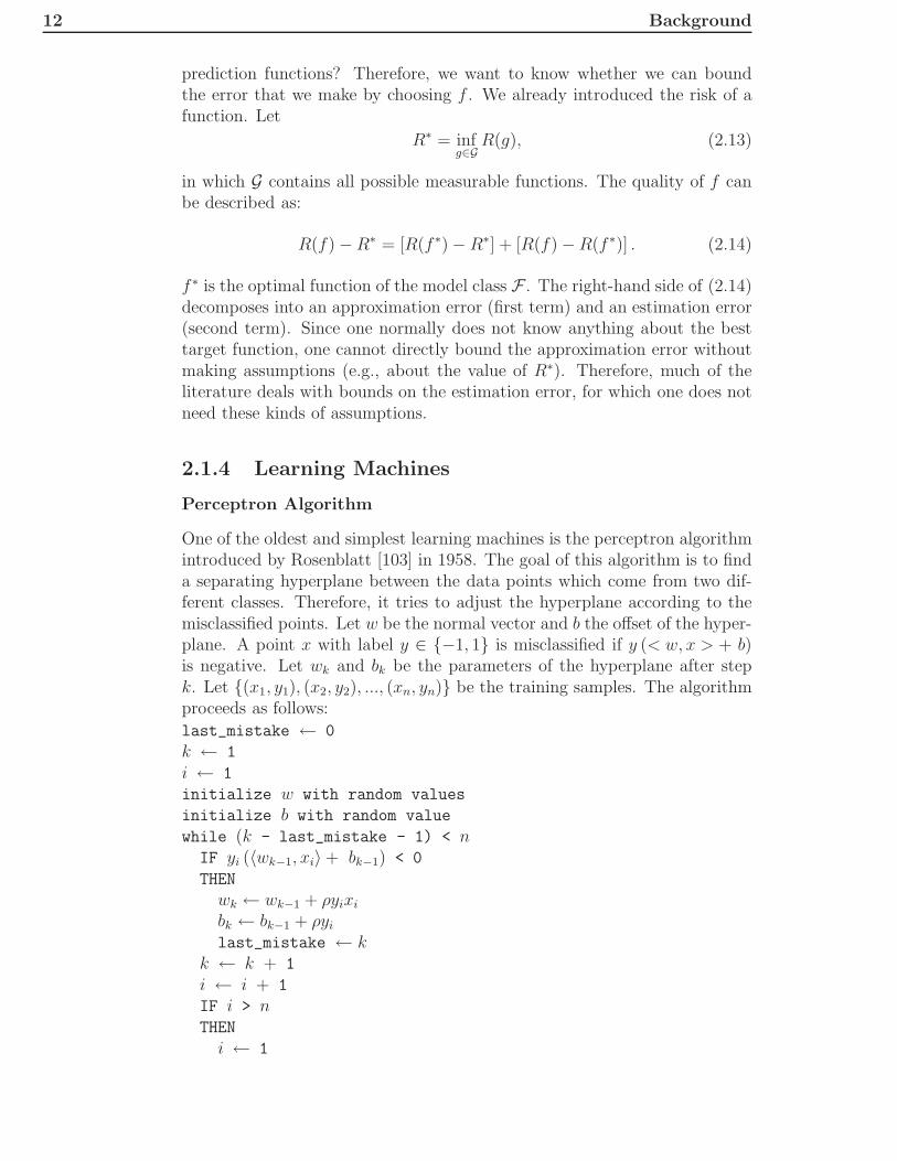
Perceptron Algorithm

One of the oldest and simplest learning machines is the perceptron algorithmintroduced by Rosenblatt [103] in 1958. The goal of this algorithm is to finda separating hyperplane between the data points which come from two dif-ferent classes. Therefore, it tries to adjust the hyperplane according to themisclassified points. Let w be the normal vector and b the offset of the hyper-plane. A point x with label y ∈ {−1, 1} is misclassified if y (< w, x > + b)is negative. Let wk and bk be the parameters of the hyperplane after stepk. Let {(x1, y1), (x2, y2), ..., (xn, yn)} be the training samples. The algorithmproceeds as follows:

last_mistake ← 0

k ← 1

i ← 1

initialize w with random values

initialize b with random value

while (k - last_mistake - 1) < nIF yi (〈wk−1, xi〉+ bk−1) < 0

THEN

wk ← wk−1 + ρyixi

bk ← bk−1 + ρyi

last_mistake ← kk ← k + 1

i ← i + 1

IF i > nTHEN

i ← 1

2.1 Machine Learning 13

The learning rate of the algorithm, ρ, has to be greater than zero. Itwas shown that the algorithm converges if the data is linearly separableby a non-zero margin [83]. The motivation behind the update procedureis that one tries to minimize the distance between the misclassified pointsand the decision boundary. Therefore, the update shifts the hyperplane to-wards the misclassified data point. If training sample xi is misclassified byhyperplane k − 1 (yi = 1 and (< wk−1, xi > +bk−1) < 0 or yi = −1 and(< wk−1, xi > +bk−1) > 0), yi (< wk−1, xi > +bk−1) is smaller than zero. Let

L(wk−1, bk−1) = −yi (< wk−1, xi > +bk−1) . (2.15)

By minimizing L with respect to wk−1 and bk−1, the distance between xi

and the actual hyperplane is minimized. This is why the algorithm descendsalong the gradient of L to find the best solution. The gradients with respectto the parameters of the hyperplane are:

∂

∂wk−1

L(wk−1, bk−1) = −yixi (2.16)

and

∂

∂bk−1L(wk−1, bk−1) = −yi. (2.17)

It is clear that the algorithm will not converge if the data is not linearlyseparable. Furthermore, the algorithm stops if a separating hyperplane isfound. This means that if there are many possible hyperplanes that canseparate the data, the values of w and b are influenced by the order of thetraining samples, because the update takes place after a misclassification.Additionally, the initial values of w and b influence the final hyperplane.Fig. 2.5 a) shows the data that is generated by 400 random draws from thenormal distribution leading to 200 two-dimensional samples. The data wassplit into two classes by adding seven to the second component of half ofthe data points. Fig. 2.5 b) shows 20 separating hyperplanes, which werefound by implementing the above pseudo-code in Matlab and executing thefunction 20 times. Fig. 2.5 c) shows the whole region which can be coveredby separating hyperplanes. Since we know how we generated the data, wealso know the best possible function f ∗ out of the function class F thatcontains all lines. In this example, f ∗ is a line which is parallel to the firstaxis and has the value 3.5 in the second dimension. To show that not everyline which separates the two classes is equally good, we drew 2000 additionalsamples from the same distributions and plotted them, the 20 discriminantsof Fig. 2.5 b), as well as the optimal separating line (thick and red) in Fig. 2.6.It can be seen that the worst separating lines are the ones which are very

14 Background

Figure 2.5: Visualization of Rosenblatt’s perceptron algorithm: This plotshows 200 data points drawn from the normal distribution. One hundred of thesepoints are shifted by seven in the second dimension (crosses): a) shows the datawithout any separating lines; b) additionally shows 20 separating lines learned onthe data using Rosenblatt’s Perceptron Algorithm; and c) additionally colors theregion in which the lines can be found by Rosenblatt’s Perceptron Algorithm.

close to the training samples. Furthermore, the best separating line (red) hasmaximal margin with respect to the nearest samples. This motivates whylarge margin hyperplane classifiers generalize well to unseen data. We willlook at these kinds of learning machines in more detail in the next subsection.

Large Margin Classifiers

Let H be a dot product space. One can define a hyperplane by the normalvector and the offset of the hyperplane. The set of points that lie on the hy-perplane can be calculated by projecting the points onto the normal vector wand adding the offset b. If the result is zero, the point lies on the hyperplane.The set of points that lie on the hyperplane is therefore:

{x ∈ H| < w, x > +b = 0}. (2.18)

Multiplying the normal vector and the offset by certain factors can yield thesame set of points which lie on the corresponding hyperplanes. Therefore,Scholkopf and Smola [111] define the hyperplane with respect to some datapoints x1, x2, ..., xn ∈ H. This hyperplane is called the canonical hyperplane:

Definition 2.1 (Canonical Hyperplane). The parameters w ∈ H and b ∈ IRdescribe a Canonical Hyperplane with respect to the data x1, x2, ..., xn ∈ H,if the point closest to the hyperplane has distance 1/‖w‖, which means that

mini=1,2,...,n

| < w, xi > +b| = 1. (2.19)

We already saw in the last section, that large margin separations seemto be more robust than other separating hyperplanes. To construct a large

2.1 Machine Learning 15

Figure 2.6: Visualization of test error of Rosenblatt’s perceptron algo-rithm: This plot shows a binary classification problem. The thin lines are 20separating lines determined by Rosenblatt’s Perceptron Algorithm based on 200samples. In addition to these 200 samples, the plot contains 2000 extra samplesdrawn from the same distributions. The thick line corresponds to the optimal sep-aration between the two classes.

margin classifier one has to find the canonical hyperplane with maximal mar-gin. Since the margin of the canonical hyperplane is 1/‖w‖, the canonicalhyperplane with maximal margin is the one with minimal ‖w‖. This can becast into a standard optimization problem:

minw∈H,b∈IR

‖w‖, (2.20)

subject to yi (〈xi, w〉+ b) ≥ 1 ∀i = 1, 2, ..., n.

The constraints assure that the w with minimal ‖w‖ is a canonical hyper-plane. This optimization problem yields the same solution as

minw∈H,b∈IR

12‖w‖2, (2.21)

subject to yi (〈xi, w〉+ b) ≥ 1 ∀i = 1, 2, ..., n.

16 Background

Since the optimization problem (2.21) has some nicer properties, it is usedin the following. This optimization problem can be solved if the data isseparable. To transform the primal problem into a dual problem we canbuild the Lagrangian:

L(w, b, α) =1

2‖w‖2 −

n∑

i=1

αi [yi (〈xi, w〉+ b)− 1]. (2.22)

To get the solution of the dual problem, the Lagrangian L has to be maxi-mized with respect to α and minimized with respect to w and b (c.f. [62]).This means that we are trying to find a saddle point at which the derivativesof L with respect to the primal variables must vanish:

∂

∂bL(w, b, α) = 0,

∂

∂wL(w, b, α) = 0. (2.23)

Therefore,

∂

∂bL(w, b, α) = 0⇔ −

n∑

i=1

αi · yi · 1 = 0⇔n∑

i=1

αi · yi · 1 = 0 (2.24)

and

∂

∂wL(w, b, α) = 0⇔ w −

n∑

i=1

αiyixi = 0⇔ w =

n∑

i=1

αiyixi. (2.25)

The xi, for which αi > 0 are called support vectors because they lie directlyat the boundary of the margin of the canonical hyperplane. This is shown inFig. 2.7. The classifier is usually called a support vector machine (SVM). Itcan be seen that the support vectors determine the hyperplane.To arrive at the dual problem, one can write equation (2.22) in the following

way:

1

2〈w, w〉 −

n∑

i=1

αiyi〈xi, w〉 − bn∑

i=1

αiyi +n∑

i=1

αi. (2.26)

Substitution of (2.24) and (2.25) into (2.26) yields

12

n∑

i,j=1

αiαjyiyj〈xi, xj〉 −n∑

i,j=1

αiαjyiyj〈xi, xj〉 − b · 0 +n∑

i=1

αi (2.27)

=n∑

i=1

αi − 12

n∑

i,j=1

αiαjyiyj〈xi, xj〉 (2.28)

The dual form of the optimization problem (2.21) is, therefore,

2.1 Machine Learning 17

Margin

Figure 2.7: Separating hyperplane for linearly separable data: This plotshows a two-class problem and a separating hyperplane. The support vectors aremarked by additional circles.

maxα∈IR

n∑

i=1

αi − 12

n∑

i,j=1

αiαjyiyj〈xi, xj〉, (2.29)

subject to 0 ≤ αi ∀i = 1, 2, ..., n andn∑

i=1

αiyi = 0.

It can be shown that the duality gap between the primal and the dual is zeroand, therefore, a solution to the dual problem also solves the primal problem.In real-world examples there are often samples, which are not linearly sep-arable. Furthermore, perfect separation is not always the best choice if, forexample, one of the points is an extreme outlier. Therefore, Cortes and Vap-nik [17] introduced so-called slack-variables ξi ≥ 0. These variables shiftthe points to the correct side of the canonical hyperplane, which is shownin Fig. 2.8. The classifiers that use slack-variables are called soft marginclassifiers. Since not every point should be allowed to have a slack variablegreater than 0, the value of the slack-variables has to be penalized in theminimization problem. This means that the minimization problem uses theregularization induction principle. There exist several different approachesin the literature to weight the slack-variables. The two most prominent onesare the 1-norm soft margin classifier and 2-norm soft margin classifier. Weshow the primal and dual problem for the 1-norm soft margin classifier. Thesteps for the 2-norm soft margin classifier are similar:

18 Background

Margin

Figure 2.8: Separating hyperplane for data that is not linearly separable:This plot shows a two-class problem as well as a separating hyperplane. The supportvectors are marked by extra circles and the penalty of the ξi is indicated by the redlines.

minw∈H,b∈IR,ξ∈IRn

12‖w‖2 + C

n∑

i=1

ξi, (2.30)

subject to yi (〈xi, w〉+ b) ≥ 1− ξi ∀i = 1, 2, ..., n.

The Lagrangian of (2.30) is

L(w, b, ξ, α, β) =

1

2〈w, w〉+ C

n∑

i=1

ξi −n∑

i=1

αi [yi (〈xi, w〉+ b) + ξi − 1]−n∑

i=1

βiξi. (2.31)

As in the separable case, we try to find a saddle point at which the derivativesof L with respect to the primal variables must vanish:

∂

∂bL(w, b, ξ, α, β) = 0⇔ −

n∑

i=1

αi · yi · 1 = 0⇔n∑

i=1

αi · yi · 1 = 0, (2.32)

∂

∂wL(w, b, , ξ, α, β) = 0⇔ w −

n∑

i=1

αiyixi = 0⇔ w =

n∑

i=1

αiyixi (2.33)

2.1 Machine Learning 19

and

∂

∂ξi

L(w, b, ξ, α, β) = 0⇔ C − αi − βi = 0. (2.34)

Substitution of (2.32) and (2.33) into (2.31) yields

12

n∑

i,j=1

αiαjyiyj〈xi, xj〉 −n∑

i,j=1

αiαjyiyj〈xi, xj〉+n∑

i=1

αi + Cn∑

i=1

ξi

−n∑

i=1

αiξi −n∑

i=1

βiξi

=n∑

i=1

αi − 12

n∑

i,j=1

αiαjyiyj〈xi, xj〉 +n∑

i=1

(C − αi − βi) ξi. (2.35)

Using equation (2.34) we obtain

n∑

i=1

αi −1

2

n∑

i,j=1

αiαjyiyj〈xi, xj〉. (2.36)

Since βi ≥ 0 ∀i = 1, 2, ..., n the dual form of the optimization problem is

maxα∈IR

n∑

i=1

αi − 12

n∑

i,j=1

αiαjyiyj〈xi, xj〉, (2.37)

subject to 0 ≤ αi ≤ C ∀i = 1, 2, ..., n andn∑

i=1

αiyi = 0.

From (2.25) and (2.33) the final prediction function for the separable as wellas the non-separable case follows:

f(x) = sign

(

n∑

i=1

αi〈x, xi〉+ b

)

. (2.38)

Up to now, we only considered binary classification. If there are more thantwo different possible labels, one has to extend the introduced approaches.Basically, there are three different ways of dealing with multi-class predictionproblems. The first possibility is to train a classifier for every class, whichdiscriminates the class from all other classes (one versus the rest). The classto which the classifier with maximal prediction value belongs determines thepredicted class.

20 Background

The second possibility is to train single classifiers for every pair of classes(pairwise classification). The final prediction is the class that is predictedthe largest number of times.The third possibility is to formulate the problem as a single optimizationproblem. This was shown in [111] but there are also very recent approachesin which the classifier tries to learn a large margin between the correct classand the other classes [145].

Support Vector Regression

To generalize support vector classification of the large margin classifiers to aregression problem, we have to restate one of the key observations from thelast subsection. The weight vector ‖w‖ can be described by a linear combina-tion of a subset of the training points (support vectors with αi > 0). To geta similarly sparse solution for regression, Cortes and Vapnik [17] introducedan ε-insensitive band around the regression function where a deviation is notpenalized. To allow for bigger deviations, the authors introduced two kindsof slack-variables ξi ∈ IR and ξ∗i ∈ IR. The ξi allow predictions which arelarger than yi + ε and the ξ∗i allow predictions smaller than yi − ε. This canbe seen in Fig 2.9. The ε-support vector regression optimization problem is

ε

ξ

ξ

ξ*

ξ*

Figure 2.9: ε-SVR: This picture shows the ε-insensitive tube around the regres-sion line. Mistakes inside the tube are not penalized. All points on and outside thetube are called support vectors in this case.

2.1 Machine Learning 21

defined as:

minw∈H,b∈IR,ξi∈IRn,ξ∗i ∈IRn

12‖w‖2 + C

n∑

i=1

(ξi + ξ∗i ), (2.39)

subject to (〈xi, w〉+ b)− yi ≤ ε + ξi ∀i = 1, 2, ..., n

yi − (〈xi, w〉+ b) ≤ ε + ξ∗i ∀i = 1, 2, ..., n

ξi ≥ 0

ξ∗i ≥ 0.

There also exists a dual formulation of the problem. Since in many appli-cations one does not know the value of ε beforehand, there exists a slightlydifferent formulation in which the optimal ε is identified during the optimiza-tion. It is called ν-support vector regression (ν-SVR).

minw∈H,ε,b∈IR,ξi∈IRn,ξ∗i ∈IRn

12‖w‖2 + C

(

νε +n∑

i=1

(ξi + ξ∗i )

)

, (2.40)

subject to (〈xi, w〉+ b)− yi ≤ ε + ξi ∀i = 1, 2, ..., n

yi − (〈xi, w〉+ b) ≤ ε + ξ∗i ∀i = 1, 2, ..., n

ξi ≥ 0

ξ∗i ≥ 0.

The Lagrangian of this problem is

12‖w‖2 + Cνε + C

n∑

i=1

(ξi + ξ∗i )− βε−n∑

i=1

(ηiξi + η∗i ξ

∗i ) (2.41)

−n∑

i=1

αi (ξi + yi − 〈w, xi〉 − b + ε)−n∑

i=1

αi (ξ∗i − 〈w, xi〉+ b− yi + ε).

Setting the derivatives equal to zero with respect to the primal variables andsubstituting into the Lagrangian leads to the dual optimization problem:

maxα∈IR,α∗∈IR

n∑

i=1

(αi − α∗i ) yi − 1

2

n∑

i,j=1

(αi − α∗i )(

αj − α∗j

)

〈xi, xj〉,

s.t.n∑

i=1

(αi − α∗i ) = 0,

αi ∈ [0, C]n∑

i=1

(αi − α∗i ) ≤ C · n · ν.

The prediction function is thus:

f(x) =

n∑

i=1

(αi − α∗i ) 〈xi, x〉+ b. (2.42)

22 Background

2.1.5 Kernels

So far we have only considered linear relationships in the data. The Per-ceptron Algorithm and the large margin classifiers were introduced to finda linear separation between classes and the SVR methods could also learnlinear functions only. In many real-world datasets there are nonlinear rela-tionships between the different entries of the input vector. A method that isnot able to detect these similarities is expected to perform badly on this kindof data. Therefore, there exist nonlinear extensions for many linear learningapproaches like SVMs, multiple linear regression, PCA, and Gaussian pro-cesses, to name just a few. Usually, this is done by mapping the data into a(mostly higher dimensional) feature space. The linear relationships in thesefeature spaces then correspond to more complex relationships in input space.A simple example is shown in Fig. 2.10. The circle in input space correspondsto a line in the feature space which, in this example, is able to separate thetwo classes visualized by blue crosses and red stars.The computation of the mapping into the potentially infinite-dimensional

−3 −2 −1 0 1 2 3 4−3

−2

−1

0

1

2

3

4

x2

x1

0 1 2 3 4 5 6 70

0.5

1

1.5

2

2.5

3

3.5

4

4.5

5

x2 2

x2

1a) b)

φ(·)

Figure 2.10: Mapping into feature space: a) This plot shows 100 data pointsdrawn from the normal distribution. All points inside the unit circle are posi-tive (crosses) and the points outside are negative (stars); b) shows the same data

mapped by the function φ : φ(

x1x2

)

=(x2

1

x22

)

.

feature spaces can be quite time-consuming. Therefore, it is desirable tocircumvent the explicit computation of the mapping. This is possible for allalgorithms for which the data is repsesented by inner products (e.g., 〈xi, xj〉).The inner product of the mapped data is replaced by the so-called kernelfunction k(xi, xj) = 〈φ(xi), φ(xj)〉. Usually the kernel computation needstime proportional to the size of the data in input space. This is why one cantackle even infinite-dimensional feature spaces by using this so-called kerneltrick . We will look at certain properties of kernels in more detail and thenintroduce specific kernels that are applicable for a huge variety of learningproblems.

2.1 Machine Learning 23

Properties of Kernels

The kernel function of two input sequences xi, xj has to be equal to the innerproduct of the mapped vectors, which means that k(xi, xj) = 〈φ(xi), φ(xj)〉.Let G be the Gram matrix with Gij = k(xi, xj) = 〈φ(xi), φ(xj)〉. Shawe-Taylor and Christianini [115] showed that every kernel function which fulfillsthis property is positive semidefinite, since for any vector v,

vT Gv =n∑

i,j=1

vivjGij =n∑

i,j=1

vivj〈φ(xi), φ(xj)〉

= 〈n∑

i=1

viφ(xi),

n∑

j=1

vjφ(xj)〉 = ‖n∑

i=1

viφ(xi)‖2 ≥ 0.

This directly implies that a function f with matrix Mij = f(xi, xj) which isnot positive semidefinite cannot correspond to an inner product of featurevectors. This can be proven by contradiction using the above result. Positivesemidefiniteness of the Gram matrix is one of the main properties a kernel hasto have. For many kernels (e.g., the polynomial kernel) a map can be directlygiven such that k(xi, xj) = 〈φ(xi), φ(xj)〉. Nevertheless, there are numerouskernels for which no suitable feature map is known. In these cases, it iscrucial to show that the corresponding Gram matrix is positive semidefinite,because otherwise the kernel could not correspond to any inner product in afeature space and, therefore, all learning algorithms would not be applicable.This is why we show positive semidefiniteness of our new kernel functions inthe later chapters. It can be shown (c.f., [111, 115]) that for every positivesemidefinite kernel k there exists a feature mapping φ into a feature space.

Reproducing Kernel Hilbert Spaces

In the last section we stated that there exists a map into a feature spacefor every positive semidefinite kernel. Furthermore, one can define a Hilbertspace for these kernels which is called the reproducing kernel Hilbert space(RKHS) [111]:

Definition 2.2 (Reproducing Kernel Hilbert Space). Let X be a nonemptyset and H a Hilbert space of functions f : X → IR. H is called a reproducingkernel Hilbert space endowed with the dot product 〈·, ·〉 and the norm ‖f‖ :=√

〈f, f〉 if there exists a function k : X×X → IR with the following properties:

1. k has the reproducing property

〈f, k(x, ·)〉 = f(x) ∀f ∈ H, (2.43)

which means in particular that

〈k(x, ·), k(x′, ·)〉 = k(x, x′). (2.44)

2. k spans H, i.e. H = span{k(x, ·)|x ∈ X}. X denotes the completionof the set X.

24 Background

One might argue that SVMs together with a kernel function which maps intoa possibly high-dimensional feature space might not allow representationof the optimal hyperplane by a linear combination of the support vectors.Fortunately, Scholkopf et al. [109] showed that this is possible for all positivesemidefinite real-valued kernels. More generally they showed [109]:

Theorem 2.1 (Nonparametric Representer Theorem). Given a nonemptyset X , a positive semidefinite real-valued kernel k on X×X , a training sample(x1, y1), (x2, y2), ..., (xn, yn) ∈ X×IR, a strictly monotonically increasing real-valued funtion g on [0,∞[, an arbitrary cost function c : (X × IR2)n →IR ∪ {∞}, and a class of functions

F =

{

f ∈ IRX |f(·) =∞∑

i=1

βik(·, zi), βi ∈ IR, zi ∈ X , ‖f‖ <∞}

. (2.45)

Here, ‖·‖ is the norm in the RKHS Hk associated with k, i.e., for any zi ∈ X ,βi ∈ IR (i ∈ N),

∥

∥

∥

∥

∥

∞∑

i=1

βik(·, zi)

∥

∥

∥

∥

∥

2

=

∞∑

i,j=1

βiβjk(zi, zj). (2.46)

Then any f ∈ F minimizing the regularized risk functional

c ((x1, y1, f(x1)) , ..., (xn, yn, f(xn))) + g (‖f‖) (2.47)

admits a representation of the form

f(·) =

n∑

i=1

αik(·, xi). (2.48)

This theorem directly shows that large margin classifiers and SVR can beextended by using a kernel function. The prediction function of large marginclassifiers was given in (2.38). Replacing the inner product in input spacewith the inner product in feature space and substituting the kernel functioninto it, we arrive at

f(x) = sign

(

n∑

i=1

αi〈φ(x), φ(xi)〉+ b

)

= sign

(

n∑

i=1

αik(x, xi) + b

)

. (2.49)

Since the representer theorem tells us that the solution to the regularizedrisk functional admits a representation of the so-called support vector expan-sion, it is guaranteed that the optimal solution of large margin classifiers infeature space and, therefore, the prediction function exists, given the kernelis positive semidefinite. For SVR the argument is analogous.

2.1 Machine Learning 25

Kernels for Real-Valued Data and Strings

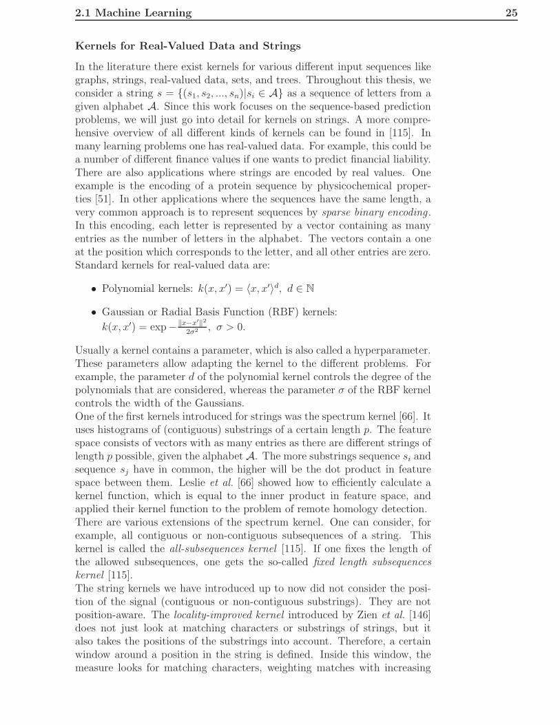
In the literature there exist kernels for various different input sequences likegraphs, strings, real-valued data, sets, and trees. Throughout this thesis, weconsider a string s = {(s1, s2, ..., sn)|si ∈ A} as a sequence of letters from agiven alphabet A. Since this work focuses on the sequence-based predictionproblems, we will just go into detail for kernels on strings. A more compre-hensive overview of all different kinds of kernels can be found in [115]. Inmany learning problems one has real-valued data. For example, this could bea number of different finance values if one wants to predict financial liability.There are also applications where strings are encoded by real values. Oneexample is the encoding of a protein sequence by physicochemical proper-ties [51]. In other applications where the sequences have the same length, avery common approach is to represent sequences by sparse binary encoding .In this encoding, each letter is represented by a vector containing as manyentries as the number of letters in the alphabet. The vectors contain a oneat the position which corresponds to the letter, and all other entries are zero.Standard kernels for real-valued data are:

• Polynomial kernels: k(x, x′) = 〈x, x′〉d, d ∈ N

• Gaussian or Radial Basis Function (RBF) kernels:

k(x, x′) = exp−‖x−x′‖2

2σ2 , σ > 0.

Usually a kernel contains a parameter, which is also called a hyperparameter.These parameters allow adapting the kernel to the different problems. Forexample, the parameter d of the polynomial kernel controls the degree of thepolynomials that are considered, whereas the parameter σ of the RBF kernelcontrols the width of the Gaussians.One of the first kernels introduced for strings was the spectrum kernel [66]. Ituses histograms of (contiguous) substrings of a certain length p. The featurespace consists of vectors with as many entries as there are different strings oflength p possible, given the alphabet A. The more substrings sequence si andsequence sj have in common, the higher will be the dot product in featurespace between them. Leslie et al. [66] showed how to efficiently calculate akernel function, which is equal to the inner product in feature space, andapplied their kernel function to the problem of remote homology detection.There are various extensions of the spectrum kernel. One can consider, forexample, all contiguous or non-contiguous subsequences of a string. Thiskernel is called the all-subsequences kernel [115]. If one fixes the length ofthe allowed subsequences, one gets the so-called fixed length subsequenceskernel [115].The string kernels we have introduced up to now did not consider the posi-tion of the signal (contiguous or non-contiguous substrings). They are notposition-aware. The locality-improved kernel introduced by Zien et al. [146]does not just look at matching characters or substrings of strings, but italso takes the positions of the substrings into account. Therefore, a certainwindow around a position in the string is defined. Inside this window, themeasure looks for matching characters, weighting matches with increasing

26 Background

weights from the border to the middle. The window is shifted over the wholesequence and an even higher-dimensional feature space is constructed by tak-ing the measure to the power of a certain value.Another position-aware string kernel is the weighted degree (WD) kernel [112].This kernel can be considered as a position-aware variant of the all-subsequen-ces kernel in which the matches of different length are weighted by a certainfactor corresponding to the lenght.A further extension to the position-aware string kernels was the incorporationof positional uncertainty. This can be motivated by considering an examplein which a random sequence s1 and the same sequence shifted by one letters2 are compared. The locality-improved kernel as well as the WD kernelwould just detect random similarities, meaning that s1 should have a higherkernel value with a sequence s3 containing parts of the sequence s1 and somerandom characters. This is certainly not desirable. A position-aware stringkernel with positional uncertainty, the so-called oligo kernel , was introducedin 2004 [76]. The kernel considers similarities of substrings of a certain lengthwhile the positional uncertainty is modelled by a Gaussian function aroundthe positions where the substring occurs. The incorporation of positional un-certainty into the WD kernel was proposed in 2005 [97] by allowing patternsto be shifted by a certain amount of letters.

2.1.6 Consistency of Support Vector Machines

We already explained why large margin classifiers should generalize well tounseen data. Nevertheless, we did not show that, given enough data, thealgorithm will converge to the best possible predictor. In this sense one isusually interested in consistency of the learning algorithm. Loosely speak-ing, this means that, given an infinite amount of data from the source, theprobability that the prediction function will deviate by ε > 0 tends to zero.More formally, consistency is defined as:

Definition 2.3 (Consistency). Let ft be the target function of the learningalgorithm. A classifier is said to be weakly/strongly universally consistent if

limn→∞

R(ft) = R∗ (2.50)

holds in probability/almost surely for all distributions P on X × Y.

Convergence in probability means that the probability that the deviationis greater than ε > 0 converges to zero as n goes to infinity. Almost sureconvergence means that

P ( limn→∞|R(ft)− R∗| = 0) = 1. (2.51)

It was shown that the 1-norm soft margin classifier and the 2-norm softmargin classifier are strongly universally consistent if a universal kernel isused and the regularization parameter is chosen properly [119].

2.2 Proteomics 27

2.2 Proteomics

2.2.1 General Overview

The proteome is the set of all proteins that can be made out of the genomeof an organism. Given a biological sample, one interesting question to askis which proteins are contained therein. The first approaches to answer thisquestion were developed by Edman and one of these methods is nowadayscalled Edman degradation [27]. In this technique, the protein is degradedfrom the N-terminus, one amino acid at a time. The identity of the removedamino acid is then determined by analytical methods like HPLC, which wewill consider in more detail in Section 2.2.2. The removal and analysis ofthe amino acid is called a cycle. To identify the protein at least six or sevencycles are usually required to get a unique protein hit. Although the methodhas been improved over the years, there are some shortcomings. First of all,each cycle takes about 45 minutes [52]. This limits the number of analyzedsamples per day to two or three. The second shortcoming is that there aremany proteins with blocked N-termini. Consequently, these proteins can-not be identified by Edman degradation. Additionally, the sensitivity of themethod is not high enough.Protein identification based on mass spectrometry (MS) analysis has beenaround for more than 40 years [5]. Nevertheless, the wide application ofMS-based methods for protein analysis did not start until the commercial-ization of electrospray ionization (ESI) and matrix-assisted laser desorp-tion/ionization (MALDI) [53]. The importance of these methods to sciencewas underlined by the Nobel committee, which awarded half of the 2002 No-bel prize in chemistry to the scientists who introduced these two methods.There are mainly two different approaches. One of them is called the ”top-down approach”. In this approach intact proteins are measured by the massspectrometer [38]. Two-dimensional (2D) gel electrophoresis is a commonmethod to separate the proteins before directing them to the mass spec-trometer. The proteins are first separated with respect to their isoelectricpoint using isoelectric focusing. Afterwards, the proteins are separated ac-cording to their molecular weight along the second, orthogonal dimension.One disadvantage of gel electrophoresis is that it cannot be directly coupledto an ESI source. Instead, the proteins of interest have to be cut out of the gelmanually. This intervention is not needed in a ”bottom-up approach” usingchromatography for separating the analytes. Typical steps in this approachare:

1. digestion of proteins into smaller parts (peptides)

2. separation of peptides according to certain properties

3. ionization of peptides

4. analysis of peptides by mass spectrometry

5. identification of peptides/proteins from mass spectrometry data.

28 Background

The first step can be performed in a solution using proteolytic enzymes liketrypsin or chymotrypsin. These enzymes usually cut at very distinct posi-tions. Trypsin, e.g., cleaves after the amino acids arginine and lysine but notbefore a proline residue.We will look at steps two, three, four, and five in more detail for strong an-ion exchange and high-performance liquid chromatography coupled to ESIMS/MS. For an introduction to MALDI, the interested reader is referred,e.g., to [52].Although spectra can be interpreted manually, current high throughput ex-periments require computational methods for fast and accurate analysis ofmass spectrometry data to identify and quantitate the measured proteins.These methods are introduced in section 2.2.5.

2.2.2 Chromatographic Separation

Due to the complexity of the sample, it is often beneficial to separate peptidesbefore analyzing them by mass spectrometry. The most widely used tech-nique for this purpose is liquid chromatography (LC), which separates thepeptides according to certain properties of the peptide. With this technique,the peptides are directed through a column and, depending on properties likehydrophobicity, length, molecular mass, and amino acid composition, eachpeptide will elute from the column at a certain timepoint. This means thatpeptides with similar properties should elute at similar timepoints. We willnow review the most common chromatography techniques.In High-Performance Liquid Chromatography (HPLC), a sample is directedthrough a column to separate the peptides depending on specific properties.The liquid that is pumped through the column is called the mobile phase.The substances that are fixed to the column are part of the stationary phase.Usually, the stationary and the mobile phases have different chemical prop-erties. According to the properties of the peptides, each peptide will havea stronger interaction with either the stationary or the mobile phase. If apeptide interacts stronger with the mobile phase than with the stationaryphase, it will flow faster through the column than peptides that interactstronger with the stationary phase. Different combinations of stationary andmobile phases are known, but the most widely used is called reversed-phase.Therefore, reversed-phase HPLC will be explained in more detail. Strong an-ion exchange chromatography is also introduced, since we also analyze dataobtained by this technique in this thesis.

Reversed-Phase HPLC

In reversed-phase HPLC, the stationary phase is non-polar and the mobilephase consists of an aqueous, moderately polar solution. The more hydropho-bic the peptides are, the greater is the tendency of the column to retainthem. Consequently, the more hydrophilic the peptides are, the faster theyflow through the column.

2.2 Proteomics 29

Strong Ion Exchange Chromatography

In ion exchange chromatography, the stationary phase either contains cationsor anions. In strong anion exchange (SAX) chromatography the peptides thathave many positively charged side-chains interact stronger with the column.The main practical difference between strong ion exchange and reversed-phase HPLC is that strong ion exchange can just separate the peptides intodifferent fractions (e.g., 15 fractions if coupled to a mass spectrometer on-line or 96 fractions via an off-line combination [86]), whereas peptides inreversed-phase HPLC elute at a distinct point in time.

Two-Dimensional Chromatographic Separation

To get even better separation, it is common to combine two chromatographicseparations that separate the peptides according to different criteria. Onepossibility for a two-dimensional separation is to use strong ion exchangechromatography prior to a reversed-phase HPLC. Washburn et al. [139] ap-plied this two-dimensional separation with a strong cation exchange chro-matography followed by a reversed-phase chromatography to perform a large-scale proteome analysis. This technique is called MudPIT and is based onwork by Link et al. [69]. Very recently, Delmotte et al. [20] introduced acombination of two reversed-phase HPLC separations at different pH values.

2.2.3 Ionization

Electrospray ionization (ESI) was introduced in 1985 by Fenn and co-workers[141]. This technique can be used to ionize peptides in the solvent phase andbring them into the gas-phase. A schematic illustration of ESI is shownin Fig. 2.11. A watery, acidic solution, which contains peptides, is sprayedthrough a very thin needle. The high positive voltage at the tip of the needleleads to sputtering of droplets. A negative voltage is applied to the massspectrometer. Therefore, the positively charged ions travel towards the massspectrometer. Since the ions travel through a heated near-vacuum region, theions get desolvated, which finally leads to protonated peptides in gas-phase.

2.2.4 Tandem Mass Spectrometry

Tandem mass spectrometry or MS/MS usually refers to the analysis of a sam-ple using two mass spectrometers consecutively. With just one mass spec-trometer only the mass-to-charge ratio (m/z) of a peptide can be measured.Since one cannot distinguish sequences with the same amino acid composi-tion from each other by this information alone, a single mass spectrometerdoes not suffice to identify peptide samples with high accuracy. In MS/MS,there is a collision chamber between the two mass spectrometers. In this col-lision chamber there is an inert gas like argon or helium. When the peptideflies through the chamber, it collides with these inert gas atoms/moleculesand breaks apart (fragmentation). For collision-induced dissociation (CID)the peptide usually breaks at an amide bond. If the charge is retained atthe N-terminus, the corresponding ion is called a b-ion and if the charge is

30 Background

+2 kV to +5 kV

Capillary column Charged droplets

Desolvated

peptide ions

Heated desolvation region Entrance to mass

spectrometer

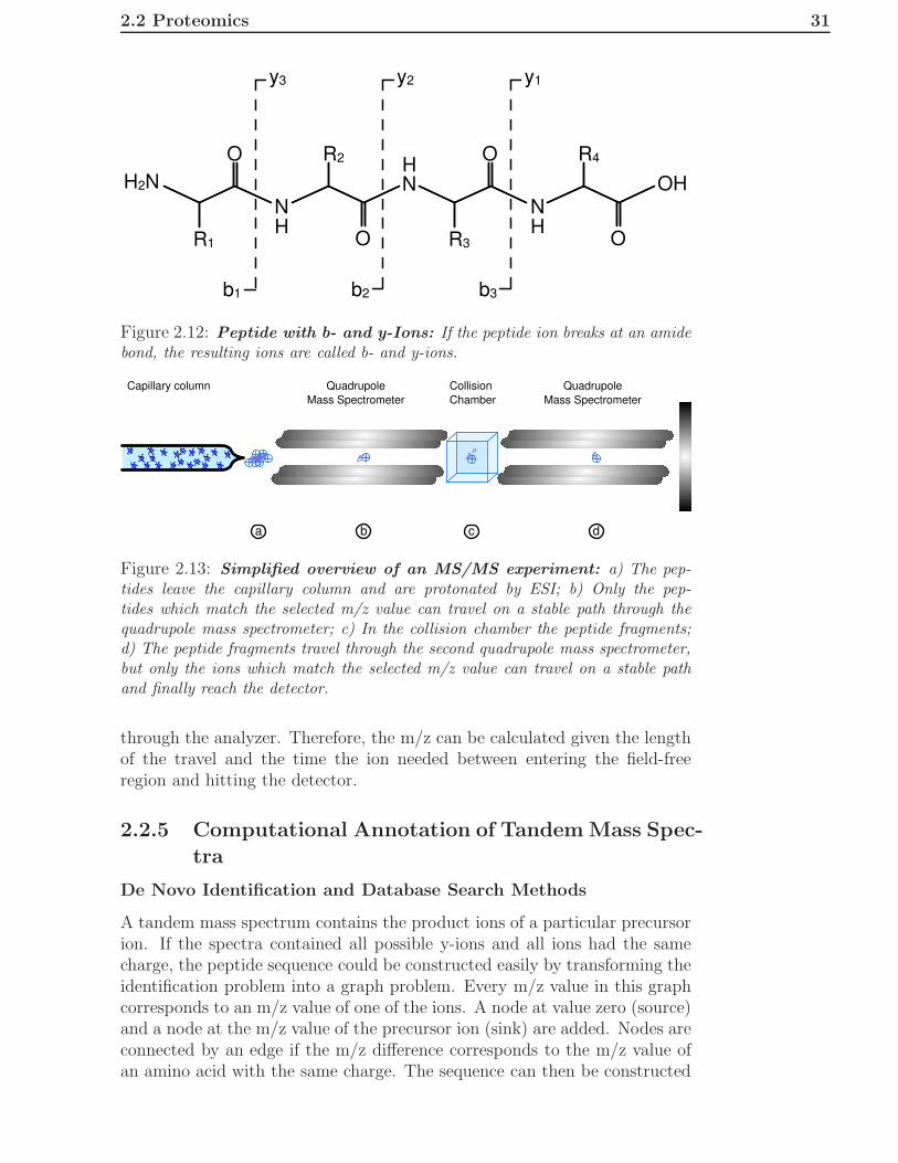
Figure 2.11: Electrospray ionization: The sample is directed through a cap-illary column in an acidic solution. At the tip of the needle, a high voltage isapplied. Positively charged droplets form, which are directed towards the entranceof the mass spectrometer. During the flight through the heated, near-vacuum re-gion, the droplets are desolvated (adapted from [54]).

retained at the C-terminal part, the ion is called a y-ion. A peptide togetherwith the b- and y-ions can be seen in Fig. 2.12. The whole measurementprocess can be seen in Fig. 2.13. The ion which flies through the first massspectrometer is usually called a precursor ion and the b- and y-ions of theprecursor ion are called product ions. Usually the three highest peaks inan MS1 spectrum are selected for further fragmentation. These peaks arefound by so-called survey scans, which scan a certain mass-to-charge range.A survey scan together with the product ion spectrum of the most intenseprecursor peak are shown in Fig. 2.14.

Two of the most prominent mass spectrometers are the quadrupole andtime-of-flight (TOF) types. In quadrupole mass spectrometers, like inFig. 2.13, only ions with a certain m/z value (± a certain tolerance) cantravel through the electrostatic field on a stable path. All other ions collidewith the rods and do not reach the detector. To measure the whole sample,the whole range of possible m/z values is probed from lowest to highest.In TOF mass spectrometers, the principle is simpler. The ions are acceler-ated towards the detector via an electric field. Then, they travel through afield-free region. The higher the m/z value of the ion, the slower it will travel

2.2 Proteomics 31

R1

H2N

NH

HN

O R2

R3

OH

O R4

O O

NH

b1

y3

b2

y2

b3

y1

Figure 2.12: Peptide with b- and y-Ions: If the peptide ion breaks at an amidebond, the resulting ions are called b- and y-ions.

a b c

Capillary column Quadrupole

Mass Spectrometer

Quadrupole

Mass Spectrometer

Collision

Chamber

d

Figure 2.13: Simplified overview of an MS/MS experiment: a) The pep-tides leave the capillary column and are protonated by ESI; b) Only the pep-tides which match the selected m/z value can travel on a stable path through thequadrupole mass spectrometer; c) In the collision chamber the peptide fragments;d) The peptide fragments travel through the second quadrupole mass spectrometer,but only the ions which match the selected m/z value can travel on a stable pathand finally reach the detector.

through the analyzer. Therefore, the m/z can be calculated given the lengthof the travel and the time the ion needed between entering the field-freeregion and hitting the detector.

2.2.5 Computational Annotation of Tandem Mass Spec-

tra

De Novo Identification and Database Search Methods

A tandem mass spectrum contains the product ions of a particular precursorion. If the spectra contained all possible y-ions and all ions had the samecharge, the peptide sequence could be constructed easily by transforming theidentification problem into a graph problem. Every m/z value in this graphcorresponds to an m/z value of one of the ions. A node at value zero (source)and a node at the m/z value of the precursor ion (sink) are added. Nodes areconnected by an edge if the m/z difference corresponds to the m/z value ofan amino acid with the same charge. The sequence can then be constructed

32 Background

a b

Figure 2.14: MS spectrum of potential precursor ions and product ionspectrum of selected precursor ion: The graphs plot m/z value against inten-sity, given in percentage, according to the peak intensity of the most intense peak.a) An MS scan of all ions at a certain retention time. The ion with the highestintensity is chosen for fragmentation. b) The product ion spectrum of the selectedprecursor ion. The graphs are made with TOPPView [123].

by finding the longest path. This kind of identification is usually called denovo identification or de novo sequencing [127, 31].Unfortunately, many b- and y-ions in a spectrum are missing and with in-struments which do not have good precision the charge state cannot be deter-mined accurately. Consequently, there are other approaches for identificationwhich are not that sensitive to spectra quality. One big class of methods canbe called database search methods. In these approaches, the experimentalspectra are compared to theoretical spectra which are constructed from allpossible peptides of the protein database. One example of an experimentalspectrum together with its theoretical spectrum (only y-ions) is shown inFig. 2.15. Various methods for scoring and assessing the significance of thesematches have been introduced. Among the first introduced methods wereSEQUEST [29] and Mascot [87], but still nowadays there is room for im-provement of database search methods since a significant number of spectraremain unidentified [12].

Perkins et al. [87] did not reveal the details of the Mascot search enginebecause it is proprietary software. Nevertheless, they stated that Mascotuses probability-based scoring. This means that for each match between anexperimental and a theoretical spectrum the probability that a match withthe same or better score occurs by chance is estimated. For each experi-mental spectrum, the match with the lowest probability is considered thebest possible identification. The peptide sequence of the corresponding the-oretical spectrum is returned as annotation of the spectrum. Furthermore,the significance of the best identification can be assessed via a p-value. Tocalculate probabilities one has to assume a certain distribution underlyingrandom matches. Since Perkins et al. did not state which distribution un-

2.2 Proteomics 33

Figure 2.15: Experimental spectrum together with theoretical spectrum:An experimental spectrum (top) is shown together with the best matching theoret-ical spectrum (bottom) visualized with TOPPView [123]. The peptide sequence isTVMENFVAFVDK.

derlies the Mascot model, we look at a database search method by Sadygovand Yates [104] called PEP PROBE. This method uses the hypergeometricdistribution to model the frequencies of matches between experimental andtheoretical spectra. It is a modified version of SEQUEST [29].Let m be the number of red balls and N the total number of balls. The hy-pergeometric distribution can be used to estimate the probability that aftern draws without replacement we end up with exactly k red balls:

P (X = k) =

(

m

k

)(

N−m

n−k

)

(

N

n

) (2.52)

In PEP PROBE, N is the number of all predicted fragment ions in a sequencedatabase that consists of all peptide sequences matching the precursor mass(M +H)+ of the tandem mass spectrum. The variable m represents the num-ber of all of these fragments that match a peak in an experimental tandemmass spectrum. If one considers just b- and y-ions, the number of draws fora peptide sequence of length L is n = 2 (L− 1). The hypergeometric distri-bution can then be used to estimate the probability that k of the fragmentsof the peptide sequence match the experimental spectrum just by chance.

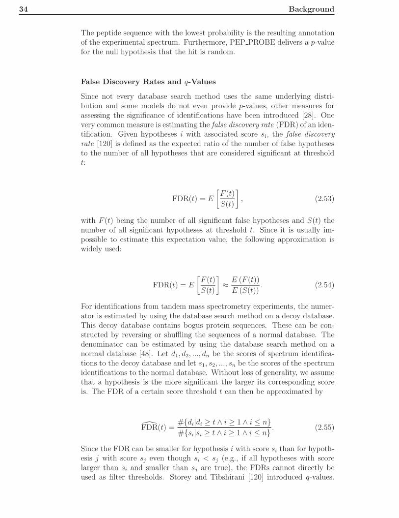
34 Background

The peptide sequence with the lowest probability is the resulting annotationof the experimental spectrum. Furthermore, PEP PROBE delivers a p-valuefor the null hypothesis that the hit is random.

False Discovery Rates and q-Values

Since not every database search method uses the same underlying distri-bution and some models do not even provide p-values, other measures forassessing the significance of identifications have been introduced [28]. Onevery common measure is estimating the false discovery rate (FDR) of an iden-tification. Given hypotheses i with associated score si, the false discoveryrate [120] is defined as the expected ratio of the number of false hypothesesto the number of all hypotheses that are considered significant at thresholdt:

FDR(t) = E

[

F (t)

S(t)

]

, (2.53)

with F (t) being the number of all significant false hypotheses and S(t) thenumber of all significant hypotheses at threshold t. Since it is usually im-possible to estimate this expectation value, the following approximation iswidely used:

FDR(t) = E

[

F (t)

S(t)

]

≈ E (F (t))

E (S(t)). (2.54)

For identifications from tandem mass spectrometry experiments, the numer-ator is estimated by using the database search method on a decoy database.This decoy database contains bogus protein sequences. These can be con-structed by reversing or shuffling the sequences of a normal database. Thedenominator can be estimated by using the database search method on anormal database [48]. Let d1, d2, ..., dn be the scores of spectrum identifica-tions to the decoy database and let s1, s2, ..., sn be the scores of the spectrumidentifications to the normal database. Without loss of generality, we assumethat a hypothesis is the more significant the larger its corresponding scoreis. The FDR of a certain score threshold t can then be approximated by

FDR(t) =#{di|di ≥ t ∧ i ≥ 1 ∧ i ≤ n}#{si|si ≥ t ∧ i ≥ 1 ∧ i ≤ n} . (2.55)

Since the FDR can be smaller for hypothesis i with score si than for hypoth-esis j with score sj even though si < sj (e.g., if all hypotheses with scorelarger than si and smaller than sj are true), the FDRs cannot directly beused as filter thresholds. Storey and Tibshirani [120] introduced q-values.

2.2 Proteomics 35

A q-value for hypothesis i is the minimum FDR that can be attained whencalling hypothesis i significant (si ≥ t). Kall et al. [48] used q-values forassigning significance to identifications from tandem mass sectrometry data.In this setting, the q-value of a certain spectrum identification is the smallestFDR at which the spectrum identification is accepted. Therefore,

q(i) = mint≤si

FDR(t). (2.56)

36 Background

2.3 Immunomics

2.3.1 General Overview

The latin word immunis can be translated as exempt. This word was chosenas a basis for immunity and immunology because the whole field emergedfrom the observation that people who had recovered from particular infec-tious diseases were afterwards exempt from falling ill to the disease. Thesepeople were immune to the corresponding disease. From then on, the goalof doctors and scientists in this field has been to make people immune toa certain disease even before a first infection. The first disease for whichreports exist was the smallpox disease. In the fifteenth century, the Chineseand Turks tried to immunize people with the dried crusts of smallpox pus-tules. In 1798, Edward Jenner made the observation that milkmaids who fellill with cowpox and subsequently recovered were later immune to smallpox.Therefore, he used the fluid of a cowpox pustule to inoculate a person andhe showed that the person was then immune to smallpox. Between this dis-covery and the current state of immunological knowledge there were manyground-breaking studies, which can also be seen by the fact that 16 Nobelprizes had been awarded for immunologic research by 1996 [100].There are different mechanisms of the body which lead to immunity to acertain infectious agent and they can be divided into two categories calledInnate Immunity and Adaptive Immunity . Innate immunity contains non-adaptive barriers to infectious agents. There are four different types of barri-ers: anatomic barriers, physiological barriers, phagocytic/endocytic barriers,and inflammatory barriers. In contrast, adaptive immunity comprises all de-fense mechamisms which are able to adaptively recognize and destroy specificagents.

2.3.2 Innate Immune System

The innate immune system can be seen as the first line of defense against in-vading microorganisms. The underlying mechanisms prevent a large class ofmicroorganisms from entering or staying in the human body. The first partof this system comprises the anatomic barriers. The skin, which is made upof the epidermis and the dermis, is the outer barrier. The epidermis containsdead cells as well as the protein keratin, which makes this layer waterproof.The dermis is composed of connective tissue. Because of the low pH, between3 and 5 in this tissue, it inhibits the growth of most infectious agents.Another important anatomic barrier is the mucosal surface. It can be foundon the mucosal membranes of the alimentary, urogenital, and respiratorytracts as well as on the mucosal membrane of the conjunctivae. Since thesemembranes are easier for the microorganisms to penetrate, there exist anumber of non-specific defense mechanisms that serve to remove the invad-ing microorganism from the body. These defense mechanisms are, e.g., tears,saliva and mucous secretion, and hairlike protrusions called cilia.The second part of the innate immune system comprises the physiologicalbarriers. All physiological conditions in the body which inhibit the growth

2.3 Immunomics 37

of, or destroy microorganisms, can be seen as manifestations of these barri-ers. The temperature of the human body, for example, inhibits the growthof certain organisms and the low pH in the stomach leads to the destruc-tion of many microorganisms. Furthermore, there are chemical mediatorslike lysozyme, complement, and interferon, which favor the lysis of certainpathogens or facilitate phagocytosis.The third part of the innate immune system comprises the phagocytic andendocytic barriers. Some specialized cells in the body (e.g., monocytes, neu-trophils, and macrophages) are able to phagocytose foreign organisms. Thismeans that the cells surround the pathogens to internalize them in so-calledphagosomes. The content of these phagosomes is then digested by lysosomalenzymes and the products of this reaction are released from the cell. Phago-cytosis is a special form of endocytosis which describes the uptake of materialfrom its surrounding. A certain type of endocytosis, which is called receptor-mediated endocytosis, allows a cell to specifically uptake certain extracellularmolecules after they have been bound by the corresponding receptors.The fourth part of the innate immune system comprises the inflammatorybarrier. If a tissue is ruptured, usually an inflammatory response is triggered,in which vascular fluid, containing serum proteins with antibacterial activityas well as phagocytic cells, are released into the affected region. After theactivation of an enzyme cascade, insoluble fibrin strands separate the rup-tured area from the rest of the body to prevent further microorganisms fromentering.

2.3.3 Adaptive Immune System

The adaptive immune system can very selectively recognize and eliminateinvading microorganisms. There are many cells and receptors involved in thisadaptive response. For such a system to work there are a few requirements.First of all, there has to be a mechanism to discriminate self from non-selfcells. Since invading microorganisms can be quite diverse, there has to bea mechanism by which the immune system can construct very diverse butalso specific cells which recognize the pathogens. To be able to react toan infectious agent as fast as possible, it is also desirable to have a sortof memory which enables a faster reaction if the person is infected by aninfectious agent against which it has already reacted. The adaptive immunesystem fulfills all these requirements. We will now look at parts of the systemin more detail.The term antigen will be used quite frequently in this thesis. When it wasfirst introduced in the literature, it stood for any substance which couldstimulate antibody generation. Nowadays, the term is used for any substancewhich can be recognized by the adaptive immune system.

Major Histocompatibility Complex

The major histocompatibility complex (MHC) is a cluster of genes whoseencoded proteins are responsible for many important parts of the adaptiveimmune system of mammals. In humans, the MHC is referred to as the hu-

38 Background

man leukocyte antigen (HLA) complex. T cells, which are introduced in thenext section, can only recognize antigens that are presented by MHC classI (MHCI) or MHC class II (MHCII) molecules. Throughout this thesis weuse MHCI molecule (sometimes also MHCI allele) as a synonym for the geneproducts HLA-A, HLA-B, and HLA-C encoded by the HLA complex regionsA, B, and C. We use the term MHCII molecule (sometimes also MHCII al-lele) as a synonym for the gene products HLA-DP, HLA-DQ, and HLA-DRencoded by the HLA complex regions DP, DQ, and DR. MHCI moleculescan be found on nearly all nucleated cells. In contrast, MHCII molecules canjust be found on antigen-presenting cells such as B cells, dendritic cells, andmacrophages. The structures of the MHCI and MHCII molecules are verysimilar. Both have a binding cleft in which about nine amino acids can fit.This enables peptides to interact with and therefore bind to the molecule.Examples of MHCI and MHCII molecules can be seen in Fig. 2.16. Themain difference between these two classes of molecules is that the bindingcleft is closed at the ends for MHCI and open for MHCII. Therefore, MHCI

Figure 2.16: Structure of MHC molecules with binding peptide: a) Thispicture shows an MHCI molecule (purple) together with a binding peptide (green).The PDB ID of the structure is 1JF1. b) This picture shows an MHCII molecule(blue) together with a binding peptide (green). The PDB ID of the structure is1BX2. Both MHC molecules were visualized with BALLView [77].

molecules can just bind peptides of a narrowly defined length. The bindingpeptides are usually between eight and twelve amino acids long. In contrast,the peptides that can bind to MHCII molecules can have even more thantwenty amino acids [16].MHCI molecules present peptides which are derived from proteins inside thecell. In contrast, MHCII molecules present peptides derived from proteinsoutside of the cell. The proteins enter the cell via the endosomal pathway.Inside the cell, they are exposed to several proteases, which cut them intosmaller parts (peptides). The peptides are then transported to a compart-ment known as the MIIC (MHCII-rich endosomal compartment). In thiscompartment, the peptides are loaded into MHCII molecules. Afterwards,the peptide-MHCII complex is transported to the cell surface.

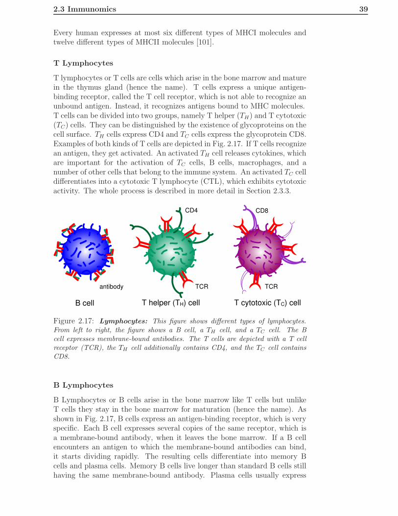
2.3 Immunomics 39

Every human expresses at most six different types of MHCI molecules andtwelve different types of MHCII molecules [101].

T Lymphocytes

T lymphocytes or T cells are cells which arise in the bone marrow and maturein the thymus gland (hence the name). T cells express a unique antigen-binding receptor, called the T cell receptor, which is not able to recognize anunbound antigen. Instead, it recognizes antigens bound to MHC molecules.T cells can be divided into two groups, namely T helper (TH) and T cytotoxic(TC) cells. They can be distinguished by the existence of glycoproteins on thecell surface. TH cells express CD4 and TC cells express the glycoprotein CD8.Examples of both kinds of T cells are depicted in Fig. 2.17. If T cells recognizean antigen, they get activated. An activated TH cell releases cytokines, whichare important for the activation of TC cells, B cells, macrophages, and anumber of other cells that belong to the immune system. An activated TC celldifferentiates into a cytotoxic T lymphocyte (CTL), which exhibits cytotoxicactivity. The whole process is described in more detail in Section 2.3.3.

B cell T helper (TH) cell T cytotoxic (TC) cell

CD4 CD8

TCR TCRantibody

Figure 2.17: Lymphocytes: This figure shows different types of lymphocytes.From left to right, the figure shows a B cell, a TH cell, and a TC cell. The Bcell expresses membrane-bound antibodies. The T cells are depicted with a T cellreceptor (TCR), the TH cell additionally contains CD4, and the TC cell containsCD8.

B Lymphocytes

B Lymphocytes or B cells arise in the bone marrow like T cells but unlikeT cells they stay in the bone marrow for maturation (hence the name). Asshown in Fig. 2.17, B cells express an antigen-binding receptor, which is veryspecific. Each B cell expresses several copies of the same receptor, which isa membrane-bound antibody, when it leaves the bone marrow. If a B cellencounters an antigen to which the membrane-bound antibodies can bind,it starts dividing rapidly. The resulting cells differentiate into memory Bcells and plasma cells. Memory B cells live longer than standard B cells stillhaving the same membrane-bound antibody. Plasma cells usually express

40 Background

little or no membrane-bound antibodies. They are able to produce copiousnumbers of the antibody and secrete them. The whole process is describedin more detail in Section 2.3.3.

Antibody Generation

a

MHCII

antigen

antigen

cytokines antibodies

b c

Figure 2.18: Antibody production after recognition of antigen: a) A naiveTH cell gets activated after recognizing an MHCII-bound antigen. b) After activa-tion it releases cytokines. The cytokines are absorbed by nearby B cells. c) If oneof these B cells recognizes an antigen, it divides into antibody-producing plasmacells and memory B cells.

The humoral response to antigens is shown in Fig. 2.18. If a naive TH

cell encounters an antigen which is presented by an MHCII molecule, theTH cell gets activated. The activation leads to the release of cytokines. AB cell, which absorbs these cytokines and recognizes an antigen via one ofits membrane-bound antibodies, divides into plasma cells and memory Bcells. The plasma cells produce a huge amount of the antibody and secreteit. Usually these plasma cells have little or no membrane-bound antibodies.Since the antibodies can bind to the antigen and these antigens are likelyto be proteins that are expressed on the exterior of bacteria or viruses, theexistence of a large number of these antibodies promotes the clearance of theinfectious agents.

CTL Response to Antigens

The cell-mediated response to an antigen is shown in Fig. 2.19. One require-ment for a TC cell to differentiate into a CTL is that it encounter cytokines.These are produced with the same mechanisms as described in Section 2.3.3.If a CTL encounters an antigen presented at the cell wall of an infected oraltered cell via an MHCI molecule, the CTL induces apoptosis in the cor-responding cell. Since MHCI molecules present peptides, which are derivedfrom proteins inside the cell, the recognition of a foreign peptide signals thateither the cell is infected by an infectious agent or the cell has altered proteinsequences, which happens, e.g., in cancer. Therefore, it can be assumed thatmechanisms which promote apoptosis of these kinds of cells proved to beadvantageous during evolution.

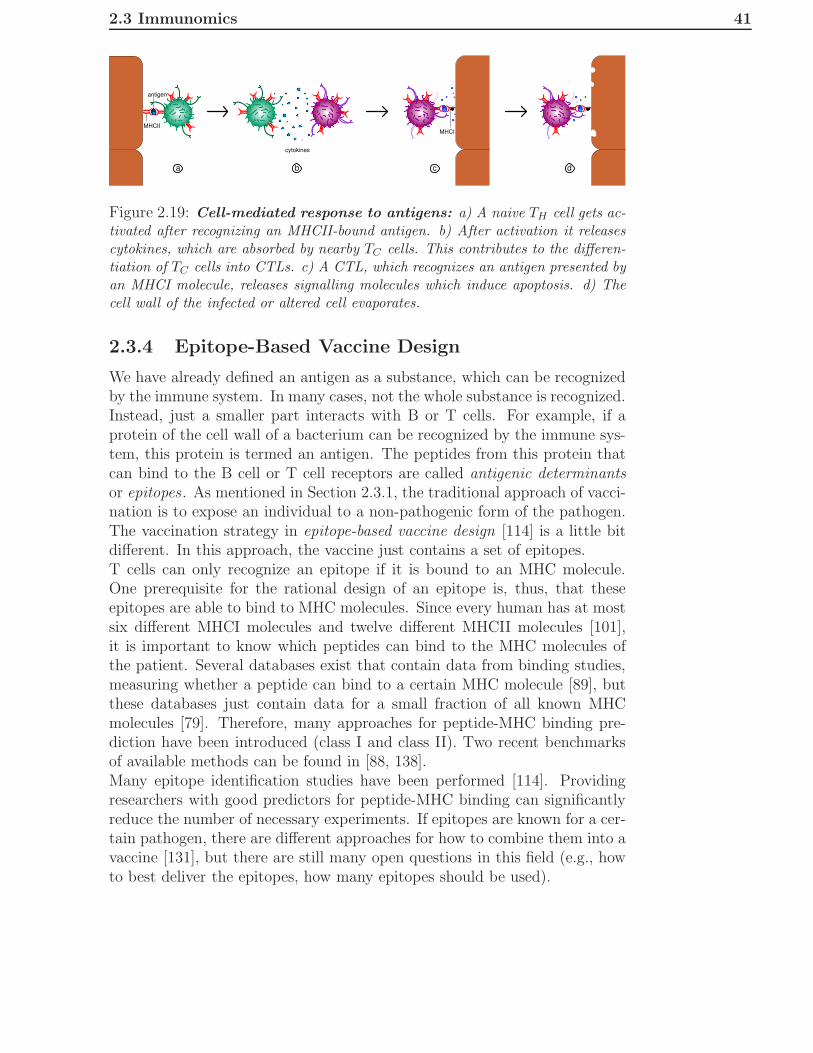
2.3 Immunomics 41

a b c d

MHCII

antigen

cytokines

MHCI

Figure 2.19: Cell-mediated response to antigens: a) A naive TH cell gets ac-tivated after recognizing an MHCII-bound antigen. b) After activation it releasescytokines, which are absorbed by nearby TC cells. This contributes to the differen-tiation of TC cells into CTLs. c) A CTL, which recognizes an antigen presented byan MHCI molecule, releases signalling molecules which induce apoptosis. d) Thecell wall of the infected or altered cell evaporates.

2.3.4 Epitope-Based Vaccine Design

We have already defined an antigen as a substance, which can be recognizedby the immune system. In many cases, not the whole substance is recognized.Instead, just a smaller part interacts with B or T cells. For example, if aprotein of the cell wall of a bacterium can be recognized by the immune sys-tem, this protein is termed an antigen. The peptides from this protein thatcan bind to the B cell or T cell receptors are called antigenic determinantsor epitopes . As mentioned in Section 2.3.1, the traditional approach of vacci-nation is to expose an individual to a non-pathogenic form of the pathogen.The vaccination strategy in epitope-based vaccine design [114] is a little bitdifferent. In this approach, the vaccine just contains a set of epitopes.T cells can only recognize an epitope if it is bound to an MHC molecule.One prerequisite for the rational design of an epitope is, thus, that theseepitopes are able to bind to MHC molecules. Since every human has at mostsix different MHCI molecules and twelve different MHCII molecules [101],it is important to know which peptides can bind to the MHC molecules ofthe patient. Several databases exist that contain data from binding studies,measuring whether a peptide can bind to a certain MHC molecule [89], butthese databases just contain data for a small fraction of all known MHCmolecules [79]. Therefore, many approaches for peptide-MHC binding pre-diction have been introduced (class I and class II). Two recent benchmarksof available methods can be found in [88, 138].Many epitope identification studies have been performed [114]. Providingresearchers with good predictors for peptide-MHC binding can significantlyreduce the number of necessary experiments. If epitopes are known for a cer-tain pathogen, there are different approaches for how to combine them into avaccine [131], but there are still many open questions in this field (e.g., howto best deliver the epitopes, how many epitopes should be used).

42 Background

Chapter 3

Applications in Proteomics

3.1 A New Kernel for Chromatographic Sep-

aration Prediction

3.1.1 Introduction

Experimental techniques for determining the composition of complex pro-teomes have been improving rapidly over the past decade. The applicationof tandem mass spectrometry-based identification has resulted in the gener-ation of enormous amounts of data, requiring efficient computational meth-ods for their evaluation. There are numerous database search algorithmsfor protein identification such as Mascot [87], Sequest [29], OMSSA [34] andX!Tandem [18], as well as de novo methods like Lutefisk [127] and Pep-Novo [31]. Furthermore, there are a few methods like InsPecT [32] whichuse sequence tags for pruning the possible search space using more computa-tionally expensive and more accurate scoring functions afterwards. Databasesearch algorithms generally construct theoretical spectra for a set of possiblepeptides and try to match these theoretical spectra to the measured ones tofind the candidate(s) which match(es) best. In order to distinguish betweentrue and random hits, it is necessary to define a scoring threshold, whicheliminates all peptide identifications with scores below the scoring threshold.This threshold value is chosen quite conservatively to get very few false pos-itives. Consequently, there is a significant number of correct identificationsbelow the threshold that are not taken into account, although these spectraoften correspond to interesting (e.g., low abundance) proteins. One of thegoals of this work was to increase the number of reliable identifications byfiltering out false positives in this ’twilight zone’ below the typical threshold.There are various studies addressing this issue [26, 72, 78] by calculating theprobability that an identification is a false positive.Standard identification algorithms are based on MS/MS data and do not usethe information inherent to the separation processes typically used prior tomass spectrometric investigation. Since this additional experimental infor-mation can be compared to predicted properties of the peptide hits suggestedby MS/MS identification, false positive identifications can be detected. InSAX-SPE, it is important to know whether a peptide binds to the column or

44 Applications in Proteomics

flows through. This information can also be incorporated into the identifica-tion process to filter out false positive identifications. Oh et al. [84] elaboratedseveral chemical features such as molecular mass, charge, length and a so-called sequence index of the peptides. These features were subsequently usedin an artificial neural network approach to predict whether a peptide bindsto the SAX column or not. The sequence index is a feature reflecting the cor-relation of pI values of consecutive residues. Strittmater et al. [121] includedthe experimental retention time from an ion-pair reversed-phase liquid chro-matographic separation process into a peptide scoring function. They used aretention time predictor based on an artificial neural network [90] but a num-ber of other retention time predictors exist [91, 35]. If the deviation betweenobserved and predicted retention time is large, then the score of the scoringfunction becomes small. Since they only consider the top scoring identifica-tions (rank = 1), they miss correct identifications of spectra where a falsepositive identification has a larger score than the correct one. We also addressthese cases in our work, demonstrating that filtering out identifications witha large deviation between observed and predicted retention time significantlyimproves the classification rate of identifications with small maximal scores.Recently, Klammer et al. [55] used support vector machines (SVMs) [11]to predict peptide retention times. Nevertheless, they used standard kernelfunctions and stated that they needed at least 200 identified spectra withhigh scores to train the learning machine.When applying machine learning techniques to the prediction of chromato-graphic retention, a concise and meaningful incorporation of the peptideproperties is crucial. The features used for this incorporation must capturethe essential properties of the interaction of the peptide with the station-ary and the mobile phases. These properties are mostly determined by theoverall amino acid composition, by the sequence of the N- and C-terminalends, and by the sequence in general. One of the most widely applied ma-chine learning techniques are SVMs, introduced in Section 2.1.4. SVMs usea kernel function which is used to encode distances between individual datapoints (in our case, the peptides). There are numerous kernel functions de-scribed in the literature which can be applied to sequence data. An overviewis presented in Section 2.1.5. All of these kernels were either introduced forsequences of the same length or not position-aware. However, the lengthof peptides typically encountered in computational proteomics experimentsvaries significantly, ranging roughly from 4 to 40 amino acids. Because itcan be assumed that the local alignment kernel [136], which can also handlesequences of different lengths, does not suit this kind of problem perfectly, wepropose a new kernel function, which can be applied to sequences of differentlengths. Consequently, this new kernel function is applicable to a wide rangeof computational proteomics applications.In 2006 Petritis et al. [91] evaluated different features like peptide length,sequence, hydrophobicity, hydrophobic moment and predicted structural ar-rangements like helix, sheet or coil for the prediction of peptide retentiontimes in reversed-phase liquid chromatography-MS. They used an artificialneural network and showed that the sequence information, together withsequence length and hydrophobic moment yield the best prediction results.

3.1 A New Kernel for Chromatographic Separation Prediction 45

In their study, they used only the border residues of the peptide sequences;their evaluation showed that a border length of 25 worked best for theirdataset. Since they used one input node for every position of the bordersof the peptide, they needed a very large training set. They trained theirlearning machine on 344,611 peptide sequences.Since one cannot routinely measure such an amount of training sequencesbefore starting the actual measurements, it is reasonable to apply a sort ofGaussian smoothing effect to the sequence positions. This means that inour representation, not every amino acid at every position is considered butrather regions (consecutive sequence positions) where the amino acid occurs.The distance of the amino acids of two sequences is scored with a Gaussianfunction. The size of this region modeled by our kernel function can be con-trolled by the kernel parameter σ of the kernel function and can be foundby cross validation. By this and because we use support vector machinesin combination with our kernel function, the number of necessary trainingsequences can be decreased dramatically. By just using the amino acid se-quence, we do not rely on features which are important for certain separationprocesses. This means that we learn the features (e.g., composition (using alarge σ in the kernel function), sequence length, hydrophobic regions) whichare important for the prediction process within the data because they arereflected in the amino acid sequence. This is why our kernel function can beused for retention time prediction in IP-RP-HPLC as well as for fractionationprediction in SAX-SPE.When applied to the same dataset as Oh et al. [84] used, our kernel func-tion in conjunction with support vector classification predicts 87% of thepeptides correctly. This is better than for all reported methods. Further-more, our retention time prediction model is based on a new kernel functionin conjunction with support vector regression [110], which allows to predictpeptide retention times very accurately, requiring only a very small amountof training data. This method has a better performance on a test set than theartificial neural network method used by Strittmater et al. [121], even with amuch smaller training set. Additionally, our method outperforms the meth-ods introduced by Klammer et al. [55]. Section 3.1.2 describes our new kernelfunction and we explain our p-value-based filtering approach. Section 3.1.3introduces the datasets used in this study. In Section 3.1.4, we demonstratethat our new kernel function, in combination with support vector classifica-tion, achieves better results in SAX-SPE fractionation prediction than anyother published method. Next, we show that our kernel function also per-forms very well for peptide retention time prediction in IP-RP-HPLC withvery little training data required. This allows us to train our predictor ona small dataset to predict retention times for further datasets, and to filterthe data by deviation in observed and predicted retention time. This leadsto a huge improvement in the precision of the identifications of spectra forwhich only identifications with small scores can be found, and also improvesthe precision of high-scoring identifications.

46 Applications in Proteomics

3.1.2 Machine Learning Methods

In this thesis, we introduce a new kernel function, which can be used topredict peptide properties using support vector classification and ν-supportvector regression [110], introduced in Section 2.1.4. We apply this kernelfunction to predict fractionation of peptides in SAX-SPE as well as peptideretention times in IP-RP-HPLC. To show the superior performance of thenew kernel function, we provide comparisons to established kernel functionsand the latest approaches of other working groups [84, 91, 55].

Kernel Function

The oligo kernel introduced by Meinicke et al. [76] is a kernel function thatcan be used to find signals in sequences for which the degree of positionaluncertainty can be controlled by the factor σ of the kernel function. Thestandard oligo kernel was introduced for sequences of fixed length. Sincethere are many problems in which the length of the sequences varies signif-icantly (e.g., peptide retention time prediction), this kernel function cannotbe applied to them directly.Petritis et al. [91] predicted peptide retention times very accurately by encod-ing the border residues directly, meaning that they accounted for 25 aminoacids from each border (starting at the termini). This led to a very large neu-ral network, which was therefore trained with about 345,000 peptides. Asstated in [43], the oligo kernel can be used as a motif kernel. Therefore, onecan focus on important signals instead of using all k-mers of a sequence. Thismotivated us to construct a kernel which only considers the border residuesof a peptide for a fixed border length b. Consequently, the kernel functionis called oligo-border kernel (OBK ). Here, a motif is a certain k-mer at aposition inside the b residue border at each side where b ∈ {1, . . . , 30}. Thismeans that every k-mer at the leftmost b residues contributes to its oligofunction as well as every k-mer at the rightmost b ones. For the peptidesequence s ∈ An, the left border L is defined as L = {1, 2, . . . , min(n, b)}and R = {max(0, n − b + 1), . . . , n}. The set SL

ω = {p1, p2, . . .} containsthe positions where the k-mer ω ∈ Ak occurs inside the left border andSR

ω = {p1, p2, . . .} the k-mer positions for the right border. This means thatSL

ω ∩ L = SLω and SR

ω ∩ R = SRω . In [76] the feature space representation

of a sequence is a vector containing all of its oligo functions. These oligofunctions are the sums of gaussians for every particular k-mer:

µω(t) =∑

p∈Sω

e−(t−p)2

2σ2 . (3.1)

Consequently, the oligo-border function is:

µMω (t) =

∑

p∈SMω

e−(t−p)2

2σ2 , (3.2)

where M ∈ {L, R}. This leads directly to the feature map:

Φ(s) = [µLω1

(t), . . . , µLω|Ak|

(t), µRω1

(t), . . . , µRω|Ak|

(t)]T (3.3)

3.1 A New Kernel for Chromatographic Separation Prediction 47

Let U = L ∪ R and let SUiω be the set SU

ω of sequence si. Let

ind(p, q) = [[(p ∈ Li ∧ q ∈ Lj)|(p ∈ Ri ∧ q ∈ Rj)]] (3.4)

for p ∈ Ui and q ∈ Uj in which [[condition]] is the indicator function. Thisfunction equals one if condition is true and zero otherwise. Similar to [76]one can derive the kernel function:

〈Φ(si), Φ(sj)〉 =

µLiω1

(t)...

µLiω|Ak|

(t)

µRiω1

(t)...

µRiω|Ak|

(t)]T

·

µLjω1(t)...

µLjω|Ak|

(t)

µRjω1 (t)...

µRjω|Ak|

(t)]T

(3.5)

=∑

ω∈Ak

∑

p∈SUiω

∑

q∈SUjω

ind(p, q) ·∫

e−(t−p)2

2σ2 · e−(t−q)2

2σ2 dt (3.6)

=∑

ω∈Ak

∑

p∈SUiω

∑

q∈SUjω

ind(p, q) ·∫

e−(t−0)2

2σ2 · e−(t−u)2

2σ2 dt (3.7)

=∑

ω∈Ak

∑

p∈SUiω

∑

q∈SUjω

ind(p, q) ·∫

e−t2

2σ2 −(t−u)2

2σ2 dt (3.8)

=∑

ω∈Ak

∑

p∈SUiω

∑

q∈SUjω

ind(p, q) ·∫

e−t2+(t−u)2

2σ2 dt (3.9)

=∑

ω∈Ak

∑

p∈SUiω

∑

q∈SUjω

ind(p, q) ·∫

e−2t2−2tu+u2

2σ2 dt (3.10)

=∑

ω∈Ak

∑

p∈SUiω

∑

q∈SUjω

ind(p, q) ·∫

e−t2−tu+ u2

4 + u2

4σ2 dt (3.11)

=∑

ω∈Ak

∑

p∈SUiω

∑

q∈SUjω

ind(p, q) ·∫

e−(t−u

2 )2

σ2 · e− u2

4σ2 dt (3.12)

=∑

ω∈Ak

∑

p∈SUiω

∑

q∈SUjω

ind(p, q) · e− u2

4σ2 ·∫

e−(t−u

2 )2

σ2 dt (3.13)

=√

πσ∑

ω∈Ak

∑

p∈SUiω

∑

q∈SUjω

ind(p, q) · e−(p−q)2

4σ2 (3.14)

=: kOBK(si, sj) (3.15)

From (3.6) to (3.7), we shifted both gaussians by min(p, q) to the left and de-

fined u = |p− q| and in (3.13) we used the fact that∫

e−(t−u

2 )2

σ2 dt =√

2πσ2

2=√

πσ. Another variant of the OBK is to also consider similarities between

48 Applications in Proteomics

opposite borders. This means that there is only one oligo function for acertain oligo and the occurrence positions of signals in the right border arenumbered from one to min(n, b) from right to left. In this way, a high sim-ilarity between the right border of a peptide and the left border of anotherpeptide can also be detected. Throughout the thesis, this kernel is called thepaired oligo-border kernel (POBK ) and the kernel function is:

kPOBK(si, sj) =√

πσ∑

ω∈Ak

×

∑

p∈SUiω

∑

q∈SUjω

ind(p, q) · e−(p−q)2

4σ2

+∑

p∈SRiω

∑

q∈SLjω

e−((n−p+1)−q)2

4σ2

+∑

p∈SLiω

∑

q∈SRjω

e−(p−(n−q+1))2

4σ2

This kernel function can be computed as efficiently as the oligo kernel byappropriate position encoding. The kernel matrix is positive definite whichfollows directly from [43], because the oligo border functions are also finitesums of Gaussians. Since preliminary experiments showed that the POBKperforms better for chromatographic separation prediction than the OBK,we used only the POBK for prediction of chromatographic separation in thisthesis. A comparison of the OBK and the POBK can be found in Sec-tion 3.3.3 for proteotypic peptide prediction. Furthermore, the preliminaryexperiments showed that the best performance of the k-mer length is onewhich is quite reasonable, since the peptides are very short compared to thenumber of different amino acids. This is also supported by a study on pro-tein sequences [68], in which histograms of monomer distances performedbetter than distance histograms of longer k-mers. A combination of differentlengths as in [43] also led to inferior results, which could be due to the nor-malization of the single kernel functions. Consequently, in the whole thesis,we only used k-mer length one.

P -Value Calculation and Filtering

As stated earlier, the retention time prediction is used in this work to im-prove the certainty of peptide identifications found by search engines likeMascot and to filter out false identifications. This is done by fitting a linearmodel to the prediction data in the training set. The model reflects the factthat retention times of late eluting peptides show a higher deviation thanearly ones. This can be explained by the constant relative error for retentiontimes, which sums up the larger the RT becomes. Poorer performance inretention time prediction for longer peptides was also observed in [91]. Forour predictions, we therefore match an area to the prediction data of the

3.1 A New Kernel for Chromatographic Separation Prediction 49

training set which contains ≥ 95% of the points and allows a larger deviationbetween observed and predicted normalized retention time (NRT) for largerretention times. An application of the model can be found in Fig. 3.8 b)and Fig. 3.8 c). We call the smallest distance in the model γ0 at NRT equalto zero, and γmax is the biggest gamma at NRT = 1. We can consequentlycalculate a corresponding gamma for every normalized retention time tnor

by γ = γ0 + tnor · (γmax − γ0). Since we assume Gaussian error distribution,gamma corresponds to double the standard deviation of the normal distribu-tion such that a p-value can be calculated for every retention time predictionby calculating the probability that a correct identification has a larger devi-ation between observed and predicted normalized retention time. The nullhypothesis is that the identification is correct. For filtering identifications,we use these p values in the following way.Since we do not want to filter out correct identifications, the probability offiltering out a correct identification can be controlled by a significance level.In the experiments, we set the significance level to 0.05. This means that theprobability that a correct identification has a deviation between observed andpredicted retention time equal or greater than the allowed deviation is 0.05.The probability of filtering out correct identifications is thus 5%. Concerningthe p-values mentioned above, this means that p has to be greater than 0.05.

Computational Resources

All methods introduced in this section were integrated into OpenMS, a soft-ware platform for computational mass spectrometry [122], which has a wrap-per for the LIBSVM [14]. This library was used for the support vectorlearning. Furthermore, we integrated the prediction models into TOPP [58].Some additional evaluations for peptide sample fractionation prediction wereperformed using shogun [117].

3.1.3 Experimental Methods and Additional Data

For peptide sample fractionation prediction, we used the data from Oh etal. [84] to assess the performance of our method. For peptide retention timeprediction, we used different datasets. The first one is a validation datasetwhich was used by Petritis et al. in 2006 [91] to predict peptide retentiontimes using artificial neural networks. In their experiment, they measuredmore than 345,000 peptides, and chose 1303 high-confidence identificationsfor testing and the remaining peptides for training. Since they only publishedthe 1303 test peptides, we could only use this small number of peptides. Thedataset was used in our study in order to to show the performance of ourmethods compared to other well established methods for peptide retentiontime prediction. Further datasets for retention time prediction were mea-sured by Andreas Leinenbach, who was then in the laboratory of Prof. Dr.Christian Huber at Saarland University, to show that training on the data ofone run suffices to predict retention times on the next runs very accuratelyand to improve spectrum identifications significantly.

50 Applications in Proteomics

Experimental Setup

The datasets for training and evaluation of the retention time predictor hadto fulfill two basic requirements. First, the identity of the studied peptideshad to be known with high certainty in order to avoid incorrect sequenceannotations for the training dataset. Second, retention times had to be mea-sured with high reproducibility. Altogether, Andreas Leinenbach measured19 different proteins, which were purchased from Sigma (St. Louis, MO) orFluka (Buchs, Switzerland). To avoid excessive overlapping of peptides in thechromatographic separations, the proteins were divided into three artificialprotein mixtures and subsequently digested using trypsin (Promega, Madi-son, WI) using published protocols [106]. The protein mixtures containedthe following proteins in concentrations between 0.4 - 3.2 pmol/µl:

• Mixture 1: β-casein (bovine milk), conalbumin (chicken egg white),myelin basic protein (bovine), hemoglobin (human), leptin (human),creatine phosphokinase (rabbit muscle), α1-acid-glycoprotein (humanplasma), albumin (bovine serum).

• Mixture 2: cytochrome C (bovine heart), β-lactoglobulin A (bovine),carbonic anhydrase (bovine erythrocytes), catalase (bovine liver), myo-globin (horse heart), lysozyme (chicken egg white), ribonuclease A(bovine pancreas), transferrin (bovine), α-lactalbumin (bovine), albu-min (bovine serum).

• Mixture 3: thyroglobulin (bovine thyroid) and albumin (bovine serum).

Adding albumin to each protein mixture was performed because in eachrun, there had to be an identical set of peptides to normalize the retentiontimes. The resulting peptide mixtures were then separated using capillaryIP-RP-HPLC and subsequently identified by electrospray ionization massspectrometry (ESI-MS) as described in detail in [129, 106]. The separationswere carried out in a capillary/nano HPLC system (Model Ultimate 3000,Dionex Benelux, Amsterdam, The Netherlands) using a 50 x 0.2 mm mono-lithic poly-(styrene/divinylbenzene) column (Dionex Benelux) and a gradientof 0-40% acetonitrile in 0.05% (v/v) aqueous trifluoroacetic acid in 60 min at55 ◦C. The injection volume was 1 µl, and each digest was analyzed in trip-licate at a flow rate of 2 µl/min. Online ESI-MS detection was carried outwith a quadrupole ion-trap mass spectrometer (Model esquire HCT, BrukerDaltonics, Bremen, Germany).

Identification of Spectra and Normalization of Retention Times

Peptides were identified on the basis of their tandem mass spectra (maxi-mum allowed mass deviations: precursor ions: ± 1.3 Da, fragment ions: ±0.3 Da) using Mascot [87] (version 2.1.03). The database was the Mass Spec-trometry Database, MSDB (version 2005-02-27) restricted to chordata. Weallowed one missed cleavage as well as charges 1+, 2+ and 3+. The massvalues were monoisotopic. The significance level of the significance threshold

3.1 A New Kernel for Chromatographic Separation Prediction 51

score for the peptide hits was 0.05. Since the amino acid sequences of the19 proteins of our mixtures are known, we could verify the identifications bysequence comparison with the protein sequences. To avoid random verifica-tions, we restricted the peptide length to be equal or greater than six. Thewhole process led to two datasets for each protein mixture — one which onlycontained the verified peptides and the other one with all Mascot identifica-tions. We call the datasets containing the verified peptide sequences vds andthe datasets with all Mascot identifications ds. The vdss are used to trainthe predictors and the dss are used to assess the classification performanceof the identification process.We chose two standard peptides which were identified in all of the runs.One of these peptides, which had the amino acid sequence TCVADESHAGCEK,elutes very early and the other one, which had the amino acid sequenceMPCTEDYLSLILNR, elutes very late. We scaled the retention times linearly sothat the early eluting peptide got an NRT of 0.1 and the late eluting pep-tide an NRT of 0.9. All peptides with an NRT below zero or above 1 wereremoved.

Reimplementation of Existing Methods for Comparison Purposes

For retention time prediction we compared our method with several methods.Therefore we had to reimplement the methods by Klammer et al. [55] as wellas the methods by Petritis et al. [91]. For the methods by Klammer et al., weimplemented the same encoding as described in the literature and used theRBF kernel of the LIBSVM [14]. The cross validation was performed with thesame parameter ranges as described in the paper (C ∈ {10−3, 10−2, . . . , 107}and σ ∈ {10−6, 10−7, 10−8}). For comparison with the models by Petritis etal. we reimplemented the models as described in the literature using Mat-lab R2007a (The MathWorks, Inc., United States) and the neural networkstoolbox version 5.0.2 (The MathWorks, Inc.). This means that for the firstmodel of Petritis et al. [90] we had a feedforward neural network with 20input nodes, two hidden nodes and one output node. The frequencies of theamino acids of the peptides served as input. For the second model of Petritiset al. [91] we had 1052 input nodes, 24 hidden nodes, and one output node.The amino acids at the 25 leftmost and the 25 rightmost residues served asinput as well as the length and the hydrophobic moment of the peptide asdescribed in [91]. Both models were trained using a backpropagation algo-rithm.

3.1.4 Results and Discussion

In this section, we present the results for two different application areas ofour new kernel function. The first one is peptide sample fractionation predic-tion in SAX-SPE, and the second one is peptide retention time prediction inIP-RP-HPLC experiments. For peptide sample fractionation prediction, wedemonstrate that our method performs better than the established method.In retention time prediction, we show that we obtain good predictions withvery little training data. This allows to train our predictor with a dataset

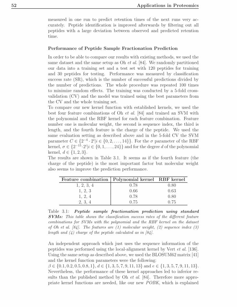
52 Applications in Proteomics

measured in one run to predict retention times of the next runs very ac-curately. Peptide identification is improved afterwards by filtering out allpeptides with a large deviation between observed and predicted retentiontime.

Performance of Peptide Sample Fractionation Prediction

In order to be able to compare our results with existing methods, we used thesame dataset and the same setup as Oh et al. [84]. We randomly partitionedour data into a training set and a test set with 120 peptides for trainingand 30 peptides for testing. Performance was measured by classificationsuccess rate (SR), which is the number of successful predictions divided bythe number of predictions. The whole procedure was repeated 100 timesto minimize random effects. The training was conducted by a 5-fold cross-validation (CV) and the model was trained using the best parameters fromthe CV and the whole training set.To compare our new kernel function with established kernels, we used thebest four feature combinations of Oh et al. [84] and trained an SVM withthe polynomial and the RBF kernel for each feature combination. Featurenumber one is molecular weight, the second is sequence index, the third islength, and the fourth feature is the charge of the peptide. We used thesame evaluation setting as described above and in the 5-fold CV the SVMparameter C ∈ {2−4 · 2i|i ∈ {0, 2, . . . , 14}}. For the σ parameter of the RBFkernel, σ ∈ {2−15 ·2i|i ∈ {0, 1, . . . , 24}} and for the degree d of the polynomialkernel, d ∈ {1, 2, 3}.The results are shown in Table 3.1. It seems as if the fourth feature (thecharge of the peptide) is the most important factor but molecular weightalso seems to improve the prediction performance.

Feature combination Polynomial kernel RBF kernel1, 2, 3, 4 0.78 0.801, 2, 3 0.66 0.631, 2, 4 0.78 0.802, 3, 4 0.75 0.75

Table 3.1: Peptide sample fractionation prediction using standardSVMs: This table shows the classification success rates of the different featurecombinations for SVMs with the polynomial and the RBF kernel on the datasetof Oh et al. [84]. The features are (1) molecular weight, (2) sequence index (3)length and (4) charge of the peptide calculated as in [84].

An independent approach which just uses the sequence information of thepeptides was performed using the local-alignment kernel by Vert et al. [136].Using the same setup as described above, we used the BLOSUM62 matrix [41]and the kernel function parameters were the following:β ∈ {0.1, 0.2, 0.5, 0.8, 1}, d ∈ {1, 3, 5, 7, 9, 11, 13} and e ∈ {1, 3, 5, 7, 9, 11, 13}.Nevertheless, the performance of these kernel approaches led to inferior re-sults than the published method by Oh et al. [84]. Therefore more appro-priate kernel functions are needed, like our new POBK, which is explained

3.1 A New Kernel for Chromatographic Separation Prediction 53

in Section 3.1.2. The kernel function has a kernel parameter b which is theborder length of the peptide. A small b means that only few border residuesof the peptides contribute to the kernel function, and a border length equalto the sequence length would mean that all residues contribute to the ker-nel function value. To determine the best border length of the POBK, weperformed the evaluation for all b ∈ {1, . . . , 30}. The evaluation of borderlength b depicted in Fig. 3.1 shows that for a b greater than 19, the SR doesnot change significantly, with a slight improvement for b = 22. This is why inthe following, only the POBK for b = 22 is considered. To study the relationbetween border length and the length of the peptides, we plotted a histogramof peptide lengths in Fig. 3.2. It can be seen that with border length 22 allamino acids of the peptides are considered in at least one of the two borders.

5 10 15 20 25 300.55

0.6

0.65

0.7

0.75

0.8

0.85

0.9

0.95

1

Border length

Cla

ssi!

cati

on

su

cce

ss r

ate

Figure 3.1: Border length evaluation of the POBK: This figure shows theevaluation of SR using different border lengths b for the POBK on the dataset ofOh et al. [84].

A comparison of the SR for different methods can be found in Fig. 3.3. Thefirst two bars represent the SR performance of the best SVMs using standardkernels of Table 3.1. The third bar demonstrates the performance of an SVMwith the local-alignment kernel. The fourth bar shows the performance ofthe best predictor in Oh et al., which is 0.84. The last bar represents the SRof the POBK for peptide sample fractionation and retention time prediction.The SR of this method is 0.87, which is significantly better than all otherapproaches. Since the dataset is very small, there is a significant deviationbetween performances of different runs. Therefore, Fig. 3.4 shows a boxplot

54 Applications in Proteomics

5 10 15 20 25 30 350

5

10

15

20

25

30

35

Number of residues

Cou

nt

Figure 3.2: Length distribution of peptides in dataset: This figure shows ahistogram of the peptide lengths of the dataset of Oh et al. [84].

of the methods, for which we performed the evaluation.

Correctly Predicted Peptides in Peptide Sample Fractionation Pre-diction

In Oh et al. [84] the prediction process with 100 random partitionings wasdone for the best four predictors, and for every peptide, the whole predictionswere stored. Oh et al. then classified a peptide by the majority label whichhad been assigned to the peptide. By this method, they were able to assign127 of the 150 peptides correctly, which corresponds to an SR of 0.85.To be able to compare this procedure with our method, we made the assump-tion, that for a particular peptide, the SVM would make a correct assignmentmore often. Furthermore, we assumed that if we also stored the predictionsfor each peptide and each run, we could also get a majority predictor whichyields good performance. The evaluation of this procedure shows that weare able to predict 134 peptides correctly in this setting, which is an SR of0.8933. Fig. 3.5 shows a histogram of the SRs for the different peptides forthe method by Oh et al. [84] and the SVM with the POBK.

3.1 A New Kernel for Chromatographic Separation Prediction 55

0.7

0.72

0.74

0.76

0.78

0.8

0.82

0.84

0.86

0.88

Cla

ssi!

cati

on

su

cce

ss r

ate

Methods

polynomial kernel

RBF kernel

Local−alignment kernel

Oh et al.

POBK

Figure 3.3: Performance comparison for peptide sample fractionationprediction: Comparison of classification success rates for different methods pre-dicting peptide sample fractionation on the dataset of Oh et al. [84].

Evaluation of Model Performance for Peptide Retention Time Pre-diction

For peptide retention time prediction, we had several goals. The first onewas to construct a retention time predictor showing equivalent performanceas established methods but requiring just a fraction of the training set size.To demonstrate that our retention time predictor fullfills the desired con-straints, we performed a 2-deep CV on the Petritis dataset [91] describedin Section 3.1.3. This means that we partitioned the data randomly intoten partitions and performed a CV with the data from nine of the ten par-titions to find the best parameters. Later, we trained our model with thebest hyperparameters and the data of the nine partitions to evaluate theperformance of the predictor on the omitted tenth partition. This was donefor every possible combination of the ten partitions and the whole procedurewas repeated ten times to minimize random effects.A plot of the observed normalized retention time against the predicted nor-malized retention time can be seen in Fig. 3.6 for one of the ten 2-deep CVruns. Since the standard deviation of the Pearson correlation between ob-served and predicted NRT over the ten runs was 0.0007, this plot is quite rep-resentative for the model performance. Petritis et al. [91] showed that theirmethod performs better than those of Meek [75], Mant et al. [74], Krokhinet al. [61] and Kaliszan et al. [46], using this dataset for validation. Thus, inTable 3.2, we only compare the performance of our method with the work ofPetritis et al. [91].

56 Applications in Proteomics

0.55

0.6

0.65

0.7

0.75

0.8

0.85

0.9

0.95

Polynomial kernel RBF kernel Local−alignment kernel POBK

Figure 3.4: Boxplot for peptide sample fractionation prediction successrates: Boxplot of classification success rates for different methods predicting pep-tide sample fractionation on the dataset of Oh et al. [84]. The boxplot is producedwith Matlab using standard parameters: The central mark of each box representsthe median. The box edges represent the 25th and the 75th percentiles and thewhiskers extend to the most extreme data points which are not considered as out-liers. Outliers are visualized by circles.

Method Number of training sequences R2

Meek 1980 [75] 344611 0.816Mant et al. 1988 [74] 344,611 0.833

Krokhin et al. 2004 [61] 344,611 0.844Kaliszan et al. 2005 [46] 344,611 0.817Petritis et al. 2003 [90] 344,611 0.870Petritis et al. 2006 [91] 344,611 0.967

This work 1040 0.880200 0.854100 0.805

Table 3.2: Comparison of different retention time predictors: This tableshows the squared correlation coefficient (R2) between observed and predicted nor-malized retention time of established retention time prediction methods presentedin [91] on the Petritis test set [91]. These values are compared to our method,the POBK, on the Petritis test set [91]. The second column gives the number oftraining sequences used. For the last two rows, subsets of the data were chosenrandomly so that 100 respectively 200 training peptides were selected.

3.1 A New Kernel for Chromatographic Separation Prediction 57

0 0.1 0.2 0.3 0.4 0.5 0.6 0.7 0.8 0.9 10

20

40

60

80

100

120

Classi cation success rate

Number of peptides

Oh et al.

POBK

Figure 3.5: Histogram of classification success rate: This figure shows ahistogram of the SR of particular peptides using the majority classifier on the dataset of Oh et al. [84]. This is compared to the ensemble prediction of Oh et al.

This comparison is somewhat biased since we only had a fraction of the orig-inal validation set for training, which means that our training set size was300 times smaller than that of the other methods. Nevertheless, our methodperforms better than the model [90] which is used by Strittmater et al. [121]in their filtering approach. The only model with a better performance is theartificial neural network with 1052 input nodes and 24 hidden nodes [91]. It isobvious that a model like this needs a very large amount training data. Petri-tis et al. [91] trained their model with more than 344,000 training peptides.Therefore, this type of model is not suitable for retention time prediction formeasurements under different conditions or with different machines becauseit is very time consuming to acquire identification and retention time datafor more than 344,000 training peptides before starting the actual measure-ments.To demonstrate that our method is robust enough for training on verifieddata of one single run, we constructed a non-redundant dataset from datasetsvds1 and vds2. A detailed description of these datasets can be found in Sec-tion 3.1.3. For different training sizes s ∈ {10, 20, . . . , 170}, we randomlyselected s peptides for training and 40 peptides for testing. Fig. 3.7 indicatesthat for the POBK, 40 verified peptides are sufficient to train a predictorwhich has a squared correlation coefficient between observed and predictednormalized retention time greater than 0.9 on the test set. This number ismuch smaller than the number of verified peptides we get for one run sincevds1 has 144 peptides, vds2 has 133 peptides and vds3 has 116. This evalu-

58 Applications in Proteomics

ation shows that with our predictor, it is possible to measure one calibrationrun with a well-defined and easily accessible peptide mixture prepared fromreal biological samples to train a predictor, which can then be used to predictretention times for the peptides very accurately. Furthermore, Fig. 3.7 showsa comparison of the POBK to the methods introduced by Klammer et al. [55]and Petritis et al. [90, 91] as described in Section 3.1.3. Our method needssignificantly less training data for a good prediction and has also superiorperformance if all training sequences of our dataset are used. One possibleexplanation for the low performance of the models from Petritis et al. is thattheir models need a larger amount of training data. This is supported by thefact that they used about 7,000 [90] and about 345,000 [91] training peptidesin their studies. To compare our method with the work by Krokhin [60],we used our verified datasets. We trained our model on vds1 and predictedthe retention times for peptides of the union of vds2 and vds3, which werenot present in vds1. If a peptide occured in vds2 and in vds3, we only keptthe peptide identification with the biggest score. For the POBK, we per-formed a 5-fold CV with SVM parameters C ∈ {2i|i ∈ {−9,−8, . . . , 0}},ν ∈ {0.4 · 1.2i|i ∈ {0, 1, 2}} and σ ∈ {0.2 · 1.221055i|i ∈ {0, 1, . . . , 21}} todetermine the best parameters. Afterwards, we trained our model with thewhole training set and the best parameters and calculated the squared cor-relation between observed and predicted retention time on the test set. Thisprocedure was repeated ten times to minimize random effects. Since thereexists a web server for the method by Krokhin [60], we could also comparethe observed retention times with the predicted ones on our test sets withthis method. To calculate the hydrophobicity parameters a and b of thismethod, we used our two standard peptides introduced in the Section 3.1.3.Furthermore, we used the 300 A column since the other columns led to in-ferior results. As can be seen in Table 3.3, the model by Krokhin performsquite well even though it had been developed on another type of sorbent.Nevertheless, the POBK achieves a significantly higher squared correlationcoefficient. It should be noted that the web-server by Krokhin is restricted tothree different columns. The advantage of our method is that there is not anyrestriction to a certain type of experimental setup. One only needs a smallamount of training peptides and can train a model which can immediatelybe used for retention time prediction.It should be mentioned that the POBK has a higher squared correlation

Training set Test sets POBK Krokhin [60]vds1 (vds2 ∪ vds3 ) \ vds1 0.9570 0.9101vds2 (vds1 ∪ vds3 ) \ vds2 0.9564 0.9212vds3 (vds1 ∪ vds2 ) \ vds3 0.9521 0.9229

Table 3.3: Evaluation of prediction performance for retention time pre-diction using the POBK: This table shows the performances of the POBK usingour verified datasets (introduced in Section 3.1.3). The other columns contain thesquared correlation coefficient between the observed normalized retention times andthe predicted ones for the POBK and the method by Krokhin [60].

between observed and predicted retention time on our datasets than on the

3.1 A New Kernel for Chromatographic Separation Prediction 59

testset by Petritis et al. This could be due to the fact that Petritis et al.performed peptide identification using database search [91]. It is commonlyaccepted that this results in a significant false positive rate.

0 0.1 0.2 0.3 0.4 0.5 0.6 0.7 0.8 0.9 10

0.1

0.2

0.3

0.4

0.5

0.6

0.7

0.8

0.9

1

Observed normalized retention time

Pre

dict

ed n

orm

aliz

ed r

eten

tion

time

R² = 0.88

Figure 3.6: Example figure for peptide retention time prediction: Thisplot shows the observed normalized retention time against the predicted normalizedretention time for one of ten 2-deep CV runs on the Petritis test set [91]. Sinceevery peptide occurs exactly once in the test set, this plot shows predictions for allof the peptides in the Petritis dataset.

Improving Peptide Identifications by Using Retention Time Pre-diction

The second goal for retention time prediction was to elaborate a retentiontime filter which could be used for improving peptide identifications. In thissetting, we trained our learning machine on one of the vds (i.e. vds1 ) andpredicted the retention times for the remaining ds (i.e. ds2 and ds3 ). Thepeptides of the training and test sets were made disjoint by removing allidentifications of the test set which belonged to spectra having an identifi-cation which was also present in the training set. On every training set, weperformed a 5-fold CV with SVM parameters C ∈ {2i|i ∈ {−9,−8, . . . , 0}},ν ∈ {0.4 · 1.2i|i ∈ {0, 1, 2}} and σ ∈ {0.2 · 1.221055i|i ∈ {0, 1, . . . , 21}}. Sincethe results of the POBK for all three datasets in Table 3.3 show nearly thesame squared correlation coefficient of about 0.95 between observed and pre-dicted normalized retention times, we restricted ourselves in the following totraining our learning machine on vds3 and evaluated the filtering capabilityof our filtering approach on ds1 and ds2.The performance evaluation of our filter model was done by a two-step ap-proach. In the first step, we measured the number of true positives and the

60 Applications in Proteomics

20 40 60 80 100 120 140 1600

0.1

0.2

0.3

0.4

0.5

0.6

0.7

0.8

0.9

1

Number of training peptides

Pea

rson

cor

rela

tion

POBKKlammer et al.Petritis et al. 2006Petritis et al. 2003

Number of verifiedidentifications acquired inone run

Figure 3.7: Learning curve for peptide retention time prediction: Thisplot shows the Pearson correlation coefficient depending on the number of train-ing samples for the union of vds1 and vds2. For every training sample size, werandomly selected the training peptides and 40 test peptides and repeated this evalu-ation 100 times. The plot shows the mean correlation coefficients of these 100 runsfor every training sample size as well as the standard deviation for the POBK, themethods introduced by Klammer et al. [55] using the RBF kernel, and the meth-ods by Petritis [90, 91]. The vertical line corresponds to the minimal number ofdistinct peptides in one of our verified datasets which was acquired in one run.

number of false positives for the identifications returned by the Mascot [87]search engine. This was conducted for different significance values. Mascotprovides a significance threshold score for the peptide identification at a givensignificance level (0.05 in all our studies). In order to be able to compare theidentification performance at different levels of certainty we chose differentfractions of the significance threshold score. This means for example, thatfor a fraction of 0.5, all identifications have to have a score which is equal toor greater than half of the significance threshold score. The evaluation wasaccomplished for varying threshold fractions t ∈ {0.01, 0.02, . . . , 1}. In thissetting, we could evaluate the precision. This is the number of true identifi-cations with a score higher than t times the significance threshold divided bythe number of spectra having at least one identification with a score higherthan t times the significance threshold score. If there was more than oneidentification with the maximal score for one spectrum, the spectrum wasexcluded from the evaluation. In the second step, we filtered the data by ourretention time model which was trained on the training set and conducted thesame evaluation as in the first step. After this, we compared the classificationperformance of these two evaluations. Fig. 3.8 a) demonstrates the good pre-cision for identifications with high Mascot scores. A threshold fraction equal

3.1 A New Kernel for Chromatographic Separation Prediction 61

to one means that all identifications have a score equal or larger than thesignificance threshold score given by the Mascot search engine. Nevertheless,even for these identifications, filtering with the retention time filter improvesthe precision from 89 to 90%. An even greater improvement can be achievedfor identifications with smaller scores. If all identifications are constrained tohave a score equal or larger than 60% of the significance threshold score, theprecision improves from 55 to 77% by using our filter. A precision of 0.77 isstill quite good and, as can be seen in Table 3.4, the number of true positivesincreases from 350 to 557. This means that a significantly larger numberof spectra can be identified with an acceptable number of false positives byapplying our retention time filtering approach. Fig. 3.8 b) shows that ourmodel is valuable for removing false identifications since many false positiveshave larger deviations between observed and predicted NRT than allowed andare removed by our filter (threshold fraction of 0.95). Fig. 3.8 c) shows thiseven more drastically for a threshold fraction of 0.6. The whole evaluationshows that our retention time prediction can be used to improve the level ofcertainty for high-scoring identifications and also to allow smaller thresholdsto find new identifications with an acceptable number of false positives.

Figure 3.8: Visualization of filter performance: This plot shows the improve-ment in precision one can get by using our retention time filter for a) varying frac-tions of the significance threshold value, b) all predictions of spectra having a scoreequal or greater than 95% of the significance threshold value, c) all predictions ofspectra having a score equal or greater than 60% of the significance threshold value.The model was trained using the vds3 dataset and the performance was measuredon ds1 and ds2. If there was more than one spectrum with the same identificationwe plotted the mean values of the observed NRT versus the predicted NRT.

62

Applic

atio

ns

inP

rote

om

ics

Fraction of threshold tp fp Precision tp with filter fp with filter Precision with filter0.0 683 2572 0.2098 699 626 0.52750.1 682 2460 0.2171 692 602 0.53480.2 678 2260 0.2308 683 555 0.55170.3 669 1909 0.2595 668 483 0.58040.4 654 1410 0.3169 646 380 0.62960.5 624 868 0.4182 609 261 0.70000.6 575 474 0.5481 557 166 0.77040.7 516 235 0.6871 500 103 0.82920.8 468 125 0.7892 452 66 0.87260.9 420 72 0.8537 404 49 0.89181.0 366 46 0.8883 350 38 0.9021

Table 3.4: Evaluation of filter performance: This table presents the precisions of the identified spectra for varying fractions of the significancethreshold with and without retention time filtering. The model was trained using the vds3 dataset and the performance was measured on ds1 andds2. In this context, tp stands for the number of true positives (correct hypotheses which are significant at the particular significance level) and fpfor the number of false positives (false hypotheses which are significant at the particular significance level). The precision is tp divided by the sumof tp and fp.

3.1 A New Kernel for Chromatographic Separation Prediction 63

3.1.5 Conclusions

In this section, we introduced a new kernel function which was successfullyapplied to two problems in computational proteomics, namely peptide samplefractionation by SAX-SPE and high resolution peptide separation by IP-RP-HPLC. Furthermore, we demonstrated that the predicted retention times canbe used to build a p-value-based model which is capable of filtering out falseidentifications very accurately.Our method performs better than all previously reported peptide samplefractionation prediction methods. For retention time prediction, our methodis (to our knowledge) the only learning method which can be trained with asmall training size of 40 peptides, while still achieving a high correlation be-tween observed and predicted retention times. This small required trainingset allows us to imagine the following application which would be very helpfulfor proteomic experiments. One could identify a well-defined protein mixturebefore starting the experiments and use the verified peptides for training thepredictor. Next, the predictor can be used to predict retention times for allidentifications of the following runs. This predicted retention time can thenbe applied to improve the certainty of the predictions. It can also be used toidentify a much larger number of spectra with an acceptable number of falsepositives. This is achieved by lowering the significance threshold and filter-ing the identifications by our p-value-based retention time filter. The best σwas usually between five and seven in our experiments. A very small valueof σ (e.g., 0.3) would indicate, that positional information is very importantand that the positional smearing does not improve prediction results. A verylarge σ (e.g., 30) would indicate that positional information is not importantfor the prediction problem. Since the optimal σ was between five and seven,this indicates that the positional smearing is reasonable. The more trainingsequences are available, the better the positional information is represented.Therefore, the optimal σ is expected to be smaller when more training se-quences are available.Since all our methods are integrated into the OpenMS [122] library, whichis open source, every researcher is able to use the presented methods freeof charge. Also, we offer the prediction models as tools which are part ofthe OpenMS proteomics pipeline (TOPP) [58]. These tools can be easilycombined with other tools from TOPP building sophisticated applications incomputational proteomics. One application is, for example, a simulator forLC-MS maps, called LC-MSsim [113], which was built using OpenMS andTOPP. The RT of the peptides are predicted using an SVM and the POBK.Another application is the combination of retention time prediction, predic-tion of peptide proteotypicity (see Section 3.3), and peptide fragmentationprediction to design scheduled multiple reaction monitoring experiments [3],which we presented at the Proteomic Forum 2009 (manuscript in prepara-tion).Further research could be pursued to enhance retention time prediction by us-ing multiple kernel learning (MKL) [117] with the 2-norm optimization [57].Therefore, one could combine the POBK and OBK for different sigmas andk-mer lengths with other kernels which contribute features that cannot be

64 Applications in Proteomics

directly learnt from the sequence. In preliminary studies, we evaluated theperformance of such kernel combinations with the 1-norm optimization but,unfortunately, did not get increased performances. The 1-norm multiple ker-nel learning tends towards sparse kernel combinations and, therefore, doesnot lead to better performances in many applications, which could explainthe results of our experiments. The 2-norm optimization problem of Kloft etal. [57] was presented only very recently. It would be very interesting to eval-uate different kernel combinations with this approach to improve retentiontime prediction.

3.2 Two-Dimensional Chromatographic Separation Prediction 65

3.2 Two-Dimensional Chromatographic Sep-

aration Prediction

3.2.1 Introduction

We already saw in Section 3.1 that there are many approaches based onmachine learning techniques in which a measured parameter such as thechromatographic retention time of a peptide is compared to a predicted oneto filter out false spectrum identifications in mass spectrometry-based exper-iments [121, 55]. In addition to chromatographic retention, there were otherproperties of the peptides which were used to improve the number of identi-fied spectra. Klammer et al. [56] predicted the fragmentation of spectra andthrough this they could improve the identification process by incorporatingthe predicted likelihood of a spectrum identification to be correct. Uwaje etal. [133] used a database of measured pairs (peptide, pI) to improve peptideidentification.Two-dimensional separations are most commonly used for the analysis ofcomplex samples due to limited peak capacities of only one separation di-mension. The most common combinations of chromatographic techniquesare strong cation exchange chromatography (SCX) with reversed-phase (RP)or ion-pair reversed-phase (IP-RP) high-performance liquid chromatography(HPLC) [2]. Toll et al. [129] and Delmotte et al. [20] were able to show thatpeptide separation on reversed-phase stationary phases using different pHand eluent additives showed significant orthogonality. In the present work,an offline combination of RP-HPLC at pH 10.0 with IP-RP-HPLC at pH 2.1was used [20]. Although the two separation dimensions are not fully orthogo-nal, the combination leads to better ”peptide identification yield” comparedto the classical combination of SCX with RP [20]. This is mainly based on thefact that in this combination the fractions collected from the first-dimensionseparation contain no salt and can, after concentration, be injected directlyinto the second separation system.In this section we significantly extend the applicability of peptide retentionprediction [94] to whole proteome analysis by incorporating retention timepredictors for both separation dimensions. By doing so, we are able to in-corporate essentially four different peptide properties into an identificationscheme, namely peptide retention in high-pH reversed chromatography, pep-tide retention in low-pH ion-pair reversed-phase chromatography, and intactmolecular mass and fragmentation pattern of a peptide. This means thatwe build a model for the first as well as the second separation dimensionand then use predicted and observed retention times to build one filter forthe first as well as one filter for the second dimension. We show that eachfilter independently improves the precision of the spectrum identifications,whereas the largest improvement in precision can be achieved by combiningthe filters. In this way, one can get about 35% more spectrum identificationsat the same precision for a standard protein mixture analyzed according tothis protocol. In order to show the feasability of this approach to the anal-ysis of whole proteomes, the filtering methods were applied to a whole cell

66 Applications in Proteomics

lysate of the Sorangium cellulosum bacteria, which also yielded an increaseof about 26% in terms of the number of uniquely identified spectra.

3.2.2 Methods and Data

Experimental Setup

The data sets for the standard mixture and the whole digested proteomewere generated with emphasis on high reproducibility in terms of retentiontimes using an actively split capillary HPLC system (Ultiate 3000, Dionex,Germering, Germany). This was done by Andreas Leinenbach, who wasthen at the laboratory of Prof. Dr. Christian Huber at Saarland University.Separated peptides were detected and identified by electrospray ionizationtandem mass spectrometry (ESI-MS/MS) in an ion trap mass spectrometer(HCT Ultra PTM Discovery System, Bruker Daltonics, Bremen, Germany).Two different tryptic peptide mixtures were analyzed: a simple protein di-gest as a training and validation data set and a tryptic digest of a wholeprotein extract from Sorangium cellulosum. The simple protein mixture con-sisted of albumin (220 fmol/µl, bovine serum, Sigma Aldrich, St. Louis, MO,USA) and thyroglobulin (410 fmol/µl, bovine thyroid gland, Fluka, Buchs,Switzerland). The proteomic sample was from Sorangium cellulosum (Soce56, digest of 690 µg of protein ectract), a soil-dwelling bacterium fromthe group of myxobacteria. Proteins were digested with trypsin (Promega,Madison, WI, USA) using published protocols [106]. The peptide mixtureswere separated using an offline two-dimensional HPLC setup as described inreference [20]. They combined reversed-phase (RP) high-performance liquidchromatography (HPLC) at pH 10.0 with micro ion-pair reversed-phase (IP-RP) HPLC at pH 2.1. Finally, the training data set was used to characterizeboth separation dimensions. In total, 36 fractions of the simple protein digest(fractions 4 to 39) and 31 fractions from the analysis of Sorangium cellulosum(fractions 14 to 44) were analyzed in triplicate in the second dimension.

Peptide Identification and Normalization of Retention Times

We aligned the MS/MS spectra of the standard mixture by the algorithmof Lange et al. [65] using standard parameters. This was also done forthe MS/MS spectra of S. cellulosum. We identified the MS/MS spectrausing Mascot (version 2.2) [87] with one missed cleavage, precursor tolerance1.3 Da, carboxymethyl as fixed modification and deamidated asparagine orglutamine as well as oxidized methionine as variable modifications. For thestandard mixture, we searched against the MSDB database, restricted tochordata (vertebrates and relatives). For the S. cellulosum spectra we usedan in-house database containing all protein sequences of the organism con-structed from the published DNA sequence [107]. For both data sets we alsosearched the spectra against a reverse version of the database. In this way,we could estimate the FDRs and q-values of the spectrum identifications asdescribed in [48] and Section 2.2.5.All spectrum identifications corresponding to peptides shorter than six amino

3.2 Two-Dimensional Chromatographic Separation Prediction 67

acids were filtered out since identifications of shorter length are less reliableand in most cases they cannot be mapped uniquely to protein sequences.

Prediction of Retention Times and Filtering by Retention Times

In this application area, the retention times were predicted with an improvedversion of the method introduced in Section 3.1. The retention time predic-tors use ν-SVR, introduced in Section 2.1.4, and the POBK to train thepredictor. All methods are integrated into the open-source framework formass spectrometry (OpenMS) [122]. The tools for retention time predictionand filtering are part of the OpenMS Proteomics Pipeline (TOPP) [58]. Wenow describe the extensions to the methods presented in Section 3.1.

The main advantage of the POBK in application to computational pro-teomics is that it enables the learning machine to learn chemical propertiesof the data (e.g., composition, sequence length, hydrophobic regions) directlyfrom the amino acid sequence. It was shown that very little training datais needed for ν-SVR in combination with the POBK to achieve very accu-rate retention time prediction models. The kernel operates directly on thesequence data on which every different amino acid is considered as a separateletter in the alphabet. In this section, we extend this alphabet to modifiedamino acids. For example, a modified methionine with an additional methylgroup is treated differently than an oxidized methionine. The method doesnot rely on any special features because it learns the necessary features for theparticular separation process directly from the training data. Therefore, thePOBK can be applied to a wide range of problems like separation predictionin strong anion-exchange chromatography and reversed-phase chromatogra-phy. It can also be used to learn peptide retention behavior under differentpH conditions.

A further extension to the method introduced in Section 3.1 is that one doesnot have to normalize the retention times to the interval between zero andone. Instead, the aligned retention times can be used directly to train thelearning machine. The learned retention time models for each dimension arethen used to build a retention time filter for the corresponding dimension.The filters are based on a statistical test which measures how likely it is,that the peptide under consideration is a true identification. Therefore, themeasured and the predicted retention times are taken into account and theuser can specify a certain significance level for the filter.

Evaluation of Precision of the Identifications

Precision (PR) was measured for different subsets of the spectrum identifi-cations. PR is defined as the number of true positives (TP) divided by thesum of the number of true positives and the number of false positives (FP):

PR =TP

TP + FP. (3.16)

68 Applications in Proteomics

In our application, the precision is the number of spectra for which the best-scoring identification is correct divided by the total number of identified spec-tra. Before the evaluation of the precision, we removed all spectra for whichthe best score was not unique among the identifications for the particularspectrum.

3.2.3 Results and Discussion

Retention Time Prediction at pH 10.0 and pH 2.1

Because fractions of peptides were taken in the first dimension, we can onlyassign retention windows for peptide elution and take the median of the elu-tion window as the retention time for all peptides contained in a fraction.To show that the method performs well for the prediction of retention timesin both dimensions, we performed a nested cross-validation on a subset ofthe data with high-quality identifications. Therefore, we utilized all spec-trum identifications with a q-value lesser than or equal to 0.1 and a peptidelength greater than five residues that were a substring of the known proteinsequences of the standard mixture. If there were several copies of the samespectrum identification, we took a median of the retention times. Before wemeasured the performance of the retention time prediction models, we mea-sured the quality of the retention times of the spectrum identifications. Todo this, we calculated the standard deviation of the retention times for eachpeptide that was identified more than once. The average standard deviationwas 1.36 min for the retention times at pH 10.0. In the second dimension,where a retention time represents the exact elution time of a peptide, theaverage standard deviation of retention times was 8.43 s.The nested CV was performed in the following way: First the spectrum iden-tifications were split randomly into five partitions. On four of the partitionswe performed a 5-fold CV to find the best parameters of the learning ma-chine (C, ν, and σ). Therefore, ν ∈ {0.4 · 1.2i|i ∈ {0, 1, 2}}, and σ ∈ {0.2 ·1.221055i|i ∈ {0, 1, . . . , 21}}. Since it is recommended to have the C values inthe range of the maximal label [13], we had C ∈ {0.001, 0.01, 0.1, 1, 10, 100}for the retention times at pH 10.0 and C ∈ {0.001, 0.01, 0.1, 1, 10, 100, 1000}for the retention times at pH 2.1 since the retention times at pH 10.0 weremeasured in minutes and the retention times at pH 2.1 were measured inseconds. Then, we trained on the four partitions with the best parametersof the 5-fold CV and measured the Pearson correlation between the observedand the predicted retention times on the residual fifth partition. This wasdone for every possible combination of the five partitions to get a mean per-formance. To exclude random effects introduced by the random partitioningof the data, we repeated the calculations five times with different randompartitionings. The average Pearson correlation coefficient between predictedand observed retention times for the evaluation at pH 10.0 is 0.93 and 0.98at pH 2.1. This means that the prediction of retention times works very wellfor both dimensions. The better performance for the second-dimension sepa-ration at pH 2.1 can be explained by the fact that we only collected fractionsat pH 10.0 every minute. Although an exact measurement of the retention

3.2 Two-Dimensional Chromatographic Separation Prediction 69

times in the first dimension would increase the performance of the predic-tion methods, this is experimentally not feasible for off-line two-dimensionalpeptide separations.

Elimination of False Identifications by Retention Time Filters

To show the applicability of retention time filters, we conducted the followingexperiment on the standard mixture. We trained the retention time modelon all peptides yielding spectra with a q-value lesser than or equal to 0.01.This data set contains 223 unique peptides. The retention times of thesepeptides in both separation dimensions and their corresponding sequenceswere utilized to perform SVR with the POBK function. Then we used thetrained models to predict retention times for both dimensions for the wholedata set, similar to Klammer et al. [55]. With the two models for retentiontime prediction, we could build a filter for each dimension as described inSection 3.2.2. Since the model for the first-dimension separation at pH 10.0 isslightly worse than the model for the second dimension at pH 2.1, we set thesignificance level of the retention time filter of this dimension to 0.01. Thismeans that the probability of filtering out a correct identification is smallerthan or equal to 0.01. The significance level for the filter of the seconddimension was set to the standard value, which is 0.05. Since we knew whichproteins were in the mixture and could therefore distinguish false positivesfrom true positives, we were able to evaluate the performance of the filteringapproach. Therefore, we measured the precision as described in Section 3.2.2on all spectrum identifications having a q-value smaller than or equal to 0.01and correspondingly for q-values 0.02, 0.03, 0.04, 0.05, 0.1, 0.15, and 0.2. Theprecision was measured for the data sets without filtering as well as with oneof the filters or with both filters in combination. Fig. 3.9 shows that eachfilter improves the precision for every evaluated subset. Furthermore, it canbe seen that the combination of both filters leads to the biggest improvementin precision. The numbers underlying the figure are shown in Table 3.5 whichcontains additional data for q-value thresholds 0.25, 0.3, ..., 0.5.The complementarity of both filters is demonstrated by Fig. 3.10, whichshows the number of correctly identified spectra with regard to precision.To calculate the underlying values, we took the precision of the differentidentification sets and evaluated for each data set how many spectra wereidentified correctly. It can be seen that both filters improve the numberof correctly identified spectra. Moreover, the biggest improvement in thenumber of correctly identified spectra can be achieved for a combinationof both filters. For example, at precision 0.94, meaning that 94% of theidentifications are correct, one gets 1567 correctly identified spectra by usingboth filters compared to 1165 spectra without filtering. This corresponds toa 35% increase in peptide identifications at the same level of precision. Thesame precision of 0.94 is achieved for the spectrum identifications havinga q-value lesser than or equal to 0.05 with additional filtering by our two-dimensional retention time filter or for all spectrum identifications with aq-value lesser than or equal to 0.01 without filtering.

70

Applic

atio

ns

inP

rote

om

ics

q value unfiltered filtered in 1st dimension filtered in 2nd dimension filtered in both dimensionsthreshold tp fp precision tp fp precision tp fp precision tp fp precision0.01 1165 70 0.943 1106 58 0.950 1165 64 0.948 1106 56 0.9520.02 1345 100 0.931 1279 80 0.941 1342 85 0.940 1277 72 0.9470.03 1468 130 0.919 1395 99 0.934 1464 101 0.935 1393 83 0.9440.04 1577 159 0.908 1495 115 0.929 1569 117 0.931 1489 91 0.9420.05 1663 183 0.901 1575 125 0.926 1653 128 0.928 1567 96 0.9420.10 1962 393 0.833 1852 239 0.886 1942 221 0.898 1836 158 0.9210.15 2104 598 0.779 1981 329 0.858 2078 292 0.877 1960 198 0.9080.20 2230 807 0.734 2102 422 0.833 2198 339 0.866 2076 223 0.9030.25 2315 1097 0.678 2185 553 0.798 2282 415 0.846 2158 267 0.8900.30 2408 1360 0.639 2268 677 0.770 2366 475 0.833 2233 303 0.8810.35 2512 1780 0.585 2367 877 0.730 2466 569 0.813 2328 356 0.8670.40 2595 2562 0.503 2443 1166 0.677 2542 783 0.765 2401 444 0.8440.45 2665 3368 0.442 2505 1523 0.622 2606 954 0.732 2458 535 0.8210.50 2723 4044 0.402 2562 1809 0.586 2663 1132 0.702 2513 619 0.802

Table 3.5: Overview of precision depending on q-value threshold and filtering: This table shows the precision for different subsets of thedata. Every row corresponds to one subset. The q-values of the spectrum identifications have to be smaller than or equal to the q-value thresholdin the first column. tp stands for the number of true positives (correct hypotheses which are significant at the particular significance level) and fpstands for the number of false positives (false hypotheses which are significant at the particular significance level). The precision is defined as tp/ (tp + fp).

3.2 Two-Dimensional Chromatographic Separation Prediction 71

0.05 0.1 0.15 0.2 0.25 0.3 0.35 0.4 0.45 0.50.010

0.1

0.2

0.3

0.4

0.5

0.6

0.7

0.8

0.9

1

q value

prec

isio

n

unfilteredfiltered in first dimensionfiltered in second dimensionfiltered in both dimensions

Figure 3.9: Comparison of precision depending on the q-value of theidentifications with and without filtering: This plot shows the precision forvarious data sets with and without filtering. At every point all spectrum identifi-cations having a q-value smaller than or equal to the x-axis value are considered.

To illustrate the filtering capabilities, we plotted the observed retention timeagainst the predicted retention time for the identifications with q-value lesserthan or equal to 0.05. Fig. 3.11 shows the performance of the filter for theseparation at pH 10.0. It can be seen that the correlation between observedand predicted retention time is quite good for the correct identifications.The lines represent the 99% confidence intervals for the retention times pre-dicted by our model for peptide separation at pH 10.0 (see Section 3.2.2 fordetails). Furthermore, one can see that there are false identifications whichare filtered out only by the filter of the first dimension (crosses without circle).This effect can also be seen in Fig. 3.12, which demonstrates the performanceof the filter for the second-dimension separation at pH 2.1. The correlationbetween observed and predicted retention time is even better than for thefirst retention time dimension.

Using RT Filters to Improve Identifications in Whole ProteomeAnalysis

The same protocol as above was applied to the Sorangium cellulosum datato obtain more identifications, keeping the precision at the same value. Wedid not train on all spectra with a q-value smaller than or equal to 0.01 sinceour learning method does not require such a large amount of training data [94].Instead, we just used the 600 best-scoring identifications. We then utilized

72 Applications in Proteomics

0.8 0.85 0.9 0.950

500

1000

1500

2000

2500

3000

precision

num

ber

of c

orre

ctly

iden

tifie

d sp

ectr

a

unfilteredfiltered in first dimensionfiltered in second dimensionfiltered in both dimensions

Figure 3.10: Comparison of correctly identified spectra with and withoutfiltering: This plot shows the number of correctly identified spectra with and with-out filtering. From right to left, the points correspond to the different partitions ofthe data which were evaluated. The first point is for all spectrum identificationswith a q-value smaller than or equal to 0.01. The following points are for theq-values 0.02, 0.03, 0.04, 0.05, 0.1, 0.15, ..., 0.5 if the corresponding measuredprecision was larger than or equal to 0.8. The numbers underlying this figure canbe found in Table 3.5 (precision vs tp).

3.2 Two-Dimensional Chromatographic Separation Prediction 73

0 5 10 15 20 25 30 350

5

10

15

20

25

30

35

40

45

50

observed RT [min] (first dimension)

pred

icte

d R

T [m

in] (

first

dim

ensi

on)

correct identificationsfalse identificationsfiltered out by both filters

Figure 3.11: Filter performance of separation at pH 10.0: This plot showsobserved against predicted retention time (first dimension) for all spectrum iden-tifications having a q-value which is lesser or equal to 0.05. The lines show theborders of the filter (at p-value 0.01). Every point which is not between the twolines is filtered out by this filter. Points having an extra circle are also filtered outby the filter of the second dimension (pH 2.1).

74 Applications in Proteomics

0 500 1000 1500 2000 2500 30000

500

1000

1500

2000

2500

3000

3500

observed RT [s] (second dimension)

pred

icte

d R

T [s

] (se

cond

dim

ensi

on)

correct identificationsfalse identificationsfiltered out by both filters

Figure 3.12: Filter performance for separation at pH 2.1: This plot showsobserved against predicted retention time (second dimension) for all spectrum iden-tifications having a q-value which is lesser or equal to 0.05. The lines show theborders of the filter (at p-value 0.05). Every point which is not between the twolines is filtered out by this filter. Points having an extra circle are also filtered outby the filter of the first dimension (pH 10.0).

3.2 Two-Dimensional Chromatographic Separation Prediction 75

the trained models to predict retention times in both dimensions for thewhole data set of mass spectrometrically identified S. cellulosum peptides.The study on the standard mixture showed that one can achieve similar pre-cision by choosing all spectrum identifications with a q-value smaller than orequal to 0.01 without filtering or choosing all spectrum identifications with aq-value smaller than or equal to 0.05 and filtering by our two retention timefilters. Since, in the whole proteome, we can not directly distinguish betweentrue and false positive identifications, we evaluated the total number of iden-tified spectra and the number of identified unique peptides for these two setsof identification parameters. At a q-value of 0.01 we annotated 21,038 spectrawhich identified 6,202 unique peptides, and at a q-value of 0.05 with addi-tional RT-filtering we annotated 25,347 spectra, which yielded 7115 uniquepeptide identifications. This represents an increase in the number of suc-cessful peptide identifications by 15% without any loss in the precision ofpeptide identifications. In this evaluation, peptides with the same aminoacid sequence but different post-translational modifications were consideredto be different peptide identifications. Furthermore, we looked at the over-lap of the unique peptide identifications between the two sets. The majorityof identifications are part of both sets. Nevertheless, there are 720 uniquepeptide identifications in the unfiltered set and 1,633 unique peptide iden-tifications in the filtered set. This means that one can get 1,633 or morethan 26% more unique peptide identifications by combining the identifica-tions of these two sets compared to the number of identifications one gets byjust taking the unfiltered identifications. The numbers are plotted as a Venndiagram in Fig. 3.13.

3.2.4 Conclusions

We present a new approach to improve the number of correctly identifiedspectra resulting from mass spectrometry experiments by using experimentaldata that are inherent to the analytical process. We are able to build reten-tion time predictors for a two-dimensional chromatographic separation usingthe retention times of peptides identified with high confidence by tandemmass spectrometry. Thus, no additional calibration using standard sampleswas necessary. The retention time filters were successfully applied to filterout false positive identifications. Moreover, we show that the scoring thresh-old can be lowered to include more previously false negatives (and to getmore correct spectrum identifications) at the same level of precision in termsof correct identifications. This is accomplished by incorporating the reten-tion time predictors into a two-dimensional filter which removes many falsepositive identifications. Therefore, we can achieve the same rate of precisionalthough the mass spectrometric scoring threshold is smaller. The methodwas validated on a standard protein mixture. Finally, we applied the samemethod to the whole proteome analysis of the Sorangium cellulosum bacte-ria. The analysis showed that by using this method we can find about 26%more unique spectrum identifications.It would be interesting to apply this two-dimensional filtering to data fromother two-dimensional chromatographic separation techniques. We already

76 Applications in Proteomics

720 5482 1633

q value 0.01q value 0.05 with filtering

Figure 3.13: Increase in unique identifications on the Sorangium cellu-losum data set: This plot shows the number of unique spectrum identificationsof two sets, for which the precision is estimated to be equal (based on empiricalresults on standard mixture). In the first set are all unfiltered identifications witha q-value smaller than or equal to 0.01 and in the second set are all spectrum iden-tifications having a q-value smaller than or equal to 0.05 which are not filtered outby any of the two retention time filters. By combining the identifications one gets7,835 instead of 6,202 unique peptide identifications.

showed in Section 3.1, that the POBK can be used to predict separationin strong anion exchange chromatography. Therefore, it is very likely, thata two-dimensional filter can be built for data measured by a combinationof strong cation exchange (SCX) chromatography and reversed-phase chro-matography (see Section 2.2.2).

3.3 Prediction of Proteotypic Peptides 77

3.3 Prediction of Proteotypic Peptides

3.3.1 Introduction

The two main goals in computational proteomics are identification and quan-titation of all proteins in a protein mixture. Unfortunately, in nearly everymixture, there are highly abundant proteins as well as low-concentration pro-teins. This creates the problem that high-abundance proteins are identifiedseveral times but those in low abundance are often missed. As explainedin Section 2.2.4, the highest peaks of the MS1 spectrum are chosen for frag-mentation in the second stage of the mass spectrometer. Only those peptideschosen for fragmentation can be identified by the instrument. This is one ofthe reasons why certain peptides have a higher likelihood of being detectedby the instruments [63]. Kuster et al. [63] showed that certain peptides of aprotein can be identified more often than others of the same protein. Theycalled peptides that are experimentally observable and uniquely identify aprotein or protein isoform proteotypic peptides. In their study, they sug-gested that instead of trying to measure all possible peptides, one shouldconcentrate on the proteotypic peptides of the proteins of interest for betterreproducibility of the results.In the same paper, they introduced a database called PeptideAtlas, whichwas intended as a resource for experimenters to obtain and store peptideidentifications. If the database contained measurements for all proteins, onecould look-up the proteotypic peptides for the proteins of interest and limitthe analysis to this small part of the whole peptide space. Unfortunately,measurements are very time-consuming and costly and the number of differ-ent proteins is large. For newly sequenced genomes, the full proteome is stillto be presented. Furthermore, peptides which are observable by a certaintype of experimental design (e.g., LC-ESI-MS/MS) may be unobserved byanother experimental design (e.g., PAGE-MALDI-TOF/TOF).To be able to measure proteins for which no experimental data of proteotypicpeptides is available, computational tools for the prediction of proteotypicpeptides are needed. Tang et al. [125] presented the first method for theprediction of proteotypic peptides, but methods for prediction of proteo-typic peptides were also introduced in the work of Mallick et al. [73], Lu etal. [70], and Webb-Robertson et al. [140]. All methods have in common thatthey use standard physico-chemical features together with standard learningtechniques to build the predictor. Unfortunately, none of the groups com-pared their method to the methods of any other group. This complicatesthe choice for the researchers. In this work, we introduce two new predic-tors of proteotypic peptides based on the OBK or the POBK and an SVM.We compare the performance of each predictor on the dataset of Mallicket al. to an SVM, which uses the same features as introduced by Mallicket al. [73] and Lu et al. [70] benchmarked in [40]. In this comparison, ourmethods perform significantly better than the other methods, although theydo not contain any specialized features. Furthermore, we investigate whichproperties of a peptide make it proteotypic. Therefore, we first analyze thedifferent datasets by standard approaches and afterwards, visualize which

78 Applications in Proteomics

amino acids are important for the resulting classifiers. This analysis showsthat positive and negative amino acids strongly determine detectability ofa peptide. For MALDI measurements, we can also support the hypothesisthat aromatic amino acids [71] contribute positively to peptide detectability.Furthermore, we support the hypothesis that an arginine at the C-terminalend of the peptide contributes more to peptide detectability than a lysine forMALDI experiments [59].

3.3.2 Methods and Data

Data

We used four different datasets for performance evaluation of methods forproteotypic peptides prediction. The datasets were introduced by Mallick etal. [73] and contain measurements of yeast proteins on four different plat-forms. For each platform it consists of a set of proteotypic peptides and a setof non-observed peptides, which are neither substrings nor do they containsubstrings of proteotypic peptides. Because of the different measurementplatforms, the datasets are named as follows:

• ICAT-ESI: This dataset is measured by ICAT labelling with LC-ESI-MS/MS.

• MudPIT-ESI: This dataset is measured by a combination of MudPITand ESI-MS/MS.

• PAGE-ESI: This dataset is measured by one-dimensional (1D) gel elec-trophoresis followed by LC-ESI-MS/MS.

• PAGE-MALDI: This dataset is measured by 1D gel electrophoresis fol-lowed by MALDI.

All sequences also contain the flanking residue at the N- and C-terminalends because Mallick et al. had better prediction results by including them.This means that the second amino acid of the sequence is the residue atthe N-terminal end and the second to last amino acid is the residue at theC-terminal end of the peptide.

Visualization of Important Amino Acids

One common argument against applying machine learning approaches is thelack of interpretability of the results. The machine learning algorithm is inthese cases called a ”Black Box”. Especially for Support Vector Machinesthis reasoning was often an argument against using string kernels althoughthere exist approaches to elucidate the importance of certain k-mers regard-ing SVM classification [144, 76, 118]. Since we use the POBK and the OBK,introduced in Section 3.1.2, with k-mer length one for classification of proteo-typic peptides, we visualize the discriminant similar to Meinicke et al. [76].POIMs of Sonnenburg et al. [118] just improve the visualization performancefor k-mer lengths greater than one.As introduced in Section 3.1.2, the feature map of the OBK is defined as:

3.3 Prediction of Proteotypic Peptides 79

Φ(s) = [µLω1

(t), . . . , µLω|Ak|

(t), µRω1

(t), . . . , µRω|Ak|

(t)]T

in which the ωi are the different k-mers, L and R are used for the left andthe right borders, and the µωi

functions are the oligo functions of the corre-sponding k-mer. One can visualize the training data by weighting them withthe αi from the SVM and summing them for each position and each oligo. Ifone is, for example, interested in the contribution of the amino acid proline(P) at position five in the left border, the importance value is calculated by:

n∑

i=1

αiµiLP (5).

Given a position t and an oligo ω, the importance weight w is calculated by:

wL|Rω (t) =

n∑

i=1

αiµi[L|R]ω (t).

The weight values can then be computed for every position-oligo combinationand the resulting matrix can be visualized by interpreting the weights as colorvalues. The weight matrix for the POBK can be computed analogously. Alow (high) weight corresponds to a signal, which can be more often found insequences which are predicted negative (positive). Therefore, the image ofthe weight matrix allows direct interpretation of the discriminant learned bythe SVM.

3.3.3 Results and Discussion

Performance Evaluation of Different Predictors

This evaluation compares the performance of the OBK and POBK to theperformance of the features introduced by Mallick et al. [73] and Lu et al. [70]presented in reference [40]. For this purpose, we chose an SVM as the clas-sifier and trained it using the OBK and POBK.The datasets contain many more negative than positive samples. We chosethe datasets exactly as in [40]. To transparently access the performanceof the different approaches, we only used balanced datasets for the evalua-tion. Furthermore, we wanted to compare the performances across datasets.Therefore, all datasets had to contain the same number of samples, whichis why the number of training samples from each class is 697: this is thenumber of positive samples in the smallest dataset. Thus, every evaluationdataset contained 697 positive samples and 697 negative samples. The sam-ples were chosen randomly if a dataset contained more than 697 of them, soas not to introduce a bias in the evaluation due to sampling. This was doneten times to get a mean performance value. The performance was measuredby 5-fold cross-validation and the performance measure was the classificationrate. The results of the comparison are shown in Table 3.6. It can be seenthat the POBK performs better than all other methods on nearly all datasetsexcept the PAGE-MALDI dataset, where the features of Lu et al. [70] leadto similar performance results.

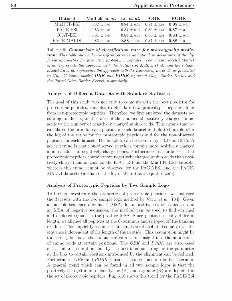
80 Applications in Proteomics

Dataset Mallick et al. Lu et al. OBK POBKMudPIT-ESI 0.82 ± 0.01 0.84 ± 0.01 0.84 ± 0.01 0.85 ± 0.01

PAGE-ESI 0.83 ± 0.01 0.84 ± 0.01 0.86 ± 0.01 0.87 ± 0.01

ICAT-ESI 0.81 ± 0.01 0.83 ± 0.01 0.83 ± 0.01 0.84 ± 0.01

PAGE-MALDI 0.86 ± 0.01 0.88 ± 0.01 0.87 ± 0.01 0.88 ± 0.01

Table 3.6: Comparison of classification rates for proteotypicity predic-tion: This table shows the classification rates and standard deviations of the dif-ferent approaches for predicting proteotypic peptides. The column labeled Mallicket al. represents the approach with the features of Mallick et al. and the columnlabeled Lu et al. represents the approach with the features of Lu et al. as presentedin [40]. Columns labeled OBK and POBK represent Oligo-Border Kernel andthe Paired Oligo-Border Kernel, respectively.

Analysis of Different Datasets with Standard Statistics

The goal of this study was not only to come up with the best predictor forproteotypic peptides, but also to elucidate how proteotypic peptides differfrom non-proteotypic peptides. Therefore, we first analyzed the datasets ac-cording to the log of the ratio of the number of positively charged aminoacids to the number of negatively charged amino acids. This means that wecalculated the ratio for each peptide in each dataset and plotted boxplots forthe log of the ratios for the proteotypic peptides and for the non-observedpeptides for each dataset. The boxplots can be seen in Figs. 3.14 and 3.15. Ageneral trend is that non-observed peptides contain more positively chargedamino acids than negatively charged ones. Furthermore, it can be seen thatproteotypic peptides contain more negatively charged amino acids than posi-tively charged amino acids for the ICAT-ESI and the MudPIT-ESI datasets,whereas this trend cannot be observed for the PAGE-ESI and the PAGE-MALDI datasets (median of the log of the ratios is equal to zero).

Analysis of Proteotypic Peptides by Two Sample Logo

To further investigate the properties of proteotypic peptides, we analyzedthe datasets with the two sample logo method by Vacic et al. [134]. Givena multiple sequence alignment (MSA) for a positive set of sequences andan MSA of negative sequences, the method can be used to find enrichedand depleted signals in the positive MSA. Since peptides usually differ inlength, we aligned all peptides at the C-terminus and stripped off the flankingresidues. This implicitly assumes that signals are distributed equally over thesequence independent of the length of the peptide. This assumption might betoo strong, but nevertheless one can gain a first insight into the importanceof amino acids at certain positions. The OBK and POBK are also basedon a similar assumption, but by the positional smearing by the parameterσ, the bias to certain positions introduced by the alignment can be reduced.Furthermore, OBK and POBK consider the alignements from both termini.A general trend which can be found in all two sample logos is that thepositively charged amino acids lysine (K) and arginine (R) are depleted inthe set of proteotypic peptides. Fig. 3.16 shows this trend for the PAGE-ESI

3.3 Prediction of Proteotypic Peptides 81

−3

−2.5

−2

−1.5

−1

−0.5

0

0.5

1

1.5

2

ICAT−ESI (proteotypic) ICAT−ESI (non−observed) MudPIT−ESI (proteotypic) MudPIT−ESI (non−observed)

log(

pept

ide

ratio

s)

Figure 3.14: Boxplot of amino acid ratios for the MudPIT-ESI andthe ICAT-ESI datasets: This plot shows a boxplot of the log of the ratios of thenumber of positively charged amino acids to the number of negatively charged aminoacids per peptide for peptides of the MudPIT-ESI and the ICAT-ESI datasets.According to the T-test and the Kolmogoroff-Smirnov test, the distributions of theratios of the proteotypic and the non-observed peptides are significantly different(p-value < 0.01) for both datasets.

82 Applications in Proteomics

−3

−2

−1

0

1

2

PAGE−ESI (proteotypic) PAGE−ESI (non−observed) PAGE−MALDI (proteotypic) PAGE−MALDI (non−observed)

log(

pept

ide

ratio

s)

Figure 3.15: Boxplot of amino acid ratios for the PAGE-ESI and thePAGE-MALDI datasets: This plot shows a boxplot of the log of the ratios of thenumber of positively charged amino acids to the number of negatively charged aminoacids per peptide for peptides of the PAGE-ESI and the PAGE-MALDI datasets.According to the T-test and the Kolmogoroff-Smirnov test, the distributions of theratios of the proteotypic and the non-observed peptides are significantly different(p-value < 0.01) for both datasets.

3.3 Prediction of Proteotypic Peptides 83

dataset. This could be an artifact of the dataset generation of the non-observed peptides. Therefore, we restrict the following two sample logo anal-ysis to fully tryptic peptides (without missed cleavages). For the ICAT-ESIdataset, it can be seen in Fig. 3.17, that the negatively charged amino acid as-partate (D) is enriched. This observation fits to the analysis in Section 3.3.3,in which we found that there are more negatively charged amino acids for theproteotypic peptides of the ICAT-ESI dataset. This fact cannot be seen forthe MudPIT-ESI dataset in Fig. 3.18, although the analysis in Section 3.3.3suggested the same trend for this dataset. An explanation could be, that theenrichment is not as significant as for the ICAT-ESI dataset. Since we usethe two sample logo method with Bonferroni correction, which is very conser-vative, some weaker enrichments are hidden. The two sample logo withoutBonferroni correction in Fig. 3.19 shows an enrichment of negatively chargedamino acids for the proteotypic peptides of the MudPIT-ESI dataset. Forthe PAGE-MALDI dataset in Fig. 3.21 arginine at the C-terminus seemsto be highly enriched in the set of proteotypic peptides. This observationwas also reported by Krause et al. [59]. The authors hypothesized, that thisis due to the chemical properties of arginine because of the basicity of theguanidino functionality of the arginine side chain which might result in betterionization in the liquid and/or gas phase. At the C-terminal end of trypticpeptides, there can only be an arginine or lysine. Therefore, an enrichmentof arginine at this position implies a depletion of lysine. An enrichment ofarginine at the C-terminal end can also be seen for the PAGE-ESI dataset inFig. 3.20, although the enrichment is not as strong as for the PAGE-MALDIdataset (41.7% compared to 7.5%). Additionally, an enrichment for alanineand valine can be seen.

Figure 3.16: Two sample logo for PAGE-ESI dataset: This plot shows thetwo sample logo [134] of the MSAs of the proteotypic and the non-observed peptidesfor the PAGE-ESI dataset. Amino acids which are enriched in the proteotypicpeptides are shown at the top and depleted amino acids are shown at the bottom.The numbers refer to the positions of the amino acids in the peptide and all peptidesare aligned to the C-terminal end without flanking residues.

Visualization of Important Amino Acids

We visualized one of the ten random draws for each dataset with the methodsintroduced in Section 3.3.2. The visualization results for the POBK com-pared to the OBK were in all experiments very similar. An example for the

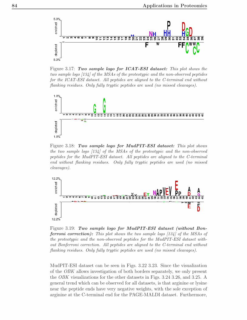
84 Applications in Proteomics

Figure 3.17: Two sample logo for ICAT-ESI dataset: This plot shows thetwo sample logo [134] of the MSAs of the proteotypic and the non-observed peptidesfor the ICAT-ESI dataset. All peptides are aligned to the C-terminal end withoutflanking residues. Only fully tryptic peptides are used (no missed cleavages).

Figure 3.18: Two sample logo for MudPIT-ESI dataset: This plot showsthe two sample logo [134] of the MSAs of the proteotypic and the non-observedpeptides for the MudPIT-ESI dataset. All peptides are aligned to the C-terminalend without flanking residues. Only fully tryptic peptides are used (no missedcleavages).

Figure 3.19: Two sample logo for MudPIT-ESI dataset (without Bon-ferroni correction): This plot shows the two sample logo [134] of the MSAs ofthe proteotypic and the non-observed peptides for the MudPIT-ESI dataset with-out Bonferroni correction. All peptides are aligned to the C-terminal end withoutflanking residues. Only fully tryptic peptides are used (no missed cleavages).

MudPIT-ESI dataset can be seen in Figs. 3.22 3.23. Since the visualizationof the OBK allows investigation of both borders separately, we only presentthe OBK visualizations for the other datasets in Figs. 3.24 3.26, and 3.25. Ageneral trend which can be observed for all datasets, is that arginine or lysinenear the peptide ends have very negative weights, with the sole exception ofarginine at the C-terminal end for the PAGE-MALDI dataset. Furthermore,

3.3 Prediction of Proteotypic Peptides 85

Figure 3.20: Two sample logo for PAGE-ESI dataset: This plot shows thetwo sample logo [134] of the MSAs of the proteotypic and the non-observed peptidesfor the PAGE-ESI dataset. All peptides are aligned to the C-terminal end withoutflanking residues. Only fully tryptic peptides are used (no missed cleavages).

Figure 3.21: Two sample logo for PAGE-MALDI dataset: This plot showsthe two sample logo [134] of the MSAs of the proteotypic and the non-observedpeptides for the PAGE-MALDI dataset. All peptides are aligned to the C-terminalend without flanking residues. Only fully tryptic peptides are used (no missedcleavages).

aspartate and glutamate near the borders of the peptide seem to be positivefor peptide detectability. Since arginine and lysine are positively chargedand aspartate and glutamate are negatively charged, this could be a generalproperty and further supports the analysis in Section 3.3.3. Mallick et al. [73]also identified positive charge (total count or average) to be one of the fivemost important features for proteotypicity prediction in each dataset.The plots for the ICAT-ESI (Fig. 3.24) and the MudPIT-ESI (Fig. 3.22)datasets are very similar, because both measurements use LC-ESI-MS/MS.Furthermore, these datasets show a stronger positive effect for glutamate inthe left border than in the right border, which shows that the visualizationof the OBK can provide more insights than that of the POBK. The visual-ization of the discriminant of the PAGE-ESI dataset shows a weaker positiveeffect of aspartate. Additionally, the aliphatic amino acids isoleucine, leucine,and valine seem to contribute positively. A very interesting observation forthe PAGE-MALDI dataset, shown in Fig. 3.25, is that amino acids witharomatic side chains seem to contribute positively to peptide detectability.The positive effect of aromatic amino acids in MALDI experiments was alsopresented in [71]. It can be assumed that peptides with aromatic aminoacids can interact better with the matrix and are therefore better ionizable.Furthermore, the classifier was able to find the positive arginine signal at the

86 Applications in Proteomics

C-terminal end, which was also found by the two sample logo analysis andreported by Krause et al. [59].

Figure 3.22: Visualization of important positions for MudPIT-ESIdataset (OBK): This plot shows the visualization of the importance weights ofthe OBK classifier calculated as described in Section 3.3.2. The first 22 positionscorrespond to the primal representation of the left border of the peptide and the re-maining positions correspond to the primal representation of the right border of thepeptide (n is the position of the amino acid at the C-terminal end of the peptide).

3.3 Prediction of Proteotypic Peptides 87

Figure 3.23: Visualization of important positions for the MudPIT-ESIdataset (POBK): This plot shows the visualization of the importance weightsof the POBK classifier calculated as described in Section 3.3.2. Since the POBKlooks at the signals in both borders simultaneously, a positive weight for position i

corresponds to the amino acids at position i and position n− i + 1.

Figure 3.24: Visualization of important positions for the ICAT-ESIdataset (OBK): This plot shows the visualization of the importance weights ofthe OBK classifier calculated as described in Section 3.3.2. The first 22 positionscorrespond to the primal representation of the left border of the peptide and the re-maining positions correspond to the primal representation of the right border of thepeptide (n is the position of the amino acid at the C-terminal end of the peptide).

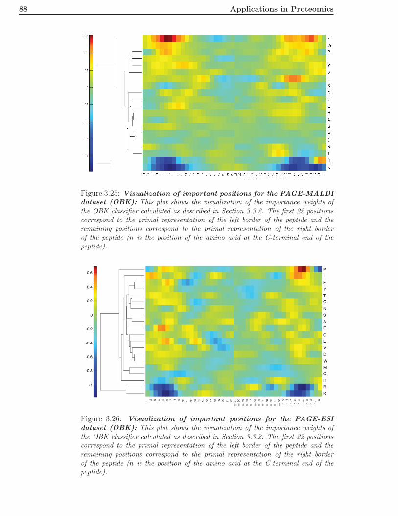
88 Applications in Proteomics

Figure 3.25: Visualization of important positions for the PAGE-MALDIdataset (OBK): This plot shows the visualization of the importance weights ofthe OBK classifier calculated as described in Section 3.3.2. The first 22 positionscorrespond to the primal representation of the left border of the peptide and theremaining positions correspond to the primal representation of the right borderof the peptide (n is the position of the amino acid at the C-terminal end of thepeptide).

Figure 3.26: Visualization of important positions for the PAGE-ESIdataset (OBK): This plot shows the visualization of the importance weights ofthe OBK classifier calculated as described in Section 3.3.2. The first 22 positionscorrespond to the primal representation of the left border of the peptide and theremaining positions correspond to the primal representation of the right borderof the peptide (n is the position of the amino acid at the C-terminal end of thepeptide).

3.3 Prediction of Proteotypic Peptides 89

3.3.4 Conclusions

We show in this section that the POBK as well as the OBK can be used topredict proteotypic peptides with high accuracy. Our kernel function in com-bination with a support vector machine performs significantly better than thefeatures of other groups together with a support vector machine and a stan-dard kernel. Furthermore, we show that amino acids have different effectson detectability depending on the experimental setup. Similar to Mallicket al. [73], we find that positively charged amino acids help distinguish be-tween proteotypic and non-observed peptides. Additionally, we can showin our analysis that the classifier discovers interesting properties concerningthe underlying biochemical mechanisms of the measurement processes. Oneexample are aromatic amino acids, which seem to contribute positively topeptide detectability in PAGE-MALDI experiments. This was also reportedby other groups [71]. Another observation is that arginine at the C-terminusseems to increase detectability, compared to lysine, in PAGE-MALDI ex-periments. This observation is found by computing the two sample logo aswell as with our analysis of the learnt classifier and is supported by a recentstudy [59]. Consequently, our method for peptide detectability has state-of-the-art performance and allows direct interpretation of the learnt classifierto provide interesting insights.It would be very intersting to extend this binary prediction problem to aregression problem, in which we could predict the degree of proteotypicity.We included the proteotypicity prediction into the LC-MSsim [113], whichcan be used to simulate LC-MS maps. Therefore, we used the probabilityestimates of the libSVM to compute the likelihood of a peptide to be pro-teotypic. To train the proteotypicity predictor, we just used binary data(peptide is proteotypic or not). Extending the proteotypicity prediction to aregression problem would mean that every peptide gets a label representingits proteotypicity. This could be, for example, the intensity of each peptidefeature normalized by the amount of protein present in the sample. A peptidefeature is the three-dimensional shape (m/z, RT, and intensity) of the pep-tide measurement, defined by the isotopic distribution as well as the elutionprofile of the peptide. An accurate predictor for peptide feature intensitycould be used to predict the absolute amount of a protein in a sample.

90 Applications in Proteomics

Chapter 4

Applications in Immunomics

4.1 Introduction

The adaptive immune system is one of the most advanced and most im-portant systems in humans. It can direct immune responses according tovarious kinds of invading microorgansims and even recognize and destroytumor cells [130]. The main components of the immune system were intro-duced in Section 2.3. MHCII presents peptides originating from the outsideof the cell. There are various different MHCII alleles which have very specificsets of peptides to which they can bind. At present there are more than 750unique MHCII alleles known [102] (regarded on the protein sequence level),but for less than 3% of them sufficient experimental data to construct a pre-dictor is available. Since every human has at most twelve different MHCIIalleles, it is very important for vaccine design to know which peptides canbind to the particular alleles. A good predictor for MHC peptide bindingcan reduce the number of possible peptides and therefore save a lot of time- and money-consuming wetlab experiments.In contrast to MHCI, the ends of the binding clefts of the MHCII are open.This is why the length of the binding peptides varies significantly (from 8to more than 30 amino acids). Nevertheless, analyses of MHCII structuresrevealed that the part of the peptide responsible for binding to MHCII isusually nine amino acids long. This part is also called binding core of thepeptide. For most of the experimental data it is unknown which part ofthe peptide actually is the binding core, which complicates the problem ofMHCII peptide binding prediction compared to MHCI peptide binding pre-diction. The binding clefts of MHCI are closed at the ends and the bindingpeptides have a length between eight and twelve. There are various meth-ods for MHCII peptide binding prediction for alleles for which there existssufficient experimental data. Some of these models are based on positionalscoring matrices [9, 80, 96, 99, 116, 124], others use Gibbs samplers [81] orhidden Markov models [82]. Further works have used the ant colony searchstrategy [49], artificial neural networks [8], partial least squares [36], evo-lutionary algorithms [95] or support vector machines with standard kernelfunctions [24, 105, 137]. Very recently Wang et al. [138] combined severalof these predictors to build a new predictor. There have also been efforts to

92 Applications in Immunomics

improve binding prediction by using structural information [143].To the best of our knowledge all but two of the models for MHCII peptidebinding prediction are based on experimental data for the particular allelesfor which the predictions are for. The models of Singh et al. [116] and Za-itlen et al. [143] are the only methods which were shown to predict bindingfor alleles without training on them. However, the model by Singh et al.is only applicable to 51 alleles [138] which is about 7 % of all known allelesand Zaitlen et al. require three-dimensional structures of a similar allele toperform this kind of predictions which limits the number of alleles accessiblethrough the method. Since the experimental data for peptide-MHCII bindingis very scarce, we introduce a method to predict peptide binding for alleles,for which few or no experimental data is available. Similar ideas have alsorecently been introduced for MHCI predictions, although based on differentmachine learning techniques and for a far simpler problem (MHCI peptideshave more or less identical lengths) [21, 44, 79].We use similarities of the binding pockets of the alleles to build predictorsfor alleles, which do not need experimental data of the target allele to reachgood prediction performance. The similarities are incorporated into the pre-dictions using a specialized kernel function, which is based on the normalizedset kernel by Gartner et al. [33]. Therefore, the problem is transformed intoa multiple instance learning problem [22]. The predictor is trained usingthe kernel function and Support Vector Regression (SVR) [110]. Using thismethod we are for the first time able to build predictors for about two thirdsof all MHCII alleles. Assessment of their quality in blind predictions foralleles with known data reveals that the predictions are of sufficient qualityfor use in vaccine design. Furthermore, we show that our transformation ofthe problem into the multiple instance learning problem enables us to buildpredictors which perform equally well or even better than the best methodsfor MHCII peptide binding prediction.

4.2 Methods and Datasets

4.2.1 Multiple Instance Learning

In standard supervised binary classification, the associated label for everyinstance out of the sets of training samples is known. The input space X isusually a Hilbert space. Every instance can be represented as (xi, yi) wherexi ∈ X and yi ∈ {−1, 1}. We define the set of positive training examples asSp = {(x, y)|x ∈ X ∧ y = 1} and the set of negative training examples asSn = {(x, y)|x ∈ X ∧ y = −1}. In multiple instance learning [22] not everylabel yi for every xi is known. The positive label is only known for sets ofinstances which are called bags. For every bag Xi with label +1 it is onlyknown that at least one instance of Xi is associated with label +1. Everyinstance in a negative bag is associated with label −1. More formally thismeans that the set of positive bags is Xp = {(Xi, 1)|∃xj ∈ Xi : (xj , yj) ∈ Sp}.The set of negative bags is Xn = {(Xi,−1)|∀xj ∈ Xi : (xj , yj) ∈ Sn}. The

4.2 Methods and Datasets 93

Figure 4.1: Binding core of a peptide: This figure shows the structure ofan MHCII molecule (grey) together with a bound peptide (blue and yellow). Thebinding core of the peptide is shown in yellow visualized with BALLView [77]. ThePDB ID of the structure is 1BX2.

multiple instance learning problem is to find the best predictor for predictingthe labels of bags.Kernels for multiple instance learning were introduced by Gartner et al. [33]in 2002. The normalized set kernel (NSK) by Gartner et al. [33] is thefollowing:

k(X, X ′) :=

∑

x∈X,x′∈X′

kX (x, x′)

fnorm(X)fnorm(X ′)(4.1)

with kX being a kernel on X . Gartner et al. [33] evaluated different normal-ization functions fnorm and showed that averaging (fnorm(X) = #X) and fea-

ture space normalization (fnorm(X) =√

∑

x∈X,x′∈X

kX (x, x′)) perform equally

well on the datasets studied. Preliminary results on our data also suggestthat both methods perform equally well (data not shown). Therefore, in thefollowing only normalization by feature space normalization is considered.Gartner et al. [33] hypothesized in their paper, that the kernel could also beused for multiple instance regression [25, 98]. In this setting every bag Xi

has a label yi ∈ IR.

4.2.2 Multiple Instance Learning for MHCII Predic-

tion

Since for most of known MHCII binders the binding core is unknown, onecannot directly use the binding core for training a learning machine. Fig. 4.1shows a structure of an MHCII molecule for which the binding core is known.Unfortunately there are very few such structures available.Previous work on MHCII prediction [37, 124] suggests that only aliphatic(Ile, Leu, Met, Val) and aromatic (Phe, Trp, Tyr) amino acids in position one

94 Applications in Immunomics

are common. Thus, we represent every putative binder by a bag containingall 9-mers (putative binding cores) with aromatic or aliphatic amino acidat position one. By this, we transformed the data directly into a multipleinstance learning problem in which every positive bag has at least one positivebinding core. All negative bags just contain false binding cores. Formally,this means that every putative binder si of length m is represented by a bag(Xi, yi).

Xi = {x|x = sik,k+1,...,k+8∧ k ≥ 1 ∧ k + 8 ≤ m ∧ x1 ∈

{Ile, Leu, Met, Val, Phe, Trp, Tyr}}

are all putative binding cores and yi is the binding affinity measured for theputative binder si.In this thesis we introduce two predictors for MHCII binding peptide predic-tion. The first predictor is just trained on parts of the data of the allele forwhich the predictions should be made. This predictor is called MHCIISinglein the following. It will be shown that the performance of MHCIISingle iscomparable to the best methods in the field. This predictor is particularlyuseful for alleles, for which sufficient binding data is available.The second predictor does not need to be trained on data of the allele forwhich the predictions should be made. Instead, data from other alleles cancombined in a way which reflects the similarity of the binding pockets of thetarget allele to the binding pockets of the other alleles. This predictor will becalled MHCIIMulti in the following. Because no data of the allele, for whichthe predictions should be made is needed, one can even build predictors foralleles with little or no experimentally determined binders.In this thesis, we use the normalized set kernel with an RBF kernel forMHCIISingle. Furthermore, we introduce a new kernel based on the normal-ized set kernel for MHCIIMulti.

4.2.3 Feature Encoding

Venkatarajan and Braun [135] evaluated in 2001 different physicochemicalproperties of amino acids. They performed a dimension reduction by princi-pal component analysis (PCA) on a large set of features from the AAindexdatabase [50] and showed that every amino acid can be represented ade-quately by a five-dimensional feature vector. This encoding was alreadyused in a recent study on MHC binding by Hertz et al. [42] and will be calledPCA encoding in the following.

4.2.4 Predictions for Alleles with Sufficient Data

For alleles, for which enough experimental data is available, we build predic-tors which are just trained on binding peptide data for the particular allele.In this setting we use the normalized set kernel [33] with kX being the RBFkernel. X is the set of all putative binding cores. This means that X is theset of every possible nine amino acid long peptide sequence in PCA encod-ing for which the first amino acid is aliphatic or aromatic. This means that

4.2 Methods and Datasets 95

every input vector has length 45. The predictor is trained using this kernelfunction together with ν-SVR [110].

4.2.5 Combining Allele Information with Peptide In-

formation

Representation of MHCII Alleles

Sturniolo et al. [124] showed in 1999 that there is a correspondence betweenthe structures of the binding pockets of the MHCII and the polymorphicresidues in this region. They defined certain positions inside the amino acidsequence of the allele sequences and showed that alleles having the sameresidues at these positions also have similar binding pocket structures. Thiswas done for several alleles and binding pockets for peptide positions 1, 4, 6,7 and 9 because these positions are assumed to have the largest influence onbinding [124].To represent each allele, we encode every polymorphic residue of the pockets1, 4, 6, 7, and 9 by PCA encoding and calculate a mean of the encodedvectors for every pocket position. This results in a 25× 1 dimensional vector

p =(

pT1 , pT

4 , pT6 , pT

7 , pT9

)Tfor every allele, which is called pocket profile vec-

tor in the following. To get the polymorphic residues for alleles that werenot defined by Sturniolo et al. [124], we used the HLA-DRB1, HLA-DRB3,HLA-DRB4 and HLA-DRB5 alignments of the IMGT/HLA database [102](release 2.18.0, 09-July-2007).We computed the sequence logo [19] for an alignment of all HLA-DRB1,HLA-DRB3, HLA-DRB4 and HLA-DRB5 alleles. It is shown in Fig. 4.2.Since the alignments show very good conservation for alleles HLA-DRB1,HLA-DRB3, HLA-DRB4 and HLA-DRB5 at the non-pocket positions, weassume that this procedure is applicable at least for these HLA-DRB alleleswhich constitute 525 of all 765 unique MHCII alleles (on the protein sequencelevel), currently contained in the IMGT/HLA database [102].

Similarity Function of MHCII Binding Pockets

Our goal was to get a similarity measure between pocket positions of alleles.Since we have the pocket profile vectors, a natural idea is to take the Pearsoncorrelation between the corresponding positions of the pocket. To get asimilarity measure we added one which means that the similarities are in theinterval [0, 2]. The resulting similarity measure for each pocket i = 1, 4, 6, 7, 9is then

simi(p, p′) := Pearson(pi, p

′i) + 1. (4.2)

This function was used in our work to measure similarity between the bind-ing pockets corresponding to peptide position 1, 4, 6, 7 and 9.

96 Applications in Immunomics

Figure 4.2: Conservation of MHCII allele protein sequences: The con-servation of the alignments of all HLA-DRB1, HLA-DRB3, HLA-DRB4 andHLA-DRB5 alleles from the IMGT/HLA database [102] is shown in this sequencelogo [19]. The arrows pointing at positions of the sequence logo are polymorphicresidues, which are used for the binding pocket profile vectors.

Combining Allele Pocket Profiles with Peptide Information

For MHCI binding peptide prediction there have been two approaches forlearning binding prediction models for alleles which do not need experimen-tal data for the target allele [44, 79]. Both methods measure the similarityof the alleles for the whole allele.Looking at the structural level, one amino acid that does not fit into a bind-ing pocket can change the whole binding affinity of the peptide. Therefore,we want to enforce similarity of peptides at a certain position of the bind-ing core if their binding pockets for the respective position are very similar.Thus, we use similarities between the binding pockets directly in our kernelfunction to be able to account for these cases, too.We now define the kernel kpw−RBF, which is defined on A × X . A is theset of all possible pocket profile vectors and X is again the set of all pos-sible nine amino acid long peptide sequences in PCA encoding. Let p =(

pT1 , pT

4 , pT6 , pT

7 , pT9

)Tbe the pocket profile vector of peptide sequence s. Let

x = (xT1 , xT

2 , ..., xT9 )T be a putative binding core of sequence s, for which ev-

ery xi is the PCA encoding of the amino acid at position i in the putativebinding core. Let p′ and x′ be defined analogously for peptide sequence s′.In MHCIISingle the inner kernel function of the normalized set kernel is astandard RBF kernel:

kRBF(x, x′) = exp−‖x−x′‖2

2σ2 . (4.3)

As mentioned above, the kernel function should be able to weight positionsaccording to the similarity of the alleles. Therefore, we use a positionally-weighted RBF-kernel:

kpw−RBF((p, x), (p′, x′)) = exp−w1×‖x1−x′1‖

2+w2×‖x2−x′2‖2+...+w9×‖x9−x′9‖

2

2σ2 . (4.4)

In our setting the weights are determined using the sim function, which wasmentioned above:

wi := simi(p, p′) ∀i = 1, 4, 6, 7, 9 (4.5)

Since the other positions are not as important for binding, we set the weightsw2, w3, w5 and w8 (which correspond to peptide positions 2, 3, 5 and 8) to0.5.In this work kpw−RBF is used as the inner kernel function of the normalizedset kernel [33] in conjunction with ν-SVR [110] for MHCIIMulti.

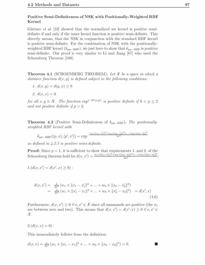
4.2 Methods and Datasets 97

Positive Semi-Definiteness of NSK with Positionally-Weighted RBFKernel

Gartner et al. [33] showed that the normalized set kernel is positive semi-definite if and only if the inner kernel function is positive semi-definite. Thisdirectly means, that the NSK in conjunction with the standard RBF kernelis positive semi-definite. For the combination of NSK with the positionally-weighted RBF kernel (kpw−RBF), we just have to show that kpw−RBF is positivesemi-definite. Our proof is very similar to Li and Jiang [67] who used theSchoenberg Theorem [108]:

Theorem 4.1 (SCHOENBERG THEOREM). Let X be a space in which adistance function d(x, y) is defined subject to the following conditions:

1. d(x, y) = d(y, x) ≥ 0

2. d(x, x) = 0

for all x, y ∈ X . The function exp(−dp(x,y)) is positive definite if 0 < p ≤ 2and not positive definite if p > 2.

Theorem 4.2 (Positive Semi-Definiteness of kpw−RBF). The positionally-weighted RBF kernel with

kpw−RBF((p, x), (p′, x′)) = exp−w1×‖x1−x′1‖

2+w2×‖x2−x′2‖2+...+w9×‖x9−x′9‖

2

2σ2

as defined in 4.2.5 is positive semi-definite.

Proof: Since p = 1, it is sufficient to show that requirements 1. and 2. of the

Schoenberg theorem hold for d(x, x′) =w1×‖x1−x′

1‖2+w2×‖x2−x′

2‖2+...+w9×‖x9−x′

9‖2

2σ2 :

1.(d(x, x′) = d(x′, x) ≥ 0) :

d(x, x′) = 12σ2 (w1 × ‖x1 − x′

1‖2 + ... + w9 × ‖x9 − x′9‖2)

= 12σ2 (w1 × ‖x′

1 − x1‖2 + ... + w9 × ‖x′9 − x9‖2) = d(x′, x)

(4.6)

Furthermore, d(x, x′) ≥ 0 ∀x, x′ ∈ X since all summands are positive (the wi

are between zero and two). This means that d(x, x′) = d(x′, x) ≥ 0 ∀x, x′ ∈X .

2.(d(x, x) = 0) :

This immeadiately follows from the definition:

d(x, x) = 12σ2 (w1 × ‖x1 − x1‖2 + ... + w9 × ‖x9 − x9‖2) = 0. �

98 Applications in Immunomics

Training Choices for MHCIIMulti

We design a procedure to get the largest possible training set, in which thesimilarities of the target allele to the other alleles are reflected in the numberof training samples from the particular alleles. The idea is that training sam-ples from more similar alleles should enable better predictions for the targetallele than distant ones. To compute similarities between alleles, we calculatethe Pearson correlation between alleles using the pocket profile vectors. Letpi and pj be the pocket profile vectors of alleles i and j. The similarity be-tween these vectors is the Pearson correlation of pi and pj scaled linearly to[0, 1]. This value is called allelesim i,j in the following. Let ni be the numberof sequences of allele i. For a particular target allele j, the procedure is thefollowing:

For every allele i 6= jCompute the maximal number ti such that allelesimi,j × ti ≤ ni.

Choose the minimum of all ti, which is now called t∗.For every allele i 6= j

Choose t∗×allelesimi,j peptide sequences randomly from allele iand assign them to the training set.

Since for the benchmark dataset the binding affinities are not distributed uni-formly, we partition the data into three parts (

[

0, 13

]

,]

13, 2

3

]

and]

23, max

]

).We then randomly choose from these partitions such that we have the samenumber of samples from each partition.

Nearest Neighbor Predictor MHCIISingleNN

To show that the kpw−RBF kernel function of MHCIIMulti really improvesthe MHCII binding prediction if data from various alleles is combined weintroduce MHCIISingleNN. This predictor is the MHCIISingle predictor ofthe nearest neighbor allele. The nearest neighbor allele j of allele i is theallele for which allelesimi,j is maximal ∀j 6= i.

Aggregating Predictor MHCIIMulti∗

We choose the number of training samples per allele according to the similar-ities of the alleles as described above. Therefore, we do not use all peptidesthat are available. Since we do not want to miss important peptides webuild aggregating predictors over ten random draws of the training sets. Theidea is similar to bagging [7]. The only difference is that we do not needbootstrapping, since we have enough data for the training alleles. The ag-gregating versions of the predictor MHCIIMulti is called MHCIIMulti∗. Thewhole workflow can be seen in a UML activity diagram in Fig. 4.3.

4.2 Methods and Datasets 99

target

allele

i < 10

i’ = i + 1Draw training

samplestrain model

sequences of

target allele

predict

affinities

storage of

(sequence, affinity)

pairs for each run

i = 0

calculate mean

predicted affinities

for each peptide

affinities of

target allele

sequences

calculate AUC

calculate AUC separately

for each run and then

calculate mean

performance of

MHCIIMulti*

for

while

do

performance of

MHCIIMulti

Figure 4.3: UML activity diagram of performance evaluation for LOAOpredictors: This UML activity diagram shows the workflow of the performanceevaluation of the leave one allele out predictors MHCIIMulti and MHCIIMulti∗.

100 Applications in Immunomics

4.2.6 Data

We show the performance of our predictors on an MHCII benchmark dataset,introduced by Wang et al. [138]. This dataset contains peptide binding data,measured in the laboratory of Wang et al. [138], for 14 human alleles aswell as three mouse alleles. Binding affinities of the benchmark dataset weregiven as IC50 values, which is defined as the concentration at which 50% ofthe MHCII molecules are bound. The smaller the IC50 value, the better isthe binder. There are many peptides with very high IC50 values. Since thecutoff for binders is between 500 and 1,000 nM there is not a big differencebetween a non-binder with IC50 value of 10,000 or 20,000 nM. Therefore, wetransformed the IC50 values like Nielsen et al. [80] to the interval [0, 1]. Letai be the binding affinity of peptide i. The log-transformed binding affinitya′

i is defined as a′i := 1 − log50000 (ai). Like Nielsen et al. [80], we set the

a′i < 0 to zero, which is needed for all peptides with IC50 value larger than

50,000 nM. In the following, the dataset will be called Dbenchmark.Peptide sequences for which no binding core could be found (aliphatic oraromatic amino acid at position one) were excluded from all evaluations.This was the case for less than 3% of peptides (270 out of all 9478). Outof these peptides only 64 peptides are considered binders (IC50 value smallerthan 1,000 nM [138] which is equal to a log-transformed value greater than0.3616). Since the whole dataset contains 6,475 binders in total, this meansthat our assumption that every binder has to have a binding core with analiphatic or aromatic amino acid at position one just misses 64 out of 6,475binders which is under 1%.

4.3 Results

In this section we compare our predictors to other state-of-the-art methods.In particular we compare our performance to the results of Wang et al. [138]who performed a large scale evaluation on MHC class II prediction meth-ods. We show on their benchmark dataset that our predictor MHCIISingle,which is trained on parts of the target allele dataset, performs equally wellor better than all other methods. Furthermore, we show that MHCIIMulti∗

can predict binding for alleles without using any training data of the targetallele and achieves performances that are comparable to the best predictorstrained on binding data of the target allele.

4.3.1 Performance on Single Allele Datasets

Wang et al. [138] recently compared the performances of state-of-the-artpredictors for MHCII binding. We show a comparison to the top fourmethods of their evaluation. All performances are measured in area un-der the ROC curve. Wang et al. [138] measured the performance of theARB method [9] by 10-fold cross-validation. The performance of the othermethods was evaluated using available webservers. The authors justified

4.3 Results 101

this procedure by the fact that they measured the performance on unpub-lished data, which had been measured in their labs. Therefore, it is un-likely that any of these methods (except the ARB method) was trained onparts of this dataset. To compare the performance of MHCIISingle to thisevaluation, we performed a 10-fold cross-validation using parameter rangesC ∈ {0.001, 0.01, 0.1, 1, 10, 100, 1000}, ν ∈ {0.2 ∗ 1.4i|i = 1, 2, ..., 5} andσ ∈ {0.0625, 0.125, 0.25, ..., 16}. Table 4.1 shows that MHCIISingle outper-forms all other single methods. The column ”Consensus” corresponds to theconsensus approach of Wang et al. [138] in which the best three predictorsfor the particular allele are combined to achieve higher accuracy. One couldassume that with MHCIISingle as one of these three predictors the accuracywill improve, since the performance of MHCIISingle is comparable to theconsensus approach.A further improvement can be achieved by incorporating binding data fromother alleles. Therefore, we performed a CV with MHCIIMulti and thesame parameters as above. Additionally, we chose data from other allelesof Dbenchmark. To minimize random effects, we performed this procedure tentimes and listed the mean performance in Table 4.1. It can be seen thatthe incorporation of extra data improves the performances on many alleles(8 out of 14). Especially for the two alleles, for which MHCIISingle per-formed worst, a significant improvement can be achieved by MHCIIMulti.The worse performance on allele HLA-DRB1*0101 can be explained by thenumber of samples in Dbenchmark since there are 3,882 peptides. For allelesfor which there exist such a big amount of training data the incorporation ofbinding data from different alleles does not improve the predictions which isin accordance with what one would expect. The bad performance on alleleHLA-DRB3*0101 can be explained by the fact that the eleventh residue ofthe beta chain (β11) of the MHCII molecule of this allele has an arginine,which reaches into pocket number four (and therefore influences binding),although it is located in pocket number six [85]. Since the arginine at β11is exclusive to the DR52a [85] alleles with the sole exception of DRB1*1446,it can be assumed that this effect is limited to this small number of alleles(37).

4.3.2 Performance of Leave-Allele-Out Predictors

To show that MHCIIMulti performs well, although it is not trained onany data of the target allele, we conducted the following experiment. Thetraining samples were chosen as described in the Section 4.2. We thenperformed a validation on the training set to determine the best hyper-parameters (C ∈ {0.01, 0.1, 1, 10}, ν ∈ {0.2 ∗ 1.4i|i = 1, 2, ..., 5} and σ ∈{0.0625, 0.125, 0.25, ..., 4}). The binding data of the alleles were stored inseparate partitions. The best hyperparameters were found by training on allbut one of these partitions and measuring the performance on the left-outpartition. With the best hyperparameters of the validation we trained ourpredictors with the whole training set. We then measured the area under theROC curve performance on the target allele. The whole process was repeatedten times to minimize random effects. The mean area under the ROC

102

Applic

atio

ns

inIm

munom

ics

MHCII type # peptides ARB PROPRED SMM-align Consensus MHCIISingle MHCIIMultiDRB1*0101 3882 0.76 0.74 0.77 0.79 0.81 0.75DRB1*0301 502 0.66 0.65 0.69 0.72 0.73 0.72DRB1*0401 512 0.67 0.69 0.68 0.69 0.67 0.78DRB1*0404 449 0.72 0.79 0.75 0.80 0.79 0.80DRB1*0405 457 0.67 0.75 0.69 0.72 0.83 0.79DRB1*0701 505 0.69 0.78 0.78 0.83 0.82 0.90DRB1*0802 245 0.74 0.77 0.75 0.82 0.76 0.79DRB1*0901 412 0.62 - 0.66 0.68 0.64 0.66DRB1*1101 520 0.73 0.80 0.81 0.80 0.85 0.87DRB1*1302 289 0.79 0.58 0.69 0.73 0.74 0.73DRB1*1501 520 0.70 0.72 0.74 0.72 0.72 0.75DRB3*0101 420 0.59 - 0.68 - 0.72 0.57DRB4*0101 245 0.74 - 0.71 0.74 0.79 0.78DRB5*0101 520 0.70 0.79 0.75 0.79 0.81 0.90Mean 0.71 0.73 0.73 0.76 0.76 0.77

Table 4.1: Performance comparison on benchmark dataset: The performance of our predictors is compared to the best four methodspresented in [138]. The performance of MHCIISingle, MHCIIMulti and ARB are measured by 10-fold cross validation. All other methods aretrained on binding data of the target allele which was not contained in the benchmark dataset. MHCIIMulti uses additional training data from theother alleles of the benchmark dataset.

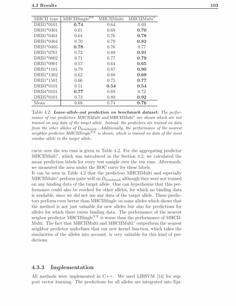
4.3 Results 103

MHCII type MHCIISingleNN MHCIIMulti MHCIIMulti∗

DRB1*0101 0.74 0.64 0.69DRB1*0301 0.61 0.69 0.70DRB1*0401 0.64 0.76 0.78DRB1*0404 0.70 0.79 0.82DRB1*0405 0.78 0.76 0.77DRB1*0701 0.72 0.89 0.91DRB1*0802 0.71 0.77 0.79DRB1*0901 0.57 0.64 0.65DRB1*1101 0.79 0.87 0.90DRB1*1302 0.62 0.68 0.69DRB1*1501 0.66 0.75 0.77DRB3*0101 0.51 0.54 0.54DRB4*0101 0.77 0.69 0.72DRB5*0101 0.73 0.89 0.92Mean 0.68 0.74 0.76

Table 4.2: Leave-allele-out prediction on benchmark dataset: The perfor-mance of our predictors MHCIIMulti and MHCIIMulti∗ are shown which are nottrained on any data of the target allele. Instead, the predictors are trained on datafrom the other alleles of Dbenchmark. Additionally, the performance of the nearestneighbor predictor MHCIISingleNN is shown, which is trained on data of the mostsimilar allele to the target allele.

curve over the ten runs is given in Table 4.2. For the aggregating predictorMHCIIMulti∗, which was introduced in the Section 4.2, we calculated themean prediction labels for every test sample over the ten runs. Afterwards,we measured the area under the ROC curve for these labels.It can be seen in Table 4.2 that the predictors MHCIIMulti and especiallyMHCIIMulti∗ perform quite well on Dbenchmark although they were not trainedon any binding data of the target allele. One can hypothesize that this per-formance could also be reached for other alleles, for which no binding datais available, since we did not use any data of the target allele. These predic-tors perform even better than MHCIISingle on some alleles which shows thatthe method is not just valuable for new alleles but also for predictions foralleles for which there exists binding data. The performance of the nearestneigbor predictor MHCIISingleNN is worse than the performance of MHCII-Multi. The fact that MHCIIMulti and MHCIIMulti∗ outperform the nearestneighbor predictor underlines that our new kernel function, which takes thesimilarities of the alleles into account, is very valuable for this kind of pre-dictions.

4.3.3 Implementation

All methods were implemented in C++. We used LIBSVM [14] for sup-port vector learning. The predictions for all alleles are integrated into Epi-

104 Applications in Immunomics

ToolKit [30], available at http://www.epitoolkit.org/mhciimulti.

4.4 Discussion

The proposed method is a novel approach for predicting MHC class II bindingpeptides for alleles lacking experimental data and thus opens up new alleysfor the design of peptide-based therapeutic or prophylactic vaccines. Obvi-ously, a conclusive validation of predicitons for alleles without experimentaldata is difficult. The leave-one-allele out predictions presented here indicate,however, that the method performs very well. One could object that restrict-ing the first amino acid of the binding core to aromatic and aliphatic aminoacids is a strong assumption. Nevertheless, if one selects all putative bindingpeptides of the 9,478 peptide sequences in Dbenchmark for which no bindingcore with an aromatic or aliphatic residue at position one can be found, apredictor which just predicts 0 (non-binder) would have 0.7630 classificationrate on these peptides. In other words, only for 270 peptides or 2.85% outof the 9,478 peptides no binding core with aromatic or aliphatic residue atposition one can be found and only 64 out of these are considered as binders(log-transformed binding affinity greater than 0.3616). This is why we thinkthat the heuristic is very well applicable and reflects a general property forMHCII binding. This is also supported by previous work [37, 124]. More-over, the restriction to these binding cores is one of the key parts of this workbecause if one selected all 9-mers as binding cores this would add a lot ofnoise to the bags and the positional weighting of the binding core would nothave a big effect since nearly every residue of a peptide (except the residuesat the ends) would be at every position in one of the instances in the bag.Ultimately, only experimental testing or structure-based studies will revealwhether some of the rarer alleles might deviate from this behavior on thefirst position.To improve peptide-MHCII affinity prediction it would be interesting to useother multiple instance learning approaches. Kwok et al. [64] presentedmarginalized multi-instance kernels in 2007 at the International Joint Con-ference on Artificial Intelligence. In this approach, the kernel k(Xi, Xj) doesnot weight every kX (xi, xj) equally, as the NSK does. Instead, it weightsthe inner kernel function by the similarity of the (estimated) labels of thesingle instances. In their paper, Kwok et al. state that their marginalizedmulti-instance kernels could be combined with the regularization frameworkthey presented at ICML 2006 [15]. A combination of this framework andthe marginalized multi-instance kernels should lead to improved results forpeptide-MHCII binding affinity prediction.Building predictors for alleles for which no experimental data exists belongsto the field of transfer learning. Bickel et al. [4] very recently presented asophisticated approach for transfer learning. It would be very interesting tocombine this approach with the marginalized multi-instance kernels.

Chapter 5

Conclusions and Discussion

“My mind seems to have become a kind of machine for grinding laws out oflarge collections of facts,...”- Charles Darwin, The Autobiography of Charles Darwin, 1881

In biology, there are always interesting traits to discover. Unfortunately,there does not exist for each object of interest an expert machine like CharlesDarwin. Therefore, we are interested in designing learning machines whichare able to learn general rules from the data of biological entities. One of themain questions to ask before building a learning machine is: “which proper-ties of the data should be learnt by the learning algorithm?” In this step it isusually beneficial if expert knowledge of the particular domain is available.If, for example, our task was to predict whether a person is able to speak,it would be very reasonable to account for the age of the person inside thelearning algorithm. Unfortunately, it is often not that easy to find meaning-ful parts of the data – which help in predicting the property of interest, andexpert knowledge is often not available. Thus, in many applications of ma-chine learning, scientists put all the “appropriate” features into the learningalgorithm and perform feature selection during the learning process.In this thesis, we focus on kernel-based approaches for machine learning.Applying a certain kernel to an application area also requires some priorknowledge. If, for example, the position of particular k-mers is very impor-tant and one chooses the spectrum kernel [66], which is not position-aware,it will be hard to come up with any reasonable results. In most cases, theassumptions one makes by choosing the kernel are milder than by choosingfeatures. We introduce the paired oligo-border kernel in this thesis, whichassumes that all interesting properties of the peptides are represented bythe amino acids. We do not directly put into the assumption that aromaticamino acids at certain positions are indicative for proteotypic peptide pre-diction in PAGE-MALDI experiments, but nevertheless, the SVM with thePOBK is able to find and exploit this feature. Thus the approach is moregeneral than deciding on a specific set of features beforehand. This leads toa wider applicability of our kernel function.We show in Sections 3.1 and 3.2 that the POBK can be used to predictchromatographic separation very accurately. For SAX-SPE behavior predic-tion, our method performs better than all other methods. For retention time

106 Conclusions and Discussion

prediction in reversed-phase chromatography, our method performs betterthan all but one of the available methods. The only method with betterperformance requires about 345,000 training peptides which are not easilymeasured before being able to use the predictor. Our method just needsa fraction of this amount of training data (40 - 200 peptides) although itachieves nearly the same performance. We show that a good predictor forchromatographic behavior is very valuable for peptide identification by apply-ing the predicted retention time in a p-value-based filter. This filter allows usto lower mass spectrometric scoring thresholds, filter out false identifications,and get more correctly identified spectra while keeping the same precision.We furthermore show that our method is applicable under different chro-matography conditions in Section 3.2 in which we predict retention timesfor chromatographic separations at different pH values. Since we are able tobuild accurate predictors for both dimensions, we can build filters for bothretention time dimensions. As both separations are nearly orthogonal [20],it is even more unlikely that a false peptide identification is not filtered outby one of the two filters. We can show that the combined filters yield thelargest increase in the number of correctly identified spectra at comparableprecision.The good performance of the POBK and the OBK at predicting proteotypicpeptides, shown in Section 3.3, is further evidence that it is generally ap-plicable to computational proteomics problems. We show that our kernelsperform better than other methods using the features of Mallick et al. [73] orLu et al. [70] on a comparative benchmark. Furthermore, the visualization ofthe resulting classifier allows gaining interesting insights into the biochemicalprocesses which are involved during the whole measurement process.For predicting peptide-MHCII affinity, we put in another mild assumptionto be able to use kernel-based learning machines. This assumption was thatthere has to exist a reasonable binding core in every peptide for which wewant to perform the prediction. This mild assumption is enough to transformthe prediction problem into a multiple instance learning problem for whichkernel approaches exist [33]. For our positionally-weighted RBF kernel, weput in the further assumption that MHCII molecules with similar pocketsshould also bind similar amino acids at the particular positions. This en-ables us to build predictors for about two thirds of all known MHCII alleles,instead of just about 6% for which there existed peptide-MHCII bindingaffinity predictors previously.

It would be interesting to use multiple kernel learning [117] together with thePOBK and OBK for different sigmas and k-mer lengths using the 2-normoptimization [57]. We performed experiments with the 1-norm optimizationbut unfortunately did not get better results. This could be explained bythe fact that 1-norm multiple kernel learning tends towards sparse kernelcombinations and therefore does not lead to better performances in manyapplications. The 2-norm optimization problem of Kloft et al. [57] was pre-sented only very recently. It would be very interesting to see whether kernelcombinations using the 2-norm optimization lead to increased performancesin retention time prediction. One could even try to add other kernels which

107

contribute features which cannot be directly learnt from the sequence. Thisshould enable even higher performances.For peptide-MHCII affinity prediction, it would be interesting to use othermultiple instance learning approaches. Kwok et al. [64] presented a kernelwhich does not weight every instance in the bag equally as the NSK does.We also performed experiments with the method of Bunescu et al. [10] butachieved performances comparable to the NSK for multiple instance classi-fication (data not presented in this thesis). We could not use the approachof Bunescu et al. for the binding affinity prediction problem since it cannotbe applied in multiple instance regression. Kwok et al. [64] state in theirpaper that their marginalized multi-instance kernels could be combined withthe regularization framework they presented at ICML 2006 [15]. It would,therefore, be interesting to see whether this combination of methods leads tobetter results.Building predictors for alleles for which no experimental data exists belongsto the field of transfer learning. Bickel et al. [4] very recently presented asophisticated approach for transfer learning. It would be very interesting tocombine these methods with the marginalized multi-instance kernels.Beyond the problems tackled in this thesis, there are many open problemsin computational biology, for which kenel-based machine learning should de-liver accurate results. The problem of spectrum intensity prediction [56], forexample, could also be approached by structured output prediction [45] usingappropriate kernels.

108 Conclusions and Discussion

Bibliography

[1] Ruedi Aebersold and Matthias Mann. Mass spectrometry-based pro-teomics. Nature, 422(6928):198–207, Mar 2003.

[2] A. J. Alpert and P. C. Andrews. Cation-exchange chromatographyof peptides on poly(2-sulfoethyl aspartamide)-silica. J Chromatogr,443:85–96, Jun 1988.

[3] Leigh Anderson and Christie L Hunter. Quantitative mass spectromet-ric multiple reaction monitoring assays for major plasma proteins. MolCell Proteomics, 5(4):573–588, Apr 2006.

[4] Steffen Bickel, Christoph Sawade, and Tobias Scheffer. Transfer learn-ing by distribution matching for targeted advertising. In NIPS ’08,pages 105–112, 2008.

[5] K. Bieman. Mass spectrometry. Ann Rev Biochem, 32:755–780, 1963.

[6] Olivier Bousquet, Stephane Boucheron, and Gabor Lugosi. Introduc-tion to Statistical Learning Theory, volume 3176 of Lecture Notes inArtificial Intelligence, pages 169–207. Springer, 2004.

[7] Leo Breiman. Bagging predictors. Machine Learning, 24(2):123–140,1996.

[8] V. Brusic, G. Rudy, G. Honeyman, J. Hammer, and L. Harrison. Pre-diction of MHC class II-binding peptides using an evolutionary algo-rithm and artificial neural network. Bioinformatics, 14(2):121–130,1998.

[9] Huynh-Hoa Bui, John Sidney, Bjoern Peters, Muthuraman Sathia-murthy, Sinichi Asabe, and et al. Automated generation and evaluationof specific MHC binding predictive tools: ARB matrix applications.Immunogenetics, 57(5):304–314, 2005.

[10] Razvan C. Bunescu and Raymond J. Mooney. Multiple instance learn-ing for sparse positive bags. In Proceedings of the 24th internationalconference on Machine learning, pages 105–112, Corvalis, Oregon,2007. ACM.

[11] Christopher J. C. Burges. A tutorial on support vector machines forpattern recognition. Data Min Knowl Discov, 2(2):121–167, 1998.

110 BIBLIOGRAPHY

[12] William R. Cannon, Danny Taasevigen, Douglas J. Baxter, and JuliaLaskin. Evaluation of the influence of amino acid composition on thepropensity for collision-induced dissociation of model peptides usingmolecular dynamics simulations. Journal of the American Society forMass Spectrometry, 18(9):1625–1637, September 2007.

[13] Athanassia Chalimourda, Bernhard Scholkopf, and Alex J. Smola.Experimentally optimal ν in support vector regression for differentnoise models and parameter settings. Neural Networks, 18(2):205–205,March 2005.

[14] Chih-Chung Chang and Chih-Jen Lin. LIBSVM: a libraryfor support vector machines, 2001. Software available athttp://www.csie.ntu.edu.tw/~cjlin/libsvm.

[15] Pak-Ming Cheung and James T. Kwok. A regularization framework formultiple-instance learning. In ICML ’06: Proceedings of the 23rd in-ternational conference on Machine learning, pages 193–200, New York,NY, USA, 2006. ACM.

[16] Roman M. Chicz, Robert G. Urban, William S. Lane, Joan C. Gorga,Lawrence J. Stern, Dario A. A. Vignali, and Jack L. Strominger. Pre-dominant naturally processed peptides bound to HLA-DR1 are derivedfrom MHC-related molecules and are heterogeneous in size. Nature,358(6389):764–768, August 1992.

[17] Corinna Cortes and Vladimir Vapnik. Support vector networks. InMachine Learning, pages 273–297, 1995.

[18] Robertson Craig and Ronald C Beavis. Tandem: matching proteinswith tandem mass spectra. Bioinformatics, 20(9):1466–1467, Jun 2004.

[19] Gavin E Crooks, Gary Hon, John-Marc Chandonia, and Steven E Bren-ner. WebLogo: a sequence logo generator. Genome Res, 14(6):1188–1190, 2004.

[20] N. Delmotte, M. Lasaosa, A. Tholey, E. Heinzle, and C.G. Huber.Two-dimensional reversed-phase x ion-pair reversed-phase hplc: Analternative approach to high-resolution peptide separation for shotgunproteome analysis. J Proteome Res, 6(11):4363–4373, 2007.

[21] David DeLuca, Barbara Khattab, and Rainer Blasczyk. A modularconcept of hla for comprehensive peptide binding prediction. Immuno-genetics, 59(1):25–35, 2007.

[22] Thomas G. Dietterich, Richard H. Lathrop, and Tomas Lozano-Perez.Solving the multiple instance problem with axis-parallel rectangles. Ar-tif Intell, 89(1-2):31–71, 1997.

[23] Bruno Domon and Ruedi Aebersold. Challenges and opportunities inproteomics data analysis. Mol Cell Proteomics, 5(10):1921–1926, Oct2006.

BIBLIOGRAPHY 111

[24] Pierre Donnes and Oliver Kohlbacher. SVMHC: a server for predic-tion of MHC-binding peptides. Nucleic Acids Res, 34 (Web Serverissue):W194–W197, 2006.

[25] Daniel R. Dooly, Qi Zhang, Sally A. Goldman, and Robert A. Amar.Multiple-instance learning of real-valued data. J Machine Learn Res,3:651–678, 2002.

[26] Jacek P Dworzanski, A. Peter Snyder, Rui Chen, Haiyan Zhang, DavidWishart, and Liang Li. Identification of bacteria using tandem massspectrometry combined with a proteome database and statistical scor-ing. Anal Chem, 76(8):2355–2366, Apr 2004.

[27] Pehr Edman. Method for Determination of the Amino Acid Sequencein Peptides. Acta Chem. Scand., 4:283–293, 1950.

[28] Joshua E Elias and Steven P Gygi. Target-decoy search strategy forincreased confidence in large-scale protein identifications by mass spec-trometry. Nat Meth, 4(3):207–214, March 2007.

[29] Jimmy K. Eng, Ashley L. McCormack, and John R. Yates. An approachto correlate tandem mass spectral data of peptides with amino acidsequences in a protein database. Journal of the American Society forMass Spectrometry, 5(11):976–989, November 1994.

[30] Magdalena Feldhahn, Philipp Thiel, Mathias M. Schuler, Nina Hillen,Stefan Stevanovic, and et al. EpiToolKit–a web server for compu-tational immunomics. Nucleic Acids Res, pages (advanced access,doi:10.1093/nar/gkn229), 2008.

[31] Ari Frank and Pavel Pevzner. Pepnovo: de novo peptide sequencingvia probabilistic network modeling. Anal Chem, 77(4):964–973, Feb2005.

[32] Ari Frank, Stephen Tanner, Vineet Bafna, and Pavel Pevzner. Pep-tide sequence tags for fast database search in mass-spectrometry. JProteome Res, 4(4):1287–1295, 2005.

[33] Thomas Gartner, Peter A. Flach, Adam Kowalczyk, and Alex J. Smola.Multi-instance kernels. In Claude Sammut and Achim G. Hoffmann,editors, ICML, pages 179–186. Morgan Kaufmann, 2002.

[34] Lewis Y Geer, Sanford P Markey, Jeffrey A Kowalak, Lukas Wagner,Ming Xu, Dawn M Maynard, Xiaoyu Yang, Wenyao Shi, and Stephen HBryant. Open mass spectrometry search algorithm. J Proteome Res,3(5):958–964, 2004.

[35] Alexander V Gorshkov, Irina A Tarasova, Victor V Evreinov,Mikhail M Savitski, Michael L Nielsen, Roman A Zubarev, andMikhail V Gorshkov. Liquid chromatography at critical conditions:comprehensive approach to sequence-dependent retention time predic-tion. Anal Chem, 78(22):7770–7777, Nov 2006.

112 BIBLIOGRAPHY

[36] Pingping Guan, Irini A Doytchinova, Christianna Zygouri, and Dar-ren R Flower. MHCPred: A server for quantitative prediction ofpeptide-MHC binding. Nucleic Acids Res, 31(13):3621–3624, 2003.

[37] J. Hammer, C. Belunis, D. Bolin, J. Papadopoulos, R. Walsky,J. Higelin, W. Danho, F. Sinigaglia, and Z. A. Nagy. High-affinitybinding of short peptides to major histocompatibility complex classII molecules by anchor combinations. Proc Natl Acad Sci U S A,91(10):4456–4460, 1994.

[38] Xuemei Han, Mi Jin, Kathrin Breuker, and Fred W. McLafferty. Ex-tending Top-Down Mass Spectrometry to Proteins with Masses GreaterThan 200 Kilodaltons. Science, 314(5796):109–112, 2006.

[39] David Heckerman, Dan Geiger, and David M. Chickering. Learningbayesian networks: The combination of knowledge and statistical data.Machine Learning, 20(3):197–243, September 1995.

[40] Till Helge Helwig. Maschinelles lernen zur vorhersage proteotypischerpeptide. Bachelor Thesis, 2008.

[41] S. Henikoff and J. G. Henikoff. Amino acid substitution matrices fromprotein blocks. Proc Natl Acad Sci U S A, 89(22):10915–10919, Nov1992.

[42] Tomer Hertz and Chen Yanover. Pepdist: A new framework for protein-peptide binding prediction based on learning peptide distance func-tions. BMC Bioinformatics, 7(Suppl 1):S3, 2006.

[43] C. Igel, T. Glasmachers, B. Mersch, N. Pfeifer, and P. Meinicke.Gradient-based optimization of kernel-target alignment for sequencekernels applied to bacterial gene start detection. IEEE/ACM TransComput Biol Bioinformatics, 4(2):216–226, 2007.

[44] Laurent Jacob and Jean-Philippe Vert. Efficient peptide-MHC-I bind-ing prediction for alleles with few known binders. Bioinformatics,24(3):358–366, 2008.

[45] Thorsten Joachims. Structured output prediction with support vectormachines, 2006.

[46] Roman Kaliszan, Tomasz Baczek, Anna Cimochowska, PaulinaJuszczyk, Kornelia Wisniewska, and Zbigniew Grzonka. Predictionof high-performance liquid chromatography retention of peptides withthe use of quantitative structure-retention relationships. Proteomics,5(2):409–415, 2005.

[47] Lukas Kall, Jesse D Canterbury, Jason Weston, William Stafford Noble,and Michael J MacCoss. Semi-supervised learning for peptide identifi-cation from shotgun proteomics datasets. Nat Methods, 4(11):923–925,Nov 2007.

BIBLIOGRAPHY 113

[48] Lukas Kall, John D. Storey, Michael J. MacCoss, and William StaffordNoble. Assigning significance to peptides identified by tandem massspectrometry using decoy databases. J Proteome Res, 7(1):29–34, 2008.

[49] Oleksiy Karpenko, Jianming Shi, and Yang Dai. Prediction of MHCclass II binders using the ant colony search strategy. Artif Intell Med,35(1-2):147–156, 2005.

[50] S. Kawashima, H. Ogata, and M. Kanehisa. AAindex: Amino acidindex database. Nucleic Acids Res, 27(1):368–369, 1999.

[51] Shuichi Kawashima, Piotr Pokarowski, Maria Pokarowska, AndrzejKolinski, Toshiaki Katayama, and Minoru Kanehisa. AAindex:amino acid index database, progress report 2008. Nucl Acids Res,36(suppl 1):D202–205, 2008.

[52] Michael Kinter and Nicholas E. Sherman. Protein Sequencing and Iden-tification Using Tandem Mass Spectrometry. John Wiley & Sons, 2000.

[53] Michael Kinter and Nicholas E. Sherman. Protein Sequencing and Iden-tification Using Tandem Mass Spectrometry, page 15. John Wiley &Sons, 2000.

[54] Michael Kinter and Nicholas E. Sherman. Protein Sequencing and Iden-tification Using Tandem Mass Spectrometry, page 32. John Wiley &Sons, 2000.

[55] A.A. Klammer, X. Yi, M.J. MacCoss, and W.S. Noble. Improv-ing tandem mass spectrum identification using peptide retention timeprediction across diverse chromatography conditions. Anal Chem,79(16):6111–6118, 2007.

[56] Aaron A Klammer, Sheila M Reynolds, Jeff A Bilmes, Michael J Mac-Coss, and William Stafford Noble. Modeling peptide fragmentationwith dynamic bayesian networks for peptide identification. Bioinfor-matics, 24(13):i348–i356, Jul 2008.

[57] Marius Kloft, Ulf Brefeld, Pavel Laskov, and Soren Sonnenburg. Non-sparse multiple kernel learning. In NIPS Workshop on Kernel Learning:Automatic Selection of Optimal Kernels, 2008.

[58] Oliver Kohlbacher, Knut Reinert, Clemens Gropl, Eva Lange, NicoPfeifer, Ole Schulz-Trieglaff, and Marc Sturm. TOPP–the OpenMSproteomics pipeline. Bioinformatics, 23(2):e191–197, 2007.

[59] Eberhard Krause, Holger Wenschuh, and Peter R. Jungblut. The dom-inance of arginine-containing peptides in maldi-derived tryptic massfingerprints of proteins. Analytical Chemistry, 71(19):4160–4165, 1999.

[60] Oleg V Krokhin. Sequence-specific retention calculator. algorithm forpeptide retention prediction in ion-pair rp-hplc: application to 300-and 100-a pore size c18 sorbents. Anal Chem, 78(22):7785–7795, Nov2006.

114 BIBLIOGRAPHY

[61] O.V. Krokhin, R. Craig, V. Spicer, W. Ens, K. G. Standing, R. C.Beavis, and J. A. Wilkins. An Improved Model for Prediction of Re-tention Times of Tryptic Peptides in Ion Pair Reversed-phase HPLC:Its Application to Protein Peptide Mapping by Off-Line HPLC-MALDIMS. Mol Cell Proteomics, 3(9):908–919, 2004.

[62] H. W. Kuhn and A. W. Tucker. Nonlinear programming. In 2nd Berke-ley Symposium on Mathematical Statistics and Probabilistics, pages481–492. University of California Press, 1951.

[63] Bernhard Kuster, Markus Schirle, Parag Mallick, and Ruedi Aebersold.Scoring proteomes with proteotypic peptide probes. Nat Rev Mol CellBiol, 6(7):577–583, Jul 2005.

[64] James T. Kwok and Pak-Ming Cheung. Marginalized multi-instancekernels. In IJCAI ’07, 2007.

[65] Eva Lange, Clemens Gropl, Ole Schulz-Trieglaff, Andreas Leinenbach,Christian Huber, and Knut Reinert. A geometric approach for thealignment of liquid chromatography mass spectrometry data. Bioin-formatics, 23(13):i273–281, 2007.

[66] Christina Leslie, Eleazar Eskin, and William Stafford Noble. The spec-trum kernel: a string kernel for svm protein classification. Pac SympBiocomput, pages 564–575, 2002.

[67] Haifeng Li and Tao Jiang. A class of edit kernels for SVMs to predicttranslation initiation sites in eukaryotic mRNAs. In RECOMB, pages262–271, 2004.

[68] Thomas Lingner and Peter Meinicke. Remote homology detectionbased on oligomer distances. Bioinformatics, 22(18):2224–2231, 2006.

[69] Andrew J. Link, Jimmy Eng, David M. Schieltz, Edwin Carmack, Gre-gory J. Mize, David R. Morris, Barbara M. Garvik, and John R. Yates.Direct analysis of protein complexes using mass spectrometry. NatBiotech, 17(7):676–682, July 1999.

[70] Peng Lu, Christine Vogel, Rong Wang, Xin Yao, and Edward M Mar-cotte. Absolute protein expression profiling estimates the relative con-tributions of transcriptional and translational regulation. Nat Biotech,25(1):117–124, February 2007.

[71] E. Giralt M.-L. Valero and D. Andreu. An evaluation of some struc-tural determinants for peptide desorption in MALDI-TOF mass spec-trometry. In Peptides 1996, pages 855–856, Kingswinford, UK, 1998.Mayflower Scientific Ltd.

[72] Michael J MacCoss, Christine C Wu, and John R Yates. Probability-based validation of protein identifications using a modified sequest al-gorithm. Anal Chem, 74(21):5593–5599, Nov 2002.

BIBLIOGRAPHY 115

[73] Parag Mallick, Markus Schirle, Sharon S Chen, Mark R Flory, HookeunLee, Daniel Martin, Jeffrey Ranish, Brian Raught, Robert Schmitt,Thilo Werner, Bernhard Kuster, and Ruedi Aebersold. Computationalprediction of proteotypic peptides for quantitative proteomics. NatBiotech, 25(1):125–131, February 2007.

[74] C. T. Mant, T. W. Burke, J. A. Black, and R. S. Hodges. Effect ofpeptide chain length on peptide retention behaviour in reversed-phasechromatography. J Chromatogr, 458:193–205, Dec 1988.

[75] James L. Meek. Prediction of Peptide Retention Times in High-Pressure Liquid Chromatography on the Basis of Amino Acid Com-position. PNAS, 77(3):1632–1636, 1980.

[76] Peter Meinicke, Maike Tech, Burkhard Morgenstern, and Rainer Merkl.Oligo kernels for datamining on biological sequences: a case study onprokaryotic translation initiation sites. BMC Bioinformatics, 5(1):169,2004.

[77] Andreas Moll, Andreas Hildebrandt, Hans-Peter Lenhof, and OliverKohlbacher. Ballview: a tool for research and education in molecularmodeling. Bioinformatics, 22(3):365–366, Feb 2006.

[78] Roger E Moore, Mary K Young, and Terry D Lee. Qscore: an algo-rithm for evaluating sequest database search results. J Am Soc MassSpectrom, 13(4):378–386, Apr 2002.

[79] Morten Nielsen, Claus Lundegaard, Thomas Blicher, Kasper Lam-berth, Mikkel Harndahl, Sune Justesen, Gustav Røder, Bjoern Peters,Alessandro Sette, Ole Lund, and Søren Buus. NetMHCpan, a methodfor quantitative predictions of peptide binding to any HLA-A and -Blocus protein of known sequence. PLoS ONE, 2(8):e796, 2007.

[80] Morten Nielsen, Claus Lundegaard, and Ole Lund. Prediction of MHCclass II binding affinity using SMM-align, a novel stabilization matrixalignment method. BMC Bioinformatics, 8:238, 2007.

[81] Morten Nielsen, Claus Lundegaard, Peder Worning, Christina SylvesterHvid, Kasper Lamberth, Søren Buus, Soren Brunak, and Ole Lund.Improved prediction of MHC class I and class II epitopes using a novelGibbs sampling approach. Bioinformatics, 20(9):1388–1397, 2004.

[82] Hideki Noguchi, Ryuji Kato, Taizo Hanai, Yukari Matsubara, HiroyukiHonda, Vladimir Brusic, and Takeshi Kobayashi. Hidden markovmodel-based prediction of antigenic peptides that interact with MHCclass II molecules. J Biosci Bioeng, 94(3):264–270, 2002.

[83] A.B.J. Novikoff. On convergence proofs on perceptrons. In Symposiumon the Mathematical Theory of Automata, volume 12, pages 615–622,1962.

116 BIBLIOGRAPHY

[84] Cheolhwan Oh, Stanislaw H Zak, Hamid Mirzaei, Charles Buck, Fred ERegnier, and Xiang Zhang. Neural network prediction of peptide sep-aration in strong anion exchange chromatography. Bioinformatics,23(1):114–118, Jan 2007.

[85] Christian S. Parry, Jack Gorski, and Lawrence J. Stern. Crystallo-graphic structure of the human leukocyte antigen DRA, DRB3*0101:Models of a directional alloimmune response and autoimmunity. Jour-nal of Molecular Biology, 371(2):435–446, August 2007.

[86] Junmin Peng, Joshua E Elias, Carson C Thoreen, Larry J Licklider,and Steven P Gygi. Evaluation of multidimensional chromatographycoupled with tandem mass spectrometry (LC/LC-MS/MS) for large-scale protein analysis: the yeast proteome. J Proteome Res, 2(1):43–50,2003.

[87] D. N. Perkins, D. J. Pappin, D. M. Creasy, and J. S. Cot-trell. Probability-based protein identification by searching sequencedatabases using mass spectrometry data. Electrophoresis, 20(18):3551–3567, Dec 1999.

[88] Bjoern Peters, Huynh-Hoa Bui, Sune Frankild, Morten Nielson, ClausLundegaard, Emrah Kostem, Derek Basch, Kasper Lamberth, MikkelHarndahl, Ward Fleri, Stephen S Wilson, John Sidney, Ole Lund, SorenBuus, and Alessandro Sette. A community resource benchmarkingpredictions of peptide binding to MHC-I molecules. PLoS ComputBiol, 2(6):e65, Jun 2006.

[89] Bjoern Peters, John Sidney, Phil Bourne, Huynh-Hoa Bui, SoerenBuus, and et al. The immune epitope database and analysis resource:from vision to blueprint. PLoS Biol, 3(3):e91, 2005.

[90] Konstantinos Petritis, Lars J Kangas, Patrick L Ferguson, Gordon AAnderson, Ljiljana Pasa-Tolic, Mary S Lipton, Kenneth J Auberry,Eric F Strittmatter, Yufeng Shen, Rui Zhao, and Richard D Smith.Use of artificial neural networks for the accurate prediction of peptideliquid chromatography elution times in proteome analyses. Anal Chem,75(5):1039–1048, Mar 2003.

[91] Konstantinos Petritis, Lars J Kangas, Bo Yan, Matthew E Mon-roe, Eric F Strittmatter, Wei-Jun Qian, Joshua N Adkins, Ronald JMoore, Ying Xu, Mary S Lipton, David G Camp, and Richard DSmith. Improved peptide elution time prediction for reversed-phaseliquid chromatography-ms by incorporating peptide sequence informa-tion. Anal Chem, 78(14):5026–5039, Jul 2006.

[92] Nico Pfeifer and Oliver Kohlbacher. Multiple Instance Learning Al-lows MHC Class II Epitope Predictions Across Alleles. Algorithms inBioinformatics, pages 210–221, 2008.

BIBLIOGRAPHY 117

[93] Nico Pfeifer, Andreas Leinenbach, Christian G. Huber, and OliverKohlbacher. Improving peptide identification in proteome analysis by atwo-dimensional retention time filtering approach. Journal of ProteomeResearch, accepted.

[94] Nico Pfeifer, Andreas Leinenbach, Christian G. Huber, and OliverKohlbacher. Statistical learning of peptide retention behavior in chro-matographic separations: a new kernel-based approach for computa-tional proteomics. BMC Bioinformatics, 8(1):468, 2007.

[95] Menaka Rajapakse, Bertil Schmidt, Lin Feng, and Vladimir Brusic.Predicting peptides binding to MHC class II molecules using multi-objective evolutionary algorithms. BMC Bioinformatics, 8:459, 2007.

[96] H. G. Rammensee, T. Friede, and S. Stevanovic. MHC ligands andpeptide motifs: first listing. Immunogenetics, 41(4):178–228, 1995.

[97] G. Ratsch, S. Sonnenburg, and B. Scholkopf. Rase: recognition ofalternatively spliced exons in c.elegans. Bioinformatics, 21(1):369–377,2005.

[98] Soumya Ray and David Page. Multiple instance regression. In ICML’01: Proceedings of the Eighteenth International Conference on Ma-chine Learning, pages 425–432, San Francisco, CA, USA, 2001. MorganKaufmann Publishers Inc.

[99] Pedro A. Reche, John-Paul Glutting, Hong Zhang, and Ellis L. Rein-herz. Enhancement to the RANKPEP resource for the prediction ofpeptide binding to MHC molecules using profiles. Immunogenetics,56(6):405–419, 2004.

[100] Thomas J. Kindt Richard A. Goldsby and Barbara A. Osborne. KubyImmunology. W.H. Freeman & Company, 5 edition, 2002.

[101] Thomas J. Kindt Richard A. Goldsby and Barbara A. Osborne. KubyImmunology, page 169. W.H. Freeman & Company, 5 edition, 2002.

[102] James Robinson, Matthew J Waller, Peter Parham, Natasja de Groot,Ronald Bontrop, and et al. IMGT/HLA and IMGT/MHC: sequencedatabases for the study of the major histocompatibility complex. Nu-cleic Acids Res, 31(1):311–314, 2003.

[103] F. Rosenblatt. The perceptron: A probabilistic model for informationstorage and organization in the brain. Psychological Review, 65(6):386–408, 1958.

[104] Rovshan G Sadygov and John R Yates. A hypergeometric probabilitymodel for protein identification and validation using tandem mass spec-tral data and protein sequence databases. Anal Chem, 75(15):3792–3798, Aug 2003.

118 BIBLIOGRAPHY

[105] Jesper Salomon and Darren Flower. Predicting class II MHC-peptidebinding: a kernel based approach using similarity scores. BMC Bioin-formatics, 7(1):501, 2006.

[106] Christian Schley, Remco Swart, and Christian G Huber. Capillary scalemonolithic trap column for desalting and preconcentration of peptidesand proteins in one- and two-dimensional separations. J ChromatogrA, 1136(2):210–220, Dec 2006.

[107] Susanne Schneiker, Olena Perlova, Olaf Kaiser, Klaus Gerth, AyselAlici, Matthias O Altmeyer, Daniela Bartels, Thomas Bekel, Ste-fan Beyer, Edna Bode, Helge B Bode, Christoph J Bolten, Jo-muna V Choudhuri, Sabrina Doss, Yasser A Elnakady, Bettina Frank,Lars Gaigalat, Alexander Goesmann, Carolin Groeger, Frank Gross,Lars Jelsbak, Lotte Jelsbak, Jorn Kalinowski, Carsten Kegler, TinaKnauber, Sebastian Konietzny, Maren Kopp, Lutz Krause, DanielKrug, Bukhard Linke, Taifo Mahmud, Rosa Martinez-Arias, Al-ice C McHardy, Michelle Merai, Folker Meyer, Sascha Mormann, JoseMunoz-Dorado, Juana Perez, Silke Pradella, Shwan Rachid, GunterRaddatz, Frank Rosenau, Christian Ruckert, Florenz Sasse, MarenScharfe, Stephan C Schuster, Garret Suen, Anke Treuner-Lange, Gre-gory J Velicer, Frank-Jorg Vorholter, Kira J Weissman, Roy D Welch,Silke C Wenzel, David E Whitworth, Susanne Wilhelm, ChristophWittmann, Helmut Blocker, Alfred Puhler, and Rolf Muller. Com-plete genome sequence of the myxobacterium sorangium cellulosum.Nat Biotech, 25(11):1281–1289, November 2007.

[108] I. J. Schoenberg. Metric spaces and positive definite functions. TransAmer Math Soc, 44(3):522–536, 1938.

[109] Bernhard Scholkopf, Ralf Herbrich, and Alex Smola. A generalizedrepresenter theorem. Computational Learning Theory, pages 416–426,2001.

[110] Bernhard Scholkopf, Alex J. Smola, Robert C. Williamson, and Pe-ter L. Bartlett. New support vector algorithms. Neural Computation,12(5):1207–1245, 2000.

[111] Bernhard Scholkopf and Alexander J. Smola. Learning with Kernels:Support Vector Machines, Regularization, Optimization, and Beyond.MIT Press, Cambridge, MA, USA, 2001.

[112] Bernhard Scholkopf, Koji Tsuda, and Jean-Philippe Vert. Kernel Meth-ods in Computational Biology. MIT press, New York, NY, USA, 2004.

[113] Ole Schulz-Trieglaff, Nico Pfeifer, Clemens Gropl, Oliver Kohlbacher,and Knut Reinert. LC-MSsim - a simulation software for liquid chro-matography mass spectrometry data. BMC Bioinformatics, 9(1):423,2008.

BIBLIOGRAPHY 119

[114] Alessandro Sette and John Fikes. Epitope-based vaccines: an updateon epitope identification, vaccine design and delivery. Curr Opin Im-munol, 15(4):461–470, Aug 2003.

[115] John Shawe-Taylor and Nello Cristianini. Kernel Methods for PatternAnalysis. Cambridge University Press, New York, NY, USA, 2004.

[116] H. Singh and G. P. Raghava. ProPred: prediction of HLA-DR bindingsites. Bioinformatics, 17(12):1236–1237, 2001.

[117] Soren Sonnenburg, Gunnar Ratsch, Christin Schafer, and BernhardScholkopf. Large scale multiple kernel learning. Journal of MachineLearning Research, 7:1531–1565, 2006.

[118] Soren Sonnenburg, Alexander Zien, Petra Philips, and Gunnar Rtsch.POIMs: positional oligomer importance matrices–understanding sup-port vector machine-based signal detectors. Bioinformatics, 24(13):i6–14, Jul 2008.

[119] Ingo Steinwart. Consistency of support vector machines and otherregularized kernel classifiers. IEEE Trans Inform Theory, 51(1):128–142, 2005.

[120] John D. Storey and Robert Tibshirani. Statistical significance forgenomewide studies. Proceedings of the National Academy of Sciencesof the United States of America, 100(16):9440–9445, 2003.

[121] Eric F Strittmatter, Lars J Kangas, Konstantinos Petritis, Heather MMottaz, Gordon A Anderson, Yufeng Shen, Jon M Jacobs, David GCamp, and Richard D Smith. Application of peptide lc retention timeinformation in a discriminant function for peptide identification by tan-dem mass spectrometry. J Proteome Res, 3(4):760–769, 2004.

[122] Marc Sturm, Andreas Bertsch, Clemens Gropl, Andreas Hildebrandt,Rene Hussong, Eva Lange, Nico Pfeifer, Ole Schulz-Trieglaff, Alexan-dra Zerck, Knut Reinert, and Oliver Kohlbacher. OpenMS - an open-source software framework for mass spectrometry. BMC Bioinformat-ics, 9(1):163, 2008.

[123] Marc Sturm and Oliver Kohlbacher. Toppview: An open-source viewerfor mass spectrometry data. Journal of Proteome Research, accepted.

[124] T. Sturniolo, E. Bono, J. Ding, L. Raddrizzani, O. Tuereci, and et al.Generation of tissue-specific and promiscuous HLA ligand databasesusing DNA microarrays and virtual HLA class II matrices. Nat Biotech-nol, 17(6):555–561, 1999.

[125] Haixu Tang, Randy J Arnold, Pedro Alves, Zhiyin Xun, David E Clem-mer, Milos V Novotny, James P Reilly, and Predrag Radivojac. Acomputational approach toward label-free protein quantification usingpredicted peptide detectability. Bioinformatics, 22(14):e481–e488, Jul2006.

120 BIBLIOGRAPHY

[126] Adi L Tarca, Vincent J Carey, Xue-wen Chen, Roberto Romero, andSorin Draghici. Machine learning and its applications to biology. PLoSComput Biol, 3(6):e116–, June 2007.

[127] J. A. Taylor and R. S. Johnson. Sequence database searches via de novopeptide sequencing by tandem mass spectrometry. Rapid CommunMass Spectrom, 11(9):1067–1075, 1997.

[128] Maike Tech, Nico Pfeifer, Burkhard Morgenstern, and Peter Meinicke.Tico: a tool for improving predictions of prokaryotic translation initi-ation sites. Bioinformatics, 21(17):3568–3569, Sep 2005.

[129] Hansjorg Toll, Reiner Wintringer, Ulrike Schweiger-Hufnagel, andChristian G Huber. Comparing monolithic and microparticular capil-lary columns for the separation and analysis of peptide mixtures by liq-uid chromatography-mass spectrometry. J Sep Sci, 28(14):1666–1674,Sep 2005.

[130] S. L. Topalian. MHC class II restricted tumor antigens and the role ofCD4+ T cells in cancer immunotherapy. Curr Opin Immunol, 6(5):741–745, 1994.

[131] Nora C. Toussaint, Pierre Donnes, and Oliver Kohlbacher. A mathe-matical framework for the selection of an optimal set of peptides forepitope-based vaccines. PLoS Comput Biol, 4(12):e1000246, 12 2008.

[132] Nora C Toussaint and Oliver Kohlbacher. Optitope–a web server forthe selection of an optimal set of peptides for epitope-based vaccines.Nucleic Acids Res, May 2009.

[133] Nkemdilim C. Uwaje, Nikola S. Mueller, Giuseppina Maccarrone, andChristoph W. Turck. Interrogation of MS/MS search data with anpI Filter algorithm to increase protein identification success. ELEC-TROPHORESIS, 28(12):1867–1874, 2007.

[134] Vladimir Vacic, Lilia M Iakoucheva, and Predrag Radivojac. Two sam-ple logo: a graphical representation of the differences between two setsof sequence alignments. Bioinformatics, 22(12):1536–1537, Jun 2006.

[135] Mathura S. Venkatarajan and Werner Braun. New quantitative de-scriptors of amino acids based on multidimensional scaling of a largenumber of physical-chemical properties. Journal of Molecular Model-ing, 7(12):445–453, 2001.

[136] J.-P. Vert, H. Saigo, and T. Akutsu. Local alignment kernels for bi-ological sequences, pages 131–154. Kernel Methods in ComputationalBiology. MIT Press, 2004.

[137] Ji Wan, Wen Liu, Qiqi Xu, Yongliang Ren, Darren R Flower, andTongbin Li. SVRMHC prediction server for MHC-binding peptides.BMC Bioinformatics, 7:463, 2006.

BIBLIOGRAPHY 121

[138] Peng Wang, John Sidney, Courtney Dow, Bianca Mothe, AlessandroSette, and Bjoern Peters. A systematic assessment of MHC class IIpeptide binding predictions and evaluation of a consensus approach.PLoS Comput Biol, 4(4):e1000048, 2008.

[139] Michael P. Washburn, Dirk Wolters, and John R. Yates. Large-scaleanalysis of the yeast proteome by multidimensional protein identifica-tion technology. Nat Biotech, 19(3):242–247, March 2001.

[140] Bobbie-Jo M Webb-Robertson, William R Cannon, Christopher SOehmen, Anuj R Shah, Vidhya Gurumoorthi, Mary S Lipton, andKatrina M Waters. A support vector machine model for the predic-tion of proteotypic peptides for accurate mass and time proteomics.Bioinformatics, 24(13):1503–1509, Jul 2008.

[141] C. M. Whitehouse, R. N. Dreyer, M. Yamashita, and J. B. Fenn. Elec-trospray interface for liquid chromatographs and mass spectrometers.Anal Chem, 57(3):675–679, Mar 1985.

[142] J. R. Yates. Mass spectrometry and the age of the proteome. J MassSpectrom, 33(1):1–19, Jan 1998.

[143] Noah Zaitlen, Manuel Reyes-Gomez, David Heckerman, and NebojsaJojic. Shift-invariant adaptive double threading: Learning MHC II -peptide binding. In RECOMB, pages 181–195, 2007.

[144] Xiang H-F Zhang, Katherine A Heller, Ilana Hefter, Christina S Leslie,and Lawrence A Chasin. Sequence information for the splicing ofhuman pre-mrna identified by support vector machine classification.Genome Res, 13(12):2637–2650, Dec 2003.

[145] Alexander Zien and Cheng Soon Ong. Multiclass multiple kernel learn-ing. In ICML ’07: Proceedings of the 24th international conference onMachine learning, pages 1191–1198, New York, NY, USA, 2007. ACM.

[146] Alexander Zien, Gunnar Ratsch, Sebastian Mika, Bernhard Scholkopf,Thomas Lengauer, and Klaus-Robert Muller. Engineering support vec-tor machine kernels that recognize translation initiation sites. Bioin-formatics, 16(9):799–807, 2000.

122 BIBLIOGRAPHY

Appendix A

Abbreviations

AI Artificial Intelligence

CID Collision-Induced Dissociation

CTL Cytotoxic T Lymphocyte

CV Cross-Validation

ESI Electro Spray Ionization

HLA Human Leukocyte Antigen

HPLC High Performance Liquid Chromatography

ICAT Isotope-Coded Affinity Tag

IP Ion-Pair

LC Liquid Chromatography

MALDI Matrix-Assisted Laser Desorption/Ionization

MHC Major Histocompatibility Complex

MHCI Major Histocompatibility Complex Class I

MHCII Major Histocompatibility Complex Class II

MS Mass Spectrometry

MSA Multiple Sequence Alignment

MSDB Mass Spectrometry Database

MudPIT Multidimensional Protein Identification Technology

NSK Normalized Set Kernel

OBK Oligo-Border Kernel

PAGE Polyacrylamide Gel Electrophoresis

124 Abbreviations

PDB ID Protein Data Bank Identifier

POBK Paired Oligo-Border Kernel

R Pearson Correlation Coefficient

RBF Radial Basis Function

RKHS Reproducing Kernel Hilbert Space

RP Reversed-Phase

RT Retention Time

SAX Strong Anion Exchange

SPE Solid Phase Extraction

SVM Support Vector Machine

SVR Support Vector Regression

SR Classification Success Rate

TOF Time-of-Flight

UML Unified Modeling Language

WD Weighted Degree

Appendix B

Publications

B.1 Published Manuscripts

1. O. Schulz-Trieglaff, N. Pfeifer, C. Gropl, O. Kohlbacher and K. Reinert.LC-MSsim - a simulation software for Liquid ChromatographyMass Spectrometry data. BMC Bioinformatics 2008, 9:423

2. N. Pfeifer and O. Kohlbacher. Multiple Instance Learning AllowsMHC Class II Epitope Predictions across Alleles. Proceedingsof WABI 2008, Lecture Notes in Computer Science, 2008, 5251:210-221.

3. M. Sturm, A. Bertsch, C. Gropl, A. Hildebrandt, R. Hussong, E. Lange,N. Pfeifer, O. Schulz-Trieglaff, A. Zerck, K. Reinert, O. Kohlbacher.OpenMS - An open-source software framework for mass spec-trometry. BMC Bioinformatics 2008, 9:163

4. N. Pfeifer, A. Leinenbach, C. G. Huber and O. Kohlbacher. Statisti-cal learning of peptide retention behavior in chromatographicseparations: A new kernel-based approach for computationalproteomics. BMC Bioinformatics 2007, 8:468

5. C. Igel, T. Glasmachers, B. Mersch, N. Pfeifer, and P. Meinicke. Gradient-based Optimization of Kernel-Target Alignment for SequenceKernels Applied to Bacterial Gene Start Detection. IEEE/ACMTransactions on Computational Biology and Bioinformatics 2007, Vol.4, No. 2:216-226

6. O. Kohlbacher, K. Reinert, C. Gropl, E. Lange, N. Pfeifer, O. Schulz-Trieglaff and M. Sturm. TOPP - The OpenMS Proteomics Pipeline.Bioinformatics 2007 23 (ECCB 2006 Conference Proceedings), e177 -e183

7. M. Tech, N. Pfeifer, B. Morgenstern, P. Meinicke. TICO: a toolfor improving predictions of prokaryotic translation initiationsites. Bioinformatics 2005 21, 3568 - 3569

126 Publications

B.2 Accepted Manuscripts

1. N. Pfeifer, A. Leinenbach, C. G. Huber and O. Kohlbacher. Improv-ing Peptide Identification in Proteome Analysis by a Two-Dimensional Retention Time Filtering Approach. Journal ofProteome Research 2009, accepted, pre-print available athttp://dx.doi.org/10.1021/pr900064b

Appendix C

Contributions

At all research topics I always talked about the latest ideas to my supervisorProf. Dr. Oliver Kohlbacher. These discussions always lead to new ideas ordirections.

1. Section 3.1- A New Kernel for Chromatographic SeparationPrediction.

The main ideas of this work were presented in a journal ar-ticle in 2007 [94]. A short introduction is published in Ref-erence [122] and preliminary ideas were presented in Ref-erence [58]. The contributions, as mentioned in the paperwere: OK and CH designed the experiment and the study.AL was responsible for the experimental data generation. NPdeveloped and implemented the theoretical methods and per-formed the data evaluation.

2. Section 3.2- Two-Dimensional Chromatographic SeparationPrediction.

This work is accepted in a similar form at the Journal ofProteome Research [93]. The contributions were the same asin the work presented in Section 3.1.

3. Section 3.3- Prediction of Proteotypic Peptides.

This work started in 2008, when Ole Schulz-Trieglaff askedme whether we could predict proteotypic peptides with OpenMS.The first evaluations were published in [113] and includedinto a simulator for LC-MS maps called LC-MSsim [113].After the publication we wanted to assess the performanceof different approaches more transparently. This was pur-sued in the bachelor thesis of Till Helge Helwig [40], which Isupervised. The evaluation of the POBK and OBK as pre-sented in this thesis were not presented in Reference [40].The visualization results presented in this thesis are also notyet presented anywhere else.

128 Contributions

4. Chapter 4- Applications in Immunomics.

Parts of this work were presented at WABI 2008 [92]. Theintroduction of the aggregating predictor is not publishedanywhere else and the proof of the positive semi-definitenessof the positionally-weighted RBF kernel is also new. We onlypresented a sketch of the proof in Reference [92].

Index

Adaptive Immunity, 36Antibody, 39, 40Antigen, 37

B Cells, 39b-ion, 29

Canonical Hyperplane, 14CD4, 39CD8, 39CID, 29Classification

Binary, 7Multi-class, 7, 19

Consistency, 26

database search methods, 32De Novo Identification, 32

Empirical Risk, 10Empirical Risk Minimization, 10EpiToolKit, 103epitope, 41epitope-based vaccine design, 41ESI, 29

FDR, 34, 66

HLA, 38

Innate Immunity, 36

Kernel Trick, 22Kernels, 25

Large Margin Classifiers, 14LC, 28LIBSVM, 49, 51, 103Loss Function, 8

MHC, 37MHCI, 38MHCII, 38MHCIIMulti, 94, 102, 103

MHCIISingle, 94, 102Mobile Phase, 28MS/MS, 29MSA, 80Multiple Instance Learning, 92Multiple Instance Regression, 93

Normalized Set Kernel, 93

OBK, 46Oligo Kernel, 26OpenMS, 49

PCA Encoding, 94Perceptron Algorithm, 12POBK, 48Positionally-Weighted RBF Kernel, 96Positive Semi-Definite, 97Precursor Ion, 30Product Ion, 30Proteotypic Peptides, 77

Regression, 7Regularization, 11Regularization Parameter, 11RKHS, 23

soft margin classifiers, 17Sparse Binary Encoding, 25Stationary Phase, 28Structural Risk Minimization, 10Support Vector Expansion, 24SVM, 16SVR, 20

T Cells, 39T Cytotoxic Cells, 39T Helper Cells, 39

Tandem Mass Spectrometry, 29TCR, 39TOPP, 49Training Data, 7

130 INDEX

Two Sample Logo, 80

WD Kernel, 26

y-ion, 30