Undergraduate Topics in Computer Science Kent D. Lee Python Programming Fundamentals Second Edition

Welcome message from author
This document is posted to help you gain knowledge. Please leave a comment to let me know what you think about it! Share it to your friends and learn new things together.
Transcript

Undergraduate Topics in Computer Science
Kent D. Lee
Python Programming Fundamentals Second Edition

Undergraduate Topics in ComputerScience

Undergraduate Topics in Computer Science (UTiCS) delivers high-quality instructional
content for undergraduates studying in all areas of computing and information science. From
core foundational and theoretical material to final-year topics and applications, UTiCS books
take a fresh, concise, and modern approach and are ideal for self-study or for a one- or two-
semester course. The texts are all authored by established experts in their fields, reviewed by
an international advisory board, and contain numerous examples and problems. Many
include fully worked solutions.
More information about this series at http://www.springer.com/series/7592

Kent D. Lee
Python ProgrammingFundamentals
Second Edition
123

Kent D. LeeLuther CollegeDecorah, IAUSA
Series editor
Ian Mackie
Advisory BoardSamson Abramsky, University of Oxford, Oxford, UKKarin Breitman, Pontifical Catholic University of Rio de Janeiro, Rio de Janeiro, BrazilChris Hankin, Imperial College London, London, UKDexter Kozen, Cornell University, Ithaca, USAAndrew Pitts, University of Cambridge, Cambridge, UKHanne Riis Nielson, Technical University of Denmark, Kongens Lyngby, DenmarkSteven Skiena, Stony Brook University, Stony Brook, USAIain Stewart, University of Durham, Durham, UK
ISSN 1863-7310 ISSN 2197-1781 (electronic)Undergraduate Topics in Computer ScienceISBN 978-1-4471-6641-2 ISBN 978-1-4471-6642-9 (eBook)DOI 10.1007/978-1-4471-6642-9
Library of Congress Control Number: 2014956498
Springer London Heidelberg New York Dordrecht© Springer-Verlag London 2014This work is subject to copyright. All rights are reserved by the Publisher, whether the whole or part ofthe material is concerned, specifically the rights of translation, reprinting, reuse of illustrations,recitation, broadcasting, reproduction on microfilms or in any other physical way, and transmission orinformation storage and retrieval, electronic adaptation, computer software, or by similar or dissimilarmethodology now known or hereafter developed.The use of general descriptive names, registered names, trademarks, service marks, etc. in thispublication does not imply, even in the absence of a specific statement, that such names are exempt fromthe relevant protective laws and regulations and therefore free for general use.The publisher, the authors and the editors are safe to assume that the advice and information in thisbook are believed to be true and accurate at the date of publication. Neither the publisher nor theauthors or the editors give a warranty, express or implied, with respect to the material containedherein or for any errors or omissions that may have been made.
Printed on acid-free paper
Springer-Verlag London Ltd. is part of Springer Science+Business Media (www.springer.com)

Preface
Computer Science is a creative, challenging, and rewarding discipline. Computer
programmers, sometimes called software engineers, solve problems involving data:
computing, moving, and handling large quantities of data are all tasks made easier
or possible by computer programs. Money magazine ranked software engineer as
the number one job in America in terms of flexibility, creativity, low stress levels,
ease of entry, compensation, and job growth within the field [4].
Learning to program a computer is a skill that can bring you great enjoyment
because of the creativity involved in designing and implementing a solution to a
problem. Python is a good first language to learn because there is very little
overhead in learning to write simple programs. Python also has many libraries
available that make it easy to write some very interesting programs including
programs in the areas of Computer Graphics and Graphical User Interfaces: two
topics that are covered in this text.
In this text, students are taught to program by giving them many examples and
practice exercises with solutions that they can work on in an interactive classroom
environment. The interaction can be accomplished using a computer or using pen
and paper. By making the classroom experience active, students reflect on and
apply what they have read and heard in the classroom. By using a skill or concept
right away, students quickly discover if they need more reinforcement of the
concept, while teachers also get immediate feedback. There is a big difference
between seeing a concept demonstrated and using it yourself and this text
encourages applying concepts immediately to test understanding. This is vital in
Computer Science since new skills and concepts build on what we have already
learned.
In several places within this book there are examples presented that highlight
patterns of programming. These patterns appear over and over in programs we
write. In this text, patterns like the Accumulator Pattern and the Guess and Check
Pattern are presented and exercises reinforce the recognition and application of
these and other abstract patterns used in problem-solving. Learning a language is
certainly one important goal of an introductory text, but acquiring the necessary
v

problem-solving skills is even more important. Students learn to solve problems on
their own by recognizing when certain patterns are relevant and then applying these
patterns in their own programs.
Recent studies in Computer Science Education indicate the use of a debugger
can greatly enhance a student’s understanding of programming [1]. A debugger is a
tool that lets the programmer inspect the state of a program at any point while it is
executing. There is something about actually seeing what is happening as a program
is executed that helps make an abstract concept more concrete. This text introduces
students to the use of a debugger and includes exercises and examples that show
students how to use a debugger to discover how programs work.
There are additional resources available for instructors teaching from this text.
They include lecture slides and a sample schedule of lectures for a semester long
course. Solutions to all programming exercises are also available upon request.
Visit http://cs.luther.edu/*leekent/CS1 for more information.
Python is a good language for teaching introductory Computer Science because
it is very accessible and can be incrementally taught so students can start to write
programs before having to learn the whole language. However, at the same time,
Python is also a developing language. Python 3.1 was recently released to the
public. This release of Python included many performance enhancements which
were very good additions to the language. There were also some language issues
with version 2.6 and earlier that were cleaned up at the same time that were not
backwards compatible. The result is that not all Python 2 programs are compatible
with Python 3 and vice versa. Because both Python 2 and Python 3 are in use today,
this text will point out the differences between the two versions where appropriate.
These differences will be described by inset boxes titled Python 2 3 within the
text where the differences are first encountered.
It is recommended that students reading this text use Python 3.1 or later for
writing and running their programs. All Python programs presented in the text are
Python 3 programs. The libraries used in this text all work with Python 3. However,
there may be some libraries that have not been ported to Python 3 that a particular
instructor would like to use. In terms of what is covered in this text, the differences
between Python 2 and 3 are pretty minor and either language implementation will
work to use with the text.
Acknowledgments
I would like to thank Nathaniel Lee, who not only let his dad teach him, but was a
great sounding board and test subject for this text. Thank you, Nathan, for all your
valuable feedback and for your willingness to learn. I’d also like to thank my wife,
Denise, for her ongoing support while I have written. Thanks Denise. I know it has
been work for you too.
vi Preface

Credits
At times in this text Microsoft Windows is referred to when installing software.
Windows is a registered trademark of Microsoft Corporation in the United States
and other countries. Mac OS X is referred to at times within this text. Mac and Mac
OS are trademarks of Apple Inc., registered in the U.S. and other countries.
This book also introduces readers to Wing IDE 101, which is used in examples
throughout the text. Wing IDE 101 is a free simplified edition of Wing IDE Pro-
fessional, a full-featured integrated development environment designed specifically
for Python. For more information on Wing IDE, see www.wingware.com. Wing-
ware and Wing IDE are trademarks or registered trademarks of Wingware in the
United States and other countries.
Suggestions
I welcome suggestions for future printings of this text. If you like this text and have
suggestions for future printings, please write up your suggestion(s) and email them
to me. The more complete your write up, the more likely I will be to consider your
suggestion. If I select your suggestion for a future printing I’ll be sure to include
your name in the preface as a contributor to the text. Suggestions can be emailed to
[email protected] or [email protected].
Preface vii

Contents
1 Introduction . . . . . . . . . . . . . . . . . . . . . . . . . . . . . . . . . . . . . . . . 1
1.1 The Python Programming Language . . . . . . . . . . . . . . . . . . . 2
1.2 Installing Python and Wing IDE 101. . . . . . . . . . . . . . . . . . . 3
1.3 Writing Your First Program . . . . . . . . . . . . . . . . . . . . . . . . . 7
1.4 What Is a Computer? . . . . . . . . . . . . . . . . . . . . . . . . . . . . . 8
1.5 Binary Number Representation . . . . . . . . . . . . . . . . . . . . . . . 10
1.6 What Is a Programming Language?. . . . . . . . . . . . . . . . . . . . 13
1.7 Hexadecimal and Octal Representation . . . . . . . . . . . . . . . . . 15
1.8 Writing Your Second Program . . . . . . . . . . . . . . . . . . . . . . . 17
1.9 Syntax Errors . . . . . . . . . . . . . . . . . . . . . . . . . . . . . . . . . . . 18
1.10 Types of Values . . . . . . . . . . . . . . . . . . . . . . . . . . . . . . . . . 20
1.11 The Reference Type and Assignment Statements . . . . . . . . . . 20
1.12 Integers and Real Numbers . . . . . . . . . . . . . . . . . . . . . . . . . 22
1.13 Strings. . . . . . . . . . . . . . . . . . . . . . . . . . . . . . . . . . . . . . . . 24
1.14 Integer to String Conversion and Back Again . . . . . . . . . . . . . 25
1.15 Getting Input . . . . . . . . . . . . . . . . . . . . . . . . . . . . . . . . . . . 26
1.16 Formatting Output. . . . . . . . . . . . . . . . . . . . . . . . . . . . . . . . 27
1.17 When Things Go Wrong . . . . . . . . . . . . . . . . . . . . . . . . . . . 30
1.18 Review Questions . . . . . . . . . . . . . . . . . . . . . . . . . . . . . . . . 33
1.19 Exercises . . . . . . . . . . . . . . . . . . . . . . . . . . . . . . . . . . . . . . 33
1.20 Solutions to Practice Problems . . . . . . . . . . . . . . . . . . . . . . . 36
2 Decision Making . . . . . . . . . . . . . . . . . . . . . . . . . . . . . . . . . . . . . 39
2.1 Finding the Max of Three Integers . . . . . . . . . . . . . . . . . . . . 43
2.2 The Guess and Check Pattern . . . . . . . . . . . . . . . . . . . . . . . . 45
2.3 Choosing from a List of Alternatives. . . . . . . . . . . . . . . . . . . 46
2.4 The Boolean Type . . . . . . . . . . . . . . . . . . . . . . . . . . . . . . . 48
2.5 Short Circuit Logic . . . . . . . . . . . . . . . . . . . . . . . . . . . . . . . 51
2.6 Comparing Floats for Equality . . . . . . . . . . . . . . . . . . . . . . . 51
2.7 Exception Handling. . . . . . . . . . . . . . . . . . . . . . . . . . . . . . . 52
2.8 Review Questions . . . . . . . . . . . . . . . . . . . . . . . . . . . . . . . . 54
2.9 Exercises . . . . . . . . . . . . . . . . . . . . . . . . . . . . . . . . . . . . . . 55
2.10 Solutions to Practice Problems . . . . . . . . . . . . . . . . . . . . . . . 58
ix

3 Repetitive Tasks . . . . . . . . . . . . . . . . . . . . . . . . . . . . . . . . . . . . . 63
3.1 Operators . . . . . . . . . . . . . . . . . . . . . . . . . . . . . . . . . . . . . . 65
3.2 Iterating Over a Sequence . . . . . . . . . . . . . . . . . . . . . . . . . . 67
3.3 Lists . . . . . . . . . . . . . . . . . . . . . . . . . . . . . . . . . . . . . . . . . 69
3.4 The Guess and Check Pattern for Lists . . . . . . . . . . . . . . . . . 72
3.5 Mutability of Lists . . . . . . . . . . . . . . . . . . . . . . . . . . . . . . . 74
3.6 The Accumulator Pattern . . . . . . . . . . . . . . . . . . . . . . . . . . . 77
3.7 Reading from and Writing to a File. . . . . . . . . . . . . . . . . . . . 78
3.8 Reading Records from a File . . . . . . . . . . . . . . . . . . . . . . . . 80
3.9 Review Questions . . . . . . . . . . . . . . . . . . . . . . . . . . . . . . . . 83
3.10 Exercises . . . . . . . . . . . . . . . . . . . . . . . . . . . . . . . . . . . . . . 84
3.11 Solutions to Practice Problems . . . . . . . . . . . . . . . . . . . . . . . 86
4 Using Objects . . . . . . . . . . . . . . . . . . . . . . . . . . . . . . . . . . . . . . . 91
4.1 Constructors . . . . . . . . . . . . . . . . . . . . . . . . . . . . . . . . . . . . 95
4.2 Accessor Methods. . . . . . . . . . . . . . . . . . . . . . . . . . . . . . . . 96
4.3 Mutator Methods . . . . . . . . . . . . . . . . . . . . . . . . . . . . . . . . 96
4.4 Immutable Classes . . . . . . . . . . . . . . . . . . . . . . . . . . . . . . . 98
4.5 Object-Oriented Programming . . . . . . . . . . . . . . . . . . . . . . . 98
4.6 Working with XML Files. . . . . . . . . . . . . . . . . . . . . . . . . . . 99
4.7 Extracting Elements from an XML File . . . . . . . . . . . . . . . . . 101
4.8 XML Attributes and Dictionaries . . . . . . . . . . . . . . . . . . . . . 102
4.9 Reading an XML File and Building Parallel Lists . . . . . . . . . . 103
4.10 Using Parallel Lists to Draw a Picture . . . . . . . . . . . . . . . . . . 105
4.11 Review Questions . . . . . . . . . . . . . . . . . . . . . . . . . . . . . . . . 107
4.12 Exercises . . . . . . . . . . . . . . . . . . . . . . . . . . . . . . . . . . . . . . 107
4.13 Solutions to Practice Problems . . . . . . . . . . . . . . . . . . . . . . . 110
5 Defining Functions . . . . . . . . . . . . . . . . . . . . . . . . . . . . . . . . . . . 115
5.1 Why Write Functions?. . . . . . . . . . . . . . . . . . . . . . . . . . . . . 116
5.2 Passing Arguments and Returning a Value. . . . . . . . . . . . . . . 117
5.3 Scope of Variables . . . . . . . . . . . . . . . . . . . . . . . . . . . . . . . 118
5.4 The Run-Time Stack . . . . . . . . . . . . . . . . . . . . . . . . . . . . . . 122
5.5 Mutable Data and Functions. . . . . . . . . . . . . . . . . . . . . . . . . 125
5.6 Predicate Functions . . . . . . . . . . . . . . . . . . . . . . . . . . . . . . . 126
5.7 Top-Down Design . . . . . . . . . . . . . . . . . . . . . . . . . . . . . . . 128
5.8 Bottom-Up Design . . . . . . . . . . . . . . . . . . . . . . . . . . . . . . . 129
5.9 Recursive Functions . . . . . . . . . . . . . . . . . . . . . . . . . . . . . . 129
5.10 The Main Function . . . . . . . . . . . . . . . . . . . . . . . . . . . . . . . 131
5.11 Keyword Arguments . . . . . . . . . . . . . . . . . . . . . . . . . . . . . . 134
5.12 Default Values . . . . . . . . . . . . . . . . . . . . . . . . . . . . . . . . . . 134
5.13 Functions with Variable Number of Parameters . . . . . . . . . . . 135
5.14 Dictionary Parameter Passing . . . . . . . . . . . . . . . . . . . . . . . . 136
x Contents

5.15 Review Questions . . . . . . . . . . . . . . . . . . . . . . . . . . . . . . . . 137
5.16 Exercises . . . . . . . . . . . . . . . . . . . . . . . . . . . . . . . . . . . . . . 137
5.17 Solutions to Practice Problems . . . . . . . . . . . . . . . . . . . . . . . 140
6 Event-Driven Programming . . . . . . . . . . . . . . . . . . . . . . . . . . . . 145
6.1 The Root Window . . . . . . . . . . . . . . . . . . . . . . . . . . . . . . . 146
6.2 Menus . . . . . . . . . . . . . . . . . . . . . . . . . . . . . . . . . . . . . . . . 147
6.3 Frames . . . . . . . . . . . . . . . . . . . . . . . . . . . . . . . . . . . . . . . 148
6.4 The Text Widget . . . . . . . . . . . . . . . . . . . . . . . . . . . . . . . . 149
6.5 The Button Widget . . . . . . . . . . . . . . . . . . . . . . . . . . . . . . . 149
6.6 Creating a Reminder! . . . . . . . . . . . . . . . . . . . . . . . . . . . . . 151
6.7 Finishing up the Reminder! Application. . . . . . . . . . . . . . . . . 152
6.8 Label and Entry Widgets . . . . . . . . . . . . . . . . . . . . . . . . . . . 153
6.9 Layout Management . . . . . . . . . . . . . . . . . . . . . . . . . . . . . . 155
6.10 Message Boxes. . . . . . . . . . . . . . . . . . . . . . . . . . . . . . . . . . 156
6.11 Review Questions . . . . . . . . . . . . . . . . . . . . . . . . . . . . . . . . 157
6.12 Exercises . . . . . . . . . . . . . . . . . . . . . . . . . . . . . . . . . . . . . . 157
6.13 Solutions to Practice Problems . . . . . . . . . . . . . . . . . . . . . . . 160
7 Defining Classes . . . . . . . . . . . . . . . . . . . . . . . . . . . . . . . . . . . . . 163
7.1 Creating an Object . . . . . . . . . . . . . . . . . . . . . . . . . . . . . . . 164
7.2 Inheritance . . . . . . . . . . . . . . . . . . . . . . . . . . . . . . . . . . . . . 169
7.3 A Bouncing Ball Example . . . . . . . . . . . . . . . . . . . . . . . . . . 174
7.4 Polymorphism . . . . . . . . . . . . . . . . . . . . . . . . . . . . . . . . . . 176
7.5 Getting Hooked on Python. . . . . . . . . . . . . . . . . . . . . . . . . . 177
7.6 Review Questions . . . . . . . . . . . . . . . . . . . . . . . . . . . . . . . . 180
7.7 Exercises . . . . . . . . . . . . . . . . . . . . . . . . . . . . . . . . . . . . . . 180
7.8 Solutions to Practice Problems . . . . . . . . . . . . . . . . . . . . . . . 186
8 Appendix A: Integer Operators . . . . . . . . . . . . . . . . . . . . . . . . . . 189
9 Appendix B: Float Operators . . . . . . . . . . . . . . . . . . . . . . . . . . . 191
10 Appendix C: String Operators and Methods . . . . . . . . . . . . . . . . 193
11 Appendix D: List Operators and Methods . . . . . . . . . . . . . . . . . . 197
12 Appendix E: Dictionary Operators and Methods . . . . . . . . . . . . . 199
13 Appendix F: Turtle Methods . . . . . . . . . . . . . . . . . . . . . . . . . . . . 201
Contents xi

14 Appendix G: TurtleScreen Methods. . . . . . . . . . . . . . . . . . . . . . . 213
15 Appendix H: The Reminder! Program . . . . . . . . . . . . . . . . . . . . . 221
16 Appendix I: The Bouncing Ball Program . . . . . . . . . . . . . . . . . . . 225
Glossary . . . . . . . . . . . . . . . . . . . . . . . . . . . . . . . . . . . . . . . . . . . . . . 229
References. . . . . . . . . . . . . . . . . . . . . . . . . . . . . . . . . . . . . . . . . . . . . 235
Index . . . . . . . . . . . . . . . . . . . . . . . . . . . . . . . . . . . . . . . . . . . . . . . . 237
xii Contents

1Introduction
The intent of this text is to introduce you to computer programming using the Python
programming language. Learning to program is a bit like learning to play piano,
although quite a bit easier since we won’t have to program while keeping time
according to a time signature. Programming is a creative process so we’ll be working
on developing some creative skills. At the same time, there are certain patterns that
can be used over and over again in this creative process. The goal of this text and
the course you are taking is to get you familiar with these patterns and show you
how they can be used in programs. After working through this text and studying and
practicing you will be able to identify which of these patterns are needed to implement
a program for a particular task and you will be able to apply these patterns to solve
new and interesting problems.
As human beings our intelligent behavior hinges on our ability to match patterns.
We are pattern-matchers from the moment we are born. We watch and listen to our
parents and siblings to learn how to react to situations. Babies watch us to learn to
talk, walk, eat, and even to smile. All these behaviors are learned through pattern
matching. Computer Science is no different. Many of the programs we create in
Computer Science are based on just a few patterns that we learn early in our education
as programmers. Once we’ve learned the patterns we become effective programmers
by learning to apply the patterns to new situations. As babies we are wired to learn
quickly with a little practice. As we grow older we can learn to use patterns that are
more abstract. That is what Computer Science is all about: the application of abstract
patterns to solve new and interesting problems.
PRACTICE is important. There is a huge difference between reading something
in this text or understanding what is said during a lecture and being able to do it
yourself. At times this may be frustrating, but with practice you will get better at it.
As you read the text make sure you take time to do the practice exercises. Practice
exercises are clearly labeled with a gray background color. These exercises are your
chance to use a concept that you have just learned. Answers to practice exercises are
included at the end of each chapter so you can check your answers.
© Springer-Verlag London 2014
K.D. Lee, Python Programming Fundamentals,
Undergraduate Topics in Computer Science, DOI 10.1007/978-1-4471-6642-9_1
1

2 1 Introduction
1.1 The Python Programming Language
Python is the programming language this text uses to introduce computer program-
ming. To run a Python program you need an interpreter. The Python interpreter is a
program that reads a Python program and then executes the statements found in it, as
depicted in Fig. 1.1. While studying this text you will write many Python programs.
Once your program is written and you are ready to try it you will tell the Python
interpreter to execute your Python program so you can see what it does.
For this process to work you must first have Python installed on your computer.
Python is free and available for download from the internet. The next section of this
chapter will take you through downloading and installing Python. Within the last
few years there were some changes to the Python programming language between
Python 2 and Python 3. The text will describe differences between the two versions
of Python as they come up. In terms of learning to program, the differences between
the two versions of Python are pretty minor.
To write Python programs you need an editor to type in the program. It is conve-
nient to have an editor that is designed for writing Python programs. An editor that
is specifically designed for writing programs is called an IDE or Integrated Devel-
opment Environment. An IDE is more than just an editor. It provides highlighting
and indentation that can help as you write a program. It also provides a way to run
your program straight from the editor. Since you will typically run your program
many times as you write it, having a way to run it quickly is handy. This text uses
the Wing IDE 101 in many of its examples. This IDE is simple to install and is free
for educational use. Wing IDE 101 is available for Mac OS X, Microsoft Windows,
and Linux.
When learning to program and even as a seasoned professional, it can be advan-
tageous to run your program using a tool called a debugger. A debugger allows you
to run your program, stop it at any point, and inspect the state of the program to help
you better understand what is happening as your program executes. The Wing IDE
includes an integrated debugger for that purpose. There are certainly other IDEs that
might be used and nothing presented in this text precludes you from using something
else. Some examples of IDEs for Python development include Netbeans, Eclipse,
Eric, and IDLE. Eric’s debugger is really quite nice and could serve as an alternative
to Wing should Wing IDE 101 not be an option for some reason.
Your
Python
Program
The
Python
Interpreter
Screen,
Keyboard,
& Other I/O
Fig. 1.1 The Python Interpreter

1.2 Installing Python and Wing IDE 101 3
Fig. 1.2 Installing Python on Windows
1.2 Installing Python and Wing IDE 101
To begin writing Python programs on your own computer, you need to have Python
installed. There were some significant changes between Python 2.7 and Python 3
which included a few changes that make programs written for version 3 incompatible
with programs written for version 2.7 and vice versa. If you are using this book as
part of an introductory course, your instructor may prefer you install one version or
the other. Example programs in this text are written using Python 3 syntax but the
differences between Python 2 and 3 are few enough that it is possible to use either
Python 2 or 3 when writing programs for the exercises in this text. Inset boxes titled
Python 2 � 3 will highlight the differences when they are first encountered in the
text.
If you are running Windows you will likely have to install Python yourself. You can
get the installation package from http://python.org. Click the DOWNLOAD link on
the page. Then pick the appropriate installer package. Most will want to download
the latest version of the Python 3 Windows x86 MSI Installer package. Once you
have downloaded it, double-click the package and take all the defaults to install it as
pictured in Fig. 1.2.
If you have a Mac, then Python is already installed and may be the version you
want to use, depending on how new your Mac is. You can find out which version of
Python you have by opening a terminal window. Go to the Applications folder and
look in the Utilities sub-folder for the Terminal application. Start a terminal and in
the window type python. You should see something like this:

4 1 Introduction
Kent’s Mac > python
Python 3.1.1 (r311 :74543 , Aug 24 2009, 18:44:04)
[GCC 4.0.1 (Apple Inc. build 5493)] on darwin
Type "help", "copyright", "credits" or "license" for more info.
>>>
You can press and hold the control key (i.e. the ctrl key) and press ‘d’ to exit Python
or just close the terminal window. If you do not have version 3.1 or newer installed on
your Mac you may wish to download the latest Python 3 MacOS Installer Disk Image
from the http://python.org web site. Once the file is downloaded you can double-
click the disk image file and then look for the Python.mpkg file and double-click it
as pictured in Fig. 1.3. You will need an administrator password to install it which in
most cases is just your own password.
While you don’t need an IDE like Wing to write and run Python programs, the
debugger support that an IDE like Wing provides will help you understand how
Python programs work. It is also convenient to write your programs in an IDE so
you can run them quickly and easily. To install Wing IDE 101 you need to go to the
Fig. 1.3 Installing Python on Mac OS X

1.2 Installing Python and Wing IDE 101 5
Fig. 1.4 Installing Wing IDE 101 on Windows
http://wingware.com web site. Find the Download link at the top of the web page and
select Wing IDE 101 to download the installation package. Be sure to pick Wing IDE
101 to download if you don’t want to pay for a license. If you are installing on a Mac,
pick the Mac version. If you are installing on Windows, pick the Windows version.
Download and run the installation package if you are using Windows. Running the
Windows installer should display an installer window like that pictured in Fig. 1.4.
Take all the defaults to install it.
If you are installing Wing IDE 101 on a Mac then you need to mount the disk
image. To do this you must double-click a file that looks like wingide-101-3.2.2-1-
i386.dmg. After double-clicking that file you will have a mounted disk image of the
same name, minus the .dmg extension). If you open a Finder window for that disk
image you will see a window that looks like Fig. 1.5. Drag the Wing IDE icon to
your Applications folder and you can add it to your dock if you like.
1.2.1 Configuring Wing
If you look at Fig. 1.8 you will see that the Python interpreter shows up as Python
3.1.1. When you install Wing, you should open it and take a look at your Python Shell
tab. If you see the wrong version of Python then you need to configure Wing to use the
correct Python Shell. To do this you must open Wing and go to the Edit menu. Under

6 1 Introduction
Fig. 1.5 Installing Wing IDE 101 on a Mac
the Edit menu, select Configure Python. . . and type in the appropriate interpreter. If
you are using a Mac and wish to use version 3.1 then you would type python3.1.
Figure 1.6 shows you what this dialog box looks like and what you would type in on
a Mac. In Windows, you should click the browse button and find python.exe. This
will be in a directory like C :\Python31 if you chose the defaults when installing.
Fig. 1.6 Configuring Wing’s Python Interpreter

1.2 Installing Python and Wing IDE 101 7
Fig. 1.7 Configuring Indent Guides
There is one more configuration change that should be made. The logical flow
of a Python program depends on the program’s indentation. Since indentation is so
important, Wing can provide a visual cue to the indentation in your program called
an indent guide. These indent guides will not show up in this chapter, but they will in
subsequent chapters. Go to the Edit menu again and select Preferences. Then click on
the Indentation selection in the dialog box as shown in Fig. 1.7. Select the checkbox
that says Show Indent Guides.
That’s it! Whether you are a Mac or Windows user if you’ve followed the directions
in this section you should have Python and Wing IDE 101 installed and ready to use.
The next section shows you how to write your first program so you can test your
installation of Wing IDE 101 and Python.
1.3 Writing Your First Program
To try out the installation of your IDE and Python you should write a program
and run it. The traditional first program is the Hello World program. This program
simply prints “Hello World!” to the screen when it is run. This can be done with one
statement in Python. Open your IDE if you have not already done so. If you are using
Windows you can select it by going to the Start menu in the bottom left hand corner
and selecting All Programs. Look for Wing IDE 101 under the Start menu and select
it. If you are using a Mac, go to the Applications folder and double-click the Wing
IDE icon or click on it in your dock if you installed the icon on your dock. Once
you’ve done this you will have a window that looks like Fig. 1.8.

8 1 Introduction
became
in Python 3 and later. A print statement prints its data and then moves to a new line
unless the newline character is suppressed. Before Python 3 the newline was suppressed
by adding a comma to the end of the print statement.
In Python 3 the same can be done by specifying an empty line end.
Prior to Python version 3 print statements were different than many other statements in
Python because they lacked parentheses[8]. Parentheses were added to print statement
in Python 3. So,
In the IDE window you go to the File menu and select New to get a new edit tab
within the IDE. You then enter one statement, the print statement shown in Fig. 1.8
to print Hello World! to the screen. After entering the one line program you can run
it by clicking the green debug button (i.e. that button that looks like a bug) at the top
of the window. You will be prompted to save the file. Click the Save Selected Files
button and save it as helloworld.py. You should then see Hello World! printed at the
bottom of the IDE window in the Debug I/O tab.
The print statement that you see in this program prints the string “Hello World!”
to standard output. Text printed to standard output appears in the Debug I/O tab in
the Wing IDE. That should do it. If it doesn’t you’ll need to re-read the installation
instructions either here or on the websites you downloaded Python and Wing IDE
from or you can find someone to help you install them properly. An IDE is used
in examples and practice exercises throughout this text so you’ll need a working
installation of an IDE and Python to make full use of this text.
1.4 What Is a Computer?
So you’ve written your first program and you’ve been using a computer all your life.
But, what is a computer, really? A computer is composed of a Central Processing

1.4 What Is a Computer? 9
Fig. 1.8 The Wing IDE
Unit (abbreviated CPU), memory, and Input/Output (abbreviated I/O) devices. A
screen is an output device. A mouse is an input device. A hard drive is an I/O device.
The CPU is the brain of the computer. It is able to store values in memory, retrieve
values from memory, add/subtract two numbers, compare two numbers and do one
of two things depending on the outcome of that comparison. The CPU can also con-
trol which instruction it will execute next. Normally there are a list of instructions,
one after another, that the CPU executes. Sometimes the CPU may jump to a dif-
ferent location within that list of instructions depending on the outcome of some
comparison.
That’s it. A CPU can’t do much more than what was described in the previous
paragraph. CPU’s aren’t intelligent by any leap of the imagination. In fact, given such
limited power, it’s amazing how much we are able to do with a computer. Everything
we use a computer for is built on the work of many, many people who have built
layers and layers of programs that make our life easier.
The memory of a computer is a place where values can be stored and retrieved.
It is a relatively fast storage device, but it loses its contents as soon as the computer
is turned off. It is called volatile store. The memory of a computer is divided into
different locations. Each location within memory has an address and can hold a value.
Figure 1.9 shows the contents of memory location 100 containing the number 48.
The hard drive is non-volatile storage or sometimes called persistent storage.
Values can be stored and retrieved from the hard drive, but it is relatively slow
compared to the memory and CPU. However, it retains its contents even when the
power is off.
In a computer, everything is stored as a sequence of 0’s and 1’s. For instance, the
string 01010011 can be interpreted as the decimal number 83. It can also represent
the capital letter ‘S’. How we interpret these strings of 0’s and 1’s is up to us. We

10 1 Introduction
Memory
CPU
Screen
Mouse
Address
100
Value
48
101
...
255
...Hard Drive
Fig. 1.9 Conceptual view of a computer
can tell the CPU how to interpret a location in memory by which instruction we
tell the CPU to execute. Some instructions treat 01010011 as the number 83. Other
instructions treat it as the letter ‘S’.
One digit in a binary number is called a bit. Eight bits grouped together are called
a byte. Four bytes grouped together are called a word. 210 bytes are called a kilobyte
(i.e. KB). 210 kilobytes are called a megabyte (i.e. MB). 210 megabytes are called a
gigabyte (i.e. GB). 210 gigabytes are called a terabyte (i.e. TB). Currently memories
on computers are usually in the 1–8 GB range. Hard Drives on computers are usually
in the 500 GB to 2 TB range.
1.5 Binary Number Representation
Each digit in a decimal number represents a power of 10. The right-most digit is the
number of ones, the next digit is the number of 10’s, and so on. To interpret integers
as binary numbers we use powers of 2 just as we use powers of 10 when interpreting
integers as decimal numbers. The right-most digit of a binary number represents the
number of times 20 = 1 is needed in the representation of the integer. Our choices
are only 0 or 1 (i.e. we can use one 20 if the number is odd), because 0 and 1 are the
only choices for digits in a binary number. The next right-most is 21 = 2 and so on.
So 01010011 is 0∗27 +1∗26 +0∗25 +1∗24 +0∗23 +0∗22 +1∗21 +1∗20 = 83.
Any binary number can be converted to its decimal representation by following the
steps given above. Any decimal number can be converted to its binary representation
by subtracting the largest power of two that is less than the number, marking that
digit as a 1 in the binary number and then repeating the process with the remainder
after subtracting that power of two from the number.
Practice 1.1 What is the decimal equivalent of the binary number 010101012?

1.5 Binary Number Representation 11
Example 1.1 There is an elegant algorithm for converting a decimal number to
a binary number. You need to carry out long division by 2 to use this algorithm.
If we want to convert 8310 to binary then we can repeatedly perform long
division by 2 on the quotient of each result until the quotient is zero. Then,
the string of the remainders that were accumulated while dividing make up the
binary number. For example,
83/2 = 41 remainder 1
41/2 = 20 remainder 1
20/2 = 10 remainder 0
10/2 = 5 remainder 0
5/2 = 2 remainder 1
2/2 = 1 remainder 0
1/2 = 0 remainder 1
The remainders from last to first are 10100112 which is 8310. This set of steps
is called an algorithm. An algorithm is like a recipe for doing a computation.
We can use this algorithm any time we want to convert a number from decimal
to binary.
Practice 1.2 Use the conversion algorithm to find the binary representation
of 5810.
To add two numbers in binary we perform addition just the way we would in
base 10 format. So, for instance, 00112 + 01012 = 10002. In decimal format this is
3 + 5 = 8. In binary format, any time we add two 1’s, the result is 0 and 1 is carried.
To represent negative numbers in a computer we would like to pick a format so
that when a binary number and its opposite are added together we get zero as the
result. For this to work we must have a specific number of bits that we are willing
to work with. Typically thirty-two or sixty-four bit addition is used. To keep things
simple we’ll do some eight bit addition in this text. Consider 000000112 = 310.
It turns out that the 2’s complement of a number is the negative of that number
in binary. For example, the numbers 310 = 000000112 and −310 = 111111012.
111111012 is the 2’s complement of 00000011. It can be found by reversing all the
1’s and 0’s (which is called the 1’s complement) and then adding 1 to the result.

12 1 Introduction
Example 1.2 Adding 00000011 and 11111101 together gives us
00000011
+11111101
= 100000000
This only works if we limit ourselves to 8 bit addition. The carried 1 is in the
ninth digit and is thrown away. The result is 0.
Practice 1.3 If 010100112 = 8310, then what does −8310 look like in binary?
HINT: Take the 2’s complement of 83 or figure out what to add to 010100112
to get 0.
If binary 111111012 = −310 does that mean that 253 can’t be represented? The
answer is yes and no. It turns out that 111111012 can represent−310 or it can represent
25310 depending on whether we want to represent both negative and positive values
or just positive values. The CPU instructions we choose to operate on these values
determine what types of values they are. We can choose to use signed integers in our
programs or unsigned integers. The type of value is determined by us when we write
the program.
Typically, 4 bytes, or one word, are used to represent an integer. This means
that 232 different signed integers can be represented from −231 to 231 − 1. In fact,
Python can handle more integers than this but it switches to a different representation
to handle integers outside this range. If we chose to use unsigned integers we could
represent numbers from 0 to 232 − 1 using one word of memory.
Not only can 010100112 represent 8310, it can also represent a character in the
alphabet. If 010100112 is to be interpreted as a character almost all computers use a
convention called ASCII which stands for the American Standard Code for Informa-
tion Interchange [12]. This standard equates numbers from 0 to 127 to characters. In
fact, numbers from 128 to 255 also define extended ASCII codes which are used for
some character graphics. Each ASCII character is contained in one byte. Figure 1.10
shows the characters and their equivalent integer representations.
Practice 1.4 What is the binary and decimal equivalent of the space character?
Practice 1.5 What determines how the bytes in memory are interpreted?
In other words, what makes 4 bytes an integer as opposed to four ASCII
characters?

1.6 What Is a Programming Language? 13
Fig. 1.10 The ASCII table
1.6 What Is a Programming Language?
If we were to have to write programs as sequences of numbers we wouldn’t get very
far. It would be so tedious to program that no one would want to be a programmer.
In the spring of 2006 Money Magazine ranked Software Engineer [4] as the num-
ber one job in America in terms of overall satisfaction which included things like
compensation, growth, and stress-levels. So it must not be all that tedious.
A programming language is really a set of tools that allow us to program at a
much higher level than the 0’s and 1’s that exist at the lowest levels of the computer.
Python and the Wing IDE provides us with a couple of tools. The lower right corner
of the Wing IDE has a tab labeled Python Shell. The shell allows programmers to
interact with the Python interpreter. The interpreter is a program that interprets the

14 1 Introduction
programs we write. If you have a Mac or Linux computer you can also start the
Python interpreter by opening up a terminal window. If you use Windows you can
start a Command Prompt by looking under the Accessories program group. Typing
python at a command prompt starts a Python interpreter as shown in Fig. 1.11.
Consider computing the area of a shape constructed of overlapping regular poly-
gons. In Fig. 1.12 all angles are right angles and all distances are in meters. Our job is
to figure out the area in square meters. The lighter lines in the middle help us figure
out how to compute the area. We can compute the area of the two rectangles and then
subtract one of the overlapping parts since otherwise the overlapping part would be
counted twice.
This can be computed on your calculator of course. The Python Shell is like a
calculator and Fig. 1.11 shows how it can be used to compute the area of the shape.
The first line sets a variable called R1_width to the value of 10. Then R1_height is set
to 8. We can store a value in memory and give it a name. This is called an assignment
statement. Your calculator can store values. So can Python. In Python these values
can be given names that mean something in our program. R1_height is the name we
gave to the height of the R1 rectangle. Anytime we want to retrieve that value we
can just write R1_height and Python will retrieve its value for us.
Fig. 1.11 The Python shell
3
9
8
10
24
6
1R1
R2
Fig. 1.12 Overlapping rectangles

1.6 What Is a Programming Language? 15
Practice 1.6 Open up the Wing IDE or a command prompt and try out the
assignment and print statements shown in Fig. 1.11. Make sure to type the
statements into the python shell. You DO NOT type the >>>. That is the
Python shell prompt and is printed by Python. Notice that you can’t fix a line
once you have pressed enter. This will be remedied soon.
Practice 1.7 Take a moment and answer these questions from the material
you just read.
1. What is an assignment statement?
2. How do we retrieve a value from memory?
3. Can we retrieve a value before it has been stored? What happens when we
try to do that?
Interacting directly with the Python shell is a good way to quickly see how some-
thing works. However, it is also painful because mistakes can’t be undone. In the next
section we’ll go back to writing programs in an editor so they can be changed and
run as many times as we like. In fact, this is how most Python programming is done.
Write a little, then test it by running it. Then write a little more and run it again. This
is called prototyping and is an effective way to write programs. You should write all
your programs using prototyping while reading this text. Write a little, then try it.
That’s an effective way to program and takes less time than writing a lot and then
trying to figure out what went wrong.
1.7 Hexadecimal and Octal Representation
Most programmers do not have to work with binary number representations. Pro-
gramming languages let programmers write numbers in base 10 and they do the
conversion for us. However, once in a while a programmer must be concerned about
the binary representation of a number. As we’ve seen, converting between binary
and decimal isn’t hard, but it is somewhat tedious. The difficulty arises because 10 is
not a power of 2. Converting between base 10 and base 2 would be a lot easier if 10
were a power of 2. When computer programmers have to work with binary numbers
they don’t want to have to write out all the zeroes and ones. This would obviously
be tedious as well. Instead of converting numbers to base 10 or writing all numbers
in binary, computer programmers have adopted two other representations for binary
numbers, base 16 (called hexadecimal) and base 8 (called octal).
In hexadecimal each digit of a number can represent 16 different binary numbers.
The 16 hexadecimal digits are 0–9, and A–F. Since 16 is a power of 2, there are exactly

16 1 Introduction
four binary digits that make up each hexadecimal digit. So, 00002 is 016 and 11112
is F16. So, the binary number 10101110 is AE in hexadecimal notation and 256 in
octal notation. If we wish to convert either of these two numbers to binary format
the conversion is just as easy. 10102 is A16 for instance. Again, these conversions
can be done quickly because there are four binary digits in each hexadecimal digit
and three binary digits in each octal digit.
Example 1.3 To convert the binary number 010100112 to hexadecimal we
have only to break the number into two four digit binary numbers 01012 and
00112. 01012 = 516 and 00112 = 316. So the hexadecimal representation of
010100112 is 5316.
Python has built-in support of hexadecimal numbers. If you want to express
a number in hexadecimal form you preface it with a 0x to signify that it is a
hexadecimal number. For instance, here is how Python responds to 0x53 being
entered into the Python shell.
Kent’s Mac > python
Python 3.1.1 (r311 :74543 , Aug 24 2009, 18:44:04)
[GCC 4.0.1 (Apple Inc. build 5493)] on darwin
Type "help", "copyright", "credits" or "license" for more info.
>>> 0x53
83
>>> 0o123
83
>>>
Originally, octal numbers were written with a leading zero (i.e. 0123). In Python 3, octal
numbers must be preceded with a zero and the letter o (i.e. 0o123).[8]
Since 8 = 23, each digit of an octal number represents three binary digits. The
octal digits are 0–7. The number 010100112 = 1238. When converting a binary
number to octal or hexadecimal we must be sure to start with the right-most bits.
Since there are only 8 bits in 01010011 the left-most octal digit corresponds to the
left-most two binary digits. The other two octal digits each have three binary digits.
Again, Python has built-in support for representing octal digits. Writing a number
with a leading zero and the letter o means that it is in octal format. So 0o123 is the
Python representation of 1238 and it is equal to 8310.

1.7 Hexadecimal and Octal Representation 17
Practice 1.8 Convert the number 5810 to binary and then to hexadecimal and
octal.
1.8 Writing Your Second Program
Writing programs is an error-prone activity. Programmer’s almost never write a
non-trivial program perfectly the first time. As programmers we need a tool like
an Integrated Development Environment (i.e. IDE) that helps us find and fix our
mistakes. Going to the File menu of the Wing IDE window and selecting New opens
a new edit pane. An edit pane can be used to write a program but it won’t execute
each line as you press enter. When writing a program we can write a little bit and then
execute it in the Python interpreter by pressing F5 on the keyboard or by clicking
the debug button.
When we write a program we will almost certainly have to debug it. Debugging
is the word we use when we have to find errors in our program. Errors are very
common and typically you will find a lot of them before the program works perfectly.
Debugging refers to removing bugs from a program. Bugs are another name for
errors. The use of the words bug and debugging in Computer Science dates back to
at least 1952 and probably much earlier. Wikipedia has an interesting discussion of
Fig. 1.13 The Wing IDE

18 1 Introduction
the word debugging if you want to know more. While you can use the Python Shell
for some limited debugging, a debugger is a program that assists you in debugging
your program. Figure 1.13 has a picture of the Wing IDE with the program we’ve
been working on typed into the editor part of the IDE. To use the debugger we can
click the mouse in the area where the red circle appears next to the numbers. This is
called setting a breakpoint. A breakpoint tells Python to stop running when Python
reaches that statement in the program. The program is not finished when it reaches
that step, but it stops so you can inspect the state of the program.
The state of the program is contained in the bottom left corner of the IDE. This
shows you the Stack Data which is just another name for the program’s state. You
can see that the variables that were defined in the program are all located here along
with their values at the present time.
Practice 1.9 Create an edit pane within the Wing IDE and write the program
as it appears in Fig. 1.13. Write a few lines, then run it by pressing F5 on the
keyboard or clicking on the Debug button. The first time you press F5 you will
be prompted to save the program. Make sure you save your program where
you can find it later.
Try setting a break point by clicking where the circle appears next to the
numbers in Fig. 1.13. You should see a red circle appear if you did it right.
Then run the program again to see that it stops at the breakpoint as it appears
in Fig. 1.13. You can stop a program at any point by setting a breakpoint on
that line. When the debugger stops at a breakpoint it stops before the statement
is executed. You must click the Debug button, not the Run button to get it to
stop at breakpoints.
Look at the Stack Data to inspect the state of the program just before the word
Done is printed. Make sure it matches what you see here. Then continue the
execution by clicking the Debug button or pressing F5 again to see that Done
is printed.
1.9 Syntax Errors
Not every error is found using a debugger. Sometimes errors are syntax errors.
A syntax error occurs when we write something that is not part of the Python lan-
guage. Many times a syntax error can occur if we forget to write something. For
instance, if we forget a parenthesis or a double quote is left out it will not be a correct
Python program. Syntax errors are typically easier to find than bugs in our program
because Python can flag them right away for us. These errors are usually highlighted
right away by the IDE or interpreter. Syntax errors are those errors that are reported
before the program starts executing. You can tell its a syntax error in Wing because

1.9 Syntax Errors 19
there will not be any Stack Data. Since a syntax error shows up before the program
runs, the program is not currently executing and therefore there is not state infor-
mation in the stack data. When a syntax error is reported the editor or Python will
typically indicate the location of the error after it actually occurs so the best way to
find syntax errors is to look backwards from where the error is first reported.
Example 1.4 Forgetting a parenthesis is a common syntax error.
p r i n t (R2_height
This is not valid syntax in Python since the right parenthesis is missing. If
we were to try to run a Python program that contains this line, the Python
interpreter complains that this is not valid syntax. Figure 1.14 shows how the
Wing IDE tells us about this syntax error. Notice that the Wing IDE announces
that the syntax error occurs on the line after where it actually occurred.
There are other types of errors we can have in our programs. Syntax errors are
perhaps the easiest errors to find. All other errors can be grouped into the category
of run-time errors. Syntax errors are detected before the program runs. Run-time
errors are detected while the program is running. Unfortunately, run-time errors are
sometimes much harder to find than syntax errors. Many run-time errors are caused by
the use of invalid operations being applied to values in our programs. It is important
to understand what types of values we can use in our programs and what operations
are valid for each of these types. That’s the topic of the next section.
Fig. 1.14 A syntax error

20 1 Introduction
1.10 Types of Values
Earlier in this chapter we found that bytes in memory can be interpreted in different
ways. The way bytes in memory are interpreted is determined by the type of the value
or object and the operations we apply to these values. Each value in Python is called
an object. Each object is of a particular type. There are several data types in Python.
These include integer (called int in Python), float, boolean (called bool in Python),
string (called str in Python), list, tuple, set, dictionary (called dict in Python), and
None.
In the next chapters we’ll cover each of these types and discuss the operations that
apply to them. Each type of data and the operations it supports is covered when it is
needed to learn a new programming skill. The sections on each of these types can
also serve as a reference for you as you continue working through the text. You may
find yourself coming back to the sections describing these types and their operations
over and over again. Reviewing types and their operations is a common practice
among programmers as they design and write new programs.
1.11 The Reference Type and Assignment Statements
There is one type in Python that is typically not seen, but nevertheless is important
to understand. It is called the reference type. A reference is a pointer that points to
an object. A pointer is the address of an object. Each object in memory is stored at
a unique address and a reference is a pointer that points to an object.
An assignment statement makes a reference point to an object. The general form
of an assignment statement is:
<identifier > = <expression >
An identifier is any letters, digits, or underscores written without spaces between
them. The identifier must begin with a letter or underscore. It cannot start with a
digit. The expression is any expression that when evaluated results in one of the types
described in Sect. 1.10. The left hand side of the equals sign must be an identifier and
only one identifier. The right hand side of the equals sign can contain any expression
that may be evaluated.
In Fig. 1.15, the variable R1_width (orange in the figure) is a reference that points
at the integer object 10 colored green in the figure. This is what happens in memory
in response to the assignment statement:
R1_width = 10
The 0x264 is the reference value, written in hexadecimal, which is a pointer (i.e.
the address) that points at the integer object 10. However, typically you don’t see
reference values in Python. Instead, you see what a reference points to. So if you
type R1_width in the Python shell after executing the statement above, you won’t see
0x264 printed to the screen, you’ll see 10, the value that R1_width refers to. When

1.11 The Reference Type and Assignment Statements 21
0x26410
R1_width
Fig. 1.15 A reference
0x1871
x
Fig. 1.16 Before
you set a breakpoint and look at the stack data in the debugger you will also see what
the reference refers to, not the reference itself (see Fig. 1.13).
It is possible, and common, in Python to write statements like this:
x = 1
# do something with x
x = x + 1
According to what we have just seen, Fig. 1.16 depicts the state of memory after
executing the first line of code and before executing the second line of code. In the
second line of code, writing x = x + 1 is not an algebraic statement. It is an assignment
statement where one is added to the value that x refers to. The correct way to read an
assignment statement is from right to left. The expression on the right hand side of
the equals sign is evaluated to produce an object. The equals sign takes the reference
to the new value and stores it in the reference named by the identifier on the left hand
side of the equals sign. So, to properly understand how an assignment statement
works, it must be read from right to left. After executing the second statement (the
line beginning with a pound sign is a comment and is not executed), the state of
memory looks like Fig. 1.17. The reference called x is updated to point to the new
value that results from adding the old value referred to by x and the 1 together.
The space for the two left over objects containing the integers 1 in Fig. 1.17
is reclaimed by the garbage collector. You can think of the garbage collector as
your favorite arcade game character running around memory looking for unattached
objects (objects with no references pointing to them—the stuff in the cloud in
Fig. 1.17). When such an object is found the garbage collector reclaims that memory
for use later much like the video game character eats dots and fruit as it runs around.
0x2681
x
2
1+
Fig. 1.17 After

22 1 Introduction
The garbage collector reclaims the space in memory occupied by unreferenced
objects so the space can be used later. Not all programming languages include garbage
collection but many languages developed recently include it and Python is one of
these languages. This is a nice feature of a language because otherwise we would
have to be responsible for freeing all of our own memory ourselves.
1.12 Integers and Real Numbers
In most programming languages, including Python, there is a distinction between
integers and real numbers. Integers, given the type name int in Python, are written as
a sequence of digits, like 83 for instance. Real numbers, called float in Python, are
written with a decimal point as in 83.0. This distinction affects how the numbers are
stored in memory and what type of value you will get as a result of some operations.
In Python 2 the floor division operator was specifically for floats. If both operands were
ints then integer (i.e. floor) division was automatically used by writing the / operator. If
you are using Python 2 and want to use integer division then you must insure that both
operands are ints. Likewise, if you want to use floating point division you must insure
that at least one operand is a float. When using Python 2, to force floating point division
of x/y you can write:
It should also be noted that in Python 2 the round function returned the same type as
its operand. In Python 3 the round function returns an int.[8]
In Fig. 1.18 the type of the result is a float if either operand is a float unless noted
otherwise in the table.
Dividing the integer 83 by 2 yields 41.5 if it is written 81/2. However, if it is
written 83//2 then the result is 41. This goes back to long division as we first learned
in elementary school. 83//2 is 41 with a remainder of 1. The result of floor division
isn’t always an int. 83//2.0 yields 41.0 so be careful. While floor division returns
an integer, it doesn’t necessarily return an int.
We can insure a number is a float or an integer by writing float or int in front of
the number. So, float(83)//2 also yields 41.0. Likewise, int(83.0)//2 yields 41.

1.12 Integers and Real Numbers 23
Operation Operator Comments
Addition x + y x and y may be floats or ints.Subtraction x - y x and y may be floats or ints.Multiplication x * y x and y may be floats or ints.Division x / y x and y may be floats or ints. The result is always a float.Floor x // y x and y may be floats or ints. The result is the firstDivision integer less than or equal to the quotient.Remainder or x % y x and y must be ints.Modulo This is the remainder of dividing x by y.Exponentiation x ** y x and y may be floats or ints.
This is the result of raising x to the yth power.Float float(x) Converts the numeric value of x to a float.ConversionInteger int(x) Converts the numeric value of x to an int.Conversion The decimal portion is truncated, not rounded.Absolute abs(x) Gives the absolute value of x.ValueRound round(x) Rounds the float, x, to the nearest whole
number. The result type is always an int.
Fig. 1.18 Numeric operations
There are infinitely many real numbers but only a finite number of floats that
can be represented by a computer. For instance, the number PI is approximately
3.14159. However, that number can’t be represented in some implementations of
Python. Instead, that number is approximated as 3.1415899999999999 in at least
one Python implementation. Writing 3.14159 in a Python program is valid, but it is
still stored internally as the approximated value. This is not a limitation of Python.
It is a limitation of computers in general. Computers can only approximate values
when there are infinitely many possibilities because computers are finite machines.
You can use what is called integer conversion to transform a floating point number
to its integer portion. In effect, integer conversion truncates the digits after the decimal
point in a floating point number to get just the whole number part. To do this you
write int in front of the floating point number you wish to convert. This does not
convert the existing number. It creates a new number using only the integer portion
of the floating point number.
Example 1.5 Assume that you work for the waste water treatment plant. Part
of your job dictates that you report the gallons of water treated at the plant.
However, your meter reports lbs of water treated. You have been told to to
report the amount of treated waste water in gallons and ounces. There are 128
ounces in a gallon and 16 ounces in a pound. Here is a short program that
performs the conversion.
1 lbs = f l o a t ( i n p u t ("Please enter the lbs of water treated:"))
2 ounces = lbs * 16
3 gallons = i n t (ounces / 128)
4 ounces = ounces - gallons * 128

24 1 Introduction
5 p r i n t ("That’s",gallons ,"gallons and", \
6 ounces ,"ounces of treated waste water.")
In Example 1.5 the lbs were first converted to ounces. Then the whole gallons
were computed from the ounces by converting to an integer the result of dividing the
ounces float by 128. On line 4 the remaining ounces were computed after taking out
the number of ounces contained in the computed gallons.
Several of the operations between ints and floats are given in Fig. 1.18. If you need
to round a float to the nearest integer (instead of truncating the fractional portion)
you can use the round function. Absolute value is taken using abs. There are other
operations between floats and ints that are not discussed in this chapter. A complete
list of all operations supported by integers and floats are given in Chaps. 8 and 9. If
you need to read some documentation about an operator you can use the appendices
or you can search for Python documentation on the internet or you can start a Python
shell and type help(float) or help(int). This help facility is built into the Python
programming language. There is extensive documentation for every type within
Python. Typing help(type) in the Python shell where type is any type within Python
will provide you with all the operations that are available on that type of value.
Practice 1.10 Write a short program that computes the length of the
hypotenuse of a right triangle given the two legs as pictured in Fig. 1.23 on
p. 35. The program should use three variables, sideA, sideB, and sideC. The
Pythagorean theorem states that the sum of the squares of the two legs of
the triangle equals the square of the hypotenuse. Be sure to assign all three
variables their correct values and print the length of sideC at the end of the
program. HINT: Raising a value to the 1/2 power is the same thing as finding
the square root. Try values 6 and 8 for sideA and sideB.
1.13 Strings
Strings are another type of data in Python. A string is a sequence of characters.
name = ’Sophus Lie’
p r i n t ("A famous Norwegian Mathematician is", name)
This is a short program that initializes a variable called name to the string ‘Sophus
Lie’. A string literal is an actual string value written in your program. String literals
are delimited by either double or single quotes. Delimited means that they start and
end with quotes. In the code above the string literal Sophus Lie is delimited by single
quotes. The string A famous Norwegian Mathematician is is delimited by double
quotes. If you use a single quote at the beginning of a string literal, you must use a
single quote at the end of the string literal. Delimiters must come in matching pairs.

1.13 Strings 25
Strings are one type of sequence in Python. There are other kinds of sequences
in Python as well, such as lists which we’ll look at in a couple of chapters. Python
supports operations on sequences. For instance, you can get an individual item from
a sequence. Writing,
p r i n t (name [0])
will print the first character of the string that name references. The 0 is called an
index. Each subsequent character is assigned a subsequent position in the string.
Notice the first position in the string is assigned 0 as its index. The second character
is assigned index 1, and so on. Strings and their operations are discussed in more
detail in Chap. 3.
Practice 1.11 Write the three line program given in the two listings on p. 24.
Then, without writing the string literal “house”, modify it to print the string
“house” to the screen using string indexing. HINT: You can add strings together
to build a new string. So,
name = "Sophus" + "Lie"
will result in name referring to the string “Sophus Lie”.
1.14 Integer to String Conversion and Back Again
It is possible in Python to convert an integer to a string. For instance,
x = s t r (83)
p r i n t (x[0])
p r i n t (x[1])
y = i n t (x)
p r i n t (y)
This program converts 83 to ‘83’ and back again. Integers and floats can be con-
verted to a string by using the str conversion operator. Likewise, an integer or a float
contained in a string can be converted to its numeric equivalent by using the int
or float conversion operator. Conversion between numeric types and string types is
frequently used in programs especially when producing output and getting input.
Conversion of numeric values to strings should not be confused with ASCII con-
version. Integers may represent ASCII codes for characters. If you want to convert
an integer to its ASCII character equivalent you use the chr conversion operator. For
instance, chr(83) is ‘S’. Likewise, if you want to convert a character to its ASCII
code equivalent you use the ord conversion operator. So ord(‘S’) is equal to 83.

26 1 Introduction
Operation Operator Comments
Indexing s[x] Yields the xth character of the string s. The index is zerobased, so s[0] is the first character.
Concatenation s + t Yields the juxtaposition of the strings s and t.Length len(s) Yields the number of characters in s.Ordinal ord(c) Yields the ordinal value of a character c.Value The ordinal value is the ASCII code of the character.Character chr(x) Yields the character that corresponds to theValue ASCII value of x.String str(x) Yields the string representation of the value of x.Conversion The value of x may be an int, float, or other type of value.Integer int(s) Yields the integer value contained in the string s. If sConversion does not contain an integer an error will occur.Float float(s) Yields the float value contained in the string s. If sConversion does not contain a float an error will occur.
Fig. 1.19 String operations
Practice 1.12 Change the program above to convert 83 to its ASCII character
equivalent. Save the value in a variable and print the following to the screen in
the exact format you see here.
The ASCII character equivalent of 83 i s S.
You might have noticed in Fig. 1.19 there is an operator called int and another
called float. Both of these operators are also numeric operators and appear in Fig. 1.18.
This is called an overloaded operator because int and float are operators that work for
both numeric and string operands. Python supports overloaded operators like this.
This is a nice feature of the language since both versions of int and float do similar
things.
1.15 Getting Input
To get input from the user you can use the input function. When the input function is
called the program stops running the program, prompts the user to enter something
at the keyboard by printing a string called the prompt to the screen, and then waits
for the user to press the Enter key. The user types a string of characters and presses
enter. Then the input function returns that string and Python continues running the
program by executing the next statement after the input statement.
Example 1.6 Consider this short program.
name = i n p u t ("Please enter your name:")
p r i n t ("The name you entered was", name)

1.15 Getting Input 27
The input function prints the prompt “Please enter your name:” to the screen and
waits for the user to enter input in the Python Shell window. The program does not
continue executing until you have provided the input requested. When the user enters
some characters and presses enter, Python takes what they typed before pressing enter
and stores it in the variable called name in this case. The type of value read by Python
is always a string. If we want to convert it to an integer or some other type of value,
then we need to use a conversion operator. For instance, if we want to get an int from
the user, we must use the int conversion operator.
Practice 1.13 Assume that we want to pause our program to display some
output and we want to let the user press some key to continue. We want to print
“press any key to continue. . .” to the screen. Can we use the input function to
implement this? If so, how would you write the input statement? If not, why
can’t you use input?
Example 1.7 This code prompts the user to enter their age. The string that
was returned by input is first converted to an integer and then stored in the
variable called age. Then the age variable can be added to another integer. It
is important to remember that input always returns a string. If some other type
of data is desired, then the appropriate type conversion must be applied to the
string.
age = i n t ( i n p u t ("Please enter your age:"))
olderAge = age + 1
p r i n t ("Next year you will be", olderAge)
1.16 Formatting Output
In this chapter just about every fragment of code prints something. When a value is
printed, it appears on the console. The location of the console can vary depending on

28 1 Introduction
how you run a program. If a program is run from within the Wing IDE, the console is
the Python Shell window in the IDE. If the program is debugged from within Wing
IDE 101, the output appears in the Debug I/O window.
When printing, we may print as many items as we like on one line by separat-
ing each item by a comma. Each time a comma appears between items in a print
statement, a space appears in the output.
Example 1.8 Here is some code that prints a few values to the screen.
name = "Sophus"
p r i n t (name ,"how are you doing?")
p r i n t ("I hope that ,", name , "is feeling well today.")
The output from this is:
Sophus how are your doing?
I hope that Sophus i s feeling well today.
To print the contents of variables without spaces appearing between the items, the
variables must be converted to strings and string concatenation can be used. The +
operator adds numbers together, but it also concatenates strings. For the correct +
operator to be called, each item must first be converted to a string before concatenation
can be performed.
Example 1.9 Assume that we ask the user to enter two floating point numbers,
x and y, and we wish to print the result of raising x to the yth power. We would
like the output to look like this.
Please enter a number: 4.5
Please enter an exponent: 3.2
4.5^3.2 = 123.10623351
Here is a program that will produce that output, with no spaces in the exponen-
tiation expression. NOTE: The caret symbol (i.e.ˆ) is not the Python symbol
for exponentiation.
1 base = f l o a t ( i n p u t ("Please enter a number:"))
2 exp = f l o a t ( i n p u t ("Please enter an exponent:"))
3 answer = base ** exp
4 p r i n t ( s t r (base) + "^" + s t r (exp), "=", answer)
In Example 1.9, line 4 of the program prints three items to the console. The last
two items are the = and the value that the answer variable references. The first item
in the print statement is the result of concatenating str(base), the caret, and str(exp).

1.16 Formatting Output 29
Both base and exp must be converted to strings first, then string concatenation will
be performed by the + operator because the operands on either side of the + are
both strings.
Practice 1.14 The sum of the first n positive integers can be computed by the
formula
sum(1..n) = 1 + 2 + 3 + 4 + · · · + n = n(n + 1)/2
Write a short Python program that computes the sum of the first 100 positive
integers and prints it to the screen in the format shown below. Use variables
to represent the 1, the 100, and the result of the computation. Your program
must compute the 5050 value. You cannot just print the result to the screen.
You must compute it first from the 100.
sum (1..100)=5050
For advanced control of the format of printing we can use string formatting. String
formatting was first used in the C language printf function back in the 1970s. It’s an
idea that has been around a long time, but is still useful. The idea is that we place
formatting instructions in a string and then tell Python to replace the formatting
instructions with the actual values. This is best described with an example.
Example 1.10 Assume we wish to re-implement the program in Example 1.9.
However, in this version of the program, if the user enters more than two
decimal places for either number we wish to round the numbers to two digits
of precision when they are printed to the console. Assume we wish to round
the answer to four decimal places when displayed. The following code will do
this.
1 base = f l o a t ( i n p u t ("Please enter a number:"))
2 exp = f l o a t ( i n p u t ("Please enter an exponent:"))
3 answer = base ** exp
4 p r i n t ("%1.2f^%1.2f = %1.4f"%(base ,exp ,answer ))
Running this program produces the following output.
Please enter a number: 4.666666667
Please enter an exponent: 3.3333333333
4.67^3.33 = 169.8332
Line 4 in Example 1.10 prints the result of formatting a string. To use Python
formatting, a format string must be written first, followed by a percent sign, followed
by the replacement values. If there is more than one replacement value, they must be
written in parentheses. Each time a % appears inside the format string it is replaced
by one of the values that appear after the format string. How a value is formatted
when it is placed in the format string is controlled by the format specifier. Figure 1.20
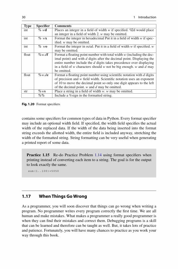
30 1 Introduction
Type Specifier Comments
int % wd Places an integer in a field of width w if specified. %2d would placean integer in a field of width 2. w may be omitted.
int % wx Format the integer in hexadecimal Put it in a field of width w if spec-ified. w may be omitted.
int % wo Format the integer in octal. Put it in a field of width w if specified. wmay be omitted.
float % w.df Format a floating point number with total width w (including the dec-imal point) and with d digits after the decimal point. Displaying theentire number include the d digits takes precedence over displaying
in a field of w characters should w not be big enough. w and d maybe omitted.
float % w.de Format a floating point number using scientific notation with d digitsof precision and w field width. Scientific notation uses an exponentof 10 to move the decimal point so only one digit appears to the leftof the decimal point. w and d may be omitted.
str % ws Place a string in a field of width w. w may be omitted.%% Include a %sign in the formatted string.
Fig. 1.20 Format specifiers
contains some specifiers for common types of data in Python. Every format specifier
may include an optional width field. If specified, the width field specifies the actual
width of the replaced data. If the width of the data being inserted into the format
string exceeds the allotted width, the entire field is included anyway, stretching the
width of the formatted string. String formatting can be very useful when generating
a printed report of some data.
Practice 1.15 Re-do Practice Problem 1.14 using format specifiers when
printing instead of converting each item to a string. The goal is for the output
to look exactly the same.
sum (1..100)=5050
1.17 When Things Go Wrong
As a programmer, you will soon discover that things can go wrong when writing a
program. No programmer writes every program correctly the first time. We are all
human and make mistakes. What makes a programmer a really good programmer is
when they can find their mistakes and correct them. Debugging programs is a skill
that can be learned and therefore can be taught as well. But, it takes lots of practice
and patience. Fortunately, you will have many chances to practice as you work your
way through this book.

1.17 When Things Go Wrong 31
Sometimes, especially when you are first learning to debug your programs, it can
help to have someone to talk to. Just the act of reading your code to someone else
may cause you to find your mistake. Of course, if you are using this text as part of
a course you may not want to read your code to another class member as that may
violate the guidelines your instructor has set forth. But, nevertheless, you might find
that reading your code to someone else may help you discover problems. This is
called a code walk-through by programming professionals. It is a common practice
and is frequently required when writing commercially available programs.
There is no substitute for thorough testing. You should run your program using
varied values for input. Try to think of values that might cause your program to
break. For instance, what if 0 is entered for an integer? What if a non-integer value
is entered when an integer was required? What happens if the user enters a string of
characters when a number was required?
Sometimes the problems in our code are not due to user input. They are just plain
old mistakes in programming caused either by temporarily forgetting something,
or by our misunderstanding how something works. For instance, in this chapter we
learned about assignment statements. You can store a value in the memory of a
computer and point a named reference at the value so you can retrieve it later. But,
you must assign a name to a value before you can retrieve it. If you don’t understand
that concept, or if you forgot where you assigned a value a name in your program, you
might accidentally write some code that tries to use that value before it is assigned a
name. For instance, consider the program in Fig. 1.21. The program is trying to use
the gallons variable which has not been assigned a value. The error message is on
the right side of the window. The line where the error was first detected by Python
is highlighted.
In the example in Fig. 1.21 the actual error is not on the line that is highlighted.
The highlighted line is the line where Python first detected the error. This is a very
common occurrence when debugging. Detection of an error frequently occurs after
the location of the actual error. To become a good programmer you must learn to
look backwards through your code from the point where an error is detected to find
the location where it occurred. In this case, the gallon variable should have been
written as gallons on line 3 but was incorrectly typed.
Another common error is the index out of range error. This can occur when trying
to access a value in a sequence by indexing into the sequence. If the index is for an
item that is outside the range of the sequence, an index out of range error will occur.
For instance, if you have a string called x that is one character long and you try to
access the second element of the string, your program will abort with an index out
of range error. Figure 1.22 shows this happening in a snippet of code.
Once again, in the example in Fig. 1.22 the error did not occur on the line that is
highlighted. The error occurred because the programmer meant to take the str(83)
which would result in “83” as a string instead of the chr(83) which results in the
string “S”. If the string had been “83” then line 3 would have worked and would
have printed 3 to the screen.
When an error occurs it is called an uncaught exception. Uncaught exceptions
result in the program terminating. They cannot be recovered from. Because uncaught

32 1 Introduction
Fig. 1.21 A run-time error
Fig. 1.22 An index out of range error
exceptions result in the program terminating it is vital to test your code so that all
variations of running the program are tested before the program is released to users.
Even so, there are times when a user may encounter an error. Perhaps it has happened
to you? In any case, thorough testing is critical to your success as a programmer and
learning to debug and test your code is as important as learning to program in the

1.17 When Thing Go Wrong 33
first place. As new topics are introduced in this text, debugging techniques will also
be introduced to provide you with the information you need to become a better
debugger.
1.18 Review Questions
1. What does the acronym IDE stand for? What does it do?
2. What does the acronym CPU stand for? What does it do?
3. How many bytes are in a GB? What does GB stand for?
4. What is the decimal equivalent of the binary number 01101100?
5. What is the hexadecimal equivalent of the binary number 01101100?
6. What is the binary equivalent of the number −62?
7. What is the ASCII equivalent of the decimal number 62?
8. What is a type in Python? Give an example. Why are there types in Python
programs?
9. How can you tell what type of value is stored in 4 contiguous bytes of memory?
10. How can you interactively work with the Python interpreter?
11. What is prototyping as it applies to computer programming?
12. Name two different types of errors that you can get when writing a computer
program? What is unique about each type of error?
13. What is a reference in a Python program?
14. Why is it that the result of 4.01−3.59 is 0.41999999999999993 when using at
least some implementations of Python 3?
15. What would you have to write to ask the user to enter an integer and then read
it into a variable in your program? Write some sample code to do this.
16. Assume that you have a constant defined for pi = 3.14159. You wish to print
just 3.14 to the screen using the pi variable. How would you print the pi variable
so it only display 3.14?
1.19 Exercises
1. Write a program that asks the user to enter their name. Then it should print out the
ASCII equivalent of each of the first four characters of your name. For instance,
here is a sample run of the program below.
Please enter your name: Kent
K ASCII value i s 75
e ASCII value i s 101
n ASCII value i s 110
t ASCII value i s 116

34 1 Introduction
2. Write a program that capitalizes the first four characters of a string by converting
the characters to their ASCII equivalent, then adding the necessary amount to cap-
italize them, and converting the integers back to characters. Print the capitalized
string. Here is a sample of running this program.
Please enter a four character string: kent
The string capitalized i s KENT
3. You can keep track of your car’s miles per gallon if you keep track of how many
miles you drive your car on a tank of gas and you always fill up your tank when
getting gas. Write a program that asks the user to enter the number of miles you
drove your car and the number of gallons of gas you put in your car and then
prints the miles per gallon you got on that tank of gas. Here is a sample run of
the program.
Please enter the miles you drove: 256
Please enter the gallons of gas you put i n the tank: 10.1
You got 25.346534653465348 mpg on that tank of gas.
4. Write a program that converts US Dollars to a Foreign Currency. You can do this
by finding the exchange rate on the internet and then prompting for the exchange
rate in your program. When you run the program it should look exactly like this:
What i s the amount of US Dollars you wish to convert? 31.67
What i s the current exchange rate
(1 US Dollar equals what i n the Foreign Currency )? 0.9825
The amount i n the Foreign Currency i s $31.12
5. Write a program that converts centimeters to yards, feet, and inches. There are
2.54 cm in an inch. You can solve this problem by doing division, multiplication,
addition, and subtraction. Converting a float to an int at the appropriate time will
help in solving this problem. When you run the program it should look exactly
like this (except possibly for decimal places in the inches):
How many centimeters do you want to convert? 127.25
This i s 1 yards , 1 feet , 2.098425 inches.
6. Write a program that computes the minimum number of bills and coins needed
to make change for a person. For instance, if you need to give $34.36 in change
you would need one twenty, one ten, four ones, a quarter, a dime, and a penny.
You don’t have to compute change for bills greater than $20 dollar bills or for
fifty cent pieces. You can solve this problem by doing division, multiplication,
subtraction, and converting floats to ints when appropriate. So, when you run the
program it should look exactly like this:
How much did the item cost: 65.64
How much did the person give you: 100.00
The person ’s change is $34.36
The bills or the change should be:
1 twenties
1 tens
0 fives
4 ones
1 quarters
1 dimes
0 nickels
1 pennies

1.19 Exercises 35
sideA
sideB
sideC
Fig. 1.23 A right triangle
7. Write a program that converts a binary number to its decimal equivalent. The
binary number will be entered as a string. Use the powers of 2 to convert each of
the digits in the binary number to its appropriate power of 2 and then add up the
powers of two to get the decimal equivalent. When the program is run, it should
have output identical to this:
Please enter an eight digit binary number: 01010011
The decimal equivalent of 01010011 i s 83.
8. Write a program that converts a decimal number to its binary equivalent. The
decimal number should be read from the user and converted to an int. Then you
should follow the algorithm presented in Example 1.1 to convert the decimal
number to its binary equivalent. The binary equivalent must be a string to get the
correct output. The output from the program must be identical to this:
Please enter a number: 83
The binary equivalent of 83 i s 01010011.
You may assume that the number that is entered is in the range 0–255. If you
want to check your work, you can use the bin function. The bin function will
take a decimal number and return a string representation of that binary number.
However, you should not use the bin function in your solution (Fig. 1.23).
9. Complete the program started in Practice Problem 1.10. Write a program that
asks the user to enter the two legs of a right triangle. The program should print
the length of the hypotenuse. If sideA and sideB are the lengths of the two legs
and sideC is the length of the third leg of a right triangle, then the Pythagorean
theorem says that sideA2 + sideB2 = sideC2. Ask the user to enter sideA and
sideB. Your program should print the value of sideC .
Please enter the length of the first leg: 3
Please enter the length of the second leg: 4
The length of the hypotenuse i s 5.0

36 1 Introduction
1.20 Solutions to Practice Problems
These are solutions to the Practice Problems in this chapter. You should only consult
these answers after you have tried each of them for yourself first. Practice Problems
are meant to help reinforce the material you have just read so make use of them.
1.20.1 Solution to Practice Problem 1.1
The decimal equivalent of the binary number 010101012 is 85.
1.20.2 Solution to Practice Problem 1.2
58/2 = 29 remainder 0
29/2 = 14 remainder 1
14/2 = 7 remainder 0
7/2 = 3 remainder 1
3/2 = 1 remainder 1
1/2 = 0 remainder 1
So the answer is 001110102.
1.20.3 Solution to Practice Problem 1.3
−8310 = 101011012
1.20.4 Solution to Practice Problem 1.4
The ASCII code for space is 32. 3210 = 001000002
1.20.5 Solution to Practice Problem 1.5
We, as programmers, determine how bytes in memory are interpreted by the state-
ments that we write. If we want to interpret the bits 01010011 as a character we write
‘S’ in our program. If we want the same bits to represent an integer, we write 83 in
our program.

1.20 Solutions to Practice Problems 37
1.20.6 Solution to Practice Problem 1.6
There is no solution needed for this exercise. Try it out and if you have problems,
talk to your instructor or someone who can help to make sure you get this working
before proceeding.
1.20.7 Solution to Practice Problem 1.7
1. An assignment statement is written as
<variable > = <expression >
where a variable is assigned the value of an expression.
2. To retrieve a value from memory we write the name of the variable that refers to
that value.
3. If we use a variable before it has been assigned a value Python will complain of
a name error, meaning the variable has not been assigned a value yet.
1.20.8 Solution to Practice Problem 1.8
The binary representation of 58 is 00111010. The number is 3A16 and 728. In Python
syntax that would be 0x3A and 0o72.
1.20.9 Solution to Practice Problem 1.9
There is no solution needed for this since it is in the text. However, you should make
sure you try this so you understand the mechanics of writing a program using the
IDE. If you can’t get it to work you should ask someone that did get it to work for
help or ask your instructor.
1.20.10 Solution to Practice Problem 1.10
sideA = 6
sideB = 8
sideC = (sideA*sideA + sideB **2) ** 0.5
p r i n t (sideC)
1.20.11 Solution to Practice Problem 1.11
Here is one program that you might get as a result.
name = ’Sophus Lie’
p r i n t ("The name is", name)
word = name [3] + name [1] + name [4] + name [5] + name [9]
p r i n t (word)

38 1 Introduction
1.20.12 Solution to Practice Problem 1.12
Here is one version of the program. Do you understand why + was used at the end
of the print statement?
x = c h r (83)
p r i n t ("The ASCII character equivalent of", o r d (x),"is",x+".")
1.20.13 Solution to Practice Problem 1.13
You cannot use input to implement this because the input function waits for the enter
key to be pressed, not just any key. You could prompt the user though with “Press
Enter to continue. . .”.
1.20.14 Solution to Practice Problem 1.14
Here is a version of the program. It must have variables to 1 and 100 to be correct
according to the directions.
start = 1
end = 100
sumOfNums = end * (end + 1) // 2
p r i n t ("sum("+ s t r (start )+".."+ s t r (end)+")="+ s t r (sumOfNums ))
1.20.15 Solution to Practice Problem 1.15
start = 1
end = 100
sumOfNums = end * (end + 1) // 2
p r i n t ("sum(%d..%d)=%d"%(start ,end ,sumOfNums ))

2Decision Making
In this chapter we explore how to make choices in our programs. Decision making
is valuable when something we want to do depends on some user input or some
other value that is not known when we write our program. This is quite often the
case and Python, along with all interesting programming languages, has the ability
to compare values and then take one action or another depending on that outcome.
For instance, you might write a program that reads data from a file and takes one
action or another based on the data it read. Or, a program might get some input from
a user and then take one of several actions based on that input.
To make a choice in Python you write an if statement. An if statement takes one
of two forms. It may be just an if statement. In this case, if the condition evaluates to
true then it will evaluate the then statements. If the condition is not true the computer
will skip to the statements after the if statement.
<statements before if statement >
if <condition >:
<then statements >
<statements after if statement >
Figure 2.1 depicts this graphically. An if statement evaluates the conditional
expression and then goes to one of two places depending on the outcome. Notice the
indentation in the if statement above. The indentation indicates the then statements
are part of the if statement. Indentation is very important in Python. Indentation deter-
mines the control flow of the program. Figure 2.1 graphically depicts this as well.
If the condition evaluates to true, a detour is taken to execute the then statements
before continuing on after the if statement.
Generally, we want to know if some value in our program is equal to, greater, or
less than another value. The comparison operators, or relational operators, in Python
allow us to compare two values. Any value in your program, usually a variable, can
be compared with another value to see how the two values relate to each other.
Figure 2.2 lists the operators you can use to compare two values. Each of these
operators is written between the two values or variables you want to compare. They
evaluate to either true or false depending on the two values. When the condition
© Springer-Verlag London 2014
K.D. Lee, Python Programming Fundamentals,
Undergraduate Topics in Computer Science, DOI 10.1007/978-1-4471-6642-9_2
39

40 2 Decision Making
condition
thenstatements
True
statementsafter
if statement
False
statements before if
statement
Fig. 2.1 If statement
Operator Condition
< Less Than> Greater Than
<= Less Than or Equal to>= Greater Than or Equal to== Equal to!= Not Equal to
Fig. 2.2 Relational operators
evaluates to true, the then statements are executed. Otherwise, the then statements
are skipped.
Example 2.1 An if statement is best described by giving an example. Assume
we want to see if a number entered by a user is divisible by 7. We can write the
program pictured in Fig. 2.3 to decide this. The program gets some input from
the user. Remember that input reads a string from the user. The int converts the
string to an integer. Then, the num variable is checked to see if it is divisible by
7. The % is called the modulo or just the mod operator. It gives us the remainder
after dividing by the divisor (i.e. 7 in this case). If the remainder after dividing
by 7 is 0 then the number entered by the user is divisible by 7.
An important feature of a debugger is the ability to step over our code and watch
the computer execute each statement. This is called stepping over or stepping into our

2 Decision Making 41
Fig. 2.3 Stepping into and over
code. Figure 2.3 depicts how this is done. For now stepping into and stepping over
code do relatively the same thing. To begin stepping through a program you press
the Step Into button. Once the program is started, you press the Step Over button to
avoid jumping to other code that your program might call. Stepping into and over
code can be very useful in understanding exactly what your program is doing.
Practice 2.1 Write a short program that asks the user to enter the name of
a month. If the user enters “December” your program should print “Merry
Christmas!”. No matter what you enter, your program should print “Have a
Happy New Year!” just before the program terminates. Then, use Step Into and
Step Over to execute each statement that you wrote. Run your program at least
twice to see how it behaves when you enter “December” and how it behaves
when you enter something else.
Sometimes, you may want your program to do one thing if a condition is true and
something else if a condition is false. Notice that the if statement does something
only when the condition evaluates to true and does not do anything otherwise. If
you want one thing to happen when a condition is true and another to happen if the
condition is false then you need to use an if-else statement. An if-else statement adds
a keyword of else to do something when the condition evaluates to false. An if-else
statement looks like this.

42 2 Decision Making
<statements before if statement >
if <condition >:
<then statements >
else:
<else statements >
<statements after if statement >
If the condition evaluates to true, the then statements are executed. Otherwise, the
else statements are executed. Figure 2.4 depicts this graphically. The control of your
program branches to one of two locations, the then statements or the else statements
depending on the outcome of the condition.
Again, indentation is very important. The else keyword must line up with the if
statement to be properly paired with the if statement by Python. If you don’t line up
the if and the else in exactly the same columns, Python will not know that the if and
the else go together. In addition, the else is only paired with the closest if that is in the
same column. Both the then statements and the else statements must be indented and
must be indented the same amount. Python is very picky about indentation because
indentation in Python determines the flow of control in the program.
In the case of the if-else statement, either the then statements or the else statements
will be executed. This is in contrast to the if statement that is described in Fig. 2.1.
When learning about if statements this seems to be where some folks get stuck.
The statements that are conditionally executed are those statements that are indented
under the if or the else.
In either case, after executing the if or the if-else statement control proceeds to
the next statement after the if or if-else. The statement after the if-else statement is
the next line of the program that is indented the same amount as the if and the else.
condition
thenstatements
True
statementsafter
if statement
statements before if
statement
elsestatements
False
Fig. 2.4 If-else statement

2 Decision Making 43
Example 2.2 Consider a program that finds the maximum of two integers. The
last line before the if-else statement is the y = assignment statement. The first
line after the if-else statement is the print(“Done.”) statement.
1 x = i n t ( i n p u t ("Please enter an integer:"))
2 y = i n t ( i n p u t ("Please enter another integer:"))
3 i f x > y:
4 p r i n t (x,"is greater than",y)
5 e l s e :
6 p r i n t (y,"is greater than or equal to",x)
7 p r i n t ("Done.")
Practice 2.2 Modify the program from practice Problem 2.1 to print “Merry
Christmas!” if the month is December and “You’ll have to wait” otherwise. It
should still print “Have a Happy New Year!” in either case as the last line of
output. Then run the program at least twice using step into and over to see how
it behaves when “December” is entered and how the program behaves when
anything else is entered.
2.1 Finding the Max of Three Integers
Any statement may be placed within an if statement, including other if statements.
When you want to check multiple conditions there may be a need to put one if
statement inside another. It can happen, but not very often. For instance, you may
need to know if a value entered by a user is between two numbers. This could be
written using two if statements, the outer if statement checking to see if the value
entered is greater than some minimum, and the inner if statement checking to see of
the value entered is less than some maximum. There are other ways to check to see
if a value is between a maximum and minimum, but nested if statements can be used
in this kind of circumstance.
Let’s consider another possibility. Suppose you are asked to write a program that
finds the maximum of three integers. This can be accomplished by writing nested if
statements. Figure 2.5 depicts the flow of control for such a program.
We could determine which of the three integers, x, y and z, was the greatest by
first comparing two of them, say x and y. Then, depending on the outcome of that
condition, we would compare two more integers. By nesting if statements we can
arrive at a decision about which is greatest. This code gets a bit complicated because
we have three if statements to deal with, two of which are nested inside the third
statement.

44 2 Decision Making
get input of integers x,y,
and z
y > x
z > x
print(x)print(z)
z > y
print(y)print(z)
print("Done")
FalserueT
FalserueFalserue TT
Fig. 2.5 Max of three integers
Example 2.3 While you wouldn’t normally write code like this, it is provided
here to show how if statements may be nested. The code prints the maximum
of three integers entered by the user.
1 x = i n t ( i n p u t ("Please enter an integer:"))
2 y = i n t ( i n p u t ("Please enter another integer:"))
3 z = i n t ( i n p u t ("Please enter a third integer:"))
4 i f y > x:
5 i f z > y:
6 p r i n t (z, "is greatest.")
7 e l s e :
8 p r i n t (y, "is greatest.")
9 e l s e :
10 i f z > x:
11 p r i n t (z, "is greatest.")
12 e l s e :
13 p r i n t (x, "is greatest.")
14 p r i n t ("Done.")

2.2 The Guess and Check Pattern 45
2.2 The Guess and Check Pattern
There is no way a good programmer would write a program that included the code
that appeared in Example 2.3. It is too complicated. Instead, it would be much better
to use a pattern or idiom called Guess and Check. Using this pattern involves first
making a guess as to a correct solution and storing that guess in a variable. Then,
you use one or more if statements to check that guess to see if it was correct or not.
If it was not a correct guess, then the variable can be updated with a new guess.
Finally, when the guess has been thoroughly checked, it should equal the value we
were looking for.
Example 2.4 Consider the max of three program in Example 2.3. This could
be rewritten using the guess and check pattern if we first make a guess as to
the maximum value and then fix it if needed.
1 x = i n t ( i n p u t ("Please enter an integer:"))
2 y = i n t ( i n p u t ("Please enter another integer:"))
3 z = i n t ( i n p u t ("Please enter a third integer:"))
4 # Here is our initial guess
5 maxNum = x
6 i f y > maxNum: # Fix our guess if needed
7 maxNum = y
8 i f z > maxNum: # Fix our guess again if needed
9 maxNum = z
10 p r i n t (maxNum ,"is greatest.")
11 p r i n t ("Done.")
The code in Examples 2.3 and 2.4 get the same input and print exactly the same
thing. However, the code in Example 2.4 is much easier to understand, mainly because
the control flow is simplified by not having nested if statements. Notice that no
else clauses were needed in Example 2.4. So, the code is simplified by having two
if statements instead of three. It is simplified by having no nested if statements.
Finally it is simplified because there are no use of else clauses in either of the if
statements.
Practice 2.3 Use the guess and check pattern to determine if a triangle is a
perfect triangle. A perfect triangle has side lengths that are multiples of 3, 4
and 5. Ask the user to enter the shortest, middle, and longest sides of a triangle
and then print “It is a perfect triangle “if it is and “It is not a perfect triangle”
if it isn’t. You may assume that the side lengths are integers. Let your guess be
that the message you will print is “It is a perfect triangle”.

46 2 Decision Making
2.3 Choosing from a List of Alternatives
Sometimes you may write some code where you need to choose from a list of
alternatives. For instance, consider a menu driven program. You may want to print a
list of choices and have a user pick from that list. In such a situation you may want to
use an if statement and then nest an if statement inside of the else clause. An example
will help clarify the situation.
Example 2.5 Consider writing a program where we want the user to enter two
floats and then choose one of several options.
1 x = f l o a t ( i n p u t ("Please enter a number:"))
2 y = f l o a t ( i n p u t ("Please enter a second number:"))
3
4 p r i n t ("1) Add the two numbers")
5 p r i n t ("2) Subtract the two numbers")
6 p r i n t ("3) Multiply the two numbers")
7 p r i n t ("4) Divide the two numbers")
8
9 choice = i n t ( i n p u t ("Please enter your choice:"))
10
11 p r i n t ("The answer is:",end="")
12
13 i f choice == 1:
14 p r i n t (x + y)
15 e l s e :
16 i f choice == 2:
17 p r i n t (x - y)
18 e l s e :
19 i f choice == 3:
20 p r i n t (x * y)
21 e l s e :
22 i f choice == 4:
23 p r i n t (x / y)
24 e l s e :
25 p r i n t ("You did not enter a valid choice.")
Do you notice the stair step pattern that appears in the code in Example 2.5?
This stair stepping is generally considered ugly and a nuisance by programmers.
Depending on how much you indent each line, the code can quickly go off the right
side of the screen or page. The need to select between several choices presents itself
often enough that Python has a special form of the if statement to handle this. It is the
if-elif statement. In this statement, one, and only one, alternative is chosen. The first
alternative whose condition evaluates to True is the code that will be executed. All
other alternatives are ignored. The general form of the if-elif statement is given here.
<statements before if statement >
if <first condition >:
<first alternative >
elif <second condition >:
<second alternative >

2.3 Choosing from a List of Alternatives 47
elif <third condition >:
<third alternative >
else:
<catch -all alternative >
<statements after the if statement >
There can be as many alternatives as are needed. In addition, the else clause
is optional so may or may not appear in the statement. If we revise our example
using this form of the if statement it looks a lot better. Not only does it look bet-
ter, it is easier to read and it is still clear which choices are being considered. In
either case, if the conditions are not mutually exclusive then priority is given to
the first condition that evaluates to true. This means that while a condition may be
true, its statements may not be executed if it is not the first true condition in the if
statement.
Example 2.6 Here is a revision of Example 2.5 that looks a lot nicer.
1 x = f l o a t ( i n p u t ("Please enter a number:"))
2 y = f l o a t ( i n p u t ("Please enter a second number:"))
3
4 p r i n t ("1) Add the two numbers")
5 p r i n t ("2) Subtract the two numbers")
6 p r i n t ("3) Multiply the two numbers")
7 p r i n t ("4) Divide the two numbers")
8
9 choice = i n t ( i n p u t ("Please enter your choice:"))
10
11 p r i n t ("The answer is:",end="")
12
13 i f choice == 1:
14 p r i n t (x + y)
15 e l i f choice == 2:
16 p r i n t (x - y)
17 e l i f choice == 3:
18 p r i n t (x * y)
19 e l i f choice == 4:
20 p r i n t (x / y)
21 e l s e :
22 p r i n t ("You did not enter a valid choice.")
Practice 2.4 Write a short program that asks the user to enter a month and
prints a message depending on the month entered according to the messages
in Fig. 2.6. Then use the step into and over ability of the debugger to examine
the code to see what happens.

48 2 Decision Making
Month Message
January Hello Snow!
February More Snow!
March No More Snow!
April Almost Golf TimeMay Time to GolfJune School’s OutJuly Happy Fourth
August Still Golfing
September Welcome Back!
October Fall ColorsNovember Turkey DayDecember Merry Christmas!
Fig. 2.6 Messages
2.4 The Boolean Type
Conditions in if statements evaluate to True or False. One of the types of values
in Python is called bool which is short for Boolean. George Boole was an English
Mathematician who lived during the 1800s. He invented the Boolean Algebra and it
is in honor of him that true and false are called Boolean values today [13].
In an if statement the condition evaluates to true or false. The Boolean value of the
condition decides which branch is to be executed. The only requirement for a condi-
tion in an if statement is that it evaluates to true or false. So writing if True . . . would
mean that the then statements would always be executed. Writing such an if statement
doesn’t really make sense, but using Boolean values in if statements sometimes does.
Example 2.7 Consider a program that must decide if a value is between 0 and
1. The program below uses a Boolean expression to discover if that is the case
or not.
x = i n t ( i n p u t ("Please enter a number:"))
i f x >= 0 a n d x <= 1:
p r i n t (x, "is between 0 and 1")
Because an if statement only requires that the condition evaluates to true or false,
any expression may be used as long as the result of evaluating it is true or false.
Compound Boolean expressions can be built from simple expressions by using the
logical operators and, or, and not. The and of two Boolean values is true when both
Boolean values are true as shown in Fig. 2.7. The or of two Boolean values is true
when one or the other is true, or when both are true as depicted in Fig. 2.8. The not of
a Boolean value is true when the original value was false. This is shown in Fig. 2.9.
The three figures describe the truth-tables for each of the Boolean operators. A
truth-table can be constructed for any compound Boolean expression. In each of the

2.4 The Boolean Type 49
A B A and B
False False FalseFalse True FalseTrue False FalseTrue True True
Fig. 2.7 The and operator
A B A or B
False False FalseFalse True TrueTrue False TrueTrue True True
Fig. 2.8 The or operator
A not A
False TrueTrue False
Fig. 2.9 The not operator
truth tables, A and B represent any Boolean expression. The tables show what the
Boolean value of the expression A and B, A or B, and not A would be, given the values
of A and B in the table. The and, or, and not logical operators can be strung together
in all sorts of ways to produce complex Boolean expressions, but writing a program
with complex Boolean expressions is generally a bad idea since it is difficult to
understand the logic of complex expressions.Keeping track of whether to use and or
or when not is involved in the expression is difficult and should be avoided if possible.
There are at least a couple of ways that negation (i.e. the use of the not operator)
can be avoided in if statements. The statement can be rewritten to test the opposite of
what you first considered. Another technique is to use the guess and check pattern.
The following two examples illustrate how this can be done.
Example 2.8 Consider a club where you must be under 18 and over 15 to join.
Here is a first try at a program that tells you whether you can join or not.
1 age = i n t ( i n p u t ("Please enter your age:"))
2 i f ( n o t age > 15) a n d ( n o t age < 18):
3 p r i n t ("You can’t join")
4 e l s e :
5 p r i n t ("You can join")
Does this program do the job? In fact, as it is written here everyone can join
the club. The problem is with the choice of and in the Boolean expression. It
should have been or. The correct program would be written as follows.

50 2 Decision Making
1 age = i n t ( i n p u t ("Please enter your age:"))
2 i f ( n o t age > 15) o r ( n o t age < 18):
3 p r i n t ("You can’t join")
4 e l s e :
5 p r i n t ("You can join")
While the program above is correct, it is still difficult to understand why it is
correct. The problem is the use of negation with the or operator. A much better
way to write it would be to remove the negation in the expression.
1 age = i n t ( i n p u t ("Please enter your age:"))
2 i f age > 15 a n d age < 18:
3 p r i n t ("You can join")
4 e l s e :
5 p r i n t ("You can’t join")
Example 2.9 The guess and check pattern can be applied to Boolean values
as well. If you need to decide a yes or no question, you can make a guess and
then fix it if needed.
1 age = i n t ( i n p u t ("Please enter your age:"))
2 member = True
3 i f age <= 15:
4 member = False
5 i f age >= 18:
6 member = False
7 i f member:
8 p r i n t ("You can join")
9 e l s e :
10 p r i n t ("You can’t join")
The technique used in Example 2.9 is especially useful when there are a number
of conditions that must be checked to make sure that the yes or no answer is correct.
In fact, when the exact number of conditions is unknown, this technique may be
necessary. How the exact number of conditions to check can be unknown will become
clearer in the next chapter.
Practice 2.5 Write a program that determines whether you can run for pres-
ident. To run for president the constitution states: No Person except a natural
born Citizen, or a Citizen of the United States, at the time of the Adoption
of this Constitution, shall be eligible to the Office of President; neither shall
any Person be eligible to that Office who shall not have attained to the Age of
thirty five Years, and been fourteen Years a Resident within the United States
[7]. Ask three questions of the user and use the guess and check pattern to
determine if they are eligible to run for President.

2.5 Short Circuit Logic 51
2.5 Short Circuit Logic
Once in a while using the guess and check pattern may not produce the desired
results. There are situations where you may want to evaluate one condition only if
another condition is true or false. An example should make this clear.
Example 2.10 Consider a program that checks to see if one integer evenly
divides another.
1 top = i n t ( i n p u t ("Please enter the numerator:"))
2 bottom = i n t ( i n p u t ("Please enter the denominator:"))
3
4 i f bottom != 0 a n d top % bottom == 0:
5 p r i n t ("The numerator is evenly divided by the denominator.")
6 e l s e :
7 p r i n t ("The fraction is not a whole number.")
Dividing top by bottom would result in a run-time error if bottom were 0. However,
division by 0 will never happen in this code because Python, and most programming
languages, uses short-circuit logic. This means that since both A and B must be true
in the expression A and B for the expression to evaluate to true, if it turns out that A
evaluates to false then there is no point in evaluating B and therefore it is skipped. In
other words, Boolean expressions are evaluated from left to right until the truth or
falsity of the expression can be determined and the condition evaluation terminates.
This is exactly what we want in the code in Example 2.10.
Practice 2.6 In Minnesota you can fish if you are 15 years old or less and your
parent has a license. If you are 16 years old or more you need to have your
own license. Write a program that uses short circuit logic to tell someone if
they are legal to fish in Minnesota. First ask them how old they are, whether
they have a license or not, and whether their parent has a license or not.
2.6 Comparing Floats for Equality
In Python, real numbers or floats are represented using eight bytes. That means that
264 different real numbers can be represented. This is a lot of real numbers, but not
enough. Since there are infinitely many real numbers between any two real numbers,
computers will never be able to represent all of them.
Because floats are only approximations of real numbers, there is some round-off
error expected when dealing with real numbers in a program. Generally this round-off
error is small and is not much of a problem unless you are comparing two real numbers

52 2 Decision Making
for equality. If you need to do this then you need to subtract the two numbers and
see if the difference is insignificant since the two numbers may be slightly different.
So, to compare two floats for equality you can subtract the two and see if the
difference is small relative to the two numbers.
Example 2.11 This program compares a guess with the result of dividing two
floats and tells you if you are correct or not.
1 top = f l o a t ( i n p u t ("Please enter the numerator:"))
2 bottom = f l o a t ( i n p u t ("Please enter the denominator:"))
3
4 guess = f l o a t ( i n p u t ("Please enter your guess:"))
5
6 result = top/bottom
7 biggest = a b s (result)
8
9 i f a b s (guess) > biggest:
10 biggest = a b s (guess)
11
12 # require the answer is within 1/10th Percent
13 # of the correct value.
14 i f a b s ((guess -result )/ biggest) < .001:
15 p r i n t ("You guessed right!")
16 e l s e :
17 p r i n t ("Sorry , that’s wrong. The correct value was",result)
Notice in the program in Example 2.11 that the abs function returns the absolute
value of the float given to it so it doesn’t matter if the numbers you are comparing
are positive or negative. The code will work either way. In this example, 0.001 or
1/10th of 1 % difference was deemed close enough. Depending on your application,
that value may be different.
Practice 2.7 Use the guess and check pattern to determine if a triangle is a
perfect triangle. You must allow the user to enter any side length for the three
sides of the triangle, not just integers. A perfect triangle has side lengths that
are multiples of 3, 4 and 5. Ask the user to enter the three side lengths and then
print “It is a perfect triangle” if it is and “It is not a perfect triangle” if it isn’t.
2.7 Exception Handling
Sometimes things go wrong in a program and it is out of your control. For instance, if
the user does not enter the proper input an error may occur in your program. Python
includes exception handling so programmers can handle errors like this. Generally,
if there is a possibility something could go wrong you should probably use some
exception handling. To use exception handling you write a try-except statement.

2.7 Exception Handling 53
<statements before try -except >
try:
<try -block statements >
except [Exception ]:
<except -block statements >
<statements after the try -except code >
A try-except block may monitor for any exception or just a certain exception.
There are many possible exceptions that might be caught. For instance, a ValueError
exception occurs when you try to convert an invalid value to an integer. A ZeroDivi-
sionError exception occurs when you try to divide by zero. In the general form shown
above, the Exception is optional. That’s what the square brackets (i.e. [ ]) mean.
You don’t actually write the square brackets. They mean the exception is optional in
this case. If the exception is omitted then any exception is caught.
Exception handling can be used to check user input for validity. It can also be
used internally in the program to catch calculations that might result in an error
depending on the values involved in the calculation. When a try block is executed if
a run-time error occurs that the try-except block is monitoring then program control
immediately skips to the beginning of the except block. If no error occurs while
executing the try block then control skips the except block and continues with the
statement following the try-except statement. If an error occurs and the except block
is executed, then when the except block finishes executing control goes to the next
statement after the try-except statement (Fig. 2.10).
Example 2.12 Here is a bulletproof version of the program first presented in
Example 2.10. This example does not use short-circuit logic. It uses exception
handling instead. Notice the use of exit(0) below. This is a Python function
that exits the program immediately, skipping anything that comes after it.
1 t r y :
2 top = i n t ( i n p u t ("Please enter the numerator:"))
3 e x c e p t ValueError: # This try -except catches only ValueErrors
4 p r i n t ("You didn’t enter an integer.")
5 exit (0)
6
7 t r y :
8 bottom = i n t ( i n p u t ("Please enter the denominator:"))
9 e x c e p t : # This try -except catches any exception
10 p r i n t ("You didn’t enter an integer.")
11 exit (0)
12
13 t r y :
14 i f top % bottom == 0:
15 p r i n t ("The numerator is evenly divided by the" + \
16 "denominator.")
17 e l s e :
18 p r i n t ("The fraction is not a whole number.")
19 e x c e p t ZeroDivisionError:
20 p r i n t ("The denominator cannot be 0.")

54 2 Decision Making
try-except
except-blockstatements
statementsafter
try-except statement
statements before
try-except statement
try-blockstatements
Exception
Fig. 2.10 Try-except statement
Try-except statements are useful when either reading input from the user or when
using data that was read earlier in the program. Example 2.12 uses three try-except
statements. The first two catch any non-integer input that might be provided. The
last catches a division by zero error.
Practice 2.8 Add exception handling to the program in practice Problem 2.6
so that if the user answers something other than their age that the program
prints “You did not enter your age correctly”.
2.8 Review Questions
1. What is the difference between an if statement and an if-else statement? Be sure
to state what the difference in meaning is between the two, not just the addition
of the else keyword.
2. What type of value is returned by the relational operators?
3. What does it mean to Step Over code? What is that referring to?
4. What is a nested if statement?
5. How can nested if statements be avoided?
6. What is the general pattern for Guess and Check?

2.8 Review Questions 55
7. What is the Mathematician George Boole famous for?
8. When is it difficult to determine whether and or or should be used in an if
statement?
9. What is short circuit logic? When does it apply? Give an example of when it
would apply. Do not use the example in the book.
10. What is the problem with comparing floats for equality?
11. If an exception occurs on line 2 of while executing this code give the line numbers
of this program in the order that they are executed. What is the output from the
program?
1 t r y :
2 x = i n t ( i n p u t ("Please enter an integer:"))
3 y = i n t ( i n p u t ("Please enter another integer:"))
4 e x c e p t :
5 p r i n t ("You entered an invalid integer.")
6 p r i n t ("The product of the two integers is",x*y)
2.9 Exercises
1. Type in the code of Example 2.6. Execute the code using a debugger like the one
included with the Wing IDE 101. Step into and over the code using the debugger.
Enter a menu choice of 1. Using the line numbers in Example 2.6, which lines of
the program are executed when you enter a 1 for the menu choice. List these lines.
Do the same for each of the other menu choice values. If you run the program and
enter a menu choice of 5, which lines of the program are executed. If you use the
debugger to answer this question you will be guaranteed to get it right and you’ll
learn a little about using a debugger.
2. Write a program that prints a user’s grade given a percent of points achieved in
the class. The program should prompt the user to enter his/her percent of points.
It should then print a letter grade A, A−, B+, B, B−, C+, C, C−, D+, D, D−, F.
The grading scale is given in Fig. 2.11. Use exception handling to check the input
from the user to be sure it is valid. Running the program should look like this:
Please enter your percentage achieved in the class: 92.32
You earned an A- in the class.
3. Write a program that converts centimeters to yards, feet, and inches. There are
2.54 cm in an inch. You can solve this problem by doing division, multiplication,
addition, and subtraction. Converting a float to an int at the appropriate time will
help in solving this problem. When you run the program it should look exactly
like this (except possibly for decimal places in the inches):
How many centimeters do you want to convert? 127.25
This is 1 yard , 1 foot , 2.098425 inches.

56 2 Decision Making
Grade If Greater Than Or Equal To
A 93.33A- 90B+ 86.67B 83.33B- 80C+ 76.67C 73.33C- 70D+ 66.67D 63.33D- 60F 0
Fig. 2.11 Grading scale
This is a modification of the program in Exercise 5 of Chap. 1. In this version of
it you should print “yard” when there is one yard, and “yards” when there is more
than one yard. If there are zero yards then it should not print “yard” or “yards”.
The same thing applies to “feet”. Use an if statement to determine the label to
print and if the label should be printed at all.
4. Write a program that computes the minimum number of bills and coins needed
to make change for a person. For instance, if you need to give $34.36 in change
you would need one twenty, one ten, four ones, a quarter, a dime, and a penny.
You don’t have to compute change for bills greater than $20 dollar bills or for
fifty cent pieces. You can solve this problem by doing division, multiplication,
subtraction, and converting floats to ints when appropriate. So, when you run the
program it should look exactly like this:
How much did the item cost: 65.64
How much did the person give you: 100.00
The person ’s change is $34.36
The bills or the change should be:
1 twenty
1 ten
4 ones
1 quarter
1 dime
1 penny
This is a modification of the program in Exercise 6 of Chap. 1. In this version,
only non-zero amounts of bills and change should be printed. In addition, when
only one bill or coin is needed for a particular denomination, you should use the
singular version of the word. When more than one bill or coin for a denomination
is needed, the plural of the label should be used.
5. Write a program that asks the user to enter an integer less than 50 and then prints
whether or not that integer is prime. To determine if a number less than 50 is
prime you only need to divide by all prime numbers that are less than or equal to

2.9 Exercises 57
the square root of 50. If any of them evenly divide the number then it is not prime.
Use the guess and check pattern to solve this problem. Use exception handling to
check the input from the user to be sure it is valid. A run of the program should
look like this:
Please enter an integer less than 50: 47
47 is prime.
6. Write a program that converts a decimal number to its binary equivalent. The
decimal number should be read from the user and converted to an int. Then you
should follow the algorithm presented in Example 1.1 to convert the decimal
number to its binary equivalent. The binary equivalent must be a string to get the
correct output. In this version of the program you must handle all 16-bit signed
integers. That means that you must handle numbers from −32768 to 32767. In
this version of the program you should not print any leading 0’s. Leading 0’s
should be omitted from the output.
If you want to check your work, you can use the bin function. The bin function will
take a decimal number and return a string representation of that binary number.
However, you should not use the bin function in your solution.
The output from the program must be identical to this:
Please enter a number: 83
The binary equivalent of 83 is 1010011.
7. Write a program that prompts the user to enter a 16-bit binary number (a string
of 1’s and 0’s). Then, the program should print the decimal equivalent. Be sure
to handle both negative and positive binary numbers correctly. If the user enters
less than 16 digits you should assume that the digits to the left of the last digit
are zeroes. When run the output should look like this:
Please enter a 16-bit binary number: 1010011
The base 10 equivalent of the binary number 1010011 is 83.
To handle negative numbers correctly you first need to detect if it is a negative
number. A 16-digit binary number is negative if it is 16 digits long and the left-
most digit is a 1. To convert a negative number to its integer equivalent, first take
the 1’s complement of the number. Then convert the 1’s complement to an integer,
then add 1 to the integer and negate the result to get the 2’s complement.
The conversion from bits to an integer can be carried out by multiplying each bit
by the power of 2 that it represents as described in Sect. 1.5 of Chap. 1.
8. Converting numbers to any base can be accomplished using the algorithm from
Example 1.1. For instance, an integer can be converted to hexadecimal using this
algorithm. Hexadecimal numbers are base 16. That means there are 16 possible
values for one digit. Counting in hexadecimal starts 0, 1, 2, 3, 4, 5, 6, 7, 8, 9, a, b,
c, d, e, f, 10, 11, 12 and so on. The algorithm changes so that instead of dividing by

58 2 Decision Making
2 you divide by 16. The one gotcha is that if the remainder after dividing is greater
or equal to 10 (base 10) then you should not append the base 10 value to the string.
Instead you should append a, b, c, d, e, or f. You can use if statements to determine
the correct value to append. Write a program that prompts the user to enter an inte-
ger and then prints its hexadecimal equivalent. Traditionally, hexadecimal num-
bers start with a “0x” to identify them as hex, so your output should look like this:
Please enter an integer: 255
The hexadecimal equivalent is 0x00ff
Your program should handle any base 10 integer from 0 to 65535. There is a
function called hex in Python that converts integers to their hexadecimal repre-
sentation. You may not use this in implementing this program, but you may use
it to see if your program is producing the correct output. For instance, calling
hex(255) will return the string 0xff.
You should check the input that the user enters to make sure that it is in the valid
range accepted by your program.
2.10 Solutions to Practice Problems
These are solutions to the practice problems in this chapter. You should only consult
these answers after you have tried each of them for yourself first. Practice problems
are meant to help reinforce the material you have just read so make use of them.
2.10.1 Solutions to Practice Problem 2.1
1 month = i n p u t ("Please enter a month:")
2 i f month =="December":
3 p r i n t ("Merry Christmas!")
4 p r i n t ("Have a Happy New Year!")
2.10.2 Solutions to Practice Problem 2.2
1 month = i n p u t ("Please enter a month:")
2 i f month =="December":
3 p r i n t ("Merry Christmas!")
4 e l s e :
5 p r i n t ("You’ll have to wait")
6 p r i n t ("Have a Happy New Year!")

2.10 Solutions to Practice Problems 59
2.10.3 Solutions to Practice Problem 2.3
1 sideone = i n t ( i n p u t ( \
2 "Please enter length of shortest side of triangle:"))
3 sidetwo = i n t ( i n p u t ( \
4 "Please enter length of middle side of triangle:"))
5 sidethree = i n t ( i n p u t ( \
6 "Please enter length of longest side of triangle:"))
7
8 msg ="It is a perfect triangle."
9
10 i f sideone % 3 != 0:
11 msg = "It is not a perfect triangle."
12
13 i f sidetwo % 4 != 0:
14 msg = "It is not a perfect triangle."
15
16 i f sidethree % 5 != 0:
17 msg = "It is not a perfect triangle."
18
19 i f sideone **2 + sidetwo **2 != sidethree **2:
20 msg = "It is not a perfect triangle."
21 p r i n t (msg)
2.10.4 Solutions to Practice Problem 2.4
1 month = i n p u t ("Please enter a month:")
2 i f month =="January":
3 msg ="Hello Snow!"
4 e l i f month =="February":
5 msg ="More Snow!"
6 e l i f month =="March":
7 msg ="No More Snow!"
8 e l i f month =="April":
9 msg ="Almost Golf Time"
10 e l i f month =="May":
11 msg ="Time to Golf"
12 e l i f month =="June":
13 msg ="School’s Out"
14 e l i f month =="July":
15 msg ="Happy Fourth"
16 e l i f month =="August":
17 msg ="Still Golfing"
18 e l i f month =="September":
19 msg ="Welcome Back!"
20 e l i f month =="October":
21 msg ="Fall Colors"
22 e l i f month =="November":
23 msg ="Turkey Day"
24 e l i f month =="December":
25 msg ="Merry Christmas!"
26 e l s e :
27 msg ="You entered an incorrect month."
28
29 p r i n t (msg)

60 2 Decision Making
2.10.5 Solutions to Practice Problem 2.5
1 age = i n t ( i n p u t ("Please enter your age:"))
2 resident = i n p u t ( \
3 "Are you a natural born citizen of the U.S. (yes/no)?")
4 years = i n t ( i n p u t ( \
5 "How many years have you resided in the U.S.?"))
6
7 eligible = True
8 i f age < 35:
9 eligible = False
10
11 i f resident !="yes":
12 eligible = False
13
14 i f years < 14:
15 eligible = False
16
17 i f eligible:
18 p r i n t ("You can run for president!")
19 e l s e :
20 p r i n t ("You are not eligible to run for president!")
2.10.6 Solutions to Practice Problem 2.6
1 age = i n t ( i n p u t ("What is your age?"))
2 license = i n p u t ( \
3 "Do you have a fishing license in MN (yes/no)?")
4 parentlic = i n p u t ( \
5 "Does your parent have a fishing license (yes/no)?")
6
7 i f (age < 16 a n d parentlic =="yes") o r license =="yes":
8 p r i n t ("You are legal to fish in MN.")
9 e l s e :
10 p r i n t ("You are not legal to fish in MN.")
2.10.7 Solutions to Practice Problem 2.7
1 sideone = f l o a t ( i n p u t ( \
2 "Please enter length of shortest side of triangle:"))
3 sidetwo = f l o a t ( i n p u t ( \
4 "Please enter length of middle side of triangle:"))
5 sidethree = f l o a t ( i n p u t ( \
6 "Please enter length of longest side of triangle:"))
7
8 ratio = sideone / 3
9
10 msg ="It is a perfect triangle."
11
12 i f a b s ((ratio - sidetwo / 4) / sidetwo) > 0.001:
13 msg ="It is not a perfect triangle."
14

2.10 Solutions to Practice Problems 61
15 i f a b s ((ratio - sidethree / 5) / sidethree) > 0.001:
16 msg ="It is not a perfect triangle."
17
18 p r i n t (msg)
2.10.8 Solutions to Practice Problem 2.8
1 t r y :
2 age = i n t ( i n p u t ("What is your age?"))
3 e x c e p t :
4 p r i n t ("You did not enter your age correctly.")
5 exit (0)
6
7 license = i n p u t ( \
8 "Do you have a fishing license in MN (yes/no)?")
9 parentlic = i n p u t ( \
10 "Does your parent have a fishing license (yes/no)?")
11
12 i f (age < 16 a n d parentlic =="yes") o r license =="yes":
13 p r i n t ("You are legal to fish in MN.")
14 e l s e :
15 p r i n t ("You are not legal to fish in MN.")

3Repetitive Tasks
When my children were very little I played with them and read books to them.
If they were particularly entertained I would get the, “Do it again!”, command from
them. And, of course, I did it or read it again. Who can say no to a three year-old
when they are being so cute. They never seemed to grow tired of repetition when
they found something entertaining. Eventually, I grew tired of it myself and would
give them the, “One more time . . .”, warning.
Computers are very good at doing repetitive tasks, often called iteration in
Computer Science lingo. Computers don’t get tired and they don’t get bored. Usu-
ally, when a task is repeated, it is repeated for the same type of data over and over
again. For instance, sending out paychecks is a repetitive job since each employee’s
deductions must be computed and then a paycheck must be printed or electronically
deposited. For large companies, this job would require many people since each per-
son would only be able to compute the withholdings for a relatively small number
of people. In fact, before the advent of electronic computers, the word Computer
referred to people whose job it was to carry out these kinds of calculations. That
certainly must have been a mundane and repetitive job. Electronic computers on the
other hand don’t get tired, can work around the clock, and can work at lightning
speed.Repeating a task in a programming language is often called iteration or a loop.
In this chapter you learn about loops in Python. You learn how to write various kinds
of loops and more importantly, you learn when to write various kinds of loops.
When doing a task over and over again it is probably the case that the data that
the computer needs to do its job is located in some sort of list or sequence. Python
has built-in support for lists. In addition, Python also supports strings, which are
sequences of characters. Since so much of what computers do are repetitive tasks, it
is important to know how to repeat code and how to manipulate strings and lists. This
chapter explores the use of strings and lists. You learn that strings and lists are types
of objects and discover what you can do with these objects. In Computer Science
sequences and iteration go hand in hand.
So, what is a string? In the first chapter a string literal was defined as any sequence
of characters surrounded by either single or double quotes. A string literal is used to
© Springer-Verlag London 2014
K.D. Lee, Python Programming Fundamentals,
Undergraduate Topics in Computer Science, DOI 10.1007/978-1-4471-6642-9_3
63

64 3 Repetitive Tasks
0x2ac"How are you?"
upper()lower()strip()
...
.
s
Fig. 3.1 A string object
represent a specific string object in Python. So a string literal is written in a Python
program when you have a specific string object that you want to use in your program.
So what is an object? Every value in Python is an object. Types of objects include
integers, floats, and strings. An object is a value along with methods that can either
change the value of the object or give us more information about its value.
Example 3.1 Consider the string literal “How are you?”. The letters in quotes
are written to construct a string object. The string object has both a value, the
string itself, and methods that may operate on that value. If we write the code
below we get the reference called s pointing to the string object containing
“How are you?” as shown in Fig. 3.1.
s = "How are you?"
We can interact with an object by sending messages to the object. We send a
message by writing the object reference or variable name, followed by a dot (i.e. a
period), followed by the method we want to call on the object. In parentheses we
may pass some information to the method. The additional information are called
arguments. So, calling a method on an object that is pointed to by a reference with
zero or more arguments looks like this:
reference.method(arguments)
Sometimes it helps us to think about this interaction as sending messages to the
object and getting the object to respond to these messages. So sending a message to
an object or calling a method on the object are the same thing. Whatever we decide
to call it, the result is the same. The object’s method does something for us.
Methods can either retrieve some information about an object or they can alter the
object in some way. The lower and upper methods of the string class return a new
copy of the string with the characters converted to lower or upper case. The strip
method returns a copy of a string with leading and trailing blanks removed. All the
methods on strings are provided in Chap. 10.

3 Repetitive Tasks 65
Example 3.2 When the following code is executed, t refers to a new string
“how are you?”. Notice the first letter of the string that t refers to is now lower
case. To call the method called lower() on s you write s.lower().
s ="How are you?"
t = s.lower ()
p r i n t (t)
Practice 3.1 Write a short program that asks the user to enter a sentence. Then
print the sentence back to the screen with all lower case letters capitalized and
all upper case letters in lower case.
Types in Python are sometimes called classes. The term class is just another name
for type in Object-Oriented Programming languages. In Object-Oriented Program-
ming (i.e. OOP) terminology a type is a class and a value is an object. These are just
different names for the same thing in Python because every type is also a class and
every value is an object.
Strings have many methods that can be called on them. To find out what methods
you can call on a string you can use the internet and search for python string class or
you can go to the Python Shell Window in the Wing IDE or some other IDE and type
help(str). Remember that str is the name of the string class in Python. Chapter 10
contains a table of most of the available string operators and methods as well.
Practice 3.2 Use Chap. 10 to help you write a program that asks the user to
enter “yes” or “no”. If they enter a string with any capital letters the program
should print a message that says, “Next time please use all lower case letters”.
3.1 Operators
If you take a look at Chap. 10 to peruse the string methods you will notice there
are two kinds of methods described there. At the beginning of the appendix there
are operators like <=. These operators are just special methods in Python. They
describe methods that are not written using the reference.method(arguments) format.
Instead, the <= method describes an infix operation that can be performed between
two string objects to see if one string is less than or equal to another string object.

66 3 Repetitive Tasks
Example 3.3 Consider the following code.
1 s = i n p u t ("Please enter a your name:")
2 t = i n p u t ("Please enter your mom’s name:")
3 i f s <= t:
4 p r i n t ("Your name comes before your mom’s name.")
5 e l s e :
6 p r i n t ("Your mom’s name comes before your name.")
The code in Example 3.3 asks the user to enter two strings and compares the two
strings. If your name would appear first alphabetically it prints the first message,
otherwise it prints the second message. The comparison of s <= t on the third line
of code is possible because of the existence of the __le__ method for strings. This
is a special method that you will see if you type help(str).
When reading Chap. 10 most of the operators are really methods that aren’t called
in the usual way. These methods are sometimes called hooks, syntactic sugar, or just
operators. A hook in Python is just a special way of calling a method. Most methods
are called in the usual way by writing reference.method(arguments). In fact, even
the special hook methods can be called in the usual way. So, comparing two strings,
s and t, to see if one is less than or equal to the other could be written s.__le__(t).
Of course, it is more convenient and descriptive to use the operator format and write
s <= t when comparing two strings. This is why it is called syntactic sugar. It
is much nicer to write the comparison operator s <= t than to write s.__le__(t).
Syntactic sugar refers to the ability to write a part of a program in a pleasing way as
opposed to having to always stick to writing code using the same rules.
Operators are methods that are not called using the reference.method(arguments)
format. Figure 3.2 has examples of calling several of the string operators and some
of the string methods. All the string methods can be found in Chap. 10. Chapters 8
and 9 describe operators on integers and floats that are similar to the string operators
and are called in a similar fashion.
Practice 3.3 Use Fig. 3.2 and Chap. 10 to help you write a program that asks
the user to enter “yes” or “no”. If they enter “yes” then you should print “You
entered yes”. and likewise if they enter “no”. However, make sure you accept
“Yes”, “yEs”, or any other combination of upper and lower case letters for
“yes” and for “no”. Identify the syntactically sugared methods that you are
calling on the string class in your answer.

3.2 Iterating Over a Sequence 67
Operator Returns Result Comments
str(90) str “90” for most argument types
chr(90) str “Z” ASCII character equivalent of int
ord(“Z”) int 90 ASCII int equivalent of character
s+t str “hithere” same as s. add (t)“how”+“are”+“you” “howareyou”
s in t bool False same as s. in (t)’he’ in “there” True
s==t bool False same as s. eq (t)s==’hi’ True
s> =t bool False same as s. ge (t)
s< =t bool True same as s. le (t)
s> t bool False same as s. gt (t)
s< t bool True same as s. lt (t)
len(s) int 2 same as s. len ()
t[1:4] str “her” same as t. getslice (1,4)t[:3] “the” same as t. getslice (0,3)t[1:] “here” same as t. getslice (1,len(t))
s.upper() str “HI” does not change s
s.strip() str “hi” removes surrounding whitespace
u.split() list [“how”,“are”,“you”] splits on whitespace
All examples assume s = “hi”, t = “there”, and u = “ how are you ”
Fig. 3.2 String operators and common methods
3.2 Iterating Over a Sequence
In Python, a string is sometimes thought of as a sequence of characters. Sequences
have special status in Python. You can iterate over sequences. Iteration refers to
repeating the same thing over and over again. In the case of string sequences, you
can write code that will be executed for each character in the string. The same code
is executed for each character in a string. However, the result of executing the code
might depend on the current character in the string. To iterate over each element of
a sequence you may write a for loop. A for loop looks like this:
<statements before for loop >
for <variable > in <sequence >:
<body of for loop >
<statements after for loop >
In this code the <variable> is any variable name you choose. The variable will be
assigned to the first element of the sequence and then the statements in the body of
the for loop will be executed. Then, the variable is assigned to the second element
of the sequence and the body of the for loop is repeated. This continues until no
elements are left in the sequence.

68 3 Repetitive Tasks
If you write a for loop and try to execute it on an empty sequence, the body of the
for loop is not executed even once. The for loop means just what is says: for each
element of a sequence. If the sequence is zero in length then it won’t execute the
body at all. If there is one element in the sequence, then the body is executed once,
and so on.
For loops are useful when you need to do something for every element of a
sequence. Since computers are useful when dealing with large amounts of similar
data, for loops are often at the center of the programs we write.
Example 3.4 Consider the following program.
1 s = i n p u t ("Please type some characters and press enter:")
2 f o r c i n s:
3 p r i n t (c)
4 p r i n t ("Done")
If the user enters how are you? the output is:
h
o
w
a
r
e
y
o
u
?
Done
Figure 3.3 depicts what happens when executing the code of Example 3.4. Each
character of the sequence is printed on a separate line. Notice that there are blank
lines, or what appear to be blank lines, between the words. This is because there are
space characters between each of the words in the original string and the for loop is
executed once for every character of the string including the space characters. Each
of these blank lines really contains one space character.
Practice 3.4 Type in the code in Example 3.4. Set a break point on the
print(c) line. Run it with the debugger and watch it as it runs. Then answer
these questions:
1. Does the string s change as the code is executed?
2. What happens if the user just presses enter when prompted instead of
typing any characters?

3.2 Iterating Over a Sequence 69
s = input(...)
c = next element of s
print(c)
is therean element
left in s?
loop
yes
print("Done")
no
Fig. 3.3 A For Loop
Practice 3.5 Modify the code in Example 3.4 to print the characters to the
screen as capital letters whether the user enters capital letters or not. For in-
stance, it would print “HOW ARE YOU?” to the screen, with one letter on
each line if “how are you?” were entered at the keyboard.
3.3 Lists
A list in Python is any sequence of values surrounded by square brackets (i.e. [ ]). So
for instance [0, 1, 2, 3] is a list. So is [‘a’, 1,‘b’, 4.2]. Lists are any sequence of values
inside square brackets. The items of the list can be of different types, although it is
quite common for all values in a list to be of the same type. The list type is called
list in Python as you might expect.
A list is a sequence too. A list can be iterated over using a for loop just like a string.
Each element of the list is used to execute the body of the for loop once. Chapter 11
contains a table that outlines the methods and operators that apply to lists. There are
several operations on sequences that are useful. For instance, len(s) returns the length
of a sequence (the number of elements in the sequence). We can concatenate two
sequences using +. So writing s + t returns a new string which is the juxtaposition of
the strings referenced by s and t. We can get part of a sequence by slicing it. A slice

70 3 Repetitive Tasks
is one or more contiguous elements of a sequence. It is created by using brackets and
a colon. For instance, if s refers to the string “how are you?”, then s[0:3] is the string
“how” and s[4:7] is the string “are”. You can even get a slice starting at the end of a
sequence. So, s[−4:] gives you the last four items of a sequence, the string “you?” in
this case. You can learn more about slicing in Chaps. 10 or 11. The length function,
concatenation operator, and slicing apply to either strings or lists since they apply to
all types of sequences in Python.
Practice 3.6 Write a for loop that prints the following output.
0
1
2
3
4
In Python 2 the range function returned a list of integers. Because this was deemed
inefficient for large lists of integers, Python 3’s range function returns a generator
which generates the list of integers as needed. This is called lazy evaluation and is
more efficient since each new value is generated only when it is needed. To see the
list that range(n) generates in Python 3 you can write list(range(n)) which will
convert the generator to a list that you can inspect.
The list of integers starting from 0 and going to n − 1 is so useful there is a
function in Python that we can use to generate such a list. It is called range. The
range function can be called on an integer, n, and it will generate a list of integers
from 0 to n − 1. For instance, range(5) generates the list [0, 1, 2, 3, 4].
The range function can be used to generate other ranges of integers, too. In general
the range function is called by writing range([start,]stop[,increment]). For example,
range(10, 110, 10) generates the list [10, 20, 30, 40, 50, 60, 70, 80, 90, 100] and
range(10, 0, −1] generates the list [10, 9, 8, 7, 6, 5, 4, 3, 2, 1]. In Sect. 1.13 we learned
that writing s[0] referred to the first character in the string s. s[1] refers to the second
character. Writing s[−1] returns the last element of s. The indexing operations apply
to all sequences, not just strings. Using indexing and a for loop together we can write
some interesting code.

3.3 Lists 71
Example 3.5 This example uses indexing to print each of the characters in a
string on separate lines. The output from this program is exactly the same as
the output from Example 3.4. Contrast this code to the code that appeared in
Example 3.4.
1 s = i n p u t ("Please type some characters and press enter:")
2 f o r i i n r a n g e ( l e n (s)):
3 p r i n t (s[i])
4 p r i n t ("Done")
Notice the use of the len function inside the call to the range function. When we
wish to go through all the elements of a list and we need an index into that list, the
len function can be used along with range to generate the proper list of integers for
the indices of the list.
Practice 3.7 Write a program that prints out the characters of a string in
reverse order. So, if “hello” is entered, the program prints:
o
l
l
e
h
To accomplish this, you must use a for loop over the indices of the list since you
cannot directly go backwards through a sequence with a for loop. However,
you can generate a list with the indices going from the last to first index.
Python includes a few methods that make it much easier to process strings in your
programs. One of these methods is called split. The split method splits a string into
words. Each word is defined as a sequence of characters separated by whitespace in
your string. Whitespace are blanks, tabs, and newline characters in your strings. The
split method splits a string into a list of strings.
Example 3.6 Contrast the code found here with the code in Example 3.4.
Notice that the for loop contains s.split() instead of just s.
1 s = i n p u t ("Please type some characters and press enter:")
2 f o r word i n s.split ():
3 p r i n t (word)
4 p r i n t ("Done")
If the user enters “how are you?” the output is:
how
are
you?
Done

72 3 Repetitive Tasks
Practice 3.8 You can see what the split method does by setting some variable
to the result of s.split(). For instance, the second line could be:
splitWords = s.split ()
Modify the code to add this line and use splitWords in the for loop. Run the code
in Example 3.6 using the debugger. Step into and over the code and watch the
word and splitWords variables. Run the program several times with different
input and make note of what splitWords ends up containing.
What is the type of the value that s.split() returns? What does the for loop
iterate over?
Another useful operator on sequences is the in operator. This operator makes it
possible to check to see if an item is in a sequence. For a string, this means you can
ask, “Is a character in this string?”. For a list it means you can ask if an item is in a
list.
Example 3.7 Consider this code that determines if you like something similar
to Sophus Lie. The in operator let’s you find an item in a list and returns True
if it does and False otherwise.
1 activity = i n p u t ("What do you like to do?")
2 liesActivities = ["math", "hike", "walk", "gymnastics"]
3 i f activity i n liesActivities:
4 p r i n t ("Sopus Lie like to do that , too!")
5 e l s e :
6 p r i n t ("Good for you!")
3.4 The Guess and Check Pattern for Lists
While the in operator works well to test for membership in a sequence, it won’t work
in all situations. Sometimes we need to know if a value with some property other
than equality is in a sequence. In these circumstances, the guess and check pattern
may be appropriate. The guess and check pattern that we learned about in the last
chapter can be applied to sequences, too. You still make a guess at the beginning of
the pattern, but then you fix your guess while executing a loop over each element in
the sequence you are working with. An example will make things clear.
Example 3.8 Assume we want to know if the user enters an even number in
a list of numbers. Here is some code that will decide if one of those numbers
is even.

3.4 The Guess and Check Pattern for Lists 73
1 s = i n p u t ("Please enter a list of integers:")
2 lst = s.split () # Now lst is a list of strings.
3
4 # make a guess first
5 containsEven = False
6
7 # the iterate over the list
8 f o r element i n lst:
9 x = i n t (element)
10 # check your guess in the loop
11 # and fix it if needed
12 i f x % 2 == 0:
13 containsEven = True
14
15 # after the loop you know whether
16 # your guess was correct or not.
17 i f containsEven:
18 p r i n t ("The list contained an even number")
19 e l s e :
20 p r i n t ("The list did not contain an even number")
The code shown in Example 3.8 works by making a guess and then running
through the list of possible counter-examples to fix the guess if needed. Notice the
if containsEven appears after the for loop. It is not indented under the for loop. This
is very important because other wise you would be checking if the property held for
the entire list before you have even looked at the entire list.
Practice 3.9 Type this code and run it using step into and over. Make sure
you get the expected output. What would happen in Example 3.8 if the if
containsEven statement were indented under the for loop?
Practice 3.10 Imagine you work at a rehabilitation center for those that
suffer from obsessive-compulsive disorders. You have to write a program that
monitors your patients by looking for key words in their daily blogs that they
are required to keep. The words are orderly, shopping, repeat, again, gamble,
and bid. If any of these words appear in their blog entry then you should print
“You really need to talk to someone about this”. Otherwise you can print,
“Thanks for updating your blog”. Here is one possible interaction with this
program.
Please make your blog entry for today: I am going to eat
breakfast , then I’ll make a bid on some items that I’m
shopping for.
You really need to talk to someone about this.
Write this program using the guess and check pattern to see if any of the
sensored words appear in their blog entry. Your blog entry will appear on the
first line only. It was wrapped around to fit on the page here.

74 3 Repetitive Tasks
3.5 Mutability of Lists
Section 1.11 on p. 20 introduced you to variables as references to objects. The mental
picture of variables pointing at objects was not really all that important at the time.
Now, it becomes more crucial that you have this mental picture formed in your mind.
Up until this moment, the objects we’ve looked at were immutable. This means that
once an object was created, it could not be modified. For instance, if x = 6 is written in
a Python program, you cannot modify the 6 later on. You can modify the reference x
to point to a new integer, but the 6 itself cannot be modified. Integers are immutable in
Python. So are float, bool, and string objects. They are all immutable. Lists, however,
are not immutable. A list object can be changed. This is because of the way list objects
are constructed.
Example 3.9 Consider the code given here. The code builds a list called
question. The question object is pictured in Fig. 3.4.
question = [’are’,’you’,’awake ’,’for’,’this’]
What we learned on p. 20 says that question is a reference to an object. However,
all the elements of the list are also objects. The way a list is formed, the elements
of a list are actually references that point to the individual items of the list. A list is
really a list of references. Unlike strings, individual references within a list can be
made to point to new objects using indexed assignment. It is valid to write:
< l i s t reference >[<index >] = <value >
Writing this changes a reference within the list object to point to a new object. This
mutates the list object. A list object is mutable because of indexed assignment. It
should be noted that indexed assignment is not valid on strings. Strings in Python
are immutable and therefore attempting to use indexed assignment on a string will
result in an error.
question 0x268 0x26c 0x28a 0x2ac 0x2fd 0x2eb
are youawake forthis
Fig. 3.4 A list object

3.5 Mutability of Lists 75
answer 0x268 0x2fd 0x2eb 0x2be 0x2db 0x2ac
are you
awake for
this I am
Fig. 3.5 A mutated list object
Example 3.10 Assume we want to change the sentence contained in the list
from “are you awake for this” to “for this I am awake”. But, we want to avoid
creating any more string objects than necessary. The code below does this and
prints [‘for’, ‘this’, ‘I’, ‘am’, ‘awake’] since answer is a list. Figure 3.5 depicts
what answer looks like in memory after the code below has been executed.
answer = question
answer [0] = answer [3]
answer [1] = answer [4]
answer [4] = answer [2]
answer [2] = ’I’
answer [3] = ’am’
p r i n t (answer)
Practice 3.11 Given what you now know about references, what would print
if the question variable were printed after executing the code in Example 3.10?
Run this code with the debugger.
In Example 3.10 the answer list started out with [‘are’, ‘you’, ‘awake’, ‘for’, ‘this’]
and ended up containing [‘for’, ‘this’, ‘I’, ‘am’, ‘awake’]. It’s not a new list. The
existing list was updated. In addition, as you just discovered, the variable question
was also mutated because both question and answer refer to the same list. This can
be seen in Fig. 3.6, which shows the code in Example 3.10 while it is being executed
and just before answer [4] is assigned its new value. In Wing, and in many IDEs, it
looks as if there are two separate lists, the answer and the question lists. However,
if you look carefully, both lists have the same reference. They are both located at
0x644bc0. If you were to type in this code and execute it you would see that the two
lists truly update in synchronization with each other. When one is updated, the other
simultaneously updates.

76 3 Repetitive Tasks
Fig. 3.6 Using wing to inspect a list
Also worth noting is that sometimes you can see the reference value when using a
debugger and other times you may not. For instance, in Fig. 3.6 you can see the two
references to the question and answer list. However, you cannot see the references
to any of the strings contained in the list. The creators of the Wing IDE chose not
to show references for strings for two reasons: Including all the references would
clutter up the debugger and make it harder to use and in the case of strings, references
are not really necessary since strings are immutable. Nevertheless, it does not mean
that the list does not contain references to the individual items. It does; the Wing
designers have just chosen not to show them in this case.
The idea that variables are really references to objects is important when objects
are mutable, like lists. Understanding how the code works depends on you having the
correct mental picture. Lists are the only objects we’ve seen so far that are mutable.

3.5 Mutability of Lists 77
Objects of type integer, floats, booleans, and strings are not mutable. There are other
types of objects that are mutable in Python including dictionaries.
3.6 The Accumulator Pattern
Iterating over sequences can be useful when we want to count something. Counting
is a common occurrence in computer programs. We may want to count the number
of people who are taking an Introduction to Computer Science, we may want to add
up the amount of money made from ticket sales to a concert. The applications of
counting could go on and on. To count we can use what is called the Accumulator
Pattern. This pattern works by initializing a variable that keeps track of how much
we have counted so far. Then we can write a for loop to go through a list of elements
in a sequence and add each element’s value to the accumulator. The pattern looks
like this:
<accumulator > = <identity >
for <element > in <sequence >:
<accumulator > = <accumulator > <operator > <element >
This pattern is pretty abstract. With an example it should make some more sense.
Example 3.11 Here is a program that counts the number of elements in a list.
Of course, we could use the len(lst) function to give us the number of elements
in the list, but this illustrates the accumulator pattern for us. This code counts
the number of integers in a list. Actually, it counts the number of whitespace
separated strings in the list since the code never converts the strings to integers.
1 s = i n p u t ("Please enter a list of integers:")
2 lst = s.split () # Now lst is a list of strings.
3 count = 0 # Here is the beginning of the accumulator pattern
4 f o r e i n lst:
5 count = count + 1
6
7 p r i n t ("There were", count ,"integers in the list.")
The Accumulator pattern can be used in a multitude of ways. It can be used to
count by adding one each time through the loop, it can be used to count the number
of items that satisfy some constraint. It can be used to add some number of items in
the list together. It can be used to compute a product if needed.
Practice 3.12 Modify the code in Example 3.11 to count the number of even
integers entered by the user.

78 3 Repetitive Tasks
Practice 3.13 Write a program that asks the user to enter an integer and
computes the factorial of that integer, usually written n! in mathematics. The
definition of factorial says that 0! = 1 and for n > 0, n! = 1 ∗ 2 ∗ 3 . . . ∗ n.
You can write this program by using the range function and the accumulator
pattern to multiply all the numbers from 1 to n together. If you need to review
how to use the range function you can refer to p. 69.
In the previous exercise it is worth mentioning that if written correctly not only
will it compute n! when n > 0, but it will also compute 0! correctly. When 0! is
computed, the body of the for loop is not executed at all. Take a look at your code or
at the solution to the practice exercise to confirm this. This sometimes happens when
writing code and is called a boundary condition. A boundary condition happens when
there is a special case that causes the program control to take a slightly different path.
In this case, computing 0! is a boundary condition and the body of the for loop is not
executed. When testing code you have written it is important that you consider your
boundary conditions and that you test them to be sure that your program handles
them correctly.
3.7 Reading from and Writing to a File
A file is a grouping of related data that can be read by a computer program. Files
may be stored in many different places including the hard drive, a thumb drive, on
a CD, at a network location, really any place where a program could have access to
it. While files occur in many forms and sizes, a text file is a bunch of text written
using an editor and usually stored on a hard drive. Files can be read and written from
Python programs. Files are another type of sequence as far as Python programs are
concerned and we can iterate over them just as we would any sequence. Files are
sequences of strings, one string for each line of the file. To read from a file we open
it and then iterate over the lines of the file.
Example 3.12 A commonly used command in the Linux operating system is
called cat which stands for catalog but actually prints the contents of a file to
the screen. We can write a similar program in Python. Here is the code. For
this to work, you must enter the name of a file in the same directory or folder
as the program that you are running.
1 filename = i n p u t ("Please enter the name of a file:")
2 catfile = o p e n (filename ,"r")
3 f o r line i n catfile:
4 p r i n t (line)
5 catfile.close ()

3.7 Reading from and Writing to a File 79
Practice 3.14 If you run the program in Example 3.12 you will notice an
extra blank line between the lines of the file. This is because there is a ‘\n’
newline character at the end of each line read from the file. You can’t see the
newline character, but it is there. The print statement prints another newline
at the end of each line. Modify the code in Example 3.12 to eliminate the
extra line. Look at Chap. 10 for a method that will help you eliminate the extra
newline character at the end of each line.
The program in Example 3.12 reads one line at a time from the file. The second
line of the example opens the file for reading. To write a file it may be opened for
writing by using a “w” instead of a “r”. You can also open a file with “a” for append
to add to the end of an existing file.
Example 3.13 The program below writes to a file named by the user. The file
is opened and it is closed. Closing is important when writing a file so you know
when the file as been completely written. Otherwise, in some situations, the
data may still be in memory and waiting to be written out. Closing the output
file insures that the data has actually made it to the file.
1 filename = i n p u t ("Please enter the name of a file:")
2 yourName = i n p u t ("What is your name? ")
3 age = i n t ( i n p u t ("How old are you? "))
4 outfile = o p e n (filename ,"w")
5 outfile.write("Hello "+ yourName +". How are you?\n")
6 outfile.write("Next year you will be "+ s t r (age+1) \
7 +" years old\n")
8 outfile.close ()
When writing to a file you use the file.write method. Unlike the print function, you
cannot write multiple items by separating them with commas. The write method takes
only one argument, the string to write. To write multiple items to a line of a file, you
must use string concatenation (i.e. the + operator) to concatenate the items together
as was done in Example 3.13. When comma separated items in a print statement are
printed, a space character is automatically added between comma separated items.
This is not true of string concatenation. If you want a space in the concatenated
strings, you must add it yourself.
If you have non-string items to write to a file, they must be converted to strings
using the str function. Otherwise, you’ll get a run-time error when Python tries to
concatenate a string to a non-string item. In Example 3.13 the age variable is an
integer because of the int conversion on the third line. In the sixth line, one is added
to the age and then the sum age + 1 is converted to a string so it can be concatenated
to the string literals and then written to the file.

80 3 Repetitive Tasks
3.8 Reading Records from a File
It is frequently the case that a file contains more than one line that relate to each other
in some way. For example, consider an address book program. Each entry in your
address book may contain last name, first name, street, city, zip code, home phone
number, and mobile number. Typically, each of these pieces of information would
be stored on a separate line in a file. A program that reads such a file would need to
read all these lines together and a for loop will not suffice. In this case it can be done
if we use a while loop. A while loop looks like this:
<statements before while loop >
while <condition >:
<body of while loop >
<statements after the while loop >
The condition of the while loop is evaluated first. If the condition evaluates to true,
then the body of the while loop is executed. The condition is evaluated again and if
the condition evaluates to true, the body of the while loop is performed again. The
body of the while loop is repeated until the condition evaluates to false. It is possible
the body of the while loop will never be executed if the condition evaluates to false
the first time as graphically depicted in Fig. 3.7.
A while loop is used to read records from a file that are composed of multiple
lines. A for loop will not suffice because a for loop only reads one line per iteration.
Since multiple lines must be read, a while loop gives you the extra control you need.
To read a multi-line record from a file we can use this pattern:
statements before while loop
body of while loop
Is while loop's
condition True?
loopyes
statements after the
while loop
no
Fig. 3.7 A While Loop

3.8 Reading Records from a File 81
<read first line from first record >
while <line > !="":
<read the rest of the record >
<process the record >
<read the first line of the next record >
<close the file >
This pattern can be illustrated by looking at part of an address book application where
each address book record resides on 6 lines of a file.
Example 3.14 Here is a program that counts the number of entries in your
phonebook. This assumes that the file looks something like the following:
Lie
Sophus
2234 Valdres Rd
Decorah , IA 52101
777 -555 -1234
777 -554 -4765
Lee
Kent D.
700 College Drive
Decorah , IA 52101
777 -555 -1212
777 -554 -0789
...
To read this file and count the entries the code would look like this:
1 phonebook = o p e n ("addressbook.txt","r")
2 numEntries = 0
3 # reads the first line of the first record
4 lastName = phonebook.readline (). rstrip ()
5 w h i l e lastName !="":
6 # when the file is completely read the lastName string
7 # will be empty. Since the lastName wasn’t an empty
8 # string , read the rest of the record.
9 firstName = phonebook.readline (). rstrip ()
10 street = phonebook.readline (). rstrip ()
11 citystatezip = phonebook.readline (). rstrip ()
12 homephone = phonebook.readline (). rstrip ()
13 mobilephone = phonebook.readline (). rstrip ()
14
15 # Process the record by adding to the accumulator
16 numEntries = numEntries + 1
17
18 # Read the first line of the next record
19 lastName = phonebook.readline (). rstrip ()
20
21 p r i n t ("You have", numEntries ,"entries in your address book.")
The code in Example 3.14 reads the first line of a record, or at least it tries to. Every
opened file has a current position that is set to the beginning of the file when the file is
opened. As lines are read from the file, the current position advances through the file.
When the current position is at the end of the file, the program in Example 3.14 will

82 3 Repetitive Tasks
attempt to read one more line on either line 4 or line 19, depending on whether the file
is empty or not. When the current position is at the end and it attempts to read a line,
the lastName variable will be a reference to an empty string. This is the indication
in Python that the current position is at the end of file sometimes abbreviated EOF.
When this happens the code exits the while loop and prints the output on line 21.
If the lastName variable is not empty, then the code assumes that because one line
was present, all six lines will be present in the file. The code depends on each record
being a six line record in the input file called addressbook.txt.
When you read a line from a file using the readline method you not only get the
data on that line, but you also get the newline character at the end of the line in
the file. The use of the rstrip method on the string read by readline strips away any
white space from the right end of the string. If you need to look at the data at all you
probably don’t want the newline character on the end of each line of the record.
Whether you are writing code in Python or some other language, this Reading
Records From a File pattern comes up over and over again. It is sometimes called
the loop and a half problem. The idea is that you must attempt to read a line from the
file before you know whether you are at the end of file or not. This can also be done
if a boolean variable is introduced to help with the while loop. This boolean variable
is the condition that gets you out of the while loop and the first time through it must
be set to get your code to execute the while loop at least one.
Example 3.15 As with nearly every program, there is more than one way to
do the same thing. The loop and a half code can be written differently as well.
Here is another variation that while slightly different, accomplishes the same
thing as Example 3.14.
1 phonebook = o p e n ("addressbook.txt","r")
2 numEntries = 0
3 eof = False
4 w h i l e n o t eof:
5 # when the file is completely read the lastName string
6 # will be empty. So will the other lines , but if the
7 # lastName is empty then we know not to process the record.
8 lastName = phonebook.readline (). rstrip ()
9 firstName = phonebook.readline (). rstrip ()
10 street = phonebook.readline (). rstrip ()
11 citystatezip = phonebook.readline (). rstrip ()
12 homephone = phonebook.readline (). rstrip ()
13 mobilephone = phonebook.readline (). rstrip ()
14
15 # if lastName is empty then we didn’t really read a record.
16 i f lastName !="":
17 # Process the record by adding to the accumulator
18 numEntries = numEntries + 1
19 e l s e :
20 eof = True
21 p r i n t ("You have", numEntries ,"entries in your address book.")
Examples 3.14 and 3.15 do exactly the same thing. They each perform a loop and
a half. The half part is one half of the body of the loop. In Example 3.14 this was

3.8 Reading Records from a File 83
reading the lastName variable before the loop started. In Example 3.15 this was the
first half of the body of the while loop. Some may feel one is easier to memorize
than the other. Some experienced programmers may even prefer another way of
writing the loop and a half. The important thing is that one of these patterns should
be memorized. You can use it any time you need to read multi-line records from a
file.
William Edward Deming was a mathematician and consultant who is widely
recognized as an important contributor to the rebuilding of Japan after the second
world war [15]. One of his principles emphasized that you should not repeat the
same process in more than one location. In Computer Science this translates to “You
should avoid writing the same code in more than one location in your program”.
If you write code more than once and have to make a change later, you have to
remember to change it in every location. If you’ve only written the code once, you
only have to remember to change it in that one location. Copying code within your
program increases the risk of there being a bug introduced by changing only some
of the locations and not all of them when new function is being added or when a
bug is being fixed. This guiding principle should be followed whenever possible.
Example 3.14 appears to violate this principle with one line of repeated code. That’s
the tradeoff for not having to include an extra if statement in the body of the while
loop as was done in Example 3.15.
3.9 Review Questions
1. Where did the term computer originate?
2. What is a sequence in Python? Give an example.
3. How do you call a method on an object? What is the general form? Give an
example that’s not in the book.
4. What is a class in Python?
5. What is a type in Python?
6. Definite iteration is when the number of iterations is known before the loop
starts. What construct in Python is used for definite iteration?
7. Indefinite iteration is what happens when the exact number of iterations is not
known before the loop begins (but still may be calculable if you know the input).
What construct in Python is used for indefinite iteration?
8. How can you get at the last element of a list? Give two examples of expressions
that return the last element of a list.
9. If you wanted to print all the items of a list in reverse order using a while loop,
how would you do it? Write some example code that demonstrates how this
might be accomplished. Remember, you must use a while loop in your answer.
10. How would you use the Guess and Check pattern to find a name in a phonebook?
Write some code that searches a list of names for someone’s name. Is there a
more efficient way of finding a name in a phonebook?

84 3 Repetitive Tasks
11. Lists and strings are similar in many ways. One major difference is that lists
are mutable and strings are not. What does that mean? Give an example of an
operation that lists support but strings do not.
12. Why does mutable data sometimes lead to confusion when programming?
13. What is the accumulator pattern? Give an example of how it might be used.
14. There are two ways to read from a file that are presented in the text. Describe
both of them. When is one more appropriate than the other?
3.10 Exercises
1. Write a program that prints all the prime numbers less than 1,000. You can write
this program by creating a list of prime numbers. To begin, the list is empty. Then
you write two nested for loops. The outer for loop runs through all the numbers
from 2 to 999. The inner for loop runs through the list of prime numbers. If the
next number in the outer for loop is not divisible by any of the prime numbers,
then it is prime and can be printed as a prime and added to the list of primes. To
add an element, e, to a list, lst, you can write lst.append(e). This program uses
both the guess and check pattern and the accumulator pattern to build the list of
prime numbers.
2. Write a menu driven program that works with an address book file as described
in Example 3.14. You may want to consult Example 2.6 to see how to print a
menu to the user and get input from them. Your program should have three menu
items, look up a name, add a contact, and quit. Interacting with your program
should look something like this:
1) Look up a person by last name
2) Add a person to the address book.
3) Quit
Enter your choice: 1
Please enter the last name to look up: Lie
Sophus Lie
2234 Valdres Rd
Decorah , IA 52101
home: 777 -555 -1234
mobile: 777 -554 -4765
1) Look up a person by last name
2) Add a person to the address book.
3) Quit
Enter your choice: 3
Done
You will want to create your own address book file for this problem. Call the
file “addressbook.txt”. You can create it by selecting New in your IDE and
then saving it in the same directory as your program. You should call the file
“addressbook.txt”. Don’t add a “.py” to the end of this text file. Be sure when

3.10 Exercises 85
you write to the file that you put a newline character at the end of each line. If
you create your own file there should be a newline character at the end of each
line. If you don’t do this then when you try to write another record to the file it
may not end up formatted correctly. You can always open the text file with Wing
to take a look at it and see if it looks like the format presented in Example 3.14.
3. Write a program that asks the user to enter a list of numbers and then prints the
count of the numbers in the list and the average of the numbers in the list. Do
not use the len function to find the length of the list. Use the accumulator pattern
instead. The program would print this when run.
Please enter a list of numbers: 1.0 10 3.5 4.2 10.6
There were 5 numbers in the list.
The average of the numbers was 5.86
4. Write a program that asks the user to enter a list of numbers. The program should
take the list of numbers and add only those numbers between 0 and 100 to a new
list. It should then print the contents of the new list. Running the program should
look something like this:
Please enter a list of numbers: 10.5 -8 105 76 83.2 206
The numbers between 0 and 100 are: 10.5 76.0 83.2
5. Write a program that asks the user to enter a list and then builds a new list which
is the reverse of the original list.
6. Draw a picture of the variable references and values that result from running the
code in Exercise 5.
7. Write a program that asks the user to enter a list and then reverses the list in place
so that after reversing, the original list has been reversed instead of creating a
new list.
8. Draw a picture of the variable references and values that result from running the
code in Exercise 7.
9. Write a program that asks the user to enter a list of integers one at a time. It should
allow the user to terminate the list by entering a − 1. Running the program would
look something like this.
Enter a list of integers terminated by a -1.
Please enter the first integer and press enter: 5
Please enter another integer: 4
Please enter another integer: 3
Please enter another integer: 8
Please enter another integer: -1
The list of integers is 5 4 3 8
10. Write a program that computes a user’s GPA on a 4 point scale. Each grade on
a 4 point scale is multiplied by the number of credits for that class. The sum of
all the credit, grade products is divided by the total number of credits earned.
Assume the 4 point scale assigns values of 4.0 for an A, 3.7 for an A−, 3.3 for
a B+, 3.0 for a B, 2.7 for a B−, 2.3 for a C+, 2.0 for a C, 1.7 for a C−, 1.3
for a D+, 1.0 for a D, 0.7 for a D−, and 0 for an F. Ask the user to enter their
credit grade pairs using the following format until the enter 0 for the number of
credits.

86 3 Repetitive Tasks
This program computes your GPA.
Please enter your completed courses.
Terminate your entry by entering 0 credits.
Credits? 4
Grade? A
Credits? 3
Grade? B+
Credits? 4
Grade? B-
Credits? 2
Grade? C
Credits? 0
Your GPA is 3.13
11. Example 1.1 on p. 11 presented a nice algorithm for converting a base 10 integer
to binary. It turns out that this algorithm works for both positive and negative
integers. Write this algorithm one more time. This time, use a loop to avoid
duplicating any code. Write the algorithm so it will convert any 32-bit signed
integer to its binary equivalent. Thirty-two bit signed integers are integers in the
range of −231 to 231 − 1. That would be integers in the range −2, 147, 483, 648
to 2, 147, 483, 647. Be sure to eliminate any leading 0s from the result before it
is printed. Your loop should terminate when the number you are converting has
reached zero (according to the algorithm) or when you’ve reached the requisite
32 bits for your number.
3.11 Solutions to Practice Problems
These are solutions to the practice problems in this chapter. You should only consult
these answers after you have tried each of them for yourself first. Practice problems
are meant to help reinforce the material you have just read so make use of them.
3.11.1 Solutions to Practice Problem 3.1
sentence = i n p u t ("Please enter a sentence: ")
p r i n t ("Here is the sentence with the case swapped.")
p r i n t (sentence.swapcase ())
3.11.2 Solutions to Practice Problem 3.2
answer = i n p u t ("Please answer yes or no: ")
i f n o t answer.islower ():
p r i n t ("Next time please user all lower case letters.")
3.11.3 Solutions to Practice Problem 3.3
The else would be optional for this exercise.
1 answer = i n p u t ("Please answer yes or no: ")

3.11 Solutions to Practice Problems 87
2 i f answer.lower ()=="yes":
3 p r i n t ("You entered yes.")
4 e l i f answer.lower ()=="no":
5 p r i n t ("You answered no.")
6 e l s e :
7 p r i n t ("You answered neither yes or no.")
3.11.4 Solutions to Practice Problem 3.4
1. Does the string s change as the code is executed?
No it does not.
2. What happens if the user just presses enter when prompted instead of typing any
characters?
The body of the for loop is not executed at all.
3.11.5 Solutions to Practice Problem 3.5
s = i n p u t ("Please type some characters and press enter:")
f o r c i n s:
p r i n t (c.upper ())
3.11.6 Solutions to Practice Problem 3.6
f o r i i n r a n g e (5):
p r i n t (i)
3.11.7 Solutions to Practice Problem 3.7
s = i n p u t ("Please type some characters and press enter:")
f o r i i n r a n g e ( l e n (s)-1,-1,-1):
p r i n t (s[i])
3.11.8 Solutions to Practice Problem 3.8
The split method returns a list of strings. The for loop iterates over the list. Each time
through the loop the word variable is referencing the next string in the list.
3.11.9 Solutions to Practice Problem 3.9
If the containsEven if statement were indented, then the for loop would check to see
if containsEven were true or false each time through the loop. The program would
print that the list did not contain an even number (even though it might) over and
over again until an even number was found. Then it would print it did contain an
even number over and over again. It would print one line for each element of the list.

88 3 Repetitive Tasks
3.11.10 Solutions to Practice Problem 3.10
1 entry = i n p u t ("Please make your blog entry for today: ")
2 found = False
3 f o r word i n entry.split ():
4 i f word i n [’orderly ’,’shopping ’,’repeat ’,’again ’, \
5 ’gamble ’,’bid’]:
6 found = True
7
8 i f found:
9 p r i n t ("You really need to talk to somone about this.")
10 e l s e :
11 p r i n t ("Thanks for you entry.")
3.11.11 Solutions to Practice Problem 3.11
If the question variable were printed it would be the same as if the answer variable
were printed. Both question and answer refer to the same list.
3.11.12 Solutions to Practice Problem 3.12
1 s = i n p u t ("Please enter a list of integers:")
2
3 lst = s.split () # Now lst is a list of strings.
4
5 count = 0 # Here is the beginning of the accumulator pattern
6
7 f o r e i n lst:
8 i f i n t (e) % 2 == 0:
9 count = count + 1
10
11 p r i n t ("There were", count ,"even integers in the list.")
3.11.13 Solutions to Practice Problem 3.13
1 n = i n t ( i n p u t ("Please enter a non -negative integer: "))
2
3 factorial = 1
4 f o r i i n r a n g e (1,n+1):
5 factorial = factorial * i
6
7 p r i n t ( s t r (n)+"! =",factorial)

3.11 Solutions to Practice Problems 89
3.11.14 Solutions to Practice Problem 3.14
1 filename = i n p u t ("Please enter the name of a file:")
2 catfile = o p e n (filename ,"r")
3 f o r line i n catfile:
4 p r i n t (line.rstrip ())
5 catfile.close ()

4Using Objects
In this chapter we explore objects and code re-use. Python is an object-oriented
language and learning to use objects can make programming fun and productive. In
this chapter we’ll explore object-oriented programming by using the turtle module.
If we had to write every program from scratch, we wouldn’t be able to get very
much done. Part of the fun of programming is using something someone else has
written to solve a problem quickly. Another fun aspect of programming is writing
code that others may want to use in their programs. In fact, programmers sometimes
become famous among their peers by writing code that turns out to be very valuable:
people like Yukihiro Matsumoto [2], who created the Ruby programming language,
or Robin Milner [6] who described the type inference system used by Standard ML,
or Guido van Rossum the creator of the Python Programming Language [10]. There
are many, many computer scientists that could be named here.
Python makes it easy for programmers who want to share code with others to do
just that. A module is a file containing Python code. When a programmer needs to
use code another programmer wrote, he or she can import the module containing
the code they want to use into their program. Modules can be imported into other
modules so one programmer can easily use code that another programmer wrote.
One such module is called turtle. The turtle module includes code that helps us draw
figures in the sand. A turtle can walk around a beach dragging his or her tail in
the sand or raising that tail. When the tail is down, the turtle leaves a track. When
the tail is up the turtle leaves no trail. With this simple analogy we can draw some
pretty interesting pictures. The idea has been around since at least the late 1960s
when Seymour Papert added turtle graphics to the Logo programming language [4].
Gregor Lingl, an Austrian high school teacher, has implemented a version of turtle
graphics for Python that now is part of the Python programming environment.
To use a module it needs to be imported into your program. There are two ways
to import a module. The decision of which to use is partly based on convenience and
partly based on safety of your program. The safe way to import a module is to write
import module where module.py is the name of a module. The module must be
in the current directory or in one of the directories where your installation of Python
knows to look. When importing a module in this way you must prefix any use of
© Springer-Verlag London 2014
K.D. Lee, Python Programming Fundamentals,
Undergraduate Topics in Computer Science, DOI 10.1007/978-1-4471-6642-9_4
91

92 4 Using Objects
code within the module with the module name. If you want to call a function or use
a type, t, that is defined in the imported module, you must write module.t. This is
safe because there will never be the possibility of using the same name within two
different modules since all names must be qualified with the module name. Using
qualified names makes importing safe, but is not the most convenient when writing
code.
Example 4.1 Here is a program that imports the turtle code and uses it to draw
a square.
1 i m p o r t turtle
2
3 t = turtle.Turtle ()
4 screen = t.getscreen ()
5 t.forward (25)
6 t.left (90)
7 t.forward (25)
8 t.left (90)
9 t.forward (25)
10 t.left (90)
11 t.forward (25)
12 screen.exitonclick ()
If you are going to try this code, DO NOT call it turtle.py. If you name your
own program the same as a module name, then Python will no longer import the
correct module. If you already did this you must delete the turtle.pyc file in your
folder and rename your module to something other than turtle.py.
Example 4.1 imports the turtle module using import turtle. Once the module is
imported, a Turtle object can be created. In this case, the programmer must write
turtle.Turtle() to create an object of type Turtle. Because the Turtle type or class
resides in the turtle module the fully qualified name of turtle.Turtle() must be written
to create a Turtle object. Figure 4.1 shows the turtle reference pointing to a Turtle
object just like integer variables are references that point to int objects and string
variables are references that point to str objects. Initializing a Turtle object and
making a reference point to it is just like creating any other object in Python.
t A Turtle Object
methods and data
0x2ac
.
Fig. 4.1 A turtle object

4 Using Objects 93
Practice 4.1 Write some code that uses a for loop to draw a square using the
turtle module.
A more convenient way to import a module is to write from module import *. In
this case we could import the turtle module by writing from turtle import *. This
imports the turtle module as before but merges all the names of functions, types, and
classes in the turtle module with the names of functions, variables, and types in your
program.
Example 4.2 Here is a program that draws a pentagon using the other form
of import.
1 f r o m turtle i m p o r t *
2
3 t = Turtle ()
4 screen = t.getscreen ()
5 t.forward (25)
6 t.left (72.5)
7 t.forward (25)
8 t.left (72.5)
9 t.forward (25)
10 t.left (72.5)
11 t.forward (25)
12 t.left (72.5)
13 t.forward (25)
14 screen.exitonclick ()
Example 4.2 imports by merging the namespace of the turtle module and the
program in the example. Both Examples 4.1 and 4.2 demonstrate how to call a
method on an object. This means that any variables defined in the turtle module
will be overridden if they are also defined in the code in Example 4.2. For example,
we would want to be careful and not name something Turtle in our code since that
would mean that we would no longer be able to create a Turtle object in our program.
Redefining a name like this is not permanent though. The problem only exists within
the program. Once the program terminates, the next time we import the turtle module,
the Turtle class would be available again.
Not every class must be imported from a module. Python already makes the int,
float, bool, and str classes available without importing anything. These classes are
called built-in classes in Python. But, the Turtle class is not built-in. It must be
imported from the turtle module.
In both examples the variable t is a reference that points to a Turtle object. The
turtle object can be told to do things. Turtles understand certain messages or methods.
We’ve already learned how to call methods on objects in Chap. 3. For instance, we’ve
called the split method on a string object. Sending a message to a Turtle object is
no different. For instance in Example 4.2 we sent the forward message to the turtle
t passing 25 as the number of steps to move forward. The forward method, and

94 4 Using Objects
other methods that turtles understand, are described in Chap. 13. Methods for the
TurtleScreen class are described in Chap. 14.
Practice 4.2 Write a short program that prompts the user to enter the number
of sides of a regular polygon. Then draw a regular polygon with that many
sides. You can use the textinput method described in Chap. 14 to get the input
or you can just use input to get the input from the Debug I/O tab of Wing IDE
101.
While actual turtles are slow and perhaps not very interesting, turtle objects can
be fun. A turtle object can be used in a lot of different ways. It can change color and
width. It can be used to draw filled in shapes. It can draw circles and even display
messages on the screen. Turtle graphics is a great way to become familiar with object-
oriented programming. The best way to learn about object-oriented programming is
just to have fun with it. Refer to Chap. 13 and use it to write some programs that
draw some interesting pictures with color, interesting shapes, filled in polygons, etc.
Practice 4.3 Use the turtle module to write a program that draws a 4WD
truck like that pictured in Fig. 4.2. A truck consists of two tires and a top of
some sort. You should use some color. You may use penup and pendown while
drawing. However, don’t use goto once you have started drawing. The reason
for this will become evident in the exercises at the end of the chapter.
You may want to change color, fill in shapes, etc. Be creative and try things out.
Just be sure the last line of your program is screen.exitonclick(). Without the call to
screen.exitonclick() the turtle graphics window may appear to freeze up.
Fig. 4.2 A 4WD truck

4.1 Constructors 95
4.1 Constructors
To create an object of a certain type or class we must write
<objectref > = <Class >(<args >)
This creates an object of type Class and then points the objectref variable at the
object that was just created. Figure 4.1 shows what happens in memory as a result of
executing the t=Turtle() line of code in Examples 4.1 and 4.2. Several things happen
when we create an object. Python first reserves enough space in memory to hold the
object’s data. Then, the object is initialized with the data that must be stored in it. All
objects have some data associated with them. For instance, a Turtle object knows its
current location on the screen, its direction, and its color, among other things. When
a Turtle object is created, all the information is stored in the object. This is called
constructing an object and it happens when we call the constructor. So, when we
write the following line of code or similar lines of code for other types of objects:
t = Turtle ()
we are instructing Python to create a Turtle object using the constructor and we
make the variable t point to the turtle object that was just created. There are lots of
constructors that are available to us for creating different types of objects in Python.
Example 4.3 Here are some examples of objects being created using con-
structors. The types (i.e. classes) str, int, float, Turtle, and list each have their
own constructors. In fact, sometimes a class has more than one constructor.
Look at the float examples below. There are at least two ways to create a float
object. You can either pass the constructor a string and it will convert the float
in the string to a float object, or you can pass an integer to the float constructor.
1 s = s t r (6)
2 x = i n t ("6")
3 y = f l o a t ("6.5")
4 z = f l o a t (6)
5 t = Turtle ()
6 lst = l i s t ("a b c")
7 u = 6
8 r = "hi there"
Except in a few special circumstances, a constructor is always called by writing
the name of the class then a left paren, then any arguments to pass to the constructor,
followed by a right paren. Calling a constructor returns an instance of the class, called
an object. For a few of the built-in classes there is some syntactic sugar available for
creating objects. In Example 4.3, the variables u and r are initialized to point to an
integer object and a string object, respectively. Syntactic sugar makes constructing
objects for some of the built-in classes more convenient and it is necessary in some
cases. Without some syntactic sugar, how would you create an object containing the
integer 6?

96 4 Using Objects
Practice 4.4 Using Wing, or some other IDE, run the code in Example 4.2.
Set a breakpoint at the line where screen is initialized. Then, look at the Stack
Data and specifically at the t variable. Expand it out so you can see the state of
the turtle and specifically the _position of the turtle. This is the (x,y) location
of the turtle on the screen. When the turtle is at the peak of the pentagon from
Example 4.2 what is its (x,y) location?
4.2 Accessor Methods
When we have an object in our program, we may wish to learn something about the
state of that object. To ask for information about an object you must call an accessor
method. Accessor methods return information about the state of an object.
Example 4.4 To learn the heading of the turtle we might call the heading
method.
1 i m p o r t turtle
2
3 t = turtle.Turtle ()
4
5 p r i n t (t.heading ())
Calling the heading method on the turtle means writing t followed by a dot (i.e.
a period) followed by the name of the method, in this case heading. The accessor
method, heading, returns some information about the object, but does not change
the object. Accessor methods do not change the object. They only access the state
of the object.
Practice 4.5 Is the forward method an accessor method? What about the
xcor method? You might have to consult Chap. 13 to figure this out.
4.3 Mutator Methods
Mutator methods, as the name suggests, change or mutate the state of the object.
Sect. 3.5 introduced the mutability of lists. Mutator methods are called the same as
accessor methods. Where an accessor method usually gives you information back, a
mutator method may require you to provide some information to the object.

4.3 Mutator Methods 97
Example 4.5 Here are some calls to mutator methods.
turtle.right (90)
turtle.begin_fill ()
turtle.penup ()
One misconception about object-oriented programming is that assigning one ref-
erence to another creates two separate objects. This is not the case as is demonstrated
by the following code. This isn’t a problem if the object doesn’t change. However,
when the object may be mutated it is important to know that the object is changing
and this means that it changes for all references that point at the object.
Example 4.6 Here is an example of one turtle with two different references
to it. Both t and r refer the the same turtle.
1 t = Turtle ()
2 t.forward (50)
3
4 r = t
5
6 r.left (90)
7 r.forward (100)
8
9 t.left (90)
10 t.forward (50)
In Example 4.6 more than one reference points to the same Turtle object as depicted
in Fig. 4.3. Writing r = t does not create a second Turtle. It only points both references
to the same Turtle object. This is clear from Example 4.6 when one Turtle seems to
pick up where the other left off. In fact, they are the same turtle.
Practice 4.6 How would you create a second Turtle object for r if that’s really
what you wanted?
0x2act
r 0x2ac
A Turtle Object
Fig. 4.3 Two references to one object

98 4 Using Objects
4.4 Immutable Classes
Section 3.5 first defined immutable classes. An immutable class is a type with no
mutator methods. If an object has no mutator methods then it is impossible to tell if
two references point to the same object or if they point to different objects. In fact it
doesn’t really matter since neither reference can be used to change the object. This
may happen frequently in Python for objects of type int, float, string, and bool. All
these classes are immutable. These classes of objects can never be changed once
they are created since they have no mutator methods!
Practice 4.7 If strings cannot be changed, what happens in the following
code? Draw a picture to show what happens in the following code.
x = "hello"
x = x + "world"
p r i n t (x)
While string objects can’t be changed, references can be. That’s what happens in
the exercise above. str objects never change once they are created. Immutable classes
are nice to work with because we can forget about their being objects and references
and just concentrate on using them without fear of changing the object accidentally.
4.5 Object-Oriented Programming
Turtles are fun to program because they make drawing easy by remembering many
of the details of generating computer graphics for us. That’s really the motivation
behind object-oriented programming and using objects. What we’ve seen in this short
chapter are all the mechanics for creating and using objects. Objects make our lives
as programmers simpler. Every object maintains some state information, its data, and
every object lets us either access that data through an accessor function or it allows
its data to be changed by calling mutator methods. Many objects have both accessor
and mutator methods.
The power of object-oriented programming is in the ability to organize the data in
our programs into logical entities that somehow make sense. A turtle is a great way
to embody many of the elements of graphics programming while giving us a way
of visualizing how the turtle works by thinking about how a real turtle might leave
marks in the sand.

4.6 Working with XML Files 99
4.6 Working with XML Files
Now that you know how to use objects and in particular how to use turtle graphics
you can put it to use. There are many applications for Turtle graphics. It can be used
to create more advanced drawing applications like the one pictured in Fig. 4.4.
The drawing application shown in Fig. 4.4 can save pictures in a file format called
XML. XML stands for eXtensible Markup Language. Computer Scientists devised
the XML format so data could be stored in a consistent format. Many applications
store their data in XML format. Some that you might be familiar with include the
Apple iTunes application or the registry in Microsoft Windows. Mac OS X uses it
as well in its application structure. XML is popular because the definition of XML
makes it possible to add additional elements to an XML file later without affecting
code that was written before the new fields were added. This ability to add to an
XML file without breaking existing code means there is a huge advantage to using
XML as the format for data in practically any application. Being able to write code
to extract data from an XML file is a very practical skill.
XML files have a fairly straight-forward structure but also contain a lot of for-
matting information that is not really part of the data. It would be painful to have
to write code that reads an XML file and extracts just the information you need.
Fortunately, it is because XML files contain this extra formatting information, often
Fig. 4.4 Flower power by Denise M. Lee

100 4 Using Objects
called meta-data, that it is possible for someone else to write code that we can use to
read an XML file. That code is called an XML parser. Parsing refers to reading data
and selecting out the individual components or elements of that data.
To parse an XML file you must import an XML parser. We’ll use the minidom
XML parser in this text. The import statement looks like this:
f r o m xml.dom i m p o r t minidom
Once you have imported the XML parser you create an Document object by telling
minidom to parse the XML file.
xmldoc = minidom.parse("flowerandbg.xml")
That’s all there is to reading an entire XML file. Looking at Fig. 4.4 it should be
clear that the picture is fairly complex. There are many colors and elements to the
drawing. Just how is all that data organized?
An XML file starts with a line at the top that helps the parser identify the contents
of the file as an XML file. The parser looks for a line that looks something like this.
<?xml version="1.0" encoding="UTF -8" standalone="no" ?>
The rest of an XML file is composed of one or more elements. And, elements may
be nested inside of other elements. Elements almost always consist of two tags with
text or other elements nested between the tags. A tag in an XML file is a string of
characters that appears within angle brackets (i.e. a less than/greater than sign pair).
For instance, this is one element from an XML file with a start-tag and end-tag and
the text “PenUp” nested inside the element.
<Command >PenUp </Command >
Each start-tag has a matching end-tag that ends one element of an XML file. The
<Command> is the start-tag of this element and the </Command> is the end-tag.
The matching end-tag always has the same name as the start-tag but is preceeded by
a slash. An XML element may also contain attributes. The attributes appear within
the XML element’s start-tag as shown here.
<Command x="299.0" y=" -45.0" width="1.0"
color="#804000">GoTo</Command >
This element contains the attributes x, y, width, and color. Each of these attributes
has a value inside the quotes associated with the attribute.
Start-tags and end-tags almost always occur in matching pairs. However, there is
one other type of element that consists of just one tag. An element with no nested
elements may be written like this.
<Command type="PenUp"/>
There are no occurrences of empty elements like this in the graphics file in the
following example. Most of the time XML elements consist of a start-tag and end-tag
pair with possibly nested elements or text between the tags.

4.6 Working with XML Files 101
Example 4.7 Here is an example of a file saved by a drawing program. This
file contains one XML element called GraphicsCommands. Within this single
XML element are many Command elements. These elements represent a subset
of the drawing commands used to produce the picture in Fig. 4.4.
1 <?xml version="1.0" encoding="UTF -8" standalone="no" ?>
2 <GraphicsCommands >
3 <Command color="#804000">BeginFill </Command >
4 <Command x="299.0" y=" -45.0" width="1.0"
5 color="#804000">GoTo </Command >
6 <Command x="302.0" y=" -297.0" width="1.0"
7 color="#804000">GoTo </Command >
8 <Command x=" -301.0" y=" -298.0" width="1.0"
9 color="#804000">GoTo </Command >
10 <Command x=" -300.0" y=" -53.0" width="1.0"
11 color="#804000">GoTo </Command >
12 <Command >EndFill </Command >
13 <Command color="#004080">BeginFill </Command >
14 <Command x=" -300.0" y="300.0" width="1.0"
15 color="#004080">GoTo </Command >
16 <Command x="299.0" y="299.0" width="1.0"
17 color="#004080">GoTo </Command >
18 <Command x="300.0" y=" -45.0" width="1.0"
19 color="#004080">GoTo </Command >
20 <Command >EndFill </Command >
21 <Command >PenUp </Command >
22 <Command x="0.0" y="0.0" width="1.0"
23 color="#000000">GoTo </Command >
24 <Command >PenDown </Command >
25 <Command radius="10.0" width="10"
26 color="#ffffff">Circle </Command >
27 <Command radius="20.0" width="10"
28 color="#ff0080">Circle </Command >
29 <Command x="2.0" y=" -4.0" width="10.0"
30 color="#ff0080">GoTo </Command >
31 <Command x="2.0" y=" -5.0" width="10.0"
32 color="#ff0080">GoTo </Command >
33 <Command x="2.0" y=" -6.0" width="10.0"
34 color="#ff0080">GoTo </Command >
35 </GraphicsCommands >
4.7 Extracting Elements from an XML File
Each element in an XML document has a name. To extract an element you ask for
all elements that match a given name. For the drawing application’s XML document
format we start by getting the GraphicsCommands element.
graphicsCommands = \
xmldoc.getElementsByTagName("GraphicsCommands")

102 4 Using Objects
The code above returns a list of all elements at the top-level of the document that
match the tag name GraphicsCommands. We know there is only one of these elements
in the file, so we can get just the first one by using index 0 into the list.
graphicsCommand = \
xmldoc.getElementsByTagName("GraphicsCommands")[0]
The graphicsCommand variable is set to the first, and only, of the matching DOM
elements returned by the minidom parser. DOM stands for Document Object Model.
Now that we have the graphicsCommand element we can get sub-elements from it.
The sub-elements of it are the list of Command elements.
commands = graphicsCommand .getElementsByTagName("Command")
Finally, if we wish to draw the picture stored in the file, we can traverse the Command
elements with a for loop.
f o r command i n commands:
# Draw the command on the screen.
# This code is omitted for now.
4.8 XML Attributes and Dictionaries
In the XML file presented in Example 4.7 many of the Command elements have
attributes. For instance, the BeginFill command has a color attribute. The GoTo
command on lines 4–5 has attributes x, y, width, and color. These attributes provide
information about each of their graphics commands. The attribute names of x, y,
width, and color are called the attribute keys and their values are the strings to which
each key is assigned.
To correctly draw the picture in one of these picture XML files, we must be
able to access the attributes of a graphics command and use them when drawing the
picture. It is possible to access the attributes of an XML element through an attributes
dictionary.
A dictionary is a little like a list. You can use indexing to look up values within the
dictionary just like you use indexing to look up values within a list. The difference
is that instead of using only integers as the index values, you can use any value you
like. To lookup an attribute in the attributes dictionary we use its key.
Example 4.8 A list and a dictionary have similarities. Both data types hold a
collection of values. The difference between a list and a dictionary are in the
values used to index into them. In a list, the index values must be non-negative
integers and the locations within the list are numbered sequentially starting at 0.
Within a dictionary there is no ordering of the index values. An index value,
called a key when working with dictionaries, can be nearly any value. A dic-
tionary is a list of key, value pairs. Each key is mapped to a value. Keys must
be unique, values do not have to be unique in the dictionary.

4.8 XML Attributes and Dictionaries 103
Here is some code that creates both a list and a dictionary and demonstrates
similar operations on the two datatypes.
1 lst = [] # an empty list
2 dct = {} # an empty dictionary
3
4 # The append method adds items to a list.
5 lst.append("Biking")
6 lst.append("Running")
7 lst.append("Other")
8
9 # The next line adds Sport/Running as a key/value pair
10 dct["x"] = "299.0"
11 dct["y"] = " -45.0"
12 dct["color"] = "#804000"
13
14 # We can iterate over a list by using a for loop.
15 f o r i i n r a n g e ( l e n (lst)):
16 p r i n t (i, lst[i])
17
18 # We can iterate over a dictionary using a for loop
19 # to go through the list of keys to the dictionary.
20 f o r key i n dct.keys ():
21 p r i n t (key , dct[key])
The output when this code is executed is as follows.
0 Biking
1 Running
2 Other
y -45.0
x 299.0
color #804000
Chapter 12 contains a complete listing of dictionary operators and methods.
4.9 Reading an XML File and Building Parallel Lists
Drawing a picture like the one in Fig. 4.4 is possible if the corresponding XML file
is parsed and the graphics commands extracted from it. Imagine that not only do we
want to read such a picture, we would like to be able to scale the picture to make it
bigger or smaller. It is possible to do this if we store all the graphics commands in
lists. We’ll store each graphics command and its attributes in separate lists. One list
will hold all the graphic command names. Another will hold the color attribute of
each graphic command. Still another will hold the x attribute of each command, and
so on.
This technique of using multiple lists to hold data that are related to each other
is called parallel lists. The lists are in a sense parallel to each other because each
list contains information that is related to the others at the same index value within
the list. Each index location within the six lists contains the six attributes of one
graphics command. Since we will need to go through the data more than once if we

104 4 Using Objects
are scaling the picture, it makes sense to store this information in parallel lists so we
can go through it as often as we need.
If a particular graphic command, like BeginFill does not have an attribute, like x
for instance, then a special value of None will be stored at that location in the list.
In this way the parallel lists will all have the same length and all the related data for
a graphics command will be stored at the same index location within all the lists.
We’ll name these parallel lists for their attribute names with a List attached to the
end. So the list of x attributes becomes xList for example. The graphic command list
will just be called commandList.
Example 4.9 Code to build these parallel lists is relatively simple. There are
five attributes. Each of these attributes corresponds to one list. Line 14 of the
code in this example deserves some further explanation. In this line the expres-
sion command.firstChild.data retrieves the text appearing between the start-tag
and end-tag of an XML element. For instance, when examining the element
from line three of the XML file in Example 4.7 the command.firstChild.data
would be “BeginFill”. The text in between the tags tells the code in this example
which graphics command is represented in each of the XML elements.
1 i m p o r t turtle
2 f r o m xml.dom i m p o r t minidom
3 xmldoc = minidom.parse("flowerandbg.xml")
4 graphicsCommand = \
5 xmldoc.getElementsByTagName("GraphicsCommands")[0]
6 commands = graphicsCommand .getElementsByTagName("Command")
7 commandList = []
8 xList = []
9 yList = []
10 widthList = []
11 colorList = []
12 radiusList = []
13 f o r command i n commands:
14 commandList.append(command.firstChild.data.strip ())
15 attr = command.attributes
16 i f "x" i n attr:
17 xList.append(attr["x"]. value)
18 e l s e :
19 xList.append(None)
20 i f "y" i n attr:
21 yList.append(attr["y"]. value)
22 e l s e :
23 yList.append(None)
24 i f "width" i n attr:
25 widthList.append(attr["width"]. value)
26 e l s e :
27 widthList.append(None)
28 i f "color" i n attr:
29 colorList.append(attr["color"]. value)
30 e l s e :
31 colorList.append(None)
32 i f "radius" i n attr:
33 radiusList.append(attr["radius"]. value)
34 e l s e :
35 radiusList.append(None)

4.9 Reading an XML File and Building Parallel Lists 105
The code above is very repetitive on lines 17–36 doing the same thing for each
attribute. All that changes is the attribute name and the list to which the value is
appended. This code could be rewritten to use two parallel lists of its own, one for
the attribute names, and another for the attribute lists. So, we end up with two more
lists, the attrributeList and the attributes list. This shortens the code considerably.
This code does exactly the same thing as the code above.
1 i m p o r t turtle
2 f r o m xml.dom i m p o r t minidom
3 xmldoc = minidom.parse("flowerandbg.xml")
4 graphicsCommand = \
5 xmldoc.getElementsByTagName("GraphicsCommands")[0]
6 commands = graphicsCommand .getElementsByTagName("Command")
7 commandList = []
8 xList = []
9 yList = []
10 widthList = []
11 colorList = []
12 radiusList = []
13 attributeList = [xList ,yList ,widthList ,colorList ,radiusList]
14 attributes = ["x","y","width","color","radius"]
15 f o r command i n commands:
16 commandList.append(command.firstChild.data.strip ())
17 attr = command.attributes
18
19 f o r i i n r a n g e ( l e n (attributes )):
20 attr = command.attributes
21 key = attributes[i]
22 i f key i n attr:
23 attributeList[i]. append(attr[key]. value)
24 e l s e :
25 attributeList[i]. append(None)
Notice the way the code above iterates over the attributes. Since the attributes
list and the attributeList list are the same length the for i in range(len(attributes))
generates the index i into both parallel lists. When working with parallel lists you
always use an indexed for loop like this or while loop so you have an index that you
can use to index into any of the parallel lists.
4.10 Using Parallel Lists to Draw a Picture
Drawing the picture from the XML file means traversing the parallel lists that were
built in Sect. 4.9. Each location in the list contains a graphics command like “GoTo”
or “Circle”. The attributes for a command are stored at the same index in a parallel
list. All that’s needed is to iterate over these parallel lists and execute the turtle
commands that are required to draw the picture.
Example 4.10 To draw the picture in one of the picture XML files it is only
necessary to iterate over the parallel lists that were built in Sect. 4.9. The code

106 4 Using Objects
below uses the colormode method. Passing 255 to this method means that
colors will be set using hexadecimal numbers. Color hexadecimal number
have 6 digits. The first two digits are for the amount of red. The second two
digits are the amount of green. The third two digits are the amount of blue.
Two hexadecimal digits can range from 00–FF, or 0–255 when converted to
decimal values. With 256 different shades of red, green, and blue there are
2563 different possible colors.
The use of screen.tracer(0) below means that the picture is drawn instanta-
neously without any screen updates. This makes the picture just appear when
the screen.update() method is called. Update must be called to force the up-
date of the screen since the setting tracer to 0 means no updates are done
automatically.
Notice the use of the for i in range(len(commandList)) below. The parallel
lists all have the same length. The only way to traverse all the lists simultane-
ously is by indexing into the list. So, i is used as the index into all the parallel
lists.
1 t = turtle.Turtle ()
2 screen = t.getscreen ()
3 screen.colormode (255)
4 screen.tracer (0)
5 f o r i i n r a n g e ( l e n (commandList )):
6 command = commandList[i]
7 i f command =="PenUp":
8 t.penup ()
9 e l i f command == "PenDown":
10 t.pendown ()
11 e l i f command == "GoTo":
12 x = f l o a t (xList[i])
13 y = f l o a t (yList[i])
14 width = f l o a t (widthList[i])
15 color = colorList[i]
16 t.width(width)
17 t.color(color)
18 t.goto(x,y)
19 e l i f command == "Circle":
20 radius = f l o a t (radiusList[i])
21 width = f l o a t (widthList[i])
22 color = colorList[i]
23 t.width(width)
24 t.pencolor(color)
25 t.circle(radius)
26 e l i f command == "BeginFill":
27 color = colorList[i]
28 t.fillcolor(color)
29 t.begin_fill ()
30 e l i f command == "EndFill":
31 t.end_fill ()
32 e l s e :
33 p r i n t ("Unknown Command:",command)
34
35 screen.update ()
36 screen.exitonclick ()

4.11 Review Questions 107
4.11 Review Questions
1. What are the two ways to import a module? How do they differ? What are the
advantages of each method of importing?
2. How do you construct an object? In general, what do you have to write to call a
constructor?
3. What happens when you construct an object?
4. What is the purpose of an accessor method?
5. What is the purpose of a mutator method?
6. Does every class contain both mutator and accessor methods? If so, why? If not,
give an example when this is not true.
7. What does an XML file contain?
8. How do you read an XML file in a program?
9. What is an attribute in an XML file? Give an example.
10. What type of value does the method getElementsByTagName return when it is
called?
11. What is a dictionary?
12. What are parallel lists? Why are they necessary in some cases?
4.12 Exercises
1. Write a program that plots the function
g(x) = x4/4 − x3/3 − 3x2
You can use the setworldcoordinates method to plot the function on the screen
from −20 to 20 on the x-axis and −20 to 20 on the y-axis. When you are done,
if you did it right, you should have a screen that looks like Fig. 4.5. To plot the
function the x values can go from −20 to 20. The y values can be found by using
the definition of the function g. Be sure to include the dots for the units on the
graph.
2. Write the program described starting in Sects. 4.9 and 4.10. Create a sample XML
file using the draw program found on the text’s website. Draw a picture and save
it. The file will be in XML format. Save the XML file in the same directory or
folder where you save your program. By saving the program and the XML file
in the same directory your program will find the XML file when you run it.
3. Write a program as described in the last exercise but after reading the XML file,
prompt the user for a scale factor and scale the entire picture by the scale factor.
Each (x,y) coordinate must be multiplied by the scale parameter. Draw the picture
with its new scale.
4. Write a program as described in last exercise. Get a scale factor from the user.
However, this time also prompt the user for a new file name. Then write a new
XML file with the new scale factor integrated into it. This can be done one of

108 4 Using Objects
Fig. 4.5 The plot of g(x) = x4/4 − x3/3 − 3x2
two ways. You can write the file with all new (x,y) coordinates, or you can add a
scale attribute to the GraphicsCommands element.
5. On the website for the text there are three files, Toyota4Runner.csv, Nissan-
Versa.csv, and SuzukiS40.csv that all contain gas mileage information for their
corresponding vehicles. Write a program that reads this data and plots average
miles per gallon in one dimension and time in the other dimension. Since the first
line of each file is not a record, but a description of the columns, you might want
to use a while loop to read the data so you can throw away the first line before
starting the while loop.
HINT: Since each field of the records is in double quotes you can read the line
from the file and put square brackets around it as follows.
x = "[" + ’"Gas " ,"0.0" ,"2010 -01 -19" ,"10:38 PM", ...’ + "]"
y = e v a l (x)
The call to the eval function will force the evaluation of the string. Calling eval
like this returns a list of the elements; in this case a list of strings as the fields of
the record. Using this technique will make parsing the input extremely easy.
You will want to create datetime objects for each fill up date. You must first import
the datetime module to create datetime objects. For a discussion of datetime
objects or you can read about them on the web. Search for “python datetime”
to read about the datetime module on the web. You can get the number of days

4.12 Exercises 109
from two datetime objects by subtracting them and then using the difference as
follows.
timeDelta = firstDay - lastDay
days = timeDelta.days
It might first appear that the difference should be computed as lastDay - firstDay.
However, this yields a negative number of days so the example in the listing
above is correct when computing days.
6. When looking at average EPA MPG for gas powered vehicles there is always a
city MPG and a highway MPG, with highway MPG being greater. Since filling
the car multiple times within a short amount of time would seem to indicate
that a person is taking a trip, there should be a correlation between filling up
over short amounts of time (i.e. highway miles) and the observed MPG. Use the
Toyota4Runner.cvs or the NissanVersa.cvs files to plot days since last fill up and
observed MPG. You will want to do this as a scatter plot. A scatter plot is simply
a dot for each data point. A dot can be made using the dot method of the Turtle
class. Observe the data that you find there and draw a regression line through that
data. A regression line is a best fit line. It minimizes the total distance of points
to the line.
To compute the days since last fill up you will probably want to use the datetime
module. See the previous exercise for a discussion of datetime objects or you
can read about them on the web. Search for “python datetime” to read about the
datetime module on the web.
To draw a regression line you need to keep track of a few things.
• The sum of all the x values
• The sum of all the y values
• The sum of all the x2 values
• The sum of all the x*y values
Decide what your x and y axis represent. Compute the values given above. When
you have gathered these values you need to use the values in the formula below.
y = y + m(x − x)
where
m =
∑ni=1 xi yi − nx y
∑ni=1 x2
i − nx2
All the values you need in the formulas are available in the values you kept track
of above. n is the number of data points. x is the average of the x values and
likewise for y. The sum of all the x2 values is the sum of the squares, NOT the
square of the sum.
To plot the regression line you can choose two x values and then compute their
corresponding y values given the formula y = y + m(x − x). This will give you

110 4 Using Objects
the two end points of the regression line. Once you have the two end points of the
line, use the turtle to draw the line between them. Plot this regression line to see the
correlation between highway miles and MPG. While this program will compute
a linear regression line, it should be noted that the correlation between number of
highway miles and MPG is definitely NOT a linear function so observed results
should be understood in that context.
7. In practice Problem 4.3 you drew a truck using a turtle. You should not have
used any goto method calls in that practice problem. In this exercise you are to
draw trucks of random size at random places on the screen. To generate random
numbers in a program you need to import the random module. You create a
random number generator as follows:
f r o m random i m p o r t *
rand = Random ()
Their are three methods that Random objects support that you may want to use:
• rand.randrange(start, stop, step)—start default is 0, step default is 1. It
returns a random integer in the range [start, stop) that is on one of the steps.
• rand.randint(start, stop)—start default is 0. It returns a random integer in
the range [start, stop).
• rand.random()—Returns a random floating point number in the range [0,1).
For this exercise you should repeatedly draw trucks at different locations on the
screen. You can use the goto method to move to a randomly selected location
on the screen. By default the screen goes from −500 to 500 in both directions so
generating a screen location in the range −400–400 in both directions will work
well.
Once you have moved to a random location on the screen, draw the truck as you did
in practice Problem 4.3. However, to make the trucks different sizes, randomly
generate a floating point number between 0 and 1 using the random method.
This random number is a scale for your truck. Multiply each forward or circle
argument by the scale when drawing the truck. By multiplying the forward and
circle arguments by a number between 0 and 1 you are creating scaled versions
of your truck from 0 (no truck at all) to 1 (a full-size truck).
NOTE: Do not multiply turns times the scale. All angles are the same in any
scaled version of the truck.
4.13 Solutions to Practice Problems
These are solutions to the practice problems in this chapter. You should only consult
these answers after you have tried each of them for yourself first. Practice problems
are meant to help reinforce the material you have just read so make use of them.

4.13 Solutions to Practice Problems 111
4.13.1 Solution to Practice Problem 4.1
i m p o r t turtle
t = turtle.Turtle ()
screen = t.getscreen ()
f o r k i n r a n g e (4):
t.forward (25)
t.left (90)
screen.exitonclick ()
4.13.2 Solution to Practice Problem 4.2
f r o m turtle i m p o r t *
t = Turtle ()
screen = t.getscreen ()
sides = i n t (screen.textinput("Polygon", \
"Please Enter the Number of Sides:"))
f o r k i n r a n g e (sides ):
t.forward (200// sides)
t.left (360/ sides)
screen.exitonclick ()
4.13.3 Solution to Practice Problem 4.3
f r o m turtle i m p o r t *
t = Turtle ()
screen = t.getscreen ()
t.fillcolor("black")
t.begin_fill ()
t.circle (20)
t.end_fill ()
t.penup ()
t.forward (120)
t.pendown ()
t.begin_fill ()
t.circle (20)
t.end_fill ()
t.penup ()
t.left (90)
t.forward (40)
t.right (90)
t.forward (30)
t.right (180)
t.pendown ()
t.fillcolor("yellow")
t.begin_fill ()
t.forward (180)
t.right (90)
t.forward (30)
t.right (90)
t.forward (90)
t.left (90)
t.forward (30)

112 4 Using Objects
t.right (90)
t.forward (30)
t.right (45)
t.forward (43)
t.left (45)
t.forward (30)
t.right (90)
t.forward (30)
t.end_fill ()
t.ht()
screen.exitonclick ()
4.13.4 Solution to Practice Problem 4.4
The turtle’s location is (12.0388, 38.18233) at the peak of the pentagon.
4.13.5 Solution to Practice Problem 4.5
The forward method is not an accessor method. The xcor method is an accessor
method. It accesses the x coordinate of the turtle.
4.13.6 Solution to Practice Problem 4.6
You create a second turtle the same way you created the first.
f r o m turtle i m p o r t *
t = Turtle ()
screen = t.getscreen ()
t.forward (100)
secondTurtle = Turtle ()
secondTurtle.left (90)
secondTurtle.forward (100)
screen.exitonclick ()
0x268hello
x
hello world
world+
Fig. 4.6 Concatenation of two strings

4.13 Solutions to Practice Problems 113
4.13.7 Solution to Practice Problem 4.7
Figure 4.6 depicts what happens when the following code is executed. This is pretty
much identical to what happens with the integers on p. 22 in Chap. 1.
x = "hello"
x = x + "world"
p r i n t (x)

5Defining Functions
Functions are something most of us are familiar with from Mathematics. A function
g might be defined as
g(x) = x4/4 − x3/3 − 3x2
When a function is defined this way we can then call the function g with the value
6—usually written g(6)—to discover that the value returned by the function would
be 144. Of course, we aren’t only limited to passing 6 to g. We could pass 0 to g and
g(0) would return 0. We could pass any of number into g and compute its result.
The identifier g represents the definition of a function and calling a function by
writing g(6) is called function application or a function call. These two concepts are
part of most programming languages including Python. In Python, functions can be
both defined and called.
Example 5.1 The function g(x) = x4/4 − x3/3 − 3x2 can be defined in
Python as shown below. It can also be called as shown here. This program
calls g and prints 144.0 to the screen.
d e f g(x):
r e t u r n x**4/4.0 - x**3/3.0 - 3 * x * x
p r i n t (g(6))
To call a function in Python we write g(6) for instance, just they way we do in
Mathematics. It means the same thing, too. Executing g(6) means calling the function
g with the value 6 to compute the value of the function call. A function in Python can
do more than a function in Mathematics. Functions can execute statements as well
as return a value. In Mathematics a value is computed and returned. There are no
side-effects of calling the function. In Python (and in just about any programming
language), there can be side-effects. A function can contain more than one statement
just like our programs contain statements.
© Springer-Verlag London 2014
K.D. Lee, Python Programming Fundamentals,
Undergraduate Topics in Computer Science, DOI 10.1007/978-1-4471-6642-9_5
115

116 5 Defining Functions
Example 5.2 Here is a function that computes and prints a value along with
some code that calls the function. Running this program prints “You called
computeAndPrint (6,5)” followed by the value 149.0 to the screen. This func-
tion is passed two arguments instead of just one.
1 d e f computeAndPrint (x, y):
2 val = x**4/4.0 - x**3/3.0 - 3 * x * x + y
3 p r i n t ("You called computeAndPrint ("+ s t r (x)+","+ s t r (y)+")")
4
5 r e t u r n val
6
7 p r i n t (computeAndPrint (6 ,5))
5.1 Why Write Functions?
The ability to define our own functions helps programmers in two ways. When you
are writing a program if you find yourself writing the same code more than once, it
is probably best to define a function with the repeated code in it. Then you can call
the function as many times as needed instead of rewriting the code again and again.
It is important that we avoid writing the same code more than once in our programs.
Writing code is error-prone. Programmers often make mistakes. If we write the same
code more than once and make a mistake in it, we must fix that mistake every place
we copied the code. When writing code that will be used commercially, mistakes
might not be found until years later. When fixing code that hasn’t been looked at
for a while it is extremely easy to fix the code in one place and to forget to fix it
everywhere.
If we make a mistake in coding a function, and then fix the code in the function, we
have automatically fixed the code in every spot that uses the function. This principle
of modular programming is a very important concept that has been around since
the early days of computer programming. Writing code once leads to well-tested
functions that work as expected. When we use a well-tested function we can be
fairly confident it will work the first time. It also leads to smaller code size, although
that is not as much of an issue these days.
Writing functions also helps make our code easier to read. When we use good
names for variables and functions in our programs we can read the code and under-
stand what we have written not only as we write it, but years later when we need to
look at the code we wrote again. Typically programmers work with a group of three
to eight other people. It is important for others in the group to be able to read and
understand the code we have written. Writing functions can lead to nice modularized
code that is much easier to maintain by you and by others in a group.

5.2 Passing Arguments and Returning a Value 117
5.2 Passing Arguments and Returning a Value
When we write a function we must decide four things:
1. What should our function be called? We should give it a name that makes sense
and describes what the function does. Since a function does something, the name
of a function is usually a verb or some description of what the function returns.
It might be one word or several words long.
2. What should we give to our function? In other words, what arguments will we
pass to the function? When thinking about arguments to pass to a function we
should think about how the function will be used and what arguments would
make it the most useful.
3. What should the function do? What is its purpose? The function needs to have
a clearly defined purpose. Either it should return a value or it should have some
well-defined side-effect.
4. Finally, what should our function return? The type and the value to be returned
should be considered. If the function is going to return a value, we should decide
what type of value it should return.
By considering these questions and answering them, we can make sure that our
functions make sense before writing them. It does us no good to define functions
that don’t have a well-defined purpose in our program.
Example 5.3 Consider a program where we are asked to reverse a string.
What should the function be called? Probably reverse. What should we give
to the function? A string would make sense. What does reverse compute? The
reverse of the given string. What should it return? The reversed string. Now
we are ready to write the function.
1 d e f reverse(s):
2
3 # Use the Accumulator Pattern
4 result =""
5 f o r c i n s:
6 result = c + result
7
8 r e t u r n result
9
10 t = i n p u t ("Please enter a string: ")
11 p r i n t ("The reverse of", t,"is", reverse(t))
It is important to decide the type of value returned from a function and the types
of the arguments given to a function. The words returned and given are words that
give us a clue about what the function should look like and what it might do. When

118 5 Defining Functions
presented with a specification for a function look for these words to help you identify
what you need to write.
The word parameter refers to the identifier used to represent the value that is
passed as an argument to the function. Sometimes the parameter is called a formal
parameter. When a function is called, it is passed an argument as in g(6) where 6 is
the argument. When the function is applied the parameter called x takes on the value
of 6. If it is called as g(5) then the parameter x takes on the value 5. In this way we
can write the function once and it will work for any argument passed to the function.
In Example 5.3 the argument is the value that t refers to, the value entered by the
user when the program is run. The parameter, s, takes on the value that t refers to
when the function is called in the print statement. The parameter passing mechanism
makes it possible for us to write a function once and use it in many different places
in our program with many different values passed in.
Practice 5.1 Write a function called explode that given a string returns a list
of the characters of the string.
Practice 5.2 Write a function called implode that given a list of characters,
or strings, returns a string which is the concatenation of those characters, or
strings.
5.3 Scope of Variables
When writing functions it is important to understand scope. Scope refers to the area
in a program where a variable is defined. Normally, a variable is defined after it has
been assigned a value. You cannot reference a variable until it has been assigned a
value.
Practice 5.3 The following program has an run-time error in it. Where does
the error occur? Be very specific.
x = x + 1
x = 6
p r i n t (x)
When we define functions there are several identifiers we write. First, the name
of the function is written. Like variables, a function identifier can be used after it is
defined. In Example 5.3 you will notice that the function is defined at the top of the

5.3 Scope of Variables 119
program and the function is called on the last line of the program. A function must
be defined before it is used.
However, the variables s, c, and result are not available where reverse(t) is called.
This is what we want to happen and is due to something called scope. The scope of a
variable refers to the area in a program where it is defined. There are several scopes
available in a Python program. Mark Lutz describes the rules of scope in Python
with what he calls the LEGB rule [3]. Memorizing the acronym LEGB will help you
memorize the scope rules of Python.
The LEGB rule refers to Local Scope, Enclosing Scope, Global Scope, and Built-in
Scope. Local scope extends for the body of a function and refers to anything indented
in the function definition. Variables, including the parameter, that are defined in the
body of a function are local to that function and cannot be accessed outside the
function. They are local variables.
The enclosing scope refers to variables that are defined outside a function defini-
tion. If a function is defined within the scope of other variables, then those variables
are available inside the function definition. The variables in the enclosing scope are
available to statements within a function.
Example 5.4 While this is not good coding practice, the following code illus-
trates the enclosing scope. The values variable keeps track of all the arguments
passed to the reverse function.
1 d e f reverse(s):
2
3 values.append(s)
4
5 # Use the Accumulator Pattern
6 result =""
7 f o r c i n s:
8 result = c + result
9
10 r e t u r n result
11
12 # The values variable is defined in the enclosing scope of
13 # the reverse function.
14 values = []
15
16 t = i n p u t ("Please enter a string: ")
17 w h i l e t.strip () !="":
18 p r i n t ("The reverse of", t,"is", reverse(t))
19 t = i n p u t ("Enter another string or press enter to quit: ")
20
21 p r i n t ("You reversed these strings:")
22 f o r val i n values:
23 p r i n t (val)
Accessing a variable in the enclosing scope can be useful in some circumstances,
but is not usually done unless the variable is a constant that does not change in a
program. In the program above the values variable is accessed by the reverse function

120 5 Defining Functions
on the first line of its body. This is an example of using enclosing scope. However,
the next example, while it does almost the same thing, has a problem.
Example 5.5 Here is an example of almost the same program. Instead of using
the mutator method append the list concatenation (i.e. the +) operator is used
to append the value s to the list of values.
1 d e f reverse(s):
2
3 # The following line of code will not work.
4 values = values + [s]
5
6 # Use the Accumulator Pattern
7 result =""
8 f o r c i n s:
9 result = c + result
10
11 r e t u r n result
12
13 # The values variable is defined in the enclosing scope of
14 # the reverse function.
15 values = []
16
17 t = i n p u t ("Please enter a string: ")
18 w h i l e t.strip () !="":
19 p r i n t ("The reverse of", t,"is", reverse(t))
20 t = i n p u t ("Enter another string or press enter to quit: ")
21
22 p r i n t ("You reversed these strings:")
23 f o r val i n values:
24 p r i n t (val)
The code in Example 5.5 does not work because of a subtle issue in Python. A
new variable, say v, is defined in Python anytime v = ... is written. In Example 5.5
the first line of the reverse function is values = values + [s]. As soon as values = ...
is written, there is a new local variable called values that is defined in the scope of
the reverse function. That means there are two variables called values: one defined in
reverse and one defined outside of reverse. The problem occurs when the right-hand
side of values = values + [s] is evaluated. Which values is being concatenated to [s].
Is it the local or the enclosing values. Clearly, we would like it to be the enclosing
values variable. But, it is not. Local scope overrides enclosing scope and the program
in Example 5.5 will complain that values does not yet have a value on the first line
of the reverse function’s body.
The problem with Example 5.5 can be fixed by declaring the values variable to
be global. When applied to a variable, global scope means that there should not be
a local copy of a variable made, even when it appears on the left hand side of an
assignment statement.

5.3 Scope of Variables 121
Example 5.6 The string concatenation operator can still be used if the values
variable is declared to be global in the reverse function.
1 d e f reverse(s):
2 g l o b a l values
3
4 #values.append(s)
5 values = values + [s]
6
7 # Use the Accumulator Pattern
8 result =""
9 f o r c i n s:
10 result = c + result
11
12 r e t u r n result
13
14 # The values variable is defined in the enclosing scope of
15 # the reverse function.
16 values = []
17
18 t = i n p u t ("Please enter a string: ")
19 w h i l e t.strip () !="":
20 p r i n t ("The reverse of", t,"is", reverse(t))
21 t = i n p u t ("Enter another string or press enter to quit: ")
22
23 p r i n t ("You reversed these strings:")
24 f o r val i n values:
25 p r i n t (val)
Example 5.6 demonstrates the use of the global scope. The use of the global
keyword forces Python to use the variable in the enclosing scope even when it
appears on the left hand side of an assignment statement.
The final scope rule is the built-in scope. The built-in scope refers to those
identifiers that are built-in to Python. For instance, the len function can be used
anywhere in a program to find the length of a sequence.
The one gotcha with scope is that local scope trumps the enclosing scope, which
trumps the global scope, which trumps the built-in scope. Hence the LEGB rule. First
local scope is scanned for the existence of an identifier. If that identifier is not defined
in the local scope, then the enclosing scope is consulted. Again, if the identifier is not
found in enclosing scope then the global scope is consulted and finally the built-in
scope. This does have some implications in our programs.
Practice 5.4 The following code does not work. What is the error message?
Do you see why? Can you suggest a way to fix it?
1 d e f length(L):
2 l e n = 1
3 f o r i i n r a n g e ( l e n (L)):
4 l e n = l e n + 1

122 5 Defining Functions
5
6 r e t u r n l e n
7
8 p r i n t (length ([1 ,2 ,3]))
5.4 The Run-Time Stack
The run-time stack is a data structure that is used by Python to execute programs.
Python needs this run-time stack to maintain information about the state of your
program as it executes. A stack is a data structure that lets you push and pop elements.
You push elements onto the top of the stack and you pop elements from the top of the
stack. Think of a stack of trays. You take trays off the top of the stack in a cafeteria.
You put clean trays back on the top of the stack. A stack is a first in/first out data
structure. Stacks can be created to hold a variety of different types of elements. The
run-time stack is a stack of activation records.
An activation record is an area of memory that holds a copy of each variable that
is defined in the local scope of a function while it is executing. As we learned in
Example 5.5, a variable is defined when it appears on the left-hand side of an equals
sign. Formal parameters of a function are also in the local scope of the function.
Example 5.7 In this example code the reverse function is called repeatedly
until the user enters an empty string (just presses enter) to end the program.
Each call to reverse pushes an activation record on the stack.
1 d e f reverse(s):
2
3 # Use the Accumulator Pattern
4 result =""
5 f o r c i n s:
6 result = c + result
7
8 r e t u r n result
9
10 t = i n p u t ("Please enter a string: ")
11 w h i l e t.strip () !="":
12 p r i n t ("The reverse of", t,"is", reverse(t))
13 t = i n p u t ("Enter another string or press enter to quit: ")
In Example 5.7, each time the reverse function returns to the main code the
activation record is popped. Assuming the user enters the string “hello”, snapshot 1
of Fig. 5.1 shows what the run-time stack would look like right before the result is
returned from the function call.
In snapshot 2, the activation record for reverse(“hello”) had been popped from the
stack but is shown grayed out in snapshot 2 to make it clear that the top activation

5.4 The Run-Time Stack 123
Main Activation Record
t
reverse("hello")s
resultc
"hello" "olleh"
o
Main Activation Record
t
reverse("hello")s
resultc
"there"
reverse("there")s
resultc
Main Activation Record
t
""
reverse("there")s
resultc
Main Activation Record
t
e
"ereht"
Snapshot 1
Snapshot 2
Snapshot 3
Snapshot 4
Fig. 5.1 The run-time stack
record is a new activation record. Snapshot 2 was taken right before the return result
statement was executed for the second call to reverse.
Snapshot 3 shows what the run-time stack looks like after returning from the
second call to reverse. Again, the grayed out activation record is not there, but is
shown to emphasize that it is popped when the function returns. Finally, snapshot 4
shows what happens when the main code exits, causing the last activation record to
be popped.
Each activation record holds a copy of the local variables and parameters that
were passed to the function. Local variables are those variables that appear on the
left-hand side of an equals sign in the body of the function or appear as parameters to
the function. Recall that variables are actually references in Python, so the references
or variables point to the actual values which are not stored in the activation records.
The run-time stack is absolutely critical to the implementation of modern pro-
gramming languages. Its existence makes it possible for a function to execute and
return independently of where it is called. This independence between functions and
the code that calls them is crucial to making functions useful in our programs.
Practice 5.5 Trace the execution of the code in Example 5.2 on paper showing
the contents of the run-time stack just before the function call returns.
The run-time stack is visible in most debuggers including the Wing IDE. To view
the activation records on the run-time stack you have to debug your program and set a
breakpoint during its execution. Figure 5.2 shows the Wing IDE running the program
from Example 5.4. A breakpoint was set just before the reverse function returns: the
same point at snapshot one in Fig. 5.1. In Wing you can click on the Stack Data tab
to view the run-time stack. The drop-down combobox directly below the Stack Data
tab contains one entry for each activation record currently on the run-time stack.
In Fig. 5.2 the <module> activation record is selected which is Wing’s name for
the Main activation record. When an activation record is selected in the Stack Data
tab, its local variables are displayed below. In Fig. 5.2 the t and values variables are

124 5 Defining Functions
Fig. 5.2 The run-time stack in the wing IDE
displayed from the Main activation record. The program is currently stopped at line
10 but the reverse function was called from line 18 so that line is highlighted since
we are displaying the activation record corresponding to the code reverse was called
from.
Practice 5.6 Trace the execution of the code in Example 5.2 using the Wing
IDE to verify the contents of the run-time stack just before the function call
returns match your answer in practice Problem 5.5.

5.5 Mutable Data and Functions 125
5.5 Mutable Data and Functions
If you consider Fig. 5.1, it should help in understanding that a function that mutates
a value passed to it will cause the code that called it to see that mutated data. The
program presented in Example 5.7 does not mutate any of the data passed to the
reverse function. In fact, since strings are immutable, it would be impossible for
reverse to mutate the parameter passed to it. However, Example 5.4 mutates the
values list. The result of appending to the list is seen in the code that called it. Lists
are not immutable. They can be changed in place. In Example 5.4 the reference to
the values list is not changed. The contents of the values list is changed. The changed
contents are seen by the main code after the function returns.
As another example, consider a reverse function that doesn’t return a value. What
if it just changed the list that was given to it. If the parameter to the list function was
called lst, then writing lst[0] =“h” will change the first element of the list lst to the
string h. That’s what is meant by mutating a data. A new list is not created in this
case. The existing list is modified. If a list is passed to a function and the function
mutates the list, the caller of the function will see the reversed list. That’s what the
append method does. It mutates the existing list as well.
When a function is called that mutates one or more of its parameters, the calling
code will see that the data has been mutated. The mutation is not somehow undone
when the function returns. Since strings, ints, floats, and bools are all immutable, this
never comes up when passing arguments of these types. But, again, lists are mutable,
and a function may mutate a list as seen in the next example.
Example 5.8 Consider the following code that reverses a list in place. It does
not build a new list. It reverses the existing list.
1 d e f reverseInPlace(lst):
2 f o r i i n r a n g e ( l e n (lst )//2):
3 tmp = lst[i]
4 lst[i] = lst[ l e n (lst)-1-i]
5 lst[ l e n (lst)-1-i]=tmp
6
7 s = i n p u t ("Please enter a sentence:")
8 lst = s.split ()
9 reverseInPlace(lst)
10 p r i n t ("The sentence backwards is:",end="")
11 f o r word i n lst:
12 p r i n t (word ,end="")
13 p r i n t ()
Notice that the reverseInPlace function in Example 5.8 does not return anything.
In addition, when reverseInPlace is called it is not set to some variable, nor is the
return value printed. It is just called on a line by itself. That’s because it modifies the
list passed to it as an argument.

126 5 Defining Functions
Practice 5.7 Why would it be very uninteresting to call reverseInPlace like
this? What would the next line of code be?
p r i n t (reverseInPlace ([1,2,3,4,5]))
In practice Problem 5.7 the value printed to the screen is None. None is a special
value in Python. It is returned by any function that does not explicitly return a value.
All functions return a value in Python. Those that don’t have a return statement in
them to explicitly return a value, return None by default. Obviously, printing None
wouldn’t tell us much about the reverse of [1, 2, 3, 4, 5].
Practice 5.8 What would happen if you tried to use reverseInPlace to reverse
a string?
5.6 Predicate Functions
A predicate is an answer to a question with respect to one or more objects. For
instance, we can ask, Is x even?. If the value that x refers to is even, the answer
would be Yes or True. If x refers to something that is not even then the answer would
be False. In Python, if we write a function that returns True or False depending
on its parameters, that function is called a Predicate function. Predicate functions
are usually implemented using the Guess and Check pattern. However, applying this
pattern to a function can look a little different than the pattern we learned about in
Chap. 2.
Example 5.9 Assume we want to write a predicate function that returns True
if one number evenly divides another and false otherwise. Here is one version
of the code that looks like the old Guess and Check pattern.
1 d e f evenlyDivides(x,y):
2 # returns true if x evenly divides y
3
4 dividesIt = False
5
6 i f y % x == 0:
7 dividesIt = True
8
9 r e t u r n dividesIt
10
11 x = i n t ( i n p u t ("Please enter an integer:"))
12 y = i n t ( i n p u t ("Please enter another integer:"))
13

5.6 Predicate Functions 127
14 i f evenlyDivides(x,y):
15 p r i n t (x,"evenly divides",y)
16 e l s e :
17 p r i n t (x,"does not evenly divide",y)
In Example 5.9 the guess and check pattern is applied to the function evenlyDivides.
Observing that the function returns True or False it could be rewritten to just return
that value instead of using a variable at all as in Example 5.10.
Example 5.10 In this example the value is just returned instead of storing
it in a variable and returning at the bottom. This is equivalent to the code in
Example 5.9 because it returns True and False in exactly the same instances as
the other version of the function. NOTE: If y % x == 0 then the return True
is executed. This terminates the function immediately and it never gets to the
statement return False in that case. If y % x == 0 is false, then the code skips
the then part of the if statement and executes the return False.
1 d e f evenlyDivides(x,y):
2 # returns true if x evenly divides y
3 i f y
4 r e t u r n True
5
6 r e t u r n False
7
8 x = i n t ( i n p u t ("Please enter an integer:"))
9 y = i n t ( i n p u t ("Please enter another integer:"))
10
11 i f evenlyDivides(x,y):
12 p r i n t (x,"evenly divides",y)
13 e l s e :
14 p r i n t (x,"does not evenly divide",y)
Since the function in Examples 5.9 and 5.10 returns True when y % x == 0 and
False when it does not, there is one more version of this function that is even more
concise in its definition. Any time you have an if statement where you see if c is true
then return true else return false it can be replaced by return c. You don’t need an if
statement if all you want to do is return true or false based on one condition.
Example 5.11 Here is the same program one more time. This is the elegant
version.
1 d e f evenlyDivides(x,y):
2 r e t u r n y % x == 0
3
4 x = i n t ( i n p u t ("Please enter an integer:"))
5 y = i n t ( i n p u t ("Please enter another integer:"))
6
7 i f evenlyDivides(x,y):
8 p r i n t (x,"evenly divides",y)

128 5 Defining Functions
9 e l s e :
10 p r i n t (x,"does not evenly divide",y)
While the third version of the evenlyDivides function is the most elegant, this
pattern may only be applied to predicate functions where only one condition needs
to be checked. If we were trying to return write a predicate function that needed to
check multiple conditions, then the second or first form of evenlyDivides would be
required.
Practice 5.9 Write a function called evenlyDividesList that returns true if
every element of a list given to the function is evenly divided by an integer
given to the function.
5.7 Top-Down Design
Functions may be called from either the main code of a program or from other
functions. A function call is allowed any place an expression may be written in
Python. One technique for dealing with the complexity of writing a complex program
is called Top-Down Design. In top-down design the programmer decides what major
actions the program must take and then rather than worry about the details of how it
is done, the programmer just defines a function that will handle that later.
Example 5.12 Assume we want to implement a program that will ask the
users to enter a list of integers and then will answer which pairs of integers are
evenly divisible. For instance, assume that the list of integers 1, 2, 3, 4, 5, 6,
8, and 12 were entered. The program should respond:
1 is evenly divisible by 1
2 is evenly divisible by 1 2
3 is evenly divisible by 1 3
4 is evenly divisible by 1 2 4
5 is evenly divisible by 1 5
6 is evenly divisible by 1 2 3 6
8 is evenly divisible by 1 2 4 8
12 is evenly divisible by 1 2 3 4 6 12
To accomplish this, a top down approach would start with getting the input
from the user.
1 s = i n p u t ("Please enter a list of ints separated by spaces:")
2 lst = []
3 f o r x i n s.split ():
4 lst.append( i n t (x))
5
6 evenlyDivisible (lst)

5.7 Top-Down Design 129
Without worrying further about how evenlyDivisible works we can just assume
that it will work once we get around to defining it. Of course, the program won’t run
until we define evenlyDivisible. But we can decide that evenlyDivisible must print a
report to the screen the way the output is specified in Example 5.12. Later we can
write the evenlyDivisible function. In a top-down design, when we write the evenly-
Divisible function we would look to see if we could somehow make the job simpler
by calling another function to help with the implementation. The evenlyDivides func-
tion could then be defined. In this way the main code calls a function to help with
its implementation. Likewise, the evenlyDivisible function calls a function to aid in
its implementation. This top-down approach continues until simple functions with
straightforward implementations are all that is left.
5.8 Bottom-Up Design
In a Bottom-Up Design we would start by defining a simple function that might be
useful in solving a more complex problem. For instance, the evenlyDivides function
that checks to see if one value evenly divides another, could be useful in solving
the problem presented in Example 5.12. Using a bottom-up approach a programmer
would then see that evenlyDivides solves a slightly simpler problem and would look
for a way to apply the evenlyDivides function to the problem we are solving.
Practice 5.10 Using the last version of the evenlyDivides function, write a
function called evenlyDivisibleElements that given an integer, x, and a list of
integers, returns the list of integers from the given list that evenly divide x.
This would be the next step in either the bottom-up design or the top-down
design of a solution to the problem in Example 5.12.
Practice 5.11 Write the function evenlyDivisible from Example 5.12 using
the evenlyDivisibleElements function to complete the program presented in
Example 5.12 and practice Problem 5.10.
5.9 Recursive Functions
Sections 5.7 and 5.8 taught us that functions can call other functions and that
sometimes this helps make a complex problem more manageable in some way. It
turns out that not only can functions call other functions, they can also call them-
selves. This too can make a problem more manageable. If you’ve ever seen a proof by

130 5 Defining Functions
induction in Mathematics, recursive functions are somewhat like inductive proofs.
In an inductive proof we are given a problem and told we know it is solvable for
a smaller sized problem. Induction says that if we can use that smaller solution to
arrive at a bigger solution, then we can conclude every instance of that problem has a
solution. What makes an inductive proof so powerful is that we don’t have to worry
about the existence of a solution to the smaller problem. It is guaranteed to exist by
the nature of the proof.
Recursion in functions works the same way. We may assume that our function
will work if we call our function on a smaller value. Let’s consider the computation
of factorial from Mathematics. 0! = 1 by definition. This is called the base case. n!
is defined as n ∗ (n − 1)!. This is the recursive part of the definition of factorial.
Example 5.13 Factorial can be written in Python much the same way it is
defined in Mathematics. The if statement must come first and is the statement
of the base case. The recursive case is always written last.
1 d e f factorial(n):
2 i f n == 0:
3 r e t u r n 1
4
5 r e t u r n n * factorial(n - 1)
6
7 p r i n t (factorial (5))
Practice 5.12 What would happen if the base case and the recursive case
were written in the opposite order in Example 5.13? HINT: What happens to
the run-time stack when a function is called?
A function is recursive if it calls itself. Recursion works in Python and other
languages because of the run-time stack. To fully understand how the factorial func-
tion works, you need to examine the run-time stack to see how the program prints
120 to the screen.
Practice 5.13 Recalling that each time a function is called an activation record
is pushed on the run-time stack, how many activation records will be pushed
on the run-time stack at its deepest point when computing factorial (5)?
Practice 5.14 Run the factorial program on an input of 5 using Wing or
your favorite IDE. Set a breakpoint in the factorial function on the two return
statements. Watch the run-time stack grow and shrink. What do you notice
about the parameter n?

5.9 Recursive Functions 131
Many problems can be formulated in terms of recursion. For instance, reversing
a string can be formulated recursively. To reverse a string we only need to reverse a
shorter string, say all but the first letter, and then tack the first letter onto the other
end of the reversed string. Here is the beautiful part of recursion. We can assume that
reversing a shorter string already works!!!
Example 5.14 Here is a recursive version of a function that reverses a string.
Remember, the base case must always come first. The base case usually defines
the simplest problem we could come up with. The result of reversing an empty
string is pretty easy to find. It is just the empty string.
1 d e f reverse(s):
2 # Base Case: Always FIRST
3 i f s == "":
4 r e t u r n ""
5
6 # Recursive Case: We may assume it works for
7 # smaller problems. So, it works for the slice starting
8 # at index 1 of the string.
9 r e t u r n reverse(s[1:]) + s[0]
10
11 p r i n t (reverse("hello"))
Practice 5.15 Write a recursive function that computes the nth Fibonacci
number. The Fibonacci numbers are defined as follows: Fib(0) = 1, Fib(1) =
1, Fib(n) = Fib(n − 1) + Fib(n − 2). Write this as a Python function and then
write some code to find the tenth Fibonacci number.
5.10 The Main Function
In most programming languages one special function is identified as the main
function. The main function is where everything gets started. When a program
in Java runs, the main function is executed first and the code in the main function
determines what the program does. The same is true in C, C++, Pascal, Fortran, and
many other languages. In Python this is not required by the language. However, it
is good programming practice to have a main function anyway.
One advantage to defining a main function is when you wish to write a module that
others may use. When importing a module a programmer probably does not want the
main function in the imported module to run since he or she is undoubtably writing
their own main function. The programmer writing the module that is imported may
want to write a main function to test the code they are providing in the module.
Python has some special handling of imported modules that allow both the provider
and the importer of a module to get the behavior they desire.

132 5 Defining Functions
By writing a main function, all variables defined in the main function are no longer
available to the whole program module. An example might help in explaining why
this might be important.
Example 5.15 This code works, but it is accessing the variable l in the
drawSquare function from the enclosing scope. It is generally a bad idea to
access the enclosing scope of a function except in some specific circumstances.
Of course, this was a mistake. It should have been length that was used in the
drawSquare function.
1 # Imports always go at the top
2 i m p o r t turtle
3
4 # Function definitions go second
5 d e f drawSquare(turtle , length ):
6 f o r k i n r a n g e (4):
7 turtle.forward(l)
8 turtle.left (90)
9
10 # Main code goes at the end
11 t = turtle.Turtle ()
12 screen = t.getscreen ()
13
14 l = i n t ( i n p u t ("Please enter a side length:"))
15 drawSquare(t,l)
16
17 screen.exitonclick ()
While the code in Example 5.15 works, it is not desirable because if a programmer
changes the main code he or she may affect the code in the drawSquare function.
For instance, if the programmer renames l to length at some future time, then the
drawSquare function will cease to work. In addition, if drawSquare is moved to
another module at some point in the future it will cease to work. A function should
be as self-contained as possible to make it independent of where it is defined and
where it is used.
The problem in the code above is easy to miss at first. You could easily think the
program is fine since it does what it is supposed to do. The problem is due to the
fact that up to this point we have not used a main function in our programs. Python
programmers sometimes write a main function and sometimes do not. However, it is
safer to write a main function and most experienced Python programmers will stick
to the convention of writing one.
Example 5.16 Here is the draw square program again, this time with a
main function. When the Python interpreter scans this file, two functions are
defined, drawSquare and main. The if statement at the end of the program is
the first statement to be executed.

5.10 The Main Function 133
1 # Imports always go at the top
2 i m p o r t turtle
3
4 # Function definitions go second
5 d e f drawSquare(turtle , length ):
6 f o r k i n r a n g e (4):
7 turtle.forward(length)
8 turtle.left (90)
9
10 # main function definition goes second to last.
11 d e f main ():
12 t = turtle.Turtle ()
13 screen = t.getscreen ()
14 l = i n t ( i n p u t ("Please enter a side length:"))
15 drawSquare(t,l)
16 screen.exitonclick ()
17
18 # the if statement that calls main goes last.
19 i f __name__ == "__main__":
20 main()
When a program has a main function in Python, the convention is to write an if
statement at the end of the program that starts everything executing. There is a special
hook in Python that controls how a Python program is started. When a program is
imported as a module the special variable called __name__ is set to the name of the
module. When a program is NOT imported, but run as the main module of a Python
program, the special variable __name__ is set to the value “__main__”. When
running the code in Example 5.16 the if statement’s condition is True and therefore
main is called to get the program started. However, this code implements a useful
function, the drawSquare function. It might be the case that some programmer would
like to use this function in their code. If this code resides a file called square.py and
a programmer has a copy of this module and writes import square in their code, then
when this module loads the __name__ variable will be set to the name of the module
and not “__main__”. If you run this code as a program then the main function gets
called. If you import this module into some other program, then the main function
does not get called. When a module is written that is intended to be imported into
other code, the main function often contains code to test the functions provided in
the module.
In Example 5.16, if the programmer were to mistakenly write turtle.forward(l)
instead of turtle.forward(length), Python would complain the first time the draw
Square function was called. It would say that l is undefined. This is much more
desirable since we would like to catch errors like that right away as opposed to some
later time.

134 5 Defining Functions
Example 5.17 Here are a few lines from the turtle.py module that would be
executed when the turtle module is run as a program instead of being imported.
1 i f __name__ == "__main__":
2 d e f switchpen ():
3 i f isdown ():
4 pu()
5 e l s e :
6 pd()
7
8 d e f demo1 ():
9 """Demo of old turtle.py - module"""
10 reset ()
11 ...
12
13 d e f demo2 ():
14 """Demo of some new features."""
15 speed (1)
16 ...
17
18 demo1 ()
19 demo2 ()
20 exitonclick ()
5.11 Keyword Arguments
Up to this point we have learned that arguments passed to a function must be in
the same order as the formal parameters in the function definition. For instance, in
Example 5.16, to call the drawSquare function we would write drawSquare(t,l) as
is done in the main function of the example.
It turns out that Python allows programmers to call functions using keyword
arguments as well [5]. This is not possible in every language, but this is one of
the very powerful features of Python. A formal parameter in the function definition
is the name given to a value that will be passed to the function. For instance, in
Example 5.16 the formal parameters to drawSquare are turtle and length. These two
names are also keywords that may be used when calling drawSquare. The drawSquare
function can be called by writing drawSquare(length=l,turtle=t) using the keyword
style of parameter passing.
5.12 Default Values
When the keyword style of parameter passing is used, some keyword values may or
may not be supplied depending on what the function does. In this case, a function
definition can supply a default value for a parameter.

5.12 Default Values 135
Example 5.18 Here is the drawSquare function with a default length value for
the side length of the square. This means that the following calls to drawSquare
would all be valid.
1 d e f drawSquare(turtle ,length =20):
2 f o r k i n r a n g e (4):
3 turtle.forward(length)
4 turtle.left (90)
5
6 drawSquare(t,40)
7 drawSquare(t)
8 drawSquare(length =30, turtle=t)
5.13 Functions with Variable Number of Parameters
Python functions may have a variable number of parameters passed to them. To deal
with this a special form of parameter is defined in Python by writing an asterisk in
front of it. Writing *args as a formal parameter defines args as a list (see [5]). Every
argument that is passed starting at args position will be passed in a list that args will
refer to.
Example 5.19 Consider a function called drawFigure that draws a figure by
making a series of forward and left moves with a turtle. Since there could be a
variable number of forward and left turns, they are represented by the formal
parameter *args which is a list of all the arguments after the named turtle
argument.
1 i m p o r t turtle
2
3 d e f drawFigure(turtle , *args):
4 f o r i i n r a n g e (0, l e n (args ),2):
5 turtle.forward(args[i])
6 turtle.left(args[i+1])
7
8 d e f main ():
9 t = turtle.Turtle ()
10 screen = t.getscreen ()
11 drawFigure(t,50 ,90 ,30 ,90 ,50 ,90 ,30 ,90)
12 screen.exitonclick ()
13
14 i f __name__ == "__main__":
15 main()

136 5 Defining Functions
5.14 Dictionary Parameter Passing
Using keyword/value pairs to pass values to functions is much like building a
dictionary. A dictionary is a set of keys and associated values. For instance, you
can assign width=20 and height=40 in a dictionary. Chapter 12 describes the
operators and methods of dictionaries.
Example 5.20 Here is a dictionary called dimensions with keys width and
height.
dimensions = {}
dimensions["width"] = 20
dimensions["height"] = 40
As an added convenience for programmers, a dictionary of keyword/value pairs
may be specified as a parameter to a function [5]. The dictionary is automatically
defined as the set of all keyword/value pairs passed to the function. A keyword/value
dictionary parameter is defined by writing two asterisks in front of the parameter
name.
Example 5.21 Here is a drawRectangle function that gets its width and height
as keyword/value arguments. The function definition specifies a dimensions
keyword/value dictionary argument. The code below shows how it can be used.
1 i m p o r t turtle
2
3 d e f drawRectangle(turtle , ** dimensions ):
4 width = 10
5 height = 10
6 i f "width" i n dimensions:
7 width = dimensions["width"]
8 i f "height" i n dimensions:
9 height = dimensions["height"]
10 drawFigure(turtle ,width ,90,height ,90,width ,90,height ,90)
11
12 d e f drawFigure(turtle , *args):
13 f o r i i n r a n g e (0, l e n (args ),2):
14 turtle.forward(args[i])
15 turtle.left(args[i+1])
16
17 d e f main ():
18 t = turtle.Turtle ()
19 screen = t.getscreen ()
20 drawRectangle(t,width =40, height =20)
21 screen.exitonclick ()
22
23 i f __name__ == "__main__":
24 main()

5.15 Review Questions 137
5.15 Review Questions
1. What is the difference between defining a function and calling a function? Give
an example of each and describe what happens when a function is both defined
and called.
2. What are two reasons to write functions when possible in your code?
3. What is an argument and what is a formal parameter?
4. What is scope and what is the name of the rule for determining the scope of a
variable? Describe what each letter means in the acronym for determining scope.
5. What is an activation record? When is one pushed and when is it popped?
6. How do activation records and scope relate to each other?
7. If a function is called and passed a string it can make all the changes it wants
to the string but when the function returns the changes will be lost. This isn’t
necessarily the case if a function is passed a list. Why?
8. What is a predicate function? What programming pattern is a predicate function
likely going to use?
9. What is the difference between top-down and bottom-up design?
10. What is a recursive function? What two things must a recursive function contain?
11. Why is a main function beneficial in a program? Give two reasons a main function
might help in the implementation of a module.
12. What is a keyword parameter/argument? How does it differ from a regular ar-
gument?
13. What is a dictionary? How can a dictionary be used in parameter passing?
5.16 Exercises
1. Write a program that contains a drawTruck function that given an x,y coordinate
on the screen draws a truck using Turtle graphics. You may use thegotomethod
on the first line of the function, but after that use only left, right, forward, and
back to draw the truck. You may use color when drawing if you would like to.
2. Modify the program in the previous exercise to add a scale parameter to the
drawTruck function. You should multiply the scale times each forward or back
method call while drawing the truck. Then use the drawTruck function at least
three times in a program to draw trucks of different sizes.
3. Write a program that contains a function called drawRegularPolygon where you
give it a Turtle, the number of sides of the polygon, and the side length and it
draws the polygon for you. NOTE: This function won’t return a value since it
has a side-effect of drawing the regular polygon. Then write some code that uses
this function at least three times to draw polygons of different sizes and shapes.
4. Write a predicate function called isEven that returns True if a number is even
and False if it is not. Use the function in a program and test your code on several
different values.

138 5 Defining Functions
5. Write a function called allEvens that given a list of integers, returns a new list
containing only the even integers. Use the function in a program and test your
code on several different values.
6. Write a function called isPalindrome that returns True if a string given to it is
a palindrome. A palindrome is a string that is the same spelled backwards or
forwards. For instance, radar is a palindrome. Use the function in a program and
test your code on several different values.
7. Write a function called isPrime that returns True if an integer given to the function
is a prime number. Use the function in a program and test your code on several
different values.
8. A tuple is a sequence of comma separated values inside of parens. For instance
(5,6) is a two-tuple. Write a function called zip that is given two lists of the same
length and creates a new list of two-tuples where each two-tuple is the tuple of
the corresponding elements from the two lists. For example, zip([1, 2, 3],[4, 5,
6]) would return [(1, 4),(2, 5),(3, 6)]. Use the function in a program and test your
code on several different values.
9. Write a function called unzip that returns a tuple of two lists that result from
unzipping a zipped list (see the previous exercise). So unzip([(1, 4),(2, 5),(3,
6)]) would return ([1, 2, 3],[4, 5, 6]). Use the function in a program and test your
code on several different values.
10. Write a function called sumIt which is given a list of numbers and returns the
sum of those numbers. Use the function in a program and test your code on
several different values.
11. Write a recursive function called recursiveSumIt which given a list of numbers,
returns the sum of those numbers. Use the function in a program and test your
code on several different values.
12. Use top-down design to write a program with three functions that capitalizes
the first letter of each word in a sentence. For instance, if the user enters “hi
there how are you” the program should print back to the screen “Hi There How
Are You”. Don’t forget to define at least three functions using top-down design.
Write comments to show what function you wrote first, followed by the second
function you wrote, followed by the third function you wrote assuming you
employed a top-down design.
13. Use bottom-up design to write a program with three functions that capitalizes
the first letter of each word in a sentence. For instance, if the user enters “hi
there how are you” the program should print back to the screen “Hi There
How Are You”. Don’t forget to define at least three functions using bottom-
up design. Write comments to show what function you wrote first, followed
by the second function you wrote, followed by the third function you wrote
assuming you employed a bottom-up design. HINT: The answer to this problem
and Exercise 12 should only differ in the order that you wrote the functions. The
solutions should otherwise be identical.
14. Write a function called factors that given an integer returns the list of the factors
of that integer. For instance, factors(6) would return [1, 2, 3, 6].

5.16 Exercises 139
15. Write a function called sumFactors that given an integer returns the sum of
the factors of that integer. For instance, sumFactors(6) would return 12 since
1 + 2 + 3 + 6 = 12.
16. Write a function called isPerfect that given an integer returns True if the number
is the sum of its factors (not including itself) and False otherwise. For instance,
6 is a perfect number because its factors, 1, 2, and 3 add up to 6.
17. Write a function called sumRange that given two integers returns the sum of
all the integers between the two given integers inclusive. For instance, sum-
Range(3,6) would return 18. Use a second function in the definition of sum-
Range to show that you can employ some top-down design to decompose this
problem into a simpler problem and then use that simpler solution to solve this
problem. HINT: Look for a function in these exercises you might use in defining
sumRange.
18. Write a function called reverseWords that given a string representing a sentence,
returns the same sentence but with each word reversed. For instance, reverse-
Words(“hi there how are you”) would return “ih ereht woh era uoy”. Use another
function in the definition of this function to make the task of writing this program
simpler.
19. Write a function called oddCharacters that given a string, returns a string con-
taining only the odd characters of the given string. The first element of a string
(i.e. index 0) is an even element. oddCharacters(“hi there”) should be “itee”.
20. Write a function called oddElements that given a list, returns a list containing
only the odd elements of the list. The first element of a list (i.e. index 0) is an
even element. oddElements ([1, 2, 3, 4]) should be [2, 4]. What do you notice
about this and the previous problem?
21. Write a function called dotProduct that computes the dot product of two lists of
numbers given to the function. Use the zip function in your solution.
22. Review Exercise 2 from Chap. 3. Use top-down design to write at least two
functions that implement an addressbook application as described there. When
you write it this time use the technique of parallel lists introduced in Chap. 4.
The program should read all the records from the file and place the contents of
the fields of each record in parallel lists so the file does not have to be read more
than once in the application. But, be sure to write the contents of the parallel
lists to the file when the user chooses to quit. Otherwise, you won’t be able to
add entries to the address book.
23. Write a program that computes a users GPA on a 4 point scale. Each grade on
a 4 point scale is multiplied by the number of credits for that class. The sum of
all the credit, grade products is divided by the total number of credits earned.
Assume the 4 point scale assigns values of 4.0 for an A, 3.7 for an A−, 3.3 for
a B+, 3.0 for a B, 2.7 for a B−, 2.3 for a C+, 2.0 for a C, 1.7 for a C−, 1.3
for a D+, 1.0 for a D, 0.7 for a D−, and 0 for an F. Ask the user to enter their
credit grade pairs using the following format until the enter 0 for the number of
credits.
In this version of the program you should read the data from the user and build
parallel lists. Then, write a function called computeWeightedAverage that given

140 5 Defining Functions
the two parallel lists computes the average and returns it. Use this function in
your program.
This program computes your GPA.
Please enter your completed courses.
Terminate your entry by entering 0 credits.
Credits? 4
Grade? A
Credits? 3
Grade? B+
Credits? 4
Grade? B-
Credits? 2
Grade? C
Credits? 0
Your GPA is 3.13
5.17 Solutions to Practice Problems
These are solutions to the practice problems in this chapter. You should only consult
these answers after you have tried each of them for yourself first. Practice problems
are meant to help reinforce the material you have just read so make use of them.
5.17.1 Solution to Practice Problem 5.1
1 d e f explode(s):
2 lst = []
3 f o r c i n s:
4 lst.append(c)
5 r e t u r n lst
6 p r i n t (explode("hello"))
5.17.2 Solution to Practice Problem 5.2
1 d e f implode(lst):
2 s = ""
3 f o r e i n lst:
4 s = s+e
5
6 r e t u r n s
7
8 p r i n t (implode ([’h’, ’e’, ’l’, ’l’, ’o’]))
5.17.3 Solution to Practice Problem 5.3
The error is variable referenced before assignment. It occurs on the first line, the
second occurrence of x. At this point x has no value.

5.17 Solutions to Practice Problems 141
Main Activation Record
computAndPrint(6,5)xy
val
6
5
149.0
Fig. 5.3 The run-time stack for Example 5.2
5.17.4 Solution to Practice Problem 5.4
The error message is below. The problem is that the len function’s name was over-
ridden in the local scope by the len variable. This means that within the local scope
of the length function, len cannot be called as a function. The error message says
that an int is not callable.
Traceback (most recent call last):
File "/Applications/WingIDE.app /...", line 8, in <module >
File "/Applications/WingIDE.app /...", line 3, in length
pass
builtins.TypeError: ’int’ object is not callable
5.17.5 Solution to Practice Problem 5.5
Figure 5.3 shows the contents of the run-time stack just before the return from the
function. There are no variables in the main activation record.
5.17.6 Solution to Practice Problem 5.6
Refer to Fig. 5.3 to compare to what you see using your IDE.
5.17.7 Solution to Practice Problem 5.7
None is returned by the function since it does not explicitly return a value. So printing
None is not very interesting, But, more importantly, since the list is reversed in place
then how should the list be accessed? There is no reference stored to the list once
the function returns so the garbage collector comes along and reclaims the space
throwing away the work that was just done. The correct way to call it is shown in
Example 5.8.

142 5 Defining Functions
5.17.8 Solution to Practice Problem 5.8
The reverseInPlace function cannot be used to reverse a string since indexed assign-
ment is not possible on strings. In other words, strings are immutable. The line of
code lst[i] = lst[len(lst)-1-i] is the line of code where the program would terminate
abnormally.
5.17.9 Solution to Practice Problem 5.9
1 d e f evenlyDividesList(x,lst):
2
3 f o r e i n lst:
4 i f n o t evenlyDivides(x,e):
5 r e t u r n False
6
7 r e t u r n True
5.17.10 Solution to Practice Problem 5.10
1 d e f evenlyDivisibleElements (x,lst):
2 result = []
3
4 f o r e i n lst:
5 i f evenlyDivides(e,x):
6 result.append(e)
7
8 r e t u r n result
5.17.11 Solution to Practice Problem 5.11
1 d e f evenlyDivisible (lst):
2
3 f o r e i n lst:
4 p r i n t (e,’is evenly divisible by ’,end="")
5 elements = evenlyDivisibleElements (e,lst)
6 f o r f i n elements:
7 p r i n t (f,end="")
8
9 p r i n t ()
5.17.12 Solution to Practice Problem 5.12
Each time a function call is made an activation record is pushed on the stack. Each
activation record takes some space. Without the base case first, the program would
repeatedly call the factorial function until the run-time stack overflowed (i.e. ran out
of space). This is called infinite recursion even though it will not continue indefinitely.

5.17 Solutions to Practice Problems 143
5.17.13 Solution to Practice Problem 5.13
There would be 7 activation records at its deepest point, one for the main activation
record, and one for each of the arguments recursively passed to factorial(5): 5, 4, 3,
2, 1, 0.
5.17.14 Solution to Practice Problem 5.14
When you run the program you should notice that there are 6 different n variables,
each with a different value from 5 to 0. This is why it is important to understand the
run-time stack and how it works when dealing with recursion. Recursive functions
cannot work without the run-time stack.
5.17.15 Solution to Practice Problem 5.15
Here is the solution. However, you would never, ever, write such a program and use
it in a commercial setting. It is too slow for anything but small values of n. There are
much better solutions to finding fibonacci numbers that are available.
1 d e f recfib(n):
2 i f n == 0:
3 r e t u r n 1
4
5 i f n == 1:
6 r e t u r n 1
7
8 r e t u r n fib(n-1) + fib(n-2)

6Event-Driven Programming
When a program runs in Python the Python interpreter scans the program from top
to bottom executing the first statement that is not part of a function definition. The
program proceeds by executing the next statement and the next. Sequential execution
is redirected by iteration (i.e. for and while loops) and function calls. Nevertheless,
the program sequentially executes until Python interprets the last statement at which
point the program terminates.
In an event-driven program sequential execution is in response to events happening
while the program is executing. Event-driven programs arise in many areas of
programming including Operating Systems, Internet Programming, Distributed
Computing, and Graphical User Interfaces, often abbreviated GUI programs. An
event-driven application begins as a sequential program executing one statement
after another until it enters a never-ending loop. This loop, sometimes called the
event dispatch loop looks for an incoming event and then dispatches that event to an
event handler. Events come in a wide variety of flavors including:
• An interrupt indicating the completion of a disk operation
• A network packet has become available
• A network connection has become unavailable
• A button was pressed in a GUI application
• A menu item was selected in a GUI application
• An incoming request has been received by a web server.
In an event-driven program, the event dispatch loop looks for events like these.
Each event will generally have its own event handler. An event handler is a function
that is called to process the event. Each time an event is found, the corresponding
event handler is called to process the event. Once the event is processed, the program
returns from the event handler to the event dispatch loop to look for the next event.
This process repeats forever or until some event is dispatched that causes the program
to terminate. For example, if a user chooses to exit a GUI application, the event
handler may tell the the event dispatch loop to quit and exit.
© Springer-Verlag London 2014
K.D. Lee, Python Programming Fundamentals,
Undergraduate Topics in Computer Science, DOI 10.1007/978-1-4471-6642-9_6
145

146 6 Event-Driven Programming
Tk is a powerful Application Programming Interface, or API, designed to make
GUI programming easy on a variety of operating systems including Mac OS X,
Windows, and Linux [11]. An API is a set of classes, or types, and functions that can
be useful when implementing a program. In the case of Python, the Tkinter API was
designed to allow Python programs to work with the Tk package to implement GUI
programs that will run on Windows, Mac OS X, or Linux [5]. The Tkinter API is
included in a module called tkinter. The module is included with most distributions
of Python and may be imported to use in your Python programs.
Tk programs use widgets to build a GUI application. The term widget has been
used at least since the 1980s to refer to any element of a GUI application including
windows, buttons, menus, text entry fields, frames, listboxes, etc. There are many
different widgets available in tkinter. Typically, any element you can see (and some
you can’t see, like frames) in a GUI application is a widget. The next sections will
introduce several widgets while building a Reminder! note application.
6.1 The Root Window
To begin using the Tk API you open a root window. Tk applications can have more
than one open window, but the main window is called the root window. It is opened
by calling a function called Tk().
Example 6.1 Here is code to open a Tk window.
1 i m p o r t sys
2 i m p o r t tkinter
3
4 d e f main ():
5 root = tkinter.Tk()
6
7 root.title("Reminder!")
8 root.resizable(width=False ,height=False)
9
10 tkinter.mainloop ()
11
12 i f __name__ == "__main__":
13 main()
The code in Example 6.1 opens a window as pictured in Fig. 6.1. The call to the
title method sets the title of the window. The call to resizable makes the window a
non-resizable window. The Tkinter.mainloop() calls the Tk event dispatch loop to
process events from the windowing application. Even with a simple window like
this, the call to mainloop is required because there are events that even a simple

6.1 The Root Window 147
Fig. 6.1 A Tk root window
window must respond to. For example, when a window is moved on the screen it
must respond to its redraw event. Redrawing the window is done automatically by
the Tk code once the mainloop function is called.
In Python 2 the module name for Tkinter was Tkinter. In Python 3 the module name
become tkinter. If you are using Tkinter in Python 2.6 you write:
to import the Tkinter module.
6.2 Menus
A menu can be added to the application by creating a Menu widget and adding it to
the root window. On Windows and Linux the menu will appear right at the top of the
window. On a Mac, the menu appears at the top of the screen on the menu bar. This
menu contains a File->Exit menu item that quits the application when selected.
Example 6.2 Here is the code that, when added right before the call to main-
loop, creates a File menu with one menu item to exit.
1 d e f quit ():
2 root.destroy ()
3 bar = tkinter.Menu(root)
4 fileMenu = tkinter.Menu(bar ,tearoff =0)
5 fileMenu.add_command(label="Exit",command=quit)
6 bar.add_cascade(label="File",menu=fileMenu)
7 root.config(menu=bar)

148 6 Event-Driven Programming
When adding a menu, you associate a command (i.e. a function) with each menu
item added to the menu. The Exit menu item is associated with the quit function
which calls the root’s destroy method. Notice the quit function has no parameters.
Most event handlers do not have parameters but do have access to the enclosing
scope.
Practice 6.1 Write a Tkinter program that creates a main window with a
menu that says Help. Within the Help menu item should be another menu item
that says About. When the About menu is selected, your program should print
“About was Selected” to the screen.
6.3 Frames
A Frame is an invisible widget that can be used as a container for other widgets.
Frames are sometimes useful in laying out a GUI application. Layout refers to getting
all the widgets in the right place and making them stay there even when the window
is resized. We don’t have to worry about resizing the window in the Reminder!
application so layout will be a little easier.
In Fig. 6.2 there is a Frame widget. The frame is invisible. The text entry area is
inside the frame and so is the New Reminder! button. Frames can be useful to group
widgets together. They can also have a border around them. The border around this
frame is 5 pixels wide. Adding the frame with a border gives a little edge to the
window.
Example 6.3 This is the code that creates the frame for the Reminder! appli-
cation.
mainFrame = tkinter.Frame(root ,borderwidth=1,padx=5,pady =5)
mainFrame.pack()
Fig. 6.2 The main Reminder! window [9]

6.3 Frames 149
When the frame is created the first parameter to the Frame constructor is the
window that the frame is to be packed into. This is true of every widget. The first
parameter to the constructor when creating a widget is the widget it belongs to. In
this way, widgets can be nested inside of widgets to form the GUI application. So,
the mainFrame frame is a part of the root window. Recall that in Example 6.1 the
variable root was set to the root Tk window.
Packing the mainFrame means to add it into the root window and make the contents
of the frame visible. While a frame itself is invisible, by packing it the contents of the
frame will be visible once the window is drawn. Packing is one method of making a
widget visible. Other methods of making widgets visible are discussed in Sect. 6.9.
Practice 6.2 Create a frame and pack it in a root window.
6.4 The Text Widget
The Text widget is a powerful multi-line editing window that can embed graphics
and other objects within it. In the Reminder! application it holds the message to be
posted. The Text widget in this application is added to the mainFrame. By creating
a Text widget and packing it into the main frame the user can enter text into it. The
widget handles all the text entry itself without any intervention by the programmer.
Example 6.4 Here is the code to create a Text widget in the Reminder! appli-
cation.
note = tkinter.Text(mainFrame ,bg="yellow",width =30, height =15)
note.pack()
Practice 6.3 Create a text widget of 3 rows and 20 columns and place it in
your practice GUI’s frame.
6.5 The Button Widget
The Button widget is used to get button press input from a user. Buttons appear in
the native button format of the operating system you are using so they may not look
exactly like the button displayed in Fig. 6.2. Since a button must respond to being
pressed, when you create a button you specify an event handler to handle the button
presses. An event handler is added to the button in the same way a command was
added to a menu item in Sect. 6.2.

150 6 Event-Driven Programming
Example 6.5 Here is the code to create a Button and its associated event
handler.
1 d e f post ():
2 p r i n t ("Post")
3 addReminder(note.get("1.0",tkinter.END), \
4 root.winfo_rootx ()+5, root.winfo_rooty ()+5, \
5 notes ,reminders)
6 note.delete("1.0",tkinter.END)
7
8
9 tkinter.Button(mainFrame ,text="New Reminder!", \
10 command=post).pack()
Example 6.5 shows a button being created, being added to the main frame, and
then being packed within the frame. The keyword argument text specifies the text to
go on the button. The keyword command is used to specify a parameterless function
to call when the button is pressed. The function post is a parameterless function and is
defined in the same scope as the Button. Normally, a function is not defined within the
scope of another function. However, in Tk programming it is much more common.
Event handlers are almost always nested functions. By nesting the event handler in
the main function, it has access to all the variables defined in the main function. In
this example the post function needs to have access to the root variable as well as the
notes and reminders variables. By defining post within the same scope as the root
variable, the post function can use these values as needed. Since the function post
cannot have any parameters as dictated by Tkinter API, the post function must access
the root variable from the enclosing scope. To see the whole program in context refer
to Chap. 15.
The post function gets the contents of the text field, called note, by using the get
method on the note. Calling the get method with “1.0” and tkinter.END gets the text
from beginning to end. The winfo_rootx() and winfo_rooty() methods get the x and
y coordinates for the upper left corner of the root window. The post function then
passes that information along with a couple of lists called notes and reminders to the
addReminder function. The addReminder function adds a new reminder note to the
screen as appears in Fig. 6.3.
Fig. 6.3 A Reminder!

6.5 The Button Widget 151
Notice that when a command like post is provided to a button it is not written
post(). This is because we are not calling post when the button is created. Instead,
we are specifying that when the button is pressed the post function should be called.
By providing the function name post to the button widget it can remember to call
that function when it is pressed.
Practice 6.4 Create a button that says “Now!” on it. Connect it to a command
that prints “Oh, now you’ve done it!” to the screen.
6.6 Creating a Reminder!
To create a Reminder! window another top level window is created. To do this,
the button calls the addReminder function. There are two parts to a reminder, the
window itself and the Text widget within the window. A list of reminder windows
is maintained in a list called notes. A list of the text widgets is maintained in a list
called reminders. These lists are parallel lists. This means that the first entry in both
lists corresponds to the first reminder, the second element in both lists is the second
reminder and so on. Parallel lists were first introduced in Sect. 4.9 on p. 103. Both the
window and the Text widget are needed to maintain the information about a reminder
in the program.
Example 6.6 Here is the code that adds reminders to the screen. The notes
and reminders lists keep track of the windows and Text widgets.
1 d e f addReminder(text ,x,y,notes ,reminders ):
2 notewin = tkinter.Toplevel ()
3 notewin.resizable(width=False ,height=False)
4 notewin.geometry("+"+ s t r (x)+"+"+ s t r (y))
5
6 reminder = tkinter.Text(notewin ,bg="yellow", \
7 width =30, height =15)
8
9 reminder.insert(tkinter.END ,text)
10 reminder.pack()
11
12 notes.append(notewin)
13 reminders.append(reminder)
14
15 d e f deleteWindowHandler ():
16 p r i n t ("Window Deleted")
17 notewin.withdraw ()
18 notes.remove(notewin)
19 reminders.remove(reminder)
20
21 notewin.protocol("WM_DELETE_WINDOW", deleteWindowHandler)

152 6 Event-Driven Programming
To add a reminder to the screen a toplevel window is created, the new window is
not resizable and is positioned over the top of the existing window using the geometry
method. Calling geometry on a window with a string like “+10+10” positions the
window at (10,10) pixels measured from the upper left corner of the screen. Since the
root window’s coordinates were passed to the function, the new window is positioned
approximately on top of the root window.
The text is copied into the reminder. Then the window and the Text widget are
copied into the notes and reminders lists, respectively. The last line of the method
adds an event handler for the window deletion event. If the reminder window is
closed, the user is getting rid of that reminder. In that case, the reminder window
and corresponding Text widget are removed from the notes and reminders lists. The
remove method looks for a matching element of the list and removes it. The only
matching element of a window or Text entry widget is the original window or widget
added to the list.
The deleteWindowHandler function is a case where accessing the enclosing scope
is exactly what we want. We can’t pass parameters to the deleteWindowHandler
function, but we can access the notes, reminders, reminder, and notewin variables
from the enclosing scope to remove the window from the program when it is closed.
6.7 Finishing up the Reminder! Application
There is only a little more code needed to finish the Reminder! application. It is
more interesting if the reminders are saved to a file when the program is closed.
Then the reminder windows can be redisplayed when the program is started again.
The application saves the information in a file called reminders.txt. The file starts with
the X,Y coordinate of the root window on the screen. Then, each reminder record
starts with an X,Y coordinate of the reminder window followed by some text on
multiple lines followed by a line of underscores and periods in a pattern that should
never be seen by accident. The application reads from the file until this special line
is found and then makes a reminder out of the text it just read. Then it continues
reading the file looking for the next reminder.
Example 6.7 Here is the code that reads and writes the reminders.txt file.
1 t r y :
2 p r i n t ("reading reminders.txt file")
3 file = o p e n ("reminders.txt","r")
4 x = i n t (file.readline ())
5 y = i n t (file.readline ())
6 root.geometry("+"+ s t r (x)+"+"+ s t r (y))
7
8 line = file.readline ()
9 w h i l e line.strip () != "":
10 x = i n t (line)
11 y = i n t (file.readline ())
12 text = ""

6.7 Finishing up the Reminder! Application 153
13 line = file.readline ()
14 w h i l e line.strip () != "____ .... ____._._._":
15 text = text + line
16 line = file.readline ()
17
18 text = text.strip ()
19 addReminder(text ,x,y,notes ,reminders)
20 line = file.readline ()
21 e x c e p t :
22 p r i n t ("reminders.txt not found")
23
24 d e f appClosing ():
25 p r i n t ("Application Closing")
26 file = o p e n ("reminders.txt","w")
27 file.write( s t r (root.winfo_x ())+"\n")
28 file.write( s t r (root.winfo_y ())+"\n")
29
30 f o r i i n r a n g e ( l e n (notes )):
31 p r i n t (notes[i]. winfo_rootx ())
32 p r i n t (notes[i]. winfo_rooty ())
33 p r i n t (reminders[i].get("1.0",tkinter.END))
34 file.write( s t r (notes[i]. winfo_rootx ())+"\n")
35 file.write( s t r (notes[i]. winfo_rooty ())+"\n")
36 file.write(reminders[i].get("1.0",tkinter.END)+"\n")
37 file.write("____ .... ____._._._\n")
38
39 file.close ()
40 root.destroy ()
41 root.quit() # May or may not be necessary
42 sys.exit()
43
44 root.protocol("WM_DELETE_WINDOW", appClosing)
The code in the try…except block attempts to read the information when the
application starts. This code is located in the main function of the application. When
the window deletion event occurs for the main window, the appClosing handler is
called. The appClosing function writes the file, overwriting any file that was read
when the application started. The complete code for the Reminder! application can
be found in Chap. 15.
6.8 Label and Entry Widgets
Assume we wish to enhance the Reminder! application by allowing the user to set the
title of each reminder. Instead of the reminder note just having Reminder! as its title,
it could have a user-defined title. So when the New Reminder! button was pressed for
the application in Fig. 6.4 a new window would appear with “Don’t forget trash!” as
its title. This can be done by adding a label and an entry widget to the application.
The Label widget is the text “Title:” that appears in the figure. The Entry widget
is the one line text field. While a Text widget can handle multiple lines, an Entry
widget holds just one line of text.

154 6 Event-Driven Programming
Fig. 6.4 A titled Reminder! application
Example 6.8 Here is the code for the Entry and Text widgets in this applica-
tion.
1 titleFrame = tkinter.Frame(mainFrame)
2 titleFrame.pack()
3
4 noteTitle = tkinter.StringVar ()
5 titleLabel = tkinter.Label(titleFrame ,text="Title:")
6 titleLabel.grid(row=1,column=1,sticky=tkinter.E)
7 titleText = tkinter.Entry(titleFrame ,textvariable=noteTitle)
8 titleText.grid(row=1,column=2, columnspan=2, \
9 sticky=tkinter.E+tkinter.W)
A new frame is created because it will need to contain the two elements on one line
in the application. Without a new frame, the “Title:” label would be packed above the
Entry widget. Within the titleFrame frame, the titleLabel and titleText widgets are
added using the grid layout instead of the pack layout. In a grid layout you specify
which row and column of the grid the widget should be placed in. The columnspan
argument specifies that the titleText widget should span 2 of the three columns of
the row.
A StringVar is an object with a get and a set method. The titleText Entry widget
is created specifying a textvariable called noteTitle which is required to be of type
StringVar. To retrieve the text of the Entry widget we can write noteTitle.get() and
to set the text of the widget we can write noteTitle.set(“Whatever Text We Want”).
StringVars make it easy to set and retrieve text from an Entry widget.
There is a little more code to write to complete the extension of this application
to include the title information in the reminders and in the text file that stores the
reminders. This code is left as an exercise.
Practice 6.5 Add a label that says “What do you want?” to the practice Tk
application from this chapter.

6.9 Layout Management 155
6.9 Layout Management
When widgets are packed or gridded in an application, their appearance within the
application is called their layout. Sometimes, when widgets are placed within an
application they appear in the right place when the application starts, but if the
window is resized, they don’t look right. Understanding something about layout
management can help you correctly plan your application’s layout and avoid these
kinds of problems.
Packing widgets places them one above another in what is sometimes called a
flow layout. Each widget appears above the next when packed. The Tk packer is
responsible for packer layout management. There are some options that can affect
how packing is done. Normally the packer places one widget above another in a flow
layout. But these options let the programmer have some control about how that flow
is managed.
• fill = You can specify that if a widget can use the extra space, then it should fill
the available space. Valid values for fill are tkinter.X, tkinter.Y, or tkinter.BOTH. X
means to fill in the horizontal direction, Y means to fill in the vertical direction,
BOTH means to fill in both directions. For a label to fill in the horizontal direction
you would write:
titleLabel = tkinter.Label(titleFrame ,text="Title:", \
bg="green",fg="blue")
titleLabel.pack(fill=tkinter.X)
The bg and fg parameters set the background and foreground color, respectively.
• side = This specifies which side to flow from. For example, writing titleLa-
bel.pack(side=tkinter.LEFT) will flow from the left rather than the top. Other valid
values are TOP, BOTTOM, or RIGHT.
The Tk gridder is responsible for grid layout management. Grid layout allows
widgets to be placed in a specific column and/or row of a container widget. As we
have seen, it is possible for one widget to span more than one column or row in a
grid. The rowspan parameter sets the number of rows a widget should span. The
columnspan option was used in Example 6.8. It is also possible to tell the gridder
how it should use the space within a row and column. Normally a widget is centered
within the available space. But, if the widget can use it, the gridder can be told to
expand the widget to take up the available space. The sticky option tells the gridder to
stick the widget to one or more sides of the available area. The tkinter.E and tkinter.W
constants stand for east and west. By adding east and west together in Example 6.8 the
entry widget will expand to the full width of its allowable size. In that example it has
no affect on the layout, since the window cannot be resized anyway, but nonetheless
it demonstrates its use.
While packing and gridding are the two most common forms of layout manage-
ment, there is also a placer. The placer places widgets explicitly within the X,Y plane
of the application. The packer, gridder, and placer are the three layout managers for

156 6 Event-Driven Programming
Tkinter. Each of these layout managers have more options available for layout that
are not discussed here but can be found by searching for “tkinter layout management”
on the internet.
Practice 6.6 Make the entry widget and the button widget in your practice
application appear next to each other at the bottom of the window.
6.10 Message Boxes
Sometimes it is necessary to pop up a message box in a GUI application to warn the
user of some invalid operation they are trying to perform. Sometimes the application
just needs to provide some quick feedback, like “Job Completed” or some other
status. Tk provides a few message boxes for these occasions. To use the message
boxes you must import tkinter.messagebox.
Here are three examples.
• tkinter.messagebox.showinfo(“Invalid Entry”, “Type a reminder first.”)
This displays an informational box with an informational icon. You can change the
icon displayed in the box by specifying the icon = parameter. More information
is available online. The dialog box appears on the screen and the application waits
for OK to be pressed.
• tkinter.messagebox.showwarning(“Invalid Entry”, “Type a reminder first.”)
This works the same as the showinfo dialog box but displays a warning icon instead
of an informational icon.
• answer = tkinter.messagebox.askyesno(“Really?”, “Are you sure you want to
create a blank reminder?”)
This displays a dialog with Yes and No buttons. If Yes is pressed, the function call
returns True. If No is pressed, the function returns False.
Python 2 3
In Python 2 the module name for message boxes was tkMessageBox. In Python 3 themodule name became tkinter.messagebox. If you are using Tkinter in Python 2.6 you write:
to import the Tkinter message box module.

6.10 Message Boxes 157
There are other dialogs available including a color chooser and file chooser. There
are also several other options that are possible with each of these dialogs. Again, more
information can be found online.
Practice 6.7 When the button of your practice application is pressed, take the
information in the entry widget and display it in a message box of your choice
with some appropriate text to go with it.
6.11 Review Questions
1. How are a event-driven program and simple sequential program the same?
2. What distinguishes an event-driven program from a sequential program?
3. What is an API?
4. Name two APIs that are available in Python. What does each API do for you as
a programmer?
5. What is a widget?
6. When writing a Tkinter application, what is the purpose of the call to mainloop?
7. What is the purpose of a frame in Tkinter?
8. What does the term layout refer to in a GUI application? Be complete in your
answer.
9. What is the purpose of the StringVar class in Tkinter applications?
10. Why are event handlers generally defined within the scope of the main function?
11. What are two methods of arranging widgets in a Tkinter application? Describe
the differences between the two methods.
6.12 Exercises
1. Extend the Reminder! application so that each Reminder! is given the title
assigned in the main application window. For example, if the New Reminder!
button is pressed for the application as it appears in Fig. 6.4, the reminder win-
dow would appear as shown in Fig. 6.5. Be sure to clear both the text and the title
from the root application window after the New Reminder! button is pressed.
2. Implement a GUI front-end to the address book application. The GUI should be
similar to that presented in Fig. 6.6. Each of the buttons in the application should
work as described here.
(a) The add button should add a new entry to the phonebook. This must append
an entry to the phonebook. The event handler for this function should look
something like this (depending on how you write the rest of your program).

158 6 Event-Driven Programming
Fig. 6.5 A titled Reminder!
Fig. 6.6 A GUI for the addressbook application
1 d e f addAddress ():
2 p r i n t "Add"
3
4 i f lname.get(). strip () == "":
5 tkMessageBox.showwarning("Missing Last Name", \
6 "You must enter a non -empty last name.")
7 r e t u r n
8
9 i f fname.get(). strip () == "":
10 tkMessageBox.showwarning("Missing First Name", \
11 "You must enter a non -empty first name.")
12 r e t u r n
13
14 file = o p e n ("addressbook.txt","a")
15
16 file.write(lname.get(). strip ()+"\n")
17 file.write(fname.get(). strip ()+"\n")
18 file.write(street.get(). strip ()+"\n")
19 file.write(city.get(). strip ()+","+state.get(). strip ()+\
20 ""+zip.get(). strip ()+"\n")
21 file.write(phone.get(). strip ()+"\n")
22 file.write(mobile.get(). strip ()+"\n")
23
24 file.close ()
25
26 tkMessageBox.showinfo("Entry Added", \
27 "The entry was successfully added.")
(b) The update button should update an existing entry or display a message
saying the entry was not found. Update must find an entry that matches the

6.12 Exercises 159
first and last name displayed in the GUI. If found, the entry in the file is
updated to reflect the new information found in the GUI. You find an entry
by matching the first and last name in the address book so updating the name
will not work. In that case a new entry needs to be added and the old one
deleted. If the entry is not found a warning message should be displayed.
Since entries cannot be deleted from files, to update an entry you must open
a new file for writing. Then you copy all the entries to the new file that don’t
match the entry to be updated. Once you find the entry to be updated you
write the GUI information to the new file. Finally, you must write the rest
of the non-matching entries to the new file. After you are done, you can
remove the old file and rename the new file to the addressbook.txt file name.
The following lines of code will delete the addressbook.txt file and rename
a file called __newbook.txt to addressbook.txt.
os.remove("addressbook.txt")
os.rename(".__newbook.txt","addressbook.txt")
(c) The delete button deletes an existing entry. To delete an existing entry the
last and first name should match the entry being deleted. Since you cannot
delete a record from a file, you must create a new file, writing all records to
the new file except for the one to be deleted. Then remove the old file and
rename the new file to addressbook.txt. See the description of the update
button implementation to see how to delete and rename the files.
(d) The find button finds the entry with the same first and last name as typed. It
should at least work when both last and first name are supplied by the user.
However, you can extend this by making it work if the last name is empty.
Then it should match only on first name. Likewise, if the first name is empty
then it should only match on last name. In either case it should display the
first matching entry in the address book.
(e) The next button displays the next address after the current entry and wraps
around to the beginning when the last entry was displayed.
3. Implement a GUI front-end for the addressbook application as described in Exer-
cise 2, but use parallel lists to hold the fields of each record instead of reading
from and writing to the file immediately. You should write code to read the entire
file when the application starts and it should be written again when the application
closes.
Each of the buttons should be implemented but instead of reading or writing to
the file, the buttons should use the parallel lists as the source of the addressbook
entries.
4. Using the Reminder! application code from Appendix 15 as a reference, rewrite
the code so that the reminders are read from an XML file when the application
starts and are written to an XML file when the application terminates. To write
an XML file you open a text file for writing and you write the data and the XML
tags for each XML element.

160 6 Event-Driven Programming
5. Implement a GUI front-end for the addressbook application but in this version
of the application define an XML file format to hold the data. Then, write the
program to read the XML file when the application starts and write the XML
file when the application terminates. Use parallel lists to hold the fields of each
record while the application is running. To write an XML file you open a text file
for writing and you write the data and the XML tags for each XML element.
6.13 Solutions to Practice Problems
These are solutions to the practice problems in this chapter. You should only consult
these answers after you have tried each of them for yourself first. Practice problems
are meant to help reinforce the material you have just read so make use of them.
6.13.1 Solutions to Practice Problem 6.1
1 i m p o r t tkinter
2
3 d e f main ():
4 d e f about ():
5 p r i n t ("About was Selected")
6
7 root = tkinter.Tk()
8
9 root.title("Silly Program")
10
11 bar = tkinter.Menu(root)
12
13 fileMenu = tkinter.Menu(bar ,tearoff =0)
14 fileMenu.add_command(label="About",command=about)
15 bar.add_cascade(label="Help",menu=fileMenu)
16 root.config(menu=bar)
17
18 i f __name__ == "__main__":
19 main()
20 tkinter.mainloop ()
6.13.2 Solutions to Practice Problem 6.2
The window will probably resize to a very tiny window when run because there isn’t
anything in the frame yet.
mainFrame = tkinter.Frame(root ,borderwidth=1,padx=5,pady =5)
mainFrame.pack()

6.13 Solutions to Practice Problems 161
6.13.3 Solutions to Practice Problem 6.3
note = tkinter.Text(mainFrame , width =20, height =3)
note.pack()
6.13.4 Solutions to Practice Problem 6.4
d e f pressedIt ():
p r i n t ("Oh, now you’ve done it!")
tkinter.Button(mainFrame ,text="Now!", \
command=pressedIt ).pack()
6.13.5 Solutions to Practice Problem 6.5
titleLabel = tkinter.Label(mainFrame , \
text="What do you want?")
titleLabel.pack()
6.13.6 Solutions to Practice Problem 6.6
1 bottomFrame = tkinter.Frame(root ,borderwidth=1, \
2 padx=5,pady =5)
3 bottomFrame.pack()
4
5 titleLabel = tkinter.Label(bottomFrame , \
6 text="What do you want?")
7 titleLabel.grid(column=1,row=1)
8
9 tkinter.Button(bottomFrame ,text="Now!", \
10 command=pressedIt ).grid(column=2,row=1)
6.13.7 Solutions to Practice Problem 6.7
1 i m p o r t tkinter.messagebox
2
3 d e f pressedIt ():
4 p r i n t ("Oh, now you’ve done it!")
5 tkinter.messagebox.showinfo("Okey dokey", \
6 "Well let me get"+note.get("1.0",tkinter.END)+ \
7 "for you!")

7Defining Classes
Python is an object-oriented language. This means, not only can we use objects, but
we can define our own classes of objects. A class is just another name for a type in
Python. We have been working with types (i.e. classes) since the first chapter of the
text. Examples of classes are int, str, bool, float and list. While these classes are all
built in to Python so we can solve problems involving these types, sometimes it is
nice if we can solve a problem where a different type or class would be helpful.
Classes provide us with a powerful tool for abstraction. Abstraction is when we
forget about details of how something works and just concentrate on using it. This
idea makes programming possible. There are many abstractions that are used in this
text without worrying about exactly how they are implemented. For example, a file
is an abstraction. So is a list. In fact, integers are abstractions, too. A turtle is an
abstraction that helps us implement Turtle graphics programs. Instead of worrying
about how a line gets drawn in a window, we can just move the turtle along the line
with its pen down to draw the line. How is this done? It’s not important to us when
we are using a Turtle. We just know it works.
So, classes are a great tool for programmers because when a programmer uses a
class they don’t have to worry about the details. But, sometimes we might be able
to save time and implement a class that could be useful to us and maybe to someone
else as well. When we use a class we don’t worry about the details of how an object
works. When we implement a class we must first decide what the abstraction is going
to look like to the user of it and then we must think about how to provide the right
methods to implement the abstraction. When defining or implementing a class, the
user is either yourself or another programmer that is going to use the class when they
create some objects of the class you defined.
Classes provide the definitions for objects. The int class defines what integers look
like and how they behave in Python. The Turtle class defines what a turtle looks like
and all the methods that control its behavior. In general, a class defines what objects
of its type look like and how they behave. We all know what an integer looks like.
Its behavior is the operations we can perform on it. For instance we might want to
be able to add two integers together, print an integer, and so on. When we define our
own classes we do two things.
© Springer-Verlag London 2014
K.D. Lee, Python Programming Fundamentals,
Undergraduate Topics in Computer Science, DOI 10.1007/978-1-4471-6642-9_7
163

164 7 Defining Classes
t A Turtle Object
methods and data
0x2ac
.
Fig. 7.1 A Turtle object
• A Class defines one or more data items to be included in the objects or instances
of the class. These data items are sometimes called the member data or instance
variables of the class. Each instance, or object, will contain the data defined by
the class.
• A Class defines the methods that operate on the data items or member data in
objects of the class. The methods are functions which are given an object. A
method defines a particular behavior for an object.
To understand how objects are created we can look at an example. In Chap. 4
we learned how to create Turtle objects and use them to do write some interesting
programs.
Example 7.1 When we execute the code below, Python creates a Turtle object
pointed to by the reference t as shown in Fig. 7.1.
t = Turtle ()
We have already learned that we could make the turtle go forward 50 units by
writing turtle.forward(50). The forward function is a method on a Turtle. It is part
of the turtle object’s behavior. As another example, consider a Circle class. A circle
must be drawn on the screen at a particular location. It must be given a radius. It
might have a fill color and it might have a width and color for its outline.
7.1 Creating an Object
When an object is created there are two things that must happen: the space or memory
of the object must be reserved, and the space must be initialized by storing some
values within the object that make sense for a newly created object. Python takes
care of reserving the appropriate amount of space for us when we create an object.
We must write some code to initialize the space within the object with reasonable
values. What are reasonable values? This depends on the program we are writing.

7.1 Creating an Object 165
0x4bshape.
x
y
color
outline
edgeWidth
radius
0x2a
0x3b
0x40
0x1a
0x0a
0xdb
30
"red"
"gray"
3
40
10
Fig. 7.2 A circle object
Example 7.2 To create a circle we might write something like this.
x = 10
y = 30
radius = 40
shape = Circle(x,y,radius ,edgeWidth =3, \
color="red",outline="gray")
Creating a circle called shape creates an object that contains the data that we give
the constructor when the circle is created. The constructor is called when we write
the class name, followed by the arguments to pass to the constructor. In this case, the
call to the constructor is Circle (x, y, radius, width=3, color=“red”, outline=“gray”).
The constructor takes care of putting the given information in the object. Figure 7.2
shows what the data looks like in the object after calling the constructor.
The data in an object doesn’t get filled in by magic. We must write some code
to do this. When programming in an object-oriented language like Python we can
write a class definition once and it can be used to create as many objects of that class
as we want. To help us do this, Python creates a special reference called self that
always points to the object we are currently working with. In this way, inside the
class, instead of writing the reference shape we can write the reference self. By using
the reference self when writing the code for the class, the code will work with any
object we create, not just the one that shape refers to. We are not stuck just creating
one circle object because Python creates the special self reference for us. We can
create a shape and any other circle we care to create by writing just one Circle class.
Example 7.3 The first method of a class definition is called the constructor
and is named __init__. It takes care of filling in the member data inside the
object. The self reference is the extra reference, provided by Python, that points
to the current object. This method gets called in response to creating an object
as occurs in the code in Example 7.2.

166 7 Defining Classes
1 c l a s s Circle:
2 d e f __init__(self ,x=0,y=0,radius =50, color="transparent", \
3 outline="black",edgeWidth =1):
4 self.x = x
5 self.y = y
6 self.color = color
7 self.outline = outline
8 self.edgeWidth = edgeWidth
9 self.radius = radius
In Example 7.3 notice that the formal parameters nearly match the arguments
provided when the circle object is created in Example 7.2. The one additional para-
meter is the extra self parameter provided by Python. When the constructor is called,
Python makes a new self local variable for the __init__ function call. This self vari-
able points at the newly created space for the object. Figure 7.3 shows the run-time
stack with the self variable pointing at the newly created object. The picture shows
what memory looks like just before returning from the __init__ constructor method.
There are two activation records on the run-time stack. The first is the activation
record for the function that creates the shape by executing the code in Example 7.2.
The second activation record is for the __init__ function call (i.e. the call to the con-
structor). When the program returns from the constructor the top activation record
will be popped and the self reference will go away.
To implement a class we must write the word class, the name of the class, and
then the methods that will operate on the objects of that class. By convention, the
first method is always the constructor. Generally other methods follow and must be
indented under the class definition. The class definition ends when the indentation
under it ends.
Practice 7.1 Decide what information you would need to implement a Ratio-
nal class. Rational numbers are numbers that can be expressed as a fraction
with an integer numerator and denominator. Then write a class definition for
it including a constructor so you can create Rational objects.
0x4bshape
self__init__
act. rec.
main
act. rec.
Run-time Stack
0x4b
x
y
color
outline
edgeWidth
radius
0x2a
0x3b
0x40
0x1a
0x0a
0xdb
30
"red"
"gray"
3
40
10
Fig. 7.3 A circle object

7.1 Creating an Object 167
Practice 7.2 Assume we want to implement a class for rectangles. A rectangle
is created at a particular (x, y) location specifying the lower left corner of
the rectangle. A rectangle has a width and height. Write a class definition
for the Rectangle class so that a rectangle can be created by writing box =
Rectangle(100, 100, 50, 30) to create a rectangle at (100, 100) with a width of
50 and a height of 30.
If we have a circle object, it would be nice to draw it on a turtle graphics screen. In
addition, we may want to change its color, width, or outline color at some point. These
are all actions that we want to perform on a circle object and because they change
the object in some way they will become mutator methods when implemented. In
addition, we may want to access the x, y, and radius values. These are implemented
with accessor methods. The mutator and accessor methods must be defined in the
class definition.
Example 7.4 Here is the complete code for the Circle class.
1 c l a s s Circle:
2 # This is the constructor for the class. It
3 # takes the data provided as arguments
4 # and stores the data in the object.
5 d e f __init__(self ,x=0,y=0,radius =50, color="transparent", \
6 outline="black",edgeWidth =1):
7 self.x = x
8 self.y = y
9 self.color = color
10 self.outline = outline
11 self.edgeWidth = edgeWidth
12 self.radius = radius
13
14 # The draw method is a mutator method , too. It does
15 # not store anything in the object , but it uses the turtle
16 # and therefore mutates the turtle object.
17 d e f draw(self ,turtle ):
18 turtle.penup ()
19 turtle.goto(self.x,self.y)
20 turtle.width(self.edgeWidth)
21 i f self.color != "transparent":
22 turtle.fillcolor(self.color)
23 turtle.color(self.outline)
24 turtle.fillcolor(self.color)
25 turtle.setheading (0)
26 turtle.forward(self.radius)
27 i f self.color != "transparent":
28 turtle.begin_fill ()
29 turtle.pendown ()
30 f o r k i n r a n g e (500):
31 radians = (2* math.pi)*(k/500.0)
32 turtle.goto(math.cos(radians )*self.radius+self.x, \
33 math.sin(radians )*self.radius+self.y)
34 i f self.color != "transparent":
35 turtle.end_fill ()
36 turtle.penup ()

168 7 Defining Classes
37 turtle.goto(self.x,self.y)
38
39 # The following three methods are mutator methods.
40 # They each take a single value passed to the
41 # method and store it in the object.
42 d e f setEdgeWidth(self ,width ):
43 self.edgeWidth = width
44
45 d e f setFill(self ,color ):
46 self.color = color
47
48 d e f setOutline(self ,color ):
49 self.outline = color
50
51 # The last three methods are accessor methods.
52 # They return three of the fields of the object.
53 d e f getX(self):
54 r e t u r n self.x
55
56 d e f getY(self):
57 r e t u r n self.y
58
59 d e f getRadius(self):
60 r e t u r n self.radius
When a method is called on an object the variable is written first, followed by a dot
(i.e. period), followed by the method name. So, for instance, to call the getX method
on the shape you would write shape.getX(). When you look at the definition of getX
there is one parameter, the self parameter. When you call getX it looks like there
are no parameters. Python sets self to point to the same object that appears on the
left side of the dot. So, in this example, the self parameter points at the shape object
because shape was written on the left hand side of the dot. The picture in Fig. 7.3
applies to calling the getX method as well. When getX is called, an activation record
is added to the stack with the self variable pointing at the object. This is true of all
classes in Python. When implementing a class the first parameter to all the methods
is always self and the object that is on the left hand side of the dot when the method
is called is the object that becomes self while executing the method.
Practice 7.3 Complete the Rectangle class by writing a draw method that
draws the rectangle on the screen. When drawing a rectangle allow the color
of the border and the color of the background to be specified. Specify these
parameters with default values of black and transparent respectively. Make
these parameters keyword parameters with the names outline and color (for
background color).

7.2 Inheritance 169
7.2 Inheritance
A class is an abstraction that helps programmers reuse code. Code reuse is important
because it frees us to solve interesting problems while allowing us to forget the details
of the classes we use to solve a problem. Code reuse can be achieved between classes
as well. When objects are similar in most respects but one is a special case of another
the relationship between the classes can be modeled using inheritance. A subclass
inherits from a superclass. When using inheritance, the subclass gets everything
that’s in the superclass. All data and methods that were a part of the superclass are
available in the subclass. The subclass can then add additional data or methods and
it can redefine existing methods in the superclass.
Inheritance in Computer Science is like inheritance in genetics. We inherit certain
physical characteristics of our birth parents. We may look different from them but
typically there are some similarities in hair color, eye color, height and so on. We
probably also inherit behaviors from our parents, although this may come from social
contact with our parents and isn’t necessarily genetic. Inheritance when applied to
Computer Science means that we don’t have to rewrite all the code of the superclass.
We can just use it in the subclass.
Inheritance comes up all over the place in OOP. For instance, the Turtle class
inherits from the RawTurtle class. The Turtle class is essentially a RawTurtle except
that a Turtle creates a TurtleScreen object if one has not already been created.
Example 7.5 Here is the entire Turtle class.
1 c l a s s Turtle(RawTurtle ):
2 """ RawTurtle auto -creating (scrolled) canvas.
3
4 When a Turtle object is created or a function derived
5 from some Turtle method is called a TurtleScreen
6 object is automatically created.
7 """
8 _pen = None
9 _screen = None
10
11 d e f __init__(self ,
12 shape=_CFG["shape"],
13 undobuffersize=_CFG["undobuffersize"],
14 visible=_CFG["visible"]):
15 i f Turtle._screen i s None:
16 Turtle._screen = Screen ()
17 RawTurtle.__init__(self , Turtle._screen ,
18 shape=shape ,
19 undobuffersize=undobuffersize ,
20 visible=visible)
While the code in Example 7.5 is difficult to completely understand out of context,
the Turtle class only consists of a constructor, the minimum amount that can be

170 7 Defining Classes
provided in a derived class. The constructor creates the screen if needed and then
calls the RawTurtle’s constructor. Every class, whether a derived class or a base class,
must provide its own constructor. When Python creates an object of a certain class, it
needs the constructor to determine how the object is initialized. So, the class Turtle
in Example 7.5 truly contains the minimal amount of methods possible for a derived
class.
Essentially a Turtle and a RawTurtle are identical. It also turns out that Turtles (and
RawTurtles) are based on Tkinter. A TurtleScreen contains a ScolledCanvas widget
from Tkinter. To create a RawTurtle object we must provide a ScrolledCanvas for
the Turtle to draw on.
Example 7.6 Here is the constructor definition for a RawTurtle.
1 c l a s s RawTurtle(TPen , TNavigator ):
2 """ Animation part of the RawTurtle.
3 Puts RawTurtle upon a TurtleScreen and provides tools for
4 its animation.
5 """
6 screens = []
7
8 d e f __init__(self , canvas=None ,
9 shape=_CFG["shape"],
10 undobuffersize=_CFG["undobuffersize"],
11 visible=_CFG["visible"]):
Because turtle graphics is based on Tkinter, we can write a program that contains
widgets including a canvas on which we can draw with turtle graphics! The construc-
tor in Example 7.6 shows us that if we provide a canvas the RawTurtle object will
use it. So, we could write a little drawing program that draws circles and rectangles
on the screen and integrates other Tk widgets, like buttons for instance.
To begin building a draw application we’ll put a ScrolledCanvas on the left side
of a window and some buttons to control drawing on the right side. Since we’ve been
looking at a Circle class, we’ll start by drawing circles on the screen. It would be
nice to provide the radius for the circle. We can do that with an entry field and a
StringVar object as was seen in the last chapter.
Example 7.7 Here is some code that creates a ScrolledCanvas widget, a Raw-
Turtle that draws on the canvas, and a Tkinter application that incorporates
both. Figure 7.4 shows what the application window looks like when it is run.
Notice the use of the class definition for DrawApp. Encapsulating all the tkin-
ter application code in a class means that self can be used to store variables
that need to be globally available to the application. In particular, the shape-
Selection variable in the object is used and set in multiple places in the class.
The main function simply creates a DrawApp object and then calls mainloop
to make the tkinter application start listening for events.

7.2 Inheritance 171
Fig. 7.4 A drawing application
1 f r o m turtle i m p o r t *
2 f r o m tkinter i m p o r t *
3 i m p o r t math
4
5 noselection = 0
6 circle = 1
7
8 # The Circle class is omitted here.
9
10 c l a s s DrawApp:
11 d e f __init__(self):
12 root = Tk()
13 root.title("Draw!")
14 self.shapeSelection = noselection
15 cv = ScrolledCanvas(root ,600 ,600 ,600 ,600)
16 cv.pack(side = LEFT)
17 aTurtle = RawTurtle(cv)
18 screen = aTurtle.getscreen ()
19 aTurtle.ht()
20 screen.tracer (0)
21
22 fram = Frame(root)
23 fram.pack(side = RIGHT ,fill=BOTH)
24
25 d e f circCommand ():
26 p r i n t ("in circCommand")
27 self.shapeSelection = circle
28

172 7 Defining Classes
29 radiusEnt = StringVar ()
30 radiusLabel = Label(fram ,text="Radius:")
31 radiusLabel.grid(row=2,column=1,sticky=E)
32 radiusEntry = Entry(fram ,textvariable=radiusEnt)
33 radiusEntry.grid(row=2,column=2,sticky=E+W)
34 circleButton = Button(fram , text = "Circle", \
35 command=circCommand)
36 circleButton.grid(row=1,column=1, columnspan =2)
37
38 d e f clickHandler(x,y):
39 p r i n t ("In clickHandler")
40 i f self.shapeSelection == circle:
41 p r i n t ("shape selection was circle")
42 radius = radiusEnt.get()
43 i f radius.strip () == "":
44 radius = 50
45 e l s e :
46 radius = f l o a t (radius)
47 shape = Circle(x,y,radius ,edgeWidth =3, \
48 color="red",outline="gray")
49 shape.draw(aTurtle)
50 screen.update ()
51
52 screen.onclick(clickHandler)
53
54 d e f main ():
55 app = DrawApp ()
56 mainloop ()
57
58 i f __name__ == "__main__":
59 main()
The program in Example 7.7 is missing the Circle class which was defined in
Example 7.4. The program waits for the Circle button to be pressed once. Then, after
each mouse click, a circle is drawn on the ScrolledCanvas on the left side of the
window.
Both a Circle and a Rectangle share a lot of common code. It makes sense for that
common code to be in one base class that both classes inherit from. If a Shape class
were defined that contained the shared code, then it would only have to be written
once, which is a requirement of elegant code.
Example 7.8 Here is a Shape class that defines the code that is common to
both Circles and Rectangles.
1 c l a s s Shape:
2 d e f __init__(self ,x=0,y=0,color="transparent", \
3 outline="black",width =1):
4 self.x = x
5 self.y = y
6 self.color = color
7 self.outline = outline
8 self.width = width
9
10 d e f setWidth(self ,width ):
11 self.width = width

7.2 Inheritance 173
12
13 d e f setFill(self ,color ):
14 self.color = color
15
16 d e f setOutline(self ,color ):
17 self.outline = color
18
19 d e f getX(self):
20 r e t u r n self.x
21
22 d e f getY(self):
23 r e t u r n self.y
With the Shape base class defined in Example 7.8 the definition of Circle can be
simplified.
Example 7.9 Here is the code for the derived Circle class. Notice the call to
super() below. Super refers to the superclass, in this case the Shape class. The
superclass is the class that is above it in the type hierarchy. Using super() when
referring to the superclass is a good idea because the code still works even if
the type hierarchy is changed at some point in the future.
1 c l a s s Circle(Shape ):
2 d e f __init__(self ,x=0,y=0,radius =50, color="transparent", \
3 outline="black",width =1):
4 s u p e r ().__init__(x,y,color ,outline ,width)
5 self.radius = radius
6
7 d e f draw(self ,turtle ):
8 Shape.draw(self ,turtle)
9 turtle.penup ()
10 turtle.goto(self.x,self.y)
11 turtle.width(self.width)
12 i f self.color != "transparent":
13 turtle.fillcolor(self.color)
14 turtle.color(self.outline)
15 turtle.fillcolor(self.color)
16 turtle.setheading (0)
17 turtle.forward(self.radius)
18 i f self.color != "transparent":
19 turtle.begin_fill ()
20 turtle.pendown ()
21 f o r k i n r a n g e (500):
22 radians = (2* math.pi)*(k/500.0)
23 turtle.goto(math.cos(radians )*self.radius+self.x, \
24 math.sin(radians )*self.radius+self.y)
25 i f self.color != "transparent":
26 turtle.end_fill ()
27 turtle.penup ()
28 turtle.goto(self.x,self.y)
29
30 d e f getRadius(self):
31 r e t u r n self.radius

174 7 Defining Classes
The Circle class still is the only class that will know how to draw a circle. And,
of course, shapes don’t have a radius in general. All the other code that isn’t circle
specific is now moved out of the Circle class.
Practice 7.4 Rewrite the Rectangle class so it inherits from the Shape class
and use it in the draw program downloaded from the text’s website.
7.3 A Bouncing Ball Example
A RawTurtle can move around the screen either with its pen up or its pen down.
With its pen up, if we can imagine the turtle as something other than a little sprite, it
can be essentially any object that we want it to be in a two dimensional world. The
creators of the turtle graphics for Python realized this and added code so that we
could change the turtle’s picture to anything we would like. For instance, we might
want to animate a bouncing ball. We can replace the turtle’s sprite with an image of
a ball.
Turtle graphics can do animation because it can be told to perform an action after
an interval of time. A timer can be set in turtle graphics. When the timer goes off,
the program can move the ball a little bit. If the interval between timer going off and
moving the ball can be small enough that it happens several times a second, then to
the human eye it will appear as if the ball is flying through the air.
A ball is a turtle. However, a turtle doesn’t remember in which direction it is
moving. It would be nice to have the ball remember the direction it is moving. At
least somewhere in the program the ball’s direction must be remembered and it makes
sense for the ball to remember its own direction in an object-oriented design of the
problem. Figure 7.5 depicts what a ball object should look like. A ball is a turtle, but
it is a little more than just a turtle. Again, this is an example of inheritance.
With the ball inheriting from the RawTurtle class we’ll automatically get all the
functionality of a turtle. We can tell a ball to goto a location on the screen. We can
access the x and y coordinate of the ball by calling the xcor and ycor methods. We
can even change its shape so it looks like a ball. As we’ve seen, for the Ball class
to inherit from the RawTurtle class, the derived Ball class must implement its own
constructor and call the constructor of the base class.

7.3 A Bouncing Ball Example 175
Example 7.10 In Chap. 16 the Ball class inherits from the RawTurtle class. To
create a Ball object we could write
ball = Ball (6.5 ,3.2)
This creates a ball object as shown in Fig. 7.5. Here is the Ball class code.
1 c l a s s Ball(RawTurtle ):
2 d e f __init__(self ,cv,dx,dy):
3 s u p e r ().__init__(cv)
4
5 self.penup ()
6 self.shape("soccerball.gif")
7 self.dx = dx
8 self.dy = dy
9
10 d e f move(self):
11 newx = self.xcor() + self.dx
12 newy = self.ycor() + self.dy
13
14 # some code goes here to make it bounce
15 # off the walls.
16
17 self.goto(newx ,newy)
When we are using the ball object in Fig. 7.5 we refer to it using the ball reference.
When we are in the Ball class we refer to the object using the self reference as
described earlier in this chapter. In Fig. 7.5 the Turtle part of the object is greyed out.
This is because the insides of the RawTurtle are available to us, but generally it is
a bad idea to access the RawTurtle part of the object directly. Instead, we can use
methods to access the RawTurtle part of the object when needed.
The constructor needs to initialize the RawTurtle part of the object as well as the
Ball part of the object. To create a RawTurtle we could write turtle = RawTurtle(cv).
However, writing this won’t work to initialize the RawTurtle part of the object.
A line of code like this would create a new RawTurtle object. Remember, a Ball
RawTurtle Part
6.5 3.2
.
.
ball
self
dx dy
Fig. 7.5 A ball object

176 7 Defining Classes
is a RawTurtle so we don’t want to create a new RawTurtle object. Instead, we
want to initialize the RawTurtle part of the Ball object. To do this, we explicitly
call the RawTurtle constructor by writing RawTurtle.__init__(self,cv). This calls the
RawTurtle’s constructor. In this case we call the constructor by writing the class
name followed by a dot followed by the constructor’s name __init__. Since self is
a Ball and a RawTurtle, we pass self as the parameter to RawTurtle’s constructor.
This line of code initializes the RawTurtle part of the object. Then the Ball specific
initialization occurs next.
The Ball class contains one more method, the move method. This is a new method
not defined in the RawTurtle class. A Ball can move on the screen while a RawTurtle
can not. A Ball moves by (dx,dy) each time the move method is called. The bouncing
balls are animated by repeatedly calling the move method on each of the balls in the
ballList defined in the main function of the program. Chapter 16 contains the complete
code for the bouncing ball example.
7.4 Polymorphism
Polymorphism is a term used in object-oriented programming that means “many
versions” or more than one version. When a subclass defines its own version of a
method then the right version, either the subclass version or the base class version
of the method, will be called depending on the type of object you have created. To
best understand this it helps to look at an example.
Let’s assume we wanted to modify the bouncing ball example so some balls
bounce according to a simulated gravity instead of simply bouncing in space forever.
It turns out this is very easy to do. We can have Ball objects bounce in space forever
and GravityBall objects bounce according to a simulated gravity. Since GravityBalls
are nearly the same as Balls we’ll use inheritance to define the GravityBall class.
The only real difference will be in the way the GravityBall moves when it is told to
move.
Example 7.11 This code uses the Ball class and relies on polymorphism to
get GravityBalls to bounce the right way.
1 c l a s s GravityBall(Ball):
2 d e f __init__(self ,cv,dx,dy):
3 s u p e r ().__init__(cv,dx,dy)
4
5 d e f move(self):
6 # Gravity 's effect is -1/2 g t^2. Time is
7 # estimated at 1/100 of a second for each
8 # call to move.
9
10 i f a b s (self.dy) < 0.2 a n d self.ycor() < 5:
11 self.dy = 0
12 e l s e :
13 self.dy = self.dy - 0.195
14

7.4 Polymorphism 177
15 i f a b s (self.dx) < 0.2:
16 self.dx = 0
17 e l s e :
18 # Friction reduces dx by a little bit
19 self.dx = 0.999 * self.dx
20
21 Ball.move(self)
Practice 7.5 Take the bouncing ball example and add the GravityBall class
to it. Then, modify the program to create some GravityBalls and watch them
bounce. The original Ball objects continue to bounce around as if they were in
space. The GravityBall objects behave differently. Polymorphism makes this
work. What is it about polymorphism that makes this work the way we want
it to?
7.5 Getting Hooked on Python
A hook is a means by which one program allows another program to modify its
behavior. The Python interpreter is a program that allows its behavior to be altered
by means of certain hooks it makes available to programmers. Consider the Rational
class described earlier in this chapter. With the definition you came up with (or the
provided solution in practice Problem 7.1) we can create Rational numbers. However,
we can’t do much more than create them at the moment. Without some more code,
our rational implementation doesn’t really do us much good.
Example 7.12 Here is some code that creates a Rational number and
prints it to the screen. When run, this program prints something like
< __main__.Rationalobjectat0x113bc70 >. It prints the name of the module
and the class and the value of the reference when printed to the screen.
1 c l a s s Rational:
2 d e f __init__(self ,num=0,den =1):
3 self.num = num
4 self.den = den
5
6 d e f main ():
7 x = Rational (4,5)
8 p r i n t (x)
9
10 i f __name__ =="__main__":
11 main()

178 7 Defining Classes
If we needed rational numbers in a program, it would be nice if they printed nicely
when they were printed to the screen. This can be done using a hook in Python for
string conversion. When an object is converted to a string, Python looks for the
existence of the __str__ method in the class. If this method exists, Python will use
it to convert the object to a string representation. If this method exists in the class,
then it must return a string representation of the object. The method must also have
only one parameter, the self parameter.
Example 7.13 If this method is added to the Rational class definition in Exam-
ple 7.12, then when the Rational 4/5 is printed, it prints as 4/5.
d e f __str__(self):
r e t u r n s t r (self.num)+"/"+ s t r (self.den)
The addition of the __str__ to the Rational class makes using rational numbers a bit
easier because we can quickly convert it to a string when we want a nice representation
of it. You can force the __str__ method to be called by calling the str built-in function
in Python. So, writing str(x) will force a string version of x to be constructed using
the __str__ method. The presence of the __str__ method doesn’t mean that rational
numbers will always be converted to a string when printed. Sometimes, the Python
interpreter isn’t interested in producing a strictly human-readable presentation of an
object. Sometimes a Python readable representation is more appropriate.
Example 7.14 Consider the following code. When Rational objects
are in a list they do not print using the __str__ method. Run-
ning this code prints [< __main__.Rationalobjectat0x113bcd0 >,
< __main__.Rationalobjectat0x113bc70 >] to the screen.
1 d e f main ():
2 x = Rational (4,5)
3 y = Rational (9,12)
4
5 lst = [x,y]
6 p r i n t (lst)
In Example 7.13 the __str__ was added and rational numbers printed nicely, but
Example 7.14 shows that the Python interpreter does not use __str__ when printing
a list of rationals. When printing a list, Python is producing a string representation
of the list that would be suitable for Python to evaluate later to rebuild the list. If
Python tried to read a number like 4/5 in the list, it would not know what to do with
it. However, there is another hook that allows the programmer to determine the best
representation of an object for Python’s purposes.

7.5 Getting Hooked on Python 179
Example 7.15 The __repr__ method is a Python hook for producing a Python
representation of an object. With the addition of the method below to the
Rational class started in Example 7.12, Python will print [Rational(4,5), Ratio-
nal(9,12)] when the code in Example 7.14 is executed.
d e f __repr__(self):
r e t u r n "Rational("+ s t r (self.num)+","+ s t r (self.den)+")"
So, what is the difference between converting to a string and converting to a
Python representation? A string version of an object can be in whatever format the
programmer determines is best. But, a Python representation should be in a format
so that if the built-in Python function eval is called on it, it will evaluate to its original
value. The eval function is given an expression contained in a string and evaluates
the expression to produce the Python value contained in the string. The appropriate
representation for most programmer-defined classes is to use the same form that is
required to construct the object in the first place. To construct the rational number
4/5 we had to write Rational(4,5). For the eval function to correctly evaluate a
string containing a Rational, the eval function should be given a rational in the
Rational(numerator,denominator) form, not the numerator/denominator form.
There is another Python hook that controls how sorting is performed in Python.
For any type of object in Python, if there is a natural ordering to those objects, Python
can sort a list of them.
Example 7.16 Here is some code that sorts a list of names, alphabetically. This
code, when run, prints the list [‘Freeman’, ‘Gorman’, ‘Lee’, ‘Lie’, ‘Morgan’]
to the screen.
nameList = ["Lee", "Lie", "Gorman", "Freeman", "Morgan"]
nameList.sort()
p r i n t (nameList)
If we attempt to sort the list lst from Example 7.14, Python will complain
with the following error message: builtins.TypeError: unorderable types: Rational()
< Rational(). While we have an understanding of rational numbers, Python has
no way of understanding that the class of Rational numbers represents an ordered
collection of values. To tell Python that it is an ordered collection, we have to imple-
ment the __lt__ method. To compare any two rational numbers, we must first make
sure they have a common denominator. Once we have a common denominator, the
numerator of the two rational numbers must be converted to units for the common
denominator. It turns out we don’t really need the common denominator at all. We
just need the converted numerators. The __lt__ method must return True if the object
self references is less than the object that other references and it must return False
otherwise.

180 7 Defining Classes
Example 7.17 The following __lt__ method, when added to the class in Exam-
ple 7.12 converts the two numerators to their common denominator form so
they can be compared.
1 d e f __lt__(self ,other ):
2 #commonDenominator = self.den * other.den
3 selfNum = self.numerator * other.den
4 otherNum = other.numerator * self.den
5 r e t u r n selfNum < otherNum
Once the __lt__ method of Example 7.17 is added to the Rational class, Python
understands how to sort them. The sort function sorts a list in place as shown in
Example 7.16. If sort is called on the list lst from Example 7.14, Python reorders the
list so it contains [Rational(9,12), Rational(4,5)].
7.6 Review Questions
1. What is another name for a class in Python?
2. What is the relationship between classes and objects?
3. What is the purpose of the __init__ method in a class definition?
4. Computer scientists say that objects have both state and behavior. What do state
and behavior refer to in a class definition?
5. How do you create an object in Python?
6. In a class definition, when you see the word self, what does self refer to?
7. What is a superclass? Explain what the term means and give an example.
8. What is the benefit of inheritance in Python?
9. What does it mean for polymorphism to exist in a program? Why would you
want this?
10. How do the __str__ and the __repr__ methods differ? Why are they both needed?
11. To be able to sort an ordered collection of your favorite type of objects, what
method must be implemented on the objects?
7.7 Exercises
1. Go back to the original Reminder! program and redo it so that the Reminder! pro-
gram contains a class called Reminder that replaces the parallel lists of reminders
and notes with one list of reminders. This list should be a list of Reminder objects.
A Reminder object keeps track of its x,y location on the screen. It also has some
text that is provided when it is created. A Reminder must take care of creating
the Text and Toplevel objects so a note can be displayed. Finally, the methods

7.7 Exercises 181
defined on a Reminder include undraw (to withdraw the window), getX to return
the X value of the window location, getY similarly gets the Y value of the window
location. The getText method should return the text field. Finally, the setDelete-
Handler should set the handler to be called when a reminder is deleted. Write
this class and modify the Reminder! application to use this new class.
Here is an outline of the Reminder class definition. You need to finish defining it
and alter the program to use it.
1 c l a s s Reminder:
2 d e f __init__(self ,x,y,text):
3 ...
4
5 d e f undraw(self):
6 ...
7
8 d e f getX(self):
9 ...
10
11 d e f getY(self):
12 ...
13
14 d e f getText(self):
15 ...
16
17 d e f setDeleteHandler(self ,command ):
18 ...
Your job is to fill in the function definitions and then use the class in the Reminder!
application.
2. Modify your address book program to use a class for address book cards. Call
the new class AddressCard. An address card contains all the information for an
address book entry including last and first name, street, city, state, zip, phone,
and mobile phone number. To use the AddressCard class you need to modify the
program so it stores all AddressCards in a list. The program should read all the
addresses when it starts and make one AddressCard object for each address in
the file. You will also write all the cards in the list to a file when the program
terminates. Look at the code in Chap. 15 to see how this can be done.
You will want to include three hook methods in your AddressCard class. The
__str__ method should be included to convert an AddressCard to a string. To do
this you will want to return a string representation of the object as discussed in
the chapter. The AddressCard entry should convert to a string as follows:
Sophus Lie
Abel Avenue
Lavanger , Norway 554433
555 -555 -5555
444 -444 -4444
Your __str__ method should return a string that looks just like this. When you
print your addresses to the file when the application closes, you can use the str
function to convert each AddressCard object to a string. Don’t forget the newline
characters at the end of each line.
The second special method is the __lt__ method. This method compares two
AddressCard objects as described for Rationals in the chapter. Your __lt__ method

182 7 Defining Classes
should return True if the last name, first name of self is less than the last name,
first name of the other AddressCard.
A third special method is the __eq__ method. This method compares two Address-
Card objects and is used by the index method on lists. If self is equal to other
then True should be returned. If self is not equal to other then False should be
returned. Here is how you might write this function.
1 c l a s s AddressCard:
2
3 ....
4
5 # This method provides a means of comparing
6 # the current object (i.e. self) with another
7 # object. It is used by the index method on lists
8 # to discover if an object in a list "equals" the
9 # object being searched for by the index method.
10
11 d e f __eq__(self ,other ):
12 i f t y p e (other) != t y p e (self):
13 r a i s e "Invalid Comparison"
14
15 i f self.last+","+self.first == \
16 other.last+","+other.first:
17
18 r e t u r n True
19
20 r e t u r n False
Each of the event handlers must be rewritten to use the new list of addresses. For
instance, here is how the Find event handler might be written to use the index
method on lists that is now possible with the definition of the __eq__ method.
1 d e f findAddress ():
2 p r i n t ("Find")
3
4 card = AddressCard(lname.get(). strip(), \
5 fname.get(). strip(),street.get(). strip(), \
6 city.get(). strip(),state.get(). strip(), \
7 z i p .get(). strip(), phone.get(). strip(), \
8 mobile.get(). strip ())
9
10 t r y :
11 j = addresses.index(card)
12 card = addresses[j]
13
14 street. s e t (card.getStreet ())
15 city. s e t (card.getCity ())
16 state. s e t (card.getState ())
17 z i p . s e t (card.getZip ())
18 phone. s e t (card.getPhone ())
19 mobile. s e t (card.getMobile ())
20 r e t u r n
21
22 e x c e p t :
23 True
24
25 messagebox.showwarning("Not Found", \
26 "The entry was not found!")

7.7 Exercises 183
Finally, you should use the list sort method to keep the address book sorted at all
times.
3. In this exercise you are to implement a game of Blackjack using the turtle package.
Blackjack is a simple game with simple rules. In this exercise you get practice
using Object-Oriented Programming to implement a fairly complex program.
Rules of the Game
Blackjack is played by dealing two cards to each player and the dealer. The
player’s cards are face up. The dealer’s first card is face down and the second is
face up.
The goal is to get to 21 points. Each face card is worth 10 points. The Ace is
worth 1 or 11 points depending on which is better for your hand. All other cards
are worth their face value.
The player bets first. Then he/she asks for cards (hits) until they are satisfied with
their score or they go over. If they have not gone over, the dealer then draws cards
until the dealer hand is 17 or over. If the dealer goes over 21, the player wins.
Otherwise, the player wins if his/her score is greater than the dealer’s score.
If the player gets a blackjack (21 with only two cards) then the player gets paid
at a 3:2 ratio. Otherwise it is a 1:1 ratio payback.
Writing the Game
You should write this game incrementally. That means, write a little bit and test
that little bit before going on. You don’t want to debug this whole program after
writing all the code.
You will need to implement a Card class. A Card object can inherit from Raw-
Turtle. When you create a Card object you will want to give it an image for the
front and back. The images can be downloaded from the text website. Download
the cards.zip file, and then unzip it in the same folder where you will write your
program. The cards folder should be a subfolder of the folder where you write
your program.
The card images are named 1.gif, 2.gif, and so on. The back image is labeled
back.gif. Images 1, 2, 3, 4 are the Aces. Images 5, 6, 7, 8 are the Kings and so on.
To get the correct rank for a card you can use the formula 14 − val/4 where val
is the value of the card name. If the formula determines the rank is 14 it should
be changed to 11. Ranks from 10–13 should be changed to 10.
The Card class will have at least four methods. You may want to define more.
Here is a suggestion for the methods you should write.
• isFaceDown—This method returns true if the card is face down. It returns
false if the card is face up.
• setFaceDown—This method sets the Turtle shape to be the back of the card
and remembers that it is now face down.
• setFaceUp—This method sets the Turtle shape to be the face of the card and
remembers that the card is now face up.
• getBlackJackRank—This method returns the Blackjack rank of the card.

184 7 Defining Classes
Fig. 7.6 A Blackjack hand
The main part of the program is placing buttons on the screen and handling the
different button presses. Figure 7.6 shows what the application might look like
during the playing of a hand. Figure 7.7 shows what the application might display
at the end of that hand. Message boxes can be used to display the outcome of a
hand.
4. Complete the Asteroids game available on the text web site as shown in Fig. 7.8.
The Asteroids video game was originally designed and written by Atari. It was
released to the public in 1979. In the game the player controls a spaceship that
navigates space and blows up asteroids by shooting at them.
When an asteroid is hit, the player scores points and the asteroid splits into
two smaller asteroids. The largest asteroids are worth 20 points. Each medium
asteroid is worth 50 points. The smallest asteroids are worth 100 points each.
When the spaceship hits a small asteroid it is obliterated into dust and it disappears
completely from the game.
If an asteroid collides with the spaceship, the spaceship is destroyed, the asteroid
that collided with it is destroyed (resulting in no points) and the player gets a new
spaceship. The game starts with four spaceships total (the original game started
with only three).
Code is available on the text’s web site. The downloadable code makes the ship
turn left when 4 is pressed. The ship will also move forward when 5 is pressed.
Complete the program by implementing the game as described above. Some
lessons are available on the text’s web site that will guide you through many
of the additions to the program described here. To make the game a little more
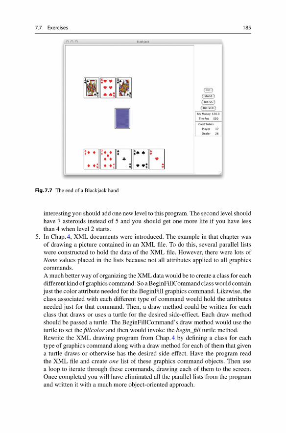
7.7 Exercises 185
Fig. 7.7 The end of a Blackjack hand
interesting you should add one new level to this program. The second level should
have 7 asteroids instead of 5 and you should get one more life if you have less
than 4 when level 2 starts.
5. In Chap. 4, XML documents were introduced. The example in that chapter was
of drawing a picture contained in an XML file. To do this, several parallel lists
were constructed to hold the data of the XML file. However, there were lots of
None values placed in the lists because not all attributes applied to all graphics
commands.
A much better way of organizing the XML data would be to create a class for each
different kind of graphics command. So a BeginFillCommand class would contain
just the color attribute needed for the BeginFill graphics command. Likewise, the
class associated with each different type of command would hold the attributes
needed just for that command. Then, a draw method could be written for each
class that draws or uses a turtle for the desired side-effiect. Each draw method
should be passed a turtle. The BeginFillCommand’s draw method would use the
turtle to set the fillcolor and then would invoke the begin_fill turtle method.
Rewrite the XML drawing program from Chap. 4 by defining a class for each
type of graphics command along with a draw method for each of them that given
a turtle draws or otherwise has the desired side-effect. Have the program read
the XML file and create one list of these graphics command objects. Then use
a loop to iterate through these commands, drawing each of them to the screen.
Once completed you will have eliminated all the parallel lists from the program
and written it with a much more object-oriented approach.

186 7 Defining Classes
Fig. 7.8 Asteroids!
7.8 Solutions to Practice Problems
These are solutions to the practice problems in this chapter. You should only consult
these answers after you have tried each of them for yourself first. Practice problems
are meant to help reinforce the material you have just read so make use of them.
7.8.1 Solutions to Practice Problem 7.1
A numerator and denominator are needed.
1 c l a s s Rational:
2 d e f __init__(self ,num=0,den =1):
3 self.num = num
4 self.den = den
7.8.2 Solutions to Practice Problem 7.2
1 c l a s s Rectangle(Shape ):
2 d e f __init__(self ,x,y,width ,height ,color="transparent", \
3 outline="black",edgeWidth =1):
4 self.x = x
5 self.y = y
6 self.color = color
7 self.outline = outline
8 self.edgeWidth = edgeWidth

7.8 Solutions to Practice Problems 187
9 self.width = width
10 self.height = height
7.8.3 Solutions to Practice Problem 7.3
1 d e f draw(self ,turtle ):
2 turtle.penup ()
3 turtle.goto(self.x,self.y)
4 turtle.setheading (0)
5 turtle.pendown ()
6 turtle.width(self.edgeWidth)
7 turtle.color(self.outline)
8 turtle.fillcolor(self.color)
9 i f self.color != "transparent":
10 turtle.begin_fill ()
11 turtle.pendown ()
12 turtle.forward(self.width)
13 turtle.left (90)
14 turtle.forward(self.height)
15 turtle.left (90)
16 turtle.forward(self.width)
17 turtle.left (90)
18 turtle.forward(self.height)
19 turtle.left (90)
20 i f self.color != "transparent":
21 turtle.end_fill ()
22 turtle.penup ()
7.8.4 Solutions to Practice Problem 7.4
Download code and try it out. Here is the Rectangle class in case you had trouble
with defining it.
1 c l a s s Rectangle(Shape ):
2 d e f __init__(self ,x,y,width ,height ,color="transparent", \
3 outline="black",edgeWidth =1):
4 s u p e r ().__init__(x,y,color ,outline ,edgeWidth)
5
6 self.width = width
7 self.height = height
8
9 d e f draw(self ,turtle ):
10 turtle.penup ()
11 turtle.goto(self.x,self.y)
12 turtle.setheading (0)
13 turtle.pendown ()
14 turtle.width(self.edgeWidth)
15 turtle.color(self.outline)
16 turtle.fillcolor(self.color)
17 i f self.color != "transparent":
18 turtle.begin_fill ()
19 turtle.pendown ()
20 turtle.forward(self.width)
21 turtle.left (90)
22 turtle.forward(self.height)
23 turtle.left (90)
24 turtle.forward(self.width)
25 turtle.left (90)
26 turtle.forward(self.height)
27 turtle.left (90)

188 7 Defining Classes
28 i f self.color != "transparent":
29 turtle.end_fill ()
30 turtle.penup ()
7.8.5 Solutions to Practice Problem 7.5
Create some GravityBall objects and add them to the ballList. That’s all that needs to
be done to have gravity balls and regular balls bouncing around with each other. The
object on the left hand side of the dot in the ball ball.move is where polymorphism
is at work. If ball is pointing to a Ball object, it behaves as a Ball would. If ball is
pointing to a GravityBall object, then ball.move is the GravityBall move method. It’s
not the name on the left hand side of the dot, its the object that the name refers to
that controls which methods are called.

8Appendix A: Integer Operators
This documentation was generated from the Python documentation available by
typing help(int) in the Python shell. In this documentation the variables x, y, and z
refer to integers (Table 8.1).
Table 8.1 Integer operators
Operator Returns Comments
x + y int Returns the sum of x and y
x − y int Returns the difference of x and y
x*y int Returns the product of x and y
x/y float Returns the quotient of x divided by y
x//y int Returns the integer quotient of x divided by y
x % y int Returns x modulo y. This is the remainder of dividing x by y
−x int Returns the negation of x
x&y int Returns the bit-wise and of x and y
x | y int Returns the bit-wise or of x and y
x ˆ y int Returns the bit-wise exclusive or of x and y
x ≪ y int Returns a bit-wise shift left of x by y bits. Shifting left by 1 bit multiplies
x by 2
x ≫ y int Returns a bit-wise right shift of x by y bits
˜ x int Returns an integer where each bit in the x has been inverted. x + x = −1
for all x
abs(x) int Returns the absolute value of x
divmod(x, y) (q,r) Returns the quotient q and the remainder r as a tuple
float(x) float Returns the float representation of x
hex(x) str Returns a hexadecimal representation of x as a string
int(x) int Returns x
(continued)
© Springer-Verlag London 2014
K.D. Lee, Python Programming Fundamentals,
Undergraduate Topics in Computer Science, DOI 10.1007/978-1-4471-6642-9_8
189

190 8 Appendix A: Integer Operators
Table 8.1 (continued)
Operator Returns Comments
oct(x) str Return an octal representation of x as a string
pow(x, y[, z]) int Returns x to the y power modulo z. If z is not specified then it returns x
to the y power
repr(x) str Returns a string representation of x
str(x) str Returns a string representation of x

9Appendix B: Float Operators
This documentation was generated from the Python documentation available by
typing help(float) in the Python shell. In this documentation at least one of the
variables x and y refer to floats (Table 9.1).
Table 9.1 Float operators
Operator Returns Comments
x + y float Returns the sum of x and y
x − y float Returns the difference of x and y
x*y float Returns the product of x and y
x/y float Returns the quotient of x divided by y
x//y float Returns the quotient of integer division of x divided by y. However, the
result is still a float
x % y float Returns x modulo y. This is the remainder of dividing x by y
abs(x) int Returns the absolute value of x
divmod(x, y) (q,r) Returns the quotient q and the remainder r as a tuple. Both q and r are
floats, but integer division is performed. The value r is the whole and
fractional part of any remainder. The value q is a whole number
float(x) float Returns the float representation of x
int(x) int Returns the floor of x as an integer
pow(x, y) float Returns x to the y power
repr(x) str Returns a string representation of x
str(x) str Returns a string representation of x
© Springer-Verlag London 2014
K.D. Lee, Python Programming Fundamentals,
Undergraduate Topics in Computer Science, DOI 10.1007/978-1-4471-6642-9_9
191

10Appendix C: String Operatorsand Methods
This documentation was generated from the Python documentation available by
typing help(str) in the Python shell. In the documentation found here the variables s
and t are references to strings (Table 10.1).
Table 10.1 String operators and methods
Operator Returns Comments
s+t str Return a new string which is the concatenation of s and t
s in t bool Returns True if s is a substring of t and False otherwise
s==t bool Returns True if s and t refer to strings with the same sequence of characters
s>=t bool Returns True if s is lexicographically greater than or equal to t
s<=t bool Returns True if s is lexicographically less than or equal to t
s>t bool Returns True if s is lexicographically greater than t
s<t bool Returns True if s is lexicographically less than t
s!=t bool Returns True if s is lexicographically not equal to t
s[i] str Returns the character at index i in the string. If i is negative then it returns the
character at index len(s)−i
s[[i]:[j]] str Returns the slice of characters starting at index i and extending to index j−1
in the string. If i is omitted then the slice begins at index 0. If j is omitted then
the slice extends to the end of the list. If i is negative then it returns the slice
starting at index len(s)+i (and likewise for the slice ending at j)
s ∗ i str Returns a new string with s repeated i times
i ∗ s str Returns a new string with s repeated i times
chr(i) str Return the ASCII character equivalent of the integer i
float(s) float Returns the float contained in the string s
int(s) int Returns the integer contained in the string s
len(s) int Returns the number of characters in s
ord(s) int Returns the ASCII decimal equivalent of the single character string s
(continued)
© Springer-Verlag London 2014
K.D. Lee, Python Programming Fundamentals,
Undergraduate Topics in Computer Science, DOI 10.1007/978-1-4471-6642-9_10
193

194 10 Appendix C: String Operators and Methods
Table 10.1 (continued)
Method Returns Comments
repr(s) Returns a string representation of s. This adds an
extra pair of quotes to s
str(s) str Returns a string representation of s. In this case you
get just the string s
s.capitalize() str Returns a copy of the string s with the first character
upper case
s.center(width[, fillchar]) str Returns s centered in a string of length width.
Padding is done using the specified fill character
(default is a space)
s.count(sub[, start[, end]]) int Returns the number of non-overlapping occurrences
of substring sub in string s[start:end]. Optional
arguments start and end are interpreted as in slice
notation
s.encode([encoding[, errors]]) bytes Encodes s using the codec registered for encoding.
encoding defaults to the default encoding. errors may
be given to set a different error handling scheme.
Default is ‘strict’ meaning that encoding errors raise
a UnicodeEncodeError. Other possible values are
‘ignore’, ‘replace’ and ‘xmlcharrefreplace’ as well as
any other name registered with codecs.register_error
that can handle UnicodeEncodeErrors
s.endswith(suffix[, start[, end]]) bool Returns True if s ends with the specified suffix, False
otherwise. With optional start, test s beginning at that
position. With optional end, stop comparing s at that
position. suffix can also be a tuple of strings to try
s.expandtabs([tabsize]) str Returns a copy of s where all tab characters are
expanded using spaces. If tabsize is not given, a tab
size of 8 characters is assumed
s.find(sub[, start[, end]]) int Returns the lowest index in s where substring sub is
found, such that sub is contained within s[start:end].
Optional arguments start and end are interpreted as
in slice notation.
Return −1 on failure
s.format(*args, **kwargs) str
s.index(sub[, start[, end]]) int Like s.find() but raise ValueError when the substring
is not found
s.isalnum() bool Returns True if all characters in s are alphanumeric
and there is at least one character in s, False
otherwise
s.isalpha() bool Returns True if all characters in s are alphabetic and
there is at least one character in s, False otherwise
s.isdecimal() bool Returns True if there are only decimal characters in
s, False otherwise
(continued)

10 Appendix C: String Operators and Methods 195
Table 10.1 (continued)
Method Returns Comments
s.isdigit() bool Returns True if all characters in s are digits and there is
at least one character in s, False otherwise
s.isidentifier() bool Returns True if s is a valid identifier according to the
language definition
s.islower() bool Returns True if all cased characters in s are lowercase
and there is at least one cased character in s, False
otherwise
s.isnumeric() bool Returns True if there are only numeric characters in s,
False otherwise
s.isprintable() bool Returns True if all characters in s are considered
printable in repr() or s is empty, False otherwise
s.isspace() bool Returns True if all characters in s are whitespace and
there is at least one character in s, False otherwise
s.istitle() bool Returns True if s is a titlecased string and there is at least
one character in s, i.e. upper- and titlecase characters
may only follow uncased characters and lowercase
characters only cased ones. Return False otherwise
s.isupper() bool Returns True if all cased characters in s are uppercase
and there is at least one cased character in s, False
otherwise
s.join(sequence) str Returns a string which is the concatenation of the strings
in the sequence. The separator between elements is s
s.ljust(width[, fillchar]) str Returns s left-justified in a Unicode string of length
width. Padding is done using the specified fill character
(default is a space)
s.lower() str Returns a copy of the string s converted to lowercase
s.lstrip([chars]) str Returns a copy of the string s with leading whitespace
removed. If chars is given and not None, remove
characters in chars instead
s.partition(sep) (h,sep,t) Searches for the separator sep in s, and returns the part
before it, the separator itself, and the part after it. If the
separator is not found, returns s and two empty strings
s.replace (old, new[, count]) str Returns a copy of s with all occurrences of substring old
replaced by new. If the optional argument count is given,
only the first count occurrences are replaced
s.rfind(sub[, start[, end]]) int Returns the highest index in s where substring sub is
found, such that sub is contained within s[start:end].
Optional arguments start and end are interpreted as in
slice notation.
Returns −1 on failure
s.rindex(sub[, start[, end]]) int Like s.rfind() but raise ValueError when the substring is
not found
(continued)

196 10 Appendix C: String Operators and Methods
Table 10.1 (continued)
Method Returns Comments
s.rjust(width[, fillchar]) str Returns s right-justified in a string of length width.
Padding is done using the specified fill character (default
is a space)
s.rpartition(sep) (t,sep,h) Searches for the separator sep in s, starting at the end of
s, and returns the part before it, the separator itself, and
the part after it. If the separator is not found, returns two
empty strings and s
s.rsplit([sep[,
maxsplit]])
string list Returns a list of the words in s, using sep as the
delimiter string, starting at the end of the string and
working to the front. If maxsplit is given, at most
maxsplit splits are done. If sep is not specified, any
whitespace string is a separator
s.rstrip([chars]) str Returns a copy of the string s with trailing whitespace
removed. If chars is given and not None, removes
characters in chars instead
s.split([sep[, maxsplit]]) string list Returns a list of the words in s, using sep as the
delimiter string. If maxsplit is given, at most maxsplit
splits are done. If sep is not specified or is None, any
whitespace string is a separator and empty strings are
removed from the result
s.splitlines([keepends]) string list Returns a list of the lines in s, breaking at line
boundaries. Line breaks are not included in the resulting
list unless keepends is given and true
s.startswith
(prefix[, start[, end]])
bool Returns True if s starts with the specified prefix, False
otherwise. With optional start, test s beginning at that
position. With optional end, stop comparing s at that
position. Prefix can also be a tuple of strings to try
s.strip([chars]) str Returns a copy of the string s with leading and trailing
whitespace removed. If chars is given and not None,
removes characters in chars instead.
s.swapcase() str Returns a copy of s with uppercase characters converted
to lowercase and vice versa
s.title() str Returns a titlecased version of s, i.e. words start with
title case characters, all remaining cased characters have
lower case
s.translate(table) str Returns a copy of the string s, where all characters have
been mapped through the given translation table, which
must be a mapping of Unicode ordinals to Unicode
ordinals, strings, or None. Unmapped characters are left
untouched. Characters mapped to None are deleted
s.upper() str Returns a copy of s converted to uppercase
s.zfill(width) str Pad a numeric string s with zeros on the left, to fill a field
of the specified width. The string s is never truncated

11Appendix D: List Operatorsand Methods
This documentation was generated from the Python documentation available by
typing help(list) in the Python shell. In the documentation found here the variables
x and y are references to lists (Table 11.1).
Table 11.1 List operators and methods
Method Returns Comments
list() list Returns a new empty list. You can also use [] to initialize a new
empty list
list(sequence) list Returns new list initialized from sequence’s items
[ item [,item]+ ] list Writing a number of comma-separated items in square brackets
constructs a new list of those items
x+y list Returns a new list containing the concatenation of the items in x
and y
e in x bool Returns True if the item e is in x and False otherwise
del x[i] Deletes the item at index i in x. This is not an expression and does
not return a value
x==y bool Returns True if x and y contain the same number of items and each
of those corresponding items are pairwise equal
x>=y bool Returns True if x is greater than or equal to y according to a
lexicographical ordering of the elements in x and y. If x and y have
different lengths their items are == up to the shortest length, then
this returns True if x is longer than y
x<=y bool Returns True if x is lexicographically before y or equal to y and
False otherwise
x>y bool Returns True if x is lexicographically after y and False otherwise
x<y bool Returns True if x is lexicographically before y and False otherwise
x!=y bool Returns True if x and y are of different length or if some item of x
is not == to some item of y. Otherwise it returns False
(continued)
© Springer-Verlag London 2014
K.D. Lee, Python Programming Fundamentals,
Undergraduate Topics in Computer Science, DOI 10.1007/978-1-4471-6642-9_11
197

198 11 Appendix D: List Operators and Methods
Table 11.1 (continued)
Method Returns Comments
x[i] item Returns the item at index i of x
x[[i]:[j]] list Returns the slice of items starting at index i and extending to index
j−1 in the string. If i is omitted then the slice begins at index 0. If j
is omitted then the slice extends to the end of the list. If i is
negative then it returns the slice starting at index len(x)+i (and
likewise for the slice ending at j)
x[i]=e Assigns the position at index i the value of e in x. The list x must
already have an item at index i before this assignment occurs. In
other words, assigning an item to a list in this way will not extend
the length of the list to accommodate it
x+=y This mutates the list x to append the items in y
x*=i This mutates the list x to be i copies of the original x
iter(x) iterator Returns an iterator over x
len(x) int Returns the number of items in x
x*i list Returns a new list with the items of x repeated i times
i*x list Returns a new list with the items of x repeated i times
repr(x) str Returns a string representation of x
x.append(e) None This mutates the value of x to add e as its last element. The function
returns None, but the return value is irrelevant since it mutates x
x.count(e) int Returns the number of occurrences of e in x by using == equality
x.extend(iter) None Mutates x by appending elements from the iterable, iter
x.index(e,[i,[j]]) int Returns the first index of an element that == e between the start
index, i, and the stop index, j−1. It raises ValueError if the value is
not present in the specified sequence. If j is omitted then it searches
to the end of the list. If i is omitted then it searches from the
beginning of the list
x.insert(i, e) None Insert e before index i in x, mutating x
x.pop([index]) item Remove and return the item at index. If index is omitted then the
item at len(x)−1 is removed. The pop method returns the item and
mutates x. It raises IndexError if list is empty or index is out of
range
x.remove(e) None remove first occurrence of e in x, mutating x. It raises ValueError if
the value is not present
x.reverse() None Reverses all the items in x, mutating x
x.sort() None Sorts all the items of x according to their natural ordering as
determined by the item’s _ _cmp_ _ method, mutating x. Two
keyword parameters are possible: key and reverse. If reverse =
True is specified, then the result of sorting will have the list in
reverse of the natural ordering. If key = f is specified then f must
be a function that takes an item of x and returns the value of that
item that should be used as the key when sorting

12Appendix E: Dictionary Operatorsand Methods
This documentation was generated from the Python documentation available by
typing help(dict) in the Python shell. In the documentation found here the variable D is
a reference to a dictionary. A few methods were omitted here for brevity (Table 12.1).
Table 12.1 Dictionary operators and methods
Method Returns Comments
dict() dict New empty dictionary
dict(mapping) dict New dictionary initialized from a mapping object’s (key, value)
pairs
dict(seq) dict New dictionary initialized as if via
D = {}
for k, v in seq
D[k] = v
dict(**kwargs) dict New dictionary initialized with the name = value pairs
in the keyword arg list. For example: dict(one = 1, two = 2)
k in D bool True if D has key k, else False
del D[k] Deletes key k from dictionary D
D1== 2 bool Returns True if dictionaries D1 and D2 have same keys mapped to
same values
D[k] value Returns value k maps to in D. If k is not mapped, it
type raises a KeyError exception
iter(D) iterator Returns an iterator over D
len(D) int Returns the number of keys in D
D1!=D2 bool Returns True if D1 and D2 have any different keys or keys map to
different values
repr(D) str Returns a string representation of D
D[k]=e – Stores the key,value pair k,e in D
(continued)
© Springer-Verlag London 2014
K.D. Lee, Python Programming Fundamentals,
Undergraduate Topics in Computer Science, DOI 10.1007/978-1-4471-6642-9_12
199

200 12 Appendix E: Dictionary Operators and Methods
Table 12.1 (continued)
Method Returns Comments
D.clear() None Remove all items from D
D.copy() dict A shallow copy of D
D.get(k[,e]) value D[k] if k in D, else e. e defaults to None
type
D.items() items A set-like object providing a view on D’s items
D.keys() keys A set-like object providing a view on D’s keys
D.pop(k[,e]) v Remove specified key and return the corresponding value. If
key is not found, e is returned if given, otherwise KeyError is
raised
D.popitem() (k, v) Remove and return some (key, value) pair as a 2-tuple; but raise
KeyError if D is empty
D.setdefault(k[,e]) D.get(k,e) Returns D.get(k,e) and also sets d[k] = e if k not in D
D.update(E, **F) None Update D from dict/iterable E and F
If E has a .keys() method, does: for k in E: D[k] = E[k]
If E lacks .keys() method, does: for (k, v) in E: D[k] = v
In either case, this is followed by: for k in F: D[k] = F[k]
D.values() values An object providing a view on D’s values

13Appendix F:Turtle Methods
This documentation was generated from the Python documentation available by
typing
f r o m turtle i m p o r t *
h e l p (Turtle)
in the Python shell. In the documentation found here the variable turtle is a ref-
erence to a Turtle object. This is a subset of that documentation. To see complete
documentation use the Python help system as described above.
Method Description
turtle.back(distance)
Aliases: backward bk
Argument:
distance – a number
Move the turtle backward by distance, opposite to the direction the
turtle is headed. Do not change the turtle’s heading.
Example (for a Turtle instance named turtle):
>>> turtle.position()
(0.00, 0.00)
>>> turtle.backward(30)
>>> turtle.position()
(-30.00, 0.00)
turtle.begin_fill()
Called just before drawing a shape to be filled.
Example (for a Turtle instance named turtle):
>>> turtle.color("black", "red")
>>> turtle.begin_fill()
>>> turtle.circle(60)
>>> turtle.end_fill()
© Springer-Verlag London 2014
K.D. Lee, Python Programming Fundamentals,
Undergraduate Topics in Computer Science, DOI 10.1007/978-1-4471-6642-9_13
201

202 13 Appendix F:Turtle Methods
Method Description
turtle.begin_poly()
Start recording the vertices of a polygon. Current turtle position
is first point of polygon.
Example (for a Turtle instance named turtle):
>>> turtle.begin_poly()
turtle.circle(radius, extent=None, steps=None)
Arguments:
radius – a number
extent (optional) – a number
steps (optional) – an integer
Draw a circle with given radius. The center is radius units left
of the turtle; extent - an angle - determines which part of the
circle is drawn. If extent is not given, draw the entire circle.
If extent is not a full circle, one endpoint of the arc is the
current pen position. Draw the arc in counterclockwise direction
if radius is positive, otherwise in clockwise direction. Finally
the direction of the turtle is changed by the amount of extent.
As the circle is approximated by an inscribed regular polygon,
steps determines the number of steps to use. If not given,
it will be calculated automatically. Maybe used to draw regular
polygons.
call: circle(radius) # full circle
–or: circle(radius, extent) # arc
–or: circle(radius, extent, steps)
–or: circle(radius, steps=6) # 6-sided polygon
Example (for a Turtle instance named turtle):
>>> turtle.circle(50)
>>> turtle.circle(120, 180) # semicircle
turtle.clear()
Delete the turtle’s drawings from the screen. Do not move turtle.
State and position of the turtle as well as drawings of other
turtles are not affected.
Examples (for a Turtle instance named turtle):
>>> turtle.clear()
turtle.color(*args)
Arguments:
Several input formats are allowed.
They use 0, 1, 2, or 3 arguments as follows:
color()

13 Appendix F:Turtle Methods 203
Method Description
Return the current pencolor and the current fillcolor
as a pair of color specification strings as are returned
by pencolor and fillcolor.
color(colorstring), color((r,g,b)), color(r,g,b)
inputs as in pencolor, set both, fillcolor and pencolor,
to the given value.
color(colorstring1, colorstring2),
color((r1,g1,b1), (r2,g2,b2))
equivalent to pencolor(colorstring1) and fillcolor(colorstring2)
and analogously, if the other input format is used.
If turtleshape is a polygon, outline and interior of that polygon
is drawn with the newly set colors.
For mor info see: pencolor, fillcolor
Example (for a Turtle instance named turtle):
>>>turtle.color(’red’, ’green’)
>>> turtle.color()
(’red’, ’green’)
>>> colormode(255)
>>> color((40, 80, 120), (160, 200, 240))
>>> color()
(’#285078’, ’#a0c8f0’)
turtle.degrees()
Set the angle measurement units to degrees.
Example (for a Turtle instance named turtle):
>>> turtle.heading()
1.5707963267948966
>>> turtle.degrees()
>>> turtle.heading()
90.0
turtle.dot(size=None, *color)
Optional arguments:
size – an integer > = 1 (if given)
color – a colorstring or a numeric color tuple
Draw a circular dot with diameter size, using color.
If size is not given, the maximum of pensize+4 and 2*pensize is used.
Example (for a Turtle instance named turtle):
>>> turtle.dot()
>>> turtle.fd(50); turtle.dot(20, "blue"); turtle.fd(50)
turtle.end_fill()
Fill the shape drawn after the call begin_fill().
Example (for a Turtle instance named turtle):
>>> turtle.color("black", "red")

204 13 Appendix F:Turtle Methods
Method Description
>>> turtle.begin_fill()
>>> turtle.circle(60)
>>> turtle.end_fill()
turtle.end_poly()
Stop recording the vertices of a polygon. Current turtle position is
last point of polygon. This will be connected with the first point.
Example (for a Turtle instance named turtle):
>>> turtle.end_poly()
turtle.filling()
Return fillstate (True if filling, False else).
Example (for a Turtle instance named turtle):
>>> turtle.begin_fill()
>>> if turtle.filling():
turtle.pensize(5)
else:
turtle.pensize(3)
turtle.fillcolor(*args)
Return or set the fillcolor.
Arguments:
Four input formats are allowed:
- fillcolor()
Return the current fillcolor as color specification string,
possibly in hex-number format (see example).
May be used as input to another color/pencolor/fillcolor call.
- fillcolor(colorstring)
s is a Tk color specification string, such as "red" or "yellow"
- fillcolor((r, g, b))
*a tuple* of r, g, and b, which represent, an RGB color,
and each of r, g, and b are in the range 0..colormode,
where colormode is either 1.0 or 255
- fillcolor(r, g, b)
r, g, and b represent an RGB color, and each of r, g, and b
are in the range 0..colormode
If turtleshape is a polygon, the interior of that polygon is drawn
with the newly set fillcolor.
Example (for a Turtle instance named turtle):
>>> turtle.fillcolor(’violet’)
>>> col = turtle.pencolor()
>>> turtle.fillcolor(col)
>>> turtle.fillcolor(0, .5, 0)

13 Appendix F:Turtle Methods 205
Method Description
turtle.forward(distance)
Aliases: fd
Argument:
distance – a number (integer or float)
Move the turtle forward by the specified distance, in the direction
the turtle is headed.
Example (for a Turtle instance named turtle):
>>> turtle.position()
(0.00, 0.00)
>>> turtle.forward(25)
>>> turtle.position()
(25.00,0.00)
>>> turtle.forward(-75)
>>> turtle.position()
(-50.00,0.00)
turtle.get_poly()
Return the lastly recorded polygon.
Example (for a Turtle instance named turtle):
>>> p = turtle.get_poly()
>>> turtle.register_shape("myFavouriteShape", p)
turtle.get_shapepoly()
Return the current shape polygon as tuple of coordinate pairs.
Examples (for a Turtle instance named turtle):
>>> turtle.shape("square")
>>> turtle.shapetransform(4, -1, 0, 2)
>>> turtle.get_shapepoly()
((50, -20), (30, 20), (-50, 20), (-30, -20))
turtle.getscreen()
Return the TurtleScreen object, the turtle is drawing on.
So TurtleScreen-methods can be called for that object.
Example (for a Turtle instance named turtle):
>>> ts = turtle.getscreen()
>>> ts
<turtle.TurtleScreen object at 0x0106B770>
>>> ts.bgcolor("pink")
turtle.goto(x, y=None)
Aliases: setpos setposition
Arguments:
x – a number or a pair/vector of numbers
y – a number None
call: goto(x, y) # two coordinates

206 13 Appendix F:Turtle Methods
Method Description
–or: goto((x, y)) # a pair (tuple) of coordinates
–or: goto(vec) # e.g. as returned by pos()
Move turtle to an absolute position. If the pen is down,
a line will be drawn. The turtle’s orientation does not change.
Example (for a Turtle instance named turtle):
>>> tp = turtle.pos()
>>> tp
(0.00, 0.00)
>>> turtle.setpos(60,30)
>>> turtle.pos()
(60.00,30.00)
>>> turtle.setpos((20,80))
>>> turtle.pos()
(20.00,80.00)
>>> turtle.setpos(tp)
>>> turtle.pos()
(0.00,0.00)
turtle.heading()
Return the turtle’s current heading.
Example (for a Turtle instance named turtle):
>>> turtle.left(67)
>>> turtle.heading()
67.0
turtle.hideturtle()
Makes the turtle invisible.
Aliases: ht
It’s a good idea to do this while you’re in the
middle of a complicated drawing, because hiding
the turtle speeds up the drawing observably.
Example (for a Turtle instance named turtle):
>>> turtle.hideturtle()
turtle.isdown()
Return True if pen is down, False if it’s up.
Example (for a Turtle instance named turtle):
>>> turtle.penup()
>>> turtle.isdown()
False
>>> turtle.pendown()
>>> turtle.isdown()
True

13 Appendix F:Turtle Methods 207
Method Description
turtle.isvisible()
Return True if the Turtle is shown, False if it’s hidden.
Example (for a Turtle instance named turtle):
>>> turtle.hideturtle()
>>> print(turtle.isvisible())
False
turtle.left(angle)
Aliases: lt
Argument:
angle – a number (integer or float)
Turn turtle left by angle units. (Units are by default degrees,
but can be set via the degrees() and radians() functions.)
Angle orientation depends on mode. (See this.)
Example (for a Turtle instance named turtle):
>>> turtle.heading()
22.0
>>> turtle.left(45)
>>> turtle.heading()
67.0
turtle.onclick(fun, btn=1, add=None)
Bind fun to mouse-click event on this turtle on canvas.
Arguments:
fun – a function with two arguments, to which will be assigned
the coordinates of the clicked point on the canvas.
num – number of the mouse-button defaults to 1 (left mouse button).
add – True or False. If True, new binding will be added, otherwise
it will replace a former binding.
Example for the anonymous turtle, i. e. the procedural way:
>>> def turn(x, y):
turtle.left(360)
>>> onclick(turn) # Now clicking into the turtle will turn it.
>>> onclick(None) # event-binding will be removed
turtle.ondrag(fun, btn=1, add=None)
Bind fun to mouse-move event on this turtle on canvas.
Arguments:
fun – a function with two arguments, to which will be assigned
the coordinates of the clicked point on the canvas.

208 13 Appendix F:Turtle Methods
Method Description
num – number of the mouse-button defaults to 1 (left mouse button).
Every sequence of mouse-move-events on a turtle is preceded by a
mouse-click event on that turtle.
Example (for a Turtle instance named turtle):
>>> turtle.ondrag(turtle.goto)
### Subsequently clicking and dragging a Turtle will
### move it across the screen thereby producing handdrawings
### (if pen is down).
turtle.onrelease(fun, btn=1, add=None)
Bind fun to mouse-button-release event on this turtle on canvas.
Arguments:
fun – a function with two arguments, to which will be assigned
the coordinates of the clicked point on the canvas.
num – number of the mouse-button defaults to 1 (left mouse button).
turtle.pencolor(*args)
Return or set the pencolor.
Arguments:
Four input formats are allowed:
- pencolor()
Return the current pencolor as color specification string,
possibly in hex-number format (see example).
May be used as input to another color/pencolor/fillcolor call.
- pencolor(colorstring)
s is a Tk color specification string, such as "red" or "yellow"
- pencolor((r, g, b))
*a tuple* of r, g, and b, which represent, an RGB color,
and each of r, g, and b are in the range 0..colormode,
where colormode is either 1.0 or 255
- pencolor(r, g, b)
r, g, and b represent an RGB color, and each of r, g, and b
are in the range 0..colormode
If turtleshape is a polygon, the outline of that polygon is drawn
with the newly set pencolor.
Example (for a Turtle instance named turtle):
>>> turtle.pencolor(’brown’)
>>> tup = (0.2, 0.8, 0.55)
>>> turtle.pencolor(tup)
>>> turtle.pencolor()
’#33cc8c’

13 Appendix F:Turtle Methods 209
Method Description
turtle.pendown()
Pull the pen down – drawing when moving.
Aliases: pd down
Example (for a Turtle instance named turtle):
>>> turtle.pendown()
turtle.pensize(width=None)
Set or return the line thickness.
Aliases: width
Argument:
width – positive number
Set the line thickness to width or return it. If resizemode is set
to "auto" and turtleshape is a polygon, that polygon is drawn with
the same line thickness. If no argument is given, current pensize
is returned.
Example (for a Turtle instance named turtle):
>>> turtle.pensize()
1
turtle.pensize(10) # from here on lines of width 10 are drawn
turtle.penup()
Pull the pen up – no drawing when moving.
Aliases: pu up
Example (for a Turtle instance named turtle):
>>> turtle.penup()
turtle.radians()
Set the angle measurement units to radians.
Example (for a Turtle instance named turtle):
>>> turtle.heading()
90
>>> turtle.radians()
>>> turtle.heading()
1.5707963267948966
turtle.reset()
Delete the turtle’s drawings from the screen, re-center the turtle
and set variables to the default values.
Example (for a Turtle instance named turtle):
>>> turtle.position()
(0.00,-22.00)
>>> turtle.heading()

210 13 Appendix F:Turtle Methods
Method Description
100.0
>>> turtle.reset()
>>> turtle.position()
(0.00,0.00)
>>> turtle.heading()
0.0
turtle.setheading(to_angle)
Set the orientation of the turtle to to_angle.
Aliases: seth
Argument:
to_angle – a number (integer or float)
Set the orientation of the turtle to to_angle.
Here are some common directions in degrees:
standard - mode: logo-mode:
—————————————
0 - east 0 - north
90 - north 90 - east
180 - west 180 - south
270 - south 270 - west
Example (for a Turtle instance named turtle):
>>> turtle.setheading(90)
>>> turtle.heading()
90
turtle.shape(name=None)
Set turtle shape to shape with given name / return current shapename.
Optional argument:
name – a string, which is a valid shapename
Set turtle shape to shape with given name or, if name is not given,
return name of current shape.
Shape with name must exist in the TurtleScreen’s shape dictionary.
Initially there are the following polygon shapes:
’arrow’, ’turtle’, ’circle’, ’square’, ’triangle’, ’classic’.
To learn about how to deal with shapes see Screen-method register_shape.
Example (for a Turtle instance named turtle):
>>> turtle.shape()
’arrow’
>>> turtle.shape("turtle")
>>> turtle.shape()
’turtle’

13 Appendix F:Turtle Methods 211
Method Description
turtle.showturtle()
Makes the turtle visible.
Aliases: st
Example (for a Turtle instance named turtle):
>>> turtle.hideturtle()
>>> turtle.showturtle()
turtle.speed(speed=None)
Return or set the turtle’s speed.
Optional argument:
speed – an integer in the range 0..10 or a speedstring (see below)
Set the turtle’s speed to an integer value in the range 0 .. 10.
If no argument is given: return current speed.
If input is a number greater than 10 or smaller than 0.5,
speed is set to 0.
Speedstrings are mapped to speedvalues in the following way:
’fastest’ : 0
’fast’ : 10
’normal’ : 6
’slow’ : 3
’slowest’ : 1
speeds from 1 to 10 enforce increasingly faster animation of
line drawing and turtle turning.
Attention:
speed = 0 : *no* animation takes place. forward/back makes turtle jump
and likewise left/right make the turtle turn instantly.
Example (for a Turtle instance named turtle):
>>> turtle.speed(3)
turtle.undo()
Undo (repeatedly) the last turtle action.
Number of available undo actions is determined by the size of
the undobuffer.
Example (for a Turtle instance named turtle):
>>> for i in range(4):
turtle.fd(50); turtle.lt(80)
>>> for i in range(8):
turtle.undo()

212 13 Appendix F:Turtle Methods
Method Description
turtle.write(arg, move=False, align=’left’, font=(’Arial’, 8, ’normal’))
Write text at the current turtle position.
Arguments:
arg – info, which is to be written to the TurtleScreen
move (optional) – True/False
align (optional) – one of the strings "left", "center" or right"
font (optional) – a triple (fontname, fontsize, fonttype)
Write text - the string representation of arg - at the current
turtle position according to align ("left", "center" or right")
and with the given font.
If move is True, the pen is moved to the bottom-right corner
of the text. By default, move is False.
Example (for a Turtle instance named turtle):
>>> turtle.write(’Home = ’, True, align="center")
>>> turtle.write((0,0), True)
turtle.xcor()
Return the turtle’s x coordinate.
Example (for a Turtle instance named turtle):
>>> reset()
>>> turtle.left(60)
>>> turtle.forward(100)
>>> print(turtle.xcor())
50.0
turtle.ycor()
Return the turtle’s y coordinate
Example (for a Turtle instance named turtle):
>>> reset()
>>> turtle.left(60)
>>> turtle.forward(100)
>>> print(turtle.ycor())
86.6025403784
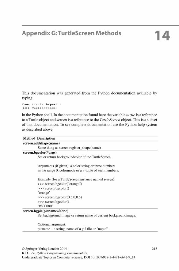
14Appendix G:TurtleScreen Methods
This documentation was generated from the Python documentation available by
typing
f r o m turtle i m p o r t *
h e l p (TurtleScreen)
in the Python shell. In the documentation found here the variable turtle is a reference
to a Turtle object and screen is a reference to the TurtleScreen object. This is a subset
of that documentation. To see complete documentation use the Python help system
as described above.
Method Description
screen.addshape(name)
Same thing as screen.register_shape(name)
screen.bgcolor(*args)
Set or return backgroundcolor of the TurtleScreen.
Arguments (if given): a color string or three numbers
in the range 0..colormode or a 3-tuple of such numbers.
Example (for a TurtleScreen instance named screen):
>>> screen.bgcolor("orange")
>>> screen.bgcolor()
’orange’
>>> screen.bgcolor(0.5,0,0.5)
>>> screen.bgcolor()
’#800080’
screen.bgpic(picname=None)
Set background image or return name of current backgroundimage.
Optional argument:
picname – a string, name of a gif-file or "nopic".
© Springer-Verlag London 2014
K.D. Lee, Python Programming Fundamentals,
Undergraduate Topics in Computer Science, DOI 10.1007/978-1-4471-6642-9_14
213

214 14 Appendix G:TurtleScreen Methods
Method Description
If picname is a filename, set the corresponing image as background.
If picname is "nopic", delete backgroundimage, if present.
If picname is None, return the filename of the current backgroundimage.
Example (for a TurtleScreen instance named screen):
>>> screen.bgpic()
’nopic’
>>> screen.bgpic("landscape.gif")
>>> screen.bgpic()
’landscape.gif’
screen.clear()
Delete all drawings and all turtles from the TurtleScreen.
Reset empty TurtleScreen to its initial state: white background,
no backgroundimage, no eventbindings and tracing on.
Example (for a TurtleScreen instance named screen):
screen.clear()
Note: this method is not available as function.
screen.colormode(cmode=None)
Return the colormode or set it to 1.0 or 255.
Optional argument:
cmode – one of the values 1.0 or 255
r, g, b values of colortriples have to be in range 0..cmode.
Example (for a TurtleScreen instance named screen):
>>> screen.colormode()
1.0
>>> screen.colormode(255)
>>> turtle.pencolor(240,160,80)
screen.delay(delay=None)
Return or set the drawing delay in milliseconds.
Optional argument:
delay – positive integer
Example (for a TurtleScreen instance named screen):
>>> screen.delay(15)
>>> screen.delay()
15

14 Appendix G:TurtleScreen Methods 215
Method Description
screen.getcanvas()
Return the Canvas of this TurtleScreen.
Example (for a Screen instance named screen):
>>> cv = screen.getcanvas()
>>> cv
<turtle.ScrolledCanvas instance at 0x010742D8>
screen.getshapes()
Return a list of names of all currently available turtle shapes.
Example (for a TurtleScreen instance named screen):
>>> screen.getshapes()
[’arrow’, ’blank’, ’circle’, ... , ’turtle’]
screen.listen(xdummy=None, ydummy=None)
Set focus on TurtleScreen (in order to collect key-events)
Dummy arguments are provided in order
to be able to pass listen to the onclick method.
Example (for a TurtleScreen instance named screen):
>>> screen.listen()
screen.mode(mode=None)
Set turtle-mode (’standard’, ’logo’ or ’world’) and perform reset.
Optional argument:
mode – on of the strings ’standard’, ’logo’ or ’world’
Mode ’standard’ is compatible with turtle.py.
Mode ’logo’ is compatible with most Logo-Turtle-Graphics.
Mode ’world’ uses userdefined ’worldcoordinates’. *Attention*: in
this mode angles appear distorted if x/y unit-ratio doesn’t equal 1.
If mode is not given, return the current mode.
Mode Initial turtle heading positive angles
——————————————————–
’standard’ to the right (east) counterclockwise
’logo’ upward (north) clockwise
Examples:
>>> mode(’logo’) # resets turtle heading to north
>>> mode()
’logo’
screen.onclick(fun, btn=1, add=None)
Bind fun to mouse-click event on canvas.
Arguments:
fun – a function with two arguments, the coordinates of the
clicked point on the canvas.
num – the number of the mouse-button, defaults to 1

216 14 Appendix G:TurtleScreen Methods
Method Description
Example (for a TurtleScreen instance named screen
and a Turtle instance named turtle):
>>> screen.onclick(turtle.goto)
### Subsequently clicking into the TurtleScreen will
### make the turtle move to the clicked point.
>>> screen.onclick(None)
### event-binding will be removed
screen.onkey(fun, key)
Bind fun to key-release event of key.
Arguments:
fun – a function with no arguments
key – a string: key (e.g. "a") or key-symbol (e.g. "space")
In order to be able to register key-events, TurtleScreen
must have focus. (See method listen.)
Example (for a TurtleScreen instance named screen
and a Turtle instance named turtle):
>>> def f():
turtle.fd(50)
turtle.lt(60)
>>> screen.onkey(f, "Up")
>>> screen.listen()
### Subsequently the turtle can be moved by
### repeatedly pressing the up-arrow key,
### consequently drawing a hexagon
screen.onkeypress(fun, key=None)
Bind fun to key-press event of key if key is given,
or to any key-press-event if no key is given.
Arguments:
fun – a function with no arguments
key – a string: key (e.g. "a") or key-symbol (e.g. "space")
In order to be able to register key-events, TurtleScreen
must have focus. (See method listen.)
Example (for a TurtleScreen instance named screen
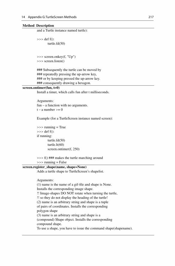
14 Appendix G:TurtleScreen Methods 217
Method Description
and a Turtle instance named turtle):
>>> def f():
turtle.fd(50)
>>> screen.onkey(f, "Up")
>>> screen.listen()
### Subsequently the turtle can be moved by
### repeatedly pressing the up-arrow key,
### or by keeping pressed the up-arrow key.
### consequently drawing a hexagon.
screen.ontimer(fun, t=0)
Install a timer, which calls fun after t milliseconds.
Arguments:
fun – a function with no arguments.
t – a number >= 0
Example (for a TurtleScreen instance named screen):
>>> running = True
>>> def f():
if running:
turtle.fd(50)
turtle.lt(60)
screen.ontimer(f, 250)
>>> f() ### makes the turtle marching around
>>> running = False
screen.register_shape(name, shape=None)
Adds a turtle shape to TurtleScreen’s shapelist.
Arguments:
(1) name is the name of a gif-file and shape is None.
Installs the corresponding image shape.
!! Image-shapes DO NOT rotate when turning the turtle,
!! so they do not display the heading of the turtle!
(2) name is an arbitrary string and shape is a tuple
of pairs of coordinates. Installs the corresponding
polygon shape
(3) name is an arbitrary string and shape is a
(compound) Shape object. Installs the corresponding
compound shape.
To use a shape, you have to issue the command shape(shapename).

218 14 Appendix G:TurtleScreen Methods
Method Description
call: register_shape("turtle.gif")
–or: register_shape("tri", ((0,0), (10,10), (-10,10)))
Example (for a TurtleScreen instance named screen):
>>> screen.register_shape("triangle", ((5,-3),(0,5),(- 5,-3)))
screen.reset()
Reset all Turtles on the Screen to their initial state.
Example (for a TurtleScreen instance named screen):
>>> screen.reset()
screen.screensize(canvwidth=None, canvheight=None, bg=None)
Resize the canvas the turtles are drawing on.
Optional arguments:
canvwidth – positive integer, new width of canvas in pixels
canvheight – positive integer, new height of canvas in pixels
bg – colorstring or color-tupel, new backgroundcolor
If no arguments are given, return current (canvaswidth, canvasheight)
Do not alter the drawing window. To observe hidden parts of
the canvas use the scrollbars. (Can make visible those parts
of a drawing, which were outside the canvas before!)
Example (for a Turtle instance named turtle):
>>> turtle.screensize(2000,1500)
### e. g. to search for an erroneously escaped turtle ;-
screen.setworldcoordinates(llx, lly, urx, ury)
Set up a user defined coordinate-system.
Arguments:
llx – a number, x-coordinate of lower left corner of canvas
lly – a number, y-coordinate of lower left corner of canvas
urx – a number, x-coordinate of upper right corner of canvas
ury – a number, y-coordinate of upper right corner of canvas
Set up user coodinat-system and switch to mode ’world’ if necessary.
This performs a screen.reset. If mode ’world’ is already active,
all drawings are redrawn according to the new coordinates.
But ATTENTION: in user-defined coordinatesystems angles may appear
distorted. (see Screen.mode())
Example (for a TurtleScreen instance named screen):
>>> screen.setworldcoordinates(-10,-0.5,50,1.5)
>>> for _ in range(36):
turtle.left(10)
turtle.forward(0.5)

14 Appendix G:TurtleScreen Methods 219
Method Description
screen.title(titlestr)
Set the title of the Turtle Graphics screen. The title appears in the title bar
of the window.
screen.tracer(n=None, delay=None)
Turns turtle animation on/off and set delay for update drawings.
Optional arguments:
n – nonnegative integer
delay – nonnegative integer
If n is given, only each n-th regular screen update is really performed.
(Can be used to accelerate the drawing of complex graphics.)
Second arguments sets delay value (see RawTurtle.delay())
Example (for a TurtleScreen instance named screen):
>>> screen.tracer(8, 25)
>>> dist = 2
>>> for i in range(200):
turtle.fd(dist)
turtle.rt(90)
dist += 2
screen.turtles()
Return the list of turtles on the screen.
Example (for a TurtleScreen instance named screen):
>>> screen.turtles()
[<turtle.Turtle object at 0x00E11FB0>]
screen.update()
Perform a TurtleScreen update.
screen.window_height()
Return the height of the turtle window.
Example (for a TurtleScreen instance named screen):
>>> screen.window_height()
480
screen.window_width()
Return the width of the turtle window.
Example (for a TurtleScreen instance named screen):
>>> screen.window_width()
640
screen.mainloop()
Starts event loop - calling Tkinter’s mainloop function.
Must be last statement in a turtle graphics program.
Must NOT be used if a script is run from within IDLE in -n mode
(No subprocess) - for interactive use of turtle graphics.

220 14 Appendix G:TurtleScreen Methods
Method Description
Example (for a TurtleScreen instance named screen):
>>> screen.mainloop()
screen.numinput(title, prompt, default=None, minval=None, maxval=None)
Pop up a dialog window for input of a number.
Arguments: title is the title of the dialog window,
prompt is a text mostly describing what numerical information to input.
default: default value
minval: minimum value for imput
maxval: maximum value for input
The number input must be in the range minval .. maxval if these are
given. If not, a hint is issued and the dialog remains open for
correction. Return the number input.
If the dialog is canceled, return None.
Example (for a TurtleScreen instance named screen):
>>> screen.numinput("Poker", "Your stakes:", 1000, minval=10, maxval=10000)
screen.textinput(title, prompt)
Pop up a dialog window for input of a string.
Arguments: title is the title of the dialog window,
prompt is a text mostly describing what information to input.
Return the string input
If the dialog is canceled, return None.
Example (for a TurtleScreen instance named screen):
>>> screen.textinput("NIM", "Name of first player:")

15Appendix H: The Reminder! Program
1 import sys
2 import tkinter
3 import tkinter.messagebox
4 import os
5
6 def addReminder(text ,x,y,notes ,reminders ):
7 notewin = tkinter.Toplevel ()
8 notewin.resizable(width=False ,height=False)
9 notewin.geometry("+"+str(x)+"+"+str(y))
10
11 reminder = tkinter.Text(notewin ,bg="yellow", width=30, height =15)
12
13 reminder.insert(tkinter.END ,text)
14
15 reminder.pack()
16
17 notes.append(notewin)
18 reminders.append(reminder)
19
20
21 def deleteWindowHandler ():
22 print("Window Deleted")
23 notewin.withdraw ()
24 notes.remove(notewin)
25 reminders.remove(reminder)
26
27 notewin.protocol("WM_DELETE_WINDOW", deleteWindowHandler)
28
29
30 def main ():
31
32 def post ():
33 print("Post")
34 addReminder(note.get("1.0",tkinter.END), \
35 root.winfo_rootx ()+5, root.winfo_rooty ()+5,notes ,reminders)
36 note.delete("1.0",tkinter.END)
37
38 root = tkinter.Tk()
39
40 root.title("Reminder!")
41 root.resizable(width=False ,height=False)
© Springer-Verlag London 2014
K.D. Lee, Python Programming Fundamentals,
Undergraduate Topics in Computer Science, DOI 10.1007/978-1-4471-6642-9_15
221

222 15 Appendix H:The Reminder! Program
42
43 notes = []
44 reminders = []
45
46 bar = tkinter.Menu(root)
47
48 fileMenu = tkinter.Menu(bar ,tearoff =0)
49 fileMenu.add_command(label="Exit",command=root.quit)
50 bar.add_cascade(label="File",menu=fileMenu)
51 root.config(menu=bar)
52
53 mainFrame = tkinter.Frame(root ,borderwidth =1,padx=5,pady =5)
54 mainFrame.pack()
55
56 note = tkinter.Text(mainFrame ,bg="yellow", width=30, height =15)
57 note.pack()
58
59 tkinter.Button(mainFrame ,text="New Reminder!", command=post).pack()
60
61 try:
62 print("reading reminders.txt file")
63 file = open("reminders.txt","r")
64 x = int(file.readline ())
65 y = int(file.readline ())
66 root.geometry("+"+str(x)+"+"+str(y))
67
68 line = file.readline ()
69 while line.strip() != "":
70 x = int(line)
71 y = int(file.readline ())
72 text = ""
73 line = file.readline ()
74 while line.strip() != "____ .... ____._._._":
75 text = text + line
76 line = file.readline ()
77
78 text = text.strip()
79
80 addReminder(text ,x,y,notes ,reminders)
81
82 line = file.readline ()
83 except:
84 print("reminders.txt not found")
85
86
87
88 def appClosing ():
89 print("Application Closing")
90 file = open("reminders.txt","w")
91
92 file.write(str(root.winfo_x ())+"\n")
93 file.write(str(root.winfo_y ())+"\n")
94
95 for i in range(len(notes )):
96 print(notes[i]. winfo_rootx ())
97 print(notes[i]. winfo_rooty ())
98 print(reminders[i].get("1.0",tkinter.END))
99
100 file.write(str(notes[i]. winfo_rootx ())+"\n")

15 Appendix H:The Reminder! Program 223
101 file.write(str(notes[i]. winfo_rooty ())+"\n")
102 file.write(reminders[i].get("1.0",tkinter.END)+"\n")
103 file.write("____ .... ____._._._\n")
104
105 file.close()
106 root.destroy ()
107 root.quit()
108 sys.exit()
109
110
111 root.protocol("WM_DELETE_WINDOW", appClosing)
112
113
114 tkinter.mainloop ()
115
116 if __name__ == "__main__":
117 main()

16Appendix I:The Bouncing Ball Program
1 f r o m turtle i m p o r t *
2 i m p o r t tkinter
3 i m p o r t random
4
5 screenMaxX = 300
6 screenMaxY = 300
7 screenMinX = -300
8 screenMinY = -300
9
10 # This is a example of a class that uses inheritance.
11 # The Ball class inherits from the RawTurtle class.
12 # This is indicated to Python by writing
13 # class Ball(RawTurtle ):
14 # That says , class Ball inherits from RawTurtle , which
15 # means that a Ball is also a RawTurtle , but it is a
16 # little more than just a RawTurtle. The Ball class also
17 # maintains a dx and dy value that is the amount
18 # to move as it is animated.
19 c l a s s Ball(RawTurtle ):
20 # The __init__ is the CONSTRUCTOR. Its purpose is to
21 # initialize the object by storing data in the object. Anytime
22 # self.variable = value is written a value is being stored in
23 # the object referred to by self. self always points to the
24 # current object.
25 d e f __init__(self ,cv,dx,dy):
26 # Because the Ball class inherits from the RawTurtle class
27 # the Ball class constructor must call the RawTurtle class
28 # constructor to initialize the RawTurtle part of the object.
29 # The RawTurtle class is called the BASE class. The Ball class
30 # is called the DERIVED class. The call to initialize the
31 # base class part of the object is always the first thing
32 # you do in the derived class's constructor.
33 RawTurtle.__init__(self ,cv)
34
35 # Then the rest of the object can be initialized.
36 self.penup()
37 self.shape("soccerball.gif")
38 self.dx = dx
39 self.dy = dy
40
41 # The move method is a mutator method. It changes the data
42 # of the object by adding something to the Ball's x and y
43 # position.
44 d e f move(self):
45 newx = self.xcor() + self.dx
46 newy = self.ycor() + self.dy
47
48 # The if statements below make the ball
© Springer-Verlag London 2014
K.D. Lee, Python Programming Fundamentals,
Undergraduate Topics in Computer Science, DOI 10.1007/978-1-4471-6642-9_16
225

226 16 Appendix I:The Bouncing Ball Program
49 # bounce off the walls.
50 i f newx < screenMinX:
51 newx = 2 * screenMinX - newx
52 self.dx = -self.dx
53 i f newy < screenMinY:
54 newy = 2 * screenMinY - newy
55 self.dy = - self.dy
56 i f newx > screenMaxX:
57 newx = 2 * screenMaxX - newx
58 self.dx = - self.dx
59 i f newy > screenMaxY:
60 newy = 2 * screenMaxY - newy
61 self.dy = -self.dy
62
63 # Then we call a method on the RawTurtle
64 # to move to the new x and y position.
65 self.goto(newx ,newy)
66
67 # Once the classes and functions have been defined we'll put our
68 # main function at the bottom of the file. Main isn't necessarily
69 # written last. It's simply put at the bottom of the file. Main
70 # is not a method. It is a plain function because it is not
71 # defined inside any class.
72 d e f main ():
73
74 # Start by creating a RawTurtle object for the window.
75 root = tkinter.Tk()
76 root.title("Bouncing Balls!")
77 cv = ScrolledCanvas(root ,600 ,600 ,600 ,600)
78 cv.pack(side = tkinter.LEFT)
79 t = RawTurtle(cv)
80 fram = tkinter.Frame(root)
81 fram.pack(side = tkinter.RIGHT ,fill=tkinter.BOTH)
82
83 screen = t.getscreen ()
84 screen.setworldcoordinates(screenMinX ,screenMinY ,screenMaxX ,screenMaxY)
85 t.ht()
86 screen.tracer (20)
87 screen.register_shape("soccerball.gif")
88
89 # The ballList is a list of all the ball objects. This
90 # list is needed so the balls can be animated by the
91 # program.
92 ballList = []
93
94 # Here is the animation handler. It is called at
95 # every timer event.
96 d e f animate ():
97 # Tell all the balls to move
98 f o r ball i n ballList:
99 ball.move()
100
101 # Set the timer to go off again
102 screen.ontimer(animate)
103
104 # This code creates 10 balls heading
105 # in random directions
106 f o r k i n r a n g e (10):
107 dx = random.random() * 3 + 1
108 dy = random.random() * 3 + 1
109 # Here is how a ball object is created. We
110 # write ball = Ball(5,4)
111 # to create an instance of the Ball class
112 # and point the ball reference at that object.
113 # That way we can refer to the object by writing
114 # ball.
115 ball = Ball(cv,dx,dy)
116 # Each new ball is added to the Ball list so
117 # it can be accessed by the animation handler.

16 Appendix I:The Bouncing Ball Program 227
118 ballList.append(ball)
119
120 # This is the code for the quit Button handling. This
121 # function will be passed to the quitButton so it can
122 # be called by the quitButton when it wasPressed.
123 d e f quitHandler ():
124 # close the window and quit
125 p r i n t ("Good Bye")
126 root.destroy ()
127 root.quit()
128
129 # Here is where the quitButton is created. To create
130 # an object we write
131 # objectReference = Class(<Parameters to Constructor >)
132 quitButton = tkinter.Button(fram , text = "Quit", command=quitHandler)
133 quitButton.pack()
134
135 # This is another example of a method call. We've been doing
136 # this all semester. It is an ontimer method call to the
137 # TurtleScreen object referred to by screen.
138 screen.ontimer(animate)
139
140 tkinter.mainloop ()
141
142 i f __name__ == "__main__":
143 main()

Glossary
API An abbreviation for Application Programming Interface. An API is a collection
of functions that provide some service or services to an application.
ASCII Abbreviation for the American Standard Code for Information Interchange.
American Standard Code for Information Interchange A widely accepted
standard for the representation of characters within a computer.
CPU The abbreviation of Central Processing Unit.
GUI An abbreviation for Graphical User Interface.
I/O device An Input/Output device. The device is capable of both storing and
retrieving information.
IDE An abbreviation for Integrated Development Environment.
Linux A freely available open source operating system originated by Linus Tor-
valds.
Mac OS X An operating system developed and supported by Apple, Inc.
Microsoft Windows An operating system developed and supported by Microsoft
Corporation.
None A special value which is the only value of its type, the NoneType.
Python An interpreted programming language.
Tk A windowing toolkit or API available for a variety of operating systems.
Wing IDE 101 A freely available IDE for educational purposes available from
http://www.wingware.com.
XML A meta-language for describing hierarchically organized data. XML stands
for eXtensible Markup Language.
XML element One node in an XML file that is delimited by start and end tags.
Accessor method A method that accesses the data of an object (and returns some
of it) but does not change the object.
Accumulator A variable that is used to count something in a program.
Accumulator pattern An idiom for counting in a program.
Activation record An area of memory that holds a copy of each variable that is
defined in the local scope of an actively executing function.
Address The name of a byte within memory. Addresses are sequentially assigned
starting at 0 and continuing to the limit of the CPU’s addressable space.
© Springer-Verlag London 2014
K.D. Lee, Python Programming Fundamentals,
Undergraduate Topics in Computer Science, DOI 10.1007/978-1-4471-6642-9
229

230 Glossary
Arguments Values passed to a method that affect the action that the method per-
forms.
Assignment statement A fundamental operation of storing a value in a named
location in a program.
Binary A counting system composed of 0’s and 1’s, the only numbers a computer
can store.
Bit A memory location that can hold a 0 or 1.
Bool The name of the type for True and False representation in Python.
Bottom-up design A design process where smaller tasks are implemented first and
then the solutions, usually in the form of functions or classes, to these smaller
tasks are integrated into a solution for a bigger problem.
Byte Eight bits grouped together. A byte is the smallest unit of addressable memory
in a computer.
Central processing unit The brain of a computer. Often abbreviated CPU.
Class A collection of methods that all work with the data of a particular type of
object. A class and a type are synonymous in Python.
Computer An electronic device that can be programmed to complete a variety of
data processing tasks.
Constructor A part of a class that is responsible for initializing the data of an object.
Debugger A program that lets a programmer set breakpoints, look at variables, and
trace the execution of a programmer the programmer is developing.
Delimiter A special character or characters, usually occurring in pairs that sets
some text off from surrounding text.
Dict A type of value that stores key/value pairs in Python.
Dictionary A mapping from keys to values. The key can be any hashable object.
The value can be any object. Keys within the dictionary must be unique. Values
do not have to be unique.
Event An abstraction used to describe the availability of some input to a program
that became available while the program was executing. Event-driven programs
are written so they can respond to events when the occur.
Exception A mechanism for handling abnormal conditions during the execution of
a program.
File A grouping of related data that can be read by a computer program. It is usually
stored on a hard drive, but may be stored on a network or any other I/O device.
Float The name of the type for real number representation in Python.
Formal parameter A name given to an argument when it is passed to a function.
Function A sequence of code that is given a name and may be called when appropri-
ate in a program. A Function is passed arguments so it can perform an appropriate
action for the current state of the program.
Garbage collector A part of the Python interpreter that periodically looks for
objects in memory that no longer have any references pointing to them. When
such an object is found the garbage collector returns the storage for the object to
the available memory for creating new objects.
Gigabyte 1024 = 210 megabytes. Abbreviated GB.

Glossary 231
Guess and check A pattern or idiom that can be used to discover a property of
the data a program is working with.
Hard drive An Input/Output device containing non-volatile storage. The contents
of the hard drive are not erased when the power is turned off.
Hashable A technical term that means that the object can be quickly converted to
an integer through some encoding of the data within the object.
Hexadecimal A counting system where each digit has sixteen different values
including 0–9 and A–F.
Hook A means by which a program allows another program to modify its behavior.
The Python interpreter has several hooks that allow a programmer.
Idiom When used in the context of computer programming, an idiom is a short
sequence of code that can be used in certain recurring situations.
If-then statement A statement where the evaluation of a condition determines
which code will executed.
Immutable A object that cannot be changed once it is created is said to be
immutable. Strings, ints, floats, and bools are examples of immutable types. Lists
are not immutable.
Index An integer used to select an item from a sequence. Indices start at 0 for the
first item in a sequence.
Inheritance The reuse of code in object-oriented programming. The reuse makes
sense when there is an is-a relationship between two class. For instance, a Circle
is-a Shape.
Instruction A simple command understood by the CPU. For instance, two numbers
can be added together by an instruction.
Int The name of the integer type in Python.
Integrated development environment A program that includes an editor and
debugger for editing and debugging computer programs.
Interpreter A program that reads another program and executes the statements
found there.
Iteration Repeating the execution of several statements of a program, more than
once. The statement are written once, but a loop construct repeats the execution
of the statements when the program executes.
Kilobyte 1024 = 210 bytes. Abbreviated KB.
List The name of the type for list representation in Python.
Loop See iteration.
Megabyte 1024 = 210 kilobytes. Abbreviated MB.
Memory A random access device that stores a program and data while the program
is executing. Frequently memory is called RAM, which stands for Random Access
Memory.
Method A sequence of code that accesses or updates the data of an object. A method
is an action we take on an object.
Module A file containing code in Python. Files or modules may be imported into
other modules using an import statement. Modules must end in .py to be imported.
Mutator method A method that changes or mutates the data of an object.
Object A grouping of data and the valid operations on that data.

232 Glossary
Octal A counting system where each digit has eight possibilities including 0–7.
Operator A method that is not called using the reference. method (arguments)
format.
Parallel lists A set of two or more lists where corresponding locations within the
multiple lists contiain related information. Using parallel lists is a programming
technique for maintaining lists of information when there are many values that
correspond to one record.
Polymorphism Literally meaning many forms, polymorphism in computer science
refers to the right version of a method being called when the same method occurs
in more than one type of object. Python supports polymorphism by dynamically
looking up the correct method each time it is called in the object it is called on.
Predicate A function that returns True or False.
Python shell An interactive session with the Python interpreter.
Record A grouping of data in a file (for example several lines in a file) that are
related to one entity in some way.
Recursion When a function calls itself it is said to be recursive. Recursion occurs
when the function is executing and either directly or indirectly calls itself.
Reference A pointer that points to an object. A reference is the address of an object
in memory.
Run-time error An error in a program discovered while the interpreter is executing
the program.
Run-time stack A data structure that is used by Python to execute programs. It is
a stack of activation records.
Scope The area in a program where a variable is defined. Scope becomes a factor
when writing functions which define a new local scope. The LEGB rule [3] helps
us remember there is local, enclosing, global, and built-in scopes in Python.
Self A reference that points at the current object when a method is executing. Python
makes self point to the object that the method was called on.
Sequence A grouping of like data that can be iterated over. Lists and strings are
sequences.
Set A container type in Python.
Short-circuit logic An evaluation strategy where a boolean expression is evaluated
from left to right only until the truth or falsity of the expression is determined.
Any error condition that may have occurred by evaluating further to the right
will not be found if the expression’s value is known before the offending part is
encountered. For instance 5 > 6 and 6/0 == 1 would evaluate to False, and
would not raise an exception using short-circuit logic.
Stack See run-time stack.
Statement The smallest executable unit in the Python programming language.
Step into The term used when the debugger stops during the execution of the next
instruction at any intermediate computation that is performed.
Step over The term used when a debugger stops after the next statement is executed.
Stepping over does not stop at any intermediate computations.
Str The name of the type for string representation in Python.

Glossary 233
Subclass A class that inherits from another class called the superclass. A subclass
is also called a derived class.
Superclass A class that was inherited from to make a subclass. A superclass is also
called a base class.
Syntactic sugar The ability to write the same thing in at least two ways in a lan-
guage, one of which is preferable to the other.
Syntax error An error in the format of a program. Syntax errors are found by the
interpreter before actually running a program.
Tag A delimiter in an XML file.
Terabyte 1024 = 210 gigabytes. Abbreviated TB.
Top-down design A design process where details are left until later and the main
part of the program is written first calling functions that will eventually take care
of the details.
Tuple An aggregate type in Python.
Turtle A module in Python that provides an abstraction for drawing pictures.
Type An interpretation of a group of bytes in memory. Certain operations are valid
only for certain types of values.
Volatile store Refers to the properties of a device. Volatile store loses its contents
when the power is turned off.
While loop A statement used for indefinite iteration. Indefinite means there is no
sequence being iterated over in a while loop. Instead the iteration continues until
a condition becomes False.
Widget An element of a GUI application.
Word Usually four bytes group together. Typically a word is used to store integers
in a computer.

References
1. Cross JH II, Dean Hendrix T, Barowski LA (2002) Using the debugger as an integral part of
teaching cs1.
2. Flanagan D, Matsumoto Y (2008) The ruby programming language. O’Reilly, Sebastopol
3. Lutz M (2003) Learning python. O’Reilly and Associates Inc, Sebastopol
4. Money Magazine. Best jobs in america (2006). http://money.cnn.com/popups/2006/
moneymag/bestjobs/frameset.exclude.html. Accessed 29 Jan 2010
5. Martelli A (2006) Python in a nutshell. A desktop quick reference, 2nd edn. Nutshell handbook.
O’Reilly, Sebastopol.
6. Milner R (1978) A theory of type polymorphism in programming. J Comput Syst Sci 17:348–
375
7. The US Consitution Online. Steve mount (2010). http://www.usconstitution.net/const.
html#A2Sec1. Accessed 29 Jan 2010
8. Pilgrim M (2010) Porting code to python 3 with 2 to 3. http://diveintopython3.org/porting-
code-to-python-3-with-2to3.html. Accessed 29 Jan 2010
9. Arild S (2002) The mathematician Sophus Lie. Springer, Berlin
10. van Rossum G (2010) Guido’s personal home page. http://www.python.org/ guido/. Accessed
29 Jan 2010
11. Welch Brent B (2000) Practical programming in Tcl and Tk, 3rd edn. Prentice Hall PTR, Upper
Saddle River
12. Wikipedia. Ascii (2010). http://en.wikipedia.org/wiki/ASCII. Accessed 29 Jan 2010
13. Wikipedia. George boole (2010). http://en.wikipedia.org/wiki/George_Boole. Accessed 29 Jan
2010
14. Wikipedia. Logo (programming language) (2010). http://en.wikipedia.org/wiki/Logo_
(programming_language). Accessed 29 Jan 2010
15. Wikipedia. W. edwards deming (2010). http://en.wikipedia.org/wiki/William_Deming.
Accessed 29 Jan 2010
© Springer-Verlag London 2014
K.D. Lee, Python Programming Fundamentals,
Undergraduate Topics in Computer Science, DOI 10.1007/978-1-4471-6642-9
235

Index
A
Accumulator pattern, 77
Activation record, 122
And, 48
Application programming interface (API), 146
Arguments, 64
ASCII, 12
B
Binary
conversion to decimal, 11
Bit, 10
Boolean, 48
relational operators, 39
Bottom-up design, 129
Breakpoint, 18
Bug, 17
Byte, 10
C
Central processing unit (CPU), 8, 9
Class, 95
constructor, 95
defining, 163
immutable, 98
Constructor, 95
D
Data
mutable, 125
Data visualization, 99
Debugger, 2
setting a breakpoint, 18
step into, 41
step over, 41
Debugging, 18
Dictionary, 102
Dispatch loop, 145
E
Element
XML, 100
Event, 145
Event-driven programming, 145
Exception, 52
handling, 52
F
File, 78
records, 80
Float, 22
comparing for equality, 51
operators, 191
Formal parameters, 122
Functions, 115
default arguments, 134
dictionary parameter passing, 136
formal parameters, 122
keyword arguments, 134
the main function, 131
variable number of parameters, 135
arguments, 64
predicate, 126
© Springer-Verlag London 2014
K.D. Lee, Python Programming Fundamentals,
Undergraduate Topics in Computer Science, DOI 10.1007/978-1-4471-6642-9
237

238 Index
G
Garbage collector, 21
Graphical user interface (GUI), 145, 146
Guess and check pattern, 45, 72
H
Hard drive, 9
Hexadecimal, 15
Hook, 66
I
IDE, 2
Idiom, 45
If-else, 41
If-then statement, 39
Immutable, 74
Inheritance, 169
Input/Output devices, 9
Int, 22
operators, 189
Interpreter, 2
Iteration, 63
L
List, 69
operators and methods, 197
indexing, 69
parallel lists, 103
slicing, 69
Logo, 91
Loop, 63
M
Memory, 9
Method, 64
accessor, 96
mutator, 96
Module, 91
importing, 91
Mutable data, 125
N
Negative numbers
binary representation, 11
Not, 48
O
Object
creating, 95
Object-oriented programming, 98, 163
inheritance, 169
self, 168
subclass, 169
superclass, 169
Octal, 15
Operators
float, 24
int, 24
list, 69
logical, 48
string, 67
Or, 48
P
Parallel lists, 103
Pattern
guess and check, 45, 72, 126
reading from a file, 82
accumulator, 77
Pointer, 20
Polymorphism, 176
Programming
object-oriented, 98
Python
2.7, 3
installing, 3
3, 3
Python 2 � 3, 8, 16, 70, 147, 156
Python Shell, 14
R
Random numbers
generating, 110
RawTurtle class, 170
Reading from a file pattern, 82
Record, 80
Recursion, 130
Reference, 20
Relational operators, 39
Ruby, 91
Run-time error, 19
S
Scope, 118
Screen
operators and methods, 213

Index 239
Self, 168
Sequence, 72
indexing, 69, 74
slicing, 69
Short-circuit logic, 51
Stack, 18
activation record, 122
run-time, 122
data, 18
Standard ML, 91
String, 67
operators and methods, 193
index, 69
Subclass, 169
Superclass, 169
Syntactic sugar, 66
Syntax error, 18
T
Tag
XML, 100
Tk, 145
Tkinter, 146
ScolledCanvas widget, 170
button widget, 149
entry widget, 154
label widget, 153
root window, 146
text widget, 149
frame, 148
menu, 147
messagebox, 156
Tkinter layout
gridder, 155
packer, 155
Top-down design, 128
Turtle, 91
methods, 201
Turtle class, 170
Turtle screen
operators and methods, 213
Type
boolean, 48
float, 22
int, 22
list, 69
string, 67
V
Variables
scope, 118
W
While loop, 80
Widget, 146
Wing IDE 101, 2
installing, 4
Word, 10
X
XML
element, 100
tag, 100
Related Documents


