Kemal Aziz - University of Chicagomazziotti.uchicago.edu/journal/aziz_k.pdf · objective of this project is to compare a conventional magnetocaloric alloy (La-Fe-Si) and an inverse

Kemal Aziz

𝐄 = 𝐦𝐜𝟐 High School Journal Submission

Our ancestors lived out life like ants on an anthill—unable to sense their presence in an ecosystem greater

than themselves. While Earth is still our anthill, a tiny speck of dust practically indistinguishable from

infinitely many others, reading Brian Greene’s “The Elegant Universe” at age nine taught me that we can

escape the ignorance of ants. Here, I realized that “superstring theory”—describing all matter as vibrations of

tiny superstrings—required the existence of seven extra spatial dimensions physically impossible for us to

perceive.

In my elementary school yearbook, next to my name, is “When I grow up, I would like to be: A Physicist”.

Physics is not the sole realm of mathematical geniuses, but those who seek to experience worlds, physical

realities so foreign yet so real. Previously, underlying philosophical questions—What is our fate? —were

relegated to individuals like Socrates. Studying the farthest of superclusters, the tiniest of superstrings, and

everything in-between, enables us to discover our place in the cosmos.

Quantum Field Theory—describing coupled systems as objects of an underlying field—is the most universal

physical theory ever constructed which possesses stringent experimental verification. As both a high school

sophomore and aspiring theorist, I was amazed that a mathematical framework could accurately predict the

magnetic moment of an electron to eleven decimal places. As such, I contacted and immediately began

collaboration with Brooklyn College’s condensed matter group under the advisement of Dr. Karl Sandeman.

The topic of my work was modelling the crystal structure of magnetic alloys (e.g., CoMnSi and GdCo) on an

atomic scale using the MATLAB library SpinW, generating simulated magnetic flux data using the C++ library

VAMPIRE, and automating Python-based comparison of thermodynamic outputs (e.g., entropy and

temperature changes) with experimental data.

A theme prevalent throughout condensed matter physics is that microscopic fluctuations manifest as

macroscopic behaviors. GdCo, for instance, exhibits the “magnetocaloric effect”, whereby the application of a

magnetic field induces temperature changes in certain alloys, currently subject to ongoing research by

General Electric. The Heisenberg Spin Hamiltonian is an operator used to calculate the total energy of a

magnetic system, given matrices which represent “spin” magnetic moments of constituent, interacting atoms

within a lattice. Geometric structures called space groups yield the periodic configuration of such a lattice in

space, dependent on the material modelled. In SpinW, I used existing space group parameters to understand

how these temperature changes emerged from atomic-scale interactions. The tensor transformation law is a

property specifying how many-component objects (e.g., vectors) evolve under rotations. Using VAMPIRE

algorithms, we modelled the switching, or “phase transition”, of magnetic states by mapping a temperature

evolution of spins whose matrix elements may also be treated as vector components.

Performing this work, realized that the human mind cannot physically visualize the motion of magnetic

interactions as it perceives leaves falling off a tree, for example. To compensate, I learned about the interface

between perceptive observables (e.g., magnetically-induced temperature changes in materials) and the

unobservable (e.g., subatomic magnetic interactions), employing mathematical relations in transforming

experimental data into a better understanding of these two scales. Integrating multiple laws to describe a

single magnetic system sparked my fascination on the interplay between mathematics and physical reality.

This fascination led me to study the Maxwell Relations, which mathematically relate different thermodynamic

potentials like pressure and temperature. Here, I interpreted the symmetry of second derivatives as one

essential to quantify observable changes in magnetic entropy. Akin to the distributive property of addition,

there exist cyclic relationships among differentiating the same functions in different orders which obey the

“Schwarz Theorem”. Given that we know how the temperature of an object varies with respect to entropy

while volume is held constant, for instance, we can also quantify entropy as a function of volume. This work

“brings to life” the textbook-based Maxwell Relation and Heisenberg Spin Hamiltonian, which describe

Kemal Aziz

incremental changes of magnetic behavior on large and small scales, respectively, by quantifying real-world

systems.

Unfortunately, only rarely do theorists make breakthroughs, and the most successful sustain a level of grit

which is superhuman. Before trying to replicate Einstein’s Annus Mirabilus, I recommend using Gerald

Hooft’s online “How to be a Good Theoretical Physicist” as a course outline, or the book “Quantum Field

Theory for the Gifted Amateur” to gain an extremely solid knowledge base. You should not only learn what

you cannot in class, but also understand the limits of your own mind. I recall a time on an AP Physics test

where I scored a 2/15 on a free response question concerning circuits. Likewise, by self-confession, Einstein

was only a mediocre mathematician, but read Immanuel Kant’s “Critique of Pure Reason” to study how

humans reasoned. In satiating your mind to its full capacity, you will discover what no one else can.

In pursuing an underlying structure driving the universe, one discovers elegance by contextualizing the

human experience against the forces which master our destiny.

Research Abstract

The magnetocaloric effect (MCE) is the temperature change of a magnetic material induced by exposing the

material to a varying external magnetic field. The primary industrial application of the MCE is magnetic

refrigeration, which is already used to achieve very low temperatures (below 4 degrees Kelvin) and has the

potential to replace conventional refrigerators for domestic use. For high cooling device efficiency, a

substantial change of magnetic entropy (ΔS) coupled with a high refrigerant capacity (RC) is desirable. The

objective of this project is to compare a conventional magnetocaloric alloy (La-Fe-Si) and an inverse

magnetocaloric alloy (CoMnSi) in terms of cooling efficiency. Both datasets were generated by using a

Vibrating Sample Magnetometer (VSM) to obtain magnetization as a function of temperature and applied

magnetic field. Entropy change (ΔS), RC as a function of applied field, hysteresis curves, gradient plots and 3D

visualization plots are incorporated to carry out a novel comparison of material behavior, based on literature

data consisting of measurements of the materials' magnetization at different temperatures given a varying

magnetic field. La-Fe-Si loses magnetic entropy upon the application of a magnetic field while CoMnSi gains

magnetic entropy upon the application of a magnetic field. As expected, La-Fe-Si has a much larger refrigerant

capacity and entropy change than CoMnSi at similar applied magnetic fields. This analysis culminates in a set

of software tools built at an interface between MATLAB, C++, and Python to both classify emergent

magnetization as a function of spin fluctuations described by the Heisenberg Spin Hamiltonian and yield a set

of mathematical tools to aid in the analysis of experimental magnetization data from other materials in the

future.

Kemal Aziz

Introduction

The conventional magnetocaloric effect (MCE) occurs when the temperature of a magnetocaloric

material (MCM) increases when it is exposed to a magnetic field and decreases when it is removed from it.

This is also known as cooling by adiabatic demagnetization (Smith, 2013). When observed in large

magnitudes, this is also known as the Giant Magnetocaloric Effect (G-MCE) (Krenke et al., 2005). The primary

MCMs include rare-earth ferromagnets such as Gadolinium (Gd) and Heusler ferromagnetic alloys containing

transition metals such as Iron (Fe), Cobalt (Co) and Manganese (Mn) (Guillou, Porcari, Yibole, Dijk, & Brück,

2014). The MCE is intrinsic to all magnetic materials but the magnitude of the effect and the Curie

temperature (TC) varies widely between different magnetic materials. The Curie temperature is defined as

the point where a ferromagnetic material becomes paramagnetic due to increasing thermal fluctuations

(Pecharsky & Gschneidner, 1999). While a ferromagnetic substance has the magnetic moments of its atoms

aligned, a paramagnetic substance has its magnetic moments in random directions (Kochmański,

Paszkiewicz, & Wolski, 2013). The largest MCE occurs in materials that have a sharp change of lattice

parameters and structure type at magnetic phase transition points, such as at the TC (Kochmański et al.,

2013).

The inverse MCE occurs when a magnetic material cools down under an applied magnetic field in an

adiabatic process. As opposed to the conventional MCE, the inverse MCE occurs when a magnetic field is

applied adiabatically, rather than removed, and the sample cools (Krenke et al., 2005). Hence, this is also

known as cooling by adiabatic magnetization. Adiabatic demagnetization is the process by which the removal

of a magnetic field from magnetic materials lowers their temperature (Khan, Ali, & Stadler, 2007). The

inverse MCE is very rare in all materials; however, it is known that transition metals such as silicon (Si) can

be used to tune alloys to induce the inverse MCE (Krenke et al., 2005). The inverse MCE can be observed in

materials where first order magnetic transitions from antiferromagnetic to ferromagnetic (AF/FM) or from

antiferromagnetic to ferrimagnetic states (AF/FI) take place (Khan et al., 2007). First order transitions are

characterized by a discontinuous change in entropy at a fixed temperature, such as most solid–liquid and

liquid–gas transitions. On the other hand, second order transitions occur when there is a continuous change

in entropy, such as metal-superconductor transitions (Schekochihin, n.d.).

There are several different quantities for evaluating the performance of an MCM which can be

derived from magnetization measurements. Two key quantities are magnetic entropy change and refrigerant

capacity (RC) (Guillou et al., 2014). Magnetic entropy change can be determined by first finding the rate of

change in magnetization (derivative of magnetization) with respect to temperature while the applied field is

held constant. Then ∆SM is found by calculating the area under curve, or definite integral, of this derivative at

different temperatures given a constant starting temperature (Franco, n.d.). RC is defined as the amount of

heat transferred between cold and hot reservoirs. RC can be calculated as the temperature integral of

magnetic entropy change. The cold and hot reservoirs are temperatures corresponding to the full width at

Kemal Aziz

half maximum (FWHM) of the peak entropy change (Franco, n.d.). Lastly, magnetic hysteresis losses occur

when magnetic induction lags the magnetizing force. First-order magnetic materials display elevated levels of

hysteresis losses (Franco, V., Blázquez, J. S., Ingale, B., & Conde, A., 2014).

The excitations of coupled spin systems form the basis of magnetism in condensed matter. The two

primary interaction mechanisms for spins are magnetic dipole-dipole coupling and exchange interactions of

quantum mechanical origin between localized electron magnetic moments (Cornell University, n.d.).

Quantized spin waves, also known as magnons, are time-dependent phenomena based on the precession of

these spin interactions through force carriers (Cornell Physics, n.d.). The Pauli Exclusion Principle, which

states that two or more fermions cannot occupy the same state in a quantum system, is implemented to

determine the spatial and spin coordinates of fermions, electrons in this case (Appelbaum, Huang, & Monsma,

2007). The wave function for the joint state of a magnetic interaction is a product of single electron states

with respect to a symmetric or asymmetric magnetic interaction (Blundell, 2014). This change in electron

states forms the basis of the Heisenberg Spin Hamiltonian, used in the determination of magnetic spin wave

spectrums in many-body states, such as interactions between several intermittent electrons (Blundell, 2014).

The magnetically sensitive transistor may be developed because of research on the ability of

electrons and other fermions to naturally possess one of two states of spin: spin up or spin down (Cheng,

Daniels, Zhu, & Xiao, 2016). Unlike the common transistor, operating on an electric current, spin transistors

operate on states of spin to store information in a binary manner (Sheremet, Kibis, Kavokin, & Shelykh,

2016). This ensures that spin states are detected and changed without requiring the constant application of

an electric current (Appelbaum et al., 2007), enabling elimination of complex electronic components such as

amplifiers.

Magnetic refrigeration is an alternative to conventional vapor compression/expansion systems,

requiring a solid magnetocaloric material as the refrigerant (Du & Du, 2005). Today, there are an estimated

65 prototypes in existence, but the technology is not yet commercially available (Kitanovski, Plaznik, Tomc, &

Poredoš, 2015). As opposed to vapor compression systems, magnetic refrigeration technology has no Ozone

Depletion Potential (ODP) and little Global Warming Potential (GWP) as vapors are not used in the system.

Energy demands for refrigeration and air conditioning account for approximately 20% of the world’s energy

consumption (Kitanovski et al., 2015).

Investigation of the Maxwell Definition for Entropy by Proof

The Maxwell integral for calculating entropy change, ∆𝑆(𝑇, ∆𝐻) = ∫ (𝜕𝑀

𝜕𝑇)

𝐻𝑑𝐻

∆𝐻

0, is derived from the

original Maxwell Relations, specifically the differential form of internal energy. The Maxwell Relations are a

set of equations in thermodynamics which are derivable from the symmetry of second derivatives as well as

from the definitions of thermodynamic potentials (Addison, n.d.). The Maxwell Relations express four basic

thermodynamic quantities in terms of their natural variables, as shown in Eqs. (1.1-1.4) and Table 1.

Kemal Aziz

The Maxwell Relations state:

+ (𝜕𝑇

𝜕𝑉)

𝑆= − (

𝜕𝑃

𝜕𝑆)

𝑉=

𝜕2𝑈

𝜕𝑆𝜕𝑉 (1.1) + (

𝜕𝑇

𝜕𝑃)

𝑆= + (

𝜕𝑉

𝜕𝑆)

𝑃=

𝜕2𝐻

𝜕𝑆𝜕𝑃 (1.2)

+ (𝜕𝑆

𝜕𝑉)

𝑇= + (

𝜕𝑃

𝜕𝑇)

𝑉= −

𝜕2𝐹

𝜕𝑇𝜕𝑉 (1.3) − (

𝜕𝑆

𝜕𝑃)

𝑇= + (

𝜕𝑉

𝜕𝑇)

𝑃=

𝜕2𝐺

𝜕𝑇𝜕𝑃. (1.4)

Thermodynamic Quantity Natural Variables

U (internal energy) S (entropy), V (volume)

H (enthalpy) S (entropy), P (pressure)

G (Gibbs Energy) T (temperature), P (pressure)

A (Helmholtz Energy) T (temperature), V (volume)

Table 1. Nomenclature of thermodynamic quantities and their respective natural variables.

We start with a basic form of internal energy:

𝑑𝑈 = 𝑇𝑑𝑆 − 𝑝𝑑𝑣 (2.1)

𝑇 = (𝜕𝑉

𝜕𝑆)

𝑉, −𝑃 = (

𝜕𝑈

𝜕𝑉)

𝑆 (2.2)

𝜕

𝜕𝑉(

𝜕𝑈

𝜕𝑆)

𝑉=

𝜕

𝜕𝑆(

𝜕𝑈

𝜕𝑉) (2.3)

(𝜕𝑇

𝜕𝑉)

𝑆= − (

𝜕𝑃

𝜕𝑆)

𝑉. (2.4)

This derivation applies to the other three basic thermodynamic relations as shown in Eqs. (2.2-2.4).

Mathematically, any relation, thermodynamic or otherwise, in in the form of

𝑑𝑧 = 𝑀𝑑𝑥 + 𝑁𝑑𝑦 may be simplified to 𝑀 = (𝜕𝑧

𝜕𝑥)

𝑦 , 𝑁 = (

𝜕𝑧

𝜕𝑦)

𝑥.

Now, we will introduce a new variable, M. In this case, internal energy (U) is not only a function of S and V but

is also a function of magnetization, M (Maxwell Relation, 2013). This differential form of internal energy can

now be written as:

𝑑𝑈 = 𝑇𝑑𝑆 − 𝑝𝑑𝑉 + 𝐻𝑑𝑀. (3.1)

Applying this to Gibbs Free Energy results in:

𝐺 = 𝑈 + 𝑝𝑉 − 𝑇𝑆 − 𝑀𝐻. (3.2)

The differential form of Gibbs Free Energy becomes:

𝑑𝐺 = 𝑑𝑈 + 𝑝𝑑𝑉 + 𝑉 𝑑𝑝 − 𝑇 𝑑𝑆 − 𝑆𝑑𝑇 − 𝑀 𝑑𝐻 − 𝐻𝑑𝑀. (3.3)

Kemal Aziz

Substituting internal energy, we get:

𝑑𝐺 = −𝑆𝑑𝑇 + 𝑉𝑑𝑝 − 𝑀𝑑𝐻. (4.1)

Eq. 4.1 expresses the total change of Gibbs free energy as a function of parameters S, V, and M and the

differential changes in T, p, and H (Maxwell’s Relations, n.d.). Meanwhile, the total differential forms of Gibbs

Free Energy, G (T, p, H) and entropy, S (T, p, H) are:

𝑑𝐺 = (𝜕𝐺

𝜕𝑇)

𝑝,𝐻 𝑑𝑇 + (

𝜕𝐺

𝜕𝑝)

𝑇,𝐻

𝑑𝑝 + (𝜕𝐺

𝜕𝐻)

𝑝,𝑇𝑑𝐻 (4.2)

𝑑𝑆 = (𝜕𝑆

𝜕𝑇)

𝑝,𝐻 𝑑𝑇 + (

𝜕𝑆

𝜕𝑝) 𝑇,𝐻 𝑑𝑝 + (

𝜕𝑆

𝜕𝐻)𝑝,𝑇 𝑑𝐻. (4.3)

Since we assume that dT=dP=0 in isothermal-isobaric (M.I.T., 2013) or closed systems, 𝒅𝑺 = (𝝏𝑺

𝝏𝑯) 𝒑,𝑻 𝒅𝑯.

(4.4)

Comparing coefficients in Eqs. (4.3) and (4.4) leads to the following expression for S, M, and V:

𝑆(𝑇, 𝐻, 𝑝) = − (𝜕𝐺

𝜕𝑇)

𝑝,𝐻 (5.1)

𝑀(𝑇, 𝐻, 𝑝) = − (𝜕𝐺

𝜕𝑇)

𝑝,𝑇 (5.2)

V (T, H, p) = (𝜕𝐺

𝜕𝑝)

𝑇,𝐻

(5.3)

Now, we can apply the Schwarz’ Theorem of the symmetry of mixed partials in Eq. (1.1) to Eqs. (5.1-5.3). The

Schwarz’ Theorem states the following (Gutenberg, n.d):

𝜕

𝜕𝑦(

𝜕𝑓

𝜕𝑥) =

𝜕

𝜕𝑥(

𝜕𝑓

𝜕𝑦) =

𝜕2𝑓

𝜕𝑥𝜕𝑦=

𝜕2𝑓

𝜕𝑦𝑥

Substituting the thermodynamic potential G for f gives us

(𝜕

𝜕𝑦(

𝜕𝐺

𝜕𝑥))

𝑦,𝑧

= (𝜕

𝜕𝑥(

𝜕𝐺

𝜕𝑦))

𝑥,𝑧

(Gutenberg, n.d). Based on the Schwarz’ Theorem, the following symmetrical

Maxwell Relations are formed in Eqs. (6.1-6.3):

(𝜕𝑆

𝜕𝑝)

𝑇,𝐻

= − (𝜕𝑉

𝜕𝑇)

𝑝,𝐻(6.1)

(𝝏𝑺

𝝏𝑯)

𝑻,𝒑 = (

𝝏𝑴

𝝏𝑻)

𝒑,𝑯(6.2)

Kemal Aziz

(𝜕𝑉

𝜕𝐻)

𝑇,𝑝= − (

𝜕𝑀

𝜕𝑝)

𝑇,𝐻

(6.3)

We can substitute (𝜕𝑀

𝜕𝑇)𝑝,𝐻 for (

𝜕𝑆

𝜕𝐻) in Eq. (4.4) to get 𝑑𝑆 = (

𝜕𝑀

𝜕𝑇) 𝑝,𝐻 𝑑𝐻. Therefore, the Maxwell Relation for

entropy change can now be written in its integral form:

∆𝑺𝑻 = ∫ (𝝏𝑴

𝝏𝑻

𝑯𝟐

𝑯𝟏

)𝒑,𝑯 𝒅𝑯.

Experimental Goals & Methods

Magnetization data is analyzed to compare the conventional MCE in La(Fe,Si)13H𝛿 , or La-Fe-

Si, to the inverse MCE in CoMnSi. La(Fe,Si)13H𝛿 notation is indicative of the 1:13 ratio in La to Fe,Si and

relatively small concentrations of hydrogen: 𝛿<2 in H𝛿 . CoMnSi samples studied here were formed by

comelting Co (99.95%), Mn (99.99%), and Si (99.9999%) in equal ratio.

The expected outcome is that La-Fe-Si has a high potential for use in refrigeration applications

while CoMnSi will demonstrate lesser potential for use in refrigerant applications. This is because

conventional magnetocaloric alloys generally demonstrate a greater magnitude of the effect than less

studied inverse alloys. However, an analysis of the inverse magnetocaloric behavior of CoMnSi will provide

insight on ways to optimize inverse magnetocaloric materials for industrial applications. The primary goal is

to understand how the magnetization behavior of CoMnSi varies from La-Fe-Si and how this difference

translates to the suitability of industrial applications. To fulfill this goal, we transform magnetization data as

a function of temperature and applied magnetic field into indicators of the MCE. Examples of these

indicators are three-dimensional (3D) surface plots, hysteresis curves, refrigerant capacity (RC) plots, and

magnetic entropy change curves. We apply the correlated relationship between material properties and

refrigerator performance to provide insight on device operation. In refrigeration technologies, for instance,

device operation is narrowly focused around the peak of the entropy curve.

Literature data were used as a part of this component of the study. The novel perspective of my

research is comparing the conventional and inverse magnetocaloric effect, as these sets of data have not

previously been used for this purpose. To enable me to analyze the conventional and inverse MCE, Dr. Karl

Sandeman at Brooklyn College provided me with raw magnetization data from previous experiments. Data

for La(Fe,Si)13H𝛿 were obtained from Vacuumschmelze GmbH & Co. KG (2015) while Dr. Sandeman’s

former Ph.D. student Alex Barcza measured data for CoMnSi (Barcza, et al., 2013). The mathematical

analyses implemented with these data were primarily conducted in MATLAB and Python.

Both datasets were generated by using a Vibrating Sample Magnetometer (VSM) to obtain

magnetization as a function of temperature and applied magnetic field. Inside a VSM, the samples were

vibrated at a known frequency through a pick-up coil while being exposed to a steady, uniform background

magnetic field (the applied field). The magnetic field may be generated by an electromagnet or a

(7.1)

Kemal Aziz

superconducting magnet. The change in magnetic flux through the pick-up coil due to the vibration of the

sample leads to a voltage across the pick-up coil, because of Faraday’s law of induction. This voltage output is

calibrated to yield the magnetization of the sample.

Computational Methods & Goals

The raw data for La-Fe-Si and CoMnSi consist of the magnetization at specific temperature and applied field

intervals. To transform magnetization data into magnetic entropy data, the Maxwell Relation is applied:

∆𝑆(𝑇, ∆𝐻) = ∫ (𝜕𝑀

𝜕𝑇)

𝐻𝑑𝐻

∆𝐻

0

. (8.1)

Here M is the magnetization, T is the temperature, ΔH is the change in applied magnetic field and ΔS is the

change in entropy. The finite difference method was used to numerically determine (𝜕𝑀

𝜕𝑇)

𝐻 at the given 𝑀

points, shown in Eqs. (9.1-9.3).

𝐹𝑜𝑟𝑤𝑎𝑟𝑑 𝐷𝑖𝑓𝑓𝑒𝑟𝑒𝑛𝑐𝑒: ∆ℎ[𝑀](𝑇) =𝑀(𝑇 + ℎ) − 𝑀(𝑇)

𝑇𝑖+1 − 𝑇𝑖 (9.1)

𝐵𝑎𝑐𝑘𝑤𝑎𝑟𝑑 𝐷𝑖𝑓𝑓𝑒𝑟𝑒𝑛𝑐𝑒: 𝛻ℎ[𝑀](𝑇) =𝑀(𝑇) − 𝑀(𝑇 + ℎ)

𝑇𝑖 − 𝑇𝑖−1 (9.2)

𝐶𝑒𝑛𝑡𝑟𝑎𝑙 𝐷𝑖𝑓𝑓𝑒𝑟𝑒𝑛𝑐𝑒: 𝛿ℎ[𝑀](𝑇) =𝑀(𝑇 + ℎ) − 𝑀(𝑇 − ℎ)

2ℎ(9.3)

The central difference method was applied to the bulk of the data while forward and backward differences

were applied at the endpoints of the data. The trapezoidal rule was then applied to these discretely

calculated partial derivatives to calculate the final Maxwell Integral at various applied magnetic field

strengths.

Two main parameters which characterize the potential of a material to be used in refrigerant

applications are Refrigerant Capacity (RC) and hysteresis. RC and hysteresis were plotted as a function of

applied magnetic field. This demonstrates how the material would behave in devices with a varying magnetic

field, such as an Active Magnetic Regenerator (AMR). The efficiency of the magnetic material in terms of the

energy transfer between the cold (Tcold) and hot (Thot) reservoirs, is quantified by its RC:

𝑅𝐶 (∆𝐻) = ∫ ∆𝑆 (𝑇, ∆𝐻)𝑑𝑇. (10.1)𝑇ℎ𝑜𝑡

𝑇𝑐𝑜𝑙𝑑

Tcold and Thot are commonly selected as the temperatures corresponding to the full width at half maximum of

ΔSM. As stated previously, ΔSM is magnetic entropy and is a function of magnetization. The RC can be

calculated discretely at different points of the applied H-field. For example, separate refrigerant capacities can

be calculated at the applied fields of 1, 2, 3, 4, and 5 Tesla.

A hysteresis loop quantifies the relationship between the magnetic flux (M) and magnetizing force

Kemal Aziz

(H). To determine the entire area enclosed by the hysteresis loop, we use the following equation:

∫ 𝑀 𝑑𝐻𝐻𝑀𝑎𝑥

𝐻𝑀𝑖𝑛

= 𝑡𝑜𝑡𝑎𝑙 𝑎𝑟𝑒𝑎 𝑒𝑛𝑐𝑙𝑜𝑠𝑒𝑑 𝑏𝑦 ℎ𝑦𝑠𝑡𝑒𝑟𝑒𝑠𝑖𝑠 𝑙𝑜𝑜𝑝. (11.1)

Due to the unavailability of decreasing field data for La-Fe-Si, we create hysteresis curves only for CoMnSi. In

future work, data can be measured for La-Fe-Si to include decreasing field data.

Raw magnetization data were read into Python from comma separated value (CSV) files. Libraries

such as matplotlib, numpy, pandas, scipy, and sympy were used for data analysis. To implement the analysis,

I applied the Maxwell relation, and numerical differentiation and integration techniques. As outlined above,

the program differentiates magnetization (M) with respect to temperature (T) at a constant magnetic field

(H). To perform this differentiation, the

program used the finite difference technique, as shown in Eqs. (9.1-9.3). The program then integrates the

result along H using the trapezoidal rule.

In addition to carrying out data analysis for this study, the code developed for this project could be

distributed as magnetocaloric analysis software. I have created a workable portion of the software. When

provided measurements of the magnetization of a material under different temperatures and applied

magnetic fields, this portion can compute the entropy change of the material as it undergoes a change in

applied field and create plots of the magnetization and entropy behavior of a material as a function of applied

magnetic field and temperature.

Results

Table 1 shows several key magnetocaloric characteristics of La-Fe-Si and CoMnSi. The second

column shows the applied H-field in units of Tesla. The third column shows the peak entropy change from 0

to the identified magnetic field as calculated by the Maxwell relation.

Material µ0∆H (T) ΔSMAX (J-1 kg-1) TPeak(K) δTFWHM (K) RC (J kg-1)

La-Fe-Si .4 -4.95 333 4.5 19.7

CoMnSi 1 .064 310 76 3.9

La-Fe-Si .8 -11.99 334 4.8 47.30

CoMnSi 2.5 1.06 280 30 52.97

La-Fe-Si 1.6 -18.32 336 7.4 108.9

CoMnSi 5 4.79 235 29 215.4

Table 1. Derived magnetocaloric properties of La-Fe-Si and CoMnSi. µ0∆H refers to the change in the applied magnetic field, or H-field.

ΔSMAX refers to the peak change in entropy of the material while the magnetic field is applied. Peak width of temperature (TPeak) was

calculated at half height. Refrigerant capacity was calculated by integrating entropy curves at half height for each respective magnetic

field.

Kemal Aziz

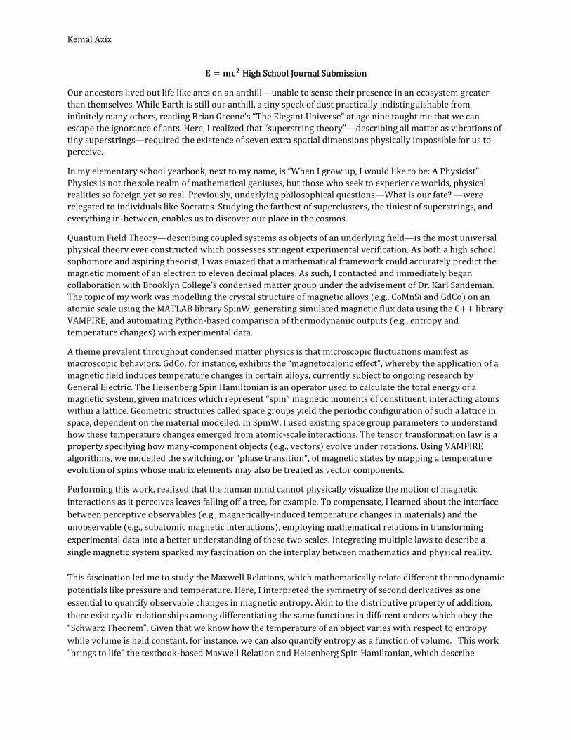
La-Fe-Si displays a much larger ΔSMAX and TPeak than CoMnSi. In fact, La-Fe-Si demonstrates the G-

MCE at room temperature. La-Fe-Si also has a greater TPeak due to the presence of hydrogen, which was

deliberately added to increase the TPeak to above room temperature. CoMnSi exhibits a much larger δTFWHM, or

peak width since CoMnSi is a second order transition material at low fields while La-Fe-Si is not. Despite

CoMnSi demonstrating the magnetocaloric effect over a broader temperature range, its ΔSMAX is considerably

smaller than La-Fe-Si. The magnetic field and temperature dependence of the magnetization behavior of La-

Fe-Si and CoMnSi are summarized in Figure 1. The temperature dependence of the magnetization of La-Fe-Si

is negative, meaning that La-Fe-Si loses magnetization as its temperature increases. CoMnSi, on the other

hand, demonstrates little temperature dependence of magnetization. Conversely, the magnetization curves of

La-Fe-Si demonstrate less magnetic field dependence. However, the magnetization curves of CoMnSi have a

positive magnetic field dependence, meaning that CoMnSi gains magnetization as the applied field increases.

Data were measured at different field and temperature intervals since the MCE occurs at different applied

field ranges in varied materials. The 2D data series in Figure 1 are cross-sections of the 3D magnetization

surface plots in Figure 2.

Figure 1. Magnetization cross-sectional curves of La-Fe-Si and CoMnSi. The first column of magnetization

curves is a function of temperature in Kelvin, or T(K). The second column of magnetization curves is a

function of H-field (applied magnetic field) in Tesla, or H(T). Am2/kg is the SI unit of magnetization.

The peak width (along the temperature axis) for La-Fe-Si is 4.5 K at a field of .4 Tesla and then increases

to 7.4 K in a field of 1.6 Tesla. The peak width appears to increase linearly as a function of applied field. This is

important to note since peak width is used in refrigerant capacity calculations. Additionally, La-Fe-Si has a

sharp change of lattice parameters whereas CoMnSi has a broad change of lattice parameters in these applied

magnetic fields. This indicates that a larger applied field is necessary to achieve an optimal level of the

magnetocaloric effect in CoMnSi than in La-Fe-Si. For example, La-Fe-Si reaches a magnetic saturation of

La-Fe-Si La-Fe-Si

CoMnSi CoMnSi

Kemal Aziz

approximately 140 Am2/kg at an applied field of 1.6 Tesla, while CoMnSi reaches a magnetic saturation of

approximately 110 Am2/kg at an applied field of 5 Tesla. Referring to the magnetic isotherm curves as a

function of temperature, CoMnSi isotherms are flat while La-Fe-Si are peaked. The relative shapes of the

magnetization curves can be observed in the 3D magnetization surface plots (Figure 2).

Figure 2. Three-dimensional visualizations of the isothermal magnetization behavior of La-Fe-Si and CoMnSi, respectively. The

horizontal axes and vertical axes are different for each plot to properly illustrate the respective magnetic behaviors of each material.

Refer to the line graphs in the Figure 1 for direct comparison of temperature and field dependent magnetization curves.

The Curie Temperature (TC) can be graphically estimated for La-Fe-Si by several methods, which do not

necessarily give results that agree within 1 K. For example, one way that the TC can be determined is by

observing the magnetization versus temperature and field plots in Figure 2. Graphically, we may say that the

TC is where a magnetic material reaches the inflection point of the downward M vs. T curve. The TC in La-Fe-

Si, or where temperature at which it becomes paramagnetic, is approximately 340K. Another means is to

search for the peak in the ∆S curve at low fields. This occurs at approximately 335 K. Likewise, the transition

temperature is ambiguous in CoMnSi, however, since there is an upwards M vs. T curve. In fact, it is not a

Curie temperature but is instead a metamagnetic temperature at which a critical field induces a high

magnetization state (Barcza et al., 2013).

The temperature of the inflection in magnetization in La-Fe-Si also shifts to the right as a greater magnetic

field is applied (Table 1 and Figure 1). This means that as the applied magnetic field increases, the

temperature at which the material magnetizes is greater. Consequently, the temperature at peak entropy

shifts to the right for La-Fe-Si (Figures 3, 4, and 5). This shift is occurring due to a phase transition occurring

at the given applied fields. If the maximum applied field was increased to larger fields such as 50 Tesla, then

this shifting to the right would not be visible in graphs. The behavior for CoMnSi is the reverse, with the

phase transition temperature decreasing as the applied field increases.

Mag

neti

zati

on

(A

m2/k

g) La-Fe-

Si

CoMnS

i

La-Fe-

Si

CoMnS

Kemal Aziz

0.1

0.3

0.5

0.7

0.9

1.1

1.3

1.5

310

315

325

335

340

348

355

365

μ0H

(T)

T(K)0-5 5-10 10-15 15-20

1

2

3

4

5

230

240

250

260

270

280

290

300

310

μ0H

(T)

T(K)

0-1 1-2 2-3 3-4 4-5

Figure 3. Entropy changes as a function of temperature for La-Fe-Si and CoMnSi while applied magnetic field is constant. Each entropy

change curve corresponds to an applied magnetic field. La-Fe-Si undergoes a negative entropy change while CoMnSi undergoes a

positive entropy change in an applied field (as indicated by the signs on the y-axis labels). The negative entropy change in La-Fe-Si is due

to magnetic moment alignment in an external magnetic field. Negative entropy change in CoMnSi is stems from the presence of a change

in the electronic density of states (Barcza et al., 2013). Differing magnetic properties of Co, Mn, and Si cause the material to undergo an

overall increase in magnetic entropy because of the mixed magnetic behaviors.

Figure 4. Two-dimensional data visualizations of the magnetic entropy behavior of La-Fe-Si and CoMnSi, respectively. The unit for

magnetic entropy (the colored gradients) is J kg-1 K-1. Note that the gradient for La-Fe-Si is positive while the gradient for CoMnSi is

negative. These gradients are a top-down perspective of the 3D surface plots presented in Figure 5.

Figure 5. Three-dimensional data visualizations of the magnetic entropy behavior of La-Fe-Si and CoMnSi, respectively. Note the negative

denotation on the y-axis of the La-Fe-Si plot. The x-axes and y-axes are different for each plot to best illustrate the respective entropy

behaviors of the materials. To directly compare the entropy curve shapes, refer to the entropy line graphs.

The entropy change of La-Fe-Si is negative and steep, which means that the magnetic moments are

aligned into a high magnetization state over a narrow applied magnetic field. However, the TPeak changes only

by a few Kelvin as the field increases. This contrasts with CoMnSi, where the TPeak is affected greatly by the

applied field, due to weaker entropy changes. CoMnSi therefore has a much larger peak width of 29K than

7.4 K for La-Fe-Si at the maximum applied fields of 5 T and 1.6 T, respectively. Since entropy change is a

measure of the cooling effect (a high positive entropy suggests heating up in the magnetic field), also CoMnSi

exhibits contrasting phase transition (Figure 6), hysteresis (Figure 7), refrigerant capacity (Figure 8)

behaviors in comparison to La-Fe-Si.

CoMnSi La-Fe-

Si

-ΔS

(J

kg

-1 K

-1)

Kemal Aziz

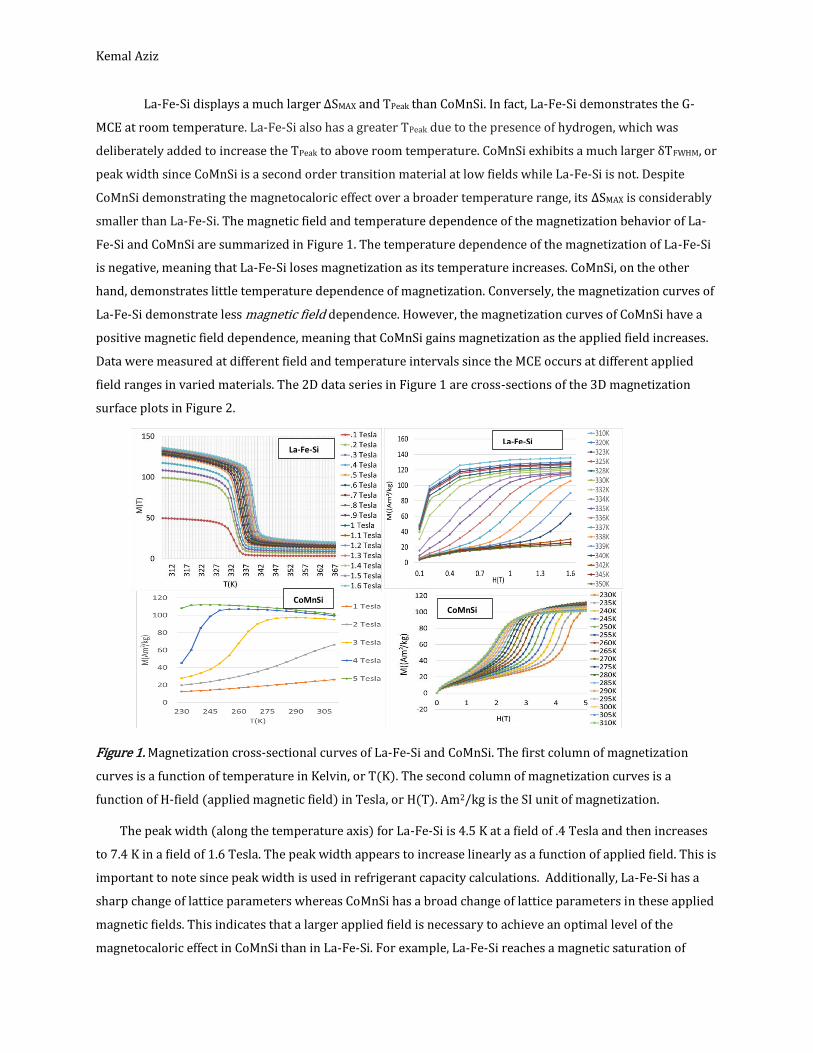
Figure 6. To generate phase diagrams, we apply a limit case of the Maxwell Relation, the Clausius-Clapeyron Equation for phase

transitions: 𝑑𝐻

𝑑𝑇=

∆𝑆

𝜇0∆𝑀. (a) Representation of ferromagnetic-paramagnetic phase transition in La-Fe-Si, whereby the application of a high

external magnetic field breaks ferromagnetic ordering. (b) Representation of the helical antiferromagnetic-high magnetization transition

in CoMnSi which characterizes the suppression of the material’s natural antiferromagnetic state.

Figure 7. Magnetic hysteresis of CoMnSi when held at constant temperature. The darker line shows magnetization values when the field

is applied while the lighter line shows magnetization behavior when the field is removed. μ0H(T) represents the applied magnetic field in

Tesla, while M refers to the magnetization of the material. Area under curve hysteresis losses (H.L), labeled in red, are expressed in the

unit J/kg.

Figure 8. Plot of RC as a function of applied field. The data table on the bottom numerically compares these values. RC for La-Fe-Si was

approximated through extrapolation from the 2T to 5T range. The ‘Threshold’ series indicates the maximum experimentally measured

RC of La-Fe-Si. Refrigerant capacity is used to compare the potential effectiveness of materials in a magnetic refrigerator. The refrigerant

capacity of CoMnSi given an applied field of 1.5 Tesla is approximately 27.3 J kg-1 while the refrigerant capacity of La-Fe-Si under the

same applied field is approximately 102.9 J kg-1. The refrigerant capacity for CoMnSi varies more strongly with magnetic field above a

threshold field value. This is due to the second to first order transition at the tricritical point.

H.L.=3.73 H.L.=8.31 H.L.=7.40 H.L.=6.12 H.L.=6.12

Antiferromagnetic

High Magnetization

State

Kemal Aziz

Hysteresis losses negatively affect effective refrigerant capacity. Hysteresis losses were not

calculated for La-Fe-Si. However, the hysteresis losses for first order materials (such as La-Fe-Si) are almost

always greater than the hysteresis losses for second order materials (Gutfleisch, et al., n.d.). In other words,

CoMnSi shows little thermal irreversibility compared to other inverse magnetocaloric materials. This can be

observed in hysteresis curves of figure 7. Unlike CoMnSi, detrimental hysteresis losses for La-Fe-Si occur due

to the magnetization of the material. The irreversible energy loss directly lowers the efficiency of the

magnetic refrigeration. Despite the moderate hysteresis effects, however, CoMnSi has a lesser utility for

industrial applications, based on a lower refrigerant capacity.

AutoCAD Drawings of Magnetic Refrigeration Prototypes

Figures 9 and 10. AutoCAD-generated cross-sections of proposed magnetic refrigerator prototypes with dimensions. The magnetocaloric

material heats upon entry into the magnetic field and cools down upon exit. To obtain continuous efficiency, the magnetocaloric material

enters and exits the external field periodically. Linear and rotational movements induce temperature changes in the material. (a) Linear

reciprocating magnetic refrigerator consisting of a screen of conventional magnetocaloric material (e.g., Gadolinium or La-Fe-Si) placed

within an electromagnetic field generated by a concave circular, superconducting magnet. Mechanical actuators enable hot and cold

reservoirs to exchange thermal energy via helium liquefaction flow. This enables calculation of simple Carnot Efficiency: 𝑇𝐻−𝑇𝐶

𝑇𝐻(100%).

(b) Rotary Active Magnetic Regenerator (AMR) consisting of a regenerator, magnet, and flow control system for heat exchange (the flow

control system is the AMR duct). The material is placed inside the yoke encasing the unit and magnetized in the presence of permanent

magnets circularly rotating magnets.

Construction of Magnetization Measurement/Magnetocaloric Effect Analysis Software

A package of software tools is built in the Python programming language to process experimental

magnetization data. Experimental data consists of magnetization data values expressed as a function of

temperature of the material system and the external applied magnetic field, as displayed in Figure 8. Three

main parameters of the experimental system are characterized by the software, in order of computation, are

graphical visualization of raw magnetization data, graphical visualization and determination of magnetic

entropy of the sample, and differential susceptibility of the sample. Raw magnetization data is provided in the

form of .CSV or an analogous text file. The user interface of the program is created via cell blocks in the

Jupyter notebook where each cell block contains a specific calculation or visualization command that the user

could call to generate analysis.

Kemal Aziz

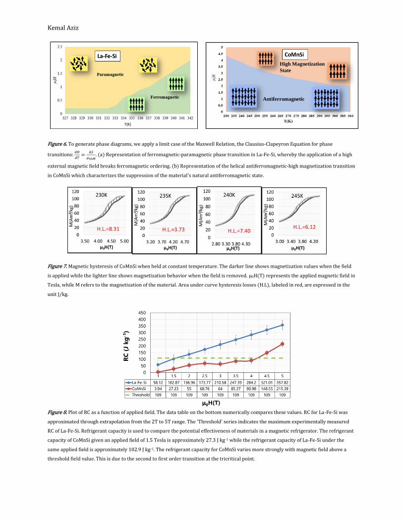
Figure 8. Inputted raw magnetization data (left) indexed by temperature (column “probe”) and field (row 1) labels is converted into

magnetic flux curve visualizations (right).

Here, we successfully test the initial component of the software based on experimental magnetization

measurements of La-Fe-Si. The initial component of program formats the data frame by recognizing and

indexing metadata (e.g., temperature and applied field labels). Specifically, the given tables of strings are

converted to float arrays. After this metadata is processed, the numpy and scipy libraries’ built-in functions

for differentiation and integration are enabled.

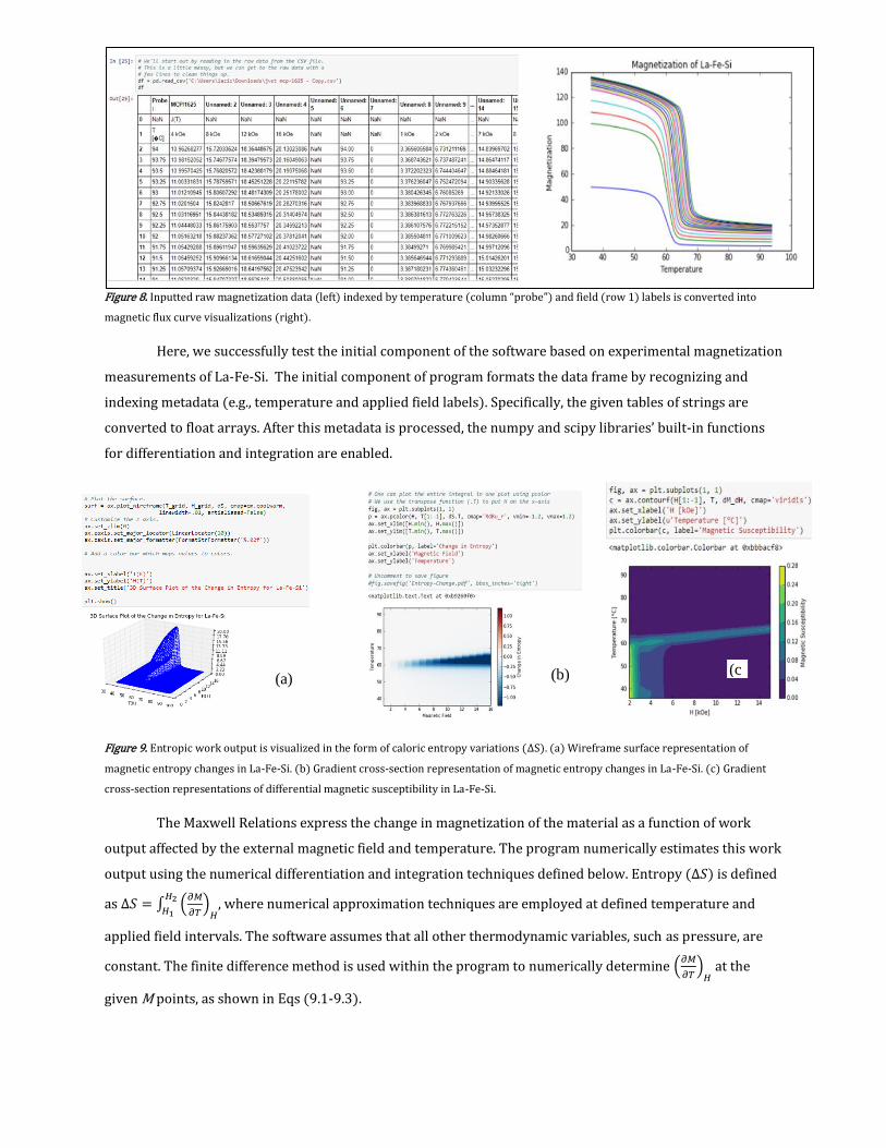
Figure 9. Entropic work output is visualized in the form of caloric entropy variations (ΔS). (a) Wireframe surface representation of

magnetic entropy changes in La-Fe-Si. (b) Gradient cross-section representation of magnetic entropy changes in La-Fe-Si. (c) Gradient

cross-section representations of differential magnetic susceptibility in La-Fe-Si.

The Maxwell Relations express the change in magnetization of the material as a function of work

output affected by the external magnetic field and temperature. The program numerically estimates this work

output using the numerical differentiation and integration techniques defined below. Entropy (∆𝑆) is defined

as ∆𝑆 = ∫ (𝜕𝑀

𝜕𝑇)

𝐻

𝐻2

𝐻1, where numerical approximation techniques are employed at defined temperature and

applied field intervals. The software assumes that all other thermodynamic variables, such as pressure, are

constant. The finite difference method is used within the program to numerically determine (𝜕𝑀

𝜕𝑇)

𝐻 at the

given M points, as shown in Eqs (9.1-9.3).

(a) (b) (c

)

Kemal Aziz

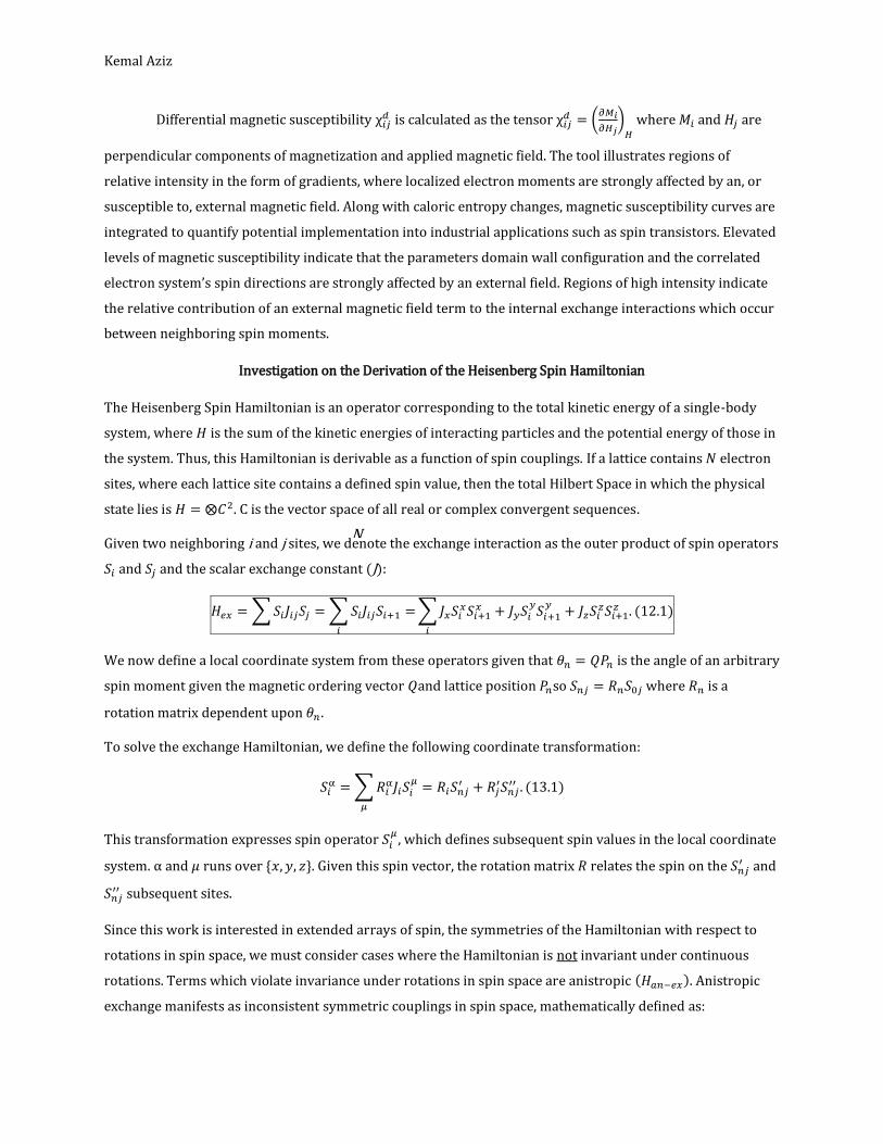
Differential magnetic susceptibility χ𝑖𝑗𝑑 is calculated as the tensor χ𝑖𝑗

𝑑 = (𝜕𝑀𝑖

𝜕𝐻𝑗)

𝐻

where 𝑀𝑖 and 𝐻𝑗 are

perpendicular components of magnetization and applied magnetic field. The tool illustrates regions of

relative intensity in the form of gradients, where localized electron moments are strongly affected by an, or

susceptible to, external magnetic field. Along with caloric entropy changes, magnetic susceptibility curves are

integrated to quantify potential implementation into industrial applications such as spin transistors. Elevated

levels of magnetic susceptibility indicate that the parameters domain wall configuration and the correlated

electron system’s spin directions are strongly affected by an external field. Regions of high intensity indicate

the relative contribution of an external magnetic field term to the internal exchange interactions which occur

between neighboring spin moments.

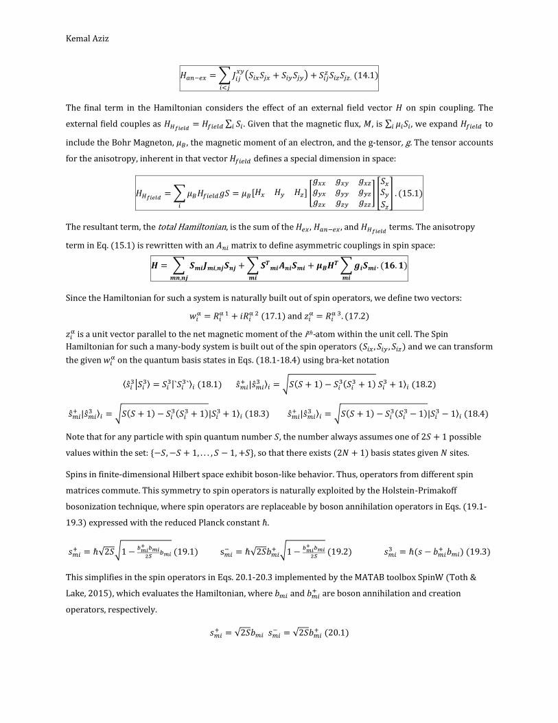
Investigation on the Derivation of the Heisenberg Spin Hamiltonian

The Heisenberg Spin Hamiltonian is an operator corresponding to the total kinetic energy of a single-body

system, where 𝐻 is the sum of the kinetic energies of interacting particles and the potential energy of those in

the system. Thus, this Hamiltonian is derivable as a function of spin couplings. If a lattice contains 𝑁 electron

sites, where each lattice site contains a defined spin value, then the total Hilbert Space in which the physical

state lies is 𝐻 = ⨂𝐶2. C is the vector space of all real or complex convergent sequences.

Given two neighboring i and j sites, we denote the exchange interaction as the outer product of spin operators

𝑆𝑖 and 𝑆𝑗 and the scalar exchange constant (J):

𝐻𝑒𝑥 = ∑ 𝑆𝑖𝐽𝑖𝑗𝑆𝑗 = ∑ 𝑆𝑖𝐽𝑖𝑗𝑆𝑖+1 =

𝑖

∑ 𝐽𝑥𝑆𝑖𝑥𝑆𝑖+1

𝑥 + 𝐽𝑦𝑆𝑖𝑦

𝑆𝑖+1𝑦

+ 𝐽𝑧𝑆𝑖𝑧𝑆𝑖+1

𝑧 .

𝑖

(12.1)

We now define a local coordinate system from these operators given that 𝜃𝑛 = 𝑄𝑃𝑛 is the angle of an arbitrary

spin moment given the magnetic ordering vector 𝑄and lattice position 𝑃𝑛so 𝑆𝑛𝑗 = 𝑅𝑛𝑆0𝑗 where 𝑅𝑛 is a

rotation matrix dependent upon 𝜃𝑛 .

To solve the exchange Hamiltonian, we define the following coordinate transformation:

𝑆𝑖α = ∑ 𝑅𝑖

α𝐽𝑖𝑆𝑖𝜇

𝜇

= 𝑅𝑖𝑆𝑛𝑗′ + 𝑅𝑗

′𝑆𝑛𝑗′′ . (13.1)

This transformation expresses spin operator 𝑆𝑖𝜇

, which defines subsequent spin values in the local coordinate

system. α and 𝜇 runs over {𝑥, 𝑦, 𝑧}. Given this spin vector, the rotation matrix 𝑅 relates the spin on the 𝑆𝑛𝑗′ and

𝑆𝑛𝑗′′ subsequent sites.

Since this work is interested in extended arrays of spin, the symmetries of the Hamiltonian with respect to

rotations in spin space, we must consider cases where the Hamiltonian is not invariant under continuous

rotations. Terms which violate invariance under rotations in spin space are anistropic (𝐻𝑎𝑛−𝑒𝑥). Anistropic

exchange manifests as inconsistent symmetric couplings in spin space, mathematically defined as:

N

Kemal Aziz

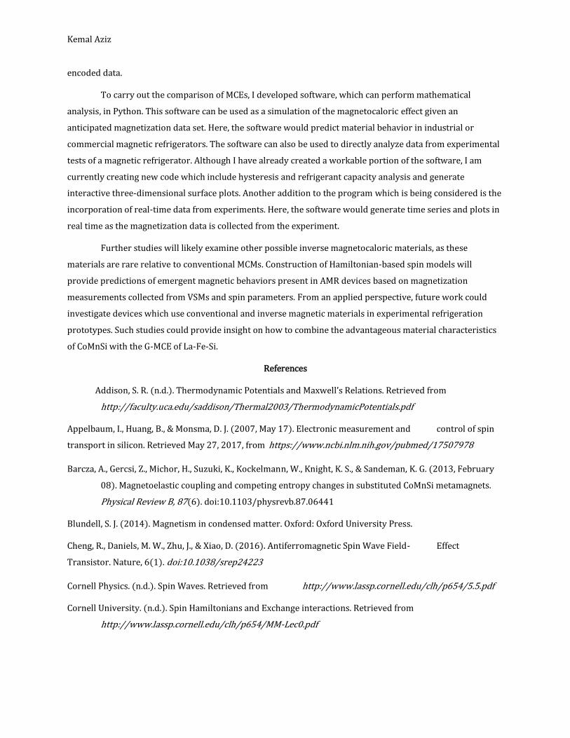
𝐻𝑎𝑛−𝑒𝑥 = ∑ 𝐽𝑖𝑗𝑥𝑦(𝑆𝑖𝑥𝑆𝑗𝑥 + 𝑆𝑖𝑦𝑆𝑗𝑦) + 𝑆𝑖𝑗

𝑧 𝑆𝑖𝑧𝑆𝑗𝑧. (14.1)

𝑖<𝑗

The final term in the Hamiltonian considers the effect of an external field vector 𝐻 on spin coupling. The

external field couples as 𝐻𝐻𝑓𝑖𝑒𝑙𝑑= 𝐻𝑓𝑖𝑒𝑙𝑑 ∑ 𝑆𝑖𝑖 . Given that the magnetic flux, 𝑀, is ∑ 𝜇𝑖𝑆𝑖𝑖 , we expand 𝐻𝑓𝑖𝑒𝑙𝑑 to

include the Bohr Magneton, 𝜇𝐵 , the magnetic moment of an electron, and the g-tensor, g. The tensor accounts

for the anisotropy, inherent in that vector 𝐻𝑓𝑖𝑒𝑙𝑑 defines a special dimension in space:

𝐻𝐻𝑓𝑖𝑒𝑙𝑑= ∑ 𝜇𝐵𝐻𝑓𝑖𝑒𝑙𝑑𝑔𝑆

𝑖

= 𝜇𝐵[𝐻𝑥 𝐻𝑦 𝐻𝑧] [

𝑔𝑥𝑥 𝑔𝑥𝑦 𝑔𝑥𝑧

𝑔𝑦𝑥 𝑔𝑦𝑦 𝑔𝑦𝑧

𝑔𝑧𝑥 𝑔𝑧𝑦 𝑔𝑧𝑧

] [

𝑆𝑥

𝑆𝑦

𝑆𝑧

] . (15.1)

The resultant term, the total Hamiltonian, is the sum of the 𝐻𝑒𝑥 , 𝐻𝑎𝑛−𝑒𝑥 , and 𝐻𝐻𝑓𝑖𝑒𝑙𝑑 terms. The anisotropy

term in Eq. (15.1) is rewritten with an 𝐴𝑛𝑖 matrix to define asymmetric couplings in spin space:

𝑯 = ∑ 𝑺𝒎𝒊𝑱𝒎𝒊,𝒏𝒋𝑺𝒏𝒋 + ∑ 𝑺𝑻𝒎𝒊𝑨𝒏𝒊𝑺𝒎𝒊 + 𝝁𝑩𝑯𝑻 ∑ 𝒈𝒊𝑺𝒎𝒊. (𝟏𝟔. 𝟏)

𝒎𝒊𝒎𝒊𝒎𝒏,𝒏𝒋

Since the Hamiltonian for such a system is naturally built out of spin operators, we define two vectors:

𝑤𝑖α = 𝑅𝑖

α 1 + 𝑖𝑅𝑖α 2 (17.1) and 𝑧𝑖

α = 𝑅𝑖α 3. (17.2)

𝑧𝑖α is a unit vector parallel to the net magnetic moment of the ith-atom within the unit cell. The Spin

Hamiltonian for such a many-body system is built out of the spin operators (𝑆𝑖𝑥 , 𝑆𝑖𝑦 , 𝑆𝑖𝑧) and we can transform

the given 𝑤𝑖α on the quantum basis states in Eqs. (18.1-18.4) using bra-ket notation

⟨�̂�𝑖3|𝑆𝑖

3⟩ = 𝑆𝑖3|`𝑆𝑖

3`⟩𝑖 (18.1) �̂�𝑚𝑖+ |�̂�𝑚𝑖

3 ⟩𝑖 = √𝑆(𝑆 + 1) − 𝑆𝑖3(𝑆𝑖

3 + 1) 𝑆𝑖3 + 1⟩𝑖 (18.2)

�̂�𝑚𝑖+ |�̂�𝑚𝑖

3 ⟩𝑖 = √𝑆(𝑆 + 1) − 𝑆𝑖3(𝑆𝑖

3 + 1)|𝑆𝑖3 + 1⟩𝑖 (18.3) �̂�𝑚𝑖

+ |�̂�𝑚𝑖3 ⟩𝑖 = √𝑆(𝑆 + 1) − 𝑆𝑖

3(𝑆𝑖3 − 1)|𝑆𝑖

3 − 1⟩𝑖 (18.4)

Note that for any particle with spin quantum number 𝑆, the number always assumes one of 2𝑆 + 1 possible

values within the set: {−𝑆, −𝑆 + 1, . . . , 𝑆 − 1, +𝑆}, so that there exists (2𝑁 + 1) basis states given 𝑁 sites.

Spins in finite-dimensional Hilbert space exhibit boson-like behavior. Thus, operators from different spin

matrices commute. This symmetry to spin operators is naturally exploited by the Holstein-Primakoff

bosonization technique, where spin operators are replaceable by boson annihilation operators in Eqs. (19.1-

19.3) expressed with the reduced Planck constant ℏ.

𝑠𝑚𝑖+ = ℏ√2𝑆√1 −

𝑏𝑚𝑖+ 𝑏𝑚𝑖

2𝑆𝑏𝑚𝑖 (19.1) s𝑚𝑖

− = ℏ√2𝑆𝑏𝑚𝑖+ √1 −

𝑏𝑚𝑖+ 𝑏𝑚𝑖

2𝑆 (19.2) 𝑠𝑚𝑖

3 = ℏ(𝑠 − 𝑏𝑚𝑖+ 𝑏𝑚𝑖) (19.3)

This simplifies in the spin operators in Eqs. 20.1-20.3 implemented by the MATAB toolbox SpinW (Toth &

Lake, 2015), which evaluates the Hamiltonian, where 𝑏𝑚𝑖 and 𝑏𝑚𝑖+ are boson annihilation and creation

operators, respectively.

𝑠𝑚𝑖+ = √2𝑆𝑏𝑚𝑖 𝑠𝑚𝑖

− = √2𝑆𝑏𝑚𝑖+ (20.1)

Kemal Aziz

𝑠𝑚𝑖1 =

√2𝑆𝑖

2(𝑏𝑚𝑖 + 𝑏𝑚𝑖

+ ) (20.2) 𝑠𝑚𝑖2 =

√2𝑆𝑖

2(𝑏𝑚𝑖 − 𝑏𝑚𝑖

+ ) (20.3) 𝑠𝑚𝑖3 = (𝑆𝑖 − 𝑏𝑚𝑖

+ 𝑏𝑚𝑖) (20.4)

As it applies to the interaction parameters, the Monte Carlo Method relies on repeated random sampling to

account for the many coupled degrees of freedom in the spin Hamiltonian. In the spin Hamiltonian, the

number of degrees of freedom refers to the number of exchange parameters that vary independently.

Quantum Mechanical Description of Magnetocaloric Effects in Gadolinium

We generate an atomistic model of magnetocaloric effects in the 2nd order ferromagnetic

nanomaterial Gadolinium by defining pairwise exchange energy (Jij) between atoms of neighbor-index in the

C++ VAMPIRE library (Evans et al., 2014). The MATLAB quantum magnetism toolbox SpinW is used to

impose magnetic interactions on the crystal structure, given Jij and μS (spin moment) of 3.5. The crystal

structure of Gadolinium is hexagonal close packed (HCP) with a P63 space group. Applying the built-in

mathematical representations of the HCP and P-63 geometric space groups in SpinW, we plot the structure in

Figure 10.

Figure 10. Atomic spatial visualizations of the ordered crystal structure within Gadolinium at its optimized ground state as calculated in

SpinW. (a) 3-dimensional ferromagnetic lattice where spin alignments are parallel in the a-b plane. (b) Singular lattice layer plane

consisting of Gd+ atoms.

Nearest-neighbor ferromagnetic exchanges (Jij) are determined by the meanfield expression, 𝐽𝑖𝑗 =

3𝐾𝐵𝑇𝐶

𝜀𝑧, where KB is the Boltzmann constant. Given 𝐽𝑖𝑗 = 5.9 𝑚𝑒𝑉, we match the experimentally known TC of

294K by adjusting the spin fluctuation factor (휀) to .95 from the expected value of .790 for the HCP structure.

The HCP structure, as plotted in Figure 14, contain four atoms per unit cell resulting in a coordination number

(𝑧) of 12. VAMPIRE maps operators in Eqs. (18.1-18.4) to the Hamiltonian in Eq. (16.1) by using the Monte-

Carlo Method to generate magnetization data (Evans et al., 2014). The external field tensor (𝜇𝐵𝐻𝑇 ∑ 𝑔𝑖𝑆𝑚𝑖𝑚𝑖 )

in Figure 11 is defined up to 𝐻𝑇 = 5 𝑇.

(a) (b)

Kemal Aziz

Figure 11. (a) Magnetization (|𝒎| =∑ 𝝁𝒊𝑺𝒊𝒊

∑ 𝝁𝒊) cross-sectional curves of Gadolinium as a function of temperature in Kelvin. 𝑀/𝑀𝑆 denotes

the normalized sum of spin moments with respect to saturation magnetization (𝑀𝑆). Increased magnitudes of the external magnetic field

induce a higher magnetic ordering critical point (TC). (b) Total energy term (𝑯 = ∑ 𝑺𝒎𝒊𝑱𝒎𝒊,𝒏𝒋𝑺𝒏𝒋 + ∑ 𝑺𝑻𝒎𝒊𝑨𝒏𝒊𝑺𝒎𝒊 +𝒎𝒊𝒎𝒏,𝒏𝒋

𝝁𝑩𝑯𝑻 ∑ 𝒈𝒊𝑺𝒎𝒊𝒎𝒊 ) of the Hamiltonian corresponding to the external magnetic field deviations from the ground state H=0. At the TC, we

note an inflection point in the total energy curve, indicating that exchange interactions (𝐻𝑒𝑥 = ∑ 𝑆𝑖𝐽𝑖𝑗𝑆𝑗) reach a constant non-zero

magnitude in the paramagnetic phase.

Experimental Thermocouple Set-Up in Gadolinium

The following is an experimental demonstration set-up of the magnetocaloric effect in Gadolinium. A 100-

gram sample of Gadolinium was used. Gadolinium is a rare-earth metal which demonstrates the conventional

magnetocaloric effect whereby its temperature increases when it enters the magnetic field and decreases

when it leaves the magnetic field. The magnetocaloric effect in Gadolinium occurs near room temperature (68

°F), which makes the material ideal for demonstration purposes. Prior to exposing Gadolinium to a magnetic

field, its temperature was measured using the Dual-channel Leaton Digital Thermocouple Thermometer,

labeled in Figure 12. Two dissimilar metals are joined as a circuit, and thus, a thermocurrent is generated

from the temperature difference between the metals. If there is a temperature difference between the

thermocouple tip and the reference end of the thermocouple, the instrument will display the temperature

value of the material being tested. In this demonstration, two different thermocouples are connected to a

single thermometer. This enables the thermometer to display two different temperature outputs which

indicate the temperature of Gadolinium at two points on its surface.

Permanent

Magnets and

Gadolinium

Magnetometer

Leaton

Thermometer Thermocouples

(a) (b)

Kemal Aziz

Figure 12. Image on the left is the experimental demonstration set-up of the magnetocaloric effect in Gadolinium. Images on the right are

close-up photographs of the Gadolinium used in this demonstration and modelled in the VAMPIRE C++ Library. After the surface

temperature of Gadolinium is measured (when it is not exposed to a magnetic field), the material is placed in an applied magnetic field.

In this case, Gadolinium was exposed to a static magnetic field using permanent magnets, as shown. Here, the magnetic field was

generated from the spin of electrons within the material itself. These permanent magnets generated an applied magnetic field of

approximately 2.2 Microtesla. Alternatively, an electromagnet could be used where the magnetic field is generated as an electric current

is applied. After Gadolinium was exposed to a magnetic field of 2.2 Microtesla, it was removed from it. As expected, Gadolinium

experienced a temperature decrease as it was removed from an applied field. To measure the strength of the magnetic field, a vector

magnetometer is utilized.

Discussion and Conclusions

Results presented here enable researchers to compare properties of the conventional and inverse

magnetocaloric effects. By taking the first-order conventional magnetocaloric material La-Fe-Si and

comparing it to the second-order inverse magnetocaloric material CoMnSi, we apply observations to general

explanations of behavior by constructing a micromagnetic spin model. We draw conclusions on the industrial

applications for each. Software we created are designed to be used in future research.

Overall, the expected outcome was supported by the data in that La-Fe-Si is a more suitable

candidate than CoMnSi for industrial applications. This because La-Fe-Si demonstrates the G-MCE over a very

narrow temperature interval, meaning that La-Fe-Si would go into a heating state very quickly. CoMnSi, on

the other hand, magnetizes very slowly as a function of applied field. La-Fe-Si also has a greater TPeak because

of the presence of hydrogen. This greater TPeak makes La-Fe-Si better suited to room-temperature

applications.

CoMnSi has smaller entropy changes and refrigerant capacities than most conventional MCMs (e.g.,

La-Fe-Si) at comparable magnetic fields, yet demonstrates advantageous characteristics for use in

refrigeration applications. By undergoing a change in the electronic density of states, CoMnSi has a broadened

transition in temperature and a reduced effective hysteresis. This broadened transition in temperature allows

CoMnSi to be used in cooling devices where cooling is needed over a wide range of temperatures. Although

multiple conventional MCMs with consecutive smaller temperature transitions could be used together

(accounting to a broad overall temperature transition), using multiple materials may not be cost effective.

The micromagnetic model built at an interface between MATLAB (via SpinW) and C++ (via

VAMPIRE) generates quantification of spin-induced magnetic interaction parameters (e.g., spin waves

corresponding to the total energy Hamiltonian) underlying emergent thermodynamic observables such as

adiabatic demagnetization. Since these spin waves carry pure spin currents in the absence of electron flow,

the possibility of using waves instead of particles for computing enables new device concepts for spin

processing such as spin logic gates and transistors. As a first step towards achieving practical realization of

magnon-based computing, it is necessary to encode binary data into spin waves. To realize a computing

device based on spin, our model may be used to simulate the control of spin polarization modes via external

fields by plotting the total energy Hamiltonian. Control of spin polarization will enable logical operations on

Kemal Aziz

encoded data.

To carry out the comparison of MCEs, I developed software, which can perform mathematical

analysis, in Python. This software can be used as a simulation of the magnetocaloric effect given an

anticipated magnetization data set. Here, the software would predict material behavior in industrial or

commercial magnetic refrigerators. The software can also be used to directly analyze data from experimental

tests of a magnetic refrigerator. Although I have already created a workable portion of the software, I am

currently creating new code which include hysteresis and refrigerant capacity analysis and generate

interactive three-dimensional surface plots. Another addition to the program which is being considered is the

incorporation of real-time data from experiments. Here, the software would generate time series and plots in

real time as the magnetization data is collected from the experiment.

Further studies will likely examine other possible inverse magnetocaloric materials, as these

materials are rare relative to conventional MCMs. Construction of Hamiltonian-based spin models will

provide predictions of emergent magnetic behaviors present in AMR devices based on magnetization

measurements collected from VSMs and spin parameters. From an applied perspective, future work could

investigate devices which use conventional and inverse magnetic materials in experimental refrigeration

prototypes. Such studies could provide insight on how to combine the advantageous material characteristics

of CoMnSi with the G-MCE of La-Fe-Si.

References

Addison, S. R. (n.d.). Thermodynamic Potentials and Maxwell’s Relations. Retrieved from

http://faculty.uca.edu/saddison/Thermal2003/ThermodynamicPotentials.pdf

Appelbaum, I., Huang, B., & Monsma, D. J. (2007, May 17). Electronic measurement and control of spin

transport in silicon. Retrieved May 27, 2017, from https://www.ncbi.nlm.nih.gov/pubmed/17507978

Barcza, A., Gercsi, Z., Michor, H., Suzuki, K., Kockelmann, W., Knight, K. S., & Sandeman, K. G. (2013, February

08). Magnetoelastic coupling and competing entropy changes in substituted CoMnSi metamagnets.

Physical Review B, 87(6). doi:10.1103/physrevb.87.06441

Blundell, S. J. (2014). Magnetism in condensed matter. Oxford: Oxford University Press.

Cheng, R., Daniels, M. W., Zhu, J., & Xiao, D. (2016). Antiferromagnetic Spin Wave Field- Effect

Transistor. Nature, 6(1). doi:10.1038/srep24223

Cornell Physics. (n.d.). Spin Waves. Retrieved from http://www.lassp.cornell.edu/clh/p654/5.5.pdf

Cornell University. (n.d.). Spin Hamiltonians and Exchange interactions. Retrieved from

http://www.lassp.cornell.edu/clh/p654/MM-Lec0.pdf

Kemal Aziz

Du, A., & Du, H. (2005, May 17). Monte Carlo calculation of the magnetization behavior and the

magnetocaloric effect of interacting particles. Journal of Magnetism and Magnetic Materials,

299(2), 247-254. doi:10.1016/j.jmmm.2005.04.011

Evans, R. F., Fan, W. J., Chureemart, P., Ostler, T. A., Ellis, M. O., & Chantrell, R. W. (2014). Atomistic spin

model simulations of magnetic nanomaterials. Journal of Physics: Condensed Matter, 26(10),

103202. doi:10.1088/0953-8984/26/10/103202

Franco, V., Blázquez, J. S., Ingale, B., & Conde, A. (2012). The Magnetocaloric Effect and Magnetic

Refrigeration Near Room Temperature: Materials and Models. Annual Review of Materials Research,

42(1), 305-342.

Franco, V. (n.d.). Determination of the Magnetic Entropy Change from Magnetic Measurements.

Retrieved from

http://www.lakeshore.com/Documents/MagneticEntropyChangefromMagneticMeasure

ments.pdf

Guillou, F., Porcari, G., Yibole, H., Dijk, N. V., & Brück, E. (2014, February 22). Taming the First-Order

Transition in Giant Magnetocaloric Materials. Adv. Mater. Advanced Materials, 26(17), 2671-

2675. doi:10.1002/adma.201304788

Gutenberg, P. (n.d.). Schwarz theorem. Retrieved from

http://www.gutenberg.us/articles/schwarz_theorem

Gutfleisch, O., Gottschall, T., Fries, M., Benke, D., Radulov, I., Skokov, K. P., . . . Farle, M.

(n.d.). Mastering hysteresis in magnetocaloric materials.

Khan, M., Ali, N., & Stadler, S. (2007, March 15). Inverse magnetocaloric effect in ferromagnetic

Ni50Mn37xSb13−x Heusler alloys. Journal of Applied Physics, 101(5), 053919.

doi:10.1063/1.2710779

Kitanovski, A., Plaznik, U., Tomc, U., & Poredoš, A. (2015). Present and future caloric refrigeration

and heat-pump technologies. International Journal of Refrigeration.

doi:10.1016/j.ijrefrig.2015.06.008

Kochmański, M., Paszkiewicz, T., & Wolski, S. (2013, July 22). Curie–Weiss magnet—a simple model of phase

transition. European Journal of Physics. doi:10.1088/0143-0807/34/6/1555

Krenke, T., Duman, E., Acet, M., Wassermann, E. F., Moya, X., Mañosa, L., & Planes, A. (2005). Inverse

magnetocaloric effect in ferromagnetic Ni–Mn–Sn alloys. Nature materials, 4(6), 450-454.

Maxwell Relation. (2013, May 09). Retrieved from https://thermodynamics-

engineer.com/maxwell-relation/

Kemal Aziz

M.I.T. (2013). Maxwell Relations: A Wealth of Partial Derivatives. Retrieved from

https://ocw.mit.edu/courses/physics/8-044-statistical-physics-i-spring-2013/readings-notes-

slides/MIT8_044S13_notes.Max.pdf

Pecharsky, V. K., & Gschneidner Jr., K. A. (1999). Magnetocaloric effect and magnetic refrigeration.

Journal of Magnetism and Magnetic Materials, 200(1-3), 44-56. doi:10.1016/s0304-

8853(99)00397-2

Sheremet, A. S., Kibis, O. V., Kavokin, A. V., & Shelykh, I. A. (2016). Datta-and-Das spin transistor

controlled by a high-frequency electromagnetic field. Physical Review B, 93(16), 165307.

Schekochihin, A. (n.d.). Classification of phase transitions. Retrieved from https://www-

thphys.physics.ox.ac.uk/people/AlexanderSchekochihin/A1/2011/handout13.pdf

Smith, A. (2013). Who discovered the magnetocaloric effect? The European Physical Journal H EPJ H, 38(4),

507-517. doi:10.1140/epjh/e2013-40001-9

Toth, S., & Lake, B. (2015). Linear spin wave theory for single-Q incommensurate magnetic

structures. Journal of Physics: Condensed Matter, 27(16), 166002.