KC‐X Tanker Replacement Program: Value of …ardent.mit.edu/real_options/Real_opts_portfolio...([email protected]) Winchesley “Chez” Vixama Engineering Systems Analysis for Design

Engineering Systems Analysis for Design

Winchesley “Chez” Vixama

Fall 2008

KC‐X Tanker Replacement Program: Value of Flexibility

([email protected])

Winchesley “Chez” Vixama Engineering Systems Analysis for Design

Table of Contents Motivation ....................................................................................................................................................3

1.0 Background...........................................................................................................................................3

1.1 Competing Designs .........................................................................................................................4

1.2 Cost and Production Schedule Data ............................................................................................5

2.0 Defining the Salient Uncertainties .....................................................................................................6

2.1 Demand Uncertainty .......................................................................................................................6

2.2 Oil Price Uncertainty .......................................................................................................................7

3.0 System Design Definition ...................................................................................................................8

3.1 Analytic Framework .........................................................................................................................8

3.1.1 DAPCA Model...........................................................................................................................8

3.1.2 Fuel Price Model.......................................................................................................................9

3.1.3 Demand Model .........................................................................................................................9

3.2 Decision Framework .......................................................................................................................9

4.0 Decision Tree Analysis .......................................................................................................................9

4.1 Fuel Cost Forecast Modeling .......................................................................................................11

4.2 Demand Modeling .........................................................................................................................13

4.3 Expected Value Determination ....................................................................................................13

4.3.1 Inflexible Design .....................................................................................................................13

4.3.2 Flexible Design .......................................................................................................................14

5.0 Lattice Analysis ..................................................................................................................................16

6.0 Lattice Valuation ................................................................................................................................18

7.0 Conclusion ..........................................................................................................................................19

([email protected])


KC‐X Tanker Replacement Program:

Value of Flexibility

Motivation This report encapsulates an investigative process focused on determining the value of imbedding flexibility in the production buy schedule of the proposed US Air Force KC-X tanker aircraft. The current arrangement locks the United States Government (USG) into a long-term, deterministic financial agreement which fails to account for future uncertainty. The forces of uncertainty may prevent USG from acting upon future opportunities or responding to unforeseen demands and requirements. Flexibility may be added to this agreement by either delaying the purchase decision and/or allowing the USG to modify the production quantity. Although such a change in the contractual agreement is mistakenly believed to be constrained by the notion of the “cost of flexibility”, the value of this action may be significant enough to warrant a more thorough review of this option.

1.0 Background The KC-X program is the first of three acquisition programs the Air Force will need to replace the entire fleet of aging KC-135 Stratotankers, which have been in service for more than 50 years. The primary mission of the KC-X will be to provide aerial refueling to United States military and coalition aircraft. However, the Air Force also intends to take full advantage of the other capabilities inherent in the platform, such as airlift, and make it an integral part of the Defense Transportation System.1

Release of the KC-X request for proposal (RFP) in January 2007, initiated a chain of events designed to produce a fair, full and open competition focused on the selection and production of a flexible and versatile platform. The submission of each contractor is evaluated by a specific set of criteria documented in the RFP. Combined with such factors as cost and past performance records the selection committee will determine which option produces the optimal blend of cost, schedule, and performance. The ultimate goal is to select the product which delivers the best value to the customer. The RFP stipulated nine primary key performance parameters (KPP):

KPPs of the KC-X

Air refueling capability (same sortie boom and drogue capable) Fuel offload and range at least as great as the KC-135 Compliant CNS/ATM equipment Airlift capability Ability to take on fuel while airborne Sufficient force protection measures

1 Office of the Assistant Secretary of Defense (Public Affairs),News Release No.113‐07, Air Force Posts Request for Proposals for Tankers

([email protected])


Ability to network into the information available in the battle space Survivability measures (defensive systems, EMP hardening, chem/bio protection, etc.) Provisioning for a multi-point refueling system to support Navy and Allied aircraft

Table 1: KPP listing for future tanker design

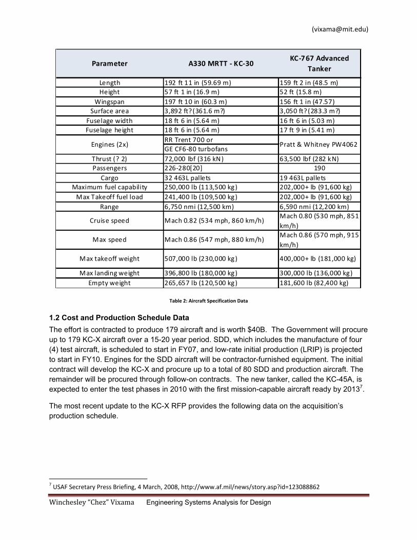
1.1 Competing Designs Two groups responded to and presented competing designs for the RFP. The Boeing Corporation presented the KC-767, a variant of the long-established 767 series. EADS/Airbus and the Northrop Grumman Corporation formed a joint venture and proposed the Airbus A330 Multi Role Tanker Transport (MRTT), based on the Airbus A330-200. Figure 1 and Table 2 present data on the relative sizes of the airframes and common parameters, respectively (Sources: Northrop Grumman KC-302, Airbus A330, KC-30 performance specifications3, KC-767 Advanced Tanker4, and Boeing 767 aircraft data5).

Figure 1: Aircraft Relative Size Comparison6

2 http://www.airforce‐technology.com/projects/a330_200/ 3 http://www.northropgrumman.com/kc30/performance/specifications.html 4 KC‐767 Advanced Tanker Product Card, http://www.boeing.com/ids/globaltanker/usaf/KC_767/767AdvProdCard.pdf 5 http://www.boeing.com/commercial/airports/acaps/767sec2.pdf 6 KC‐X Tanker Replacement Program, http://www.globalsecurity.org/military/systems/aircraft/kc‐x.htm

A330 in red

KC‐767 in blue

KC‐135 in white

([email protected])


Parameter A330 MRTT ‐ KC‐30KC‐767 Advanced

Tanker

Length 192 ft 11 in (59.69 m) 159 ft 2 in (48.5 m)Height 57 ft 1 in (16.9 m) 52 ft (15.8 m)

Wingspan 197 ft 10 in (60.3 m) 156 ft 1 in (47.57)Surface area 3,892 ft? (361.6 m?) 3,050 ft? (283.3 m?)

Fuselage width 18 ft 6 in (5.64 m) 16 ft 6 in (5.03 m)Fuselage height 18 ft 6 in (5.64 m) 17 ft 9 in (5.41 m)

RR Trent 700 orGE CF6‐80 turbofans

Thrust (? 2) 72,000 lbf (316 kN) 63,500 lbf (282 kN)Passengers 226‐280[20] 190

Cargo 32 463L pallets 19 463L palletsMaximum fuel capability 250,000 lb (113,500 kg) 202,000+ lb (91,600 kg)Max Takeoff fuel load 241,400 lb (109,500 kg) 202,000+ lb (91,600 kg)

Range 6,750 nmi (12,500 km) 6,590 nmi (12,200 km)

Cruise speed Mach 0.82 (534 mph, 860 km/h)Mach 0.80 (530 mph, 851 km/h)

Max speed Mach 0.86 (547 mph, 880 km/h)Mach 0.86 (570 mph, 915 km/h)

Max takeoff weight 507,000 lb (230,000 kg) 400,000+ lb (181,000 kg)

Max landing weight 396,800 lb (180,000 kg) 300,000 lb (136,000 kg)Empty weight 265,657 lb (120,500 kg) 181,600 lb (82,400 kg)

Engines (2x) Pratt & Whitney PW4062

Table 2: Aircraft Specification Data

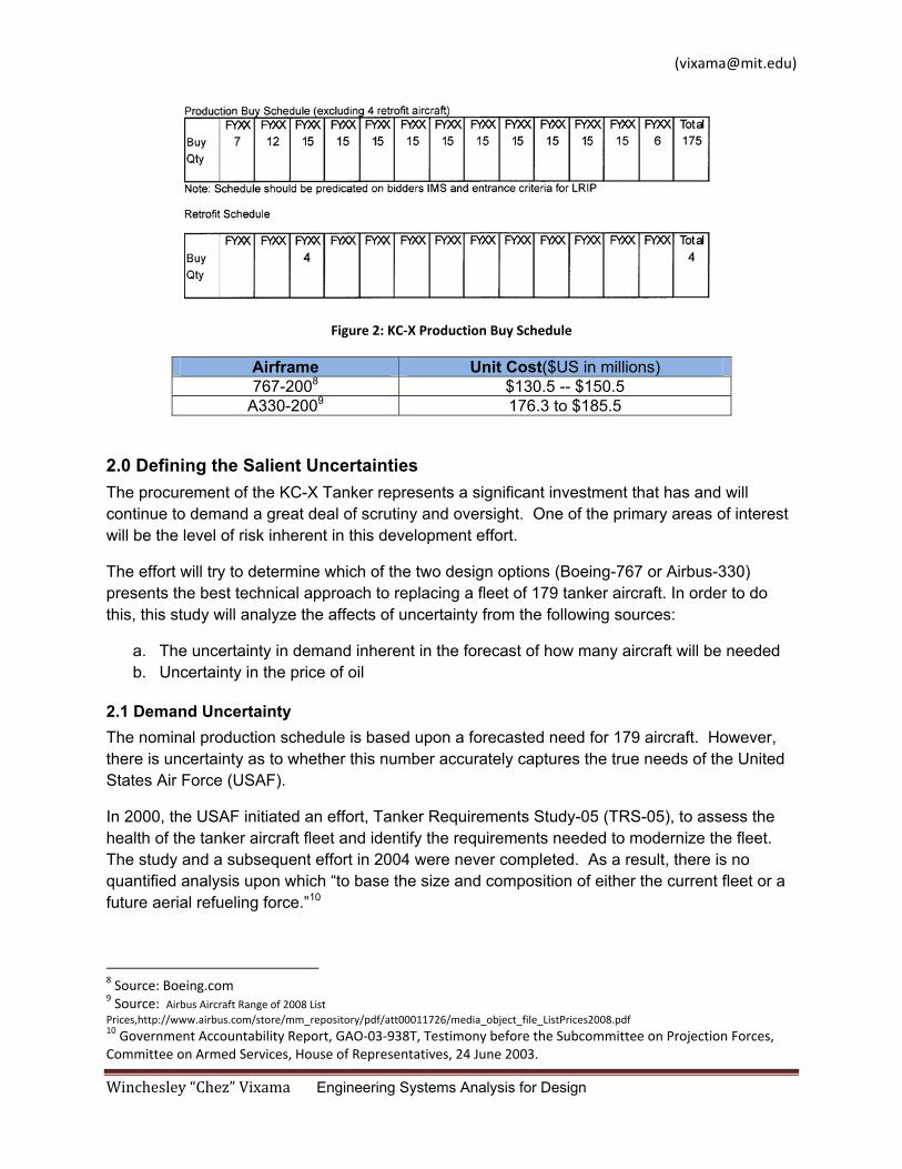
1.2 Cost and Production Schedule Data The effort is contracted to produce 179 aircraft and is worth $40B. The Government will procure up to 179 KC-X aircraft over a 15-20 year period. SDD, which includes the manufacture of four (4) test aircraft, is scheduled to start in FY07, and low-rate initial production (LRIP) is projected to start in FY10. Engines for the SDD aircraft will be contractor-furnished equipment. The initial contract will develop the KC-X and procure up to a total of 80 SDD and production aircraft. The remainder will be procured through follow-on contracts. The new tanker, called the KC-45A, is expected to enter the test phases in 2010 with the first mission-capable aircraft ready by 20137.

The most recent update to the KC-X RFP provides the following data on the acquisition’s production schedule.

7 USAF Secretary Press Briefing, 4 March, 2008, http://www.af.mil/news/story.asp?id=123088862

([email protected])


Figure 2: KC‐X Production Buy Schedule

Airframe Unit Cost($US in millions) 767-2008 $130.5 -- $150.5

A330-2009 176.3 to $185.5

2.0 Defining the Salient Uncertainties The procurement of the KC-X Tanker represents a significant investment that has and will continue to demand a great deal of scrutiny and oversight. One of the primary areas of interest will be the level of risk inherent in this development effort.

The effort will try to determine which of the two design options (Boeing-767 or Airbus-330) presents the best technical approach to replacing a fleet of 179 tanker aircraft. In order to do this, this study will analyze the affects of uncertainty from the following sources:

a. The uncertainty in demand inherent in the forecast of how many aircraft will be needed b. Uncertainty in the price of oil

2.1 Demand Uncertainty The nominal production schedule is based upon a forecasted need for 179 aircraft. However, there is uncertainty as to whether this number accurately captures the true needs of the United States Air Force (USAF).

In 2000, the USAF initiated an effort, Tanker Requirements Study-05 (TRS-05), to assess the health of the tanker aircraft fleet and identify the requirements needed to modernize the fleet. The study and a subsequent effort in 2004 were never completed. As a result, there is no quantified analysis upon which “to base the size and composition of either the current fleet or a future aerial refueling force.”10

8 Source: Boeing.com 9 Source: Airbus Aircraft Range of 2008 List Prices,http://www.airbus.com/store/mm_repository/pdf/att00011726/media_object_file_ListPrices2008.pdf 10 Government Accountability Report, GAO‐03‐938T, Testimony before the Subcommittee on Projection Forces, Committee on Armed Services, House of Representatives, 24 June 2003.

([email protected])


Beyond this, the forecast of 179 aircraft used in the current tanker procurement process does not account for significant changes in the structure and operational tempo of the USAF that have occurred since 2000. TRS-05 preliminary results were based on the then Soviet Era Cold-War construct of being able to support two major theatre wars. Since that time, the Soviet Union has expired and US military operations have been characterized by mid-level operations in multiple, regional conflicts. The ever-changing and protracted levels of engagements bring appreciable doubt to the accuracy of 179-tanker aircraft forecast. With an average age of nearly 50 years per aircraft, modernization of the tanker fleet could require as many as 500 aircraft. On the other hand, if the findings of a recent Rand study are followed, the demand may be met by simply refurbishing older, less sophisticated aircraft. If this is true, the true forecast may be significantly lower than 179.

To account for this uncertainty, the forecasted demand needs to be modeled and incorporated in the analysis. For the purposes of this effort, the maximum demand will be assumed not to exceed the overall fleet size (545 aircraft) and not go below 79 aircraft. Modeling the distribution of the demand will be more difficult. A simple random (normal) distribution will be initially used. Other distributions will be reviewed and considered for suitability.

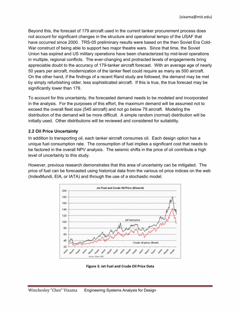
2.2 Oil Price Uncertainty In addition to transporting oil, each tanker aircraft consumes oil. Each design option has a unique fuel consumption rate. The consumption of fuel implies a significant cost that needs to be factored in the overall NPV analysis. The seismic shifts in the price of oil contribute a high level of uncertainty to this study.

However, previous research demonstrates that this area of uncertainty can be mitigated. The price of fuel can be forecasted using historical data from the various oil price indices on the web (IndexMundi, EIA, or IATA) and through the use of a stochastic model.

Figure 3: Jet Fuel and Crude Oil Price Data

([email protected])


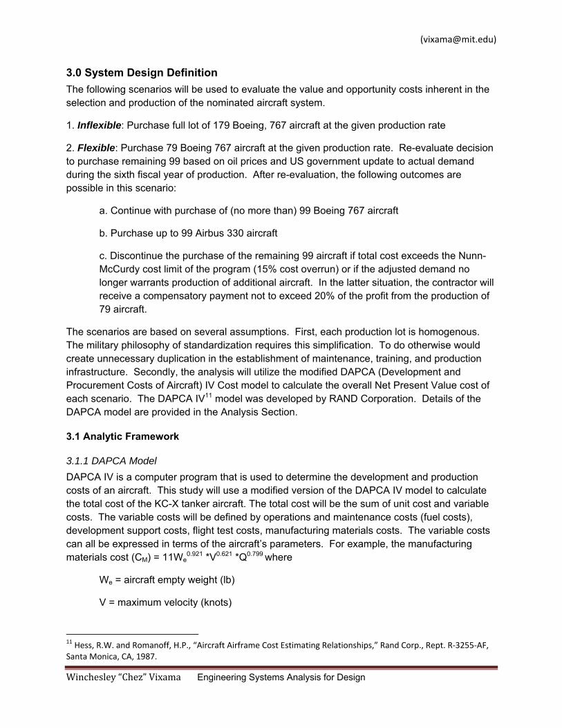
3.0 System Design Definition The following scenarios will be used to evaluate the value and opportunity costs inherent in the selection and production of the nominated aircraft system.

1. Inflexible: Purchase full lot of 179 Boeing, 767 aircraft at the given production rate

2. Flexible: Purchase 79 Boeing 767 aircraft at the given production rate. Re-evaluate decision to purchase remaining 99 based on oil prices and US government update to actual demand during the sixth fiscal year of production. After re-evaluation, the following outcomes are possible in this scenario:

a. Continue with purchase of (no more than) 99 Boeing 767 aircraft

b. Purchase up to 99 Airbus 330 aircraft

c. Discontinue the purchase of the remaining 99 aircraft if total cost exceeds the Nunn-McCurdy cost limit of the program (15% cost overrun) or if the adjusted demand no longer warrants production of additional aircraft. In the latter situation, the contractor will receive a compensatory payment not to exceed 20% of the profit from the production of 79 aircraft.

The scenarios are based on several assumptions. First, each production lot is homogenous. The military philosophy of standardization requires this simplification. To do otherwise would create unnecessary duplication in the establishment of maintenance, training, and production infrastructure. Secondly, the analysis will utilize the modified DAPCA (Development and Procurement Costs of Aircraft) IV Cost model to calculate the overall Net Present Value cost of each scenario. The DAPCA IV11 model was developed by RAND Corporation. Details of the DAPCA model are provided in the Analysis Section.

3.1 Analytic Framework

3.1.1 DAPCA Model DAPCA IV is a computer program that is used to determine the development and production costs of an aircraft. This study will use a modified version of the DAPCA IV model to calculate the total cost of the KC-X tanker aircraft. The total cost will be the sum of unit cost and variable costs. The variable costs will be defined by operations and maintenance costs (fuel costs), development support costs, flight test costs, manufacturing materials costs. The variable costs can all be expressed in terms of the aircraft’s parameters. For example, the manufacturing materials cost (CM) = 11We

0.921 *V0.621 *Q0.799 where

We = aircraft empty weight (lb)

V = maximum velocity (knots)

11 Hess, R.W. and Romanoff, H.P., “Aircraft Airframe Cost Estimating Relationships,” Rand Corp., Rept. R‐3255‐AF, Santa Monica, CA, 1987.

([email protected])


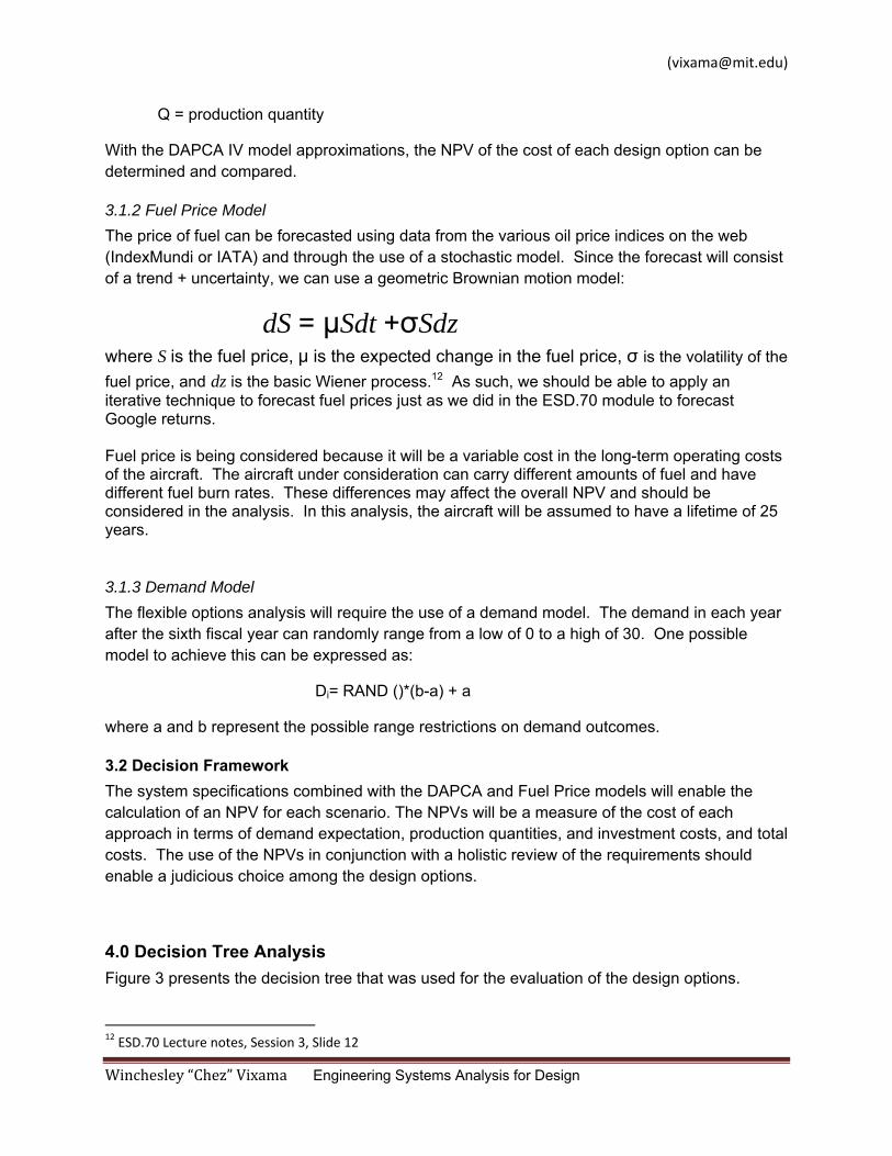
Q = production quantity

With the DAPCA IV model approximations, the NPV of the cost of each design option can be determined and compared.

3.1.2 Fuel Price Model The price of fuel can be forecasted using data from the various oil price indices on the web (IndexMundi or IATA) and through the use of a stochastic model. Since the forecast will consist of a trend + uncertainty, we can use a geometric Brownian motion model:

dS = μSdt +σSdz where S is the fuel price, μ is the expected change in the fuel price, σ is the volatility of the fuel price, and dz is the basic Wiener process.12 As such, we should be able to apply an iterative technique to forecast fuel prices just as we did in the ESD.70 module to forecast Google returns. Fuel price is being considered because it will be a variable cost in the long-term operating costs of the aircraft. The aircraft under consideration can carry different amounts of fuel and have different fuel burn rates. These differences may affect the overall NPV and should be considered in the analysis. In this analysis, the aircraft will be assumed to have a lifetime of 25 years.

3.1.3 Demand Model The flexible options analysis will require the use of a demand model. The demand in each year after the sixth fiscal year can randomly range from a low of 0 to a high of 30. One possible model to achieve this can be expressed as:

Di= RAND ()*(b-a) + a

where a and b represent the possible range restrictions on demand outcomes.

3.2 Decision Framework The system specifications combined with the DAPCA and Fuel Price models will enable the calculation of an NPV for each scenario. The NPVs will be a measure of the cost of each approach in terms of demand expectation, production quantities, and investment costs, and total costs. The use of the NPVs in conjunction with a holistic review of the requirements should enable a judicious choice among the design options.

4.0 Decision Tree Analysis Figure 3 presents the decision tree that was used for the evaluation of the design options.

12 ESD.70 Lecture notes, Session 3, Slide 12

([email protected])


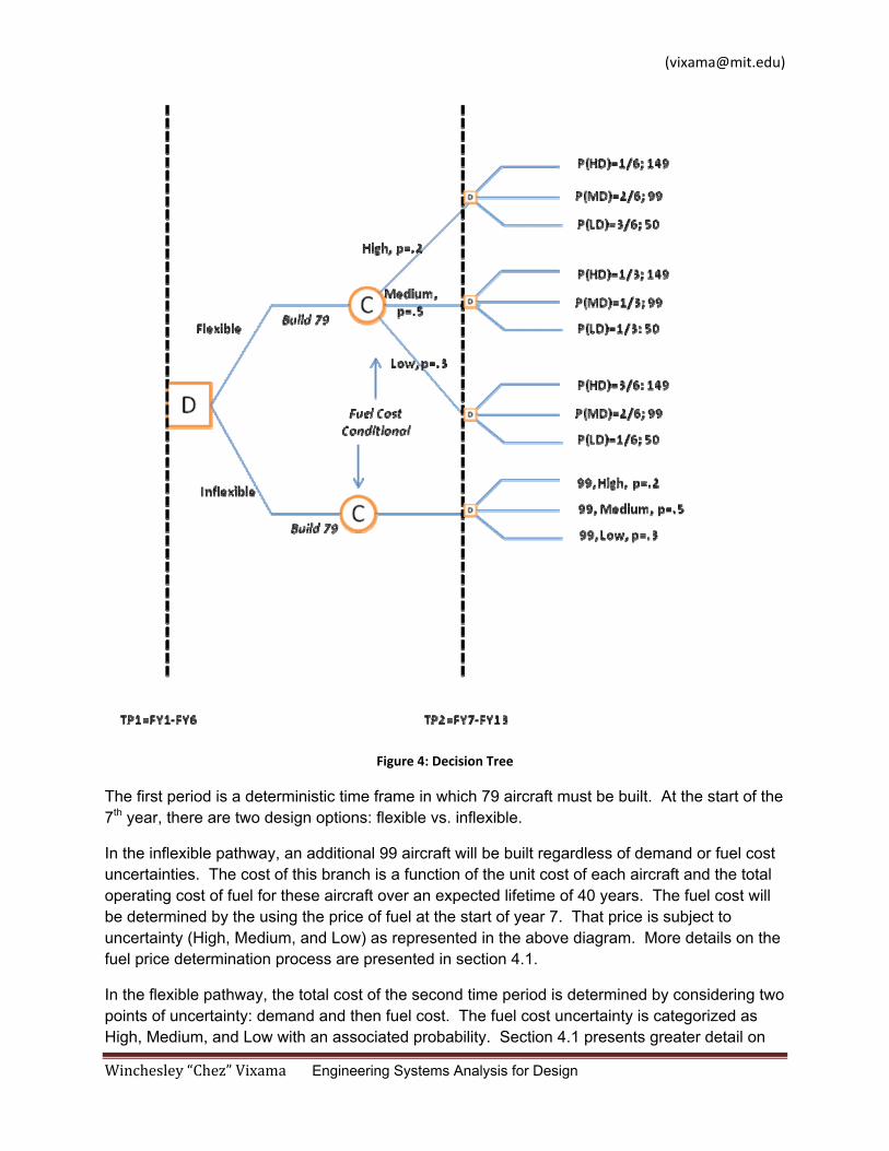
Figure 4: Decision Tree

The first period is a deterministic time frame in which 79 aircraft must be built. At the start of the 7th year, there are two design options: flexible vs. inflexible.

In the inflexible pathway, an additional 99 aircraft will be built regardless of demand or fuel cost uncertainties. The cost of this branch is a function of the unit cost of each aircraft and the total operating cost of fuel for these aircraft over an expected lifetime of 40 years. The fuel cost will be determined by the using the price of fuel at the start of year 7. That price is subject to uncertainty (High, Medium, and Low) as represented in the above diagram. More details on the fuel price determination process are presented in section 4.1.

In the flexible pathway, the total cost of the second time period is determined by considering two points of uncertainty: demand and then fuel cost. The fuel cost uncertainty is categorized as High, Medium, and Low with an associated probability. Section 4.1 presents greater detail on

([email protected])


the stochastic modeling and Monte Carlo simulation used to determine the price of fuel at the start of the second time period. Similarly, the demand uncertainty is also modeled as High, Medium, and Low with an associated probability. Additional details on the demand likelihood determination is presented in section 4.2

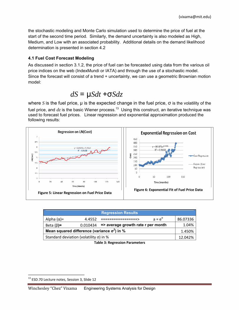
4.1 Fuel Cost Forecast Modeling As discussed in section 3.1.2, the price of fuel can be forecasted using data from the various oil price indices on the web (IndexMundi or IATA) and through the use of a stochastic model. Since the forecast will consist of a trend + uncertainty, we can use a geometric Brownian motion model:

dS = μSdt +σSdz where S is the fuel price, μ is the expected change in the fuel price, σ is the volatility of the fuel price, and dz is the basic Wiener process.13 Using this construct, an iterative technique was used to forecast fuel prices. Linear regression and exponential approximation produced the following results:

Figure 5: Linear Regression on Fuel Price Data Figure 6: Exponential Fit of Fuel Price Data

Regression Results Alpha (α)= 4.4552 =================> a = eα 86.07336Beta (β)= 0.010434 => average growth rate r per month 1.04%Mean squared difference (variance σ2) in % 1.450%Standard deviation (volatility σ) in % 12.042%

Table 3: Regression Parameters

13 ESD.70 Lecture notes, Session 3, Slide 12

([email protected])


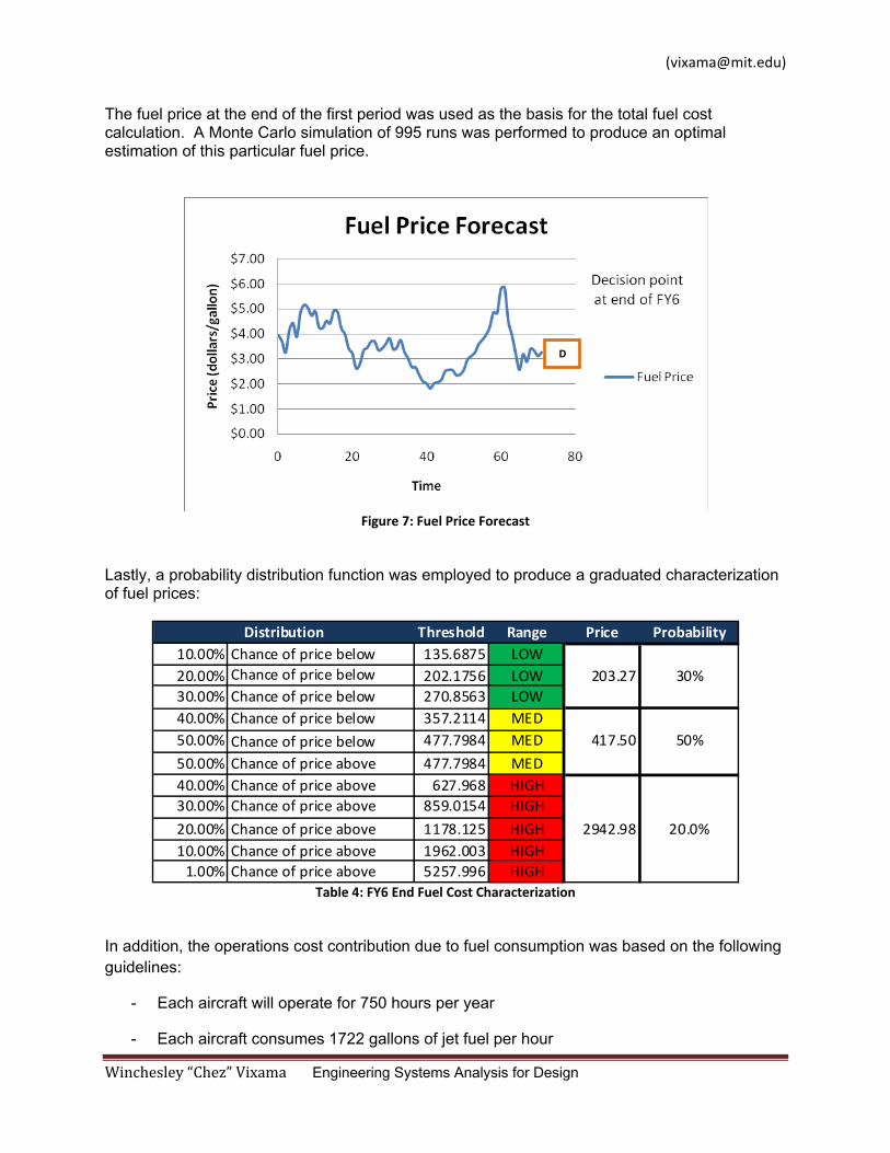
The fuel price at the end of the first period was used as the basis for the total fuel cost calculation. A Monte Carlo simulation of 995 runs was performed to produce an optimal estimation of this particular fuel price.

Figure 7: Fuel Price Forecast

Lastly, a probability distribution function was employed to produce a graduated characterization of fuel prices:

Threshold Range Price Probability10.00% 135.6875 LOW20.00% 202.1756 LOW 203.27 30%30.00% 270.8563 LOW40.00% 357.2114 MED50.00% 477.7984 MED 417.50 50%

50.00% Chance of price above 477.7984 MED40.00% Chance of price above 627.968 HIGH30.00% Chance of price above 859.0154 HIGH

20.00% Chance of price above 1178.125 HIGH 2942.98 20.0%10.00% Chance of price above 1962.003 HIGH1.00% Chance of price above 5257.996 HIGH

DistributionChance of price belowChance of price belowChance of price belowChance of price below

Chance of price below

Table 4: FY6 End Fuel Cost Characterization

In addition, the operations cost contribution due to fuel consumption was based on the following guidelines:

- Each aircraft will operate for 750 hours per year

- Each aircraft consumes 1722 gallons of jet fuel per hour

D

([email protected])


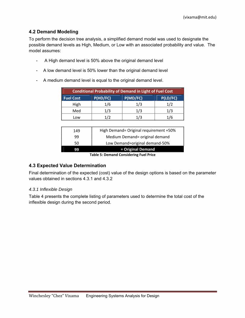
4.2 Demand Modeling To perform the decision tree analysis, a simplified demand model was used to designate the possible demand levels as High, Medium, or Low with an associated probability and value. The model assumes:

- A High demand level is 50% above the original demand level

- A low demand level is 50% lower than the original demand level

- A medium demand level is equal to the original demand level.

Conditional Probability of Demand in Light of Fuel Cost

Fuel Cost P(HD/FC) P(MD/FC) P(LD/FC) High 1/6 1/3 1/2

Med 1/3 1/3 1/3

Low 1/2 1/3 1/6

149 High Demand= Original requirement +50%

99 Medium Demand= original demand

50 Low Demand=original demand‐50%

99 = Original Demand Table 5: Demand Considering Fuel Price

4.3 Expected Value Determination Final determination of the expected (cost) value of the design options is based on the parameter values obtained in sections 4.3.1 and 4.3.2

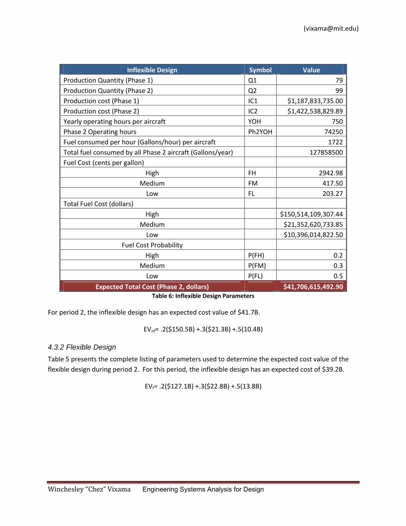
4.3.1 Inflexible Design Table 4 presents the complete listing of parameters used to determine the total cost of the inflexible design during the second period.

([email protected])


Inflexible Design Symbol Value Production Quantity (Phase 1) Q1 79Production Quantity (Phase 2) Q2 99Production cost (Phase 1) IC1 $1,187,833,735.00Production cost (Phase 2) IC2 $1,422,538,829.89Yearly operating hours per aircraft YOH 750Phase 2 Operating hours Ph2YOH 74250Fuel consumed per hour (Gallons/hour) per aircraft 1722Total fuel consumed by all Phase 2 aircraft (Gallons/year) 127858500Fuel Cost (cents per gallon)

High FH 2942.98Medium FM 417.50Low FL 203.27

Total Fuel Cost (dollars) High $150,514,109,307.44

Medium $21,352,620,733.85Low $10,396,014,822.50

Fuel Cost Probability High P(FH) 0.2

Medium P(FM) 0.3Low P(FL) 0.5

Expected Total Cost (Phase 2, dollars) $41,706,615,492.90Table 6: Inflexible Design Parameters

For period 2, the inflexible design has an expected cost value of $41.7B.

EVnf= .2($150.5B) +.3($21.3B) +.5(10.4B)

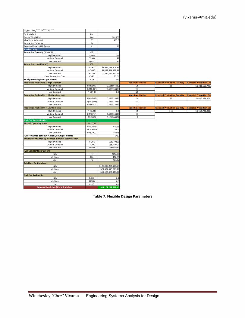
4.3.2 Flexible Design Table 5 presents the complete listing of parameters used to determine the expected cost value of the flexible design during period 2. For this period, the inflexible design has an expected cost of $39.2B.

EVf= .2($127.1B) +.3($22.8B) +.5(13.8B)

([email protected])


CM) = 11We0.921 *V0.621 *Q0.799

Cost (dollars) CmEmpty Weight(lb) We 181600Max Velocity(knots) V 495.3Production Quantity QExpected Service Life (years) L 40Flexible DesignProduction Quantity (Phase 2) Q2

High Demand Q2HD 149Medium Demand Q2MD 99Low Demand Q2LD 50

Production cost (Phase 2) IC2High Demand PC2HD $1,972,093,209.95

Medium Demand PC2MD $1,422,538,829.89Low Demand PC2LD $824,192,470.75

EV of Production Cost EVPC $0.00Yearly operating hours per aircraft YOH 750Production Probability if High Fuel cost Node Contribution Expected Production Quantity Expected Production Cos

High Demand P(HD/HF) 0.166666667 25

Medium Demand P(MD/HF) 0.333333333 33Low Demand P(LD/HF) 0.5 25

Production Probability if Medium Fuel cost Node Contribution Expected Production Quantity Expected Production Cos

High Demand P(HD/MF) 0.333333333 50Medium Demand P(MD/MF) 0.333333333 33Low Demand P(LD/MF) 0.333333333 17

Production Probability if Low Fuel cost Node Contribution Expected Production Quantity Expected Production CosHigh Demand P(HD/LF) 0.5 75

Medium Demand P(MD/LF) 0.333333333 33Low Demand P(LD/LF) 0.166666667 8

Fuel Cost DeterminationPhase 2 Operating hours Ph2YOH

High Demand Ph2OHHD 62125Medium Demand Ph2OHMD 74500Low Demand Ph2OHLD 86875

Fuel consumed per hour (Gallons/hour) per aircrfat 1722Total fuel consumed by all Phase 2 aircraft (Gallons/year)

High Demand TFCHD 106979250Medium Demand TFCMD 128289000Low Demand TFCLD 149598750

Fuel Cost (cents per gallon)High FH 2942.98

Medium FM 417.50Low FL 203.27

Total Fuel Cost (dollars)High $125,935,205,935.69

Medium $21,424,515,079.76Low $12,163,687,376.50

Fuel Cost ProbabilityHigh P(FH) 0.2

Medium P(FM) 0.3Low P(FL) 0.5

Expected Total Cost (Phase 2, dollars) $39,177,233,822.13

83 $1,233,665,770.

$1,426,364,501.99

116 $1,612,703,836.

Table 7: Flexible Design Parameters

([email protected])


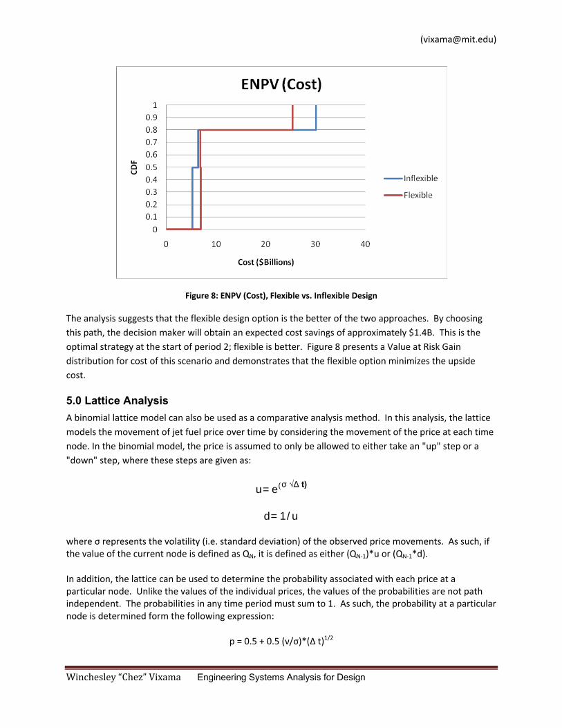
Figure 8: ENPV (Cost), Flexible vs. Inflexible Design

The analysis suggests that the flexible design option is the better of the two approaches. By choosing this path, the decision maker will obtain an expected cost savings of approximately $1.4B. This is the optimal strategy at the start of period 2; flexible is better. Figure 8 presents a Value at Risk Gain distribution for cost of this scenario and demonstrates that the flexible option minimizes the upside cost.

5.0 Lattice Analysis A binomial lattice model can also be used as a comparative analysis method. In this analysis, the lattice models the movement of jet fuel price over time by considering the movement of the price at each time node. In the binomial model, the price is assumed to only be allowed to either take an "up" step or a "down" step, where these steps are given as:

u=e(σ √Δ t)

d=1/u

where σ represents the volatility (i.e. standard deviation) of the observed price movements. As such, if the value of the current node is defined as QN, it is defined as either (QN‐1)*u or (QN‐1*d).

In addition, the lattice can be used to determine the probability associated with each price at a particular node. Unlike the values of the individual prices, the values of the probabilities are not path independent. The probabilities in any time period must sum to 1. As such, the probability at a particular node is determined form the following expression:

p = 0.5 + 0.5 (ν/σ)*(Δ t)1/2

([email protected])


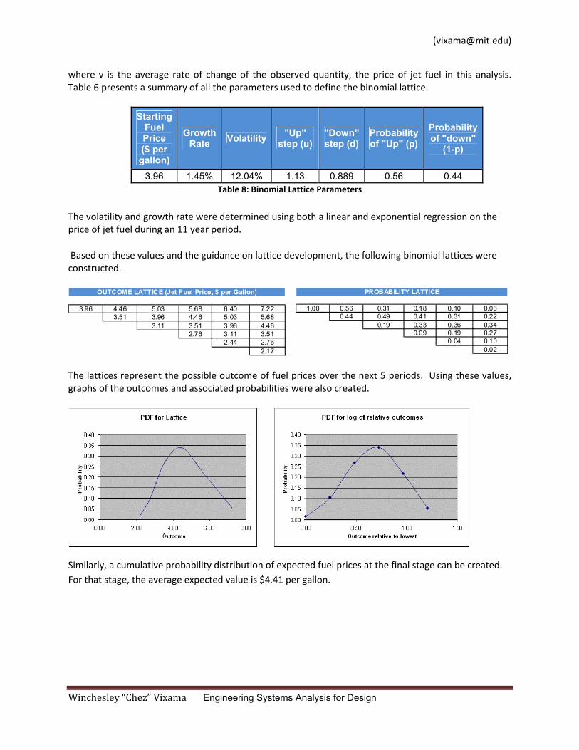
where v is the average rate of change of the observed quantity, the price of jet fuel in this analysis. Table 6 presents a summary of all the parameters used to define the binomial lattice.

Starting Fuel Price ($ per gallon)

Growth Rate Volatility "Up"

step (u) "Down" step (d)

Probability of "Up" (p)

Probability of "down"

(1-p)

3.96 1.45% 12.04% 1.13 0.889 0.56 0.44 Table 8: Binomial Lattice Parameters

The volatility and growth rate were determined using both a linear and exponential regression on the price of jet fuel during an 11 year period.

Based on these values and the guidance on lattice development, the following binomial lattices were constructed.

1 2 3 4 53.96 4.46 5.03 5.68 6.40 7.22

3.51 3.96 4.46 5.03 5.683.11 3.51 3.96 4.46

2.76 3.11 3.512.44 2.76

2.17

OUTCOME LATTICE (Jet Fuel Price, $ per Gallon)

1 2 3 4 51.00 0.56 0.31 0.18 0.10 0.06

0.44 0.49 0.41 0.31 0.220.19 0.33 0.36 0.34

0.09 0.19 0.270.04 0.10

0.02

PROBABILITY LATTICE

The lattices represent the possible outcome of fuel prices over the next 5 periods. Using these values, graphs of the outcomes and associated probabilities were also created.

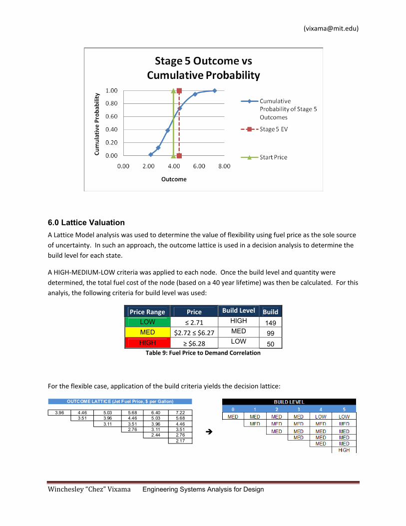
Similarly, a cumulative probability distribution of expected fuel prices at the final stage can be created. For that stage, the average expected value is $4.41 per gallon.

([email protected])


6.0 Lattice Valuation A Lattice Model analysis was used to determine the value of flexibility using fuel price as the sole source of uncertainty. In such an approach, the outcome lattice is used in a decision analysis to determine the build level for each state.

A HIGH‐MEDIUM‐LOW criteria was applied to each node. Once the build level and quantity were determined, the total fuel cost of the node (based on a 40 year lifetime) was then be calculated. For this analyis, the following criteria for build level was used:

Price Range Price Build Level BuildLOW ≤ 2.71 HIGH 149 MED $2.72 ≤ $6.27 MED 99 HIGH ≥ $6.28 LOW 50 Table 9: Fuel Price to Demand Correlation

For the flexible case, application of the build criteria yields the decision lattice:

1 2 3 4 53.96 4.46 5.03 5.68 6.40 7.22

3.51 3.96 4.46 5.03 5.683.11 3.51 3.96 4.46

2.76 3.11 3.512.44 2.76

2.17

OUTCOME LATTICE (Jet Fuel Price, $ per Gallon)

([email protected])


In the inflexible case, each node is locked to a build level of MEDIUM (99 aircraft) regardless of the price of jet fuel.

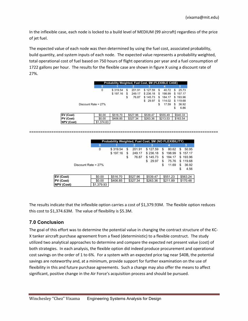
The expected value of each node was then determined by using the fuel cost, associated probability, build quantity, and system inputs of each node. The expected value represents a probability weighted, total operational cost of fuel based on 750 hours of flight operations per year and a fuel consumption of 1722 gallons per hour. The results for the flexible case are shown in figure X using a discount rate of 27%.

0 1 2 3 4 5750 0 319.54$ 201.91$ 127.59$ 40.72$ 25.73$

1722 197.16$ 249.17$ 236.18$ 198.99$ 157.17$ 27% 76.87$ 145.73$ 184.17$ 193.96$

29.97$ 114.02$ 119.68$ Discount Rate = 27% 17.59$ 36.92$

6.86$

$0.00 $516.70 $527.96 $539.47 $555.49 $540.33$0.00 $406.85 $327.34 $263.36 $213.53 $163.54

$1,374.63

Probability Weighted, Fuel Cost, $M (FLEXIBLE CASE)

EV (Cost)PV (Cost)NPV (Cost)

=====================================================================================

0 1 2 3 4 5750 0 319.54$ 201.91$ 127.59$ 80.62$ 50.95$

1722 197.16$ 249.17$ 236.18$ 198.99$ 157.17$ 27% 76.87$ 145.73$ 184.17$ 193.96$

29.97$ 75.76$ 119.68$ Discount Rate = 27% 11.69$ 36.92$

4.56$

$0.00 $516.70 $527.96 $539.47 $551.23 $563.24$0.00 $406.85 $327.34 $263.36 $211.89 $170.48

$1,379.93PV (Cost)NPV (Cost)

Probability Weighted, Fuel Cost, $M (NO FLEXIBILITY)

EV (Cost)

The results indicate that the inflexible option carries a cost of $1,379.93M. The flexible option reduces this cost to $1,374.63M. The value of flexibility is $5.3M.

7.0 Conclusion The goal of this effort was to determine the potential value in changing the contract structure of the KC‐X tanker aircraft purchase agreement from a fixed (deterministic) to a flexible construct. The study utilized two analytical approaches to determine and compare the expected net present value (cost) of both strategies. In each analysis, the flexible option did indeed produce procurement and operational cost savings on the order of 1 to 6%. For a system with an expected price tag near $40B, the potential savings are noteworthy and, at a minimum, provide support for further examination on the use of flexibility in this and future purchase agreements. Such a change may also offer the means to affect significant, positive change in the Air Force’s acquisition process and should be pursued.

KC‐X Tanker Replacement Program: Value of …ardent.mit.edu/real_options/Real_opts_portfolio...([email protected]) Winchesley “Chez” Vixama Engineering Systems Analysis for Design

Documents