Kaon photoproduction in a multipole approach

arX

iv:n

ucl-

th/0

6090

77v1

28

Sep

2006

Kaon photoproduction in a multipole approach

T. Mart and A. Sulaksono

Departemen Fisika, FMIPA, Universitas Indonesia, Depok 16424, Indonesia

(Dated: February 9, 2008)

Abstract

The recently published experimental data on K+Λ photoproduction by the SAPHIR, CLAS,

and LEPS collaborations are analyzed by means of a multipole approach. For this purpose the

background amplitudes are constructed from appropriate Feynman diagrams in a gauge-invariant

and crossing-symmetric fashion. The results of our calculation emphasize the lack of mutual

consistency between the SAPHIR and CLAS data previously found by several independent research

groups, whereas the LEPS data are found to be more consistent with those of CLAS. The use

of SAPHIR and CLAS data, individually or simultaneously, leads to quite different resonance

parameters which, therefore, could lead to different conclusions on “missing resonances”. Fitting

to the SAPHIR and LEPS data simultaneously indicates that the S11(1650), P13(1720), D13(1700),

D13(2080), F15(1680), and F15(2000) resonances are required, while fitting to the combination of

CLAS and LEPS data leads alternatively to the P13(1900), D13(2080), D15(1675), F15(1680), and

F17(1990) resonances. Although yielding different results in most cases, both SAPHIR and CLAS

data indicate that the second peak in the cross sections at W ∼ 1900 MeV originates from the

D13(2080) resonance with a mass between 1911 – 1936 MeV. Furthermore, in contrast to the results

of currently available models and the Table of Particle Properties, both data sets do not exhibit

the need for a P11(1710) resonance. The few data points available for target asymmetry can not

be described by the models proposed in the present work.

PACS numbers: 13.60.Le, 25.20.Lj, 14.20.Gk

1

I. INTRODUCTION

Modern theories of the strong interaction would certainly be incomplete if we ignored

the necessity to understand hadronic interactions in the medium energy region. However,

due to the nonperturbative nature of QCD at these energies, hadronic physics continues to

be a challenging field of investigation. This is also supported by the fact that methods like

chiral perturbation theory are not amenable to this energy region. Lattice QCD, which is

expected to alleviate this problem, has only recently begun to contribute to this field.

One of the most intensively studied topics in the realm of hadronic physics is the asso-

ciated strangeness photoproduction. High-intensity continuous electron beams produced by

modern accelerator technologies, along with unprecedented precise detectors, are among the

important aspects that have brought renewed attention to this 40 years old field of research.

On the other hand, the argument that some of the resonances predicted by constituent quark

models are strongly coupled to strangeness channels, and therefore intangible to πN → πN

reactions that are used by Particle Data Group (PDG) to extract the properties of nucleon

resonances, has raised the issue of “missing” resonances. As a consequence, photoproduc-

tion of strange particles becomes a unique tool that can shed important information on

the structure of resonances and, thus, complement the πN → πN channels. Among the

possible reactions, the γp → K+Λ is the most intensively studied channel since it does not

involve isospin-3/2 intermediate states which makes theoretical formalism much simpler. It

is also this channel for which most of the good quality experimental data are available.

Furthermore, in this process the self-analyzing power of the weak decay Λ → pπ− can be

utilized to determine the polarization of the recoiled Λ. Therefore, the beauty of working

with K+Λ photoproduction is that precise Λ polarizations will accompany accurate cross

section measurements.

In the last decades a large number of attempts have been devoted to model the above

reaction process. Most of these have been performed in the framework of tree-level isobar

models [1, 2, 3, 4, 5], coupled channel calculations [6, 7, 8], or quark models [9, 10]. Extending

the validity of isobar models to higher energy regions has also been recently pursued [11,

12, 13].

In contrast to pion and eta photoproduction, the kaon photoproduction process is not

dominated by a single resonant state. Therefore, the main difference among the models

2

is chiefly in the use of nucleon, hyperon, and kaon resonances. The widely used KAON-

MAID model [5], for instance, uses nucleon resonances S11(1650), P11(1710), P13(1720),

and D13(1895), where the latter is known as the missing resonance in this model. On

the other hand, the Adelseck-Saghai model [2] has solely one nucleon resonance S11(1650)

and one hyperon resonance S01(1670). The more complicated Saclay-Lyon model [14] uti-

lizes the P11(1440), P13(1720), and D15(1675) nucleon resonances, along with the S01(1405),

S01(1670), P01(1810), and P11(1660) hyperon resonances. Although those models vary with

the number of resonances, they mostly use low spin states, because higher spin propagators

and vertices are quite complicated in such a framework and, moreover, are not free of some

fundamental ambiguities. Only in the Saclay-Lyon [14] and Renard-Renard models [15] is a

spin-5/2 nucleon resonance utilized. Other models argue that the use of resonance excitation

up to spin 3/2, or even up to spin 1/2, is sufficient.

Clearly, there is a lack of systematic procedure to determine how many resonances should

be built into the process. There has been no attempt to include the F15, F17, G17, and G19

states, although some of them could have sizable branching fractions to the KΛ channel (see

Table II in the next section or Review of Particle Properties [16]).

The main motivation of the present work is to explore the possibility of using higher

spin states in kaon photoproduction. Ideally, this should be performed on the basis of a

coupled-channels formalism. However, the level of complexity in such a framework increases

quickly with the addition of resonance states. In view of this, we constrain the present work

to a single-channel analysis, but we use as much as possible nucleon resonances listed by

PDG. This argument is also supported by the fact that the recently available SAPHIR [17]

and CLAS [18] data have a problem of mutual consistency [7, 19]. Thus, another purpose

of this work is to investigate the physics consequence of using each data set. The present

work is basically an extension of our previous analysis [20] which was performed using a

slightly different method and only the SAPHIR data [17]. To this end, we will use the same

formalism developed for pion photoproduction [21, 22] which has the advantage that it

provides a direct comparison of the extracted helicity photon coupling with the PDG values

and paves the way for extending the present work to include the effect of other channels.

This paper is organized as follows. In Section II we present the formalism of our work.

Section III briefly discusses the experimental data used in the fitting process as well as

the chosen fitting strategy. In Section IV we discuss the comparison of the results of our

3

calculation with the current available data. In this section we also discuss the possible origin

of the second peak in the cross sections at W ∼ 1900 MeV. In Section V we summarize our

findings.

II. FORMALISM

A. The Background Amplitudes

The background amplitudes are obtained from a series of tree-level Feynman diagrams

[23]. They consist of the standard s-, u-, and t-channel Born terms along with the K∗(892)

and K1(1270) t-channel vector mesons. Altogether they are often called extended Born

terms. Apart from the K1(1270) exchange, these background terms are similar to the ones

used by Thom [24]. The importance of the K1(1270) intermediate state has been pointed

out for the first time by Ref. [25] and since then it has been extensively used in almost

all isobar models. To account for hadronic structures of interacting baryons and mesons

we include the appropriate hadronic form factors in the hadronic vertices by utilizing the

method developed by Haberzettl in order to maintain gauge invariance of the amplitudes.

We have also tested the gauge method proposed by Ohta [26], but since the produced χ2 is

substantially larger, we will not discuss Ohta method here. Furthermore, to comply with

the crossing symmetry requirement we use a special form factor in the gauge terms

F (s, t, u) = F1(s) + F1(u) + F3(t) − F1(s)F1(u)

−F1(s)F3(t) − F1(u)F3(t) + F1(s)F1(u)F3(t) , (1)

proposed by Davidson and Workman [27], with Mandelstam variables s, t, and u, and

Fi(x) =Λ4

Λ4 + (x − m2i )

2, (2)

where Λ and mi are the form factor cut-off and the intermediate state mass, respectively

[28]. Thus, comparing to the previous pioneering work [24], the major improvement in the

background sector is the use of hadronic form factors in a gauge-invariant fashion and the

crossing-symmetric properties of the Born terms.

4

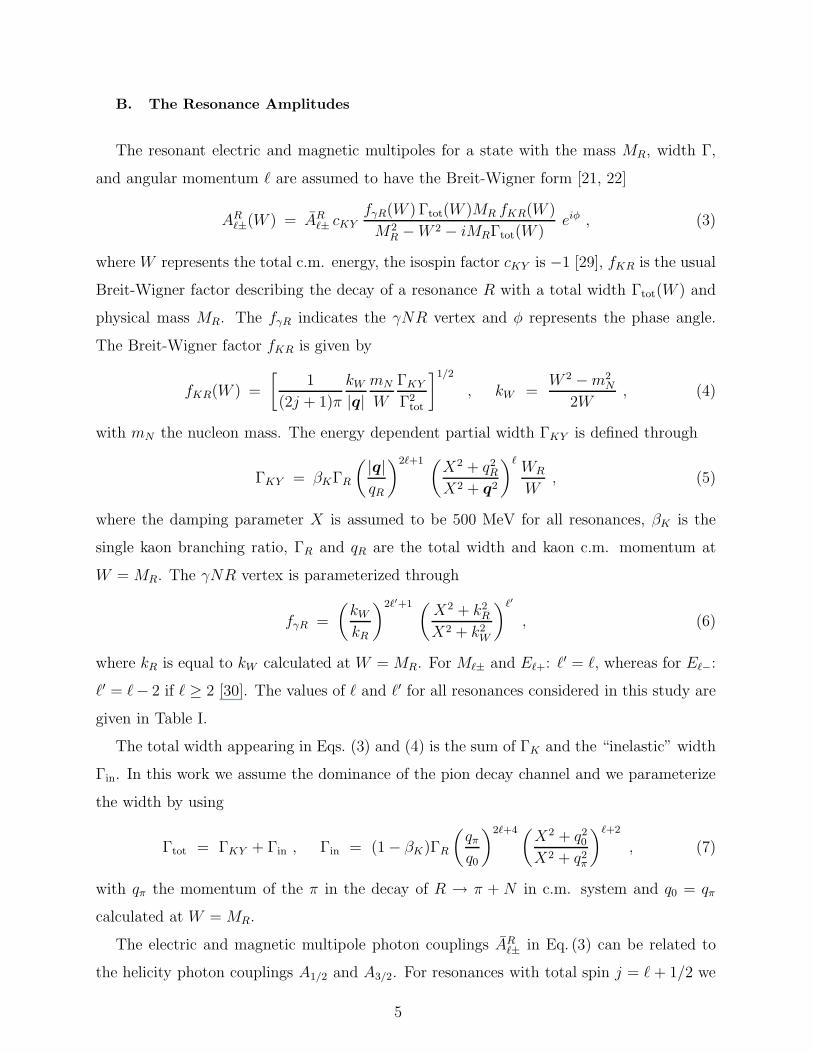
B. The Resonance Amplitudes

The resonant electric and magnetic multipoles for a state with the mass MR, width Γ,

and angular momentum ℓ are assumed to have the Breit-Wigner form [21, 22]

ARℓ±(W ) = AR

ℓ± cKYfγR(W ) Γtot(W )MR fKR(W )

M2R − W 2 − iMRΓtot(W )

eiφ , (3)

where W represents the total c.m. energy, the isospin factor cKY is −1 [29], fKR is the usual

Breit-Wigner factor describing the decay of a resonance R with a total width Γtot(W ) and

physical mass MR. The fγR indicates the γNR vertex and φ represents the phase angle.

The Breit-Wigner factor fKR is given by

fKR(W ) =

[1

(2j + 1)π

kW

|q|mN

W

ΓKY

Γ2tot

]1/2

, kW =W 2 − m2

N

2W, (4)

with mN the nucleon mass. The energy dependent partial width ΓKY is defined through

ΓKY = βKΓR

( |q|qR

)2ℓ+1 (X2 + q2

R

X2 + q2

)ℓWR

W, (5)

where the damping parameter X is assumed to be 500 MeV for all resonances, βK is the

single kaon branching ratio, ΓR and qR are the total width and kaon c.m. momentum at

W = MR. The γNR vertex is parameterized through

fγR =

(kW

kR

)2ℓ′+1 (X2 + k2

R

X2 + k2W

)ℓ′

, (6)

where kR is equal to kW calculated at W = MR. For Mℓ± and Eℓ+: ℓ′ = ℓ, whereas for Eℓ−:

ℓ′ = ℓ− 2 if ℓ ≥ 2 [30]. The values of ℓ and ℓ′ for all resonances considered in this study are

given in Table I.

The total width appearing in Eqs. (3) and (4) is the sum of ΓK and the “inelastic” width

Γin. In this work we assume the dominance of the pion decay channel and we parameterize

the width by using

Γtot = ΓKY + Γin , Γin = (1 − βK)ΓR

(qπ

q0

)2ℓ+4 (X2 + q2

0

X2 + q2π

)ℓ+2

, (7)

with qπ the momentum of the π in the decay of R → π + N in c.m. system and q0 = qπ

calculated at W = MR.

The electric and magnetic multipole photon couplings ARℓ± in Eq. (3) can be related to

the helicity photon couplings A1/2 and A3/2. For resonances with total spin j = ℓ + 1/2 we

5

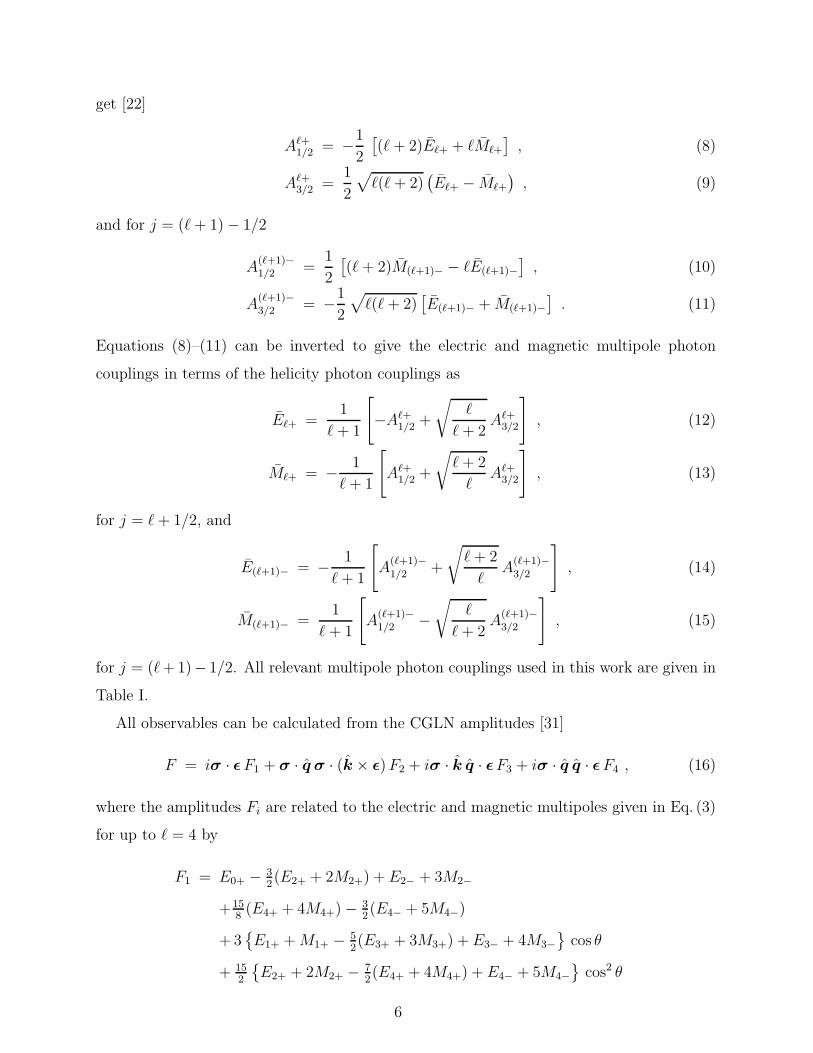
get [22]

Aℓ+1/2 = −1

2

[(ℓ + 2)Eℓ+ + ℓMℓ+

], (8)

Aℓ+3/2 =

1

2

√ℓ(ℓ + 2)

(Eℓ+ − Mℓ+

), (9)

and for j = (ℓ + 1) − 1/2

A(ℓ+1)−1/2 =

1

2

[(ℓ + 2)M(ℓ+1)− − ℓE(ℓ+1)−

], (10)

A(ℓ+1)−3/2 = −1

2

√ℓ(ℓ + 2)

[E(ℓ+1)− + M(ℓ+1)−

]. (11)

Equations (8)–(11) can be inverted to give the electric and magnetic multipole photon

couplings in terms of the helicity photon couplings as

Eℓ+ =1

ℓ + 1

[

−Aℓ+1/2 +

√ℓ

ℓ + 2Aℓ+

3/2

]

, (12)

Mℓ+ = − 1

ℓ + 1

[Aℓ+

1/2 +

√ℓ + 2

ℓAℓ+

3/2

], (13)

for j = ℓ + 1/2, and

E(ℓ+1)− = − 1

ℓ + 1

[A

(ℓ+1)−1/2 +

√ℓ + 2

ℓA

(ℓ+1)−3/2

], (14)

M(ℓ+1)− =1

ℓ + 1

[A

(ℓ+1)−1/2 −

√ℓ

ℓ + 2A

(ℓ+1)−3/2

], (15)

for j = (ℓ + 1)− 1/2. All relevant multipole photon couplings used in this work are given in

Table I.

All observables can be calculated from the CGLN amplitudes [31]

F = iσ · ǫ F1 + σ · q σ · (k × ǫ) F2 + iσ · k q · ǫF3 + iσ · q q · ǫ F4 , (16)

where the amplitudes Fi are related to the electric and magnetic multipoles given in Eq. (3)

for up to ℓ = 4 by

F1 = E0+ − 32(E2+ + 2M2+) + E2− + 3M2−

+158(E4+ + 4M4+) − 3

2(E4− + 5M4−)

+ 3E1+ + M1+ − 5

2(E3+ + 3M3+) + E3− + 4M3−

cos θ

+ 152

E2+ + 2M2+ − 7

2(E4+ + 4M4+) + E4− + 5M4−

cos2 θ

6

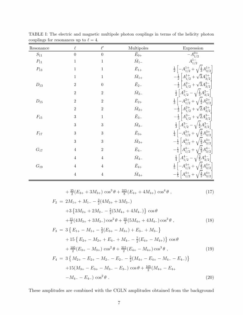
TABLE I: The electric and magnetic multipole photon couplings in terms of the helicity photon

couplings for resonances up to ℓ = 4.

Resonance ℓ ℓ′ Multipoles Expression

S11 0 0 E0+ −A0+1/2

P11 1 1 M1− A1−1/2

P13 1 1 E1+12

[−A1+

1/2 +√

13A1+

3/2

]

1 1 M1+ −12

[A1+

1/2 +√

3A1+3/2

]

D13 2 0 E2− −12

[A2−

1/2 +√

3A2−3/2

]

2 2 M2−12

[A2−

1/2 −√

13A2−

3/2

]

D15 2 2 E2+13

[−A2+

1/2 +√

12A2+

3/2

]

2 2 M2+ −13

[A2+

1/2 +√

2A2+3/2

]

F15 3 1 E3− −13

[A3−

1/2 +√

2A3−3/2

]

3 3 M3−13

[A3−

1/2 −√

12A3−

3/2

]

F17 3 3 E3+14

[−A3+

1/2 +√

35A3+

3/2

]

3 3 M3+ −14

[A3+

1/2 +√

53A3+

3/2

]

G17 4 2 E4− −14

[A4−

1/2 +√

53A4−

3/2

]

4 4 M4−14

[A4−

1/2 −√

35A4−

3/2

]

G19 4 4 E4+15

[−A4+

1/2 +√

23A4+

3/2

]

4 4 M4+ −15

[A4+

1/2 +√

32A4+

3/2

]

+ 352(E3+ + 3M3+) cos3 θ + 315

8(E4+ + 4M4+) cos4 θ , (17)

F2 = 2M1+ + M1− − 32(4M3+ + 3M3−)

+33M2+ + 2M2− − 5

2(5M4+ + 4M4−)

cos θ

+152(4M3+ + 3M3−) cos2 θ + 35

2(5M4+ + 4M4−) cos3 θ , (18)

F3 = 3

E1+ − M1+ − 52(E3+ − M3+) + E3− + M3−

+ 15

E2+ − M2+ + E4− + M4− − 72(E4+ − M4+)

cos θ

+ 1052

(E3+ − M3+) cos2 θ + 3152

(E4+ − M4+) cos3 θ , (19)

F4 = 3

M2+ − E2+ − M2− − E2− − 52(M4+ − E4+ − M4− − E4−)

+15(M3+ − E3+ − M3− − E3−) cos θ + 1052

(M4+ − E4+

−M4− − E4−) cos2 θ . (20)

These amplitudes are combined with the CGLN amplitudes obtained from the background

7

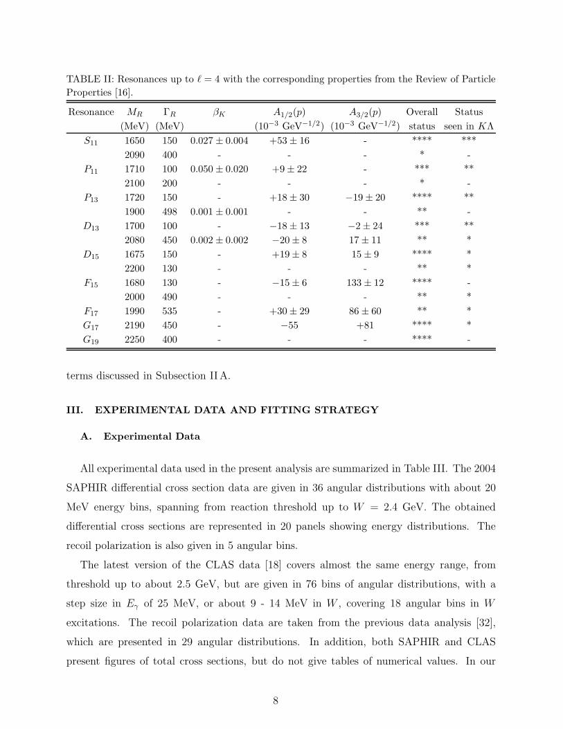
TABLE II: Resonances up to ℓ = 4 with the corresponding properties from the Review of Particle

Properties [16].

Resonance MR ΓR βK A1/2(p) A3/2(p) Overall Status

(MeV) (MeV) (10−3 GeV−1/2) (10−3 GeV−1/2) status seen in KΛ

S11 1650 150 0.027 ± 0.004 +53 ± 16 - **** ***

2090 400 - - - * -

P11 1710 100 0.050 ± 0.020 +9 ± 22 - *** **

2100 200 - - - * -

P13 1720 150 - +18 ± 30 −19 ± 20 **** **

1900 498 0.001 ± 0.001 - - ** -

D13 1700 100 - −18 ± 13 −2 ± 24 *** **

2080 450 0.002 ± 0.002 −20 ± 8 17 ± 11 ** *

D15 1675 150 - +19 ± 8 15 ± 9 **** *

2200 130 - - - ** *

F15 1680 130 - −15 ± 6 133 ± 12 **** -

2000 490 - - - ** *

F17 1990 535 - +30 ± 29 86 ± 60 ** *

G17 2190 450 - −55 +81 **** *

G19 2250 400 - - - **** -

terms discussed in Subsection IIA.

III. EXPERIMENTAL DATA AND FITTING STRATEGY

A. Experimental Data

All experimental data used in the present analysis are summarized in Table III. The 2004

SAPHIR differential cross section data are given in 36 angular distributions with about 20

MeV energy bins, spanning from reaction threshold up to W = 2.4 GeV. The obtained

differential cross sections are represented in 20 panels showing energy distributions. The

recoil polarization is also given in 5 angular bins.

The latest version of the CLAS data [18] covers almost the same energy range, from

threshold up to about 2.5 GeV, but are given in 76 bins of angular distributions, with a

step size in Eγ of 25 MeV, or about 9 - 14 MeV in W , covering 18 angular bins in W

excitations. The recoil polarization data are taken from the previous data analysis [32],

which are presented in 29 angular distributions. In addition, both SAPHIR and CLAS

present figures of total cross sections, but do not give tables of numerical values. In our

8

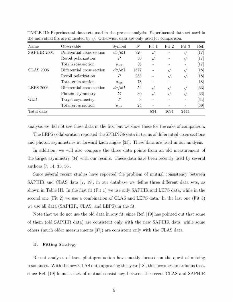
TABLE III: Experimental data sets used in the present analysis. Experimental data set used in

the individual fits are indicated by√

. Otherwise, data are only used for comparison.

Name Observable Symbol N Fit 1 Fit 2 Fit 3 Ref.

SAPHIR 2004 Differential cross section dσ/dΩ 720√

-√

[17]

Recoil polarization P 30√

-√

[17]

Total cross section σtot 36 - - - [17]

CLAS 2006 Differential cross section dσ/dΩ 1377 -√ √

[18]

Recoil polarization P 233 -√ √

[18]

Total cross section σtot 78 - - - [18]

LEPS 2006 Differential cross section dσ/dΩ 54√ √ √

[33]

Photon asymmetry Σ 30√ √ √

[33]

OLD Target asymmetry T 3 - - - [34]

Total cross section σtot 24 - - - [39]

Total data 834 1694 2444

analysis we did not use these data in the fits, but we show these for the sake of comparison.

The LEPS collaboration reported the SPRING8 data in terms of differential cross sections

and photon asymmetries at forward kaon angles [33]. These data are used in our analysis.

In addition, we will also compare the three data points from an old measurement of

the target asymmetry [34] with our results. These data have been recently used by several

authors [7, 14, 35, 36].

Since several recent studies have reported the problem of mutual consistency between

SAPHIR and CLAS data [7, 19], in our database we define three different data sets, as

shown in Table III. In the first fit (Fit 1) we use only SAPHIR and LEPS data, while in the

second one (Fit 2) we use a combination of CLAS and LEPS data. In the last one (Fit 3)

we use all data (SAPHIR, CLAS, and LEPS) in the fit.

Note that we do not use the old data in any fit, since Ref. [19] has pointed out that some

of them (old SAPHIR data) are consistent only with the new SAPHIR data, while some

others (much older measurements [37]) are consistent only with the CLAS data.

B. Fitting Strategy

Recent analyses of kaon photoproduction have mostly focused on the quest of missing

resonances. With the new CLAS data appearing this year [18], this becomes an arduous task,

since Ref. [19] found a lack of mutual consistency between the recent CLAS and SAPHIR

9

data. As will be shown in the next section, the use of the two data sets, individually or

simultaneously, leads to quite different values of the extracted resonance parameters and,

therefore, could yield different conclusions on the missing resonances studied by this reaction.

In view of this, in the present work we do not focus our attention on searching for missing

resonances. Instead, we will use all nucleon resonances listed by PDG up to spin 9/2 and

fit their parameters to new data. Along with their known parameters those resonances are

listed in Table II. Note that we do not use resonances with masses below the reaction

threshold (1610 MeV) since their contributions would only contribute to the background

terms and, therefore, would be difficult to see in the present formalism. Furthermore, we do

not include the two resonances with spin higher than 9/2 (i.e., I1 11 and K1 13) for practical

reasons and because too little information is available for both states.

The number of free parameters is relatively large, i.e., 7 from the background amplitude

and 86 from the resonance part. To reduce this we fix both gKΛN and gKΣN coupling

constants to the SU(3) predictions, i.e., gKΛN/√

4π = −3.80 and gKΣN/√

4π = 1.20, and

fix masses as well as widths of the four-star resonances to their PDG values. To avoid

unrealistically large values obtained from fitting to experimental data, the total width ΓR is

limited to 500 MeV and the kaon branching ratio βK is limited to 0.3. The χ2 minimization

fit is performed by using the CERN-MINUIT code.

IV. RESULTS AND DISCUSSION

A. Numerical Results

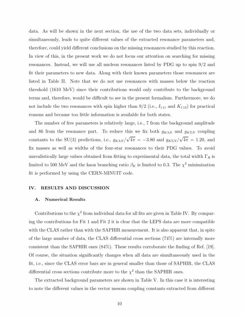
Contributions to the χ2 from individual data for all fits are given in Table IV. By compar-

ing the contributions for Fit 1 and Fit 2 it is clear that the LEPS data are more compatible

with the CLAS rather than with the SAPHIR measurement. It is also apparent that, in spite

of the large number of data, the CLAS differential cross sections (74%) are internally more

consistent than the SAPHIR ones (84%). These results corroborate the finding of Ref. [19].

Of course, the situation significantly changes when all data are simultaneously used in the

fit, i.e., since the CLAS error bars are in general smaller than those of SAPHIR, the CLAS

differential cross sections contribute more to the χ2 than the SAPHIR ones.

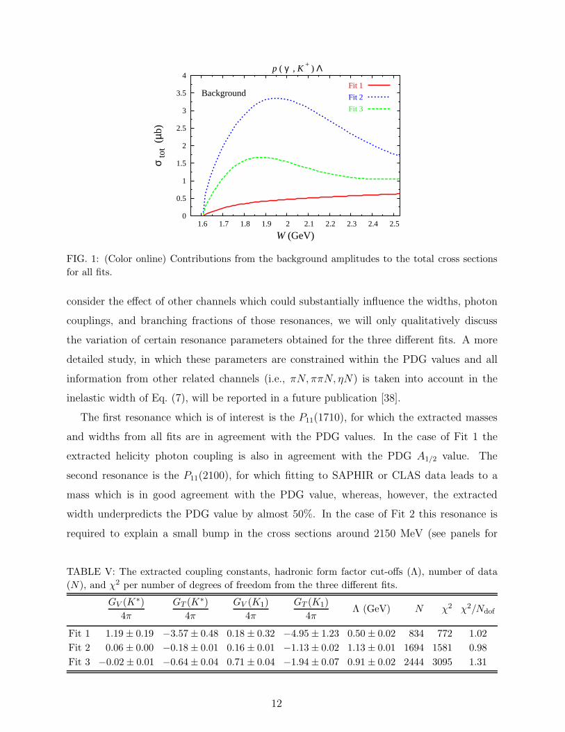
The extracted background parameters are shown in Table V. In this case it is interesting

to note the different values in the vector mesons coupling constants extracted from different

10

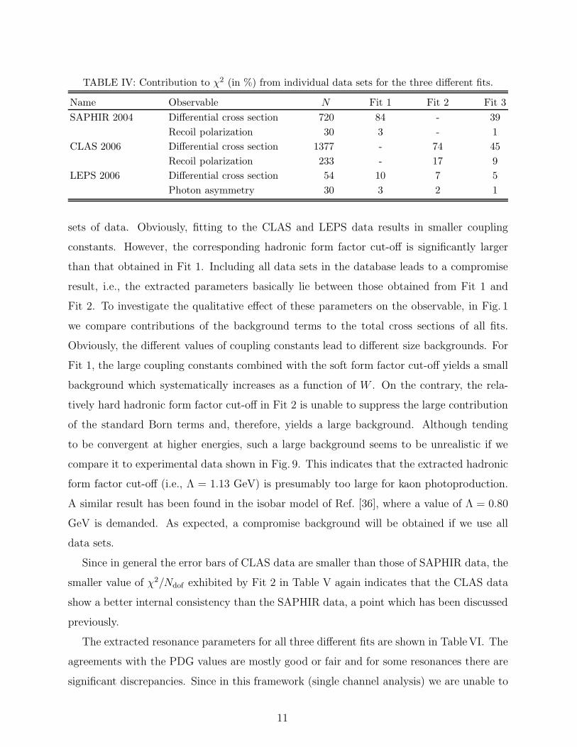
TABLE IV: Contribution to χ2 (in %) from individual data sets for the three different fits.

Name Observable N Fit 1 Fit 2 Fit 3

SAPHIR 2004 Differential cross section 720 84 - 39

Recoil polarization 30 3 - 1

CLAS 2006 Differential cross section 1377 - 74 45

Recoil polarization 233 - 17 9

LEPS 2006 Differential cross section 54 10 7 5

Photon asymmetry 30 3 2 1

sets of data. Obviously, fitting to the CLAS and LEPS data results in smaller coupling

constants. However, the corresponding hadronic form factor cut-off is significantly larger

than that obtained in Fit 1. Including all data sets in the database leads to a compromise

result, i.e., the extracted parameters basically lie between those obtained from Fit 1 and

Fit 2. To investigate the qualitative effect of these parameters on the observable, in Fig. 1

we compare contributions of the background terms to the total cross sections of all fits.

Obviously, the different values of coupling constants lead to different size backgrounds. For

Fit 1, the large coupling constants combined with the soft form factor cut-off yields a small

background which systematically increases as a function of W . On the contrary, the rela-

tively hard hadronic form factor cut-off in Fit 2 is unable to suppress the large contribution

of the standard Born terms and, therefore, yields a large background. Although tending

to be convergent at higher energies, such a large background seems to be unrealistic if we

compare it to experimental data shown in Fig. 9. This indicates that the extracted hadronic

form factor cut-off (i.e., Λ = 1.13 GeV) is presumably too large for kaon photoproduction.

A similar result has been found in the isobar model of Ref. [36], where a value of Λ = 0.80

GeV is demanded. As expected, a compromise background will be obtained if we use all

data sets.

Since in general the error bars of CLAS data are smaller than those of SAPHIR data, the

smaller value of χ2/Ndof exhibited by Fit 2 in Table V again indicates that the CLAS data

show a better internal consistency than the SAPHIR data, a point which has been discussed

previously.

The extracted resonance parameters for all three different fits are shown in TableVI. The

agreements with the PDG values are mostly good or fair and for some resonances there are

significant discrepancies. Since in this framework (single channel analysis) we are unable to

11

0

0.5

1

1.5

2

2.5

3

3.5

4

1.6 1.7 1.8 1.9 2 2.1 2.2 2.3 2.4 2.5

σ to

t (µ

b)

W (GeV)

p ( γ , K + ) Λ

BackgroundFit 1

Fit 2

Fit 3

FIG. 1: (Color online) Contributions from the background amplitudes to the total cross sections

for all fits.

consider the effect of other channels which could substantially influence the widths, photon

couplings, and branching fractions of those resonances, we will only qualitatively discuss

the variation of certain resonance parameters obtained for the three different fits. A more

detailed study, in which these parameters are constrained within the PDG values and all

information from other related channels (i.e., πN, ππN, ηN) is taken into account in the

inelastic width of Eq. (7), will be reported in a future publication [38].

The first resonance which is of interest is the P11(1710), for which the extracted masses

and widths from all fits are in agreement with the PDG values. In the case of Fit 1 the

extracted helicity photon coupling is also in agreement with the PDG A1/2 value. The

second resonance is the P11(2100), for which fitting to SAPHIR or CLAS data leads to a

mass which is in good agreement with the PDG value, whereas, however, the extracted

width underpredicts the PDG value by almost 50%. In the case of Fit 2 this resonance is

required to explain a small bump in the cross sections around 2150 MeV (see panels for

TABLE V: The extracted coupling constants, hadronic form factor cut-offs (Λ), number of data

(N), and χ2 per number of degrees of freedom from the three different fits.

GV (K∗)

4π

GT (K∗)

4π

GV (K1)

4π

GT (K1)

4πΛ (GeV) N χ2 χ2/Ndof

Fit 1 1.19 ± 0.19 −3.57 ± 0.48 0.18 ± 0.32 −4.95 ± 1.23 0.50 ± 0.02 834 772 1.02

Fit 2 0.06 ± 0.00 −0.18 ± 0.01 0.16 ± 0.01 −1.13 ± 0.02 1.13 ± 0.01 1694 1581 0.98

Fit 3 −0.02 ± 0.01 −0.64 ± 0.04 0.71 ± 0.04 −1.94 ± 0.07 0.91 ± 0.02 2444 3095 1.31

12

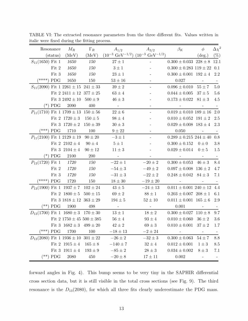
TABLE VI: The extracted resonance parameters from the three different fits. Values written in

italic were fixed during the fitting process.

Resonance MR ΓR A1/2 A3/2 βK φ ∆χ2

(status) (MeV) (MeV) (10−3 GeV−1/2) (10−3 GeV−1/2) (deg.) (%)

S11(1650) Fit 1 1650 150 27 ± 1 - 0.300 ± 0.033 228 ± 8 12.1

Fit 2 1650 150 3 ± 1 - 0.300 ± 0.283 119 ± 22 0.1

Fit 3 1650 150 23 ± 1 - 0.300 ± 0.001 192 ± 4 2.2

(****) PDG 1650 150 53 ± 16 - 0.027 - -

S11(2090) Fit 1 2261 ± 15 241 ± 33 39 ± 2 - 0.096 ± 0.010 55 ± 7 5.0

Fit 2 2411 ± 12 377 ± 25 63 ± 4 - 0.044 ± 0.005 37 ± 5 5.6

Fit 3 2492 ± 10 500 ± 9 46 ± 3 - 0.173 ± 0.022 81 ± 3 4.5

(*) PDG 2090 400 - - - - -

P11(1710) Fit 1 1709 ± 13 150 ± 56 22 ± 6 - 0.019 ± 0.010 189 ± 16 2.0

Fit 2 1720 ± 3 150 ± 5 98 ± 4 - 0.010 ± 0.052 191 ± 2 2.5

Fit 3 1720 ± 2 150 ± 39 30 ± 3 - 0.029 ± 0.008 183 ± 4 2.3

(***) PDG 1710 100 9 ± 22 - 0.050 - -

P11(2100) Fit 1 2129 ± 19 90 ± 20 −3 ± 1 - 0.289 ± 0.215 244 ± 40 0.8

Fit 2 2102 ± 4 90 ± 4 5 ± 1 - 0.300 ± 0.152 0 ± 0 3.8

Fit 3 2104 ± 4 90 ± 12 11 ± 3 - 0.029 ± 0.014 0 ± 5 1.5

(*) PDG 2100 200 - - - - -

P13(1720) Fit 1 1720 150 −22 ± 1 −20 ± 2 0.300 ± 0.053 46 ± 3 8.4

Fit 2 1720 150 −54 ± 3 −49 ± 2 0.097 ± 0.008 136 ± 2 4.7

Fit 3 1720 150 −31 ± 3 −22 ± 2 0.248 ± 0.042 84 ± 3 7.1

(****) PDG 1720 150 18 ± 30 −19 ± 20 - - -

P13(1900) Fit 1 1937 ± 7 102 ± 24 43 ± 5 −24 ± 13 0.011 ± 0.001 240 ± 12 4.4

Fit 2 1800 ± 5 500 ± 15 69 ± 2 88 ± 1 0.203 ± 0.007 208 ± 1 6.1

Fit 3 1818 ± 12 363 ± 29 194 ± 5 52 ± 10 0.011 ± 0.001 165 ± 6 2.9

(**) PDG 1900 498 - - 0.001 - -

D13(1700) Fit 1 1680 ± 3 170 ± 30 13 ± 1 18 ± 2 0.300 ± 0.027 110 ± 8 9.7

Fit 2 1750 ± 45 500 ± 385 56 ± 4 93 ± 4 0.010 ± 0.060 36 ± 2 3.6

Fit 3 1682 ± 3 499 ± 20 42 ± 2 69 ± 3 0.010 ± 0.001 37 ± 2 1.7

(***) PDG 1700 100 −18 ± 13 −2 ± 24 - - -

D13(2080) Fit 1 1936 ± 10 301 ± 22 −26 ± 2 −32 ± 3 0.300 ± 0.063 54 ± 7 8.8

Fit 2 1915 ± 4 165 ± 8 −140 ± 7 32 ± 4 0.012 ± 0.001 1 ± 3 8.5

Fit 3 1911 ± 4 193 ± 9 −85 ± 2 28 ± 3 0.034 ± 0.002 8 ± 3 7.1

(**) PDG 2080 450 −20 ± 8 17 ± 11 0.002 - -

forward angles in Fig. 4). This bump seems to be very tiny in the SAPHIR differential

cross section data, but it is still visible in the total cross sections (see Fig. 9). The third

resonance is the D13(2080), for which all three fits clearly underestimate the PDG mass.

13

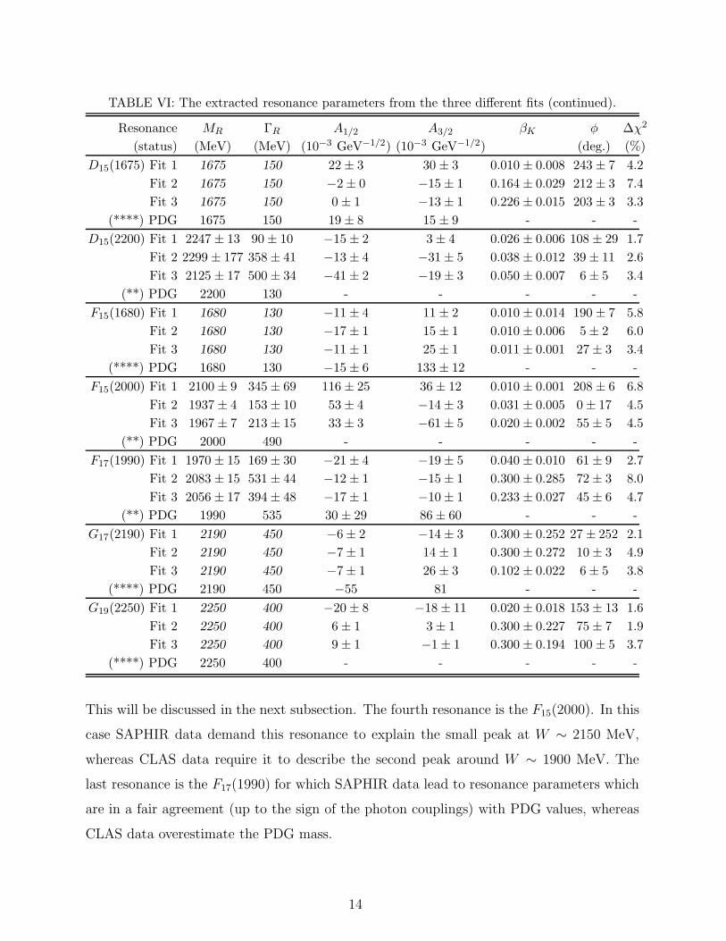
TABLE VI: The extracted resonance parameters from the three different fits (continued).

Resonance MR ΓR A1/2 A3/2 βK φ ∆χ2

(status) (MeV) (MeV) (10−3 GeV−1/2) (10−3 GeV−1/2) (deg.) (%)

D15(1675) Fit 1 1675 150 22 ± 3 30 ± 3 0.010 ± 0.008 243 ± 7 4.2

Fit 2 1675 150 −2 ± 0 −15 ± 1 0.164 ± 0.029 212 ± 3 7.4

Fit 3 1675 150 0 ± 1 −13 ± 1 0.226 ± 0.015 203 ± 3 3.3

(****) PDG 1675 150 19 ± 8 15 ± 9 - - -

D15(2200) Fit 1 2247 ± 13 90 ± 10 −15 ± 2 3 ± 4 0.026 ± 0.006 108 ± 29 1.7

Fit 2 2299 ± 177 358 ± 41 −13 ± 4 −31 ± 5 0.038 ± 0.012 39 ± 11 2.6

Fit 3 2125 ± 17 500 ± 34 −41 ± 2 −19 ± 3 0.050 ± 0.007 6 ± 5 3.4

(**) PDG 2200 130 - - - - -

F15(1680) Fit 1 1680 130 −11 ± 4 11 ± 2 0.010 ± 0.014 190 ± 7 5.8

Fit 2 1680 130 −17 ± 1 15 ± 1 0.010 ± 0.006 5 ± 2 6.0

Fit 3 1680 130 −11 ± 1 25 ± 1 0.011 ± 0.001 27 ± 3 3.4

(****) PDG 1680 130 −15 ± 6 133 ± 12 - - -

F15(2000) Fit 1 2100 ± 9 345 ± 69 116 ± 25 36 ± 12 0.010 ± 0.001 208 ± 6 6.8

Fit 2 1937 ± 4 153 ± 10 53 ± 4 −14 ± 3 0.031 ± 0.005 0 ± 17 4.5

Fit 3 1967 ± 7 213 ± 15 33 ± 3 −61 ± 5 0.020 ± 0.002 55 ± 5 4.5

(**) PDG 2000 490 - - - - -

F17(1990) Fit 1 1970 ± 15 169 ± 30 −21 ± 4 −19 ± 5 0.040 ± 0.010 61 ± 9 2.7

Fit 2 2083 ± 15 531 ± 44 −12 ± 1 −15 ± 1 0.300 ± 0.285 72 ± 3 8.0

Fit 3 2056 ± 17 394 ± 48 −17 ± 1 −10 ± 1 0.233 ± 0.027 45 ± 6 4.7

(**) PDG 1990 535 30 ± 29 86 ± 60 - - -

G17(2190) Fit 1 2190 450 −6 ± 2 −14 ± 3 0.300 ± 0.252 27 ± 252 2.1

Fit 2 2190 450 −7 ± 1 14 ± 1 0.300 ± 0.272 10 ± 3 4.9

Fit 3 2190 450 −7 ± 1 26 ± 3 0.102 ± 0.022 6 ± 5 3.8

(****) PDG 2190 450 −55 81 - - -

G19(2250) Fit 1 2250 400 −20 ± 8 −18 ± 11 0.020 ± 0.018 153 ± 13 1.6

Fit 2 2250 400 6 ± 1 3 ± 1 0.300 ± 0.227 75 ± 7 1.9

Fit 3 2250 400 9 ± 1 −1 ± 1 0.300 ± 0.194 100 ± 5 3.7

(****) PDG 2250 400 - - - - -

This will be discussed in the next subsection. The fourth resonance is the F15(2000). In this

case SAPHIR data demand this resonance to explain the small peak at W ∼ 2150 MeV,

whereas CLAS data require it to describe the second peak around W ∼ 1900 MeV. The

last resonance is the F17(1990) for which SAPHIR data lead to resonance parameters which

are in a fair agreement (up to the sign of the photon couplings) with PDG values, whereas

CLAS data overestimate the PDG mass.

14

To further investigate the importance of the individual resonances we define a parameter

∆χ2 =χ2

All − χ2All−N∗

χ2All

× 100 % , (21)

where χ2All is the χ2 obtained by using all resonances and χ2

All−N∗ is the χ2 obtained by using

all but a specific resonance. Therefore, ∆χ2 measures the relative difference between the χ2 of

including and of excluding the corresponding resonance. Note that the ∆χ2 does not measure

the “strength” of the resonance in the process but it merely reveals information on how

difficult to reproduce experimental data without that resonance. A similar ratio has been

also defined in Ref. [7] in order to investigate the role of individual resonances. The numerical

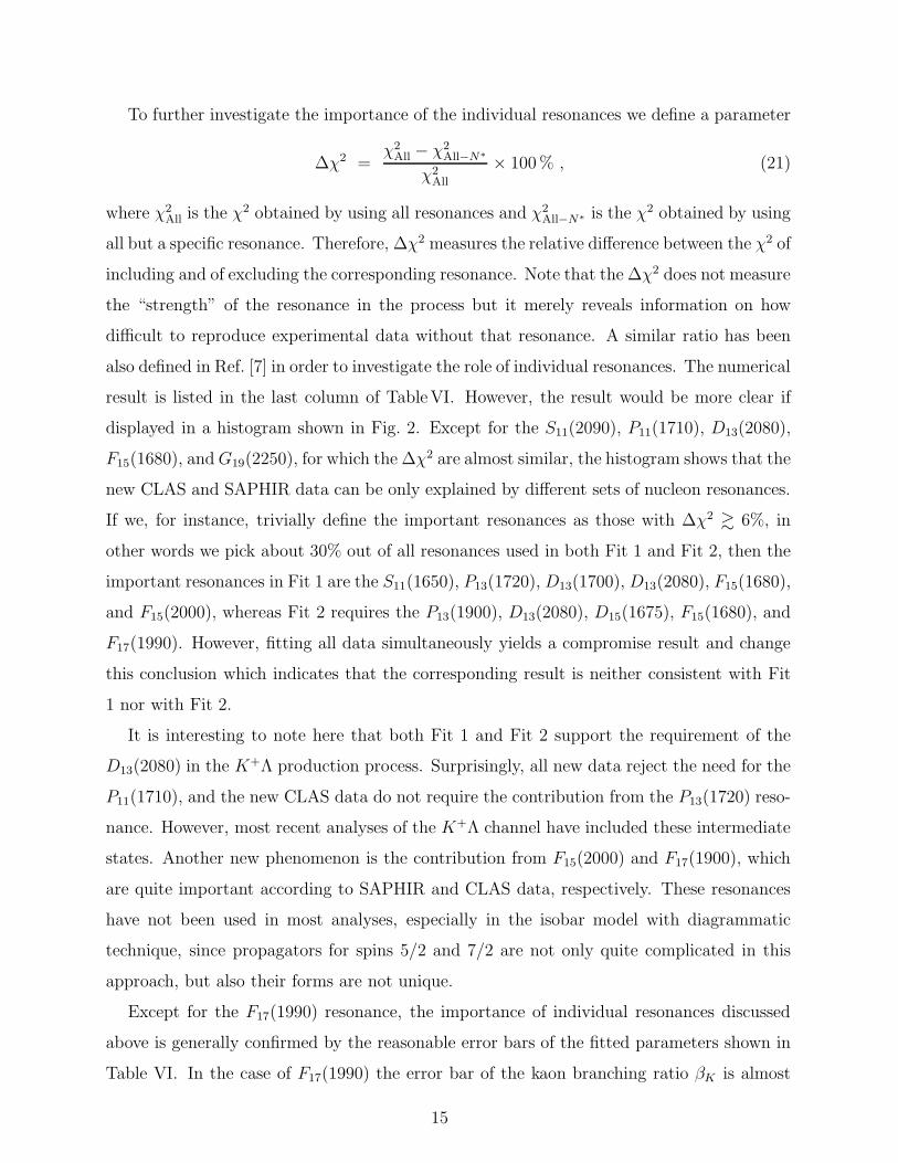
result is listed in the last column of TableVI. However, the result would be more clear if

displayed in a histogram shown in Fig. 2. Except for the S11(2090), P11(1710), D13(2080),

F15(1680), and G19(2250), for which the ∆χ2 are almost similar, the histogram shows that the

new CLAS and SAPHIR data can be only explained by different sets of nucleon resonances.

If we, for instance, trivially define the important resonances as those with ∆χ2 & 6%, in

other words we pick about 30% out of all resonances used in both Fit 1 and Fit 2, then the

important resonances in Fit 1 are the S11(1650), P13(1720), D13(1700), D13(2080), F15(1680),

and F15(2000), whereas Fit 2 requires the P13(1900), D13(2080), D15(1675), F15(1680), and

F17(1990). However, fitting all data simultaneously yields a compromise result and change

this conclusion which indicates that the corresponding result is neither consistent with Fit

1 nor with Fit 2.

It is interesting to note here that both Fit 1 and Fit 2 support the requirement of the

D13(2080) in the K+Λ production process. Surprisingly, all new data reject the need for the

P11(1710), and the new CLAS data do not require the contribution from the P13(1720) reso-

nance. However, most recent analyses of the K+Λ channel have included these intermediate

states. Another new phenomenon is the contribution from F15(2000) and F17(1900), which

are quite important according to SAPHIR and CLAS data, respectively. These resonances

have not been used in most analyses, especially in the isobar model with diagrammatic

technique, since propagators for spins 5/2 and 7/2 are not only quite complicated in this

approach, but also their forms are not unique.

Except for the F17(1990) resonance, the importance of individual resonances discussed

above is generally confirmed by the reasonable error bars of the fitted parameters shown in

Table VI. In the case of F17(1990) the error bar of the kaon branching ratio βK is almost

15

0 2 4 6 8 10 12 14 16

S11 (1650)

S11 (2090)

P11 (1710)

P11 (2100)

P13 (1720)

P13 (1900)

D13 (1700)

D13 (2080)

D15 (1675)

D15 (2200)

F15 (1680)

F15 (2000)

F17 (1990)

G17 (2190)

G19 (2250)

165016501650

226124112492

170917201720

212921022104

172017201720

193718001818

168017501682

193619151911

167516751675

224722992125

168016801680

210019371967

197020832056

219021902190

225022502250

∆ χ2 (%)

Fit 1Fit 2Fit 3

FIG. 2: (Color online) The significance of individual resonances in the three different fits. Values

written in italic were fixed during the fit process.

the same as the value of βK itself, whereas, on the other hand, the corresponding ∆χ2

indicates that this resonance is strongly needed to explain the CLAS data. We have tried

to understand this by relaxing the upper limit of βK and refitting the F17(1990) resonance

parameters. It is found that with the same value of χ2 the extracted βK is 0.387 ± 0.150,

which indicates that this resonance is still important for Fit 2.

Since the CLAS and SAPHIR data are binned in different energy and angular bins,

16

1.628

0.0

0.1

0.2

0.31.643

p ( γ , K + ) Λ

1.657 1.671 1.685

1.699

0.00.10.20.3 1.713 1.727 1.740 1.753

1.767

0.00.10.20.3 1.780 1.793 1.806 1.819

1.832

0.00.10.20.3 1.845 1.858 1.870 1.883

1.896

0.00.10.20.3 1.908 1.920 1.933 1.945

1.957

0.00.10.20.3 1.969 1.981 1.993 2.005

2.016

0.00.10.20.3 2.028 2.040 2.052 2.063

2.075

dσ /

dΩ

(µb

/ sr

)

0.00.10.20.3 2.086 2.097 2.108 2.120

2.131

0.00.10.20.3 2.142 2.153 2.164 2.175

2.185

0.00.10.20.3 2.196 2.207 2.217 2.228

2.239

0.00.10.20.3 2.249 2.260 2.270 2.281

2.291

0.00.10.20.3 2.301 2.332 2.343 2.353

2.363

0.00.10.20.3 2.372 2.382 2.392 2.402

2.411

0.00.10.20.3 2.421 2.431 2.440 2.450

2.459

0.00.10.20.3 2.469 2.478 2.487 2.496

2.506

0.00.10.20.3

-1.0 -0.5 0.0 0.5 1.0 -0.5 0.0 0.5 1.0

2.515

-0.5 0.0 0.5 1.0

cos θ

2.524

-0.5 0.0 0.5 1.0

2.533

-0.5 0.0 0.5 1.0

Fit1Fit2Fit3

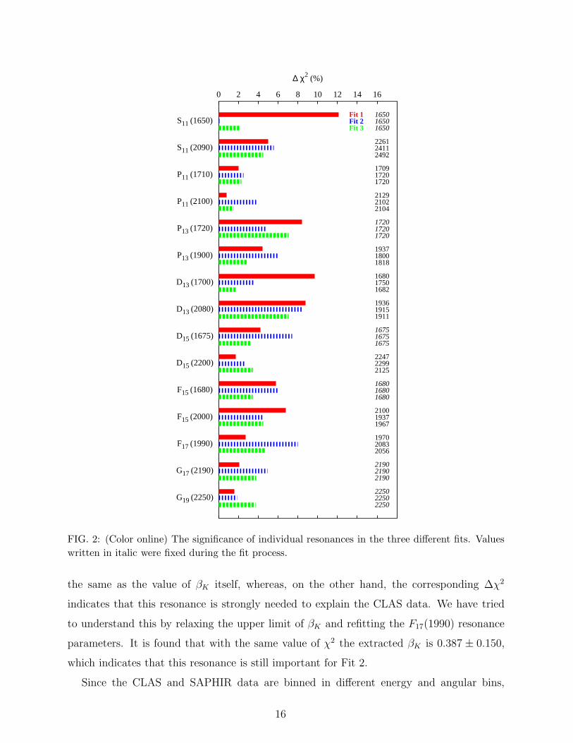
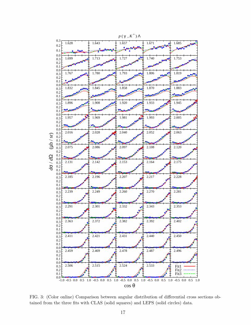
FIG. 3: (Color online) Comparison between angular distribution of differential cross sections ob-

tained from the three fits with CLAS (solid squares) and LEPS (solid circles) data.

17

cos θ = − 0.80

0.0

0.1

0.2

0.3

cos θ = − 0.70

p ( γ , K + ) Λ1.625

cos θ = − 0.60

0.0

0.1

0.2 cos θ = − 0.50

1.674

cos θ = − 0.40

0.0

0.1

0.2 cos θ = − 0.30

cos θ = − 0.20

0.00.10.20.3 cos θ = − 0.10

cos θ = 0.00

0.00.10.20.3

dσ /

dΩ

(µb

/sr)

cos θ = 0.10

cos θ = 0.20

0.00.10.20.3 cos θ = 0.30

cos θ = 0.40

0.00.10.20.3 cos θ = 0.50

cos θ = 0.60

0.00.10.20.30.4 cos θ = 0.70

cos θ = 0.80

0.00.10.20.30.4

1.6 1.7 1.8 1.9 2.0 2.1 2.2 2.3 2.4 2.5

W (GeV)

cos θ = 0.90

1.6 1.7 1.8 1.9 2.0 2.1 2.2 2.3 2.4 2.5

W (GeV)

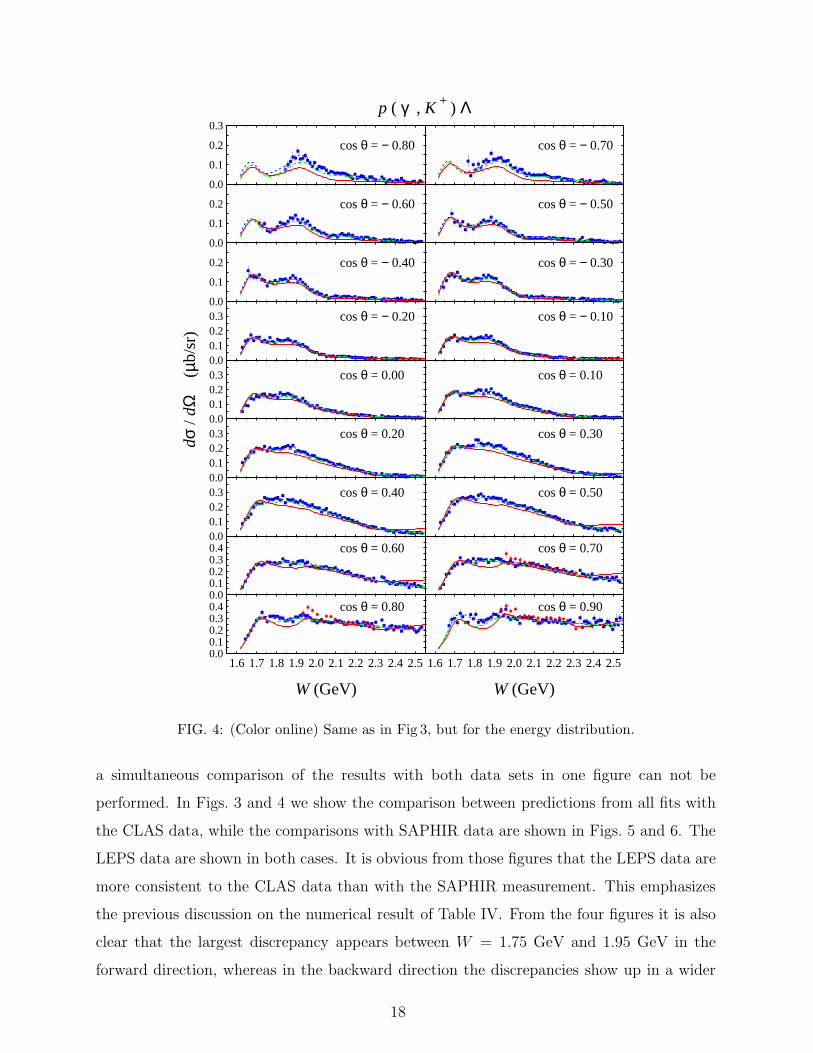
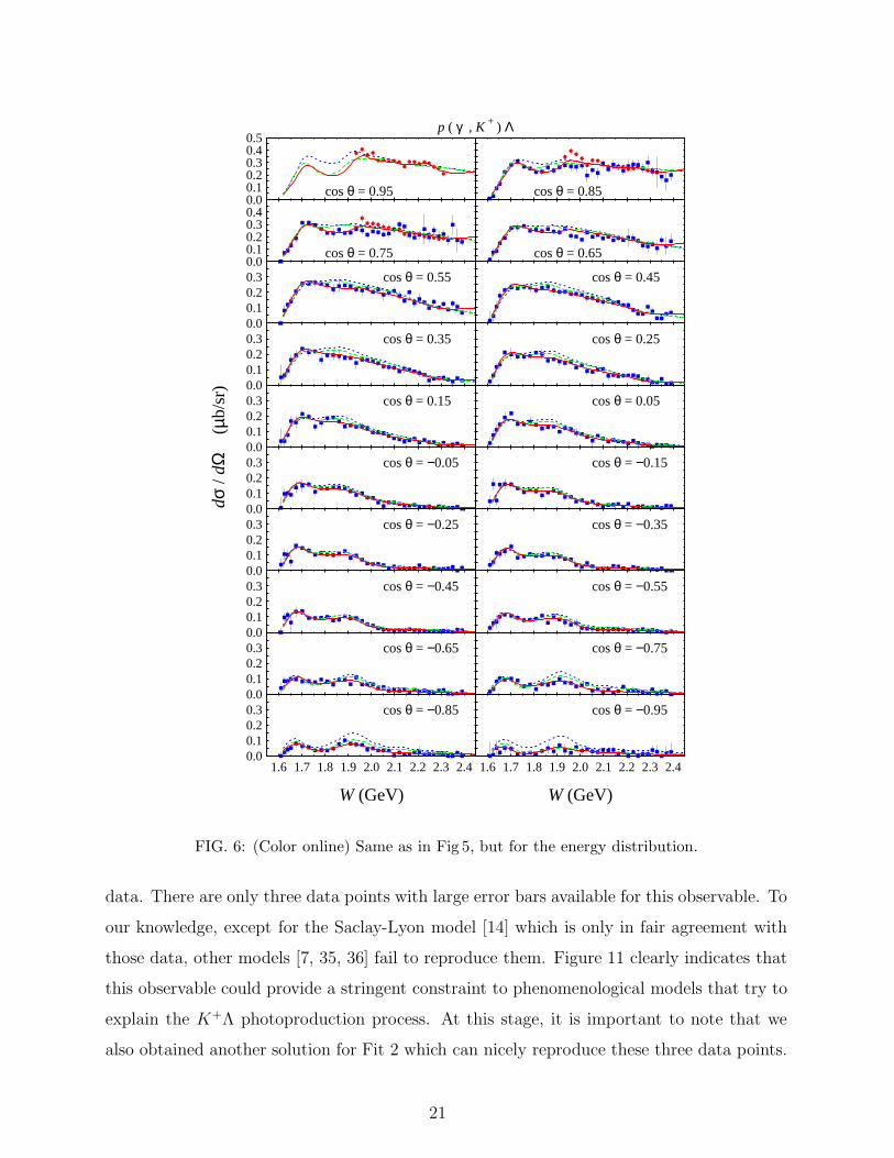
FIG. 4: (Color online) Same as in Fig 3, but for the energy distribution.

a simultaneous comparison of the results with both data sets in one figure can not be

performed. In Figs. 3 and 4 we show the comparison between predictions from all fits with

the CLAS data, while the comparisons with SAPHIR data are shown in Figs. 5 and 6. The

LEPS data are shown in both cases. It is obvious from those figures that the LEPS data are

more consistent to the CLAS data than with the SAPHIR measurement. This emphasizes

the previous discussion on the numerical result of Table IV. From the four figures it is also

clear that the largest discrepancy appears between W = 1.75 GeV and 1.95 GeV in the

forward direction, whereas in the backward direction the discrepancies show up in a wider

18

range, i.e., from 1.8 to 2.4 GeV. It is also important to note that at the very forward and

backward angles the two data sets (also, as a consequence, Fit 1 and Fit 2) exhibit very

different trends. The CLAS data tend to rise at these regions, while the SAPHIR data tend

to decrease.

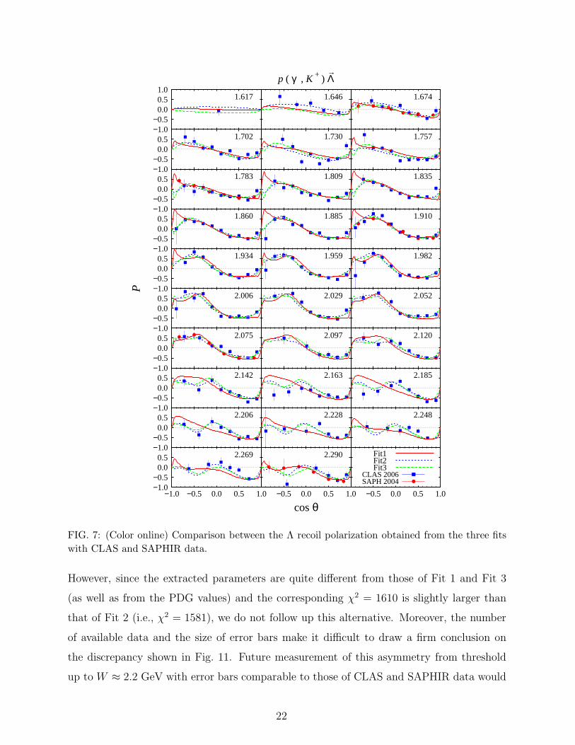
The Λ recoil polarizations obtained from all fits are compared with experimental data

in Fig. 7. Except at higher energies and in backward directions, where experimental data

have large error bars, no result shows any significant difference. Therefore, in view of the

present error bars, the Λ recoil polarization is not a decisive observable for revealing further

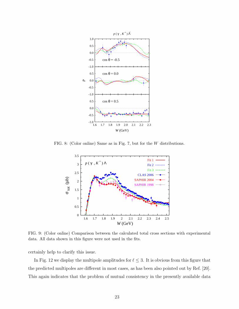
information from the three fits. The energy distribution of this observable shown in Fig. 8

emphasizes this argument. At cos θ = 0.5 it is interesting to remark that the polarizations

predicted by the three fits are almost similar and the values are almost constant at about

−0.5 over the whole energy range, except very close to threshold.

Both CLAS and SAPHIR collaborations extracted the total cross sections and displayed

them graphically. The numerical data points shown in Fig. 9 were taken from total cross

section figures of Refs. [17, 18] and, for the sake of consistency, not used in the fits. In

Ref. [7] it was suspected that the two collaborations have extracted the total cross sections

in different ways, hence the discrepancy between them seems to be larger than that in

differential cross sections. However, by comparing the solid line and solid squares, as well

as the dotted line and solid circles in Fig. 9, we conclude that the extracted total cross

sections from both collaborations are consistent with their differential cross sections. The

fact that the discrepancy is more profound in the total cross sections is seemingly due to the

cumulative effect of the integration, which can be immediately comprehended if we compare

the solid lines (fit to the SAPHIR data) with dotted lines (fit to the CLAS data) in Fig. 4.

On the other hand, the result of Fit 3 (dashed line in Fig. 9) clearly indicates that including

both data sets in the fit results in a model which is consistent with no data set, as has been

previously pointed out by Ref. [19].

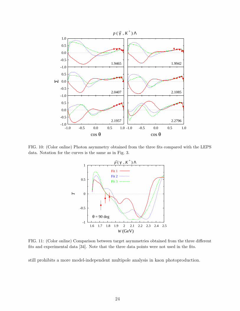
The result for the polarized photon beam asymmetry is shown in Fig. 10, where we can

obviously see a good agreement between predictions of all fits and the experimental data

from LEPS. This result also corroborates the finding of Ref. [7] that further measurements

of this observable in the backward directions would put a strong constraint on the model.

Reference [7] found that the currently available experimental data of this observable (see the

last line of Table IV) generate about 13% of the total χ2. In contrast to this, we found that

19

1.610

0.0

0.1

0.2

0.3SAPH 2004SPR8 2006

p ( γ , K + ) Λ

1.625 1.639

1.653

0.00.10.20.3 1.674 1.702

1.730

0.00.10.20.30.4 1.757 1.783

1.809

0.00.10.20.30.4 1.835 1.860

1.885

0.00.10.20.30.4 1.910 1.934

1.959

dσ /

dΩ

(µb

/sr)

0.00.10.20.30.4 1.982 2.006

2.029

0.00.10.20.30.4 2.052 2.075

2.097

0.00.10.20.30.4 2.120 2.142

2.163

0.00.10.20.30.4 2.185 2.206

2.228

0.00.10.20.30.4 2.248 2.269

2.290

0.00.10.20.30.4 2.310 2.330

2.350

0.00.10.20.30.4

-1.0 -0.5 0.0 0.5 1.0

2.370

-0.5 0.0 0.5 1.0

cos θ

2.390

-0.5 0.0 0.5 1.0

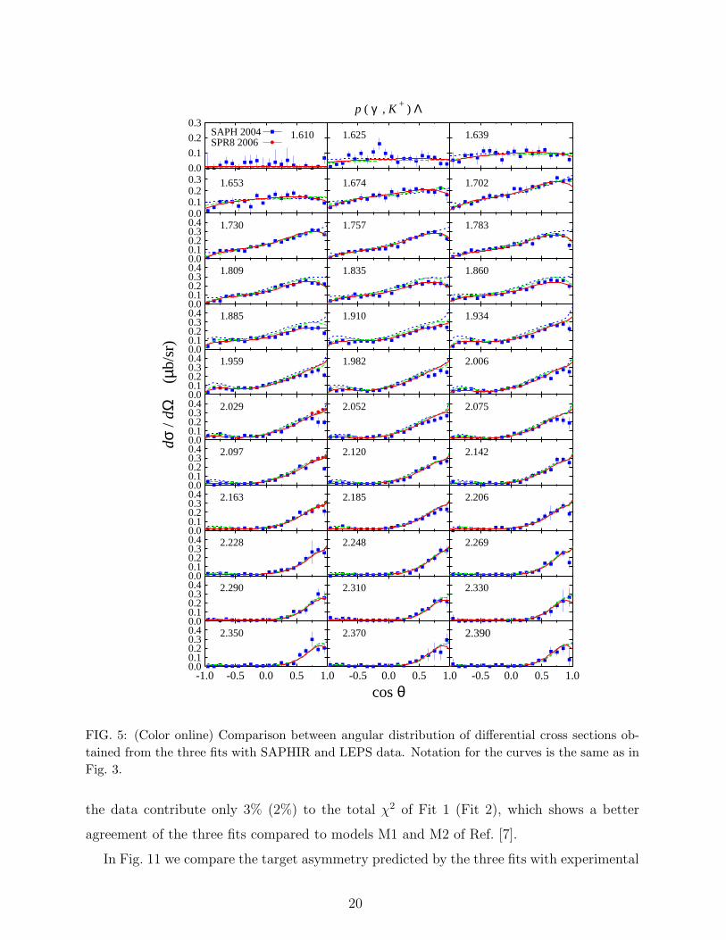
FIG. 5: (Color online) Comparison between angular distribution of differential cross sections ob-

tained from the three fits with SAPHIR and LEPS data. Notation for the curves is the same as in

Fig. 3.

the data contribute only 3% (2%) to the total χ2 of Fit 1 (Fit 2), which shows a better

agreement of the three fits compared to models M1 and M2 of Ref. [7].

In Fig. 11 we compare the target asymmetry predicted by the three fits with experimental

20

cos θ = 0.950.00.10.20.30.40.5

cos θ = 0.85

p ( γ , K + ) Λ

cos θ = 0.750.00.10.20.30.4

cos θ = 0.65

cos θ = 0.55

0.00.10.20.3 cos θ = 0.45

cos θ = 0.35

0.00.10.20.3 cos θ = 0.25

cos θ = 0.15

0.00.10.20.3

dσ /

dΩ

(µb

/sr) cos θ = 0.05

cos θ = −0.05

0.00.10.20.3 cos θ = −0.15

cos θ = −0.25

0.00.10.20.3 cos θ = −0.35

cos θ = −0.45

0.00.10.20.3 cos θ = −0.55

cos θ = −0.65

0.00.10.20.3 cos θ = −0.75

cos θ = −0.85

0.00.10.20.3

1.6 1.7 1.8 1.9 2.0 2.1 2.2 2.3 2.4

W (GeV)

cos θ = −0.95

1.6 1.7 1.8 1.9 2.0 2.1 2.2 2.3 2.4

W (GeV)

FIG. 6: (Color online) Same as in Fig 5, but for the energy distribution.

data. There are only three data points with large error bars available for this observable. To

our knowledge, except for the Saclay-Lyon model [14] which is only in fair agreement with

those data, other models [7, 35, 36] fail to reproduce them. Figure 11 clearly indicates that

this observable could provide a stringent constraint to phenomenological models that try to

explain the K+Λ photoproduction process. At this stage, it is important to note that we

also obtained another solution for Fit 2 which can nicely reproduce these three data points.

21

1.6171.00.50.0

−0.5−1.0

p ( γ , K + ) Λ

1.646

→

1.674

1.7020.50.0

−0.5−1.0

1.730 1.757

1.7830.50.0

−0.5−1.0

1.809 1.835

1.8600.50.0

−0.5−1.0

1.885 1.910

1.934

P

0.50.0

−0.5−1.0

1.959 1.982

2.0060.50.0

−0.5−1.0

2.029 2.052

2.0750.50.0

−0.5−1.0

2.097 2.120

2.1420.50.0

−0.5−1.0

2.163 2.185

2.2060.50.0

−0.5−1.0

2.228 2.248

2.2690.50.0

−0.5−1.0

−1.0 −0.5 0.0 0.5 1.0

2.290

−0.5 0.0 0.5 1.0

cos θ−0.5 0.0 0.5 1.0

Fit1Fit2Fit3

CLAS 2006SAPH 2004

FIG. 7: (Color online) Comparison between the Λ recoil polarization obtained from the three fits

with CLAS and SAPHIR data.

However, since the extracted parameters are quite different from those of Fit 1 and Fit 3

(as well as from the PDG values) and the corresponding χ2 = 1610 is slightly larger than

that of Fit 2 (i.e., χ2 = 1581), we do not follow up this alternative. Moreover, the number

of available data and the size of error bars make it difficult to draw a firm conclusion on

the discrepancy shown in Fig. 11. Future measurement of this asymmetry from threshold

up to W ≈ 2.2 GeV with error bars comparable to those of CLAS and SAPHIR data would

22

cos θ = 0.50.5

0.0

-0.5

-1.0

W (GeV)

1.6 1.7 1.8 1.9 2.0 2.1 2.2 2.3

P

cos θ = 0.00.5

0.0

-0.5

-1.0

p ( γ , K + ) Λ→

cos θ = -0.5

1.0

0.5

0.0

-0.5

-1.0

FIG. 8: (Color online) Same as in Fig. 7, but for the W distributions.

0

0.5

1

1.5

2

2.5

3

3.5

1.6 1.7 1.8 1.9 2 2.1 2.2 2.3 2.4 2.5

σ to

t (µ

b)

W (GeV)

p ( γ , K + ) ΛFit 1

Fit 2

Fit 3

CLAS 2006

SAPHIR 2004

SAPHIR 1998

FIG. 9: (Color online) Comparison between the calculated total cross sections with experimental

data. All data shown in this figure were not used in the fits.

certainly help to clarify this issue.

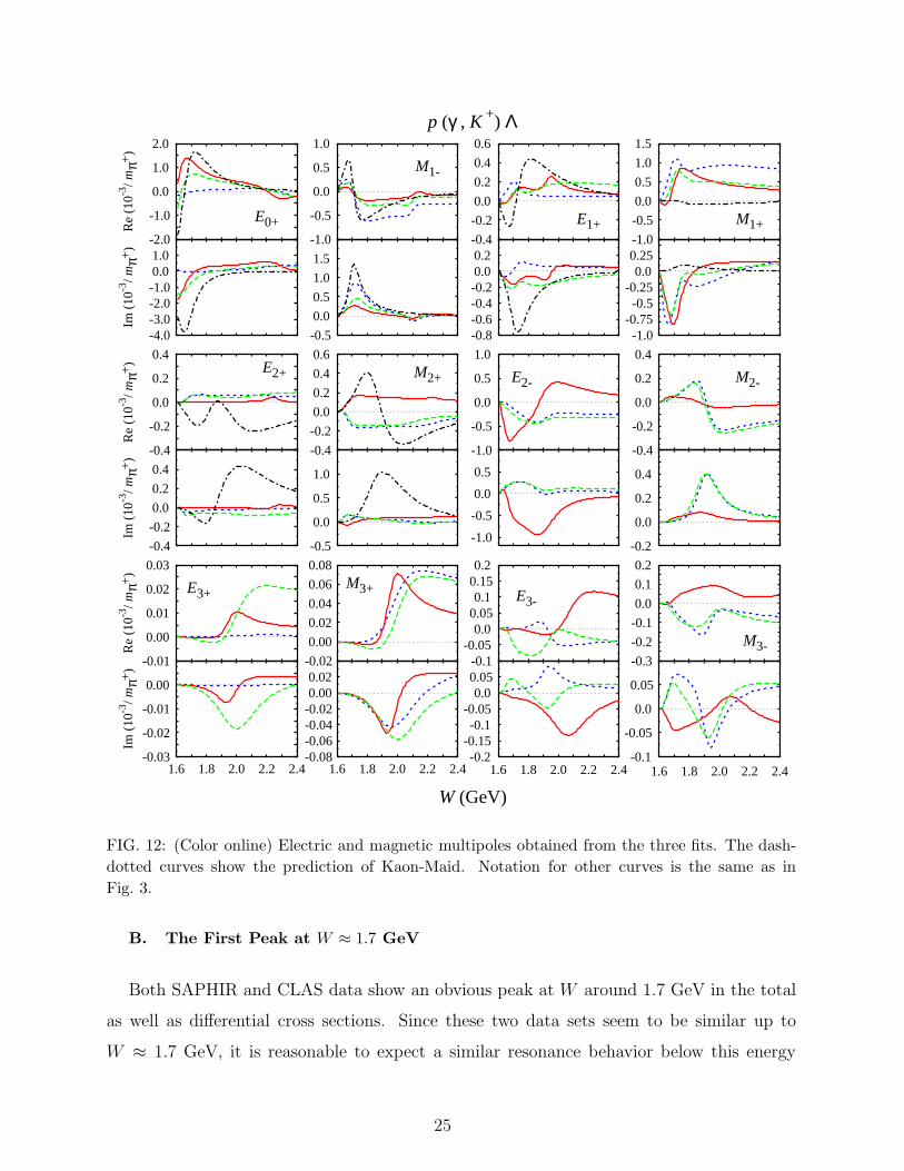
In Fig. 12 we display the multipole amplitudes for ℓ ≤ 3. It is obvious from this figure that

the predicted multipoles are different in most cases, as has been also pointed out by Ref. [20].

This again indicates that the problem of mutual consistency in the presently available data

23

1.9465

1.0

0.5

0.0

-0.5

-1.01.9942

p ( γ , K + ) Λ→

2.0407

Σ

0.5

0.0

-0.5

-1.02.1085

0.5

0.0

-0.5

-1.0-1.0 -0.5 0.0 0.5 1.0

cos θ

2.1957 2.2796

-1.0 -0.5 0.0 0.5 1.0

cos θ

FIG. 10: (Color online) Photon asymmetry obtained from the three fits compared with the LEPS

data. Notation for the curves is the same as in Fig. 3.

-1

-0.5

0

0.5

1

1.6 1.7 1.8 1.9 2 2.1 2.2 2.3 2.4 2.5

T

W (GeV)

θ = 90 deg

p ( γ , K + ) Λ→

Fit 1

Fit 2

Fit 3

FIG. 11: (Color online) Comparison between target asymmetries obtained from the three different

fits and experimental data [34]. Note that the three data points were not used in the fits.

still prohibits a more model-independent multipole analysis in kaon photoproduction.

24

Re

(10-3

/ mπ+

)

E0+-2.0

-1.0

0.0

1.0

2.0Im

(10

-3/ m

π+)

1.00.0-1.0-2.0-3.0-4.0

p (γ , K +) Λ

M1-

-1.0

-0.5

0.0

0.5

1.0

-0.5

0.0

0.5

1.0

1.5

E1+-0.4

-0.2

0.0

0.2

0.4

0.6

0.20.0-0.2-0.4-0.6-0.8

M1+-0.5

-1.0

0.0

0.5

1.0

1.5

0.250.0

-0.25-0.5

-0.75-1.0

E2+

Re

(10-3

/ mπ+

)

-0.4

-0.2

0.0

0.2

0.4

Im (

10-3

/ mπ+

)

-0.4

-0.2

0.0

0.2

0.4

M2+

-0.4

-0.2

0.0

0.2

0.4

0.6

1.0

0.5

0.0

-0.5

E2-

-1.0

-0.5

0.0

0.5

1.0

-1.0

-0.5

0.0

0.5

M2-

-0.4

-0.2

0.0

0.2

0.4

-0.2

0.0

0.2

0.4

E3+

Re

(10-3

/ mπ+

)

-0.01

0.00

0.01

0.02

0.03

Im (

10-3

/ mπ+

)

-0.03

-0.02

-0.01

0.00

1.6 1.8 2.0 2.2 2.4

M3+

-0.02

0.00

0.02

0.04

0.06

0.08

1.6 1.8 2.0 2.2 2.4

W (GeV)

-0.08-0.06-0.04-0.020.000.02

E3-

-0.1-0.05

0.00.050.1

0.150.2

-0.2-0.15-0.1

-0.050.0

0.05

1.6 1.8 2.0 2.2 2.4

M3- -0.3

-0.2

-0.1

0.0

0.1

0.2

-0.1

-0.05

0.0

0.05

1.6 1.8 2.0 2.2 2.4

FIG. 12: (Color online) Electric and magnetic multipoles obtained from the three fits. The dash-

dotted curves show the prediction of Kaon-Maid. Notation for other curves is the same as in

Fig. 3.

B. The First Peak at W ≈ 1.7 GeV

Both SAPHIR and CLAS data show an obvious peak at W around 1.7 GeV in the total

as well as differential cross sections. Since these two data sets seem to be similar up to

W ≈ 1.7 GeV, it is reasonable to expect a similar resonance behavior below this energy

25

0

0.5

1

1.5

2

2.5

3

3.5

4

1.6 1.65 1.7 1.75 1.8

σ to

t (µ

b)Fit to SAPHIR data All

no S11 (1650) [1650]no P13 (1720) [1720]no D13 (1700) [1680]no F15 (1680) [1680]

0

0.5

1

1.5

2

2.5

3

3.5

4

1.6 1.65 1.7 1.75 1.8

σ to

t (µ

b)

W (GeV)

Fit to CLAS data Allno P13 (1720) [1720]no D15 (1675) [1675]no F15 (1680) [1680]

0

0.5

1

1.5

2

2.5

3

3.5

4

1.6 1.65 1.7 1.75 1.8

p ( γ , K + ) Λ

Fit to SAPHIR data AllS11 (1650) [1650]P13 (1720) [1720]D13 (1700) [1680]F15 (1680) [1680]

0

0.5

1

1.5

2

2.5

3

3.5

4

1.6 1.65 1.7 1.75 1.8

W (GeV)

Fit to CLAS data AllP13 (1720) [1720]D15 (1675) [1675]F15 (1680) [1680]

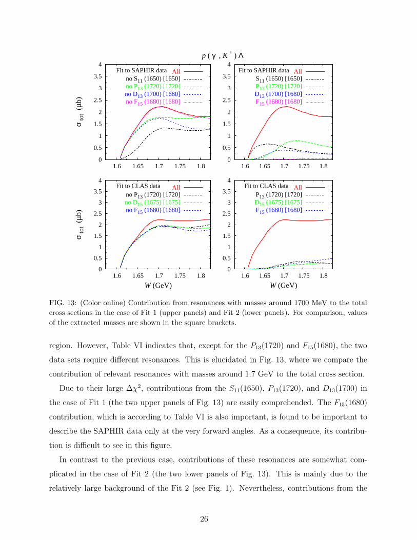
FIG. 13: (Color online) Contribution from resonances with masses around 1700 MeV to the total

cross sections in the case of Fit 1 (upper panels) and Fit 2 (lower panels). For comparison, values

of the extracted masses are shown in the square brackets.

region. However, Table VI indicates that, except for the P13(1720) and F15(1680), the two

data sets require different resonances. This is elucidated in Fig. 13, where we compare the

contribution of relevant resonances with masses around 1.7 GeV to the total cross section.

Due to their large ∆χ2, contributions from the S11(1650), P13(1720), and D13(1700) in

the case of Fit 1 (the two upper panels of Fig. 13) are easily comprehended. The F15(1680)

contribution, which is according to Table VI is also important, is found to be important to

describe the SAPHIR data only at the very forward angles. As a consequence, its contribu-

tion is difficult to see in this figure.

In contrast to the previous case, contributions of these resonances are somewhat com-

plicated in the case of Fit 2 (the two lower panels of Fig. 13). This is mainly due to the

relatively large background of the Fit 2 (see Fig. 1). Nevertheless, contributions from the

26

P13(1720), D15(1675), and F15(1680) are still sizable. These contributions are required to

decrease the cross section down to the experimental value through destructive interference.

The above result is clearly unexpected. However, we can understand this by carefully

examine the total cross section data shown in Fig. 9 or the differential cross section data

shown in Figs. 4 and 6, where we can see that at W = 1.7 GeV the discrepancy between the

two data sets starts to appear. Given that the lowest lying resonance used in this analysis

is the S11(1650), which has a width of 150 MeV, all experimental data up to W = 1.8 GeV

will certainly influence the extracted resonance parameters.

Another possible origin of the above finding is that the two data sets are already different

for W . 1.7 GeV. To investigate this, we separately fitted both SAPHIR and CLAS differ-

ential cross sections data from threshold up to W ≈ 1.7 GeV, by including the S11(1650),

P11(1710), P13(1720), D13(1700), D15(1675), and F15(1680) resonances. We found that the

extracted resonance parameters from the two fits are quite different, which, therefore, con-

firms that the two data sets are already different at W . 1.7 GeV.

C. The Second Peak at W ≈ 1.9 GeV

For almost one decade since the previous SAPHIR data were published in 1998 [39] there

has been a lot of discussion on which resonance is responsible for explaining the second peak

at W ≈ 1.9 GeV in the total as well as differential cross sections. Here, it is important to

note that, although varying as a function of the kaon angle in the latter case, the peak still

exists in both CLAS and SAPHIR data.

The debate was ignited by the authors of Ref. [36], who, by means of the results from

a certain constituent quark model [40] and an isobar model, interpreted the peak as the

existence of the missing resonance D13(1895). Subsequently, it was shown by Janssen et al.

[41] that the peak could be also equally well reproduced by including a P13(1950) resonance.

However, most of analyses based on the isobar model after that confirmed that including

the D13(1895) will significantly improve the agreement with experimental data [42].

A recent partial wave analysis by Anisovich et al. [43] found that a new D13 with M =

1875 ± 25 MeV and Γ = 80 ± 20 MeV is needed in order to explain the processes γp →πN, ηN, KΛ and KΣ. Experimental data on the γp → N∗(∆∗) → π0p published by CB-

ELSA collaboration not long after that shifted this resonance to a higher mass, i.e., M =

27

0

0.5

1

1.5

2

2.5

3

3.5

1.6 1.7 1.8 1.9 2 2.1 2.2 2.3 2.4 2.5

σ to

t (µ

b)Fit to SAPHIR data All

no P13 (1900) [1937]no D13 (2080) [1936]no F17 (1990) [1970]

0

0.5

1

1.5

2

2.5

3

3.5

4

1.6 1.7 1.8 1.9 2 2.1 2.2 2.3 2.4 2.5

σ to

t (µ

b)

W (GeV)

Fit to CLAS data Allno D13 (2080) [1915]no F15 (2000) [1937]

0

0.5

1

1.5

2

2.5

3

3.5

1.6 1.7 1.8 1.9 2 2.1 2.2 2.3 2.4 2.5

p ( γ , K + ) Λ

Fit to SAPHIR data AllP13 (1900) [1937]D13 (2080) [1936]F17 (1990) [1970]

0

0.5

1

1.5

2

2.5

3

3.5

4

1.6 1.7 1.8 1.9 2 2.1 2.2 2.3 2.4 2.5

W (GeV)

Fit to CLAS data AllD13 (2080) [1915]F15 (2000) [1937]

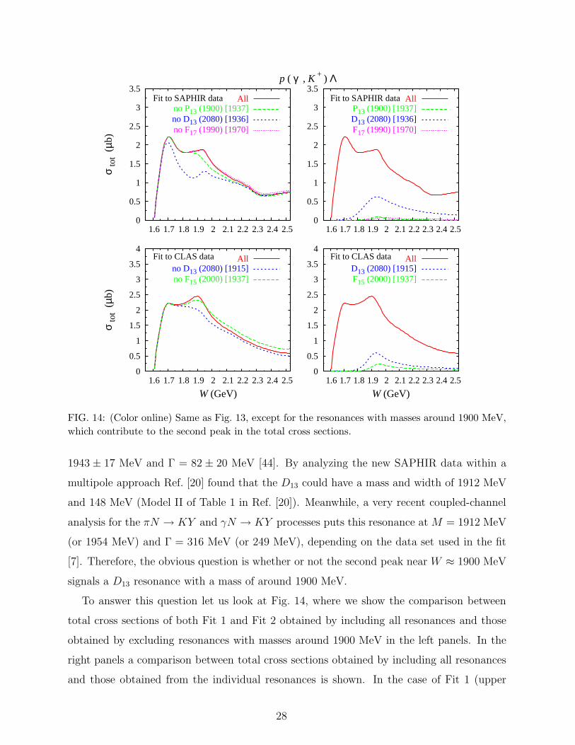
FIG. 14: (Color online) Same as Fig. 13, except for the resonances with masses around 1900 MeV,

which contribute to the second peak in the total cross sections.

1943 ± 17 MeV and Γ = 82 ± 20 MeV [44]. By analyzing the new SAPHIR data within a

multipole approach Ref. [20] found that the D13 could have a mass and width of 1912 MeV

and 148 MeV (Model II of Table 1 in Ref. [20]). Meanwhile, a very recent coupled-channel

analysis for the πN → KY and γN → KY processes puts this resonance at M = 1912 MeV

(or 1954 MeV) and Γ = 316 MeV (or 249 MeV), depending on the data set used in the fit

[7]. Therefore, the obvious question is whether or not the second peak near W ≈ 1900 MeV

signals a D13 resonance with a mass of around 1900 MeV.

To answer this question let us look at Fig. 14, where we show the comparison between

total cross sections of both Fit 1 and Fit 2 obtained by including all resonances and those

obtained by excluding resonances with masses around 1900 MeV in the left panels. In the

right panels a comparison between total cross sections obtained by including all resonances

and those obtained from the individual resonances is shown. In the case of Fit 1 (upper

28

panels), it is obvious that the D13(2080) with a mass of 1936 MeV provides the dominant

contribution to this second peak. This can also immediately be seen from Fig. 2 or from

Table VI, where we see that the corresponding ∆χ2 = 8.8% is larger than that of the

P13(1900) (4.4%), or the F17(1990) (2.7%). Albeit using a different formalism, this result

is consistent with our previous finding [20], as well as with various analyses [7, 44]. The

reason that the mass of this D13 is shifted toward a higher value compared with the previous

observation (1895 MeV as obtained in Ref. [36]) seemingly originates from the new SAPHIR

data [17] which have the second peak at higher W compared with the previous ones [39]

(see Fig. 6).

Interestingly, as shown by Fig. 2 and Table VI, the new CLAS data yield the same

conclusion. Using this data set (Fit 2) the extracted mass of D13 is 1915 MeV, which is very

close to the value given by Fit 1 (1936 MeV). As shown by Fig. 2 this resonance appears

to be quite decisive in the process (∆χ2 = 8.5%), and from the lower-left panel of Fig. 14

it is obvious that excluding this resonance in the process drastically changes the shape of

the cross section. We also note that including all data sets in the fit does not change this

conclusion.

To summarize this subsection we may say that within this multipole approach the two

data sets lead to the same conclusion on the origin of the second peak in the W distribution

of the cross sections, i.e., the D13(2080) with a mass between 1911 – 1936 MeV.

V. CONCLUSIONS AND OUTLOOK

We have analyzed the γp → K+Λ process by means of a multipole approach with a

gauge-invariant, crossing-symmetric background amplitude obtained from tree-level Feyn-

man diagrams. The corresponding free parameters are fitted to three different data sets,

i.e., combinations of SAPHIR and LEPS data, CLAS and LEPS data, and all of these data.

Results of the fit indicate the lack of mutual consistency between SAPHIR and CLAS data,

whereas the LEPS data are shown to be more consistent with the CLAS ones. In most cases,

the extracted parameters from the three data sets are found to be different and, therefore,

could lead to different conclusions if those data were used individually or simultaneously to

extract the information on missing resonances.

From a fit to SAPHIR and LEPS data it is found that the S11(1650), P13(1720), D13(1700),

29

D13(2080), F15(1680), and F15(2000) resonances are more important than other resonances

used in this analysis, whereas fitting to the combination of CLAS and LEPS data indicates

that the P13(1900), D13(2080), D15(1675), F15(1680), and F17(1990) resonances to be more

decisive ones. It is shown that fitting to all data simultaneously changes this conclusion and

results in a model which is inconsistent to all data sets.

Our analysis indicates that the target asymmetry cannot be described by any of the

models. In view of the current available experimental data we conclude that measurement

of this observable should be addressed in a future experimental proposal.

The three-star resonance P11(1710) that has been used in almost all isobar models within

both single-channel and multi-channel approaches is found to be insignificant to the K+Λ

photoproduction by both SAPHIR and CLAS data.

It is also found that the second peak in cross sections at W ∼ 1900 MeV is originated

from the D13(2080) resonance. The extracted mass would be 1936 MeV if SAPHIR data

were used or 1915 MeV if CLAS data were used. This finding would not change if all data

sets were used.

We have observed that the total cross sections reported by the two collaborations are

consistent with their differential cross sections. The fact that the discrepancy is larger in

the total cross sections stems from the cumulative effect of the integration.

Although results of the present work could reveal certain consequences of using SAPHIR

or CLAS data in the database, it is still difficult to determine which data set should be

used in order to obtain the correct resonance parameters. We also realize that the results

presented here are not final, because a more representative calculation should ideally be

performed in a coupled-channels formalism where other channels such as πN , ηN , ππN ,

and ωN are also taken into account. Nevertheless, the simple calculation presented here has

revealed two most important issues that will need to be addressed in future calculations:

(1) contribution from higher spin resonances are important, (2) until we can settle the

problem of data consistency, the results of all calculations are now data dependent. Future

measurements such as the one planned at MAMI in Mainz are, therefore, expected to remedy

this unfortunate situation.

Our next goal is to consider the γp → K+Σ0 channel and to incorporate the effect of

other channels.

30

Acknowledgment

The authors thank William J. Briscoe for carefully reading the manuscript and acknowl-

edge the support from the Faculty of Mathematics and Sciences, University of Indonesia, as

well as from the Hibah Pascasarjana grant.

[1] R. A. Adelseck, C. Bennhold and L. E. Wright, Phys. Rev. C 32, 1681 (1985).

[2] R. A. Adelseck and B. Saghai, Phys. Rev. C 42, 108 (1990).

[3] R. A. Williams, C. R. Ji and S. R. Cotanch, Phys. Rev. C 43, 452 (1991).

[4] B. S. Han, M. K. Cheoun, K. S. Kim and I. T. Cheon, Nucl. Phys. A 691, 713 (2001).

[5] T. Mart, C. Bennhold, H. Haberzettl, and L. Tiator, Kaon-Maid, available at

http://www.kph.uni-mainz.de/MAID/kaon/kaonmaid.html. The published versions are avail-

able in: [36]; T. Mart, Phys. Rev. C 62, 038201 (2000); C. Bennhold, H. Haberzettl and

T. Mart, arXiv:nucl-th/9909022.

[6] T. Feuster and U. Mosel, Phys. Rev. C 59, 460 (1999).

[7] B. Julia-Diaz, B. Saghai, T. S. Lee and F. Tabakin, Phys. Rev. C 73, 055204 (2006).

[8] W. T. Chiang, F. Tabakin, T. S. H. Lee and B. Saghai, Phys. Lett. B 517, 101 (2001).

[9] Z. P. Li, Phys. Rev. C 52, 1648 (1995).

[10] D. H. Lu, R. H. Landau and S. C. Phatak, Phys. Rev. C 52, 1662 (1995).

[11] T. Mart and T. Wijaya, Acta Phys. Polon. B 34, 2651 (2003).

[12] T. Mart and C. Bennhold,“Kaon photoproduction in the Feynman and Regge theories,”

arXiv:nucl-th/0412097.

[13] T. Corthals, J. Ryckebusch and T. Van Cauteren, Phys. Rev. C 73, 045207 (2006).

[14] J. C. David, C. Fayard, G. H. Lamot and B. Saghai, Phys. Rev. C 53, 2613 (1996).

[15] F. M. Renard and Y. Renard, Nucl. Phys. B 25, 490 (1971); Y. Renard, Nucl. Phys. B 40, 499

(1972); Y. Renard, These de Doctorat d’Etat es-Sciences Physiques, Universite des Sciences

et Techniques du Languedoc, 1971 (unpublished).

[16] S. Eidelman et al. [Particle Data Group], Phys. Lett. B 592, 1 (2004).

[17] K. H. Glander et al., Eur. Phys. J. A 19, 251 (2004).

[18] R. Bradford et al. [CLAS Collaboration], Phys. Rev. C 73, 035202 (2006).

31

[19] P. Bydzovsky and T. Mart, “Analysis of the data consistency on kaon photoproduction with

Lambda in the final state,” arXiv:nucl-th/0605014.

[20] T. Mart, A. Sulaksono and C. Bennhold, arXiv:nucl-th/0411035; also in [42].

[21] D. Drechsel, O. Hanstein, S. S. Kamalov and L. Tiator, Nucl. Phys. A 645, 145 (1999);

[arXiv:nucl-th/9807001].

[22] L. Tiator, D. Drechsel, S. Kamalov, M. M. Giannini, E. Santopinto and A. Vassallo, Eur.

Phys. J. A 19, 55 (2004); [arXiv:nucl-th/0310041].

[23] The explicit expression for the background amplitudes are given, e.g., in Ref. [11], or in

T. Mart, Ph.D Thesis, Universitat Mainz, 1996 (unpublished).

[24] H. Thom, Phys. Rev. 151, 1322 (1966).

[25] R. A. Adelseck and L. E. Wright, Phys. Rev. C 38, 1965 (1988).

[26] K. Ohta, Phys. Rev. C 40, 1335 (1989).

[27] R. M. Davidson and R. Workman, Phys. Rev. C 63, 025210 (2001).

[28] H. Haberzettl, C. Bennhold, T. Mart and T. Feuster, Phys. Rev. C 58, 40 (1998).

[29] W. T. Chiang, S. N. Yang, L. Tiator and D. Drechsel, Nucl. Phys. A 700, 429 (2002).

[30] I. G. Aznauryan, Phys. Rev. C 67, 015209 (2003).

[31] G. Knochlein, D. Drechsel and L. Tiator, Z. Phys. A 352, 327 (1995).

[32] J. W. C. McNabb et al. [The CLAS Collaboration], Phys. Rev. C 69, 042201 (2004);

J. W. C. McNabb, PhD Thesis, Carnegie Mellon University (2002); R. Schumacher, private

communication.

[33] M. Sumihama et al. [LEPS Collaboration], Phys. Rev. C 73, 035214 (2006).

[34] K. H. Althoff et al., Nucl. Phys. B 137, 269 (1978).

[35] O. V. Maxwell, Phys. Rev. C 70, 044612 (2004).

[36] T. Mart and C. Bennhold, Phys. Rev. C 61, 012201 (2000).

[37] References for old measurements are listed in Table IX of [2], or in references of [39].

[38] T. Mart and L. Tiator, work in progress.

[39] M. Q. Tran et al. [SAPHIR Collaboration], Phys. Lett. B 445, 20 (1998).

[40] S. Capstick and W. Roberts, Phys. Rev. D 49, 4570 (1994); Phys. Rev. D 58, 074011 (1998);

S. Capstick, Phys. Rev. D 46, 2864 (1992).

[41] S. Janssen, J. Ryckebusch, D. Debruyne and T. Van Cauteren, Phys. Rev. C 65, 015201

(2001).

32

[42] See e.g.: T. K. Choi, M. K. Cheoun, K. S. Kim and B. G. Yu, in Proceedings of the Inter-

national Symposium On Electrophoto-Production Of Strangeness On Nucleons And Nuclei

(SENDAI 03), 16-18 Jun 2003, Sendai, Japan, edited by K. Maeda, H. Tamura, S.N. Naka-

mura, O. Hashimoto. River Edge, World Scientific, 2004, pp. 85.

[43] A. V. Anisovich, A. Sarantsev, O. Bartholomy, E. Klempt, V. A. Nikonov and U. Thoma,

Eur. Phys. J. A 25, 427 (2005).

[44] O. Bartholomy et al. [CB-ELSA Collaboration], Phys. Rev. Lett. 94, 012003 (2005).

33