Kalman smoothing improves the estimation of joint kinematics and kinetics in marker-based human gait analysis

Kalman smoothing improves the estimation of joint 

kinematics and kinetics in marker­based human gait analysis.

De Groote, F. a, De Laet, T. a, Jonkers, I. b, De Schutter, J. a.

(a):  Div. PMA, Dept. of Mechanical Engineering, Katholieke Universiteit Leuven, 

Celestijnenlaan 300B, B­3001 Heverlee, Belgium

(b):  Dept. of Biomedical Kinesiology, Katholieke Universiteit Leuven, 

Tervuursevest 101, B­3001 Heverlee, Belgium

Corresponding author: 

De Groote, Friedl

Katholieke Universiteit Leuven

Dept. of Mechanical Engineering, Div. PMA

Celestijnenlaan 300B

B­3001 Leuven

Belgium

Tel: +32 16 32 24 87

Fax: +32 16 32 29 87

E­mail: [email protected] 

Type of manuscript:

original article

Keywords:

Multi­link model, soft tissue artefacts, inverse kinematics, gait

Word count: 3251

1

Kalman smoothing improves the estimation of joint 

kinematics and kinetics in marker­based human gait analysis.

De Groote, F. a, De Laet, T. a, Jonkers, I. b, De Schutter, J. a.

(a):  Div. PMA, Dept. of Mechanical Engineering, Katholieke Universiteit Leuven, 

Celestijnenlaan 300B, B­3001 Heverlee, Belgium

(b):  Dept. of Biomedical Kinesiology, Katholieke Universiteit Leuven, 

Tervuursevest 101, B­3001 Heverlee, Belgium

2

ABSTRACT

We developed a Kalman smoothing algorithm to improve estimates of joint 

kinematics from measured marker trajectories during motion analysis. Kalman 

smoothing estimates are based on complete marker trajectories. This is an 

improvement over other techniques, such as the Global Optimisation Method (GOM), 

Kalman filtering, and Local Marker Estimation (LME), where the estimate at each 

time instant is only based on part of the marker trajectories. We applied GOM, 

Kalman filtering, LME, and Kalman smoothing to marker trajectories from both 

simulated and experimental gait motion, to estimate the joint kinematics of a ten 

segment biomechanical model, with 21 degrees of freedom. Three simulated marker 

trajectories were studied: without errors, with instrumental errors, and with soft tissue 

artefacts (STA). Two modelling errors were studied: increased thigh length and hip 

centre dislocation. We calculated estimation errors from the known joint kinematics in 

the simulation study. Compared with other techniques, Kalman smoothing reduced 

the estimation errors for the joint positions, by more than 50% for the simulated 

marker trajectories without errors and with instrumental errors. Compared with GOM, 

Kalman smoothing reduced the estimation errors for the joint moments by more than 

35%. Compared with Kalman filtering and LME, Kalman smoothing reduced the 

estimation errors for the joint accelerations by at least 50%. Our simulation results 

show that the use of Kalman smoothing substantially improves the estimates of joint 

kinematics and kinetics compared with previously proposed techniques (GOM, 

Kalman filtering, and LME) for both simulated, with and without modelling errors, 

and experimentally measured gait motion.

3

LIST OF ABBREVIATIONS

DOF degree of freedom

GOM Global Optimisation Method

KF Kalman filtering

KS Kalman smoothing

LME Local Marker Estimation

RMS root mean square

SOM Segmental Optimisation Method

STA soft tissue artefacts

4

1. INTRODUCTION

Inverse kinematics, the estimation of joint kinematics based on measured trajectories 

of skin­mounted markers, is complicated by instrumental errors and soft tissue 

artefacts (STA) (Cappozzo et al., 1996; Chiari et al., 2005; Leardini et al., 2005). 

Different techniques to reduce the effect of these errors on the estimated joint 

kinematics have been proposed (Chiari et al., 2005; Leardini et al., 2005). Spoor and 

Veldpaus (1980) estimated the positions and orientations of each body segment 

separately using a Segmental Optimisation Method (SOM). SOM minimises the 

marker displacement in the segmental reference frame between any two time instants. 

Lu and O’Connor (1999) used a multi­link model relating the marker positions to the 

generalized co­ordinates that describe the motion of the body segments along the 

degrees of freedom (DOFs). At each time instant, their Global Optimisation Method 

(GOM) estimates all generalized co­ordinates at once from a weighted nonlinear least­

squares fit between the measured marker positions and those predicted by the model. 

GOM outperformed SOM in simulation for a serial three­link model (pelvis, thigh and 

shank) joined by two spherical joints (hip and knee), suggesting that imposed joint 

constraints reduce the effect of errors. Cerveri et al. (2003 a&b) used a Kalman filter 

to estimate joint kinematics. Kalman filtering is based on a measurement model 

obtained from the biomechanical model and a process model, which includes prior 

knowledge about the smoothness of the motion. In addition, the generalized co­

ordinates, velocities, and accelerations are estimated simultaneously. Cerveri et al. 

(2005) proposed Local Marker Estimation (LME), an extension of Kalman filtering to 

estimate marker displacements in the segmental reference frames to account for STA. 

In their simulation study (Cerveri et al., 2005) in which systematic, sinusoidal 

perturbations added to the three thigh markers modelled STA, LME estimates were at 

least 50% more accurate than SOM estimates.

Kalman filtering has two potential advantages over GOM. Firstly, including 

knowledge about motion smoothness may improve the accuracy of estimated joint 

kinematics. Secondly, estimating accelerations eliminates the need to differentiate 

generalized co­ordinates numerically, which can introduce large errors. As these 

5

accelerations, in addition to the measured ground reaction forces, are the input for 

inverse dynamics to calculate joint moments, more accurate joint acceleration 

estimates will improve the accuracy of joint kinetics. Since Cerveri et al. (2005) did 

not compare LME with GOM, these advantages have not yet been confirmed. 

A drawback of Kalman filtering is the asymmetrical use of data. At each time instant, 

estimates are based on the measured marker trajectories up to the considered time 

instant only. We therefore propose Kalman smoothing (Rauch et al., 1965), a 

combination of two filters, to calculate the estimates at each time instant based on the 

complete marker trajectories. The proposed Kalman smoothing is an extension of the 

Kalman filter without local marker estimation. The purpose of this study was to 

compare the accuracies of the generalized coordinates and accelerations using GOM, 

Kalman filtering, LME, and Kalman smoothing using both simulated marker 

trajectories, with and without modelling errors, and experimentally measured marker 

trajectories during gait. 

6

2. KALMAN SMOOTHING ALGORITHM

The Kalman smoother (Bar­Shalom and Li, 1993; Rauch et al., 1965) combines prior 

knowledge, described by a process and measurement model, with the measured 

marker trajectories to produce an estimate of the joint kinematics while minimising 

the estimation error statistically. The generalized co­ordinates  q  and their derivatives 

up to the  K th order, which describe the joint kinematics, are collected in a vector  x :

[ ]TKJJJ

KK qqqqqqqqqx )()1()(2

)1(22

)(1

)1(11 = ,

with  Jj 1=  indicating the DOF and  )(kjq  the  k  th time derivative of  jq .  

The process model describes the expected time evolution of the joint kinematics x  and 

is composed of  J  submodels describing the motion of each DOF. While the 

submodels are based on the assumption that the K th derivative of the generalized co­

ordinate  )(Kjq  is constant, a noise term  jn  takes into account the errors introduced by 

this assumption:

( )( )

( )

( )( )

( )

)(

10

)!1(10

!21

)(

)1(1

2

)(

)1(

ij

iK

j

ij

ij

K

K

iK

j

ij

ij

tn

tq

tq

tq

Kt

t

Ktt

t

t+tq

t+tq

t+tq

+

−∆∆

∆∆∆

=

∆

∆∆

−

,

with  t  the time,  Ii 1=  indicating the time instant, and t∆  the sample time. The 

)1( +K th derivative of the generalized co­ordinate is modelled as zero mean Gaussian 

noise with covariance  2,1 jK +σ . Therefore the process noise is given by:

),0()( jj QNtn =  with  GGQ TjKj

2,1+= σ and 

∆∆

+∆=

+

tKt

Kt

GKK

!)!1(

1

.

The measurement model relates the joint kinematics  )(tx  to the measured marker 

positions, collected in  ( )tz . This model is composed of a noiseless measurement 

model  ( )( )txh  and measurement noise  ( )tv :

( ) ( )( ) ( )tv+txh=tz .

7

The noiseless measurement model  ( )( )txh  is based on a biomechanical model 

consisting of ten body segments including 21 DOFs (Figure 1, Delp et al., 1990). The 

measurement noise,  ( )tv , is drawn from a zero mean Gaussian distribution and 

expresses the uncertainty for the marker position measurements. 

Kalman smoothing has two consecutive steps. First, a Kalman filter (Kalman, 1960) 

estimates the joint kinematics at  it  using only the measured marker trajectories up to 

it . Second, a backward recursion using the measured marker trajectories from the last 

instant down to  it , follows the Kalman filter. The resulting Kalman smoother 

estimates the generalized co­ordinates and their derivatives based on all the 

information available: the complete marker trajectories, the process model, and the 

measurement model. An extended smoother (Bar­Shalom and Li, 1993) is used to 

cope with the nonlinearity of the measurement model.

8

3. VALIDATION

We compared the kinematics estimated with GOM, Kalman filtering (KF), LME, and 

Kalman smoothing (KS), first using simulated marker trajectories and second using 

experimentally measured marker trajectories both sampled at 200Hz. The marker set 

comprised 30 markers including five clusters of three markers (Figure 1). 

3.1 Validation in simulation 

We used the biomechanical model to calculate three sets of marker trajectories from 

the kinematics of a gait motion described by generalized co­ordinates  gtq (ground 

truth): (1) ideal marker trajectories without errors, consistent with  gtq  and the 

biomechanical model; (2) marker trajectories with instrumental errors, obtained by 

adding zero mean Gaussian noise with standard deviation of 1mm to the ideal marker 

trajectories; (3) marker trajectories corrupted with STA calculated as explained below.

STA are related to the angles of adjacent joints (Cappozzo et al., 1996). We calculated 

such a relation from marker trajectories measured experimentally during gait. Inverse 

kinematics (SIMM, Motion Analysis Corporation) estimated the generalized co­

ordinates  )(exp tq  corresponding to these trajectories. Using the biomechanical model, 

the measured marker positions were projected in the segmental reference frame. We 

considered the time dependent distances between the projected and modelled marker 

positions to be an approximation of the STA. For each marker, this distance,  )(td  was 

calculated along the x­, y­, and z­direction of the segmental reference frame and a 

linear relation between this distance and the adjacent joint angles  lqexp,  was calculated 

using least squares:

−∑ ∑

= =

I

ii

L

lllia

tqatd1

2

1exp, )()(min ,

with  Ll 1=  indicating the adjacent joints. The resulting coefficients  la  were used 

to calculate the modelled STA as: 

9

∑=

L

llgtl qa

1, .

The modelled STA (Figure 2) had amplitudes between 5 and 25 mm. It should be 

noted that, in contrast to the observations of Cappozzo et al. (1996), the x­ and z­

components of the STA trajectories in the shank and foot are correlated in our data 

set.

We applied GOM, KF, LME, and KS to the simulated marker trajectories. All 

methods were based on the biomechanical model of Delp et al. (1990). The algorithm 

for inverse kinematics implemented in SIMM (Delp et al., 1990) calculated the GOM 

estimates according to Lu and O’Connor (1999). SIMM uses the Levenberg­

Marquardt algorithm (Moré, 1977) to solve the underlying nonlinear least­squares 

problem with the estimated generalized co­ordinates at the previous time instant as 

initial values. KF used a 3rd order process model. LME was applied to all 30 markers. 

As recommended by Cerveri et al. (2005), we used a 2nd order process model and the 

covariance associated with the local marker co­ordinates was two orders of magnitude 

smaller than those associated with the generalized co­ordinates. To investigate the 

influence of the order of the process model, we performed KS for  2=K ,  3=K , and 

4=K . 

The effect of modelling errors was investigated by applying GOM, KF, and KS to the 

ideal marker trajectories using a biomechanical model that differed from the model 

used to simulate marker trajectories. The studied modelling errors were a thigh length 

increased by 10% and a dislocation of the joint centre of the hip of 16.8 mm.

For all estimates, we calculated the marker error, i.e. the root mean square (RMS) 

distance between the simulated marker trajectories and those predicted by the 

estimates and the biomechanical model averaged over all markers,  RMSd .  

Thereafter we calculated the percentage error for the generalized co­ordinates 

averaged over the 21 DOFs,  posε :

10

( )∑

∑=

=

−

−=

J

j jgtjgt

I

iijgtij

pos qq

tqtqI

J 1 ,,

1

2

,

)min()max(

)()(1

1001ε ,

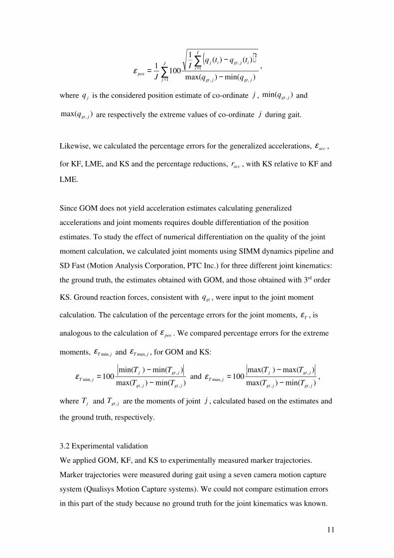
where  jq  is the considered position estimate of co­ordinate  j ,  )min( , jgtq  and 

)max( , jgtq  are respectively the extreme values of co­ordinate  j  during gait. 

Likewise, we calculated the percentage errors for the generalized accelerations,  accε , 

for KF, LME, and KS and the percentage reductions,  accr , with KS relative to KF and 

LME.

Since GOM does not yield acceleration estimates calculating generalized 

accelerations and joint moments requires double differentiation of the position 

estimates. To study the effect of numerical differentiation on the quality of the joint 

moment calculation, we calculated joint moments using SIMM dynamics pipeline and 

SD Fast (Motion Analysis Corporation, PTC Inc.) for three different joint kinematics: 

the ground truth, the estimates obtained with GOM, and those obtained with 3rd order 

KS. Ground reaction forces, consistent with  gtq , were input to the joint moment 

calculation. The calculation of the percentage errors for the joint moments,  Tε , is 

analogous to the calculation of  posε . We compared percentage errors for the extreme 

moments,  jT min,ε  and  jT max,ε , for GOM and KS:

)min()max(

)min()min(100

,,

,min,

jgtjgt

jgtjjT TT

TT

−

−=ε  and 

)min()max(

)max()max(100

,,

,max,

jgtjgt

jgtjjT TT

TT

−

−=ε ,

where  jT  and  jgtT ,  are the moments of joint  j , calculated based on the estimates and 

the ground truth, respectively.

3.2 Experimental validation

We applied GOM, KF, and KS to experimentally measured marker trajectories. 

Marker trajectories were measured during gait using a seven camera motion capture 

system (Qualisys Motion Capture systems). We could not compare estimation errors 

in this part of the study because no ground truth for the joint kinematics was known. 

11

We therefore assumed that improved estimates of the generalized co­ordinates would 

better predict the trajectories of validation markers. The trajectories of validation 

markers are measured but are not used to estimate the generalized co­ordinates. To 

validate our method based on this assumption, estimates of the generalized co­

ordinates were calculated from a subset of the measured markers including only one 

marker on the thigh, while the other two markers on the thigh were used as validation 

markers. The positions of the validation markers were calculated from the estimates of 

the generalized co­ordinates using the biomechanical model. Then, the root RMS 

distance between the measured and calculated positions of the validation markers,  d , 

was used as a measure of the estimation quality. 

12

4. RESULTS

4.1 Simulation results

The smallest marker errors,  RMSd , were obtained with LME, the largest marker errors 

were obtained with GOM (Table 1).

KS resulted in a smaller estimation error for the generalized co­ordinates,  posε , than 

GOM, KF, and LME (Table 2a). Compared with GOM and KF respectively, KS (

3=K ) reduced the estimation error by 97.8% and 59.3% (without errors), 88.1%  and 

53.0% (instrumental errors), 4.5% and 0.2 % (STA), 6.5% and 0.9% (increased thigh 

length), and 10.8% and 0.1% (hip centre dislocation). Percentage reductions are 

calculated from the estimation errors (supplementary material). The errors for the 

LME position estimates were two to three orders of magnitude larger than the errors 

with the other techniques (Table 2b).

The effect of the order  K  of the process model of KS on the estimation errors 

depended on the errors of the input marker trajectories. A 2nd order process model 

outperformed 3rd and 4th order process models for marker trajectories without errors. 

In the presence of instrumental errors, 3rd and even 4th order process models produced 

better estimates than a 2nd order process model. In the presence of STA, the estimation 

errors were similar for all three orders (Table 2).

KS resulted in a smaller estimation error for the generalized accelerations,  accε , than 

KF and LME (Table 3a). Compared with KF, KS ( 3=K ) reduced the estimation 

error by 83.3% (without errors), 80.6% (instrumental errors), 53.4% (STA), 55.9% 

(increased thigh length), and 72.8% (hip centre dislocation) (Table 3b). The KF 

estimates showed a time lag with respect to the ground truth (Figure 3). This time lag 

was larger for higher derivatives of the generalized co­ordinates and disappeared 

when smoothing was applied. Compared with LME, KS reduced estimation errors by 

one to two orders of magnitude.  

13

Compared with GOM, KS reduced the estimation error for the joint moments,  Tε , by 

87.7% (without errors), 85.1% (instrumental errors), 45.6% (STA), 36.2% (increased 

thigh length) and 57.4% (hip centre dislocation) (Table 4a­b, Figure 4). KS estimated 

more accurate extreme joint moments than GOM (Figure 5).

4.2 Experimental results

Marker positions calculated using KS showed higher correspondence with measured 

marker positions, than those calculated with GOM (Table 5a, Figure 6). Compared 

with GOM, KS reduced the RMS distance between measured and calculated marker 

positions by 16.2% for the thigh marker used for estimation and by 15.5% and 24.3% 

for the two validation markers. RMS distances resulting from KF and KS were similar 

(Table 5b).

14

5. DISCUSSION

Several methods to reduce the sensitivity of inverse kinematics to instrumental errors 

and STA, have been proposed in the literature: SOM, GOM, Kalman filtering, and 

LME. A drawback of these methods is that they only use part of the marker 

trajectories to estimate the joint kinematics at a considered time instant. We therefore 

developed a Kalman smoothing algorithm to calculate the estimate at each time 

instant based on the complete marker trajectories. To assess whether Kalman 

smoothing improves estimates of joint kinematics and kinetics, we compared this 

technique with GOM, Kalman filtering, and LME. We did not include SOM in our 

study, since GOM and LME have already been shown to outperform SOM (Cerveri et 

al., 2005; Lu and O’Connor, 1999).

Kalman smoothing resulted in better estimates of the generalized co­ordinates 

calculated from simulated marker trajectories than GOM, Kalman filtering, and LME. 

Furthermore, Kalman filtering outperformed GOM in terms of estimation errors 

(Table 2a and 3a). The smaller estimation errors using Kalman filtering and 

smoothing compared to GOM confirm our assumption that inverse kinematics 

benefits from integrating prior knowledge on motion smoothness.

Although GOM narrowly focuses on minimising marker error at a given time instant, 

Kalman filtering and Kalman smoothing outperform GOM in the reduction of marker 

error (Table 1). In the absence of measurement and modelling errors (validation in 

simulation with the marker trajectories without errors), a perfect fit between the 

measurements and the biomechanical model exists. Nevertheless, the obtained marker 

error for the GOM estimate is 10.27mm, showing that GOM does not return the 

global optimum. It is a well­known problem that solvers for nonlinear (nonconvex) 

optimisation problems find a locally optimal solution depending on the initial values 

of the optimisation variables. Since in this study the initial values at the first time 

instant were equal for all methods, this shows that Kalman filtering and Kalman 

smoothing are more suitable to solve this problem.

15

Cerveri et al. (2005) improved the estimation of joint kinematics by applying LME to 

three thigh markers. However, our results (Table 2 and 3) show that LME is not 

suitable to cope with STA of the full marker set during gait. Estimating all 30 local 

marker positions, velocities, and accelerations leads to a huge number of variables in 

the underlying Kalman filter. Compared to the simulation study of Cerveri (2005), the 

joint range of motion during gait and therefore the information contained in the 

marker positions is limited. Since this information is insufficient to correctly estimate 

all local marker positions, the estimated joint kinematics diverge from the ground 

truth, although LME outperforms all other methods in terms of marker error,  RMSd  

(Table1).

Simulation results (Tables 2 and 3) showed that in the presence of instrumental errors, 

a 3rd or 4th order process model outperformed a 2nd order process model for the 

Kalman smoother.

We addressed the effect of Kalman filtering and Kalman smoothing on the accuracy 

of the estimated accelerations. While the Kalman smoother estimates of the 

generalized co­ordinates where twice as accurate (without errors, instrumental errors) 

or as accurate (STA, modelling errors) as the corresponding Kalman filter estimates 

(Table 2), the Kalman smoother estimates of the generalized accelerations were 

respectively about five times (without errors, instrumental errors) and about two times 

(STA, modelling errors) better than the corresponding Kalman filter estimates (Table 

3). The inferior acceleration estimates of Kalman filtering were due to the filter lag 

(Figure 3) caused by the asymmetrical use of data in time. The backward recursion 

added by the Kalman smoother not only improves the velocity and acceleration 

estimates but, through the process model, also consistently improves the position 

estimates. 

Using Kalman smoothing instead of GOM greatly improved the estimation of joint 

moments and consequently the assessment of maximum joint loading from peak 

moments even when STA or modelling errors were present and the reduction of the 

estimation errors for the positions was rather limited. The inferior joint moment 

16

estimation of GOM results from the numerical differentiation of the nonsmooth 

positions. GOM associated with a double differentiation technique does not yield 

results that are as good as those obtained with Kalman filtering or Kalman smoothing 

since such a technique only finds accelerations corresponding to the estimated 

positions but does not improve the position estimates. The advantage of Kalman 

filtering and Kalman smoothing relies on the use of a process model that links one 

time instant to the next reflecting the knowledge that the state of the system is not 

independent of the states at neighbouring time instances. 

GOM, Kalman filtering and Kalman smoothing were applied to marker trajectories 

measured experimentally during gait. The estimates obtained with Kalman filtering 

and smoothing better explained the marker trajectories and better predicted additional 

validation trajectories than the estimates obtained with GOM (Table 5). In accordance 

with the simulation results, the quality of the position estimates was similar for 

filtering and smoothing. However, the simulation study shows that Kalman filtering 

and smoothing differed for the acceleration estimates. Accelerations were not 

measured experimentally and consequently no validation at this level was performed.

The Kalman smoother is based on a complex biomechanical model with 21 DOFs. 

Our implementation however, is not model­specific. Any model can be used in which 

the joint kinematics is described as a user­defined sequence of three orthogonal 

translations and three rotations around user­defined axes, which are either constant or 

a function of the generalized co­ordinates.  

Parameters of process and measurement noise were determined based on the expected 

)1( +K st derivative of the generalized co­ordinates and the expected errors in the 

measurement of the marker positions, respectively. Varying these parameters over an 

order of magnitude did not influence the results significantly. In contrast to Cerveri et 

al. (2005), we found that accurate tuning of these parameters was not crucial.

The main limitation of 3rd order Kalman smoothing is that STA and modelling errors 

are not yet adequately handled. Kalman smoothing is a stochastic technique, in which 

17

the stochastic model noise accounts for modelling and measuring errors. Both STA 

and modelling errors are deterministic and consequently not adequately handled. 

Cerveri et al. (2005) already mentioned that it is impossible to discriminate between a 

translation of the segment and STA, if all markers on the segment undergo identical 

STA. We feel that effective handling of STA requires additional information, such as 

a good model of STA during gait. However, such models are not currently available 

(Leardini et al., 2005).

In conclusion, 3rd order Kalman smoothing substantially improves the estimation of 

joint kinematics and kinetics compared with previously proposed techniques, GOM, 

Kalman filtering, and LME, for both simulated, with and without modelling errors, 

and experimentally measured gait motion.

18

ACKNOWLEDGEMENTS

Friedl De Groote and Tinne De Laet are Research Assistants of the Research 

Foundation ­ Flanders (FWO­Vlaanderen). Ilse Jonkers is a Postdoctoral Fellow of the 

Research Foundation ­ Flanders. Ilse Jonkers receives additional funding from the 

Belgian Educational Foundation and the Koning Boudewijn Fonds. This work is also 

supported by BOF EF/05/006 Centre­of­Excellence Optimisation in Engineering and 

K.U.Leuven Concerted Research Action GOA/05/10. The authors wish to thank 

Stefaan Decramer for performing the initial simulations underlying this work.

19

REFERENCES

Bar­Shalom, Y., Li, X., 1993. Estimation and tracking, principles, techniques and 

software, Artech House, Norwood, MA, pp. 382­388.

Cappozzo, A., Catani, F., Leardini, A., Benedetti, M. G., Della Croce, U., 1996. 

Position and orientation in space of bones during movement, experimental artefacts. 

Clinical Biomechanics 11(2), 90­100.

aCerveri, P., Pedotti, A., Ferrigno, G., 2003. Robust recovery of human motion from 

video using Kalman filters and virtual humans. Human Movement Science 22, 

377­404.

bCerveri, P., Rabufetti, M., Pedotti, A., Ferrigno, G., 2003. Real­time human motion 

estimation using biomechanical models and nonlinear state­space filters. Medical & 

Biological Engineering & Computing 41, 109­123.

Cerveri, P., Pedotti, A., Ferrigno, G., 2005. Kinematical models to reduce the effect of 

skin artifacts on marker­based human motion estimation. Journal of Biomechanics 38, 

2228­2236.

Chiari, L., Della Croche, U., Leardini, A., Cappozzo, A., 2005. Human movement 

analysis using stereophotogrammetry Part 2: Instrumental errors. Gait and Posture 21, 

197­211.

Delp, S. L., Loan, J. P., Hoy, M. G., Zajac, F. E., Topp, E. L., Rosen, J. M., 1990. An 

interactive graphics­based model of the lower extremity to study orthopaedic surgical 

procedures. IEEE Transactions on Biomedical Engineering 37(8), 757­767.

Kalman, R.E., 1960. A new approach to linear filtering and prediction problems. 

Transactions of the ASME, Journal of Basic Engineering 82, 34­35.

20

Leardini, A., Chiari, L., Della Croce, U., Cappozzo, A., 2005. Human movement 

analysis using stereophotogrammetry Part 3. Soft tissue artifact assessment and 

compensation. Gait and Posture 21, 212­225.

Lu, T.­W., O’Connor, J.J., 1999. Bone position estimation from skin marker co­

ordinates using global optimisation with joint constraints. Journal of Biomechanics 

32, 129­134.

Moré, J. J., 1977. The Levenberg­Marquardt algorithm: Implementation and theory. 

In: G.A. Watson (Ed.), Numerical Analysis. Lecture Notes in Mathematics vol. 630. 

Springer­Verlag, Heidelberg, pp.105–116.

Rauch, H.E., Tung, F., Striebel, C.T., 1965. Maximum likelihood estimates of linear 

dynamic systems, AIAA Journal 3(8), 1445­1450.

Spoor, C.W., Veldpaus, F.E., 1980. Rigid body motion calculated from spatial co­

ordinates of markers. Journal of Biomechanics 13, 391­393.

Sutherland, D.H., 2002. The evolution of clinical gait analysis Part II: Kinematics. 

Gait and Posture 16, 159­179.

Yamaguchi, G.T., Zajac, F.E., 1989. A planar model of the knee joint to characterize 

the knee extensor mechanism. Journal of Biomechanics 22(1), 1­10. 

21

Captions for figures and tables:

Figure 1: Biomechanical model and marker placement protocol. The biomechanical 

model consists of ten body segments: a head­arms­trunk segment, the pelvis, left and 

right thigh, shank, hindfoot and forefoot (Delp et al., 1990). This model includes 21 

DOFs. Spherical joints connect the head­arms­trunk­segment to the pelvis and the 

pelvis to the thighs. The ankle and subtalar joints are modelled as simple hinges, 

whereas the knee joints are modelled as sliding hinges (Yamaguchi and Zajac, 1989). 

The remaining six DOFs correspond to the position and orientation of the pelvis.  The 

generic biomechanical model was scaled to the subject’s dimensions. A modified 

Cleveland marker placement protocol (Sutherland, 2002) was used for the data 

collection. The marker set consisted of 30 markers, including five clusters of three 

markers. Three anatomical markers defined the trunk: a marker on the lateral aspects 

of the left (1) and right (2) shoulder and a marker on the sternum (3). The pelvis 

segment is defined by a cluster of three technical markers on the sacrum (4a, 4b, 4c) 

and two anatomical markers on the left (5) and right (6) Anterior Superior Iliac Spine 

(ASIS). The thigh segment is defined by a cluster of three technical markers (7a, 7b, 

7c). The shank segment is defined by a cluster of three technical markers (8a, 8b, 8c), 

an anatomical marker on the lateral epicondyle (9), and an anatomical marker on the 

lateral malleolus (10). The foot segment is defined by three anatomical markers on the 

heel (11), the lateral foot (12) and the first metatarsal head (13). During a static 

calibration trial, additional anatomical markers were added to the medial femoral 

condyles and the medial malleoli to define the knee and ankle joint axis.

Figure 2: Time trajectories of the simulated STA for the markers on the trunk, pelvis 

and right leg: x­component (dotted black), y­component (solid black), z­component 

(dashed black) in segment reference frame and magnitude (gray). Marker numbering 

is consistent with Figure 1.

Figure 3: Estimates of angular position, velocity, acceleration and jerk of the right hip 

flexion as a function of time obtained from the set of marker trajectories without 

22

errors with Kalman filtering (solid black) and smoothing (dashed black). The ground 

truth (gray) serves as a reference. The filter estimate suffers from a time lag. 

Figure 4: Estimates of angular positions and internal joint moments of the right hip as 

a function of time obtained from the set of marker trajectories with instrumental errors 

above, and with soft tissue artefacts (STA), below. Estimates obtained with the global 

optimisation method (GOM) are represented by a solid black line, estimates obtained 

with 3rd order Kalman smoothing are represented by a dashed black line. The ground 

truth (gray) serves as a reference.

Figure 5: Percentage errors for the minimum and maximum internal joint moments of 

the right leg (instrumental errors: above, soft tissue artefacts (STA): below) using the 

global optimisation method (GOM) and Kalman smoothing.

Figure 6: RMS distance between the marker trajectories calculated based on the 

estimates of the generalized co­ordinates obtained with the global optimisation 

method (GOM) (black) and 3rd order Kalman smoothing (gray), and the measured 

marker trajectories for the thigh marker used for estimation (left) and the two 

validation markers (middle, right).

Table 1: Marker error, that is the root mean square (RMS) distance between the 

marker trajectories calculated based on the estimates of the generalized co­ordinates 

and the simulated marker trajectories averaged over all markers,  RMSd .

Table 2: Percentage errors for the estimates of the generalized co­ordinates,  posε , 

obtained with different methods from simulated marker trajectories without errors, 

with instrumental errors, and with soft tissue artefacts (STA) using a biomechanical 

model without modelling errors, and from simulated marker trajectories without 

errors using a biomechanical model with an increased thigh length and a hip centre 

dislocation. The best estimate is indicated in bold. 

23

Table 3: Percentage errors for the estimates of the generalized accelerations,  accε , 

obtained with different methods from simulated marker trajectories without errors, 

with instrumental errors, and with soft tissue artefacts (STA) using a biomechanical 

model without modelling errors, and from simulated marker trajectories without 

errors using a biomechanical model with an increased thigh length and a hip centre 

dislocation. The best estimate is indicated in bold. 

Table 4: Percentage errors for the joint moments,  Tε , calculated based on the 

estimates of the generalized co­ordinates obtained with the global optimisation 

method (GOM) and Kalman smoothing from simulated marker trajectories without 

errors, with instrumental errors, and with STA using a biomechanical model without 

modelling errors, and from simulated marker trajectories without errors using a 

biomechanical model with an increased thigh length and a hip centre dislocation.

Table 5: RMS distance between the marker trajectories calculated based on the 

estimates of the generalized co­ordinates obtained with the global optimisation 

method (GOM), Kalman filtering and Kalman smoothing, and the measured marker 

trajectories of three thigh markers. Estimation was based on a marker set, including 

only one marker on the thigh (estimation marker). The other two markers on the thigh 

(validation marker) were used for validation.

24

Figure 1

1

4b

7 a

4c

4 b

4a

32

7b

2

6 65

111 010

9

8c8b

8a

7c7b

7a

7c

8a

8b8c

9

1

13 1212

F R O N T B A C KFigure 1: Biomechanical model and marker placement protocol. The biomechanical 

model consists of ten body segments: a head­arms­trunk segment, the pelvis, left and 

right thigh, shank, hindfoot and forefoot (Delp et al., 1990). This model includes 21 

DOFs. Spherical joints connect the head­arms­trunk­segment to the pelvis and the 

pelvis to the thighs. The ankle and subtalar joints are modelled as simple hinges, 

whereas the knee joints are modelled as sliding hinges (Yamaguchi and Zajac, 1989). 

The remaining six DOFs correspond to the position and orientation of the pelvis.  The 

generic biomechanical model was scaled to the subject’s dimensions. A modified 

Cleveland marker placement protocol (Sutherland, 2002) was used for the data 

collection. The marker set consisted of 30 markers, including five clusters of three 

markers. Three anatomical markers defined the trunk: a marker on the lateral aspects 

of the left (1) and right (2) shoulder and a marker on the sternum (3). The pelvis 

segment is defined by a cluster of three technical markers on the sacrum (4a, 4b, 4c) 

25

and two anatomical markers on the left (5) and right (6) Anterior Superior Iliac Spine 

(ASIS). The thigh segment is defined by a cluster of three technical markers (7a, 7b, 

7c). The shank segment is defined by a cluster of three technical markers (8a, 8b, 8c), 

an anatomical marker on the lateral epicondyle (9), and an anatomical marker on the 

lateral malleolus (10). The foot segment is defined by three anatomical markers on the 

heel (11), the lateral foot (12) and the first metatarsal head (13). During a static 

calibration trial, additional anatomical markers were added to the medial femoral 

condyles and the medial malleoli to define the knee and ankle joint axis.

26

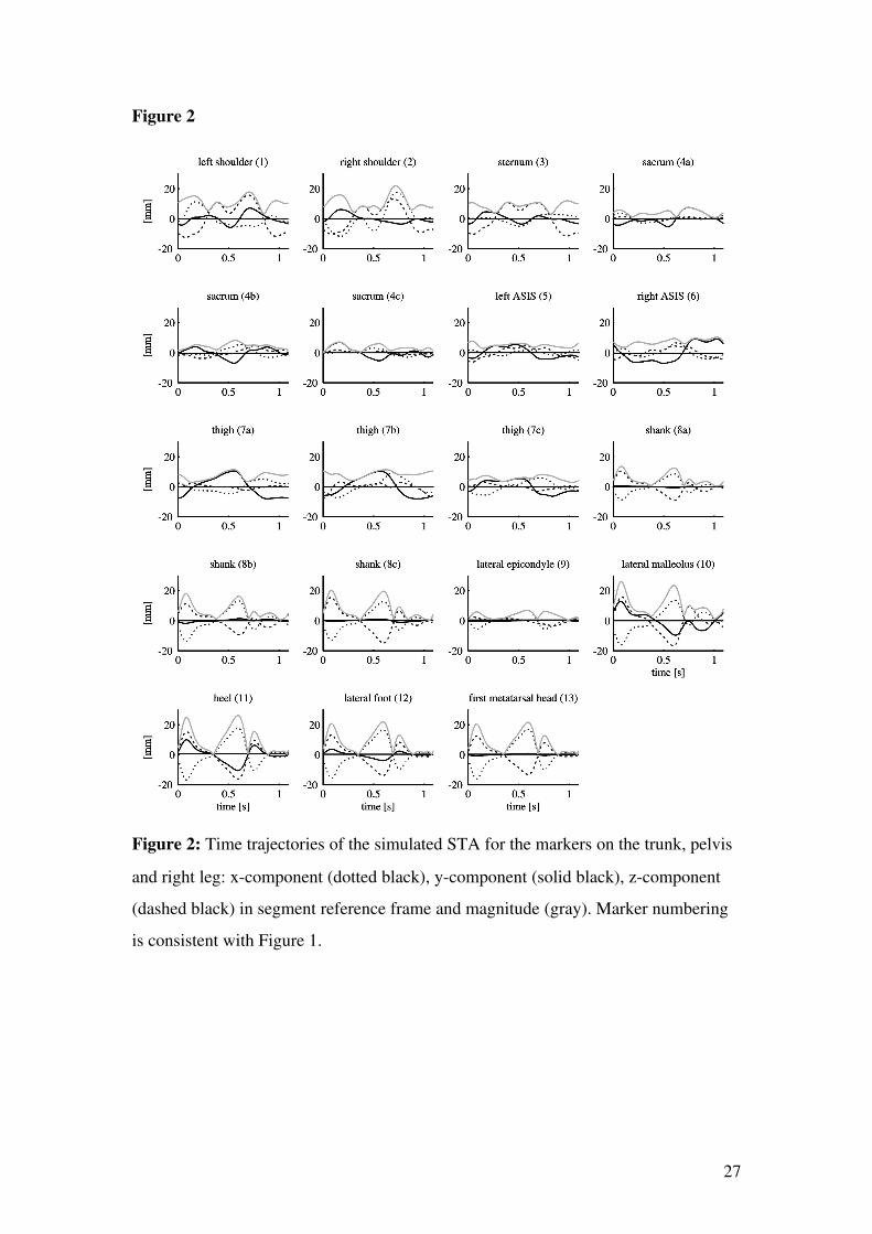
Figure 2

Figure 2: Time trajectories of the simulated STA for the markers on the trunk, pelvis 

and right leg: x­component (dotted black), y­component (solid black), z­component 

(dashed black) in segment reference frame and magnitude (gray). Marker numbering 

is consistent with Figure 1.

27

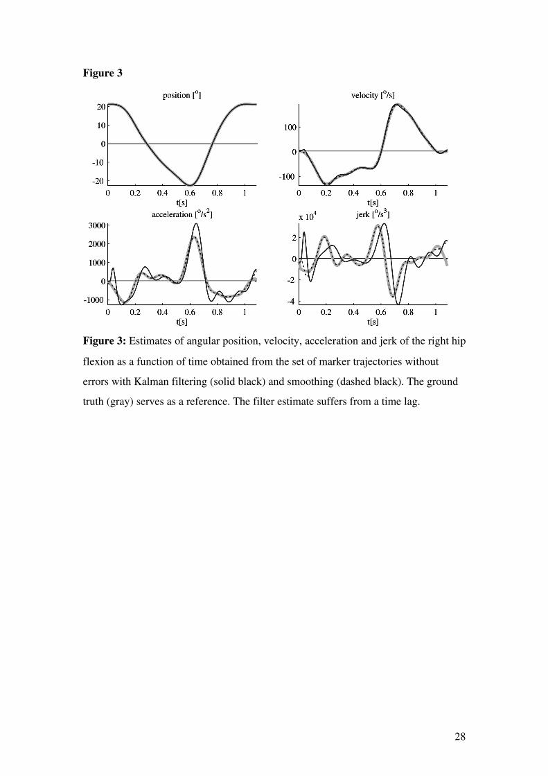
Figure 3

Figure 3: Estimates of angular position, velocity, acceleration and jerk of the right hip 

flexion as a function of time obtained from the set of marker trajectories without 

errors with Kalman filtering (solid black) and smoothing (dashed black). The ground 

truth (gray) serves as a reference. The filter estimate suffers from a time lag. 

28

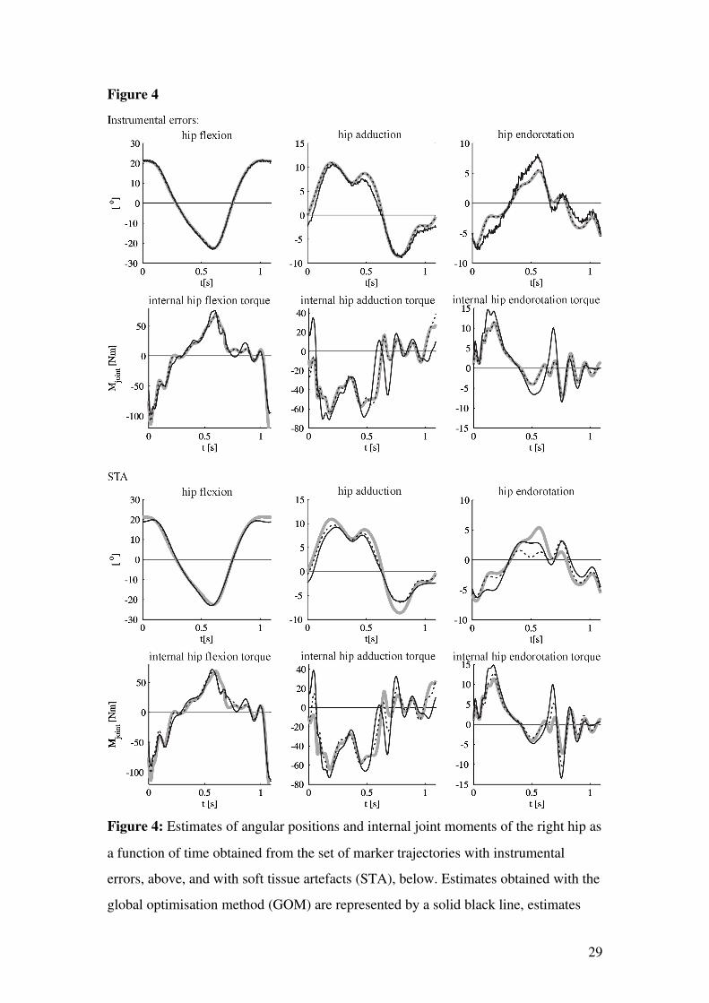
Figure 4

Figure 4: Estimates of angular positions and internal joint moments of the right hip as 

a function of time obtained from the set of marker trajectories with instrumental 

errors, above, and with soft tissue artefacts (STA), below. Estimates obtained with the 

global optimisation method (GOM) are represented by a solid black line, estimates 

29

obtained with 3rd order Kalman smoothing are represented by a dashed black line. The 

ground truth (gray) serves as a reference.

30

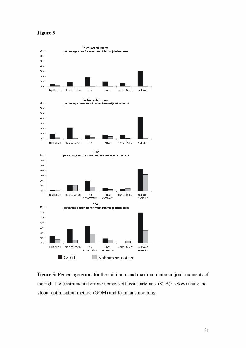
Figure 5

Figure 5: Percentage errors for the minimum and maximum internal joint moments of 

the right leg (instrumental errors: above, soft tissue artefacts (STA): below) using the 

global optimisation method (GOM) and Kalman smoothing.

31

Figure 6

Figure 6: RMS distance between the marker trajectories calculated based on the 

estimates of the generalized co­ordinates obtained with the global optimisation 

method (GOM) (black) and 3rd order Kalman smoothing (gray), and the measured 

marker trajectories for the thigh marker used for estimation (left) and the two 

validation markers (middle, right).

32

Table 1: Marker error, that is the root mean square (RMS) distance between the 

marker trajectories calculated based on the estimates of the generalized co­ordinates 

and the simulated marker trajectories averaged over all markers,  RMSd .

Marker error 

RMSd  [mm]GOM LME

Kalman 

filter 

(K=3)

Kalman 

smoother 

(K=2)

Kalman 

smoother 

(K=3)

Kalman 

smoother 

(K=4)Without errors 10.27 0.01 0.04 0.01 0.03 0.08Instrumental errors 10.52 0.10 1.45 1.55 1.59 1.58Soft Tissue Artefacts 9.57 0.01 3.46 3.46 3.46 3.46Modelling errors:

­ increased thigh length

­ hip centre dislocation

23.40

12.82

15.19

3.60

15.19

3.60

33

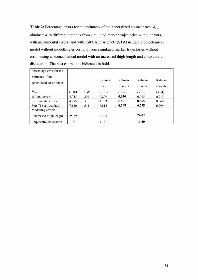
Table 2: Percentage errors for the estimates of the generalized co­ordinates,  posε , 

obtained with different methods from simulated marker trajectories without errors, 

with instrumental errors, and with soft tissue artefacts (STA) using a biomechanical 

model without modelling errors, and from simulated marker trajectories without 

errors using a biomechanical model with an increased thigh length and a hip centre 

dislocation. The best estimate is indicated in bold.

Percentage error for the 

estimates of the 

generalized co­ordinates 

posε GOM LME

Kalman 

filter 

(K=3)

Kalman 

smoother 

(K=2)

Kalman 

smoother 

(K=3)

Kalman 

smoother 

(K=4)Without errors 4.045 204 0.209 0.030 0.085 0.215Instrumental errors 4.785 585 1.203 0.621 0.565 0.568Soft Tissue Artefacts 7.120 541 6.814 6.798 6.798 6.799Modelling errors:

­ increased thigh length

­ hip centre dislocation

25.69

13.01

24.23

11.61

24.02

11.60

34

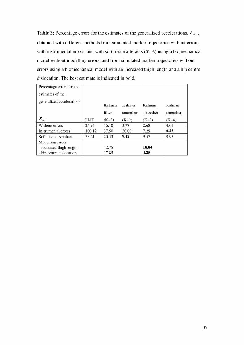
Table 3: Percentage errors for the estimates of the generalized accelerations,  accε , 

obtained with different methods from simulated marker trajectories without errors, 

with instrumental errors, and with soft tissue artefacts (STA) using a biomechanical 

model without modelling errors, and from simulated marker trajectories without 

errors using a biomechanical model with an increased thigh length and a hip centre 

dislocation. The best estimate is indicated in bold.

Percentage errors for the 

estimates of the 

generalized accelerations 

accε LME

Kalman 

filter 

(K=3)

Kalman 

smoother 

(K=2)

Kalman 

smoother 

(K=3)

Kalman 

smoother 

(K=4)Without errors 25.93 16.10 1.77 2.68 4.01Instrumental errors 100.12 37.50 20.00 7.29 6.46Soft Tissue Artefacts 53.21 20.53 9.42 9.57 9.95Modelling errors­ increased thigh length 42.75 18.84­ hip centre dislocation 17.85 4.85

35

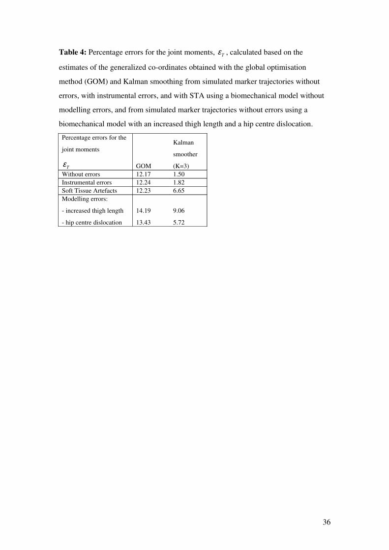
Table 4: Percentage errors for the joint moments,  Tε , calculated based on the 

estimates of the generalized co­ordinates obtained with the global optimisation 

method (GOM) and Kalman smoothing from simulated marker trajectories without 

errors, with instrumental errors, and with STA using a biomechanical model without 

modelling errors, and from simulated marker trajectories without errors using a 

biomechanical model with an increased thigh length and a hip centre dislocation.

Percentage errors for the 

joint moments

Tε GOM

Kalman 

smoother 

(K=3)Without errors 12.17 1.50Instrumental errors 12.24 1.82Soft Tissue Artefacts 12.23 6.65Modelling errors:

­ increased thigh length

­ hip centre dislocation 

14.19

13.43

9.06

5.72

36

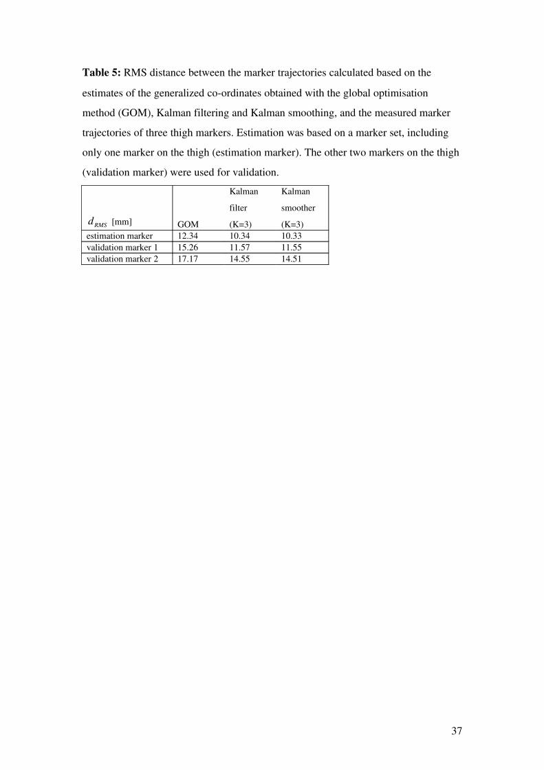
Table 5: RMS distance between the marker trajectories calculated based on the 

estimates of the generalized co­ordinates obtained with the global optimisation 

method (GOM), Kalman filtering and Kalman smoothing, and the measured marker 

trajectories of three thigh markers. Estimation was based on a marker set, including 

only one marker on the thigh (estimation marker). The other two markers on the thigh 

(validation marker) were used for validation. 

RMSd  [mm] GOM

Kalman 

filter 

(K=3)

Kalman 

smoother 

(K=3)estimation marker  12.34 10.34 10.33validation marker 1 15.26 11.57 11.55validation marker 2 17.17 14.55 14.51

37