Kalman Filtering and Model Estimation Steven Lillywhite Steven Lillywhite () Kalman Filtering and Model Estimation 1 / 29

Welcome message from author
This document is posted to help you gain knowledge. Please leave a comment to let me know what you think about it! Share it to your friends and learn new things together.
Transcript

Kalman Filtering and Model Estimation
Steven Lillywhite
Steven Lillywhite () Kalman Filtering and Model Estimation 1 / 29

Introduction
We aim to do the following.
Explain the basics of the Kalman Filter .
Explain the relationship with MLE estimation.
Show some real applications.
Steven Lillywhite () Kalman Filtering and Model Estimation 2 / 29
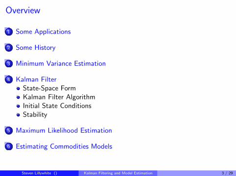
Overview
1 Some Applications
2 Some History
3 Minimum Variance Estimation
4 Kalman FilterState-Space FormKalman Filter AlgorithmInitial State ConditionsStability
5 Maximum Likelihood Estimation
6 Estimating Commodities Models
Steven Lillywhite () Kalman Filtering and Model Estimation 3 / 29

Applications
Keywords: estimation, control theory, signal processing, filtering,linear stochastic systems.
Navigational systems. Used in the Apollo lunar landing. From theNASA Ames’ website:“The Kalman-Schmidt filter was embedded in the Apollo navigationcomputer and ultimately into all air navigation systems, and laid thefoundation for Ames’ future leadership in flight and air trafficresearch.”
Satellite tracking. Missile tracking. Radar tracking.
Computer vision. Robotics. Speech enhancement.
Economics, Math Finance.
Steven Lillywhite () Kalman Filtering and Model Estimation 4 / 29

Gauss was no dummy!
Late 1700s. Problem: estimate planet and comet motion using datafrom telescopes.
1795. Gauss first uses least-squares method at age of 18.
1912. Fisher introduces the method of maximum likelihood.
1940s. Wiener-Kolmogorov linear minimum variance estimationtechnique. Signal processing. Unwieldly for large data sets.
1960. Kalman introduces Kalman filter.
Steven Lillywhite () Kalman Filtering and Model Estimation 5 / 29

Minimum Variance Estimators
Let (Ω,P) be a probability space.
Definition (Estimator)
Let X , Y1,Y2, . . .Yn ∈ L2(P) be random variables. Let
Ydef= (Y1,Y2, . . . ,Yn). By an estimator X for X given Y we mean a
random variable of the form X = gY, where g : Rn → R is a givenBorel-measurable function.
Definition (Minimum Variance Estimator)
An estimator X of X given Y is called a minimum variance estimator if
‖X − X‖ ≤ ‖hY − X‖ (1)
for all Borel-measurable h. Let us denote MVE (X |Y)def= X .
Steven Lillywhite () Kalman Filtering and Model Estimation 6 / 29
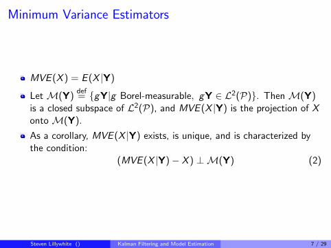
Minimum Variance Estimators
MVE (X ) = E (X |Y)
Let M(Y)def= gY|g Borel-measurable, gY ∈ L2(P). Then M(Y)
is a closed subspace of L2(P), and MVE (X |Y) is the projection of Xonto M(Y).
As a corollary, MVE (X |Y) exists, is unique, and is characterized bythe condition:
(MVE (X |Y)− X ) ⊥M(Y) (2)
Steven Lillywhite () Kalman Filtering and Model Estimation 7 / 29
Linear Minimum Variance Estimators
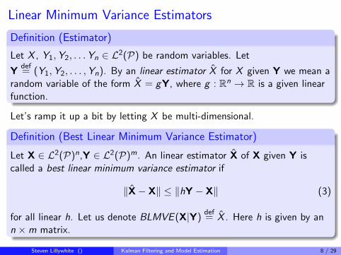
Definition (Estimator)
Let X , Y1,Y2, . . .Yn ∈ L2(P) be random variables. Let
Ydef= (Y1,Y2, . . . ,Yn). By an linear estimator X for X given Y we mean a
random variable of the form X = gY, where g : Rn → R is a given linearfunction.
Let’s ramp it up a bit by letting X be multi-dimensional.
Definition (Best Linear Minimum Variance Estimator)
Let X ∈ L2(P)n,Y ∈ L2(P)m. An linear estimator X of X given Y iscalled a best linear minimum variance estimator if
‖X− X‖ ≤ ‖hY − X‖ (3)
for all linear h. Let us denote BLMVE (X|Y)def= X . Here h is given by an
n ×m matrix.
Steven Lillywhite () Kalman Filtering and Model Estimation 8 / 29
Linear Minimum Variance Estimators
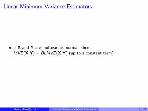
If X and Y are multivariate normal, thenMVE (X|Y) = BLMVE (X|Y) (up to a constant term).
Steven Lillywhite () Kalman Filtering and Model Estimation 9 / 29

State-Space Form
Definition (State-Space Form)
The state-space form is defined by the following pair of equations:
xi+1 = Jixi + gi + ui (state)
zi = Hixi + bi + wi (observation)
Here xi , zi are vectors representing a discrete random variables.
In general the elements of xi are not observable.
We assume that the elements of zi are observable.
ui and wi are white noise processes.
We assume that all vectors and matrices take values in Euclideanspace and can vary with i , but apart from xi and zi , that they onlyvary in a deterministic manner.
Steven Lillywhite () Kalman Filtering and Model Estimation 10 / 29

State-Space Form
Furthermore, we denote Qidef= E (uiu
Ti ) and Ri
def= E (wiw
Ti ), and assume
that the following hold:
E (uixT0 ) = 0 (4)
E (wixT0 ) = 0 (5)
E (uiwTj ) = 0 for all i , j (6)
Steven Lillywhite () Kalman Filtering and Model Estimation 11 / 29

Kalman Filter Notation
Definition
Denote Yjdef= (z0, z1, . . . zj). By xi |j , (resp. zi |j) we shall mean the best
linear minimum variance estimate(BLMVE) of xi (resp. zi ) based on Yj .We also define
Pi |jdef= E(xi − xi |j)(xi − xi |j)
T (7)
and call this the error matrix. When i = j , the estimate is called a filteredestimate, when i > j , the estimate is called a predicted estimate, andwhen i < j , the estimate is called a smoothed estimate
Steven Lillywhite () Kalman Filtering and Model Estimation 12 / 29
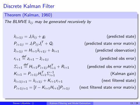
Discrete Kalman Filter
Theorem (Kalman, 1960)
The BLMVE xi |i may be generated recursively by
xi+1|i = Ji xi |i + gi (predicted state)
Pi+1|i = JiPi |iJTi + Qi (predicted state error matrix)
zi+1|i = Hi+1xi+1|i + bi+1 (predicted observation)
ri+1def= zi+1 − zi+1|i (predicted obs error)
Σi+1def= Hi+1Pi+1|iH
Ti+1 + Ri+1 (predicted obs error matrix)
Ki+1 = Pi+1|iHTi+1Σ
−1i+1 (Kalman gain)
xi+1|i+1 = xi+1|i + Ki+1ri+1 (next filtered state)
Pi+1|i+1 = [I − Ki+1Hi+1]Pi+1|i (next filtered state error matrix)
Steven Lillywhite () Kalman Filtering and Model Estimation 13 / 29

Discrete Kalman Filter
If the initial state x0 and the innovations ui , wi are multivariateGaussian, then the forecasts xi |j , (resp. zi |j) are minimum varianceestimators(MVE).
Note that the updated filtered state estimate is a sum of thepredicted state estimate and the predicted observation error weightedby the gain matrix.
Observe that the gain matrix is proportional to the predicted stateerror covariance matrix, and inversely proportional to the predictedobservation error covariance matrix. Thus, in updating the stateestimator, more weight is given to the observation error when theerror in the predicted state estimate is large, and less when theobservation error is large.
Steven Lillywhite () Kalman Filtering and Model Estimation 14 / 29

Kalman Filter Initial State Conditions
To run the Kalman filter, we begin with the pair x0|0, P0|0 (alternatively,one may also use x1|0, P1|0). A difficuly with the Kalman filter is thedetermination of these initial conditions. In many real applications, thedistribution for x0 is unknown. Several approaches are possible.
For stationary state series, we can compute x0|0, P0|0 directly.
Prior information.
Diffuse prior: x0|0 = 0, and P0|0 = kI , k 0. The details are moreinvolved.
Or one may treat x0 as a fixed vector, taking x0|0 = x0, and P0|0 = 0,and estimate its components by treating them as extra parameters inthe model. The details are more involved.
General rule of thumb is that for long time series, the initial stateconditions will have little impact.
Steven Lillywhite () Kalman Filtering and Model Estimation 15 / 29
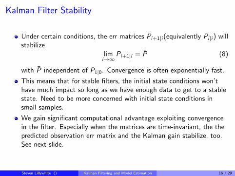
Kalman Filter Stability
Under certain conditions, the err matrices Pi+1|i (equivalently Pi |i ) willstabilize
limi→∞
Pi+1|i = P (8)
with P independent of P1|0. Convergence is often exponentially fast.
This means that for stable filters, the initial state conditions won’thave much impact so long as we have enough data to get to a stablestate. Need to be more concerned with initial state conditions insmall samples.
We gain significant computational advantage exploiting convergencein the filter. Especially when the matrices are time-invariant, the thepredicted observation err matrix and the Kalman gain stabilize, too.See next slide.
Steven Lillywhite () Kalman Filtering and Model Estimation 16 / 29

Kalman Filter Stability
This part is independent of the data
Pi+1|i = JiPi |iJTi + Qi (predicted state error matrix)
Σi+1def= Hi+1Pi+1|iH
Ti+1 + Ri+1 (predicted obs error matrix)
Ki+1 = Pi+1|iHTi+1Σ
−1i+1 (Kalman gain)
Pi+1|i+1 = [I − Ki+1Hi+1]Pi+1|i (next filtered state error matrix)
xi+1|i = Ji xi |i + gi (predicted state)
zi+1|i = Hi+1xi+1|i + bi+1 (predicted observation)
ri+1def= zi+1 − zi+1|i (predicted obs error)
xi+1|i+1 = xi+1|i + Ki+1ri+1 (next filtered state)
Steven Lillywhite () Kalman Filtering and Model Estimation 17 / 29

Kalman Filter Divergence
Numerical instability in the algorithm, round-off errors, etc., cancause divergence in the filter.
Model fit. If the underlying state model does not fit the real-worldprocess well, then the filter can diverge.
Observability. If we cannot observe some of the state variables(orlinear combinations), then we can get divergence in the filter.
Steven Lillywhite () Kalman Filtering and Model Estimation 18 / 29

Kalman Filter Other Items
Kalman advantage: real-time updating. No need to store past data toupdate current data.
Can handle missing data, since the matrices in the algorithm can varyover time.
Smoothing. The filter algorithm above gives BLMVE at time t basedon data up to time t. However, once all data is in, we can make betterestimates of the state variables at time t using also data after time t.
Alternative forms for the filter algorithm based on algebraicmanipulation of the equations. Information filter computes P−1
i |i .
Depending on the situation, this can be more(or less) useful.Square-Root filter uses square roots of P−1
i |i . It is morecomputationally burdensome, but can improve numerical instabilityproblems.
Steven Lillywhite () Kalman Filtering and Model Estimation 19 / 29

Kalman Filter Other Items
Non-linear state-space filters. This is called the Extended KalmanFilter. Here, we allow arbitrary functions in the state-spaceformulation, rather than the linear functions above.
xi+1 = f (xi , gi , ui ) (state)
zi = h(xi , bi ,wi ) (observation)
One proceeds by linearizing the functions about the estimates at eachstep, and thereby obtain an analogous filter algorithm.
There is a continuous version of the filter due to Kalman and Bucy.
Steven Lillywhite () Kalman Filtering and Model Estimation 20 / 29
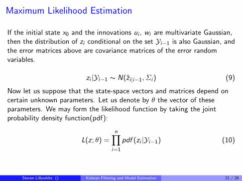
Maximum Likelihood Estimation
If the initial state x0 and the innovations ui , wi are multivariate Gaussian,then the distribution of zi conditional on the set Yi−1 is also Gaussian, andthe error matrices above are covariance matrices of the error randomvariables.
zi |Yi−1 ∼ N(zi |i−1, Σi ) (9)
Now let us suppose that the state-space vectors and matrices depend oncertain unknown parameters. Let us denote by θ the vector of theseparameters. We may form the likelihood function by taking the jointprobability density function(pdf):
L(z ; θ) =n∏
i=1
pdf (zi |Yi−1) (10)
Steven Lillywhite () Kalman Filtering and Model Estimation 21 / 29
Maximum Likelihood Estimation
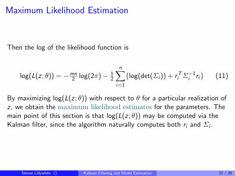
Then the log of the likelihood function is
log(L(z ; θ)) = −mn2 log(2π)− 1
2
n∑i=1
log(det(Σi )) + rTi Σ−1i ri (11)
By maximizing log(L(z ; θ)) with respect to θ for a particular realization ofz , we obtain the maximum likelihood estimates for the parameters. Themain point of this section is that log(L(z ; θ)) may be computed via theKalman filter, since the algorithm naturally computes both ri and Σi .
Steven Lillywhite () Kalman Filtering and Model Estimation 22 / 29
Estimating Commodities Models
Kalman filtering with maximum likelihood can be used to estimateparameters in various models in financial engineering applications.
One such use is for the estimation of parameters in commoditiesmodels. Here the state system would model the spot price, and theobservation system would be futures prices.Kalman filtering can be useful here for the following reasons
It is not uncommon that there is no true spot price process in the realworld.
Even if there is a spot price process, it can be be highly illiquid, errorprone, and unreliable for modelling.
In multi-factor models, we may have the spot price divided intounobservable components.
Steven Lillywhite () Kalman Filtering and Model Estimation 23 / 29

A Two-Factor Model of Schwartz-Smith for Oil prices
Combining geometric brownian motion with mean-reversion. This is theshort-long model of Schwartz-Smith. The idea is that short-termvariations revert back to an equilibrium level. But the equilibrium level isuncertain, and follows a Brownian motion process with drift.
ln(St) = ξt + χt (12)
dξt = µξdt + σξdWχ (13)
dχt = −κχtdt + σχdWξ (14)
dWχdWξ = ρχξdt (15)
Steven Lillywhite () Kalman Filtering and Model Estimation 24 / 29

A Two-Factor Model of Schwartz-Smith for Oil pricesWe shall use the risk-neutral framework to price derivatives. We shallassume that the market price of risk is constant, and we write:
dξt = (µξ − λξ)dt + σξdWχ (16)
dχt = (−κχt − λχ)dt + σχdWξ (17)
Here (λξσξ, λχσχ) denotes the change of measure according to theGirsanov theorem. We shall denote µ∗ξ = µξ − λξ. Under theseassumptions, we obtain that the distribution of ln(St) is normal, and
ln(F (t,T )) = e−κ(T−t)χt + ξt + A(T − t) (18)
A(T − t) = µ∗ξ(T − t)− (1− e(−κ(T−t))λχ/κ
+ 12 (1− e−2κ(T−t)) + 1
2σ2ξ (T − t)
+(1− e−κ(T−t))ρχξσχσξ/κ
Steven Lillywhite () Kalman Filtering and Model Estimation 25 / 29

Parameter Estimation Via Kalman filter MLE
State Equation: discretize the model for the spot price
Measurement Equation: discretize the formula for the futures price interms of the spot. Add noise term.
We estimate the parameters in the model using maximum likelihoodwith the Kalman filter.
Steven Lillywhite () Kalman Filtering and Model Estimation 26 / 29

State-Space Formulation
xt = Jxt−1 + g + ut−1 (19)
where
xt =
[χt
ξt
]g =
[0
µ∆t
]J =
[e−κ∆t 0
0 1
](20)
and ut ∼ N(0,Q), with
Q =
[(1− e−2κ∆t)σ2
χ/2κ (1− e−κ∆t)ρσχσξ/κ(1− e−κ∆t)ρσχσξ/κ σ2
ξ∆t
](21)
Here, ∆t represents the data frequency, or time between observations.Note that J, g , and Q do not vary with time.
Steven Lillywhite () Kalman Filtering and Model Estimation 27 / 29

State-Space Formulation
For the observation equation, we have
zt = Htxt + bt + wt (22)
wherezt = [log FT1(t) log FT2(t) . . . log FTm(t)]T (23)
bt = [A(φ(t,T1)− t) A(φ(t,T2)− t) . . . A(φ(t,Tm)− t)]T (24)
Ht =
e−κ(φ(t,T1)−t) 1
e−κ(φ(t,T2)−t) 1. . .
e−κ(φ(t,Tm)−t) 1
(25)
Steven Lillywhite () Kalman Filtering and Model Estimation 28 / 29
State-Space Formulation
Here wt ∼ N(0,R) represents measurement error, which could come aboutvia error in price reporting, or alternatively can represent errors in fittingthe model. To simplify the problem, it is common practice to take thematrix R to be diagonal, or even a constant times the identity. Thiscorresponds to assuming that the measurement errors are not correlated,resp. that measurement errors are uncorrelated and equal for allmaturities. This assumption has the effect of introducing m, resp. 1, extraparameter(s) to be estimated with the model.
Steven Lillywhite () Kalman Filtering and Model Estimation 29 / 29
Related Documents