Ka-fu Wong © 2004 ECON1003: Analysis of Economic Data Lesson3-1 Lesson 3: A Survey of Probability Concepts.

Lesson3-1 Ka-fu Wong © 2004 ECON1003: Analysis of Economic Data

Lesson 3:

A Survey of Probability Concepts


Outline

Definitions

Learning Exercise #1

Definitions

Learning Exercise #2 and #3

Basic rules of Probability

Independence

Bayes’ Theorem

Probabilities for throwing n dice

Some principles of counting

Ka-fu Wong © 2004 ECON1003: Analysis of Economic Data

Definition: Probability

A probability is a measure of the likelihood that an event in the future will happen.

It can only assume a value between 0 and 1.

A value near zero means the event is not likely to happen. A value near one means it is likely.

There are three definitions of probability: classical, empirical, and subjective.


Definition: Classical probability

The classical definition applies when there are n equally likely outcomes.

For example, in the tossing of a single perfectly cubical die, made of completely homogeneous material, the equally likely events are the appearance of any of the specific number of dots (from 1 to 6) on its upper face.


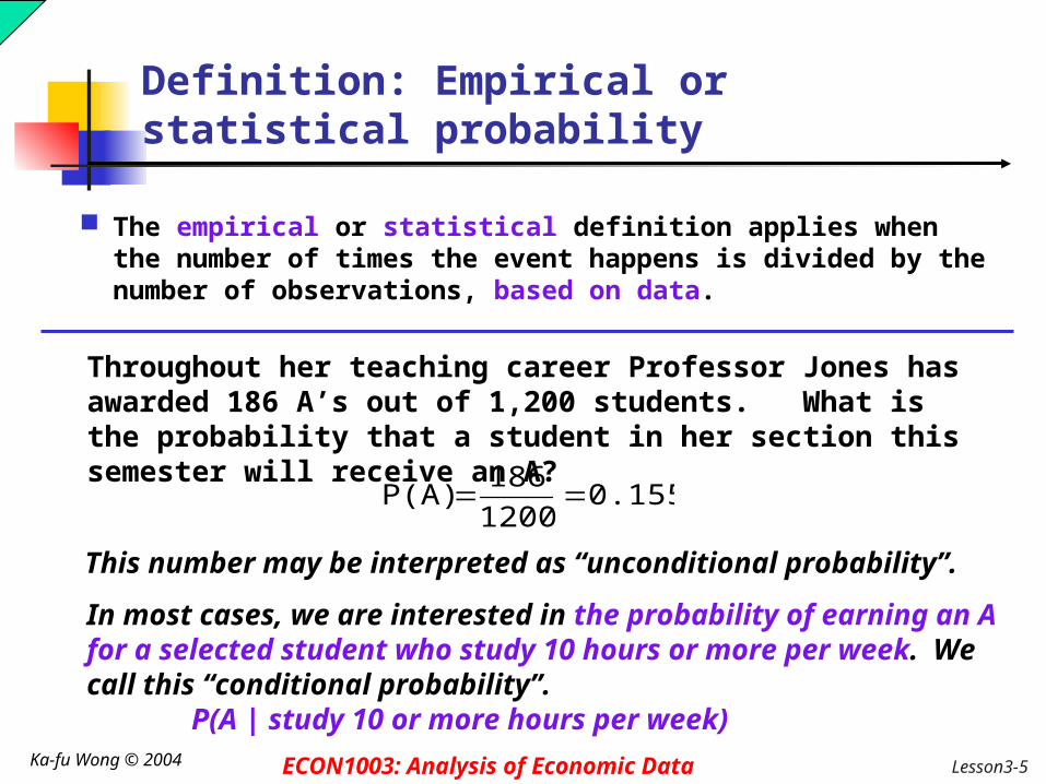
Definition: Empirical or statistical probability

The empirical or statistical definition applies when the number of times the event happens is divided by the number of observations, based on data.

0.1551200186

P(A)

This number may be interpreted as “unconditional probability”.In most cases, we are interested in the probability of earning an A for a selected student who study 10 hours or more per week. We call this “conditional probability”. P(A | study 10 or more hours per week)

Throughout her teaching career Professor Jones has awarded 186 A’s out of 1,200 students. What is the probability that a student in her section this semester will receive an A?


Definition: Subjective probability

Subjective probability is based on whatever information is available, based on subjective feelings. Estimating the probability mortgage rates for

home loans will top 8 percent this year. Estimating the probability that HK’s economic

growth will be 3% this year. Estimating the probability that HK will solve its

deficit problem in 2006.


A fair die is rolled once. Peter is concerned with whether the resulted

number is even, i.e., 2, 4, 6. Paul is concerned with whether the resulted number

is less than or equal to 3, i.e., 1, 2, 3. Mary is concerned with whether the resulted number

is 6. Sonia is concerned with whether the resulted

number is odd, i.e., 1, 3, 5.

A fair die is rolled twice. John is concerned with whether the resulted number

of first roll is even, i.e., 2, 4, 6. Sarah is concerned with whether the resulted

number of second roll is even, i.e., 2, 4, 6.

Example 1(to be used to illustrate the definitions)


Definitions: Experiment and outcome

An experiment is the observation of some activity or the act of taking some measurement. The experiment is rolling the one die in the first

example, and rolling one die twice in the second example.

An outcome is the particular result of an experiment. The possible outcomes are the numbers 1, 2, 3, 4,

5, and 6 in the first example. The possible outcomes are number pairs (1,1),

(1,2), …, (6,6), in the second example.


Definition: Event

An event is the collection of one or more outcomes of an experiment. For Peter: the occurrence of an even number, i.e.,

2, 4, 6. For Paul: the occurrence of a number less than or

equal to 3, i.e., 1, 2, 3. For Mary: the occurrence of a number 6. For Sonia: the occurrence of an odd number, i.e.,

1, 3, 5. For John: the occurrence of (2,1), (2,2), (2,3),…,

(2,6), (4,1),…,(4,6), (6,1),…,(6,6) [John does not care about the result of the second roll].


Learning exercise 1: University Demographics

Current enrollments by college and by sex appear in the following table.

College

Ag-For

Arts-Sci

Bus-Econ

Educ Engr

Law Undecl

Totals

Female

500 1500 400 1000

200 100 800 4500

Male 900 1200 500 500 1300

200 900 5500

Totals 1400 2700 900 1500

1500

300 1700 10000 If we select a student at random, what is the probability

that the student is : A female or male, i.e., P(Female or Male). Not from Agricultural and Forestry, i.e., P(not-Ag-For) A female given that the student is known to be from

BusEcon, i.e., P(Female |BusEcon). A female and from BusEcon, i.e., P(Female and BusEcon). From BusEcon, i.e., P(BusEcon).


Learning exercise 1: University Demographics

College

Ag-For

Arts-Sci

Bus-Econ

Educ

Engr

Law Undecl

Totals

Female

500 1500 400 1000

200 100 800 4500

Male 900 1200 500 500 1300

200 900 5500

Totals 1400 2700 900 1500

1500

300 1700 10000P(Female or Male)=(4500 + 5500)/10000 = 1

P(not-Ag-For)=(10000 – 1400) /10000 = 0.86

P(Female | Bus Econ)= 400 /900 = 0.44

P(Female and BusEcon)= 400 /10000 = 0.04

P(BusEcon)= 900 /10000 = 0.09

P(Female and BusEcon) = P(BusEcon) P(Female | Bus Econ)


Definition: Mutually Exclusive events

Events are mutually exclusive if the occurrence of any one event means that none of the others can occur at the same time. Peter’s event and Paul’s event are not mutually

exclusive – both contains 2. Peter’s event and Mary’s event are not mutually

exclusive – both contains 6. Paul’s event and Mary’s event are mutually

exclusive – no common numbers. Peter’s event and Sonia’s event are mutually

exclusive – no common numbers.


Definition: Exhaustive events

Events are collectively exhaustive if at least one of the events must occur when an experiment is conducted. Peter’s event (even numbers) and Sonia’s event

(odd numbers) are collectively exhaustive. Peter’s event (even numbers) and Mary’s event

(number 6) are not collectively exhaustive.


Conditional Probability

A conditional probability is the probability of a particular event occurring, given that another event has occurred.

The probability of the event A given that the event B has occurred is written P(A|B). P(female | BusEcon) P(girl | test says girl)


Learning exercise 2: Predicting Sex of Babies

Many couples take advantage of ultrasound exams to determine the sex of their baby before it is born. Some couples prefer not to know beforehand. In any case, ultrasound examination is not always accurate. About 1 in 5 predictions are wrong. In one medical group, the proportion of girls correctly

identified is 9 out of 10, i.e., applying the test to 100 baby girls, 90 of the tests will indicate girls.

and the number of boys correctly identified is 3 out of 4.

i.e., applying the test to 100 baby boys, 75 of the tests will indicate boys.

The proportion of girls born is 48 out of 100.

What is the probability that a baby predicted to be a girl actually turns out to be a girl? Formally, find P(girl | test says girl).



P(girl | test says girl) In one medical group, the proportion of girls correctly

identified is 9 out of 10 and the number of boys correctly identified is 3 out of 4. The proportion of girls born is 48 out of 100.

Think about the next 1000 births handled by this medical group. 480 = 1000*0.48 are girls 520 = 1000*0.52 are boys Of the girls, 432 (=480*0.9) tests indicate that they are girls. Of the boys, 130 (=520*0.25) tests indicate that they are

girls. In total, 562 (=432+130) tests indicate girls. Out of these

562 babies, 432 are girls. Thus P(girl | test says girl ) = 432/562 = 0.769



Test says girl

Test says boy

Totals

Girl (4) 432 (7) 48 (2) 480

Boy (5) 130 (8) 390 (3) 520

Totals (6) 562 (9) 438 (1) 1000

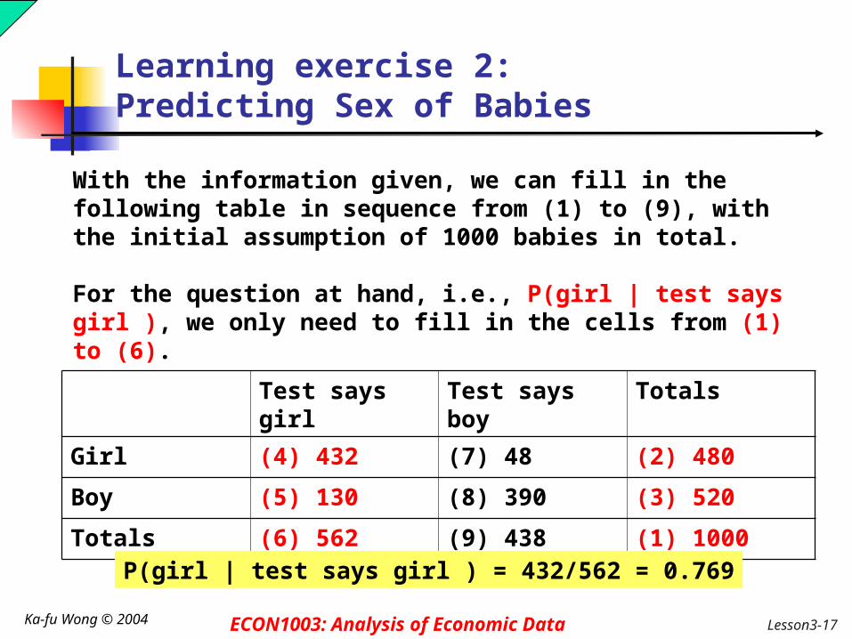
With the information given, we can fill in the following table in sequence from (1) to (9), with the initial assumption of 1000 babies in total.

For the question at hand, i.e., P(girl | test says girl ), we only need to fill in the cells from (1) to (6).

P(girl | test says girl ) = 432/562 = 0.769



480 = 1000*0.48 are girls 520 = 1000*0.52 are boys Of the girls, 432 (=480*0.9) tests indicate that they are girls.

Of the boys, 130 (=520*0.25) tests indicate that they are girls.

In total, 562 tests indicate girls.

Out of these 562 babies, 432 are girls. Thus P(girls | test syas girls ) = 432/562 = 0.769

1000*P(girls)

1000*P(boys)

1000*[P(girls)*P(test says girls|girls) + P(boys)*P(test says girls|boys)]

1000*P(boys)*P(test says girls | boys)

1000*P(girls)*P(test says girls|girls)

1000*P(girls)*P(test says girls|girls)

1000*[P(girls)*P(test says girls|girls) + P(boys)*P(test says girls|boys)]


Learning exercise 3: Putting in Extra Trunk Lines

Given recent flooding (or other condition more appropriate to your area) between Town A and Town B, the local telephone company is assessing the value of adding an independent trunk line between the two towns. The second line will fail independently of the first because it will depend on different equipment and routing (we assume a regional disaster is highly unlikely).

Under current conditions, the present line works 98 out of 100 times someone wishes to make a call. If the second line performs as well, what is the chance that a caller will be able to get through? Formally, P( Line 1 works ) = 98/100 P( Line 2 works ) = 98/100

Find P( Line 1 or Line 2 works ).



P( Line 1 works ) = 98/100 P( Line 2 works ) = 98/100 Find P( Line 1 or Line 2 works ).

P( Line 1 or Line 2 works ) = 1 – P(Both line1 and Line 2 fail)= 1 – P(Line 1 fails)*P(line 2 fails)= 1 – 0.02*0.02= 0.9996.

Line 2 works Line 2 fails

Line 1 works 0.98*0.98 0.98*0.02

Line 1 fails 0.02*0.98 0.02*0.02



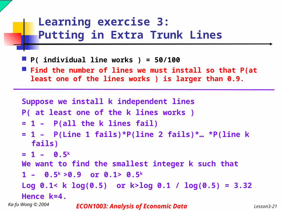
P( individual line works ) = 50/100 Find the number of lines we must install so that P(at

least one of the lines works ) is larger than 0.9.

Suppose we install k independent linesP( at least one of the k lines works ) = 1 – P(all the k lines fail)= 1 – P(Line 1 fails)*P(line 2 fails)*… *P(line k fails)= 1 – 0.5k

We want to find the smallest integer k such that 1 – 0.5k >0.9 or 0.1> 0.5k

Log 0.1< k log(0.5) or k>log 0.1 / log(0.5) = 3.32Hence k=4.


Basic Rules of Probability

If two events A and B are mutually exclusive, the special rule of addition states that the probability of A or B occurring equals the sum of their respective probabilities:

P(A or B) = P(A) + P(B)


EXAMPLE 3

New England Commuter Airways recently supplied the following information on their commuter flights from Boston to New York:

Arrival Frequency

Early 100

On Time 800

Late 75

Canceled 25

Total 1000


EXAMPLE 3

If A is the event that a flight arrives early, thenP(A) = 100/1000 = .10.

If B is the event that a flight arrives late, then P(B) = 75/1000 = .075.

Arrival Frequency Early 100

On Time 800

Late 75

Canceled 25

Total 1000

The probability that a flight is either early or late is:P(A or B) = P(A) + P(B) = .10 + .075 =.175.


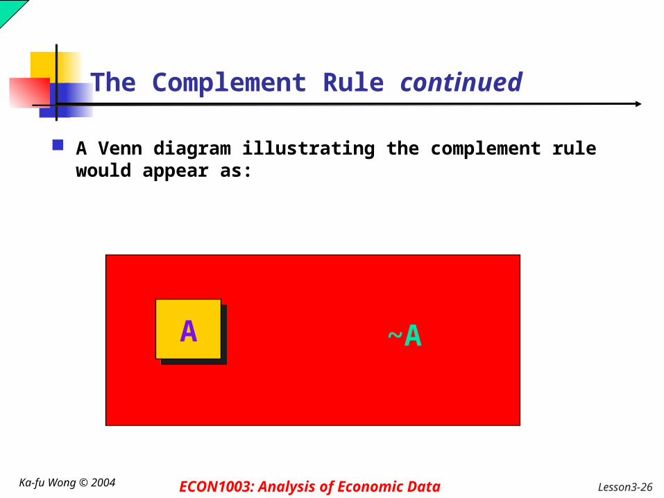
The Complement Rule

The complement rule is used to determine the probability of an event occurring by subtracting the probability of the event not occurring from 1.

If P(A) is the probability of event A and P(~A) is the complement of A,

P(A) + P(~A) = 1 or P(A) = 1 - P(~A).


The Complement Rule continued

A Venn diagram illustrating the complement rule would appear as:

A ~A


EXAMPLE 4

Recall EXAMPLE 3. Use the complement rule to find the probability of an early (A) or a late (B) flight

P(A or B) = 1 - P(C or D)

If C is the event that a flight arrives on time, then P(C) = 800/1000 = .8.

If D is the event that a flight is canceled, then P(D) = 25/1000 = .025.

Arrival Frequency Early 100

On Time 800

Late 75

Canceled 25

Total 1000

P(A or B) = 1 - P(C or D) = 1 - [.8 +.025] =.175


EXAMPLE 4 continued

P(A or B) = 1 - P(C or D) = 1 - [.8 +.025] =.175

C.8

D.025

~(C or D) = (A or B) .175


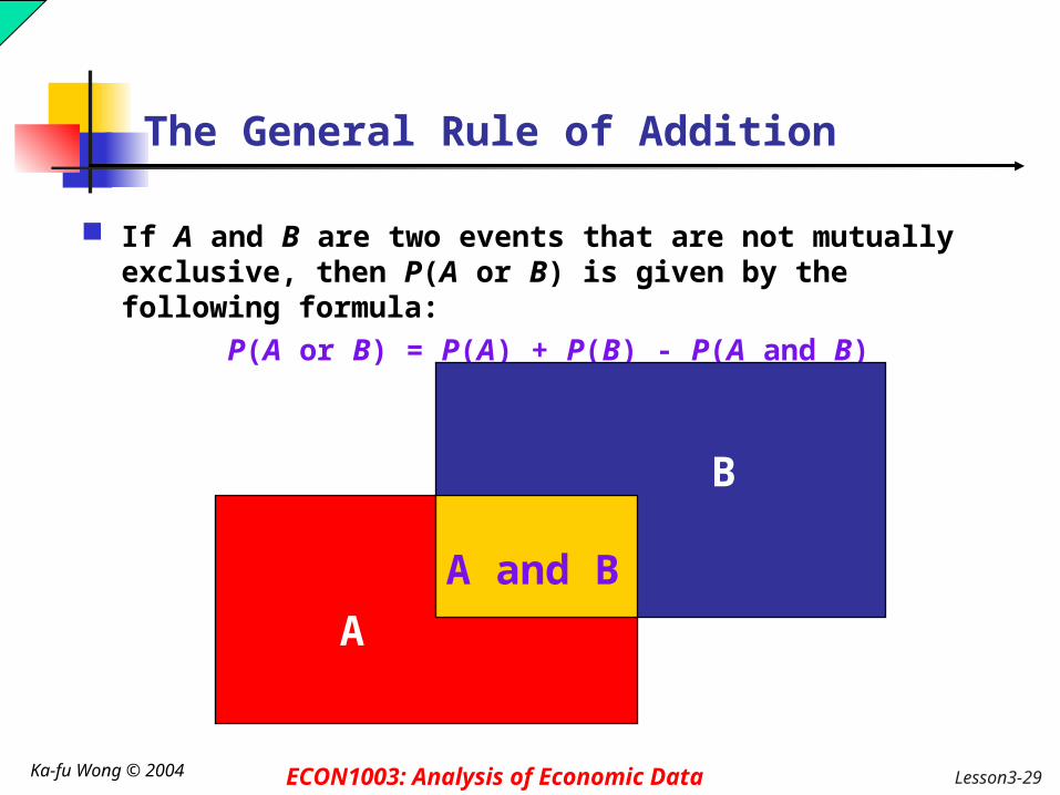
The General Rule of Addition

If A and B are two events that are not mutually exclusive, then P(A or B) is given by the following formula:

P(A or B) = P(A) + P(B) - P(A and B)

A and B

A

B


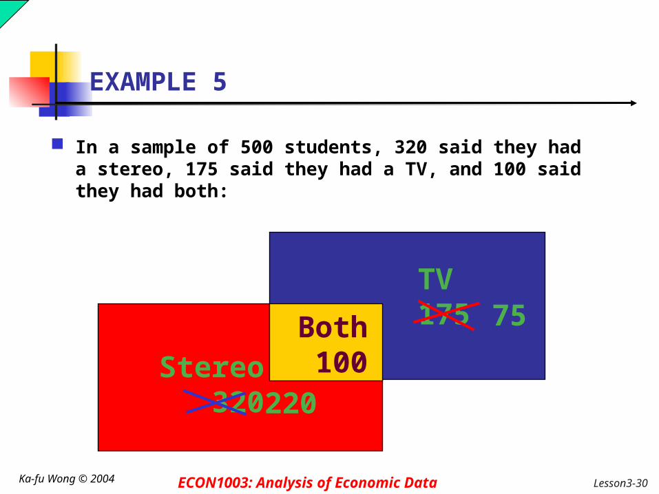
EXAMPLE 5

In a sample of 500 students, 320 said they had a stereo, 175 said they had a TV, and 100 said they had both:

Stereo 320

Both 100

TV175 75

220


EXAMPLE 5 continued

If a student is selected at random, what is the probability that the student has only a stereo, only a TV, and both a stereo and TV?

P(student has a stereo) = 320/500 = .64.P(student has a TV) = 175/500 = .35.P(student has both a stereo and TV) = 100/500 = .20.P(student as only a stereo) = 220/500 = .44.P(student has only a TV) = 75/500 = .15.

In a sample of 500 students, 320 said they had a stereo, 175 said they had a TV, and 100 said they had both.

P(student as only a stereo) = P(student has a stereo) - P(student has both a stereo and

TV)P(student has only a TV) = P(student has a TV)

- P(student has both a stereo and TV)


EXAMPLE 5 continued

If a student is selected at random, what is the probability that the student has either a stereo or a TV in his or her room?

P(either S or T) = P(only S) + P (only T)= [P(S) - P(S and T)] +[P(T) - P(S and T)]= .64 - .20 +.35 - .20 = .59.

In a sample of 500 students, 320 said they had a stereo, 175 said they had a TV, and 100 said they had both.

P(S) = 320/500 = .64.P(T) = 175/500 = .35.P(S and T) = 100/500 = .20.


Joint Probability

A joint probability measures the likelihood that two or more events will happen concurrently.

An example would be the event that a student has both a stereo and TV in his or her dorm room.

In an experiment of throwing only one die, let x denote the outcome,

P(x=5, and x=6) =0 because the two outcomes are mutually exclusive.


Special Rule of Multiplication

The special rule of multiplication requires that two events A and B are independent.

Two events A and B are independent if the occurrence of one has no effect on the probability of the occurrence of the other.

This rule is written: P(A and B) = P(A)P(B)


EXAMPLE 6

Chris owns two stocks, IBM and General Electric (GE). The probability that IBM stock will increase in value next year is .5 and the probability that GE stock will increase in value next year is .7. Assume the two stocks are independent. What is the probability that both stocks will increase in value next year?

P(IBM and GE) = (.5)(.7) = .35.


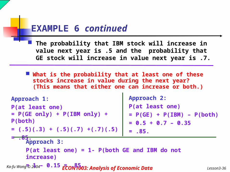
EXAMPLE 6 continued

What is the probability that at least one of these stocks increase in value during the next year? (This means that either one can increase or both.)

Approach 1:P(at least one) = P(GE only) + P(IBM only) + P(both)= (.5)(.3) + (.5)(.7) +(.7)(.5) = .85.

Approach 2:P(at least one) = P(GE) + P(IBM) – P(both)= 0.5 + 0.7 – 0.35 = .85.

The probability that IBM stock will increase in value next year is .5 and the probability that GE stock will increase in value next year is .7.

Approach 3:P(at least one) = 1- P(both GE and IBM do not increase)= 1 – 0.15 = .85.


General Multiplication Rule

The general rule of multiplication is used to find the joint probability that two events will occur.

It states that for two events A and B, the joint probability that both events will happen is found by multiplying the probability that event A will happen by the conditional probability of B given that A has occurred.


General Multiplication Rule

The joint probability, P(A and B) is given by the following formula:

P(A and B) = P(A)P(B|A)

or

P(A and B) = P(B)P(A|B)

Examples: P(test says girl and girl)

= P(girls) * P(test says girls | girls) P(test says boy and boy)

= P(boys) * P(test says boys | boys)


Independence -- an illustration

Consider whether the decision of a young man going to party depends on whether his girlfriend goes to the same party.

Assume the probability of the young man going to party is 0.7 (i.e., he goes to 70 out of 100 parties on average).

If he tends to go to whichever party his girlfriend goes, his party behavior depends on his girlfriend’s. That is, the probability of going to a party conditional on his girlfriend’s presence is larger than 0.7 (extreme case being 1.0).

If he tends to avoid going to whichever party his girlfriend goes, his party behavior also depends on his girlfriend’s. That is, the probability of going to a party conditional on his girlfriend’s presence is less than 0.7 (extreme case being 0.0).

If in making the party decision, he never considers whether his girlfriend is going to a party, his party behavior does not depends on his girlfriend’s. That means, the probability of going to a party conditional on his girlfriend’s presence is 0.7.


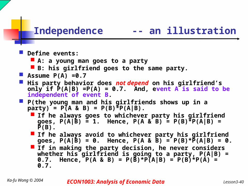
Independence -- an illustration

Define events: A: a young man goes to a party B: his girlfriend goes to the same party.

Assume P(A) =0.7 His party behavior does not depend on his girlfriend’s

only if P(A|B) =P(A) = 0.7. And, event A is said to be independent of event B.

P(the young man and his girlfriends shows up in a party) = P(A & B) = P(B)*P(A|B). If he always goes to whichever party his girlfriend

goes, P(A|B) = 1. Hence, P(A & B) = P(B)*P(A|B) = P(B).

If he always avoid to whichever party his girlfriend goes, P(A|B) = 0. Hence, P(A & B) = P(B)*P(A|B) = 0.

If in making the party decision, he never considers whether his girlfriend is going to a party, P(A|B) = 0.7. Hence, P(A & B) = P(B)*P(A|B) = P(B)*P(A) = 0.7.


Independence

Event A is independent of B P(A|B) = P (A)

Event B is independent of A P(B|A) = P (B)

P(B|A) = P (B) implies P(A&B) = P(B|A) * P(A) = P(B) * P(A)

P(A|B) = P (A) impliesP(A&B) = P(A|B) * P(B) = P(A) * P(B)

Thus, if P(A&B) = P(B) * P(A), we must have either P(A|B) = P (A) or P(B|A) = P (B).


EXAMPLE 7

The Dean of the School of Business at Owens University collected the following information about undergraduate students in her college:

MAJOR Male Female Total

Accounting 170 110 280

Finance 120 100 220

Marketing 160 70 230

Management 150 120 270

Total 600 400 1000


EXAMPLE 7 continued

If a student is selected at random, what is the probability that the student is a female (F) accounting major (A)

P(A and F) = 110/1000.

Given that the student is a female, what is the probability that she is an accounting major?

MAJOR Male Female Total

Accounting 170 110 280

Finance 120 100 220

Marketing 160 70 230

Management 150 120 270

Total 600 400 1000

Approach 1:P(A|F) = P(A and F)/P(F)= [110/1000]/[400/1000] = .275

Approach 2:P(A|F) = 110/400= .275


Tree Diagrams

A tree diagram is useful for portraying conditional and joint probabilities. It is particularly useful for analyzing business decisions involving several stages.

EXAMPLE 8: In a bag containing 7 red chips and 5 blue chips you select 2 chips one after the other without replacement. Construct a tree diagram showing this information.


EXAMPLE 8 continued

R1

B1

R2

B2

R2

B2

7/12

5/12

6/11

5/11

7/11

4/11


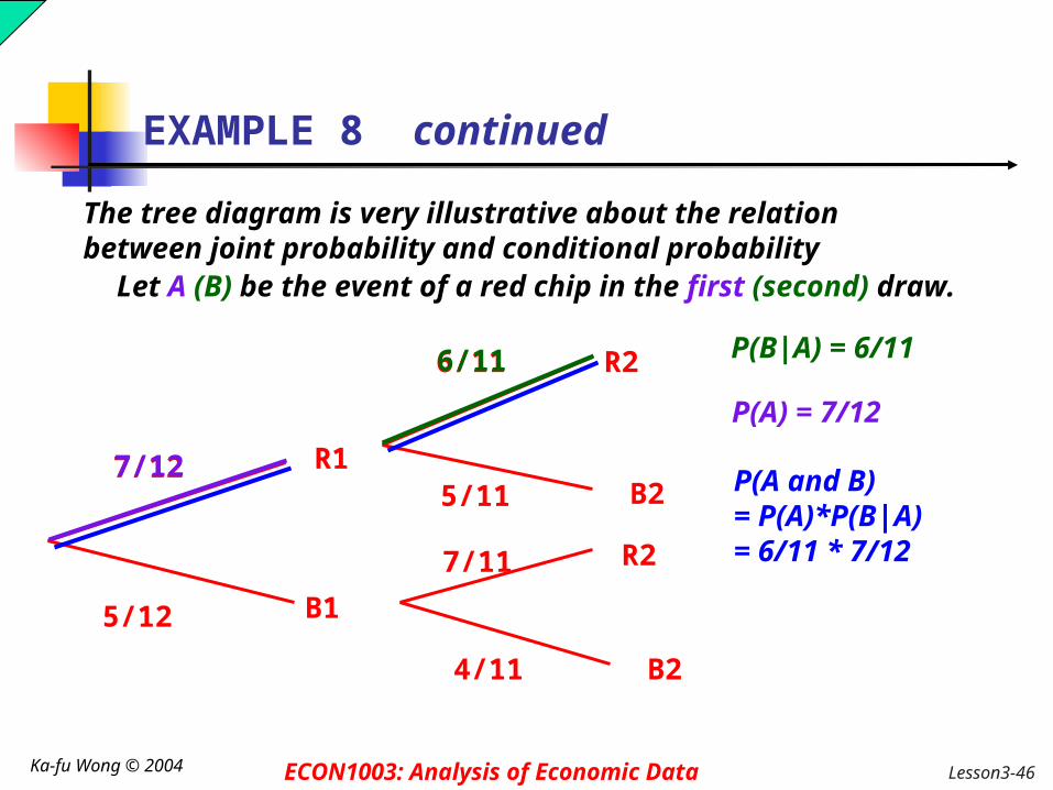
EXAMPLE 8 continued

R1

B1

R2

B2

R2

B2

7/12

5/12

6/11

5/11

7/11

4/11

The tree diagram is very illustrative about the relation between joint probability and conditional probabilityLet A (B) be the event of a red chip in the first (second) draw.

P(B|A) = 6/11

P(A) = 7/12

P(A and B) = P(A)*P(B|A)= 6/11 * 7/12

7/12

6/11


Bayes’ Theorem

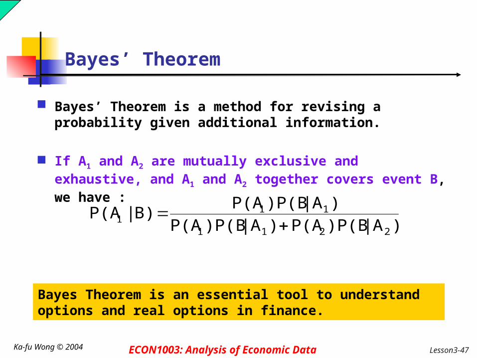
Bayes’ Theorem is a method for revising a probability given additional information.

If A1 and A2 are mutually exclusive and exhaustive, and A1 and A2 together covers event B, we have :

)A|)P(BP(A)A|)P(BP(A)A|)P(BP(A

B)|P(A2211

111

Bayes Theorem is an essential tool to understand options and real options in finance.


Bayes’ Theorem

A1 and A2 are mutually exclusive means

P (A1 or A2 ) = P(A1) + P(A2 )

P (A1 and A2 ) = 0

A1 and A2 are exhaustive means

P (A1 or A2 ) = P(A1) + P(A2 ) = 1

A1 and A2 together covers event B means

P(B) = P(A1 & B) + P(A2 & B) (see the Venn diagram illustration)


Venn Diagram illustration of Bayes’ theorem

BA1 A2

A2 & BA1 & B


Bayes’ Theorem

Bayes’ Theorem can be derived based on simple manipulation of the general multiplication rule.

P(A1|B)

= P(A1 & B) /P(B)

= [P(A1) P(B|A1)] / P(B)

= [P(A1) P(B|A1)] / [P(A1 & B) + P(A2 & B)]

= [P(A1) P(B|A1) ]/ [P(A1) P(B|A1) + P(A2) P(B|A2)]

)A|)P(BP(A)A|)P(BP(A)A|)P(BP(A

B)|P(A2211

111


EXAMPLE 9

Duff Cola Company recently received several complaints that their bottles are under-filled. A complaint was received today but the production manager is unable to identify which of the two Springfield plants (A or B) filled this bottle. The following table summarizes the Duff production experience.

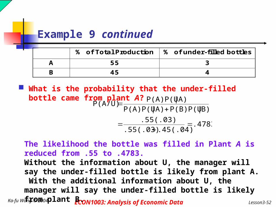
What is the probability that the under-filled bottle came from plant A?

% of Total Production % of under-filled bottles

A 55 3

B 45 4


Example 9 continued

.4783.45(.04).55(.03)

.55(.03)

B)|P(B)P(UA)|P(A)P(UA)|P(A)P(U

P(A/U)

The likelihood the bottle was filled in Plant A is reduced from .55 to .4783. Without the information about U, the manager will say the under-filled bottle is likely from plant A. With the additional information about U, the manager will say the under-filled bottle is likely from plant B.

What is the probability that the under-filled bottle came from plant A?

% of Total Production % of under-filled bottles

A 55 3

B 45 4


Probabilities for throwing n Dice

Suppose we roll n regular balanced six-sided dice. If the event X is the sum of the n values which appear, what are the probabilities associated for each value of X, for the possible values X = n, ... , 6n?

In the case n =1, these probabilities are all 1/6.



(1,1) (1,2)

(1,3)

(1,4)

(1,5)

(1,6)

(2,1) (2,2)

(2,3)

(2,4)

(2,5)

(2,6)

(3,1) (3,2)

(3,3)

(3,4)

(3,5)

(3,6)

(4,1) (4,2)

(4,3)

(4,4)

(4,5)

(4,6)

(5,1) (5,2)

(5,3)

(5,4)

(5,5)

(5,6)

(6,1) (6,2)

(6,3)

(6,4)

(6,5)

(6,6)

2 3 4 5 6 7

3 4 5 6 7 8

4 5 6 7 8 9

5 6 7 8 9 10

6 7 8 9 10 11

7 8 9 10 11 12

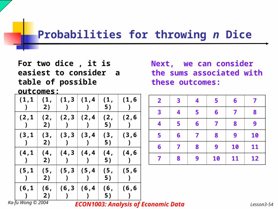
For two dice , it is easiest to consider a table of possible outcomes:

Next, we can consider the sums associated with these outcomes:



X # P(X) X # P(X)

2 1 1/36 8 5 5/36

3 2 2/36 9 4 4/36

4 3 3/36 10 3 3/36

5 4 4/36 11 2 2/36

6 5 5/36 12 1 1/36

7 6 6/36

2 3 4 5 6 7

3 4 5 6 7 8

4 5 6 7 8 9

5 6 7 8 9 10

6 7 8 9 10 11

7 8 9 10 11 12

Next, we can consider the sums associated with these outcomes:

Since there are 36 outcomes, each equally likely, we see that the probabilities are:



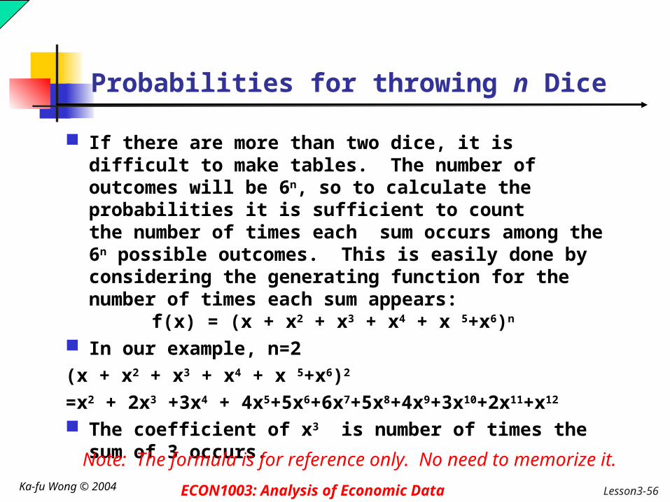
If there are more than two dice, it is difficult to make tables. The number of outcomes will be 6n, so to calculate the probabilities it is sufficient to count the number of times each sum occurs among the 6n possible outcomes. This is easily done by considering the generating function for the number of times each sum appears: f(x) = (x + x2 + x3 + x4 + x 5+x6)n

In our example, n=2(x + x2 + x3 + x4 + x 5+x6)2

=x2 + 2x3 +3x4 + 4x5+5x6+6x7+5x8+4x9+3x10+2x11+x12

The coefficient of x3 is number of times the sum of 3 occurs.

Note: The formula is for reference only. No need to memorize it.


Some Principles of Counting

The multiplication formula indicates that if there are m ways of doing one thing and n ways of doing another thing, there are m x n ways of doing both.

Example 10: Dr. Delong has 10 shirts and 8 ties. How many shirt and tie outfits does he have?

(10)(8) = 80



A permutation is any arrangement of r objects selected from n possible objects.

Note: The order of arrangement is important in permutations.

r)!(nn!

Prn

n! = n(n-1) (n-2)… 21n=1, n!=1n=2, n!=21=2n=3, n!=321=6n=4, n!=4321=24n=5, n!=54321=120



A combination is the number of ways to choose r objects from a group of n objects without regard to order.

r)!(nr!n!

Crn


EXAMPLE 11

There are 12 players on the Carolina Forest High School basketball team. Coach Thompson must pick five players among the twelve on the team to comprise the starting lineup. How many different groups are possible?

7925)!(125!

12!C512


Example 11 continued

Suppose that in addition to selecting the group, he must also rank each of the players in that starting lineup according to their ability.

95,0405)!(12

12!P512


- END -

Lesson 3: Lesson 3: A Survey of Probability Concepts

Ka-fu Wong © 2004 ECON1003: Analysis of Economic Data Lesson3-1 Lesson 3: A Survey of Probability Concepts.

Documents

definitions of probability

classical probability

statistical probability

unconditional probability

kafu wong

resulted number

definitions slide

survey of probability