K-TIME SIGNATURES FOR MULTICAST DATA AUTHENTICATION ...

K-TIME SIGNATURES FOR MULTICAST

DATA AUTHENTICATION

by

KELSEY LAUREN CAIRNS

A dissertation submitted in partial fulfillment ofthe requirements for the degree of

DOCTOR OF PHILOSOPHY

WASHINGTON STATE UNIVERSITYSchool of Electrical Engineering and Computer Science

DECEMBER 2016

© Copyright by KELSEY LAUREN CAIRNS, 2016All Rights Reserved

© Copyright by KELSEY LAUREN CAIRNS, 2016All Rights Reserved

To the Faculty of Washington State University:

The members of the Committee appointed to examine the dissertation

of KELSEY LAUREN CAIRNS find it satisfactory and recommend that it be accepted.

Carl H. Hauser, Ph.D., Chair

Adam L. Hahn, Ph.D.

Ananth Kalyanaraman, Ph.D.

Anurag K. Srivastava, Ph.D.

ii

ACKNOWLEDGMENTS

I never truly understood acknowledgments until I wrote a dissertation. To me, acknowl-

edgments seemed like an obligatory list of thank-yous. Courteous, yes, but I failed to

see the significance. But in the midst of writing, the significance hit. I realized it’s the

people around me who got me through those pages. It’s your friends that convince you

that it’s worth it, and that with each idea you fight to fit into words, you’re one step

closer to achieving your goal.

Then you realize it’s not just during the writing process that your friends are there for

you – they’ve been there all along. Through the ups and downs of grad student life, I’ve

been surrounded by exceptional friends and they all deserve an earnest thank-you. So to

all those people – the friends who brought me surprise donuts, ordered soup to my door

when I was sick, snuck into my apartment while I was away to clean it, helped me steal

couches in the middle of the night, engineered ways to hold my car together with office

supplies, and generally helped me through the grad school years: thank you. Thank

you for your support and your friendship. Thank you also to the people back home who

taught me what I can do with hard work and dedication. Sincere thanks also go to my

parents, who by now probably think the purpose of trips home is to do laundry rather to

see them. I swear this isn’t true, and even once I own my own washing machine, visiting

home will be just as important.

I also want to acknowedge everyone that contributed to my work academically, including

Qiyan Wang, Himanshu Khurana, Ying Huang, and Klara Nahrstedt, whose work pro-

vided the foundation for my project. I also want to thank Julio Deleon and Mackenzie

Meade for their contributions, Dave Anderson and Ryan Goodfellow for their time and

iii

assistance, and Thoshitha Gamage for his advice and direction. Last but not least, thank

you to my advisor, Carl Hauser, and my committee, Adam Hahn, Ananth Kalyanara-

man, and Anurag Srivastava, all good people dedicated to good research, who made this

degree possible.

This research was funded in part by Department of Energy Award Number DE-OE0000097

(TCIPG).

This material is based upon work supported by the Department of Energy under Award

Number DE-OE0000780 (CREDC).

Disclaimer This report was prepared as an account of work sponsored by an agency of

the United States Government. Neither the United States Government nor any agency

thereof, nor any of their employees, makes any warranty, express or implied, or assumes

any legal liability or responsibility for the accuracy, completeness, or usefulness of any

information, apparatus, product, or process disclosed, or represents that its use would

not infringe privately owned rights. Reference herein to any specific commercial product,

process, or service by trade name, trademark, manufacturer, or otherwise does not nec-

essarily constitute or imply its endorsement, recommendation, or favoring by the United

States Government or any agency thereof. The views and opinions of authors expressed

herein do not necessarily state or reflect those of the United States Government or any

agency thereof.

iv

K-TIME SIGNATURE FOR MULTICAST

DATA AUTHENTICATION

Abstract

by Kelsey Lauren Cairns, Ph.D.Washington State University

December 2016

Chair: Carl H. Hauser

This dissertation focuses on Time-Valid One-Time-Signatures or TV-OTS, an experi-

mental k-time digital signature scheme for source authentication and integrity protection

of multicast data streams. Our motivating use case, status data for smart grid appli-

cations, requires high throughput, low latency signing and verifying of each data point.

TV-OTS provides this but sacrifices “perfect” security to do so: either a very small

fraction of messages may be forged or a small number of suspicious messages must be

discarded.

TV-OTS’s imperfect security can be measured probabilistically which leads to a new

idea: signature confidence. Our concept leverages the fact that even TV-OTS signatures

that aren’t fully verifiable may be partially verifiable. Instead of following the traditional

v

approach of reporting a boolean “yes” or “no” for signature verifiability, we take the

approach of reporting a numerical confidence value which is based on the percentage of

the signature that is verifiable as well as system state. The reported confidence reflects

the receiver’s belief that the signature originated at the expected sender and was not

forged by an adversary. In our work, we analyzed the probability of successful attacks

against signatures, as well as the effectiveness of confidence metrics in detecting these

forged messages. Our results show that confidence based evaluation successfully detects

simulated attacks against TV-OTS.

We use results of our security analysis to choose applicable settings for a performance

evaluation of TV-OTS. Our implementation is fully functional, including a streamed key

distribution service that distributes new public keys as necessary. TV-OTS showed better

average latencies than the standard algorithms that are its closest competitors, namely

ECDSA and RSA.

Confidence-based signature evaluation further inspires feedback controlled security. We

consider TV-OTS in the context of the emerging field of systems engineering applied

to cyber-secure systems. We show how to incorporate TV-OTS into a system designed

with these principles, using confidence and other statistical behavior as a way to detect

system abnormalities which can be reported to a control layer. Our approach is intended

to detect and react to attacks against TV-OTS as well as monitor the overall health of

the system.

vi

Contents

Page

Acknowledgments . . . . . . . . . . . . . . . . . . . . . . . . . . . . . . . . . . iii

Abstract . . . . . . . . . . . . . . . . . . . . . . . . . . . . . . . . . . . . . . . . v

List of Figures . . . . . . . . . . . . . . . . . . . . . . . . . . . . . . . . . . . . xi

List of Tables . . . . . . . . . . . . . . . . . . . . . . . . . . . . . . . . . . . . . xiii

1 Introduction . . . . . . . . . . . . . . . . . . . . . . . . . . . . . . . . . . . . 1

1.0.1 Integrity and Authentication . . . . . . . . . . . . . . . . . . . . . 1

1.0.2 Symmetric and Asymmetric Primitives . . . . . . . . . . . . . . . 3

1.0.3 Real-Time Multicast Reliant Applications . . . . . . . . . . . . . 5

1.0.4 Data Communication Requirements . . . . . . . . . . . . . . . . . 9

1.1 Thesis Contributions . . . . . . . . . . . . . . . . . . . . . . . . . . . . . 10

2 Authentication Techniques for Multicast . . . . . . . . . . . . . . . . . . 13

2.1 Standards . . . . . . . . . . . . . . . . . . . . . . . . . . . . . . . . . . . 13

2.1.1 One-way and hash functions . . . . . . . . . . . . . . . . . . . . . 14

2.1.2 Symmetric Standards for Authentication . . . . . . . . . . . . . . 15

2.1.3 HMAC for Multicast Communication . . . . . . . . . . . . . . . . 16

2.1.4 Asymmetric Standards for Authentication . . . . . . . . . . . . . 18

2.1.5 Key Distribution . . . . . . . . . . . . . . . . . . . . . . . . . . . 20

vii

2.2 Alternatives to Standards . . . . . . . . . . . . . . . . . . . . . . . . . . 21

2.2.1 Commonly Used Components . . . . . . . . . . . . . . . . . . . . 21

2.2.2 Chained Signatures . . . . . . . . . . . . . . . . . . . . . . . . . . 24

2.2.3 Amortized Block Signatures . . . . . . . . . . . . . . . . . . . . . 28

2.2.4 Delayed Key Release . . . . . . . . . . . . . . . . . . . . . . . . . 30

2.2.5 Precomputed Expensive Signatures . . . . . . . . . . . . . . . . . 33

2.2.6 Identity based signatures . . . . . . . . . . . . . . . . . . . . . . . 34

2.2.7 One and K-Time Signatures . . . . . . . . . . . . . . . . . . . . . 35

2.3 One- and K-Time Signatures . . . . . . . . . . . . . . . . . . . . . . . . . 37

2.3.1 Source Authentication Using One-Way Functions . . . . . . . . . 37

2.3.2 Source and Content Authentication . . . . . . . . . . . . . . . . . 39

2.3.3 Lowering Authentication Overhead . . . . . . . . . . . . . . . . . 40

2.3.4 K-Time signatures . . . . . . . . . . . . . . . . . . . . . . . . . . 43

2.3.5 Chained K-Time Signatures . . . . . . . . . . . . . . . . . . . . . 46

2.4 Hash Chains Management Structures . . . . . . . . . . . . . . . . . . . . 51

2.4.1 Fractal Hash Sequencing and Traversal . . . . . . . . . . . . . . . 51

2.4.2 Related Traversals . . . . . . . . . . . . . . . . . . . . . . . . . . 55

2.5 Problem Statement . . . . . . . . . . . . . . . . . . . . . . . . . . . . . . 56

2.5.1 Research Directions . . . . . . . . . . . . . . . . . . . . . . . . . . 57

2.5.2 Relation to Power Grid Applications . . . . . . . . . . . . . . . . 59

3 Science of TV-OTS . . . . . . . . . . . . . . . . . . . . . . . . . . . . . . . 60

3.1 Security of TV-OTS . . . . . . . . . . . . . . . . . . . . . . . . . . . . . 60

3.1.1 Attacker Model . . . . . . . . . . . . . . . . . . . . . . . . . . . . 61

3.1.2 Introduction and Setup . . . . . . . . . . . . . . . . . . . . . . . . 61

3.1.3 Probability of Forging Messages . . . . . . . . . . . . . . . . . . . 65

3.2 Receiver Confidence . . . . . . . . . . . . . . . . . . . . . . . . . . . . . . 76

viii

3.2.1 Receivers’ Attacker Models . . . . . . . . . . . . . . . . . . . . . . 78

3.2.2 Confidence Functions . . . . . . . . . . . . . . . . . . . . . . . . . 81

3.2.3 Implementations of Confidence Functions . . . . . . . . . . . . . . 84

3.3 Periodic Key Distribution . . . . . . . . . . . . . . . . . . . . . . . . . . 90

3.3.1 Principles and Design . . . . . . . . . . . . . . . . . . . . . . . . . 95

3.3.2 Future Work on Keystreams . . . . . . . . . . . . . . . . . . . . . 96

4 Engineering TV-OTS . . . . . . . . . . . . . . . . . . . . . . . . . . . . . . 99

4.1 TV-OTS in GridStat . . . . . . . . . . . . . . . . . . . . . . . . . . . . . 99

4.1.1 GridStat Architecture . . . . . . . . . . . . . . . . . . . . . . . . 100

4.1.2 TV-OTS in GridStat . . . . . . . . . . . . . . . . . . . . . . . . . 101

4.1.3 Keystream Architecture . . . . . . . . . . . . . . . . . . . . . . . 101

4.2 Hash Function Choices and Hash Length . . . . . . . . . . . . . . . . . . 102

4.2.1 Brute Force Attacks against TV-OTS . . . . . . . . . . . . . . . . 103

4.3 Hash Chains . . . . . . . . . . . . . . . . . . . . . . . . . . . . . . . . . . 106

4.3.1 Current Chain Managers and TV-OTS . . . . . . . . . . . . . . . 106

4.3.2 A New Management Strategy . . . . . . . . . . . . . . . . . . . . 107

4.3.3 Traveling Pebble Algorithm . . . . . . . . . . . . . . . . . . . . . 109

4.3.4 Traveling Pebble Correctness . . . . . . . . . . . . . . . . . . . . 114

4.3.5 Jump Sweep Algorithm . . . . . . . . . . . . . . . . . . . . . . . . 120

4.3.6 Theoretical Performance . . . . . . . . . . . . . . . . . . . . . . . 122

5 TV-OTS Testing and Results . . . . . . . . . . . . . . . . . . . . . . . . . 126

5.1 Experimental Setup . . . . . . . . . . . . . . . . . . . . . . . . . . . . . . 126

5.1.1 Parameter Choices . . . . . . . . . . . . . . . . . . . . . . . . . . 126

5.1.2 Logistics . . . . . . . . . . . . . . . . . . . . . . . . . . . . . . . . 131

5.2 Experimental Results . . . . . . . . . . . . . . . . . . . . . . . . . . . . . 132

ix

5.2.1 Latency Measurements . . . . . . . . . . . . . . . . . . . . . . . . 132

5.2.2 Keystream Messages . . . . . . . . . . . . . . . . . . . . . . . . . 141

5.2.3 Exposed Secrets . . . . . . . . . . . . . . . . . . . . . . . . . . . . 141

5.3 Analysis . . . . . . . . . . . . . . . . . . . . . . . . . . . . . . . . . . . . 144

6 Feedback Controlled Security . . . . . . . . . . . . . . . . . . . . . . . . . 146

6.1 Systems Theory and Cyber Security . . . . . . . . . . . . . . . . . . . . . 146

6.2 Support for Feedback and Control . . . . . . . . . . . . . . . . . . . . . . 148

6.2.1 TV-OTS and Exposed Secrets . . . . . . . . . . . . . . . . . . . . 149

6.2.2 Model Statistics . . . . . . . . . . . . . . . . . . . . . . . . . . . . 150

6.2.3 Feedback Between Layers . . . . . . . . . . . . . . . . . . . . . . 154

6.3 Summary . . . . . . . . . . . . . . . . . . . . . . . . . . . . . . . . . . . 155

7 Conclusion . . . . . . . . . . . . . . . . . . . . . . . . . . . . . . . . . . . . . 157

7.1 Discussion of Results . . . . . . . . . . . . . . . . . . . . . . . . . . . . . 157

7.2 Future Work . . . . . . . . . . . . . . . . . . . . . . . . . . . . . . . . . . 159

Appendices . . . . . . . . . . . . . . . . . . . . . . . . . . . . . . . . . . . . . . 180

Appendices . . . . . . . . . . . . . . . . . . . . . . . . . . . . . . . . . . . . . .

A Consequence of n Not Being a Power of Two . . . . . . . . . . . . . . . 181

x

List of Figures

2.1 Hash Chain Structure . . . . . . . . . . . . . . . . . . . . . . . . . . . . . 22

2.2 Example Pebble Movement . . . . . . . . . . . . . . . . . . . . . . . . . . 53

3.1 Forgery Probability for a Specific Message with d Secrets . . . . . . . . . 67

3.2 Example Forgery Probabilities for Specific Messages at Various Settings . 68

3.3 Comparison of Arbitrary Message Forgery Probabilities . . . . . . . . . . 71

3.4 Basic Confidence Simulation Graph: n = 2048 and k = 14 . . . . . . . . 86

3.5 Basic Confidence Simulation Graph: n = 16384 and k = 11 . . . . . . . . 86

3.6 Attacker Known Secrets . . . . . . . . . . . . . . . . . . . . . . . . . . . 88

3.7 Simple Attacker Model Simulation Graphs . . . . . . . . . . . . . . . . . 89

3.8 State Machine Attacker Model Simulation Graphs . . . . . . . . . . . . . 89

3.9 Realistic Attacker Simulation Graphs . . . . . . . . . . . . . . . . . . . . 90

4.1 Comparison of Required Pebble Movements . . . . . . . . . . . . . . . . 107

5.1 Average Latency Comparison for Various Settings . . . . . . . . . . . . . 134

5.2 Average Latencies of Standard Algorithms . . . . . . . . . . . . . . . . . 135

5.3 Average Verifying Latencies after Packet Loss . . . . . . . . . . . . . . . 136

5.4 Average Signing Latency for Different Chain Lengths . . . . . . . . . . . 137

5.5 Iterative Algorithm Latency Streams . . . . . . . . . . . . . . . . . . . . 137

5.6 Jump-Sweep Algorithm Latency Streams . . . . . . . . . . . . . . . . . . 138

5.7 Traveling Pebble Algorithm Latency Streams . . . . . . . . . . . . . . . . 138

xi

5.8 Iterative Algorithm Hash Workload . . . . . . . . . . . . . . . . . . . . . 138

5.9 Jump-Sweep Algorithm Hash Workload . . . . . . . . . . . . . . . . . . . 139

5.10 Traveling Pebble Algorithm Hash Workload . . . . . . . . . . . . . . . . 139

5.11 Receiver Latency Streams . . . . . . . . . . . . . . . . . . . . . . . . . . 139

5.12 Latency Comparisons between SHA1 and SHA512 . . . . . . . . . . . . . 140

6.1 Stream and Success Rate Simulation Graphs: n = 8192, k = 12 . . . . . 152

6.2 Stream and Success Rate Simulation Graphs: n = 16384, k = 11 . . . . . 153

6.3 Feedback Control System with TV-OTS . . . . . . . . . . . . . . . . . . 154

A.1 Secrets Revealed Based On n . . . . . . . . . . . . . . . . . . . . . . . . 183

A.2 Secrets Usable by an Attacker . . . . . . . . . . . . . . . . . . . . . . . . 184

A.3 Forgery Probabilities Based on Attacker-Usable Secrets . . . . . . . . . . 185

xii

List of Tables

2.1 Variations of Chained Signature Schemes . . . . . . . . . . . . . . . . . . 27

3.1 System Variables . . . . . . . . . . . . . . . . . . . . . . . . . . . . . . . 62

3.2 Universal Assumptions . . . . . . . . . . . . . . . . . . . . . . . . . . . . 63

3.3 Timing Relevant Branch Assumptions . . . . . . . . . . . . . . . . . . . . 64

3.4 Learning Rate Branch Assumptions . . . . . . . . . . . . . . . . . . . . . 65

3.5 Helper Functions . . . . . . . . . . . . . . . . . . . . . . . . . . . . . . . 66

3.6 Arbitrary Message Forgery Probabilities . . . . . . . . . . . . . . . . . . 69

3.7 Forgery Probabilities: n = 1024 and n = 2048 . . . . . . . . . . . . . . . 73

3.8 Forgery Probabilities: n = 4096 and n = 8192 . . . . . . . . . . . . . . . 74

3.9 Forgery Probabilities: n = 16384 and n = 32768 . . . . . . . . . . . . . . 75

3.10 TV-OTS Specific Confidence Factors . . . . . . . . . . . . . . . . . . . . 77

3.11 Confidence Factors from Operating Environment . . . . . . . . . . . . . . 77

3.12 Receiver-Attacker Models . . . . . . . . . . . . . . . . . . . . . . . . . . 79

3.13 Confidence Function Inputs . . . . . . . . . . . . . . . . . . . . . . . . . 82

3.14 Confidence Functions . . . . . . . . . . . . . . . . . . . . . . . . . . . . . 85

3.15 Sensitivity and Specificity Rates . . . . . . . . . . . . . . . . . . . . . . . 91

3.16 Sensitivity and Specificity Rates . . . . . . . . . . . . . . . . . . . . . . . 92

3.17 Sensitivity and Specificity Rates . . . . . . . . . . . . . . . . . . . . . . . 93

3.18 Sensitivity and Specificity Rates . . . . . . . . . . . . . . . . . . . . . . . 94

4.1 Hash Operations Required for Brute Force Attacks . . . . . . . . . . . . 105

xiii

4.2 Hash Chain Retrieval Bounds . . . . . . . . . . . . . . . . . . . . . . . . 124

5.1 Settings of n and k . . . . . . . . . . . . . . . . . . . . . . . . . . . . . . 127

5.2 GPU Hashing Results . . . . . . . . . . . . . . . . . . . . . . . . . . . . 128

5.3 Translation Between Hashes-per-Second and Hashes-per-Message . . . . . 129

5.4 TV-OTS Test Settings . . . . . . . . . . . . . . . . . . . . . . . . . . . . 131

5.5 Frequency of Keystream Messages . . . . . . . . . . . . . . . . . . . . . . 142

5.6 Emperically Measured Exposes Secrets . . . . . . . . . . . . . . . . . . . 143

6.1 Properties Useful for Feedback Monitoring . . . . . . . . . . . . . . . . . 156

xiv

Chapter 1

Introduction

Digital communication brings up many problems that weren’t so much of a concern the

analog world. The networks that computers use to communicate usually also carry the

communications of a very large number of other computers. Given the shared nature

of this channel, it is hard to predict what networked entities may receive or alter com-

munication. Sometimes, alterations to messages sent between networked entities are

intentional and unavoidable: underlying communication mechanisms aren’t always capa-

ble of delivering messages with complete accuracy. In other situations, malicious actors

may be present on the network, with the intent to steal information or deceive others

into acting on incorrect information. Such threats inspire security mechanisms to help

protect messages sent through the network.

1.0.1 Integrity and Authentication

One popular model often used to describe properties that networked entities (or more

accurately, their owners and users) may be concerned about is the CIA triad. CIA stands

for confidentiality, integrity and availability. Each property implies robustness against a

1

particular type of threat.

Confidentiality Hosts that are worried about unintended recipients reading their com-

munication are concerned about confidentiality.

Integrity The integrity property means that when an entity receives a message,

it has assurance that the message is complete, accurate and the origin

of the message is known.

Availability For various reasons, messages sent via network may disappear and never

reach the receiving end. Entities that are concerned about this possi-

bility are concerned with availability.

Ensuring confidentiality and integrity is usually done with the use of cryptography. Dif-

ferent cryptographic protocols have been designed to supply confidentiality, integrity,

or both. Availability, on the other hand, is often in conflict with availability and in-

tegrity. One thing cryptographic protocols must be careful about is not conflicting with

availability. If an error in a cryptographic system prevents a receiver from reading a

message when the receiver should have been able to read it, this is considered failure in

availability.

In the CIA model, “integrity” is used as an umbrella term encompassing both data in-

tegrity and data authentication, which are two independant properties. Authentication

most commonly refers to correct binding of networked entities to their real-world iden-

tities. That is, among multiple communicating entities, others can verify the identity of

authenticated entities. Authentication appears in multiple contexts. For example, user

login systems use passwords to authenticate users as they log into the system. The act of

logging in initiates a secure session during which the user can interact with the system.

In the context of distributed systems, or in general systems that communicate by passing

2

messages over a network, authentication means that sent messages contain information

allowing receivers to verify the source of the message.

Data integrity (independent of authentication) is a distinct term meaning that messages

cannot be altered after being sent from the sender without the receiver detecting the

change. This is used to protect against both accidental and malicious alterations. For

example, the communication channel may introduce flipped bits in a message which would

change the meaning, but if integrity mechanisms are used, receivers are able to detect

this change. It is also possible for a malicious entity to alter the contents of a message

while it is in flight between sender and receiver. This change would not necessarily

be detectable using integrity mechanisms alone if the perpetrator is able to modify the

integrity information to correspond with the malicious data change. However systems

that use both authentication and integrity protection are able to detect such malicious

changes. In some cases the term integrity protection is used to mean both, but not always.

We use the term message or data authentication to mean both source authentication and

integrity protection on messages sent between networked entities. That is, receivers

of authenticated messages can be assured that messages were sent by the entity that

they claim to have come from, and that the contents have not been modified since the

messages were sent. When both authentication and integrity protection are provided,

the data that the senders append to the message to provide this mechanism is called

a signature. Receivers go through the process of verifying signatures to determine if a

message is acceptable or has been modified.

1.0.2 Symmetric and Asymmetric Primitives

Cryptographic primitives are building blocks that are used in making cryptographic pro-

tocols. A protocol may contain just one primitive or combine multiple to ensure one or

3

more of confidentiality, authentication and integrity. Schemes that provide confidential-

ity by applying a cipher to the message contents are encryption schemes. Authentication

and integrity schemes do not hide the contents of message, but append extra information

to the end that allows receivers to verify correctness of the content [5]. Some schemes,

such as AEAD ciphers [142, 106] provide both.

Cryptographic primitives, both encryption and authentication mechanisms, tend to come

in one of two variants: symmetric or asymmetric. The two types have different advantages

and disadvantages, are best chosen to fit the needs of the operating environment.

In symmetric mechanisms, the communicating entities each have a copy of the same

shared secret. This secret serves as the key to cryptographic operations at both ends of

the communication channel. In the context of authentication this means that the signer

uses the shared secret to create a signature for each message. The incorporation of this

secret is what prevents an attacker from modifying the message – an attacker would not

be able to create a valid signature for the modified message without knowing the shared

secret. Receivers use the same secret to verify that the signature attached to the message

was correct.

Symmetric operations have the advantage of being inexpensive from a computational

standpoint. Their primary drawback stems from the difficulty setting up shared secrets.

For every pair of communicating entities, a shared secret must be set up beforehand.

However, if it is known that two endpoints intend to be communicating for more than

a few messages, usually setup of a shared secret is justified. Any entity knowing the

key can perform both signing and verification, meaning this method should not be used

between more than two entities without all entities being explicitly trusted.

Asymmetric primitives use different mechanisms and keys at the endpoints. Keys come

in pairs, one for each side of the operation. One key is kept private and is specific to an

4

entity. The other key is public and can be distributed to anyone wishing to communicate

with the entity owning the secret private key. To create authenticated messages, an entity

signs and sends messages with their private key, and any entity with a copy of the public

key can perform the inverse operation to verify the messages.

Asymmetric operations are more flexible in that one entity may use only a single key to

communicate with an unbounded number of other hosts, with the caveat that this applies

to only one direction of communication. In order to establish two way communication

between entities, each must have their own private key and the other’s public key, but the

advantage is that each may use their private key in communication with any number of

other entities. The primary disadvantage is that the mathematics underlying the common

asymmetric schemes causes slower computation times, making asymmetric protocols a

poor choice when communication needs to happen rapidly.

Symmetric and asymmetric cryptography complement each other very well in the infras-

tructure of the internet. Secure internet communication (using TLS [45]) starts by using

asymmetric protocols to sign and encrypt communications. The process is bootstrapped

using certificates, which allow hosts to verify the association between public keys and

their corresponding real-world entities. Knowledge of a public key is enough to initiate a

secure conversation. Once a secure connection is started, the end points use asymmetric

operations to provide security while they establish one or more shared secrets, which are

used to continue the connection using less costly symmetric operations.

1.0.3 Real-Time Multicast Reliant Applications

The combination of asymmetric and symmetric cryptography works very well in the inter-

net, where the typical communication pattern is clients that sporadically begin sessions

with servers. Unfortunately, this paradigm is not the best fit for all types of networked

5

applications. Multicast and broadcast communication, which both allow a single sender

to sent to a group of receivers, can be especially difficult to authenticate. Specifically, any

application that would benefit from the one-to-many paradigm of asymmetric cryptog-

raphy but cannot afford the computational overhead is forced to make do with solutions

that aren’t necessarily ideal.

Applications for Power System Control and Optimization

The family of applications that motivated our work are all related to the power grid,

and designed to control and optimize the grid, as interruptions in operation can be

quite costly [90]. One of the technologies that led to the inception of a smarter grid

is Synchrophasor Measurement Units (PMUs). These devices are being increasingly

deployed throughout the grid to gather precise, time synchronized measurements on how

the system is operating at each measurement point [104, 162, 39, 133]. The data collected

by these devices are expected to enable a number of applications [145, 15, 8, 146, 147]

that help control, protect and optimize the grid. However, applications depending on

PMU data bring up a spacial problem: data are collected at numerous points distributed

throughout the grid, yet applications require data to be delivered to multiple points where

calculations occur. This implies a distribution system for PMU data to deliver data to

the various applications. Ideally, a single communications infrastructure would be built

enabling delivery of PMU data to all relevant applications [30]. The requirements of this

system become evident by examining the types of applications reliant on the data.

State estimation, voltage stability detection, frequency stability monitoring and volt/VAR

controllers are all example techniques that rely on real-time data to ensure grid safety

and stability [145]. All these systems can improve operations by making use of PMU

data which provide more of a wide-area view than SCADA data, which have been the

6

classic data source. Both state estimation and volt/VAR controller have been studied for

the effects of false data injection attacks by an intelligent adversary, and effective attacks

have been found against both systems [99, 160]. Many suggestions have been made on

how to detect or protect the data assuming authentication is too expensive to be applied

consistently [29, 114].

PMU measurements also enable more reliable islanding detection and control, which is

critical for incorporating renewable generation resources into the grid. Old detection

schemes used only frequency measurements to determine whether two sections of the

grid were connected, but this can lead to false positives when two disconnected sections

are operating at a similar frequency. Using PMU data allows both frequency and phase

angle to be used for detection which eliminates the false positives when two sections

operate at the same frequency but show an angle difference. An example solution for

control of distributed generation resources relies on PMU data measured at a rate of

60Hz [116].

Historically, power grid operators relied on locally gathered SCADA information and

measurements and lacked a wide area view of the power system. PMU data enable

advanced operator consoles which give operators time to detect and react to changing

conditions outside of their immediate region [163]. While the concept for such applica-

tions is relatively simple, transporting PMU data to the console using TCP has been

shown to impede the ability to visualize data in real time [115].

Media Delivery

Media delivery, such as video or audio streams, is another application that would benefit

from multicast style authentication assuming privacy isn’t a concern. Broadcasters of

video streams to many users want to be able to ensure that streams arrive correctly,

7

but the high throughput streams prohibit many security mechanisms. For video, another

desirable feature is that receivers be able to verify packets independently of other packets.

This addsa robustness in the case of lost packets and also help receivers maintain a

consistent buffer size.

Multicast has been found to be a reasonable way to distribute media to a large number

of viewers [120, 10]. However, security of this approach is an open problem. Huang et al.

agree that multicast is the most efficient dissemination method and investigate adding

fingerprints to multicast media to protect against copyright infringement [78]. Many of

the authentication protocols introduced in Section 2.2 were designed for the purpose of

authenticating video or audio streams [63, 64, 40].

Electronic Markets

Another area in which applications send data to large numbers of potentially unknown

receivers is electronic markets. The U.S. stock exchange was forced to switch from a

broadcast variant of IBM’s much outdated Bisync protocol [2] to I.P. multicast [111] in

the late 90’s [14]. The reason cited was a high volume of broadcast data that was valuable

for only a short time, and more efficient delivery methods were becoming necessary.

Before much longer, multicast protocols were being designed specifically for the stock

market [105]. The aim was to provide fairness in the timing of when messages were

received, however, information security did not seem to be a concern at the time. Outside

of the stock market, much research has gone into electronic markets and trading and

technological constraints are recognized in that field, but only a small percentage of that

research focuses on removing those constraints [152].

Electronic markets even tie back into the power grid. Advanced metering infrastructure

(AMI) will improve control and usage on the consumers’ end, but will rely on authenti-

8

cated data [24]. Literature suggests that grid efficiency and energy consumption could

benefit from real-time pricing in the grid, but one of the largest obstacles to that is dis-

tributing the pricing data to customers [151]. Many papers outline schemes for scheduling

based on pricing information, but assume information is already distributed to customers

[113, 101]. Tarasak presents an example system for communicating between customers

and pricing information brokers which specifically calls for pricing information to be

broadcast to customers [159].

1.0.4 Data Communication Requirements

The data delivery requirements for these applications will always be fundamentally dif-

ferent from the internet [61, 156] and a communications infrastructure will need to be

designed to match. The ideal infrastructure will include fast, reliable multicast for deliv-

ering data to the many places they are required [75]. The requirements for a multicast

delivery system can be described as follows:

• Senders don’t necessarily know who receivers are: to support applications where the

receivers are dynamic, senders must be able to operate independently of knowing

receiver’s identities.

• Senders only send one instance of each message, which should be delivered to all

receivers – since the sender does not know the receivers, the sender is not able to

customize messages.

• High throughput: senders should be able to process data points very quickly, i.e.,

processing of each data point should be fast and immediate, incurring no unneces-

sary buffering or computation delays.

• Robustness to failure: Failures should be localized and not have effects that propa-

9

gate to other parts of the system. One of the requirements of this is that messages

be independent: one message failing to be delivered should not delay or prevent

other messages from being delivered.

• Security requirements: Application specific security requirements should be sup-

ported. In this work we consider only data authentication and integrity since this

requirement is the highest priority in many of the applications discussed, and one

of the hardest to achieve given the other requirements for these systems.

The design of a security architecture for such a system will require careful forethought as

security is often difficult to design correctly [65, 102, 11, 157] and decoupling of senders

and receivers only adds to the difficulty [164, 137, 132]. For many of these applications,

solving the problem of data authentication and integrity takes priority over offering confi-

dentiality. Khurana et al. describe the operating environment for data communication in

the smart grid and the need for a cohesive security architecture for data delivery. They

conclude that authentication mechanisms will need to support high message through-

put, high availability including graceful degradation in the face of failures, the ability to

not impede real-time deadlines, comprehensions of attacks, and adaptability to future

operation conditions [86].

1.1 Thesis Contributions

One trait commonly observed in multicast applications is the processing of vast amounts

of data and a natural robustness towards small amounts of data loss. Leveraging this

robustness is a central theme in this dissertation. We explore ideas related to offering

very lightweight authentication mechanisms that can’t carry the same guarantees as

standard protocols, but are capable of authenticating a very high percentage of the data.

10

We study one particular k-time signature protocol, Time-Valid One-Time-Signatures

(TV-OTS) [165], which offers probabilistic security, meaning each message has a small,

controllable probability of being forged by an attacker. Along with this probabilistic

view of security comes an entirely new metric not seen in protocol standards. We call

this metric message confidence, which is assessed on a per-message basis. Confidence

based analysis arises very naturally from TV-OTS due to the fact that its signatures

can be partially verified. Receivers that fully verify a message’s signature would assign

that messages full confidence. If verification fails completely, the message would be

assigned zero confidence. Messages that are partially authenticated are assigned a value

somewhere in between. Confidence can be reported to the application along with the

messages, leaving it up to the application designers to place requirements on minimum

confidence.

Confidence assessment also gives rise to the idea of feedback controlled security. Trends

in message confidence should follow statistical patterns that can be predicted based on

TV-OTS parameters. A mismatch between the patterns may indicate a problem in the

system, whether the network is not behaving as expected or the system is under attack.

TV-OTS can also monitor and incorporate factors such as patterns in network traffic.

Even feedback from the application layer can be used: TV-OTS assess confidence based

strictly on the signature and has no expectations for message content. However, the

application layer is capable of detecting messages whose contents are syntactically or

even semantically incorrect. If the application layer’s interpretation of messages conflicts

with the confidence assigned by TV-OTS, feedback from the application layer can be

used to instruct TV-OTS to adjust its settings. Regardless of the cause, TV-OTS should

be able to adjust its confidence calculations to account for disturbances. This layered

approach, which is likely to work with other k-time signatures besides TV-OTS, is aimed

not only at protecting data, but monitoring the overall health of the system for failures

11

and potential attacks.

This thesis focuses on TV-OTS k-time signatures for fast, probabilistic authentication.

The contributions of this thesis are:

• A survey of data authentication techniques relevant to authentication of multicast

data. This survey introduces TV-OTS, which is the scheme all our work is based

on (Chapter 2)

• Multiple different methods for analyzing forgery probabilities against TV-OTS (Sec-

tion 3.1)

• Design and evaluation of confidence based security metrics (Section 3.2)

• Design of a keystream method which reduces the key distribution problem of TV-

OTS (and other k-time signatures) to the standard key distribution problem faced

by widely-used authentication methods (Section 3.3)

• New methods of storing and traversing hash chains that work with TV-OTS, opti-

mizing the interaction between the two system components (Section 4.3)

• Performance results from a full TV-OTS implementation (Chapter 5)

• The concept of feedback controlled security, which compares knowledge about the

operating environment with run-time statistics to detect system failures and dy-

namically adjust security metrics(Chapter 6)

12

Chapter 2

Authentication Techniques for

Multicast

This chapter surveys a variety of data authentication techniques ranges from standard

algorithms commonly used today to theoretical suggestions found only in literature. Our

focus with each protocol is its relationship to our requirements for multicast. We narrow

in on TV-OTS as a candidate for providing our required properties and introduce the

related research questions that are the subject of this dissertation.

2.1 Standards

This section introduces standardized algorithms – algorithms which have been vetted by

standards organizations as solutions relating to data authentication.

13

2.1.1 One-way and hash functions

An essential primitive used by almost all cryptographic signature schemes is the hash

function. The primary purpose of a hash function is to map arbitrary sized inputs to fixed

length outputs in such a way that computing the inverse of the function is difficult. Hash

functions come in various strengths. Non-cryptographic hash functions are used mainly

for the property that large inputs can be mapped to small outputs. Finding the inverse

of a non-cryptographic hash function is often easily solved with a brute force attack.

Applications that use hash functions for security require cryptographic hash functions

which have much stricter requirements.

To be considered a cryptographic hash function, a function h must have certain properties

[118]. Most notably, it should be easy to compute, but computing its inverse should be as

difficult as a brute force search over a space large enough to be considered computationally

infeasible. That is, given y it is computationally infeasible to find x such that h(x) = y.

Additionally, it should be collision resistant, meaning it is difficult to find two inputs x1

and x2 such that h(x1) = h(x2). An additional desirable property is that small changes

in input cause large changes in output, so that for any two similar inputs, their hash

outputs appear uncorrelated. For the remainder of this document, we use the term hash

function to denote a cryptographic hash function that maps inputs of arbitrary length to

fixed length outputs. In addition, we often will use the term hash to denote the output

of a hash function.

One of the factors affecting the security of a hash function is the length of its output. The

most feasible way to invert a hash function is by brute force search. That is, in the quest

to find x for a given y such that h(x) = y, arbitrary guesses x′ must be made, computing

the value h(x′), and continuing this process until h(x′) = y. The size of the hash output

affects the size of the input space that must be searched. Hash functions with longer

14

outputs are generally harder to invert than their shorter counterparts, assuming all other

properties are the same.

The standard cryptographic hash function has evolved over time. At the time of writing,

MD5 [140], a once popularly used as a cryptographic hash, is deprecated due to the

presence of numerous vulnerabilities. Attacks were found capable of finding collisions

within 224 operations [153], making this attack feasible on modern desktop hardware.

In addition, a specified-prefix attack has been found which can, given two prefixes, find

extensions to these prefixes that produce the same hash output with a complexity of 239

[155]. Attacks against MD5 have been demonstrated in practical attacks against internet

infrastructure [154], causing a shift to its successor, SHA1 [83]. Currently, SHA1 is also

being phased out due to the presence of collision attacks. Although not as severe as the

attacks against MD5, attacks have been found that reduce the complexity of finding a

collision to 269 and, more recently, 263, expected operations [167, 166]. The current hash

function which is considered safe is SHA2 [52]. SHA3 has been recently announced by

NIST as the next generation of the SHA family of hash functions [51]. a

2.1.2 Symmetric Standards for Authentication

The canonical symmetric cryptographic authentication method is HMAC – Hash Message

Authentication Code(s) [89]. Message authentication codes (MACS) provide integrity

protection only. The introduction of a keyed hash function provides source authentication

as well. Message authentication codes work as follows: the sender of a message takes the

message as input and follows a specific algorithm to generate a signature. The signature

is appended to the message which is then sent to the receiver. The receiver separates

the message and signature, and follows the same algorithm to compute the signature

using the message as input. The receiver then checks the signature it computed with the

15

signature it received attached to the message. The message is only considered valid if

they match, since any change to the message in flight would cause the signature generated

by the receiver to be different. If they are the same, the receiver can be confident that

the message had not been altered.

The HMAC algorithm for computing signatures incorporates a crypotgraphic hash func-

tion and a shared key. The hash function can be any hash that meets cryptographic

standards. Including the secret key in the input to the hash function prevents anyone

who doesn’t know the key, such as an attacker, from making a valid signature. HMAC

signatures are computed as follows given a message m and a properly sized key k:

HMAC = H(k ⊕ opad||H(k ⊕ ipad||m))

Where opad and ipad are two significantly distinct padding values. The use of inner

and outer hashes combined with the different paddings prevents various length extension

attacks that would be possible if HMACs were computed as just the hash of the concate-

nated message and key [50]. With the current design, the security of HMAC reduces to

the security of the chosen hash function.

2.1.3 HMAC for Multicast Communication

Two approaches can be taken to secure multicast communication using symmetric au-

thentication. Either the same key can be distributed to all recipients or a separate

key could be distributed to each receiver. There are difficulties involved with both ap-

proaches.

Distributing the same key to all recipients prevents precise source authentication from

being achieved. Since all members of the group have the same key, all members are

16

capable of creating a signature that is indistinguishable from the signature any other

group member (including the intended sender) would create. Thus, receivers cannot

determine which of the members of the group is responsible for each message. In small

groups where group members are familiar with each other, this may be a risk participants

are willing to aaccept. But for applications maintaining large recipient groups, the use

of shared keys would be a liability.

The only way to use symmetric authentication and avoid the group key problem is to

maintain a distinct key for each receiver. In this approach, the sender must compute

a different signature for each receiver using the receiver’s specific key. To ensure each

receiver receives their specific signature, two approaches may be taken. Either each

combination of message and receiver-specific signature is sent to the individual receivers,

or all signatures must be appended to the message. Creating one signature for every

receiver forces the sender’s workload and key storage requirements to grow linearly with

the number of receivers in the group. It also forces provisioning of a new key before any

new receiver can join the group.

We argue that the drawbacks of these two approaches are inherently in conflict with the

idea of secure multicast communication. The first approach simply cannot provide the

property that receivers can identify the source of a message. The second approach, aside

from the scaling problems, conflicts with the underlying idea of multicast. A key prop-

erty of multicast is that the sender sends the same message which will be delivered to all

receivers. The underlying delivery mechanism is responsible for forwarding a copy to all

receivers, and these mechanisms have the option to deliver one copy of the message as far

through the network as possible, only copying the message onto a new network branch

when the physical network necessitates doing so. Using different keys for all receivers

essentially creates a different copy for the message for each receiver, all redundant except

for the signature, forcing the network to carry each version independently to its destina-

17

tion. This is no longer a multicast scenario, so we rule out this approach. Appending a

large list of signatures would not conflict with the underlying network multicast mecha-

nisms, but the fact that the sender must be aware of all receivers still conflicts with our

definition of multicast.

2.1.4 Asymmetric Standards for Authentication

Public key algorithms, such as RSA [141], DSA [4] and ECDSA [82], can be used securely

in one-to-many environments, but the underlying mathematical problems that these al-

gorithms are based on limit how quickly signatures can be computed. For each of these

schemes, an attacker is faced with the problem of solving a certain computationally dif-

ficult problem. However, even hard problems are easy to compute if the instances are

small. To create problem instances big enough to be secure, the senders and receivers

must also perform a non-trivial amount of computing, making these schemes noticeably

slower than symmetric algorithms.

DSA was made the NIST standard for digital signature algorithms in 1993 [59]. DSA is

based on the ElGamel signature algorithm [53] with its security based on the difficulty

of computing discrete logarithms. However, DSA has fallen out of use for a number

of reasons. Earlier editions of the standard limited DSA to 1024-bit keys [60], causing

a natural shift to RSA which did not face this limitation. At the same time, certain

implementations were found to be insecure on systems with weak pseudo random num-

ber generators [43, 171, 57, 92]. This combination of events lead to adoption of other

algorithms in place of DSA.

RSA is a popular encryption algorithm based on modular exponentiation that has been

extended to also provide authentication. The RSA signing algorithm creates a signature

by first hashing a message and encrypting the hash with the private key [62]. Receivers

18

verify messages by decrypting the hash with the public key and matching it against a

hash of the message they computed independently. Unfortunately since encryption and

decryption involve treating binary encoded messages as numbers and raising them to

large powers, the computation required is much more intensive than what is required

for symmetric algorithms [67, 9]. This problem is exacerbated by the fact that private

keys (used as the exponents), must be quite large to avoid factoring [37, 22, 72]. Efforts

have been made to improve the performance of RSA [31] including hardware acceleration

[161, 44], however these special capabilities cannot be expected in widespread use.

ECDSA, based on elliptic curve cryptography, is a much more recent addition with def-

inite advantages over both RSA and DSA. Elliptic curve operations require smaller key

sizes and are much easier to compute and verify [67], though still much slower than sym-

metric operations. While ECDSA is subject to the same weakness as DSA on systems

with poor quality random numbers, this problem can be overcome with careful imple-

mentation [135]. The primary drawback to ECDSA is a lack of trust. EC operations are

always performed relative to some agreed upon parameter set or curve, however safe and

efficient curves are not always obvious. Many standards organizations have published

curves that are purported to be efficient and secure [82, 12, 60, 100, 69, 66]. After it was

identified that a NSA-created curve backing a pseudo random number generator con-

tained a back door, suspicion arose that curves used for encryption and signing may be

back-doored as well [150]. While no evidence exists that any of the standardized curves

have back doors, it is recommended choices be made carefully even among standard

curves [23].

19

2.1.5 Key Distribution

All cryptographic algorithms require the use of either shared secret keys or public/private

key pairs and therefore face a key distribution problem of some form. For symmetric

algorithms the problem is ensuring that:

1. Both endpoints have the same secret key

2. No one else has the secret key

3. Each endpoint is confident that the other is indeed the endpoint they wish to talk

to.

The Diffie-Hellman key exchange algorithm [138] can be used to solve the first two crite-

ria, but it cannot guarantee the third. A common solution is to combine Diffie-Hellman

key exchange with an authentication mechanism to verify the identities, but the authenti-

cation itself usually relies on some pre-distributed keys. Another solution is that trusted

system operators load externally generated keys onto the end points. In all solutions, the

same secret must arrive at both endpoints via a source that is trusted by both endpoints.

This general concept is often referred to as out-of-band key distribution, meaning it re-

quires a security mechanism separate from the security mechanism that will use the keys

being distributed.

The problem is slightly simpler for asymmetric algorithms. Key distribution for asym-

metric requires:

1. Only one entity has the private key

2. Entities with the public key are confident that it corresponds to the private key of

the entity they want to talk to

20

The first part is easily solved by letting the entities compute their own private key and

publish the corresponding public key for others to use. However, this does not solve the

problem of entities publishing fake public keys. One solution to this problem is the Public

Key Infrastructure (PKI) used for the internet which uses certificates which state that an

entity is bound to a particular public key [76]. Certificates are issued by trusted entities

called Certificate Authorities (CAs). CA’s themselves are issued certificates by other

CAs, meaning the chain of verifications can get quite long in some cases. To prevent

the need for an infinite chain of certificates, root CAs issue public keys for operating

system vendors to include in their installations. Using these pre-installed public keys, a

system may authenticate any entity with a public key that can be linked back to the root

certificates. This infrastructure is not bullet proof due issues like compromised CAs, but

thus far a better solution has not been found [97, 54].

2.2 Alternatives to Standards

Many alternative authentication schemes have been proposed in literature, showcasing a

variety of cryptographic techniques. This section covers suggested authentication proto-

cols intended for use in multicast environments.

2.2.1 Commonly Used Components

Before discussing signature schemes, we cover some concepts that appear in multiple

places throughout the rest of this chapter.

21

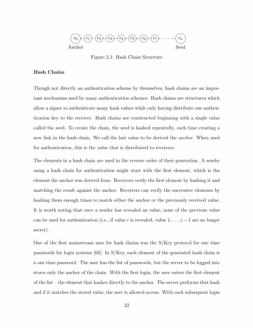
v0

Anchor

v1 v2 v3 v4 v5 v6 v7 . . . vn

Seed

Figure 2.1: Hash Chain Structure

Hash Chains

Though not directly an authentication scheme by themselves, hash chains are an impor-

tant mechanism used by many authentication schemes. Hash chains are structures which

allow a signer to authenticate many hash values while only having distribute one authen-

tication key to the receiver. Hash chains are constructed beginning with a single value

called the seed. To create the chain, the seed is hashed repeatedly, each time creating a

new link in the hash chain. We call the last value to be derived the anchor. When used

for authentication, this is the value that is distributed to receivers.

The elements in a hash chain are used in the reverse order of their generation. A sender

using a hash chain for authentication might start with the first element, which is the

element the anchor was derived from. Receivers verify the first element by hashing it and

matching the result against the anchor. Receivers can verify the successive elements by

hashing them enough times to match either the anchor or the previously received value.

It is worth noting that once a sender has revealed an value, none of the previous value

can be used for authentication (i.e., if value i is revealed, value 1, . . . , i− 1 are no longer

secret).

One of the first mainstream uses for hash chains was the S/Key protocol for one time

passwords for login systems [68]. In S/Key, each element of the generated hash chain is

a one time password. The user has the list of passwords, but the server to be logged into

stores only the anchor of the chain. With the first login, the user enters the first element

of the list – the element that hashes directly to the anchor. The server performs that hash

and if it matches the stored value, the user is allowed access. With each subsequent login

22

the user enters the next element of the chain, and the server ensure values are hashed to

the previous value. This system provides a limited number of one-time passwords which

are useful when a user may be logging in from an unsafe environment where a long term

password might be unsafe.

Hash Trees

Hash trees were originally constructed by Merkle as the basis for his tree signatures [?],

but have since appeared in many other places. Hash trees are inverted in the sense that

they are calculated from their leaves. A tree can be created from a list of values which

are treated as leaves. Generally the number of leaves will be a power of two. The tree is

then computed recursively by concatenating the values from pairs of nodes and hashing

this value to get the value of their parent node. The last layer will contain only one node

which is the root.

One-Time and K-Time signatures

One- and k-time signatures are important enough to have their own section in Section 2.3.

Until then, a few basics will be helpful. A one-time signature scheme is an asymmetric

signature scheme that can be used to sign at most one message for every generated

key pair. A k-time signature can be used to sign a (usually small) constant number of

messages per key pair. One-time signatures can be based on hash functions, which make

them extremely quick. One-time signatures are also thought to be very secure since they

can never be reused.

23

2.2.2 Chained Signatures

There are many chained signing techniques, all with the same basic premise. The idea is

to sign only one message from a stream of messages with an asymmetric signature such as

RSA and have all the remaining messages carry a small additional amount of information

that would authenticate the one or more other messages in the stream. Authentication is

considered amortized because for any arbitrary number of messages sent, only one needs

to be signed with a computationally expensive signing method function.

The simplest examples of this type of scheme were presented by Gennaro [63]. Two

stream signing modes are given: online mode and offline mode. Online mode is necessary

when messages arrive at the sender sequentially and need to be sent as soon as possible.

Offline mode takes advantage of messages arriving at the sender as a group, so the sender

can access the entire batch of messages before any are sent. The basic idea of the two

modes is the same, but the algorithms vary slightly.

In both versions, each message also carries with it the hash from another message. Mes-

sages are authenticated at the receiving end when both the message and its corresponding

hash have arrived. The difference between Gennaro’s online and online modes is whether

a message carries the hash of the message before it, or the message after it. One end or

the other of the chain will need to be verified with an asymmetric signature, depending

on the direction taken by the chain.

In the online version, each message carries the hash of the message that was previously

sent. When sending message mi, the hash that was saved from mi−1 is appended to mi.

The hash of the two concatenated values is saved and the message is sent. After all the

messages are sent, one message hash will remain that needs to be sent to allow receivers

to verify the final message. This hash is signed with an asymmetric signature scheme

before sending.

24

When the receiver receives mi, it can use the hash contained in mi to verify mi−1.

However, mi cannot be verified until mi+1 is received, meaning a one-message delay is

necessary on the receiving side before the message contents can be verified against their

hash. However, source authentication is not achieved until the very last packet containing

the asymmetric signature. The advantage of this strategy, however, is that no buffering

is required by the sender: messages can be sent as soon as they are available to the

sender.

In the offline version, each message carries the hash of the message to be sent after it.

The reason it is called offline is that the entire stream of data must be known to the

sender before the first message can be sent. Because the first message contains a hash of

the second message, the second message must be known before the first message can be

constructed. However, the hash of the second message covers the content of the second

message and the hash of the third message, meaning the second message cannot be

constructed until the third message is known. This principle applies to the entire chain

of messages, meaning every message is essentially dependent on the final message. Since

there is no message to carry the hash of the first message, the first message is signed with

an asymmetric signature. The advantage is that on the receiver’s side, no buffering delay

is necessary. The asymmetric signature verifies the sender’s identity, and each message

carries the information necessary to verify the next message to arrive.

The biggest downside of the stream signing protocols is that a single lost message will cre-

ate a break in the stream, preventing all the messages on one side of the break from being

verified. Many different strategies have been proposed to circumvent this by including

redundant hashes.

Efficient Multi-chained Stream Signature (EMSS) is a protocol built on the stream signing

techniques which poses a solution to the problem of loss intolerance [130]. EMSS builds

25

on the online version of stream signing. Loss intolerance is combated by introducing

redundant hashes. In short, each message carries with it the hashes of not just one,

but multiple other messages. Viewed another way, the hash of each message is sent

with multiple other messages instead of just one. After the last message is sent, a final

signature packet is sent containing the hash of the last message and a digital signature

verifying the sender’s identity. Since individual verification only covers message content.

Sender identity is not verified until the final message in the stream. To reduce this wait

in a long stream, the sender may intermittently include signature packets.

The amount of loss tolerance can be adjusted by changing different parameters. In EMSSs

most basic mode, each message is hashed as it is sent and a copy of this hash is appended

to the next n messages. Losing a single message is no longer critical. Of the n messages

containing the hash to a given message, only one needs to arrive to deliver the necessary

authentication information. Of course larger values of n lead to increased tolerance.

Many authors have suggested that another way to increase tolerance is to widen the

distribution of messages containing a given hash. These approaches are summarized in

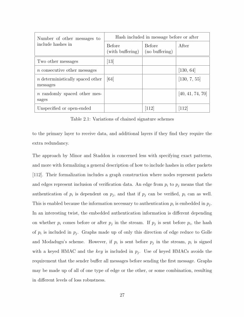
Table 2.1. Each author gives their own suggested strategy for distributing hashes to gain

robustness against specific patterns of packet loss that they expect.

Many of the schemes make small adjustments besides how they distribute hashes. Aslan

reduces buffering by limiting the packets that can be send with one public key to a small

number [13]. Multiple schemes add additional robustness by including the hashes from

every intermediate packet in the signature packet [7, 70, 55].

Challal and Hinard’s construction [40, 41, 74] gives receivers a way to adjust the amount

of redundancy required to support their network connection. This scheme follows a very

standard chained approach, but adds layers of redundant hashes: each layer contains

extra packets containing only message hashes and no actual data. Receivers subscribe

26

Number of other messages toinclude hashes in

Hash included in message before or after

Before(with buffering)

Before(no buffering)

After

Two other messages [13]

n consecutive other messages [130, 64]

n deterministically spaced othermessages

[64] [130, 7, 55]

n randomly spaced other mes-sages

[40, 41, 74, 70]

Unspecified or open-ended [112] [112]

Table 2.1: Variations of chained signature schemes

to the primary layer to receive data, and additional layers if they find they require the

extra redundancy.

The approach by Minor and Staddon is concerned less with specifying exact patterns,

and more with formalizing a general description of how to include hashes in other packets

[112]. Their formalization includes a graph construction where nodes represent packets

and edges represent inclusion of verification data. An edge from pi to pj means that the

authentication of pi is dependent on pj, and that if pj can be verified, pi can as well.

This is enabled because the information necessary to authentication pi is embedded in pj.

In an interesting twist, the embedded authentication information is different depending

on whether pi comes before or after pj in the stream. If pj is sent before pi, the hash

of pi is included in pj. Graphs made up of only this direction of edge reduce to Golle

and Modadugu’s scheme. However, if pi is sent before pj in the stream, pi is signed

with a keyed HMAC and the key is included in pj. Use of keyed HMACs avoids the

requirement that the sender buffer all messages before sending the first message. Graphs

may be made up of all of one type of edge or the other, or some combination, resulting

in different levels of loss robustness.

27

The signing and verification of these approaches are very lightweight, but delays must

be incurred on one end or the other if not both. In schemes where each packet includes

information from packets to be sent later, those later packets must be known ahead of

time. For schemes where packets are verified based on information in packets received

later, verification must be delayed until those later packets are available. In the presence

of packet loss, this delay is not necessarily bounded.

2.2.3 Amortized Block Signatures

A class of signature schemes signs messages in blocks, computing one a single signature

for an entire block of messages. The signature is included in all the messages of a block

in some cases, or distributed over the messages in others.

As a response to chained schemes, Wong and Lam proposed Star and Tree Chaining

[168]. In these schemes, messages are signed in blocks, but once sent, each message can be

verified individually. In the Star scheme, each individual signature in a block contains the

hashes of all other messages of the block, along with a block signature that is computed

once for all messages of a block. To create the block signature, the hashes of all the

messages are concatenated together which is then hashed and signed with an asymmetric

scheme (e.g., RSA). To verify a message, the message hash is calculated and used along

with the other hashes included in the signature to verify the block signature.

The Tree Chaining scheme follows the same idea except that instead of concatenating

all the message hashes to create the block hash, the individual messages are recursively

hashed together in pairs forming a hash tree. The root of the tree is the block hash

which is signed asymmetrically. The tree structure allows smaller signatures because

each message no longer needs to include the hashes of all other messages in the signature

– just the hashes that are necessary to compute the root of the tree.

28

Based on the observation that the asymmetric signature in the Star and Tree schemes

only needs to be verified once, He et al. propose a simple extension to the Tree scheme

which separates the signature into its own packet which is sent before all messages of

the block [71]. Later, they extended this scheme again creating Hybrid Multicast Source

Authentication (HMSA) [71]. HMSA replaces the asymmetric block signatures with

Gennaro’s offline stream signature: only the first block hash is signed asymmetrically.

After that the block signatures of the next block are included with the messages of the

current block so that if the current block is verified, the next block will by verifiable

simply by comparing hashes. Yet another variant based on HMSA shortens signatures’

size by including only one other hash value in the tree, assuming the receiver will have

already received enough path components to reconstruct the root [98].

Kang and Ruland also take the same approach as HMSA with DiffSig [84], but weaken the

asymmetric signature scheme for cases where messages are only useful for a short period

of time – if the attacker needs to spend much time to forge a signature, it is likely tpo

late to be useful. Finally, Berbecaru et al. created ForwardDiffSig [20], a forward-secure

version of DiffSig, by augmenting it with a key update scheme, OptiSum [19]

A different style of authentication technique that splits the signature between multiple

messages is the Signature Amortization using Information Dispersal Algorithm (SAIDA),

which is used to sign a block of messages with a single signing operation [123]. SAIDA

uses the Information Dispersal Algorithm (IDA) described in [136]. IDA was originally

invented to introduce redundancy in distributed file storage. The idea behind IDA is

that a file could be strategically split into n parts, each with size m > 1n. Since the sum

of the parts sizes is greater than the original file (and no space is wasted), it becomes

intuitive that some overlap must exist between the parts. This redundancy is introduced

through a set of vectorizing operations. The advantage to introducing redundancy in

this way is that the original file can be reconstructed with only a subset of parts. The

29

minimum number of parts necessary is dictated by the amount of redundancy, but as

long the minimum is met, the parts used to reconstruct the file can be any subset of the

originals. This allows for a certain number to be lost without harm to the file.

SAIDA uses IDAs technique, but instead of storing and reconstructing files, signatures

are transmitted and reconstructed. To lower overhead, the transmitted signatures are

based on message hashes. To send a group of messages, the sender begins by hashing

each message and concatenating the hashes together. This value will be treated like a file

within IDA and split into parts, one for each message in the block. Additionally the con-

catenated hashes are hashed and signed with an asymmetric scheme, and this signature

is also split into parts using IDA. One hash-part and one signature-part is concatenated

to each message as the signature. Receivers need to only receive the specified minimum

number of messages in order to reconstruct and verify the asymmetric signature.

The same technique has been suggested with multiple types of dispersal algorithms pro-

posed in place of IDA. Tornado codes [34] fulfill the same general purpose and can be

computed more quickly but result in larger signatures [124]. This technique is suggested

for applications where saving time is more important than saving bandwidth. Erasure

codes offer more robustness against pollution attacks [85, 6]. Erasure codes have been

suggested in conjunction with block chaining [121, 122], meaning the block hashes are

included in messages of either the previous or next block and either the first or last one

is signed, just like the chained signatures described in Section 2.2.1.

2.2.4 Delayed Key Release

A very prominent protocol based on hash chains is Timed Efficient Stream Loss-tolerant

Authentication or TESLA [130, 131]. The idea behind TESLA is similar in spirit to the

chained protocols, but with a few very important differences. One of the key differences

30

is a dependence on time. It also uses hash chains, described in Section 2.2.1. Time is

divided into intervals, each interval associated with an element in a hash chain. During

each interval, messages sent are signed with symmetric signature using the corresponding

key from the hash chain. Some number of intervals later, the key is publicized, allowing

receivers to verify the packets.

The hash chain anchor serves as the public key. The process starts at the beginning of

the chain and works towards the seed. During the first interval, signers sign with the first

element of the hash chain. Receivers receive these packets, but must buffer the messages

since they have no way of verifying them yet. Some number of intervals later, the sender

begins including previously used keys in the packets. The interval difference between

when a key is used for signing and when it is sent is known to the receivers, and long

enough to ensure that at the time the message was signed, only the sender knew the

signing key. The receivers verify each newly received key against the hash chain. Once

verified, the key can be applied to all messages from the time interval in which it was

used for signing.

TESLA relies on loosely synchronize clocks to ensure messages cannot be forged. Through

the loose synchronization, receivers are able to discern if, at the time a message was sent,

the key used to sign it was known only to the sender. If a receiver cannot determine

that a message was sent before the key used to sign it was publicized, it disregards the

message.

TESLAs big advantages are efficiency and loss tolerance. Even if enough messages are

lost in the network that an entire key is never delivered, that key can be derived from the

next key that is delivered to the receiver. The downside is the need to buffer messages

at the receiver side. Normally this buffer will grow and shrink predictably, but on lossy

networks the number of packets waiting for keys may become less predictable.

31

Several extensions have been proposed to TESLA. One of the simpler extensions, TESLA

with immediate verification [129] makes TESLA appear very similar to offline stream

signing. In this variant, TESLA packets carry MACs of packets to be sent later. Packets

are buffered on the sender side for one key disclosure interval allowing MACs of buffered

packets to be attached to the packets being sent. The buffering on the sender side removes

most of the need for buffering on the receiver side. Once receivers begin receiving keys,

they can authenticate the already received packets based on the delivered keys which

in turn allows them to authenticate the packets delivering the keys based on the hashes

in buffered packets. From then on, as long as the delivered keys are authentic relative

to the hash chain, the messages delivering the keys can be authenticated immediately

using the hashes in previously received packets. The removal of the receiver buffering

delay removes the possibility of an attack by flooding the receivers buffer with invalid

packets.

Other extensions define other patterns of key usage. One is a method for having multiple

TESLA instances use the same chain with a different key-release delay to facilitate re-

ceivers with different time synchronization capabilities [129]. Another, Staggered TESLA

[94] introduces the idea of multigrade authentication for authenticating a message at mul-

tiple levels. Partial authentication of a message can be done in a shorter time than full

authentication. In an open multicast system, subscribers are likely to use data for differ-

ent applications. Some might have stricter trust requirements than others. Some would

possibly rather have a partially authenticated packet at a shorter delay, while others

would prefer to wait for a fully authenticated message.

Staggered TESLA [94] differs from TESLA by signing each packet with multiple keys.

The primary key, used to sign the message first, is chosen exactly as it would be in

normal TESLA. The second key is the primary key used in the previous interval. The

third was the primary key in the interval before that. The last key used to sign the

32

message will be the oldest. That is to say, the last key was used as a primary key before

the others were used at all. Naturally, this key will be the first to be published, and the

first to be available on the receiving side. Receivers can authenticate messages only as

quickly as keys are published and messages must wait in between authentication levels.

While waiting, messages are organized into queues. One queue will contain completely

unauthenticated messages. Messages in the next queue will have been authenticated with

one key - the oldest. The next level will have been authenticated with the oldest two keys.

This pattern continues, and messages move from queue to queue until authenticated by

all keys used to sign them. Of course, an application can retrieve messages out of any

of the queues at any time if it is willing to accept a the corresponding level of partial

authentication.

TESLA has been combined with Tree Chaining to create a hybrid scheme: signing is

basically done with the Tree Chaining algorithm, but instead of using an asymmetric

signature to verify block hashes, the block hashes are signed with TESLA signatures.

The key to the TESLA signatures are carried in messages from later blocks [96]. When

combined with TESLA with immediate verification, signatures are as efficient as the basic

tree scheme but without the need to ever compute an asymmetric signature.

2.2.5 Precomputed Expensive Signatures

The idea of pre-computing expensive asymmetric signatures and linking them to messages

at run-time was introduced by Even et al. [56]. In this scheme, a large number of one-

time signature key pairs are created, and the public keys are in turn signed with an

asymmetric scheme. As messages become available for signing, each is signed with one

of the one-time signature private keys. The one time signature, corresponding public

key, and asymmetric signature of the public key are all included as the signature to

33

the message. A similar scheme follows the same mechanics but replaces the one-time

signatures with k-time signatures [143]. This allows more messages to be signed per

public key computation. The goal is to be able to run slow asymmetric signatures on

public keys concurrently with sending k-time signed messages and have the next k-time

public key ready by the time the current one is used up.

Rapid Authentication (RA) is a scheme developed specifically for command and control

systems based on RSA [169]. RA leverages the fact that the message space of messages

sent from command and control servers is limited, thus the RSA signatures of parts of

messages can be computed in an offline phase. During the online phase, the precomputed

signatures can be combined with the actual message using an inexpensive Condensed-

RSA operation. Verification is based on RSA verification which can also be done quickly.

RA is ideal in that it is quick to compute and requires no buffering delays on either side,

but the drawback is the dependency on precomputed signatures.

2.2.6 Identity based signatures

Identity based cryptosystems [149] are a concept first proposed by Shamir, though at

the time of its proposal it was only known how to do identity based signing (IBS) – a

method for identity based encryption (IBE) was not actually known. It is a variant of a

public key cryptosystem where each user’s public key is a string based on their identity

and they are assigned a private key by a trusted authority analogous to a CA in today’s

PKI systems. Once keys are assigned, usage is the same as any of today’s standard PKI

schemes.

IBS and IBE requires a cryptographic primitive that allows private keys to be derived

from public keys, but only by a trusted authority with its own secret key. Schemes like

RSA derive public keys from private keys, and if private keys could be derived from

34

public keys, any user could derive any other user’s private key. Thus it is imperative that

the third party trusted to generate keys incorporate its own secret key in the process

and that private keys are impossible to derive without knowing this secret. The signing

scheme in Shamir’s proposal is based on modular exponentiation, similar to RSA. A key

difference is that private keys are calculated from identities based on the factorization

the modulus which is known only to the key generator.

Many IBS systems have been proposed with various mathematical underpinnings [38, 73,

170, 125, 17]. However, the oracle model [18], the model that these systems were proven

secure against, was later found to be flawed where concrete hash functions are involved

[36]. A scheme based on the hardness of the Diffie-Hellman problem was eventually

created that was shown secure in the standard model [126].

2.2.7 One and K-Time Signatures

One-time and k-time signature schemes have appeared in many variants over the years,

but there is little evidence that they’ve been deployed on actual networks. The most

sophisticated schemes that appear in literature probably require further assessment before

they can be considered safe for deployment. In general one- and k-time schemes all build

off of a common idea: they employ a conceptual structure of secret and public key

values, which can be used to sign between one and several messages, depending on the

structure and algorithm used to compute and verify signatures. Values in the structure

of secrets are computed from other secrets using hash functions. The one-way property

of the structure is leveraged to create signatures that are as safe in a multicast setting

as they are in a point-to-point setting. Basing signatures on hash functions has the

advantage that they are very quick to compute. Even signatures that involve many hash

computations can be faster than the computation of a single signature using one of the

35

standardized algorithms. One and k-time signatures also have two additional properties

that make them suitable for a broader class of applications: messages can be verified

independently of each other and immediately upon arrival at the receiver, meaning no

additional delays are incurred at either the signing or verifying end.

K-Time signatures are not without downsides. The number of messages that can be sent

with a single structure of keys is always limited, and once exhausted, new keys must

be distributed so that the stream of signatures can continue using a new structure with

different secrets. Several different strategies have been used to extend the number of

messages that can be signed with a single structure. Of course no strategy is free, and

each strategy has it’s own disadvantage. One obvious strategy is to increase the size of

the structure. In several schemes this increases the latency of signing and/or verifying

messages and in some cases, it increases the size of the signature as well. Another common

strategy is to decrease the average security of a message, introducing a small risk of forged

signatures in order to increase the number of messages that can be sent using a single

key structure. Although decreasing security may seem like an odd approach, the number

of signatures that can be gained is often considered a reasonable justification.

The relative advantages and disadvantages of k-time signatures make them a good can-

didate for further investigation. The idea of decreasing overall security would make

many k-time signatures unsuitable for applications that rely on the utmost security, but

for many high-throughput applications, the amount of data being sent is massive enough

that a small amount of corrupted data is overshadowed by the remaining good data. And

even though keys must be redistributed frequently, re-keying is considered good practice

anyway. The absolute need for new keys simply enforces this practice. When consider-

ing the features that are shared with the standards – message independence, immediate

signing and verification, and security in a multicast context – in combination with the

performance gained by using hash functions, the idea of k-time signatures becomes wor-

36

thy of further exploration. The next section explains one- and k-time signatures in much

greater detail.

2.3 One- and K-Time Signatures

This section starts by explaining some primitives and operations encountered in multiple

k-time signature schemes: hash chains and hash splitting. Then it moves on to a survey

of one- and k-time signature schemes. These descriptions also serve to demonstrate the

evolution of one-time signatures from source authentication to content authentication

and finally authentication of both source and content for multiple messages.

Before diving into descriptions of signature schemes, we describe and name a technique

seen in many of the schemes below. This technique that we call hash splitting is the

process of transforming a large bit string (most often a hash output) into a list of indices.

To create the list, the hash value is split into an appropriate number of short bit strings.

Each of these bit strings is then reinterpreted as an integer. We name this function

split(·). The number and size of the indices output by the split function is dependent on

the needs of the protocol.

2.3.1 Source Authentication Using One-Way Functions

Diffie and Hellman, and Lamport

The first one-time signatures were motivated by the need to legally sign electronic doc-

uments. Solutions using hash functions were suggested independently by Lamport [91]

and working as a team, Diffie and Hellman [46].

The first one-time signatures demonstrate the principle of authentication using hash func-

37

tions. Suppose a sender and a receiver anticipate the need for the sender to authenticate

to the receiver over an insecure channel. Before the anticipated authenticated communi-

cation takes place, the sender chooses a secret value x and shares the value y = h(x) with

the receiver by some separate secure means. When the time comes to authenticate to the

receiver, the sender reveals the secret x. The receiver, assuming x has been kept secret,

knows that the sender is the only one who would know a value x′ such that h(x′) = y.

The receiver computes h(x′) and is ensured of the sender’s identity if h(x′) = y. More

formally,

Key Generation The sender chooses a secret value x and computes y = h(x). y is the

public key distributed to the receiver.

Signing The sender authenticates by including x in the message.

Verification The receiver receives a value x′ and checks that y = f(x′). If and only

if these values match, the receiver believes x′ was the same x that was sent from the

sender.

This procedure can be performed only once for each chosen value of x since malicious

parties may learn x once it has been revealed to the receiver. A receiver seeing x used

as an authentication value after it has already been used can’t be sure if x is being sent

by the expected sender or some other party.

The above example only provides authentication for the sending entity but would not

work as a digital signature since no authentication is provided for the contents of the

message. That is, the receiver has no proof that a malicious third party hasn’t intercepted

the signed message and changed the contents of the message (without altering the one-

time authentication secret).

38

2.3.2 Source and Content Authentication

The next iteration of one-time signatures solved the lack of content authentication by

using the contents of the message to determine which of multiple possible values should

be appended to the message as a signature. If the signature wasn’t correct for the receiver

and the message contents, the message is not considered safe.

The signature schemes covered in this section all follow the pattern of distributing a

hash or list of hashes as a public key and signing the message with secrets that can

be used to derive some (or all) of the public key. Both sender and receiver know the

formula used to choose the secret or combination of secrets contained in the signature.

This pattern of signing and verification is common enough that we will assume that the

verification procedure can be understood once signing is explained: when a receiver is

given a signature containing secrets, it determines which secrets are expected based on

the message and uses them to re-derive the appropriate portion of the public key. If the

re-derived values match the expected part of the public key, the message is considered

valid.

Lamport’s Solution

The first content authentication using hash based signatures was achieved by Lamport.

His technique involved signing each bit (1 or 0) of a message. A pair of public keys is

pre-distributed for each bit that would be transmitted. To sign the actual message, a

secret would be included for each bit: which secret is chosen from each pair depends on

whether the bit is a 1 or 0. In this way, the receivers can verify not only the identity of

the sender, but also that each of the received bits match the bits sent. Specifically, if the

message to be sent is l bits:

Key Generation The sender selects a list of 2× l secrets, 〈x00, x10, x01, x11, . . . , x0l, x1l〉

39

and distributes 〈y00, y10, y01, y11, . . . , y0l, y1l〉 where yab = h(xab).

Signing Let m = b0b1b2 · · · bl. For each bi in m, append xbii to the signature.

Verification The receiver, given m = b0b1b2 · · · bl and a list of values 〈x1, x2, · · · , xl〉,

assumes that each xi is the sender’s xbii and verifies that ybii = h(xi) for all i.

The bit-by-bit signature ensures that the receiver can detect a change in any of the bits:

receivers assume the attached secrets correspond to the bits they receives. If any of the

bits were flipped between sending and receiving, the corresponding secret will not match

the expected public key value for that bit.

2.3.3 Lowering Authentication Overhead

Lamport’s content authentication scheme served as proof of concept, but wasn’t practical

given the massive size of signatures. However, the basic premise caught on and soon

optimized schemes were published.

Bos & Chaum

One optimization was suggested by Bos and Chaum [32] based on a simple observation:

if the sender has 2× l secrets to choose from and will include l of them in the signature,

then the number of messages that can be potentially signed should be C(2l, l). Lam-

port’s scheme is limited to signing 2l messages because not all possible subsets are valid

signatures.

This scheme was also published independently by Bicakci et al [25] who used it as part

of a more sophisticated scheme.

40

Reyzin & Reyzin

Reyzin and Reyzin generalize Bos and Chaum’s idea one step further [139]. The idea is

practically identical to that of Bos and Chaum, except without the requirement that the

signatures contain l secrets. Their requirement is that signatures contain a fixed number

of secrets k such that, C(n, k) > m where n is the total number of generated keys and m

is the size of the message space. This flexibility allows for some amount of adjustment

between the signature size and the size of the message space.

Winternitz

Another scheme was invented by Winternitz but presented by Merkle as part of his

scheme for signing multiple messages with one-time signatures [110, 109]. Winternitz’

suggestion used a list of hash chains as a structure of secrets. The entire list is known or

computable by the sender. The chain anchors make up the public key (as described in

Section 2.2.1). Before a message is signed, a checksum is computed and appended to the

message. To sign the message, the split function is applied to the concatenation of the

message and checksum, creating a list of indices corresponding to the list of hash chains.

Then for each 〈index, chain〉 pair, the secret from that index in that chain is included in

the signature.

The main advantage to Winternitz’s scheme is its flexibility in that signing time can be

traded for signature size to suit the implementor’s needs. If a fast scheme is required,

many short chains can be used. However, if signature size is more of a concern than

speed, using a few long chains would be more advantageous.

41

Bleichenbacher

Through a series of papers, Bleichenbacher presents a theoretical way to describe signa-

tures and also provides some concrete authentication schemes [26, 27, 28]. The schemes

presented were designed to be efficient in terms of the number of different possible values

for the signature given the overall number of secrets. Emphasis is placed on formalizing

graphs in such a way as to prove that the number of signature possibilities is optimal.

Methods of mapping messages to signatures are regarded as implementation details and

not included in these works.

Bleichenbacher’s framework involves creating signatures based on a graph where nodes

are secrets. Secrets are derived from one or more other secrets using a hash function. An

edge from node x to node y represents that x is necessary (but not necessarily sufficient)

to compute y. Note that y can only be computed if the values for all nodes with edges

to y are known. The public key is the set of nodes with out-degree 0.

A signature in one of Bleichanbacher’s schemes is defined as a Minimal Verifiable Subset:

a subset S is verifiable if the public key can be derived from the subset and minimal if

no other verifiable subset T exists where T ⊂ S. A set of signatures associated with a

graph G is a set of minimal verifiable subsets such that no signature can be computed

from any other. In other words, no single signature reveals enough information to derive

any other signature.

Given the complex formalization, Bleichanbacher’s complete schemes are surprisingly

simple. One graph is simply based on a hash tree. The root node is the public key. More

complicated trees are also described. The graph for his Rake Scheme can be visualized

as a list of hash chains, except extended by hashing the anchors together to form a hash

tree. Signatures in the rake scheme include one node from each chain.

A more complicated scheme involves blocks of short hash chains, where each block con-

42

tains a small number of chains. For all but the first block, hash chain seeds are computed

from some combination of elements in the previous block. A signature contains one node

from each chain in each block. The anchors from the block are also included in the sig-

nature. The anchors don’t contribute to the strength of the signature, but are there to

satisfy the requirement that the entire public key be derivable from each signature.

2.3.4 K-Time signatures

Despite the optimizations to the signature size, one-time signatures were still considered

impractical due to the large public key that needed to be securely transmitted prior to

each message. This led to the idea of k-time signatures, which could sign a fixed number

of messages for each public key. Interestingly, many k-time schemes incorporate a small

amount of risk: they have the same security as one-time schemes if used as a one-time

scheme, but they are designed so that the same key can be used a fixed number of times

with the threat probability remaining acceptably low. In general schemes that don’t

introduce intentional risk require larger keys or signatures.

BiBa

One of the first schemes to accept additional risk is BiBa, designed by Perrig [128]. Like

many other schemes, BiBa distributes a large list of hash values as the public key. The

signing process is unusual in comparison to many other k-time schemes. Essentially, the

contents of the message are used to choose a hash function which is applied to all the

secrets. In the basic version, if any two secrets produce matching outputs under the

specialized hash function, these inputs form the signature. In more advanced versions,

a more complicated pattern of hash outputs might be necessary (for example, three

matching, producing consecutive values, etc.). In the event that a signature pattern is

43

not found, the message is incremented and the process is retried until a signature pattern

is found. The signature includes the private secrets that form the correct pattern and

the increment.

The security of BiBa stems from the sender having a large list of secrets in which to

find a pattern but an adversary, even after listening to multiple messages, will have very

few. Thus, after a single message is signed, it is almost certainly safe to send another

created using the same set of secrets. This extends over a set number of messages,

however eventually enough secrets will be exposed that the risk of sending another will

be deemed too high, and the entire list of keys must be replaced with a new set.

Tree Based Signatures

Merkle’s tree formulation may have been one of the first attempts to use one-time signa-

ture schemes to sign more than one message [107, 108]. Merkle’s trees allow k instances

of any one-time signature scheme to be verified by the same public key. Merkle used Win-

ternitz one-time signatures, but any signature can be used as long as the entire public

key can be derived from a signature.

The k messages that can be sent correspond to k leaves in a hash tree. To start, k key

pairs of the chosen one-time signature are generated. Each public key is then hashed

forming the k leaves of the tree. Once the tree is generated, the root is distributed as

the public key.

Steps to creating a signature include calculating the one-time signature with the chosen

one-time scheme and then traversing the tree to determine the remainder of the Merkle

signature. The one-time signature evaluation is exactly as it would be independently of

the Merkle scheme. The tree traversal step determines which additional values must be

included in the signatures to create a path through the tree and allow the receiver to

44

compute the public key. The receiver will be able to derive one value at each layer of the

tree from the information given in the signature, but at each level, the node that is the

sibling to the derived information must be given. These siblings are the nodes that the

traversal determines must be included in the signature. Thus signatures can grow with

the number of layers in the tree.

Multiple extensions have been published including optimizations to the tree traversal

[81, 158, 21], combining these optimizations with increased numbers of signatures for

the same tree [117], and extending the scheme to trees of trees to allow more signatures

[33]. Use of incomplete trees has also been studied to avoid restrictions on the number

of leaves being powers of two [88].

HORS

Inspired by BiBa [129], Reyzin and Reyzin created Hash of Random Subsets (HORS)

with the idea that risk should grow only slowly with the number of messages sent [139].

The structure of the keys is simple: the sender owns a list of secrets and distributes

the corresponding list of hashes to the receiver(s). Signing starts with calling the split

function on the hash of the original message, creating a list of indices. Each index is used

to identify one secret from the list to include in the signature. Receivers verify these

included secrets to verify the signature.

Key Generation The sender generates 〈s0, s1, . . . , sn−1〉 which is the private key. The

list 〈v0, v1, . . . , vn−1〉 forms the public key where vj = h(sj) for 0 ≤ j < n.

Signing Given m and hm = hash(m), the sender generates split(hm) = 〈i0, i1, . . . , ik−1〉

such that 0 ≤ ij < n for 0 ≤ j < k. The signature is si0si1 . . . sik−1.

Verification Given m and s0s1 . . . sk−1, the receiver calculates hm and split(hm) =

〈i0, i1, . . . , ik−1〉 and checks that h(sj) = bij for all j.

45

An important factor is that the number of secrets used to sign a message is very small in

comparison to the number available. This should allow nearly any application that can

tolerate at least some risk to determine a reasonable number of messages that may be

sent before that risk threshold is exceeded.

2.3.5 Chained K-Time Signatures

The advent of k-time signatures made one-time style signatures more feasible, but ulti-

mately the ratio between numbers of bits signed and the number required for the public

key needed to be improved. Taking advantage of the pattern of using hash outputs as

keys, the next evolution uses hash chains to refresh the private key. Thus, more messages

can be signed between when public keys are distributed.

HORS++

HORS++ [134] is similar to Bleichanbacher’s work in motivation. Bleichenbacher created

a one-time scheme where no signature could be derived from another. Pieprzyk created

k-time signatures where no signature can be derived from any combination of other

signatures. Pieprzyk doesn’t bother with a complicated graph: as with HORS, signatures

are subsets of a set of secrets, and the set of hashes corresponding to the set of secrets

forms the public key.

Signatures are objects in a cover-free family which allows the scheme to be secure for some

exact fixed number k of signatures. The required property is that every signature contains

at least one secret that is not contained in all other signatures. Three constructions are

presented for mapping signatures to messages, one based on polynomials, one based on

error correcting codes and one based on algebraic curves.

46

An extension of HORS++ replaces the set of secrets with a set of hash chains. The chain

anchors are the public key. The first k messages are signed using the first element from

each hash chain as the set of secrets. Verification is the same with the addition of saving

the secrets as the new public key. The next k signatures are created with the value from

each hash chain. The process repeats until the hash chains are exhausted.

HORSE

HORSE extends the number of messages sent with HORS signatures by extending the key

structure using hash chains [119]. Instead of a list of secrets, HORSE senders maintain

a list of hash chains. The original list of secrets serves as the seeds of the hash chains.

The chain anchors make up the public key.

To sign a message, the sender begins computation as a normal HORS signature, trans-

forming the message into a list of indices. Each index in the list specifies a hash chain.

From each identified hash chain, the first element that has not yet been used in a signa-

ture will be included in the current signature, along with the value’s position in the hash

chain. This mechanism ensures each hash chain secret will be used only once.

Receivers verify each secret in the received HORSE signature by verifying the secret

against the chain. In case the receiver has not received all messages, the position numbers

associated with each secret tell the receivers how many times each secret will need to be

hashed to recreate a known value. If all secrets are verified, the signature is considered

valid.

HORSE has the disadvantage that an adversary can skew the likelihood of a successful

attack by preventing messages from being delivered to the receiver. While the receiver is

not receiving messages, the attacker can be collecting secrets from various hash chains.

Each secret collected enables the attacker to calculate the length of the chain from the

47

learned value to the public key. This greatly increases the chance that the adversary will

come to possess the specific secrets necessary for signing a message without the receiver

realizing those secrets have been publicly revealed.

TV-OTS

TV-OTS is a chained scheme that incorporates time as a controlling factor [165]. TV-

OTS uses a list of hash chains and uses time to determine which secrets are used for each

signature. Time is divided into windows called epochs, and within each epoch signatures

are created using the HORS signature scheme. In the first epoch HORS signatures are

created using the chain anchors as public hash values and the first elements in the chains

as the secrets. At each new epoch, the next set of hash chain values are used as the

current secrets and the previous set becomes part of the public key.

For additional robustness against precomputed attacks, TV-OTS incorporates a salt chain

into the creation of the list of hash chains. The salt chain is computed as a normal chain,

where each value is the hash of the next. The remaining chains are computed by a slightly

different method: before hashing each value, the corresponding value from the salt chain

in concatenated. The two values hashed together form the next chain element.

Key Generation The sender starts by choosing a random salt ss, and n random values

〈s0, s1, . . . sn−1〉. The salt ss is concatenated with each si to form the seeds for n hash

chains of length `. Each hash chain element sIj is computed by sIj = h(ssj+1||sij+1

). We

use the notation hj(si) to mean the jth salted hash from the ith chain. The public key is

the list of chain anchors 〈v0, v1, . . . , vn−1〉, where vi = h`−t(si).

Signing The current time τs is recorded and used to calculate the index of the current

epoch t. The signature is created over the message t||m||st, where m is the original

message and sst is the salt chain element corresponding to time t. The signature is a

48

standard HORS signature, using h`−t(si) for each secret corresponding to HORS index

i.

Verification The current time τr is recorded when the message is received and compared

to τs included in the received signature. If the transit time is above a specified threshold,

the message is discarded. If the timestamp check passes, the HORS part of the signature

is verified. The keys in the packet are treated as h`−t(si) and hashed until the receiver

recreates either vi or a value from the chain received more recently. Receivers may save

received secrets in place of the vi values in order to reduce the number of hashes needed

to verify future signatures.

HSLV, LSHV & TSV

Lastly, we cover three schemes presented by Li and Cao [95]. The schemes are presented

as k-time signatures with the suggestion that they may be chained in the same style as

HORSE. The three different schemes are presented, motivated by addressing a specific

weakness in HORS: the weakness they are concerned with is that an attacker, having

learned a certain number of secrets, can use any permutation of these secrets to create

a forged signature. None of the three presented schemes have this weakness. Two of

the schemes use different approaches to solving this problem and the third is a hybrid

combination of the first two.

The first of the three schemes is Heavy Signing Light Verification (HSLV) which is a

simple variant of HORS. The variation occurs before choosing secrets. Once the message

is hashed and split into indices, the list is checked to see if the indices are sorted. If

not, an increment is added to the message and the process repeated until a sorted list

of indices is produced. The remainder of the signing process is the same as HORS, with

the increment value included in the signature. The “Heavy Signing” in the name comes

49

from the fact that the signing process may need to iterate many times before finding an

allowable list of indices. The advantage is that even once the attacker learns secrets, they

have only a limited number of ways to use them to form a signature.

The second of the three schemes, Light Signing Heavy Verification (LSHV) demonstrates

another approach to the problem. The scheme is again similar to HORS, but also remi-

niscent of Winternitz’ scheme. The private key is made up of a large array of relatively

short hash chains, with the hash chain anchors serving as the public key. Signature cre-

ation starts as usual, by hashing and splitting the message into indices. If the resulting

list does not contain all unique values, the process is repeated with an increment added

to the message. Each index is used to identify a hash chain from which to use a secret.

The position of the secret in the hash chain is the same as the position of the index in the

list: the first hash chain value will be used from the first hash chain chosen, the second

value will be used from the second chain chosen, etc. The signature consists of all the

secrets and the increment. The advantage of this scheme is that the amount of re-hashing

is expected to be far smaller compared to HSLV while still limiting the number of ways

an adversary can combine secrets to form a signature.

The third scheme combines the ideas from the two previous schemes. Like LSHV, the

keys are created by a list of short hash chains. This time, when the message is hashed

and split, the indices are considered in groups. The group size is a parameter chosen by

the implementors. The requirement on the list of indices is that within each group indices

must be sorted, and rehashing is performed until this is achieved. The indices are still

used to choose chains, but the secret to use from each chain is determined by the position

of the group that each particular index is in. This scheme balances the advantages and

disadvantages of the other two schemes.

50

2.4 Hash Chains Management Structures

Hash chains are used prominently in k-time signatures and will be of importance in this

thesis. We discuss the practical issues surrounding them, and survey solutions to these

problems.

The hash chain structure, described in Section 2.2.1, works very well with the principles

behind one-time signatures, but hash chains can be difficult to manage in practice. The

term traversal refers to the sequential output of hash chain values starting with the

first value and working toward the seed. Traversals present a challenge because the

output order is opposite the order of generation. For long chains, storing all values may

be impractical, but otherwise, needed values must be recomputed. If only the seed is

available as a starting point, calculating values near the beginning of the chain requires

heavily repetitious hashing. Wiser strategies look for ways to balance the cost of storage

and computation so that neither becomes too costly.

2.4.1 Fractal Hash Sequencing and Traversal

In the search for a traversal strategy balancing storage and computation costs, Fractal

Hash Sequence Representation and Traversal (FHT) [80] has emerged as a practical and

elegant solution to achieving O(log2(n)) bounds for both storage and time. While FHT

can’t maintain these bounds unless values are retrieved consecutively, the bounds for

retrieving a sequence of values are still sufficiently low to make it a traversal candidate

for TV-OTS.

FHT stores only log2(n) chain values, chosen in such a way that retrieving new values

requires minimal computation. The arrangement of these stored values is dynamic and

continually changes to accommodate future requests more easily. When one of the stored

51

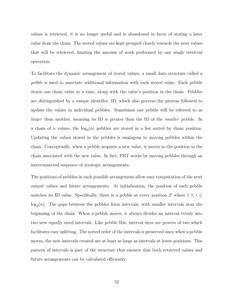
values is retrieved, it is no longer useful and is abandoned in favor of storing a later

value from the chain. The stored values are kept grouped closely towards the next values

that will be retrieved, limiting the amount of work performed by any single retrieval

operation.

To facilitate the dynamic arrangement of stored values, a small data structure called a

pebble is used to associate additional information with each stored value. Each pebble

stores one chain value at a time, along with the value’s position in the chain. Pebbles

are distinguished by a unique identifier, ID, which also governs the process followed to

update the values in individual pebbles. Sometimes one pebble will be referred to as

larger than another, meaning its ID is greater than the ID of the smaller pebble. In

a chain of n values, the log2(n) pebbles are stored in a list sorted by chain position.

Updating the values stored in the pebbles is analogous to moving pebbles within the

chain. Conceptually, when a pebble acquires a new value, it moves to the position in the

chain associated with the new value. In fact, FHT works by moving pebbles through an

interconnected sequence of strategic arrangements.

The positions of pebbles in each possible arrangement allow easy computation of the next

output values and future arrangements. At initialization, the position of each pebble

matches its ID value. Specifically, there is a pebble at every position 2i where 1 ≤ i ≤

log2(n). The gaps between the pebbles form intervals, with smaller intervals near the

beginning of the chain. When a pebble moves, it always divides an interval evenly into

two new equally sized intervals. Like pebble IDs, interval sizes are powers of two which

facilitates easy splitting. The sorted order of the intervals is preserved since when a pebble

moves, the new intervals created are at least as large as intervals at lower positions. This

pattern of intervals is part of the structure that ensures that both retrieved values and

future arrangements can be calculated efficiently.

52

Figure 2.2: When a pebble moves, it cannot move directly to its destination.It must calculate the desired value by first moving upward past its destination.Once it copies the value from a stored pebble, the desired value is calculated byadditional hash operations as the pebble moves downwards to its destination.

The method for calculating chain values limits the ways in which pebbles can move.

When a pebble moves to a new position, it can not acquire the new value directly. Recall

that pebble values must be computed from one another. The one-way properties restrict

each value to being computed from values at higher positions. Moving a pebble requires

finding and copying the value stored in some higher pebble and calculating the desired

value from there. In essence, pebbles move in two phases, as illustrated in Figure 2.2.

In the first phase, the pebble moves upwards to the same location as a higher pebble.

In the second phase, the pebble’s new value is hashed repeatedly, effectively moving the

pebble downward in the chain to its destination.

The pattern maintained by the arrangements of pebbles is governed by the pebble IDs

and provides the ability to retrieve keys within a logarithmic time bound. This pattern

is formed by the second stage of pebble movement. In this second stage, pebbles step

downward from their new position acquired in the first stage. The number of downward

steps a pebble takes equals the value of its ID. Eventually, this creates an interval between

each newly moved pebble and the pebble it copied from with the new interval size equal

to the moved pebble’s ID. The pebble at the upper edge of the interval, whose value

was copied, was chosen because the interval it bounded before the move was twice the

size of the ID of the moving pebble. (The existence of such an interval is guaranteed

53

[80].) Thus, on each move, a pebble splits an interval into two new equally sized intervals.

Furthermore, pebbles always move into the nearest interval large enough to evenly divide.

Naturally, the pebbles with smaller IDs move shorter distances. Since the size of newly

created intervals is at least as large as the intervals at lower positions, the intervals

remain sorted by size. The pebble with the ID value of 2 never moves beyond the lowest

four values in the unused chain, and ensures these lowest values are part of intervals

of size two. Consequently, any value retrieved from this section of the chain will never

require more than a single hash operation to compute. The remaining hash operations

are performed in stepping the other pebbles towards their destinations.

To provide the amortized upper bound on retrieval time, moving pebbles rarely perform

their downward movement phase all at once. Instead, moving pebbles distribute these

downward steps over several retrieval operations, taking only enough steps to ensure they

reach their destination by the time the value at that destination is needed by some other

moving pebble. Notice that pebbles with larger IDs move further and are therefore not

needed at their new positions as quickly as smaller pebbles. The number of retrievals

that occur before a pebble must reach its destination is directly related to how far the

pebble must travel. In fact, only the pebble with ID value 2 must reach its destination by

the time the next pebble is moved. This happens exactly two retrievals after this pebble

was moved. For all other pebbles, these intermediate retrievals are used to distribute

hashing costs over time, avoiding a situation where some retrievals are inexpensive and

others are costly. The total number of hash operations per retrieval is limited to two per

actively moving pebble, plus at most one to calculate the retrieved value. The maximum

hash operations per retrieval is thus 2× log2(n) + 1.

54

2.4.2 Related Traversals

The idea of efficient hash chain traversal introduced by Itkis and Reyzin [79] started

a wave of traversals with varying efficiencies and trade-offs. The traversal suggested

by Itkis and Reyzin was soon followed by Jakobsson’s FHT [80], described above, from

which all the others drew either direct or indirect inspiration. However, the dependency

on consecutive value retrieval is common in all of such traversals. Traversals presented

by Coppersmith and Jakobsson [42], and Yum et al. [172] build directly on FHT by

modifying the pebble movement pattern. Coppersmith and Jakobsson achieve near max-

imum theoretical efficiency for consecutive retrievals by allocating a hash budget on each

round, and using a sophisticated movement pattern that distributes this budget between

two sets of pebbles. A set of greedy pebbles consumes as much of the hash budget as

possible, and any extra is alloted to the remaining pebbles. In this way, the variance

in hash operations between iterations is eliminated, lowering the worst-case number to

12

log2(n) hashes per round, though at a storage cost of slightly greater than log2(n) peb-

bles. This technique is further improved upon by Yum et al. who use the same strategy

to balance the distribution of hash operations over the rounds, but with a less complex

movement pattern. The resulting algorithm is simpler than the Coppersmith and Jakob-

sson algorithm, and achieves the same lowered time bound without requiring additional

storage.

In response to the traversals where computational bounds scale with chain length, Sella

proposed a traversal where computation time could be fixed at the expense of storage

space [148]. Using a slightly different chain partitioning technique, the number of peb-

bles can be increased to accommodate lower computational bounds. Later, a scheme

devised by Kim improved the storage requirement while still providing the same fixed

time bounds [87].

55

One remaining strategy, capable of lowering retrieval complexity even further, stems from

the introduction of multidimensional chains. Hu et al. present two traversals based on

a modified structure of the underlying chain [77]. Sandwich chains intertwine multiple

chains to form a construction whose primary purpose is efficient verification of keys.

Their second construction, Comb Skip-Chains, lowers retrieval bounds by amortizing the

FHT over the secondary dimension of a two-dimensional chain structure. With a total

of log2(n) secondary chains, the amortization brings retrieval time down to a constant,

while storage is bounded by O(log2(n)).

2.5 Problem Statement

For the class of applications we address, no existing scheme can claim to be satisfactory

– at least not without further investigation. As seen from Section 1.0.3, multiple types of

applications will benefit from an authentication mechanism that is safe for multicast and

adds minimal latency. In Section 2.1, we discussed standard authentication protocols,

and why they do not meet our requirements. We turned to literature that surveyed

alternative authentication methods. Many of these had application-specific features that

did not align with our requirements. However k-time signatures, as a general class,

provide the combination of features we require.

K-Time signatures have some very promising properties in theory, but there is little

empirical evidence supporting these theories. The k-time signatures surveyed are based

on hash functions. Hash functions can be computed very quickly, meaning even signatures

relying many hash function evaluations can be very fast. The one-way property of hash

functions is used to give these schemes the asymmetry needed to make them safe for

multicast. In most k-time schemes, the structures of the secrets allowed signatures to

be verified independently of one another and with no delays on either side. However,

56

some of these features need to be supported by real-world testing. For example, both the

speed and security of k-time signatures are subjective properties that will change based

on real-world operating environments.

TV-OTS stands out as a candidate for investigation due to the combination of properties

it offers. Because it is one of the chained schemes, the number of messages that can be

signed between key distributions can be quite large. The number of signatures is also

independent of signature size, allowing one to be adjusted without affecting the other.

Progress through the chain is based on clock time, which allows TV-OTS to function

even in unreliable networks, which contrasts schemes where progress through the chain

is based on the messages sent and received. Another very important property is that

TV-OTS is relatively simple given the features it provides. HORS is one of the most

straightforward k-time signatures, and this technique is composed with a simple timed

chaining technique. K-Time schemes are already quite complex, so starting with simpler

protocols makes sense. In addition, an analysis of TV-OTS is a good starting point for

anyone wishing to work with the more complex k-time signatures, making TV-OTS an

ideal candidate for investigation.

2.5.1 Research Directions

There are many open questions still surrounding the use of TV-OTS. It is the purpose of

this dissertation to provide answers and insights. Specifically, we address the following

questions:

Is TV-OTS safe and secure?

TV-OTS is known to be susceptible to a class of attacks we call eavesdrop attacks. These

are probabilistic attacks, meaning the attacker has a small probability of forging a mes-

57

sage. This probability can be controlled by adjusting the various parameters of TV-

OTS. In order to understand the security of TV-OTS, we must first understand how to

accurately quantify the risks associated with these adjustments, as well as mitigation

techniques that can be added. This question is addressed in Section 3.1.

Is confidence-based analysis a useful metric?

This thesis introduces the concept of confidence-based evaluation of signatures. In this

system, signatures are evaluated individually and each assigned a confidence value that

represents the receiver’s certainty in the goodness of the message’s signature, based on

some set of available evidence. We evaluate confidence metrics for TV-OTS and conclude

that they are useful for identifying the attacks that inherently exist against TV-OTS due

to its probabilistic nature. Confidence-based assessment is covered in Section 3.2.

Is TV-OTS fast in practice?

The majority of the work of generating and verifying TV-OTS signatures is evaluating

hash functions, which are known to be fast to compute. However, evidence is still needed

to show how TV-OTS fares in terms of wall-clock time compared with other signature

schemes. The effect of changing the parameters that adjust security is also important

to measure empirically. Our performance measurements on TV-OTS are presented in

Chapter 5.

Can key distribution be handled in a practical way?

Standard authentication mechanisms require keys to be distributed before authenticated

communication can occur, but ultimately, key distribution only needs to happen once.

In order to run indefinitely, TV-OTS requires new keys to be distributed periodically. In

58

order for TV-OTS to be feasible for deployment in actual networks, we need proof that

a periodic key distribution system can be implemented without imposing a prohibitive

burden on the network. Our key distribution system is introduced in Chapter 3 and

results are presented in Chapter 5.

2.5.2 Relation to Power Grid Applications

We assess these questions in the context of status data disseminated for power grid

applications, discussed in Section 1.0.3. This affects our test environment: our tests are

all run with periodic, high-rate data, so our conclusions are most applicable to this type

of system. Many of our tests target messages rates of 30Hz or more, since 30Hz is a

common sampling rate for PMU data, but this rate is predicted to increase to 60 or

120Hz in the future[15]. In general, we expect many specific usage and implementation

details to vary from application to application. While our analysis is always focused on

our target application, we provide details that illuminate use cases for as many other

applications as possible.

59

Chapter 3

Science of TV-OTS

This chapter discusses our primary theoretical contributions: security analysis and key

distribution. The security analysis includes several approaches, and introduces the idea

of confidence based feedback from TV-OTS to the application layer.

3.1 Security of TV-OTS

This section covers security from several different aspects. First we answer a simple and

intuitive question: what is the chance that during an epoch of TV-OTS, an attacker

succeeds in forging a message? This leads to a more advanced question: given a message,

can receivers estimate how likely it is that the given message is forged? To answer this,

we introduce confidence-based metrics, wherein receivers evaluate confidence separately

for each signature. We evaluated confidence metrics based on their ability to classify

good and bad messages from a simulated attack against TV-OTS.

60

3.1.1 Attacker Model

The attacker we use for our model is relatively advanced in terms of resources and intelli-

gence and is based on the standard Dolev-Yao model [49]. We assume the attacker has the

ability to read network traffic, inject packets of its own, and cause packets sent by others

to be lost. The ability to selectively block network traffic requires control of a forwarding

device, but we don’t want to assume this is beyond an attacker’s capability.

In addition to the ability to modify network traffic, we assume our attacker has significant

computational resources. The most feasible attacks against TV-OTS involve searching

the message space for partial hash collisions. The process is similar to brute force re-

versing hashes, but the criteria for a successful partial collision make the odds of success

much higher. Attackers with more computational power will have a better chance of per-

forming a successful attack – computational power of the attacker is one of the variables

in the security analysis, allowing security metrics to be found for attackers with various

powers.

3.1.2 Introduction and Setup

The HORS protocol is the weakest link in TV-OTS. This section explains how adjusting

the various HORS parameters affects the security, which is important to understand in

order to run TV-OTS safely. We start with an analysis that gives the probability that the

attacker will succeed in forging a message. This method is helpful for choosing adequate

system parameters. In Section 3.2, we explain how, based off the chosen parameters, the

receivers can assign a confidence level to each received message.

The primary attacks against TV-OTS are eavesdrop attacks that apply to HORS. These

attacks use the attacker’s capabilities of reading messages and signatures to gather ex-

61

posed secrets. The attacker’s goal is to use these learned secrets to form signatures that

will appear valid to receivers. The attacker’s strategy is to gather secrets while guessing

messages, searching for one that can be signed maliciously with the exposed secrets.

Parameters

The parameters of TV-OTS are used to control the trade off between performance and

security are listed in Table 3.1. This table includes all the relevant parameters, leaving

out the length of hash chains which doesn’t affect the security analysis.

Type Name Description Sample Range

EnvironmentalProperties

` Length of hash output 160 (SHA1),256 (SHA256),512 (SHA512)

x Attacker power – The rate, inhashes/epoch, that we assume theattacker can perform a brute force attack.Security analysis is relative to this rate.

104 to 109

(Chapter 5)

SystemProperties(easilyadjusted)

r Messages sent per epoch 10 - 500

n Number of hash chains. Equivalently, thenumber of secrets available to the senderwhen signing a message

29 - 215

k Number of secrets per signature 10 - 15

Table 3.1: System Variables

The variables can be categorized by how much control the implementor has. The length

of the hash output is one of the less adjustable variables: it is likely that a hash function

will be chosen at the outset, fixing this parameter. In contrast, the number of hash

chains and the number of messages sent per epoch can be readily adjusted to fit the

system. Given choices for these parameters, the number of secrets in signatures becomes

apparent. Lastly, the power of the attacker can’t be controlled at all, but it is up the the

62

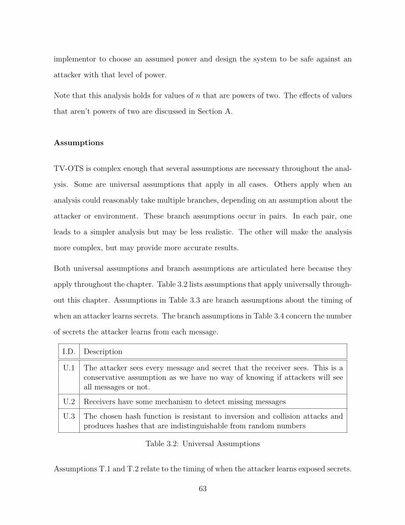
implementor to choose an assumed power and design the system to be safe against an

attacker with that level of power.

Note that this analysis holds for values of n that are powers of two. The effects of values

that aren’t powers of two are discussed in Section A.

Assumptions

TV-OTS is complex enough that several assumptions are necessary throughout the anal-

ysis. Some are universal assumptions that apply in all cases. Others apply when an

analysis could reasonably take multiple branches, depending on an assumption about the

attacker or environment. These branch assumptions occur in pairs. In each pair, one

leads to a simpler analysis but may be less realistic. The other will make the analysis

more complex, but may provide more accurate results.

Both universal assumptions and branch assumptions are articulated here because they

apply throughout the chapter. Table 3.2 lists assumptions that apply universally through-

out this chapter. Assumptions in Table 3.3 are branch assumptions about the timing of

when an attacker learns secrets. The branch assumptions in Table 3.4 concern the number

of secrets the attacker learns from each message.

I.D. Description

U.1 The attacker sees every message and secret that the receiver sees. This is aconservative assumption as we have no way of knowing if attackers will seeall messages or not.

U.2 Receivers have some mechanism to detect missing messages

U.3 The chosen hash function is resistant to inversion and collision attacks andproduces hashes that are indistinguishable from random numbers

Table 3.2: Universal Assumptions

Assumptions T.1 and T.2 relate to the timing of when the attacker learns exposed secrets.

63

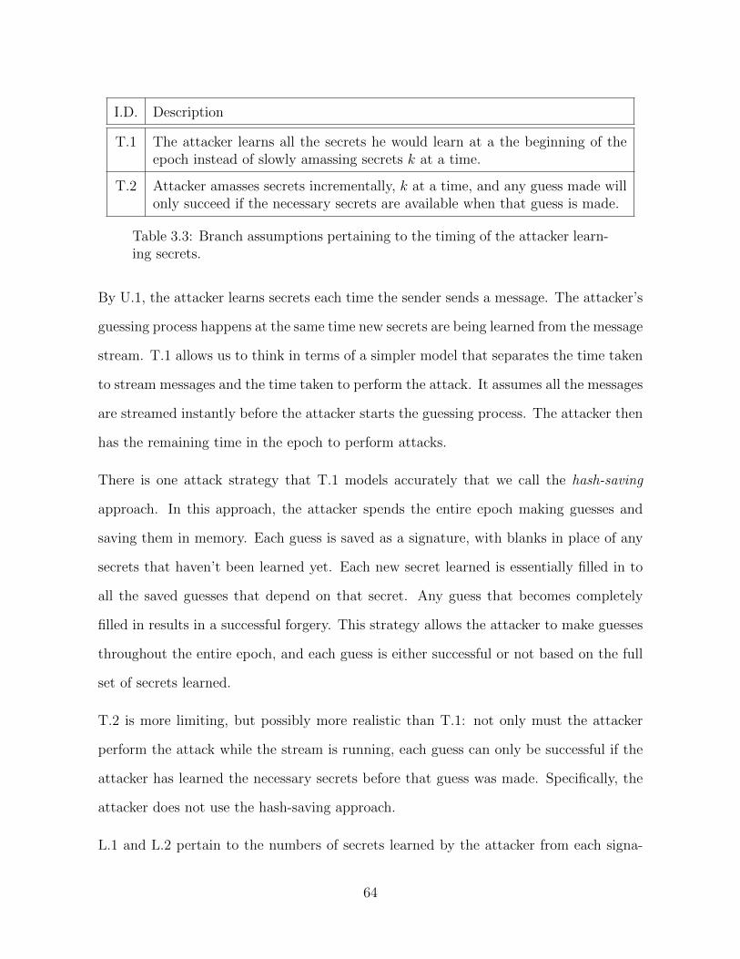
I.D. Description

T.1 The attacker learns all the secrets he would learn at a the beginning of theepoch instead of slowly amassing secrets k at a time.

T.2 Attacker amasses secrets incrementally, k at a time, and any guess made willonly succeed if the necessary secrets are available when that guess is made.

Table 3.3: Branch assumptions pertaining to the timing of the attacker learn-ing secrets.

By U.1, the attacker learns secrets each time the sender sends a message. The attacker’s

guessing process happens at the same time new secrets are being learned from the message

stream. T.1 allows us to think in terms of a simpler model that separates the time taken

to stream messages and the time taken to perform the attack. It assumes all the messages

are streamed instantly before the attacker starts the guessing process. The attacker then

has the remaining time in the epoch to perform attacks.

There is one attack strategy that T.1 models accurately that we call the hash-saving

approach. In this approach, the attacker spends the entire epoch making guesses and

saving them in memory. Each guess is saved as a signature, with blanks in place of any

secrets that haven’t been learned yet. Each new secret learned is essentially filled in to

all the saved guesses that depend on that secret. Any guess that becomes completely

filled in results in a successful forgery. This strategy allows the attacker to make guesses

throughout the entire epoch, and each guess is either successful or not based on the full

set of secrets learned.

T.2 is more limiting, but possibly more realistic than T.1: not only must the attacker

perform the attack while the stream is running, each guess can only be successful if the

attacker has learned the necessary secrets before that guess was made. Specifically, the

attacker does not use the hash-saving approach.

L.1 and L.2 pertain to the numbers of secrets learned by the attacker from each signa-

64

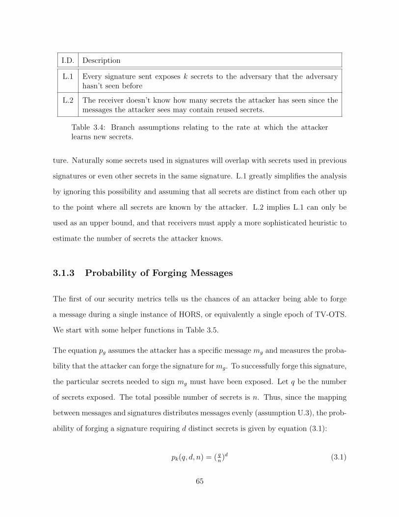
I.D. Description

L.1 Every signature sent exposes k secrets to the adversary that the adversaryhasn’t seen before

L.2 The receiver doesn’t know how many secrets the attacker has seen since themessages the attacker sees may contain reused secrets.

Table 3.4: Branch assumptions relating to the rate at which the attackerlearns new secrets.

ture. Naturally some secrets used in signatures will overlap with secrets used in previous

signatures or even other secrets in the same signature. L.1 greatly simplifies the analysis

by ignoring this possibility and assuming that all secrets are distinct from each other up

to the point where all secrets are known by the attacker. L.2 implies L.1 can only be

used as an upper bound, and that receivers must apply a more sophisticated heuristic to

estimate the number of secrets the attacker knows.

3.1.3 Probability of Forging Messages

The first of our security metrics tells us the chances of an attacker being able to forge

a message during a single instance of HORS, or equivalently a single epoch of TV-OTS.

We start with some helper functions in Table 3.5.

The equation pg assumes the attacker has a specific message mg and measures the proba-

bility that the attacker can forge the signature formg. To successfully forge this signature,

the particular secrets needed to sign mg must have been exposed. Let q be the number

of secrets exposed. The total possible number of secrets is n. Thus, since the mapping

between messages and signatures distributes messages evenly (assumption U.3), the prob-

ability of forging a signature requiring d distinct secrets is given by equation (3.1):

pk(q, d, n) = ( qn)d (3.1)

65

Equation Description Parameters

pk When choosing d distinct secrets randomly from a largernumber of secrets n, the probability that all d choices willbelong to a specific subset of size q.

n, d, q

dk The number of combinations of k different secrets whereonly d of them are distinct

d, k

pd The number of unique signatures that contain k of npossible secrets where exactly d of them are distinct

k, n, d

pg Probability of an attacker guess being correct, given acertain number of secrets (depending on k and r) exposedto the attacker

k, n, r

Table 3.5: Helper Functions

Most signatures will require d = k distinct secrets, but assuming this for all signatures

will result in a forgery probability that too small to be accurate. This is due to the small

fraction of signatures containing repeated secrets, making them easier for the attacker to

forge. As Figure 3.1 shows, the probability of forging a message with d = k is much more

difficult than forging a message with a smaller d. The number of ways to use d distinct

secrets to make a signature with a total of k secrets is given by equation 3.2:

dk(k, d) =d−1∑i=0

(−1)i(

d

d− i

)(d− i)k (3.2)

Taking into account the n possible choices for the k secrets, the probability that the

attacker will need d distinct secrets is given by:

pd(n, k, d) =

(nd

)dk(k, d)

nk(3.3)

Essentially, pd gives a probability distribution for the number of distinct secrets for a

signature of k keys, which can be used to find the final probability of forging a signature

66

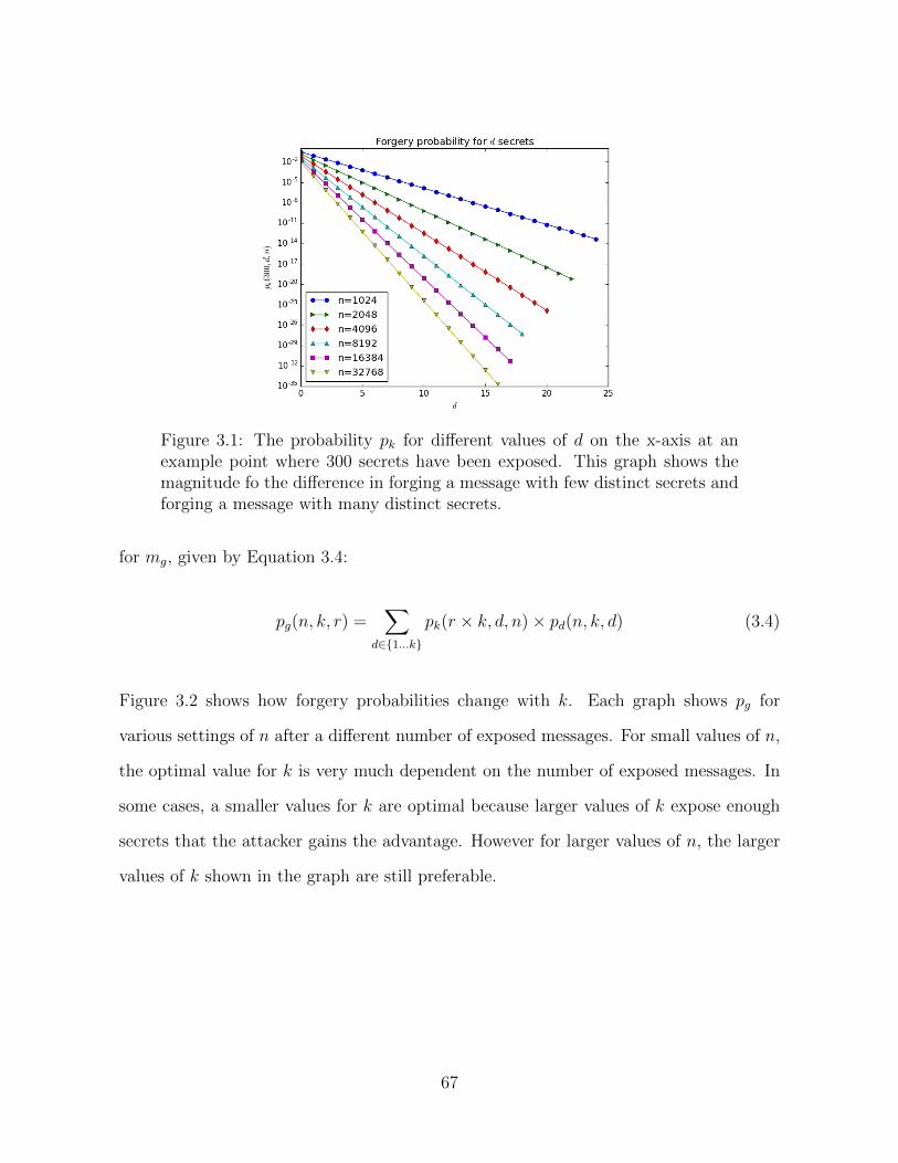
Figure 3.1: The probability pk for different values of d on the x-axis at anexample point where 300 secrets have been exposed. This graph shows themagnitude fo the difference in forging a message with few distinct secrets andforging a message with many distinct secrets.

for mg, given by Equation 3.4:

pg(n, k, r) =∑

d∈1...k

pk(r × k, d, n)× pd(n, k, d) (3.4)

Figure 3.2 shows how forgery probabilities change with k. Each graph shows pg for

various settings of n after a different number of exposed messages. For small values of n,

the optimal value for k is very much dependent on the number of exposed messages. In

some cases, a smaller values for k are optimal because larger values of k expose enough

secrets that the attacker gains the advantage. However for larger values of n, the larger

values of k shown in the graph are still preferable.

67

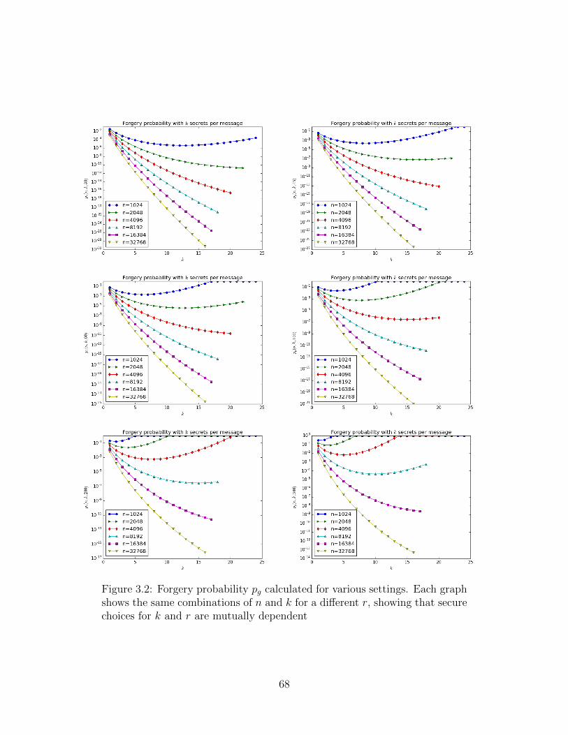
Figure 3.2: Forgery probability pg calculated for various settings. Each graphshows the same combinations of n and k for a different r, showing that securechoices for k and r are mutually dependent

68

The probability pg describes an attacker’s ability to forge a specific message. However, in

some cases the attacker will be willing to forge any message they can. The probabilities

described in Table 3.6 are the forgery probabilities over the course of an epoch in this

case. We assume that the attacker does not care about the contents of the message and

will search the message space for any message that can be forged. In reality a useful

attack may not allow the attacker to search the message space because not all messages

would be useful to the attacker. However, any flexibility in the authentication protocol

or underlying message format would increase the attacker’s search space even beyond the

content of possible malicious messages. For example, if the message contains a timestamp

with an allowable range, the attacker could try forging a single message with a number

of valid timestamps, increasing the chances of finding that a signature could be forged

for any one of the possible messages. The TV-OTS timestamp itself may be exploited

by the attacker for this purpose.

I.D. Assumptions Implications

P1 T.1, L.1 Simple analysis assuming the attacker knows r×k secrets dur-ing every guess

P2 T.2, L.1 Less simple analysis assuming the simple attack strategy ofperforming each guess against the secrets currently availableto the attacker.

Table 3.6: Probability that the attacker, while guessing messages, will get atleast one correct the time that it takes the sender to send r messages.

These probabilities take into account x, the assumed rate at which the attacker can guess

and hash messages. The set of assumptions chosen corresponds to the scenario being

modeled. P1 assumes T.1 and L.1 meaning the attacker has r × k secrets available with

every guess and the attacker has time x guesses. This itself is not necessarily an accurate

model, however, since it requires the hash-saving approach described in Section 3.1.2.

The logistics of data storage for this style of attack is complex enough that the attacker

69

may be limited to a simpler approach. A more practical strategy for the attacker would

be to maintain a pool of secrets which grows when new secrets are received. Guesses

would be made the entire time, but only checked against the pool that existed when the

guess was made. This case is modeled more accurately with assumptions T.2, L.1, but

its analysis is more complicated, resulting in pfa

First we look at the easier-to-analyze T.1, L.1 case where we can evaluate each guess in

the same way. This probability, pfw , is the complement of the probability that in all the

attacker’s attempts, not one yields a successful forgery. The probability pfw is given by

Equation 3.5:

pfw = 1− (1− pg(n, k, r))x (3.5)

Using T.1 implies the success probability is the same for all guesses, but replacing T.1

with T.2 results in an evaluation that takes into account the number of secrets the

attacker has learned when each guess is made. The attacker makes guesses continually,

checking each against the pool as it exists when the guess was made. A more accurate

probability for this scenario is pfa , which is very similar to pfw , but accounts for the

changing number of secrets the attacker can choose from:

pfa = 1−((1− pg(n, k, 1))x/r(1− pg(n, k, 2))x/r(1− pg(n, k, 3))x/r · · · (1− pg(n, k, r))x/r

)= 1−

(r∏i=1

(1− pg(n, k, r))

)x/r

(3.6)

Figure 3.3 shows the difference between pfw and pfa for different values of n and r. In

each case, the forgery probability of pfw is noticeably higher than it is for pfa .

70

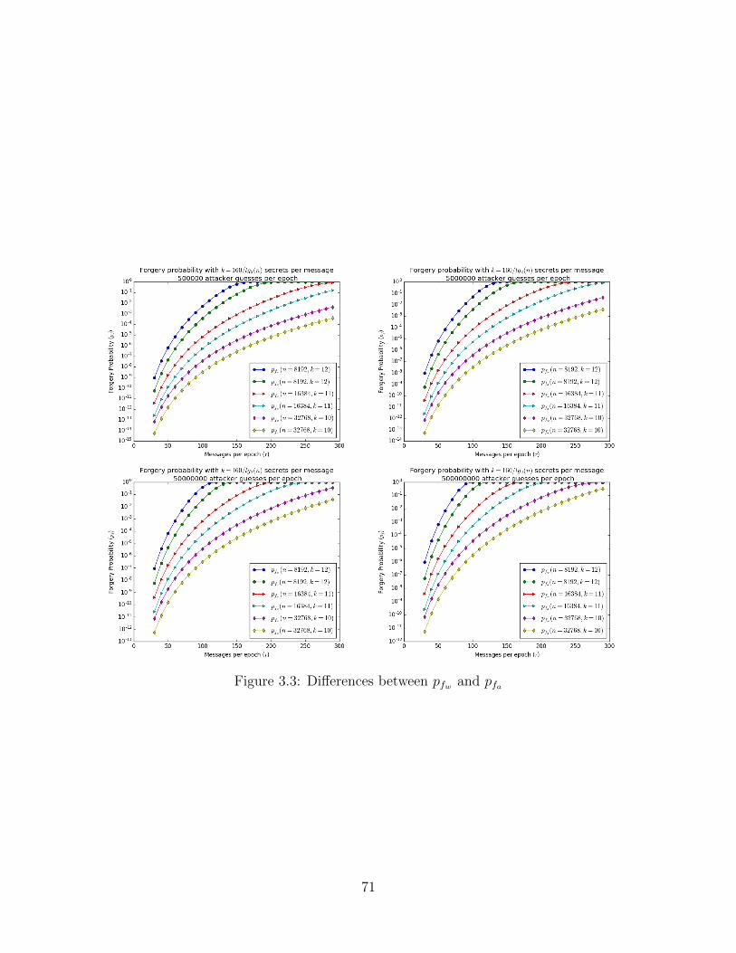
Figure 3.3: Differences between pfw and pfa

71

Tables 3.7, 3.8 and 3.9 show a variety security of data points for varying combinations

of n, k, and r. Values of x, r and k were chosen to provide a meaningful sample of data.

These table were calculated using x = 2 × 109, inspired by a GPU-based system that

achieves x = 1.4 × 109 SHA1 hashes per second [103]. If we take x to be per-second,

then r is also per-second. A sampling rate of 30 hertz is common for PMU data, though

it is anticipated this rate may increase to 60 or 120Hz [15]. Our choices for r are aimed

to show which values of r are acceptable for various security requirements. Among our

choices for k, we use the maximum possible values when messages are hashed using SHA1,

as well as surrounding values that may be of interest. In some cases higher security is

achieved by smaller k as shown in Figure 3.2. In other cases, increasing k by using a

larger hash such as SHA256 or SHA512 increases security, but at the cost of lengthened

signatures.

72

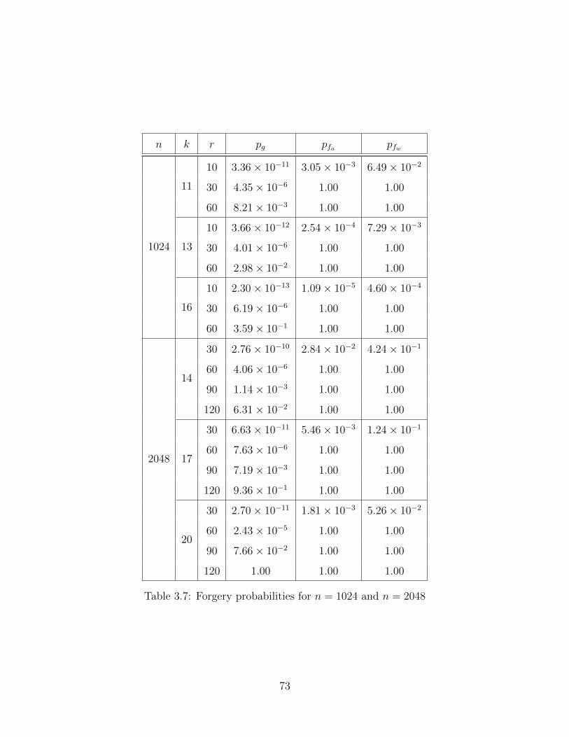
n k r pg pfa pfw

1024

11

10 3.36× 10−11 3.05× 10−3 6.49× 10−2

30 4.35× 10−6 1.00 1.00

60 8.21× 10−3 1.00 1.00

13

10 3.66× 10−12 2.54× 10−4 7.29× 10−3

30 4.01× 10−6 1.00 1.00

60 2.98× 10−2 1.00 1.00

16

10 2.30× 10−13 1.09× 10−5 4.60× 10−4

30 6.19× 10−6 1.00 1.00

60 3.59× 10−1 1.00 1.00

2048

14

30 2.76× 10−10 2.84× 10−2 4.24× 10−1

60 4.06× 10−6 1.00 1.00

90 1.14× 10−3 1.00 1.00

120 6.31× 10−2 1.00 1.00

17

30 6.63× 10−11 5.46× 10−3 1.24× 10−1

60 7.63× 10−6 1.00 1.00

90 7.19× 10−3 1.00 1.00

120 9.36× 10−1 1.00 1.00

20

30 2.70× 10−11 1.81× 10−3 5.26× 10−2

60 2.43× 10−5 1.00 1.00

90 7.66× 10−2 1.00 1.00

120 1.00 1.00 1.00

Table 3.7: Forgery probabilities for n = 1024 and n = 2048

73

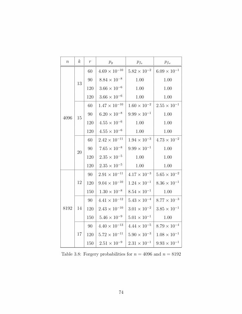
n k r pg pfa pfw

4096

13

60 4.69× 10−10 5.82× 10−2 6.09× 10−1

90 8.84× 10−8 1.00 1.00

120 3.66× 10−6 1.00 1.00

120 3.66× 10−6 1.00 1.00

15

60 1.47× 10−10 1.60× 10−2 2.55× 10−1

90 6.20× 10−8 9.99× 10−1 1.00

120 4.55× 10−6 1.00 1.00

120 4.55× 10−6 1.00 1.00

20

60 2.42× 10−11 1.94× 10−3 4.73× 10−2

90 7.65× 10−8 9.99× 10−1 1.00

120 2.35× 10−5 1.00 1.00

120 2.35× 10−5 1.00 1.00

8192

12

90 2.91× 10−11 4.17× 10−3 5.65× 10−2

120 9.04× 10−10 1.24× 10−1 8.36× 10−1

150 1.30× 10−8 8.54× 10−1 1.00

14

90 4.41× 10−12 5.43× 10−4 8.77× 10−3

120 2.43× 10−10 3.01× 10−2 3.85× 10−1

150 5.46× 10−9 5.01× 10−1 1.00

17

90 4.40× 10−13 4.44× 10−5 8.79× 10−4

120 5.72× 10−11 5.90× 10−3 1.08× 10−1

150 2.51× 10−9 2.31× 10−1 9.93× 10−1

Table 3.8: Forgery probabilities for n = 4096 and n = 8192

74

n k r pg pfa pfw

16384

11

120 9.64× 10−13 1.53× 10−4 1.93× 10−3

150 1.11× 10−11 1.79× 10−3 2.20× 10−2

200 2.61× 10−10 4.15× 10−2 4.07× 10−1

15

120 4.32× 10−15 5.07× 10−7 8.63× 10−6

150 1.21× 10−13 1.44× 10−5 2.43× 10−4

200 8.97× 10−12 1.08× 10−3 1.78× 10−2

20

120 2.21× 10−17 1.94× 10−9 4.43× 10−8

150 1.89× 10−15 1.68× 10−7 3.78× 10−6

200 5.87× 10−13 5.31× 10−5 1.17× 10−3

32768

10

120 4.50× 10−15 7.84× 10−7 8.99× 10−6

150 4.16× 10−14 7.31× 10−6 8.31× 10−5

200 7.33× 10−13 1.30× 10−4 1.46× 10−3

300 4.19× 10−11 7.47× 10−3 8.05× 10−2

15

120 1.32× 10−19 1.55× 10−11 2.64× 10−10

150 3.71× 10−18 4.41× 10−10 7.43× 10−9

200 2.75× 10−16 3.31× 10−8 5.49× 10−7

300 1.19× 10−13 1.45× 10−5 2.38× 10−4

20

120 2.12× 10−23 1.86× 10−15 4.25× 10−14

150 1.81× 10−21 1.61× 10−13 3.63× 10−12

200 5.63× 10−19 5.09× 10−11 1.13× 10−9

300 1.84× 10−15 1.70× 10−7 3.68× 10−6

Table 3.9: Forgery probabilities for n = 16384 and n = 32768

75

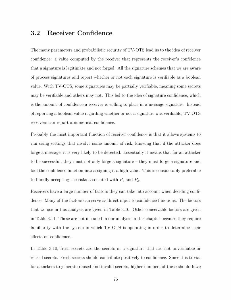
3.2 Receiver Confidence

The many parameters and probabilistic security of TV-OTS lead us to the idea of receiver

confidence: a value computed by the receiver that represents the receiver’s confidence

that a signature is legitimate and not forged. All the signature schemes that we are aware

of process signatures and report whether or not each signature is verifiable as a boolean

value. With TV-OTS, some signatures may be partially verifiable, meaning some secrets

may be verifiable and others may not. This led to the idea of signature confidence, which

is the amount of confidence a receiver is willing to place in a message signature. Instead

of reporting a boolean value regarding whether or not a signature was verifiable, TV-OTS

receivers can report a numerical confidence.

Probably the most important function of receiver confidence is that it allows systems to

run using settings that involve some amount of risk, knowing that if the attacker does

forge a message, it is very likely to be detected. Essentially it means that for an attacker

to be successful, they must not only forge a signature – they must forge a signature and

fool the confidence function into assigning it a high value. This is considerably preferable

to blindly accepting the risks associated with P1 and P2.

Receivers have a large number of factors they can take into account when deciding confi-

dence. Many of the factors can serve as direct input to confidence functions. The factors

that we use in this analysis are given in Table 3.10. Other conceivable factors are given

in Table 3.11. These are not included in our analysis in this chapter because they require

familiarity with the system in which TV-OTS is operating in order to determine their

effects on confidence.

In Table 3.10, fresh secrets are the secrets in a signature that are not unverifiable or

reused secrets. Fresh secrets should contribute positively to confidence. Since it is trivial

for attackers to generate reused and invalid secrets, higher numbers of these should have

76

Name Description Increases with Decreaseswith

Unverifiable Secrets Secrets that the receiver isunable to verify for any rea-son

Unreliablenetworks,audaciousattackers

Cautious at-tackers, reli-able networks

Reused secrets Secrets that are verifiable,but the receiver has seenthem previously, implyingthe attacker knows them aswell

r n

Fresh Secrets The secrets in a signaturethat are neither unverifiablenor reused

n r

Table 3.10: Confidence factors inherent to TV-OTS

Name Description

Sequence numbers If a gap in sequence numbers appears, receivers may as-sume attackers are learning secrets from the missing mes-sages. Note that this is weaker than checking periodicity ina periodic system, but necessary in an aperiodic system.

Latency or Jitter Messages arriving with unusual timing characteristics

Duplication Different messages with the same metadata (e.g., timestampor sequence number) may be suspicious

Stats gathered over extended periods:

Total Reuse If the amount of overall reuse is significantly higher thanexpected, the attacker may be more powerful than expected

If the authentication code has communication with the upper layer:

Syntactically orsemantically invalidmessages

Indicative of an attack or malfunctioning sender

Table 3.11: Confidence factors that require knowledge of the operating envi-ronment

77

a negative effect on confidence. Simply put, more fresh secrets yields a higher confidence.

Fortunately, messages that naturally have very few fresh secrets should be rare.

3.2.1 Receivers’ Attacker Models

Estimating signature confidence involves evaluating a confidence function for each sig-

nature, potentially taking into account an estimated state of the attacker. Specifically

one of the inputs that confidence functions may consider is the number of secrets known

to the attacker. Since the receiver can’t actually know this number, the receiver must

estimate it using some model.

Certain circumstances can lead to the attacker knowing more secrets than the receiver,

such as when the receiver hasn’t received all the messages sent from the sender. This

may be due to messages that have been dropped or replaced with forged messages by

the attacker. The receiver can’t possibly find out which secrets the attacker knows,

but by keeping a model, the receiver can estimate or at least bound the number. The

accuracy of this estimate depends on how much effort the receiver puts into modeling

the attacker.

The process of attackers learning secrets is somewhat circular in nature. Attackers learn

more secrets than the receivers know by blocking messages or performing successful

forgeries. Subsequent forgeries then become easier due to the extra secrets known. The

first forgery is the most difficult and probably the most detectable: the secrets in the

forged signature must be either 1) secrets that the receiver knows, 2) injected secrets that

the attacker has learned by blocking previous messages or 3) secrets just learned in the

message being replaced by a forged message. In the first case, the receiver will not include

those secrets in confidence calculation because they’ve been seen before. In the second

case, the receiver will have detected the missing messages and should be assuming the

78

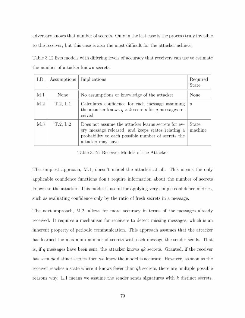
adversary knows that number of secrets. Only in the last case is the process truly invisible

to the receiver, but this case is also the most difficult for the attacker achieve.

Table 3.12 lists models with differing levels of accuracy that receivers can use to estimate

the number of attacker-known secrets.

I.D. Assumptions Implications RequiredState

M.1 None No assumptions or knowledge of the attacker None

M.2 T.2, L.1 Calculates confidence for each message assumingthe attacker knows q × k secrets for q messages re-ceived

q

M.3 T.2, L.2 Does not assume the attacker learns secrets for ev-ery message released, and keeps states relating aprobability to each possible number of secrets theattacker may have

Statemachine

Table 3.12: Receiver Models of the Attacker

The simplest approach, M.1, doesn’t model the attacker at all. This means the only

applicable confidence functions don’t require information about the number of secrets

known to the attacker. This model is useful for applying very simple confidence metrics,

such as evaluating confidence only by the ratio of fresh secrets in a message.

The next approach, M.2, allows for more accuracy in terms of the messages already

received. It requires a mechanism for receivers to detect missing messages, which is an

inherent property of periodic communication. This approach assumes that the attacker

has learned the maximum number of secrets with each message the sender sends. That

is, if q messages have been sent, the attacker knows qk secrets. Granted, if the receiver

has seen qk distinct secrets then we know the model is accurate. However, as soon as the

receiver reaches a state where it knows fewer than qk secrets, there are multiple possible

reasons why. L.1 means we assume the sender sends signatures with k distinct secrets.

79

Even when a signature contains fewer than k fresh secrets, we assume the attacker still

somehow learned k secrets. Therefore, we assume the attacker has learned the secrets

that make up the difference between what the sender has sent and what the receiver has

seen.

M.2 is still not an accurate estimate on the number of secrets the attacker knows. As

previously stated, when the receiver has seen fewer than qk secrets, one of the explana-

tions is natural overlap that sometimes occurs among secrets. The motivation behind

M.3 is that when the receiver sees reused secrets, it has no way to know if the cause is

malicious or a natural byproduct of the sender’s process.

M.3 takes into account the uncertainty surrounding messages with reused secrets. This

model is easiest to describe in terms of states. A state is defined by the number of secrets

that the attacker knows that the receiver doesn’t. The receiver keeps a set of states

that represents the attacker’s possible states. When the receiver receives a signature

made entirely of fresh secrets, it doesn’t update the states, knowing that the attacker’s

relative knowledge has not increased. When the receiver receives a message with some

reused secrets, the receiver knows the attacker’s state may have changed. The receiver

updates the set of states based on sb, the number of secrets in the signature that are not

fresh. The number of states is doubled, by adding sb to the number associated with each

preexisting state, essentially splitting each state into two new states.

Each state is associated with a probability. In the initial state, we assume the attacker

has k secrets to represent the fact that even before the receiver receives a message, the

attacker can make guesses against the secrets in the initial message. This initial state, Sk,

has probability 1. When a state is split, the probability of the new states is based on the

message confidence, c. Let Sj, pj denote a state and it’s associated probability before an

update. The new probability associated with Sj is pj×c. The probability associated with

80

the new state Sj+sb is pj × (1 − c). To use this model to evaluate signature confidence,

confidence is evaluated for each state. The weighted average of the resulting list of

confidences is the reported confidence.

3.2.2 Confidence Functions

The confidence for each message is evaluated by a confidence function. The goal of

the confidence functions is to assess the strength of each signature individually, allowing

upper layer applications decide the confidence thresholds they want to apply. We present

two choices for confidence functions: one that is very simple and another that is more

complex but more accurate. The simple method evaluates each function independently

of the state of the system. The more complex method uses an estimate of the attacker’s

state and estimates relative confidence.

Confidence functions can operate on a number of different inputs, the most meaningful

being the number of fresh secrets contained in a signature. Table 3.13 lists the different

variables we use as inputs. Larger numbers of fresh secrets contribute to higher confi-

dence. When a receiver receives a signature containing fresh secrets, the message can’t

be forged unless the attacker somehow knew those fresh secrets. This is possible if the

attacker has seen messages that the receiver hasn’t. The receiver’s attacker models are

useful for estimating the number of secrets that the attacker may know that the receiver

doesn’t.

81

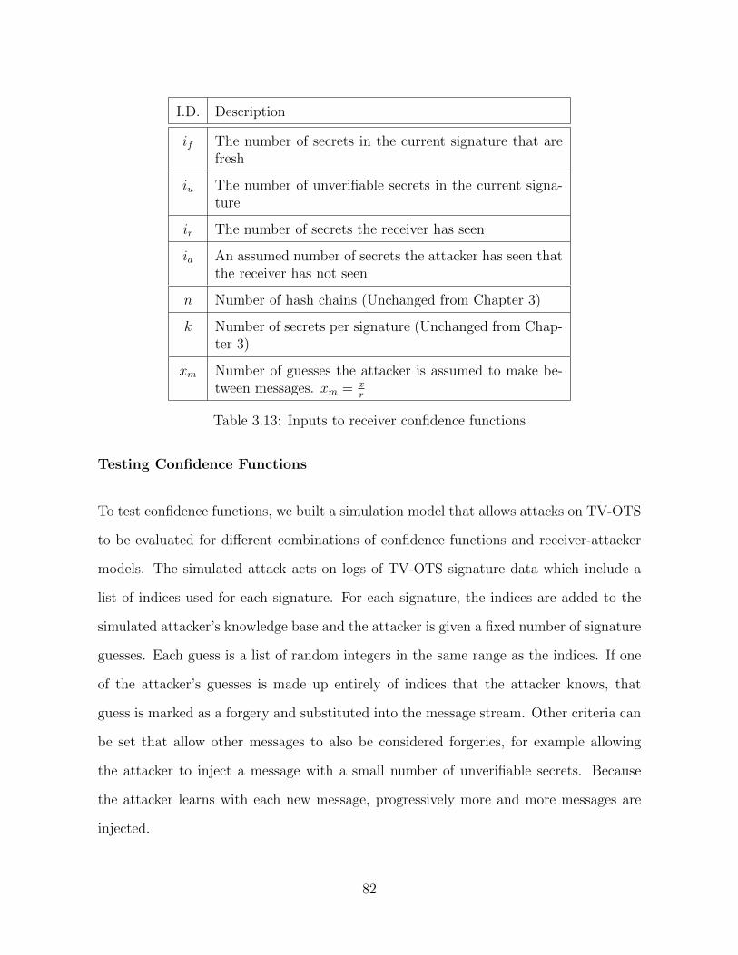
I.D. Description

if The number of secrets in the current signature that arefresh

iu The number of unverifiable secrets in the current signa-ture

ir The number of secrets the receiver has seen

ia An assumed number of secrets the attacker has seen thatthe receiver has not seen

n Number of hash chains (Unchanged from Chapter 3)

k Number of secrets per signature (Unchanged from Chap-ter 3)

xm Number of guesses the attacker is assumed to make be-tween messages. xm = x

r

Table 3.13: Inputs to receiver confidence functions

Testing Confidence Functions

To test confidence functions, we built a simulation model that allows attacks on TV-OTS

to be evaluated for different combinations of confidence functions and receiver-attacker

models. The simulated attack acts on logs of TV-OTS signature data which include a

list of indices used for each signature. For each signature, the indices are added to the

simulated attacker’s knowledge base and the attacker is given a fixed number of signature

guesses. Each guess is a list of random integers in the same range as the indices. If one

of the attacker’s guesses is made up entirely of indices that the attacker knows, that

guess is marked as a forgery and substituted into the message stream. Other criteria can

be set that allow other messages to also be considered forgeries, for example allowing

the attacker to inject a message with a small number of unverifiable secrets. Because

the attacker learns with each new message, progressively more and more messages are

injected.

82

Signatures from the attacker model are processed next by a modeled receiver. The mod-

eled receiver evaluates confidence for each signature, building its model of the attacker

as it goes. The resulting data is a stream of confidences, tagged with the meta data

of whether the message was actually forged. Algorithm 5 gives pseudocode for the ba-

sic combined attacker and receiver simulation, though this description is independent of

the confidence function and receiver-attacker model actually used. In Algorithm 5 each

message processed by the attacker is immediately evaluated by the receiver before the

attacker moves on to the next message.

Our model allows confidence functions to be evaluated for accuracy. One of our measure-

ments evaluates the area under a ROC curve[58] based on the generated data. To ensure

a significant sample of forged messages, we intentionally ran our model on unrealistically

long epochs. Our epochs are long enough that each epoch ends in a series of forged mes-

sages. To prevent results from being skewed by an arbitrarily long string of forgeries at

the end of each epoch, we truncated each epoch after the last good, un-forged message.

This means that our confidence functions are evaluated from the beginning of each epoch

until the last good message, including all forgeries before the last good message.

This approach also allows us to visualize data in a convenient format. Each graph shows

the confidence evaluated for each message, with sequence numbers on the x-axis. The

lines extending vertically from the x-axis represent the amount of confidence in each mes-

sage. Forged messages have appear on the graph with 1 subtracted from the confidence,

so that messages that were tagged as forgeries appear below the x-axis. Intuitively, lines

extending farther from the x-axis are better estimates: long positive lines are good mes-

sages with high confidence and long negative lines are bad messages with low confidence.

Short lines are either good messages with low confidence or bad messages with high con-

fidence. These figures are also useful for showing when and how quickly the attacker

learns enough secrets to begin forging messages. For the settings with fewer hash chains

83

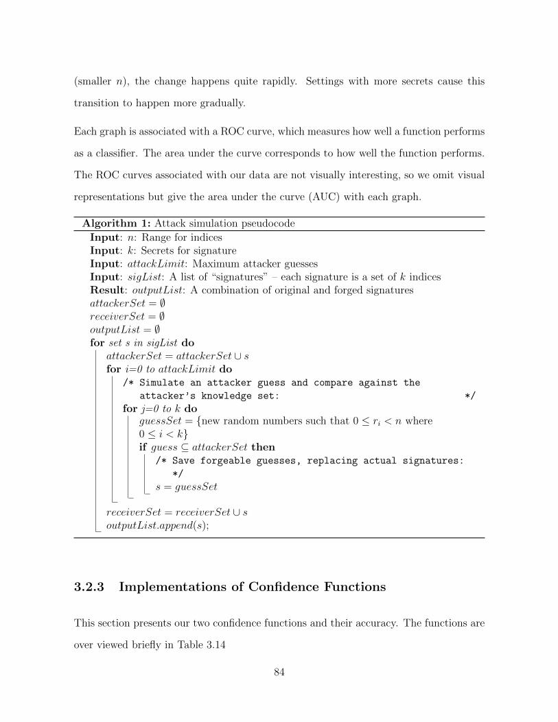
(smaller n), the change happens quite rapidly. Settings with more secrets cause this

transition to happen more gradually.

Each graph is associated with a ROC curve, which measures how well a function performs

as a classifier. The area under the curve corresponds to how well the function performs.

The ROC curves associated with our data are not visually interesting, so we omit visual

representations but give the area under the curve (AUC) with each graph.

Algorithm 1: Attack simulation pseudocode

Input: n: Range for indicesInput: k: Secrets for signatureInput: attackLimit: Maximum attacker guessesInput: sigList: A list of “signatures” – each signature is a set of k indicesResult: outputList: A combination of original and forged signaturesattackerSet = ∅receiverSet = ∅outputList = ∅for set s in sigList do

attackerSet = attackerSet ∪ sfor i=0 to attackLimit do

/* Simulate an attacker guess and compare against the

attacker’s knowledge set: */

for j=0 to k doguessSet = new random numbers such that 0 ≤ ri < n where0 ≤ i < kif guess ⊆ attackerSet then

/* Save forgeable guesses, replacing actual signatures:

*/

s = guessSet

receiverSet = receiverSet ∪ soutputList.append(s);

3.2.3 Implementations of Confidence Functions

This section presents our two confidence functions and their accuracy. The functions are

over viewed briefly in Table 3.14

84

I.D. Description Applicable models

C1 Fraction of fresh secrets Not affected by receivermodels

C2 Based on the chances that the attacker willbe able to forge the fresh secrets seen

M.2, M.3

Table 3.14: Confidence Functions

C1 – Fraction of Fresh Secrets

Our first confidence function is very basic and simply returns the fraction of fresh secrets

in each signature. This function is limited by the fact that it does not incorporate any

data about the state of the system. C1 is given by:

C1(k, if ) =ifk

(3.7)

Figures 3.4 and 3.5 show graphs produced by the model for n = 2048 and n = 16384. Two

noteworthy features stand out about these graphs. First, the confidence function does

fairly well at differentiating messages earlier in the stream, but the vertical confidence

lines grow smaller as the epoch grows longer. Secondly, the graphs show the length of

the transition between no successful forgeries and continual success. For smaller n this

transition happens very rapidly. For larger n the transition is more prolonged.

C2 – Fresh Secrets from the Attacker

Our goal for C2 was to create a confidence function capable of reacting to the evolution

of the system. This approach uses an estimate on the number of secrets the attacker

knows. The intuition behind this approach is that if a message containing fresh secrets

was forged, the attacker would have had to know those secrets. In the beginning of an

85

Figure 3.4: Simulation graphs for the settings n = 2048, k = 14 and confidencefunction C1. These graphs show five epochs which are truncated after the lastgood message. The graphs show results from giving the attacker 20,000 and200,000 guesses between messages.

Figure 3.5: Simulation graphs for the settings n = 16384, k = 11 and confi-dence function C1. These graphs show five epochs which are truncated afterthe last good message. The graphs show results from giving the attacker20,000 and 200,000 guesses between messages.

86

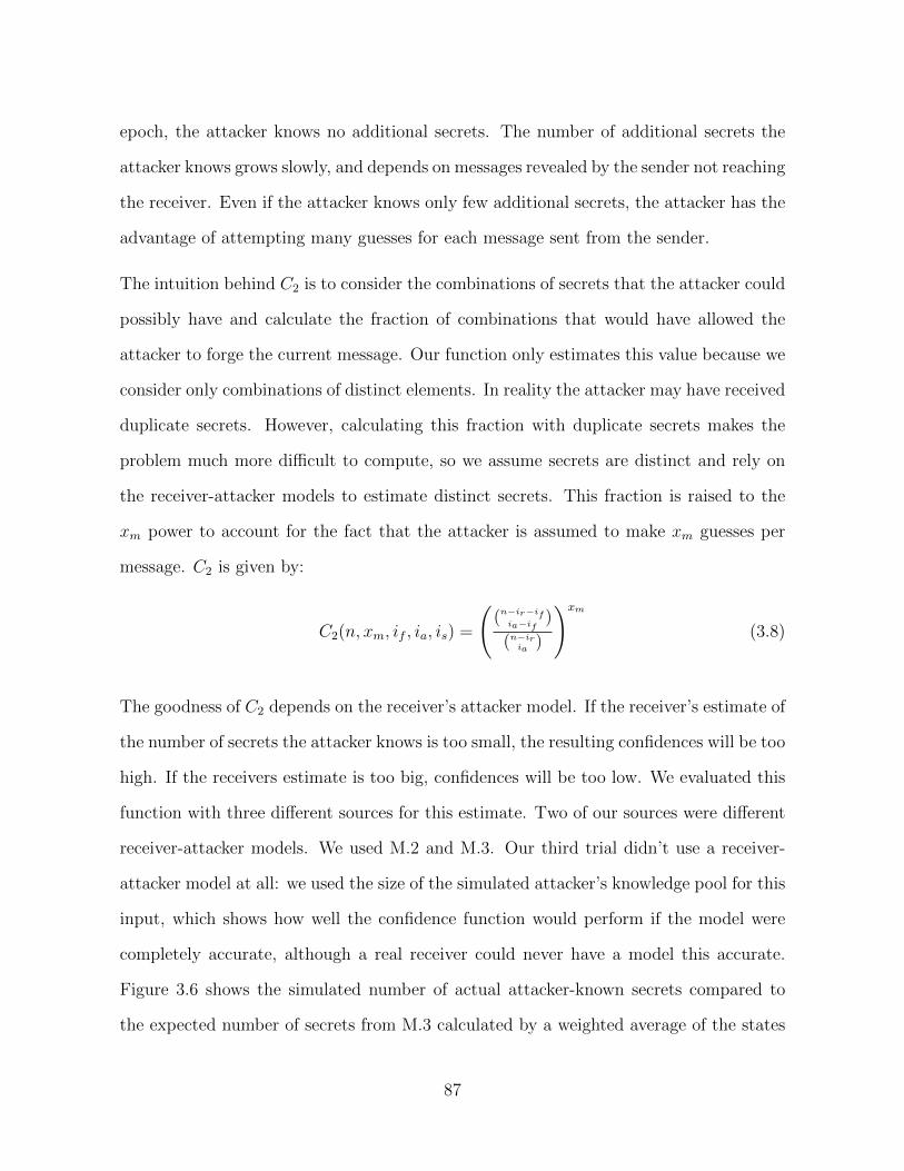
epoch, the attacker knows no additional secrets. The number of additional secrets the

attacker knows grows slowly, and depends on messages revealed by the sender not reaching

the receiver. Even if the attacker knows only few additional secrets, the attacker has the

advantage of attempting many guesses for each message sent from the sender.

The intuition behind C2 is to consider the combinations of secrets that the attacker could

possibly have and calculate the fraction of combinations that would have allowed the

attacker to forge the current message. Our function only estimates this value because we

consider only combinations of distinct elements. In reality the attacker may have received

duplicate secrets. However, calculating this fraction with duplicate secrets makes the

problem much more difficult to compute, so we assume secrets are distinct and rely on

the receiver-attacker models to estimate distinct secrets. This fraction is raised to the

xm power to account for the fact that the attacker is assumed to make xm guesses per

message. C2 is given by:

C2(n, xm, if , ia, is) =

((n−ir−if

ia−if)

(n−iria

)

)xm

(3.8)

The goodness of C2 depends on the receiver’s attacker model. If the receiver’s estimate of

the number of secrets the attacker knows is too small, the resulting confidences will be too

high. If the receivers estimate is too big, confidences will be too low. We evaluated this

function with three different sources for this estimate. Two of our sources were different

receiver-attacker models. We used M.2 and M.3. Our third trial didn’t use a receiver-

attacker model at all: we used the size of the simulated attacker’s knowledge pool for this

input, which shows how well the confidence function would perform if the model were

completely accurate, although a real receiver could never have a model this accurate.

Figure 3.6 shows the simulated number of actual attacker-known secrets compared to

the expected number of secrets from M.3 calculated by a weighted average of the states

87

Figure 3.6: Comparison between the expected number of secrets known bythe attacker calculated by M.3 and the actual number of secrets learned bythe simulated attacker.

(described in Section 3.2.1), showing that M.3 provides a reasonable, though not perfect,

estimate of the number of attacker-known secrets.

Figures 3.7, 3.8 and 3.9 show the graphs for C2 using three different models. These

graphs show that confidence given by C2 is either very high or very low, but switches

from high to low appropriately when the attacker begins to forge messages. Figure 3.7

shows more uncertainty than the other two: the confidence for good messages starts to

taper towards the end of the good messages. However this is to be expected. Figure 3.7

uses the least accurate receiver-attacker model. The model purposefully overestimates

the number of secrets the attacker has. The lowered confidences align with our prediction

that higher estimates of attacker-known secrets results in lower confidence. The remaining

two graphs, which show results using the state machine model and the attacker’s actual

number of secrets are quite similar. Still, the confidences using the state machine model

are slightly lower near the end of the epoch than the confidences using actual data,

meaning our state machine over estimates the number of secrets somewhat.

Tables 3.15 through 3.18 show rates of true and false positives and true and false negatives

for some threshold confidence levels. The thresholds shown were the highest confidences

88

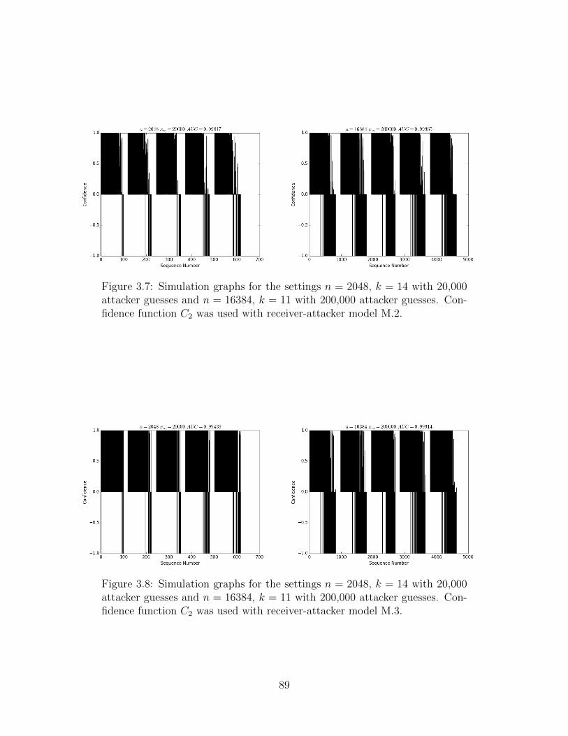
Figure 3.7: Simulation graphs for the settings n = 2048, k = 14 with 20,000attacker guesses and n = 16384, k = 11 with 200,000 attacker guesses. Con-fidence function C2 was used with receiver-attacker model M.2.

Figure 3.8: Simulation graphs for the settings n = 2048, k = 14 with 20,000attacker guesses and n = 16384, k = 11 with 200,000 attacker guesses. Con-fidence function C2 was used with receiver-attacker model M.3.

89

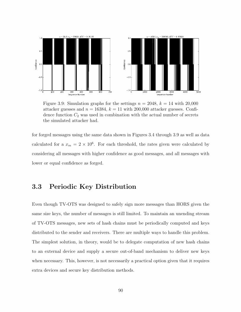
Figure 3.9: Simulation graphs for the settings n = 2048, k = 14 with 20,000attacker guesses and n = 16384, k = 11 with 200,000 attacker guesses. Confi-dence function C2 was used in combination with the actual number of secretsthe simulated attacker had.

for forged messages using the same data shown in Figures 3.4 through 3.9 as well as data

calculated for a xm = 2 × 106. For each threshold, the rates given were calculated by

considering all messages with higher confidence as good messages, and all messages with

lower or equal confidence as forged.

3.3 Periodic Key Distribution

Even though TV-OTS was designed to safely sign more messages than HORS given the

same size keys, the number of messages is still limited. To maintain an unending stream

of TV-OTS messages, new sets of hash chains must be periodically computed and keys

distributed to the sender and receivers. There are multiple ways to handle this problem.

The simplest solution, in theory, would be to delegate computation of new hash chains

to an external device and supply a secure out-of-band mechanism to deliver new keys

when necessary. This, however, is not necessarily a practical option given that it requires

extra devices and secure key distribution methods.

90

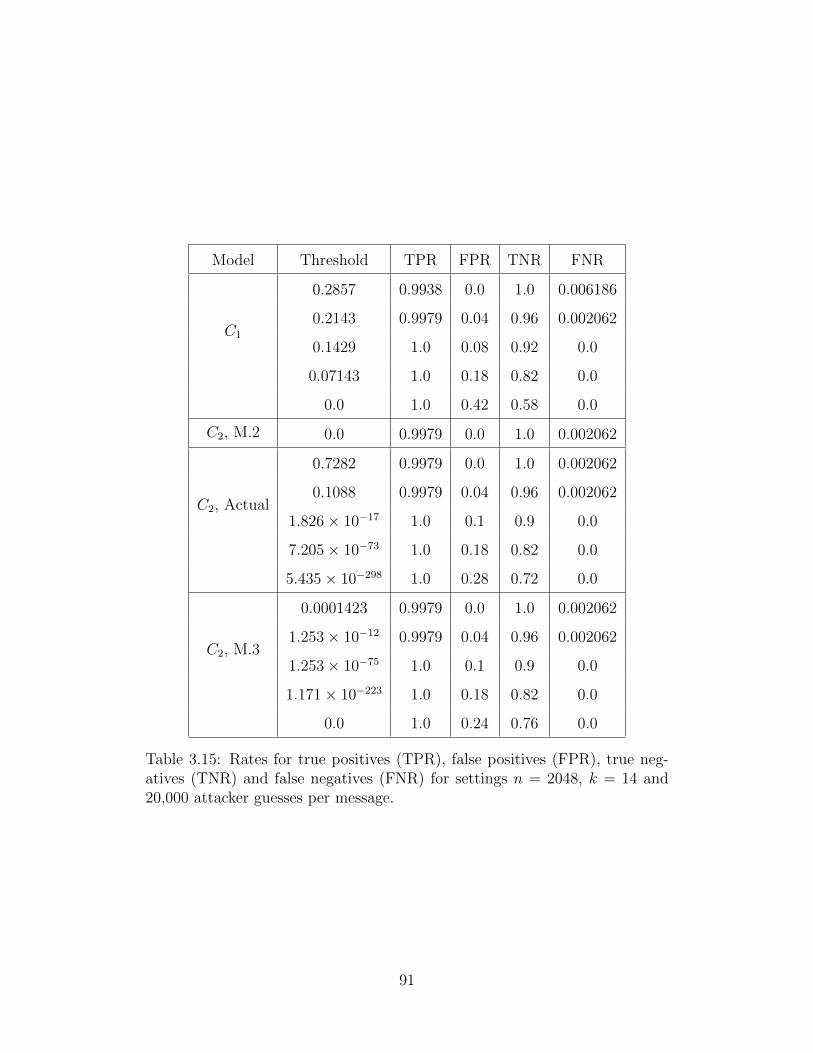
Model Threshold TPR FPR TNR FNR

C1

0.2857 0.9938 0.0 1.0 0.006186

0.2143 0.9979 0.04 0.96 0.002062

0.1429 1.0 0.08 0.92 0.0

0.07143 1.0 0.18 0.82 0.0

0.0 1.0 0.42 0.58 0.0

C2, M.2 0.0 0.9979 0.0 1.0 0.002062

C2, Actual

0.7282 0.9979 0.0 1.0 0.002062

0.1088 0.9979 0.04 0.96 0.002062

1.826× 10−17 1.0 0.1 0.9 0.0

7.205× 10−73 1.0 0.18 0.82 0.0

5.435× 10−298 1.0 0.28 0.72 0.0

C2, M.3

0.0001423 0.9979 0.0 1.0 0.002062

1.253× 10−12 0.9979 0.04 0.96 0.002062

1.253× 10−75 1.0 0.1 0.9 0.0

1.171× 10−223 1.0 0.18 0.82 0.0

0.0 1.0 0.24 0.76 0.0

Table 3.15: Rates for true positives (TPR), false positives (FPR), true neg-atives (TNR) and false negatives (FNR) for settings n = 2048, k = 14 and20,000 attacker guesses per message.

91

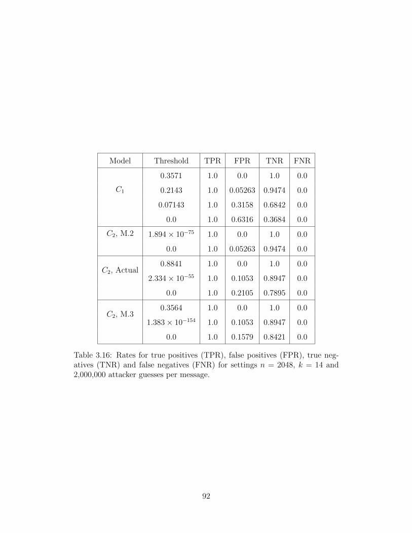
Model Threshold TPR FPR TNR FNR

C1

0.3571 1.0 0.0 1.0 0.0

0.2143 1.0 0.05263 0.9474 0.0

0.07143 1.0 0.3158 0.6842 0.0

0.0 1.0 0.6316 0.3684 0.0

C2, M.2 1.894× 10−75 1.0 0.0 1.0 0.0

0.0 1.0 0.05263 0.9474 0.0

C2, Actual0.8841 1.0 0.0 1.0 0.0

2.334× 10−55 1.0 0.1053 0.8947 0.0

0.0 1.0 0.2105 0.7895 0.0

C2, M.30.3564 1.0 0.0 1.0 0.0

1.383× 10−154 1.0 0.1053 0.8947 0.0

0.0 1.0 0.1579 0.8421 0.0

Table 3.16: Rates for true positives (TPR), false positives (FPR), true neg-atives (TNR) and false negatives (FNR) for settings n = 2048, k = 14 and2,000,000 attacker guesses per message.

92

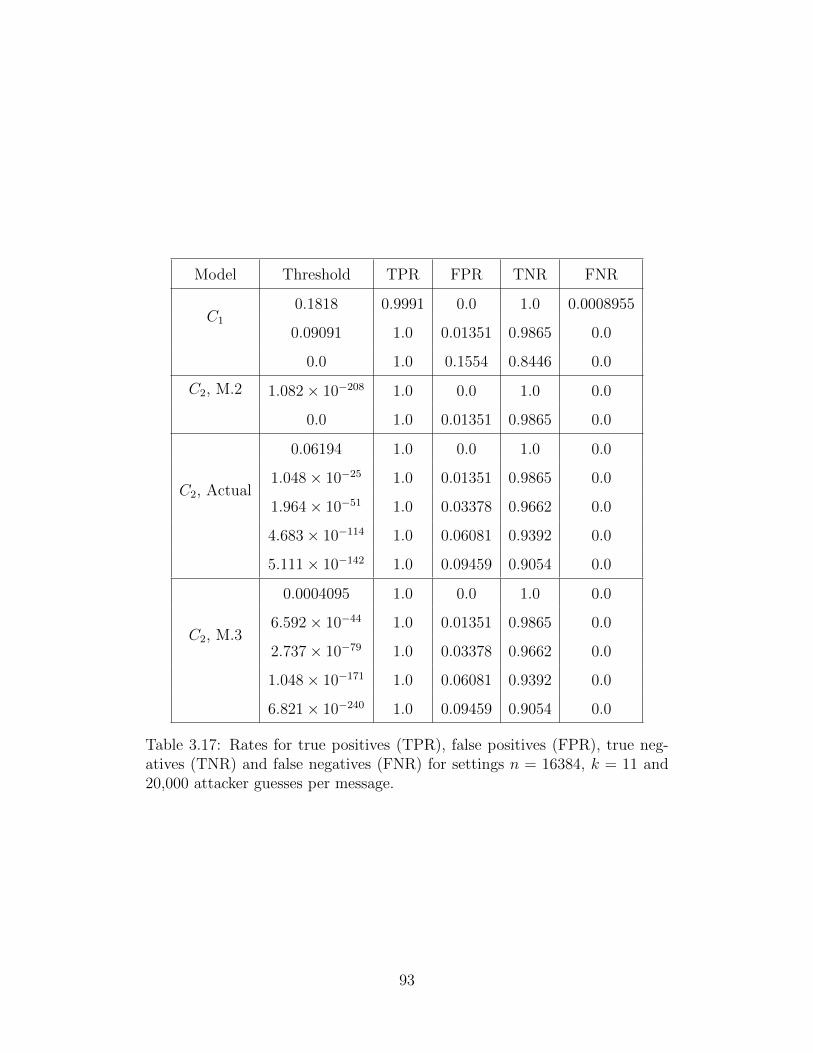
Model Threshold TPR FPR TNR FNR

C1

0.1818 0.9991 0.0 1.0 0.0008955

0.09091 1.0 0.01351 0.9865 0.0

0.0 1.0 0.1554 0.8446 0.0

C2, M.2 1.082× 10−208 1.0 0.0 1.0 0.0

0.0 1.0 0.01351 0.9865 0.0

C2, Actual

0.06194 1.0 0.0 1.0 0.0

1.048× 10−25 1.0 0.01351 0.9865 0.0

1.964× 10−51 1.0 0.03378 0.9662 0.0

4.683× 10−114 1.0 0.06081 0.9392 0.0

5.111× 10−142 1.0 0.09459 0.9054 0.0

C2, M.3

0.0004095 1.0 0.0 1.0 0.0

6.592× 10−44 1.0 0.01351 0.9865 0.0

2.737× 10−79 1.0 0.03378 0.9662 0.0

1.048× 10−171 1.0 0.06081 0.9392 0.0

6.821× 10−240 1.0 0.09459 0.9054 0.0

Table 3.17: Rates for true positives (TPR), false positives (FPR), true neg-atives (TNR) and false negatives (FNR) for settings n = 16384, k = 11 and20,000 attacker guesses per message.

93

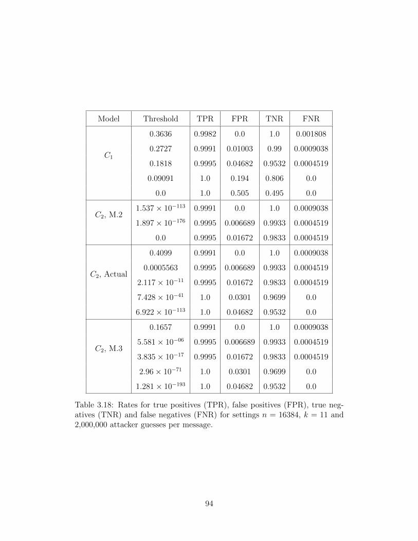
Model Threshold TPR FPR TNR FNR

C1

0.3636 0.9982 0.0 1.0 0.001808

0.2727 0.9991 0.01003 0.99 0.0009038

0.1818 0.9995 0.04682 0.9532 0.0004519

0.09091 1.0 0.194 0.806 0.0

0.0 1.0 0.505 0.495 0.0

C2, M.21.537× 10−113 0.9991 0.0 1.0 0.0009038

1.897× 10−176 0.9995 0.006689 0.9933 0.0004519

0.0 0.9995 0.01672 0.9833 0.0004519

C2, Actual

0.4099 0.9991 0.0 1.0 0.0009038

0.0005563 0.9995 0.006689 0.9933 0.0004519

2.117× 10−11 0.9995 0.01672 0.9833 0.0004519

7.428× 10−41 1.0 0.0301 0.9699 0.0

6.922× 10−113 1.0 0.04682 0.9532 0.0

C2, M.3

0.1657 0.9991 0.0 1.0 0.0009038

5.581× 10−06 0.9995 0.006689 0.9933 0.0004519

3.835× 10−17 0.9995 0.01672 0.9833 0.0004519

2.96× 10−71 1.0 0.0301 0.9699 0.0

1.281× 10−193 1.0 0.04682 0.9532 0.0

Table 3.18: Rates for true positives (TPR), false positives (FPR), true neg-atives (TNR) and false negatives (FNR) for settings n = 16384, k = 11 and2,000,000 attacker guesses per message.

94

The method we present is designed to run using the same resources as the system already

running TV-OTS. It does not use external devices to compute secrets, and places no extra

requirements on the underlying network besides the additional capacity necessary to carry

keystream packets. Creation and distribution of keys is integrated into the sender side

of the TV-OTS system. The design is intended to use only the sender’s leftover compute

resources and not interfere with signing and sending payload messages. The goal is to

be able to slowly and steadily create and distribute new keys so that they are ready to

be used at both ends by the time they’re needed. The packets used to distribute keys

are protected by any standard asymmetric signing algorithm such as RSA or ECDSA,

reducing the TV-OTS key distribution problem to the classic key distribution problem

faced by any asymmetric system.

3.3.1 Principles and Design

In our design, the sender starts two processes in addition to the normal signing and

sending of payload messages. These processes are:

1. Sending the anchors for the next set of hash chains to be used

2. Generating new hash chains for the next set of anchors to be sent in the keystream

On the receiving side, there is one additional process with the purpose of receiving anchors

to be used once the current chains run out. Exhausting the current set of chains triggers

an update at both the sender and receivers. The receivers discard the current set of chains

and swap in the set of anchors it has been receiving. Similiarly, the sender replaces the

chains it has been using for signing with the chains whose anchors were most recently

sent. In addition, it replaces the chains whose anchors were being sent with the chains

that were just being generated, and prepares to generate a brand new set of chains.

95

The sending process sends a number of anchors – as many as will fit in an underlying

network packet – at a time to receivers. To increase the chances the receivers will receive

all anchors, each anchor may be included in one or more redundant keystream packets.

Once all anchors have been sent once, the method used to group anchors in packets is

changed to reduce overlap in content between the initial round of packets and the re-

dundant packets. Allowing keystream packets to carry the exact same sets of anchors

each time allows an entire set to be blocked by blocking the packets carrying that set.

Preventing the overlap increases the number of keystream packets that must be blocked

in order to prevent the same number of anchors from reaching the receivers. It is still

possible for TV-OTS to be attacked this way, but payload messages are as much suscept-

able to a DoS attack as keystream packets, so allocating extra resources to protecting

the keystream does little to increase the overall robustness of the system.

Even with redundancy, the keystream packets are sent much less frequently than payload

messages allowing the use of slower but more secure authentication methods such as RSA

or ECDSA for the keystream packets. The security of the TV-OTS messages depends on

the security of the keystream authentication since anchors injected by an adversary would

compromise the entire system. Therefore it is imperative that the keystream authentica-

tion is at least as strong as the TV-OTS signatures. Chapter 5.2.2 includes information

about the workload balance between TV-OTS payload and keystream messages.

3.3.2 Future Work on Keystreams

The fact that keystreams do not guarantee receipt of all anchors motivates another feature

which allows TV-OTS to continue running in spite of a some missing anchors. The basic

idea is that if a message is received with a signature that would be verifiable except

that the anchor of one of the necessary chains is missing, the confidence for the message

96

is evaluated for that signature as normal except the secret from the missing chain is

treated as an unverifiable secret. More importantly, the secret from the missing chain is

saved, repopulating the chain and allowing future messages containing secrets that use

this chain are verified against the saved secret. In this example, the signature has one

secret missing its chain, but the same idea applies to signatures containing more than

one secret from missing chains.

The idea of saving secrets brings us to yet another idea: hash chain confidence. All the

models thus far have assumed that secrets have equal verification weight. But until now,

we assumed that all the hash chain anchors were distributed with no possibility of failure.

The new idea is to assign a confidence value to individual hash chains. Any hash chain

with an anchor received in the keystream has full confidence. Hash chains with missing

anchors have zero confidence. When a secret belonging to a missing chain is received,

that hash chain can be repopulated. This chain is no longer considered missing, but

is not assigned full confidence either. A logical value to assign is the confidence that

was calculated for the signature that delivered the saved secret. This value must be less

than full confidence for any realistic choice of confidence function since a signature with

unverifiable secrets should never be treated with full confidence.

Research along these lines would be needed to determine the benefits and risks of chain

re-population. The potential benefit is a more accurate classification of messages. In

situations where some keystream anchors are lost, those chains are unusable for verifying

messages. If a good message uses secrets from that chain, the inability to verify those

secrets from its signature would lower the confidence for that message. However, if those

secrets can be saved for those chains, future messages using those chains will not suffer

as much lowered confidence.

The downside of allowing chains to be initialized from secrets is the potential for attackers

97

to inject their own secrets. The fact that hash chains are salted prevents the attacker

from being able to inject their own chains and use those secrets in future epochs, however

the attacker is still able to use those values for the rest of the epoch. They could also use

this method to perform a variant of denial of service attack against TV-OTS: if a chain

is repopulated with a secret injected from the attacker, messages in future epochs that

use this chain will not be able to verify against the injected saved value. This may not

be worse than being unverifiable due to the missing hash chain, but it certainly does not

allow any improvement. To prevent attackers from injecting secrets, secrets should only

be saved if the message delivering them had a fairly high confidence. Careful analysis

will be needed to associate risk levels with possible cutoff points for this confidence.

New confidence functions may be necessary that account for secrets that are unverifiable

due to missing chains. The current confidence functions would treat them as unverifiable

– the same as secrets that exist but fail to hash to the correct value. However the

meaning of secrets with missing chains and secrets that are unverifiable may be different

and should possibly be reflected in confidence.

The ultimate test will be to determine the benefit of chain repopulation. An interesting

metric will be to see how quickly chains repopulate with the correct secrets and how

this affects the attacker’s success rate. Before a chain is repopulated, that missing chain

benefits the attacker since they don’t need to know the values from that chain in order to

use it to forge a signature. However, once chains are repopulated with good values, that

chain is no longer of benefit to the attacker. If using the re-population technique reduces

the attacker’s success rate, it may be well worth implementing as part of TV-OTS.

98

Chapter 4

Engineering TV-OTS

This chapter covers details relevant to implementing TV-OTS. We discuss the design of

our implementation as well as practical considerations concerning choice of hash functions

and management of hash chains. The choices of hash functions used to implement TV-

OTS has both performance and security implications. The strategy used to manage hash

chains affects the performance of TV-OTS in terms of the number of hash operations

necessary to compute signatures.

4.1 TV-OTS in GridStat

Our implementation of TV-OTS was designed to be part of the GridStat data delivery

service. Design and details are discussed here. It’s all very high level. Anything else

would probably be really tedious.

99

4.1.1 GridStat Architecture

The design of our implementation is guided by GridStat, a data delivery system designed

for status data in the power grid which supports large volumes of high-rate data written

in Java [16, ?]. To support efficient data flow to multiple recipients, GridStat uses a

publish-subscribe multicast paradigm. An additional feature of GridStat is rate-based

publication, where the rate at which publishers publish new data in fixed in advance of

publishing.

GridStat is a layered system, with logically separate management and data communica-

tion planes. Publishers and subscribers connect to the data plane, which is responsible for

actually delivering data. The data plane is governed by the management plane is respon-

sible for configuring the data plane based on the current publications and subscriptions.

When an endpoint wishes to join GridStat as either a publisher or subscriber, it first

contacts the management plane with the relevant information. The management plane

reconfigures the data plane to provide the necessary route for the data and responds to

the new participant with connection details.

One of the features of GridStat is configurable security modules. Each module adds a

layer of security – encryption or authentication – to the a publication. Modules can

be stacked together in any combination. A new publisher planning to publish informs

the management plane of the module or modules it intends to use. The management

plane acts as a trusted key-management service. For each module the management plane

generates the necessary keys (either a shared secret or a public/private key pair). The

management plane responds to the publisher with the key necessary to start publishing.

When a subscriber requests a certain subscription, the management plane sends the

appropriate keys to the subscriber.

100

4.1.2 TV-OTS in GridStat

TV-OTS is implemented as a security module in GridStat. The module handles all

aspects of signing and verification, including management of the hash chains. Modules

rely only on being initialized with the correct public or private key. When used for signing,

the module takes in messages and returns messages with an appended signature. When

used for verifying, the module assumes a signature is appended to the input message.

This part of the message is verified as if it was a signature. If it verification succeeds,

the message is returned with the signature removed. Otherwise an error is raised.

A key generation method is used by the management plane to generate new keys. For

TV-OTS, the necessary information to distribute are the hash chains seeds as the private

key and the anchors as the public key. As an additional optimization, we implemented

an option for the private key to contain more values from each hash chain than just the

seeds. This increases the size of the private key, but since senders must compute the first

hash chain values before beginning to publish, the extra values in the keys allow senders

to complete this process more quickly. For synchronization purposes, a timestamp is

included with the key. The publishers and receivers calculate epoch timing relative to

this timestamp.

4.1.3 Keystream Architecture

The TV-OTS payload stream and keystream form two logically independent streams,

one of keys and one for payload messages. The publishing TV-OTS module in Grid-

Stat creates its own publisher, essentially forming a publisher within a module within

a publisher. An analogous extra subscriber is started in all instances of the subscribing

module, creating subscribers within modules within subscribers. The inner publication

is used for key distribution and uses GridStat’s RSA module for authentication.

101

The keystream publishers and subscribers automatically calculate the sending rate for

the keystream packets. This calculation is based on the size of the secrets and the number

of secrets that fit in a GridStat packet, the number of secrets that need to be sent and

the amount of time available for sending. The formula used by the senders and receivers

to calculate the interval between keystream messages is:

intvl = epochLength×chainLength×anchorsInUpdateredundancy×numChains (4.1)

Gridstat packets are limited to 1280 bytes. The first 16 bytes are reserved for header

information, leaving the remaining 2064 bytes for content and signature. Reserving 256

bytes for an RSA signature leaves 1008 bytes for transporting anchors. Each anchor

is accompanied by a 4-byte index used to notify subscribers of which anchors they are

receiving. At 24 bytes per anchor, each key stream packet is capable of transporting up

to 42 anchors.

4.2 Hash Function Choices and Hash Length

Choice of hash function is important for both the speed and security of TV-OTS. It may

make sense to use two different hash functions: one for hashing messages and the other

for creating hash chains. The signing latency of TV-OTS depends mostly on the hash

chain hash, so choosing a faster hash here will make TV-OTS perform better. However,

a slower hash function may be wise for the message hash. Senders and receivers need

to only evaluate this function once per message, but adversaries must use this function

repeatedly to perform an eavesdrop attack. Choosing a slow hash function has a negligible

effect on senders and receivers but greatly reduces the attacker’s capabilities.

102

It is important that the message hash function be robust against collision attacks, since

inverting this function just once could lead to a forgery. Collision attacks find two inputs

that hash to the same value. They are especially dangerous when the first input is given:

if the given input is a message with an already known signature, the colliding value

will be verifiable by that signature as well. Attacks have been found against MD5 that

produce collisions in 224 operations [153]. The best currently known attack against SHA1

produces collisions in 263 operations [166].

These attacks are efficient enough that MD5 is completely deprecated and SHA1 is be-

ginning to see a decline in use. Given the current state of attacks against these functions,

SHA1 is the the weakest hash function that should be considered for the message hash.

However, it may be that SHA1 and even MD5 are safe to use as the hash chain hash

function. These hash functions have been deprecated because of applications where the

entire security of a system is dependent on inverting a single hash (or a small number

of hashes), and attackers have unlimited time to do it. To forge a TV-OTS signature

through hash chain inversions, many hash inversions, each requiring many hash compu-

tations, are necessary and the attacker is limited to only a very short time.

4.2.1 Brute Force Attacks against TV-OTS

For some cases, the chance of a successful brute force attack against full length hashes is

so much smaller than the chance of a successful eavesdrop attack (the attack discussed

in Section 3.1) that it makes sense to truncate the hash outputs of the hash chains to a

shorter length. This decreases key size and signature size as well as saving disk space for

senders and receivers. It is safe as long as the work necessary to perform a brute force

attack is still greater than the work to perform an eavesdrop attack.

A brute force attack against the hash chains involves inverting enough of each hash chain

103

to form a signature. Inverting a hash requires starting from an output and searching the

input space until a value is found that hashes to the given output. Against TV-OTS,

the attacker must start with known secrets and the current salt, and repeatedly guess

and hash input values, searching for one that produces a known secrets as output. This

process must be repeated until all the secrets necessary to sign the attack message are

found. The output length of the hash function affects the amount of work necessary to

invert a hash by changing the necessary search space.

We assume the attacker will not succeed in inverting the message hash function. Im-

plementing TV-OTS with an invertible hash function completely breaks TV-OTS, so we

rely on a message hash function chosen using current best practices. Assuming the mes-

sage hash is safe, we turn to the hash chain hash, which may be invertible but still safe

if inversions take enough effort. The expected number of hash operations necessary to

perform a successful brute force attack is dependent on the number of hashes that need

to be inverted to create the necessary secrets and the length of the hashes to be inverted.

To use this method to forge a TV-OTS signature, several hashes need to be inverted for

each secret. The number of hashes necessary is based on how frequently secrets are used

from hash chains, since the attacker must invert hashes all the way from the last exposed

secret. In the worst case, the number of secrets used is:

k × r × L

Where L is the length of the hash chains. Dividing by n gives the number of secrets used

per hash chain:

k×r×Ln

104

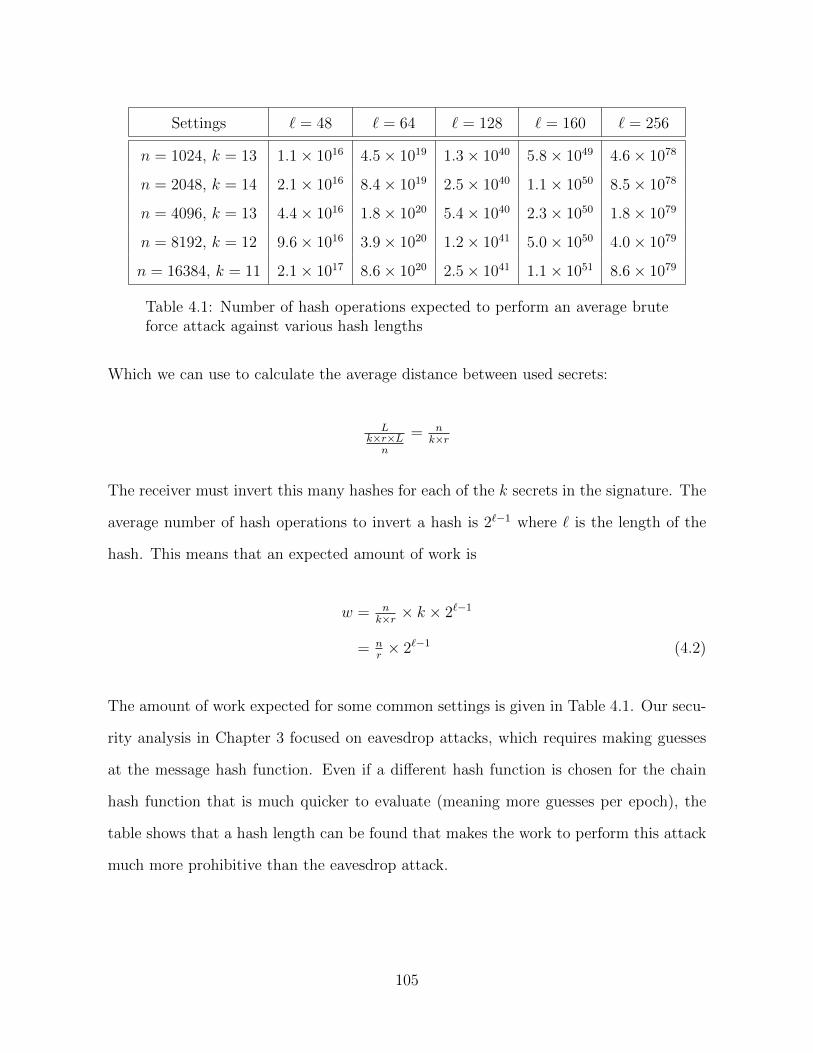
Settings ` = 48 ` = 64 ` = 128 ` = 160 ` = 256

n = 1024, k = 13 1.1× 1016 4.5× 1019 1.3× 1040 5.8× 1049 4.6× 1078

n = 2048, k = 14 2.1× 1016 8.4× 1019 2.5× 1040 1.1× 1050 8.5× 1078

n = 4096, k = 13 4.4× 1016 1.8× 1020 5.4× 1040 2.3× 1050 1.8× 1079

n = 8192, k = 12 9.6× 1016 3.9× 1020 1.2× 1041 5.0× 1050 4.0× 1079

n = 16384, k = 11 2.1× 1017 8.6× 1020 2.5× 1041 1.1× 1051 8.6× 1079

Table 4.1: Number of hash operations expected to perform an average bruteforce attack against various hash lengths

Which we can use to calculate the average distance between used secrets:

Lk×r×L

n

= nk×r

The receiver must invert this many hashes for each of the k secrets in the signature. The

average number of hash operations to invert a hash is 2`−1 where ` is the length of the

hash. This means that an expected amount of work is

w = nk×r × k × 2`−1

= nr× 2`−1 (4.2)

The amount of work expected for some common settings is given in Table 4.1. Our secu-

rity analysis in Chapter 3 focused on eavesdrop attacks, which requires making guesses

at the message hash function. Even if a different hash function is chosen for the chain

hash function that is much quicker to evaluate (meaning more guesses per epoch), the

table shows that a hash length can be found that makes the work to perform this attack

much more prohibitive than the eavesdrop attack.

105

4.3 Hash Chains

One of the biggest practical hurdles to implementing TV-OTS is efficient management

of hash chains. When studied from a high level, hash chain managers in literature, such

as FHT, appear to be a good choice. However, when studied at the level necessary for

implementation, it becomes apparent that many of the steps that FHT uses to achieve

its performance are completely wasted when integrated with TV-OTS. Using these hash

chain managers without modification would cause TV-OTS to run more slowly than

necessary.

4.3.1 Current Chain Managers and TV-OTS

The interdependency of successive FHT retrievals, used to establish an upper bound

on retrieval time described in Section 2.4.1, causes unnecessary operations when the

interval between desired values is large. The movement of any pebble relies on the

correct completion of prior pebble movements. Practically, this implies that values must

be retrieved from the chain in the expected, consecutive order, discarding unneeded

values. This iterative process is highly wasteful.

One prominent source of wasted computation when used with TV-OTS is the calculation

of values within ranges of values that ultimately go unused. For example, when a specific

target value is being retrieved, consider the pebbles moved to positions below the target

value. Since use of values is ordered (once a value is retrieved, the values at lower positions

will never be needed), the hash computations used to move pebbles into unused ranges

are completely wasted. For TV-OTS especially, a pebble is only useful once it moves

above its target value. We can use this observation to reduce unnecessary operations by

predicting each pebble’s final position and grouping each pebble’s individual movements

106

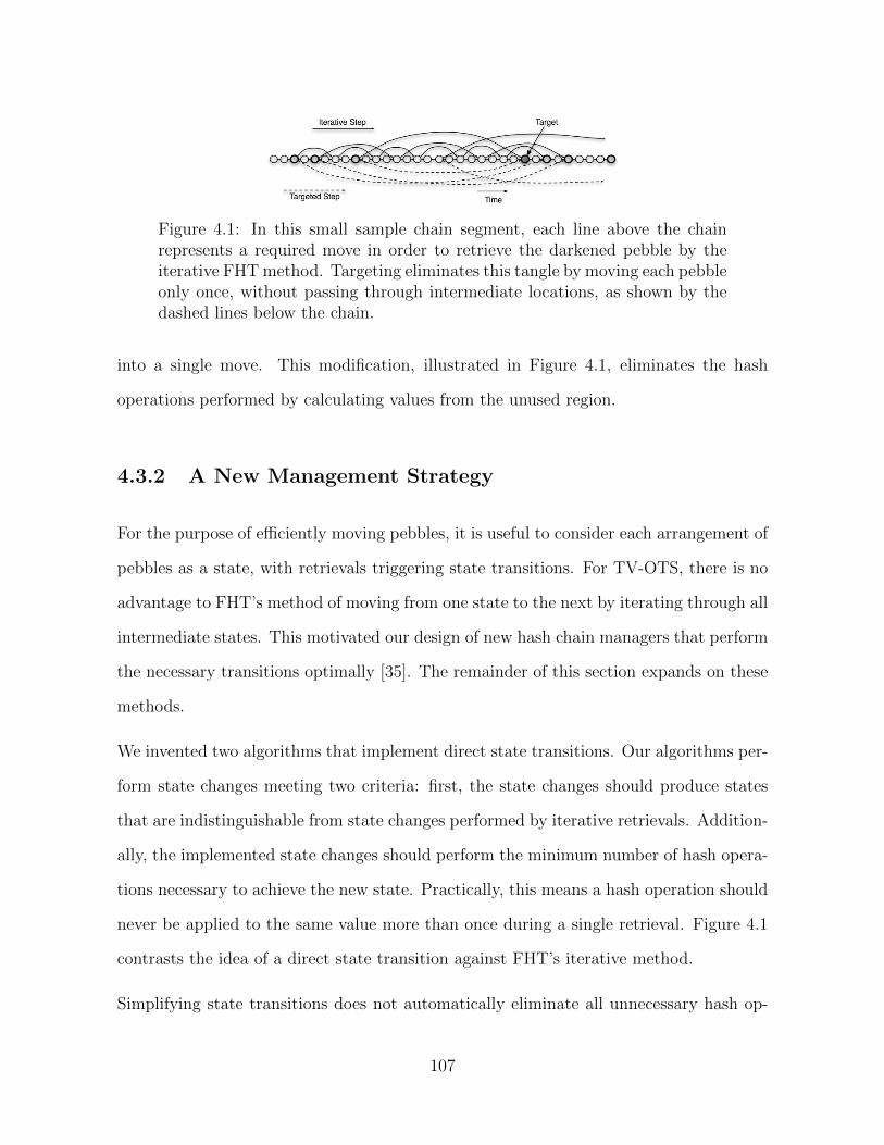
Figure 4.1: In this small sample chain segment, each line above the chainrepresents a required move in order to retrieve the darkened pebble by theiterative FHT method. Targeting eliminates this tangle by moving each pebbleonly once, without passing through intermediate locations, as shown by thedashed lines below the chain.

into a single move. This modification, illustrated in Figure 4.1, eliminates the hash

operations performed by calculating values from the unused region.

4.3.2 A New Management Strategy

For the purpose of efficiently moving pebbles, it is useful to consider each arrangement of

pebbles as a state, with retrievals triggering state transitions. For TV-OTS, there is no

advantage to FHT’s method of moving from one state to the next by iterating through all

intermediate states. This motivated our design of new hash chain managers that perform

the necessary transitions optimally [35]. The remainder of this section expands on these

methods.

We invented two algorithms that implement direct state transitions. Our algorithms per-

form state changes meeting two criteria: first, the state changes should produce states

that are indistinguishable from state changes performed by iterative retrievals. Addition-

ally, the implemented state changes should perform the minimum number of hash opera-

tions necessary to achieve the new state. Practically, this means a hash operation should

never be applied to the same value more than once during a single retrieval. Figure 4.1

contrasts the idea of a direct state transition against FHT’s iterative method.

Simplifying state transitions does not automatically eliminate all unnecessary hash op-

107

erations if pebbles are moved individually to their final destinations. Since calculating

the final value for a pebble involves hashing a value from later in the chain, it is possi-

ble, even likely, that values for multiple pebbles will be calculated from the same later

value. If pebbles are moved independently, the same values may get hashed with each

moved pebble, introducing redundant hash operations. To avoid this, movement should

be coordinated so that values are hashed only once and shared among the appropriate

pebbles.

Our two algorithms differ in how they handle the calculation of the new states. For

the purpose of explanation, the targeting algorithm has been divided into two stages:

state calculation and state transition. State calculation determines new destinations for

all pebbles that need to move and state transition performs the actual movements. The

major difference between the algorithms occurs in state calculation stage. One algorithm,

the Traveling Pebble algorithm, chooses destinations for each pebble iteratively relative

to pebbles that already have destinations. The other, the Jump Sweep algorithm, chooses

new destinations computationally based on the position of the target, and sorts the list by

destination. The Jump Sweep algorithm has a much simpler rule set than the Traveling

Pebble algorithm.

Once state calculation is complete, both algorithms perform what can be thought of as a

sweep which hashes values across the whole range into which pebbles will move. During

this sweep, pebbles end up with values corresponding to their final destination. In the

traveling pebble variation, the job of hashing each part of the range is given to the pebble

that must traverse the length of chain, and the values in that range are copied into other

pebbles when required. In the jump sweep algorithm, no particular entity is responsible

for the hashing, but the values are copied into the correct pebbles as the hash sweep

proceeds.

108

4.3.3 Traveling Pebble Algorithm

Traveling Pebble State Calculation

The correct state for any retrieval can be determined by a small set of rules which the state

calculator (given by Algorithm 2) uses to determine final pebble positions. The primary

property used in determining new positions is that each moving pebble must create an

interval below a larger pebble that matches the moving pebble’s ID. The larger pebbles

that assist in finding new destinations for moving pebbles are referred to as reference

pebbles. The reference pebbles limit the possible destinations of the moving pebbles,

some of which lie above the target and some below. Those below are disregarded as they

lie in a region of skipped values. Of the remaining possibilities, the lowest is chosen for

the moving pebble’s new destination. The choice of lowest position reflects that pebbles

moved iteratively will stop as soon as they move past the target. The availability of the

correct reference location is ensured by deciding the destinations for larger pebbles before

smaller ones. By knowing the destinations for all larger pebbles, the correct destination

is certain to be found for each moving pebble.

Because state calculation always chooses the lowest possible position, only one pebble

needs to be considered as a reference. Anticipating pebble movements, there are only

two pebbles that serve as possible references. These are the two closest in position to the

retrieval target. Of these two, the lower will be chosen assuming the moving pebble, when

positioned below this lower reference, will still be above the target. If this is not the case,

the other reference is chosen. In this second case, the two potential reference pebbles

border the interval for the moving pebble to split. Since this division is even, placing

the moving pebble at an interval below the higher of the two references is equivalent

to placing the moving pebble above the lower reference. Because this process is only

responsible for finding destinations and not for moving pebbles, knowing the position of

109

only this lower reference is sufficient to find the proper destination.

With these guiding principles in place, state calculation can be described as an iterative

algorithm for calculating individual pebble destinations. Setup requires finding the loca-

tion, β, of a pebble to use as the initial reference. Specifically, β is the position of the

pebble whose ID is the smallest from a certain set of pebbles. This set is comprised of all

the pebbles whose IDs are larger than the IDs of all the pebbles below the target1. The

number of pebbles below the target is a function of the interval length between retrieved

values. Once the number of pebbles to move is known, finding a pebble to use for β re-

quires checking pebbles above the target until one satisfies the criterion just mentioned.

Once β is determined, iteration can start with the pebble of the next lower ID.

The complete state calculation algorithm is given in Algorithm 2. The choice of pebble

used for β likely changes as iteration progresses through the moving pebbles. At any point

in time, β is intended to represent the lowest possible reference. Whenever a pebble’s

new destination is chosen to be below β, the current value of β is no longer valid as the

lowest reference. β is then updated using the most recently found destination. Once

the iteration completes, destinations have been determined for all pebbles. The lowest

destination matches the position of, or one step above, the position of the target.

Traveling Pebble State Transition

With a newly calculated target state, the challenge becomes efficient movement of pebbles

to their new positions. The Traveling Pebble algorithm uses the Function movePebble

to accomplish state transition with minimal hash operations.

The general approach of the Traveling Pebble method, given in Algorithm 3, is to begin

1Note that this set is not equivalent to all the pebbles above the target: a pebble below the targetcould have an ID larger than that of a pebble above the target.

110

Algorithm 2: State Calculation

Data: A list of pebbles L of length nInput: A target position tResult: L is modified/* initialize iteration control variables */

idx← b log2(t− L.getPebbleByIndex(0).pos+ 1)cnxtId← 2idx

p← L.getPebbleByIndex(idx)while p.dest < t or p.id ≤ nxtId do

idx← idx + 1nxtId← 2× nxtIdp← L.getPebbleByIndex(idx)

β ← p.pos/* begin iteration */

while nxtId > 1 dop← L.getPebbleByID(nxtId)/* Decide new position for p */

if p.id < β − t then/* p fits below β and above t */

β ← β − p.idp.dest← β

elsep.dest← β + p.id

/* update nxtId */

nxtId← nxtId/2

moving each value as quickly as possible, considering pebbles from largest to smallest.

In this way, larger pebbles begin their moves before smaller ones. When a pebble pt

is found to move, a lookahead operation is performed to determine the destination of

the next smaller pebble, ps. The destination of ps determines whether pt may complete

its move, or whether it must begin its move but pause when it reaches ps’s destination,

allowing ps to copy the value at pt’s position. If this is indeed the case, this procedure

is followed and then repeated for a new ps, performing lookahead operations for smaller

pebbles until one is found whose destination lies below that of pt. At this point, no more

smaller pebbles need to move above pt and pt completes its move.

111

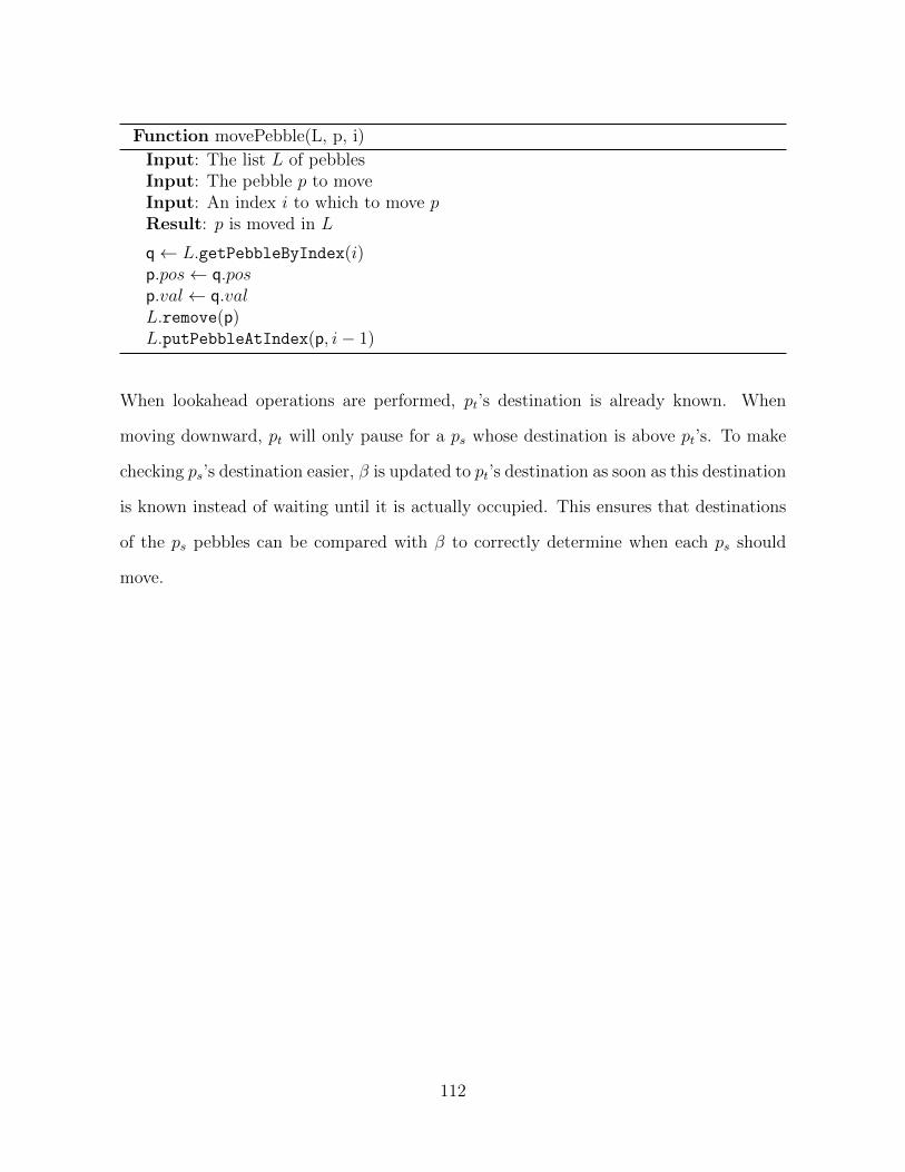
Function movePebble(L, p, i)

Input: The list L of pebblesInput: The pebble p to moveInput: An index i to which to move pResult: p is moved in L

q← L.getPebbleByIndex(i)p.pos← q.posp.val← q.valL.remove(p)L.putPebbleAtIndex(p, i− 1)

When lookahead operations are performed, pt’s destination is already known. When

moving downward, pt will only pause for a ps whose destination is above pt’s. To make

checking ps’s destination easier, β is updated to pt’s destination as soon as this destination

is known instead of waiting until it is actually occupied. This ensures that destinations

of the ps pebbles can be compared with β to correctly determine when each ps should

move.

112

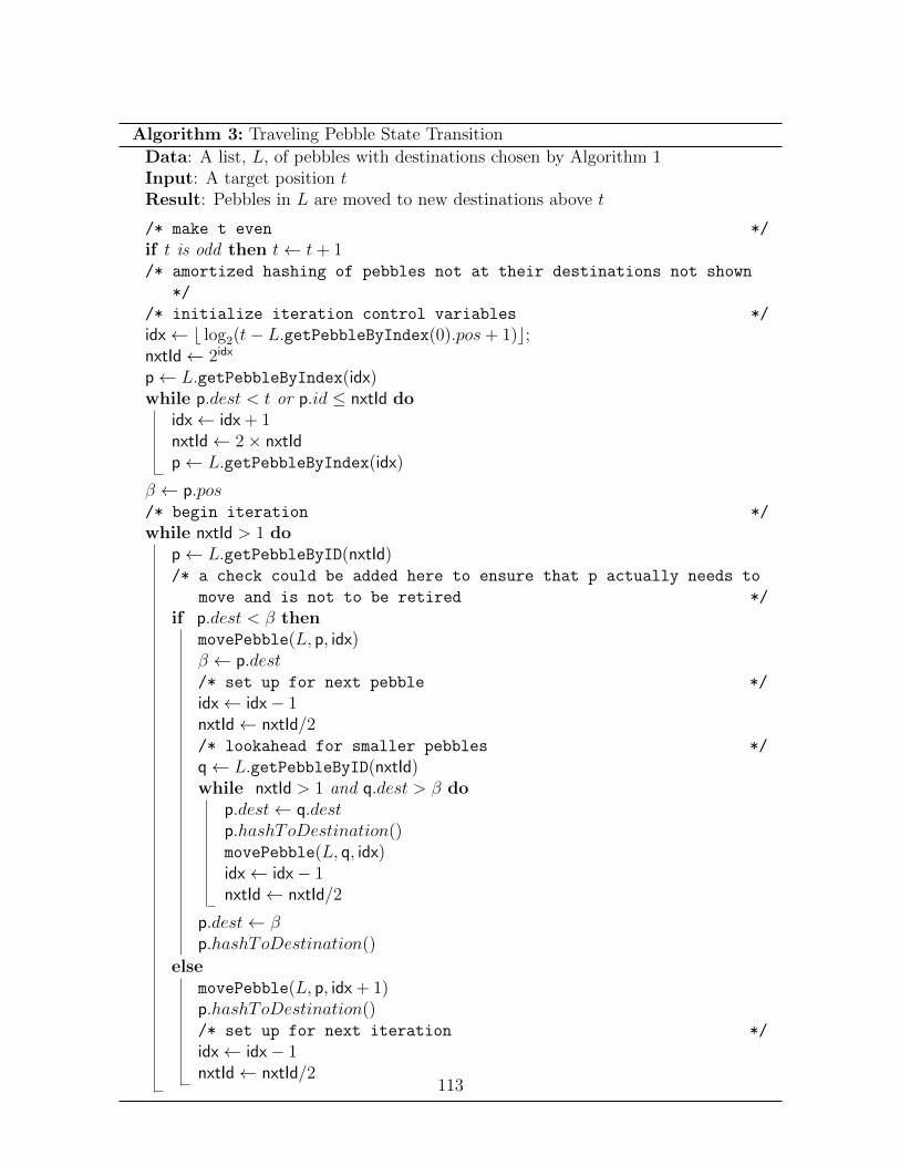
Algorithm 3: Traveling Pebble State Transition

Data: A list, L, of pebbles with destinations chosen by Algorithm 1Input: A target position tResult: Pebbles in L are moved to new destinations above t

/* make t even */

if t is odd then t← t+ 1/* amortized hashing of pebbles not at their destinations not shown

*/

/* initialize iteration control variables */

idx← b log2(t− L.getPebbleByIndex(0).pos+ 1)c;nxtId← 2idx

p← L.getPebbleByIndex(idx)while p.dest < t or p.id ≤ nxtId do

idx← idx + 1nxtId← 2× nxtIdp← L.getPebbleByIndex(idx)

β ← p.pos/* begin iteration */

while nxtId > 1 dop← L.getPebbleByID(nxtId)/* a check could be added here to ensure that p actually needs to

move and is not to be retired */

if p.dest < β thenmovePebble(L, p, idx)β ← p.dest/* set up for next pebble */

idx← idx− 1nxtId← nxtId/2/* lookahead for smaller pebbles */

q← L.getPebbleByID(nxtId)while nxtId > 1 and q.dest > β do

p.dest← q.destp.hashToDestination()movePebble(L, q, idx)idx← idx− 1nxtId← nxtId/2

p.dest← βp.hashToDestination()

elsemovePebble(L, p, idx + 1)p.hashToDestination()/* set up for next iteration */

idx← idx− 1nxtId← nxtId/2

113

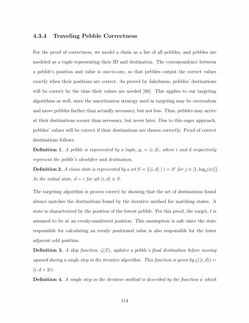
4.3.4 Traveling Pebble Correctness

For the proof of correctness, we model a chain as a list of all pebbles, and pebbles are

modeled as a tuple representing their ID and destination. The correspondence between

a pebble’s position and value is one-to-one, so that pebbles output the correct values

exactly when their positions are correct. As proved by Jakobsson, pebbles’ destinations

will be correct by the time their values are needed [80]. This applies to our targeting

algorithms as well, since the amortization strategy used in targeting may be overzealous

and move pebbles farther than actually necessary, but not less. Thus, pebbles may arrive

at their destinations sooner than necessary, but never later. Due to this eager approach,

pebbles’ values will be correct if their destinations are chosen correctly. Proof of correct

destinations follows.

Definition 1. A pebble is represented by a tuple, pi = 〈i, d〉, where i and d respectively

represent the pebble’s identifier and destination.

Definition 2. A chain state is represented by a set S = 〈i, d〉 | i = 2j for j ∈ [1, log2(n)].

In the initial state, d = i for all 〈i, d〉 ∈ S.

The targeting algorithm is proven correct by showing that the set of destinations found

always matches the destinations found by the iterative method for matching states. A

state is characterized by the position of the lowest pebble. For this proof, the target, t is

assumed to be at an evenly-numbered position. This assumption is safe since the state

responsible for calculating an evenly positioned value is also responsible for the lower

adjacent odd position.

Definition 3. A skip function, ζ(S), updates a pebble’s final destination before moving

upward during a single step in the iterative algorithm. This function is given by ζ(〈i, d〉) =

(i, d+ 2i).

Definition 4. A single step in the iterative method is described by the function ψ which

114

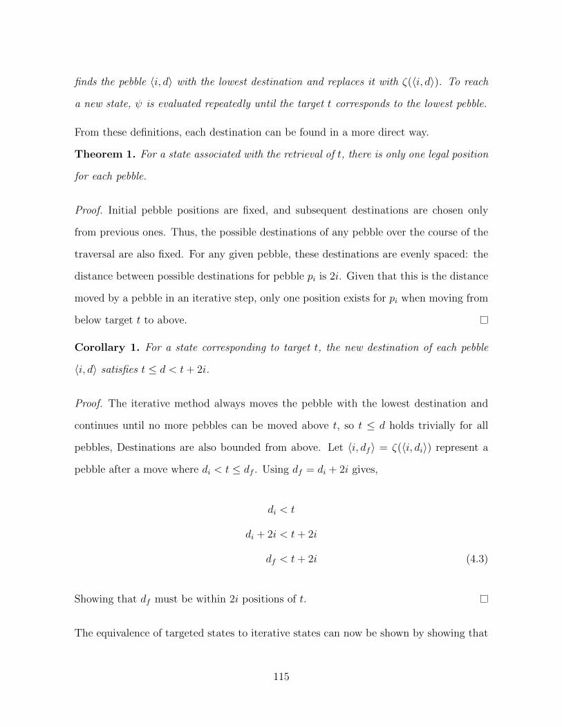
finds the pebble 〈i, d〉 with the lowest destination and replaces it with ζ(〈i, d〉). To reach

a new state, ψ is evaluated repeatedly until the target t corresponds to the lowest pebble.

From these definitions, each destination can be found in a more direct way.

Theorem 1. For a state associated with the retrieval of t, there is only one legal position

for each pebble.

Proof. Initial pebble positions are fixed, and subsequent destinations are chosen only

from previous ones. Thus, the possible destinations of any pebble over the course of the

traversal are also fixed. For any given pebble, these destinations are evenly spaced: the

distance between possible destinations for pebble pi is 2i. Given that this is the distance

moved by a pebble in an iterative step, only one position exists for pi when moving from

below target t to above.

Corollary 1. For a state corresponding to target t, the new destination of each pebble

〈i, d〉 satisfies t ≤ d < t+ 2i.

Proof. The iterative method always moves the pebble with the lowest destination and

continues until no more pebbles can be moved above t, so t ≤ d holds trivially for all

pebbles, Destinations are also bounded from above. Let 〈i, df〉 = ζ(〈i, di〉) represent a

pebble after a move where di < t ≤ df . Using df = di + 2i gives,

di < t

di + 2i < t+ 2i

df < t+ 2i (4.3)

Showing that df must be within 2i positions of t.

The equivalence of targeted states to iterative states can now be shown by showing that

115

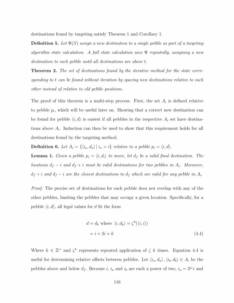
destinations found by targeting satisfy Theorem 1 and Corollary 1.

Definition 5. Let Ψ(S) assign a new destination to a single pebble as part of a targeting

algorithm state calculation. A full state calculation uses Ψ repeatedly, assigning a new

destination to each pebble until all destinations are above t.

Theorem 2. The set of destinations found by the iterative method for the state corre-

sponding to t can be found without iteration by spacing new destinations relative to each

other instead of relative to old pebble positions.

The proof of this theorem is a multi-step process. First, the set Ai is defined relative

to pebble pi, which will be useful later on. Showing that a correct new destination can

be found for pebble 〈i, d〉 is easiest if all pebbles in the respective Ai set have destina-

tions above Ai. Induction can then be used to show that this requirement holds for all

destinations found by the targeting method.

Definition 6. Let Ai = 〈ia, da〉 | ia > i relative to a pebble pi = 〈i, d〉.

Lemma 1. Given a pebble pi = 〈i, di〉 to move, let df be a valid final destination. The

locations df − i and df + i must be valid destinations for two pebbles in Ai. Moreover,

df + i and df − i are the closest destinations to df which are valid for any pebble in Ai.

Proof. The precise set of destinations for each pebble does not overlap with any of the

other pebbles, limiting the pebbles that may occupy a given location. Specifically, for a

pebble 〈i, d〉, all legal values for d fit the form

d = dk where 〈i, dk〉 = ζk(〈i, i〉)

= i+ 2i× k (4.4)

Where k ∈ Z+ and ζk represents repeated application of ζ k times. Equation 4.4 is

useful for determining relative offsets between pebbles. Let 〈ia, da〉 , 〈ib, db〉 ∈ Ai be the

pebbles above and below df . Because i, ia and ib are each a power of two, ia = 2jai and

116

ib = 2jbi for some ja, jb ∈ Z+. Using Equation 4.4, da and db can be rewritten to obtain

expressions in terms of df and i: such that da = df + i and db = df − i.

For da:

da = ia + 2iaka

= 2jai+ 2(2jaika)

= 2i(2ja−1 + 2jaka)

Setting k = 2jaka + 2ja−1 − 1 :

da = 2i(k + 1)

= 2i+ 2ik

= df + i (4.5)

And similarly for db:

db = ib + 2ibkb

= 2jbi+ 2(2jbikb)

= 2i(2jb−1 + 2jbkb)

Setting k = 2jbkb + 2jb−1 :

db = 2i(k)

= df − i (4.6)

The fact that there is no third pebble 〈ic, dc〉 ∈ Ai satisfying db ≤ dc ≤ da stems from

the same positional relationships that relate i, ia and ib. By Equations 4.5 and 4.6, the

distance between ia and ib is 2i. Moreover, the distances between any two pebbles in

Ai must be a multiple of 2i. No pebble from Ai could be between da and db without

violating this condition.

117

Lemma 2 shifts perspective, building on Lemma 1 to show that the destinations for larger

pebbles surrounding each new destination can be used to find this new destination.

Lemma 2 builds on Lemma 1 to show that the larger pebbles surrounding each new

destination can be used to find this destination.

Lemma 2. Let 〈i, d〉 be a pebble to be moved to an unknown destination df . Assume

that all pebbles in Ai currently have destinations above t. In this situation, a pebble from

Ai will be located at either df + i or df − i.

Proof. By definition, Ai must contain a pebble, 〈i2i, d2i〉, such that i2i = 2i. Corollary 1

requires that t ≤ d2i < t+ 2i2i. Note 2i2i = 4i, so if

t ≤ d2i < t+ 3i,

then Lemma 2 is clearly satisfied with df − i = d2i. In the remaining case,

t+ 3i ≤ d2i < t+ 4i.

Here, Equation 4.6 states that there must be a pebble destination at d2i − i2i = df − i.

Furthermore, with df ± i above t, the pebbles corresponding to these destinations must

be in Ai and therefore actively present in these positions.

Moreover, there must be a pebble at this location; this pebble must be in Ai and thus

must be above t. Letting da = d2i − i2i gives

t ≤ da < t+ i and

df = da + i < t+ 2i

satisfying Lemma 2.

118

The Ψ function applies the above procedure, finding a pebble pi with a valid Ai set and

updating its destination. Induction can now be applied in a full proof of Theorem 2,

showing that starting from any correct state, the new destinations found for all pebbles

form a new correct state.

Proof. Base case: A pebble pi = 〈i, d〉 exists such that the corresponding Ai set contains

only pebbles that are above t. This is necessarily true unless pi will move beyond the end

of the chain, in which case this proof is unnecessary. In such a state, a new destination

for pi can be correctly determined.

The targeting algorithm begins by finding a pebble 〈i, d〉 such that d < t and every

pebble in the relative Ai set is above t. The pebble 〈i, d〉 is the pebble detected by Ψ

and moved.

Since all the pebbles that need to move are in S − Ai, then all pebbles in Ai are in

position and by Lemma 2, Ψ will be able to correctly determine a new location for 〈i, d〉.

Inductive Step: Given a state where a new destination can be determined for pi = 〈i, d〉,

applying Ψ(S) and updating this pebble’s destination results in a state where either 1)

no more pebbles need to be updated, or 2) there is now a new pebble to which Ψ can be

applied. The first case trivially halts the induction. In the second, using Ψ to determine a

new destination for pi automatically results in a new partitioning where all the pebbles in

Ai/2 = Ai∪〈i, d〉 now have destinations above t. Thus, a new pebble, p1/2 =⟨ii/2, di/2

⟩,

is found for which a new destination can be found. In some cases, d1/2 will already be

above t, however, this causes no change since exactly the same two cases apply as if p1/2

had just been updated.

Targeting transitions follow these steps of iteratively applying Ψ(S) and moving each

pebble, and hence the new destination of each pebble will be correct. Thus, each state

119

will correctly match the state found by the iterative method for the same target. Since

both algorithms start from identical initial states, correctness is ensured over arbitrary

state changes.

4.3.5 Jump Sweep Algorithm

Jump Sweep State Calculation and Transition

The jump sweep algorithm is a much simpler, intuitive algorithm albeit with higher

complexity bounds. The entire algorithm is given in Algorithm 4. The state calculation

phase simply iterates through pebbles, mathematically calculating new destinations for

each pebble. The calculation finds the smallest multiple of the distance the pebble would

move in an iterative step such that this new distance is greater than the pebble’s current

distance from the target. That is, for pebble with position pos id ID, we find the smallest

possible multiplier κ such that pos+ κ× (2× ID) > t for target t.

This value is the pebble’s next destination. Once all pebbles have destinations, the list is

sorted by destination. The list is now ready for the hashing phase of the algorithm.

In the hashing phase, all the moving pebbles copy a value from the next higher pebble

and hash it until they reach their destination. We take advantage of the fact that the

pebble holding the seed of the hash chain never moves, meaning at least one pebble is

stationary and always has the correct value that other pebbles may copy. The process

of moving pebbles iterates backward through the list, starting with the seed. For each

pebble, pc, we check if the pc’s position matches its destination. If not, we know that

the position and destination of the previously iterated pebble, pp, do match. In this case

pp’s value and position are copied into pc, and pc is hashed until its target destination

for that pebble is reached, meaning its position and destination are the same. When

120

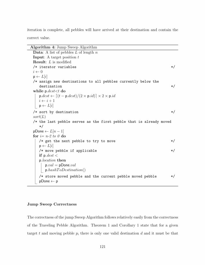
iteration is complete, all pebbles will have arrived at their destination and contain the

correct value.

Algorithm 4: Jump Sweep Algorithm

Data: A list of pebbles L of length nInput: A target position tResult: L is modified/* iterator variables */

i← 0p← L[i]/* assign new destinations to all pebbles currently below the

destination */

while p.dest<t dop.dest← d(t− p.dest)/(2× p.id)e × 2× p.idi← i+ 1p← L[i]

/* sort by destination */

sort(L)/* the last pebble serves as the first pebble that is already moved

*/

pDone← L[n− 1]for i= n-2 to 0 do

/* get the next pebble to try to move */

p← L[i]/* move pebble if applicable */

if p.dest <p.location then

p.val = pDone.valp.hashToDestination()

/* store moved pebble and the current pebble moved pebble */

pDone← p

Jump Sweep Correctness

The correctness of the jump Sweep Algorithm follows relatively easily from the correctness

of the Traveling Pebble Algorithm. Theorem 1 and Corollary 1 state that for a given

target t and moving pebble pi there is only one valid destination d and it must be that

121

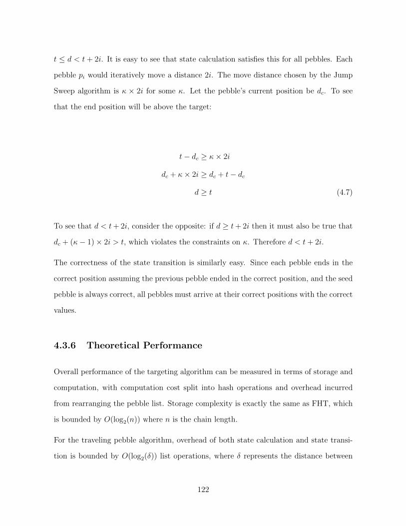
t ≤ d < t + 2i. It is easy to see that state calculation satisfies this for all pebbles. Each

pebble pi would iteratively move a distance 2i. The move distance chosen by the Jump

Sweep algorithm is κ × 2i for some κ. Let the pebble’s current position be dc. To see

that the end position will be above the target:

t− dc ≥ κ× 2i

dc + κ× 2i ≥ dc + t− dc

d ≥ t (4.7)

To see that d < t+ 2i, consider the opposite: if d ≥ t+ 2i then it must also be true that

dc + (κ− 1)× 2i > t, which violates the constraints on κ. Therefore d < t+ 2i.

The correctness of the state transition is similarly easy. Since each pebble ends in the

correct position assuming the previous pebble ended in the correct position, and the seed

pebble is always correct, all pebbles must arrive at their correct positions with the correct

values.

4.3.6 Theoretical Performance

Overall performance of the targeting algorithm can be measured in terms of storage and

computation, with computation cost split into hash operations and overhead incurred

from rearranging the pebble list. Storage complexity is exactly the same as FHT, which

is bounded by O(log2(n)) where n is the chain length.

For the traveling pebble algorithm, overhead of both state calculation and state transi-

tion is bounded by O(log2(δ)) list operations, where δ represents the distance between

122

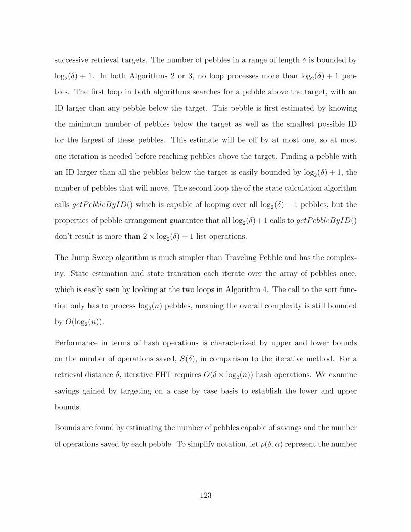
successive retrieval targets. The number of pebbles in a range of length δ is bounded by

log2(δ) + 1. In both Algorithms 2 or 3, no loop processes more than log2(δ) + 1 peb-

bles. The first loop in both algorithms searches for a pebble above the target, with an

ID larger than any pebble below the target. This pebble is first estimated by knowing

the minimum number of pebbles below the target as well as the smallest possible ID

for the largest of these pebbles. This estimate will be off by at most one, so at most

one iteration is needed before reaching pebbles above the target. Finding a pebble with

an ID larger than all the pebbles below the target is easily bounded by log2(δ) + 1, the

number of pebbles that will move. The second loop the of the state calculation algorithm

calls getPebbleByID() which is capable of looping over all log2(δ) + 1 pebbles, but the

properties of pebble arrangement guarantee that all log2(δ)+1 calls to getPebbleByID()

don’t result is more than 2× log2(δ) + 1 list operations.

The Jump Sweep algorithm is much simpler than Traveling Pebble and has the complex-

ity. State estimation and state transition each iterate over the array of pebbles once,

which is easily seen by looking at the two loops in Algorithm 4. The call to the sort func-

tion only has to process log2(n) pebbles, meaning the overall complexity is still bounded

by O(log2(n)).

Performance in terms of hash operations is characterized by upper and lower bounds

on the number of operations saved, S(δ), in comparison to the iterative method. For a

retrieval distance δ, iterative FHT requires O(δ× log2(n)) hash operations. We examine

savings gained by targeting on a case by case basis to establish the lower and upper

bounds.

Bounds are found by estimating the number of pebbles capable of savings and the number

of operations saved by each pebble. To simplify notation, let ρ(δ, α) represent the number

123

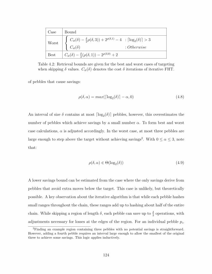
Case Bound

Worst

Cit(δ)− δ2ρ(δ, 3)) + 2ρ(δ,1) − 4 : dlog2(δ)e > 3

Cit(δ) : Otherwise

Best Cit(δ)− δ2(ρ(δ, 1))− 2ρ(δ,0) + 2

Table 4.2: Retrieval bounds are given for the best and worst cases of targetingwhen skipping δ values. Cit(δ) denotes the cost δ iterations of iterative FHT.

of pebbles that cause savings:

ρ(δ, α) = max(dlog2(δ)e − α, 0) (4.8)

An interval of size δ contains at most dlog2(δ)e pebbles, however, this overestimates the

number of pebbles which achieve savings by a small number α. To form best and worst

case calculations, α is adjusted accordingly. In the worst case, at most three pebbles are

large enough to step above the target without achieving savings2. With 0 ≤ α ≤ 3, note

that:

ρ(δ, α) ∈ Θ(log2(δ)) (4.9)

A lower savings bound can be estimated from the case where the only savings derive from

pebbles that avoid extra moves below the target. This case is unlikely, but theoretically

possible. A key observation about the iterative algorithm is that while each pebble hashes

small ranges throughout the chain, these ranges add up to hashing about half of the entire

chain. While skipping a region of length δ, each pebble can save up to δ2

operations, with

adjustments necessary for losses at the edges of the region. For an individual pebble pi,

2Finding an example region containing three pebbles with no potential savings is straightforward.However, adding a fourth pebble requires an interval large enough to allow the smallest of the originalthree to achieve some savings. This logic applies inductively.

124

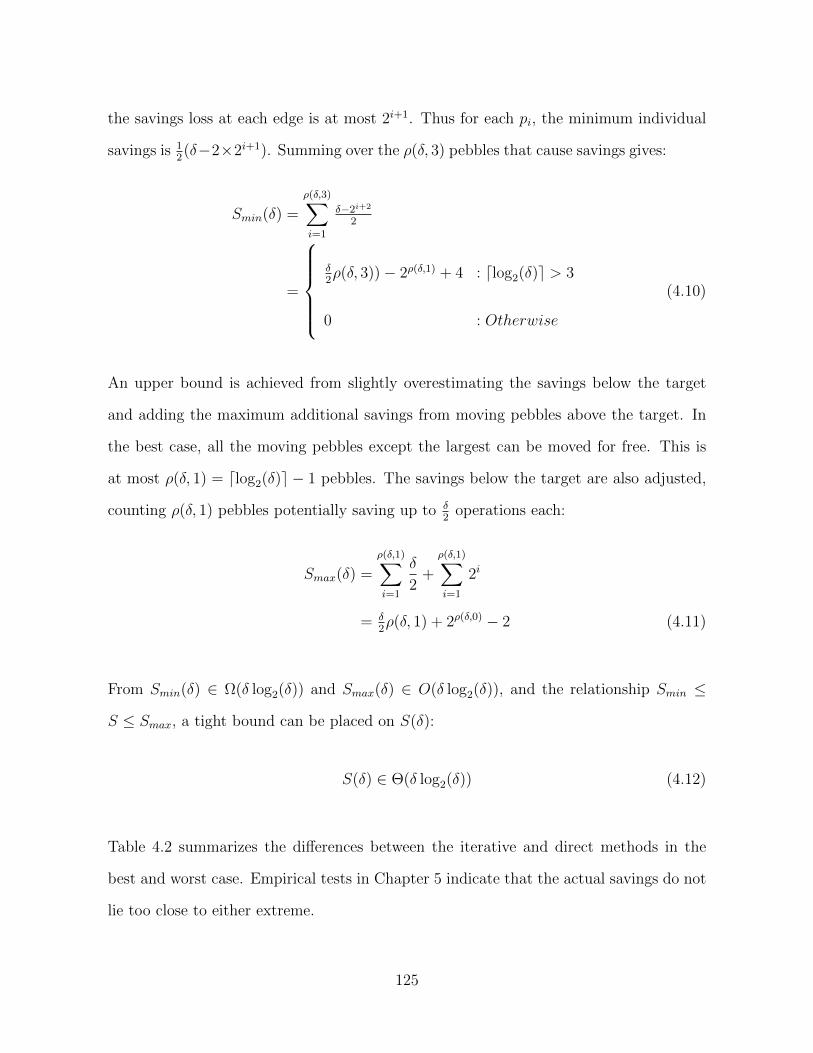
the savings loss at each edge is at most 2i+1. Thus for each pi, the minimum individual

savings is 12(δ−2×2i+1). Summing over the ρ(δ, 3) pebbles that cause savings gives:

Smin(δ) =

ρ(δ,3)∑i=1

δ−2i+2

2

=

δ2ρ(δ, 3))− 2ρ(δ,1) + 4 : dlog2(δ)e > 3

0 : Otherwise

(4.10)

An upper bound is achieved from slightly overestimating the savings below the target

and adding the maximum additional savings from moving pebbles above the target. In

the best case, all the moving pebbles except the largest can be moved for free. This is

at most ρ(δ, 1) = dlog2(δ)e − 1 pebbles. The savings below the target are also adjusted,

counting ρ(δ, 1) pebbles potentially saving up to δ2

operations each:

Smax(δ) =

ρ(δ,1)∑i=1

δ

2+

ρ(δ,1)∑i=1

2i

= δ2ρ(δ, 1) + 2ρ(δ,0) − 2 (4.11)

From Smin(δ) ∈ Ω(δ log2(δ)) and Smax(δ) ∈ O(δ log2(δ)), and the relationship Smin ≤

S ≤ Smax, a tight bound can be placed on S(δ):

S(δ) ∈ Θ(δ log2(δ)) (4.12)

Table 4.2 summarizes the differences between the iterative and direct methods in the

best and worst case. Empirical tests in Chapter 5 indicate that the actual savings do not

lie too close to either extreme.

125

Chapter 5

TV-OTS Testing and Results

5.1 Experimental Setup

5.1.1 Parameter Choices

In order for latency testing to provide meaningful results, we needed parameter choices

that balance the tradeoff between security and runtime efficiency. Because different

systems will have different requirements, our test cases include choices for the number

of chains, n, ranging from 1024 to 32768. Each n allows different possible values for the

number of messages per epoch, r, and secrets per signature, k, depending on the security

requirements of the system. We tested a large number of parameter combinations in

order to show the change in performance based on parameter choices.

To choose parameters we started with various values for n and fixed values of k. As seen

in Chapter 3, optimal choices for r and k are mutually dependent. For testing purposes,

we chose to fix k relative to n and vary r. This means that is some cases, specifically for

smaller n, our test results are not necessarily based on optimally secure settings. Results

126

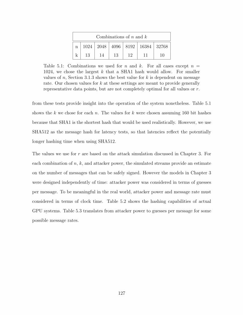
Combinations of n and k

n 1024 2048 4096 8192 16384 32768

k 13 14 13 12 11 10

Table 5.1: Combinations we used for n and k. For all cases except n =1024, we chose the largest k that a SHA1 hash would allow. For smallervalues of n, Section 3.1.3 shows the best value for k is dependent on messagerate. Our chosen values for k at these settings are meant to provide generallyrepresentative data points, but are not completely optimal for all values or r.

from these tests provide insight into the operation of the system nonetheless. Table 5.1

shows the k we chose for each n. The values for k were chosen assuming 160 bit hashes

because that SHA1 is the shortest hash that would be used realistically. However, we use

SHA512 as the message hash for latency tests, so that latencies reflect the potentially

longer hashing time when using SHA512.

The values we use for r are based on the attack simulation discussed in Chapter 3. For

each combination of n, k, and attacker power, the simulated streams provide an estimate

on the number of messages that can be safely signed. However the models in Chapter 3

were designed independently of time: attacker power was considered in terms of guesses

per message. To be meaningful in the real world, attacker power and message rate must

considered in terms of clock time. Table 5.2 shows the hashing capabilities of actual

GPU systems. Table 5.3 translates from attacker power to guesses per message for some

possible message rates.

127

System SHA1 SHA256 SHA512 SHA512crypt BCrypt

8×NVIDIATesla M20501.15GHz GPUs[103]

1.41× 109

2× AMDRadeon 880MHzGPUs [3]

7.97× 109 3.09× 109 2.67× 108

25× AMDRadeon 725 to925 MHz GPUs[127]

6.3× 1010 2.30× 1010 3.64× 105 7× 104

8× Nvidia GTX1080 1.6GHzGPUs [1]

6.87× 1010 2.30× 1010 8.62× 109 1.17× 106 1.05× 105

Table 5.2: Real-world hashing systems and their capabilities (in hashes persecond)

128

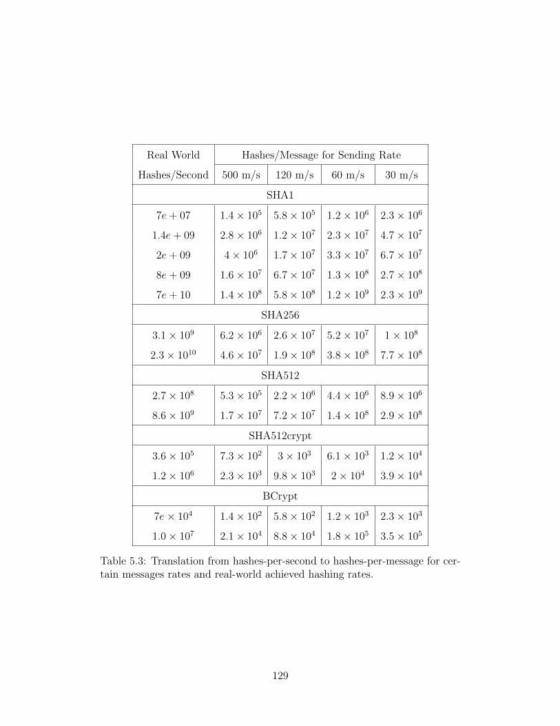
Real World Hashes/Message for Sending Rate

Hashes/Second 500 m/s 120 m/s 60 m/s 30 m/s

SHA1

7e+ 07 1.4× 105 5.8× 105 1.2× 106 2.3× 106

1.4e+ 09 2.8× 106 1.2× 107 2.3× 107 4.7× 107

2e+ 09 4× 106 1.7× 107 3.3× 107 6.7× 107

8e+ 09 1.6× 107 6.7× 107 1.3× 108 2.7× 108

7e+ 10 1.4× 108 5.8× 108 1.2× 109 2.3× 109

SHA256

3.1× 109 6.2× 106 2.6× 107 5.2× 107 1× 108

2.3× 1010 4.6× 107 1.9× 108 3.8× 108 7.7× 108

SHA512

2.7× 108 5.3× 105 2.2× 106 4.4× 106 8.9× 106

8.6× 109 1.7× 107 7.2× 107 1.4× 108 2.9× 108

SHA512crypt

3.6× 105 7.3× 102 3× 103 6.1× 103 1.2× 104

1.2× 106 2.3× 103 9.8× 103 2× 104 3.9× 104

BCrypt

7e× 104 1.4× 102 5.8× 102 1.2× 103 2.3× 103

1.0× 107 2.1× 104 8.8× 104 1.8× 105 3.5× 105

Table 5.3: Translation from hashes-per-second to hashes-per-message for cer-tain messages rates and real-world achieved hashing rates.

129

With current technology, a realistic adversary could be capable of up to 109 guesses

per message depending on their resources, the system’s message rate, and the choice

of message hash function. The attacker’s rate can be limited by using slower functions

for the message hash. We use the models from Chapter 3 to identify the largest safe

choices for r for attacker strengths between 104 and 106 guesses per message. Table 5.4

presents our chosen test settings. Unless otherwise specified, we used relatively short

chain lengths of L = 1024 which allows us to observe the behavior over multiple chains

without having to gather an excessive amount of data. Note that the probability of

eavesdrop attacks is independent of L, the a small increase in signing latency can be

expected as L increases.

130

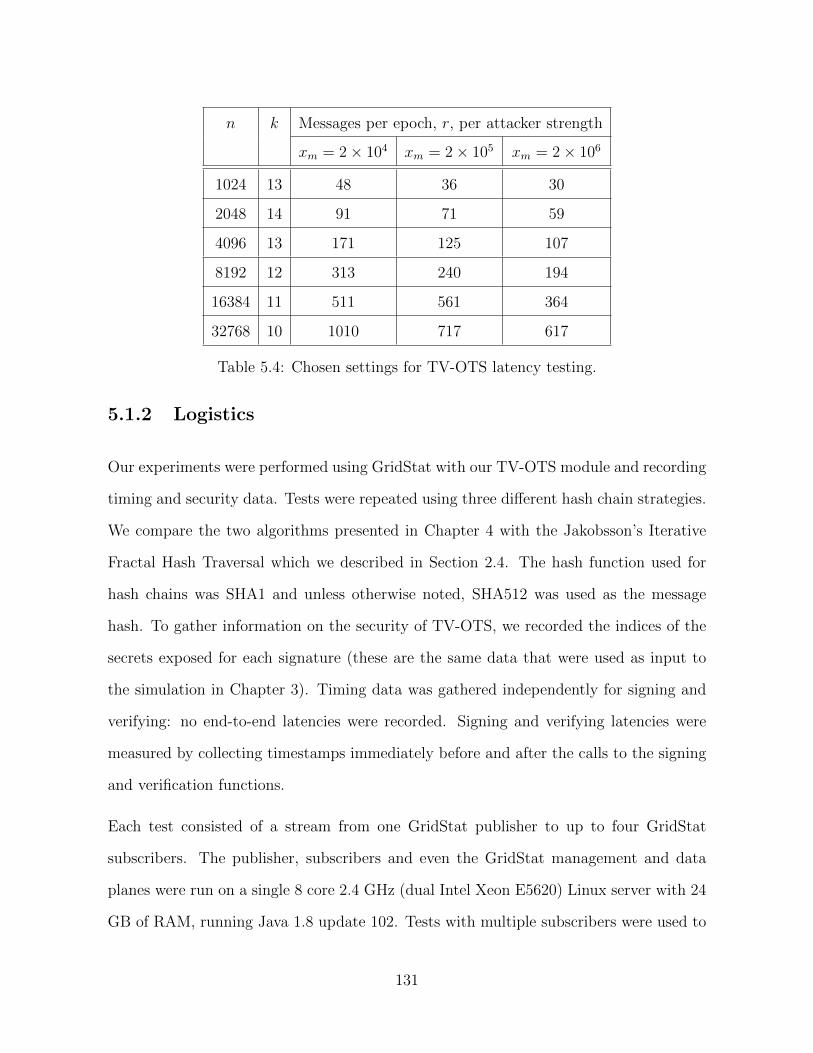
n k Messages per epoch, r, per attacker strength

xm = 2× 104 xm = 2× 105 xm = 2× 106

1024 13 48 36 30

2048 14 91 71 59

4096 13 171 125 107

8192 12 313 240 194

16384 11 511 561 364

32768 10 1010 717 617

Table 5.4: Chosen settings for TV-OTS latency testing.

5.1.2 Logistics

Our experiments were performed using GridStat with our TV-OTS module and recording

timing and security data. Tests were repeated using three different hash chain strategies.

We compare the two algorithms presented in Chapter 4 with the Jakobsson’s Iterative

Fractal Hash Traversal which we described in Section 2.4. The hash function used for

hash chains was SHA1 and unless otherwise noted, SHA512 was used as the message

hash. To gather information on the security of TV-OTS, we recorded the indices of the

secrets exposed for each signature (these are the same data that were used as input to

the simulation in Chapter 3). Timing data was gathered independently for signing and

verifying: no end-to-end latencies were recorded. Signing and verifying latencies were

measured by collecting timestamps immediately before and after the calls to the signing

and verification functions.

Each test consisted of a stream from one GridStat publisher to up to four GridStat

subscribers. The publisher, subscribers and even the GridStat management and data

planes were run on a single 8 core 2.4 GHz (dual Intel Xeon E5620) Linux server with 24

GB of RAM, running Java 1.8 update 102. Tests with multiple subscribers were used to

131

show how different loss rates would affect verification latency. We simulated packet loss

by adding an option to GridStat subscribers which would randomly drop packets before

passing them to the security modules. Except for tests using long chains, 40 minutes

were allowed for the combined key generation and message streaming time. Tests with

long chains (L ≥ 16384) were allowed twice the time to allow for significantly greater

initial key generation times. For efficient testing, TV-OTS messages were published every

two milliseconds with an epoch length set to 2× r milliseconds. Note that latencies are

dependent on the number of messages sent per epoch and not the epoch length itself,

meaning latency results are relative to r, regardless of the amount of time taken to send

r messages.

5.2 Experimental Results

Our primary goal was to show the latencies of a real-world implementation of TV-OTS.

We also measured performance in terms of number of chain hashes, which helps determine

the cause of jitter in TV-OTS latencies. We also measured the ratio between keystream

and payload messages and collected security data to support our theoretical conclusions

about security from Chapter 3.

5.2.1 Latency Measurements

This section shows a sample of our test results. We present results in two forms: av-

erage latencies and per-message latency measurements. We use bar charts to compare

average latencies between various parameter sets. When signing and verifying are shown

on the same graph, signing is shown above the x-axis and verifying is shown below.

Where relevant, the three different hash chain management algorithms, Iterative FHT,

132

the Jump-Sweep algorithm, and the Traveling Pebble algorithm are shown side by side.

Note that hash chain management algorithms affect only signing latencies.

We performed a variety of tests to compare performance between different TV-OTS

parameter settings. We show the general effects of n, k and r on signing latency and

compare to ECDSA, RSA and DSA in Figures 5.1 and 5.2. Tests to reveal the effects

of chain length showed little difference, but did demonstrate the general effectiveness

of the optimized hash chain algorithms for long chains as shown in Figure 5.4. Finally,

Figure 5.3 shows that average verifying latency does increase if the receivers are connected

via a lossy network, as expected.

We also zoom in on the behavior of TV-OTS by showing stream graphs, which show each

individual latency point in a stream of TV-OTS messages. These graphs show that our

implementation of TV-OTS is not absolutely consistent and outlying signing latencies of

3-5 milliseconds are not uncommon, and ever longer latencies do occur. These graphs

are more interesting for the patterns that emerge. Figures 5.5, 5.6 and 5.7 show signing

latency stream graphs for the different algorithms and a sample of settings. These graphs

show periodic behavior emerging in signing latencies. However, no such patterns appear

for verifying latencies, as shown in Figure 5.11. Graphs that show the hash workload per

message, instead of latency per message, help explain the patterns that emerge in signing

latency. These graphs, shown in Figures 5.8, 5.9 and 5.10, roughly show the amount of

hashing performed per message. However, the graphs are only approximate because they

count all hashes that occur between the sending of sequential messages, whether those

hashes occur due to signing or calculating new hash chains for keystreams. Figure 5.12

compares signing latencies using SHA1 and SHA512 as the message hash, showing no

observable difference.

133

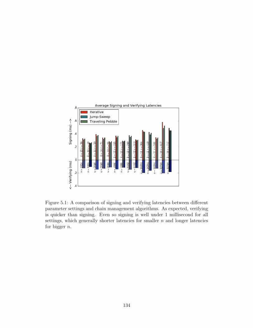
Figure 5.1: A comparison of signing and verifying latencies between differentparameter settings and chain management algorithms. As expected, verifyingis quicker than signing. Even so signing is well under 1 millisecond for allsettings, which generally shorter latencies for smaller n and longer latenciesfor bigger n.

134

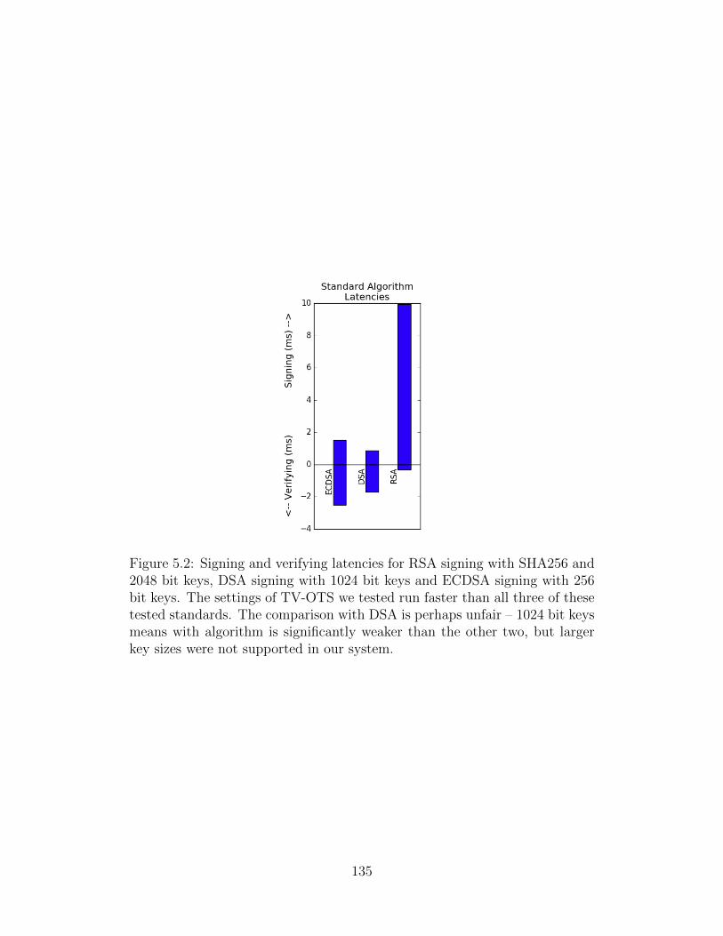
Figure 5.2: Signing and verifying latencies for RSA signing with SHA256 and2048 bit keys, DSA signing with 1024 bit keys and ECDSA signing with 256bit keys. The settings of TV-OTS we tested run faster than all three of thesetested standards. The comparison with DSA is perhaps unfair – 1024 bit keysmeans with algorithm is significantly weaker than the other two, but largerkey sizes were not supported in our system.

135

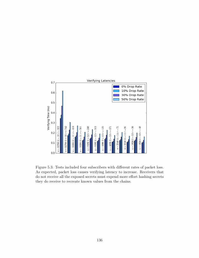
Figure 5.3: Tests included four subscribers with different rates of packet loss.As expected, packet loss causes verifying latency to increase. Receivers thatdo not receive all the exposed secrets must expend more effort hashing secretsthey do receive to recreate known values from the chains.

136

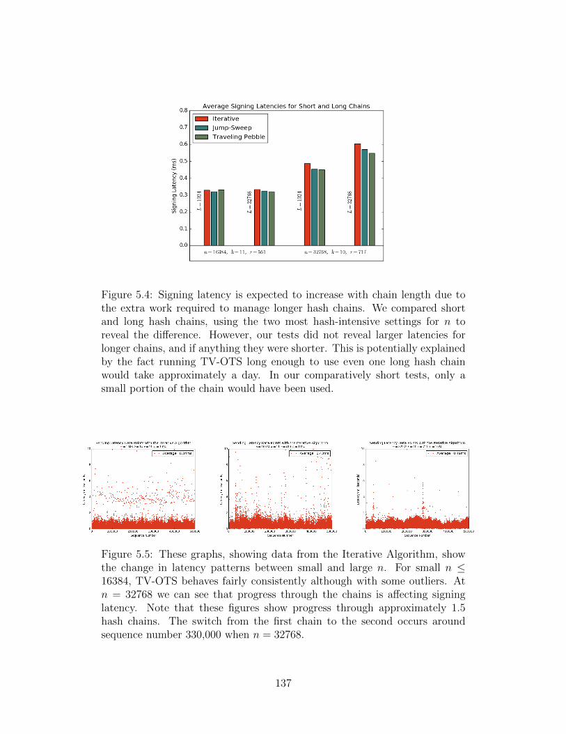
Figure 5.4: Signing latency is expected to increase with chain length due tothe extra work required to manage longer hash chains. We compared shortand long hash chains, using the two most hash-intensive settings for n toreveal the difference. However, our tests did not reveal larger latencies forlonger chains, and if anything they were shorter. This is potentially explainedby the fact running TV-OTS long enough to use even one long hash chainwould take approximately a day. In our comparatively short tests, only asmall portion of the chain would have been used.

Figure 5.5: These graphs, showing data from the Iterative Algorithm, showthe change in latency patterns between small and large n. For small n ≤16384, TV-OTS behaves fairly consistently although with some outliers. Atn = 32768 we can see that progress through the chains is affecting signinglatency. Note that these figures show progress through approximately 1.5hash chains. The switch from the first chain to the second occurs aroundsequence number 330,000 when n = 32768.

137

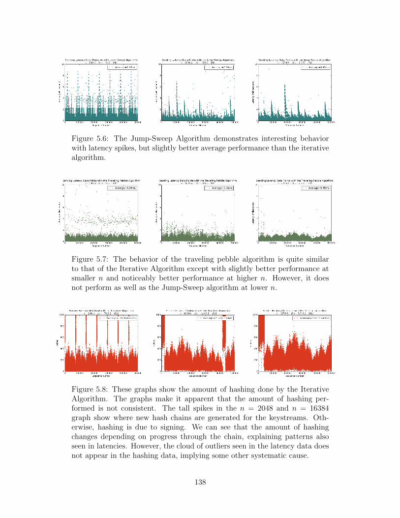
Figure 5.6: The Jump-Sweep Algorithm demonstrates interesting behaviorwith latency spikes, but slightly better average performance than the iterativealgorithm.

Figure 5.7: The behavior of the traveling pebble algorithm is quite similarto that of the Iterative Algorithm except with slightly better performance atsmaller n and noticeably better performance at higher n. However, it doesnot perform as well as the Jump-Sweep algorithm at lower n.

Figure 5.8: These graphs show the amount of hashing done by the IterativeAlgorithm. The graphs make it apparent that the amount of hashing per-formed is not consistent. The tall spikes in the n = 2048 and n = 16384graph show where new hash chains are generated for the keystreams. Oth-erwise, hashing is due to signing. We can see that the amount of hashingchanges depending on progress through the chain, explaining patterns alsoseen in latencies. However, the cloud of outliers seen in the latency data doesnot appear in the hashing data, implying some other systematic cause.

138

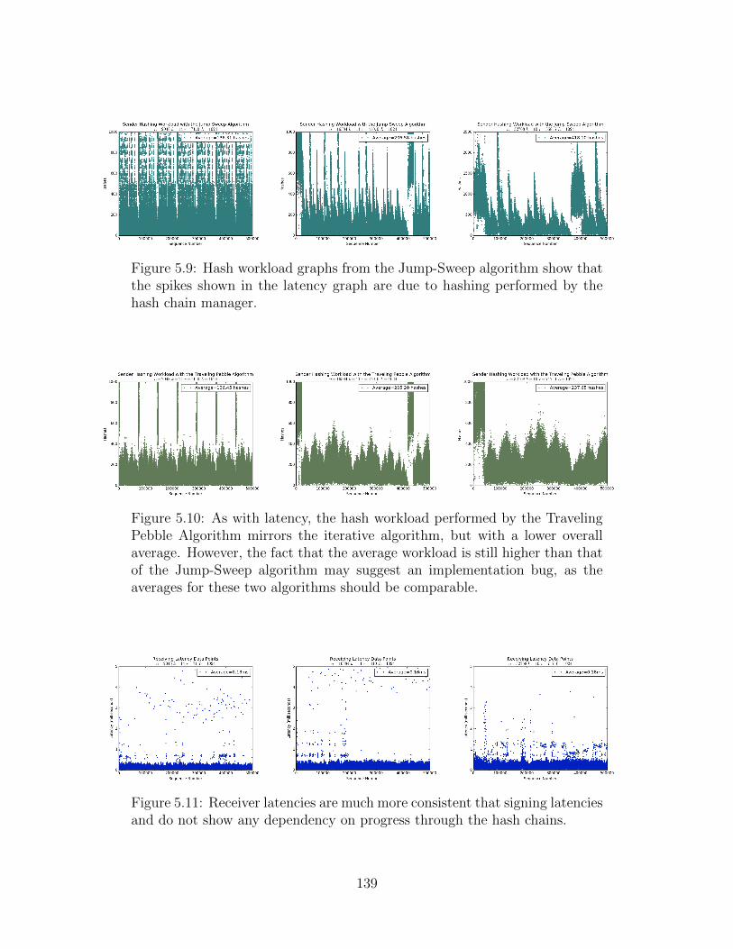
Figure 5.9: Hash workload graphs from the Jump-Sweep algorithm show thatthe spikes shown in the latency graph are due to hashing performed by thehash chain manager.

Figure 5.10: As with latency, the hash workload performed by the TravelingPebble Algorithm mirrors the iterative algorithm, but with a lower overallaverage. However, the fact that the average workload is still higher than thatof the Jump-Sweep algorithm may suggest an implementation bug, as theaverages for these two algorithms should be comparable.

Figure 5.11: Receiver latencies are much more consistent that signing latenciesand do not show any dependency on progress through the hash chains.

139

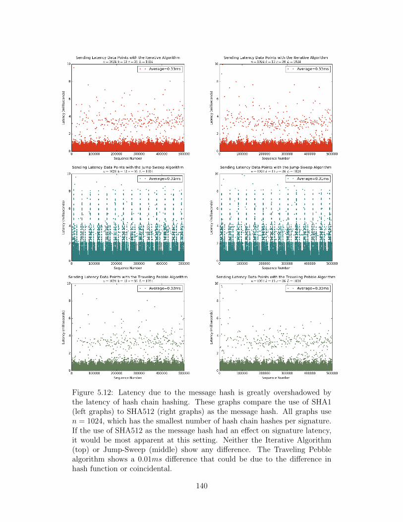
Figure 5.12: Latency due to the message hash is greatly overshadowed bythe latency of hash chain hashing. These graphs compare the use of SHA1(left graphs) to SHA512 (right graphs) as the message hash. All graphs usen = 1024, which has the smallest number of hash chain hashes per signature.If the use of SHA512 as the message hash had an effect on signature latency,it would be most apparent at this setting. Neither the Iterative Algorithm(top) or Jump-Sweep (middle) show any difference. The Traveling Pebblealgorithm shows a 0.01ms difference that could be due to the difference inhash function or coincidental.

140

5.2.2 Keystream Messages

We measured the number of payload messages sent per keystream message for each

setting of TV-OTS we tested. The keystream rates were calculated using a redundancy

factor of 2, meaning each anchor is sent to receivers in two different keystream packets.

Keytream message rate decreases linearly as hash chain length increases: if the hash chain

length is doubled, the keystream has twice as much time to deliver keystream anchors,

so keystream packets will be sent half as often. Even with the most frequent keystream

rate, 400 payload messages can be sent per keystream packet.

5.2.3 Exposed Secrets

Table 5.6 shows the numbers of secrets actually exposed for each parameter setting

when running our implementation of TV-OTS. Forgery probabilities in Section 3.1 were

calculated using r× k as an estimate on the number of secrets exposed. Table 5.6 shows

that r × k is a conservative estimate, and the actual numbers of exposed secrets are

smaller.

141

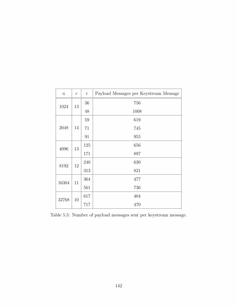
n r r Payload Messages per Keystream Message

1024 1336 756

48 1008

2048 14

59 619

71 745

91 955

4096 13125 656

171 897

8192 12240 630

313 821

16384 11364 477

561 736

32768 10617 404

717 470

Table 5.5: Number of payload messages sent per keystream message.

142

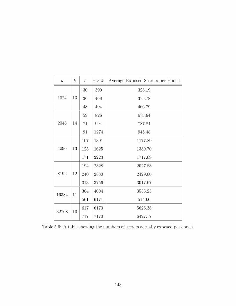
n k r r × k Average Exposed Secrets per Epoch

1024 13

30 390 325.19

36 468 375.78

48 494 466.79

2048 14

59 826 678.64

71 994 787.84

91 1274 945.48

4096 13

107 1391 1177.89

125 1625 1339.70

171 2223 1717.69

8192 12

194 2328 2027.88

240 2880 2429.60

313 3756 3017.67

16384 11364 4004 3555.23

561 6171 5140.0

32768 10617 6170 5625.38

717 7170 6427.17

Table 5.6: A table showing the numbers of secrets actually exposed per epoch.

143

5.3 Analysis

These data show that TV-OTS is capable of signing and verify messages with relatively

low latency, even though a large amount of hashing is required. In general, we see

expected trends relative to settings changes. We expect latency to increase with larger

n, which is noticeable in Figures 5.1 and 5.3. However, this increase is balanced by r: for

a given n, larger r yields faster signing and verifying latencies. This is consistent with

expectations because signing more messages per epoch causes more values to be retrieved

from each hash chain, meaning individual retrievals are less expensive on average.

Latency comparisons between TV-OTS and standard algorithms show that TV-OTS is

faster on average. Compared to RSA signing, TV-OTS signing is significantly faster,

given that RSA signing requires 10ms while TV-OTS signing is in the 0.4 to 1ms range.

The comparison against DSA and ECDSA is not as dramatic but TV-OTS still performs

favorably. Even DSA, which we ran at a lower security level than the other two due to

platform constraints, has a slightly higher signing time and verifying time is longer by a

factor of 10.

The latency stream graphs and hash workload graphs show that TV-OTS has room for

improvement. Even if the average latencies perform better than the standard algorithms,

many outlying data points have much longer latencies. Some points appear on latency

graphs that do not appear on hash workload graphs. These are likely to be explained by

system attributes that are difficult to control, such as garbage collection. However, the

majority of the latencies appear correlated with the amount of hashing required. It also

appears that the amount of required hashing varies depending on progress through the

chains. Our optimized algorithms reduce overall required hashing, but the next necessary

step is to develop chain management algorithms that distribute the workload more evenly

across retrievals.

144

The latency averages in Figure 5.1 lead to an interesting observation. This figure shows

that increases in n lead to only slight increases in latency. If r were kept constant, this

increase would be more dramatic. However, in these cases which were chosen relative to

our attack simulation, the effect of increasing n is balanced by also increasing r. Even

though latency performance is quite similar, the settings with larger n have more room

for adjustment in cases where higher security is needed. Large r can be decreased to

compensate for a more powerful attacker whereas a small r is much more limiting.

145

Chapter 6

Feedback Controlled Security

6.1 Systems Theory and Cyber Security

An idea beginning to emerge in literature is that system security relies on many inter-

connected components and should be treated as such. Similar ideas have been explored

in the context of distributed systems: trust modeling takes into account the interactions

of many components that need to sustain some standard of operation in order for the

system as a whole to function [47, 48]. More recently, Nancy Leveson introduced sys-

tems theory for safety engineering in her book [93]. Systems theory views systems as a

network of components that operate independently to perform individual tasks, but in-

fluence and interact with other components as well. Leveson’s System-Theoretic Accident

Model and Processes (STAMP) model describes systems in terms of interacting, hierar-

chically controlled processes with control flowing one direction through the hierarchy and

feedback flowing the other direction. In STAMP, higher level processes send control ac-

tions to lower level processes based on feedback from the lower layers. Correctness of this

methodology relies on the upper layer processes accurately understanding the behavior

146

and function of lower level processes.

The application of systems theory to safety engineering is beginning to inspire applica-

tion of these methods to cyber security. Causal Analysis based on STAMP (CAST) is a

STAMP based procedure for determining why system failures have occurred. Salim and

Madnick conjecture that traditional security models that consider components in isola-

tion are incomplete and apply CAST to an attack on commercial cyber infrastructure,

concluding the STAMP and CAST may be used effectively in postmortem analysis of

cyber events [144].

Traditional cyber security design often takes the approach of adding off-the-shelf security

methods to pre-designed systems. For example, encrypted or authenticated network

communication is added by inserting a cryptographic layer into the system. Messages

that pass through the layer are processed by some cryptographic mechanism. The system

is considered secure and the remainder of the other components are unaffected. Such

systems usually support a small amount of configuration (e.g., security algorithms and

key sizes), but the remainder of their functionality is independent. This method provides

little to no contextual awareness, for either cryptographic layer or encompassing system,

and cannot use system-specific attributes to increase security. This does not mesh with

the systems engineering approach as there is no communication between layers that

would enable feedback and control. From the systems engineering perspective, security

mechanisms should work with the environment, communicating with other components

and reacting accordingly.

Systems engineering has been used to evaluate security of cyber systems, but has not yet

been applied to designing them. The use of systems theory would be enabled by pro-

tocols capable of providing feedback about observed system operating states. A system

designed with the systems engineering approach could potentially use the feedback and

147

control mechanisms to detect abnormalities in various components and react accordingly.

Feedback could enable detection of system malfunctions or attacks, which could trigger

alarms or control actions that dictate a systematic response. However, the process that

decides appropriate control actions requires data to support these decisions. The remain-

der of this chapter focuses on how TV-OTS supports feedback control mechanisms, and

the enabling features that may exist in other protocols as well.

6.2 Support for Feedback and Control

TV-OTS and other k-time signatures have properties that support monitoring and control

mechanisms. Our strategy compares observed behavior of the system with statistically

expected behavior to detect abnormalities and attacks. In general, protocols that intro-

duce predictable behavior into the system enable this approach to monitoring. TV-OTS

is an example of an authentication mechanism that adds predictable behavior. Authen-

tication standards as HMAC and RSA signatures do not appear to add predictability

to the system, but many of the k-time signatures schemes described in Chapter 2 would

provide additional statistical behavior.

Many systems have some element of statistical behavior relating to metadata and tim-

ing of messages. In rate based systems such as GridStat, unexpected latency should

signal an abnormality. In aperiodic systems, timing information is more likely to be

measured in terms of jitter. Unexplained increases or decreases in message frequency

may be cause for investigation and should be included in feedback to the upper layers.

Additionally, timestamps or sequence numbers that appear inconsistent could also be

cause for alarm.

148

6.2.1 TV-OTS and Exposed Secrets

Protocols like TV-OTS can use statistical behavior by incorporating the expected statis-

tics of the protocol to detect general failures as well as attacks that may be taking

advantage of the probabilistic security. Eavesdrop attacks against TV-OTS involve the

attacker using secrets that are either already seen by the receiver or that were somehow

prevented from reaching the receiver. If the receiver did not receive the secrets, some

disruption in message timing would have been noticeable and the receiver should be

aware of the possible attack from that evidence alone. In the other case, the receiver will

have some expectation on the number of distinct secrets to expect, and how they should

be distributed across messages. An adversary reusing secrets will cause the number of

distinct secrets to decrease. If the number of distinct secrets falls outside the expected

statistical variance, this could indicate that the TV-OTS settings have not been chosen

adequately to protect against the present adversary.

A feedback control mechanism to detect reused secrets and adjust confidence can be

implemented entirely within the receiver. Qualitatively, the receiver monitors the num-

bers of secrets it’s learning and compares to what is expected. When the difference

is outside of some threshold, the receiver can take control steps and adjust confidence

functions to account for more attacker power as described in Section 3.2. The confi-

dence statistics should be taken into account in determining the allowable differences.

If confidences were fairly high over the course of the epoch, the received number of se-

crets should match reasonably closely with what’s expected. If confidences values were

generally lower, larger discrepancies can be expected, as some amount of forgery would

be expected by the confidence functions. When the discrepancy is large enough that it

isn’t accounted for by the lowered confidence, then the confidence functions should be

adjusted to compensate.

149

The above approach is quantifiable. The expected number of secrets can be calculated

with the help of Equation 6.1 from Section 3.1.3 which is presented again here for con-

venience. This equation gives the probability that d distinct secrets are exposed when k

randomly chosen secrets are chosen from a total of n possible secrets.

pd(n, k, d) =

(nd

)(dk +

d−1∑i=1

(−1)i(dd−i

)(d− i)k

)nk

(6.1)

We can apply this equation over the course of an epoch. Let κ be the total number of

secrets used during one epoch. Let δ be the number of secrets that are distinct. The

expected value for δ can be calculated by:

E(δ) = d×κ∑d=0

pd(n, κ, d) (6.2)

Abnormalities would be detected by comparing the expected δ to the actual number of

secrets seen. Of course some amount of variation is acceptable, and monitoring trends can

be used to reveal when slight deviations are harmless or if they are cause for alarm. For

example, the number of exposed secrets is anticipated to be low upon occasion. However,

if this were to happen consistently, it may indicate a problem.

6.2.2 Model Statistics

Figures 6.2 and 6.1 show data collected from the attacks modeled against TV-OTS in

Chapter 3. Pseudocode for this attack is given in Algorithm 5. The figures compare

the numbers of secrets exposed with and without an attacker present. The numbers

showing no attack were generated by running our GridStat implementation of TV-OTS

150

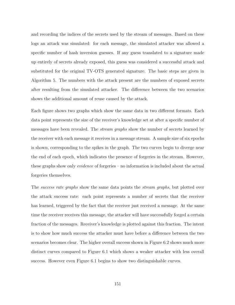
and recording the indices of the secrets used by the stream of messages. Based on these

logs an attack was simulated: for each message, the simulated attacker was allowed a

specific number of hash inversion guesses. If any guess translated to a signature made

up entirely of secrets already exposed, this guess was considered a successful attack and

substituted for the original TV-OTS generated signature. The basic steps are given in

Algorithm 5. The numbers with the attack present are the numbers of exposed secrets

after resulting from the simulated attacker. The difference between the two scenarios

shows the additional amount of reuse caused by the attack.

Each figure shows two graphs which show the same data in two different formats. Each

data point represents the size of the receiver’s knowledge set at after a specific number of

messages have been revealed. The stream graphs show the number of secrets learned by

the receiver with each message it receives in a message stream. A sample size of six epochs

is shown, corresponding to the spikes in the graph. The two curves begin to diverge near

the end of each epoch, which indicates the presence of forgeries in the stream. However,

these graphs show only evidence of forgeries – no information is included about the actual

forgeries themselves.

The success rate graphs show the same data points the stream graphs, but plotted over

the attack success rate: each point represents a number of secrets that the receiver

has learned, triggered by the fact that the receiver just received a message. At the same

time the receiver receives this message, the attacker will have successfully forged a certain

fraction of the messages. Receiver’s knowledge is plotted against this fraction. The intent

is to show how much success the attacker must have before a difference between the two

scenarios becomes clear. The higher overall success shown in Figure 6.2 shows much more

distinct curves compared to Figure 6.1 which shows a weaker attacker with less overall

success. However even Figure 6.1 begins to show two distinguishable curves.

151

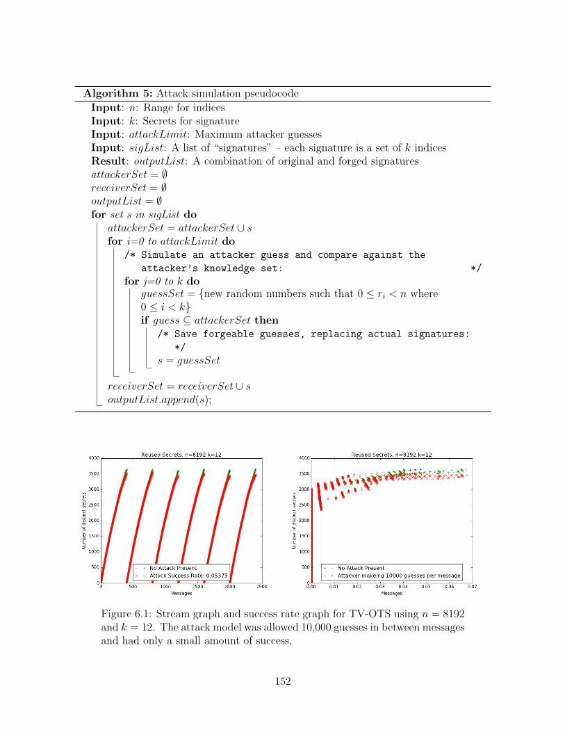
Algorithm 5: Attack simulation pseudocode

Input: n: Range for indicesInput: k: Secrets for signatureInput: attackLimit: Maximum attacker guessesInput: sigList: A list of “signatures” – each signature is a set of k indicesResult: outputList: A combination of original and forged signaturesattackerSet = ∅receiverSet = ∅outputList = ∅for set s in sigList do

attackerSet = attackerSet ∪ sfor i=0 to attackLimit do

/* Simulate an attacker guess and compare against the

attacker’s knowledge set: */

for j=0 to k doguessSet = new random numbers such that 0 ≤ ri < n where0 ≤ i < kif guess ⊆ attackerSet then

/* Save forgeable guesses, replacing actual signatures:

*/

s = guessSet

receiverSet = receiverSet ∪ soutputList.append(s);

Figure 6.1: Stream graph and success rate graph for TV-OTS using n = 8192and k = 12. The attack model was allowed 10,000 guesses in between messagesand had only a small amount of success.

152

Figure 6.2: Stream graph and success rate graph for TV-OTS using n =16384 and k = 11. The attack model was allowed 200,000 guesses in betweenmessages and intentionally run long enough to ensure the attacker would bereasonably successful.

Future Work on Attack Detection Through Reuse

The fact that numbers of exposed secrets change with attacks is promising, but future

efforts are still necessary to determine how well this metric serves as an indicator of

attack. Further questions relate to the dynamic between reused secret detection and

confidence assessment. Ideally the two would complement each other, since confidence

assessment works at a very narrow scope and reused secret detection operates over more

data.

The exact effect of the confidence function on the expected reused secrets will also require

investigation. The expected value for secrets is calculated assuming no attacker is present.

If, over the course of an epoch, confidence values have been abnormally low, it is likely

that an attacker is present and launching an attack. In this case E(δ) is not a realistic

expectation: some amount of deviation should be expected, and is accounted for by the

lowered confidence. However, it is possible for an amount of deviation from E(δ) to be

large enough that it is not explained by the lowered confidence. This relationship depends

on the confidence function itself and can only be decided once that is determined.

153

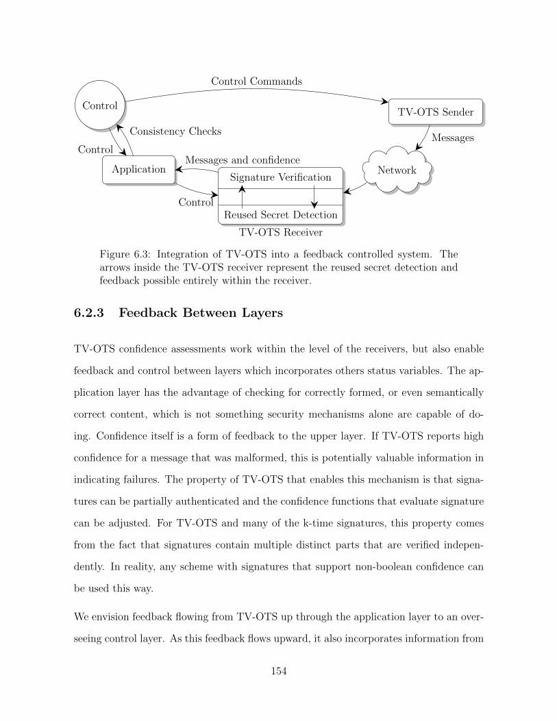
Control

Application

TV-OTS Sender

Signature Verification

Reused Secret Detection

TV-OTS Receiver

Network

Control

Consistency Checks

Control Commands

Messages

Messages and confidence

Control

Figure 6.3: Integration of TV-OTS into a feedback controlled system. Thearrows inside the TV-OTS receiver represent the reused secret detection andfeedback possible entirely within the receiver.

6.2.3 Feedback Between Layers

TV-OTS confidence assessments work within the level of the receivers, but also enable

feedback and control between layers which incorporates others status variables. The ap-

plication layer has the advantage of checking for correctly formed, or even semantically

correct content, which is not something security mechanisms alone are capable of do-

ing. Confidence itself is a form of feedback to the upper layer. If TV-OTS reports high

confidence for a message that was malformed, this is potentially valuable information in

indicating failures. The property of TV-OTS that enables this mechanism is that signa-

tures can be partially authenticated and the confidence functions that evaluate signature

can be adjusted. For TV-OTS and many of the k-time signatures, this property comes

from the fact that signatures contain multiple distinct parts that are verified indepen-

dently. In reality, any scheme with signatures that support non-boolean confidence can

be used this way.

We envision feedback flowing from TV-OTS up through the application layer to an over-

seeing control layer. As this feedback flows upward, it also incorporates information from

154

the application layer that includes consistency checks between the confidence and the va-

lidity of message content. Feedback would potentially enable an operator control panel,

providing visuals indicating system health in near-real time. The controls that flow back

down on the receiver side may be used to signal the receiver that confidence assessment

does not appear to align with observations at the higher layers. A more complicated

system could send feedback to the sender side, informing the sender to provide more (or

less) security by adjusting the epoch length or changing the number of available secrets.

Figure 6.3 shows how feedback and control flows between TV-OTS and other components

in an interconnected system.

We used confidence and reused secrets as examples of feedback that TV-OTS can provide,

but many other metrics may be available as well. Table 6.1 lists potentially useful

properties. Change in any of these properties could indicate either an attack or simply

a malfunctioning component. Specific combinations may be more revealing, for example

if the TV-OTS layer reports a high number of bad secrets, and the application layer

is reporting syntactically incorrect messages, but the numbers of reused secrets are not

abnormally high, the cause may simply be a failing network component that is no longer

transmitting messages correctly. Even though this is not an attack, action still needs to

be taken to correct this problem and ensure continuous operation in the future.

6.3 Summary

As the trend emerges to design cyber-secure systems from a systems-theoretic viewpoint,

protocols that support feedback and control will become desirable. For example, the

statistical behavior in TV-OTS may be useful in detecting attacks and other system

disturbances that can be reported as feedback to a control layer. This enables a holistic

approach to security which incorporates information from all parts of the system to detect

155

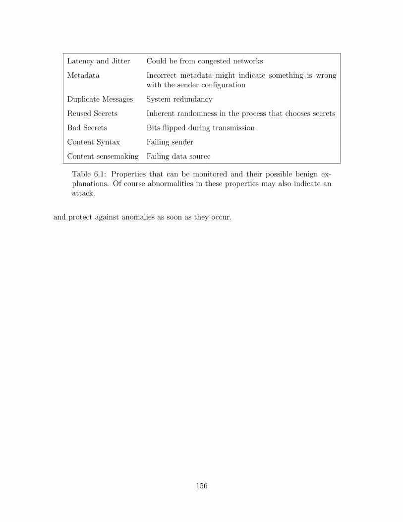
Latency and Jitter Could be from congested networks

Metadata Incorrect metadata might indicate something is wrongwith the sender configuration

Duplicate Messages System redundancy

Reused Secrets Inherent randomness in the process that chooses secrets

Bad Secrets Bits flipped during transmission

Content Syntax Failing sender

Content sensemaking Failing data source

Table 6.1: Properties that can be monitored and their possible benign ex-planations. Of course abnormalities in these properties may also indicate anattack.

and protect against anomalies as soon as they occur.

156

Chapter 7

Conclusion

7.1 Discussion of Results

Our research has lead to significant insights into both the security and performance of

TV-OTS. Many of our performance results are relatively unsurprising: TV-OTS provides

lower signing and verification latency than its competitors and performance can be reli-

ably controlled by changing parameter settings. Results from our security analysis are

much more insightful: basic forgery probability analysis provides a worst-case predictive

bounds but fails to describe the complete picture. The probabilistic nature of TV-OTS

allows us to implement confidence based assessment which detects signatures forged by an

attacker. Thus, an attacker must not only forge a signature, but also bypass confidence

assessment in order to be truly successful.

To implement confidence based assessment in TV-OTS, we used characteristics about

individual signatures as well as system state information to calculate a numerical confi-

dence value for each signature representing the receiver’s belief that the signature was not

forged. We tested our confidence functions on a simulated attack against TV-OTS. We

157

compared two different confidence function implementations, one that took into account

system state and one that did not. Both were reasonably good at detecting forged mes-

sages, but the one that incorporates system state provided clearer differentiation between

good and forged messages.

Our performance results show that TV-OTS provides low latency signing and verification,

even under the more secure parameter choices. Our tests shows that TV-OTS can be

used to authenticate messages with signing latencies under 0.6ms and verifying latencies

under 0.2ms at settings that are generally safe against attackers capable of 106 guesses

per message. At these settings, Table 5.4 gives estimates on the maximum safe value for

r, the number of messages that can safely be sent per epoch. At our weakest setting,

n = 1024, r ≥ 30 for the attacker strengths we modeled. As an example, a PMU

data delivery application sending messages 30 times a second may use 1 second epoch

lengths and expect that a small number of messages may be forged near the end of each

epoch. Tables in Chapter 3 show that in our tests for these settings, all confidences

for forged messages were less than 0.3. Using this as a confidence threshold caused at

most 0.6% of good messages to be erroneously mistaken for forgeries. By increasing n,

epoch lengths could be extended or security can be increased to protect against more

capable attackers. For comparison, occasional forged messages are not a concern in the

standards we measured, but if the private key is discovered all subsequent messages may

be compromised.

Our latency testing revealed that TV-OTS must compute a large number of hashes

for each signature, but is still faster than standard asymmetric algorithms. Results

showed that many settings of TV-OTS signed message substantially faster than RSA

(less than 1ms compared to 10ms), with comparable signing times. TV-OTS performed

more similarly to ECDSA, although still more than two times faster at signing (0.4 −

0.6ms vs. approximately 1.5ms) and 10 times faster at verifying (0.2ms vs. 2ms).

158

We further note that we are comparing a research implementation of TV-OTS against

processional implementations of ECDSA and RSA. The variations in latency seen in our

implementation of TV-OTS suggests it would benefit from professional implementation

and optimization. Such an implementation would be expected to run at least as fast, if

not faster, than the implementation we have now.

7.2 Future Work

We think TV-OTS has significant implications for the idea of feedback controlled secu-

rity. The application of systems theory to cyber security is a relatively new idea. Sys-

tems theory relies on the ability of components to provide feedback to control layers and

potentially respond to control actions. However, standard security and authentication

protocols used today were not designed with these ideas in mind and function indepen-

dently of other systems. The maximum amount of feedback today’s standards provide

is alerts when an error occurs, such as when a signature is not verifiable. TV-OTS, on

the other hand, fits quite naturally into feedback controlled environments. Confidence

reporting is already a level of feedback beyond what current protocols are capable of.

In addition, the system state monitoring used to compute confidences can also be useful

information for making control decisions.

Feedback controlled security is a new idea with a broad scope, opening the door to

many types of research problems. Ultimately such systems will need to have individual

components, control algorithms, and communications designed, implemented and tested.

From the perspective of designing individual components, the extent to which security

protocols can contribute to such a system requires investigation. TV-OTS contributes to

system monitoring due to naturally arising statistical behavior. This inevitably leads to

the question of whether other protocols produce statistics that can be monitored, or if

159

statistical behavior could be injected in such a way that attacks would cause detectable

perturbations.

Alternatively, monitoring of TV-OTS (and potentially other protocols) has the potential

to take into account additional network-specific data such as expected end-to-end network

latencies or drop rates. It would be interesting, especially for control systems or other

systems with predictable behavior, to test what a monitoring system, monitoring TV-

OTS behavior as well as network behavior, could detect. The ultimate goal would be to

detect abnormalities, classify them as either attacks or component failures, and adjust

system behavior as necessary to ensure continuous, reliable operation.

160

Bibliography

[1] 8x nvidia gtx 1080 hashcat benchmarks. https://gist.github.com/epixoip/

a83d38f412b4737e99bbef804a270c40. Accessed: Oct. 2016.

[2] General information – binary synchronous communications.

[3] The password project. http://http://thepasswordproject.com/oclhashcat_

benchmarking. Accessed: Oct. 2016.

[4] FIPS PUB 186 FEDERAL INFORMATION PROCESSING STANDARDS PUB-

LICATION Digital Signature Standard (DSS). Technical report, 2009.

[5] Iso/iec 9798-4, 2010.

[6] Riham Abdellatif, Heba K. Aslan, and Salwa H. Elramly. New real time multicast

authentication protocol. Int. J. Netw. Secur., 12:13–20, 2011.

[7] Qusai Abuein and Susumu Shibusawa. A Graph-based New Amortization Scheme

for Multicast Streams Authentication. Adv. Model. Optim., 7(2):238–261, 2005.

[8] Ali Abur and Antonio Gomez Exposito. Power system state estimation: theory and

implementation. CRC press, 2004.

[9] Abdullah Al Hasib and Abul Ahsan Md Mahmudul Haque. A comparative study

of the performance and security issues of aes and rsa cryptography. In Conver-

161

gence and Hybrid Information Technology, 2008. ICCIT’08. Third International

Conference on, volume 2, pages 505–510. IEEE, 2008.

[10] Ozgu Alay, Kyle Guan, Yao Wang, Elza Erkip, Shivendra Panwar, and Reza

Ghanadan. Wireless video multicast in tactical environments. In Proc. - IEEE

Mil. Commun. Conf. MILCOM, 2008.

[11] Ross Anderson and Roger Needham. Robustness principles for public key protocols.

Lect. Notes Comput. Sci. (including Subser. Lect. Notes Artif. Intell. Lect. Notes

Bioinformatics), 963:236–247, 1995.

[12] X9 ANSI. 63: Public key cryptography for the financial services industry: Key

agreement and key transport using elliptic curve cryptography. American National

Standards Institute, 1998.

[13] Heba K. Aslan. A hybrid scheme for multicast authentication over lossy networks.

Comput. Secur., 23:705–713, 2004.

[14] A. Francis Bach. Wall Street Takes Stock of IP Multicast. Bus. Commun. Rev.,

28:48—-52, 1998.

[15] David E Bakken, Anjan Bose, Carl H Hauser, O Schweitzer, Edmond, David E

Whitehead, and Gregary C Zweigle. Smart Generation and Transmission with

Coherent, Real-Time Data. pages 1–62, 2010.

[16] David E Bakken, Carl H. Hauser, Anjan Bose, and Harald Gjermundrød. Towards

More Flexible and Robust Data Delivery for Monitoring and Control of the Electric

Power Grid. 2007.

[17] Paulo S L M Barreto, Benoıt Libert, Noel McCullagh, and Jean Jacques

Quisquater. Efficient and provably-secure identity-based signatures and signcryp-

162

tion from bilinear maps. In Lect. Notes Comput. Sci. (including Subser. Lect. Notes

Artif. Intell. Lect. Notes Bioinformatics), volume 3788 LNCS, pages 515–532, 2005.

[18] Mihir Bellare and Phillip Rogaway. Random oracles are practical: A paradigm

for designing efficient protocols. Proc. 1st ACM Conf. Comput. Commun. Secur.,

(November 1993):62–73, 1993.

[19] Diana Berbecaru and Luca Albertalli. An optimized double cache technique for

efficient use of forward-secure signature schemes. In 16th Euromicro Conference on

Parallel, Distributed and Network-Based Processing (PDP 2008), pages 581–589.

IEEE, 2008.

[20] Diana Berbecaru, Luca Albertalli, and Antonio Lioy. The forwarddiffsig scheme

for multicast authentication. IEEE/ACM Trans. Netw., 18:1855–1868, 2010.

[21] Piotr Berman, Marek Karpinski, and Yakov Nekrich. Optimal Trade-Off for Merkle

Tree Traversal. Commun. Comput. Inf. Sci., 3 CCIS:150–162, 2007.

[22] Daniel J Bernstein. Circuits for integer factorization: a proposal. At the time of

writing available electronically at http://cr. yp. to/papers/nfscircuit. pdf, 2001.

[23] Daniel J Bernstein and Tanja Lange. Safecurves: choosing safe curves for elliptic-

curve cryptography. URL: http://safecurves.cr.yp.to, 2013.

[24] Robin Berthier, Jorjeta G. Jetcheva, Daisuke Mashima, Jun Ho Huh, David Gro-

chocki, Rakesh B. Bobba, Alvaro A. Cardenas, and William H. Sanders. Reconciling

security protection and monitoring requirements in advanced metering infrastruc-

tures. In 2013 IEEE Int. Conf. Smart Grid Commun. SmartGridComm 2013, pages

450–455, 2013.

[25] Kemal Bicakci, Gene Tsudik, and Brian Tung. How to construct optimal one-time

signatures. Comput. Networks, 43(3):339–349, oct 2003.

163

[26] Daniel Bleichenbacher and Ueli Maurer. Directed Acyclic Graphs, One-way Func-

tions and Digital Signatures. In Adv. Cryptol. — CRYPTO 1994, volume 839,

pages 75–82, 1994.

[27] Daniel Bleichenbacher and Ueli Maurer. On the Efficiency of One-time Digital

Signatures. In Adv. Cryptol. ASIACRYPT 96, volume 1163, pages 196–209, 1996.

[28] Daniel Bleichenbacher and Ueli Maurer. Optimal tree-based one-time digital sig-

nature schemes, 1996.

[29] Rakesh Bobba, Katherine Rogers, Qiyan Wang, Himanshu Khurana, Klara Nahrst-

edt, and Thomas Overbye. Detecting False Data Injection Attacks on DC State

Estimation. First Work. Secur. Control Syst., pages 1–9, 2010.

[30] Rakesh B. Bobba, Jeff Dagle, Erich Heine, Himanshu Khurana, William H. Sanders,

Peter Sauer, and Tim Yardley. Enhancing Grid Measurements: Wide Area Mea-

surement Systems, NASPInet, and Security. IEEE Power Energy Mag., 10(1):67–

73, 2012.

[31] Dan Boneh and Hovav Shacham. Fast variants of rsa. CryptoBytes, 5(1):1–9, 2002.

[32] Jurjen N E Bos and David Chaum. Provable Unforgeable Signatures. Adv.

Cryptology—CRYPTO˜’92, pages 1–14, 1992.

[33] Johannes Buchmann, Erik Dahmen, Elena Klintsevich, Katsuyuki Okeya, Camille

Vuillaume, and Technische Universitat Darmstadt. Merkle signatures with virtually

unlimited signature capacity, 2007.

[34] John W. Byers, Michael Luby, Michael Mitzenmacher, and Ashutosh Rege. A

digital fountain approach to reliable distribution of bulk data. ACM SIGCOMM

Comput. Commun. Rev., 28(4):56–67, 1998.

164

[35] Kelsey Cairns, Thoshitha Gamage, and Carl Hauser. Efficient Targeted Key Subset

Retrieval in Fractal Hash Sequences. In CCS, 2013.

[36] Ran Canetti, Oded Goldreich, and Shai Halevi. The Random Oracle Methodology,

Revisited. J. ACM, 51(4):38, 2004.

[37] Stefania Cavallar, Bruce Dodson, Arjen K Lenstra, Walter Lioen, Peter L Mont-

gomery, Brian Murphy, Herman Te Riele, Karen Aardal, Jeff Gilchrist, Gerard

Guillerm, et al. Factorization of a 512-bit rsa modulus. In International Con-

ference on the Theory and Applications of Cryptographic Techniques, pages 1–18.

Springer, 2000.

[38] Jae Choon Cha and Jung Hee Cheon. An Identity-Based Signature from Gap

Diffie-Hellman Groups. Int. Assoc. Cryptologic Res., pages 18–30, 2002.

[39] Saikat Chakrabarti, Elias Kyriakides, Tianshu Bi, Deyu Cai, and Vladimir Terzija.

Measurements get together. IEEE Power and Energy Magazine, 7(1):41–49, 2009.

[40] Yacine Challal, Abdelmadjid Bouabdallah, and Yoann Hinard. Efficient multicast

source authentication using layered hash-chaining scheme. In Proc. - Conf. Local

Comput. Networks, LCN, pages 411–412, 2004.

[41] Yacine Challal, Abdelmadjid Bouabdallah, and Yoann Hinard. RLH: Receiver

driven layered hash-chaining for multicast data origin authentication. Comput.

Commun., 28:726–740, 2005.

[42] D. Coppersmith and M. Jakobsson. Almost optimal hash sequence traversal. In

Financial Cryptography, pages 102–119. Springer, 2003.

[43] National Vulnerability Database. Cve-2008-0166. online, May 2008.

[44] J De Gelas. Intel woodcrest, amds opteron and suns ultrasparc t1: Server cpu

shoot-out.

165

[45] Tim Dierks and Eric Rescorla. Rfc 5246: The transport layer security (tls) protocol.

The Internet Engineering Task Force, 2008.

[46] W. Diffie and M. Hellman. New directions in cryptography. IEEE Trans. Inf.

Theory, 22, 1976.

[47] Ioanna Dionysiou. Dynamic and composable trust for indirect interactions. PhD

thesis, Washington State University, 2006.

[48] Ioanna Dionysiou, Deborah Frincke, David E Bakken, and Carl Hauser. Actor-

oriented trust. Technical report, Technical Report EECS-GS-006, School of Elec-

trical Engineering and Computer SCience, Washington State University, Pullman,

WA, USA, 2005.

[49] Danny Dolev and Andrew Yao. On the security of public key protocols. IEEE

Transactions on information theory, 29(2):198–208, 1983.

[50] Thai Duong and Juliano Rizzo. Flickrs api signature forgery vulnerability, 2009.

[51] Morris J. Dworkin. SHA-3 Standard: Permutation-Based Hash and Extendable-

Output Functions. Technical Report August, 2015.

[52] D Eastlake III and T Hansen. Rfc 4634-us secure hash algorithms (sha and hmac-

sha). Motorola Labs and AT &T Labs, 2006.

[53] Taher ElGamal. A public key cryptosystem and a signature scheme based on

discrete logarithms. In Workshop on the Theory and Application of Cryptographic

Techniques, pages 10–18. Springer, 1984.

[54] Carl Ellison and Bruce Schneier. Ten risks of pki: What you’re not being told

about public key infrastructure. Comput Secur J, 16(1):1–7, 2000.

166

[55] Hamdi Eltaief and Habib Youssef. Efficient sender authentication and signing of

multicast streams over lossy channels. In 2010 ACS/IEEE Int. Conf. Comput. Syst.

Appl. AICCSA 2010, 2010.

[56] Shimon Even, Oded Goldreich, and Silvio Micali. On-line/off-line digital signatures.

pages 263–275, 1990.

[57] Jean-Charles Faugere, Christopher Goyet, and Guenael Renault. Attacking (ec)

dsa given only an implicit hint. In International Conference on Selected Areas in

Cryptography, pages 252–274. Springer, 2012.

[58] Tom Fawcett. Roc graphs: Notes and practical considerations for researchers.

Machine learning, 31(1):1–38, 2004.

[59] NIST FIPS. 186 digital signature standard, 1994.

[60] PUB Fips. 186-2. digital signature standard (dss). National Institute of Standards

and Technology (NIST), 2000.

[61] Terry Fleury, Himanshu Khurana, and Von Welch. Towards a taxonomy of attacks

against energy control systems. IFIP Int. Fed. Inf. Process., 290:71–85, 2008.

[62] P Gallagher and C Kerry. Fips pub 186-4: Digital signature standard, dss (2013).

[63] Rosario Gennaro and Pankaj Rohatgi. How to sign digital streams. In Adv. Cryptol.

- CRYPTO’97, pages pp 180–197, 1997.

[64] Philippe Golle and Nagendra Modadugu. Authenticating Streamed Data in the

Presence of Random Packet Loss. Proc. Symp. Netw. Distrib. Syst. Secur. (NDSS

2001), pages 13–22, 2001.

[65] Li Gong and Menlo Park. Fail-Stop Protocols : An Approach to Designing Secure

Protocols 1 Background and Motivation. pages 1–14, 1994.

167

[66] IEEE P1363 Working Group et al. Ieee p1363: Standard specifications for public

key cryptography. URL: http://grouper.ieee.org/groups/1363, 1999.

[67] Vipul Gupta, Sumit Gupta, Sheueling Chang, and Douglas Stebila. Performance

analysis of elliptic curve cryptography for ssl. In Proceedings of the 1st ACM

workshop on Wireless security, pages 87–94. ACM, 2002.

[68] Neil Haller. The s/key one-time password system. 1995.

[69] Darrel Hankerson and Alfred Menezes. Nsa suite b. In Encyclopedia of Cryptography

and Security, pages 857–857. Springer, 2011.

[70] Jinxin He, Gaochao Xu, Xiaodong Fu, Zhiguo Zhou, and Jianghua Jiang. LMCM:

Layered Multiple Chaining Model for authenticating multicast streams. In Proc.

9th ACIS Int. Conf. Softw. Eng. Artif. Intell. Netw. Parallel/Distributed Comput.

SNPD 2008 2nd Int. Work. Adv. Internet Technol. Appl., pages 206–211, 2008.

[71] Jinxin He, Gaochao Xu, Zhiguo Zhou, and Guannan Gong. A New Approach for

Source Authentication of Multicast Data. Secur. Manag., (20050522), 2006.

[72] Nadia Heninger, Zakir Durumeric, Eric Wustrow, and J Alex Halderman. Mining

your ps and qs: Detection of widespread weak keys in network devices. In Presented

as part of the 21st USENIX Security Symposium (USENIX Security 12), pages 205–

220, 2012.

[73] Florian Hess. Efficient Identity Based Signature Schemes Based on Pairings. Sel.

Areas Cryptogr., pages 310–324, 2003.

[74] Yoann Hinard, Hatem Bettahar, Yacine Challal, and Abdelmadjid Bouabdallah.

Layered multicast data origin authentication and non-repudiation over lossy net-

works. In Proc. - Int. Symp. Comput. Commun., pages 662–667, 2006.

168

[75] By Stanley H Horowitz, Arun G Phadke, Bruce A Renz, Stanley Horowitz, Arun G

Phadke, and Bruce A Renz. The Future of Power Transmission. IEEE Power

Energy Mag., 8(2):34–40, 2010.

[76] Russell Housley, W Polk, Warwick Ford, and David Solo. Internet x. 509 public

key infrastructure certificate and certificate revocation list (crl) profile. Technical

report, 2002.

[77] Yih-Chun Hu, Markus Jakobsson, and Adrian Perrig. Efficient constructions for

one-way hash chains. In International Conference on Applied Cryptography and

Network Security, pages 423–441. Springer, 2005.

[78] Hsiang Cheh Huang and Yueh Hong Chen. Genetic fingerprinting for copyright

protection of multicast media. In Soft Comput., volume 13, pages 383–391, 2009.

[79] G. Itkis and L. Reyzin. Forward-secure signatures with optimal signing and veri-

fying. In Advances in Cryptology–Crypto 2001, pages 332–354. Springer, 2001.

[80] M. Jakobsson. Fractal hash sequence representation and traversal. In 2002 IEEE

International Symposium on Information Theory, page 437. IEEE, 2002.

[81] Markus Jakobsson, Tom Leighton, Silvio Micali, and Michael Szydlo. Fractal

Merkle Tree Representation and Traversal. Work, pages 314–326, 2003.

[82] Don Johnson, Alfred Menezes, and Scott Vanstone. The Elliptic Curve Digital

Signature Algorithm (ECDSA). Int. J. Inf. Secur., 1:36–63, 2001.

[83] P. Jones. US secure hash algorithm 1 (SHA1) RFC 3174, 2001.

[84] Namhi Kang and Christoph Ruland. Diffsig: Differentiated digital signature for

real-time multicast packet flows. In International Conference on Trust, Privacy

and Security in Digital Business, pages 251–260. Springer, 2004.

169

[85] Chris Karlof, Naveen Sastry, Yaping Li, Adrian Perrig, and J. D. Tygar. Distillation

codes and applications to DoS resistant multicast authentication. Proc. ISOC . . . ,

(February):37–56, 2004.

[86] Himanshu Khurana, Rakesh Bobba, Tim Yardley, Pooja Agarwal, and Erich Heine.

Design principles for power grid cyber-infrastructure authentication protocols.

Proc. Annu. Hawaii Int. Conf. Syst. Sci., pages 1–10, 2010.

[87] S.R. Kim. Improved scalable hash chain traversal. In Applied Cryptography and

Network Security, pages 86–95. Springer, 2003.

[88] Veronika Kondratieva and Seung W. Seo. Optimized hash tree for authentication

in sensor networks. IEEE Commun. Lett., 11:149–151, 2007.

[89] H. Krawczyk, M. Bellare, and R. Canetti. RFC2104 - HMAC: Keyed-hashing for

message authentication. Technical report, 1997.

[90] Kristina Hamachi LaCommare and Joseph H. Eto. Cost of power interruptions to

electricity consumers in the United States (US). Energy, 31(12):1509–1519, 2006.

[91] Leslie Lamport. Constructing digital signatures from a one-way function. SRI Int.

Comput. Sci. Lab., 94025(October):1–8, 1979.

[92] Peter J Leadbitter, Dan Page, and Nigel P Smart. Attacking dsa under a repeated

bits assumption. In International Workshop on Cryptographic Hardware and Em-

bedded Systems, pages 428–440. Springer, 2004.

[93] Nancy Leveson. Engineering a safer world: Systems thinking applied to safety. Mit

Press, 2011.

[94] Qing Li and Wade Trappe. Reducing delay and enhancing DoS resistance in multi-

cast authentication through multigrade security. IEEE Trans. Inf. Forensics Secur.,

1:190–204, 2006.

170

[95] Qinghua Li and Guohong Cao. Multicast Authentication in the Smart Grid With.

2(4):686–696, 2011.

[96] Yang Li, Miao Zhang, Yanhui Guo, and Guoai Xu. Optimized source authentication

scheme for multicast based on merkle tree and TESLA. In Proc. 2010 IEEE Int.

Conf. Inf. Theory Inf. Secur. ICITIS 2010, pages 195–198, 2010.

[97] Wang Lidong, Yu Xiangzhan, and Fang Binxing. Research on several security

problems in pki [j]. COMPUTER ENGINEERING, 1:006, 2000.

[98] Iuon Chang Lin and Chia Chang Sung. An efficient source authentication for

multicast based on Merkle hash tree. In Proc. - 2010 6th Int. Conf. Intell. Inf.

Hiding Multimed. Signal Process. IIHMSP 2010, pages 5–8, 2010.

[99] Yao Liu, Peng Ning, and Michael K. Reiter. False data injection attacks against

state estimation in electric power grids. Ccs, 14(1):1–33, 2009.

[100] Manfred Lochter and Johannes Merkle. Elliptic curve cryptography (ecc) brainpool

standard curves and curve generation. Technical report, 2010.

[101] Peter B. Luh, Yu Chi Ho, and Ramal Muralidharan. Load Adaptive Pricing: An

Emerging Tool for Electric Utilities. IEEE Trans. Automat. Contr., 27(2):320–329,

1982.

[102] Wenbo Mao and C. Boyd. Development of Authentication Protocols : Some Mis-

conceptions and a New Approach 2 Authentication : Use of One-way or. Proc.

Comput. Secur. Found. Work. VII, pages 178–186, 1994.

[103] Michal Marks, Jaroslaw Jantura, Ewa Niewiadomska-Szynkiewicz, Przemyslaw

Strzelczyk, and Krzysztof Gozdz. Heterogeneous gpu&cpu cluster for high per-

formance computing in cryptography. Computer Science, 13:63–79, 2012.

171

[104] Kenneth Martin and James Ritchie Carroll. Phasing in the technology. IEEE

Power Energy Mag., 6(5):24–33, 2008.

[105] N. F. Maxemchuk and D. H. Shur. An Internet Multicast System for the Stock

Market. page 19, 2000.

[106] David McGrew. An interface and algorithms for authenticated encryption. 2008.

[107] Ralph C. Merkle. A Digital Signature Based on a Conventional Encryption Func-

tion. In Advances, volume 293, pages 369–378, 1988.

[108] Ralph C. Merkle. A Certified Digital Signature. PhD thesis, 1989.

[109] Ralph C. Merkle. A certified digital signature. Adv. CryptologyCRYPTO’89 Proc.,

pages 218–238, 1990.

[110] Ralph Charles Merkle, Ralph Charles, et al. Secrecy, authentication, and public

key systems. 1979.

[111] David Meyer. Administratively scoped ip multicast. Technical report, 1998.

[112] Sara Miner, Sara Miner, Jessica Staddon, and Jessica Staddon. Graph-Based Au-

thentication of Digital Streams. Proc. IEEE Symp. Res. Secur. Priv., pages

232–246, 2001.

[113] Amir-Hamed Mohsenian-Rad and Alberto Leon-Garcia. Optimal residential load

control with price prediction in real-time electricity pricing environments. IEEE

transactions on Smart Grid, 1(2):120–133, 2010.

[114] Kate L. Morrow, Erich Heine, Katherine M. Rogers, Rakesh B. Bobba, and

Thomas J. Overbye. Topology perturbation for detecting malicious data injection.

In Proc. Annu. Hawaii Int. Conf. Syst. Sci., pages 2104–2113, 2011.

172

[115] Roy Moxley, Chuck Petras, Chris Anderson, and K Fodero. Display and analysis of

transcontinental synchrophasors. Schweitzer Engineering Laboratories, Inc, 2004.

[116] John Mulhausen, Joe Schaefer, Mangapathirao Mynam, Armando Guzman, and

Marcos Donolo. Anti-islanding today, successful islanding in the future. 2010 63rd

Annu. Conf. Prot. Relay Eng., (May 2010), 2010.

[117] Dalit Naor, Amir Shenhav, and Avashai Wool. One-Time Signatures Revisited:

Have They Become Practical? pages 1–20, 2005.

[118] M. Naor and M. Yung. Universal one-way hash functions and their cryptographic

applications. Proc. twenty-first Annu. ACM . . . , pages 33–43, 1989.

[119] WD Neumann. HORSE: an extension of an r-time signature scheme with fast

signing and verification. Inf. Technol. Coding . . . , pages 1–6, 2004.

[120] Jeonghun Noh, Pierpaolo Baccichet, and Bernd Girod. Experiences with a large-

scale deployment of stanford peer-to-peer multicast. In 2009 17th Int. Pack. Video

Work. PV 2009, 2009.

[121] Alain Pannetrat and Refik Molva. Authenticating real time packet streams and

multicasts. In Proc. IEEE Symp. Comput. Commun., pages 490–495, 2002.

[122] Alain Pannetrat and Refik Molva. Efficient multicast packet authentication. Proc.

Netw. Distrib. Syst. Secur. . . . , 2003.

[123] Jung Min Park, Edwin K. P. Chong, and Howard Jay Siegel. Efficient multicast

packet authentication using signature amortization. Proc. 2002 IEEE Symp. Secur.

Priv., 2002.

[124] Jung Min Park, Edwin K. P. Chong, and Howard Jay Siegel. Efficient multicast

stream authentication using erasure codes. ACM Trans. Inf. Syst. Secur., 6:258–

285, 2003.

173

[125] Kenneth G. Paterson. ID-based Signatures from Pairings on Elliptic Curves. Int.

Assoc. Cryptologic Res., (04), 2004.

[126] Kenneth G. Paterson and Jacob C N Schuldt. Efficient identity-based signatures

secure in the standard model. In Lect. Notes Comput. Sci. (including Subser. Lect.

Notes Artif. Intell. Lect. Notes Bioinformatics), volume 4058 LNCS, pages 207–222,

2006.

[127] paul. Update: New 25 gpu monster devours pass-

words in seconds. https://securityledger.com/2012/12/

new-25-gpu-monster-devours-passwords-in-seconds/, December 2012.

Accessed: Oct. 2016.

[128] Adrian Perrig. The BiBa One-Time Signature and Broadcast Authentication Pro-

tocol. 2001.

[129] Adrian Perrig, Ran Canetti, and Dawn Song. Efficient and Secure Source Au-

thentication for Multicast. Proc. Internet Soc. Netw. Distrib. Syst. Secur. Symp.,

(February):35–46, 2001.

[130] Adrian Perrig, Ran Canetti, J. D. Tygar, and Dawn Song. Efcient Authentication

and Signing of Multicast Streams over Lossy Channels. Proc. IEEE Symp. Secur.

Priv., 28913:56–73, 2000.

[131] Adrian Perrig, Ran Canetti, J Doug Tygar, and Dawn Song. The tesla broadcast

authentication protocol. RSA CryptoBytes, 5, 2005.

[132] Lauri I. W. Pesonen, David M. Eyers, and Jean Bacon. Encryption-enforced access

control in dynamic multi-domain publish/subscribe networks. Computer (Long.

Beach. Calif)., pages 104–115, 2007.

174

[133] Arun G Phadke and John Samuel Thorp. Synchronized phasor measurements and

their applications. Springer Science & Business Media, 2008.

[134] Josef Pieprzyk, Huaxiong Wang, and Chaoping Xing. Multiple-Time Signature

Schemes. pages 88–100, 2004.

[135] Thomas Pornin. Deterministic usage of the digital signature algorithm (dsa) and

elliptic curve digital signature algorithm (ecdsa). Technical report, 2013.

[136] Michael O Rabin. Efficient dispersal of information for security, load balancing,

and fault tolerance. Journal of the ACM (JACM), 36(2):335–348, 1989.

[137] C Raiciu and Ds Rosenblum. Enabling confidentiality in content-based publish/sub

scribe infrastructures. SecureComm, pages 1–11, 2006.

[138] Eric Rescorla. Diffie-hellman key agreement method. 1999.

[139] Leonid Reyzin and Natan Reyzin. Better than BiBa: Short One-Time Signatures

with Fast Signing and Verifying. Inf. Secur. Priv., 2384:1–47, 2002.

[140] Ronald Rivest. The md5 message-digest algorithm. 1992.

[141] Ronald L. Rivest, Adi Shamir, and L Adleman. A method for obtaining digital

signatures and public-key cryptosystems, 1978.

[142] Phillip Rogaway. Authenticated-encryption with associated-data. In Proceedings of

the 9th ACM conference on Computer and communications security, pages 98–107.

ACM, 2002.

[143] Pankaj Rohatgi. A compact and fast hybrid signature scheme for multicast packet

authentication. Proc. 6th ACM Conf. Comput. Commun. Secur. - CCS ’99, pages

93–100, 1999.

175

[144] Hamid M Salim. Cyber safety: A systems thinking and systems theory approach to

managing cyber security risks. PhD thesis, Massachusetts Institute of Technology,

2014.

[145] Edmund O Schweitzer, David Whitehead, Greg Zweigle, Krishnanjan Gubba

Ravikumar, Edmund Schweitzer, David Whitehead, Greg Zweigle, and Krishnanjan

Gubba. Synchrophasor-Based Power System Protection and Control Applications.

Mod. Electr. Power Syst. (MEPS), 2010 Proc. Int. Symp., (May):1–10, 2010.

[146] Edmund O. Schweitzer and David E. Whitehead. Real-time power system control

using synchrophasors. In 2008 61st Annu. Conf. Prot. Relay Eng., pages 78–88,

2008.

[147] Edmund O Schweitzer and David E Whitehead. Real-world synchrophasor solu-

tions. In Protective Relay Engineers, 2009 62nd Annual Conference for, pages

536–547. IEEE, 2009.

[148] Y. Sella. On the computation-storage trade-offs of hash chain traversal. In Financial

Cryptography, Lecture Notes in Computer Science, pages 270–285. Springer, 2003.

[149] Adi Shamir. Identity-based cryptosystems and signature schemes. In Workshop on

the Theory and Application of Cryptographic Techniques, pages 47–53. Springer,

1984.

[150] Daniel Shurmow and Niels Ferguson. On the possibility of a back door in the

nist sp800-90 dual ec prng. crypto rump session (2007). Microsoft. Disponible sur:

http://rump2007.cr.yp.to/15-shumow.pdf.

[151] Kathleen Spees and Lester B Lave. Demand Response and Electricity Market

Efficienc. Electr. J., 20(3):69–85, 2007.

176

[152] Susan Standing, Craig Standing, and Peter Love. A Review of Research on E-

Marketplaces. In Pacific Asia Conf. Inf. Syst., 2008.

[153] Marc Stevens. On collisions for md5, 2007.

[154] Marc Stevens, Arjen Lenstra, and Benne de Weger. Chosen-Prefix Collisions for

MD5 and Colliding X.509 Certificates for Different Identities. In Adv. Cryptol.

Eurocrypt 2007, volume vol. 4515, pages 1–22. 2007.

[155] Marc Stevens, Arjen K Lenstra, and Benne De Weger. Chosen-prefix collisions for

MD5 and applications. Int. J. Appl. Cryptogr., 2(4):322–359, 2012.

[156] K Stouffer, J Falco, and K Kent. Guide to Supervisory Control And Data Aquisition

(SCADA) and industrial control systems security. Recomm. Natl. Inst. . . . , page

155 pp, 2006.

[157] Paul Syverson. Limitations on Design Principles for Public Key Protocols. , 1996

IEEE Symp. Secur. Privacy, 1996. Proc., pages 62–72, 1996.

[158] M Szydlo and M Szydlo. Merkle tree traversal in log space and time. Lect. notes

Comput. Sci., 4:81–95, 2004.

[159] Poramate Tarasak. Optimal real-time pricing under load uncertainty based on

utility maximization for smart grid. 2011 IEEE Int. Conf. Smart Grid Commun.

SmartGridComm 2011, pages 321–326, 2011.

[160] Andre Teixeira, Gyorgy Dan, Henrik Sandberg, Robin Berthier, Rakesh B. Bobba,

and Alfonso Valdes. Security of smart distribution grids: Data integrity attacks

on integrated volt/VAR control and countermeasures. Proc. Am. Control Conf.,

pages 4372–4378, 2014.

[161] Himanshu Thapliyal and MB Srinivas. Vlsi implementation of rsa encryption sys-

tem using ancient indian vedic mathematics. In Microtechnologies for the New

177

Millennium 2005, pages 888–892. International Society for Optics and Photonics,

2005.

[162] James S Thorp, Ali Abur, Miroslav Begovic, Jay Giri, and Rene Avila-Rosales.

Gaining a wider perspective. IEEE Power and Energy Magazine, 6(5):43–51, 2008.

[163] Daniel J Trudnowski, John W Pierre, Ning Zhou, John F Hauer, and Manu

Parashar. Performance of three mode-meter block-processing algorithms for au-

tomated dynamic stability assessment. IEEE Transactions on Power Systems,

23(2):680–690, 2008.

[164] Chenxi Wang, A. Carzaniga, D. Evans, and A. L. Wolf. Security issues and re-

quirements for Internet-scale publish-subscribe systems. Proc. Annu. Hawaii Int.

Conf. Syst. Sci., 2002-Janua(c):3940–3947, 2002.

[165] Q. Wang, H. Khurana, Y. Huang, and K. Nahrstedt. Time Valid One-Time Sig-

nature for Time-Critical Multicast Data Authentication. IEEE INFOCOM 2009 -

28th Conf. Comput. Commun., pages 1233–1241, apr 2009.

[166] Xiaoyun Wang, Andrew C Yao, and Frances Yao. Cryptanalysis on sha-1. In

Cryptographic Hash Workshop hosted by NIST, 2005.

[167] Xiaoyun Wang, Yiqun Lisa Yin, and Hongbo Yu. Finding collisions in the full sha-1.

In Annual International Cryptology Conference, pages 17–36. Springer, 2005.

[168] Chung Kei Wong and Simon S. Lam. Digital signatures for flows and multicasts.

IEEE/ACM Trans. Netw., 7(4):502–513, 1999.

[169] Attila Altay Yavuz. An efficient real-time broadcast authentication scheme for

command and control messages. IEEE Trans. Inf. Forensics Secur., 9(10):1733–

1742, 2014.

178

[170] Xun Yi. An identity-based signature scheme from the Weil pairing. IEEE Commun.

Lett., 7(2):76–78, 2003.

[171] Scott Yilek, Eric Rescorla, Hovav Shacham, Brandon Enright, and Stefan Savage.

When private keys are public: results from the 2008 debian openssl vulnerability.

In Proceedings of the 9th ACM SIGCOMM conference on Internet measurement

conference, pages 15–27. ACM, 2009.

[172] D. Yum, J. Seo, S. Eom, and P. Lee. Single-layer fractal hash chain traversal with

almost optimal complexity. Topics in Cryptology–CT-RSA 2009, pages 325–339,

2009.

179

Appendices

Appendix A

Consequence of n Not Being a

Power of Two

As was mentioned earlier, our analysis is only accurate if n is a power of two. If n is not

a power of two the TV-OTS algorithm must be modified slightly in order to still work.

However the modification changes the security analysis. This section works through

an example to show the how the analysis behaves differently if TV-OTS is modified to

facilitate non-power-of-two values for n.

The modification stems from the fact that indices are an integer formed from a bit string.

Let’s call the length of this bit string q. If n is a power of two, n = 2q. If n is not a

power of two, q must be chosen so that n < 2q. The possible range of indices would be

0, 2q− 1, but since there are only n total secrets, there is no possible one-to-one mapping

between indices and secrets. Since each index must be associated with a secret, it follows

that some secrets must be associated with more than one index. Since the indices are

considered random, n being a power of two makes the selection of secrets also random,

but the reductive mapping results in some secrets being chosen with a higher probability

181

than others.

For our example, we define our mapping as follows. For index i, secret Ss will be chosen

where:

s = i mod n

To illustrate our points, a simple model is created showing a single moment in time after

30 messages have been released, each with 10 distinct secrets. 300 random numbers were

generated to represent the secrets released. The model shows the difference when these

numbers are generated in the range 0, n− 1 and when they are generated from the range

0, 2q − 1 and reduced by the mod function. Data shown is the average of 100 trials.

Graphs show the data for different values of n on the x-axis.

Figure A.1 simply shows the difference in the number of secrets exposed to the attacker

for varying values of n. The difference is subtle, and not extremely significant. The real

significant difference is shown in Figure A.2, which compares the number of indices for

which the receiver has corresponding secrets in the two models. It is easy to see that

in the model that applies the reduction mapping, the attacker will have a much larger

range of indices usable to forge signatures.

Figure A.3 estimates the probability of a single attacker guess being successful. The

numerator (q) in Equation 3.1 is replaced with the number of indices the attacker can

use as estimated by the models. The function is evaluated for k = b160/nc secrets per

signature. The result shows that increasing n slightly above a power of two is actually

harmful to security, but improvement can still be reached before n is only slightly below

a power of two. More importantly it shows the discrepancies between models, and how

the non-reducing model will provide inaccurately good results when n is not a power of

two.

182

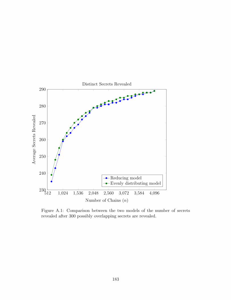
512 1,024 1,536 2,048 2,560 3,072 3,584 4,096230

240

250

260

270

280

290

Number of Chains (n)

Ave

rage

Sec

rets

Rev

eale

d

Distinct Secrets Revealed

Reducing modelEvenly distributing model

Figure A.1: Comparison between the two models of the number of secretsrevealed after 300 possibly overlapping secrets are revealed.

183

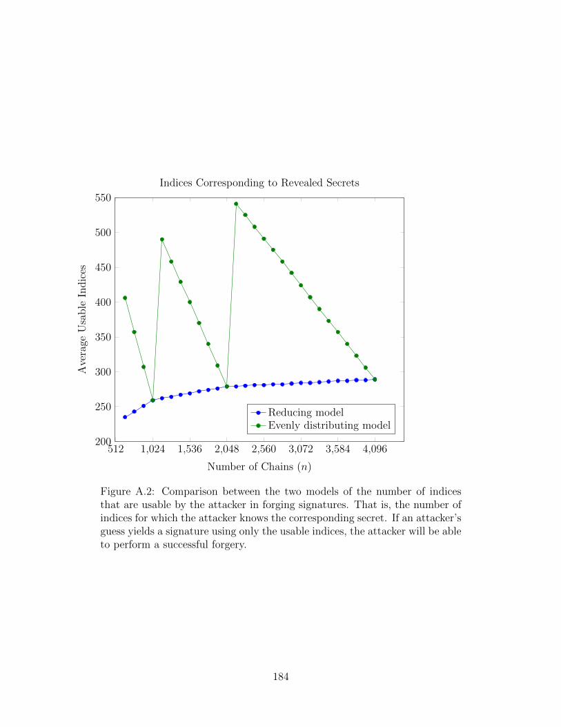
512 1,024 1,536 2,048 2,560 3,072 3,584 4,096200

250

300

350

400

450

500

550

Number of Chains (n)

Ave

rage

Usa

ble

Indic

es

Indices Corresponding to Revealed Secrets

Reducing modelEvenly distributing model

Figure A.2: Comparison between the two models of the number of indicesthat are usable by the attacker in forging signatures. That is, the number ofindices for which the attacker knows the corresponding secret. If an attacker’sguess yields a signature using only the usable indices, the attacker will be ableto perform a successful forgery.

184

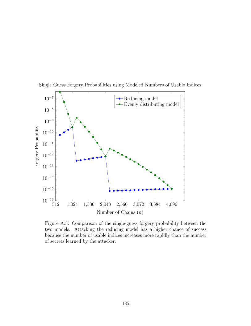
512 1,024 1,536 2,048 2,560 3,072 3,584 4,09610−16

10−15

10−14

10−13

10−12

10−11

10−10

10−9

10−8

10−7

Number of Chains (n)

For

gery

Pro

bab

ilit

y

Single Guess Forgery Probabilities using Modeled Numbers of Usable Indices

Reducing modelEvenly distributing model

Figure A.3: Comparison of the single-guess forgery probability between thetwo models. Attacking the reducing model has a higher chance of successbecause the number of usable indices increases more rapidly than the numberof secrets learned by the attacker.

185