JWG-B2/B4/C1.17 Impacts of HVDC Lines on the Economics of HVDC Projects Task Force JWG-B2/B4/C1.17 Brochure 388 Jose Antonio Jardini João Felix Nolasco John Francis Grahan Günter Bruske [email protected] [email protected] [email protected] [email protected]

JWG-B2/B4/C1.17 Impacts of HVDC Lines on the Economics of HVDC Projects Task Force JWG-B2/B4/C1.17 Brochure 388 Jose Antonio Jardini João Felix Nolasco.
Dec 14, 2015
Welcome message from author
This document is posted to help you gain knowledge. Please leave a comment to let me know what you think about it! Share it to your friends and learn new things together.
Transcript

JWG-B2/B4/C1.17
Impacts of HVDC Lines on the Economics of HVDC ProjectsTask Force
JWG-B2/B4/C1.17Brochure 388
Jose Antonio Jardini João Felix Nolasco John Francis Grahan Günter Bruske [email protected] [email protected] [email protected] [email protected]

JWG-B2/B4/C1.17
Impacts of HVDC Lines on the Economics of HVDC ProjectsFrom José Antonio Jardini, João Felix Nolasco
on behalf of CIGRE JWG-B2.17/B4/C1.17
João Francisco Nolasco, JWG Convenor (Brazil); José Antonio Jardini, TF Convenor (Brazil); John Francis Graham, Secretary (Brazil)
Regular members:João F. Nolasco (Brazil); John F. Graham (Brazil); José A. Jardini (Brazil); Carlos A.O. Peixoto (Brazil); Carlos Gama (Brazil; Luis C. Bertola (Argentina); Mario Masuda (Brazil); Rogério P. Guimarães (Brazil); José I. Gomes (Brazil); P. Sarma Maruvada (Canada); Diarmid Loudon (Norway); Günter Bruske – (Germany); Hans-Peter Oswald (Germany); Alf Persson (Sweden); Walter Flassbeck (Germany)
Corresponding members:Kees Koreman (Netherlands); Tim Wu (USA); Dzevad Muftig (South Africa); Bernard Dalle (France); Pat Naidoo (Zaire); José Henrique M. Fernandes (Brazil); Jutta Hanson (Germany); Riaz Amod Vajeth (Germany); Angus Ketley (Australia)
Reviewers: Rob Stephen (South Africa); Elias Ghannoun (Canada); Samuel
NguefeuGabriel Olguin (Chile) (France)

JWG-B2/B4/C1.17
Content
• Overview and Configurations Studied
• Transmission Line Considerations
• Converter Station Cost Equation
• Electrodes, Electrode Lines and Metallic Return
• System Economics
• Conclusions
• REFERENCES
JWG-B2/B4/C1.17Overview and Configurations Studied
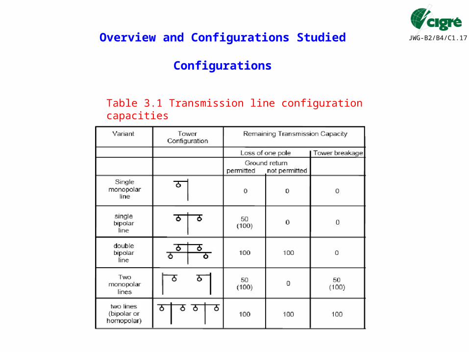
Configurations
Table 3.1 Transmission line configuration capacities
JWG-B2/B4/C1.17
Id
Ud
PdId
Ud
Pd
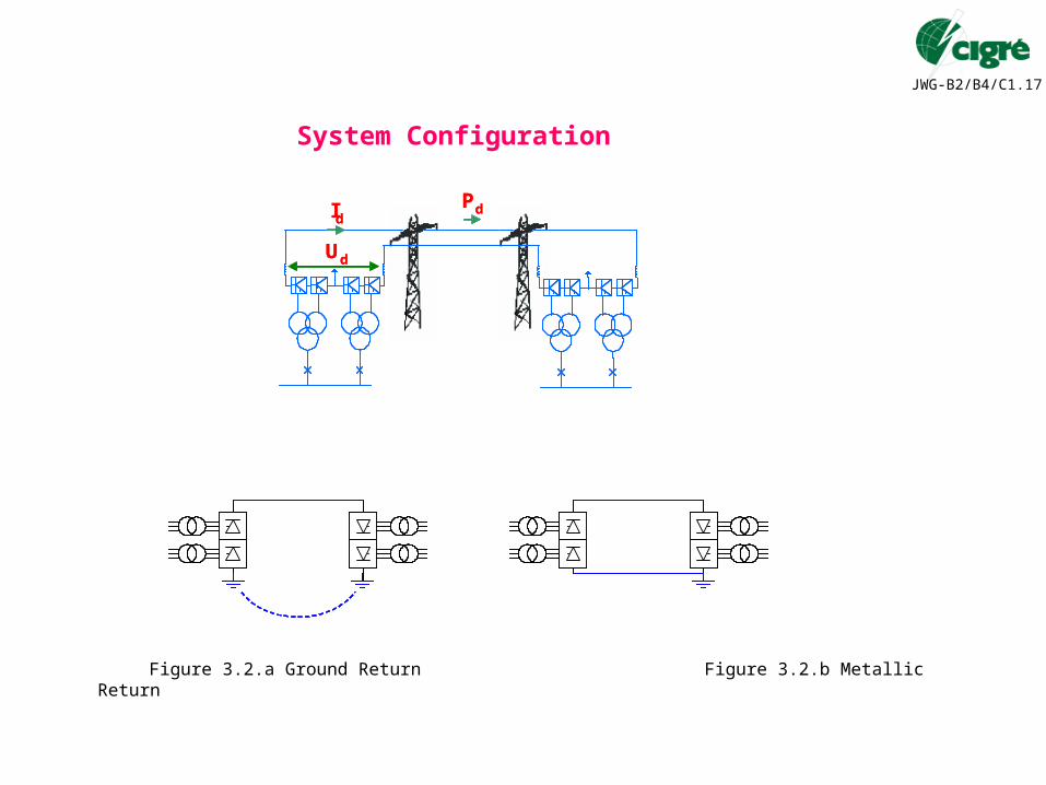
Figure 3.2.a Ground Return Figure 3.2.b Metallic Return
System Configuration

JWG-B2/B4/C1.17
Table 3.2 Cases studied
Bipole 750 MW 1,500 MW 3,000 MW 6,000 MW
750 km
± 300 kV
± 300 kV ± 500 kV ± 600 kV
± 500 kV
1,500 km ± 300 kV ± 500kV ± 500 kV ± 600 kV
± 500 kV ± 600 kV ± 800 kV
± 800 kV
3,000 km
± 500 kV ± 600 kV
± 600 kV ± 800 kV
± 800 kV

JWG-B2/B4/C1.17
Table 3.3 Converter configurations studied
1 2 3 4 5 6 7 8 9 10 11 12
Bipolar(MW) 750 750 750 750 1,500 1,500 3,000 3,000 3,000 6,000 6,000 6,000
Rating (kV) ±300 ±300 ±300 ±500 ±300 ±500 ±500 ±600 ±800 ±600 ±800 ±800
Conv/pole VSC
1x6 pulse 1 1 1 1 1 1 1
2 parallel 2 series
2 parallel

JWG-B2/B4/C1.17
One per pole - 3,000 MW Two Series - 6,000 MW Two Parallel - 6,000 MW
Figure 3.3 Basic converter station configurations

JWG-B2/B4/C1.17
Transmission Line Considerations

JWG-B2/B4/C1.17
TOPICS
• Overvoltages
• Insulation Coordination
• Corona Effects and Fields
• Line cost
• Line economics
JWG-B2/B4/C1.17
Overvoltages
Switching Surge
Operating Voltage
Lightning

JWG-B2/B4/C1.17

JWG-B2/B4/C1.17Switching Surge Related to (L-C) oscillations
• Energization
• Reclosing
• Fault Clearing
• Load Rejection
• Resonances
All above are important in the AC side of the stations (limitted by surge arrester)
DC side control ramp up and ramp down (no overvoltages)
Fault Application (the only one to be considered)

JWG-B2/B4/C1.17
Modeling

JWG-B2/B4/C1.17
1,4
1,5
1,6
1,7
1,8
1,9
2,0
2,1
0,0 187,5 375,0 562,5 750,0 937,5 1125,0 1312,5 1500,0
Transmission Line Length (km)
Ove
rvo
ltag
e (p
u)
Mid
Rectifier InverterMid
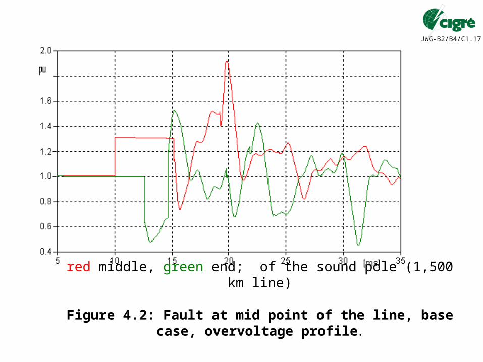
Fault at mid point of the line base case
overvoltage profile
JWG-B2/B4/C1.17
red middle, green end; of the sound pole (1,500 km line)
Figure 4.2: Fault at mid point of the line, base case, overvoltage profile.
JWG-B2/B4/C1.17
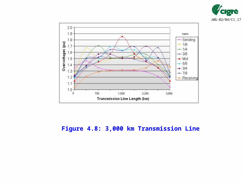
Figure 4.8: 3,000 km Transmission Line
JWG-B2/B4/C1.17
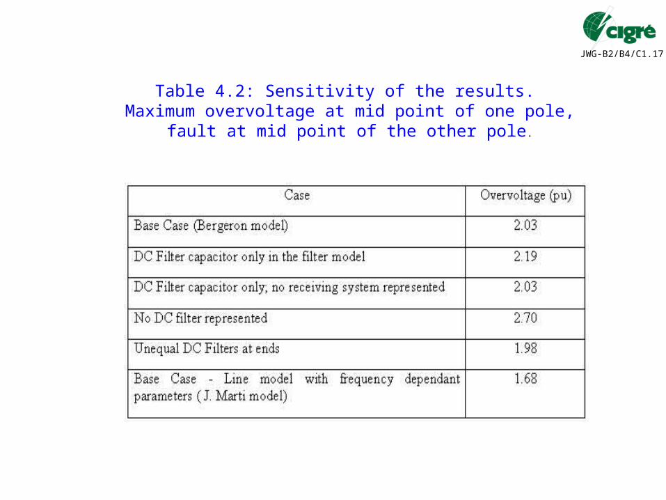
Table 4.2: Sensitivity of the results. Maximum overvoltage at mid point of one pole,
fault at mid point of the other pole.
JWG-B2/B4/C1.17
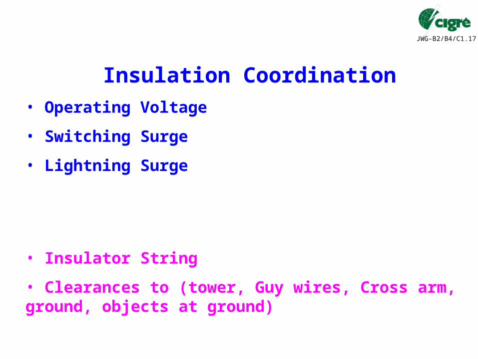
Insulation Coordination• Operating Voltage
• Switching Surge
• Lightning Surge
• Insulator String
• Clearances to (tower, Guy wires, Cross arm, ground, objects at ground)

JWG-B2/B4/C1.17
Contamination Severity
HVDC
very light light moderate heavy
leakage distance cm/kV 2 - 2.5 2.5 – 3.2 3.2 – 4 4 - 7
HVAC IEC71-1
light medium heavy very heavy
cm/kV(ph-ph rms) 1.6 2.0 2.5 3.1

JWG-B2/B4/C1.17
- Anti-fog insulator, pitch of 165mm and leakage distance 508mm;
-hardware length: 0,25m.
ITAIPU 27 mm/kV OK
Operating Voltage (kV)
Creepage distance 30mm/kV
Insulators Number
String Length (m)
(*)
300 18 3,22
500 30 5,20
600 36 6,20
800 48 8,17

JWG-B2/B4/C1.17
JWG-B2/B4/C1.17
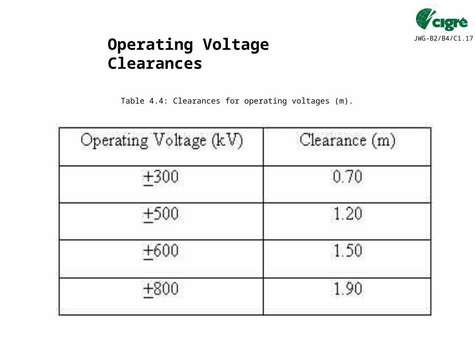
Operating Voltage Clearances
Table 4.4: Clearances for operating voltages (m).

JWG-B2/B4/C1.17
REGION ILine altitude: 300 to1000 m Average temperature: 16ºC
Ratio of vertical/horizontal span : 0.7wind return period: 50 years
Alfa of Gumbel distribution (m/s)-1: 0.30Beta of Gumbel distribution (m/s): 16.62
Distribution with 30 years of samples
Note: mean wind intensity 10 min 18.39 m/s standard deviation of 3.68 m/s.
wind intensity is 29.52 m/s for 50 year return periodTerrain classification: B
calculations based on CIGRE Brochure 48REGION II ICE

JWG-B2/B4/C1.17
Swing Angle to be used together with Operating Voltage Clearances
Conductor code MCMAluminum
mm2 Swing Angle ()
Joree 2,515 1274.35 44.5
Thrasher 2,312 1171.49 45.6
Kiwi 2,167 1098.02 46.9
2,034 2,034 1030.63 47.7
Chukar 1,780 901.93 47.5
Lapwing 1,590 805.65 49.5
Bobolink 1,431 725.09 50.7
Dipper 1,351.5 684.80 51.4
Bittern 1,272 644.52 52.0
Bluejay 1,113 563.93 53.4
Rail 954 483.39 55.0
Tern 795 402.83 56.7
1MCM=0.5067 mm2

JWG-B2/B4/C1.17
Insulation Coordination for Switching Surge
V50= k 500 d 0,6
V50 is the insulation critical flashover (50% probability) in kV
d is the gap distance in m
k is the gap factor:
K= 1,15 conductor-plane
K= 1,30 conductor–structure under
K= 1,35 conductor–structure (lateral or above)
K= 1,4 conductor-guy wires
K= 1,50 conductor–cross arms (with insulator string)
d
KV8
1
340050

JWG-B2/B4/C1.17

JWG-B2/B4/C1.17
Risk of Failure P1Withstand (1- P1)N gaps withstand (1- P1) n
Risk n 1-(1- P1) n ~ n P1
P1=0,02 2% with 200 gaps P=4%

JWG-B2/B4/C1.17
1,4
1,5
1,6
1,7
1,8
1,9
2,0
2,1
0,0 187,5 375,0 562,5 750,0 937,5 1125,0 1312,5 1500,0
Transmission Line Length (km)
Ove
rvo
ltag
e (p
u)
Mid
Rectifier InverterMid

JWG-B2/B4/C1.17
Figure 4.9: Conductor to tower clearances.

JWG-B2/B4/C1.17
Conductor-to-Ground (object; 4.5m; under)
0.0
1.0
2.0
3.0
4.0
5.0
6.0
7.0
8.0
300 400 500 600 700 800
Voltage (kV)
Cle
aran
ce (
m)
750 km
1,500 km
2,250 km
3,000 km

JWG-B2/B4/C1.17
CIGRE Brochure 48
Table 4.7: Swing angle to be used together with Switching Surge Clearances according [8]
ACSR Conductor code
MCM Swing Angle ()
Joree 2,515 13.4
Thrasher 2,312 13.8
Kiwi 2,167 14.3
2,034 2,034 14.6
Chukar 1,780 14.5
Lapwing 1,590 15.3
Bobolink 1,431 15.8
Dipper 1,351.5 16.1
Bittern 1,272 16.4
Bluejay 1,113 17.0
Rail 954 17.7
Tern 795 18.6
JWG-B2/B4/C1.17
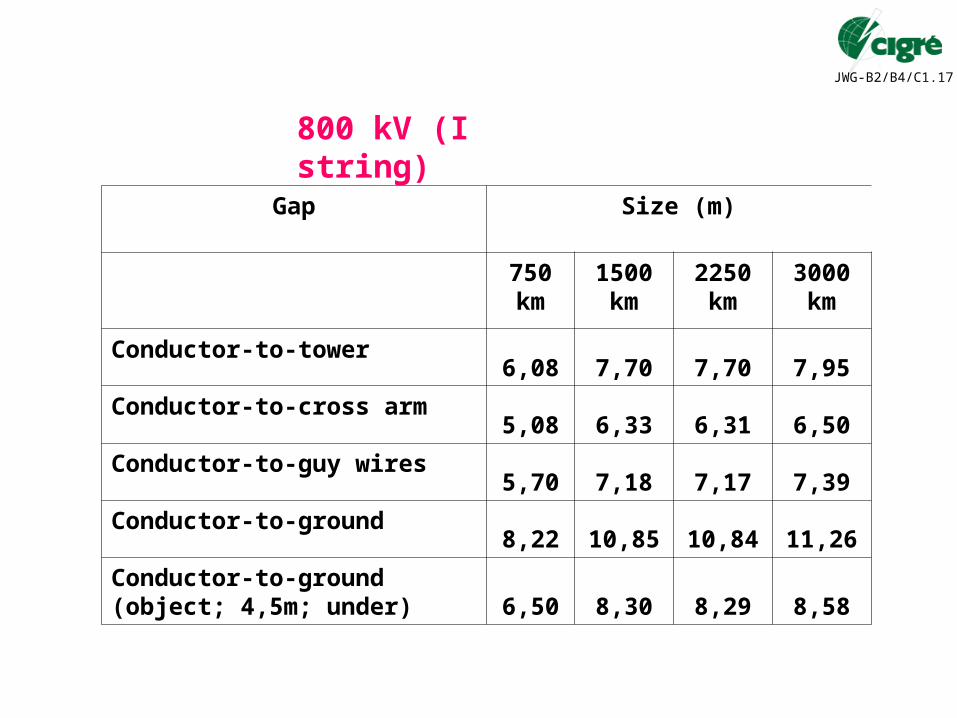
Gap Size (m)
750 km
1500 km
2250 km
3000 km
Conductor-to-tower6,08 7,70 7,70 7,95
Conductor-to-cross arm5,08 6,33 6,31 6,50
Conductor-to-guy wires5,70 7,18 7,17 7,39
Conductor-to-ground 8,22 10,85 10,84 11,26
Conductor-to-ground (object; 4,5m; under) 6,50 8,30 8,29 8,58
800 kV (I string)

JWG-B2/B4/C1.17
dmin
w
2R

JWG-B2/B4/C1.17
Pole Spacing Determination
• Pole Spacing Required for Operating Voltage
•DPTO = (R + dmin + (L + R) sin) 2 + w
•dmin : operating voltage clearance (m)
•R: bundle’s radius (m)
•L: insulators string length (m)
: swing angle (degree)
•w: tower width (m)

JWG-B2/B4/C1.17
POLE SPACING FOR 800 kV
14,0
15,0
16,0
17,0
18,0
19,0
20,0
21,0
22,0
500 1000 1500 2000 2500 3000
Conductor Cros Section (kcmil)
Po
le S
pac
ing
(m
) OV
SS 750km
SS 1500km
SS 2250km
SS 3000km
I string
governed by operating voltage (OV) plus conductor swing

JWG-B2/B4/C1.17
Table 4.10 - Pole Spacing (m) for Operating Voltage I strings
ACSR Conductor
Cross Section (MCM)
Pole Spacing (m)
±300 kV ±500 kV ±600 kV ±800 kV
Joree 2,515 8.2 12.5 14.6 18.8
Thrasher 2,312 8.3 12.6 14.8 19.1
Kiwi 2,167 8.4 12.8 15.0 19.3
2,034 2,034 8.5 12.9 15.1 19.5
Chukar 1,780 8.5 12.9 15.1 19.5
Lapwing 1,590 8.6 13.1 15.4 19.8
Bobolink 1,431 8.7 13.3 15.6 20.1
Dipper 1,351.5 8.8 13.4 15.7 20.2
Bittern 1,272 8.8 13.4 15.8 20.3
Bluejay 1,113 8.9 13.6 16.0 20.6
Rail 954 9.0 13.8 16.2 20.8
Tern 795 9.2 14.0 16.4 21.1

JWG-B2/B4/C1.17
Current capability
wind speed (lowest) 1 m/swind angle 45
degreeambient temperature 35ºCheight above sea level 300 to
1000 msolar emissivity of surface 0.5solar absorvity of surface 0.5global solar radiation 1000
W/m2R I2 + Wrad = k Δθ + W dessip
θcond = θambient + Δθ

JWG-B2/B4/C1.17
Conductor Current Carrying Capability
0
500
1000
1500
2000
2500
0 500 1000 1500 2000 2500 3000
Conductor Cross Section (MCM)
Cu
rre
nt
(A) 90º
70º
60º
50º

JWG-B2/B4/C1.17
CONDUCTOR SAG
17
18
19
20
21
22
23
795 954 1272 1590 2167 2515
Conductor Cross Section (MCM)
Sag
(m
)
50º
60º
70º
90º
EDS Every Day Stress condition . Traction 20% of the rupture load . Temperature 20 oC

JWG-B2/B4/C1.17
Conductor and shield wire height at tallest tower(2 shield wires - for one add 2.5 m to hg)
Voltage ( kV) hp (m) hg (m)
300 38.3 44.3
500 42.8 50.8
600 44.8 53.8
800 50.8 61.8
ExtsgChp S
GDdisRhphg
Conductor (hp) and shield wire (hg) heights

JWG-B2/B4/C1.17
Shield Wire Position
position of the shield wire => to provide effective shielding against direct strokes in the conductors.
The better coupling => means as closed as possible of the conductor
Z
E2Ioc
8.0
ocI7.6krsc
terrain “rolling”hp*= hpb*= (hg-hp) + (Sc-Sg)(2/3)hg*= hp* +b*

JWG-B2/B4/C1.17
θ
ground
ground protection
shield wire and conductor protection

JWG-B2/B4/C1.17Protection angle
2 shield wires
1 shield wire 5 m above
cross arm Voltag
e
(kV)
E
(kV)
Hg*
(m)
Hp*
(m) Ioc
(kA)
rsc
(m)
X
(m)
degre
e
X (m) Minimum pole
spacing (m)
300 1900 43.1 32,3 11.9 48.7 2.5 13 2.
5.2
500 3000 49.6 36,8 18.9 70.2 5.4 22 5.
11.7
600 3600 52.6 38,8 22.6 81.2 6.8 26 6.4
14.8
800 4850 60.6 44,8 30.5 103.1 8.9 29 8.4
21.3 As the shield wires should be close to the conductors a protection angle of 10 degrees can be assumed when using 2 shield wires.If one shield wire is used than the protection is almost good for tower with V strings. If I string are used than one shield wire may be used in location with low lightning activity.

JWG-B2/B4/C1.17Table 4.14: Swing angles for ROW width definition
ConductorSwing Angle
(degree)ACSR Code Section (MCM)
Joree 2,515 34.1
Thrasher 2,312 35.1
Kiwi 2,167 36.4
2,034 2,034 37.2
Chukar 1,780 37.0
Lapwing 1,590 39.1
Bobolink 1,431 40.4
Dipper 1,351.5 41.1
Bittern 1,272 41.9
Bluejay 1,113 43.5
Rail 954 45.4
Tern 795 47.5

JWG-B2/B4/C1.17
Right Of Way ( I strings) Operating Voltage plus conductor swing due to high wind. Verification of corona effects and fields
CROSS SECTION
(kcmil)300 kV 500 kV 600 kV 800 kV
2515 54,7 62,2 65,9 73,32312 56,0 63,6 67,4 74,92167 59,3 67,0 70,9 78,52034 60,1 67,9 71,8 79,51780 54,3 62,1 66,0 73,71590 58,7 66,7 70,7 78,51431 59,6 67,7 71,8 79,8
1351,5 60,4 68,6 72,7 80,81272 61,1 69,4 73,5 81,61113 62,9 71,3 75,5 83,8954 63,8 72,4 76,7 85,1795 65,5 74,3 78,6 87,2
RAILTERN
BITTERNBLUEJAY
BOBOLINKDIPPER
CONDUCTOR
CHUKARLAPWING
JOREETHRASHER
KIWI2034
JWG-B2/B4/C1.17
Corona effects and Fields

JWG-B2/B4/C1.17
]
1)2
(
2[
/*)1(1
2
S
HR
HLnrN
RrNVG
e
Corona Visual
9.0
82.0
/))(
613.01(5.24
4.00
m
cmkVr
mG
G < 0.95 G0
rmEc
301.0130

JWG-B2/B4/C1.17

JWG-B2/B4/C1.17
JWG-B2/B4/C1.17
300
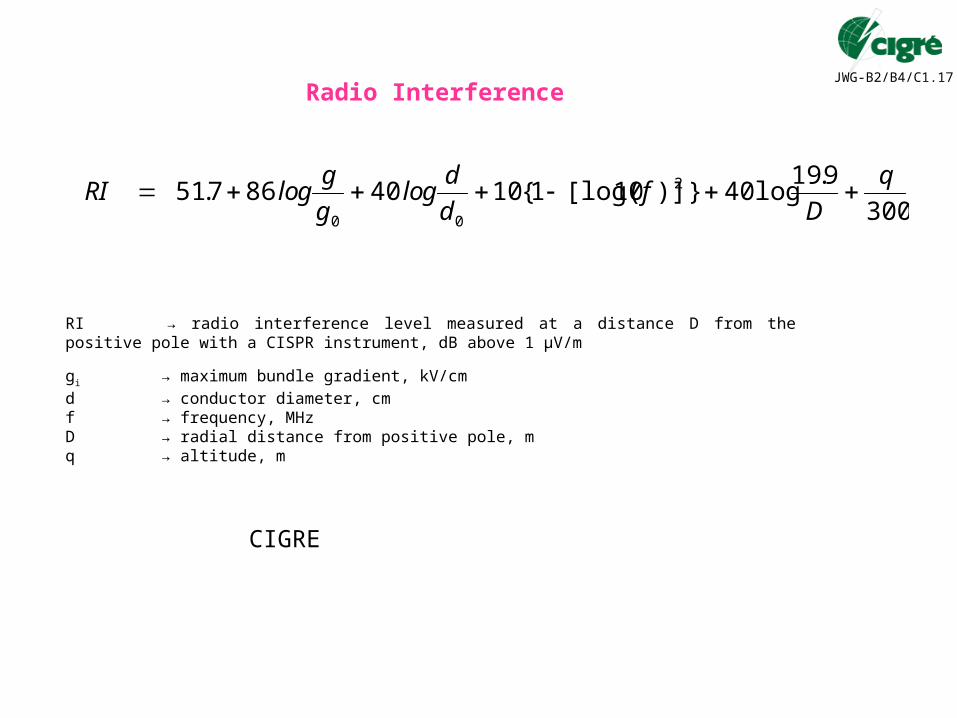
9.19log40})]10[log(1{1040867.51 2
00
q
Df
d
dgol
g
ggolRI
RI → radio interference level measured at a distance D from the positive pole with a CISPR instrument, dB above 1 μV/m
gi → maximum bundle gradient, kV/cm
d → conductor diameter, cmf → frequency, MHzD → radial distance from positive pole, mq → altitude, m
Radio Interference
CIGRE

JWG-B2/B4/C1.17

JWG-B2/B4/C1.17Criteria: at the edge of the right of way
SNR = 20 dBu
Signal 66 dBu => Noise = 46 dBu
Noise=46 dBu. 50% value? in which season?
needs statistical consideration subtract 4 dBu
Noise 42 dBu for 90% probability
JWG-B2/B4/C1.17
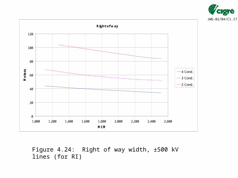
Right of way
0
20
40
60
80
100
120
1,000 1,200 1,400 1,600 1,800 2,000 2,200 2,400 2,600
MCM
Mete
rs 4 Cond.
3 Cond.
2 Cond.
Figure 4.24: Right of way width, ±500 kV lines (for RI)

JWG-B2/B4/C1.17
RgoldgolngolkggolANAN 4.1140860 300
q +
g → average maximum bundle gradient, kV/cm n → number of sub-conductorsd → conductor diameter, cm R → radial distance from the positive conductor to the point of observation
The empirical constants k and AN0 are given as:
k = 25.6 for n 2k = 0 for n = 1,2
AN0 = -100.62 for n 2
AN0 = -93.4 for n = 1,2
Audible Noise CIGRE

JWG-B2/B4/C1.17
JWG-B2/B4/C1.17
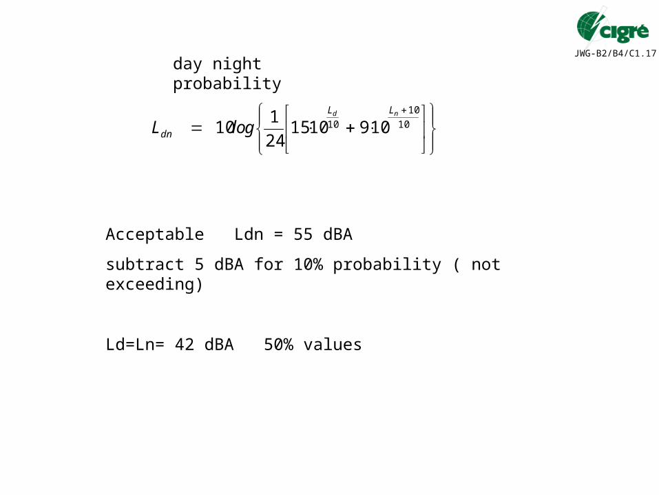
10
10
10 109101524
110
nd LL
dn golL
day night probability
Acceptable Ldn = 55 dBA
subtract 5 dBA for 10% probability ( not exceeding)
Ld=Ln= 42 dBA 50% values

JWG-B2/B4/C1.17
Figure 4.25: Right-of-way width, ±500 kV line (for AN)

JWG-B2/B4/C1.17
Figure 4.25: Right-of-way width (RI and AN), ± 500 kV, 3 cond. /pole

JWG-B2/B4/C1.17Table 4.21: ROW (m) requirements for ±600 kV lines, I strings.
kV n MCMROW
RIROWAN
600 3
2,515 70 52
2,167 76 62
1,780 80 78
600 4
2,515 48 16
1,780 52 30
1,113 62 60
600 5
2,515 30 16
1,780 34 16
795 50 44
Table 4.22: ROW (m) requirements for ±800 kV lines, I strings.
kV n MCMROW
RIROWAN
800 4
2,515 76 144 *
2,167 76 144 *
1,590 88 -
800 5
2,515 50 80
2,167 54 96
1,272 64 136**
800 6
2,515 20 34
1,590 40 74
1,272 46 94
Notes: * If the criteria are relaxed by 2 dB, then the right of way can be reduced to 90 and
100 m, ** If the criteria are relaxed by 2 dB, then the right of way can be reduced to 100 m.

JWG-B2/B4/C1.17
RoW 3 conductor per pole 500 kV
15
25
35
45
55
65
75
1,000 1,500 2,000 2,500
MCM
m o
r kV/c
m
RI (m)
AN (m)
gradient (kV/cm)
insulation clearance (m)
Figure 4.27: Half ROW and gradient for 500 kV bipole having three conductors per pole.

JWG-B2/B4/C1.17
HVeE HP /)1(31.1 /7.132/7.015 /)1(1065.1 HVexJ HP
32/7.015 /)1(1015.2 HVexJ hp
a)- maximum saturated values, within right of way (in the ground, close to conductors, bipolar lines) [15].
P= pole spacing (m)H= conductor height (m)V= Voltage (kV)E= Electric field (kV/m)J = Ion flow (A/m2)
Electrical Field - Space Charge

JWG-B2/B4/C1.17
4/)2/(1 Hpx
HVeeE HPxHP /].1[46.1 ./)2/(7.0/5.2
32./)2/(75.1/5.115 /].1[1054.1)( HVeeJ HPxHP
32./)2/(75.1/5.115 /].1[10.2)( HVeeJ HPxHP
b) maximum saturated values in the ground, at any distance “x” from the tower center provided that

JWG-B2/B4/C1.17c) Electrical Field without space charge
2222
2
22 )2/(
1
)2/(
1.
41
2
1)
4(1
2
PxHPxH
P
PHn
deq
Hn
HVE
d) Saturation factor
where: k empirical coefficient G= surface gradient (kV/cm) Go empirical coefficient
)( QeQsSQeQ
)(1 OGGKeS
e) Values considering the degree of saturation

JWG-B2/B4/C1.17
Summer fair (moderated case)- Positive (field and current) peak50% value Go= 9 kV/cm k= 0.03795% value Go= 3 kV/cm k= 0.067- Negative (field and current) peak50% value Go= 9 kV/cm k= 0.01595% value Go= 3 kV/cm k= 0.032Summer height humidity/fog (worst case)- Positive (field and current) peak50% value Go= 7.5 kV/cm k= 0.0695% value Go= 3 kV/cm k= 0.086- Negative (field and current) peak50% value Go= 8.5 kV/cm k= 0.04595% value Go= 3 kV/cm k= 0.063

JWG-B2/B4/C1.17Table 4.28: Minimum clearance to ground
Voltage kVConductor per pole
I stringsMCM/MCM
I stringsHeight (m)
V stringMCM
V stringHeight (m)
±300
1 1,590/2515 > 6 2,034/2,515 6.5
2 605/2,515 7 795/2,515 6.5
3 336.4/2,515 7 336.4/2,515 6.5
±500
2 2,312/2,515 10.7 None
3 1,113/2,515 11.51,351.5/2,51
511
4 605/2,515 11.8 795/2,515 11
5 477/2,515 11.8 < 477/2,515 11
±600
3 1,780/2,515 13.2 2,167/2,515 13.5
4 954/2,515 13.8 1,272/2,515 13.5
5 605/2,515 14.3 795/2,515 13.5
±800
4 2,167/2,515 17.5 2,515 17.5
5 1,272/2,515 18.0 1,590/2,515 17.5
6 954/2,515 18.7 1,113/2,515 17.5
Criteria 12.5 kV/m without space charge
JWG-B2/B4/C1.17
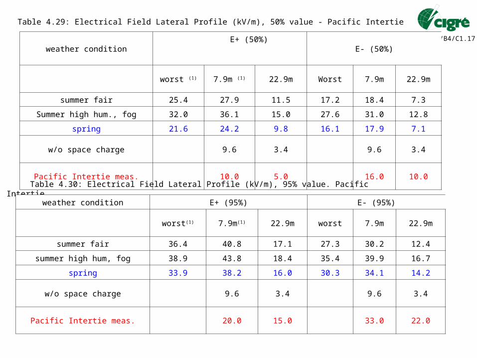
Table 4.29: Electrical Field Lateral Profile (kV/m), 50% value - Pacific Intertie
weather condition E+ (50%) E- (50%)
worst (1) 7.9m (1) 22.9m Worst 7.9m 22.9m
summer fair 25.4 27.9 11.5 17.2 18.4 7.3
Summer high hum., fog 32.0 36.1 15.0 27.6 31.0 12.8
spring 21.6 24.2 9.8 16.1 17.9 7.1
w/o space charge 9.6 3.4 9.6 3.4
Pacific Intertie meas. 10.0 5.0 16.0 10.0
Table 4.30: Electrical Field Lateral Profile (kV/m), 95% value. Pacific Intertie
weather condition E+ (95%) E- (95%)
worst(1) 7.9m(1) 22.9m worst 7.9m 22.9m
summer fair 36.4 40.8 17.1 27.3 30.2 12.4
summer high hum, fog 38.9 43.8 18.4 35.4 39.9 16.7
spring 33.9 38.2 16.0 30.3 34.1 14.2
w/o space charge 9.6 3.4 9.6 3.4
Pacific Intertie meas. 20.0 15.0 33.0 22.0

JWG-B2/B4/C1.17Table 4.31: Ion Current Lateral Profile (nA/m²), 50% value
weather condition J+ (50 %) J- (50%)
worst(*) 7.9m(*) 22.9m worst 7.9m 22.9m
summer fair 52.5 47.5 5.5 32.8 36.4 4.2
summer high hum., fog 75.7 68.6 8.0 80.0 88.7 10.3
spring 41.8 37.8 4.4 31.0 34.4 4.0
Pacific Intertie meas. 2.0 2.0 20.0 5.0
Table 4.32: Ion Current Lateral Profile (nA/m²), 95% value
weather condition J+ (95%) J- (95%)
worst(*) 7.9m(*) 22.9m worst 7.9m 22.9m
summer fair 89.2 80.7 9.4 76.7 85.1 9.9
summer high hum., fog 98.0 88.7 10.3 113.1 125.4 14.6
spring 81.8 74.0 8.6 91.3 101.3 11.8
Pacific Intertie meas. 45.0 20.0 125.0 50.0
Calculation with BPA software resulted in 145.0 and 25.5 nA/m2 at 7.9 and 22.9 m (sic)

JWG-B2/B4/C1.17a) Electrical field
The electrical field should be bellow 40 kV/m, (correspondent to the level of annoyance “disturbing nuisance”)
In fact depend on kV plus nA/m2
b) Ion currentThe ion current, value with 95% probability of not being exceeded,
in any place, shall not result in a current higher than 3,5 mA “threshold of perception for woman, DC current”.
A person has an equivalent area o f 5 m2, so:
2/7,05
5,3mmAJ
GREEN BOOK OLD

JWG-B2/B4/C1.17
Considerations made
Person normally grounded with a current It = 4 mA current through him
Person highly insulated touching ground objects, It = 4 mA
Person grounded touching large vehicle (grounded through 1 MW).

JWG-B2/B4/C1.17
Condition I: Through a person with a resistance to ground Rp= 200 Mohm, pass I= 4 uA (they found no measurements with current above 3 uA). The voltage across him will be 800 V and the nuisance is classified as “ No Sensation”. The ion flow in this case is 4/5= 0.8 uA/m2
Condition II: A person with Rp= 500 Mohm and capacitance Cp= 100 pF, subjected to a current of I= 4 uA, touch a grounded object (R=100 ohm). The initial discharge current is than 20A but only 1mA after 0.1 us; the energy is 0.2 mJ (acceptable is 250 mJ “uncomfortable chock”). The ion flow is also 0.8 uA/m2
Condition III: A person Rp= 1500 ohm, Cp=0, touch a truck Ro= 1 Mohm, Co= 10 000 pF where 1000 uA is passing through it ( measurements by Moris in a car 14X2.4X4m placed under a 600 kV line, with a clearance of 2.5 from conductor to truck top was bellow 300 uA). In this case the voltage truck to ground would be 1kV ten initial current is 670 uA , 1mA after 100 us, and an energy of 5 mJ (1/50 of 250 mJ “uncomfortable chock”). The ion flow in this case is 1000/(14*2.4*4)=7.5 uA/m2
Analyzing these conditions it can be proposed the ion flows limits: 0.8 uA/m2 places with access to people 7.5 uA/m2 places with access to truck Note: The criteria above is conservative by at least a factor 10

JWG-B2/B4/C1.17Perception of the field

JWG-B2/B4/C1.17
Reference
[46] Chinese 2006 30 kV/m in the ROW 25 kV/m close to building
[48] Italian manuscript standard
42 kV/m 1-8 Hz 14 kV/m general public (GP)
[49] Kosheev Russia GP=40 kV/m 100 nA/m2 Work =3600/(E+0.25 E)2
Health Council Netherland 340 kV/m (nothing on blood, reproduction, prenatal mortality
DIN 40 kV/m 60 kV/m for 2 hours
B4-45 25 kV/m 100 nA/m2 Probability? season?
[51} EPRI proj. 1 proj. 2 (basic) proj. 3 (severe)
(kv/m; nA/ m2)no requirements40; 100 inside ROW20;20 inside ROW
no requirements10; 5 edge ROW5;1 edge
Criteria
Conclusion:
40 kV/m 100 nA/m2 in the ROW
10 kV/m 5 nA/m2 at the edge
Worst weather; 5% of not being exceeded
Allowance for 1 h work at midspan as per Russian criteria

JWG-B2/B4/C1.17
Mechanical design

JWG-B2/B4/C1.17
Voltage Pole spacing PS
distance between
shield wires
H conduct
H shield wires
Dins n cond
MCM code Condsag
Shield wire
sag
(kV) (m) (m) (m) (m) (m) (m) (m)
300 8,4 6,8 36,9 42,6 3,22 2 2167 Kiwi 22,7 18,2
300 8,5 6,9 35,9 41,6 3,22 4 1780 Chukar 21,7 17,4
500 13,4 11,1 39,5 47,2 5,2 2 1272 Bittern 20,8 16,6
500 13 10,7 39,7 47,4 5,2 3 1590 Lapwing 21 16,8
500 12,8 10,5 41,9 49,6 5,2 4 2167 kiwi 22,7 18,2
600 15,8 13,1 41,5 50,2 6,2 3 1272 Bittern 20,8 16,6
600 15,1 12,4 42,9 51,6 6,2 4 1780 Chukar 21,7 17,4
600 15 12,3 43,9 52,6 6,2 6 2167 Kiwi 22,7 18,2
800 20,8 17,4 46,2 56,9 8,17 5 954 Rail 20,5 16,4
800 19,3 15,9 48,4 59,1 8,17 5 2167 Kiwi 22,7 18,2

JWG-B2/B4/C1.17
General dimensions (guyed tower with I string)
Voltage
Pole spacing PS
distance between
shield wires
Conductor Height H
shield wires heights H
Dinsn
conductMCM code
(kV) (m) (m) (m) (m) (m)
300 8.4 6.8 36.9 42.6 3.22 2 2167 Kiwi
300 8.5 6.9 35.9 41.6 3.22 4 1780 Chukar
500 13.4 11.1 39.5 47.2 5.2 2 1272 Bittern
500 13 10.7 39.7 47.4 5.2 3 1590 Lapwing
500 12.8 10.5 41.9 49.6 5.2 4 2167 kiwi
600 15.8 13.1 41.5 50.2 6.2 3 1272 Bittern
600 15.1 12.4 42.9 51.6 6.2 4 1780 Chukar
600 15 12.3 43.9 52.6 6.2 6 2167 Kiwi
800 20.8 17.4 46.2 56.9 8.17 5 954 Rail
800 19.3 15.9 48.4 59.1 8.17 5 2167 Kiwi

JWG-B2/B4/C1.17
Minimum Clearances and Swing Angle
Voltage n
cond.
MCM code
Operating OperatingSwitching
surgeSwitching surge Switching
surge
(kV)Voltage
Clearance (m)Voltage Angle
(degree)Clearance to
tower (m)Clearance to guy
wires (m)Angle (degree)
300 2 2167 Kiwi 0.7 46.9 1.3 1.23 7
300 4 1780 Chukar 0.7 47.5 1.3 1.23 7.1
500 2 1272 Bittern 1.2 52 3.06 2.87 8.1
500 3 1590 Lapwing
1.2 49.5 3.06 2.87 7,5
500 4 2167 kiwi 1.,2 46.9 3.06 2.87 7
600 3 1272 Bittern 1.5 52 4.14 3.89 8.1
600 4 1780 Chukar 1.5 47.5 4.14 3.89 7.1
600 6 2167 Kiwi 1.5 46.9 4.14 3.89 7
800 5 954 Rail 1.9 55 6.81 6.37 8.8
800 5 2167 Kiwi 1.9 46.9 6.81 6.37 7

JWG-B2/B4/C1.17
• Region I without ice • Region II with ice.
Table 4.39: Region I Design Temperatures (°C)
Condition Temperatures (ºC)
EDS Every Day Stress 20
Minimum 0
Coincident with wind 15
Mean maximum 30
Table 4.40: Wind data
Description Data Values
Reference height (m) 10
Intensity - mean of the sample (m/s) (10 min average wind) 18.4
Standard deviation (m/s) 3.68 (20% of mean)
Sample period (years) 30
Ground roughness B
[40} IEC/TR 60826

JWG-B2/B4/C1.17Table 4.44: Region II Design Temperatures (°C).
Condition Temperatures (ºC)
EDS Every Day Stress (Installation condition)
0
Minimum -18
Ice load condition -5
Table 4.45: Wind data.
Description Data Values
Reference height (m) 10
Intensity - mean of the sample (m/s) (10 min average wind) 20
Standard deviation (m/s) 3.60 (18% of mean)
Sample period (years) 30
Ground roughness C
Table 4.46: Ice data
•Description •Data Values
•Intensity - mean of the sample - gm
(N/m)•16.0
•Standard deviation (% of mean) •70
•Sample period (years) •12
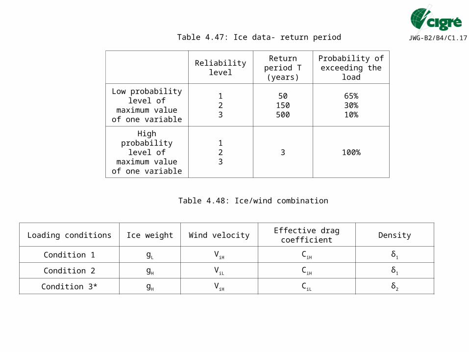
JWG-B2/B4/C1.17Table 4.47: Ice data- return period
Reliability levelReturn period T
(years)Probability of
exceeding the load
Low probability level of maximum value of
one variable
123
50150500
65%30%10%
High probability level of maximum value of
one variable
123
3 100%
Table 4.48: Ice/wind combination
Loading conditions Ice weight Wind velocity Effective drag coefficient Density
Condition 1 gL ViH CiH δ1
Condition 2 gH ViL CiH δ1
Condition 3* gH ViH CiL δ2

JWG-B2/B4/C1.174- Sag and tension calculations
initial state:- EDS Every Day Stress: 20% of rupture load for conductor, and 11% for shield wire extra high strength steel.- Temperature 20º C- Creep corresponding to 10 years- High wind simultaneous with temperature of 15 ºC. In this case the tension shall be lower than 50% of the cable rupture
load.
-At minimum temperature (equal to 0 ºC), with no wind , the tension shall be lower than 33 % of the cable rupture load

JWG-B2/B4/C1.17
4.3- TensionsAn average span of 450 m is considered, and the conditions checked are:
- high wind transverse- high wind 45 o- temperature 10ºC, no wind- temperature 0 ºC, no wind- temperature 65 ºC, no wind- storm wind, transverse- storm wind, 45 o- EDS, 20ºC, no wind

JWG-B2/B4/C1.17
Conductor tensions
TOWER
CONDUCTOR TENSION (kgf)
Voltage (kV)
Conductor Code
High wind.
Transv.
High wind 45º Wind
10ºC no Wind
0ºC no Wind
65ºC no Wind
Thunderstorm Wind
transv.
Thunderstorm Wind 45º
EDS 20ºC no Wind
300 Kiwi 6.775 5.890 4.618 5.036 4.166 5.166 4.763 4.526
Chukar 8.642 6.044 4.738 5.255 4.190 5.310 4.890 4.624
500 Bittern 6.754 4.453 3.173 3.533 2.804 3.614 3.271 3.096
Lapwing 7.693 5.218 3.920 4.354 3.473 4.477 4.069 3.827
Kiwi 8.610 5.942 4.618 5.036 4.166 5.166 4.763 4.526
600 Bittern 6.775 4.463 3.173 3.533 2.127 3.724 3.322 3.096
Chukar 8.850 6.129 4.738 5.255 4.190 5.310 4.890 4.624
Kiwi 8.687 5.973 4.618 5.036 4.166 5.166 4.763 4.526
800 Kiwi 8.851 6.038 4.618 5.036 4.166 5.166 4.763 4.526
Rail 5.828 3.706 2.413 2.694 2.127 2.953 2.563 2.353

JWG-B2/B4/C1.17
Tower series
The tower and foundation weights are calculated only for suspension tower.
Possible line angles are d=0 o, or d=2 o
Loading tree

JWG-B2/B4/C1.17
Code Description
V0 HW at 90º; d = 0; highest VS
VOR HW at 90º; d = 0; lowest VS
V1 HW 90º; d = 2; highest VS
V1R HW at 90º; d = 2; lowest VS
V4 HW at 450; d = 2; highest VS
V4R HW at 450; d = 2; lowest VS
W1 TW at 90º; d = 2; highest VS
W1R TW at 90º; d = 2; lowest VS
W3 TW at 45º; d = 2; highest VS
W3R TW at 45º; d = 2; lowest VS
W4 TW at 0º; d = 2; highest VS
W4R TW at 0º; d = 2; lowest VS
R1 No wind; shield wire 1 rupture; d = 2; highest VS
R1R No wind; shield wire 1 rupture; d = 2; lowest VS
R2 Same as R1 but for shield wire 2 rupture
R2R Same as R1R but for shield wire 2 rupture
R4 No wind; pole 1 conductor 1 rupture; d = 2; highest VS
R4R No wind; pole 1 conductor 1 rupture; d = 2; lowest VS

JWG-B2/B4/C1.17
R5 Same as R4 but for pole 2 conductor rupture
R5R Same as R4R but for pole 2 conductor rupture
D1 No wind longitudinal unbalance; d = 2; highest VS
D1R No wind longitudinal unbalance; d = 2; lowest VS
M1 Shield wire 1 on shivers and maintenance; d = 2
M2 As before; shield wire 2
M4 As before; pole 1 conductors
M5 As before; pole 2 conductors
MVR Cables on shivers; wind = 0,6 HW
MS1 Shield wire 1 erection; no dynamic forces; d = 2
MS2 As before; shield wire 2
MS4 Same as before; pole 1 conductors
MS5 Same as before; pole 2 conductor
MS7 As MS5 but pole 1 is the last pole to be erected
MC1 Shield wire 1 erection; with dynamic forces; d = 2
MC2 Same before; shield wire 2
MC4 Same before; pole 1 conductors
MC5 Same before; pole 2 conductors
MC7 Same as MC5 but pole 1 is the last to be erected
514440 MS;D;R;W;V;V
JWG-B2/B4/C1.17
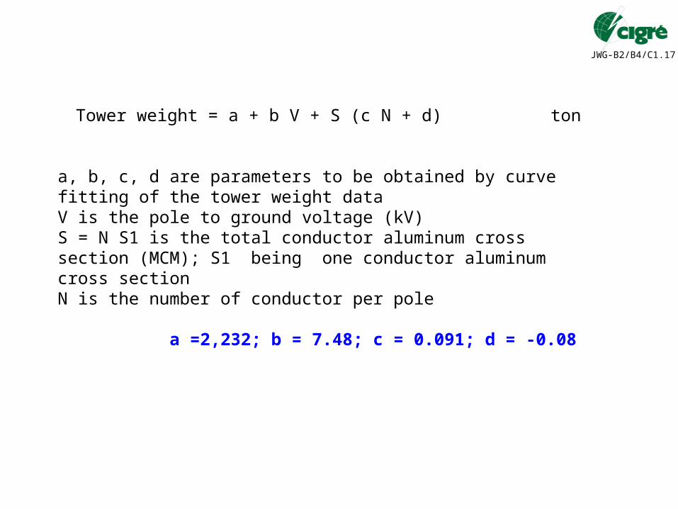
Tower weight = a + b V + S (c N + d) ton
a, b, c, d are parameters to be obtained by curve fitting of the tower weight dataV is the pole to ground voltage (kV)S = N S1 is the total conductor aluminum cross section (MCM); S1 being one conductor aluminum cross sectionN is the number of conductor per pole
a =2,232; b = 7.48; c = 0.091; d = -0.08

JWG-B2/B4/C1.17
Table 4.53: Regression analysis, tower weight calculation
kV NTotal
section(MCM)
Original weight(Ton)
Weight from equation
(ton)Error (%)
±3002 4,334 4,218 4,904 -14.0
4 7,120 6,676 6,477 3.1
+500
2 2,544 5,960 6,223 -4.2
3 4,770 7,248 6,878 5.4
4 8,668 8,727 8,408 3.8
+600
3 3,816 6,232* 7,445 -16.3
4 7,120 9,303 8,721 6.7
6 13,002 18,354 * 12,743 44.0
+8006 5,724 11,027 10,868 1.5
5 10,835 11,570 12,248 -5.5

JWG-B2/B4/C1.17
case DescriptionTower Weight
(kg)
1 Base Case: increase 2m in the pole spacing 7,498
2 Base Case: increase 3m in the tower height 7,579
3 Tower with V string, +500 kV, 3xLapwing 9,7
4Self supporting tower, +500 kV, 3xLapwing, I string 15,6
5 Only one shield wire, Base Case 7,749
6Region with ice, 500 kV, 3xFalcon, guyed tower, I string 12,983
7 Monopolar line, Base Case 6,38
8 Metallic return by the shield 10,384
9 Base Case: period return wind 500 years 10,454
10 Base Case: cross-rope tower 7,878
11BASE CASE (+500kV,3xLapwing, guyed, I string, non ice, bipolar, no metallic return, 2 shield wires) 7,248
Sensitivity

JWG-B2/B4/C1.17
line material and labor
. Engineering DesignTopographySurveyEnvironmental studies. MaterialsTowerFoundation conductor shield wireguy wire grounding (counterpoise) insulator conductor hardwareshield wire hardwareguy wire hardwarespacer damping accessories
• Man laborROW and access Tower erectionTower foundation erectionTower foundation excavationGuy wire foundation erectionGuy wire foundation excavationConductor installationShield wire installationGuy wire installationGrounding installation • Administration & Supervisionmaterial transportation to siteinspection at manufacturer siteconstruction administration. Contingencies. Taxes were considered separately
from items above

JWG-B2/B4/C1.17
• Operation costs joule and corona losses,
• operation and maintenance
• electrode and electrode lines
• converter station staging

JWG-B2/B4/C1.17
ITEM DESCRIPTION
±300kV ±300kV ±500kV ±500kV ±500kV ± 600kV ±600kV ±600kV ±800kV ±800kV
2 Kiwi 4 Chukar 2 Bittern3
Lapwing 4 Kiwi 3 Bittern 4 Chukar 6 Kiwi 6 Rail 5 Kiwi
MCM total 4334 7120 2544 4770 8668 3816 7120 13002 5724 10835
1 Engineering %
Engineering (design, topography, survey, environmental studies) 4.79 3.44 4.57 3.95 2.94 3.86 3.04 2.06 2.88 2.19
2 Materials %
Tower, foundation, guy and hardware 17.53 16.40 19.84 19.28 17.66 20.22 19.01 19.09 21.45 20.16
Conductor 30.93 39.96 18.5 29.80 37.98 23.21 35.27 39.84 26.07 35.33
Shield wire, insulator, grounding, cond & shield wire hardware ,spacers, accessories 4.53 4.08 4.70 4.63 5.17 4.45 4.61 5.10 5.61 5.15
Sub total materials 52.99 60.44 42.89 53.71 60.81 47.88 58.89 64.03 53.13 60.63
3 Man labor %
ROW and access 15.05 9.89 26.63 15.91 10.45 22.45 11.89 7.73 16.78 11.60
Tower, foundation and guy erection 6.58 6.19 7.67 7.35 6.81 7.85 7.34 7.34 8.46 7.61
Conductor installation 7.62 7.74 5.73 6.62 6.98 5.77 6.83 7.32 7.01 6.49
Shield wires and grounding installation 3.29 2.36 3.14 2.72 2.02 2.65 2.08 1.41 1.98 1.50
Sub total man labor 32.54 26.18 43.17 32.60 26.26 38.72 28.15 23.80 34.23 27.20
4 Administration & Fiscalization %
Material transportation to site 1.18 1.31 1.06 1.24 1.35 1.15 1.33 1.42 1.28 1.35
Inspection at manufacturer site 3.71 4.23 3.00 3.76 4.26 3.35 4.12 4.48 3.72 4.24
Construction administration 1.87 1.48 2.39 1.83 1.46 2.13 1.56 1.29 1.86 1.47
Sub total adm & fiscaliz 6.76 7.02 6.45 6.83 7.07 6.63 7.01 7.19 6.85 7.06
5 Contingencies %
2.9 2.9 2.9 2.9 2.9 2.9 2.9 2.9 2.9 2.9
6 TOTAL U$/km (100%) 155,719 217,101 163,273 188,79 253,618 193,636 245,952 362,673 259,063 340,877
Table 4.56: Bipolar line costs parcels in percent (100% is the reference in Line 6 of the Table)

JWG-B2/B4/C1.17
Curve fitting
Cline = a + b V + S (c N + d)
a, b, c, d are parameters obtained by curve fitting of the data
V is the pole to ground voltage (kV)
S is the conductor cross section (MCM)
N is the number of conductor per pole.
a = 69,950 b = 115.37 c = 1.177 d = 10.25

JWG-B2/B4/C1.17
Line cost as function of voltage
100,000
150,000
200,000
250,000
300,000
350,000
400,000
450,000
0 2,500 5,000 7,500 10,000 12,500 15,000
Total cross section (MCM)
Co
st (
US
$/km
)
2x300
3x500
4x600
5x800
Figure 4. 29: Adjusted line costs (2X300: means 2 conductor and 300kV)

JWG-B2/B4/C1.17
Table 4.58: Estimated bipolar transmission line costs, region I, in U$
kV conductor U$/km
±3002x2,167 Kiwi 159,181
4x1780 Chukar 211,061
±500
2x1,272 Bittern 159,691
3x1,590 Lapwing 193,365
4x2,167 Kiwi 257,291
±600
3x1,272 Bittern 191,753
4x1,780 Chukar 245,671
6x2,167 Kiwi 364,272
±8005x954 Rail 261,337
5x2,167 Kiwi 337,072

JWG-B2/B4/C1.17
JWG-B2/B4/C1.17
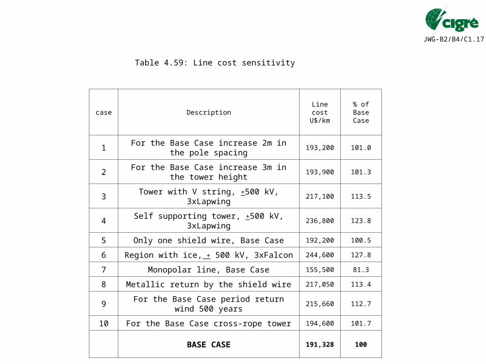
Table 4.59: Line cost sensitivity
case DescriptionLine cost U$/km
% of Base Case
1 For the Base Case increase 2m in the pole spacing 193,200 101.0
2 For the Base Case increase 3m in the tower height 193,900 101.3
3 Tower with V string, +500 kV, 3xLapwing 217,100 113.5
4 Self supporting tower, +500 kV, 3xLapwing 236,800 123.8
5 Only one shield wire, Base Case 192,200 100.5
6 Region with ice, + 500 kV, 3xFalcon 244,600 127.8
7 Monopolar line, Base Case 155,500 81.3
8 Metallic return by the shield wire 217,050 113.4
9 For the Base Case period return wind 500 years 215,660 112.7
10 For the Base Case cross-rope tower 194,600 101.7
BASE CASE 191,328 100

JWG-B2/B4/C1.17
km/MWV
Pr
2
1JL
2
P is the rated bipole power MWV is the Voltage to ground kVr is the bundle resistance ohms/kmr = ro L / Sro conductor resistivity 58 ohms MCM/ kmL, S are the length and cross section in km and MCM
Joule losses
JL*ClJLlfFc8760CpCJL
typical value 230 U$/kW
alternative 15% lower

JWG-B2/B4/C1.17
000000 10203050
SH
SHgol
n
ngol
d
dgol
g
ggolPPfair
000000 10152040
SH
SHgol
n
ngol
d
dgol
g
ggolPPfoul
dB
dB
10/)(10)/( dBPmWP bipole losses in watt per meter
corona loss
go=25 kV/cm; do= 3.05 cm; no= 3
Ho=15 m; So=15 m; Po= 2.9 dB fair weather and 11 dB foul weather
JWG-B2/B4/C1.17
B
CSec
CBACty 2min
CBACline min
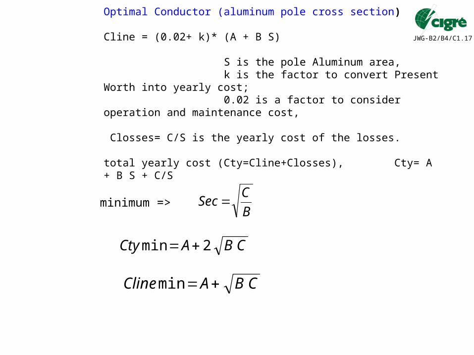
Optimal Conductor (aluminum pole cross section)
Cline = (0.02+ k)* (A + B S)
S is the pole Aluminum area, k is the factor to convert Present Worth into yearly cost; 0.02 is a factor to consider operation and maintenance cost,
Closses= C/S is the yearly cost of the losses.
total yearly cost (Cty=Cline+Closses), Cty= A + B S + C/S
minimum =>

JWG-B2/B4/C1.17Most Economical line for 6000 MW
Table 4.64 Economic line for 6,000 MW
kV +600 +800
cond/pole 6 5
MCM (1) 2,515 2,515
tot U$/yr/km 101,473 83,290
A) Most favorable solution – losses cost base case
kV +600 +800
cond/pole 6 4
MCM (1) 2,515 2515
tot U$/yr/km 94,321 78,154
B) Losses cost reduced by 15%

JWG-B2/B4/C1.17
Impact of corona losses (800 kV line)
•solution desconsidering corona losses
** solution considering corona losses
MW 3,000 3,000 3,000 3,000 3,000
kV +800 +800 +800 +800 +800
cond/pole 4 4 4 4 4
MCM 1,680* 1,800** 1,900 2,000 2,200
tot U$/yr 54,789 54,700 54,730 54,839 55,251
line U$/yr 36,442 37,438 38,268 39,097 40,756
Joule U$/yr 13,970 13,039 12,352 11,735 10,668
Corona loss U$/yr 4,377 4,224 4,110 4,007 3,826

JWG-B2/B4/C1.17
Table 5.1: Converter Station Costs
voltage
Bipolar Rating MW
Cost U$/k
W
Total cost
Million U$
Source
500 1,000 170 170[44] CIGRE Brochure
186
500 2,000 145 290[44] CIGRE Brochure
186
600 3,000 150 450[44] CIGRE Brochure
186
500 3,000 420[45] IEEE Power and
Energy 500 4,000 680 [45]
600 3,000 450-460 [45]
800 3,000 510 [45]
CONVETER STATION

JWG-B2/B4/C1.17Table 5.2: Costs of Converter Stations (Rectifier plus Inverter) obtained by JWG-B2.B4.C1.17 from manufacturers FOB prices without tax and duties.
Bipolar Rating MW
kV 12 pulse Conv./poleSuggested
Costs M U$
CostsM €
1 750 +300Voltage Source
Converter165 115
2 750 +300 1 (6 pulse)* 155 108
3 750 +300 1 165 115
4 750 +500 1 185 129
5 1,500 +300 1 265 184
6 1,500 +500 1 305 212
7 3,000 +500 1 425 295
8 3,000 +600 1 460 320
9 3,000 +800 1 505 351
10 6,000 +600 2 parallel 875 608
11 6,000 +800 2 series 965 671
12 6,000 +800 2 parallel 965 671

JWG-B2/B4/C1.17
Ct= A (VB) ( PC) Ct Millions U$P bipole power in MWV pole voltage kV
Table 5.3: Converter Station costs: Results and accuracy
case kV MWObtained Cost
without * 6,000 MW
DIF (%)with *
6,000 MW
DIF (%)
1 300 750 165 170 2,8 135 -18,0
2 500 750 185 199 7,8 153 -17,2
3 300 1,500 265 250 -5,8 238 -10,3
4 500 1,500 305 293 -3,8 269 -11,7
5 500 3,000 420 432 2,7 473 12,7
6 600 3,000 450 457 1,6 495 10,0
7 800 3,000 510 501 -1,8 531 4,1
8 600 6,000 875 673 -23,1 870 -0,6
9 800 6,000 965 737 -23,7 933 -3,3
A= 0,698 A= 0,154
B= 0,317 B= 0,244
C= 0,557 C= 0,814
JWG-B2/B4/C1.17
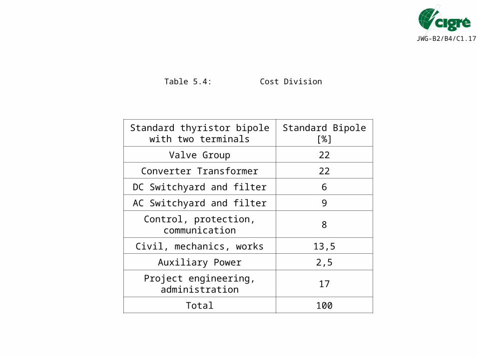
Table 5.4: Cost Division
Standard thyristor bipole with two terminals
Standard Bipole [%]
Valve Group 22
Converter Transformer 22
DC Switchyard and filter 6
AC Switchyard and filter 9
Control, protection, communication 8
Civil, mechanics, works 13,5
Auxiliary Power 2,5
Project engineering, administration 17
Total 100

JWG-B2/B4/C1.17
Figure 5.4: General single line diagram

JWG-B2/B4/C1.17
Table 5.6: Typical Losses of one Converter Station
ComponentsNo Load(Standby)
Rated Load
Filters:AC-FiltersDC-Filters
4 %0 %
4 %0.1 %
Converter Transformer, 1phase, 3 winding 53 % 47 %
Thyristor Valves 10 % 36 %
Smoothing Reactor 0 % 4 %
Auxiliary Power ConsumptionCooling System, Converter ValvesCooling System, Converter TransformerAir-Conditioning SystemOthers
4 %4 %
15 %10 %
3 %1 %4 %1 %
Referred to rated power of one 2000 MW Bipole-Station
2,2 MW 14 MW

JWG-B2/B4/C1.17
Figure 5.8: Thyristor development

JWG-B2/B4/C1.17
line current Line Voltage Rated Power Diameter of wafer
2 kA ±500 kV 2,000 MW 4’’ / 10.0 cm3 kA ±500 kV 3,000 MW 5’’ / 12.5 cm3,125 kA ±800 kV 5,000 MW 5’’ / 12.5 cm3,75 kA ±800 kV 6,000 MW 6’’ / 15.0 cm

JWG-B2/B4/C1.17
Figure 5.11: Example of a ± 500 kV 12-Pulses Valve Tower Configuration

JWG-B2/B4/C1.17
Figure 5.12 VSC converters and cables

JWG-B2/B4/C1.17
Figure 5.13 Tapping using VSC

JWG-B2/B4/C1.17
Figure 5.14 VSC with multi level converter

JWG-B2/B4/C1.17
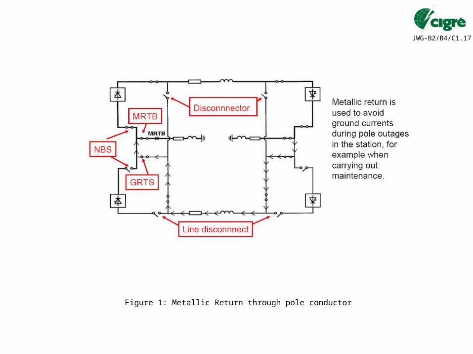
Current Return
• Electrode Line
• Metalic Return
• Eletrode

JWG-B2/B4/C1.17Electrode line and electrode
converter
capacitor and breaker
Return by shield wires
Current Return
eletrodo de terra retorno metálico
JWG-B2/B4/C1.17
Figure 1: Metallic Return through pole conductor
JWG-B2/B4/C1.17
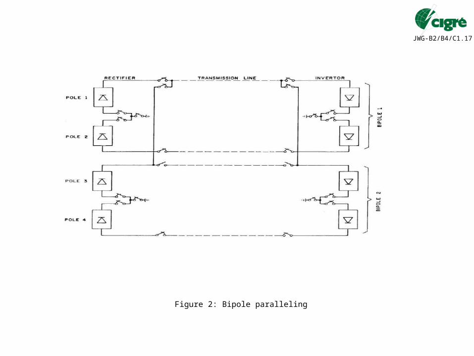
Figure 2: Bipole paralleling

JWG-B2/B4/C1.17Electrode Line
• in the same tower of the bipole
• separated line
• cables
More than one bipole
• 1 electrode and different electrode lines
• different lines e different electrodes (Itaipu)

JWG-B2/B4/C1.17
design criteria for electrode line:
• The line shall have more than one conductor as a failure of it cause bipole outage
• Choice of the number and type of insulators in a string, this depends on the voltage drop in the electrode line due to DC current flow during monopolar operation, the electrode length and the conductor selected dictate the choice.
• The pollution level in the electrode area has also an influence.
• A gap shall be provided to get arc extinction after fault in the electrode line to ground.
• The relative position of the electrode line as related to bipole is an important aspect as related to the electrode line insulation design.
• The electrode line tower grounding is an important aspect in order to limit the flashovers to ground (structure).
• An adequate clearance to ground has to be provided to comply with the current passing through and eventual loss of one of the conductor

JWG-B2/B4/C1.17Linha do Eletrodo

JWG-B2/B4/C1.17
1.Electrode Line costs parcels in percent (100% are table ITEM 6 values)
ITEM DESCRIPTION 2xJoree 2xLapwing 4xLapwing 4xRail
MCM total 5030 3180 6360 3816
1 Engineering %
Engineering (design & topography.) 2.19 2.84 1.74 2.38
2 Materials %
Poles and foundation 12.22 14.61 12.59 14.91
Conductor 42.09 35.57 43.6 35.74
Insulatior,hardware & accessories, grounding 2.53 3.28 2.32 3.17
sub total materials 56.84 53.46 58.52 53.83
3 Man labor %
ROW and access 3.01 3.9 2.39 3.26
Pole erection 7.16 7.36 7 8.46
Conductor installation 16.05 16.79 15.44 16.34
Poles foundation excavation 0.33 0.42 0.29 0.37
sub total man labor 26.55 28.46 25.11 28.43
4 Administration & Fiscalization %
material transportation to site 6.09 7.01 6.28 7.14
inspection at manufacturer site 3.98 3.74 4.1 3.77
construction administration 1.44 1.57 1.34 1.54
sub total adm & fiscaliz 11.51 12.32 11.72 12.45
5 Contingencies %
2.91 2.91 2.91 2.91
6 TOTAL kU$/km (100%) 68.31 52.72 86.03 62.98

JWG-B2/B4/C1.17ELECTRODE LINE COST (US$/km)
40,000
50,000
60,000
70,000
80,000
90,000
3,000 4,000 5,000 6,000 7,000
Total Cross Section (MCM)
CO
ST
(U
S$/
km
)
2 conductor
4 conductor

JWG-B2/B4/C1.17
Power (MW) 700 700 1500 1500 3000 3000 3000 6000 6000
Pole Voltage (kV) 300 500 500 600 500 600 800 600 800
Pole Current (kA) 1.17 0.70 1.50 1.25 3.00 2.50 1.88 5.00 3.75
Pole cond number 2 2 3 3 4 4 4 6 5
MCM one cond. 2400 1950 2,017 1,681 2,515 2,420 1,815 2,515 2,515
MCM total 4800 3900 6051 5043 10060 9680 7260 15090 12575
current/conductor (kA) 0.58 0.35 0.50 0.42 0.75 0.63 0.47 0.83 0.75
cond. Temp (oC) 45 40 45 45 55 45 45 55 55
sag (m) 19 19 19 19 19 19 19 19 19
Proposed electrode line design
Electr. Line cond. number 2 2 2 2 2 2 2 3 3
Electr. Line MCM 1200 1033.5 1513 1261 2515 2420 1815 2515 2096
MCM tot 2400 1950 3025.5 2521.5 5030 4840 3630 7545 6287.5
curr/cond (A) 1.17 0.70 0.75 0.63 1.50 1.25 0.94 1.67 1.25
Temp (oC) 65 55 55 55 70 65 60 75 65
sag (m) 20.5 20.5 20.5 20.5 20.5 20.5 20.5 20.5 20.5
Elect. Line Voltage drop and losses
kV/km 0.028 0.021 0.029 0.029 0.035 0.030 0.030 0.038 0.035
losses MW/km 0.033 0.015 0.043 0.036 0.104 0.075 0.056 0.192 0.130
kV for 50 km (elect line) 1.41 1.04 1.44 1.44 1.73 1.50 1.50 1.92 1.73
losses two 50 km elect lines (MW) 3.29 1.46 4.31 3.59 10.38 7.49 5.62 19.22 12.97
Metallic return through pole
kV/km 0.014 0.010 0.014 0.014 0.017 0.015 0.015 0.019 0.017
Return cond. losses (%) for 3000 km - 3.1 4.3 3.6 5.2 3.7 2.8 4.8 3.2
kV for 1000 km (metallic ret.) 14.1 10.4 14.4 14.4 17.3 15.0 15.0 19.2 17.3
kV for 1500 km(metallic ret.) 21.1 15.6 21.6 21.6 25.9 22.5 22.5 28.8 25.9
kV for 3000 km(metallic ret.) 42.3 31.2 43.1 43.1 51.9 44.9 44.9 57.7 51.9
Metallic return by shield wire
kV/km 0.028 0.021 0.029 0.029 0.035 0.030 0.030 0.038 0.035
Return cond. losses (%) for 3000 km NA NA 8.6 7.2 10.4 7.5 5.6 9.6 6.5
Electrode and metallic return lines design

JWG-B2/B4/C1.17
Electrode Design
•Full current 2.5% of the time;•2.5% of unbalance current permanently.
Potential gradient and step voltage at electrode site;Current density to avoid electro-osmosis in the anode operation;Touch voltages to fences, metallic structures and buried pipes nearby;Corrosion of buried pipes or foundations;Stray current in power lines, especially via transformer neutrals;Stray current in telephone circuits.

JWG-B2/B4/C1.17
Figure 6.5: Ground surface potential as a function of distance from electrode center

JWG-B2/B4/C1.17

JWG-B2/B4/C1.17
JWG-B2/B4/C1.17
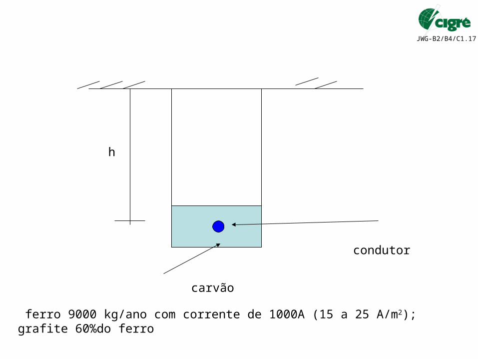
h
carvão
condutor
ferro 9000 kg/ano com corrente de 1000A (15 a 25 A/m2); grafite 60%do ferro

JWG-B2/B4/C1.17
Table 6.4: One electrode cost
item %
Materials
buried wire 8.0
coke 13.8
connections house 1.6
sub total materials 23.5
Man labor 73.6
Engineering - contingencies- land
2.9
Materials taxes 9.4
Man labor taxes 7.4
Total cost (100%) U$483,000
U$

JWG-B2/B4/C1.17
Cline = a + b V + S (c N + d)
a, b, c, d are parameters obtained by curve fitting of the data
V is the pole to ground voltage (kV)
S is the total conductor cross section (MCM)
N is the number of conductor per pole.
System Economics
a = 69,950 U$/kmb = 115.37 U$/kVc = 1.177d = 10.25

JWG-B2/B4/C1.17
km/MWV
Pr
2
1JL
2
P is the rated bipole power MWV is the Voltage to ground kVr is the bundle resistance ohms/kmr = ro L / Sro conductor resistivity 58 ohms MCM/ kmL, S are the length and cross section in km and MCM
Joule losses
JL*ClJLlfFc8760CpCJL
typical value 230 U$/kW
alternative 15% lower

JWG-B2/B4/C1.17
000000 10203050
SH
SHgol
n
ngol
d
dgol
g
ggolPP (9)
000000 10152040
SH
SHgol
n
ngol
d
dgol
g
ggolPP (10)
where P is the corona loss in dB above 1W/m, d is conductor diameter in cm and the line parameters g, n, H and S have the same significance as described above. The reference values assumed are g0 = 25 kV/cm, d0 = 3.05 cm, n0 = 3, H0 = 15 m and S0 = 15 m. The corresponding reference values of P0 were obtained by regression analysis to minimize the arithmetic average of the differences between the calculated and measured losses. The values obtained are P0 = 2.9 dB for fair weather and P0 = 11 dB for foul weather.
10/10)/( PmWP losses in watt per meter
In the economic evaluation it will be considered 80% of time weather fair and 20% foul.

JWG-B2/B4/C1.17
B
CSec
CBACty 2min
CBACline min
optimal Conductor (aluminum pole cross section)
Cline = (0.02+ k)* (A + B S)
S is the pole Aluminum area, k is the factor to convert Present Worth into yearly cost; 0.02 is a factor to consider operation and maintenance cost,
Closses= C/S is the yearly cost of the losses.
total yearly cost (Cty=Cline+Closses), Cty= A + B S + C/S
minimum =>

JWG-B2/B4/C1.17
Three conditions may occur
• Sec conductor is to large for N subconductor configuration
adopt Nx2515
• Sec conductor is too small
adopt configuration to get 28 kV/cm surface grad
• Sec conductor is Ok
adopt the Sec configuration
NO alternative is descarded

JWG-B2/B4/C1.17
Ccs = a* Vb * P c U$
P bipole power (MW)
V voltage (kV)
Station Cost
• For power rating up to 4000MW, one converter per pole:a = 106*0.698*1.5 (1.5 is a factor to include taxes in Brazil, for every country a specific value should be used); b = 0.317; c = 0.557;
•For power rating above 4000 MW (2 series converters per pole)a = 106*0.154*1.5 (1.5 is a factor to include taxes in Brazil); b = 0.244; c = 0.814
Yearly cost including maintenanceCstaty = 1.1 * ( 0.02+ k) * Ccs
JWG-B2/B4/C1.17
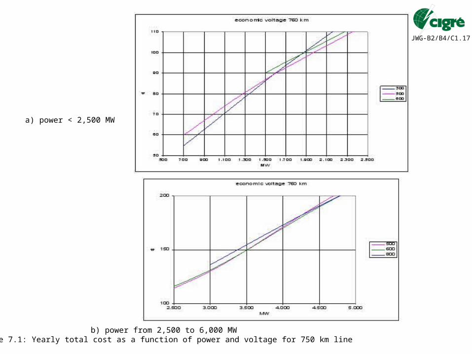
a) power < 2,500 MW
b) power from 2,500 to 6,000 MWFigure 7.1: Yearly total cost as a function of power and voltage for 750 km line

JWG-B2/B4/C1.17
a) power < 2,500 MW
b) power from 1,500 to 6,000 MWFigure 7.2: Yearly total cost as function of power and voltage for 1,500 km line

JWG-B2/B4/C1.17
a)power < 2,500 MW
a)power from 1,500 to 6,000 MWFigure 7.3: Yearly total cost as function of power and voltage for 3,000 km line

JWG-B2/B4/C1.17
Figure 7.4: Optimal voltages as a function of power and lengthLegend: Red → ±800 kV; green → ±600 kV; pink → ±500 kV; blue → ±300 kV

JWG-B2/B4/C1.17
MW 700 1,500 3,000 4,500 6,000
kV +300 +500 +600 +600 +800
N x MCM 2X2,280 2X2,515 4X2,242 5X2,515 5X2,515
MU$/yr % MU$/yr % MU$/yr % MU$/yr % MU$/yr %
line 67,4 53,5 79,5 44,1 113,7 43,0 142,3 38,6 151,9 35,6
corona 3,8 3,0 9,5 5,2 8,2 3,1 6,2 1,7 8,4 2,0
joule 23,9 19,0 35,8 19,9 55,8 21,1 89,6 24,3 89,6 21,0
converter 30,9 24,5 55,6 30,8 86,7 32,8 130,6 35,4 177,0 41,5
U$/year 126,1 100,0 180,4 100,0 264,5 100,0 368,7 100,0 426,9 100,0
Figure 7.7: Cost Parcels, 3,000 km line

JWG-B2/B4/C1.17
To take this into consideration a methodology will be used here consisting of:
Set a spreadsheet where the different costs are located
Cost of lines and station are located in the beginning of the year o starting operation
Losses, and maintenance costs are located in the end of the due year
The sum of all cost in every year is calculated (yearly parcels Yi)
The present worth of Yi are obtained and summed
PWYi = Yi/(1+j) i
j is the interest rate per year
Calculations Considering Cost Components Allocated in Different Years

JWG-B2/B4/C1.17
4.1 Study Case 1: Basic Case
P= 3000 MW for year 1 to 30 V= 600 and 800 kV
Table 7.6: Comparison between ± 600 kV and ± 800 kV
JWG-B2/B4/C1.17
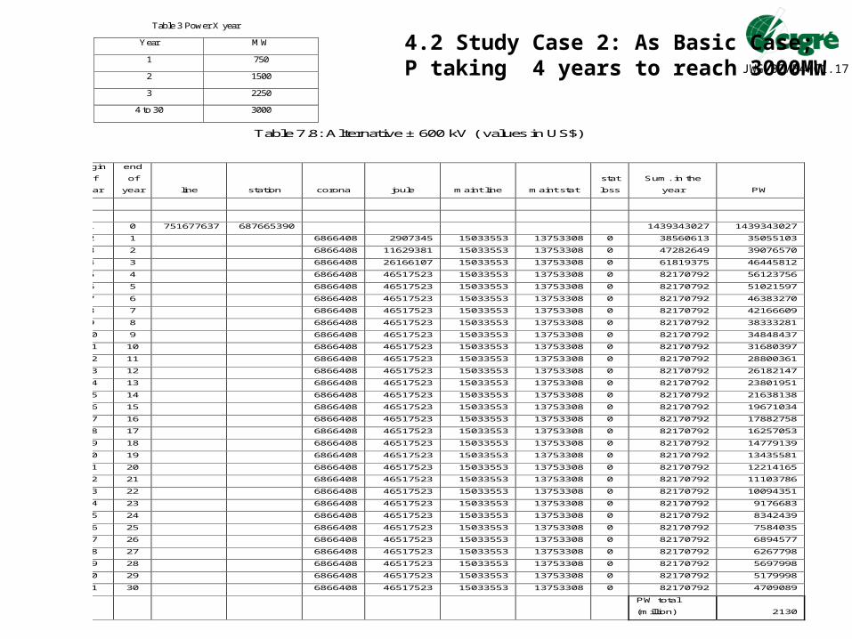
Table 3 Power X year
Year MW
1 750
2 1500
3 2250
4 to 30 3000
4.2 Study Case 2: As Basic Case; P taking 4 years to reach 3000MW
Table 7.8: Alternative ± 600 kV ( values in US$)
Begin
of
year
end
of
year line station corona joule maint line maint stat
stat
loss
Sum. in the
year PW
1 0 751677637 687665390 1439343027 1439343027
2 1 6866408 2907345 15033553 13753308 0 38560613 35055103
3 2 6866408 11629381 15033553 13753308 0 47282649 39076570
4 3 6866408 26166107 15033553 13753308 0 61819375 46445812
5 4 6866408 46517523 15033553 13753308 0 82170792 56123756
6 5 6866408 46517523 15033553 13753308 0 82170792 51021597
7 6 6866408 46517523 15033553 13753308 0 82170792 46383270
8 7 6866408 46517523 15033553 13753308 0 82170792 42166609
9 8 6866408 46517523 15033553 13753308 0 82170792 38333281
10 9 6866408 46517523 15033553 13753308 0 82170792 34848437
11 10 6866408 46517523 15033553 13753308 0 82170792 31680397
12 11 6866408 46517523 15033553 13753308 0 82170792 28800361
13 12 6866408 46517523 15033553 13753308 0 82170792 26182147
14 13 6866408 46517523 15033553 13753308 0 82170792 23801951
15 14 6866408 46517523 15033553 13753308 0 82170792 21638138
16 15 6866408 46517523 15033553 13753308 0 82170792 19671034
17 16 6866408 46517523 15033553 13753308 0 82170792 17882758
18 17 6866408 46517523 15033553 13753308 0 82170792 16257053
19 18 6866408 46517523 15033553 13753308 0 82170792 14779139
20 19 6866408 46517523 15033553 13753308 0 82170792 13435581
21 20 6866408 46517523 15033553 13753308 0 82170792 12214165
22 21 6866408 46517523 15033553 13753308 0 82170792 11103786
23 22 6866408 46517523 15033553 13753308 0 82170792 10094351
24 23 6866408 46517523 15033553 13753308 0 82170792 9176683
25 24 6866408 46517523 15033553 13753308 0 82170792 8342439
26 25 6866408 46517523 15033553 13753308 0 82170792 7584035
27 26 6866408 46517523 15033553 13753308 0 82170792 6894577
28 27 6866408 46517523 15033553 13753308 0 82170792 6267798
29 28 6866408 46517523 15033553 13753308 0 82170792 5697998
30 29 6866408 46517523 15033553 13753308 0 82170792 5179998
31 30 6866408 46517523 15033553 13753308 0 82170792 4709089
PW total
(million) 2130

JWG-B2/B4/C1.17
Table 7.9: Alternative ± 800 kV ( values in US$)
Begin.
of year
end of
yr line station corona joule maint line mait stat
station
losses
summ in the
yr PW
1 0 722892478 753325635 1476218113 1476218113
2 1 10935753 2180509 14457850 15066513 0 42640624 38764204
3 2 10935753 8722036 14457850 15066513 0 49182151 40646406
4 3 10935753 19624580 14457850 15066513 0 60084695 45142521
5 4 10935753 34888142 14457850 15066513 0 75348258 51463874
6 5 10935753 34888142 14457850 15066513 0 75348258 46785340
7 6 10935753 34888142 14457850 15066513 0 75348258 42532127
8 7 10935753 34888142 14457850 15066513 0 75348258 38665570
9 8 10935753 34888142 14457850 15066513 0 75348258 35150518
10 9 10935753 34888142 14457850 15066513 0 75348258 31955017
11 10 10935753 34888142 14457850 15066513 0 75348258 29050015
12 11 10935753 34888142 14457850 15066513 0 75348258 26409105
13 12 10935753 34888142 14457850 15066513 0 75348258 24008277
14 13 10935753 34888142 14457850 15066513 0 75348258 21825706
15 14 10935753 34888142 14457850 15066513 0 75348258 19841551
16 15 10935753 34888142 14457850 15066513 0 75348258 18037774
17 16 10935753 34888142 14457850 15066513 0 75348258 16397976
18 17 10935753 34888142 14457850 15066513 0 75348258 14907251
19 18 10935753 34888142 14457850 15066513 0 75348258 13552046
20 19 10935753 34888142 14457850 15066513 0 75348258 12320042
21 20 10935753 34888142 14457850 15066513 0 75348258 11200038
22 21 10935753 34888142 14457850 15066513 0 75348258 10181853
23 22 10935753 34888142 14457850 15066513 0 75348258 9256230
24 23 10935753 34888142 14457850 15066513 0 75348258 8414755
25 24 10935753 34888142 14457850 15066513 0 75348258 7649777
26 25 10935753 34888142 14457850 15066513 0 75348258 6954343
27 26 10935753 34888142 14457850 15066513 0 75348258 6322130
28 27 10935753 34888142 14457850 15066513 0 75348258 5747391
29 28 10935753 34888142 14457850 15066513 0 75348258 5224901
30 29 10935753 34888142 14457850 15066513 0 75348258 4749910
31 30 10935753 34888142 14457850 15066513 0 75348258 4318100
PW total
(million) 2124
Note that, in this case the alternatives have almost the same cost:100.3%.
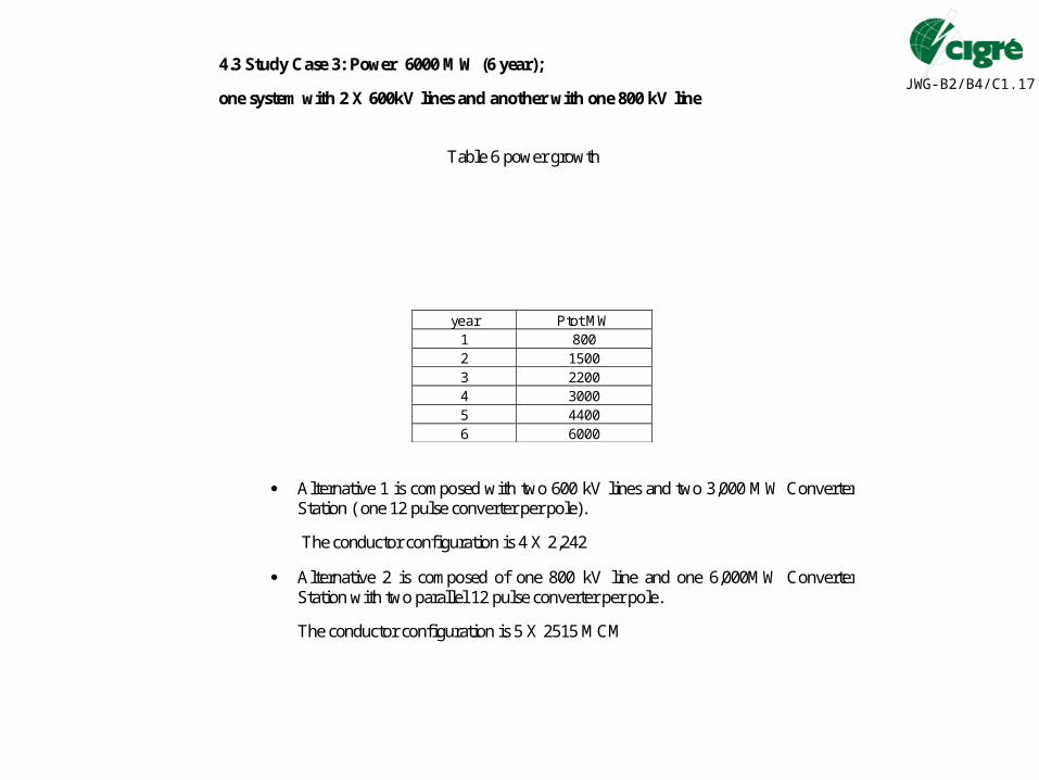
JWG-B2/B4/C1.174.3 Study Case 3: Power 6000 MW (6 year);
one system with 2 X 600kV lines and another with one 800 kV line
Table 6 power growth
year Ptot MW 1 800 2 1500 3 2200 4 3000 5 4400 6 6000
Alternative 1 is composed with two 600 kV lines and two 3,000 MW Converter Station ( one 12 pulse converter per pole).
The conductor configuration is 4 X 2,242
Alternative 2 is composed of one 800 kV line and one 6,000MW Converter Station with two parallel 12 pulse converter per pole.
The conductor configuration is 5 X 2515 MCM

JWG-B2/B4/C1.17
Table 7.11: Alternative ±600kV
Begin.
of year
end
of yr line station corona joule maint line mait stat
station
losses
summ in the
yr PW
1 0 751677637 690000000 1441677637 1441677637
2 1 6866408 3307913 15033553 13800000 982187 39990060 36354600
3 2 6866408 11629381 15033553 13800000 3453000 50782341 41968877
4 3 6866408 25016090 15033553 13800000 7427787 68143837 51197474
5 4 751677637 690000000 6866408 46517523 15033553 13800000 13812000 1537707121 1050274654
6 5 13732815 50032181 30067105 27600000 14855573 136287675 84623923
7 6 13732815 93035047 30067105 27600000 27624000 192058968 108412280
8 7 13732815 93035047 30067105 27600000 27624000 192058968 98556618
9 8 13732815 93035047 30067105 27600000 27624000 192058968 89596926
10 9 13732815 93035047 30067105 27600000 27624000 192058968 81451751
11 10 13732815 93035047 30067105 27600000 27624000 192058968 74047046
12 11 13732815 93035047 30067105 27600000 27624000 192058968 67315496
13 12 13732815 93035047 30067105 27600000 27624000 192058968 61195906
14 13 13732815 93035047 30067105 27600000 27624000 192058968 55632642
15 14 13732815 93035047 30067105 27600000 27624000 192058968 50575129
16 15 13732815 93035047 30067105 27600000 27624000 192058968 45977390
17 16 13732815 93035047 30067105 27600000 27624000 192058968 41797627
18 17 13732815 93035047 30067105 27600000 27624000 192058968 37997843
19 18 13732815 93035047 30067105 27600000 27624000 192058968 34543494
20 19 13732815 93035047 30067105 27600000 27624000 192058968 31403176
21 20 13732815 93035047 30067105 27600000 27624000 192058968 28548342
22 21 13732815 93035047 30067105 27600000 27624000 192058968 25953038
23 22 13732815 93035047 30067105 27600000 27624000 192058968 23593671
24 23 13732815 93035047 30067105 27600000 27624000 192058968 21448792
25 24 13732815 93035047 30067105 27600000 27624000 192058968 19498902
26 25 13732815 93035047 30067105 27600000 27624000 192058968 17726274
27 26 13732815 93035047 30067105 27600000 27624000 192058968 16114795
28 27 13732815 93035047 30067105 27600000 27624000 192058968 14649813
29 28 13732815 93035047 30067105 27600000 27624000 192058968 13318012
30 29 13732815 93035047 30067105 27600000 27624000 192058968 12107284
31 30 13732815 93035047 30067105 27600000 27624000 192058968 11006622
PW total
(million) 3789

JWG-B2/B4/C1.17
Table 7.12: Alternative:±800kV
Begi
n. of
year
end
of yr line station corona joule maint line maint stat
station
losses
summ in the
yr PW
1 0 1004144969 940875000 1945019969 1945019969
2 1 325000 5308787 20082899 18817500 982187 45516373 41378521
3 2 325000 18663705 20082899 18817500 3453000 61342105 50695954
4 3 325000 40147703 20082899 18817500 7427787 86800890 65214793
5 4 506625000 325000 74654821 20082899 18817500 13812000 634317220 433247197
6 5 6967114 40147704 20082899 28950000 14855573 111003291 68924310
7 6 6967114 74654821 20082899 28950000 27624000 158278834 89344276
8 7 6967114 74654821 20082899 28950000 27624000 158278834 81222069
9 8 6967114 74654821 20082899 28950000 27624000 158278834 73838244
10 9 6967114 74654821 20082899 28950000 27624000 158278834 67125677
11 10 6967114 74654821 20082899 28950000 27624000 158278834 61023342
12 11 6967114 74654821 20082899 28950000 27624000 158278834 55475766
13 12 6967114 74654821 20082899 28950000 27624000 158278834 50432514
14 13 6967114 74654821 20082899 28950000 27624000 158278834 45847740
15 14 6967114 74654821 20082899 28950000 27624000 158278834 41679764
16 15 6967114 74654821 20082899 28950000 27624000 158278834 37890695
17 16 6967114 74654821 20082899 28950000 27624000 158278834 34446086
18 17 6967114 74654821 20082899 28950000 27624000 158278834 31314624
19 18 6967114 74654821 20082899 28950000 27624000 158278834 28467840
20 19 6967114 74654821 20082899 28950000 27624000 158278834 25879854
21 20 6967114 74654821 20082899 28950000 27624000 158278834 23527140
22 21 6967114 74654821 20082899 28950000 27624000 158278834 21388309
23 22 6967114 74654821 20082899 28950000 27624000 158278834 19443918
24 23 6967114 74654821 20082899 28950000 27624000 158278834 17676289
25 24 6967114 74654821 20082899 28950000 27624000 158278834 16069353
26 25 6967114 74654821 20082899 28950000 27624000 158278834 14608503
27 26 6967114 74654821 20082899 28950000 27624000 158278834 13280457
28 27 6967114 74654821 20082899 28950000 27624000 158278834 12073143
29 28 6967114 74654821 20082899 28950000 27624000 158278834 10975585
30 29 6967114 74654821 20082899 28950000 27624000 158278834 9977804
31 30 6967114 74654821 20082899 28950000 27624000 158278834 9070731
PW total
(million) 3497

JWG-B2/B4/C1.17
•CIGRE Brochure 178 “Probabilistic Design of Overhead Transmission Lines”, •CIGRE Brochure 48 “Tower Top Geometry”, •CIGRE Brochure 109 “Review of IEC 826: Loading and Strength of Overhead Lines” •CIGRE Brochure 256 “Report on Current Practices Regarding Frequencies and Magnitude of High Intensity Winds”, •IEC/TR 60 826 Loading and Strength of Overhead Transmission Lines•CIGRE “Brochure 207 Thermal Behavior of Overhead Conductors”•Gilman D W; Whitehead E R “The mechanism of Lightning Flashover on HV and EHV Transmission Lines”, Electra no 27, 1975
Related Documents