04-lila • Integrating a ScaLAPACK call in an MPI code (for Householder QRF) • MPI_OP to compute || x || (for Gram-Schmidt) • Example of construction of Datatype for triangular matrices, Example of MPI_OP on triangular martrices (for CholeskyQR) • RFP: Trick to have continuous memory for triangular matrices (for CholeskyQR) • Weirdest MPI_OP ever: motivation & results • Weirdest MPI_OP ever: how to attach attributes to a datatype

julien-missing-slides.ppt
Jul 14, 2015
Welcome message from author
This document is posted to help you gain knowledge. Please leave a comment to let me know what you think about it! Share it to your friends and learn new things together.
Transcript

04-lila
• Integrating a ScaLAPACK call in an MPI code (for Householder QRF)• MPI_OP to compute || x || (for Gram-Schmidt)• Example of construction of Datatype for triangular matrices, Example of MPI_OP on triangular
martrices (for CholeskyQR)• RFP: Trick to have continuous memory for triangular matrices (for CholeskyQR)• Weirdest MPI_OP ever: motivation & results• Weirdest MPI_OP ever: how to attach attributes to a datatype
1. Integrating a ScaLAPACK call in an MPI code …
• See – scalapackqrf_A.c– scalapackqrf_B.c– scalapackqr2_A.c– scalapackqr2_B.c
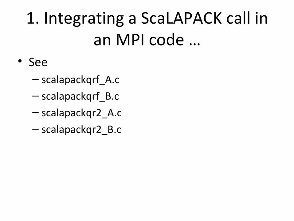
2. MPI_OP to compute || x ||
• Consider the vector x = [ 1e+200 1e+200 1e+200 1e+200 ]
• The 2-norm of x is || x || = sqrt( x(1)^2 + x(2)^2 + x(3)^2 + x(4)^2 )
= 2e+200

2. MPI_OP to compute || x ||• Consider the vector
x = [ 1e+200 1e+200 1e+200 1e+200 ]
• The 2-norm of x is || x || = sqrt( x(1)^2 + x(2)^2 + x(3)^2 + x(4)^2 ) = 2e+200
• However a note careful implementation would overflow in double precision arithmetic
• To compute z = sqrt(x^2+y^2) without unnecessary overflowz = max(|x|,|y|)*sqrt(1+(min(|x|,|y|)/max(|x|,|y|))^2 )See LAPACK routine DLAPY2, BLAS DNORM, etc.
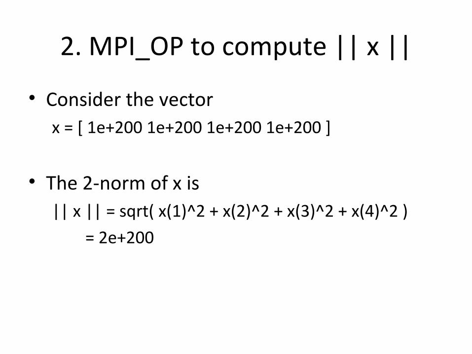
2. MPI_OPThe MPI_OP is in LILA_mpiop_dlapy2.c
Example of use are in:– check_representativity.c– rowmgs_v1.c– mgs_v1.c– cgs_v1.c
• very simple MPI_OP (but very useful as well) used to compute a norm without unnecessary overflow
• the idea is that a not careful computation of || x ||_2 would easily overflow: alpha = x^Tx (might overflow) alpha = MPI_Allreduce(alpha) (might overflow as well) alpha = sqrt(alpha) (too late if you have already overflowed ....)
• good implementation: alpha = || x ||_2 (good seq dnorm will not overflow) alpha = MPI_Allreduce_dlapy2 ( alpha )
• NOTE:DLAPY2 is an LAPACK routine that computes z = sqrt(x^2+y^2) with:z = max(|x|,|y|) * sqrt( 1 +(min(|x|,|y|)/max(|x|,|y|))^2 )

2. Examples.• mpirun -np 4 ./xtest -verbose 2 -m 1000 -n 100 -cgs_v0• mpirun -np 4 ./xtest -verbose 2 -m 1000 -n 100 -cgs_v1
• mpirun -np 4 ./xtest -verbose 2 -m 1000 -n 100 -mgs_v0• mpirun -np 4 ./xtest -verbose 2 -m 1000 -n 100 -mgs_v1
• (and then multiply the entries of the initial matrix by 1e200)

3. EXAMPLE OF CONSTRUCTION OF DATA_TYPE FOR TRIANGULAR MATRICES, EXAMPLE OF MPI_OP ON
TRIANGULAR MATRICES
• See:– choleskyqr_A_v1.c– choleskyqr_B_v1.c– LILA_mpiop_sum_upper.c
• starting from choleskyqr_A_v0.c, this– shows how to construct a datatype for a triangular matrix– show how to use a MPI_OP on the datatype for an
AllReduce operation– here we simply want to summ the upper triangular
matrices together

4. TRICK FOR TRIANGULAR MATRICES DATATYPES
• See:– check_orthogonality_RFP.c– choleskyqr_A_v2.c– choleskyqr_A_v3.c– choleskyqr_B_v2.c– choleskyqr_B_v3.c
• A trick to use RFP format to do an fast allreduce on P triangular matrices without datatypes. The trick is at the user level.

Idea behind RFP
• Rectangular full packed format
• Just be careful in the case for odd and even matrices

5. A very weird MPI_OP: motivation & examples
Gram-Schmidt algorithm
11
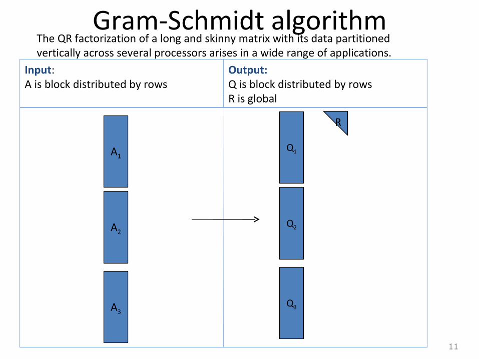
The QR factorization of a long and skinny matrix with its data partitioned vertically across several processors arises in a wide range of applications.
A1
A2
A3
Q1
Q2
Q3
R
Input:A is block distributed by rows
Output:Q is block distributed by rowsR is global
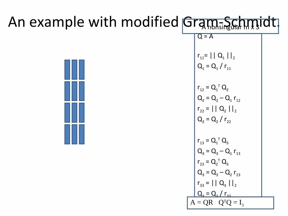
Q = A
r11= || Q1 ||2
Q1 = Q1 / r11
= Q1 / r11
r12 = Q1T Q2
Q2 = Q2 – Q1 r12
r22 = || Q2 ||2
Q2 = Q2 / r22
r13 = Q1T Q3
Q3 = Q3 – Q1 r13
r23 = Q2T Q3
Q3 = Q3 – Q2 r23
r33 = || Q3 ||2
Q3 = Q3 / r33
An example with modified Gram-Schmidt.A nonsingular m x 3
A = QR QTQ = I3
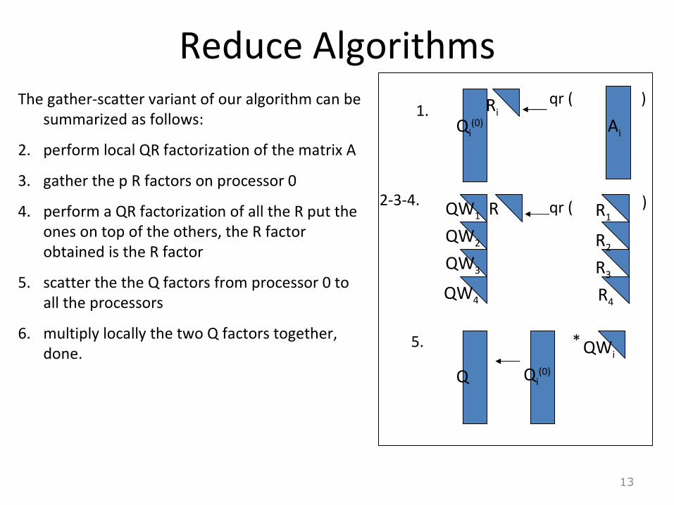
Reduce AlgorithmsThe gather-scatter variant of our algorithm can be
summarized as follows:
2. perform local QR factorization of the matrix A
3. gather the p R factors on processor 0
4. perform a QR factorization of all the R put the ones on top of the others, the R factor obtained is the R factor
5. scatter the the Q factors from processor 0 to all the processors
6. multiply locally the two Q factors together, done.
13
*
1.
2-3-4.
5.
Qi(0)
Ri
Ai
R R1
R2
R3
R4QW4
QW3
QW2
QW1
QWi
Qi(0)Q
qr (
qr ( )
)
Reduce Algorithms
• This is the scatter-gather version of our algorithm.
• This variant is not very efficient for two reasons: – first the communication phases 2 and 4 are highly involving
processor 0 ;– second the cost of step 3 is p/3*n3, so can get prohibitive for
large p.
• Note that the CholeskyQR algorithm can also be implemented in a scatter-gather way but reduce-broadcast. This leads naturally to the algorithm presented below where a reduce-broadcast version of the previous algorithm is described. This will be our final algorithm.
14
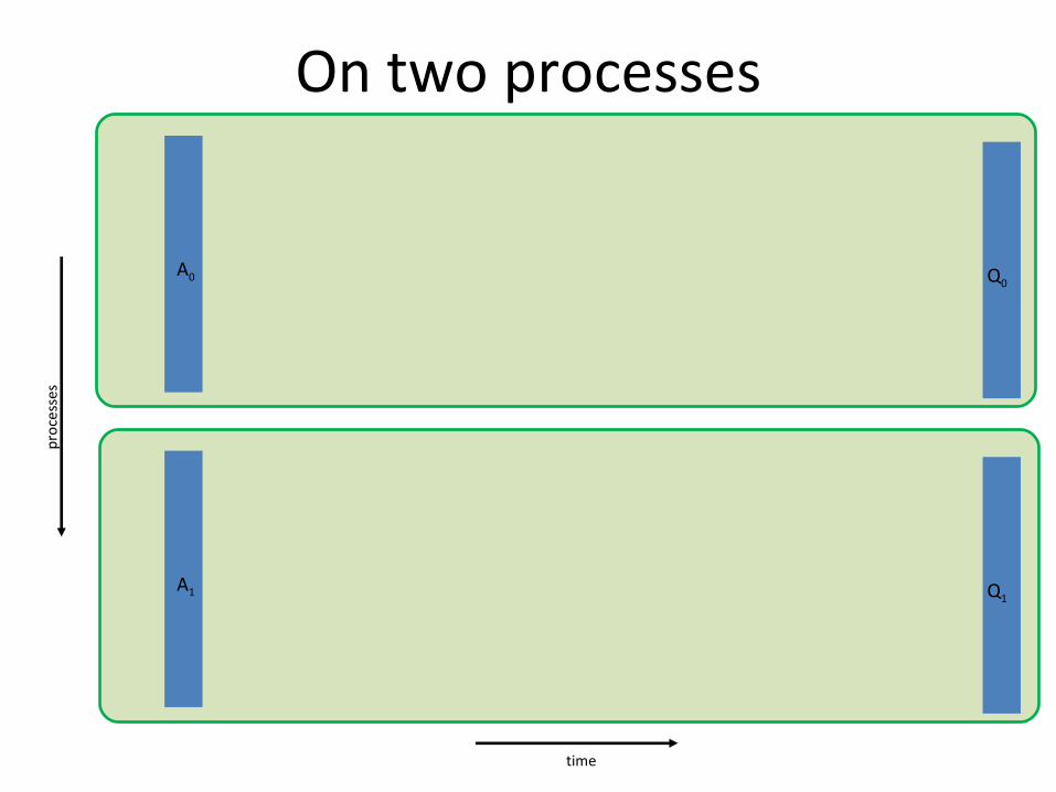
On two processes
A0 Q0
A1 Q1
proc
esse
s
time
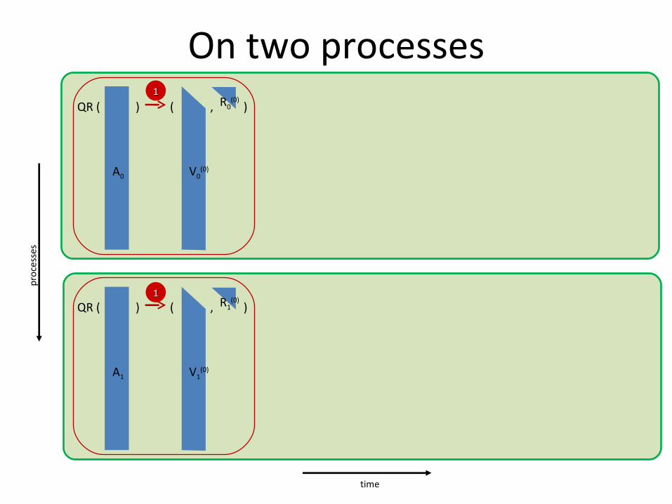
On two processesR0
(0)( , )QR ( )
A0 V0(0)
R1(0)
( , )QR ( )
A1 V1(0)
proc
esse
s
time
11
11

On two processesR0
(0)( , )QR ( )
A0 V0(0)
)R0(0)
R1(0)
R1(0)
( , )QR ( )
A1 V1(0)
proc
esse
s
time
11
11
11
(

On two processesR0
(0)( , )QR ( )
A0 V0(0)
R0(1)
( , )QR ( )R0(0)
R1(0)
V0(1)
V1(1)
R1(0)
( , )QR ( )
A1 V1(0)
proc
esse
s
time
11
11
22
11
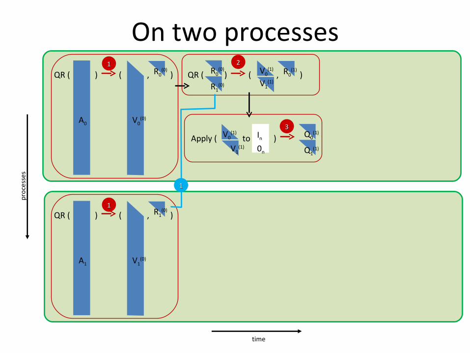
On two processesR0
(0)( , )QR ( )
A0 V0(0)
R0(1)
( , )QR ( )R0(0)
R1(0)
V0(1)
V1(1)
InApply ( to )V0(1)
0nV1(1)
Q0(1)
Q1(1)
R1(0)
( , )QR ( )
A1 V1(0)
proc
esse
s
time
11
11
22
33
11

On two processesR0
(0)( , )QR ( )
A0 V0(0)
R0(1)
( , )QR ( )R0(0)
R1(0)
V0(1)
V1(1)
InApply ( to )V0(1)
0nV1(1)
Q0(1)
Q1(1)
Q0(1)
R1(0)
( , )QR ( )
A1 V1(0)
proc
esse
s
time
11
11
22
33
11 22
Q1(1)
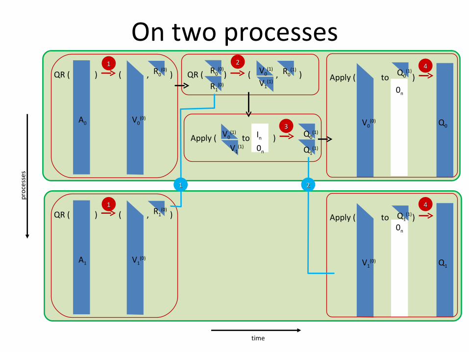
On two processesR0
(0)( , )QR ( )
A0 V0(0)
R0(1)
( , )QR ( )R0(0)
R1(0)
V0(1)
V1(1)
InApply ( to )V0(1)
0nV1(1)
Q0(1)
Q1(1)
Apply ( to )0n
V0(0)
Q0(1)
Q0
R1(0)
( , )QR ( )
A1 V1(0)
Apply ( to )
V1(0)
Q1(1)
Q1
proc
esse
s
time
0n
11
11
22
33
44
44
11 22

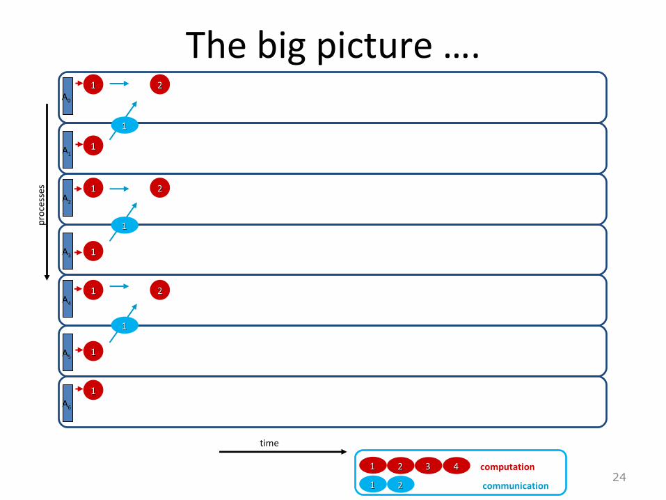
The big picture ….
22
A1
A2
A3
A4
A5
A6
Q0
Q4
Q1
Q5
Q6
Q3
Q2
R
R
R
R
R
R
R
A QRtime
proc
esse
s
A0

The big picture ….
23
A1
A2
A3
A4
A5
A6
time
proc
esse
s
communication
computation
A0
11 22 33 44
11 22
11
11
11
11
11
11
11
The big picture ….
24
A1
A2
A3
A4
A5
A6
time
proc
esse
s
communication
computation
A0
11 22 33 44
11 22
11
11
11
22
22
11
11
11
11
22
11
11
11

The big picture ….
25
A1
A2
A3
A4
A5
A6
time
proc
esse
s
communication
computation
A0
11 22 33 44
11 22
11
11
11
22
22
11
11
11
11
22 22
11
11
11
1111
22
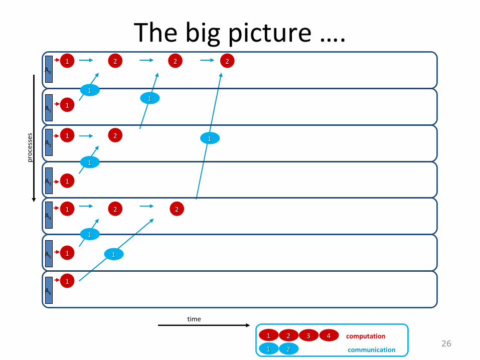
The big picture ….
26
A1
A2
A3
A4
A5
A6
time
proc
esse
s
communication
computation
A0
11 22 33 44
11 22
11
11
11
22
22
11
11
11
11
22 22
11
11
11
1111
11
22 22

The big picture ….
27
A1
A2
A3
A4
A5
A6
time
proc
esse
s
communication
computation
A0
11 22 33 44
11 22
11
11
11
22
22
11
11
11
11
22 22
11
11
11
1111
11
22 22 33

The big picture ….
28
A1
A2
A3
A4
A5
A6
time
proc
esse
s
communication
computation
A0
11 22 33 44
11 22
22
11
11
11
22
22
11
11
11
11
22 22
11
11
11
1111
11
22 22 33 33
33

The big picture ….
29
A1
A2
A3
A4
A5
A6
time
proc
esse
s
communication
computation
A0
11 22 33 44
11 22
22
22
22
11
11
11
22
22
11
11
11
11
22 22
11
11
11
1111
11
22 22 33 33
33
33
33
33
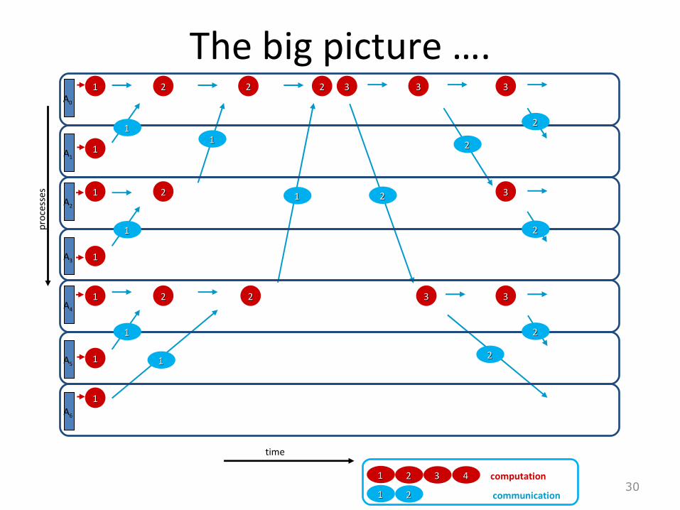
The big picture ….
30
A1
A2
A3
A4
A5
A6
time
proc
esse
s
communication
computation
A0
11 22 33 44
11 22
22
22
22
22
22
22
11
11
11
22
22
11
11
11
11
22 22
11
11
11
1111
11
22 22 33 33
33
33
33
33
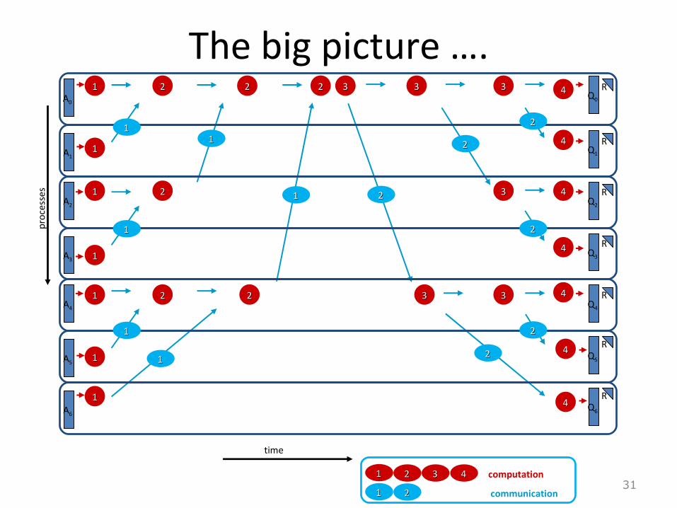
The big picture ….
31
A1
A2
A3
A4
A5
A6
Q0
Q4
Q1
Q5
Q6
Q3
Q2
R
R
R
R
R
R
R
time
proc
esse
s
communication
computation
A0
11 22 33 44
11 22
22
22
22
22
22
22
11
11
11
22
22
11
11
11
11
22 22
11
11
11
1111
11
22 22 33 33
33
33
33
33 44
44
44
44
44
44
44

Latency but also possibility of fast panel factorization.
• DGEQR3 is the recursive algorithm (see Elmroth and Gustavson, 2000), DGEQRF and DGEQR2 are the LAPACK routines.
• Times include QR and DLARFT.
• Run on Pentium III.
32
QR factorization and construction of T m = 10,000
Perf in MFLOP/sec (Times in sec)
n DGEQR3 DGEQRF DGEQR2
50 173.6 (0.29) 65.0 (0.77) 64.6 (0.77)
100 240.5 (0.83) 62.6 (3.17) 65.3 (3.04)
150 277.9 (1.60) 81.6 (5.46) 64.2 (6.94)
200 312.5 (2.53) 111.3 (7.09) 65.9 (11.98)
m=1000,000, the x axis is n
MFL
OP/
sec
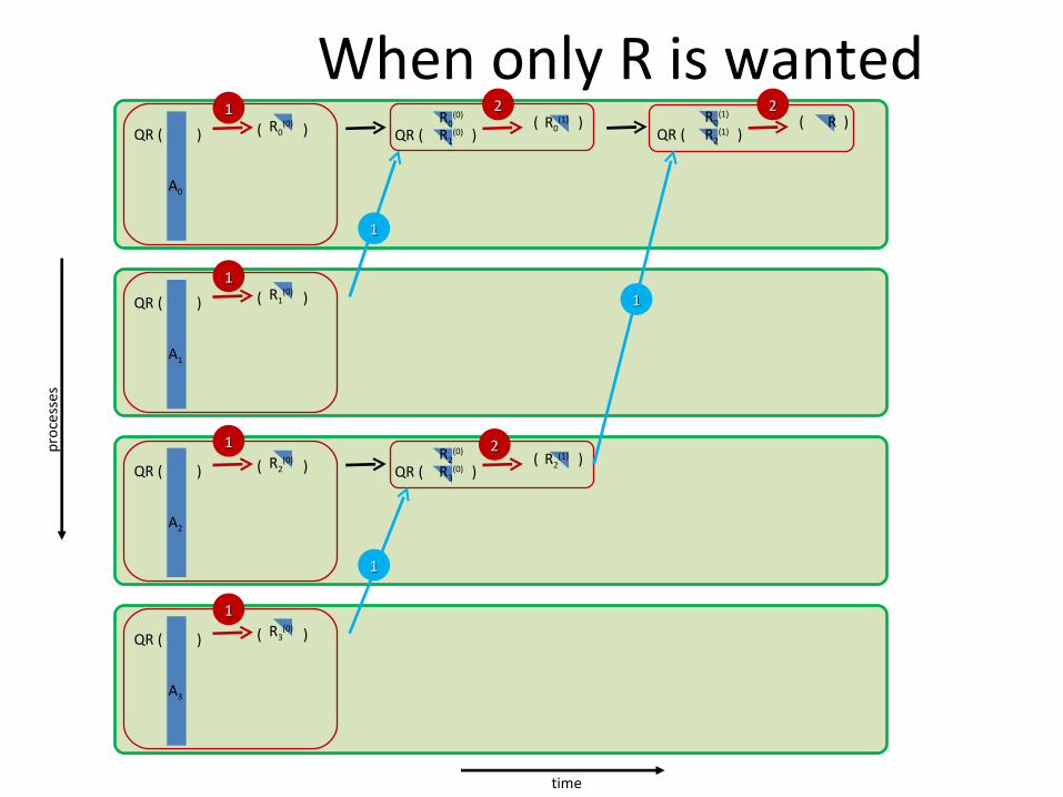
When only R is wantedpr
oces
ses
time
R0(0)( )QR ( )
A0
R0(1)( )
QR ( )R0
(0)
R1(0)
R1(0)( )QR ( )
A1
R2(0)( )QR ( )
A2
R2(1)( )
QR ( )R2
(0)
R3(0)
R3(0)( )QR ( )
A3
R( )QR ( )
R0(1)
R2(1)
11
11
11
2222
22
11
11
11
11
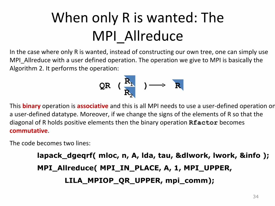
When only R is wanted: The MPI_Allreduce
34
In the case where only R is wanted, instead of constructing our own tree, one can simply use MPI_Allreduce with a user defined operation. The operation we give to MPI is basically the Algorithm 2. It performs the operation:
This binary operation is associative and this is all MPI needs to use a user-defined operation on a user-defined datatype. Moreover, if we change the signs of the elements of R so that the diagonal of R holds positive elements then the binary operation Rfactor becomes commutative.
The code becomes two lines:
lapack_dgeqrf( mloc, n, A, lda, tau, &dlwork, lwork, &info );
MPI_Allreduce( MPI_IN_PLACE, A, 1, MPI_UPPER,
LILA_MPIOP_QR_UPPER, mpi_comm);
QR ( )R1
R2
R

Does it work?• The experiments are performed on the beowulf cluster at the University of Colorado at Denver. The
cluster is made of 35 bi-pro Pentium III (900MHz) connected with Dolphin interconnect.• Number of operations is taken as 2mn2 for all the methods
• The block size used in ScaLAPACK is 32.
• The code is written in C, use MPI (mpich-2.1), LAPACK (3.1.1), BLAS (goto-1.10), the LAPACK Cwrappers (http://icl.cs.utk.edu/~delmas/lapwrapmw.htm ) and the BLAS C wrappers (http://www.netlib.org/blas/blast-forum/cblas.tgz)
• The codes has been tested in various configuration and have never failed to produce a correct answer, releasing those codes is in the agenda
35
FLOPs (total) for R only FLOPs (total) for Q and R
CholeskyQR mn2+ n3/3 2mn2+ n3/3
Gram-Schmidt 2mn2 2mn2
Householder 2mn2-2/3n3 4mn2-4/3n3
Allreduce HH (2mn2-2/3n3)+2/3 n3 p (4mn2-4/3n3)+4/3 n3 p
» Number of operations is taken as 2mn2 for all the methods
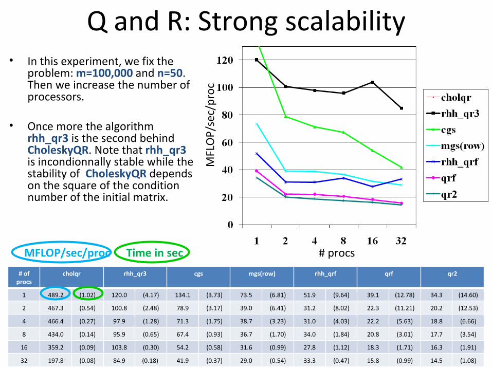
Q and R: Strong scalability• In this experiment, we fix the
problem: m=100,000 and n=50. Then we increase the number of processors.
• Once more the algorithm rhh_qr3 is the second behind CholeskyQR. Note that rhh_qr3 is incondionnally stable while the stability of CholeskyQR depends on the square of the condition number of the initial matrix.
05/31/10 11:43 36
# of procs
cholqr rhh_qr3 cgs mgs(row) rhh_qrf qrf qr2
1 489.2 (1.02) 120.0 (4.17) 134.1 (3.73) 73.5 (6.81) 51.9 (9.64) 39.1 (12.78) 34.3 (14.60)
2 467.3 (0.54) 100.8 (2.48) 78.9 (3.17) 39.0 (6.41) 31.2 (8.02) 22.3 (11.21) 20.2 (12.53)
4 466.4 (0.27) 97.9 (1.28) 71.3 (1.75) 38.7 (3.23) 31.0 (4.03) 22.2 (5.63) 18.8 (6.66)
8 434.0 (0.14) 95.9 (0.65) 67.4 (0.93) 36.7 (1.70) 34.0 (1.84) 20.8 (3.01) 17.7 (3.54)
16 359.2 (0.09) 103.8 (0.30) 54.2 (0.58) 31.6 (0.99) 27.8 (1.12) 18.3 (1.71) 16.3 (1.91)
32 197.8 (0.08) 84.9 (0.18) 41.9 (0.37) 29.0 (0.54) 33.3 (0.47) 15.8 (0.99) 14.5 (1.08)
# procs
MFL
OP/
sec/
proc
MFLOP/sec/proc Time in sec

Q and R: Weak scalability with respect to m• We fix the local size to be mloc=100,000
and n=50. When we increase the number of processors, the global m grows proportionally.
• rhh_qr3 is the Allreduce algorithm with recursive panel factorization, rhh_qrf is the same with LAPACK Householder QR. We see the obvious benefit of using recursion. See as well (6). qr2 and qrf correspond to the ScaLAPACK Householder QR factorization routines.
05/31/10 11:43 37
# of procs
cholqr rhh_qr3 Cgs mgs(row) rhh_qrf qrf qr2
1 489.2 (1.02) 121.2 (4.13) 135.7 (3.69) 70.2 (7.13) 51.9 (9.64) 39.8 (12.56) 35.1 (14.23)
2 466.9 (1.07) 102.3 (4.89) 84.4 (5.93) 35.6 (14.04) 27.7 (18.06) 20.9 (23.87) 20.2 (24.80)
4 454.1 (1.10) 96.7 (5.17) 67.2 (7.44) 41.4 (12.09) 32.3 (15.48) 20.6 (24.28) 18.3 (27.29)
8 458.7 (1.09) 96.2 (5.20) 67.1 (7.46) 33.2 (15.06) 28.3 (17.67) 20.5 (24.43) 17.8 (28.07)
16 451.3 (1.11) 94.8 (5.27) 67.2 (7.45) 33.3 (15.04) 27.4 (18.22) 20.0 (24.95) 17.2 (29.10)
32 442.1 (1.13) 94.6 (5.29) 62.8 (7.97) 32.5 (15.38) 26.5 (18.84) 19.8 (25.27) 16.9 (29.61)
64 414.9 (1.21) 93.0 (5.38) 62.8 (7.96) 32.3 (15.46) 27.0 (18.53) 19.4 (25.79) 16.6 (30.13)
# procsM
FLO
P/se
c/pr
ocMFLOP/sec/proc Time in sec
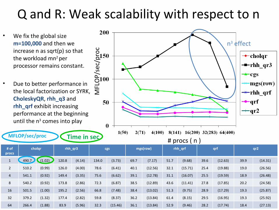
Q and R: Weak scalability with respect to n• We fix the global size
m=100,000 and then we increase n as sqrt(p) so that the workload mn2 per processor remains constant.
• Due to better performance in the local factorization or SYRK, CholeskyQR, rhh_q3 and rhh_qrf exhibit increasing performance at the beginning until the n3 comes into play
05/31/10 11:43 38
# of procs
cholqr rhh_qr3 cgs mgs(row) rhh_qrf qrf qr2
1 490.7 (1.02) 120.8 (4.14) 134.0 (3.73) 69.7 (7.17) 51.7 (9.68) 39.6 (12.63) 39.9 (14.31)
2 510.2 (0.99) 126.0 (4.00) 78.6 (6.41) 40.1 (12.56) 32.1 (15.71) 25.4 (19.88) 19.0 (26.56)
4 541.1 (0.92) 149.4 (3.35) 75.6 (6.62) 39.1 (12.78) 31.1 (16.07) 25.5 (19.59) 18.9 (26.48)
8 540.2 (0.92) 173.8 (2.86) 72.3 (6.87) 38.5 (12.89) 43.6 (11.41) 27.8 (17.85) 20.2 (24.58)
16 501.5 (1.00) 195.2 (2.56) 66.8 (7.48) 38.4 (13.02) 51.3 (9.75) 28.9 (17.29) 19.3 (25.87)
32 379.2 (1.32) 177.4 (2.82) 59.8 (8.37) 36.2 (13.84) 61.4 (8.15) 29.5 (16.95) 19.3 (25.92)
64 266.4 (1.88) 83.9 (5.96) 32.3 (15.46) 36.1 (13.84) 52.9 (9.46) 28.2 (17.74) 18.4 (27.13)
MFL
OP/
sec/
proc
# procs ( n )MFLOP/sec/proc Time in sec
n3 effect

R only: Strong scalability• In this experiment, we fix the
problem: m=100,000 and n=50. Then we increase the number of processors.
05/31/10 11:43 39
# of procs
cholqr rhh_qr3 cgs mgs(row) rhh_qrf qrf qr2
1 1099.046 (0.45) 147.6 (3.38) 139.309 (3.58) 73.5 (6.81) 69.049 (7.24) 69.108 (7.23) 68.782 (7.27)
2 1067.856 (0.23) 123.424 (2.02) 78.649 (3.17) 39.0 (6.41) 41.837 (5.97) 38.008 (6.57) 40.782 (6.13)
4 1034.203 (0.12) 116.774 (1.07) 71.101 (1.76) 38.7 (3.23) 39.295 (3.18) 36.263 (3.44) 36.046 (3.47)
8 876.724 (0.07) 119.856 (0.52) 66.513 (0.94) 36.7 (1.70) 37.397 (1.67) 35.313 (1.77) 34.081 (1.83)
16 619.02 (0.05) 129.808 (0.24) 53.352 (0.59) 31.6 (0.99) 33.581 (0.93) 31.339 (0.99) 31.697 (0.98)
32 468.332 (0.03) 95.607 (0.16) 42.276 (0.37) 29.0 (0.54) 37.226 (0.42) 25.695 (0.60) 25.971 (0.60)
64 195.885 (0.04) 77.084 (0.10) 25.89 (0.30) 22.8 (0.34) 36.126 (0.22) 17.746 (0.44) 17.725 (0.44)
# procs
MFL
OP/
sec/
proc
MFLOP/sec/proc Time in sec

R only: Weak scalability with respect to m
• We fix the local size to be mloc=100,000 and n=50. When we increase the number of processors, the global m grows proportionally.
05/31/10 11:43 40
# of procs
cholqr rhh_qr3 cgs mgs(row) rhh_qrf qrf qr2
1 1098.7 (0.45) 145.4 (3.43) 138.2 (3.61) 70.2 (7.13) 70.6 (7.07) 68.7 (7.26) 69.1 (7.22)
2 1048.3 (0.47) 124.3 (4.02) 70.3 (7.11) 35.6 (14.04) 43.1 (11.59) 35.8 (13.95) 36.3 (13.76)
4 1044.0 (0.47) 116.5 (4.29) 82.0 (6.09) 41.4 (12.09) 35.8 (13.94) 36.3 (13.74) 34.7 (14.40)
8 993.9 (0.50) 116.2 (4.30) 66.3 (7.53) 33.2 (15.06) 35.1 (14.21) 35.5 (14.05) 33.8 (14.75)
16 918.7 (0.54) 115.2 (4.33) 64.1 (7.79) 33.3 (15.04) 34.0 (14.66) 33.4 (14.94) 33.0 (15.11)
32 950.7 (0.52) 112.9 (4.42) 63.6 (7.85) 32.5 (15.38) 33.4 (14.95) 33.3 (15.01) 32.9 (15.19)
64 764.6 (0.65) 112.3 (4.45) 62.7 (7.96) 32.3 (15.46) 34.0 (14.66) 32.6 (15.33) 32.3 (15.46)
# procsM
FLO
P/se
c/pr
ocMFLOP/sec/proc Time in sec
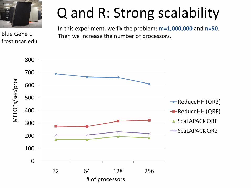
Q and R: Strong scalabilityIn this experiment, we fix the problem: m=1,000,000 and n=50. Then we increase the number of processors. Blue Gene L
frost.ncar.edu
# of processors
MFL
OPs
/sec
/pro
c
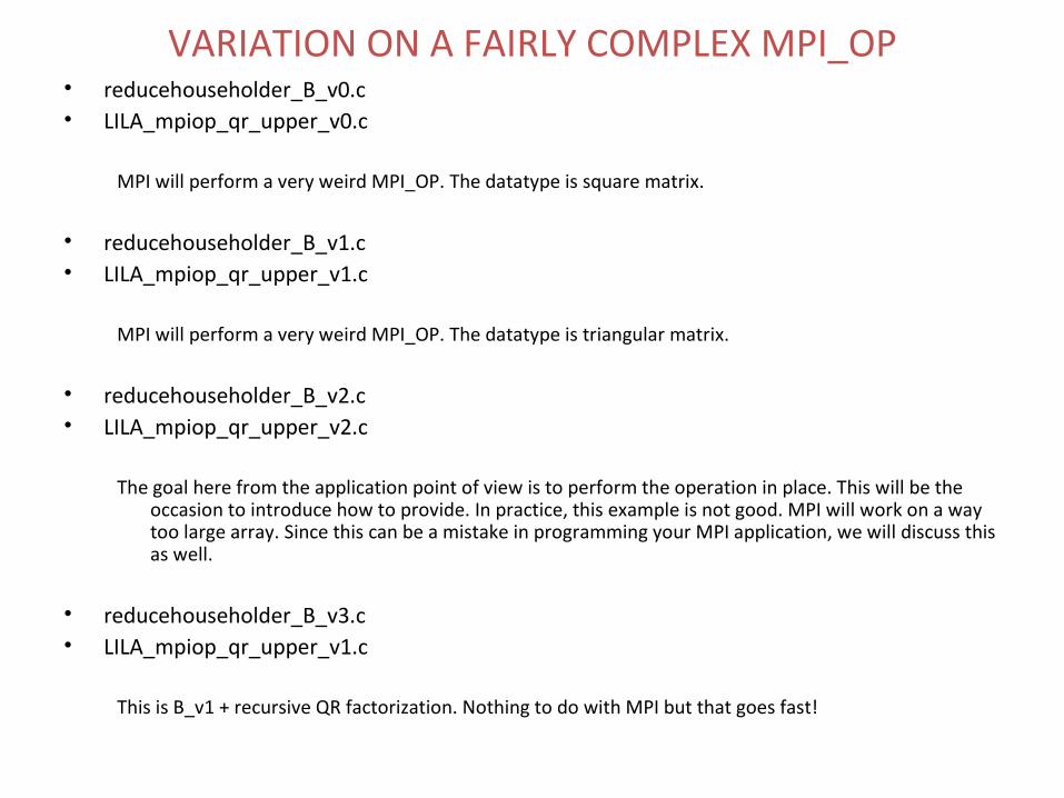
VARIATION ON A FAIRLY COMPLEX MPI_OP• reducehouseholder_B_v0.c• LILA_mpiop_qr_upper_v0.c
MPI will perform a very weird MPI_OP. The datatype is square matrix.
• reducehouseholder_B_v1.c• LILA_mpiop_qr_upper_v1.c
MPI will perform a very weird MPI_OP. The datatype is triangular matrix.
• reducehouseholder_B_v2.c• LILA_mpiop_qr_upper_v2.c
The goal here from the application point of view is to perform the operation in place. This will be the occasion to introduce how to provide. In practice, this example is not good. MPI will work on a way too large array. Since this can be a mistake in programming your MPI application, we will discuss this as well.
• reducehouseholder_B_v3.c• LILA_mpiop_qr_upper_v1.c
This is B_v1 + recursive QR factorization. Nothing to do with MPI but that goes fast!
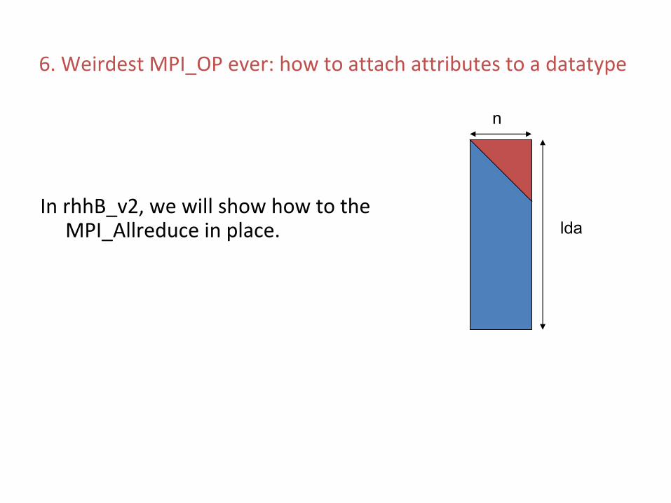
6. Weirdest MPI_OP ever: how to attach attributes to a datatype
In rhhB_v2, we will show how to the MPI_Allreduce in place.
n
lda
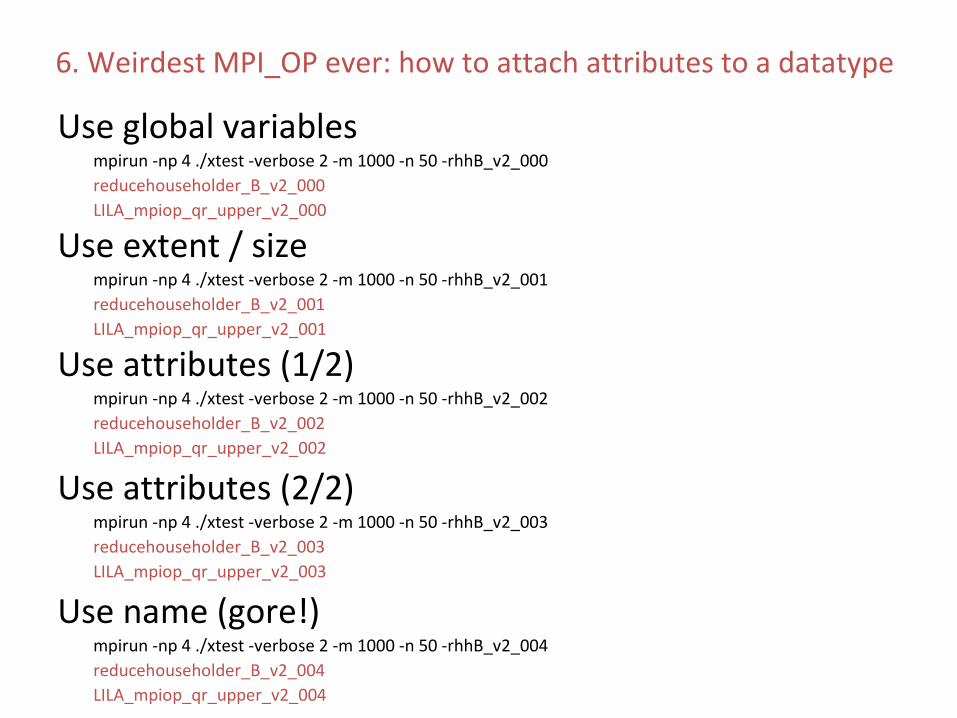
6. Weirdest MPI_OP ever: how to attach attributes to a datatype
Use global variables mpirun -np 4 ./xtest -verbose 2 -m 1000 -n 50 -rhhB_v2_000reducehouseholder_B_v2_000LILA_mpiop_qr_upper_v2_000
Use extent / sizempirun -np 4 ./xtest -verbose 2 -m 1000 -n 50 -rhhB_v2_001reducehouseholder_B_v2_001LILA_mpiop_qr_upper_v2_001
Use attributes (1/2)mpirun -np 4 ./xtest -verbose 2 -m 1000 -n 50 -rhhB_v2_002reducehouseholder_B_v2_002LILA_mpiop_qr_upper_v2_002
Use attributes (2/2)mpirun -np 4 ./xtest -verbose 2 -m 1000 -n 50 -rhhB_v2_003reducehouseholder_B_v2_003LILA_mpiop_qr_upper_v2_003
Use name (gore!)mpirun -np 4 ./xtest -verbose 2 -m 1000 -n 50 -rhhB_v2_004reducehouseholder_B_v2_004LILA_mpiop_qr_upper_v2_004

v2_001
MPI_Type_size( (*mpidatatype), &n);n = n / sizeof(double);n =(int) ( (-1.00e+00 + sqrt( 1.00e+00
+8.00e+00*((double)n) ) )/2.00e+00 );
MPI_Type_get_extent( (*mpidatatype), &lb, &extent);lda = ( extent / sizeof(double) - n ) / ( n - 1 );
n
lda
Two equations / Two unknowns:
size = n * ( n + 1 ) / 2 = 1/2 n^2 + 1/2 nextent = (n-1)*lda + n
Related Documents