Jules Lamers Institute for Theoretical Physics arXiv:1501 ...

ITP-UU-15/01

A pedagogical introduction to quantum integrability

with a view towards theoretical high-energy physics

Jules Lamers

Institute for Theoretical PhysicsCenter for Extreme Matter and Emergent Phenomena, Utrecht University

Leuvenlaan 4, 3584 CE Utrecht, The Netherlands

[email protected]

Abstract

These are lecture notes of an introduction to quantum integrability given at the TenthModave Summer School in Mathematical Physics, 2014, aimed at PhD candidates and juniorresearchers in theoretical physics.

We introduce spin chains and discuss the coordinate Bethe ansatz (cba) for a repres-entative example: the Heisenberg xxz model. The focus lies on the structure of the cbaand on its main results, deferring a detailed treatment of the cba for the general M -particlesector of the xxz model to an appendix. Subsequently the transfer-matrix method is dis-cussed for the six-vertex model, uncovering a relation between that model and the xxz spinchain. Equipped with this background the quantum inverse-scattering method (qism) andalgebraic Bethe ansatz (aba) are treated. We emphasize the use of graphical notation foralgebraic quantities as well as computations.

Finally we turn to quantum integrability in the context of theoretical high-energy physics.We discuss factorized scattering in two-dimensional qft, and conclude with a qualitativeintroduction to one current research topic relating quantum integrability to theoretical high-energy physics: the Bethe/gauge correspondence.

Contents

1 Introduction 2

2 Bethe’s method for the xxz model 52.1 The xxz spin chain and its symmetries . . . . . . . . . . . . . . . . . . . . . . . . 52.2 The coordinate Bethe ansatz . . . . . . . . . . . . . . . . . . . . . . . . . . . . . 112.3 Results and Bethe-ansatz equations . . . . . . . . . . . . . . . . . . . . . . . . . . 13

arX

iv:1

501.

0680

5v2

[m

ath-

ph]

3 J

un 2

015

3 Transfer matrices and the six-vertex model 183.1 The six-vertex model . . . . . . . . . . . . . . . . . . . . . . . . . . . . . . . . . . 183.2 The transfer-matrix method and cba . . . . . . . . . . . . . . . . . . . . . . . . . 223.3 Unexpected results . . . . . . . . . . . . . . . . . . . . . . . . . . . . . . . . . . . 27

4 The quantum inverse-scattering method 314.1 Conserved quantities from Lax operators . . . . . . . . . . . . . . . . . . . . . . . 324.2 The Yang-Baxter algebra . . . . . . . . . . . . . . . . . . . . . . . . . . . . . . . 354.3 The algebraic Bethe ansatz . . . . . . . . . . . . . . . . . . . . . . . . . . . . . . 43

5 Relation to theoretical high-energy physics 495.1 Quantum integrability and 2d qft . . . . . . . . . . . . . . . . . . . . . . . . . . 505.2 The Bethe/gauge correspondence . . . . . . . . . . . . . . . . . . . . . . . . . . . 54

A Completeness and the Yang-Yang function 59

B Computations for the M-particle sector 62

C Solving the fcr 67

References 74

1 Introduction

Quantum integrability is a beautiful and rich topic in mathematical physics, lying at the in-terface between condensed-matter physics, theoretical high-energy physics and mathematics.Usually, a (quantum) statistical model is considered ‘solved’ if the ground states, elementaryexcitations, and various thermodynamic quantities are known. Quantum-integrable models pos-sess a deep underlying structure that often allows for exact computation of such quantities. Atthe same time several of these models are quite realistic, and theoretic results may be tested withexperiments. Inevitably, then, the theory of quantum integrability is rather technical, whichmay obscure its beauty to newcomers. These notes aim to give a pedagogical introduction toquantum integrability and help the reader cross that first potential barrier.

Historical overview. Quantum-integrable models emerged in two different branches of phys-ics. The first example came from quantum mechanics: the isotropic Heisenberg ‘xxx’ spin chainfor (ferro)magnetism. In a seminal paper from 1931, Bethe solved this model using a methodthat now goes under the name of coordinate Bethe ansatz (cba), turning the problem of findingthe model’s spectrum into the problem of solving certain coupled equations, called the Bethe-ansatz equations (bae). In the subsequent decades Bethe’s work was developed further byothers, and in the 1960s Yang and Yang applied the cba to the more general ‘xxz’ spin chain.

The second source of quantum-integrable models was statistical mechanics. Here the proto-type is the six-vertex or ice-type model for two-dimensional hydrogen-bonded crystals. In thelate 1960s Lieb and Sutherland were able to solve the six-vertex model via the transfer-matrix

2

method — famously used by Onsager to tackle the 2d square-lattice Ising model in 1944 — to-gether with the cba as in the work of Yang and Yang. This solution uncovered several strikingsimilarities between the six-vertex model and the xxz spin chain, and shed light on the reasonwhy these models could be solved.

In the late 1970s these two stories were unified by the quantum inverse-scatteringmethod (qism) developed by the ‘Leningrad group’ of Faddeev et al, and others. Using ideasfrom classical integrability and soliton theory, the qism provides an algebraic framework forquantum-integrable models, in particular yielding the bae via the algebraic Bethe ansatz (aba).

Outline. These notes are organized as follows. Sections 2, 3 and 4 contain an introduction toquantum integrability, roughly following the above historical account. (The four-hour Modavelectures on which these notes are based covered most of this material.) The quantum-mechanicalside of the story is treated in Section 2. We introduce spin chains like the xxx and xxz models,present the cba for such models, and discuss the main results for the xxz spin chain. In Section 3we switch to the statistical-mechanical side. We introduce the six-vertex model, treat it usingthe transfer-matrix method and cba, and provide the results. By examining the outcome moreclosely we uncover the correspondence with the xxz model. Equipped with this background,the qism is developed in Section 4. This provides the precise relation between the xxz andsix-vertex models and, via the aba, allows us to rederive the results of the cba for these modelsusing a single computation.

In Section 5 we move on to qft and theoretical high-energy physics. After providing anoverview of the various relations that have been found with quantum integrability, and a dis-cussion of factorized scattering in qft in two dimensions, we give a qualitative introduction tothe Bethe/gauge correspondence as a recent example of such a relation.

There are three appendices containing further details and background. In Appendix A wepresent the Yang-Yang function. The details of the cba are worked out for the xxz spin chainin Appendix B. Finally, in Appendix C the R-matrix of the six-vertex model is found.

Although none of the material in these notes is new, this introduction is somewhat differentfrom most other introductory texts. For example, in Sections 2.2 and 2.3 we focus on theconceptual basis and the physics of the cba and its results rather than on computations. Still,the cba is worked out not just for the two-particle sector but, following [1, §8.4], also forthe general case in Appendix B. Our presentation of the transfer-matrix method and qismin Sections 3.2 and 4 consistently exploits a graphical notation adapted from [2]. Thoughnot always the most practical way to perform computations, this diagrammatic notation is aconvenient way to understand what is going on algebraically.

Further references. Many important topics in quantum integrability are barely touched inthese notes; examples include Baxter’s TQ-method, the thermodynamic limit, correlation func-tions, and quantum groups. Luckily the literature on quantum-integrable models is extensive,ranging from introductory texts to very technical papers. The following references, here orderedalphabetically, have been useful for preparing these notes:

• The renowned book by Baxter [1] gives a very detailed account of the cba and the TQ-method for several quantum-integrable models in statistical mechanics, including the six-

3

vertex model. The notation is perhaps a bit old fashioned at times.

• Faddeev’s famous Les Houches lecture notes [3] provide a good basis for the aba and thexxx model. Some familiarity with quantum integrability may be useful.

• Gaudin’s book [4] was recently translated into English. Amongst others the xxz spinchain and the six-vertex model are treated using the cba, and the thermodynamic limitis studied.

• Chapters 1–3 of the book by Gomez, Ruiz-Altaba and Sierra [2] treat the cba and abafor the xxz spin chain and the six-vertex model. The underlying quantum-algebraicstructure is pointed out, though perhaps somewhat vaguely at times, and there are nicediagrammatic computations.

• Chapters 0–2 of the book by Jimbo and Miwa [5] form a neat concise introduction tostatistical physics, the xxz spin chain and the six-vertex model. Although the aba is notdiscussed, the qism is essentially treated in Sections 2.4–3.3 and 3.7.

• Karbach, Hu and Muller [6, 7] have written a nice three-part introduction to the cba forthe xxx model, including a discussion of the low-lying excitations in the physical spectrumfor both the ferromagnetic and antiferromagnetic regime.

• The well-known book by Korepin, Bogoliubov and Izergin [8] contains a lot of informationabout the qism and its applications to correlation functions. The discussion of the basicsis quite condensed.

A standard reference for classical integrability and soliton theory is the book by Babelon,Bernard and Talon [9]. For more about the history of quantum integrability see e.g. [10]. Ex-perimental realizations of quantum-integrable models are described in [11]. Numerical methodsfor the xxx spin chain are discussed e.g. in [6, 7] and [12, Eds. 1 and 4]. For quantum groupssee e.g. the chatty introduction [13, §1–6] and the mathematics books [14–16].

Acknowledgements. I thank the organisers of the Tenth Modave Summer School in Math-ematical Physics for giving me the opportunity to share my enthusiasm for quantum integrabilitywith my peers. I am grateful to the participants of the school for their interest and questions.In preparing the lectures and these notes I benefited from discussions with G. Arutyunov,R. Borsato, W. Galleas, A. Henriques, R. Klabbers and D. Schuricht.

I gratefully acknowledge the support of the Netherlands Organization for Scientific Re-search (nwo) under the vici grant 680-47-602. This work is part of the erc Advanced Grantno. 246974, Supersymmetry: a window to non-perturbative physics, and of the d-itp consortium,a program of the nwo funded by the Dutch Ministry of Education, Culture and Science (ocw).

4

2 Bethe’s method for the xxz model

The pioneering work of Bethe on the one-dimensional Heisenberg model for ferromagnetismis one of the corner stones of the theory of quantum integrability. Although nowadays manyquantum-integrable models can be tackled in more sophisticated ways, as we will e.g. see inSection 4, Bethe’s method remains a concrete and physical way to introduce the basic ingredientsand obtain the main results.

2.1 The xxz spin chain and its symmetries

At the dawn of the 20th century Maxwell had formulated his laws describing the connectionbetween electric and magnetic forces and optics, but the microscopic mechanism behind mag-netism was not understood. The advent of quantum mechanics brought new insights, andHeisenberg and Dirac independently showed in 1926 that Pauli’s exclusion principle leads to aneffective interaction between electron spins of atoms with overlapping wave functions [17]. Thisexchange interaction formed the basis for an important model for ferromagnetism published byHeisenberg two years later [18] (see also [19, §8]). In one spatial dimension this is an exampleof a spin chain — a special class of quantum-mechanical models that are rather simple in theirset-up, yet lead to a wide variety of interesting physics and mathematics.

Spin chains. Consider a one-dimensional array of L atoms, modelled by a lattice of length Lwith uniform lattice spacing that we take equal to one. We impose periodic boundary conditions,so that the lattice is ZL := Z/LZ. This choice of boundary conditions is very convenient, andnot unreasonable since one is typically interested in the physics in the thermodynamic limitwhere L→∞ becomes macroscopically large.#1

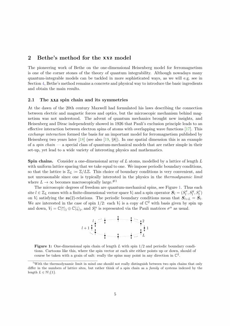
The microscopic degrees of freedom are quantum-mechanical spins, see Figure 1. Thus eachsite l ∈ ZL comes with a finite-dimensional vector space Vl and a spin operator Sl = (Sxl , S

yl , S

zl )

on Vl satisfying the su(2)-relations. The periodic boundary conditions mean that Sl+L = Sl.We are interested in the case of spin 1/2: each Vl is a copy of C2 with basis given by spin upand down, Vl = C|↑〉l ⊕ C|↓〉l, and Sαl is represented via the Pauli matrices σα as usual.

1

2l

l + 1

L

······

······

Figure 1: One-dimensional spin chain of length L with spin 1/2 and periodic boundary condi-tions. Cartoons like this, where the spin vector at each site either points up or down, should ofcourse be taken with a grain of salt: really the spins may point in any direction in C2.

1With the thermodynamic limit in mind one should not really distinguish between two spin chains that onlydiffer in the numbers of lattice sites, but rather think of a spin chain as a family of systems indexed by thelength L ∈ N\1.

5

The Hilbert space of the spin chain is the tensor product of the Vl over the lattice,

H =⊗l∈ZL

Vl , (2.1)

with (orthonormal) basis consisting of tensor products of the local spin vectors |↑〉l and |↓〉l.The subscript of Sl keeps track of the factor Vl in (2.1) on which this local spin operator actsnontrivially:

Sl = 1

1

⊗ · · · ⊗ 1⊗ ~2 σl

⊗ 1⊗ · · · ⊗ 1

L

. (2.2)

This tensor-leg notation is used throughout the literature on quantum integrability and willbe particularly helpful in Section 4. (Note that it does not make sense to use a summationconvention for these subscripts as there is nothing special about precisely two operators actingnontrivially at the same Vl.) While we are at it, let us also introduce the following commonnotation. For any vector space W , ‘End(W )’ denotes the space of all linear operators W −→W ,i.e. square matrices of size dim(W ). For example: Sαl ∈ End(Vl) ⊆ End(H) for α = x, y, z.

The relations between the local spin operators can be packaged together into a ‘global’ spinLie algebra governing the entire spin chain,

[Sαk , Sβl ] = i ~ δk,l

∑γ=x,y,z

εαβγ Sγl , (2.3)

where the totally antisymmetric su(2)-structure constant is fixed by εxyz = 1. The relation (2.3)is sometimes called ultralocal since the spin operators at different sites commute. For compu-tations it is convenient to work with the (sl(2) = su(2)C) ladder operators S±l := Sxl ± iSyltogether with Szl , satisfying

[Szk , S±l ] = ±~ δk,l S

±l , [S+

k , S−l ] = 2 ~ δk,l S

zl , [S±k , S

±l ] = 0 . (2.4)

With respect to the basis |↑〉l, |↓〉l of Vl these operators are given by

S+l = ~

(0 10 0

), S−l = ~

(0 01 0

), Szl =

~2

(1 00 −1

). (2.5)

The set-up so far can be summarized in more mathematical terms by saying that a spin chainis a Hilbert space H as in (2.1) carrying for each l ∈ ZL an irreducible su(2)-representation; forus this is the two-dimensional (defining) representation (2.2). In fact H also carries a ‘global’su(2)-representation, given by the total spin operator S = (Sz, Sy, Sz) defined as

Sα :=∑l∈ZL

Sαl ∈ End(H) , α = x, y, z . (2.6)

This representation is reducible, as we will see in (2.17).

Exercise 2.1. To practice with this notation, compute the matrix of Sz with respect to thestandard basis for H for L = 2 and L = 3.

6

The last piece of input is a (hermitean) Hamiltonian H ∈ End(H) describing the exchangeinteraction between the spins. We will need the following properties from these interactions:they are

i) only nearest neighbour ;ii) homogeneous, i.e. translationally invariant; andiii) at least partially isotropic, i.e. [Sz, H] = 0.

Exercise 2.2. Argue that any spin-chain Hamiltonian obeying property (i) can be written asH =

∑lHl,l+1. What does (ii) mean for the boundary conditions when L is finite? Try to find

the form of the most general local contributions Hl,l+1 satisfying (ii)–(iii).

Examples. The simplest spin chain satisfying (i)–(iii) is the Heisenberg ‘xxx’ model,

Hxxx = −J∑l∈ZL

Sl · Sl+1 , (2.7)

where the exchange coupling J sets the energy scale. Since [S, Hxxx] = 0 this model is com-pletely isotropic and the spins have no preferred direction. Accordingly the spectrum is highlydegenerate: the states come in an su(2)-multiplet for each energy eigenvalue. When J > 0the lowest energy is attained when each of the local terms in (2.7) contributes maximally, sothe spins tend to align. This is the ferromagnetic regime studied by Bethe in 1931. In con-trast, for J < 0, the spins tend to anti-align and the macroscopic magnetization vanishes. Thisantiferromagnetic regime was first analyzed by Neel in 1948.

A more general spin chain obeying properties (i)–(iii) is the ‘xxz’ or Heisenberg-Ising model,

Hxxz = −J∑l∈ZL

(Sxl S

xl+1 + Syl S

yl+1 + ∆Szl S

zl+1

), (2.8)

where ∆ ∈ R is the anisotropy parameter. This model was introduced by Orbach in 1958 andthoroughly studied by Yang and Yang in the 1960s (see [20] and references therein). In termsof the ladder operators (2.4) the Hamiltonian (2.8) reads

Hxxz = −J2

∑l∈ZL

(S+l S−l+1 + S−l S

+l+1 + 2 ∆Szl S

zl+1

). (2.9)

This form clearly shows that the first two terms describe the hopping of excited spins while thethird term counts the number of (mis)aligned neighbouring spins.

Exercise 2.3. To get more feeling for the xxz Hamiltonian consider the summand in (2.9). By(2.2) and (2.5), we have e.g. Szl S

zl+1 ∝ (σz ⊗ 1)l,l+1(1⊗σz)l,l+1 = (σz ⊗ σz)l,l+1. Use this to

check that with respect to the standard basis of Vl ⊗ Vl+1

Hl,l+1 = −J2

(S+l S−l+1 + S−l S

+l+1 + 2 ∆Szl S

zl+1

)= −~2J

4

∆−∆ 22 −∆

∆

l,l+1

, (2.10)

where zeroes are suppressed.

7

Exercise 2.4. Show that for L even it suffices to take J > 0 and ∆ ∈ R by using (2.4) to computeV Hxxz V

−1 for V :=∏l S

z2l ∈ End(H). Which value of ∆ corresponds to the antiferromagnetic

xxx model in this way?

Exercise 2.5. An external magnetic field in the z-direction can be included by adding −h∑

l Szl

to the Hamiltonian, preserving properties (i)–(iii). Show that it is enough to consider h > 0 bycalculating W Hxxz(h)W−1 with W :=

∏l S

xl ∈ End(H) the spin-flip operator.

There exists a further generalization, the ‘xyz’ model, which has a different coupling con-stant for each spin-direction α. This spoils property (iii) and the model cannot be treated usingthe Bethe ansatz (but see [1, §9–10]).

Symmetries. Our goal is to find the spectrum of the xxz model, Hxxz|Ψ〉 = E|Ψ〉. Thiswill be achieved in Sections 2.2 and 2.3 using the cba, and again in Section 4.3 with a moreslick method. As always, the symmetries come to our aid, and we can exploit properties (ii)–(iii) to break our problem into smaller pieces. The following symmetries are at our disposal:translations along the lattice, by any amount of sites, and rotations around the z-axis, generatedby Sz. Thus the symmetry group is

G = Z× U(1)z ⊆ Z× SU(2) . (2.11)

In mathematical terms these symmetries can be used to decompose H into a direct sum ofirreducible G-representations, or ‘sectors’, which are preserved by the Hamiltonian. Let us seewhat this means concretely.

Exercise 2.6. Without reading any further, find the consequence of partial isotropy for L = 2 bycomparing the result of Exercise 2.1 with (2.10). What are the sectors corresponding to U(1)z?

M-particle sectors. First we exploit the partial isotropy. H and Sz can be simultaneouslydiagonalized by (iii), so the eigenvectors of Sz form a basis for H in which the Hamiltonian isblock diagonal. Let us show that it has the following form with respect to this basis:

H =

···

···

. (2.12)

The first block in (2.12) is 1× 1 and corresponds to the pseudovacuum, which we take to be

|Ω〉 :=⊗l∈ZL

|↑〉l = |↑1· · · ↑

L〉 ∈ H . (2.13)

This vector happens to be a ground state of (2.8) if J∆ > 0, as we will see in (2.19), but thepoint is that |Ω〉 is an eigenvector of Sz (with spin ~L/2) and killed by all S+

l : it is a highest-weight vector. This makes it a suitable reference point for constructing all other Sz-eigenvectors.

8

For example, the second block in (2.12) is obtained by flipping any single spin,

|l〉 := ~−1 S−l |Ω〉 = |↑1· · · ↑↓

l↑ · · · ↑

L〉 ∈ H , (2.14)

producing L vectors (so the block has size L× L) with spin L/2− 1. Likewise the third blockcorresponds to flipping yet another spin; since (S−l )2 = 0 and S−k S

−l = S−l S

−k this yields

(L2

)different vectors |k, l〉 for 1 ≤ k < l ≤ L.

In general, by repeatedly applying lowering operators S−l to |Ω〉 we construct an orthonormalbasis describing configurations with 0 ≤M ≤ L flipped spins:

|l1, · · · , lM 〉 := ~−M S−l1 · · ·S−lM|Ω〉 ∈ H , 1 ≤ l1 < · · · < lM ≤ L . (2.15)

This is the coordinate basis of H, which is responsible for the ‘coordinate’ in ‘cba’. A niceaspect of this basis is that it is very physical; its elements can be depicted as in Figure 1 (forwhich M = 5). The price we pay is that we lose manifest periodicity by restricting ourselves tothe ‘standard domain’ 1 ≤ l1 < · · · < lM ≤ L to avoid overcounting. Consequently the periodicboundary conditions Sl+L = Sl must be imposed explicitly when working with the coordinatebasis. This will be important in Section 2.2 and Appendix B.

From (2.4) it follows that all spin configurations (2.15) are eigenvectors of the total spin-zoperator:

Sz |l1, · · · , lM 〉 = ~ (L/2−M) |l1, · · · , lM 〉 . (2.16)

Let us write HM ⊆ H for the M -particle sector consisting of all vectors with M spins down.The (weight) decomposition of our Hilbert space into these subspaces,

H =

L⊕M=0

HM , (2.17)

corresponds to the block-diagonal form of H in (2.12).

Exercise 2.7. Compute the size of the Mth block in (2.12). Check that the dimensions on bothsides of (2.17) agree.

The upshot is that partial isotropy allows us to focus on diagonalizing the Hamiltonian inthe M -particle sector: our new goal is to solve the eigenvalue problem

Hxxz |ΨM 〉 = EM |ΨM 〉 , |ΨM 〉 ∈ HM . (2.18)

Magnons. Next we exploit the homogeneity; let us see how far that gets us. By (ii) theHamiltonian satisfies UHU−1 = H where the shift operator U ∈ End(H) shifts all sites to theleft, mapping each Vl to Vl−1.#2 In analogy with continuous (as opposed to lattice) modelsone often writes U =: eiP . Since U is unitary its eigenvalues are of the form eip for some

2In Section 4.1 we will see that defining the shift operator as acting by translations to the right would be morenatural from the viewpoint of the qism, cf. (4.13). However, using that convention would result in a sign in theexponent in (2.20), and similarly in e.g. (2.26) and (2.29) for higher M . At any rate, this choice of conventionessentially only affects the sign of the (quasi)momentum; of course the physical results do not depend on it.

9

real momentum p. (Note that p is defined mod 2π.) Periodic boundary conditions imply thatUL = 1 is the identity operator on H, leading to momentum quantization p ∈ 2π

L ZL as expectedfor particles on a circle.

Exercise 2.8. For the zero-particle sector H0 use homogeneity to find the momentum of thepseudovacuum (2.13). Check that Hxxz |Ω〉 = E0 |Ω〉 with ‘vacuum’ energy

E0 = −~2J∆L/4 . (2.19)

The one-particle sector is fixed by homogeneity as well. Indeed, any vector in H1 canbe expressed in terms of the coordinate basis. Translational invariance means that |Ψ1; p〉 =∑

l Ψp(l) |l〉 should be an eigenvector of U for some momentum p. Using U † = U−1 it followsthat the wave functions satisfy the recursion Ψp(l + 1) = 〈l|U |Ψ1; p〉 = eip Ψp(l), yielding aplane-wave expansion:

|Ψ1; p〉 =1√L

∑l∈ZL

eip l|l〉 ∈ H1 . (2.20)

Exercise 2.9. Use 〈k|l〉 = δk,l to check that the #ZL = L = dim(H1) vectors (2.20) constitutean orthonormal basis for H1.

The basis vectors (2.20) describe excitations around the pseudovacuum |Ω〉 called magnons:spin waves with quantized wavelength 2π/p travelling along the chain. With respect to themagnon basis (2.20) for H1 any translationally-invariant Hamiltonian is diagonal in the one-particle sector. Whether or not magnons are ‘quasiparticles’ describing low-lying excitations inthe physical spectrum depends on the model’s parameters.

Exercise 2.10. Compute the action of (2.9) on (2.14) to check that the dispersion relation of amagnon in the xxz spin chain is

ε1(p) := E1(p)− E0 = ~2J (∆− cos p) . (2.21)

Notice that for the xxx case (∆ = 1) the magnon with vanishing momentum contributeszero to the energy. This is a direct consequence of the symmetries: Hxxx has full rotationalsymmetry, so its eigenstates come in su(2)-multiplets. The zero-momentum magnon is simplythe first su(2)-descendant of the pseudovacuum: |Ψ1; 0〉 ∝ S−|Ω〉 with S− =

∑l S−l the total

lowering operator. Turning on the anisotropy lifts the degeneracy in the spectrum.For M ≥ 2 we can again write any translationally-invariant vector with momentum p as

|ΨM ; p〉 =∑

1≤l1<···<lM≤LΨp(l1, · · · , lM ) |l1, · · · , lM 〉 ∈ HM (2.22)

with respect to the coordinate basis (2.15) of HM . This time, however, the wave functions Ψp(l)are not completely determined by the symmetries (2.11).#3 To diagonalize the larger blocks ofthe Hamiltonian we have to be smart: this is where the Bethe ansatz comes in.

3For example, expand |Ψ2; p〉 ∈ H2 as in (2.22). Homogeneity again recursively relates wave functions forexcited spins at equal separation d12 := d(l1, l2), where d(k, l) := minn∈Z |l − k + nL| is the distance function(metric) on ZL. Indeed, Ψp(l1 + 1, l2 + 1) = 〈l1, l2|U |Ψ2; p〉 = eip Ψp(l1, l2), so Ψp(l1, l2) = eip l1 Ψ′p(d12) =eip l2 Ψ′′p(d12) for some function Ψ′p (or equivalently Ψ′′p) depending on the lattice only through the separationbetween the two flipped spins. However, the values of this function for different d12 are not related by thesymmetries (2.11).

10

2.2 The coordinate Bethe ansatz

In a ground-breaking paper from 1931, Bethe solved the ferromagnetic regime of the xxx spinchain [21]. This subsection introduces the coordinate Bethe ansatz (cba) for any spin chainobeying properties (i)–(iii) above. The focus lies on the structure and physics of the method;computational details can be found in Appendix B.

The basic idea of the cba is to parametrize the states in the M -particle sector via para-meters pm, 1 ≤ m ≤ M . In the simplest case this boils down to the result (2.20), while ingeneral it is a symmetrized version of the Fourier transform. The spectrum of the Hamiltonianfollows once the values of the pm are found from a system of coupled nonlinear equations: theBethe-ansatz equations (bae). Thus, in principle, the cba provides a concrete and physical wayof converting the problem of diagonalizing the Hamiltonian to that of solving the bae.

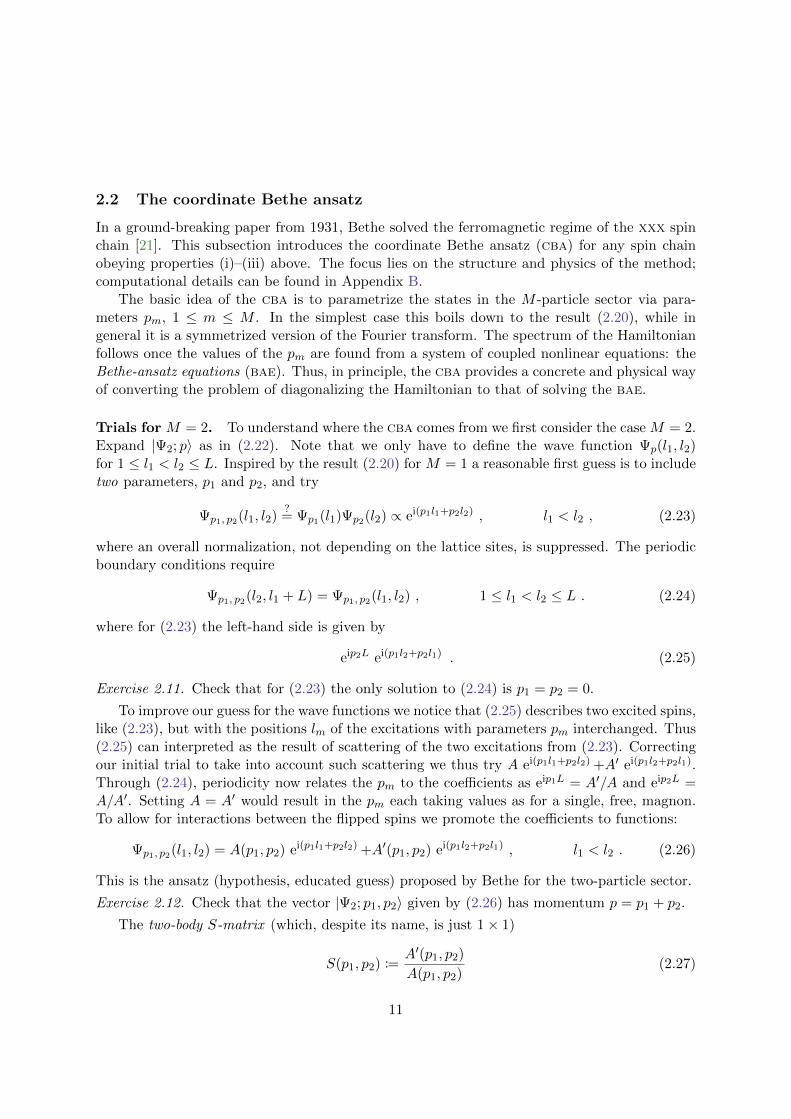
Trials for M = 2. To understand where the cba comes from we first consider the case M = 2.Expand |Ψ2; p〉 as in (2.22). Note that we only have to define the wave function Ψp(l1, l2)for 1 ≤ l1 < l2 ≤ L. Inspired by the result (2.20) for M = 1 a reasonable first guess is to includetwo parameters, p1 and p2, and try

Ψp1, p2(l1, l2)?= Ψp1(l1)Ψp2(l2) ∝ ei(p1l1+p2l2) , l1 < l2 , (2.23)

where an overall normalization, not depending on the lattice sites, is suppressed. The periodicboundary conditions require

Ψp1, p2(l2, l1 + L) = Ψp1, p2(l1, l2) , 1 ≤ l1 < l2 ≤ L . (2.24)

where for (2.23) the left-hand side is given by

eip2L ei(p1l2+p2l1) . (2.25)

Exercise 2.11. Check that for (2.23) the only solution to (2.24) is p1 = p2 = 0.

To improve our guess for the wave functions we notice that (2.25) describes two excited spins,like (2.23), but with the positions lm of the excitations with parameters pm interchanged. Thus(2.25) can interpreted as the result of scattering of the two excitations from (2.23). Correctingour initial trial to take into account such scattering we thus try A ei(p1l1+p2l2) +A′ ei(p1l2+p2l1).Through (2.24), periodicity now relates the pm to the coefficients as eip1L = A′/A and eip2L =A/A′. Setting A = A′ would result in the pm each taking values as for a single, free, magnon.To allow for interactions between the flipped spins we promote the coefficients to functions:

Ψp1, p2(l1, l2) = A(p1, p2) ei(p1l1+p2l2) +A′(p1, p2) ei(p1l2+p2l1) , l1 < l2 . (2.26)

This is the ansatz (hypothesis, educated guess) proposed by Bethe for the two-particle sector.

Exercise 2.12. Check that the vector |Ψ2; p1, p2〉 given by (2.26) has momentum p = p1 + p2.

The two-body S-matrix (which, despite its name, is just 1× 1)

S(p1, p2) :=A′(p1, p2)

A(p1, p2)(2.27)

11

describes the scattering of the two excitations, as can be seen by rewriting (2.26) in the formΨp1, p2(l1, l2) ∝ ei(p1l1+p2l2) +S(p1, p2) ei(p1l2+p2l1).

The periodic boundary conditions (2.24) impose two equations:

eip1L = S(p1, p2) , eip2L = S(p1, p2)−1 . (2.28)

These are the bae for the parameters pm in the two-particle sector. Physically they say thatwhen either of the excited spins is moved once around the chain (in clockwise direction) itscatters on the other excitation. Note that the bae together imply the periodicity condi-tion ei(p1+p2)L = 1 and hence momentum quantization p = p1 + p2 ∈ 2π

L ZL for the two-particlesector. The dependence on the details of the spin chain are hidden in the two-body S-matrixon the right-hand side of the bae. Until a model is specified we cannot say whether the baehave the right amount of, or even any, solutions for the pm. We will look at the results for thexxz model in Section 2.3.

Before proceeding to the M -particle sector let us quickly recap our notation for M = 2. Wewrite ‘|Ψ2〉’ for an arbitrary vector in the two-particle sector, ‘|Ψ2; p〉’ for any vector in H2 thatis translationally invariant (with momentum p), and ‘|Ψ2; p1, p2〉’ for the specific vectors (withparameters p1 and p2) given by (2.26).

cba for general M . Expand |ΨM 〉 ∈ HM in terms of the coordinate basis |l1, · · · , lM 〉 asin (2.22). Again we associate to each excitation lm a parameter pm that is to be determined.We abbreviate l := (l1, · · · , lM ) and p := (p1, · · · , pM ).

By property (i) above we only have (very) short-ranged interactions, so the M excited spinsdo not interact when they are well separated, i.e. when no two excitations are next to eachother. Thus, for such well-separated configurations it makes sense to look for a wave functionof the product form Ψp1(l1) · · ·ΨpM (lM ) ∝ exp(ip· l): this is the generalization of (2.23) to theM -particle sector.

Next, as for M = 2, we include all scattered configurations, labelled by permutations in SMdescribing the ordering after the scattering. A linear combination of these M ! configurations,with coefficients depending on p to account for interactions between the excitations, gives thecba for the (unnormalized) wave function in the M -particle sector:

Ψp(l) =∑π∈SM

Aπ(p) eipπ·l , l1 < · · · < lM . (2.29)

Here pπ is a shorthand for the (right) action of π ∈ SM on p; concretely this just means thatpπ · l =

∑m pπ(m) lm. The ansatz (2.29) is also referred to as the Bethe wave function. As a

check we note that (2.29) reduces to the magnon (2.20) when M = 1, while for M = 2 the sumin (2.29) runs over two elements, the identity and a transposition, correctly reproducing (2.26).

Strategy. The Bethe wave functions (2.29) yield eigenstates of the Hamiltonian in the M -particle sector if we can solve the equations

〈l|Hxxz|ΨM ;p〉 = EM (p)Ψp(l) , 1 ≤ l1 < · · · < lM ≤ L . (2.30)

12

The unknowns are the energy eigenvalues EM (p) and the coefficients Aπ(p) (up to an overallnormalization) as functions of p, together with the actual values of the p. The strategy todetermine these consists of three steps:

1. Solve the equations in (2.30) for configurations l with well-separated excitations. This isquite easy and will yield the M -particle dispersion relation εM (p) := EM (p)− E0.

2. The equations in (2.30) with at least one pair of neighbouring excitations in l. Althoughthis is more tricky, it can be done, giving the coefficients Aπ(p)/Ae(p).

3. Impose the periodic boundary conditions. This will result in one equation for each expo-nent in (2.29): the bae, a priori M ! in total, for the allowed (‘on shell’) values of p.

Of course this is really only half of the work: the bae still have to be solved, which hasnot been done for general M and L, and one has to let L → ∞ to study the thermodynamicproperties of the model. In addition it remains to be seen whether all eigenstates are of theBethe-form, so that the cba does really produce the full spectrum. The above strategy is carriedout for the M -particle sector of the xxz model in Appendix B; let us turn to the results.

2.3 Results and Bethe-ansatz equations

For brevity we set ~ = J = 1. This essentially only affects the energy eigenvalues, which can berestored by multiplication by ~2J .

Results for M = 2. We first collect the results of the strategy in the two-particle sector. Thecomputations can be found in Appendix B.

Step 1. For the well-separated case the equations (2.30) are satisfied by the cba (2.26)provided the energy is given by the dispersion relation

ε2(p1, p2) = 2 ∆− cos p1 − cos p2 = ε1(p1) + ε1(p2) . (2.31)

This is a nice result: the energy consists of two contributions, one from each of the magnons.Although the values of the pm remain to be determined, and will be different from the free(single-magnon) case to give rise to an interaction energy, this means that the excited spinsin the two-particle sector behave like magnons. In particular, the two parameters pm can beinterpreted as the quasimomenta of these magnons.

Step 2. For neighbouring excitations the equations can be solved using a trick, see Ap-pendix B, yielding the two-body S-matrix (2.27):

S(p1, p2) = −1− 2 ∆ eip2 + ei(p1+p2)

1− 2 ∆ eip1 + ei(p1+p2)(2.32)

Two-body scattering is unitary by virtue of the property |S(p1, p2)|2 = 1 for pm ∈ R.This property, sometimes called physical unitarity, suggests defining the (real-valued) functionΘ(p1, p2) := −i logS(p1, p2) known as the two-body scattering phase.

The result (2.32) has two important physical implications. As S(p2, p1) = S(p1, p2)−1 theBethe wave function Ψp1,p2(l1, l2) is symmetric in the two pm upon normalizing (2.26) by

13

A(p1, p2) = S(p1, p2)−1/2. Thus |Ψ2; p1, p2〉 = |Ψ2; p2, p1〉: the magnons obey Bose-Einsteinstatistics. Interestingly, (2.32) also satisfies the fermion-like property S(p1, p1) = −1. Therefore|Ψ2; p1, p1〉 = 0, yielding a Pauli exclusion principle for the quasimomenta.#4 However, there isno spin-statistics connection in 1 + 1 dimensions, so these two properties are compatible.

Step 3. The remaining task is to find equations for the values of the pm. Plugging (2.32)into (2.28) we obtain the bae for the two-particle sector of the xxz model:

eip1L = −1− 2 ∆ eip2 + ei(p1+p2)

1− 2 ∆ eip1 + ei(p1+p2)= e−iΘ(p1,p2) ,

eip2L = −1− 2 ∆ eip1 + ei(p1+p2)

1− 2 ∆ eip2 + ei(p1+p2)= e−iΘ(p2,p1) .

(2.33)

Taking the logarithm shows that these are just quantization conditions for the quasimomenta:

Lp1 = 2πI1 −Θ(p1, p2) , L p2 = 2πI2 + Θ(p1, p2) , Im ∈ ZL , (2.34)

where the Im are known as the Bethe quantum numbers. Thus the quasimomenta in the two-particle sector are no longer the ‘bare’ quantities (valued in 2π

L ZL) of a free theory: (2.34) showsthat they are ‘renormalized’ as a result of interactions between the two magnons.

Exercise 2.13. Find an expression for Θ(p1, p2) by multiplying the numerator and denominatorin (2.32) by e−i(p1+p2)/2 and using log u+iv

u−iv = 2i arctan vu .

Exercise 2.14. Check (2.31) and (2.32) without consulting Appendix B.

Two-particle spectrum for ∆ = 1. To see whether we have succeeded in diagonalizing theHamiltonian for M = 2 one has to check whether the bae admit dim(H2) =

(L2

)solutions giving

rise to linearly independent states. To get some feeling for the physics we briefly discuss thespectrum that Bethe found for the ferromagnetic xxx model. More details, including some niceplots, can be found in [6] (for the antiferromagnetic case see [7]). The solutions fall into threeclasses:

i) There are L solutions describing a superposition of two free magnons, p1 = 0 and p =p2 = 2πI2/L. These can also be understood as the su(2)-descendants of the states in theone-particle sector,

∑l1<l2

(eip l1 + eip l2)|l1, l2〉 ∝ S−|Ψ1; p〉.

ii) The remaining solutions 0 < p1 < p2 < 2π can be interpreted as nearly free superpositionsof magnons whose interactions vanish for L→∞. Together with the first class these arescattering states.

However, there are not enough of these solutions. To find the remaining states the cba has tobe improved by extending the quasimomenta to complex values, pm ∈ C. Unitarity of the shiftoperator U = eiP requires the total momentum p = p1 + p2 to remain real. These account forthe third class of solutions:

4Anticipating the Pauli exclusing principle some authors include a sign in the cba from the start, replacing(2.29) by Ψp(l) =

∑π∈SM

(−1)sgn(π)Aπ(p) eipπ·l.

14

iii) Quasimomenta with Im(p1) = − Im(p2) 6= 0 cause |Ψp(l1, l2)| to decrease with increasingseparation between the magnons. These solutions can be interpreted as bound states.

Such results were confirmed by neutron-scattering experiments, also for other models solvableby Bethe-ansatz techniques, see e.g. [11].

Let us briefly comment on a source of possible confusion. The appearance of the secondsu(2)-descendent of the pseudovacuum in the M = 2 spectrum (with p1 = p2 = 0) may appearto conflict with the Pauli exclusion principle for the two-body S-matrix. This issue is resolvedby noticing that in the isotropic case the two-body S-matrix,

S(p1, p2)|∆=1 = −1− 2 eip2 + ei(p1+p2)

1− 2 eip1 + ei(p1+p2)=

cot p12 − cot p22 + 2i

cot p12 − cot p22 − 2i, (2.35)

is not continuous at the origin. Indeed, along the diagonal in the quasimomentum plane wehave S(p1, p1) = −1, cf. the Pauli exclusion principle. However, along either axis (2.35) satisfiesS(p1, 0)|∆=1 = S(0, p2)|∆=1 = +1, so the su(2)-descendants do not vanish. This discontinuityhints at the fact that the xxz model with ‘generic’ anisotropy ∆ 6= ±1 is mathematically betterbehaved than the isotropic spin chain (cf. Appendix A). From this perspective ∆ can be seenas a regulator for the xxx spin chain.

Exercise 2.15. Check that, as ∆ → 1, the result of Exercise 2.13 matches the expression forΘ(p1, p2)|∆=1 obtained directly from (2.35).

Results for general M . Working out the strategy for the general M -particle sector, seeAppendix B, gives the following results.

Step 1. The equations (2.30) are solved by the cba (2.29) for well-separated excitations ifthe contribution to the energy is

εM (p) = M ∆−M∑m=1

cos pm =M∑m=1

ε1(pm) . (2.36)

Thus, the dispersion relation behaves additively for general M as well: the energy splits intoseparate contributions for each pm. Let us stress once more that this does not mean that (2.36)is simply the sum of free-magnon contributions; the quasimomenta pm are determined by thebae to account for the interaction energy. At any rate, (2.36) does justify our quasiparticleinterpretation for all M , so that we may conclude that M counts the number of magnons. Inparticular, since the HM are preserved by the Hamiltonian, the magnon-number is conserved:there is no magnon production or annihilation.

Step 2. The coefficients Aπ(p) in the Bethe wave function (2.29) also have to satisfy (2.30)for one or more pairs of neighbouring excitations. For general M there are many more suchequations than unknowns, but it turns out that they can in fact be solved. Up to an overallfactor the Aπ are expressed in terms of the two-body S-matrix (2.32):

Aπ(p)

Ae(p)=

∏1≤m<m′≤M

s.t. π(m)>π(m′)

S(pm, pm′) . (2.37)

15

This is a very remarkable result: physically, (2.37) says that M -magnon scattering is two-bodyreducible, i.e. factors into successive two-magnon scattering processes, governed by the two-bodyS-matrix (2.32). This is a extremely useful aspect of the model; we essentially know everythingabout the many-body scattering of magnons once we understand two-magnon scattering. Mod-els exhibiting this property are rather special. Indeed, note that if the scattering were one-bodyreducible, magnons would move freely along the spin chain. The xxz model, with two-body re-ducible scattering, is just one level up in complexity, allowing one to study interesting dynamicsin a controlled setting.

The results that there is no magnon-production and that scattering is two-body reduciblehint at the existence of hidden symmetries and conserved quantities that render the xxz spinchain quantum integrable, see Section 5.1. This is indeed the case; we will find these conservedquantities in Sections 3.3 and 4.1.

There is a nice graphical way to understand the result (2.37) [22]. Depict the initial andfinal configurations of quasimomenta (magnons) in the scattering process π ∈ SM as follows:

final: pπ(1) pπ(2) · · · pπ(M)

initial: p1 p2 · · · pM

Now connect equal quasimomenta by arrows in such a way that there are no points where threeor more lines meet. Typically there are several ways in which this can be done; these (must anddo) give the same result. For every pair n < m that is switched by π there is a crossing of pnand pm, contributing a factor of S(pn, pm) to Aπ(p). For example, the coefficient Aπ describinga three-magnon scattering process is depicted in Figure 2.

Exercise 2.16. Rewrite the result (2.37) in terms of the two-body scattering phase for thenormalization Ae(p) =

∏m<m′ S(pm, pm′)

−1/2.

Exercise 2.17. Prove the Pauli exclusion principle for the quasimomenta in the M -particle sectorby showing that (2.29) with (2.37) vanishes whenever pm = pn for some m 6= n.

p1

p1

p2

p2

p3

p3

=

p1

p1

p2

p2

p3

p3

=

p1

p1

p2

p2

p3

p3

Figure 2: Diagrammatic representation of (the coefficient Aπ describing) three-body scatteringwhere magnons 1 and 3 are interchanged. There are two ways in which this can be done, so thesecond equality expresses a consistency condition — which is trivially satisfied since the two-bodyS-matrix is 1× 1.

Step 3. Finally periodic boundary conditions must be imposed on the Bethe wave func-tion (2.29) with coefficients (2.37). It turns out that there are M independent bae for the

16

quasimomenta p in the M -particle sector:

eipmL =M∏n=1n6=m

S(pn, pm) , 1 ≤ m ≤M . (2.38)

Like (2.28) these have a nice physical interpretation. Since pm is the quasimomentum of themth magnon, eipmL is the phase acquired by that magnon as it is moved once around the spinchain (in clockwise direction). The bae (2.38) say that this phase consists of contributions dueto scattering on the other magnons.

To sum up, under the assumption that all states are of the Bethe form, the cba convertsthe problem of diagonalizing the Hamiltonian in the M -particle sector to that of solving theM coupled equations (2.38) for p ∈ CM . The bae are rather complicated (see also Appendix A),but that was to be expected: no approximations were used to obtain them; they are exact. Thebae can be studied numerically as well as analytically. By plugging in the resulting on-shellvalues for the pm one finally obtains the actual eigenstates |ΨM 〉 and their energies.

Since the bae are usually hard to solve one may wonder what we have gained by all ofthis. Notice that, although the bae become more complicated as M increases, they are notso sensitive to the length of the spin chain, unlike the size

(LM

)of the M -particle block of the

Hamiltonian. This renders them useful for studying the ground states, elementary excitationsand several thermodynamic quantities even as L→∞ (under certain assumptions on the natureof the solutions in that limit).

Rapidities. To conclude this subsection we introduce alternative variables that are in somesense more natural than the quasimomenta pm. Indeed, due to the factorization of magnonscattering the two-body S-matrix plays an important role in the analysis of the model. Thus itis convenient to switch to coordinates for which the two-body S-matrix takes a simple form.

For the xxx spin chain, (2.35) suggests defining rapidities as

λm :=1

2cot

pm2

(2.39)

so that the two-body S-matrix simply depends on the rapidity difference (cf. Section 5.1),

S(λn, λm)|∆=1 =λm − λn + i

λm − λn − i. (2.40)

(Depending on the context, rescaled or shifted versions of these are also used in literature.)

Exercise 2.18. Invert (2.39) and use (2.21) to check that the quasimomentum and energy con-tribution of a magnon with rapidity λ are

p(λ)|∆=1 =1

ilog

λ+ i/2

λ− i/2, ε1(λ)|∆=1 =

2

4λ2 + 1. (2.41)

17

We conclude that in terms of rapidities the bae (2.38) for the M -particle sector of the xxxspin chain read (

λm + i/2

λm − i/2

)L=

M∏n=1n6=m

λm − λn + i

λm − λn − i, 1 ≤ m ≤M . (2.42)

In the regime |∆| ≤ 1 the xxz spin chain involves hyperbolic generalizations of the aboveexpressions: parametrizing the anisotropy as ∆ = cos γ we have

p(λ) =1

ilog

sinh(λ+ iγ/2)

sinh(λ− iγ/2), (2.43)

ε1(λ) =1

2

sin2 γ

sinh(λ+ iγ/2) sinh(λ− iγ/2), (2.44)

and the bae become(sinh(λm + iγ/2)

sinh(λm − iγ/2)

)L=

M∏n=1n6=m

sinh(λm − λn + iγ)

sinh(λm − λn − iγ), 1 ≤ m ≤M . (2.45)

Exercise 2.19. Compute p′(λm) and compare the result with ε1(λm). (We will understand wherethis relation comes from in Section 4.3.)

Exercise 2.20. Note that (2.43)–(2.45) become trivial in the isotropic limit. Check that theequations for the xxx spin chain can nevertheless be recovered by rescaling the rapidities asλ 7→ γλ before taking the limit γ → 0.

3 Transfer matrices and the six-vertex model

Before turning to the abstract algebraic but very powerful formalism to treat the xxz modelonce more in Section 4 it is insightful to switch to the world of classical statistical physics on atwo-dimensional lattice. We focus on the six-vertex model, which will turn out to be intimatelyrelated to the xxz spin chain. Several concepts that we encounter along the way will play animportant role in Section 4 too.

3.1 The six-vertex model

Any lattice can be turned into a statistical model by assigning some microscopic degrees offreedom to the lattice and specifying a rule C 7−→ w(β,C) that gives for each microscopicconfiguration C a temperature-dependent weight w(τ, C), where τ := kBT as usual. Often theseare Boltzmann weights, wB(τ, C) := exp

(−E(C)/τ

), and the energy E(C) of a configuration

determines its weight. The main object in statistical physics is the partition function

Z(τ) =∑C

w(τ, C) (3.1)

18

governing the statistical properties of the model.A well-known class of examples are Ising models, where the microscopic degrees of freedom

are discrete ‘spin’ variables εl = ±1 at the vertices of the lattice, labelled by l, and the weightsare determined by the energy E(C) of the ‘spin’ configurations C = εll. These modelsdescribe molecules with highly anisotropic interactions in crystals. A discussion of severalexactly solvable Ising models can be found in [1].

Exercise 3.1. Check that the (anti)ferromagnetic Ising model is in fact obtained from the xxzspin chain in the anisotropic limits ∆→ ±∞.

More generally spin chains from Section 2.1 also fit within this formalism. The lattice is ZL,and the local degrees of freedom are the quantum-mechanical spins in the local spaces Vl ' C2.For a(n) (eigen)configuration C ∈ H =

⊗l Vl of spins the energy E(C) is the eigenvalue of

the Hamiltonian H, from which we find the corresponding Boltzmann weight. The partitionfunction arises as a trace over H:

Z(τ) = tr exp(−H(C)/τ

). (3.2)

For any model the goal is to get a grip on the typically huge sum in (3.1). Indeed, interestingthermodynamics, like phase transitions, is related to non-smooth behaviour of Z in 1/τ . Theweights usually depend smoothly on the temperature, so this can only occur in the limit wherethe lattice becomes infinite. For some statistical models there are methods that, in principle,allow for an exact evaluation of (3.1). The six-vertex model is an example of such an exactlysolved model, and as we will see it can be tackled with the cba from Section 2.2. Sincethe thermodynamics will not be relevant for us the dependence on the temperature τ will besuppressed from now on.

Vertex models. The model that we are going to study is an example of a vertex model intwo dimensions.#5 Consider a finite square lattice consisting of L rows and K columns, withuniform lattice spacing. We impose periodic boundary conditions in both directions, yielding adiscrete torus ZL×ZK . The microscopic degrees of freedom are ‘spins’, as for Ising models, butthis time they are not assigned to the vertices of the lattice but rather to the edges, as shownon the left in Figure 3.

For a vertex model the weight of a configuration C on the entire lattice is obtained as theproduct of vertex weights w(C, v) assigned to the vertices v of the lattice:

w(C) =∏

v∈ZL×ZK

w(C, v) . (3.3)

For nearest-neighbour interactions the vertex weights only depend on the four ‘spins’ surround-ing the vertex. If, in addition, the model is homogeneous (translationally invariant in both

5In contrast to the quantum-mechanical spin chains, classical statistical models on a one-dimensional latticeare usually not so interesting. Instead, the intriguing systems in statistical physics live in two spatial dimensions.Actually, since 1 + 1 = 2 + 0, this is not very surprising: through the (time-dependent) Schrodinger equationspin chains are really (1 + 1)-dimensional, whereas time does not play a role for statistical models in thermalequilibrium. In Section 5.1 we will see that 2d is also special in qft.

19

Figure 3: Example of a configuration of microscopic ‘spins’ ε = ±1 on the edges in a portionof a two-dimensional lattice. On the left the ‘spins’ are indicated by arrows, with ↑ and → forε = −1 and ↓ and ← for ε = +1; on the right these values are represented by a dotted and thickline, respectively.

directions) the vertex weights can be denoted as follows: given ‘spin’ variables α, β, γ, δ ∈ ±1on the four edges surrounding v as shown in Figure 4 we write w(C, v) = w

( γβ δα

). There are

sixteen vertex weights w( γβ δα

)that have to be specified, corresponding to the possible configur-

ations of the ‘spins’ on the surrounding edges.

β δ

α

γ

Figure 4: A vertex v ∈ ZL × ZK with ‘spin’ variables α, β, γ, δ ∈ ±1 on the surroundingedges.

Main example. The six-vertex or ice-type model describes hydrogen-bonded crystals. Thevertices of the lattice represent larger atoms, oxygen in the case of water ice, and the edgesmodel hydrogen bonds. (The square lattice is a reasonable two-dimensional approximation ofthe hexagonal structure of ice crystals found in nature, depicted in Figure 5.) The ‘spin’ onthe edge encodes at which end of each bond the proton is, say with ‘spin’ −1 correspondingto the right (top) of a horizontal (vertical) edge as in Figure 3. For electric neutrality eachoxygen atom should have precisely two hydrogen atoms close by. This translates to the ice ruleα+ β = γ + δ, which leaves us with the six ‘allowed’ vertices shown in Figure 6. For example,in Figure 3 the ice rule is only satisfied for the two vertices on the right.

In addition ‘spin’-reversal or reflection symmetry is often imposed: w( γβ δα

)= w

( γβ δα

),

where the bar denotes negation. This can be interpreted as the absence of an external field, sothat there is no preferred direction for the ‘spins’. This symmetry further cuts the number ofindependent vertex weights down to three, which are denoted by a, b, c as shown in Figure 6.Thinking of these as (local) Boltzmann weights with energies Ea, Eb and Ec, we must havea, b, c ≥ 0 for physical applications. The ice model corresponds to the special case a = b = cwhere each vertex is equally likely.

Exercise 3.2. Argue that, because of the periodic boundaries, the two vertices shown on theright in Figure 6 must occur in equal amounts in any configuration contribution to the partition

20

Figure 5: In ordinary, ‘type Ih’, ice the oxygens constitute a (nearly) perfect hexagonal crystal,where the four nearest neighbours of each oxygen form a tetrahedron centred at that oxygen. Wehave indicated the hydrogen bonds in grey. The protons near each oxygen satisfy the ice rule.

w(−− −−

)= a w

(+− −+

)= b w

(−− ++

)= c

w(

++ +

+

)= a w

(−

+ +−

)= b w

(+

+ −−

)= c

Figure 6: The ‘allowed’ vertex configurations, with nonzero weights w( γβ δα

), for the six-vertex

model. The dotted and thick lines denote ‘spin’ −1 and +1 on those edges, respectively.

function. Conclude that one may take them to have equal vertex weights even without imposing‘spin’-reversal symmetry.

Another example of a vertex model is the eight-vertex model. This is a generalization of thesix-vertex model where each edge still has two possible ‘spin’ configurations but the ice ruleno longer holds, thus allowing for two more vertices with vertex weight d. These are the twovertices in the middle of the configuration from Figure 3. We will briefly come back to theeight-vertex model at the end of Section 3.3.

Graphical notation. To set up the formalism in Sections 3.2, 4.1 and 4.2 we use a graphicalnotation. It is based on the following four rules:

i) The basic building blocks are the vertex weights w( γβ δα

), drawn as in Figure 4.

ii) Fixed ‘spins’ are depicted using dotted (ε = −1) and thick (ε = +1) lines like in Figure 6.

21

iii) There is a summation convention for internal lines: whenever two vertices are connectedby an ordinary (i.e. not dotted or thick) line there is an implicit sum over the two possiblevalues of the ‘spins’ on the connecting edge. Thus

β δ′

α

γ

α′

γ′

:= β δ′

α

γ

α′

γ′

+ β δ′

α

γ

α′

γ′

(3.4)

represents∑

ε∈±1w( γβ εα

)w( γ′ε δ′α′

).

iv) In view of the periodic boundary conditions we also need a way to indicate that oppositeedges of a row or column in the lattice are connected. We draw little hooks to depict thisperiodicity. For example, the partition function specified by (3.1) and (3.3) becomes

Z(C) =

· · ·

···

· · ·

···

· · ·

···

(3.5)

This represents a rather complicated expression involving 2KL sums as in (3.4), with thesummands being products of KL vertex weights a, b, c from Figure 6.

A nice exercise to get some feeling for this notation and the six-vertex model is the follow-ing [5, §2.2]. Suppose that c a, b. The ground state, with maximal w(C), in this regime onlyinvolves the two vertices on the right in Figure 6. There are two such states: one is shown inFigure 7 and the other is obtained from this by a translation by one unit in the horizontal orvertical direction. To compute the leading correction to the partition function we may thereforerestrict our attention to one ground state and calculate Z/2 instead.

Exercise 3.3. Use the graphical notation to verify that to ninth order in a, b the partitionfunction is given by

12Z = 1 + V a2b2 + V a2b2(a2 + b2) + 1

2V (V + 1) a4b4 + V a2b2(a4 + b4) + · · · , (3.6)

where V := KL and we have set c = 1 for convenience.

3.2 The transfer-matrix method and cba

The six-vertex model was solved for three important special cases in 1967 by Lieb [23] and thenin general by Sutherland [24]. Their solutions combine the transfer-matrix method, allowing

22

Figure 7: A portion of one of the two ground states of the ‘F -model’ in the ‘low-temperature’regime, arising as the special case of the six-vertex model for which c a, b.

one to rewrite the partition function in a quantum-mechanical (linear-algebraic) language, withthe cba from Section 2.2. We use tildes to distinguish the six-vertex model’s set-up, developedin this subsection, from that of the xxz spin chain.

Transfer-matrix method. The transfer-matrix method enables one to treat classical stat-istical systems as if they are quantum mechanical by rewriting the partition function as thetrace of some operator to get something like in (3.2). The basic idea of the method is to divide(3.5) into pieces corresponding to the rows of the lattice.

To define the Hilbert space over which the trace is taken we start locally, like we did forspin chains. Consider a vertical edge in the lth column of the lattice. To this edge we assign atwo-dimensional vector space Vl with basis vectors |αl〉 labelled by the ‘spin’ αl ∈ ±1 on thatedge:

Vl = C|−〉l ⊕ C|+〉l = C ⊕ C . (3.7)

The Hilbert space associated to a row of vertical edges is constructed as a tensor product ofthese local vector spaces:

H :=⊗l∈ZL

Vl =⊕

α∈±1LC |α〉 =

⊕α∈±1L

C

(α1 α2 αL

· · ·

). (3.8)

The next step is to define the (row-to-row) transfer matrix t on H, which counts the con-tribution to the partition function from the vertices in one row of the lattice:

t := · · ·

1 2 L

∈ End(H) . (3.9)

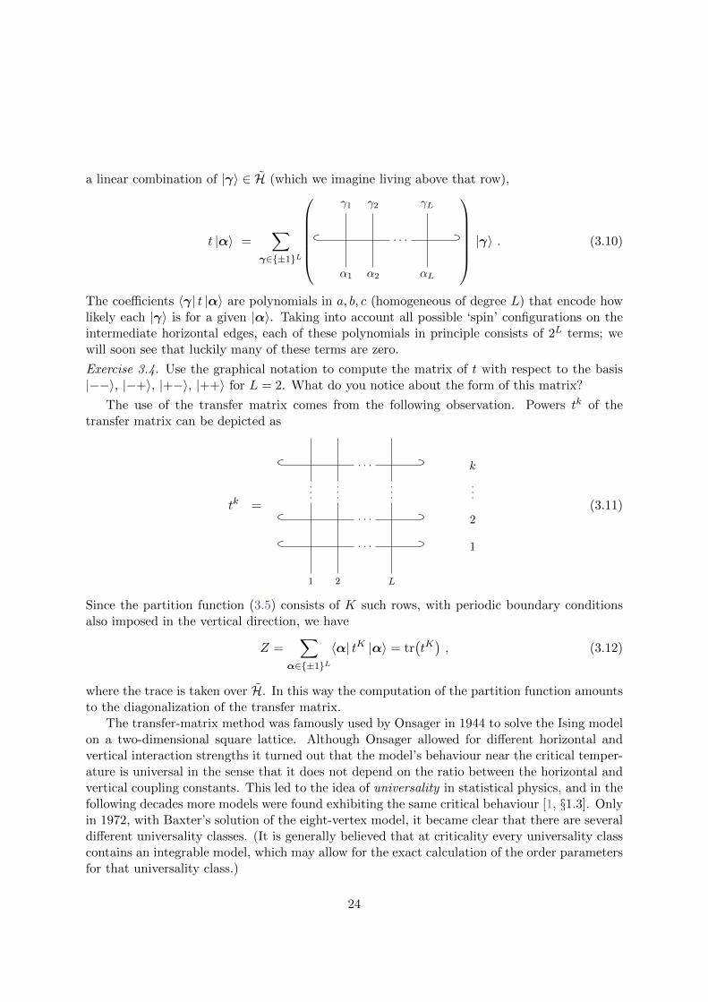
More concretely, t transfers |α〉 ∈ H (which we think of as a configuration below some row) to

23

a linear combination of |γ〉 ∈ H (which we imagine living above that row),

t |α〉 =∑

γ∈±1L

α1

γ1

α2

γ2

αL

γL

· · ·

|γ〉 . (3.10)

The coefficients 〈γ| t |α〉 are polynomials in a, b, c (homogeneous of degree L) that encode howlikely each |γ〉 is for a given |α〉. Taking into account all possible ‘spin’ configurations on theintermediate horizontal edges, each of these polynomials in principle consists of 2L terms; wewill soon see that luckily many of these terms are zero.

Exercise 3.4. Use the graphical notation to compute the matrix of t with respect to the basis|−−〉, |−+〉, |+−〉, |++〉 for L = 2. What do you notice about the form of this matrix?

The use of the transfer matrix comes from the following observation. Powers tk of thetransfer matrix can be depicted as

tk =

· · ·

···

· · ·

···

· · ·

···

···

1

2

k

1 2 L

(3.11)

Since the partition function (3.5) consists of K such rows, with periodic boundary conditionsalso imposed in the vertical direction, we have

Z =∑

α∈±1L〈α| tK |α〉 = tr

(tK), (3.12)

where the trace is taken over H. In this way the computation of the partition function amountsto the diagonalization of the transfer matrix.

The transfer-matrix method was famously used by Onsager in 1944 to solve the Ising modelon a two-dimensional square lattice. Although Onsager allowed for different horizontal andvertical interaction strengths it turned out that the model’s behaviour near the critical temper-ature is universal in the sense that it does not depend on the ratio between the horizontal andvertical coupling constants. This led to the idea of universality in statistical physics, and in thefollowing decades more models were found exhibiting the same critical behaviour [1, §1.3]. Onlyin 1972, with Baxter’s solution of the eight-vertex model, it became clear that there are severaldifferent universality classes. (It is generally believed that at criticality every universality classcontains an integrable model, which may allow for the exact calculation of the order parametersfor that universality class.)

24

Towards the cba. Being familiar with the work on the xxz spin chain, Lieb and Sutherlandrealized that the transfer matrix of the six-vertex model can be diagonalized using the cba. Tounderstand why this is so let us compare the settings of the two models. The first observationis that the two Hilbert spaces, H from (2.1) for the xxz spin chain and H from (3.8) for thesix-vertex model, clearly have the same form. Call the edges of ZL × ZK vacant when theyhave ‘spin’ −1 (dotted line) and occupied for ‘spin’ +1 (thick line). The two Hilbert spaces areisomorphic via the identification of spin down and up with vacant and occupied vertical edges,respectively:

H 3 |l〉 = |↑1· · · ↑↓

l1

↑ · · ·〉 ←→ |α〉 = |−1· · · −+

l1− · · ·〉 ∈ H . (3.13)

(Note the difference between the labellings on the two sides: l has just M components 1 ≤ l1 <· · · < lM ≤ L, while the corresponding α always has L components, M of which are a plus.)

Exercise 3.5. Compute the matrix elements 〈k|t|l〉 from (3.10) for |k〉, |l〉 ∈ H1, distinguishingthe cases k < l, k = l, k > l.

The second thing to observe is that the operators that we want to diagonalize, Hxxz

from (2.8) and t from (3.9), are different. A quick way to see this is by comparing the paramet-ers: the xxz Hamiltonian depends on two parameters (J,∆) while the transfer matrix dependson the values of the three vertex weights (a, b, c). Despite this difference it may of course bepossible to diagonalize the two operators using the same Bethe-ansatz technique.

Exercise 3.6. For another difference between Hxxz and t compare the ways in which excitationsand occupations in (3.13) are moved by (a single application of) these operators, and comparethe number of terms in Hxxz|l〉 and t|l〉.

Let us take a closer look at the properties of Hxxz and t. In Section 2.1 we exploited thefact that the xxz Hamiltonian is

i) nearest neighbour;ii) translationally invariant; andiii) partially isotropic.

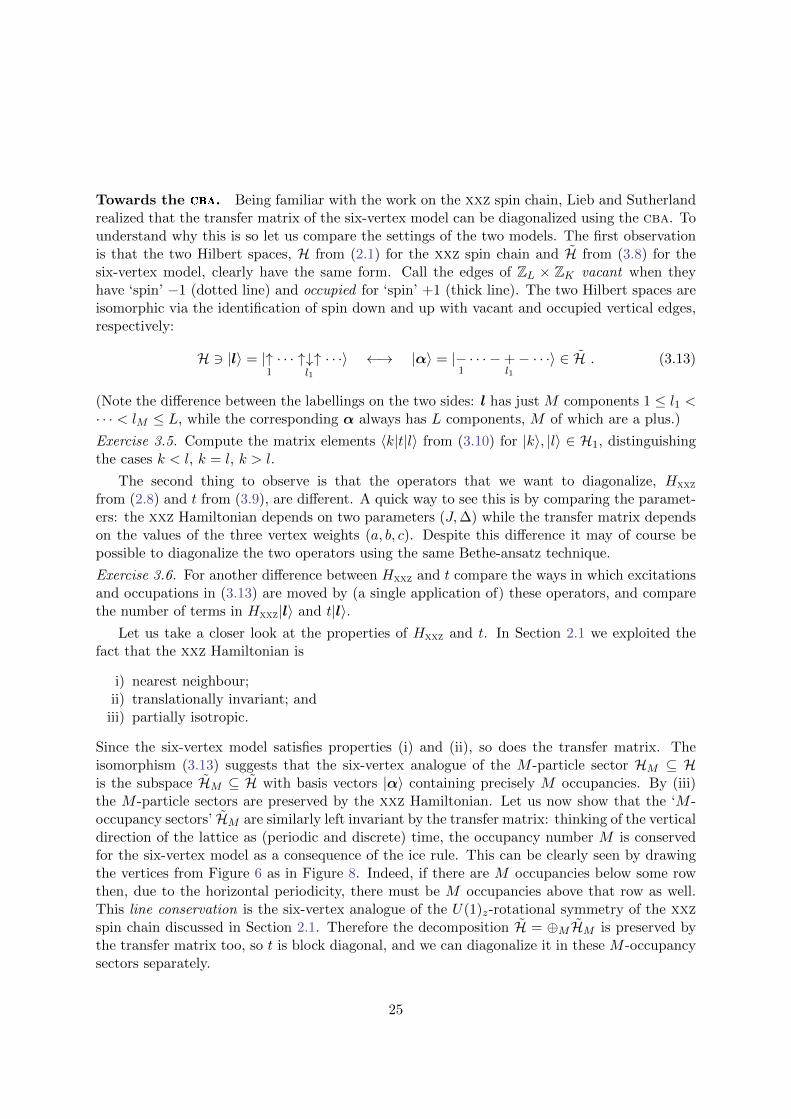
Since the six-vertex model satisfies properties (i) and (ii), so does the transfer matrix. Theisomorphism (3.13) suggests that the six-vertex analogue of the M -particle sector HM ⊆ His the subspace HM ⊆ H with basis vectors |α〉 containing precisely M occupancies. By (iii)the M -particle sectors are preserved by the xxz Hamiltonian. Let us now show that the ‘M -occupancy sectors’ HM are similarly left invariant by the transfer matrix: thinking of the verticaldirection of the lattice as (periodic and discrete) time, the occupancy number M is conservedfor the six-vertex model as a consequence of the ice rule. This can be clearly seen by drawingthe vertices from Figure 6 as in Figure 8. Indeed, if there are M occupancies below some rowthen, due to the horizontal periodicity, there must be M occupancies above that row as well.This line conservation is the six-vertex analogue of the U(1)z-rotational symmetry of the xxzspin chain discussed in Section 2.1. Therefore the decomposition H = ⊕MHM is preserved bythe transfer matrix too, so t is block diagonal, and we can diagonalize it in these M -occupancysectors separately.

25

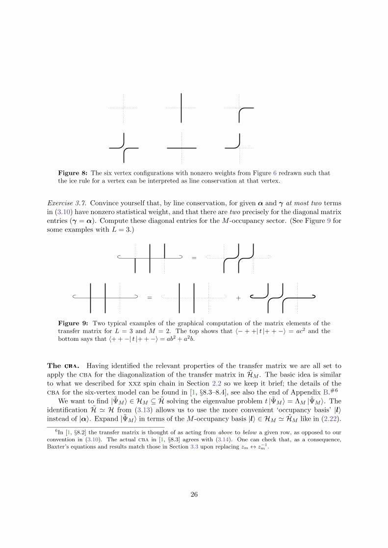
Figure 8: The six vertex configurations with nonzero weights from Figure 6 redrawn such thatthe ice rule for a vertex can be interpreted as line conservation at that vertex.

Exercise 3.7. Convince yourself that, by line conservation, for given α and γ at most two termsin (3.10) have nonzero statistical weight, and that there are two precisely for the diagonal matrixentries (γ = α). Compute these diagonal entries for the M -occupancy sector. (See Figure 9 forsome examples with L = 3.)

=

= +

Figure 9: Two typical examples of the graphical computation of the matrix elements of thetransfer matrix for L = 3 and M = 2. The top shows that 〈− + +| t |+ + −〉 = ac2 and thebottom says that 〈+ +−| t |+ +−〉 = ab2 + a2b.

The cba. Having identified the relevant properties of the transfer matrix we are all set toapply the cba for the diagonalization of the transfer matrix in HM . The basic idea is similarto what we described for xxz spin chain in Section 2.2 so we keep it brief; the details of thecba for the six-vertex model can be found in [1, §8.3–8.4], see also the end of Appendix B.#6

We want to find |ΨM 〉 ∈ HM ⊆ H solving the eigenvalue problem t |ΨM 〉 = ΛM |ΨM 〉. Theidentification H ' H from (3.13) allows us to use the more convenient ‘occupancy basis’ |l〉instead of |α〉. Expand |ΨM 〉 in terms of the M -occupancy basis |l〉 ∈ HM ' HM like in (2.22).

6In [1, §8.2] the transfer matrix is thought of as acting from above to below a given row, as opposed to ourconvention in (3.10). The actual cba in [1, §8.3] agrees with (3.14). One can check that, as a consequence,Baxter’s equations and results match those in Section 3.3 upon replacing zm ↔ z−1

m .

26

The cba for the coefficients involves parameters pm ∈ C or equivalently zm := eipm ∈ C,

Ψz(l) =∑π∈SM

Aπ(z)zπl , zπ

l :=

M∏m=1

(zπ(m))lm , l1 < · · · < lM . (3.14)

This produces eigenvectors for the transfer matrix provided we can solve the equations

〈l| t |ΨM ; z〉 = ΛM (z) Ψz(l) , 1 ≤ l1 < · · · < lM ≤ L , (3.15)

for the eigenvalues ΛM (z), the coefficients Aπ(z) and the values of the parameters z. Thestrategy is roughly as before:

1. Focus on the wanted terms, i.e. terms proportional to zπl as in the cba, to find ΛM (z).

2. Find Aπ(z) so as to cancel certain unwanted (‘internal’) terms.

3. Demand that remaining unwanted (‘boundary’) terms also cancel to get the bae determ-ining the allowed values of z.

However, in accordance with Exercise 3.6, the left-hand side of (3.15) contains many more termsthan its xxz-analogue (2.30). Correspondingly the precise formulation of the strategy is a bitmore involved than before too, see the end of Appendix B. Let us proceed to the outcome.

3.3 Unexpected results

In Section 3.2 we have already found some striking similarities between the xxz spin chainand the six-vertex model. Now we will see that the results of the cba uncover a much deeperrelation between the two models.

Results for general M . The results of the cba for the transfer matrix are as follows.Step 1. The eigenvalues of the transfer matrix are

ΛM (z) = aLM∏m=1

b (a− b z−1m ) + c2 z−1

m

a (a− b z−1m )

+ bLM∏m=1

a (a− b z−1m )− c2

b (a− b z−1m )

. (3.16)

Not being additive, the result is clearly different from (2.36), once more showing that Hxxz

and t really are different operators.Step 2. Again the coefficients Aπ in the cba factor into two-occupancy contributions.

Interestingly they are very similar to what we found for the xxz spin chain:

Aπ(z)

Ae(z)=

∏1≤m<m′≤M

s.t. π(m)>π(m′)

S(zm, zm′) , S(z, z′) := −1− 2 ∆(a, b, c) z′ + z z′

1− 2 ∆(a, b, c) z + z z′. (3.17)

The only difference with (2.37) and (2.32) is that the anisotropy parameter ∆ of the xxz modelis replaced by a particular combination of the six-vertex weights,

∆(a, b, c) :=a2 + b2 − c2

2 a b. (3.18)

This striking similarity will play a crucial role in what follows.

27

Step 3. There are M bae for the parameters z:

zLm = (−1)M−1M∏n=1n6=m

1− 2 ∆(a, b, c) zm + zmzn

1− 2 ∆(a, b, c) zn + zmzn, 1 ≤ m ≤M . (3.19)

Up to the dependence on (3.18) instead of ∆ these are identical to the xxz bae (2.38).

Exercise 3.8. Use the results of Exercises 3.5 and 3.7 to check (3.16) and (3.19) for M = 0, 1.For M = 1 recognize geometric series in z to sum many terms on the left-hand side of (3.15).

Commuting transfer matrices. The solution (3.17) for Aπ(z), and therefore |ΨM ; z〉, isremarkable. Firstly, the coefficients (3.17) and the bae (3.19) are precisely the same as thoseof the xxz spin chain when the function (3.18) has fixed value ∆(a, b, c) = ∆ equal to the xxzanisotropy parameter. Indeed, from (3.19) we see that the allowed values of the parameterspm = −i log zm match those of the pm. Secondly, the eigenvectors of the transfer matrix onlydepend on the six-vertex weights through the combination (3.18). Therefore varying the valuesof a, b, c while keeping (3.18) fixed does not change the (Bethe) eigenvectors of t(a, b, c).

Under the assumption that all 2L eigenvectors of t and Hxxz are of the Bethe form (see Ap-pendix A), these two facts mean that the cba simultaneously diagonalizes the xxz Hamiltonianand all transfer matrices with matching value of (3.18):

[ t(a, b, c), Hxxz(∆) ] = 0 if ∆(a, b, c) = ∆ , (3.20)

[ t(a, b, c), t(a′, b′, c′) ] = 0 if ∆(a, b, c) = ∆(a′, b′, c′) . (3.21)

As we will soon see these two observations hold the key to understanding the integrability ofthe six-vertex model — and that of the xxz spin chain.

To understand the consequences of (3.20)–(3.21) let us first look at the degrees of freedomcontained in the six-vertex model’s parameters (a, b, c).

Exercise 3.9. Check that simultaneous nonzero rescalings (a, b, c) 7−→ (r a, r b, r c) do not affectthe combination (3.18) and only modify the partition function (3.5) by an overall factor.

Motivated by this let us fix the ratio a : b : c and the value of the function (3.18). Thisleaves a single remaining degree of freedom, known as the spectral parameter, which we denoteby u. Observe that, through the vertex weights, the transfer matrix also depends on the spectralparameter, t(u) = t

(a(u), b(u), c(u)

). We can now recast (3.20)–(3.21) in the form

[ t(u), Hxxz ] = 0 for all u , (3.22)

[ t(u), t(v) ] = 0 for all u, v . (3.23)

Therefore there is a one-parameter family of six-vertex models, with a : b : c and ∆ fixed butvarying u, whose transfer matrices t(u) commute with Hxxz and each other.

Exercise 3.10. Check that the parametrization

a = ρ sinh(u+ iγ) , b = ρ sinhu , c = ρ sinh(iγ) = iρ sin γ (3.24)

28

does the job, with ∆(a, b, c) = cos γ. Determine the values of the crossing parameter γ corres-ponding to the regimes ∆ < −1, −1 ≤ ∆ ≤ 1 and ∆ > 1 of the xxz model. (Correspondingly,shifted or rescaled parameters are also commonly used in the literature.)

Z-invariant models. How should the commutator (3.23) be interpreted from the vertex-model viewpoint? In terms of our graphical notation it consists of two terms of the form

t(u) t(v) =· · ·

· · ·

u

v

1 2 L

(3.25)

with a separate spectral parameter associated to each row as indicated. This can be viewed asa portion of a vertex model with different values of the spectral parameter — hence differentvertex weights yielding the same value of (3.18) — for each row of horizontal edges in thelattice. By (3.23) the partition function Z (3.1) of such vertex models are invariant under theexchange of any two rows in the lattice; accordingly those models are called Z-invariant. Thusthe six-vertex model admits inhomogeneous generalizations that can still be tackled using thecba: the translational invariance in the vertical direction is broken in such a way that the modelremains exactly solvable.

Analyticity. Baxter realized that it is extremely useful to allow for complex vertex weightsand let u ∈ C. Indeed, (3.24) then gives an analytic parametrization of the six-vertex weightswhich is even entire (in fact, this is how that parametrization can be found, see [1, §9.7]). Thereal power of the transfer-matrix method lies in the fact that all functions u 7−→ 〈k|t(u)|l〉 areentire as well, because they are polynomial in a, b, c. This highly constrains the properties of thexxz and six-vertex model and ultimately renders these models exactly solvable. For example,the bae have a natural interpretation in this context:

Exercise 3.11. Since the transfer matrix is entire in u, so must be its eigenvalues Λz(z). However,the right-hand side of (3.16) seems to have a simple pole for each u such that a(u)/b(u) = z−1

m

for some 1 ≤ m ≤M . Use that Res(f, z∗) = g(z∗)/h′(z∗) when f(z) = g(z)/h(z) with h(z∗) = 0

but h′(z∗) 6= 0 to check that the residues at these poles satisfy

Res(ΛM , zm = b

a

)∝ aL

M∏n=1n 6=m

(1− b2 − c2

a bz−1n

)− bL

M∏n=1n6=m

(a2 − c2

a bz−1m − z−1

m z−1n

), (3.26)

and conclude that the poles of ΛM disappear by virtue of the bae (3.19) with zm = b/a.

In particular, if one would be able to obtain the eigenvalues (3.16) of t in a different way, onemight be able to derive bae also for models for which the Bethe-ansatz techniques describedin these lecture notes fail, such as the xyz spin chain and eight-vertex model. This is preciselywhat Baxter’s TQ-method manages to do by constructing another one-parameter family of

29

commuting operators Q(u) ∈ End(H) that satisfy certain ‘TQ-relations’ determining ΛM . Formore about the TQ-method we refer to [1, §9]; see [25, §4–5] and [2, 4.2] for an account in thealgebraic language of Section 4.

Quantum integrability. To get a better understanding of the importance of the relations(3.22)–(3.23) let us parametrize the vertex weights as in (3.24). Since the transfer matrix then isa Laurent polynomial in eu, it makes sense to take logarithmic derivatives and define operatorsHk via the trace identities

Hk :=dk

duk

∣∣∣∣u=u∗

log t(u) ∈ End(H) ' End(H) (3.27)

for some value u∗ of the spectral parameter. (In Section 4.1 we will see that u∗ = 0 is aconvenient choice for our parametrization.)

The equations (3.22)–(3.23) then imply

[Hk, Hxxz] = 0 for all k , (3.28)

[Hj , Hk] = 0 for all j, k . (3.29)

Now we can see the fruits of our labour more clearly. According to (3.28) the operators Hk areconserved quantities: we have found symmetries of the xxz spin chain! Moreover, by (3.29)these symmetry operators commute with each other (they are in involution). The presence ofsuch a tower of commuting conserved charges is a very special property; it ‘proves’ that themodel is quantum integrable in analogy with the notion of Liouville integrability and explainswhy magnon-scattering is two-body reducible, see Section 5.1. Thus, from the spin-chain view-point, there is a one-parameter family of six-vertex models whose transfer matrices producesymmetries Hk of the xxz model through the trace identities. (In more mathematical termsthe t(u) generate an abelian subalgebra in End(H) that commutes with Hxxz.) What about thesix-vertex model itself?

Consider a six-vertex model with vertex weights (a0, b0, c0) and transfer matrix t0 :=t(a0, b0, c0). Setting ∆0 := ∆(a0, b0, c0), by the above argument there exists a one-parameterfamily of six-vertex models with commuting transfer matrices, like in (3.29), such that t(u0) = t0for some u0. From the original six-vertex model’s perspective each of these transfer matricesgenerates a discrete Euclidean ‘time’ evolution with respect to which the Hk are ‘conserved’.In particular it follows that

[Hk, t0] = 0 for all k , (3.30)

so t0 enjoys the same symmetries (3.27) as Hxxz(∆0)!

Exercise 3.12. Go back to Section 2.1 to find a few operators that one may expect (or hope) tofind amongst the Hk ∈ End(H).

30

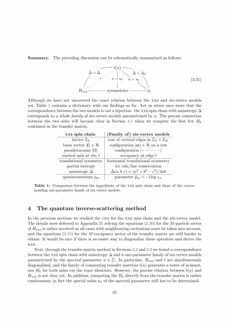
Summary. The preceding discussion can be schematically summarized as follows:

t(u)

Hxxz symmetries t0

? u = u∗ u = u0

∆ = ∆ ∆ = ∆0

(3.31)

Although we have not uncovered the exact relation between the xxz and six-vertex modelsyet, Table 1 contains a dictionary with our findings so far. Let us stress once more that thecorrespondence between the two models is not a bijection: the xxz spin chain with anisotropy ∆corresponds to a whole family of six-vertex models parametrized by u. The precise connectionbetween the two sides will become clear in Section 4.1 when we compute the first few Hk

contained in the transfer matrix.

xxz spin chain (Family of) six-vertex models

lattice ZL row of vertical edges in ZL × ZKbasis vector |l〉 ∈ H configuration |α〉 ∈ H on a rowpseudovacuum |Ω〉 configuration |− − · · · −〉

excited spin at site l occupancy at edge l

translational symmetry horizontal translational symmetrypartial isotropy ice rule/line conservation

anisotropy ∆ ∆(a, b, c) = (a2 + b2 − c2)/2ab

quasimomentum pm parameter pm = −i log zm

Table 1: Comparison between the ingredients of the xxz spin chain and those of the corres-ponding one-parameter family of six-vertex models.

4 The quantum inverse-scattering method

In the previous sections we studied the cba for the xxz spin chain and the six-vertex model.The details were deferred to Appendix B: solving the equations (2.30) for the M -particle sectorof Hxxz is rather involved as all cases with neighbouring excitations must be taken into account,and the equations (3.15) for the M -occupancy sector of the transfer matrix are still harder toobtain. It would be nice if there is an easier way to diagonalize these operators and derive thebae.

Next, through the transfer-matrix method in Sections 3.2 and 3.3 we found a correspondencebetween the xxz spin chain with anisotropy ∆ and a one-parameter family of six-vertex modelsparametrized by the spectral parameter u ∈ C. In particular, Hxxz and t are simultaneouslydiagonalized, and the family of commuting transfer matrices t(u) generates a tower of symmet-ries Hk for both sides via the trace identities. However, the precise relation between t(u) andHxxz is not clear yet. In addition, computing the Hk directly from the transfer matrix is rathercumbersome; in fact the special value u∗ of the spectral parameter still has to be determined.

31

In this section the quantum inverse-scattering method (qism) is introduced. This algebraicformalism can be used to rederive the results from Sections 2.3 and 3.3 while addressing theabove issues, and more:

• it provides a convenient way to find an appropriate value u∗ and compute the Hk usingthe trace identities;• it has the all-important commutativity of the t(u) built in;• the Fock space of (Bethe) states is constructed via creation and annihilation operators,

and the eigenvalues and bae are derived with a single computation for general M ;• it allows one to define several new quantum-integrable models.

Since the xxz and six-vertex models are treated simultaneously in the qism we no longer needto distinguish between H ' H, et cetera, and can safely drop the tildes used in Sections 3.2and 3.3 from now on. We keep ~ = J = 1.

4.1 Conserved quantities from Lax operators

We keep using the graphical notation introduced in Section 3.1, with one additional rule:

v) To keep track of the ordering of the various operators in products we add little arrows tothe end of lines. (Thus these arrows are not related to the ‘spins’.)

We will see an example of this rule soon, e.g. in (4.8).

Lax operators. From the six-vertex point of view the choice to associate a vector space tothe rows of ZL × ZK , but not its columns, is somewhat unnatural. To treat the horizontal andvertical edges on a more equal footing we introduce the vector space

Va := C |−〉a ⊕ C |+〉a = C ⊕ C . (4.1)

spanned by the two possible ‘spins’ on a horizontal edge in the lattice. (The subscript in Va isnot related to the vertex weight a(u).) Motivated by the spin-chain viewpoint, the ‘vertical’ Vland H from (3.7)–(3.8) are then often called physical or quantum spaces, while Va is an auxiliaryspace. It is quite convenient to think of the spectral parameter u of the transfer matrix as beingassociated to Va.

The auxiliary space allows us to introduce ‘local’ (vertex) operators acting at a single vertexof the lattice: the Lax operator,#7 defined as

Lal(u) := a a

l

l

∈ End(Va ⊗ Vl) . (4.2)

7This operator is sometimes called the ‘R-matrix’, but we follow Faddeev [3] and reserve the latter terminologyfor a closely related operator acting on Va ⊗ Vb, see Section 4.2.

32

The subscripts in Lal(u) remind us on which vector spaces this operator acts nontrivially, inaccordance with the tensor-leg notation from the start of Section 2.1. The labels on the topand right of (4.2) will be omitted in the graphical notation from now on.

Explicitly, writing |β, α〉 := |β〉 ⊗ |α〉 for the (pure) vectors in Va ⊗ Vl, (4.2) means that

Lal(u) |β, α〉 =∑

γ,δ∈±1

β δ

α

γ |γ, δ〉 =

∑γ,δ∈±1

w(u∣∣ γβ δα

)|δ, γ〉 , (4.3)

where we also indicated the dependence of the vertex weights on u ∈ C on the right-hand side.We point out that one has to be a bit careful when reading off the coefficients for the

‘outgoing’ vector |γ, δ〉 ∈ Va ⊗ Vl in our graphical notation: unlike for the ‘incoming’ vector|β, α〉, the order of the labels δ and γ is reversed in the coefficients in the middle and on theright-hand side of (4.3), cf. the labels in (4.2). This reversal will come back in (4.17) below.

Exercise 4.1. Use Figure 6 to check that the matrix of the Lax operator with respect to the(standard) basis

|−−〉 = ⊗ , |−+〉 = ⊗ , |+−〉 = ⊗ , |++〉 = ⊗ (4.4)

of Va ⊗ Vl is given by

Lal(u) =

a(u)

b(u) c(u)c(u) b(u)

a(u)

al

. (4.5)

Exercise 4.2. Argue that the ice rule for the vertex weights is equivalent to the invariance ofthe Lax operator under simultaneous U(1)z-rotations in Va and Vl:

[Sza + Szl , Lal(u) ] = 0 . (4.6)

Exercise 4.3. Check that (4.5) can be written in a basis-independent way as

Lal(u) =a(u) + b(u)

21al + c(u)σ+

a S−l + c(u)σ−a S

+l +

(a(u)− b(u)

)σzaS

zl , (4.7)

and use this to verify (4.6) directly via the su(2)-relations (2.4).

Trace identities. Lax operators can be used as building blocks of other, more involved op-erators. In particular, the transfer matrix (3.9) can be constructed as

t(u) = tra(LaL(u) · · · La2(u)La1(u)

)=

1 2 L

· · · ∈ End(H) . (4.8)

33

This way of writing the transfer matrix is very useful for the computation of conservedcharges Hk of the xxz and six-vertex models using the trace identities.

As we will soon see, it is actually convenient to alter (3.27) slightly by setting

Hk := idk

duk

∣∣∣∣u=u∗

logt(u)

a(u)L∈ End(H) . (4.9)

From Section 3.3 we know that the trace identities yield symmetries for any choice of the value u∗of the spectral parameter; let us see whether there are any particularly convenient choices. Weparametrize vertex weights by (3.24) with ρ = 1,

a(u) = sinh(u+ iγ) , b(u) = sinh(u) , c = sinh(iγ) = i sin γ . (4.10)

Observe that b(u) vanishes at u∗ = 0, while a(u∗) = c. At this point the Lax operator takes aparticularly simple form:

Lal(u∗) = c Pal , (4.11)

where the permutation operator (braiding) is defined as

Pal = a

l

l

a :=1

21al +σ+

a S−l + σ−a S

+l + σzaS

zl ∈ End(Va ⊗ Vl) . (4.12)

Exercise 4.4. To justify this graphical notation, check that the permutation operator switchesvectors: Pal|β, α〉 = |α, β〉 for (basis) vectors |β, α〉 = |β〉⊗|α〉 ∈ Va⊗Vl. Show that tra Pal = 1l

both algebraically and using the graphical notation.

Conserved charges. Now we are all set to compute the first few symmetries using (4.9).H0 = log t(u∗) is easy to find. By (4.8) and (4.11) we have t(u∗) = cL tra(PaL · · ·Pa2 Pa1).Focus on the product of permutation operators. It is quite standard to rearrange such productsby repeated application of the rule Pak Pal = Pal Pkl, see e.g. Faddeev [3]. For a slightly moreslick way to do this we exploit the relations in the permutation group by introducing for eachpermutation π ∈ SL+1 an operator Pπ ∈ End(Va⊗H) switching vectors in Va⊗H = Va⊗

⊗l Vl in

the way specified by π. For example, from the transposition (al) ∈ SL+1 we recover P(al) = Pal.(The above rule now is clear from Pak Pal = P(alk) = Pal Pkl.) We calculate

t(u∗) = cL tra(P(a12···L)

)= cL tra

(Pa1 P(12···L)

)= cL tra(Pa1) P(12···L) = cL U−1 , (4.13)

where we have used tra Pal = 1l and recognized the cyclic permutation operator P(12···L) as the

inverse of the shift operator U = eiP ∈ End(H). Thus

H0 = i logt(u∗)

a(u∗)L= P (4.14)

is the momentum operator of the xxz spin chain!

34

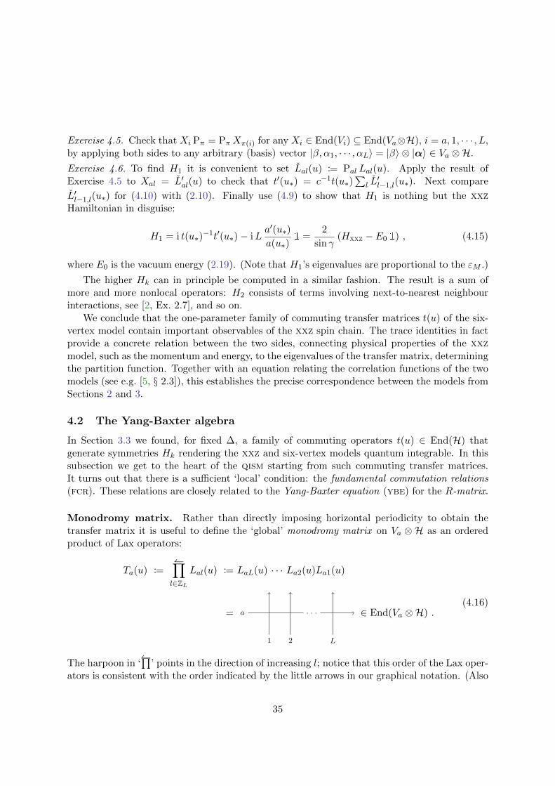
Exercise 4.5. Check that Xi Pπ = PπXπ(i) for any Xi ∈ End(Vi) ⊆ End(Va⊗H), i = a, 1, · · · , L,by applying both sides to any arbitrary (basis) vector |β, α1, · · · , αL〉 = |β〉 ⊗ |α〉 ∈ Va ⊗H.

Exercise 4.6. To find H1 it is convenient to set Lal(u) := Pal Lal(u). Apply the result ofExercise 4.5 to Xal = L′al(u) to check that t′(u∗) = c−1t(u∗)

∑l L′l−1,l(u∗). Next compare

L′l−1,l(u∗) for (4.10) with (2.10). Finally use (4.9) to show that H1 is nothing but the xxzHamiltonian in disguise:

H1 = i t(u∗)−1t′(u∗)− iL

a′(u∗)

a(u∗)1 =

2

sin γ(Hxxz − E0 1) , (4.15)

where E0 is the vacuum energy (2.19). (Note that H1’s eigenvalues are proportional to the εM .)

The higher Hk can in principle be computed in a similar fashion. The result is a sum ofmore and more nonlocal operators: H2 consists of terms involving next-to-nearest neighbourinteractions, see [2, Ex. 2.7], and so on.

We conclude that the one-parameter family of commuting transfer matrices t(u) of the six-vertex model contain important observables of the xxz spin chain. The trace identities in factprovide a concrete relation between the two sides, connecting physical properties of the xxzmodel, such as the momentum and energy, to the eigenvalues of the transfer matrix, determiningthe partition function. Together with an equation relating the correlation functions of the twomodels (see e.g. [5, § 2.3]), this establishes the precise correspondence between the models fromSections 2 and 3.

4.2 The Yang-Baxter algebra

In Section 3.3 we found, for fixed ∆, a family of commuting operators t(u) ∈ End(H) thatgenerate symmetries Hk rendering the xxz and six-vertex models quantum integrable. In thissubsection we get to the heart of the qism starting from such commuting transfer matrices.It turns out that there is a sufficient ‘local’ condition: the fundamental commutation relations(fcr). These relations are closely related to the Yang-Baxter equation (ybe) for the R-matrix.

Monodromy matrix. Rather than directly imposing horizontal periodicity to obtain thetransfer matrix it is useful to define the ‘global’ monodromy matrix on Va ⊗ H as an orderedproduct of Lax operators:

Ta(u) :=∏l∈ZL

Lal(u) := LaL(u) · · · La2(u)La1(u)

= a

1 2 L

· · · ∈ End(Va ⊗H) .(4.16)

The harpoon in ‘∏

’ points in the direction of increasing l; notice that this order of the Lax oper-ators is consistent with the order indicated by the little arrows in our graphical notation. (Also

35

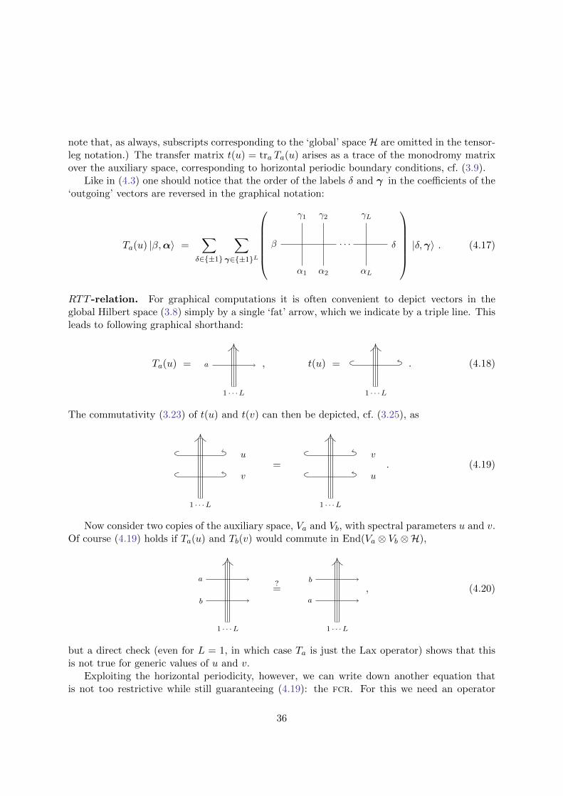
note that, as always, subscripts corresponding to the ‘global’ space H are omitted in the tensor-leg notation.) The transfer matrix t(u) = tra Ta(u) arises as a trace of the monodromy matrixover the auxiliary space, corresponding to horizontal periodic boundary conditions, cf. (3.9).

Like in (4.3) one should notice that the order of the labels δ and γ in the coefficients of the‘outgoing’ vectors are reversed in the graphical notation:

Ta(u) |β,α〉 =∑

δ∈±1

∑γ∈±1L

β δ

α1

γ1

α2

γ2

αL

γL

· · ·

|δ,γ〉 . (4.17)

RTT -relation. For graphical computations it is often convenient to depict vectors in theglobal Hilbert space (3.8) simply by a single ‘fat’ arrow, which we indicate by a triple line. Thisleads to following graphical shorthand:

Ta(u) =

1 · · ·L

a , t(u) =

1 · · ·L

. (4.18)

The commutativity (3.23) of t(u) and t(v) can then be depicted, cf. (3.25), as

1 · · ·L

v

u=

1 · · ·L

u

v. (4.19)

Now consider two copies of the auxiliary space, Va and Vb, with spectral parameters u and v.Of course (4.19) holds if Ta(u) and Tb(v) would commute in End(Va ⊗ Vb ⊗H),

1 · · ·L

a

b

?=

1 · · ·L

b

a

, (4.20)

but a direct check (even for L = 1, in which case Ta is just the Lax operator) shows that thisis not true for generic values of u and v.

Exploiting the horizontal periodicity, however, we can write down another equation thatis not too restrictive while still guaranteeing (4.19): the fcr. For this we need an operator

36

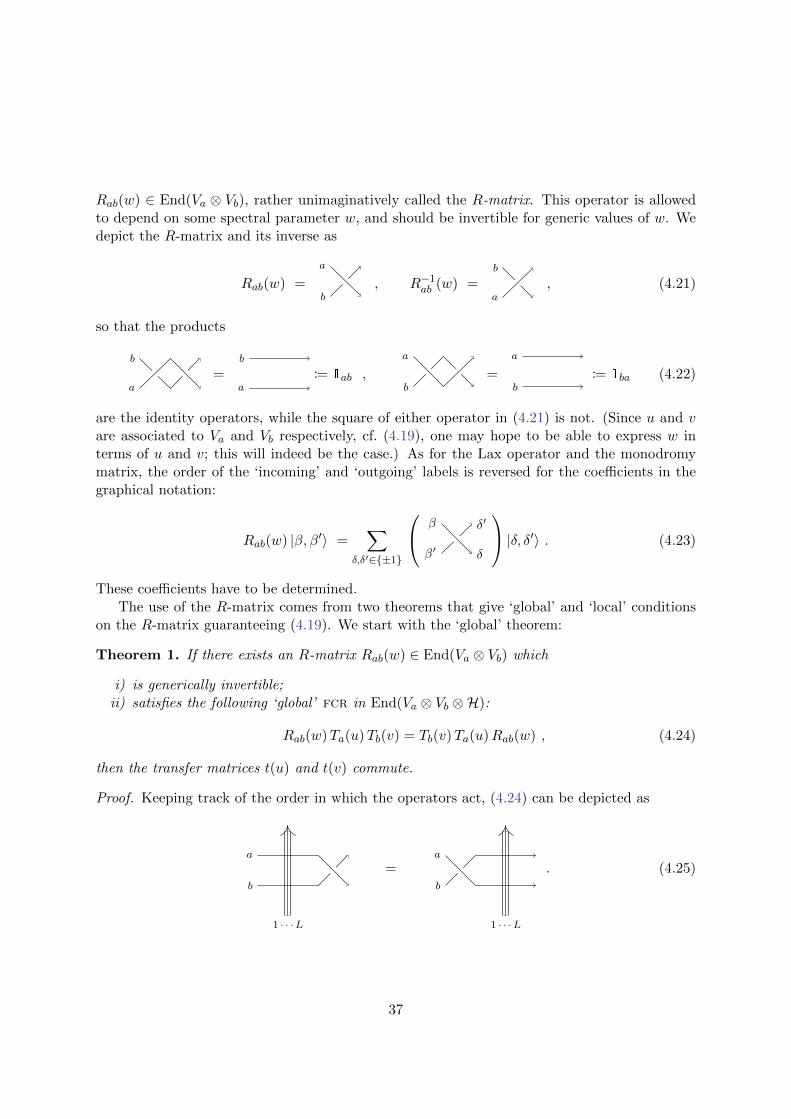
Rab(w) ∈ End(Va ⊗ Vb), rather unimaginatively called the R-matrix. This operator is allowedto depend on some spectral parameter w, and should be invertible for generic values of w. Wedepict the R-matrix and its inverse as

Rab(w) =b

a

, R−1ab (w) =

b

a, (4.21)

so that the products

b

a=

a

b

:= 1ab ,b

a

=

a

b:= 1ba (4.22)

are the identity operators, while the square of either operator in (4.21) is not. (Since u and vare associated to Va and Vb respectively, cf. (4.19), one may hope to be able to express w interms of u and v; this will indeed be the case.) As for the Lax operator and the monodromymatrix, the order of the ‘incoming’ and ‘outgoing’ labels is reversed for the coefficients in thegraphical notation:

Rab(w) |β, β′〉 =∑

δ,δ′∈±1

β′

δ′β

δ

|δ, δ′〉 . (4.23)

These coefficients have to be determined.The use of the R-matrix comes from two theorems that give ‘global’ and ‘local’ conditions

on the R-matrix guaranteeing (4.19). We start with the ‘global’ theorem:

Theorem 1. If there exists an R-matrix Rab(w) ∈ End(Va ⊗ Vb) which

i) is generically invertible;ii) satisfies the following ‘global’ fcr in End(Va ⊗ Vb ⊗H):

Rab(w)Ta(u)Tb(v) = Tb(v)Ta(u)Rab(w) , (4.24)

then the transfer matrices t(u) and t(v) commute.

Proof. Keeping track of the order in which the operators act, (4.24) can be depicted as

1 · · ·L

a

b

=

1 · · ·L

b

a

. (4.25)

37

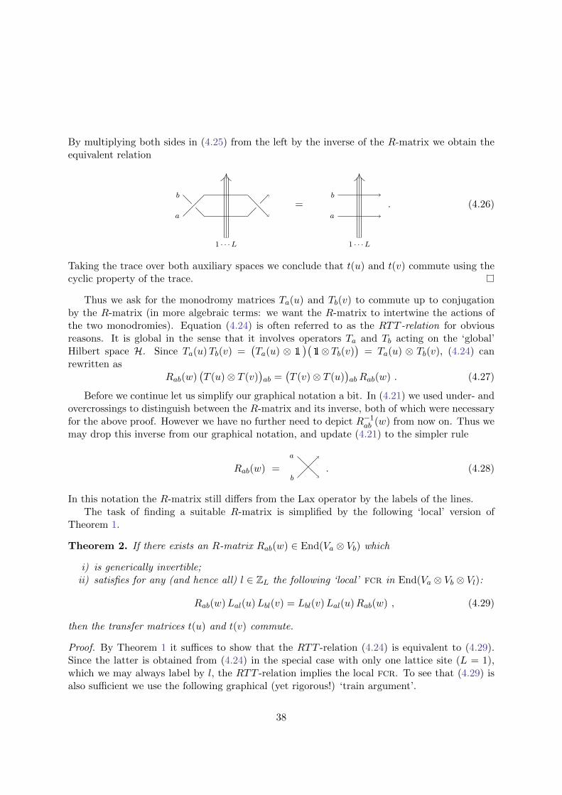
By multiplying both sides in (4.25) from the left by the inverse of the R-matrix we obtain theequivalent relation

1 · · ·L

b

a

=

1 · · ·L

b

a

. (4.26)

Taking the trace over both auxiliary spaces we conclude that t(u) and t(v) commute using thecyclic property of the trace.

Thus we ask for the monodromy matrices Ta(u) and Tb(v) to commute up to conjugationby the R-matrix (in more algebraic terms: we want the R-matrix to intertwine the actions ofthe two monodromies). Equation (4.24) is often referred to as the RTT -relation for obviousreasons. It is global in the sense that it involves operators Ta and Tb acting on the ‘global’Hilbert space H. Since Ta(u)Tb(v) =

(Ta(u) ⊗ 1

)(1⊗Tb(v)

)= Ta(u) ⊗ Tb(v), (4.24) can

rewritten asRab(w)

(T (u)⊗ T (v)

)ab =

(T (v)⊗ T (u)

)abRab(w) . (4.27)

Before we continue let us simplify our graphical notation a bit. In (4.21) we used under- andovercrossings to distinguish between the R-matrix and its inverse, both of which were necessaryfor the above proof. However we have no further need to depict R−1

ab (w) from now on. Thus wemay drop this inverse from our graphical notation, and update (4.21) to the simpler rule

Rab(w) =

a

b. (4.28)

In this notation the R-matrix still differs from the Lax operator by the labels of the lines.The task of finding a suitable R-matrix is simplified by the following ‘local’ version of

Theorem 1.

Theorem 2. If there exists an R-matrix Rab(w) ∈ End(Va ⊗ Vb) which

i) is generically invertible;ii) satisfies for any (and hence all) l ∈ ZL the following ‘local’ fcr in End(Va ⊗ Vb ⊗ Vl):

Rab(w)Lal(u)Lbl(v) = Lbl(v)Lal(u)Rab(w) , (4.29)

then the transfer matrices t(u) and t(v) commute.

Proof. By Theorem 1 it suffices to show that the RTT -relation (4.24) is equivalent to (4.29).Since the latter is obtained from (4.24) in the special case with only one lattice site (L = 1),which we may always label by l, the RTT -relation implies the local fcr. To see that (4.29) isalso sufficient we use the following graphical (yet rigorous!) ‘train argument’.

38

Suppose that (4.29) holds, so that Lax operators acting in the same local physical space,but different auxiliary spaces, commute up to conjugation by the R-matrix. Diagrammatically(4.29) says that the vertical line, corresponding to Lax operators acting on two vertices aboveeach other, can be moved through the crossing representing the R-matrix:

b

a

l

=b

a

l

. (4.30)

From the definition (4.16) of the monodromy matrix, L applications of (4.30) do the job:

b

a

· · ·

· · ·

1 2 L

=b

a

· · ·

· · ·

1 2 L

= · · ·

=b

a

· · ·

· · ·

1 2 L

.

In statistical mechanics (4.29) is often referred to as the star-triangle relation.#8 If a modeladmits an R-matrix that satisfies conditions (i)–(ii) one can construct symmetries Hk from thetransfer matrix as described in Section 4.1. Such models are moreover solvable via techniques likethe algebraic Bethe ansatz, see Section 4.3. For this reason such an R-matrix is the integrabilitydatum allowing one to study quantum-integrable models from an algebraic point of view. Indeed,in practice one often uses this structure to define ‘quantum integrability’.

R-matrix. The upshot of the preceding discussion is that if we can find an R-matrix sat-isfying the fcr (4.29) for a given Lax operator then the transfer matrices constructed fromthat Lax operator commute. In Appendix C the fcr of the xxz/six-vertex model, with Laxoperator (4.2), is solved for a nontrivial R-matrix that respects the symmetries of the model:it satisfies both line conservation (the ice rule) and spin-reversal symmetry. The result is of the

8We reserve the name ‘Yang-Baxter equation’ for the rather similar and intimately related (but algebraicallystill more fundamental) equation that we will encounter soon.

39

same form as the Lax operator (4.5):

Rab(w) =

a(w)

b(w) c(w)c(w) b(w)

a(w)

ab

, (4.31)

where the functions a, b and c were defined in (4.10). Accordingly, the entries of the R-matrixmay be interpreted as the vertex weights of another six-vertex model with the same valueof ∆ = cos γ but with different spectral parameter w.

Clearly (4.31) is indeed invertible for almost all values of the spectral parameter. In Ap-pendix C we further show that this R-matrix solves the fcr provided the spectral parametersare related by the difference property w = u− v. (Of course one can also directly check that inthis case (4.31) does indeed satisfy the fcr, see e.g. [3, §10].) Due to the difference propertythe fcr is often written as

Rab(u− v)Lal(u)Lbl(v) = Lbl(v)Lal(u)Rab(u− v) , (4.32)

and likewise for the RTT -relation. This result nicely fits in the graphical notation if westraighten out the lines in (4.30):

a

l

b

u

u− v

v

=

a

l

bu

u− vv

(4.33)

Here the spectral parameters of the operators are included as angles, and the fcr says that anysingle line may be shifted past the intersection point of the other two lines if it is kept parallelto the original line. (Note that such shifts are in fact used in Section 5.1 to derive the ybe forfactorized scattering.)

Yang-Baxter algebra. The following algebraic construction lies at the core of the qism andprovides the mathematical setting for the computations in the framework of the algebraic Betheansatz, as we will see in Section 4.3. Since the monodromy matrix Ta(u) ∈ End(Va ⊗ H) alsoacts in auxiliary space we can write it as a matrix on Va,

Ta(u) =

(A(u) B(u)C(u) D(u)

)a

, (4.34)

whose entries act on the physical space H of the spin chain.

40

Exercise 4.7. Check that in our graphical notation

A(u) =

1 · · ·L

, B(u) =

1 · · ·L

,

C(u) =

1 · · ·L

, D(u) =

1 · · ·L

.

(4.35)

These (one-parameter families of) operators in End(H) generate a (unital, associative) al-gebra, known as the Yang-Baxter algebra (yba), whose commutation rules are given by theRTT -relation (4.24) with w = u−v. The latter encodes 22×22 = 16 relations in End(Va⊗Vb) forthe generators (4.35). The explicit form of these relations can be found from (4.27) by straight-forward matrix multiplication, see [3, §4]. Instead one can also use the graphical form (4.25) ofthe RTT -relation to find these relations. For example, the (1, 4)-entry of (4.27) corresponds to

1 · · ·L

=

1 · · ·L

, (4.36)

implying thatB(u)B(v) = B(v)B(u) . (4.37)

Likewise, paying attention to the different ordering of ‘incoming’ and ‘outgoing’ auxiliary vec-tors, the (1, 3)- and (3, 4)-entries of (4.27) correspond to

1 · · ·L

=

1 · · ·L

=

1 · · ·L

+

1 · · ·L

, (4.38)

1 · · ·L

+

1 · · ·L

=

1 · · ·L

=

1 · · ·L

. (4.39)

41

Upon interchanging u↔ v in (4.38) these yield more complicated commutation rules:

A(u)B(v) =a(v − u)

b(v − u)B(v)A(u)− c(v − u)

b(v − u)B(u)A(v) , (4.40)

D(u)B(v) =a(u− v)

b(u− v)B(v)D(u)− c(u− v)

b(u− v)B(u)D(v) . (4.41)

In both of these relations the first term on the right-hand side just contains the commutedoperators (up to a factor), whereas in the second term the two operators have in additioninterchanged their spectral parameters.

The physical use of the yba stems from the quantum inverse-scattering problem, whichasks whether it is possible to reconstruct arbitrary operators in End(Vl), and thus those inEnd(H), from Ta(u). The solution to this problem was found for many models, including thexxz/six-vertex model, in [26]. The conclusion is that A(u), · · · , D(u) generate all of End(H).For example, the transfer matrix is an element of the Yang-Baxter algebra:

t(u) =

1 · · ·L

=

1 · · ·L

+

1 · · ·L

= A(u) +D(u) . (4.42)

Exercise 4.8. Find relations like (4.36) for A and for D. Next use (4.25) to compute [A(u), D(v)].Check in this way that t(u) and t(v) do indeed commute.

Yang-Baxter equation. The entries of the R-matrix play the role of structure constants forthe Yang-Baxter algebra. In the present context there also is an analogue of the Jacobi identityfor these ‘structure constants’. Indeed, consider one more copy of the auxiliary space, Vc, withassociated spectral parameter w. The RTT -relation can be used to reverse the order in theproduct Ta(u)Tb(v)Tc(w) to get Tc(w)Tb(v)Ta(u) up to conjugation by products of R-matrices.Now there are two ways in which this can be done, corresponding to the two decompositions(13) = (12)(23)(12) = (23)(12)(23) of the permutation switching the first and third monodromymatrix. To avoid 23× 23 = 64 additional relations for the Yang-Baxter algebra, the two resultsmust coincide. This is true when the R-matrix satisfies the famous Yang-Baxter equation (ybe)in End(Va ⊗ Vb ⊗ Vc):

Rab(u− v)Rac(u− w)Rbc(v − w) = Rbc(v − w)Rac(u− w)Rab(u− v) . (4.43)

Like the Jacobi equation, this relation is cubic in the ‘structure constants’. One can check thatthe solution (4.31) of the six-vertex fcr does indeed satisfy the ybe. In our graphical notation(4.43) becomes

c

b

a

=

c

b

a

. (4.44)

42

Readers familiar with the braid group may recognize this as an analogue of the braid relationbut involving spectral parameters. Of course the lines may again be straightened out like wedid in (4.33).

Summary. To conclude this subsection we present a brief overview of the formalism that wehave set up. The operators of the qism, the equations that they satisfy, and relation betweenthese operators is shown in Table 2. Any physical operator, in End(H), can be expressed as anelement of the yba, i.e. in terms of the generators A(u), · · · , D(u). In particular the yba canbe used to construct the Bethe vectors, which is our next topic.

auxiliary Vb local Vl global Hauxiliary Va Rab(u) : ybe Lal(u) : fcr Ta(u) : RTT

physical resultA(u), · · · , D(u) : ybat(u) : commute

Table 2: Summary of the qism in the spin-chain language, where Va plays an auxiliary role.

4.3 The algebraic Bethe ansatz

Our final task is to reproduce the results of the cba from Sections 2.3 and 3.3 in the contextof the qism. The goal is to diagonalize the transfer matrix (4.42); the spectrum of the xxzHamiltonian (4.15) then follows from the trace identity (4.15). We proceed along the linesof Faddeev [3]. Although there are still some nontrivial calculations involved in the algebraicBethe ansatz (aba), it is much easier to get the eigenvalues ΛM and the bae for any M -particlesector than it is with the cba.

Second quantization. The cba from Section 2.2 features the Bethe wave function (2.29):this is the first-quantized approach to the quantum-mechanical spin chains. In contrast, theaba corresponds to second quantization through the explicit construction of a Fock space ofstates for the model. As a first attempt to construct such a Fock space let us briefly go back tothe cba. We already have a good candidate for the Fock vacuum: the pseudovacuum |Ω〉 ∈ H0

from (2.13). For M = 1, (2.20) suggests that∑

l eipml S−l may serve as a creation operator for

a magnon with quasimomentum pm. Unfortunately already for M = 2 we see that this cannotbe true. Indeed, applying that operator twice on |Ω〉 gives A(p1, p2) = A′(p1, p2) in (2.26), onlyallowing for trivial two-body scattering. To proceed we have to exploit the Yang-Baxter algebrafrom the previous subsection.

Again we start from the pseudovacuum, which is depicted in our shorthand as

|Ω〉 = . (4.45)

43

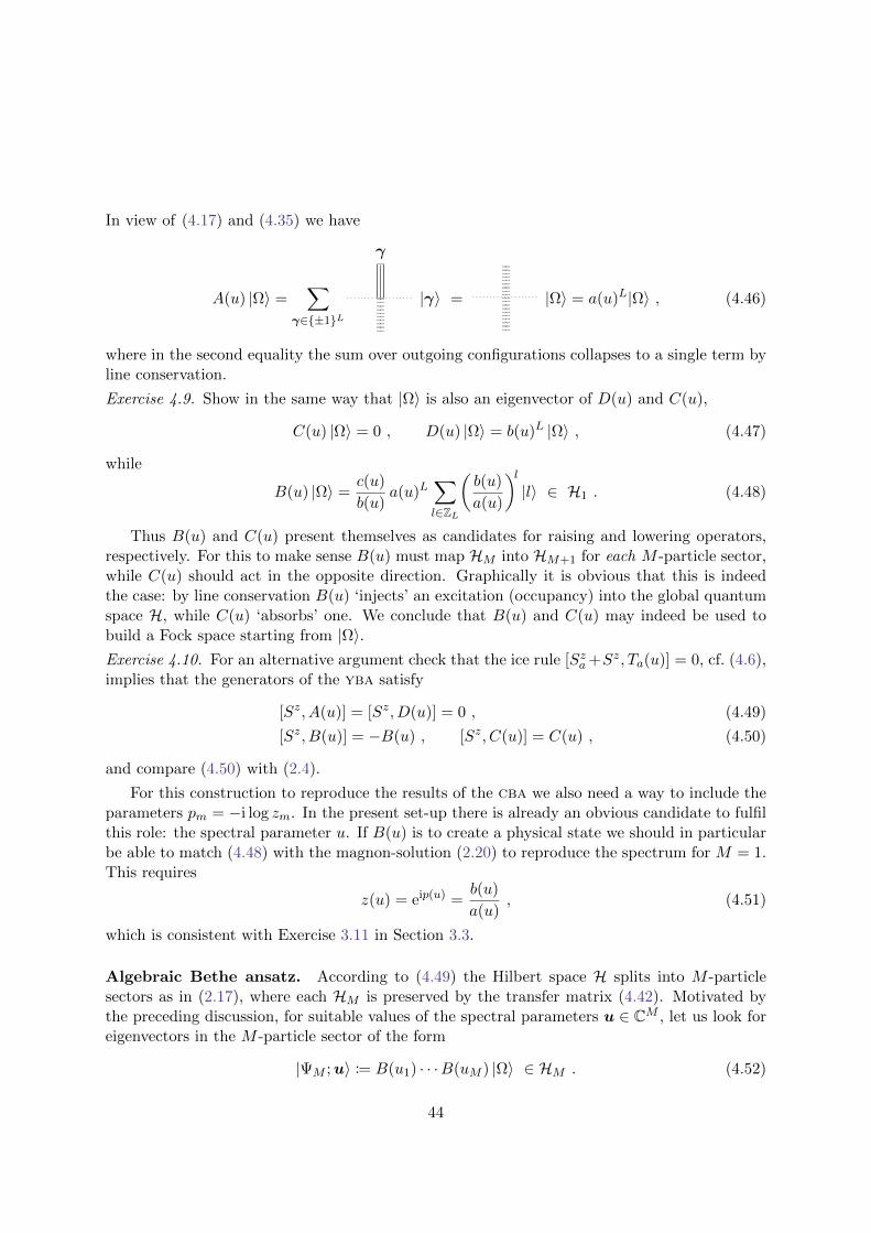
In view of (4.17) and (4.35) we have

A(u) |Ω〉 =∑

γ∈±1L

γ

|γ〉 = |Ω〉 = a(u)L|Ω〉 , (4.46)

where in the second equality the sum over outgoing configurations collapses to a single term byline conservation.

Exercise 4.9. Show in the same way that |Ω〉 is also an eigenvector of D(u) and C(u),

C(u) |Ω〉 = 0 , D(u) |Ω〉 = b(u)L |Ω〉 , (4.47)

while

B(u) |Ω〉 =c(u)

b(u)a(u)L

∑l∈ZL

(b(u)

a(u)

)l|l〉 ∈ H1 . (4.48)

Thus B(u) and C(u) present themselves as candidates for raising and lowering operators,respectively. For this to make sense B(u) must map HM into HM+1 for each M -particle sector,while C(u) should act in the opposite direction. Graphically it is obvious that this is indeedthe case: by line conservation B(u) ‘injects’ an excitation (occupancy) into the global quantumspace H, while C(u) ‘absorbs’ one. We conclude that B(u) and C(u) may indeed be used tobuild a Fock space starting from |Ω〉.Exercise 4.10. For an alternative argument check that the ice rule [Sza+Sz, Ta(u)] = 0, cf. (4.6),implies that the generators of the yba satisfy

[Sz, A(u)] = [Sz, D(u)] = 0 , (4.49)

[Sz, B(u)] = −B(u) , [Sz, C(u)] = C(u) , (4.50)

and compare (4.50) with (2.4).

For this construction to reproduce the results of the cba we also need a way to include theparameters pm = −i log zm. In the present set-up there is already an obvious candidate to fulfilthis role: the spectral parameter u. If B(u) is to create a physical state we should in particularbe able to match (4.48) with the magnon-solution (2.20) to reproduce the spectrum for M = 1.This requires

z(u) = eip(u) =b(u)

a(u), (4.51)

which is consistent with Exercise 3.11 in Section 3.3.

Algebraic Bethe ansatz. According to (4.49) the Hilbert space H splits into M -particlesectors as in (2.17), where each HM is preserved by the transfer matrix (4.42). Motivated bythe preceding discussion, for suitable values of the spectral parameters u ∈ CM , let us look foreigenvectors in the M -particle sector of the form

|ΨM ;u〉 := B(u1) · · ·B(uM ) |Ω〉 ∈ HM . (4.52)

44

This is the algebraic Bethe ansatz for the Bethe vectors employed to diagonalize the transfermatrix and spin-chain Hamiltonian. The strategy is as follows:

1. Use (4.42) and the relations from the Yang-Baxter algebra to work out t(u0) |ΨM ;u〉.

2. Read off ΛM (z) from the wanted terms, proportional to |ΨM ;u〉 as in the aba.

3. Demand that the unwanted terms cancel to get the bae for the allowed values of u.

Like for the cba, the ansatz (4.52) will only work for specific values of u, but unlike beforethere are no unknown coefficients that have to be determined. Thus, this time all effort goesinto Step 1, which can be done using a nice trick based on (4.37).

Step 1. We have to compute the two terms in

t(u0) |ΨM ;u〉 = A(u0)

M∏m=1

B(um) |Ω〉+D(u0)

M∏m=1

B(um) |Ω〉 . (4.53)

We start with the first term on the right-hand side. Using (4.40) we can move A(u0) past B(u1):

A(u0)M∏m=1

B(um) =

(a(u1 − u0)

b(u1 − u0)B(u1)A(u0)− c(u1 − u0)

b(u1 − u0)B(u0)A(u1)

) M∏m=2

B(um) . (4.54)

Continuing in this way we obtain 2M terms, each proportional to(∏

ν 6=µB(uν))A(uµ) for some

0 ≤ µ ≤M . As |Ω〉 is an eigenvector of A(uµ), see (4.46), the result must be of the form

A(u0) |ΨM ;u〉 =

M∑µ=0

Mµ(u0,u)

M∏ν=0ν 6=µ

B(uν) |Ω〉 . (4.55)

Two of the coefficients Mµ are easy to compute. Firstly, only one of the 2M terms contributesto µ = 0: this is the term where we always pick up the first term in (4.40), giving

M0(u0,u) = a(u0)LM∏m=1

a(um − u0)

b(um − u0). (4.56)

Secondly, the coefficient for µ = 1 also only has one contribution: this comes from the secondterm on the right-hand side of (4.54), where we always pick up the first term in the subsequentsteps of (4.40). Thus we find

M1(u0,u) = −a(u1)Lc(u1 − u0)

b(u1 − u0)

M∏n=2

a(un − u0)

b(un − u0). (4.57)

The other coefficients receive more and more contributions, and their calculation appears tobe a complicated task. Luckily there is a neat trick that exploits the yba to obtain the othercoefficients without much effort. Indeed, recall that by (4.37) the B’s commute. (We actually

45

already used this in writing an ordinary product in the aba; else we should have specified anordering.) Therefore we may rearrange the creation operators in (4.54) in any way we like;in particular we may put B(um) in front. Then, by switching 1 and m in (4.57), the aboveargument immediately yields

Mm(u0,u) = −a(um)Lc(um − u0)

b(um − u0)

M∏n=1n6=m

a(un − um)

b(un − um). (4.58)

The coefficients Nµ(u0,u) in

D(u0) |ΨM ;u〉 =M∑µ=0

Nµ(u0,u)M∏ν=0ν 6=µ

B(uν) |Ω〉 (4.59)

are computed in a similar way, now using relation (4.41) from the yba together with (4.47) andof course the trick. The result is

N0(u0,u) = b(u0)LM∏m=1

a(u0 − um)

b(u0 − um), (4.60)

Nm(u0,u) = −b(um)Lc(u0 − um)

b(u0 − um)

M∏n=1n6=m

a(um − un)

b(um − un). (4.61)

Step 2. Since only the terms with µ = 0 in (4.55) and (4.59) are of the wanted form, theeigenvalues are given by

ΛM (u0;u) = a(u0)LM∏m=1

a(um − u0)

b(um − u0)+ b(u0)L

M∏m=1

a(u0 − um)

b(u0 − um). (4.62)

Step 3. The remaining terms in (4.55) and (4.59) cancel when Mm(u0,u) +Nm(u0,u) = 0for all 1 ≤ m ≤M , that is, when(

b(um)

a(um)

)L= −c(um − u0)

b(um − u0)

b(u0 − um)

c(u0 − um)

M∏n=1n6=m

a(un − um)

b(un − um)

b(um − un)

b(um − un), 1 ≤ m ≤M . (4.63)

Results. Notice that (4.62)–(4.63) have the same form as ΛM and the bae found in Sec-tion 3.3. Moreover, the left-hand side of (4.63) matches with that in (2.38) and in (3.19)when (4.51) holds. To make contact with the results obtained through the cba we use theparametrization (4.10).

Exercise 4.11. Using some trigonometric identities, show that (4.62) precisely matches with(3.16) if we recognize a(u0) = a, b(u0) = b, c(u0) = c and b(um)/a(um) = zm.

46

Exercise 4.12. Check that (4.63) now reduces to(b(um)

a(um)

)L= (−1)M−1

M∏n=1n6=m

a(un − um)

a(um − un), (4.64)

and that this correctly reproduces (2.45) when the spectral parameters are identified withrapidities via

um = −(λm + iγ/2) . (4.65)

Now let us use the trace identities to compute the momentum and energy of the Bethevectors. Notice that the second term in (4.62), and almost all of its derivatives, vanish at u∗ = 0.By (4.14) the momentum of the Bethe vector (4.52) is

p(u) = i logΛM (u∗,u)

a(u∗)L= i

M∑m=1

loga(um)

b(um)=

M∑m=1

p(um) , (4.66)

nicely generalizing (4.51) to the M -particle sector.

Exercise 4.13. Use (4.15) to check that the energy of |ΨM ;u〉 is given by

εM (u) =i sin γ

2ΛM (u∗,u)−1 ∂

∂u0

∣∣∣∣u0=u∗

ΛM (u0,u) =M∑m=1

ε1(um) ,

ε1(u) =i sin γ

2

b(u)

a(u)

(a(u)

b(u)

)′=

sin γ

2p′(u) ,

(4.67)

and plug in (4.65) to check that this agrees with (2.44).

In the framework of the qism it did not require much effort to derive these results even foran arbitrary M -particle sector. A comparison with the amount of work needed to obtain thesame results using the cba in Appendix B goes a long way to justify the abstract algebraicmachinery developed in the previous subsections!

Rational limit. Let us briefly turn to the isotropic limit ∆ → 1. Notice that the paramet-rization (3.24) yields a = b and c = 0 as γ → 0. Thus the Lax operator (4.5) reduces to thetrivial operator ρ sinh(u)1 in this limit. This is directly related to the issue pointed out inExercise 2.20 at the end of Section 2.3. To study the isotropic limit one can use the paramet-rization obtained from (3.24) by rescaling u = γ u′ and ρ = 1/γ before taking γ → 0. Droppingthe primes we find that the result is rational in u, and in our case even linear:

a(u) = u+ i , b(u) = u , c(u) = i . (4.68)

The Lax operator (4.7) thus becomes a simple linear combination of the identity operator andthe permutation operator (4.12):

Lal(u) = u1al + i Pal . (4.69)

47

The R-matrix (4.31) acquires the same form in the isotropic limit.From the xxx yba it can be shown that on-shell Bethe vectors are always highest weight:

they are annihilated by the total spin-raising operator, S+|ΨM ;u〉 = 0, by virtue of the bae;see e.g. [3, §4]. The su(2)-descendants in the spectrum are obtained by applying S− to theBethe vectors. The xxx spin chain is analyzed using the qism in [27, §3].

Exercise 4.14. Check that for Rab like in (4.69) the RTT -relations (4.27) can be written as

(u− v) [Tij(u), Tkl(v)] = i(Tkj(v)Til(u)− Tkj(u)Til(v)

)(4.70)

where T11(u) = A(u), T12(u) = B(u), T21(u) = C(u), T22(u) = D(u).

More spin chains. To conclude this section we show how the qism allows one to define newquantum-integrable spin chains. In Section 2.1 we looked at spin chains whose interactions are

i) only nearest neighbour;ii) homogeneous (translationally invariant); andiii) at least partially isotropic.

The xxx and xxz magnets are the main examples of such models. Let us briefly recall whereproperties (i)–(iii) were used in the analysis of these spin chains. Property (iii) was necessaryto define the M -particle sectors, forming the starting point for both the cba and the aba. Forthe diagonalization of the Hamiltonian in the one-particle sector property (ii) came in handy,directly yielding the magnons (2.20). Property (i) was also important for the cba, leading tothe Bethe wave function (2.29).

In the present section we have seen how, starting from the Lax operator (4.2) for the xxzmodel, via the monodromy matrix (4.16) one obtains the Yang-Baxter algebra that allows oneto solve the model via the aba. The latter still crucially depends on (iii), but it is possible torelax the other two properties in such a way that we can still use the aba to solve the resultingmodels.

Twisted boundaries. The periodic boundary conditions can be modified (‘deformed’) toallow for quasi-periodic or twisted boundary conditions, Sl+L = exp

(12 iϑσz

)Sl exp

(−1

2 iϑσz),

where the twist parameter ϑ is 2π-periodic, cf. exp(±πiσz) = −1. Such boundary conditionsare accounted for in the qism by introducing a twist operator

Ka(ϑ) := exp(12 iϑσza) = diag(eiϑ/2, e−iϑ/2) = a ∈ End(Va) . (4.71)

Although this operator breaks the full isotropy group when one starts with the xxx spin chain,the partial isotropy subgroup U(1)z ⊆ SU(2) corresponding to the ice rule, cf. (4.6), is preserved:

[Ka(ϑ)Kb(ϑ), Rab(u)] = [exp 12 iϑ(σza + σzb ), Rab(u)] = 0 . (4.72)

This implies that the twisted monodromy matrix

Ta(u;ϑ) := Ka(ϑ)∏l∈ZL

Lal(u) =

1 · · ·L

a ∈ End(Va ⊗H) (4.73)

48

satisfies the RTT -relation for the same R-matrix (4.31), so one can use the aba to diagonalizethe twisted transfer matrix t(u;ϑ) = tra Ta(u;ϑ) = eiϑ/2A(u) + e−iϑ/2D(u).

Exercise 4.15. Extend the results from Sections 4.1, 4.2 and 4.3 to the case of twisted boundaryconditions: compute H0 and H1, use (4.72) to verify (4.25), check whether the relations (4.37)and (4.40)–(4.41) of the yba are modified, and compute the eigenvalues and bae for the Bethevectors (4.52).

Inhomogeneities. Translational invariance can be broken by considering Lax operatorsLal(u;µl) := Lal(u − µl) that depend on inhomogeneity parameters µl ∈ C. Integrability ispreserved since the shifted arguments do not affect the fcr (4.32) in an essential way, and thesame R-matrix (4.31) does the job. As the shifts generically differ from site to site, however, thistime there is no value u∗ of the spectral parameter at which all Lax operators become propor-tional to the permutation operator as in (4.11), and the Hk cannot be expressed in a nice way;in particular the Hamiltonian H1 does no longer involve only nearest-neighbour interactions.Nevertheless, one can still define the monodromy matrix as

Ta(u;µ) :=∏l∈ZL

Lal(u− µl) , (4.74)

and proceed as before to diagonalize t(u;µ) = tra Ta(u;µ) = A(u;µ) +D(u;µ).

Exercise 4.16. Extend the results from Section 4.2 and 4.3 to the inhomogeneous xxz spinchain: check if the relevant relations of the yba are altered, find the vacuum eigenvalues (4.46)and (4.47), and compute the eigenvalues and bae for the Bethe vectors (4.52).

Further generalizations. Other quantum-integrable spin chains that can be tackled usingthe qism include models with higher spins (Vl ∼= C2s+1, see e.g. [2, §2.4, 3.4] or [3, §10]), openspin chains with reflecting boundaries (see e.g. [2, §3.5] or [28]), local spins that vary from siteto site (obtained by ‘fusion’), and even exotic ‘spin’ where su(2) is replaced by any simple Lie(super)algebra [29].

5 Relation to theoretical high-energy physics

In Section 2, 3 and 4 we have dealt with quantum integrability in the context of quantumand statistical mechanics. In this section we turn to qft. The following (possibly biased andcertainly incomplete) overview of applications of quantum integrability to qft may serve as amotivation for studying quantum integrability for the more ‘hep-th’-oriented reader:

• Exact S-matrix theory in 2d qft is governed by a Yang-Baxter equation (ybe) for thetwo-body S-matrix (Zamolodchikov-Zamolodchikov, 1979 [30]). See Section 5.1 and thenice lecture notes by Dorey [31].

• Also in two dimensions, conformal field theories (with central charge c < 1) possess aquantum-integrable structure (Bazhanov-Lukyanov-Zamolodchikov, 1990s [32]).

• The high-energy scattering of four-dimensional Yang-Mills theories, such as qcd, ap-pears to exhibit hidden symmetries governed by quantum-integrable spin chains (Faddeev-Korchemsky, 1995 [33]).

49

Moving up a notch and adding supersymmetry:

• The gauge/ybe correspondence interprets Seiberg duality for 4d N = 1 quiver gauge the-ories as a Yang-Baxter relation for vertex models on those quivers (Yamazaki, 2013 [34]);

• The Bethe/gauge correspondence relates supersymmetric vacua of certain N = 2 gaugetheories to quantum-integrable models (Nekrasov-Shatashvili, 2009 [35–38]). This topicis introduced in Section 5.2.

• The AdS/cft correspondence has led to what is currently the largest and most activeresearch area relating quantum integrability to high-energy physics. The case that isunderstood best is based on the following two ingredients:

i) It is well known that the IIB superstring in the AdS5 × S5 background is classicallyintegrable. The one-loop corrected two-body S-matrix satisfies a ybe, providingstrong evidence that the theory is integrable at the quantum level too.

ii) Correlators of gauge-invariant operators in planar 4d N = 4 Yang-Mills theory canbe computed using spin chains.

Crucially, these two appear to yield exactly the same quantum-integrable structure, andthere is a quantum-integrable model interpolating between the two sides, as is indicatedby several nontrivial tests. See the big review [39], and [40] for a detailed account of thestring-theory side.

Let us also mention few more ‘math-ph’-oriented connections between quantum integrabilityand gauge theories:

• Certain deformations of 2d Yang-Mills theory are related to exactly solvable statistical-physical models (Migdal, 1975; Rusakov, 1990; Witten, 1991). See the review [41] andreferences therein.

• Chern-Simons theory and other 3d topological qfts have quantum-group symmetries(Witten, 1989; Reshetikhin-Turaev, early 90s). See the review [42] and references therein.

• Twisted deformed 4d N = 1 gauge theories are in a similar way related to quantum-integrable models (Costello, 2013 [43]).

Thus, quantum integrability also appears to have close ties to theoretical high-energy andmathematical physics. To get some feeling for how quantum integrability may appear in suchcontexts we turn to two examples: one old — the theory of exact S-matrices and factorizedscattering in two-dimensional qft, which also sheds more light on the results from Sections 2.3and 3.3 — and one much more recent: the Bethe/gauge correspondence.

5.1 Quantum integrability and 2d qft

Physics in two dimensions is special. This is well-known for conformal field theory, but moregenerally applies to two-dimensional qft. For example, the spin-statistics connection no longer

50

holds in lower dimensions, in accordance with the results for magnons on a spin chain in Sec-tion 2.3. In condensed-matter physics this also shows up in two spatial dimensions: the rotationgroup SO(2) is abelian, so spin is not restricted to take half-integer values in the quantum the-ory, and at the same time there is a whole range of possible (‘anyonic’ or ‘braid’) statistics.The situation for statistics in one spatial dimension is even more peculiar, as is illustrated bybosonization.#9 In the relativistic setting of high-energy physics in spacetime dimension two,the little group SO(1) ⊆ SO(1, 1) is trivial, so (Lorentz) spin in does not even have an intrinsicmeaning in 1 + 1 dimensions.

Another notable feature of two-dimensional physics that is more relevant for us is, of course,the presence of quantum-integrable models. However, there is in fact no generally accepteddefinition of ‘quantum integrability’, so let us pause for a moment to think what this couldactually mean.

Motivated by the definition of Liouville integrability in classical mechanics (see below) oneoften would like to ask for a maximal set of commuting conserved quantities, such as the Hk

in Section 3.3. However, for quantum-mechanical models with a finite-dimensional Hilbertspace such a family always exists: like for any hermitean operator, the eigenstates |Ψk〉 of theHamiltonian can be taken to be orthogonal; then Hk := |Ψk〉 ⊗ 〈Ψk| does the job. In additionthere is an issue with the number of independent operators, and hence with the notion of‘maximality’, see [45].

In practice, then, one often demands the existence of an underlying R-matrix satisfying theybe, see Section 4.2. This equation is closely related to some of the main results from Sections2.3 and 3.3:

i) the xxz and six-vertex models have a tower of commuting symmetries;ii) the number M of magnons/occupancies is conserved in scattering processes;iii) such scattering is two-body reducible: it factorizes into two-body processes.

Indeed, the discussion in Section 3.3 and 4.2 shows how the ybe is related to (i). In thissubsection we explain how the ybe may appear in qfts with many conserved quantities in twodimensions, and how results (ii) and (iii) fit in.

Classical integrability. Let us first summarize the situation in classical mechanics, wherethere is a well-defined notion of integrability. In the Hamiltonian framework classical mechanicalmodels are described in terms of a finite-dimensional phase space, say with coordinates qi (posi-tions) and pi (momenta), and Poisson brackets · , · between (functions of) those coordinates.The time evolution of any observable f(p, q) is determined by the Hamiltonian H(p, q) throughHamilton’s equation f := ∂tf = H, f. A familiar example is a collection of point particlesmoving on a line in a potential U(q), for which H(p, q) =

∑i p

2i /2m+ U(q) and the equations

pi, qj = δij yield qi = pi/m and pi = −∂iU(q), giving Newton’s mqi = −∂iU(q).Now, in brief, if a classical mechanical system has a maximal set of independent conserved

quantities, and if those quantities Poisson-commute with each other, then the system is solvable.Liouville’s theorem makes this statement precise and provides a recipe for finding the solution.

9For bosonization and other techniques in many-body quantum physics in one spatial dimension we refer tothe book by Giamarchi [44]. In particular, bosonization can also be applied to the xxz spin chain, see [44, §6.1].

51

Systems that can be solved in this way are called Liouville integrable and include the harmonicoscillator, Kepler problem and several spinning tops, see [9, §2] or the classic [46, §49–50].

The next step is the notion of a Lax pair, which opens up the road to the beautiful theory ofclassical integrable models. This theory contains the (semi)classical version of concepts that playan important role in quantum integrability, notably the classical r-matrix and classical Yang-Baxter equation as well as spectral parameters. Unfortunately this takes us too far from ourtopic, but see e.g. [9]. We suffice by mentioning that this story also has an infinite-dimensionalincarnation in the theory of integrable nonlinear pdes in two dimensions, like the Korteweg-DeVries (KdV) equation, for which there exists an infinite set of conserved quantities that canbe obtained from a generating function called the monodromy matrix. These systems havesolitonic solutions that can be obtained via the so-called classical inverse-scattering method,whose quantization is the qism from Section 4, see also [8, §V].

The main message to take away is that in classical mechanics the existence of sufficientlymany conserved quantities signals its integrability. What happens if there exist many conservedquantities in a field theory?

Symmetries of the S-matrix. One of the main goals in quantum field theory is to computescattering amplitudes. All such amplitudes are contained in the S-matrix, which relates asymp-totic incoming states to all possible asymptotic final states: schematically S|i〉 =

∑f S

fi |f〉,

where the S-matrix entries Sfi depend on parameters such as the momenta of the asymptoticstates. The S-matrix is a very complicated object and ordinarily one can at best hope to cal-culate its entries perturbatively. The presence of symmetries (and thus conserved quantities),however, may restrict the S-matrix to such an extent that its entries can be computed exactly.

In many field theories the momentum Pµ is conserved. In addition there may be ‘internal’symmetry operators, which commute with the Lorentz algebra o(d − 1, 1), such as flavour orgauge symmetries. These operators are also symmetries of the S-matrix. Can the S-matrixhave symmetries that are not Lorentz scalars or vectors? In three or more spacetime dimensionsthe Coleman-Mandula theorem says the answer is negative [47]. More precisely: if a Lorentz-invariant theory has a mass gap and its S-matrix is analytic, under some technical assumptionsthe presence of any ‘forbidden’ infinitesimal (bosonic) symmetry operator forces the S-matrix ofthe theory to be trivial. Clearly such theories, having no interactions, are not very interesting.

In spacetime dimension two, though, the Coleman-Mandula theorem no longer holds, andthere are interesting two-dimensional theories, such as the sine-Gordon model, exhibiting (in-finitely many!) conserved charges transforming in higher representations of the Lorentz al-gebra o(1, 1) ∼= R. The existence of such higher symmetries in a field theory does, however,severely constrain the S-matrix of the theory. There are two important restrictions; let us takea look at each of them.

Elastic scattering. The first restriction arises in the following way. A local operator Qs of‘Lorentz spin’ s acts on asymptotic states by multiplication with a polynomial, homogeneous ofdegree s,

∑a ca,s (p±a )s in the lightcone momenta (p± = p0 ± p1) of the asymptotic particles a.

(For s = 1 the coefficients ca,1 all equal one and this is just the total momentum.) Conservation

52

of Qs thus implies ∑i∈in

ci,s (p±i )s =∑f∈out

cf,s (p′±f )s . (5.1)

If, for N → N ′ scattering, the number of Qs with different s is large enough we get an overde-termined system of equations in the N+N ′ asymptotic momenta, and the solutions are trivial upto relabelling: the sets of initial and final momenta must coincide, pi | i ∈ in = p′f | f ∈ out.

Now if there exist infinitely many symmetries Qs then it follows that there is no macroscopicparticle creation or annihilation in such theories: N = N ′. (Microscopically there may becontributions due to virtual processes where the number of particles are not conserved.) Havinginfinitely many conserved charges thus constrains the S-matrix to be block-diagonal, with ablock for each number N of asymptotic particles. In addition it follows that all scattering iselastic: the energy of each asymptotic particle is conserved in the process.

Factorized scattering. The second remarkable consequence of the presence of higher sym-metries Qs in a two-dimensional field theory is that all blocks with N ≥ 3 turn out to bedetermined by

(N2

)two-body scattering processes. This phenomenon, known as factorized scat-

tering, turns the computation of the full S-matrix into a finite task, bringing exact results withinreach. It can be understood as a result of the fact that higher symmetries act on particles bymomentum-dependent translations; let us sketch the argument.#10

It is convenient to parametrize momentum by the rapidity λ via p± = m e±λ, which takesinto account the mass-shell condition p2 = p+p− = m2. In a spacetime diagram (with timeincreasing upwards) the worldline of a free particle with momentum p is a straight line withslope λ. Lorentz invariance implies that the S-matrix entries only depend on rapidity differences.The two-body S-matrix for i1i2 → f1f2 corresponds to

Sf1f2i1i2(λ1 − λ2) =

i1

f2

i2

f1

λ12

, λ12 := λ1 − λ2 . (5.2)

To see that this quantity completely determines the full S-matrix of the theory let us considerthree-body scattering with corresponding S-matrix element

Sf1f2f3i1i2i3(λ1 − λ2, λ2 − λ3) =

i1

f3

i2

f2

i3

f1

. (5.3)

10As for the Coleman-Mandula theorem (see Witten’s [48, Lect. 4]): in three or more dimensions we can usea ‘forbidden’ symmetry to shift any two intersecting particle trajectories by momentum-dependent (and thusdifferent) amounts to obtain two non-intersecting lines, so that there is no scattering. This argument fails in twodimensions since there two lines generically do intersect.

53

In a local field theory this scattering must happen in one of following ways, depending on theinitial positions:

i1

f3

i2

f2

i3

f1

,

i1

f3

i2

f2

i3

f1

,

i1

f3

i2

f2

i3

f1

. (5.4)

Now the higher symmetries at our disposal enable us to shift the worldlines by an amountthat is momentum dependent and thus different for each of the lines. Thus we can pick suitableQs’s to turn each situation from (5.4) into either of the others. The conclusion is that allthree situations must represent the same physical process, so that (5.3) indeed factorizes into

two-body processes. In addition we obtain a consistency condition for the entries Sf1f2i1i2of the

two-body S-matrix:

∑j1, j2, j3

i1

f3

j2

i2

f2

j3

i3

f1

j1

=∑

j1, j2, j3

i1

f3

j2

i2

f2

j1

i3

f1

j3

(5.5)

This is the ybe in the context of factorized scattering. Further guaranteeing the consistency ofthe factorization of any N -body scattering processes, the ybe is of central importance to thetheory of factorized scattering and exact S-matrices in two dimensions. For more about thesetopics we refer to the nice lecture notes by Dorey [31] and to [2, §1.1].

5.2 The Bethe/gauge correspondence

Over the last two decades it is becoming apparent that gauge theories enjoying N = 2 super-symmetry seem to come with an integrable structure for free. One class of such supersymmetricgauge theories was studied intensively by Seiberg and Witten [49] in the mid-1990s. It was soonrealized [50] that at low energies these theories give rise to so-called classical algebraic integ-rable systems, closely related to (Liouville) integrable models from classical mechanics. Thesesystems can be solved exactly, at least in principle, and such a low-energy classical integrablestructure is a surprising and pleasant feature of the original gauge theories.

An interesting question is whether this story also has a quantum-mechanical analogue: dothere exist gauge theories which yield quantum-integrable models at low energies? In 2009,Nekrasov and Shatashvili showed that this question can be answered positively for a large classof supersymmetric gauge theories: this is the Bethe/gauge correspondence [35–38, 51].

This subsection provides a qualitative overview of the main idea presented in [35]. Ratherthan discussing the correspondence in full generality we describe what it entails for its main

54

example. Much more can be found in e.g. the following references. Nonperturbative qft andsusy are introduced in the book by Shifman [52]. A classic reference for supersymmetry is Wessand Bagger [53]. For two-dimensional N = (2, 2) gauge theories see Witten [54] and the bookby Hori et al. [55]; see also the author’s MSc thesis [56, §3] and the references therein. Other,closely related, developments concerning exact results in N = 2 gauge theories are reviewed inthe recent series of papers by Teschner et al. [57]. The Bethe/gauge correspondence is introducedin [56, §4]. For a mathematical version of the Bethe/gauge correspondence see [58].

Rough version. We already know a lot about the ‘Bethe’ side of the correspondence. The‘gauge’ side of the story is about a very different area of theoretical physics, namely thatof supersymmetric gauge theory. Although these arise naturally in string theory let us giveanother, more concrete, motivation coming from qcd. At high energies, the gauge couplingis very small, and the standard tools of perturbative quantum field theory are available: thisis the asymptotically free regime. As we flow to the infrared, however, the coupling constantof the non-abelian gauge theory ceases to be small and perturbation theory breaks down. Atthe same time, the vacuum structure of a gauge theory determines the possible phases of thattheory. Getting a grip on this low-energy regime is one of the great open problems in present-daytheoretical physics. Out of the various approaches to try and overcome this problem we considerthe following. Instead of studying qcd itself we shift our attention to its idealizations possessingsupersymmetry (susy). This leads to a class of toy models that allow for more control whilstat the same time keeping several key features of qcd, providing an arena to test ideas aboutquantum field theory and non-abelian gauge theory in a controlled setting. Supersymmetryprovides us with exact tools, so that a better insight can be gained into the structure of theseidealized models. One may hope that some of this insight persists into the real world, where itmay ultimately shed more light on qcd itself.

Roughly speaking the Bethe/gauge correspondence amounts to the observation that

There exists a class of susy gauge theories for which the (‘gauge-theoretic part’ ofthe) low-energy effective theory has the structure of a quantum-integrable model.

Of course, this statement has to be supplemented with the specification which susy gaugetheories this applies to. A more precise version of the statement is the following:

For susy gauge theories with effective two-dimensional ‘N = (2, 2)’ super-Poincareinvariance at low energies, the (‘Coulomb branch’ of the) susy vacuum structurecorresponds to a quantum-integrable model.

Let us illustrate these statements via the main example presented in [35], which features thexxx spin chain with Hamiltonian (2.7) on the ‘Bethe’ side. Before getting to the actual cor-respondence we take a look the ‘gauge’ side and describe the specific theories featuring in thisexample.

Gauge-theory set-up. We begin with an ordinary non-abelian gauge theory with matter,rather like qcd, in 3 + 1 dimensions. The field content of the theory we want to study is asfollows. The gauge group is G = U(Nc), so the gauge field Aµ describes Nc colours of gluons.

55

Next there are massive matter fields in the fundamental and antifundamental representations ofthe gauge group: these are the quarks and their antiparticles. Equally many of these fields areincluded, so that we have Nf flavours of quarks and antiquarks. This is similar to the situation inthe Standard Model in the absence of the Yukawa couplings, where there is a flavour symmetrymixing the different generations of fermions. Finally we add one further massive field, living inthe adjoint representation of U(Nc), these are like the W -bosons in the Standard Model.

The next step is to enhance the theory by making it supersymmetric. Although susy is abeautiful topic we suffice by saying that it is a boson-fermion symmetry, so each field now has asuperpartner with the opposite statistics. The fields and their superpartners are nicely packagedtogether in representations of the susy algebra known as supermultiplets. For example, Aµ andits fermionic superpartner are contained in a ‘vector supermultiplet’, and each of the matterfields and their bosonic superpartners ‘chiral supermultiplets’, also in the (anti)fundamental oradjoint representation of the gauge group.

So far the set-up is quite standard for susy gauge theories. Now we proceed towards themore specific situation that we need for our example: the number of spacetime dimensions hasto be reduced to two. This can be arranged via a procedure known as dimensional reductionwhere we consider theories that are translationally invariant in two directions, so that we canrestrict ourselves to physics in a (1 + 1)-dimensional slice of spacetime, say the (t, z)-plane. Atthe level of fields this reduction is achieved by simply forgetting the dependence of the fields onthe coordinates x and y. Although the result may seem pathological, non-abelian gauge theoriesin two dimensions still exhibit interesting phenomena such as asymptotic freedom, confinement,dimensional transmutation, and topological effects such as solitons. Thus, two-dimensionalmodels provide a playground to learn about such aspects in an easier setting.

The dimensional reduction has two consequences that are relevant for us here. Firstly, theoriginal gauge theory the vector field Aµ has four components, describing two physical degreesof freedom corresponding to the transverse polarizations. As in Kaluza-Klein reduction, upongoing down to two dimensions these components recombine into a two-dimensional gauge fieldwith components A0 and A1 together with a complex scalar field σ. Since there are no transversedirections in the reduced spacetime (there are no photons in two dimensions!), A0 and A1 donot correspond to physical degrees of freedom; therefore, the field σ encodes the physics of thegauge field from the four-dimensional viewpoint.

The second consequence of the reduction is that the amount of susy is enhanced, and weget N = 2 extended susy. This is a powerful tool for computations, bringing exact methodswithin our reach. In brief the reason for this enhancement is the following: susy operators arespinorial quantities, and the four real components that a Majorana spinor has in four dimensionsrecombine into two Majorana spinors worth of susy operators in two dimensions. In fact, in twodimensions, the Majorana (reality) and Weyl (chirality) conditions for spinors are compatibleand can be simultaneously imposed, so that the minimal spinors in 1 + 1 dimension have onlyone component. In terms of the chirality of the susy operators we now have two left-handedand two right-handed such components: this is called ‘N = (2, 2)’ susy in two dimensions.

Goal: finding susy vacua. Even in lower dimensions and with extended susy, the full non-abelian gauge theory is still too complicated to solve. However, what can be computed exactly

56

is the effective theory in the infrared. When the energy is sufficiently low, the (massive) matteris effectively non dynamical, so the resulting effective theory is a pure gauge theory: it does nolonger involve any matter fields. Our goal is to find the susy vacuum structure on the Coulombbranch, which is parametrized by (the vacuum expectation value of) the complex scalar field σencoding the four-dimensional physical degrees of freedom of the gauge field.

The low-energy theory is governed by a scalar potential whose zeroes are the supersymmetricvacua. Amongst others this requires σ, which lives in the adjoint representation of U(Nc), to bediagonalizable. As a result the gauge group breaks down to its diagonal subgroup U(1)Nc , sothat the low-energy effective theory constitutes Nc copies of electrodynamics; this is where thename ‘Coulomb branch’ comes from. Write σm for the mth diagonal component of (the vacuumexpectation value of) σ, corresponding to the mth U(1)-factor. The goal is to determine thevalues of the susy vacua σm, also known as ‘Coulomb moduli’, through the vacuum equationsfor σ = (σ1, · · · , σNc):

exp

(2π∂Weff(σ)

∂σm

)= 1, 1 ≤ m ≤ Nc , (5.6)

where Weff is known as the (shifted) effective twisted superpotential. Thus, the supersymmetricvacua on the Coulomb branch are similar to critical points of Weff; the exponential is a peculiarityof N = (2, 2) theories in two dimensions.

Approach: Wilsonian effective action. To find the effective theory in the infrared allmatter fields have to be integrated out, as well as the higher modes of the gauge fields, to findWeff. This is where N = 2 susy comes in handy: by general arguments, it allows one to derivecertain (‘non-renormalization’ and ‘decoupling’) theorems that highly restrict what can happenwhen fields are integrated out; in particular, Weff is one-loop exact. With the help of suchtheorems, the low-energy effective theory on the Coulomb branch can be computed exactly.

Result: vacuum equations. When the dust has settled the vacuum equations for our theoryturn out to be as follows:(

σm + i/2

σm − i/2

)Nf

=

Nc∏n=1n6=m

σm − σn + i

σm − σn − i, 1 ≤ m ≤ Nc . (5.7)

On the left-hand side each factor in the numerator comes from a one-loop diagram due a singleflavour of quarks; likewise, the denominator is due to the anti-quarks. The product on theright-hand side is the contribution from the off-diagonal components of the gauge field.

Guiding observation; dictionary. Recalling the discussion at the end of Section 2.3 it isclear that the vacuum equations (5.7) are precisely the same as the bae (2.42) for the M -particle sector of the xxx spin chain. This is the guiding observation behind the Bethe/gaugecorrespondence. Comparing (5.7) with (2.42) we arrive at the identifications listed in Table 3.Thus, the Bethe/gauge correspondence provides a dictionary which allows us to go back and

57

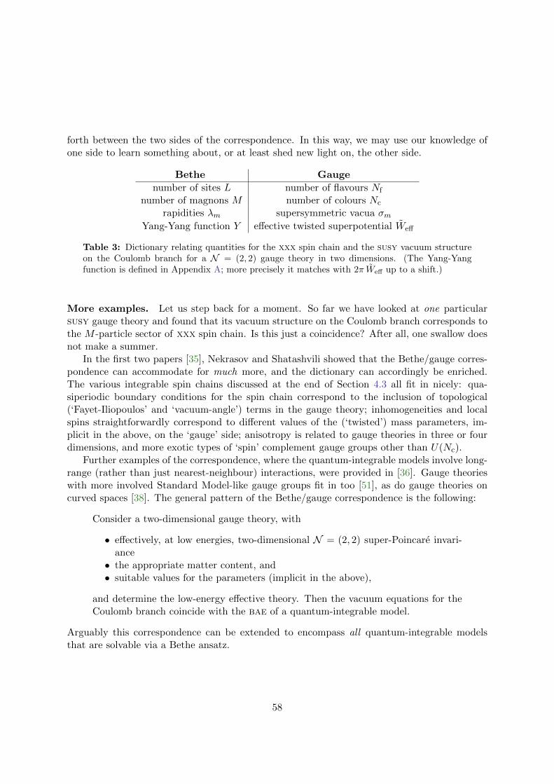
forth between the two sides of the correspondence. In this way, we may use our knowledge ofone side to learn something about, or at least shed new light on, the other side.

Bethe Gauge

number of sites L number of flavours Nf

number of magnons M number of colours Nc

rapidities λm supersymmetric vacua σmYang-Yang function Y effective twisted superpotential Weff

Table 3: Dictionary relating quantities for the xxx spin chain and the susy vacuum structureon the Coulomb branch for a N = (2, 2) gauge theory in two dimensions. (The Yang-Yangfunction is defined in Appendix A; more precisely it matches with 2π Weff up to a shift.)

More examples. Let us step back for a moment. So far we have looked at one particularsusy gauge theory and found that its vacuum structure on the Coulomb branch corresponds tothe M -particle sector of xxx spin chain. Is this just a coincidence? After all, one swallow doesnot make a summer.

In the first two papers [35], Nekrasov and Shatashvili showed that the Bethe/gauge corres-pondence can accommodate for much more, and the dictionary can accordingly be enriched.The various integrable spin chains discussed at the end of Section 4.3 all fit in nicely: qua-siperiodic boundary conditions for the spin chain correspond to the inclusion of topological(‘Fayet-Iliopoulos’ and ‘vacuum-angle’) terms in the gauge theory; inhomogeneities and localspins straightforwardly correspond to different values of the (‘twisted’) mass parameters, im-plicit in the above, on the ‘gauge’ side; anisotropy is related to gauge theories in three or fourdimensions, and more exotic types of ‘spin’ complement gauge groups other than U(Nc).

Further examples of the correspondence, where the quantum-integrable models involve long-range (rather than just nearest-neighbour) interactions, were provided in [36]. Gauge theorieswith more involved Standard Model-like gauge groups fit in too [51], as do gauge theories oncurved spaces [38]. The general pattern of the Bethe/gauge correspondence is the following:

Consider a two-dimensional gauge theory, with

• effectively, at low energies, two-dimensional N = (2, 2) super-Poincare invari-ance• the appropriate matter content, and• suitable values for the parameters (implicit in the above),

and determine the low-energy effective theory. Then the vacuum equations for theCoulomb branch coincide with the bae of a quantum-integrable model.

Arguably this correspondence can be extended to encompass all quantum-integrable modelsthat are solvable via a Bethe ansatz.

58

Achievements. Let us conclude with some words about the use of the Bethe/gauge corres-pondence. The ideas that we have described so far are of course nice and perhaps unexpected:they relate two seemingly very different areas of theoretical and mathematical physics. Howeverit should be stressed that to the extent described so far this correspondence is not predictive.Indeed, in order to establish it one has to start with the appropriate models on both sides andcalculate the bae and the vacuum equations in order to set up a dictionary between the twosides. Thus, a lot of information is needed as input, and one may wonder to what novel resultsit may lead. Here are a few examples of its early achievements:

• In [36] the Bethe/gauge correspondence and related ideas were used to find so-calledthermodynamic Bethe-ansatz (tba) equations for several long-range quantum-integrablemodels. These results later confirmed for the Toda chain with integrability techniques [59].

• Many new (quantum) integrable models have been obtained from ADE-quiver gaugetheories in four dimensions (in the Ω-background) [60].

• Dualities between supersymmetric gauge theories have been used obtain relations betweendifferent quantum-integrable models [61]; some of these are already known in the integ-rability literature but others appear to be novel.

Thus, in short, the Bethe/gauge correspondence provides a way to translate knowledge aboutone side into statements about the other side, leading to new insights.

A Completeness and the Yang-Yang function

In Sections 2, 3 and 4 we have seen how, for a finite system with periodic boundary conditions,the coordinate and algebraic Bethe Ansatze lead to the bae. For the eigenvectors in HM ⊆ Hthese consist of M coupled equations determining the allowed values of the parameters in theBethe ansatz. An important question is whether the Bethe ansatz is complete: does it give all(LM

)independent eigenstates in HM? Note that the problem is more complicated than ‘just’

trying to count the number of solutions to the bae: not all such solutions necessarily lead tophysically acceptable states; in particular, the resulting Bethe vectors must be normalizable,i.e. have nonzero norm. The three possible situations are illustrated in Figure 10.

The issue of completeness was already investigated for the xxx model by Bethe [21, §8],but it has remained a topic of debate to the present day, with approaches ranging from heavynumerics to combinatorics and algebraic geometry, see e.g. [62] and references therein. Tounderstand why, notice that symmetries lead to degeneracies, while counting becomes harderby the presence of degeneracies in the spectrum. Indeed, since the Hamiltonian is hermitean,its eigenvectors are orthogonal for different eigenvalues. When there are no degeneracies in thespectrum, one can count the number of distinct eigenvalues to find the number of eigenvectors.

From this point of view it is not surprising that the situation is better for the case withonly partial isotropy. In this brief appendix we introduce an important tool for the study ofcompleteness for the xxz model: the Yang-Yang function.

59

bae

spec(H)

spec(H) bae spec(H)

bae

Figure 10: The three typical cases in the completeness problem of the Bethe ansatz. Theleft shows the incomplete case, where the bae do not have enough solutions to obtain the fullspectrum of the Hamiltonian. The right, instead, corresponds to the overcomplete case, whereall eigenvectors are of the Bethe form but the bae have more than 2L solutions and it has to bedetermined which of those are physically acceptable. The middle depicts the intermediate case.

xxz case. Consider the Bethe ansatz parametrized in terms of rapidities λ ∈ CM like at theend of Section 2.3; see also (4.65). In logarithmic form the bae for the M -particle sector read

Lp(λm) = 2πIm +M∑n=1n 6=m

Θ(λn, λm) , 1 ≤ m ≤M , (A.1)

where I = (I1, · · · , IM ) are the Bethe quantum numbers, cf. (2.34), and the two-body scatteringphase Θ depends on the rapidity difference and the anisotropy ∆ = cos γ, cf. Exercise 2.13 inSection 2.3.

It may come as a surprise that the bae admit a ‘potential’: there exists a functionY : CM −→ C such that (A.1) is equivalent to the extremality conditions

∂Y (λ)

∂λm= 0 , 1 ≤ m ≤M . (A.2)

This Yang-Yang function or Yang-Yang action can be defined as

Y (λ) := LM∑m=1

p(λm)− 2πM∑m=1

Imλm +1

2

M∑m,n=1

Θ(λn − λm) , (A.3)

where

p(λ) =

∫ λ

ϕ1/2(µ) dµ , Θ(λ) =

∫ λ

ϕ1(µ) dµ ,

ϕs(λ) :=1

ilog

sinh(λ+ iγs)

sinh(λ− iγs).

(A.4)

Exercise A.1. Check that the solutions of the bae (A.1) are precisely the critical points of (A.3).

Yang and Yang employed Y (λ) to show that the bae admit a class of real solutions [20].

Theorem 3. When 0 < ∆ < 1 the bae (A.1) have a unique real solution λ ∈ RM for any I.

60

Proof. The uniqueness is proven with a convexity argument, see also [8, §II.1], which only workswhen λ is real. Using

ϕ′s(λ) =1

i

−i sin(γs)

sinh(λ+ iγs) sinh(λ− iγs)= − 2 sin(γs)

cosh(2λ)− cos(2γs)(A.5)

it is easy to see that the Hessian matrix ∂m∂nY is negative when 0 < γ < π/2: then

M∑m,n=1

∂2Y (λ)

∂λm∂λnvm vn =

M∑m=1

Lϕ′1/2(λm) v2m +

1

2

M∑m,n=1

ϕ′1(λm − λn) (vm − vn)2 < 0 (A.6)

for any λ,v ∈ RM . This implies that Y has at most one critical point, which, if it exists, isa global maximum. The existence of this critical point, however, requires some care: one hasto show that the critical point does not run away to infinity, as happens e.g. for the convexfunction y(λ) = − eλ on R. The proof can be found in [20, §4].

Now by construction the Bethe ansatz is symmetric in the λm, so solutions to the bae thatonly differ by a permutation (relabelling) of the λm correspond to the same Bethe vector; suchsolutions should only be counted once. Since the bae (A.1) are symmetric under simultaneousinterchange of λm ↔ λn and Im ↔ In, this amounts to taking into account only Bethe quantumnumbers I with 0 ≤ I1 ≤ · · · ≤ IM ≤ L− 1. Moreover, by the Pauli exclusion principle, Bethevectors vanish whenever two rapidities coincide, so in fact it suffices to consider 0 ≤ I1 < · · · <IM ≤ L− 1. There are precisely

(LM

)such choices for I, and by the theorem there is a unique

real solution λ ∈ RM for each of these. Since the corresponding energies (2.44) are different,this goes a long way towards a proof of the completeness for the regime 0 < ∆ < 1 of the xxzspin chain.

A few years later Yang and Yang applied the same technique to analyze the (simpler) one-dimensional Bose gas [63]; see also [8, §I.2]. It is worth mentioning that Y (λ) also featuresin Gaudin’s hypothesis, which says that the (square) norm of the Bethe wave function can becomputed as the determinant of the Hessian matrix ∂m∂nY , see e.g. [8, §X].

xxx case. In the isotropic case the functions ϕs in the Yang-Yang function have a simpleprimitive (cf. Exercise 2.20 at the end of Section 2.3), and the integrals in (A.4) can be performedexplicitly: ∫ λ

ϕs|∆=1(µ) dµ =1

i

[(λ+ is) log(λ+ is)− (λ− is) log(λ− is)

]+ const , (A.7)

where the constant on the right-hand side does not affect the bae (A.2). However, the Yang-Yang function is no longer convex for ∆ = 1, and Theorem 3 does not apply. However, whenthe degeneracies of the xxx spin chain are lifted by turning on ‘generic’ quasiperiodic boundaryconditions or inhomogeneities (see the end of Section 4.3), completeness of the Bethe ansatzcan be proven [64].

61

B Computations for the M-particle sector

In this appendix the cba from Section 2.2 is worked out for the M -particle sector of the xxzspin chain to derive the results quoted in Section 2.3. Recall that the cba

Ψp(l) =∑π∈SM

Aπ(p) eipπ·l , l1 < · · · < lM (B.1)

for the wave functions in the M -particle sector,

|ΨM ; p〉 =∑

1≤l1<···<lM≤LΨp(l1, · · · , lM ) |l1, · · · , lM 〉 ∈ HM , (B.2)

yields eigenstates of the Hamiltonian if the equations

〈l|Hxxz|ΨM ;p〉 = EM (p) Ψp(l) , 1 ≤ l1 < · · · < lM ≤ L . (B.3)

can be solved. Our goal is to find the energies EM (p), the coefficients Aπ(p) and equationsdetermining the values of the parameters p. Let us write Nl ∈ N for the number of pairs ofneighbouring excitations in the configuration l of excited spins, i.e. Nl := #ln | ln+1 = ln + 1,so 0 ≤ Nl ≤M − 1 (unless M = L = Nl). For example, Figure 1 from Section 2.1 has Nl = 1.In terms of this notation the strategy (cf. Section 2.2) is as follows:

0. Compute the left-hand side of (B.3).

1. Solve (B.3) for the energy contribution εM (p) := EM (p) − E0 as a function of p byconsidering configurations l with well-separated excitations (Nl = 0).

2. Solve (B.3) for the Aπ(p)/Ae(p) as functions of p by considering l with Nl ≥ 1. (Luckilyit will turn out that it suffices to consider a single pair of neighbouring excitations.)

3. Impose periodic boundary conditions to get the bae for the allowed values of p.

As in Section 2.3 we put ~ = J = 1. At the end of this appendix we comment on the six-vertexcase and give the strategy to derive the results given in Section 3.3.

Warm-up: M = 2. It is instructive to work out the strategy for the two-particle sector beforetackling the general case.

Step 0. Expand the vector |Ψ2;p〉 via the coordinate basis of H2 as in (B.2):

|Ψ2;p〉 =∑

1≤l1<l2≤LΨp(l1, l2) |l1, l2〉 ∈ H2 . (B.4)

We compute Hxxz|l1, l2〉 using (2.4) and (2.9). The first two terms in (2.9) give∑k S±k S∓k+1|l1, l2〉 = |l1± 1, l2〉+ |l1, l2∓ 1〉, where one of the two vectors on the right-hand side

vanishes when the excitations are next to each other. The third term,∑

k SzkS

zk+1, multiplies

|l1, l2〉 by (L/4− 2) if l1 and l2 are well separated, and by (L/4− 1) if they are neighbours.

62

Step 1. In the well-separated case, Nl = 0, (B.3) gives

2 ε2(p) Ψp(l1, l2) = 4 ∆ Ψp(l1, l2)−Ψp(l1 − 1, l2)−Ψp(l1 + 1, l2)

−Ψp(l1, l2 − 1)−Ψp(l1, l2 + 1) .(B.5)

These difference equations have to be satisfied by the wave function for all pairs l1 < l2 − 1.Plugging in the cba

Ψp1, p2(l1, l2) = Ae(p1, p2) ei(p1l1+p2l2) +Aτ (p1, p2) ei(p1l2+p2l1) , l1 < l2 , (B.6)

immediately yields the result

ε2(p1, p2) = 2 ∆− cos p1 − cos p2 = ε1(p1) + ε1(p2) . (B.7)

2 ε2(p) Ψp(l, l + 1) = 2 ∆ Ψp(l, l + 1)−Ψp(l − 1, l + 1)−Ψp(l, l + 2) . (B.8)

These equations can be solved using a trick exploiting the similarity between (B.8) and (B.5).

Exercise B.1. Check that (B.5) is satisfied by Ψp from (B.6) and ε2(p) from (2.31) independentlyof the values of l1 and l2.

In particular, given (B.6) and (B.7), (B.5) holds true even when Nl = 1. When l2 = l1 + 1,however, the right-hand side of (B.5) features wave functions with equal arguments, which arenot defined. Although such Ψp(l, l) are not physical — they do not enter (B.4) — the trick isto extend the Bethe wave function to the diagonal l1 = l2 using the formula (B.6). In this waynothing changes for Nl = 0, while (B.5) with l2 = l1 + 1 gives extra information that we canuse to solve (B.8).

To see if the so-extended cba does indeed satisfy (B.8) we subtract (B.5) with l2 = l1 + 1from (B.8) to get

2 ∆ Ψp(l, l + 1) = Ψp(l, l) + Ψp(l + 1, l + 1) . (B.9)

Up to an overall normalization the coefficients in the cba (B.6) are determined by these equa-tions: (B.9) is satisfied if the two-body S-matrix (2.27) is the 1 × 1 matrix given by the res-ult (2.32) from Section 2.3.

Step 3. We already obtained the bae for M = 2 in Section 2.2, see (2.28).

General M . We carry out the strategy following 1[1, §8.4]. The reader is advised to compareeach step with the corresponding step for the case M = 2.

Step 0. The equations (B.3) are computed for the M -particle sector as for M = 2. Theresult can be compactly written as

2 εM (p) Ψp(l) = 2(M −Nl

)∆Ψp(l)−

∑′

k

Ψp(k) , (B.10)

where the prime indicates that the sum runs over the 2 (M − Nl) configurations k obtainedfrom l by letting any single excited spin hop to an unexcited neighbour.

Exercise B.2. Check that (B.10) contains both (B.5) and (B.8) for M = 2.

63

Step 1. For Nl = 0 we have to solve

2 εM (p) Ψp(l) = 2M∆Ψp(l)−∑′

k

Ψp(k) , (B.11)

where the sum runs over 2M configurations. Plugging in the cba (B.1) it is easy to see that(B.11) is satisfied provided the energy contribution is given by the result (2.36) quoted inSection 2.3.

Step 2. Here the real work begins. Repeating the trick of extending the cba to l1 ≤ l2 ≤· · · ≤ lM the equations for Nl = 0 can again be used to simplify those for Nl ≥ 1. Indeed,the extended Ψp(l) satisfies (B.11), still involving a sum over 2M configurations, also for all(nonphysical) l with at least one pair lm = lm+1. Subtracting that equation from (B.10) weobtain

2Nl ∆ Ψp(l) =∑′′

k

Ψp(k) , (B.12)

where the sum now runs over the 2Nl configurations obtained from l by moving one excitationin any single pair of neighbours on top of the other one. For example, when Nl = 1, say withln+1 = ln + 1, (B.12) boils down to a simple generalization of (B.9):

2 ∆ Ψp(l1, · · · , ln, ln + 1, · · · , lM ) = Ψp(l1, · · · , ln, ln, · · · , lM )

+ Ψp(l1, · · · , ln + 1, ln + 1, · · · , lM ) .(B.13)

Usually (B.12) contains many more equations than there are unknowns (the functions Aπand the values of p), so our task seems daunting. Luckily the equations that we have to solveare simplified by the following observation, exploiting the similarity between (B.12) and (B.13).Suppose that we would be able to solve (B.13) not just for Nl = 1, but for any Nl ≥ 1.Because (B.12) can be recognized as the sum of Nl copies of (B.13), one for each pair ofneighbouring excitations, then all other equations in (B.12) would automatically be satisfied aswell! Although this observation does not change the number of equations that we have to solve,the new equations all have the same form, which moreover is very similar to that of (B.9).

Thus we focus on (B.13) for some 1 ≤ n ≤M−1, where l may or may not contain additionalpair of neighbours. (The special case n = M , for which lM = L is next to l1 = 1, correspondsto periodic boundary conditions. This is tackled in step 3 below.)

Exercise B.3. Let us abbreviate k := (l1, · · · , ln, ln, · · · , lM ). Plug the cba (B.1) into (B.13) tofind ∑

π∈SM

s(pπ(n), pπ(n+1))Aπ(p) eipπ·k = 0 , s(p, p′) := 1− 2 ∆ eip′ + ei(p+p′) . (B.14)

Not all eipπ·k, π ∈ SM , are independent. Indeed, since kn = kn+1 these exponentials onlycontain the quasimomenta pπ(n) and pπ(n+1) in the combination pπ(n) + pπ(n+1). Writing τn :=

(n, n+ 1) ∈ SM for the transposition switching n↔ n+ 1, this means that eipπ·k = eipπ′ ·k whenπ = π′ τn. Thus the terms in (B.14) come in pairs, and we find

Aπτn(p)

Aπ(p)= −

s(pπ(n), pπ(n+1))

s(pπ(n+1), pπ(n))= S(pπ(n), pπ(n+1)) . (B.15)

64

This is the M -particle generalization of equation (2.32) for the two-body S-matrix. In summary,for each 1 ≤ n ≤M − 1 we obtain M !/2 equations (B.15).

Any permutation π ∈ SM admits a (non-unique) decomposition as a product of transpos-itions interchanging neighbouring pm, so repeated application of (B.15) allows us to expressAπ(p) in terms of products of two-body S-matrices and an overall normalization Ae(p), withe ∈ SM denoting the identity. The non-uniqueness of this decomposition leads to new compat-ibility conditions, which are always satisfied since the two-body S-matrix is a scalar quantity.

Exercise B.4. Check that π = (1, 3) ∈ SM can be decomposed as π = τ1 τ2 τ1 = τ2 τ1 τ2.Carefully apply (B.15) to find A(1,3)(p). Compare the result with Figure 2 from Section 3.3.

Up to an overall normalization, the (unique) general solution of (B.15) is

Aπ(p)

Ae(p)= sgn(π)

∏1≤m<m′≤M

s(pπ(m′), pπ(m))

s(pm′ , pm)=

∏(m,m′)∈inv(π)

S(pm, pm′) , (B.16)

where inv(π) := 1 ≤ m < m′ ≤ M | π(m) > π(m′) is the set of inversions for π. Thus wehave derived the result (2.37).

Exercise B.5. As a warm-up take π = τn and check that (B.16) solves (B.15). For the generalcase verify the solution by splitting the product into four parts, depending on whether or notm and m′ lie in n, n+ 1. Use sgn(π) = (−1)# inv(π) to verify the second equality in (B.16).

Step 3. It remains to impose periodic boundary conditions on the Bethe wave function.Indeed, when working with the coordinate basis (2.15) for HM a subtlety arises because ofperiodicity. To avoid linear dependence amongst the vectors in (B.2) we have ordered thepositions of the excited spins as l1 < l2 < · · · < lM . However, the circle ZL does not possessan ordering. In the above we have implicitly chosen representatives in 1, 2, · · · , L ⊆ Z forthe sites lm ∈ ZL (in a more pictorial language: we have cut open the circle between sites Land 1). Of course we could have chosen to cut ZL at any other point; for example, a cut justafter l1 corresponds to choosing representatives l1 +1, l1 +2, · · · , l1 +L and yields the orderingl2 < l3 < · · · < lM < l1 + L. Independence of the choice of representatives for ZL thus requires|l2, · · · , lM , l1+L〉 = |l1, · · · , lM 〉. This just expresses the periodic boundary conditions Sl+L = Slin terms of the coordinate basis.

The upshot is that any vector |ΨM 〉 ∈ HM may be expressed in terms of the co-ordinate basis (2.15) as in (B.2) provided periodicity is imposed on the wave function asΨ(lM − L, l1, · · · , lM−1) = Ψ(l1, · · · , lM ) or, equivalently,

Ψ(l2, · · · , lM , l1 + L) = Ψ(l1, · · · , lM ) , l1 < · · · < lM . (B.17)

Write σ = (12 · · ·M) ∈ SM for the cyclic permutation. For the Bethe wave function (B.1)we get Ψp(l2, · · · , lM , l1 + L) =

∑π′ Aπ′(p) eipπ′(1)L eipπ′ ·l, where π′ := π σ−1. Dropping these

primes and equating coefficients in (B.17) we obtain M ! bae:

eipπ(1)L =Aπ(p)

Aπσ(p), π ∈ SM . (B.18)

65

Exercise B.6. Plug in the solution (B.16) for Aπ. Check that factors with 2 ≤ m′ < m ≤ L inthe numerator cancel those with 1 ≤ m′ < m ≤ L− 1 in the denominator. Note that the resultis symmetric in the pπ(2), · · · , pπ(M) so that the equations are the same for any two π, π′ ∈ SMwith the same value π(1) = π′(1). Thus it suffices to consider transpositions of the formπ = (1, n) ∈ SM . Check that this yields the bae (2.38) for the M -particle sector:

eipmL = (−1)M−1M∏n=1n6=m

s(pn, pm)

s(pm, pn)=

M∏n=1n 6=m

S(pn, pm) , 1 ≤ m ≤M . (B.19)

Thus we have derived all results quoted in Section 2.3.

Exercise B.7. Work out the cba for the xxz in an external magnetic field, see Exercise 2.5 inSection 2.1, starting with the cases M = 0, 1, 2 before attacking the general case.

Six-vertex case. To conclude this appendix we briefly turn to the strategy to work out thecba for the six-vertex model. Thus, the goal now is to use

Ψz(l) =∑π∈SM

Aπ(z) zπl , zπ

l :=M∏m=1

(zπ(m))lm , l1 < · · · < lM . (B.20)

This produces eigenvectors for the transfer matrix provided we can solve the equations∑k

〈l| t |k〉 Ψz(k) = 〈l| t |ΨM ; z〉 = ΛM (z) Ψz(l) , 1 ≤ l1 < · · · < lM ≤ L . (B.21)

The left-hand side of (B.21) is much more complicated than its xxz-analogue in (B.10). Thisrequires more care in formulating the strategy for using the cba in this case:

0. Rewrite the left-hand side of (B.21) by summing geometric series in the zm,

N∑k=n

zk =zn

1− z− zN+1

1− z. (B.22)

1. Focus on the wanted terms, involving zπl like the cba, to find ΛM (z).

2. Consider unwanted internal terms, containing (znzn+1)ln or (znzn+1)ln+1 . Demand thatthese cancel to get (B.14), with pm = −i log(zm) instead of pm, and proceed as for thexxz spin chain to find Aπ(z).

3. Demand that the unwanted boundary terms, obtained in (B.22) when n = 1 or N = L,cancel to get (B.18) in terms of the zm. The bae for the allowed values of z are thenfound as above.

The details can be found in [1, §8.3–8.4] (cf. the footnote at the end of Section 3.2).

Exercise B.8. Compare this strategy with that for the xxz model keeping in mind Exercise 3.6in Section 3.2.

66

C Solving the fcr

Theorem 2 from Section 4.2 tells us that if we can find an R-matrix satisfying the fundamentalcommutation relations (fcr) then the corresponding transfer matrices commute, resulting inconserved quantities for the xxz and six-vertex models, cf. Sections 3.3 and 4.1. Consider twomonodromy matrices depending on different sets of vertex weights, such that the correspondingLax operators are given by

Lal = a

l

=

a

b cc b

a

al

, Lbl = b

l

=

a′

b′ c′

c′ b′

a′

bl

(C.1)

with respect to the standard bases of Va ⊗ Vl and Vb ⊗ Vl, as in Section 4.1. The entries arevertex weights of two different six-vertex models.

In this appendix we follow Baxter [1, §9.6–9.7] to obtain an R-matrix solving the fcr

Rab Lal Lbl = Lbl LalRab , (C.2)

or in graphical notation

b

a

l

=b

a

l

. (C.3)

As a byproduct we will find conditions on vertex weights w and w′ necessary to get com-mutating transfer matrices: from (C.3) we will rederive the condition ∆(a, b, c) = ∆(a′, b′, c′)from Section 3.3 in the more algebraic setting from Section 4.

Reduction by symmetries. Since Va ⊗ Vb ⊗ Vl has dimension eight, (C.2) a priori consistsof 8× 8 = 64 equations:

β′

δ′β

δ

α

γ

=β′

δ′β

δ

α

γ

, α, · · · , δ′ = ±1 . (C.4)

It is reasonable to look for solutions Rab ∈ End(Va⊗Vb) that preserve the two symmetries of thesix-vertex model: the ice rule (line conservation) and spin-reversal symmetry. Thus we assume

67

that the R-matrix is of the same form as the Lax operators (C.1),

Rab =

a

b=

a′′

b′′ c′′

c′′ b′′

a′′

ab

, (C.5)

where the three entries have to be determined. Let us emphasize once more that, both forthe Lax operator and for the R-matrix, the order of the ‘outgoing’ labels is reversed in thecoefficients, see (4.3) and (4.23).

Due to parity reversal these equations come in 32 equal pairs. Line conservation requires theoccupancy number to be preserved: α+β+β′ = γ+ δ+ δ′. This further reduces the number ofnontrivial equations to 10. Using parity reversal we may restrict our attention to the ten caseswith at least two incoming occupancies. Simultaneously switching α ↔ γ, β ↔ δ and β′ ↔ δ′

in (C.4) yields

δ′

β′δ

β

γ

α

=δ′

β′δ

β

γ

α

. (C.6)

When we rotate this over 180 we precisely recover (C.4). But the vertex weights are invariantunder such a rotation (see Figure 6 in Section 3.1), so it follows that the four equations withα = γ, β = δ and β′ = δ′ are automatically satisfied while the six remaining equations come inequal pairs. Thus we are left with just three independent equations. Paying attention to whichcrossing corresponds to Lal, Lbl and Rab these equations read

a b′c′′ + c c′b′′ = = = b a′c′′ , (C.7)

a c′b′′ + c b′c′′ = = = b c′a′′ , (C.8)

a c′c′′ + c b′b′′ = = = c a′a′′ , (C.9)

68

Solving the fcr. Let us first show how (C.7)–(C.9) result in constraints on Lal and Lbl thatare necessary for the existence of an R-matrix satisfying the fcr (and thus yield commutingtransfer matrices). Eliminating the (doubly primed) entries of the R-matrix we recover theconstraint ∆(a, b, c) = ∆(a′, b′, c′) from (3.21), where ∆ was defined in (3.18). Recall from thediscussion following (3.21) that, for fixed value of the function ∆, the vertex weights of thesix-vertex model are parametrized (up to an overall normalization) by the spectral parameter.Thus we are once more led to Lax operators depending on spectral parameters as in Theorem 2.In Section 3.3 we found the condition ∆(a, b, c) = ∆(a′, b′, c′) for commuting transfer matricesthrough the results of the cba; presently we obtained it by purely algebraic methods!

Now we turn to the R-matrix itself. Notice that (C.7) and (C.8) only differ by the positionof the single and double primes, while (C.9) is symmetric in this respect. It follows that if weinstead eliminate the (primed) entries of Lbl from (C.7)–(C.9) we similarly obtain the furthercondition ∆(a, b, c) = ∆(a′′, b′′, c′′). Thus, again up to an normalization (which drops out of thefcr at any rate), the entries of the R-matrix differ from those of the two Lax operators only bythe value of the spectral parameter w. Using the explicit parametrization (4.10) we find that(C.7)–(C.9) are satisfied provided that the spectral parameters are related by the differenceproperty sinh(w) = sinh(u− v), which holds for w = u− v. Explicitly we thus obtain

a′′ = ρ′′ sinh(u− v + iγ) , b′′ = ρ′′ sinh(u− v) , c′′ = ρ′′ sinh(iγ) , (C.10)

where cos γ = ∆(a, b, c) = ∆(a′, b′, c′), for the entries of the R-matrix of the six-vertex model.

References

[1] R. Baxter, Exactly Solved Models in Statistical Mechanics. Dover Publications, 2007. Un-abridged republication of the 3rd Ed. of the work originally published by Academic Press,London, 1982.

[2] C. Gomez, M. Ruiz-Altaba, and G. Sierra, Quantum Groups in Two-Dimensional Physics.Cambridge University Press, 1996.

[3] L. Faddeev, “How Algebraic Bethe Ansatz works for integrable model,” 1995. arXiv:hep-th/9605187.

[4] M. Gaudin, The Bethe Wavefunction. Cambridge University Press, 2014. Translated byJ.-S. Caux.

[5] M. Jimbo and T. Miwa, Algebraic Analysis of Solvable Lattice Models. American Mathem-atical Society, 1995.

[6] M. Karbach and G. Muller, “Introduction to the Bethe Ansatz I,” Comput. Phys., vol. 11,pp. 36–43, 1997. arXiv:cond-mat/9809162.

[7] M. Karbach, K. Hu, and G. Muller, “Introduction to the Bethe Ansatz II,” Comput. Phys.,vol. 12, pp. 565–573, 1998. arXiv:cond-mat/9809163.M. Karbach, K. Hu, and G. Muller, “Introduction to the Bethe Ansatz III,” 2000.arXiv:cond-mat/0008018.

69

[8] V. Korepin, N. Bogoluibov, and A. Izergin, Quantum Inverse Scattering Method and Cor-relation Functions. Cambridge University Press, 1993.

[9] O. Babelon, D. Bernard, and M. Talon, Introduction to Classical Integrable Systems. Cam-bridge University Press, 2003.

[10] M. Batchelor, “The Bethe ansatz after 75 years,” Physics Today, vol. 60, pp. 36–40, 2007.R. Baxter, “Solvable models in statistical mechanics, from Onsager onward,” J. Stat. Phys.,vol. 78, pp. 7–16, 1995.L. Faddeev, “Instructive History of the Quantum Inverse Scattering Method,” Acta Appl.Math., vol. 39, pp. 69–84, 1995.

[11] M. Mourigal, M. Enderle, A. Klopperpieper, J.-S. Caux, A. Stunault, and H. Rønnow,“Fractional spinon excitations in the quantum Heisenberg antiferromagnetic chain,” Nat.Phys., vol. 9, pp. 435–441, 2013. arXiv:1306.4678 [cond-mat.str-el].X.-W. Guan, M. Batchelor, and C. Lee, “Fermi gases in one dimension: From BetheAnsatz to experiments,” Rev. Mod. Phys., vol. 85, pp. 1633–1691, 2013. arXiv:1301.6446[cond-mat.quant-gas]. See especially §I.T. Kinoshita, T. Wenger, and D. Weiss, “A quantum Newton’s cradle,” Nature, vol. 440,pp. 900–903, 2006.

[12] “The Mathematica Summer School on Theoretical Physics.” http://msstp.org/, Ac-cessed: January 23, 2015.

[13] G. Duchamp, P. Blasiak, A. Horzela, K. Penson, and A. Solomon, “Hopf Algebras inGeneral and in Combinatorial Physics: A Practical introduction.” arXiv:0802.0249 [quant-ph].

[14] S. Majid, A Quantum Groups Primer. Cambridge University Press, 2002.

[15] V. Chari and A. Pressley, A Guide to Quantum Groups. Cambridge University Press, 1994.

[16] C. Kassel, Quantum Groups. Springer, 1995.

[17] W. Heisenberg, “Mehrkorperproblem und Resonanz in der Quantenmechanik,” Z. Phys.,vol. 38, pp. 411–426, 1926.P. Dirac, “On the Theory of Quantum Mechanics,” Proc. Roy. Soc. Lond., vol. 112A,pp. 661–677, 1926.

[18] W. Heisenberg, “Zur Theorie der Ferromagnetismus,” Z. Phys., vol. 49, pp. 619–636, 1928.

[19] J. Hook and H. Hall, Solid State Physics. Wiley, 1995.

[20] C. Yang and C. Yang, “One-Dimensional Chain of Anisotropic Spin-Spin Interactions. I.Proof of Bethe’s Hypothesis for Ground State in a Finite System,” Phys. Rev., vol. 150,pp. 321–327, 1966.

70

[21] H. Bethe, “Zur Theorie der Metalle. I. Eigenwerte und Eigenfunktionen der LineairenAtomkette,” Z. Phys., vol. 71, pp. 205–226, 1931. See also the English translation byT.C. Dorlas (2009).

[22] E. Lieb and W. Liniger, “Exact Analysis of an Interacting Bose Gas. I. The General Solutionand the Ground State,” Phys. Rev., vol. 130, pp. 1605–1616, 1963.

[23] E. Lieb, “Residual Entropy of Square Ice,” Phys. Rev., vol. 162, pp. 162–172, 1967.E. Lieb, “Exact Solution of the F Model of An Antiferroelectric,” Phys. Rev. Lett., vol. 18,pp. 1046–1048, 1967.E. Lieb, “Exact Solution of the Two-Dimensional Slater KDP Model of a Ferroelectric,”Phys. Rev. Lett., vol. 19, pp. 108–110, 1967.

[24] B. Sutherland, “Exact Solution of a Two-Dimensional Model for Hydrogen-Bonded Crys-tals,” Phys. Rev. Lett., vol. 19, pp. 103–104, 1967.

[25] L. A. Takhtadzhan and L. D. Faddeev, “The Quantum method of the inverse problem andthe Heisenberg XYZ model,” Russ. Math. Surv., vol. 34, pp. 11–68, 1979.

[26] J. Maillet and V. Terras, “On the quantum inverse scattering problem,” Nucl. Phys.,vol. B575, pp. 627–644, 2000. arXiv:hep-th/9911030.N. Kitanine, J. Maillet, and V. Terras, “Correlation functions of the XXZ Heisenberg spin-1/2 chain in a magnetic field,” Nucl. Phys., vol. B567, pp. 554–582, 2000. arXiv:math-ph/9907019.

[27] L. Faddeev and L. Takhtadzhyan, “Spectrum and scattering of excitations in the one-dimensional isotropic Heisenberg model,” J. Sov. Math., vol. 24, pp. 241–267, 1984.

[28] E. Sklyanin, “Boundary Conditions for Integrable Quantum Systems,” J. Phys. A: Math.Gen., vol. 21, no. 10, p. 2375, 1988.

[29] P. Kulish, N. Reshetikhin, and E. Sklyanin, “Yang-Baxter Equation and RepresentationTheory. 1.,” Lett. Math. Phys., vol. 5, pp. 393–403, 1981.

[30] A. Zamolodchikov and A. Zamolodchikov, “Factorized S-Matrices in Two Dimensions asthe Exact Solutions of Certain Relativistic Quantum Field Models,” Ann. Phys., vol. 120,pp. 253–291, 1979.

[31] P. Dorey, “Exact S-Matrices,” in Conformal Field Theories and Integrable Models, vol. 498of Lecture Notes in Physics, pp. 85–125, Springer-Verlag, 1997. arXiv:hep-th/9810026.

[32] V. Bazhanov, S. Lukyanov, and A. Zamolodchikov, “Integrable structure of conformal fieldtheory, quantum KdV theory and thermodynamic Bethe ansatz,” Comm. Math. Phys.,vol. 177, pp. 381–398, 1996. arXiv:hep-th/9412229.V. Bazhanov, S. Lukyanov, and A. Zamolodchikov, “Integrable structure of conformal fieldtheory. 2. Q operator and DDV equation,” Comm. Math. Phys., vol. 190, pp. 247–278,1997. arXiv:hep-th/9604044.V. Bazhanov, S. Lukyanov, and A. Zamolodchikov, “Integrable structure of conformal field

71

theory. 3. The Yang-Baxter relation,” Comm. Math. Phys., vol. 200, pp. 297–324, 1999.arXiv:hep-th/9805008.

[33] G. Korchemsky, “Review of AdS/CFT Integrability, Chapter IV.4: Integrability in QCDand N < 4 SYM,” Lett. Math. Phys., vol. 99, pp. 425–453, 2012. arXiv:1012.4000 [hep-th].L. Faddeev and G. Korchemsky, “High-energy QCD as a completely integrable model,”Phys. Lett., vol. B342, pp. 311–322, 1995. arXiv:hep-th/9404173.

[34] M. Yamazaki, “New Integrable Models from the Gauge/YBE Correspondence,” J. Stat.Phys., vol. 154, pp. 895–911, 2014. arXiv:1307.1128 [hep-th].

[35] N. Nekrasov and S. Shatashvili, “Supersymmetric vacua and Bethe ansatz,” Nucl. Phys.Proc. Suppl., vol. 192, pp. 91–112, 2009. arXiv:0901.4744 [hep-th].N. Nekrasov and S. Shatashvili, “Quantum Integrability and Supersymmetric Vacua,”Prog. Theor. Phys. Suppl., vol. 177, pp. 105–119, 2009. arXiv:0901.4748 [hep-th].

[36] N. Nekrasov and S. Shatashvili, “Quantization of Integrable Systems and Four DimensionalGauge Theories,” in XVIth International Congress on Mathematical Physics. Prague, Au-gust 2009 (P. Exner, ed.), pp. 265–289, World Scientific, 2010. arXiv:0908.4052 [hep-th].

[37] N. Nekrasov, A. Rosly, and S. Shatashvili, “Darboux coordinates, Yang-Yang functional,and gauge theory,” Nucl. Phys. Proc. Suppl., vol. 216, pp. 69–93, 2011. arXiv:1103.3919[hep-th].

[38] N. Nekrasov and S. Shatashvili, “Bethe/Gauge correspondence on curved spaces,” 2014.arXiv:1405.6046 [hep-th].

[39] N. Beisert, C. Ahn, L. Alday, Z. Bajnok, J. Drummond, et al., “Review of AdS/CFTIntegrability: An Overview,” Lett. Math. Phys., vol. 99, pp. 3–32, 2012. arXiv:1012.3982[hep-th].

[40] G. Arutyunov and S. Frolov, “Foundations of the AdS5×S5 Superstring. Part I,” J. Phys.,vol. A42, p. 254003, 2009. arXiv:0901.4937 [hep-th].

[41] S. Cordes, G. Moore, and S. Ramgoolam, “Lectures on 2-d Yang-Mills theory, equivariantcohomology and topological field theories,” Nucl. Phys. Proc. Suppl., vol. 41, pp. 184–244,1995. arXiv:hep-th/9411210.

[42] D. Freed, “Quantum groups from path integrals,” in Particles and Fields (G. Semenoffand L. Vinet, eds.), CRM Series in Mathematical Physics, pp. 63–107, Springer New York,1999. arXiv:q-alg/9501025.

[43] K. Costello, “Integrable lattice models from four-dimensional field theories,” 2013.arXiv:1308.0370 [hep-th].K. Costello, “Supersymmetric gauge theory and the Yangian,” 2013. arXiv:1303.2632 [hep-th].

[44] T. Giamarchi, Quantum Physics in One Dimension. Clarendon Press, 2004.

72

[45] S. Weigert, “The Problem of Quantum Integrability,” Physica, vol. D56, no. 1, pp. 107–119,1992.J.-S. Caux and J. Mossel, “Remarks on the notion of quantum integrability,” J. Stat. Mech.,vol. 2011, p. 02023, 2011. arXiv:1012.3587 [cond-mat.str-el].

[46] V. Arnol’d, Mathematical Methods of Classical Mechanics, vol. 60 of Graduate Texts inMathematics. Springer-Verlag, second ed., 1997.

[47] S. Coleman and J. Mandula, “All Possible Symmetries of the S Matrix,” Phys. Rev.,vol. 159, pp. 1251–1256, 1967.O. Pelc and L. Horwitz, “Generalization of the Coleman-Mandula theorem to higher di-mension,” J. Math. Phys., vol. 38, pp. 139–172, 1997. arXiv:hep-th/9605147.

[48] E. Witten, Quantum Fields and Strings: A Course for Mathematicians, vol. 2, ch. Dynam-ics of Quantum Field Theory, pp. 1119–1424. American Mathematical Society, 1999.

[49] N. Seiberg and E. Witten, “Electric-magnetic duality, monopole condensation, and con-finement in N = 2 supersymmetric Yang-Mills theory,” Nucl. Phys., vol. B426, pp. 19–52,1994. arXiv:hep-th/9407087.

[50] A. Gorsky, I. Krichever, A. Marshakov, A. Mironov, and A. Morozov, “Integrability andSeiberg-Witten exact solution,” Phys. Lett., vol. B355, pp. 466–474, 1995. arXiv:hep-th/9505035.R. Donagi and E. Witten, “Supersymmetric Yang-Mills Systems And Integrable Systems,”Nucl. Phys., vol. B460, pp. 299–334, 1996. arXiv:hep-th/9510101.

[51] N. Nekrasov, V. Pestun, and S. Shatashvili, “Quantum Geometry and Quiver Gauge The-ories.” arXiv:1312.6689 [hep-th].

[52] M. Shifman, Advanced topics in quantum field theory: A lecture course. Cambridge Uni-versity Press, 2012.

[53] J. Wess and J. Bagger, Supersymmetry And Supergravity. Princeton University Press,second ed., 1992.

[54] E. Witten, “Phases of N = 2 theories in two-dimensions,” Nucl. Phys., vol. B403, pp. 159–222, 1993. arXiv:hep-th/9301042.

[55] K. Hori, S. Katz, A. Klemm, R. Pandharipande, R. Thomas, et al., Mirror Symmetry.American Mathematical Society, 2003. See also www.claymath.org/library/monographs/

cmim01c.pdf.

[56] J. Lamers, “The Bethe/Gauge Correspondence, A mysterious link between quantum integ-rability and supersymmetric gauge theory,” 2012. MSc thesis, http://dspace.library.uu.nl/handle/1874/253835.

[57] J. Teschner, “Exact results on N = 2 supersymmetric gauge theories,” 2014.arXiv:1412.7145 [hep-th].

73

[58] D. Maulik and A. Okounkov, “Quantum Groups and Quantum Cohomology.”arXiv:1211.1287 [math.AG].

[59] K. Kozlowski and J. Teschner, “TBA for the Toda chain,” in New Trends in QuantumIntegrable Systems: Proceedings of the Infinite Analysis 09 (B. Feigin, M. Jimbo, andM. Okado, eds.), pp. 195–219, World Scientific, 2011. arXiv:1006.2906 [math-ph].

[60] N. Nekrasov and V. Pestun, “Seiberg-Witten geometry of four dimensional N = 2 quivergauge theories,” 2012. arXiv:1211.2240 [hep-th].

[61] D. Gaiotto and P. Koroteev, “On Three Dimensional Quiver Gauge Theories and Integ-rability,” jhep, vol. 1305, p. 126, 2013. arXiv:1304.0779 [hep-th].H.-Y. Chen, P.-S. Hsin, and P. Koroteev, “On the Integrability of Four Dimensional N = 2Gauge Theories in the Omega Background,” jhep, vol. 1308, p. 076, 2013. arXiv:1305.5614[hep-th].

[62] A. Kirillov and R. Sakamoto, “Singular Solutions to the Bethe Ansatz Equationsand Rigged Configurations,” J. Phys. A: Math. Theor., vol. 47, p. 205207, 2014.arXiv:1402.0651 [math-ph].R. Baxter, “Completeness of the Bethe ansatz for the six and eight-vertex model,” J. Stat.Phys., vol. 108, pp. 1–48, 2002. arXiv:cond-mat/0111188.

[63] C. Yang and C. Yang, “Thermodynamics of One-Dimensional System of Bosons with Re-pulsive Delta-Function Interaction,” J. Math. Phys., vol. 10, pp. 1115–1122, 1969.

[64] E. Mukhin, V. Tarasov, and A. Varchenko, “Bethe Algebra of Homogeneous XXX Heis-enberg Model has Simple Spectrum,” Comm. Math. Phys., vol. 288, pp. 1–42, 2009.arXiv:0706.0688 [math.QA].

74