j_su_030206

A HEURISTIC SLOW VOLTAGE CONTROL SCHEME

FOR

LARGE POWER SYSTEMS

By

JINGDONG SU

A dissertation submitted in partial fulfillment of the requirements for the degree of

DOCTOR OF PHILOSOPHY

WASHINGTON STATE UNIVERSITY School of Electrical Engineering and Computer Science

May 2006

© Copyright by Jingdong Su, 2006 All Rights Reserved

© Copyright by Jingdong Su, 2006 All Rights Reserved

ii

To the Faculty of Washington State University: The members of the Committee appointed to examine the dissertation of JINGDONG SU find it satisfactory and recommend that it be accepted.

iii

ACKNOWLEDGEMENT

I would like to express my sincere appreciation to my advisor, Professor Vaithianathan

Venkatasubramanian, for his valuable advice, skilled guidance and continuous support

throughout my doctoral study. His profound knowledge and kindness will always be an

inspiration to me. I am also grateful to Mr. Carson Taylor and Mr. Ramu Ramanathan for

their counsel, insight and support. I have enjoyed the enlightening instruction and

advisement of Professor Anjan Bose and Professor Kevin Tomsovic, and I am thankful

for their participation in my advisory committee.

Funding in part from Bonneville Power Administration (BPA) is gratefully

acknowledged. Funding in part from the Consortium for Electric Reliability Technology

Solutions (CERTS) is gratefully appreciated. The valuable comments and feedback from

BPA planning and operation engineers and National System Research (NSR) engineers

are specially appreciated. The support of the Power System Engineering Research Center

(PSERC) is gratefully acknowledged.

I am also deeply indebted to my friends and colleagues at Washington State University,

for their friendship and their help, which made this long journey a joyful one. Finally I

would like to thank my family for their encouragement, support and enduring love,

without them I would never have been able to make it this far.

iv

A HEURISTIC SLOW VOLTAGE CONTROL SCHEME

FOR

LARGE POWER SYSTEMS

Abstract

by Jingdong Su, Ph.D.

Washington State University May 2006

Chair: Vaithianathan Venkatasubramanian

Automatic control of transmission network voltage provides significant improvements

in security, quality and efficiency of power system operation. In Europe, voltage control

is traditionally organized in a three levels hierarchical structure. At the second level, the

so called “secondary voltage control” divides the network into multiple control regions

based on the pilot node concept and all generators in a given region are operated in an

“aligned” mode. In North America, transmission grid voltage control is mostly achieved

through manual switching of capacitor/reactor banks and LTC transformers by operators.

Recently, an automatic discrete slow voltage controller is proposed to regulate voltage of

the western Oregon area in the Pacific Northwest. The controller acts upon SCADA

measurements and relies on state estimator model to evaluate the incremental effects of

control device switching by running localized power flow.

This dissertation first proposes an alternate heuristic slow voltage controller, which can

be easily integrated with the above controller and implemented under a common

framework. Then the controller scheme is extended so that it is applicable to any large

v

power systems. In view of a state estimator model maybe unavailable or unreliable

because of topology errors under certain conditions, the proposed alternate controller

operates independent of the state estimator model and can be either used as back-up

controller under these conditions or used to reinforce the decision recommended by the

model-based controller. A local voltage estimator is formulated based on linearized

reactive power flow model to approximate switching effects by utilizing only the local

SCADA measurements around the control devices.

For large power systems, several voltage problems may occur simultaneously in

different areas, a multiple problematic area voltage control scheme is proposed to make

simultaneous corrective control actions accordingly such that the system voltages are

quickly brought back to normal range. This control scheme is quite open and can be

easily extended to handle different objective functions. For many power systems, it is

also necessary to consider generators as voltage control devices, which leads to the

problem of coordinating generator controls and discrete device controls. A multi-phase

hybrid voltage control scheme is proposed to deal with the problem by formulating

generator and discrete device controls as continuous and discrete problems separately

while taking reactive power security into consideration. The controller solves the

problems in different operating phases using linear programming and integer

programming algorithms respectively and sends alarms to operators if reactive power

reserve limits are hit.

vi

Contents

ACKNOWLEDGEMENT . . . . . . . . . . . . . . . . . . . . . . . . . . . . . . . . . . . . . iii

ABSTRACT . . . . . . . . . . . . . . . . . . . . . . . . . . . . . . . . . . . . . . . . . . . . . . . . iv

LIST OF TABLES . . . . . . . . . . . . . . . . . . . . . . . . . . . . . . . . . . . . . . . . . . . ix

LIST OF FIGURES . . . . . . . . . . . . . . . . . . . . . . . . . . . . . . . . . . . . . . . . . . . xi

1. Introduction . . . . . . . . . . . . . . . . . . . . . . . . . . . . . . . . . . . . . . . . . . . . . . . 1

1.1 Power System Voltage Control . . . . . . . . . . . . . . . . . . . . . . . . . . . . . . . . . . . . . . . . . 1

1.2 Literature Review . . . . . . . . . . . . . . . . . . . . . . . . . . . . . . . . . . . . . . . . . . . . . . . . . . 8

1.3 Background and Motivation . . . . . . . . . . . . . . . . . . . . . . . . . . . . . . . . . . . . . . . . . . 16

1.4 Summary . . . . . . . . . . . . . . . . . . . . . . . . . . . . . . . . . . . . . . . . . . . . . . . . . . . . . . . . . 18

2. Local Voltage Estimation . . . . . . . . . . . . . . . . . . . . . . . . . . . . . . . . . . . . 21

2.1 Formulation of the Local Voltage Estimator . . . . . . . . . . . . . . . . . . . . . . . . . . . . . 21

2.1.1 Estimation of Capacitor/Reactor Switching Effects . . . . . . . . . . . . . . . . . . . 23

2.1.2 Estimation of Transformer Tap Changing Effects . . . . . . . . . . . . . . . . . . . . 26

2.1.3 Estimation of Generator Voltage Adjusting Effects . . . . . . . . . . . . . . . . . . . 28

2.2 Feasibility Studies of the Local Voltage Estimator . . . . . . . . . . . . . . . . . . . . . . . . 29

2.2.1 Tests on IEEE 30 Bus System . . . . . . . . . . . . . . . . . . . . . . . . . . . . . . . . . . . 30

2.2.2 Tests on WECC System . . . . . . . . . . . . . . . . . . . . . . . . . . . . . . . . . . . . . . . . 33

2.3 Summary . . . . . . . . . . . . . . . . . . . . . . . . . . . . . . . . . . . . . . . . . . . . . . . . . . . . . . . . . 40

vii

3. Alternate Heuristic Voltage Control . . . . . . . . . . . . . . . . . . . . . . . . . . . . 42

3.1 On-line Slow Voltage Control Framework . . . . . . . . . . . . . . . . . . . . . . . . . . . . . . . 42

3.2 Formulation of the Alternate Heuristic Control . . . . . . . . . . . . . . . . . . . . . . . . . . . 47

3.3 Testing of the Alternate Voltage Controller . . . . . . . . . . . . . . . . . . . . . . . . . . . . . 53



3.4 Summary . . . . . . . . . . . . . . . . . . . . . . . . . . . . . . . . . . . . . . . . . . . . . . . . . . . . . . . . 68

4. Large Power System Considerations . . . . . . . . . . . . . . . . . . . . . . . . . . . 70

4.1 Multiple Problematic Area Voltage Control . . . . . . . . . . . . . . . . . . . . . . . . . . . . . . 71

4.1.1 Multiple-area Voltage Control Scheme . . . . . . . . . . . . . . . . . . . . . . . . . . . . . 71

4.1.2 Tests on WECC System . . . . . . . . . . . . . . . . . . . . . . . . . . . . . . . . . . . . . . . . . 73

4.2 Multi-phase Hybrid Voltage Control . . . . . . . . . . . . . . . . . . . . . . . . . . . . . . . . . . . 78

4.2.1 Multi-phase Hybrid Control Scheme . . . . . . . . . . . . . . . . . . . . . . . . . . . . . . 79

4.2.2 Formulation of the Optimization . . . . . . . . . . . . . . . . . . . . . . . . . . . . . . . . . 81



4.3 Summary . . . . . . . . . . . . . . . . . . . . . . . . . . . . . . . . . . . . . . . . . . . . . . . . . . . . . . . . 97

5. Conclusions and Future Works . . . . . . . . . . . . . . . . . . . . . . . . . . . . . . . 99

5.1 Conclusions . . . . . . . . . . . . . . . . . . . . . . . . . . . . . . . . . . . . . . . . . . . . . . . . . . . . . . 99

5.2 Future Works . . . . . . . . . . . . . . . . . . . . . . . . . . . . . . . . . . . . . . . . . . . . . . . . . . . . 100

viii

BIBLIOGRAPHY . . . . . . . . . . . . . . . . . . . . . . . . . . . . . . . . . . . . . . . . . . . 102

APPENDIX . . . . . . . . . . . . . . . . . . . . . . . . . . . . . . . . . . . . . . . . . . . . . . . . 107

A. IEEE 30 Bus Test System . . . . . . . . . . . . . . . . . . . . . . . . . . . . . . . . . . . . . . . . . . . 107

A.1 One-line Diagram of IEEE 30 Bus Test System . . . . . . . . . . . . . . . . . . . . . . . 107

A.2 System Data of IEEE 30 Bus Test System . . . . . . . . . . . . . . . . . . . . . . . . . . . 108

B. README of the Programs . . . . . . . . . . . . . . . . . . . . . . . . . . . . . . . . . . . . . . . . . . 110

B.1 Standard programs used and case studied . . . . . . . . . . . . . . . . . . . . . . . . . . . . 110

B.2 MATLAB files . . . . . . . . . . . . . . . . . . . . . . . . . . . . . . . . . . . . . . . . . . . . . . . . 111

B.3 C/C++ files . . . . . . . . . . . . . . . . . . . . . . . . . . . . . . . . . . . . . . . . . . . . . . . . . . . 113

ix

List of Tables

2.1 Selection of estimation parameters for IEEE 30 bus system . . . . . . . . . . . . . . . 30

2.2 Estimation results for capacitor switching on IEEE 30 bus system . . . . . . . . . . 31

2.3 Estimation results for LTC tap changing on IEEE 30 bus system . . . . . . . . . . . 31

2.4 Estimation results for generator voltage adjusting on IEEE 30 bus system . . . . 32

2.5 Estimation results for capacitor switching on WECC Base Case . . . . . . . . . . . . 34

2.6 Estimation results for capacitor switching on WECC Case #1. . . . . . . . . . . . . . 35

2.7 Estimation results for capacitor switching on WECC Case #2. . . . . . . . . . . . . . 35

2.8 Estimation results for transformer tap changing on WECC Base Case. . . . . . . . 36

2.9 Estimation results for transformer tap changing on WECC Case #1 . . . . . . . . . 36



2.12 Estimation results for generator voltage adjusting on WECC Base Case. . . . . . 38

2.13 Estimation results for generator voltage adjusting on WECC Case #1. . . . . . . . 38



3.1 Rules to choose candidate device and its control action . . . . . . . . . . . . . . . . . . . 48

3.2 Control devices available in IEEE 30 bus system . . . . . . . . . . . . . . . . . . . . . . . 54

3.3 Results of voltage control on IEEE 30 bus system (A) . . . . . . . . . . . . . . . . . . . 55

3.4 Results of voltage control on IEEE 30 bus system (B) . . . . . . . . . . . . . . . . . . . 55

x

3.5 Control devices available in west Oregon area . . . . . . . . . . . . . . . . . . . . . . . . . . 57

3.6 Generator controlled buses . . . . . . . . . . . . . . . . . . . . . . . . . . . . . . . . . . . . . . . . . 57

3.7 Voltage control results with capacitor/reactor only (LVE) . . . . . . . . . . . . . . . . 59

3.8 Voltage control results with capacitor/reactor only (PF) . . . . . . . . . . . . . . . . . . 60

3.9 Voltage control results with capacitor/reactor/LTC (LVE) . . . . . . . . . . . . . . . . 62

3.10 Voltage control results with capacitor/reactor/LTC (LPF) . . . . . . . . . . . . . . . . . 63

3.11 System static limit increases with voltage controller . . . . . . . . . . . . . . . . . . . . . 66

3.12 Capacitors available in the test case for generator control . . . . . . . . . . . . . . . . . 67

3.13 Voltage control results with capacitor/reactor/LTC/generator (LVE) . . . . . . . . 68

4.1 Additional control devices available in Spokane area . . . . . . . . . . . . . . . . . . . . 73

4.2 Additional control devices available in Seattle/Tacoma area . . . . . . . . . . . . . . . 74

4.3 Multiple area voltage control results [Oregon and Seattle areas] . . . . . . . . . . . . 75

4.4 Multiple area voltage control results [Oregon and Spokane areas] . . . . . . . . . . 77

4.5 Results of multi-phase hybrid voltage control (IEEE 30 ─ A) . . . . . . . . . . . . . . 89

4.6 Modified LTC tap range on IEEE 30 bus system . . . . . . . . . . . . . . . . . . . . . . . . 89

4.7 Results of multi-phase hybrid voltage control (IEEE 30 ─ B) . . . . . . . . . . . . . . 90

4.8 Control devices available in west Oregon area . . . . . . . . . . . . . . . . . . . . . . . . . . 92

4.9 Results of multi-phase hybrid voltage control (WECC - A) . . . . . . . . . . . . . . . 94

4.10 Results of multi-phase hybrid voltage control (WECC - B) . . . . . . . . . . . . . . . 96

xi

List of Figures

1.1 Simple model of power transfer through transmission line . . . . . . . . . . . . . . . . . 2

1.2 Load voltage versus active and reactive power . . . . . . . . . . . . . . . . . . . . . . . . . . 4

1.3 The normalized P-V curves . . . . . . . . . . . . . . . . . . . . . .. . . . . . . . . . . . . . . . . . . . 5

1.4 The hierarchical voltage control structure . . . . . . . . . .. . . . . . . . . . . . . . . . . . . . 14

2.1 Power transmission line π-equivalent model . . . . . . . . . . . . . . . . . . . . . . . . . . . 22

2.2 Power transformer line π-equivalent model . . . . . . . . . . . . . . . . . . . . . . . . . . . . 26

2.3 Part of the one-line diagram for the west Oregon area of WECC . . . . . . . . . . . 33

3.1 Common on-line slow voltage control framework . . . . . . . . . . . . . . . . . . . . . . . 43

3.2 Alternate on-line slow voltage controller flowchart . . . . . . . . . . . . . . . . . . . . . . 46

3.3 Penalty function of voltage violation . . . . . . . . . . . . . . . . . . . . . . . . . . . . . . . . . 51

4.1 Multiple problematic area voltage control diagram . . . . . . . . . . . . . . . . . . . . . . 72

4.2 Phase transition diagram of the multi-phase hybrid voltage control . . . . . . . . . 80

A.1 One-line diagram of IEEE 30 bus test system. . . . . . . . . . . . . . . . . . . . . . . . . . . 95

To My Family

1

Chapter 1

Introduction

Power systems are sometimes referred to as the largest machines built by man. A

modern power system is typically composed of a large number of equipments that

perform generation, delivery and consumption of electricity. One of the main objectives

in operating a power system is to maintain the system voltage properly to avoid

equipment damage and transfer power efficiently. In recent years, voltage control has

become more and more important for secure and economic operation of power systems

because the grid is operated ever so nearer to its limits to meet continuously growing

loads and more uncertainty in operating conditions is introduced by the electricity market.

This dissertation is essentially concerned with the control of power system voltage with

an emphasis on transmission network voltage control. In this chapter, a brief introduction

to power system voltage control is presented in Section 1.1. Section 1.2 reviews the

existing voltage control methods for transmission grid. Section 1.3 addresses the

background and motivation of the research. The contributions and the structure of this

dissertation are summarized in Section 1.4.

1.1 Power System Voltage Control

Active (real) and reactive power transfer depends on the voltage magnitudes and

angles of transmission network, hence control of voltage is closely related to control of

2

the real and reactive power. To facilitate understanding, let us first recall some

fundamentals of the power transfer between a generator and a load, and use the simple

model of Figure 1.1 to represents a constant voltage source with voltage E supplying a

remote load through a transmission line modeled as a series reactance.

Figure 1.1 Simple model of power transfer through transmission line.

The receiving end voltage magnitude V and angle δ depend on the active power P and

reactive power Q transmitted through the line. The active and reactive power received at

the load end can be written as [1] - [3]

δδ sinsin maxPX

EVP =−= (1.1)

δcos2

XEV

XVQ +−= (1.2)

For practical power transfer and power angles, say less than 30°, the above equations

can be approximated by using the relation δδ ≅sin and 1cos ≅δ , then we have

δmaxPP ≅ (1.3)

XVEVQ )( −

= (1.4)

Equations (1.3) and (1.4) imply that (a). Active (real) power transfer depends mainly

on the power angles, i.e. P and δ are closely coupled. (b). Reactive power transmission

depends mainly on voltage magnitudes and current from the high voltage to low voltage,

3

i.e. Q and V are closely couples. These relationships are often taken advantage of in

analysis of power systems, such as fast decoupled power flow algorithm.

Next, solving (1.1) and (1.2) with respect to V2 yields

XEQP

XEXQXEV

22

2

422

42−−±−= (1.5)

The problem has solution if the inner square root is large or equal to zero

2

422

4XE

XEQP ≤+ (1.6)

It can be observed from the inequality (1.6) that the active and reactive power transfer

limits are proportional to the line admittance and to the square of the source voltage E.

The reactive power transfer limit isX

E4

2

for all conditions. The active power transfer limit

is X

E2

2

for 0≥Q , but this limit can be exceeded by injection of reactive power at the load

end, i.e. 0<Q . Thus, it appears more difficult to transfer reactive power than active

power over the inductive line, and it seems that reactive power can influence the ability

of the line to transfer active power.

Figure 1.2 shows the so-called “onion surface” given by equation (1.5) drawn in

normalized variables (assuming power factor is φtan ). It illustrates how the receiving end

voltage V changes with the transferred active power P and reactive power Q. Each point

on the surface corresponds to a feasible operating point and in normal conditions the

operating point lies on the upper part of the surface with load voltage V close to source

voltage E. The solid lines drawn on the surface correspond to operating points with

varying load and constant power factor. The figure also visualizes the set of maximum

4

load power points located on the “equator” of the surface which corresponds to the

transfer limit according to condition (1.6).

Figure 1.2 Load voltage versus active and reactive power (“onion surface”) [3].

A more traditional way (and common industry practice) of illustrating the phenomenon

is to plot the curves that relate terminal voltage V to active power P. Figure 1.3 shows so-

called P-V curves or “nose curves” which are projections of the solid lines drawn on the

onion surface onto the P-V plane. The rightmost point of each P-V curve marks the

maximum active power transfer (referred to as theoretical transfer limit) and the

corresponding load end voltage (referred to as the critical voltage) for a particular load

power factor. The critical voltage and theoretical transfer limit increase with decreasing

power factor. In normal operation the voltages of both ends of the line are kept close (to

the rated voltage, typical 5 % deviation from the nominal voltage. The practical transfer

limit is therefore about XE 2

35.0 or even lower for the load with a lagging power factor.

Reactive power injection at the load end, such as capacitor banks, decreases the apparent

5

power factor of the load, thus the operating point shifts to another P-V curve for a lower

value of φtan and the transfer limit increases correspondingly. However, the critical

voltage is also brought closer to the nominal voltage, which makes the system more

vulnerable to load variations and more prone to voltage collapse.

Figure 1.3 The normalized P-V curves (“nose curves”) [3].

It is clear from the above analysis of the simple system that the real power transfer

capability and load end voltage are highly dependent on the absorption or injection of

reactive power; the control of voltage is in fact closely related to the control of reactive

power. Since reactive power balance is a fundamental aspect of reactive power and

voltage control, it is necessary to briefly review the power system components from the

viewpoint of reactive power production and absorption [1] – [4].

Loads seen from the transmission system are usually inductive and therefore absorb

reactive power. Typically, a transmission system load is composed of significant amount

of induction motor loads, which exhibit potentially very complex voltage behavior. For

6

small voltage excursions, say less than 5 %, the active power drawn by induction motors

can be approximated as constant and the reactive power as proportional to an exponential

of the voltage. Since the transmission loads are usually connected through tap changers

that keep the load voltages close to their nominal values, they can normally be considered

as constant power in the long term.

Transmission lines both produce and consume reactive power, which is one of the

factors that make voltage control complicated. The reactive power production (V2B) of

transmission line due to the line shunt capacitance is relatively constant since voltage

must be kept within about %5± of nominal voltage, while the reactive power

consumption (I2X) of transmission line due to the line impedance varies because the

current changes with the load level. Overhead lines thus generate reactive power under

light load and absorb reactive power under heavy load. Underground cables always

produce reactive power since the reactive losses never exceed the production because of

their high shunt capacitance. However, because the production of reactive power by

cables and overhead lines is quadratically dependent on the voltage, it provides less

support at low voltages when reactive power is likely to be needed most.

Synchronous generators and synchronous condensers can be controlled to regulate bus

voltage by continuously generating or absorbing reactive power according to the need of

the surrounding network. Generators normally provide the most basic yet most effective

means of system voltage control. The automatic voltage regulator (AVR) acts on the

exciter of a synchronous machine to adjust field current within capability its limits, thus

maintain a scheduled terminal voltage. The response time of the primary controllers is

short, typically fractions of a second, for generators with modern excitation systems.

7

Synchronous condensers are nothing but synchronous machines designed to operate

without mechanical power source. Because of their high initial and operating costs, they

are not widely used nowadays.

Transformers always consume reactive power because of their reactive losses. In

addition, transformers equipped with load tap changers (LTCs) can regulate network

voltage by shifting reactive power between their primary and secondary sides. However,

the regulation of the voltage of one side affects the voltage at the other side in the

opposite direction. Thus it is necessary to carefully coordinate tap changing with other

network voltage control methods such as switching capacitor/reactor banks.

Series capacitors are connected in series with the line conductors and can lower the

inductive reactance of heavily loaded lines and thereby reduce their reactive losses. They

have the effect of increasing the maximum transfer capability of the lines without

increasing the critical voltage, thus appear to be the ideal compensation devices. However

they could cause subsynchronous resonance and need complicated protection equipment

to protect them from fault currents and therefore not in widespread use for the purpose of

alleviating voltage problems.

Shunt capacitors and shunt reactors are passive devices that generate or absorb reactive

power. Shunt capacitors act by adding capacitive admittance to improve the power factor

of the load or compensate transmission system reactive power losses under heavy load

conditions. The amount of reactive power generated by a capacitor is quadratically

dependent on the voltage so it will provide less support at low voltages. Compensation by

capacitor banks increases the practical transfer limit but also pushes the critical voltage

closer to nominal voltage which makes the system more prone to voltage collapse. Shunt

8

reactors have the opposite effect compared to capacitor banks and are sometimes used to

absorb excess reactive power produced by lightly loaded lines and cables.

Static var compensators (SVCs) combine conventional capacitors and reactors with

fast switching capability of modern power electronics. They provide rapid, direct and

continuous regulation of voltage and are ideally suited for preventing transient voltage

instability associated with motor loads. Because SVCs use capacitors, they suffer from

the same degradation in reactive power capability as voltage drops and require harmonic

filters to reduce the amount of harmonics injected into the power system.

In general, the reactive demand from loads close to generation areas is often supplied

by the generators. Shunt capacitor/reactor banks are usually used to meet the reactive

demand in load areas far from generators. In terms of time frames, power system voltage

control can be classified as “fast” (transient, dynamic) control with a time frame less than

10 seconds, and “slow” (static, long-term) control with a time frame of tens of seconds or

several minutes [1], [5], [6]. Another way to categorize voltage control is transmission

system voltage control and distribution system voltage control because of the topological

differences between them. Transmission grid voltage control is largely provided by

generator AVRs, capacitor/reactor banks, LTC transformers and sometimes SVCs, while

LTC transformers and capacitor/reactor banks are often coordinated to regulate

distribution system voltage. This dissertation is mainly focused on “slow” control of

transmission system steady state voltage. The following section contains review of

different voltage control strategies for transmission network.

1.2 Literature Review

9

Voltage and reactive power control problems are not new in the operation of electric

power systems but are receiving special attentions in recent years because the steadily

growing loads (for instance, at 3% annually in the USA, [7]) force the grid to be operated

much closer to its limits, but the transmission networks are hardly expanded due to social

and economical reasons, and the operating uncertainty has greatly increased owing to the

deregulation of electricity market. Under such circumstance, it is becoming more and

more difficult for power system operators, based on their experience and offline studies,

to determine proper control strategies that could ensure the quality of power supply and

the power system security. For example, it is reported in [6] that incorrect switching

action by operators has led to partial voltage collapse and loss of loads on the Olympic

Peninsula in January 1995. Besides, with retirements of the experienced operators, this

traditional man-in-loop way of voltage control will become more challenging. Automatic

control of system voltages can improve voltage security greatly since the voltages of the

transmission system will be quickly brought back to normal ranges following any

contingency and reactive power resources are continuously managed to increase the

operating margins for preventing potential collapse. Furthermore, transmission losses can

be reduced by continuously keeping the system voltages near the optimal profile.

However, the diversity of the control devices and the nonlinear interactions between them

make the control problem particularly difficult. The literature of the past shows how

different voltage control strategies have evolved over the years.

In the late seventies and early eighties, although the voltage magnitude changes were

available through state estimator, these data were typically not used for any direct control

of voltage. One reason is that it is much easier to monitor and understand smaller data

10

sets, such as the system frequency and tie line flows, which clearly reflect the system-

wide active power imbalances than the large amount of the voltage magnitudes associated

with the load buses throughout the system. Another reason is that active power

disturbances have stronger system-wide effect, whereas reactive power and voltage

related problems tend to be more local in a geographical sense and relatively rare because

transmission grid were seldom over-loaded at that time. Besides, there were not enough

economic incentives for voltage and reactive power control, because the operation costs

are mostly associated with real power generation and distribution.

After a number of severe voltage-related operational problems had been reported

worldwide, the interest in voltage and reactive power control has increased dramatically

[1], [2]. Considerable research efforts have been made to find effective ways of managing

reactive power and maintaining desired system voltage profile. In the beginning,

researchers were trying to adapt the well-developed planning tools such as optimal power

flow (OPF) for this purpose [8] – [10]. The objective is generally modified to keep all bus

voltages within acceptable bounds, while at the same time satisfying some optimality

criteria (minimum losses, maximum reactive reserve, minimum shifts of controls, etc).

However, the specific nature and some deficiencies of the OPF-related methods, such as

hardness in defining a well-balanced objective, computational burden, infeasibility under

certain conditions and complexity for human operators, have limited their scope of

application, especially in real-time environment [11].

In the mid-eighties, improvements in the artificial intelligence (AI) technology,

especially expert systems, had made it possible to develop some prototype rule-based

tools to assist operators in reactive power/voltage control [12] – [15]. In [12] an expert

11

system based on 28 rules is proposed to deal with voltage problems of low severity.

Sensitivities of bus voltages to control variables are incorporated to enhance the

capability of the expert system. Based on the ‘sparse” sensitivity matrix, a sensitivity tree

is used in the expert system proposed in [13] to check if a control action will cause new

voltage violations. The concept of “local network” (a set of load buses surrounded by

some PV boundary buses) is adopted in [14] to simplify the task of computing, since

effective control devices must lie on the boundary. Two rule-based techniques are

presented in [15] based on the so-called “reactive path” concept. The first one allocates to

each controller the load buses on which it has significant effects. Then two most efficient

controllers are identified for a bus with voltage problems. Besides expert systems, other

branches of AI technology, such as fuzzy logic and neural network, have also been

explored to solve the reactive power /voltage control problem [16] - [18].

Strictly speaking, all of the above OPF-based methods and AI-based methods are not

close-loop control because these methods are generally intended to be implemented as

on-line decision-making tools that help system operators dispatching reactive resources to

maintain desired voltage profile. Ideally, a system-wide voltage control should follow a

philosophy similar to that of automatic generation control (AGC) which compares some

feedback values with reference values and automatically establish appropriate control

actions. However, the enormous amount of voltages makes this type of control

impossible in real-time without reducing the amount of information. This is exactly the

consideration that leads to another approach of voltage control - the so-called secondary

voltage control originally proposed by EDF in late seventies and implemented in late

eighties [19].

12

The French control concept is a pilot point based hierarchical information and control

structure that works with fewer voltage data and therefore makes the real time monitoring

and control more manageable. A pilot point is a carefully chosen load bus at which the

voltage is to be measured in real-time and used as feedback value to controller for

deriving control actions. At the primary control level of this structure, voltage-control

devices, including automatic voltage regulator (AVR) of generators, load tap changing

(LTC) transformers and capacitor banks, attempt to maintain local bus voltages within a

threshold of the desired reference values. At the secondary control level, the network is

divided in to several regions (or zones) by off-line studies using empirical methods or

using the concept of electrical distance [21], an on-line control scheme using information

from the pilot points in each region takes action to update the reference voltages of the

primary control devices.

The pilot points are selected such that, although there are few of them, the information

from them is sufficient to control the voltage profile of the region. At the beginning of the

implementation in the French system, one pilot point is selected for each region that is

simply the load bus with the largest short circuit current [21]. Once the pilot points are

found, a control scheme is implemented such that all generators in a given region are

operated at the same rate of relative reactive power (“aligned” operation). Thus control of

the pilot point voltage in a given region involves only one measurement and one control

decision. Since the pilot point selection is critical for the successful implementation of the

reduced information control structure, several other algorithms for pilot point selection

are explained in [20], [24], [26]. However, as modern power systems become more

13

meshed and heavily loaded, it is quite difficult to divide a power system into separated

control regions, and to determine a proper pilot node for a control region.

The secondary voltage control assumes negligible interaction with the neighboring

region. As the power system has become increasingly meshed and is operated closer to its

transmission limits, an improved control design at the secondary level was proposed,

which uses additional measurements to cancel the effects of the neighboring regions on a

regional performance criterion [23]. However, it is effective only when there are

sufficient reactive power reserves. EDF and some other utilities also considered a

coordinated secondary voltage control scheme to take into account operating constraints

and to manage interaction between coupled area [22] [24] [25].

The tertiary voltage control operates at the highest hierarchical level to provide system-

wide coordination of the reactive power flow between different regions. It coordinates in

a centralized way the actions of the regional voltage control by defining and actuating in

real-time the optimal voltage pattern of the pilot nodes [22][27]. In Italy ENEL, the

tertiary voltage regulator has strong interaction with the reactive power scheduling

functions [22]. In Belgium, coordinated voltage control has been in operation since 1998.

Every 15 minutes or on request (e.g. following important disturbances) a tertiary voltage

control scheme is computed using an optimal power flow (OPF) with dedicated objective

function. It optimizes system-wide generator reactive reserves and shunt capacitor bank

switching under constraints of voltage limits and reactive power area balance. The actual

optimization is carried out by linear programming (LP), with the quadratic objective

function linearized by segments and all control variables are basically treated as

“continuous” [27].

14

Figure 1.4 The hierarchical voltage control structure.

To ensure that different levels of control do not interact and thus reduce the risk of

oscillation or instability, the hierarchical voltage control operates in a way such that the

three levels of control are both spatially (or geographically) and temporally independent.

At primary level, control devices such as generator AVRs act locally on fast and random

voltage variations, attempt to maintain local voltage at its reference value. The time

constant is generally in the range of hundreds of milliseconds to tens of seconds. At

secondary level, slow and large regional voltage variations, such as those caused by

hourly load changes, are fed back to the controller as the voltage deviations of several

pilot bus voltages from their optimal values. The controllers act upon these deviations

and update the reference values of the primary level controls within a time scale ranging

from tens of seconds to a few minutes. Finally at tertiary level, system-wide information

is used to compute optimal pilot bus voltages with the purpose of economy and security

of power system operation. This is achieved by solving, either automatically or manually

15

by operators, a large-scale optimization problem such as the optimal power flow with the

objective of minimizing real power losses while taking security constraints into account.

The time constant could range from about 15 minutes up to a few hours.

In the Unites State, an on-line voltage control using full SCADA (Supervisory Control

and Data Acquisition) information was introduced in early nineties and implemented in

the New England system in late nineties [28] – [30]. It is a generation-based scheme to

maintain least square minimization of voltage deviations from their desired “optimal”

voltage profile as system load level or topology changes. The localized echelon-based

approach is proposed to reach the solution for a small portion of the system. In the above

schemes, the formation is basically for a continuous control problem. In [30], it was

indicated that the software developed based on [29] is not being used by the utility, partly

because the operators hesitate to switch capacitors frequently.

In all of above schemes, the formulations are basically for continuous control problems,

discrete controls are handled by solving a continuous problem first and later

approximating the solution with nearest discrete values. These formulations have the

potential deficiencies such as poor convergence and hunting for discrete problems.

Recently, a discrete formulation of online voltage control scheme is proposed in [31].

This model-based controller targets primarily on the west Oregon area of WECC system,

where there is little generation support but many discrete devices, such as

capacitor/reactor banks and LTC transformers, available for voltage control purpose. The

controller acts on SCADA measurements and utilizes localized power flow based on state

estimator (SE) model to evaluate the incremental effects of control device switching. The

control objective is to keep the voltages within constraints with minimum switching

16

actions and minimum circular reactive flow. Bonneville Power Administration (BPA)

and National System Research Inc. (NSR) have started to implement the controller

prototype for evaluation on Pacific Northwest system since August 2001.

1.3 Background and Motivation

The Pacific Northwest power system is characterized by high spring and summer

power transfer to California, and winter peaking of load. The major load centers are on

the west side of the Cascade Mountains, including the Vancouver B.C., Seattle/Tacoma,

Portland metropolitan areas, and the Willamette River Valley between Portland and

Eugene, Oregon. Generation concentrations are along the Columbia River on the east side

of the Cascade Mountains. Some power plants are far more distant in northern British

Columbia, eastern Montana, and Wyoming.

During normal operation, reactive compensation switching is mainly done by SCADA

operators. For voltage changes of several per cent or more, voltage relays with seconds of

time delay will initiate compensation switching. With dozens of transmission-level shunt

capacitor banks and shunt reactors, good coordination of control is challenging. BPA

autotransformers (500/230-kV and 230/115-kV) have under-load tap changers, but are

controlled by SCADA operators. Tap changing has lower priority than reactive power

compensation switching. Switching frequency is restricted to several tap changes per day

because tap changer failure results in transformer outage.

To improve wintertime voltage stability and provide spring/summer voltage support

for high power transfer on the Pacific Intertie, Bonneville Power Administration (BPA) is

developing a response-based wide-area stability and voltage control in close collaboration

17

with Washington State University (WSU) [5], [6]. The wide-area control can be

categorized as fast control to ensure transient stability following major disturbances, and

slow control for wintertime voltage stability. Slow controls also provide reactive power

“management” during normal operation. The fast controls are corrective

countermeasures taken in less than one second following a disturbance. The slow

controls are either corrective countermeasures taken in a time frame of tens of seconds

following a disturbance, or preventive countermeasures ensuring security for potential

disturbances.

Under BPA contract, Washington State University has been developing methods for

automating the slow voltage control of the western Oregon region south of Portland. A

model-based discrete slow voltage controller has been proposed for switching of the

many capacitor/reactor banks and LTC autotransformers in western Oregon [31]. Owing

to the close proximity of discrete devices in this area, the system is treated as one coupled

system instead of several sub-control areas. The controller uses adaptive local

computations based on state estimator models to evaluate the incremental effects of

control switching. For each device, a small local area is constructed first by using the

concept of electrical distance, and the power-flow computation is restricted to this small

area. For switching decisions, the computed incremental values are added to the

measured actual voltage values from SCADA. Based on the discrete nature of the

problem, an integer-programming formulation is proposed with the objective of

maintaining acceptable voltage profile while minimizing circulating VAR flows,

minimizing number of control actions and respecting specified control preferences. A

robust formulation is also proposed so that the controller decision is based upon a

18

weighted average of current operating conditions together with the expected conditions

from the short-term load forecast.

The advantage of the model based approach is that the effects of switching actions can

be computed directly by power-flow calculations. However, state estimator model maybe

unavailable or unreliable because of topology errors under certain conditions, thus an

alternate formulation of heuristic voltage controller independent of the state estimator

model is proposed in this dissertation. A multiple problematic area parallel control is also

proposed to deal with voltage problems occurring simultaneously in different areas of

large power system. For general large power systems with not only discrete devices but

also many generators, a hybrid automatic voltage control scheme is proposed to

coordinate continuous generator controls and discrete device controls while taking

reactive power security into consideration.

1.4 Summary

Motivated by the BPA voltage control project, this dissertation first proposes an

alternate heuristic slow voltage controller that can be easily integrated with the model-

based controller and implemented under a common framework. Then the controller

scheme is extended so that it is applicable to any large power systems. The time frame of

the controller is similar to the secondary voltage control in Europe, namely about tens of

seconds.

The major contributions of this dissertation include:

1) In view of a state estimator model maybe unavailable or unreliable because of

topology errors under certain conditions, the proposed alternate voltage controller

19

operates independent of the state estimator model and can be either used as back-up

controller under these conditions, or used to reinforce the decisions recommended by

the model-based controller.

2) Based on the discrete nature of the problem, an integer programming formulation is

used to find the optimal controls. The objective is to maintain an acceptable voltage

profile with minimum number of switchings while respecting control preferences.

Some heuristic rules are employed in search of optimal control actions.

3) A local voltage estimator is formulated based on linearized reactive power flow

model to approximate switching effects by utilizing only the local SCADA

measurements around the control devices. The control effects of capacitor/reactor

switching, LTC tap changing, and generator voltage adjusting are evaluated in a

unified way by treating them as some reactive power injection changes.

4) For large power systems covering vast geographical areas, several voltage problems

may occur in different places at same time, a multiple problematic area parallel

control scheme is proposed to make simultaneous corrective control actions

accordingly to quickly bring the system voltages back to normal range.

5) To extend the control scheme to general power systems, a hybrid automatic voltage

control scheme is proposed to deal with the problem of coordinating continuous

generator controls and discrete device controls while taking reactive power security

into consideration. The controller operates in three phase with the generators and

discrete devices control formulated as continuous and discrete problems and solved

using linear programming and integer programming respectively.

20

6) The prototypes of the above control schemes are implemented with MATLAB and

C/C++ languages. Feasibility tests of the controls are performed on both standard

IEEE 30 bus system and a few actual WECC planning test cases. Simulation results

show that the proposed controllers are very effective for solving the coordinated

voltage control problem in large power systems.

The rest of this dissertation is organized as follows. Chapter 2 describes the

formulation of the local voltage estimator. The feasibility studies of the local voltage

estimator are also presented at the end of the chapter. In chapter 3, an on-line control

framework integrated both model-based controller and heuristic controller is presented.

The formulation of the heuristic controller and some heuristic rules are addressed and the

test results are shown in the same chapter. Chapter 4 extends the voltage control to

general large power systems. A multiple problematic area parallel control scheme and a

multi-phase hybrid automatic voltage control scheme are proposed and formulated with

their feasibility demonstrated by simulation results on IEEE 30 bus system and WECC

planning cases. In Chapter 5, the conclusions of this dissertation are made and possible

future research directions are pointed out.

21

Chapter 2

Local Voltage Estimation

The alternate heuristic voltage control differs from the model-based voltage control in

that the state estimator model is assumed to be unavailable; hence the switching effects

can not be evaluated by power flow computation. For the heuristic approach of voltage

control, the challenge is how to “predict” or “estimate” the load bus voltage changes after

a switching action under different topology/load conditions. In this chapter, a local

voltage estimator (LVE) is formulated to approximate the bus voltage changes after a

switching action by using only the local measurements from SCADA before switching.

Section 2.1 presents the formulation of the local voltage estimator in details. The

feasibility studies of the proposed local voltage estimation method are presented in

Section 2.2. The conclusions are made in Section 2.3.

2.1 Formulation of the Local Voltage Estimator

The formulation of the local voltage estimator is based on the fact that reactive power

flow and voltage magnitude are closely coupled, and their relationship is considered as

linear for small changes under normal operating conditions. For the voltage control

problem, it is also a valid assumption that a reactive power control device only has a

limited geographic effect. The local control area can be formed using the concept of

electrical distance as in [21], [31] or the localized echelon-based approach in [29]. In this

22

dissertation, a tier-based method similar to localized echelon-based approach is employed

to make the local area formation process simple and fast, without the hassle of inverting

system susceptance matrix.

If the parameters of transmission lines are known and measurements of bus voltage

magnitudes and reactive line flows are available from SCADA near the buses with

candidate control devices, here our goal is to find an alternate method to approximate the

effects of candidate device switching actions by using these available measurements and

known parameters only without running state estimator model-based power flow.

Figure 2.1 Power transmission line π-equivalent model.

As a starting point, the detailed reactive power line flow model needs to be developed

and investigated. Let the transmission line between bus i and bus j be represented by π-

equivalent model with known line admittance ijijij jBGY += and shunt admittances

000 iii jBGY += and 000 jjj jBGY += as shown in Figure 2.1. If the two complex terminal

voltages are represented by iii VV δ∠=v

and jjj VV δ∠=v

, the complex power line flow

equation is [2], [32], [33]

[ ] [ ]*0* )0()( iiiijjiiij YVVYVVVS −+−=

vvvvvv (2.1)

23

Substitute line/shunt admittances and bus voltages/angles into (2.1), the active and

reactive power line flow equations are

)sincos()( 02

ijijijijjiiijiij BGVVGGVP δδ +−+= (2.2)

)cossin()( 02

ijijijijjiiijiij BGVVBBVQ δδ −−+−= (2.3)

where jiij δδδ −= is the difference between two bus voltage angles.

2.1.1 Estimation of Capacitor/Reactor Switching Effects

Under normal operating conditions, capacitor/reactor switching could be treated as

nearly constant reactive power injection change which will be distributed along the

transmission lines connected to the shunt switching bus and cause the voltage changes on

the buses in surrounding area. Assume that the changes of reactive flow of transmission

lines are related only to terminal voltage magnitude changes under normal conditions, the

following linearized reactive power line flow equation can be derived from (2.3)

jj

iji

i

ijjiijij V

VQ

VVQ

VVQQ ∆∂

∂+∆

∂

∂=∆∆∆=∆ ),( (2.4)

where

)cossin()(2 0 ijijijijjiijii

ij BGVBBVVQ

δδ −−+−=∂

∂ (2.5)

)cossin( ijijijijij

ij BGVVQ

δδ −−=∂

∂ (2.6)

From equation (2.3), the following equation holds

ji

ijiijiijijijij VV

QBBVBG

−+−=−

)()cossin( 0

2

δδ (2.7)

Substitute (2.7) into (2.5) and (2.6), the two partial derivatives now become

24

j

ijiiji

i

ij

VQ

BBVVQ

++−=∂

∂)( 0 (2.8)

j

ijiij

j

i

j

ij

VQ

BBVV

VQ

++=∂

∂)( 0

2

(2.9)

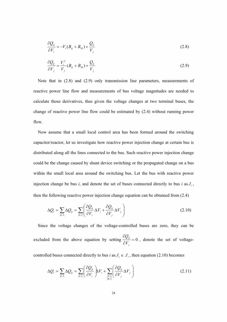
Note that in (2.8) and (2.9) only transmission line parameters, measurements of

reactive power line flow and measurements of bus voltage magnitudes are needed to

calculate those derivatives, thus given the voltage changes at two terminal buses, the

change of reactive power line flow could be estimated by (2.4) without running power

flow.

Now assume that a small local control area has been formed around the switching

capacitor/reactor, let us investigate how reactive power injection change at certain bus is

distributed along all the lines connected to the bus. Such reactive power injection change

could be the change caused by shunt device switching or the propagated change on a bus

within the small local area around the switching bus. Let the bus with reactive power

injection change be bus i, and denote the set of buses connected directly to bus i as iJ ,

then the following reactive power injection change equation can be obtained from (2.4)

∑∑∈∈

⎟⎟⎠

⎞⎜⎜⎝

⎛∆

∂

∂+∆

∂

∂=∆=∆

ii Jjj

j

iji

i

ij

Jjiji V

VQ

VVQ

QQ (2.10)

Since the voltage changes of the voltage-controlled buses are zero, they can be

excluded from the above equation by setting 0=∂

∂

j

ij

VQ

, denote the set of voltage-

controlled buses connected directly to bus i as ic JJ ∈ , then equation (2.10) becomes

∑∑∑∉∈∈∈

⎟⎟⎠

⎞⎜⎜⎝

⎛∆

∂

∂+∆⎟⎟

⎠

⎞⎜⎜⎝

⎛∂

∂=∆=∆

ciii

JjJj

jj

iji

Jj i

ij

Jjiji V

VQ

VVQ

QQ (2.11)

25

If bus i is a boundary bus of the local control area, because of the local nature of the

reactive power change, we could assume that the voltage change of an outside bus j

connected to the boundary bus can be approximated by ijj VV ∆=∆ α with a constant α

between 0 and 1. Denote the set of outside buses connected directly to bus i as io JJ ∈ ,

then equation (2.11) can be written as

∑∑∑∑∉∈

∉∈∈∈

⎟⎟⎠

⎞⎜⎜⎝

⎛∆

∂

∂+∆

⎥⎥⎥

⎦

⎤

⎢⎢⎢

⎣

⎡

⎟⎟⎠

⎞⎜⎜⎝

⎛

∂

∂+⎟⎟

⎠

⎞⎜⎜⎝

⎛∂

∂=∆=∆

ci

coii

JjJj

jj

iji

JjJj

jj

ij

Jj i

ij

Jjiji V

VQ

VVQ

VQ

QQ α (2.12)

Finally assume that the small local control area around the switching capacitor/reactor

has N buses inside, the following vector-form equation can be derived from (2.12)

⎥⎥⎥⎥

⎦

⎤

⎢⎢⎢⎢

⎣

⎡

∆

∆∆

⎥⎥⎥⎥

⎦

⎤

⎢⎢⎢⎢

⎣

⎡

=

⎥⎥⎥⎥

⎦

⎤

⎢⎢⎢⎢

⎣

⎡

∆

∆∆

NNNNN

N

N

N V

VV

BBB

BBBBBB

Q

QQ

M

L

MOMM

L

L

M2

1

21

22221

11211

2

1

(2.13)

where

NiVQ

VQ

B

coi

JjJj

jj

ij

Jj i

ijii ,...,2,1; =

⎥⎥⎥

⎦

⎤

⎢⎢⎢

⎣

⎡

⎟⎟⎠

⎞⎜⎜⎝

⎛

∂

∂+⎟⎟

⎠

⎞⎜⎜⎝

⎛∂

∂= ∑∑

∉∈∈

α (2.14)

NiJj

JjVQ

B

c

cj

ij

ij ,...,2,1;;0

;=

⎪⎩

⎪⎨⎧

∈

∉∂

∂=

U

U (2.15)

Since the local area constructed is quite small, so is the number of buses inside N, thus

the following equation can be used to estimate the voltage changes on the buses inside

the control area very quickly

[ ] [ ] QSQBV ∆=∆=∆ −1 (2.16)

26

where [ ]0,...,0,,0,...,0 shQQ =∆ is the vector of reactive power injection changes with

switching device’s capacity denoted as shQ .

2.1.2 Estimation of Transformer Tap Changing Effects

For transformer, reactive power line flow equation (2.3) needs some modification to

include transformer ratio or tap position such that they can be used to estimate the effects

of transformer tap changing. Let the transformer between bus i and bus j be represented

by π-equivalent model with the transformer ratio t , the original transformer

admittance TTT jBGY += , the equivalent line admittance ijijij jBGY += , and shunt

admittances 000 iii jBGY += and 000 jjj jBGY += as shown in Figure 2.2.

Figure 2.2 Power transformer line π-equivalent model.

The relationship between the original transformer’s parameters and the equivalent line

model’s parameters can be written as

tB

BBt

GGG T

jiijT

jiij ==== ; (2.17)

20201;1t

tBBt

tGG TiTi−

=−

= (2.18)

27

ttBB

ttGG TjTj

1;100

−=

−= (2.19)

Substitute (2.17), (2.18) and (2.19) to (2.3), the equations for reactive power line flows

of both directions are

)cossin(22

ijT

ijT

jiT

iij tB

tGVV

tBVQ δδ −−−= (2.20)

)cossin(2ji

Tji

TijTjji t

Bt

GVVBVQ δδ −−−= (2.21)

Assume that reactive line flow changes of transformer line are related only to terminal

voltage changes and transformer ratio change (or equivalently the reactive line flow

changes caused by factors other than voltage and ratio changes are close to zero), then the

linearized reactive power line flow equations for transformer can be derived from (2.20)

and (2.21) and written as

0),,( =∆∂

∂+∆

∂

∂+∆

∂

∂=∆∆∆∆=∆ j

j

iji

i

ijijjiijij V

VQ

VVQ

tt

QtVVQQ (2.22)

0),,( =∆∂

∂+∆

∂

∂+∆

∂

∂=∆∆∆∆=∆ i

i

jij

j

jijiijjiji V

VQ

VVQ

tt

QtVVQQ (2.23)

where

i

jijjij

j

ji

j

ijiiji

i

ij

VQ

BBVVQ

VQ

BBVVQ

++−=∂

∂++−=

∂

∂)(;)( 00 (2.24)

i

jijji

i

j

i

ji

j

ijiij

j

i

j

ij

VQ

BBVV

VQ

VQ

BBVV

VQ

++=∂

∂++=

∂

∂)(;)( 0

2

0

2

(2.25)

tQ

BBt

Vt

QB

tV

tQ ij

iijiij

Tiij −+=−=

∂

∂)( 0

2

3

2

(2.26)

tQ

BBt

Vt

QB

tV

tQ ji

jjijji

Tjji −+−=−−=

∂

∂)( 0

22

(2.27)

28

Note that in (2.24) – (2.27) only transformer line parameters, transformer ratio, and

measurements of reactive power line flows and bus voltage magnitudes are needed to

calculate these derivatives. In fact, (2.24) and (2.25) are exactly same as the equations

(2.8) and (2.9) in transmission line reactive power flow model. If we define virtual

reactive power injection changes caused by transformer ratio change at two terminal

buses of the transformer line as tt

QQ ij

Ti ∆∂

∂−=∆ and t

tQ

Q jiTj ∆

∂

∂−=∆ , then equations

(2.22) and (2.23) become

jj

iji

i

ijijTi V

VQ

VVQ

tt

QQ ∆

∂

∂+∆

∂

∂=∆

∂

∂−=∆ (2.28)

ii

jij

j

jijiTj V

VQ

VVQ

tt

QQ ∆

∂

∂+∆

∂

∂=∆

∂

∂−=∆ (2.29)

Comparing equations (2.28) and (2.29) with equation (2.4), it is obvious that they are

almost same, thus the effects of transformer tap changing can be approximated in a way

similar to the one used for capacitor/reactor switching. For a transformer tap change, the

corresponding transformer ratio change is a fixed value, thus transformer tap changing

action is in effect equivalent to two constant reactive power injection changes at both

ends of the transformer line. With this consideration, the voltage changes on the buses

inside the local control area around the LTC transformer can be estimated using

equations (2.13) – (2.16) with the only difference in vector of injection changes

[ ] ⎥⎦

⎤⎢⎣

⎡∆

∂

∂−∆

∂

∂−=∆∆=∆ 0,...,,...,,...,00,...,,...,,...,0 t

tQ

tt

QQQQ jiij

TjTi (2.30)

2.1.3 Estimation of Generator Voltage Adjusting Effects

29

For generators, the terminal voltage setpoint adjusting values GiQ∆ , instead of reactive

power injection changes GiV∆ , on the control generator buses are known. To estimate the

effects of generator voltage setpoint adjusting in a way similar to that of capacitor/reactor

switching, the generator bus is temporarily treated as PQ bus with variable shunt capacity.

With an initial guess of reactive power injection change 0GiV∆ , the voltage changes on the

buses within local area (including control generator bus i) can be estimated by (2.13) –

(2.16), and the generator reactor power output change can be updated with following

equation until the difference becomes less than certain tolerance.

mGi

Gim

Gi

GimGi Q

VVV

Q ∆∆+∆

∆=∆ + 21 (2.30)

In summary, a local voltage estimator (LVE) has been formulated to approximate the

effects of the shunt switching, LTC transformer tap changing and generator voltage

setpoint adjusting in a unified way. By treating these control actions as some reactive

power injection changes inside their local control areas, the local voltage estimator is able

to predict the bus voltage changes using linearized computations based only on the local

measurements from SCADA before control actions.

2.2 Feasibility Studies of the Local Voltage Estimator

In this section, the local voltage estimator formulated in the last section will be

evaluated with numerical examples. The standard IEEE 30-bus system and an actual

WECC 2001-2003 Winter (case ID 213SNK) planning case will be used to test the

accuracy and feasibility of the local voltage estimator formulation. The simulations of

local voltage estimator and power flow on IEEE 30 bus system are all done with

30

MATLAB programs, while the simulations of local voltage estimator and power flow on

WECC system are done with C/C++ program and BPA Power Flow package [39].

2.2.1 Tests on IEEE 30 Bus System

The standard IEEE 30-bus system is a widely used test case for power system

researchers. The system data is available at the website of power research group of

University of Washington [34], the system one-line diagram is shown in Figure A.1 of

Appendix A. The local control areas are chosen such that the buses within 3 tiers of the

control bus are included. Before the tests on the local voltage estimator, let us choose a

proper parameterα for this system to approximate the voltage changes on outside buses.

The results are shown as in the following table

Bus 10 (19 Mvar) Bus 24 (4.3 Mvar)

α Max error Total error Max error Total error

0.75 25 0.0039 0.0244 20 -0.0018 0.0044

0.85 12 0.0031 0.0167 24 -0.0015 0.0028

0.95 19 -0.0053 0.0270 24 -0.0019 0.0032

Table 2.1 Selection of estimation parameters for IEEE 30 bus system.

It is obvious from the above table that 85.0=α is the best for this system in terms of

both maximum error and total error and will be applied in the following tests. The IEEE

30 bus test case is slightly modified to facilitate the test. All capacitors are switched out

and all voltage setpoints of generators are set to 0.01 lower than their original values. The

tests include switching in each of the shunt capacitors, changing ratios of each

transformer, and adjusting voltage setpoints of all generators. Table 2.2, Table 2.3 and

Table 2.4 show the simulation results.

31

First tier buses and Max error bus Control

Cap. Action Tier Bus V0 VPF VLVE VERR

Total err

1 6 1.0080 1.0102 1.0103 -0.0001

1 9 1.0397 1.0509 1.0513 -0.0004

1 10 1.0233 1.0451 1.0460 -0.0009

1 17 1.0206 1.0399 1.0400 -0.0002

1 20 1.0116 1.0297 1.0319 -0.0021

1 21 1.0118 1.0327 1.0334 -0.0007

1 22 1.0127 1.0332 1.0339 -0.0006

10 19

Mvar In

3 18 1.0138 1.0281 1.0317 -0.0035

0.0152

1 22 1.0283 1.0332 1.0329 0.0003

1 23 1.0214 1.0272 1.0275 -0.0003

1 24 1.0124 1.0216 1.0227 -0.0012

1 25 1.0110 1.0173 1.0176 -0.0003

24 3.4

Mvar In

3 20 1.0263 1.0297 1.0283 0.0014

0.0037

Table 2.2 Estimation results for capacitor switching on IEEE 30 bus system.

First tier buses and Max error bus Control LTC Action

Tier Bus V0 VPF VLVE VERR Total err

1 4 1.0119 1.0117 1.0116 0.0001

1 6 1.0107 1.0102 1.0102 0.0000

1 7 1.0026 1.0024 1.0023 0.0000

1 9 1.0472 1.0509 1.0506 0.0003

1 10 1.0428 1.0451 1.0449 0.0002

1 28 1.0071 1.0068 1.0067 0.0001

6-9 0.978

to 0.988

3 15 1.0367 1.0377 1.0369 0.0008

0.0025

1 3 1.0217 1.0207 1.0208 -0.0001

1 4 1.0129 1.0117 1.0118 -0.0001

1 6 1.0106 1.0102 1.0102 0.0000

1 12 1.0541 1.0571 1.0565 0.0006

4-12 0.932

to 0.942

3 20 1.0283 1.0297 1.0285 0.0012

0.0034

Table 2.3 Estimation results for LTC tap changing on IEEE 30 bus system.

32

First tier buses and Max error bus Control Gen. Action

Tier Bus V0 VPF VLVE VERR Total err

1 2 1.0330 1.0430 1. 0430 0.0000

1 4 1.0089 1.0117 1.0114 0.0003

1 6 1.0083 1.0102 1.0100 0.0003 2

1.0330 To

1.0430 3 20 1.0284 1.0297 1.0290 0.0007

0.0025

1 5 1. 0000 1. 0100 1. 0100 0.0000

1 7 0.9976 1.0024 1.0023 0.0001 5 1.0000

to 1.0100 3 12 1.0567 1.0571 1.0569 0.0002

0.0003

1 6 1.0047 1.0102 1.0101 0.0001

1 8 1. 0000 1. 0100 1. 0100 0.0000

1 28 1.0003 1.0068 1.0066 0.0002 8

1.0000 to

1.0100 3 20 1.0266 1.0297 1.0283 0.0014

0.0023

1 9 1.0468 1.0509 1.0509 0.0000

1 11 1. 072 1. 0820 1. 0820 0.0000 11 1.0720

to 1.0820 3 20 1.0274 1.0297 1.0294 0.0003

0.0000

1 12 1.0515 1.0571 1.0572 -0.0001

1 13 1. 061 1. 0710 1. 0710 -0.0000 13 1.0610

to 1.0710 3 17 1.0369 1.0399 1.0403 -0.0004

0.0006

Table 2.4 Estimation results for generator voltage adjusting on IEEE 30 bus system.

In above tables, V0 are the voltages before any control actions, VPF are the voltages

after control actions obtained from power flow, VLVE are the estimated voltages after

control actions given by local voltage estimator, and VERR are normalized estimation

errors. The total error shown is the summation of the absolute estimation errors on the

local buses excluding the boundary buses (tier 3 buses).

From above tables, it can be seen that the estimation errors for most local buses are

quite small, especially for those buses in the first tier. The maximum errors usually occur

on the boundary buses (tier 3 buses), which may caused by our approximation using a

constantα for all boundary buses. The errors could be further reduced by using different

parameters for each boundary buses. Also it is observed that the total error increases as

33

the switching capacity increases in table 2.2, which is reasonable due to the linearization

model. The results could be improved by extending the computations to say four or five

tier local subsystems instead of the three tier networks used in the study above.

2.2.2 Tests on WECC System

The simulations are based on WECC 2001-2003 Winter (case ID 213SNK) planning

case which has more than 6000 buses in the system. For the part of the system of our

interest, west Oregon area of WECC northwest system has dozens of 230KV, 115 KV

and 69 KV capacitor banks, a couple of 500 KV reactor banks, a few 500/230-kV and

230/115-kV LTC autotransformers. Part of the one-line diagram for the west Oregon area

of WECC northwest system is shown in Figure 2.3. For test purpose, the local control

areas are constructed such that the buses within 6 tiers of the control bus are included. To

facilitate the test, a base case is setup by modifying the original planning case slightly.

All capacitors are switched out and reactors are switched in, the voltage setpoints of

generators are also adjusted a little bit different from their original values.

Figure 2.3 Part of the one-line diagram for the west Oregon area of WECC.

34

First the local voltage estimator is applied to capacitor/reactor switching and part of the

tests results on the base case and several modified cases under different topology and

loading conditions are shown in Table 2.5, Table 2.6 and Table 2.7.

Base Case [213snk0b]: All capacitors are OFF, all reactors are ON.

α = 0.85 α = 0.98 Tier Bus Name V0 VPF

VLVE Err% VLVE Err%

ALVEY 230 capacitor [58.9 Mvar] switching IN.

1 ALVEY 230 1.0200 1.0250 1.0245 0.0452 1.0251 -0.0125

2 ALVEY 115 1.0250 1.0290 1.0283 0.0715 1.0289 0.0139

2 ALVEY 500 1.0750 1.0780 1.0773 0.0666 1.0779 0.0079

2 E SPRING 230 1.0210 1.0260 1.0251 0.0895 1.0257 0.0337

2 LANE 230 1.0220 1.0260 1.0249 0.1102 1.0254 0.0564

2 MARTINTP 230 1.0200 1.0250 1.0236 0.1364 1.0242 0.0811

2 MCKEN TP 230 1.0130 1.0170 1.0166 0.0403 1.0172 -0.0224

2 SPENCER 230 1.0200 1.0250 1.0245 0.0536 1.0250 -0.0045

MARION 500 reactor [-149.0 Mvar] switching OUT.

1 MARION 500 1.0750 1.0820 1.0805 0.1397 1.0810 0.0907

2 ALVEY 500 1.0750 1.0800 1.0788 0.1145 1.0796 0.0416

2 ASHE 500 1.0860 1.0870 1.0860 0.0000 1.0860 0.0000

2 BUCKLEY 500 1.0910 1.0930 1.0924 0.0525 1.0927 0.0273

2 JOHNDAY 500 1.0900 1.0900 1.0900 0.0000 1.0900 0.0000

2 LANE 500 1.0730 1.0790 1.0770 0.1894 1.0778 0.1117

2 PEARL 500 1.0770 1.0800 1.0787 0.1171 1.0790 0.0914

2 SANTIAM 500 1.0740 1.0810 1.0794 0.1505 1.0799 0.1008

Table 2.5 Estimation results for capacitor switching on WECC Base Case.

Case #1 [213snk0b1]: Line JOHN DAY 500 – MARION 500 out of service, Load change on ALVEY 115 [PL = 300 MW, QL = 100 MW], DIXONVLE 115 [PL = 259 MW, QL = 107 MW].


VLVE Err% VLVE Err%

ALBANY 115 capacitor [50.0 Mvar] switching IN.

1 ALBANY 115 0.9920 1.0080 1.0028 0.4914 1.0042 0.3790

2 ADAIR 115 0.9910 1.0060 0.9995 0.6237 1.0010 0.5036

35

2 ALBANY 230 0.9780 0.9890 0.9854 0.3375 0.9867 0.2306

2 BURNTWD 115 0.9910 1.0070 1.0018 0.4909 1.0033 0.3783

2 CONSER 115 0.9940 1.0080 1.0026 0.5128 1.0041 0.3933

2 HARRISBG 115 0.9840 0.9940 0.9893 0.3076 0.9925 0.1551

2 HAZELWOD 115 0.9910 1.0080 1.0017 0.6017 1.0032 0.4891

2 LOCKNER 115 0.9940 1.0100 1.0039 0.5821 1.0052 0.4792

MARION 500 reactor [-248.0 Mvar] switching OUT.

1 MARION 500 1.0600 1.0740 1.0706 0.3207 1.0718 0.2114

2 ALVEY 500 1.0600 1.0710 1.0672 0.3547 1.0688 0.2039

2 ASHE 500 1.0830 1.0840 1.0830 0.0000 1.0830 0.0000

2 BUCKLEY 500 1.0840 1.0870 1.0867 0.0250 1.0873 -0.0266

2 LANE 500 1.0540 1.0670 1.0616 0.5086 1.0634 0.3457

2 PEARL 500 1.0710 1.0770 1.0744 0.2460 1.0749 0.1915

2 SANTIAM 500 1.0590 1.0730 1.0694 0.3417 1.0705 0.2315

Table 2.6 Estimation results for capacitor switching on WECC Case #1.

Case #2 [213snk0b2]: Base on Case #1, Load change on ALVEY 115 [PL = 600 MW, QL = 200 MW].


VLVE Err% VLVE Err%

TOLEDO 69.0 capacitor [15.4 Mvar] switching IN.

1 TOLEDO 69.0 0.9430 0.9560 0.9563 -0.0359 0.9566 -0.0644

2 TOLEDO 230 0.9550 0.9660 0.9645 0.1568 0.9648 0.1289

3 WENDSON 230 0.9860 0.9900 0.9887 0.1338 0.9889 0.1106

3 WREN 230 0.9700 0.9770 0.9762 0.0823 0.9765 0.0532

4 LANE 230 0.9800 0.9820 0.9805 0.1507 0.9809 0.1112

4 TAHKNICH 230 0.9990 1.0040 1.0005 0.3509 1.0006 0.3381

4 WENDSON 115 0.9900 0.9940 0.9919 0.2087 0.9922 0.1839

4 SANTIAM 230 0.9980 0.9990 0.9987 0.0282 0.9990 -0.0027

DIXONVLE 500 reactor [-149.0 Mvar] switching OUT.

1 DIXONVLE 500 1.0520 1.0690 1.0642 0.4578 1.0653 0.3481

2 ALVEY 500 1.0450 1.0570 1.0524 0.4354 1.0536 0.3225

2 DIXONVLE 230 0.9910 1.0030 0.9986 0.4478 0.9997 0.3296

2 MERIDINP 500 1.0730 1.0850 1.0814 0.3392 1.0824 0.2398

Table 2.7 Estimation results for capacitor switching on WECC Case #2.

36

Next, we apply the local voltage estimator with modification for LTC transformer to

west Oregon area of WECC northwest system. The simulations are done on base case and

several modified cases, part of the results are given below in Table 2.8, Table 2.9, Table

2.10 and Table 2.11.

Base Case [213snk0b]: All capacitors are OFF, all reactors are ON.


VLVE Err% VLVE Err%

ALVEY 230 →|− ALVEY 115 (3) LTC tap DOWN from 4/9 to 3/9. 1 ALVEY 230 1.0200 1.0190 1.0189 0.0098 1.0189 0.0107

2 ALVEY 115 1.0250 1.0280 1.0278 0.0157 1.0279 0.0110

2 ALVEY 500 1.0750 1.0750 1.0745 0.0477 1.0744 0.0536

2 E SPRING 230 1.0210 1.0210 1.0200 0.0961 1.0200 0.0975

2 LANE 230 1.0220 1.0230 1.0219 0.1076 1.0219 0.1056

2 MARTINTP 230 1.0200 1.0200 1.0191 0.0856 1.0191 0.0883

2 MCKEN TP 230 1.0130 1.0130 1.0126 0.0350 1.0126 0.0346

2 SPENCER 230 1.0200 1.0190 1.0189 0.0077 1.0189 0.0089

Table 2.8 Estimation results for transformer tap changing on WECC Base Case.

Case #1 [213snk0b1]: Line JOHN DAY 500 – MARION 500 out of service, Load change on ALVEY 115 [PL = 300 MW, QL = 100 MW], DIXONVLE 115 [PL = 259 MW, QL = 107 MW].


VLVE Err% VLVE Err%

DIXONVLE 230 →|− DIXONVLE 115 (1) LTC tap DOWN from 11/17 to 10/17.

1 DIXONVLE 230 1.0010 1.0000 1.0003 -0.0319 1.0003 -0.0270

2 DIXONVLE 115 1.0100 1.0150 1.0145 0.0525 1.0144 0.0565

2 DIXONVLE 500 1.0640 1.0640 1.0637 0.0237 1.0637 0.0284

2 HANNA 230 1.0130 1.0130 1.0125 0.0499 1.0124 0.0559

2 RESTON 230 1.0030 1.0020 1.0025 -0.0501 1.0025 -0.0452

2 SPENCER 230 0.9990 0.9990 0.9989 0.0135 0.9988 0.0192

Table 2.9 Estimation results for transformer tap changing on WECC Case #1.

37



VLVE Err% VLVE Err%

ALVEY 230 →|− ALVEY 115 (4) LTC tap DOWN from 4/9 to 3/9.

1 ALVEY 230 0.9760 0.9750 0.9749 0.0098 0.9749 0.0117

2 ALVEY 115 0.9580 0.9620 0.9606 0.1432 0.9607 0.1394

2 ALVEY 500 1.0450 1.0450 1.0445 0.0503 1.0444 0.0570

2 E SPRING 230 0.9790 0.9790 0.9780 0.1002 0.9780 0.1026

2 LANE 230 0.9800 0.9810 0.9799 0.1160 0.9799 0.1149

2 MARTINTP 230 0.9820 0.9810 0.9811 0.0132 0.9811 -0.0097

2 MCKEN TP 230 0.9670 0.9680 0.9666 0.1427 0.9666 0.1434

2 SPENCER 230 0.9760 0.9760 0.9749 0.1102 0.9749 0.1123


1 ALVEY 500 1.0450 1.0430 1.0415 0.1441 1.0417 0.1196

2 ALVEY 230 0.9760 0.9810 0.9793 0.1709 0.9799 0.1144

2 DIXONVLE 500 1.0520 1.0500 1.0494 0.0539 1.0496 0.0388

2 MARION 500 1.0480 1.0480 1.0469 0.1088 1.0470 0.0912




VLVE Err% VLVE Err%

DIXONVLE 230 →|− DIXONVLE 115 (2) LTC tap DOWN from 11/17 to 10/17.

1 DIXONVLE 230 0.9760 0.9760 0.9753 0.0722 0.9752 0.0774

2 DIXONVLE 115 0.9900 0.9940 0.9947 -0.0745 0.9947 -0.0702

2 DIXONVLE 500 1.0360 1.0350 1.0357 -0.0714 1.0357 -0.0665

2 HANNA 230 0.9970 0.9970 0.9965 0.0524 0.9964 0.0586

2 RESTON 230 0.9810 0.9800 0.9805 -0.0496 0.9804 -0.0445

2 SPENCER 230 0.9470 0.9470 0.9469 0.0147 0.9468 0.0209


1 ALVEY 500 1.0260 1.0250 1.0224 0.2539 1.0226 0.2303

2 ALVEY 230 0.9460 0.9520 0.9493 0.2875 0.9498 0.2311

2 DIXONVLE 500 1.0360 1.0350 1.0334 0.1586 1.0335 0.1446

2 MARION 500 1.0360 1.0360 1.0348 0.1144 1.0350 0.0975


38

Finally the modified local estimator for generators is applied to west Oregon area of

WECC northwest system and part of the tests results on the base case and several

modified cases are shown in Table 2.12, Table 2.13, Table 2.14 and Table 2.15.

Base Case [213snk0c]: All capacitors are OFF, all reactors are ON.


VLVE Err% VLVE Err%

BIG EDDY 230 generator voltage setpoint UP from 1.050 to 1.060.

1 BIG EDDY 230 1.0500 1.0600 1.0600 0.0000 1.0600 0.0000

2 BIG EDDY 500 1.0720 1.0770 1.0775 -0.0473 1.0775 -0.0475

2 CELILO 230 1.0510 1.0610 1.0594 0.1549 1.0594 0.1548

2 CHEMAWA 230 0.9920 0.9950 0.9929 0.2118 0.9931 0.1910

2 CHENOWTH 230 1.0420 1.0510 1.0505 0.0439 1.0506 0.0381

2 MABTON 230 1.0450 1.0480 1.0482 -0.0166 1.0482 -0.0173

2 MAUPIN 230 1.0490 1.0570 1.0563 0.0631 1.0564 0.0542

2 MCLOUGLN 230 1.0380 1.0380 1.0389 -0.0861 1.0390 -0.0952

2 PARKDALE 230 1.0410 1.0480 1.0479 0.0128 1.0479 0.0128

Table 2.12 Estimation results for generator voltage adjusting on WECC Base Case.

Case #1 [213snk0c1]: Line JOHN DAY 500 – MARION 500 out of service.


VLVE Err% VLVE Err%

JOHN DAY 500 generator voltage setpoint UP from 1.050 to 1.060.

1 JOHN DAY 500 1.0500 1.0600 1.0600 0.0000 1.0600 0.0000

2 BIG EDDY 500 1.0720 1.0760 1.0720 0.3720 1.0720 0.3718

2 GRIZZLY 500 1.0770 1.0800 1.0776 0.2183 1.0778 0.2087

2 HANFORD 500 1.0810 1.0830 1.0810 0.1840 1.0810 0.1838

2 MARION 500 1.0620 1.0660 1.0637 0.2144 1.0638 0.2060

2 SLATT 500 1.0740 1.0790 1.0765 0.2298 1.0765 0.2287

Table 2.13 Estimation results for generator voltage adjusting on WECC Case #1.

39

Case #2 [213snk0c2]: Base on Case #1, Load change on ALVEY 115 [PL = 300 MW, QL = 100 MW], DIXONVLE 115 [PL = 259 MW, QL = 107 MW].


VLVE Err% VLVE Err%

BIG EDDY 230 generator voltage setpoint UP from 1.050 to 1.060.

1 BIG EDDY 230 1.0500 1.0600 1.0600 0.0000 1.0600 0.0000

2 BIG EDDY 500 1.0720 1.0780 1.0775 0.0461 1.0775 0.0459

2 CELILO 230 1.0510 1.0610 1.0594 0.1549 1.0594 0.1549

2 CHEMAWA 230 0.9830 0.9850 0.9839 0.1117 0.9841 0.0917

2 CHENOWTH 230 1.0420 1.0510 1.0505 0.0439 1.0506 0.0381

2 MABTON 230 1.0440 1.0470 1.0472 -0.0168 1.0472 -0.0175

2 MAUPIN 230 1.0490 1.0560 1.0563 -0.0313 1.0564 -0.0405

2 MCLOUGLN 230 1.0360 1.0370 1.0369 0.0098 1.0370 0.0012

2 PARKDALE 230 1.0410 1.0480 1.0479 0.0127 1.0479 0.0127


Case #3 [213snk0c3]: Base on Case #2, Load change on ALVEY 115 [PL = 600 MW, QL = 200 MW].


VLVE Err% VLVE Err%

JOHN DAY 500 generator voltage setpoint UP from 1.050 to 1.060.

1 JOHN DAY 500 1.0500 1.0600 1.0600 0.0000 1.0600 0.0000

2 BIG EDDY 500 1.0720 1.0760 1.0720 0.3720 1.0720 0.3718

2 GRIZZLY 500 1.0800 1.0870 1.0806 0.5891 1.0807 0.5797

2 HANFORD 500 1.0790 1.0810 1.0790 0.1843 1.0790 0.1842

2 MARION 500 1.0470 1.0510 1.0487 0.2185 1.0488 0.2102

2 SLATT 500 1.0720 1.0780 1.0745 0.3237 1.0745 0.3226


In above tables, V0 are the voltages before any control actions, VPF are the voltages

after each control actions obtained by running BPA power flow on the whole WECC

system. The estimated voltages VLVE after control actions given by local voltage estimator

40

and normalized estimation errors %100%PF

PFLVE

VVV

Err−

= under 85.0=α and 98.0=α are

also shown in the table.

From above tables, it can be seen that the estimated voltages in most buses of the

system under different conditions are quite close to the voltages obtained by running

power flow, and the results are better with 98.0=α than those with 85.0=α . The

estimation results for capacitor/reactor and generator voltage adjusting are generally

better than those for transformer tap changing. Actually, because the voltage changes

caused by the tap change are much smaller that those cause by switching

capacitor/reactor banks, the absolute voltage changes on some buses with very small

changes are different in direction from those obtained from running power flow. For the

buses with large enough voltage changes, the estimation results are still quite close to

power flow results.

It is also observed that in some cases, the estimated results are not very good. The

reason seems to be that in the formulation of the B matrix used in estimation algorithm,

the ‘BX’, ‘BQ’ and ‘BC’ type of buses are assumed to be PV buses, but this assumption

does not always hold in BPA power flow program [39]. The ‘BX’ type bus voltages are

controlled by switched capacitor/reactor banks and the voltages may not be constant

because the devices are discrete. The ‘BC’ and ‘BQ’ type voltages are controlled by

“BG’ generators or other reactive resources such as static var compensators (SVC), if the

reactive powers or generator voltages hit the limits, the ‘BC’ and ‘BQ’ type bus voltages

may be far from their setpoint values. Also the ‘BG’ type buses change their voltage

setpoint values automatically, which cause voltages of the surrounding buses change

accordingly. Besides, there are some buses with regulating transformers (e.g. LANE 230,

41

MCKEN TP 230, etc) change their voltage automatically in BPA power flow, although

the solution option of the program is set to turning on DC line terminal transformer

automatic control only.

2.3 Summary

A local voltage estimator has been formulated based on linearized reactive power flow

model. For each device, a small local area is constructed and local voltage estimator is

used to evaluate the switching effects. The local estimator treats switching of

capacitor/reactor, adjusting LTC tap and generator voltage setting in a unified way, and is

able to approximate voltage changes after a switching action based only on the local

measurements from SCADA before switching. The accuracy and feasibility of the local

voltage estimator formulation are proven by the simulation results on the standard IEEE

30-bus system and the actual WECC planning case.

42

Chapter 3

Alternate Heuristic Voltage Control

The discrete slow voltage controller proposed in [31] relies on the availability of state

estimator model to make correct control decisions. In practice, state estimator model

maybe unavailable or unreliable because of topology errors under certain conditions.

With the local voltage estimator (LVE) formulated in last chapter, the effects of any

control actions can be evaluated without state estimator model, thus make a model-free

voltage control scheme possible under such conditions. In this chapter, an alternate on-

line heuristic slow voltage controller is formulated to make control decisions based on

SCADA measurements only. In section 3.1, a common slow voltage control framework

integrated the model-based controller and the alternate controller is presented. The

optimization problem of the alternate voltage control is formulated in Section 3.2. The

feasibility tests results on small and large power systems are given in Section 3.3. Finally,

Section 3.4 summarizes the conclusions of this chapter.

3.1 On-line Slow Voltage Control Framework

Since the goal of on-line slow voltage control is to automate actions of an alert and

experienced operator, it is necessary to briefly review the current operation practice on

western Oregon subsystem in Pacific Northwest before introducing the slow voltage

controller framework. This part of system is a large load area without significant local

43

generation. Power is imported from other parts of Pacific Northwest and western Canada.

There are tens of small capacitor/reactor banks and LTC transformers available for

voltage control purpose in this area. During normal operation, voltage problems are

alleviated by reactive compensation performed by system operators based on their

experience, current and predicted network conditions. Switching out in-service devices is

preferable than switching in alternate devices such that the maximum number of devices

are available for future exercises. Tap changing has lower priority than reactive power

compensation switching and tap changing frequency is restricted to several tap changes

per day because tap changer failure results in transformer outage. Circular VAR flows are

monitored by routinely checking the VAR flows on specific transformer banks and

transmission paths and are mitigated by switching of capacitor banks or transformer tap

changer settings.

Figure 3.1 Common on-line slow voltage control framework.

44

The common slow voltage control framework integrated the state estimator model-

based controller and the alternate heuristic controller is shown in Figure 3.1. The

controller is intended to be used for “slow” control and has a time frame of tens of

seconds or a few minutes. Similar to a system operator, the automatic controller primarily

acts upon voltage alarms and checks SCADA measurements for the acceptability of the

system voltage profile. As a first step, the controllers can be required to process only the

voltage alarms. Other types of alarms relating to outages and contingencies can be

handled directly by the system operators.

The common slow voltage controller consists of two sub-controllers that operate

independently. Under normal conditions when state estimator program has valid results,

the model-based controller will act as main controller and its control decisions will be

cross-checked against the outputs of the alternate controller. If the control decisions made

by the two controllers are different but similar, the decisions made by model-based

controller will be adopted. If there are significant differences between the actions

recommended by the two controllers, the system operator will be notified and responsible

for making the final control decisions. When the state estimator model is unavailable or

unreliable because of topology errors under certain conditions, the model-based

controller will go into standby state, and the backup alternate controller will take over to

make control decisions based on SCADA measurements only.

The model-based controller proposed in [31] calculates the incremental changes in bus

voltages after switching control devices by carrying out an adaptive local power-flow

starting from the system model output of the state estimation program. Then these

incremental changes are assessed with respect to actual SCADA measurements to

45

compute the expected voltage profile after the switching actions. In order to reduce the

number of switchings during periods of rapid load growths and declines (for instance,

during morning and evening pick-ups), load forecasting estimates for individual loads in

the area are computed using existing distribution factor formulas and the system total

load forecast available from the EPRI AGC load forecasting program. These forecasted

loads are then used to form a set of possible future power flow cases in the robust

formulation of the controller and each future power-flow case is associated with a

confidence level that gradually increases after verifying its reliability during operation.

The model-based controller decides whether any control action is necessary by

analyzing the SCADA measurement data and the expected voltage levels from future

power-flow runs. If an action is required, a subset of candidate control devices which will

have an impact on the problem is selected by using the concept of electrical distance. The

controller as formulated minimizes the switching cost associated with these devices while

keeping the voltage feasible in a robust sense by incorporating load forecast models, and

while minimizing circular reactive flow through transformers. Specifically, the penalty

for switching each device is a weighted average of the following terms: 1) switching

penalty based on the switching history and the type of the device, 2) voltage violation

penalty based on expected voltages after switching from state estimation power-flow

model and future power-flow models, and 3) circular VAR flow penalty computed from

the state estimation power-flow model and future power-flow models. Switching action

on the device with the minimum penalty will be recommended by the controller.

The alternate controller, in contrast, calculates the incremental changes in bus voltages

after switching control devices using local voltage estimator proposed in last chapter

46

based purely on the available local measurements from SCADA. The expected voltages

after the switching actions also can be computed directly by adding the incremental

changes to the actual SCADA voltage measurements. The following flowchart shows the

computation procedure of the alternate voltage controller.

Figure 3.2 Alternate on-line slow voltage controller flowchart.

By checking the SCADA voltage measurements, the alternate controller first decides

whether there is any voltage outside a specified band around some “optimal” voltage

profile. If any voltage violation exists, the controller locates the bus with the worst

violation, forms a problem area within several tiers of the bus, and tries to find a subset of

candidate control devices that will have an impact on the problem inside the area. If there

is no control device available, an alarm will be sent to the operator. Otherwise, a small

local control area will be formed for each control device, and the switching costs will be

47

calculated using the local voltage estimator (LVE) formulated in last chapter. The

controller as formulated minimizes the switching cost associated with these devices while

keeping the voltage as close as possible to the “optimal” profile. Specifically, the penalty

for any control device is a weighted average of the switching penalty calculated based on

the type and switching history of the device and the voltage violation penalty based on

expected voltages after switching obtained from local voltage estimator. Switching action

on the device with the minimum penalty is then recommended by the controller.

After issuing switching commands, the two sub-controllers will compare the voltages

after the switching with their expected voltages from the state estimation based

computations or local voltage estimator computations. Significant mismatches between

expected and actual voltage levels will be reported to the operator via alarms.

The main features of the common voltage controller are

1) Efficient automation of switching slow voltage control devices no matter state

estimator model is available or not.

2) Cross checking of the decisions made by two controllers to ensure correct control

device switching.

3) Loss minimization in the sense that voltage profile is maintained as close as

possible to the “optimal” profile.

4) Reactive reserve maximization in the sense that fewer reactive compensation

devices are switched in.

5) Operating cost minimization in a deregulated market.

3.2 Formulation of the Alternate Heuristic Control

48

Assuming that the desired “optimal” voltage profile dsrV , maximum voltage maxV , and

minimum voltage minV at each bus for different time periods of the day are pre-

determined through off-line studies, the proposed alternate heuristic control scheme is

designed to find the “best” control actions to keep all bus voltage within the pre-specified

limits while respecting some practical rules. This actually involves finding the available

candidate control devices inside the problem area and choosing effective control devices

by solving optimization problem.

LTC Transformer Shunt Problem

Type VTap > Vload VTap < Vload VTap = Vload Capacitor Reactor Generator

Vload High Tap Up Tap Down None Out In Vgen Down

Vload Low Tap Down Tap Up None In Out Vgen Up

Table 3.1 Rules to choose candidate device and its control action.

Some heuristic rules are used in searching for the candidate control devices. First, a

breadth-first search (BFS) algorithm [40] is employed to find all control devices within

several tiers around the problem center bus (i.e. the bus with worst violation), then some

rules are applied to determine the availability of a control device. For low-limit violating

voltage problem, only the in-service reactor banks and out-of-service capacitor banks are

chosen as shunt type candidate control devices, generators that do not reach their high

reactive power or voltage limits are chosen as generation type control devices. For a

transformer, if the tap-side nominal voltage is higher than the worst-violating bus

nominal voltage, then the transformer is selected only if its tap position does not reach its

low limits. If the tap-side nominal voltage is lower than the worst-violating bus nominal

49

voltage, then the transformer is selected only if its tap position does not reach its high

limit. Similar rules are also applied to low-limit violating voltage problem. By using

these selection rules, the number of available candidate control devices can be reduced so

as to speed up the computation. These rules are also used to determine proper direction of

a control action as shown in Table 3.1.

To choose “best” or most effective control actions by optimization, a cost needs to be

set for each control action, including capacitor/reactor bank switching, LTC transformer

tap changing and generator-controlled bus reference voltage adjusting, such that it

reflects the practical rules and preference used by system operators. In general, it is

preferable to switching out a device in service than switching in another so that maximum

numbers of control devices are available for control purposes at any time. Accordingly, a

higher cost is set for switching in a device as compared to switching out the same device.

Tap change should be avoided whenever the voltages can be maintained by switching of

capacitor/reactor banks alone, because the maintenance costs for transformer banks are

higher than those for capacitor banks and tap changer failure results in transformer outage.

If in some case tap changes have to be implemented, only one tap change is allowed each

time, which is consistent with the BPA operating policy. The switching costs for

transformer banks are thus set significantly higher than those for capacitor/reactor banks

in the formulation. The generator-controlled bus reference voltage adjusting also has

lower priority than capacitor/reactor bank switching. However, depending on being

within or outside the system, it may have higher or lower priority than LTC tap changing.

For all devices, switching cost increases substantially after one switching and the cost

50

then decreases slowly. This is used to prevent repeated switching in and out of the same

shunt device or adjusting tap of the same LTC transformer.

With the cost well defined above, now the problem of choosing “best” control actions

can be formulated as an integer programming optimization problem as follows

{ }1,0,1;

,...,1;:..

)(:min

1

max1

,0

min

1

−∈≤

=<∆+<

∑

∑

∑

=

=

=

isw

N

ii

j

N

ijijj

N

iiii

kNk

NjVVVVts

kCk

D

D

D

(3.1)

In the above formulation, ik represents the switching type: -1 for switching out

capacitor/reactor, one tap decrease of LTC or one step decrease of generator voltage

setting, 0 for no control action and +1 for switching in capacitor/reactor, one tap increase

of LTC or one step increase of generator voltage setting. )( ii kC denotes the cost of the ith

control device under control action type ik . 0jV is the bus voltage before control actions,

jiV ,∆ is the voltage change on jth bus caused control action of ith device, which can be

calculated using the local voltage estimator equation (2.16). DNN , and swN are the

number of buses inside the local area, the number of feasible control devices, and the

maximum number of control actions, respectively.

The objective of optimization as formulated is to find the minimum control cost while

keeping all the voltages within limits. However, it may turn out that for some power flow

scenario, no feasible solution exists. In this case, a penalty function can be defined to

indicate how far the solution is away from the feasibility region, as shown in Figure 3.3.

If the voltage at a bus is within limits, the penalty is zero. If it is too high or too low

51

(higher than maxV or lower than minV ) then a very large value 0P is set to the penalty term.

Between ),( maxVVhigh or ),( min lowVV , the penalty function is linear. For any control actions,

the estimated bus voltages are checked against their limits. If any violation exists, penalty

functions are calculated for all the voltage violating buses. The penalty cost is defined as

the norm of the voltage-violating vector. Either the summation of all the absolute value of

the voltage violation (i.e. normF 11 || ⋅ ) or the maximum absolute voltage violation

(i.e. ))|(| normF ∞∞ ⋅ can be used for this purpose. Here normF 11 || ⋅ is used to define the

penalty cost.

Figure 3.3 Penalty function of voltage violation

Now the optimization problem (3.1) can be transformed as follows

{ }1,0,1;:..

)()(:min

1

1 1,

−∈≤

⎥⎦

⎤⎢⎣

⎡∆+

∑

∑ ∑

=

= =

isw

N

ii

N

i

N

jjiiiii

kNkts

VPkCk

D

D

λ (3.2)

Here )( , jii VP ∆ denotes the voltage penalty value of jth bus under ith control action. λ

represents the weighting factor of voltage violation penalty cost. As noted earlier, the cost

)( ii kC for tap changing action is significantly higher than that for capacitor or reactor

52

bank switching action. Moreover, the cost associated with switching in a device

(with 1=ik ) is set higher than the cost for switching out a device (with 1−=ik ).

The optimization problem can also be formulated as minimizing active power loss or

maximizing reactive reserves. The formulation in (3.2) is equivalent to minimizing the

number of switching actions. In some sense, the formulation also maximizes the reactive

resource reserves in the subsystem, since (3.2) keeps the minimum number of control

devices in service, and therefore keeps the maximum number of control devices available

for future control exercises.

Algorithms for integer programming problems typically go through a sequence of steps,

with a set of choices at each step. However, using dynamic programming to determine

the best choices is overkill for many optimization problems; simple, more efficient

algorithms will do. A greedy algorithm always makes the choice that looks best at the

moment. That is, it makes a locally optimal choice in the hope that this choice will lead to

a globally optimal solution, but the greedy algorithm does not guarantee to yield globally

optimal solutions.

In (3.2), swN defines the maximum number of control actions, which are permitted in

any one of the iteration of the controller. For the formulation with 1>swN , the

optimization problem needs to be solved using dynamic programming algorithm.

However, swN is set to be 1 at present, since the operators usually hesitate to switch a

large number of devices at one time, and 1=swN is consistent with a conservative policy

for an automatic controller. With the maximum number of switching 1=swN , the solution

of optimization (3.2) becomes easy to handle. Basically, we evaluate voltage change after

the control action of each candidate control device by a local voltage estimator described

53

in Chapter 2 and select the one with minimum cost. This is equivalent to choose the

locally optimal control action at each step, so it is a greedy algorithm. Although the final

result is not necessarily the global optimum for this integer problem, it is good enough for

the backup controller. More importantly, this one device at a time conservative control

action make it easy for the operators to understand and to keep track of the decision taken

by the automatic controller.

3.3 Testing of the Alternate Voltage Controller

In this section, feasibility tests of the alternate voltage controller formulated in section

3.2 will be performed on the standard IEEE 30-bus system and an actual WECC 2001-

2003 Winter planning case (case ID 213SNK) with more than 6000 buses. The

simulations of alternate controller and power flow on IEEE 30 bus system are done with

MATLAB programs, while the simulations of alternate controller and power flow on

WECC system are conducted with C/C++ program and BPA Power Flow package [39].


The system data for the standard IEEE 30-bus system is available at the website of

power research group of University of Washington [34], and the system one-line diagram

is shown in Figure A.1 of Appendix A. Table 3.2 lists all control devices in IEEE 30 bus

system available for voltage control purpose and their initial settings.

Device Type Bus / Transformer Capacity / Range Setting / Status

Bus 10 19.0 OFF Capacitor

Bus 24 4.3 OFF

54

Bus 6 →|− Bus 9 0.938 ~ 1.018 0.988

Bus 6 →|− Bus 10 0.929 ~ 1.009 0.979

Bus4 →|− Bus 12 0.892 ~ 0.972 0.942 LTC

Transformer

Bus 28 →|− Bus 27 0.928 ~ 1.008 0.978

Bus 1 -80.0 ~ 100.0 Mvar 1.050

Bus 2 -40.0 ~ 50.0 Mvar 1.033

Bus 5 -40.0 ~ 40.0 Mvar 1.000

Bus 8 -100.0 ~ 40.0 Mvar 1.000

Bus 11 -6.0 ~ 24.0 Mvar 1.072

Generator

Bus 13 -6.0 ~ 24.0 Mvar 1.061

Table 3.2 Control devices available in IEEE 30 bus system.

In the following tests, the local control areas are chosen such that the buses within 3

tiers of the control bus are included. The step-sizes for LTC tap changing and generator

voltage adjusting are set to be 0.01 p.u. The costs of different control device’s actions are

calculated according the following rules: the cost for switching out a capacitor or reactor

bank is set to zero, the cost for switching in a capacitor or reactor bank is set to 10.0, the

cost for LTC tap changing is set to 20.0, and cost for generator voltage adjusting is set to

larger than 10.0, but may or may not larger than 20.0, depending the priority of the LTC

and generator. For any type of device, the cost of next action will increase by 5.0, and

decrease by 1.0 at each time step. The control objective is to maintain all bus voltages

within 2% band around the normal voltage profile, and the maximum allowed voltage

deviation is 5% away from the normal value. The voltage penalty coefficient λ is set to

1.0 and the maximum voltage penalty P0 is set to 1.0 for test purpose.

Many scenarios with different load levels, load distributions and topology have been

tested on the system. The results on one of the scenarios are shown in Table 3.3 and 3.4.

55

Tim Step ∆Vmax (Before Control) Control Device (Bus) Control

Action ∆Vmax (After Control)

Stage 1: Line 16 – 17 out of service

1 -0.0492 Bus 17 Bus 10 19 Mvar In -0.0279 Bus 24

2 -0.0279 Bus 24 Bus 24 4.3 Mvar In -0.0216 Bus 17

3 -0.0216 Bus 17 LTC Bus 28 →|− Bus 27 0.978→ 0.968 -0.0208 Bus 17

4 -0.0208 Bus 17 LTC Bus 6 →|− Bus 9 0.988→0.978 No Violation

Stage 2: Loads on Bus 16 and 17 increases by 50%.

5 - 0.0271 Bus 17 LTC Bus 6 →|− Bus 10 0.979→0.969 - 0.0249 Bus 17




9 - 0.0209 Bus 17 LTC Bus 6 →|− Bus 10 0.969→0.959 No Violation

Stage 3: Line 16 – 17 in service, loads on Bus 16 and 17 back to normal.

10 No Violation

Table 3.3 Results of voltage control on IEEE 30 bus system (A).



Stage 1: Line 16 – 17 out of service

1 -0.0492 Bus 17 Bus 10 19 Mvar In -0.0279 Bus 24

2 -0.0279 Bus 24 Bus 24 4.3 Mvar In -0.0216 Bus 17

3 -0.0216 Bus 17 Gen. Bus 11 1.072 →1.082 No Violation

Stage 2: Loads on Bus 16 and 17 increases by 50%.

4 - 0.0274 Bus 17 Gen. Bus 13 1.061 →1.071 - 0.0258 Bus 17

5 - 0.0258 Bus 17 Gen. Bus 8 1.000 →1.010 - 0.0222 Bus 17

6 - 0.0222 Bus 17 LTC Bus 6 →|− Bus 9 0.988→0.978 No Violation

Stage 3: Line 16 – 17 in service, loads on Bus 16 and 17 back to normal.

7 No Violation

Table 3.4 Results of voltage control on IEEE 30 bus system (B).

56

From above tables, it can be seen that the alternate controller correctly locates the

worst violation buses, identifies the most effective control devices with the lowest costs

at each step, and finally brings voltage back to normal range. For this system, capacitors

are switched in first; then LTC taps are changed or generator voltage setpoint are adjusted

depending on their relative priority. The effects of the relative priority are shown clearly

by the different control actions between Table 3.3 and Table 3.4 after step 3. In Table 3.4,

the switching costs of LTC tap changing and generator voltage adjusting are set equal,

thus the generators are chosen before LTCs as controls because the voltage penalties of

generator actions are smaller than that of LTC. In contrast, the switching costs of

generator voltage adjusting are set significantly higher than that of LTC tap changing in

Table 3.3, thus the LTCs are chosen to act before generators at each step. It is also noted

that the control steps taken in Table 3.4 are less than that in Table 3.3, since the adjusting

generator voltage setpoints is more effective than changing transformer taps in terms of

the bus voltage magnitude increments.


The WECC 2001-2003 Winter (case ID 213SNK) planning case has more than 6000

buses in the system, specifically west Oregon area of WECC northwest system has

dozens of 230KV, 115 KV and 69 KV capacitor banks, a couple of 500 KV reactor banks,

a few 500/230-kV and 230/115-kV LTC autotransformers. For test purpose, only parts of

these devices are selected as candidate devices for voltage control and a modified base

case is setup to facilitate the tests. Table 3.5 lists these control devices and their initial

settings. Note that the bus names listed as generator type controls are actually generator-

controlled high-side voltage buses, the control generators are shown in table 3.6.

57


ALBANY 115 50.0 OFF

ALVEY 115 19.5, 19.5, 25.6 OFF

ALVEY 230 58.9, 58.9, 58.9, 117.8 OFF

CHEMAWA 115 23.7 OFF


LANE 115 30.4 OFF

LANE 230 108.2 OFF

SANTIAM 230 147.0, 58.9 OFF

TILLAMOK 115 30.4, 22.8 OFF

TOLEDO 69.0 27.1, 15.4, 15.4 OFF

Capacitor

TOLEDO 230 30.0 OFF

DIXONVLE 500 -149.0 ON Reactor

MARION 500 -248.0, -149.0 ON

ALVEY 230 →|− ALVEY 115 3 1/9 ~ 9/9 4/9

ALVEY 230 →|− ALVEY 115 4 1/9 ~ 9/9 4/9

ALVEY 500 →|− ALVEY 230 5 1/9 ~ 9/9 9/9

DIXONVLE 230 →|− DIXONVLE 115 1 1/17 ~ 17/17 11/17

LTC Transformer


JOHN DAY 500 1.03 ~ 1.10 1.05 Generator

BIG EDDY 230 1.03 ~ 1.10 1.05

Table 3.5 Control devices available in west Oregon area.

Controlled Bus Control Generator Vref range

JOHN DAY 500 JOHN DAY 13.8 1.03 ~ 1.10

DALLES 3 13.8

DALLES 21 13.8 BIG EDDY 230

DALLES 22 13.8

1.03 ~ 1.10

Table 3.6 Generator controlled buses.

58

In the following simulations, the local control areas are constructed such that the buses

within 6 or 7 tiers of the control bus are included. The step-size for LTC tap changing is

set to one tap at a time and the step-size for generator voltage adjusting is set to 0.02 p.u.

The following rules are used to calculate the costs of different control actions: the cost for

switching out a capacitor or reactor bank is zero, the cost for switching in a capacitor or

reactor bank is 100.0, the cost for LTC tap changing is 200.0, and cost for generator

voltage adjusting is set to 300.0, since it is assumed to be have lower priority than the

other two types of actions. For any type of device, the cost of next action will increase by

10.0, and decrease by 1.0 at each time step. The control objective is to maintain all bus

voltages within 2% band around the pre-defined voltage profile, and the maximum

allowed voltage deviation is 5% away from the optimal value. The voltage penalty

coefficient λ is set to 1.0 and the maximum voltage penalty P0 is set to 7.5 for test

purpose. Numerous tests have been conducted on the WECC planning cases under

different topology and loading conditions, only parts of the results are shown here.

First the results of alternate voltage control with only capacitor/reactor banks available

are shown in Table 3.7. The simulation scenario is that a line is out of service along with

load increase, and then the line goes back to service with load back to normal. To

investigate the feasibility of the local voltage estimator applied to voltage control, the

control results using voltage sensitivities obtained from running power flow (PF) under

current condition are also presented in Table 3.8.



Stage 1: Line Outage: JOHN DAY 500 – MARION 500 Load Increase: ALVEY 115 → [PL = 300 MW, QL = 100 Mvar]

DIXONVLE 115 → [PL = 259 MW, QL = 107 Mvar]

59

1 -0.053 TOLEDO 69.0 MARION 500 -248 Mvar OFF -0.042 TOLEDO 69.0


3 -0.039 TOLEDO 69.0 ALVEY 230 118 Mvar ON -0.034 TOLEDO 69.0

4 -0.034 TOLEDO 69.0 LANE 230 108 Mvar ON -0.028 TOLEDO 69.0

5 -0.028 TOLEDO 69.0 TOLEDO 230 30 Mvar ON -0.026 DIXONVLE 115

6 -0.026 DIXONVLE 115 DIXONVLE 115 -149 Mvar OFF No Violation

Stage 2: Load Increase: ALVEY 115 → [PL = 600 MW, QL = 200 Mvar]

7 -0.040 GOSHN 115 ALVEY 230 58.9 Mvar ON -0.034 GOSHN 115


9 -0.028 GOSHN 115 ALVEY 230 58.9 Mvar ON -0.021 ALVEY 115

10 -0.021 ALVEY 115 ALVEY 115 25.6 Mvar ON No Violation

Stage 3: Line In-service: JOHN DAY 500 – MARION 500 Load Decrease: ALVEY 115 → [PL = 4.4 MW, QL = 1.4 Mvar]

DIXONVLE 115 → [PL = 130 MW, QL = 57.7 Mvar]

11 +0.039 LANE 500 ALVEY 230 118 Mvar OFF +0.031 LANE 500

12 +0.031 LANE 500 LANE 230 108 Mvar OFF +0.023 DIXONVLE 500

13 +0.023 DIXONVLE 500 ALVEY 230 58.9 Mvar OFF No Violation

Table 3.7 Voltage control results with capacitor/reactor only (LVE).








4 -0.034 TOLEDO 69.0 DIXONVLE 115 -149 Mvar OFF -0.030 TOLEDO 69.0

5 -0.030 TOLEDO 69.0 SANTIAM 230 147 Mvar ON -0.022 TOLEDO 69.0

6 -0.022 TOLEDO 69.0 CHEMAWA 230 54 Mvar ON -0.021 TOLEDO 69.0

7 -0.021 TOLEDO 69.0 TOLEDO 230 30 Mvar ON No Violation


8 -0.042 ALVEY 115 LANE 230 108 Mvar ON -0.032 LANE 500

9 -0.032 ALVEY 115 ALVEY 230 58.9 Mvar ON -0.027 VILLAGEG 115

10 -0.027 VILLAGEG 115 ALVEY 230 58.9 Mvar ON -0.021 GOSHN 115

60

11 -0.021 GOSHN 115 SANTIAM 230 58.9 Mvar ON -0.021 GOSHN 115

12 -0.021 GOSHN 115 ALVEY 230 58.9 Mvar ON No Violation



13 +0.049 LANE 500 LANE 230 108 Mvar OFF +0.035 LANE 500

14 +0.035 LANE 500 ALVEY 230 118 Mvar OFF +0.028 LANE 500

15 +0.028 LANE 500 SANTIAM 230 147 Mvar OFF +0.025 DIXONVLE 500

16 +0.025 DIXONVLE 500 ALVEY 230 58.9 Mvar OFF +0.022 DIXONVLE 500

17 +0.022 DIXONVLE 500 SANTIAM 230 58.9 Mvar OFF No Violation

Table 3.8 Voltage control results with capacitor/reactor only (PF).

It can be seen from above tables that the alternate controller locates the worst violation

buses, identifies the most effective control devices at each step, and brings bus voltages

back to normal range. Since the switching out action has higher priority (or lower cost)

than switching in action, the reactors are normally switched out before capacitors are

switched in, such as in the first two step. However, if the voltage penalty cost for

switching out reactor is larger than the difference between costs of switching-out and

switching-in actions, capacitor may be switched out even a reactor is available. For

example in step 3, capacitor at ALVEY 230 is switched in although reactor at

DIXONVLE 115 is still in-service.

Note that in above two tables, the control actions taken are quite similar for same

problematic bus. The different order of the control actions is due to the fact that the local

control area constructed in Table 3.8 has one more tier than that of Table 3.7. This

difference along with the coefficient of the voltage penalty may affect the control action

orders made by the voltage control algorithm. For example, TOLEDO 69.0 is in the 7th

tier of DIXONVLE 115, thus in Table 3.8 the reactor on DIXONVLE 115 is switched out

61

at step 4 before capacitors on other control buses are switched in. However in Table 3.7,

since TOLEDO 69.0 is not inside the 6-tier local area of DIXONVLE 115, the reactor on

this bus is switched out later in step 6 when the worst bus has been changed to

DIXONVLE 115. The total control steps made in Table 3.7 (using local voltage estimator)

are actually less than that in Table 3.8 (using “real” voltage sensitivities), thus the local

voltage estimator could be successfully used in alternate voltage control scheme.

Next, the LTC transformers will be included along with capacitor/reactor banks as

available control devices, the results are shown in Table 3.9. The simulation scenario is

same as before. For comparison of the model-based controller and the alternate controller,

the control results from model-based control running localized power flow (LPF) are

taken from Table 2.12 of [31] and listed in Table 3.10.









5 -0.028 TOLEDO 69.0 TOLEDO 230 30 Mvar ON -0.026 DIXONVLE 115

6 -0.026 DIXONVLE 115 DIXONVLE 115 -149 Mvar OFF No Violation




9 -0.028 GOSHN 115 ALVEY 230 58.9 Mvar ON -0.021 ALVEY 115

10 -0.021 ALVEY 115 ALVEY 115 25.6 Mvar ON No Violation


11 -0.054 GOSHN 115 LANE 115 30.4 Mvar ON -0.050 GOSHN 115

62



14 -0.041 GOSHN 115 ALVEY 230 →|− ALVEY 115 (3) 4/9→3/9 -0.037 VILLAGEG 115

15 -0.037 VILLAGEG 115 ALVEY 230 →|− ALVEY 115 (4) 4/9→3/9 -0.033 VILLAGEG 115

16 -0.033 VILLAGEG 115 ALVEY 500 →|− ALVEY 230 (5) 9/9→8/9 -0.028 VILLAGEG 115

17 -0.028 VILLAGEG 115 ALVEY 230 →|− ALVEY 115 (3) 3/9→2/9 -0.025 DIXONVLE 115

18 -0.025 DIXONVLE 115 DIXONLE 230→|− DIXONLE 115 (1)

11/17→ 10/17 -0.024 VILLAGEG 115

19 -0.024 VILLAGEG 115 ALVEY 230 →|− ALVEY 115 (4) 3/9→2/9 -0.023 BURNT WD 115

20 -0.023 BURNT WD 115 CHEMAWA 230 54 Mvar ON No Violation



21 +0.069 CRESWELL 115 ALVEY 230 118 Mvar OFF +0.054 ALVEY 115

22 +0.054 ALVEY 115 LANE 230 108 Mvar OFF +0.044 ALVEY 115

23 +0.044 ALVEY 115 ALVEY 230 58.9 Mvar OFF +0.037 ALVEY 115

24 +0.037 ALVEY 115 ALVEY 230 58.9 Mvar OFF +0.030 ALVEY 115

25 +0.030 ALVEY 115 ALVEY 230 58.9 Mvar OFF +0.024 CRESWELL 115

26 +0.024 CRESWELL 115 ALVEY 115 25.6 Mvar OFF No Violation

Table 3.9 Voltage control results with capacitor/reactor/LTC (LVE).








4 -0.031 TOLEDO 69.0 SANTIAM 230 147 Mvar ON -0.027 DIXONVLE 115

5 -0.027 DIXONVLE 115 DIXONVLE 115 -149 Mvar OFF -0.022 TOLEDO 69.0

6 -0.022 TOLEDO 69.0 ALVEY 230 118 Mvar ON No Violation


7 -0.034 VILLAGEG 115 ALVEY 230 58.9 Mvar ON -0.029 VILLAGEG 115


9 -0.023 VILLAGEG 115 ALVEY 230 58.9 Mvar ON No Violation

63





13 -0.039 GOSHN 115 LANE 115 30.4 Mvar ON -0.035 VILLAGEG 115

14 -0.035 VILLAGEG 115 ALVEY 500 |− ALVEY 230 (5) 9/9 8/9 -0.030 VILLAGEG 115

15 -0.030 VILLAGEG 115 ALVEY 500 |− ALVEY 230 (5) 8/9 7/9 -0.025 GOSHN 115

16 -0.025 GOSHN 115 SANTIAM 230 58.9 Mvar ON -0.023 GOSHN 115

17 -0.023 GOSHN 115 ALVEY 230 |− ALVEY 115 (1) 4/9 3/9 -0.021 DIXONVLE 115

18 -0.021 DIXONVLE 115 DIXONVLE230 |−DIXONVLE11(5)

11/17 10/17 -0.020 VILLAGEG 115

19 -0.020 VILLAGEG 115 ALVEY 230 |− ALVEY 115 (2) 4/9 3/9 No Violation



20 +0.071 VILLAGEG 115 ALVEY 115 25.6 Mvar OFF +0.071 VILLAGEG 115

21 +0.065 VILLAGEG 115 ALVEY 230 118 Mvar OFF +0.065 VILLAGEG 115

22 +0.051 CRESWELL 115 LANE 230 108 Mvar OFF +0.051 CRESWELL 115


24 +0.033 CRESWELL 115 ALVEY 230 58.9 Mvar OFF +0.033 CRESWELL 115


26 +0.020 LANE 500 LANE 115 30.4 Mvar OFF No Violation

Table 3.10 Voltage control results with capacitor/reactor/LTC (LPF) [31].

It can be observed from above tables that when loads increase, the reactors are first

switched out, and then the capacitors are switched in. The LTC taps are changed only if

there is no suitable capacitor/reactor bank available. When loads are restored to the

original values, capacitor banks are switched out to make the voltage within limits. The

results show that the preferences of the operators are properly implemented into the

algorithm. It is also noted that the order of control actions made by two controllers are

almost same, especially in stage1 and state 4. The major difference in control decisions is

in stage 3, more LTC tap changing are made by the alternate controller than that of the

64

model-based controller, because the alternate controller does not include circular VAR

flow penalty into objective function while the model-based controller does. Overall the

tests show that the alternate controller can be used to reinforce the decisions made by

model-based controller and act as backup controller effectively.

In above tests, we have shown that the alternate slow voltage controller successfully

recover the violating voltages back to their normal ranges. We will now go further to

investigate how the controller defers system collapse, or equivalently increases the

system static limit, in extreme cases. Ten load buses in western Oregon area are chosen

for the test: ALBANY 115, ALVEY 115, DIXONVLE 115, RAINBOW 115, EUGENE

115, LANE 115, CURRIN 115, WILLOW C 115, KEELER 115, and CHEMAWA 115.

The simulation scenario is that the total active load keeps increasing while one line is out

of service. The increased load is allocated to each of the above load bus in such a way

that the power factors on those buses remain unchanged. Table 3.11 shows the total load

increase when the system collapse with or without the control actions.



Stage 1: Line Outage: JOHN DAY 500 – MARION 500 Load Increase: PL + 200 MW on 10 buses,

QL keep power factor

Without Control -0.044 TOLEDO 69.0




4 -0.032 TOLEDO 69.0 ALBANY 115 50 Mvar ON -0.030 TOLEDO 69.0

5 -0.030 TOLEDO 69.0 TOLEDO 69.0 27 Mvar ON No Violation

Stage 2: Load Increase: PL + 400 MW on 10 buses, QL keep power factor

Without Control -0.051 TOLEDO 69.0

6 -0.025 EUGENE 115 DIXONVLE 115 -149 Mvar OFF -0.021 ALDRWD T 115

7 -0.021 ALDRWD T 115 ALVEY 115 19.59 Mvar ON No Violation

65


Without Control -0.064 PARKER 12.5

8 -0.029 PARKER 12.5 LANE 230 108 Mvar ON No Violation



9 -0.031 PARKER 12.5 LANE 115 30.4 Mvar ON -0.027 ALDRWD T 115

10 -0.027 ALDRWD T 115 SANTIAM 230 147 Mvar ON -0.024 ALDERWOD 115

11 -0.024 ALDERWOD 115 Out of range



12 -0.039 PARKER 12.5 ALVEY 230 58.9 Mvar ON -0.033 PARKER 12.5

13 -0.033 PARKER 12.5 ALVEY 230 58.9 Mvar ON -0.028 PARKER 12.5

14 -0.028 PARKER 12.5 ALVEY 230 58.9 Mvar ON -0.025 BURNT WD 115

15 -0.025 BURNT WD 115 SANTIAM 230 58.9 Mvar ON -0.022 BURNT WD 115

16 -0.022 BURNT WD 115 TOLEDO 230 30 Mvar ON -0.021 BURNT WD 115

17 -0.021 BURNT WD 115 CHEMAWA 115 23.7 Mvar ON 0.021 TOLEDO 69.0

18 0.021 TOLEDO 69.0 SANTIAM 230 58.9 Mvar OFF -0.022 BURNT WD 115

19 -0.022 BURNT WD 115 CHEMAWA 230 54 Mvar ON No Violation



20 -0.031 PARKER 12.5 ALVEY 115 25.6 Mvar ON -0.027 ALDRWD T 115

21 -0.027 ALDRWD T 115 ALVEY 115 19.5 Mvar ON -0.026 DIXONVLE 115

22 -0.026 DIXONVLE 115 ALVEY 230 →|− ALVEY 115 (3) 4/9→3/9 -0.026 DIXONVLE 115

23 -0.026 DIXONVLE 115 DIXONLE 230→|− DIXONLE 115 (1)

11/17→ 10/17 -0.025 PARKER 12.5

24 -0.025 PARKER 12.5 ALVEY 230 →|− ALVEY 115 (4) 4/9→3/9 -0.023 ALDERWOD 115




26 -0.036 PARKER 12.5 ALVEY 230 →|− ALVEY 115 (3) 3/9→2/9 -0.035 PARKER 12.5

27 -0.035 PARKER 12.5 ALVEY 230 →|− ALVEY 115 (4) 3/9→2/9 -0.034 ALDRWD T 115

28 -0.034 ALDRWD T 115 SANTIAM 230 58.9 Mvar ON -0.031 ALDERWOD 115




30 -0.049 PARKER 12.5 ALVEY 230 →|− ALVEY 115 (3) 2/9→1/9 -0.047 PARKER 12.5

31 -0.047 PARKER 12.5 ALVEY 230 →|− ALVEY 115 (4) 2/9→1/9 -0.045 ALDRWD T 115

32 -0.045 ALDRWD T 115 Out of range

66



33 -0.056 PARKER 12.5 Out of range





Without Control Diverge







37 Diverge

Table 3.11 System static limit increases with voltage controller.

From table above, it is obvious that the system static limit increases about 400 MW

with the voltage controller switching available control devices in. The system without

control collapses as the active load increases about 2200 MW, while the collapse is

deferred to load increase of 2600 MW when the controller is used. The total capacity of

capacitors that are switched in is about 880 MW. At some intermediate stages, when the

worst violating bus is out of control region of any available control devices, the controller

just stop making control decision. But as the scenario evolves, the worst violating bus

may move to another bus and thus controller can act again as shown in the table.

Finally the alternate controller will be tested with generators available as control

devices. Two generator-controlled buses in west Oregon area are included as shown in

Table 3.5. To facilitate studying the generator control effects, lesser capacitors are chosen

as control devices in Table 3.12, as compared to the capacitors considered in the previous

67

cases (Table 3.5). The available reactors and LTC transformers are remained the same.

The voltage control results are shown in Table 3.13.


ALBANY 115 50.0 OFF

ALVEY 115 19.5 OFF


LANE 115 30.4 OFF


TOLEDO 69.0 27.1 OFF

Capacitor

TOLEDO 230 30.0 OFF

Table 3.12 Capacitors available in the test case for generator control.



Stage 1: Line Outage: ALVEY 500 – MARION 500



3 -0.034 TOLEDO 69.0 TOLEDO 230 30 Mvar ON -0.025 BURNT WD 115

4 -0.025 BURNT WD 115 ALBANY 115 50 Mvar ON -0.024 COYO D1 250

5 -0.024 COYO D1 250 JOHN DAY 500 1.050 →1.060 -0.021 ALVEY 230

6 -0.021 ALVEY 230 DIXONVLE 115 -149 Mvar OFF No Violation

Stage 2: Load Increase: ALVEY 115 → [PL = 300 MW, QL = 200 Mvar] DIXONVLE 115 → [PL = 259 MW, QL = 107 Mvar]

7 -0.039 GOSHN 115 LANE 115 30.4 Mvar ON -0.036 VILLAGEG 115


9 -0.034 GOSHN 115 ALVEY 500 →|− ALVEY 230 (5) 9/9→8/9 -0.031 DIXONVLE 115



12 -0.032 DIXONVLE 115 DIXONLE 230 →|− DIXONLE 115 (2)

11/17→ 10/17 -0.027 DIXONVLE 115

13 -0.027 DIXONVLE 115 DIXONLE 230 →|− DIXONLE 115 (1)

11/17→ 10/17 -0.026 ALVEY 500

14 -0.026 ALVEY 500 TOLEDO 69.0 27.1 Mvar ON -0.025 ALVEY 500

68

15 -0.025 ALVEY 500 JOHN DAY 500 1.060 →1.080 -0.024 ALVEY 500

16 -0.024 ALVEY 500 JOHN DAY 500 1.080 →1.100 No Violation

Stage 3: Line In-service: ALVEY 500 – MARION 500 Load Decrease: ALVEY 115 → [PL = 4.4 MW, QL = 1.4 Mvar]


17 +0.023 TOLEDO 69.0 TOLEDO 69.0 27.1 Mvar OFF No Violation

Table 3.13 Voltage control results with capacitor/reactor/LTC/generator (LVE).

The control sequences in Table 3.13 clearly show the preference of capacitor and LTC

actions to generator-controlled bus voltage adjusting. Also it can be seen that the

generator-controlled bus voltage settings are continuously adjusted twice at stage 2,

because the voltage settings are treated as discrete “tap” as LTC taps in this formulation.

The multiple adjustments could be removed either by using linear approximation to

evaluate the voltage changes for multiple voltage tap adjustment or formulating generator

voltage adjusting as a continuous problem as shown in next chapter.

3.4 Summary

A common slow voltage control framework is proposed to integrate the model-based

controller and a backup heuristic controller. The common controller acts upon voltage

alarms and SCADA measurements to make control decisions. Under normal conditions

when state estimator program has valid results, two sub-controller make their own control

decisions and cross-checked against each other to make the final decisions. When the

state estimator model is unavailable, the backup alternate controller will take over to

make control decisions based on SCADA measurements only.

An integer programming formulation of the heuristic alternate voltage controller is also

presented, which is based on the local voltage estimator proposed in chapter 2. The

69

alternate controller is essentially formulated to simulate how the operators would act

when the voltage problems happen. The one switching at a time formulation is essentially

straightforward and the solving process is exhaustive. The decision is based on the local

voltage estimation results from current measurements instead of operator’s experience

and off-line studies. Therefore the one switching decision by the controller would be

more efficient than that of the operators. The simulation results on the standard IEEE 30-

bus system and the actual WECC planning case clearly show that the controller is

feasible, scalable to large-scale power system and suitable for on-line implementation.

70

Chapter 4

Large Power System Considerations

The discrete slow voltage controller presented in last chapter mainly targets on

controlling voltages of the west Oregon area of Pacific Northwest. Since this area is

relatively small, the controller assumes that all voltage problems will be within several

tiers around the control devices, and form a single problematic area. Besides, because of

the discrete nature of the available control devices in this area, the integer programming

formulation is adopted and the generator’s voltage settings are treated as discrete values.

However, for general large power systems that expand large geographic areas, voltage

problems may happen simultaneously in several places that are far away from each others.

Moreover, for power systems with a large amount of generators close to load centers, it is

more natural to consider generator’s voltage settings as continuous control devices and

coordinate their actions with discrete devices. In this chapter, the on-line slow voltage

control scheme is extended to be applicable to general large power systems. In section 4.1,

a multiple problematic area voltage control scheme is presented and tested on a large

power system. In section 4.2, a multi-phase hybrid voltage control scheme is proposed to

coordinate continuous and discrete controls. The tests results on small and large power

systems are also given in this section. Finally, the conclusions of this chapter are

summarized in Section 4.3.

71

4.1 Multiple Problematic Area Voltage Control

For a large power system such as Pacific Northwest, it is highly possible that several

voltage problems occur simultaneously in different places that are too far to be

considered as one control area. It is desirable to make simultaneous corrective control

actions accordingly such that the system voltages could be quickly brought back to

normal range. The secondary voltage control scheme introduced by EDF handles this

situation by dividing the network into separate “control regions” through offline studies.

Any voltage problems inside a given region are assumed to be reflected by the feedback

voltages from some pilot point of that region, and will be mitigated by corresponding

control actions inside the region. However, for a heavily-meshed system such as Pacific

Northwest, it is not easy to divide into separate control regions. Thus, a multiple

problematic area voltage control scheme is proposed under such considerations.

4.1.1 Multiple-area Voltage Control Scheme

The proposed multi-area voltage control scheme is essentially “problem-oriented”,

which closely follows system operator’s philosophy. It divides the network into separate

control areas dynamically according to current system conditions. The basic control

framework is same as the one presented in Section 3.1. The computation procedure of the

control scheme is shown in Figure 4.1. First, the SCADA voltage measurements are

checked to decide whether there is any voltage outside a specified band around some

“optimal” voltage profile. If any voltage violation exists, the violating buses are located

and grouped into separate problematic control areas. The grouping is actually achieved

by finding the worst violation bus and forming a problematic area that includes several

72

tiers of buses around the bus, then expanding the area diameter 3 times to preventing

control interference of neighboring areas. After excluding all busses inside the expanded

area, the voltages on remaining buses are checked. If any violation buses exist, a new

problematic area is formed around the worst violation bus, and the process is repeated

until there is no violation bus. For each problematic area, the best control actions are

found by using some optimization algorithms. If there is no control device available, an

alarm will be sent to the operator. After issuing switching commands, the voltages after

the switching will be compared with their expected voltages. Significant mismatches

between expected and actual voltage levels will be reported to the operator via alarms.

Figure 4.1 Multiple problematic area voltage control diagram.

Note that this control scheme is in general an expansion of the voltage control

presented in chapter 3 to handle multiple voltage problems simultaneously. The scheme

itself is quite open, in the sense that any voltage control algorithm can be integrated into

it for a particular area. For example, if the state estimator has a partial solution, then the

73

model-based controller could be used with minor modification in the areas with valid

state estimation solutions, while the alternate controller could be applied to those areas

without valid state estimation solutions. Moreover, for those problematic areas with large

amount of generators inside, the hybrid multi-phase automatic voltage controller that will

be presented could also be integrated into the scheme easily.


Since the standard IEEE 30 bus system is too small to be divided to several control

areas, the tests are performed on the WECC system only. Again, the WECC 2001-2003

Winter (case ID 213SNK) planning case is used and modified for test purpose. Except the

candidate control devices available in west Oregon area listed in Table 3.5, additional

devices in Seattle/Tacoma area and Spokane area are chosen as candidate control devices

and these control devices and their initial settings are listed in Table 4.1 and Table 4.2.


ADDY 2 230 49.1 OFF

BELL MI 230 64.5, 64.5, 64.5 OFF

BONNERS 115 11.9, 11.9 OFF

COLV BPA 115 13.5, 13.5, 15.0 OFF

CUSICK 230 50.9 OFF

DEER PRK 115 15.0 OFF

SAND CRK 115 11.9, 11.9 OFF

Capacitor

TRENTWOD 115 25.4, 25.4 OFF

BOUNDARY 230 1.009 ~ 1.079 1.039 Generator

LIT GOOS 500 1.040 ~ 1.110 1.080

Table 4.1 Additional control devices available in Spokane area.

74


FAIRMONT 115 10.6, 15.6, 21.0, 22.8 OFF

KITSAP 115 37.3, 60.7, 60.7 OFF

OLYMPIA 115 55.6 OFF

OLYMPIA 230 21.0 OFF

SHELTON 115 21.0, 21.0 OFF

Capacitor

TACOMA 230 58.9 OFF

Generator PAUL 500 1.050 ~ 1.110 1.080

Table 4.2 Additional control devices available in Seattle/Tacoma area.


within 6 tiers of the control bus are included. The step-size for LTC tap changing is set to

one tap at a time and the step-size for generator voltage adjusting is set to 0.01 p.u. The

rules for calculating the costs of control actions are same as before, i.e. the cost for

switching out a capacitor or reactor bank is zero, the cost for switching in a capacitor or

reactor bank is 100.0, the cost for LTC tap changing is 200.0, and cost for generator

voltage adjusting is set to 300.0. For any type of device, the cost of next action will

increase by 10.0, and decrease by 1.0 at each time step. The control objective is to

maintain all bus voltages within 2% band around the pre-defined voltage profile, and the

maximum allowed voltage deviation is 5% away from the optimal value. The voltage

penalty coefficient λ is set to 1.0 and the maximum voltage penalty P0 is set to 7.5 for test

purpose.

The first simulation scenario is that both west Oregon and Seattle areas of the Pacific

Northwest system experience line outages and/or load variations, thus voltage problems

occurs simultaneously in both areas, and then the lines go back to service with load back

75

to normal. The control results using the multiple problematic area control are shown in

Table 4.3.

Tim Step

A r e a

∆Vmax (Before Control) Control Device (Bus) Control Action ∆Vmax (After Control)

Stage 1: Line Outage: ECHOLAKE 500 – RAVER 500 Line Outage: ALVEY 500 – MARION 500

1 -0.058 BANGOR 115 FAIRMONT 115 22.8 Mvar ON -0.054 BANGOR 115 1


1 -0.054 BANGOR 115 FAIRMONT 115 21 Mvar ON -0.050 BANGOR 115 2


1 -0.050 BANGOR 115 KITSAP 115 60.7 Mvar ON -0.025 BURNT WD 115 3

2 -0.034 TOLEDO 69.0 TOLEDO 230 30 Mvar ON -0.021 ELKTON 69.0

1 -0.025 BURNT WD 115 ALBANY 115 50 Mvar ON 4

2 -0.021 ELKTON 69.0 Out of range -0.024 COYO D1 250

5 1 -0.024 COYO D1 250 JOHN DAY 500 1.050→1.060 No Violation

Stage 2: Load Increase: MASON 115 → [PL = 151 MW, QL = 50 Mvar] Load Increase: ALVEY 115 → [PL = 154 MW, QL = 51 Mvar]


1 -0.049 MASON 115 KITSAP 115 60.7 Mvar ON -0.040 MASON 115

2 -0.033 DIXONVLE 115 DIXONVLE 115 -149 Mvar OFF 6

3 -0.032 MUR COVE 115 Out of range -0.027 DIXONVLE 115

1 -0.040 MASON 115 OLYMPIA 230 152.4 Mvar ON -0.028 DIXONVLE 115 7

2 -0.027 DIXONVLE 115 ALVEY 115 19.5 Mvar ON -0.027 MASON 115

1 -0.028 DIXONVLE 115 LANE 115 30.4 Mvar ON 8

2 -0.027 MASON 115 SHELTON 115 21 Mvar ON -0.027 DIXONVLE 115

9 1 -0.027 DIXONVLE 115 DIXONLE 230 →| DIXONLE 115 (2)

11/17→ 10/17 -0.023 DIXONVLE 115


11/17→ 10/17 No Violation

Stage 3: Line In-service: ECHOLAKE 500 – RAVER 500 Line In-service: ALVEY 500 – MARION 500 Load Decrease: ALVEY 115 → [PL = 4.4 MW, QL = 1.4 Mvar] DIXONVLE 115 → [PL = 130 MW, QL = 57.7 Mvar]

11 1 No Violation

Table 4.3 Multiple area voltage control results [Oregon and Seattle areas].

76

The second simulation scenario is that both west Oregon and Spokane areas of the

Pacific Northwest system experience line outages and/or load variations, thus voltage

problems occurs simultaneously in both areas, and then the lines go back to service with

load back to normal. Six load buses in Spokane area are chosen for the test: CHENEY

115, CRESTN 115, DEER PRK 115, GREEN BL 115, PRIEST 115, and SPRNGHIL

115. The control results using the multiple problematic area control are shown in Table

4.4.

Tim Step

A r e a


Stage 1: Line Outage: BELL MI 230 – COULEE 230, BELL BPA – 500 TAFT 500 [1] Line Outage: ALVEY 500 – MARION 500

1 -0.052 MT HALL 115 BONNERS 115 11.9 Mvar ON -0.034 BONNERS 115

2 -0.045 TOLEDO 69.0 MARION 500 -248 Mvar OFF -0.038 TOLEDO 69.0 1

3 -0.032 VALY WAY 115 TRENTWOD 115 5.4 Mvar ON -0.022 DEER PRK 115

1 -0.038 TOLEDO 69.0 MARION 500 -149 Mvar OFF

2 -0.034 BONNERS 115 BONNERS 115 11.9 Mvar ON 2

3 -0.022 DEER PRK 115 CUSICK 230 50.9 Mvar ON

-0.034 TOLEDO 69.0

3 1 -0.034 TOLEDO 69.0 DIXONVLE 115 -149 Mvar OFF

4 1 -0.032 TOLEDO 69.0 TOLEDO 230 30 Mvar ON -0.032 TOLEDO 69.0

-0.026 COYO D1 250

5 1 -0.026 COYO D1 250 CHEMAWA 230 54 Mvar ON -0.026 COYO D1 250

6 1 -0.026 COYO D1 250 JOHN DAY 500 1.050 →1.060

No Violation

Stage 2: Load Increase: on 6 buses → [PL + 121 MW, QL + 47 Mvar] Load Increase: ALVEY 115 → [PL = 154 MW, QL = 51 Mvar]


1 -0.032 DEER PRK 115 DEER PRK 115 15.0 Mvar ON

2 -0.027 DIXONVLE 115 ALVEY 115 19.5 Mvar ON -0.029 DIXONVLE 115

3 -0.024 SAND CRK 115 SAND CRK 115 11.9 Mvar ON 7

4 -0.021 CHENEY 115 Out of range -0.027 GREEN BL 115

1 -0.029 DIXONVLE 115 LANE 115 30.4 Mvar ON -0.028 DIXONVLE 115 8

2 -0.027 GREEN BL 115 TRENTWOD 115 25.4 Mvar ON -0.027 CRESTN 115

77

1 -0.028 DIXONVLE 115 JOHN DAY 500 1.060 →1.070 9

2 -0.027 CRESTN 115 BELL MI 230 64.5 Mvar ON -0.028 DIXONVLE 115

10 1 -0.028 DIXONVLE 115 JOHN DAY 500 1.070 →1.080 -0.028 DIXONVLE 115




11/17→ 10/17 -0.021 DIXONVLE 115


11/17→ 10/17

No Violation

Stage 3: Line In-service: BELL MI 230 – COULEE 230, BELL BPA – 500 TAFT 500 [1] Load Decrease: on 6 buses → [PL, QL back to original normal values] Line In-service: ALVEY 500 – MARION 500 Load Decrease: ALVEY 115 → [PL = 4.4 MW, QL = 1.4 Mvar] DIXONVLE 115 → [PL = 130 MW, QL = 57.7 Mvar]

15 1 No Violation

Table 4.4 Multiple area voltage control results [Oregon and Spokane areas].

It can be observed from above tables that at the beginning of each iteration, the

controller will group the violation buses into different problematic areas and then tries to

find the best control devices available in each control areas, send out parallel switching

commands. At some intermediate stages, the voltage violation buses maybe out of control

range for some control areas. But as the control devices are switched in the other areas,

this center of the voltage violations may moved to a new bus and the problematic areas

may be merged to form a new problematic area. This means that there are still some

minor interactions between different control areas, which are supposed to be totally

separated. This problem could be solved by either enlarging the control area or by

forming control area using other methods such as electric distance concept. In fact, this

interaction will not affect the selection of the best control devices in each area, so as long

as the interaction effects are small, it could be neglected.

78

The control sequences in above tables clearly show the preference of control devices

and their actions. The reactors are normally switched out before capacitors are switched

in. The LTC taps are changed and generator-controlled bus voltages are adjusted only if

there is no suitable capacitor/reactor bank available. Also it is noted that the generator-

controlled bus voltage settings are continuously adjusted in Table 4.4, because the

voltage settings are treated as discrete “tap” in this formulation. The multiple adjustments

could be removed either by using linear approximation to evaluate the voltage changes

for multiple voltage tap adjustment or formulating generator voltage adjusting as a

continuous problem as shown in next section.

4.2 Multiple-phase Hybrid Voltage Control

It is indicated in some literatures [1] – [3] that although extensive use of capacitor

banks can increase the practical transfer limits of real power, it may results in a brittle,

voltage collapse-prone network. Thus it is necessary to consider generators as major

voltage control devices for more secure operation, especially for those power systems

with large amount of generation resources close to their load centers. This leads to the

problem of coordinating generator controls and discrete device controls. Some control

schemes in the literatures deal with the problem as a continuous problem under the OPF

framework, where discrete devices are first treated as continuous variables and then a

closest discrete value is chosen from the OPF solution. Such approaches have the

limitations such as poor convergence and hunting. Other schemes deal with the problem

as a pure discrete problem, such as the discrete controller presented in the last chapters.

The generator voltage settings are basically treated as discrete “tap” with several fixed

79

values. This may lead to the inaccuracy and repeated changes of same generator setting in

contiguous steps. In this section, a multi-phase hybrid automatic voltage control scheme

is proposed to treat the continuous generator settings and discrete control devices in their

true form and in the meantime, take reactive power security into consideration.

4.2.1 Multiple-phase Hybrid Control Scheme

The control scheme has three operation phases: In the first phase and second phase, the

controller will try to maintain system voltage profiles and keep adequate generator

reactive reserves at the same time. In the third phase, which is meant to be under extreme

or emergency operating conditions, the controller will use all of the available reactive

reserves to restore system voltages. In Phase I, the controller tries to maintain prescribed

voltage profiles by adjusting high side voltages of generators within a certain local

problematic area, while keeping the generator VAR outputs within their reserved limits.

In this phase, the reserved VAR limits of the generators are set to a certain percentage of

the full steady state VAR limits of the generators. In other words, we reserve some of the

VAR capacity of the generators for dynamic voltage support and for voltage security.

When the controller can no longer maintain voltages by adjusting generator VAR outputs

in Phase I, that is, when all of the generators have reached their reserved VAR limits

within the local area or the controller could not restore the voltage back to normal even

with the reactive outputs reaching reserved VAR limits, the controller will operate in

Phase II, where it switches local discrete devices to correct the voltage profile, which

may in turn relieve the reactive power demands on generators, thus make the generator

VAR outputs reduced and the controller goes back to operate in Phase I again. When the

controller can no longer maintain voltages by adjusting generator VAR outputs in Phase I

80

and there is no more discrete devices available for Phase II, the controller will enter

Phase III, where the full reactive power capacity of generators will be utilized to restore

the voltage as close as possible to the prescribed values.

Figure 4.2 Phase transition diagram of the multi-phase hybrid voltage control.

In the first phase and third phase, the controller employs generators as continuous

control devices, and the reactive power demand is distributed among generators within

respective local areas using linear programming. In the second phase, the controller

utilizes discrete devices within local areas, and the previous discrete formulation

presented in chapter 3 is used to determine proper switching actions. The controller will

send alarms to operators if reactive power reserve or full limits are hit in the third phase.

Figure 4.2 illustrates the phase transition diagram of the controller.

81

The above control scheme is hybrid in the sense that it integrates continuous and

discrete formulation into one scheme. The controller is meant to be used in those power

systems with large amount of generation resource available and close to load centers.

Under normal operating conditions such as morning load pickups, the controller will act

in the way similar to that of AGC, trying to adjust generator reactive outputs to maintain

the desired voltage profile. The discrete control devices are treated as supplemental

reactive power to generator reactive reserves, which need to be kept at certain level such

that there could be enough fast reactive power support in case of emergency. The

formulation details of the three phases are presented in the following section.

4.2.2 Formulation of the Optimization

With the three phases clearly defined above, now the problem of choosing “best”

control actions in each phase can be formulated as linear programming or integer

programming optimization problem as follows.

(1). Phase I: Linear programming.

In the first phase, linear programming is employed to distribute reactive power demand

among generators that operate in aligned mode. The objective is to maintain all bus

voltages within 2% variation range of their desired values with the minimum changes of

the generator voltage settings and/or maximum level of generator reactive power reserves.

Meanwhile, the total reactive power outputs need to be kept within the generator reactive

power reserve limits (for example, 75% of full limits). The linear programming problem

is formulated as

82

NjVVV

NipQQpQts

QV

jjj

GrGiGi

rGi

N

Gi

N

Gi

GG

...1;

...1;:..

)1(:min

maxmin

maxmin

11

=≤≤

=≤≤

∆−+∆ ∑∑ αα

(4.1)

In above formulation, GiV∆ and GiQ∆ are voltage setting and reactive power output

change of ith generator. GiGiGi QQQ ∆+= 0 is the reactive power output of ith generator

after control action. rGiQ min and r

GiQ max are lower and upper reserved limits of the reactive

power output. jjj VVV ∆+= 0 denotes the bus voltage after control action. minjV and maxjV

represent lower and upper limits of the bus voltage. p is the percentage of full reactive

power limit as reserve limit for phase I. α represents a weighting factor between 0 and 1.

N and GN are the number of buses the number of control generators inside the local area,

respectively.

Note that after obtaining GQ∆ under given expGV∆ using equation (2.30) of local

voltage estimator for generator, the sensitivity of generator reactive power output change

to its voltage setting change can be derived as follows

GGi

Gii NiV

Q ...1;exp =∆

∆=β (4.2)

Normally, the sensitivity can be assumed to be positive. If under certain conditions, the

sensitivity of a generator becomes negative, then this generator will be excluded as a

candidate control device.

From equation (2.16) of local voltage estimator for generator, the load bus voltage

change can be written as

NjQsVGN

iGiijj ...1;

1, =∆=∆ ∑

=

(4.3)

83

Using equations (4.2) and (4.3), the above LP problem (4.1) can be reformulated as

NjVVsV

NiQVQts

V

j

N

iGiiijj

GrGiGii

rGi

N

Gii

G

G

...1;

...1;:..

])1([:min

max1

,min

maxmin

1

=∆≤∆≤∆

=∆≤∆≤∆

∆−+

∑

∑

=

β

β

βαα

(4.4)

Here GiV∆ denotes the generator voltage setting change.

0minmin Gi

rGi

rGi QpQQ −=∆ and 0

minmin GirGi

rGi QpQQ −=∆ are lower and upper limits of the

generator reactive power change. 0minmin jjj VVV −=∆ and 0

maxmax jjj VVV −=∆ are lower

and upper limits of the bus voltage change.

Note that parameterα could be adjusted to reflect the preference of either minimizing

voltage changes or minimizing reactive power output changes. The cost function can be

readily modified to incorporate other objectives such as reactive reserve maximization, or

reactive loss minimization.

(2). Phase II: Integer programming.

In the second phase, the total reactive power outputs hit the generator reactive power

reserve limits within the local area or the linear programming in the first phase could not

converge to a solution. Thus the available discrete control devices within the local area

will be utilized to maintain the desired voltage profile. The integer programming

formulation (3.2) is used here and re-written as follows

{ }1,0,1;:..

)()(:min

1

1 1,

−∈≤

⎥⎦

⎤⎢⎣

⎡∆+

∑

∑ ∑

=

= =

isw

N

ii

N

i

N

jjiiiii

kNkts

VPkCk

D

D

λ (4.5)

84

In the formulation, ik represents the switching type: -1 for switching out

capacitor/reactor, one tap decrease of LTC or one step decrease of generator voltage

setting, 0 for no control action and +1 for switching in capacitor/reactor, one tap increase

of LTC or one step increase of generator voltage setting. )( ii kC denotes the cost of the ith

control device under control action type ik . jiV ,∆ is the voltage change on jth bus caused

control action of ith device. )( , jii VP ∆ denotes the voltage penalty cost of jth bus under ith

control action, as shown in Figure 3.3. λ represents the weighting factor of voltage

violation penalty cost. DNN , and swN are the number of buses inside the local area, the

number of feasible control devices, and the maximum number of control actions,

respectively.

Note that after switching of the discrete control devices, the nearby generators will be

relieved from the reactive power demand and thus the total reactive power outputs may

come back to be within the reactive power reserve limits, and the controller may go back

to operate in Phase I again.

(3). Phase III: Linear programming.

When the total reactive power outputs hit the generator reactive power reserve limits

and no more discrete control devices are available to provide supplemental reactive

support, the controller will operate in Phase III. In this phase, the system is under much

stress and the full generator reactive capacity will be utilized in an aligned mode to

restore the system voltages or at least mitigate the voltage violations. The linear

programming formulation is different from that in Phase I, with the objective of

minimizing voltage violations under the constraints of full generator reactive power

limits. The formulation is written as

85

GGiGiGi

N

jjj

NiQQQts

VV

...1;:..

:min

maxmin

1

exp

=≤≤

−∑= (4.6)

In the formulation, jjj VVV ∆+= 0 represents the bus voltage after control action. expjV

denotes the desired bus voltage. GiGiGi QQQ ∆+= 0 is the reactive power output of

generator i after control action. minGiQ and maxGiQ are lower and upper full limits of the

generator reactive power output. N and GN are the number of buses the number of control

generators inside the local area, respectively.

Using equations (4.2) and (4.3), the above linear programming problem can be

reformulated as

GGiGiiGi

N

j

N

iGiiijjj

NiQVQts

VsVVG

...1;:..

:min

maxmin

1 1,

exp0

=∆≤∆≤∆

∆+−∑ ∑= =

β

β (4.7)

Here GiV∆ denotes the voltage setting change of generator i. 0minmin GiGiGi QQQ −=∆

and 0minmin GiGiGi QQQ −=∆ are lower and upper full limits of the generator reactive power

output change.

Now considering the following equivalence of minimization problem

⎪⎩

⎪⎨

⎧

=≥≤≤−⇔

∑∑ == Njyyuyts

yu

jjjj

N

jj

N

jj

,...,1,0,:..

:min:min 1

1 (4.8)

The linear programming problem (4.7) can be transformed to

86

GGiGiiGi

jj

N

iGiiijjjj

N

jj

NiQVQ

NjyyVsVVyts

y

G

...1;

...1;0;:..

:min

maxmin

1,

exp0

1

=∆≤∆≤∆

=≥≤∆+−≤− ∑

∑

=

=

β

β (4.9)

To make the controller more practical, several modifications have been made to above

Phase I and III linear programming formulation such that the controller could reach

feasible solution in most cases. These modifications include (a). To make the generator’s

voltage adjusted in same direction, set the limits according to the current condition. If the

voltage is low, then set the lower limits of the generator’s reactive power to zero. If the

voltage is high, then set the upper limits to zero. (b). Always check lower limit against

corresponding upper limit of each generator reactive output. If a lower limit is larger than

corresponding upper limit, then set them equal, which in effect inhibit the generator from

any control action. (c). For Phase I controller, since the number of load buses is generally

much more than the number of the generators in any control area, the number of

constraints is much more than the number of free control variables. This often makes the

linear programming problem infeasible. To deal with this problem, some preliminary

examination of the constraints is performed by setting control variables to their

lower/upper limits. If the constraints are still not satisfied in this extreme case, then the

corresponding constraints will be relaxed, which is equivalent to relax the voltage

constraints on some load buses.

The computations in the formulation above do not require the state estimator model.

All measurements are directly from SCADA, thus it is meant to be fast and aimed at real-

time implementation with short iteration time (say 30 seconds). However, if the state

87

estimator model is available and valid, the above formulation could be easily modified to

utilize the model data for computation.


The simulations of hybrid voltage controller and power flow on IEEE 30 bus system

are conducted with MATLAB programs. The available control devices in IEEE 30 bus

system and their initial settings are listed in Table 3.2. In the following tests, the local

control areas are chosen such that the buses within 3 tiers of the control bus are included.

The step-sizes for LTC tap changing is set to be 0.01 p.u. The costs of different control

device’s actions are calculated according the following rules: the cost for switching out a

capacitor or reactor bank is set to zero, the cost for switching in a capacitor or reactor

bank is set to 10.0, and the cost for LTC tap changing is set to 20.0. Since generators are

not used as discrete controls, their step-sizes and costs of switching are not set in the tests.

For any type of device, the cost of next action will increase by 5.0, and decrease by 1.0 at

each time step. The control objective is to maintain all bus voltages within 2% band

around the normal voltage profile, and the maximum allowed voltage deviation is 5%

away from the normal value. The voltage penalty coefficient λ is set to 1.0 and the

maximum voltage penalty P0 is set to 1.0 for test purpose. The weighting factor α is set

to 0.7 and the percentage p is set to 0.75 in the tests.

Many scenarios with different load levels, load distributions and topology have been

tested on the system. Table 4.5 shows the control actions under the scenario that the

system experience some line outage and load increases, then the line goes back to service

and loads return to normal values.

88

Tim Step Phas ∆Vmax (Before Control) Control Device (Bus) Control


Stage 1: Line Outage: Line Bus 16 – Bus 17

I -0.0492 Bus 17 Gen. Bus 2, Bus 8 Infeasible 1

II -0.0492 Bus 17 Bus 10 19.0 Mvar ON -0.0279 Bus 24

I -0.0279 Bus 24 No gen. inside 2


Gen Bus 2

Gen Bus 8 1.0000 →1.0062 3 I -0.0216 Bus 17

Gen Bus 11

No Violation

Stage 2: Load Increase: Bus 16 → [PL = 4.375 MW, QL = 2.25 Mvar] Bus 17 → [PL = 11.25 MW, QL = 7.25 Mvar]

I -0.0216 Bus 17 Gen Bus 2, Bus 8, Bus 11 Infeasible 4

II -0.0216 Bus 17 LTC Bus 6 →|− Bus 9 0.988→ 0.978 -0.0212 Bus 17

Gen Bus 2

Gen Bus 8 1.0062 →1.0094 5 I -0.0216 Bus 17

Gen Bus 11 1.0720 →1.0732

No Violation








Gen Bus 2 1.0330 →1.0332

Gen Bus 8 1.0094 →1.0146 9 I -0.0218 Bus 17

Gen Bus 11 1.0732 →1.0744

No Violation




89



Gen Bus 2

Gen Bus 8 12 I -0.0216 Bus 17

Gen Bus 11 1.0744 →1.0794

No Violation

Stage 5: Line In-service: Line Bus 16 – Bus 17 Load Decrease: Bus 16 → [PL = 5.469 MW, QL = 2.813 Mvar]

Bus 17 → [PL = 14.063 MW, QL = 9.063 Mvar]

13 ─ No Violation

Table 4.5 Results of multi-phase hybrid voltage control (IEEE 30 ─ A).

Now if we further limit the number of taps that LTC transformers can change, as

shown in Table 4.6, then at stage 4 the controller will operate in Phase III and the results

are listed in Table 4.7.

Device Type Transformer Range Setting

Bus 6 →|− Bus 9 0.9780 ~ 1.0180 0.988

Bus 6 →|− Bus 10 0.9690 ~ 1.0090 0.979

Bus4 →|− Bus 12 0.8420 ~ 0.9720 0.942 LTC

Transformer

Bus 28 →|− Bus 27 0.9680 ~ 1.0080 0.978

Table 4.6 Modified LTC tap range on IEEE 30 bus system.

Tim Step Phas ∆Vmax (Before Control) Control Device (Bus) Control


Stage 1 to Stage 3: Same as in Table 4.5.

I -0.0492 Bus 17 Gen. Bus 2, Bus 8 Infeasible 1


… … …… …… … ……

Gen Bus 2 1.0330 →1.0332 9 I -0.0218 Bus 17

Gen Bus 8 1.0094 →1.0146

No Violation

90

Gen Bus 11 1.0732 →1.0744


I -0.0266 Bus 17 Gen Bus 2, Bus 8, Bus 11 Infeasible

II -0.0266 Bus 17 No discrete control

Gen Bus 2 1.0332 →1.0377

Gen Bus 8 1.0146→1.0208

10

III -0.0266 Bus 17

Gen Bus 11 1.0744 →1.0923

No Violation

Stage 5: Line In-service: Line Bus 16 – Bus 17 Load Decrease: Bus 16 → [PL = 5.469 MW, QL = 2.813 Mvar]

Bus 17 → [PL = 14.063 MW, QL = 9.063 Mvar]

13 ─ No Violation

Table 4.7 Results of multi-phase hybrid voltage control (IEEE 30 ─ B).

From above tables, it can be seen that at each stage, the hybrid voltage controller first

operates in Phase I, trying to find all of the available control generators inside a local area,

and using linear programming algorithm to obtain best voltage settings to maintain

desired load bus voltage profile. If the linear programming algorithm successfully finds

solution, then voltage setpoint adjusting commands are sent, and the load bus voltages are

restored. If there is no generator available or the generator’s reactive power is not enough

to recover the load bus voltages (i.e. the linear programming algorithm could not reach a

solution), then the controller will operate in Phase II. In this phase, the controller will act

as a discrete controller presented in chapter 3 without generator controls, locating the

worst violation bus first, then trying to identify the most effective discrete control devices

depending on their relative priority and switching costs. After the switching, if either the

problematic center bus changes or the generator reactive power outputs are relieved and

back to their limits, the controller may go back to operate in Phase I again. If under some

91

conditions such as stage 4 in Table 4.7, the controller could not find appropriate discrete

control devices to alleviate the voltage problem, the controller will operate in Phase III.

In this phase, the generator’s full reactive power capacity will be used to minimize the

differences between bus voltages and the desired voltage profile. It is also noted from the

above table that even some generators are inside the local area, they are not necessarily

change their settings, either because they are far away from problematic center or because

their sensitivities are too small to be effective in alleviating the voltage problem.


In this section, feasibility tests of the hybrid voltage controller formulated in section

4.2 will be performed on an actual WECC 2001-2003 Winter planning case (case ID

213SNK) with more than 6000 buses. The hybrid controller is simulated with C/C++

program, while the WECC system is simulated with BPA Power Flow package [39]. For

test purpose, the selected candidate devices as listed in Table 3.5 are adjusted to reduce

the number of capacitors and increase the number of generators. Table 4.8 lists the

control devices and their initial settings. Note that the bus names listed as generator type

controls are actually generator-controlled high-side voltage buses. The corresponding

control generators are not listed here, but can be easily identified in the WECC case file.

The KEELER-SVC bus is originally a “BQ’ type of bus, but is modified to be treated as

generator-controlled “BC’ type of bus.


ALBANY 115 50.0 OFF Capacitor

ALVEY 115 19.5, 19.5, 25.6 OFF

92

ALVEY 230 58.9, 58.9, 58.9, 117.8 OFF



LANE 115 30.4 OFF

LANE 230 108.2 OFF


TOLEDO 69.0 27.1, 15.4, 15.4 OFF

TOLEDO 230 30.0 OFF

DIXONVLE 500 -149.0 ON Reactor

MARION 500 -248.0, -149.0 ON

ALVEY 230 →|− ALVEY 115 3 1/9 ~ 9/9 4/9

ALVEY 230 →|− ALVEY 115 4 1/9 ~ 9/9 4/9

ALVEY 500 →|− ALVEY 230 5 1/9 ~ 9/9 9/9


LTC Transformer


JOHN DAY 500 -1096.0 ~ 796.0 1.05

BIG EDDY 230 -569.0 ~ 407.0 1.05

BONNVILE 230 -200.0 ~ 312.0 1.039

MCNARY 230 -430.0 ~ 262.0 1.050

SWIFT 230 -153.0 ~ 153.0 1.050

Generator

KEEL-SVC 230 -450.0 ~ 800.0 1.043

Table 4.8 Control devices available in west Oregon area.


within 6 tiers of the control bus are included. The step-size for LTC tap changing is set to

one tap at a time and the following rules are applied to calculate the costs of different

control actions: the cost for switching out a capacitor or reactor bank is zero, the cost for

switching in a capacitor or reactor bank is 100.0, and the cost for LTC tap changing is

200.0. Since generators are not used as discrete controls, their step-sizes and costs of

switching are not set in the tests. For any type of device, the cost of next action will

93

increase by 10.0, and decrease by 1.0 at each time step. The control objective is to

maintain all bus voltages within 2% band around the pre-defined voltage profile, and the

maximum allowed voltage deviation is 5% away from the optimal value. The voltage

penalty coefficient λ is set to 1.0 and the maximum voltage penalty P0 is set to 7.5 for test

purpose. The weighting factor α is set to 0.5 and the percentage p is set to 0.75 in the

simulations.

Numerous tests have been conducted on the WECC planning cases under different

topology and loading conditions, only parts of the results are shown here. The first

simulation scenario shows how the multi-phase hybrid controller responds to load

increases in west Oregon area. Eight load buses in western Oregon area are chosen for the

tests: ROSS 230, ALCOA 230, RIVRGATE 230, ROSS 115, SIFT TP1 230, SIFT TP2

230, ST JOHNS 230, and WOODLAND 230. The second scenario assume the power

system has some further changes in topology and loads before the controller restoring

voltages in the first stage, the controller will operate in different phase and make different

control decisions. The control results are presented in Table 4.9 and table 4.10.

Tm Stp

A r e a

P h a s


Stage 1: Load increase: ROSS 230 → [PL = 450.0 MW, QL = 142.0 Mvar] ALCOA 230 → [PL = 45.0 MW, QL = 14.2 Mvar] RIVRGATE 230 → [PL = 45.0 MW, QL = 14.2 Mvar] ROSS 115 → [PL = 45.0 MW, QL = 14.2 Mvar] SIFT TP1 230 → [PL = 45.0 MW, QL = 14.2 Mvar] SIFT TP2 230 → [PL = 45.0 MW, QL = 14.2 Mvar] ST JOHNS 230 → [PL = 45.0 MW, QL = 14.2 Mvar] WOODLAND 230 → [PL = 45.0 MW, QL = 14.2 Mvar]

I -0.041 TOLEDO 69.0 No feasible gen. 1

II -0.041 TOLEDO 69.0 MARION 500 -248 Mvar OFF -0.034 TOLEDO 69.0

1

2 I -0.025 BRBTN SW 115 No feasible gen.

94

II -0.025 BRBTN SW 115 No discrete control

I -0.022 BALD MT 69.0 No feasible gen.

3 II -0.022 BALD MT 69.0 No discrete control


II -0.034 TOLEDO 69.0 MARION 500 -149Mvar OFF -0.030 TOLEDO 69.0

I -0.025 BRBTN SW 115 No feasible gen. 2



2



II -0.030 TOLEDO 69.0 DIXONVLE 500 -149 Mvar OFF -0.027 TOLEDO 69.0




3



II -0.027 TOLEDO 69.0 LANE 230 108 Mvar ON -0.026 ROSS 345

I -0.025 WALNUT 115 No feasible gen. 2

II -0.025 WALNUT 115 No discrete control


4


I -0.026 ROSS 345 4 gen. inside Infeasible 5 1

II -0.026 ROSS 345 CHEMAWA 230 54 Mvar ON -0.026 ROSS 345

I -0.026 ROSS 345 4 gen. inside Infeasible

II -0.026 ROSS 345 No discrete control

BONNVILE 230 1.039 →1.053

MCNARY 230

SWIFT 230 1.050 →1.081

6 1

III -0.026 ROSS 345

KEEL-SVC 230 1.043 →1.055

No Violation

Table 4.9 Results of multi-phase hybrid voltage control (WECC - A).

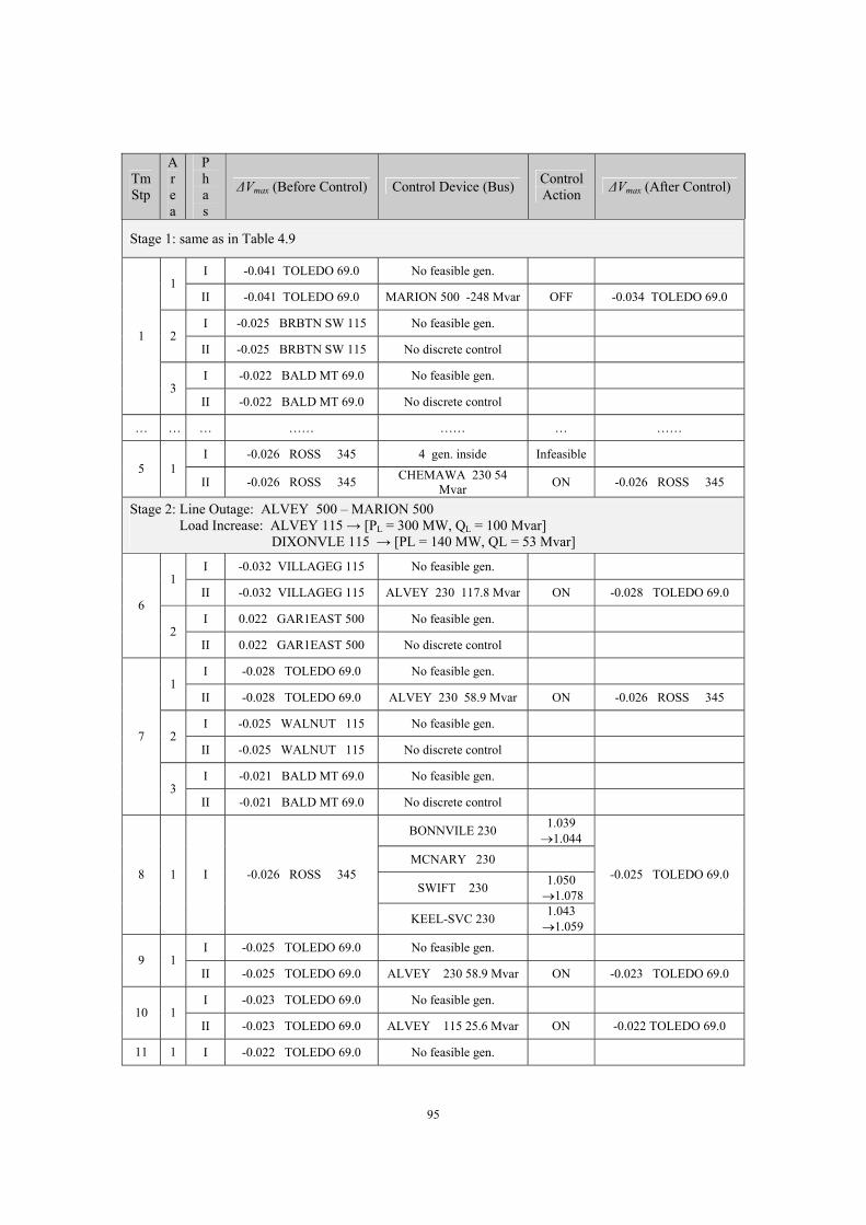
95

Tm Stp

A r e a

P h a s


Stage 1: same as in Table 4.9


II -0.041 TOLEDO 69.0 MARION 500 -248 Mvar OFF -0.034 TOLEDO 69.0




1


… … … …… …… … ……

I -0.026 ROSS 345 4 gen. inside Infeasible 5 1

II -0.026 ROSS 345 CHEMAWA 230 54 Mvar ON -0.026 ROSS 345

Stage 2: Line Outage: ALVEY 500 – MARION 500 Load Increase: ALVEY 115 → [PL = 300 MW, QL = 100 Mvar]


I -0.032 VILLAGEG 115 No feasible gen. 1

II -0.032 VILLAGEG 115 ALVEY 230 117.8 Mvar ON -0.028 TOLEDO 69.0

I 0.022 GAR1EAST 500 No feasible gen. 6

2 II 0.022 GAR1EAST 500 No discrete control


II -0.028 TOLEDO 69.0 ALVEY 230 58.9 Mvar ON -0.026 ROSS 345

I -0.025 WALNUT 115 No feasible gen. 2

II -0.025 WALNUT 115 No discrete control


7


BONNVILE 230 1.039 →1.044

MCNARY 230

SWIFT 230 1.050 →1.078

8 1 I -0.026 ROSS 345

KEEL-SVC 230 1.043 →1.059

-0.025 TOLEDO 69.0

I -0.025 TOLEDO 69.0 No feasible gen. 9 1

II -0.025 TOLEDO 69.0 ALVEY 230 58.9 Mvar ON -0.023 TOLEDO 69.0


II -0.023 TOLEDO 69.0 ALVEY 115 25.6 Mvar ON -0.022 TOLEDO 69.0

11 1 I -0.022 TOLEDO 69.0 No feasible gen.

96

II -0.022 TOLEDO 69.0 ALBANY 115 50.0 Mvar ON -0.021 TOLEDO 69.0


II -0.021 TOLEDO 69.0 ALVEY 115 25.6 Mvar ON No Violation

Table 4.10 Results of multi-phase hybrid voltage control (WECC - B).

It can be observed from above tables that at each stage, the controller first groups the

violation buses into different problematic areas and operates in Phase I. It tries to find the

available control generators in each local area, using linear programming algorithm to

calculate optimal generator voltage adjustments such that load bus voltage profiles are

maintained as desired. If the linear programming algorithm successfully finds solutions

for one or more control areas, then parallel switching commands are sent, and the load

bus voltages may be restored for those areas, or the problem center may change and

problematic areas may merge into new areas. If there is no generator available or the

generator’s reactive power is not enough to recover the load bus voltages (i.e. the linear

programming algorithm could not reach a solution), then the controller will operate in

Phase II, trying to find the best (highest priority and lowest cost) discrete control devices

available for switching. If such control devices exists, then after switching either the

problematic center bus changes or the generator reactive outputs are back to their limits,

the controller may go back to operate in Phase I again. If under certain condition, the

controller could not find appropriate discrete control devices to switch, then the controller

will operate in phase III, and the generator’s full reactive power capacity will be utilized

to restore the voltage or at least alleviate the voltage problem.

It is worth mentioning that although some generators are inside a local area, they are

not necessarily change their settings, such as MCNARY 230 in step 6 of Table 4.9 and

97

step 8 in Table 4.10, because either they are far away from problematic center or their

sensitivities are too small or their reactive power outputs reach their limits. It is also

noted that although the control solutions in Phase I are supposed to bring bus voltages

back to normal range, this is not always the case, especially with the constraint relaxing

technique. For example, in step 8 of Table 4.10 the controller successfully reach a

solution in Phase I, but the voltage on TOLEDO 69.0 remains outside the normal range

after control actions, since the voltage constraint on TOLEDO 69.0 is relaxed in the

linear programming formulation. In effect, the voltages on most buses are still brought

back to normal range, and the voltage on TOLEDO 69.0 can be restored later by

switching discrete devices. Finally it is noted that in above tables, the reactors are

switched out before the capacitors are switched in, which shows that the preferences of

the operators are properly implemented into the algorithm.

4.3 Summary

To deal with voltage problems happened simultaneously in several places in large

power systems, the on-line slow voltage control scheme in last chapter is extended to

divides the network into separate control areas dynamically according to current system

conditions and make control decisions for each area respectively. The scheme itself is

open, in the sense that any voltage control algorithm can be integrated into it, including

the model-based algorithm and the alternate control algorithm. The simulation results on

the actual WECC planning case show that the controller is effective in alleviate multiple

voltage problems simultaneously.

98

For power systems with a large amount of generation resources, a multi-phase hybrid

voltage control scheme is proposed to coordinate continuous generation controls and

discrete controls while taking reactive power security into consideration. The controller is

meant to act in the way similar to that of AGC under normal operating conditions such as

morning load pickups, adjusting generator reactive outputs to maintain the desired

voltage profile with the discrete devices as supplemental reactive power resource. The

controller operated in three phases and use linear programming / integer programming to

search for the best control actions in each phase. The test results on the standard IEEE

30-bus system and the actual WECC planning case clearly show that the hybrid scheme is

feasible, scalable to large-scale power system and suitable for on-line implementation.

99

Chapter 5

Conclusions and Future Works

This chapter summarizes the main results of the research by providing general

conclusions and discussions on the key contributions, which is followed by suggestions

for possible extensions of the work reported in this dissertation.

5.1 Conclusions

In view of a state estimator model maybe unavailable or unreliable, this dissertation

proposes an alternate heuristic slow voltage controller that can be easily integrated with

the model-based controller and motivated towards implementation under a common

framework in the western Oregon area of Pacific Northwest. An integer-programming

formulation is presented with preferences of control actions built into the switching cost

function, and the objective is to keep the voltages within certain range around optimal

profile with minimum switching cost. The alternate controller operates independent of the

state estimator model and can be used as back-up controller, or used to reinforce the

decisions made by the model-based controller.

A local voltage estimator is formulated based on linearized reactive power flow model

to approximate switching effects by utilizing only the local SCADA measurements

around the control devices. The control effects of capacitor/reactor switching, LTC tap

100

changing, and generator voltage adjusting are quickly assessed in a unified way by

treating them as some reactive power injection changes.

Parallel control of multiple problematic areas of a large power system is also addressed.

The system is dynamically divided into separated control areas around several problem

center buses and simultaneous corrective control actions are made such that voltage

problems occurred in different areas are quickly alleviated.

To coordinate continuous generator controls and discrete device controls for large

power systems with lots of generators as main voltage controls, a hybrid multi-phase

automatic voltage control scheme is proposed to maintain system voltage profile while

taking reactive power security into consideration. The controller operates in three phases

with the optimization problems in each phase formulated as continuous or discrete

problems and solved using linear programming or integer programming respectively.

Simulation results on the IEEE 30 bus test system and an actual WECC planning case

show that the above schemes are effective in handling the voltage problem, scalable to

large-scale power system and suitable for on-line implementation.

5.2 Future Works

As with any work of research, there is always more that can be done. Aside from

further testing of the algorithms with more cases and on other power systems, there are

several extensions and modifications which could be explored.

In the local voltage estimator, it is assumed that the SCADA measurements are

available and valid inside the small local area, but this is not always the case. Although

the unavailable data could be replaced with the last good measurements or last good state

101

estimator results if there is no significant change in network topology and loading

conditions within certain time period, it is necessary to find a simple way to detect the

bad measurements or at least report the obvious erroneous measurements.

Apart from the using local voltage estimator to approximate the effects of control

actions, pattern recognition approach with the help of engineering experience might be

also worth doing. This approach actually involves defining the typical cases offline by

pattern classification or clustering algorithm and then identifying a typical case that is

closest to current operating conditions by pattern recognition.

It is also possible to consider other objective functions such as loss minimization,

reactive margin maximization and operating cost minimization under the possible

reactive power market environment.

102

Bibliography

[1] C. W. Taylor, Power System Voltage Stability, McGraw-Hill Inc., 1994.

[2] P. Kundur, Power System Stability and Control, McGraw-Hill Inc., 1994.

[3] T. V. Cutsem, “Voltage Instability: Phenomena, Countermeasures, and Analysis

Methods”, Proceedings of the IEEE, Vol. 88, No. 2, pp. 208-227, February 2000.

[4] B. Kirby and E. Hirst, “Ancillary Service Details: Voltage Control”, Report

ORNL/CON-453, Oak Ridge National Laboratory, Oak Ridge, TN, December 1997.

[5] C. W. Taylor, V. Venkatasubramanian, and Y. Chen, “Wide-Area Stability and

Voltage Control,” Proceedings of VII Symposium of Specialist in Electric

Operational and Expansion Planning (VII SEPOPE), Brazil, May 2000.

[6] C. W. Taylor, “Response-Based, Feedforward Wide-Area Control”, Position Paper

for NSF/DOE/EPRI Sponsored Workshop on Future Research Directions for

Complex Interactive Electric Networks, Washington D.C., November 2000.

[7] K. T. Vu, C. Liu, C. W. Taylor, and K. M. Jimma, “Voltage Instability: Mechanisms

and Control Strategies”, Proceedings of the IEEE, Vol. 83, No. 11, pp. 1442-1455,

November 1995.

[8] B. Stott and E. Hobson, “Power System Security Control Calculation Using Linear

Programming, Part 1 and 2”, IEEE Transactions on Power Apparatus and Systems,

Vol. PAS-97, No. 5, pp. 1713-1731, October 1978.

103

[9] D. I. Sun, B. Ashley, B. Brewer, A. Hughes, and W. F. Tinney, “Optimal Power

Flow by Newton Approach”, IEEE Transactions on Power Apparatus and Systems,

Vol. PAS-103, No. 2, pp. 2864-2880, October 1984.

[10] O. Alsac, J. Bright, M. Prais, and B. Stott, “Further Developments in LP-Based

Optimal Power Flow”, IEEE Transactions on Power Systems, Vol. 5, No. 3, pp. 697-

711, August 1990.

[11] W. F. Tinney, J. M. Bright, K. D. Demaree, and B. A. Hughes, “Some Deficiencies

in Optimal Power Flow”, IEEE Transactions on Power Systems, Vol. 3, No. 2, pp.

676-683, May 1988.

[12] C. Liu and K. Tomsovic, “An Expert System Assisting Decision-Making of Reactive

Power/Voltage Control”, IEEE Transactions on Power Systems, Vol. PWRS-1, No. 3,

pp. 195-201, August 1986.

[13] S. J. Cheng, O. P. Malik, and G. S. Hope, “An Expert System for Voltage and

Reactive Power Control of a Power System”, IEEE Transactions on Power Systems,

Vol. 3, No. 4, pp. 1449-1455, November 1988.

[14] W. R. Wagner, A. Keyhani, S. Hao, and T. C. Wong, “A Rule-Based Approach to

Decentralized Voltage Control”, IEEE Transactions on Power Systems, Vol. 5, No. 2,

pp. 643-651, May 1990.

[15] T. F. Godart and H. B. Puttgen, “A Reactive Path Concept Applied within a Voltage

Control Expert System”, IEEE Transactions on Power Systems, Vol. 6, No. 2, pp.

787-793, May 1991.

104

[16] K. Tomsovic, “A Fuzzy Linear Programming Approach to the Reactive

Power/Voltage Control Problem”, IEEE Transactions on Power Systems, Vol. 7, No.

1, pp. 287-293, February 1992.

[17] R. Yohoyama, T. Niimura, and Y. Nakanishi, “A Coordinated Control of Voltage

and Reactive Power by Heuristic Modeling and Approximate Reasoning”, IEEE

Transactions on Power Systems, Vol. 8, No. 2, pp. 636-645, May 1993.

[18] C-T. Su and C-T. Lin, “Application of a Neural Network and Heuristic Model for

Voltage-Reactive Power Control”, Electric Power Systems Research, Vol. 34, No. 3,

pp. 143-148, May 1995.

[19] J.P. Paul, J.T. Leost, and J.M. Tesseron, “Survey of the Secondary Voltage Control

in France: Present Realization and Investigations,” IEEE Transactions on Power

Systems, Vol. PWRS-2, No.2, pp. 505-511, 1987.

[20] M. Ilic, J. Christensen, and K.L. Eichorn, “Secondary Voltage Control Using Pilot

Point Information”, IEEE Transactions on Power Systems, Vol. 3, No. 2, May 1988.

[21] P. Lagonotte, J.C. Sabonnadiere, J.Y. Leost, and J.P. Paul, “Structural Analysis of

the Electrical System: Application to the Secondary Voltage Control in France”,

IEEE Transactions on Power Systems, Vol. 4, No. 2, pp. 479-484, May 1989.

[22] S. Corsi, P. Marannino, N. Losignore, G Moreschini, and G. Piccini, “Coordination

Between the Reactive Power Scheduling Function and the Hierarchical Voltage

Control of the EHV ENEL System”, IEEE Transactions on Power Systems, Vol. 10,

No. 2, pp. 686-694, May 1995.

105

[23] M. Ilic, X. Liu, G. L.eung, M. Athans, C. Vialas, and P. Pruvot, “Improved

Secondary and New Tertiary Voltage Control,” IEEE Transactions on Power

Systems, Vol. 10, No. 4, Nov. 1995.

[24] J. L. Sancha, J. L. Fernandez, A. Cortes, and J. T. Abarca, “Secondary Voltage

Control: Analysis, Solutions and Simulation Results for Spanish Transmission

System”, IEEE Transactions on Power Systems, Vol. 11, No. 2, pp. 630-638, May

1996.

[25] H. Vu, P. Pruvot, C. Launay, and Y. Harmand, “An Improved Voltage Control on

Large Scale Power System”, IEEE Transactions on Power Systems, Vol. 11, No. 3,

pp. 1295-1303, August 1996.

[26] A. Conjo and M. J. Aguilar, “Secondary Voltage Control: Nonlinear Selection of

Pilot uses, Design of an Optimal Control Law, and Simulation Results”, IEE

Proceedings of Generation, Transmission, and Distribution, Vol. 145, No. 1,

January 1998.

[27] J. Van Hecke, N. Janssens, J. Deuse, and F. Promel, “Coordinated Voltage Control

Experience in Belgium”, CIGRE Session Report 38-111, Paris, September 2000.

[28] M. Ilic and W. Stobart, “Development of A Smart Algorithm for Voltage Monitoring

and Control”, IEEE Transactions on Power Systems, Vol. 5, No. 4, November 1990.

[29] A. Zobian and M. Ilic, “A Steady State Voltage Monitoring and Control Algorithm

Using Localized Least Square Minimization of Load Voltage Deviations”, IEEE

Transactions on Power Systems, Vol. 11, No. 2, pp. 929-938, May 1996.

106

[30] C. Yu, Y.T. Yoon, M. Ilic, and A. Catelli, “On-line Voltage Regulation: The Case of

New England”, IEEE Transactions on Power Systems, Vol. 14, pp. 1477-1483,

November 1999.

[31] Y. Chen, Development of Automatic Slow Voltage Control for Large Power Systems,

Ph.D. dissertation, School of Electrical Engineering And Computer Science,

Washington State University, Pullman, WA, August 2001.

[32] J. J. Grainger and W. D. Stevenson, Jr., Power System Analysis, McGraw-Hill Inc.,

1994.

[33] A. J. Wood and B. F. Wollenberg, Power Generation, Operation and Control, John

Wiley & Sons, 1996.

[34] http://www.ee.washington.edu/research/pstca/

[35] N. Christofides, A. Mingozzi, P. Toth, and C. Sandi, Combinatorial Optimization,

John Wiley & Sons, 1979.

[36] G. L. Nemhauser and L. A. Wolsey, Integer and Combinatorial Optimization, John

Wiley & Sons, 1988.

[37] M. S. Bazaraa and J. J. Jarvis, Linear Programming and Network Flows, John Wiley

& Sons, 1977.

[38] J. P. Ignizio and T. M. Cavalier, Linear Programming, Prentice-Hall Inc., 1994.

[39] Bonneville Power Administration, IPF Batch PowerFlow (BPF) User’s Guide,

Portland, OR, 1998.

[40] T. S. Corman, C. E. Leiserson, R. L. Rivest, and C. Stein, Introduction to Algorithms,

Second Edition, The MIT Press, 2001.

[41] http://www.gnu.org/software/glpk

107

APPENDIX A

IEEE 30 Bus Test System

The system data and one-line diagram of IEEE 30 bus standard test system is available

on at the website of power research group of University of Washington [34].

A.1 One-line Diagram of IEEE 30 Bus Test System [34]

Figure A.1 One-line Diagram of IEEE 30 Bus Test System [34].

108

A.2 System Data of IEEE 30 Bus Test System [34]

08/20/93 UW ARCHIVE 100.0 1961 W IEEE 30 Bus Test Case BUS DATA FOLLOWS 30 ITEMS 1 Glen Lyn 132 1 1 3 1.060 0.0 0.0 0.0 260.2 -16.1 132.0 1.060 0.0 0.0 0.0 0.0 0 2 Claytor 132 1 1 2 1.043 -5.48 21.7 12.7 40.0 50.0 132.0 1.045 50.0 -40.0 0.0 0.0 0 3 Kumis 132 1 1 0 1.021 -7.96 2.4 1.2 0.0 0.0 132.0 0.0 0.0 0.0 0.0 0.0 0 4 Hancock 132 1 1 0 1.012 -9.62 7.6 1.6 0.0 0.0 132.0 0.0 0.0 0.0 0.0 0.0 0 5 Fieldale 132 1 1 2 1.010 -14.37 94.2 19.0 0.0 37.0 132.0 1.010 40.0 -40.0 0.0 0.0 0 6 Roanoke 132 1 1 0 1.010 -11.34 0.0 0.0 0.0 0.0 132.0 0.0 0.0 0.0 0.0 0.0 0 7 Blaine 132 1 1 0 1.002 -13.12 22.8 10.9 0.0 0.0 132.0 0.0 0.0 0.0 0.0 0.0 0 8 Reusens 132 1 1 2 1.010 -12.10 30.0 30.0 0.0 37.3 132.0 1.010 40.0 -10.0 0.0 0.0 0 9 Roanoke 1.0 1 1 0 1.051 -14.38 0.0 0.0 0.0 0.0 1.0 0.0 0.0 0.0 0.0 0.0 0 10 Roanoke 33 1 1 0 1.045 -15.97 5.8 2.0 0.0 0.0 33.0 0.0 0.0 0.0 0.0 0.19 0 11 Roanoke 11 1 1 2 1.082 -14.39 0.0 0.0 0.0 16.2 11.0 1.082 24.0 -6.0 0.0 0.0 0 12 Hancock 33 1 1 0 1.057 -15.24 11.2 7.5 0.0 0.0 33.0 0.0 0.0 0.0 0.0 0.0 0 13 Hancock 11 1 1 2 1.071 -15.24 0.0 0.0 0.0 10.6 11.0 1.071 24.0 -6.0 0.0 0.0 0 14 Bus 14 33 1 1 0 1.042 -16.13 6.2 1.6 0.0 0.0 33.0 0.0 0.0 0.0 0.0 0.0 0 15 Bus 15 33 1 1 0 1.038 -16.22 8.2 2.5 0.0 0.0 33.0 0.0 0.0 0.0 0.0 0.0 0 16 Bus 16 33 1 1 0 1.045 -15.83 3.5 1.8 0.0 0.0 33.0 0.0 0.0 0.0 0.0 0.0 0 17 Bus 17 33 1 1 0 1.040 -16.14 9.0 5.8 0.0 0.0 33.0 0.0 0.0 0.0 0.0 0.0 0 18 Bus 18 33 1 1 0 1.028 -16.82 3.2 0.9 0.0 0.0 33.0 0.0 0.0 0.0 0.0 0.0 0 19 Bus 19 33 1 1 0 1.026 -17.00 9.5 3.4 0.0 0.0 33.0 0.0 0.0 0.0 0.0 0.0 0 20 Bus 20 33 1 1 0 1.030 -16.80 2.2 0.7 0.0 0.0 33.0 0.0 0.0 0.0 0.0 0.0 0 21 Bus 21 33 1 1 0 1.033 -16.42 17.5 11.2 0.0 0.0 33.0 0.0 0.0 0.0 0.0 0.0 0 22 Bus 22 33 1 1 0 1.033 -16.41 0.0 0.0 0.0 0.0 33.0 0.0 0.0 0.0 0.0 0.0 0 23 Bus 23 33 1 1 0 1.027 -16.61 3.2 1.6 0.0 0.0 33.0 0.0 0.0 0.0 0.0 0.0 0 24 Bus 24 33 1 1 0 1.021 -16.78 8.7 6.7 0.0 0.0 33.0 0.0 0.0 0.0 0.0 0.043 0 25 Bus 25 33 1 1 0 1.017 -16.35 0.0 0.0 0.0 0.0 33.0 0.0 0.0 0.0 0.0 0.0 0 26 Bus 26 33 1 1 0 1.000 -16.77 3.5 2.3 0.0 0.0 33.0 0.0 0.0 0.0 0.0 0.0 0 27 Cloverdle 33 1 1 0 1.023 -15.82 0.0 0.0 0.0 0.0 33.0 0.0 0.0 0.0 0.0 0.0 0 28 Cloverdle132 1 1 0 1.007 -11.97 0.0 0.0 0.0 0.0 132.0 0.0 0.0 0.0 0.0 0.0 0 29 Bus 29 33 1 1 0 1.003 -17.06 2.4 0.9 0.0 0.0 33.0 0.0 0.0 0.0 0.0 0.0 0 30 Bus 30 33 1 1 0 0.992 -17.94 10.6 1.9 0.0 0.0 33.0 0.0 0.0 0.0 0.0 0.0 0 -999 BRANCH DATA FOLLOWS 41 ITEMS 1 2 1 1 1 0 0.0192 0.0575 0.0528 0 0 0 0 0 0.0 0.0 0.0 0.0 0.0 0.0 0.0 1 3 1 1 1 0 0.0452 0.1652 0.0408 0 0 0 0 0 0.0 0.0 0.0 0.0 0.0 0.0 0.0 2 4 1 1 1 0 0.0570 0.1737 0.0368 0 0 0 0 0 0.0 0.0 0.0 0.0 0.0 0.0 0.0 3 4 1 1 1 0 0.0132 0.0379 0.0084 0 0 0 0 0 0.0 0.0 0.0 0.0 0.0 0.0 0.0 2 5 1 1 1 0 0.0472 0.1983 0.0418 0 0 0 0 0 0.0 0.0 0.0 0.0 0.0 0.0 0.0 2 6 1 1 1 0 0.0581 0.1763 0.0374 0 0 0 0 0 0.0 0.0 0.0 0.0 0.0 0.0 0.0 4 6 1 1 1 0 0.0119 0.0414 0.0090 0 0 0 0 0 0.0 0.0 0.0 0.0 0.0 0.0 0.0 5 7 1 1 1 0 0.0460 0.1160 0.0204 0 0 0 0 0 0.0 0.0 0.0 0.0 0.0 0.0 0.0 6 7 1 1 1 0 0.0267 0.0820 0.0170 0 0 0 0 0 0.0 0.0 0.0 0.0 0.0 0.0 0.0 6 8 1 1 1 0 0.0120 0.0420 0.0090 0 0 0 0 0 0.0 0.0 0.0 0.0 0.0 0.0 0.0 6 9 1 1 1 0 0.0 0.2080 0.0 0 0 0 0 0 0.978 0.0 0.0 0.0 0.0 0.0 0.0 6 10 1 1 1 0 0.0 0.5560 0.0 0 0 0 0 0 0.969 0.0 0.0 0.0 0.0 0.0 0.0 9 11 1 1 1 0 0.0 0.2080 0.0 0 0 0 0 0 0.0 0.0 0.0 0.0 0.0 0.0 0.0 9 10 1 1 1 0 0.0 0.1100 0.0 0 0 0 0 0 0.0 0.0 0.0 0.0 0.0 0.0 0.0 4 12 1 1 1 0 0.0 0.2560 0.0 0 0 0 0 0 0.932 0.0 0.0 0.0 0.0 0.0 0.0 12 13 1 1 1 0 0.0 0.1400 0.0 0 0 0 0 0 0.0 0.0 0.0 0.0 0.0 0.0 0.0 12 14 1 1 1 0 0.1231 0.2559 0.0 0 0 0 0 0 0.0 0.0 0.0 0.0 0.0 0.0 0.0 12 15 1 1 1 0 0.0662 0.1304 0.0 0 0 0 0 0 0.0 0.0 0.0 0.0 0.0 0.0 0.0 12 16 1 1 1 0 0.0945 0.1987 0.0 0 0 0 0 0 0.0 0.0 0.0 0.0 0.0 0.0 0.0 14 15 1 1 1 0 0.2210 0.1997 0.0 0 0 0 0 0 0.0 0.0 0.0 0.0 0.0 0.0 0.0

109

16 17 1 1 1 0 0.0524 0.1923 0.0 0 0 0 0 0 0.0 0.0 0.0 0.0 0.0 0.0 0.0 15 18 1 1 1 0 0.1073 0.2185 0.0 0 0 0 0 0 0.0 0.0 0.0 0.0 0.0 0.0 0.0 18 19 1 1 1 0 0.0639 0.1292 0.0 0 0 0 0 0 0.0 0.0 0.0 0.0 0.0 0.0 0.0 19 20 1 1 1 0 0.0340 0.0680 0.0 0 0 0 0 0 0.0 0.0 0.0 0.0 0.0 0.0 0.0 10 20 1 1 1 0 0.0936 0.2090 0.0 0 0 0 0 0 0.0 0.0 0.0 0.0 0.0 0.0 0.0 10 17 1 1 1 0 0.0324 0.0845 0.0 0 0 0 0 0 0.0 0.0 0.0 0.0 0.0 0.0 0.0 10 21 1 1 1 0 0.0348 0.0749 0.0 0 0 0 0 0 0.0 0.0 0.0 0.0 0.0 0.0 0.0 10 22 1 1 1 0 0.0727 0.1499 0.0 0 0 0 0 0 0.0 0.0 0.0 0.0 0.0 0.0 0.0 21 22 1 1 1 0 0.0116 0.0236 0.0 0 0 0 0 0 0.0 0.0 0.0 0.0 0.0 0.0 0.0 15 23 1 1 1 0 0.1000 0.2020 0.0 0 0 0 0 0 0.0 0.0 0.0 0.0 0.0 0.0 0.0 22 24 1 1 1 0 0.1150 0.1790 0.0 0 0 0 0 0 0.0 0.0 0.0 0.0 0.0 0.0 0.0 23 24 1 1 1 0 0.1320 0.2700 0.0 0 0 0 0 0 0.0 0.0 0.0 0.0 0.0 0.0 0.0 24 25 1 1 1 0 0.1885 0.3292 0.0 0 0 0 0 0 0.0 0.0 0.0 0.0 0.0 0.0 0.0 25 26 1 1 1 0 0.2544 0.3800 0.0 0 0 0 0 0 0.0 0.0 0.0 0.0 0.0 0.0 0.0 25 27 1 1 1 0 0.1093 0.2087 0.0 0 0 0 0 0 0.0 0.0 0.0 0.0 0.0 0.0 0.0 28 27 1 1 1 0 0.0 0.3960 0.0 0 0 0 0 0 0.968 0.0 0.0 0.0 0.0 0.0 0.0 27 29 1 1 1 0 0.2198 0.4153 0.0 0 0 0 0 0 0.0 0.0 0.0 0.0 0.0 0.0 0.0 27 30 1 1 1 0 0.3202 0.6027 0.0 0 0 0 0 0 0.0 0.0 0.0 0.0 0.0 0.0 0.0 29 30 1 1 1 0 0.2399 0.4533 0.0 0 0 0 0 0 0.0 0.0 0.0 0.0 0.0 0.0 0.0 8 28 1 1 1 0 0.0636 0.2000 0.0428 0 0 0 0 0 0.0 0.0 0.0 0.0 0.0 0.0 0.0 6 28 1 1 1 0 0.0169 0.0599 0.0130 0 0 0 0 0 0.0 0.0 0.0 0.0 0.0 0.0 0.0 -999 LOSS ZONES FOLLOWS 1 ITEMS 1 IEEE 30 BUS -99 INTERCHANGE DATA FOLLOWS 1 ITEMS -9 1 2 Claytor 132 0.0 999.99 IEEE30 IEEE 30 Bus Test Case TIE LINES FOLLOWS 0 ITEMS -999 END OF DATA

110

APPENDIX B

README of the Programs

B.1 Standard programs used and case studied

In the simulations of WECC system, BPA standard power flow program (Cygwin

version) [39] is used to approximate the system’s response to any control action. Before

the simulations, the power flow for the original case is calculated by BPA power flow

program and the resulting voltage profile is treated as the desired voltage profile. At the

beginning of each time step of the simulations, the BPA power flow program is called to

calculate the actual power flow on the large system. The resulting “*.PFO” file is read

and treated as the SCADA measurements, and based on these “measurements” the

control decision is made.

To solve the large-scale linear programming problems in Chapter 4, the GLPK (GNU

Linear Programming Kit) package [41] is used. This package includes a set of routines

written in ANSI C and organized in the form of a callable library, which is intended for

solving large-scale linear programming (LP), mixed integer programming (MIP), and

other related problems.

The BPA planning case studied is 2001 to 2003 winter planning case with case ID:

213SNK. The total number of buses of the case is 6815 and the total number of lines is

111

9245. For test purpose, about 20 to 30 discrete devices in the western Oregon area are

considered as candidate controls.

To simulate the response of IEEE 30 bus system, a simple power flow program is

implemented with MATLAB language that takes advantage of the built-in matrix

manipulation and sparse matrix storage. Solving a set of linear equations is a built-in

function and therefore made it an attractive choice for quick implementation and testing

of ideas.

The IEEE 30 bus system is a standard test system, the system data and one-line

diagram of IEEE 30 bus is available on at the website of power research group of

University of Washington [34] and listed in Appendix A.

B.2 MATLAB files

1) bpa_ctrl.m: main program

The main program read in the standard case file, and calls the power flow program

to obtain the desired voltage profile first. Then for each time step, the power flow is

calculated and the result is saved as the control results from SCADA. It also controls

the loop of the stages, and calls different controller subroutines to determine the best

control actions.

2) devIPctrl.m: discrete controller (integer programming) subroutine

The subroutine uses integer programming to search for the discrete control devices

with lowest total switching cost and highest priority.

3) estimate.m: voltage estimator subroutine

112

The subroutine calculates the estimated local bus voltages after control actions,

which will be used to calculated the voltage penalty costs later.

4) fd_pf.m / nr_pf.m: Fast-Decoupled / Newton-Raphson power flow subroutine

These subroutines calculate the power flow with fast-decoupled or Newton-Raphson

algorithms.

5) findctrlact.m: control action finding subroutine

The subroutine finds appropriate control actions for all control devices under current

network topology and loads conditions.

6) findonelocal.m: local control are formation subroutine

The subroutine formulates appropriate local area around a specific bus using

breadth-first search algorithm.

7) genLPctrlOne.m: Phase I hybrid controller subroutine

The subroutine solves linear programming to obtain the best generator voltage

setpoints to restore the bus voltages

8) genLPctrlThree.m: Phase III hybrid controller subroutine

The subroutine solves linear programming to minimize the difference between local

bus voltages and the desired voltage profile.

9) ieee30chg.m / ieee30state.m: IEEE 30 bus base case / stage definition subroutine

These subroutines modify the original IEEE 30 bus system data to form base case

and the changes at each stage.

10) lfdfPQ.m: IEEE 30 bus base case / stage definition subroutine

The subroutine calculates the sensitivities of the bus voltages to any control actions

11) readcdf.m: IEEE Common Data Format file reading subroutine

113

The subroutine read in the Common Data Format file to proper data structures.

12) savecontrol.m: control result saving subroutine

The subroutine save the control results into a text file for further investigation.

B.3 C/C++ files

1) voltctrl_estim.c: main program

The main program read in the WECC *.NET case file, and calls the BPA power

flow program to obtain the desired voltage profile first. Then for each time step, the

BPA power flow is called and the result in *.PFO file is saved as the control results

from SCADA. It also controls the loop of the stages and control steps, and calls the

controller subroutine to determine the best control actions.

2) voltctrl_estim.h: header file for the program

The header file includes definitions of constants, data structures and function

prototype declarations.

3) control.c: includes subroutines implementing the voltage controllers

getAllCtrl_Act(): Obtains appropriate control action for each device.

tryLPCtrl_I(): Phase I hybrid voltage controller subroutine.

tryLPCtrl_III(): Phase III hybrid voltage controller subroutine.

findAllCtrl_Gen(): Locates all control generators for each control area.

formLPprog_I(): Formulate linear programming problem for Phase I controller.

formLPprog_III(): Formulate linear programming problem for Phase III controller.

tryIPCtrl_II(): Discrete controller (integer programming) subroutine.

findOneCtrl_Dev(): Find the best control device inside a control area.

114

calcSwitch_Cost(): Calculate the switching cost for certain control action.

updatAllDev_Rec(): Update the control device status after control actions.

4) estimate.c: includes subroutines implementing the voltage estimator

calcLine_Flow(): Calculate line P/Q flows from bus voltages and angles .

calcLine_LFDF(): Calculate line flow (P/Q) sensitivities to voltages.

calcLTC_LFDF(): Calculate line flow (P/Q) sensitivities to LTC taps.

formB_Matrix(): Formulate B matrix from measurements.

estimBus_Volt(): Estimate bus voltages after control actions.

5) miscs.c: includes miscellaneous subroutines supporting the program

runBpa_Pf(): Call BPA power flow to run a specified case.

findSel_LocalBus(): Locates all selected local load buses.

findMax_Diff(): Local the worst violation bus inside each area.

findCtrl_Reg(): Formulate separated problematic areas.

findAll_Loc():Find local buses and local lines of all the control buses.

6) read.c: includes subroutines to read case/result/control files

readAll_CASE(): Read in case definition file.

readAllBus_NET(): Read in bus data *.NET file to proper data structures.

readAllBus_PFO(): Read in bus voltage from BPA power flow result *.PFO file.

readAllDev_CTRL1(): Read in control device status file.

readAllLine_NET(): Read in line data *.NET file to proper data structures.

readAllCtrl_PARA(): Read in controller parameters file.

readAllLine_CHG(): Read in line outage data for each case.

readAllBus_CHG(): Read in bus load change data for each case.

115

readLP_SOL(): Read in GLPK solution file for linear programming problems.

7) write.c: includes subroutines to write case/result/control files

writeNew_PFC(): Write a *.PFC BPA power flow control file for a case.

writeCase_CHG1():Write case change to a *.CHG BPA power flow change file.

writeCtrl_CHG():Write control change to a *.CHG BPA power flow change file.

writeCtrl_RES(): Save the control results to a text file.

writeCtrl_COST(): Save the costs of control actions for comparing purpose.

writeNext_CTRL(): Save the control device status to file.

writeLP_LPT_I(): Write the formulated Phase I LP problems to a *.LPT file.

writeLP_LPT_III(): Write the formulated Phase III LP problems to a *.LPT file.

j_su_030206

Documents