Report on the activities realized within the Service Level Agreement between JRC and EFSA as a support of the FATE and ECOREGION Working Groups of EFSA PPR (SLA/EFSA-JRC/2008/01) Ciro Gardi, Panos Panagos, Roland Hiederer, Luca Montanarella, Fabio Micale EUR 24744 EN - 2011

Welcome message from author
This document is posted to help you gain knowledge. Please leave a comment to let me know what you think about it! Share it to your friends and learn new things together.
Transcript
Report on the activities realized within the Service Level Agreement between
JRC and EFSAas a support of the FATE and ECOREGION Working Groups of EFSA PPR
(SLAEFSA-JRC200801)
Ciro Gardi Panos Panagos Roland HiedererLuca Montanarella Fabio Micale
EUR 24744 EN - 2011
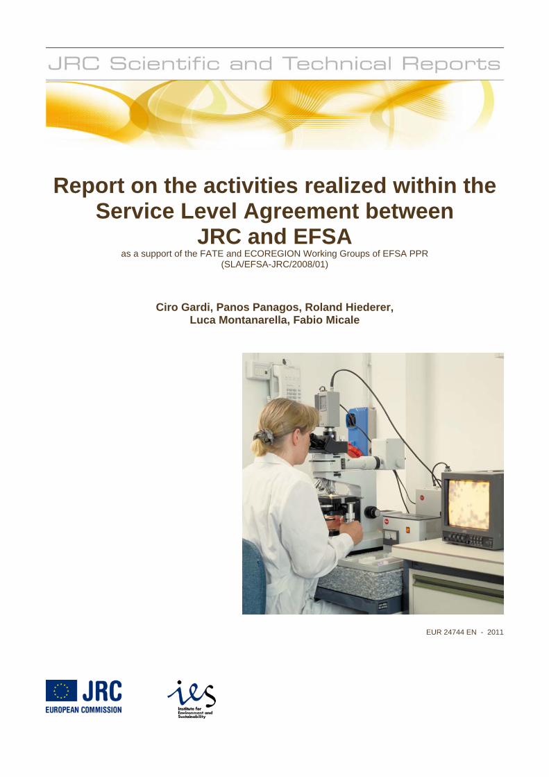
The mission of the JRC-IES is to provide scientific-technical support to the European Unionrsquos policies for the protection and sustainable development of the European and global environment European Commission Joint Research Centre Institute for Environment and Sustainability Contact information Address E Fermi 2749 Ispra(VA) ITALY E-mail cirogardijrceceuropaeu Tel +39-0332-785015 Fax +39-0332-786394 httpeusoilsjrceceuropaeu httpiesjrceceuropaeu httpwwwjrceceuropaeu Legal Notice Neither the European Commission nor any person acting on behalf of the Commission is responsible for the use which might be made of this publication
Europe Direct is a service to help you find answers to your questions about the European Union
Freephone number ()
00 800 6 7 8 9 10 11
() Certain mobile telephone operators do not allow access to 00 800 numbers or these calls may be billed
A great deal of additional information on the European Union is available on the Internet It can be accessed through the Europa server httpeuropaeu JRC62504 EUR 24744 EN ISBN 978-92-79-19521-1 ISSN 1018-5593 doi10278861018 Luxembourg Publications Office of the European Union copy European Union 2011 Reproduction is authorised provided the source is acknowledged Printed in Italy
JRC TECHNICAL REPORT
Report on the activities realized in 2010 within the Service Level Agreement between JRC and EFSA as a support of the FATE and ECOREGION Working Groups of EFSA
PPR
(SLAEFSA-JRC200801)
Final Report of 15th December 2010
SUMMARY The activities realized in 2010 by JRC as support to the FATE and the ECOREGION EFSA PPR Working Groups are shortly described For the FATE WG the vast majority of data has been provided in 2009 during the first year of the Service Level Agreement (SLA) and in 2010 the daily weather data for the six selected sites were produced All the data used for the scenario selection procedures with additional data on land use-land cover crop distribution soil and climate parameters will be made available for external user in first half of 2011 For the ECOREGION WG the analysis has been carried out for three Member States covering a North-South gradient from Finland Germany to Portugal Soil and weather data have been used for the characterisation of biogeographic sampling sites and for the implementation of the ecoregion model Ecoregion maps were produced for earthworms and enchytraeids for Finland and Germany and revealed marked differences between the countries The same approach has been applied also to Collembola and Isopoda but for these two taxa led to a rather poor discrimination both between and within countries
Key words Meteorological data Biogeographic data Ecoregions Earthworm Enchytraeid Collembola Isopoda Soil Plant Protection Products
TABLE OF CONTENTS Summary Table of Contents 1 FATE WG - 1 - 11 Introduction and Objectives - 1 - 12 Collection and Interpolation of Daily Meteorological Data Onto a Regular Climatic Grid - 2 - 13 EXTRACTION of Daily Meteorological data for the Tier-2 Scenarios - 4 - 14 Preparation of Data Sets allowing application of Higher Tiers - 5 -
141 List of Datasets - 5 - 15 Set-up of Dedicated Web Site for Data Download - 6 -
151 Web Page structure - 7 - 152 Data Users Record - 7 -
2 ECOREGION WG - 1 - 21 Introduction and Objectives - 1 -
22 DESCRIPTION OF THE PROCEDURES ADOPTED - 1 - 221 From an attribute database to a geographic database - 2 - 222 Characterization of biogeographic sampling sites in terms of soil climate and land use - 4 - 223 Implementation of the provisional model in the selected Member States - 5 - 224 Soil Ecoregions Mapping - 6 -
3 Conclusions and Recommendations - 8 - 31 FATE - 8 - 32 ECOREGION - 8 -
4 Metadata for EFSA dataset - 9 - Map properties - 9 - 41 Masker of all files (EU27asc) 10 42 Countries of the EU-27 (countriesasc) 11 43 Regulatory zones (zonesasc)13 44 Corine land cover data (CLC2000asc) 14 45 Generalised land-use map (landuseasc)16 46 Mean monthly temperature (T1ascT12asc) 17 47 Mean annual temperature (TMeanasc) 17 48 Arrhenius weighted mean annual temperature (TEffasc) 18 49 Mean monthly precipitation (P1ascP12asc) 20 410 Mean annual precipitation (Ptotasc) 20 411 FOCUS Zones (FOCUSasc) 21 412 Organic matter content of the topsoil (OMasc) 23 413 pH of the topsoil (pHasc)24 414 Bulk density of the topsoil (Rhoasc) 25 415 Texture of the topsoil (Textureasc)26 416 Water content at field capacity (ThetaFCasc)27 417 Capri land cover maps (Cropnamesasc) 29
5 References 33 APPENDICES Ecoregion Maps 34
Authors Ciro Gardi Panos Panagos Roland Hiederer Luca Montanarella Fabio Micale
- 1 -
1 FATE WG
11 INTRODUCTION AND OBJECTIVES The revision of the Guidance Document on Persistence in Soil (9188VI97 rev 8) will provide notifiers Member States and the EFSA peer review process with guidance in the area of environmental fate and behaviour of pesticides in soil in the context of the review of active substances notified for inclusion in Annex I of Directive 91414EEC and Council Regulation 11072009 as well as for the review of plant protection products for national registrations in Member States The aim of this revision is to develop a tiered approach for exposure assessment in soil at EU level including
bull the development of a range of scenarios representing realistic worst-case conditions including ecological and climatic considerations
bull the appropriate definition of the role of results of field persistence and soil accumulation experiments in the tiered assessment
The tiered approach will consist of lower tiers that provide conservative estimates and higher tiers that provide more refined and realistic exposure estimates (EFSA 2010a) The parametrisation of the scenarios selected for the Tier-1 and Tier-2 require the availability of daily weather data over 20 years time One of the objectives of the second year of activities in 2010 was the extraction of these data sets in correspondence to the selected scenarios Furthermore in order to allow the external users to apply the models for Tier-3 and Tier-4 assessments all the data sets used in Tier 1 with additional data on land use-land cover crop distribution soil and climate parameters will be made available on a dedicated web portal hosted by the JRC web site
- 2 -
12 COLLECTION AND INTERPOLATION OF DAILY METEOROLOGICAL DATA ONTO A REGULAR CLIMATIC GRID
The MARS Unit currently collects and manages a large meteorological data set from Europe and from the Western part of North Africa For a detailed description of the procedures of collection and validation of meteorological data refer to the paper of Erik van der Goot (1998) or to the JRC Scientific Report (Gardi et al 2010) available online on the EFSA Website (httpwwwefsaeuropaeuenscdocsdoc64epdf) In this section is described the methodology adopted by the MARS Unit for the interpolation of daily meteorological data onto a 50 x 50 km grids (25 x 25 km grids is now also available) Globally in the MARS Data Base (DB) are present data referring to more than 6000 stations distributed in 48 countries but of these only one third present an adequate level of reliability and regular provided data In table 11 are reported the number of meteorological stations by country used in an operational way in the MCYFS In general the density of the meteo stations in the monitored areas is sufficient for the purpose of the project In figure 11 it is shown which is in average is the surface covered by one station Considering that each cell of the CGMS-grid is 50x50 km (equivalent to 2500 km2) is evident that the main agricultural areas present at least one station for each grid cell or one station for a group of four cells (equivalent to 10000 Km2) Observations of maximum and minimum temperatures precipitation amounts and sunshine duration (when available) are contained in the main hours synoptic METAR data provide temperature dew point visibility and cloud amount As far as available they can be used for intermediate or even non-standard (ie all but main and intermediate) hours From most countries outside Europe 3-hourly synoptic data are exchanged world wide and can be made available through Meteo Consult
The daily meteorological data is interpolated towards the centres of a regular climatic grid that measures 50 by 50 kilometres and amounts to 5625 cells The data of the climatic grid is stored in table GRID_WEATHER and are related to the parameters listed in table 12
- 3 -
Table 11 Available number of meteorological stations by country
- 4 -
Figure 11 The meteorological stations for which data are available for (part of) the period from1975 until the current day
Table 12 List of parameters contained in GRID_WEATHER table
All the input and output data such as the climatic grid presented are given in Lambert-Azimuthal projection system with meters as units and the parameters
bull Radius of sphere of reference 6370997 (m)
bull Longitude of centre of projection 900ordm
bull Latitude of centre of projection 4800ordm
13 EXTRACTION OF DAILY METEOROLOGICAL DATA FOR THE TIER-2 SCENARIOS For the development of the lower tiers - Tier 1 and Tier 2 the EFSA Fate working group selected six sites (two for each regulatory zone) across EU Each site has been attributed to grid cells of MARS DB and the completeness of weather data series was evaluated In particular for one of these grids
- 5 -
due to some lack in rainfall data it was necessary to find among the nearest grids an alternative cells with a complete daily data set (Fig 12)
Figure 12 Identification of alternatives weather stations in case of incompleteness of data set
Meteorological data have been exported as text files with the structure reported in table 13
Table 13 Structure of the meteorological data provided for the selected scenarios
GRID_NO DAY MAXIMUM_TEMPERATURE MINIMUM_TEMPERATURE WINDSPEED RAINFALL ET0 CALCULATED_RADIATION VAPOUR_PRESSURE
53067 111990 127 29 17 06 071527922 6129 92553067 211990 105 58 24 30 085431975 5791 88153067 311990 93 45 33 70 063213211 3312 91353067 411990 85 43 33 70 056450325 3099 90053067 511990 95 49 04 00 056357884 4853 82453067 611990 101 09 17 00 065470117 7619 79753067 711990 91 07 14 15 057378882 6874 79553067 811990 73 -01 22 00 064395052 6074 68953067 911990 69 19 02 00 048847278 5714 73553067 1011990 63 -17 15 00 05382598 5797 654
14 PREPARATION OF DATA SETS ALLOWING APPLICATION OF HIGHER TIERS For the higher tiers Tier-3 and Tier-4 options exist for refinement eg specific crops andor specific plant protection products with specific properties may be considered The procedures is essentially the same adopted for Tier-1 and Tier-2 but instead of using the total area of annual crops the area may be limited to the intended area of use and the selection is made only for the substance under consideration In order to enable assessors and applicants to apply the proposed methodology the following datasets will be made available as ASCII files on the JRC Soil Portal (see Paragraph 15 )
141 List of Datasets
In the following paragraphs a list of the available data sets are reported These data sets have been provided by JRC or made available thank to the elaboration performed by the EFSA Fate working group members Aaldrik Tiktak and Micheal Klein
- 6 -
General maps Masker of all files
Countries of the EU-27 (countriesmap)
Regulatory zones (Northern Central and Southern zone)
FOCUS Zones
Soil maps Organic matter content of the topsoil
pH of the topsoil
Bulk density of the topsoil
Texture of the topsoil
Water content at field capacity
Meteorological maps Mean monthly temperature (12 maps)
Mean annual temperature
Arrhenius weighted mean annual temperature
Mean monthly precipitation (12 maps)
Mean annual precipitation
Land use land cover maps Corine land cover data
Generalised land-use map (landusemap)
Capri land cover maps (24 maps)
15 SET-UP OF DEDICATED WEB SITE FOR DATA DOWNLOAD
In order to allow the data download a specific web page within the JRC Soil Portal will be realized on (httpeusoilsjrceceuropaeulibraryDataEFSA ) A print screen of the main web page is shown in Fig 13
JRC will require users of the data to fill an online form before proceeding with the data download (Fig 14) The information collected by JRC will be used for updating the data users on the possible release of new soil and weather related information and data sets However release of new information for the JRC Soil Portal will only happen after the FOCUS version control group chaired by EFSA has accepted the change of the new information
- 7 -
151 Web Page structure
Figure 13 Print-screen of the page dedicated to the data download
152 Data Users Record
Figure 14 Registration form to be filled for downloading the data
- 1 -
2 ECOREGION WG
21 INTRODUCTION AND OBJECTIVES The European Food Safety Authority (EFSA) asked the Panel on Plant Protection Products and their Residues (PPR) to further develop the concept of soil ecoregions in the context of the revision of the Guidance Document on Terrestrial Ecotoxicology (EFSA-Q-2009-00002) A modelling approach for defining soil ecoregions within Europe was developed to improve the realism of exposure scenarios for plant protection products Biogeographic data on four soil organisms groups (earthworms enchytraeids collembolans and isopods) were used to assign each functional group to different life forms representing depth horizons in which they occur Based on information from three Member States covering a North-South gradient Finland Germany and Portugal species presence-absence data were modelled using soil and climate data The objectives of JRC contribution were
- create a geographic database from the tabular data of the biogeographic survey
- extract soil and weather data in correspondence of biogeographic sampling sites
- implement the ecoregion models and create ecoregion maps
The technical details of the activities performed for the achievement of the above reported objectives are described in the following paragraphs and in the EFSA PPR Scientific Opinion on the development of a soil ecoregions concept using distribution data on invertebrates (EFSA 2010b) 22 DESCRIPTION OF THE PROCEDURES ADOPTED
The production of the Ecoregion maps for Finland Germany and Portugal represent the application of the proposed methodology to three test countries according to a North-South gradient
- 2 -
The complete description of the adopted approach is published as EFSA Opinion (EFSA 2010b) In the following paragraphs however is provided a more detailed description of the technical procedures adopted by JRC The conceptual framework for the development of soil Ecoregions is reported in the scheme of Figure 21 and the activities reported in the green boxes have been developed by JRC and described in the following paragraphs
Figure 21 Conceptual frame of the approach adopted for the definition of Soil Ecoregion
221 From an attribute database to a geographic database
The original biogeographical database provided for the three test Member States Finland Germany and Portugal was organized in separate Excel spreadsheets for the different groups of soil organisms and the geographic coordinates were based on UTM1 coordinate system based on Datum WGS842
1 UTM Universal Transver Maercator coordinate system is a grid-based method of specifying locations on the surface of the Earth that is
a practical application of a 2-dimensional Cartesian coordinate system 2 WGS 84 WGS (World Geodetic System) is a standard for use in cartography geodesy and navigation It comprises a standard
coordinate frame for the Earth a standard spheroidal reference surface (the datum or reference ellipsoid) for raw altitude data and a gravitational equipotential surface (the geoid) that defines the nominal sea level The GS 84 represent the latest revision of this standard
- 3 -
In order to project these data in the EU coordinate system (Lambert Azimuthal Equal Area) and to the process in the most efficient way it has been necessary to reorganize the database
One global spreadsheet for each of the three Member States has been produced
From each of these global spreadsheets partial spreadsheets have been derived grouping the records located in the same UTM zone
In order to keep the track of the changes a new field have been added (Fig 22) produced by the concatenation of
- Two capital letters for the organisms group (CO= collembola EW= earthworms IS= isopoda)
- The numeric value of ID Site
- The initial letter of the country name
Figure 22 Structure of the country-based spreadsheet the column with the new field has been outlined
These individual spreadsheets have been exported in DB4 format in order to be easily managed in ArcGIS ArcGIS 93 is the GIS software that has been used for the management and the analysis of the geographic information
The following phase in the management of the data has been the generation of Point Shapefiles representing the locations in which the soil organism inventory has been carried out and the re-projection of these maps
The extraction of soil and climate data from the raster dataset in correspondence of the of the soil organisms survey points has been realized using the ldquoExtract value to pointsrdquo procedure this procedure that is a classical example of spatial query allow to extract the cell values of a raster based on set of points
- 4 -
222Characterization of biogeographic sampling sites in terms of soil climate and land use characteristics
The biogeographic database consists of data on presenceabsence and in some cases abundance of selected groups of soil organisms and in some cases also data on land use vegetation soil and climate were reported The completeness of these environmental parameters essential for the ecological characterization of soil community however was very weak For this reason the data on land use soil and climate provided by JRC has been used to fill the gaps present in the original dataset
This process has been carried out using the utilities of spatial analysis present in a Geographical Information System (GIS) Once the geographic position of a sampling point is known it is possible do a spatial query in the GIS concerning the values of soil pH organic matter total precipitation and any other parameter that is available in a form of geographic database (Fig 23)
Figure 23 Schematic representation of the procedure adopted in a GIS for the extraction of given parameters (ie climate soil) for a given geographic position (ie observations)
- 5 -
223 Implementation of the provisional model in the selected Member States
The computation of the ecoregion maps has been based on the equations obtained in the data analysis implemented using the Map Algebra tools of Arc GIS (Raster Calculator Single Output Map Algebra) In Table 22 and 23 are reported the equations used for the computation of earthworm and enchytraeids maps respectively The first set of equations implying only the use of algebraic operators have been calculated using the lsquoraster calculatorrdquo within the Spatial Analyst toolset while the last expression based on logical operators have applied using the Single Output Map Algebra operator
Table 21 Equations used for earthworms Ecoregion Map
Map Algebra Operation with Raster Calculator t1
-0498 + ([Cropland] 00481) + ([Grassland] 09844) +([Forest3] -02298) + ([ph_top_efsa] 0317) + ([OC_efsa] -00905) + ([tmean] -02494) + ([Tdiff] -00418)
t2
27379 + ([Cropland] -01215) + ([Grassland] 02189) +([Forest3] -11576) + ([ph_top_efsa] 00567) + ([OC_efsa] -00105) +([total_prec] -00018) + ([tmean] 00956) + ([Tdiff] -01229)
z1 Exp([t1]) (1 + Exp([t1]))
z2 Exp([t2]) (1 + Exp([t2]))
ear_arr1 z1
ear_arr2 [z2] (1 - [z1])
ear_arr3 (1 - [z2]) (1 - [z1])
Map Algebra Operation with Single Output Map Algebra Earthworms Ecorgegion Map
con( ear_arr1 gt= 0667 1 ear_arr2 gt= 0667 2 ear_arr3 gt= 0667 3 arr1+arr2 gt= 0833 amp ear_arr1 lt= 0667 amp ear_arr2 lt= 0667 12 arr1+arr3 gt= 0833 amp ear_arr1 lt= 0667 amp ear_arr3 lt= 0667 13 arr2+arr3 gt= 0833 amp ear_arr2 lt= 0667 amp ear_arr3 lt= 0667 23 arr1+arr2 lt= 0833 amp arr2+arr3 lt= 0833 amp arr1+arr3 lt= 0833 123 )
- 6 -
Table 22 Equations used for enchytraeids Ecoregion Map
Map Algebra Operation with Raster Calculator t1
33243 + ([Grassland] 04764) + ([Forest3] 20354) + ([ph_top_efsa] -02776) + ([OC_efsa] -00206) + ([Clay] -00114) + ([total_prec] -00025) + ([tmean] -02286) + ([Tdiff] -00348)
t2
-65979 + ([Grassland] -05418) + ([Forest3] 10585) + ([ph_top_efsa] -02322) + ([OC_efsa] -01102) + ([Clay] -00505) + ([total_prec] -00010) + ([tmean] 03911) + ([Tdiff] 02961)
z1 Exp([t1]) (1 + Exp([t1]))
z2 Exp([t2]) (1 + Exp([t2]))
enc_arr1 z1
enc_arr2 [z2] (1 - [z1])
enc_arr3 (1 - [z2]) (1 - [z1])
Map Algebra Operation with Single Output Map Algebra Enchytraeids Ecorgegion Map
con( enc_arr1 gt= 0667 1 enc_arr2 gt= 0667 2 enc_arr3 gt= 0667 3 arr1+arr2 gt= 0833 amp enc_arr1 lt= 0667 amp enc_arr2 lt= 0667 12 arr1+arr3 gt= 0833 amp enc_arr1 lt= 0667 amp enc_arr3 lt= 0667 13 arr2+arr3 gt= 0833 amp enc_arr2 lt= 0667 amp enc_arr3 lt= 0667 23 arr1+arr2 lt= 0833 amp arr2+arr3 lt= 0833 amp arr1+arr3 lt= 0833 123 )
224 Soil Ecoregions Mapping
The output of the provisional models were a series of maps (one for each organism) where the territories of Finland Germany and Portugal have been classified in seven classes according to the triangles reported in figure 24
Earthworm ecoregion maps have been produced only for the three investigated countries but restricting Finland to its Southern part Enchytraeid ecoregions maps were limited to Germany and Finland since almost no enchytraeid data were available for Portugal For Collembola the fit of the model was very poor and the maps based on the modelled results did not show a convincing ecological meaning based on expert knowledge In case of Isopoda the model presented a good plausibility check with the observed and the modelled values However the analysis gave no clear indication for patterns differing between or within countries therefore isopods were excluded from further analysis and are not shown as maps
- 7 -
Although in principle the interpolation over the entire EU 27 territory would have been technically feasible mapping of territories without observed values were considered not to be reliable for the purpose of this opinion
The concepts of exposure scenario and the definition of soil profile depth relevant for different soil organisms communities led to the production of maps for earthworms and Enchytraeids where the territory of the investigated countries has been classified on the base of the depth relevant for the proposed Risk Assessment
Figure 24 Classification triangles used to classify the earthworms and enchytraeids soil communities
- 8 -
3 CONCLUSIONS AND RECOMMENDATIONS
31 FATE
The occurrence of gaps in daily meteorological data is relatively frequent especially over 20 year time frame For this reason it should be preferred the adoption of a statistical procedures for gap filling instead of selecting alternative nearest meteorological stations
For future applications the availability of 25 km grids will provide an improved geographic resolution for the representation of European climate
32 ECOREGION
During the analysis of the biogeographic database it was found the lack of complete soil land use and climate data sets for the vast majority of the observation sites For this reason it has been necessary to derive such data from the 1 km grid data set (soil and land use) and from the 50 km grids (meteorological data)
It should be outlined that while the use of these EU wide geographic data set is optimal for modelling application probably does not have the necessary spatial resolution for the characterization of point observation sites
- 9 -
4 METADATA FOR EFSA DATASET
A database of maps was created on the basis of the dataset provided by JRC (see Gardi et al 2008) This dataset was supplemented with data from the CAPRI land cover database (Leip et al 2008) JRC is acknowledged for making the data available in a common resolution and projection
Map properties
Common metadata properties for the maps are Format compressed ASCII grid Reference system ETRS 89 LAEA Rows 4098 Columns 3500 Lower left 2500000 Upper left 1412000 Cell size 1000 Unit m Nr of cells with a value 3997812
10
41 Masker of all files (EU27asc)
1 This map is a mask created including all the EU-27 countries and the Corine land-use classes 1-38 and 49 Surface waters and coastal lagoons are excluded from the mask
Legend There is only one legend unit ie 1 which means that the grid cell is included
Figure 41 Masker for the dataset The masker has only one value ie 1
11
42 Countries of the EU-27 (countriesasc)
The map shows the countries of the EU-27 It was obtained by masking the NUTS level 0 map with the mask EU27 Legend Number Country 1 Albania 5 Austria 8 Belgium 9 Bulgaria 15 Czech Republic 16 Germany 17 Denmark 20 Estonia 23 Spain 24 Finland 26 France 31 Greece 34 Hungary 35 Ireland 41 Italy 48 Lithuania 49 Luxemburg 50 Latvia 58 Netherlands 61 Poland 62 Portugal 64 Romania 67 Sweden 68 Slovenia 70 Slovakia 78 United Kingdom
12
Figure 42 Countries of the EU-27
13
43 Regulatory zones (zonesasc)
This map shows the regulatory zones of the EU-27 The map is a reclassification of the map countriesmap Legend Number Name Countries 1 North 17 20 24 48 50 and 67 2 Centre 5 8 16 34 35 49 58 61 64 68 70 and 78 3 South 1 9 23 26 31 41 and 62
Figure 43 The regulatory zones of the EU-27
14
44 Corine land cover data (CLC2000asc)
The map shows all the possible land use classes at the Corine map The map presented here is at a resolution of 1x1 km2 the original map was at a resolution of 025 km2 For each 1x1 km2 grid cell the dominant of the four underlying grid cells was taken The dataset is described in Nunes de Lima (2005) Legend Number CLC
code Description
1 111 Continuous urban fabric 2 112 Discontinuous urban fabric 3 121 Industrial or commercial units 4 122 Road and rail networks and associated land 5 123 Port areas 6 124 Airports 7 131 Mineral extraction sites 8 132 Dump sites 9 133 Construction sites 10 141 Green urban areas 11 142 Sport and leisure facilities 12 211 Non-irrigated arable land 13 212 Permanently irrigated land 14 213 Rice fields 15 221 Vineyards 16 222 Fruit trees and berry plantations 17 223 Olive groves 18 231 Pastures 19 241 Annual crops associated with permanent crops 20 242 Complex cultivation patterns 21 243 Land occupied by agriculture with significant areas of natural
vegetation 22 244 Agro-forestry areas 23 311 Broad-leaved forest 24 312 Coniferous forest 25 313 Mixed forest 26 321 Natural grasslands 27 322 Moors and heathland 28 323 Sclerophyllous vegetation 29 324 Transitional woodland-shrub 30 331 Beaches dunes sands 31 332 Bare rocks 32 333 Sparsely vegetated areas 33 334 Burnt areas 34 335 Glaciers and perpetual snow 35 411 Inland marshes 36 412 Peat bogs 37 421 Salt marshes
15
38 422 Salines 39 423 Intertidal flats 40 511 Water courses 41 512 Water bodies 42 521 Coastal lagoons 43 522 Estuaries 44 523 Sea and ocean 48 999 NODATA 49 990 UNCLASSIFIED LAND SURFACE 50 995 UNCLASSIFIED WATER BODIES
16
45 Generalised land-use map (landuseasc)
The generalised land-use map is a reclassification of the Corine 2000 land-use map It is created to distinguish the most important land-use types Land use class 1 serves as the masker in EFSA (2010)
Legend Number Description Number in map above 1 Annual Crops 12 13 19-21 2 Grass 18 3 Permanent crops 15-17 and 22 4 Rice 14 5 Non agricultural all other classes
Figure 44 The generalised land-use map
17
46 Mean monthly temperature (T1ascT12asc)
The dataset consists of 12 maps containing the monthly mean temperature (deg C) for the period 1960-1990 The dataset is described in Hijmans et al (2005) Legend Mean monthly temperature (deg C) data type Real 47 Mean annual temperature (TMeanasc)
The map shows the mean annual temperature (deg C) for the period 1960-1990 It is calculating by taking the arithmetic mean of maps T1T12asc The dataset is described in Hijmans et al (2005) Legend Mean annual temperature (deg C) data type Real
Figure 45 Mean annual temperature for the period 1960-1990 taken from Worldclim dataset
18
48 Arrhenius weighted mean annual temperature (TEffasc)
The map shows the Arrhenius weighted mean annual temperature (deg C) for the period 1960-1990 It is calculated using the equation (EFSA 2010 Appendix A3)
( )
( ) ( )( ) 0
exp273)(
1ln0
=
⎥⎦
⎤⎢⎣
⎡minus=gt
⎥⎥⎦
⎤
⎢⎢⎣
⎡minus=
int
tTfelsetRT
EtTfthentTif
dttTft
R
ET
act
t
end
acteff
end
(1)
where Teff (K) is the Arrhenius weighted mean annual temperature Eact is the Arrhenius activation energy (kJ mol-1) R (kJ mol-1 K-1) is the gas constant T (K) is the temperature and t is time Eact was set to 654 kJ mol-1 according to EFSA (2007) See further EFSA (2010) Notice that the temperatures in the equation are in K whereas the temperature in the maps is in deg C Legend Arrhenius weighted mean annual temperature (deg C) data type Real
19
Figure 46 Arrhenius weighted mean temperature (deg C) for the period 1960-1990 For a description of the averaging procedure refer to EFSA (2010)
20
49 Mean monthly precipitation (P1ascP12asc)
The dataset consists of 12 maps containing the monthly mean precipitation (mmmonth) for the period 1960-1990 The dataset is described in Hijmans et al (2005) Legend Mean monthly precipitation (mmmo) data type Real 410 Mean annual precipitation (Ptotasc)
The map shows the mean annual precipitation for the period 1960-1990 (mmyear) It is calculated by summing P1P12map The dataset is described in Hijmans et al (2005) Legend Mean annual precipitation (mmyr) data type Real
Figure 47 Mean annual precipitation (mm) for the period 1960-1990 as taken from the Worldclim dataset
21
411 FOCUS Zones (FOCUSasc)
The map shows the FOCUS zones according to the classification in FOCUS (2000) The maps Tmeanmap and Ptotmap were used to create the overlay so the classification is based on WorldClim (Hijmans et al 2005)
Legend Number Name Tmean (deg C) Ptot (mmyr) 1 Jokioinen lt5 deg C gt 0 mmyr 2 Chateaudun 5 ndash 125 deg C lt 600 mmyr 3 Hamburg 5 ndash 125 deg C 600 ndash 800 mmyr 4 Kremsmuumlnster 5 ndash 125 deg C 800 ndash 1000 mmyr 5 Okehampton 5 ndash 125 deg C gt 1000 mmyr 6 Sevilla gt 125 deg C lt 600 mmyr 7 Thiva gt 125 deg C 600 ndash 800 mmyr 8 Piacenza gt 125 deg C 800 ndash 1000 mmyr 9 Porto gt 125 deg C gt 1000 mmyr
22
Figure 48 FOCUS climatic zones based on the mean annual temperature and mean annual precipitation from Worldclim
23
412 Organic matter content of the topsoil (OMasc)
The map shows the organic matter content of the topsoil It is obtained by multiplying the original OCTOP map described in Jones et al (2005) by 172 Legend Organic matter content of the topsoil (gg) data type Real
Figure 49 Organic matter content of the top 30 cm of the soil (gg)
24
413 pH of the topsoil (pHasc)
The map shows the mean pH measured in water (125) of the top 30 cm of the soil See FAO (2008) for details Legend pH measured in water of the topsoil data type Real
Figure 410 pH water (125) of the top 30 cm of the soil
25
414 Bulk density of the topsoil (Rhoasc)
The map shows the bulk density of the topsoil It is calculated from the organic matter content map using the equation (Tiktak et al 2002)
)910(291012361800 2 =minus+= rff omomρ (2)
Legend Dry bulk density of the topsoil (kg m-3) data type Real
Figure 411 Bulk density of the top 30 cm of the soil calculated by the pedotransfer function described in Tiktak et al (2002)
26
415 Texture of the topsoil (Textureasc)
The map shows the textural class of the topsoil It is obtained from the soil geographical database of Eurasia at a scale of 11000000 (for each grid cell the dominant soil textural class was taken) Legend Number Description 1 Coarse (18 lt clay and gt 65 sand) 2 Medium (18 lt clay lt 35 and gt= 15 sand or 18 ltclay and 15 lt sand lt
65) 3 Medium fine (lt 35 clay and lt 15 sand) 4 Fine (35 lt clay lt 60) 5 Very fine (clay gt 60 ) 9 No mineral texture (Peat soils)
Figure 412Topsoil texture obtained from the soil database of Europe 11000000
27
416 Water content at field capacity (ThetaFCasc)
The map shows the water content at field capacity (m3 m-3) It is calculated for each soil textural class with the Mualem-Van Genuchten equation
( ) mnrs
rh
h minus+
minus+=
α
θθθθ1
)( (1)
where θ (m3 m-3) is the volume fraction of water h (cm) is the soil water pressure head θs (m3 m-3) is the volume fraction of water at saturation θr (m3 m-3) is the residual water content in the extremely dry range α (cm-1) and n (-) are empirical parameters and m (-) can be taken equal to
nm 11minus=
The soil water pressure head was set at -100 cm Parameter values were obtained from the HYPRES pedotransfer rule (Woumlsten et al 1999) and are given in EFSA (2010) table 3 Legend Volumetric water content at field capacity (m3 m-3) data type Real The map contains six discrete classes
28
Figure 413 Volume fraction of water at field capacity calculated from the soil textural class using the HYPRES pedotransfer rule
29
417 Capri land cover maps (Cropnamesasc)
These maps show for each pixel of 1x1 km2 the area covered with a certain crop The CAPRI maps were obtained by combining remote sensing data administrative crop data land suitability data and statistical modelling The CORINE land cover map serves as a starting point Subdivisions within CORINE land cover classes were made based on a statistical model regressing point observations of cropping activities on soil relief and climate parameters (land suitability) Statistical data of agricultural production and land cover available for administrative regions were additionally used to scale the land cover classes 18 of the CAPRI land cover classes are classified as annual crops and are included in the EFSA dataset See Leip et al (2008) for a description of the dataset Legend Area (100) covered by a crop data type Real The names of the maps are self explaining The values range from 0 to 10000
30
Figure 414 Crop cover maps ( of area) for barley common wheat texture crops floriculture other fodder crops and industrial crops
31
Figure 415 Crop cover maps ( of area) for maize oats other cereals pulses rapes and root crops
32
Figure 416 Crop cover maps ( of area) for rye soya sugar beet sunflowers vegetables and durum wheat
33
5 REFERENCES
Goot E van der 1998 Spatial interpolation of daily meteorological data for the Crop Growth Monitoring System (CGMS) In M Bindi B Gozzini (eds) Proceedings of seminar on dataspatial distribution in meteorology and climatology 28 September - 3 October 1997 Volterra Italy EUR 18472 EN Office for Official Publications of the EU Luxembourg p 141-153
Gardi C Montanarella L Hiederer R Jones A Micale F 2010 Activities realized within the Service Level Agreement between JRC and EFSA as a support of the FATE Working Group of EFSA PPR in support of the revision of the guidance document Persistence in Soil JRC Technical Svientific and Technical Report 39 pp - EUR 24345
Gardi C2010 Report on the Activities realised within the Service Licence Agreement between JRC and EFSA as a support of the FATE Working Group of EFSA PPR JRC Scientific Report (SLAEFSA-JRC200801)
EFSA 2010a Opinion of the Scientific Panel on Plant Protection products and their Residues on outline proposals for assessment of exposure of organisms to substances in soil EFSA Journal 8(1)1442
EFSA 2010b Opinion of the Scientific Panel on Plant Protection products and their Residues on on the development of a soil ecoregions concept using distribution data on invertebrates EFSA Journal 8(10)1820
EFSA 2007 Opinion on a request from EFSA related to the default Q10 value used to describe the temperature effect on transformation rates of pesticides in soil Scientific Opinion of the Panel on Plant Protection Products and their Residues (PPR-Panel) The EFSA Journal (622)1 32
EFSA 2010 Selection of scenarios for exposure of soil organisms The EFSA Journal (2010) 8(46)1642
FAOIIASAISRICISS-CASJRC 2008 Harmonized World Soil Database (version 10) FAO Rome Italy and IIASA Laxenburg Austria 37pp
FOCUS 2010 Assessing potential movement of active substances and their metabolites to ground water in the EU EC Document reference Sancoxxx2010 Available at FOCUS website httpvisoeijrcitfocus
Hijmans RJ SE Cameron JL Parra PG Jones and A Jarvis 2005 Very high resolution interpolated climate surfaces for global land areas Int J Climatology (25)1965-1978
Jones RJA R Hiederer E Rusco PJ Loveland and L Montanarella 2005 Estimating organic carbon in the soils of Europe for policy support European Journal of Soil Science (56)655-671
Leip A G Marchi R Koeble M Kempen W Britz and C Li 2008 Linking an economic model for European agriculture with a mechanistic model to estimate nitrogen and carbon losses from arable soils in Europe Biogeosciences (5)73-94
Tiktak A DS de Nie AMA van der Linden and R Kruijne 2002 Modelling the leaching and drainage of pesticides in the Netherlands the GeoPEARL model Agronomie (22)373-387
Woumlsten JHM A Nemes A Lilly and C Le Bas 1999 Development and use of a database of hydraulic properties of European soils Geoderma (90)169ndash185
34
APPENDICES ECOREGION MAPS
Earthworm Finland
35
Earthworm Germany
36
Earthworm Portugal
37
Enchytraeids Finland
38
Enchytraeids Germany
39
European Commission EUR 24744 EN ndash Joint Research Centre ndash Institute for Environment and Sustainability Title Report on the activities realized within the Service Level Agreement between JRC and EFSA Author(s) Ciro Gardi Panos Panagos Roland Hiederer Luca Montanarella Fabio Micale Luxembourg Publications Office of the European Union 2011 ndash 38 pp ndash 210 x 297 cm EUR ndash Scientific and Technical Research series ndash ISSN 1018-5593 ISBN 978-92-79-19521-1 doi10278861018 Abstract The activities realized in 2010 by JRC as support to the FATE and the ECOREGION EFSA PPR Working Groups are shortly described For the FATE WG the vast majority of data has been provided in 2009 during the first year of the Service Level Agreement (SLA) and in 2010 the daily weather data for the six selected sites were produced All the data used for the scenario selection procedures with additional data on land use-land cover crop distribution soil and climate parameters will be made available for external user in first half of 2011 For the ECOREGION WG the analysis has been carried out for three Member States covering a North-South gradient from Finland Germany to Portugal Soil and weather data have been used for the characterisation of bio-geographic sampling sites and for the implementation of the ecoregion model Ecoregion maps were produced for earthworms and enchytraeids for Finland and Germany and revealed marked differences between the countries The same approach has been applied also to Collembola and Isopoda but for these two taxa led to a rather poor discrimination both between and within countries
How to obtain EU publications Our priced publications are available from EU Bookshop (httpbookshopeuropaeu) where you can place an order with the sales agent of your choice The Publications Office has a worldwide network of sales agents You can obtain their contact details by sending a fax to (352) 29 29-42758
The mission of the JRC is to provide customer-driven scientific and technical supportfor the conception development implementation and monitoring of EU policies As a service of the European Commission the JRC functions as a reference centre of science and technology for the Union Close to the policy-making process it serves the common interest of the Member States while being independent of special interests whether private or national
LB
-NA
-24744-EN-C
- 141 List of Datasets
- 151 Web Page structure
- 152 Data Users Record
- 22 Description of the Procedures Adopted
- 221 From an attribute database to a geographic database
- 222Characterization of biogeographic sampling sites in terms of soil climate and land use characteristics
- 223 Implementation of the provisional model in the selected Member States
- 224 Soil Ecoregions Mapping
- 3 Conclusions and Recommendations
-
- 31 FATE
- 32 ECOREGION
-
- 4 Metadata for EFSA dataset
-
- Map properties
- 41 Masker of all files (EU27asc)
- 42 Countries of the EU-27 (countriesasc)
- 43 Regulatory zones (zonesasc)
- 44 Corine land cover data (CLC2000asc)
- 45 Generalised land-use map (landuseasc)
- 46 Mean monthly temperature (T1ascT12asc)
- 47 Mean annual temperature (TMeanasc)
- 48 Arrhenius weighted mean annual temperature (TEffasc)
- 49 Mean monthly precipitation (P1ascP12asc)
- 410 Mean annual precipitation (Ptotasc)
- 411 FOCUS Zones (FOCUSasc)
- 412 Organic matter content of the topsoil (OMasc)
- 413 pH of the topsoil (pHasc)
- 414 Bulk density of the topsoil (Rhoasc)
- 415 Texture of the topsoil (Textureasc)
- 416 Water content at field capacity (ThetaFCasc)
- 417 Capri land cover maps (Cropnamesasc)
-
- 5 References
-
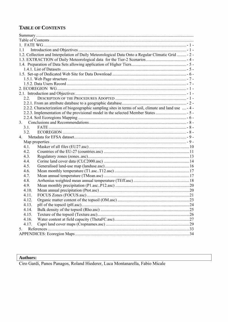
- 1 -
1 FATE WG
11 INTRODUCTION AND OBJECTIVES The revision of the Guidance Document on Persistence in Soil (9188VI97 rev 8) will provide notifiers Member States and the EFSA peer review process with guidance in the area of environmental fate and behaviour of pesticides in soil in the context of the review of active substances notified for inclusion in Annex I of Directive 91414EEC and Council Regulation 11072009 as well as for the review of plant protection products for national registrations in Member States The aim of this revision is to develop a tiered approach for exposure assessment in soil at EU level including
bull the development of a range of scenarios representing realistic worst-case conditions including ecological and climatic considerations
bull the appropriate definition of the role of results of field persistence and soil accumulation experiments in the tiered assessment
The tiered approach will consist of lower tiers that provide conservative estimates and higher tiers that provide more refined and realistic exposure estimates (EFSA 2010a) The parametrisation of the scenarios selected for the Tier-1 and Tier-2 require the availability of daily weather data over 20 years time One of the objectives of the second year of activities in 2010 was the extraction of these data sets in correspondence to the selected scenarios Furthermore in order to allow the external users to apply the models for Tier-3 and Tier-4 assessments all the data sets used in Tier 1 with additional data on land use-land cover crop distribution soil and climate parameters will be made available on a dedicated web portal hosted by the JRC web site
- 2 -
12 COLLECTION AND INTERPOLATION OF DAILY METEOROLOGICAL DATA ONTO A REGULAR CLIMATIC GRID
The MARS Unit currently collects and manages a large meteorological data set from Europe and from the Western part of North Africa For a detailed description of the procedures of collection and validation of meteorological data refer to the paper of Erik van der Goot (1998) or to the JRC Scientific Report (Gardi et al 2010) available online on the EFSA Website (httpwwwefsaeuropaeuenscdocsdoc64epdf) In this section is described the methodology adopted by the MARS Unit for the interpolation of daily meteorological data onto a 50 x 50 km grids (25 x 25 km grids is now also available) Globally in the MARS Data Base (DB) are present data referring to more than 6000 stations distributed in 48 countries but of these only one third present an adequate level of reliability and regular provided data In table 11 are reported the number of meteorological stations by country used in an operational way in the MCYFS In general the density of the meteo stations in the monitored areas is sufficient for the purpose of the project In figure 11 it is shown which is in average is the surface covered by one station Considering that each cell of the CGMS-grid is 50x50 km (equivalent to 2500 km2) is evident that the main agricultural areas present at least one station for each grid cell or one station for a group of four cells (equivalent to 10000 Km2) Observations of maximum and minimum temperatures precipitation amounts and sunshine duration (when available) are contained in the main hours synoptic METAR data provide temperature dew point visibility and cloud amount As far as available they can be used for intermediate or even non-standard (ie all but main and intermediate) hours From most countries outside Europe 3-hourly synoptic data are exchanged world wide and can be made available through Meteo Consult
The daily meteorological data is interpolated towards the centres of a regular climatic grid that measures 50 by 50 kilometres and amounts to 5625 cells The data of the climatic grid is stored in table GRID_WEATHER and are related to the parameters listed in table 12
- 3 -
Table 11 Available number of meteorological stations by country
- 4 -
Figure 11 The meteorological stations for which data are available for (part of) the period from1975 until the current day
Table 12 List of parameters contained in GRID_WEATHER table
All the input and output data such as the climatic grid presented are given in Lambert-Azimuthal projection system with meters as units and the parameters
bull Radius of sphere of reference 6370997 (m)
bull Longitude of centre of projection 900ordm
bull Latitude of centre of projection 4800ordm
13 EXTRACTION OF DAILY METEOROLOGICAL DATA FOR THE TIER-2 SCENARIOS For the development of the lower tiers - Tier 1 and Tier 2 the EFSA Fate working group selected six sites (two for each regulatory zone) across EU Each site has been attributed to grid cells of MARS DB and the completeness of weather data series was evaluated In particular for one of these grids
- 5 -
due to some lack in rainfall data it was necessary to find among the nearest grids an alternative cells with a complete daily data set (Fig 12)
Figure 12 Identification of alternatives weather stations in case of incompleteness of data set
Meteorological data have been exported as text files with the structure reported in table 13
Table 13 Structure of the meteorological data provided for the selected scenarios
GRID_NO DAY MAXIMUM_TEMPERATURE MINIMUM_TEMPERATURE WINDSPEED RAINFALL ET0 CALCULATED_RADIATION VAPOUR_PRESSURE
53067 111990 127 29 17 06 071527922 6129 92553067 211990 105 58 24 30 085431975 5791 88153067 311990 93 45 33 70 063213211 3312 91353067 411990 85 43 33 70 056450325 3099 90053067 511990 95 49 04 00 056357884 4853 82453067 611990 101 09 17 00 065470117 7619 79753067 711990 91 07 14 15 057378882 6874 79553067 811990 73 -01 22 00 064395052 6074 68953067 911990 69 19 02 00 048847278 5714 73553067 1011990 63 -17 15 00 05382598 5797 654
14 PREPARATION OF DATA SETS ALLOWING APPLICATION OF HIGHER TIERS For the higher tiers Tier-3 and Tier-4 options exist for refinement eg specific crops andor specific plant protection products with specific properties may be considered The procedures is essentially the same adopted for Tier-1 and Tier-2 but instead of using the total area of annual crops the area may be limited to the intended area of use and the selection is made only for the substance under consideration In order to enable assessors and applicants to apply the proposed methodology the following datasets will be made available as ASCII files on the JRC Soil Portal (see Paragraph 15 )
141 List of Datasets
In the following paragraphs a list of the available data sets are reported These data sets have been provided by JRC or made available thank to the elaboration performed by the EFSA Fate working group members Aaldrik Tiktak and Micheal Klein
- 6 -
General maps Masker of all files
Countries of the EU-27 (countriesmap)
Regulatory zones (Northern Central and Southern zone)
FOCUS Zones
Soil maps Organic matter content of the topsoil
pH of the topsoil
Bulk density of the topsoil
Texture of the topsoil
Water content at field capacity
Meteorological maps Mean monthly temperature (12 maps)
Mean annual temperature
Arrhenius weighted mean annual temperature
Mean monthly precipitation (12 maps)
Mean annual precipitation
Land use land cover maps Corine land cover data
Generalised land-use map (landusemap)
Capri land cover maps (24 maps)
15 SET-UP OF DEDICATED WEB SITE FOR DATA DOWNLOAD
In order to allow the data download a specific web page within the JRC Soil Portal will be realized on (httpeusoilsjrceceuropaeulibraryDataEFSA ) A print screen of the main web page is shown in Fig 13
JRC will require users of the data to fill an online form before proceeding with the data download (Fig 14) The information collected by JRC will be used for updating the data users on the possible release of new soil and weather related information and data sets However release of new information for the JRC Soil Portal will only happen after the FOCUS version control group chaired by EFSA has accepted the change of the new information
- 7 -
151 Web Page structure
Figure 13 Print-screen of the page dedicated to the data download
152 Data Users Record
Figure 14 Registration form to be filled for downloading the data
- 1 -
2 ECOREGION WG
21 INTRODUCTION AND OBJECTIVES The European Food Safety Authority (EFSA) asked the Panel on Plant Protection Products and their Residues (PPR) to further develop the concept of soil ecoregions in the context of the revision of the Guidance Document on Terrestrial Ecotoxicology (EFSA-Q-2009-00002) A modelling approach for defining soil ecoregions within Europe was developed to improve the realism of exposure scenarios for plant protection products Biogeographic data on four soil organisms groups (earthworms enchytraeids collembolans and isopods) were used to assign each functional group to different life forms representing depth horizons in which they occur Based on information from three Member States covering a North-South gradient Finland Germany and Portugal species presence-absence data were modelled using soil and climate data The objectives of JRC contribution were
- create a geographic database from the tabular data of the biogeographic survey
- extract soil and weather data in correspondence of biogeographic sampling sites
- implement the ecoregion models and create ecoregion maps
The technical details of the activities performed for the achievement of the above reported objectives are described in the following paragraphs and in the EFSA PPR Scientific Opinion on the development of a soil ecoregions concept using distribution data on invertebrates (EFSA 2010b) 22 DESCRIPTION OF THE PROCEDURES ADOPTED
The production of the Ecoregion maps for Finland Germany and Portugal represent the application of the proposed methodology to three test countries according to a North-South gradient
- 2 -
The complete description of the adopted approach is published as EFSA Opinion (EFSA 2010b) In the following paragraphs however is provided a more detailed description of the technical procedures adopted by JRC The conceptual framework for the development of soil Ecoregions is reported in the scheme of Figure 21 and the activities reported in the green boxes have been developed by JRC and described in the following paragraphs
Figure 21 Conceptual frame of the approach adopted for the definition of Soil Ecoregion
221 From an attribute database to a geographic database
The original biogeographical database provided for the three test Member States Finland Germany and Portugal was organized in separate Excel spreadsheets for the different groups of soil organisms and the geographic coordinates were based on UTM1 coordinate system based on Datum WGS842
1 UTM Universal Transver Maercator coordinate system is a grid-based method of specifying locations on the surface of the Earth that is
a practical application of a 2-dimensional Cartesian coordinate system 2 WGS 84 WGS (World Geodetic System) is a standard for use in cartography geodesy and navigation It comprises a standard
coordinate frame for the Earth a standard spheroidal reference surface (the datum or reference ellipsoid) for raw altitude data and a gravitational equipotential surface (the geoid) that defines the nominal sea level The GS 84 represent the latest revision of this standard
- 3 -
In order to project these data in the EU coordinate system (Lambert Azimuthal Equal Area) and to the process in the most efficient way it has been necessary to reorganize the database
One global spreadsheet for each of the three Member States has been produced
From each of these global spreadsheets partial spreadsheets have been derived grouping the records located in the same UTM zone
In order to keep the track of the changes a new field have been added (Fig 22) produced by the concatenation of
- Two capital letters for the organisms group (CO= collembola EW= earthworms IS= isopoda)
- The numeric value of ID Site
- The initial letter of the country name
Figure 22 Structure of the country-based spreadsheet the column with the new field has been outlined
These individual spreadsheets have been exported in DB4 format in order to be easily managed in ArcGIS ArcGIS 93 is the GIS software that has been used for the management and the analysis of the geographic information
The following phase in the management of the data has been the generation of Point Shapefiles representing the locations in which the soil organism inventory has been carried out and the re-projection of these maps
The extraction of soil and climate data from the raster dataset in correspondence of the of the soil organisms survey points has been realized using the ldquoExtract value to pointsrdquo procedure this procedure that is a classical example of spatial query allow to extract the cell values of a raster based on set of points
- 4 -
222Characterization of biogeographic sampling sites in terms of soil climate and land use characteristics
The biogeographic database consists of data on presenceabsence and in some cases abundance of selected groups of soil organisms and in some cases also data on land use vegetation soil and climate were reported The completeness of these environmental parameters essential for the ecological characterization of soil community however was very weak For this reason the data on land use soil and climate provided by JRC has been used to fill the gaps present in the original dataset
This process has been carried out using the utilities of spatial analysis present in a Geographical Information System (GIS) Once the geographic position of a sampling point is known it is possible do a spatial query in the GIS concerning the values of soil pH organic matter total precipitation and any other parameter that is available in a form of geographic database (Fig 23)
Figure 23 Schematic representation of the procedure adopted in a GIS for the extraction of given parameters (ie climate soil) for a given geographic position (ie observations)
- 5 -
223 Implementation of the provisional model in the selected Member States
The computation of the ecoregion maps has been based on the equations obtained in the data analysis implemented using the Map Algebra tools of Arc GIS (Raster Calculator Single Output Map Algebra) In Table 22 and 23 are reported the equations used for the computation of earthworm and enchytraeids maps respectively The first set of equations implying only the use of algebraic operators have been calculated using the lsquoraster calculatorrdquo within the Spatial Analyst toolset while the last expression based on logical operators have applied using the Single Output Map Algebra operator
Table 21 Equations used for earthworms Ecoregion Map
Map Algebra Operation with Raster Calculator t1
-0498 + ([Cropland] 00481) + ([Grassland] 09844) +([Forest3] -02298) + ([ph_top_efsa] 0317) + ([OC_efsa] -00905) + ([tmean] -02494) + ([Tdiff] -00418)
t2
27379 + ([Cropland] -01215) + ([Grassland] 02189) +([Forest3] -11576) + ([ph_top_efsa] 00567) + ([OC_efsa] -00105) +([total_prec] -00018) + ([tmean] 00956) + ([Tdiff] -01229)
z1 Exp([t1]) (1 + Exp([t1]))
z2 Exp([t2]) (1 + Exp([t2]))
ear_arr1 z1
ear_arr2 [z2] (1 - [z1])
ear_arr3 (1 - [z2]) (1 - [z1])
Map Algebra Operation with Single Output Map Algebra Earthworms Ecorgegion Map
con( ear_arr1 gt= 0667 1 ear_arr2 gt= 0667 2 ear_arr3 gt= 0667 3 arr1+arr2 gt= 0833 amp ear_arr1 lt= 0667 amp ear_arr2 lt= 0667 12 arr1+arr3 gt= 0833 amp ear_arr1 lt= 0667 amp ear_arr3 lt= 0667 13 arr2+arr3 gt= 0833 amp ear_arr2 lt= 0667 amp ear_arr3 lt= 0667 23 arr1+arr2 lt= 0833 amp arr2+arr3 lt= 0833 amp arr1+arr3 lt= 0833 123 )
- 6 -
Table 22 Equations used for enchytraeids Ecoregion Map
Map Algebra Operation with Raster Calculator t1
33243 + ([Grassland] 04764) + ([Forest3] 20354) + ([ph_top_efsa] -02776) + ([OC_efsa] -00206) + ([Clay] -00114) + ([total_prec] -00025) + ([tmean] -02286) + ([Tdiff] -00348)
t2
-65979 + ([Grassland] -05418) + ([Forest3] 10585) + ([ph_top_efsa] -02322) + ([OC_efsa] -01102) + ([Clay] -00505) + ([total_prec] -00010) + ([tmean] 03911) + ([Tdiff] 02961)
z1 Exp([t1]) (1 + Exp([t1]))
z2 Exp([t2]) (1 + Exp([t2]))
enc_arr1 z1
enc_arr2 [z2] (1 - [z1])
enc_arr3 (1 - [z2]) (1 - [z1])
Map Algebra Operation with Single Output Map Algebra Enchytraeids Ecorgegion Map
con( enc_arr1 gt= 0667 1 enc_arr2 gt= 0667 2 enc_arr3 gt= 0667 3 arr1+arr2 gt= 0833 amp enc_arr1 lt= 0667 amp enc_arr2 lt= 0667 12 arr1+arr3 gt= 0833 amp enc_arr1 lt= 0667 amp enc_arr3 lt= 0667 13 arr2+arr3 gt= 0833 amp enc_arr2 lt= 0667 amp enc_arr3 lt= 0667 23 arr1+arr2 lt= 0833 amp arr2+arr3 lt= 0833 amp arr1+arr3 lt= 0833 123 )
224 Soil Ecoregions Mapping
The output of the provisional models were a series of maps (one for each organism) where the territories of Finland Germany and Portugal have been classified in seven classes according to the triangles reported in figure 24
Earthworm ecoregion maps have been produced only for the three investigated countries but restricting Finland to its Southern part Enchytraeid ecoregions maps were limited to Germany and Finland since almost no enchytraeid data were available for Portugal For Collembola the fit of the model was very poor and the maps based on the modelled results did not show a convincing ecological meaning based on expert knowledge In case of Isopoda the model presented a good plausibility check with the observed and the modelled values However the analysis gave no clear indication for patterns differing between or within countries therefore isopods were excluded from further analysis and are not shown as maps
- 7 -
Although in principle the interpolation over the entire EU 27 territory would have been technically feasible mapping of territories without observed values were considered not to be reliable for the purpose of this opinion
The concepts of exposure scenario and the definition of soil profile depth relevant for different soil organisms communities led to the production of maps for earthworms and Enchytraeids where the territory of the investigated countries has been classified on the base of the depth relevant for the proposed Risk Assessment
Figure 24 Classification triangles used to classify the earthworms and enchytraeids soil communities
- 8 -
3 CONCLUSIONS AND RECOMMENDATIONS
31 FATE
The occurrence of gaps in daily meteorological data is relatively frequent especially over 20 year time frame For this reason it should be preferred the adoption of a statistical procedures for gap filling instead of selecting alternative nearest meteorological stations
For future applications the availability of 25 km grids will provide an improved geographic resolution for the representation of European climate
32 ECOREGION
During the analysis of the biogeographic database it was found the lack of complete soil land use and climate data sets for the vast majority of the observation sites For this reason it has been necessary to derive such data from the 1 km grid data set (soil and land use) and from the 50 km grids (meteorological data)
It should be outlined that while the use of these EU wide geographic data set is optimal for modelling application probably does not have the necessary spatial resolution for the characterization of point observation sites
- 9 -
4 METADATA FOR EFSA DATASET
A database of maps was created on the basis of the dataset provided by JRC (see Gardi et al 2008) This dataset was supplemented with data from the CAPRI land cover database (Leip et al 2008) JRC is acknowledged for making the data available in a common resolution and projection
Map properties
Common metadata properties for the maps are Format compressed ASCII grid Reference system ETRS 89 LAEA Rows 4098 Columns 3500 Lower left 2500000 Upper left 1412000 Cell size 1000 Unit m Nr of cells with a value 3997812
10
41 Masker of all files (EU27asc)
1 This map is a mask created including all the EU-27 countries and the Corine land-use classes 1-38 and 49 Surface waters and coastal lagoons are excluded from the mask
Legend There is only one legend unit ie 1 which means that the grid cell is included
Figure 41 Masker for the dataset The masker has only one value ie 1
11
42 Countries of the EU-27 (countriesasc)
The map shows the countries of the EU-27 It was obtained by masking the NUTS level 0 map with the mask EU27 Legend Number Country 1 Albania 5 Austria 8 Belgium 9 Bulgaria 15 Czech Republic 16 Germany 17 Denmark 20 Estonia 23 Spain 24 Finland 26 France 31 Greece 34 Hungary 35 Ireland 41 Italy 48 Lithuania 49 Luxemburg 50 Latvia 58 Netherlands 61 Poland 62 Portugal 64 Romania 67 Sweden 68 Slovenia 70 Slovakia 78 United Kingdom
12
Figure 42 Countries of the EU-27
13
43 Regulatory zones (zonesasc)
This map shows the regulatory zones of the EU-27 The map is a reclassification of the map countriesmap Legend Number Name Countries 1 North 17 20 24 48 50 and 67 2 Centre 5 8 16 34 35 49 58 61 64 68 70 and 78 3 South 1 9 23 26 31 41 and 62
Figure 43 The regulatory zones of the EU-27
14
44 Corine land cover data (CLC2000asc)
The map shows all the possible land use classes at the Corine map The map presented here is at a resolution of 1x1 km2 the original map was at a resolution of 025 km2 For each 1x1 km2 grid cell the dominant of the four underlying grid cells was taken The dataset is described in Nunes de Lima (2005) Legend Number CLC
code Description
1 111 Continuous urban fabric 2 112 Discontinuous urban fabric 3 121 Industrial or commercial units 4 122 Road and rail networks and associated land 5 123 Port areas 6 124 Airports 7 131 Mineral extraction sites 8 132 Dump sites 9 133 Construction sites 10 141 Green urban areas 11 142 Sport and leisure facilities 12 211 Non-irrigated arable land 13 212 Permanently irrigated land 14 213 Rice fields 15 221 Vineyards 16 222 Fruit trees and berry plantations 17 223 Olive groves 18 231 Pastures 19 241 Annual crops associated with permanent crops 20 242 Complex cultivation patterns 21 243 Land occupied by agriculture with significant areas of natural
vegetation 22 244 Agro-forestry areas 23 311 Broad-leaved forest 24 312 Coniferous forest 25 313 Mixed forest 26 321 Natural grasslands 27 322 Moors and heathland 28 323 Sclerophyllous vegetation 29 324 Transitional woodland-shrub 30 331 Beaches dunes sands 31 332 Bare rocks 32 333 Sparsely vegetated areas 33 334 Burnt areas 34 335 Glaciers and perpetual snow 35 411 Inland marshes 36 412 Peat bogs 37 421 Salt marshes
15
38 422 Salines 39 423 Intertidal flats 40 511 Water courses 41 512 Water bodies 42 521 Coastal lagoons 43 522 Estuaries 44 523 Sea and ocean 48 999 NODATA 49 990 UNCLASSIFIED LAND SURFACE 50 995 UNCLASSIFIED WATER BODIES
16
45 Generalised land-use map (landuseasc)
The generalised land-use map is a reclassification of the Corine 2000 land-use map It is created to distinguish the most important land-use types Land use class 1 serves as the masker in EFSA (2010)
Legend Number Description Number in map above 1 Annual Crops 12 13 19-21 2 Grass 18 3 Permanent crops 15-17 and 22 4 Rice 14 5 Non agricultural all other classes
Figure 44 The generalised land-use map
17
46 Mean monthly temperature (T1ascT12asc)
The dataset consists of 12 maps containing the monthly mean temperature (deg C) for the period 1960-1990 The dataset is described in Hijmans et al (2005) Legend Mean monthly temperature (deg C) data type Real 47 Mean annual temperature (TMeanasc)
The map shows the mean annual temperature (deg C) for the period 1960-1990 It is calculating by taking the arithmetic mean of maps T1T12asc The dataset is described in Hijmans et al (2005) Legend Mean annual temperature (deg C) data type Real
Figure 45 Mean annual temperature for the period 1960-1990 taken from Worldclim dataset
18
48 Arrhenius weighted mean annual temperature (TEffasc)
The map shows the Arrhenius weighted mean annual temperature (deg C) for the period 1960-1990 It is calculated using the equation (EFSA 2010 Appendix A3)
( )
( ) ( )( ) 0
exp273)(
1ln0
=
⎥⎦
⎤⎢⎣
⎡minus=gt
⎥⎥⎦
⎤
⎢⎢⎣
⎡minus=
int
tTfelsetRT
EtTfthentTif
dttTft
R
ET
act
t
end
acteff
end
(1)
where Teff (K) is the Arrhenius weighted mean annual temperature Eact is the Arrhenius activation energy (kJ mol-1) R (kJ mol-1 K-1) is the gas constant T (K) is the temperature and t is time Eact was set to 654 kJ mol-1 according to EFSA (2007) See further EFSA (2010) Notice that the temperatures in the equation are in K whereas the temperature in the maps is in deg C Legend Arrhenius weighted mean annual temperature (deg C) data type Real
19
Figure 46 Arrhenius weighted mean temperature (deg C) for the period 1960-1990 For a description of the averaging procedure refer to EFSA (2010)
20
49 Mean monthly precipitation (P1ascP12asc)
The dataset consists of 12 maps containing the monthly mean precipitation (mmmonth) for the period 1960-1990 The dataset is described in Hijmans et al (2005) Legend Mean monthly precipitation (mmmo) data type Real 410 Mean annual precipitation (Ptotasc)
The map shows the mean annual precipitation for the period 1960-1990 (mmyear) It is calculated by summing P1P12map The dataset is described in Hijmans et al (2005) Legend Mean annual precipitation (mmyr) data type Real
Figure 47 Mean annual precipitation (mm) for the period 1960-1990 as taken from the Worldclim dataset
21
411 FOCUS Zones (FOCUSasc)
The map shows the FOCUS zones according to the classification in FOCUS (2000) The maps Tmeanmap and Ptotmap were used to create the overlay so the classification is based on WorldClim (Hijmans et al 2005)
Legend Number Name Tmean (deg C) Ptot (mmyr) 1 Jokioinen lt5 deg C gt 0 mmyr 2 Chateaudun 5 ndash 125 deg C lt 600 mmyr 3 Hamburg 5 ndash 125 deg C 600 ndash 800 mmyr 4 Kremsmuumlnster 5 ndash 125 deg C 800 ndash 1000 mmyr 5 Okehampton 5 ndash 125 deg C gt 1000 mmyr 6 Sevilla gt 125 deg C lt 600 mmyr 7 Thiva gt 125 deg C 600 ndash 800 mmyr 8 Piacenza gt 125 deg C 800 ndash 1000 mmyr 9 Porto gt 125 deg C gt 1000 mmyr
22
Figure 48 FOCUS climatic zones based on the mean annual temperature and mean annual precipitation from Worldclim
23
412 Organic matter content of the topsoil (OMasc)
The map shows the organic matter content of the topsoil It is obtained by multiplying the original OCTOP map described in Jones et al (2005) by 172 Legend Organic matter content of the topsoil (gg) data type Real
Figure 49 Organic matter content of the top 30 cm of the soil (gg)
24
413 pH of the topsoil (pHasc)
The map shows the mean pH measured in water (125) of the top 30 cm of the soil See FAO (2008) for details Legend pH measured in water of the topsoil data type Real
Figure 410 pH water (125) of the top 30 cm of the soil
25
414 Bulk density of the topsoil (Rhoasc)
The map shows the bulk density of the topsoil It is calculated from the organic matter content map using the equation (Tiktak et al 2002)
)910(291012361800 2 =minus+= rff omomρ (2)
Legend Dry bulk density of the topsoil (kg m-3) data type Real
Figure 411 Bulk density of the top 30 cm of the soil calculated by the pedotransfer function described in Tiktak et al (2002)
26
415 Texture of the topsoil (Textureasc)
The map shows the textural class of the topsoil It is obtained from the soil geographical database of Eurasia at a scale of 11000000 (for each grid cell the dominant soil textural class was taken) Legend Number Description 1 Coarse (18 lt clay and gt 65 sand) 2 Medium (18 lt clay lt 35 and gt= 15 sand or 18 ltclay and 15 lt sand lt
65) 3 Medium fine (lt 35 clay and lt 15 sand) 4 Fine (35 lt clay lt 60) 5 Very fine (clay gt 60 ) 9 No mineral texture (Peat soils)
Figure 412Topsoil texture obtained from the soil database of Europe 11000000
27
416 Water content at field capacity (ThetaFCasc)
The map shows the water content at field capacity (m3 m-3) It is calculated for each soil textural class with the Mualem-Van Genuchten equation
( ) mnrs
rh
h minus+
minus+=
α
θθθθ1
)( (1)
where θ (m3 m-3) is the volume fraction of water h (cm) is the soil water pressure head θs (m3 m-3) is the volume fraction of water at saturation θr (m3 m-3) is the residual water content in the extremely dry range α (cm-1) and n (-) are empirical parameters and m (-) can be taken equal to
nm 11minus=
The soil water pressure head was set at -100 cm Parameter values were obtained from the HYPRES pedotransfer rule (Woumlsten et al 1999) and are given in EFSA (2010) table 3 Legend Volumetric water content at field capacity (m3 m-3) data type Real The map contains six discrete classes
28
Figure 413 Volume fraction of water at field capacity calculated from the soil textural class using the HYPRES pedotransfer rule
29
417 Capri land cover maps (Cropnamesasc)
These maps show for each pixel of 1x1 km2 the area covered with a certain crop The CAPRI maps were obtained by combining remote sensing data administrative crop data land suitability data and statistical modelling The CORINE land cover map serves as a starting point Subdivisions within CORINE land cover classes were made based on a statistical model regressing point observations of cropping activities on soil relief and climate parameters (land suitability) Statistical data of agricultural production and land cover available for administrative regions were additionally used to scale the land cover classes 18 of the CAPRI land cover classes are classified as annual crops and are included in the EFSA dataset See Leip et al (2008) for a description of the dataset Legend Area (100) covered by a crop data type Real The names of the maps are self explaining The values range from 0 to 10000
30
Figure 414 Crop cover maps ( of area) for barley common wheat texture crops floriculture other fodder crops and industrial crops
31
Figure 415 Crop cover maps ( of area) for maize oats other cereals pulses rapes and root crops
32
Figure 416 Crop cover maps ( of area) for rye soya sugar beet sunflowers vegetables and durum wheat
33
5 REFERENCES
Goot E van der 1998 Spatial interpolation of daily meteorological data for the Crop Growth Monitoring System (CGMS) In M Bindi B Gozzini (eds) Proceedings of seminar on dataspatial distribution in meteorology and climatology 28 September - 3 October 1997 Volterra Italy EUR 18472 EN Office for Official Publications of the EU Luxembourg p 141-153
Gardi C Montanarella L Hiederer R Jones A Micale F 2010 Activities realized within the Service Level Agreement between JRC and EFSA as a support of the FATE Working Group of EFSA PPR in support of the revision of the guidance document Persistence in Soil JRC Technical Svientific and Technical Report 39 pp - EUR 24345
Gardi C2010 Report on the Activities realised within the Service Licence Agreement between JRC and EFSA as a support of the FATE Working Group of EFSA PPR JRC Scientific Report (SLAEFSA-JRC200801)
EFSA 2010a Opinion of the Scientific Panel on Plant Protection products and their Residues on outline proposals for assessment of exposure of organisms to substances in soil EFSA Journal 8(1)1442
EFSA 2010b Opinion of the Scientific Panel on Plant Protection products and their Residues on on the development of a soil ecoregions concept using distribution data on invertebrates EFSA Journal 8(10)1820
EFSA 2007 Opinion on a request from EFSA related to the default Q10 value used to describe the temperature effect on transformation rates of pesticides in soil Scientific Opinion of the Panel on Plant Protection Products and their Residues (PPR-Panel) The EFSA Journal (622)1 32
EFSA 2010 Selection of scenarios for exposure of soil organisms The EFSA Journal (2010) 8(46)1642
FAOIIASAISRICISS-CASJRC 2008 Harmonized World Soil Database (version 10) FAO Rome Italy and IIASA Laxenburg Austria 37pp
FOCUS 2010 Assessing potential movement of active substances and their metabolites to ground water in the EU EC Document reference Sancoxxx2010 Available at FOCUS website httpvisoeijrcitfocus
Hijmans RJ SE Cameron JL Parra PG Jones and A Jarvis 2005 Very high resolution interpolated climate surfaces for global land areas Int J Climatology (25)1965-1978
Jones RJA R Hiederer E Rusco PJ Loveland and L Montanarella 2005 Estimating organic carbon in the soils of Europe for policy support European Journal of Soil Science (56)655-671
Leip A G Marchi R Koeble M Kempen W Britz and C Li 2008 Linking an economic model for European agriculture with a mechanistic model to estimate nitrogen and carbon losses from arable soils in Europe Biogeosciences (5)73-94
Tiktak A DS de Nie AMA van der Linden and R Kruijne 2002 Modelling the leaching and drainage of pesticides in the Netherlands the GeoPEARL model Agronomie (22)373-387
Woumlsten JHM A Nemes A Lilly and C Le Bas 1999 Development and use of a database of hydraulic properties of European soils Geoderma (90)169ndash185
34
APPENDICES ECOREGION MAPS
Earthworm Finland
35
Earthworm Germany
36
Earthworm Portugal
37
Enchytraeids Finland
38
Enchytraeids Germany
39
European Commission EUR 24744 EN ndash Joint Research Centre ndash Institute for Environment and Sustainability Title Report on the activities realized within the Service Level Agreement between JRC and EFSA Author(s) Ciro Gardi Panos Panagos Roland Hiederer Luca Montanarella Fabio Micale Luxembourg Publications Office of the European Union 2011 ndash 38 pp ndash 210 x 297 cm EUR ndash Scientific and Technical Research series ndash ISSN 1018-5593 ISBN 978-92-79-19521-1 doi10278861018 Abstract The activities realized in 2010 by JRC as support to the FATE and the ECOREGION EFSA PPR Working Groups are shortly described For the FATE WG the vast majority of data has been provided in 2009 during the first year of the Service Level Agreement (SLA) and in 2010 the daily weather data for the six selected sites were produced All the data used for the scenario selection procedures with additional data on land use-land cover crop distribution soil and climate parameters will be made available for external user in first half of 2011 For the ECOREGION WG the analysis has been carried out for three Member States covering a North-South gradient from Finland Germany to Portugal Soil and weather data have been used for the characterisation of bio-geographic sampling sites and for the implementation of the ecoregion model Ecoregion maps were produced for earthworms and enchytraeids for Finland and Germany and revealed marked differences between the countries The same approach has been applied also to Collembola and Isopoda but for these two taxa led to a rather poor discrimination both between and within countries
How to obtain EU publications Our priced publications are available from EU Bookshop (httpbookshopeuropaeu) where you can place an order with the sales agent of your choice The Publications Office has a worldwide network of sales agents You can obtain their contact details by sending a fax to (352) 29 29-42758
The mission of the JRC is to provide customer-driven scientific and technical supportfor the conception development implementation and monitoring of EU policies As a service of the European Commission the JRC functions as a reference centre of science and technology for the Union Close to the policy-making process it serves the common interest of the Member States while being independent of special interests whether private or national
LB
-NA
-24744-EN-C
- 141 List of Datasets
- 151 Web Page structure
- 152 Data Users Record
- 22 Description of the Procedures Adopted
- 221 From an attribute database to a geographic database
- 222Characterization of biogeographic sampling sites in terms of soil climate and land use characteristics
- 223 Implementation of the provisional model in the selected Member States
- 224 Soil Ecoregions Mapping
- 3 Conclusions and Recommendations
-
- 31 FATE
- 32 ECOREGION
-
- 4 Metadata for EFSA dataset
-
- Map properties
- 41 Masker of all files (EU27asc)
- 42 Countries of the EU-27 (countriesasc)
- 43 Regulatory zones (zonesasc)
- 44 Corine land cover data (CLC2000asc)
- 45 Generalised land-use map (landuseasc)
- 46 Mean monthly temperature (T1ascT12asc)
- 47 Mean annual temperature (TMeanasc)
- 48 Arrhenius weighted mean annual temperature (TEffasc)
- 49 Mean monthly precipitation (P1ascP12asc)
- 410 Mean annual precipitation (Ptotasc)
- 411 FOCUS Zones (FOCUSasc)
- 412 Organic matter content of the topsoil (OMasc)
- 413 pH of the topsoil (pHasc)
- 414 Bulk density of the topsoil (Rhoasc)
- 415 Texture of the topsoil (Textureasc)
- 416 Water content at field capacity (ThetaFCasc)
- 417 Capri land cover maps (Cropnamesasc)
-
- 5 References
-
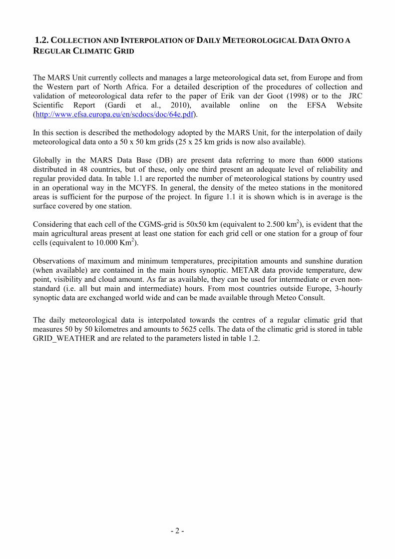
- 2 -
12 COLLECTION AND INTERPOLATION OF DAILY METEOROLOGICAL DATA ONTO A REGULAR CLIMATIC GRID
The MARS Unit currently collects and manages a large meteorological data set from Europe and from the Western part of North Africa For a detailed description of the procedures of collection and validation of meteorological data refer to the paper of Erik van der Goot (1998) or to the JRC Scientific Report (Gardi et al 2010) available online on the EFSA Website (httpwwwefsaeuropaeuenscdocsdoc64epdf) In this section is described the methodology adopted by the MARS Unit for the interpolation of daily meteorological data onto a 50 x 50 km grids (25 x 25 km grids is now also available) Globally in the MARS Data Base (DB) are present data referring to more than 6000 stations distributed in 48 countries but of these only one third present an adequate level of reliability and regular provided data In table 11 are reported the number of meteorological stations by country used in an operational way in the MCYFS In general the density of the meteo stations in the monitored areas is sufficient for the purpose of the project In figure 11 it is shown which is in average is the surface covered by one station Considering that each cell of the CGMS-grid is 50x50 km (equivalent to 2500 km2) is evident that the main agricultural areas present at least one station for each grid cell or one station for a group of four cells (equivalent to 10000 Km2) Observations of maximum and minimum temperatures precipitation amounts and sunshine duration (when available) are contained in the main hours synoptic METAR data provide temperature dew point visibility and cloud amount As far as available they can be used for intermediate or even non-standard (ie all but main and intermediate) hours From most countries outside Europe 3-hourly synoptic data are exchanged world wide and can be made available through Meteo Consult
The daily meteorological data is interpolated towards the centres of a regular climatic grid that measures 50 by 50 kilometres and amounts to 5625 cells The data of the climatic grid is stored in table GRID_WEATHER and are related to the parameters listed in table 12
- 3 -
Table 11 Available number of meteorological stations by country
- 4 -
Figure 11 The meteorological stations for which data are available for (part of) the period from1975 until the current day
Table 12 List of parameters contained in GRID_WEATHER table
All the input and output data such as the climatic grid presented are given in Lambert-Azimuthal projection system with meters as units and the parameters
bull Radius of sphere of reference 6370997 (m)
bull Longitude of centre of projection 900ordm
bull Latitude of centre of projection 4800ordm
13 EXTRACTION OF DAILY METEOROLOGICAL DATA FOR THE TIER-2 SCENARIOS For the development of the lower tiers - Tier 1 and Tier 2 the EFSA Fate working group selected six sites (two for each regulatory zone) across EU Each site has been attributed to grid cells of MARS DB and the completeness of weather data series was evaluated In particular for one of these grids
- 5 -
due to some lack in rainfall data it was necessary to find among the nearest grids an alternative cells with a complete daily data set (Fig 12)
Figure 12 Identification of alternatives weather stations in case of incompleteness of data set
Meteorological data have been exported as text files with the structure reported in table 13
Table 13 Structure of the meteorological data provided for the selected scenarios
GRID_NO DAY MAXIMUM_TEMPERATURE MINIMUM_TEMPERATURE WINDSPEED RAINFALL ET0 CALCULATED_RADIATION VAPOUR_PRESSURE
53067 111990 127 29 17 06 071527922 6129 92553067 211990 105 58 24 30 085431975 5791 88153067 311990 93 45 33 70 063213211 3312 91353067 411990 85 43 33 70 056450325 3099 90053067 511990 95 49 04 00 056357884 4853 82453067 611990 101 09 17 00 065470117 7619 79753067 711990 91 07 14 15 057378882 6874 79553067 811990 73 -01 22 00 064395052 6074 68953067 911990 69 19 02 00 048847278 5714 73553067 1011990 63 -17 15 00 05382598 5797 654
14 PREPARATION OF DATA SETS ALLOWING APPLICATION OF HIGHER TIERS For the higher tiers Tier-3 and Tier-4 options exist for refinement eg specific crops andor specific plant protection products with specific properties may be considered The procedures is essentially the same adopted for Tier-1 and Tier-2 but instead of using the total area of annual crops the area may be limited to the intended area of use and the selection is made only for the substance under consideration In order to enable assessors and applicants to apply the proposed methodology the following datasets will be made available as ASCII files on the JRC Soil Portal (see Paragraph 15 )
141 List of Datasets
In the following paragraphs a list of the available data sets are reported These data sets have been provided by JRC or made available thank to the elaboration performed by the EFSA Fate working group members Aaldrik Tiktak and Micheal Klein
- 6 -
General maps Masker of all files
Countries of the EU-27 (countriesmap)
Regulatory zones (Northern Central and Southern zone)
FOCUS Zones
Soil maps Organic matter content of the topsoil
pH of the topsoil
Bulk density of the topsoil
Texture of the topsoil
Water content at field capacity
Meteorological maps Mean monthly temperature (12 maps)
Mean annual temperature
Arrhenius weighted mean annual temperature
Mean monthly precipitation (12 maps)
Mean annual precipitation
Land use land cover maps Corine land cover data
Generalised land-use map (landusemap)
Capri land cover maps (24 maps)
15 SET-UP OF DEDICATED WEB SITE FOR DATA DOWNLOAD
In order to allow the data download a specific web page within the JRC Soil Portal will be realized on (httpeusoilsjrceceuropaeulibraryDataEFSA ) A print screen of the main web page is shown in Fig 13
JRC will require users of the data to fill an online form before proceeding with the data download (Fig 14) The information collected by JRC will be used for updating the data users on the possible release of new soil and weather related information and data sets However release of new information for the JRC Soil Portal will only happen after the FOCUS version control group chaired by EFSA has accepted the change of the new information
- 7 -
151 Web Page structure
Figure 13 Print-screen of the page dedicated to the data download
152 Data Users Record
Figure 14 Registration form to be filled for downloading the data
- 1 -
2 ECOREGION WG
21 INTRODUCTION AND OBJECTIVES The European Food Safety Authority (EFSA) asked the Panel on Plant Protection Products and their Residues (PPR) to further develop the concept of soil ecoregions in the context of the revision of the Guidance Document on Terrestrial Ecotoxicology (EFSA-Q-2009-00002) A modelling approach for defining soil ecoregions within Europe was developed to improve the realism of exposure scenarios for plant protection products Biogeographic data on four soil organisms groups (earthworms enchytraeids collembolans and isopods) were used to assign each functional group to different life forms representing depth horizons in which they occur Based on information from three Member States covering a North-South gradient Finland Germany and Portugal species presence-absence data were modelled using soil and climate data The objectives of JRC contribution were
- create a geographic database from the tabular data of the biogeographic survey
- extract soil and weather data in correspondence of biogeographic sampling sites
- implement the ecoregion models and create ecoregion maps
The technical details of the activities performed for the achievement of the above reported objectives are described in the following paragraphs and in the EFSA PPR Scientific Opinion on the development of a soil ecoregions concept using distribution data on invertebrates (EFSA 2010b) 22 DESCRIPTION OF THE PROCEDURES ADOPTED
The production of the Ecoregion maps for Finland Germany and Portugal represent the application of the proposed methodology to three test countries according to a North-South gradient
- 2 -
The complete description of the adopted approach is published as EFSA Opinion (EFSA 2010b) In the following paragraphs however is provided a more detailed description of the technical procedures adopted by JRC The conceptual framework for the development of soil Ecoregions is reported in the scheme of Figure 21 and the activities reported in the green boxes have been developed by JRC and described in the following paragraphs
Figure 21 Conceptual frame of the approach adopted for the definition of Soil Ecoregion
221 From an attribute database to a geographic database
The original biogeographical database provided for the three test Member States Finland Germany and Portugal was organized in separate Excel spreadsheets for the different groups of soil organisms and the geographic coordinates were based on UTM1 coordinate system based on Datum WGS842
1 UTM Universal Transver Maercator coordinate system is a grid-based method of specifying locations on the surface of the Earth that is
a practical application of a 2-dimensional Cartesian coordinate system 2 WGS 84 WGS (World Geodetic System) is a standard for use in cartography geodesy and navigation It comprises a standard
coordinate frame for the Earth a standard spheroidal reference surface (the datum or reference ellipsoid) for raw altitude data and a gravitational equipotential surface (the geoid) that defines the nominal sea level The GS 84 represent the latest revision of this standard
- 3 -
In order to project these data in the EU coordinate system (Lambert Azimuthal Equal Area) and to the process in the most efficient way it has been necessary to reorganize the database
One global spreadsheet for each of the three Member States has been produced
From each of these global spreadsheets partial spreadsheets have been derived grouping the records located in the same UTM zone
In order to keep the track of the changes a new field have been added (Fig 22) produced by the concatenation of
- Two capital letters for the organisms group (CO= collembola EW= earthworms IS= isopoda)
- The numeric value of ID Site
- The initial letter of the country name
Figure 22 Structure of the country-based spreadsheet the column with the new field has been outlined
These individual spreadsheets have been exported in DB4 format in order to be easily managed in ArcGIS ArcGIS 93 is the GIS software that has been used for the management and the analysis of the geographic information
The following phase in the management of the data has been the generation of Point Shapefiles representing the locations in which the soil organism inventory has been carried out and the re-projection of these maps
The extraction of soil and climate data from the raster dataset in correspondence of the of the soil organisms survey points has been realized using the ldquoExtract value to pointsrdquo procedure this procedure that is a classical example of spatial query allow to extract the cell values of a raster based on set of points
- 4 -
222Characterization of biogeographic sampling sites in terms of soil climate and land use characteristics
The biogeographic database consists of data on presenceabsence and in some cases abundance of selected groups of soil organisms and in some cases also data on land use vegetation soil and climate were reported The completeness of these environmental parameters essential for the ecological characterization of soil community however was very weak For this reason the data on land use soil and climate provided by JRC has been used to fill the gaps present in the original dataset
This process has been carried out using the utilities of spatial analysis present in a Geographical Information System (GIS) Once the geographic position of a sampling point is known it is possible do a spatial query in the GIS concerning the values of soil pH organic matter total precipitation and any other parameter that is available in a form of geographic database (Fig 23)
Figure 23 Schematic representation of the procedure adopted in a GIS for the extraction of given parameters (ie climate soil) for a given geographic position (ie observations)
- 5 -
223 Implementation of the provisional model in the selected Member States
The computation of the ecoregion maps has been based on the equations obtained in the data analysis implemented using the Map Algebra tools of Arc GIS (Raster Calculator Single Output Map Algebra) In Table 22 and 23 are reported the equations used for the computation of earthworm and enchytraeids maps respectively The first set of equations implying only the use of algebraic operators have been calculated using the lsquoraster calculatorrdquo within the Spatial Analyst toolset while the last expression based on logical operators have applied using the Single Output Map Algebra operator
Table 21 Equations used for earthworms Ecoregion Map
Map Algebra Operation with Raster Calculator t1
-0498 + ([Cropland] 00481) + ([Grassland] 09844) +([Forest3] -02298) + ([ph_top_efsa] 0317) + ([OC_efsa] -00905) + ([tmean] -02494) + ([Tdiff] -00418)
t2
27379 + ([Cropland] -01215) + ([Grassland] 02189) +([Forest3] -11576) + ([ph_top_efsa] 00567) + ([OC_efsa] -00105) +([total_prec] -00018) + ([tmean] 00956) + ([Tdiff] -01229)
z1 Exp([t1]) (1 + Exp([t1]))
z2 Exp([t2]) (1 + Exp([t2]))
ear_arr1 z1
ear_arr2 [z2] (1 - [z1])
ear_arr3 (1 - [z2]) (1 - [z1])
Map Algebra Operation with Single Output Map Algebra Earthworms Ecorgegion Map
con( ear_arr1 gt= 0667 1 ear_arr2 gt= 0667 2 ear_arr3 gt= 0667 3 arr1+arr2 gt= 0833 amp ear_arr1 lt= 0667 amp ear_arr2 lt= 0667 12 arr1+arr3 gt= 0833 amp ear_arr1 lt= 0667 amp ear_arr3 lt= 0667 13 arr2+arr3 gt= 0833 amp ear_arr2 lt= 0667 amp ear_arr3 lt= 0667 23 arr1+arr2 lt= 0833 amp arr2+arr3 lt= 0833 amp arr1+arr3 lt= 0833 123 )
- 6 -
Table 22 Equations used for enchytraeids Ecoregion Map
Map Algebra Operation with Raster Calculator t1
33243 + ([Grassland] 04764) + ([Forest3] 20354) + ([ph_top_efsa] -02776) + ([OC_efsa] -00206) + ([Clay] -00114) + ([total_prec] -00025) + ([tmean] -02286) + ([Tdiff] -00348)
t2
-65979 + ([Grassland] -05418) + ([Forest3] 10585) + ([ph_top_efsa] -02322) + ([OC_efsa] -01102) + ([Clay] -00505) + ([total_prec] -00010) + ([tmean] 03911) + ([Tdiff] 02961)
z1 Exp([t1]) (1 + Exp([t1]))
z2 Exp([t2]) (1 + Exp([t2]))
enc_arr1 z1
enc_arr2 [z2] (1 - [z1])
enc_arr3 (1 - [z2]) (1 - [z1])
Map Algebra Operation with Single Output Map Algebra Enchytraeids Ecorgegion Map
con( enc_arr1 gt= 0667 1 enc_arr2 gt= 0667 2 enc_arr3 gt= 0667 3 arr1+arr2 gt= 0833 amp enc_arr1 lt= 0667 amp enc_arr2 lt= 0667 12 arr1+arr3 gt= 0833 amp enc_arr1 lt= 0667 amp enc_arr3 lt= 0667 13 arr2+arr3 gt= 0833 amp enc_arr2 lt= 0667 amp enc_arr3 lt= 0667 23 arr1+arr2 lt= 0833 amp arr2+arr3 lt= 0833 amp arr1+arr3 lt= 0833 123 )
224 Soil Ecoregions Mapping
The output of the provisional models were a series of maps (one for each organism) where the territories of Finland Germany and Portugal have been classified in seven classes according to the triangles reported in figure 24
Earthworm ecoregion maps have been produced only for the three investigated countries but restricting Finland to its Southern part Enchytraeid ecoregions maps were limited to Germany and Finland since almost no enchytraeid data were available for Portugal For Collembola the fit of the model was very poor and the maps based on the modelled results did not show a convincing ecological meaning based on expert knowledge In case of Isopoda the model presented a good plausibility check with the observed and the modelled values However the analysis gave no clear indication for patterns differing between or within countries therefore isopods were excluded from further analysis and are not shown as maps
- 7 -
Although in principle the interpolation over the entire EU 27 territory would have been technically feasible mapping of territories without observed values were considered not to be reliable for the purpose of this opinion
The concepts of exposure scenario and the definition of soil profile depth relevant for different soil organisms communities led to the production of maps for earthworms and Enchytraeids where the territory of the investigated countries has been classified on the base of the depth relevant for the proposed Risk Assessment
Figure 24 Classification triangles used to classify the earthworms and enchytraeids soil communities
- 8 -
3 CONCLUSIONS AND RECOMMENDATIONS
31 FATE
The occurrence of gaps in daily meteorological data is relatively frequent especially over 20 year time frame For this reason it should be preferred the adoption of a statistical procedures for gap filling instead of selecting alternative nearest meteorological stations
For future applications the availability of 25 km grids will provide an improved geographic resolution for the representation of European climate
32 ECOREGION
During the analysis of the biogeographic database it was found the lack of complete soil land use and climate data sets for the vast majority of the observation sites For this reason it has been necessary to derive such data from the 1 km grid data set (soil and land use) and from the 50 km grids (meteorological data)
It should be outlined that while the use of these EU wide geographic data set is optimal for modelling application probably does not have the necessary spatial resolution for the characterization of point observation sites
- 9 -
4 METADATA FOR EFSA DATASET
A database of maps was created on the basis of the dataset provided by JRC (see Gardi et al 2008) This dataset was supplemented with data from the CAPRI land cover database (Leip et al 2008) JRC is acknowledged for making the data available in a common resolution and projection
Map properties
Common metadata properties for the maps are Format compressed ASCII grid Reference system ETRS 89 LAEA Rows 4098 Columns 3500 Lower left 2500000 Upper left 1412000 Cell size 1000 Unit m Nr of cells with a value 3997812
10
41 Masker of all files (EU27asc)
1 This map is a mask created including all the EU-27 countries and the Corine land-use classes 1-38 and 49 Surface waters and coastal lagoons are excluded from the mask
Legend There is only one legend unit ie 1 which means that the grid cell is included
Figure 41 Masker for the dataset The masker has only one value ie 1
11
42 Countries of the EU-27 (countriesasc)
The map shows the countries of the EU-27 It was obtained by masking the NUTS level 0 map with the mask EU27 Legend Number Country 1 Albania 5 Austria 8 Belgium 9 Bulgaria 15 Czech Republic 16 Germany 17 Denmark 20 Estonia 23 Spain 24 Finland 26 France 31 Greece 34 Hungary 35 Ireland 41 Italy 48 Lithuania 49 Luxemburg 50 Latvia 58 Netherlands 61 Poland 62 Portugal 64 Romania 67 Sweden 68 Slovenia 70 Slovakia 78 United Kingdom
12
Figure 42 Countries of the EU-27
13
43 Regulatory zones (zonesasc)
This map shows the regulatory zones of the EU-27 The map is a reclassification of the map countriesmap Legend Number Name Countries 1 North 17 20 24 48 50 and 67 2 Centre 5 8 16 34 35 49 58 61 64 68 70 and 78 3 South 1 9 23 26 31 41 and 62
Figure 43 The regulatory zones of the EU-27
14
44 Corine land cover data (CLC2000asc)
The map shows all the possible land use classes at the Corine map The map presented here is at a resolution of 1x1 km2 the original map was at a resolution of 025 km2 For each 1x1 km2 grid cell the dominant of the four underlying grid cells was taken The dataset is described in Nunes de Lima (2005) Legend Number CLC
code Description
1 111 Continuous urban fabric 2 112 Discontinuous urban fabric 3 121 Industrial or commercial units 4 122 Road and rail networks and associated land 5 123 Port areas 6 124 Airports 7 131 Mineral extraction sites 8 132 Dump sites 9 133 Construction sites 10 141 Green urban areas 11 142 Sport and leisure facilities 12 211 Non-irrigated arable land 13 212 Permanently irrigated land 14 213 Rice fields 15 221 Vineyards 16 222 Fruit trees and berry plantations 17 223 Olive groves 18 231 Pastures 19 241 Annual crops associated with permanent crops 20 242 Complex cultivation patterns 21 243 Land occupied by agriculture with significant areas of natural
vegetation 22 244 Agro-forestry areas 23 311 Broad-leaved forest 24 312 Coniferous forest 25 313 Mixed forest 26 321 Natural grasslands 27 322 Moors and heathland 28 323 Sclerophyllous vegetation 29 324 Transitional woodland-shrub 30 331 Beaches dunes sands 31 332 Bare rocks 32 333 Sparsely vegetated areas 33 334 Burnt areas 34 335 Glaciers and perpetual snow 35 411 Inland marshes 36 412 Peat bogs 37 421 Salt marshes
15
38 422 Salines 39 423 Intertidal flats 40 511 Water courses 41 512 Water bodies 42 521 Coastal lagoons 43 522 Estuaries 44 523 Sea and ocean 48 999 NODATA 49 990 UNCLASSIFIED LAND SURFACE 50 995 UNCLASSIFIED WATER BODIES
16
45 Generalised land-use map (landuseasc)
The generalised land-use map is a reclassification of the Corine 2000 land-use map It is created to distinguish the most important land-use types Land use class 1 serves as the masker in EFSA (2010)
Legend Number Description Number in map above 1 Annual Crops 12 13 19-21 2 Grass 18 3 Permanent crops 15-17 and 22 4 Rice 14 5 Non agricultural all other classes
Figure 44 The generalised land-use map
17
46 Mean monthly temperature (T1ascT12asc)
The dataset consists of 12 maps containing the monthly mean temperature (deg C) for the period 1960-1990 The dataset is described in Hijmans et al (2005) Legend Mean monthly temperature (deg C) data type Real 47 Mean annual temperature (TMeanasc)
The map shows the mean annual temperature (deg C) for the period 1960-1990 It is calculating by taking the arithmetic mean of maps T1T12asc The dataset is described in Hijmans et al (2005) Legend Mean annual temperature (deg C) data type Real
Figure 45 Mean annual temperature for the period 1960-1990 taken from Worldclim dataset
18
48 Arrhenius weighted mean annual temperature (TEffasc)
The map shows the Arrhenius weighted mean annual temperature (deg C) for the period 1960-1990 It is calculated using the equation (EFSA 2010 Appendix A3)
( )
( ) ( )( ) 0
exp273)(
1ln0
=
⎥⎦
⎤⎢⎣
⎡minus=gt
⎥⎥⎦
⎤
⎢⎢⎣
⎡minus=
int
tTfelsetRT
EtTfthentTif
dttTft
R
ET
act
t
end
acteff
end
(1)
where Teff (K) is the Arrhenius weighted mean annual temperature Eact is the Arrhenius activation energy (kJ mol-1) R (kJ mol-1 K-1) is the gas constant T (K) is the temperature and t is time Eact was set to 654 kJ mol-1 according to EFSA (2007) See further EFSA (2010) Notice that the temperatures in the equation are in K whereas the temperature in the maps is in deg C Legend Arrhenius weighted mean annual temperature (deg C) data type Real
19
Figure 46 Arrhenius weighted mean temperature (deg C) for the period 1960-1990 For a description of the averaging procedure refer to EFSA (2010)
20
49 Mean monthly precipitation (P1ascP12asc)
The dataset consists of 12 maps containing the monthly mean precipitation (mmmonth) for the period 1960-1990 The dataset is described in Hijmans et al (2005) Legend Mean monthly precipitation (mmmo) data type Real 410 Mean annual precipitation (Ptotasc)
The map shows the mean annual precipitation for the period 1960-1990 (mmyear) It is calculated by summing P1P12map The dataset is described in Hijmans et al (2005) Legend Mean annual precipitation (mmyr) data type Real
Figure 47 Mean annual precipitation (mm) for the period 1960-1990 as taken from the Worldclim dataset
21
411 FOCUS Zones (FOCUSasc)
The map shows the FOCUS zones according to the classification in FOCUS (2000) The maps Tmeanmap and Ptotmap were used to create the overlay so the classification is based on WorldClim (Hijmans et al 2005)
Legend Number Name Tmean (deg C) Ptot (mmyr) 1 Jokioinen lt5 deg C gt 0 mmyr 2 Chateaudun 5 ndash 125 deg C lt 600 mmyr 3 Hamburg 5 ndash 125 deg C 600 ndash 800 mmyr 4 Kremsmuumlnster 5 ndash 125 deg C 800 ndash 1000 mmyr 5 Okehampton 5 ndash 125 deg C gt 1000 mmyr 6 Sevilla gt 125 deg C lt 600 mmyr 7 Thiva gt 125 deg C 600 ndash 800 mmyr 8 Piacenza gt 125 deg C 800 ndash 1000 mmyr 9 Porto gt 125 deg C gt 1000 mmyr
22
Figure 48 FOCUS climatic zones based on the mean annual temperature and mean annual precipitation from Worldclim
23
412 Organic matter content of the topsoil (OMasc)
The map shows the organic matter content of the topsoil It is obtained by multiplying the original OCTOP map described in Jones et al (2005) by 172 Legend Organic matter content of the topsoil (gg) data type Real
Figure 49 Organic matter content of the top 30 cm of the soil (gg)
24
413 pH of the topsoil (pHasc)
The map shows the mean pH measured in water (125) of the top 30 cm of the soil See FAO (2008) for details Legend pH measured in water of the topsoil data type Real
Figure 410 pH water (125) of the top 30 cm of the soil
25
414 Bulk density of the topsoil (Rhoasc)
The map shows the bulk density of the topsoil It is calculated from the organic matter content map using the equation (Tiktak et al 2002)
)910(291012361800 2 =minus+= rff omomρ (2)
Legend Dry bulk density of the topsoil (kg m-3) data type Real
Figure 411 Bulk density of the top 30 cm of the soil calculated by the pedotransfer function described in Tiktak et al (2002)
26
415 Texture of the topsoil (Textureasc)
The map shows the textural class of the topsoil It is obtained from the soil geographical database of Eurasia at a scale of 11000000 (for each grid cell the dominant soil textural class was taken) Legend Number Description 1 Coarse (18 lt clay and gt 65 sand) 2 Medium (18 lt clay lt 35 and gt= 15 sand or 18 ltclay and 15 lt sand lt
65) 3 Medium fine (lt 35 clay and lt 15 sand) 4 Fine (35 lt clay lt 60) 5 Very fine (clay gt 60 ) 9 No mineral texture (Peat soils)
Figure 412Topsoil texture obtained from the soil database of Europe 11000000
27
416 Water content at field capacity (ThetaFCasc)
The map shows the water content at field capacity (m3 m-3) It is calculated for each soil textural class with the Mualem-Van Genuchten equation
( ) mnrs
rh
h minus+
minus+=
α
θθθθ1
)( (1)
where θ (m3 m-3) is the volume fraction of water h (cm) is the soil water pressure head θs (m3 m-3) is the volume fraction of water at saturation θr (m3 m-3) is the residual water content in the extremely dry range α (cm-1) and n (-) are empirical parameters and m (-) can be taken equal to
nm 11minus=
The soil water pressure head was set at -100 cm Parameter values were obtained from the HYPRES pedotransfer rule (Woumlsten et al 1999) and are given in EFSA (2010) table 3 Legend Volumetric water content at field capacity (m3 m-3) data type Real The map contains six discrete classes
28
Figure 413 Volume fraction of water at field capacity calculated from the soil textural class using the HYPRES pedotransfer rule
29
417 Capri land cover maps (Cropnamesasc)
These maps show for each pixel of 1x1 km2 the area covered with a certain crop The CAPRI maps were obtained by combining remote sensing data administrative crop data land suitability data and statistical modelling The CORINE land cover map serves as a starting point Subdivisions within CORINE land cover classes were made based on a statistical model regressing point observations of cropping activities on soil relief and climate parameters (land suitability) Statistical data of agricultural production and land cover available for administrative regions were additionally used to scale the land cover classes 18 of the CAPRI land cover classes are classified as annual crops and are included in the EFSA dataset See Leip et al (2008) for a description of the dataset Legend Area (100) covered by a crop data type Real The names of the maps are self explaining The values range from 0 to 10000
30
Figure 414 Crop cover maps ( of area) for barley common wheat texture crops floriculture other fodder crops and industrial crops
31
Figure 415 Crop cover maps ( of area) for maize oats other cereals pulses rapes and root crops
32
Figure 416 Crop cover maps ( of area) for rye soya sugar beet sunflowers vegetables and durum wheat
33
5 REFERENCES
Goot E van der 1998 Spatial interpolation of daily meteorological data for the Crop Growth Monitoring System (CGMS) In M Bindi B Gozzini (eds) Proceedings of seminar on dataspatial distribution in meteorology and climatology 28 September - 3 October 1997 Volterra Italy EUR 18472 EN Office for Official Publications of the EU Luxembourg p 141-153
Gardi C Montanarella L Hiederer R Jones A Micale F 2010 Activities realized within the Service Level Agreement between JRC and EFSA as a support of the FATE Working Group of EFSA PPR in support of the revision of the guidance document Persistence in Soil JRC Technical Svientific and Technical Report 39 pp - EUR 24345
Gardi C2010 Report on the Activities realised within the Service Licence Agreement between JRC and EFSA as a support of the FATE Working Group of EFSA PPR JRC Scientific Report (SLAEFSA-JRC200801)
EFSA 2010a Opinion of the Scientific Panel on Plant Protection products and their Residues on outline proposals for assessment of exposure of organisms to substances in soil EFSA Journal 8(1)1442
EFSA 2010b Opinion of the Scientific Panel on Plant Protection products and their Residues on on the development of a soil ecoregions concept using distribution data on invertebrates EFSA Journal 8(10)1820
EFSA 2007 Opinion on a request from EFSA related to the default Q10 value used to describe the temperature effect on transformation rates of pesticides in soil Scientific Opinion of the Panel on Plant Protection Products and their Residues (PPR-Panel) The EFSA Journal (622)1 32
EFSA 2010 Selection of scenarios for exposure of soil organisms The EFSA Journal (2010) 8(46)1642
FAOIIASAISRICISS-CASJRC 2008 Harmonized World Soil Database (version 10) FAO Rome Italy and IIASA Laxenburg Austria 37pp
FOCUS 2010 Assessing potential movement of active substances and their metabolites to ground water in the EU EC Document reference Sancoxxx2010 Available at FOCUS website httpvisoeijrcitfocus
Hijmans RJ SE Cameron JL Parra PG Jones and A Jarvis 2005 Very high resolution interpolated climate surfaces for global land areas Int J Climatology (25)1965-1978
Jones RJA R Hiederer E Rusco PJ Loveland and L Montanarella 2005 Estimating organic carbon in the soils of Europe for policy support European Journal of Soil Science (56)655-671
Leip A G Marchi R Koeble M Kempen W Britz and C Li 2008 Linking an economic model for European agriculture with a mechanistic model to estimate nitrogen and carbon losses from arable soils in Europe Biogeosciences (5)73-94
Tiktak A DS de Nie AMA van der Linden and R Kruijne 2002 Modelling the leaching and drainage of pesticides in the Netherlands the GeoPEARL model Agronomie (22)373-387
Woumlsten JHM A Nemes A Lilly and C Le Bas 1999 Development and use of a database of hydraulic properties of European soils Geoderma (90)169ndash185
34
APPENDICES ECOREGION MAPS
Earthworm Finland
35
Earthworm Germany
36
Earthworm Portugal
37
Enchytraeids Finland
38
Enchytraeids Germany
39
European Commission EUR 24744 EN ndash Joint Research Centre ndash Institute for Environment and Sustainability Title Report on the activities realized within the Service Level Agreement between JRC and EFSA Author(s) Ciro Gardi Panos Panagos Roland Hiederer Luca Montanarella Fabio Micale Luxembourg Publications Office of the European Union 2011 ndash 38 pp ndash 210 x 297 cm EUR ndash Scientific and Technical Research series ndash ISSN 1018-5593 ISBN 978-92-79-19521-1 doi10278861018 Abstract The activities realized in 2010 by JRC as support to the FATE and the ECOREGION EFSA PPR Working Groups are shortly described For the FATE WG the vast majority of data has been provided in 2009 during the first year of the Service Level Agreement (SLA) and in 2010 the daily weather data for the six selected sites were produced All the data used for the scenario selection procedures with additional data on land use-land cover crop distribution soil and climate parameters will be made available for external user in first half of 2011 For the ECOREGION WG the analysis has been carried out for three Member States covering a North-South gradient from Finland Germany to Portugal Soil and weather data have been used for the characterisation of bio-geographic sampling sites and for the implementation of the ecoregion model Ecoregion maps were produced for earthworms and enchytraeids for Finland and Germany and revealed marked differences between the countries The same approach has been applied also to Collembola and Isopoda but for these two taxa led to a rather poor discrimination both between and within countries
How to obtain EU publications Our priced publications are available from EU Bookshop (httpbookshopeuropaeu) where you can place an order with the sales agent of your choice The Publications Office has a worldwide network of sales agents You can obtain their contact details by sending a fax to (352) 29 29-42758
The mission of the JRC is to provide customer-driven scientific and technical supportfor the conception development implementation and monitoring of EU policies As a service of the European Commission the JRC functions as a reference centre of science and technology for the Union Close to the policy-making process it serves the common interest of the Member States while being independent of special interests whether private or national
LB
-NA
-24744-EN-C
- 141 List of Datasets
- 151 Web Page structure
- 152 Data Users Record
- 22 Description of the Procedures Adopted
- 221 From an attribute database to a geographic database
- 222Characterization of biogeographic sampling sites in terms of soil climate and land use characteristics
- 223 Implementation of the provisional model in the selected Member States
- 224 Soil Ecoregions Mapping
- 3 Conclusions and Recommendations
-
- 31 FATE
- 32 ECOREGION
-
- 4 Metadata for EFSA dataset
-
- Map properties
- 41 Masker of all files (EU27asc)
- 42 Countries of the EU-27 (countriesasc)
- 43 Regulatory zones (zonesasc)
- 44 Corine land cover data (CLC2000asc)
- 45 Generalised land-use map (landuseasc)
- 46 Mean monthly temperature (T1ascT12asc)
- 47 Mean annual temperature (TMeanasc)
- 48 Arrhenius weighted mean annual temperature (TEffasc)
- 49 Mean monthly precipitation (P1ascP12asc)
- 410 Mean annual precipitation (Ptotasc)
- 411 FOCUS Zones (FOCUSasc)
- 412 Organic matter content of the topsoil (OMasc)
- 413 pH of the topsoil (pHasc)
- 414 Bulk density of the topsoil (Rhoasc)
- 415 Texture of the topsoil (Textureasc)
- 416 Water content at field capacity (ThetaFCasc)
- 417 Capri land cover maps (Cropnamesasc)
-
- 5 References
-
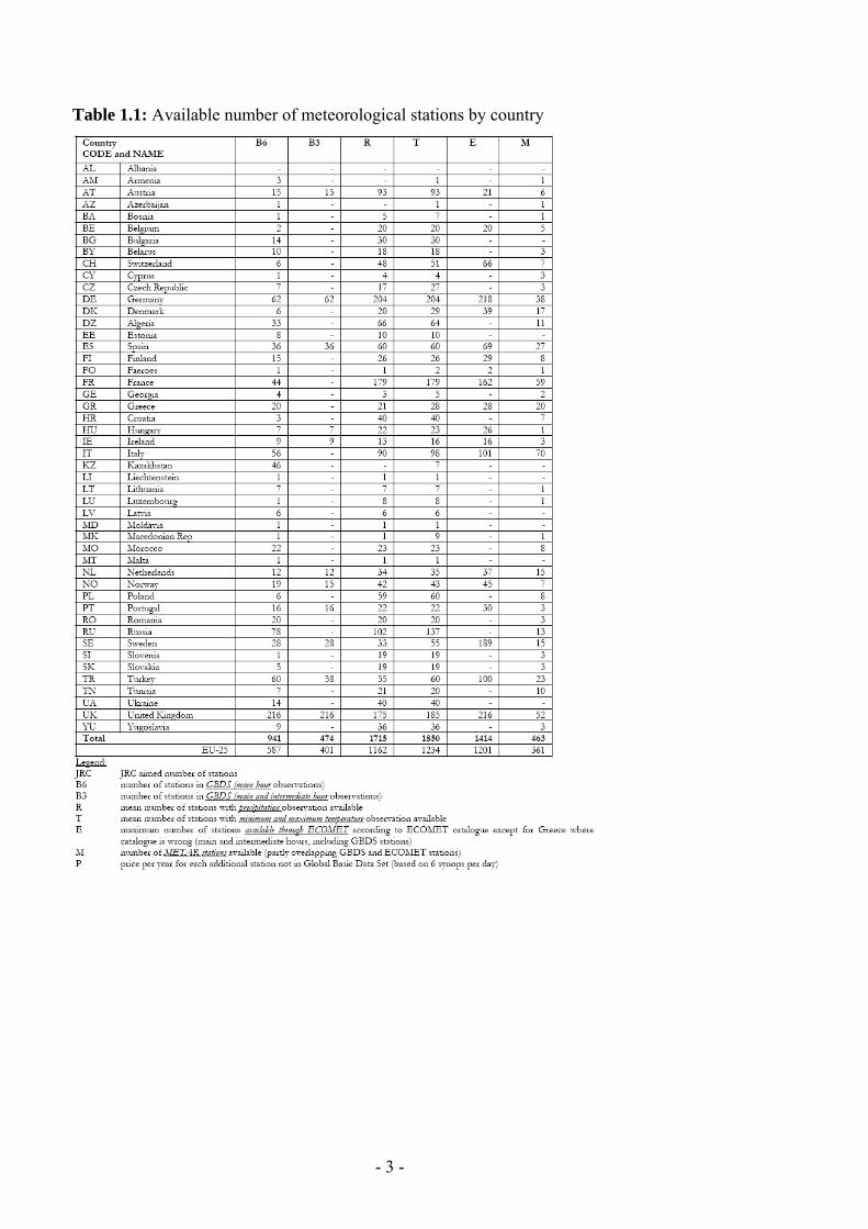
- 3 -
Table 11 Available number of meteorological stations by country
- 4 -
Figure 11 The meteorological stations for which data are available for (part of) the period from1975 until the current day
Table 12 List of parameters contained in GRID_WEATHER table
All the input and output data such as the climatic grid presented are given in Lambert-Azimuthal projection system with meters as units and the parameters
bull Radius of sphere of reference 6370997 (m)
bull Longitude of centre of projection 900ordm
bull Latitude of centre of projection 4800ordm
13 EXTRACTION OF DAILY METEOROLOGICAL DATA FOR THE TIER-2 SCENARIOS For the development of the lower tiers - Tier 1 and Tier 2 the EFSA Fate working group selected six sites (two for each regulatory zone) across EU Each site has been attributed to grid cells of MARS DB and the completeness of weather data series was evaluated In particular for one of these grids
- 5 -
due to some lack in rainfall data it was necessary to find among the nearest grids an alternative cells with a complete daily data set (Fig 12)
Figure 12 Identification of alternatives weather stations in case of incompleteness of data set
Meteorological data have been exported as text files with the structure reported in table 13
Table 13 Structure of the meteorological data provided for the selected scenarios
GRID_NO DAY MAXIMUM_TEMPERATURE MINIMUM_TEMPERATURE WINDSPEED RAINFALL ET0 CALCULATED_RADIATION VAPOUR_PRESSURE
53067 111990 127 29 17 06 071527922 6129 92553067 211990 105 58 24 30 085431975 5791 88153067 311990 93 45 33 70 063213211 3312 91353067 411990 85 43 33 70 056450325 3099 90053067 511990 95 49 04 00 056357884 4853 82453067 611990 101 09 17 00 065470117 7619 79753067 711990 91 07 14 15 057378882 6874 79553067 811990 73 -01 22 00 064395052 6074 68953067 911990 69 19 02 00 048847278 5714 73553067 1011990 63 -17 15 00 05382598 5797 654
14 PREPARATION OF DATA SETS ALLOWING APPLICATION OF HIGHER TIERS For the higher tiers Tier-3 and Tier-4 options exist for refinement eg specific crops andor specific plant protection products with specific properties may be considered The procedures is essentially the same adopted for Tier-1 and Tier-2 but instead of using the total area of annual crops the area may be limited to the intended area of use and the selection is made only for the substance under consideration In order to enable assessors and applicants to apply the proposed methodology the following datasets will be made available as ASCII files on the JRC Soil Portal (see Paragraph 15 )
141 List of Datasets
In the following paragraphs a list of the available data sets are reported These data sets have been provided by JRC or made available thank to the elaboration performed by the EFSA Fate working group members Aaldrik Tiktak and Micheal Klein
- 6 -
General maps Masker of all files
Countries of the EU-27 (countriesmap)
Regulatory zones (Northern Central and Southern zone)
FOCUS Zones
Soil maps Organic matter content of the topsoil
pH of the topsoil
Bulk density of the topsoil
Texture of the topsoil
Water content at field capacity
Meteorological maps Mean monthly temperature (12 maps)
Mean annual temperature
Arrhenius weighted mean annual temperature
Mean monthly precipitation (12 maps)
Mean annual precipitation
Land use land cover maps Corine land cover data
Generalised land-use map (landusemap)
Capri land cover maps (24 maps)
15 SET-UP OF DEDICATED WEB SITE FOR DATA DOWNLOAD
In order to allow the data download a specific web page within the JRC Soil Portal will be realized on (httpeusoilsjrceceuropaeulibraryDataEFSA ) A print screen of the main web page is shown in Fig 13
JRC will require users of the data to fill an online form before proceeding with the data download (Fig 14) The information collected by JRC will be used for updating the data users on the possible release of new soil and weather related information and data sets However release of new information for the JRC Soil Portal will only happen after the FOCUS version control group chaired by EFSA has accepted the change of the new information
- 7 -
151 Web Page structure
Figure 13 Print-screen of the page dedicated to the data download
152 Data Users Record
Figure 14 Registration form to be filled for downloading the data
- 1 -
2 ECOREGION WG
21 INTRODUCTION AND OBJECTIVES The European Food Safety Authority (EFSA) asked the Panel on Plant Protection Products and their Residues (PPR) to further develop the concept of soil ecoregions in the context of the revision of the Guidance Document on Terrestrial Ecotoxicology (EFSA-Q-2009-00002) A modelling approach for defining soil ecoregions within Europe was developed to improve the realism of exposure scenarios for plant protection products Biogeographic data on four soil organisms groups (earthworms enchytraeids collembolans and isopods) were used to assign each functional group to different life forms representing depth horizons in which they occur Based on information from three Member States covering a North-South gradient Finland Germany and Portugal species presence-absence data were modelled using soil and climate data The objectives of JRC contribution were
- create a geographic database from the tabular data of the biogeographic survey
- extract soil and weather data in correspondence of biogeographic sampling sites
- implement the ecoregion models and create ecoregion maps
The technical details of the activities performed for the achievement of the above reported objectives are described in the following paragraphs and in the EFSA PPR Scientific Opinion on the development of a soil ecoregions concept using distribution data on invertebrates (EFSA 2010b) 22 DESCRIPTION OF THE PROCEDURES ADOPTED
The production of the Ecoregion maps for Finland Germany and Portugal represent the application of the proposed methodology to three test countries according to a North-South gradient
- 2 -
The complete description of the adopted approach is published as EFSA Opinion (EFSA 2010b) In the following paragraphs however is provided a more detailed description of the technical procedures adopted by JRC The conceptual framework for the development of soil Ecoregions is reported in the scheme of Figure 21 and the activities reported in the green boxes have been developed by JRC and described in the following paragraphs
Figure 21 Conceptual frame of the approach adopted for the definition of Soil Ecoregion
221 From an attribute database to a geographic database
The original biogeographical database provided for the three test Member States Finland Germany and Portugal was organized in separate Excel spreadsheets for the different groups of soil organisms and the geographic coordinates were based on UTM1 coordinate system based on Datum WGS842
1 UTM Universal Transver Maercator coordinate system is a grid-based method of specifying locations on the surface of the Earth that is
a practical application of a 2-dimensional Cartesian coordinate system 2 WGS 84 WGS (World Geodetic System) is a standard for use in cartography geodesy and navigation It comprises a standard
coordinate frame for the Earth a standard spheroidal reference surface (the datum or reference ellipsoid) for raw altitude data and a gravitational equipotential surface (the geoid) that defines the nominal sea level The GS 84 represent the latest revision of this standard
- 3 -
In order to project these data in the EU coordinate system (Lambert Azimuthal Equal Area) and to the process in the most efficient way it has been necessary to reorganize the database
One global spreadsheet for each of the three Member States has been produced
From each of these global spreadsheets partial spreadsheets have been derived grouping the records located in the same UTM zone
In order to keep the track of the changes a new field have been added (Fig 22) produced by the concatenation of
- Two capital letters for the organisms group (CO= collembola EW= earthworms IS= isopoda)
- The numeric value of ID Site
- The initial letter of the country name
Figure 22 Structure of the country-based spreadsheet the column with the new field has been outlined
These individual spreadsheets have been exported in DB4 format in order to be easily managed in ArcGIS ArcGIS 93 is the GIS software that has been used for the management and the analysis of the geographic information
The following phase in the management of the data has been the generation of Point Shapefiles representing the locations in which the soil organism inventory has been carried out and the re-projection of these maps
The extraction of soil and climate data from the raster dataset in correspondence of the of the soil organisms survey points has been realized using the ldquoExtract value to pointsrdquo procedure this procedure that is a classical example of spatial query allow to extract the cell values of a raster based on set of points
- 4 -
222Characterization of biogeographic sampling sites in terms of soil climate and land use characteristics
The biogeographic database consists of data on presenceabsence and in some cases abundance of selected groups of soil organisms and in some cases also data on land use vegetation soil and climate were reported The completeness of these environmental parameters essential for the ecological characterization of soil community however was very weak For this reason the data on land use soil and climate provided by JRC has been used to fill the gaps present in the original dataset
This process has been carried out using the utilities of spatial analysis present in a Geographical Information System (GIS) Once the geographic position of a sampling point is known it is possible do a spatial query in the GIS concerning the values of soil pH organic matter total precipitation and any other parameter that is available in a form of geographic database (Fig 23)
Figure 23 Schematic representation of the procedure adopted in a GIS for the extraction of given parameters (ie climate soil) for a given geographic position (ie observations)
- 5 -
223 Implementation of the provisional model in the selected Member States
The computation of the ecoregion maps has been based on the equations obtained in the data analysis implemented using the Map Algebra tools of Arc GIS (Raster Calculator Single Output Map Algebra) In Table 22 and 23 are reported the equations used for the computation of earthworm and enchytraeids maps respectively The first set of equations implying only the use of algebraic operators have been calculated using the lsquoraster calculatorrdquo within the Spatial Analyst toolset while the last expression based on logical operators have applied using the Single Output Map Algebra operator
Table 21 Equations used for earthworms Ecoregion Map
Map Algebra Operation with Raster Calculator t1
-0498 + ([Cropland] 00481) + ([Grassland] 09844) +([Forest3] -02298) + ([ph_top_efsa] 0317) + ([OC_efsa] -00905) + ([tmean] -02494) + ([Tdiff] -00418)
t2
27379 + ([Cropland] -01215) + ([Grassland] 02189) +([Forest3] -11576) + ([ph_top_efsa] 00567) + ([OC_efsa] -00105) +([total_prec] -00018) + ([tmean] 00956) + ([Tdiff] -01229)
z1 Exp([t1]) (1 + Exp([t1]))
z2 Exp([t2]) (1 + Exp([t2]))
ear_arr1 z1
ear_arr2 [z2] (1 - [z1])
ear_arr3 (1 - [z2]) (1 - [z1])
Map Algebra Operation with Single Output Map Algebra Earthworms Ecorgegion Map
con( ear_arr1 gt= 0667 1 ear_arr2 gt= 0667 2 ear_arr3 gt= 0667 3 arr1+arr2 gt= 0833 amp ear_arr1 lt= 0667 amp ear_arr2 lt= 0667 12 arr1+arr3 gt= 0833 amp ear_arr1 lt= 0667 amp ear_arr3 lt= 0667 13 arr2+arr3 gt= 0833 amp ear_arr2 lt= 0667 amp ear_arr3 lt= 0667 23 arr1+arr2 lt= 0833 amp arr2+arr3 lt= 0833 amp arr1+arr3 lt= 0833 123 )
- 6 -
Table 22 Equations used for enchytraeids Ecoregion Map
Map Algebra Operation with Raster Calculator t1
33243 + ([Grassland] 04764) + ([Forest3] 20354) + ([ph_top_efsa] -02776) + ([OC_efsa] -00206) + ([Clay] -00114) + ([total_prec] -00025) + ([tmean] -02286) + ([Tdiff] -00348)
t2
-65979 + ([Grassland] -05418) + ([Forest3] 10585) + ([ph_top_efsa] -02322) + ([OC_efsa] -01102) + ([Clay] -00505) + ([total_prec] -00010) + ([tmean] 03911) + ([Tdiff] 02961)
z1 Exp([t1]) (1 + Exp([t1]))
z2 Exp([t2]) (1 + Exp([t2]))
enc_arr1 z1
enc_arr2 [z2] (1 - [z1])
enc_arr3 (1 - [z2]) (1 - [z1])
Map Algebra Operation with Single Output Map Algebra Enchytraeids Ecorgegion Map
con( enc_arr1 gt= 0667 1 enc_arr2 gt= 0667 2 enc_arr3 gt= 0667 3 arr1+arr2 gt= 0833 amp enc_arr1 lt= 0667 amp enc_arr2 lt= 0667 12 arr1+arr3 gt= 0833 amp enc_arr1 lt= 0667 amp enc_arr3 lt= 0667 13 arr2+arr3 gt= 0833 amp enc_arr2 lt= 0667 amp enc_arr3 lt= 0667 23 arr1+arr2 lt= 0833 amp arr2+arr3 lt= 0833 amp arr1+arr3 lt= 0833 123 )
224 Soil Ecoregions Mapping
The output of the provisional models were a series of maps (one for each organism) where the territories of Finland Germany and Portugal have been classified in seven classes according to the triangles reported in figure 24
Earthworm ecoregion maps have been produced only for the three investigated countries but restricting Finland to its Southern part Enchytraeid ecoregions maps were limited to Germany and Finland since almost no enchytraeid data were available for Portugal For Collembola the fit of the model was very poor and the maps based on the modelled results did not show a convincing ecological meaning based on expert knowledge In case of Isopoda the model presented a good plausibility check with the observed and the modelled values However the analysis gave no clear indication for patterns differing between or within countries therefore isopods were excluded from further analysis and are not shown as maps
- 7 -
Although in principle the interpolation over the entire EU 27 territory would have been technically feasible mapping of territories without observed values were considered not to be reliable for the purpose of this opinion
The concepts of exposure scenario and the definition of soil profile depth relevant for different soil organisms communities led to the production of maps for earthworms and Enchytraeids where the territory of the investigated countries has been classified on the base of the depth relevant for the proposed Risk Assessment
Figure 24 Classification triangles used to classify the earthworms and enchytraeids soil communities
- 8 -
3 CONCLUSIONS AND RECOMMENDATIONS
31 FATE
The occurrence of gaps in daily meteorological data is relatively frequent especially over 20 year time frame For this reason it should be preferred the adoption of a statistical procedures for gap filling instead of selecting alternative nearest meteorological stations
For future applications the availability of 25 km grids will provide an improved geographic resolution for the representation of European climate
32 ECOREGION
During the analysis of the biogeographic database it was found the lack of complete soil land use and climate data sets for the vast majority of the observation sites For this reason it has been necessary to derive such data from the 1 km grid data set (soil and land use) and from the 50 km grids (meteorological data)
It should be outlined that while the use of these EU wide geographic data set is optimal for modelling application probably does not have the necessary spatial resolution for the characterization of point observation sites
- 9 -
4 METADATA FOR EFSA DATASET
A database of maps was created on the basis of the dataset provided by JRC (see Gardi et al 2008) This dataset was supplemented with data from the CAPRI land cover database (Leip et al 2008) JRC is acknowledged for making the data available in a common resolution and projection
Map properties
Common metadata properties for the maps are Format compressed ASCII grid Reference system ETRS 89 LAEA Rows 4098 Columns 3500 Lower left 2500000 Upper left 1412000 Cell size 1000 Unit m Nr of cells with a value 3997812
10
41 Masker of all files (EU27asc)
1 This map is a mask created including all the EU-27 countries and the Corine land-use classes 1-38 and 49 Surface waters and coastal lagoons are excluded from the mask
Legend There is only one legend unit ie 1 which means that the grid cell is included
Figure 41 Masker for the dataset The masker has only one value ie 1
11
42 Countries of the EU-27 (countriesasc)
The map shows the countries of the EU-27 It was obtained by masking the NUTS level 0 map with the mask EU27 Legend Number Country 1 Albania 5 Austria 8 Belgium 9 Bulgaria 15 Czech Republic 16 Germany 17 Denmark 20 Estonia 23 Spain 24 Finland 26 France 31 Greece 34 Hungary 35 Ireland 41 Italy 48 Lithuania 49 Luxemburg 50 Latvia 58 Netherlands 61 Poland 62 Portugal 64 Romania 67 Sweden 68 Slovenia 70 Slovakia 78 United Kingdom
12
Figure 42 Countries of the EU-27
13
43 Regulatory zones (zonesasc)
This map shows the regulatory zones of the EU-27 The map is a reclassification of the map countriesmap Legend Number Name Countries 1 North 17 20 24 48 50 and 67 2 Centre 5 8 16 34 35 49 58 61 64 68 70 and 78 3 South 1 9 23 26 31 41 and 62
Figure 43 The regulatory zones of the EU-27
14
44 Corine land cover data (CLC2000asc)
The map shows all the possible land use classes at the Corine map The map presented here is at a resolution of 1x1 km2 the original map was at a resolution of 025 km2 For each 1x1 km2 grid cell the dominant of the four underlying grid cells was taken The dataset is described in Nunes de Lima (2005) Legend Number CLC
code Description
1 111 Continuous urban fabric 2 112 Discontinuous urban fabric 3 121 Industrial or commercial units 4 122 Road and rail networks and associated land 5 123 Port areas 6 124 Airports 7 131 Mineral extraction sites 8 132 Dump sites 9 133 Construction sites 10 141 Green urban areas 11 142 Sport and leisure facilities 12 211 Non-irrigated arable land 13 212 Permanently irrigated land 14 213 Rice fields 15 221 Vineyards 16 222 Fruit trees and berry plantations 17 223 Olive groves 18 231 Pastures 19 241 Annual crops associated with permanent crops 20 242 Complex cultivation patterns 21 243 Land occupied by agriculture with significant areas of natural
vegetation 22 244 Agro-forestry areas 23 311 Broad-leaved forest 24 312 Coniferous forest 25 313 Mixed forest 26 321 Natural grasslands 27 322 Moors and heathland 28 323 Sclerophyllous vegetation 29 324 Transitional woodland-shrub 30 331 Beaches dunes sands 31 332 Bare rocks 32 333 Sparsely vegetated areas 33 334 Burnt areas 34 335 Glaciers and perpetual snow 35 411 Inland marshes 36 412 Peat bogs 37 421 Salt marshes
15
38 422 Salines 39 423 Intertidal flats 40 511 Water courses 41 512 Water bodies 42 521 Coastal lagoons 43 522 Estuaries 44 523 Sea and ocean 48 999 NODATA 49 990 UNCLASSIFIED LAND SURFACE 50 995 UNCLASSIFIED WATER BODIES
16
45 Generalised land-use map (landuseasc)
The generalised land-use map is a reclassification of the Corine 2000 land-use map It is created to distinguish the most important land-use types Land use class 1 serves as the masker in EFSA (2010)
Legend Number Description Number in map above 1 Annual Crops 12 13 19-21 2 Grass 18 3 Permanent crops 15-17 and 22 4 Rice 14 5 Non agricultural all other classes
Figure 44 The generalised land-use map
17
46 Mean monthly temperature (T1ascT12asc)
The dataset consists of 12 maps containing the monthly mean temperature (deg C) for the period 1960-1990 The dataset is described in Hijmans et al (2005) Legend Mean monthly temperature (deg C) data type Real 47 Mean annual temperature (TMeanasc)
The map shows the mean annual temperature (deg C) for the period 1960-1990 It is calculating by taking the arithmetic mean of maps T1T12asc The dataset is described in Hijmans et al (2005) Legend Mean annual temperature (deg C) data type Real
Figure 45 Mean annual temperature for the period 1960-1990 taken from Worldclim dataset
18
48 Arrhenius weighted mean annual temperature (TEffasc)
The map shows the Arrhenius weighted mean annual temperature (deg C) for the period 1960-1990 It is calculated using the equation (EFSA 2010 Appendix A3)
( )
( ) ( )( ) 0
exp273)(
1ln0
=
⎥⎦
⎤⎢⎣
⎡minus=gt
⎥⎥⎦
⎤
⎢⎢⎣
⎡minus=
int
tTfelsetRT
EtTfthentTif
dttTft
R
ET
act
t
end
acteff
end
(1)
where Teff (K) is the Arrhenius weighted mean annual temperature Eact is the Arrhenius activation energy (kJ mol-1) R (kJ mol-1 K-1) is the gas constant T (K) is the temperature and t is time Eact was set to 654 kJ mol-1 according to EFSA (2007) See further EFSA (2010) Notice that the temperatures in the equation are in K whereas the temperature in the maps is in deg C Legend Arrhenius weighted mean annual temperature (deg C) data type Real
19
Figure 46 Arrhenius weighted mean temperature (deg C) for the period 1960-1990 For a description of the averaging procedure refer to EFSA (2010)
20
49 Mean monthly precipitation (P1ascP12asc)
The dataset consists of 12 maps containing the monthly mean precipitation (mmmonth) for the period 1960-1990 The dataset is described in Hijmans et al (2005) Legend Mean monthly precipitation (mmmo) data type Real 410 Mean annual precipitation (Ptotasc)
The map shows the mean annual precipitation for the period 1960-1990 (mmyear) It is calculated by summing P1P12map The dataset is described in Hijmans et al (2005) Legend Mean annual precipitation (mmyr) data type Real
Figure 47 Mean annual precipitation (mm) for the period 1960-1990 as taken from the Worldclim dataset
21
411 FOCUS Zones (FOCUSasc)
The map shows the FOCUS zones according to the classification in FOCUS (2000) The maps Tmeanmap and Ptotmap were used to create the overlay so the classification is based on WorldClim (Hijmans et al 2005)
Legend Number Name Tmean (deg C) Ptot (mmyr) 1 Jokioinen lt5 deg C gt 0 mmyr 2 Chateaudun 5 ndash 125 deg C lt 600 mmyr 3 Hamburg 5 ndash 125 deg C 600 ndash 800 mmyr 4 Kremsmuumlnster 5 ndash 125 deg C 800 ndash 1000 mmyr 5 Okehampton 5 ndash 125 deg C gt 1000 mmyr 6 Sevilla gt 125 deg C lt 600 mmyr 7 Thiva gt 125 deg C 600 ndash 800 mmyr 8 Piacenza gt 125 deg C 800 ndash 1000 mmyr 9 Porto gt 125 deg C gt 1000 mmyr
22
Figure 48 FOCUS climatic zones based on the mean annual temperature and mean annual precipitation from Worldclim
23
412 Organic matter content of the topsoil (OMasc)
The map shows the organic matter content of the topsoil It is obtained by multiplying the original OCTOP map described in Jones et al (2005) by 172 Legend Organic matter content of the topsoil (gg) data type Real
Figure 49 Organic matter content of the top 30 cm of the soil (gg)
24
413 pH of the topsoil (pHasc)
The map shows the mean pH measured in water (125) of the top 30 cm of the soil See FAO (2008) for details Legend pH measured in water of the topsoil data type Real
Figure 410 pH water (125) of the top 30 cm of the soil
25
414 Bulk density of the topsoil (Rhoasc)
The map shows the bulk density of the topsoil It is calculated from the organic matter content map using the equation (Tiktak et al 2002)
)910(291012361800 2 =minus+= rff omomρ (2)
Legend Dry bulk density of the topsoil (kg m-3) data type Real
Figure 411 Bulk density of the top 30 cm of the soil calculated by the pedotransfer function described in Tiktak et al (2002)
26
415 Texture of the topsoil (Textureasc)
The map shows the textural class of the topsoil It is obtained from the soil geographical database of Eurasia at a scale of 11000000 (for each grid cell the dominant soil textural class was taken) Legend Number Description 1 Coarse (18 lt clay and gt 65 sand) 2 Medium (18 lt clay lt 35 and gt= 15 sand or 18 ltclay and 15 lt sand lt
65) 3 Medium fine (lt 35 clay and lt 15 sand) 4 Fine (35 lt clay lt 60) 5 Very fine (clay gt 60 ) 9 No mineral texture (Peat soils)
Figure 412Topsoil texture obtained from the soil database of Europe 11000000
27
416 Water content at field capacity (ThetaFCasc)
The map shows the water content at field capacity (m3 m-3) It is calculated for each soil textural class with the Mualem-Van Genuchten equation
( ) mnrs
rh
h minus+
minus+=
α
θθθθ1
)( (1)
where θ (m3 m-3) is the volume fraction of water h (cm) is the soil water pressure head θs (m3 m-3) is the volume fraction of water at saturation θr (m3 m-3) is the residual water content in the extremely dry range α (cm-1) and n (-) are empirical parameters and m (-) can be taken equal to
nm 11minus=
The soil water pressure head was set at -100 cm Parameter values were obtained from the HYPRES pedotransfer rule (Woumlsten et al 1999) and are given in EFSA (2010) table 3 Legend Volumetric water content at field capacity (m3 m-3) data type Real The map contains six discrete classes
28
Figure 413 Volume fraction of water at field capacity calculated from the soil textural class using the HYPRES pedotransfer rule
29
417 Capri land cover maps (Cropnamesasc)
These maps show for each pixel of 1x1 km2 the area covered with a certain crop The CAPRI maps were obtained by combining remote sensing data administrative crop data land suitability data and statistical modelling The CORINE land cover map serves as a starting point Subdivisions within CORINE land cover classes were made based on a statistical model regressing point observations of cropping activities on soil relief and climate parameters (land suitability) Statistical data of agricultural production and land cover available for administrative regions were additionally used to scale the land cover classes 18 of the CAPRI land cover classes are classified as annual crops and are included in the EFSA dataset See Leip et al (2008) for a description of the dataset Legend Area (100) covered by a crop data type Real The names of the maps are self explaining The values range from 0 to 10000
30
Figure 414 Crop cover maps ( of area) for barley common wheat texture crops floriculture other fodder crops and industrial crops
31
Figure 415 Crop cover maps ( of area) for maize oats other cereals pulses rapes and root crops
32
Figure 416 Crop cover maps ( of area) for rye soya sugar beet sunflowers vegetables and durum wheat
33
5 REFERENCES
Goot E van der 1998 Spatial interpolation of daily meteorological data for the Crop Growth Monitoring System (CGMS) In M Bindi B Gozzini (eds) Proceedings of seminar on dataspatial distribution in meteorology and climatology 28 September - 3 October 1997 Volterra Italy EUR 18472 EN Office for Official Publications of the EU Luxembourg p 141-153
Gardi C Montanarella L Hiederer R Jones A Micale F 2010 Activities realized within the Service Level Agreement between JRC and EFSA as a support of the FATE Working Group of EFSA PPR in support of the revision of the guidance document Persistence in Soil JRC Technical Svientific and Technical Report 39 pp - EUR 24345
Gardi C2010 Report on the Activities realised within the Service Licence Agreement between JRC and EFSA as a support of the FATE Working Group of EFSA PPR JRC Scientific Report (SLAEFSA-JRC200801)
EFSA 2010a Opinion of the Scientific Panel on Plant Protection products and their Residues on outline proposals for assessment of exposure of organisms to substances in soil EFSA Journal 8(1)1442
EFSA 2010b Opinion of the Scientific Panel on Plant Protection products and their Residues on on the development of a soil ecoregions concept using distribution data on invertebrates EFSA Journal 8(10)1820
EFSA 2007 Opinion on a request from EFSA related to the default Q10 value used to describe the temperature effect on transformation rates of pesticides in soil Scientific Opinion of the Panel on Plant Protection Products and their Residues (PPR-Panel) The EFSA Journal (622)1 32
EFSA 2010 Selection of scenarios for exposure of soil organisms The EFSA Journal (2010) 8(46)1642
FAOIIASAISRICISS-CASJRC 2008 Harmonized World Soil Database (version 10) FAO Rome Italy and IIASA Laxenburg Austria 37pp
FOCUS 2010 Assessing potential movement of active substances and their metabolites to ground water in the EU EC Document reference Sancoxxx2010 Available at FOCUS website httpvisoeijrcitfocus
Hijmans RJ SE Cameron JL Parra PG Jones and A Jarvis 2005 Very high resolution interpolated climate surfaces for global land areas Int J Climatology (25)1965-1978
Jones RJA R Hiederer E Rusco PJ Loveland and L Montanarella 2005 Estimating organic carbon in the soils of Europe for policy support European Journal of Soil Science (56)655-671
Leip A G Marchi R Koeble M Kempen W Britz and C Li 2008 Linking an economic model for European agriculture with a mechanistic model to estimate nitrogen and carbon losses from arable soils in Europe Biogeosciences (5)73-94
Tiktak A DS de Nie AMA van der Linden and R Kruijne 2002 Modelling the leaching and drainage of pesticides in the Netherlands the GeoPEARL model Agronomie (22)373-387
Woumlsten JHM A Nemes A Lilly and C Le Bas 1999 Development and use of a database of hydraulic properties of European soils Geoderma (90)169ndash185
34
APPENDICES ECOREGION MAPS
Earthworm Finland
35
Earthworm Germany
36
Earthworm Portugal
37
Enchytraeids Finland
38
Enchytraeids Germany
39
European Commission EUR 24744 EN ndash Joint Research Centre ndash Institute for Environment and Sustainability Title Report on the activities realized within the Service Level Agreement between JRC and EFSA Author(s) Ciro Gardi Panos Panagos Roland Hiederer Luca Montanarella Fabio Micale Luxembourg Publications Office of the European Union 2011 ndash 38 pp ndash 210 x 297 cm EUR ndash Scientific and Technical Research series ndash ISSN 1018-5593 ISBN 978-92-79-19521-1 doi10278861018 Abstract The activities realized in 2010 by JRC as support to the FATE and the ECOREGION EFSA PPR Working Groups are shortly described For the FATE WG the vast majority of data has been provided in 2009 during the first year of the Service Level Agreement (SLA) and in 2010 the daily weather data for the six selected sites were produced All the data used for the scenario selection procedures with additional data on land use-land cover crop distribution soil and climate parameters will be made available for external user in first half of 2011 For the ECOREGION WG the analysis has been carried out for three Member States covering a North-South gradient from Finland Germany to Portugal Soil and weather data have been used for the characterisation of bio-geographic sampling sites and for the implementation of the ecoregion model Ecoregion maps were produced for earthworms and enchytraeids for Finland and Germany and revealed marked differences between the countries The same approach has been applied also to Collembola and Isopoda but for these two taxa led to a rather poor discrimination both between and within countries
How to obtain EU publications Our priced publications are available from EU Bookshop (httpbookshopeuropaeu) where you can place an order with the sales agent of your choice The Publications Office has a worldwide network of sales agents You can obtain their contact details by sending a fax to (352) 29 29-42758
The mission of the JRC is to provide customer-driven scientific and technical supportfor the conception development implementation and monitoring of EU policies As a service of the European Commission the JRC functions as a reference centre of science and technology for the Union Close to the policy-making process it serves the common interest of the Member States while being independent of special interests whether private or national
LB
-NA
-24744-EN-C
- 141 List of Datasets
- 151 Web Page structure
- 152 Data Users Record
- 22 Description of the Procedures Adopted
- 221 From an attribute database to a geographic database
- 222Characterization of biogeographic sampling sites in terms of soil climate and land use characteristics
- 223 Implementation of the provisional model in the selected Member States
- 224 Soil Ecoregions Mapping
- 3 Conclusions and Recommendations
-
- 31 FATE
- 32 ECOREGION
-
- 4 Metadata for EFSA dataset
-
- Map properties
- 41 Masker of all files (EU27asc)
- 42 Countries of the EU-27 (countriesasc)
- 43 Regulatory zones (zonesasc)
- 44 Corine land cover data (CLC2000asc)
- 45 Generalised land-use map (landuseasc)
- 46 Mean monthly temperature (T1ascT12asc)
- 47 Mean annual temperature (TMeanasc)
- 48 Arrhenius weighted mean annual temperature (TEffasc)
- 49 Mean monthly precipitation (P1ascP12asc)
- 410 Mean annual precipitation (Ptotasc)
- 411 FOCUS Zones (FOCUSasc)
- 412 Organic matter content of the topsoil (OMasc)
- 413 pH of the topsoil (pHasc)
- 414 Bulk density of the topsoil (Rhoasc)
- 415 Texture of the topsoil (Textureasc)
- 416 Water content at field capacity (ThetaFCasc)
- 417 Capri land cover maps (Cropnamesasc)
-
- 5 References
-
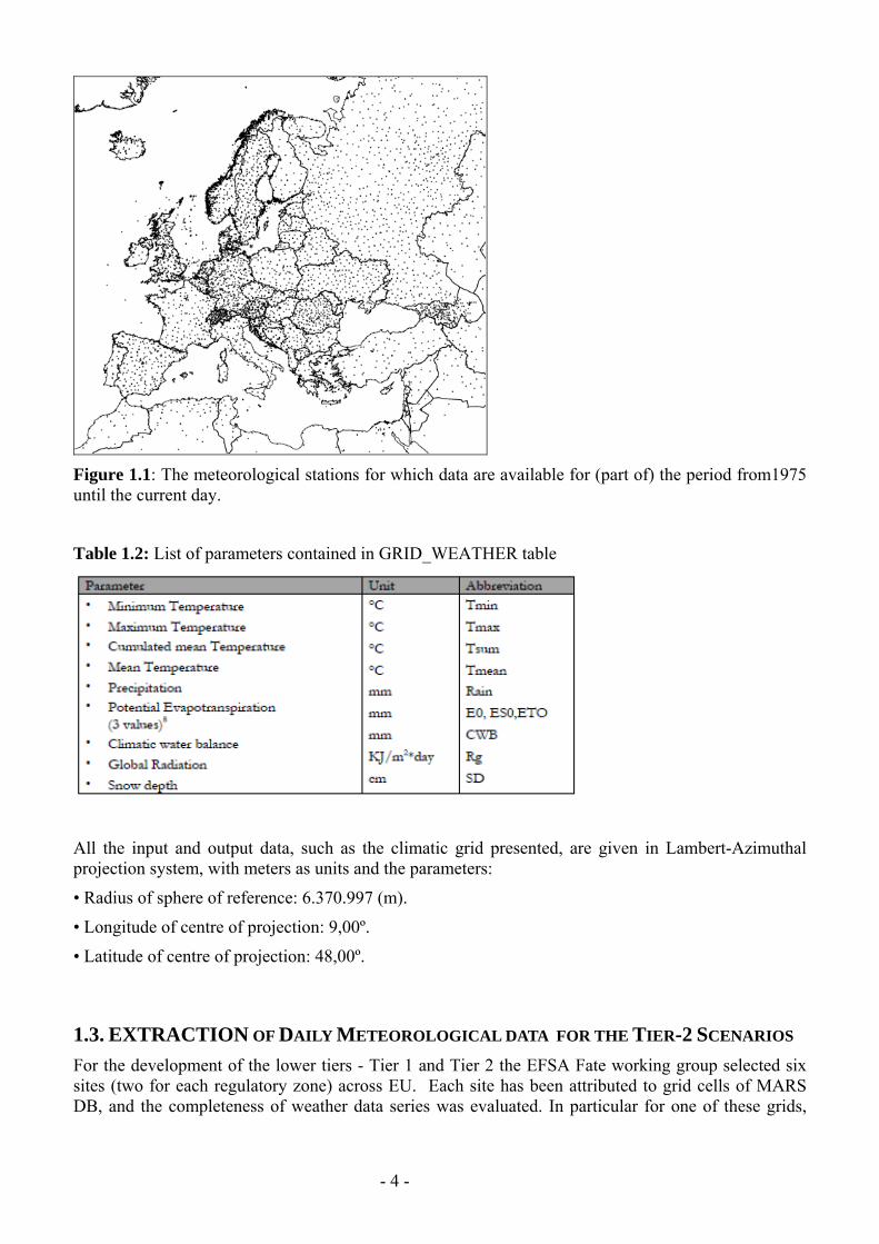
- 4 -
Figure 11 The meteorological stations for which data are available for (part of) the period from1975 until the current day
Table 12 List of parameters contained in GRID_WEATHER table
All the input and output data such as the climatic grid presented are given in Lambert-Azimuthal projection system with meters as units and the parameters
bull Radius of sphere of reference 6370997 (m)
bull Longitude of centre of projection 900ordm
bull Latitude of centre of projection 4800ordm
13 EXTRACTION OF DAILY METEOROLOGICAL DATA FOR THE TIER-2 SCENARIOS For the development of the lower tiers - Tier 1 and Tier 2 the EFSA Fate working group selected six sites (two for each regulatory zone) across EU Each site has been attributed to grid cells of MARS DB and the completeness of weather data series was evaluated In particular for one of these grids
- 5 -
due to some lack in rainfall data it was necessary to find among the nearest grids an alternative cells with a complete daily data set (Fig 12)
Figure 12 Identification of alternatives weather stations in case of incompleteness of data set
Meteorological data have been exported as text files with the structure reported in table 13
Table 13 Structure of the meteorological data provided for the selected scenarios
GRID_NO DAY MAXIMUM_TEMPERATURE MINIMUM_TEMPERATURE WINDSPEED RAINFALL ET0 CALCULATED_RADIATION VAPOUR_PRESSURE
53067 111990 127 29 17 06 071527922 6129 92553067 211990 105 58 24 30 085431975 5791 88153067 311990 93 45 33 70 063213211 3312 91353067 411990 85 43 33 70 056450325 3099 90053067 511990 95 49 04 00 056357884 4853 82453067 611990 101 09 17 00 065470117 7619 79753067 711990 91 07 14 15 057378882 6874 79553067 811990 73 -01 22 00 064395052 6074 68953067 911990 69 19 02 00 048847278 5714 73553067 1011990 63 -17 15 00 05382598 5797 654
14 PREPARATION OF DATA SETS ALLOWING APPLICATION OF HIGHER TIERS For the higher tiers Tier-3 and Tier-4 options exist for refinement eg specific crops andor specific plant protection products with specific properties may be considered The procedures is essentially the same adopted for Tier-1 and Tier-2 but instead of using the total area of annual crops the area may be limited to the intended area of use and the selection is made only for the substance under consideration In order to enable assessors and applicants to apply the proposed methodology the following datasets will be made available as ASCII files on the JRC Soil Portal (see Paragraph 15 )
141 List of Datasets
In the following paragraphs a list of the available data sets are reported These data sets have been provided by JRC or made available thank to the elaboration performed by the EFSA Fate working group members Aaldrik Tiktak and Micheal Klein
- 6 -
General maps Masker of all files
Countries of the EU-27 (countriesmap)
Regulatory zones (Northern Central and Southern zone)
FOCUS Zones
Soil maps Organic matter content of the topsoil
pH of the topsoil
Bulk density of the topsoil
Texture of the topsoil
Water content at field capacity
Meteorological maps Mean monthly temperature (12 maps)
Mean annual temperature
Arrhenius weighted mean annual temperature
Mean monthly precipitation (12 maps)
Mean annual precipitation
Land use land cover maps Corine land cover data
Generalised land-use map (landusemap)
Capri land cover maps (24 maps)
15 SET-UP OF DEDICATED WEB SITE FOR DATA DOWNLOAD
In order to allow the data download a specific web page within the JRC Soil Portal will be realized on (httpeusoilsjrceceuropaeulibraryDataEFSA ) A print screen of the main web page is shown in Fig 13
JRC will require users of the data to fill an online form before proceeding with the data download (Fig 14) The information collected by JRC will be used for updating the data users on the possible release of new soil and weather related information and data sets However release of new information for the JRC Soil Portal will only happen after the FOCUS version control group chaired by EFSA has accepted the change of the new information
- 7 -
151 Web Page structure
Figure 13 Print-screen of the page dedicated to the data download
152 Data Users Record
Figure 14 Registration form to be filled for downloading the data
- 1 -
2 ECOREGION WG
21 INTRODUCTION AND OBJECTIVES The European Food Safety Authority (EFSA) asked the Panel on Plant Protection Products and their Residues (PPR) to further develop the concept of soil ecoregions in the context of the revision of the Guidance Document on Terrestrial Ecotoxicology (EFSA-Q-2009-00002) A modelling approach for defining soil ecoregions within Europe was developed to improve the realism of exposure scenarios for plant protection products Biogeographic data on four soil organisms groups (earthworms enchytraeids collembolans and isopods) were used to assign each functional group to different life forms representing depth horizons in which they occur Based on information from three Member States covering a North-South gradient Finland Germany and Portugal species presence-absence data were modelled using soil and climate data The objectives of JRC contribution were
- create a geographic database from the tabular data of the biogeographic survey
- extract soil and weather data in correspondence of biogeographic sampling sites
- implement the ecoregion models and create ecoregion maps
The technical details of the activities performed for the achievement of the above reported objectives are described in the following paragraphs and in the EFSA PPR Scientific Opinion on the development of a soil ecoregions concept using distribution data on invertebrates (EFSA 2010b) 22 DESCRIPTION OF THE PROCEDURES ADOPTED
The production of the Ecoregion maps for Finland Germany and Portugal represent the application of the proposed methodology to three test countries according to a North-South gradient
- 2 -
The complete description of the adopted approach is published as EFSA Opinion (EFSA 2010b) In the following paragraphs however is provided a more detailed description of the technical procedures adopted by JRC The conceptual framework for the development of soil Ecoregions is reported in the scheme of Figure 21 and the activities reported in the green boxes have been developed by JRC and described in the following paragraphs
Figure 21 Conceptual frame of the approach adopted for the definition of Soil Ecoregion
221 From an attribute database to a geographic database
The original biogeographical database provided for the three test Member States Finland Germany and Portugal was organized in separate Excel spreadsheets for the different groups of soil organisms and the geographic coordinates were based on UTM1 coordinate system based on Datum WGS842
1 UTM Universal Transver Maercator coordinate system is a grid-based method of specifying locations on the surface of the Earth that is
a practical application of a 2-dimensional Cartesian coordinate system 2 WGS 84 WGS (World Geodetic System) is a standard for use in cartography geodesy and navigation It comprises a standard
coordinate frame for the Earth a standard spheroidal reference surface (the datum or reference ellipsoid) for raw altitude data and a gravitational equipotential surface (the geoid) that defines the nominal sea level The GS 84 represent the latest revision of this standard
- 3 -
In order to project these data in the EU coordinate system (Lambert Azimuthal Equal Area) and to the process in the most efficient way it has been necessary to reorganize the database
One global spreadsheet for each of the three Member States has been produced
From each of these global spreadsheets partial spreadsheets have been derived grouping the records located in the same UTM zone
In order to keep the track of the changes a new field have been added (Fig 22) produced by the concatenation of
- Two capital letters for the organisms group (CO= collembola EW= earthworms IS= isopoda)
- The numeric value of ID Site
- The initial letter of the country name
Figure 22 Structure of the country-based spreadsheet the column with the new field has been outlined
These individual spreadsheets have been exported in DB4 format in order to be easily managed in ArcGIS ArcGIS 93 is the GIS software that has been used for the management and the analysis of the geographic information
The following phase in the management of the data has been the generation of Point Shapefiles representing the locations in which the soil organism inventory has been carried out and the re-projection of these maps
The extraction of soil and climate data from the raster dataset in correspondence of the of the soil organisms survey points has been realized using the ldquoExtract value to pointsrdquo procedure this procedure that is a classical example of spatial query allow to extract the cell values of a raster based on set of points
- 4 -
222Characterization of biogeographic sampling sites in terms of soil climate and land use characteristics
The biogeographic database consists of data on presenceabsence and in some cases abundance of selected groups of soil organisms and in some cases also data on land use vegetation soil and climate were reported The completeness of these environmental parameters essential for the ecological characterization of soil community however was very weak For this reason the data on land use soil and climate provided by JRC has been used to fill the gaps present in the original dataset
This process has been carried out using the utilities of spatial analysis present in a Geographical Information System (GIS) Once the geographic position of a sampling point is known it is possible do a spatial query in the GIS concerning the values of soil pH organic matter total precipitation and any other parameter that is available in a form of geographic database (Fig 23)
Figure 23 Schematic representation of the procedure adopted in a GIS for the extraction of given parameters (ie climate soil) for a given geographic position (ie observations)
- 5 -
223 Implementation of the provisional model in the selected Member States
The computation of the ecoregion maps has been based on the equations obtained in the data analysis implemented using the Map Algebra tools of Arc GIS (Raster Calculator Single Output Map Algebra) In Table 22 and 23 are reported the equations used for the computation of earthworm and enchytraeids maps respectively The first set of equations implying only the use of algebraic operators have been calculated using the lsquoraster calculatorrdquo within the Spatial Analyst toolset while the last expression based on logical operators have applied using the Single Output Map Algebra operator
Table 21 Equations used for earthworms Ecoregion Map
Map Algebra Operation with Raster Calculator t1
-0498 + ([Cropland] 00481) + ([Grassland] 09844) +([Forest3] -02298) + ([ph_top_efsa] 0317) + ([OC_efsa] -00905) + ([tmean] -02494) + ([Tdiff] -00418)
t2
27379 + ([Cropland] -01215) + ([Grassland] 02189) +([Forest3] -11576) + ([ph_top_efsa] 00567) + ([OC_efsa] -00105) +([total_prec] -00018) + ([tmean] 00956) + ([Tdiff] -01229)
z1 Exp([t1]) (1 + Exp([t1]))
z2 Exp([t2]) (1 + Exp([t2]))
ear_arr1 z1
ear_arr2 [z2] (1 - [z1])
ear_arr3 (1 - [z2]) (1 - [z1])
Map Algebra Operation with Single Output Map Algebra Earthworms Ecorgegion Map
con( ear_arr1 gt= 0667 1 ear_arr2 gt= 0667 2 ear_arr3 gt= 0667 3 arr1+arr2 gt= 0833 amp ear_arr1 lt= 0667 amp ear_arr2 lt= 0667 12 arr1+arr3 gt= 0833 amp ear_arr1 lt= 0667 amp ear_arr3 lt= 0667 13 arr2+arr3 gt= 0833 amp ear_arr2 lt= 0667 amp ear_arr3 lt= 0667 23 arr1+arr2 lt= 0833 amp arr2+arr3 lt= 0833 amp arr1+arr3 lt= 0833 123 )
- 6 -
Table 22 Equations used for enchytraeids Ecoregion Map
Map Algebra Operation with Raster Calculator t1
33243 + ([Grassland] 04764) + ([Forest3] 20354) + ([ph_top_efsa] -02776) + ([OC_efsa] -00206) + ([Clay] -00114) + ([total_prec] -00025) + ([tmean] -02286) + ([Tdiff] -00348)
t2
-65979 + ([Grassland] -05418) + ([Forest3] 10585) + ([ph_top_efsa] -02322) + ([OC_efsa] -01102) + ([Clay] -00505) + ([total_prec] -00010) + ([tmean] 03911) + ([Tdiff] 02961)
z1 Exp([t1]) (1 + Exp([t1]))
z2 Exp([t2]) (1 + Exp([t2]))
enc_arr1 z1
enc_arr2 [z2] (1 - [z1])
enc_arr3 (1 - [z2]) (1 - [z1])
Map Algebra Operation with Single Output Map Algebra Enchytraeids Ecorgegion Map
con( enc_arr1 gt= 0667 1 enc_arr2 gt= 0667 2 enc_arr3 gt= 0667 3 arr1+arr2 gt= 0833 amp enc_arr1 lt= 0667 amp enc_arr2 lt= 0667 12 arr1+arr3 gt= 0833 amp enc_arr1 lt= 0667 amp enc_arr3 lt= 0667 13 arr2+arr3 gt= 0833 amp enc_arr2 lt= 0667 amp enc_arr3 lt= 0667 23 arr1+arr2 lt= 0833 amp arr2+arr3 lt= 0833 amp arr1+arr3 lt= 0833 123 )
224 Soil Ecoregions Mapping
The output of the provisional models were a series of maps (one for each organism) where the territories of Finland Germany and Portugal have been classified in seven classes according to the triangles reported in figure 24
Earthworm ecoregion maps have been produced only for the three investigated countries but restricting Finland to its Southern part Enchytraeid ecoregions maps were limited to Germany and Finland since almost no enchytraeid data were available for Portugal For Collembola the fit of the model was very poor and the maps based on the modelled results did not show a convincing ecological meaning based on expert knowledge In case of Isopoda the model presented a good plausibility check with the observed and the modelled values However the analysis gave no clear indication for patterns differing between or within countries therefore isopods were excluded from further analysis and are not shown as maps
- 7 -
Although in principle the interpolation over the entire EU 27 territory would have been technically feasible mapping of territories without observed values were considered not to be reliable for the purpose of this opinion
The concepts of exposure scenario and the definition of soil profile depth relevant for different soil organisms communities led to the production of maps for earthworms and Enchytraeids where the territory of the investigated countries has been classified on the base of the depth relevant for the proposed Risk Assessment
Figure 24 Classification triangles used to classify the earthworms and enchytraeids soil communities
- 8 -
3 CONCLUSIONS AND RECOMMENDATIONS
31 FATE
The occurrence of gaps in daily meteorological data is relatively frequent especially over 20 year time frame For this reason it should be preferred the adoption of a statistical procedures for gap filling instead of selecting alternative nearest meteorological stations
For future applications the availability of 25 km grids will provide an improved geographic resolution for the representation of European climate
32 ECOREGION
During the analysis of the biogeographic database it was found the lack of complete soil land use and climate data sets for the vast majority of the observation sites For this reason it has been necessary to derive such data from the 1 km grid data set (soil and land use) and from the 50 km grids (meteorological data)
It should be outlined that while the use of these EU wide geographic data set is optimal for modelling application probably does not have the necessary spatial resolution for the characterization of point observation sites
- 9 -
4 METADATA FOR EFSA DATASET
A database of maps was created on the basis of the dataset provided by JRC (see Gardi et al 2008) This dataset was supplemented with data from the CAPRI land cover database (Leip et al 2008) JRC is acknowledged for making the data available in a common resolution and projection
Map properties
Common metadata properties for the maps are Format compressed ASCII grid Reference system ETRS 89 LAEA Rows 4098 Columns 3500 Lower left 2500000 Upper left 1412000 Cell size 1000 Unit m Nr of cells with a value 3997812
10
41 Masker of all files (EU27asc)
1 This map is a mask created including all the EU-27 countries and the Corine land-use classes 1-38 and 49 Surface waters and coastal lagoons are excluded from the mask
Legend There is only one legend unit ie 1 which means that the grid cell is included
Figure 41 Masker for the dataset The masker has only one value ie 1
11
42 Countries of the EU-27 (countriesasc)
The map shows the countries of the EU-27 It was obtained by masking the NUTS level 0 map with the mask EU27 Legend Number Country 1 Albania 5 Austria 8 Belgium 9 Bulgaria 15 Czech Republic 16 Germany 17 Denmark 20 Estonia 23 Spain 24 Finland 26 France 31 Greece 34 Hungary 35 Ireland 41 Italy 48 Lithuania 49 Luxemburg 50 Latvia 58 Netherlands 61 Poland 62 Portugal 64 Romania 67 Sweden 68 Slovenia 70 Slovakia 78 United Kingdom
12
Figure 42 Countries of the EU-27
13
43 Regulatory zones (zonesasc)
This map shows the regulatory zones of the EU-27 The map is a reclassification of the map countriesmap Legend Number Name Countries 1 North 17 20 24 48 50 and 67 2 Centre 5 8 16 34 35 49 58 61 64 68 70 and 78 3 South 1 9 23 26 31 41 and 62
Figure 43 The regulatory zones of the EU-27
14
44 Corine land cover data (CLC2000asc)
The map shows all the possible land use classes at the Corine map The map presented here is at a resolution of 1x1 km2 the original map was at a resolution of 025 km2 For each 1x1 km2 grid cell the dominant of the four underlying grid cells was taken The dataset is described in Nunes de Lima (2005) Legend Number CLC
code Description
1 111 Continuous urban fabric 2 112 Discontinuous urban fabric 3 121 Industrial or commercial units 4 122 Road and rail networks and associated land 5 123 Port areas 6 124 Airports 7 131 Mineral extraction sites 8 132 Dump sites 9 133 Construction sites 10 141 Green urban areas 11 142 Sport and leisure facilities 12 211 Non-irrigated arable land 13 212 Permanently irrigated land 14 213 Rice fields 15 221 Vineyards 16 222 Fruit trees and berry plantations 17 223 Olive groves 18 231 Pastures 19 241 Annual crops associated with permanent crops 20 242 Complex cultivation patterns 21 243 Land occupied by agriculture with significant areas of natural
vegetation 22 244 Agro-forestry areas 23 311 Broad-leaved forest 24 312 Coniferous forest 25 313 Mixed forest 26 321 Natural grasslands 27 322 Moors and heathland 28 323 Sclerophyllous vegetation 29 324 Transitional woodland-shrub 30 331 Beaches dunes sands 31 332 Bare rocks 32 333 Sparsely vegetated areas 33 334 Burnt areas 34 335 Glaciers and perpetual snow 35 411 Inland marshes 36 412 Peat bogs 37 421 Salt marshes
15
38 422 Salines 39 423 Intertidal flats 40 511 Water courses 41 512 Water bodies 42 521 Coastal lagoons 43 522 Estuaries 44 523 Sea and ocean 48 999 NODATA 49 990 UNCLASSIFIED LAND SURFACE 50 995 UNCLASSIFIED WATER BODIES
16
45 Generalised land-use map (landuseasc)
The generalised land-use map is a reclassification of the Corine 2000 land-use map It is created to distinguish the most important land-use types Land use class 1 serves as the masker in EFSA (2010)
Legend Number Description Number in map above 1 Annual Crops 12 13 19-21 2 Grass 18 3 Permanent crops 15-17 and 22 4 Rice 14 5 Non agricultural all other classes
Figure 44 The generalised land-use map
17
46 Mean monthly temperature (T1ascT12asc)
The dataset consists of 12 maps containing the monthly mean temperature (deg C) for the period 1960-1990 The dataset is described in Hijmans et al (2005) Legend Mean monthly temperature (deg C) data type Real 47 Mean annual temperature (TMeanasc)
The map shows the mean annual temperature (deg C) for the period 1960-1990 It is calculating by taking the arithmetic mean of maps T1T12asc The dataset is described in Hijmans et al (2005) Legend Mean annual temperature (deg C) data type Real
Figure 45 Mean annual temperature for the period 1960-1990 taken from Worldclim dataset
18
48 Arrhenius weighted mean annual temperature (TEffasc)
The map shows the Arrhenius weighted mean annual temperature (deg C) for the period 1960-1990 It is calculated using the equation (EFSA 2010 Appendix A3)
( )
( ) ( )( ) 0
exp273)(
1ln0
=
⎥⎦
⎤⎢⎣
⎡minus=gt
⎥⎥⎦
⎤
⎢⎢⎣
⎡minus=
int
tTfelsetRT
EtTfthentTif
dttTft
R
ET
act
t
end
acteff
end
(1)
where Teff (K) is the Arrhenius weighted mean annual temperature Eact is the Arrhenius activation energy (kJ mol-1) R (kJ mol-1 K-1) is the gas constant T (K) is the temperature and t is time Eact was set to 654 kJ mol-1 according to EFSA (2007) See further EFSA (2010) Notice that the temperatures in the equation are in K whereas the temperature in the maps is in deg C Legend Arrhenius weighted mean annual temperature (deg C) data type Real
19
Figure 46 Arrhenius weighted mean temperature (deg C) for the period 1960-1990 For a description of the averaging procedure refer to EFSA (2010)
20
49 Mean monthly precipitation (P1ascP12asc)
The dataset consists of 12 maps containing the monthly mean precipitation (mmmonth) for the period 1960-1990 The dataset is described in Hijmans et al (2005) Legend Mean monthly precipitation (mmmo) data type Real 410 Mean annual precipitation (Ptotasc)
The map shows the mean annual precipitation for the period 1960-1990 (mmyear) It is calculated by summing P1P12map The dataset is described in Hijmans et al (2005) Legend Mean annual precipitation (mmyr) data type Real
Figure 47 Mean annual precipitation (mm) for the period 1960-1990 as taken from the Worldclim dataset
21
411 FOCUS Zones (FOCUSasc)
The map shows the FOCUS zones according to the classification in FOCUS (2000) The maps Tmeanmap and Ptotmap were used to create the overlay so the classification is based on WorldClim (Hijmans et al 2005)
Legend Number Name Tmean (deg C) Ptot (mmyr) 1 Jokioinen lt5 deg C gt 0 mmyr 2 Chateaudun 5 ndash 125 deg C lt 600 mmyr 3 Hamburg 5 ndash 125 deg C 600 ndash 800 mmyr 4 Kremsmuumlnster 5 ndash 125 deg C 800 ndash 1000 mmyr 5 Okehampton 5 ndash 125 deg C gt 1000 mmyr 6 Sevilla gt 125 deg C lt 600 mmyr 7 Thiva gt 125 deg C 600 ndash 800 mmyr 8 Piacenza gt 125 deg C 800 ndash 1000 mmyr 9 Porto gt 125 deg C gt 1000 mmyr
22
Figure 48 FOCUS climatic zones based on the mean annual temperature and mean annual precipitation from Worldclim
23
412 Organic matter content of the topsoil (OMasc)
The map shows the organic matter content of the topsoil It is obtained by multiplying the original OCTOP map described in Jones et al (2005) by 172 Legend Organic matter content of the topsoil (gg) data type Real
Figure 49 Organic matter content of the top 30 cm of the soil (gg)
24
413 pH of the topsoil (pHasc)
The map shows the mean pH measured in water (125) of the top 30 cm of the soil See FAO (2008) for details Legend pH measured in water of the topsoil data type Real
Figure 410 pH water (125) of the top 30 cm of the soil
25
414 Bulk density of the topsoil (Rhoasc)
The map shows the bulk density of the topsoil It is calculated from the organic matter content map using the equation (Tiktak et al 2002)
)910(291012361800 2 =minus+= rff omomρ (2)
Legend Dry bulk density of the topsoil (kg m-3) data type Real
Figure 411 Bulk density of the top 30 cm of the soil calculated by the pedotransfer function described in Tiktak et al (2002)
26
415 Texture of the topsoil (Textureasc)
The map shows the textural class of the topsoil It is obtained from the soil geographical database of Eurasia at a scale of 11000000 (for each grid cell the dominant soil textural class was taken) Legend Number Description 1 Coarse (18 lt clay and gt 65 sand) 2 Medium (18 lt clay lt 35 and gt= 15 sand or 18 ltclay and 15 lt sand lt
65) 3 Medium fine (lt 35 clay and lt 15 sand) 4 Fine (35 lt clay lt 60) 5 Very fine (clay gt 60 ) 9 No mineral texture (Peat soils)
Figure 412Topsoil texture obtained from the soil database of Europe 11000000
27
416 Water content at field capacity (ThetaFCasc)
The map shows the water content at field capacity (m3 m-3) It is calculated for each soil textural class with the Mualem-Van Genuchten equation
( ) mnrs
rh
h minus+
minus+=
α
θθθθ1
)( (1)
where θ (m3 m-3) is the volume fraction of water h (cm) is the soil water pressure head θs (m3 m-3) is the volume fraction of water at saturation θr (m3 m-3) is the residual water content in the extremely dry range α (cm-1) and n (-) are empirical parameters and m (-) can be taken equal to
nm 11minus=
The soil water pressure head was set at -100 cm Parameter values were obtained from the HYPRES pedotransfer rule (Woumlsten et al 1999) and are given in EFSA (2010) table 3 Legend Volumetric water content at field capacity (m3 m-3) data type Real The map contains six discrete classes
28
Figure 413 Volume fraction of water at field capacity calculated from the soil textural class using the HYPRES pedotransfer rule
29
417 Capri land cover maps (Cropnamesasc)
These maps show for each pixel of 1x1 km2 the area covered with a certain crop The CAPRI maps were obtained by combining remote sensing data administrative crop data land suitability data and statistical modelling The CORINE land cover map serves as a starting point Subdivisions within CORINE land cover classes were made based on a statistical model regressing point observations of cropping activities on soil relief and climate parameters (land suitability) Statistical data of agricultural production and land cover available for administrative regions were additionally used to scale the land cover classes 18 of the CAPRI land cover classes are classified as annual crops and are included in the EFSA dataset See Leip et al (2008) for a description of the dataset Legend Area (100) covered by a crop data type Real The names of the maps are self explaining The values range from 0 to 10000
30
Figure 414 Crop cover maps ( of area) for barley common wheat texture crops floriculture other fodder crops and industrial crops
31
Figure 415 Crop cover maps ( of area) for maize oats other cereals pulses rapes and root crops
32
Figure 416 Crop cover maps ( of area) for rye soya sugar beet sunflowers vegetables and durum wheat
33
5 REFERENCES
Goot E van der 1998 Spatial interpolation of daily meteorological data for the Crop Growth Monitoring System (CGMS) In M Bindi B Gozzini (eds) Proceedings of seminar on dataspatial distribution in meteorology and climatology 28 September - 3 October 1997 Volterra Italy EUR 18472 EN Office for Official Publications of the EU Luxembourg p 141-153
Gardi C Montanarella L Hiederer R Jones A Micale F 2010 Activities realized within the Service Level Agreement between JRC and EFSA as a support of the FATE Working Group of EFSA PPR in support of the revision of the guidance document Persistence in Soil JRC Technical Svientific and Technical Report 39 pp - EUR 24345
Gardi C2010 Report on the Activities realised within the Service Licence Agreement between JRC and EFSA as a support of the FATE Working Group of EFSA PPR JRC Scientific Report (SLAEFSA-JRC200801)
EFSA 2010a Opinion of the Scientific Panel on Plant Protection products and their Residues on outline proposals for assessment of exposure of organisms to substances in soil EFSA Journal 8(1)1442
EFSA 2010b Opinion of the Scientific Panel on Plant Protection products and their Residues on on the development of a soil ecoregions concept using distribution data on invertebrates EFSA Journal 8(10)1820
EFSA 2007 Opinion on a request from EFSA related to the default Q10 value used to describe the temperature effect on transformation rates of pesticides in soil Scientific Opinion of the Panel on Plant Protection Products and their Residues (PPR-Panel) The EFSA Journal (622)1 32
EFSA 2010 Selection of scenarios for exposure of soil organisms The EFSA Journal (2010) 8(46)1642
FAOIIASAISRICISS-CASJRC 2008 Harmonized World Soil Database (version 10) FAO Rome Italy and IIASA Laxenburg Austria 37pp
FOCUS 2010 Assessing potential movement of active substances and their metabolites to ground water in the EU EC Document reference Sancoxxx2010 Available at FOCUS website httpvisoeijrcitfocus
Hijmans RJ SE Cameron JL Parra PG Jones and A Jarvis 2005 Very high resolution interpolated climate surfaces for global land areas Int J Climatology (25)1965-1978
Jones RJA R Hiederer E Rusco PJ Loveland and L Montanarella 2005 Estimating organic carbon in the soils of Europe for policy support European Journal of Soil Science (56)655-671
Leip A G Marchi R Koeble M Kempen W Britz and C Li 2008 Linking an economic model for European agriculture with a mechanistic model to estimate nitrogen and carbon losses from arable soils in Europe Biogeosciences (5)73-94
Tiktak A DS de Nie AMA van der Linden and R Kruijne 2002 Modelling the leaching and drainage of pesticides in the Netherlands the GeoPEARL model Agronomie (22)373-387
Woumlsten JHM A Nemes A Lilly and C Le Bas 1999 Development and use of a database of hydraulic properties of European soils Geoderma (90)169ndash185
34
APPENDICES ECOREGION MAPS
Earthworm Finland
35
Earthworm Germany
36
Earthworm Portugal
37
Enchytraeids Finland
38
Enchytraeids Germany
39
European Commission EUR 24744 EN ndash Joint Research Centre ndash Institute for Environment and Sustainability Title Report on the activities realized within the Service Level Agreement between JRC and EFSA Author(s) Ciro Gardi Panos Panagos Roland Hiederer Luca Montanarella Fabio Micale Luxembourg Publications Office of the European Union 2011 ndash 38 pp ndash 210 x 297 cm EUR ndash Scientific and Technical Research series ndash ISSN 1018-5593 ISBN 978-92-79-19521-1 doi10278861018 Abstract The activities realized in 2010 by JRC as support to the FATE and the ECOREGION EFSA PPR Working Groups are shortly described For the FATE WG the vast majority of data has been provided in 2009 during the first year of the Service Level Agreement (SLA) and in 2010 the daily weather data for the six selected sites were produced All the data used for the scenario selection procedures with additional data on land use-land cover crop distribution soil and climate parameters will be made available for external user in first half of 2011 For the ECOREGION WG the analysis has been carried out for three Member States covering a North-South gradient from Finland Germany to Portugal Soil and weather data have been used for the characterisation of bio-geographic sampling sites and for the implementation of the ecoregion model Ecoregion maps were produced for earthworms and enchytraeids for Finland and Germany and revealed marked differences between the countries The same approach has been applied also to Collembola and Isopoda but for these two taxa led to a rather poor discrimination both between and within countries
How to obtain EU publications Our priced publications are available from EU Bookshop (httpbookshopeuropaeu) where you can place an order with the sales agent of your choice The Publications Office has a worldwide network of sales agents You can obtain their contact details by sending a fax to (352) 29 29-42758
The mission of the JRC is to provide customer-driven scientific and technical supportfor the conception development implementation and monitoring of EU policies As a service of the European Commission the JRC functions as a reference centre of science and technology for the Union Close to the policy-making process it serves the common interest of the Member States while being independent of special interests whether private or national
LB
-NA
-24744-EN-C
- 141 List of Datasets
- 151 Web Page structure
- 152 Data Users Record
- 22 Description of the Procedures Adopted
- 221 From an attribute database to a geographic database
- 222Characterization of biogeographic sampling sites in terms of soil climate and land use characteristics
- 223 Implementation of the provisional model in the selected Member States
- 224 Soil Ecoregions Mapping
- 3 Conclusions and Recommendations
-
- 31 FATE
- 32 ECOREGION
-
- 4 Metadata for EFSA dataset
-
- Map properties
- 41 Masker of all files (EU27asc)
- 42 Countries of the EU-27 (countriesasc)
- 43 Regulatory zones (zonesasc)
- 44 Corine land cover data (CLC2000asc)
- 45 Generalised land-use map (landuseasc)
- 46 Mean monthly temperature (T1ascT12asc)
- 47 Mean annual temperature (TMeanasc)
- 48 Arrhenius weighted mean annual temperature (TEffasc)
- 49 Mean monthly precipitation (P1ascP12asc)
- 410 Mean annual precipitation (Ptotasc)
- 411 FOCUS Zones (FOCUSasc)
- 412 Organic matter content of the topsoil (OMasc)
- 413 pH of the topsoil (pHasc)
- 414 Bulk density of the topsoil (Rhoasc)
- 415 Texture of the topsoil (Textureasc)
- 416 Water content at field capacity (ThetaFCasc)
- 417 Capri land cover maps (Cropnamesasc)
-
- 5 References
-
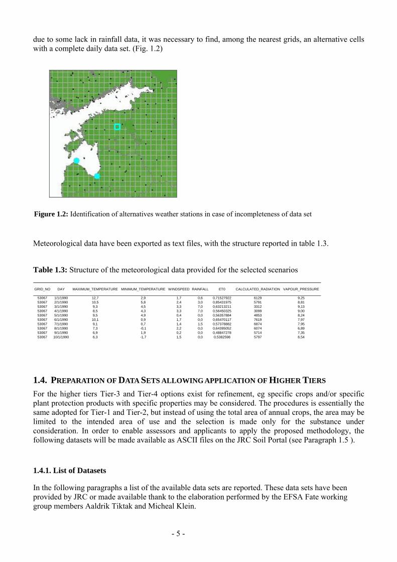
- 5 -
due to some lack in rainfall data it was necessary to find among the nearest grids an alternative cells with a complete daily data set (Fig 12)
Figure 12 Identification of alternatives weather stations in case of incompleteness of data set
Meteorological data have been exported as text files with the structure reported in table 13
Table 13 Structure of the meteorological data provided for the selected scenarios
GRID_NO DAY MAXIMUM_TEMPERATURE MINIMUM_TEMPERATURE WINDSPEED RAINFALL ET0 CALCULATED_RADIATION VAPOUR_PRESSURE
53067 111990 127 29 17 06 071527922 6129 92553067 211990 105 58 24 30 085431975 5791 88153067 311990 93 45 33 70 063213211 3312 91353067 411990 85 43 33 70 056450325 3099 90053067 511990 95 49 04 00 056357884 4853 82453067 611990 101 09 17 00 065470117 7619 79753067 711990 91 07 14 15 057378882 6874 79553067 811990 73 -01 22 00 064395052 6074 68953067 911990 69 19 02 00 048847278 5714 73553067 1011990 63 -17 15 00 05382598 5797 654
14 PREPARATION OF DATA SETS ALLOWING APPLICATION OF HIGHER TIERS For the higher tiers Tier-3 and Tier-4 options exist for refinement eg specific crops andor specific plant protection products with specific properties may be considered The procedures is essentially the same adopted for Tier-1 and Tier-2 but instead of using the total area of annual crops the area may be limited to the intended area of use and the selection is made only for the substance under consideration In order to enable assessors and applicants to apply the proposed methodology the following datasets will be made available as ASCII files on the JRC Soil Portal (see Paragraph 15 )
141 List of Datasets
In the following paragraphs a list of the available data sets are reported These data sets have been provided by JRC or made available thank to the elaboration performed by the EFSA Fate working group members Aaldrik Tiktak and Micheal Klein
- 6 -
General maps Masker of all files
Countries of the EU-27 (countriesmap)
Regulatory zones (Northern Central and Southern zone)
FOCUS Zones
Soil maps Organic matter content of the topsoil
pH of the topsoil
Bulk density of the topsoil
Texture of the topsoil
Water content at field capacity
Meteorological maps Mean monthly temperature (12 maps)
Mean annual temperature
Arrhenius weighted mean annual temperature
Mean monthly precipitation (12 maps)
Mean annual precipitation
Land use land cover maps Corine land cover data
Generalised land-use map (landusemap)
Capri land cover maps (24 maps)
15 SET-UP OF DEDICATED WEB SITE FOR DATA DOWNLOAD
In order to allow the data download a specific web page within the JRC Soil Portal will be realized on (httpeusoilsjrceceuropaeulibraryDataEFSA ) A print screen of the main web page is shown in Fig 13
JRC will require users of the data to fill an online form before proceeding with the data download (Fig 14) The information collected by JRC will be used for updating the data users on the possible release of new soil and weather related information and data sets However release of new information for the JRC Soil Portal will only happen after the FOCUS version control group chaired by EFSA has accepted the change of the new information
- 7 -
151 Web Page structure
Figure 13 Print-screen of the page dedicated to the data download
152 Data Users Record
Figure 14 Registration form to be filled for downloading the data
- 1 -
2 ECOREGION WG
21 INTRODUCTION AND OBJECTIVES The European Food Safety Authority (EFSA) asked the Panel on Plant Protection Products and their Residues (PPR) to further develop the concept of soil ecoregions in the context of the revision of the Guidance Document on Terrestrial Ecotoxicology (EFSA-Q-2009-00002) A modelling approach for defining soil ecoregions within Europe was developed to improve the realism of exposure scenarios for plant protection products Biogeographic data on four soil organisms groups (earthworms enchytraeids collembolans and isopods) were used to assign each functional group to different life forms representing depth horizons in which they occur Based on information from three Member States covering a North-South gradient Finland Germany and Portugal species presence-absence data were modelled using soil and climate data The objectives of JRC contribution were
- create a geographic database from the tabular data of the biogeographic survey
- extract soil and weather data in correspondence of biogeographic sampling sites
- implement the ecoregion models and create ecoregion maps
The technical details of the activities performed for the achievement of the above reported objectives are described in the following paragraphs and in the EFSA PPR Scientific Opinion on the development of a soil ecoregions concept using distribution data on invertebrates (EFSA 2010b) 22 DESCRIPTION OF THE PROCEDURES ADOPTED
The production of the Ecoregion maps for Finland Germany and Portugal represent the application of the proposed methodology to three test countries according to a North-South gradient
- 2 -
The complete description of the adopted approach is published as EFSA Opinion (EFSA 2010b) In the following paragraphs however is provided a more detailed description of the technical procedures adopted by JRC The conceptual framework for the development of soil Ecoregions is reported in the scheme of Figure 21 and the activities reported in the green boxes have been developed by JRC and described in the following paragraphs
Figure 21 Conceptual frame of the approach adopted for the definition of Soil Ecoregion
221 From an attribute database to a geographic database
The original biogeographical database provided for the three test Member States Finland Germany and Portugal was organized in separate Excel spreadsheets for the different groups of soil organisms and the geographic coordinates were based on UTM1 coordinate system based on Datum WGS842
1 UTM Universal Transver Maercator coordinate system is a grid-based method of specifying locations on the surface of the Earth that is
a practical application of a 2-dimensional Cartesian coordinate system 2 WGS 84 WGS (World Geodetic System) is a standard for use in cartography geodesy and navigation It comprises a standard
coordinate frame for the Earth a standard spheroidal reference surface (the datum or reference ellipsoid) for raw altitude data and a gravitational equipotential surface (the geoid) that defines the nominal sea level The GS 84 represent the latest revision of this standard
- 3 -
In order to project these data in the EU coordinate system (Lambert Azimuthal Equal Area) and to the process in the most efficient way it has been necessary to reorganize the database
One global spreadsheet for each of the three Member States has been produced
From each of these global spreadsheets partial spreadsheets have been derived grouping the records located in the same UTM zone
In order to keep the track of the changes a new field have been added (Fig 22) produced by the concatenation of
- Two capital letters for the organisms group (CO= collembola EW= earthworms IS= isopoda)
- The numeric value of ID Site
- The initial letter of the country name
Figure 22 Structure of the country-based spreadsheet the column with the new field has been outlined
These individual spreadsheets have been exported in DB4 format in order to be easily managed in ArcGIS ArcGIS 93 is the GIS software that has been used for the management and the analysis of the geographic information
The following phase in the management of the data has been the generation of Point Shapefiles representing the locations in which the soil organism inventory has been carried out and the re-projection of these maps
The extraction of soil and climate data from the raster dataset in correspondence of the of the soil organisms survey points has been realized using the ldquoExtract value to pointsrdquo procedure this procedure that is a classical example of spatial query allow to extract the cell values of a raster based on set of points
- 4 -
222Characterization of biogeographic sampling sites in terms of soil climate and land use characteristics
The biogeographic database consists of data on presenceabsence and in some cases abundance of selected groups of soil organisms and in some cases also data on land use vegetation soil and climate were reported The completeness of these environmental parameters essential for the ecological characterization of soil community however was very weak For this reason the data on land use soil and climate provided by JRC has been used to fill the gaps present in the original dataset
This process has been carried out using the utilities of spatial analysis present in a Geographical Information System (GIS) Once the geographic position of a sampling point is known it is possible do a spatial query in the GIS concerning the values of soil pH organic matter total precipitation and any other parameter that is available in a form of geographic database (Fig 23)
Figure 23 Schematic representation of the procedure adopted in a GIS for the extraction of given parameters (ie climate soil) for a given geographic position (ie observations)
- 5 -
223 Implementation of the provisional model in the selected Member States
The computation of the ecoregion maps has been based on the equations obtained in the data analysis implemented using the Map Algebra tools of Arc GIS (Raster Calculator Single Output Map Algebra) In Table 22 and 23 are reported the equations used for the computation of earthworm and enchytraeids maps respectively The first set of equations implying only the use of algebraic operators have been calculated using the lsquoraster calculatorrdquo within the Spatial Analyst toolset while the last expression based on logical operators have applied using the Single Output Map Algebra operator
Table 21 Equations used for earthworms Ecoregion Map
Map Algebra Operation with Raster Calculator t1
-0498 + ([Cropland] 00481) + ([Grassland] 09844) +([Forest3] -02298) + ([ph_top_efsa] 0317) + ([OC_efsa] -00905) + ([tmean] -02494) + ([Tdiff] -00418)
t2
27379 + ([Cropland] -01215) + ([Grassland] 02189) +([Forest3] -11576) + ([ph_top_efsa] 00567) + ([OC_efsa] -00105) +([total_prec] -00018) + ([tmean] 00956) + ([Tdiff] -01229)
z1 Exp([t1]) (1 + Exp([t1]))
z2 Exp([t2]) (1 + Exp([t2]))
ear_arr1 z1
ear_arr2 [z2] (1 - [z1])
ear_arr3 (1 - [z2]) (1 - [z1])
Map Algebra Operation with Single Output Map Algebra Earthworms Ecorgegion Map
con( ear_arr1 gt= 0667 1 ear_arr2 gt= 0667 2 ear_arr3 gt= 0667 3 arr1+arr2 gt= 0833 amp ear_arr1 lt= 0667 amp ear_arr2 lt= 0667 12 arr1+arr3 gt= 0833 amp ear_arr1 lt= 0667 amp ear_arr3 lt= 0667 13 arr2+arr3 gt= 0833 amp ear_arr2 lt= 0667 amp ear_arr3 lt= 0667 23 arr1+arr2 lt= 0833 amp arr2+arr3 lt= 0833 amp arr1+arr3 lt= 0833 123 )
- 6 -
Table 22 Equations used for enchytraeids Ecoregion Map
Map Algebra Operation with Raster Calculator t1
33243 + ([Grassland] 04764) + ([Forest3] 20354) + ([ph_top_efsa] -02776) + ([OC_efsa] -00206) + ([Clay] -00114) + ([total_prec] -00025) + ([tmean] -02286) + ([Tdiff] -00348)
t2
-65979 + ([Grassland] -05418) + ([Forest3] 10585) + ([ph_top_efsa] -02322) + ([OC_efsa] -01102) + ([Clay] -00505) + ([total_prec] -00010) + ([tmean] 03911) + ([Tdiff] 02961)
z1 Exp([t1]) (1 + Exp([t1]))
z2 Exp([t2]) (1 + Exp([t2]))
enc_arr1 z1
enc_arr2 [z2] (1 - [z1])
enc_arr3 (1 - [z2]) (1 - [z1])
Map Algebra Operation with Single Output Map Algebra Enchytraeids Ecorgegion Map
con( enc_arr1 gt= 0667 1 enc_arr2 gt= 0667 2 enc_arr3 gt= 0667 3 arr1+arr2 gt= 0833 amp enc_arr1 lt= 0667 amp enc_arr2 lt= 0667 12 arr1+arr3 gt= 0833 amp enc_arr1 lt= 0667 amp enc_arr3 lt= 0667 13 arr2+arr3 gt= 0833 amp enc_arr2 lt= 0667 amp enc_arr3 lt= 0667 23 arr1+arr2 lt= 0833 amp arr2+arr3 lt= 0833 amp arr1+arr3 lt= 0833 123 )
224 Soil Ecoregions Mapping
The output of the provisional models were a series of maps (one for each organism) where the territories of Finland Germany and Portugal have been classified in seven classes according to the triangles reported in figure 24
Earthworm ecoregion maps have been produced only for the three investigated countries but restricting Finland to its Southern part Enchytraeid ecoregions maps were limited to Germany and Finland since almost no enchytraeid data were available for Portugal For Collembola the fit of the model was very poor and the maps based on the modelled results did not show a convincing ecological meaning based on expert knowledge In case of Isopoda the model presented a good plausibility check with the observed and the modelled values However the analysis gave no clear indication for patterns differing between or within countries therefore isopods were excluded from further analysis and are not shown as maps
- 7 -
Although in principle the interpolation over the entire EU 27 territory would have been technically feasible mapping of territories without observed values were considered not to be reliable for the purpose of this opinion
The concepts of exposure scenario and the definition of soil profile depth relevant for different soil organisms communities led to the production of maps for earthworms and Enchytraeids where the territory of the investigated countries has been classified on the base of the depth relevant for the proposed Risk Assessment
Figure 24 Classification triangles used to classify the earthworms and enchytraeids soil communities
- 8 -
3 CONCLUSIONS AND RECOMMENDATIONS
31 FATE
The occurrence of gaps in daily meteorological data is relatively frequent especially over 20 year time frame For this reason it should be preferred the adoption of a statistical procedures for gap filling instead of selecting alternative nearest meteorological stations
For future applications the availability of 25 km grids will provide an improved geographic resolution for the representation of European climate
32 ECOREGION
During the analysis of the biogeographic database it was found the lack of complete soil land use and climate data sets for the vast majority of the observation sites For this reason it has been necessary to derive such data from the 1 km grid data set (soil and land use) and from the 50 km grids (meteorological data)
It should be outlined that while the use of these EU wide geographic data set is optimal for modelling application probably does not have the necessary spatial resolution for the characterization of point observation sites
- 9 -
4 METADATA FOR EFSA DATASET
A database of maps was created on the basis of the dataset provided by JRC (see Gardi et al 2008) This dataset was supplemented with data from the CAPRI land cover database (Leip et al 2008) JRC is acknowledged for making the data available in a common resolution and projection
Map properties
Common metadata properties for the maps are Format compressed ASCII grid Reference system ETRS 89 LAEA Rows 4098 Columns 3500 Lower left 2500000 Upper left 1412000 Cell size 1000 Unit m Nr of cells with a value 3997812
10
41 Masker of all files (EU27asc)
1 This map is a mask created including all the EU-27 countries and the Corine land-use classes 1-38 and 49 Surface waters and coastal lagoons are excluded from the mask
Legend There is only one legend unit ie 1 which means that the grid cell is included
Figure 41 Masker for the dataset The masker has only one value ie 1
11
42 Countries of the EU-27 (countriesasc)
The map shows the countries of the EU-27 It was obtained by masking the NUTS level 0 map with the mask EU27 Legend Number Country 1 Albania 5 Austria 8 Belgium 9 Bulgaria 15 Czech Republic 16 Germany 17 Denmark 20 Estonia 23 Spain 24 Finland 26 France 31 Greece 34 Hungary 35 Ireland 41 Italy 48 Lithuania 49 Luxemburg 50 Latvia 58 Netherlands 61 Poland 62 Portugal 64 Romania 67 Sweden 68 Slovenia 70 Slovakia 78 United Kingdom
12
Figure 42 Countries of the EU-27
13
43 Regulatory zones (zonesasc)
This map shows the regulatory zones of the EU-27 The map is a reclassification of the map countriesmap Legend Number Name Countries 1 North 17 20 24 48 50 and 67 2 Centre 5 8 16 34 35 49 58 61 64 68 70 and 78 3 South 1 9 23 26 31 41 and 62
Figure 43 The regulatory zones of the EU-27
14
44 Corine land cover data (CLC2000asc)
The map shows all the possible land use classes at the Corine map The map presented here is at a resolution of 1x1 km2 the original map was at a resolution of 025 km2 For each 1x1 km2 grid cell the dominant of the four underlying grid cells was taken The dataset is described in Nunes de Lima (2005) Legend Number CLC
code Description
1 111 Continuous urban fabric 2 112 Discontinuous urban fabric 3 121 Industrial or commercial units 4 122 Road and rail networks and associated land 5 123 Port areas 6 124 Airports 7 131 Mineral extraction sites 8 132 Dump sites 9 133 Construction sites 10 141 Green urban areas 11 142 Sport and leisure facilities 12 211 Non-irrigated arable land 13 212 Permanently irrigated land 14 213 Rice fields 15 221 Vineyards 16 222 Fruit trees and berry plantations 17 223 Olive groves 18 231 Pastures 19 241 Annual crops associated with permanent crops 20 242 Complex cultivation patterns 21 243 Land occupied by agriculture with significant areas of natural
vegetation 22 244 Agro-forestry areas 23 311 Broad-leaved forest 24 312 Coniferous forest 25 313 Mixed forest 26 321 Natural grasslands 27 322 Moors and heathland 28 323 Sclerophyllous vegetation 29 324 Transitional woodland-shrub 30 331 Beaches dunes sands 31 332 Bare rocks 32 333 Sparsely vegetated areas 33 334 Burnt areas 34 335 Glaciers and perpetual snow 35 411 Inland marshes 36 412 Peat bogs 37 421 Salt marshes
15
38 422 Salines 39 423 Intertidal flats 40 511 Water courses 41 512 Water bodies 42 521 Coastal lagoons 43 522 Estuaries 44 523 Sea and ocean 48 999 NODATA 49 990 UNCLASSIFIED LAND SURFACE 50 995 UNCLASSIFIED WATER BODIES
16
45 Generalised land-use map (landuseasc)
The generalised land-use map is a reclassification of the Corine 2000 land-use map It is created to distinguish the most important land-use types Land use class 1 serves as the masker in EFSA (2010)
Legend Number Description Number in map above 1 Annual Crops 12 13 19-21 2 Grass 18 3 Permanent crops 15-17 and 22 4 Rice 14 5 Non agricultural all other classes
Figure 44 The generalised land-use map
17
46 Mean monthly temperature (T1ascT12asc)
The dataset consists of 12 maps containing the monthly mean temperature (deg C) for the period 1960-1990 The dataset is described in Hijmans et al (2005) Legend Mean monthly temperature (deg C) data type Real 47 Mean annual temperature (TMeanasc)
The map shows the mean annual temperature (deg C) for the period 1960-1990 It is calculating by taking the arithmetic mean of maps T1T12asc The dataset is described in Hijmans et al (2005) Legend Mean annual temperature (deg C) data type Real
Figure 45 Mean annual temperature for the period 1960-1990 taken from Worldclim dataset
18
48 Arrhenius weighted mean annual temperature (TEffasc)
The map shows the Arrhenius weighted mean annual temperature (deg C) for the period 1960-1990 It is calculated using the equation (EFSA 2010 Appendix A3)
( )
( ) ( )( ) 0
exp273)(
1ln0
=
⎥⎦
⎤⎢⎣
⎡minus=gt
⎥⎥⎦
⎤
⎢⎢⎣
⎡minus=
int
tTfelsetRT
EtTfthentTif
dttTft
R
ET
act
t
end
acteff
end
(1)
where Teff (K) is the Arrhenius weighted mean annual temperature Eact is the Arrhenius activation energy (kJ mol-1) R (kJ mol-1 K-1) is the gas constant T (K) is the temperature and t is time Eact was set to 654 kJ mol-1 according to EFSA (2007) See further EFSA (2010) Notice that the temperatures in the equation are in K whereas the temperature in the maps is in deg C Legend Arrhenius weighted mean annual temperature (deg C) data type Real
19
Figure 46 Arrhenius weighted mean temperature (deg C) for the period 1960-1990 For a description of the averaging procedure refer to EFSA (2010)
20
49 Mean monthly precipitation (P1ascP12asc)
The dataset consists of 12 maps containing the monthly mean precipitation (mmmonth) for the period 1960-1990 The dataset is described in Hijmans et al (2005) Legend Mean monthly precipitation (mmmo) data type Real 410 Mean annual precipitation (Ptotasc)
The map shows the mean annual precipitation for the period 1960-1990 (mmyear) It is calculated by summing P1P12map The dataset is described in Hijmans et al (2005) Legend Mean annual precipitation (mmyr) data type Real
Figure 47 Mean annual precipitation (mm) for the period 1960-1990 as taken from the Worldclim dataset
21
411 FOCUS Zones (FOCUSasc)
The map shows the FOCUS zones according to the classification in FOCUS (2000) The maps Tmeanmap and Ptotmap were used to create the overlay so the classification is based on WorldClim (Hijmans et al 2005)
Legend Number Name Tmean (deg C) Ptot (mmyr) 1 Jokioinen lt5 deg C gt 0 mmyr 2 Chateaudun 5 ndash 125 deg C lt 600 mmyr 3 Hamburg 5 ndash 125 deg C 600 ndash 800 mmyr 4 Kremsmuumlnster 5 ndash 125 deg C 800 ndash 1000 mmyr 5 Okehampton 5 ndash 125 deg C gt 1000 mmyr 6 Sevilla gt 125 deg C lt 600 mmyr 7 Thiva gt 125 deg C 600 ndash 800 mmyr 8 Piacenza gt 125 deg C 800 ndash 1000 mmyr 9 Porto gt 125 deg C gt 1000 mmyr
22
Figure 48 FOCUS climatic zones based on the mean annual temperature and mean annual precipitation from Worldclim
23
412 Organic matter content of the topsoil (OMasc)
The map shows the organic matter content of the topsoil It is obtained by multiplying the original OCTOP map described in Jones et al (2005) by 172 Legend Organic matter content of the topsoil (gg) data type Real
Figure 49 Organic matter content of the top 30 cm of the soil (gg)
24
413 pH of the topsoil (pHasc)
The map shows the mean pH measured in water (125) of the top 30 cm of the soil See FAO (2008) for details Legend pH measured in water of the topsoil data type Real
Figure 410 pH water (125) of the top 30 cm of the soil
25
414 Bulk density of the topsoil (Rhoasc)
The map shows the bulk density of the topsoil It is calculated from the organic matter content map using the equation (Tiktak et al 2002)
)910(291012361800 2 =minus+= rff omomρ (2)
Legend Dry bulk density of the topsoil (kg m-3) data type Real
Figure 411 Bulk density of the top 30 cm of the soil calculated by the pedotransfer function described in Tiktak et al (2002)
26
415 Texture of the topsoil (Textureasc)
The map shows the textural class of the topsoil It is obtained from the soil geographical database of Eurasia at a scale of 11000000 (for each grid cell the dominant soil textural class was taken) Legend Number Description 1 Coarse (18 lt clay and gt 65 sand) 2 Medium (18 lt clay lt 35 and gt= 15 sand or 18 ltclay and 15 lt sand lt
65) 3 Medium fine (lt 35 clay and lt 15 sand) 4 Fine (35 lt clay lt 60) 5 Very fine (clay gt 60 ) 9 No mineral texture (Peat soils)
Figure 412Topsoil texture obtained from the soil database of Europe 11000000
27
416 Water content at field capacity (ThetaFCasc)
The map shows the water content at field capacity (m3 m-3) It is calculated for each soil textural class with the Mualem-Van Genuchten equation
( ) mnrs
rh
h minus+
minus+=
α
θθθθ1
)( (1)
where θ (m3 m-3) is the volume fraction of water h (cm) is the soil water pressure head θs (m3 m-3) is the volume fraction of water at saturation θr (m3 m-3) is the residual water content in the extremely dry range α (cm-1) and n (-) are empirical parameters and m (-) can be taken equal to
nm 11minus=
The soil water pressure head was set at -100 cm Parameter values were obtained from the HYPRES pedotransfer rule (Woumlsten et al 1999) and are given in EFSA (2010) table 3 Legend Volumetric water content at field capacity (m3 m-3) data type Real The map contains six discrete classes
28
Figure 413 Volume fraction of water at field capacity calculated from the soil textural class using the HYPRES pedotransfer rule
29
417 Capri land cover maps (Cropnamesasc)
These maps show for each pixel of 1x1 km2 the area covered with a certain crop The CAPRI maps were obtained by combining remote sensing data administrative crop data land suitability data and statistical modelling The CORINE land cover map serves as a starting point Subdivisions within CORINE land cover classes were made based on a statistical model regressing point observations of cropping activities on soil relief and climate parameters (land suitability) Statistical data of agricultural production and land cover available for administrative regions were additionally used to scale the land cover classes 18 of the CAPRI land cover classes are classified as annual crops and are included in the EFSA dataset See Leip et al (2008) for a description of the dataset Legend Area (100) covered by a crop data type Real The names of the maps are self explaining The values range from 0 to 10000
30
Figure 414 Crop cover maps ( of area) for barley common wheat texture crops floriculture other fodder crops and industrial crops
31
Figure 415 Crop cover maps ( of area) for maize oats other cereals pulses rapes and root crops
32
Figure 416 Crop cover maps ( of area) for rye soya sugar beet sunflowers vegetables and durum wheat
33
5 REFERENCES
Goot E van der 1998 Spatial interpolation of daily meteorological data for the Crop Growth Monitoring System (CGMS) In M Bindi B Gozzini (eds) Proceedings of seminar on dataspatial distribution in meteorology and climatology 28 September - 3 October 1997 Volterra Italy EUR 18472 EN Office for Official Publications of the EU Luxembourg p 141-153
Gardi C Montanarella L Hiederer R Jones A Micale F 2010 Activities realized within the Service Level Agreement between JRC and EFSA as a support of the FATE Working Group of EFSA PPR in support of the revision of the guidance document Persistence in Soil JRC Technical Svientific and Technical Report 39 pp - EUR 24345
Gardi C2010 Report on the Activities realised within the Service Licence Agreement between JRC and EFSA as a support of the FATE Working Group of EFSA PPR JRC Scientific Report (SLAEFSA-JRC200801)
EFSA 2010a Opinion of the Scientific Panel on Plant Protection products and their Residues on outline proposals for assessment of exposure of organisms to substances in soil EFSA Journal 8(1)1442
EFSA 2010b Opinion of the Scientific Panel on Plant Protection products and their Residues on on the development of a soil ecoregions concept using distribution data on invertebrates EFSA Journal 8(10)1820
EFSA 2007 Opinion on a request from EFSA related to the default Q10 value used to describe the temperature effect on transformation rates of pesticides in soil Scientific Opinion of the Panel on Plant Protection Products and their Residues (PPR-Panel) The EFSA Journal (622)1 32
EFSA 2010 Selection of scenarios for exposure of soil organisms The EFSA Journal (2010) 8(46)1642
FAOIIASAISRICISS-CASJRC 2008 Harmonized World Soil Database (version 10) FAO Rome Italy and IIASA Laxenburg Austria 37pp
FOCUS 2010 Assessing potential movement of active substances and their metabolites to ground water in the EU EC Document reference Sancoxxx2010 Available at FOCUS website httpvisoeijrcitfocus
Hijmans RJ SE Cameron JL Parra PG Jones and A Jarvis 2005 Very high resolution interpolated climate surfaces for global land areas Int J Climatology (25)1965-1978
Jones RJA R Hiederer E Rusco PJ Loveland and L Montanarella 2005 Estimating organic carbon in the soils of Europe for policy support European Journal of Soil Science (56)655-671
Leip A G Marchi R Koeble M Kempen W Britz and C Li 2008 Linking an economic model for European agriculture with a mechanistic model to estimate nitrogen and carbon losses from arable soils in Europe Biogeosciences (5)73-94
Tiktak A DS de Nie AMA van der Linden and R Kruijne 2002 Modelling the leaching and drainage of pesticides in the Netherlands the GeoPEARL model Agronomie (22)373-387
Woumlsten JHM A Nemes A Lilly and C Le Bas 1999 Development and use of a database of hydraulic properties of European soils Geoderma (90)169ndash185
34
APPENDICES ECOREGION MAPS
Earthworm Finland
35
Earthworm Germany
36
Earthworm Portugal
37
Enchytraeids Finland
38
Enchytraeids Germany
39
European Commission EUR 24744 EN ndash Joint Research Centre ndash Institute for Environment and Sustainability Title Report on the activities realized within the Service Level Agreement between JRC and EFSA Author(s) Ciro Gardi Panos Panagos Roland Hiederer Luca Montanarella Fabio Micale Luxembourg Publications Office of the European Union 2011 ndash 38 pp ndash 210 x 297 cm EUR ndash Scientific and Technical Research series ndash ISSN 1018-5593 ISBN 978-92-79-19521-1 doi10278861018 Abstract The activities realized in 2010 by JRC as support to the FATE and the ECOREGION EFSA PPR Working Groups are shortly described For the FATE WG the vast majority of data has been provided in 2009 during the first year of the Service Level Agreement (SLA) and in 2010 the daily weather data for the six selected sites were produced All the data used for the scenario selection procedures with additional data on land use-land cover crop distribution soil and climate parameters will be made available for external user in first half of 2011 For the ECOREGION WG the analysis has been carried out for three Member States covering a North-South gradient from Finland Germany to Portugal Soil and weather data have been used for the characterisation of bio-geographic sampling sites and for the implementation of the ecoregion model Ecoregion maps were produced for earthworms and enchytraeids for Finland and Germany and revealed marked differences between the countries The same approach has been applied also to Collembola and Isopoda but for these two taxa led to a rather poor discrimination both between and within countries
How to obtain EU publications Our priced publications are available from EU Bookshop (httpbookshopeuropaeu) where you can place an order with the sales agent of your choice The Publications Office has a worldwide network of sales agents You can obtain their contact details by sending a fax to (352) 29 29-42758
The mission of the JRC is to provide customer-driven scientific and technical supportfor the conception development implementation and monitoring of EU policies As a service of the European Commission the JRC functions as a reference centre of science and technology for the Union Close to the policy-making process it serves the common interest of the Member States while being independent of special interests whether private or national
LB
-NA
-24744-EN-C
- 141 List of Datasets
- 151 Web Page structure
- 152 Data Users Record
- 22 Description of the Procedures Adopted
- 221 From an attribute database to a geographic database
- 222Characterization of biogeographic sampling sites in terms of soil climate and land use characteristics
- 223 Implementation of the provisional model in the selected Member States
- 224 Soil Ecoregions Mapping
- 3 Conclusions and Recommendations
-
- 31 FATE
- 32 ECOREGION
-
- 4 Metadata for EFSA dataset
-
- Map properties
- 41 Masker of all files (EU27asc)
- 42 Countries of the EU-27 (countriesasc)
- 43 Regulatory zones (zonesasc)
- 44 Corine land cover data (CLC2000asc)
- 45 Generalised land-use map (landuseasc)
- 46 Mean monthly temperature (T1ascT12asc)
- 47 Mean annual temperature (TMeanasc)
- 48 Arrhenius weighted mean annual temperature (TEffasc)
- 49 Mean monthly precipitation (P1ascP12asc)
- 410 Mean annual precipitation (Ptotasc)
- 411 FOCUS Zones (FOCUSasc)
- 412 Organic matter content of the topsoil (OMasc)
- 413 pH of the topsoil (pHasc)
- 414 Bulk density of the topsoil (Rhoasc)
- 415 Texture of the topsoil (Textureasc)
- 416 Water content at field capacity (ThetaFCasc)
- 417 Capri land cover maps (Cropnamesasc)
-
- 5 References
-
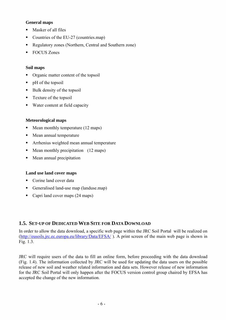
- 6 -
General maps Masker of all files
Countries of the EU-27 (countriesmap)
Regulatory zones (Northern Central and Southern zone)
FOCUS Zones
Soil maps Organic matter content of the topsoil
pH of the topsoil
Bulk density of the topsoil
Texture of the topsoil
Water content at field capacity
Meteorological maps Mean monthly temperature (12 maps)
Mean annual temperature
Arrhenius weighted mean annual temperature
Mean monthly precipitation (12 maps)
Mean annual precipitation
Land use land cover maps Corine land cover data
Generalised land-use map (landusemap)
Capri land cover maps (24 maps)
15 SET-UP OF DEDICATED WEB SITE FOR DATA DOWNLOAD
In order to allow the data download a specific web page within the JRC Soil Portal will be realized on (httpeusoilsjrceceuropaeulibraryDataEFSA ) A print screen of the main web page is shown in Fig 13
JRC will require users of the data to fill an online form before proceeding with the data download (Fig 14) The information collected by JRC will be used for updating the data users on the possible release of new soil and weather related information and data sets However release of new information for the JRC Soil Portal will only happen after the FOCUS version control group chaired by EFSA has accepted the change of the new information
- 7 -
151 Web Page structure
Figure 13 Print-screen of the page dedicated to the data download
152 Data Users Record
Figure 14 Registration form to be filled for downloading the data
- 1 -
2 ECOREGION WG
21 INTRODUCTION AND OBJECTIVES The European Food Safety Authority (EFSA) asked the Panel on Plant Protection Products and their Residues (PPR) to further develop the concept of soil ecoregions in the context of the revision of the Guidance Document on Terrestrial Ecotoxicology (EFSA-Q-2009-00002) A modelling approach for defining soil ecoregions within Europe was developed to improve the realism of exposure scenarios for plant protection products Biogeographic data on four soil organisms groups (earthworms enchytraeids collembolans and isopods) were used to assign each functional group to different life forms representing depth horizons in which they occur Based on information from three Member States covering a North-South gradient Finland Germany and Portugal species presence-absence data were modelled using soil and climate data The objectives of JRC contribution were
- create a geographic database from the tabular data of the biogeographic survey
- extract soil and weather data in correspondence of biogeographic sampling sites
- implement the ecoregion models and create ecoregion maps
The technical details of the activities performed for the achievement of the above reported objectives are described in the following paragraphs and in the EFSA PPR Scientific Opinion on the development of a soil ecoregions concept using distribution data on invertebrates (EFSA 2010b) 22 DESCRIPTION OF THE PROCEDURES ADOPTED
The production of the Ecoregion maps for Finland Germany and Portugal represent the application of the proposed methodology to three test countries according to a North-South gradient
- 2 -
The complete description of the adopted approach is published as EFSA Opinion (EFSA 2010b) In the following paragraphs however is provided a more detailed description of the technical procedures adopted by JRC The conceptual framework for the development of soil Ecoregions is reported in the scheme of Figure 21 and the activities reported in the green boxes have been developed by JRC and described in the following paragraphs
Figure 21 Conceptual frame of the approach adopted for the definition of Soil Ecoregion
221 From an attribute database to a geographic database
The original biogeographical database provided for the three test Member States Finland Germany and Portugal was organized in separate Excel spreadsheets for the different groups of soil organisms and the geographic coordinates were based on UTM1 coordinate system based on Datum WGS842
1 UTM Universal Transver Maercator coordinate system is a grid-based method of specifying locations on the surface of the Earth that is
a practical application of a 2-dimensional Cartesian coordinate system 2 WGS 84 WGS (World Geodetic System) is a standard for use in cartography geodesy and navigation It comprises a standard
coordinate frame for the Earth a standard spheroidal reference surface (the datum or reference ellipsoid) for raw altitude data and a gravitational equipotential surface (the geoid) that defines the nominal sea level The GS 84 represent the latest revision of this standard
- 3 -
In order to project these data in the EU coordinate system (Lambert Azimuthal Equal Area) and to the process in the most efficient way it has been necessary to reorganize the database
One global spreadsheet for each of the three Member States has been produced
From each of these global spreadsheets partial spreadsheets have been derived grouping the records located in the same UTM zone
In order to keep the track of the changes a new field have been added (Fig 22) produced by the concatenation of
- Two capital letters for the organisms group (CO= collembola EW= earthworms IS= isopoda)
- The numeric value of ID Site
- The initial letter of the country name
Figure 22 Structure of the country-based spreadsheet the column with the new field has been outlined
These individual spreadsheets have been exported in DB4 format in order to be easily managed in ArcGIS ArcGIS 93 is the GIS software that has been used for the management and the analysis of the geographic information
The following phase in the management of the data has been the generation of Point Shapefiles representing the locations in which the soil organism inventory has been carried out and the re-projection of these maps
The extraction of soil and climate data from the raster dataset in correspondence of the of the soil organisms survey points has been realized using the ldquoExtract value to pointsrdquo procedure this procedure that is a classical example of spatial query allow to extract the cell values of a raster based on set of points
- 4 -
222Characterization of biogeographic sampling sites in terms of soil climate and land use characteristics
The biogeographic database consists of data on presenceabsence and in some cases abundance of selected groups of soil organisms and in some cases also data on land use vegetation soil and climate were reported The completeness of these environmental parameters essential for the ecological characterization of soil community however was very weak For this reason the data on land use soil and climate provided by JRC has been used to fill the gaps present in the original dataset
This process has been carried out using the utilities of spatial analysis present in a Geographical Information System (GIS) Once the geographic position of a sampling point is known it is possible do a spatial query in the GIS concerning the values of soil pH organic matter total precipitation and any other parameter that is available in a form of geographic database (Fig 23)
Figure 23 Schematic representation of the procedure adopted in a GIS for the extraction of given parameters (ie climate soil) for a given geographic position (ie observations)
- 5 -
223 Implementation of the provisional model in the selected Member States
The computation of the ecoregion maps has been based on the equations obtained in the data analysis implemented using the Map Algebra tools of Arc GIS (Raster Calculator Single Output Map Algebra) In Table 22 and 23 are reported the equations used for the computation of earthworm and enchytraeids maps respectively The first set of equations implying only the use of algebraic operators have been calculated using the lsquoraster calculatorrdquo within the Spatial Analyst toolset while the last expression based on logical operators have applied using the Single Output Map Algebra operator
Table 21 Equations used for earthworms Ecoregion Map
Map Algebra Operation with Raster Calculator t1
-0498 + ([Cropland] 00481) + ([Grassland] 09844) +([Forest3] -02298) + ([ph_top_efsa] 0317) + ([OC_efsa] -00905) + ([tmean] -02494) + ([Tdiff] -00418)
t2
27379 + ([Cropland] -01215) + ([Grassland] 02189) +([Forest3] -11576) + ([ph_top_efsa] 00567) + ([OC_efsa] -00105) +([total_prec] -00018) + ([tmean] 00956) + ([Tdiff] -01229)
z1 Exp([t1]) (1 + Exp([t1]))
z2 Exp([t2]) (1 + Exp([t2]))
ear_arr1 z1
ear_arr2 [z2] (1 - [z1])
ear_arr3 (1 - [z2]) (1 - [z1])
Map Algebra Operation with Single Output Map Algebra Earthworms Ecorgegion Map
con( ear_arr1 gt= 0667 1 ear_arr2 gt= 0667 2 ear_arr3 gt= 0667 3 arr1+arr2 gt= 0833 amp ear_arr1 lt= 0667 amp ear_arr2 lt= 0667 12 arr1+arr3 gt= 0833 amp ear_arr1 lt= 0667 amp ear_arr3 lt= 0667 13 arr2+arr3 gt= 0833 amp ear_arr2 lt= 0667 amp ear_arr3 lt= 0667 23 arr1+arr2 lt= 0833 amp arr2+arr3 lt= 0833 amp arr1+arr3 lt= 0833 123 )
- 6 -
Table 22 Equations used for enchytraeids Ecoregion Map
Map Algebra Operation with Raster Calculator t1
33243 + ([Grassland] 04764) + ([Forest3] 20354) + ([ph_top_efsa] -02776) + ([OC_efsa] -00206) + ([Clay] -00114) + ([total_prec] -00025) + ([tmean] -02286) + ([Tdiff] -00348)
t2
-65979 + ([Grassland] -05418) + ([Forest3] 10585) + ([ph_top_efsa] -02322) + ([OC_efsa] -01102) + ([Clay] -00505) + ([total_prec] -00010) + ([tmean] 03911) + ([Tdiff] 02961)
z1 Exp([t1]) (1 + Exp([t1]))
z2 Exp([t2]) (1 + Exp([t2]))
enc_arr1 z1
enc_arr2 [z2] (1 - [z1])
enc_arr3 (1 - [z2]) (1 - [z1])
Map Algebra Operation with Single Output Map Algebra Enchytraeids Ecorgegion Map
con( enc_arr1 gt= 0667 1 enc_arr2 gt= 0667 2 enc_arr3 gt= 0667 3 arr1+arr2 gt= 0833 amp enc_arr1 lt= 0667 amp enc_arr2 lt= 0667 12 arr1+arr3 gt= 0833 amp enc_arr1 lt= 0667 amp enc_arr3 lt= 0667 13 arr2+arr3 gt= 0833 amp enc_arr2 lt= 0667 amp enc_arr3 lt= 0667 23 arr1+arr2 lt= 0833 amp arr2+arr3 lt= 0833 amp arr1+arr3 lt= 0833 123 )
224 Soil Ecoregions Mapping
The output of the provisional models were a series of maps (one for each organism) where the territories of Finland Germany and Portugal have been classified in seven classes according to the triangles reported in figure 24
Earthworm ecoregion maps have been produced only for the three investigated countries but restricting Finland to its Southern part Enchytraeid ecoregions maps were limited to Germany and Finland since almost no enchytraeid data were available for Portugal For Collembola the fit of the model was very poor and the maps based on the modelled results did not show a convincing ecological meaning based on expert knowledge In case of Isopoda the model presented a good plausibility check with the observed and the modelled values However the analysis gave no clear indication for patterns differing between or within countries therefore isopods were excluded from further analysis and are not shown as maps
- 7 -
Although in principle the interpolation over the entire EU 27 territory would have been technically feasible mapping of territories without observed values were considered not to be reliable for the purpose of this opinion
The concepts of exposure scenario and the definition of soil profile depth relevant for different soil organisms communities led to the production of maps for earthworms and Enchytraeids where the territory of the investigated countries has been classified on the base of the depth relevant for the proposed Risk Assessment
Figure 24 Classification triangles used to classify the earthworms and enchytraeids soil communities
- 8 -
3 CONCLUSIONS AND RECOMMENDATIONS
31 FATE
The occurrence of gaps in daily meteorological data is relatively frequent especially over 20 year time frame For this reason it should be preferred the adoption of a statistical procedures for gap filling instead of selecting alternative nearest meteorological stations
For future applications the availability of 25 km grids will provide an improved geographic resolution for the representation of European climate
32 ECOREGION
During the analysis of the biogeographic database it was found the lack of complete soil land use and climate data sets for the vast majority of the observation sites For this reason it has been necessary to derive such data from the 1 km grid data set (soil and land use) and from the 50 km grids (meteorological data)
It should be outlined that while the use of these EU wide geographic data set is optimal for modelling application probably does not have the necessary spatial resolution for the characterization of point observation sites
- 9 -
4 METADATA FOR EFSA DATASET
A database of maps was created on the basis of the dataset provided by JRC (see Gardi et al 2008) This dataset was supplemented with data from the CAPRI land cover database (Leip et al 2008) JRC is acknowledged for making the data available in a common resolution and projection
Map properties
Common metadata properties for the maps are Format compressed ASCII grid Reference system ETRS 89 LAEA Rows 4098 Columns 3500 Lower left 2500000 Upper left 1412000 Cell size 1000 Unit m Nr of cells with a value 3997812
10
41 Masker of all files (EU27asc)
1 This map is a mask created including all the EU-27 countries and the Corine land-use classes 1-38 and 49 Surface waters and coastal lagoons are excluded from the mask
Legend There is only one legend unit ie 1 which means that the grid cell is included
Figure 41 Masker for the dataset The masker has only one value ie 1
11
42 Countries of the EU-27 (countriesasc)
The map shows the countries of the EU-27 It was obtained by masking the NUTS level 0 map with the mask EU27 Legend Number Country 1 Albania 5 Austria 8 Belgium 9 Bulgaria 15 Czech Republic 16 Germany 17 Denmark 20 Estonia 23 Spain 24 Finland 26 France 31 Greece 34 Hungary 35 Ireland 41 Italy 48 Lithuania 49 Luxemburg 50 Latvia 58 Netherlands 61 Poland 62 Portugal 64 Romania 67 Sweden 68 Slovenia 70 Slovakia 78 United Kingdom
12
Figure 42 Countries of the EU-27
13
43 Regulatory zones (zonesasc)
This map shows the regulatory zones of the EU-27 The map is a reclassification of the map countriesmap Legend Number Name Countries 1 North 17 20 24 48 50 and 67 2 Centre 5 8 16 34 35 49 58 61 64 68 70 and 78 3 South 1 9 23 26 31 41 and 62
Figure 43 The regulatory zones of the EU-27
14
44 Corine land cover data (CLC2000asc)
The map shows all the possible land use classes at the Corine map The map presented here is at a resolution of 1x1 km2 the original map was at a resolution of 025 km2 For each 1x1 km2 grid cell the dominant of the four underlying grid cells was taken The dataset is described in Nunes de Lima (2005) Legend Number CLC
code Description
1 111 Continuous urban fabric 2 112 Discontinuous urban fabric 3 121 Industrial or commercial units 4 122 Road and rail networks and associated land 5 123 Port areas 6 124 Airports 7 131 Mineral extraction sites 8 132 Dump sites 9 133 Construction sites 10 141 Green urban areas 11 142 Sport and leisure facilities 12 211 Non-irrigated arable land 13 212 Permanently irrigated land 14 213 Rice fields 15 221 Vineyards 16 222 Fruit trees and berry plantations 17 223 Olive groves 18 231 Pastures 19 241 Annual crops associated with permanent crops 20 242 Complex cultivation patterns 21 243 Land occupied by agriculture with significant areas of natural
vegetation 22 244 Agro-forestry areas 23 311 Broad-leaved forest 24 312 Coniferous forest 25 313 Mixed forest 26 321 Natural grasslands 27 322 Moors and heathland 28 323 Sclerophyllous vegetation 29 324 Transitional woodland-shrub 30 331 Beaches dunes sands 31 332 Bare rocks 32 333 Sparsely vegetated areas 33 334 Burnt areas 34 335 Glaciers and perpetual snow 35 411 Inland marshes 36 412 Peat bogs 37 421 Salt marshes
15
38 422 Salines 39 423 Intertidal flats 40 511 Water courses 41 512 Water bodies 42 521 Coastal lagoons 43 522 Estuaries 44 523 Sea and ocean 48 999 NODATA 49 990 UNCLASSIFIED LAND SURFACE 50 995 UNCLASSIFIED WATER BODIES
16
45 Generalised land-use map (landuseasc)
The generalised land-use map is a reclassification of the Corine 2000 land-use map It is created to distinguish the most important land-use types Land use class 1 serves as the masker in EFSA (2010)
Legend Number Description Number in map above 1 Annual Crops 12 13 19-21 2 Grass 18 3 Permanent crops 15-17 and 22 4 Rice 14 5 Non agricultural all other classes
Figure 44 The generalised land-use map
17
46 Mean monthly temperature (T1ascT12asc)
The dataset consists of 12 maps containing the monthly mean temperature (deg C) for the period 1960-1990 The dataset is described in Hijmans et al (2005) Legend Mean monthly temperature (deg C) data type Real 47 Mean annual temperature (TMeanasc)
The map shows the mean annual temperature (deg C) for the period 1960-1990 It is calculating by taking the arithmetic mean of maps T1T12asc The dataset is described in Hijmans et al (2005) Legend Mean annual temperature (deg C) data type Real
Figure 45 Mean annual temperature for the period 1960-1990 taken from Worldclim dataset
18
48 Arrhenius weighted mean annual temperature (TEffasc)
The map shows the Arrhenius weighted mean annual temperature (deg C) for the period 1960-1990 It is calculated using the equation (EFSA 2010 Appendix A3)
( )
( ) ( )( ) 0
exp273)(
1ln0
=
⎥⎦
⎤⎢⎣
⎡minus=gt
⎥⎥⎦
⎤
⎢⎢⎣
⎡minus=
int
tTfelsetRT
EtTfthentTif
dttTft
R
ET
act
t
end
acteff
end
(1)
where Teff (K) is the Arrhenius weighted mean annual temperature Eact is the Arrhenius activation energy (kJ mol-1) R (kJ mol-1 K-1) is the gas constant T (K) is the temperature and t is time Eact was set to 654 kJ mol-1 according to EFSA (2007) See further EFSA (2010) Notice that the temperatures in the equation are in K whereas the temperature in the maps is in deg C Legend Arrhenius weighted mean annual temperature (deg C) data type Real
19
Figure 46 Arrhenius weighted mean temperature (deg C) for the period 1960-1990 For a description of the averaging procedure refer to EFSA (2010)
20
49 Mean monthly precipitation (P1ascP12asc)
The dataset consists of 12 maps containing the monthly mean precipitation (mmmonth) for the period 1960-1990 The dataset is described in Hijmans et al (2005) Legend Mean monthly precipitation (mmmo) data type Real 410 Mean annual precipitation (Ptotasc)
The map shows the mean annual precipitation for the period 1960-1990 (mmyear) It is calculated by summing P1P12map The dataset is described in Hijmans et al (2005) Legend Mean annual precipitation (mmyr) data type Real
Figure 47 Mean annual precipitation (mm) for the period 1960-1990 as taken from the Worldclim dataset
21
411 FOCUS Zones (FOCUSasc)
The map shows the FOCUS zones according to the classification in FOCUS (2000) The maps Tmeanmap and Ptotmap were used to create the overlay so the classification is based on WorldClim (Hijmans et al 2005)
Legend Number Name Tmean (deg C) Ptot (mmyr) 1 Jokioinen lt5 deg C gt 0 mmyr 2 Chateaudun 5 ndash 125 deg C lt 600 mmyr 3 Hamburg 5 ndash 125 deg C 600 ndash 800 mmyr 4 Kremsmuumlnster 5 ndash 125 deg C 800 ndash 1000 mmyr 5 Okehampton 5 ndash 125 deg C gt 1000 mmyr 6 Sevilla gt 125 deg C lt 600 mmyr 7 Thiva gt 125 deg C 600 ndash 800 mmyr 8 Piacenza gt 125 deg C 800 ndash 1000 mmyr 9 Porto gt 125 deg C gt 1000 mmyr
22
Figure 48 FOCUS climatic zones based on the mean annual temperature and mean annual precipitation from Worldclim
23
412 Organic matter content of the topsoil (OMasc)
The map shows the organic matter content of the topsoil It is obtained by multiplying the original OCTOP map described in Jones et al (2005) by 172 Legend Organic matter content of the topsoil (gg) data type Real
Figure 49 Organic matter content of the top 30 cm of the soil (gg)
24
413 pH of the topsoil (pHasc)
The map shows the mean pH measured in water (125) of the top 30 cm of the soil See FAO (2008) for details Legend pH measured in water of the topsoil data type Real
Figure 410 pH water (125) of the top 30 cm of the soil
25
414 Bulk density of the topsoil (Rhoasc)
The map shows the bulk density of the topsoil It is calculated from the organic matter content map using the equation (Tiktak et al 2002)
)910(291012361800 2 =minus+= rff omomρ (2)
Legend Dry bulk density of the topsoil (kg m-3) data type Real
Figure 411 Bulk density of the top 30 cm of the soil calculated by the pedotransfer function described in Tiktak et al (2002)
26
415 Texture of the topsoil (Textureasc)
The map shows the textural class of the topsoil It is obtained from the soil geographical database of Eurasia at a scale of 11000000 (for each grid cell the dominant soil textural class was taken) Legend Number Description 1 Coarse (18 lt clay and gt 65 sand) 2 Medium (18 lt clay lt 35 and gt= 15 sand or 18 ltclay and 15 lt sand lt
65) 3 Medium fine (lt 35 clay and lt 15 sand) 4 Fine (35 lt clay lt 60) 5 Very fine (clay gt 60 ) 9 No mineral texture (Peat soils)
Figure 412Topsoil texture obtained from the soil database of Europe 11000000
27
416 Water content at field capacity (ThetaFCasc)
The map shows the water content at field capacity (m3 m-3) It is calculated for each soil textural class with the Mualem-Van Genuchten equation
( ) mnrs
rh
h minus+
minus+=
α
θθθθ1
)( (1)
where θ (m3 m-3) is the volume fraction of water h (cm) is the soil water pressure head θs (m3 m-3) is the volume fraction of water at saturation θr (m3 m-3) is the residual water content in the extremely dry range α (cm-1) and n (-) are empirical parameters and m (-) can be taken equal to
nm 11minus=
The soil water pressure head was set at -100 cm Parameter values were obtained from the HYPRES pedotransfer rule (Woumlsten et al 1999) and are given in EFSA (2010) table 3 Legend Volumetric water content at field capacity (m3 m-3) data type Real The map contains six discrete classes
28
Figure 413 Volume fraction of water at field capacity calculated from the soil textural class using the HYPRES pedotransfer rule
29
417 Capri land cover maps (Cropnamesasc)
These maps show for each pixel of 1x1 km2 the area covered with a certain crop The CAPRI maps were obtained by combining remote sensing data administrative crop data land suitability data and statistical modelling The CORINE land cover map serves as a starting point Subdivisions within CORINE land cover classes were made based on a statistical model regressing point observations of cropping activities on soil relief and climate parameters (land suitability) Statistical data of agricultural production and land cover available for administrative regions were additionally used to scale the land cover classes 18 of the CAPRI land cover classes are classified as annual crops and are included in the EFSA dataset See Leip et al (2008) for a description of the dataset Legend Area (100) covered by a crop data type Real The names of the maps are self explaining The values range from 0 to 10000
30
Figure 414 Crop cover maps ( of area) for barley common wheat texture crops floriculture other fodder crops and industrial crops
31
Figure 415 Crop cover maps ( of area) for maize oats other cereals pulses rapes and root crops
32
Figure 416 Crop cover maps ( of area) for rye soya sugar beet sunflowers vegetables and durum wheat
33
5 REFERENCES
Goot E van der 1998 Spatial interpolation of daily meteorological data for the Crop Growth Monitoring System (CGMS) In M Bindi B Gozzini (eds) Proceedings of seminar on dataspatial distribution in meteorology and climatology 28 September - 3 October 1997 Volterra Italy EUR 18472 EN Office for Official Publications of the EU Luxembourg p 141-153
Gardi C Montanarella L Hiederer R Jones A Micale F 2010 Activities realized within the Service Level Agreement between JRC and EFSA as a support of the FATE Working Group of EFSA PPR in support of the revision of the guidance document Persistence in Soil JRC Technical Svientific and Technical Report 39 pp - EUR 24345
Gardi C2010 Report on the Activities realised within the Service Licence Agreement between JRC and EFSA as a support of the FATE Working Group of EFSA PPR JRC Scientific Report (SLAEFSA-JRC200801)
EFSA 2010a Opinion of the Scientific Panel on Plant Protection products and their Residues on outline proposals for assessment of exposure of organisms to substances in soil EFSA Journal 8(1)1442
EFSA 2010b Opinion of the Scientific Panel on Plant Protection products and their Residues on on the development of a soil ecoregions concept using distribution data on invertebrates EFSA Journal 8(10)1820
EFSA 2007 Opinion on a request from EFSA related to the default Q10 value used to describe the temperature effect on transformation rates of pesticides in soil Scientific Opinion of the Panel on Plant Protection Products and their Residues (PPR-Panel) The EFSA Journal (622)1 32
EFSA 2010 Selection of scenarios for exposure of soil organisms The EFSA Journal (2010) 8(46)1642
FAOIIASAISRICISS-CASJRC 2008 Harmonized World Soil Database (version 10) FAO Rome Italy and IIASA Laxenburg Austria 37pp
FOCUS 2010 Assessing potential movement of active substances and their metabolites to ground water in the EU EC Document reference Sancoxxx2010 Available at FOCUS website httpvisoeijrcitfocus
Hijmans RJ SE Cameron JL Parra PG Jones and A Jarvis 2005 Very high resolution interpolated climate surfaces for global land areas Int J Climatology (25)1965-1978
Jones RJA R Hiederer E Rusco PJ Loveland and L Montanarella 2005 Estimating organic carbon in the soils of Europe for policy support European Journal of Soil Science (56)655-671
Leip A G Marchi R Koeble M Kempen W Britz and C Li 2008 Linking an economic model for European agriculture with a mechanistic model to estimate nitrogen and carbon losses from arable soils in Europe Biogeosciences (5)73-94
Tiktak A DS de Nie AMA van der Linden and R Kruijne 2002 Modelling the leaching and drainage of pesticides in the Netherlands the GeoPEARL model Agronomie (22)373-387
Woumlsten JHM A Nemes A Lilly and C Le Bas 1999 Development and use of a database of hydraulic properties of European soils Geoderma (90)169ndash185
34
APPENDICES ECOREGION MAPS
Earthworm Finland
35
Earthworm Germany
36
Earthworm Portugal
37
Enchytraeids Finland
38
Enchytraeids Germany
39
European Commission EUR 24744 EN ndash Joint Research Centre ndash Institute for Environment and Sustainability Title Report on the activities realized within the Service Level Agreement between JRC and EFSA Author(s) Ciro Gardi Panos Panagos Roland Hiederer Luca Montanarella Fabio Micale Luxembourg Publications Office of the European Union 2011 ndash 38 pp ndash 210 x 297 cm EUR ndash Scientific and Technical Research series ndash ISSN 1018-5593 ISBN 978-92-79-19521-1 doi10278861018 Abstract The activities realized in 2010 by JRC as support to the FATE and the ECOREGION EFSA PPR Working Groups are shortly described For the FATE WG the vast majority of data has been provided in 2009 during the first year of the Service Level Agreement (SLA) and in 2010 the daily weather data for the six selected sites were produced All the data used for the scenario selection procedures with additional data on land use-land cover crop distribution soil and climate parameters will be made available for external user in first half of 2011 For the ECOREGION WG the analysis has been carried out for three Member States covering a North-South gradient from Finland Germany to Portugal Soil and weather data have been used for the characterisation of bio-geographic sampling sites and for the implementation of the ecoregion model Ecoregion maps were produced for earthworms and enchytraeids for Finland and Germany and revealed marked differences between the countries The same approach has been applied also to Collembola and Isopoda but for these two taxa led to a rather poor discrimination both between and within countries
How to obtain EU publications Our priced publications are available from EU Bookshop (httpbookshopeuropaeu) where you can place an order with the sales agent of your choice The Publications Office has a worldwide network of sales agents You can obtain their contact details by sending a fax to (352) 29 29-42758
The mission of the JRC is to provide customer-driven scientific and technical supportfor the conception development implementation and monitoring of EU policies As a service of the European Commission the JRC functions as a reference centre of science and technology for the Union Close to the policy-making process it serves the common interest of the Member States while being independent of special interests whether private or national
LB
-NA
-24744-EN-C
- 141 List of Datasets
- 151 Web Page structure
- 152 Data Users Record
- 22 Description of the Procedures Adopted
- 221 From an attribute database to a geographic database
- 222Characterization of biogeographic sampling sites in terms of soil climate and land use characteristics
- 223 Implementation of the provisional model in the selected Member States
- 224 Soil Ecoregions Mapping
- 3 Conclusions and Recommendations
-
- 31 FATE
- 32 ECOREGION
-
- 4 Metadata for EFSA dataset
-
- Map properties
- 41 Masker of all files (EU27asc)
- 42 Countries of the EU-27 (countriesasc)
- 43 Regulatory zones (zonesasc)
- 44 Corine land cover data (CLC2000asc)
- 45 Generalised land-use map (landuseasc)
- 46 Mean monthly temperature (T1ascT12asc)
- 47 Mean annual temperature (TMeanasc)
- 48 Arrhenius weighted mean annual temperature (TEffasc)
- 49 Mean monthly precipitation (P1ascP12asc)
- 410 Mean annual precipitation (Ptotasc)
- 411 FOCUS Zones (FOCUSasc)
- 412 Organic matter content of the topsoil (OMasc)
- 413 pH of the topsoil (pHasc)
- 414 Bulk density of the topsoil (Rhoasc)
- 415 Texture of the topsoil (Textureasc)
- 416 Water content at field capacity (ThetaFCasc)
- 417 Capri land cover maps (Cropnamesasc)
-
- 5 References
-
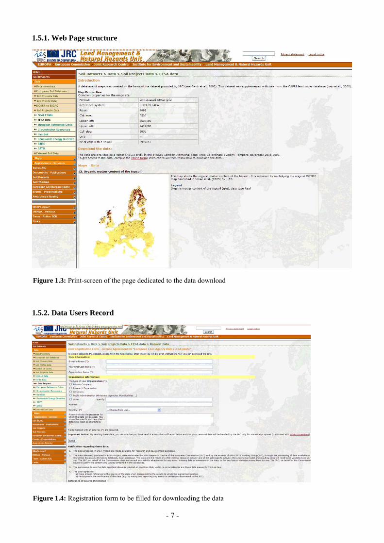
- 7 -
151 Web Page structure
Figure 13 Print-screen of the page dedicated to the data download
152 Data Users Record
Figure 14 Registration form to be filled for downloading the data
- 1 -
2 ECOREGION WG
21 INTRODUCTION AND OBJECTIVES The European Food Safety Authority (EFSA) asked the Panel on Plant Protection Products and their Residues (PPR) to further develop the concept of soil ecoregions in the context of the revision of the Guidance Document on Terrestrial Ecotoxicology (EFSA-Q-2009-00002) A modelling approach for defining soil ecoregions within Europe was developed to improve the realism of exposure scenarios for plant protection products Biogeographic data on four soil organisms groups (earthworms enchytraeids collembolans and isopods) were used to assign each functional group to different life forms representing depth horizons in which they occur Based on information from three Member States covering a North-South gradient Finland Germany and Portugal species presence-absence data were modelled using soil and climate data The objectives of JRC contribution were
- create a geographic database from the tabular data of the biogeographic survey
- extract soil and weather data in correspondence of biogeographic sampling sites
- implement the ecoregion models and create ecoregion maps
The technical details of the activities performed for the achievement of the above reported objectives are described in the following paragraphs and in the EFSA PPR Scientific Opinion on the development of a soil ecoregions concept using distribution data on invertebrates (EFSA 2010b) 22 DESCRIPTION OF THE PROCEDURES ADOPTED
The production of the Ecoregion maps for Finland Germany and Portugal represent the application of the proposed methodology to three test countries according to a North-South gradient
- 2 -
The complete description of the adopted approach is published as EFSA Opinion (EFSA 2010b) In the following paragraphs however is provided a more detailed description of the technical procedures adopted by JRC The conceptual framework for the development of soil Ecoregions is reported in the scheme of Figure 21 and the activities reported in the green boxes have been developed by JRC and described in the following paragraphs
Figure 21 Conceptual frame of the approach adopted for the definition of Soil Ecoregion
221 From an attribute database to a geographic database
The original biogeographical database provided for the three test Member States Finland Germany and Portugal was organized in separate Excel spreadsheets for the different groups of soil organisms and the geographic coordinates were based on UTM1 coordinate system based on Datum WGS842
1 UTM Universal Transver Maercator coordinate system is a grid-based method of specifying locations on the surface of the Earth that is
a practical application of a 2-dimensional Cartesian coordinate system 2 WGS 84 WGS (World Geodetic System) is a standard for use in cartography geodesy and navigation It comprises a standard
coordinate frame for the Earth a standard spheroidal reference surface (the datum or reference ellipsoid) for raw altitude data and a gravitational equipotential surface (the geoid) that defines the nominal sea level The GS 84 represent the latest revision of this standard
- 3 -
In order to project these data in the EU coordinate system (Lambert Azimuthal Equal Area) and to the process in the most efficient way it has been necessary to reorganize the database
One global spreadsheet for each of the three Member States has been produced
From each of these global spreadsheets partial spreadsheets have been derived grouping the records located in the same UTM zone
In order to keep the track of the changes a new field have been added (Fig 22) produced by the concatenation of
- Two capital letters for the organisms group (CO= collembola EW= earthworms IS= isopoda)
- The numeric value of ID Site
- The initial letter of the country name
Figure 22 Structure of the country-based spreadsheet the column with the new field has been outlined
These individual spreadsheets have been exported in DB4 format in order to be easily managed in ArcGIS ArcGIS 93 is the GIS software that has been used for the management and the analysis of the geographic information
The following phase in the management of the data has been the generation of Point Shapefiles representing the locations in which the soil organism inventory has been carried out and the re-projection of these maps
The extraction of soil and climate data from the raster dataset in correspondence of the of the soil organisms survey points has been realized using the ldquoExtract value to pointsrdquo procedure this procedure that is a classical example of spatial query allow to extract the cell values of a raster based on set of points
- 4 -
222Characterization of biogeographic sampling sites in terms of soil climate and land use characteristics
The biogeographic database consists of data on presenceabsence and in some cases abundance of selected groups of soil organisms and in some cases also data on land use vegetation soil and climate were reported The completeness of these environmental parameters essential for the ecological characterization of soil community however was very weak For this reason the data on land use soil and climate provided by JRC has been used to fill the gaps present in the original dataset
This process has been carried out using the utilities of spatial analysis present in a Geographical Information System (GIS) Once the geographic position of a sampling point is known it is possible do a spatial query in the GIS concerning the values of soil pH organic matter total precipitation and any other parameter that is available in a form of geographic database (Fig 23)
Figure 23 Schematic representation of the procedure adopted in a GIS for the extraction of given parameters (ie climate soil) for a given geographic position (ie observations)
- 5 -
223 Implementation of the provisional model in the selected Member States
The computation of the ecoregion maps has been based on the equations obtained in the data analysis implemented using the Map Algebra tools of Arc GIS (Raster Calculator Single Output Map Algebra) In Table 22 and 23 are reported the equations used for the computation of earthworm and enchytraeids maps respectively The first set of equations implying only the use of algebraic operators have been calculated using the lsquoraster calculatorrdquo within the Spatial Analyst toolset while the last expression based on logical operators have applied using the Single Output Map Algebra operator
Table 21 Equations used for earthworms Ecoregion Map
Map Algebra Operation with Raster Calculator t1
-0498 + ([Cropland] 00481) + ([Grassland] 09844) +([Forest3] -02298) + ([ph_top_efsa] 0317) + ([OC_efsa] -00905) + ([tmean] -02494) + ([Tdiff] -00418)
t2
27379 + ([Cropland] -01215) + ([Grassland] 02189) +([Forest3] -11576) + ([ph_top_efsa] 00567) + ([OC_efsa] -00105) +([total_prec] -00018) + ([tmean] 00956) + ([Tdiff] -01229)
z1 Exp([t1]) (1 + Exp([t1]))
z2 Exp([t2]) (1 + Exp([t2]))
ear_arr1 z1
ear_arr2 [z2] (1 - [z1])
ear_arr3 (1 - [z2]) (1 - [z1])
Map Algebra Operation with Single Output Map Algebra Earthworms Ecorgegion Map
con( ear_arr1 gt= 0667 1 ear_arr2 gt= 0667 2 ear_arr3 gt= 0667 3 arr1+arr2 gt= 0833 amp ear_arr1 lt= 0667 amp ear_arr2 lt= 0667 12 arr1+arr3 gt= 0833 amp ear_arr1 lt= 0667 amp ear_arr3 lt= 0667 13 arr2+arr3 gt= 0833 amp ear_arr2 lt= 0667 amp ear_arr3 lt= 0667 23 arr1+arr2 lt= 0833 amp arr2+arr3 lt= 0833 amp arr1+arr3 lt= 0833 123 )
- 6 -
Table 22 Equations used for enchytraeids Ecoregion Map
Map Algebra Operation with Raster Calculator t1
33243 + ([Grassland] 04764) + ([Forest3] 20354) + ([ph_top_efsa] -02776) + ([OC_efsa] -00206) + ([Clay] -00114) + ([total_prec] -00025) + ([tmean] -02286) + ([Tdiff] -00348)
t2
-65979 + ([Grassland] -05418) + ([Forest3] 10585) + ([ph_top_efsa] -02322) + ([OC_efsa] -01102) + ([Clay] -00505) + ([total_prec] -00010) + ([tmean] 03911) + ([Tdiff] 02961)
z1 Exp([t1]) (1 + Exp([t1]))
z2 Exp([t2]) (1 + Exp([t2]))
enc_arr1 z1
enc_arr2 [z2] (1 - [z1])
enc_arr3 (1 - [z2]) (1 - [z1])
Map Algebra Operation with Single Output Map Algebra Enchytraeids Ecorgegion Map
con( enc_arr1 gt= 0667 1 enc_arr2 gt= 0667 2 enc_arr3 gt= 0667 3 arr1+arr2 gt= 0833 amp enc_arr1 lt= 0667 amp enc_arr2 lt= 0667 12 arr1+arr3 gt= 0833 amp enc_arr1 lt= 0667 amp enc_arr3 lt= 0667 13 arr2+arr3 gt= 0833 amp enc_arr2 lt= 0667 amp enc_arr3 lt= 0667 23 arr1+arr2 lt= 0833 amp arr2+arr3 lt= 0833 amp arr1+arr3 lt= 0833 123 )
224 Soil Ecoregions Mapping
The output of the provisional models were a series of maps (one for each organism) where the territories of Finland Germany and Portugal have been classified in seven classes according to the triangles reported in figure 24
Earthworm ecoregion maps have been produced only for the three investigated countries but restricting Finland to its Southern part Enchytraeid ecoregions maps were limited to Germany and Finland since almost no enchytraeid data were available for Portugal For Collembola the fit of the model was very poor and the maps based on the modelled results did not show a convincing ecological meaning based on expert knowledge In case of Isopoda the model presented a good plausibility check with the observed and the modelled values However the analysis gave no clear indication for patterns differing between or within countries therefore isopods were excluded from further analysis and are not shown as maps
- 7 -
Although in principle the interpolation over the entire EU 27 territory would have been technically feasible mapping of territories without observed values were considered not to be reliable for the purpose of this opinion
The concepts of exposure scenario and the definition of soil profile depth relevant for different soil organisms communities led to the production of maps for earthworms and Enchytraeids where the territory of the investigated countries has been classified on the base of the depth relevant for the proposed Risk Assessment
Figure 24 Classification triangles used to classify the earthworms and enchytraeids soil communities
- 8 -
3 CONCLUSIONS AND RECOMMENDATIONS
31 FATE
The occurrence of gaps in daily meteorological data is relatively frequent especially over 20 year time frame For this reason it should be preferred the adoption of a statistical procedures for gap filling instead of selecting alternative nearest meteorological stations
For future applications the availability of 25 km grids will provide an improved geographic resolution for the representation of European climate
32 ECOREGION
During the analysis of the biogeographic database it was found the lack of complete soil land use and climate data sets for the vast majority of the observation sites For this reason it has been necessary to derive such data from the 1 km grid data set (soil and land use) and from the 50 km grids (meteorological data)
It should be outlined that while the use of these EU wide geographic data set is optimal for modelling application probably does not have the necessary spatial resolution for the characterization of point observation sites
- 9 -
4 METADATA FOR EFSA DATASET
A database of maps was created on the basis of the dataset provided by JRC (see Gardi et al 2008) This dataset was supplemented with data from the CAPRI land cover database (Leip et al 2008) JRC is acknowledged for making the data available in a common resolution and projection
Map properties
Common metadata properties for the maps are Format compressed ASCII grid Reference system ETRS 89 LAEA Rows 4098 Columns 3500 Lower left 2500000 Upper left 1412000 Cell size 1000 Unit m Nr of cells with a value 3997812
10
41 Masker of all files (EU27asc)
1 This map is a mask created including all the EU-27 countries and the Corine land-use classes 1-38 and 49 Surface waters and coastal lagoons are excluded from the mask
Legend There is only one legend unit ie 1 which means that the grid cell is included
Figure 41 Masker for the dataset The masker has only one value ie 1
11
42 Countries of the EU-27 (countriesasc)
The map shows the countries of the EU-27 It was obtained by masking the NUTS level 0 map with the mask EU27 Legend Number Country 1 Albania 5 Austria 8 Belgium 9 Bulgaria 15 Czech Republic 16 Germany 17 Denmark 20 Estonia 23 Spain 24 Finland 26 France 31 Greece 34 Hungary 35 Ireland 41 Italy 48 Lithuania 49 Luxemburg 50 Latvia 58 Netherlands 61 Poland 62 Portugal 64 Romania 67 Sweden 68 Slovenia 70 Slovakia 78 United Kingdom
12
Figure 42 Countries of the EU-27
13
43 Regulatory zones (zonesasc)
This map shows the regulatory zones of the EU-27 The map is a reclassification of the map countriesmap Legend Number Name Countries 1 North 17 20 24 48 50 and 67 2 Centre 5 8 16 34 35 49 58 61 64 68 70 and 78 3 South 1 9 23 26 31 41 and 62
Figure 43 The regulatory zones of the EU-27
14
44 Corine land cover data (CLC2000asc)
The map shows all the possible land use classes at the Corine map The map presented here is at a resolution of 1x1 km2 the original map was at a resolution of 025 km2 For each 1x1 km2 grid cell the dominant of the four underlying grid cells was taken The dataset is described in Nunes de Lima (2005) Legend Number CLC
code Description
1 111 Continuous urban fabric 2 112 Discontinuous urban fabric 3 121 Industrial or commercial units 4 122 Road and rail networks and associated land 5 123 Port areas 6 124 Airports 7 131 Mineral extraction sites 8 132 Dump sites 9 133 Construction sites 10 141 Green urban areas 11 142 Sport and leisure facilities 12 211 Non-irrigated arable land 13 212 Permanently irrigated land 14 213 Rice fields 15 221 Vineyards 16 222 Fruit trees and berry plantations 17 223 Olive groves 18 231 Pastures 19 241 Annual crops associated with permanent crops 20 242 Complex cultivation patterns 21 243 Land occupied by agriculture with significant areas of natural
vegetation 22 244 Agro-forestry areas 23 311 Broad-leaved forest 24 312 Coniferous forest 25 313 Mixed forest 26 321 Natural grasslands 27 322 Moors and heathland 28 323 Sclerophyllous vegetation 29 324 Transitional woodland-shrub 30 331 Beaches dunes sands 31 332 Bare rocks 32 333 Sparsely vegetated areas 33 334 Burnt areas 34 335 Glaciers and perpetual snow 35 411 Inland marshes 36 412 Peat bogs 37 421 Salt marshes
15
38 422 Salines 39 423 Intertidal flats 40 511 Water courses 41 512 Water bodies 42 521 Coastal lagoons 43 522 Estuaries 44 523 Sea and ocean 48 999 NODATA 49 990 UNCLASSIFIED LAND SURFACE 50 995 UNCLASSIFIED WATER BODIES
16
45 Generalised land-use map (landuseasc)
The generalised land-use map is a reclassification of the Corine 2000 land-use map It is created to distinguish the most important land-use types Land use class 1 serves as the masker in EFSA (2010)
Legend Number Description Number in map above 1 Annual Crops 12 13 19-21 2 Grass 18 3 Permanent crops 15-17 and 22 4 Rice 14 5 Non agricultural all other classes
Figure 44 The generalised land-use map
17
46 Mean monthly temperature (T1ascT12asc)
The dataset consists of 12 maps containing the monthly mean temperature (deg C) for the period 1960-1990 The dataset is described in Hijmans et al (2005) Legend Mean monthly temperature (deg C) data type Real 47 Mean annual temperature (TMeanasc)
The map shows the mean annual temperature (deg C) for the period 1960-1990 It is calculating by taking the arithmetic mean of maps T1T12asc The dataset is described in Hijmans et al (2005) Legend Mean annual temperature (deg C) data type Real
Figure 45 Mean annual temperature for the period 1960-1990 taken from Worldclim dataset
18
48 Arrhenius weighted mean annual temperature (TEffasc)
The map shows the Arrhenius weighted mean annual temperature (deg C) for the period 1960-1990 It is calculated using the equation (EFSA 2010 Appendix A3)
( )
( ) ( )( ) 0
exp273)(
1ln0
=
⎥⎦
⎤⎢⎣
⎡minus=gt
⎥⎥⎦
⎤
⎢⎢⎣
⎡minus=
int
tTfelsetRT
EtTfthentTif
dttTft
R
ET
act
t
end
acteff
end
(1)
where Teff (K) is the Arrhenius weighted mean annual temperature Eact is the Arrhenius activation energy (kJ mol-1) R (kJ mol-1 K-1) is the gas constant T (K) is the temperature and t is time Eact was set to 654 kJ mol-1 according to EFSA (2007) See further EFSA (2010) Notice that the temperatures in the equation are in K whereas the temperature in the maps is in deg C Legend Arrhenius weighted mean annual temperature (deg C) data type Real
19
Figure 46 Arrhenius weighted mean temperature (deg C) for the period 1960-1990 For a description of the averaging procedure refer to EFSA (2010)
20
49 Mean monthly precipitation (P1ascP12asc)
The dataset consists of 12 maps containing the monthly mean precipitation (mmmonth) for the period 1960-1990 The dataset is described in Hijmans et al (2005) Legend Mean monthly precipitation (mmmo) data type Real 410 Mean annual precipitation (Ptotasc)
The map shows the mean annual precipitation for the period 1960-1990 (mmyear) It is calculated by summing P1P12map The dataset is described in Hijmans et al (2005) Legend Mean annual precipitation (mmyr) data type Real
Figure 47 Mean annual precipitation (mm) for the period 1960-1990 as taken from the Worldclim dataset
21
411 FOCUS Zones (FOCUSasc)
The map shows the FOCUS zones according to the classification in FOCUS (2000) The maps Tmeanmap and Ptotmap were used to create the overlay so the classification is based on WorldClim (Hijmans et al 2005)
Legend Number Name Tmean (deg C) Ptot (mmyr) 1 Jokioinen lt5 deg C gt 0 mmyr 2 Chateaudun 5 ndash 125 deg C lt 600 mmyr 3 Hamburg 5 ndash 125 deg C 600 ndash 800 mmyr 4 Kremsmuumlnster 5 ndash 125 deg C 800 ndash 1000 mmyr 5 Okehampton 5 ndash 125 deg C gt 1000 mmyr 6 Sevilla gt 125 deg C lt 600 mmyr 7 Thiva gt 125 deg C 600 ndash 800 mmyr 8 Piacenza gt 125 deg C 800 ndash 1000 mmyr 9 Porto gt 125 deg C gt 1000 mmyr
22
Figure 48 FOCUS climatic zones based on the mean annual temperature and mean annual precipitation from Worldclim
23
412 Organic matter content of the topsoil (OMasc)
The map shows the organic matter content of the topsoil It is obtained by multiplying the original OCTOP map described in Jones et al (2005) by 172 Legend Organic matter content of the topsoil (gg) data type Real
Figure 49 Organic matter content of the top 30 cm of the soil (gg)
24
413 pH of the topsoil (pHasc)
The map shows the mean pH measured in water (125) of the top 30 cm of the soil See FAO (2008) for details Legend pH measured in water of the topsoil data type Real
Figure 410 pH water (125) of the top 30 cm of the soil
25
414 Bulk density of the topsoil (Rhoasc)
The map shows the bulk density of the topsoil It is calculated from the organic matter content map using the equation (Tiktak et al 2002)
)910(291012361800 2 =minus+= rff omomρ (2)
Legend Dry bulk density of the topsoil (kg m-3) data type Real
Figure 411 Bulk density of the top 30 cm of the soil calculated by the pedotransfer function described in Tiktak et al (2002)
26
415 Texture of the topsoil (Textureasc)
The map shows the textural class of the topsoil It is obtained from the soil geographical database of Eurasia at a scale of 11000000 (for each grid cell the dominant soil textural class was taken) Legend Number Description 1 Coarse (18 lt clay and gt 65 sand) 2 Medium (18 lt clay lt 35 and gt= 15 sand or 18 ltclay and 15 lt sand lt
65) 3 Medium fine (lt 35 clay and lt 15 sand) 4 Fine (35 lt clay lt 60) 5 Very fine (clay gt 60 ) 9 No mineral texture (Peat soils)
Figure 412Topsoil texture obtained from the soil database of Europe 11000000
27
416 Water content at field capacity (ThetaFCasc)
The map shows the water content at field capacity (m3 m-3) It is calculated for each soil textural class with the Mualem-Van Genuchten equation
( ) mnrs
rh
h minus+
minus+=
α
θθθθ1
)( (1)
where θ (m3 m-3) is the volume fraction of water h (cm) is the soil water pressure head θs (m3 m-3) is the volume fraction of water at saturation θr (m3 m-3) is the residual water content in the extremely dry range α (cm-1) and n (-) are empirical parameters and m (-) can be taken equal to
nm 11minus=
The soil water pressure head was set at -100 cm Parameter values were obtained from the HYPRES pedotransfer rule (Woumlsten et al 1999) and are given in EFSA (2010) table 3 Legend Volumetric water content at field capacity (m3 m-3) data type Real The map contains six discrete classes
28
Figure 413 Volume fraction of water at field capacity calculated from the soil textural class using the HYPRES pedotransfer rule
29
417 Capri land cover maps (Cropnamesasc)
These maps show for each pixel of 1x1 km2 the area covered with a certain crop The CAPRI maps were obtained by combining remote sensing data administrative crop data land suitability data and statistical modelling The CORINE land cover map serves as a starting point Subdivisions within CORINE land cover classes were made based on a statistical model regressing point observations of cropping activities on soil relief and climate parameters (land suitability) Statistical data of agricultural production and land cover available for administrative regions were additionally used to scale the land cover classes 18 of the CAPRI land cover classes are classified as annual crops and are included in the EFSA dataset See Leip et al (2008) for a description of the dataset Legend Area (100) covered by a crop data type Real The names of the maps are self explaining The values range from 0 to 10000
30
Figure 414 Crop cover maps ( of area) for barley common wheat texture crops floriculture other fodder crops and industrial crops
31
Figure 415 Crop cover maps ( of area) for maize oats other cereals pulses rapes and root crops
32
Figure 416 Crop cover maps ( of area) for rye soya sugar beet sunflowers vegetables and durum wheat
33
5 REFERENCES
Goot E van der 1998 Spatial interpolation of daily meteorological data for the Crop Growth Monitoring System (CGMS) In M Bindi B Gozzini (eds) Proceedings of seminar on dataspatial distribution in meteorology and climatology 28 September - 3 October 1997 Volterra Italy EUR 18472 EN Office for Official Publications of the EU Luxembourg p 141-153
Gardi C Montanarella L Hiederer R Jones A Micale F 2010 Activities realized within the Service Level Agreement between JRC and EFSA as a support of the FATE Working Group of EFSA PPR in support of the revision of the guidance document Persistence in Soil JRC Technical Svientific and Technical Report 39 pp - EUR 24345
Gardi C2010 Report on the Activities realised within the Service Licence Agreement between JRC and EFSA as a support of the FATE Working Group of EFSA PPR JRC Scientific Report (SLAEFSA-JRC200801)
EFSA 2010a Opinion of the Scientific Panel on Plant Protection products and their Residues on outline proposals for assessment of exposure of organisms to substances in soil EFSA Journal 8(1)1442
EFSA 2010b Opinion of the Scientific Panel on Plant Protection products and their Residues on on the development of a soil ecoregions concept using distribution data on invertebrates EFSA Journal 8(10)1820
EFSA 2007 Opinion on a request from EFSA related to the default Q10 value used to describe the temperature effect on transformation rates of pesticides in soil Scientific Opinion of the Panel on Plant Protection Products and their Residues (PPR-Panel) The EFSA Journal (622)1 32
EFSA 2010 Selection of scenarios for exposure of soil organisms The EFSA Journal (2010) 8(46)1642
FAOIIASAISRICISS-CASJRC 2008 Harmonized World Soil Database (version 10) FAO Rome Italy and IIASA Laxenburg Austria 37pp
FOCUS 2010 Assessing potential movement of active substances and their metabolites to ground water in the EU EC Document reference Sancoxxx2010 Available at FOCUS website httpvisoeijrcitfocus
Hijmans RJ SE Cameron JL Parra PG Jones and A Jarvis 2005 Very high resolution interpolated climate surfaces for global land areas Int J Climatology (25)1965-1978
Jones RJA R Hiederer E Rusco PJ Loveland and L Montanarella 2005 Estimating organic carbon in the soils of Europe for policy support European Journal of Soil Science (56)655-671
Leip A G Marchi R Koeble M Kempen W Britz and C Li 2008 Linking an economic model for European agriculture with a mechanistic model to estimate nitrogen and carbon losses from arable soils in Europe Biogeosciences (5)73-94
Tiktak A DS de Nie AMA van der Linden and R Kruijne 2002 Modelling the leaching and drainage of pesticides in the Netherlands the GeoPEARL model Agronomie (22)373-387
Woumlsten JHM A Nemes A Lilly and C Le Bas 1999 Development and use of a database of hydraulic properties of European soils Geoderma (90)169ndash185
34
APPENDICES ECOREGION MAPS
Earthworm Finland
35
Earthworm Germany
36
Earthworm Portugal
37
Enchytraeids Finland
38
Enchytraeids Germany
39
European Commission EUR 24744 EN ndash Joint Research Centre ndash Institute for Environment and Sustainability Title Report on the activities realized within the Service Level Agreement between JRC and EFSA Author(s) Ciro Gardi Panos Panagos Roland Hiederer Luca Montanarella Fabio Micale Luxembourg Publications Office of the European Union 2011 ndash 38 pp ndash 210 x 297 cm EUR ndash Scientific and Technical Research series ndash ISSN 1018-5593 ISBN 978-92-79-19521-1 doi10278861018 Abstract The activities realized in 2010 by JRC as support to the FATE and the ECOREGION EFSA PPR Working Groups are shortly described For the FATE WG the vast majority of data has been provided in 2009 during the first year of the Service Level Agreement (SLA) and in 2010 the daily weather data for the six selected sites were produced All the data used for the scenario selection procedures with additional data on land use-land cover crop distribution soil and climate parameters will be made available for external user in first half of 2011 For the ECOREGION WG the analysis has been carried out for three Member States covering a North-South gradient from Finland Germany to Portugal Soil and weather data have been used for the characterisation of bio-geographic sampling sites and for the implementation of the ecoregion model Ecoregion maps were produced for earthworms and enchytraeids for Finland and Germany and revealed marked differences between the countries The same approach has been applied also to Collembola and Isopoda but for these two taxa led to a rather poor discrimination both between and within countries
How to obtain EU publications Our priced publications are available from EU Bookshop (httpbookshopeuropaeu) where you can place an order with the sales agent of your choice The Publications Office has a worldwide network of sales agents You can obtain their contact details by sending a fax to (352) 29 29-42758
The mission of the JRC is to provide customer-driven scientific and technical supportfor the conception development implementation and monitoring of EU policies As a service of the European Commission the JRC functions as a reference centre of science and technology for the Union Close to the policy-making process it serves the common interest of the Member States while being independent of special interests whether private or national
LB
-NA
-24744-EN-C
- 141 List of Datasets
- 151 Web Page structure
- 152 Data Users Record
- 22 Description of the Procedures Adopted
- 221 From an attribute database to a geographic database
- 222Characterization of biogeographic sampling sites in terms of soil climate and land use characteristics
- 223 Implementation of the provisional model in the selected Member States
- 224 Soil Ecoregions Mapping
- 3 Conclusions and Recommendations
-
- 31 FATE
- 32 ECOREGION
-
- 4 Metadata for EFSA dataset
-
- Map properties
- 41 Masker of all files (EU27asc)
- 42 Countries of the EU-27 (countriesasc)
- 43 Regulatory zones (zonesasc)
- 44 Corine land cover data (CLC2000asc)
- 45 Generalised land-use map (landuseasc)
- 46 Mean monthly temperature (T1ascT12asc)
- 47 Mean annual temperature (TMeanasc)
- 48 Arrhenius weighted mean annual temperature (TEffasc)
- 49 Mean monthly precipitation (P1ascP12asc)
- 410 Mean annual precipitation (Ptotasc)
- 411 FOCUS Zones (FOCUSasc)
- 412 Organic matter content of the topsoil (OMasc)
- 413 pH of the topsoil (pHasc)
- 414 Bulk density of the topsoil (Rhoasc)
- 415 Texture of the topsoil (Textureasc)
- 416 Water content at field capacity (ThetaFCasc)
- 417 Capri land cover maps (Cropnamesasc)
-
- 5 References
-
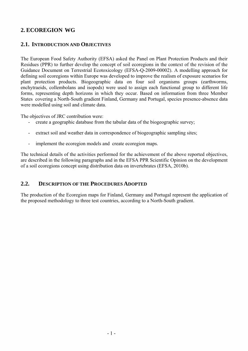
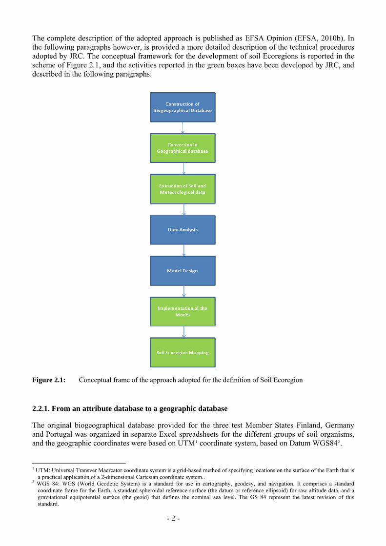
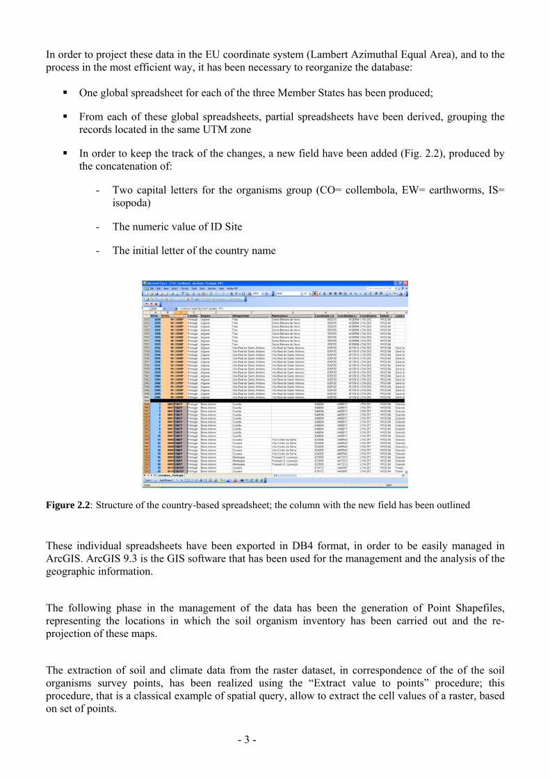
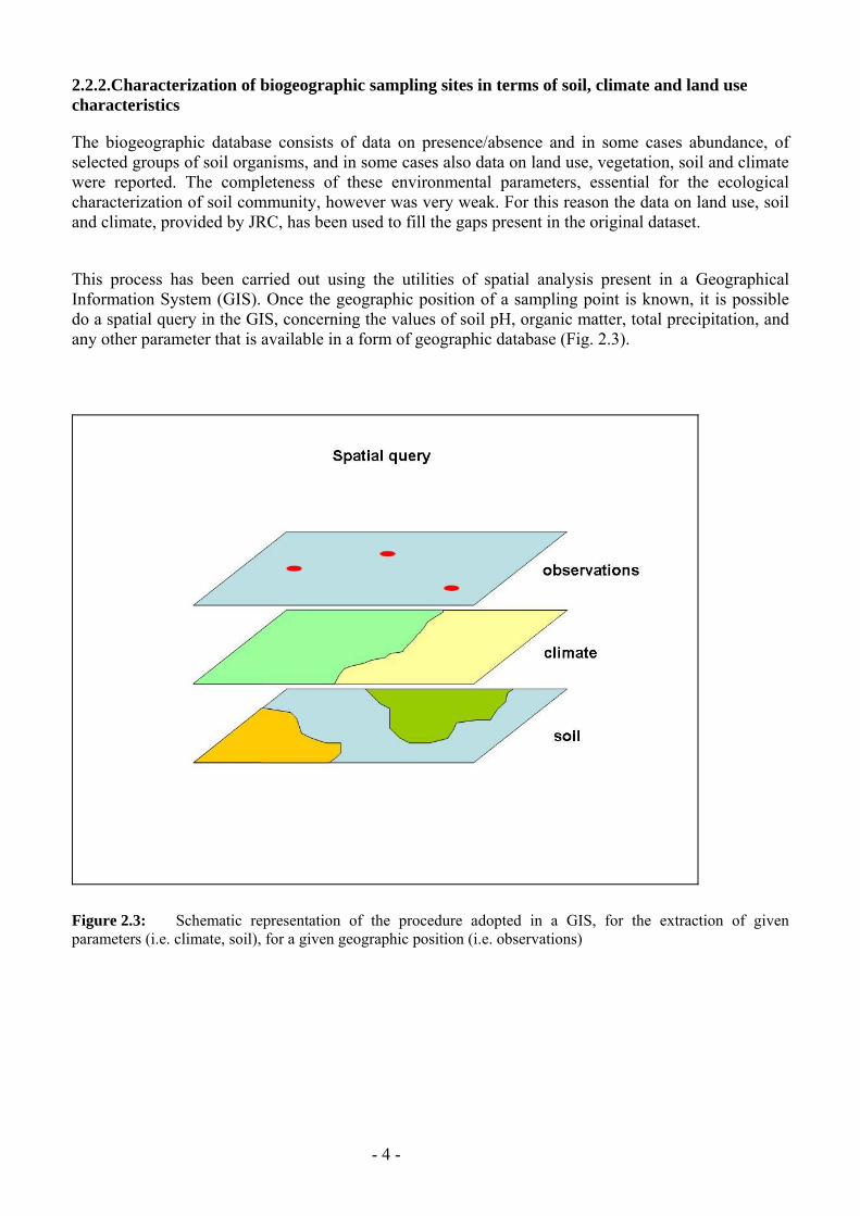
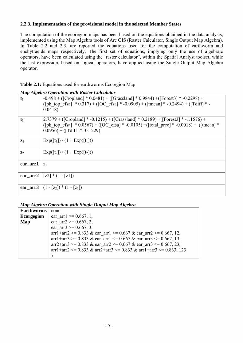
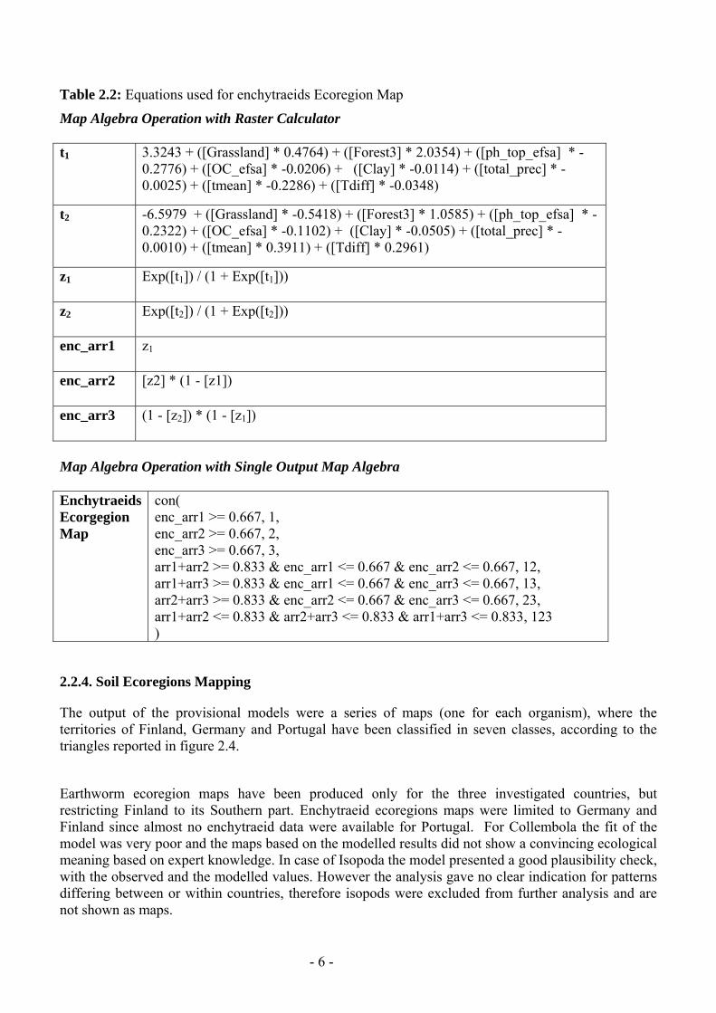
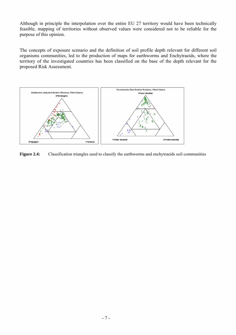
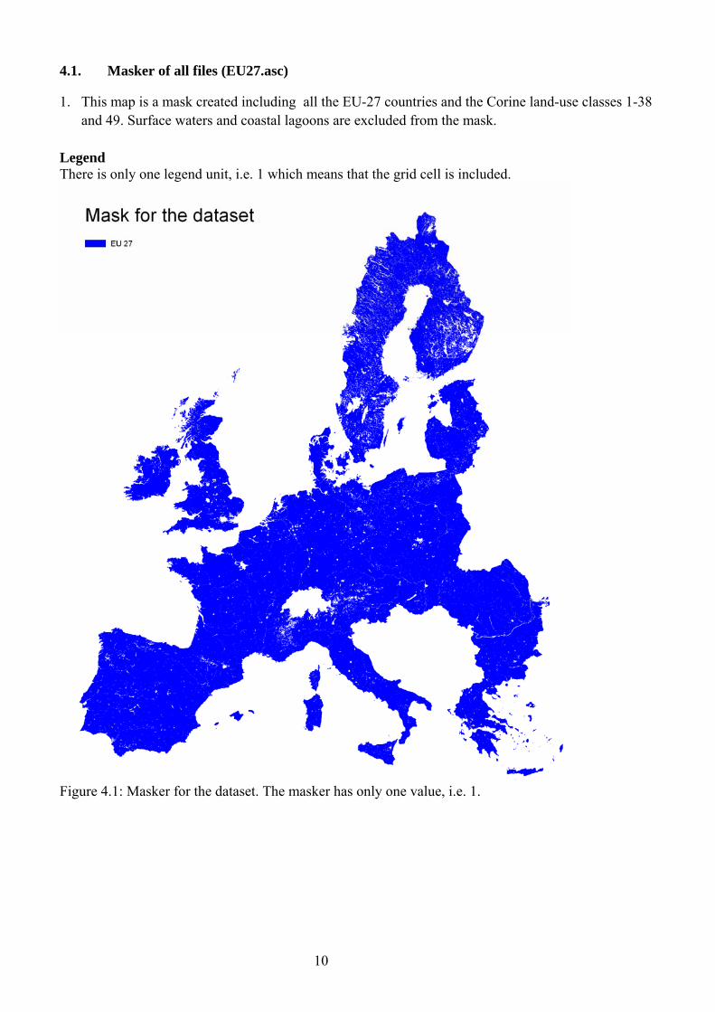
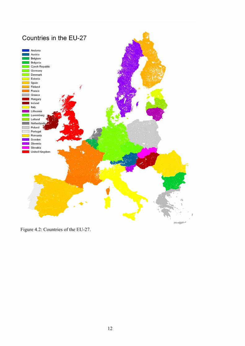
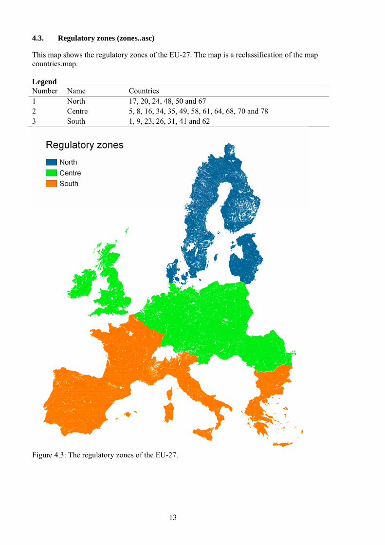
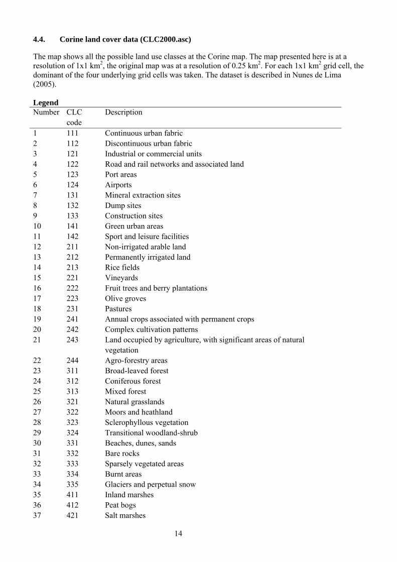
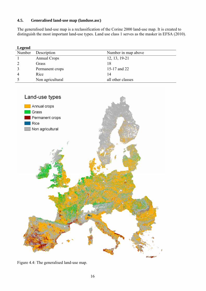
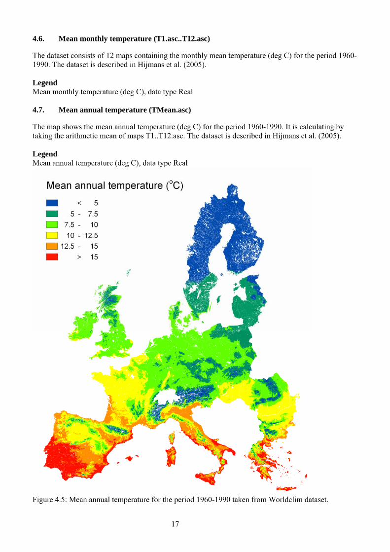
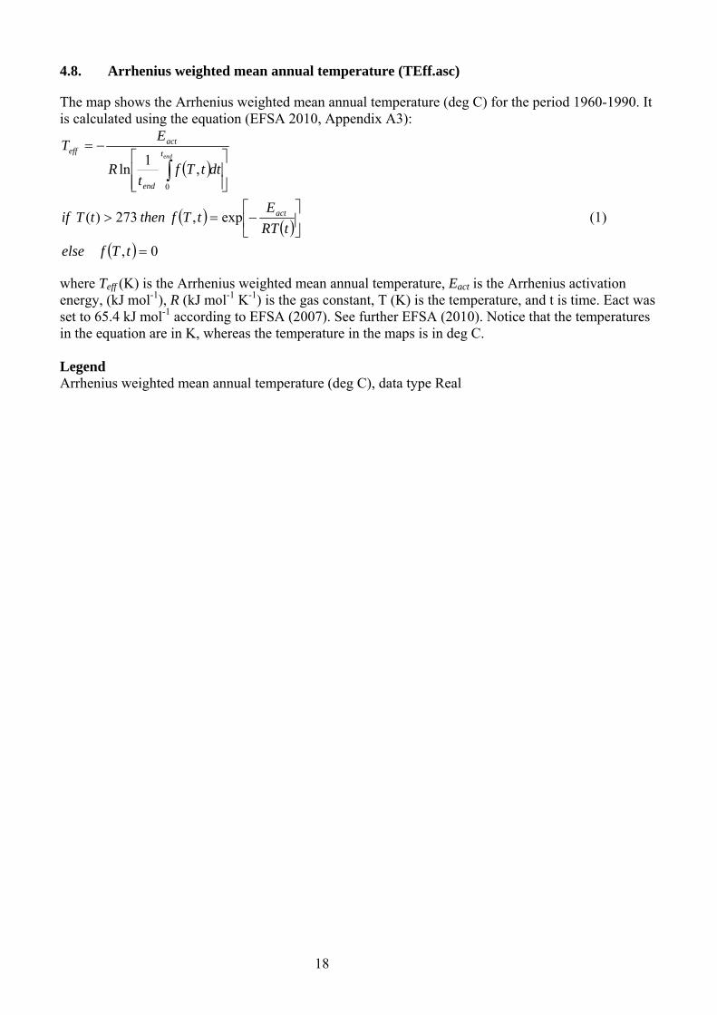
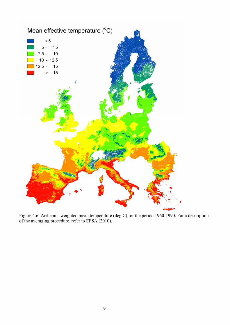
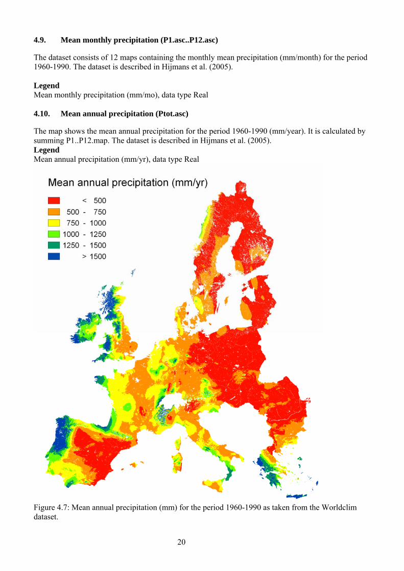
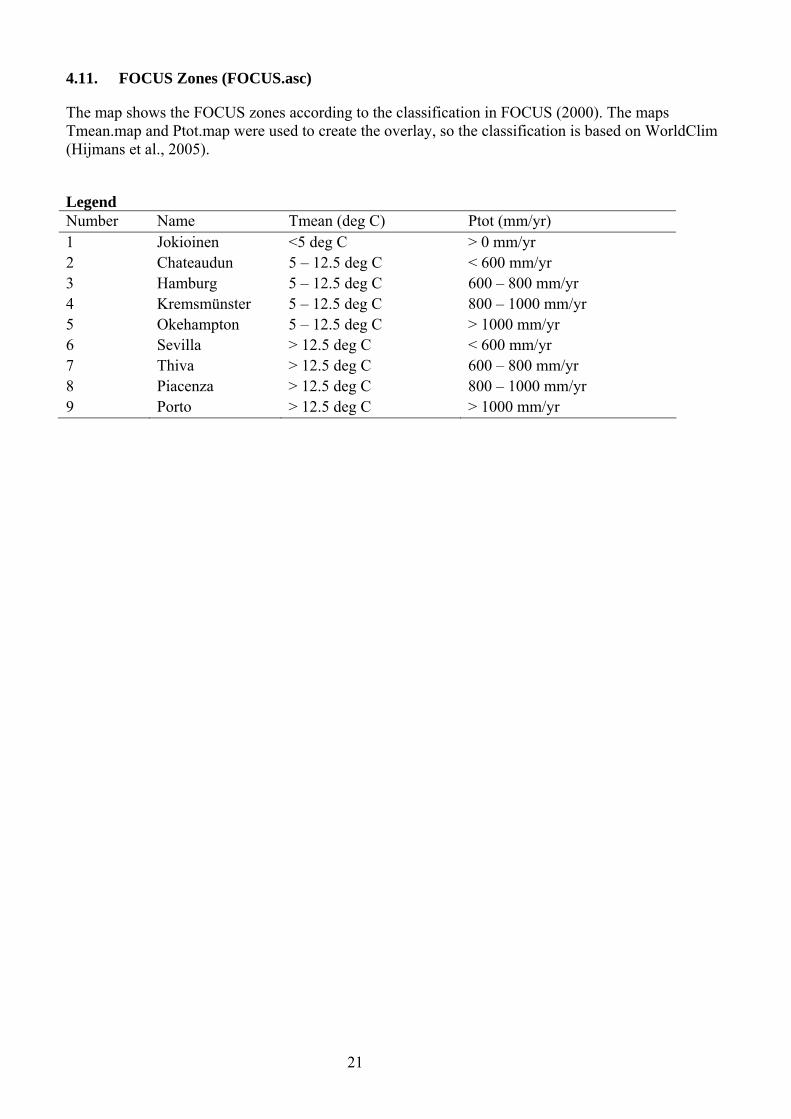
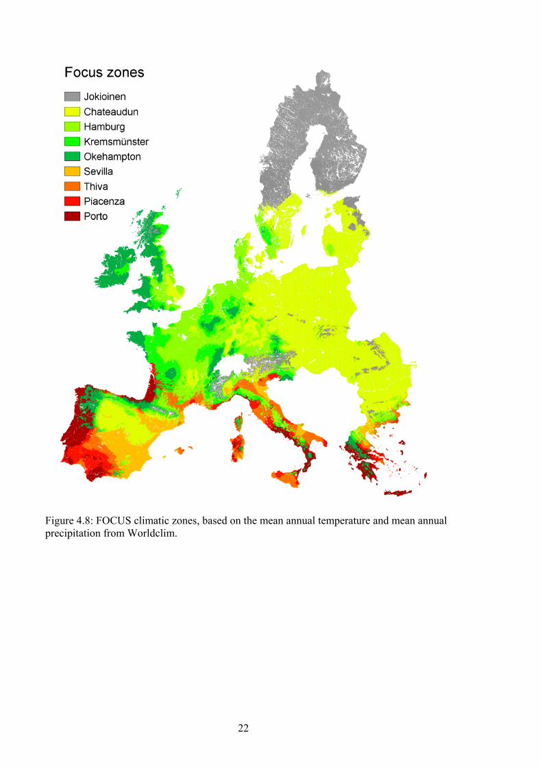
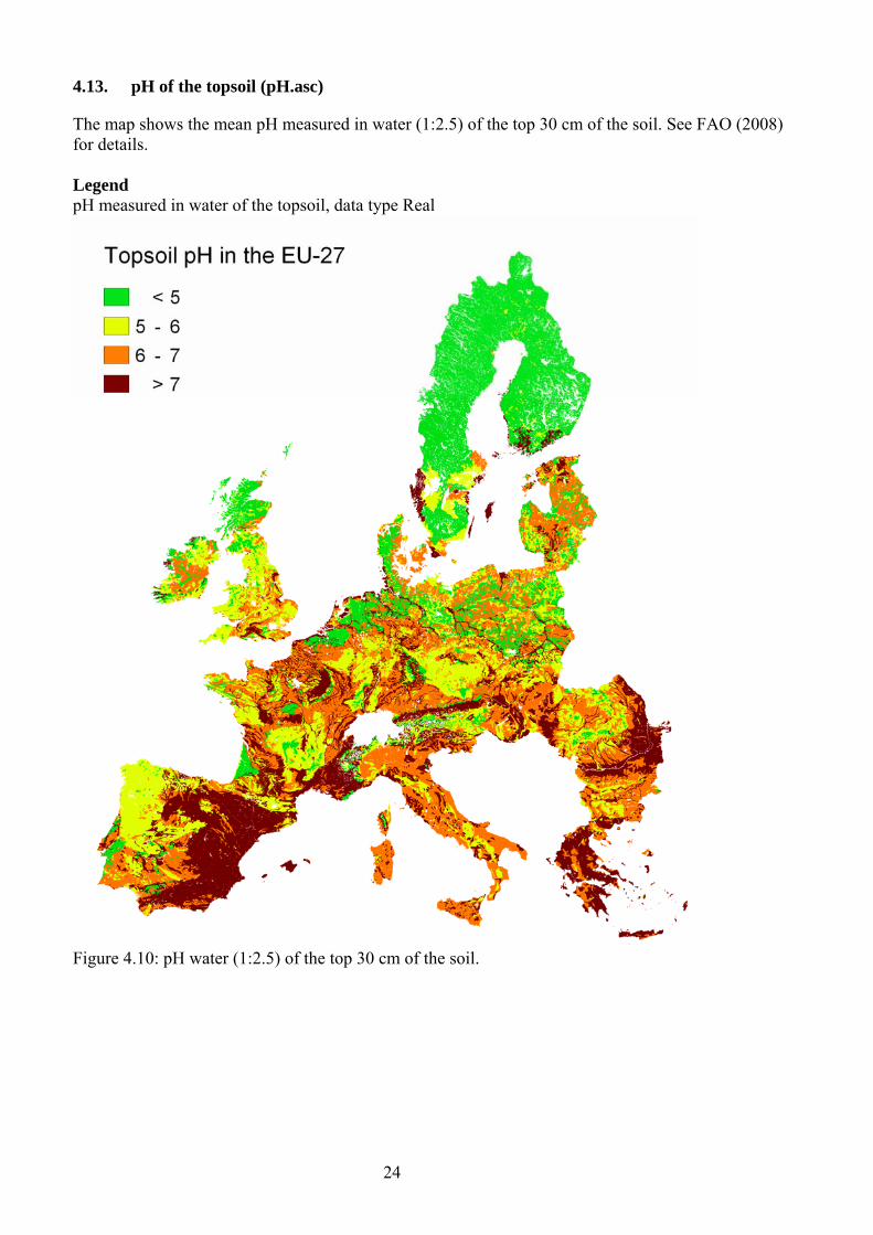
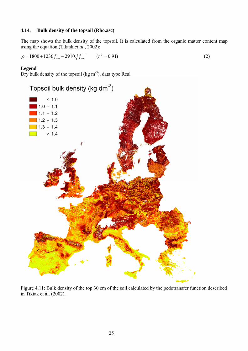
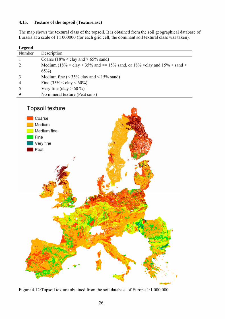
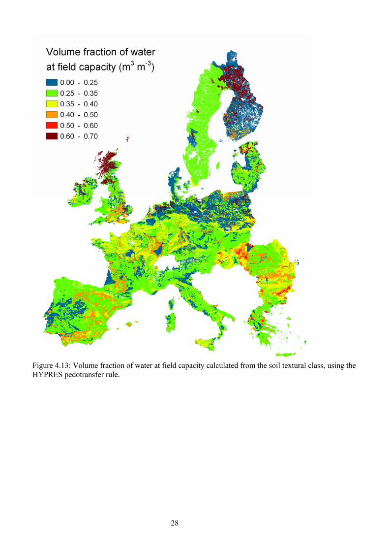
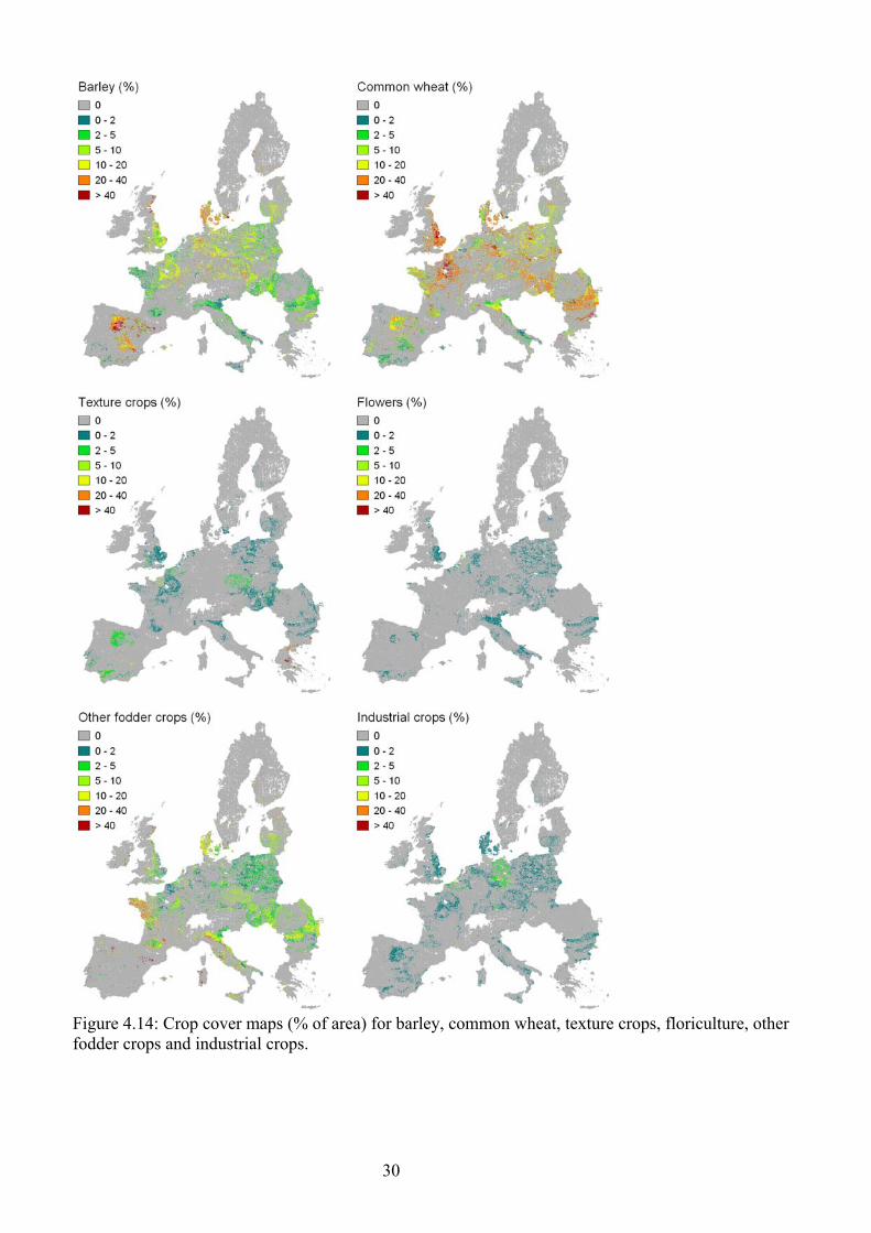
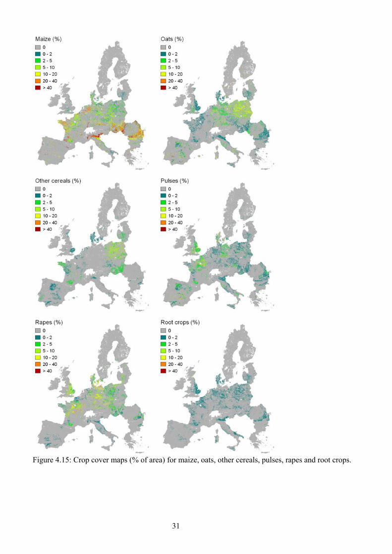
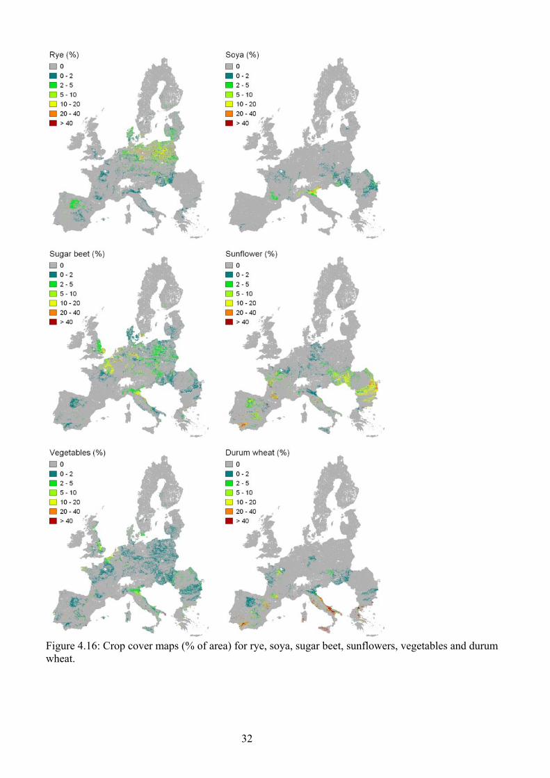
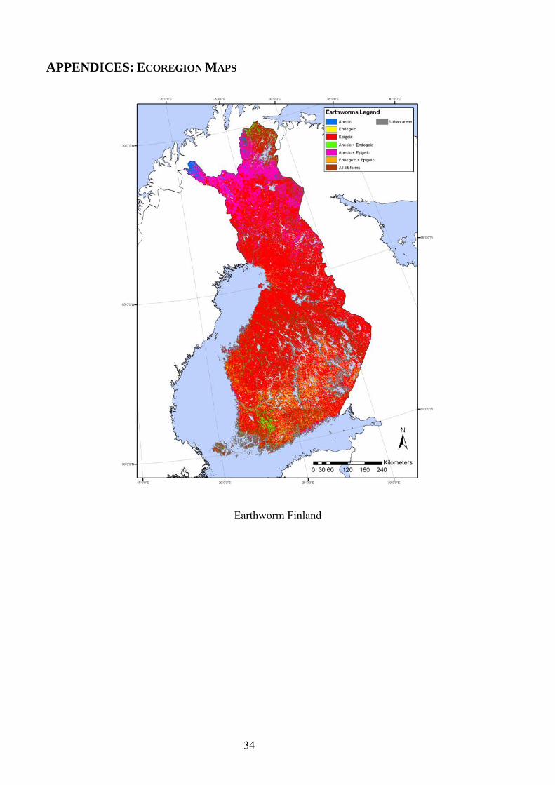
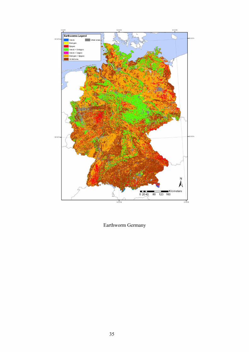
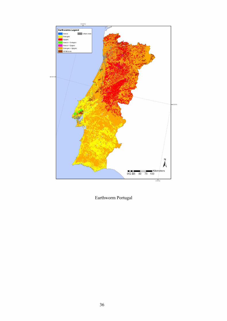
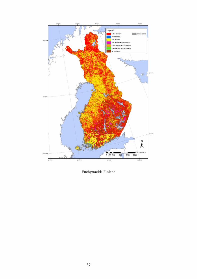
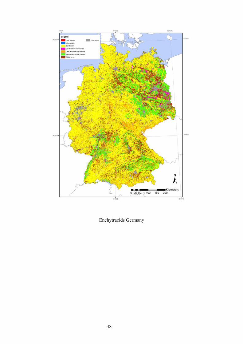
Related Documents