JOURNAL ON EMERGING AND SELECTED TOPICS IN CIRCUITS …

JOURNAL ON EMERGING AND SELECTED TOPICS IN CIRCUITS AND SYSTEMS 1

Benchmarking Open-Source Static 3D MeshCodecs for Immersive Media Interactive Live

StreamingAlexandros Doumanoglou*, Petros Drakoulis*, Nikolaos Zioulis, Dimitrios Zarpalas, and Petros

Daras, Senior Member, IEEE

Abstract—This work provides a systematic understanding of the requirements of live 3D mesh coding, targeting (tele-)immersivemedia streaming applications. We thoroughly benchmark in rate-distortion and runtime performance terms, four static 3D mesh codingsolutions that are openly available. Apart from mesh geometry and connectivity, our analysis includes experiments for compressingvertex normals and attributes, something scarcely found in literature. Additionally, we provide a theoretical model of the tele-immersionpipeline that calculates its expected frame-rate, as well as lower and upper bounds for its end-to-end latency. In order to obtain thesemeasures, the theoretical model takes into account the compression performance of the codecs and some indicative networkconditions. Based on the results we obtained through our codec benchmarking, we used our theoretical model to calculate and provideconcrete measures for these tele-immersion pipeline’s metrics and discuss on the optimal codec choice depending on the networksetup. This offers deep insight into the available solutions and paves the way for future research.

Index Terms—3D Compression, Mesh Coding, Tele-Immersion, 3D Media Streaming, Performance Evaluation, Time Varying Meshes.

F

1 INTRODUCTION & RELATED WORK

W E have reached a milestone where it is now possibleto capture high quality 3D content in real-time. When

remotely transmitted, this new type of three-dimensional(3D) media can facilitate the concepts of tele-presence[1], [2] and tele-immersion (TI) [3], or otherwise more

recently referred to as Holoportation [4]. ContemporaryTI platforms [2], [3], [4] produce 3D media content in theform of Time-Varying Meshes (TVMs), which - in contrast todynamic meshes - are challenging to compress efficiently inan online manner. This stems from their varying vertex andtriangle counts, and therefore connectivity, across frames.

Consequently, TVM compression is accomplished eitherby using specialized TVM codecs that exploit inter-frame re-dundancy or by compressing each frame individually, usingstandard static 3D mesh coding. A noteable example for theformer is [5] which, however, has increased time complexityand cannot operate at high frame rates in order to supportreal-time applications. For the latter, most works focus onencoding time-varying geometry and neglect connectivity.In [6] a first attempt to efficiently encode TVM geometryis discussed. However, this method does not deal withconnectivity coding and also requires storing an increasedamount of side-information in order to properly decode thegeometry of the TVM stream. In [7] the authors improvethe geometry coding, but otherwise handle connectivity inan equally inefficient way.

* Indicates equal contribution.

• A. Doumanoglou, P. Drakoulis, N. Zioulis, D. Zarpalas and P. Daras arewith the Visual Computing Lab (VCL) of the Information TechnologiesInstitute (ITI), Centre for Research and Technology Hellas (CERTH),Thessaloniki, Greece.E-mail: {aldoum, petros.drakoulis, nzioulis, zarpalas, daras}@iti.gr.Website: vcl.iti.gr.

The ongoing MPEG-I [8] standardization work alsofocuses on point cloud coding [9], which deals with time-varying geometry omitting the connectivity information.Two notable recent works focusing on point cloud compres-sion are [10] and [11] which deal with motion estimationusing octree subdivided macro-blocks and spectral graphtransforms respectively, albeit operating at rates prohibitivefor remote interaction scenarios. Moreover, point cloud rep-resentations require specialized rendering and very densesampling in order to reach the levels of fidelity that texturedmeshes provide.

All these characteristics, namely the lack of proper con-nectivity handling and the incapability of current TVMinter-frame codecs to operate at real-time speeds, alongwith the relatively immature state of current point cloudsolutions, make the use of static mesh codecs for real-timeTI streaming a quite appealing choice.

In this work, we focus on benchmarking the perfor-mance of existing, open-source, static 3D mesh compressionmethods, in the context of 3D immersive media interactivelive streaming1. More specifically, we consider the followingcodecs: Google Draco [12], Corto [13], MPEG’s Open 3DGraphics Compression (O3dgc) [14] and OpenCTM [15].Among those open-source implementations, Draco is basedon [16], Corto is based on [17], O3dgc is based on [18], whileOpenCTM is the only library which is not based on anyacademic publication.

While summarizing surveys on 3D mesh compressionpresent in the literature [19], [20], [21], currently, there isa gap on the evaluation of contemporary 3D mesh codecs

1. We consider live streaming in the context of interactive (tele-)immersion media applications and not live broadcasting scenarios. Thelatter has relaxed latency requirements, but the former imposes morestrict latency restrictions to enable multi-user interactions.


in a consistent experimental setup that takes into accountnot only geometric rate-distortion (RD) performance of thecodecs but also their RD performance when compressingnormals and attributes, as well as their time complexity,which is crucial for live streaming. This paper aims to beone of the first works towards filling this scarcity with itsmain contributions being:

• A thorough and extensive benchmarking, based onmore than 50000 experiments of the most popularavailable open source static 3D mesh codecs in aconsistent experimental setup, taking into accounttheir RD performance not only for vertex geometrybut also for normals and attributes.

• A run-time performance benchmarking of thesecodecs which uncovers their time complexity.

• A live TI streaming case study which estimates theirimpact on the end-to-end performance of the TIpipeline, in terms of frame-rate and latency.

2 EVALUATED 3D MESH CODECS OVERVIEW

In this section, a brief overview of the underlying encodingalgorithms that are utilized by the studied open-source 3Dmesh codecs is presented. All codecs use a similar geometryquantization scheme that is based on quantizing the meshcoordinates to a predefined grid, sized according to themeshes’ bounding box. For Draco, Corto and O3dgc we givedetails on their connectivity compression algorithm whilefor OpenCTM, apart from the connectivity compression al-gorithm we give further details on its geometry compressionscheme which slightly deviates from the rest of the codecs.

2.1 Corto

Corto is a simple, yet fast, mesh compression algorithm. Theencoding process visits one triangle at a time and maintainsa list of the edges of the processed region’s boundary. Theprocessed region is always homeomorphic to a disk andis always growing, as new neighboring triangles to theregion are being visited. The three edges of the first triangleare first added to the list. Then, iteratively one edge isbeing extracted from the list and the algorithm encodes therelation of the not-yet-visited triangle incident to the edgewith respect to the boundary of the already encoded region.Four cases are distinguished:

• SKIP: This is the case when the extracted edge isa boundary edge (i.e. it has no other non-processedtriangles adjacent) or the adjacent triangle is alreadyprocessed.

• LEFT or RIGHT: These cases denote the conditionwhen the adjacent to the extracted edge triangle,shares two edges with the processed region’s bound-ary.

• VERTEX: This case indicates that the adjacent to theextracted edge triangle, shares exactly one edge withthe processed region’s boundary.

Fig. 1 depicts all the previously mentioned cases.

2.2 Draco

Draco uses Edgebreaker [16] as its underlying mesh com-pression algorithm. Edgebreaker traverses the 3D mesh ina series of steps. At each step the algorithm visits andencodes one not-yet-visited triangle of the mesh. At eachstage the input mesh is divided into disjointed regions thatmay share a vertex but no edges. The edges bounding eachregion constitute a polygonal curve which is called a “loop”.The edges of the loop are called “gates” with one gatebeing active at each step. At every step, there is a triangleincident to the active gate that is not yet visited. Let v denotethe vertex of this triangle that is not incident to the gate.Edgebreaker encodes the relation of v with respect to thegate’s loop boundary and the gate itself. Edgebreaker standsout 5 cases labeled: C, L, E, R, S. When v does not belongto the active gate’s loop, this case is marked as C. Whenv belongs to the active gate’s loop and is also incident tothe active gate, then this condition is marked as R, L or E,depending on the side of the active gate where v is incidentto (R or L). When v is incident to both sides of the active gatethe condition is marked as E. Finally, the condition where vbelongs to the loop but is not incident to the active gate, ismarked as S. In Fig. 2 an example of all Edgebreaker casesis depicted.

2.3 O3dgc

O3dgc uses TFAN [18] as its mesh compression algorithm.TFAN is based on traversing the mesh vertices from neigh-bor to neighbor. At each step of the process, one vertexis marked as the focus vertex. TFAN traverses the inputmesh by visiting triangles incident to the focus vertex inthe order they appear in the Triangle Fan (TF) represen-tation. In the TF representation, an ordered set of vertices{v0, v1, v2, ..., vd+1} form a set of d triangles {tj} such that∀j ∈ {0, 1, ..., d−1}, tj = {v0, vj+1, vj+2}. In that case, v0 isconsidered to be the center of the TF. At each step of TFAN,a new focus vertex is extracted from a queue and the setof its incident triangles is partitioned in TFs. Let O(vj) = jdenote the traversal order of the j-th vertex extracted fromthe queue, i.e. O(vj) denotes the order in which vj wasextracted from the queue. Let also L(j) denote the orderedset of vertices sharing with vj at least one visited triangle.The vertices in the set L(j) are ordered by their traversalorder. All the vertices of the TF of the focus vertex aretraversed is the order they define the TF. Let “active” vertexdenote the currently traversed vertex of the TF. If the activevertex of the TF has been previously visited, a binary valueof 0 is emitted to the S binary vector, while 1 is emittedin the opposite case. When the active vertex is visited forthe first time, it is marked as visited and is inserted to thequeue in order to later process it as a focus vertex. Further,the active vertex is inserted to the set L(j). In the casewhere the active vertex was already visited, two differentconditions are considered. In the first case, the active vertexis already included to the set L(j). In that case, the relativeindex of the vertex inside L(j) is stored into an additionalinteger vector I . On the other hand, if the active vertex doesnot belong to L(j), the traversal order difference betweenthe active vertex of the TF and the focus vertex, whichconsists a negative value to aid decoding, is stored in I .


Fig. 1. Enumerating Corto various cases. From left to right: (S)kip, (S)kip, (L)eft, (R)ight, (V)ertex. Already processed triangles in black. Not-yet-processed triangles in blue. Currently encoded triangle in gray. Current active edge in red. Boundary edges in yellow and removed boundary edgesin magenta. Newly added edges in green.

Fig. 2. Edgebreaker triangle traversal example. The active gate wheretraversal begins is in green. The grown boundary as the triangle travers-ing evolves in time in black.

Fig. 3. Example of TFAN coding. Already processed triangles in black.Not-yet-processed triangles in blue. Currently encoded TF in gray. Focusvertex in green. Vertices visited for the first time are in yellow. Verticesalready visited in red. Vertices are labeled according to their traversalorder as focus vertices. Left: Encoding vectors: S = {1, 1, 1, 1, 1}, I ={}. Right: S = {0, 1, 1, 1, 0}, I = {2, 1}.

This procedure continues until all mesh vertices have beenprocessed as focus vertices. TFAN, further improves uponcompression ratio by exploiting common configurations ofthe S and I vectors and encoding them as a single integerin the C vector and only further encoding parts of S and Ias appropriate.

2.4 OpenCTM

OpenCTM has three different algorithm variants namely:Raw, MG1 and MG2. In this study, we consider only theMG2 variant since it is the one performing always the bestin rate-distortion terms. MG2 is a simple algorithm that isbased on sorting and delta coding for both geometry andconnectivity. Initially, a grid that fits the bounding box of themesh is constructed and the mesh vertices are sorted basedon their index inside the grid and subsequently (upon equal-ity) based on their x coordinate. The difference between eachvertex and its grid cell’s origin is computed and quantizedbased on the requested precision. Then, the sorted vertices’grid indices are delta coded and appended to the outputbitstream along with the quantized delta coordinates. For

connectivity, the standard 3 integer representation is con-sidered, with each integer referencing one vertex of eachtriangle. Firstly, the vertex references inside each triangleare rearranged so that the first index is the smallest one.Then, the triangles are sorted based on their first and secondindices, with the second indices being used when the firstindices are equal. Finally, a delta coding scheme on the finaltriangle list is applied so that the first index of each triangleis delta coded with respect to the previous triangle in thelist, while the other two indices of the triangle are encodedas a difference with respect to the first index of the sametriangle.

3 TELE-IMMERSIVE STREAMING

Tele-immersion is based on the next-generation video,which is 3D video of live performances and is groundedon two pillars: i) real-time 3D reconstruction of dynamicscenes and ii) real-time compression and transmission ofthe generated 3D media. There are two main directions thatcan be pursued for the production of 3D media. The firstone reconstructs the user out of acquired sensor data in aper frame basis and is also the direction that preliminaryattempts in capturing humans in full 3D initially pursued[1], [2], [22]. Recently, another direction emerged as non-rigid registration in real-time became possible. These recentnon-rigid production systems [4] fuse all information into acanonical model representation by deforming the input ona per frame basis, achieving higher fidelity results as a con-sequence of the implicit denoising that integrating temporalinformation into the canonical model offers. Despite theirdifferences however, both types of 3D production methodsextract an isosurface from an implicit representation andtransform it into a triangulated surface, using the marchingcubes algorithm [23]. This results in a TVM M : {V,T},where V and T are the set of vertices and triangle indicesrespectively.

This geometric representation facilitates an elevatedsense of presence as it can naturally position a user’s 3Drepresentation into a shared space, be it either virtual or real,in appropriate scale and in a coherent manner with respectto the surroundings. However, fully transferring a user’sidentity in 3D requires photorealism which is achieved byalso capturing and transmitting her/his realistic appearancein the form of color information. The aforementioned 3Dcapture and production systems [3], [4] accomplish this byadditionally transmitting the color camera feeds in real-time, which are then used as supplementary textures to thegeometry. In order to render the final representation in a


photorealistic and high quality manner, these textures needto be blended appropriately during rendering. This meansthat additional information that will drive the blendingof the textures needs to be transmitted. Such metadatatypically involve blending weights b and/or texture iden-tifiers i. From a 3D codec point of view, they are mainlydistinguished by their data type, be it either floating orfixed point data. Furthermore, realistic embedding of thetransmitted 3D representation also requires lightening therenderings appropriately, so as to appear blended into theenvironment. This requirement is met with the transmissionof extra surface information in the form of the surface’snormals n.

We can thus conclude that streaming TI payloads consistof texture and geometry M : {V,T,N,A} encoded infor-mation, where N and A : {B, I} are the set of normals andattributes accompanying the TVM, with the attributes com-prising of the necessary metadata (blending weights andtexture indices respectively) to render the TVM. As a result,3D codecs used for encoding TI TVMs need to also encode avariety of custom attributes in addition to the vertex V andconnectivity T information. Therefore, when comparingdifferent codecs and analyzing their performance, we needto follow a holistic approach and benchmark heterogeneouspayload coding efficiency, as well as computational perfor-mance, given that the targeted application requires minimallatency to facilitate multi-party interactions.

4 CODEC EVALUATION

In this section, we discuss on the benchmarking of the stud-ied 3D mesh codecs with respect to all different evaluationaspects. First, in subsection 4.1, we begin by commentingon the generation of the TI dataset which all codecs areevaluated on.

Most of the available codecs are able to be configured inways that allow faster encoding / decoding times at the costof achieving lower compression rates for the same distortionlevel. An exhaustive benchmarking of all available configu-rations of each codec is not practical. Thus, for each codec,we have chosen some preset values for those configurationsthat span the available parameter ranges. We call thosepreset configurations codec “profiles”. The specifications ofthose profiles that we have chosen to benchmark are givenin detail in subsection 4.2.

Subsequently, in subsection 4.3, we report RD perfor-mance of the codecs for three different cases: a) encodingconnectivity along with vertex positions (also referred toas “geometry”), b) encoding connectivity along with vertexpositions and normals and c) encoding connectivity alongwith vertex positions and attributes. In their respectivesubsections, we also comment on the methodology andthe employed error metrics. Not all profiles affect the rate-distortion performance in all of the previously mentionedcases (i.e. there are profiles that only affect the compres-sion of normals and not positions, or the compression ofattributes and not normals or positions, etc.). Thus, onlyrelevant profiles are being benchmarked for each case, whilefor illustration purposes, equivalent profiles are groupedtogether.

Finally, in subsection 4.4, we report the relative per-formance for all codec profiles while also adding anotherdimension into the analysis, runtime performance. To thatend, we benchmark the time taken to compress and de-compress the TI meshes. This is accomplished by settingtarget distortion values for all attributes specific to the TIstreaming scenario, which are used to drive the relativeperformance analysis. This analysis is conducted for thethree aforementioned cases, as well as for the complete(i.e. full) case that includes vertex positions, normals andattributes all together.

4.1 DatasetIt is apparent, that the RD performance of any codec doesnot solely depend on the chosen profile, but also on thestructure of the provided input mesh. The most relevant 3Dmesh codec evaluations that are presented in the literature,evaluate the codecs’ performance on 3D meshes generatedby 3D artists, or meshes that are generated by a surfacereconstruction algorithm applied on high precision rangescanned data. The meshes generated by either of thosemethods are clean and free of noise, as opposed to 3Dmeshes that are generated by 3D reconstruction methodsthat are applied on data acquired by depth sensors operat-ing at high frame-rates.

In this work, we focus our analysis on a practical applica-tion of mesh compression, live TI streaming. Consequently,we use a set of meshes generated by an actual TI pipeline,and more specifically by the 3D reconstruction method of[22]. Our TI dataset comprises 10 randomly selected distinctframes (i.e. 3D models) depicting 5 different subjects withvariability in poses, as the subjects were captured whileexecuting different performances (i.e. punching, kicking,conversing, expressing emotions, etc.). We use 10 differ-ent models with their average vertex count being 16868,spanning the range of [10242 − 21064] vertices, and theiraverage triangle count being 30713, spanning the range of[18792− 36520] triangles.

4.2 Codec ProfilesIn this subsection, we give a brief overview of the availableconfiguration options that are made accessible via the pro-grammable interface of each 3D mesh codec participatingin this benchmark. For each one of them, the values ofthe corresponding configuration implicitly affects its rate-distortion performance and execution time. As previouslyintroduced in the beginning of Section 4, we select and namespecific “profiles” that comprise sets of specific configura-tion options for each codec. In the following subsectionsthese profiles and their options are presented.

4.2.1 CortoCorto encodes geometry and vertex normals at a qualityspecified in the form of quantization bits while custom float-ing point vertex attributes are quantized using an explicitquantization step. Custom integer vertex attributes are notdirectly supported. To overcome this limitation, we treatthese attributes as floating points quantized with a quantiza-tion step of 1.0 unit. Corto is benchmarked in two variationsthat differ only in the normals prediction scheme. In Corto’s


default profile, which we call “Corto1”, the normals are esti-mated from the quantized geometry and their differenceswith the quantized actual normals is encoded using theoctahedron projection representation [24]. In Corto’s secondprofile (“Corto2”) the quantized normals in the octahedronprojection representation are delta coded with respect to aneighboring quantized normal belonging to a quad incidentto the normal’s vertex. In both profiles, the encoding of thenormals are driven by the Corto’s connectivity traversal ofthe mesh.

4.2.2 DracoDraco encodes all kinds of floating point vertex attributes(positions, normals and custom attributes) at a detail levelspecified by a given number of quantization bits. Custominteger attributes are supported as well. In our case, the per-vertex texture identifiers are losslessly encoded as integers,while the texture blending weights’ precision is controlledby a specified number of quantization bits. The Draco inter-face allows adjusting the processing time versus compres-sion ratio mixture via a “speed” setting expressed on aninteger scale from 10 (denoting the combination of optionsthat minimize processing time) to 0 (denoting the ones thatlead to the most possibly compressed representation). Wechose to benchmark three configurations, namely “Draco2”,“Draco5” and “Draco9”, with the speed setting set to 2, 5(the default) and 9 (the fastest setting possible that utilizesthe underlying EdgeBreaker [16] algorithm) respectively.

4.2.3 O3dgcApart from standard support for controlling geometric lossvia an externally provided number of quantization bits,and in a way similar to Draco, O3dgc also supports vertexnormals as well as custom integer and floating point vertexattributes. Using a combination of available options, weopted for the benchmark of three encoding configurationsthat differ in the geometry and custom attributes’ pre-diction strategy. The “default” profile (O3d) makes use ofparallelogram prediction [25] for the geometry, differentialprediction for the custom floating point attributes and noprediction for the integer ones. The “fast” profile (O3f ) usesdifferential prediction for the geometry and no predictionfor both integer and floating point custom attributes. Finally,the “small” profile (O3s) uses differential prediction for all,geometry, integer and floating point vertex attributes. In allof the aforementioned selected profiles, the (unit) normalsare first converted into a representation that exploits unitsphere inscription in a cube. Apart from parallelogramprediction which only applies to geometry, in the differentialprediction mode each vertex position, normal or attribute isdelta coded with respect to the value of the correspondingposition, normal or attribute belonging to a neighboringvertex based on the connectivity of the mesh.

4.2.4 OpenCTMInstead of specifying the number of quantization bits,OpenCTM only allows controlling the geometric, nor-mal and attribute loss via an explicit quantization step.OpenCTM does not support integer attributes and thus, aswith Corto, we encode the per-vertex texture identifiers in a

floating point representation using a quantization step of 1.0unit. Apart from the standard OpenCTM implementationwhich uses LZMA (a variant of [26]) for entropy compres-sion, we have implemented a custom version which replacesthe LZMA entropy compression module with LZ4 [27] (afaster but less efficient variant of [26]). Therefore, we havechosen to use two OpenCTM profiles, called “CTM-LZMA”and ”CTM-LZ4”, which both use the OpenCTM’s internalMG2 algorithm but differ in the lossless entropy compres-sion algorithm. Both entropy compression algorithms werechosen to be operated at the fastest possible speed setting,favoring fast execution times over high compression ratio.

4.3 Rate-Distortion Performance EvaluationIn this subsection we report RD curves for the cases (a),(b) and (c) that were introduced in the beginning of thissection. For each case we report average performance inbit-rate and the corresponding distortion metric across allthe models of the respective dataset. This is accomplishedvia averaging the bit-rate and the distortion metric forconstant quantization step or number of quantization bitsacross the different models of the dataset. This analysisleads to extracting average codec performance in real-worldcaptured data for each fixed value of the parameters thatcontrol distortion.

4.3.1 Case A: Connectivity & Vertex PositionsFirst, we evaluate the codecs’ average RD performancewhen compressing geometry and connectivity only. Thegeometric distortion metric that we use is the standardHausdorff distance between the compressed and the un-compressed meshes which is reported by the METRO [28]tool with respect to (wrt) the mesh’s bounding box diagonal.For the evaluation of the distortion metric, the METROtool was used with its default parameterization to samplevertices, edges and faces by taking a number of samplesthat is approximately 10 times the number of triangles inthe model.

Benchmark resultsThe benchmark results of this experiment for all profilesof the mesh codecs are depicted in Fig. 4, top. It can beeasily observed that in geometry RD terms, both OpenCTMprofiles perform significantly worse than the other codecs,hampering graph’s readability. Thus, a detailed view thathelps to better illustrate the performance differences of theother codecs, in their various profiles, is also offered as aninset.

The best codec in terms of RD is the slowest profileof Draco. The second best profile in the same terms isDraco5, which has very similar performance to O3d. Thirdin order, O3f/s profiles perform similar to Draco9. ExcludingOpenCTM, Corto has the least efficient algorithm in termsof RD, producing about one half the compression ratesproduced by the best profile of Draco, for high to middistortion levels.

Finally, another important element depicted in Fig. 4is that, for all codecs, when compressing geometry alone,the geometric distortion of the compressed mesh is solelydetermined by the value of the quantization parameter and


does not depend in any way on the codec profile settings.On the other hand, bit-rate depends on the combination ofthe quantization parameter’s value and the codec profilesetting.

4.3.2 Case B: Connectivity, Vertex Positions & Vertex Nor-malsSecondly, we conduct an experiment to evaluate the RDperformance of the various codec profiles for the case ofcompressing mesh geometry and connectivity jointly withvertex normals. The nature of this experiment is two-dimensional, as the final bit-rate is affected by two quan-tization parameters: one for the vertex geometry and onefor the vertex normals. Each quantization parameter con-trols the distortion level in its domain respectively. For anevenhanded approach to benchmarking the various codecprofiles, we first pick a fixed level of geometric (Hausdorff)distance and for each codec profile we try to tune thequantization parameter for vertex positions to a propervalue that leads to this level of geometric distortion. Subse-quently, we variate the normal quantization parameter foreach codec profile and draw RD curves that illustrate thenormal distortion for a given bit-rate. We repeat the above-mentioned process for two different levels of geometricdistortion, resulting into 2 different normal RD curves. Sinceeach codec has its own way to perform quantization, exactgeometric distortion equivalence across codecs cannot beachieved. However, our strategy to tune the vertex positionquantization values for each codec individually, ensures thatwhen evaluating the normal distortion versus bit-rate, thedistortion level of vertex positions across codecs is as closeas possible to the preset target level.

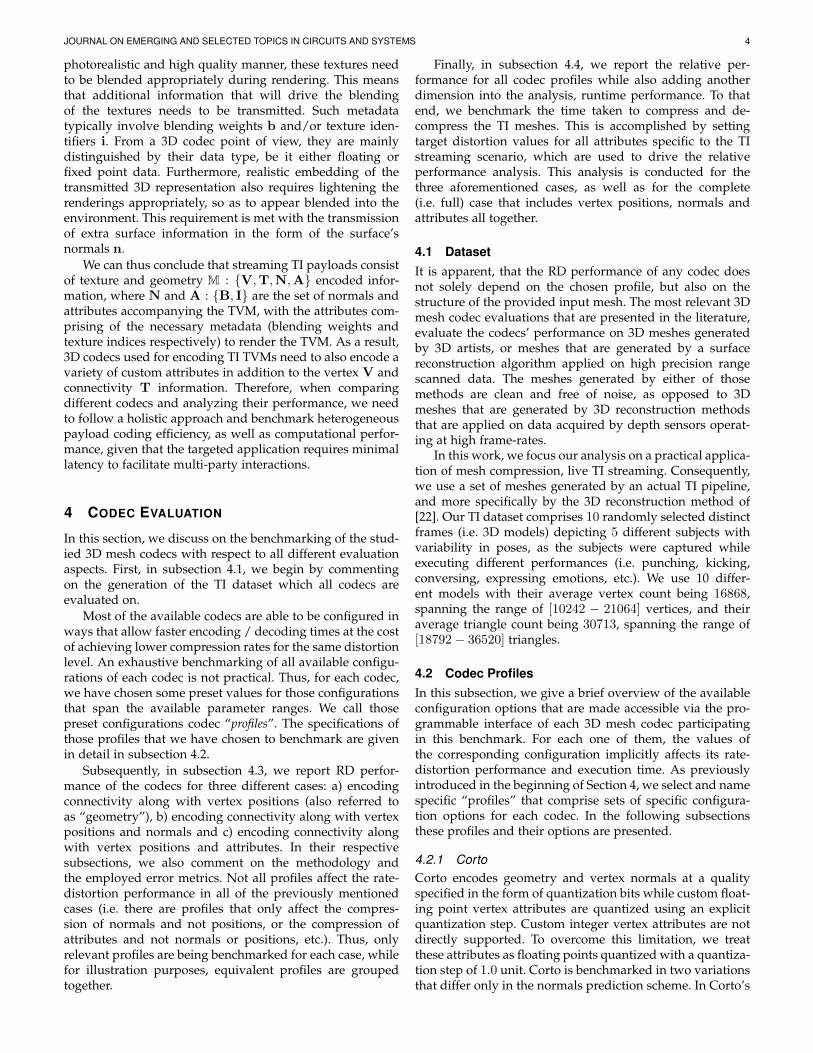
For the definition of the normal distortion metric, wefollow a Hausdorff-like root mean squared error (RMSE)approach that measures the angle difference between thecompressed and original mesh’s vertex normals, relying ona vertex correspondence strategy based on proximity. Morespecifically, let A and B denote two meshes with verticesv ∈ A and u ∈ B. Let also n(v) and n(u) denote thenormals of vertex v and u, respectively. Then we define thefollowing error function that calculates the normal distor-tion from mesh A to mesh B:

nerr(A,B) =√

1

N

∑v∈A

[min

u∈N (v)∠(n(v),n(u))

]2(1)

with N ∈ N∗ denoting the vertex count in A and N (v) ={u ∈ B : ||u−v|| < r}, with r a predefined radius distance.Let Mr denote a reference (uncompressed) mesh and Mc

denote its compressed version. We define the final normalerror distortion metric betweenMc andMr to be:

en(Mr,Mc) = max(nerr(Mr,Mc), nerr(Mc,Mr)) (2)

For each pair of Mc and Mr we set the parameter requal to their Hausdorff distance.

Benchmark resultsThe benchmark results of this experiment are presentedin Fig. 4 middle and bottom sub-figures, with each onepresenting results for a different geometric distortion level.

One of the most important observations of this experimentis that the RMS error for normals for the first profile ofCorto1 and both profiles of OpenCTM does not convergeto zero, even for the higher bit-rates. Thus, in general, theyare significantly outperformed in rate distortion terms bythe rest of the codecs.

As with the previous case, when compressing geometryalong with normals, the best codec in RD terms is Draco2,followed by the same codec’s Draco5 profile. For highergeometric distortion (Hausdorff distance with respect tothe bounding box diagonal ≈ 0.0027) third in order comesDraco9. Fourth and fifth come the O3dgc’s profiles (O3d andO3f/s) respectively, while last in order is Corto2. For lowergeometric distortion (Hausdorff distance wrt bounding boxdiagonal≈ 0.00065) the two O3dgc’s profiles perform closerto Draco9.

In contrast to the previous case, in the present scenarioand for the Corto codec, the distortion of normals in thecompressed mesh is not solely controlled by the quantiza-tion parameter but is also affected by the codec’s profile.In RD terms, the first profile of Corto is clearly surpassedby the second profile of the same Codec. Furthermore,while for Draco, O3dgc and Corto2 the geometric distortionhas an insignificant impact on the final distortion of thecompressed normals, this is not the case for Corto1 and bothprofiles of OpenCTM. The latter codec profiles compressnormals in a way that their distortion is also affected bythe distorted geometry of the compressed mesh, with lowergeometric loss improving the distortion of the normals forthe same quantization parameters.

4.3.3 Case C: Connectivity, Vertex Positions & Vertex At-tributesLast, we benchmark the RD performance of the variouscodec profiles for the case of compressing mesh geometryand connectivity along with vertex attributes. Similar tothe case with normals (Case B - subsection 4.3.2), the na-ture of this experiment is also two-dimensional, with twoquantization parameters controlling geometric and attributedistortions respectively. We follow the same approach as wedid previously, by first picking an appropriate value forthe corresponding quantization parameter that leads to apreset level of geometric distortion. Then, we proceed inevaluating attribute distortion versus bit-rate by adjustingthe attribute quantization parameter to various values. Asalready discussed in Section 3 in the TI streaming case, thevertices of the meshes have both integer and floating pointattributes. Specifically for the case of [22], they have twointeger texture identifiers and one floating point blendingweight for each texture pair which are used during render-ing. In our experiments, the attributes corresponding to thetexture identifiers are encoded losslessly while the only at-tribute that is subject to distortion is the one correspondingto the blending weight. The final bit-rate though, is affectedby both types of vertex attributes.

To measure the attribute distortion between the com-pressed and the original (uncompressed) meshes we definean error metric which resembles the error metric we usedfor normal distortion. In particular, if A and B denote twomeshes with vertices v ∈ A and u ∈ B and a(v) and a(u)denote a single floating point attribute of vertices v and


Fig. 4. Rate-distortion curves for all codecs when compressing geom-etry (vertex positions and connectivity) only - top - and geometry withnormals - middle and bottom. For all cases, zoom-ins are provided asinsets to better illustrate differences for those codecs whose RD curvesare very close. For the normals RD curves, results are shown for aconstant geometric distortion level as mentioned in each plot’s subtitle.

u, respectively we define the following error function thatcalculates the attribute distortion from mesh A to mesh B:

aerr(A,B) =√

1

N

∑v∈A

[min

u∈N (v)|a(v)− a(u)|

]2(3)

with N and N (v), having the same notion as in subsection4.3.2. For the uncompressed mesh Mr and its compressedversion Mc, we define the final attribute error distortionmetric betweenMc andMr to be:

ea(Mr,Mc) = max(aerr(Mr,Mc), aerr(Mc,Mr)) (4)

Fig. 5. Rate-Distortion performance (Attribute RMS distortion vs bit-rate,for two fixed geometric distortion levels) when compressing Geometryalong with Vertex Attributes. On the top and bottom, rate-distortioncomparisons for high and low geometric losses, respectively.

Similar to subsection 4.3.2, for each pair ofMc andMr

we set the parameter r equal to their Hausdorff distance.

Benchmark results

We benchmark the various codec profiles for their RDperformance in encoding attributes for the two levels ofgeometric distortion that we set in subsection 4.3.2, namelyHausdorff distance (with respect to the bounding box)≈ 0.0027 and ≈ 0.00065. The respective RD curves aredepicted in Fig. 5.

Ordering the various codec profiles in RD terms for thisparticular case is very clear. Draco is the best performingcodec under the RD criterion, with its faster profiles con-sistently producing higher bit-rates for the same level ofdistortion, but still achieving better RD performance thanall other codecs. Fourth in order comes O3s followed byO3d and O3f . Last in order are Corto (both of its profilesperform the same) and the two profiles of OpenCTM.

From Fig. 5 it can be deduced that the final attributedistortion level achieved by all codecs is not affected by theirprofiles. The codec profiles only affect the final bit-rate. Fur-ther, as observed in Fig. 5, the level of geometric distortionhas only a small impact on the achieved distortion levels ofthe attributes. In addition, the ordering of the codecs in RDterms does not change when geometric distortion decreases,except that O3s reaches the performance of Draco9.


4.4 Relative Comparison of Codec Performances

In the current section of the paper we discuss the relativeperformance of the studied codec profiles in four aspects ofmesh compression namely bit-rate, distortion, encoding anddecoding times. We perform the analysis for four total cases:compressing connectivity with vertex positions, compress-ing connectivity with vertex positions and normals, com-pressing connectivity with vertex positions and attributes,and finally compressing connectivity along with vertex po-sitions, normals and attributes altogether. An exhaustivecomparison in all of those aspects for all the possible valuesof the quantization parameters is impractical, thus, we aimto set a specific target level of distortion for each genericvertex attribute and compare the various codec profiles inthe four aforementioned aspects.

Since our study is motivated by the application of thosecodecs in a TI scenario, we pick the target distortion levelsfor geometry, normals and attributes as such, in order toalign with this practical use case. In particular, for geom-etry, we choose the Hausdorff distance with respect to thebounding box diagonal to be ≈ 0.00065 which is equivalentto ≈ 0.0003 meters, i.e. 0.3mm RMS error (as reportedby the METRO tool) and ≈ 0.0012 meters, i.e. 1.2mm ofactual Hausdorff distance. For normals, we target the 1◦

RMS angle distortion and for the attribute corresponding tothe texture blending weight (a value which lies in the range[0− 1]), we aim at an RMS distortion level of about 0.0145.As already discussed in the previous section, the exact targetlevel of distortion, in all the generic vertex attributes, cannotbe achieved by all codecs and thus, for each codec profile,we find the value of the quantization parameter that leadsto a distortion which is as close as possible to the target levelthat we have set.

To measure the encoding and decoding times for eachcodec profile, we average the time taken for each codecto compress / decompress the respective mesh 30 times,in order to estimate the time taken to complete a singlecompression / decompression pass. For each mesh weconvert the time measured by this process in per vertextime units by dividing the time needed for each pass withthe mesh’s vertex count. Finally, we average the numberscorresponding to the encoding / decoding times per vertexfor all the meshes in the dataset to get a representativevalue of the codecs’ runtime performance. At this point itis important to note that all codecs were built from sourcecode with all speed optimization options turned on2.

The figures that we present show the relative perfor-mance of each codec with respect to the performance of thebest codec in each aspect and for each case. In all figures,lower values indicate better performance. The figures are inthe form of bar charts, with the values of the bars being theaverage codec performance in the respective aspect, acrossall models. Additionally, we show error bars that indicatethe standard deviation of the measurements around theaverage for the different models of the dataset.

2. Further, no codec implementation contains any type of assemblyoptimizations or any CPU specific instruction extension sets.

4.4.1 Case A: Connectivity & Vertex PositionsThe results of the first case when compressing connectivityand geometry alone are depicted in Fig. 6. The geometricdistortion for all codecs is approximately equal, except forOpenCTM which produced meshes with 26% more geo-metric distortion than the rest of the codecs. In all aspectsand for all codecs, the standard deviation of each metricacross the different models of the dataset is relatively smallcompared to the average value, making the average value agood representative of the codec performances.

Comparing O3d with the O3f/s profiles, the latter twoproduce ≈ 4.5% larger bit-rate but are about ≈ 20.5% and≈ 27.35% faster in encoding and decoding respectively.Draco9 produces ≈ 18% larger bit rate than Draco2 but atthe same time it is ≈ 20% and ≈ 16.3% faster in encodingand decoding. Thus, Draco’s profiles showcase a bettertrade-off between bit-rate and speed than O3dgc’s. Further,comparing Draco with O3dgc, we observe that Draco2 isbetter than O3d in all aspects while the same holds forDraco5 when compared to the O3f/s profiles. Corto has thefaster encoder about ≈ 30.5% faster than Draco9 but at thesame time producing ≈ 48.3% larger bit-rate. The fastestdecoder is CTM-LZ4, but coming at a very increased bit-rate compared to other codecs. Further, the performance ofCTM-LZMA is inferior to all profiles of Draco, Corto and theO3f/s profiles in all aspects.

In order to showcase the discrepancy in RD betweenquick and performant encoding we also offer BD-rates[29], [30] for those codecs lying at these opposite perfor-

mance ends. While Fig. 6 showcases Draco’s superiority inproducing low bit-rates, there is no clear decision betweenCorto and OpenCTM with respect to encoding/decodingspeed. To that end, we also factor in their relative perfor-mance in lower bit-rate production, and thus, offer BD-rate comparisons for Draco and Corto. Table 1 presents theresults for signal-to-noise ratio and bit-rate gains in relationto the different profiles. For Corto both profiles producethe same geometric rate-distortion curves, while for Dracoseparate comparisons are offered for each speed preset.Similar to [31], when calculating the PSNR we use closestpoint correspondences and the bounding box’s diagonalas the peak value3. While it is evident that coding speedcomes at the expense of efficiency, we also observe smallerdifferences between Draco’s slow and fast speed profiles.

4.4.2 Case B: Connectivity, Vertex Positions & Vertex Nor-malsIn Fig. 7 relative codec performances for the case of com-pressing vertex normals along with mesh connectivity andgeometry are given. The geometric distortions in this casefor all codec profiles are the same as presented in subsection4.4.1. While we have set a target of 1◦ (degree) RMS, Corto1could not achieve a better distortion performance than ≈ 6◦

RMS. This behaviour has been mentioned in the discussionof Section 4.3.2. For Corto1 we’ve set the quantization pa-rameter to the value that led to the best distortion levelit can achieve with the minimum possible bit-rate, since

3. Given that our test models are reconstructed in life-size scale aftera uniform voxelization process, we expect consistent results acrossmodels.


TABLE 1BD rates for Draco’s and Corto’s profiles. BD-SNR presents the quality gain for equal bit-rates, while BD-BR presents the percentage gain in

bit-rate for the same quality.

BD-SNR (dB) BD-BR (%)

Corto12 Draco2 Draco5 Draco9 Corto12 Draco2 Draco5 Draco9

Corto12 N/A -26.57 (1.82) -23.1 (1.75) -22.48 (1.97) N/A 88.59 (6.99) 67.44 (5.66) 60.36 (5.51)Draco2 26.57 (1.82) N/A 4.12 (0.25) 5.6 (0.42) -46.91 (2.01) N/A -10.39 (0.6) -12.98 (0.86)Draco5 23.1 (1.75) -4.12 (0.25) N/A 1.45 (0.41) -40.22 (2.078) 11.6 (0.75) N/A -2.89 (0.97)Draco9 22.48 (1.97) -5.6 (0.42) -1.45 (0.41) N/A -37.57 (2.19) 14.93 (1.13) 2.98 (1.03) N/A

Fig. 6. Relative Comparison of Codec Performances: Geometric Distortion, Bitrate, Encoding and Decoding times when compressing connectivityalong with geometry alone. The presented results correspond to a ≈ 0.00065 geometric Hausdorff distortion (with respect to the bounding box’sdiagonal).

further increasing the bit-rate did not significantly reducethe normal distortion. In addition, the normal distortionmeasurements taken for the previously mentioned profilehave large standard deviation across the different modelscompared to all other codecs whose distortion performanceis consistent for all models in the dataset.

Although Draco2 produces the best bit-rate, it has asignificant shortcoming in decoding time which is signifi-cantly worse than the rest of the codecs. However, Draco5is better than O3d in all aspects, while the same holdsfor Draco9 over O3f/s. The fastest encoder and decoder isCorto2. Moreover, Corto2 is consistently better than Corto1and both OpenCTM’s profiles in all aspects. Finally, Corto2produces ≈ 40% larger bit-rate compared to Draco9 but isabout ≈ 31.5% and ≈ 50% faster in encoding and decodingtime, respectively.

4.4.3 Case C: Connectivity, Vertex Positions & Vertex At-tributes

We present relative codec performances for the case ofcompressing mesh connectivity along with vertex geometryand attributes in Fig. 8. Geometric distortion across codecs isthe same as in subsection 4.4.1. Corto produces about≈ 50%more RMS attribute distortion than the best performingcodec (OpenCTM), while the others (Draco and O3dgc)produced ≈ 7% more distortion than OpenCTM.

In this case, regarding O3dgc, the O3f performs closelyto O3d in bit-rate terms, while for the encoding and decod-ing times it performs significantly better. O3s produces thelowest bit-rate (closely to Draco9) at the cost of increasedtime complexity.

Draco’s profiles produce the best bit-rates. However,relative to one another, their encoding and decoding timesvary disproportionately to the bit-rate gain. Draco’s fasterprofile (Draco9) surpasses O3d and O3f in all aspects. Fur-thermore, it competes with O3s in bit-rate but outperformsit in encoding and decoding runtimes.

Corto, still, has the fastest encoder and the second fastest,but competitive, decoder after CTM-LZ4. Moreover, Cortoperforms better than CTM-LZMA in all aspects and betterthan O3f in all other aspects apart from decoding time.Comparing Corto with the fastest profile of Draco we seethat Draco’s profile produces about ≈ 33.3% reduced bit-rate while it is ≈ 51% and ≈ 65.8% slower in encodingand decoding times, respectively. Thus, Corto offers a goodbalance between produced bit-rate and encoding/decodingruntimes.

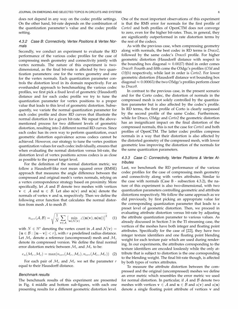
4.4.4 Case D: Connectivity, Vertex Positions, Vertex Nor-mals & Vertex AttributesFinally, in Fig. 9 relative codec performances for the case ofcompressing connectivity along with all of vertex positions,normals and attributes are given. The distortion levels forthis case are the same as the ones discussed in all theprevious paragraphs of this section.

Regarding O3dgc, O3f produces slightly larger bit-ratethat the other profiles of the same codec, but it has asignificant improvement on encoding and decoding times.For Draco, once again we observe that the various profilesperform relatively close to one another in bit-rate, but theybehave very much differently in encoding/decoding timeswith the profile performing better in bit-rate being consid-erably slower. When comparing Draco with O3dgc, we ob-


Fig. 7. Relative Comparison of Codec Performances: Normal Distortion, Bit-rate, Encoding and Decoding times when compressing connectivityalong with geometry and normals. The presented results correspond to ≈ 0.00065 geometric Hausdorff distortion (with respect to the boundingbox’s diagonal) and ≈ 1o normal angle distortion.

Fig. 8. Relative Comparison of Codec Performances: Attribute Distortion, Bit-rate, Encoding and Decoding times when compressing connectivityalong with geometry and attributes. The presented results correspond to ≈ 0.00065 geometric Hausdorff distortion (with respect to the boundingbox’s diagonal) and ≈ 0.0145 attribute RMS distortion.

serve that the fastest profile of Draco (Draco9) outperformsall O3dgc’s profiles in all aspects.

In this experiment, Corto has the fastest encoder and de-coder. Further, it surpasses both OpenCTM’s profiles in allaspects. Compared to Draco9 it produces ≈ 43% increasedbit-rate but it is ≈ 33.7% faster in encoding and ≈ 48.7%faster in decoding.

4.4.5 Discussion on codec relative performancesOverall, in all the cases above, in terms of bit-rate, the bestperforming codecs are Draco and O3dgc with their variousprofiles performing close to one another. Corto’s profilesare the best next followed by CTM-LZMA and CTM-LZ4.Regarding the encoding time, the best codec in all experi-ments is Corto, while for decoding time Corto remains thefastest decoder except from the case of decoding a meshthat contains only geometry and connectivity, in whichcase CTM-LZ4 performs better. Evidently, we observe thatwhen attributes (normals, texture indices, blending weights)are progressively added into the payload, Corto2 performsslightly better in terms of bit-rate wrt the Draco baseline pro-file (Draco2), and that its runtime performance gain increasesmultifold. Moreover, O3dgc’s slightly inferior performancein attribute coding is also observed when compared toDraco’s baseline. Interestingly, OpenCTM’s attribute codingappears to be the most performant in terms of relative gains,albeit still being overally inefficient.

5 LIVE STREAMING STUDY

In this section of the paper we conduct a theoretical study onthe performance of all codec profiles in a TI live streamingscenario by plugging the actual measurements we haveacquired via benchmarking to a theoretical model of thetypical TI pipeline. The theoretical model aims to determinethe end-to-end latency of the streamed frames and the actualframe-rate at the receiver’s side. The results of this theoret-ical analysis are influenced by the codecs’ performances inall the aspects we have benchmarked previously (namelybit-rate, encoding and decoding runtimes). Futhermore, theanalysis would not be complete if we didn’t take intoaccount the different possible network conditions that mayapply in a TI scenario. Since none of the codecs participatingin this study can decompress incomplete or erroneous com-pressed payloads, in the following study we assume thatthe employed network layer uses the Transmission ControlProtocol (TCP) which guarantees both payload integrity andpayload delivery.

In subsection 5.1 we introduce the TI pipeline alongwith the theoretical model that we use to opine aboutframe latency and frame-rate at the side of the receiver. Insubsection 5.2 we present the calculation of the theoreticalmodel’s variables, while in subsection 5.3 we depict theresults of the theoretical analysis for each codec profile andfor various network conditions.


Fig. 9. Relative Comparison of Codec Performances: Bit-rate, Encoding and Decoding times when compressing connectivity along with geometry,vertex normals and vertex attributes. The presented results correspond to ≈ 0.00065 geometric Hausdorff distortion (with respect to the boundingbox’s diagonal), ≈ 1o normal angle distortion and ≈ 0.0145 attribute RMS distortion.

5.1 The Tele-Immersion Pipeline and the TheoreticalModelIn Fig. 10, the main components of a TI pipeline are given.The source is supposed to be a 3D reconstruction componentthat produces 3D meshes to be transmitted in real-time toremote parties. We do not impose any restrictions on thesource (such as a specific output frame rate) because wewant to study the capacity of the pipeline independent fromsource’s characteristics. The 3D meshes produced by thesource are subsequently compressed using anyone of thepreviously introduced codec profiles and then transmittedto a remote party which receives and decompresses the re-ceived payload prior to rendering. At the sender’s side, thecompression and transmission of the frames are assumed tobe run in parallel (e.g. in separate threads with one threadcompressing the next frame while the previous frame istransmitted to the network). When the compression of thecurrent frame has been finished, the compressed representa-tion is enqueued to the transmission queue (“Queue #1”) inorder to be sent to the network when the transmission of theprevious frame finishes. Similarly, at the receiving side, thedata received by the network are put in the decompressionqueue (“Queue #2”) in order to be decompressed after thepreviously received frame has finished decompression. Forthe system to be as real-time as possible (i.e. minimizelatency), both previously mentioned queues are assumedto store only one frame. If a new frame is enqueued whilethe previous frame has not been processed yet, the previousframe is dropped and its place is taken by the newer frame.

At each point of the pipeline we define auxiliary vari-able names that will help us with analyzing its end-to-endperformance. These variables are:

• cmprs out: The rate at which the encoder can pro-vide compressed frames in frames per second.

• cmprs lat: The time needed by the encoder to com-press a single frame in seconds.

• q1 wait t: The maximum time a frame will wait inthe transmission queue (“Queue # 1”) in seconds.

• trans push: The maximum rate at which the com-pressed frames can be pushed into the network inframes per second

• trans lat: The time, in seconds, that is required fora compressed frame to be transmitted over to the

remote party.• trans out: The rate at which the frames arrive at the

receiver from the network, in frames per second.• q2 wait t: The maximum time a frame will wait in

the decompression queue (“Queue # 2”) in seconds.• decmprs push: The maximum rate at which the re-

ceived frames can be sent for decoding, in frames persecond.

• decmprs lat: The time, in seconds, needed by thedecoder to decompress a single frame.

• decmprs out: The output frame rate of the decoderin frames per second.

Following an analytic path to estimate the actual frame-rate and end-to-end latency of the TI pipeline can get cum-bersome and complex. However, by making a few, simple,reasonable assumptions, we can calculate analytically lowerand upper bounds of the pipeline’s end-to-end latency andan estimate of its frame-rate.

We will first assume that the source is producing 3Dmeshes of approximate equal vertex and triangle count ineach frame, which is a reasonable assumption when 3Dreconstructing real humans standing at natural poses with afixed resolution volumetric 3D reconstruction method.

Then, from the benchmark results that we have con-ducted for the various mesh codecs, we can acquire a goodestimate on the encoding/decoding time needed by eachcodec in order to compress or decompress a frame. This isaccomplished by first calculating an intermediate variablemeasured in “seconds per vertex” for the encoding anddecoding operations, respectively. This variable is calculatedby dividing the encoding / decoding time required tocompress a mesh by the total number of vertices in themesh and average across all models of the dataset, forgiven quantization parameters. With this data we can thenestimate the average encoding and decoding time requiredby the respective codec in order to compress / decompressthe meshes of approximately equal vertex count producedby the source.

In a typical TI pipeline the 3D reconstructed humanmeshes are further textured using the color images thatwere captured during frame acquisition. In our study, weaccount for an additional payload size that corresponds to4 texture images (i.e. when using a 360◦ capturing setup of


Fig. 10. Tele-Immersion Pipeline with variable names for live streaming study. Components of the Tele-Immersion pipeline are in teal (source andsink) or gray (processing stages), while variable names are depicted in orange.

four cameras) compressed separately, via the standard H.264video codec [32] at a moderate quality. Concerning the ad-ditional processing time for compressing / decompressingthe four textures, we will use typical encoding / decodingtimes that we calculated with internal benchmarking usingthe nVIDIA’s GPU accelerated video codec NVENC [33]running on a GTX 1070 GPU.

For the network conditions we will assume a moderate,constant packet loss probability. Furthermore, since we as-sume TCP as the underlying network protocol, we will usethe Mathis equation [34] to calculate the effective bandwidthof the network link based on the line’s round trip time(RTT), bandwidth and packet loss probability. The Mathisequation is applicable to limit the effective bandwidth ofthe line when the maximum TCP congestion window (forthe given packet loss) is smaller than the line’s bandwidthdelay product. Otherwise, the effective bandwidth of thelink is equal to the line’s bandwidth.

Finally, we will assume that the mesh compression / de-compression components will be run on modern hardware,similar to what we used for these experiments (i.e. an IntelCore i7-7700K CPU clocked at 4.5 GHz - 4 physical cores, 8logical threads - equipped with 32 GB of DDR4 RAM).

5.2 Calculating the variables of the TI pipeline’s theo-retical model

In order to calculate the aforementioned variables of the the-oretical model of the TI pipeline, we will first need to definesome additional supplementary variables that depend onthe mesh codec used and the network line’s characteristics.Those supplementary variables are given next:

• cmprs t: The time needed to compress the 3D meshand its four accompanying textures, in seconds. Thistime is the time needed by the mesh codec to com-press the 3D mesh and the video codec to compressthe four textures.

• decmprs t: The time needed to decompress the 3Dmesh and its four accompanying textures, in seconds.

• EBW: The effective bandwidth of the network line inMbps.

• frame size: The average compressed frame size inbytes with its payload corresponding to the sum ofthe compressed 3D mesh and the size of the fourcompressed accompanying textures.

• RTT: The line’s round-trip time is seconds.

With the above definitions given, we are now able to calcu-late the variables of the TI pipeline’s theoretical model:

cmprs rate = 1/cmprs t, cmprs lat = cmprs t

trans push = 106 ×EBW/8× frame size

q1 wait t = min(1/cmprs rate, 1/trans push

)trans lat = 1/trans push+ 0.5×RTT

trans out = min(cmprs rate, trans push

)decmprs push = 1/decmprs t

q2 wait t = min(1/decmprs push, 1/trans out

)decmprs lat = dcmprs t

decmprs out = min(decmprs push, trans out

)According to the previous analysis, the approximate

end-to-end frame-rate of the TI pipeline is equal todecmprs out. A lower bound on the end-to-end latencyis the quantity: cmprs lat + trans lat + decmprs lat,while a respective upper bound is equal to cmprs lat +q1 wait t+ trans lat+ q2 wait t+ decmprs lat.

5.3 Codec Live-Streaming Performance

In this paragraph we apply the theoretical model we de-scribed in the previous subsection in order to obtain theo-retical lower and upper bounds on the end-to-end latencyof the TI pipeline and an estimate of the final achievedframe-rate. To accomplish this, we first set the scope of theevaluation. We are going to provide a study for the caseof compressing and transmitting a full TVM representationwith connectivity, geometry, normals and attributes as wellas four texture images.

The meshes of our dataset that were generated by the3D reconstruction method of [22] had an average vertexcount of 16868, and thus we pick this number as our averagemesh size. Subsequently, we set a target level of distortionfor each generic vertex attribute that all codecs must meetfor a fair comparison. The distortion levels that we haveset have already been discussed in the previous sectionof the paper. More specifically, for geometry we’ve set atarget distortion level of ≈ 0.00065 Hausdorff distance withrespect to the bounding box diagonal. For normals, we setthe RMS distortion to 1◦ and for attributes to 0.0145 RMS.

From the benchmark analysis that we have performedand discussed in the previous section, we are able to doinverse calculation and compute the quantization parametervalues that lead to this average distortion behavior for eachcodec. For the obtained quantization parameter values wecan calculate the estimated resulting bit-rate and encoding


/ decoding time performance of each codec. Thus, theframe size variable can be estimated by the calculated bit-rate, while the encoding and decoding times of the codecare calculated according to the methodology described inSection 5.1.

In addition, we assume that the four accompanying tex-tures of each mesh are half the Full HD resolution (960×540pixels) and are compressed independently using the H.264video codec, configured in its low-latency / high perfor-mance “zerolatency” mode (i.e. not using B frames) andconstant quality across frames with quantization parameter31, which is equivalent to per-frame JPEG compressionwith 50% quality in PSNR sense (determined after exper-imentation with textures from our dataset). An extensivebenchmarking experiment that we have conducted in ourlabs concerning the texture compression has shown that forthis texture size and compression parameters the averageencoding time for four textures is 4 ms (1ms per texture)while for decoding is 2 ms producing an average size pertexture (per frame) of 1KB (total of 4KB for four textures).The implementation of the H.264 encoder that we used washardware accelerated in GPU [33].

Regarding the network conditions, we pick a fixed, mod-erate, packet loss probability of p = 0.0005 for all of ourexperiments. For the network line’s bandwidth we evaluateon a typical value of 100Mbps . Moreover, we consider RTTof 1ms, 20ms and 50ms which implies that the remote partymay be in the same city, country or continent as the sender,respectively. The actual numbers for the upper and lowerbounds of the end-to-end latency as well as the expectedframe-rate (in frames per second - fps) for each codec profileare given in Table 2.

Discussion on codec live streaming performanceRegarding the RTT of 1ms, we observe that among the samecodec, the fastest profiles perform better in both latencybound terms and expected frame rate. In particular, Draco9,O3f and CTM-LZ4 perform better than the other profilesof the respective codecs. Corto’s profiles perform similarly.Overall, in terms of end-to-end latency and frame-rate thebest performance is achieved by Corto2.

For the case of 20 ms RTT , the fastest profiles of eachcodec performs better than other profiles of the same codecin all aspects. However, in contrast to the previous case,the codec with the lowest lower bound end-to-end latencyand highest frame rate is Draco9, while the lowest upperbound end-to-end latency is achieved by Corto2, but notsignificantly less than Draco9.

Finally, when considering a network line with RTT of 50ms, for each codec, the profile that achieves the highest com-pression leads to the highest frame-rate. On the other hand,the fastest profiles generally achieve better performance interms of end-to-end latency. Overall, the best performingcodec is Draco with “speed - 2” achieving the highest frame-rate and “speed - 9” achieving the lowest end-to-end latency.

To sum up, a general observation is that the processingspeed of the mesh codecs is more important when thenetwork line’s RTT is small, while for larger values of RTTthe best performing codecs are the ones having a goodtrade-off between processing time and compression rate.This can easily be explained by the theoretical model we

have discussed in Subsection 5.1. When effective bandwidthis high, the frame rate is only affected by the compressiontime (since compression time is always worse than decom-pression time for all codec profiles). Furthermore, in thesame case, the transmission latency is negligibly affectedby the frame size, adding to the fact that compression ratiohere is less important. On the other hand, when the effectivebandwidth is low, the frame rate is inversely proportional tothe frame size, and latency is dominated by transmissiontime, which is proportional to the frame’s size. Thus, inthat case, the RD performance matters more than runtimeperformance.

6 CONCLUSION

In this paper we have conduced an extensive, systematicand consistent benchmarking in terms of bit-rate, distortionand processing time of four Open-Source static 3D meshcodecs namely Corto, Draco, O3dgc and OpenCTM. Incontrast to other works, our work examines thoroughlythe performance of the codecs not only in compressinggeometry along with connectivity, but also in compressingvertex normals and attributes.

Firstly, we evaluated the codecs in rate-distortion terms,accounting for geometry, normal as well as attribute distor-tion. Subsequently, we set target levels of distortion in all ofthe aforementioned aspects, that led to a compressed repre-sentation of good quality (at least in objective terms) but stillsignificantly compressible. For these preset distortion levels,we evaluated the performance of the codecs in relation toone another, in the aspects of bit-rate and processing time.We’ve concluded that by the relative analysis it is not easyto opine on which codec performs best, since none of thecodecs tops in all of the bit-rate, encoding and decodingtime aspects. Thus, we continued our investigation on theperformance of the codecs by examining their theoreticalperformance in the case they were employed in a tele-immersive interactive live streaming scenario. We createda theoretical model of a TI pipeline and analytically com-puted the end-to-end latency lower and upper bounds aswell, as the expected frame-rate for some common networkconditions when utilizing each one of those codecs. Thevalues that we fit to the TI pipeline’s theoretical model wereobtained by previously conduced extensive benchmarking.

Overall, we found that in the live streaming scenario,for each profile of O3dgc there does exist one profile ofDraco that performs better in all of the relevant codecaspects. Furthermore, except of the case of compressing justgeometry along with connectivity, the Corto codec alwaysperformes better than the OpenCTM’s profiles in all terms.Our live streaming analysis showed that choosing betweenCorto and Draco in a TI pipeline should be a decisionbased on network conditions, with Corto performing beston network setups with low RTT, while Draco being betterwhen the line’s RTT increases. The results of this studymay be used to help designers of Tele-Immersive systemsto chose the best 3D mesh codec for their application. Inaddition, the aforementioned analysis can be used as a base-line for future 3D compression research, as it is evident thatthere is still room for improvement, given that according toour theoretical analysis, when the networking parameters


TABLE 2Expected frame-rate and end-to-end latency lower (LB) and upper (UB) bounds for each codec profile in a live streaming scenario for a set of

networking conditions with line bandwidth 100 MBps and RTT of 1ms, 20ms and 50ms. Each case’s effective bandwidth is also reported.

Line BW: 100Mbps, RTT: 1ms, EBW: 100Mbps Line BW: 100Mbps, RTT: 20ms, EBW: 26.12Mbps Line BW: 100Mbps, RTT: 50ms, EBW: 10.47MbpsCodec Profile Latency LB Latency UB Frame-Rate Latency LB Latency UB Frame-Rate Latency LB Latency UB Frame-Rate

Corto1 25.65 38.75 82.95 57.49 74.74 33.07 117.83 135.09 13.23Corto2 24.58 37.02 85.82 55.70 72.15 34.17 114.60 131.04 13.66Draco2 65.69 92.99 26.39 89.14 130.40 26.39 132.47 192.73 21.18Draco5 47.32 66.83 36.60 71.85 106.39 36.60 117.36 158.88 19.66Draco9 28.94 41.81 64.19 53.80 76.82 48.12 99.97 122.99 19.24

O3d 47.12 67.58 38.23 74.40 112.65 38.23 125.51 165.85 16.61O3f 38.05 55.91 50.78 65.68 96.82 40.73 117.51 148.65 16.29O3s 49.62 70.49 35.38 74.91 111.56 35.38 121.96 165.50 18.72

CTM-LZMA 67.95 91.82 22.93 105.07 156.54 22.93 176.12 233.82 10.70CTM-LZ4 41.75 65.68 57.73 98.47 123.02 15.64 209.33 233.89 6.25

used resemble the actual Internet more closely, sub-optimalframe-rates are being achieved by the majority of codecs.

ACKNOWLEDGMENTS

This work has been supported by the EU’s H2020 pro-gramme 5G-MEDIA (GA 761699).

REFERENCES

[1] A. Maimone and H. Fuchs, “Encumbrance-free telepresence sys-tem with real-time 3d capture and display using commodity depthcameras,” in Mixed and augmented reality (ISMAR), 2011 10th IEEEinternational symposium on. IEEE, 2011, pp. 137–146.

[2] S. Beck, A. Kunert, A. Kulik, and B. Froehlich, “Immersive group-to-group telepresence,” IEEE Transactions on Visualization andComputer Graphics, vol. 19, no. 4, pp. 616–625, 2013.

[3] N. Zioulis, D. Alexiadis, A. Doumanoglou, G. Louizis, K. Apos-tolakis, D. Zarpalas, and P. Daras, “3D tele-immersion platformfor interactive immersive experiences between remote users,” inImage Processing (ICIP), 2016 IEEE International Conference on. IEEE,2016, pp. 365–369.

[4] S. Orts-Escolano, C. Rhemann, S. Fanello, W. Chang, A. Kowdle,Y. Degtyarev, D. Kim, P. Davidson, S. Khamis, M. Dou, et al.,“Holoportation: Virtual 3d teleportation in real-time,” in Proceed-ings of the 29th Annual Symposium on User Interface Software andTechnology. ACM, 2016, pp. 741–754.

[5] A. Doumanoglou, D. S. Alexiadis, D. Zarpalas, and P. Daras,“Toward real-time and efficient compression of human time-varying meshes,” IEEE Transactions on Circuits and Systems for VideoTechnology, vol. 24, no. 12, pp. 2099–2116, Dec 2014.

[6] S. R. Han, T. Yamasaki, and K. Aizawa, “Time-varying meshcompression using an extended block matching algorithm,” IEEETransactions on Circuits and Systems for Video Technology, vol. 17, no.11, pp. 1506–1518, Nov 2007.

[7] T. Yamasaki and K. Aizawa, “Patch-based compression for time-varying meshes,” in 2010 IEEE International Conference on ImageProcessing, Sept 2010, pp. 3433–3436.

[8] “MPEG-I, 2018. Coded Representationof Immersive Media. ISO/IEC 23090,”https://mpeg.chiariglione.org/standards/mpeg-i.

[9] “MPEG-PCC, 2018. Coded representation of Point Clouds,”https://mpeg.chiariglione.org/standards/mpeg-i/point-cloud-compression.

[10] R. Mekuria, K. Blom, and P. Cesar, “Design, implementation, andevaluation of a point cloud codec for tele-immersive video,” IEEETransactions on Circuits and Systems for Video Technology, vol. 27, no.4, pp. 828–842, April 2017.

[11] D. Thanou, P. A. Chou, and P. Frossard, “Graph-based compres-sion of dynamic 3d point cloud sequences,” IEEE Transactions onImage Processing, vol. 25, no. 4, pp. 1765–1778, April 2016.

[12] “Google Draco,” https://github.com/google/draco, accessed:2018-06-07.

[13] “Corto,” https://github.com/cnr-isti-vclab/corto, accessed: 2018-06-07.

[14] “Open 3D Graphics Compression (O3DGC),”https://github.com/amd/rest3d/tree/master/server/o3dgc,accessed: 2018-06-07.

[15] “OpenCTM,” http://openctm.sourceforge.net/, accessed: 2018-06-07.

[16] J. Rossignac, “Edgebreaker: Connectivity compression for trianglemeshes,” IEEE Transactions on Visualization and Computer Graphics,vol. 5, no. 1, pp. 47–61, Jan. 1999.

[17] F. Ponchio and M. Dellepiane, “Fast decompression for web-based view-dependent 3d rendering,” in Proceedings of the 20thInternational Conference on 3D Web Technology, New York, NY, USA,2015, Web3D ’15, pp. 199–207, ACM.

[18] K. Mamou, T. Zaharia, and F. Preteux, “TFAN: A low complexity3D mesh compression algorithm,” Comput. Animat. Virtual Worlds,vol. 20, no. 2-3, pp. 343–354, June 2009.

[19] Faxin Yu, Hao Luo, Zheming Lu, and Pinghui Wang, “3d meshcompression,” in Three-Dimensional Model Analysis and Processing,pp. 91–160. Springer, 2010.

[20] J. Peng, C-S. Kim, and C. Jay Kuo, “Technologies for 3d meshcompression: A survey,” J. Vis. Comun. Image Represent., vol. 16,no. 6, pp. 688–733, Dec. 2005.

[21] A. Maglo, G. Lavoue, F. Dupont, and C. Hudelot, “3d meshcompression: Survey, comparisons, and emerging trends,” ACMComput. Surv., vol. 47, no. 3, pp. 44:1–44:41, Feb. 2015.

[22] D. Alexiadis, A. Chatzitofis, N. Zioulis, O. Zoidi, G. Louizis,D. Zarpalas, and P. Daras, “An integrated platform for live 3Dhuman reconstruction and motion capturing,” IEEE Transactionson Circuits and Systems for Video Technology, vol. 27, no. 4, pp. 798–813, 2017.

[23] William E. Lorensen and Harvey E. Cline, “Marching cubes: Ahigh resolution 3d surface construction algorithm,” in Proceedingsof the 14th Annual Conference on Computer Graphics and InteractiveTechniques. 1987, SIGGRAPH ’87, pp. 163–169, ACM.

[24] Quirin Meyer, Jochen Sußmuth, Gerd Sußner, Marc Stamminger,and Gunther Greiner, “On floating-point normal vectors,” inComputer Graphics Forum. Wiley Online Library, 2010, number 4in EGSR’10, pp. 1405–1409.

[25] C. Touma and C. Gotsman, “Triangle mesh compression,” Dec. 262000, US Patent 6,167,159.

[26] J. Ziv and A. Lempel, “Compression of individual sequences viavariable-rate coding,” IEEE transactions on Information Theory, vol.24, no. 5, pp. 530–536, 1978.

[27] Y. Collet et al., “Lz4: Extremely fast compression algorithm,” code.google. com, 2013.

[28] P Cignoni, C. Rocchini, and R. Scopigno, “Metro: measuring erroron simplified surfaces,” 1998.

[29] Gisle Bjontegaard, “Calculation of average psnr differences be-tween rd-curves,” VCEG-M33, 2001.

[30] Gisle Bjontegaard, “Improvements of the bd-psnr model, vceg-ai11,” in ITU-T Q. 6/SG16, 34th VCEG Meeting, Berlin, Germany(July 2008), 2008.

[31] Philip A Chou, Eduardo Pavez, Ricardo L de Queiroz, and An-tonio Ortega, “Dynamic polygon clouds: Representation andcompression for vr/ar,” arXiv preprint arXiv:1610.00402, 2016.

[32] Iain E. Richardson, The H.264 Advanced Video Compression Standard,Wiley Publishing, 2nd edition, 2010.

[33] “NVIDIA NVENC,” https://developer.nvidia.com/nvidia-video-codec-sdk.

[34] M. Mathis, J. Semke, J. Mahdavi, and T. Ott, “The macroscopicbehavior of the tcp congestion avoidance algorithm,” ACM SIG-COMM Computer Communication Review, vol. 27, no. 3, pp. 67–82,1997.


Alexandros Doumanoglou received hisdiploma in Electrical & Computer Engineeringfrom the Aristotle University of Thessaloniki(AUTh) in 2009. His thesis was about thestudy and construction (in hardware andsoftware) of a passive acoustic radar. In thepast, he has been involved in in-depth studyof several fields of computer science, withsoftware security, cryptography, algorithmsand theory of computation, 3D graphics andartificial intelligence in computer games being

the most notable. He is fond of applied informatics and engineering. Hehas been working in the Information Technologies Institute (ITI) as aresearch assistant since April 2012. His main research interests includecomputer vision, pattern recognition, 3D reconstruction, 3D graphics,mesh compression, signal processing and mathematical optimization.

Petros Drakoulis received his BSc in IT En-gineering from Alexander TEI and his MSc inDigital Media from Aristotle University of Thes-saloniki. In 2018, he joined information technolo-gies institute (ITI) of the Greek national cen-tre for research and technological advancement(CERTH) as a research assistant. His interestsinclude software engineering, computer visionand machine learning.

Nikolaos Zioulis is an Electrical and Com-puter Engineer (Aristotle University of Thessa-loniki, 2012) working in the Information Tech-nologies Institute (ITI) of the Centre for Researchand Technology Hellas (CERTH) since October2013. His interests include 3D processing andgraphics, particularly performance oriented real-time computer vision. Having been involved invarious research projects, his research interestslie in the intersection of computer vision andgraphics technologies and, more specifically, 3D

capturing and rendering, 3D scene understanding and tele-immersiveapplications.

Dimitrios Zarpalas has joined the InformationTechnologies Institute in 2007, and is currentlyworking as a post-doctoral Research Associate.His current research interests include real timetele-immersion applications (3D reconstructionof moving humans and their compression), 3Dcomputer vision, 3D medical image processing,shape analysis of anatomical structures, 3D ob-ject recognition, motion capturing and evalua-tion, while in the past has also worked in in-dexing, search and retrieval and classification of

3D objects and 3D model watermarking. His involvement with thoseresearch areas has led to the co-authoring of 3 book chapter, 1 articlesin refereed journals and 42 papers in international conferences. He hasbeen involved in more than 10 research projects funded by EC, andGreek Secretariat of Research and Technology. He is a member of theTechnical Chamber of Greece.

Petros Daras is a Principal Researcher GradeA’, at the Information Technologies Institute ofthe Centre for Research and Technology Hellas.He received the Diploma in Electrical and Com-puter Engineering, the MSc degree in MedicalInformatics and the Ph.D. degree in Electricaland Computer Engineering all from the Aristo-tle University of Thessaloniki, Greece in 1999,2002 and 2005, respectively. He is the headresearcher of the Visual Computing Lab coor-dinating the research efforts of more than 35

scientists. His research interests include 3D media processing and com-pression, multimedia indexing, classification and retrieval, annotationpropagation and relevance feedback, bioinformatics and medical imageprocessing. He has co-authored more than 160 papers in refereedjournals and international conferences, and has been involved in morethan 30 national and international research projects.

JOURNAL ON EMERGING AND SELECTED TOPICS IN CIRCUITS …

Documents