Journal of Statistical Planning and Inference 108 - Department of

Journal of Statistical Planning andInference 108 (2002) 99–119

www.elsevier.com/locate/jspi

Asymptotics of maximum likelihood estimator ina two-phase linear regression model

Hira L. Koula ; ∗, Lianfen Qianb

aDepartment of Statistics and Probability, Michigan State University, East Lansing,MI 48824-1027, USA

bFlorida Atlantic University, USA

Abstract

This paper considers two-phase random design linear regression models with arbitrary errordensities and where the regression function has a /xed jump at the true change-point. It obtainsthe consistency and the limiting distributions of maximum likelihood estimators of the underlyingparameters in these models. The left end point of the maximizing interval with respect to thechange point, herein called the maximum likelihood estimator rn of the change-point parameter r,is shown to be n-consistent and the underlying likelihood process, as a process in the standardizedchange-point parameter, is shown to converge weakly to a compound Poisson process. Thisprocess obtains maximum over a bounded interval and n(rn − r) converges weakly to the leftend point of this interval. These results are di2erent from those available in the literature forthe case of the two-phase linear regression models when jump sizes tend to zero as n tends toin/nity.c© 2002 Elsevier Science B.V. All rights reserved.

MSC: primary 62F12; secondary 62E20; 62J99; 62G05

Keywords: Change-point estimator; Fixed jump size; n-consistency; Compound Poisson process

1. Introduction

A two-phase linear regression model is piecewise linear over di2erent domains ofthe design variable, each segment possibly being a di2erent straight line. The sta-tistical inference in such models is heavily in<uenced by the continuity or discon-tinuity of the regression function at the change-point. Most of the inference aboutthe change-point has been developed when the regression function is continuous and

∗ Corresponding author. Fax: +1-517-432-1405.E-mail address: [email protected] (H.L. Koul).

0378-3758/02/$ - see front matter c© 2002 Elsevier Science B.V. All rights reserved.PII: S0378 -3758(02)00273 -2

100 H.L. Koul, L. Qian / Journal of Statistical Planning and Inference 108 (2002) 99–119

the design is non-random: Hudson (1966) gave a concise method for calculating theleast-squares estimator (LSE) for the change-point while Hinkley (1969, 1971) derivedasymptotic results for maximum likelihood estimate (MLE) of the point of intersec-tion for the special case of two line segments under normally distributed errors. Undercontinuity and suitable identi/ability assumptions, Feder (1975a, b) derived the asymp-totic distributions of the LSE and the log likelihood ratio statistic for the two-phasenon-random design regression model with the Gaussian errors. Schulze (1987) providesa collection of existing methods mainly focusing on the least-squares estimation, test-ing of hypotheses and testing of model stability for analyzing data using multiphaseregression models.

The review paper of Battacharya (1994) discusses various aspects of change-pointanalysis including testing of hypothesis of no change, interval and point estimation ofa change-point, changes in non-parametric models, changes in regression, and detectionof a change in distribution of sequentially observed data. In particular, he discussesMLE of the change-point of a discontinuous two-phase linear regression model and thelimiting behavior of the log-likelihood ratio process when the errors are Gaussian. Inboth problems the jump size at the change-point is assumed to tend to zero at the rateslower than n−1=2 as the sample size n tends to in/nity. See also CsGorgo and HorvHath(1988), van de Geer (1988) and Battacharya (1990) for many other results in this case.

Most of the above literature deals with the parametric setup. MGuller (1992), Wuand Chu (1993), Loader (1996) and MGuller and Song (1997), among others, usenon-parametric curve estimation methods to construct estimates of the change-pointin non-random design regression models. To our knowledge, there is no result avail-able on the limiting distribution of MLE of the change-point or on the limiting behaviorof the likelihood ratio process for a two-phase random design linear regression modelwith a 4xed jump size at the change-point.

This paper obtains the consistency and the limiting distribution of the MLE of theunderlying parameters in the discontinuous case with /xed jump size of the regres-sion function in the two-phase linear regression models with random designs and gen-eral error distributions. The MLE rn of the change-point parameter r is shown to ben-consistent and the underlying likelihood process, as a process in the standardizedchange-point parameter, is shown to converge weakly to a compound Poisson process.This process obtains maximum over a bounded random interval and n(rn − r) con-verges weakly to the left end point of this interval. These /ndings are thus di2erentfrom those in the case when the jump size tends to zero as n → ∞.

The paper is organized as follows. Section 2 describes the model and a computationalscheme for MLE. Section 3 proves the consistency of the MLE and n-consistency ofthe change-point estimator. Section 4 derives the limiting properties of the coeJcientparameter estimator and the limiting distribution of the change-point estimator. Section5 reports a simulation study.

2. Model

This section describes the model and the MLE. Accordingly, let (X; Y ) be a bivariaterandom vector and (X1; Y1); : : : ; (Xn; Yn) be independent observations with the same joint

H.L. Koul, L. Qian / Journal of Statistical Planning and Inference 108 (2002) 99–119 101

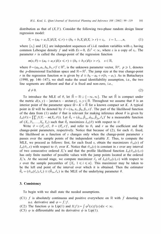
distribution as that of (X; Y ). Consider the following two-phase random design linearregression model:

Yi = (a0 + a1Xi)I(Xi6 r) + (b0 + b1Xi)I(Xi ¿ r) + i; i = 1; : : : ; n; (1)

where { i} and {Xi} are independent sequences of i.i.d. random variables with i havingcommon Lebesgue density f and with E = 0; E 2 ¡∞, where is a copy of 1. Theparameter r is called the change-point of the regression function

m(x; �) = (a0 + a1x)I(x6 r) + (b0 + b1x)I(x¿ r); x∈R;where �=(a0; a1; b0; b1; r)′ ∈R5, is the unknown parameter vector, Rp; p¿ 1, denotesthe p-dimensional Euclidean space and R=R1. The jump size at the true change-pointr in the regression function m is given by d ≡ b0 − a0 + r(b1 − a1). As in Battacharya(1990, pp. 146–147), we shall make the usual identi/ability assumption, i.e., the twoline segments are di2erent and that d is /xed and non-zero, i.e.,

d �= 0: (2)

To introduce the MLE of �, let LR = R ∪ {−∞;∞}. The set LR is compact underthe metric d(x; y) − |arctan x − arctan y|; x; y∈R. Throughout we assume that � is aninterior point of the parameter space �=K × LR for a known compact set K . A typicalpoint in � will be denoted by #=(�0; �1; �0; �1; s)′. The part of the likelihood functionof the data from (1) under # that is relevant for making inference about � is given byLn(#):=

∏n1 f(Yi − m(Xi; #)). Let �n = (a1n; �1n; a2n; �2n; rn)

′ be a measurable functionof (X1; Y1; : : : ; Xn; Yn) such that �n maximizes Ln(#) with respect to #.

Write # = (#′1; s)

′; � = (�′1; r)′, and refer to �1 and r as the coeJcient and the

change-point parameters, respectively. Notice that because of (2), for each #1 /xed,the likelihood as a function of s changes only when the change-point parameter spasses over the sample points of the independent variable X . Thus, to compute theMLE, we proceed as follows: /rst, for each /xed s, obtain the maximizers #1n(s) ofLn(#1; s) with respect to #1 over K . Notice that #1n(s) is constant in s over any intervalof two consecutive ordered Xi’s and that the pro/le likelihood function Ln(#1n(s); s)has only /nite number of possible values with the jump points located at the orderedXi’s. At the second stage, we compute maximizer rn of Ln(#1n(s); s) with respect tos over the sample percentiles of {Xi; 16 i6 n}. This maximizer may be taken tobe the left end point of the interval over which it is obtained. Then the estimator�n = (#1n(rn); rn) ≡ (�1n; rn) is the MLE of the underlying parameter �.

3. Consistency

To begin with we shall state the needed assumptions.

(C1) f is absolutely continuous and positive everywhere on R with f denoting itsa.e. derivative and ’ = f=f.

(C2) The function ’ is Lip(1) and I(f):=∫’2(x)f(x) dx¡∞.

(C3) ’ is di2erentiable and its derivative ’ is Lip(1).


(C4) The r.v. X has a bounded and positive Lebesgue density g on R.(C5) E|X |3 ¡∞.

To proceed further, it is convenient to write m(x; #) =ms(x; #1), for #= (#′1; s)

′ ∈�,and let

ms(x) ≡ (@=@#1)(ms(x; #1))

= (I(x6 s); xI(x6 s); I(x¿ s); xI(x¿ s))′; s∈ LR; x∈R;denote the vector of partial derivatives of ms(x; #1) with respect to #1, and observethat m(x; #) ≡ #′

1ms(x). Let ‖ · ‖ denote the Euclidean norm. Note that

‖ms(x)‖ =√

1 + x2; x∈R; #∈�; (3)

so that for all x∈R; #∗; #∈�,

‖m(x; #)‖6 ‖#1‖√

1 + x2;

‖ms(x; #1) − ms(x; #∗1)‖6 ‖#1 − #∗

1‖√

1 + x2: (4)

Moreover, for x∈R; s∈ LR; t ∈ LR,

‖ms(x) − mt(x)‖6√

2(1 + x2)I(s ∧ t ¡ x6 s ∨ t) (5)

6√

2(1 + x2)I(|x − s|6 |s− t|): (6)

We are now ready to state the strong consistency result. In the sequel, C denotes ageneric positive /nite constant that may be di2erent in di2erent context, but will notdepend on n.

Theorem 3.1. Suppose that (C1) holds; and either

’ is bounded and E|X |¡∞ (7)

or

(C2) holds and EX 2 ¡∞: (8)

Then; �n → �; a.s.; under �; as n → ∞.

Remark 3.1. Let �o be the set of interior points of �. Theorem 3.1 implies thatP(�n ∈�o) → 1 as n → ∞ which in turn implies that P(rn ∈R) → 1 as n → ∞.

Remark 3.2. Examples of the error densities satisfying the conditions of this theoreminclude normal; logistic; double exponential and Student’s tm; m¿ 2.

The following lemma is needed for the proof of the above theorem. Let U*(#) ={#∗=(#∗′

1 ; s∗)′ ∈�: |#∗1−#1|¡*; d(s∗; s)¡*} denote an *-neighborhood of #; *¿ 0,

and let

(x; y; #) = lnf(y − m(x; #))f(y − m(x; �))

; x; y∈R:


Lemma 3.1. Under the assumptions of Theorem 3.1; for any #∈�;

E sup#∗∈U*(#)

| (X; Y; #∗) − (X; Y; #)| → 0 as * → 0: (9)

Proof. Fix a #∈� and let (#)=Y−m(X; #); ,(X; #∗):=m(X; #)−m(X; #∗)=#′1ms(X )−

#∗′1 ms∗(X ); #∗ ∈�. For an *¿ 0; s∈R; let s(*) be de/ned by the relation d(s(*); s)

= *.By (4) and (6), on U*(#) and for an s∈R,

|,(X; #∗)|6 |#′1[ms(X ) − ms∗(X )| + |[#1 − #∗

1 ]′ms∗(X )|

6 [√

2‖#1‖I (|X − s|6 |s∗ − s|) + ‖#1 − #∗1‖]√

(1 + X 2)

6 [√

2‖#1‖I (|X − s|6 |s(*) − s|) + *]√

(1 + X 2)

≡ -(*; X ) (say): (10)

The absolute continuity of ln f, which follows from (C1), and (10) imply that

| (X; Y; #∗) − (X; Y; #)|6∫ -(*; X )

−-(*; X )|’( (#) + v)| dv:

Now, suppose (7) holds. Then the left-hand side of (9) is bounded above byCE-(*; X ). But

E-(*; X )6E(1 + |X |)[√

2‖#1‖I (|X − s|6 |s0(*) − s|) + *] → 0; as * → 0;

thereby proving (9) in this case, for any s∈R.Now assume (8) holds. Rewrite ’( (#)) = [’( +m(X; �)−m(X; #))−’( )] +’( ),

and use (4) to obtain

E’2( (#))6CE[’2( ) + |m(X; �) − m(X; #)|2]

6C[I(f) + (‖�1‖2 + ‖#1‖2)E(1 + X 2)]¡∞:

Thus, by the Cauchy–Schwarz inequality,

LHS of (9)6 E{[|2’( (#))| + L-(*; X )]-(*; X )}6 2(E’2( (#)))1=2(E-2(*; X ))1=2 + LE-2(*; X ):

But, EX 2 ¡∞ implies

E-2(*; X ) = E(1 + X 2)(√

2|#1|I(|X − s|6 |s0(*) − s|) + *)2 → 0; as * → 0;

thereby proving (9) in this case, for any s∈R.In the case s = ∞, similar to (10),

|,(X; #∗)|6 (√

2‖#1‖I(X ¿s∗) + *)√

(1 + X 2)

6 (√

2‖#1‖I(X ¿s0(*)) + *)√

(1 + X 2) ≡ -1(*; X );


where d(s0(*);∞) = *. Again, E|X |j ¡∞ implies E-j1(*; X ) → 0, as * → 0; j = 1; 2.

The proof is similar in the case s=−∞, except one replaces I(X ¿s∗) by I(X ¡s∗)in the above inequality. This completes the proof of Lemma 3.1.

Proof of Theorem 3.1. Let h(x):=(‖�1‖ + ‖#1‖)(1 + |x|). By (C1) and (4),

| (X; Y; #)|6∫ h(X )

−h(X )|’( + v)| dv:

From this it follows that E| (X; Y; #)|¡∞; ∀#∈�, if either (7) or (8) hold. Hencethe function �(#) = E (X; Y; #) for #∈� is well de/ned with �(�) = 0. In view ofLemma 3.1, � is continuous. Use this, the compactness of the parameter space and anargument like the one in Huber (1967) to conclude the theorem.

The next result gives the n-consistency of the estimator rn.

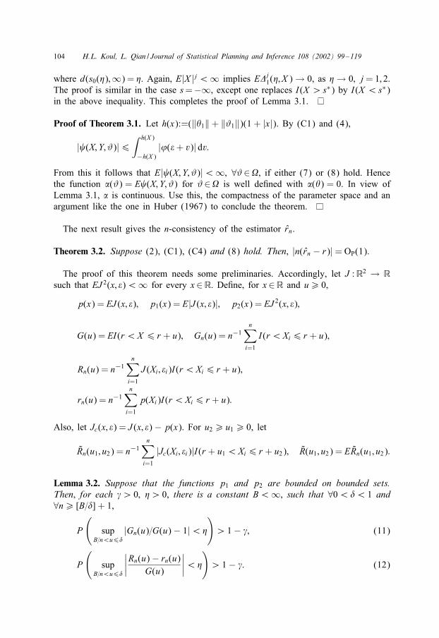
Theorem 3.2. Suppose (2), (C1), (C4) and (8) hold. Then, |n(rn − r)| = OP(1).

The proof of this theorem needs some preliminaries. Accordingly, let J :R2 → Rsuch that EJ 2(x; )¡∞ for every x∈R. De/ne, for x∈R and u¿ 0,

p(x) = EJ (x; ); p1(x) = E|J (x; )|; p2(x) = EJ 2(x; );

G(u) = EI(r ¡X 6 r + u); Gn(u) = n−1n∑

i=1

I(r ¡Xi6 r + u);

Rn(u) = n−1n∑

i=1

J (Xi; i)I(r ¡Xi6 r + u);

rn(u) = n−1n∑

i=1

p(Xi)I(r ¡Xi6 r + u):

Also, let Jc(x; ) = J (x; ) − p(x). For u2¿ u1¿ 0, let

Rn(u1; u2) = n−1n∑

i=1

|Jc(Xi; i)|I(r + u1 ¡Xi6 r + u2); R(u1; u2) = ERn(u1; u2):

Lemma 3.2. Suppose that the functions p1 and p2 are bounded on bounded sets.Then, for each 4¿ 0; *¿ 0, there is a constant B¡∞, such that ∀0¡,¡ 1 and∀n¿ [B=,] + 1,

P

(sup

B=n¡u6,|Gn(u)=G(u) − 1|¡*

)¿ 1 − 4; (11)

P

(sup

B=n¡u6,

∣∣∣∣Rn(u) − rn(u)G(u)

∣∣∣∣¡*

)¿ 1 − 4: (12)


Proof. Details will be given only for (12); they being similar for (11). We begin withthe following elementary facts: under (C4) and the assumed independence; there existsconstants 0¡m6M ¡∞ such that ∀u¿ 0; and ∀n¿ 1;

mu6G(u)6Mu; Var(I(r ¡X 6 r + u))6G(u); Var(nGn(u))6 nG(u):

(13)

The boundedness of the functions p1 and p2 over bounded sets implies that there existsa constant 0¡C ¡∞ such that ∀0¡,¡ 1; u; u1; u2 ∈ [0; ,]; u2¿ u1; and ∀n¿ 1;

R(u1; u2)6C(G(u2) − G(u1)); (14)

Var(|Jc(X; )|I(r + u1 ¡X 6 r + u2))6C(G(u2) − G(u1)); (15)

Var(Rn(u1; u2))6C(G(u2) − G(u1))=n; (16)

Var(Rn(u) − rn(u))6CG(u)=n: (17)

Now we proceed to prove (12). For a B¿ 0 and 0¡,¡ 1, choose a partition ofthe interval (B=n; ,] as follows: /x a b¿ 1 and let N be the greatest integer less thanor equal to ln(n,=B)=ln b. Let Ii = (biB=n; bi+1B=n]; i = 0; : : : ; N − 1; IN = (bNB=n; ,].Note that (B=n; ,] =

⋃Ni=0 Ii. For a u∈ Ii,

|Rn(u) − rn(u)|6 |Rn(u) − rn(u) − (Rn(biB=n) − rn(biB=n)|+ |Rn(biB=n) − rn(biB=n)|

6 Rn(biB=n; u) + |Rn(biB=n) − rn(biB=n)|; 06 i6N:

The /rst term of this bound and G(u) are non-decreasing in u. Hence,

supu∈Ii

∣∣∣∣Rn(u) − rn(u)G(u)

∣∣∣∣6 Rn(biB=n; bi+1B=n)G(biB=n)

+|Rn(biB=n) − rn(biB=n)|

G(biB=n): (18)

By (13) and (17), for any *1 ¿ 0,

P(

max06i6N

∣∣∣∣Rn(biB=n) − rn(biB=n)G(biB=n)

∣∣∣∣¿ *1

)

6N∑i=0

Var{Rn(biB=n) − rn(biB=n)}*2

1G2(biB=n)6C

∑i

1m*2

1Bbi=

Cm*2

1B(1 − b−1)(19)

and, similarly, (13) and (16) yield that

P(

max06i6N

∣∣∣∣ Rn(biB=n; bi+1B=n)G(biB=n)

− R(biB=n; bi+1B=n)G(biB=n)

∣∣∣∣¿ *1

)6C

b*2

1m2B: (20)


By (13) and (14),

max06i6N

∣∣∣∣ R(biB=n; bi+1B=n)G(biB=n)

∣∣∣∣6CbiB(b− 1)=n

mbiB=n6

C(b− 1)m

: (21)

Thus for any 4¿ 0; *¿ 0, one can choose *1 ¿ 0 and b¿ 1 suJciently small suchthat *1 + C(b− 1)=m¡* and then choose suJciently large B such that

B¿2C

m*21(1 − b−1)4

∨ 2bm2*2

14:

Then, (18)–(21) imply (12) for all n¿ [B=,] + 1, in an obvious fashion.

Now, let

J (x; z) ≡ 9(x; z) ≡ lnf(z + a + bx)

f(z); x; z ∈R; (22)

where a= b0 − a0; b= b1 − a1. Note that, for r6 s; 9(Xi; i) ≡ (Xi; Yi; �s), on the setr ¡Xi6 s, for all 16 i6 n, where �′s:=(�′1; s) = (a0; a1; b0; b1; s). De/ne the functionsp; p1 and p2 accordingly, and let, for u¿ 0,

Dn(u) = n−1n∑

i=1

9(Xi; i)I(r ¡Xi6 r + u);

dn(u) = n−1n∑

i=1

p(Xi)I(r ¡Xi6 r + u):

Note that by (C1), for x6y,

E[9(y; ) − 9(x; )]26 b2E(∫ y

x|’( + a + bv)| dv

)2

:

From this it follows that if ’ is bounded then E[9(y; )− 9(x; )]26C(y− x)2, and if(C2) holds, then E[9(y; )− 9(x; )]26C(y− x)[I(f)(y− x) +

∫ yx (a+bv)2 dv]. Similar

bounds hold when x¿y. It follows that 9(·; ) is continuous in L2 under (C1), and ifeither ’ is bounded or (C2) holds. This in turn implies the continuity of p;p1 and p2

under these conditions. Hence, these functions are bounded on bounded sets and thefollowing corollary readily follows from Lemma 3.1.

Corollary 3.1. Suppose that (C1) and (C4) hold and either ’ is bounded or (C2)holds. Then; for every 4¿ 0 and *¿ 0; there is a constant B¡∞ such that ∀0¡,¡ 1 and ∀n¿ [B=,] + 1;

P

(sup

B=n¡u6,

∣∣∣∣Dn(u) − dn(u)G(u)

∣∣∣∣¡*

)¿ 1 − 4:

Next, let

;i(#1; s):=lnf(Yi − #′

1ms(Xi))f(Yi − #′

1mr(Xi)); #1 ∈R4; s∈ LR; 16 i6 n:


Under (C1), the almost everywhere di2erential of ;i with respect to the coeJcientparameter #1 exists and is given by

;i(#1; s) = −’(Yi − #′1ms(Xi))ms(Xi) − ’(Yi − #′

1mr(Xi))mr(Xi)

= −[’(Yi − #′1ms(Xi)) − ’(Yi − #′

1mr(Xi))]ms(Xi)

−’(Yi − #′1mr(Xi))[ms(Xi) − mr(Xi)]

for all 16 i6 n; #1 ∈R4; s∈ LR. Facts (3)–(5) and ’ being Lip(1) imply

‖;1(#1; s)‖6C([‖#1‖ + ‖�1 − #1‖]√

1 + X 2i + |’( i)|)

×√

1 + X 2i I(s ∧ r ¡Xi6 s ∨ r); 16 i6 n; #1 ∈R4; s∈ LR:

(23)

we are now ready to give the

Proof of Theorem 3.2. Let ln(#1; s):=n−1∑ni=1 ln [f(Yi−#′

1ms(Xi))=f(Yi−�′1mr(Xi))].Rewrite

ln(#1; s) − ln(#1; r) = [ln(#1; s) − ln(#1; r) − (ln(�1; s) − ln(�1; r))]

+[ln(�1; s) − ln(�1; r)]

≡ l1n(#) + l2

n(s) (say):

It suJces to show that ln(#1; s)−ln(#1; r) is negative for n|s−r| large enough. Since�n is strongly consistent by Theorem 3.1, without a loss of generality, the parameterspace can be restricted to a neighborhood of �, say,

�(,) = {#∈�: ‖#1 − �1‖¡,; |s− r|¡,};for some 0¡,¡ 1 to be determined later. More precisely, we shall show that ∀4¿ 0;∃aB¡∞; 41 ¿ 0; 0¡,¡ 1 and an n0 such that

P

(sup

B=n¡|s−r|6,;#∈�(,)

[ln(#1; s) − ln(#1; r)]G(|s− r|) ¡− 41

)¿ 1 − 24 ∀n¿n0: (24)

But this will be implied by showing that ∀4¿ 0; ∃aB¡∞; 41 ¿ 0; 0¡,¡ 1 and ann0 such that ∀n¿n0,

P

(sup

B=n¡|s−r|6,;#∈�(,)

∣∣∣∣ l1n(#)

G(|s− r|)∣∣∣∣¿41

)¡4 (25)

and

P

(sup

B=n¡|s−r|6,

l2n(s)

G(|s− r|) ¡− 241

)¿ 1 − 4: (26)


The details will be given for the case s¿ r only, they being similar for the case s¡ r.Write s = r + u for some u¿ 0.

To prove (25), by the absolute continuity of ;i for each i,

l1n(#) ≡ n−1

n∑i=1

[;i(#1; s) − ;i(�1; s)]

= n−1n∑

i=1

∫ 1

0;′i(�1 + v(#1 − �1); s) dv(#1 − �1):

Now apply (23) with s=r+u; u¿ 0, and use the fact 1+x26 3+3r2; 1+|x|6 2+2ron the set r ¡x6 r + u; 0¡u6 ,¡ 1, to obtain, for all #∈�(,),

|l1n(#)|6C,

[Gn(u) + n−1

n∑i=1

|’( i)|I(r ¡Xi6 r + u)

]:

Take J (x; y) = |’(y)| in the de/nitions of Rn and rn. Note that here rn(u) = Gn(u) E|’( )|. Use this to /nally conclude that for all #∈V(,),∣∣∣∣ l1

n(#)G(u)

∣∣∣∣6C,[∣∣∣∣Gn(u)

G(u)

∣∣∣∣+∣∣∣∣Rn(u) − rn(u)

G(u)

∣∣∣∣]:

This together with Lemma 3.2 implies (25) in an obvious fashion.To prove (26), recall that a = b0 − a0; b = b1 − a1 and rewrite

l2n(r + u) = n−1

n∑i=1

9(Xi; i)I(r ¡Xi6 r + u)

= n−1n∑

i=1

[ln

f( i + a + bXi)f( i)

− p(Xi)]I(r ¡Xi6 r + u)

+ n−1n∑

i=1

[p(Xi) − p(r)]I(r ¡Xi6 r + u) + p(r)Gn(u)

= [Dn(u) − dn(u)] + En(u) + p(r)Gn(u) (say);

where p(x) = E9(x; ) and Dn; dn are as in Corollary 3.1. Thus, for all u¿ 0,

l2n(r + u)G(u)

6{∣∣∣∣Dn(u) − dn(u)

G(u)

∣∣∣∣+∣∣∣∣En(u)G(u)

∣∣∣∣+∣∣∣∣Gn(u)G(u)

− 1∣∣∣∣ |p(r)|

}+ p(r): (27)

Recall that d = a + br, and in view of (2) and the fact ln x¡x − 1; x �= 1,

p(r) =∫

ln[f(x + a + br)=f(x)] dF(x)¡ 0:


Also, for all u6 ,; |En(u)|6 sup06x6, |p(r + x)−p(r)|Gn(u). Thus, by (11) and thecontinuity of p; supB=n¡u6, |En(u)=G(u)| = op(1), as n → ∞ and then , → 0. Thisfact, (11), (27) and Corollary 3.1 now readily imply (26) with 41:=[ − p(r) − *(2 +|p(r)|)]=2¿ 0 in an obvious fashion.

4. Limiting distributions

This sections gives the limiting distribution of the MLE and the weak limit ofthe likelihood process with respect to the standardized change-point parameter. First,focus on the limiting distribution of �1n. Analogous to Lemma 3.1, we have a uniformconsistency result:

Lemma 4.1. Suppose (C1); (C2) hold and EX 2 ¡∞. Then; ∀0¡B¡∞;

sup|s−r|6B=n

|#1n(s) − �1| = oP(1):

The proof of this lemma is facilitated by the fact that under the assumed conditions,∀#1 ∈K ,

E sups∈ LR;#∗

1 ∈U#1 (*)| (X; ; #∗

1 ; s) − (X; ; #1; s)| → 0; as * → 0;

where U#1 (*)={#∗1 ∈K : |#∗

1 −#1|¡*}; *¿ 0. The proof of this fact in turn is similarto, and a bit simpler than, that of Lemma 3.1. The proof of Lemma 4.1 uses this factin a similar fashion as Lemma 3.1 is used in the proof of Theorem 3.1. Details areleft out for the sake of brevity.

To state the next result that gives the uniform CLT for #1n(s), we need to de/ne

ui(#1; s) ≡ −’(Yi − #′1ms(Xi))ms(Xi); As(x) ≡ ms(x)ms(x)′;

i¿ 1; (#1; s)∈�; x∈R:

Theorem 4.1. Suppose that conditions (C1)–(C5) hold. Then; ∀0¡B¡∞;

sup|s−r|6B=n

∣∣∣∣∣∣n1=2(#1n(s) − �1) + >−1n−1=2∑

uir(�1)∣∣∣∣∣∣= oP(1): (28)

Consequently;

sup|s−r|6B=n

n1=2(#1n(s) − �1) ⇒ N (0; >−1); >:=I(f)Emr(X )mr(X )′:

Proof. Let ln(#1; s) denote the partial di2erential of ln(#1; s); w.r.t. #1. Note thatln(#1; s) = n−1∑n

i=1 ui(#1; s). Clearly; ln(#1n(s); s) ≡ 0; and Taylor’s expansion of


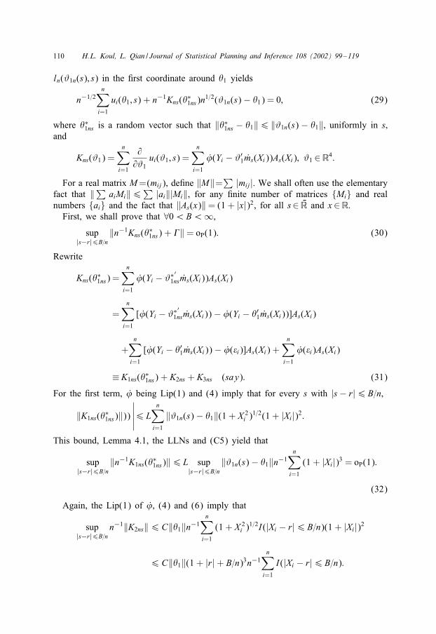
ln(#1n(s); s) in the /rst coordinate around �1 yields

n−1=2n∑

i=1

ui(�1; s) + n−1Kns(�∗1ns)n1=2(#1n(s) − �1) = 0; (29)

where �∗1ns is a random vector such that ‖�∗1ns − �1‖6 ‖#1n(s) − �1‖; uniformly in s;and

Kns(#1) =n∑

i=1

@@#1

ui(#1; s) =n∑

i=1

’(Yi − #′1ms(Xi))As(Xi); #1 ∈R4:

For a real matrix M =(mij), de/ne ‖M‖=∑ |mij|. We shall often use the elementary

fact that ‖∑ aiMi‖6∑ |ai‖|Mi‖, for any /nite number of matrices {Mi} and real

numbers {ai} and the fact that ‖As(x)‖ = (1 + |x|)2, for all s∈ LR and x∈R.First, we shall prove that ∀0¡B¡∞,

sup|s−r|6B=n

‖n−1Kns(�∗1ns) + >‖ = oP(1): (30)

Rewrite

Kns(�∗1ns) =n∑

i=1

’(Yi − #∗′1nsms(Xi))As(Xi)

=n∑

i=1

[’(Yi − #∗′1nsms(Xi)) − ’(Yi − �′1ms(Xi))]As(Xi)

+n∑

i=1

[’(Yi − �′1ms(Xi)) − ’( i)]As(Xi) +n∑

i=1

’( i)As(Xi)

≡K1ns(�∗1ns) + K2ns + K3ns (say): (31)

For the /rst term, ’ being Lip(1) and (4) imply that for every s with |s− r|6B=n,

‖K1ns(�∗1ns)‖))

∣∣∣∣∣6Ln∑

i=1

‖#1n(s) − �1‖(1 + X 2i )1=2(1 + |Xi|)2:

This bound, Lemma 4.1, the LLNs and (C5) yield that

sup|s−r|6B=n

‖n−1K1ns(�∗1ns)‖6L sup|s−r|6B=n

‖#1n(s) − �1‖n−1n∑

i=1

(1 + |Xi|)3 = oP(1):

(32)

Again, the Lip(1) of ’, (4) and (6) imply that

sup|s−r|6B=n

n−1‖K2ns‖6C‖�1‖n−1n∑

i=1

(1 + X 2i )1=2I(|Xi − r|6B=n)(1 + |Xi|)2

6C‖�1‖(1 + |r| + B=n)3n−1n∑

i=1

I(|Xi − r|6B=n):


Hence, by (C4),

E sup|s−r|6B=n

‖n−1K2ns‖6C‖�1‖(1 + |r| + B=n)3[G(r + B=n) − G(r − B=n)]

= O(n−1): (33)

For K3ns, observe that ‖As(x)−Ar(x)‖6 2(1 + |x|)2I(|x− r|6 |s− r|), for all x∈R.This and an argument like the one used for (33), imply that

E sup|s−r|6B=n

‖As(X ) − Ar(X )‖6 2(1 + |r| + B=n)2EI(|X − r|6B=n) = O(n−1):

Also, by the LLNs, ‖n−1∑ni=1 ’( i)Ar(Xi) + >‖ = oP(1). These facts together with

the triangle inequality now readily yield sup|s−r|6B=n‖n−1K3ns + >‖ = oP(1). Put thistogether with (31)–(33) to obtain (30).

Next, we shall show that ∀0¡B¡∞,

E

[sup

|s−r|6B=n

∣∣∣∣∣∣∣∣∣∣n−1=2

n∑i=1

[uis(�1) − uir(�1)]

∣∣∣∣∣∣∣∣∣∣]

= O(n−1=2): (34)

Rewriten∑

i=1

[uis(�1) − uir(�1)] =n∑

i=1

[ − ’( i + �′1mr(Xi) − �′1ms(Xi)) + ’( i)]ms(Xi)

−n∑

i=1

’( i)[ms(Xi) − mr(Xi)]

≡ I1ns − I2ns (say):

The Lip(1) property of ’, (6), and an argument like the one used for (33), yield

E sup|s−r|6B=n

∣∣∣∣n−1=2I1ns∣∣∣∣6 Ln1=2(1 + (|r| + B=n)2)[G(r + B=n) − G(r − B=n)]

= O(n−1=2): (35)

Similarly, the independence of { i} and {Xi}, the LLNs, the integrability of ’ and(6) imply that E(sup|s−r|6B=n‖n−1=2I2ns‖) = O(n−1=2), which together with (35) readilyyields (34).

The inequalities

EI(X 6 r)EX 2I(X 6 r)¿ (EXI(X 6 r))2;EI(X ¿r)EX 2I(X ¿r)¿ (EXI(X ¿r))2;

imply that EAr(X ) and > are positive de/nite. Hence, sup|s−r|6B=n ‖>−1ns −>−1‖=oP(1),

where >ns = −Kns(�∗1ns)=n. This fact, (29) and (35) together imply (28). The proof ofTheorem 4.1 is completed by applying the CLT to {uir(�1)}.


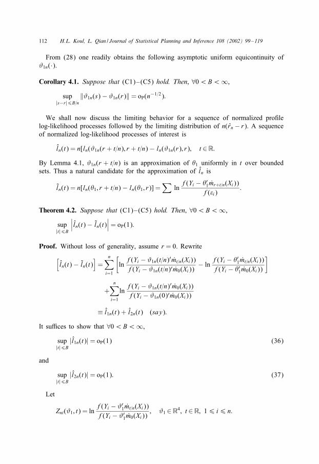
From (28) one readily obtains the following asymptotic uniform equicontinuity of#1n(·).

Corollary 4.1. Suppose that (C1)–(C5) hold. Then, ∀0¡B¡∞,

sup|s−r|6B=n

‖#1n(s) − #1n(r)‖ = oP(n−1=2):

We shall now discuss the limiting behavior for a sequence of normalized pro/lelog-likelihood processes followed by the limiting distribution of n(rn − r). A sequenceof normalized log-likelihood processes of interest is

ln(t) = n[ln(#1n(r + t=n); r + t=n) − ln(#1n(r); r); t ∈R:By Lemma 4.1, #1n(r + t=n) is an approximation of �1 uniformly in t over boundedsets. Thus a natural candidate for the approximation of ln is

ln(t) = n[ln(�1; r + t=n) − ln(�1; r)] =∑

lnf(Yi − �′1mr+t=n(Xi))

f( i):

Theorem 4.2. Suppose that (C1)–(C5) hold. Then, ∀0¡B¡∞,

sup|t|6B

∣∣∣ln(t) − ln(t)∣∣∣= oP(1):

Proof. Without loss of generality, assume r = 0. Rewrite

[ln(t) − ln(t)

]=

n∑i=1

[ln

f(Yi − #1n(t=n)′mt=n(Xi))f(Yi − #1n(t=n)′m0(Xi))

− lnf(Yi − �′1mt=n(Xi))f(Yi − �′1m0(Xi))

]

+n∑

i=1

lnf(Yi − #1n(t=n)′m0(Xi))f(Yi − #1n(0)′m0(Xi))

≡ l1n(t) + l2n(t) (say):

It suJces to show that ∀0¡B¡∞,

sup|t|6B

|l1n(t)| = oP(1) (36)

and

sup|t|6B

|l2n(t)| = oP(1): (37)

Let

Zni(#1; t) = lnf(Yi − #′

1mt=n(Xi))f(Yi − #′

1m0(Xi)); #1 ∈R4; t ∈R; 16 i6 n:


Note that l1n(t)=∑n

i=1 [Zni(#1n; (t=n); t)−Zni(�1; t)]. In view of Theorem 4.1, (36) willfollow from the following stronger result: ∀0¡b¡∞,

E

{sup

|t|6B;n−1=2‖#1−�1‖6b

∣∣∣∣∣n∑

i=1

[Zni(#1; t) − Zni(�1; t)]

∣∣∣∣∣}

= O(n−1=2): (38)

To prove this, let

Zni(#1; t) = −’(Yi − #′1mt=n(Xi))mt=n(Xi) + ’(Yi − #′

1m0(Xi))m0(Xi)

= [ − ’(Yi − #′1mt=n(Xi)) + ’(Yi − #′

1m0(Xi))]mt=n(Xi)

+[ − ’(Yi − #′1m0(Xi)) + ’( i)][mt=n(Xi) − m0(Xi)]

−’( i)[mt=n(Xi) − m0(Xi)]; #1 ∈R4; t ∈R; 16 i6 n: (39)

Let #14 = �1 + 4(#1 − �1); 06 46 1. By the absolute continuity of ln f,

Zni(#1; t) − Zni(�1; t) =∫ 1

0Zni(#14; t)′d4(#1 − �1)

≡U1i(#1; t) + U2i(#1; t) + U3i(#1; t) (say);

where, by (39),

U1i(#1; t) =∫ 1

0[ − ’(Yi − #′

14mt=n(Xi))+’(Yi − #′14m0(Xi))]mt=n(Xi)′ d4(#1−�1);

U2i(#1; t) =∫ 1

0[ − ’(Yi − #′

14m0(Xi)) + ’( i)][mt=n(Xi) − m0(Xi)]′ ds(#1 − �1);

U3i(#1; t) = −’( i)[mt=n(Xi) − m0(Xi)]′(#1 − �1):

Write - for n1=2(#1 − �1). Now, ’ being Lip(1), (3), (5) and (6) imply that

sup|t|6B;‖-‖6b

|U1i(#1; t)|B=n)

6Cn−1=2[‖�1‖ + bn−1=2](1 + X 2i )I(|Xi|6B=n);

so that by (C4), and arguing as for (33), we obtain

E

{sup

|t|6B;‖-‖6b

∣∣∣∣∣n∑

i=1

U1i(#1; t)

∣∣∣∣∣}

= O(n−1=2):

Analogously, one proves

E

{sup

|t|6B;‖-‖6b

∣∣∣∣∣n∑

i=1

U2i(#1; t)

∣∣∣∣∣}

= O(n−1); E

{sup

|t|6B;‖-‖6b

∣∣∣∣∣n∑

i=1

U3i(#1; t)

∣∣∣∣∣}

= O(n−1=2):

This completes the proof of (38).


To prove (37), we shall need Corollary 4.1. Recall that

l2n(t) =n∑

i=1

lnf(Yi − #1n(t=n)′m0(Xi))f(Yi − #1n(0)′m0(Xi))

:

For a t ∈R, let #1nu(t) =#1n(0) + u(#1n(t=n)−#1n(0)); 06 u6 1. Then the absolutelycontinuity of ln f gives

l2n(t) =n∑

i=1

∫ 1

0[ − ’(Yi − #1nu(t)′m0(Xi)) + ’( i)]du m0(Xi)′(#1n(t=n) − #1n(0))

−n∑

i=1

’( i)m0(Xi)′(#1n(t=n) − #1n(0)):

Thus, (C2), (3), (5), Theorem 4.1 and Corollary 4.1 imply that the /rst term in theabove decomposition is bounded above uniformly in |t|6B by

L sup|t|6B

‖#1n(t=n) − #1n(0)‖n∑

i=1

‖m0(Xi)‖∫ 1

0|#1nu(t)′m0(Xi) − �′1m0(Xi)| du

6 oP(n−1=2) sup

|t|6B‖#1n(t) − �1‖

n∑i=1

(1 + X 2i ) = oP

(n−1=2)OP

(n−1=2)OP(n)

=oP(1):

The second term of l2n(t) is uniformly oP(1), because of Corollary 4.1 and be-cause, by the CLT, |∑’( i)m0(Xi)|= OP

(n1=2). This completes the proof of (37) and

Theorem 4.2.

Next, we shall describe the weak limit of the sequence ln. Let g denote Lebesgue

density of X and let {l (1)(t); t¿ 0} and {l (2)

(t); t¿ 0} be two independent compound

Poisson processes, both with rate g(r), such that the following hold: l(1)

(0)=l(2)

(0)=0,a.s.; the distribution of jumps being given by the conditional distribution of ln[f( +a+bX )=f( )], given X = r+ and the conditional distribution of ln[f( −a−bX )=f( )]given X = r−, respectively. The former is the limiting conditional distribution of @1

given r ¡X 6 r + , as , ↓ 0 and the latter is that of @2 given r − ,¡X 6 r as, ↓ 0. By the independence of X and , these distributions are equivalent to that ofln[f( + a + br)=f( )] and ln[f( − a− br)=f( )], respectively.

Theorem 4.3. Suppose (C1) and (C4) hold and the density g of the r.v. X is con-tinuous and positive at r. Then ({ln(−t); t¿ 0}; {ln(t); t¿ 0}) converges weakly to

({l(1)(t); t¿ 0}; {l(2)

(t); t¿ 0}) in D[0;∞) × D[0;∞); the product space beingequipped with the product Skorokhod metric.


Proof. We shall sketch the proof for the case t¿ 0 only; it being similar in the caset6 0. With 9 as in (22); rewrite h = 9 and

ln(t) =n∑

j=1

h(Xj; j)I(r ¡Xj6 r + t=n); t¿ 0:

Thus; ln is a pure jump process in D[0;∞) and its tightness follows from (C4) andan argument similar to the one used in the proof of Lemma 3.2 in Ibragimov andHas’minskii (1981; p. 261). Take Ai of this lemma to be the event that the samplepath of ln has at least i discontinuities on the interval (u; u+,]; u¿ 0; 06 i6 n. Then;by (C4); P(A1)6

∑ni=1 P(r ¡Xi6 r+t=n)6C,; P(A2)6

∑ni �=j=1 P(r ¡Xi; Xj6 r+

t=n)6C,2. The rest of the argument is similar to that of the cited lemma. Details areomitted for the sake of brevity.

To prove the convergence of the /nite dimensional distributions, we shall showthat the joint characteristic function of /nite dimensional increments of the process lnconverges to that of the said compound process. Let

A(x; u):=E(exp{iuh(X; )} |X = x) = E exp{iuh(x; )}; x; u∈R:Note that the continuity of f implies that A is continuous in x, for each u∈R. Fora positive integer m, let t0 = 0¡t1 ¡t2 ¡ · · ·¡tm ¡∞ be m positive numbers.Using also the continuity of g at r, the joint characteristic function of the incre-ments ln(t1); ln(t2) − ln(t1); : : : ; ln(tm) − ln(tm−1) behaves as follows in the limit asn → ∞:

E exp

{i

m∑k=1

uk [ln(tk) − ln(tk−1)]

}

=E exp

i

m∑k=1

uk

n∑j=1

h(Xj; j)I(r +

tk−1

n¡Xj6 r +

tkn

)

=

(E exp

{h(X; )

m∑k=1

iukI(r +

tk−1

n¡X 6 r +

tkn

)})n

=

m∑

k=1

∫ r+tkn

r+tk−1

n

A(x; uk)g(x)dx + 1 −m∑

k=1

[G(r +

tkn

)− G

(r +

tk−1

n

)]n

→ exp

{−

m∑k=1

(tk − tk−1)g(r){1 − A(r; uk)}}

∀(u1; : : : ; um)∈Rm:

This limit is seen to be the joint characteristic function of the increments

(l(1)

(t1); l(1)

(t2) − l(1)

(t1); : : : ; l(1)

(tm) − l(1)

(tm−1));


where l(1)

is the compound Poisson process describe above. This completes the sketchof the proof of the theorem.

Let l(t)= l(1)

(−t)I(t6 0)+ l(2)

(t)I(t¿ 0); t ∈R. The two random walks associatedwith this processes tend to −∞, a.s., as |t| → ∞ which implies the existence of theunique random interval [M−; M+) on which the process {l(t): t ∈R} attains its globalmaximum, a.s. This leads us to

Theorem 4.4. Suppose that conditions (C1)–(C5); (2) hold and g is continuous andpositive at r. Then; n(rn − r) converges weakly to M− and n1=2(�1n − �1) convergesweakly to a N (0; >−1) r.v.

Proof. This proof is similar to that of Theorem V.4.6 in Ibragimov and Has’minskii(1981; p. 271). For any l∈D ≡ D(−∞;∞); and any x∈R; de/ne the functionals onD as follows:

Sx(l) = supt¿x

l(t); sx(l) = supt6x

l(t):

By the de/nition of rn and M−; we have

P(n(rn − r)¿x) = P(Sx(ln) − sx(ln)¿ 0) and

P(M− ¿x) = P(Sx(l) − sx(l)¿ 0):

The functionals Sx and sx are continuous in D on those elements l∈D that are contin-uous at x. Let x be a continuity point of the distribution of M−. Then; P(M− = x) = 0and the de/nition of M− implies that x is also a continuity point of the realizationof l with probability 1. Hence; Sx and sx are continuous functionals with probability 1.Therefore; Theorems 4.2 and 4.3 and Theorem 9.5.2 (Gikhman and Skorokhod; 1969;p. 477) imply that

P(n(rn − r)¿x) = P(Sx(ln) − sx(ln)¿ 0) → P(Sx(l) − sx(l)¿ 0)

= P(M− ¿x); n → ∞:

The claim about �1n follows in an obvious fashion from Theorem 3.2 andCorollary 4.1.

5. Simulation results

This section gives results from a Monte Carlo study of the above MLEs. In thisstudy, the samples were generated from model (1) with � = (0:5;−1;−0:7; 1; 0), andfor three di2erent error distributions: N(0; 1), logistic (1; 1), and t4. Table 1 providesthe sample means and mean squared errors of the MLEs of the true parameter vector �.


Table 1Monte Carlo means (Mean) and mean square errors (MSE) of MLEs of � = (0:5;−1;−0:7; 1; 0), in thetwo-phase regression model with 500 replicates

MLE True Error distribution

N(0; 1) Logistic (1; 1) t(4)

Mean (MSE) Mean (MSE) Mean (MSE)

(n = 100)r 0.0 0.0743 (0.0781) 0.0426 (0.0652) 0.0231 (0.0383)a0 0.5 0.5284 (0.0838) 0.6105 (0.3418) 0.5608 (0.1288)a1 −1.0 −0.9844 (0.0750) −0.9234 (0.2970) −0.9592 (0.1279)b0 −0.7 −0.6857 (0.2127) −0.7824 (0.5723) −0.7611 (0.1995)b1 1.0 0.9979 (0.1261) 1.0875 (0.3911) 1.0567 (0.1446)

(n = 200)r 0.0 0.0256 (0.0231) 0.0183 (0.0191) 0.0552 (0.0543)a0 0.5 0.5098 (0.0341) 0.5252 (0.0528) 0.5196 (0.0522)a1 −1.0 −0.9918 (0.0314) −0.9836 (0.0479) −0.9825 (0.0492)b0 −0.7 −0.7226 (0.0489) −0.7301 (0.0696) −0.6798 (0.1671)b1 1.0 1.0189 (0.0362) 1.0270 (0.0594) 0.9964 (0.0897)

(n = 500)r 0.0 0.0071 (0.0076) 0.0066 (0.0041) 0.0028 (0.0039)a0 0.5 0.5274 (0.0243) 0.5041 (0.0195) 0.5110 (0.0177)a1 −1.0 −0.9727 (0.0241) −0.9984 (0.0181) −0.9872 (0.0173)b0 −0.7 −0.7239 (0.0365) −0.7101 (0.0192) −0.7150 (0.0193)b1 1.0 1.0185 (0.0277) 1.0027 (0.0173) 1.0068 (0.0175)

The sample sizes used are 100, 200 and 500, and for each sample size, the results arebased on 500 replications.

From Table 1, we see that the consistency of the estimates is shown by theirmeans and mean squared errors computed from the average value of the squared de-viation from the true parameters. Over all, we can see that the MSEs are smallerfor the change-point estimates than ones for the coeJcient estimates. This illustratesthe n-consistency of the change-point estimate. Typically, as n increases (for examplen = 500), Table 1 shows that the estimates of the change-point approach to the trueparameter much faster than the coeJcient parameter estimates.

Table 2 shows the empirical coverages of the estimates of the true parameters withintwo standard deviations from the sample means for n= 100; 200 and 500, respectively.One observes that the estimates have very high percent coverage within two standarddeviations from the simulated sample means. For the change-point estimator, it is seenthat as the sample size increases, the coverage increases dramatically with the coveragerange from 91.4% to 98.6%, while the range of the coverage for the coeJcient param-eters is from 93.6% to 97.6%. This also con/rms the n-consistency of the change-pointestimator.


Table 2The empirical coverage probabilities of the estimates within two standard deviations from the sample means

True Error distribution

N(0; 1) Logistic (1; 1) t(4)

(n = 100)r 0.0 0.914 0.928 0.926a0 0.5 0.960 0.962 0.944a1 −1.0 0.954 0.958 0.940b0 −0.7 0.946 0.936 0.952b1 1.0 0.949 0.942 0.946

(n = 200)r 0.0 0.959 0.950 0.933a0 0.5 0.950 0.934 0.953a1 −1.0 0.960 0.938 0.948b0 −0.7 0.965 0.950 0.961b1 1.0 0.964 0.948 0.964

(n = 500)r 0.0 0.980 0.980 0.986a0 0.5 0.950 0.944 0.960a1 −1.0 0.948 0.944 0.954b0 −0.7 0.976 0.960 0.962b1 1.0 0.968 0.952 0.950

References

Battacharya, P.K., 1990. Weak convergence of the log-likelihood process in the two-phase linear regressionproblem. In Probability, Statistics and Design of Experiments, Wiley Eastern, New Delhi, pp. 145–156.

Battacharya, P.K., 1994. Some Aspects of Change-point analysis, IMS Lecture Notes-Monograph Series,Vol. 23, Inst. Math. Statist., Hayward, CA, pp. 28–56.

CsGorgo, M., HorvHath, L., 1988. Nonparametric methods for change point problems. In: Krishnaiah, P.R.,Rao, C.R. (Eds.), Handbook of Statistis, 7. Elsevier, Amsterdam, pp. 403–425.

Feder, P.I., 1975a. On asymptotic distribution theory in segmented regression problems-identi/ed case. Ann.Statist. 3, 49–83.

Feder, P.I., 1975b. The log likelihood ratio in segmented regression. Ann. Statist. 3, 84–97.Gikhman, I.I., Skorokhod, A.V., 1969. Introduction to the Theory of Random Processes. W.B. Saunders

Company, Philadelphia.Hinkley, D.V., 1969. Inference about the intersection in two-phase regression. Biometrika 56, 495–504.Hinkley, D.V., 1971. Inference in two-phase regression. J. Amer. Statist. Assoc. 66, 736–743.Huber, P.J., 1967. The behavior of maximum likelihood estimates under nonstandard conditions. Proceedings

of the Fifth Berkeley Symposium on Mathematical Statistics & Probability, Vol. 1, University of CaliforniaPress, Berkeley, pp. 221–234.

Hudson, D.J., 1966. Fitting segmented curves whose join points have to be estimated. J. Amer. Statist. Assoc.61, 1097–1129.

Ibragimov, I.A., Has’minskii, R.Z., 1981. Statistical Estimation: Asymptotic Theory, Vol. 16. Springer, Berlin.Loader, C.R., 1996. Change point estimation using nonparametric regression. Ann. Statist. 24 (4), 1667–1678.MGuller, H.G., 1992. Change-point in nonparametric regression analysis. Ann. Statist 20 (2), 737–761.MGuller, H.G., Song, K.S., 1997. Two-stage change-point estimators in smooth regression models. Statist.

Probab. Lett. 34, 323–335 (time series).


Schulze, U., 1987. Multiphase Regression: Stability esting, Estimation, Hypothesis Testing. Akademie-Verlag,Berlin. ISBN 3-05-500224-5

van de Geer, S., 1988. Regression Analysis and Empirical Processes, CWI tract Vol. 45. Amsterdam, NL.Wu, J.S., Chu, C.K., 1993. Kernel-type estimators of jump points and values of a regression function. Ann.

Statist. 21 (3), 1545–1566.

Journal of Statistical Planning and Inference 108 - Department of

Documents