Journal of Financial Economics 122 (2016) 221–247 Contents lists available at ScienceDirect Journal of Financial Economics journal homepage: www.elsevier.com/locate/jfec Momentum crashes Kent Daniel a,b , Tobias J. Moskowitz b,c,∗ a Columbia Business School, New York, NY USA b National Bureau of Economic Research, Cambridge, MA, USA c Yale SOM, Yale University, New Haven, CT, USA a r t i c l e i n f o Article history: Received 22 October 2013 Revised 17 June 2015 Accepted 17 December 2015 Available online 1 September 2016 JEL Classification: G12 Keywords: Asset pricing Market anomalies Market efficiency Momentum a b s t r a c t Despite their strong positive average returns across numerous asset classes, momentum strategies can experience infrequent and persistent strings of negative returns. These mo- mentum crashes are partly forecastable. They occur in panic states, following market de- clines and when market volatility is high, and are contemporaneous with market rebounds. The low ex ante expected returns in panic states are consistent with a conditionally high premium attached to the option like payoffs of past losers. An implementable dynamic momentum strategy based on forecasts of momentum’s mean and variance approximately doubles the alpha and Sharpe ratio of a static momentum strategy and is not explained by other factors. These results are robust across multiple time periods, international equity markets, and other asset classes. © 2016 The Authors. Published by Elsevier B.V. This is an open access article under the CC BY license (http://creativecommons.org/licenses/by/4.0/). 1. Introduction A momentum strategy is a bet on past returns pre- dicting the cross section of future returns, typically im- plemented by buying past winners and selling past losers. Momentum is pervasive: the academic literature shows the efficacy of momentum strategies across multiple time pe- riods, in many markets, and in numerous asset classes. 1 ∗ Corresponding author at: Yale School of Management, New Haven, CT USA. Tel: (203) 436-5361; Fax: (203) 742-3257. E-mail address: [email protected] (T.J. Moskowitz). 1 Momentum strategies were first shown in US common stock re- turns from 1965 to 1989 by Jegadeesh and Titman (1993) and Asness (1994), by sorting firms on the basis of three- to 12-month past re- turns. Subsequently, Jegadeesh and Titman (2001) show the continuing efficacy of US equity momentum portfolios in common stock returns in the 1990 to 1998 period. Israel and Moskowitz (2013) show the robust- ness of momentum prior to and after these studies from 1927 to 1965 and from 1990 to 2012. Evidence of momentum going back to the Vic- torian age from Chabot, Ghysels, and Jagannathan (2009) and for 1801 to 2012 from Geczy and Samonov (2015) in what the authors call “the world’s longest backtest.” Moskowitz and Grinblatt (1999) find momen- tum in industry portfolios. Rouwenhorst (1998); 1999) finds momentum However, the strong positive average returns and Sharpe ratios of momentum strategies are punctuated with occasional crashes. Like the returns to the carry trade in currencies (e.g., Brunnermeier, Nagel, and Pedersen, 2008), momentum returns are negatively skewed, and the neg- ative returns can be pronounced and persistent. In our 1927–2013 US equity sample, the two worst months for a momentum strategy that buys the top decile of past 12- month winners and shorts the bottom decile of losers are consecutive: July and August of 1932. Over this short pe- riod, the past-loser decile portfolio returned 232% and the past-winner decile portfolio had a gain of only 32%. In a more recent crash, over the three-month period from March to May of 2009, the past-loser decile rose by 163% and the decile portfolio of past winners gained only 8%. in developed and emerging equity markets, respectively. Asness, Liew, and Stevens (1997) find momentum in country indices. Okunev and White (2003) find momentum in currencies; Erb and Harvey (2006) in com- modities and Moskowitz, Ooi, and Pedersen (2012) in exchange traded futures contracts. Asness, Moskowitz, and Pedersen (2013) integrate this evidence across markets and asset classes and find momentum in bonds as well. http://dx.doi.org/10.1016/j.jfineco.2015.12.002 0304-405X/© 2016 The Authors. Published by Elsevier B.V. This is an open access article under the CC BY license (http://creativecommons.org/licenses/by/4.0/).

Welcome message from author
This document is posted to help you gain knowledge. Please leave a comment to let me know what you think about it! Share it to your friends and learn new things together.
Transcript

Journal of Financial Economics 122 (2016) 221–247 Contents lists available at ScienceDirect
Journal of Financial Economics journal homepage: www.elsevier.com/locate/jfec
Momentum crashes Kent Daniel a , b , Tobias J. Moskowitz b , c , ∗a Columbia Business School, New York, NY USA b National Bureau of Economic Research, Cambridge, MA, USA c Yale SOM, Yale University, New Haven, CT, USA a r t i c l e i n f o Article history: Received 22 October 2013 Revised 17 June 2015 Accepted 17 December 2015 Available online 1 September 2016 JEL Classification: G12 Keywords: Asset pricing Market anomalies Market efficiency Momentum
a b s t r a c t Despite their strong positive average returns across numerous asset classes, momentum strategies can experience infrequent and persistent strings of negative returns. These mo- mentum crashes are partly forecastable. They occur in panic states, following market de- clines and when market volatility is high, and are contemporaneous with market rebounds. The low ex ante expected returns in panic states are consistent with a conditionally high premium attached to the option like payoffs of past losers. An implementable dynamic momentum strategy based on forecasts of momentum’s mean and variance approximately doubles the alpha and Sharpe ratio of a static momentum strategy and is not explained by other factors. These results are robust across multiple time periods, international equity markets, and other asset classes.
© 2016 The Authors. Published by Elsevier B.V. This is an open access article under the CC BY license
( http://creativecommons.org/licenses/by/4.0/ ). 1. Introduction
A momentum strategy is a bet on past returns pre- dicting the cross section of future returns, typically im- plemented by buying past winners and selling past losers. Momentum is pervasive: the academic literature shows the efficacy of momentum strategies across multiple time pe- riods, in many markets, and in numerous asset classes. 1
∗ Corresponding author at: Yale School of Management, New Haven, CT USA. Tel: (203) 436-5361; Fax: (203) 742-3257.
E-mail address: [email protected] (T.J. Moskowitz). 1 Momentum strategies were first shown in US common stock re-
turns from 1965 to 1989 by Jegadeesh and Titman (1993) and Asness (1994) , by sorting firms on the basis of three- to 12-month past re- turns. Subsequently, Jegadeesh and Titman (2001) show the continuing efficacy of US equity momentum portfolios in common stock returns in the 1990 to 1998 period. Israel and Moskowitz (2013) show the robust- ness of momentum prior to and after these studies from 1927 to 1965 and from 1990 to 2012. Evidence of momentum going back to the Vic- torian age from Chabot, Ghysels, and Jagannathan (2009) and for 1801 to 2012 from Geczy and Samonov (2015) in what the authors call “the world’s longest backtest.” Moskowitz and Grinblatt (1999) find momen- tum in industry portfolios. Rouwenhorst (1998) ; 1999 ) finds momentum
However, the strong positive average returns and Sharpe ratios of momentum strategies are punctuated with occasional crashes. Like the returns to the carry trade in currencies (e.g., Brunnermeier, Nagel, and Pedersen, 2008 ), momentum returns are negatively skewed, and the neg- ative returns can be pronounced and persistent. In our 1927–2013 US equity sample, the two worst months for a momentum strategy that buys the top decile of past 12- month winners and shorts the bottom decile of losers are consecutive: July and August of 1932. Over this short pe- riod, the past-loser decile portfolio returned 232% and the past-winner decile portfolio had a gain of only 32%. In a more recent crash, over the three-month period from March to May of 2009, the past-loser decile rose by 163% and the decile portfolio of past winners gained only 8%. in developed and emerging equity markets, respectively. Asness, Liew, and Stevens (1997) find momentum in country indices. Okunev and White (2003) find momentum in currencies; Erb and Harvey (2006) in com- modities and Moskowitz, Ooi, and Pedersen (2012) in exchange traded futures contracts. Asness, Moskowitz, and Pedersen (2013) integrate this evidence across markets and asset classes and find momentum in bonds as well.
http://dx.doi.org/10.1016/j.jfineco.2015.12.002 0304-405X/© 2016 The Authors. Published by Elsevier B.V. This is an open access article under the CC BY license ( http://creativecommons.org/licenses/by/4.0/ ).

222 K. Daniel, T.J. Moskowitz / Journal of Financial Economics 122 (2016) 221–247 We investigate the impact and potential predictability
of these momentum crashes, which appear to be a key and robust feature of momentum strategies. We find that crashes tend to occur in times of market stress, when the market has fallen and ex ante measures of volatility are high, coupled with an abrupt rise in contemporaneous market returns.
Our result is consistent with that of Cooper, Gutier- rez, and Hameed (2004) and Stivers and Sun (2010) , who find, respectively, that the momentum premium falls when the past three-year market return has been negative and that the momentum premium is low when market volatil- ity is high. Cooper, Gutierrez, and Hameed (2004) offer a behavioral explanation for these facts that may also be consistent with momentum performing particularly poorly during market rebounds if those are also times when as- sets become more mispriced. However, we investigate an- other source for these crashes by examining conditional risk measures.
The patterns we find are suggestive of the changing beta of the momentum portfolio partly driving the mo- mentum crashes. The time variation in betas of return- sorted portfolios was first shown by Kothari and Shanken (1992) , who argue that, by their nature, past-return sorted portfolios have significant time-varying exposure to sys- tematic factors. Because momentum strategies are long past winners and short past losers, they have positive load- ings on factors which have had a positive realization, and negative loadings on factors that have had negative re- alizations, over the formation period of the momentum strategy.
Grundy and Martin (2001) apply Kothari and Shanken’s insights to price momentum strategies. Intuitively, the re- sult is straightforward, if not often appreciated: when the market has fallen significantly over the momentum forma- tion period (in our case from 12 months ago to one month ago) a good chance exists that the firms that fell in tandem with the market were and are high-beta firms, and those that performed the best were low-beta firms. Thus, follow- ing market declines, the momentum portfolio is likely to be long low-beta stocks (the past winners) and short high- beta stocks (the past losers). We verify empirically that dramatic time variation exists in the betas of momentum portfolios. We find that, following major market declines, betas for the past-loser decile can rise above 3 and fall below 0.5 for past winners. Hence, when the market re- bounds quickly, momentum strategies crash because they have a conditionally large negative beta.
Grundy and Martin (2001) argue that performance of momentum strategies is dramatically improved, particu- larly in the pre-World War II era, by dynamically hedg- ing market and size risk. However, their hedged portfo- lio is constructed based on forward-looking betas, and is therefore not an implementable strategy. We show that this results in a strong bias in estimated returns and that a hedging strategy based on ex ante betas does not ex- hibit the performance improvement noted in Grundy and Martin (2001) .
The source of the bias is a striking correlation of the loser-portfolio beta with the contemporaneous return on the market. Using a Henriksson and Merton (1981) specifi-
cation, we calculate up- and down-betas for the momen- tum portfolios and show that, in a bear market, a mo- mentum portfolio’s up-market beta is more than double its down-market beta ( −1 . 51 versus −0 . 70 with a t -statistic of the difference = 4 . 5 ). Outside of bear markets, there is no statistically reliable difference in betas.
More detailed analysis reveals that most of the up- ver- sus down-beta asymmetry in bear markets is driven by the past losers. This pattern in dynamic betas of the loser portfolio implies that momentum strategies in bear mar- kets behave like written call options on the market; that is, when the market falls, they gain a little, but when the market rises, they lose much.
Consistent with the written call option like behavior of the momentum strategy in bear markets, we show that the momentum premium is correlated with the strategy’s time-varying exposure to volatility risk. Using volatility index (VIX) imputed variance swap returns, we find that the momentum strategy payoff has a strong negative ex- posure to innovations in market variance in bear markets, but not in normal (bull) markets. However, we also show that hedging out this time- varying exposure to market variance (by buying Standard & Poor’s (S&P) variance swaps in bear markets, for instance) does not restore the profitability of momentum in bear markets. Hence, time-varying exposure to volatility risk does not explain the time variation in the momentum premium.
Using the insights developed about the forecastability of momentum payoffs, and the fact that the momentum strategy volatility is itself predictable and distinct from the predictability in its mean return, we design an opti- mal dynamic momentum strategy in which the winner- minus-loser (WML) portfolio is levered up or down over time so as to maximize the unconditional Sharpe ratio of the portfolio. We first show theoretically that, to maximize the unconditional Sharpe ratio, a dynamic strategy should scale the WML weight at each particular time so that the dynamic strategy’s conditional volatility is proportional to the conditional Sharpe ratio of the strategy. This insight comes directly from an intertemporal version of the stan- dard Markowitz (1952) optimization problem. Then, using the results from our analysis on the forecastability of both the momentum premium and momentum volatility, we es- timate these conditional moments to generate the dynamic weights.
We find that the optimal dynamic strategy significantly outperforms the standard static momentum strategy, more than doubling its Sharpe ratio and delivering significant positive alpha relative to the market, Fama and French fac- tors, the static momentum portfolio, and conditional ver- sions of all of these models that allow betas to vary in the crash states. In addition, the dynamic momentum strat- egy significantly outperforms constant volatility momen- tum strategies suggested in the literature (e.g., Barroso and Santa-Clara (2015) ), producing positive alpha relative to the constant volatility strategy and capturing the constant volatility strategy’s returns in spanning tests. The dynamic strategy not only helps smooth the volatility of momen- tum portfolios, as does the constant volatility approach, but also exploits the strong forecastability of the momen- tum premium.

K. Daniel, T.J. Moskowitz / Journal of Financial Economics 122 (2016) 221–247 223 Given the paucity of momentum crashes and the perni-
cious effects of data mining from an ever-expanding search across studies (and in practice) for strategies that improve performance, we challenge the robustness of our findings by replicating the results in different sample periods, four different equity markets, and five distinct asset classes. Across different time periods, markets, and asset classes, we find remarkably consistent results. First, the results are robust in every quarter-century subsample in US equities. Second, momentum strategies in all markets and asset classes suffer from crashes, which are consistently driven by the conditional beta and option-like feature of losers. The same option-like behavior of losers in bear markets is present in Europe, Japan, and the UK and is a feature of index futures-, commodity-, fixed income-, and currency-momentum strategies. Third, the same dynamic momentum strategy applied in these alternative markets and asset classes is ubiquitously successful in generating superior performance over the static and constant volatil- ity momentum strategies in each market and asset class. The additional improvement from dynamic weighting is large enough to produce significant momentum profits even in markets in which the static momentum strategy has famously failed to yield positive profits, e.g., Japan. Taken together, and applied across all markets and asset classes, an implementable dynamic momentum strategy delivers an annualized Sharpe ratio of 1.19, which is four times larger than that of the static momentum strategy applied to US equities over the same period and thus poses an even greater challenge for rational asset pricing models ( Hansen and Jagannathan, 1991 ).
Finally, we consider several possible explanations for the option-like behavior of momentum payoffs, particularly for losers. For equity momentum strategies, one possibility is that the optionality arises because a share of common stock is a call option on the underlying firm’s assets when there is debt in the capital structure ( Merton, 1974 ). Partic- ularly in distressed periods when this option-like behav- ior is manifested, the underlying firm values among past losers have generally suffered severely and are, therefore potentially much closer to a level in which the option con- vexity is strong. The past winners, in contrast, would not have suffered the same losses and are likely still in-the- money. While this explanation seems to have merit for eq- uity momentum portfolios, this hypothesis does not seem applicable for index future, commodity, fixed income, and currency momentum, which also exhibit option-like behav- ior. In the conclusion, we briefly discuss a behaviorally mo- tivated possible explanation for these option-like features that could apply to all asset classes, but a fuller under- standing of these convex payoffs is an open area for future research.
The layout of the paper is as follows: Section 2 de- scribes the data and portfolio construction and dissects momentum crashes in US equities. Section 3 measures the conditional betas and option-like payoffs of losers and as- sesses to what extent these crashes are predictable based on these insights. Section 4 examines the performance of an optimal dynamic strategy based on our findings and whether its performance can be explained by dynamic loadings on other known factors or other momentum
strategies proposed in the literature. Section 5 examines the robustness of our findings in different time periods, international equity markets, and other asset classes. Section 6 concludes by speculating about the sources of the premia we observe and discusses areas for future research. 2. US equity momentum
In this section, we present the results of our analysis of momentum in US common stocks over the 1927–2013 time period. 2.1. US equity data and momentum portfolio construction
Our principal data source is the Center for Research in Security Prices (CRSP). We construct monthly and daily momentum decile portfolios, both of which are rebalanced at the end of each month. The universe starts with all firms listed on NYSE, Amex, or Nasdaq as of the forma- tion date, using only the returns of common shares (with CRSP sharecode of 10 or 11). We require that a firm have a valid share price and number of shares as of the forma- tion date and that there be a minimum of eight monthly returns over the past 11 months, skipping the most recent month, which is our formation period. Following conven- tion and CRSP availability, all prices are closing prices, and all returns are from close to close.
To form the momentum portfolios, we first rank stocks based on their cumulative returns from 12 months before to one month before the formation date (i.e., the t − 12 to t − 2 -month returns), where, consistent with the liter- ature ( Jegadeesh and Titman, 1993; Asness, 1994; Fama and French, 1996 ), we use a one-month gap between the end of the ranking period and the start of the holding pe- riod to avoid the short-term reversals shown by Jegadeesh (1990) and Lehmann (1990) . All firms meeting the data re- quirements are then placed into one of ten decile portfo- lios based on this ranking, where portfolio 10 represents the winners (those with the highest past returns) and port- folio 1 the losers. The value-weighted (VW) holding pe- riod returns of the decile portfolios are computed, in which portfolio membership does not change within a month ex- cept in the case of delisting. 2
The market return is the value weighted index of all listed firms in CRSP and the risk free rate series is the one- month Treasury bill rate, both obtained from Ken French’s data library. 3 We convert the monthly risk-free rate series to a daily series by converting the risk-free rate at the be- ginning of each month to a daily rate and assuming that that daily rate is valid throughout the month. 2.2. Momentum portfolio performance
Fig. 1 presents the cumulative monthly returns from 1927:01 to 2013:03 for investments in the risk-free asset,
2 Daily and monthly returns to these portfolios, and additional details on their construction, are available at Kent Daniel’s website: http://www. kentdaniel.net/data.php .
3 http://mba.tuck.dartmouth.edu/pages/faculty/ken.french/data _ library. html .

224 K. Daniel, T.J. Moskowitz / Journal of Financial Economics 122 (2016) 221–247
Fig. 1. Winners and losers, 1927–2013. Plotted are the cumulative returns to four assets: (1) the risk-free asset; (2) the Center for Research in Security Prices (CRSP) value-weighted index; (3) the bottom decile “past loser” portfolio and (4) the top decile “past winner” portfolio over the full sample period 1927:01 to 2013:03. To the right of the plot we tabulate the final dollar values for each of the four portfolios, given a $1 investment in January 1927. Table 1 Momentum portfolio characteristics, 1927:01–2013:03.
This table presents characteristics of the monthly momentum decile portfolio excess returns over the 87-year full sample period from 1927:01 through 2013:03. The decile 1 portfolio—the loser portfolio—contains the 10% of stocks with the worst losses, and decile 10—the winner portfolio—contains the 10% of the stocks with the largest gains. WML is the zero-investment winner-minus-loser portfolio which is long the Decile 1 and short the Decile 10 portfolio. The mean excess return, standard deviation, and alpha are in percent, and annualized. SR denotes the annualized Sharpe Ratio. The α, t ( α), and β are estimated from a full-period regression of each decile portfolio’s excess return on the excess Center for Research in Securities Prices value-weighted index. For all portfolios except WML, sk (m) denotes the full-period realized skewness of the monthly log returns (not excess) to the portfolios and sk (d) denotes the full-period realized skewness of the daily log returns. For WML, sk is the realized skewness of log (1 + r WML + r f ) .
Return statistic Momentum decile portfolios WML Market 1 2 3 4 5 6 7 8 9 10
r − r f −2.5 2.9 2.9 6.4 7.1 7.1 9.2 10.4 11.3 15.3 17.9 7.7 σ 36.5 30.5 25.9 23.2 21.3 20.2 19.5 19.0 20.3 23.7 30.0 18.8 α −14.7 −7.8 −6.4 −2.1 −0.9 −0.6 1.8 3.2 3.8 7.5 22.2 0 t ( α) ( −6.7) ( −4.7) ( −5.3) ( −2.1) ( −1.1) ( −1.0) (2.8) (4.5) (4.3) (5.1) (7.3) (0) β 1.61 1.41 1.23 1.13 1.05 1.02 0.98 0.95 0.99 1.03 −0.58 1 SR −0.07 0.09 0.11 0.28 0.33 0.35 0.47 0.54 0.56 0.65 0.60 0.41 sk (m) 0.09 −0.05 −0.19 0.21 −0.13 −0.30 −0.55 −0.54 −0.76 −0.82 −4.70 −0.57 sk (d) 0.12 0.29 0.22 0.27 0.10 −0.10 −0.44 −0.66 −0.67 −0.61 −1.18 −0.44
the market portfolio, the bottom decile past loser portfolio, and the top decile past winner portfolio. On the right side of the plot, we present the final dollar values for each of the four portfolios, given a $1 investment in January 1927 (and assuming no transaction costs).
Consistent with the existing literature, a strong momen- tum premium emerges over the last century. The winners significantly outperform the losers and by much more than equities have outperformed Treasuries. Table 1 presents re- turn moments for the momentum decile portfolios over this period. The winner decile excess return averages 15.3% per year, and the loser portfolio averages - 2.5% per year. In contrast, the average excess market return is 7.6%. The
Sharpe ratio of the WML portfolio is 0.71, and that of the market is 0.40. Over this period, the beta of the WML port- folio is negative, −0.58, giving it an unconditional capi- tal asset pricing model (CAPM) alpha of 22.3% per year ( t -statistic = 8.5). Consistent with the high alpha, an ex post optimal combination of the market and WML portfo- lio has a Sharpe ratio more than double that of the market. 2.3. Momentum crashes
The momentum strategy’s average returns are large and highly statistically significant, but since 1927 there have been a number of long periods over which momentum
K. Daniel, T.J. Moskowitz / Journal of Financial Economics 122 (2016) 221–247 225 under-performed dramatically. Fig. 1 highlights two mo- mentum crashes June 1932 to December 1939 and March 2009 to March 2013. These periods represent the two largest sustained drawdown periods for the momentum strategy and are selected purposely to illustrate the crashes we study more generally in this paper. The starting dates for these two periods are not selected randomly March 2009 and June 1932 are, respectively, the market bottoms following the stock market decline associated with the re- cent financial crisis and with the market decline from the great depression.
Zeroing in on these crash periods, Fig. 2 shows the cu- mulative daily returns to the same set of portfolios from Fig. 1 —risk-free, market, past losers, past winners—over these subsamples. Over both of these periods, the loser portfolio strongly outperforms the winner portfolio. From March 8, 2009 to March 28, 2013, the losers produce more than twice the profits of the winners, which also under- perform the market over this period. From June 1, 1932 to December 30, 1939 the losers outperform the winners by 50%.
Table 1 also shows that the winner portfolios are con- siderably more negatively skewed (monthly and daily) than the loser portfolios. While the winners still outperform the losers over time, the Sharpe ratio and alpha understate the significance of these crashes. Looking at the skewness of the portfolios, winners become more negatively skewed moving to more extreme deciles. For the top winner decile portfolio, the monthly (daily) skewness is −0.82 ( −0.61), and while for the most extreme bottom decile of losers the skewness is 0.09 (0.12). The WML portfolio over this full sample period has a monthly (daily) skewness of −4.70 ( −1.18).
Table 2 presents the 15 worst monthly returns to the WML strategy, as well as the lagged two-year returns on the market and the contemporaneous monthly mar- ket return. Five key points emerge from Table 2 and from Figs. 1 and 2 . 1. While past winners have generally outperformed past
losers, there are relatively long periods over which mo- mentum experiences severe losses or crashes.
2. Fourteen of the 15 worst momentum returns occur when the lagged two-year market return is negative. All occur in months in which the market rose contempora- neously, often in a dramatic fashion.
3. The clustering evident in Table 2 and in the daily cumu- lative returns in Fig. 2 makes it clear that the crashes have relatively long duration. They do not occur over the span of minutes or days; a crash is not a Poisson jump. They take place slowly, over the span of multiple months.
4. Similarly, the extreme losses are clustered. The two worst months for momentum are back-to-back, in July and August of 1932, following a market decline of roughly 90% from the 1929 peak. March and April of 2009 are the seventh and fourth worst momentum months, respectively, and April and May of 1933 are the sixth and 12th worst. Three of the ten worst momen- tum monthly returns are from 2009, a three-month pe- riod in which the market rose dramatically and volatil-
ity fell. While it might not seem surprising that the most extreme returns occur in periods of high volatility, the effect is asymmetric for losses versus gains. The ex- treme momentum gains are not nearly as large in mag- nitude or as concentrated in time.
5. Closer examination reveals that the crash performance is mostly attributable to the short side or the perfor- mance of losers. For example, in July and August of 1932, the market rose by 82%. Over these two months, the winner decile rose by 32%, but the loser decile was up by 232%. Similarly, over the three- month period from March to May of 2009, the market was up by 26%, but the loser decile was up by 163%. Thus, to the extent that the strong momentum reversals we observe in the data can be characterized as a crash, they are a crash in which the short side of the portfolio—the losers—crash up, not down. Table 2 also suggests that large changes in market beta
can help to explain some of the large negative returns earned by momentum strategies. For example, as of the beginning of March 2009, the firms in the loser decile portfolio were, on average, down from their peak by 84%. These firms included those hit hardest by the financial cri- sis: Citigroup, Bank of America, Ford, GM, and International Paper (which was highly levered). In contrast, the past winner portfolio was composed of defensive or counter cyclical firms such as Autozone. The loser firms, in particu- lar, were often extremely levered and at risk of bankruptcy. In the sense of the Merton (1974) model, their common stock was effectively an out-of-the-money option on the underlying firm value. This suggests that potentially large differences exist in the market betas of the winner and loser portfolios that generate convex, option-like payoffs. 3. Time-varying beta and option-like payoffs
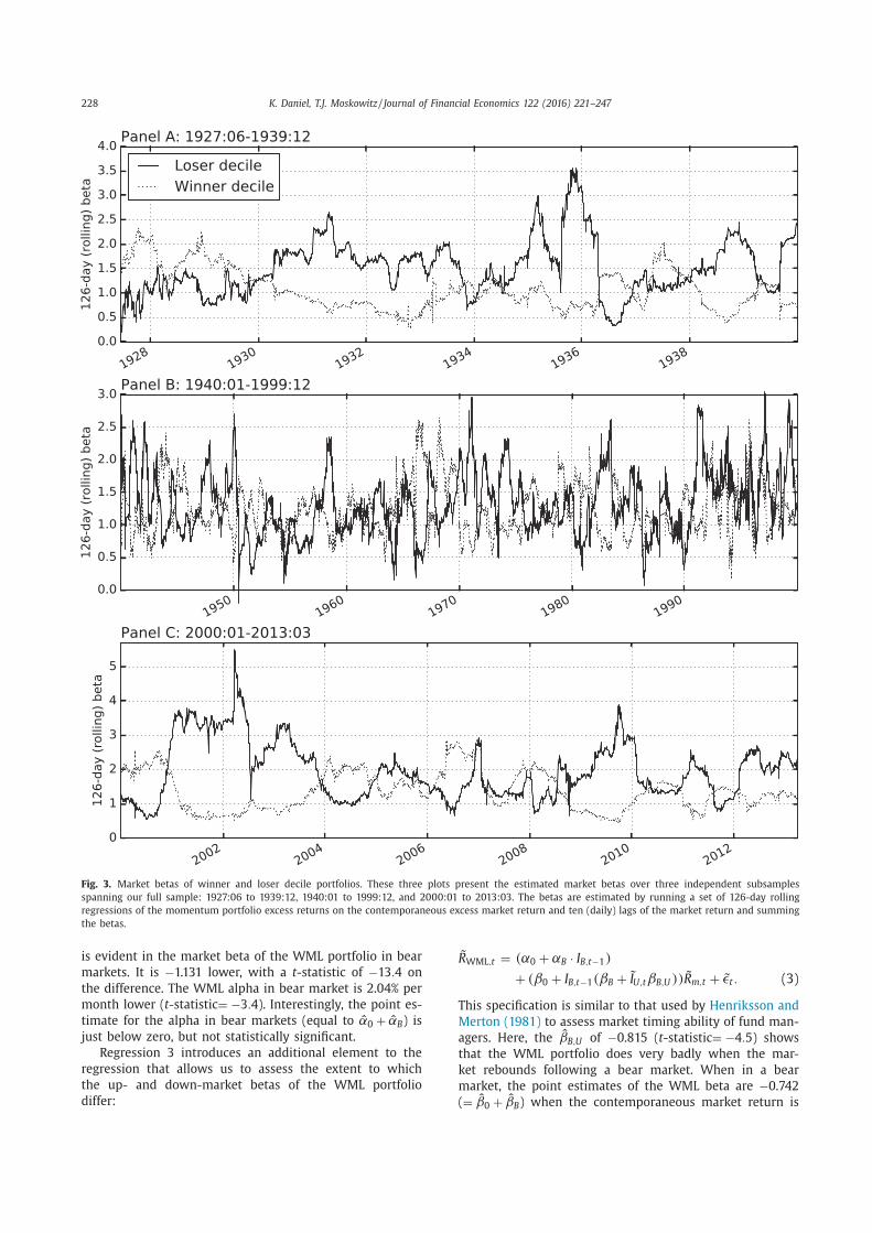
To investigate the time-varying betas of winners and losers, Fig. 3 plots the market betas for the winner and loser momentum deciles, estimated using 126-day ( ≈ six month) rolling market model regressions with daily data. 4 Fig. 3 plots the betas over three non overlapping subsam- ples that span the full sample period: June 1927 to De- cember 1939, January 1940 to December 1999, and January 20 0 0 to March 2013.
The betas vary substantially, especially for the loser portfolio, whose beta tends to increase dramatically dur- ing volatile periods. The first and third plots highlight the betas several years before, during, and after the momen- tum crashes. The beta of the winner portfolio is some- times above 2 following large market rises, but, for the
4 We use ten daily lags of the market return in estimating the market betas. We estimate a daily regression specification of the form ˜ r e i,t = β0 ̃ r e m,t + β1 ̃ r e m,t−1 + · · · + β10 ̃ r e m,t−10 + ̃ ϵi,t and then report the sum of the estimated coefficients ˆ β0 + ˆ β1 + · · · + ˆ β10 . Particularly for the past loser portfolios, and especially in the pre-WWII period, the lagged coefficients are strongly significant, suggesting that market wide information is incorporated into the prices of many of the firms in these portfolios over the span of multiple days. See Lo and MacKinlay (1990) and Jegadeesh and Titman (1995) .

226 K. Daniel, T.J. Moskowitz / Journal of Financial Economics 122 (2016) 221–247
Fig. 2. Momentum crashes, following the Great Depression and the 20 08–20 09 financial crisis. These plots show the cumulative daily returns to four portfolios: (1) the risk-free asset, (2) the Center for Research in Security Prices (CRSP) value-weighted index, (3) the bottom decile past loser portfolio; and (4) the top decile past winner portfolio over the period from March 9, 2009 through March 28 2013 (Panel A) and from June 1, 1932 through December 30, 1939 (Panel B).

K. Daniel, T.J. Moskowitz / Journal of Financial Economics 122 (2016) 221–247 227 Table 2 Worst monthly momentum returns.
This table lists the 15 worst monthly returns to the winner-minus-loser (WML) momentum portfolio over the 1927:01–2013:03 time period. Also tabulated are Mkt-2y, the two-year market returns leading up to the port- folio formation date, and Mkt t , the contemporaneous market return. The dates between July 1932 and September 1939 are marked with an aster- isk ( ∗), those between April and August of 2009 with † , and those from January 2001 and November 2002 with ‡ . All numbers in the table are in percent.
Rank Month WML t MKT-2y Mkt t 1 1932:08 ∗ −74 .36 −67 .77 36 .49 2 1932:07 ∗ −60 .98 −74 .91 33 .63 3 2001:01 ‡ −49 .19 10 .74 3 .66 4 2009:04 † −45 .52 −40 .62 10 .20 5 1939:09 ∗ −43 .83 −21 .46 16 .97 6 1933:04 ∗ −43 .14 −59 .00 38 .14 7 2009:03 † −42 .28 −44 .90 8 .97 8 2002:11 ‡ −37 .04 −36 .23 6 .08 9 1938:06 ∗ −33 .36 −27 .83 23 .72
10 2009:08 † −30 .54 −27 .33 3 .33 11 1931:06 ∗ −29 .72 −47 .59 13 .87 12 1933:05 ∗ −28 .90 −37 .18 21 .42 13 2001:11 ‡ −25 .31 −19 .77 7 .71 14 2001:10 ‡ −24 .98 −16 .77 2 .68 15 1974:01 −24 .04 −5 .67 0 .46
loser portfolio, the beta reaches far higher levels (as high as 4 or 5). The widening beta differences between winners and losers, coupled with the facts from Table 2 that these crash periods are characterized by sudden and dramatic market upswings, mean that the WML strategy experiences huge losses during these times. We examine these patterns more formally by investigating how the mean return of the momentum portfolio is linked to time variation in market beta. 3.1. Hedging market risk in the momentum portfolio
Grundy and Martin (2001) explore this same question, arguing that the poor performance of the momentum port- folio in the pre-WWII period first shown by Jegadeesh and Titman (1993) is a result of time-varying market and size exposure. They argue that a hedged momentum portfolio, for which conditional market and size exposure is zero, has a high average return and a high Sharpe ratio in the pre-WWII period when the unhedged momentum portfo- lio suffers.
At the time that Grundy and Martin (2001) under- took their study, daily stock return data were not available through CRSP in the pre-1962 period. Given the dynamic nature of momentum’s risk exposures, estimating the fu- ture hedge coefficients ex ante with monthly data is prob- lematic. As a result, Grundy and Martin (2001) construct their hedge portfolio based on a regression with monthly returns over the current month and the future five months. That is, the hedge portfolio was not an ex-ante imple- mentable portfolio.
However, to the extent that the future momentum- portfolio beta is correlated with the future return of the market, this procedure results in a biased estimate of the returns of the hedged portfolio. We show there is in fact a strong correlation of this type, which results in a large
upward bias in the estimated performance of the hedged portfolio. 5 3.2. Option-like behavior of the WML portfolio
The source of the bias using the ex post beta of the mo- mentum portfolio to construct the hedge portfolio is that, in bear markets, the market beta of the WML portfolio is strongly negatively correlated with the contemporaneous realized market return. This means that a hedge portfo- lio constructed using the ex post beta will have a higher beta in anticipation of a higher future market return, mak- ing its performance much better that what would be pos- sible with a hedge portfolio based on the ex ante beta.
In this subsection, we also show that the return of the momentum portfolio, net of properly estimated (i.e., ex ante) market risk, is significantly lower in bear markets. Both of these results are linked to the fact that, in bear markets, the momentum strategy behaves as if it is effec- tively short a call option on the market.
We first illustrate these issues with a set of four monthly time series regressions, the results of which are presented in Table 3 . The dependent variable in all regres- sions is ˜ R WML ,t , the WML return in month t . The indepen- dent variables are combinations of 1. ˜ R e m,t , the CRSP value-weighted index excess return in
month t . 2. I B,t−1 , an ex ante bear market indicator that equals one
if the cumulative CRSP VW index return in the past 24 months is negative and is zero otherwise;
3. ˜ I U,t , a contemporaneous, i.e., not ex ante, up-market in- dicator variable that is one if the excess CRSP VW index return is greater than the risk-free rate in month t (e.g., R e m,t > 0 ), and is zero otherwise. 6 Regression 1 in Table 3 fits an unconditional market
model to the WML portfolio: ˜ R WML ,t = α0 + β0 ̃ R m,t + ˜ ϵt . (1) Consistent with the results in the literature, the estimated market beta is negative, −0.576, and the intercept, ˆ α, is both economically large (1.852% per month) and statisti- cally significant ( t -statistic = 7.3).
Regression 2 in Table 3 fits a conditional CAPM with the bear market indicator, I B , as an instrument: ˜ R WML ,t = (α0 + αB I B,t−1 ) + (β0 + βB I B,t−1 ) ̃ R m,t + ˜ ϵt . (2) This specification is an attempt to capture both expected return and market-beta differences in bear markets. Con- sistent with Grundy and Martin (2001) , a striking change
5 The result that the betas of winner-minus-loser portfolios are non- linearly related to contemporaneous market returns has also been shown in Rouwenhorst (1998) who finds this feature for non-US equity momen- tum strategies (Table V, p. 279). Chan (1988) and DeBondt and Thaler (1987) show this nonlinearity for longer-term winner and loser portfolios. However, Boguth, Carlson, Fisher, and Simutin (2011) , building on the re- sults of Jagannathan and Korajczyk (1986) , note that the interpretation of the measures of abnormal performance (i.e., the alphas) in Chan (1988) , Grundy and Martin (2001) , and Rouwenhorst (1998) are problematic and provide a critique of Grundy and Martin (2001) and other studies that overcondition in a similar way.
6 Of the 1,035 months in the 1927:01-2013:03 period, I B,t−1 = 1 in 183, and ̃ I U,t = 1 in 618.
228 K. Daniel, T.J. Moskowitz / Journal of Financial Economics 122 (2016) 221–247
Fig. 3. Market betas of winner and loser decile portfolios. These three plots present the estimated market betas over three independent subsamples spanning our full sample: 1927:06 to 1939:12, 1940:01 to 1999:12, and 20 0 0:01 to 2013:03. The betas are estimated by running a set of 126-day rolling regressions of the momentum portfolio excess returns on the contemporaneous excess market return and ten (daily) lags of the market return and summing the betas. is evident in the market beta of the WML portfolio in bear markets. It is −1.131 lower, with a t -statistic of −13 . 4 on the difference. The WML alpha in bear market is 2.04% per month lower ( t -statistic = −3 . 4 ). Interestingly, the point es- timate for the alpha in bear markets (equal to ˆ α0 + ˆ αB ) is just below zero, but not statistically significant.
Regression 3 introduces an additional element to the regression that allows us to assess the extent to which the up- and down-market betas of the WML portfolio differ:
˜ R WML ,t = (α0 + αB · I B,t−1 ) + (β0 + I B,t−1 (βB + ̃ I U,t βB,U )) ̃ R m,t + ˜ ϵt . (3)
This specification is similar to that used by Henriksson and Merton (1981) to assess market timing ability of fund man- agers. Here, the ˆ βB,U of −0.815 ( t -statistic = −4 . 5 ) shows that the WML portfolio does very badly when the mar- ket rebounds following a bear market. When in a bear market, the point estimates of the WML beta are −0.742 ( = ˆ β0 + ˆ βB ) when the contemporaneous market return is
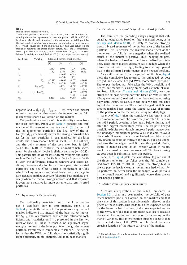
K. Daniel, T.J. Moskowitz / Journal of Financial Economics 122 (2016) 221–247 229 Table 3 Market timing regression results.
This table presents the results of estimating four specifications of a monthly time-series regressions run over the period 1927:01 to 2013:03. In all cases the dependent variable is the return on the WML portfolio. The independent variables are a constant; an indicator for bear markets, I B,t−1 , which equals one if the cumulative past two-year return on the market is negative; the excess market return, R e m,t ; and a contempora- neous up-market indicator, I U, t , which equals one if R e m,t > 0 . The coef- ficients ˆ α0 and ˆ αB are multiplied by 100 (i.e., are in percent per month).
Coefficient Variable Estimated coefficients (t-statistics) (1) (2) (3) (4)
ˆ α0 1 1.852 1.976 1.976 2.030 (7.3) (7.7) (7.8) (8.4)
ˆ αB I B,t−1 −2.040 0.583 ( −3.4) (0.7)
ˆ β0 ˜ R e m,t −0.576 −0.032 −0.032 −0.034 ( −12.5) ( −0.5) ( −0.6) ( −0.6)
ˆ βB I B,t−1 · ˜ R e m,t −1.131 −0.661 −0.708 ( −13.4) ( −5.0) ( −6.1)
ˆ βB,U I B,t−1 ·I U,t · ˜ R e m,t −0.815 −0.727 ( −4.5) ( −5.6)
R 2 adj 0.130 0.269 0.283 0.283
negative and = ˆ β0 + ˆ βB + ˆ βB,U = −1 . 796 when the market return is positive. In other words, the momentum portfolio is effectively short a call option on the market
The predominant source of this optionality comes from the loser portfolio. Panel A of Table 4 presents the esti- mation of the regression specification in (3) for each of the ten momentum portfolios. The final row of the ta- ble (the ˆ βB,U coefficient) shows the strong up-market be- tas for the loser portfolios in bear markets. For the loser decile, the down-market beta is 1.560 ( = 1 . 338 + 0 . 222 ) and the point estimate of the up-market beta is 2.160 ( = 1 . 560 + 0 . 600 ). In contrast, the up-market beta incre- ment for the winner decile is slightly negative ( = −0 . 215 ). This pattern also holds for less extreme winners and losers, such as Decile 2 versus Decile 9 or Decile 3 versus Decile 8, with the differences between winners and losers de- clining monotonically for less extreme past return-sorted portfolios. The net effect is that a momentum portfolio which is long winners and short losers will have signifi- cant negative market exposure following bear markets pre- cisely when the market swings upward and that exposure is even more negative for more extreme past return-sorted portfolios. 3.3. Asymmetry in the optionality
The optionality associated with the loser portfo- lios is significant only in bear markets. Panel B of Table 4 presents the same set of regressions using the bull market indicator I L,t−1 instead of the bear-market indica- tor I B,t−1 . The key variables here are the estimated coef- ficients and t -statistics on βL, U , presented in the last two rows of Panel B. Unlike in Panel A, no significant asym- metry is present in the loser portfolio, though the winner portfolio asymmetry is comparable to Panel A. The net ef- fect is that the WML portfolio shows no statistically signif- icant optionality in bull markets, unlike in bear markets.
3.4. Ex ante versus ex post hedge of market risk for WML The results of the preceding analysis suggest that cal-
culating hedge ratios based on future realized betas, as in Grundy and Martin (2001) , is likely to produce strongly upward biased estimates of the performance of the hedged portfolio. This is because the realized market beta of the momentum portfolio is more negative when the realized return of the market is positive. Thus, hedging ex post, when the hedge is based on the future realized portfolio beta, takes more market exposure (as a hedge) when the future market return is high, leading to a strong upward bias in the estimated performance of the hedged portfolio.
As an illustration of the magnitude of the bias, Fig. 4 plots the cumulative log return to the unhedged, ex post hedged, and ex ante hedged WML momentum portfolio. 7 The ex post hedged portfolio takes the WML portfolio and hedges out market risk using an ex post estimate of mar- ket beta. Following Grundy and Martin (2001) , we con- struct the ex post hedged portfolio based on WML’s future 42-day (two-month) realized market beta, estimated using daily data. Again, to calculate the beta we use ten daily lags of the market return. The ex ante hedged portfolio es- timates market betas using the lagged 42 days of returns of the portfolio on the market, including ten daily lags.
Panel A of Fig. 4 plots the cumulative log returns to all three momentum portfolios over the June 1927 to Decem- ber 1939 period, covering a few years before, during, and after the biggest momentum crash. The ex post hedged portfolio exhibits considerably improved performance over the unhedged momentum portfolio as it is able to avoid the crash. However, the ex ante hedged portfolio is not only unable to avoid or mitigate the crash, but also under- performs the unhedged portfolio over this period. Hence, trying to hedge ex ante, as an investor would in reality, would have made an investor worse off. The bias in using ex post betas is substantial over this period.
Panel B of Fig. 4 plots the cumulative log returns of the three momentum portfolios over the full sample pe- riod from 1927:01 to 2013:03. Again, the strong bias in the ex post hedge is clear, as the ex ante hedged portfo- lio performs no better than the unhedged WML portfolio in the overall period and significantly worse than the ex post hedged portfolio. 3.5. Market stress and momentum returns
A casual interpretation of the results presented in Section 3.2 is that, in a bear market, the portfolio of past losers behaves like a call option on the market and that the value of this option is not adequately reflected in the prices of these assets. This leads to a high expected return on the losers in bear markets, and a low expected return to the WML portfolio that shorts these past losers. Because the value of an option on the market is increasing in the market variance, this interpretation further suggests that the expected return of the WML portfolio should be a de- creasing function of the future variance of the market.
7 The calculation of cumulative returns for long-short portfolios is de- scribed in Appendix A.1 .

230 K. Daniel, T.J. Moskowitz / Journal of Financial Economics 122 (2016) 221–247 Table 4 Momentum portfolio optionality.
This table presents estimated coefficients (t-statistics) from regressions of the monthly excess returns of the momentum decile portfolios and the winner- minus-loser (WML) long-short portfolio on the Center for Research in Securities Prices (CRSP) value-weighted (VW) excess market returns, and a number of indicator variables. Panel A reports results for optionality in bear markets in which, for each of the momentum portfolios, the following regression is estimated:
˜ R e i,t = [ α0 + αB I B,t−1 ] + [ β0 + I B,t−1 (βB + ̃ I U,t βB,U )] ̃ R e m,t + ̃ ϵt , where R e m is the CRSP VW excess market return, I B,t−1 is an ex ante bear market indicator that equals one if the cumulative CRSP VW index return in the past 24 months is negative and is zero otherwise. I U, t is a contemporaneous up-market indicator that equals one if the excess CRSP VW index return is positive in month t , and is zero otherwise. Panel B reports results for optionality in bull markets where for each of the momentum portfolios, the following regression is estimated:
˜ R e i,t = [ α0 + αL I L,t−1 ] + [ β0 + I L,t−1 (βL + ̃ I U,t βL,U )] ̃ R m,t + ̃ ϵt where I L,t−1 is an ex ante bull market indicator (defined as 1 − I B,t−1 ). The sample period is 1927:01-2013:03. The coefficients ˆ α0 , ˆ αB and ˆ αL are multiplied by 100 (i.e., are in percent per month).
Coefficient Momentum decile portfolio 1 2 3 4 5 6 7 8 9 10 WML
Panel A: Optionality in bear markets ˆ α0 −1.406 −0.804 −0.509 −0.200 −0.054 −0.050 0.159 0.260 0.294 0.570 1.976
( −7.3) ( −5.7) ( −4.9) ( −2.4) ( −0.7) ( −0.9) (2.7) (4.1) (3.8) (4.6) (7.8) ˆ αB −0.261 0.370 −0.192 −0.583 −0.317 −0.231 −0.001 −0.039 0.420 0.321 0.583
( −0.4) (0.8) ( −0.6) ( −2.1) ( −1.3) ( −1.2) ( −0.0) ( −0.2) (1.7) (0.8) (0.7) ˆ β0 1.338 1.152 1.014 0.955 0.922 0.952 0.974 1.018 1.114 1.306 −0.032
(30.4) (35.7) (42.6) (49.5) (55.6) (72.1) (72.3) (69.9) (62.7) (46.1) ( −0.6) ˆ βB 0.222 0.326 0.354 0.156 0.180 0.081 0.028 −0.126 −0.158 −0.439 −0.661
(2.2) (4.4) (6.5) (3.5) (4.7) (2.7) (0.9) ( −3.8) ( −3.9) ( −6.8) ( −5.0) ˆ βB,U 0.600 0.349 0.180 0.351 0.163 0.121 −0.013 −0.031 −0.183 −0.215 −0.815
(4.4) (3.5) (2.4) (5.9) (3.2) (3.0) ( −0.3) ( −0.7) ( −3.3) ( −2.5) ( −4.5) Panel B: Optionality in bull markets
ˆ α0 0.041 0.392 −0.249 0.222 0.089 0.048 0.097 0.079 0.188 0.388 0.347 (0.1) (1.4) ( −1.2) (1.3) (0.6) (0.4) (0.8) (0.6) (1.2) (1.5) (0.7)
ˆ αL −1.436 −1.135 −0.286 −0.653 −0.303 −0.084 −0.164 0.164 0.239 0.593 2.029 ( −2.9) ( −3.1) ( −1.1) ( −2.9) ( −1.6) ( −0.6) ( −1.1) (1.0) (1.2) (1.9) (3.1)
ˆ β0 1.890 1.664 1.459 1.304 1.188 1.097 0.992 0.877 0.860 0.754 −1.136 (41.3) (49.6) (59.2) (64.5) (69.3) (80.5) (72.2) (58.7) (46.7) (25.9) ( −18.7)
ˆ βL −0.545 −0.498 −0.451 −0.411 −0.308 −0.141 −0.078 0.133 0.285 0.670 1.215 ( −6.0) ( −7.4) ( −9.2) ( −10.2) ( −9.0) ( −5.2) ( −2.9) (4.5) (7.8) (11.5) (10.0)
ˆ βL,U −0.010 −0.025 0.017 0.138 0.094 −0.006 0.136 0.021 −0.077 −0.251 −0.242 ( −0.1) ( −0.2) (0.2) (2.2) (1.8) ( −0.1) (3.2) (0.4) ( −1.4) ( −2.8) ( −1.3)
To examine this hypothesis, we use daily market return data to construct an ex ante estimate of the market volatil- ity over the coming month, and we use this market vari- ance estimate in combination with the bear market indi- cator, I B, t-1 , to forecast future WML returns. We run the regression ˜ R WML ,t = γ0 + γB , t −1 · I B , t −1 + γσ 2
m · ˆ σ 2 m,t−1
+ γint · I B · ˆ σ 2 m,t−1 + ˜ ϵt , (4)
where I B is the bear market indicator and ˆ σ 2 m,t−1 is the
variance of the daily returns of the market over the 126 days prior to time t .
Table 5 reports the regression results, showing that both estimated market variance and the bear market indicator independently forecast future momentum re- turns. Columns 1 and 2 report regression results for each variable separately, and column 3 reports results us- ing both variables simultaneously. The results are con- sistent with those from Section 3.4 . That is, in peri- ods of high market stress, as indicated by bear mar- kets and high volatility, future momentum returns are low. Finally, the last two columns of Table 5 report re-
sults for the interaction between the bear market indica- tor and volatility, in which momentum returns are shown to be particularly poor during bear markets with high volatility. 3.6. Exposure to other risk factors
Our results show that time-varying exposure to mar- ket risk cannot explain the low returns of the momen- tum portfolio in crash states. However, the option-like be- havior of the momentum portfolio raises the intriguing question of whether the premium associated with momen- tum could be related to exposure to variance risk because, in panic states, a long-short momentum portfolio behaves like a short (written) call option on the market and be- cause shorting options (i.e., selling variance) has histori- cally earned a large premium ( Carr and Wu, 2009; Chris- tensen and Prabhala, 1998 ).
To assess the dynamic exposure of the momentum strategy to variance innovations, we regress daily WML re- turns on the inferred daily (excess) returns of a variance swap on the S&P 500, which we calculate using the VIX and S&P 500 returns. Section A.2 of Appendix A provides

K. Daniel, T.J. Moskowitz / Journal of Financial Economics 122 (2016) 221–247 231
Fig. 4. Ex ante versus ex post hedged portfolio performance. These plots show the cumulative returns to the baseline static winner-minus-loser (WML) strategy, the WML strategy hedged ex post with respect to the market, and the WML strategy hedged ex ante with respect to the market. The ex post hedged portfolio conditionally hedges the market exposure using the procedure of Grundy and Martin (2001) , but using the future 42-day (two-month) realized market beta of the WML portfolio using Eq. (4) . The ex ante hedged momentum portfolio estimates market betas using the lagged 42 days of returns on the portfolio and the market from Eq. (4) . Panel A covers the 1927:06–1939:12 time period. Panel B plots the cumulative returns over the full sample (1927:06–2013:03). details of the swap return calculation. We run a time-series regression with a conditioning variable designed to cap- ture the time variation in factor loadings on the market and, potentially, on other variables. The conditioning vari- able I B σ 2 ≡ (1 / ̄v B )I B,t−1 ̂ σ 2
m,t−1 is the interaction used earlier but with a slight twist. That is • I B, t-1 is the bear market indicator defined earlier
( I B , t −1 = 1 if the cumulative past two-year market re- turn is negative and is zero otherwise);
• ˆ σ 2 m,t−1 is the variance of the market excess return over
the preceding 126 days; and
• (1 / ̄v B ) is the inverse of the full-sample mean of ˆ σ 2 m,t−1
over all months in which I B,t−1 = 1 . Normalizing the interaction term with the constant
1 / ̄v B does not affect the statistical significance of the re- sults, but it gives the coefficients a simple interpretation. Because ∑
I B,t−1 =1 I Bσ 2 = 1 , (5) the coefficients on I Bσ 2 and on variables interacted with I Bσ 2 can be interpreted as the weighted average change

232 K. Daniel, T.J. Moskowitz / Journal of Financial Economics 122 (2016) 221–247 Table 5 Momentum returns and estimated market variance.
This table presents the estimated coefficients ( t -statistics) for a set of time series regression based on the following regression specification:
˜ R WML ,t = γ0 + γB · I B,t−1 + γσ 2 m · ˆ σ 2
m,t−1 + γint · I B , t −1 · ˆ σ 2 m,t−1 + ̃ ϵt ,
where I B,t−1 is the bear market indicator and ˆ σ 2 m,t−1 is the variance of the
daily returns on the market, measured over the 126 days preceding the start of month t . Each regression is estimated using monthly data over the period 1927:07–2013:03. The coefficients ˆ γ0 and ˆ γB are multiplied by one hundred (i.e., are in percent per month).
Coefficient Regression (1) (2) (3) (4) (5)
ˆ γ0 1.955 2.428 2.500 1.973 2.129 (6.6) (7.5) (7.7) (7.1) (5.8)
ˆ γB −2.626 −1.281 0.023 ( −3.8) ( −1.6) (0.0)
ˆ γσ 2 m −0.330 −0.275 −0.088
( −5.1) ( −3.8) ( −0.8) ˆ γint −0.397 −0.323
( −5.7) ( −2.2) Table 6 Regression of winner-minus-loser (WML) portfolio returns on variance swap returns.
This table presents the estimated coefficients (t-statistics) from three daily time-series regressions of the zero-investment WML portfolio re- turns on sets of independent variables including a constant term and the normalized ex ante forecasting variable I Bσ 2 , and on this forecasting vari- able interacted with the excess market return ( ̃ r e m,t ) and the return on a (zero-investment) variance swap on the Standard & Poors 500 ( ̃ r e v s,t ). (See Subsection A.2 of Appendix A for details on how these swap returns are calculated.) The sample period is January 2, 1990 to March 28, 2013. t- statistics are in parentheses. The intercepts and the coefficients for I Bσ 2 are converted to annualized, percentage terms by multiplying by 25,200 ( = 252 × 100 .)
Independent variable Regression (1) (2) (3)
α 31.48 29.93 30.29 (4.7) (4.8) (4.9)
I Bσ 2 −58.62 −49.16 −54.83 ( −5.2) ( −4.7) ( −5.3)
˜ r e m,t 0.11 0.10 (4.5) (3.1)
I Bσ 2 · ˜ r e m,t −0.52 −0.63 ( −28.4) ( −24.7)
˜ r v s,t −0.02 ( −0.4)
I Bσ 2 · ˜ r v s,t −0.10 ( −4.7)
in the corresponding coefficient during a bear market, in which the weight on each observation is proportional to the ex ante market variance leading up to that month.
Table 6 presents the results of this analysis. In regres- sion 1 the intercept ( α) estimates the mean return of the WML portfolio when I B,t−1 = 0 as 31.48% per year. How- ever, the coefficient on I Bσ 2 shows that the weighted- average return in panic periods (volatile bear markets) is almost 59% per year lower
Regression 2 controls for the market return and condi- tional market risk. Consistent with our earlier results, the last coefficient in this column shows that the estimated WML beta falls by 0.518 ( t -statistic = −28 . 4 ) in panic states.
However, both the mean WML return in calm periods and the change in the WML premium in the panic periods (given, respectively, by α and the coefficient on I Bσ 2 ), re- main about the same.
In regression 3, we add the return on the variance swap and its interaction with I Bσ 2 . The coefficient on ˜ r v s,t shows that outside of panic states (i.e., when I B,t−1 = 0 ), the WML return does not co-vary significantly with the variance swap return. However, the coefficient on I Bσ 2 · ˜ r v s,t shows that in panic states, WML has a strongly significant nega- tive loading on the variance swap return. That is, WML is effectively short volatility during these periods. This is con- sistent with our previous results, in which WML behaves like a short call option, but only in panic periods. Outside of these periods, there is no evidence of any optionality.
However, the intercept and estimated I Bσ 2 coefficient in regression 3 are essentially unchanged, even after control- ling for the variance swap return. The estimated WML pre- mium in non-panic states remains large, and the change in this premium in panic states (i.e., the coefficient on I Bσ 2 ) is just as negative as before, indicating that although mo- mentum returns are related to variance risk, neither the unconditional nor the conditional returns to momentum are explained by it.
We also regress the WML momentum portfolio returns on the three Fama and French (1993) factors consisting of the CRSP VW index return in excess of the risk-free rate, a small minus big (SMB) stock factor, and a high book eq- uity to market equity (BE/ME) minus low BE/ME (HML) factor, all obtained from Ken French’s website. In addition, we interact each of the factors with the panic state vari- able I Bσ 2 . The results are reported in Appendix B , in which the abnormal performance of momentum continues to be significantly more negative in bear market states, whether we measure abnormal performance relative to the mar- ket model or to the Fama and French (1993) three-factor model, with little difference in the point estimates. 8 4. Dynamic weighting of the momentum portfolio
Using the insights from Section 3 , we evaluate the per- formance of a strategy that dynamically adjusts the weight on the WML momentum strategy using the forecasted re- turn and variance of the strategy. We show that the dy- namic strategy generates a Sharpe ratio more than double that of the baseline $1 long/$1 short WML strategy and is not explained by other factors or other suggested dynamic momentum portfolios such as a constant volatility momen- tum strategy ( Barroso and Santa-Clara, 2015 ). Moreover, we employ an out-of-sample dynamic momentum strat- egy that is implementable in real time and show that this portfolio performs about as well as an in-sample version
8 Although beyond the scope of this paper, we also examine HML and SMB as the dependent variable in similar regressions. We find that HML has opposite signed market exposure in panic states relative to WML, which is not surprising because value strategies buy long-term losers and sell winners, the opposite of what a momentum strategy does. The corre- lation between WML and HML is −0 . 50 . However, an equal combination of HML and WML does not completely hedge the panic state optionality as the effects on WML are quantitatively stronger. The details are pro- vided in Appendix B .
K. Daniel, T.J. Moskowitz / Journal of Financial Economics 122 (2016) 221–247 233 whose parameters are estimated more precisely over the full sample period.
We begin with the design of the dynamic strategy. We show in Appendix C that, for the objective function of maximizing the in-sample unconditional Sharpe ratio, the optimal weight on the risky asset (WML) at time t −1 is w ∗t−1 = ( 1
2 λ)µt−1 σ 2
t−1 (6) where µt−1 ≡ E t−1 [ R WML ,t ] is the conditional expected re- turn on the (zero-investment) WML portfolio over the coming month, σ 2
t−1 ≡ E t−1 [(R 2 WML ,t − µt−1 ) 2 ] is the condi- tional variance of the WML portfolio return over the com- ing month, and λ is a time-invariant scalar that controls the unconditional risk and return of the dynamic portfolio. This optimal weighting scheme comes from an intertem- poral version of Markowitz (1952) portfolio optimization.
We then use the insights from our previous analysis to provide an estimate of µt−1 , the conditional mean return of WML. The results from Table 5 provide an instrument for the time t conditional expected return on the WML portfolio. As a proxy for the expected return, we use the fitted regression of the WML returns on the interaction be- tween the bear market indicator I B,t−1 and the market vari- ance over the preceding six months (i.e., the regression es- timated in the fourth column of Table 5 ).
To forecast the volatility of the WML series, we first fit a the generalized autoregressive conditional heterostedas- ticity (GARCH) model proposed by Glosten, Jagannathan, and Runkle (1993) —the GJR-GARCH model—to the WML re- turn series. The process is defined by R W ML,t = µ + ϵt , (7) where ϵt ∼ N (0 , σ 2
t ) and where the evolution of σ 2 t is gov-
erned by the process: σ 2
t = ω + βσ 2 t−1 + ( α + γ I(ϵt−1 < 0) ) ϵ2
t−1 (8) where I(ϵt−1 < 0) is an indicator variable equal to one if ϵt−1 < 0 , and zero otherwise. 9 We use maximum likeli- hood to estimate the parameter set ( µ, ω, α, γ , β) over the full time series (estimates of the parameters and stan- dard errors are provided in Appendix D ).
We form a linear combination of the forecast of future volatility from the fitted GJR-GARCH process with the re- alized standard deviation of the 126 daily returns preced- ing the current month. We show in Appendix D that both components contribute to forecasting future daily realized WML volatility.
Our analysis in this section is also related to work by Barroso and Santa-Clara (2015) , who argue that momen- tum crashes can be avoided with a momentum portfo- lio that is scaled by its trailing volatility. They further show that the unconditional Sharpe ratio of the constant- volatility momentum strategy is far better than a simple $1-long/$1-short strategy.
9 Engle and Ng (1993) investigate the performance of a number of para- metric models in explaining daily market volatility for Japan. They find that the GJR model that we use here best fits the dynamic structure of volatility for that market.
Eq. (6) shows that our results would be approximately the same as those of Barroso and Santa-Clara (2015) if the Sharpe ratio of the momentum strategy were time invari- ant, i.e., if the forecast mean were always proportional to the forecast volatility. Eq. (6) shows that, in this setting, the weight on WML would be inversely proportional to the forecast WML volatility – that is the optimal dynamic strategy would be a constant volatility strategy like the one proposed by Barroso and Santa-Clara (2015) .
However, this is not the case for momentum. In fact, the return of WML is negatively related to the forecast WML return volatility, related in part to our findings of lower momentum returns following periods of market stress. This means that the Sharpe ratio of the optimal dynamic portfolio varies over time and is lowest when WML’s volatility is forecast to be high (and its mean re- turn low). To test this hypothesis, in Section 4.1 we imple- ment a dynamic momentum portfolio using these insights and show that the dynamic strategy outperforms a con- stant volatility strategy.
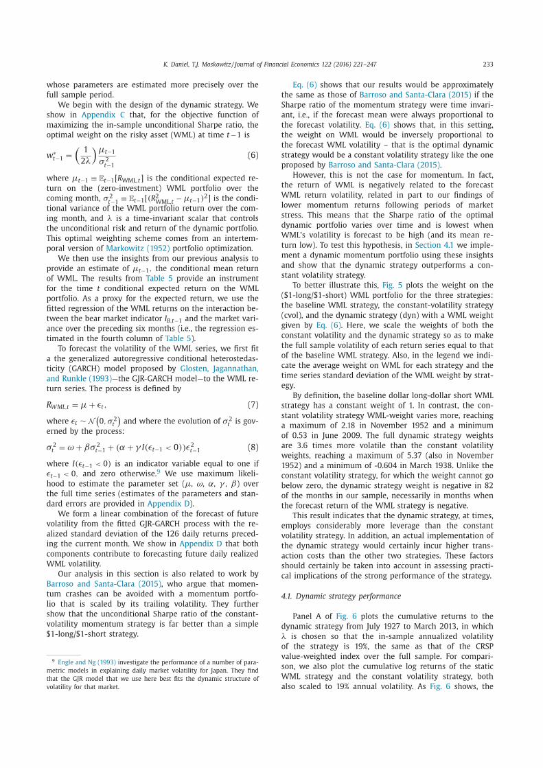
To better illustrate this, Fig. 5 plots the weight on the ($1-long/$1-short) WML portfolio for the three strategies: the baseline WML strategy, the constant-volatility strategy (cvol), and the dynamic strategy (dyn) with a WML weight given by Eq. (6) . Here, we scale the weights of both the constant volatility and the dynamic strategy so as to make the full sample volatility of each return series equal to that of the baseline WML strategy. Also, in the legend we indi- cate the average weight on WML for each strategy and the time series standard deviation of the WML weight by strat- egy.
By definition, the baseline dollar long-dollar short WML strategy has a constant weight of 1. In contrast, the con- stant volatility strategy WML-weight varies more, reaching a maximum of 2.18 in November 1952 and a minimum of 0.53 in June 2009. The full dynamic strategy weights are 3.6 times more volatile than the constant volatility weights, reaching a maximum of 5.37 (also in November 1952) and a minimum of -0.604 in March 1938. Unlike the constant volatility strategy, for which the weight cannot go below zero, the dynamic strategy weight is negative in 82 of the months in our sample, necessarily in months when the forecast return of the WML strategy is negative.
This result indicates that the dynamic strategy, at times, employs considerably more leverage than the constant volatility strategy. In addition, an actual implementation of the dynamic strategy would certainly incur higher trans- action costs than the other two strategies. These factors should certainly be taken into account in assessing practi- cal implications of the strong performance of the strategy. 4.1. Dynamic strategy performance
Panel A of Fig. 6 plots the cumulative returns to the dynamic strategy from July 1927 to March 2013, in which λ is chosen so that the in-sample annualized volatility of the strategy is 19%, the same as that of the CRSP value-weighted index over the full sample. For compari- son, we also plot the cumulative log returns of the static WML strategy and the constant volatility strategy, both also scaled to 19% annual volatility. As Fig. 6 shows, the

234 K. Daniel, T.J. Moskowitz / Journal of Financial Economics 122 (2016) 221–247
Fig. 5. Dynamic strategy weights on winner-minus-loser (WML) portfolio. We plot the weight on the WML portfolio as a function of time for in static WML portfolio, the constant volatility strategy (cvol), and the dynmaic strategy (dyn). The figure legend reports the time series mean and standard deviation for the WML weight for each portfolio. dynamic portfolio outperforms the constant volatility port- folio, which, in turn, outperforms the basic WML portfolio. The Sharpe ratio (in parentheses on the figure legend) of the dynamic portfolio is nearly twice that of the static WML portfolio and a bit higher than the constant volatility momentum portfolio. In section 4.4 , we conduct formal spanning tests among these portfolios as well as other fac- tors. Consistent with our previous results, part of the out- performance of the dynamic strategy comes from its ability to mitigate momentum crashes. However, the dynamic strategy outperforms the other momentum strategies even outside of the 1930s and the financial crisis period. 4.2. Subsample performance
As a check on the robustness of our results, we perform the same analysis over a set of approximately quarter- century subsamples: 1927 to 1949, 1950 to 1974, 1975 to 1999, and 20 0 0 to 2013. We use the same mean and vari- ance forecasting equation and the same calibration in each of the four subsamples. Panels B–E of Fig. 6 plot the cu- mulative log returns by subsample and present the strat- egy Sharpe ratios (in parentheses) by subsample. For ease of comparison, returns for each of the strategies are scaled to an annualized volatility of 19% in each subsample.
In each of the four subsamples,the ordering of perfor- mance remains the same. The dynamic strategy outper-
forms the constant volatility strategy, which outperforms the static WML strategy. As the subsample plots show, part of the improved performance of the constant volatility, and especially dynamic strategy, over the static WML portfolio is the amelioration of big crashes. But, even over subperi- ods devoid of those crashes, there is still improvement. 4.3. Out-of-sample performance
One important potential concern with the dynamic strategy performance results presented above is that the trading strategy relies on parameters estimated over the full sample. This is a particular concern here, as our dy- namic strategy relies on the conditional expected WML- return estimate from the fitted regression in column 4 of Table 5 .
To shed some light on whether the dynamic strategy re- turns could have been achieved by an actual investor who would not have known these parameters, we construct an out-of-sample strategy. We continue to use Eq. (6) to de- termine the weight on the WML portfolio, and we continue to use the fitted regression specification in Column 4 of Table 5 for the forecast mean, that is, µt−1 ≡ E t−1 [ ̃ R WML ,t ] = ˆ γ0 ,t−1 + ˆ γint ,t −1 · I B , t −1 · ˆ σ 2
m,t−1 , (9) only now the ˆ γ0 ,t−1 and ˆ γint ,t −1 in our forecasting speci- fication are the estimated regression coefficients not over

K. Daniel, T.J. Moskowitz / Journal of Financial Economics 122 (2016) 221–247 235
Fig. 6. Dynamic momentum strategy performance. These plots show the cumulative returns to the dynamic strategy, (dyn), from Eqn. (6) , in which λis chosen so that the in-sample annualized volatility of the strategy is 19%, the same as that of the Center for Research in Security Prices (CRSP) value- weighted index over the full sample. For comparison, we also plot the cumulative log returns of the static winner-minus-lower (WML) strategy and a constant volatility strategy (cvol), similar to that of Barroso and Santa-Clara (2015) , also scaled to an annualized volatility of 19%. Panel A plots the cumu- lative returns over the full sample period from 1927:07 to 2013:03. Panels B–E plot the returns over four roughly quarter-century subsamples: 1927–1949, 1950–1974, 1975–1999, and 20 0 0–2013. The annualized Sharpe ratios of each strategy in each period are reported in parentheses in the corresponding legend.

236 K. Daniel, T.J. Moskowitz / Journal of Financial Economics 122 (2016) 221–247
Fig. 7. Mean forecast coefficients: expanding window. We use the fitted regression specification in column 4 of Table 5 for the forecast mean; that is µt−1 ≡ E t−1 [ ̃ R WML ,t ] = ˆ γ0 ,t−1 + ̂ γint ,t −1 · I B , t −1 · ˆ σ 2
m,t−1 , only now the ˆ γ0 ,t−1 and ˆ γint ,t −1 are the estimated regression coefficients not over the full sample, but rather from a regression run from the start of our sample (1927:07) up through month t−1 (as indicated by the t−1 subscripts on these coefficients). the full sample, but rather from a regression run from the start of our sample (1927:07) up through month t −1 . 10 To estimate the month t WML variance we use the 126-day WML variance estimated through the last day of month t −1 .
Fig. 7 plots the coefficients for this expanding window regression as a function of the date. The slope coefficient begins only in October 1930, because the bear market in- dicator ( I B ) is zero up until October 1930. 11 From January 1933 until the end of our sample, the slope coefficient is always in the range of −0.43 to −0.21.The slope coefficient rises dramatically just before the poor performance of the momentum strategy in the 2001 and 2009 periods. These were bear markets (i.e., I B = 1 ) in which the market con- tinued to fall and momentum performed well. However, in each of these cases the forecasting variable eventually works in the sense that momentum does experience very bad performance and the slope coefficient falls. Following the fairly extreme 2009 momentum crash, the slope coef- ficient falls below −0.40 in August and September 2009. 4.3.1. Out-of-sample strategy performance
Table 7 presents a comparison of the performance of the various momentum strategies: the $1 long–$1 short static WML strategy, the constant volatility strategy, and strategy scaled by variance instead of standard deviation,
10 We have added t − 1 subscripts to these coefficients to emphasize the fact that they are in the investor’s information set at the end of month t − 1 .
11 Also, the intercept up to October 1930 is simply the mean monthly return on the momentum portfolio up to that time. After October 1930, it is the intercept coefficient for the regression.
Table 7 Strategy performance comparison.
This table presents the annualized Sharpe ratios of five zero-investment portfolio strategies, based on the monthly returns of these strategies over the 1934:01–2013:03 time period. WML is the baseline winner-minus- loser momentum strategy. cvol is the constant volatility strategy, in which the WML returns each month are scaled by the realized volatility of the daily WML returns over the preceding 126 trading days. For the variance scaled portfolio, the WML returns each month are scaled by the realized variance of the daily WML returns over the preceding 126 trading days. For the strategy labeled “dyn, out-of-sample,” the WML portfolio weights each month are multiplied each month by w ∗ in Eq. (6) , where µt−1 is the out-of-sample WML mean-return forecast (in Eq. 9) , and σ 2
t−1 is the realized variance of the daily WML returns over the preceding 126 trad- ing days. The strategy labeled “dyn, in-sample” is the dynamic strategy discussed in Section 4.1 , with the parameters in the mean and variance forecast estimated over the full sample. The column labeled “Appraisal ra- tio” gives the annualized Treynor and Black (1973) appraisal ratio of the strategy in that row, relative to the strategy in the preceding row.
Strategy Sharpe Appraisal ratio ratio
WML 0.682 cvol 1.041 0.786 variance scaled 1.126 0.431 dyn, out-of-sample 1.194 0.396 dyn, in-sample 1.202 0.144
the dynamic out-of-sample strategy, and the dynamic in- sample strategy. Next to each strategy (except the first one), there are two numbers. The first number is the Sharpe ratio of that strategy over the period from Jan- uary 1934 up through the end of our sample (March 2013). The second number is the Treynor and Black (1973) ap- praisal ratio of that strategy relative to the preceding one in the list. So, for example going from WML to the constant

K. Daniel, T.J. Moskowitz / Journal of Financial Economics 122 (2016) 221–247 237 Table 8 Spanning tests of the dynamic momentum portfolio. This table presents the results of spanning tests of the dynamic (Panel A) and constant volatility (Panel B) portfolios with respect to the market (Mkt), the Fama and French (1993; FF) small-minus-big (SMB), and high-minus-low (HML) factors, the static wiinner-minus-loser (WML) portfolio, and each other by running daily time-series regressions of the dynamic (dyn) portfolio’s and constant volatility (cvol) portfolio’s returns on these factors. In addition, we interact each of these factors with the market stress indicator I Bσ 2 to estimate conditional betas with respect to these factors, which are labeled “conditional.” For ease of comparison, the dyn and cvol portfolios are scaled to have the same annualized volatility as the static WML portfolio (23%). The reported intercepts or αs from these regressions are converted to annualized, percentage terms by multiplying by 252 times one hundred.
Coefficient Factor Set 1 2 3 4 5 6
Panel A: Dependent variable = returns to dynamic (dyn) momentum portfolio Mkt+WML Mkt+WML FF+WML Mkt+cvol Mkt+cvol FF+cvol
conditional conditional conditional conditional ˆ α 23.74 23.23 22.04 7.27 6.92 6.10 t ( α) (11.99) (11.76) (11.60) (6.86) (6.44) (6.08) Panel B: Dependent variable = returns to constant volatility (cvol) momentum portfolio
Mkt+WML Mkt+WML FF+WML Mkt+dyn Mkt+dyn FF+dyn conditional conditional conditional conditional
ˆ α 14.27 14.28 13.88 −0.72 −0.15 −0.02 t ( α) (11.44) (11.55) (11.28) ( −0.66) ( −0.13) ( −0.02)
volatility strategy increases the Sharpe ratio from 0.682 to 1.041. We know that to increase the Sharpe ratio by that amount, the WML strategy is combined with an (orthog- onal) strategy with a Sharpe ratio of √
1 . 041 2 − 0 . 682 2 = 0 . 786 , which is also the value of the Treynor and Black ap- praisal ratio.
The last two rows of Table 7 show that going from in-sample to out-of-sample results in only a very small decrease in performance for the dynamic strategy. Going from the constant volatility strategy to the out-of-sample dynamic strategy continues to result in a fairly substantial performance increase equivalent to adding on an orthog- onal strategy with a Sharpe ratio of √
1 . 194 2 − 1 . 041 2 = 0 . 585 . This performance increase can be decomposed into two roughly equal parts: one part is the performance in- crease that comes from scaling by variance instead of by volatility, and the other second component comes from forecasting the mean, which continues to result in a sub- stantial performance gain (AR = 0.396) even though we are doing a full out-of-sample forecast of the mean return and variance of WML. 4.4. Spanning tests
A more formal test of the dynamic portfolio’s success is to conduct spanning tests with respect to the other momentum strategies and other factors. Using daily re- turns, we regress the dynamic portfolio’s returns on a host of factors that include the market and Fama and French (1993) factors as well as the static WML and constant volatility (cvol) momentum strategies. The annualized al- phas from these regressions are reported in Table 8 .
The first column of Panel A of Table 8 reports re- sults from regressions of our dynamic momentum port- folio on the market plus the static momentum portfolio, WML. The intercept is highly significant at 23.74% per an- num ( t -statistic = 11.99), indicating that the dynamic port- folio’s returns are not captured by the market or the static
momentum portfolio. Because this regression controls only for unconditional market exposure, the second column of Panel A reports regression results that include interactions of our panic state indicators with the market to capture the conditional variability in beta. The alpha is virtually unchanged and remains positive and highly significant. The third column then adds the Fama and French (1993) factors SMB and HML and their interactions with the panic state variables to account for conditional variability in exposure to the market, size, and value factors. This regression ac- counts for whether our dynamic portfolio is merely rotat- ing exposure to these factors. 12 Again, the alpha with re- spect to this conditional model is strong and significant at 22% per year, nearly identical in magnitude to the first two columns. Hence, our dynamic momentum strategy’s abnor- mal performance is not being driven by dynamic exposure to these other factors or to the static momentum portfolio.
Columns 4 through 6 of Panel A of Table 8 repeat the regressions from Columns 1 through 3 by replacing the static WML portfolio with the constant volatility (cvol) momentum portfolio. The alphas drop in magnitude to about 7% per year but remain highly statistically signifi- cant ( t -statistic between 6 and 7), suggesting that the dy- namic momentum portfolio is not spanned by the constant volatility portfolio.
Panel B of Table 8 flips the analysis around and exam- ines whether the constant volatility portfolio is spanned by the static WML portfolio or the dynamic portfolio. The first three columns of Panel B indicate that the constant volatil- ity portfolio is not spanned by the static WML portfolio or the Fama and French (1993) factors, generating alphas of
12 Because the optimal dynamic portfolio solved in Appendix C is not conditional on other factors, to form this portfolio in the presence of other factors we first regress the static momentum portfolio on the other factors using daily returns and then use the residuals to form our dy- namic strategy by forecasting the conditional mean and variance of those residuals to form the dynamic weights.

238 K. Daniel, T.J. Moskowitz / Journal of Financial Economics 122 (2016) 221–247 about 14% per annum with highly significant t -statistics. These results are consistent with Barroso and Santa-Clara (2015) . However, the alphas of the constant volatility port- folio are slightly smaller in magnitude than those from the dynamic strategy, consistent with the Sharpe ratio compar- isons from Fig. 6 . (Because we scale both the dynamic and constant volatility portfolios to have the same variance, these alphas are comparable and give the same rankings as information ratios would.)
Columns 4 through 6 of Panel B report results from re- gressing the constant volatility portfolio’s returns on the dynamic portfolio’s returns. Here, the alphas are all zero, both economically and statistically, suggesting that the dy- namic portfolio spans the constant volatility portfolio. Ac- cording to Appendix C , this should be the case in the- ory, thus implying that we obtain decent ex ante forecasts of the conditional mean and variance of the static WML portfolio to form a dynamic strategy that reliably captures and improves upon the returns to a constant volatility and static momentum portfolio. 5. International equities and other asset classes
Price momentum was first shown in individual equi- ties in the US. However, subsequent research has demon- strated the existence of strong momentum effects both among common stocks in other investment regions and in other asset classes (see Asness, Moskowitz, and Pedersen (2013) for a summary).
We investigate whether the same momentum crash patterns we observe in US equities are also present in these other asset markets and whether our dynamic mo- mentum portfolio helps ameliorate these crashes and im- proves momentum performance in other markets. 5.1. Data
The data come from Asness, Moskowitz, and Pedersen (2013) and for equities cover the US, UK, Japan, and Conti- nental Europe. Details on data description and sources can be found in Asness, Moskowitz, and Pedersen (2013) . The US and UK data begin in January 1972 and Europe and Japan in February 1974, extending to May 2013. 13 We also examine a global equity momentum strategy (GE), which weights each region’s equity momentum strategy by the ex post volatility of the portfolio over the full sample, follow- ing Asness, Moskowitz, and Pedersen (2013) .
The non-equity data also come from Asness, Moskowitz, and Pedersen (2013) . They contain equity country index fu- tures across 18 developed equity markets beginning in Jan- uary 1978, ten currencies across developed markets start- ing in January 1979, ten country government bonds begin- ning January 1982, and 27 different commodity futures be- ginning in January 1972. All series end in May 2013.
13 These data extend beyond the original sample period used in Asness, Moskowitz, and Pedersen (2013) , as the data are updated monthly follow- ing the same procedure for portfolio construction in Asness, Moskowitz, and Pedersen (2013) . The data are available from: https://www.aqr.com/ library/data-sets/value-and-momentum-everywhere-factors-monthly .
In addition, we examine two composite portfolios: GA is a global momentum strategy across the non-equity asset classes, which weights each asset class momentum strat- egy portfolio by the ex post volatility of that portfolio. GAll is a global momentum strategy across all of the equity and non-equity asset classes, which weights the GE and GA portfolios by their ex post return volatilities over the full sample.
The definition of the market index is different for each market and asset class. It is the MSCI local index for the US, UK, Europe, and Japan, the MSCI World index for coun- try index futures, an equal-weighted average of all country bonds for bond markets, an equal-weighted average of all currencies for currency markets, and the Goldman Sachs Commodity Index (GSCI) for commodities. 5.2. Cross-sectional equity momentum outside the US
The portfolio formation procedure here is similar to that used earlier in the paper, except that, instead of taking the top and bottom decile portfolios, we use the Asness, Moskowitz, and Pedersen (2013) P3–P1 momentum portfo- lios, which is long the top third and short the bottom third of securities ranked on returns from month t − 12 through month t − 2 . Both the long and the short side of the port- folio are value weighted. As shown in Asness, Moskowitz, and Pedersen (2013) , over this time period there are strong momentum effects in each of the regions except Japan.
Panels A through D of Table 9 present the results of the regressions run in Section 2 , but for the other stock market universes. Panel A shows the estimated coefficients and t -statistics from the regression specification in Eq. (2) . Consistent with the results presented earlier, the market betas of the momentum strategy are dramatically lower in bear markets across the other stock markets as well. The strategies implemented using European and Japanese stocks have market betas that are approximately 0.5 lower during bear markets (with t -statistics of about −7). The UK momentum strategy beta falls by 0.2. The drop in this pe- riod for the US momentum strategy is 0.58, comparable to the WML portfolio over the longer 1927–2013 period. Globally, averaging across the US, UK, Europe, and Japan, the market betas of the momentum strategy are markedly lower in bear markets.
The abnormal returns of the momentum strategies are significantly positive in bull markets for all regions except Japan. Consistent with our analysis in Section 2 , the return is lower in bear markets in each region, although, using only the bear market indicator as a proxy for panic periods, none of the differences is statistically significant over these shorter sample periods.
Panel B investigates the optionality in the momentum strategy in bear markets using the regression specification in Eq. (3) . Consistent with the longer period US results, there is statistically significant optionality in bear markets in the European, UK, and Japan stock markets and globally across all markets. For this subsample and methodology, the optionality is of the right sign, but it is not statis- tically significant for the US market. The negative beta of long-short momentum strategies is particularly acute when the contemporaneous market return is positive. That
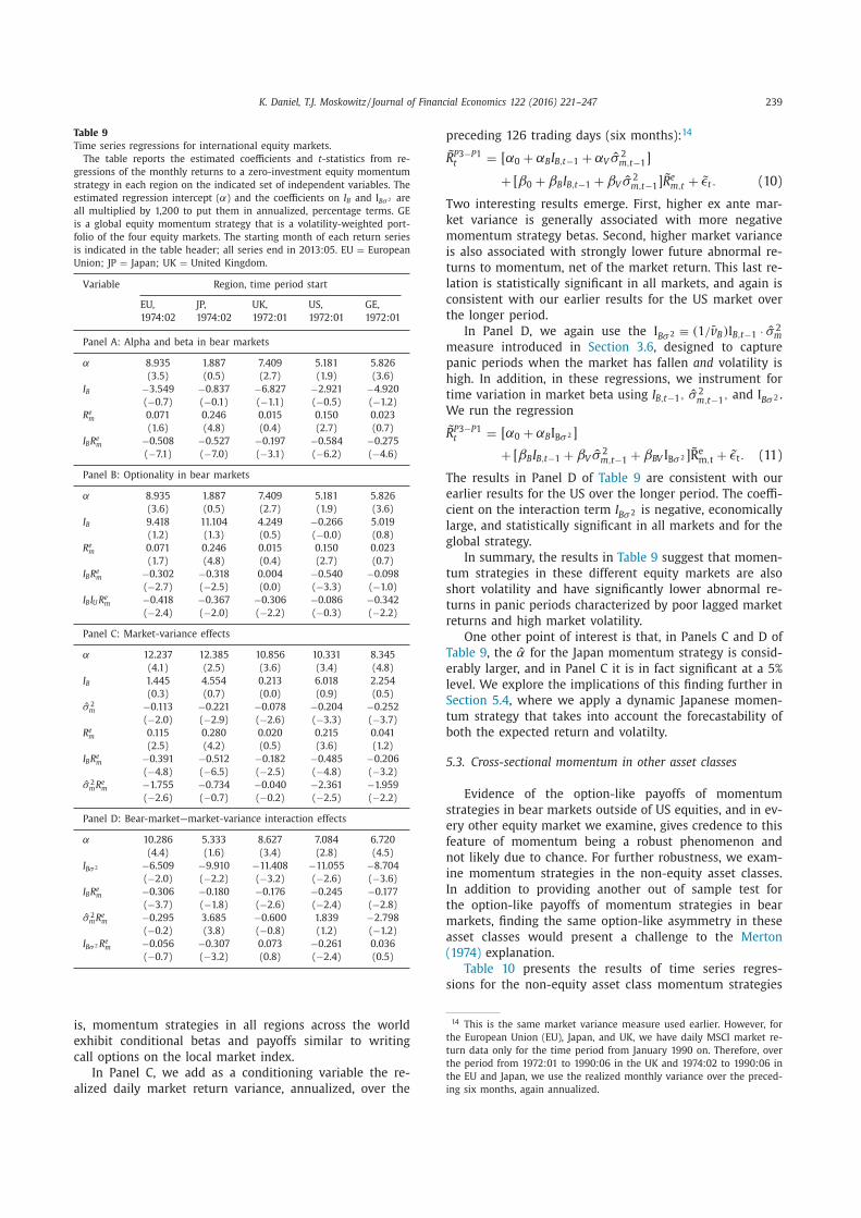
K. Daniel, T.J. Moskowitz / Journal of Financial Economics 122 (2016) 221–247 239 Table 9 Time series regressions for international equity markets.
The table reports the estimated coefficients and t -statistics from re- gressions of the monthly returns to a zero-investment equity momentum strategy in each region on the indicated set of independent variables. The estimated regression intercept ( α) and the coefficients on I B and I Bσ 2 are all multiplied by 1,200 to put them in annualized, percentage terms. GE is a global equity momentum strategy that is a volatility-weighted port- folio of the four equity markets. The starting month of each return series is indicated in the table header; all series end in 2013:05. EU = European Union; JP = Japan; UK = United Kingdom.
Variable Region, time period start EU, JP, UK, US, GE, 1974:02 1974:02 1972:01 1972:01 1972:01
Panel A: Alpha and beta in bear markets α 8.935 1.887 7.409 5.181 5.826
(3.5) (0.5) (2.7) (1.9) (3.6) I B −3.549 −0.837 −6.827 −2.921 −4.920
( −0.7) ( −0.1) ( −1.1) ( −0.5) ( −1.2) R e m 0.071 0.246 0.015 0.150 0.023
(1.6) (4.8) (0.4) (2.7) (0.7) I B R e m −0.508 −0.527 −0.197 −0.584 −0.275
( −7.1) ( −7.0) ( −3.1) ( −6.2) ( −4.6) Panel B: Optionality in bear markets α 8.935 1.887 7.409 5.181 5.826
(3.6) (0.5) (2.7) (1.9) (3.6) I B 9.418 11.104 4.249 −0.266 5.019
(1.2) (1.3) (0.5) ( −0.0) (0.8) R e m 0.071 0.246 0.015 0.150 0.023
(1.7) (4.8) (0.4) (2.7) (0.7) I B R e m −0.302 −0.318 0.004 −0.540 −0.098
( −2.7) ( −2.5) (0.0) ( −3.3) ( −1.0) I B I U R e m −0.418 −0.367 −0.306 −0.086 −0.342
( −2.4) ( −2.0) ( −2.2) ( −0.3) ( −2.2) Panel C: Market-variance effects α 12.237 12.385 10.856 10.331 8.345
(4.1) (2.5) (3.6) (3.4) (4.8) I B 1.445 4.554 0.213 6.018 2.254
(0.3) (0.7) (0.0) (0.9) (0.5) ˆ σ 2
m −0.113 −0.221 −0.078 −0.204 −0.252 ( −2.0) ( −2.9) ( −2.6) ( −3.3) ( −3.7)
R e m 0.115 0.280 0.020 0.215 0.041 (2.5) (4.2) (0.5) (3.6) (1.2)
I B R e m −0.391 −0.512 −0.182 −0.485 −0.206 ( −4.8) ( −6.5) ( −2.5) ( −4.8) ( −3.2)
ˆ σ 2 m R e m −1.755 −0.734 −0.040 −2.361 −1.959
( −2.6) ( −0.7) ( −0.2) ( −2.5) ( −2.2) Panel D: Bear-market—market-variance interaction effects α 10.286 5.333 8.627 7.084 6.720
(4.4) (1.6) (3.4) (2.8) (4.5) I Bσ 2 −6.509 −9.910 −11.408 −11.055 −8.704
( −2.0) ( −2.2) ( −3.2) ( −2.6) ( −3.6) I B R e m −0.306 −0.180 −0.176 −0.245 −0.177
( −3.7) ( −1.8) ( −2.6) ( −2.4) ( −2.8) ˆ σ 2
m R e m −0.295 3.685 −0.600 1.839 −2.798 ( −0.2) (3.8) ( −0.8) (1.2) ( −1.2)
I Bσ 2 R e m −0.056 −0.307 0.073 −0.261 0.036 ( −0.7) ( −3.2) (0.8) ( −2.4) (0.5)
is, momentum strategies in all regions across the world exhibit conditional betas and payoffs similar to writing call options on the local market index.
In Panel C, we add as a conditioning variable the re- alized daily market return variance, annualized, over the
preceding 126 trading days (six months): 14 ˜ R P 3 −P 1
t = [ α0 + αB I B,t−1 + αV ˆ σ 2 m,t−1 ]
+ [ β0 + βB I B,t−1 + βV ˆ σ 2 m,t−1 ] ̃ R e m,t + ˜ ϵt . (10)
Two interesting results emerge. First, higher ex ante mar- ket variance is generally associated with more negative momentum strategy betas. Second, higher market variance is also associated with strongly lower future abnormal re- turns to momentum, net of the market return. This last re- lation is statistically significant in all markets, and again is consistent with our earlier results for the US market over the longer period.
In Panel D, we again use the I Bσ 2 ≡ (1 / ̄v B )I B,t−1 · ˆ σ 2 m
measure introduced in Section 3.6 , designed to capture panic periods when the market has fallen and volatility is high. In addition, in these regressions, we instrument for time variation in market beta using I B,t−1 , ˆ σ 2
m,t−1 , and I Bσ 2 . We run the regression ˜ R P 3 −P 1
t = [ α0 + αB I B σ 2 ] + [ βB I B,t−1 + βV ˆ σ 2
m,t−1 + βBV I B σ 2 ] ̃ R e m , t + ˜ ϵt . (11) The results in Panel D of Table 9 are consistent with our earlier results for the US over the longer period. The coeffi- cient on the interaction term I Bσ 2 is negative, economically large, and statistically significant in all markets and for the global strategy.
In summary, the results in Table 9 suggest that momen- tum strategies in these different equity markets are also short volatility and have significantly lower abnormal re- turns in panic periods characterized by poor lagged market returns and high market volatility.
One other point of interest is that, in Panels C and D of Table 9 , the ˆ α for the Japan momentum strategy is consid- erably larger, and in Panel C it is in fact significant at a 5% level. We explore the implications of this finding further in Section 5.4 , where we apply a dynamic Japanese momen- tum strategy that takes into account the forecastability of both the expected return and volatilty. 5.3. Cross-sectional momentum in other asset classes
Evidence of the option-like payoffs of momentum strategies in bear markets outside of US equities, and in ev- ery other equity market we examine, gives credence to this feature of momentum being a robust phenomenon and not likely due to chance. For further robustness, we exam- ine momentum strategies in the non-equity asset classes. In addition to providing another out of sample test for the option-like payoffs of momentum strategies in bear markets, finding the same option-like asymmetry in these asset classes would present a challenge to the Merton (1974) explanation.
Table 10 presents the results of time series regres- sions for the non-equity asset class momentum strategies
14 This is the same market variance measure used earlier. However, for the European Union (EU), Japan, and UK, we have daily MSCI market re- turn data only for the time period from January 1990 on. Therefore, over the period from 1972:01 to 1990:06 in the UK and 1974:02 to 1990:06 in the EU and Japan, we use the realized monthly variance over the preced- ing six months, again annualized.
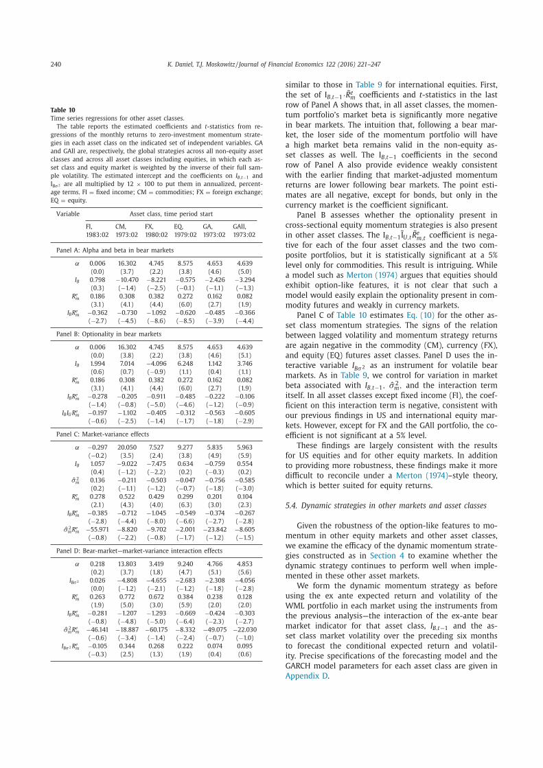
240 K. Daniel, T.J. Moskowitz / Journal of Financial Economics 122 (2016) 221–247
Table 10 Time series regressions for other asset classes.
The table reports the estimated coefficients and t -statistics from re- gressions of the monthly returns to zero-investment momentum strate- gies in each asset class on the indicated set of independent variables. GA and GAll are, respectively, the global strategies across all non-equity asset classes and across all asset classes including equities, in which each as- set class and equity market is weighted by the inverse of their full sam- ple volatility. The estimated intercept and the coefficients on I B,t−1 and I Bσ 2 are all multiplied by 12 × 100 to put them in annualized, percent- age terms. FI = fixed income; CM = commodities; FX = foreign exchange; EQ = equity.
Variable Asset class, time period start FI, CM, FX, EQ, GA, GAll, 1983:02 1973:02 1980:02 1979:02 1973:02 1973:02
Panel A: Alpha and beta in bear markets α 0.006 16.302 4.745 8.575 4.653 4.639
(0.0) (3.7) (2.2) (3.8) (4.6) (5.0) I B 0.798 −10.470 −8.221 −0.575 −2.426 −3.294
(0.3) ( −1.4) ( −2.5) ( −0.1) ( −1.1) ( −1.3) R e m 0.186 0.308 0.382 0.272 0.162 0.082
(3.1) (4.1) (4.4) (6.0) (2.7) (1.9) I B R e m −0.362 −0.730 −1.092 −0.620 −0.485 −0.366
( −2.7) ( −4.5) ( −8.6) ( −8.5) ( −3.9) ( −4.4) Panel B: Optionality in bear markets
α 0.006 16.302 4.745 8.575 4.653 4.639 (0.0) (3.8) (2.2) (3.8) (4.6) (5.1)
I B 1.994 7.014 −4.096 6.248 1.142 3.746 (0.6) (0.7) ( −0.9) (1.1) (0.4) (1.1)
R e m 0.186 0.308 0.382 0.272 0.162 0.082 (3.1) (4.1) (4.4) (6.0) (2.7) (1.9)
I B R e m −0.278 −0.205 −0.911 −0.485 −0.222 −0.106 ( −1.4) ( −0.8) ( −5.0) ( −4.6) ( −1.2) ( −0.9)
I B I U R e m −0.197 −1.102 −0.405 −0.312 −0.563 −0.605 ( −0.6) ( −2.5) ( −1.4) ( −1.7) ( −1.8) ( −2.9)
Panel C: Market-variance effects α −0.297 20.050 7.527 9.277 5.835 5.963
( −0.2) (3.5) (2.4) (3.8) (4.9) (5.9) I B 1.057 −9.022 −7.475 0.634 −0.759 0.554
(0.4) ( −1.2) ( −2.2) (0.2) ( −0.3) (0.2) ˆ σ 2
m 0.136 −0.211 −0.503 −0.047 −0.756 −0.585 (0.2) ( −1.1) ( −1.2) ( −0.7) ( −1.8) ( −3.0)
R e m 0.278 0.522 0.429 0.299 0.201 0.104 (2.1) (4.3) (4.0) (6.3) (3.0) (2.3)
I B R e m −0.385 −0.712 −1.045 −0.549 −0.374 −0.267 ( −2.8) ( −4.4) ( −8.0) ( −6.6) ( −2.7) ( −2.8)
ˆ σ 2 m R e m −55.971 −8.820 −9.702 −2.001 −23.842 −8.605
( −0.8) ( −2.2) ( −0.8) ( −1.7) ( −1.2) ( −1.5) Panel D: Bear-market—market-variance interaction effects
α 0.218 13.803 3.419 9.240 4.766 4.853 (0.2) (3.7) (1.8) (4.7) (5.1) (5.6)
I Bσ 2 0.026 −4.808 −4.655 −2.683 −2.308 −4.056 (0.0) ( −1.2) ( −2.1) ( −1.2) ( −1.8) ( −2.8)
R e m 0.263 0.772 0.672 0.384 0.238 0.128 (1.9) (5.0) (3.0) (5.9) (2.0) (2.0)
I B R e m −0.281 −1.207 −1.293 −0.669 −0.424 −0.303 ( −0.8) ( −4.8) ( −5.0) ( −6.4) ( −2.3) ( −2.7)
ˆ σ 2 m R e m −46.141 −18.887 −60.175 −8.332 −49.075 −22.030
( −0.6) ( −3.4) ( −1.4) ( −2.4) ( −0.7) ( −1.0) I Bσ 2 R e m −0.105 0.344 0.268 0.222 0.074 0.095
( −0.3) (2.5) (1.3) (1.9) (0.4) (0.6)
similar to those in Table 9 for international equities. First, the set of I B,t−1 · ˜ R e m coefficients and t -statistics in the last row of Panel A shows that, in all asset classes, the momen- tum portfolio’s market beta is significantly more negative in bear markets. The intuition that, following a bear mar- ket, the loser side of the momentum portfolio will have a high market beta remains valid in the non-equity as- set classes as well. The I B,t−1 coefficients in the second row of Panel A also provide evidence weakly consistent with the earlier finding that market-adjusted momentum returns are lower following bear markets. The point esti- mates are all negative, except for bonds, but only in the currency market is the coefficient significant.
Panel B assesses whether the optionality present in cross-sectional equity momentum strategies is also present in other asset classes. The I B,t−1 ̃ I U,t ̃ R e m,t coefficient is nega- tive for each of the four asset classes and the two com- posite portfolios, but it is statistically significant at a 5% level only for commodities. This result is intriguing. While a model such as Merton (1974) argues that equities should exhibit option-like features, it is not clear that such a model would easily explain the optionality present in com- modity futures and weakly in currency markets.
Panel C of Table 10 estimates Eq. (10) for the other as- set class momentum strategies. The signs of the relation between lagged volatility and momentum strategy returns are again negative in the commodity (CM), currency (FX), and equity (EQ) futures asset classes. Panel D uses the in- teractive variable I Bσ 2 as an instrument for volatile bear markets. As in Table 9 , we control for variation in market beta associated with I B,t−1 , ˆ σ 2
m , and the interaction term itself. In all asset classes except fixed income (FI), the coef- ficient on this interaction term is negative, consistent with our previous findings in US and international equity mar- kets. However, except for FX and the GAll portfolio, the co- efficient is not significant at a 5% level.
These findings are largely consistent with the results for US equities and for other equity markets. In addition to providing more robustness, these findings make it more difficult to reconcile under a Merton (1974) –style theory, which is better suited for equity returns. 5.4. Dynamic strategies in other markets and asset classes
Given the robustness of the option-like features to mo- mentum in other equity markets and other asset classes, we examine the efficacy of the dynamic momentum strate- gies constructed as in Section 4 to examine whether the dynamic strategy continues to perform well when imple- mented in these other asset markets.
We form the dynamic momentum strategy as before using the ex ante expected return and volatility of the WML portfolio in each market using the instruments from the previous analysis—the interaction of the ex-ante bear market indicator for that asset class, I B,t−1 and the as- set class market volatility over the preceding six months to forecast the conditional expected return and volatil- ity. Precise specifications of the forecasting model and the GARCH model parameters for each asset class are given in Appendix D .

K. Daniel, T.J. Moskowitz / Journal of Financial Economics 122 (2016) 221–247 241 Table 11 Dynamic and constant volatility momentum across asset classes.
Panel A presents the annualized Sharpe ratios of monthly momentum strategies in each of the different asset classes and markets we study. For each asset class, WML (winner-minus-loser) denotes the baseline $1 long–$1 short static momentum strategy, cvol denotes the constant-volatility strategy in which the WML weights are scaled by the ex ante forecast volatility of the WML strategy, using daily returns over the prior six months to estimate volatility, and dyn is the dynamic, maximum Sharpe ratio strategy described in Appendix C , which dynamically weights the momentum strategy by the conditional Sharpe ratio using ex ante forecasts of the conditional mean and variance of the momentum strategy’s returns using our market stress indicators and past six-month volatility estimates. ∗ indicates a fully dynamic implementation in which the weighted combination of the dynamic strategies themselves is also employed to aggregate up to the global equity (GE) global asset class (GA) and global all (GAll) strategies that combine strategies across regions and asset classes. For all other global combinations, each of the component strategies is scaled to have equal volatility and then the strategies are equally weighted. Panel B reports the intercepts or alphas and their t -statistics from spanning regressions of the cvol and optimal dynamic (dyn) portfolios in each market and asset class on the static WML momentum strategy and on each other, within each market and asset class. Each spanning regression also includes the market portfolio for that asset class and the interactions of the market portfolio with the panic state indicator I Bσ 2 for each asset class to capture conditional variation in the betas. The starting date for each series is indicated in the table; all series end in 2013:05. EU = European Union; JP = Japan; UK = United Kingdom; FI = fixed income; CM = commodities; FX = foreign exchange; EQ = equity.
Series Asset class/market, series start month EU, JP, UK, US, GE, GE ∗ , FI, CM, FX, EQ, GA, GA ∗ , GAll, GAll ∗ , 90:06 90:06 90:06 72:07 72:07 72:07 83:06 73:02 80:02 79:02 73:02 73:02 73:02 73:02
Panel A: Annualized strategy Sharpe ratio (Skewness) WML 0.462 0.067 0.465 0.283 0.513 0.004 0.587 0.296 0.705 0.676 0.754
( −0.34) (0.02) ( −0.62) ( −0.04) ( −0.34) ( −0.24) (0.01) ( −0.54) ( −0.18) ( −0.48) ( −0.33) cvol 0.886 0.160 0.751 0.519 0.732 0.020 0.686 0.423 0.800 0.791 0.942
(0.55) ( −0.13) ( −0.02) ( −0.09) (0.13) ( −0.45) ( −0.07) ( −0.47) (0.05) ( −0.31) ( −0.18) dyn 1.130 0.416 0.891 0.646 0.752 0.956 0.066 0.803 0.653 0.843 0.973 1.028 1.139 1.223
(0.97) (1.41) (0.36) (0.08) (0.33) (1.11) (0.06) (0.39) ( −0.20) (0.25) (0.11) ( −0.19) (0.20) (0.44) Panel B: Spanning tests Regression of cvol on WML, R e m and I Bσ 2 R e m α 5.44 3.09 6.14 5.09 2.77 0.11 2.01 1.34 1.47 0.58 0.86 t ( α) (4.1) (1.8) (3.4) (4.3) (4.7) (0.4) (3.2) (3.4) (2.8) (4.4) (5.2) Regression of dyn on WML, R e m and I Bσ 2 R e m α 13.75 8.50 14.28 7.26 4.59 6.60 2.51 6.71 3.36 3.31 2.34 3.24 2.83 4.69 t ( α) (4.9) (2.7) (3.7) (3.5) (4.8) (6.6) (2.5) (3.3) (2.9) (2.9) (4.5) (5.3) (5.3) (7.6) Regression of dyn on cvol, R e m and I Bσ 2 R e m α 9.01 7.27 8.99 3.00 1.95 4.48 2.48 3.98 1.84 1.30 1.59 2.68 1.77 3.97 t ( α) (3.9) (2.4) (2.9) (1.9) (2.8) (5.3) (2.5) (2.5) (2.0) (1.8) (3.7) (4.7) (4.2) (6.9) Regression of cvol on dyn, R e m and I Bσ 2 R e m α 0.01 0.38 0.72 1.92 0.48 0.30 −0.21 0.14 −0.11 −0.02 −0.20 0.21 −0.16 −0.06 t ( α) (0.0) (0.1) (0.2) (1.2) (0.7) (0.4) ( −0.2) (0.1) ( −0.1) ( −0.0) ( −0.5) (0.4) ( −0.4) ( −0.1)
Panel A of Table 11 reports the Sharpe ratio and skew- ness (in parentheses) of the simple $1 long–$1 short WML momentum strategy in each market and asset class, as well as a constant volatility momentum strategy and the dy- namic momentum strategy as described above. In addi- tion, we report global combinations of the equity momen- tum strategies across all markets (GE), the non-equity asset classes (GA), and a combination of all equity markets and non-equity asset classes (GAll).
As Panel A of Table 11 shows, a marked improvement in Sharpe ratio exists going from the static WML momen- tum strategy to a constant volatility momentum strategy to our dynamic momentum strategy in every single mar- ket and asset class we study except fixed income. In most cases, our dynamic strategy doubles the Sharpe ratio over the traditional static momentum portfolio. Furthermore, our dynamic momentum strategy resurrects positive re- turns in markets in which the typical momentum port- folio has failed to produce positive profits, such as Japan. In Japan, the static, classic momentum portfolio delivers a 0.07 Sharpe ratio, but our dynamic momentum portfolio in Japan produces a 0.42 Sharpe ratio. (Alas, even the dy-
namic strategy does not deliver a significant Sharpe ratio for fixed income.)
The skewness numbers (in parentheses) are also in- teresting, as the predominantly negative skewness of the static momentum strategies across all markets is apparent, but the dynamic momentum strategies deliver mostly pos- itive skewness consistent with amelioration of the crashes in plots of the returns to these strategies.
We also report results for a fully dynamic portfolio that is a weighted combination of the individual asset class or market dynamic strategies, in which the weighs are based on the ex ante conditional volatility of each com- ponent strategy. That is, each of the component strate- gies is scaled to have equal volatility (ex ante), and then the strategies are equally weighted. In this way, we are also using cross-sectional information on the strength of the dynamic signal of each component strategy to build a fully dynamic combination portfolio across all asset classes. We denote these fully dynamic strategies with an asterisk ( ∗) in Table 11 . As the table indicates additional Sharpe ratio improvement is evident from this additional twist on our dynamic momentum strategies, providing another

242 K. Daniel, T.J. Moskowitz / Journal of Financial Economics 122 (2016) 221–247 robustness test on the use of conditional mean and vari- ance forecastability in enhancing the returns to momen- tum strategies.
Panel B of Table 11 reports results from spanning tests of the static WML portfolio, the constant volatility strategy, and the dynamic strategy within each market and asset class. These daily return regressions also include interactions of the excess market return and the excess market return (for that asset class) interacted with the asset class specific panic state indicator I Bσ 2 to capture conditional variation in the betas. 15 The first row reports alphas (and their t -statistics) of the constant volatility strategy on WML in each market and asset class, as well as globally across equity markets (GE), asset classes (GA), and all markets and asset classes (GAll). Consistent with the results of Barroso and Santa-Clara (2015) for US equi- ties, the constant volatility strategy delivers positive alpha relative to the static momentum strategy in every single market and asset class that is highly significant (except Japan and fixed income, where momentum does not yield statistically significant positive returns to begin with).
The second row reports alphas of the dynamic momen- tum strategy with respect to WML. Here too the alphas are all positive and statistically significant and, in every single market and asset class, are larger than the constant volatil- ity momentum alphas. Because both the dynamic and con- stant volatility strategies are scaled to the same volatility, this suggests that the dynamic momentum portfolio of- fers improved mean-variance efficiency over the constant volatility portfolio, which it should according to theory.
To test this notion more formally, the last two sets of rows of Panel B of Table 11 report the alphas from re- gressions of the dynamic strategy returns on the constant volatility strategy returns, and vice versa. The results are consistent with our previous findings. In virtually every market and asset class, the dynamic momentum portfolio delivers positive and statistically significant alpha relative to the constant volatility strategy, suggesting that the con- stant volatility strategy does not span the dynamic strat- egy in any market or asset class. Conversely, in every mar- ket and asset class the constant volatility strategy fails to produce a significant alpha with respect to the dynamic strategy, suggesting that the dynamic momentum strategy spans the constant volatility strategy in every market and asset class. These results, shown out-of-sample in eight other markets and asset classes, make a compelling case for the robustness of the dynamic momentum portfolio based on the optionality insights of momentum strategies in every market.
Overall, the consistent evidence of the optionality of momentum strategies, conditional betas and return pre- mia, and the significant improvement from our dynamic weighting scheme across many different markets and vastly different asset classes provides a wealth of out- of-
15 As with our spanning tests in Section 4 , the dynamic strategy used in Panel B is based on ex ante forecasts of the mean and variance of the residual from a regression of the WML strategy on the excess market re- turn R e m and the interacted market return I Bσ 2 R e m , using the panic state indicator and lagged residual variances as forecasting variables. See foot- note 12.
sample evidence. Momentum crashes and their forecasta- bility by bear market and ex ante volatility measures are a reliable and robust feature of momentum strategies that can provide clues as to the underlying source of this return factor. 16 6. Conclusions
In normal environments, consistent price momentum is both statistically and economically strong and manifests it- self across numerous equity markets and a wide range of diverse asset classes.
However, in panic states, following multi year market drawdowns and in periods of high market volatility, the prices of past losers embody a high premium. When poor market conditions ameliorate and the market starts to re- bound, the losers experience strong gains, resulting in a momentum crash as momentum strategies short these as- sets. We find that, in bear market states, and in particu- lar when market volatility is high, the down-market be- tas of the past losers are low, but the up-market betas are very large. This optionality does not appear to generally be reflected in the prices of the past losers. Consequently, the expected returns of the past losers are very high, and the momentum effect is reversed during these times. This feature does not apply equally to winners during good times, however, resulting in an asymmetry in the win- ner and loser exposure to market returns during extreme times.
These results are shown to be robust. We obtain con- sistent results in eight different markets and asset classes, as well as in multiple time periods. Moreover, these crash periods are predictable. We use bear market indicators and ex ante volatility estimates to forecast the conditional mean and variance of momentum strategies. Armed with these estimates, we create a simple dynamically weighted version of the momentum portfolio that approximately doubles the Sharpe ratio of the static momentum strat- egy and is not spanned by constant volatility momentum strategies or other factors, and we do so consistently in ev- ery market, asset class, and time period we study.
What can explain these findings? We examine a vari- ety of explanations ranging from compensation for crash risk to volatility risk, to other factor risks such as the Fama and French (1993) factors, but we find that none of these explanations can account fully for our findings. For eq- uity momentum, a Merton (1974) story for the option-like payoffs of equities could make sense, but the existence of the same phenomena and option-like features for momen- tum strategies in futures, bonds, currencies, and commodi- ties makes this story more challenging. Alternatively, these effects can be loosely consistent with several behavioral findings, in which in extreme situations individuals tend to be fearful and appear to focus on losses, largely ignoring
16 Although beyond the scope of this paper, it would be interesting to see if other momentum-type strategies, such as earnings momentum in equities ( Chan, Jegadeesh, and Lakonishok, 1996 ), or time-series momen- tum in futures contracts ( Moskowitz, Ooi, and Pedersen, 2012 ), or cross- momentum effects ( Cohen and Frazzini, 2008 ) exhibit similar features.
K. Daniel, T.J. Moskowitz / Journal of Financial Economics 122 (2016) 221–247 243 probabilities. 17 Whether this behavioral phenomenon is fully consistent with the empirical results shown here is a subject for further research and would indicate that the behavior of market participants in each of these markets and asset classes is affected similarly, despite the fact that the average and marginal investor in these various markets are likely to be different along many other dimensions. Acknowledgment
For helpful comments and discussions, we thank an anonymous referee, the editor Bill Schwert, Cliff Asness, John Cochrane, Pierre Collin-Dufresne, Eugene Fama, An- drea Frazzini, Will Goetzmann, Gur Huberman, Ronen Is- rael, Narasimhan Jegadeesh, Mike Johannes, John Liew, Spencer Martin, Lasse Pedersen, Tano Santos, Paul Tetlock, Sheridan Titman, and participants of the National Bureau of Economic Research Asset Pricing Summer Institute, the American Finance Association meetings, the Quantitative Trading and Asset Management Conference at Columbia, the Five-Star Conference at New York University, and sem- inars at Columbia University, Rutgers University, University of Texas at Austin, University of Southern California, Yale University, Aalto University, BI Norwegian Business School, Copenhagen Business School, École Polytechnique Fédérale de Lausanne (EPFL), McGill University, Rice University, Pur- due University, Baruch College, Tulane University, Univer- sity of California at San Diego, the New York Fed, Temple University, the Swiss Finance Institute, University of Min- nesota, the Q Group, Kepos Capital, and SAC Capital. Tobias J. Moskowitz has an ongoing relationship with AQR Capi- tal, which invests in, among many other things, momen- tum strategies. Appendix A. Detailed description of calculations A.1. Cumulative return calculations
The cumulative return on an (implementable) strategy is an investment at time 0, which is fully reinvested at each point i.e., when no cash is put in or taken out. That is, the cumulative arithmetic returns between times t and T is denoted R ( t, T ). R (t, T ) = T ∏
s = t+1 (1 + R s ) − 1 , (12) where R s denotes the arithmetic return in the period end- ing at time t , and r s = log (1 + R s ) denotes the log-return over period s , r(t, T ) = T ∑
s = t+1 r s . (13) For long-short portfolios, the cumulative return is R (t, T ) = T ∏
s = t+1 (1 + R L,s − R S,s + R f,t ) − 1 , (14) 17 See Sunstein and Zeckhauser (2008) , Loewenstein, Weber, Hsee, and
Welch (2001) , and Loewenstein (2000) .
where the terms R L, s , R S, s , and R f, s are, respectively, the return on the long side of the portfolio, the short side of the portfolio, and the risk-free rate. Thus, the strategy re- flects the cumulative return, with an initial investment of V t , which is managed in the following two steps. 1. Using the $ V 0 as margin, you purchase $ V 0 of the long
side of the portfolio, and short $ V 0 worth of the short side of the portfolio. Note that this is consistent with Regulation T requirements. Over each period s , the mar- gin posted earns interest at rate R f, s .
2. At the end of each period, the value of the investments on the long and the short side of the portfolio are ad- justed to reflect gains to both the long and short side of the portfolio. So, for example, at the end of the first pe- riod, the investments in both the long and short side of the portfolio are adjusted to set their value equal to the total value of the portfolio to V t+1 = V t · (1 + R L − R S + R f ) . This methodology assumes that there are no margin
calls, etc., except at the end of each month. These calcu- lated returns do not incorporate transaction costs. A.2. Calculation of variance swap returns
We calculate the returns to a daily variance swap on the S&P 500 using daily observations on the Standard & Poor’s 500 Index (SPX) and the VIX and daily levels of the one- month Treasury bill rate. The historical daily observations on the SPX and the VIX, beginning on January 2, 1990, are taken from the Chicago Board Options Exhange (CBOE) VIX website. 18 The daily one-month interest rate series is taken from Ken French’s data library.
The VIX is calculated using a panel of S&P 500 in- dex options with a wide range of strike prices and with two maturity dates, generally the two closest-to-maturity contracts, weighted in such a way so as to most closely approximate the swap rate for a variance swap with a constant maturity of 30 calendar days. 19 The calculation method used by the CBOE makes the VIX equivalent to the swap rate for a variance swap on the S&P 500 over the coming 30 calendar days. However, the methodology used by the CBOE is to 1 annualize this variance (2) and take the square-root of the variance (to convert to volatility), mul- tiply by one hundred to convert to percentage terms.
Given the VIX construction methodology, we can calcu- late the daily return on a variance swap, from day t −1 to day t , as R v s,t = D t [ 1
21 (
252 [ 100 · log ( S t S t−1
)] 2 − VIX 2 t−1 )
+ 20 21 (VIX 2 t − VIX 2 t−1 )] . (15)
D t is the 20 trading day discount factor. This is calcu- lated as D t = (1 + r 1 m,t ) 20 / 252 , where r 1 m, t is the annual- ized one-month treasury bill yield as of day t , from Ken
18 The daily data for the new VIX are available at http://www.cboe.com/ micro/VIX/historical.aspx .
19 See Exchange (2003) for a full description of the VIX calculation.
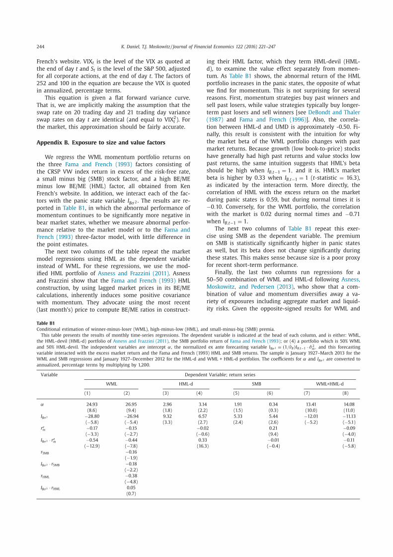
244 K. Daniel, T.J. Moskowitz / Journal of Financial Economics 122 (2016) 221–247 French’s website. VIX t is the level of the VIX as quoted at the end of day t and S t is the level of the S&P 500, adjusted for all corporate actions, at the end of day t . The factors of 252 and 100 in the equation are because the VIX is quoted in annualized, percentage terms.
This equation is given a flat forward variance curve. That is, we are implicitly making the assumption that the swap rate on 20 trading day and 21 trading day variance swap rates on day t are identical (and equal to VIX 2 t ). For the market, this approximation should be fairly accurate. Appendix B. Exposure to size and value factors
We regress the WML momentum portfolio returns on the three Fama and French (1993) factors consisting of the CRSP VW index return in excess of the risk-free rate, a small minus big (SMB) stock factor, and a high BE/ME minus low BE/ME (HML) factor, all obtained from Ken French’s website. In addition, we interact each of the fac- tors with the panic state variable I Bσ 2 . The results are re- ported in Table B1 , in which the abnormal performance of momentum continues to be significantly more negative in bear market states, whether we measure abnormal perfor- mance relative to the market model or to the Fama and French (1993) three-factor model, with little difference in the point estimates.
The next two columns of the table repeat the market model regressions using HML as the dependent variable instead of WML. For these regressions, we use the mod- ified HML portfolio of Asness and Frazzini (2011) . Asness and Frazzini show that the Fama and French (1993) HML construction, by using lagged market prices in its BE/ME calculations, inherently induces some positive covariance with momentum. They advocate using the most recent (last month’s) price to compute BE/ME ratios in construct-
ing their HML factor, which they term HML-devil (HML- d), to examine the value effect separately from momen- tum. As Table B1 shows, the abnormal return of the HML portfolio increases in the panic states, the opposite of what we find for momentum. This is not surprising for several reasons. First, momentum strategies buy past winners and sell past losers, while value strategies typically buy longer- term past losers and sell winners [see DeBondt and Thaler (1987) and Fama and French (1996) ]. Also, the correla- tion between HML-d and UMD is approximately -0.50. Fi- nally, this result is consistent with the intuition for why the market beta of the WML portfolio changes with past market returns. Because growth (low book-to-price) stocks have generally had high past returns and value stocks low past returns, the same intuition suggests that HML’s beta should be high when I B,t−1 = 1 , and it is. HML’s market beta is higher by 0.33 when I B,t−1 = 1 ( t -statistic = 16.3), as indicated by the interaction term. More directly, the correlation of HML with the excess return on the market during panic states is 0.59, but during normal times it is −0 . 10 . Conversely, for the WML portfolio, the correlation with the market is 0.02 during normal times and −0.71 when I B,t−1 = 1 .
The next two columns of Table B1 repeat this exer- cise using SMB as the dependent variable. The premium on SMB is statistically significantly higher in panic states as well, but its beta does not change significantly during these states. This makes sense because size is a poor proxy for recent short-term performance.
Finally, the last two columns run regressions for a 50–50 combination of WML and HML-d following Asness, Moskowitz, and Pedersen (2013) , who show that a com- bination of value and momentum diversifies away a va- riety of exposures including aggregate market and liquid- ity risks. Given the opposite-signed results for WML and
Table B1 Conditional estimation of winner-minus-loser (WML), high-minus-low (HML), and small-minus-big (SMB) premia.
This table presents the results of monthly time-series regressions. The dependent variable is indicated at the head of each column, and is either: WML, the HML–devil (HML-d) portfolio of Asness and Frazzini (2011) , the SMB portfolio return of Fama and French (1993) ; or (4) a portfolio which is 50% WML and 50% HML-devil. The independent variables are intercept α, the normalized ex ante forecasting variable I Bσ 2 ≡ (1 / ̄v B )I B,t−1 · ˆ σ 2
m , and this forecasting variable interacted with the excess market return and the Fama and French (1993) HML and SMB returns. The sample is January 1927–March 2013 for the WML and SMB regressions and January 1927–December 2012 for the HML-d and WML + HML-d portfolios. The coefficients for α and I Bσ 2 are converted to annualized, percentage terms by multiplying by 1,200.
Variable Dependent Variable; return series WML HML-d SMB WML+HML-d
(1) (2) (3) (4) (5) (6) (7) (8) α 24.93 26.95 2.96 3.14 1.91 0.34 13.41 14.08
(8.6) (9.4) (1.8) (2.2) (1.5) (0.3) (10.0) (11.0) I Bσ 2 −28.80 −26.94 9.32 6.57 5.33 5.44 −12.01 −11.13
( −5.8) ( −5.4) (3.3) (2.7) (2.4) (2.6) ( −5.2) ( −5.1) r e m −0.17 −0.15 −0.02 0.21 −0.09
( −3.3) ( −2.7) ( −0.6) (9.4) ( −4.0) I Bσ 2 · r e m −0.54 −0.44 0.33 −0.01 −0.11
( −12.9) ( −7.8) (16.3) ( −0.4) ( −5.8) r SMB −0.16
( −1.9) I Bσ 2 · r SMB −0.18
( −2.2) r HML −0.38
( −4.8) I Bσ 2 · r HML 0.05
(0.7)

K. Daniel, T.J. Moskowitz / Journal of Financial Economics 122 (2016) 221–247 245 HML-d on the panic state variables, it is not surprising that a combination of WML and HML-d hedges some of this risk. However, since the magnitude of the effects on WML are much larger than those of HML, the net effect is still a reduction in returns and a decrease in beta during panic states for the momentum-value combination. 20 Appendix C. Maximum Sharpe ratio strategy
The setting is discrete time with T periods from 1 , . . . , T . We can trade in two assets, a risky asset and a risk free asset. Our objective is to maximize the Sharpe ra- tio of a portfolio in which, each period, we can trade in or out of the risky asset with no cost.
Over period t + 1 which is the span from t to t + 1 , the excess return on a risky asset ˜ r t+1 is distributed normally, with time- t conditional mean µt and conditional variance σ 2
t . That is, µt = E t [ ̃ r t+1 ] (16) and σ 2
t = E t [( ̃ r t+1 − µt ) 2 ], (17) where we assume that at t = 0 the agent knows µt and σ t for t ∈ { 0 , . . . , T − 1 } .
The agent’s objective is to maximize the full-period Sharpe ratio of a managed portfolio. The agent manages the portfolio by placing, at the beginning of each period, a fraction w t of the value of the managed portfolio in the risky asset and a fraction 1 − w t in the risk-free asset. The time t expected excess return and variance of the managed portfolio in period t + 1 is then given by ˜ r p,t+1 = w t ̃ r t+1 ∼ N (w t µt , w 2 t σ 2
t ). (18) The Sharpe ratio over the T periods is SR = E [ 1
T ∑ T t=1 ̃ r p,t ]√
E [ 1 T ∑ T
t=1 ( ̃ r p,t − r̄ p ) 2 ] , (19) where the r̄ p in the denominator is the sample average per period excess return ( 1 T ∑ T
t=1 ̃ r p,t ). Given the information structure of this optimization
problem, maximizing the Sharpe ratio is equivalent to solv- ing the constrained maximization problem:
max w 0 , ... ,w T−1 E
[ 1 T
T ∑ t=1 ˜ r p,t
] subject to E
[ 1 T
T ∑ t=1 ( ̃ r p,t − r̄ ) 2
] = σ 2
p . (20)
If the period length is sufficiently short, then E [( ̃ r p,t − r̄ ) 2 ] ≈ σ 2
t = E t [( ̃ r t+1 − µt ) 2 ]. With this ap- proximation, substituting in the conditional expectations
20 One possibility for the dominance of momentum here is that the 50–
50 momentum-value weighting is based on equal dollar allocation to both rather than equal risk allocation. Since momentum is more volatile than value, this may be tilting the overall exposure of the combination portfo- lio more toward momentum.
for the managed portfolio from Eq. (16) to (17) gives the Lagrangian:
max w 0 , ... ,w T−1 L ≡ max
w t (
1 T
T −1 ∑ t=0 w t µt
) − λ
( 1 T
T −1 ∑ t=0 w 2 t σ 2
t = σ 2 p ) .
(21) The T first order conditions for optimality are ∂L ∂w t
∣∣∣∣w t = w ∗t = 1
T (µt − 2 λw ∗t σ 2 t ) = 0 ∀ t ∈ { 0 , . . . , T −1 }
(22) giving an optimal weight on the risky asset at time t of w ∗t = ( 1
2 λ)
µt σ 2
t . (23) That is, the weight placed on the risky asset at time t should be proportional to the expected excess return over the next period and inversely proportional to the condi- tional variance. Appendix D. GJR-GARCH forecasts of volatility
The construction of the dynamic portfolio strategy we explore in Sections 4 and 5.4 requires estimates of the con- ditional mean return and the conditional volatility of the momentum strategies. To forecast the volatility, we first fit a GARCH process to the daily momentum returns of each asset class. We fit the GARCH model proposed by Glosten, Jagannathan, and Runkle (1993) and summarized by Eqs. (7) and (8) .The maximum likelihood estimates and t -statistics are:
Parameter: ˆ µ ˆ ω ˆ α ˆ γ ˆ β
ML-est 0.86 ×10 −3 1.17 ×10 −6 0.111 −0.016 0.896 t-stat (14.7) (4.2) (14.4) ( −1.6) (85.1)
We then regress the future realized 22-day WML return volatility ˆ σ22 ,t+1 on the GJR-GARCH estimate ( ̂ σGARCH , t ), the lagged 126-day WML return volatility ( ̂ σ126 ,t ), and a constant. The ordinary least squares (OLS) coefficient es- timates and t -statistics are
coefficient: ˆ α ˆ σGARCH , t ˆ σ126 ,t coef. est. 0.0010 0.6114 0.2640 t-stat (3.0) (16.7) (7.2)
with a regression R 2 adj = 0 . 617 . 21 The fitted estimate of
ˆ σ22 ,t+1 is then used as an input to the dynamic WML port- folio weight, as discussed in Sections 4 and 5.4 .
The same estimation procedure is used to generate a forecast of the future 22-day WML return volatility in each of the alternative asset classes. The maximum- likelihood GJR-GARCH parameter estimates and t -statistics
21 The lag one residual autocorrelation is 0.013 ( t -statistic = 0 . 44 ), jus- tifying the use of OLS standard errors. Also, the t -statistics on the lag 2–
5 autocorrelations never exceed 1.14. The autocorrelation of the depen- dent variable of the regression ( ̂ σ22 ,t ) is large and statistically significant ( ̂ ρ1 = 0 . 55 , t -statistic = 24 . 5 ). This suggests that the autocorrelation in ˆ σ22 ,t results from its forecastable component. The residual from its pro- jection on the forecast variables is uncorrelated at any conventional sta- tistically significant level.

246 K. Daniel, T.J. Moskowitz / Journal of Financial Economics 122 (2016) 221–247 Table D1 Maximum likelihood estimates of GJR-GARCH model for momentum portfolios.
Panel A presents the maximum-likelihood estimates of the coefficients of the Glosten, Jagannathan, and Runkle (1993) –generalized autoregressive con- ditional heteroskedasticity (GJR–GARCH) model, given by Eqs. (7) and (8) , fitted to daily returns for each of the momentum portfolios we examine in Section 5.4 . The estimates of the µ and ω coefficients are multiplied by 10 3 and 10 6 , respectively. Maximum likelihood–based t-statistics are given in parentheses. For β , this t-statistic tests whether β = 1 ; for all other parameters, it tests whether the parameter is zero. Panel B presents the results of monthly regressions in which we regress the future one month daily volatility of the winner-minus-loser (WML) portfolio on an intercept ( α), on the lagged 126-day WML return volatility ( σ 126 ), and on the lagged GJR-GARCH volatility ( σ GARCH ). The starting date for each series is indicated in the table. All equity series end on 2013:05:31, and all asset-class series end on 2013:06:03. EU = European Union; JP = Japan; UK = United Kingdom; GLE = global equity; FI = fixed income; CM = commodities; FX = foreign exchange; EQ = equity; GA = global asset class; GAll = Global Asset Class + Equity
Coefficient Asset class/market, series start date EU, JP, UK, US, GLE, FI, CM, FX, EQ, GA, GAll,
90:01:02 90:01:02 90:01:02 72:02:01 72:02:01 83:01:03 72:02:01 79:01:01 78:01:02 72:02:01 72:02:01 Panel A: GJR–GARCH coefficient estimates µ( × 10 3 ) 0.387 0.187 0.316 0.314 0.124 0.024 0.516 0.238 0.322 0.154 0.159
(5.3) (3.0) (3.4) (6.2) (6.7) (0.6) (5.0) (4.2) (5.3) (5.8) (5.6) ω( × 10 6 ) 0.569 0.616 0.364 0.298 0.024 0.027 1.525 0.455 0.619 0.034 0.035
(2.4) (4.3) (3.3) (4.1) (3.3) (1.4) (4.1) (4.3) (3.9) (1.6) (1.6) α 0.089 0.160 0.094 0.104 0.107 0.060 0.055 0.092 0.074 0.037 0.046
(6.4) (9.8) (7.7) (12.4) (12.1) (4.1) (9.0) (9.0) (6.9) (3.7) (4.2) γ −0.020 −0.007 −0.022 −0.026 −0.024 −0.002 −0.008 −0.020 −0.002 −0.011 −0.007
( −1.6) ( −1.6) ( −2.0) ( −2.8) ( −2.0) ( −1.6) ( −2.3) ( −1.8) ( −1.6) ( −1.6) ( −0.8) β 0.912 0.848 0.918 0.907 0.909 0.945 0.940 0.909 0.916 0.966 0.955
( −5.9) ( −11.4) ( −8.9) ( −11.1) ( −11.4) ( −4.2) ( −8.1) ( −9.6) ( −7.1) ( −2.9) ( −3.2) Panel B: Time series regression coefficient estimates α( × 10 2 ) 0.053 0.083 0.067 0.036 0.016 0.082 0.177 0.144 0.096 0.065 0.034
(1.3) (1.8) (1.4) (1.5) (1.5) (4.7) (3.0) (4.4) (2.8) (4.0) (2.8) ˆ σ126 0.334 0.126 0.159 0.227 0.280 0.475 0.161 0.125 0.233 0.113 0.180
(4.7) (1.8) (2.1) (4.3) (5.1) (5.7) (2.2) (1.8) (3.5) (1.1) (2.2) ˆ σGARCH 0.561 0.754 0.758 0.682 0.632 0.220 0.665 0.581 0.594 0.637 0.655
(8.0) (11.4) (9.9) (13.1) (11.6) (2.9) (9.1) (9.3) (9.2) (6.1) (7.9) and regression estimates and t -statistics are presented in Table D1 .
The parameters above and in Table D1 tell an inter- esting story. First, in the regressions, the coefficient on the GJR-GARCH estimate of volatility is always significant, and the coefficient on the lagged 126-day volatility is al- ways smaller but not always statistically significant. There appears to be a longer-lived component of volatility that ˆ σ126 ,t is capturing.
Also interesting is the leverage parameter γ . In each of the asset classes, the maximum-likelihood estimate of γis negative, which means that a strong negative return on the WML portfolio is generally associated with a decrease in the WML return variance. As noted elsewhere in the lit- erature, this coefficient is positive at high levels of statis- tical significance for the market return (see, e.g., Glosten, Jagannathan, and Runkle (1993) and Engle and Ng (1993) ). References Asness, C. , Frazzini, A. , 2011. The devil in HML’s details, AQR capital man-
agement paper . Asness, C.S. , 1994. The power of past stock returns to explain future stock
returns, working paper. University of Chicago . Asness, C.S. , Liew, J.M. , Stevens, R.L. , 1997. Parallels between the cross-sec-
tional predictability of stock and country returns. Journal of Portfolio Management 23, 79–87 .
Asness, C.S. , Moskowitz, T.J. , Pedersen, L.H. , 2013. Value and momentum everywhere. The Journal of Finance 58, 929–985 .
Barroso, P. , Santa-Clara, P. , 2015. Momentum has its moments. Journal of Financial Economics 116, 111–120 .
Boguth, O. , Carlson, M. , Fisher, A. , Simutin, M. , 2011. Conditional risk and performance evaluation: volatility timing, overconditioning, and new
estimates of momentum alphas. Journal of Financial Economics 102, 363–389 .
Brunnermeier, M.K. , Nagel, S. , Pedersen, L.H. , 2008. Carry trades and cur- rency crashes. NBER Macroeconomics Annual 23 .
Carr, P. , Wu, L. , 2009. Variance risk premiums. Review of Financial Studies 22, 1311–1341 .
Chabot, B. , Remy Ghysels, E. , Jagannathan, R. , 2009. Momentum cycles and limits to arbitrage - evidence from Victorian England and post-De- pression US stock markets. Northwestern University, Evanston, IL . Un- published working paper.
Chan, K. , 1988. On the contrarian investment strategy. Journal of Business 61, 147–163 .
Chan, L.K. , Jegadeesh, N. , Lakonishok, J. , 1996. Momentum strategies. Jour- nal of Finance 51, 1681–1714 .
Christensen, B.J. , Prabhala, N.R. , 1998. The relation between implied and realized volatility. Journal of Financial Economics 50, 125–150 .
Cohen, L. , Frazzini, A. , 2008. Economic links and predictable returns. The Journal of Finance 63, 1977–2011 .
Cooper, M.J. , Gutierrez, R.C. , Hameed, A. , 2004. Market states and momen- tum. Journal of Finance 59, 1345–1365 .
DeBondt, W.F.M. , Thaler, R.H. , 1987. Further evidence on investor overre- action and stock market seasonality. Journal of Finance 42, 557–581 .
Engle, R.F. , Ng, V.K. , 1993. Measuring and testing the impact of news on volatility. Journal of Finance 48, 1749–1778 .
Erb, C.B. , Harvey, C.R. , 2006. The strategic and tactical value of commodity futures. Financial Analysts Journal 62, 69–97 .
Exchange, C.B.O., 2003. VIX: CBOE volatility index, chicago board options exchange (CBOE) white paper . www.cboe.com
Fama, E.F. , French, K.R. , 1993. Common risk factors in the returns on stocks and bonds. Journal of Financial Economics 33, 3–56 .
Fama, E.F. , French, K.R. , 1996. Multifactor explanations of asset pricing anomalies. Journal of Finance 51, 55–84 .
Geczy, C., Samonov, M., 2015. Two centuries of price return momen- tum . Unpublished working paper, Wharton school of the University of Pennsylvania, http://papers.ssrn.com/sol3/abstract=2292544
Glosten, L.R. , Jagannathan, R. , Runkle, D. , 1993. On the relation between the expected value and the volatility of the nominal excess return on stocks. Journal of Finance 48, 1779–1801 .

K. Daniel, T.J. Moskowitz / Journal of Financial Economics 122 (2016) 221–247 247 Grundy, B. , Martin, J.S. , 2001. Understanding the nature of the risks and
the source of the rewards to momentum investing. Review of Finan- cial Studies 14, 29–78 .
Hansen, L.P. , Jagannathan, R. , 1991. Implications of security market data for models of dynamic economies. Journal of Political Economy 99, 225–262 .
Henriksson, R.D. , Merton, R.C. , 1981. On market timing and investment performance. II. statistical procedures for evaluating forecasting skills. Journal of Business 54, 513–533 .
Israel, R. , Moskowitz, T.J. , 2013. The role of shorting, firm size, and time on market anomalies. Journal of Financial Economics 108, 275–301 .
Jagannathan, R. , Korajczyk, R.A. , 1986. Assessing the market timing perfor- mance of managed portfolio. Journal of Business 59, 217–235 .
Jegadeesh, N. , 1990. Evidence of predictable behavior of security returns. Journal of Finance 45, 881–898 .
Jegadeesh, N. , Titman, S. , 1993. Returns to buying winners and selling losers: implications for stock market efficiency. Journal of Finance 48, 65–91 .
Jegadeesh, N. , Titman, S. , 1995. Overreaction, delayed reaction, and con- trarian profits. Review of Financial Studies 8, 973–999 .
Jegadeesh, N. , Titman, S. , 2001. Profitability of momentum strategies: an evaluation of alternative explanations. Journal of Finance 56, 699–720 .
Kothari, S. , Shanken, J. , 1992. Stock return variation and expected divi- dends. Journal of Financial Economics 31, 177–210 .
Lehmann, B.N. , 1990. Fads, martingales, and market efficiency. Quarterly Journal of Economics 105, 1–28 .
Lo, A.W. , MacKinlay, A.C. , 1990. When are contrarian profits due to stock market overreaction? Review of Financial Studies 3, 175–205 .
Loewenstein, G. , Weber, E.U. , Hsee, C.K. , Welch, N. , 2001. Risk as feelings. Psychological bulletin 127, 267–286 .
Loewenstein, G.F. , 20 0 0. Emotions in economic theory and economic be- havior. American Economic Review 65, 426–432 .
Markowitz, H.M. , 1952. Portfolio selection. Journal of Finance 7, 77–91 . Merton, R.C. , 1974. On the pricing of corporate debt: the risk structure of
interest rates. Journal of Finance 29, 449–470 . Moskowitz, T.J. , Grinblatt, M. , 1999. Do industries explain momentum?
Journal of Finance 54, 1249–1290 . Moskowitz, T.J. , Ooi, Y.H. , Pedersen, L.H. , 2012. Time series momentum.
Journal of Financial Economics 104, 228–250 . Okunev, J. , White, D. , 2003. Do momentum-based strategies still work in
foreign currency markets? Journal of Financial and Quantitative Anal- ysis 38, 425–447 .
Rouwenhorst, K.G. , 1998. International momentum strategies. Journal of Finance 53, 267–284 .
Rouwenhorst, K.G. , 1999. Local return factors and turnover in emerging stock markets. Journal of Finance 54, 1439–1464 .
Stivers, C. , Sun, L. , 2010. Cross-sectional return dispersion and time-varia- tion in value and momentum premia. Journal of Financial and Quan- titative Analysis 45, 987–1014 .
Sunstein, C.R. , Zeckhauser, R. , 2008. Overreaction to Fearsome Risks. Cam- bridge, MA . Unpublished working paper, Harvard University
Treynor, J.L. , Black, F. , 1973. How to use security analysis to improve port- folio selection. Journal of Business 46, 66–86 .
Related Documents