Journal of Applied Geophysics · 2019-08-20 · Inversion of multiple intersecting high-resolution crosshole GPR profiles for hydrological characterization at the Boise Hydrogeophysical

Journal of Applied Geophysics 73 (2011) 305–314

Contents lists available at ScienceDirect

Journal of Applied Geophysics

j ourna l homepage: www.e lsev ie r.com/ locate / jappgeo

Inversion of multiple intersecting high-resolution crosshole GPR profiles forhydrological characterization at the Boise Hydrogeophysical Research Site

B. Dafflon a,⁎, J. Irving b, W. Barrash a

a Center for Geophysical Investigation of the Shallow Subsurface, Boise State University, Boise, ID, USAb School of Engineering, University of Guelph, Ontario, Canada

⁎ Corresponding author. Tel.: +1 208 426 46 78; fax:E-mail address: [email protected] (B. Daffl

0926-9851/$ – see front matter © 2011 Elsevier B.V. Aldoi:10.1016/j.jappgeo.2011.02.001

a b s t r a c t

Article history:Received 25 August 2010Accepted 3 February 2011Available online 12 February 2011

Keywords:GPRHydrogeophysicsCrosshole tomographyInversion

The integration of geophysical data into the subsurface characterization problem has been shown in manycases to significantly improve hydrological knowledge by providing information at spatial scales and locationsthat is unattainable using conventional hydrological measurement techniques. In particular, crossholeground-penetrating radar (GPR) tomography has shown much promise in hydrology because of its ability toprovide highly detailed images of subsurface radar wave velocity, which is strongly linked to soil watercontent. Here, we develop and demonstrate a procedure for inverting together multiple crosshole GPR datasets in order to characterize the spatial distribution of radar wave velocity below the water table at the BoiseHydrogeophysical Research Site (BHRS) near Boise, Idaho, USA. Specifically, we jointly invert 31 intersectingcrosshole GPR profiles to obtain a highly resolved and consistent radar velocity model along the variousprofile directions. The model is found to be strongly correlated with complementary neutron porosity-logdata and is further corroborated by larger-scale structural information at the BHRS. This work is an importantprerequisite to using crosshole GPR data together with existing hydrological measurements for improvedgroundwater flow and contaminant transport modeling.

+1 208 426 38 88.on).

l rights reserved.

© 2011 Elsevier B.V. All rights reserved.

1. Introduction

Knowledge regarding spatial heterogeneity in hydrological proper-ties is required for effective modeling of subsurface contaminanttransport (e.g., Gelhar, 1993; Hubbard and Rubin, 2005). To this end,geophysical methods offer much potential because they provide a scaleof spatial resolution and degree of subsurface coverage not availablewith traditional hydrologicalmeasurement techniques such as boreholelog and core analyses and pumping and tracer tests (e.g., Hubbard et al.,2001; Hyndman and Gorelick, 1996). Initially, the use of geophysicalmethods in hydrologywas geared towards the qualitative delineation oflarger-scale subsurface features such as facies boundaries and uncon-formities (e.g., Beres and Haeni, 1991; Keller and Frischknecht, 1966).More recently, however, the goal has been to extract detailedquantitative information regarding the spatial distribution of hydrolog-ical properties from these data (e.g., Chen et al., 2001; Dafflon et al.,2009; Harp et al., 2008; Hyndman et al., 2000; Kowalsky et al., 2005;Linde et al., 2006b; Tronicke et al., 2004). Such information has thepotential to greatly improve hydrological models and thus predictionsof groundwater flow and contaminant transport (e.g., Dafflon et al.,2010; Hubbard et al., 2001; Hyndman andGorelick, 1996;McKenna andPoeter, 1995; Scheibe and Chien, 2003).

Two of themost important hydrological parameters controllingflowand transport in the subsurface are the hydraulic conductivity and theporosity. Although the spatial distribution of hydraulic conductivityremains generally muchmore difficult to estimate than that of porosity,both parameters are often seen to exhibit a significant degree ofsimilarity with regard to their spatial variability and/or spatialcorrelation. For example, a large number of studies have shown that,for the sand- and gravel-type unconsolidated sediments commonlyseen in near-surface studies, changes in the porosity are often linked tocorresponding changes in the hydraulic conductivity and can play animportant role in transport behavior (e.g., Chen et al., 2001; Hu et al.,2009; Hubbard et al., 2001; Kowalsky et al., 2005; Linde et al., 2006b;Scheibe and Chien, 2003). In this regard, a number of geophysicalmeasurements are sensitive to the subsurface porosity distribution. Inparticular, crosshole ground-penetrating radar (GPR) tomography is ofmuch interest because of its ability to provide images of porosity insaturated environments with unsurpassed spatial resolution. This ispossible because of the strong relationship that exists between radarwave velocity and soil water content.

In recent years, awide variety of approaches have been developed togenerate crosshole GPR tomograms (e.g., Ernst et al., 2007; Giroux et al.,2007; Gloaguen et al., 2007; Hansen and Mosegaard, 2008; Irving et al.,2007; Johnson et al., 2007; Paasche and Tronicke, 2007). Each of theseapproaches differs in the way that the crosshole data are modeled and/or inverted, and has advantages and limitations depending on the dataquality, nature of the subsurface environment, and particular objectives

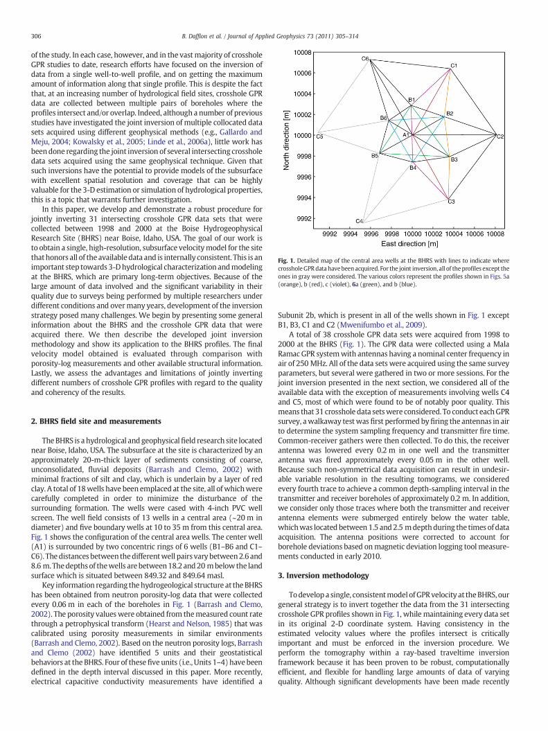
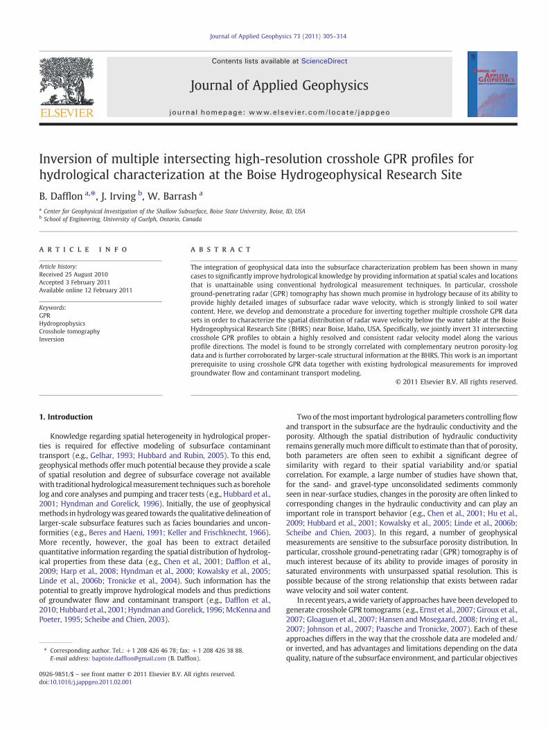
Fig. 1. Detailed map of the central area wells at the BHRS with lines to indicate wherecrossholeGPRdata havebeenacquired. For the joint inversion, all of theprofiles except theones in gray were considered. The various colors represent the profiles shown in Figs. 5a(orange), b (red), c (violet), 6a (green), and b (blue).

306 B. Dafflon et al. / Journal of Applied Geophysics 73 (2011) 305–314

of the study. In each case, however, and in the vastmajority of crossholeGPR studies to date, research efforts have focused on the inversion ofdata from a single well-to-well profile, and on getting the maximumamount of information along that single profile. This is despite the factthat, at an increasing number of hydrological field sites, crosshole GPRdata are collected between multiple pairs of boreholes where theprofiles intersect and/or overlap. Indeed, although a number of previousstudies have investigated the joint inversion of multiple collocated datasets acquired using different geophysical methods (e.g., Gallardo andMeju, 2004; Kowalsky et al., 2005; Linde et al., 2006a), little work hasbeendone regarding the joint inversion of several intersecting crossholedata sets acquired using the same geophysical technique. Given thatsuch inversions have the potential to provide models of the subsurfacewith excellent spatial resolution and coverage that can be highlyvaluable for the 3-D estimation or simulation of hydrological properties,this is a topic that warrants further investigation.

In this paper, we develop and demonstrate a robust procedure forjointly inverting 31 intersecting crosshole GPR data sets that werecollected between 1998 and 2000 at the Boise HydrogeophysicalResearch Site (BHRS) near Boise, Idaho, USA. The goal of our work isto obtain a single, high-resolution, subsurface velocitymodel for the sitethathonors all of the availabledata and is internally consistent. This is animportant step towards 3-Dhydrological characterization andmodelingat the BHRS, which are primary long-term objectives. Because of thelarge amount of data involved and the significant variability in theirquality due to surveys being performed by multiple researchers underdifferent conditions and overmany years, development of the inversionstrategy posed many challenges. We begin by presenting some generalinformation about the BHRS and the crosshole GPR data that wereacquired there. We then describe the developed joint inversionmethodology and show its application to the BHRS profiles. The finalvelocity model obtained is evaluated through comparison withporosity-log measurements and other available structural information.Lastly, we assess the advantages and limitations of jointly invertingdifferent numbers of crosshole GPR profiles with regard to the qualityand coherency of the results.

2. BHRS field site and measurements

TheBHRS is a hydrological and geophysicalfield research site locatednear Boise, Idaho, USA. The subsurface at the site is characterized by anapproximately 20-m-thick layer of sediments consisting of coarse,unconsolidated, fluvial deposits (Barrash and Clemo, 2002) withminimal fractions of silt and clay, which is underlain by a layer of redclay. A total of 18wells have been emplaced at the site, all ofwhichwerecarefully completed in order to minimize the disturbance of thesurrounding formation. The wells were cased with 4-inch PVC wellscreen. The well field consists of 13 wells in a central area (~20 m indiameter) and five boundary wells at 10 to 35 m from this central area.Fig. 1 shows the configuration of the central area wells. The center well(A1) is surrounded by two concentric rings of 6 wells (B1–B6 and C1–C6). Thedistances between thedifferentwell pairs vary between2.6 and8.6 m.Thedepthsof thewells arebetween18.2 and20 mbelow the landsurface which is situated between 849.32 and 849.64 masl.

Key information regarding thehydrogeological structure at theBHRShas been obtained from neutron porosity-log data that were collectedevery 0.06 m in each of the boreholes in Fig. 1 (Barrash and Clemo,2002). The porosity valueswere obtained from themeasured count ratethrough a petrophysical transform (Hearst and Nelson, 1985) that wascalibrated using porosity measurements in similar environments(Barrash and Clemo, 2002). Based on the neutron porosity logs, Barrashand Clemo (2002) have identified 5 units and their geostatisticalbehaviors at the BHRS. Four of these five units (i.e., Units 1–4)have beendefined in the depth interval discussed in this paper. More recently,electrical capacitive conductivity measurements have identified a

Subunit 2b, which is present in all of the wells shown in Fig. 1 exceptB1, B3, C1 and C2 (Mwenifumbo et al., 2009).

A total of 38 crosshole GPR data sets were acquired from 1998 to2000 at the BHRS (Fig. 1). The GPR data were collected using a MalaRamac GPR systemwith antennas having a nominal center frequency inair of 250 MHz. All of the data sets were acquired using the same surveyparameters, but several were gathered in two or more sessions. For thejoint inversion presented in the next section, we considered all of theavailable data with the exception of measurements involving wells C4and C5, most of which were found to be of notably poor quality. Thismeans that 31crosshole data setswere considered. To conduct eachGPRsurvey, awalkaway testwas first performed byfiring the antennas in airto determine the system sampling frequency and transmitter fire time.Common-receiver gathers were then collected. To do this, the receiverantenna was lowered every 0.2 m in one well and the transmitterantenna was fired approximately every 0.05 m in the other well.Because such non-symmetrical data acquisition can result in undesir-able variable resolution in the resulting tomograms, we consideredevery fourth trace to achieve a common depth-sampling interval in thetransmitter and receiver boreholes of approximately 0.2 m. In addition,we consider only those traces where both the transmitter and receiverantenna elements were submerged entirely below the water table,whichwas located between1.5 and2.5 mdepthduring the times of dataacquisition. The antenna positions were corrected to account forborehole deviations based onmagnetic deviation logging tool measure-ments conducted in early 2010.

3. Inversion methodology

Todevelop a single, consistentmodel ofGPRvelocity at theBHRS, ourgeneral strategy is to invert together the data from the 31 intersectingcrosshole GPR profiles shown in Fig. 1, while maintaining every data setin its original 2-D coordinate system. Having consistency in theestimated velocity values where the profiles intersect is criticallyimportant and must be enforced in the inversion procedure. Weperform the tomography within a ray-based traveltime inversionframework because it has been proven to be robust, computationallyefficient, and flexible for handling large amounts of data of varyingquality. Although significant developments have been made recently

307B. Dafflon et al. / Journal of Applied Geophysics 73 (2011) 305–314

with respect to full-waveform inversion of crosshole GPR data (e.g.,Ernst et al., 2007), this method is still very much in the research stageand is far too computationally burdensome for the task considered here.Also note that we have purposely chosen a “multi-directional 2-D”rather than fully 3-D inversion approach for our work. This avoids theestimation of GPR velocities at locations in the subsurface where wehave very few data. In the fully 3-D problem, the presence of manypoorly constrained model cells means that the tomographic system isextremely ill-posed and thus extensive regularization is required toobtain a stable solution. This results in overly smooth velocity estimatesin many regions of the subsurface, which does not lend well tosubsequent hydrological characterization and modeling, especially inthe context of solute transport. In contrast, with a multi-directional 2-Dapproach, we estimate velocities only where we have data along thedifferent tomographic profiles. The resulting joint 2-D velocity modelcan then be used to effectively infer multi-directional geostatistics andprovide soft data for the subsequent conditional simulation ofhydrological properties over the entire 3-D volume.

The first step in our inversion approach consists of defining thegeometry for the joint traveltime tomography. To deal with thedifferences between the 3-D reality involving deviated boreholes andthe required 2-D tomographic planes, all transmitter and receivercoordinates, as well as the coordinates of the profile intersections, areprojected into 2-D on a depth-by-depth basis (Fig. 2). The profileintersection coordinates are first obtained at each depth from thecrossing of horizontal straight lines linking the wells. Then the antennalocations are projected onto a 2-D plane by (i) calculating the horizontaldistance between the transmitter and receiver antennas at every depth,and (ii)finding the corresponding coordinates in the 2-Dplanebasedonthe vertical projection of a reference point defined by the horizontalposition of the transmitter antenna at the surface. This approach allowsus to preserve the true horizontal distance between the wells.

Once the 2-D tomographic geometries have been defined, the nextstep is to build the joint system of equations that is solved for thesubsurface GPR velocitymodel. Again, instead of solving for the velocityvalues in a set of 3-D voxels, we estimate velocities in a collection of 2-Dcells that are contained within the various tomographic planes. This isdone by considering all of the profiles together in a single expanded ray-based tomographic system. In other words, the tomographic kernelmatrices and model parameter vectors corresponding to the individualcrosshole GPR profiles are merged together and solved as one linearsystem. The expanded system is constructed such that common cells areconsidered where profiles intersect, thereby enforcing consistency in

Fig. 2. Illustration to show the basic concept of inverting together multiple intersectingcrosshole GPR data sets in 2-D. Profile intersections are determined in 3-D on a depth-by-depth basis, projected onto the 2-D tomographic planes, and then set as common cells inthe inversion procedure.

the velocity values at those locations. Themodel regularizationmatrix isalso constructed to enforce continuity between intersecting cells andtheir surroundings.

Based on extensive testing, we invert for four additional correctionparameters for each profile when performing the joint inversion of theBHRS data sets. Three of these parameters follow thework of Irving et al.(2007), who demonstrated the benefits of inverting for additionalcorrections in crosshole GPR tomography to account for possible errorsin the survey geometry and traveltimes, along with the nature of theantennas. Detailed information about these corrections can be found intheir paper. Thefirst correctionwe consider is related to the observationthat, when considering the average velocity along a ray versus thetransmitter–receiver angle, the velocity is often smaller at low anglesthan at higher ones. Irving et al. (2007) suggest that this results becausefirst-arriving energy does not always travel directly between theantenna centers, as is normally assumed by crosshole GPR practitioners.To address this issue, an angle-dependent traveltime correction isincluded in the inversion. The second and third corrections that weconsider are related to the fact that, when collecting each crosshole GPRgather, one antenna is held fixed while the other is lowered down theborehole. Because of this, the potential exists formany traveltimes to beaffected by a single error in the location of one antenna in its well, or bydifferences in the coupling of this antenna with its surroundings. Inaddition, slight drifts in the transmitter fire time over the duration of acrosshole survey can result in static time shifts between differentreceiver gathers. To account for these issues,we also include transmitterand receiver static traveltime correction parameters (e.g., Irving et al.,2007). Note that the implementation of the receiver static corrections,although not explicitly stated in Irving et al. (2007), is performedidentically to the transmitter static corrections.

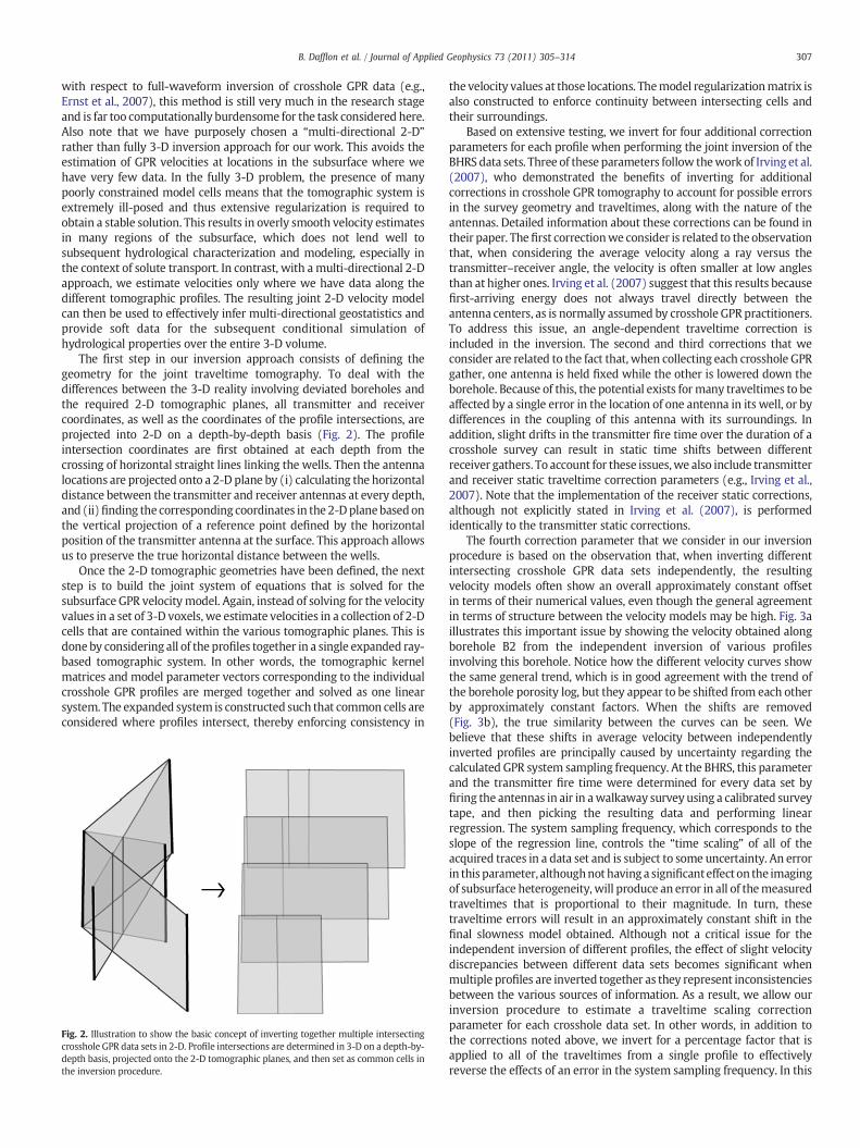
The fourth correction parameter that we consider in our inversionprocedure is based on the observation that, when inverting differentintersecting crosshole GPR data sets independently, the resultingvelocity models often show an overall approximately constant offsetin terms of their numerical values, even though the general agreementin terms of structure between the velocity models may be high. Fig. 3aillustrates this important issue by showing the velocity obtained alongborehole B2 from the independent inversion of various profilesinvolving this borehole. Notice how the different velocity curves showthe same general trend, which is in good agreement with the trend ofthe borehole porosity log, but they appear to be shifted from each otherby approximately constant factors. When the shifts are removed(Fig. 3b), the true similarity between the curves can be seen. Webelieve that these shifts in average velocity between independentlyinverted profiles are principally caused by uncertainty regarding thecalculated GPR system sampling frequency. At the BHRS, this parameterand the transmitter fire time were determined for every data set byfiring the antennas in air in awalkaway survey using a calibrated surveytape, and then picking the resulting data and performing linearregression. The system sampling frequency, which corresponds to theslope of the regression line, controls the “time scaling” of all of theacquired traces in a data set and is subject to some uncertainty. An errorin this parameter, althoughnot having a significanteffect on the imagingof subsurface heterogeneity, will produce an error in all of themeasuredtraveltimes that is proportional to their magnitude. In turn, thesetraveltime errors will result in an approximately constant shift in thefinal slowness model obtained. Although not a critical issue for theindependent inversion of different profiles, the effect of slight velocitydiscrepancies between different data sets becomes significant whenmultiple profiles are inverted together as they represent inconsistenciesbetween the various sources of information. As a result, we allow ourinversion procedure to estimate a traveltime scaling correctionparameter for each crosshole data set. In other words, in addition tothe corrections noted above, we invert for a percentage factor that isapplied to all of the traveltimes from a single profile to effectivelyreverse the effects of an error in the system sampling frequency. In this

Fig. 3. (a) Neutron porosity-log data (black) and collocated tomographic velocitiesestimatedby independently inverting a numberof profiles involvingwell B2. (b) The samedata shown in (a), but after shifting the velocity curves by a constant factor to bestillustrate the similarity to each other and the porosity-log data.

308 B. Dafflon et al. / Journal of Applied Geophysics 73 (2011) 305–314

way, the inversion can find a single velocity model that is able toadequately satisfy all of the different data sets.

Considering the above details, the ray-based tomographic systemthat we consider in our work can be described by the followingmatrixequation, which links perturbations in traveltime to thecorresponding slowness perturbations in the subsurface and correc-tion parameters (e.g., Irving et al., 2007):

Δt = LART F½ �

ΔsΔpaΔprΔptΔpf

266664

377775: ð1Þ

Here, Δt and Δs are vectors containing the traveltime and slownessperturbations, respectively, and L is the ray-based tomographic kernelmatrix whose rows contain the length of each ray in every model cell.Vector Δpa contains the values for the angle-dependent traveltimecorrection curve at a set of reference angles, and the rows of matrix Acontain linear interpolation weights to obtain, from these values, thetraveltime correction for each ray. Vectors Δpr and Δpt contain thereceiver and transmitter position traveltime corrections, respectively(i.e., a static correction for each receiver and transmitter location), andthe corresponding matrices R and T select, for each ray, the appropriatevalues. Finally, vectorΔpf contains for each crosshole data set the systemsampling frequency correction parameter (i.e., a percentage adjustmentof the traveltimes), and the corresponding matrix F contains, for eachray, the traveltime. It is important to note that Eq. (1) is simply astandard ray-based tomographic system linking changes in modelslowness to traveltime perturbations, that has been augmented to allowfor estimation of the additional traveltime correction parameters. Inother words, the correction parameters are added to the solution vectorand are estimated during the inversion alongwith the slowness in eachmodel cell. Also remember that all of the available crosshole GPR datasets are considered together in Eq. (1), such that we estimate a single

multi-directional 2-D velocity model that is consistent with all of themeasured traveltimes from each profile.

With Eq. (1) we implicitly assume that the measured crosshole GPRtraveltimes, once they havebeen suitably corrected for incompatibilitiesbetween high- and low-angle data, errors in transmitter fire time andborehole-location measurements, and velocity discrepancies related tothe system sampling frequency, can be adequately reproduced by thesubsurface slowness model. In other words, the corrections adjust theobserved traveltimes based on the transmitter–receiver angle, antennalocations, and profile being inverted, with the goal of reducing artifactsin the output velocity model that would otherwise be created bycorrelated errors related to these phenomena. Note that if such errorsare not present in the data, we have found that estimation of thetraveltime correction parameters does not influence significantly theresults obtained. In a large number of tests, we have also found thatinverting the tomographic system in Eq. (1) is reasonably robustbecause of the added corrections and themultiple data sets considered.Indeed, enforcing amatchbetweenmodel cells fromdifferent profiles atthe intersection locations has a significant effect on improving stability.To solve Eq. (1), we use a conjugate-gradient-based least-squaresapproach (e.g., Menke, 1984; Scales, 1987; Sen and Stoffa, 1995).Regularization on the slowness model is imposed using second-derivative smoothness constraints in the x and z directions.

4. Data picking and inversion parameters

The traveltimes of the direct transmitted wavefield for eachcrosshole GPR data set collected at the BHRS were determined using asemi-automated picking procedure. Specifically, we used the cross-correlation-based approach developed by Irving et al. (2007) fortransmitter–receiver angles greater than 30°, and standard threshold-based picking for lower angles. During subsequent quality control, asmall number of traveltimes were re-picked manually. All of the traceshaving transmitter–receiver angles ranging from −45 to 45° from thehorizontal were included in our analysis. This was decided based onobservations of the general quality of the data and the reliability of thepicks. The number of traces per crosshole data set ranged from 1888 to4089, with an average of 3260 traces. The data covered a depth rangebetween 3.5 and 18.5 m.

In the joint profile inversion, model cells were prescribed a size of0.2×0.2 m. Inverting all of the profiles together meant that we solvedfor the slowness in 58751 cells. The starting model for the ray-basedinversion was 1-D and was obtained by taking the mean of all of thecalculated 1-D velocity models generated by inverting each data setindependently. In thisway, the startingmodelwas the same for all of theprofiles, which ensured starting lateral continuity around the intersec-tion cells. In the inversion, every profile intersection was considered tobe 0.6 m thick (i.e., 3 cells wide). This choice was based on resolutionconsiderations; that is, taking into account the regularization imposedon the inversion procedure in order to ensure numerical stability, andthe inherent physical resolution limits imposed by the dominantwavelength of the GPR data combined with the ray-based “infinitefrequency” approach for modeling the first-arrival traveltimes. Regu-larization coefficients were carefully chosen based on the observedtradeoff between data fit and model structure.

5. Results

5.1. Joint inversion of all 31 crosshole data sets

Fig. 4 shows a 3-D view of the GPR velocity model obtained byinverting together the 31 intersecting data sets from the BHRS using thepreviously described methodology. It is clear that continuity betweenthe intersecting tomograms has been successfully enforced. The modelcan be seen to contain a number of large, laterally continuous featureshaving smaller scale internal variations. The general architecture of the

Fig. 4. 3-D view of the joint velocity tomogram obtained by inverting together the 31 crosshole GPR data sets at the BHRS. For better consideration of intersecting profiles around thecentral area, profiles B5–B6, B5–B4, and B4–C3 are not displayed. The main lithological units that have been identified at the BHRS in this depth interval (Units 1, 2a, 2b, 3, and 4) areindicated on the right-hand side of the model.

309B. Dafflon et al. / Journal of Applied Geophysics 73 (2011) 305–314

model is largely in accordance with the principal sedimentary units atthe BHRS and their statistical characteristics, as described for example inBarrash and Clemo (2002). In particular, the main unit boundariesobserved in previous studies (Barrash and Clemo, 2002; Mwenifumboet al., 2009) are found at similar depths in the tomographic model:around 834 m for the Unit 1–2a boundary; around 838 m for the Unit2a–2b boundary; between 838 m and 840 m for the Unit 2b–3boundary; and around 843.5 m for the Unit 3–4 boundary. AlthoughUnit 2b does not exist everywhere at the BHRS, where it does exist itsboundary with Unit 3 is themost difficult to observe in the tomograms.Unlike the neutron porosity logs, velocities for Unit 2b show moresimilarity to Unit 3 than to Unit 2a. Nevertheless, some light variation invelocity in Fig. 4 still allows us to recognize Unit 2b from Unit 3, whichdemonstrates that even small velocity differences can be relevant forgeological classification. Looking at the variousunits imaged in Fig. 4,wealso see that some of them show relatively low internal variability(e.g., Units 1 and 3), whereas others exhibit numerous smaller scalevariations (e.g., Units 2 and 4). This is also in agreement with thegeostatistical work of Barrash and Clemo (2002), who found that thevariance in porosity in Units 2 and 4 is more than two times larger thanthat in Units 1 and 3.

To consider the above results in more detail, in Fig. 5 we show threemulti-well tomographic profiles betweenboreholes C1andC3 thatwereextracted from the joint velocity tomogram in Fig. 4: C1–B2–B3–C3, C1–A1–C3, and C1–B1–B4–C3. The obtained GPR velocities along wells C1,

C3, and A1 are also compared to neutron porosity-log data collected inthese wells. Similar comparisons along wells B1, B2, B3 and B4 can befound in Fig. 6. Notice in Fig. 5 that some geological structures can beseen to extend through several profiles while others are shorter thanthe covered lateral distance of one profile. Continuity is also visiblewith regard to the variability across the various tomographic profiles.All of the tomograms again show features that are realistic andconsistent with existing structural information at the BHRS andprevious observations (Barrash and Clemo, 2002; Bradford et al.,2009; Mwenifumbo et al., 2009), and thus the inversion approachappears to perform well. In addition, note the generally goodcorrelation between velocity and the neutron porosity-log data. Thecorrelation coefficient inwell C1has a valueof−0.79, and similar trendscan be seen in wells C3 and A1, with values of −0.74 and −0.54,respectively. A smaller correlation coefficient is most likely related tothe different way that the GPR and neutron porosity logs image Unit2b between 838 and 840 m. Indeed, omitting this depth intervalincreases the correlation coefficients in wells C3 and A1 to −0.82 and−0.66, respectively.

In Fig. 6, we show two other multi-well tomographic profiles thatwere extracted from the joint velocity tomogram in Fig. 4. In this case,the profiles link the B wells and circle around borehole A1: B1–B3–B5–B1 and B2–B4–B6–B2. Again, the GPR velocity at the borehole locationsis compared to neutron porosity-log data. Compared to Fig. 5, moreprofiles intersect each tomogram in this figure. We see that even in the

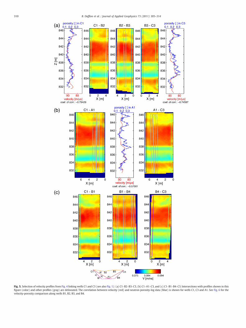
Fig. 5. Selection of velocity profiles from Fig. 4 linking wells C1 and C3 (see also Fig. 1): (a) C1–B2–B3–C3, (b) C1–A1–C3, and (c) C1–B1–B4–C3. Intersections with profiles shown in thisfigure (color) and other profiles (gray) are delineated. The correlation between velocity (red) and neutron porosity-log data (blue) is shown for wells C1, C3 and A1. See Fig. 6 for thevelocity-porosity comparison along wells B1, B2, B3, and B4.

310 B. Dafflon et al. / Journal of Applied Geophysics 73 (2011) 305–314

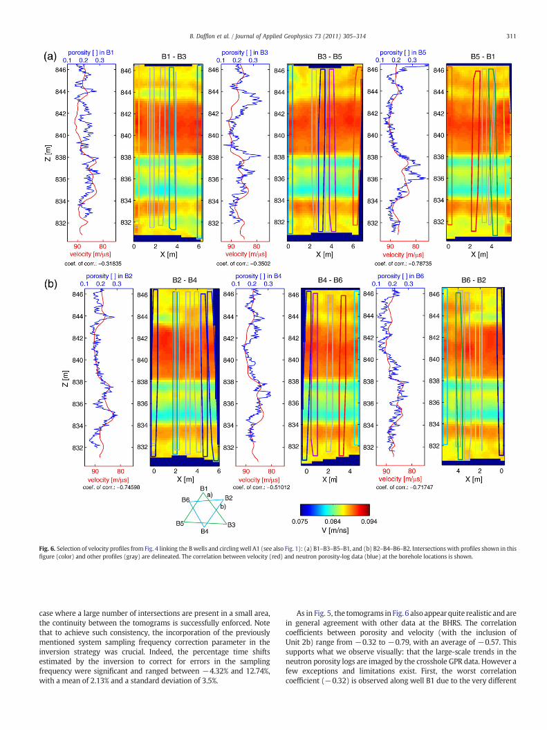
Fig. 6. Selection of velocity profiles from Fig. 4 linking the B wells and circlingwell A1 (see also Fig. 1): (a) B1–B3–B5–B1, and (b) B2–B4–B6–B2. Intersections with profiles shown in thisfigure (color) and other profiles (gray) are delineated. The correlation between velocity (red) and neutron porosity-log data (blue) at the borehole locations is shown.

311B. Dafflon et al. / Journal of Applied Geophysics 73 (2011) 305–314

case where a large number of intersections are present in a small area,the continuity between the tomograms is successfully enforced. Notethat to achieve such consistency, the incorporation of the previouslymentioned system sampling frequency correction parameter in theinversion strategy was crucial. Indeed, the percentage time shiftsestimated by the inversion to correct for errors in the samplingfrequency were significant and ranged between −4.32% and 12.74%,with a mean of 2.13% and a standard deviation of 3.5%.

As in Fig. 5, the tomograms in Fig. 6 alsoappearquite realistic and arein general agreement with other data at the BHRS. The correlationcoefficients between porosity and velocity (with the inclusion ofUnit 2b) range from −0.32 to −0.79, with an average of −0.57. Thissupports what we observe visually: that the large-scale trends in theneutron porosity logs are imaged by the crosshole GPR data. However afew exceptions and limitations exist. First, the worst correlationcoefficient (−0.32) is observed along well B1 due to the very different

Fig. 7. Velocity tomograms for profiles A1–C1 and A1–B2 that were obtained by inverting together (a) 31 and (b) 7 crosshole GPR data sets, and (c) independently inverted.Intersections with profiles shown in this figure (color) and other profiles (gray) are delineated. The correlation between velocity (red) and neutron porosity-log data (blue) at theborehole locations is shown. Note that the velocity and porosity data along well A1 are shown twice because different velocity data are obtained when the profiles are invertedindependently.

312 B. Dafflon et al. / Journal of Applied Geophysics 73 (2011) 305–314

313B. Dafflon et al. / Journal of Applied Geophysics 73 (2011) 305–314

behavior of velocity and porosity between 839 and 843 m.Although it isnot clear why this occurs, the neutron porosity log shows at thisparticular location something very different from all of the other wells,and thus it cannot be excluded that these data may contain an error.Secondly, we see a difference in imaging Unit 2b between the velocityand porosity log data along well B6 that is similar to what we observedalongwells A1andC3 in Fig. 5. Although the truepetrophysical nature ofUnit 2b is still the subject of investigation, this difference could arisefrom the presence of thin, high-porosity zones that the GPR techniquefailed to resolve. Finally, from Figs. 5 and 6, it is clear that the multi-directional velocity tomogram allows us to image smaller-scalevariations that are seen in the neutron porosity logs, although theshape and the amplitude of these variations are often not wellreproduced (see also Allumbaugh et al., 2002; Clement and Barrash,2006). The main reason for this is the support volume of themeasurements; the GPR data have a more limited spatial resolutionand are clearly not able to image small-scale heterogeneity around theborehole compared to the neutron porosity measurements. As a result,the use of a site-specificfield relationship between velocity and porositywill be generally more appropriate than the application of a givenlaboratory-based petrophysical transform. This is consistent withprevious findings from a numerical study where we showed theimportance and potential of rescaling velocity tomography through anappropriatefield relationship for hydrological predictions (Dafflon et al.,2010).

5.2. Resolution of the resulting velocity model

We now investigate the issue of resolution when performing thejoint profile inversion, and in particular how the number of data setsemployed, their quality, and their consistency can affect the final resultsobtained. Fig. 7 compares two profiles (A1–C1 and A1–B2) that wereextracted from the joint tomograms obtained using all 31 (Fig. 7a) andthena selected seven (Fig. 7b)of theBHRS crossholeGPRdata sets, alongwith the independent inversion results for these two profiles (Fig. 7c).The seven data sets that were inverted together for Fig. 7b were A1–C1,A1–B2, B1–B2, B2–B6, B1–B3, B2–B4 and C1–B2. These were among thebest quality of those that were collected at the BHRS. For theindependent inversions, the approach described by Irving et al. (2007)was employed. Note that there is a difference in appearance betweenFig. 10d of Irving et al. (2007) and Fig. 7c of this paper, both of whichcorrespond to the same A1–B2 profile and data. This difference resultsprimarily from the use of a different color scale between the figures, butalso becausemore recent andmore accurate deviation logswere used inour analysis.

Comparing Fig. 7a, b and c, we see that jointly inverting all 31 GPRdata sets tends to yield a “smoother” velocitymodel thanwhen only theseven profiles were considered, or when the profiles were invertedindependently. Indeed, there appears to be a tradeoff between thenumber of data sets employed in the inversion procedure and theresolution of small-scale structure in the output tomogram. The reasonfor this is related to the agreement between the various sources of dataused for the tomography. When a large number of profiles are invertedtogether, there is greater potential for inconsistency between thetraveltime data with respect to what they tell us about the subsurface.Although our use of the traveltime correction parameters attempts toreduce as much as possible the effects of such inconsistencies in theinversion, in general thismeans that a smoother velocity tomogramwillbe required to fit the data in a geologically reasonable way. Note,however, that this additional smoothingwhen inverting larger numbersof profiles is not necessarily a negative aspect of the joint inversionprocedure. That is, by using more data and by enforcing consistencyalong the various profile intersections, we are likely to reduce artifactsthat are caused by the fitting of data errors when smaller numbers ofprofiles are inverted.

Considering the above points, let us attempt to get a feeling for theaccuracy of the various tomographic inversion results shown in Fig. 7through comparison of the velocities obtained along the boreholes withporosity-logmeasurementsmade inwells A1, C1, and B2. For the A1–C1profile, the correlation coefficient between velocity and porosity alongwells A1 and C1 can be seen to be higher when inverting all 31 data setstogether than when the profile is inverted independently. Conversely,for the A1–B2 profile, the correlation coefficient along bothwells is seento be lower when inverting the 31 data sets compared to independentinversion. Similarly, we see that there is no consistent trend in thedegree of correlation between velocity and porosity in the case whereseven data sets were used for the joint inversion, compared to using all31 profiles together and inverting independently. These results arerepresentative of ourfindingswith the joint inversionmethodology, andthey demonstrate that inverting more profiles together may allow insomecases abetterfit to complementary sitedata, but inother cases not.In this regard, there are many reasons for a better or worse fit to theporosity logs, including the quality and coherency of the considereddata, the nature of the profile intersections, the corresponding surveygeometries, and the type of subsurface heterogeneity. The importantpoint is that, in all instances, the correlation between velocity along theboreholes and the neutron porosity logs is reasonably high. In otherwords, inverting all 31 profiles together not only provides a reasonablelooking velocity model that is consistent with all of the availabletraveltime data, but it also provides on average no worse fit to theneutron porosity-log data than inversions using fewer numbers ofprofiles.

6. Conclusions

Inverting together multiple intersecting crosshole GPR data sets canprovide key constraints for the 3-D quantitative characterization ofporosity, and lithological andhydrological properties related toporosity,in saturated sediments. Here, our objective was to develop a robustprocedure for jointly inverting 31 intersecting crosshole GPR profilescollected at the BHRS, with the end goal of having a single realistic radarvelocity model that can be used in subsequent hydrological investiga-tions. The developed approach, which consists ofmaintaining each dataset in its original 2-D coordinate system and inverting for velocity onlyalong the various tomographic planes, has benefits compared to fully 3-D inversion in that model parameters are only estimated in regions ofthe subsurface where we have data. This means that the inverseproblem is well behaved and does not require extensive regularizationto obtain a stable result, which in turnmeans that the final tomogram isbetter suited to hydrological characterization and modeling. We alsosaw that the inversion approach presented in this paper is robust,flexible, and able to handle many data sets of different quality throughthe incorporation of various traveltime correction parameters.

The results in this paper are part of an increasing number of recentstudies that investigate the degree of correlation between geophysicallyinverted parameters and hydrological and geological data at the fieldscale. In this regard, the multi-directional velocity model that weobtained at the BHRS was found to contain realistic features that arecorroborated by other sources of structural information. The modelallows us to: (1) recognize and trace the contacts between majorstratigraphic units at the site; (2) delineate Subunit 2b, which exhibitsanomalous behavior in both the electrical conductivity and dielectricpermittivity that is not dominated by thewater-saturated porosity; and(3) confirm variability differences within and between units includingthe recognition of smaller-scale subfacies structures. Further, the jointvelocity tomogramwehave obtained shows significant correlationwithneutron porosity-log data from the BHRS.With regard to this last point,several issues remain to be explored in futurework. First, the correlationbetween velocity and porosity for Subunit 2b is low for reasons that arenot well understood. Secondly, the spatial resolution of the final GPRvelocitymodel depends onmany factors, including the number, quality,

314 B. Dafflon et al. / Journal of Applied Geophysics 73 (2011) 305–314

and consistency of the various profiles involved, and thus case-specificrelationships between velocity and porosity should be considered forsubsequent hydrological characterization. Finally, the smoothness in thetomographic velocity model implies uncertainty in the location of unitboundaries at the BHRS. Theseuncertainties shouldbe incorporated intofuture hydrological work.

This research represents an important step forwards in character-izing the3-D spatial distributionof hydrological parameters in saturatedheterogeneous aquifers. As mentioned, our goal is to now use theobtained GPR velocity model as part of a detailed hydrologicalcharacterization effort at the BHRS. Using directional geostatisticsinferred from the joint tomogram and the velocity model as soft data,a fully 3-D conditional simulation of hydrological properties will beperformed for use in subsequent flow and transport modeling. Thehydrological benefits of including the geophysical data will then beevaluated by comparing the obtained predictionswith hydrological testresults at the BHRS.

Acknowledgments

This research was supported by funding to B. Dafflon from the SwissNational Science Foundation and Boise State University.W. Barrashwassupported by EPA under grants X-96004601-0 and X-96004601-1, andby the U.S. RDECOM ARL Army Research Office under grant W911NF-09-1-0534. The authors would like to thank the various researchersresponsible for collecting and archiving the BHRS data sets used in thisanalysis.

References

Allumbaugh, D., Chang, P.Y., Paprocki, L., Brainard, J.R., Glass, R.J., Rautman, C.Z., 2002.Estimating moisture contents in the vadose zone using cross borehole groundpenetrating radar; a studyof accuracy and repeatability.WaterResourcesResearch 38,1309.

Barrash, W., Clemo, T., 2002. Hierarchical geostatistics and multifacies systems: BoiseHydrogeophysical Research Site, Boise, Idaho. Water Resources Research 38 (10),1196.

Beres, M., Haeni, F.P., 1991. Application of ground-penetrating-radar methods inhydrogeologic studies. Ground Water 29 (3), 375–386.

Bradford, J.H., Clement, W.P., Barrash, W., 2009. Estimating porosity with ground-penetrating radar reflection tomography: a controlled 3-D experiment at the BoiseHydrogeophysical Research Site. Water Resources Research 45, W00D26.

Chen, J.S., Hubbard, S., Rubin, Y., 2001. Estimating the hydraulic conductivity at the SouthOyster Site from geophysical tomographic data using Bayesian techniques based onthe normal linear regression model. Water Resources Research 37 (6), 1603–1613.

Clement, W.P., Barrash, W., 2006. Crosshole radar tomography in a fluvial aquifer nearBoise, Idaho. Journal of Environmental and Engineering Geophysics 11 (3), 171–184.

Dafflon, B., Irving, J., Holliger, K., 2009. Simulated-annealing-based conditionalsimulation for the local-scale characterization of heterogeneous aquifers. Journalof Applied Geophysics 68 (1), 60–70.

Dafflon, B., Irving, J., Holliger, K., 2010. Calibration of high-resolution geophysical datawith tracer test measurements to improve hydrological predictions. Advances inWater Resources 33 (1), 55–68.

Ernst, J.R., Maurer, H., Green, A.G., Holliger, K., 2007. Application of a new 2D time-domainfull-waveform inversion scheme to crosshole radar data. Geophysics 72, J53–J64.

Gallardo, L.A., Meju, M.A., 2004. Joint two-dimensional DC resistivity and seismic traveltime inversion with cross-gradients constraints. Journal of Geophysical Research,Solid Earth 109 (B3), B03311.

Gelhar, L.W., 1993. Stochastic Subsurface Hydrology. Prentice-Hall, Englewood Cliffs.480 p.

Giroux, B., Gloaguen, E., Chouteau, M., 2007. bh_tomo— a Matlab borehole georadar 2Dtomography package. Computers and Geosciences 33 (1), 126–137.

Gloaguen, E., Marcotte, D., Giroux, B., Dubreuil-Boisclair, C., Chouteau, M., Aubertin, M.,2007. Stochastic borehole radar velocity and attenuation tomographies usingcokriging and cosimulation. Journal of Applied Geophysics 62 (2), 141–157.

Hansen, T.M., Mosegaard, K., 2008. VISIM: sequential simulation for linear inverseproblems. Computers and Geosciences 34 (1), 53–76.

Harp, D.R., Dai, Z.X., Wolfsberg, A.V., Vrugt, J.A., Robinson, B.A., Vesselinov, V.V., 2008.Aquifer structure identification using stochastic inversion. Geophysical ResearchLetters 35 (8), L08404.

Hearst, J.R., Nelson, P.H., 1985. Well Logging for Physical Properties. McGraw-Hill,New York.

Hu, B.X., Meerschaert, M.M., Barrash, W., Hyndman, D.W., He, C.M., Li, X.Y., Guo, L.J.,2009. Examining the influence of heterogeneous porosity fields on conservativesolute transport. Journal of Contaminant Hydrology 108 (3–4), 77–88.

Hubbard, S.S., Rubin, Y., 2005. Introduction to hydrogeophysics. In: Rubin, Y., Hubbard,S.S. (Eds.), Hydrogeophysics: Dordrecht. The Netherlands, Springer, pp. 3–21.

Hubbard, S.S., Chen, J.S., Peterson, J., Majer, E.L., Williams, K.H., Swift, D.J., Mailloux, B.,Rubin, Y., 2001. Hydrogeological characterization of the South Oyster BacterialTransport Site using geophysical data.Water Resources Research 37 (10), 2431–2456.

Hyndman, D.W., Gorelick, S.M., 1996. Estimating lithologic and transport properties inthree dimensions using seismic and tracer data: the Kesterson aquifer. WaterResources Research 32 (9), 2659–2670.

Hyndman, D.W., Harris, J.M., Gorelick, S.M., 2000. Inferring the relation betweenseismic slowness and hydraulic conductivity in heterogeneous aquifers. WaterResources Research 36 (8), 2121–2132.

Irving, J.D., Knoll, M.D., Knight, R.J., 2007. Improving crosshole radar velocitytomograms: a new approach to incorporating high-angle traveltime data.Geophysics 72 (4), J31–J41.

Johnson, T.C., Routh, P.S., Barrash,W., Knoll,M.D., 2007. A field comparison of Fresnel zoneand ray-based GPR attenuation-difference tomography for time-lapse imaging ofelectrically anomalous tracer or contaminant plumes. Geophysics 72 (2), G21–G29.

Keller, G.V., Frischknecht, F.C., 1966. Electrical Methods in Geophysical Prospecting.Pergamon Press Inc, Oxford. 526 p.

Kowalsky, M.B., Finsterle, S., Peterson, J., Hubbard, S., Rubin, Y., Majer, E., Ward, A., Gee, G.,2005. Estimation of field-scale soil hydraulic and dielectric parameters through jointinversion of GPR and hydrological data. Water Resources Research 41 (11), W11425.

Linde, N., Binley, A., Tryggvason, A., Pedersen, L.B., Revil, A., 2006a. Improvedhydrogeophysical characterization using joint inversion of cross-hole electricalresistance and ground-penetrating radar traveltime data. Water Resources Research42 (12), W12404.

Linde, N., Finsterle, S., Hubbard, S., 2006b. Inversion of tracer test data usingtomographic constraints. Water Resources Research 42 (4), W04410.

McKenna, S.A., Poeter, E.P., 1995. Field example of data fusion in site characterization.Water Resources Research 31 (12), 3229–3240.

Menke,W., 1984. Geophysical Data Analysis: Discrete Inverse Theory. Academic Press Inc.289 p.

Mwenifumbo, C.J., Barrash, W., Knoll, M.D., 2009. Capacitive conductivity logging andelectrical stratigraphy in a high-resistivity aquifer, Boise HydrogeophysicalResearch Site. Geophysics 74 (3), E125–E133.

Paasche, H., Tronicke, J., 2007. Cooperative inversion of 2D geophysical data sets: a zonalapproach based on fuzzy c-means cluster analysis. Geophysics 72 (3), A35–A39.

Scales, J.A., 1987. Tomographic inversion via the conjugate-gradient method.Geophysics 52 (2), 179–185.

Scheibe, T.D., Chien, Y.J., 2003. An evaluation of conditioning data for solute transportprediction. Ground Water 41 (2), 128–141.

Sen, M., Stoffa, P.L., 1995. Global Optimization Methods in Geophysical Inversion.Netherlands, 281 p.

Tronicke, J., Holliger, K., Barrash, W., Knoll, M.D., 2004. Multivariate analysis of cross-holegeoradar velocity and attenuation tomograms for aquifer zonation. Water ResourcesResearch 40 (1), W01519.