Journal of Applied Economics Volume XIII, Number 1, May 2010 XIII Edited by the Universidad del CEMA Print ISSN 1514-0326 Online ISSN 1667-6726 Hakan Berument Afsin Sahin Seasonality in inflation volatility: Evidence from Turkey

Welcome message from author
This document is posted to help you gain knowledge. Please leave a comment to let me know what you think about it! Share it to your friends and learn new things together.
Transcript
Journal ofAppliedEconomics
Volume XIII, Number 1, May 2010XIII
Edited by the Universidad del CEMA Print ISSN 1514-0326Online ISSN 1667-6726
Hakan BerumentAfsin Sahin
Seasonality in inflation volatility: Evidence from Turkey

Journal of Applied Economics. Vol XIII, No. 1 (May 2010), 39-65
SEASONALITY IN INFLATION VOLATILITY: EVIDENCE FROM TURKEY
M. Hakan Berument*Bilkent University
Afsin SahinGazi University
Submitted May 2008; accepted July 2009
This paper assesses the presence of seasonal volatility in price indexes where a similar typeof pattern has been reported in asset prices in financial markets. The empirical evidence fromTurkey for the monthly period from 1987:01 to 2007:05 suggests the presence of seasonalityin the conditional variance of inflation. Thus, inferences for the models that do not accountfor the seasonality in the conditional variance will be misleading.
JEL classification codes: E31; E37, E30.Key words: inflation volatility, seasonality, EGARCH.
I. Introduction
Economists are interested not only in the level of inflation but in its volatility
because the latter also adversely affects economic performance.1 The purpose of
* M. Hakan Berument (corresponding author): Department of Economics, Bilkent University, 06800Ankara, Turkey; phone: +90 312 2902342, fax: +90 312 2665140, e-mail: [email protected],URL: http://www.bilkent.edu.tr/~berument. Afsin Sahin: School of Banking and Insurance, GaziUniversity, 06500 Ankara, Turkey; phone: +90 312 582 1100; fax +90 312 221 3202; email:[email protected]. URL: http://afsinsahin.googlepages.com. We would like to thank two anonymousreferees and Rana Nelson for their helpful comments.
1 Hafer (1986) and Holland (1986) report the negative effects of inflation volatility on employment.Friedman (1977), Froyen and Waud (1987) and Holland (1988) argue that there is a negative relationshipbetween output and inflation volatility. Wilson (2006) suggests that increased inflation volatility isassociated with higher average inflation and lower average growth. Berument and Guner (1997), Berument(1999) and Berument and Malatyali (2001) find a positive relationship between inflation volatility andinterest rates.
jaeXIII_1:jaeXIII_1 5/11/10 9:20 PM Página 39

this paper is to assess whether there is any regularity in inflation volatility. To be
specific, we will assess whether there is any seasonal pattern in the conditional
inflation variability series by considering seasonally unadjusted as well as seasonally
adjusted monthly data.2 Understanding any seasonal pattern in inflation volatility
is important. First, more efficient estimates of inflation forecasts will be gathered
by better modeling conditional inflation variances. Second, if seasonal patterns
exist using seasonally adjusted data, one may need to develop a new set of
algorithms that addresses the seasonality in volatility. Third, since inflation
volatility explains the behaviors of other macroeconomic variables, addressing
the seasonality of inflation volatility may help to better capture the effects of
inflation volatility on those variables.
There are a limited number of studies that analyze the determinants of inflation
volatility. Bowdler and Malik (2005) provide evidence that openness reduces
inflation volatility. Smith (1999) and Engel and Rogers (2001) argue that exchange
rate volatility explains part of price volatility, and Ghosh et al. (1996) claim that
pegged exchange rates are associated with significantly lower variability. Similarly,
Bleaney and Fielding (2002) find that countries that peg exchange rates have
lower inflation volatilities than floating-rate countries. According to Rother (2004),
activist fiscal policies may have an important impact on inflation volatility, and
volatility in discretionary fiscal policies increases inflation volatility. Aisen and
Veiga (2008) argue that higher degrees of political instability, ideological polarization
and political fragmentation are associated with higher inflation volatility. Dittmar
et al. (1999), Gavin (2003) and Berument and Yuksel (2007) discuss the effect of
inflation targeting regimes; Grier and Perry (1998), Kontonikas (2004), and
Berument and Dincer (2005) point out the effect of inflation on inflation volatility.
All these studies analyze the effect of economic and political variables on inflation
volatility. The aim of this paper is to model inflation volatility by considering
seasonal patterns of the general Consumer Price Index (CPI) inflation and its sub-
components.
This paper provides evidence regarding the seasonal pattern of Turkish inflation
volatilities for the period from January 1987 to May 2007. Although most prices
are set monthly in Turkey, price changes make their biggest adjustment once a year
–at the beginning of the year or when a new set of products enters the market. For
some products, prices are generally set to include the expected inflation for the year,
Journal of Applied Economics40
2 Similar analyses have been performed on stock market volatilities since the mid-1980s. See, forexample, French and Roll (1986), and Savva, Osborn and Gill (2006).
jaeXIII_1:jaeXIII_1 5/11/10 9:20 PM Página 40
according to the government’s prediction, such as refrigerators, health services.3
The credibility of the government’s policies is assessed with the announced targets
when the budget details are released at the beginning of the fiscal year. Thus, one
may expect that volatility reaches its peak at the beginning of the fiscal year –
January. Thus, it is expected that for most products and for the general CPI, January
has the highest volatility. For some other products, prices are quite seasonal, such
as those for food, or prices are set mostly by the rest of the world, such as those for
automobiles.4 However, for agriculture, new seasonal products enter the market
around April and May, and for automobiles, around July and August. Thus, one
may expect that food and transportation volatilities peak around April-May and
July-August, respectively. In regulated sectors such as health and housing, volatility
is at its minimum just after a month after the price increases made because most
adjustments for the year are made in the previous month or towards the end of the
fiscal year when firms are close to finalizing their balance sheets.
The paper is organized as follows: Section II introduces and elaborates on the
data. Section III introduces the model employed in the paper. Section IV reports
the empirical evidence, while Section V provides a set of extensions of our models
as robustness tests. The last section concludes the paper.
II. Data Characteristics
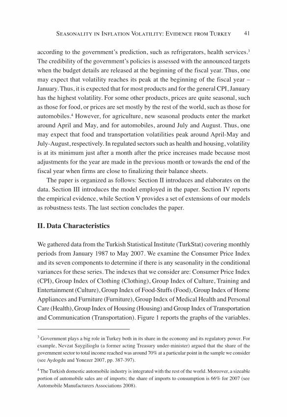
We gathered data from the Turkish Statistical Institute (TurkStat) covering monthly
periods from January 1987 to May 2007. We examine the Consumer Price Index
and its seven components to determine if there is any seasonality in the conditional
variances for these series. The indexes that we consider are: Consumer Price Index
(CPI), Group Index of Clothing (Clothing), Group Index of Culture, Training and
Entertainment (Culture), Group Index of Food-Stuffs (Food), Group Index of Home
Appliances and Furniture (Furniture), Group Index of Medical Health and Personal
Care (Health), Group Index of Housing (Housing) and Group Index of Transportation
and Communication (Transportation). Figure 1 reports the graphs of the variables.
Seasonality in Inflation Volatility: Evidence from Turkey 41
3 Government plays a big role in Turkey both in its share in the economy and its regulatory power. Forexample, Nevzat Saygilioglu (a former acting Treasury under-minister) argued that the share of thegovernment sector to total income reached was around 70% at a particular point in the sample we consider(see Aydogdu and Yonezer 2007, pp. 387-397).
4 The Turkish domestic automobile industry is integrated with the rest of the world. Moreover, a sizeableportion of automobile sales are of imports; the share of imports to consumption is 66% for 2007 (seeAutomobile Manufacturers Associations 2008).
jaeXIII_1:jaeXIII_1 5/11/10 9:20 PM Página 41

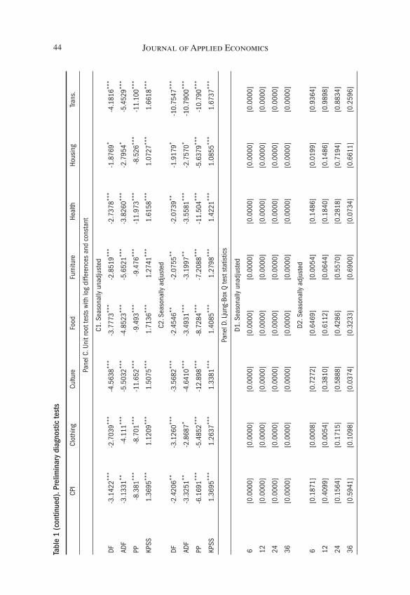
Table 1 reports various diagnostic tests. Panels A, B and C report the unit root
tests of the price indexes that we consider in their logarithmic form, with a constant
(Panel A), with a constant and time trend (Panel B) and a constant in logarithmic
first differences (Panel C). Each panel reports unit root tests for seasonally unadjusted
Journal of Applied Economics42
Figure 1. Graphs of observed data series (logarithmic, monthly change, seasonally unadjusted)
CPI Clothing
Culture Food
Furniture Health
Housing Transportation
jaeXIII_1:jaeXIII_1 5/11/10 9:20 PM Página 42

Seasonality in Inflation Volatility: Evidence from Turkey 43Ta
ble
1. P
relim
inar
y di
agno
stic
test
s
CPI
Clot
hing
Cultu
reFo
odFu
rnitu
reHe
alth
Hous
ing
Trans
.
Pane
l A. U
nit r
oot w
ith lo
g le
vels
and
con
stan
t
A1. S
easo
nally
una
djus
ted
DF-0
.796
0-0
.788
8-0
.913
3-0
.204
30.
7974
-0.4
415
-1.4
335
0.48
81
ADF
-1.9
599
-1.7
796
-2.0
432
-2.2
506
-2.4
737
-1.6
244
-1.9
028
-2.4
117
PP-1
.827
3-1
.753
2-1
.757
4-2
.502
2-1
.424
9-1
.950
5-1
.482
5-1
.491
3
KPSS
2.01
6***
2.00
4***
2.01
1***
2.01
3***
2.00
9***
2.01
2***
2.02
2***
2.01
6***
A2. S
easo
nally
adj
uste
d
DF-0
.699
20.
3205
0.81
37-0
.121
60.
8022
0.25
45-0
.563
80.
152
ADF
-2.2
34-1
.805
5-2
.075
8-2
.423
1-2
.466
7-2
.478
2-2
.353
8-2
.547
7
PP-2
.037
5-2
.279
8-1
.599
3-1
.621
-1.5
772
-1.6
14-1
.780
8-1
.531
8
KPSS
2.01
6***
2.00
4***
2.01
1***
2.01
3***
2.00
9***
2.01
2***
2.02
2***
2.01
6***
Pane
l B. U
nit r
oot t
ests
with
log
leve
ls, c
onst
ant a
nd tr
end
B1. S
easo
nally
una
djus
ted
DF-1
.448
8-1
.923
3-1
.223
3-0
.841
5-0
.123
3-1
.075
3-2
.347
70.
8917
ADF
3.05
11-0
.852
90.
3526
2.12
472.
8131
3.64
35-0
.922
31.
7452
PP2.
7186
1.27
492.
536
2.06
952.
4438
2.95
632.
8143
2.58
41
KPSS
0.44
3***
0.44
2***
0.44
7***
0.45
5***
0.43
4***
0.44
0***
0.41
91**
*0.
4367
***
B2. S
easo
nally
adj
uste
d
DF-0
.203
8-0
.913
50.
5845
0.13
08-0
.189
6-0
.125
7-0
.931
30.
9809
ADF
3.13
450.
4079
2.51
932.
3901
2.48
841.
8037
0.53
121.
8603
PP2.
9457
3.01
073.
3137
3.27
912.
3762
2.33
52.
6934
2.55
23
KPSS
0.44
33**
*0.
4418
***
0.44
73**
*0.
4558
***
0.43
50**
*0.
4406
***
0.41
91**
*0.
4368
***
jaeXIII_1:jaeXIII_1 5/11/10 9:20 PM Página 43
Journal of Applied Economics44Ta
ble
1 (c
ontin
ued)
. Pre
limin
ary
diag
nost
ic te
sts
CPI
Clot
hing
Cultu
reFo
odFu
rnitu
reHe
alth
Hous
ing
Trans
.
Pane
l C. U
nit r
oot t
ests
with
log
diffe
renc
es a
nd c
onst
ant
C1. S
easo
nally
una
djus
ted
DF-3
.142
2***
-2.7
039**
*-4
.563
8***
-3.7
773**
*-2
.851
9***
-2.7
378**
*-1
.876
9*-4
.181
6***
ADF
-3.1
331**
-4.1
11**
*-5
.503
2***
-4.8
523**
*-5
.652
1***
-3.8
260**
*-2
.795
4*-5
.452
9***
PP-8
.381
***
-8.7
01**
*-1
1.65
2***
-9.4
93**
*-9
.476
***
-11.
973**
*-8
.526
***
-11.
100**
*
KPSS
1.36
95**
*1.
1209
***
1.50
75**
*1.
7136
***
1.27
41**
*1.
6158
***
1.07
27**
*1.
6618
***
C2. S
easo
nally
adj
uste
d
DF-2
.420
6**-3
.126
0***
-3.5
682**
*-2
.454
6**-2
.075
5**-2
.073
9**-1
.917
9*-1
0.75
47**
*
ADF
-3.3
251**
-2.8
687*
-4.6
410**
*-3
.493
1***
-3.1
997**
-3.5
581**
*-2
.757
0*-1
0.79
00**
*
PP-6
.169
1***
-5.4
852**
*-1
2.89
8***
-8.7
284**
*-7
.208
8***
-11.
504**
*-5
.637
9***
-10.
790**
*
KPSS
1.36
95**
*1.
2637
***
1.33
81**
*1.
4085
***
1.27
98**
*1.
4221
***
1.08
55**
*1.
6737
***
Pane
l D. L
jung
-Box
Q te
st s
tatis
tics
D1. S
easo
nally
una
djus
ted
6[0
.000
0][0
.000
0][0
.000
0][0
.000
0][0
.000
0][0
.000
0][0
.000
0][0
.000
0]
12[0
.000
0][0
.000
0][0
.000
0][0
.000
0][0
.000
0][0
.000
0][0
.000
0][0
.000
0]
24[0
.000
0][0
.000
0][0
.000
0][0
.000
0][0
.000
0][0
.000
0][0
.000
0][0
.000
0]
36[0
.000
0][0
.000
0][0
.000
0][0
.000
0][0
.000
0][0
.000
0][0
.000
0][0
.000
0]
D2. S
easo
nally
adj
uste
d
6[0
.187
1][0
.000
8][0
.727
2][0
.646
9][0
.005
4][0
.148
6][0
.019
9][0
.936
4]
12[0
.409
9][0
.005
4][0
.381
0][0
.611
2][0
.064
4][0
.184
0][0
.148
6][0
.989
8]
24[0
.156
4][0
.171
5][0
.588
8][0
.428
6][0
.557
0][0
.281
8][0
.719
4][0
.883
4]
36[0
.594
1][0
.109
8][0
.037
4][0
.323
3][0
.690
0][0
.073
4][0
.661
1][0
.259
6]
jaeXIII_1:jaeXIII_1 5/11/10 9:20 PM Página 44
Seasonality in Inflation Volatility: Evidence from Turkey 45Ta
ble
1 (c
ontin
ued)
. Pre
limin
ary
diag
nost
ic te
sts
CPI
Clot
hing
Cultu
reFo
odFu
rnitu
reHe
alth
Hous
ing
Trans
.
Pane
l E. A
RCH-
LM te
st s
tatis
tics
E1. S
easo
nally
una
djus
ted
6[0
.000
0][0
.000
0][0
.000
0][0
.000
0][0
.000
0][0
.000
0][0
.000
0][0
.000
0]
12[0
.000
0][0
.000
0][0
.000
0][0
.000
0][0
.000
0][0
.000
0][0
.000
0][0
.000
0]
24[0
.000
0][0
.000
0][0
.000
0][0
.000
0][0
.000
0][0
.000
0][0
.000
0][0
.000
0]
36[0
.000
0][0
.000
0][0
.000
0][0
.000
0][0
.000
0][0
.000
0][0
.000
0][0
.000
0]
E2. S
easo
nally
adj
uste
d
6[0
.013
1][0
.025
9][0
.352
9][0
.129
4][0
.013
5][0
.403
6][0
.044
2][0
.825
1]
12[0
.022
2][0
.125
2][0
.000
2][0
.012
3][0
.038
1][0
.215
4][0
.089
3][0
.986
9]
24[0
.206
6][0
.382
2][0
.001
2][0
.036
9][0
.448
9][0
.112
3][0
.555
6][0
.841
3]
36[0
.195
8][0
.766
8][0
.001
8][0
.192
4][0
.666
2][0
.036
5][0
.976
7][0
.282
6]
Note
: p-v
alue
s ar
e re
porte
d in
bra
cket
s. **
* , **an
d *
indi
cate
reje
ctio
n of
the
null
at th
e 0.
01%
, 0.0
5% a
nd 0
.10%
leve
ls, r
espe
ctive
ly.
jaeXIII_1:jaeXIII_1 5/11/10 9:20 PM Página 45
and adjusted series.5 We consider four unit root tests: Dickey-Fuller (DF), Augmented
Dickey-Fuller (ADF), Phillips-Perron (PP) and Kwiatkowski, Phillips, Schmidt and
Shin (KPSS). For DF, ADF and PP, the null hypothesis is unit root (rejecting the
null suggests stationarity) and for KPSS, the null is stationarity (rejecting the null
suggest non-stationarity). Panels A, B and C overall suggest that the series that we
consider have a unit root in log levels, but the differenced series do not have a unit
root. Thus, we carried our analyses for the indexes in their logarithmic first differences.
Panel D of Table 1 reports the p-values of Ljung-Box Q test statistics for 6, 12,
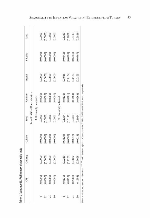
24 and 36 lags of the series in their logarithmic first differences. Panel E of Table
1 reports the ARCH-LM tests of the same series for 6, 12, 24 and 36 lags. We reject
the null of no autocorrelation for the non-seasonally adjusted data, but no general
pattern appears for the presence of autocorrelation for the seasonally adjusted data.
However, the strong contrast between Panels D1 (for the seasonally unadjusted
series) and D2 (for the seasonally adjusted series) suggests a strong presence of
seasonality in the mean equation of the seasonally unadjusted series.
Panel E of Table 1 reports the ARCH-LM test statistics.6 The null hypothesis
that there is no ARCH effect up to order q in the residuals fails to be rejected when
we employ seasonally unadjusted data for all the lag orders that we consider. When
we employ seasonally adjusted data, the null is rejected at the 5% for at least one
lag order that we consider but Transportation; for Transportation we cannot reject
the null for any of the lag orders that we consider. Thus, inflation volatility needs
to be modeled somehow.
Table 2 reports the descriptive statistics for the general CPI and its seven
components. Panel A reports the statistics when we used the original (seasonally
unadjusted) inflation data; Panel B uses the seasonally adjusted data. The means
of Housing, Health, Transportation and Food are higher than the CPI for both the
seasonally unadjusted and adjusted data and the means of Culture, Clothing and
Furniture are less than the CPI. Table 3 reports the p-values for the test statistics:
the mean and variance of each item are equal to the mean and variance of the general
Journal of Applied Economics46
5 Although the price series that we consider have a high degree of seasonality, there is no officialseasonally adjusted data for Turkey. However, the Central Bank of the Republic of Turkey uses theCensus X11 (historical, additive) procedure to seasonally adjust series in its annual reports. Thus, weused the same procedure to seasonally adjust our series.
6 We specify the autoregressive equation with its q-lags (where q-lags are determined by the finalprediction error (FPE) criteria, whose properties we discuss later in the text) and a constant term. Whenwe used seasonally unadjusted data, 11 seasonal dummies are also included.
jaeXIII_1:jaeXIII_1 5/11/10 9:20 PM Página 46

Seasonality in Inflation Volatility: Evidence from Turkey 47Ta
ble
2. D
escr
iptiv
e st
atis
tics
CPI
Clot
hing
Cultu
reFo
odFu
rnitu
reHe
alth
Hous
ing
Trans
.
Pane
l A.
Seas
onal
ly u
nadj
uste
d un
ivaria
te d
ata
stat
istic
s
Mea
n3.
5597
3.38
863.
5057
3.57
883.
3641
3.65
33.
6237
3.59
81
Med
ian
3.28
242.
5739
2.30
533.
4895
3.16
992.
6023
3.48
972.
8982
Max
imum
22.0
7818
.107
23.5
9626
.53
18.1
0819
.038
13.2
2139
.027
Min
imum
-0.9
286
-8.8
068
-1.8
828
-5.0
766
-2.2
154
-0.9
337
0.20
74-1
.776
4
Varia
nce
6.72
7329
.309
18.8
1613
.625
6.68
3811
.004
4.58
3916
.087
Coef
f. of
var
.0.
7286
1.59
771.
2373
1.03
140.
7685
0.90
810.
5908
1.11
47
Skew
ness
1.76
070.
3869
2.22
941.
0114
1.56
071.
5261
0.83
673.
9839
Kurto
sis
12.7
642.
8059
8.43
498.
1013
9.86
425.
8259
4.24
2930
.093
Jarq
ue-B
era
1041
.56.
1515
477.
7229
1.12
549.
6516
7.25
42.0
0277
09.5
Sum
sq.
dev
.15
54.1
6770
.443
46.5
3147
1543
.925
41.8
1058
.937
15.9
Obse
rvat
ions
232
232
232
232
232
232
232
232
Pane
l B. S
easo
nally
adj
uste
d un
ivaria
te d
ata
stat
istic
s
Mea
n3.
5586
3.37
23.
529
3.56
163.
3761
3.66
123.
6376
3.61
13
Med
ian
3.83
153.
719
3.40
933.
4119
3.58
293.
3845
3.74
672.
9871
Max
imum
20.6
4612
.235
16.1
0124
.955
17.3
1917
.733
14.2
9337
.787
Min
imum
0.09
89-4
.038
2-5
.296
4-2
.063
-1.8
975
-1.5
033
0.02
31-1
.908
8
Varia
nce
4.76
465.
3033
8.77
527.
6706
5.77
487.
4327
3.62
2514
.512
Coef
f. of
var
.0.
6134
0.68
30.
8394
0.77
760.
7118
0.74
470.
5232
1.05
49
Skew
ness
2.05
67-0
.020
60.
9378
2.16
551.
4753
1.27
290.
7218
4.07
75
Kurto
sis
17.8
784.
4885
6.40
1317
.065
10.5
676.
4475
5.84
231
.876
Jarq
ue-B
era
2303
.221
.435
145.
8420
93.5
637.
7217
7.54
98.2
2187
03.4
Sum
sq.
dev
.11
00.6
1225
.120
27.1
1771
.913
34.1
1717
.183
6.8
3352
.4
Obse
rvat
ions
232
232
232
232
232
232
232
232
Note
: Coe
ffici
ent o
f var
iatio
n is
def
ined
as
(std
. dev
/mea
n).
jaeXIII_1:jaeXIII_1 5/11/10 9:20 PM Página 47
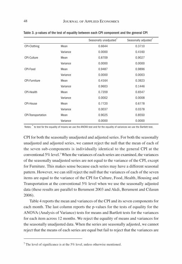
CPI for both the seasonally unadjusted and adjusted series. For both the seasonally
unadjusted and adjusted series, we cannot reject the null that the mean of each of
the seven sub-components is individually identical to the general CPI at the
conventional 5% level.7 When the variances of each series are examined, the variances
of the seasonally unadjusted series are not equal to the variance of the CPI, except
for Furniture. This makes sense because each series may have a different seasonal
pattern. However, we can still reject the null that the variances of each of the seven
items are equal to the variance of the CPI for Culture, Food, Health, Housing and
Transportation at the conventional 5% level when we use the seasonally adjusted
data (these results are parallel to Berument 2003 and Akdi, Berument and Cilasun
2006).
Table 4 reports the mean and variances of the CPI and its seven components for
each month. The last column reports the p-values for the tests of equality for the
ANOVA (Analysis of Variance) tests for means and Bartlett tests for the variances
for each item across 12 months. We reject the equality of means and variances for
the seasonally unadjusted data. When the series are seasonally adjusted, we cannot
reject that the means of each series are equal but fail to reject that the variances are
Journal of Applied Economics48
7 The level of significance is at the 5% level, unless otherwise mentioned.
Table 3. p-values of the test of equality between each CPI component and the general CPI
Seasonally unadjusted* Seasonally adjusted*
CPI-Clothing Mean 0.6644 0.3710
Variance 0.0000 0.4160
CPI-Culture Mean 0.8709 0.9027
Variance 0.0000 0.0000
CPI-Food Mean 0.9487 0.9896
Variance 0.0000 0.0003
CPI-Furniture Mean 0.4164 0.3923
Variance 0.9603 0.1446
CPI-Health Mean 0.7359 0.6547
Variance 0.0002 0.0008
CPI-House Mean 0.7720 0.6778
Variance 0.0037 0.0378
CPI-Transportation Mean 0.9025 0.8550
Variance 0.0000 0.0000
Notes: * to test for the equality of means we use the ANOVA test and for the equality of variances we use the Bartlett test.
jaeXIII_1:jaeXIII_1 5/11/10 9:20 PM Página 48

Seasonality in Inflation Volatility: Evidence from Turkey 49Ta
ble
4. Te
st o
f equ
ality
acr
oss
each
mon
th o
f the
yea
r for
diff
eren
t pric
e in
dexe
s
Jan.
Feb.
Mar
.Ap
r.M
ayJu
n.Ju
l.Au
g.Se
p.Oc
t.No
v.De
c.Te
st o
f equ
ality
*
CPI
Mea
n (N
SA)
4.20
003.
2718
3.44
115.
3458
2.99
961.
3776
1.80
272.
6384
5.11
825.
4975
4.24
902.
7234
0.00
Varia
nce
(NSA
)6.
0187
3.75
863.
3244
21.7
590
4.29
061.
0333
2.64
962.
5773
5.54
516.
0239
3.31
902.
8045
0.00
Mea
n(SA
)3.
6360
3.41
723.
3360
4.27
523.
4695
3.37
413.
5295
3.46
613.
6351
3.47
093.
4843
3.59
490.
99
Varia
nce
(SA)
4.35
823.
0260
2.93
4019
.545
05.
1658
2.34
143.
9187
2.98
423.
9786
3.70
293.
0673
3.68
830.
00
Clot
hing
Mea
n (N
SA)
-2.1
504
-2.5
737
1.28
4810
.369
07.
1558
2.68
38-1
.370
1-1
.225
46.
1456
11.8
430
6.60
611.
7536
0.00
Varia
nce
(NSA
)7.
4792
5.98
686.
1892
9.05
875.
7122
0.95
807.
5411
5.01
367.
4604
14.6
030
10.5
580
3.25
860.
00
Mea
n(SA
)2.
9827
3.36
913.
4002
3.53
563.
7706
3.13
653.
4578
2.91
263.
7007
3.62
643.
4353
3.10
570.
99
Varia
nce
(SA)
5.42
003.
9198
4.38
5811
.604
05.
2767
2.82
064.
8468
5.17
896.
0144
6.12
086.
3948
3.76
290.
29
Cultu
re
Mea
n (N
SA)
4.56
132.
3393
2.19
082.
7409
2.24
661.
3944
2.32
817.
1181
10.9
540
3.05
651.
4674
1.90
920.
00
Varia
nce
(NSA
)12
.195
05.
0940
4.31
3713
.273
06.
1425
0.96
574.
6484
37.7
840
51.1
020
6.36
352.
5135
2.66
320.
00
Mea
n(SA
)3.
5384
3.35
713.
3191
3.98
743.
2921
3.49
573.
4912
5.12
082.
2407
3.75
353.
3234
3.43
730.
52
Varia
nce
(SA)
6.06
223.
8257
3.80
1613
.204
08.
1052
1.86
044.
7580
27.7
340
20.9
830
7.67
214.
5979
3.49
190.
00
Food
Mea
n (N
SA)
4.90
325.
3741
4.94
165.
6553
1.70
61-1
.148
90.
3015
1.97
734.
7980
5.99
435.
2477
3.01
780.
00
Varia
nce
(NSA
)6.
7521
8.38
816.
9163
35.9
600
7.97
842.
2885
6.08
146.
0152
6.08
669.
3748
4.84
316.
0608
0.00
Mea
n(SA
)3.
6379
3.31
473.
1368
4.42
363.
3536
3.46
923.
8705
3.39
023.
4984
3.57
153.
4422
3.63
170.
99
Varia
nce
(SA)
6.22
884.
2521
5.70
3730
.648
08.
6871
3.44
177.
8488
6.56
614.
2922
5.86
424.
4939
6.36
560.
00
jaeXIII_1:jaeXIII_1 5/11/10 9:20 PM Página 49

Journal of Applied Economics50Ta
ble
4 (c
ontin
ued)
. Tes
t of e
qual
ity a
cros
s ea
ch m
onth
of t
he y
ear f
or d
iffer
ent p
rice
inde
xes
Jan.
Feb.
Mar
.Ap
r.M
ayJu
n.Ju
l.Au
g.Se
p.Oc
t.No
v.De
c.Te
st o
f equ
ality
*
Furn
iture
Mea
n (N
SA)
5.20
162.
7502
2.93
103.
9806
3.74
182.
8023
3.31
562.
8943
4.10
503.
1210
2.91
472.
6140
0.07
Varia
nce
(NSA
)10
.516
04.
7781
4.58
8418
.637
013
.224
02.
5668
2.98
862.
9183
5.64
274.
2244
2.91
483.
6943
0.00
Mea
n(SA
)3.
4213
3.53
133.
1039
3.78
143.
6760
3.37
062.
9696
3.24
543.
4004
3.44
083.
3293
3.21
190.
99
Varia
nce
(SA)
5.81
176.
3183
2.99
8017
.206
012
.199
03.
8097
2.89
543.
7209
4.95
613.
7567
3.99
593.
6693
0.00
Heal
th
Mea
n (N
SA)
7.78
234.
6732
3.79
733.
8286
2.71
893.
1433
4.74
303.
3855
2.58
152.
1725
2.88
372.
1045
0.00
Varia
nce
(NSA
)22
.700
010
.275
07.
2182
18.3
360
8.17
517.
5612
13.1
840
4.29
174.
0879
2.91
916.
4727
5.07
950.
00
Mea
n(SA
)4.
0809
3.82
783.
3843
3.78
613.
8349
3.52
753.
6853
3.43
343.
5116
3.42
093.
6571
3.77
440.
99
Varia
nce
(SA)
12.5
750
8.44
757.
8395
15.6
000
8.81
015.
3113
8.20
973.
6593
4.52
763.
0364
7.15
967.
4277
0.03
Hous
ing
Mea
n (N
SA)
5.47
253.
2884
2.60
283.
2967
2.78
733.
1579
3.89
804.
1606
4.88
743.
9334
3.26
402.
8685
0.00
Varia
nce
(NSA
)9.
6567
3.30
452.
5935
8.84
632.
6843
2.07
123.
0808
3.79
964.
9050
3.36
992.
3308
2.28
940.
00
Mea
n(SA
)3.
4637
3.42
743.
5104
4.09
023.
5033
3.62
793.
6470
3.70
273.
8684
3.53
923.
6428
3.62
940.
99
Varia
nce
(SA)
4.02
552.
7438
3.24
619.
4232
2.87
532.
6115
2.74
833.
3001
5.06
963.
0984
2.77
283.
1404
0.11
Trans
porta
tion
Mea
n (N
SA)
5.52
932.
7648
2.85
255.
5041
3.03
413.
3619
4.59
023.
3837
4.15
042.
4856
2.06
663.
4665
0.11
Varia
nce
(NSA
)24
.649
05.
0216
4.00
8573
.968
04.
5966
8.32
4216
.643
07.
9424
24.3
000
4.74
642.
3389
10.0
520
0.00
Mea
n(SA
)4.
6285
3.12
753.
3552
5.20
073.
2463
3.22
713.
3225
3.21
384.
1544
3.31
003.
1728
3.35
090.
82
Varia
nce
(SA)
23.3
320
4.05
164.
6444
69.6
870
4.65
947.
8631
15.9
170
6.76
0722
.879
05.
2835
3.48
357.
5971
0.00
Note
s: *
test
of e
qual
ity re
ports
the
p-va
lues
of A
NOVA
and
Bar
tlett
test
s fo
r the
mea
n an
d va
rianc
es o
f ser
ies,
resp
ectiv
ely.
jaeXIII_1:jaeXIII_1 5/11/10 9:21 PM Página 50

the same for all but Clothing and Housing. Therefore, these three tables suggest
that even if we account for seasonality, the volatility of each series from the general
CPI and the volatility of each series from each other are different. When we consider
the seasonally unadjusted and seasonally adjusted series, Table 4 also suggests that
the lowest variances are observed in June for the general CPI, Culture, Food and
Housing; in October for Health; in November for Transportation; in June and
December for Clothing. On the other hand, the highest variances are observed in
April for the general CPI; October, November and April for Clothing; August and
September for Culture; April for Food; April and May for Furniture; January and
April for Health; January, April and September for Housing; January and April for
Transportation. These highest and lowest volatilities do not take into account the
dynamics of the economy and assume that positive and negative inflation shocks
affect volatility in the same way. In the next section, we will employ Nelson’s (1991)
Exponential Generalized ARCH model to assess any regularity in the conditional
variances of inflation series.
III. Method
The economic literature suggests various methods for measuring inflation volatility,
either through direct measures of volatility, by using survey data, or through indirect
measures of volatility, usually by using sophisticated econometric techniques.
Bomberger (1996) argues that using dispersion of the survey data measures
disagreement rather than inflation volatility. Moreover, he argues that some forecasters
may not want to deviate from other forecasters’ estimates, so the value of expected
inflation may be biased.
The Kalman filtering and ARCH types of conditional variance modeling are the
two most common sophisticated econometric techniques researchers employ to
measure inflation volatility indirectly. The Kalman filter is a discrete, recursive
linear filter that measures instability of the structural variability of the parameters
of an equation. ARCH-type models assume that the parameters of the model are
stable but estimate the variance of the residual term for the inflation specification.
Evans (1991) and Berument et al. (2005) argue that the ARCH class of models is
a better way of measuring risk/uncertainty, whereas the Kalman filter is better for
capturing model (or parameter) instability. Therefore, we model volatility employing
ARCH/GARCH models.
The conventional ARCH models are not capable of capturing the asymmetric
effects of negative or positive inflation surprises on the volatility specification
Seasonality in Inflation Volatility: Evidence from Turkey 51
jaeXIII_1:jaeXIII_1 5/11/10 9:21 PM Página 51
(Black 1976, Engle and Ng 1993). In order to account for this, we use the EGARCH
specification. The contribution of this paper is to assess whether there is any regularity
in the volatility of price indexes that is beyond the dynamics of the volatility captured
by the lagged conditional variance and the innovation of inflation.
Following Berument (1999 and 2003), we model inflation using lagged inflation
and monthly seasonal dummies to account for seasonality. Whether seasonality is
significantly related to volatility can be tested by examining the statistical significance
of the estimates of each month’s coefficients. The model allows for both autoregressive
and moving average components in the heteroskedastic variance.
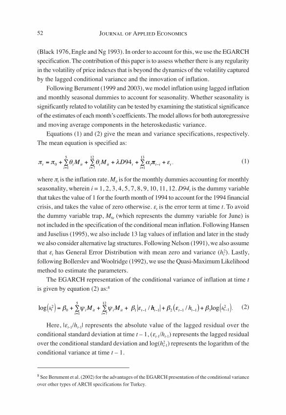
Equations (1) and (2) give the mean and variance specifications, respectively.
The mean equation is specified as:
(1)
where πt is the inflation rate. Mit is for the monthly dummies accounting for monthly
seasonality, wherein i = 1, 2, 3, 4, 5, 7, 8, 9, 10, 11, 12. D94t is the dummy variable
that takes the value of 1 for the fourth month of 1994 to account for the 1994 financial
crisis, and takes the value of zero otherwise. εt is the error term at time t. To avoid
the dummy variable trap, M6t (which represents the dummy variable for June) is
not included in the specification of the conditional mean inflation. Following Hansen
and Juselius (1995), we also include 13 lag values of inflation and later in the study
we also consider alternative lag structures. Following Nelson (1991), we also assume
that εt has General Error Distribution with mean zero and variance (ht2). Lastly,
following Bollerslev and Woolridge (1992), we use the Quasi-Maximum Likelihood
method to estimate the parameters.
The EGARCH representation of the conditional variance of inflation at time t
is given by equation (2) as:8
(2)
Here, |εt-1/ht-1| represents the absolute value of the lagged residual over the
conditional standard deviation at time t – 1, (εt-1/ht-1) represents the lagged residual
over the conditional standard deviation and log(h2t-1) represents the logarithm of the
conditional variance at time t – 1.
log ht i iti
i iti
tM M20
1
5
7
12
1 1( ) = + ∑ + +∑= =
−β ψ ψ β ε / hh ht t t th− − − −+ +( ) ( )1 2 1 1 3 12β ε β/ .log
π π θ θ λ αt i iti
i iti
t ii
M M D= + ∑ + ∑ + + ∑= = =
01
5
7
12
1
13
94 ππ εt i t− + ,
Journal of Applied Economics52
8 See Berument et al. (2002) for the advantages of the EGARCH presentation of the conditional varianceover other types of ARCH specifications for Turkey.
jaeXIII_1:jaeXIII_1 5/11/10 9:21 PM Página 52

In Equation (2), several meaningful restrictions can be tested. |β3| < 1 implies
that inflation volatility is not explosive. If β2 > 0, then a positive shock to inflation
increases volatility more than a negative shock. If β2 < 0, a positive shock generates
less volatility than a negative shock.
IV. Empirical Evidence
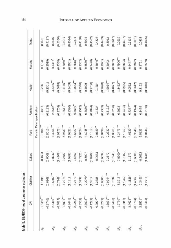
Table 5 reports the estimates of Equations (1) and (2) for the general CPI and its
seven sub-components by using seasonally unadjusted data. Panel A reports the
estimates of the inflation equation (Equation 1) and Panel B reports the estimates
of the conditional variance equation (Equation 2). Panel C reports two diagnostic
test (Ljung-Box-Q and ARCH-LM) statistics for the standardized residuals by using
various lag orders and Panel D is for summary statistics. Variables M1t to M12t are
estimated coefficients for the monthly dummies.
Panel A of Table 5 suggests that the lowest monthly effects in the mean equation
are observed in June for the general CPI; in February for Clothing; in November
for Culture; in June for Food; in February for Furniture; in May for Health; in March
for Housing; and in November for Transportation. The highest monthly effects in
the mean equation are observed in October for the general CPI; in October for
Clothing; in August for Culture; in January for Food, Furniture and Health; in
September for Housing; in January for Transportation. These findings are parallel
with the results listed in Table 4. Here, we do not interpret the estimated coefficients
for the lag values of inflation but the characteristic roots of the polynomials are all
inside the unit circle; thus the series are considered as stationary.
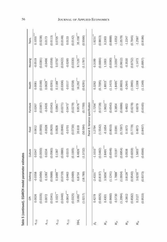
Panel B of Table 5 suggests that for the general CPI the highest volatility is in
January; in September for Clothing; in August for Culture; in April for Food; in
January for Furniture, Health and Housing; in July for Transportation. The lowest
volatilities are observed in November for the general CPI; in June for Clothing; in
December for Culture; in November for Food and Furniture; in February for Health
and Housing; in November for Transportation. These findings are parallel to the
expectations stated in the introduction. For the general CPI and most other items
January is the month that conditional inflation variance is highest except for food
(April) and Transportation (July). The lowest volatilities are observed towards the
end of year except for Health (February) and Housing (February).
Next, we test whether the conditional variance is the same across each month.
In particular, we test the null hypothesis that the estimated coefficients for the eleven
monthly dummy coefficients are jointly zero for the conditional variance specification
Seasonality in Inflation Volatility: Evidence from Turkey 53
jaeXIII_1:jaeXIII_1 5/11/10 9:21 PM Página 53
Journal of Applied Economics54Ta
ble
5. E
GARC
H-m
odel
par
amet
er e
stim
ates
CPI
Clot
hing
Cultu
reFo
odFu
rnitu
reHe
alth
Hous
ing
Trans
.
Pane
l A. M
ean
spec
ifica
tion
π 0-1
.848
0***
1.11
98-0
.160
3-3
.710
6***
-0.0
714
-0.2
263
0.17
280.
1431
(0.2
740)
(0.6
969)
(0.6
068)
(0.8
015)
(0.2
133)
(0.2
301)
(0.2
019)
(0.4
137)
M1t
2.53
60**
*-3
.630
2***
2.87
42*
6.39
56**
*2.
3512
***
3.33
65**
*0.
7487
*0.
8415
(0.4
017)
(0.7
748)
(1.4
708)
(1.9
973)
(0.3
708)
(0.5
678)
(0.4
368)
(0.5
360)
M2t
1.60
91**
*-4
.297
4***
0.24
825.
9633
***
-1.2
511**
*1.
1145
***
-0.7
050**
*-0
.101
7
(0.3
445)
(1.1
319)
(1.0
883)
(1.0
823)
(0.3
380)
(0.3
409)
(0.2
061)
(0.4
514)
M3t
2.02
58**
*-4
.267
9***
0.53
674.
6322
***
-0.5
530**
1.16
83**
*-0
.751
8***
-0.2
371
(0.3
502)
(1.3
732)
(0.7
925)
(1.0
424)
(0.2
512)
(0.3
540)
(0.2
362)
(0.4
188)
M4t
2.36
98**
*2.
2070
*-0
.509
74.
6045
***
0.86
80**
*0.
1029
-0.6
580**
*0.
6094
(0.4
229)
(1.3
314)
(0.8
204)
(1.1
517)
(0.2
874)
(0.2
706)
(0.2
428)
(0.4
532)
M5t
0.99
07**
*1.
2588
-0.0
653
2.06
89**
-0.1
734
-0.1
284
-0.4
040**
-0.4
323
(0.3
242)
(0.8
885)
(0.6
032)
(0.8
496)
(0.2
383)
(0.2
690)
(0.1
971)
(0.4
483)
M7t
1.30
31**
*-2
.994
4***
0.26
722.
2332
**-0
.813
2**1.
9074
***
0.20
420.
8013
(0.3
498)
(0.7
634)
(0.7
943)
(1.0
369)
(0.3
238)
(0.4
077)
(0.2
602)
(0.6
617)
M8t
1.97
70**
*-3
.391
3***
7.09
00**
*3.
2479
***
0.26
281.
3472
***
0.79
06**
*-0
.293
9
(0.3
317)
(1.1
267)
(1.7
507)
(1.1
867)
(0.2
406)
(0.2
995)
(0.2
684)
(0.4
487)
M9t
3.46
23**
*-1
.182
8*5.
1377
4.63
30**
*0.
7377
***
0.05
720.
9447
***
-0.3
137
(0.3
704)
(1.4
662)
(3.6
908)
(0.9
548)
(0.1
924)
(0.2
642)
(0.2
872)
(0.5
061)
M10
t3.
1521
***
2.34
53*
-0.6
672
5.51
39**
*0.
1475
0.31
530.
2791
-0.0
833
(0.3
444)
(1.2
714)
(1.8
285)
(1.0
446)
(0.2
180)
(0.2
816)
(0.2
589)
(0.4
895)
jaeXIII_1:jaeXIII_1 5/11/10 9:21 PM Página 54

Seasonality in Inflation Volatility: Evidence from Turkey 55Ta
ble
5 (c
ontin
ued)
. EGA
RCH-
mod
el p
aram
eter
est
imat
es
CPI
Clot
hing
Cultu
reFo
odFu
rnitu
reHe
alth
Hous
ing
Trans
.
M11
t2.
0317
***
0.33
35-0
.904
65.
2943
***
-0.4
453*
0.27
62-0
.205
2-0
.752
6*
(0.2
993)
(0.9
054)
(0.9
818)
(0.9
921)
(0.2
455)
(0.2
736)
(0.2
392)
(0.4
316)
M12
t1.
5123
***
-0.0
571
0.43
643.
9950
***
-0.8
099**
*0.
0355
-0.5
819**
-0.0
724
(0.2
957)
(0.3
796)
(0.8
110)
(1.1
566)
(0.2
499)
(0.2
405)
(0.2
436)
(0.4
393)
π t-1
0.44
13**
*0.
2735
***
0.27
00**
0.37
34**
*0.
3073
***
0.16
12**
*0.
2897
***
0.23
77**
*
(0.0
334)
(0.0
525)
(0.1
116)
(0.0
767)
(0.0
509)
(0.0
310)
(0.0
290)
(0.0
334)
π t-2
0.06
74-0
.095
2*0.
1120
0.08
480.
3287
***
0.10
37**
*0.
0597
-0.0
028
(0.0
460)
(0.0
539)
(0.0
727)
(0.0
771)
(0.0
411)
(0.0
281)
(0.0
375)
(0.0
244)
π t-3
-0.0
694
0.04
110.
0652
-0.1
133
-0.0
208
0.06
67**
*0.
1260
***
-0.0
496**
(0.0
486)
(0.0
477)
(0.0
445)
(0.0
862)
(0.0
389)
(0.0
240)
(0.0
378)
(0.0
214)
π t-4
-0.0
039
0.05
15-0
.043
7-0
.033
50.
1484
***
0.10
87**
*0.
1042
***
0.06
99**
*
(0.0
337)
(0.0
566)
(0.0
500)
(0.0
719)
(0.0
339)
(0.0
197)
(0.0
347)
(0.0
196)
π t-5
0.13
40**
*0.
1083
*0.
0574
0.19
78**
0.02
330.
0044
0.10
25**
0.08
00**
*
(0.0
356)
(0.0
609)
(0.0
674)
(0.0
834)
(0.0
310)
(0.0
259)
(0.0
418)
(0.0
238)
π t-6
0.09
66**
*0.
1363
**0.
0484
0.11
030.
1476
***
-0.0
043
0.17
64**
*0.
0468
**
(0.0
326)
(0.0
641)
(0.0
552)
(0.0
713)
(0.0
361)
(0.0
276)
(0.0
435)
(0.0
235)
π t-7
0.05
01**
-0.0
565
-0.0
318
0.02
200.
0205
0.01
50-0
.066
10.
0257
**
(0.0
232)
(0.0
512)
(0.0
537)
(0.0
760)
(0.0
285)
(0.0
261)
(0.0
434)
(0.0
120)
π t-8
0.03
11-0
.029
20.
0682
0.09
81-0
.034
60.
0220
0.03
800.
1549
***
(0.0
266)
(0.0
472)
(0.0
496)
(0.0
696)
(0.0
327)
(0.0
173)
(0.0
371)
(0.0
175)
π t-9
0.13
20**
*0.
1126
***
0.01
820.
0462
0.01
64-0
.027
10.
1092
***
-0.0
415*
(0.0
373)
(0.0
417)
(0.0
493)
(0.0
829)
(0.0
343)
(0.0
199)
(0.0
399)
(0.0
233)
jaeXIII_1:jaeXIII_1 5/11/10 9:21 PM Página 55
Journal of Applied Economics56Ta
ble
5 (c
ontin
ued)
. EGA
RCH-
mod
el p
aram
eter
est
imat
es
CPI
Clot
hing
Cultu
reFo
odFu
rnitu
reHe
alth
Hous
ing
Trans
.
π t-1
00.
0026
-0.0
358
0.03
470.
0612
0.02
670.
0081
-0.0
519
0.10
55**
*
(0.0
335)
(0.0
496)
(0.0
550)
(0.0
950)
(0.0
387)
(0.0
166)
(0.0
381)
(0.0
238)
π t-1
10.
0072
0.12
83*
0.02
34-0
.002
8-0
.043
50.
0629
**-0
.049
60.
0173
(0.0
341)
(0.0
688)
(0.0
583)
(0.0
620)
(0.0
343)
(0.0
261)
(0.0
358)
(0.0
113)
π t-1
20.
1021
**0.
3489
***
0.13
870.
0928
0.09
61**
*0.
1189
***
0.07
55*
0.07
05**
*
(0.0
440)
(0.0
719)
(0.0
880)
(0.0
940)
(0.0
271)
(0.0
306)
(0.0
422)
(0.0
148)
π t-1
3-0
.081
4***
-0.0
463
-0.0
315
-0.0
701
-0.0
473*
-0.0
117
-0.0
265
0.01
33
(0.0
325)
(0.0
489)
(0.1
005)
(0.0
730)
(0.0
279)
(0.0
258)
(0.0
330)
(0.0
142)
D94 t
16.6
92**
*6.
8734
8.48
26**
*20
.618
9.95
76**
*16
.292
***
9.71
20**
*35
.158
***
(1.0
217)
(18.
789)
(1.3
732)
(50.
584)
(0.7
700)
(0.6
291)
(1.1
787)
(0.5
566)
Pane
l B. V
aria
nce
spec
ifica
tion
β 00.
4279
-2.4
331**
*-1
.101
0**1.
2794
-1.7
256**
*0.
3262
0.31
991.
9231
**
(0.6
925)
(0.8
197)
(0.5
482)
(1.5
542)
(0.5
728)
(0.7
095)
(0.6
684)
(0.8
813)
M1t
0.43
013.
5656
***
2.84
91**
*-0
.165
41.
9622
***
1.89
15*
1.10
030.
2303
(0.9
660)
(1.1
241)
(0.6
546)
(0.8
010)
(0.6
543)
(1.1
415)
(0.9
390)
(0.8
888)
M2t
-0.5
730
1.78
88*
-0.5
197
0.03
810.
3854
-1.8
495*
-3.3
350**
*-1
.035
2
(1.2
994)
(1.0
934)
(0.6
954)
(0.7
397)
(0.6
686)
(0.9
603)
(0.9
612)
(1.0
579)
M3t
-0.3
812
3.81
28**
*0.
0538
0.16
730.
4822
-0.2
641
-0.3
530
-1.2
247
(0.8
582)
(0.9
540)
(0.6
059)
(0.7
779)
(0.6
278)
(1.0
965)
(0.8
752)
(0.7
945)
M4t
0.21
273.
6230
***
1.56
03**
0.48
730.
6079
-1.1
308
-1.1
473
-1.2
587
(0.9
533)
(0.9
373)
(0.6
566)
(0.8
407)
(0.6
165)
(1.1
349)
(0.8
957)
(0.9
186)
jaeXIII_1:jaeXIII_1 5/11/10 9:21 PM Página 56
Seasonality in Inflation Volatility: Evidence from Turkey 57Ta
ble
5 (c
ontin
ued)
. EGA
RCH-
mod
el p
aram
eter
est
imat
es
CPI
Clot
hing
Cultu
reFo
odFu
rnitu
reHe
alth
Hous
ing
Trans
.
M5t
-0.8
588
2.65
95**
-0.0
771
-0.1
253
0.23
72-0
.251
4-1
.994
5*-0
.572
1
(1.3
133)
(1.1
228)
(0.6
764)
(1.0
791)
(0.4
481)
(1.1
984)
(1.0
973)
(0.8
935)
M7t
-0.3
288
4.19
94**
*0.
4563
0.35
751.
1272
**0.
0631
-1.0
397
0.38
55
(1.1
599)
(1.4
894)
(0.6
929)
(0.6
991)
(0.4
987)
(1.2
908)
(1.0
103)
(0.8
255)
M8t
-1.1
582
2.29
73**
3.49
71**
*0.
1250
-0.4
209
-1.6
579
-0.3
781
-1.3
342
(1.0
313)
(1.0
749)
(0.6
479)
(0.9
247)
(0.6
630)
(1.1
652)
(0.8
936)
(0.8
581)
M9t
-0.1
208
4.25
67**
*1.
8683
**-0
.932
4-0
.366
20.
0265
-0.9
316
0.01
75
(0.8
194)
(0.9
932)
(0.7
978)
(0.8
975)
(0.5
963)
(1.1
833)
(0.9
217)
(0.9
281)
M10
t-1
.003
73.
1697
***
-0.1
863
-0.6
303
0.33
32-1
.221
9-1
.257
7-0
.725
6
(0.9
592)
(1.0
205)
(0.8
592)
(1.1
469)
(0.7
253)
(0.9
643)
(0.8
963)
(1.0
031)
M11
t-2
.054
1**2.
2834
**-0
.307
2-1
.212
9-0
.606
80.
1051
-1.6
397*
-1.5
972*
(0.8
228)
(0.9
871)
(0.7
383)
(0.8
890)
(0.6
805)
(1.0
061)
(0.8
417)
(0.9
440)
M12
t-0
.663
31.
2874
-0.9
635
-0.2
644
0.28
87-0
.564
9-0
.675
3-1
.350
7
(1.5
817)
(1.0
012)
(0.6
999)
(1.3
330)
(0.7
435)
(1.0
607)
(0.9
318)
(0.9
300)
|εt-1
/ht-1
|0.
2642
-0.2
930**
0.95
40**
*0.
2468
2.01
58**
*0.
1779
0.82
79**
*0.
2683
(0.2
456)
(0.1
363)
(0.2
671)
(0.2
497)
(0.2
200)
(0.1
720)
(0.2
415)
(0.3
623)
ε t-1
/ht-1
-0.1
068
0.15
310.
2258
-0.0
264
-0.0
152
0.15
86-0
.034
50.
5855
**
(0.1
801)
(0.0
983)
(0.1
723)
(0.1
386)
(0.1
526)
(0.1
453)
(0.1
575)
(0.2
297)
Logh
2 t-20.
3295
0.83
01**
*0.
7038
***
-0.0
406
0.19
090.
9505
***
0.82
30**
*0.
0335
(0.8
832)
(0.0
841)
(0.1
675)
(1.1
004)
(0.1
207)
(0.0
397)
(0.0
952)
(0.2
511)
LRT
2.51
3253
.134
***
105.
44**
*13
.295
022
.805
**35
.113
***
28.7
90**
*6.
1122
jaeXIII_1:jaeXIII_1 5/11/10 9:21 PM Página 57

Journal of Applied Economics58Ta
ble
5 (c
ontin
ued)
. EGA
RCH-
mod
el p
aram
eter
est
imat
es
CPI
Clot
hing
Cultu
reFo
odFu
rnitu
reHe
alth
Hous
ing
Trans
.
Pane
l C. D
iagn
ostic
test
s
Lags
Ljun
g-Bo
x Q
stat
istic
s
12[0
.445
0][0
.631
0][0
.601
0][0
.398
0][0
.238
0][0
.225
0][0
.520
0][0
.117
0]
24[0
.550
0][0
.700
0][0
.700
0][0
.538
0][0
.405
0][0
.275
0][0
.377
0][0
.248
0]
36[0
.507
0][0
.844
0][0
.734
0][0
.478
0][0
.644
0][0
.603
0][0
.371
0][0
.244
0]
ARCH
-LM
test
s
12[0
.585
3][0
.957
2][0
.743
8][0
.070
6][0
.413
3][0
.582
7][0
.254
6][0
.573
1]
24[0
.333
4][0
.978
1][0
.516
2][0
.481
3][0
.061
2][0
.960
1][0
.403
9][0
.999
5]
36[0
.744
2][0
.772
5][0
.185
2][0
.659
9][0
.319
9][0
.901
4][0
.494
1][0
.758
9]
Pane
l D. S
umm
ary
stat
istic
s
GED
para
met
er0.
9731
1.98
2119
2.68
002.
1339
6.60
780.
7850
1.09
060.
8500
(0.1
528)
(0.4
410)
(119
6.90
00)
(0.5
047)
(2.7
116)
(0.1
104)
(0.1
819)
(0.1
049)
R-sq
uare
d0.
8072
0.90
750.
4943
0.71
000.
5634
0.43
700.
7267
0.49
06
Adj.
R-sq
.0.
7625
0.88
610.
3771
0.64
290.
4623
0.30
660.
6634
0.37
26
S.E.
of
regr
essi
on1.
2826
1.85
253.
4276
2.20
851.
9036
2.75
871.
2557
3.21
28
Sum
sq.
resi
d29
1.32
607.
4720
88.1
086
3.35
641.
4513
48.1
027
8.95
1827
.40
DW s
tat
1.71
161.
6929
2.38
141.
9268
1.97
582.
0451
1.87
491.
6224
Log
likel
ihoo
d-3
04.3
6-3
67.2
9-4
18.6
3-4
47.6
7-3
46.1
2-4
35.9
1-2
69.5
3-4
51.6
9
Note
s: S
tand
ard
erro
rs a
re re
porte
d in
par
enth
eses
and
p-v
alue
s ar
e re
porte
d in
bra
cket
s. **
*in
dica
tes
sign
ifica
nce
at th
e 1%
leve
l z =
2.5
8. **
indi
cate
s si
gnifi
canc
e at
the
5% le
vel z
= 1
.96.
*in
dica
tes
sign
ifica
nce
at th
e 10
% le
vel z
= 1
.64.
jaeXIII_1:jaeXIII_1 5/11/10 9:21 PM Página 58
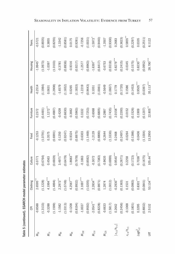
(this does not rule out that each individual coefficient is not zero). Log Likelihood
Ratio (LRT) statistics report the corresponding value. We can reject the null for
Clothing, Culture, Furniture, Health and Housing. In order to see whether the month
the conditional variance is maximum (or minimum) and statistically significant for
the other indexes (general CPI, Food and Transportation) as reported in Table 5,
we include just one dummy variable for the month corresponding to the conditional
variance specification. These coefficients are statistically significant individually
(not reported to save space.) Thus, we can claim that the conditional variance is not
the same across each month.
In volatility specifications, our estimates of the lagged value of the conditional
variances are less than one for each item; this implies that inflation volatility is not
explosive (Panel B). However, there is higher persistence in the volatilities for
Clothing, Culture, Health and Housing than for the others. Moreover, for Clothing,
Culture, Health and Transportation a positive shock to inflation increases volatility
more than a negative shock – the leverage effect. For the rest of the series, in the
general CPI, Food, Furniture and Housing, negative residuals tend to produce higher
variances. Panel C reports the Ljung-Box Q statistics and ARCH-LM tests for the
12, 24 and 36 lags. None of the test statistics is significant at the 5% level.
It is plausible that the results we gathered might be a type of seasonal accounting
and that the estimates could be sensitive to deseasonalization. Thus, we repeat the
exercise with the seasonally adjusted data (these estimates are available from the
authors upon request). The lowest volatilities are in November for the general CPI
and in February for Housing. Moreover, the highest volatilities in January for the
general CPI, in August for Culture and in January for Furniture and Health are
robust. This finding is the same for the estimates from Table 5. Furthermore, even
if the volatilities in June for Clothing, in December for Culture and in November
for Furniture are not the lowest, as reported in Table 5, they are the second-lowest
volatilities. This exercise reveals that November for Transportation is the third
lowest and the same month for Food is the fourth lowest. January is the second
highest for Transportation. Last, September for Clothing and January for Housing
are fourth highest. Thus, one may claim that the results from Table 5 are mostly
robust.9
Seasonality in Inflation Volatility: Evidence from Turkey 59
9 We also tried different deseasonalization methods; although the specific month for the maximums andminimums changes, the results are mostly robust.
jaeXIII_1:jaeXIII_1 5/11/10 9:21 PM Página 59

V. Extensions
In this section of the paper, we will consider a set of specifications to assess the
robustness of our estimates. First, it is plausible that the seasonality in volatility
may exist due to other determinants of inflation (or its volatility). In order to account
for this we set up two models, both of which include a set of additional variables
with a lag to both mean and variance equations. The first (unrestricted) model
includes monthly dummies in the variance specification and the second (restricted)
model does not include monthly dummies in the variance specification. The additional
variables included in these two sets of specifications are the: squared industrial
production deviation (calculated by the square of deviations from the trend obtained
by Hodrick’s and Prescott’s 1997 methodology), logarithmic first difference of the
exchange rate basket (basket is the Turkish lira value of the US dollar + the Euro),
logarithmic first difference of oil prices (Dubai spot), logarithmic first difference
of the real exchange rate; interbank rate, and an election dummy (general and local).10
As in the paper, for the seasonally unadjusted series our unrestricted model includes
seasonal dummies in the variance and mean equation and our restricted model
excludes seasonal dummies from the variance specification, but keeps seasonal
dummies in the mean equation only. For the seasonally adjusted series, we also
exclude seasonal dummies from the mean equation for both specifications. Panel
A of Table 6 reports the likelihood values of the estimates that use seasonally
unadjusted data and Panel B reports the same value for the seasonally adjusted data.
Likelihood Ratio Test (LRT) statistics clearly reject the null that the estimated
coefficients for the seasonal dummies are jointly zero in the variance specification
when the other explanatory variables are included.11
Second, it is plausible that the final models are mis-specified because the same
lag structure for each of the mean and variance equations for different price indexes
are used. Thus, we estimate a set of models such that lag selection is determined
by a set of statistical criteria for the seasonally unadjusted and adjusted data. We
Journal of Applied Economics60
10 We gathered the industrial production, exchange rate basket and interbank rate data from the CentralBank of the Republic of Turkey’s electronic data delivery system. The data for oil prices is gatheredfrom the International Monetary Fund’s International Financial Statistics Database. We constructedelection dummy data from the Office of the Prime Minister, the Director General of Press and Informationand the Grand National Assembly of Turkey.
11 Both the exchange rate depreciation and the real exchange rate depreciation variables are statisticallysignificant in both the mean and variance specifications.
jaeXIII_1:jaeXIII_1 5/11/10 9:21 PM Página 60
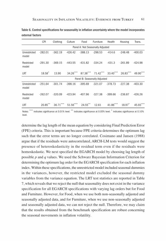
determine the lag length of the mean equation by considering Final Prediction Error
(FPE) criteria. This is important because FPE criteria determines the optimum lag
such that the error terms are no longer correlated. Cosimano and Jansen (1988)
argue that if the residuals were autocorrelated, ARCH-LM tests would suggest the
presence of heteroskedasticity in the residual term even if the residuals were
homoskedastic. We next specified the EGARCH model by choosing lag length of
possible p and q values. We used the Schwarz Bayesian Information Criterion for
determining the optimum lag order for the EGARCH specification for each inflation
index. Within these specifications, the unrestricted model included seasonal dummies
in the variances, however, the restricted model excluded the seasonal dummy
variables from the variance equation. The LRT test statistics are reported in Table
7, which reveals that we reject the null that seasonality does not exist in the variance
specification for all EGARCH specifications with varying lag orders but for Food
and Furniture. However, for Food, when we use both non-seasonally adjusted and
seasonally adjusted data, and for Furniture, when we use non-seasonally adjusted
and seasonally adjusted data, we can not reject the null. Therefore, we may claim
that the results obtained from the benchmark specification are robust concerning
the seasonal movements in inflation volatility.
Seasonality in Inflation Volatility: Evidence from Turkey 61
Table 6. Control specifications for seasonality in inflation uncertainty where the model incorporates
external factors
CPI Clothing Culture Food Furniture Health Housing Trans.
Panel A: Not Seasonally Adjusted
Unrestrictedmodel
-282.01 -362.19 -426.42 -388.13 -298.53 -414.6 -248.48 -400.03
Restrictedmodel
-291.30 -369.15 -443.55 -431.82 -334.24 -431.3 -261.89 -424.98
LRT 18.58* 13.90 34.26*** 87.38*** 71.42*** 33.40*** 26.83*** 49.90***
Panel B: Seasonally Adjusted
Unrestrictedmodel
-251.64 -301.74 -398.16 -395.69 -321.07 -378.73 -227.38 -403.30
Restrictedmodel
-262.07 -320.09 -423.94 -407.96 -327.38 -399.66 -236.87 -426.26
LRT 20.85** 36.71*** 51.56*** 24.55** 12.61 41.86*** 18.97* 45.93***
Notes: *** indicates significance at 0.01% level. ** indicates significance at 0.05% level. * indicates significance at 0.10%level.
jaeXIII_1:jaeXIII_1 5/11/10 9:21 PM Página 61
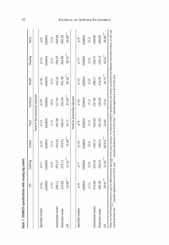
Journal of Applied Economics62Ta
ble
7. E
GARC
H sp
ecifi
catio
ns w
ith v
aryi
ng la
g or
ders
CPI
Clot
hing
Cultu
reFo
odFu
rnitu
reHe
alth
Hous
ing
Trans
.
Pane
l A. N
ot s
easo
nally
adj
uste
d
Spec
ified
mod
els
p=12
p=17
p=12
p=12
p=15
p=18
p=13
p=9
EGAR
CHEG
ARCH
EGAR
CHEG
ARCH
EGAR
CHEG
ARCH
EGAR
CHEG
ARCH
(1,2
)(2
,2)
(1,1
)(1
,1)
(2,2
)(2
,1)
(1,1
)(1
,2)
Unre
stric
ted
mod
el-2
98.1
1-3
53.3
7-4
44.4
2-4
51.6
8-3
17.6
4-4
23.2
4-2
69.5
3-4
39.8
9
Rest
ricte
d m
odel
-3
14.6
5-3
79.1
3-4
79.6
1-4
59.5
7-3
63.4
9-4
41.3
8-2
83.8
8-4
65.3
9
LRT
33.0
9***
51.5
2***
70.3
8***
15.7
791
.69**
*36
.28**
*28
.70**
*50
.98**
*
Pane
l B. S
easo
nally
adj
uste
d
Spec
ified
mod
els
p=9
p=7
p=10
p=9
p=15
p=12
p=17
p=9
EGAR
CHEG
ARCH
EGAR
CHEG
ARCH
EGAR
CHEG
ARCH
EGAR
CHEG
ARCH
(1,1
)(2
,2)
(2,1
)(1
,1)
(1,1
)(1
,2)
(2,1
)(2
,1)
Unre
stric
ted
mod
el-2
70.6
0-3
43.3
4-4
30.1
7-4
25.0
0-3
37.8
0-3
98.1
7-2
28.5
1-4
48.8
0
Rest
ricte
d m
odel
-285
.59
-359
.15
-459
.51
-431
.00
-344
.00
-418
.05
-238
.13
-466
.84
LRT
29.9
7***
31.6
3***
58.6
74**
*10
.90
12.4
139
.74**
*19
.22**
36.0
9***
Note
s: (a
) Fin
al P
redi
ctio
n Cr
iteria
is u
sed
for d
eter
min
ing
the
lag
leng
th o
f the
mea
n eq
uatio
n. (b
) Opt
imum
EGA
RCH
spec
ifica
tions
are
cho
sen
acco
rdin
g to
the
Baye
sian
Info
rmat
ion
Crite
ria. (
c) L
RT: L
ogLi
kelih
ood
Ratio
Test
. ***
indi
cate
s si
gnifi
canc
e at
the
0.01
% le
vel.
**in
dica
tes
sign
ifica
nce
at th
e 0.
05%
leve
l. *
indi
cate
s si
gnifi
canc
e at
the
0.10
% le
vel.
jaeXIII_1:jaeXIII_1 5/11/10 9:21 PM Página 62
VI. Conclusion
This paper assesses whether there is any regularity in the conditional variance of
inflation using Turkish data. The empirical evidence provided here suggests that
there is an increase in inflation volatility during the periods when agents set prices
for the next year, at the beginning of the year or when new products enter to the
markets. There is, thus, a seasonal pattern in inflation volatility and this variation
has implications. First, new de-seasonality methods may be needed to address
seasonality in volatility. It is a common practice to estimate conditional variance
models of inflation using seasonally adjusted data but not to control for seasonality
in the conditional variances. If there is seasonality in the conditional variance, then
this suggests that the models are mis-specificied and subsequent hypothesis tests
are inaccurate. Second, a better method of forecasting inflation may be to incorporate
regularity volatility in inflation, and third, one could better model other variables
that are potentially affected by inflation volatility, such as inflation volatility-growth
relationships and inflation volatility-interest rate relationships.
References
Aisen, Ari, and Francisco Jose Veiga (2008), Political instability and inflation volatility, Public Choice135: 207-223.
Akdi, Yılmaz, Hakan Berument, and Seyit Cilasun (2006), The relationship between different priceindices: Evidence from Turkey, Physica A 360: 483-92.
Automobile Manufacturers Association (2008), Automotive industry annual report presentation, Istanbul,Turkey.
Aydogdu, Hatice, and Nurhan Yonezer (2007), The verbal history of the crises, Ankara, Turkey, DipnotPress (in Turkish).
Berument, Hakan (1999), Interest rates, expected inflation and inflation risk, Scottish Journal of PoliticalEconomy 46: 207-218.
Berument, Hakan (2003), Public sector pricing behavior and inflation risk premium in Turkey, EasternEuropean Economics 41: 68-78.
Berument, Hakan, and Ebru Yuksel (2007), Effects of adopting inflation targeting regimes on inflationvariability, Physica A 375: 265-73.
Berument Hakan, and Kamuran Malatyali (2001), Determinants of interest rates in Turkey, Russian andEast European Finance and Trade 37: 5-16.
Berument, Hakan, Kivilcim Metin-Ozcan, and Bilin Neyapti (2002), Modeling inflation uncertaintyusing EGARCH: An application to Turkey, unpublished manuscript, Bilkent University.
Berument, Hakan, and Nergiz Dincer (2005), Inflation and inflation uncertainty in the G-7 countries,Physica A 348: 371-379.
Berument, Hakan, and Nuray Guner (1997), Inflation, inflation risk and interest rates: A case study forTurkey, Middle East Technical University Studies in Development 24: 319-27.
Seasonality in Inflation Volatility: Evidence from Turkey 63
jaeXIII_1:jaeXIII_1 5/11/10 9:21 PM Página 63
Berument, Hakan, Zubeyir Kilinc and Umit Ozlale (2005), The missing link between inflation uncertaintyand interest rates, Scottish Journal of Political Economy, 52: 222-241
Black, Fisher (1976), Studies in stock price volatility changes, in Proceedings of the 1976 Meetings ofthe American Statistical Association, Business and Economics Statistics Section, 177-181.
Bleaney, Michael, and David Fielding (2002), Exchange rate regimes, inflation and output volatility indeveloping countries, Journal of Development Economics 68: 233-245.
Bollerslev, Tim, and Jeffrey Marc Wooldridge (1992), Quasi-maximum likelihood estimation andinference in dynamic models with time-varying covariances, Econometric Reviews 11: 143-172.
Bomberger, William A. (1996), Disagreement as a measure of uncertainty, Journal of Money, Creditand Banking 28: 381-92.
Bowdler, Christopher, and Adeel Malik (2005), Openness and inflation volatility: Panel data evidence,Working Paper 2005-W14, University of Oxford Nuffield College.
Cosimano, Thomas F, and Dennis W. Jansen (1988), Estimates of the variance of U.S. inflation basedupon ARCH model, Journal of Money, Credit and Banking 20: 409–421.
Dittmar, Robert, William T. Gavin, and Finn E. Kydland (1999), Price-level uncertainty and inflationtargeting, Federal Reseve Bank St. Louis Review 81: 23-33.
Engle, Robert F. (1982), Autoregressive conditional heteroskedasticity with estimates of the varianceof U.K. inflation, Econometrica 50: 987-1008.
Engle, Robert F., and Victor K. Ng (1993), Measuring and testing the impact of news on volatility,Journal of Finance 48: 1749-1778.
Engel, Charles, and John H. Rogers (2001), Deviations from purchasing power parities: Causes andwelfare costs, Journal of International Economics 55: 29-57.
Evans, Martin (1991), Discovering the link between inflation rates and inflation uncertainty, Journal ofMoney, Credit, and Banking 23: 169–84.
French, Kenneth R, and Richard Roll (1986), Stock return variances: The arrival of information and thereaction of traders, Journal of Financial Economics 17: 5-26.
Friedman, Milton (1977), Nobel lecture: Inflation and unemployment, Journal of Political Economy85: 451-72.
Froyen, Richard T., and Roger N. Waud (1987), An examination of aggregate price uncertainty in fourcountries and some implications for real output, International Economic Review 28: 353-373.
Gavin, William T. (2003), Inflation targeting: Why it works and how to make it work better?, WorkingPaper 2003-027B, Federal Reserve Bank of St. Louis.
Ghosh, Atish R., Anne-Marie Gulde, Jonathan D. Ostry, and Holger Wolf (1996), Does the exchangerate regime matter for inflation and growth?, Economic Issues Series No, 2, International MonetaryFund.
Grier, Kevin B., and Mark J. Perry (1998), On inflation and inflation uncertainty in the G7 countries,Journal of International Money and Finance 17: 671-689.
Hafer, Rik W. (1986), Inflation uncertainty and a test of the Friedman hypothesis, Journal ofMacroeconomics 8: 365-72.
Hansen, Henrik, and Katarina Juselius (1995), CATS in RATS: Cointegration analysis of time series,Estima, Evanston, Illinois.
Holland, Steven A. (1986), Wage indexation and the effect of inflation uncertainty on employment: Anempirical analysis, American Economic Review 76: 235-43.
Holland, Steven A. (1988), Indexation and the effect of inflation uncertainty on real GNP, Journal ofBusiness 61: 473-484.
Kontonikas, Alexandros (2004), Inflation and inflation uncertainty in the United Kingdom evidencefrom GARCH modeling, Economic Modelling 21: 525-543.
Journal of Applied Economics64
jaeXIII_1:jaeXIII_1 5/11/10 9:21 PM Página 64
Nelson, Daniel B. (1991), Conditional heteroskedasticity in asset returns: A new approach, Econometrica59: 347-370.
Hodrick, Robert James, and Edward C. Prescott (1997), Postwar U.S. business cycles: An empiricalinvestigation, Journal of Money, Credit, and Banking 29: 1-16.
Rother, Philipp C. (2004), Fiscal policy and inflation volatility, Working Paper 317, European CentralBank.
Savva, Christos S., Denise R. Osborn, and Len Gill (2006), The day of the week effect in fifteen Europeanstock markets, unpublished manuscript, University of Manchester.
Smith, Constance E. (1999), Exchange rate variation, commodity price variation and the implicationsfor international trade, Journal of International Money and Finance 18: 471-491.
Wilson, Bradley K. (2006), The links between inflation, inflation uncertainty and output growth: Newtime series evidence from Japan, Journal of Macroeconomics 28: 609-620.
Seasonality in Inflation Volatility: Evidence from Turkey 65
jaeXIII_1:jaeXIII_1 5/11/10 9:21 PM Página 65

jaeXIII_1:jaeXIII_1 5/11/10 9:21 PM Página 66
Related Documents