Optimization of Process Flowsheets through Metaheuristic Techniques José María Ponce-Ortega Luis Germán Hernández-Pérez

Welcome message from author
This document is posted to help you gain knowledge. Please leave a comment to let me know what you think about it! Share it to your friends and learn new things together.
Transcript
Optimization ofProcess Flowsheets through Metaheuristic Techniques
José María Ponce-OrtegaLuis Germán Hernández-Pérez

Optimization of Process Flowsheets through Metaheuristic Techniques

José María Ponce-Ortega Luis Germán Hernández-Pérez
Optimization of Process Flowsheets through Metaheuristic Techniques

Additional material to this book can be downloaded from http://extras.springer.com.
ISBN 978-3-319-91721-4 ISBN 978-3-319-91722-1 (eBook)https://doi.org/10.1007/978-3-319-91722-1
Library of Congress Control Number: 2018947157
© Springer International Publishing AG, part of Springer Nature 2019, corrected publication 2019This work is subject to copyright. All rights are reserved by the Publisher, whether the whole or part of the material is concerned, specifically the rights of translation, reprinting, reuse of illustrations, recitation, broadcasting, reproduction on microfilms or in any other physical way, and transmission or information storage and retrieval, electronic adaptation, computer software, or by similar or dissimilar methodology now known or hereafter developed.The use of general descriptive names, registered names, trademarks, service marks, etc. in this publication does not imply, even in the absence of a specific statement, that such names are exempt from the relevant protective laws and regulations and therefore free for general use.The publisher, the authors and the editors are safe to assume that the advice and information in this book are believed to be true and accurate at the date of publication. Neither the publisher nor the authors or the editors give a warranty, express or implied, with respect to the material contained herein or for any errors or omissions that may have been made. The publisher remains neutral with regard to jurisdictional claims in published maps and institutional affiliations.
Printed on acid-free paper
This Springer imprint is published by the registered company Springer International Publishing AG part of Springer Nature.The registered company address is: Gewerbestrasse 11, 6330 Cham, Switzerland
José María Ponce-OrtegaUniversidad Michoacana de San Nicolás de Hidalgo Morelia, Michoacán, Mexico
Luis Germán Hernández-PérezUniversidad Michoacana de San Nicolás de Hidalgo Morelia, Michoacán, Mexico

v
Preface
This book presents a general framework to implement a link between process
simulators and optimization through metaheuristic techniques. The book describes
step- by- step the methodology to implement this link for different process simula-
tors and with different metaheuristic methods.
The aim of this book is to provide the readers the needed knowledge to
implement optimizations of process flowsheets through links between process sim-
ulators and metaheuristic approaches. This way, basic knowledge about simulation
through process simulators is needed. To implement this link between process simu-
lation and metaheuristic techniques, the approach is divided into three fundamental
sections: process simulation, metaheuristic algorithm, and implementation of the
link between process simulation and optimization, which are described in the
following chapters.
Chapter 1 presents some basic concepts needed. Chapter 2 presents an introduc-
tion about the general concepts that are involved in the process simulation and the
main commercial software currently available to efficiently carry out this function.
Chapter 2 also presents the basics about the management to manipulate simulations
of chemical and industrial processes.
Chapter 3 presents an introduction about metaheuristic optimization methods,
which can be then included in the link to process simulators and optimization.
Chapter 4 explains how to implement the link between the process simulators and
optimization programs containing metaheuristic techniques, which correspond to
the optimization of the flowsheet of the simulation of the process to be optimized.
Chapter 4 also presents a detailed explanation of the presented methodology to
implement the link between process simulators and optimization, which corre-
sponds to the linking of programs. This part of the book is the main contribution of
the proposed methodology. For its better understanding, the steps of the proposed
methodology are first explained. Then, the needed code is provided to implement
the appropriate link between simulation software and stochastic algorithms. For this
purpose, the sequence to be followed is mentioned step by step, indicating how to
call the needed variables.

vi
Chapter 5 shows the evaluation performance of the different software considered
for implementing the link for the optimization of process flowsheets through pro-
cess simulators and metaheuristic techniques.
Chapters 6 and 7 show two case studies to present the application of the proposed
methodology. Chapter 6 shows the optimization of an industrial process (steam
power plant in Aspen Plus®). In the same way, Chap. 7 shows the optimization of
another industrial process (biodiesel in SuperPro Designer®).
This book also includes some tutorial videos that show, step by step, the pro-
posed methodology to implement a link between process simulators and optimiza-
tion through metaheuristic optimization approaches. These videos are prepared to
show the implementation of the proposed approach for different process simulators
and with different alternatives to implement the metaheuristic approach.
Morelia, Michoacán, Mexico José María Ponce-Ortega
Luis Germán Hernández-Pérez
Preface

vii
Abstract
This book presents a multi-objective optimization framework for optimizing
chemical processes. The proposed framework implements a link between process
simulators and metaheuristic techniques. The proposed approach is general, and
there can be used any process simulator and any metaheuristic technique. This
book shows how to implement links between different process simulators such as
Aspen Plus®, HYSYS®, SuperPro Designer®, and others, linked to metaheuris-
tic techniques implemented in Matlab®, Excel®, C++, or other programs. This
way, the proposed framework allows optimizing any process flowsheet imple-
mented in the process simulator and using the metaheuristic technique, and this
way the numerical complications through the optimization process can be elimi-
nated. Furthermore, the proposed framework allows using the thermodynamic,
design, and constitutive equations implemented in the process simulator to imple-
ment any process.
Keywords: Optimal design, Metaheuristic optimization, Multi-objective
optimization, Process simulators, Simulation

ix
Contents
1 Introduction . . . . . . . . . . . . . . . . . . . . . . . . . . . . . . . . . . . . . . . . . . . . . . . 1
1.1 Process Simulation . . . . . . . . . . . . . . . . . . . . . . . . . . . . . . . . . . . . . . 1
1.2 Searching Methods . . . . . . . . . . . . . . . . . . . . . . . . . . . . . . . . . . . . . . 2
1.2.1 Classification of Search Methods. . . . . . . . . . . . . . . . . . . . . 2
1.2.2 Deterministic Algorithms . . . . . . . . . . . . . . . . . . . . . . . . . . . 3
1.3 Interaction Between Programs . . . . . . . . . . . . . . . . . . . . . . . . . . . . . 4
1.4 Nomenclature . . . . . . . . . . . . . . . . . . . . . . . . . . . . . . . . . . . . . . . . . . 4
2 Process Simulators . . . . . . . . . . . . . . . . . . . . . . . . . . . . . . . . . . . . . . . . . 5
2.1 Aspen Plus® . . . . . . . . . . . . . . . . . . . . . . . . . . . . . . . . . . . . . . . . . . . 6
2.2 Example of the Conventional Rankine Cycle . . . . . . . . . . . . . . . . . 12
2.3 Aspen HYSYS® . . . . . . . . . . . . . . . . . . . . . . . . . . . . . . . . . . . . . . . . 19
2.4 SuperPro Designer® . . . . . . . . . . . . . . . . . . . . . . . . . . . . . . . . . . . . . 20
2.5 PRO/II® Process Engineering . . . . . . . . . . . . . . . . . . . . . . . . . . . . . . 23
2.6 UniSim® Design Suite . . . . . . . . . . . . . . . . . . . . . . . . . . . . . . . . . . . 23
2.7 gPROMS® ProcessBuilder . . . . . . . . . . . . . . . . . . . . . . . . . . . . . . . . 24
2.8 Process Simulation Exercises . . . . . . . . . . . . . . . . . . . . . . . . . . . . . 24
2.9 Nomenclature . . . . . . . . . . . . . . . . . . . . . . . . . . . . . . . . . . . . . . . . . . 25
3 Metaheuristic Optimization Programs . . . . . . . . . . . . . . . . . . . . . . . . . 27
3.1 Simulated Annealing . . . . . . . . . . . . . . . . . . . . . . . . . . . . . . . . . . . . 27
3.2 Genetic Algorithms . . . . . . . . . . . . . . . . . . . . . . . . . . . . . . . . . . . . . 30
3.2.1 Example of Codification . . . . . . . . . . . . . . . . . . . . . . . . . . . 33
3.2.2 Management of Restrictions . . . . . . . . . . . . . . . . . . . . . . . . 36
3.3 GA Toolbox of MATLAB® . . . . . . . . . . . . . . . . . . . . . . . . . . . . . . . 38
3.4 EMOO Tool in MS Excel . . . . . . . . . . . . . . . . . . . . . . . . . . . . . . . . . 41
3.4.1 Main Program Interface . . . . . . . . . . . . . . . . . . . . . . . . . . . . 44
3.4.2 Objectives and Constraints . . . . . . . . . . . . . . . . . . . . . . . . . . 47
3.5 Stochastic Optimization Exercises . . . . . . . . . . . . . . . . . . . . . . . . . . 47
3.6 Nomenclature . . . . . . . . . . . . . . . . . . . . . . . . . . . . . . . . . . . . . . . . . . 50

x
4 Interlinking Between Process Simulators and Optimization
Programs . . . . . . . . . . . . . . . . . . . . . . . . . . . . . . . . . . . . . . . . . . . . . . . . . 53
4.1 Previous Knowledge . . . . . . . . . . . . . . . . . . . . . . . . . . . . . . . . . . . . 55
4.1.1 MS Excel® Configuration . . . . . . . . . . . . . . . . . . . . . . . . . . 55
4.1.2 Object Name of the Simulator File . . . . . . . . . . . . . . . . . . . 55
4.2 Link Between Aspen Plus® and MS Excel® . . . . . . . . . . . . . . . . . 56
4.2.1 Subroutine to Link Aspen Plus® and MS Excel® . . . . . . . . 57
4.2.2 Files to Link Aspen Plus® and MS Excel® . . . . . . . . . . . . 58
4.2.3 Call Name of Aspen Plus® Variables . . . . . . . . . . . . . . . . . 61
4.3 Link Between SuperPro Designer® and MS Excel® . . . . . . . . . . . 62
4.3.1 Subroutine to Link SuperPro Designer®
and MS Excel® . . . . . . . . . . . . . . . . . . . . . . . . . . . . . . . . . . 62
4.3.2 Files to Link SuperPro Designer® and MS Excel® . . . . . . 63
4.3.3 Call Name of SuperPro Designer® Variables . . . . . . . . . . . 65
4.4 Link Between MS Excel® and MATLAB® . . . . . . . . . . . . . . . . . . 67
4.4.1 Subroutine to Link MS Excel® and MATLAB® . . . . . . . . 68
4.4.2 Files Needed to Link MS Excel® and MATLAB® . . . . . . . 68
4.4.3 Object Name of the Linker Program File . . . . . . . . . . . . . . 70
4.4.4 Specification for the Optimization Parameters
in MATLAB® . . . . . . . . . . . . . . . . . . . . . . . . . . . . . . . . . . . 71
4.5 Exercises . . . . . . . . . . . . . . . . . . . . . . . . . . . . . . . . . . . . . . . . . . . . . 72
4.6 Nomenclature . . . . . . . . . . . . . . . . . . . . . . . . . . . . . . . . . . . . . . . . . . 73
5 Performance Evaluation . . . . . . . . . . . . . . . . . . . . . . . . . . . . . . . . . . . . . 75
5.1 Objective Functions . . . . . . . . . . . . . . . . . . . . . . . . . . . . . . . . . . . . . 75
5.1.1 Net Present Value . . . . . . . . . . . . . . . . . . . . . . . . . . . . . . . . . 75
5.1.2 Profit . . . . . . . . . . . . . . . . . . . . . . . . . . . . . . . . . . . . . . . . . . . 76
5.1.3 Capital Cost . . . . . . . . . . . . . . . . . . . . . . . . . . . . . . . . . . . . . 76
5.2 Capital Cost Estimation Programs . . . . . . . . . . . . . . . . . . . . . . . . . . 76
5.2.1 CapCost . . . . . . . . . . . . . . . . . . . . . . . . . . . . . . . . . . . . . . . . 76
5.2.2 Detailed Factorial Program (DFP) . . . . . . . . . . . . . . . . . . . . 77
5.2.3 Capital Cost Estimation Program (CCEP) . . . . . . . . . . . . . . 77
5.2.4 EconExpert . . . . . . . . . . . . . . . . . . . . . . . . . . . . . . . . . . . . . . 78
5.2.5 AspenTech Process Economic Analyzer (Aspen-PEA) . . . . 78
5.3 Nomenclature . . . . . . . . . . . . . . . . . . . . . . . . . . . . . . . . . . . . . . . . . . 78
6 Optimization of Industrial Process 1 . . . . . . . . . . . . . . . . . . . . . . . . . . . 79
6.1 Problem Statement . . . . . . . . . . . . . . . . . . . . . . . . . . . . . . . . . . . . . . 79
6.2 Model Formulation . . . . . . . . . . . . . . . . . . . . . . . . . . . . . . . . . . . . . 80
6.2.1 Model Simulation Using the Aspen Plus® Software. . . . . . 81
6.2.2 Mathematical Formulation . . . . . . . . . . . . . . . . . . . . . . . . . . 82
6.2.3 Definition of the Objective Functions . . . . . . . . . . . . . . . . . 83
6.2.4 Economic Objective Function . . . . . . . . . . . . . . . . . . . . . . . 84
6.2.5 Environmental Objective Function . . . . . . . . . . . . . . . . . . . 84
6.3 Stochastic Optimization Algorithm Used . . . . . . . . . . . . . . . . . . . . 84
Contents
xi
6.4 Link Between the Process Simulator and Optimization
Algorithm . . . . . . . . . . . . . . . . . . . . . . . . . . . . . . . . . . . . . . . . . . . . . 85
6.5 Results . . . . . . . . . . . . . . . . . . . . . . . . . . . . . . . . . . . . . . . . . . . . . . . 86
6.6 Exercises . . . . . . . . . . . . . . . . . . . . . . . . . . . . . . . . . . . . . . . . . . . . . 89
6.7 Nomenclature . . . . . . . . . . . . . . . . . . . . . . . . . . . . . . . . . . . . . . . . . . 90
7 Optimization of Industrial Process 2 . . . . . . . . . . . . . . . . . . . . . . . . . . . 91
7.1 Problem Statement . . . . . . . . . . . . . . . . . . . . . . . . . . . . . . . . . . . . . . 92
7.2 Model Formulation . . . . . . . . . . . . . . . . . . . . . . . . . . . . . . . . . . . . . 93
7.2.1 Model Simulation Using the SuperPro Designer®
Software . . . . . . . . . . . . . . . . . . . . . . . . . . . . . . . . . . . . . . . . 94
7.2.2 Definition of the Objective Functions . . . . . . . . . . . . . . . . . 95
7.2.3 Economic Objective Function . . . . . . . . . . . . . . . . . . . . . . . 95
7.2.4 Environmental Objective Function . . . . . . . . . . . . . . . . . . . 95
7.3 Stochastic Optimization Algorithm Used . . . . . . . . . . . . . . . . . . . . 95
7.4 Link Between the Process Simulator and Optimization
Algorithm . . . . . . . . . . . . . . . . . . . . . . . . . . . . . . . . . . . . . . . . . . . . . 96
7.5 Exercises . . . . . . . . . . . . . . . . . . . . . . . . . . . . . . . . . . . . . . . . . . . . . 97
Correction to: Optimization of Process Flowsheets through
Metaheuristic Techniques . . . . . . . . . . . . . . . . . . . . . . . . . . . . . . . . . . . . . . . . C1
Appendix . . . . . . . . . . . . . . . . . . . . . . . . . . . . . . . . . . . . . . . . . . . . . . . . . . . . . 99
Bibliography . . . . . . . . . . . . . . . . . . . . . . . . . . . . . . . . . . . . . . . . . . . . . . . . . . 103
Index . . . . . . . . . . . . . . . . . . . . . . . . . . . . . . . . . . . . . . . . . . . . . . . . . . . . . . . . . 107
The original version of this book was revised. The correction is available at
https://doi.org/10.1007/978-3-319-91722-1_8
Contents

xiii
List of Figures
Fig. 1.1 Global optimization approaches and different classes of search
methods (Coello-Coello et al. 2002; Devillers 1996) . . . . . . . . . . . 3
Fig. 2.1 Aspen Plus V8.8 Start-up . . . . . . . . . . . . . . . . . . . . . . . . . . . . . . . . . 8
Fig. 2.2 Window to open a New Simulation . . . . . . . . . . . . . . . . . . . . . . . . . 8
Fig. 2.3 Properties of Aspen Plus . . . . . . . . . . . . . . . . . . . . . . . . . . . . . . . . . 9
Fig. 2.4 Find Component Window (Contains option) . . . . . . . . . . . . . . . . . . 10
Fig. 2.5 Find Component Window (Equals option) . . . . . . . . . . . . . . . . . . . 10
Fig. 2.6 Component window . . . . . . . . . . . . . . . . . . . . . . . . . . . . . . . . . . . . . 11
Fig. 2.7 Methods window . . . . . . . . . . . . . . . . . . . . . . . . . . . . . . . . . . . . . . . 11
Fig. 2.8 Simulation section of Aspen Plus . . . . . . . . . . . . . . . . . . . . . . . . . . 12
Fig. 2.9 Rankine cycle flowsheet in Aspen Plus® . . . . . . . . . . . . . . . . . . . . . 13
Fig. 2.10 Location of the model palette . . . . . . . . . . . . . . . . . . . . . . . . . . . . . 13
Fig. 2.11 Location of the boiler in the model palette . . . . . . . . . . . . . . . . . . . 14
Fig. 2.12 Necessary blocks for the conventional Rankine cycle . . . . . . . . . . . 14
Fig. 2.13 Appearance of the blocks when the stream option is selected . . . . . 15
Fig. 2.14 Specification of the WATER stream values . . . . . . . . . . . . . . . . . . . 15
Fig. 2.15 Specification of the BOILER block values . . . . . . . . . . . . . . . . . . . 16
Fig. 2.16 Specification of the CONDENSE block values . . . . . . . . . . . . . . . . 16
Fig. 2.17 Specification of the PUMP block values . . . . . . . . . . . . . . . . . . . . . 17
Fig. 2.18 Specification of the TURBINE block values . . . . . . . . . . . . . . . . . . 17
Fig. 2.19 Message before running the simulation . . . . . . . . . . . . . . . . . . . . . . 18
Fig. 2.20 Results Summary after running the simulation . . . . . . . . . . . . . . . . 18
Fig. 2.21 Results Summary Streams Table (Material) . . . . . . . . . . . . . . . . . . 18
Fig. 2.22 Results Summary Streams Table (Work) . . . . . . . . . . . . . . . . . . . . . 19
Fig. 2.23 User interface of SuperPro Designer® . . . . . . . . . . . . . . . . . . . . . . 21
Fig. 2.24 Operation Sequence for Procedure . . . . . . . . . . . . . . . . . . . . . . . . . 22
Fig. 2.25 Charge operation of SuperPro Designer . . . . . . . . . . . . . . . . . . . . . 22
Fig. 2.26 User interface of gPROMS® ProcessBuilder . . . . . . . . . . . . . . . . . 24
Fig. 2.27 Flowsheet of the regenerative Rankine cycle . . . . . . . . . . . . . . . . . . 25

xiv
Fig. 3.1 Cost versus pressure drop graph for a particular case of a heat
exchanger . . . . . . . . . . . . . . . . . . . . . . . . . . . . . . . . . . . . . . . . . . . . . 28
Fig. 3.2 Example of a function in which stochastic algorithms can be
applied to find the global optimum . . . . . . . . . . . . . . . . . . . . . . . . . 28
Fig. 3.3 Classification of stochastic search algorithms . . . . . . . . . . . . . . . . . 29
Fig. 3.4 General structure of the simulated annealing algorithm . . . . . . . . . 30
Fig. 3.5 General structure of genetic algorithms . . . . . . . . . . . . . . . . . . . . . . 31
Fig. 3.6 GA toolbox of MATLAB® . . . . . . . . . . . . . . . . . . . . . . . . . . . . . . . 41
Fig. 3.7 Flowchart of simple genetic algorithm sequence of genetic
algorithm . . . . . . . . . . . . . . . . . . . . . . . . . . . . . . . . . . . . . . . . . . . . . 42
Fig. 3.8 Flowchart of I-MODE algorithm (Sharma and Rangaiah 2013) . . . 43
Fig. 3.9 Main program interface of I-MODE algorithm 45
Fig. 3.10 Input objective function of I-MODE algorithm . . . . . . . . . . . . . . . . 45
Fig. 3.11 Input decision variables of I-MODE algorithm . . . . . . . . . . . . . . . . 46
Fig. 3.12 Input constraints of I-MODE algorithm . . . . . . . . . . . . . . . . . . . . . 46
Fig. 3.13 Objectives and constraints of I-MODE algorithm . . . . . . . . . . . . . . 47
Fig. 3.14 Behavior of the function of problem 4 . . . . . . . . . . . . . . . . . . . . . . . 48
Fig. 4.1 Interface between a process simulator and Excel® (containing
an optimization program) . . . . . . . . . . . . . . . . . . . . . . . . . . . . . . . . . 54
Fig. 4.2 Screenshot of the position of Visual Basic® button . . . . . . . . . . . . 56
Fig. 4.3 Screenshot of the MS Visual Basic for Applications . . . . . . . . . . . . 56
Fig. 4.4 Screenshot of the position of References button . . . . . . . . . . . . . . . 57
Fig. 4.5 Screenshot of the References window . . . . . . . . . . . . . . . . . . . . . . . 57
Fig. 4.6 Screenshot of windows explorer with the “Properties” option
of the Aspen Plus® file . . . . . . . . . . . . . . . . . . . . . . . . . . . . . . . . . . 58
Fig. 4.7 Screenshot of windows explorer with the “Properties” option
of the SuperPro Designer® file . . . . . . . . . . . . . . . . . . . . . . . . . . . . 58
Fig. 4.8 Screenshot of windows explorer with the “Security” tab of
the Aspen Plus® file where the “Object Name” can be seen . . . . . . 59
Fig. 4.9 Screenshot of windows explorer with the “Security” tab
of the SuperPro Designer® file where the “Object Name”
can be seen . . . . . . . . . . . . . . . . . . . . . . . . . . . . . . . . . . . . . . . . . . . . 59
Fig. 4.10 Screenshot of linking subroutine where the
simulation file route must be pasted . . . . . . . . . . . . . . . . . . . . . . . . . 60
Fig. 4.11 Interface between Aspen Plus® and MS Excel® . . . . . . . . . . . . . . 60
Fig. 4.12 Pseudo code for the link between Aspen Plus®
and MS Excel® . . . . . . . . . . . . . . . . . . . . . . . . . . . . . . . . . . . . . . . . 60
Fig. 4.13 Two files needed to start linking Aspen Plus®
and MS Excel® . . . . . . . . . . . . . . . . . . . . . . . . . . . . . . . . . . . . . . . . 61
Fig. 4.14 Screenshot of windows explorer with the two files needed
to start linking: Aspen Plus® and MS Excel® . . . . . . . . . . . . . . . . 61
Fig. 4.15 Screenshot of variable explorer position in Aspen Plus® . . . . . . . . 62
Fig. 4.16 Screenshot of variable explorer tree in Aspen Plus® . . . . . . . . . . . . 63
Fig. 4.17 Screenshot of linking subroutine where the variable name
call must be pasted . . . . . . . . . . . . . . . . . . . . . . . . . . . . . . . . . . . . . . 63
List of Figures

xv
Fig. 4.18 Interface between SuperPro Designer® and MS Excel® . . . . . . . . 64
Fig. 4.19 Pseudo code for the link between SuperPro Designer®
and MS Excel® . . . . . . . . . . . . . . . . . . . . . . . . . . . . . . . . . . . . . . . . 64
Fig. 4.20 Two files needed to start linking SuperPro Designer®
and MS Excel® . . . . . . . . . . . . . . . . . . . . . . . . . . . . . . . . . . . . . . . . 64
Fig. 4.21 Screenshot of windows explorer with the two files needed
to start linking SuperPro Designer® and MS Excel® . . . . . . . . . . . 65
Fig. 4.22 Screenshot of COM interface in SuperPro Designer® . . . . . . . . . . 65
Fig. 4.23 Screenshot of variable explorer tree in Aspen Plus® . . . . . . . . . . . . 66
Fig. 4.24 Screenshot of COM Library tree in SuperPro Designer® . . . . . . . . 66
Fig. 4.25 Screenshot of linking subroutine where the variable name call
must be pasted . . . . . . . . . . . . . . . . . . . . . . . . . . . . . . . . . . . . . . . . . 67
Fig. 4.26 Interface between Aspen Plus® and MATLAB® using
MS Excel® as linking program . . . . . . . . . . . . . . . . . . . . . . . . . . . . 67
Fig. 4.27 Pseudo code for the link between MS Excel®
and MATLAB® . . . . . . . . . . . . . . . . . . . . . . . . . . . . . . . . . . . . . . . . 68
Fig. 4.28 Four files needed to start the linking Aspen Plus®,
MATLAB®, and MS Excel® . . . . . . . . . . . . . . . . . . . . . . . . . . . . . 69
Fig. 4.29 Screenshot of windows explorer with the four files needed to start
linking Aspen Plus®, MATLAB®, and MS Excel® . . . . . . . . . . . . 69
Fig. 4.30 Screenshot of windows explorer with the “Properties” option
of the linker program . . . . . . . . . . . . . . . . . . . . . . . . . . . . . . . . . . . . 70
Fig. 4.31 Screenshot of windows explorer with the “Security” tab
of the linker program where the “Object Name” can be seen . . . . . 70
Fig. 4.32 Screenshot of function declaration file, where the linker
program route must be pasted . . . . . . . . . . . . . . . . . . . . . . . . . . . . . 71
Fig. 4.33 Screenshot of optimization parameter file, where the function
is called . . . . . . . . . . . . . . . . . . . . . . . . . . . . . . . . . . . . . . . . . . . . . . 72
Fig. 4.34 Steam reformer for the production of syngas from shale gas . . . . . 73
Fig. 6.1 Generation power plant based on regenerative Rankine cycle. . . . . 80
Fig. 6.2 Process flowsheet in Aspen Plus® for a simple steam power
plant for electric generation based on regenerative
Rankine cycle . . . . . . . . . . . . . . . . . . . . . . . . . . . . . . . . . . . . . . . . . . 81
Fig. 6.3 MS Excel® sheet were main program user interface
of the I-MODE (case 1) . . . . . . . . . . . . . . . . . . . . . . . . . . . . . . . . . . 85
Fig. 6.4 MS Excel® sheet were decision variable values will be sent
to the process simulator (case 1) . . . . . . . . . . . . . . . . . . . . . . . . . . . 86
Fig. 6.5 MS Excel® sheet were response variable values will be received
from the simulator (case 1) . . . . . . . . . . . . . . . . . . . . . . . . . . . . . . . 86
Fig. 6.6 Graphic of the results at the Chi-squared termination
criterion (ChiTC) . . . . . . . . . . . . . . . . . . . . . . . . . . . . . . . . . . . . . . . 87
Fig. 6.7 Graphic of the results at the steady-state termination
criterion (SSTC) . . . . . . . . . . . . . . . . . . . . . . . . . . . . . . . . . . . . . . . . 87
Fig. 6.8 Graphic of the results of the last generation . . . . . . . . . . . . . . . . . . 87
List of Figures

xvi
Fig. 7.1 Biodiesel formation reaction . . . . . . . . . . . . . . . . . . . . . . . . . . . . . . 92
Fig. 7.2 Process flowsheet in SuperPro Designer® for a biodiesel
production plant from degummed soybean oil . . . . . . . . . . . . . . . . 92
Fig. 7.3 Excel® sheet for the main program user interface
of the I-MODE (case 2) . . . . . . . . . . . . . . . . . . . . . . . . . . . . . . . . . . 96
Fig. 7.4 MS Excel® sheet where decision variable values will be sent
to the process simulator (case 2) . . . . . . . . . . . . . . . . . . . . . . . . . . . 96
Fig. 7.5 MS Excel® sheet where response variable values will be
received from the simulator (case 2) . . . . . . . . . . . . . . . . . . . . . . . . 97
List of Figures

xvii
List of Table
Table 3.1 Options for GA in MATLAB® . . . . . . . . . . . . . . . . . . . . . . . . . . . 40

1© Springer International Publishing AG, part of Springer Nature 2019
J. M. Ponce-Ortega, L. G. Hernández-Pérez, Optimization of Process
Flowsheets through Metaheuristic Techniques,
https://doi.org/10.1007/978-3-319-91722-1_1
Chapter 1
Introduction
The fundamental concepts used in this book are described below. To implement the
link between any process simulator and metaheuristic techniques, the methodology
has been divided in three parts: simulation, optimization, and link software; and the
involved concepts are described as follows.
1.1 Process Simulation
A mathematical model of a chemical process is a simplified representation of the
physicochemical behavior of a real process, which is used to predict values of out-
put variables for given input variables and process design (including operating)
variables. A model can be used for what-if studies and process troubleshooting, and
it has many applications for process optimization, process control, and operator
training. Models are often difficult to solve analytically, and so they are mostly
solved numerically (Sharma and Rangaiah 2016).
Process simulation allows predicting the behavior of a process by using basic
engineering relationships, such as mass and energy balances, and phase and chemi-
cal equilibrium. Given reliable thermodynamic data, realistic operating conditions,
and rigorous equipment models, one can simulate the plant behavior. Process simu-
lation enables to run many cases, conduct “what-if” analyses, and perform sensitiv-
ity studies and optimization runs. With simulation, one can design better plants and
increase profitability in existing plants. Process simulation is useful throughout the
entire life cycle of a process, from research and development through process design
to production (AspenTech 2015).
Modeling refers to all the steps involved in developing and validating a model
for the process, whereas simulation refers to the use of the developed model for
studying the process behavior/response for one or more sets of input and design
variables. In general, modeling and simulation are used to optimize the process

2
operation and design. Optimization improves the performance of a process by
changing the operating conditions such as temperature, pressure, and flow rate of
process streams but without changing the size of any equipment or process flow-
sheet. Process retrofitting and revamping refer to redesign a plant for specific
objective(s), such as increasing throughput, decreasing energy consumption, and
revising product quality. This is achieved by changes in existing equipment and/or
addition of new equipment (leading to a new process configuration) besides changes
in operating conditions (Sharma and Rangaiah 2016).
1.2 Searching Methods
Optimization is the act of making something as good as possible (Cambridge dic-
tionary). The word optimum means “the best.” Optimization consists in finding the
optimum point in which the best values are found for certain variables and in which
they achieve some specific objectives. There are different search methods to achieve
optimization, which will be analyzed in depth in the corresponding chapter.
The decision variables correspond to those that have been previously determined
and will be manipulated in order to find the optimal point. These variables must
operate within a range in which they offer feasible results for the objectives being
sought; this is the operating range. Also, the decision variables can be subject to
certain constraints that the user must know for the studied processes; these con-
straints help to limit the search range and make the optimization more efficient,
reducing the computation time.
The objective function is an equation in which is reflected the performance of the
process that is being optimized; it is achieving its maximum or its minimum value
by manipulating the variables of dissolution and considering the established search
restrictions.
1.2.1 Classification of Search Methods
General search and optimization techniques are classified into three categories:
enumerative, deterministic, and stochastic (Coello-Coello et al. 2002). Figure 1.1
shows common examples of each type. Some authors classify calculus-based meth-
ods in indirect and direct, and classify evolutionary computation in evolution strate-
gies, evolutionary programming, genetic algorithms, and genetic programing
(Devillers 1996).
To overcome some drawbacks associated to the deterministic optimization
approaches, metaheuristic optimization approaches have been reported (Wang and
Tang 2013; Guo et al. 2014; Ouyang et al. 2015; Wong et al. 2016). The metaheuris-
tic optimization approaches mimic some evolution processes and are based on
1 Introduction

3
repeatedly simulating a given process to assign a fitness function for given values of
the degrees of freedom (Sharma and Rangaiah 2016). This way, the possibility to
get trapped prematurely in a suboptimal solution is avoided (Devillers 1996), the
complication associated to the form of the optimization model is avoided (Sharma
and Rangaiah 2014), and mainly because these are based on simulation of the pro-
cess, these can be easily linked to the process simulators to optimize different
flowsheets.
1.2.2 Deterministic Algorithms
Deterministic methods have been successfully used in solving a wide variety of
problems. However, these methods are inefficient for solving non-convex and non-
linear problems. For the implementation of these optimization methods, it is neces-
sary to implement all the equations that describe the behavior of the process by the
formulation of a mathematical model.
Deterministic methods are often ineffective when applied to NP-complete or
other high-dimensional problems because they are limited by their requirements
associated to the problem domain, knowledge (heuristics), and the search space,
which can be exceptionally large. Because many real-world scientific and engineer-
ing multi-objective problems (MOPs) exhibit one or more of the abovementioned
characteristics, stochastic searches have been developed as alternative approaches
for solving these irregular problems (Coello-Coello et al. 2002).
Fig. 1.1 Global optimization approaches and different classes of search methods (Coello-
Coello et al. 2002; Devillers 1996)
1.2 Searching Methods
4
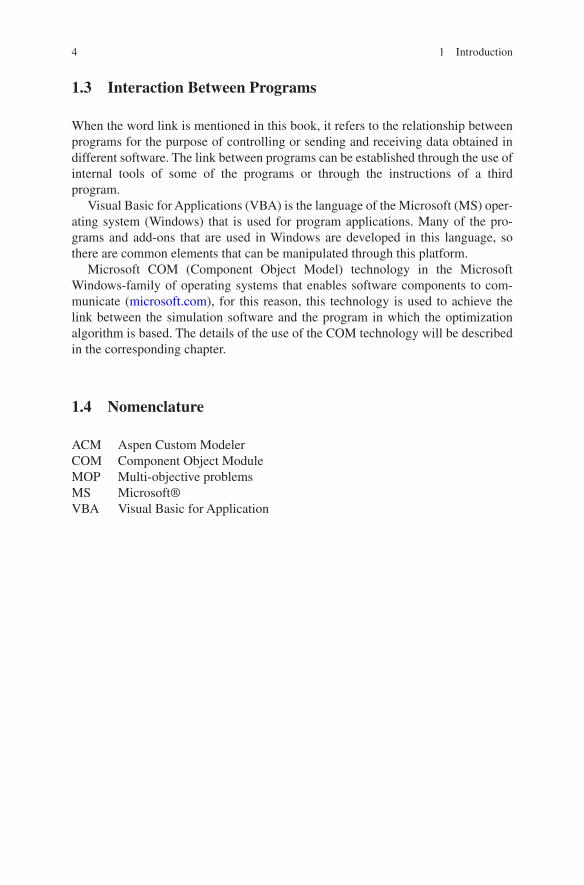
1.3 Interaction Between Programs
When the word link is mentioned in this book, it refers to the relationship between
programs for the purpose of controlling or sending and receiving data obtained in
different software. The link between programs can be established through the use of
internal tools of some of the programs or through the instructions of a third
program.
Visual Basic for Applications (VBA) is the language of the Microsoft (MS) oper-
ating system (Windows) that is used for program applications. Many of the pro-
grams and add-ons that are used in Windows are developed in this language, so
there are common elements that can be manipulated through this platform.
Microsoft COM (Component Object Model) technology in the Microsoft
Windows-family of operating systems that enables software components to com-
municate (microsoft.com), for this reason, this technology is used to achieve the
link between the simulation software and the program in which the optimization
algorithm is based. The details of the use of the COM technology will be described
in the corresponding chapter.
1.4 Nomenclature
ACM Aspen Custom Modeler
COM Component Object Module
MOP Multi-objective problems
MS Microsoft®
VBA Visual Basic for Application
1 Introduction

5© Springer International Publishing AG, part of Springer Nature 2019
J. M. Ponce-Ortega, L. G. Hernández-Pérez, Optimization of Process
Flowsheets through Metaheuristic Techniques,
https://doi.org/10.1007/978-3-319-91722-1_2
Chapter 2
Process Simulators
Process simulator is a computer program that allows modeling different processes
depending on the area of study for which it was designed; this way, there are process
simulators for industrial, chemical, and biochemical processes. A process simulation
software is the best way to perform the simulation of industrial processes; this is due
to the large number of equations and numerical methods that are needed to use for
proper representation and prediction of behavior in reality.
In addition, the process simulators usually are programmed for using in the oper-
ating system of a computer, so it is advisable to verify the compatibility of the
software that will be used with the equipment where it is going to work. Currently,
there are several process simulators that are distributed commercially and which
already have modeling equations for certain equipment and numerical methods
programmed for the solution of specific thermodynamic equations. Another
important aspect of commercial simulation software is that they have a simple
database with components usually used in the chemical and process industry, as
well as their physicochemical and thermodynamic properties.
Process simulators have been widely used for analyzing chemical processes
(Morgan et al. 2017; Gómez-Ríos et al. 2017; Pauls et al. 2016); these offer a
tremendous advantage associated with the implemented thermodynamic correlations
as well as the powerful numerical methods for solving the mass and energy balances
together with design and constitutive relationships (Hauck et al. 2017). Process
simulators allow analyzing the process flowsheets for zero degrees of freedom.
Some optimization approaches have been implemented in process simulators;
however, important drawbacks have been identified associated with the number of
degrees of freedom, the use of explicit constraints, as well as the number of objective
functions. Furthermore, the implemented optimization techniques can be
prematurely trapped in suboptimal solutions, or even no feasible solutions can be
obtained (Coello-Coello et al. 2002) because usually deterministic optimization
techniques have been implemented (Ponce-Ortega et al. 2012).

6
Nowadays, several process simulators, such as Aspen Plus® and Aspen
HYSYS®, are commercially available for simulating complete chemical processes,
where common process units and a property database for numerous chemicals are
available (Sharma and Rangaiah 2016). Most of chemical and biochemical process
simulators are not equipped with adequate optimization tools. However, in very few
simulators (e.g., Aspen Plus®), there are some optimization tools, but the formulation
of optimization problems and available solution techniques is not good enough
(Woinaroschy 2009). For example, the number of degrees of freedom is limited,
only deterministic techniques can be implemented, it is complicated to manipulate
explicit constraints for not manipulated variables, and only one objective can be
considered.
For the proposed multi-objective optimization framework, the first step consists
in implementing the flowsheet in the process simulator. The input variables and the
operating conditions for the included equipment must be specified. Also, the
thermodynamic method and the mathematical solution technique with the maximum
number of iterations are necessary to be declared. All these values are for the first
simulation process, and it must be run without any error or warning. It is
recommended to validate the response variables for checking the values of the
results after implementing the optimization approach.
2.1 Aspen Plus®
Aspen Plus® is the market-leading chemical process simulation software used by
the bulk, specialty, and biochemical industries for the design and operation
(aspentech.com). The main advantages of this simulator consist of a large database
of specific chemical compounds and unit operations.
However, models for less common and/or new process units are not readily avail-
able in the simulators, but they may be available in the literature or can be developed
from first principles. A mathematical model for a new process unit can be imple-
mented in Aspen Custom Modeler (ACM), and then it can be exported to Aspen
Plus® or Aspen HYSYS® for simulating processes, having a new process unit
besides common process units such as heat exchangers, compressors, reactors, and
columns (Sharma and Rangaiah 2016).
For the correct functioning of these simulations, it is necessary to feed the pro-
gram with values that are within a suitable range, the previous one in order to avoid
errors in the equipment so that indeterminacies arise due to the thermodynamic
behavior of the substances used and the interconnections of the equipment must be
correctly indicated.
Aspen Plus® is a process simulation program that can also be used for many
types of thermodynamic calculations or to retrieve and/or correlate thermodynamic
and transport data (Sandler 2015). With the purpose of obtaining a better
understanding of the use of this software for process simulation, we will present
some fundamental aspects for its use. However, it is worth noting that if the reader
2 Process Simulators

7
requires further information about the use of this specific software, it is better to
consult the user guide that the program developers offer on the official website. As
the Aspen Plus® V8.8 Help indicates, one can translate any process into an Aspen
Plus® process simulation model by performing the following steps:
1. Specify the chemical components used in the process. You can take these com-
ponents from the Aspen Plus® databanks, or you can define them.
2. Specify the thermodynamic models to represent the physical properties of the
components and mixtures in the process. These models are included in the Aspen
Plus® software.
3. Define the process flowsheet, which includes:
(a) Define the unit operations in the process.
(b) Define the process streams that flow to and from the unit operations.
(c) Select models from the Aspen Plus® Model Library to describe each unit
operation and place them on the process flowsheet.
(d) Place labeled streams on the process flowsheet and connect them to the unit
operation models.
4. Specify the component flow rates and the thermodynamic conditions (e.g., tem-
perature and pressure) of feed streams.
5. Specify the operating conditions for the unit operation models.
With Aspen Plus®, one can interactively change specifications, such as flow-
sheet configuration, operating conditions, and feed compositions, to run new cases
and analyze process alternatives. In addition to process simulation, Aspen Plus®
allows to perform a wide range of other tasks such as estimating and regressing
physical properties, generating custom graphical and tabular output results, fitting
plant data to simulation models, optimizing processes, and interfacing results to
spreadsheets (AspenTech 2015).
The user interface of Aspen Plus® is very intuitive and easy to use, due to the
remarkable efforts that the developers of this software have implemented to make
the use friendlier. This important aspect can be noticed with the improvements that
the new version has with respect to the previous one.
To start, open the Aspen Plus V8.x, which you may have to locate depending on
the setup of your computer. (It may be on your desktop or you may have to follow
the path All Programs > Aspen Tech > Process Modeling V8.x > Aspen Plus > Aspen
Plus V8.x.)
When you open Aspen Plus V8.2 or higher version, you will briefly see the Aspen
logo of Fig. 2.1. There is then a slight delay while the program connects to the
server, and then the Start Using Aspen Plus window with resent simulations appears.
To proceed, click on New, which brings up the window shown in Fig. 2.2 for all
versions of Aspen Plus V8.0 or higher.
Click on Blank Simulation and then Create. This will bring up Fig. 2.3.
On the lower-left-hand corner of this window, there are three choices. The first
one, which Aspen Plus opens, is Properties; the drop-down menu under
Components > Specifications is used to specify the component or components for
2.1 Aspen Plus®

8
Fig. 2.1 Aspen Plus V8.8 Start-up
Fig. 2.2 Window to open a New Simulation
2 Process Simulators

9
the calculation, and the drop-down menu under Methods is used to specify the
thermodynamic models and parameters that will be used in the calculation. The
second general area is Simulation that will take you to a flowsheet window, to be
discussed later, and the third one is the Energy Analysis that is used to implement
energetic analysis and integration. The default is to start with Properties.
For example, we will proceed to entering the component water. There are two
ways to enter component names. The simples and most reliable way to ensure that
you will get the correct component and its properties from the Aspen Plus® database
is to click on the Find box that brings up the Find Compounds window and to enter
the component name by typing in water and then clicking on Find Now, which
produces the window shown in Fig. 2.4.
A long list of compounds, shown in Fig. 2.4, is generated because the default
Contains was used in the Find Compounds window; as a result, every compound in
the database that contains water either in its compound name or in its alternate name
appears in the list. The compound we are interested will be first on this list, but that
will not always be the case. Therefore, a better way to proceed in the Find Compounds
window is to click Equals instead of the default Contains and then click Find Now,
which produces, instead of a list, only water (Fig. 2.5).
Click on WATER and the Add selected compounds, and for this example, click
on Close. You will then see Fig. 2.6.
Another alternative is to type in all or part of the name directly in the Components-
Specification window and see whether Aspen Plus® finds the correct name. Notice
that water has now been added to the Select components list and that both components
and Specifications now have check marks indicating that sufficient information has
been provided to proceed to the next step. However, this may not be sufficient
information for the problem of interest to the user. If the problem to be solved
involves a mixture, one or more additional components may be added following the
Fig. 2.3 Properties of Aspen Plus
2.1 Aspen Plus®

10
Fig. 2.4 Find Component Window (Contains option)
Fig. 2.5 Find Component Window (Equals option)
2 Process Simulators

11
procedure described above except that the Close button in the Find Compounds
window is used only after all the components have been added.
The next step is to go to Methods by clicking on it. The window shown in Fig. 2.7
appears, and here a number of thermodynamic models can be used through any
other equation of state for which parameters are available can be used. Notice that
if you need help in choosing a thermodynamic model, you can click on Methods
Assistant for help. After accepting the equation by clicking Enter, Methods on the
left-hand side of Fig. 2.7 will also have a check.
Checking on Simulation brings up the Main Flowsheet window of Fig. 2.8
together with Model palette at the bottom of the window.
Fig. 2.6 Component window
Fig. 2.7 Methods window
2.1 Aspen Plus®

12
The next step is to draw the process flowsheet, or even a single process unit such
as a boiler or a turbine, which will be described in the next section.
2.2 Example of the Conventional Rankine Cycle
With the purpose of introducing the reader to the basic principles about how simula-
tions work in the Aspen Plus® process simulator software, this section will present
a simple example. As a case study, a conventional Rankine cycle was considered,
which consists of a boiler, a turbine, a condenser, and a pump (Fig. 2.9).
The first step to do is to introduce the water component into the Aspen properties
part, as shown in the previous section. After that, we proceed to choose the
thermodynamic method that will be used to perform the simulation calculations (in
this case STEAMNBS with a method filter of WATER). Once this is done, we select
the Aspen Simulation part, where we proceed to build the process flowsheet selecting
each equipment that conforms the process of the conventional Rankine cycle. To
select each equipment, go to the model palette (in case this is not visible, go to the
display tab in the show section and select model palette) (Fig. 2.10).
The first unit for the flowsheet process of a conventional Rankine cycle is the
boiler. You have to go to the model palette, in the heat exchanger tab, and look for
the boiler symbol. To select it, you must click on the corresponding symbol and
click again in any part of the work area of the Aspen simulation part (as Fig. 2.11
shows). A small symbol will appear as the one with a default name, which will be
“B1”; to change it just click on the symbol and with right click select the “Rename
Block” option. Now we can assign a more appropriate name to better identify it; in
this case, it can be “BOILER.”
Fig. 2.8 Simulation section of Aspen Plus
2 Process Simulators

13
In the same way, we proceed to select and rename the rest and the necessary
equipment for the flowsheet of the process of a conventional Rankine cycle
(Fig. 2.12).
The next step is to complete the processes flowsheet of the conventional Rankine
cycle joining the blocks using material streams for that. To do this, select the
Material option from the model palette with a click. You will notice that in the
blocks of the diagram, there will appear small red and blue arrows; the first common
meaning is obligatory to complete the process flowsheet, while the blue ones are
optional (Fig. 2.13).
Fig. 2.9 Rankine cycle flowsheet in Aspen Plus®
Fig. 2.10 Location of the model palette
2.2 Example of the Conventional Rankine Cycle

14
Connect the blocks using the material streams. This is done by clicking and hold-
ing on an arrow, moving the pointer to the desired location, and releasing it. Rename
the streams to obtain the process flowsheet of the conventional Rankine cycle shown
in Fig. 2.9.
To proceed, the user must now provide the specifications for the process, which
includes the inlet stream component(s) and conditions, pressures and temperatures
needed, and the type of each process unit or block (e.g., an isentropic turbine).
Click on Streams > WATER and complete with a temperature of 98 °C, a pressure
of 1 atm, a total flow rate of 20,000 kg/h, and a molar fraction of 1 in water
compound, as shown in Fig. 2.14. This is the only stream that needs to be specified;
Fig. 2.12 Necessary blocks for the conventional Rankine cycle
Fig. 2.11 Location of the boiler in the model palette
2 Process Simulators
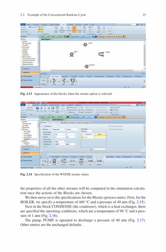
15
the properties of all the other streams will be computed in the simulation calcula-
tion once the actions of the Blocks are chosen.
We then move on to the specifications for the Blocks (process units). First, for the
BOILER, we specify a temperature of 460 °C and a pressure of 40 atm (Fig. 2.15).
Next in the block CONDENSE (the condenser), which is a heat exchanger, there
are specified the operating conditions, which are a temperature of 98 °C and a pres-
sure of 1 atm (Fig. 2.16).
The pump, PUMP, is operated to discharge a pressure of 40 atm (Fig. 2.17).
Other entries are the unchanged defaults.
Fig. 2.13 Appearance of the blocks when the stream option is selected
Fig. 2.14 Specification of the WATER stream values
2.2 Example of the Conventional Rankine Cycle

16
Finally, the specifications for the turbine, TURBINE, are that it is operated as an
isentropic turbine and it discharges at a pressure of 1 atm (Fig. 2.18).
Now all necessary boxes are checked, and in the lower-right-hand corner of the
window, there is the message “Required Input Complete.” We are ready to run the
simulation. There are five ways to start the simulation. The first way is to press the
F5 key (not function F5, just the F5 key). The second and third ways are to press one
of the two forward arrow keys on the Main Toolbar and click on the forward arrow
above Run (which will gray if not all the information for the simulation has been
entered, but turn dark blue when all necessary data have been entered). The final two
Fig. 2.15 Specification of the BOILER block values
Fig. 2.16 Specification of the CONDENSE block values
2 Process Simulators

17
ways are to click on one of the Aspen Plus Next keys on the Main Toolbar that will
bring up the message of Fig. 2.19. Clicking OK will then run the simulation.
After running the simulation, you can check the results clicking on Results
Summary (Fig. 2.20).
Then, going to Streams, it brings up a window (Fig. 2.21) containing the table of
stream results.
As you can see, Fig. 2.21 shows the Material Streams. If you want to see the
work generated in the turbine, you can see it clicking on the Work tab and it brings
up a window with the value (Fig. 2.22).
Fig. 2.17 Specification of the PUMP block values
Fig. 2.18 Specification of the TURBINE block values
2.2 Example of the Conventional Rankine Cycle

18
Fig. 2.19 Message before running the simulation
Fig. 2.20 Results Summary after running the simulation
Fig. 2.21 Results Summary Streams Table (Material)
2 Process Simulators

19
As you can see, Aspen Plus® is a process simulator software with a user inter-
face very easy and intuitive to manipulate. If you need to deep in the use of Aspen
Plus, it is recommended to consult a specialized text as mentioned in the bibliogra-
phy of this book.
2.3 Aspen HYSYS®
Aspen HYSYS® is a process simulation software focused on oil and gas, refining,
and engineering processes (aspentech.com). With an extensive array of unit
operations, specialized work environments, and a robust solver, modeling in Aspen
HYSYS V8 enables the user to:
• Improve equipment design and performance
• Monitor safety and operational issues in the plant
• Analyze processing capacity and operating conditions
• Identify energy savings opportunities and reduce greenhouse gas emissions
• Perform economic evaluation to obtain savings in the process design
Aspen HYSYS V8 builds upon the legacy modeling environment, adding
increased value with integrated products and an improved user experience. The ease
of use and flexibility of model calculations have been preserved, while new
capabilities have also been added.
Fig. 2.22 Results Summary Streams Table (Work)
2.3 Aspen HYSYS®

20
2.4 SuperPro Designer®
SuperPro Designer® is a software that facilitates modeling, evaluation, and optimi-
zation of integrated processes in a wide range of industries (intelligent.com), which
includes batch operations and several biochemical processes. The main reason for
using this simulator is because it allows the analysis of biochemical processes that
other commercial simulators do not include in their modeling options.
SuperPro Designer® is the only commercial process simulator that can handle
equally well continuous and batch processes as well as combinations of batch and
continuous.
Graphical Interface: This software includes an intuitive and user-friendly inter-
face (see Fig. 2.23). The equipment-looking icons represent unit operations for con-
tinuous processes and unit procedures for batch processes.
In this environment, developing a process flowsheet or modifying values is as
easy as point and click. The interface is very similar to other MS Windows
applications, making its features very intuitive.
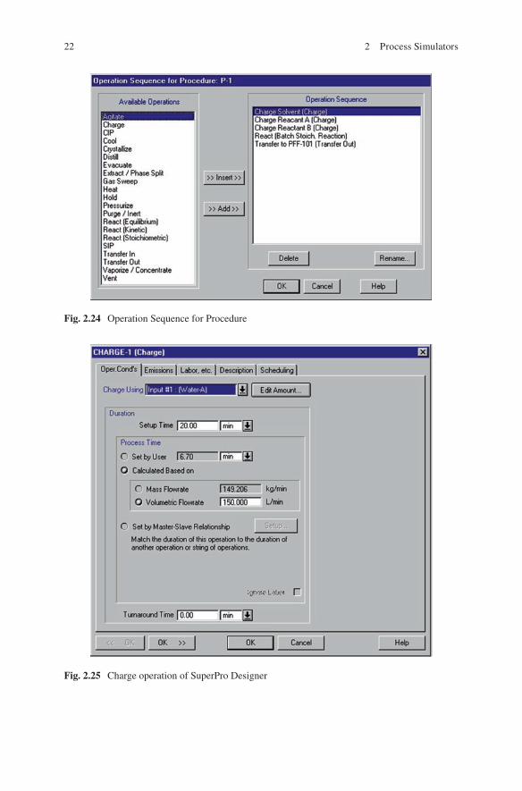
Unit Procedures: A unit procedure is a set of operations that take place sequen-
tially in a piece of equipment. For instance, the P-1 vessel unit procedure (see
Fig. 2.24) includes the following operations: Charge Solvent, Charge Reactant A,
Charge Reactant B, and Transfer to PFF-101. The concept of unit procedures
enables the user to model batch processes in great detail. A unit procedure is repre-
sented with a single equipment-looking icon on the screen. Multiple procedures can
share the same equipment item as long as their cycle times do not overlap.
Operations: For every operation within a unit procedure, the simulator includes a
mathematical model that performs material and energy balance calculations. Based
on the material balances, it performs equipment-sizing calculations. If multiple
operations within a unit procedure dictate different sizes for a certain piece of
equipment, the software reconciles the different demands and selects an equipment
size that is appropriate for all operations. In other words, the equipment is sized so
that it is large enough that it will not be overfilled during any operation, but it is no
larger than necessary (in order to minimize capital costs). In addition, the software
checks to ensure that the vessel contents will not fall below a user-specified
minimum volume (e.g., a minimum stir volume) for applicable operations.
The initialization of operations is done through appropriate windows. For
instance, Fig. 2.25 shows the Oper.Cond’s tab of a charge operation. Through this,
the user specifies either the process time (duration) of the operation or the charge
rate (based on mass or volumetric flowrate), and the program uses that information
to calculate the duration. A third option is to set the duration of an operation equal
to the duration of another operation or equal to the sum of durations of some other
operations (through the “Set by Master-Slave Relationship” interface). The
Emissions tab is used to specify parameters that affect emissions of volatile organic
2 Process Simulators

21
compounds (VOCs). The Labor tab is used to specify the labor requirement for this
operation. The Description tab displays a description of the process generated by
the model (e.g., Charge 1000 L of Water at a rate of 150 L/min using stream
Water-A). The user has the flexibility to edit the description and enter his/her own
comments for documentation purposes. The Scheduling tab is used for specifying
the Start Time of this operation relative to other events (e.g., the beginning of the
batch, the beginning or end of some other operation in the same or a different
procedure, etc.). SuperPro Designer® includes more than 120 operation models.
Component and Mixture Databases: The registration of pure components and
mixtures is something that typically precedes the initialization of operations.
SuperPro Designer® is equipped with two component databases, its own of 600
compounds and a version of DIPPR that includes 1700 compounds (the DIPPR
Fig. 2.23 User interface of SuperPro Designer®
2.4 SuperPro Designer®
22
Fig. 2.25 Charge operation of SuperPro Designer
Fig. 2.24 Operation Sequence for Procedure
2 Process Simulators

23
database must be purchased separately from Brigham Young University of Utah).
It also comes with a user database where modified and newly created compounds
can be saved. All database files are in MS Access format. Furthermore, SuperPro
Designer® comes with mixture databases to represent buffers and other solutions
that are commonly used in the biotech and other industries. Again, the user has the
option to create his/her mixtures and save them in the user database.
For each pure component, the SuperPro Designer® databank includes thermody-
namic (e.g., molecular weight, critical pressure and temperature, acentric factor,
vapor pressure, density, specific heat, particle size, etc.), environmental (e.g., bio-
degradation data, octanol to water distribution ratio, Henry’s law constant, compo-
nent contribution to TOC, COD, BOD5, TSS, etc.), cost (e.g., purchasing price,
selling price, etc.), and regulatory (e.g., type of pollutant) data.
2.5 PRO/II® Process Engineering
PRO/II® Process Engineering optimizes plant performance by improving process
design and operational analysis and performing engineering studies
(software.schneider-electric.com). This software was designed to perform rigorous
heat and material balance calculations for a wide range of chemical processes. PRO/
II® Process Engineering offers a wide variety of thermodynamic models to virtually
every industry. PRO/II® Process Engineering is cost-effective, thereby decreasing
both capital and operating costs.
PRO/II® is now available via the cloud in addition to the traditional on-premise
access method. This cloud access has not only many benefits over on-premise access
but also over other products with cloud access due to platform technology developed
with simulation users in mind. PRO/II® has the following advantages:
• A secure user access control that allows the administrator to add and delete users
or edit privileges as needed
• Simplify IT Overhead with the use of the product on pure on-demand cloud
machines via a secure URL with no need for installation
• Seamless maintenance with new versions available as soon as they are released
• Flexible Usage and Pricing with SaaS business model based on minimum usage
subscription and flexible, incremental usage credits
• Computer-based introductory training included
2.6 UniSim® Design Suite
Honeywell’s UniSim® Design Suite is a process modeling software that provides
steady-state and dynamic process simulation in an integrated environment
(honeywellprocess.com). It provides powerful tools to help engineers evolve process
2.6 UniSim® Design Suite

24
optimization designs with lower project risks, prior to committing to capital
expenditures. Some applications in process modeling using UniSim® Design Suite
include:
• Process flowsheet development
• Utilizing case scenarios tool to optimize designs against business criteria
• Equipment rating across a broad range of operating conditions
• Evaluating the effect of feed changes, upsets and alternate operations on process
safety, reliability, and profitability
• Accurately sizing and selecting the appropriate material for blowdown systems
• Monitoring equipment performance against operating objectives
2.7 gPROMS® ProcessBuilder
gPROMS® ProcessBuilder is an advanced process modeling environment for opti-
mizing the design and operation of process plants (psenterprise.com). ProcessBuilder
combines industry-leading steady-state and dynamic models with all the power of
the gPROMS equation-oriented modeling, analysis, and optimization platform in an
easy-to-use process flowsheeting environment (Fig. 2.26).
2.8 Process Simulation Exercises
With the purpose of offering the reader the opportunity to put into practice the
knowledge acquired in this chapter, the following exercises are proposed:
Fig. 2.26 User interface of gPROMS® ProcessBuilder
2 Process Simulators

25
1. Implement in Aspen Plus® the process flowsheet of a conventional Rankine cycle
just as shown in Sect. 2.2 of this chapter (Fig. 2.12) with the following
specifications:
(a) Change the operating conditions in the boiler with a temperature equal to
500 °C and pressure of 50 atm (the discharge pressure of the pump must be
of 50 atm too). What happened with the value of the ELECTR stream? Why?
(b) Change the total flow rate of the WATER stream, with a value of 30,000 kg/h.
What happened with the value of the ELECTR stream? Why?
2. Implement in Aspen Plus® the process flowsheet of a regenerative Rankine cycle,
which is shown in Fig. 2.27, using the following operating conditions: a
temperature of 580 °C, pressure of 38 atm, and a total flow of 1000 ton/day for
the boiler output stream. The hot stream outlet temperature from the condenser
is equal to 100 °C, hot stream temperature decrease of 10 °C in the first preheater
and 100 °C in the second one, pressure of the pump of 40 atm, temperature of
600 °C, and pressure of 40 atm in the boiler. The split fraction is 0.8 in both
splitters, and the pressure decreases are 20, 10, and 5 atm in the HP, LP, and LP
turbines, respectively. Explain the results from this simulation.
2.9 Nomenclature
COM Component Object Module
MS Microsoft®
OLE Object Linking and Embedding
VBA Visual Basic for Application
Fig. 2.27 Flowsheet of the regenerative Rankine cycle
2.9 Nomenclature

27© Springer International Publishing AG, part of Springer Nature 2019
J. M. Ponce-Ortega, L. G. Hernández-Pérez, Optimization of Process
Flowsheets through Metaheuristic Techniques,
https://doi.org/10.1007/978-3-319-91722-1_3
Chapter 3
Metaheuristic Optimization Programs
There are optimization processes of industrial interest that involve functions that
present a large number of local solutions, and therefore it is very difficult to
determine the optimal solution using deterministic optimization techniques. For
example, consider the case shown in Fig. 3.1, in which the cost function for the
design of a heat exchanger relative to pressure drops is represented in a diagram.
In this case, we can see that there are two local solutions, so if we use a local
search procedure, the algorithm could be trapped in the solution that does not
present the minimum cost since it complies with the stopping criteria of these
optimization algorithms.
To solve these problems, we have proposed stochastic search algorithms based
on natural phenomena such as simulated annealing (Kirkpatrick et al. 1983) and
genetic algorithms (Goldberg 1989). These algorithms allow to search for prob-
lems that present a large number of local solutions as complex as the one shown
in Fig. 3.2.
In this chapter, we present the general structure of simulated annealing (SA)
and genetic algorithms (GA) as stochastic algorithms (other stochastic search
algorithms can be seen in Fig. 3.3). These algorithms are applied directly to unre-
stricted problems where the problem consists of Min f(x), with limits for the vari-
ables, a ≤ x ≤ b.
3.1 Simulated Annealing
Simulated annealing (SA) is a metaheuristic technique based on an analogy of
metal annealing. To describe this phenomenon, first consider a solid with a crys-
talline structure that is heated to melt, and then the molten metal is cooled to
solidify again. If the temperature decreases rapidly, irregularities appear in the
crystalline structure of the cooled solid, and the energy level of the solid is much

28
greater than a perfectly crystalline structure. If the material is cooled slowly, the
energy level will be minimal. The state of the system at any temperature level is
described by the coordinate vector q. At a given temperature, while the system
remains in equilibrium, the state changes randomly, but the transition to states
with lower energy level is more likely at low temperatures.
PT , PC VS CTA
CT
A
PC PT
02
46
890
x 104x 104
x 104
Local Minimum
Global Minimum
21
1.95
1.85
1.75
1.7
1.65
1.6
1.55
1.8
1.9
03 4 5 6 7 8
Fig. 3.1 Cost versus pressure drop graph for a particular case of a heat exchanger
Global Optimum
Local Solutions
5
0
-5 x1x2 -5
0
5
0
10
20
f(x1,x
2) 30
40
50
Fig. 3.2 Example of a function in which stochastic algorithms can be applied to find the global
optimum
3 Metaheuristic Optimization Programs

29
To apply these ideas to a general optimization problem, we will designate the
system state q as the optimization goal denoted as x. The energy level corresponds
to the objective function, f(x). The basic steps of the optimization algorithm SA are
shown below (see Fig. 3.4):
0. Select a set of initial values for the search vector x, an initial temperature T, a
lower limit for the temperature Tlow, and a limit for the maximum number of
iterations L.
1. Make k = 0.
2. Make k = k + 1.
3. Randomly select values for the unknown vector x′.
4. If f(x′) − f(x) = 0, make x = x′.
5. If f(x′) − f(x) > 0, make x = x′ with a probability of exp-(f(x′) − f(x))/T.
6. If k < L, return to step 2; otherwise continue with step 7.
7. Reduce the temperature T = cT, where 0 < c < 1.
8. If T > Tlow, returns to step 1; otherwise terminate the search procedure.
SA depends on the random strategy to diversify the search. The basic SA algo-
rithm uses the Metropolis criterion to accept a motion. In this sense, the move-
ments in which the objective function decrease are always accepted, whereas the
movements that increase the objective function are accepted but with a probability
of exp (f(x′) − f(x)/T). When T approaches zero, the probability of accepting a
movement in which the objective function increases is zero. Thus, when the tem-
perature is high, many movements in which the objective function increases are
accepted; in this way the method prevents it from being trapped prematurely in a
local solution.
Enumerative
Global Search & Optimization
Deterministic Stochastic
RandomSearch/Walk
Monte Carlo
Simulated Annealing
Taboo Search
Evolutionary Computation
Evolution strategies
Evolution programming
Genetic algorithms
Genetic programming
Fig. 3.3 Classification of stochastic search algorithms
3.1 Simulated Annealing

30
3.2 Genetic Algorithms
Genetic algorithms (GA) are stochastic search techniques based on the mechanism
of natural selection and genetics. GAs are particularly useful in non-convex prob-
lems or that include discontinuous functions. GAs differ from conventional optimi-
zation techniques because instead of having an initial solution (values for the
optimization variable vector x), we have a set of solutions for the search vector
called population. Each individual in the population is called a chromosome, which
represents a solution to the problem. The chromosomes evolve through successive
iterations which are called generations. During each generation, chromosomes are
evaluated, using some form of measuring their abilities. To create the next genera-
tion, the new chromosomes are called descendants, which are created either by
Select
Initial x
Initial T
Tlow
L
k = 0
k = k + 1
Randomly Select x’
f(x’) - f(x) ≤ 0 x = x’Yes
x = x’
with probability
exp -(f(x’)-f(x))/T
No
k ≤ LT = c T
0 < c < 1No
Yes
T > Tlow
EndNo
Yes
Fig. 3.4 General structure of the simulated annealing algorithm
3 Metaheuristic Optimization Programs

31
combining two chromosomes of the current generation using the fusion operation or
by modifying a chromosome at random using the mutation operation. The new gen-
eration is created by selecting, according to the value of their abilities, parents and
descendants, and rejecting others to keep the size of the population constant. The
more able chromosomes have a higher probability of being selected. After several
generations, the algorithm converges to the best chromosome, which probably rep-
resents the optimal solution of the problem or a solution close to the optimal one. To
explain this in detail, let us designate P(t) and C(t) as the parents and descendants of
the current generation t. The general structure of the genetic algorithms (see Fig. 3.5)
is described as follows:
0. Make t = 0.
1. Initialize P(t).
2. Evaluate P(t).
3. Combine P(t) to produce C(t).
4. Evaluate C(t).
5. Select P(t + 1) from P(t) and C(t).
6. Do t ← t + 1.
7. Finish if one of the convergence criteria is met; otherwise return to step 3.
Initial solutionsCoding
1100101010
1011101110
0011011001
1100110001
Chromosomes
Fusion
Mutation
1100101010
1011101110
1100101110
1011101010
0011011001
↓
0011001001
Evaluation
Decendents
1100101110
1011101010
0011001001
↓
Solutions
↑
Capacity calculationRoulette
Selection
New population
Fig. 3.5 General structure of genetic algorithms
3.2 Genetic Algorithms

32
Usually, the initial population is randomly selected. Recombination typically
involves the fusion and mutation operations to produce the offspring. In fact, there
are only two types of operations in genetic algorithms: (1) genetic operations (fusion
and mutation) and (2) the evolution (selection) operation.
Genetic operators simulate the hereditary genetic process to create new offspring
in each generation. The evolutionary operation imitates the process of Darwinian
evolution to create populations from generation to generation.
Fusion is the main genetic operator. It operates on two chromosomes at a time
and generates the offspring by combining the characteristics of two chromo-
somes. The simplest way to carry out the fusion operation is by randomly select-
ing a cut point and generating a descendant by combining the segment of one
parent to the right of the cut point and the segment of the other parent of the left
side of the cut point.
This method works correctly with the representation of the genes through bit
strings, for example, with binary variables. The general behavior of genetic
algorithms depends to a great extent on the effectiveness of the fusion operation
used.
The fusion ratio (designated pc) is defined as the fraction of the number of
descendants produced in each generation relative to the total population size
(usually referred to as pop_size). This fraction controls the expected number of
pc × pop_size chromosomes that undergo the merge operation. A high number of
the fusion ratio allow the exploration of a larger solution space and reduce the
possibility of installing in a false optimum. But if this ratio is too high, it could
result in a waste of computation time in exploring non-promising regions of solu-
tion space.
Mutation is a fundamental operation, which produces spontaneous random
changes in several chromosomes. A simple way to perform the mutation opera-
tion is to alter one or more genes. In genetic algorithms, the mutation operation
plays a crucial role in (a) replenishing the lost genes of the population during the
selection process so that they can be combined in a new context or (b) providing
genes that were not considered in the initial population.
The mutation rate (designated by pm) is defined as the percentage of indi-
viduals in the population generated by mutation. The mutation rate controls the
newly introduced genes in the population to be tested. If it is very low, many
genes that could be useful will never be tested. But, if it is very high, there will
be many random permutations, descendants will begin to lose their parent
resemblance, and the algorithm will lose the ability to learn historically in the
search process.
The convergence criteria for genetic algorithms are as follows: (a) if the maxi-
mum number of generations is exceeded, (b) if the maximum computation time is
reached, (c) if the optimal solution is localized, or (d) if there are no improve-
ments in successive generations or with respect to computation time.
3 Metaheuristic Optimization Programs

33
3.2.1 Example of Codification
Consider the following problem:
max cos cosf x x x x x x
x
1 2 1
2
2
2
1 2
1
3
5
,
subject to
( ) = − − + ( )+ ( )
− ≤
π π
≤≤
− ≤ ≤
5
5 52x
Figure 3.2 shows a three-dimensional graph of the behavior of the objective
function with respect to optimization variables, note the large number of local solu-
tions associated with the problem.
To solve this problem, we first need to find a way to represent continuous optimi-
zation variables through binary strings. To perform this task, a strategy is to use a
binary encoding of continuous variables. In this sense, we assume that the boundar-
ies of the continuous variable xj are defined in the interval [aj, bj] and require a preci-
sion of decimal places; the mapping of that number can be represented by the
following expression:
x a
b aj j j
j j
m j
= + ( )×−
−decimal subchain
2 1
where mj represents the number of positions required by the subchain bit string to
be able to represent the continuous variable xj. To determine the value of mj, we use
the following expression:
2 10 2 1
1 1m
j j
d mj j jb a− −< −( )× ≤ −
where dj represents the number of positions after the decimal point needed to repre-
sent the continuous variable xj. Thus, for our example, if we require three decimal
places, we have the following for the variable x1:
5 0 10 500
2−( ) =
then m1 is equal to 9 (since 29 − 1 < 500 ≤ 29 − 1). For the variable x2, m2 is equal to
9 also since it is defined in the same interval. Therefore, the total number of bits
needed to represent a chromosome in the example analyzed is equal to
m = m1 + m2 = 18.
The decimal function (subchainj) consists of the following summation:
Decimal subchainj
m
m
my
j
j( ) =∑ −2
1
3.2 Genetic Algorithms

34
Thus, for the continuous variable of the present example x1, we have:
Position, m1 9 8 7 6 5 4 3 2 1
Value, 2m1–1 28 27 26 25 24 23 22 21 20
Binary, ym1 0 1 0 1 0 1 0 1 0
In this case, the decimal (subchain1) is equal to 170 and the variable x1 is equal
to −1.673. Note that if all binary variables are equal to one, we reproduce an upper
limit (in this example 5). On the other hand, if all binary variables are equal to zero,
we have the lower limit (in this example −5).
Thus, combining these two genes to represent x1 and x2, we form an 18-position
chromosome representing a solution of the objective function:
v = 010101010 101010101
x1 x2
After explaining how to encode a binary variable through a binary string, we will
randomly propose an initial population, considering a population size of five chro-
mosomes as shown below:
v
v
v
1
2
3
000110011 011001010
001101101 011010110
010110011
= [ ]= [ ]= 0010001010
110110110 110111010
011101000 010010011
4
5
[ ]= [ ]= [ ]
v
v
Whose corresponding decimal values are as follows:
v
v
v
v
1
2
3
4
2 984 1 751
2 123 0 812
2 984 1 751
0 7
= −[ ]= −[ ]= −[ ]= −
. .
. .
. .
.
,
,
,
114 1 340
4 099 2 8665
,
,
−[ ]= −[ ]
.
. .v
Subsequently, we proceed with the evaluation of the capacities of each individual
of the population through the objective function:
eval ,
eval ,
v f
v f
1
2
2 984 1 851 37 160
2 123 0 812 45
( ) = −( ) =
( ) = −( ) =. . .
. . ..
. . .
. .
117
2 984 1 751 37 099
0 714 1 34
3
4
eval ,
eval ,
v f
v f
( ) = −( ) =
( ) = − − 00 44 381
4 099 2 866 25 0845
( ) =
( ) = −( ) =.
. . .eval ,v f
3 Metaheuristic Optimization Programs

35
To produce the new generation, a number of elite individuals are selected to
prevail as such in the next generation (this operation is known as elite count), in our
example only one elite individual will prevail in the next generation, and this will be
the one that presents a better adaptability (in our example this chromosome corre-
sponds to v2).
The other individuals from the next population will be generated through cross-
over and mutation operations. The percentage of individuals generated by fusion in
our example will be 80%, and therefore the remaining 20% will be generated by
mutation (in our case, we will have three descendants by fusion and one by muta-
tion). To perform this task, we must first select the parents of the next generation. To
perform this operation, the basic genetic algorithm uses the procedure known as
roulette wheel, this operation is explained below. First, we calculate the total capaci-
ties of the current population:
F v
k
k= ( )
=
∑1
pop size
eval_
In our case, this value is F = 188,843. Then, we calculate the probability of each
individual as follows:
p
v
Fk
k=
( )eval
In this case we have:
p
p
p
p
p
1
2
3
4
5
0 196
0 238
0 196
0 234
0 132
=====
.
.
.
.
.
Also, we need to determine the cumulative probability as follows:
q pk
j
k
j=
=
∑1
In this example, we have the following:
q
q
q
q
q
1
2
3
4
5
0 196
0 435
0 632
0 867
1
=====
.
.
.
.
3.2 Genetic Algorithms

36
Subsequently, two random numbers are generated in the interval [0,1] to select
from the cumulative probability the parents of the first individual generated by
fusion. Thus, if the first random number is 0.301, then the first parent will be v2,
since 0.301 falls between q1 and q2. In the same way, if the second random number
is 0.453, the other parent will be v3. Now, by applying the crossover operation, a
cutoff point is generated in a random fashion, and we merge the two chromosomes
to have:
v2 = 001101101 011010110
v3 = 010110011 010001010
V’2 = 001101101 010001010
V’3 = 010110011 011010110
Cut Point
Decendents
While the mutation operation involves making a random change in a gene on a
chromosome. Thus, if in our example we generate a random number between 0 and
1 equal to 0.785, the selected chromosome to undergo a random change will be v4,
and the element to be changed is also randomly selected as shown below:
v4= 001101101 011010110
V’4= 001101101 011010110
Selection tomutate
Decendents
In this way, all descendants of the current generation are generated, and in turn
these will be the parents of the next generation. The process is repeated, and after
102 generations we obtain the solution of the problem, in which the objective func-
tion is 56.00 with values for the optimization variables of x1 = 0 and x2 = 0 (point
representing the overall optimal solution of the problem).
3.2.2 Management of Restrictions
The general procedure of genetic algorithms works correctly for problems of
minimization or maximization of functions without restrictions. However, for
handling additional constraints to the objective function, they must be treated in
a special way. The most common strategy for the management of constraints
3 Metaheuristic Optimization Programs

37
through GA is to include a penalty function in the objective function, which
includes the violation of the constraints within the objective function, and in this
way the problem with constraints is transformed into an unrestricted problem by
penalizing infeasible solutions. In general, there are two ways of representing the
objective function including the penalty factor, one is by adding the objective
function to the penalty term:
eval x x x( ) = ( )+ ( )f p
For a minimization problem, we have the following:
p xx
x( ) =
>
0
0
if isfeasible
if is infeasible
The second strategy is to multiply the value of the objective function by the pen-
alty term:
eval x x x( ) = ( ) ( )f p
In this second case, we have for a minimization problem:
p xx
x( ) =
>
1
1
if isfeasible
if is infeasible
There are several ways to determine the penalty term. For example, suppose that
you want to solve the following problem:
min
, , , ,
f x
g x i mi
( )
( ) ≥ = …
suject to
0 1 2
If we take the form of addition for the function to be optimized without restric-
tions, in this case the penalty term would be equal to:
pr g
i
m
i i
x
x
x x( ) = ( )
=∑
0
1
2
,
,
if is feasible
if is feasible
where ri is a variable penalty coefficient for the restriction i.
Another way to handle a constrained optimization problem is shown below.
Consider the following optimization problem:
3.2 Genetic Algorithms

38
min
, , , ,
, , ,
f x
g x i m
h x i m m
i
i
( )
( ) ≥ = …
( ) = = + …
suject to
0 1 2
0 1
1
1
The evaluation of the objective function as an unrestricted problem will be given
by the following expression:
eval ,x x x( ) = ( )+ ( )f p t
where
p t dt
i
m
i,x x( ) = ( )
=
∑ρα β
1
here t is the iteration of GA. The penalty term is given as follows:
p g i m
h
i
i
x
x
x x
x x
( ) = ( ) ≤ ≤
( )
0
11
,
,
,
if isfeasible
if is infeasible to
if iis infeasible tom i m1
1+ ≤ ≤
ρt
Ct=
where C is a constant.
There are several additional forms for penalty terms that can be studied in spe-
cialized sources; see, for example, Gen and Cheng (1997).
3.3 GA Toolbox of MATLAB®
First, make sure you have installed the toolbox for genetic algorithms. This toolbox
contains the functions necessary to solve optimization problems through GA.
The first thing we need to do is an M file that must accept the vector of the inde-
pendent optimization variables, and it returns a scalar representing the variable to be
optimized.
To write an M file in MATLAB®, it is needed to follow these steps:
1. From the File menu, select New.
2. Select M File to open the file editor.
3. In the editor, write the function to be optimized, for example, presented in this
chapter, we would have the following:
3 Metaheuristic Optimization Programs

39
functionz f x
z x x pi x pi x
= ( )
= − − ( )( ) + ( ) − ( )( )+ (∗ ∗50 1 2 2 2 3 1 2^ cos cos ))( )( );
Here, z represents the objective function to be minimized, and x is the vector of
optimization variables.
4. Record the f.m file in the working directory of MATLAB®.
There are two ways to use the GA in MATLAB®, one is through the command
line and another is through the GA tool.
Firstly, we will explain how to solve the problem using the command line. The
syntax of the MATLAB® GA routine from the command line is shown below:
x fval ga f,nvariables,options[ ] = ( )@
where
@f is the function that evaluates the capabilities of the chromosomes.
nvariables is the number of independent variables in the optimization
function.
Options is an array that contains the options for the GA. If this argument is not
included, the defaults are used.
x is the vector of optimization variables.
fval is the final value of the optimization function
To change the default settings in GA in MATLAB®, you must include the fol-
lowing instruction before calling the GA:
Options gaoptimset Parameter value , Parameter value ,= “ ,” “ ,”1 1 2 2……( );
gaoptimset is a sub-routine that modifies the GA conditions used, and Parameter1 is
the parameter to be modified and assigned the value value1. The same is true for
Parameter2 and value2 and thus for all the parameters to be modified.
Some of the most important parameters that can be modified in the MATLAB®
GA are shown in Table 3.1:
Additionally, MATLAB® has an application called GA tool. This application
can be used to solve optimization problems with GA directly. To use the GA tool
first, it is necessary to create an M file containing the objective function to be mini-
mized. Afterward, open the GA tool working screen by entering the following com-
mand on the MATLAB® working screen gatool.
This will open a screen (see Fig. 3.6) where you first enter the function to be
optimized (@f) in the fitness function field, as well as the number of optimization
3.3 GA Toolbox of MATLAB®
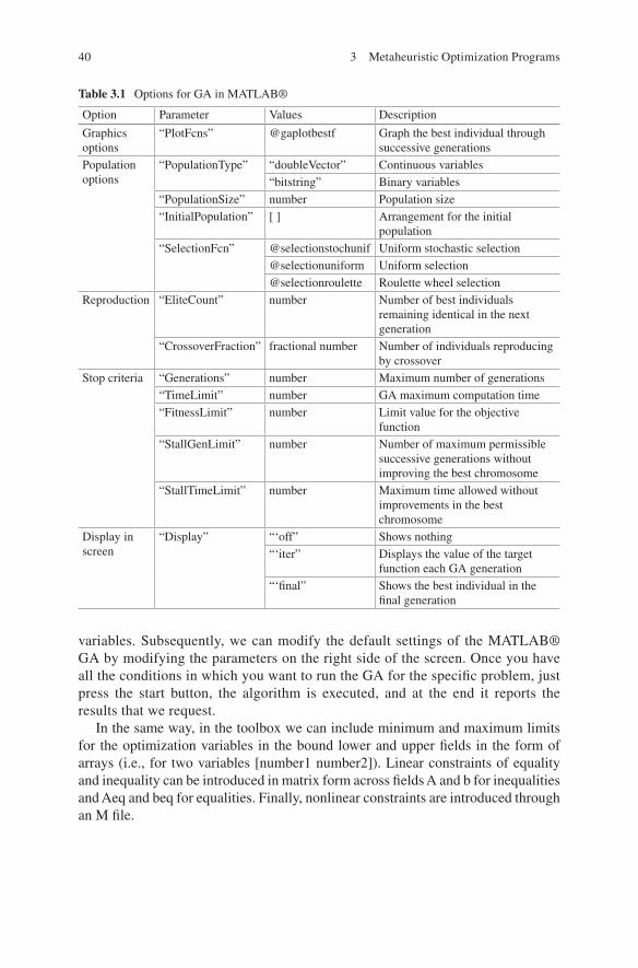
40
variables. Subsequently, we can modify the default settings of the MATLAB®
GA by modifying the parameters on the right side of the screen. Once you have
all the conditions in which you want to run the GA for the specific problem, just
press the start button, the algorithm is executed, and at the end it reports the
results that we request.
In the same way, in the toolbox we can include minimum and maximum limits
for the optimization variables in the bound lower and upper fields in the form of
arrays (i.e., for two variables [number1 number2]). Linear constraints of equality
and inequality can be introduced in matrix form across fields A and b for inequalities
and Aeq and beq for equalities. Finally, nonlinear constraints are introduced through
an M file.
Table 3.1 Options for GA in MATLAB®
Option Parameter Values Description
Graphics
options
“PlotFcns” @gaplotbestf Graph the best individual through
successive generations
Population
options
“PopulationType” “doubleVector” Continuous variables
“bitstring” Binary variables
“PopulationSize” number Population size
“InitialPopulation” [ ] Arrangement for the initial
population
“SelectionFcn” @selectionstochunif Uniform stochastic selection
@selectionuniform Uniform selection
@selectionroulette Roulette wheel selection
Reproduction “EliteCount” number Number of best individuals
remaining identical in the next
generation
“CrossoverFraction” fractional number Number of individuals reproducing
by crossover
Stop criteria “Generations” number Maximum number of generations
“TimeLimit” number GA maximum computation time
“FitnessLimit” number Limit value for the objective
function
“StallGenLimit” number Number of maximum permissible
successive generations without
improving the best chromosome
“StallTimeLimit” number Maximum time allowed without
improvements in the best
chromosome
Display in
screen
“Display” “‘off” Shows nothing
“‘iter” Displays the value of the target
function each GA generation
“‘final” Shows the best individual in the
final generation
3 Metaheuristic Optimization Programs

41
3.4 EMOO Tool in MS Excel
Genetic algorithms (the flowchart is presented in Fig. 3.7) have proved to be a
versatile and effective approach for solving optimization problems, but there are
many situations in which the simple genetic algorithm does not perform
particularly well, and various methods of hybridization have been proposed (Gen
and Cheng 1997).
However, almost all these applications have been done using programs/platforms
that are not readily used in the industry. On the other hand, engineers are familiar
with MS Excel® and use it in both research and industrial practice (Sharma et al.
2012). Hence, an Excel-based multi-objective optimization (EMOO) program may
represent a good alternative to develop stochastic optimization algorithms.
An improved multi-objective differential evolution algorithm with a termination
criterion for optimizing chemical processes was developed by Sharma and Rangaiah
(2013), which works with a termination criterion using the non-dominated solutions
obtained as the search process. The multi-objective optimization hybrid method is,
namely, the improved multi-objective differential evolution (I-MODE).
Fig. 3.6 GA toolbox of MATLAB®
3.4 EMOO Tool in MS Excel

42
In the I-MODE (whose flowsheet is presented in Fig. 3.8), a population of NP
individuals is randomly initialized inside the bounds of decision variables. Then,
values of the objectives and constraints are calculated for each individual of the
initial population. The taboo list size (TLS) is half of the population size, and taboo
list (TL) is randomly filled with 50% individuals of the initial population; initial
individuals are also identified as target individuals (i). A trial individual is generated
for each target individual by mutation and crossover on three randomly selected
individuals from initial/current/parent population. The elements of the mutant
vector compete with those of the target vector, with a probability Cr to generate a
trial vector. Taboo check is implemented in the generation step of the trial vector of
I-MODE, and the trial individual is generated repeatedly until it is away from each
individual in the TL by a specified distance called taboo radius (Tr). The Euclidean
distance between trial individual and each individual in TL is calculated in the nor-
malized space of decision variables for accepting the trial individual. After that,
objectives and constraints are calculated for the temporarily accepted trial individ-
ual. The trial individual is stored in the child population and added to TL. After
generating the trial individuals for all the target individuals of the current popula-
tion, non-dominated sorting of the combined current and child populations followed
by crowding distance calculation, if required, is performed to select the individuals
for the next generation (G). The best NP individuals are used as the population in
the subsequent generation.
Fig. 3.7 Flowchart of simple genetic algorithm sequence of genetic algorithm
3 Metaheuristic Optimization Programs

43
Start Set values N, MNG, TR, δGD and δSP.
Randomly initialize population and evaluate values of objectives
and constraints of all individuals in the population. Randomly select
50% initial individuals and store them in taboo list.
Set generation no., G = 1
Set indiviual no., i = 1
Generate a mutant individual and then a
trial individual as a per DE operations.
Check the trial individual for the violation of decision
variable bounds; if there is any violation, randomly
reinitialize that particular decision variable inside the bounds.
Perform taboo check to reject the trial individual near to
those in taboo list. Evaluate values of objectives and
constraints of accepted trial individual, and update taboo list.
Store the accepted trial individual in the child population
Is i < N?
Combine parent and child populations
Non-dominating sorting of combinedpopulation
and calculate crowdin distance, if required
Selection of the population for the next generation
If G > 1, then calculate GD & SP
If G > λ , then perform x2-test
Are P(G) > 0.99
& P(SP) > 0.99?
Is i < MNG?G = G +1 Stop
i = i +1
YesNo
No
Yes
Yes
No
Fig. 3.8 Flowchart of I-MODE algorithm (Sharma and Rangaiah 2013)
3.4 EMOO Tool in MS Excel

44
For more details about how the I-MODE works and to obtain the optimization
routine, you can consult the paper or contact the authors (Sharma and Rangaiah
2013).
For the optimization of a particular process, it is necessary to specify the values
for the parameters associated with the used I-MODE algorithm, which are the
following: population size (NP), number of generations (GenMax), taboo list size
(TLS), taboo radius (TR), crossover fraction (Cr), and mutation fraction (F). In
addition, it is necessary to select the decision variables and introduce the values for
the lower and upper bounds expressed in homogenous units. All decision variables
must be selected as a continuous or discontinuous variables, and the initial value for
each is automatically the half between the minimum and the maximum possible
values. The user interface of the optimization algorithm accepts inequality
constraints, which can be introduced to run the optimization approach without any
inequality constraint.
3.4.1 Main Program Interface
In order to give the reader the necessary knowledge to adequately manage the
I-MODE, below are general notions of the user interface that use this stochastic
algorithm in MS Excel®. For a detailed description of all the sheets that compose
the I-MODE algorithm, it is recommended to review the user guide. Figure 3.9
shows the main program interface of the I-MODE.
As can be seen, the I-MODE algorithm has four fundamental parts in its main
program interface, which are objective functions, design variables, inequality
constraints, and algorithm parameters. Each of these sections will then be analyzed.
Objective Functions: As expected, this part is designed to introduce the objective
function to be optimized by simply clicking the Add Objective Functions button.
Next, a small window called Input Objective Function shown in Fig. 3.10 will
appear where you have to fill three boxes.
The first box, which corresponds to Name, proposes a name for the function. In
the second box, you are prompted to specify a cell value, that is, a cell where the
target function is already specified. The last box corresponds to Goal, where you
specify if you want to maximize or minimize the objective function, by default a
minimization will appear. After specifying the information of the new objective
function in each of the boxes, click on the Add button, and the specific information
in the boxes will appear in the corresponding cell. If you want to cancel the
introduction of a new click function on the Done button, this will erase all informa-
tion previously entered in the boxes and will exit the Input Objective Function
window.
Design Variables: In this part of the main program interface, you must enter the
decision variables; it is the selected variables which will be manipulated in order
3 Metaheuristic Optimization Programs

45
to find the optimal point. To begin, you have to click the Add Decision Variables
button, after which the window shown in Fig. 3.11 will appear.
As can be seen in Fig. 3.11, the input decision variables of I-MODE algorithm
window contains four boxes where you must specify the name of the decision
variable, the maximum and minimum values, as well as the type of variable, as
appropriate. After entering the requested information, click on the Add button;
otherwise to delete the information in the boxes, click on the Done button. The
specific information in the boxes will appear in the corresponding cell.
Inequality Constraints: In the inequality restrictions, part of the main program
interface of I-MODE algorithm, the constraints of the optimization problem must be
Fig. 3.9 Main program interface of I-MODE algorithm
Fig. 3.10 Input objective
function of I-MODE
algorithm
3.4 EMOO Tool in MS Excel

46
specified, if any. To proceed, click the Add Constraints button after which the
window shown in the Fig. 3.12 will be displayed.
The input constraints window contains four boxes in which you must enter the
name that will be assigned to the constraint, the cell containing the constraint, the
type of comparison, and the limit of the constraint. The information contained in the
boxes structure the restriction, as shown by the example in the figure.
Algorithm Parameters: This is the part of the main program interface where it
is necessary to specify the parameters associated with the used I-MODE
algorithm, which are the following: population size (NP), number of generations
(GenMax), taboo list size (TLS), taboo radius (TR), crossover fraction (Cr), and
mutation fraction (F). All these values are entered directly into the corresponding
Fig. 3.11 Input decision
variables of I-MODE
algorithm
Fig. 3.12 Input constraints
of I-MODE algorithm
3 Metaheuristic Optimization Programs

47
cell that indicates its name without needing to click on any button to add them.
The numerical values of these parameters depend on the nature of the problem
to be solved.
3.4.2 Objectives and Constraints
Many of the values that are entered in the main program interface of the I-MODE
are referenced to another MS Excel sheet where they contain mainly the objectives
and constraints of the problem to be optimized. In the objectives and constraints
sheet shown in Fig. 3.13, you can identify the decision variables, objectives, and
constraints. It is convenient to write in this part the numerical values of each aspect
and to refer to them in the sheet of main program interface, this with the purpose of
its easy modification in subsequent optimizations.
The value must be entered in its respective cell. It is important to emphasize that
the number of decision variables, objective functions, and inequality constraints is
not limited to the number proposed but can add more uncertainty of the cells of the
usual way in MS Excel®.
3.5 Stochastic Optimization Exercises
1. Propose a chromosome to represent a string of bits for the variables x1 and x2. x1
is defined in the interval [−10 10], while x2 is defined in the interval [−20 20].
Accuracy of five decimal places is required.
Fig. 3.13 Objectives and constraints of I-MODE algorithm
3.5 Stochastic Optimization Exercises

48
2. Propose a chromosome to model through a string of bits a set of variables given
by x1, x2, and x3 with an accuracy of six decimal places. The variables are defined
in the following intervals:
x1 defined in [0–1]
x2 defined in [0.1 0.9]
x3 defined in [0–0.8]
3. For the example presented in the Section of GA, perform the calculations for the
next ten generations, and see the behavior of the objective function as well as the
evolution of the chromosomes. Plot the value of the objective function with
respect to the generation number.
4. Consider the following problem:
min
sin .
.
f x x
x x
x x1 2
1
2
2
2
1
2
2
20 0 1 4 4
0 1 4
,( ) =− + −( ) + −( )
+ −( ) + − 442( )
Figure 3.14 shows the behavior of the previous function:
As can be seen in Fig. 3.14, this problem presents a large number of local solu-
tions in which the deterministic algorithms could fail to locate the global optimal
solution.
Solve this problem using MATLAB® GA under the following conditions:
00
x1x2
0
1010
-10-10
-10
-15
-5
-20-20
2020
f(x1,x2)
Fig. 3.14 Behavior of the function of problem 4
3 Metaheuristic Optimization Programs
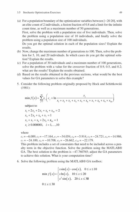
49
(a) For a population boundary of the optimization variables between [−20 20], with
an elite count of 2 individuals, a fusion fraction of 0.8 and a limit for the infinite
count time, as well as a maximum number of 50 generations.
First, solve the problem with a population size of five individuals. Then, solve
the problem using a population size of 10 individuals, and finally solve the
problem using a population size of 100 individuals.
Do you get the optimal solution in each of the population sizes? Explain the
results.
(b) Now, change the maximum number of generations to 100. Then, solve the prob-
lem for 5, 10, and 20 individuals. In which cases do you get the optimal solu-
tion? Explain the results.
(c) For a population of 30 individuals and a maximum number of 100 generations,
solve the problem with a value for the crossover fraction of 0.9, 0.5, and 0.2;
what are the results? Explain the results obtained.
(d) Based on the results obtained in the previous sections, what would be the best
values for GA parameters to solve this example?
5. Consider the following problem originally proposed by Hock and Schittkowski
(1981):
min lnf x x cx
x x x x x x x x x xj
j j
j( ) = ++ + + + + + + + +
=∑
1
10
1 2 3 4 5 6 7 8 9 10
+ + + + =
+ + + =
+ + + +
subject to
x x x x x
x x x x
x x x x
1 2 3 6 10
4 5 6 7
3 7 8 9
2 2 2
2 1
2 xx
x ii
101
0 000001 1 10
=
≥ = …. , , ,
where
c1 = −6.089, c2 = −17.164, c3 = −34.054, c4 = −5.914, c5 = −24.721, c6 = −14.986,
c7 = −24.100, c8 = −10.708, c9 = −26.662, c10 = −22.179.
This problem includes a set of constraints that need to be included across a pen-
alty term in the objective function. Solve the problem using the MATLAB®
GA. The best solution to the problem is −47.760765; adjust the GA parameters
to achieve this solution. What is your computation time?
6. Solve the following problem using the MATLAB® GA toolbox:
min
sin cos ,
ln ,
sin ,
f x
x x x x
x x x
x x x
( ) =( )− ( ) ≤ ≤
( ) ≤ ≤
( ) ≤ ≤
0 10
10 20
20 32
00
0 30
≤ ≤x
3.5 Stochastic Optimization Exercises
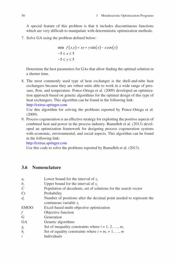
50
A special feature of this problem is that it includes discontinuous functions
which are very difficult to manipulate with deterministic optimization methods.
7. Solve GA using the problem defined below:
min sin cosf x y xy y x x y
x
y
,( ) = + ( )− ( )− ≤ ≤
− ≤ ≤
5 5
5 5
Determine the best parameters for GAs that allow finding the optimal solution in
a shorter time.
8. The most commonly used type of heat exchanger is the shell-and-tube heat
exchangers because they are robust units able to work in a wide range of pres-
sure, flow, and temperature. Ponce-Ortega et al. (2009) developed an optimiza-
tion approach based on genetic algorithms for the optimal design of this type of
heat exchangers. This algorithm can be found in the following link:
http://extras.springer.com
Use this algorithm for solving the problems reported by Ponce-Ortega et al.
(2009).
9. Process cogeneration is an effective strategy for exploiting the positive aspects of
combined heat and power in the process industry. Bamufleh et al. (2013) devel-
oped an optimization framework for designing process cogeneration systems
with economic, environmental, and social aspects. This algorithm can be found
in the following link:
http://extras.springer.com
Use this code to solve the problems reported by Bamufleh et al. (2013).
3.6 Nomenclature
aj Lower bound for the interval of xj
bj Upper bound for the interval of xj
C Population of decedents, set of solutions for the search vector
Cr Probability
dj Number of positions after the decimal point needed to represent the
continuous variable xj
EMOO Excel-based multi-objective optimization
f Objective function
G Generation
GA Genetic algorithms
gj Set of inequality constraints where i = 1, 2, …, m1
hj Set of equality constraints where i = m1 + 1, …, m
i Individuals
3 Metaheuristic Optimization Programs

51
I-MODE Improved multi-objective differential evolution
k Number of iterations
L Limit for the maximum number of iterations
mj Number of positions required by the subchain bit string to be able to
represent the continuous variable
MODE-TL Multi-objective differential evolution taboo list
MOO Multi-objective optimization
NP Population size
P Population of parents, set of solutions for the search vector
pc Fusion ratio
q Coordinate vector
ri Variable penalty coefficient for the constraint i
SA Simulated annealing
t Number of generation (iteration of GA)
T Temperature
TL Taboo list
Tlow Lower limit for the temperature
TLS Taboo list size
Tr Taboo radius
x Optimization variable vector
x′ Unknown vector
xj Continuous variable
α Penalty constant
β Penalty constant
ρ Penalty constant
3.6 Nomenclature

53© Springer International Publishing AG, part of Springer Nature 2019
J. M. Ponce-Ortega, L. G. Hernández-Pérez, Optimization of Process
Flowsheets through Metaheuristic Techniques,
https://doi.org/10.1007/978-3-319-91722-1_4
Chapter 4
Interlinking Between Process Simulators and Optimization Programs
In this chapter, the methodology to achieve a successful link between the process
simulator software and optimization programs using MS Excel® as a linker pro-
gram will be described, as well as the direct linking of process simulator software
with MS Excel® where it has been included a routine containing a stochastic opti-
mization algorithm.
Recently, some approaches have been reported to optimize different processes
based on process simulators and linked with different optimization approaches. For
example, Segovia-Hernandez and Gomez-Castro (2017) reported an approach for
optimizing chemical processes using stochastic optimization techniques and Aspen
Plus®; Woinaroschy (2009) developed a simulation and optimization of citric acid
production with SuperPro Designer using a client-server interface. Quiroz-Ramírez
et al. (2017a) reported an optimization approach for selecting the feedstocks for
biobutanol production considering economic and environmental aspects. Quiroz-
Ramírez et al. (2017b) also reported a multi-objective stochastic optimization
approach applied to a hybrid process production-separation in the production of
biobutanol. Medina-Herrera et al. (2017) presented an optimal design of a multi-
product reactive distillation system for producing silanes using a metaheuristic
approach. Contreras-Zarazúa et al. (2016) presented a multi-objective optimization
approach involving cost and control properties in reactive distillation processes to
produce diphenyl carbonate. Santibañez-Aguilar et al. (2016) used a stochastic
algorithm for designing biorefinery supply chains considering economic and envi-
ronmental objectives. González-Bravo et al. (2016) developed a multi-objective
optimization for dual-purpose power plants and water distribution networks.
It is noteworthy that there is not reported a general framework to link any process
simulator to any metaheuristic optimization technique. This way, in this chapter is
presented a general framework to link any process simulator to metaheuristic opti-
mization approaches to optimize process flowsheets. The proposed approach imple-
ments a link between the process simulator (Aspen Plus®, Aspen HYSYS®,
SuperPro Designer®, etc.) and an optimization algorithm (it can be a multi- objective

54
differential evolution with taboo list implanted in MS Excel or other metaheuristic
techniques implemented in other software), which can be linked through a COM
software via Visual Basic for Applications (VBA).
The implementation of the global optimization approach involves a hybrid plat-
form, which links simulator software and Microsoft Excel® through the implemen-
tation of a Component Object Module (COM) technology (the flowchart is presented
in Fig. 4.1).
A client-server interface based on COM technology can be implemented. Using
COM technology, it is possible to add code so that the applications behave as an
Object Linking and Embedding (OLE) automation server. The use of the methods
of this library to interoperate with other Windows applications (such as Excel®)
requires the use of a common scripting language, and Visual Basic® for Applications
(VBA) can be used in this case. An interface between Excel® and Aspen Plus®,
based on COM technology, using Excel-VBA scripts (Birnbaum 2005) can be
implemented.
During the optimization process, a decision vector of design variables is sent
from Excel® to Aspen Plus®; for example, in this process simulator rigorous
calculations for the data that identify a particular design of process are obtained
(e.g., temperature and pressure in the boiler, split fraction in the splitter, etc.) via
resolution of phase equilibrium along with the complete set of mass and energy
balances. These data are returned from Aspen Plus® to Excel® for the calculation
Process Simulation
using Simulator
Values of
Decision VariablesActivate/Deactivate
Simulator using VBA
Excel
(Program
Interface)
Algorithm
Parameters
Save Data Transferred
from Simulator after
Convergence
Calculate Objectives
and Constraints using
Simulation Data
Save Optimization
Results at Different
Generations
New Values of
Decision Variables
Algorithm
Parameters,
Objectives and
Constraints
Optimization Algorithm in Visual
Basic for Applications (VBA)
Transfer
Required
Data after
Simulation
Converged
Optimization
Results after
First,
Intermediate
and Last
Generations
Fig. 4.1 Interface between a process simulator and Excel® (containing an optimization
program)
4 Interlinking Between Process Simulators and Optimization Programs

55
of objective functions; the values obtained for the objective functions are
evaluated, and new vectors of design variables are generated according to the sto-
chastic procedure of this method.
4.1 Previous Knowledge
4.1.1 MS Excel® Configuration
A very important aspect to take into account is that to achieve this type of linking
requires access to the routines and optimization algorithms; for this it is necessary
to configure the tabs of MS Excel® so that the “Developer” tab appears; since in the
startup configuration of this MS Office® program this tab does not appear, it is
necessary to customize the ribbon when it is first used, after which it is no longer
necessary to do so again. For more details about how to configure the ribbon, it is
recommended to the readers to see the appendices in this book.
Another important aspect to consider for the previous configuration in the MS
Excel® program is in the section of MS VBA (Microsoft Visual Basic for
Applications). To access to this part of the program, you have to click the button
shown in Fig. 4.2.
Then, the window shown in Fig. 4.3 appears, and you can select the project that
contains the optimization algorithm or the linking subroutine.
To adequately run the algorithm that contains the Aspen Plus® variable call, it is
necessary to activate the libraries for this program. It is called Aspen library. For
activating this, we must go to the Tools tab and the References option (see Fig. 4.4).
Later, we proceed to look for the Aspen Plus® libraries included, and we select
all of them (see Fig. 4.5).
4.1.2 Object Name of the Simulator File
To do this, it is necessary to open the windows explorer in the folder containing the
files needed for linking. Then, to check the exact route of the simulation, select the
simulator software backup file and right click on it, and then a menu will be dis-
played where we will select the last option “Properties” (Figs. 4.6 and 4.7).
A window will open where we select the “Security” tab. Here, there are shown
some data security of the file; you must copy the whole path of the box “Object
Name” (Figs. 4.8 and 4.9).
After that, we open the routine that contains the stochastic optimization algo-
rithm in Visual Basic that is inside the “Developer” tab. It is necessary to select the
appropriate module that contains the optimization algorithm and that is located in
the part of the linking subroutine. In this part, we declare the path of the simulation
backup file by pasting the object name that we copied (Fig. 4.10).
4.1 Previous Knowledge
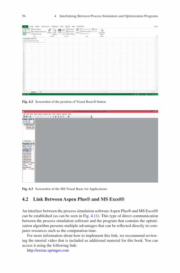
56
4.2 Link Between Aspen Plus® and MS Excel®
An interface between the process simulation software Aspen Plus® and MS Excel®
can be established (as can be seen in Fig. 4.11). This type of direct communication
between the process simulation software and the program that contains the optimi-
zation algorithm presents multiple advantages that can be reflected directly in com-
puter resources such as the computation time.
For more information about how to implement this link, we recommend review-
ing the tutorial video that is included as additional material for this book. You can
access it using the following link:
http://extras.springer.com
Fig. 4.2 Screenshot of the position of Visual Basic® button
Fig. 4.3 Screenshot of the MS Visual Basic for Applications
4 Interlinking Between Process Simulators and Optimization Programs

57
4.2.1 Subroutine to Link Aspen Plus® and MS Excel®
To perform the successful link between the process simulator software Aspen Plus®
and a program that has the stochastic optimization tools using MS Excel® as a
linker program, it is necessary to follow the steps described by the general syntax
for the code used, which is shown in Fig. 4.12.
Fig. 4.4 Screenshot of the position of References button
Fig. 4.5 Screenshot of the References window
4.2 Link Between Aspen Plus® and MS Excel®
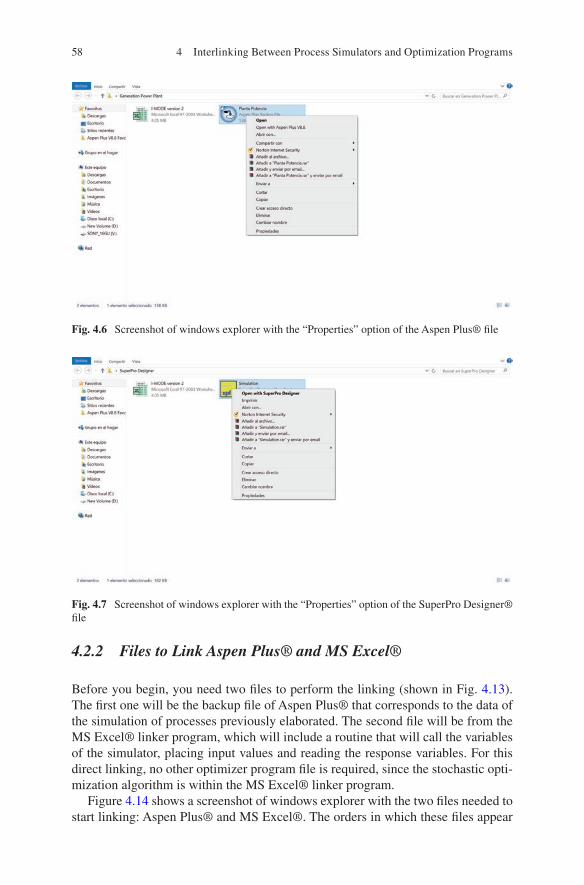
58
4.2.2 Files to Link Aspen Plus® and MS Excel®
Before you begin, you need two files to perform the linking (shown in Fig. 4.13).
The first one will be the backup file of Aspen Plus® that corresponds to the data of
the simulation of processes previously elaborated. The second file will be from the
MS Excel® linker program, which will include a routine that will call the variables
of the simulator, placing input values and reading the response variables. For this
direct linking, no other optimizer program file is required, since the stochastic opti-
mization algorithm is within the MS Excel® linker program.
Figure 4.14 shows a screenshot of windows explorer with the two files needed to
start linking: Aspen Plus® and MS Excel®. The orders in which these files appear
Fig. 4.6 Screenshot of windows explorer with the “Properties” option of the Aspen Plus® file
Fig. 4.7 Screenshot of windows explorer with the “Properties” option of the SuperPro Designer®
file
4 Interlinking Between Process Simulators and Optimization Programs

59
from left to right are linker program with the optimization algorithm and backup
simulator file.
Once it has been corroborated that you have the essential files for implementing
the link, we can begin with the explanation of the steps to follow, which are described
in the next section.
If the user does not have any files for the process simulation in Aspen Plus® and
for the optimization algorithm in MS Excel®, the files shown in Fig. 4.14 can be
found in the following link:
http://extras.springer.com
Fig. 4.8 Screenshot of windows explorer with the “Security” tab of the Aspen Plus® file where
the “Object Name” can be seen
Fig. 4.9 Screenshot of windows explorer with the “Security” tab of the SuperPro Designer® file
where the “Object Name” can be seen
4.2 Link Between Aspen Plus® and MS Excel®

60
Fig. 4.10 Screenshot of linking subroutine where the simulation file route must be pasted
Fig. 4.11 Interface between Aspen Plus® and MS Excel®
CODEINSTRUCTION CODEINSINSINSTRTRTRUCUCUCRRRR TIOTIOTIONNNSTRUCTURE
Sub Routine name and
Simulator file route
P
S
E
U
D
O
C
O
D
E
Decision variable transfer
from Excel to Simulator
Variable Declaration Dim VARIABLE1 As IHNode, VARIABLE2 As IHNode, … VARIABLEN As IHNode
Set VARIABLE1 = PROYECT1.Tree.FindNode("\Data\Blocks\EQUIP1\Input\VARIABLE1")
Variable Declaration Dim PROYECT1 As IHapp
Simulator file route Set PROYECT1 = GetObject("SIMULATOR FILE ROUTE")
File Visualization PRYECT1.Visible = True
Run Continuity PROYECT1.SuppressDialogs = True
Variable Assignations Set VARIABLE2 = PROYECT1.Tree.FindNode("\Data\Blocks\EQUIP2\Input\VARIABLE2")
Set VARIABLEN = PROYECT1.Tree.FindNode("\Data\Blocks\EQUIPN\Input\VARIABLEN")
VARIABLE1.Value = Sheets("DV to Aspen Plus").Range("C3")
Variable Translations VARIABLE2.Value = Sheets("DV to Aspen Plus").Range("C4")
VARIABLEN.Value = Sheets("DV to Aspen Plus").Range("CN")
Decision variable transfer
from Simulator to Excel
Variable Declaration Dim RESPONSE1 As IHNode, RESPONSE2 As IHNode,… RESPONSEN As IHNode
Set RESPONSE1 = PROYECT1.Tree.FindNode("\Data\Blocks\EQUIP1\Output\RESPONSE1")
Variable Assignations Set RESPONSE2 = PROYECT1.Tree.FindNode("\Data\Blocks\EQUIP2\Output\RESPONSE2")
Set RESPONSEN = PROYECT1.Tree.FindNode("\Data\Blocks\EQUIPN\Output\RESPONSEN")
Sheets("Data from Aspen Plus").Range("C3") = RESPONSE1
Variable Translations Sheets("Data from Aspen Plus").Range("C4") = RESPONSE2
Sheets("Data from Aspen Plus").Range("CN") = RESPONSEN
Run SimulatorReinitialize Simulator
Activate Simulator
PROYECT1.Reinit
PROYECT1.Run
Sub Routine Name Public Sub PROYECT_NAME()
Fig. 4.12 Pseudo code for the link between Aspen Plus® and MS Excel®
4 Interlinking Between Process Simulators and Optimization Programs

61
4.2.3 Call Name of Aspen Plus® Variables
Once the path of the backup file of the process simulation has been declared, we
proceed with the declaration of decision variables and response variables in the
linker program. To do this, we need to open the file containing the simulation in
Aspen Plus® and select the “Customize” tab and choose the “Variable Explorer”
option (Fig. 4.15).
Then, you will see a tree of options where we proceed to find the name of the
variable that uses the Aspen Plus® variable explorer and that corresponds to the
process variable that we want to link. The user must look at the tree of the vari-
able explorer, the variable that wants to be either as a decision variable or as a
response variable. In order to find the desired variable, a logical sequence of
search is followed according to the equipment or stream to which this variable
belongs. For example, if the user is looking for the variable “Feeding tempera-
ture” of an equipment called “Boiler,” the path to be followed in the variable
explorer tree is as follows: Root > Data > Blocks > BOILER > Input > Temperat
ure. Once the path has been followed to the desired variable, a series of data
appears on the right-hand side of the variable explorer. There are many variables
with a similar name, so one way to verify that it is the appropriate variable is to
verify in the attribute “Value” effectively that variable has the numerical value
Linker Program
and optimization
algorithm
Backup Simulator File
MS ExcelAspen Plus
Fig. 4.13 Two files needed
to start linking Aspen
Plus® and MS Excel®
Fig. 4.14 Screenshot of windows explorer with the two files needed to start linking: Aspen Plus®
and MS Excel®
4.2 Link Between Aspen Plus® and MS Excel®

62
that corresponds to it. Since we are sure that it is the searched variable, we copy
the contents of the value corresponding to the “Call” attribute (Fig. 4.16).
Once you have copied the name of the variable with which the COM technology
will make the call, proceed to open the link subroutine again, and look for the part
in which the variables are assigned; pasted here is the variable name for the call
(Fig. 4.17).
4.3 Link Between SuperPro Designer® and MS Excel®
An interface between the process simulation software SuperPro Designer® and MS
Excel® can be established (as can be seen in Fig. 4.18).
For more information about how to implement this link, we recommend review-
ing the tutorial video that is included as additional material for this book. You can
access it using the following link:
http://extras.springer.com
4.3.1 Subroutine to Link SuperPro Designer® and MS Excel®
To successfully perform the link between the process simulator software SuperPro
Designer® and a program that has the stochastic optimization tools using MS
Excel® as a linker program, it is necessary to follow the steps described by the
general syntax for the used code, which is shown in Fig. 4.19.
Fig. 4.15 Screenshot of variable explorer position in Aspen Plus®
4 Interlinking Between Process Simulators and Optimization Programs

63
4.3.2 Files to Link SuperPro Designer® and MS Excel®
Before you begin, you need two files to perform the linking (shown in Fig. 4.20). In
the first one, there is implemented the backup file of SuperPro Designer® that cor-
responds to the data of the simulation of processes previously elaborated. The sec-
ond file will be the MS Excel® linker program, which will include a routine that
will call the variables of the simulator, placing input values and reading the response
variables. For this direct linking, no other optimizer program file is required, since
the stochastic optimization algorithm is within the MS Excel® linker program.
Fig. 4.16 Screenshot of variable explorer tree in Aspen Plus®
Fig. 4.17 Screenshot of linking subroutine where the variable name call must be pasted
4.3 Link Between SuperPro Designer® and MS Excel®

64
Figure 4.21 shows a screenshot of windows explorer with the two files needed to
start linking SuperPro Designer® and MS Excel®. The orders in which these files
appear from left to right are linker program with the optimization algorithm and
backup simulator file.
Once it has been corroborated that you have the essential files for the link, we can
begin with the explanation of the steps to follow, which are described in the next
section.
If the user does not have any files for the process simulation in SuperPro
Designer® and for the optimization algorithm in MS Excel®, the files shown in
Fig. 4.21 can be found in the follow link:
http://extras.springer.com
Simulation of the Process
(Obtaining Results)
Optimization Process
(Genetic Algorithms)
Decision
Variables
Response
Variables
Iteration
Simulation
Metaheuristic Algorithm
(Differential Evolution with
Tabu List)
Evaluation of Objective Function.
MS ExcelSuperPro
Designer
Fig. 4.18 Interface between SuperPro Designer® and MS Excel®
CODEINSTRUCTION COCOCODDDEEEIIINSNSNSTTTRRRUUUCCCTTTIIIONONONSTRUCTURE
Sub Routine name and
Simulator file route
P
S
E
U
D
O
C
O
D
E
Decision variable transfer
from Excel to Simulator
Stream Assignations STREAM2 = “S-002”
VARIABLE1 = Worksheets("DV to SPro Designer").Range("C3")
Variable Declaration Dim VARIABLE1, VARIABLE2, … VARIABLEN As Variant
Variable Translations VARIABLE2 = Worksheets("DV to SPro Designer").Range("C4")
VARIABLE3 = Worksheets("DV to SPro Designer").Range("C5")
PROJECT1.SetStreamVarVal STREAM1, VarID.temperature_VID, VARIABLE1, STREAM1
Variable Assignations PROJECT1.SetStreamVarVal STREAM2, VarID.pressure_VID, VARIABLE2, STREAM2
PROJECT1.SetStreamVarVal STREAM3, VarID.temperature_VID, VARIABLE3, STREAM3
Response variable transfer
from Simulator to Excel
PROJECT1.GetStreamVarVal STREAMN-3, VarID.temperature_VID, VARIABLEN-3, STREAMN-3
Variable Assignations PROJECT1.GetStreamVarVal STREAMN-2, VarID.temperature_VID, VARIABLEN-2, STREAMN-2
PROJECT1.GetStreamVarVal STREAMN-1, VarID.temperature_VID, VARIABLEN-1, STREAMN-1
Worksheets("Data from SPro Designer").Range("CN-3") = VARIABLEN-1
Variable Translations Worksheets("Data from SPro Designer ").Range("CN-2") = VARIABLEN-2
Worksheets("Data from SPro Designer ").Range("CN-1") = VARIABLEN-3
Run SimulatorSimulator Balances
Simulator Calculations
PROYECT1.DoMEBalances VARIABLE1, VARIABLE2, … VARIABLEN
PROYECT1.DoEconomicCalculations
Sub Routine Name Public Sub PROYECT_NAME()
Stream Declaration Dim STREAM1, STREAM2, … STREAMN As String
Simulator file route Set PROYECT1 = GetObject("SIMULATOR FILE ROUTE")
STREAM1 = “S-001”
STREAM3 = “S-003”
Fig. 4.19 Pseudo code for the link between SuperPro Designer® and MS Excel®
Linker Program
and optimization
algorithm
Backup Simulator File
MS ExcelSuperPro
Designer
Fig. 4.20 Two files needed
to start linking SuperPro
Designer® and MS
Excel®
4 Interlinking Between Process Simulators and Optimization Programs

65
4.3.3 Call Name of SuperPro Designer® Variables
Once the path of the backup file of the process simulation has been declared, we
proceed with the declaration of decision variables and response variables in the
linker program. To do this, we need to open the file containing the simulation in
SuperPro Designer® and go to Help > COM interface (Fig. 4.22).
Then, you will see the COM Library where we proceed to find the name of the
variable that uses the COM interface and that corresponds to the process variable
that we want to link (Fig. 4.23).
The user must look in the tree of the COM Library, the variable that wants to bind
either as a decision variable or as a response variable. In order to find the desired
Fig. 4.21 Screenshot of windows explorer with the two files needed to start linking SuperPro
Designer® and MS Excel®
Fig. 4.22 Screenshot of COM interface in SuperPro Designer®
4.3 Link Between SuperPro Designer® and MS Excel®

66
variable, a logical sequence of search is followed according to the equipment or
stream to which this variable belongs. For example, if the user is looking for the
variable “Feeding temperature” of an equipment, the path to be followed in the
COM Library tree is as follows: COM Library > Accessing SuperPro Designer®
Variable with COM > Stream Variables > Stream Temperature. Once the path has
been followed to the desired variable, a series of variables appears on the right side
of the COM Library. Since we are sure that it is the searched variable, we copy the
contents of the value corresponding to the “Variable ID” column (Fig. 4.24).
Once you have copied the name of the variable with which the COM technology
will make the call, proceed to open the link subroutine again, and look for the part
in which the variables are assigned; pasted here is the variable name for the call
(Fig. 4.25).
Fig. 4.23 Screenshot of variable explorer tree in Aspen Plus®
Fig. 4.24 Screenshot of COM Library tree in SuperPro Designer®
4 Interlinking Between Process Simulators and Optimization Programs

67
4.4 Link Between MS Excel® and MATLAB®
An interface between the process simulation software Aspen Plus® and MATLAB®
can be established using MS Excel® as linking program (as can be seen in
Fig. 4.26). Direct communication between the process simulation software (Aspen
Plus®) and the program containing the stochastic optimization tools (MATLAB®)
cannot be established; therefore, it is necessary to use a third program that works
Fig. 4.25 Screenshot of linking subroutine where the variable name call must be pasted
MS Excel
Simulation of the Process
(Obtaining Results)
Optimization Process
(Genetic Algorithms)
Iteration
Simulation
Simulator Control
(Linking Programs)
Evaluation of Objective Function.
Matlab Aspen Plus
Fig. 4.26 Interface between Aspen Plus® and MATLAB® using MS Excel® as linking program
4.4 Link Between MS Excel® and MATLAB®

68
as a linker. Due to the multiple advantages of the use of COM technology and
because there are programs that easily allow their use, MS Excel® has been
selected as a linker program.
For a detailed information about how to make this link, we recommend review-
ing the tutorial video that is included as additional material for this book. You can
access it using the following link:
http://extras.springer.com
4.4.1 Subroutine to Link MS Excel® and MATLAB®
To perform the successful link between a software process simulator and a program
that has stochastic optimization tools using MS Excel® as a linker program, it is
necessary to follow the steps described by the general syntaxes for the used code
which is shown in Fig. 4.27.
4.4.2 Files Needed to Link MS Excel® and MATLAB®
Before you begin, you need four files to perform the link (shown in Fig. 4.28). The
first one corresponds to the backup file of Aspen Plus® that corresponds to the
data of the simulation processes previously elaborated. The second file will be
from the MS Excel® linker program, which will include a routine that will call the
variables of the simulator, placing input values and reading the response variables.
The following two files will be from the program containing the MATLAB® sto-
chastic optimization tool; one of them declares the used function by the
CODEINSTRUCTION CCOODDEEIINSNSTTRRUURRR CCTTIIONONSTRUCTURE
FILE 1:
Function name and linker
program file route
P
S
E
U
D
O
C
O
D
EFILE 2:
Optimization parameters
and function call
clc;
Application Type excelO bject=actxserver(´Exel.Application´);
Clear Screen
clear;
Function Name Function F=FUNCTIONNAME(pop)
Variable Declaration pop
Linker file route excelObject.Workbooks.Open(”LINKER FILE ROUTE.xls")
Workbooks Hworkbook=excelObject.workbooks;
Run Linking Routine F=excelObject.Run(´Rankine´,pop(1),pop(2))
Close Workbook Hworkbook.Close;
Optimization Instruction F=-F
Clear Variable Values
lb=[100 5];Lower Boundary
ub=[100 5];Upper Boundary
opts=gaoptimset(`Generations`,10,`PopInitRange´,[0 0;500
100],`PopulationSize´,10,´EliteCount´,2,´CrossoverFraction´,0.8,´TimeLimit´,Inf,…;Parameter Specification
[x,fval,reason,output]=ga(@FUNCTIONNAME,2,[],[],[],[],lb,ub,[],opts)GA Call
Fig. 4.27 Pseudo code for the link between MS Excel® and MATLAB®
4 Interlinking Between Process Simulators and Optimization Programs

69
optimization, and the other file introduces the parameters that will be used in the
genetic algorithm and serves to make the call of the declared function.
Figure 4.29 shows a screenshot of windows explorer with the four files needed to
start linking Aspen Plus®, MATLAB®, and MS Excel®. The orders in which these
files appears from left to right are optimization parameters, linker program, function
declaration, and backup simulator file. It is very important to distinguish each of
these files to avoid future confusions; the most practical and simple way to do this
is through the characteristic symbol of each program; however, it can also be done
by the extension of each file (.bkp for Aspen Plus®, .xls for MS Excel®, and .m for
MATLAB®). It is also recommended to use clear names that the user can easily
relate to the contents of each file.
Once there has been corroborated that you have the essential files for the link, we
can begin with the explanation of the steps to follow, which are described next.
If the user does not have any files for the process simulation in Aspen Plus®, for
the optimization algorithm in MATLAB®, and for the linker program in MS
Excel®, the files shown in Fig. 4.29 can be found in the following link:
http://extras.springer.com
Backup Simulator File Function Declaration Optimization
Parameters
Linker Program
MS ExcelAspen Plus Matlab Matlab
Fig. 4.28 Four files needed to start the linking Aspen Plus®, MATLAB®, and MS Excel®
Fig. 4.29 Screenshot of windows explorer with the four files needed to start linking Aspen Plus®,
MATLAB®, and MS Excel®
4.4 Link Between MS Excel® and MATLAB®

70
4.4.3 Object Name of the Linker Program File
In a similar way to the simulator file route declaration in the linker program, it is
necessary to open the windows explorer in the folder containing the four files
needed for linking. Then, to check the exact route of the simulation, select the Aspen
Plus® backup file and right click on it, and the same menu will be displayed where
we will select the last option “Properties” (Fig. 4.30).
As expected, a window will open where we select the “Security” tab and copy
the whole path of the box “Object Name” (Fig. 4.31).
Fig. 4.30 Screenshot of windows explorer with the “Properties” option of the linker program
Fig. 4.31 Screenshot of windows explorer with the “Security” tab of the linker program where the
“Object Name” can be seen
4 Interlinking Between Process Simulators and Optimization Programs

71
Now, you need to open the file containing the function to be optimized in
MATLAB®. In this file, it is necessary to look for the part in which the file of the
linker program is declared as object, which must be the fifth line of the code. Once
this instruction is located, we proceed to paste the file path of the linker program
(Fig. 4.32).
4.4.4 Specification for the Optimization Parameters
in MATLAB®
In this part, the simulator file route has been declared in the linker program, the
variables have been declared in the linker program, and the linker program file route
has been declared in the function file. What corresponds now is the specification of
the variables related to the MATLAB® stochastic optimization tool; so the first
thing to do is open the file containing the function call. In this file, we proceed to
indicate the upper and lower search limits for the variables to be optimized. In addi-
tion, the optimization parameters must be specified according to the considerations
that we have to get an adequate search (Fig. 4.33).
Each process has different parameters so it is impossible to standardize them, so
the user must know the process very well to propose the ones that work best. For
more information about each parameter used in genetic algorithms, we recommend
that the reader review the previous chapter about process optimization and stochas-
tic search algorithms.
After that, it only remains to run the optimization, which is done from this last
MATLAB® file by clicking on the “Run and Time” option.
Fig. 4.32 Screenshot of function declaration file, where the linker program route must be pasted
4.4 Link Between MS Excel® and MATLAB®

72
4.5 Exercises
1. The following link shows the simulation process of a reactive distillation pro-
cess, this corresponds to the process flowsheet in Aspen Plus® for the production
of methyl tert-butyl ether (MTBE):http://extras.springer.com
(a) Implement the link between Aspen Plus® and the I-MODE algorithm in MS
Excel® specifying the path where it was saved as the simulation program
file.
(b) Declare the following decision variables in the main program user interface
with their respective lower and upper limits: number of plates (5–8) and
stage of feeding (3–5).
(c) Run the optimization and find the optimal values for these variables.
2. Martinez-Gomez et al. (2017) reported an optimization-based approach for
incorporating economic and safety considerations in the selection of reforming
technology for the production of syngas from shale gas. Use the process flow-
sheet shown in Fig. 4.34 to implement the following:
(a) Implement a link between Aspen Plus® and GA from MATLAB® using MS
Excel® as a linker program, specifying the path where it was saved as the
simulation program file.
(b) Declare the following decision variables in the GA from MATLAB® with
their respective lower and upper limits: temperature (1100–1200 K) and
pressure (0.1–0.2 MPa).
(c) Run the optimization and find the optimal values for these variables.
Fig. 4.33 Screenshot of optimization parameter file, where the function is called
4 Interlinking Between Process Simulators and Optimization Programs

73
4.6 Nomenclature
COM Component Object Module
MS Microsoft®
MTBE Methyl tert-butyl ether
VBA Visual Basic for Applications
GAS
STEAM
5
hkmolInlet Shale Gas /150:
hkmolSteamInlet /7.399:
9.2/2
CO =H
ReformerSteam
Ke:Temperatur 75.1120
MPaPressure 11.0:
Fig. 4.34 Steam reformer
for the production of
syngas from shale gas
4.6 Nomenclature

75© Springer International Publishing AG, part of Springer Nature 2019
J. M. Ponce-Ortega, L. G. Hernández-Pérez, Optimization of Process
Flowsheets through Metaheuristic Techniques,
https://doi.org/10.1007/978-3-319-91722-1_5
Chapter 5
Performance Evaluation
The performance evaluation is of vital importance to determine the effectiveness of
both the search methods and the optimization parameters. Likewise, the perfor-
mance evaluation allows us to evaluate if the selected decision variables have a
considerable impact on the final result of the optimization and if the search range is
adequate. This performance evaluation is achieved through one or several objective
functions that the different search algorithms will try to satisfy at the same time as
the restrictions specified by the user.
As it is mentioned above, the objective function is an equation in which is
reflected the performance of the process that is being optimized; it is achieving its
maximum or its minimum value by manipulating the variables of dissolution and
considering the established search restrictions.
5.1 Objective Functions
It should be noted that there are many and varied ways to calculate an objective
function; this will depend on what the user seeks. Next, some of the main objective
functions commonly used in optimization will be described.
5.1.1 Net Present Value
A very common way of objective function is the net present value (NPV), which is
an economic measure that considers the value of money over time. It is the present
value of an investment’s future net cash flow (= difference between the money com-
ing in and going out) after the cost of the original investment has been subtracted
(Cambridge dictionary).

76
5.1.2 Profit
Another important objective function is the profit. The profit is money that is earned
in trade or business after paying the costs of producing and selling goods and ser-
vices (Cambridge dictionary).
5.1.3 Capital Cost
The capital cost is the amount of money that a company must pay out in dividends
to its shareholders and in interest on bonds and other loans (Cambridge
dictionary).
5.2 Capital Cost Estimation Programs
There are many tools to achieve a good estimation of the capital cost. Some of
which can be programmed directly by the user in different platforms. Likewise,
there are some programs that are dedicated exclusively to the estimation of the capi-
tal cost and that allow obtaining good values from the requested data. Feng and
Rangaiah (2011) made an evaluation of capital cost estimation programs in which
five programs were compared using a set of case studies. The most popular pro-
grams for the capital cost estimation are CapCost, EconExpert, AspenTech Process
Economic Analyzer (Aspen-PEA), detailed factorial method (DFP), and capital cost
estimation program (CCEP).
5.2.1 CapCost
The CapCost is based on the module costing method, written in Visual Basic, and
can be used for estimating preliminary process cost. Bare module cost (CBM) is
defined as the sum of the direct and indirect expenses for purchasing and installing
equipment; the total module cost (CTM) is defined as the sum of the bare module
cost, contingency, and fee; and the grassroots plant cost (CGR) is defined as the sum
of the total module cost and the auxiliary facilities costs. To estimate the bare mod-
ule cost and purchase cost of equipment, Turton et al. (2009) proposed the
following:
C C F C B B F F
p pBM BM M P= × = +( )0 0
1 2 (5.1)
5 Performance Evaluation

77
log log logC K K S K S
p
0
1 2 3
2
= + ( )+ ( ) (5.2)
where S represents a parameter for the equipment size or capacity. Values for the
constants B1 and B2, equipment-specific constants K1, K2, and K3, as well as correla-
tions and plots for FBM, FM, FP, and Co of different equipment can be found in the
appendices in Turton et al. (2009).
5.2.2 Detailed Factorial Program (DFP)
The detailed factorial program (DFP) is based on the detailed factorial estimates
method described in Sinnott and Towler (2009). For this program, the purchase cost,
Cp
0 , of the major equipment items is estimated using the following:
C a bS
p
n0= +
(5.3)
Cost constants a and b, available in Sinnott and Towler (2009) for different
equipment items, are mainly for carbon-steel material.
5.2.3 Capital Cost Estimation Program (CCEP)
Capital cost estimation program (CCEP) uses cost correlations in Seider et al.
(2010) for estimation of free-on-board purchase cost of equipment. The material
factor and Guthrie’s bare module factor are used thereafter to estimate the installed
cost of that equipment. Seider et al. (2010) developed the purchase cost correlations
for common process equipment, based on available literature sources and vendor
data. A list of these cost correlations can be found in Seider et al. (2010), using
CEPCI = 500. The purchase cost of the major equipment items is estimated using
the following:
C e A A S A S
p
0
0 1 2
2
= + ( ) + ( ) +{ }ln ln
(5.4)
Values of constants A0, A1, and A2 for various equipment items can be found in
Seider et al. (2010). CCEP and DFP were developed in Microsoft Excel and Visual
Basic environments, by Wong (2010) and Huang (2010), respectively, as part of
research projects supervised by the second author (these programs can be obtained
from the authors).
5.2 Capital Cost Estimation Programs

78
5.2.4 EconExpert
EconExpert is a Web-based interactive software for capital cost estimation
(Vasudevan and Agrawal 1999). Similar to CapCost, the equipment module costing
method is used to calculate bare module cost and total module cost from the pur-
chase cost of equipment. The purchase cost data and bare module factors used can
be found in Ulrich and Vasudevan (2004). In this book, the cost data are expressed
in graphical form, whereas in EconExpert, the plots are represented as polynomial
equations for calculation of the purchase cost. Multiple regression is used to fit the
data if the purchase cost is dependent on more than one variable. The cost data and
correlations in EconExpert are for a CEPCI of 400 (Ulrich and Vasudevan 2004).
5.2.5 AspenTech Process Economic Analyzer (Aspen-PEA)
AspenTech Process Economic Analyzer (Aspen-PEA) is built on Aspen Icarus
technology and is designed to generate both conceptual and detailed estimates
(AspenTech 2009). It takes a unique approach, representing equipment by compre-
hensive design-based installation models. Aspen-PEA claims to contain time-
proven, field-tested, industry-standard cost modeling and scheduling methods
(AspenTech 2009).
5.3 Nomenclature
A0, A1, and A2 Values of constants
B1 and B2 Values for constants
CBM Bare module cost
CCEP Capital cost estimation program
CGR Grassroots plant cost
CTM Total module cost
DFP Detailed factorial method
FBM, FM, FP, and Co Correlations for different equipment
K1, K2, and K3 Equipment-specific constants
PEA Process Economic Analyzer
S Parameter for the equipment size or capacity
5 Performance Evaluation

79© Springer International Publishing AG, part of Springer Nature 2019 J. M. Ponce-Ortega, L. G. Hernández-Pérez, Optimization of Process
Flowsheets through Metaheuristic Techniques, https://doi.org/10.1007/978-3-319-91722-1_6
Chapter 6
Optimization of Industrial Process 1
To illustrate the application of the method described in the previous chapter, the
multi-objective optimization problem of the regenerative steam power plant with
superheat and reheat shown in Fig. 6.1 is taken as an example. It consists of one
stage of steam reheat and two closed feed water heaters with drains cascaded
backward that operates at different pressure levels. Each feed water heater is a
heat exchanger that receives steam bled from the turbine and feed water or high-
pressure subcooled liquid water from the condenser. The water stream passes
through successive steam-fed preheaters from the turbines and the condensation
of which causes the heat to flow to the boiler feed stream to preheat. As the bled
steam condenses in each feed water heater, it is passed through a pressure reduc-
ing valve to flow to a lower pressure region, such as either the next lower-pressure
feed water heater or the condenser. In the condenser, cooling water provided by a
wet-cooling tower removes the waste heat from the turbine exhaust steam at the
lowest pressure level of the plant, leaving subcooled liquid water or condensate
for reuse in the cycle. A pump is placed after the condenser to deliver water
through the three-high- pressure closed feed water heaters to the boiler. The boiler
generates high-pressure superheated steam from boiler feed water by combusting
natural gas. Superheated high-pressure steam from the boiler is used to generate
electric power in HP, IP, and LP turbines.
6.1 Problem Statement
In this example, it was addressed the simultaneous economic and environmental
optimization of regenerative-reheat steam power plants for electric generation as
the one illustrated in Fig. 6.1. Given are the plant configuration, temperature, pres-
sure, and flow rate of the boiler output stream and the feed stream to the condenser,
hot stream outlet temperature in the condenser, hot stream temperature decrease in

80
both preheaters, pressure of the pump, temperature and pressure of the boiler, split
fraction of both splitters, and pressure decrease in HP, IP, and LP turbines.
The solution of the problem is defined by a set of optimal designs called Pareto
optimal set (i.e., the set of the best possible trade-offs between the considered objec-
tives). Each of these solution alternatives achieves a unique combination of profit
and environmental impact. For each solution of the Pareto set of the problem, the
goal is to determine the optimal values of the temperature and pressure in the boiler,
the pressure decrease in HP, IP, and LP turbines, the pressure in the pump, and the
split fraction in both splitters as well as the optimal combination of energy sources
that simultaneously maximizes the profit and minimizes the environmental impact
of the plant (Gutiérrez-Arriaga et al. 2013).
6.2 Model Formulation
As can be seen in Fig. 6.1, simple electric power stations have configurations that
comprise the following main components: a boiler; HP, IP, and LP turbines; a feed
water pump; two feed water preheaters; and a cooling tower as condenser. A variety
of steam power plant configurations can result from the different number, type, and
connections of these components.
To facilitate the multi-objective optimization of such complex systems character-
ized by a large number of thermodynamic, economic, and environmental parameters,
a simulation framework and a posterior optimization are proposed in this work.
Fresh Water
Boiler
Turb-HP Turb-IP Turb-LP
Heater2 Heater1
Pump
Cooling
TowerSplit1 Split2
Mixer2
Mixer1
Water
Vapor
Fuel Contenedor
Natural Gas
Water
Contenedor
Fig. 6.1 Generation power plant based on regenerative Rankine cycle
6 Optimization of Industrial Process 1

81
In this section, we present the details of the proposed approach to tackle the problem
described above taking as an example the regenerative steam power plant with
superheat and reheat shown in Fig. 6.1.
6.2.1 Model Simulation Using the Aspen Plus® Software
The first step corresponds to the simulation of the process, i.e., to set the equipment
and connections of streams that relate process units under the specific conditions of
each one that allow to offer a representation of the process. For this purpose, Aspen
Plus® was used, which is the market-leading chemical process simulation software
used by the bulk, specialty, and biochemical industries for the design and operation
(aspentech.com). The main advantages of this simulator consist in a large database
of specific chemical compounds and unit operations. The process flowsheet in
Aspen Plus® for a simple steam power plan for electric generation based on regen-
erative Rankine cycle is shown in Fig. 6.2.
Economic and environmental objective functions were defined through a math-
ematical formulation of the problem to be considered. The application of chemical
and biochemical engineering simulators was not involved up today in the search of
the optimum solutions. Due to this fact, the use of a multi-objective optimization
algorithm is necessary which must be stochastic (e.g., genetic algorithm (GA) and
differential evolution (DE)). A useful client-server application was developed in
order to call Aspen Plus® simulator repetitively for various sets of input
variables.
For the first simulation, the following values were used: a temperature of
580 °C, pressure of 38 atm, and total flow of 1000 ton/day for the boiler output
stream. The hot stream outlet temperature in the condenser is equal to 100 °C, hot
stream temperature decrease of 10 °C in the first preheater and 100 °C in the
Fig. 6.2 Process flowsheet in Aspen Plus® for a simple steam power plant for electric generation based on regenerative Rankine cycle
6.2 Model Formulation

82
second one, pressure of the pump of 40 atm, temperature of 600 °C, and pressure
of 40 atm in the boiler. The split fraction is 0.8 in both splitters, and the pressure
decreases are 20, 10, and 5 atm in the HP, LP, and LP turbines, respectively.
6.2.2 Mathematical Formulation
In this step, the multi-objective optimization of steam power plants contains two
objective functions including the annual gross profit and the environmental impact
that must be satisfied simultaneously. For this purpose, the values of the response
variables were used to calculate the performance of the objective functions using the
following equations taken from Gutiérrez-Arriaga et al. (2015). The main benefit of
using biofuels (i.e., natural gas) as energy sources in steam power plants is the
reduction of the net CO2 emissions (i.e., overall environmental impact). However, a
lower environmental impact is associated with a lower plant annual gross profit.
This poses a challenging multi-objective optimization problem of steam power
plants where the overall environmental impact needs to be minimized while maxi-
mizing the system annual gross profit. The total income is calculated with the nega-
tive of electric energy produced by HP, IP, and LP turbines (WT) in kW and the
electric power price of $0.1039/kWh. The operating time (tOP) was set to an average
of 24 h for 360 days.
First, it is necessary to calculate the saturation temperature in the boiler (Tsb),
which is calculated in °C using Eq. (6.1) starting with the value of the boiler pres-
sure (Pb) expressed in atm:
T Psb b= 13 8 0 2264
..
(6.1)
For calculating the bulb temperature of the boiler (Tsh) in °C, we used Eq. (6.2)
introducing the boiler operating temperature (Tb) in °C:
T T Tsh sb b= +
(6.2)
Also, two dimensionless factors are necessary for calculating the capital cost of
the boiler, the boiler superheat factor (Nt), and the cost factor in the boiler pressure
(Np), and they are calculated through Eqs. (6.3) and (6.4), respectively:
N T T
t sh sh= × + × +
− −1 5 10 1 13 10 1
6 2 3. .
(6.3)
N P
p b= × +
−7 10 14
(6.4)
The value of capital cost of the boiler (CB) is obtained by Eq. (6.5) using the
dimensionless factors and the net heat required in the boiler operation (Qnetboiler)
in kW:
6 Optimization of Industrial Process 1

83
CB
t p netboiler=
⋅ ⋅ ⋅3
3412 14
0 77N N Q
.
. (6.5)
while the cost of the pump (CP) is calculated through Eq. (6.6) using the value of
the work done on the pump (WP) in kW:
CP WP WP= + ⋅ − ⋅475 3 34 95 0 03012
. . . (6.6)
Another cost is the one associated with the turbine (CT), which is found for the
use of Eq. (6.7) starting with the electric energy produced by HP, IP, and LP turbines
(WT) in kW:
CT WT= ⋅2 2370 41
..
(6.7)
The cost of the cooling tower (CC), given in Eq. (6.8), is calculated using the
heat removed from the cooling tower (Qc) in kW:
CC
c= ⋅43
0 68Q .
(6.8)
The cost for operating the pump (COPP) is the electrical energy consumption in
the operation of this equipment in kW, which is calculated by Eq. (6.9) starting with
the work done in the pump (WP):
COPP
WP=
⋅ ⋅0 1039 8640
0 6
.
. (6.9)
The operating costs of the boiler (COPB) and cooling tower (COPC) are taken
from the costs of the utilities used; these are variables that Aspen Plus® provides
specifying the type of utility and the unit cost of everyone: for the boiler, it is a
natural gas with a unit cost of 0.8552 $/kg, and for the cooling tower, water was
used as a cooling utility with a unit cost of 5.28 × 10⁻⁴ $/kg. The capital cost factor
(CCF) is taken into account for thermoelectric plants with a value of 0.1.
6.2.3 Definition of the Objective Functions
The gross annual profit (to be maximized) and the environmental impact (to be
minimized) of steam power plants are taken as the two objectives to be simultane-
ously optimized. Next, we present the equations used to calculate these objective
functions.
6.2 Model Formulation

84
6.2.4 Economic Objective Function
The economic objective function consists in the maximization of the gross annual
profit, which represents the difference between the total income and the total annual
cost of the steam power plant. The performance of the economic objective function
is calculated repetitively using the presented equations starting with the response
variables obtained by the simulation software. The economic objective function is
expressed in Eq. (6.10):
NetProfit WT PkWh CB CP CT CC CCF
COPP COPB COPC
OP= − ⋅ ⋅( )− + + +( ) ⋅− + +(
t
))
(6.10)
6.2.5 Environmental Objective Function
In this study, the environmental objective function is to minimize the entire CO2
emissions associated with electricity generation in power plants that use natural gas
as primary energy source.
Aspen Plus® can calculate CO2 emissions using US-EPA-Rule-E9-5711 as CO2
emission factor data source with a value of 2.3e−07 kg/cal for natural gas. We assume
a CO2 energy source efficiency factor of 0.85, and starting with the needed heat in
the boiler, which is a response variable calculated by Aspen Plus® after running the
simulation of the power plant, we can calculate the total CO2 emission.
6.3 Stochastic Optimization Algorithm Used
The multi-objective optimization hybrid method, namely, improved multi-objec-
tive differential evolution (I-MODE) developed by Sharma and Rangaiah (2013),
is used as stochastic algorithm for the optimization of the process in this example.
This improved multi-objective differential evolution algorithm works with a ter-
mination criterion using the non-dominated solutions obtained as the search
process.
There were selected eight decision variables and introducing a value for the
lower and upper boundary. The values of the selected decision variables for the
lower and upper bounds, respectively, are 590 and 610 °C for operation temperature
in the boiler, 38 and 42 atm for the pressure in the boiler, 18 and 22 atm for the pres-
sure decrease in the HP turbine, 8 and 12 atm for the pressure decrease in the IP
turbine, 4 and 6 atm for the pressure decrease in the LP turbine, 38 and 42 atm for
the pressure in the pump, and 0.7 and 0.9 for the split fraction in both splitters. All
decision variables were selected as continuous variables and the initial value for
each was the half between the minimum and the maximum possible value. The
6 Optimization of Industrial Process 1

85
optimization was developed without any inequality constraint. These values of the
decision variables are introduced into the Main Program User Interface of the
I-MODE as shown in Fig. 6.3.
For the optimization process, in this case study, the values for the parameters
associated with the used I-MODE algorithm are the following: population size (NP)
of 100 individuals, generation number (GenMax) of 100, taboo list size (TLS) of 50
individuals, taboo radius (TR) of 0.01, crossover fractions (Cr) of 0.8, and mutation
fractions (F) of 0.5. These values of the parameters associated with the used of the
algorithm are also introduced into the main program user interface of the I-MODE
as shown in Fig. 6.3.
6.4 Link Between the Process Simulator and Optimization
Algorithm
For the adequate link between the process simulator software (Aspen Plus for this
example) and the stochastic optimization algorithm (the I-MODE in this case), it is
necessary to follow the methodology mentioned in previous chapters. It is recom-
mendable to add two more MS Excel® sheets, the first one for the decision variable
values that will be sent to the simulator (Fig. 6.4) and the second one for the response
variable values that will be received from the simulator (Fig. 6.5).
As can be seen, the additional equations of the mathematical formulation must
be introduced in the MS Excel® sheet shown in Fig. 6.5. After that, the appropriated
internal link between the decision variables, response variables, and objective func-
tions must be established. Then, run the I-MODE since main program user
interface.
Fig. 6.3 MS Excel® sheet were main program user interface of the I-MODE (case 1)
6.4 Link Between the Process Simulator and Optimization Algorithm

86
6.5 Results
This section presents the results of the multi-objective optimization method applied
to the case study described in this chapter. All the runs were obtained from an
Intel(R) Core TM i7-4700MQ CPU at 2.4 GHz, 32 GB computer; the computing
time required to obtain the Pareto optimal solutions varied from 10 to 15 min.
The proposed strategy yields the Pareto sets shown in Figs. 6.6, 6.7, and 6.8,
which show the optimal solution generated according to the stochastic procedure of
Fig. 6.4 MS Excel® sheet were decision variable values will be sent to the process simulator (case 1)
Fig. 6.5 MS Excel® sheet were response variable values will be received from the simulator (case 1)
6 Optimization of Industrial Process 1

87
Fig. 6.6 Graphic of the results at the Chi-squared termination criterion (ChiTC)
Fig. 6.7 Graphic of the results at the steady-state termination criterion (SSTC)
Fig. 6.8 Graphic of the results of the last generation
6.5 Results
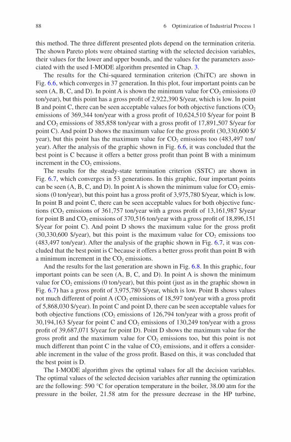
88
this method. The three different presented plots depend on the termination criteria.
The shown Pareto plots were obtained starting with the selected decision variables,
their values for the lower and upper bounds, and the values for the parameters asso-
ciated with the used I-MODE algorithm presented in Chap. 3.
The results for the Chi-squared termination criterion (ChiTC) are shown in
Fig. 6.6, which converges in 37 generation. In this plot, four important points can be
seen (A, B, C, and D). In point A is shown the minimum value for CO2 emissions (0
ton/year), but this point has a gross profit of 2,922,390 $/year, which is low. In point
B and point C, there can be seen acceptable values for both objective functions (CO2
emissions of 369,344 ton/year with a gross profit of 10,624,510 $/year for point B
and CO2 emissions of 385,858 ton/year with a gross profit of 17,891,507 $/year for
point C). And point D shows the maximum value for the gross profit (30,330,600 $/
year), but this point has the maximum value for CO2 emissions too (483,497 ton/
year). After the analysis of the graphic shown in Fig. 6.6, it was concluded that the
best point is C because it offers a better gross profit than point B with a minimum
increment in the CO2 emissions.
The results for the steady-state termination criterion (SSTC) are shown in
Fig. 6.7, which converges in 53 generations. In this graphic, four important points
can be seen (A, B, C, and D). In point A is shown the minimum value for CO2 emis-
sions (0 ton/year), but this point has a gross profit of 3,975,780 $/year, which is low.
In point B and point C, there can be seen acceptable values for both objective func-
tions (CO2 emissions of 361,757 ton/year with a gross profit of 13,161,987 $/year
for point B and CO2 emissions of 370,516 ton/year with a gross profit of 18,896,151
$/year for point C). And point D shows the maximum value for the gross profit
(30,330,600 $/year), but this point is the maximum value for CO2 emissions too
(483,497 ton/year). After the analysis of the graphic shown in Fig. 6.7, it was con-
cluded that the best point is C because it offers a better gross profit than point B with
a minimum increment in the CO2 emissions.
And the results for the last generation are shown in Fig. 6.8. In this graphic, four
important points can be seen (A, B, C, and D). In point A is shown the minimum
value for CO2 emissions (0 ton/year), but this point (just as in the graphic shown in
Fig. 6.7) has a gross profit of 3,975,780 $/year, which is low. Point B shows values
not much different of point A (CO2 emissions of 18,597 ton/year with a gross profit
of 5,868,030 $/year). In point C and point D, there can be seen acceptable values for
both objective functions (CO2 emissions of 126,794 ton/year with a gross profit of
30,194,163 $/year for point C and CO2 emissions of 130,249 ton/year with a gross
profit of 39,687,071 $/year for point D). Point D shows the maximum value for the
gross profit and the maximum value for CO2 emissions too, but this point is not
much different than point C in the value of CO2 emissions, and it offers a consider-
able increment in the value of the gross profit. Based on this, it was concluded that
the best point is D.
The I-MODE algorithm gives the optimal values for all the decision variables.
The optimal values of the selected decision variables after running the optimization
are the following: 590 °C for operation temperature in the boiler, 38.00 atm for the
pressure in the boiler, 21.58 atm for the pressure decrease in the HP turbine,
6 Optimization of Industrial Process 1

89
11.59 atm for the pressure decrease in the IP turbine, 4.76 atm for the pressure
decrease in the LP turbine, 41.96 atm for the pressure in the pump, and 0.84 and
0.72 for the split fraction in the first and second splitters, respectively.
The optimal value of the economic objective function, which consists in the
maximization of the annual gross profit, is $2,572,350/year. The optimal value of
the environmental objective function, which consists in the minimization of the
entire CO2 emissions associated with electricity generation in power plants that use
natural gas as primary energy source, is 55,532 ton/year.
6.6 Exercises
To download the example of the Generation Power Plant, please click on the follow-
ing link:
http://extras.springer.com
1. Use the process flowsheet of a regenerative Rankine cycle made in Aspen Plus
just as shown in this chapter (Fig. 6.2).
2. Do the following (remember run the simulation after change of any
specification):
(a) Change the operation specification in the boiler, temperature of 590 °C and
pressure of 18 atm (the discharge pressure of the pump must be of 18 atm
too). What happen with the value of the generated work in the turbines?
Why?
(b) Change the total flow rate of the stream number 1, with a value of 2000 ton/
day. What happen with the value of the generated work in the turbines?
Why?
3. Use the main program user interface of the I-MODE algorithm shown in Fig. 6.3.
4. Implement the following:
(a) Change the lower and upper bounds of the decision variables, 580 and
620 °C for the operation temperature in the boiler, 38 and 42 atm for the
pressure in the boiler, 16 and 24 atm for the pressure decrease in the HP
turbine, 6 and 14 atm for the pressure decrease in the IP turbine, 2 and 8 atm
for the pressure decrease in the LP turbine, 36 and 44 atm for the pressure in
the pump, and 0.65 and 0.95 for the split fractions in both splitters.
(b) For the optimization process, in this case study, the values for the parameters
associated with the used I-MODE algorithm are the following: population
size (NP) of 1000 individuals, generation number (GenMax) of 1000, taboo
list size (TLS) of 50 individuals, taboo radius (TR) of 0.01, crossover frac-
tions (Cr) of 0.9, and mutation fractions (F) of 0.6.
(c) Apply the same methodology to the conventional Rankine cycle, choose
four decision variables, and propose different objective functions. Explain
the obtained results.
6.6 Exercises

90
6.7 Nomenclature
CB Cost of the boiler
CC Cost of the cooling tower
CP Cost of the pump
CT Cost of the turbine
COPB Cost of operation of the boiler
COPC Operation cost of the cooling tower
COPP Cost of operation of the pump
COPT Turbine operating cost
FCC Capital cost factor
Net profit Net profit
Np Cost factor in the boiler pressure
Nt Overheating factor in the boiler
Pb Boiler outlet pressure
Pc Pressure of the cooling tower
Pp Discharge pressure of the pump
Pt Turbine output pressure
Qb Heat produced in the boiler
Qc Heat removed from the cooling tower
Tb Temperature of the boiler
Tc Temperature of the cooling tower
Tp Temperature in the pump
Tt Turbine output temperature
Tsb Saturation temperature in the boiler
Tsh Wet bulb temperature
Wn Electric energy produced in the turbine
Wp Work required by the pump
6 Optimization of Industrial Process 1

91© Springer International Publishing AG, part of Springer Nature 2019 J. M. Ponce-Ortega, L. G. Hernández-Pérez, Optimization of Process
Flowsheets through Metaheuristic Techniques, https://doi.org/10.1007/978-3-319-91722-1_7
Chapter 7
Optimization of Industrial Process 2
This example analyzes the production of biodiesel from degummed soybean oil.
The included SuperPro Designer® model is a slightly modified version of a process
model developed by Haas et al. (2006).
There has been intense investigation on the development of fuel producing
processes that are based on the use of renewable agricultural materials as feed-
stock. This activity is driven by the quest of national fuel self-reliance as well as
reducing emissions of particulates, hydrocarbons, and carbon monoxide. Most of
efforts have been concentrated on bioethanol and biodiesel. Biodiesel consists of
the simple alkyl esters of the fatty acids found in agricultural acylglycerol-based
fats and oils. It has been shown to give engine performance similar to that of con-
ventional fuels.
Biodiesel can be produced from any material that contains fatty acids. Thus, vari-
ous vegetable fats and oils or animal fats can be used as feedstocks for the biodiesel
process. The choice depends on local availability, cost, and government
regulations.
Here are the three most dominant ways of biodiesel production:
• Base-catalyzed transesterification of the oil
• Direct acid-catalyzed transesterification of the oil
• Conversion of the oil to its fatty acids and then to biodiesel
Most of the biodiesel produced today is done with the base-catalyzed reaction for
several reasons:
• It requires low temperature and pressure.
• It yields high conversion (98%) with minimal side reactions and reaction time.
• It is a direct conversion to biodiesel with no intermediate compounds.
• No need for exotic materials of construction.
The chemical reaction for base-catalyzed biodiesel production is depicted below
(Fig. 7.1).

92
7.1 Problem Statement
One hundred pounds of fat or oil (such as soybean oil) are reacted with 10 pounds
of a short-chain alcohol in the presence of a catalyst to produce 10 pounds of glyc-
erol and 100 pounds of biodiesel. It is a reversible reaction so the short-chain alco-
hol, signified by ROH (usually methanol, but sometimes ethanol), is charged in
excess to ensure quick conversion. The catalyst is usually sodium or potassium
hydroxide that has already been mixed with methanol. R′, R″, and R‴ indicate the
fatty acid chains associated with the oil or fat which are largely palmitic, stearic,
oleic, and linoleic acids for naturally occurring oils and fats. Part of the process
described before is shown in Fig. 7.2.
Fig. 7.1 Biodiesel formation reaction
Fig. 7.2 Process flowsheet in SuperPro Designer® for a biodiesel production plant from degummed soybean oil
7 Optimization of Industrial Process 2
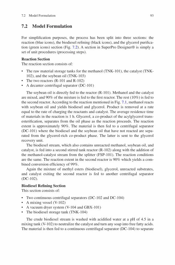
93
7.2 Model Formulation
For simplification purposes, the process has been split into three sections: the
reaction (blue icons), the biodiesel refining (black icons), and the glycerol purifica-
tion (green icons) section (Fig. 7.2). A section in SuperPro Designer® is simply a
set of unit procedures (processing steps).
Reaction Section
The reaction section consists of:
• The raw material storage tanks for the methanol (TNK-101), the catalyst (TNK-
102), and the soybean oil (TNK-103)
• The two reactors (R-101 and R-102)
• A decanter centrifugal separator (DC-101)
The soybean oil is directly fed to the reactor (R-101). Methanol and the catalyst
are mixed, and 90% of the mixture is fed to the first reactor. The rest (10%) is fed to
the second reactor. According to the reaction mentioned in Fig. 7.1, methanol reacts
with soybean oil and yields biodiesel and glycerol. Product is removed at a rate
equal to the rate of charging the reactants and catalyst. The average residence time
of materials in the reaction is 1 h. Glycerol, a co-product of the acylglycerol trans-
esterification, separates from the oil phase as the reaction proceeds. The reaction
extent is approximately 90%. The material is then fed to a centrifugal separator
(DC-101) where the biodiesel and the soybean oil that have not reacted are sepa-
rated from the glycerol-rich co-product phase. The latter is sent to the glycerol
recovery unit.
The biodiesel stream, which also contains unreacted methanol, soybean oil, and
catalyst, is fed into a second stirred tank reactor (R-102) along with the addition of
the methanol-catalyst stream from the splitter (FSP-101). The reaction conditions
are the same. The reaction extent in the second reactor is 90% which yields a com-
bined conversion efficiency of 99%.
Again the mixture of methyl esters (biodiesel), glycerol, unreacted substrates,
and catalyst exiting the second reactor is fed to another centrifugal separator
(DC-102).
Biodiesel Refining Section
This section consists of:
• Two continuous centrifugal separators (DC-102 and DC-104)
• A mixing vessel (V-102)
• A vacuum dryer system (V-104 and GBX-101)
• The biodiesel storage tank (TNK-104)
The crude biodiesel stream is washed with acidified water at a pH of 4.5 in a
mixing tank (V-102) to neutralize the catalyst and turn any soap into free fatty acids.
The material is then fed to a continuous centrifugal separator (DC-104) to separate
7.2 Model Formulation

94
the biodiesel from the aqueous phase, which is fed to the glycerol recovery section.
The crude biodiesel product must contain a maximum of 0.050% w/w water. This is
achieved by using a vacuum dryer system (V-104 and GBX-101). It lowers the
water content from 2.3% to app. 0.04%.
Glycerol Purification Section
This section consists of:
• Two mixing vessels (V-101 and V-103)
• A centrifugal separator (DC-103)
• Two distillation columns (C-101 and C-102)
• Two storage tanks (TNK-105 and TNK-106)
The produced glycerol during the transesterification process requires purification
before it can be sold. The equipment is sized to remove methanol, the fatty acids,
and most of the product to yield an 80% pure glycerol which is then sold to indus-
trial glycerol refiners at a price of $0.33/kg.
Both glycerol streams (S-119 and S-132) and fatty acid contaminants (S-137)
exiting the reactors are pooled and treated with acid (HCl) in V-101 to convert soaps
into free fatty acids, which are subsequently removed by centrifugation (DC-103).
The fatty acid stream is destined to disposal.
The glycerol stream is then neutralized with caustic soda (in V-103). The metha-
nol contained in the glycerol stream is recovered by distillation (C-101) and recy-
cled back to the first reactor (R-101). Finally, the glycerol stream is concentrated to
reach 80% purity by another distillation step (C-102) that removes the water, which
is recycled back to the mixing vessel V-102.
7.2.1 Model Simulation Using the SuperPro Designer®
Software
This example analyzes the production of 33,635 metric tons (MT) per year of bio-
diesel using crude degummed soybean oil.
The following SuperPro Designer® flowsheet file has been included with this
example:
• Bdsl8_0.spf
This flowsheet shows the base case for the process. The Bdsl8_0.spf file was
used to produce the tables and graphs in the rest of this chapter.
Below is a brief description of the basic features of the biodiesel process (file
Bdsl8_0.spf). All files for this example can be found in the “C:\Program Files\
Intelligen\SuperPro Designer \ EXAMPLES\BioDiesl” directory.
7 Optimization of Industrial Process 2

95
7.2.2 Definition of the Objective Functions
The gross annual profit (to be maximized) and the environmental impact (to be
minimized) of steam power plants are taken as the two objectives to be simultane-
ously optimized. Next, we present the equations used to calculate these objective
functions.
7.2.3 Economic Objective Function
The economic objective function consists in the maximization of the gross annual
profit, which represents the difference between the total income and the total annual
cost of the biodiesel production plant.
7.2.4 Environmental Objective Function
In this study, the environmental objective function is to minimize the entire CO2
emissions associated with heating utilities of the biodiesel production plant.
7.3 Stochastic Optimization Algorithm Used
The multi-objective optimization hybrid method, namely, improved multi-objective
differential evolution (I-MODE) developed by Sharma and Rangaiah (2013), is
used as stochastic algorithm for the optimization of the process in this example.
There were selected four decision variables and introducing a value for the lower
and upper boundary. The values of the selected decision variables for the lower and
upper bounds, respectively, are 60 and 70 psi for operation pressure in the stream
110, 60 and 70 psi for operation pressure in the stream 111, 55 and 65 °C for opera-
tion temperature in the stream 116, and 60 and 70 psi for operation pressure in the
stream 116. These values of the decision variables are introduced into the main
program user interface of the I-MODE as shown in Fig. 7.3.
For the optimization process, in this case study, the values for the parameters
associated with the used I-MODE algorithm are the following: population size (NP)
of 100 individuals, generations number (GenMax) of 100, taboo list size (TLS) of
50 individuals, taboo radius (TR) of 0.01, crossover fractions (Cr) of 0.8, and muta-
tion fractions (F) of 0.5. These values of the parameters associated with the used of
the algorithm are also introduced into the main program user interface of the
I-MODE as shown in Fig. 7.3.
7.3 Stochastic Optimization Algorithm Used

96
7.4 Link Between the Process Simulator and Optimization
Algorithm
For the adequate link between the process simulator software (Aspen Plus® for this
example) and the stochastic optimization algorithm (the I-MODE in this case), it is
necessary to follow the methodology mentioned in previous chapters. It is recom-
mendable to add two more MS Excel® sheets, the first one for the decision variable
values that will be sent to the simulator (Fig. 7.4) and the second one for the response
variable values that will be received from the simulator (Fig. 7.5).
Fig. 7.3 Excel® sheet for the main program user interface of the I-MODE (case 2)
Fig. 7.4 MS Excel® sheet where decision variable values will be sent to the process simulator (case 2)
7 Optimization of Industrial Process 2

97
7.5 Exercises
To download the example of the Generation Power Plant, please click on the
following link:
http://extras.springer.com
1. Use the process flowsheet for the biodiesel production from degummed soybean
oil implemented in SuperPro Designer® as shown in Fig. 7.2 and implement the
following:
(a) Implement a link between the SuperPro Designer® and the I-MODE algo-
rithm in MS Excel®.
(b) Analyze the Pareto curves obtained after running the optimization with the
same selected decision variables for the lower and upper bounds shown in
this chapter.
Fig. 7.5 MS Excel® sheet where response variable values will be received from the simulator (case 2)
7.5 Exercises
C1
Correction to: Optimization of Process Flowsheets through Metaheuristic Techniques
José María Ponce-Ortega and Luis Germán Hernández-Pérez
The updated online version of the book can be found at
https://doi.org/10.1007/978-3-319-91722-1
Correction to:
J. M. Ponce-Ortega, L. G. Hernández-Pérez, Optimization of
Process Flowsheets through Metaheuristic Techniques,
https://doi.org/10.1007/978-3-319-91722-1
Book was originally published with inaccessible ESM links; Link has been updated.
© Springer International Publishing AG, part of Springer Nature 2019
J. M. Ponce-Ortega, L. G. Hernández-Pérez, Optimization of Process
Flowsheets through Metaheuristic Techniques,
https://doi.org/10.1007/978-3-319-91722-1_8

99© Springer International Publishing AG, part of Springer Nature 2019
J. M. Ponce-Ortega, L. G. Hernández-Pérez, Optimization of Process
Flowsheets through Metaheuristic Techniques,
https://doi.org/10.1007/978-3-319-91722-1
Appendix
In this part of the text, you can find some details of the topics treated in this book.
Appendix A: Code for the link between Aspen Plus and MS
Excel®
Public Sub REGENERATIVE_RANKINE_CYCLE()
Dim Power_Plant As IHapp
Set Power_Plant = GetObject("SIMULATOR FILE ROUTE\FILE NAME.bkp")
Power_Plant.Visible = True
Power_Plant.SuppressDialogs = True
'DECISION VARIABLES TRANSFER FROM EXCEL TO ASPEN PLUS
Dim Boiler_Temp As IHNode, Boiler_Pres As IHNode, TurbHP_Pres As
IHNode, TurbIP_Pres As IHNode, TurbLP_Pres As IHNode, Pump_Pres As
IHNode, Div1_Frac As IHNode, Div2_Frac As IHNode
Set Boiler_Temp = Power_Plant.Tree.FindNode("\Data\Blocks\
BOILER\Input\TEMP")
Set Boiler_Pres = Power_Plant.Tree.FindNode("\Data\Blocks\
BOILER\Input\PRES")
Set TurbHP_Pres = Power_Plant.Tree.FindNode("\Data\Blocks\
TURB-HP\Input\DELP")

100
Set TurbIP_Pres = Power_Plant.Tree.FindNode("\Data\Blocks\
TURB-IP\Input\DELP")
Set TurbLP_Pres = Power_Plant.Tree.FindNode("\Data\Blocks\
TURB-LP\Input\DELP")
Set Pump_Pres = Power_Plant.Tree.FindNode("\Data\Blocks\PUMP\
Input\PRES")
Set Div1_Frac = Power_Plant.Tree.FindNode("\Data\Blocks\SPLIT1\
Input\FRAC\3")
Set Div2_Frac = Power_Plant.Tree.FindNode("\Data\Blocks\SPLIT2\
Input\FRAC\6")
Boiler_Temp.Value = Sheets("DV to Aspen Plus").Range("C3")
Boiler_Pres.Value = Sheets("DV to Aspen Plus").Range("C4")
TurbHP_Pres.Value = Sheets("DV to Aspen Plus").Range("C5")
TurbIP_Pres.Value = Sheets("DV to Aspen Plus").Range("C6")
TurbLP_Pres.Value = Sheets("DV to Aspen Plus").Range("C7")
Pump_Pres.Value = Sheets("DV to Aspen Plus").Range("C8")
Div1_Frac.Value = Sheets("DV to Aspen Plus").Range("C9")
Div2_Frac.Value = Sheets("DV to Aspen Plus").Range("C10")
Power_Plant.Reinit 'REINITIALIZE ASPEN PLUS
Power_Plant.Run 'ACTIVATE ASPEN PLUS
'DATA TRANSFER FROM ASPEN HYSYS TO EXCEL
Dim Boiler_Q As IHNode, TurbHP_W As IHNode, TurbIP_W As IHNode,
TurbLP_W As IHNode, Tower_Q As IHNode, Pump_W As IHNode, Boiler_
Cost As IHNode, Tower_Cost As IHNode, Boiler_Op_Cost As IHNode
Set Boiler_Q = Power_Plant.Tree.FindNode("\Data\Blocks\BOILER\
Output\QNET")
Set TurbHP_W = Power_Plant.Tree.FindNode("\Data\Blocks\TURB-HP\
Output\WNET")
Set TurbIP_W = Power_Plant.Tree.FindNode("\Data\Blocks\TURB-IP\
Output\WNET")
Set TurbLP_W = Power_Plant.Tree.FindNode("\Data\Blocks\TURB-LP\
Output\WNET")
Set Tower_Q = Power_Plant.Tree.FindNode("\Data\Blocks\TOWER\
Output\HX_DUTY")
Set Pump_W = Power_Plant.Tree.FindNode("\Data\Blocks\PUMP\
Output\WNET")
Set Boiler_Cost = Power_Plant.Tree.FindNode("\Data\Blocks\
BOILER\Output\UTIL_COST")
Appendix
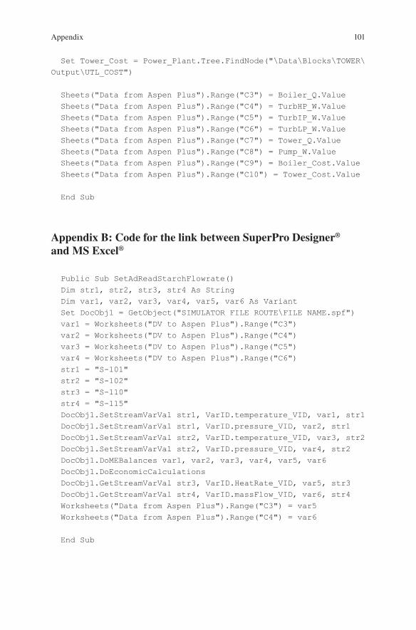
101
Set Tower_Cost = Power_Plant.Tree.FindNode("\Data\Blocks\TOWER\
Output\UTL_COST")
Sheets("Data from Aspen Plus").Range("C3") = Boiler_Q.Value
Sheets("Data from Aspen Plus").Range("C4") = TurbHP_W.Value
Sheets("Data from Aspen Plus").Range("C5") = TurbIP_W.Value
Sheets("Data from Aspen Plus").Range("C6") = TurbLP_W.Value
Sheets("Data from Aspen Plus").Range("C7") = Tower_Q.Value
Sheets("Data from Aspen Plus").Range("C8") = Pump_W.Value
Sheets("Data from Aspen Plus").Range("C9") = Boiler_Cost.Value
Sheets("Data from Aspen Plus").Range("C10") = Tower_Cost.Value
End Sub
Appendix B: Code for the link between SuperPro Designer®
and MS Excel®
Public Sub SetAdReadStarchFlowrate()
Dim str1, str2, str3, str4 As String
Dim var1, var2, var3, var4, var5, var6 As Variant
Set DocObj1 = GetObject("SIMULATOR FILE ROUTE\FILE NAME.spf")
var1 = Worksheets("DV to Aspen Plus").Range("C3")
var2 = Worksheets("DV to Aspen Plus").Range("C4")
var3 = Worksheets("DV to Aspen Plus").Range("C5")
var4 = Worksheets("DV to Aspen Plus").Range("C6")
str1 = "S-101"
str2 = "S-102"
str3 = "S-110"
str4 = "S-115"
DocObj1.SetStreamVarVal str1, VarID.temperature_VID, var1, str1
DocObj1.SetStreamVarVal str1, VarID.pressure_VID, var2, str1
DocObj1.SetStreamVarVal str2, VarID.temperature_VID, var3, str2
DocObj1.SetStreamVarVal str2, VarID.pressure_VID, var4, str2
DocObj1.DoMEBalances var1, var2, var3, var4, var5, var6
DocObj1.DoEconomicCalculations
DocObj1.GetStreamVarVal str3, VarID.HeatRate_VID, var5, str3
DocObj1.GetStreamVarVal str4, VarID.massFlow_VID, var6, str4
Worksheets("Data from Aspen Plus").Range("C3") = var5
Worksheets("Data from Aspen Plus").Range("C4") = var6
End Sub
Appendix

102
Appendix C: Code for the link between MS Excel®
and MATLAB®
File 1: Function name and linker program file route
function F=g(pop)
pop
excelObject=actxserver('Excel.Application');
excelObject.Workbooks.Open ('LIKER FILE ROUTE\FILE NAME.xlsm')
hworkbook=excelObject.workbooks;
F=excelObject.Run ('Rankine',pop(1),pop(2))
hworkbook.Close;
F=-F
File 2: Optimization parameters and function call
clc;
clear;
lb=[100 5]';
ub=[500 100]';
opts = gaoptimset('Generations',10,'PopInitRange',[0 0;500
100],'PopulationSize',10,'EliteCount',2,'CrossoverFraction',0.8,'
TimeLimit',Inf,'StallGenLimit',Inf,'StallTimeLimit',inf,'Display'
,'iter','PlotFcns',@gaplotbestf);
[x,fval,reason,output] = ga(@g,2,[],[],[],[],lb,ub,[],opts)
Appendix

Bibliography
AspenTech. (2009). Aspen Process Evaluator User’s Guide, V7.1. s.l.: Aspen Technology Inc.
AspenTech. (2015). Aspen Plus User’s Guide, V8.8. s.l.: Aspen Technology Inc.
Bamufleh, H. S., Ponce-Ortega, J. M., & El-Halwagi, M. M. (2013). Multi-objective optimization
of process cogeneration systems with economic, environmental, and social tradeoffs. Clean
Technologies and Environmental Policy, 15(1), 185–197.
Birnbaum, D. (2005). Excel VBA programming for the absolute beginner. Boston, MA: Thomson
Course Technology PTR.
Coello-Coello, C. A., Van-Veldhuizen, D. A., & Lamont, G. B. (2002). Evolutionary algorithms
for solving multi-objective problems. New York, NY: Kluwer Academic.
Contreras-Zarazúa, G., et al. (2016). Multi-objective optimization involving cost and control prop-
erties in reactive distillation processes to produce diphenyl carbonate. Computers & Chemical
Engineering, 105, 185–196.
Devillers, J. (1996). Genetic algorithms in molecular modeling. San Diego, CA: Academic Press.
Feng, Y., & Rangaiah, G. P. (2011). Evaluating capital cost estimation programs. Singapore:
National University of Singapore.
Gen, M., & Cheng, R. (1997). Genetic algorithms and engineering design. Ashikaga: Wiley.
Goldberg, D. E. (1989). Genetic algorithms and Walsh functions: Part I, A gentle introduction.
Complex Systems, 3, 129–152.
Gómez-Ríos, D., Barrera-Zapata, R., & Ríos-Estepa, R. (2017). Comparison of process technol-
ogies for chitosan production from shrimp shell waste: A techno-economic approach using
Aspen Plus. Food and Bioproducts Processing, 103, 49–57.
González-Bravo, R., Nápoles-Rivera, F., Ponce-Ortega, J. M., & El-Halwagi, M. M. (2016).
Multiobjective optimization of dual-purpose power plants and water distribution networks.
ACS Sustainable Chemistry & Engineering, 4(12), 6852–6866.
Guo, H., et al. (2014). Differential evolution improved with self-adaptive control parameters based
on simulated annealing. Swarm and Evolutionary Computation, 19, 52–67.
Gutiérrez-Arriaga, C. G., Serna-González, M., Ponce-Ortega, J. M., & El-Halwagi, M. M. (2013).
Multi-objective optimization of steam power plants for sustainable generation of electricity.
Clean Technologies and Environmental Policy, 15, 551–556.
Gutiérrez-Arriaga, C. G., et al. (2015). Industrial waste heat recovery and cogeneration involving
organic Rankine cycles. Clean Technologies and Environmental Policy, 17(3), 767–779.
Haas, M. J., McAloon, A. J., & Ye, W. C. (2006). A process model to estimate biodiesel production
costs. Bioresource Technology, 97, 671–678.
103© Springer International Publishing AG, part of Springer Nature 2019
J. M. Ponce-Ortega, L. G. Hernández-Pérez, Optimization of Process
Flowsheets through Metaheuristic Techniques,
https://doi.org/10.1007/978-3-319-91722-1

104
Hauck, M., Herrmann, S., & Spliethoff, H. (2017). Simulation of a reversible SOFC with Aspen
Plus. International Journal of Hydrogen Energy, 42(15), 10329–10340.
Hock, W., & Schittkowski, K. (1981). Test examples for nonlinear programming codes. New York,
NY: Springer-Verlag.
Huang, Y. Y. (2010). Analysis of capital cost estimation methods and computer programs.
Singapore: Department of Chemical & Biomolecular Engineering, National University of
Singapore.
Kirkpatrick, S., Gelatt, C. D., & Vecchi, M. P. (1983). Optimization by Simulated Annealing.
Science, 220(4598), 671–680.
Martinez-Gomez, J., Nápoles-Rivera, F., Ponce-Ortega, J. M., & El-Halwagi, M. M. (2017).
Optimization of the production of syngas from shale gas with economic and safety consider-
ations. Applied Thermal Engineering, 110, 678–685.
Medina-Herrera, N., Tututi-Avila, S., Jiménez-Gutiérrez, A., & Segovia-Hernández, J. G. (2017).
Optimal design of a multi-product reactive distillation system for silanes production. Computers
& Chemical Engineering, 105, 132–141.
Morgan, J. C., et al. (2017). Thermodynamic modeling and uncertainty quantification of CO2-
loaded aqueous MEA solutions. Chemical Engineering Science, 168, 309–324.
Ouyang, A., et al. (2015). A novel hybrid multi-objective population migration algorithm.
International Journal of Pattern Recognition and Artificial Intelligence, 29(01), 1559001.
Pauls, J. H., Mahinpey, N., & Mostafavi, E. (2016). Simulation of air-steam gasification of woody
biomass in a bubbling fluidized bed using Aspen Plus: A comprehensive model including
pyrolysis, hydrodynamics and tar production. Biomass and Bioenergy, 95, 157–166.
Ponce-Ortega, J. M., Nápoles-Rivera, F., El-Halwagi, M. M., & Jiménez-Gutiérrez, A. (2012).
An optimization approach for the synthesis of recycle and reuse water integration networks.
Clean Technologies and Environmental Policy, 14(1), 133–151.
Ponce-Ortega, J. M., Serna-González, M., & Jiménez-Gutiérrez, A. (2009). Use of genetic algo-
rithms for the optimal design of shell-and-tube heat exchangers. Applied Thermal Engineering,
29(2–3), 203–209.
Quiroz-Ramírez, J. J., et al. (2017a). Multiobjective stochastic optimization approach applied
to a hybrid process production–separation in the production of biobutanol. Industrial &
Engineering Chemistry Research, 56(7), 1823–1833.
Quiroz-Ramírez, J. J., et al. (2017b). Optimal selection of feedstock for biobutanol production
considering economic and environmental aspects. ACS Sustainable Chemistry & Engineering,
5, 4018–4030.
Sandler, S. I. (2015). Using Aspen Plus in thermodynamics instruction (1st ed.). Hoboken, NJ:
Wiley.
Santibañez-Aguilar, J. E., Morales-Rodriguez, R., González-Campos, J. B., & Ponce-Ortega, J. M.
(2016). Stochastic design of biorefinery supply chains considering economic and environmen-
tal objectives. Journal of Cleaner Production, 136, 224–245.
Segovia-Hernández, J. G., & Gómez-Castro, F. I. (2017). Stochastic process optimization using
Aspen Plus®. s.l.: s.n.
Seider, W. D., Seader, J. D., & Lewin, D. R. (2010). Product and process design principles
(3rd ed.). New York, NY: Wiley.
Sharma, S., Rangaiah, G. P. & Cheah, K. S. (2012). Multi-objective optimization using MS
Excel with an application to design of a falling-film evaporator system. Food and Bioproducts
Processing, 90(2), 123–134.
Sharma, S., & Rangaiah, G. P. (2013). An improved multi-objective differential evolution with a
termination criterion for optimizing chemical processes. Computers & Chemical Engineering,
56, 155–173.
Sharma, S., & Rangaiah, G. P. (2014). Hybrid approach for multiobjective optimization and its
application to process engineering problems. In J. Valadi & P. Siarry (Eds.), Applications of
metaheuristics in process engineering (pp. 423–444). s.l.: Springer International Publishing.
Bibliography

105
Sharma, S., & Rangaiah, G. P. (2016). Mathematical modeling simulation and optimization for pro-
cess design. In G. P. Rangaiah (Ed.), Chemical process retrofitting and revamping: Techniques
and applications (pp. 99–128). Singapore: Wiley.
Sinnott, R. K., & Towler, G. (2009). Chemical engineering design (5th ed.). Burlington, MA:
Butterworth and Heinemann.
Turton, R., Bailie, R. C., Whiting, W. B., & Shaeiwitz, J. A. (2009). Analysis, synthesis, and design
of chemical processes (3rd ed.). Upper Saddle River, NJ: Prentice Hall.
Ulrich, G. D., & Vasudevan, P. T. (2004). Chemical engineering process design and economics – a
practical guide (2nd ed.). Durham, NH: Process Publishing.
Vasudevan, P. T., & Agrawal, D. A. (1999). Software package for capital cost estimation. Chemical
Engineering Education, 33(3), 254–256.
Wang, X., & Tang, L. (2013). Multiobjective operation optimization of naphtha pyrolysis process
using parallel differential evolution. Industrial & Engineering Chemistry Research, 52(40),
14415–14428.
Woinaroschy, A. (2009). Simulation and optimization of citric acid production with SuperPro
designer using a client-server interface. CHIM, 9, 979–983.
Wong, C. L. (2010). Development and application of a capital cost estimation program. Singapore:
Department of Chemical & Biomolecular Engineering, National University of Singapore.
Wong, J. Y., Sharma, S., & Rangaiah, G. P. (2016). Design of shell-and-tube heat exchangers
for multiple objectives using elitist non-dominated sorting genetic algorithm with termination
criteria. Applied Thermal Engineering, 93, 888–899.
Websites
aspentech.com
honeywellprocess.com
intelligent.com
mathworks.com
microsoft.com
psenterprise.com
software.schneider-electric.com
Bibliography
107© Springer International Publishing AG, part of Springer Nature 2019
J. M. Ponce-Ortega, L. G. Hernández-Pérez, Optimization of Process
Flowsheets through Metaheuristic Techniques,
https://doi.org/10.1007/978-3-319-91722-1
A
Algorithm parameters, 46
Annealing, 27
Aspen Custom Modeler (ACM), 6
Aspen HYSYS®, 6, 19
Aspen Icarus technology, 78
Aspen library, 55
Aspen Plus®, 6, 84
chemical components, 7
component water, 9
database, 9
Find Compounds window, 9
mathematical model, 6
and MS Excel®, 99–101
COM technology, 62
interface, 60
linking, 58
process simulation, 59, 61
process simulation software, 56
start linking, 61
subroutine, 57–58
properties, 9
simulation section, 12
thermodynamic and transport data, 6
thermodynamic models, 11
Aspen Plus® databanks, 7
Aspen Plus® libraries, 55
Aspen Plus® Model Library, 7
Aspen Plus® process simulation model, 7
Aspen Plus® simulator, 81
Aspen Plus® software, 7
Aspen Plus V8.0, 7
Aspen Plus V8.8 Start-up, 8
Aspen Simulation part, 12
AspenTech process economic analyzer
(Aspen-PEA), 78
B
Bare module cost (CBM), 76
Base-catalyzed biodiesel production, 91
Biodiesel
acylglycerol transesterification, 93
annual profit, 95
base-catalyzed reaction, 91
economic objective function, 95
environmental objective function, 95
features, 94
glycerol purification, 94
I-MODE, 95
process simulator software, 96
production, 91
refining, 93
short-chain alcohol, 92
simplification purposes, 93
soybean oil, 92
SuperPro Designer®, 92, 93
Biodiesel formation reaction, 92
Biodiesel refining, 93
Biodiesel stream, 93
Boiler, 61
C
Capital cost estimation program (CCEP), 76, 77
CapCost, 76
Capital cost factor (CCF), 83
Chemical and biochemical engineering
simulators, 81
Chi-squared termination criterion (ChiTC), 87,
88
CO2 emissions, 89
COM Library, 65
Commercial simulation software, 5
Index

108
Component object module (COM) technology,
4, 54
Comprehensive design-based installation
models, 78
Conventional Rankine cycle, 12–14
boiler block values, 16
condense block values, 16
material streams, 17
message, running simulation, 18
outcomes, running simulation, 17
pump block values, 17
turbine block values, 17
water stream values, 15
Cost for operating the pump (COPP), 83
Cost vs. pressure drop graph, 28
Crude biodiesel stream, 93
D
Darwinian evolution, 32
Detailed factorial program (DFP), 77
Deterministic algorithms, 3
Deterministic optimization techniques, 27
E
EconExpert, 78
Economic and environmental objective
functions, 81
Economic objective function, 89, 95
Electrical energy consumption, 83
Environmental objective function, 95
Euclidean distance, 42
Excel-based multi-objective optimization
(EMOO) program, 41–47
I-MODE, 44
MS Excel®, 41
user interface, 44
F
Feed water heater, 79
Feeding temperature, 61
Find component window, 10
Find compounds window, 9, 11
Function name and linker program file route, 102
G
Generation Power Plant, 89
Genetic algorithms (GA), 27
behavior, 32
binary variable, 34
chromosomes, 34
codification, 33–36
convergence criteria, 32
fusion, 32
fusion ratio, 32
GA tool, 39
gaoptimset, 39
MATLAB®, 38–40
minimization problem, 37
mutation, 32
mutation operation, 32, 36
mutation rate controls, 32
optimization problem, 37
parameters, 39, 50
population, 30
procedure, 36
roulette wheel, 35
structure, 31
toolbox, 38, 41
types, 32
Global optimization approaches, 3
Glycerol purification, 94
Glycerol stream, 94
gPROMS® ProcessBuilder, 24
Grassroots plant cost (CGR), 76
H
Hot stream outlet temperature, 79
Hot stream temperature, 79
I
I-MODE algorithm, 41, 43, 44, 84, 88, 89, 95
flowchart, 43
inequality restrictions, 45
input constraints, 46
input decision variables, 46
input objective function, 45
parameters, 44
program interface, 45
Industrial process
feed water heater, 79
I-MODE, 85
model formulation, 80–84
Pareto optimal set, 80
problem statement, 79–80
process simulator and optimization
algorithm, 85
pump, 79
Input objective function, 44
L
Linker Program File, 70–71
Index

109
M
Main program interface, 44–47
Main Program User Interface, 85
Mathematical formulation, 82–83
Mathematical solution technique, 6
MATLAB® GA toolbox, 49
MATLAB® stochastic optimization tool, 71
Metaheuristic optimization approaches, 2
Metaheuristic optimization programs, 27
cost function, 27
EMOO tool, 41–47
GAs, 30
SA (see Simulated annealing (SA))
Metaheuristic optimization technique, 53
Microsoft Excel®, 54
Model formulation
Aspen Plus® Software, 81–82
economic objective function, 84
electric power stations, 80
environmental objective function, 84
mathematical formulation, 82–83
objective functions, 83
regenerative steam power plant, 81
Model palette, 13
MS Excel®, 53
MS Excel® and MATLAB®, 102–103
interface, 67
linking, 69
pseudo code, 68
subroutine to link, 68
MS Excel® configuration
Aspen library, 55
linking subroutine, 55
MS VBA, 55
MS visual basic, 56
stochastic optimization algorithm, 55
MS Excel® linker program, 63
MS Excel® sheet, 85, 86, 96, 97
Multi-objective optimization algorithm, 81
Multi-objective optimization problem, 82
Multi-objective problems (MOPs), 3
N
Net present value (NPV), 75
O
Object linking and embedding (OLE), 54
Optimization approaches, 2
Optimization parameters and function call,
102
P
Pareto optimal set, 80
Performance evaluation
capital cost, 76
NPV, 75
objective function, 75
profit, 76
search algorithms, 75
PRO/II® Process Engineering, 23
Process simulation, 1
Process simulator
Aspen HYSYS®, 19
Aspen Plus®, 6
conventional Rankine cycle, 12
description, 5
exercises, 24–25
gPROMS® ProcessBuilder, 24
optimization approaches, 5, 85
and optimization programs
Aspen Plus®, 54
COM technology, 54
MS Excel® configuration, 55
PRO/II® Process Engineering, 23
SuperPro Designer®, 20
UniSim® Design Suite, 23
R
Rankine cycle flowsheet, 13
Regenerative Rankine cycle, 25, 80
Regenerative-reheat steam power plants, 79
S
Searching methods
COM technology, 4
deterministic methods, 3
enumerative, 2
optimization, 2
stochastic, 2
VBA, 4
Shell-and-tube heat exchangers, 50
Simulated annealing (SA), 27
algorithm, 29
steps, 29
structure, 30
Simulator file, 55–56
Software process simulator, 68
Soybean oil, 93
Steady-state termination criterion (SSTC), 87,
88
Steam power plant configurations, 80
Steam reformer, 73
Index

110
Stochastic algorithms, 28
Stochastic optimization algorithm, 84–85
Stochastic optimization exercises, 47–50
Stochastic search algorithms, 29
SuperPro Designer®, 20, 66, 97
charge operation, 22
components and mixtures, 21
graphical interface, 20
operation models, 21
operations, 20
unit procedure, 20
user interface, 21
SuperPro Designer® and MS Excel®, 101–102
COM interface, 65
interface, 64
linking, 63
optimization algorithm, 64
subroutine to link, 62–63
SuperPro Designer® flowsheet, 94
SuperPro Designer® Software, 94
Syngas production, 73
T
Taboo list (TL), 42
Taboo list size (TLS), 42, 85
Taboo radius (Tr), 42
Thermodynamic method, 6
U
UniSim® Design Suite, 23
V
Visual basic for applications (VBA), 4
Volatile organic compounds (VOCs),
20–21
Index
Related Documents