UC Riverside UC Riverside Electronic Theses and Dissertations Title Joint Visible Light Communication and Navigation via LEDs Permalink https://escholarship.org/uc/item/2s11034b Author Zheng, Dongfang Publication Date 2014-01-01 Peer reviewed|Thesis/dissertation eScholarship.org Powered by the California Digital Library University of California

Welcome message from author
This document is posted to help you gain knowledge. Please leave a comment to let me know what you think about it! Share it to your friends and learn new things together.
Transcript

UC RiversideUC Riverside Electronic Theses and Dissertations
TitleJoint Visible Light Communication and Navigation via LEDs
Permalinkhttps://escholarship.org/uc/item/2s11034b
AuthorZheng, Dongfang
Publication Date2014-01-01 Peer reviewed|Thesis/dissertation
eScholarship.org Powered by the California Digital LibraryUniversity of California

UNIVERSITY OF CALIFORNIARIVERSIDE
Joint Visible Light Communication and Navigation via LEDs
A Dissertation submitted in partial satisfactionof the requirements for the degree of
Doctor of Philosophy
in
Electrical Engineering
by
Dongfang Zheng
December 2014
Dissertation Committee:
Dr. Jay A. Farrell , ChairpersonDr. Matthew BarthDr. Amit Roy-Chowdhury

Copyright byDongfang Zheng
2014

The Dissertation of Dongfang Zheng is approved:
Committee Chairperson
University of California, Riverside

Acknowledgments
This dissertation could not be finished without the help and support from many people.
Here I would like to express my deepest gratitude to them.
First of all, I would like to thank my advisor, Dr. Jay A. Farrell, for his
support, guidance, encouragement and patience during my Ph.D. years at UC Riverside.
I still remember the first time I talked with him, and the first email I received from
him accepting me to participate this research project. I am thankful not only for his
instructive advice and useful suggestions on my research, but also for his encouragement
and patience for me. His words of encouragement after my first presentation in a group
meeting still make me feel strength today.
I also want to thank the committee members Prof. Matthew Barth and Prof.
Amit Roy-Chowdhury in my final defense. The talking with Prof. Matthew Barth
after my oral exam encouraged me to continue my research following the ideas. The
questions from Prof. Amit Roy-Chowdhury in the group meeting really helped me a
lot in learning new technologies. I want to thank Prof. Jie Chen for providing me this
opportunity to study at UC Riverside. I also want to thank Prof. Christian Shelton
for his strict attitude and helpful suggestions during my oral defense. I also want to
thank Prof. Anastasios Mourikis for his help in the group meetings and classes. I am
grateful to the help from Dr. Gang Chen and Prof. Albert Wang when I was preparing
the demonstrations. Dr. Chen’s expert knowledge on the hardware helps me solve lots
of problems of the experimental platform.
I would like to express my gratitude to my co-works Yiming Chen, Lingchao
Liao, Tian Lang, Zening Li, Bo Bai, Kaiyun Cui, Rathavut (Biggie) Vanitsthian and
Dr. Paul Miller for their hard work. Without their help, it is impossible for me to have
iv

the work completed. I appreciate for the help from the former students Dr. Anning
Chen, Dr. Lili Huang, Dr. Qichi Yang, Dr. Yiqian Li and Dr. Arvind Ramanandan.
They gave me so much help both in research and everyday life in my first few years in
the US.
I also want to thank my classmates Mingyang Li, Haiyu Zhang, Sheng Zhao
and Sarath Suvanah in the lab WCH 396 for discussing with me the technical problems
in research. Thanks the current students Xing Zheng, Hongsheng Yu, Shukui Zhang and
Paul Roysdon for making our lab a great place to learn and work. I am also grateful for
having the friends Yulin Zhang, Dr. Ergude Bao, Ming Wang, Zhen Qin, Zongyu Dong,
Lunshao Chai, Lin Wang, Kuili Fang during my Ph.D. years at UCR. They brought me
so much happiness in the years passed.
At last, thanks my parents, my wife, for their unconditional love, encourage-
ment and support to me. They always gave me hope when I was depressed, without
which this work would never have been possible. They are always the most important
people in my life.
v

To my parents and wife, for their love and support.
vi

ABSTRACT OF THE DISSERTATION
Joint Visible Light Communication and Navigation via LEDs
by
Dongfang Zheng
Doctor of Philosophy, Graduate Program in Electrical EngineeringUniversity of California, Riverside, December 2014
Dr. Jay A. Farrell , Chairperson
Visible light communications (VLC) based on illuminative LED lamps are attracting
increasing attentions due to its numerous advantages. Compared with conventional
lamps, LED illumination sources have long operational life, low power consumption,
and are mechanically robust. Therefore LEDs are expected to be the next generation of
lamps that will be widely installed to replace conventional lamps. Besides, LEDs can be
modulated at very high-speeds, which allows the possibility of simultaneously providing
communication while illuminating. The light modulation frequency is sufficiently high
that it is undetectable by the human eye, yet detectable by arrays of photodiodes.
Considering these facts, a system can be designed to receive (using a single photodiode
or a camera) and analyze LED signals. Furthermore, such a system should be able to
facilitate position estimation tasks either for people or vehicles.
Two kinds of sensors - single photo-detector and array photo-detector (camera
or linear array) C can be used to detect the LEDs. The single photo-detector approach is
used to detect the existence and the specific identity of an LED. The array photo-detector
approach measures the angle-of-arrival of the LED signal. A single photo detector
provides the simplest hardware approach and could communicate with LED’s at a very
vii

high data rate, but only offers the most basic level of positioning. Cameras provide much
more informative position measurements; however, there are challenges to achieving high
rate LED-to-camera data communications due to the current hardware architectures of
cameras. Alternatively, linear PD arrays allow high sample rates, high accuracy and
low cost. This dissertation will investigates the issues (observability, extrinsic parameter
calibration, and vehicle state initialization) related to implementation of a positioning
and communications system built on a linear optical sensor array.
The VLC based navigation methods require recovering the LED ID from a
sequence of photo-detector scans. This ID will help the data association in the navigation
system or the data communication in the VLC system. Recovering LED data (ID)
requires identifying each LED’s projection position and on-off status in each photo-
detector scan. Identifying the LED projection is challenging because: 1) Clutter and
noise corrupt the measurements; 2) The LED status will be “off” in some frames; 3) The
predicted projection location sequence depends on the estimated vehicle state trajectory,
which is uncertain. This dissertation presents two new methods determining the most
probable data and LED position sequences simultaneously, using Bayesian techniques
by maximizing posterior probabilities. The first method is based on Viterbi algorithm
and developed under the assumption that the frame rate of the array sensor is high
relative to the rover motion bandwidth. The second one is based on multiple hypothesis
tracking (MHT) techniques with no assumption assumed. Both the two methods are
analyzed theoretically and demonstrated by experimental results.
viii

Contents
List of Figures xii
List of Tables xiv
1 Introduction 11.1 Motivation . . . . . . . . . . . . . . . . . . . . . . . . . . . . . . . . . . 11.2 Problem Statement . . . . . . . . . . . . . . . . . . . . . . . . . . . . . . 31.3 Contributions . . . . . . . . . . . . . . . . . . . . . . . . . . . . . . . . . 41.4 Organization . . . . . . . . . . . . . . . . . . . . . . . . . . . . . . . . . 5
2 Background 72.1 Visible Light Communication (VLC) . . . . . . . . . . . . . . . . . . . . 72.2 Visible Light Positioning (VLP) . . . . . . . . . . . . . . . . . . . . . . . 92.3 LED Detection and Data Recovery . . . . . . . . . . . . . . . . . . . . . 132.4 Related Work . . . . . . . . . . . . . . . . . . . . . . . . . . . . . . . . . 16
3 Navigation using Linear Photo Detector Arrays 203.1 Introduction . . . . . . . . . . . . . . . . . . . . . . . . . . . . . . . . . . 203.2 Problem Description . . . . . . . . . . . . . . . . . . . . . . . . . . . . . 25
3.2.1 General Navigation System . . . . . . . . . . . . . . . . . . . . . 253.2.1.1 State Propagation . . . . . . . . . . . . . . . . . . . . . 263.2.1.2 Aiding Sensor Model . . . . . . . . . . . . . . . . . . . 273.2.1.3 Sensor Fusion . . . . . . . . . . . . . . . . . . . . . . . 29
3.2.2 Kinematic Equations . . . . . . . . . . . . . . . . . . . . . . . . . 303.2.3 Measurement Equation . . . . . . . . . . . . . . . . . . . . . . . 31
3.3 Observability Analysis . . . . . . . . . . . . . . . . . . . . . . . . . . . . 343.3.1 Nonlinear Observability . . . . . . . . . . . . . . . . . . . . . . . 343.3.2 Observability Analysis . . . . . . . . . . . . . . . . . . . . . . . . 35
3.4 Calibration and Initialization . . . . . . . . . . . . . . . . . . . . . . . . 393.4.1 Extrinsic Parameter Calibration . . . . . . . . . . . . . . . . . . 393.4.2 Initialization . . . . . . . . . . . . . . . . . . . . . . . . . . . . . 41
3.5 Results . . . . . . . . . . . . . . . . . . . . . . . . . . . . . . . . . . . . . 443.5.1 Extrinsic Parameters Calibration . . . . . . . . . . . . . . . . . . 453.5.2 Initialization . . . . . . . . . . . . . . . . . . . . . . . . . . . . . 46
ix

4 Data Recovery in a Stationary Sensor 514.1 Introduction . . . . . . . . . . . . . . . . . . . . . . . . . . . . . . . . . . 514.2 Problem Formulation . . . . . . . . . . . . . . . . . . . . . . . . . . . . . 54
4.2.1 Linear Array Measurement . . . . . . . . . . . . . . . . . . . . . 554.2.2 LED Measurement Prior . . . . . . . . . . . . . . . . . . . . . . . 574.2.3 LED State Definition . . . . . . . . . . . . . . . . . . . . . . . . 574.2.4 Problem Statement . . . . . . . . . . . . . . . . . . . . . . . . . . 58
4.3 Method . . . . . . . . . . . . . . . . . . . . . . . . . . . . . . . . . . . . 594.3.1 Viterbi Algorithm . . . . . . . . . . . . . . . . . . . . . . . . . . 594.3.2 Probabilistic Model . . . . . . . . . . . . . . . . . . . . . . . . . 614.3.3 Effect of LED Image Width . . . . . . . . . . . . . . . . . . . . . 64
4.4 Results . . . . . . . . . . . . . . . . . . . . . . . . . . . . . . . . . . . . . 674.4.1 Experimental Setup . . . . . . . . . . . . . . . . . . . . . . . . . 674.4.2 State Transition Model . . . . . . . . . . . . . . . . . . . . . . . 674.4.3 Stationary . . . . . . . . . . . . . . . . . . . . . . . . . . . . . . . 694.4.4 Moving . . . . . . . . . . . . . . . . . . . . . . . . . . . . . . . . 70
5 LED Data Recovery in a Moving Sensor 735.1 Introduction . . . . . . . . . . . . . . . . . . . . . . . . . . . . . . . . . . 73
5.1.1 Multiple Hypothesis Data Association . . . . . . . . . . . . . . . 755.2 Problem Formulation . . . . . . . . . . . . . . . . . . . . . . . . . . . . . 76
5.2.1 Predicted Measurement Region . . . . . . . . . . . . . . . . . . . 775.2.2 Data Association Hypothesis . . . . . . . . . . . . . . . . . . . . 775.2.3 Technical Problem Statement . . . . . . . . . . . . . . . . . . . . 79
5.3 MHT-based LED Data Recovery Method . . . . . . . . . . . . . . . . . 805.3.1 Hypothesis Probability . . . . . . . . . . . . . . . . . . . . . . . . 805.3.2 Hypothesis for Multiple LEDs . . . . . . . . . . . . . . . . . . . . 855.3.3 q-best Hypotheses . . . . . . . . . . . . . . . . . . . . . . . . . . 865.3.4 Hypothesis: Computed Quantities . . . . . . . . . . . . . . . . . 88
5.4 Vehicle Trajectory Recovery . . . . . . . . . . . . . . . . . . . . . . . . . 905.4.1 Motion Sensor Model . . . . . . . . . . . . . . . . . . . . . . . . 905.4.2 Photo-Detector Model . . . . . . . . . . . . . . . . . . . . . . . . 94
5.5 Results . . . . . . . . . . . . . . . . . . . . . . . . . . . . . . . . . . . . . 955.5.1 Stationary . . . . . . . . . . . . . . . . . . . . . . . . . . . . . . . 95
5.5.1.1 Camera . . . . . . . . . . . . . . . . . . . . . . . . . . . 965.5.1.2 Linear Array . . . . . . . . . . . . . . . . . . . . . . . . 103
5.5.2 Moving . . . . . . . . . . . . . . . . . . . . . . . . . . . . . . . . 1055.5.2.1 Camera . . . . . . . . . . . . . . . . . . . . . . . . . . . 1055.5.2.2 Linear Array . . . . . . . . . . . . . . . . . . . . . . . . 108
6 Conclusion and Future Work 1116.1 Conclusion . . . . . . . . . . . . . . . . . . . . . . . . . . . . . . . . . . 1116.2 Future work . . . . . . . . . . . . . . . . . . . . . . . . . . . . . . . . . . 113
Bibliography 117
x

A Nonlinear Optimization Methods 124A.1 Gradient Descent Method . . . . . . . . . . . . . . . . . . . . . . . . . . 125A.2 Newton Method . . . . . . . . . . . . . . . . . . . . . . . . . . . . . . . . 125A.3 Gauss-Newton Method . . . . . . . . . . . . . . . . . . . . . . . . . . . . 126
B Deirvation of Encoder Model 127B.1 Compute Velocity and Angular Rate From Encoder Measurements . . . 127B.2 State Transition Matrix . . . . . . . . . . . . . . . . . . . . . . . . . . . 129
C Derivation of IMU Error Model 131
D Camera Linearized Measurement Matrix 135
xi

List of Figures
1.1 The evolution of illuminating lamps. . . . . . . . . . . . . . . . . . . . . 2
2.1 LED market revenue in 2011-2015 . . . . . . . . . . . . . . . . . . . . . 82.2 LED stop lights and street lights. . . . . . . . . . . . . . . . . . . . . . . 92.3 Airport LED guiding lights. . . . . . . . . . . . . . . . . . . . . . . . . . 92.4 Indoor applications. . . . . . . . . . . . . . . . . . . . . . . . . . . . . . 112.5 Outdoor applications. . . . . . . . . . . . . . . . . . . . . . . . . . . . . 112.6 Comparison between different navigation methods (Source: [79]). . . . . 122.7 Photo-detectors . . . . . . . . . . . . . . . . . . . . . . . . . . . . . . . . 132.8 LED data transmission methods . . . . . . . . . . . . . . . . . . . . . . 142.9 The measured LEDs in the image and linear array. . . . . . . . . . . . . 15
3.1 Camera continuously takes images of a scene with an LED light [31]. . . 213.2 EoSens CL camera . . . . . . . . . . . . . . . . . . . . . . . . . . . . . . 223.3 Physical structure of linear photodiode array sensor. . . . . . . . . . . . 243.4 The side and top view of linear array. . . . . . . . . . . . . . . . . . . . 253.5 Aided navigation system . . . . . . . . . . . . . . . . . . . . . . . . . . . 263.6 Growing of the state error covariance due to the process noise. . . . . . 283.7 The state error ellipse evolves over time when the aiding sensor measure-
ments are added. . . . . . . . . . . . . . . . . . . . . . . . . . . . . . . . 303.8 Camera and linear array measurement model . . . . . . . . . . . . . . . 343.9 Two LEDs not laterally separated. . . . . . . . . . . . . . . . . . . . . . 433.10 Estimated translation lpbl. . . . . . . . . . . . . . . . . . . . . . . . . . . 453.11 Estimated Euler angles. . . . . . . . . . . . . . . . . . . . . . . . . . . . 463.12 Initialization results. The blue asterisk marks the location that is consid-
ered to be correct. . . . . . . . . . . . . . . . . . . . . . . . . . . . . . . 493.13 Initialization results. . . . . . . . . . . . . . . . . . . . . . . . . . . . . . 50
4.1 LED data in a sequence of photo-detector scans . . . . . . . . . . . . . . 524.2 Linear array measurement . . . . . . . . . . . . . . . . . . . . . . . . . . 564.3 LED state definition. . . . . . . . . . . . . . . . . . . . . . . . . . . . . . 584.4 EoSens CL camera and cylindrical lens. . . . . . . . . . . . . . . . . . . 674.5 State transition process defined in matrix A (4.29). . . . . . . . . . . . . 684.6 Stationary platform sequence of raw (left) and thresholded (right) linear
array measurement data represented as an image. . . . . . . . . . . . . . 694.7 Stationary probability image and recovered LED path (green line). . . . 704.8 Moving platform experimental results. . . . . . . . . . . . . . . . . . . 71
xii

4.9 The LED data based on the recovered LED path. . . . . . . . . . . . . 72
5.1 Predicted LEDs’ positions in the image plane based on the prior informa-tion of the rover state: Predicted positions (green stars), 3-σ error ellipseregions (red) . . . . . . . . . . . . . . . . . . . . . . . . . . . . . . . . . 97
5.2 Camera measurements of LED 0 and LED 1 in the first few seconds:Predicted LED positions (green stars), 3-σ error regions (red), LED mea-surements (magenta “+”). . . . . . . . . . . . . . . . . . . . . . . . . . . 98
5.3 The measurements and hypotheses at the first two steps. . . . . . . . . . 995.4 Estimation results associated with each hypothesis sequence. . . . . . . 1015.5 Camera measurements with the most probable selection of the measure-
ments at each time step. . . . . . . . . . . . . . . . . . . . . . . . . . . . 1025.6 Predicted LEDs’ positions and their uncertainty intervals in the linear
array. . . . . . . . . . . . . . . . . . . . . . . . . . . . . . . . . . . . . . 1035.7 The linear array measurements and the new hypotheses. . . . . . . . . . 1035.8 Estimation results associated with each hypothesis sequence using linear
array measurements. . . . . . . . . . . . . . . . . . . . . . . . . . . . . . 1045.9 Linear array measurements with the most probable selection of the mea-
surements at each time step. . . . . . . . . . . . . . . . . . . . . . . . . . 1055.10 Coordinates of LED 0 and LED 1 in the image plane: Predicted LED
positions (green stars), 3-σ error regions (red), LED measurements (blue“+”), noise and clutter measurements (magenta “+”). . . . . . . . . . . 106
5.11 Estimation results associated with each hypothesis: State estimates onlyby motion sensors (green), standard deviation (red), and posterior stateestimates of each hypothesis (other colors). . . . . . . . . . . . . . . . . 107
5.12 Prior prediction (left) and posterior prediction of each hypothesis (right). 1085.13 Linear array measurements with the most probable selection of the mea-
surements at each time step when the rover is moving. . . . . . . . . . . 1095.14 Estimation results associated with each hypothesis sequence using linear
array measurements when the rover is moving. . . . . . . . . . . . . . . 110
6.1 Linear array with one candidate measurement (yellow) falls into both thepredicted region of two LEDs. . . . . . . . . . . . . . . . . . . . . . . . . 114
xiii

List of Tables
2.1 Comparison between photo-detectors . . . . . . . . . . . . . . . . . . . . 14
3.1 LED coordinates in meters in the NED frame. . . . . . . . . . . . . . . . 473.2 initialization results using 2 LEDs . . . . . . . . . . . . . . . . . . . . . 483.3 Initialization results using 3 and 8 LEDs . . . . . . . . . . . . . . . . . . 49
4.1 Viterbi algorithm . . . . . . . . . . . . . . . . . . . . . . . . . . . . . . . 604.2 LED path recovery algorithm . . . . . . . . . . . . . . . . . . . . . . . . 66
5.1 q-best hypotheses algorithm . . . . . . . . . . . . . . . . . . . . . . . . . 89
xiv
Chapter 1
Introduction
1.1 Motivation
Visible light communications (VLC) based on illuminative LED lamps are at-
tracting increasing attentions due to its numerous advantages. Compared with con-
ventional lamps, LED illumination sources have long operational life, low power con-
sumption, and are mechanically robust. It is viewed as the next generation lamps in
the future. Fig. 1.1 shows the evolution of the illuminating lamps and their luminous
efficacy comparison. Besides, LEDs can be modulated at very high-speeds, which al-
lows the possibility of simultaneously providing communication while illuminating. The
light modulation frequency is sufficiently high that it is undetectable by the human
eye, yet detectable by arrays of photodiodes. For example, their fast switching rates
(> 300MHz) enables LED’s installed for illumination to also be used for communica-
tion and positioning [38]. Considering these facts, a system can be designed to receive
(using a photo-detector) and analyze LED signals. Furthermore, such a system should
be able to facilitate position estimation tasks either for people or vehicles. The multi-
1

Figure 1.1: The evolution of illuminating lamps.
purpose operations of LED alleviate installing specific infrastructures for each purpose.
There is a growing need for position and navigation solutions other than Global
Navigation Satellite System (GNSS), especially indoors or in urban environment where
GPS does not function well. The indoor navigation applications include automated
guided vehicles for office tasks, emergency guidance systems, equipment location deter-
mination, shopping assistance, and indoor navigation for the visually impaired [78]. The
outdoor applications like positioning systems based on street light or stop lights can be
a helpful compensate for GNSS. Besides, using LEDs as the detecting features could
fully take advantage of their unique IDs [61, 85]. Compared with other data association
algorithms such as Mahalanobis distance [53] and template matching [15], using the
unique ID will be much more precise and reliable. Imagining that all the illuminating
lamps indoors and outdoors are replaced by LEDs, the navigation and communication
system built based on it will require installation of no other additional infrastructures.
The visible light communication (VLC) requires line-of-sight (LOS) commu-
nication channel [39]. That is, only when the LED sources are in the sight of receiver
(photodiode or image sensor) that their signal has chances to be detected. Due to this
2

fact, VLC becomes more difficult when the receiver is moving. Taking camera for ex-
ample, if it is installed on a vehicle that is traveling around, the LEDs’ positions in the
image are not fixed, then it is impossible to control the camera sampling a specific pixel
to recover the data. On the other hand, searching each whole image to firstly find the
LED’s position before extracting the signal would make the communication inefficient.
This difficulty in VLC encourages us the idea that combines the communication and
navigation together. The navigation system estimates the position of camera, and fur-
ther the LEDs’ coordinates in the image are predicted. The navigation system also gives
the error covariance of the predicted LED position. With this knowledge, the commu-
nication system could focus on a much smaller ellipse region in the image to find the
LED and extract the signal. Communication requires knowledge of which LED ID’s to
expect for efficiency of demodulation and knowledge of where each LED is expected to
be in the image for efficiency of image processing. Accurate navigation combined with
an LED map enables both aspects.
1.2 Problem Statement
Even though the LOS requirement somehow increases the communication dif-
ficulty, it could be greatly useful for navigation purpose. For navigation purpose, a
single photodiode provides the simplest hardware approach that could detect LED data
at rates exceeding 300MHz, but only offers the most basic level of positioning. The
use of image sensors (cameras) makes it possible to detect the accurate direction of the
incoming vector from a LED to the image sensor, but only samples at a low frame rate
(about 30Hz). A challenge in LED-based navigation system is how to improve the data
transmission rate and the image processing efficiency while maintaining the capability
3

for accurate navigation. The large number of pixels (usually several mega-pixels) in the
image sensor limits the frame rate. This dissertation investigates the ability of a linear
array to preserve the cameras precise position measurement and simultaneously achieve
high data rates.
Any kind of photo-detector based visible light communication and positioning
systems require recovering the LED ID from a sequence of photo-detector scans. This
ID will help the data association in the navigation system or the data communication in
the VLC system. Recovering the LED data from the photo-detector’s measurements is
not so straightforward because: 1) Clutter and noise corrupt the measurements; 2) The
LED status will be “off” in some frames; 3) The predicted projection location sequence
depends on the estimated vehicle state trajectory, which is uncertain. To make matters
worse, the LED projections in the sensor frame moves when the rover moves. The
challenges of recovering the LED data in the sensor frames will be discussed and the
potential solutions are also introduced.
1.3 Contributions
There are several contributions in the areas of Visible Light Communication,
Navigation, and Computer Vision:
• Discussed the characteristics of VLC-based navigation system. Compared it with
the other navigation method such as GPS, WiFi, radio and vision based methods.
• Proposed a new kind of sensor - linear array to overcome the shortcomings of
photodiode and camera. The linear array will improve the data transmission rate
and the image processing efficiency while maintaining the capability for accurate
navigation result when the rover moves in a 2D plane.
4
• Described the basic physical structure of the linear array, and discussed its initial-
ization and calibration, and analyzed the observability of the navigation system
based on it.
• Analyzed the problems of the LED data recovery when using camera or linear
array, and reviewed the existing methods.
• Proposed and analyzed two new methods based on Viterbi algorithm and multiple
hypothesis tracking (MHT) algorithm, respectively. The Viterbi-based algorithm
tries to recover the most probable LED path when the rover is stationary or
the moving bandwidth is much smaller than the frame rate. The MHT-based
algorithm recovers several possible LED paths other than one.
• Applied these two algorithms in our rover platform and tested the results.
1.4 Organization
This dissertation is organized as follows:
Chapter 2 introduces the background and the related issues in the VLC-based
communication and navigation system. Chapter 3 proposes a new kinds of sensor - linear
array to overcome the shortcomings of photodiode and camera. The basic physical
structure will be described, and its initialization and calibration will be introduced,
and the observability of the navigation system based on it will be analyzed. Chapter
4 analyzes the problems met in the LED data recovery processes by the camera or
linear array. This chapter proposes a Viterbi-based algorithm to solve the data recovery
problem when the photo-detector is stationary or moving with a bandwidth much lower
than that of the frame rate. Chapter 5 further more proposes a more robust LED
5

data recovery algorithm which could be applied to the case that no matter the sensor is
stationary or moving. Chapter 6 gives the conclusions of all the topics in this dissertation
and discussed the future work.
6
Chapter 2
Background
2.1 Visible Light Communication (VLC)
Using visible light for data transmission is not a new idea. People started using
smoke to send messages from thousands of years ago. The emperors in ancient China
used the beacon-fires to call in the troops around the country when their capital was
invaded. The fishermen in many places today are still using lighthouses to find their
destinations on the sea. Today, the bandwidth and application areas of the visible light
communication system are greatly expanded due to LED’s many useful characteristics.
Communication systems using photodiodes, cameras or linear arrays have been intro-
duced in [58, 51, 4, 84]. Their applications include indoor information broadcasting
system via ceiling lamps [44, 28], and communication systems between cars on road via
car headlights, and so on. Using visible light to transmit music has been demonstrated
in [48].
The number of LED lights in our surrounding is growing quickly as the prices
are declining, which can be seen from Fig. 2.1. Now the LEDs are used as stop lights,
7

Figure 2.1: LED market revenue in 2011-2015
road lamps, and guiding lights in the airport, see Fig. 2.2 and 2.3. The indoor LED
illuminating lights are also used more and more widely. This fact provides the opportu-
nities for visible light communications to compensate or replace the radio-wave wireless
communications indoors and outdoors. Compared with the radio-wave communication,
the visible light part of the electromagnetic spectrum is still unlicensed and unregulated,
and the power consumption of LED is lower than other radio wave transmitters [31].
Besides, the visible light has inherent security due to the line-of-sight (LOS) requirement
of visible light communications. The light in room cannot be received outside because
it will be blocked by the wall. On the other hand, the LOS requirement limits the VLC
communication distance to 1 to 100 meters which is shorter than the radio-wave commu-
nication distance [32]. It also increases the complexities of receiving LED data when the
photo-detector is moving, since different LEDs come and leave the photo-detector’s field-
of-view (FOV) and their projections on the photo-detector are also moving. However,
the LOS property is useful for estimating the photo-detector’s position and attitude,
8

which will be introduced in the following section.
(a) Stop lights. (b) Street lights and airport guiding lights.
Figure 2.2: LED stop lights and street lights.
Figure 2.3: Airport LED guiding lights.
2.2 Visible Light Positioning (VLP)
As we have briefly introduced in Chapter 1, the LOS property could provide
information of the photo-detector’s relative position and rotation with respect to each
detected LED. Once the global position of each LED transmitter is known, the photo-
detector’s global position will be able to be calculated. Such VLC-based navigation
systems have utility in a variety of environments, especially indoors or in urban envi-
9

ronments, where the current generation of GNSS technologies does not function well.
Indoor applications include emergency guidance systems, equipment location, personnel
location, indoor navigation for the visually impaired, and automated guided vehicles for
office tasks [78]. In the near future, it is even possible to help mobile users to obtain
their real-time position information by receiving the LED data using the camera on
smart-phone. For outdoor applications, the largest market would relate to a variety of
automotive applications including mobile collision avoidance system, automatic guided
vehicle, and so on. One most important advantage of VLC-based navigation systems is
that the unique ID of each LED transmitter could help solve the data association prob-
lem. Navigation systems using the communication between LEDs’ and photo-detectors
have been discussed in [85, 86, 84]. Fig. 2.4 illustrates the indoor visible light communi-
cation and positioning system used in smart-phone or shopping cart. Fig. 2.5 illustrates
the airport guidance system which determines the airplane’s position by the LED guid-
ing lights, and mobile collision avoidance system which is able to compute the relative
position of a vehicle with respect to its vicinities by detecting the LEDs installed on the
vehicles.
Fig. 2.6 gives the comparison between different navigation technologies. Here
we assume that VLC belongs to the vision based methods, which will be explained later.
From this figure, we will find that the VLC method will be much more accurate than
that of using cell phone signal, Wi-Fi, and GPS.
For navigation purpose, a single photodiode provides the simplest hardware
approach that could detect LED data at rates exceeding 300MHz [38], but only offers
the most basic level of positioning. This is basically a form of finger-printing [78, 27].
10

(a) Indoor visible light localization and commu-
nication systems using smart-phones and com-
puters.
(b) Shopping assistant in the super markets.
Figure 2.4: Indoor applications.
(a) Airport guidance system using LED lamps. (b) Mobile collision avoidance system by detecting
the LEDs installed on the the vehicles.
Figure 2.5: Outdoor applications.
11

Figure 2.6: Comparison between different navigation methods (Source: [79]).
Given a map of LED locations, when the photodiode through signaling knows that it
detects the i-th LED, it can look up that LEDs location, and know that it is in the
same vicinity. If multiple LEDs are detected, then the estimated location can be further
refined. This approach is rather binary. Either it knows its position, or not. A camera
provides a much more informative measurement for navigation purposes, by detecting
the LEDs’ positions in the image to form angle-of-arrival measurements. The camera
also spatially separates the LEDs’ signal so that they do not interfere. However, a
camera’s limited frame rate (up to thousands of frames per second) limits the rate of
high speed communication. Compared with a single photodiode and the camera, the
linear array could simultaneously provide high sampling rate and accurate estimation
results. A linear array is a set of photodiodes that form one or several straight lines
to receive the light signal. The number of pixels in a linear array is much smaller than
that in a camera, since the linear array could be viewed as a small part of the camera
sensor. The linear array preserves the sensitivity to angle-of-arrival relative to a single
axis, so it is useful when the sensor moves in a 2D plane. The comparisons between
12

the photodiode, linear array, and camera are listed in Tab. 2.1. The analysis of the
navigation and communication using a linear array, as well as the simulation results will
be presented in Chapter 3. Due to the localization accuracy, we are more interested in
the navigation system using photo-detector arrays (camera or linear array).
(a) Photodiode (b) Linear array (c) Image sensor
Figure 2.7: Photo-detectors
2.3 LED Detection and Data Recovery
Generally, there are two data transmission methods using LEDs: pattern based
method and binary based method. The pattern based method uses an array of LEDs
as the transmitter. Each time the LEDs with status “on” together represent a symbol
which will be recognized by the photo-detector. The binary based method sends message
only using the transmitter’s “on” and “off” status, so that it could only send one bit
each time. By comparison, the pattern based method has more communication efficiency
but requires complex image processing technology to recognize the pattern. These two
methods are illustrated in Fig. 2.8, where the photo-detector is an image sensor.
In this dissertation, we mainly focus on the binary based method so that the
13

Table 2.1: Comparison between photo-detectors
Photodiode Linear array Camera
>100MHz 100MHz per pixel 1KHz per frame
LED vicinity
Not linearizable
Lateral projection u
Linearly related to
yaw and position error
orthogonal to LOS vector
Lateral projection u, v
Linearly related to yaw,
pitch and position errors
orthogonal to LOS vector
Inexpensive (<$1) Inexpensive (∼$10) Expensive (>$10k)
No image processing No image processing Reqs. image processing
All LEDs utilize same PDLaterally separated LEDs
use distinct PDs
Each LED uses a
separated pixel (PD)
X
Y
Z
c
LED pattern
image plane
(a) Pattern based communication
X
Y
Z
c
LED
image plane
datasequ
ence
(b) Binary based communication
Figure 2.8: LED data transmission methods
14

transmitters can be single LEDs. The LED data is modulated using as on-off keying
(OOK) scheme [40]. Recovering the LED data requires extracting the “on” and “off”
sequence of the LED from a record of consecutive scans. The turned on LEDs are point
light sources with their projections bright blobs in a two-dimensional image, or bright
segments in a linear array. The measured LEDs in a camera images and linear array are
illustrated in Fig. 2.9.
(a) LED projection in the image (b) LED projection in the linear array
Figure 2.9: The measured LEDs in the image and linear array.
For two-dimensional image measurements, various feature detectors and de-
scriptors, including corner and blob detectors, have been developed to find and describe
the features in the image. Both these existing corner and blob detectors can be used to
search candidate LED projections in the image. Other simpler techniques like searching
LEDs based on the pixel value or color can also be used, which are especially useful for
linear array measurements where the existing corner or blob detector cannot be used.
The LED detection methods mentioned above will extract all the features in the image
besides LED’s, so we cannot determine which ones are due to LEDs in a single image
without any projection location information. For typical vision-aided navigation sys-
15

tems, in order to find the desired features (LEDs) in the image, their search regions
are predicted based on the navigation state to narrow the searching area and reject
unexpected measurements. The search region of each LED in the image is the inner of
an ellipse defined by the residual covariance. However, due to the clutter measurements
and noise, there still can be multiple potential measurements appearing in this search
region. This can be the case even when the LED is off.
2.4 Related Work
The Visible Light Communications Consortium (VLCC) has been in estab-
lished in 2003 aiming to publicize and standardize the visible light communication tech-
nology [59, 54]. The communication between the photodiode and a single white LED
has been introduced in [74, 75, 46, 44, 80, 1]. In [44], up to 300Mb/s data rate can be
realized using OOK modulation scheme, while a gross transmission rate of 513Mb/s is
achieved in [80]. The communication between the photodiode and a single LED has been
demonstrated by UC-Light lab. The music and video have been transmitted through
VLC in the demonstration, and even the internet link can be connected by VLC. Toy
cars equipped with LEDs exchange short messages is demonstrated in [16]. The commu-
nication between the photodiode and multiple LEDs are also discussed in [45, 49, 18].
Literature [49] uses on-off keying link to communicate with 16 LEDs simultaneously
achieving an overall bandwidth of 25MHz. An OFDM (orthogonal frequency division
multiplexing) modulation scheme is proposed for VLC in [1].
Using image sensor to communication with LEDs is another choice, which has
advantage of spatially separating different LED sources to prevent interferences. An
image sensor with an in-pixel demodulation function for detecting modulated LED light
16

is proposed and demonstrated in [60]. The method that decodes the LED data from a
sequence of image is proposed in [64]. The random accessing characteristic of CMOS
image sensor provides the opportunity of visual-MIMO (multiple-input multiple-output)
where optical signal from multiple LEDs are received by multiple pixels in the CMOS
image, which is introduced in [6]. The visual-MIMO demo that employs a LED array
and a high speed camera is introduced in [76]. Another advantage of image sensor is
the ability to detect LED patterns. Literature [62, 50] discussed a LED pattern based
communication method by dividing the LED panel into regions to show different visual
patterns. Literatures [5, 4, 58] proposed a hierarchical coding scheme to modulate the
LED array and realized this method in the road-to-vehicle communication.
Even though the VLC based positioning research is still at a preliminary stage
[66], there have been various methods proposed and implemented in many literatures.
Due to its short range property (less than tens of meters), most proposed VLC based
positioning methods are used indoors. These indoor positioning methods can be found in
literatures [43, 83, 71, 29, 66, 65, 41, 42, 82, 87, 63]. Despite the difficulty, there are still
some literatures like [69, 7] developed VLC based outdoor positioning methods, both of
which detect the modulated automobile LED lightings to estimate the vehicle relative
positions. Methods in [69, 71, 43, 7, 82, 87, 63] all use photodiodes to detect LEDs. Since
the photodiode could not sensor the accurate angle-of-arrival of the LED signal, these
methods mainly focus on the measured light intensity, time difference of arrival (TDOA)
and phase difference of arrival (PDOA). The method in [69] modulates the automobile
LED lighting - either taillights or headlights - to send high rate repetitive on-off keying
pattern, then the phase difference from two LED lamps are detected, while methods in
[7, 63] try to detect the time difference of arrival from two LED lights. Once the TDOA
or PDOA is detected, the range difference from the receiver to the two LED lights can
17

be computed and further the position of the receiver can be determined. Methods in
[71, 41, 42, 82, 87] try to model the visible light channel and infer the range between
receiver and LED lights based on the measured light intensity, and then calculate the
receiver’s position by trilateration. A probabilistic positioning utilizing VLC is proposed
in [43]. The basic idea of the algorithm is to sample the signal strength for selected
orientations at each reference point during the off-line phase and combine a subset of
these values to histogram in the online phase, so that an orientation-specific signal
strength distribution can be computed and utilized to increase the accuracy of position
estimate. Positioning methods using image sensors are introduced in [29, 83, 66, 65], all
of which measure the LED coordinates in the image frame and calculate the receiver’s
position based on geometry methods. Most of the existing positioning method use
photo-detector alone, while method in [43] uses compass to improve the accuracy of
training data, and method in [71] uses 6-axes to help estimate azimuth and tilt angle.
All the methods introduced above use the LED ID to recognize each light source. Some
of them like [83, 66, 65] even modulate each LED’s own global position coordinates in
the signal, so that the receiver does not have to previous known each LED’s position.
All the visible light positioning methods mentioned above compute the re-
ceiver’s position merely by the latest photo-detector’s measurement, but the Markov
property of the photo-detector’s state is not considered. The inertial sensor and com-
pass in [71, 43] are only used to help estimate the pose of receiver instead of predicting
the receiver’s state at the next time step. For the image sensor based positioning meth-
ods above, either the image sensor is stationary or no LED tracking algorithm is applied
to extract the LED data. From the view of a vision aided navigation system [56], the
positioning result can be greatly improved by incorporating motion and LED measure-
ments together. One essential problem to combine vision aided navigation method with
18

VLC together is to track the LED in the image to extract its data. To solve this problem,
the measurements in a sequence of images need to be considered jointly. The measure-
ments of the same object (LED) at multiple time instances should be matched together
to recover the data sequence.
As mentioned in Sec. 2.3, the existing corner detectors (Moravec [55], Forstner
[24], Harris [30], Shi-Tomasi [72], and FAST [70]) or blob detectors (SIFT [52], SURF
[12], and CENSURE [2]) can be used to match the projections of the same feature in
different two-dimensional images. These detectors keep the description of each feature
and these descriptions can be compared to determine whether multiple features are
originated from the same object. However, the projection can be wrongly matched,
especially when the sequence of images are long. Moreover, the existing feature descrip-
tors cannot be applied to the linear array measurement, so that they cannot be used to
match the measurements in different linear array scans.
For the global positioning system (GPS), the technology of receiver autonomous
integrity monitoring (RAIM) [35] is developed to detect the fault measurements of the
receiver. The RAIM technology performs consistency checks between all estimation so-
lutions, and provides an alert to the system if the consistency checks fail [36]. Another
outlier rejection method, named Least Soft-threshold Squares (LSS) [81], is newly devel-
oped. This method models the measurement error as the sum of Gaussian component
and Laplacian component. The LSS method is efficient and easy to implement. Both
of the two algorithms are designed to detect and reject the incorrect measurement, but
cannot deal with multiple measurements.
19

Chapter 3
Navigation using Linear Photo
Detector Arrays
3.1 Introduction
There are three kinds of optical sensors suitable for detecting the LED signal:
single photo-detector (photodiode), two-dimensional photo-detector array (camera), and
linear photo-detector array. As we have mentioned in Sec. 2.2, a single PD could
communicate with LED’s at rates exceeding 300MHz, but only offers the most basic
level of positioning. The camera provides a much more precise measurement by detecting
the LEDs positions in the image to form angle-of-arrival measurements, but could only
work at low frame rate (30Hz). The low frame rate of camera will greatly restrict the
information sent from the LEDs to camera.
A challenge in LED-based navigation system is how to improve the data trans-
mission rate and the image processing efficiency while maintaining the capability for
accurate navigation. To extract the ID, a sequence of images are grabbed and processed
to find the on or off status of the LEDs. The frame rate fs has to be at least two times
20

higher than the data rate f . Fig. 3.1 illustrates the data sequence of the LED sampled
by the camera image, where the camera frame rate is two times of the LED data rate.
Figure 3.1: Camera continuously takes images of a scene with an LED light [31].
The large number of pixels (usually several mega-pixels) in the image sensor
limits the frame rate. The frame rate of common commercial video camera is about
only 30fps (frames per second), which indicates that the LED blinking rate has to be
no higher than 15Hz which is too low. The frame rate of some special designed high-
speed cameras is higher, for example the EoSens CL camera produced by Mikrotron
GmbH could achieve 1800fps. The Eosens CL camera is shown in Fig. 3.2. Progress has
been demonstrated in our experiments, where the LED signal is modulated at 800bps
(bits per second) and the camera recovers the signal with a sampling rate of 1600fps
[85, 86]. To further improve the frame rate, a solution is proposed in our former paper
[85] that narrows the sampling area to a small portion of the whole image. To realize this
proposition, the camera should have the capability to sample an arbitrary selected area
in the image. The high-speed camera or the camera with small area sampling function
usually has very high cost (≥ 10k).
21

Figure 3.2: EoSens CL camera
This chapter investigates the ability of a linear array to preserve the cameras
precise position measurement and simultaneously achieve high data rates. A linear array
is a set of photodiodes that form one or several straight lines to receive the light signal.
The number of pixels in a linear array is much smaller than that in a camera, since the
linear array could be viewed as a small part of camera sensor. The linear array preserves
the sensitivity to angle of arrival relative to a single axis. The advantages of linear array
are:
• Fast sampling frequency: The low frame rate of camera is mainly due to its large
number of pixels. In contrast, a linear array has only one or several rows of pixels.
• High accuracy: The measurement accuracy is mainly dependent on the number of
pixels. Although the total pixel number of linear array is much smaller than that
of camera, the pixel number in one direction could be much larger leading to a
higher resolution in that direction.
22

• Low cost: The linear array has simple physical structure and small number of
pixels.
On the other hand, having only one-dimensional sensitivity of the linear array
also increases the difficulties of initialization, calibration and navigation since it cannot
sense angular rotation around the axis of the array or linear motion in the direction to
the plane defined by the sensitive axis and the LED array. A well-known result that
the camera pose is observable [73] and can be computed in closed-form [3] when four or
more known features are detected in each image will not apply to the linear array. In
this chapter we analyze the extrinsic parameter calibration process and the navigation
system state initialization for linear arrays.
Due to the one-dimensional sensitivity, navigation using the linear array is
especially useful when the carrier is constrained to move in a 2D plane. For example,
for cars equipped with linear arrays driving on roads, existing LED traffic lights are ideal
navigation features. For vehicles moving in 3D space, by employing two linear arrays
with their perpendicular sensitive directions, this problem can also be solved.
Currently, the linear array could be found in a variety of applications such as
photocopiers, barcode scanners, and line scan cameras. Their light spectrum sensitivity
ranges from short wave infrared to ultra violet, and the pixel number ranges from tens
to thousands. The pixel read-out speed is up to 100MHz. Taking the Melexis’s 3rd
generation linear optical array MLX75306 as an example, it is 7.1mm long with 142
pixels, and has 12MHz read-out speed.
Unfortunately, none of the applications mentioned above is specifically designed
for navigation and communication purposes. For this application we propose combining
a linear array and cylindrical lens. Its physical structure is illustrated in Fig. 3.3.
23

Shutter
LensLinear photodiode array
Y
X
Z
Figure 3.3: Physical structure of linear photodiode array sensor.
The basic physical structure includes a linear array, a convex-cylindrical lens
and the shutter. The convex-cylindrical lens will focus the light that passes through
onto a line instead of a point. The linear array will be put that perpendicular to the line
which the lens focuses on. In the lateral plane, the elementary ray trace is similar with
that of convex lens. The ray trace is illustrated in the right of Fig. 3.4. In the vertical
plane, the cylindrical lens can be viewed as a flat glass plate which will not affect the
ray trace. It is illustrated in the left of Fig. 3.4.
This chapter is organized as follows: Section 3.2 describes the problem details
including the kinematic equation and measurement model of the system; Section 3.3
analyzes the nonlinear observability of this linear array based navigation system; Section
3.4 discusses the extrinsic calibration of the linear array and the initialization of the
linear array based navigation system; Section 3.5 gives all the experimental results.
24

Lens
Linear array
LED’s
Z
Y
shutter
LensLinear array
Z
X
Figure 3.4: The side and top view of linear array.
3.2 Problem Description
In the following analysis, we firstly describe the general navigation system
structure as well as kinematic equations and measurement models. After introducing
the general model, we give descriptions of the specific navigation systems considered in
this chapter.
3.2.1 General Navigation System
The structure of a general aided navigation system is illustrated in Fig. 3.5.
The input of the system is the measurements of the high rate sensor and aiding sensors,
and the output is the system state estimate at each time step. The high rate sensors
include wheel encoders and IMU, which usually measure the velocity, acceleration and
angular rate of the platform. The aiding sensors include GPS receiver, magnetometer,
camera, thermometer and so on. In Fig. 3.5, the high rate part is colored by green,
while the low rate part is red. The general kinematic model and aiding sensor model
will be discussed in the following sections.
25

+
+
ˆkXd
ˆkX-
1
ˆkX+
-
ˆkX+
y
-yd+
y
1Z-
u%
Figure 3.5: Aided navigation system
3.2.1.1 State Propagation
The aiding sensor is assumed to be part of a rigid system with kinematic state
(i.e., position, velocity, attitude) denoted by x(t) ∈ Rn. We will refer to this rigid system
as a rover. The rover trajectory evolves over time according to
x(t) = f (x(t),u(t)) , (3.1)
where f : Rn × Rm → Rn is a known nonlinear mapping and u(t) ∈ Rm is the system
input. In a navigation system, the input u represents the rover’s motion information,
which could be measured by an encoder or inertial measurement unit (IMU).
Throughout this article, we use symbol a to represent the estimate of variable
a. Given an initial condition x(0) ∼ N (x0,P0), the computer calculates an estimate x
of x according to
˙x(t) = f (x(t), u(t)) , (3.2)
where u is the estimate of u computed from its measurement u. In the simplest case, the
measurement is modeled as u = u+ ω, where the process noise ω has power spectrum
density (PSD) denoted by Q.
26

Define δx = x − x as the state error, then its propagation model can be ap-
proximated by subtracting eqn. (3.2) from (3.1) and linearizing the result along the
estimated trajectory:
δx(t) = F (t)δx(t) +G(t)ω(t), (3.3)
where
F (t) =∂f
∂x|x=x,u=u (3.4)
G(t) =∂f
∂u|x=x,u=u. (3.5)
If we are only concerned with the state estimates and their errors at the times
tk at which the aiding measurements happen, and use the subscript k as the shorthand
notation for tk, we can use the following error propagation model:
δx(k) = Φk−1δx(k − 1) + ωk−1, (3.6)
where x(k) is the short for x(tk), and ωk−1 ∼ N (0,Qk−1). Computation of the state
error transition matrix Φk−1 and process noise covariance Qk−1 are discussed in [22].
From (3.6), the state error covariance Pk evolves over time according to
Pk = Φk−1Pk−1Φ⊤k−1 +Qk−1. (3.7)
According to eqn. (3.7), the state error can be accumulated quickly because of
the process noise ωk Usually after only a few second, the estimation error could become
unacceptable, which is illustrated in Fig. 3.6. That is why we need aiding sensors to
correct the state estimation.
3.2.1.2 Aiding Sensor Model
The general aiding sensor measurement model is
z(k) = h (x(k)) + nk, (3.8)
27

Tracjectory
Covariance ellipse
Figure 3.6: Growing of the state error covariance due to the process noise.
where z(k) ∈ Rp, and h : Rn → Rp is the measurement function, and nk ∼ N (0,Rk)
is the measurement noise. Given the state estimate at time step k, it is straightforward
to compute both the predicted measurement z(k) according to
z(k) = h(x(k)). (3.9)
The prediction error is defined as δz = z − z, and its model can be approximated by
subtracting eqn. (3.9) from (3.8):
δz(k) = Hkδx(k) +Rk, (3.10)
where Hk ∈ Rp×n is the linearized measurement matrix obtained from
Hk =∂h
∂x|x=x(k). (3.11)
From eqn. (3.10), its error covariance S(k) is computed as
S(k) = HkPkH⊤k +Rk. (3.12)
The quantities z(k) and S(k) define a prior distribution for the feature measurement.
28

3.2.1.3 Sensor Fusion
As showed in Fig. 3.6, the state estimate error will accumulate if the state
estimate is calculated only by integrating the measurements from the motion sensor.
The extended Kalman filter (EKF) is frequently used to fuse the measurements from
motion sensor and aiding sensors. The state estimate propagates based on eqn. (3.2)
where u(t) is viewed as a constant between each time interval [tk−1, tk]. Integrating eqn.
(3.2), the state estimate propagates according to
x(k) = x(k − 1) +
∫ tk
tk−1
f (x(t), u(t)) dt (3.13)
The state error propagates according to eqn. (3.7).
The state computed from eqn. (3.13) and the error covariance propagated
from eqn. (3.7) are the prior state estimate covariance denoted by x−(k) and P−k ,
respectively. When a measurement arrives at time tk, the state and its error covariance
are updated according to
Kk = P−k H⊤
k (HkP−k H⊤
k +Rk)−1
x+(k) = x−(k) +Kk(z(k)− h(xk))
P+k = P−
k −KkHkP−k , (3.14)
where Kk is the EKF gain evaluated at time tk, and x+ and P+ are the posterior state
estimate and error covariance. Fig. 3.7 illustrates the how the state error ellipse evolves
over time when the aiding sensor measurements are added in the estimation process.
The state error decreases when the aiding measurement happens, so that state error
keeps in a tolerable range when the rover moves.
29

Tracjectory
varCo iance ellipse
update
update
Figure 3.7: The state error ellipse evolves over time when the aiding sensor measurementsare added.
3.2.2 Kinematic Equations
In this chapter, we consider a vehicle moving in a 2D plane where the vehicle is
equipped with a linear array. The vehicle also has linear and rotational velocity inputs
(µ and ω) which are measured via additional sensors like wheel encoders. The goal is
to estimate the vehicle position coordinates n (north), e (east) and heading ψ in the
world frame. The state vector is x = [n, e, ψ]⊤, and input is u = [µ, ω]⊤. The kinematic
equations are n
e
ψ
=
cosψ
sinψ
0
µ+
0
0
1
ω. (3.15)
30

The state estimate vector is written as x =[n, e, ψ
]⊤, and it propagates discretely
according to eqn. (3.13). The state error vector is defined as δx = [δn, δe, δψ]⊤ and
δx = x− x =
n− n
e− e
ψ − ψ
. (3.16)
The state error propagate equation is defined in (3.3), where the linearized matrix F
and G are
F =
0 0 − sinψ
0 0 cosψ
0 0 0
,G =
cosψ 0
sinψ 0
0 1
. (3.17)
The state error covariance is propagated according to eqn. (3.7).
3.2.3 Measurement Equation
The linear array measurement, viewed as the lateral portion of a camera mea-
surement. So firstly we will describe the pinhole camera measurement model. Let
cpcL =
[cX cY cZ
]⊤(3.18)
denote the coordinates of an LED in camera frame. This vector is computed as
cpcL =
[cwR
cpcw
] wpwL
1
(3.19)
cwR = c
bRbwR
cpcw = cbR
(bpcb − b
wRwpwb
), (3.20)
where bpcb and cbR are the camera extrinsic calibration parameters, and wpwL is the
known LED location in navigation frame. Throughout this dissertation, the symbol baR
31

denotes the rotation matrix transforming a vector from frame a to frame b. The symbol
cpab denotes the vector pointing from location a to location b represented in frame c.
The measurement yd =
[ud vd
]⊤accounting for camera distortion is mod-
eled as follows:
u =cXcZ
(3.21)
v =cYcZ
(3.22)
r2 = u2 + v2 (3.23)
cX ′ = u(1 + k1r2 + k2r
4)
+2p1uv + p2(r2 + 2u2) (3.24)
cY ′ = v(1 + k1r2 + k2r
4)
+2p2uv + p1(r2 + 2v2) (3.25)
ud = fx · cX ′ + cx (3.26)
vd = fy · cY ′ + cy (3.27)
where (fx, fy, cx, cy) are camera intrinsic parameters and (k1, k2, p1, p2) are the distor-
tion parameters. The intrinsic parameters and distortions are determined offline using
standard calibration methods in [14]. For convenience, we usually use the undistorted
camera measurements defined in eqn. (3.22). The undistorted camera measurements
can be computed from the distorted measurements if the camera intrinstic parameters
are known. Several approaches are introduced in linteratures [33].
From the introductions above, the linear array measurement without consid-
ering the distortions is modeled as
z = h(x) =lxlz, (3.28)
where lplf =
[lx ly lz
]⊤is the feature position in the linear array frame which is
32

similar to the definition of lplf . It is modeled as
lplf = lbR
(bpbf − bpbl
), (3.29)
bpbf = bwR (wpwf − wpwb) , (3.30)
where the letter w and b in the above equations represent the world frame and body
frame, respectively.
From the eqns. (3.18–3.22), the linearized measurement matrix Hc for the
camera measurement model is
Hc =∂h
∂cpcL
∂cpcL∂x
= H1H2, (3.31)
where
H1 =
1cZ 0 − cX
(cZ)2
0 1cZ − cY
(cZ)2
(3.32)
has two rows as the vectors in the two directions orthogonal to cpcL. From equations
(3.19) and (3.20), we have
H2 =
[−cnR(:, 1 : 2) c
bRJψbpbL 03×2
], (3.33)
where
Jψ =
0 1 0
−1 0 0
0 0 0
(3.34)
and cnR(:, 1 : 2) is the first two columns of matrix c
nR.
The linearized measurement matrix Hl for the linear array measurement model
corresponds the first row of matrix Hc, and it can also be decomposed as
Hl = H1,lH2, (3.35)
33
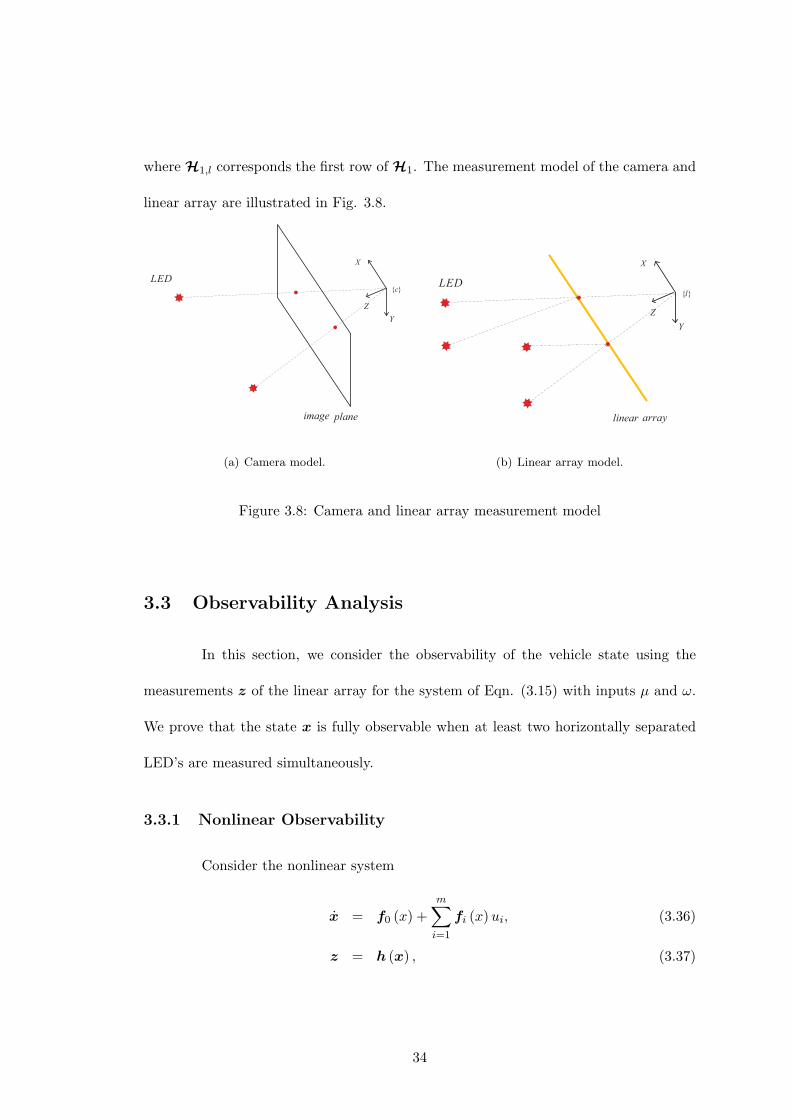
where H1,l corresponds the first row of H1. The measurement model of the camera and
linear array are illustrated in Fig. 3.8.
X
Y
Z
c
image plane
LED
(a) Camera model.
X
Y
Z
l
linear array
LED
(b) Linear array model.
Figure 3.8: Camera and linear array measurement model
3.3 Observability Analysis
In this section, we consider the observability of the vehicle state using the
measurements z of the linear array for the system of Eqn. (3.15) with inputs µ and ω.
We prove that the state x is fully observable when at least two horizontally separated
LED’s are measured simultaneously.
3.3.1 Nonlinear Observability
Consider the nonlinear system
x = f0 (x) +
m∑i=1
fi (x)ui, (3.36)
z = h (x) , (3.37)
34

where x ∈ Rn, z ∈ Rp, fi : Rn → Rn, and u1, . . . , um are m scalar inputs. The
nonlinear system described by (3.36)-(3.37) is locally weakly observable over a region D
if its observability matrix has full rank on D [34]. The observability matrix is defined
as a matrix with rows:
O , ∇Lℓfi1 ···fiℓ
hk (x) | k = 1, . . . , p; ℓ ∈ N, (3.38)
where Lℓfi1 ···fiℓ
is the Lie-derivative of order ℓ with respect to fi1 · · ·fiℓ , and hk(x)
is the kth element of h(x). For the system (3.15), we have m = 2, p = 1, f0 = 0
f1 =
[cosψ sinψ 0
]⊤, and f2 =
[0 0 1
]⊤.
3.3.2 Observability Analysis
Since the vehicle moves in the 2D plane, the height component of the vehicle
position in the world frame is fixed which is 0 in our frame definition. Using the following
standard notations
bwR =
cosψ sinψ 0
− sinψ cosψ 0
0 0 1
, (3.39)
wpwf =
[xf yf zf
]⊤, (3.40)
wpwb =
[n e 0
]⊤, (3.41)
to reorganize matrix H2 in (3.33), we have
H2 =lbR
− cosψ − sinψ a1
sinψ − cosψ a2
0 0 0
(3.42)
35

where
a1 = − (xf − n) sinψ + (yf − e) cosψ,
a2 = − (xf − n) cosψ − (yf − e) sinψ.
From Eqn. (3.42)-(3.43), if we use hi to represent the ith column of Hl, we have
h3 = − (yf − e)h1 + (xf − n)h2. (3.43)
For the system (3.15), if three rows (columns) in the observability matrix O
are found to be linearly independent, the state x will be fully observable. Obviously,
the first row of O is the linearized measurement matrix H. Before discussing the rank
of O, we firstly state the following lemma:
Lemma 1 For the system defined in (3.15), let G : R3 → Rp be a function defined on
the state space. Suppose equation
∂G
∂ψ= − (yf − e)
∂G
∂n+ (xf − n)
∂G
∂e(3.44)
holds for G, then (3.44) still holds when we replace G by LfiG, i = 1, 2.
Proof. Firstly, let fi = f1, then
Lf1G =∂G
∂ncosψ +
∂G
∂esinψ. (3.45)
Then
∂Lf1G
∂n=
∂2G
∂n2cosψ +
∂2G
∂n∂esinψ (3.46)
∂Lf1G
∂e=
∂2G
∂e∂ncosψ +
∂2G
∂2esinψ (3.47)
∂Lf1G
∂ψ=
∂2G
∂ψ∂ncosψ +
∂2G
∂ψ∂esinψ
−∂G∂n
sinψ +∂G
∂ecosψ. (3.48)
36

Take the partial derivative with respect to n for the both left and right hand sides of
eqn. (3.44), we have
∂2G
∂ψ∂n=
∂2G
∂n∂ψ=
∂
∂n
(∂G
∂ψ
)= − (yL − e)
∂2G
∂n2+ (xL − n)
∂2G
∂n∂e− ∂G
∂e. (3.49)
Substitute eqn. (3.49) into the right hand side of eqn. (3.48) and reorganize it, we have
∂Lf1G
∂ψ= − (yL − e)
(∂2G
∂n2cosψ +
∂2G
∂e∂nsinψ
)+(xL − n)
(∂2G
∂n∂ecosψ +
∂2G
∂e2sinψ
)= − (yL − e)
∂Lf1G
∂n+ (xL − n)
∂Lf1G
∂e. (3.50)
Secondly, following the similar analysis above, let fi = f2.
Lf2G =∂G
∂ψ. (3.51)
Then
∂Lf2G
∂n=
∂2G
∂ψ∂n(3.52)
∂Lf2G
∂e=
∂2G
∂ψ∂e(3.53)
∂Lf2G
∂ψ=
∂2G
∂ψ2. (3.54)
Take the partial derivative with respect to ψ for the both left and right hand sides of
eqn. (3.44), we have
∂2G
∂ψ2=
∂
∂ψ
(− (yf − e)
∂G
∂n+ (xf − n)
∂G
∂e
)= − (yL − e)
∂2G
∂n∂ψ+ (xL − n)
∂2G
∂e∂ψ. (3.55)
Substitute eqn. (3.55) into the right hand side of eqn. (3.54), we have
∂Lf2G
∂ψ= − (yL − e)
∂2G
∂n∂ψ+ (xL − n)
∂2G
∂e∂ψ
= − (yL − e)∂Lf2G
∂n+ (xL − n)
∂Lf2G
∂e. (3.56)
37
Then the proof is finished.
From the lemma, when property (3.44) holds for a function, it also holds for
its Lie-derivative, and of course its Lie-derivative of any order.
Theorem 2 The observability matrix defined in (3.38), for a single LED, does not have
full rank for the system in (3.15).
Proof. Eqn. (3.43) indicates that the measurement function h(x) has property
(3.44). Then from Lemma 1, Lℓfi1 ...fiℓ
h (fi1 . . .fiℓ = 1, 2.) satisfies (3.44) for any ℓ ∈ N,
so that each column in the observability matrix satisfies eqn. (3.44). This means the
third column of the observability matrix in (3.38) is always the linear combination of its
first two columns, so it does not have full rank.
Next, we are going to prove that the observability matrix has exactly rank 2
when only one LED is measured. Since Theorem 2 says rank(O) ≤ 2, we only need to
show rank(O) ≥ 2 in the following analysis.
Considering the row ∇Lf1h in O, we have
Lf1h = Hlf1 = −r11lz
+r31
lxlz2
(3.57)
∇Lf1h =
[r31lz2
0r11lz2
− 2r31lx
lz3
]H2
=r31lz
H +
[0 0
r11lz2
− r31lx
lz3
]H2, (3.58)
where rij is the element of matrix lbR at ith row and jth column. Then rank(O) ≥
2 is true when ∇Lf1h is linearly independent of H, since ∇Lf1h and O are two
different rows in the observability matrix. Eqn. (3.58) shows that ∇Lf1h is the linear
combination of H and the third row of H2, which indicates that ∇Lf1h is linearly
independent of H if and only if the third row of H2 is linearly independent of H. From
Eqn. (3.31), (3.32) and (3.35), H itself is the linear combination of the first and third
38

rows of H2, then H is linearly independent on the third row of H2 if and only if the first
and third rows of H2 are linearly independent. From Eqn. (3.42), the independency of
the first and third rows in H2 requires the first and third rows of lbR are independent.
Moreover, since the third row of the matrix in the right hand side of (3.42) is 0, then the
independency of the first and third rows in H2 only requires that the following matrix r11 r12
r31 r32
(3.59)
is nonsingular. This matrix is dependent on the pose of the linear array on the carrier.
If more than one LED’s are measured, and not all of the LED’s have the same
xf and yf coordinates, then the observability matrix O will have full rank since Eqn.
(3.43) is no longer true. To estimate state x, at least two horizontally separated LED’s
should be observed simultaneously.
3.4 Calibration and Initialization
The calibration of the extrinsic parameters of linear array is a little more
difficult than that of the standard camera because of its one-dimensional sensitivity.
The well-known result that the camera pose is observable [73] and can be computed
in closed-form [3] when four or more known features are detected in each image will
not apply to the linear array. In this section, we are going to estimate the extrinsic
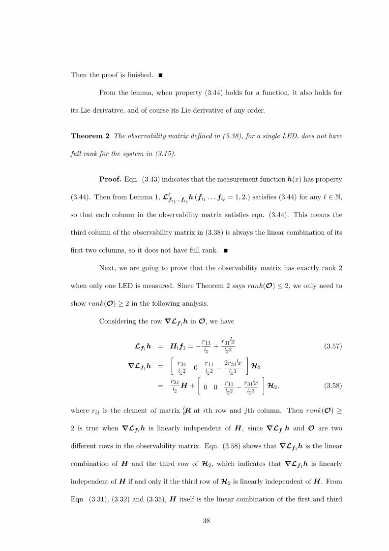
parameters using the nonlinear optimization method, initialized with approximate prior
knowledge of these parameters. The initialization method follows the method in [86].
3.4.1 Extrinsic Parameter Calibration
Being different from the extrinsic calibration of camera, the extrinsic parame-
ters of linear array cannot be estimated only by its measurement without prior knowl-
39

edge. Taking the computation of bpbl for example, even though when all the other
parameters except bpbl in Eqn. (3.28)-(3.29) are perfectly known, the vector bpbl still
could not be obtained. Assume there are m LEDs are measured with measurement set
z1, z2, . . . , zm and their corresponding coordinates in the body frame are
bpbfi =
[fi,1, fi,2, fi,3
]⊤, for i = 1, . . . ,m. (3.60)
Use pi and rij to represent the elements in bpbl andbRbl, respectively. Now we can
construct the equation set with the pi as the unknown parameters.
(z1r31 − r11)(p1 − f1,1) + (z1r32 − r12)(p2 − f1,2) + (z1r33 − r13)(p3 − f1,3) = 0
...
(zmr31 − r11)(p1 − fm,1) + (zmr32 − r12)(p2 − fm,2) + (zmr33 − r13)(p3 − fm,3) = 0
The coefficient matrix isz1r31 − r11 z1r32 − r12 z1r33 − r13
.... . .
...
zmr31 − r11 zmr32 − r12 zmr33 − r13
, (3.61)
which is not full rank since each row in this matrix is the linear combination of the first
and third rows of matrix bRbl. This fact indicates that there will be no unique solution
no matter how many LED’s are measured simultaneously.
The prior values of lbR and bpbl can be measured roughly by a tape. The vehicle’s
pose is accurately known by putting the vehicle at a well measured position. Nonlinear
optimization methods could be employed to obtain the accurate extrinsic parameter
estimation. Some nonlinear optimization methods such as Gradient Descent, Newton
method and Gauss-Newton method are introduced in Appendix A.
Using lqb to denote the quarternion of lbR, and defining xe =
[lqb
bpbl
]⊤,
40

the estimation of the extrinsic parameters is calculated according to
xk+1e = xke + δxke (3.62)
δxke =(H⊤g R
−1g Hg
)−1H⊤g R
−1g
(z − h(xke)
)(3.63)
Pe =(H⊤g R
−1g Hg
)−1, (3.64)
whereRg and Hg are constructed in Sec. 3.5.1, xke is the estimation of xe at the kth
iteration.
3.4.2 Initialization
We firstly introduce the initialization method using the camera measurements,
then the similar method using linear array measurements will be derived. According to
the definition of u and v in Eqn. (3.22), using (3.18) and (3.19), we have
cZ
u
v
1
= cpcL =
[cnR
cpcn
] npnL
1
(3.65)
Reorganizing Eqn. (3.65), we have
bcR
cZ u
cZ v
cZ
=
[bnR
bpcb − bnR
npnb
] npnL
1
, (3.66)
where (u, v), cZ, bcR, bpcb andnpnL are all known, bnR and npnb are
bnR =
cosψ sinψ 0
− sinψ cosψ 0
0 0 1
(3.67)
npnb =
[n e 0
]⊤. (3.68)
41

Define matrix P =
[bnR
bpcb − bnR
npnb
]. By (3.67) and (3.68), P = [pij ] is
cosψ sinψ 0 bxcb − n cosψ − e sinψ
− sinψ cosψ 0 bycb + n sinψ − e cosψ
0 0 1 bzcb
. (3.69)
From (3.69), only elements [p11, p12, p14, p24] are unknown. Using the following notation
a =
a1
a2
a3
= npnL (3.70)
b =
b1
b2
b3
= bcR
u
v
1
(3.71)
to reorganize Eqn. (3.66), we havea1p11 + a2p12 + p14 =
b1b3(a3 + p34)
a2p11 − a1p12 + p24 =b2b3(a3 + p34)
(3.72)
Notice that this equation array has two linear equations and four unknown variables
(p11, p12, p14, p24). In order to solve (3.72), at least two LEDs should be measured
simultaneously. The solution is found by the standard least square (LS). A deeper
insight of eqn. (3.72) will find that at least two laterally separated (different a1 and a2)
LEDs required to solve this equation set. Fig. 3.9 illustrates the situation that the two
vehicle positions can not be distinguished by merely measuring these two LEDs.
An additional known constraint is that the unknown variables in (3.72) should
strictly satisfy
p211 + p212 = 1. (3.73)
42
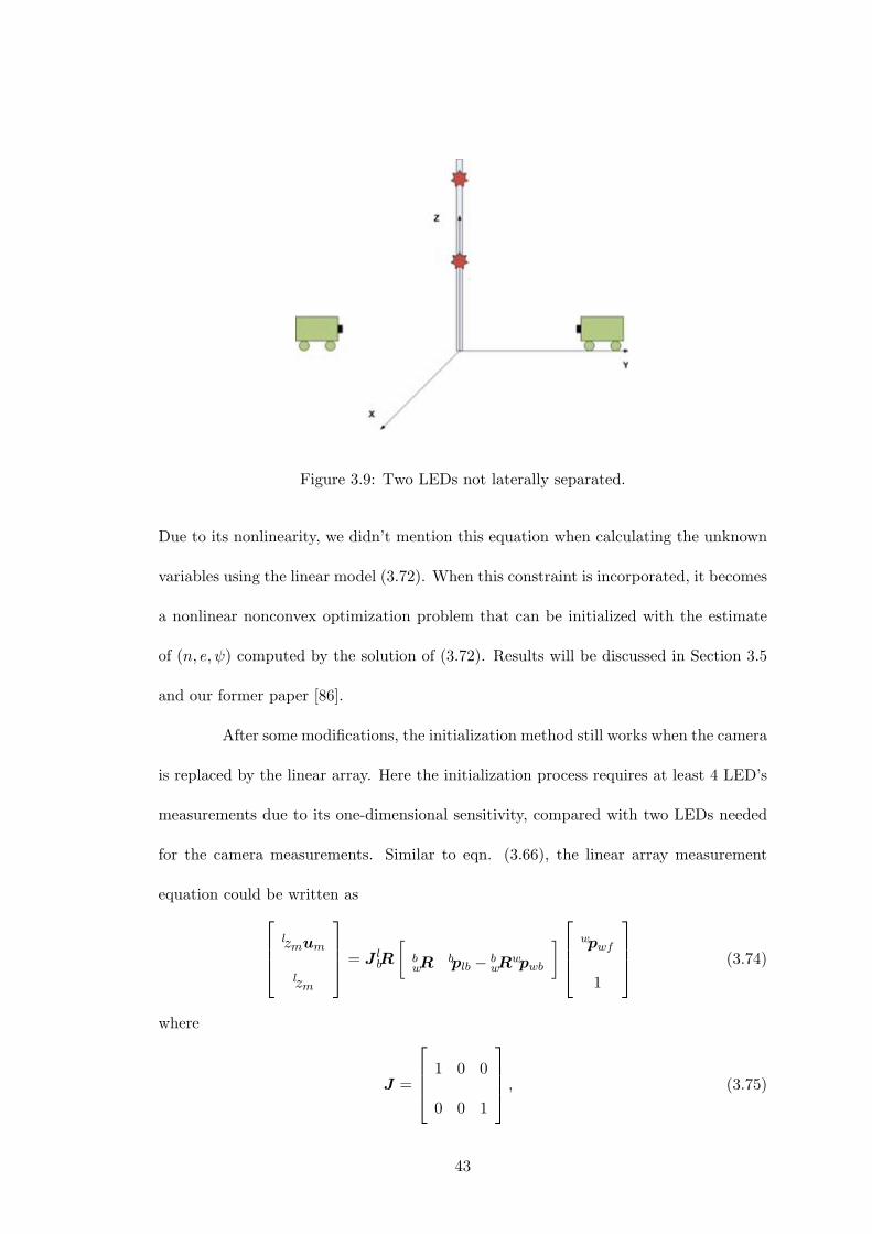
Figure 3.9: Two LEDs not laterally separated.
Due to its nonlinearity, we didn’t mention this equation when calculating the unknown
variables using the linear model (3.72). When this constraint is incorporated, it becomes
a nonlinear nonconvex optimization problem that can be initialized with the estimate
of (n, e, ψ) computed by the solution of (3.72). Results will be discussed in Section 3.5
and our former paper [86].
After some modifications, the initialization method still works when the camera
is replaced by the linear array. Here the initialization process requires at least 4 LED’s
measurements due to its one-dimensional sensitivity, compared with two LEDs needed
for the camera measurements. Similar to eqn. (3.66), the linear array measurement
equation could be written as lzmum
lzm
= J lbR
[bwR
bplb − bwR
wpwb
] wpwf
1
(3.74)
where
J =
1 0 0
0 0 1
, (3.75)
43

and um denotes the mth measurement. Reorganizing (3.74), we have
(r11a1m + r12a2m)p11 + (r11a2m − r12a1m)p12
+r11p14 + r12p24 − umlzm = −r13(a3m + bzlb) (3.76)
(r31a1m + r32a2m)p11 + (r31a2m − r32a1m)p12
+r31p14 + r32p24 − lzm = −r33(a3m + bzlb) (3.77)
where the definition of rij , ai and pij are same with that in eqn. (3.61) and (3.72).
For each LED measurement, we obtain two linear equations. Since lzm varies for dif-
ferent LED’s, to solve the linear equation set, at least 4 LED’s should be measured
simultaneously. Similarly, these 4 LEDs can not simultaneously have the same x and y
coordinates.
3.5 Results
The matrix He is the linearized matrix that evaluated at xke .
He = H1H3 (3.78)
H3 =
[∂lplf∂lqb
∂lplf∂bpbl
]∂lplf∂lqb
= Ψ(lqb,
bpbf − bpbl
)∂lplf∂bpbl
= −lbR. (3.79)
If several lED’s are measured simultaneously, He is constructed by stacking the He
calculated above together.
44

3.5.1 Extrinsic Parameters Calibration
Let φ represent the rotation from the computed frame l to the true frame l.
llR = I +
sinφ
φ[φ×] +
1− cosφ
φ2[φ×][φ×]
≈ I + [φ×]. (3.80)
Then we have lbR = l
lRlbR ≈ (I − [φ×])lbR. If we define δxe =
[δbpbl φ
]⊤, then
H3 =
[−lbR [lplf×]
].
Assuming N LED’s are measured by the linear array, and the initial covariance
of the extrinsic parameters is Pe0 ∈ R6×6, the Gauss-Newton correction is computed as
δxe =(H⊤g R
−1g Hg
)−1H⊤g R
−1g re, (3.81)
where
Hg =
[H⊤e1 · · · H⊤
eN I6×6
]⊤(3.82)
Rg = diag[R⊤
1 · · · R⊤N Pe0
] (3.83)
re =
[z1 − z1 · · · zN − zN xe0 − xe
]⊤(3.84)
10 20 30 40 50 60 70 80 90 100
−0.05
0
0.05
0.1
Experiment Number
p bl(1
) [m
]
True valueInitial valueCalibration value
(a) Estimated lpbl(1).
10 20 30 40 50 60 70 80 90 100
−0.05
0
0.05
0.1
Experiment Number
p bl(1
) [m
]
True valueInitial valueCalibration value
(b) Estimated lpbl(2).
10 20 30 40 50 60 70 80 90 100
−0.05
0
0.05
0.1
Experiment Number
p bl(1
) [m
]
True valueInitial valueCalibration value
(c) Estimated lpbl(3).
Figure 3.10: Estimated translation lpbl.
The first three figures show the calibration results of lpbl. The red and green
lines represent the standard deviation of the initial guess and calibration results, re-
spectively. To generate the result, 8 LED’s are measured by the linear array. The
45

experiment is repeated for 100 trials. In each trial, we randomly choose the initial guess
value according to its true value and covariance Pe0. In the figures, lpbl(3) representing
the height of linear array in the body frame is unchanged after the calibration process,
which is due to the pose of the linear array and its one-dimensional sensitivity.
10 20 30 40 50 60 70 80 90 100
82
84
86
88
90
92
94
96
98
100
Experiment Number
Rol
l [de
gree
]
True valueInitial valueCalibration value
(a) Estimated roll.
10 20 30 40 50 60 70 80 90 100−10
−5
0
5
10
Experiment Number
Pitc
h [d
egre
e]
True valueInitial valueCalibration value
(b) Estimated pitch.
10 20 30 40 50 60 70 80 90 100
85
90
95
100
Experiment Number
Yaw
[deg
ree]
True valueInitial valueCalibration value
(c) Estimated yaw.
Figure 3.11: Estimated Euler angles.
3.5.2 Initialization
We firstly test the initialization result using camera measurements. The vehicle
was placed at n = −0.575m, e = −2.046m and ψ ≈ 0.401 deg, which is known to an
accuracy of 0.002 m, 0.006 m and 0.002 deg, respectively. In this section, these coordinate
will be referred to as ‘correct.’ The vehicle is stationary at the stated location throughout
the results reported in this section. There are 8 LEDs in front of the vehicle (camera).
The LED navigation frame position vectors are listed in Table 3.1.
The initialization algorithm is firstly tested using different two-LED measure-
ment combinations to compute the state of the vehicle. The computed coordinates and
yaw angle computed using eqn. (3.72, 3.73) and their error standard deviation as com-
puted using eqn. (3.64) are given in Table 3.2, along with the LED identifiers. The
initialization state works well for all combinations with the exception of LED combi-
nations: (1,2), (3,4),(6,8). For each of the three combinations, both LED’s have the
46

Table 3.1: LED coordinates in meters in the NED frame.
LED ID n e d
1 2.797 -1.500 -1.500
2 2.797 -1.500 -2.000
3 2.797 -0.500 -2.000
4 2.797 -0.500 -1.500
5 2.797 -4.250 -2.000
6 2.797 -3.500 -2.000
7 2.797 -2.500 -2.000
8 2.797 -3.500 -1.500
same n and e coordinates differing only in their d coordinate. In this case, the line
that connects the two LED’s is parallel to the vehicle frame z-axis and the NED frame
d-axes. Such LED combinations cause the equations in (3.72) being linear dependent.
Due to this, the vehicle’s state can not be uniquely determined.
There are many combinations of three or more LED’s. Representative initial-
ization results using three and all eight LEDs are shown in Table. 3.3. The data in
these Tables confirms that the accuracy of initialization result depends on the number
and spatial distribution of the LEDs that are used.
Fig. 3.12 contains scatter plots of the computed vehicle coordinates (red dots)
for the 2 (top) and 3 (bottom) LED combinations. The blue asterisk (‘*’) marks the
coordinates considered to be correct. The positions computed using 3 LED’s are more
concentrated.
Next, we will show the initialization results using linear array measurements.
The correct vehicle state is approximately
[−2.5 0 −45
]⊤. The state is firstly
47

LED n e ψ σn σe σψ
1,2 NaN NaN NaN 3.7e+4 7.3e+3 1.2e+7
1,3 -0.432 -2.248 3.610 0.092 0.150 2.789
1,4 -0.416 -2.237 3.511 0.096 0.150 2.795
1,5 -0.565 -1.992 -1.325 0.055 0.114 1.756
1,6 -0.562 -2.002 -1.146 0.046 0.150 2.387
1,7 -0.558 -1.990 -1.328 0.033 0.261 4.362
1,8 -0.544 -1.872 -3.221 0.055 0.166 2.672
2,3 -0.513 -2.150 1.599 0.056 0.124 2.151
2,4 -0.517 -2.135 1.340 0.056 0.132 2.247
2,5 -0.568 -2.014 -1.052 0.030 0.069 1.034
2,6 -0.563 -2.030 -0.753 0.026 0.096 1.508
2,7 -0.558 -2.033 -0.664 0.025 0.185 3.096
2,8 -0.566 -1.976 -1.628 0.028 0.109 1.712
3,4 NaN NaN NaN 0.000 7.5e+17 0.000
3,5 -0.593 -2.031 -0.641 0.016 0.066 0.852
3,6 -0.584 -2.049 -0.329 0.016 0.075 1.064
3,7 -0.569 -2.077 0.160 0.030 0.090 1.434
3,8 -0.599 -1.965 -1.560 0.018 0.100 1.414
4,5 -0.600 -2.077 -0.061 0.020 0.092 1.190
4,6 -0.584 -2.082 0.119 0.017 0.093 1.324
4,7 -0.567 -2.091 0.361 0.030 0.099 1.565
4,8 -0.596 -1.969 -1.519 0.019 0.148 2.098
5,6 -0.465 -1.945 -2.750 0.084 0.122 2.165
5,7 -0.535 -1.990 -1.619 0.047 0.075 1.276
5,8 -0.419 -1.922 -3.447 0.113 0.135 2.569
6,7 -0.542 -2.017 -1.118 0.054 0.143 2.438
6,8 NaN NaN NaN 7.5e+11 0.000 0.000
7,8 -0.535 -1.964 -2.016 0.056 0.150 2.537
Table 3.2: initialization results using 2 LEDs
48

LED n e ψ σn σe σψ
1,2,3 -0.503 -2.164 1.873 0.050 0.107 1.889
1,2,4 -0.506 -2.146 1.573 0.050 0.113 1.962
1,3,5 -0.588 -2.014 -0.866 0.016 0.047 0.647
1,3,7 -0.564 -2.072 0.116 0.027 0.078 1.279
1,4,5 -0.588 -2.017 -0.843 0.019 0.056 0.781
1,4,8 -0.590 -1.988 -1.264 0.018 0.078 1.162
1,5,8 -0.583 -2.041 -0.612 0.038 0.085 1.328
2,3,4 -0.508 -2.136 1.453 0.055 0.116 1.999
2,3,8 -0.588 -2.014 -0.894 0.016 0.066 0.979
2,4,6 -0.578 -2.055 -0.271 0.016 0.065 0.960
2,5,7 -0.561 -2.004 -1.216 0.024 0.052 0.813
3,5,7 -0.590 -2.039 -0.550 0.014 0.042 0.590
3,5,8 -0.595 -2.059 -0.300 0.014 0.053 0.722
5,6,7 -0.524 -1.984 -1.767 0.042 0.070 1.208
6,7,8 -0.536 -2.007 -1.354 0.054 0.134 2.271
8LEDs -0.586 -2.036 -0.591 0.010 0.032 0.465
Table 3.3: Initialization results using 3 and 8 LEDs
−2.2 −2.1 −2 −1.9 −1.8 −1.7−0.65
−0.6
−0.55
−0.5
−0.45
−0.4
e (m)
n (m
)
(a) Initialization results using 2 LEDs.
−2.2 −2.1 −2 −1.9 −1.8 −1.7−0.65
−0.6
−0.55
−0.5
−0.45
−0.4
e (m)
n (m
)
(b) Initialization results using 3 LEDs.
Figure 3.12: Initialization results. The blue asterisk marks the location that is consideredto be correct.
49

computed according to the linear equations (3.76) and (3.77). The estimation results
are further refined by minimizing the residual using nonlinear optimization methods.
In these figures, the results are optimized using Gauss-Newton method. The error
covariance of the estimation result is also computed based on the covariance of the
linear array measurement noise.
10 20 30 40 50 60 70 80 90 100
−2.6
−2.55
−2.5
−2.45
−2.4
Experiment Number
n [m
]
True valueEstimated Init. valueStandare deviation
(a) Estimated n.
10 20 30 40 50 60 70 80 90 100
−0.08
−0.06
−0.04
−0.02
0
0.02
0.04
0.06
0.08
Experiment Number
e [m
]
True valueEstimated Init. valueStandare deviation
(b) Estimated e.
10 20 30 40 50 60 70 80 90 100
−46
−45.5
−45
−44.5
−44
Experiment Number
psi [
degr
ee]
True valueEstimated Init. valueStandare deviation
(c) Estimated ψ.
Figure 3.13: Initialization results.
50

Chapter 4
Data Recovery in a Stationary
Sensor
4.1 Introduction
LED’s are bright point light sources, the pixels that they project onto have
high intensity values. The LED projections are bright blobs and segmentations in the
image sensor and linear array, which are shown in Fig. 4.1. As the linear array platform
moves, the LED projection moves along the one-dimensional pixel array.
In the linear array-LED navigation system discussed in Chapter 3, each LED’s
ID was used to assist data association. Extracting the LED ID is equivalent to recovering
the LED’s on-off data pattern from a sequence of linear array measurements. The LED’s
on-off status can be recovered only after its position in each scan is found. Finding the
LED projection is not straightforward since: 1) There be multiple pixels measuring high
intensity (e.g., LED’s, clutter, and noise). The incorrect measurements are referred to as
false detections. 2) The position of a turned-off LED in the image can not be extracted
51

(a) Camera continuously takes images of a scene
with an LED light [31].
Time
(b) Linear array continuously scans a scene with
an LED light.
Figure 4.1: LED data in a sequence of photo-detector scans
by evaluating the intensity value of each pixel.
LED status recovery is a process that first identifies which measurement is
from each LED in each time step. A simple approach is, in each scan, to choose the
measurement that is closest to the predicted measurement position in a Mahalanobis
sense. This fails because the LED is off in some scans. Another method that avoids this
problem might use the probabilistic data association filter [10]. At each scan, it would
compute the probability of each association hypothesis (which one is from the LED or
none is from LED) and choose the most probable one. Though this method works,
there is a very low probability to obtain a correct ID, because correctly extracting an
ID requires that the data association in each time step of a scan sequence is correct,
which could be extremely hard especially when the ID is long.
To solve this problem, the measurements in a sequence of images need to be
considered jointly. The measurements of the same object (LED) at multiple time in-
stances should be matched together to recover the data sequence. However, the existing
descriptors for image features can not be applied to the linear array measurement, so
that they can not be used to match the measurements in different linear array scans.
52

More sophistic methods could be constructed within the framework of multiple hypothe-
ses tracking (MHT) [67, 9, 47]. MHT takes a deferred-decision approach in which they
maintain the complete set of possible data associations within a sliding window, putting
off hard decisions as long as possible [25]. The ultimate decision is made by evaluating
the probability of each sequence of data association hypothesis. Because the number
of possible sequences increases exponentially, this approach is expensive to implement,
especially for a system having fast frame rate.
To accurately and efficiently recover the LED status, we proposed a method
based on Viterbi algorithm [23, 77]. The Viterbi algorithm is a dynamic programming
algorithm that can be adapted to generate the most likely state path given a sequence
of observations. In this chapter, we focus on the typical case where the frame rate of the
linear array sensor is high relative to the array motion bandwidth. This implies that the
pixel projection changes smoothly from one frame to the next. With this assumption,
the LED projection on the linear array at current time step is highly dependent on
that in the former time step. This yields a Markov model representation. The Markov
property leaves opportunity to break the LED status recovery problem down into simpler
subproblems.
This chapter is organized as follows: Section 4.2 defines the state and linear
array measurement, and formulates the problem mathematically. Section 4.3.1 briefly
reviews the Viterbi algorithm. Section 4.3.2 and Section 4.4.2 analyze the state transi-
tion and measurement model, respectively. Section 4.4 shows the experimental results.
53

4.2 Problem Formulation
In this chapter, we use symbol χ instead of x to represent the kinematic state
of the rover. The new definition of symbol x in this chapter will be introduced in Sec.
4.2.3. The rover’s kinematic state χ evolves over time according to eqn. (3.1). The l-th
LED location Fl is put explicitly into the measurement model defined in (3.8), so the
LED’s projection is
z(t) = h(χ(t),Fl). (4.1)
Each LED is switching its “on” or “off” status to communicate information to the rover.
Given a time interval λ ∈ [ts, t], each projected LED position z(λ) defines a
trajectory across the linear array. Detection of the projected LED position depends
on the LED “on” or “off” status, as well as environmental conditions and interference
from other light sources. The accuracy of each LED’s recovered on-off status is highly
dependent on the accuracy of our knowledge of this LED trajectory. Therefore, the data
recovery and trajectory estimation problems are coupled. Improvement in the solution
of either problem enhances the solution of the other.
The purpose of this chapter is to develop an algorithm that simultaneously esti-
mates the most likely LED trajectory and data sequence for each time interval λ ∈ [ts, t].
The algorithm that we develop is general and independent of vehicle motion assump-
tions. To simplify algorithm implementation, we make the following assumption which
simplifies the pixel state transition model. Assume that the change in the projected
LED position is less that ϵ pixels per frame:
z(λ) ≤ FIϵ, ∀λ ∈ [ts, t], (4.2)
54

where FI is the frame rate. This is equivalent to
∂h
∂χχ ≤ FIϵ,∀λ ∈ [ts, t], (4.3)
which will allow derivation of a diagonally dominant transition matrix in Section 4.4.2.
4.2.1 Linear Array Measurement
In the former chapters, we have discussed the linear array measurement model.
Here we will introduce more details of the light intensity measurement for each pixel in
the linear array. A linear array measures the light intensity
Y (t) , yi(t)Ni=1
received by each of N pixels. Throughout this chapter, we use the counter i to indicate
the value associated with the i-th pixel. Pixels at the LED projection location have
higher intensity values when the LED is on. In this chapter, we threshold the intensity
values
ζi(t) =
1 if yi ≥ τ
0 otherwise,
(4.4)
to generate a set of candidate LED pixel positions:
Z(t) , zj(t)mtj=1, (4.5)
where mt is the total number of pixels whose intensity values are greater than the
threshold τ at time t, and zj(t) is the index of the jth “on” pixel. Note zj(t) ∈ [1, N ]
is an integer.
The pixel index zj represents a position in the linear array. A pixel in the
set Z(t) may be the projection of an “on” LED or a false detection due to noise or
55

50 100 150 200 250 3000
5
10
15
20
25
30
pixel index
valu
e
Figure 4.2: Linear array measurement
clutter. The other pixels (i /∈ Z(t)) may each be the projection of an “off” LED, a
missed detection, or a pixel onto which no LED projects.
Fig. 4.2 illustrates an original linear array scan (blue) and the processed mea-
surements (black). The threshold τ is graphed as the constant red curve. For the
processed measurements, each black dot is an element of the set Z defined in eqn. (4.5).
The value of black dots are set as 10 to be highlighted.
For theoretical convenience, an LED is assumed to project on only one pixel.
We also assume that other lights sources (clutter) and noise project independently to
each pixel. For example, a bright segment that is composed of n connected pixels will
be viewed as n independent measurements. Fig. 4.2 illustrates that these simplifying
assumptions are not strictly valid. Section 4.3.3 proves that the final result is insensitive
to the assumptions.
56

4.2.2 LED Measurement Prior
Our approach assumes a navigation system [22, 84, 85, 86] that maintains an
estimate χ(t) of the system state χ(t) in realtime. This system state estimate enables
prediction of the trajectory of each LED across the linear array. For example, the l-th
LED at location Fl, is expected to project to z(t) = h(χ(t),Fl) at time t. The covariance
of the projected LED position is Sl(t) = HPH⊤ +R where H is the Jacobean of h,
P is the prior covariance of χ(t), and R is the measurement noise covariance matrix.
Each of these quantities is computed by the navigation system for each LED.
Given time interval λ ∈ [ts, t], it is straightforward to compute both z(λ) and
Sl(λ). These quantities define the prior distribution for the LED trajectory that can
focus the algorithm. In the following presentation, we define ts = 0 and λ ∈ [0,K],
without loss of generality. We also will only consider a single LED; therefore, we drop
the l subscript.
4.2.3 LED State Definition
In the first linear array scan (i.e., t = 0), the predicted LED position z0
and its error covariance S0 are known. Define the detection range to be the inter-
val[⌊z0 − ρ
√S0⌋, ⌈z0 + ρ
√S0⌉
]where ⌊a⌋ and ⌈a⌉ represent the largest integer smaller
than a and the smallest integer larger than a, respectively. The parameter ρ determines
the probability that the actual LED projection is in the specified segment. For example,
setting ρ ≥ 3 yields the probability being greater than 0.997.
Given the assumption in eqn. (4.3), the sequence of detection intervals
[⌊zλ − ρ
√Sλ⌋, ⌈zλ + ρ
√Sλ⌉
]changes very little. Therefore, to find the most likely LED trajectory, it is sufficient to
57

focus on this smaller array segment, instead of the whole linear array. Effectively, this
decreases the search space and the computational requirements of the algorithm.
Assume there are N pixels in the detection range, and they are indexed from
left to right. The LED state space is
X(λ) ∈ X, where X , 1, 2, 3, . . . , N. (4.6)
LED state X(λ) = i means that the LED projects onto the i-th linear array pixel at
step λ. Fig. 4.3 illustrates the detection range and LED state.
Detection range
1 … ... j … ... N
state
… ...… ...
Linear array
Figure 4.3: LED state definition.
4.2.4 Problem Statement
Given a sequence of linear array thresholded measurement sets for λ ∈ [0,K]:
ZK = Z(λ)Kλ=1,
where Z(λ) is defined in eqn. (4.5), find the optimal state sequence XK = X(λ)Kλ=1
such that
X∗ = argmaxXK
p(XK | ZK
), (4.7)
58

where p(XK | ZK
)is the posterior probability mass function (PMF) of XK . Once X∗
is available, it is straightforward to extract the LED data sequence and to correct the
rover vehicle trajectory χ(λ).
4.3 Method
This section proposes a method to solve the problem defined in Sec. 4.2. This
method is based on the Viterbi algorithm [23, 77], which is a dynamic programming
algorithm that can be adapted to generate the most likely state trajectory (i.e., path)
given a sequence of observations. Sec. 4.3.1 reviews the Viterbi algorithm. Sec. 4.4.2
and Sec. 4.3.2 discuss the transition matrix and measurement model, respectively. Sec.
4.3.3 analyzes the influence of optical distortion that affects the width of the LED
projection and presents the path recovery algorithm.
4.3.1 Viterbi Algorithm
The Viterbi algorithm is described in Table 4.1. A brief review derivation is as
follows.
The probability of a state sequence Xt given the first t observation sets Zt is
p(Xt | Zt)
=1
cp(Xt, z(t) | Zt−1) (4.8)
=1
cp(z(t) | Xt,Zt−1)p(Xt | Zt−1) (4.9)
=1
cp(z(t) | x(t))p(x(t) | x(t− 1))p(Xt−1 | Zt−1) (4.10)
where c = p(z(t) | Zt−1). The derivation of eqn. (4.10) is possible due to two facts.
First, p(z(t) | Xt,Zt−1) = p(z(t) | x(t)) because the measurement depends only on the
59

Table 4.1: Viterbi algorithm
Input: observation sequence Zt
state prior probability p0
Output: the most probable state sequence Xt
1. Initialize V1,j
V1,j = p(z(1) | j) · p0(j)
2. Compute Vt,j from Vt−1,i, transition matrix A(t− 1) and z(t)
Vt,j = p(z(t) | j)maxiaij(t− 1) · Vt−1,i
3. Compute the t-th column of matrix Ptr. The value of Ptr(j, t) is state i that used to
compute Vt,j .
4. Retrieve the most likely state sequence
xt = argmaxj∈X(Vt,j)
xt−1 = Ptr(xt, t)
current state. Second, p(Xt | Zt−1) = p(x(t) | x(t − 1))p(Xt−1 | Zt−1) because the
state is a Markov process.
Let Vt,j be the probability of the most probable state sequence that has j as
its final state, given the first t observation sets. From eqn. (4.10), we have
Vt,j = maxXt−1
p(z(t) | j)p(j | x(t− 1))p(Xt−1 | Zt−1)
= p(z(t) | j)maxi
p(j | x(t− 1) = i) · Vt−1,i
= p(z(t) | j)maxi
aij(t− 1) · Vt−1,i, (4.11)
where aij(t−1) = p(j | x(t−1) = i) represents the probability of the transition of state
from i at time t− 1 to j at time t.
Given that the state space is discrete with maximum number of states N , this
60

state transition can be represented by the matrix
A(t) = [aij(t)] ∈ RN×N . (4.12)
Note that since the state at each time step t must go someplace at t + 1, we have the
constraint that∑N
l=1 ail(t) = 1. In this chapter, we ignore the case that the LED leaves
the field of view; however, this case can be accomodated by augmenting the matrix with
an additional row and column.
Eqn. (4.11) shows the scheme of computing Vt,j recursively. It is initialized by
equation V1,j = p(z(1) | j) · p0(j) where p0(j) is the prior probability of state j. To
recover the state path, define the pointer matrix
Ptr = [Ptr(j, t)] ∈ RN×K . (4.13)
Its total number of rows and columns represent the state space and the time steps,
respectively. The value of an entry in Ptr at j-th row and t-th column represents the
the state value at time step t−1 that belongs to the most probable state sequence ended
in state j at time step t. This can be shown using the following equation
Ptr(j, t) = argmaxi
aij(t− 1) · Vt−1,i. (4.14)
After constructing this matrix iteratively until time step K according to eqn. (4.11) and
(4.14) Then the most probable state path through time step t can be retrieved by
xt = argmaxj∈X
(Vt,j) and xt−1 = Ptr(xt, t). (4.15)
4.3.2 Probabilistic Model
The measurement set Z(t) contains two types of information: the total number
of pixels mt that are above threshold and their positions Z(t). That is:
Z(t) = Z(t),mt.
61

The probability of a measurement set Z(t) conditioned on the state x(t) = j can be
decomposed as
p (Z(t) | x(t) = j)
= p (Z(t),mt | x(t) = j)
= p (Z(t) | mt,x(t) = j)p (mt | x(t) = j) . (4.16)
The second term in eqn. (4.16) is the probability of there being mt detections in Z(t),
which does not depend on the LED pixel position j. Due to this fact, this term will not
affect the results achieved by the Viterbi algorithm, so only the first term need to be
considered when evaluating the measurement probability.
To compute the first term in eqn. (4.16), let the symbol θi(t) represent the
hypothesis that zi(t) is the measurement of the LED for i = 1, · · · ,mt and the symbol
θ0(t) represent the hypothesis that the LED is not detected. Using the total probability
theorem, the first term in the right hand side of eqn. (4.16) is decomposed as
p (Z(t) | mt, j) =
mt∑i=0
p (Z(t), θi(t) | mt, j) . (4.17)
For each term in the right hand side of eqn. (4.17), when i = 0 and j = zi(t) this
(physically) means that the LED is projected on pixel j, but that the measured LED
position is not pixel j; due to this contradiction, this probability has value 0. Eqn.
(4.17) can therefore be simplified to
p (Z(t) | mt, j) =
p(Z(t), θ0(t) | mt, j), j /∈ Z(t)∑
l∈0,ip(Z(t), θl(t) | mt, j), j = zi(t)
(4.18)
The notation j /∈ Z(t) represents that there is no element in the measurement set Z(t)
equaling j.
62

The right hand side of eqn. (4.18) is further decomposed as
p (Z(t), θi(t) | mt, j) = p (Z(t) | θi(t),mt, j)p (θi(t) | mt, j) . (4.19)
The first term is the probability of the measurement position distribution given the
hypothesis θi(t), state and number of measurements. It is reasonable to assume the
positions of measurements due to clutter or noise in set Z(t) are independently and
uniformly distributed in the detection space. When i = 0 in the first term of eqn. (4.19),
none of the measurements in set Z(t) is originated from the LED, so it is computed
according to
p (Z(t) | θ0(t),mt, j) =
mt∏j=1
1
N=
1
Nmt. (4.20)
When i = 0, one measurement say it zi(t) in the set Z(t) is originated from the LED
and the others are due to the noise, so it is decomposed as
p (Z(t) | θi(t),mt, j) =
∏j =i
1
N
· p (zi(t) | θi(t),mt, j) =1
Nmt−1. (4.21)
Combine these two cases together, the first term in eqn. (4.19) is computed by
p (Z(t) | θi(t),mt, j) =
1
Nmt , i = 0
1Nmt−1 , i = 0, j = zi(t)
(4.22)
The second term in eqn. (4.19) is the prior hypothesis probability given the
number of measurements and LED projection position are known. When i = 0, this
means the LED is not detected, so the LED must be “off”. When i = 0, this means the
LED is detected, so the LED must be “on”. The second term can be analyzed as
p (θi(t) | mt, j) =p (θi(t),mt | j)
p (mt | j)
=
1c′ (1− Pon)µF (mt), i = 0
1c′
1mtPonµF (mt − 1). i = 0
(4.23)
63

where normalized factor c′ = p (mt | j) is independent of the state j, Pon is the probabil-
ity that the LED is on, and µF (m) is the PMF of the number of clutter measurements.
Here we assume µF is a diffuse pmf [11], that is, all number of clutter measurements are
equally likely.
Substituting eqn. (4.17)-(4.23) into eqn. (4.16), after combining all constants
into c′ and significant simplification, the final expression is
p (Z(t) | j) =
1c′
1−PonN , j /∈ Z(t)
1c′
(1−PonN + Pon
mt
). j ∈ Z(t)
(4.24)
4.3.3 Effect of LED Image Width
Due to optical distortion and the non-zero LED size, both the LED and clut-
ter measurements may occupy more than one pixel. Actual LED projections will be
composed of several connected pixels whose intensity values may be greater than the
threshold. The elements in the measurement set Z(t) are no longer independent, since
some of them may belong to a same measurement. The assumptions made to derive
eqns. (4.22) and (4.23) are no longer valid. For example, the measurement set shown in
Fig. 4.2 is
Z(t) = 44 . . . 48, 231 . . . 235, 241 . . . 243, (4.25)
where there are three measurement clusters that contain a total of 13 pixels. The
measurements in each cluster are not independent. It is important to consider how the
violation of these assumptions affects the performance of the algorithm.
In Sec. 4.2.3, the state is defined as the true LED projection location on the
linear array, which causes no ambiguity when the LED occupies only one pixel. When
considering the nonzero LED intensity measurement width, the state is redefined to be
the center position of the LED projection on the linear array. This definition will not
64

contradict with the one in Sec. 4.2.3 when the optics are perfect. This new definition
does not influence the state transition matrix, to be defined in eqn. (4.29).
The measurement set Z(t) still has the definition as in eqn. (4.5). Its elements
are the pixel locations that have above threshold intensity values. Suppose that the mt
pixel locations in Z(t) form m′t clusters with the jth cluster containing nt,j pixels, so
that∑m′
tj=1 nt,j = mt. For a cluster composed of several pixels, each pixel of the cluster
can be viewed as the center of the LED projection. The definition of hypothesis θi(t) in
Sec. 4.3.2 is extended to be zi(t) is the center of the LED projection.
In eqn. (4.22), since the total number of measurements is m′t, there will be
only m′t independent terms. Eqn. (4.22) is modified as
p (Z(t) | θi(t),mt, j) =
1
Nm′t, i = 0
1
Nm′t−1
, i = 0, j = zi(t).
(4.26)
Similarly, eqn. (4.23) is modified as
p (θi(t) | mt, j) =
1c′′ (1− Pon)µF (m
′t), i = 0,
1c′′
1mtPonµF (m
′t − 1), i = 0.
(4.27)
Notice that the term 1/mt in the eqn. (4.27) is not replaced by 1/m′t when i = 0 The
reason is there are still mt (not m′t) candidates for the center of an LED that is “on”.
Combining all the constants into c′′, eqn. (4.24) becomes
p (Z(t) | j) =
1c′′
1−PonN , j /∈ Z(t),
1c′′
(1−PonN + Pon
mt
), j ∈ Z(t).
(4.28)
Notice that the only difference between eqn. (4.28) and eqn. (4.24) is the constant
term, which does not influence the most likely path final result. Table 4.2 summarizes
the LED path recovery algorithm.
65

Table 4.2: LED path recovery algorithm
Input: linear array measurements for t ∈ [0,K]
state prior probability p0 = N (x0,S0)
Output: the most probable state sequence XT
1. Find the detection range defined by the state prior p0[⌊x0 − ρ ∗
√S0⌋, ⌈x0 + ρ ∗
√S0⌉
]2. Extract the measurement sets defined in eqn. (4.5) for t ∈ [0,K]
3. Initialize V1,j in eqn. (4.11)
V1,j = p(z(1) | j) · p0(j)
4. Compute Vt,j using the transition matrix A(t− 1) and measurement model
defined in eqns. (4.29) and (4.16)
Vt,j = p(z(t) | j)maxi
aij(t− 1) · Vt−1,i
5. Assign values to the elements in the t-th column of matrix Ptr. The value
of Ptr(j, t) is the state i that used to compute Vt,j .
Ptr(j, t) = argmaxi
aij(t− 1) · Vt−1,i
6. Retrieve the most likely state sequence
xt = argmaxj∈X
(Vt,j)
xt−1 = Ptr(xt, t)
66
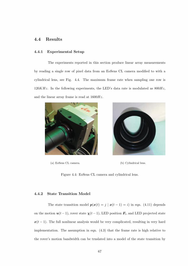
4.4 Results
4.4.1 Experimental Setup
The experiments reported in this section produce linear array measurements
by reading a single row of pixel data from an EoSens CL camera modified to with a
cylindrical lens, see Fig. 4.4. The maximum frame rate when sampling one row is
120KHz. In the following experiments, the LED’s data rate is modulated as 800Hz,
and the linear array frame is read at 1600Hz.
(a) EoSens CL camera. (b) Cylindrical lens.
Figure 4.4: EoSens CL camera and cylindrical lens.
4.4.2 State Transition Model
The state transition model p(x(t) = j | x(t − 1) = i) in eqn. (4.11) depends
on the motion u(t− 1), rover state χ(t− 1), LED position Fl, and LED projected state
x(t− 1). The full nonlinear analysis would be very complicated, resulting in very hard
implementation. The assumption in eqn. (4.3) that the frame rate is high relative to
the rover’s motion bandwidth can be trnslated into a model of the state transition by
67

assuming that the LED state has probability α ∈ (0, 1) of staying in its current state
and probability (1−α) of moving to an adjacent state in each sample instant. Ignoring
the issue of LED’s leaving the field-of-view, this means that the state transition matrix
of eqn. (4.12) is tri-diagonal:
A =
α 1− α 0 · · · 0 0
1−α2 α 1−α
2 · · · 0 0
0 1−α2 α · · · 0 0
......
.... . .
......
0 0 0 · · · α 1−α2
0 0 0 · · · 1− α α
. (4.29)
This matrix representation also assumes that the LED has identical probability moving
to either side. The state transition process defined by matrix A is illustrated by Fig.
4.5. The algorithm extends directly to state transition matrices that represent more
general motion models. In this implementation, the state transition probability α is set
as 1/3.
1 2 … ... j … ... N
a
1
2
a-
1 … ... j … ... Nj-1 j+1
1
2
a-step t-1
step t
Figure 4.5: State transition process defined in matrix A (4.29).
68

4.4.3 Stationary
The left image of Fig. 4.6 shows a series of stationary linear array measurements
as a single image. The linear array of greyscale pixel readings from any one time instant
is represented as a column of the image. This figure is formed by stacking a sequence
of linear array measurements together each as one column. The time sequence of array
measurements forms a matrix, shown as an image, with time increasing to the right along
the horizontal axis. Because the linear array is stationary, the communicating LED
always projects to essentially the same pixel array elements. The number of columns in
the image matrix is 300, corresponding to a time interval of 0.1875s. The right image
in Fig. 4.6 shows the binary image after thresholding. Notice the on-off alternation of
the LED and the noise in the figure.
Time step
Pixelindex
Figure 4.6: Stationary platform sequence of raw (left) and thresholded (right) lineararray measurement data represented as an image.
The Viterbi algorithm in Table 4.2 is implemented using the thresholded data
to calculate the probability of the most likely LED path ending at each pixel. The
results Vt,j are shown in the colored map at left image of Fig. 4.7, where brightness
69
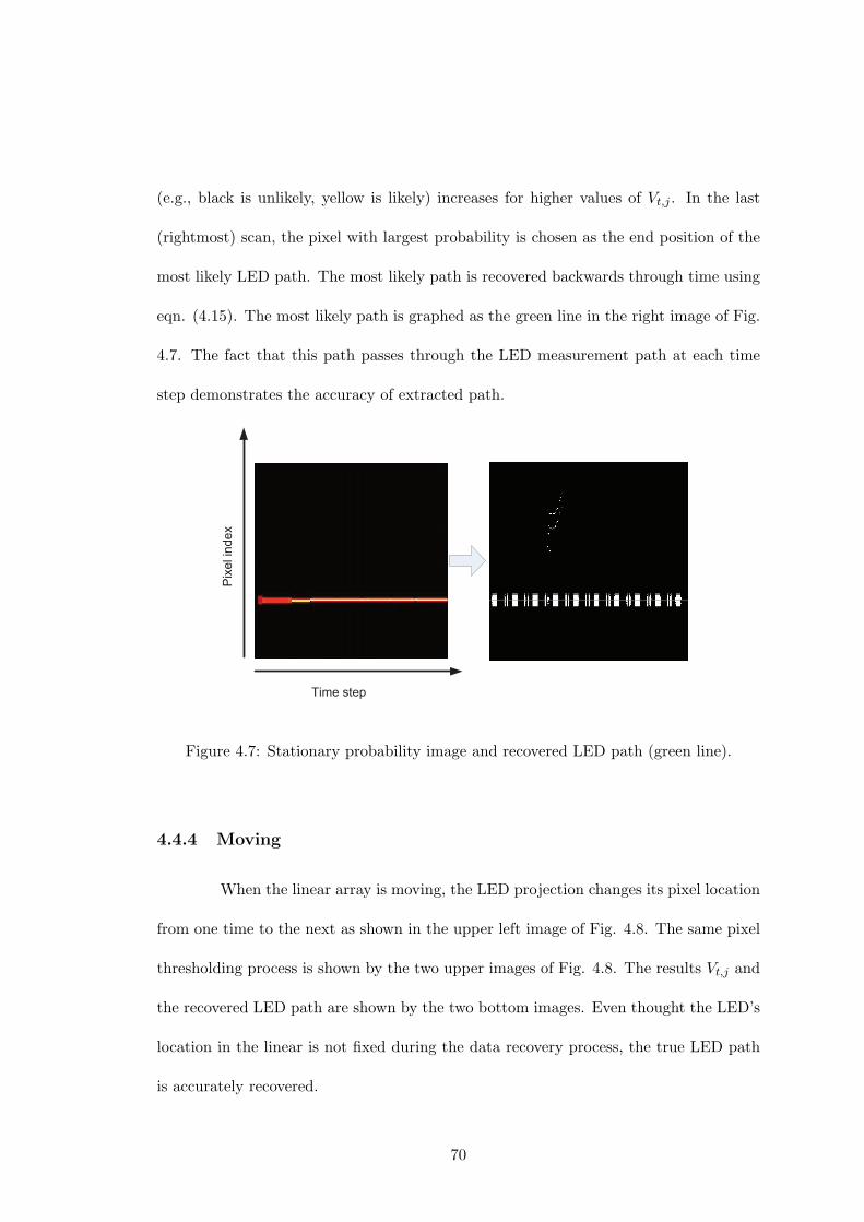
(e.g., black is unlikely, yellow is likely) increases for higher values of Vt,j . In the last
(rightmost) scan, the pixel with largest probability is chosen as the end position of the
most likely LED path. The most likely path is recovered backwards through time using
eqn. (4.15). The most likely path is graphed as the green line in the right image of Fig.
4.7. The fact that this path passes through the LED measurement path at each time
step demonstrates the accuracy of extracted path.
Time step
Pixelindex
Figure 4.7: Stationary probability image and recovered LED path (green line).
4.4.4 Moving
When the linear array is moving, the LED projection changes its pixel location
from one time to the next as shown in the upper left image of Fig. 4.8. The same pixel
thresholding process is shown by the two upper images of Fig. 4.8. The results Vt,j and
the recovered LED path are shown by the two bottom images. Even thought the LED’s
location in the linear is not fixed during the data recovery process, the true LED path
is accurately recovered.
70
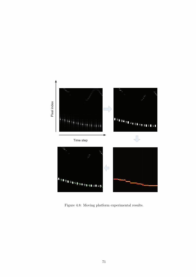
Time step
Pixelindex
Figure 4.8: Moving platform experimental results.
71

The LED signal is modulated to send a data sequence. The data sequence was
extracted without error after the path was recovered. The following Fig. 4.9 illustrates
the recovered data after the LED path is found.
Time step
Pixelindex
Figure 4.9: The LED data based on the recovered LED path.
72

Chapter 5
LED Data Recovery in a Moving
Sensor
5.1 Introduction
Chapter 4 introduces a Viterbi-based algorithm to recover the LED data in
the linear array when the linear array is stationary or moving with a bandwidth that
is low relative to the imaging rate. This algorithm evaluates the probability of LED
projections in a sequence of linear array measurements, and keeps the most probable
projection sequence ended in each pixel. Based on these kept projection sequences, the
most probable LED projection positions in the linear array sequence can be recovered
backwards. A problem of this algorithm is that it is hard to be applied to the two-
dimensional photo-detector such as camera. The enumeration and connection between
the pixels in the two-dimensional image is much more complicated than that in the linear
array, so the state transition matrix for the two-dimensional measurements may not be
diagonal any more and hard to define. Another problem of this Viterbi-based algorithm
is the moving bandwidth requirement. Even though the LED switching frequency can
73

be modulated up to hundreds of megahertz, sometimes we still prefer to utilize a low
rate sensor (i.e., 30Hz) such as a webcam or a cellphone camera to receive the data
using undersampling methods [68]. In such a case, the assumption for the algorithm in
Chapter 4 is no longer valid. Due to the above facts, more general and robust algorithm
should be developed to recover the LED data in the photo-detector.
To solve this problem, we follow the idea in Chapter 4 to consider the mea-
surements in a sequence of images jointly. The measurements of the same object (LED)
at multiple time instances should be matched together to recover the data sequence.
For image measurements, the features in different images can be tried matched by com-
paring their descriptors. Multiple existing corner detectors (Moravec [55], Forstner [24],
Harris [30], Shi-Tomasi [72], and FAST [70]) or blob detectors (SIFT [52], SURF [12],
and CENSURE [2]) can be used to match the projections of the same feature in differ-
ent two-dimensional images. These detectors keep the description of each feature and
these descriptions can be compared to determine whether multiple features are origi-
nated from the same object. However, there is still probabilities that incorrect pairs are
matched or multiple measurements in the same image are matched to the same feature.
This incorrect matches happen more frequently when measurements in a relative long
sequence of images (hundreds of images) are to be matched instead of only two images,
like the case of recovering LED data. In typical vision aided navigation systems, usually
only measurements in two consecutive image are to be matched. If multiple measure-
ments in another image are matched to one measurement in the current image, these
measurements would be ignored to prevent incorrect matches. If we follow the same
strategy to extract the LED data, there would be a low probability to obtain a correct
data sequence, so that both the navigation and communication will become unreliable.
Moreover, the existing feature descriptors can not be applied to the linear array mea-
74

surement, so that they can not be used to match the measurements in different linear
array scans. All the analysis above indicate that accurately and reliably recovering the
LED data sequence merely by the image processing techniques is not enough.
5.1.1 Multiple Hypothesis Data Association
Multiple detections existing within the search area results in a multiple hy-
pothesis data association problem [21]. This data association problem could be solved
by choosing the measurement that is closest to the predicted measurement position in
Mahalanobis sense, see [53]. Among other issues, this method does not work in this
application, as it fails in the presence of noise or clutter when the LED is off. Another
method that accounts for the null hypothesis (the LED is off) can be implemented using
the probabilistic data association filter, as in [10]. Though this method works in theory,
there is a very low probability to obtain a correct data sequence when it is long.
More sophistic methods can be developed using MHT methods, see [67, 9, 47].
MHT uses a deferred-decision approach in which they maintain the complete set of pos-
sible data associations within a sliding window, putting off hard decisions as long as
possible, see [26]. Decisions are made by evaluating the probabilities of each sequence of
data association hypotheses. Since the number of possible sequences increases exponen-
tially, it is expensive to keep all of them. It is also inefficient to compute the probabilities
of all possible sequences and then discarding most of them. To solve these problems, an
efficient Hypothesis Oriented MHT (HOMHT) was firstly proposed in [17]. The basic
idea of this method is to keep only the q best sequences, discarding the other sequences
that have low probability.
All the above data recovery techniques require the information from the nav-
igation system. The motion measurements provide additional constraints for matching
75

objects at different time instances. Accurate navigation enables both efficiency of which
LED ID’s to expect for and where each LED is expected to be in the image. For both
the camera and linear array, the LED’s unique ID would facilitate the task of feature
association, which is a limiting factor to the use of more generic non-LED features. Mea-
surement confirmation is straightforward using the extracted and expected ID. From all
the analysis above, we can again conclude that the communication and navigation ap-
plications are synergistic.
5.2 Problem Formulation
As discussed in Sec. 4.2, given a time interval λ ∈ [ts, t], the projected position
of the l-th LED zl(λ) defines a trajectory across the photo-detector. Detection of the
projected LED position depends on the LED “on” or “off” status, as well as environ-
mental conditions and interference from other light sources. The accuracy of each LED’s
recovered on-off status is highly dependent on the accuracy of the data association at
each time step. Therefore, the data recovery and trajectory estimation problems are
coupled. Improvement in the solution of either problem enhances the solution of the
other.
The purpose of this chapter is to develop an algorithm that simultaneously
estimates the most likely data association sequences and rover state over each time
interval λ ∈ [ts, t]. Without loss of generality, we define ts = 0, and the pixel array
is sampled at times tk = kT ∈ [ts, t] for k = 0, 1, · · · ,K. After the data association
step, and the validity of the LED data and therefore the association is established, the
validated sequence of measurements zl(tk) will be referred to aiding measurements and
used to correct the estimated state trajectory.
76

5.2.1 Predicted Measurement Region
Given the state estimate at time step k, it is straightforward to compute both
the predicted measurement position of the l-th LED zl(k) and its error covariance Sl(k)
according to eqn. (3.9) and (3.12). The quantities zl(k) and Sl(k) define a prior distribu-
tion for the LED trajectory that can focus the algorithm. A region in the measurement
space for the l-th LED can be defined as
Vl,γ(k) , z : (z − zl(k))⊤S−1
l (k)(z − zl(k)) ≤ γ
= z : rl(k)⊤S−1
l (k)rl(k) ≤ γ, (5.1)
where rl(k) = z(k) − zl(k) is the residual and γ is a parameter that determines the
probability that the real measurement falls in Vl,γ(k). For the camera measurement,
the region Vl,γ(k) represents the interior of an ellipse at each time k. For the linear
array measurement, the region Vl,γ(k) represents the interior of a segment at each time
k, respectively. In the following, without loss of generality, we only consider a single
LED in its predicted region Vl,γ ; therefore, we drop the l subscript. The parameter γ is
selected using a χ2-distribution table.
5.2.2 Data Association Hypothesis
Let mk ≥ 0 denote the number of detected LED like features in the predicted
region Vγ(k) at time k, where zj(k) for j ∈ [0,mk] denotes projected location of the j-th
measurement hypothesis. Define the measurement set at time step k as
Z(k) , zj(k)mkj=1. (5.2)
Note that at most one of them originated from the LED. The others are false detections
due to noise, interference, or clutter. Since each or none of the measurements in this
77

set could be originated from the LED, the number of data association hypotheses is
(mk + 1).
Suppose there are total of K time steps, the state estimates x(k)Kk=1 and
their error covariance matrices PkKk=1 are calculated using eqns. (3.2) and (3.7).
Then the predicted region at each time step is calculated by eqns. (3.9, 3.12, 5.1), and
the measurements that fall into Vγ are extracted. Define
Zk , Z(l)kl=1andUk , u(l)kl=1 (5.3)
as the set of measurements and inputs up to time step k, respectively. Since there are
a total of K time steps, the number of joint data association hypotheses is
LK =
K∏k=1
(mk + 1). (5.4)
Each data association sequence defines a LED trajectory across the detector, which in
turn decodes a sequence of detection and nondetection events into a bit sequence con-
taining an ID, checksum, data, etc. The total number of time steps K in the algorithm
is a parameter selected by the designer. It choice depends on the length (number of
bits) of each LED data package and the sampling rate of photo-detector. If the length
of LED data package is ld and the sampling rate is ns times of the data rate, the total
number of time steps K is at least (ns ld). Only after the LED status is recovered at
each time instant in the sequence of K measurements, can the LED data be extracted.
Fig. 4.1(b) a sequence of linear array measurements. Both the variation of the LED
projected position due to rover motion and the on-off status of the LED due to the data
sequence can be clearly seen.
Let θk,ℓ represent a specific list of joint data association hypotheses up to time
step k. The superscript ℓ ∈ [1, Lk] is the numeration index for the hypothesis sequence.
78

Each hypothesis θk,ℓ has the form
θk,ℓ = j1, j2, · · · , ji, · · · , jk, (5.5)
where ji ∈ [0,mi]. When θk,ℓ(i) = j > 0, it represents that at time step i the j-th
measurement originated from the LED. When θk,ℓ(i) = 0 it represents that at time step
i none of the measurements has originated from the LED. We say the joint hypothesis
θk,ℓ is an extension of θk−1,s, if
θk,ℓ = θk−1,s, jk,
where θk,ℓ(k) = jk ∈ [0,mk]. In this nomenclature, θk−1,s is the parent hypothesis of θk,ℓ.
Herein, the indices ℓ and s in the superscript of θ are not necessarily identical, since the
two hypotheses are enumerated independently at different time steps. Note that each
joint data association hypothesis corresponds to a potentially distinct posterior vehicle
trajectory.
5.2.3 Technical Problem Statement
Given the measurement set ZK , we would like to find the most probable joint
data association hypotheses (i.e. q-best hypotheses θK,ℓqℓ=1). After these hypotheses
are found, their corresponding ID sequences are straightforward to recover. By compar-
ing each of the recovered ID’s with the predicted ID, the most probable data association
hypothesis with correct ID is found and used both for data extraction and the navigation
state update. The advantage of finding the q-best hypotheses instead of only the most
probable one is that having several candidate hypotheses yields a higher probability to
recover the correct ID.
The problem is stated as: Given measurements ZK and navigation system
inputs UK , find the q-best joint data association hypotheses θK,ℓqℓ=1 among the total
79

number of LK hypotheses, where q-best means the q hypotheses that maximize the
hypothesis posterior probability.
5.3 MHT-based LED Data Recovery Method
This section evaluates the posterior probability mass function (PMF) of a joint
data association hypothesis up to time step k. The analysis follows the method in [67]
while adding details to clarify the measurement quantity information. Here we make
an assumption that the measurements due to clutter are uniformly distributed in the
predicted region Vγ .
5.3.1 Hypothesis Probability
The joint probability of an association hypothesis up to time step k ∈ [1,K]
can be decomposed as
p(θk,ℓ | Zk,Uk−1
)(5.6)
=1
cp(Z(k) | θk,ℓ,Zk−1,Uk−1) p(θk,ℓ | Zk−1,Uk−1)
where the normalization factor c = p(Z(k) | Zk−1,Uk−1
)is independent of the data
association hypothesis θk,ℓ. The decomposition on the right hand side of eqn. (5.6) is
based on Bayes Rule. The last term on the right hand side can be further simplified by
application of the general multiplication rule of conditional probability
(i.e., p(A,B) = p(A | B)p(B)):
p(θk,ℓ | Zk−1,Uk−1)
= p(θk,ℓ(k), θk−1,s | Zk−1,Uk−1)
= p(θk,ℓ(k) | θk−1,s,Zk−1,Uk−1)p(θk−1,s | Zk−1,Uk−1).
Combining the last equation above with eqn. (5.6) yields the final desired result:
p(θk,ℓ | Zk,Uk−1
)=
1
cp(Z(k) | θk,ℓ,Zk−1,Uk−1) (5.7)
80
p(θk,ℓ(k) | θk−1,s,Zk−1,Uk−1)p(θk−1,s | Zk−1,Uk−2
)
When analyzing this joint probability, we have to take notice of the measure-
ment quantity information mk = miki=1 which is not explicitly represented in eqn.
(5.7). In [8], this quantity information mk is considered to be part of the measurement
set Zk, while in [67] it is viewed to be in the hypothesis set θk,ℓ. The results given by
the two approaches are identical except for a scale factor p(mk
)that is independent of
θk,ℓ, which can be seen from
p(θk,ℓ,mk | Zk,Uk−1
)= p
(θk,ℓ | Zk,mk,Uk−1
)p(mk
).
We use the later approach in the following analysis, so that Zk and Z(k) will only
contain the measurement position information.
The first term in the right hand side of eqn. (5.7) is the joint prior probability of
the current position measurements given the data association hypotheses, measurements
and inputs of all the previous time steps. The measurements in Z(k) are independent
because they come from different sources, potentially one from the LED and the others
from clutter, etc. Because the different measurements in set Z(k) are independent, this
term decomposes as
p(Z(k) | θk,ℓ, Zk−1, Uk−1)
=
mk∏j=1
p(zj(k) | θk,ℓ, Zk−1, Uk−1) =
mk∏j=1
f(j). (5.8)
Note that the measurement quantity mk is considerred to be known when evaluating the
probability of measurement set Z(k) in eqn. (5.8). The measurements due to clutter or
false alarms are assumed to be uniformly distributed in the predicted region, while the
81

one from the LED is assumed to be corrupted by Gaussian noise. Therefore, we have
f(j) =
1Vk
for clutter,
N (zj(k); zs(k), Ss(k)) for the LED,
(5.9)
where Vk is the volume (area) of the predicted region Vγ(k), and N (zj(k); zs(k), Ss(k))
is the Gaussian distribution evaluated at zj(k) with expectation zs(k) and covariance
Ss(k).
Because θk,ℓ is an extension of θk,ℓ−1 as defined by eqn. (5.2.2), the conditioning
variables allow the distributions in eqn. (5.8) to be written as
mk∏j=1
p(zj(k) | θk−1,s, jk, Zk−1, Uk−1).
The variable jk and the index j determine the form of fj as defined in eqn. (5.9). The
variables θk−1,s, Zk−1, Uk−1 are the prior information used to compute xs(k − 1), zs(k)
and Ss(k), where the superscript s indicates its corresponding hypothesis θk−1,s, which
are computed based on eqns. (3.2)-(3.12) with measurement updates implemented by
an optimal estimator (e.g., Kalman filter). More details of computing zs(k) and Ss(k)
for a specific example are discussed in Sec. 5.4.
Substituting eqn. (5.9) into (5.8), the first term of (5.7) is
p(Z(k) | θk,ℓ, Zk−1, Uk−1)
=
1
Vmkk
for θk,ℓ(k) = 0
N (zj(k);zs(k),Ss(k))
Vmk−1
k
for θk,ℓ(k) = 0
(5.10)
The second term of eqn. (5.7) is the prior probability of the current association
82
hypothesis θk,ℓ(k) conditioned on θk−1,s, Zk−1, and Uk−1. This term is computed as
p(θk,ℓ(k) | θk−1,s, Zk−1, Uk−1)
=
(1− Pon)µλVk(mk) for θk,ℓ(k) = 0,
1mkPonµλVk(mk − 1) for θk,ℓ(k) = 1 · · ·mk,
(5.11)
where Pon is the probability that the LED is on, and µF is the PMF of the number of
false measurements due to clutter or noise. The existence of term µλVk is due to the
measurement quantity information mk in θk,ℓ(k). When θk,ℓ(k) = 0, all the measure-
ments in the predicted region are not from the LED, so the LED is off. We do not
consider the case of the missing detections. When θk,ℓ(k) = 0, the hypothesis is that
the LED is on and that it is associated with a specific measurement in the predicted
region. Because the distribution is not conditioned on the current position measurement
Z(k), when evaluating this prior probability, each measurement has equal probability
(i.e., 1/mk) to be the correct one.
The number of measurements due to clutter and false alarms is modeled as a
Poisson process [67, 9], so its distribution function µF at time step k is
µλVk(ϕ) = exp−λVk (λVk)ϕ
ϕ! . (5.12)
The parameter λ represents the spatial density of noise measurements. The term λVk is
the expected number of noise measurements in the predicted region (i.e., E⟨mk⟩ = λVk).
In some applications, the parameter λ is unknown. A common solution [9] is to use the
true number of measurements mk to replace its expected value, λVk, in eqn. (5.12).
This results in the nonparametric model of µmk . Note that in this special case it can
be shown that µmk(mk) = µmk(mk − 1).
Let βk,ℓ = p(θk,ℓ | Zk,Uk−1) denote the posterior PMF of θk,ℓ in eqn. (5.7).
83

Substituting eqn. (5.10) - (5.12) into eqn. (5.7) and combining the constants into c′,
the probability is
βk,ℓ =
1c′λ(1− Pon)β
k−1,s for θ(k) = 0
1c′N
k−1,s(zj(k))Ponβk−1,s for θ(k) = j = 0,
(5.13)
where N k−1,s(zj(k)) = N (zj(k); zs(k),Ss(k)), and c′ = c · eλVk ·mk! · λ1−mk . If using
the nonparametric model of µF , the probability is
βk,ℓ =
1c′′mkVk
(1− Pon)βk−1,s for θ(k) = 0
1c′′N
k−1,s(zj(k))Ponβk−1,s for θ(k) = j = 0,
(5.14)
where c′′ = c · V mk−1k ·mk. Eqn. (5.13) or (5.14) shows how to compute the probability
of joint data association incrementally.
From eqn. (5.13), the marginal likelihood function for the hypothesis that the
j-th measurement at time step k has originated from the LED is
Ls,j(k) = N k−1,s(zj(k))Pon, (5.15)
and the marginal likelihood function for the hypothesis that no measurement at time
step k is from the LED is
Ls,0(k) = λ(1− Pon). (5.16)
Therefore, the probability that hypothesis θ(k) = j is the extension of joint hypothesis
θk−1,s is
p(θ(k) = j | Zk, θk−1,s,Uk−1) =Ls,j(k)∑mki=0 Ls,i(k)
. (5.17)
84

5.3.2 Hypothesis for Multiple LEDs
When there are Nk (Nk > 1) LEDs predicted in the image or linear array at
time step k, the data association hypothesis at this single step θ(k) becomes a Nk tuple.
Assuming the number of measurements at the i-th LED’s predicted region is mi,k, the
number of hypothesis at a single step will be
ℓk =
Nk∏i=1
(mi,k + 1) . (5.18)
For total of K time steps, the number of joint data association hypotheses LK becomes
LK =
K∏k=1
ℓk. (5.19)
Comparing eqn. (5.19) with (5.4), the total number of hypothesis is greatly increased for
multiple LEDs measurements. The measurement set Z(k) at step k contains Nk subsets,
and the i-th subset is denoted by symbol Zi(k). Their relations can be explained by the
following equations:
Z(k) , IDi(k),Zi(k)Nki=1 (5.20)
Zi(k) , zi,j(k)mi,kj=1 , (5.21)
where IDi(k) represents the ID index of subset Zi(k). The definition in eqn. (5.21) is
similar to that in eqn. (5.2) where the subscript i is omitted due to single LED.
After redefining the hypothesis and measurement set, the probability of the
hypothesis could be analyzed identical to eqn. (5.7). However, the calculation of the
first and second terms in eqn. (5.7) are different due to multiple LEDs. Different from
85

eqn. (5.8), the first term is decomposed as
p(Z(k) | θk,ℓ,Zk−1,Uk−1) =
Nk∏i=1
p(Zi(k) | θk,ℓ,Zk−1,Uk−1)
=
Nk∏i=1
mi,k∏j=1
p(zi,j(k) | θk,ℓ,Zk−1,Uk−1)
=
Nk∏i=1
mi,k∏j=1
f(i, j). (5.22)
Similar to eqn. (5.9), the function f(i, j) is calculated by
f(i, j) =
1Vi,k
for clutter,
N (zi,j(k); zsi (k),S
si (k)) for i-th the LED,
(5.23)
where Vi,k is the volume of the i-th LED’s predicted region at time step k, and zsi (k) and
Ssi (k)) are the i-th LED’s predicted position and error covariance matrix. Substituting
(5.23) into (5.22), the first term is computed by
p(Z(k) | θk,ℓ,Zk−1,Uk−1)
=Vi1,k · · ·Vir,k
Vm1,k
1,k · · ·V mNk,kNk,k
r∏h=1
N (zθih (k)(k); zsih(k),S
sih(k)) (5.24)
where θih(k) = 0 for h = 1 . . . r. The second term in eqn. (5.7) is computed as
p(θ(k) | θk−1,s,Zk−1,Uk−1)
=1
mi1,k · · ·mir,kP ron(1− Pon)
Nk−rµF (mk − r). (5.25)
5.3.3 q-best Hypotheses
From eqn. (5.4), the total number of possible hypotheses grows exponentilly
with the time step K, while only one of them is correct. Computing the probability of
all possible hypotheses and then discarding most of them is inefficient. To over come
this problem, it is preferable to only compute those hypotheses having relatively high
probability. This is reasonable since the correct hypothesis (LED path) should be always
86

among the most probable hypotheses. An efficient method to implement this approach
was first introduced in [17]. The basic idea of this method is, at each time step, to only
keep the q-best hypotheses, discarding the hypotheses that have lower probability. This
method employs Murty’s algorithm [57] to find the j-th best hypothesis solution.
Given the q-best hypotheses θk−1,iqi=1 and their corresponding probabilities
βk−1,iqi=1 up to the former step k−1, and measurement set Z(k) at current time step k,
the new q-best hypotheses θk,iqi=1 up to the current time step will be generated. Define
θk−1,i to be the parent hypothesis of θk,j , if the latter is the extension of the former.
Choosing the single hypothesis jk at time step k, θk,∗ = θk−1,i, jk is one possible
extension of θk−1,i, where ‘*’ is replaced by an integer to enumerate the extensions. The
best extension of θk−1,i is
θk,i1 = θk−1,i, jk where jk = argmaxj
Li,j(k). (5.26)
The notation i1 in the superscript of θk,i1 means that this hypothesis is the most probable
extension of θk−1,i. The best extension corresponds to the hypothesis having maximum
marginal likelihood.
The following text describes the implementation details of the approach in [17].
To generate the q-best joint hypotheses up to current time step k, the first step is for
each hypothesis θk−1,i to generate its best extension according to eqns. (5.15–5.16) and
(5.26). These new joint hypotheses are ordered according to their probabilities and
stored in the ordered list HYP-LIST. Their probabilities are calculated according to
eqn. (5.13) and stored in PROB-LIST. The second step is for each hypothesis in HYP-
LIST to use its parent hypothesis to generate the j-th (j = 2, 3, · · · ) best extension. If
the probability of this extension is higher than the lowest probability in PROB-LIST,
add it to HYP-LIST and the corresponding probability to PROB-LIST, and delete the
87

hypothesis with lowest probability from HYP-LIST and its corresponding probability
from PROB-LIST. If the probability of this extension is lower than the lowest probability
in PROB-LIST, stop generating new extensions by its parent hypothesis. After these
processes conclude, the algorithm has produced the q-best hypotheses up to current
time step. The algorithm is described in Table 5.1.
Note the factor N k−1,s(zj(k)) in eqn. (5.13) is the Gaussian distribution eval-
uated at zj(k) with expectation zs(k) and covariance Ss(k). The process of computing
the two parameters zs(k) and Ss(k) is discussed in Section 5.3.4.
5.3.4 Hypothesis: Computed Quantities
As we mentioned in Sec. 5.2, the rover state estimation and the LED path
recovery are coupled. When computing the probability of each LED path hypothesis
from eqn. (5.13), the algorithm also computes various other useful items as illustrated
in (5.27):
xs+(k − 1)
P s+k−1
⇒
xs−(k)
P s−k
⇒
zs(k)
Ss(k)
(5.27)
At time step k− 1, we have the posterior state estimate xs+(k− 1) and error covariance
matrix P s+k−1 of each hypothesis θk−1,s where s = 1, · · · , q. The ‘+’ in the superscript
indicates a posterior estimate. The ‘−’ in the superscript indicates a prior estimate. The
first arrow in (5.27) represents the state and covariance temporal propagation processes
generating the prior quantities at time k for hypethesis s. The state and error covariance
are temporally propagated using eqns. (3.2) and (3.6). The second arrow in (5.27)
represents the (prior) measurement prediction process using eqns. (3.9) and (3.12).
88

Table 5.1: q-best hypotheses algorithm
Input: q-best hypotheses up to former time step θk−1,iqi=1
the corresponding probabilities βk−1,iqi=1
the corresponding state estimate xiqi=1
current measurement set Z(k)
Output: q-best hypotheses up to current time step θk,iqi=1
and their corresponding probabilities βk,iqi=1
1. Initialize HYP-LIST and PROB-LIST
HYP-LIST, θk,i1qi=1
θk,i1 , θi,1(k), θk−1,i
θi,1(k) = argmaxθ(k)
p(θ(k) | Zk, θk−1,s, Uk−1)
2. Sort the hypotheses in HYP-LIST according to their probabilities
3. for i = 1 : q
If the j-th best new hypothesis generated by θk−1,i is still in
HYP-LIST, then generate its (j + 1)-th best new hypothesis.
If the probability of the new hypothesis is higher than the lowest
probability in PROB-LIST, then add it into the list and delete
the hypothesis with the lowest probability.
If not, break.
end
89

Here these processes are repeated for each hypothesis in set θk−1,sqs=1.
The probability of new hypothesis θk−1,s, j can be evaluated after computing
N k−1,s(zj(k)). Using the algorithm presented in Sec. 5.3.3, the new q-best hypotheses
up to current time step k are selected. Given each new hypothesis, for which j = 0, its
posterior state estimate is updated according to the standard EKF measurement update
process:
x+(k) = x−(k) + P−k H
⊤k S
−1(zj(k)− z(k)) (5.28)
P+k = P−
k − P−k H
⊤k S
−1HkP−k (5.29)
If j = 0, there is no measurement due to LED at current time step k; therefore, the
posterior state estimate will be identical to the prior.
5.4 Vehicle Trajectory Recovery
This section derives the specific details of the presented approach for a land
vehicle example that will be fully developed with application results presented in the
next section.
5.4.1 Motion Sensor Model
For a land vehicle moving on a 2D plane (i.e., building floor), the rover nav-
igation state vector can be defined as x =
[n e ψ
]⊤, where n, e represent the
2D position coordinates in the navigation frame, and ψ represents the rover’s yaw angle
(heading). The (Dubbin’s vehicle [20]) kinematic model is
n = cos(ψ)u, e = sin(ψ)u, ψ = ω. (5.30)
90

The linear velocity u and angular rate ω can be computed as
u = 12(RLϕL + RRϕR), ω = 1
L(RLϕL − RRϕR), (5.31)
where ϕL and ϕR denote the radian angular rates of rotation of each wheel and R are the
wheel radii estimates. The quanitities ϕL and ϕR can be accurately computed based on
encoder measurements so that eqn. (5.30) can be accurately computed in discrete-time,
see Chapter 9 in [22].
The wheel radii errors are modeled as Gauss-Markov processes:
δRL = −λLδRL + ωL, δRR = −λRδRR + ωR, (5.32)
where the choice of time constant 1/λL and PSD of ωL are discussed in Sec. 9.2 in
[22]. The augmented state vector is x = [n, e, ψ,RL, RR]⊤. With the error state vector
defined as
δx = [δn, δe, δψ, δRL, δRR]⊤ , (5.33)
91

the error model is
δx = F δx+Gν where (5.34)
F =
0 0 − sin(ψ)u˜ϕL cos(ψ)
2
˜ϕR cos(ψ)
2
0 0 cos(ψ)u˜ϕL sin(ψ)
2
˜ϕR sin(ψ)
2
0 0 0 1L˜ϕL − 1
L˜ϕR
0 0 0 −λL 0
0 0 0 0 −λR
G =
RL cos(ψ)2
RR cos(ψ)2 0 0
RL sin(ψ)2
RR sin(ψ)2 0 0
1LRL − 1
LRR 0 0
0 0 1 0
0 0 0 1
ν =
[ωϕL ωϕR ωL ωR
]⊤. (5.35)
The derivation of matrices F and G with encoder measurements can be found in Ap-
pendix B. The encoder measurement noises are ωϕL and ωϕR .
When the rover moves freely in 3D space, its motion information can be mea-
sured by inertial sensors such as IMU (inertial measurement unit). The IMU measures
the rover’s acceleration a and angular velocity ω in three directions of the body frame.
The state vector can be defined as x =[np⊤, nv⊤, bnq
⊤, b⊤a , b⊤g
]⊤to represent the po-
sition, velocity, rotation, and biases of acceleration and angular rate. The kinematic
model using the measurements from IMU can be described by
np = nv, nv = na, bn˙q = 1
2Ω(ω)bnq
ba = ωba , bg = ωbg
92

The IMU measurements are modeled as
a = Rq(na− ng + 2⌊ωn×⌋nv + ⌊ωn×⌋2np) + ba + ωa (5.36)
ω = ω +R(bnq)ωn + bg + ωg, (5.37)
where R(·) denotes the rotation matrix, and ωn is the rotation vector of the navigation
frame with respect to the Earth centered inertial frame (ECI), and ng is the gravity
represented in the navigation frame, and ωa and ωg are the measurement noise.
The state estimate propagates according to
n˙p = nv (5.38)
n ˙v = R⊤ˆq a− 2⌊ωn×⌋nv − ⌊ωn×⌋2np+ ng (5.39)
bn˙q = 1
2Ω(ω)bnˆq,˙ba = 0,
˙bg = 0 (5.40)
where a = a − ba and ω = ω − R(bnq)ωn − bg. The error state is defined as x =[δnp⊤, δnv⊤, δθ⊤, δb⊤a , δb
⊤g
]⊤, where δθ represent the rotation from the computed frame
b to the true frame b. Its model has the same structure as (3.3) with the following matrix
format.
F =
03×3 I3 03×3 03×3 03×3
−⌊ωn×⌋2−2⌊ωn×⌋ −R⊤ˆq⌊a×⌋ −R⊤
ˆq03×3
03×3 03×3 −⌊(ω +R ˆqωn)×⌋03×3 −I3
03×3 03×3 03×3 03×3 03×3
03×3 03×3 03×3 03×3 03×3
(5.41)
G =
03×3 03×3 03×3 03×3
−R⊤ˆq
03×3 03×3 03×3
03×3 −I3 03×3 03×3
03×3 03×3 I3 03×3
03×3 03×3 03×3 I3
, ν =
ωa
ωg
ωba
ωbg
.
93

The derivation of matrices F and G with IMU measurements can be found in Appendix
C.
5.4.2 Photo-Detector Model
When using a camera to measure the LEDs, each LED projection in the image
is a bright blob. The camera measurement model is described by eqn. (3.21) and (3.22)
in Chapter 3. The camera measurement error model is defined in Sec. 3.2.3 of Chapter
3 with linearized measurement matrix derived in eqn. (3.31). The camera measurement
error model is
δz = Hδx+ n
= −J cnR δnp+ J c
bR ⌊bpbL×⌋ δθ + n (5.42)
where
J =1cz
1 0 − cxcz
0 1 −cycz
, (5.43)
where δnp is the position error vector of which the only nonzero components are δn and
δe. The symbol δθ represents the attitude error vector for which the only nonzero term
is δψ. Therefore, with the IMU error state as defined in eqn. (5.33), the camera aiding
H matrix is
H = J
[−cnR(:, 1 : 2) c
bRJψbpbL 03×2
](5.44)
Jψ =
0 1 0
−1 0 0
0 0 0
. (5.45)
The linear array measurement contains only half of the information in camera
measurement, effectively only providing the u measurement defined in (5.44). Therefore,
94

its measurement model is
z = cx/cz + n, (5.46)
where cx and cz have the same meaning with that in (3.21).
5.5 Results
In the experiment, we use a rover equipped with wheel encoders and a camera
to test and demonstrate the algorithm. Encoder based navigation is discussed in Chapter
9 of [22]. The rover implements a trajectory tracking controller which is a (nonadaptive)
version of the command filtered backstepping approach described in the example section
of [19]. The rover moves in a 5m×5m area with eleven LEDs mounted on the four walls
at known locations. The position of the rover in the navigation frame is represented by
the vector np = (n, e, d) where d = 0. Encoders attached to each rear wheel measure
the wheel rotation, which allows computation of the rover speed u and angular rate w.
The origin of the body frame is the center of the axle connecting the two rear wheels.
The camera’s position bpbl and pose cbR relative to the body frame are calibrated off-line.
The parameter γ in eqn. (5.1) is selected such that the probability that the residual
falls within Vl,γ is 0.997.
5.5.1 Stationary
This section considers the case that the rover is stationary while the camera or
linear array is detecting the LEDs. The rover is put close to position np = (−0.5, 0, 0)
with rotation angle ψ = 0o, so the prior estimate of the rover state is x0 = [−0.5, 0, 0]⊤.
95

5.5.1.1 Camera
Since the inputs from encoders are zero, the estimate of the vehicle state re-
mains unchanged prior to incorporating the camera measurements. At any time instant,
for the current vehicle pose, only some of the LEDs will be within the field-of-view of
the camera. An example of the predicted LED positions with error covariance ellipse
projected onto the image plane is illustrate in Fig. 5.1. The resolution of the image is
640 × 512. We can see that only two LEDs are predicted to be in the image for the
current rover state.
A time sequence of camera measurements is illustrated in Fig. 5.2. These
measurements are extracted by thresholding the pixel intensities within each LED’s
predicted region. The green stars are the predicted LED positions at each time step
based on the rover state estimate. The magenta crosses are the detected measurements.
We can see from this figure that multiple measurement candidates exist in both of the
predicted LED regions.
At the k-th measurement time step, the detected potential LED projection
locations that fall into the detection region are enumerated and stored in the mea-
surement set Z(k) defined in eqn (5.3) of Section 5.2.2. The detection region is the
minimum rectangle containing the predicted ellipse. The upper left image of Fig. 5.3
shows the detected and predicted measurements along with the prior uncertainty ellipse
at time t = 0. Since there are two detected measurements in the detection region of
LED 1 and no measurement in the detection region for LED 0, accounting for the null
hypotheses, three data association hypotheses will be generated. Using each data asso-
ciation hypothesis to update the state estimate and then repredict the LED projection
96

0 100 200 300 400 500 600
0
50
100
150
200
250
300
350
400
450
500
LED 0LED 1
u(pixel)
v(pi
xel)
Figure 5.1: Predicted LEDs’ positions in the image plane based on the prior informationof the rover state: Predicted positions (green stars), 3-σ error ellipse regions (red)
location based on each hypothesis, the results are shown in the upper right image of
Fig. 5.3. The blue “∗” symbol represents the predicted LED projection location after
updating the state by a hypothesis, and the corresponding blue ellipse represents shows
its uncertainty. Note that the two null hypotheses have left the state estimate and its
uncertainty unchanged, so they are identical to the prior and each other. The single
measurement hypothesis has corrected the state according to its hypothesis and reduced
the uncertainty. The bottom right image of Fig. 5.3 shows the predicted LED projection
locations at the second measurement time t = 0.05s with two detected measurements
for LED 0 and four detected measurements for LED 1. At each time step, only the first
q = 10 most probable hypotheses are kept and shown in the bottom left image by their
corresponding posterior predicted LED locations and error ellipses.
The final navigation state estimation results for each hypothesis are shown in
97

0 1 2 3
250
300
350
u (p
ixel
)
0 1 2 3130
135
140
145
v (p
ixel
)
time (sec)
(a) LED 0
0 1 2 3
60
80
100
120
140
160
180
u (p
ixel
)
0 1 2 3
130
135
140
145
150
v (p
ixel
)
time (sec)
(b) LED 1
Figure 5.2: Camera measurements of LED 0 and LED 1 in the first few seconds: Pre-dicted LED positions (green stars), 3-σ error regions (red), LED measurements (magenta“+”).
98

0 100 200 300 400 500 600
100
120
140
160
180
200
LED 0LED 1
u(pixel)
v(pi
xel)
0 100 200 300 400 500 600
100
120
140
160
180
200
LED 0LED 1
u(pixel)
v(pi
xel)
0 100 200 300 400 500 600
100
120
140
160
180
200
u(pixel)
v(pi
xel)
LED 0LED 1
0 100 200 300 400 500 600
100
120
140
160
180
200
u(pixel)
v(pi
xel)
LED 0LED 1
Figure 5.3: The measurements and hypotheses at the first two steps.
99

Fig. 5.4. The estimation results for the q = 10 different hypotheses are shown in different
colors. Fig. 5.5 is revised version of Fig. 5.2 where we have changed the coloring of the
measurements that have been selected as the most probable hypothesis sequence from
magenta to blue.
The q = 10 data sequences shown below are recovered for LED 0 whose true
ID is 00000000. When sending the ID, each LED will add a 4-bit header 1010
in the front and another 4-bit checksum in the back. For the correct data sequence,
the checksum is 1010. In this experiment, the camera works at a frame rate twice
of the LED data rate, which means that each bit is recovered from two consecutive
sampled images. The symbols “∗” in the sequences indicates that this bit could not
be determined due to different recovered statuses in the corresponding two consecutive
steps. The numbers to the right of each sequence are the normalized probabilities. From
these sequences, we will find the second one is the most probable correct data sequence.
∗0000000001010101000000000101010, p = 0.24,
10000000001010101000000000101010, p = 0.16,
10000000001010101000000000101010, p = 0.13,
∗0000000001010101000000000101010, p = 0.08,
00000000001010101000000000101010, p = 0.07,
∗000000000 ∗ 010101000000000101010, p = 0.06,
∗0000000001010 ∗ 01000000000101010, p = 0.06,
∗000000000101010 ∗ 000000000101010, p = 0.06,
∗000000000101010100000000010 ∗ 010, p = 0.06,
∗0000000001010101000000000 ∗ 01010, p = 0.06,
100

0 0.5 1 1.5 2 2.5 3−0.6
−0.58
−0.56
−0.54
−0.52
−0.5
−0.48
−0.46
−0.44
−0.42n
(m)
0 0.5 1 1.5 2 2.5 3−0.1
−0.05
0
0.05
0.1
e (m
)
0 0.5 1 1.5 2 2.5 3−3
−2
−1
0
1
2
3
ψ (
degr
ee)
time (sec)
Figure 5.4: Estimation results associated with each hypothesis sequence.
101

0 1 2 3
250
300
350
u (p
ixel
)
0 1 2 3130
135
140
145
v (p
ixel
)
time (sec)
(a) LED 0
0 1 2 3
60
80
100
120
140
160
180
u (p
ixel
)
0 1 2 3
130
135
140
145
150
v (p
ixel
)
time (sec)
(b) LED 1
Figure 5.5: Camera measurements with the most probable selection of the measurementsat each time step.
102

5.5.1.2 Linear Array
The predicted LED position and error covariance in the linear array are il-
lustrate in Fig. 5.6. The green stars are the predicted LED positions and the red
parentheses are its uncertainty interval.
0 100 200 300 400 500 600
LED 0LED 1
u(pixel)
Linear array
Figure 5.6: Predicted LEDs’ positions and their uncertainty intervals in the linear array.
Similar to the process of camera measurements in Fig. 5.3, the process to
generate new hypotheses by linear array measurements is illustrated in Fig. 5.7.
0 100 200 300 400 500 600
Linear array
u(pixel)
LED 0LED 1
0 100 200 300 400 500 600
Linear array
u(pixel)
LED 0LED 1
Figure 5.7: The linear array measurements and the new hypotheses.
The estimation result of each hypothesis using linear array measurements is
shown in Fig. 5.8. The estimation result of each hypothesis is more disperse than the
result of camera due to less informative measurements.
Fig. 5.9 shows the linear array measurements at each time step and the ones
103

0 0.5 1 1.5 2 2.5 3
−0.55
−0.5
−0.45
−0.4
n (m
)
0 0.5 1 1.5 2 2.5 3−0.1
−0.05
0
0.05
0.1
e (m
)
0 0.5 1 1.5 2 2.5 3−3
−2
−1
0
1
2
3
ψ (
degr
ee)
time (sec)
Figure 5.8: Estimation results associated with each hypothesis sequence using lineararray measurements.
104

(blue “+”) selected by the most probable hypothesis.
0 0.5 1 1.5 2 2.5 3
250
300
350
time (sec)
(a) LED 0
0 0.5 1 1.5 2 2.5 3
60
80
100
120
140
160
180
time (sec)
(b) LED 1
Figure 5.9: Linear array measurements with the most probable selection of the mea-surements at each time step.
5.5.2 Moving
5.5.2.1 Camera
When the vehicle is moving, the outputs from motion sensors (i.e. encoders)
help to maintain an accurate state estimate for navigation and which enables accurate
prediction of the LED projection locations in the image. Since the encoder measurements
do not perfectly reproduce the rover speed and angular rate, the state error covariance of
the prior state as well as the residual covariance both grow with time. An example set of
actual and predicted LED location measurements at each time step are illustrated in Fig.
5.10. After applying the data recovery algorithm, the most probable data sequence with
the correct ID is illustrated at blue “+”. The process of generating the new hypotheses
at one time step is illustrated in Fig. 5.12. The left and right images illustrate the
predicted LED positions and their error covariances based on the prior and posterior
state estimate, respectively. In this figure, all the measurements are not selected by
105

these most probable hypotheses. The prior and posterior state estimates associate with
each hypothesis are shown in Fig. 5.11.
0 1 2 3
300
400
500
600
u (p
ixel
)
0 1 2 3
110
120
130
140
v (p
ixel
)
time (sec)
(a) LED 0
0 1 2 3
100
150
200
250
300
350
400
u (p
ixel
)
0 1 2 3
130
135
140
145
150
155
v (p
ixel
)
time (sec)
(b) LED 1
Figure 5.10: Coordinates of LED 0 and LED 1 in the image plane: Predicted LEDpositions (green stars), 3-σ error regions (red), LED measurements (blue “+”), noiseand clutter measurements (magenta “+”).
The following are the recovered data sequences of LED 0 for each hypothesis
when the rover is moving. The second one is the most probable and correct data
sequence. Note that several data sequences are identical, which doesn’t not mean their
hypothesis sequences are same since different choices may result in the same recovered
106

0 0.5 1 1.5 2 2.5 3
−0.55
−0.5
−0.45
−0.4
−0.35
−0.3n
(m)
0 0.5 1 1.5 2 2.5 3
−0.1
−0.05
0
0.05
e (m
)
0 0.5 1 1.5 2 2.5 3−45
−40
−35
−30
−25
−20
−15
−10
−5
0
ψ (
degr
ee)
time (sec)
Figure 5.11: Estimation results associated with each hypothesis: State estimates onlyby motion sensors (green), standard deviation (red), and posterior state estimates ofeach hypothesis (other colors).
107

0 100 200 300 400 500 600
100
120
140
160
180
200
u(pixel)
v(pi
xel)
LED 0
LED 1
(a) Prior prediction.
0 100 200 300 400 500 600
100
120
140
160
180
200
u(pixel)
v(pi
xel)
LED 0
LED 1
(b) Posterior prediction.
Figure 5.12: Prior prediction (left) and posterior prediction of each hypothesis (right).
data.
∗0101010000000001010101000000000, p = 0.23,
10101010000000001010101000000000, p = 0.21,
∗01010100000000010 ∗ 0101000000000, p = 0.12,
∗010101000000000101010 ∗ 000000000, p = 0.10,
∗0101010000000001010101000000000, p = 0.06,
∗0101010000000001010101000000000, p = 0.06,
10101010000000001010101000000000, p = 0.06,
∗0101010000000001010101000000000, p = 0.05,
10101010000000001010101000000000, p = 0.05,
10101010000000001010101000000000, p = 0.05,
5.5.2.2 Linear Array
The estimation result when the rover is moving is shown in Fig. 5.14. Compare
with Fig. 5.8, the estimation results are very close, which also proved accuracy of
108

estimating 2D state using linear array measurements. Fig. 5.13 shows the linear array
measurements at each time step and the ones (blue “+”) selected by the most probable
hypothesis.
0 0.5 1 1.5 2 2.5 3250
300
350
400
450
500
550
600
time (sec)
(a) LED 0
v0 0.5 1 1.5 2 2.5 3
100
150
200
250
300
350
400
time (sec)
(b) LED 1
Figure 5.13: Linear array measurements with the most probable selection of the mea-surements at each time step when the rover is moving.
109

0 0.5 1 1.5 2 2.5 3
−0.55
−0.5
−0.45
−0.4
−0.35
−0.3n
(m)
0 0.5 1 1.5 2 2.5 3
−0.1
−0.05
0
0.05
e (m
)
0 0.5 1 1.5 2 2.5 3
−40
−30
−20
−10
0
ψ (
degr
ee)
time (sec)
Figure 5.14: Estimation results associated with each hypothesis sequence using lineararray measurements when the rover is moving.
110

Chapter 6
Conclusion and Future Work
6.1 Conclusion
Many personnel, equipment, and vehicular applications would have enhanced
performance given more accurate knowledge of their location. LED light and signaling
is in its infancy, offering unique dual use opportunities. Due to their high switching
rates, which enables communication of unique ID’s, compared with other vision-based
navigation method, the detection and feature association sub-problems are more easily
and reliably solved for LED features.
This dissertation has discussed various aspects of the communication and nav-
igation using LED features. For the camera sensor, we demonstrate that the vehicle
confined to move in the 2D-plane can be initialized by measuring at least two LEDs, as
long as the vector joining the two LED’s is not parallel to the world frame D-axis. With
the initialization algorithm, no prior knowledge is required about the vehicle state and
the EKF can be robustly and accurately initialized. When this rover is equipped with
wheel encoders, the observability analysis shows that at least two LEDs are enough to
ensure the observable of the navigation state.
111

To overcome the problem of low frame rate of normal camera, a new sensor is
proposed that could simultaneously receive signals from LED’s at a high rate and enable
accurate navigation. This sensor combines a linear array, a convex-cylindrical lens and
the shutter together to form a one-dimension photo-detector. The convex-cylindrical
lens will focus the light that passes through onto a line instead of a point, so that the
linear array preserves the sensitivity to angle of arrival relative to a single axis. Its
one-dimension sensitivity increases the difficulty of the extrinsic parameter calibration
and state initialization. An offline calibration method is proposed in this dissertation.
The state initialization method is also analyzed. We also analyzed the observability of
the navigation system and proved that at least two LED’s with different xf and yf must
be measured to have full observability of the vehicle state.
When using the photo-detector array (camera or linear array) to communicate
with blinking LEDs, it is necessary to track the LED status in the sensor to extract
the data. Two methods have been developed in this dissertation to solve the problem
of accurately and efficiently extracting a data sequence. The first one is applicable to
the situation when the data communication rate is high relative to the bandwidth of
the moving platform so that the LED pixel projection changes little from one frame to
the next. This approach is based on the Viterbi algorithm. The presentation included
analysis and discussion of the necessary probability models, transition matrix, and mea-
surement model. We also proved that the LED projection image size does not influence
the final result. The results in Sec. 4.4 show the performance of this algorithm.
When the rover motion bandwidth is significant relative to the frame rate, the
position of LED in the linear array can change significantly from one frame to the next.
The assumption for the Viterbi-based algorithm is no longer valid. Another problem of
this algorithm is that it is hard to be applied to the two-dimensional photo-detector such
112
as camera. The enumeration and connection between the pixels in the two-dimensional
image is much more complicated than that in the linear array, so the state transition
matrix for the two-dimensional measurements may not be diagonal anymore and hard to
define. A second method is developed to overcome the above problems. This method is
based on multiple hypothesis tracking, which tries to find the most probable candidate
measurements at each time step instead of recover the LED positions in the sensor.
The presentation included analysis and discussion of the hypothesis probability model
and measurement model, and the experimental results both for camera and linear array
measurements.
6.2 Future work
LED-based navigation and optical communication offer future synergistic per-
formance improvement opportunities. In Chapter 3, we proposed a new sensor by com-
bining a linear array and a cylindrical lens. DSP (digital signal processing) hardware
will also be designed to sampling and process the data collected by the linear array to
further improve the sampling and processing efficiency. The observability of the nav-
igation equipped with a linear array and wheel encoders are analyzed when the rover
moves in the 2D plane. Future research will consider the case that the rover can move
freely in the 3D space. The wheel encoders could be replaced by the inertial measure-
ment unit (IMU) to measure the acceleration and rotation. Lots of more issues should be
considered for this linear array-IMU system including its observability and initialization.
Chapter 4 has focused on processing of a single thresholded LED. Future work
will consider the approaches suitable for either multiple LED projections or multiple
simultaneous hypotheses. Algorithms incorporating the measured intensity could also
113

be of interest. Finally, knowledge of the most likely LED image path provides useful
information for correcting the rover trajectory over the corresponding time window.
Chapter 5 gives a more accurate data recovery algorithm based on MHT. The
situation when a measurement can fall into multiple LEDs’ uncertainty ellipse is not
considered. This is illustrated in Fig. 6.1 for linear array measurements. Future work
will consider the approach that associates the measurements to multiple LEDs’ jointly.
When multiple LED’s data associations are jointly considered, each LED’s data associa-
tion hypothesis at a time step not only depends on its own former association hypotheses,
but also other LEDs’ association hypotheses. This could greatly increase the complex-
ity of the assignment of the measurements to the LED’s. This could be addressed by
efficient assignment algorithms such as Auction [13] and JVC algorithm [37].
Figure 6.1: Linear array with one candidate measurement (yellow) falls into both thepredicted region of two LEDs.
Another problem that should be considered in the future is the missing de-
tection of LEDs. The proposed LED data recovery algorithm in this paper focuses on
114

solving the problem of LED false detections. As we mentioned in Sec. 5.3, the case
of missing detection of LEDs is not considered. However, due to various reasons, both
the camera and linear array may not detect the LEDs in the predicted region when
the LED is “on”. When the missing detection happens but not considered properly,
inaccurate data will be recovered. Future work should also consider the LED passing
in and out of the field of view. Chapter 4 and 5 both use the prior state estimate to
calculate the measurement uncertainty region. This uncertainty region is considered to
be fully contained in the image or linear array, which is not always true in practice. If
this happens, some noise measurements or the LED measurement itself may be lost by
merely processing the part of the predicted region that falls into the image or linear
array. This is even more complicated than the case of missing detection.
Both the LED data recovery algorithms introduced in this dissertation requires
extracting the whole ID data sequence firstly in order to judge them later based on the
expected ID sequence later. In practice, it is not necessary to obtain the whole length of
ID to determine whether it is valid. For example, assume that the frame rate is two time
of the LED data rate, then the recovered status sequences are wrong if their “on” or
“off” do not appear in pairs. This fact could greatly help delete the incorrect hypothesis
sequences, so that computation will not be wasted on these incorrect ones. Future work
should consider how to take advantage of these hypothesis pruning methods.
Besides the algorithms introduced in this dissertation, random sample consen-
sus (RANSAC) is another choice for solving this data recovery algorithm. The advantage
of using RANSAC is that more accurate data recovery as well as the rover state estimate
may be obtained. The reason is that RANSAC estimates the parameters (rover states)
simultaneously by all the measurements in the consensus set, which is similar to the
update process of smoothing algorithms. The set of observations is ZK . The consensus
115

set should be modified to contain at most one measurement at each time step for each
LED. Instead of fitting a trajectory that has as many as inliers, the objective should be
modified to search for the most probable trajectory.
Data transmission using multiple colors [31] provides other methods to separate
the LEDs from clutter or noise. LEDs can change their colors easily by modulating the
driving signal. When the data is sent by LED’s colored light, extracting the LED data
will be very different from the algorithms in this dissertation. Data transmission using
patterns should also be considered in the future work. Higher data rate can be achieved
when transmitting patterns, but more complicated image processing technique is also
required to accurately extract the pattern in the image.
116

Bibliography
[1] Mostafa Z Afgani, Harald Haas, Hany Elgala, and Dietmar Knipp. Visible lightcommunication using ofdm. In Testbeds and Research Infrastructures for the De-velopment of Networks and Communities, 2006. TRIDENTCOM 2006. 2nd Inter-national Conference on, pages 6–pp. IEEE, 2006.
[2] Motilal Agrawal, Kurt Konolige, and Morten Rufus Blas. Censure: Center surroundextremas for realtime feature detection and matching. In Computer Vision–ECCV2008, pages 102–115. Springer, 2008.
[3] A. Ansar and K. Daniilidis. Linear pose estimation from points or lines. PatternAnalysis and Machine Intelligence, IEEE Transactions on, 25(5):578–589, 2003.
[4] S. Arai, S. Mase, T. Yamazato, T. Yendo, T. Fujii, M. Tanimoto, and Y. Kimur.Feasible study of road-to-vehicle communication system using LED array and high-speed camera. 15th World Congress on IT, 2008.
[5] Shintaro Arai, Shohei Mase, Takaya Yamazato, Tomohiro Endo, Toshiaki Fujii,Masayuki Tanimoto, Kiyosumi Kidono, Yoshikatsu Kimura, and Yoshiki Ninomiya.Experimental on hierarchical transmission scheme for visible light communicationusing led traffic light and high-speed camera. In Vehicular Technology Conference,2007. VTC-2007 Fall. 2007 IEEE 66th, pages 2174–2178. IEEE, 2007.
[6] Ashwin Ashok, Marco Gruteser, Narayan Mandayam, Jayant Silva, Michael Varga,and Kristin Dana. Challenge: mobile optical networks through visual mimo. InProceedings of the sixteenth annual international conference on Mobile computingand networking, pages 105–112. ACM, 2010.
[7] Bo Bai, Gang Chen, Zhengyuan Xu, and Yangyu Fan. Visible light positioningbased on led traffic light and photodiode. In Vehicular Technology Conference(VTC Fall), 2011 IEEE, pages 1–5. IEEE, 2011.
[8] Yaakov Bar-Shalom. Tracking and data association. Academic Press Professional,Inc., 1987.
[9] Yaakov Bar-Shalom, Sam S Blackman, and Robert J Fitzgerald. The dimensionlessscore function for multiple hypothesis decision in tracking. In Systems, Man andCybernetics, IEEE International Conference on, 2005.
[10] Yaakov Bar-Shalom, Fred Daum, and Jim Huang. The probabilistic data associationfilter. Control Systems Magazine, IEEE, 29(6):82–100, 2009.
117
[11] Yaakov Bar-Shalom, X Rong Li, and Thiagalingam Kirubarajan. Estimation withapplications to tracking and navigation: theory algorithms and software. John Wiley& Sons, 2004.
[12] Herbert Bay, Tinne Tuytelaars, and Luc Van Gool. Surf: Speeded up robust fea-tures. In Computer Vision–ECCV 2006, pages 404–417. Springer, 2006.
[13] Dimitri P Bertsekas. The auction algorithm: A distributed relaxation method forthe assignment problem. Annals of operations research, 1988.
[14] Y.-Y. Bouguet. Camera calibration toolbox for Matlab. Online,http://www.vision.caltech.edu/bouguetj/calib doc/index.html, 2010.
[15] R. Brunelli. Template Matching Techniques in Computer Vision: Theory and Prac-tice. John Wiley and Sons, New York, 2009.
[16] Giorgio Corbellini, Stefan Schmid, Stefan Mangold, Thomas R Gross, and ArmenMkrtchyan. Demo: Led-to-led visible light communication for mobile applications.2012.
[17] Ingemar J. Cox and Sunita L. Hingorani. An efficient implementation of reid’smultiple hypothesis tracking algorithm and its evaluation for the purpose of vi-sual tracking. Pattern Analysis and Machine Intelligence, IEEE Transactions on,18(2):138–150, 1996.
[18] Kaiyun Cui, Gang Chen, Zhengyuan Xu, and Richard D Roberts. Line-of-sightvisible light communication system design and demonstration. In CommunicationSystems Networks and Digital Signal Processing (CSNDSP), 2010 7th InternationalSymposium on, pages 621–625. IEEE, 2010.
[19] W. Dong, J. A. Farrell, M. M. Polycarpou, V. Djapic, and M. Sharma. Com-mand filtered adaptive backstepping. IEEE Trans. on Control Systems Technology,20(3):566–580, 2012.
[20] L.E. Dubins. On curves of minimal length with a constraint on average curvature,and with prescribed initial and terminal positions and tangents. American Journalof Mathematics, 79(3):497516, 1957.
[21] Jos Elfring, Rob Janssen, and Rene van de Molengraft. Data association andtracking: A literature survey. Technical report, RoboEarth, 2010.
[22] J. A. Farrell. Aided Navigation: GPS with High Rate Sensors. McGraw-Hill, 2008.
[23] G. David Forney. The Viterbi algorithm. Proc. IEEE, 61(3):268–278, 1973.
[24] Wolfgang Forstner. A feature based correspondence algorithm for image match-ing. International Archives of Photogrammetry and Remote Sensing, 26(3):150–166,1986.
[25] A. Frank, P. Smyth, and A. Ihler. A graphical model representation of the track-oriented multiple hypothesis tracker. In Statistical Signal Processing Workshop(SSP), IEEE, pages 768–771, 2012.
118

[26] A. Frank, P. Smyth, and A. Ihler. A graphical model representation of the track-oriented multiple hypothesis tracker. In Statistical Signal Processing Workshop,IEEE, pages 768–771, 2012.
[27] A. Golding and N Lesh. Indoor navigation using a diverse set of cheap wearablesensors. The Third Int. Sym. on Wearable Computer, 1999.
[28] J Grubor, OC Jamett, JW Walewski, S Randel, and K-D Langer. High-speed wire-less indoor communication via visible light. ITG-Fachbericht-Breitbandversorgungin Deutschland-Vielfalt fur alle?, 2007.
[29] Swook Hann, Jung-Hun Kim, Soo-Yong Jung, and Chang-Soo Park. White ledceiling lights positioning systems for optical wireless indoor applications. In Proc.ECOC, pages 1–3, 2010.
[30] Christopher G Harris and JM Pike. 3d positional integration from image sequences.Image and Vision Computing, 6(2):87–90, 1988.
[31] Schnichiro Haruyama. Visible light communications: Recent activities in japan.Smart Spaces: A Smart Lighting ERC Industry Academia Day at BU PhotonicsCenter, Boston University (Feb. 8, 2011)(49 pages), 2011.
[32] Shinichiro Haruyama. Advances in visible light communication technologies. InEuropean Conference and Exhibition on Optical Communication. Optical Societyof America, 2012.
[33] J. Heikkila and O. Silven. A four-step camera calibration procedure with implicitimage correction. In IEEE Computer Society Conference on Computer Vision andPattern Recognition, 1997.
[34] R. Hermann and A. Krener. Nonlinear controllability and observability. AutomaticControl, IEEE Transactions on, 22(5):728 – 740, Oct 1977.
[35] Steve Hewitson, Hung Kyu Lee, and Jinling Wang. Localizability analysis forgps/galileo receiver autonomous integrity monitoring. Journal of Navigation,57(02):245–259, 2004.
[36] Steve Hewitson and JinlingWang. Extended receiver autonomous integrity monitor-ing (e raim) for gnss/ins integration. Journal of Surveying Engineering, 136(1):13–22, 2010.
[37] Roy Jonker and Anton Volgenant. A shortest augmenting path algorithm for denseand sparse linear assignment problems. Computing, 1987.
[38] Mohsen Kavehrad. Broadband room service by light. Scientific American, 2007.
[39] Talha Ahmed Khan. Visible light communications using wavelength division mul-tiplexing. Bachelor’s thesis, Electrical Engineering Department of the University ofEngineering and Technology Lahore, 2006.
[40] Kamran Kiasaleh. Performance analysis of free-space on-off-keying optical com-munication systems impaired by turbulence. In Proc. SPIE, volume 4635, pages150–161, 2002.
119

[41] Hyun-Seung Kim, Deok-Rae Kim, Se-Hoon Yang, Yong-Hwan Son, and Sang-KookHan. Indoor positioning system based on carrier allocation visible light communica-tion. In Conference on Lasers and Electro-Optics/Pacific Rim, page C327. OpticalSociety of America, 2011.
[42] Hyun-Seung Kim, Deok-Rae Kim, Se-Hoon Yang, Yong-Hwan Son, and Sang-KookHan. An indoor visible light communication positioning system using a rf carrierallocation technique. Lightwave Technology, Journal of, 31(1):134–144, 2013.
[43] Thomas King, Stephan Kopf, Thomas Haenselmann, Christian Lubberger, andWolfgang Effelsberg. Compass: A probabilistic indoor positioning system based on802.11 and digital compasses. In Proceedings of the 1st international workshop onWireless network testbeds, experimental evaluation & characterization, pages 34–40.ACM, 2006.
[44] T. Komine and M. Nakagawa. Fundamental analysis for visible-light communicationsystem using LED lights. IEEE Trans. Consumer Electron, 50(1), 2004.
[45] Toshihiko Komine, Shinichiro Haruyama, and Masao Nakagawa. A study of shad-owing on indoor visible-light wireless communication utilizing plural white led light-ings. Wireless Personal Communications, 34(1-2):211–225, 2005.
[46] Toshihiko Komine and Masao Nakagawa. Integrated system of white led visible-light communication and power-line communication. Consumer Electronics, IEEETransactions on, 49(1):71–79, 2003.
[47] T Kurien. Issues in the design of practical multitarget tracking algorithms.Multitarget-Multisensor Tracking: Advanced Applications, 1990.
[48] H. Le-Minh, L. Zeng, D.C. O’Brien, O. Bouchet, S. Randel, J. Walewski, J.A.R.Borges, K.-D. Langer, J.G. grubor, K. Lee, and E.T Won. Short-range visible lightcommunications. Wireless World Research Forum, 2007.
[49] Hao Le Minh, Dominic O’Brien, Grahame Faulkner, Lubin Zeng, Kyungwoo Lee,Daekwang Jung, and YunJe Oh. High-speed visible light communications usingmultiple-resonant equalization. Photonics Technology Letters, IEEE, 20(14):1243–1245, 2008.
[50] Hugh Sing Liu and Grantham Pang. Positioning beacon system using digital cameraand leds. Vehicular Technology, IEEE Transactions on, 52(2):406–419, 2003.
[51] Jiang Liu, W. Noonpakdee, H. Takano, and S. Shimamoto. Foundational analysisof spatial optical wireless communication utilizing image sensor. In IEEE Int. Conf.on Imaging Systems and Techniques, 2011.
[52] David G Lowe. Distinctive image features from scale-invariant keypoints. Interna-tional journal of computer vision, 60(2):91–110, 2004.
[53] De Maesschalck, D. Jouan-Rimbaud, and D.L. Massart. The Mahalanobis distance.Chemometrics and Intelligent Laboratory Systems, 50, 2000.
[54] Nakagawa Masao. Visible light communications consortium (vlcc). http://www.
vlcc.net.
120
[55] Hans P Moravec. Obstacle avoidance and navigation in the real world by a seeingrobot rover. Technical report, DTIC Document, 1980.
[56] Anastasios I Mourikis and Stergios I Roumeliotis. A multi-state constraint kalmanfilter for vision-aided inertial navigation. In Robotics and Automation, 2007 IEEEInternational Conference on, pages 3565–3572. IEEE, 2007.
[57] Katta G. Murty. An algorithm for ranking all the assignments in order of increasingcost. Operations Research, 16:682–687, 1968.
[58] T. Nagura, T. Yamazato, M. Katayama, T. Yendo, T. Fujii, and H. Okada. Im-proved decoding methods of visible light communication system for ITS using LEDarray and high-speed camera. In IEEE 71st Vehicular Technology Conf., 2010.
[59] Dominic O’brien, Lubin Zeng, Hoa Le-Minh, Grahame Faulkner, Joachim WWalewski, and Sebastian Randel. Visible light communications: Challenges andpossibilities. In Personal, Indoor and Mobile Radio Communications, 2008. PIMRC2008. IEEE 19th International Symposium on, pages 1–5. IEEE, 2008.
[60] Jun Ohta, Koji Yamamoto, Takao Hirai, Keiichiro Kagawa, Masahiro Nunoshita,Masashi Yamada, Yasushi Yamasaki, Shozo Sugishita, and Kunihiro Watanabe. Animage sensor with an in-pixel demodulation function for detecting the intensity ofa modulated light signal. Electron Devices, IEEE Transactions on, 50(1):166–172,2003.
[61] Grantham Pang, Chi ho Chan, Hugh Liu, and Thomas Kwan. Dual use of LEDs:Signaling and communications in ITS. 5th World Congr. Intelligent TransportSystems, 1998.
[62] Grantham KH Pang and Hugh HS Liu. Led location beacon system based onprocessing of digital images. Intelligent Transportation Systems, IEEE Transactionson, 2(3):135–150, 2001.
[63] Kusha Panta and Jean Armstrong. Indoor localisation using white leds. Electronicsletters, 48(4):228–230, 2012.
[64] Halpage Chinthaka Nuwandika Premachandra, Tomohiro Yendo, Mehrdad Panah-pour Tehrani, Takaya Yamazato, Hiraku Okada, Toshiaki Fujii, and MasayukiTanimoto. High-speed-camera image processing based led traffic light detectionfor road-to-vehicle visible light communication. In Intelligent Vehicles Symposium(IV), 2010 IEEE, pages 793–798. IEEE, 2010.
[65] Mohammad Shaifur Rahman, Md Mejbaul Haque, and Ki-Doo Kim. High precisionindoor positioning using lighting led and image sensor. In Computer and Informa-tion Technology (ICCIT), 2011 14th International Conference on, pages 309–314.IEEE, 2011.
[66] Mohammad Shaifur Rahman, Md Mejbaul Haque, and Ki-Doo Kim. Indoor posi-tioning by led visible light communication and image sensors. International Journalof Electrical and Computer Engineering (IJECE), 1(2):161–170, 2011.
[67] Donald Reid. An algorithm for tracking multiple targets. Automatic Control, IEEETransactions on, 24(6):843–854, 1979.
121

[68] Rick Robert. Intel labs camera communications (CamCom). Technical report, IntelLab, 2013.
[69] Richard Roberts, Praveen Gopalakrishnan, and Somya Rathi. Visible light posi-tioning: automotive use case. In Vehicular Networking Conference (VNC), 2010IEEE, pages 309–314. IEEE, 2010.
[70] Edward Rosten and Tom Drummond. Machine learning for high-speed corner de-tection. In Computer Vision–ECCV 2006, pages 430–443. Springer, 2006.
[71] Chinnapat Sertthin, Emiko Tsuji, Masao Nakagawa, Shigeru Kuwano, and KazujiWatanabe. A switching estimated receiver position scheme for visible light basedindoor positioning system. In Wireless Pervasive Computing, 2009. ISWPC 2009.4th International Symposium on, pages 1–5. IEEE, 2009.
[72] Jianbo Shi and Carlo Tomasi. Good features to track. In Computer Vision andPattern Recognition, 1994. Proceedings CVPR’94., 1994 IEEE Computer SocietyConference on, pages 593–600. IEEE, 1994.
[73] D. Sun and J.L. Crassidis. Observability analysis of six-degree-of-freedom configu-ration determination using vector observations. Journal of guidance, control, anddynamics, 25(6):1149–1157, 2002.
[74] Y Tanaka, T Komine, Shinichiro Haruyama, and M Nakagawa. Indoor visible com-munication utilizing plural white leds as lighting. In Personal, Indoor and MobileRadio Communications, 2001 12th IEEE International Symposium on, volume 2,pages F–81. IEEE, 2001.
[75] Yuichi Tanaka, Toshihiko Komine, Shinichiro Haruyama, and Masao Nakagawa.Indoor visible light data transmission system utilizing white led lights. IEICEtransactions on communications, 86(8):2440–2454, 2003.
[76] Michael Varga, Ashwin Ashok, Marco Gruteser, Narayan Mandayam, Wenjia Yuan,and Kristin Dana. Demo: visual mimo based led-camera communication appliedto automobile safety. In Proceedings of the 9th international conference on Mobilesystems, applications, and services, pages 383–384. ACM, 2011.
[77] Andrew Viterbi. Error bounds for convolutional codes and an asymptotically opti-mum decoding algorithm. Information Theory, IEEE Trans., 13(2):260–269, 1967.
[78] V.Kulyukin, C. Gharpure, J. Nicholson, and S. Pavithran. RFID in robot-assistedindoor navigation for the visually impaired. IEEE/RSJ Int. Conf. Intell. RobotsSyst, 2004.
[79] Anh Quoc Vu. Robust Vehicle State Estimation for Improved Traffic Sensing andManagement. PhD thesis, University of California, Riverside, 2011.
[80] Jelena Vucic, Christoph Kottke, Stefan Nerreter, Klaus-Dieter Langer, andJoachim W Walewski. 513 mbit/s visible light communications link based on dmt-modulation of a white led. Journal of Lightwave Technology, 28(24):3512–3518,2010.
122

[81] Dong Wang, Huchuan Lu, and Ming-Hsuan Yang. Least soft-threshold squarestracking. In Computer Vision and Pattern Recognition (CVPR), 2013 IEEE Con-ference on, pages 2371–2378. IEEE, 2013.
[82] S-H Yang, E-M Jeong, D-R Kim, H-S Kim, Y-H Son, and S-K Han. Indoor three-dimensional location estimation based on led visible light communication. Elec-tronics Letters, 49(1):54–56, 2013.
[83] Masaki Yoshino, Shinichiro Haruyama, and Masao Nakagawa. High-accuracy po-sitioning system using visible led lights and image sensor. In Radio and WirelessSymposium, 2008 IEEE, pages 439–442. IEEE, 2008.
[84] Dongfang Zheng, Gang Chen, and Jay A. Farrell. Navigation using linear photo-detector arrays. In IEEE Multi-conference on Systems and Control, 2013.
[85] Dongfang Zheng, Kaiyun Cui, Bo Bai, Gang Chen, and Jay A. Farrell. Indoorlocalization based on LEDs. In IEEE Multi-conference on Systems and Control,pages 573–578, 2011.
[86] Dongfang Zheng, Rathavut Vanitsthian, Gang Chen, and Jay A. Farrell. LED-basedinitialization and navigation. In American Control Conference, pages 6199–6205,2013.
[87] Zhou Zhou, Mohsen Kavehrad, and Peng Deng. Indoor positioning algorithmusing light-emitting diode visible light communications. Optical Engineering,51(8):085009–1, 2012.
123

Appendix A
Nonlinear Optimization Methods
The general nonlinear convex optimization problem could be modeled as
xopt = arg minx∈Rn
r(x), (A.1)
where x ∈ Rn, and r(x) : Rn → R is a nonlinear convex function of x. Lots of algorithms
have been proposed to find x to minimize Eqn. (A.1): Gauss-Newton, Gradient Descent
and Powell’s Dog-Leg method. The commonality between these methods is that they
all compute x iteratively based on a initial value x0. In iteration l, they try to compute
a correction δxl to obtain a better estimation xl+1 = xl + δxl.
In iteration l, the value of objective function r(x) in the neighborhood of xl
could be approximated as
r(x) ≈ r(xl) +∇r⊤(xl)δxl, (A.2)
where δxl = x − xl and ∇r(xl) ∈ Rn×1 is the gradient vector of r(x) at xl. In
the following text, we will introduce the nonlinear optimization methods of Gradient
Descent, Newton and Gauss-Newton.
124

A.1 Gradient Descent Method
Within the neighborhood of current point xl, the objective function decreases
fastest opposite to the direction of its gradient ∇r at xl. Based on this fact, the next
better point xl+1 could be computed by
xl+1 = xl − γl∇r(xl), (A.3)
where γl > 0 is the length of this step. To choose the step length γl that makes the
objective function r(x) decrease most, we can take the derivative of r(xl − γl∇r(xl))
with respect to γl and set it be zero:
∇r⊤(xl+1)∇r(xl) = 0. (A.4)
Eqn. (A.4) indicates that the step length γl is chosen such that the gradients of r at
point xl and xl+1 are perpendicular to each other.
A.2 Newton Method
The Newton method approximates the function r at at the neighborhood of
xl as its second order Taylor expansion:
r(x) ≈ r(xl) +∇r⊤(xl)δxl +1
2δxl⊤∆r(xl)δxl, (A.5)
where ∆r(xl) ∈ Rn×n is the Hessian matrix of r at xl. Taking the derivative of eqn.
(A.5) with respect to δxl and setting it to zero, we have
∇r⊤(xl) + δxl⊤∆r(xl) = 0. (A.6)
Using eqn. (A.6), the step vector at iteration l is
δxl = −∆r(xl)−1∇r(xl). (A.7)
125

A.3 Gauss-Newton Method
Gauss-Newton method is a modification of Newton method to solve nonlinear
least square (NLS) problems. Nonlinear least square problem is a special case of the
nonlinear optimization problem defined in (A.1), where the objective function r(x) is
the sum of squares. Nonlinear least square problem could be modeled as
xopt = arg minx∈Rn
∥ v(x) ∥22, (A.8)
where v(x) : Rn → Rm is a vector function of x.
In the neighborhood of xl, the function v(x) is approximated as
v(x) ≈ v(xl) + J(xl)δxl, (A.9)
where J(xl) ∈ Rm×n is the Jacobian matrix of v at xl. To compute the Gauss-Newton
step, substitute Eqn. (A.9) into (A.8), take derivative of (A.8) with respect to δxl and
set it equal to zero. We have
J⊤Jδxlgn = −J⊤v ⇒ δxlgn = −(J⊤J)−1J⊤v, (A.10)
where we simplify the notation by using J and v instead of J(xl) and v(xl), respectively.
We also use δxlgn to emphasize the solution is Gauss-Newton step.
126
Appendix B
Deirvation of Encoder Model
B.1 Compute Velocity and Angular Rate From Encoder
Measurements
Let eL and eR denote the outputs of the left and right encoders. They are
discrete and quantized from the continuous valued encoder signal eL and eR. Assuming
C is the encoder scale factor in units of counts per revolution and (ϕL(t), ϕR(t)) are
the radian angular rotation from time t0 to t. Then, the continuous encoder signal and
angular rotation of the two wheels have the relation that
eL(t) =C
2πϕL(t)
eR(t) =C
2πϕR(t). (B.1)
The true outputs of encoder are the integer remainder resulting from dividing continuous
valued encoder signal by scale factor C.
Let RL and RR denote the radius of left and right wheels, sL(t) and sR(t)
127

denote the length that they have traveled up to time t. Then
ϕL(t) =1
RLsL(t)
ϕR(t) =1
RRsR(t). (B.2)
Substitute Eqn. (B.2) into Eqn. (B.1) and take the derivation with respect to t, then
we have
eL(t) =C
2πRLsL(t) =
C
2πRLuL
eR(t) =C
2πRRsR(t) =
C
2πRRuR, (B.3)
where we use the speed of the two wheels uL(t) and uR(t) to replace sL(t) and sL(t),
respectively.
Since the vehicle’s body frame is centered at the middle of the axle that con-
nects the two wheels and the heading is perpendicular to it, the velocity of the vehicle
u and rotation rate ω have the following relations with uL and uR.
u =1
2(uL + uR)
ω =1
L(uL − uR) , (B.4)
where L is the length of the axle. From Eqn. (B.3) and Ean. (B.4), the velocity and
rotation rate of vehicle and the outputs of encoder are related by
u =π
C(RLeL +RReR)
ω =2π
CL(RLeL −RReR) . (B.5)
128

B.2 State Transition Matrix
In 2D frame, the kinematic model is
n = cos(ψ)π
C(RLeL +RReR)
e = sin(ψ)π
C(RLeL +RReR)
ψ =2π
CL(RLeL −RReR) . (B.6)
The error propagation model is
δx = F δx+Gν, (B.7)
where δx =
[δn, δe, δψ, δRL, δRR
]T, the matrix F is
F =
0 0 − πC
(RL ˙eL + RR ˙eR
)sin(ψ) cos(ψ) π
C˙eL cos(ψ) π
C˙eR
0 0 πC
(RL ˙eL + RR ˙eR
)cos(ψ) sin(ψ) π
C˙eL sin(ψ) π
C˙eR
0 0 0 2πCL
˙eL − 2πCL
˙eR
0 0 0 λ 0
0 0 0 0 λ
,
the matrix G is
cos(ψ) πC RL cos(ψ) πC RR 0 0
sin(ψ) πC RL sin(ψ) πC RR 0 0
2πCLRL − 2π
CLRR 0 0
0 0 1 0
0 0 0 1
, (B.8)
and ν = [δeL, δeR, νL, νR]T . The radius errors are added into the state vector, and they
are modeled as scalar Gauss-Markov processes
δRL = −λδRL + νL
δRR = −λδRR + νR, (B.9)
129

where λ > 0, E[δRL(0)] = E[δRL(0)] = 0. The discrete error propagation model is
δxk+1 = Φδxk + ωk, (B.10)
where T is the time interval, Φ = eFT and ωk =∫ (k+1)TkT eF tGνdt.
130

Appendix C
Derivation of IMU Error Model
The IMUmeasures the acceleration a and angular rate ω, and they are modeled
as
a = C(IGq)(Ga− Gg + 2⌊ωG×⌋GvI + ⌊ωG×⌋2 GpI
)+ ba + na (C.1)
ω = ω +C(IGq)ωG + bg + ng (C.2)
where IGq is the quaternion that represents the rotation from global frame to inertial
frame, and C(IGq) represents its corresponding rotation matrix. The angular rate of
Earth Centered Earth Fixed (ECEF) frame rotation with respect to the inertial frame
is represented by ωG.
The Kinematics model is
GpI =GpI ,
GvI =GaI ,
IG˙q =
1
2Ω(ω)IGq, ba = nωa , bg = nωg , (C.3)
where
Ω(ω) =
−⌊ω×⌋ ω
−ω⊤ 0
, ⌊ω×⌋ =
0 −ωz ωy
ωz 0 −ωx
−ωy ωx 0
. (C.4)
131

The state estimate propagates according to
G˙pI =GvI ,
G˙vI =GaI ,
IG˙q =
1
2Ω(ω)IGˆq,
˙ba = 0,
˙bg = 0, (C.5)
where
GaI = C(GI ˆq)(a− ba) +Gg − 2⌊ωG×⌋GvI − ⌊ωG×⌋2 GpI , (C.6)
ω = ω −C(IGˆq)ωG − bg (C.7)
Define the state error vector as
δx =
[δGpI δGvI δθ δba δbg
]⊤∈ R15×1, (C.8)
where δθ ∈ R3×1 represents the rotation from the estimated inertial frame to the true
inertial frame. We also have
IIq = I
Gq ⊗ GIˆq =
12δθ
1
, C(IIq) = I + ⌊δθ×⌋ (C.9)
The state error model is obtained from eqn. (C.5) and (C.3):
δGpI = GpI − GˆpI =GvI − GvI = δGvI (C.10)
δGvI = GvI − G˙vI =GaI − GaI
= C(GI q) (a− ba − na) +Gg − 2⌊ωG×⌋GvI − ⌊ωG×⌋2 GpI
−[C(GI ˆq)(a− ba) +
Gg − 2⌊ωG×⌋GvI − ⌊ωG×⌋2 GpI
]= C(GI ˆq)C(I
Iq) (a− ba − na)−C(GI ˆq)(a− ba)
−2⌊ωG×⌋δGvI − ⌊ωG×⌋2δGpI
= C(GI ˆq)(I + ⌊δθ×⌋) (a− ba − na)−C(GI ˆq)(a− ba)
−2⌊ωG×⌋δGvI − ⌊ωG×⌋2δGpI
132

= −C(GI ˆq)δba −C(GI ˆq)na −C(GI ˆq)⌊δθ×⌋(ba + δba)
+C(GI ˆq)⌊δθ×⌋a− 2⌊ωG×⌋δGvI − ⌊ωG×⌋2δGpI
= −⌊ωG×⌋2δGpI − 2⌊ωG×⌋δGvI −C(GI ˆq)⌊(a− ba)×⌋δθ
−C(GI ˆq)δba −C(GI ˆq)na. (C.11)
To compute the rotation error model, we firstly evaluate the derivative of quaternion.
From eqn. (C.9), we have
II˙q = I
G˙q ⊗ G
Iˆq + I
Gq ⊗ GI˙q
=1
2Ω(ω)IGq ⊗ G
Iˆq + I
Gq ⊗ GIˆq ⊗
−1
2
ω
0
=1
2
ω
0
⊗ IIˆq − 1
2IIˆq ⊗
ω
0
=1
2
−⌊ω×⌋ ω
−ω⊤ 0
IIˆq − 1
2
⌊ω×⌋ ω
−ω⊤ 0
IIˆq
=1
2
−⌊ω×⌋ − ⌊ω×⌋ ω − ω
−(ω − ω)⊤ 0
IIˆq
=1
2
−⌊ω×⌋ − ⌊ω×⌋ ω − ω
−(ω − ω)⊤ 0
1
2δθ
1
. (C.12)
That is 12δθ
0
=1
2
−⌊ω×⌋ − ⌊ω×⌋ ω − ω
−(ω − ω)⊤ 0
1
2δθ
1
, (C.13)
133

so the rotation error evolves over time according to
δθ =1
2(−⌊ω×⌋ − ⌊ω×⌋) δθ + ω − ω
=1
2(−⌊(ω − ω + ω)×⌋ − ⌊ω×⌋) δθ + ω −C(IGq)ωG − bg − ng
−(ω −C(IGˆq)ωG − bg
)= −
(⌊ω×⌋+ ⌊C(IG ˆq)ωG×⌋
)δθ − δbg − ng (C.14)
The acceleration and angular rate measurement bias errors evolve over time according
to
δba = ba − ˙ba = nωa (C.15)
δbg = bg − ˙bg = nωg . (C.16)
The IMU state error can be written in the form
δx = F δx+Gn, (C.17)
where from the above analysis, the matrices and vector have the forms:
F =
03×3 I3×3 03×3 03×3 03×3
−⌊ωG×⌋2 −2⌊ωG×⌋ −C(GI ˆq)⌊(a− ba)×⌋ −C(GI ˆq) 03×3
03×3 03×3 ⌊(ω +C(IGˆq)ωG)×⌋ 03×3 −I3×3
03×3 03×3 03×3 03×3 03×3
03×3 03×3 03×3 03×3 03×3
(C.18)
G =
03×3 03×3 03×3 03×3
−C(GI ˆq) 03×3 03×3 03×3
03×3 −I3×3 03×3 03×3
03×3 03×3 I3×3 03×3
03×3 03×3 03×3 I3×3
, n =
na
ng
nba
nbg
. (C.19)
134

Appendix D
Camera Linearized Measurement
Matrix
The camera measurement is modeled as
z = h(x) + n
cxcz
cycz
+ n, cpcf =
cx
cy
cz
(D.1)
where cpcf is modeled as
cpcf = cIR
(IpIf − IpIc
)= c
IR(IGR
(Gpf − GpI
)− IpIc
). (D.2)
The camera measurement residual error is modeled as
δz = Hδx+R. (D.3)
The linearized measurement matrix can be computed by
H = H1H2, (D.4)
135
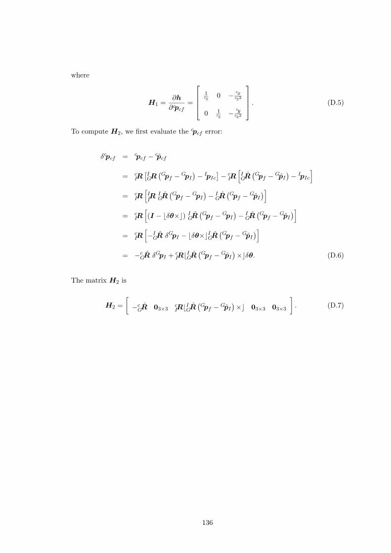
where
H1 =∂h
∂cpcf=
1cz 0 − cx
cz2
0 1cz −
cycz2
. (D.5)
To compute H2, we first evaluate the cpcf error:
δcpcf = cpcf − cpcf
= cIR
[IGR
(Gpf − GpI
)− IpIc
]− cIR
[IGR
(Gpf − GpI
)− IpIc
]= c
IR[IIR I
GR(Gpf − GpI
)− IGR
(Gpf − GpI
)]= c
IR[(I − ⌊δθ×⌋) IGR
(Gpf − GpI
)− IGR
(Gpf − GpI
)]= c
IR[−IGR δGpI − ⌊δθ×⌋IGR
(Gpf − GpI
)]= −c
GR δGpI +cIR⌊IGR
(Gpf − GpI
)×⌋δθ. (D.6)
The matrix H2 is
H2 =
[−cGR 03×3
cIR⌊IGR
(Gpf − GpI
)×⌋ 03×3 03×3
]. (D.7)
136
Related Documents


