Joint target tracking and classification with particle filtering and ...

This is a repository copy of Joint target tracking and classification with particle filtering andmixture Kalman filtering using kinematic radar information.

White Rose Research Online URL for this paper:http://eprints.whiterose.ac.uk/82261/

Version: Submitted Version

Article:

Angelova, D. and Mihaylova, L. (2006) Joint target tracking and classification with particle filtering and mixture Kalman filtering using kinematic radar information. Digital Signal Processing , 16 (2). 180 - 204. ISSN 1051-2004

https://doi.org/10.1016/j.dsp.2005.04.007

[email protected]://eprints.whiterose.ac.uk/

Reuse

Unless indicated otherwise, fulltext items are protected by copyright with all rights reserved. The copyright exception in section 29 of the Copyright, Designs and Patents Act 1988 allows the making of a single copy solely for the purpose of non-commercial research or private study within the limits of fair dealing. The publisher or other rights-holder may allow further reproduction and re-use of this version - refer to the White Rose Research Online record for this item. Where records identify the publisher as the copyright holder, users can verify any specific terms of use on the publisher’s website.

Takedown

If you consider content in White Rose Research Online to be in breach of UK law, please notify us by emailing [email protected] including the URL of the record and the reason for the withdrawal request.

Joint Target Tracking and Classification with ParticleFiltering and Mixture Kalman Filtering

Using Kinematic Radar Information

Donka Angelovaa, Lyudmila Mihaylova∗,b,

aCentral Laboratory for Parallel Processing, Bulgarian Academy of Sciences, 25A Acad.G. Bonchev St, 1113 Sofia, Bulgaria

bDepartment of Electrical and Electronic Engineering, University of Bristol, MerchantVenturers Building, Woodland Road, Bristol BS8 1UB, UK

Abstract

This paper considers the problem of joint maneuvering target tracking and classification.Based on recently proposed Monte Carlo techniques, a multiple model (MM) particle filterand a mixture Kalman filter (MKF) are designed for two-class identification of air targets:commercial and military aircraft. The classification task is carried out by processing radarmeasurements only, no class (feature) measurements are used. A speed likelihood functionfor each class is defined using a prior information about speed constraints. Class-dependentspeed likelihoods are calculated through the state estimates of each class-dependent tracker.They are combined with the kinematic measurement likelihoods in order to improve theclassification process. The two designed estimators are compared and evaluated over rathercomplex target scenarios. The results demonstrate the usefulness of the proposed schemefor the incorporation of additional speed information. Both filters illustrate the opportunityof the particle filtering and mixture Kalman filtering to incorporate constraints in a natu-ral way, providing reliable tracking and correct classification. Future observations containvaluable information about the current state of the dynamic systems. In the framework ofthe MKF, an algorithm for delayed estimation is designed for improving the current modalstate estimate. It is used as an additional, more reliable information in resolving compli-cated classification situations.

Key Words:Joint tracking and classification, particle filtering, mixture Kalman fil-tering, multiple models, maneuvering target tracking

∗ Corresponding authorEmail addresses:[email protected] (Donka Angelova),

[email protected] (Lyudmila Mihaylova).

1 Introduction

Recently there has been great interest in the problem of joint target tracking andclassification. It is due to the fact that the simultaneous implementation of thesetwo important tasks in the surveillance systems facilitates the situation assessment,resource allocation and decision-making.Classification(or identification) usuallyincludes target allegiance determination and/or target profile assessment such asve-hicle, shipor aircraft type. Target class information could be obtained from anelec-tronic support measure(ESM) sensor, friend-and-foe identification system, highresolution radar or other identity sensors. It can be inferred from a tracker, usingkinematic measurements only or in combination with identity sensors. On the otherhand, target type knowledge applied to the tracker can improve the tracking per-formance by the possibility of selecting appropriate target models. Classificationinformation can assist in correct data association and false tracks elimination inmultiple target tracking systems. The notion ofjoint tracking and classification(JTC)was introduced by Challa and Pulford in [1].

Several methods such asBayesian[1–4], Dempster-Shafer[5,6] methods andfuzzysettheory [7] have been applied to solve different identification problems. Compar-ative studies of these techniques have been published in the specialized literature[5]. The inferences for their advantages and disadvantages are usually conflicting.They are highly dependent on the particularities of the problem of interest. In ad-dition, the combination of elements from different approaches often leads to inter-esting results [6]. We focus here on the Bayesian methodology because it offers atheoretically valid framework for overcoming the uncertainties of the JTC. From aBayesian point of view the problem is reduced to reconstructing of thejoint poste-rior probability density function of the target state and class over time. However, theoptimal solution is infeasible in practice due to the prohibitively time-consumingcomputations.

Suboptimal solutions can be found in different directions. One of them is relatedto multiple modelestimation algorithms relying on approximate Bayesian filteringof hybrid dynamic systems [2,8]. The well-known Generalized Pseudo-Bayesianand the Interacting Multiple Model (IMM) estimation algorithms are essentiallya bank of Kalman filters or Extended Kalman filters, which approximate highlynonlinear functions by Taylor series expansions. A Bayesian mechanism organizesthe cooperation between the individual filters and the estimation of classificationprobabilities. An IMM-based algorithm for JTC is proposed in [3] by fusing mea-surements from a suite of sensors: low resolution surveillance radar, high resolu-tion imaging radar and an ESM sensor. An alternative approximation strategy isaimed at a direct approximation of the underlying density functions. Grid-basedand Monte Carlo methods are representatives of this tendency. Challa and Pulford[1] suggest a grid-based algorithm for JTC using ESM and radar data. However, thecomputational efficiency of the grid-based algorithms depends on the state vectordimension. In contrast to the grid-based algorithms, the Monte Carlo algorithms

2

are more easily implementable for systems of high dimension.

Particle filters [9,10] are sequential Monte Carlo methods based on “particle” (sam-ple) representation of probability densities. Multiple particles of the variables ofinterest are generated, each associated with a weight which characterizes the qual-ity of a specific particle. An estimate of the variable of interest is obtained by theweighted sum of particles. In the grid-based algorithms the grid points are chosenby the designer, whereas in the particle filter the particles are randomly generatedaccording to the model of the dynamic system and then naturally follow the state.Sequential Monte Carlo algorithms are particularly suitable for classification pur-poses. The highly non-linear relationships between state and class measurementsand non-Gaussian noise processes can be easily processed by the particle filteringtechnique. Moreover, flight envelope constraints, especially useful for this task, canbe incorporated into the filtering algorithm in a natural and consistent way [11].

One of the first papers where particle filtering techniques are applied to trackingand identification is [12] addressing two closely spaced objects in clutter. Laterother feasible implementations are reported [4,13]. Automatic target recognitionand tracking of multiple targets with particle filters is proposed in [14] by the in-clusion of radar cross section measurements into the measurement vector.

The main idea of using sequential Monte Carlo filtering for JTC consists of fillingthe state and class space with particles and then running the filtering procedure.Since the probability of switching between classes is zero, all the particles mighteventually cluster around one class [4]. This is a crucial shortcoming in some casesof classification. This could happen in many practical situations, for instance, whenthe classification decision is not yet been taken, and all particles might be clusteredaround one of the classes. Therefore, the number of particles for each class shouldremain constant. To overcome this drawback, Gordon, Maskell and Kirubarajan [4]suggest the following algorithm for JTC: a bank of independent filters, coveringthe state and feature space are run in parallel with each filter matched to a differ-ent target class. The class-conditioned independent filters stay in position “alert”and the filtering system can “change its mind” regarding the class identification ifchanges in the target behavior occur. An example of a successful application of thisapproach to littoral tracking with classification is proposed in [13].

In the present paper we develop twosequentialMonte Carlo algorithms, a particlefilter (PF) and a mixture Kalman filter (MKF). They are intended for simultaneoustracking and classification ofa maneuvering targetusing kinematic measurementsonly, primarily in the air surveillance context. Maneuvering target tracking is imple-mented by themultiple model(MM) estimation in the particle filtering framework[15–18]. Multiple models, corresponding to different regimes of flight provide reli-able tracking of fast maneuvering targets. In the particle filter the multiple modelscorrespond to different acceleration levels. Within the mixture Kalman filtering, themaneuvering target is modelled by using a random indicator variable, called latent.

3

The latent variable can take values over a given set of possible values depending onthe acceleration range. Given the indicator variable, a set of Kalman filters realizeon-line filtering based on dynamic linear models. In such a way a multiple modelstructure is implemented together with Monte Carlo sampling in the space of thelatent variables, instead of in the space of the state variables. The paper representsa further development and generalization of the results reported in [19,20]. Two airtarget classes are considered:commercialaircraft (slowly maneuverable, mainlystraight line) andmilitary aircraft (highly maneuverable turns are possible). Thefeatures of the proposed algorithms include the following:

• for each target class a separate filter is designed. These filters operate in parallel,covering the class space.

• each class-dependent filter represents aswitchingmultiple model filtering proce-dure, covering the class-dependent kinematic state space.

• two kinds of constraints are imposed on the target kinematic parameters: on theaccelerationand on thespeed. Two speed likelihood functions are defined basedon a prior information about the speed constraints of each class. At every filteringstep, the estimated speed from each class-dependent filter is used to calculateclass-dependent speed likelihoods. These speed likelihoods are combined withkinematic likelihoods in order to improve the process of classification.

• Future observations contain valuable information about the current target state[21] and a delayed sampling scheme applied to fading communication channelswas shown to improve the estimation accuracy. The JTC solution can achievebetter performance when such a delayed estimation of the currentmaneuveringmodestate is incorporated into the MKF structure. It is used as an additional,more reliable information in resolving ambiguous classification situations.

The novelty of the present paper relies on combining the multiple model (MM)approach with the particle filtering and mixture Kalman filtering for JTC purposes,the manner of imposing the speed constraints on target behavior and the use ofdelayed estimation for classification. Although we consider only two classes, thegeneralization for more target classes is straightforward.

The remaining part of the paper is organized as follows. Section 2 summarizes theBayesian formulation of the JTC problem according to [4,13,22]. Section 3 presentsthe developed MM particle filter, MKF, and delayed-pilot MKF using speed andacceleration constraints. Simulation results are given in Section 5. Finally, Section6 contains the conclusions.

2 Bayesian joint target tracking and classification

Consider the following model describing the target dynamics and sensor measure-ments

4

xk = F (mk) xk−1 + G (mk) uk(mk) + B (mk) wk, (1)zk = h (mk,xk) + D (mk) vk, k = 1, 2, . . . , (2)

wherexk ∈ Rnx is the base (continuous) statevector with transition matrix

F , zk ∈ Rnz specifies the measurement vector with measurement functionh,

uk ∈ Rnu represents a known control input andk is a discrete time. The in-

put noise processwk and the measurement noisevk are independent identicallydistributedGaussian processes having characteristicswk ∼ N (0,Q) andvk ∼N (0,R), respectively. Themodal (discrete) statemk, characterizing the differ-ent system modes (regimes), can take values over a finite setS, i.e. mk ∈ S ,

1, 2, . . . , s. We assume thatmk is evolving according to a time-homogeneousfirst-order Markov chain with transition probabilities

πij , Pr mk = j | mk−1 = i , (i, j ∈ S) (3)

and initial probability distributionP0(i) , Pr m0 = i for i ∈ S, such thatP0(i) ≥ 0, and

∑si=1 P0(i) = 1. Next we suppose that the target belongs to one

of M classesc ∈ C whereC = c1, c2, . . . , cM represents the set of the targetclasses. Generally, the number of the discrete statess = s(c), the initial probabilitydistributionP c

0 (i) and the transition probability matrixπ(c) =[

πcij

]

, i, j ∈ S(c)are different for each target class. Note that the joint state and class is time varyingwith respect to the state and time invariant with respect to the class [4].

Denote withωk , zk, yk the set ofkinematiczk andclass (feature)yk measure-ments obtained at time instantk. Then Ω

k =

Zk,Y k

specifies the cumulative

set of kinematicZk = z1, z2, . . . , zk and featureY k = y1,y2, . . . , yk mea-surements, available up to timek.

Thegoal of the joint tracking and classification task is to estimate simultaneouslythebase statexk, themodal statemk and theposterior classification probabilitiesP

(

c | Ωk)

, c ∈ C based on all available measurement informationΩk.

If we can construct theposterior joint state-mode-class probability density func-tion (pdf) p

(

xk,mk, c | Ωk)

, then the posterior classification probabilities can beobtained by marginalization overxk andmk:

P(

c | Ωk)

=∑

mk∈S(c)

∫

xk∈Rnx

p(

xk,mk, c | Ωk)

dxk. (4)

Suppose that we know the posterior joint state-mode-class pdfp(

xk−1,mk−1, c | Ωk−1)

at time instantk−1. According to the Bayesian framework,p(

xk,mk, c | Ωk)

can

be computed recursively fromp(

xk−1,mk−1, c | Ωk−1)

in two steps –predictionandmeasurement update[4,13].

The predicted state-mode-class pdfp(

xk,mk, c | Ωk−1)

at timek is given by the

5

equation

p(

xk,mk, c | Ωk−1)

= (5)∑

mk−1∈S(c)

∫

xk−1∈Rnx

p(

xk, mk | xk−1,mk−1, c,Ωk−1

)

× p(

xk−1,mk−1, c | Ωk−1)

dxk−1,

where the state prediction pdfp(

xk,mk | xk−1,mk−1, c,Ωk−1

)

is obtained fromthe state transition equation (1)

p(

xk,mk | xk−1,mk−1, c,Ωk−1

)

∝

∝∑

mk∈S(c)

p(

xk | mk, xk−1, mk−1, c,Ωk−1

)

× P(

mk | xk−1,mk−1, c,Ωk−1

)

=

=∑

mk∈S(c)

p(

xk | mk, xk−1, mk−1, c,Ωk−1

)

∑

mk−1∈S(c)

πcmk−1mk

P(

mk−1 | xk−1, c,Ωk−1

)

.

(6)

The form of the conditional pdf of the measurements

p (ωk | xk,mk, c) = λxk,mk,c (ωk) (7)

is usually known. This is the likelihood of the joint state and feature and has a keyrole in the classification algorithm. In our case we do not have feature measure-mentsyk, k = 1, 2, . . . . The speed estimates from theM classes, together withspeed envelope constraints, whose shapes are given in Section 3.3, form avirtual“feature measurement” setY k.

When the measurementωk arrives, the update step can be completed

p(

xk,mk, c | Ωk)

=λxk,mk,c (ωk) p

(

xk, mk, c | Ωk−1)

p(

ωk | Ωk−1) , (8)

where

p(

ωk | Ωk−1)

=∑

c∈C

∑

mk∈S(c)

∫

xk∈Rnx

p (ωk | xk,mk, c) p(

xk,mk, c | Ωk−1)

dxk.

The recursion (5)-(8) begins with the prior densityP x0,m0, c, assumed known,wherex0 ∈ R

nx , c ∈ C, m0 ∈ S(c). Using Bayes’ theorem, the posterior probabil-ity of the discrete statemk for classc is expressed by

P(

mk | xk, c,Ωk)

= (9)1

αk

λxk,mk,c (ωk) ×∑

mk−1∈S(c)

∫

xk−1∈Rnx

πcmk−1mk

P(

mk−1 | xk−1, c,Ωk−1

)

× p(xk−1, c|Ωk−1)dxk−1,

6

whereαk is a normalizing constant. Eq. (9) is substituted into (6) in order to predictthe state pdf at timek + 1.

Then the target classification probability is calculated by the equation

P(

c | Ωk)

=

∑

mk∈S(c)

∫

xk∈Rnx p(

ωk | xk,mk, c,Ωk−1

)

p(xk,mk, c | Ωk−1)dxk

p(

ωk | Ωk−1

(10)

that can be expressed as

P(

c | Ωk)

=p

(

ωk | c,Ωk−1)

P(

c | Ωk−1)

∑Mi=1 p

(

ωk | ci,Ωk−1

)

P(

ci | Ωk−1)

with an initial prior target classification probabilityP0(c),∑

c∈C P0(c) = 1.

The state estimatexck for each classc

xck =

∑

mk∈S(c)

∫

xk∈Rnx

xkp(

xk,mk, c | Ωk)

dxk, c ∈ C (11)

takes part in the calculation of thecombinedstate estimate

xk =∑

c∈C

xckP

(

c | Ωk)

. (12)

It is obvious from (5)-(12) that the estimates, needed for each class, can be calcu-lated independently from the other classes. Therefore, the JTC task can be accom-plished by the simultaneous work ofM independent filters.

3 Maneuvering target tracking and classification

3.1 Maneuvering target model

The two-dimensional target dynamics are given by

xk = Fxk−1 + G (uk + wk) , k = 1, 2, . . . , (13)

where the state vectorx = (x, x, y, y)′ contains target positions and velocities inthe horizontal (Oxy) Cartesian coordinate frame. The control input vectoru =(ax, ay)

′ includes target accelerations alongx andy coordinates. The process noise

7

w = (wx, wy)′ models perturbations in the accelerations. The transition matrices

F andG are [23]

F = diag (F 1,F 1) , G = diag (g1, g1) ,

where

F 1 =

1 T

0 1

, for g1 =(

T 2

2T

)′

,

T is the sampling interval andB = G. The target is assumed to belong to one oftwo classes (M = 2), representing either a lower speedcommercial aircraftwithlimited maneuvering capability (c1) or a highly maneuveringmilitary aircraft (c2)[1]. The flight envelope information comprises speed and acceleration constrains,characterizing each class. The speed v=

√x2 + y2 of each class is limited respec-

tively to the interval:

c1 : v ∈ (100, 300) [m/s] andc2 : v ∈ (150, 650) [m/s].

The range of the speed overlap section is[150, 300] [m/s]. The control inputs arerestricted to the following sets of accelerations:

c1 : u ∈ (0, +2g,−2g) [m/s2] andc2 : u ∈ (0, +5g,−5g) [m/s2],

whereg = 9.81 [m/s2] is the acceleration due to gravity. The acceleration process

uk is a Markov chain with five states (modes)s(c1) = s(c2) = 5 [24]:

1. ax = 0, ay = 0, 2. ax = A, ay = A, 3. ax = A, ay = −A,

4. ax = −A, ay = A, 5. ax = −A, ay = −A, (14)

whereA = 2g stands for classc1 target andA = 5g refers to the classc2 (as shownon Fig. 1 (a)).

The initial probabilities of the Markov chain are selected equal for the two classesas follows:P0(1) = 0.6, P0(i) = 0.1, i = 2, . . . , 5. The matrixπ(c) of transitionprobabilities πc

ij, i, j ∈ S is assumed of the same form for both types of targets:pij = 0.7 for i = j; p1j = 0.075 for j = 2, . . . , 5; pi1 = 0.15 for i =2, . . . , 5; pij = 0.05 for j 6= i, i, j = 2, . . . , 5.

The process noise is Gaussian,w ∼ N (0,Q), Q = diag(σ2wx, σ

2wy), having differ-

ent standard deviations for each mode and class:

c1 : σ1w = 5.5; σj

w = 7.5 [m/s2], j = 2, . . . , 5 and

c2 : σ1w = 7.5, σj

w = 17.5 [m/s2], j = 2, . . . , 5 ,

where (σw = σwx = σwy).

8

3.2 Measurement model

The measurement model at timek is described by

zk = h(xk) + vk, (15)

with

h(xk) =

(

√

x2k + y2

k, arctanxk

yk

)′

, (16)

where the measurement vectorz = (D, β)′ consists of the distanceD to the targetand bearingβ, measured by the radar. The measurement error vectorv ∼ N (0,R)is assumed to be independent fromw. The measurement noise covariance matrixfor the particle filter has the formR = diag(σ2

D, σ2β). The measurement function

h(x) is highly nonlinear and can be easily processed by the particle filter.

The MKF algorithm, however, works with linear state and measurement equations.For the purposes of the MKF design, a measurement conversion is performed frompolar (D , β) to Cartesian (x , y) coordinates:z = (D cos(β), D sin(β))′. Thus,the measurement equation becomes linear with anz × nx measurement matrixH,where all elements are zeros, except forH11 = H23 = 1. The components of thecorresponding measurement noise covariance matrixR are

R11 = σ2D sin2(β) + D2σ2

β cos2(β); R22 = σ2D cos2(β) + D2σ2

β sin2(β);

R12 = (σ2D − D2σ2

β) sin(β) cos(β); R21 = R12.

The following sensor parameters are selected in the simulations:σD = 100.0 [m]σβ = 0.15 [deg]. The sampling interval isT = 5 s.

3.3 Speed constraints

Acceleration constraints are imposed on the filter operation by the use of an appro-priate control input in the target model. The speed constraints are enforced throughthe speed likelihood functions. They are constructed based on the speed envelopeinformation (3.1). Such constraints are incorporated into other approaches for deci-sion making [25]. We define the following speed likelihood functions, respectivelyfor each class

g1 (vc1k ) =

0.9, if v c1k ≤ 100 [m/s]

0.9 − κ1 (vc1k − 100) , if (100 < vc1

k ≤ 300 [m/s])

0.05 if v c1k > 300 [m/s]

9

and

g2 (vc2k ) =

0.1, if v c2k ≤ 150 [m/s]

0.1 + κ2 (vc2k − 150) , if (150 < vc2

k ≤ 650 [m/s])

0.95, if v c2k > 650 [m/s]

whereκ1 = 0.7/200 andκ2 = 0.85/500. Fig. 1 (b) illustrates the evolution of thelikelihoods as a function of the speed.

−60 −40 −20 0 20 40 60

−60

−40

−20

0

20

40

60

acceleration interval for ax [m/s2]

acce

lera

tio

n in

terv

al fo

r a

y [m

/s2]

Class c1

Class c2

m1= (0,0)

m2 = (2g,2g)

m3 = (2g,−2g)

m4 = (−2g,2g)

m5 = (−2g,−2g)

m22 = (5g,5g)

m32 = (5g,−5g)

m42 = (−5g,5g)

m5 = (−5g,−5g)

0 100 200 300 400 500 600 7000

0.1

0.2

0.3

0.4

0.5

0.6

0.7

0.8

0.9

1

Speed interval

gc(v

)

class 1

class 2

Fig. 1. (a) Mode sets for two classes (b) Speed likelihood functions

According to the problem formulation, presented in Section 2, two class-dependentfilters work in parallel withNc number of particles for each class. At time stepkeach filter gives a state estimatexc

k, c = 1, 2. Let us assume that the estimatedspeed from the previous time step,

vck−1, c = 1, 2

, is a kind of “feature measure-ment”.

The likelihoodλxk,mk,c (ωk) = λxk,mk,c (zk, yk) is factorized [4]

λxk,mk,c (zk,yk) = f (zk|xk,mk) gc (yck) , (17)

whereyck = vc

k−1. Practically, the normalized speed likelihoods represent speed-based class probabilities estimated by the filters. The posterior class probabilitiesare modified by this additional speed information at every time stepk. The inclusionof the speed likelihoods is done after some “warming-up” interval, comprising thefilter initialization.

3.4 Multiple Model Particle Filter Algorithm

Within the JTC formulation problem as given in Section 2 a separate PF is designedfor each target class. Assuming two classes of targets – commercial and military, wedevelop a bank of two independent PFs (M = 2). Each PF propagates a set ofNc

10

hybrid particlesx(i)k ,m

(i)k Nc

i=1, containing all the necessary information about thetarget base state and modal state (mode). Each mode takes values from the setS(c).The modes evolve in time according to a Markov chain with a transition probabilitymatrix (3). The cloud of particles for every PF allows a sequential update of thepdfs (5)-(12) by two main stages:prediction and update. During the predictioneach particle is modified according to the state model, including the addition of arandom noise simulating the effect of the uncertainties on the state. Then in theupdate stage, each particle’s weight is re-evaluated based on the new sensor data.Theresamplingprocedure deals with the elimination of particles with small weightsand replicates the particles with higher weights.

A detailed scheme of the proposed particle filter is given in Table 1.

Table 1: A Particle Filter for Joint Target Tracking and Classification

(1) Initialization, k = 0.

For class c = 1, 2, . . . , M set class probabilitiesP(

c | Ω0)

= P0(c).

* For j = 1, 2, . . . , Nc,

sample

x(j)0 ∼ p0(x0, c), m

(j)0 ∼ P c

0 (ℓ)s(c)ℓ=1

and set initial weightsW (j)0 = 1/Nc ;

* End for jEnd forc

Set k = 1.

(2) For c = 1, 2, . . . , M (possibly in parallel) perform

* Prediction step

For j = 1, 2, . . . , Nc

drawm(j)k from the setS(c) = 1, 2, . . . s(c) with probability

P(

m(j)k = i

)

∝ πcℓ i , for ℓ = m

(j)k−1 ,

draw w(j)k ∼ N (0, Q(m

(j)k , c)),

calculatex(j)k = Fx

(j)k−1 + Gu(m

(j)k , c) + Gw

(j)k ,

whereu(m(j)k , c) denotes the pair of accelerations from (14) corresponding tom

(j)k .

End forj

* Measurement processing step: on receipt of a measurementωk = zk, yk:

For j = 1, 2, . . . , Nc evaluate the weights

W(j)k = W

(j)k−1f(zk | x

(j)k )gc (yc

k) ,

11

wheref(zk | x(j)k ) = N (h(x

(j)k ),R) and gc (yc

k) = gc

(

vck−1

)

;

calculatep(

ωk | c,Ωk−1)

=∑Nc

j=1 W(j)k and set L(c) =

∑Nc

j=1 W(j)k

End forj

normalize the weightsW (j)k = W

(j)k /

∑Nc

j=1 W(j)k ;

* Compute updated state estimate and posterior mode probabilities

xck =

∑Nc

j=1 x(j)k W

(j)k ,

P(

mk = ℓ | c,Ωk)

= E

1 (mk = ℓ) | c,Ωk

∼=∑Nc

j=1 1(m(j)k = ℓ)W

(j)k , ℓ = 1, 2, . . . , s(c),

where1(·) is an indicator function such that1(mk = ℓ) = 1, if mk = ℓ and1(mk = ℓ) = 0 otherwise;

* Obtain a hard mode decision:

mck = arg max

ℓ∈S(c)P

(

mk = ℓ | c,Ωk)

∼= arg maxℓ∈S(c)

Nc∑

j=1

1(m(j)k = ℓ)W

(j)k

* Compute effective sample size:Neff (c) = 1/∑Nc

j=1

(

W(j)k

)2

End forc

(3) Output: Compute posterior class probabilities and combined output estimate

P(

c | Ωk)

=L(c)P(c|Ωk−1)

∑M

i=1L(ci)P(ci|Ω

k−1), c = 1, 2, . . . , M

xk =∑M

c=1 P(

c | Ωk)

xck

(4) If Neff (c) < Nthres, c = 1, 2, . . . , M

resample with replacementNc particlesx(j)k ,m

(j)k ; j = 1, . . . , Nc

from the setx(j)k , m

(j)k ; j = 1, . . . , Nc according to the weights;

setW (j)k = 1/Nc, j = 1, . . . , Nc

(5) Setk ←− k + 1 and go to step 2.

In step (3) the posterior class probabilities are computed after applying the Bayesrule, i.e. the posterior is equal to the product of the likelihood and the prior, dividedby the evidence.

12

3.5 The Mixture Kalman Filter Algorithm

The mixture Kalman filter (MKF) [26,27] is another sequential Monte Carlo esti-mation technique which has been successfully applied to different problems in tar-get tracking and digital communications (see e.g. [28,29]). It is essentially a bank ofKalman filters (KFs) run with the Monte Carlo sampling approach. The MKF is de-rived for state-space models in a special form, namelyconditional dynamic linearmodel(CDLM), conditional linear Gaussian model, or partially linear Gaussianmodel:

xk = F λkxk−1 + Gλk

uλk+ Gλk

wk,

zk = Hλkxk + V λk

vk,(18)

wherewk ∼ N (0, Q) andvk ∼ N (0, Rc) are Gaussian distributed processes.λk is a sequence of random indicator variables (calledlatent), independent ofwk, vk and the past statexs and measurementzs, s < k. The termconditionaljustifies the characteristic of these models: they are linear for a given trajectoryof the indicatorλk. Then, the Monte Carlo sampling works in the space oflatentvariablesinstead of in the space of the state variables. The matricesF λk

, Gλk, Hλk

andV λkare known, assuming thatλk is known. For simplicity, in the remaining

part of the paper we are omitting the subscriptλk from the matrices of (18). Theindicatorλk usually takes values from a preliminary known finite set. The MKFrelies on the conditional Gaussian property and uses a marginalization operation inorder to improve the efficiency of the sequential Monte Carlo estimation technique.

Let Λk = λ0, λ1, λ2, . . . , λk be the set of indicator variables up to time in-stant k. By recursively generating a set of properly weighted random samples(Λ(j)

k ,W(j)k )N

j=1 to represent the pdfp(Λk|Ωk), the MKF approximates the statepdf p(xk|Ωk) by a random mixture of Gaussian distributions [27]

N∑

j=1

W(j)k N (µk

(j),Σk(j)), (19)

whereµk(j) = µk(Λ

(j)k ) andΣk

(j) = Σk(Λ(j)k ) are obtained by a KF, designed

with the system model (18). We denote byKF(j)k = µk

(j),Σ(j)k the sufficient

statistics that characterize the posterior mean and covariance matrix of the statexk,conditional on the set of accumulated observationsΩ

k and the indicator trajectoryΛ

(j)k . Then based on the set of samples(Λ(j)

k−1, KF(j)k−1,W

(j)k−1)N

j=1 at the previous

time(k−1), the MKF produces a respective set of samples(Λ(j)k , KF

(j)k ,W

(j)k )N

j=1

at the current timek. It is shown in [27] that the samples(Λ(j)k , KF

(j)k ,W

(j)k )N

j=1

are indeed properly weighted with respect top(Λk|Ωk), if the samples(Λ(j)

k−1, KF(j)k−1,W

(j)k−1)N

j=1 are properly weighted at time(k − 1) with respect top(Λk−1|Ωk−1). The MKF for JTC is described in Table 2.

13

Table 2: The Mixture Kalman Filter for Joint Tracking and Classification

(1) Initialization, k = 0For classc = 1, 2, . . . , M set initial class probabilitiesP

(

c | Ω0)

= P0(c).

* For j = 1, . . . , Nc,

sampleλ(j)0 ∼ P c

0 (λ)s(c)λ=1, whereP c

0 (λ) are the initial indicator

probabilities (for the target accelerations).

SetKF(j)0 = µ0(λ

(j)0 ),Σ0(λ

(j)0 ), whereµ0(λ

(j)0 ) = µ0 and

Σ0(λ(j)0 ) = Σ0 are the mean and covariance of the initial statex0 ∼ N (µ0,Σ0).

Set the initial weightsW (j)0 = 1/Nc.

* end for jEnd for classcSet k = 1.

(2) Forclassc = 1, 2, . . . , M complete

* For j = 1, . . . , Nc,

• For eachλk = i, i ∈ S(c), compute- KF prediction step

(µ(j)k|k−1)

(i) = Fµ(j)k−1|k−1 + Gu(λk = i, c),

(Σ(j)k|k−1)

(i) = FΣ(j)k−1|k−1F

′ + GQ(λk = i, c)G′,

(z(j)k|k−1)

(i) = H(µ(j)k|k−1)

(i),

(S(j)k )(i) = H(Σ

(j)k|k−1)

(i)H ′ + V RV ′.

Note thatj is a particle index, whilei = 1, 2, . . . , s(c) is an index of the Kalman

filters with the different acceleration levels (14).

- on receipt of a measurementzk calculate the likelihood

L(j)k,i = f(zk|λk = i,KF

(j)k−1) p(λk = i|λ(j)

k−1), where

f(zk|λk = i,KF(j)k−1) = N ( (z

(j)k|k−1)

(i), (S(j)k )(i) ), and

p(λk = i|λ(j)k−1) is the prior transition probability of the indicator

• Sampleλ(j)k from a setS(c) with a probability, proportional toL(j)

k,i , i ∈ S(c); sup-

pose thatλ(j)k = ℓ, whereℓ ∈ S(c). Appendλ

(j)k to Λ

(j)k−1 and obtainΛ(j)

k .

• perform the KF update step forλ(j)k = ℓ:

K(j)k|k = (Σ

(j)k|k−1)

(ℓ)(H)′[(S(j)k )(ℓ)]−1,

14

µ(j)k|k = (µ

(j)k|k−1)

(ℓ) + K(j)k|k[zk − (z

(j)k|k−1)

(ℓ)],

Σ(j)k|k = (Σ

(j)k|k−1)

(ℓ) − K(j)k|k(S

(j)k )(ℓ)K

(j)′

k|k ,

• update the importance weights

W(j)k = W

(j)k−1gc

(

vck−1

)∑s(c)

i=1 L(j)k,i

* end forj

SetL(c) =∑Nc

j=1 W(j)k ;

Normalize the weightsW (j)k = W

(j)k /

∑Nc

j=1 W(j)k

Computethe updated state estimate, posterior mode probabilities and hard mode de-cision

xck =

∑Nc

j=1 µ(j)k|kW

(j)k , P (λc

k = i) =∑Nc

j=1 1(λ(j)k = i)W

(j)k , i ∈ S(c)

λck = arg max

i∈S(c)P (λc

k = i)

Computethe effective sample size:Neff (c) = 1/∑Nc

j=1

(

W(j)k

)2

Endfor classc

(3) Output: Compute the posterior class probabilities and combined output estimate(such as in the PF)

P(

c | Ωk)

=L(c)P(c|Ωk−1)

∑M

i=1L(ci)P(ci|Ω

k−1), c = 1, 2, . . . ,M

xk =∑M

c=1 P(

c | Ωk)

xck

(4) If Neff (c) < Nthres, c = 1, 2, . . . , M

resample with replacementNc particles for each class:

λ(j)k , µ

(j)k|k, Σ(j)

k|k; j = 1, . . . , Nc according to the weights;

SetW (j)k = 1/Nc, j = 1, . . . , Nc

(5) Setk ←− k + 1 and go to step 2.

Two MKFs are run in parallel, each of them according to the hypothesis: respec-tively commercial or military aircraft. In our JTC problem theindicator variableλcorresponds to themodevariablem from the previous sections. It takes values froma finite discrete setS(c) , 1, 2, . . . , s(c) and evolves according to a Markovchain with transition probabilities (3).

At every time instantk, for each particle(j), j = 1, . . . , Nc, the MKF schemerunss(c) KF prediction steps, according to eachλ ∈ S(c). The likelihood func-tions of the predicted states are calculated based on the received measurementzk.

15

They form a trial sampling distribution, according to which the newλk is selected.The MKF explores the predicted space in order to select the most likely value ofλ. Then the KF update step is accomplished only for the selectedλk. In the par-ticle filtering approach this procedure is realized in some chaotic (random) sense.This fact, together with the lack of the base state sampling, make the MK filteringmore precise and more computationally efficient. However, the MKF application islimited to the CDLM. For that purpose the measurement equation (2) is linearizedthrough a coordinate conversion. It is assumed that the matricesF ,G,H ,V havethe same structure for two classes.

Notice that in both MM PF and MKF the updated state estimates and posteriormode probabilities are calculated before the resampling step, because resamplingbrings extra variation to the current samples ([30], [26], pp. 103).

3.6 Delayed-Pilot Mixture Kalman Filter

Since both types of aircraft can perform slow maneuvers, the recognition can onlybe achieved during the aircraft maneuvers with high speed and acceleration. Insome cases it might take a rather long tracking time to distinguish the types. Theestimated posterior mode probabilities can be used for a classification in compli-cated ambiguous situations. The reliability of the mode information can be furtherimproved by using of a delayed mode estimation scheme. Since target maneuversare usually modelled as ahighly correlatedacceleration process, the observationsin the near future can provide a valuable information about the current mode state.

Recently, delayed estimation methods have been proposed for the purposes of mo-bile communications [29,21]. The idea of the delayed estimation consists in thefollowing. Based on the posterior distributionp(xk, λk | c,Ωk), an instantaneousinference is made on the statexk and the indicator variableλk. If we use the nextmeasurements(ωk, . . . , ωk+, ≥ 0) with the distributionp(xk, λk | Ω

k+),the current state and mode accuracy can be improved at the cost of delayed es-timation at timek + . Consequently, the aim of delayed estimation is to gener-

ate samples and weights

λ(j)k ,W

(j)k

Nc

j=1from the distributionp(Λk | Ω

k+) at

timek +. However, the algorithms for delayed estimation are more complicated.Several schemes for delayed estimation are suggested in [29,21] in the context ofmixture Kalman filtering: delayed-weight, delayed-sample sampling, delayed-pilotsampling. A highly effective delayed-sample sampling method is developed andstudied in [29]. It realizes a full exploration of the space of future states of steps,and generates samples of both the current state and the weights. Due to the need ofmarginalization over the future states, its computational complexity is exponentialin terms of the delay.

A less complicated delayed-pilot sampling method is proposed in [21]. Instead of

16

exploring the entire space of future states, the delayed-pilot sampling generates anumber of random pilot streams, each of which indicates what would happen in thefuture if the current state takes a particular value. The sampling distribution of thecurrent state is then determined by the incremental importance weight associatedwith each pilot stream. For each classc, at each time stepk, the delayed-pilotalgorithm generatess(c) random pilot streams of the future states of steps. Eachpilot stream starts with one of the possible valuesλi, i ∈ S and implementsMKF steps. An incremental importance weight of this pilot stream is calculatedand assigned toλi. The aim is to utilize this information (that can forecast whatwould happen in the future) for generating better samples ofλ. A sample of thecurrent state is drawn proportionally to the incremental importance weight. Thisalgorithm partially explores the space of future states. This fact explains why thepilot approximation introduces a bias, which is additionally corrected by the inverseof the pilot weights. A scheme of the delayed-pilot MKF [21], adapted to the JTCis given in Table 3. The algorithm starts with a conventional MKF, described inthe previous section. The inclusion of the delayed estimation is done after the timeinterval of15 scans. Only the steps that are different are described for conciseness(the other steps : initialization, output and resampling are the same as given inTable 2).

Suppose at time(k−1), a set of properly weighted samples(

Λ(j)k−1, KF

(j)k−1,W

(j)k−1

)Nc

j=1

with respect top(

Λk−1 | c,Ωk−1)

are available. Then, as the new dataωk, . . . , ωk+

arrive, the following steps are implemented to obtain(

Λ(j)k , KF

(j)k ,W

(j)k

)Nc

j=1for

each classc:

Table 3: The delayed-pilot MKF for Joint Tracking and Classification

For j = 1, . . . , Nc,

• for eachλk = i, i = 1, 2, . . . , s(c) run a Kalman filterKF

(j)k−1 → zk → KF

(j)k,i , N

[

µk

(

Λ(j)k−1, λk = i

)

,Σk

(

Λ(j)k−1, λk = i

)]

compute L(j)k,i = f(zk|Λ(j)

k−1, λk = i,KF(j)k−1)p(λk = i|Λ(j)

k−1),

• for eachλ = i do the following:

for s = k + 1, . . . , k + , repeat

* Let Λ(i,j)s−1 =

[

Λ(j)k−1, λk = i, λk+1 = λ

(i,j)k+1, . . . , λs−1 = λ

(i,j)s−1

]

for each λs = q, q ∈ S(c), run a Kalman filter

KF(j)s−1,i → zs → KF

(q,j)s,i , N

[

µs

(

Λ(i,j)s−1 , λs = q

)

,Σs

(

Λ(i,j)s−1 , λs = q

)]

* compute the sampling density

L(q,j)s,i = f(zs|Λ(i,j)

s−1 , λs = q, KF(j)s−1,i)p(λs = q|Λ(i,j)

s−1 )

17

and draw a sampleλ(i,j)s according to the sampling density;

if λ(i,j)s = ℓ, then setKF

(j)s,i = KF

(ℓ,j)s,i

* compute the incremental importance weight

L(j)s,i =

∑s(c)q=1 L(q,j)

s,i

end fors

ρ(j)k,i = L(j)

k,i

∏k+s=k+1 L(j)

s,i ,

end for eachλk = i,

ρ(j)k,i = ρ

(j)k,i/

∑s(c)r=1 ρ

(j)k,r, i = 1, 2, . . . , s(c),

use ρ(j)k,i , i = 1, 2, . . . , s(c) as the sampling distribution, draw a sample

λ(j)k and obtainΛ(j)

k =[

Λ(j)k−1, λ

(j)k

]

,

if λ(j)k = ℓ, set KF

(j)k = KF

(j)k,ℓ

• Compute the importance weights:

if λ(j)k = ℓ, W

(j)k = W

(j)k−1

L(j)k,ℓ

ρ(j)k,ℓ

gc

(

vck−1

)

,

calculate the auxiliary weight W(j)k = W

(j)k

∏k+s=k+1 L(j)

s,ℓ ,endof j

use the auxiliary weight to compute the posterior mode probabilities,• Output: compute updated state estimate, posterior class probabilities and

combined output estimate according to the MKF scheme in Table 2.• Resamplingif the effective sample size is below a certain threshold.

• Setk ←− k + 1 and go to the beginning of the scheme.

Comment: The delayed-pilot MKF algorithm for JTC generates at time(k + ) a

weighted sample set(

Λ(j)k ,W

(j)k

)Nc

j=1, which is not properly weighted with respect

top(Λk | Ωk+k ). A better inference onλk at time(k+) is done by the calculation

of auxiliary weights [21]. The auxiliary weights are used both for inference onλk

and in the resampling step. The investigation of this algorithm for JTC shows, thatthe scheme slightly deteriorates the posterior class probabilities in comparison withthe MKF.

18

4 Simulation results

The performance of the implemented filters for JTC is evaluated by simulationsover representative trajectories (shown on Figures 2 and 11) together with the radarlocation, indicated by a triangle. The target motion is generated without a processnoise. The target trajectories were generated with a model ([31] Eqs. (57)–(60))differing from the models used in the filters. The MM particle filter and the MKFusing both speed and acceleration constraints with likelihood computed accordingto (17) are compared to filters without speed constraints, which likelihood is equalto λxk,mk,c = fxk

(zk|xk,mk, c). The performance of the designed delayed-pilotsampling algorithm for JTC is demonstrated on a specially selected target scenario(Fig. 22).

Measures of performance. Root-Mean Squared Errors(RMSEs) [32]: on position(both coordinates combined) and speed (magnitude of the velocity vector),averageprobability of correct class identificationand average time per updateare usedto evaluate the filters performance. The results presented below are based on 100Monte Carlo runs. The PF hasNc = 3000 particles per class, the MKF hasNc =300 particles per class, and the resampling threshold isNthresh = Nc/10. The priorclass probabilities are chosen to be equal:P0(1) = P0(2) = 0.5. The parameters ofthe base state vector initial distributionx0 ∼ N (m0, P 0) in the PF are selected asfollows: P 0 = diag(1502 [m], 20.02 [m/s], 1502 [m], 20.02 [m/s]); m0 containsthe exact initial target states. The MKF initial parameters (mean and covarianceµ0

Σ0 of the initial statex0 ∼ N (µ0,Σ0)) are obtained by a two-point differencingtechnique [23] (p. 253), andV = I. The sampling period isT = 5 [s].

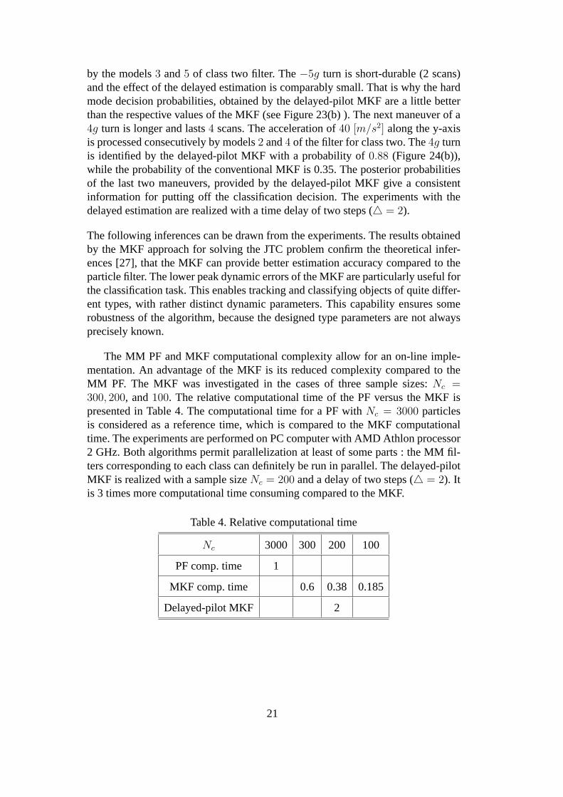
Test trajectory 1.The simulated target path is shown in Figure 2. The target accom-plishes two turn maneuvers with normal accelerations2g [m/s2] and1g [m/s2],respectively with a constant speed of v= 200 [m/s]. Then a maneuver is per-formed with a longitudinal acceleration of2g [m/s2] in the frame of 3 scans. Thespeed increases up to500 [m/s]. Practically, these maneuvers are typical for targetsof the first class. If the speed constraints are not imposed, the target is classified asbelonging to the first class as it can be seen from Figure 7. But it actually belongs tothe second class which is correctly distinguished by the speed likelihoods (Figure9) when the target speed exceeds the value of300 [m/s] (during the maneuver withlongitudinal acceleration). After this maneuver, one observes switching in the classprobabilities (Figure 8), which shows the importance of the speed information forclassifying the target in the proper class. The class probabilities for both filters arealmost identical and for this reason only the class probabilities of the PF are pre-sented (Figures 7 and 8). Figure 10 shows the mode probabilities of the MKF forclass 1. The speed RMSEs are nearly identical for the two filters as well (Figures 5and 6), whilst the PF position RMSE is larger than those of MKF (Figures 3 and 4).The RMSEs shown are for each separate class, and the combined RMSE obtainedafter averaging with the class probabilities, similarly to (12).

19

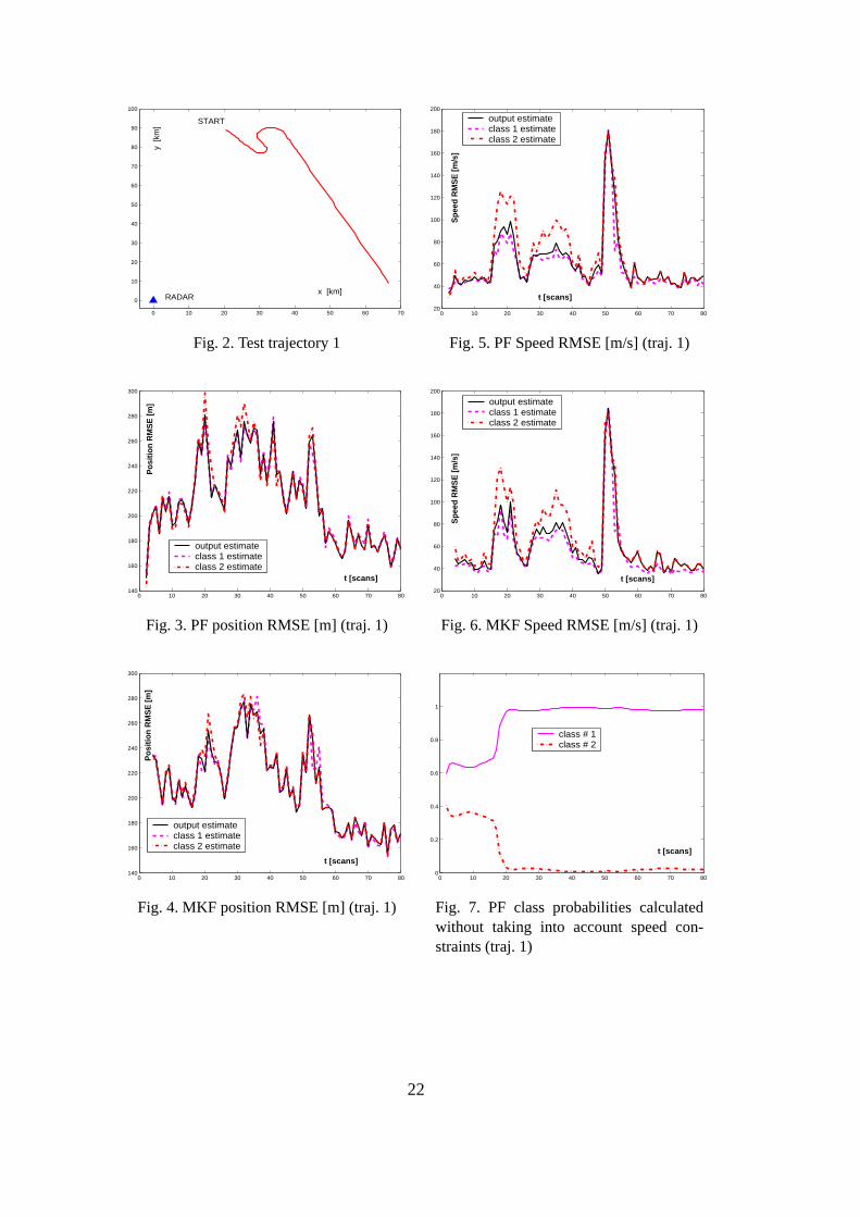
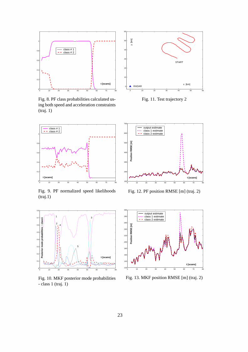
Test trajectory 2.The target performs four turn maneuvers (Figure 11) with inten-sity 1g, 2g, −5g, 2g. The third5g turn provides an insufficient true class infor-mation, since the maneuver is of short duration, and the next2g turn leads to amisclassification in the PF and MKF without speed constraints (Figure 16). Thetarget speed of260 [m/s] provides better conditions for the probability, that thetarget belongs to class 2, according to the speed constraints. The estimated speedprobabilities assist in the proper class identification, as we can see in Figure 17. Thenormalized speed likelihoodsgc(v

c), c = 1, 2, obtained by the MM particle filterand MKF are quite similar. For these reasons we present only the results from theMKF (Figure 18). According to the results from the RMSEs (Figures 12, 13, 14,15) the peak dynamic errors of the PF are considerably larger than the respectiveMKF results.

The chosen target model (13) in combination with the sequential Monte Carlotechnique provides an easy way of imposing acceleration constraints on the targetdynamics. Air targets usually perform turn maneuvers with varying accelerationsalongx andy coordinates. These varying accelerations consecutively make activedifferent models from the designed multiple model configuration, since the modelshave fixed accelerations alongx andy directions. During the maneuver differentmodels may have similar probabilities which makes it difficult to infer which isthe most probable between them. The approach proposed here clearly distinguishesdifferent motion segments, as can be seen from the plots of the posterior modelprobabilities, Figure 10 for scenario 1, and Figure 19 for scenario 2.

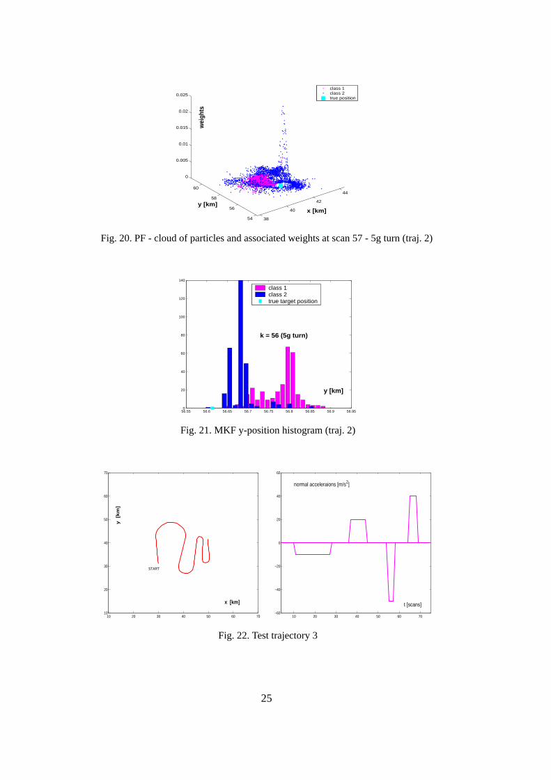
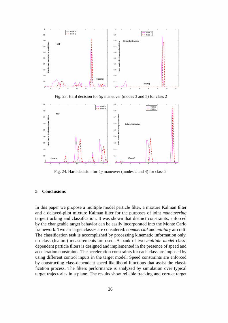
Figure 20 shows the clouds of the PF particles for both classes and the true targetposition indicated by a square. The particles corresponding to class 2 have higherlikelihoods: conclusions can definitely be drawn that the target is of class 2. Figure21 represents the MKFy-position histogram at time instantk = 56 (at the begin-ning of the5g turn). The particles corresponding to class 2 are in proximity to thetrue target position. They quickly adapt to the changeable target dynamics.

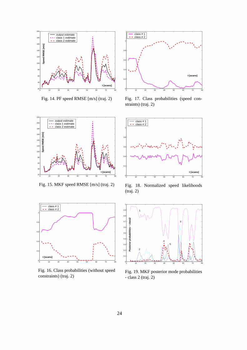
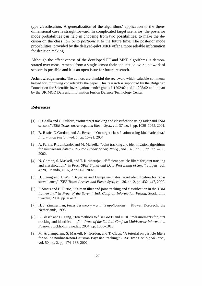
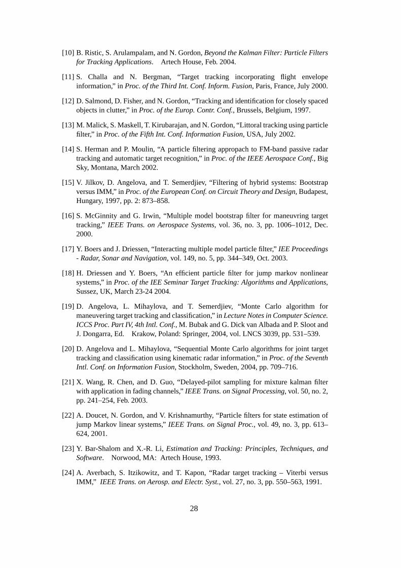
Test trajectory 3.The trajectory is similar in shape to the previous scenario 2. Thetarget performs four turn maneuvers with normal accelerations−1g, 2g, −5g, 4g,displayed in Figure 22(b). In scenario 2, the target speed of260 [m/s] providedbetter conditions for the probability that the target belongs to class 2 according tothe speed constraints. Now the target speed is245 [m/s] and the speed informationis insufficient to distinguish the classes. The short-durable−5g turn is followedby a4g turn, which is located between the acceleration constraints, bounding theclasses -2g and5g. The situation is vague from the point of view of the classifi-cation logic. It is difficult for the MKF to solve the classification task - within 100Monte Carlo runs, there are more than 50 realizations with wrong classification.The posterior mode probabilities can help to choose between : making the decisionon the classnow or postponingit to the future time. The delayed-pilot samplingalgorithm provides more reliable mode information. It can be seen from Figures 23and 24. The acceleration of−50 [m/s2] along they-axis is processed consecutively

20

by the models3 and5 of class two filter. The−5g turn is short-durable (2 scans)and the effect of the delayed estimation is comparably small. That is why the hardmode decision probabilities, obtained by the delayed-pilot MKF are a little betterthan the respective values of the MKF (see Figure 23(b) ). The next maneuver of a4g turn is longer and lasts4 scans. The acceleration of40 [m/s2] along the y-axisis processed consecutively by models2 and4 of the filter for class two. The4g turnis identified by the delayed-pilot MKF with a probability of0.88 (Figure 24(b)),while the probability of the conventional MKF is 0.35. The posterior probabilitiesof the last two maneuvers, provided by the delayed-pilot MKF give a consistentinformation for putting off the classification decision. The experiments with thedelayed estimation are realized with a time delay of two steps ( = 2).

The following inferences can be drawn from the experiments. The results obtainedby the MKF approach for solving the JTC problem confirm the theoretical infer-ences [27], that the MKF can provide better estimation accuracy compared to theparticle filter. The lower peak dynamic errors of the MKF are particularly useful forthe classification task. This enables tracking and classifying objects of quite differ-ent types, with rather distinct dynamic parameters. This capability ensures somerobustness of the algorithm, because the designed type parameters are not alwaysprecisely known.

The MM PF and MKF computational complexity allow for an on-line imple-mentation. An advantage of the MKF is its reduced complexity compared to theMM PF. The MKF was investigated in the cases of three sample sizes:Nc =300, 200, and100. The relative computational time of the PF versus the MKF ispresented in Table 4. The computational time for a PF withNc = 3000 particlesis considered as a reference time, which is compared to the MKF computationaltime. The experiments are performed on PC computer with AMD Athlon processor2 GHz. Both algorithms permit parallelization at least of some parts : the MM fil-ters corresponding to each class can definitely be run in parallel. The delayed-pilotMKF is realized with a sample sizeNc = 200 and a delay of two steps ( = 2). Itis 3 times more computational time consuming compared to the MKF.

Table 4. Relative computational time

Nc 3000 300 200 100

PF comp. time 1

MKF comp. time 0.6 0.38 0.185

Delayed-pilot MKF 2

21

0 10 20 30 40 50 60 70

0

10

20

30

40

50

60

70

80

90

100

x [km]

y [k

m]

START

RADAR

Fig. 2. Test trajectory 1

0 10 20 30 40 50 60 70 80140

160

180

200

220

240

260

280

300

t [scans]

Pos

ition

RM

SE

[m]

output estimateclass 1 estimateclass 2 estimate

Fig. 3. PF position RMSE [m] (traj. 1)

0 10 20 30 40 50 60 70 80140

160

180

200

220

240

260

280

300

t [scans]

Pos

ition

RM

SE

[m]

output estimateclass 1 estimateclass 2 estimate

Fig. 4. MKF position RMSE [m] (traj. 1)

0 10 20 30 40 50 60 70 8020

40

60

80

100

120

140

160

180

200

t [scans]

Spe

ed R

MS

E [m

/s]

output estimateclass 1 estimateclass 2 estimate

Fig. 5. PF Speed RMSE [m/s] (traj. 1)

0 10 20 30 40 50 60 70 8020

40

60

80

100

120

140

160

180

200

t [scans]

Spe

ed R

MS

E [m

/s]

output estimateclass 1 estimateclass 2 estimate

Fig. 6. MKF Speed RMSE [m/s] (traj. 1)

0 10 20 30 40 50 60 70 800

0.2

0.4

0.6

0.8

1

t [scans]

class # 1class # 2

Fig. 7. PF class probabilities calculatedwithout taking into account speed con-straints (traj. 1)

22

0 10 20 30 40 50 60 70 800

0.2

0.4

0.6

0.8

1

t [scans]

class # 1class # 2

Fig. 8. PF class probabilities calculated us-ing both speed and acceleration constraints(traj. 1)

0 10 20 30 40 50 60 70 800

0.2

0.4

0.6

0.8

1

t [scans]

class # 1class # 2

Fig. 9. PF normalized speed likelihoods(traj.1)

0 10 20 30 40 50 60 70 800

0.1

0.2

0.3

0.4

0.5

0.6

0.7

0.8

Pos

terio

r mod

e pr

obab

ilitie

s −

clas

s1

t [scans]

1

2

3

4

5

Fig. 10. MKF posterior mode probabilities- class 1 (traj. 1)

0 10 20 30 40 50 60

0

10

20

30

40

50

60

x [km]

y [k

m]

START

RADAR

Fig. 11. Test trajectory 2

0 10 20 30 40 50 60 70 80100

200

300

400

500

600

700

t [scans]

Pos

ition

RM

SE

[m]

output estimateclass 1 estimateclass 2 estimate

Fig. 12. PF position RMSE [m] (traj. 2)

0 10 20 30 40 50 60 70 80120

140

160

180

200

220

240

260

280

300

t [scans]

Pos

ition

RM

SE

[m]

output estimateclass 1 estimateclass 2 estimate

Fig. 13. MKF position RMSE [m] (traj. 2)

23

0 10 20 30 40 50 60 70 8020

40

60

80

100

120

140

160

180

200

t [scans]

Spe

ed R

MS

E [m

/s]

output estimateclass 1 estimateclass 2 estimate

Fig. 14. PF speed RMSE [m/s] (traj. 2)

0 10 20 30 40 50 60 70 8020

40

60

80

100

120

140

160

180

200

220

t [scans]

Spe

ed R

MS

E [m

/s]

output estimateclass 1 estimateclass 2 estimate

Fig. 15. MKF speed RMSE [m/s] (traj. 2)

0 10 20 30 40 50 60 70 800

0.2

0.4

0.6

0.8

1

t [scans]

class # 1class # 2

Fig. 16. Class probabilities (without speedconstraints) (traj. 2)

0 10 20 30 40 50 60 70 800

0.2

0.4

0.6

0.8

1

t [scans]

class # 1class # 2

Fig. 17. Class probabilities (speed con-straints) (traj. 2)

0 10 20 30 40 50 60 70 800

0.2

0.4

0.6

0.8

1

t [scans]

class # 1class # 2

Fig. 18. Normalized speed likelihoods(traj. 2)

0 10 20 30 40 50 60 70 800

0.1

0.2

0.3

0.4

0.5

0.6

0.7

0.8

0.9

1

Pos

terio

r pro

babi

litie

s −

clas

s2

1

2

3

45

Fig. 19. MKF posterior mode probabilities- class 2 (traj. 2)

24

38

40

42

44

54

56

58

60

0

0.005

0.01

0.015

0.02

0.025

x [km]y [km]

wei

ghts

class 1class 2true position

Fig. 20. PF - cloud of particles and associated weights at scan 57 - 5g turn (traj. 2)

56.55 56.6 56.65 56.7 56.75 56.8 56.85 56.9 56.950

20

40

60

80

100

120

140

y [km]

k = 56 (5g turn)

class 1class 2true target position

Fig. 21. MKF y-position histogram (traj. 2)

10 20 30 40 50 60 7010

20

30

40

50

60

70

x [km]

y [

km]

START

10 20 30 40 50 60 70−60

−40

−20

0

20

40

60

t [scans]

normal acceleraions [m/s2]

Fig. 22. Test trajectory 3

25

10 20 30 40 50 60 700

0.1

0.2

0.3

0.4

0.5

0.6

0.7

0.8

0.9

1

MKF

t [scans]

Ha

rd m

od

e d

eci

sio

n p

rob

ab

ilitie

s

mode 3mode 5

10 20 30 40 50 60 700

0.1

0.2

0.3

0.4

0.5

0.6

0.7

0.8

0.9

1

t [scans]

Ha

rd m

od

e d

eci

sio

n p

rob

ab

ilitie

s

Delayed estimation

mode 3mode 5

Fig. 23. Hard decision for5g maneuver (modes 3 and 5) for class 2

10 20 30 40 50 60 700

0.1

0.2

0.3

0.4

0.5

0.6

0.7

0.8

0.9

MKF

t [scans]

Ha

rd m

od

e d

eci

sio

n p

rob

ab

ilitie

s

mode 2mode 4

10 20 30 40 50 60 700

0.1

0.2

0.3

0.4

0.5

0.6

0.7

0.8

0.9

t [scans]

Delayed estimation

Ha

rd m

od

e d

eci

sio

n p

rob

ab

ilitie

s

mode 2mode 4

Fig. 24. Hard decision for4g maneuver (modes 2 and 4) for class 2

5 Conclusions

In this paper we propose a multiple model particle filter, a mixture Kalman filterand a delayed-pilot mixture Kalman filter for the purposes of jointmaneuveringtarget tracking and classification. It was shown that distinct constraints, enforcedby the changeable target behavior can be easily incorporated into the Monte Carloframework. Two air target classes are considered:commercialandmilitary aircraft.The classification task is accomplished by processing kinematic information only,no class (feature) measurements are used. A bank of twomultiple modelclass-dependent particle filters is designed and implemented in the presence of speed andacceleration constraints. The acceleration constraints for each class are imposed byusing different control inputs in the target model. Speed constraints are enforcedby constructing class-dependent speed likelihood functions that assist the classi-fication process. The filters performance is analyzed by simulation over typicaltarget trajectories in a plane. The results show reliable tracking and correct target

26

type classification. A generalization of the algorithms’ application to the three-dimensional case is straightforward. In complicated target scenarios, the posteriormode probabilities can help in choosing from two possibilities: to make the de-cision on the classnow or to postponeit to the future time. The posterior modeprobabilities, provided by the delayed-pilot MKF offer a more reliable informationfor decision making.

Although the effectiveness of the developed PF and MKF algorithms is demon-strated over measurements from a single sensor their application over a network ofsensors is possible and it is an open issue for future research.

Acknowledgements.The authors are thankful the reviewers which valuable commentshelped for improving considerably the paper. This research is supported by the BulgarianFoundation for Scientific Investigations under grants I-1202/02 and I-1205/02 and in partby the UK MOD Data and Information Fusion Defence Technology Center.

References

[1] S. Challa and G. Pulford, “Joint target tracking and classification using radar and ESMsensors,”IEEE Trans. on Aerosp. and Electr. Syst., vol. 37, no. 3, pp. 1039–1055, 2001.

[2] B. Ristic, N.Gordon, and A. Bessell, “On target classification using kinematic data,”Information Fusion, vol. 5, pp. 15–21, 2004.

[3] A. Farina, P. Lombardo, and M. Marsella, “Joint tracking and identification algorithmsfor multisensor data,”IEE Proc.-Radar Sonar, Navig., vol. 149, no. 6, pp. 271–280,2002.

[4] N. Gordon, S. Maskell, and T. Kirubarajan, “Efficient particle filters for joint trackingand classification,” inProc. SPIE Signal and Data Processing of Small Targets, vol.4728, Orlando, USA, April 1–5 2002.

[5] H. Leung and J. Wu, “Bayesian and Dempster-Shafer target identification for radarsurveillance,”IEEE Trans. Aerosp. and Electr. Syst., vol. 36, no. 2, pp. 432–447, 2000.

[6] P. Smets and B. Ristic, “Kalman filter and joint tracking and classification in the TBMframework,” in Proc. of the Seventh Intl. Conf. on Information Fusion, Stockholm,Sweden, 2004, pp. 46–53.

[7] H. J. Zimmerman,Fuzzy Set theory – and its applications. Kluwer, Dordrecht, theNetherlands, 1996.

[8] E. Blasch and C. Yang, “Ten methods to fuse GMTI and HRRR measurements for jointtracking and identification,” inProc. of the 7th Intl. Conf. on Multisensor InformationFusion, Stockholm, Sweden, 2004, pp. 1006–1013.

[9] M. Arulampalam, S. Maskell, N. Gordon, and T. Clapp, “A tutorial on particle filtersfor online nonlinear/non-Gaussian Bayesian tracking,”IEEE Trans. on Signal Proc.,vol. 50, no. 2, pp. 174–188, 2002.

27

[10] B. Ristic, S. Arulampalam, and N. Gordon,Beyond the Kalman Filter: Particle Filtersfor Tracking Applications. Artech House, Feb. 2004.

[11] S. Challa and N. Bergman, “Target tracking incorporating flight envelopeinformation,” inProc. of the Third Int. Conf. Inform. Fusion, Paris, France, July 2000.

[12] D. Salmond, D. Fisher, and N. Gordon, “Tracking and identification for closely spacedobjects in clutter,” inProc. of the Europ. Contr. Conf., Brussels, Belgium, 1997.

[13] M. Malick, S. Maskell, T. Kirubarajan, and N. Gordon, “Littoral tracking using particlefilter,” in Proc. of the Fifth Int. Conf. Information Fusion, USA, July 2002.

[14] S. Herman and P. Moulin, “A particle filtering appropach to FM-band passive radartracking and automatic target recognition,” inProc. of the IEEE Aerospace Conf., BigSky, Montana, March 2002.

[15] V. Jilkov, D. Angelova, and T. Semerdjiev, “Filtering of hybrid systems: Bootstrapversus IMM,” inProc. of the European Conf. on Circuit Theory and Design, Budapest,Hungary, 1997, pp. 2: 873–858.

[16] S. McGinnity and G. Irwin, “Multiple model bootstrap filter for maneuvring targettracking,” IEEE Trans. on Aerospace Systems, vol. 36, no. 3, pp. 1006–1012, Dec.2000.

[17] Y. Boers and J. Driessen, “Interacting multiple model particle filter,”IEE Proceedings- Radar, Sonar and Navigation, vol. 149, no. 5, pp. 344–349, Oct. 2003.

[18] H. Driessen and Y. Boers, “An efficient particle filter for jump markov nonlinearsystems,” inProc. of the IEE Seminar Target Tracking: Algorithms and Applications,Sussez, UK, March 23-24 2004.

[19] D. Angelova, L. Mihaylova, and T. Semerdjiev, “Monte Carlo algorithm formaneuvering target tracking and classification,” inLecture Notes in Computer Science.ICCS Proc. Part IV, 4th Intl. Conf., M. Bubak and G. Dick van Albada and P. Sloot andJ. Dongarra, Ed. Krakow, Poland: Springer, 2004, vol. LNCS 3039, pp. 531–539.

[20] D. Angelova and L. Mihaylova, “Sequential Monte Carlo algorithms for joint targettracking and classification using kinematic radar information,” inProc. of the SeventhIntl. Conf. on Information Fusion, Stockholm, Sweden, 2004, pp. 709–716.

[21] X. Wang, R. Chen, and D. Guo, “Delayed-pilot sampling for mixture kalman filterwith application in fading channels,”IEEE Trans. on Signal Processing, vol. 50, no. 2,pp. 241–254, Feb. 2003.

[22] A. Doucet, N. Gordon, and V. Krishnamurthy, “Particle filters for state estimation ofjump Markov linear systems,”IEEE Trans. on Signal Proc., vol. 49, no. 3, pp. 613–624, 2001.

[23] Y. Bar-Shalom and X.-R. Li,Estimation and Tracking: Principles, Techniques, andSoftware. Norwood, MA: Artech House, 1993.

[24] A. Averbach, S. Itzikowitz, and T. Kapon, “Radar target tracking – Viterbi versusIMM,” IEEE Trans. on Aerosp. and Electr. Syst., vol. 27, no. 3, pp. 550–563, 1991.

28

[25] A. Tchamova, T. Semerdjiev, and J. Dezert, “Estimation of target behaviour tendenciesusing Dezert-Smarandache theory,” inProc. of the Sixth Intl. Conf. Inform. Fusion,Australia, July 2003, pp. 1349–1356.

[26] J. S. Liu and R. Chen, “Sequential Monte Carlo methods for dynamic systems,”Journal of the American Statistical Association, vol. 93, no. 443, pp. 1032–1044,1998. [Online]. Available: citeseer.nj.nec.com/article/liu98sequential.html

[27] R. Chen and J. S. Liu, “Mixture Kalman filters,”Journal of the Royal StatisticalSociety B, no. 62, pp. 493–508, 2000.

[28] Z. Chen, “Bayesian filtering: From Kalman filters to particle filters, andbeyond,” Adaptive Syst. Lab., McMaster Univ., Hamilton, ON, Canada. [Online],http://soma.crl.mcmaster.ca/˜zhechen/homepage.htm, 2003.

[29] R. Chen, X. Wang, and J. Liu, “Adaptive joint detection and decoding in flat-fadingchannels via mixture Kalman filtering,”IEEE Trans. on Inform. Theory, vol. 46, no. 6,pp. 493–508, 2000.

[30] G. Casella, “Statistical inference and Monte Carlo algorithms,”Test, vol. 5, pp. 249–344, 1997.

[31] X. R. Li and V. Jilkov, “A survey of maneuveuvering target tracking. Part I: Dynamicmodels,”IEEE Trans. on Aerospace and Electr. Systems, vol. 39, no. 4, pp. 1333–1364,2003.

[32] Y. Bar-Shalom and X.-R. Li,Multitarget-Multisensor Tracking: Principles andTechniques. Storrs, CT: YBS Publishing, 1995.

29