Joint penalized-likelihood reconstruction of time-activity curves and regions-of-interest from projection data in brain PET

IOP PUBLISHING PHYSICS IN MEDICINE AND BIOLOGY

Phys. Med. Biol. 53 (2008) 2877–2896 doi:10.1088/0031-9155/53/11/008

Joint penalized-likelihood reconstruction oftime-activity curves and regions-of-interest fromprojection data in brain PET

E Krestyannikov, J Tohka and U Ruotsalainen

Department of Signal Processing, Tampere University of Technology, Tampere,PO Box 553, FIN-33101, Finland

E-mail: [email protected] and [email protected]

Received 10 December 2007, in final form 19 March 2008Published 6 May 2008Online at stacks.iop.org/PMB/53/2877

AbstractThis paper presents a novel statistical approach for joint estimation of regions-of-interest (ROIs) and the corresponding time–activity curves (TACs) fromdynamic positron emission tomography (PET) brain projection data. It is basedon optimizing the joint objective function that consists of a data log-likelihoodterm and two penalty terms reflecting the available a priori information aboutthe human brain anatomy. The developed local optimization strategy iterativelyupdates both the ROI and TAC parameters and is guaranteed to monotonicallyincrease the objective function. The quantitative evaluation of the algorithmis performed with numerically and Monte Carlo-simulated dynamic PET braindata of the 11C-Raclopride and 18F-FDG tracers. The results demonstrate thatthe method outperforms the existing sequential ROI quantification approachesin terms of accuracy, and can noticeably reduce the errors in TACs arising dueto the finite spatial resolution and ROI delineation.

1. Introduction

Positron emission tomography (PET) is a unique method to quantify physiological processesin the human brain. Quantitative estimates of the kinetic rate constants of specific tracersprovide an important information for a broad range of clinical and research problems,including the investigation of brain disorders and drug development. The quantitativeassessment of PET studies relies on the tracer kinetic models and the accurate measurementsof the regional radiotracer concentrations in the brain. The conventional way to define theradiotracer concentration in the brain structure of interest is based on frame-by-frame imagereconstruction followed by manual drawing of regions-of-interest (ROIs) on the images.The ROI definition is typically guided by a set of structural images which have been

0031-9155/08/112877+20$30.00 © 2008 Institute of Physics and Engineering in Medicine Printed in the UK 2877

2878 E Krestyannikov et al

co-registered with the PET images. The time–activity curves (TACs) needed for the modelcalculations are determined by averaging the pixel-by-pixel radioactivity concentrations ina ROI.

The image-based definition of TACs is limited by numerous sources of errors. Finitespatial resolution and the resulting partial volume effect (PVE) are the key issues affectingthe accuracy of ROI quantification. They depend upon many factors including positronrange, photon non-collinearity, detector material and design and image reconstruction.PVE causes the reconstructed image to appear as a spatial convolution of the true imagewith a point spread function. This produces serious systematic biases in regional TACestimates, especially for small brain structures, such as putamen and caudate. Anotherimportant source of errors is the process of image segmentation into a set of ROIs. Apoor resolution and low contrast of reconstructed PET images combined with a highnoise level impair the ability of human observer to produce a reliable delineation ofROIs.

A significant amount of research work has been devoted to address each of theaforementioned problems. Numerous partial volume correction strategies have been proposedto reduce the negative effect of PVE (Aston et al 2002, Frouin et al 2002). Automatedfunctional image segmentation has evolved in two different directions: toward the physiology-based and the anatomy-based methods. Approaches relying solely on PET data partitionthe dynamic image into a fixed number of ROIs by applying cluster analysis techniques(O’Sullivan 1993, Ashburner et al 1996, Acton et al 1999). In anatomy-based methods, theROIs are obtained from a high-resolution structural, typically MR, image co-registered withthe PET image (Yasuno et al 2002, Hammers et al 2003, Svarer et al 2005). Completelydifferent methods have been developed for estimating the regional radioactivity concentrationdirectly from projection data (Carson 1986, Formiconi 1993, Reutter et al 2000). Theyare based on the maximization of appropriate objective function (likelihood (Carson 1986,Reutter et al 2000) or weighted least squares (Formiconi 1993)) and allow the incorporationof resolution factors into the system model. Despite the seeming attractiveness and ability toovercome the limitations of image reconstruction algorithms, these methods still presumethat the exact partitioning of an image volume into anatomical structures is available.Therefore, they should always be considered in conjunction with one of the ROI delineationtechniques.

In this paper, we present a novel approach for the reconstruction of TACs which isconceptually different from the existing sequential methods. Our key idea is to jointly estimatethe ROIs and the corresponding TACs from dynamic PET projection data within a singlestatistically-based reconstruction procedure. We formulate the problem as an optimization taskwithin the maximum-likelihood (ML) framework in order to take into account the Poissonnature of the data acquisition process. In that sense, our approach can be considered asan extension of Carson’s algorithm. There are three major components of the developedmethod: (1) the joint log-likelihood function modified with two penalty terms so that the ROIand TAC estimates satisfy the feasibility assumptions, (2) the penalized maximum-likelihoodexpectation-maximization (PML-EM-ROI) optimization algorithm monotonically increasingthe objective function toward at least a local optimum and (3) the proper initialization ofROIs. By iteratively refining the ROI and the TAC parameters, we expect to reduce the errorsdue to incorrect ROI delineation and the finite spatial resolution. We perform the validationof the developed joint reconstruction algorithm with simulated PET brain volumes of the11C-Raclopride and 18F-FDG tracers, and compare the results to the existing image-based andsinogram-based approaches.

Joint penalized-likelihood reconstruction of TACs and ROIs 2879

2. Problem formulation within the penalized-likelihood framework

2.1. Observation model

Assume that the field of view is discretized into I voxels. A random number of photonpairs is produced through the annihilation of positrons emitted from the tracer at each voxeli = 1, . . . , I during the data acquisition period. Let g

promptdt be the number of counts recorded

by a detector pair d = 1, . . . , D at time interval t = 1, . . . , T . Provided that the detection ofeach photon event is independent, g

promptdt is Poisson distributed (Leahy and Qi 2000)

Gpromptdt ∼ Poisson

(wdt

∑i

pdiµit + rdt + sdt

), (1)

where pdi � 0 is the conditional probability that the photon emitted by the ith voxel wascounted by the jth detector pair, wdt � 0 is the detector-dependent factor accounting forattenuation correction, detector efficiencies, dead-time correction and spatially variant detectorresponse, µit � 0 is the unknown mean radioactivity at the ith voxel and rdt � 0 and sdt � 0are the means of the accidental coincidence and scattered events.

We assume that the whole field of view can be partitioned into a set of regions�k, k = 1, . . . , K , of arbitrary shape, such that µit = λkt ,∀i ∈ �k , where λkt is themean radioactivity quantified within the kth ROI at time interval t. The model (1) can then berewritten as

Gpromptdt ∼ Poisson

(wdt

∑k

bdkλkt + rdt + sdt

). (2)

The non-negative weighting factor bdk , as shown in figure 1, defines the area of all the voxelsaccounting for the kth tissue overlapped with the line of response (LOR) of the detector paird. It relates to pdi through the following equation:

bdk =∑i∈�k

pdi . (3)

Direct computation of bdk using (3) is not possible, as the explicit partitioning of ROIs to �k

is not available.Alternatively to representation (3), the matrix B can be viewed from another perspective.

The kth column of the matrix B is a projection of the kth spatial ROI, where each ROI is afuzzy labeled image that models the fraction of the kth tissue type present in a particular voxel.

Ignoring the constants independent of λ and B, the Poisson log-likelihood is obtained as

Lprompt(λ, B) = ln p(gprompt; λ, B) =∑d,t

[−

(wdt

∑k

bdkλkt + rdt + sdt

)

+ gpromptdt ln

(wdt

∑k

bdkλkt + rdt + sdt

)]=

∑d,t

hpromptdt (ldt (λ, B)), (4)

where

ldt (λ, B) = wdt

∑k

bdkλkt (5)

and

hpromptdt (l) = −(l + rdt + sdt ) + g

promptdt ln(l + rdt + sdt ). (6)

2880 E Krestyannikov et al

Figure 1. The geometric model showing the contribution of the kth ROI to the dth detector pair.The constraint parameter bmask

d equals bd1 + bd2. The volume constraint parameters bvol1 and bvol

2 ,respectively, are equal to the expected values of the volumes of �1 and �2.

2.2. Approximations to joint log-likelihood

In modern PET scanners, the prompt data are usually pre-corrected for accidental coincidencesby real-time subtraction of the delayed-window coincidences (Hoffman et al 1981). Thecorrection step may further involve the subtraction of scattered coincidences. The distributionof the corrected data has a numerically intractable form. A simple approach that does notneed estimation of either accidental coincidence or scattered events is to approximate thepre-corrected measurements as Poisson random variables

Gdt

OP∼ Poisson

(wdt

∑k

bdkλkt

). (7)

The ordinary Poisson approximation ‘OP’ leads to the log-likelihood

LOP(λ, B) =∑d,t

hOPdt (ldt (λ, B)), (8)

with

hOPdt (l) = −l + gdt ln l. (9)

An ML estimate of the unknown parameters for the ‘OP’ model is then given as

{λ, B} = arg maxλ�0,B�0

LOP(λ, B). (10)

In the following sections, we focus on estimating the unknown parameters for the ‘OP’ model,although all the derivations can be generalized to the prompt data model, whenever sdt and rdt

are available.

2.3. Model identifiability and penalized log-likelihood

Both λ and B are not identifiable given the joint log-likelihood LOP. That is, there does notexist a unique solution to problem (10) since different values of latent variables can correspond

Joint penalized-likelihood reconstruction of TACs and ROIs 2881

to nearly identical log-likelihood scores. In the absence of any prior information, neither λnor B can be accurately inferred from the model, as the change in one parameter vector canbe balanced by the corresponding change in the other.

To address this problem, we regularize the parameter estimates by penalizing the log-likelihood, LOP. The objective function becomes a penalized log-likelihood of the form

�(λ, B) = LOP(λ, B) − C1(B) − C2(B), (11)

where C1(B) and C2(B) are quadratic penalty functions given as

C1(B) =∑

d

βd/(2bmask

d

) (∑k bdk

bmaskd

− 1

)2

, (12)

C2(B) =∑

k

γk/(2bvol

k

) (∑d bdk

bvolk

− 1

)2

, (13)

where βd and γk are the regularization parameters controlling the weight of the penalty terms.These penalties ensure that the kth column of the weighting matrix B represents the projectionof the kth spatial ROI. In particular, the penalty function (12) implements a geometric constraintwhich ensures that all the spatial ROIs are enclosed within the reference mask. The elementbmask

d is the projection of the reference binary mask along the LOR corresponding to a detectorpair d (see figure 1). This mask can be delineated prior to the TAC/ROI reconstruction usinga surface extraction technique (see section 4.1). The penalty function (13) alters the initialsinogram volume of different structures toward an a priori defined averaged values. Thefactor bvol

k defines the expected area of intersection of all the voxels inside the kth ROI withall the detector pairs (see figure 1). It is calculated with respect to the reference sinogramvolume

∑d bmask

d . The expected volume for certain brain structures within a population canbe obtained either from numerous research studies (Lange et al 1997, Allen et al 2003) orfrom the probabilistic atlases of the human brain anatomy.

3. Reconstruction algorithm

3.1. Alternating maximization

When there are no negative gdt values, the Poisson log-likelihood LOP is concave for parameterλ if B is fixed and vice versa (Lange and Carson 1984, Shepp and Vardi 1982). However, it isnot jointly concave for {λ, B}. The number of imposed equality constraints is not enough todefine a unique maximizer of the constrained optimization problem. The penalized-likelihood�(λ, B), therefore, remains non-concave. The situation becomes even more complicated whennegative sinogram counts are present. Finding a global maximum may require computationallyintensive optimization strategies.

A conceptually simple method that converges toward at least a local maximum is basedon the maximization of the penalized log-likelihood iteratively over one set of unknownswhile holding the other set fixed (Ziskind and Wax 1988). Suppose that λ(j) and B(j) are theestimates of the parameters after iteration j . Holding the elements of B(j) fixed at their currentvalues, we update λ as

λ(j+1) = arg maxλ�0

�(λ, B(j)) = arg maxλ�0

LOP(λ, B(j)). (14)

Next, we update B holding λ(j+1) constant as

B(j+1) = arg maxB�0

�(λ(j+1), B) = arg maxB�0

(LOP(λ(j+1), B) − C1(B) − C2(B)). (15)

2882 E Krestyannikov et al

In the absence of negative counts, the functions LOP(λ, B(j)) and �(λ(j+1), B) are strictlyconcave. Since a maximization is performed at each iteration, the value of the maximizedfunction �(λ, B) cannot decrease, and the sequence of parameter estimates is bound toconverge to a local stationary point. An analytical solution to (14) and (15), however, does notexist due to the further coupling of parameters λkt in LOP(λ, B(j)) and bdk in �(λ(j+1), B).We resort to numerical methods for solving (14) and (15).

3.2. PML-EM-ROI algorithm allowing negative sinogram values

The expectation-maximization (EM) algorithm (Dempster et al 1977) is a monotonic iterativeprocedure for calculating the ML estimates in situations where the log-likelihood functioncannot be maximized analytically. One of the most insightful explanations of the EM is interms of the optimization transfer algorithms (Lange et al 2000). These algorithms rely ona lower bound, or minorizing, function that serves as a surrogate for the objective function.Hence, at each iteration of the EM algorithm the expectation, or E-step, can be viewedas constructing a lower bound for the log-likelihood function using the current estimate ofthe parameters. The maximization, or M-step, optimizes the bound, thereby improving theestimate for the unknowns.

Following the derivation of the EM algorithm using surrogate functions for pre-correctedPET data with negative sinogram counts (De Pierro 1993, De Pierro 1995, Ahn and Fessler2004), the maximization of functions �(λ, B(j)) and �(λ(j+1), B) yields the following updaterules (see the appendix for a complete derivation):

λ(j+1)

kt = λ(j)

kt∑d wdtb

(j)

dk

(1 + [−gdt ]+

g(j)

dt

) ∑d

wdtb(j)

dk

[gdt ]+

g(j)

dt

, (16)

b(j+1)

dk =−Edk/2 +

√E2

dk/4 − AdkFdk

Adk

, (17)

where

[gdt ]+ = max{gdt , 0}, (18)

Adk = βd

αdkbmaskd

+γk

ωdkbvolk

, (19)

Edk =∑

t

wdtλ(j+1)

kt

(1 +

[−gdt ]+

g(j)

dt

)(20)

− βd

(b

(j)

dk

αdkbmaskd

−∑

k b(j)

dk

bmaskd

+ 1

)− γk

(b

(j)

dk

ωdkbvolk

−∑

d b(j)

dk

bvolk

+ 1

), (21)

Fdk = −b(j)

dk

∑t

wdtλ(j)

kt

[gdt ]+

g(j)

dt

. (22)

The update rules (16) and (17) guarantee the non-negativity of λ(j+1)

kt and b(j+1)

dk providedthat the initial estimates are non-negative. Due to the use of overall surrogates satisfying themonotonicity conditions, the penalized ML EM (PML-EM-ROI) algorithm is guaranteed tomonotonically increase the original functions LOP(λ, B(j)) and �(λ(j+1), B) at each iteration.

Joint penalized-likelihood reconstruction of TACs and ROIs 2883

4. Initialization of the PML-EM-ROI algorithm

4.1. Initialization of parameters bmaskd and bvol

k

The optimization of the penalized log-likelihood (11) requires the estimation of auxiliaryparameters bmask

d and bvolk . In this paper, each projection bmask

d of a binary mask was determinedas follows. At first, a time-averaged sinogram was formed by averaging the frames of themeasured dynamic sinogram data. A binary mask was automatically delineated from thereconstructed time-averaged image using the method of Tohka and Mykkanen (2004). Finally,the parameter vector Bmask was formed by projecting the binary-labeled image to the sinogramdomain.

An alternative approach to the estimation of bmaskd can be derived if one has an access

to the elements of the system matrix P. By slightly modifying equation (3), the constraintparameters can now be evaluated as follows:

bmaskd =

∑i

pdi . (23)

The expected volumes of brain structures of interest bvolk can be computed based on spatially

varying prior probability maps. These maps represent the averaged binary segmentations ofMR brain images from a large number of manually segmented subjects. The parameter bvol

d

for a particular tissue type is merely an average proportion of that tissue in the atlas spacenormalized with respect to the total number of voxels in the brain mask.

4.2. Initialization of ROIs and TACs

We propose two strategies for the initialization of the matrix B(0) depending upon the type ofthe utilized tracer. For tracers distributed all over the brain, such as 18F-fluorodeoxyglucose(FDG), relevant gross brain structures (white matter (WM) and gray matter (GM)) wereinitialized based on the initial segmentation of the time-averaged emission images (used forthe delineation of the head mask) by using an automatic clustering method (Tohka et al 2007).This method offers a sufficient level of accuracy and does not require the structural image ofthe subject.

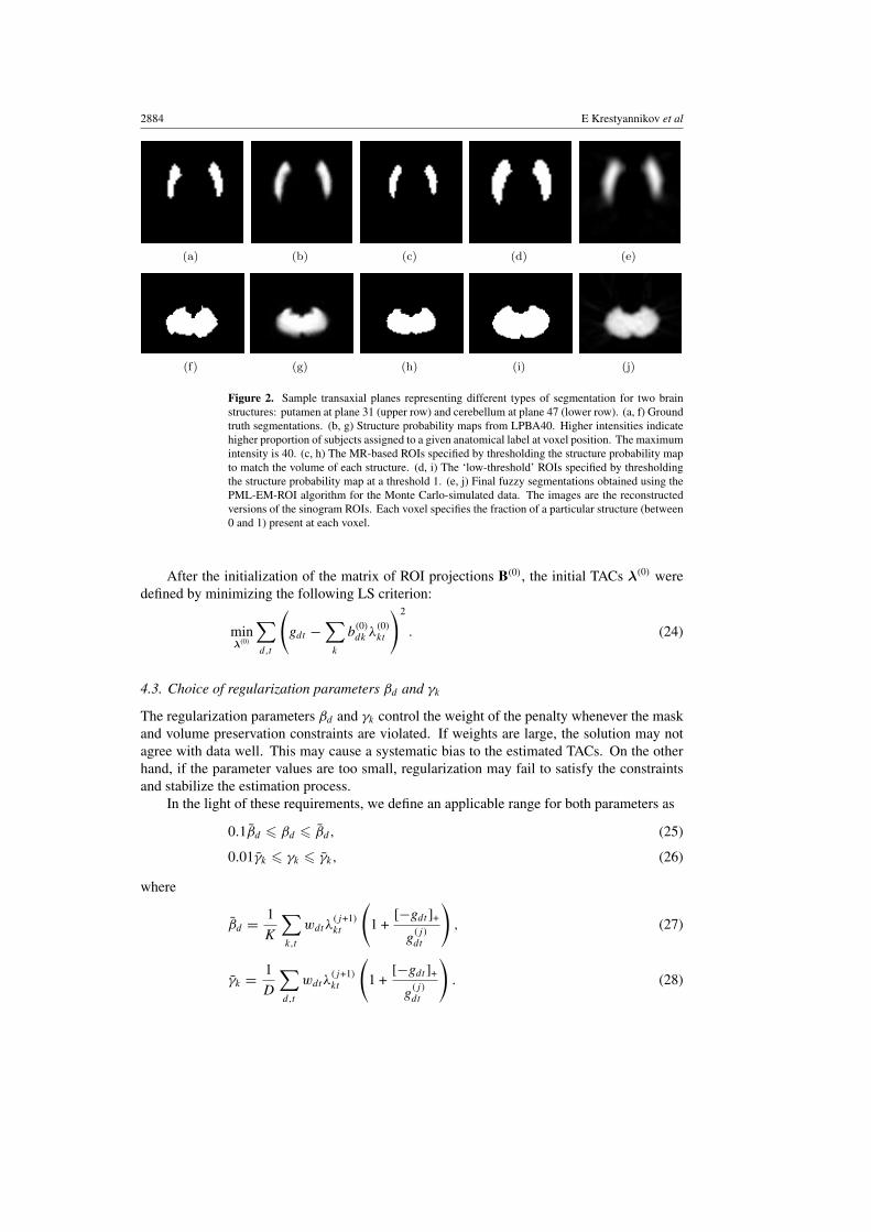
For brain images with a localized tracer concentration, as with 11C-Raclopride, theprocedure of initial ROI delineation is more challenging. Assuming that the anatomicalMR image of the same subject is available, an atlas-based technique was utilized to initializethe structures. A set of ROIs was derived by thresholding the spatially varying prior probabilitymap from LONI (Laboratory of NeuroImaging) Probabilistic Brain Atlas (LPBA40) (Shattucket al 2008). Conventional atlas-based segmentation techniques often fail to fit a particularsubject’s data to standard ROIs due to a considerable anatomical variation and possible errorsin atlas-MRI and MRI-PET registration. To overcome this problem, we thresholded thestructural probability map at a lower value to yield a set of ‘low-threshold’ ROIs. In contrastto the traditional atlas-based segmentation in which a voxel can belong to only one ROI, the‘low-threshold’ ROIs may naturally overlap. The larger is the region of support, the higheris the likelihood to enclose the true structure of interest (see figure 2). After the thresholdingof the structure probability map, the reference MR image in the atlas space was warped tothe subject’s MRI with AIR 5.2.5 (Automatic Image Registration) tool (Woods et al 1992)using a 12-parameter transformation model. The identified spatial transformation parameterswere applied to transform the ‘low-threshold’ ROIs from the template space to the space ofthe subject.

2884 E Krestyannikov et al

Figure 2. Sample transaxial planes representing different types of segmentation for two brainstructures: putamen at plane 31 (upper row) and cerebellum at plane 47 (lower row). (a, f) Groundtruth segmentations. (b, g) Structure probability maps from LPBA40. Higher intensities indicatehigher proportion of subjects assigned to a given anatomical label at voxel position. The maximumintensity is 40. (c, h) The MR-based ROIs specified by thresholding the structure probability mapto match the volume of each structure. (d, i) The ‘low-threshold’ ROIs specified by thresholdingthe structure probability map at a threshold 1. (e, j) Final fuzzy segmentations obtained using thePML-EM-ROI algorithm for the Monte Carlo-simulated data. The images are the reconstructedversions of the sinogram ROIs. Each voxel specifies the fraction of a particular structure (between0 and 1) present at each voxel.

After the initialization of the matrix of ROI projections B(0), the initial TACs λ(0) weredefined by minimizing the following LS criterion:

minλ(0)

∑d,t

(gdt −

∑k

b(0)dk λ

(0)kt

)2

. (24)

4.3. Choice of regularization parameters βd and γk

The regularization parameters βd and γk control the weight of the penalty whenever the maskand volume preservation constraints are violated. If weights are large, the solution may notagree with data well. This may cause a systematic bias to the estimated TACs. On the otherhand, if the parameter values are too small, regularization may fail to satisfy the constraintsand stabilize the estimation process.

In the light of these requirements, we define an applicable range for both parameters as

0.1βd � βd � βd , (25)

0.01γk � γk � γk, (26)

where

βd = 1

K

∑k,t

wdtλ(j+1)

kt

(1 +

[−gdt ]+

g(j)

dt

), (27)

γk = 1

D

∑d,t

wdtλ(j+1)

kt

(1 +

[−gdt ]+

g(j)

dt

). (28)

Joint penalized-likelihood reconstruction of TACs and ROIs 2885

One can observe that both βd and γk are chosen in relative units depending upon the first termof the expression for Edk (see (20)).

Due to a considerable anatomical variability in the relative volumes of different brainstructures, a certain deviation from the second penalty term (13) might be helpful. To givemore freedom for deviation, the parameter γk can be set to a smaller value than βd . This willtreat the second constraint more cautiously, thereby putting more confidence on data and thefirst penalty term.

4.4. Stopping criteria

The algorithm was terminated when both of the following criteria were satisfied:∣∣∣∣∣ 1

D

∑d

(∑k b

(j)

dk

bmaskd

− 1

)∣∣∣∣∣ < θ1, (29)

∣∣∣∣∣ 1

K

∑k

(∑d b

(j)

dk

bvolk

− 1

)∣∣∣∣∣ < θ2, (30)

where θ1 and θ2 denote sufficiently small positive thresholds. When initialized with theoverlapping ‘low-threshold’ ROIs, these stopping rules are convenient measures to determinethat the algorithm has reached the predefined volume proportions for all tissue types, and atthe same time has fitted the mask enclosing all the estimated ROIs to the reference mask.

Alternatively, a stopping criterion can be formulated when consecutive iterations do notrepresent much improvement in the solution, or when the difference in likelihood scores fallsbelow a certain threshold.

5. Experimental results

We evaluated our method with simulated dynamic PET brain volumes of the 11C-Racloprideand 18F-FDG tracers. The experiments consisted of two distinct parts. In the first part, weperformed the reconstruction of TACs from the simplified numerical dynamic PET study withcomputer-simulated Poisson measurements and no additional sources of noise. In the secondpart, we applied our approach to PET measurements generated with a Monte Carlo-basedsimulation tool. This simulation platform is able to generate realistic 2D and 3D emissionand transmission projections in accordance to the numerical representations of the activityand attenuating media distributions as well as scanner geometry and physical characteristics(Reilhac et al 2004).

5.1. Material

5.1.1. Anatomical model. The dynamic emission brain phantoms were derived from thehigh-resolution labeled anatomical Zubal phantom (Zubal et al 1994) with the voxel size of1.1 × 1.1 × 1.4 mm3. The Zubal phantom is composed of 62 structures within and external tothe brain. For 11C-Raclopride, we considered six distinct structures of the anatomical Zubalphantom: caudate nuclei (right and left), putamen (right and left), WM, GM, cerebellum andskin/skull/bone/fat/muscle structures. The true proportions of tissue types were as follows:skin/skull/bone/fat/muscle 47.66%, GM 23.85%, WM 22.07%, putamen 0.39%, caudate0.40% and cerebellum 5.63%. For 18F-FDG, we selected three different brain structures:WM, GM and cerebellum.

2886 E Krestyannikov et al

5.1.2. Physiological model. Realistic TAC’s characteristics of 11C-Raclopride weredetermined from human studies and assigned to the appropriate structures. The simulatedimaging protocol lasted for 1 h: six frames of 30 s, seven frames of 60 s, five frames of 120 sand eight frames of 300 s. In total, phantom consisted of 26 time frames of data volumes with128 × 128 × 63 voxels of the size 2.25 × 2.25 × 2.43 mm3 per each frame.

Realistic TAC’s characteristics of the 18F-FDG tracer were computed based on the three-compartment model and the rate constants characteristic of each brain structure. The rateconstants for GM and WM were from (Phelps et al 1979) and those for cerebellum fromSakamoto and Ishii (2000). The TACs for GM and cerebellum were almost identical, and forsimplicity we applied the GM TAC to describe cerebellum. The simulated imaging protocollasted for 50 min: four frames of 30 s, three frames of 60 s and nine frames of 300 s. In total,the phantom consisted of 16 time frames of data volumes with 128 × 128 × 63 voxels of thesize 2.25 × 2.25 × 2.43 mm3 per each frame.

5.1.3. Error measures. The quantitative accuracy of reconstruction of regional TACs wasassessed using the bias and the coefficient of variation (CoV) measures evaluated for eachtime frame as follows:

bias(λkt ) = λkt − λkt

λkt

× 100%, (31)

CoV(λkt ) =√

1N

∑n(λkt − λnkt )2

λkt

× 100%, (32)

where λnkt is the estimate of the kth TAC at the time instant t from noise realizationn = 1, . . . , N, λkt is the estimated value of the kth TAC at the time interval t averaged overN noise realizations and λkt is the ground truth value. For the simplified numerical dynamicPET study, the number of different noise realizations N was equal to 100. For the MonteCarlo study, the number of noise realizations was limited to 10 due to the high computationaldemands, as each disintegration needs to be tracked to obtain realistic simulation. We shouldnote, however, that for Monte Carlo-simulated phantoms, it is typical to generate from 1 to 10noise realizations per 3D anatomical phantom (Reilhac et al 2008).

The bias term (31) measures frame-by-frame bias between the averaged over N noiserealizations TAC and the ground truth TAC. The coefficient of variation (32) does not dependupon the ground truth values and measures the dispersion of estimates around the mean.

In addition, the overall accuracy of the kth ROI delineation was measured using the errorin the estimated region volume defined as

σ vol(bk) =∑

d bdk − bvolk

bvolk

× 100%, (33)

where bdk is the estimate of the weighting factor and bvolk is the true volume for the kth structure.

This measure is similar to the stopping criterion (30) and can be considered as an analogue ofthe misclassification rate in sinogram domain.

5.2. Experiments with simplified numerical phantom

5.2.1. Data generation, initialization and experimental settings. With the simplifiednumerical phantom for the 11C-Raclopride tracer, we evaluated the performance of the PML-EM-ROI algorithm under ideal noise conditions in the presence of segmentation errors. The

Joint penalized-likelihood reconstruction of TACs and ROIs 2887

purpose of this experimental part was to see how the errors in ROI delineation affect thequantification of regional TACs. For that reason, the true parameters bmask

d and bvolk were

assumed to be known. We simulated the stochastic nature of the data acquisition process bygenerating the Poisson noise to the projection measurements. We did not model attenuation,finite spatial resolution, system dead-time, randoms or scatter in the simulation. That is, weassumed that all the emitted counts were detected by one of the detector pairs. The totalnumber of photon pairs simulated during the whole study was 1.65 × 109, or on average2.53 × 107 photon pairs per plane, that corresponds to a PET study with high count statistics.

The PML-EM-ROI algorithm was initialized by the deformable atlases approach describedin section 4.2. The regularization parameters βd and γk were set to 0.4βd and 0.2γk ,respectively. The stopping criteria (29) and (30) with the threshold parameters θ1 = θ2 = 0.001were applied. The algorithm stopped after 80 iterations with these settings.

The performance of the PML-EM-ROI algorithm was compared to the following twoquantification strategies: (1) frame-by-frame averaging of ROI values on images reconstructedwith the ordered subsets expectation-maximization (OSEM) algorithm (referred to as OSEM-MR) and (2) quantification of ROI values in sinogram domain using the generalization ofFormiconi’s LS algorithm (Formiconi 1993, Krestyannikov et al 2006) (referred to as LS-MR). With an iterative image reconstruction, each plane was obtained using 20 iterationswith 4 subsets yielding a total of 80 ML-EM iterations. A set of non-overlapping ROIs wasdetermined by using the atlas-based segmentation for both OSEM-MR and LS-MR approaches.Putamen, caudate and cerebellum ROIs were delineated by thresholding the probability mapto match the true volume for each structure. This was done for a fair comparison, as the truevalues for bvol

k were expected for the PML-EM-ROI algorithm. Gross GM and WM structureswere segmented by assigning the most likely structure from the probability map of LPBA40atlas to the rest of the tissue voxels. The Jaccard similarity coefficient, that is the size ofthe intersection divided by the size of the union of two ROIs (segmented and ground truth)was equal to 0.47 for GM, 0.39 for WM, 0.57 for putamen, 0.54 for caudate and 0.71 forcerebellum. Those MR-based ROIs were then propagated to the subject space using nonlinearwarp obtained with the AIR software. Figures 2(a)–(d) and (f)–(i) compare the ground truthROIs versus the structural probability maps, ‘low-threshold’ ROIs and MR-based ROIs forputamen and cerebellum structures at different transaxial planes.

5.2.2. Results. Figure 3 shows that the TACs reconstructed with the PML-EM-ROI algorithmhave the lowest bias among the three compared methods. A good performance of the algorithmwas due to its remarkable ability to shrink the ‘low-threshold’ ROIs enclosing the true structureof interest to a correct size (as justified in table 1). Higher bias for putamen and caudate TACs,as compared to the cerebellum curve, was primarily explained by inaccuracies in the algorithminitialization. The initial ‘low-threshold’ ROIs enclosed 91.7% of true caudate and 97.9% oftrue putamen structures that have produced slightly worse reconstruction results.

The accuracy of reconstruction using the LS-MR algorithm was lower compared to theresults of the PML-EM-ROI approach due to the errors in the delineation of MR-based ROIs.As the spatial resolution was not included into the simulations and the regions were perfectlyhomogeneous, the application of the LS-MR method to the ground truth delineation would haveyielded almost unbiased estimates, i.e. true values. The OSEM-MR algorithm produced theworst reconstruction results, with particularly high bias for the putamen and caudate structures.The algorithm exhibited a poor performance because of the delineation errors coupled withthe spatial resolution effects added after the application of the image reconstruction procedure.

2888 E Krestyannikov et al

Figure 3. TACs from the numerically simulated 11C-Raclopride study (left column) reconstructedwith different approaches, and the corresponding bias (center column) and CoV (right column)curves.

Table 1. Errors in volume, σ vol, for different brain ROIs delineated with presented approaches forsimplified numerical phantom.

σ vol(λk), %

Structure MR-based ROI ‘Low-threshold’ ROI PML-EM-ROI

GM 2.56 56.73 −0.34WM −19.68 28.57 0.24Putamen 0.63 119.54 0.27Caudate 1.44 89.18 0.36Cerebellum 3.35 59.41 0.04

5.3. Experiments with the Monte Carlo-simulated phantom

5.3.1. Data generation, initialization and experimental settings. The PET-SORTEOsimulation platform (Reilhac et al 2004) was utilized to generate realistic dynamic PETvolumes for the 11C-Raclopride and 18F-FDG tracers. This simulation tool uses Monte Carlotechniques to create a realistic PET data from voxelized descriptions of tracer distributions. Itaccounts for all the major sources of noise and biases that can occur within the formation of PETdata including the statistical Poisson nature of the emission process, scatter, randoms, body

Joint penalized-likelihood reconstruction of TACs and ROIs 2889

attenuation, system dead-time and finite spatial resolution. The count rates of the simulatorreproduce the performance of the ECAT EXACT HR+ scanner (CTI/Siemens, Knoxville,USA) operating in the 2D mode.

On average, 1.56 × 108 and 1.33 × 108 simulated positron–electron disintegrations weretracked for each of the 2 D 11C-Raclopride and 18F-FDG studies, respectively. The whole brainwas considered as a single volume of water with a constant attenuation coefficient 0.096 cm−1.A second simulation of the randoms was performed and the resulting counts were subtracted,so as to mimic the online randoms subtraction technique. The scatter component and thenormalization factors were estimated using the methods from Watson et al (1996) and Caseyet al (1995), respectively. The axial, radial and tangential resolutions of the simulator weremeasured as a function of the radial distance (up to 20 cm) from the center of the field ofview. The range of full width half-maximum (FWHM) was 5.8–7.8 mm for axial resolution,3.5–8.3 mm for radial resolution and 4.5–6.1 mm for tangential resolution (Reilhac et al2005). The attenuation, normalization and dead-time factors were incorporated into thedetector-dependent coefficients wdt .

For the 11C-Raclopride study, the PML-EM-ROI algorithm was initialized with the ‘low-threshold’ ROIs using the deformable atlases approach as described in section 4.2. Theprimary application of the 11C-Raclopride is the striatal imaging of D2 dopamine receptors.Hence, the TACs of putamen, caudate and cerebellum (typically used as the reference region)are the most interesting, whereas the GM and WM TACs are of little biological interest. Forthis reason, only four distinct ROIs were delineated, namely putamen, caudate, cerebellumand the rest of the head (skin/skull/muscle/WM/GM). The reduction in the number of ROIsdecreased the statistical uncertainty in TACs reconstructed from the realistic PET data with apoor signal-to-noise ratio and limited spatial resolution.

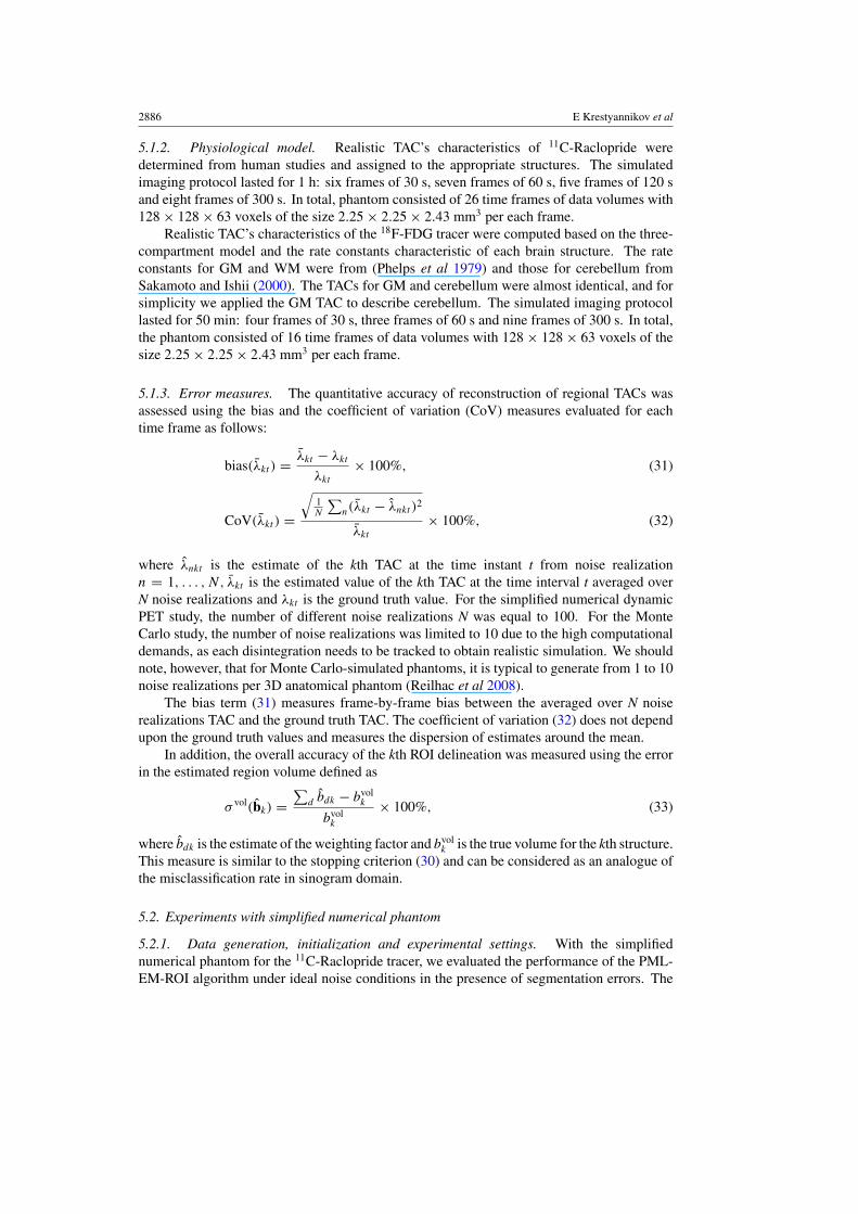
For the 18F-FDG study, the initial WM and GM ROIs were automatically extractedfrom the time-averaged emission images by using a finite mixture models (FMMs)-basedclustering method (Tohka et al 2007). The time-averaged image from the 21st transaxialplane, the corresponding ground truth and the cluster-analysis-based segmentations are shownin figures 5(a)–(c). Due to partial volume effect, about 30% of the voxels in the WMstructure were incorrectly labeled as GM. The initial structures were expanded with the 2Dmorphological dilation operator with the square structuring element of 6 pixels width toaccount for misclassification errors and anatomical variability. At first, only the GM ROIwas extended, and the corresponding TAC was estimated by treating the WM as a marginalstructure. After that the WM ROI was dilated and the WM TAC was reconstructed from thedilated ROI by treating the GM structure as unimportant.

For both studies, the regularization parameters βd and γk were set to 0.1βd and 0.1γk ,respectively. The threshold parameters were set to θ1 = θ2 = 0.05 for the stopping criteria(29), (30). With these settings the algorithm terminated in 42 iterations for 11C-Raclopridestudy and in 38 iterations for the 18F-FDG study.

The PML-EM-ROI algorithm was compared to the sinogram-based LS estimation (24)and the image-domain averaging, both performed over the ground truth ROIs (referred toas LS-GT and OSEM-GT, respectively). Image reconstruction was done with the OSEMalgorithm using 20 iterations and 4 subsets. Averaging over the ground truth ROIs was doneto exclude the segmentation errors, and to evaluate the ability of the PML-EM-ROI algorithmto reduce the partial volume effect errors. Additionally, the performance of the FMM-basedclustering approach (Tohka et al 2007) was examined for the 18F-FDG study. The GM andWM TACs were estimated using the image-domain averaging over the ROIs automaticallysegmented using the FMM-based method (referred to as OSEM-FMM).

2890 E Krestyannikov et al

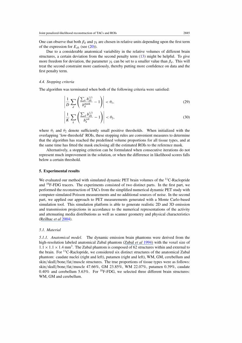
Figure 4. TACs from the Monte Carlo-simulated 11C-Raclopride study (left column) reconstructedwith different approaches, and the corresponding bias (center column) and CoV (right column)curves.

Figure 5. 21st transaxial plane from the Monte Carlo-simulated 18F-FDG study. (a) Time-averagedimage. (b) Ground truth segmentation. (c) FMM-based segmentation. (d) Morphologically dilatedWM structure. (e) Morphologically dilated GM structure.

5.3.2. Results. Figures 4 and 6 show the TACs for the 11C-Raclopride and 18F-FDGthe studies reconstructed with different methods. The PML-EM-ROI algorithm againdemonstrated the best performance among the four compared methods. The LS-GT, OSEM-GT and OSEM-FMM approaches exhibited substantial negative bias even for relatively largestructures, such as GM and cerebellum. Such a degree of underestimation was primarilyexplained by low spatial resolution of the system and the resulting partial volume effect.Moreover, much higher complexity in modeling the 2D acquisition mode (photon propagationthrough the septa), as compared to the 3D mode, has been shown to contribute additionalerrors to simulated data (Reilhac et al 2005).

Joint penalized-likelihood reconstruction of TACs and ROIs 2891

M

Figure 6. TACs from the Monte Carlo 18F-FDG study (left column) reconstructed with differentapproaches, and the corresponding bias (center column) and CoV (right column) curves.

For the 11C-Raclopride tracer, the PML-EM-ROI algorithm substantially decreased thebias component for all the three structures of interest. The error in volume σ vol(bk) betweenthe PML-EM-ROI estimated and the true ROIs for all the three structures stayed in the rangebetween 0.2% and 0.5%. Figures 2(e) and (j) show the final reconstructed ROIs for the putamenand cerebellum structures obtained with the PML-EM-ROI algorithm. A clear improvementin the accuracy of TACs was due to the ability of the algorithm to accommodate the partialvolume effect by using fuzzy ROIs. Fuzzy ROIs are able to represent the exact proportions ofpure tissue types within a voxel (see figures 2(e) and (j)) contrary to the conventional ‘binary’image segmentations restricted to contain one dominant tissue type per voxel.

For the 18F-FDG study, the PML-EM-ROI algorithm improved the accuracy of both GMand WM TACs at the expense of increased variability of TAC estimates, as compared to theLS-GT, OSEM-GT and OSEM-FMM methods. A higher coefficient of variation was causedby relatively large area of support for both WM and GM structures (see figures 5(d) and (e)).Also, as we expected, the PML-EM-ROI algorithm could not completely remove the highnegative bias for GM, arising due to a spill-over of activity beyond the tightly defined truebrain mask. A more accurate reconstruction of structures adjoined to the background couldbe achieved via the inclusion of the detector blurring factors into wdt . The LS-GT, OSEM-GTand OSEM-FMM approaches exhibited a similar performance in the reconstruction of GMand WM TACs, thus justifying the fact that the system spatial resolution is the primary sourceof bias in quantitative PET imaging. The higher negative bias for WM TAC reconstructedwith the OSEM-FMM resulted from severe thinning of the WM structure segmented with theFMM-based clustering approach, as shown in figure 5(c).

6. Discussion and conclusion

We have described a statistical approach for the joint reconstruction of tissue TACs andsegmented 3D ROIs from dynamic PET brain projection data. The problem was formulatedas an optimization task within the penalized-likelihood framework. This offered a potentialway to improve the quantification of ROIs in PET through an accurate modeling of the data

2892 E Krestyannikov et al

acquisition process, proper handling of the Poisson characteristics of sinogram data and theuse of a priori information about the brain anatomy.

The experimental results demonstrated that the joint reconstruction strategy is superior tothe conventional image- and sinogram-based approaches for quantitative ROI-based analysis,specifically to those automatic methods that use the anatomical atlases or deformationsthereof. In particular, the experiments with simplified numerical PET data showed thatthe PML-EM-ROI algorithm is able to correct for the errors arising due to inaccuracies inROI specification. The validation study with the realistic Monte Carlo-simulated PET dataindicated that the PML-EM-ROI algorithm is able to reduce the partial volume effect relatederrors. These errors, primarily induced by a finite spatial resolution, were lowered due tothe unique capability of sinogram ROIs to support the presence of multiple tissue types inone voxel.

The determination of the number of distinct ROIs is an important issue that deserves aseparate discussion. In general, increasing the number of distinct ROIs K increases the size ofthe matrix B. This, in turn, makes the optimization problem more challenging, since the sizeof the number of admissible solutions grows. For low-noise data, when a reliable initializationof all the parameters is available, selecting K equal to the assumed number of structures withdistinct tracer uptake seems reasonable (as was shown with the simplified numerical phantomin section 5.2). If all sources of errors in PET data are taken into account, the uncertaintiesin the resulting TACs may become large. The quantification of large number of distinct ROIsfrom such data may increase the risk of bias in the resulting TACs. We proposed a simple,yet efficient way for reducing the number of distinct ROIs by treating the brain structures ofinterest as distinct ROIs, while combining the rest of the brain into a single ROI. The resultspresented in section 5.3 have shown that this impreciseness does not cause the PML-EM-ROI algorithm to fail. Rather, it makes the reconstruction of TACs more stable, robust andpredictable.

This paper is focused on 2D data acquisition mode. An important application of theiterative PML-EM-ROI would be the quantification of 3D sinograms rebinned to 2D datasets.A very interesting challenge for future work would be to generalize the joint reconstructionapproach to fully 3D mode.

Acknowledgments

The authors would like to thank Anu Juslin and Liisa Karkkainen from the Tampere Universityof Technology, and Anthonin Reilhac from the CERMEP imaging center in Lyon for their helpin generating the phantom on the PET-SORTEO simulator. The work was financially supportedby the Tampere Graduate School in Information Technology (TISE) and the Academy ofFinland under the grant nos 108517, 104834 and 213462 (Finnish Centre of ExcellenceProgram (2006–2011)).

Appendix A. Derivation of the PML-EM-ROI algorithm for the ‘OP’ model

The derivation of the PML-EM-ROI algorithm is based on the ‘optimization transfer’ principle,which replaces at each iteration the original objective function with the surrogate function thatis easier to optimize. Representing the functions �OP(λ, B(j)) and �OP(λ(j+1), B) as (Ahnand Fessler 2004)

LOP(λ, B(j)) = L+(λ, B(j)) + L−(λ, B(j)), (A.1)

�OP(λ(j+1), B) = L+(λ(j+1), B) + L−(λ(j+1), B) − C1(B) − C2(B)), (A.2)

Joint penalized-likelihood reconstruction of TACs and ROIs 2893

where

L+(·, ·) =∑

t

∑d:gdt�0

hOPdt (ldt (·, ·)), (A.3)

L−(·, ·) =∑

t

∑d:gdt<0

hOPdt (ldt (·, ·)), (A.4)

we seek the monotonic surrogates for concave functions L+(·, ·), C1(B) and C2(B)), and forconvex functions L−(·, ·).

We use the idea of De Pierro (1993) to find a lower bound for the log-likelihoodL+(λ, B(j)). Letting g

(j)

dt = wdt

∑k b

(j)

dk λ(j)

kt , we represent the summation term wdt

∑k b

(j)

dk λkt

under the logarithm as

wdt

∑k

b(j)

dk λkt = wdt

∑k

(b

(j)

dk λ(j)

kt

g(j)

dt

g(j)

dt λkt

λ(j)

kt

). (A.5)

Due to Jensen’s inequality and concavity of the function hOPdt (l) defined in (6), the following

holds:

hOPdt (ldt (λ, B(j))) = hOP

dt

(wdt

∑k

(b

(j)

dk λ(j)

kt

g(j)

dt

g(j)

dt λkt

λ(j)

kt

))� wdt

g(j)

dt

∑k

b(j)

dk λ(j)

kt hOPdt

(g

(j)

dt λkt

λ(j)

kt

).

(A.6)

A separable surrogate function that minorizes L+(λ, B(j)) is then defined as

Q1(λ, B(j); λ(j), B(j)) =∑

t

∑d:gdt�0

wdt

g(j)

dt

∑k

b(j)

dk λ(j)

kt hOPdt

(g

(j)

dt λkt

λ(j)

kt

). (A.7)

Similarly, we formulate a surrogate for L+(λ(j+1), B) as

Q2(λ(j+1), B; λ(j), B(j)) =

∑t

∑d:gdt�0

wdt

g(j)

dt

∑k

b(j)

dk λ(j)

kt hOPdt

(g

(j)

dt bdkλ(j+1)

dt

b(j)

dk λ(j)

kt

). (A.8)

When gdt < 0 and log-likelihoods hOPdt (ldt (λ, B(j))) and hOP

dt (ldt (λ(j+1), B)) are convex, we

choose linear minorizing surrogates

qdt (ldt (λ, B(j)); ldt (λ(j), B(j))) = hOP

dt (ldt (λ(j), B(j)))(ldt (λ, B(j)) − ldt (λ

(j), B(j)))

+ hOPdt (ldt (λ

(j), B(j))), (A.9)

qdt (ldt (λ(j+1), B); ldt (λ

(j), B(j))) = hOPdt (ldt (λ

(j), B(j)))(ldt (λ(j+1), B) − ldt (λ

(j), B(j)))

+ hOPdt (ldt (λ

(j), B(j))). (A.10)

In fact, according to Ahn and Fessler (2004), a tangent line qdt at current iterate ldt (λ(j), B(j))

is a proper surrogate for hOPdt , since qdt lies below for all ldt (λ, B(j)) � 0 and ldt (λ

(j+1), B) � 0due to the convexity of hOP

dt . Utilizing (A.9), (A.10), we define surrogates for L−(λ, B(j)) andL−(λ(j+1), B) as follows:

2894 E Krestyannikov et al

L−(λ, B(j)) �∑

t

∑d:gdt<0

qdt (ldt (λ, B(j)); ldt (λ(j), B(j))

=∑

t

∑d:gdt<0

[(gdt

g(j)

dt

− 1

)wdt

∑k

b(j)

dk λkt + Const

]

= Q3(λ, B(j); λ(j), B(j)), (A.11)

L−(λ(j+1), B) �∑

t

∑d:gdt<0

qdt (ldt (λ(j+1), B); ldt (λ

(j), B(j))

=∑

t

∑d:gdt<0

[(gdt

g(j)

dt

− 1

)wdt

∑k

bdkλ(j+1)

kt + Const

]

= Q4(λ(j+1), B; λ(j), B(j)), (A.12)

where ‘Const’ is a constant with respect to the unknown parameter.Finally, to construct surrogates for the penalty functions C1(B) and C2(B), we invoke the

following substitutions (De Pierro 1995):∑k bdk

bmaskd

− 1 =∑

k

αdk

(bdk − b

(j)

dk

αdkbmaskd

+

∑k b

(j)

dk

bmaskd

− 1

), (A.13)

∑d bdk

bvolk

− 1 =∑

d

ωdk

(bdk − b

(j)

dk

ωdkbvolk

+

∑d b

(j)

dk

bvolk

− 1

), (A.14)

where αdk and ωdk are non-negative real numbers, such that∑

k αdk = 1,∀d = 1, . . . , D and∑d ωdk = 1,∀k = 1, . . . , K . To satisfy these conditions, we choose αdk as 1/K , where K is

the number of different ROIs. We define ωdk as 1/D+, if the dth row of the matrix B containsat least one nonzero element, and 0 otherwise. D+ is the total number of rows with at leastone nonzero element in B.

The separable majorizing functions for C1(B) and C2(B) are then given by

Q5(B; B(j)) =∑d,k

βd

2bmaskd

αdk

(bdk − b

(j)

dk

αdkbmaskd

+

∑k b

(j)

dk

bmaskd

− 1

)2

, (A.15)

Q6(B; B(j)) =∑d,k

γk

2bvolk

ωdk

(bdk − b

(j)

dk

ωdkbvolk

+

∑d b

(j)

dk

bvolk

− 1

)2

. (A.16)

The overall surrogates for �(λ, B(j)) and �(λ(j+1), B) can now be constructed during theE-step of the algorithm as

Q(λ, B(j); λ(j), B(j)) = Q1(λ, B(j); λ(j), B(j)) + Q3(λ, B(j); λ(j), B(j)), (A.17)

Q(λ(j+1), B; λ(j), B(j)) = Q2(λ(j+1), B; λ(j), B(j)) + Q4(λ

(j+1), B; λ(j), B(j)) (A.18)

− Q5(B; B(j)) − Q6(B; B(j)). (A.19)

The maximization of surrogates during the M-step yields the update rules (16) and (17).

Joint penalized-likelihood reconstruction of TACs and ROIs 2895

References

Acton P D, Pilowsky L S, Kung H F and Ell P J 1999 Automatic segmentation of dynamic neuroreceptor single-photonemission tomography images using fuzzy clustering Eur. J. Nucl. Med. 26 582–90

Ahn S and Fessler J A 2004 Emission image reconstruction for randoms-precorrected PET data allowing negativesinogram values IEEE Trans. Med. Imaging 23 591–601

Allen J S, Damasio H, Grabowski T, Bruss J and Zhang W 2003 Sexual dimorphism and assymetries in the gray-whitecomposition of the human cerebrum Neuroimage 18 880–94

Ashburner J, Haslam J, Taylor C, Cunningham V J and Jones T 1996 A cluster analysis approach for the characterizationof dynamic PET data Quantification of Brain Function Using PET ed R Myers, V Cunningham, D Bailey andT Jones (New York: Academic) pp 301–6

Aston J A, Cunningham V J, Asselin M C, Hammers A, Evans A C and Gunn R N 2002 Positron emission tomographypartial volume correction: estimation and algorithms J. Cereb. Blood Flow Metab. 22 1019–34

Carson R E 1986 A maximum-likelihood method for region of interest evaluation in emission tomography J. Comput.Assist. Tomogr. 10 654–63

Casey M E, Gadagkar H and Newport D 1995 A component based method for normalization in volume PETProc. Int. Meeting on Fully Three-Dimensional Image Reconstruction in Radiology and Nuclear Medicinepp 67–71

De Pierro A R 1993 On the relation between the ISRA and the EM algorithm for positron emission tomography IEEETrans. Med. Imaging 12 328–33

De Pierro A R 1995 A modified expectation maximization algorithm for penalized likelihood estimation in emissiontomography IEEE Trans. Med. Imaging 14 132–7

Dempster A P, Laird N M and Rubin D B 1977 Maximum likelihood from incomplete data via the EM algorithmJ. R. Statist. Soc. Ser. B 39 1–38

Formiconi A R 1993 Least squares algorithm for region-of-interest evaluation in emission tomography IEEE Trans.Med. Imaging 12 90–100

Frouin V, Comtat C, Reilhac A and Gregoire M-C 2002 Correction of partial-volume effect for PET striatal imaging:fast implementation and study of robustness J. Nucl. Med. 43 1715–26

Hammers A, Allom R, Koepp M J, Free S L, Myers R, Lemieux L, Mitchell T N, Brooks D J and Duncan J S 2003Three-dimensional maximum probability atlas of the human brain with particular reference to the temporal lobeHum. Brain Mapp. 19 224–47

Hoffman E J, Huang S C, Phelps M E and Kuhl D E 1981 Quantitation in positron emission computed tomography:4. Effect of accidental coincidences J. Comput. Assist. Tomogr. 5 391–400

Krestyannikov E, Tohka J and Ruotsalainen U 2006 Segmentation of dynamic emission tomography data in projectionspace Proc. Computer Vision Approaches to Medical Image Analysis (CVAMIA) Workshop ed R Beichel andM Sonka LNCS 4241 pp 108–19

Lange K and Carson R E 1984 EM reconstruction algorithms for emission and transmission tomography J. Comput.Assist. Tomogr. 8 306–16

Lange N, Giedd J N, Castellanos F X, Vaituzis A C and Rapoport J L 1997 Variability of human brain structure size:ages 4–20 years Psychiatry Res.: Neuroimaging Sect. 74 1–12

Lange K, Hunter D R and Yang I 2000 Optimization transfer using surrogate objective functions J. Comput. GraphicalStat. 9 1–20

Leahy R M and Qi J 2000 Statistical approaches in quantitative positron emission tomography Stat.Comput. 10 147–65

O’Sullivan F 1993 Imaging radiotracer model parameters in PET: a mixture analysis approach IEEE Trans. Med.Imaging 12 399–412

Phelps M, Huang S, Hoffman E, Selin C, Sokoloff L and Kuhl D 1979 Tomographic measurement of localcerebral glucose metabolic rate in humans with (F-18)2-fluoro-2-deoxy-D-glucose: validation of method Ann.Neurol. 6 371–88

Reilhac A, Batan G, Michel C, Grova C, Tohka J, Collins D L, Costes N and Evans A 2005 PET-SORTEO: validationand development of database of simulated PET volumes IEEE Trans. Nucl. Sci. 52 1321–8

Reilhac A, Lartizien C, Costes N, Sans S, Comtat C, Gunn R and Evans A 2004 PET-SORTEO: a Monte Carlo-basedsimulator with high count rate capabilities IEEE Trans. Nucl. Sci. 51 46–52

Reilhac A, Tomei S, Buvat I, Michel C, Keheren F and Costes N 2008 Simulation-based evaluation of OSEM iterativereconstruction methods in dynamic brain PET studies Neuroimage 39 359–68

Reutter B W, Gullberg G T and Huesman R H 2000 Direct least-squares estimation of spatiotemporal distributionsfrom dynamic SPECT projections using a spatial segmentation and temporal B-splines IEEE Trans. Med.Imaging 19 434–50

2896 E Krestyannikov et al

Sakamoto S and Ishii K 2000 Low cerebral glucose extraction rates in the human medial temporal cortex andcerebellum J. Neurolog. Sci. 172 41–8

Shattuck D W, Mirza M, Adisetiyo V, Hojatkashani C, Salamon G, Narr K L, Poldrack R A, Bilder R M andToga A W 2008 Construction of a 3D probabilistic atlas of human brain structures Neuroimage 39 1064–80

Shepp L A and Vardi Y 1982 Maximum-likelihood reconstruction for emission tomography IEEE Trans. Med.Imaging MI-1 113–22

Svarer C, Madsen K, Hasselbach S G, Pinborg L H, Haugbol S, Frokjaer V G, Holm S, Paulson O B and KnudsenG 2005 MR-based automatic delineation of volumes of interest in human brain PET images using probabilitymaps Neuroimage 24 969–79

Tohka J and Mykkanen J 2004 Deformable mesh for automated surface extraction from noisy images Int. J. ImageGraph. 4 405–32

Tohka J, Krestyannikov E, Dinov I D, MacKenzie-Graham A, Shattuck D W, Ruotsalainen U and Toga A 2007Genetic algorithms for finite mixture model based voxel classification in neuroimaging IEEE Trans. Med.Imaging 26 696–711

Watson C C, Newport D and Casey M E 1996 A single scatter simulation technique for scatter correction in 3DPET Proc. Int. Meeting on Fully Three-Dimensional Image Reconstruction in Radiology and Nuclear Medicineed P Grangeat and J L Amans pp 225–68

Woods R P, Cherry S R and Mazziotta J C 1992 Rapid automated algorithm for aligning and reslicing PET imagesJ. Comput. Assist. Tomogr. 16 620–33

Yasuno F, Hasine A H, Suhara T, Ichimiya T, Sudo Y, Inoue M, Takano A, Ou T, Ando T and Toyama H 2002Template-based method for multiple volumes of interest of human brain PET images Neuroimage 16 577–86

Ziskind I and Wax M 1988 Maximum likelihood localization of multiple sources by alternating projection IEEETrans. Acoust. Speech Signal Process. 36 1553–60

Zubal I, Harell C C, Smith E, Rattner Z, Gindi G and Hoffer P 1994 Computerized three-dimensional segmentedhuman anatomy Med. Phys. 21 299–302