Joint Factor Analysis (JFA) and i-vector Tutorial Howard Lei

Welcome message from author
This document is posted to help you gain knowledge. Please leave a comment to let me know what you think about it! Share it to your friends and learn new things together.
Transcript
Joint Factor Analysis (JFA) and i-vector Tutorial
Howard Lei
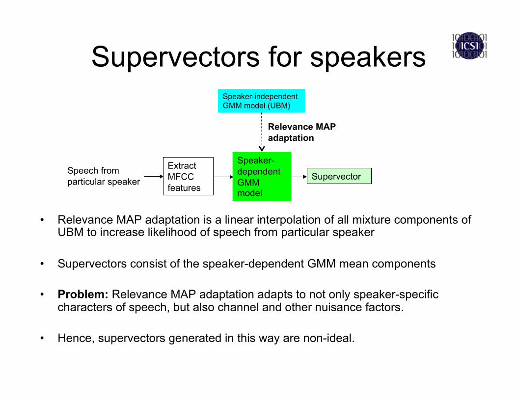
• Relevance MAP adaptation is a linear interpolation of all mixture components of UBM to increase likelihood of speech from particular speaker
• Supervectors consist of the speaker-dependent GMM mean components
• Problem: Relevance MAP adaptation adapts to not only speaker-specific characters of speech, but also channel and other nuisance factors.
• Hence, supervectors generated in this way are non-ideal.
Supervectors for speakers
Speech from particular speaker
Speaker-independent GMM model (UBM)
Extract MFCC features
Speaker-dependent GMM model
Supervector
Relevance MAP adaptation
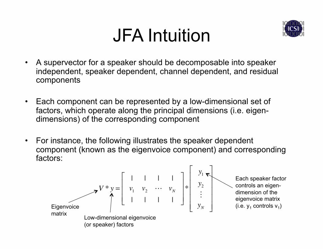
• A supervector for a speaker should be decomposable into speaker independent, speaker dependent, channel dependent, and residual components
• Each component can be represented by a low-dimensional set of factors, which operate along the principal dimensions (i.e. eigen-dimensions) of the corresponding component
• For instance, the following illustrates the speaker dependent component (known as the eigenvoice component) and corresponding factors:
JFA Intuition
V * y =| | | |v1 v2 vN| | | |
⎡
⎣
⎢⎢⎢
⎤
⎦
⎥⎥⎥*
y1y2yN
⎡
⎣
⎢⎢⎢⎢⎢
⎤
⎦
⎥⎥⎥⎥⎥Eigenvoice
matrix Low-dimensional eigenvoice (or speaker) factors
Each speaker factor controls an eigen-dimension of the eigenvoice matrix (i.e. y1 controls v1)

• A given speaker GMM supervector s can be decomposed as follows:
• where: – Vector m is a speaker-independent supervector (from UBM) – Matrix V is the eigenvoice matrix – Vector y is the speaker factors. Assumed to have N(0,1) prior distribution – Matrix U is the eigenchannel matrix – Vector x is the channel factors. Assumed to have N(0,1) prior distribution – Matrix D is the residual matrix, and is diagonal – Vector z is the speaker-specific residual factors. Assumed to have N(0,1)
prior distribution
JFA Model
s = m +Vy +Ux + DzSpeaker-independent component
Speaker-dependent component
Channel-dependent component
Speaker-dependent residual component “Ideal” speaker
supervector
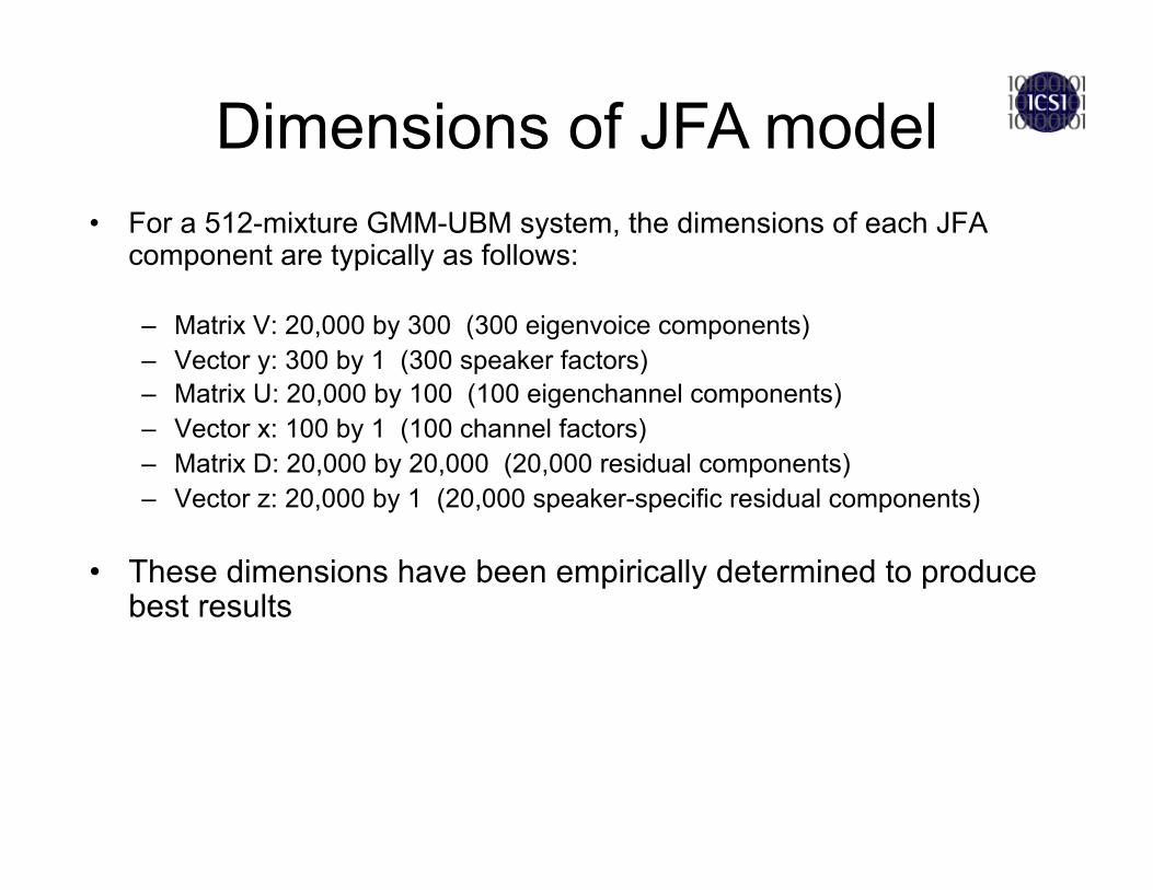
• For a 512-mixture GMM-UBM system, the dimensions of each JFA component are typically as follows:
– Matrix V: 20,000 by 300 (300 eigenvoice components) – Vector y: 300 by 1 (300 speaker factors) – Matrix U: 20,000 by 100 (100 eigenchannel components) – Vector x: 100 by 1 (100 channel factors) – Matrix D: 20,000 by 20,000 (20,000 residual components) – Vector z: 20,000 by 1 (20,000 speaker-specific residual components)
• These dimensions have been empirically determined to produce best results
Dimensions of JFA model
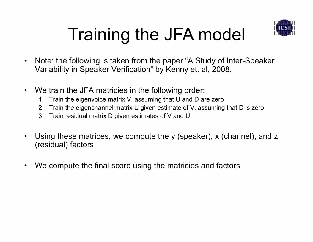
• Note: the following is taken from the paper “A Study of Inter-Speaker Variability in Speaker Verification” by Kenny et. al, 2008.
• We train the JFA matricies in the following order: 1. Train the eigenvoice matrix V, assuming that U and D are zero 2. Train the eigenchannel matrix U given estimate of V, assuming that D is zero 3. Train residual matrix D given estimates of V and U
• Using these matrices, we compute the y (speaker), x (channel), and z (residual) factors
• We compute the final score using the matricies and factors
Training the JFA model
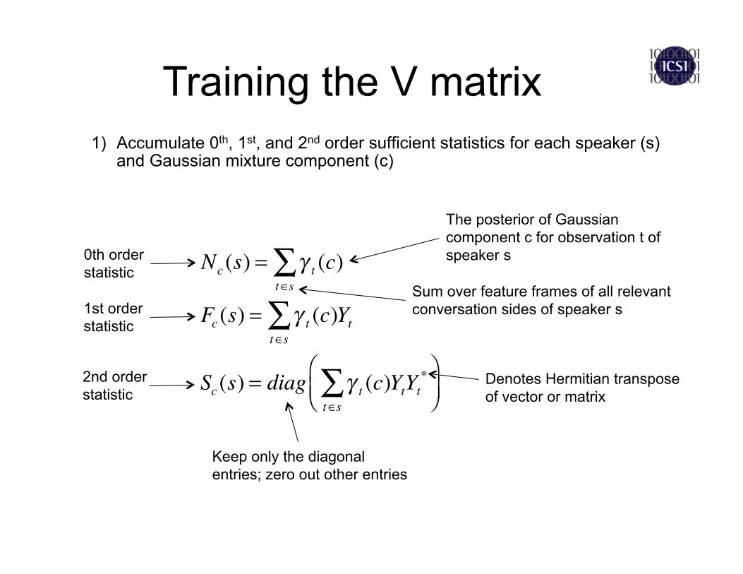
1) Accumulate 0th, 1st, and 2nd order sufficient statistics for each speaker (s) and Gaussian mixture component (c)
Training the V matrix
Nc (s) = γ tt∈s∑ (c)
Fc (s) = γ tt∈s∑ (c)Yt
Sc (s) = diag γ tt∈s∑ (c)YtYt
*⎛⎝⎜
⎞⎠⎟
The posterior of Gaussian component c for observation t of speaker s
Keep only the diagonal entries; zero out other entries
0th order statistic
1st order statistic
2nd order statistic
Denotes Hermitian transpose of vector or matrix
Sum over feature frames of all relevant conversation sides of speaker s

2) Center the 1st and 2nd order statistics
Fc (s) = Fc (s) − Nc (s)mc
Sc (s) = Sc (s) − diag Fc (s)mc* + mcFc (s)
* − Nc (s)mcmc*( )
0th order statistic
Centered 1st order statistic
Centered 2nd order statistic
UBM mean for mixture component c
Training the V matrix
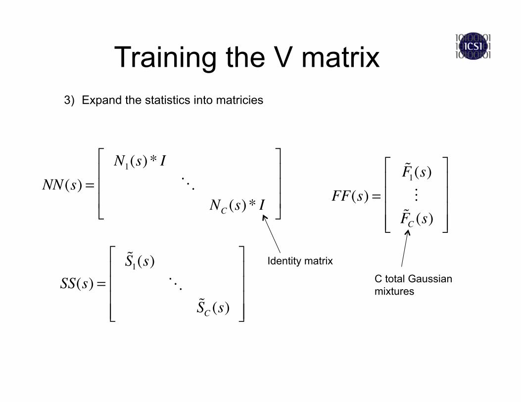
3) Expand the statistics into matricies
NN(s) =N1(s) * I
NC (s) * I
⎡
⎣
⎢⎢⎢
⎤
⎦
⎥⎥⎥ FF(s) =
F1(s)FC (s)
⎡
⎣
⎢⎢⎢⎢
⎤
⎦
⎥⎥⎥⎥
C total Gaussian mixtures
Identity matrix
SS(s) =
S1(s)
SC (s)
⎡
⎣
⎢⎢⎢⎢
⎤
⎦
⎥⎥⎥⎥
Training the V matrix
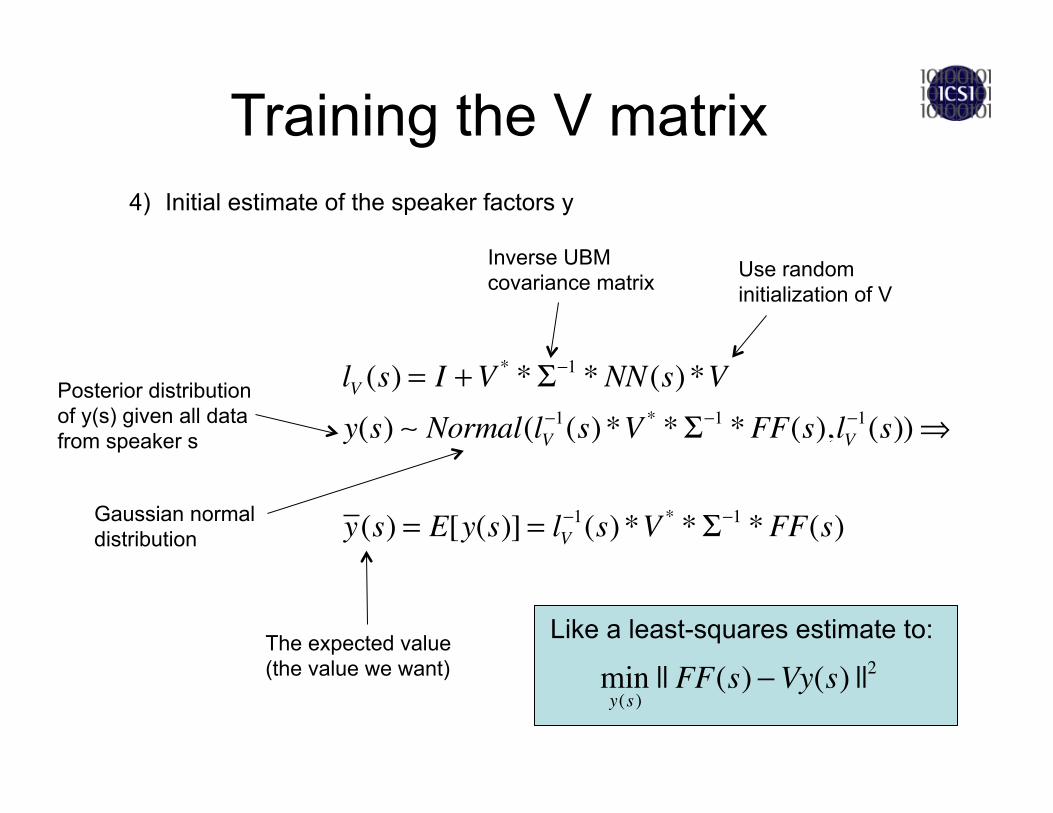
4) Initial estimate of the speaker factors y
lV (s) = I +V* *Σ−1 *NN(s) *V
y(s) Normal(lV−1(s) *V * *Σ−1 *FF(s),lV
−1(s))⇒
y(s) = E[y(s)] = lV−1(s) *V * *Σ−1 *FF(s)
Posterior distribution of y(s) given all data from speaker s
The expected value (the value we want)
Gaussian normal distribution
Use random initialization of V
Training the V matrix
Inverse UBM covariance matrix
Like a least-squares estimate to:
miny(s )
|| FF(s) −Vy(s) ||2
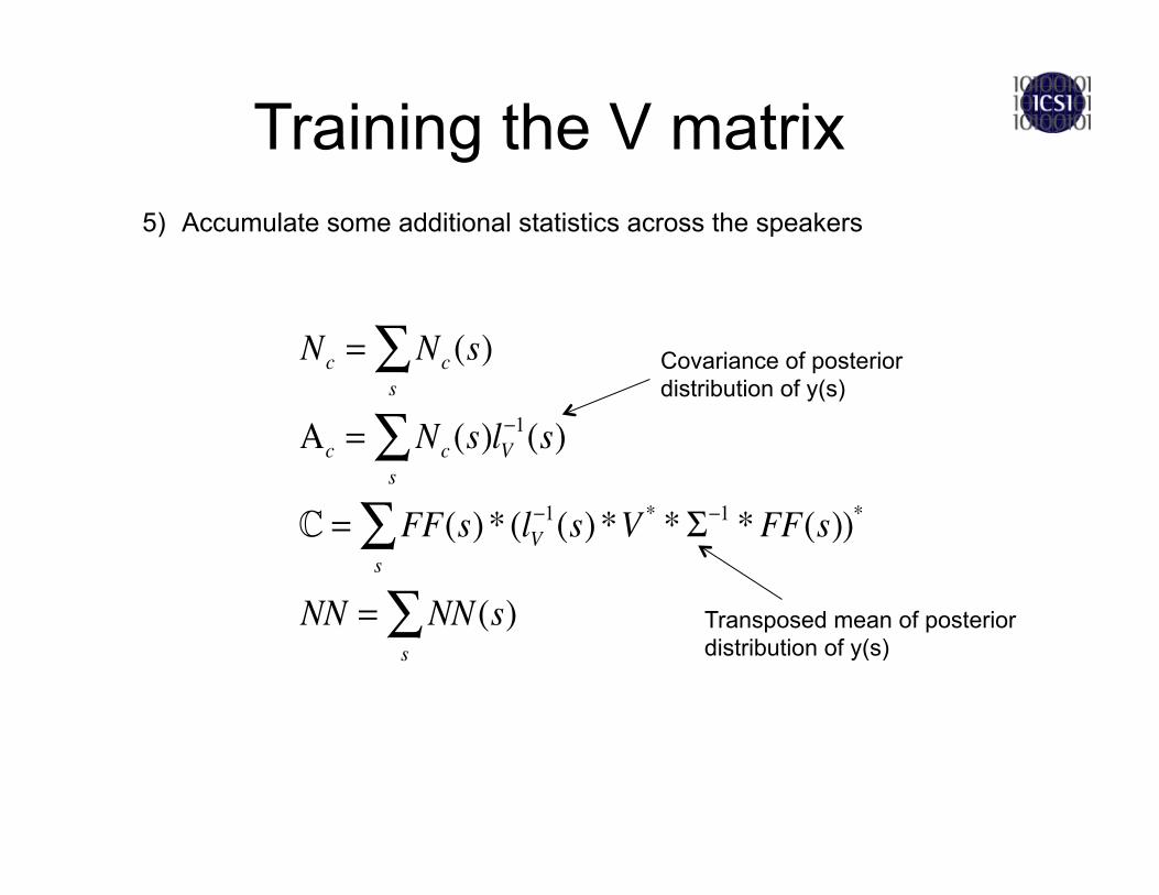
5) Accumulate some additional statistics across the speakers
Nc = Nc (s)s∑
Αc = Nc (s)lV−1(s)
s∑
= FF(s) * (lV−1(s) *V * *Σ−1 *FF(s))*
s∑
NN = NN(s)s∑
Covariance of posterior distribution of y(s)
Transposed mean of posterior distribution of y(s)
Training the V matrix
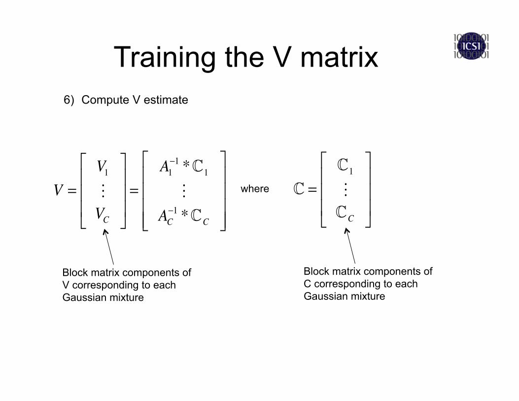
6) Compute V estimate
V =V1VC
⎡
⎣
⎢⎢⎢
⎤
⎦
⎥⎥⎥=
A1−1 *1
AC−1 *C
⎡
⎣
⎢⎢⎢⎢
⎤
⎦
⎥⎥⎥⎥
Block matrix components of V corresponding to each Gaussian mixture
where =1C
⎡
⎣
⎢⎢⎢
⎤
⎦
⎥⎥⎥
Block matrix components of C corresponding to each Gaussian mixture
Training the V matrix
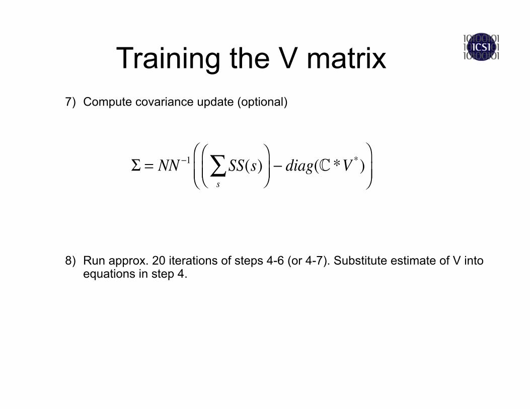
7) Compute covariance update (optional)
8) Run approx. 20 iterations of steps 4-6 (or 4-7). Substitute estimate of V into equations in step 4.
Σ = NN −1 SS(s)s∑⎛⎝⎜
⎞⎠⎟− diag( *V *)
⎛⎝⎜
⎞⎠⎟
Training the V matrix
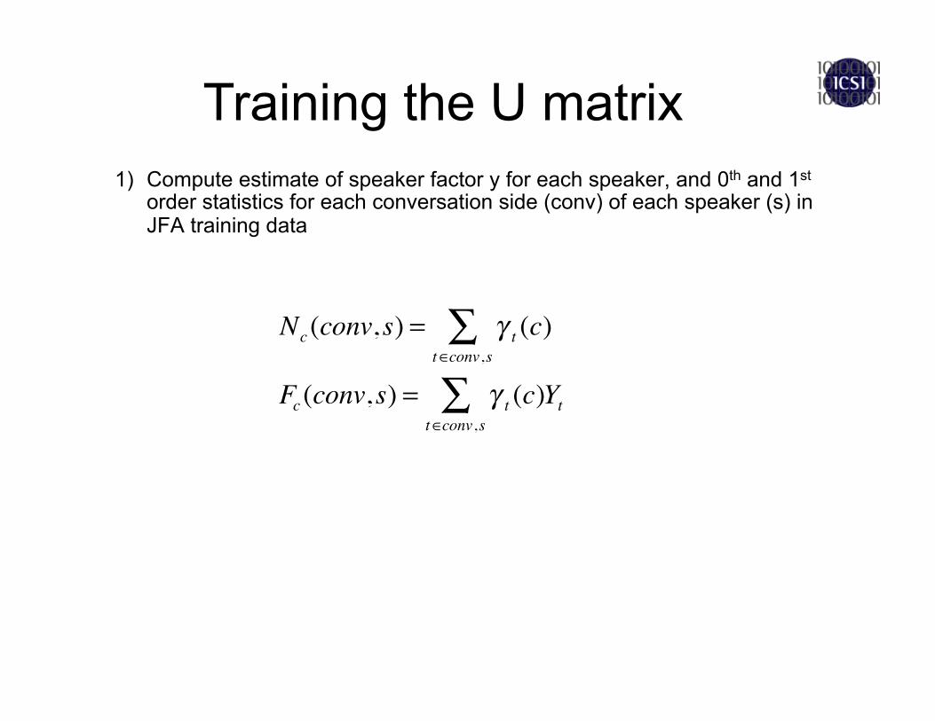
1) Compute estimate of speaker factor y for each speaker, and 0th and 1st order statistics for each conversation side (conv) of each speaker (s) in JFA training data
Training the U matrix
Nc (conv, s) = γ tt∈conv,s∑ (c)
Fc (conv, s) = γ tt∈conv,s∑ (c)Yt
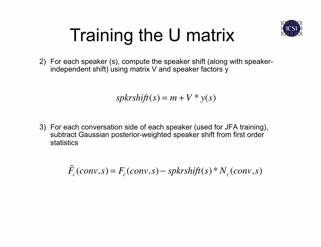
2) For each speaker (s), compute the speaker shift (along with speaker-independent shift) using matrix V and speaker factors y
3) For each conversation side of each speaker (used for JFA training), subtract Gaussian posterior-weighted speaker shift from first order statistics
Training the U matrix
spkrshift(s) = m +V * y(s)
Fc (conv, s) = Fc (conv, s) − spkrshift(s) *Nc (conv, s)
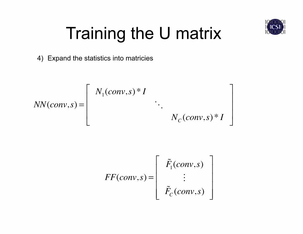
4) Expand the statistics into matricies
NN(conv, s) =N1(conv, s) * I
NC (conv, s) * I
⎡
⎣
⎢⎢⎢
⎤
⎦
⎥⎥⎥
FF(conv, s) =
F1(conv, s)
FC (conv, s)
⎡
⎣
⎢⎢⎢⎢
⎤
⎦
⎥⎥⎥⎥
Training the U matrix
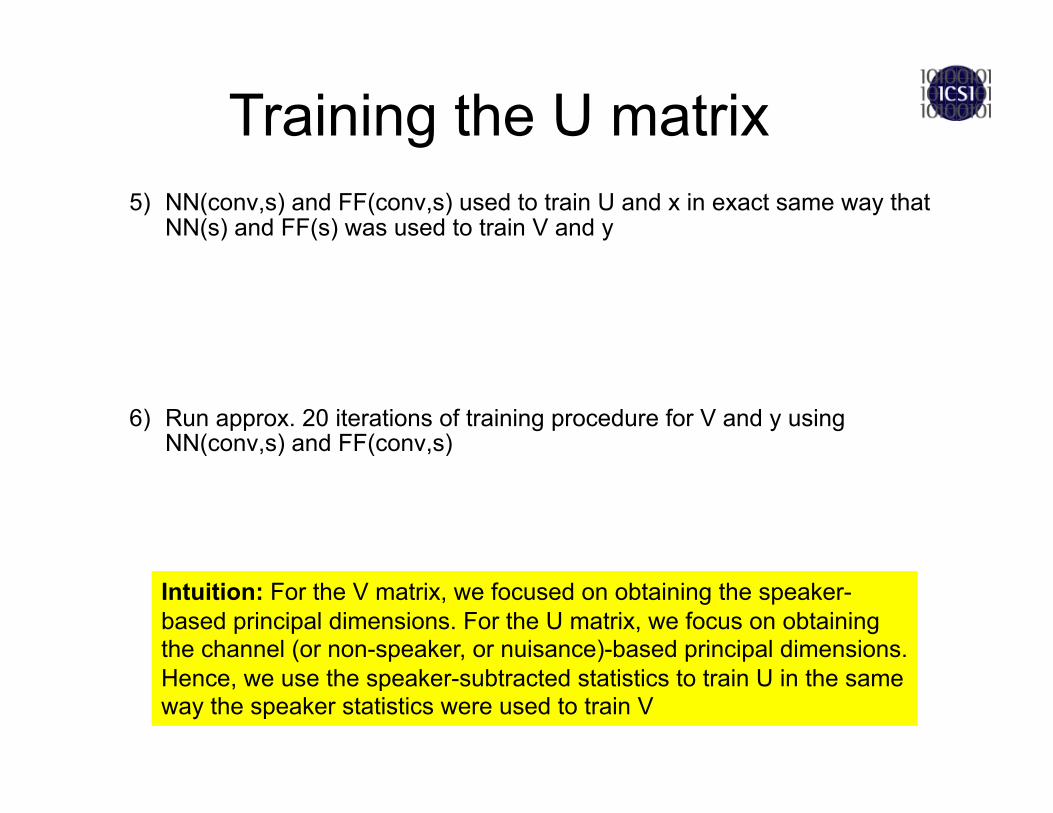
5) NN(conv,s) and FF(conv,s) used to train U and x in exact same way that NN(s) and FF(s) was used to train V and y
6) Run approx. 20 iterations of training procedure for V and y using NN(conv,s) and FF(conv,s)
Training the U matrix
Intuition: For the V matrix, we focused on obtaining the speaker-based principal dimensions. For the U matrix, we focus on obtaining the channel (or non-speaker, or nuisance)-based principal dimensions. Hence, we use the speaker-subtracted statistics to train U in the same way the speaker statistics were used to train V
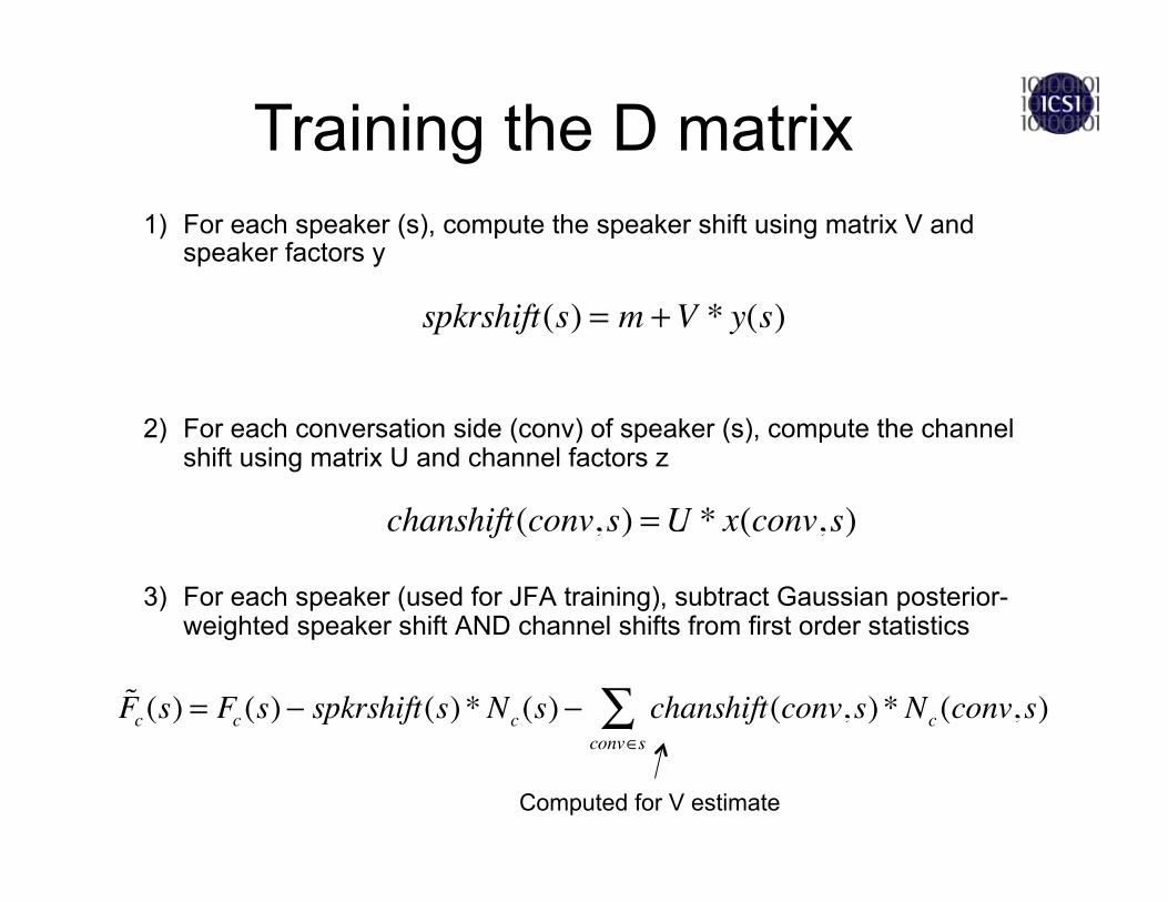
1) For each speaker (s), compute the speaker shift using matrix V and speaker factors y
2) For each conversation side (conv) of speaker (s), compute the channel shift using matrix U and channel factors z
3) For each speaker (used for JFA training), subtract Gaussian posterior-weighted speaker shift AND channel shifts from first order statistics
Training the D matrix
spkrshift(s) = m +V * y(s)
chanshift(conv, s) =U * x(conv, s)
Fc (s) = Fc (s) − spkrshift(s) *Nc (s) − chanshift(conv, s) *Nc (conv, s)conv∈s∑
Computed for V estimate
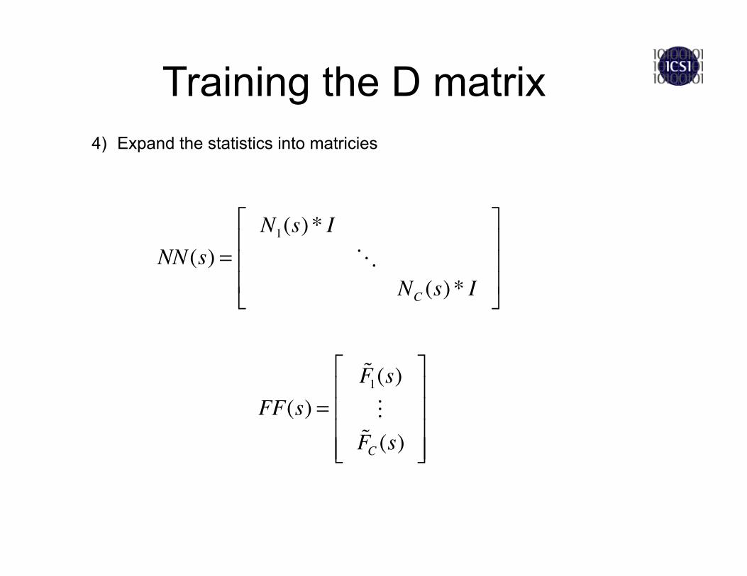
4) Expand the statistics into matricies
NN(s) =N1(s) * I
NC (s) * I
⎡
⎣
⎢⎢⎢
⎤
⎦
⎥⎥⎥
FF(s) =
F1(s)FC (s)
⎡
⎣
⎢⎢⎢⎢
⎤
⎦
⎥⎥⎥⎥
Training the D matrix
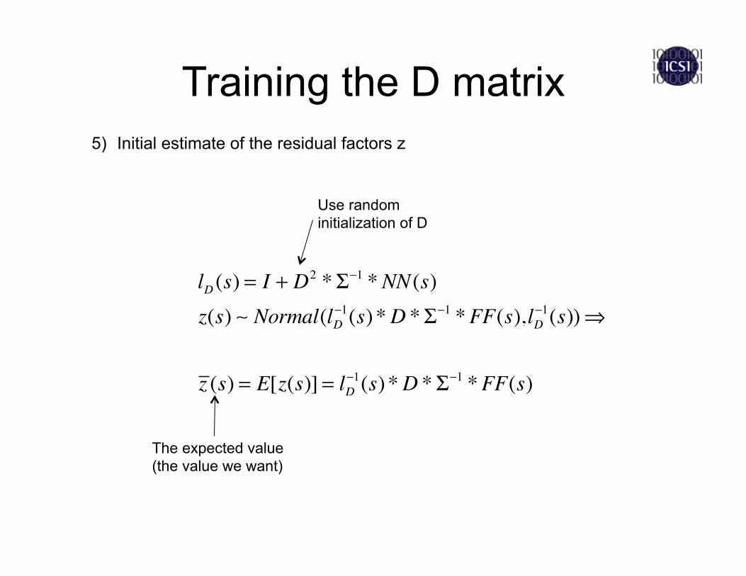
5) Initial estimate of the residual factors z
Training the D matrix
lD (s) = I + D2 *Σ−1 *NN(s)
z(s) Normal(lD−1(s) *D *Σ−1 *FF(s),lD
−1(s))⇒
z (s) = E[z(s)] = lD−1(s) *D *Σ−1 *FF(s)
The expected value (the value we want)
Use random initialization of D

6) Accumulate some additional statistics across the speakers
Nc = Nc (s)s∑
a = diag(NN(s) * lD−1(s))
s∑
b = diag(FF(s) * (lD−1(s) *D *Σ−1 *FF(s))*)
s∑
NN = NN(s)s∑
Covariance of posterior distribution of y(s)
Transposed mean of posterior distribution of y(s)
Training the D matrix
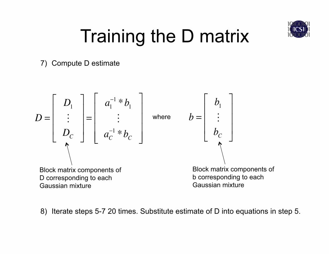
7) Compute D estimate
8) Iterate steps 5-7 20 times. Substitute estimate of D into equations in step 5.
D =D1DC
⎡
⎣
⎢⎢⎢
⎤
⎦
⎥⎥⎥=
a1−1 *b1
aC−1 *bC
⎡
⎣
⎢⎢⎢⎢
⎤
⎦
⎥⎥⎥⎥
Block matrix components of D corresponding to each Gaussian mixture
where b =b1bC
⎡
⎣
⎢⎢⎢
⎤
⎦
⎥⎥⎥
Block matrix components of b corresponding to each Gaussian mixture
Training the D matrix

• Refer to “Comparison of Scoring Methods used in Speaker Recognition with Joint Factor Analysis” by Glembek, et. al.
1) Use the matricies V, U, and D to get estimates of y, x, and z, in terms of their posterior means given the observations
2) For test conversation side (tst) and target speaker conversation side (tar), one way to obtain final score is via the following linear product:
Score = (V * y(tar) + D * z(tar))* *Σ−1 * (FF(tst) − NN(tst) *m − NN(tst) *U * x(tst))
Computing linear score
Target speaker conversation side centered around speaker and residual factors
Test conversation side has speaker- independent and channel factors removed, and hence also centered around speaker and residual factors
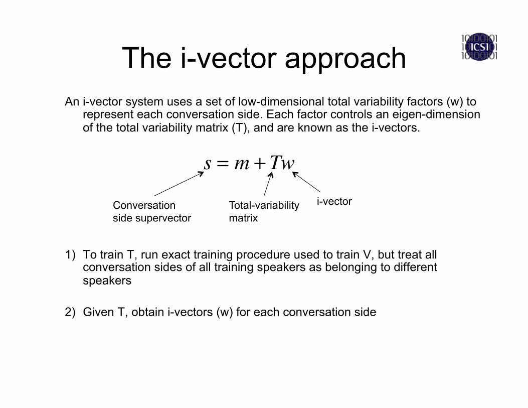
An i-vector system uses a set of low-dimensional total variability factors (w) to represent each conversation side. Each factor controls an eigen-dimension of the total variability matrix (T), and are known as the i-vectors.
1) To train T, run exact training procedure used to train V, but treat all conversation sides of all training speakers as belonging to different speakers
2) Given T, obtain i-vectors (w) for each conversation side
The i-vector approach
i-vector
s = m + Tw
Total-variability matrix
Conversation side supervector
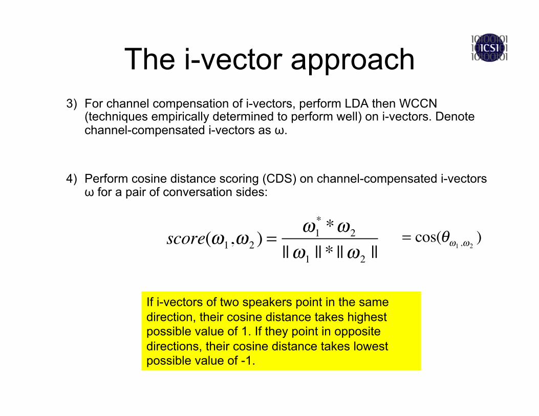
3) For channel compensation of i-vectors, perform LDA then WCCN (techniques empirically determined to perform well) on i-vectors. Denote channel-compensated i-vectors as ω.
4) Perform cosine distance scoring (CDS) on channel-compensated i-vectors ω for a pair of conversation sides:
The i-vector approach
score(ω1,ω2 ) =ω1* *ω2
||ω1 || * ||ω2 ||
If i-vectors of two speakers point in the same direction, their cosine distance takes highest possible value of 1. If they point in opposite directions, their cosine distance takes lowest possible value of -1.
= cos(θω1 ,ω2)

The End
Related Documents