Joint Bidding in the Name-Your-Own-Price Channel: A Strategic Analysis

MANAGEMENT SCIENCEVol. 54, No. 10, October 2008, pp. 1685–1699issn 0025-1909 �eissn 1526-5501 �08 �5410 �1685

informs ®

doi 10.1287/mnsc.1080.0888©2008 INFORMS

Joint Bidding in the Name-Your-Own-PriceChannel: A Strategic Analysis

Wilfred AmaldossFuqua School of Business, Duke University, Durham, North Carolina 27708, [email protected]

Sanjay JainMays Business School, Texas A&M University, College Station, Texas 77843, [email protected]

In this paper, we study the name-your-own-price (NYOP) channel. We examine theoretically and empiricallywhether asking consumers to place a joint bid for multiple items, rather than bid one item at a time aspracticed today, can increase NYOP retailers’ profits. Relatedly, we also examine whether allowing consumersto self-select whether to place a joint bid or itemwise bids increases retailers’ profits and consumers’ surplus. Weconstruct a dynamic model that incorporates both demand uncertainty and supply uncertainty to address theseissues. Our theoretical analysis identifies the conditions under which joint bidding can increase both NYOPretailers’ profits and consumers’ surplus. We find that some consumers might bid more for the very same itemswhen they place joint bids. The increase in bid amount is related to the fact that joint bidding reduces the chanceof mismatch between NYOP retailers’ costs and consumer bids. We conducted a laboratory study to assess thedescriptive validity of some of the model predictions, because there are no field data on joint bidding in theNYOP channel. The results of the study are directionally consistent with our theory.

Key words : pricing; bidding; Internet; experimental economicsHistory : Accepted by David E. Bell, decision analysis; received July 9, 2007. This paper was with the authors1 month for 1 revision. Published online in Articles in Advance August 20, 2008.

1. IntroductionWith the advent of the Internet, retailers have adoptedseveral innovative pricing mechanisms. One suchmethod is the name-your-own-price (NYOP) mecha-nism pioneered by Priceline. In this pricing method,the NYOP retailer lists a set of perishable goodsavailable for sale but does not post prices. Thesegoods are also opaque in the sense that some impor-tant product information (e.g., flight time, numberof stops, and identity of the service provider) is notrevealed to consumers at the time of bidding. Theconsumers, who arrive asynchronously to the mar-ket, evaluate the opaque products and then place bidsfor them. The bid is visible to the NYOP retailer butnot to the service providers such as airlines or hotels.The service providers frequently change the prices ofgoods according to their yield management policy,but the price changes are not revealed to consumers.The spread between a consumer’s bid and the pre-vailing lowest price is retained by the NYOP retailer(Kannan and Kopalle 2001). The sales revenue ofPriceline, which is the leading NYOP retailer in theUnited States, was more than $2 billion in 2005, andit is expected to cross $4 billion in 2007, implying thatthe NYOP mechanism is a viable business model.1

1 Priceline has also extended its business to international marketssuch as the United Kingdom, Hong Kong, and Taiwan (source:priceline.com).

The NYOP model is still evolving, and there isno consensus on how best to structure the pricingmechanism. For example, prominent NYOP retail-ers like Priceline and Expedia’s Price Matcher allowconsumers only to place a single bid for a givenitem. A German NYOP retailer, however, allows con-sumers to bid repeatedly for the very same item (seeHann and Terwiesch 2003). A recent theoretical anal-ysis shows that if it is prohibitively costly to preventsurreptitious repeat bidding then the NYOP retailermight benefit by encouraging repeat bidding (Fay2004).In practice, NYOP retailers often sell more than

one category of products. For example, Priceline andExpedia’s Price Matcher sell airline tickets, hotelrooms, and car rentals. This observation raises aninteresting question. In theory, would it be prof-itable for NYOP retailers to ask consumers to placea joint bid for multiple items rather than bid sepa-rately for each item? It seems that joint bidding mightencourage consumers to place lower joint bids thanthey would have if they were bidding individuallyfor each item. Therefore, a NYOP retailer’s profitscould potentially decline if it allowed joint bidding.Intuitively, joint bidding might encourage consumersto bid less than what they would bid under item-wise bidding. Indeed, consumers usually expect adiscount when buying multiple items in a bundle

1685

INFORMS

holds

copyrightto

this

article

and

distrib

uted

this

copy

asa

courtesy

tothe

author(s).

Add

ition

alinform

ation,

includ

ingrig

htsan

dpe

rmission

policies,

isav

ailableat

http://journa

ls.in

form

s.org/.

Amaldoss and Jain: Joint Bidding in the Name-Your-Own-Price Channel: A Strategic Analysis1686 Management Science 54(10), pp. 1685–1699, © 2008 INFORMS

(Estelami 1999).2 However, one needs to recognizethat a consumer’s willingness to pay for some of theindividual items is sometimes inconsistent with theseller’s corresponding reservation price. A joint bidis more flexible in that it is more likely to cover thesum of the seller’s reservation prices. Furthermore,the improved chances of getting both of the itemscould increase a bidder’s willingness to place a higherjoint bid. This raises the possibility that joint bid-ding could improve both consumer surplus and theretailer’s profits.

1.1. OverviewThe focus of this paper is to examine how NYOPretailers can augment the basic bidding mechanismto increase their profits. In particular, we examinethe theoretical and managerial implications of threedifferent types of bidding strategies: itemwise bidding,where consumers place a separate bid for each item;joint bidding, in which consumers place a joint bidfor several items; and mixed bidding, where consumerscan place itemwise or joint bids. Our theoretical anal-ysis suggests that often joint bidding, rather thanitemwise bidding, is more profitable for a NYOPretailer. This is because, when consumers are askedto place joint bids, some consumers bid more for thevery same items. Thus, joint bidding can be moreprofitable than itemwise bidding even when we donot take into account the convenience of placing asingle bid. Yet this increase in profits is not necessar-ily at the expense of the consumer—in fact, consumersurplus can also be higher under the joint biddingstrategy. Furthermore, joint bidding may also domi-nate mixed bidding.Because there are no field data on these new

bidding mechanisms, we conducted a laboratoryinvestigation to examine whether the behavior offinancially motivated agents conforms to the modelpredictions. We ran a between-subject experimentwith 100 subjects—50 subjects were allowed onlyitemwise bidding, and the other 50 subjects weregiven the additional option of bidding jointly. Theexperimental results are encouraging. As predicted,allowing for joint bidding increased NYOP retailerprofits and consumer surplus. Additionally, subjectsbid more for the very same items when they wereallowed to bid jointly.

1.2. Related LiteratureOur work is in the spirit of the initial efforts to refinethe NYOP mechanism (Hann and Terwiesch 2003,Fay 2004, Terwiesch et al. 2005). They examined thetheoretical implications of allowing for repeat bid-ding, whereas we are interested in understanding the

2 On surveying the prices of 480 product bundles, Estelami (1999)reports that on average consumers save 8% by purchasing bundles.

impact of joint bidding. In contrast to conventionalwisdom, the frictional costs involved in placing repeatbids in a NYOP channel are substantial (Hann andTerwiesch 2003). The joint bidding option consideredin our model will help to reduce frictional costs facedby consumers. Frictional costs, however, are not nec-essary to obtain our theoretical results.As noted earlier, the goods sold through NYOP

channels are opaque. For example, a consumer bid-ding for an air ticket may not know exact flighttimes, number of stops, or even the name of the air-line. Because of the resulting uncertainty about prod-uct features, goods sold through NYOP retailers areex ante very different from the goods that can be pur-chased from posted price markets such as the serviceprovider’s direct channel and traditional retail outlets.Consequently, the NYOP channel tends to attract low-valuation consumers. However, at the time of con-sumption (ex post) the products are similar. Thus, theopacity of the goods may help the service provider toliquidate excess supply by attracting a different seg-ment of consumers through the NYOP channel (Fayand Xie 2008, Wang et al. 2005). Fay (2007) examinedthe role of competition among firms selling opaquegoods. If firms are competing to sell opaque productswith little brand loyalty, then opaque goods increaseprice competition and dampen firm profits. However,if there is significant brand loyalty, opaque goods helpsoften competition and improve a firm’s profits (Fay2007). Our focus is on how to further improve theprofitability of the NYOP channel by allowing con-sumers to place joint bids.Some researchers have investigated how consumers

behave in this channel. On studying the bids placed ata German NYOP retailer, Spann and Tellis (2006) notethat sometimes there is a drop in the sequence of bidsmade by individual customers, and they attribute thisdrop to irrational consumer behavior. However, sucha drop in bid sequence may be observed if consumersare allowed to bid repeatedly and if they expect aservice provider’s prices to vary over time because ofyield management policy. Unlike the German NYOPretailer, but consistent with Priceline, we do not allowrepeated bidding in our model. However, we allowfor the possibility that a service provider’s costs couldvary over time. In another study, Ding et al. (2005)examine how emotions temper bidding behavior. Ourexperimental investigation examines how financiallymotivated individuals may behave if given the optionto place joint bids.Our work is also related to the literature on optimal

stopping theory, where researchers typically attemptto answer the question: When should a decisionmaker optimally stop searching for new alternatives?(e.g., Bertesekas 1987). For example, when should afirm trying to sell an asset stop searching for new

INFORMS

holds

copyrightto

this

article

and

distrib

uted

this

copy

asa

courtesy

tothe

author(s).

Add

ition

alinform

ation,

includ

ingrig

htsan

dpe

rmission

policies,

isav

ailableat

http://journa

ls.in

form

s.org/.

Amaldoss and Jain: Joint Bidding in the Name-Your-Own-Price Channel: A Strategic AnalysisManagement Science 54(10), pp. 1685–1699, © 2008 INFORMS 1687

offers? It is useful to note that offers are randomlygenerated in these models, and hence offers are notthe outcome of a strategic process. In the NYOPmechanism, on the contrary, consumers are strategicdecision makers and hence make offers in responseto a firm’s equilibrium strategy. Thus, our work ismore closely related to equilibrium search models inwhich consumers search for prices and firms decideon prices based on consumers’ equilibrium strategies(see for example, Reinganum 1979). However, this lit-erature examines price search by consumers and doesnot focus on the issue of bidding for multiple items.The product bundling literature uses a static modelto examine the advantages of selling multiple goods(Adams and Yellen 1976, Schmalensee 1984, McAfeeet al. 1989, Bakos and Brynjolfsson 2000). Our workdiffers from the bundling literature because we con-sider a multi-period search model that involves sup-ply and demand uncertainties.Finally, the literature on auctions is related to our

work. There are several formats of auctions suchas the English auction, the Dutch auction, the first-price sealed-bid auction, and the second-price sealed-bid auction (see McAfee and McMillan 1987 for areview, Rothkopf 1991, Sinha and Greenleaf 2000).3 AsRothkopf and Harstad (1994) showed, the results ofsingle-item auctions may not apply to multi-item auc-tions. Demange et al. (1986) study a multi-item auc-tion where each item is auctioned independently in anEnglish auction but all of the auctions open and closeat the same time. The final price vector in this auctioncan be close to the minimum competitive equilibriumprice vector. Mishra and Garg (2006) obtain similarresults for the Dutch auction. In all of these one-sidedauctions, there are several buyers and one seller andconsequently the buyers compete to win the object.In contrast, in the basic NYOP mechanism consumersarrive asynchronously and hence there is no directcompetition among consumers.The remainder of this paper is organized as follows.

Section 2 introduces the theoretical model and ana-lyzes its implications. Section 3 discusses a laboratorystudy. Finally, §4 concludes the paper by summa-rizing the findings and discussing their managerialimplications.

2. ModelConsider a NYOP retailer who sells perishable goodssuch as airline tickets and hotel rooms. The ser-vice provider varies its price over time for thesegoods according to the prevailing demand condition

3 The first-price sealed-bid auction and the Dutch auction are strate-gically equivalent in some conditions, in that the bids are the samein both auctions. Similarly, the English auction and the second-pricesealed-bid auction are strategically equivalent.

and its yield management policy. Note that the ser-vice provider’s selling price is the marginal cost forthe NYOP retailer. We capture the variation in themarginal costs of the NYOP retailer by assuming thatthe marginal cost at time t for product j , namely cj �t�,is a random variable distributed according to a cumu-lative distribution �j�c� t�. The marginal costs can beviewed as the minimum prices at which the NYOPretailer will be open to sell its goods (see Hann andTerwiesch 2003 and Fay 2004 for a similar assump-tion).4 An important feature of the NYOP channel isthat retailers often face an uncertain supply of goods.For example, Priceline is not certain that if it rejectsa consumer bid, the same airline ticket will be avail-able for sale in the next period at the same cost. Onereason for this uncertainty is that Priceline gets anopportunity to sell tickets at low prices only whenthe airlines are not able to sell them at higher pricesthrough their direct channels of distribution. Becausethe same tickets are being concurrently sold usingmultiple channels, Priceline cannot be sure that thetickets will remain available at the same price in thenext period. This uncertainty is captured in our modelby letting the costs vary over time. For simplicity, weassume that �j�c� t�=�j�c�. In other words, the costsare drawn from the same distribution in each period.Having outlined some important characteristics of themarket, we proceed to discuss the behavior of con-sumers and retailers in our framework.

2.1. NYOP Retailer BehaviorIn our formulation, the NYOP retailer first decideswhether it wants to (i) sell the items separately or(ii) sell them jointly or (iii) allow consumers to decidewhether to place a joint bid or itemwise bids. Welabel the first mechanism as itemwise bidding, the sec-ond as joint bidding, and the third as mixed bidding.The NYOP retailer’s decision about which mecha-nism to use, of course, depends on which mechanismwill help the NYOP retailer earn more expected prof-its. Note that the NYOP retailer is unaware of itsexact costs at the beginning of our game because ofthe yield management policy of the firm producingthe good. However, the retailer discovers the prevail-ing marginal costs before it decides whether or notto accept a bid from a consumer. On comparing itsmarginal cost against the consumer bid amount andassessing the resulting expected profits, the NYOPretailer decides whether to accept or reject a bid.

2.2. Consumer BehaviorWe assume that consumer i places a value vi

j onitem j . If the consumer bids for multiple items, then

4 In the case of airline tickets, cj �t�≥ 0 is the amount that a retailerlike Priceline will be asked to pay the airlines for procuring theticket(s).

INFORMS

holds

copyrightto

this

article

and

distrib

uted

this

copy

asa

courtesy

tothe

author(s).

Add

ition

alinform

ation,

includ

ingrig

htsan

dpe

rmission

policies,

isav

ailableat

http://journa

ls.in

form

s.org/.


we assume that the valuation of the two items isthe sum of the two individual valuations, implyingthat the products are neither complements nor substi-tutes. The valuation vi

j is distributed across the pop-ulation according to the pdf fj�·�, which is commonknowledge. In our formulation, the consumer is notaware of the costs of the retailer but knows the cor-responding cumulative distribution �j�c�. It is a stan-dard practice in modeling games with asymmetricinformation among players to assume that the costdistribution is common knowledge (e.g., Fudenbergand Tirole 1991). This is equivalent to assuming thatconsumers have some belief about the distribution ofNYOP retailer’s threshold prices and that the belief iscorrect in equilibrium. Thus, the assumption of com-mon knowledge of costs makes the presentation sim-ple but is not critical for our model formulation.Based on her knowledge of the NYOP retailer’s

cost distribution �j�c� and her own valuation for theitems, the consumer decides on the bid amount x. Onobserving the bid, the NYOP retailer decides whetheror not to accept the bid. If the retailer accepts the bid,then the game ends with the NYOP retailer earninga profit of (x − c) and the consumer gaining a sur-plus of (v−x), where v is the valuation of the productby the consumer. But if the NYOP retailer rejects thebid, then there is some probability � that the retailermay get an opportunity to sell to another consumer inthe following period. Because 0≤ � < 1, there is someprobability that there will not be a new consumer inthe next period. The parameter �, therefore, reflectsthe uncertainty in demand. Next we examine the the-oretical implications of this parsimonious model.

2.3. AnalysisConsider first the simplest case where vi

j = vik = vi. In

this case, because the valuations of both the productsare identical, we are ruling out traditional reasons forselling products together.5 In this polar case, is thereany incentive still to allow for joint or mixed bidding?To appreciate the answer to this question, let the costdistribution function be identical and binomial so thatp is the probability that the cost is cL and (1− p) isthe probability that the cost is cH (cH > cL). Thoughthe cost distributions for the two items are identical,the realized cost of each item could be different. InOnline Appendix B (all appendices are provided in

5 For example, it is argued that when the valuations of thetwo products are negatively correlated then offering bundles canbe attractive to the sellers (Adams and Yellen 1976; see alsoSchmalensee 1984 and McAfee et al. 1989 for a discussion of thetheoretical implications of bundling in contexts where consumerreservation values follow a wider class of distributions). But whenthe reservation prices are perfectly positively correlated, then thereis no additional incentive for firms to bundle products. Hence, wefocus on this extreme case.

the e-companion)6 we show that the main insights ofour analysis would apply in the case when the costsare continuously distributed. In Online Appendix C,we show that our main result would also hold incases where the valuations for the two products aredifferent and not perfectly correlated. Furthermore,the analysis can accommodate situations in which thecost distributions for the two products are different.Thus, the main insights of our analysis would hold inmore general models.In our formulation, the NYOP retailer’s decision

problem seems to resemble the classical search prob-lem where the retailer decides when to terminate itssearch and accept a bid. Because the consumer is notpassive in our game, it adds a layer of complexity tothe traditional search models. Indeed, the consumercan optimally react to the NYOP retailer’s equilib-rium strategy. To analyze equilibrium behavior in thisgame, we study the stationary Markov perfect equi-librium. Next we discuss equilibrium implications ofitemwise and joint bidding.Itemwise Bidding. Denote the NYOP retailer’s eq-

uilibrium strategy by �I �x� c�, which gives the proba-bility that a NYOP retailer with a cost c will accept aconsumer bid of x. Similarly, denote the consumer’sequilibrium strategy by x�vi

j �, which specifies theamount x that consumer i with valuation vi

j wouldbid for item j . Then let VI be the equilibrium valueof the game for the NYOP retailer. This value couldbe affected by the equilibrium behavior of both theretailer and the consumer. The NYOP retailer’s deci-sion of whether or not to accept the bid x is given by

�I �x� c�={1 if x ≥ c+�VI�

0 otherwise�(1)

This is consistent with the business practice of aGerman NYOP retailer that Hann and Terwiesch(2003) studied. Much like the German NYOP retailer,Priceline typically accepts a bid if it exceeds a thresh-old but rejects it otherwise (see Fay 2004). This thresh-old may be greater than the NYOP retailer’s marginalcost, because VI ≥ 0. Thus, the retailer will earn posi-tive margins in all situations. This result makes intu-itive sense. Note that if the retailer waits for the nextperiod there is some chance that a high-valuationconsumer may enter the market and bid bH . Conse-quently, the low-cost retailer is more aggressive in itsbid acceptance strategy and consumers, in turn, arewilling to bid a higher amount for low-cost items.The consumer, of course, does not observe the

retailer’s costs and knows only the cost distribution.7

6 An electronic companion to this paper is available as part ofthe online version that can be found at http://mansci.journal.informs.org/.7 Alternatively, we could assume that the consumers are aware ofthe distribution of thresholds �I �·�.

INFORMS

holds

copyrightto

this

article

and

distrib

uted

this

copy

asa

courtesy

tothe

author(s).

Add

ition

alinform

ation,

includ

ingrig

htsan

dpe

rmission

policies,

isav

ailableat

http://journa

ls.in

form

s.org/.


Consequently, consumer i has to choose the optimalbid xI �v

ij �, given the retailer’s equilibrium strategy.

Therefore, we have

xI �vij � ∈ argmax

0≤xij≤vi

j

{∫

0�vi

j − xij ��I �x�y�d�j�y�

}� (2)

Equations (1) and (2) define the conditions neces-sary for determining the equilibrium Markov perfectstrategies, given the equilibrium value of the game.The value of the game in turn depends on the equi-librium strategies of the players. Next we determinethe equilibrium value of the game.Recall that the cost distribution is binominal. Fur-

ther denote the NYOP retailer’s acceptable bid by�I �x� cH� = bH and �I �x� cL� = bL when the costs arehigh and low, respectively. In this case, it is easy tosee that a consumer cannot benefit by bidding anyamount other than �0� bL� bH�. A consumer with valu-ation v therefore has to compare the expected payoffsfor bidding 0, bL, and bH and then bid the amountthat maximizes her profits. First note that, if v < bL,the consumer bids nothing because she will not getthe product by bidding any positive amount less thanbL. Among the consumers making a positive bid, theconsumer who is indifferent between bidding bL andbH is given by v1, which is defined as

�v1− bL�p = v1− bH � (3)

Note that the cutoffs must satisfy

bL = cL +�VI� (4)

bH = cH +�VI � (5)

Using these bids, we obtain

v1 =bH − pbL

1− p(6)

= cH − pcL +�VI�1− p�

1− p� (7)

Note that as � increases, the cutoff increases. This isreasonable because an increase in � increases the out-side option for the retailer and fewer consumers willbe able to afford the resulting bH . It follows from thisdiscussion that the optimal bidding strategy for theconsumer is

xI �vij �=

bH if vij ≥ v1�

bL if vij ∈ �bL�v1��

0 otherwise�

(8)

The value of the itemwise bidding game for NYOPretailer, when it knows that it has low costs in thecurrent period, is given by

WL = �bL − cL��F �v1�− F �bL��

+ �bH − cL��1− F �v1��+�F �bL�VI � (9)

Similarly, the value of the game when the retailer hashigh costs is

WH = �bH − cH��1− F �v1��+�F �v1�VI � (10)

Hence, the overall value of the itemwise biddinggame VI is implicity defined by the followingequation:

VI = pWL + �1− p�WH� (11)

Because bL and v1 are functions of VI , it is not pos-sible to give a closed-form solution for a general F �·�.However, we can obtain a closed-form solution fora uniform distribution of consumer valuations. Forother distributions, it is possible to numerically assessthe value of the game. If f �·� is uniform with range(0�1) and we focus on interior solutions, then thevalue of the game is given by

VI =p�cH − cL��pcL + 1− p− cH�

�1− p��1−� + p��cH − cL�� (12)

Now using (12) we can calculate NYOP retailer’sbid acceptance thresholds for different biddingmechanisms.Joint Bidding. In this case a consumer places a single

bid xijk for both items j and k. Let �jk�·� denote the

cumulative distribution for the total cost of the twoitems. Also let �J �xjk� cjk� define the NYOP retailer’sbid acceptance strategy when it receives a joint bidxjk and its total cost is cjk. Note that the retailer willhave different thresholds for the three possible totalcosts for the two products: 2cL, cL+cH , or 2cH . Denotethe corresponding thresholds by bll, blh, and bhh. If thevalue of the joint game is VJ then we have

bll = 2cL +�VJ � (13)

blh = cL + cH +�VJ � (14)

bhh = 2cH +�VJ � (15)

Given these bid acceptance thresholds, a consumerwill place a joint bid from the set �0� bll� blh� bhh�depending on her total valuation for the two prod-ucts. As discussed earlier in itemwise bidding, we cannow compute the value of the game. If f �·� is uni-form, then we find that (see Online Appendix A fordetails)

VJ =p�cH −cL�"�−p3−3p2+6p�cL+�−5p2+10p+p3−8�cH +8�1−p�2#

4�1−p�2�1−�+p��cH −cL��

(16)With the aid of the preceding equation, we can com-pute the equilibrium bid acceptance thresholds forNYOP retailer and optimal consumer bids.Mixed Bidding. Now consider the case where the

consumer can decide whether to place a joint bid orseveral itemwise bids. As before, the retailer will havethreshold bid acceptance values for joint bidding as

INFORMS

holds

copyrightto

this

article

and

distrib

uted

this

copy

asa

courtesy

tothe

author(s).

Add

ition

alinform

ation,

includ

ingrig

htsan

dpe

rmission

policies,

isav

ailableat

http://journa

ls.in

form

s.org/.


well as itemwise bidding. Note, however, that thesethresholds will be different from those for the con-sumer who places only itemwise bids or only jointbids. Let the value of this mixed game be denotedby VM . The retailer will accept a joint bid xjk if

xjk ≥ cjk +�VM� (17)

Hence, the retailer’s cutoffs for joint bids are given by

bmll = 2cL +�VM� (18)

bmlh = cL + cH +�VM� (19)

bmhh = 2cH +�VM� (20)

where the superscript m is used to denote mixed bid-ding. Similarly, if the consumer bids itemwise, we candetermine the corresponding cutoffs. In this case, weassume that if the retailer is left with only one item,then the expected value of this item is VM/2. Notethat, if the products are similar and the retailer hasnumerous products to offer, then the retailer can bun-dle the unsold item and offer it to another consumerand earn VM/2. Therefore, the cutoffs in this case are

bmL = cL +

�VM

2� (21)

bmH = cH + �VM

2� (22)

It is easy to see why the consumer will never placea joint bid bm

ll when she can place itemwise bids(bm

L � bmL ).

8 With the itemwise bids the consumer canget one product when the costs are (cL� cH ) but getsnothing with the joint bid bm

ll . Also note that the con-sumer is indifferent between bidding bm

hh and (bmh � bm

h )because she gets both of the products in either caseand the total bid amount remains the same. There-fore, the consumer’s choice set is �0� �bm

L � bmL �� bm

lh� bmhh�.

With this setup, we can study a consumer’s bid-ding strategy for a given valuation v and game valueVM . Of course, VM is endogenous and needs to bedetermined. Using the approach discussed before, wecan now determine VM (see Online Appendix A fordetails). If f ∼U�0�1� then we obtain

VM = p�cH −cL��4pcL−3p2cL+4−4cH +4p2−8p−p2cH +4pcH�

2�1−p�2�1−�+�p�cH −cL��

(23)

2.3.1. Comparison of Bidding Mechanisms. Onexamining the profitability of mixed bidding, we havethe following result:

8 This holds as long as there are no complementarities in theproduct.

Proposition 1. For any distribution f �·�, mixed bid-ding is always dominated by joint bidding when � = 0. If� > 0 and f �·� is uniform with range �0�1�, then mixedbidding is dominated by joint bidding.9

The proposition establishes that a NYOP retailercan benefit by adopting the joint bidding mechanism.In other words, mixed bidding is less profitable.10 Weclarify the intuition for this result along with thatfor the next proposition, where we compare the prof-itability of joint bidding mechanism against that ofitemwise bidding. On assuming that f �·� ∼ U�0�1�,we obtain the following result:

Proposition 2. (a) If p < 5/2−√17/2≈ 0�44 or p >

�1 − cH�/�1 − cL�, then joint bidding weakly dominatesitemwise bidding, and furthermore bll ≥ 2bL and bhh ≥ 2bH .(b) There exist parameter ranges for which mixed biddingdominates itemwise bidding.

The first part of the proposition identifies the condi-tions in which a NYOP retailer may find it profitableto ask consumers to place joint bids. Under these con-ditions, a consumer places a higher total bid underthe joint bidding mechanism than she would underitemwise bidding. The second part of the proposi-tion states that there exist conditions where it is prof-itable for a NYOP retailer to let consumers self-selectwhether they want to place a joint bid or bid sepa-rately for each item. In an attempt to clearly explainthe intuition for Proposition 2, we first discuss thesimple case when � = 0 and then examine the casewhen � > 0.Case where � = 0. If � = 0, the NYOP retailer will

accept any bid that is at or above its costs.11 To graspthe intuition for the key results, we need to under-stand the answers to the following questions:1. How does a consumer equilibrium bidding strat-

egy change as a NYOP retailer moves from itemwisebidding to joint bidding?2. How does a NYOP retailer’s profits change as it

moves from itemwise to joint bidding?3. How does consumer surplus change as a

NYOP retailer moves from itemwise bidding to jointbidding?4. How can mixed bidding lead to improved con-

sumer surplus and retailers’ profits?Consumer Bidding Strategy. Figure 1 shows con-

sumer’s bidding strategy when the NYOP retailer

9 The proposition can also be shown to hold for a uniform distri-bution with range �a� b� where cH < b.10 Of course, in our framework we did not include factors such asease of implementation, which could make mixed bidding a desir-able option.11 When � > 0 the NYOP retailer can pursue a more aggressive bidacceptance strategy, namely accept only bids above costs. This, inturn, will influence consumers’ bidding behavior.

INFORMS

holds

copyrightto

this

article

and

distrib

uted

this

copy

asa

courtesy

tothe

author(s).

Add

ition

alinform

ation,

includ

ingrig

htsan

dpe

rmission

policies,

isav

ailableat

http://journa

ls.in

form

s.org/.


Figure 1 Comparison of Bidding Under Itemwise and Joint BiddingMechanisms When � = 0

Bid (cL, cL) under itemwisebidding and (cL + cL)under joint bidding

Bid (cH, cH) under itemwisebidding and switch down to(cL + cH) under joint bidding

Bid (cL, cL) under itemwisebidding and switch up to(cL + cH) under joint bidding

Bid (cH, cH) under itemwisebidding and switch to(cH + cH) under joint bidding

�0 �1 �2 �3

v2 v1 v3Product

valuation

allows itemwise bidding or joint bidding. The low-valuation consumers lie on the left side of thevaluation line depicted in Figure 1. Consumers in seg-ment �0, namely v < v2, place itemwise bids (bL� bL)or a joint bid bll. In this case, because bL = cL and bll =cL + cL, we denote itemwise bids (bL� bL) by �cL� cL�and denote joint bid bll by (cL + cL) to facilitate expo-sition. Shifting attention to the adjoining region �1,that is v2 < v < v1, note that consumers in this regionalso place itemwise bids (cL� cL). But under the jointbidding mechanism they bid (cL + cH ), which is morethan 2cL. Thus, the consumers place a higher totalbid under joint bidding. To understand the rationalefor such behavior, focus attention on the consumerlocated at v1. Recall that this consumer is indifferentbetween bidding (cL� cL) and (cH� cH ) in the case ofitemwise bidding. If this consumer were to place thejoint bid (cL+cL), then her expected surplus would be

U�cL + cL�= 2p2�v− cL�= pU�cL� cL� < U�cL� cL�� (24)

But if the same consumer were to place a joint bid(cL + cH ), then her surplus would be

U�cL + cH�= �1− �1− p�2��2v− cL − cH�� (25)

It can be easily shown that for the consumer at v = v1,U�cL + cH� > U�cL + cL�. Hence, this consumer willplace a higher bid under joint bidding than underitemwise bidding. Interestingly, we also find thatU�cL + cH� > U�cL� cL� if v = v1. This implies that theconsumer at v1 would switch to placing a higher jointbid, even if she had the freedom to choose between item-wise bidding and joint bidding. Now to understand howjoint bidding can sometimes increase the chance ofgetting both of the items, consider the implications ofplacing itemwise bids (cL� cH ) against placing a jointbid of (cL + cH ). If the retailer’s costs were (cH� cL),then the joint bid would go through, but not the item-wise bids, because of the mismatch between costsand itemwise bids. Thus, if only joint bidding were

allowed, then some consumers, who might have bid(cL� cL) under itemwise bidding, may place a higherjoint bid (cL + cH ), because it increases the chance ofgetting both items. In essence, the joint bidding mecha-nism eliminates mismatch between costs and bids, which ispossible under itemwise bidding.Next consider the segment �2, namely v1 < v < v3.

In this segment some consumers who place itemwisebids (cH� cH ) will switch to placing a lower joint bid(cL + cH ). Because the joint bid amount is lower, con-sumers are not guaranteed of getting both the items.However, the joint bid (cL + cH ) increases the chanceof getting both of the items relative to itemwise bids(cL� cH ) or (cH� cL). Consequently, consumers in thissegment are willing to take their chances by reduc-ing their total bid amount and placing a joint bid.Finally, in region �3, namely v > v3, consumers bid(cH� cH ) under itemwise bidding and bhh = �cH + cH�under joint bidding. Because the total bids as wellas the probability of bids going through remain thesame under both bidding mechanisms, consumers areindifferent between them.Impact on Consumer Surplus. In segment �0, as dis-

cussed earlier and illustrated in Figure 1, consumerswill bid bll = �cL + cL� under joint bidding but bid(cL� cL) under itemwise bidding. These consumers areworse off under joint bidding because it reduces theirchance of getting at least one of the products. Moreprecisely, under itemwise bidding these consumerswill get both products with probability p2 and anyone product with probability 2p�1 − p�. Under jointbidding, they will still get both products with prob-ability p2. However, they cannot get a single productunder joint bidding. Thus, these consumers are betteroff if they bid itemwise. Next consider segment �1.Consumers in segment �1 end up bidding more

under the joint bidding mechanism, and this shouldhurt their surplus. However, as we have discussedbefore, the joint bid increases the probability of thetransaction going through by reducing the likelihoodof a mismatch between bid and costs. This aspectof joint bidding is helpful to consumers. We canshow that low-valuation consumers, namely con-sumers with v ∈ �v2�v4� as shown in Figure 2, areworse off under joint bidding. But consumers withvaluations in the region (v4�v1) are actually betteroff under joint bidding even though they are bid-ding higher amounts (the derivation of the cutoff v4is in Online Appendix A and depicted in Figure 2).Again, this improvement in consumer surplus is aconsequence of joint bidding reducing the probabilityof mismatch and thereby increasing the possibility thata consumer gets both items. Thus, the overall impactof the change in bidding mechanism on consumer wel-fare is ambiguous.

INFORMS

holds

copyrightto

this

article

and

distrib

uted

this

copy

asa

courtesy

tothe

author(s).

Add

ition

alinform

ation,

includ

ingrig

htsan

dpe

rmission

policies,

isav

ailableat

http://journa

ls.in

form

s.org/.


Figure 2 Comparison of Bidding Under Itemwise and Mixed BiddingMechanisms When � = 0

Bid (cH, cH) under itemwisebidding and switch down to(cL + cH) under mixed bidding

Bid (cL, cL) under itemwiseand mixed bidding

v4 v1 v5 Productvaluation

Bid (cL, cL) under itemwisebidding and switch up to(cL + cH) under mixed bidding

Bid (cH, cH) under itemwisebidding and switch to(cL + cH) under mixed bidding

Note. v4 > v2.

Turning attention to segment �2, we find that con-sumers switch down to bidding blh = �cL + cH�. Notethat these consumers always had the option of bid-ding bhh = 2cH , which is strategically equivalent to(cH� cH ) when � = 0 case, implying that consumersurplus improves with joint bidding in the segment.Finally, consumer surplus remains unchanged forpeople in segment �3. Thus, whether the overall con-sumer surplus is higher or lower will depend on thesize of the segment �v4�v1�∪�2 versus the size of thesegment (cL�v4).Impact on the NYOP Retailer’s Profits. When � = 0,

the NYOP retailer does not earn any profits from con-sumers in segment �0, because their bids just coverthe product costs under both itemwise bidding andjoint bidding. However, consumers in segment �1

bid a higher amount under joint bidding as opposedto itemwise bidding. The higher bid amount alsoincreases the chance that the NYOP retailer willbe able to sell its products. The increased expectedprofits due to consumers switching to higher bids isgiven by

)1 = �cH − cL�p2∫ v2

v1

f �v�dv = �cH − cL�p2�1� (26)

where the first term (cH − cL) is the additional rev-enue. Note that this additional revenue is realizedonly when the retailer has low costs for both prod-ucts, which happens with probability p2. Thus, as thesize of segment �1 increases, the NYOP retailer’s prof-its under the joint bidding mechanism increase com-pared with the profits under itemwise bidding.In region �2, however, some consumers scale down

their bids. This downward transition dampens theNYOP retailer’s profits because the total bid blh =�cL + cH� is lower than 2bH = 2cH , and furthermore itreduces the chance of the transaction going through.

The expected loss that the retailer incurs as a result ofconsumers bidding a lower amount is given by

)2 = �cH − cL��1− �1− p�2�∫ v3

v1

f �v�dv

= p�cH − cL��2− p��2� (27)

Thus, as the size of segment �2 increases, it reducesthe profitability of the joint bidding mechanism.Finally note that in segment �3 the total bid amountand the probability of the transaction going throughare the same under both bidding mechanisms. Con-sequently, the size of �3 does not affect the rela-tive profitability of joint bidding. Hence, whether theNYOP retailer prefers joint bidding or itemwise bid-ding will depend on the relative sizes of segments�1 and �2. The total impact on profits, if the NYOPretailer switches from the itemwise to the joint bid-ding mechanism, is given by

)=)1+)2 = p�cH − cL��p�1− �2− p��2�� (28)

This implies that joint bidding is more profitable iff

�1

�2>2− p

p� (29)

If segment �1 is sufficiently large compared with �2,then the retailer is better off under the joint biddingmechanism.It is also useful to examine how (28) changes with

model parameters. First, consider the case when cH

increases. We find that, as cost increases, the numberof consumers who are able to make bids acceptableto the firm decreases. This implies that v1 increasesas cH increases. Also note that an increase in cH

increases the other cutoffs, namely v2 and v3. Fora uniform distribution with range (0�1), it turnsout that as cH increases both �1 and �2 increase.Furthermore, we find that an increase in cH increasesthe profitability of the joint bidding option as long asp < �5−√

17�/2≈ 0�44.12 An increase in cL has ananalogous but opposite effect on the profitability ofthe joint bidding mechanism.Let us consider the impact of an increase in p on

the size of valuation segments �1 and �2. Note that,unlike changes in costs, a change in p not only affectsthe sizes of regions �1 and �2 but also the probabil-ity of a transaction going through.13 For the uniform

12 This is under the assumption that v3 < 1. If there is a cornersolution then joint bidding always becomes more attractive as cH

increases. Also, note that if the distribution is skewed towards 0(such as the exponential distribution) the positive effect of a changein cH on �1 is likely to be higher than the negative effect of anincrease in �2. Therefore, the result is likely to be stronger for theexponential distribution.13 More specifically, we have

*)

*p= �cH − cL�"p��1+�2�−�2#+ p�cH − cL�

[p

*�1

*p− �2− p�

*�2

*p

]�

INFORMS

holds

copyrightto

this

article

and

distrib

uted

this

copy

asa

courtesy

tothe

author(s).

Add

ition

alinform

ation,

includ

ingrig

htsan

dpe

rmission

policies,

isav

ailableat

http://journa

ls.in

form

s.org/.


case with range (0�1), it turns out that the sizes ofconsumer segment �1 and �2 are increasing in p. Fur-thermore, if p < 0�32 then joint bidding becomes moreattractive as p increases. If v3 = 1 (which happens forlarge values of p), an increase in p always increasesthe profitability of the joint bidding.14

Impact of Mixed Bidding. Figure 2 draws a contrastbetween mixed bidding and itemwise bidding. Ourprevious discussion shows that both consumer sur-plus and the NYOP retailer’s profits increase in theregion �v4�v1� ∩ �1 = �v4�v1�. This raises the possi-bility that both consumer welfare and retailer profitscould increase if the region (v4�v1) grows in size. Inthis case, a NYOP retailer could give consumers theflexibility to place itemwise or joint bids. For � = 0,a consumer cannot be worse off under mixed bid-ding because she will always choose the mechanismthat gives her higher utility.15 However, if the region(v4�v1) is large enough and the region (v1�v5) is nottoo large, then the retailer’s profits could also behigher. However, because the region �v4�v1� ∈�1, theNYOP retailer always finds joint bidding to be moreprofitable than mixed bidding. Now we proceed toexamine the case when � > 0.Case where � > 0. We find that � > 0 creates scope

for the NYOP retailer to entertain the possibility thatin the next period it may get more favorable costsor demand conditions. Consequently, the retailer willnot sell its products at cost in the current period. LetbL and bH denote the itemwise bids acceptable to theNYOP retailer when the costs are cL and cH , respec-tively, and the corresponding value of the game fortwo items is 2VI . Also let the acceptable joint bids bebll� blh� bhh, when both items’ costs are low, one item’scost is low, and no item’s cost is low, respectively.Denote the value of the joint bidding game by VJ . IfVJ > 2VI , then from (4) and (13) we know that

bll − 2bL = ��VJ − 2VI� > 0� (30)

In other words, when joint bidding is more prof-itable than itemwise bidding, the NYOP retailer willdemand a joint bid bll which is more than the totalitemwise bid amount 2bL. Thus, under joint biddingall consumers place a higher total joint bid exceptpossibly those consumers who are transitioning down

Note that the first term captures the direct effect of change in pon probability of transaction going through, and the second termcaptures the effect of p due to changes in �1 and �2.14 Although regions �0 and �3 do not affect profits, for complete-ness we also report how model parameters affect the sizes ofthese regions. In particular, we find that, for interior solutions,�0 increases in p and cH while �3 decreases in cH and p.15 When � > 0, this observation does not necessarily holdbecause the threshold values would differ across the two biddingmechanisms.

from placing itemwise bids (bH� bH ) to placing a jointbid blh. Note, however, that the opposite will holdwhen joint bidding is less attractive. This implies thatan increase in � can exacerbate the difference betweenthe profitability of the two bidding mechanisms.

2.3.2. Numerical Simulation. We now study thecase when the distribution of valuations is not uni-form. Specifically, we examine how model parametersaffect the profitability of the different bidding mecha-nisms when � > 0. This allows us to explore the gen-eralizability of our results and also address issues thatwe could not study using the uniform distribution.We consider the case where the value distributionis exponential. The exponential distribution, which isused widely in the marketing literature, captures animportant market reality (e.g., Xie and Sirbu 1994).A large proportion of the consumers place low val-uation for goods, and the exponential distribution isskewed toward the lower end of valuation. The prob-ability density function for the exponential distribu-tion is given by

f �x�={

+exp�−+x� if x > 0�

0 otherwise�(31)

The analysis of this case cannot be done using ana-lytical methods, and, therefore, we employ simula-tion methods. In particular, we draw different valuesof model parameters and solve for the equilibriumbids and acceptance thresholds for the NYOP retailer.Using this we calculate the equilibrium expected prof-its for the retailer under the joint and itemwise bid-ding mechanisms. We assume cL = 0, p varies from 0�1to 0.9, cH varies from 0.1 to 0.9, � varies from 0 to 1,+ from 0.1 to 1, with the parameter values changingin increments of 0.1.Although it is not possible to obtain a closed-form

equilibrium solution for the exponential distributionof valuations, we can still use the methodologydescribed earlier to numerically determine a con-sumer’s equilibrium bids and a retailer’s bid accep-tance thresholds for the three bidding mechanisms.For the itemwise bidding case, we have

WL = �bL − cL�∫ v1

bL

+exp�−+x�dx+ �bH − cL�

·∫

v1

+exp�−+x�dx+�∫ bL

0+exp�−+x�VI dx� (32)

WH = �bH − cH�∫

v1

+exp�−+x�dx

+�∫ v1

0+exp�−+x�VI dx� (33)

The overall value of the itemwise bidding gamemust also satisfy the following equation:

VI = pWL + �1− p�WH� (34)

INFORMS

holds

copyrightto

this

article

and

distrib

uted

this

copy

asa

courtesy

tothe

author(s).

Add

ition

alinform

ation,

includ

ingrig

htsan

dpe

rmission

policies,

isav

ailableat

http://journa

ls.in

form

s.org/.


For given values of +, p, �, cH , and cL we cansolve (6), (32), (33), and (34) simultaneously to deter-mine v1, bL, bH , and VI . Using a similar approach,we can calculate the cutoffs and value functionsfor the joint and mixed bidding cases (see OnlineAppendix A for more details).This additional analysis shows that joint bidding

always dominates the mixed bidding mechanism.Thus, the finding reported in Proposition 1 is gener-alizable to an exponential distribution of valuations.Next we focus our attention on understanding howthe model parameters affect a NYOP retailer’s deci-sion about whether to use itemwise bidding or jointbidding.It is a standard practice in simulation studies to use

regression analysis to understand the effect of modelparameters on the key decision variable (e.g., Souzaet al. 2004). In our data we find that in 67.75% of thecases joint bidding is more profitable than itemwisebidding.Note that, for the exponential distribution, an

increase in + leads to a decrease in the mean valuationand the variance of the distribution. A logit analysisshows that joint bidding becomes less attractive fora NYOP retailer when the mean of valuation distri-bution increases (beta for + = 3�92� p < 0�001). Notethat as + increases the exponential distribution shiftsto the left and the variance also decreases. This leadsto an increase in the proportion of consumers withmoderate valuations who could switch from placingitemwise bids (bL� bL) to placing joint bid blh. Con-sequently, when + grows in size the profitability ofjoint bidding increases. In other words, as the meanof the distribution increases then joint bidding is lessattractive.An increase in cH , however, increases the attractive-

ness of joint bidding for a NYOP retailer (beta forcH = 7�55� p < 0�001). This is because an increase incH raises v1. Therefore, the mass of consumers whoplace itemwise bids (bL� bL) grows as cH increases. Fur-thermore, these consumers will switch to placing ahigher joint bid blh if given the option to place jointbids. The logit analysis also shows that joint bid-ding becomes less attractive as p increases (beta forp =−25�77� p < 0�001).In general, as � increases, the retailer can be more

patient, and this should increase the value of game(both VI and VJ ). The logit analysis examines therelative profitability of joint bidding and item-wise bidding. We find that, as � increases, jointbidding becomes more profitable (beta for � = 0�6868�p < 0�001). This is because an increase in � raises v1.Therefore, the mass of consumers who place itemwisebids (bL� bL) grows as � increases. These consumerswill switch to placing a higher joint bid blh under the

joint bidding scenario. Thus, as � increases, joint bid-ding is more profitable.16

2.3.3. Discussion. In sum, our analysis of thethree bidding mechanisms shows that both joint bid-ding and mixed bidding can help improve NYOPretailers’ profits and consumer surplus compared tothe itemwise bidding that is practiced today. The theo-retical analysis also suggests that mixed bidding maydominate joint bidding if consumer valuations areuniformly distributed. The numerical analysis furtherclarifies that the theoretical results are generalizableto an exponential distribution of valuations.

3. Empirical InvestigationExperimental economists have used the laboratory asa test bed for designing innovative market institu-tions such as the Arizona Stock Exchange, the auctionmechanism for leasing offshore drilling rights by theU.S. Government, and spot auction markets for elec-tricity (e.g., Kagel et al. 1989, Rassenti et al. 2001).A laboratory test is often a useful first step in test-ing theoretical models, though it does not reflect allof the complexities of a field setting. Note that, if amodel performs poorly in a controlled laboratory set-ting, then there is very little chance that it will survivein the field. But if a model survives a laboratory test,then it would be worthwhile to test it under rigorousfield conditions and better understand the extent towhich the model predictions are generalizable.Because NYOP retailers do not currently offer joint

bidding or mixed bidding, it is not possible to testour model predictions with field data. However, wecan assess these bidding mechanisms in a laboratorysetting. The goal of our experimental investigationis to examine whether giving consumers the optionto place joint bids increases consumer surplus andretailers’ profits as predicted by our model. Note that,if mixed bidding performs better than itemwise bid-ding, it follows that joint bidding will also performbetter than itemwise bidding as pointed out in Propo-sition 1. Thus, by comparing itemwise bidding with

16 In regions where joint bidding is superior to itemwise bid-ding, the mean profits from joint bidding, itemwise bidding, andmixed bidding are 0.375 (std= 0�268), 0.310 (std= 0�222), and 0.303(std= 0�222), respectively. But in regions where itemwise biddingis more profitable than joint bidding, we find that the mean profitsfrom joint bidding, itemwise bidding, and mixed bidding are 0.307(std = 0�303), 0.329 (std = 0�326), and 0.283 (std = 0�280), respec-tively. Also note that itemwise bidding dominates mixed biddingon 79.59% of the occasions. We have also explored the issue of cor-relation in values using a normal distribution. In general, we findthat joint bidding is more profitable for items with positively cor-related valuations. This makes intuitive sense, because an increasein correlation increases the standard deviation of the joint valuedistribution, which improves the profitability of the joint biddingoption.

INFORMS

holds

copyrightto

this

article

and

distrib

uted

this

copy

asa

courtesy

tothe

author(s).

Add

ition

alinform

ation,

includ

ingrig

htsan

dpe

rmission

policies,

isav

ailableat

http://journa

ls.in

form

s.org/.


mixed bidding, we seek answers for the followingempirical questions:1. Will consumers bid more when mixed bidding is

allowed?2. Will consumer surplus increase when mixed bid-

ding is permitted?3. Will NYOP retailers’ profits improve if mixed

bidding is allowed?It is quite unlikely that our subjects solve for opti-

mal behavior and accordingly bid for different items.It is possible that their bidding decisions are guidedby some heuristics. For example, subjects could bidless when they have the option of placing joint bids.After all, they are used to getting discounts whenproducts are purchased in bulk. If all subjects sys-tematically engage in such discounting, then retailersare unlikely to realize more profits by allowing jointbidding. It is definitely convenient to place a singlebid for multiple items rather than a separate bid foreach item. However, it is cognitively more demand-ing to figure what that joint bid should be. Thus, tosave cognitive effort and also avoid the potential riskof making financially imprudent decisions, some sub-jects might choose to bid one item at a time, evenwhen offered the option of placing joint bids. Fur-thermore, some subjects, while making itemwise bids,might bid different amounts even if the items are thesame. Such a behavior could potentially hurt con-sumer surplus, as well as retailers’ profits. Thus, it isnot clear whether, on average, subjects will bid morewithout hurting their surplus, and whether retail-ers will make more profit as implied by our model.Hence, we test our model in the laboratory.

3.1. ParametersIn our experimental study, we focused attention onthe case where � = 0, the probability of cost c being$20 is p = 0�7, and the probability of its being $40is 1 − p = 0�3. Though the two items have identicalcost distributions, the realized cost of the items couldbe different. The valuations for the two items wereidentical and were drawn from the exponential dis-tribution with mean 20. All subjects were exposed tothe same set of valuations for items 1 and 2 overthe 160 trials so that their bidding behavior couldbe compared. It is important to note that the valu-ations of the items changed from trial to trial andthat the costs were different in each trial dependingon the draws from the binomial distribution. Conse-quently, the decision faced by the subjects was nota trivial one. Furthermore, it is not easy to learnin such a noisy environment. The predicted meanprofit for both items was $4.57 if only itemwise bid-ding was allowed. The corresponding predicted meanbid and consumer surplus were $46.5 and $69.99,respectively. On the other hand, under mixed bidding

the NYOP retailer’s profit should improve to $5.15for both items. The predicted mean bid for the twoitems and consumer surplus were $55.35 and $72.86,respectively.

3.2. SubjectsThe subjects were undergraduate and graduate stu-dents who volunteered to participate in a biddingexperiment for a monetary reward contingent on theirperformance in the experiment. In addition to theirearnings, the subjects were promised a show-up fee of$5.00. For this experimental study, we considered twotreatments: itemwise bidding only, and mixed biddingwhere subjects were offered the option of placing jointbids. In each treatment, 50 subjects participated in 160trials. Thus, a total of 100 subjects participated in thisstudy.

3.3. ProcedureThis study was conducted on the Web, with the serverplaying the role of seller and subjects playing the roleof buyers. See Online Appendix D for instructions.Below we discuss the roles of the seller and buyer,rules of the bidding game, and information providedto subjects.Seller. The seller had two different products, namely

item 1 and item 2. It was not certain whether theseller’s cost of these items would be high or low.The seller would accept an offer as long as it cov-ered her cost. There was a 70% chance that the costof item 1 was $20 for the seller and a 30% chancethat it was $40. The cost distribution was the samefor item 2. As noted earlier, the actual realized costsof items 1 and 2 could be different. On each trial,whether the cost of each item was high or low wasdetermined by drawing a random number between 0and 1 separately for each item. If the random numberdrawn for item 1 was less than or equal to 0.7, thenitem 1’s realized cost was $20, else the cost was $40.Similarly, another random number was drawn foritem 2. If this random number was less than or equalto 0.7, then item 2’s realized cost was $20, otherwisethe cost was $40. The computer played the role ofthe seller, and subjects were aware of this fact. Thisexperimental design helped us to eliminate potentialnoise in the decisions of sellers and to more closelyinvestigate the bidding behavior of buyers.Buyer. Subjects played the role of buyers. We

induced the desired valuations for items 1 and 2 bypromising resale values for these items. Specifically,if subjects happened to win an item, then the differ-ence between the resale value and their bid would betheir profit. In each trial of the experiment, the sub-jects had to bid depending on the treatment and theresale values of the items. If only itemwise biddingwas allowed, then they made separate bids for item 1

INFORMS

holds

copyrightto

this

article

and

distrib

uted

this

copy

asa

courtesy

tothe

author(s).

Add

ition

alinform

ation,

includ

ingrig

htsan

dpe

rmission

policies,

isav

ailableat

http://journa

ls.in

form

s.org/.


and item 2. On the other hand, if both types of bid-ding were allowed, then they first decided whether tobid itemwise or jointly, and then the bid amounts.Bidding Rules. In itemwise bidding, the seller made

independent decisions on whether or not to acceptthe bid for each item depending on the realized costof that item. If the seller accepted the bid for anitem, her profit was the difference between the bidand the realized cost while the buyer earned the dif-ference between the resale value of that item andthe accepted bid. In joint bidding, the seller eitheraccepted or rejected the joint bid for both items. Inother words, the seller sold both items or none. Whena joint bid was accepted, the buyer earned the differ-ence between the total resale value of the two itemsand the joint bid. The corresponding seller’s profitwas the difference between the joint bid and the totalrealized cost of items 1 and 2.Information Provided to Subjects. At the commence-

ment of each trial, subjects were informed of thevalues of item 1 and item 2, which changed overthe 160 trials. They were also informed of the highand low costs and their corresponding probabilities.These costs and their probabilities remained the samethroughout the experiment. After subjects decided onthe bids, the realized cost of each item, along withthe resulting earning for that trial, was communicatedto subjects. To help subjects better appreciate theexperiment, detailed examples were provided as partof the instructions to subjects. In addition, subjectsplayed three practice trials to become conversant withthe decision task. After becoming familiar with thegame, subjects played 160 actual trials of the biddinggame. At the end of the experiment, they were paidaccording to their cumulative earnings and then weredebriefed and dismissed.

3.4. ResultsThe model makes specific predictions about how giv-ing consumers the option to place joint bids will affectretailers’ profits, consumer surplus, and bid amounts.The experimental results were qualitatively consistentwith many of the predictions of the model predic-tions. We saw some departures, however, from thepoint predictions of the model.

3.4.1. Qualitative Predictions. We computed themean profit, mean consumer surplus, and mean bidfor each of the 100 subjects. Then we performed aone-way ANOVA on each of these dependent vari-ables using bidding mechanism as the independentvariable.Bids. According to our model, subjects should bid

more under mixed bidding. On average, subjects bid$47.28 when only itemwise bidding was allowed.When subjects were provided the option to place jointbids, they bid $55.35 on average. We could reject the

null hypothesis that these mean bids were the same(F�1�98� = 133�14� p < 0�001).Our theory also makes specific predictions about

how itemwise bids should change with consumer val-uations of items. Specifically, consumers should bid(bL� bL) if valuations were low (namely, 20= bL < v <v1 = 86�67), else they should bid (bH� bH ). We foundthat the average bid increased from $46.25 to $52.58 aswe moved from the valuation region below v1 to theone above it. On performing a subjectwise compari-son of the average itemwise bids in these two regionsof valuations, we found that the bids were not thesame in the two regions (t = 5�23� p < 0�01)Turning attention to mixed bidding, we found

that bids increased when valuations were greaterthan v1, that is 86�67. The average bid for v < v1was $54.99, and it increased to $57.15 for v > v1(t = 3�47� p < 0�01). Furthermore, in theory, mixed bid-ding should motivate consumers with intermediatevaluations (v4 = 63�33 < v < v1 = 86�67) to bid blh,which is more than placing itemwise bids (bL� bL).Accordingly, in this intermediate range of valuationswe found that the average bid was $47.90 under item-wise bidding but increased to $56.22 under mixed bid-ding. The difference in bid amounts was significant(F�1�98� = 85�08� p < 0�001).17

Another interesting question in the case of mixedbidding is whether subjects systematically switchedfrom itemwise to joint bidding as predicted by the-ory.18 According to our theory subjects with low val-uations (namely v < 63�33) should place itemwisebids (bL� bL). In actuality, only 32.71% of the bids inthis region were itemwise bids, implying that evensubjects with low valuations placed joint bids andconsequently bid larger amounts. Next subjects withintermediate valuations (63�33< v < 86�67) should optfor joint bidding. Indeed, 75.83% of the bids in thisregion were joint bids blh as predicted by theory, andthe rest were itemwise bids. Consumers with a littlehigher valuation (86�67< v < 141�1) should also placea joint bid blh instead of itemwise bids (bH� bH ). Wefound that subjects with such valuations preferred toplace joint bids on 78.62% of occasions.Consumer Surplus. Theoretically, the consumer can-

not be worse off when accorded the option of plac-ing joint bids. However, subjects could easily hurtthemselves by making errors in bidding decisions. It

17 On comparing the mean bid in the first 80 trials against that inthe later 80 trials, we found no significant difference. This is notvery surprising because the valuations were randomized over the160 trials.18 Note that in the mixed bidding treatment we have bid informa-tion from 50 subjects for 160 trials each (50 × 160 = 8�000 bids).Of the 8,000 bids, 3,800 bids were for v < 63�33, 2,900 bids for63�33< v < 86�67, and 1,300 bids for v > 86�67.

INFORMS

holds

copyrightto

this

article

and

distrib

uted

this

copy

asa

courtesy

tothe

author(s).

Add

ition

alinform

ation,

includ

ingrig

htsan

dpe

rmission

policies,

isav

ailableat

http://journa

ls.in

form

s.org/.


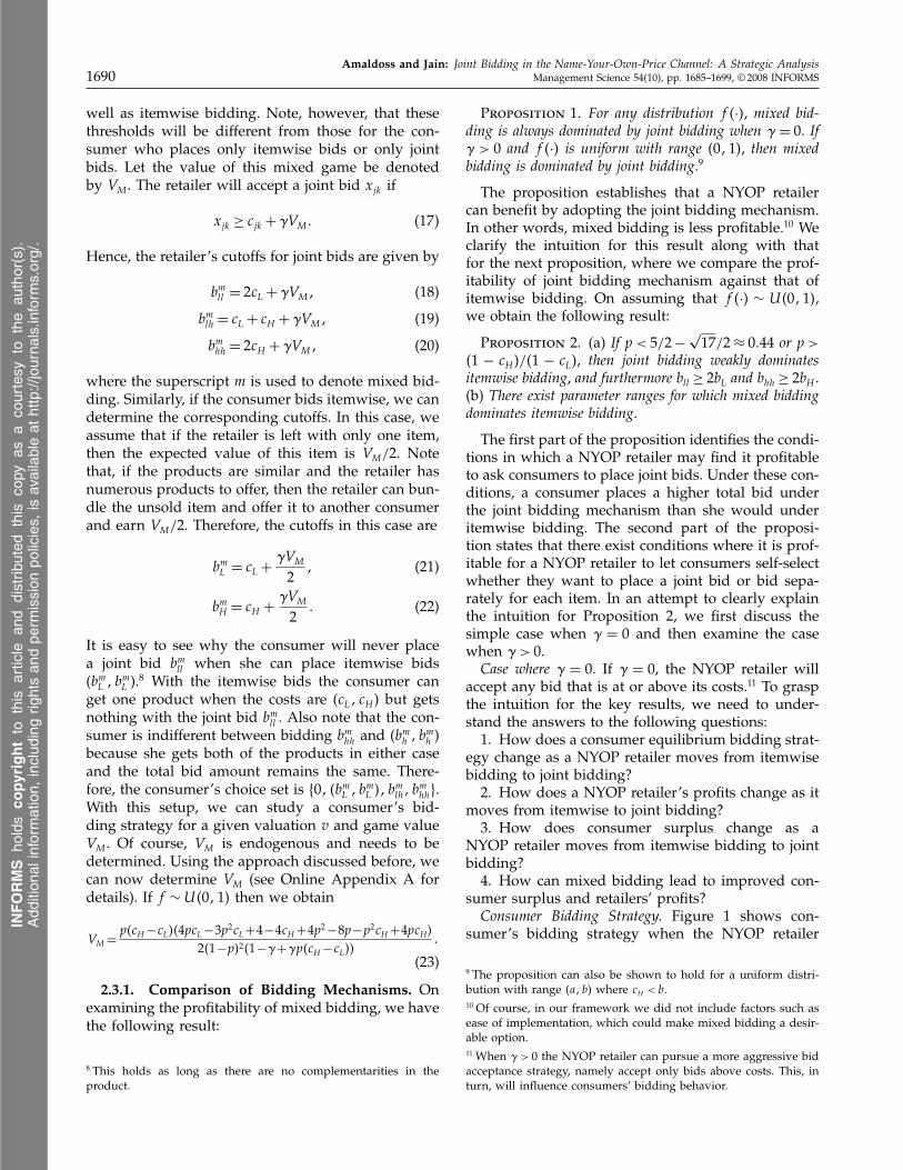
was encouraging to note that the mean consumer sur-plus was $72.34 under mixed bidding. In contrast,the consumer surplus when only itemwise biddingwas allowed was $68.33 (F�1�98� = 44�76� p < 0�001).As noted earlier, consumers with intermediate val-uations (namely, v4 < v < v1) should place a jointbid blh under mixed bidding but bid (bL� bL) underitemwise bidding. Despite bidding more, consumersearned a larger surplus under mixed bidding even inthis region of valuations. Specifically, consumer sur-plus improved from $75.6 under itemwise bidding to$81.35 under mixed bidding (F�1�98� = 50�12� p < 0�001).Retailer’s Profit. The model predicts that allowing for

mixed bidding should increase the NYOP retailer’sprofit. The mean retailer’s profit when only item-wise bidding was allowed was $5.10, whereas theactual profit increased to $8.37 under mixed bid-ding (F�1�98� = 46�92� p < 0�0001). Note that consumersurplus increased for intermediate valuations of v(namely, v4 < v < v1). This might raise the questionof whether the retailer’s profits declined for interme-diate valuations of v. In theory, the retailer’s profitsshould also improve in this region. In actuality, theretailer’s profit was $5.53 under itemwise bidding inthis region but increased to $8.87 on offering mixedbidding (F�1�98� = 27�84� p < 0�001).

3.4.2. Point Predictions. The experimental resultswere directionally consistent with many qualitativepredictions of the theory. For completeness, we alsoreport whether the actual outcomes conformed to thepoint predictions of the model.Bids. If only itemwise bids were allowed then sub-

jects should bid $46.5, on average, for the two items.In actuality, subjects placed a mean bid of $47.28,which was not significantly different from the theoret-ical prediction (t = 1�61� p > 0�11). Though the overallbehavior is consistent with the equilibrium prediction,we observe deviations from the equilibrium predic-tions at the level of consumer valuation segments.Table 1 details the predicted and actual outcomes.For example, subjects actually bid $46.25 instead ofthe predicted $40.0 when v < v1 (t = 11� p < 0�001).Though subjects should bid $80 when v > v1, they bidonly $52.58 (t = 23� p < 0�001).Under mixed bidding, subjects bid $55.25 on aver-

age, which is significantly more than the theoret-ical prediction of $48.75 (t = 13�05� p < 0�01). Thisexcessive bidding could be a consequence of either

Table 1 Itemwise Bidding

Valuation region Predicted bid Actual bid

20< v < 86�67 40 46�25v > 86�67 80 52�58

Table 2 Mixed Bidding

Valuation region Bidding strategy Predicted bid Actual bid

20< v < 63�33 Itemwise bidding 40 46�9263�33< v < 86�7 Joint bidding 60 58�0986�7< v < 141�1 Joint bidding 60 58�26

(i) subjects choosing inappropriate bidding mecha-nisms such as a joint bid when they should placeitemwise bids or (ii) subjects bidding large amountseven though they have chosen the correct biddingmechanism. Table 2 shows the theoretical predictionsand corresponding observed outcomes when subjectsuse the appropriate bidding mechanism. In theory,subjects should place joint bid blh = $60 in the inter-mediate valuation region 63�33< v < 86�67 and in thehigher valuation region 86�67 < v < 141�1. In actual-ity, the average joint bids in these regions were $58.09and $58.23, respectively, which are close to the equi-librium prediction (p > 0�10). Next subjects should biditemwise �bL� bL� = $40 in the low-valuation region.But the observed average itemwise bid was higher at$46.92 (p < 0�01), and itemwise bids were placed ononly 32.71% of occasions. Thus, the departures fromequilibrium predictions were primarily driven by thetendency of our subjects to use inappropriate biddingmechanisms, especially using the joint bidding optionin the low-valuation region.Consumer Surplus. Using the bids predicted by the-

ory and the actual valuations of items, we computedthe mean earnings of individual subjects. If only item-wise bidding was permitted, then consumer surplusshould be $69.99 for items 1 and 2. On average, sub-jects actually earned $68.32 for the two items. Wecould not reject the null hypothesis that the actual andpredicted earnings were the same (t = 0�59� p > 0�55).The results were similar when subjects were given theoption of placing joint bids (actual earning = 72�34,prediction= 72�86, t = 0�16� p > 0�87).Retailer’s Profit. The model provides point predic-

tions on bids that subjects should place for differentvaluations of items. Using the predicted bid and theexpected costs, we computed the expected profit asper theory. If only itemwise bidding were allowed,the mean profit should be $4.57 for items 1 and 2.The actual mean profit was $5.10. We could not rejectthe null hypothesis that these profits were the same(t = 1�61� p > 0�11). On the other hand, under mixedbidding the predicted mean profit for both itemsshould be $5.15, but the actual mean profit was $8.37.Thus, mixed bidding produced more than the pre-dicted increase in profit (t = 9�47� p < 0�01).

3.5. DiscussionIn sum, our experimental investigation suggests thatthe aggregate behavior of subjects is qualitatively

INFORMS

holds

copyrightto

this

article

and

distrib

uted

this

copy

asa

courtesy

tothe

author(s).

Add

ition

alinform

ation,

includ

ingrig

htsan

dpe

rmission

policies,

isav

ailableat

http://journa

ls.in

form

s.org/.


consistent with many predictions of our model. Onaverage, retailers made more profits and subjectsincreased their bids without reducing their earningswhen provided the option to bid jointly. Though theoverall behavior is directionally consistent with themodel, we observe deviations at the level of valuationsegments and subjects tend to use joint bidding moreoften than predicted.

4. ConclusionThe NYOP channel has drawn a lot of attentionfrom the public and the press for its innovativeness.The focus of our research was to explore whetherthe existing market institution can be further aug-mented. Toward this end, we developed a dynamicmodel of a NYOP retailer who faces both demandand supply uncertainty and examined the retailer’sequilibrium bid acceptance strategy in the presenceof strategic bidders. Our analysis focused on evalu-ating the profit and consumer surplus implicationsof three different bidding mechanisms: itemwise bid-ding, joint bidding, and mixed bidding. We find thatin the presence of joint bidding some consumers maybid a higher amount than they would bid if they wereplacing itemwise bids. This increase in bid amountis related to the fact that joint bidding reduces thechance of a mismatch between the NYOP retailer’srealized costs and consumer bids. Interestingly, theimproved NYOP retailer’s profit need not come atthe cost of consumers, because joint bidding can alsoimprove consumer surplus. Even if the NYOP retaileroffers mixed bidding, where consumers can self-selectwhether they want to place itemwise or joint bids, wecan observe improved profits and consumer surplus.In our framework, we also observe that joint biddingdominates mixed bidding. We conducted an experi-mental test of our model predictions. The test lendssupport to many qualitative predictions of our model.In particular, offering the option of joint bidding sig-nificantly improved consumer surplus and retailers’profits.There are several avenues for further research.

Although we investigated how NYOP retailers canaugment their pricing mechanisms, we did not studythe conditions under which service providers shouldconsider selling their products through a NYOP chan-nel in addition to selling their product through tradi-tional retailers (see Fay and Xie 2008 and Wang et al.2005 for possible modeling approaches). In our for-mulation, we assumed that the NYOP retailer’s costsare exogenously determined. However, in a modelthat includes strategic upstream service providers(such as airlines) these costs can be endogenousto the model. It would also be useful to examinehow joint bidding and mixed bidding may affect the

equilibrium strategies of service providers and NYOPretailers in such settings. It would also be interest-ing to study the implications of competition amongNYOP retailers (see also Fay 2007). Finally, in the cur-rent research we subjected the model to a laboratorytest, and future research can confront the model withfield data when such data become available.

5. Electronic CompanionAn electronic companion to this paper is available aspart of the online version that can be found at http://mansci.journal.informs.org/.

AcknowledgmentsBoth authors contributed equally to the paper. The authorsthank Teck Ho, Amnon Rapoport, Ambar Rao, the anony-mous reviewers, the associate editor, and the departmenteditor for helpful comments.

ReferencesAdams, W., J. Yellen. 1976. Commodity bundling and the burden

of monopoly. Quart. J. Econom. 90 475–498.Bakos, Y., E. Brynjolfsson. 2000. Bundling and competition on the

Internet. Marketing Sci. 19(1) 63–82.Berteskas, D. 1987. Dynamic Programming, Deterministic and Stochas-

tic Models. Prentice Hall, Englewood Cliffs, NJ.Demange, G., D. Gale, M. Sotomayor. 1986. Multi-item auctions.

J. Political Econom. 94(4) 863–872.Ding, M., J. Eliashberg, J. Huber, R. Saini. 2005. Emotional bidders—

An analytical and experimental examination of consumers’behavior in a Priceline-like reverse auction. Management Sci.51(3) 352–364.

Estelami, H. 1999. Consumer savings in complementary productbundles. J. Marketing Theory Practice 7(3) 107–114.

Fay, S. 2004. Partial repeat bidding in the name-your-own-pricechannel. Marketing Sci. 23(3) 407–418.

Fay, S. 2007. Selling an opaque product through an interme-diary: The case of disguising one’s product. J. Retailing.Forthcoming.

Fay, S., J. Xie. 2008. Probabilistic goods: A creative way of sellingproducts and services. Marketing Sci., ePub ahead of printMarch 31, http://mktsci.journal.informs.org/cgi/content/abstract/mksc.1070.0318v1.

Fudenberg, D., J. Tirole. 1991. Game Theory. MIT Press, Cambridge,MA.

Hann, I.-H., C. Terwiesch. 2003. Measuring the frictional costs ofonline transactions: The case of a name-your-own-price chan-nel. Management Sci. 49(11) 1563–1579.

Kagel, J., D. Levin, R. Battalio, D. Meyer. 1989. First-price com-mon valuation auctions: Bidder behavior and winner’s curse.Econom. Enquiry 27 241–258.

Kannan, P., P. Kopalle. 2001. Dynamic pricing on the internet:Importance and implications for consumer behavior. Internat.J. Electronic Commerce 5(3) 63–82.

McAfee, R., J. McMillan. 1987. Auctions and bidding. J. Econom.Literature 25(2) 699–738.

McAfee, R., J. McMillan, M. Whinston. 1989. Multiproductmonopoly, commodity bundling and correlation of valuations.Quart. J. Econom. 104 371–383.

Mishra, D., R. Garg. 2006. Descending price multi-item auctions.J. Math. Econom. 42 161–179.

INFORMS

holds

copyrightto

this

article

and

distrib

uted

this

copy

asa

courtesy

tothe

author(s).

Add

ition

alinform

ation,

includ

ingrig

htsan

dpe

rmission

policies,

isav

ailableat

http://journa

ls.in

form

s.org/.


Rassenti, S., V. Smith, B. Wilson. 2001. Using experiments toinform the privatization/deregulation movement in electricity.Working paper, Economics Science Laboratory, University ofArizona, Tucson.

Reinganum, J. 1979. A simple model of equilibrium price disper-sion. J. Political Econom. 87(4) 851–858.

Rothkopf, M. 1991. On auctions with withdrawable winning bids.Marketing Sci. 10(1) 40–57.

Rothkopf, M., R. Harstad. 1994. Modeling competitive bidding:A critical essay. Management Sci. 40(3) 364–384.

Schmalensee, R. 1984. Gaussian demand and commodity bundling.J. Bus. 57(1) S211–S230.

Sinha, A., E. Greenleaf. 2000. The impact of discrete bidding andbidder aggressiveness on sellers’ strategies in open English auc-tions: Reserves and covert shilling.Marketing Sci. 19(3) 244–265.

Souza, G., B. Bayus, H. Wagner. 2004. New-product strategy andindustry clockspeed. Management Sci. 50(4) 537–549.

Spann, M., G. J. Tellis. 2006. Does the internet promote better con-sumer decisions? The case of name-your-own-price auctions.J. Marketing 70(1) 65–78.

Terwiesch, C., I. Hann, S. Savin. 2005. Online haggling at a name-your-price retailer: Theory and application. Management Sci.51(3) 339–351.

Wang, T., E. Gal-Or, R. Chatterjee. 2005. Why a name-your-own-price channel makes sense for service providers (Or: Whoneeds Priceline anyway?). Working paper, Marketing Depart-ment, University of Pittsburgh, Pittsburgh.

Xie, J., M. Sirbu. 1994. Price competition and compatibility in thepresence of positive demand externalities. Management Sci.41(5) 909–926.

INFORMS

holds

copyrightto

this

article

and

distrib

uted

this

copy

asa

courtesy

tothe

author(s).

Add

ition

alinform

ation,

includ

ingrig

htsan

dpe

rmission

policies,

isav

ailableat

http://journa

ls.in

form

s.org/.

Joint Bidding in the Name-Your-Own-Price Channel: A Strategic Analysis

Documents