Volume 9, Number 5, May 2013 (Serial Number 96) Journal of Modern Accounting and Auditing David Publishing Company www.davidpublishing.com Publishing David

Welcome message from author
This document is posted to help you gain knowledge. Please leave a comment to let me know what you think about it! Share it to your friends and learn new things together.
Transcript
Volume 9, Number 5, May 2013 (Serial Number 96)
Journal ofModern Accounting and Auditing
David Publishing Company
www.davidpublishing.com
PublishingDavid

Publication Information: Journal of Modern Accounting and Auditing is published monthly in hard copy (ISSN1548-6583) and online (ISSN1935-9683) by David Publishing Company located at 9460 Telstar Ave Suite 5, EL Monte, CA 91731, USA. Aims and Scope: Journal of Modern Accounting and Auditing, a monthly professional academic journal, covers all sorts of researches on accounting research, financial theory, capital market, audit theory and practice from experts and scholars all over the world. Editorial Board Members: Benedetta Siboni, Italy. Brad S. Trinkle, USA. Daniela Cretu, Romania. Elisabete Fátima Simões Vieira, Portugal. Haihong He, USA. Joanna Błach, Poland. João Paulo Torre Vieito, Portugal. Liang Song, USA. Lindita Rova, Albania. Mohammed Al-Omiri, Saudi Arabia. Mohamed Rochdi Keffala, Tunisia. Mohammad Talha, Saudi Arabia. Monika Wieczorek-Kosmala, Poland. Narumon Saardchom, Thailand.
Peter Harris, USA. Philip Yim Kwong Cheng, Australia. Rosa Lombardi, Italy. Sheikh Abdur Rahim, Bangladesh. Thomas Gstraunthaler, South Africa. Tita Djuitaningsih, SE, M.Si., Ak., Indonesia. Tiziana Di Cimbrini, Italy. Tumellano Sebehela, United Kingdom. Valdir de Jesus Lameira, Brazil. Valerio Pesic, Italy. Vintilescu Belciug Adrian, Romanian. Wan Mansor W. Mahmood, Malaysia. Zeynep Özsoy, Turkey.
Manuscripts and correspondence are invited for publication. You can submit your papers via Web Submission, or E-mail to [email protected]. Submission guidelines and Web Submission system are available at http://www.davidpublishing.com. Editorial Office: 9460 Telstar Ave Suite 5, EL Monte, CA 91731 E-mail: [email protected], [email protected] Copyright©2013 by David Publishing Company and individual contributors. All rights reserved. David Publishing Company holds the exclusive copyright of all the contents of this journal. In accordance with the international convention, no part of this journal may be reproduced or transmitted by any media or publishing organs (including various websites) without the written permission of the copyright holder. Otherwise, any conduct would be considered as the violation of the copyright. The contents of this journal are available for any citation, however, all the citations should be clearly indicated with the title of this journal, serial number, and the name of the author. Abstracted/Indexed in: Database of EBSCO, Massachusetts, USA ProQuest Cambridge Scientific Abstracts (CSA)-Natural Sciences Australian ERA Universe Digital Library Sdn Bhd (UDLSB), Malaysia Chinese Database of CEPS, Airiti Inc. & OCLC Chinese Scientific Journals Database, VIP Corporation, Chongqing, P.R.China Ulrich’s Periodicals Directory Database of Summon Serials Solutions, USA Subscription Information: Price (per year): Print $640; Online $480; Print and Online $800 David Publishing Company 9460 Telstar Ave Suite 5, EL Monte, CA 91731, USA Tel: 1-323-984-7526, 323-410-1082; Fax: 1-323-984-7374, 323-908-0457; E-mail: [email protected]
David Publishing Company
www.davidpublishing.com
DAVID PUBLISHING
D

Journal of Modern Accounting and Auditing
Volume 9, Number 5, May 2013 (Serial Number 96)
Contents Accounting, Auditing & Financial Management
Financial Statement Comparability: Empirical Evidence From Brazil 587
Sirlei Lemes, Luciana de Almeida Araújo Santos, Núbia Aparecida Rodrigues
Can the Dominant Trait Indicator Predict Success in a Financial Accounting Principles
Course? A Preliminary Look 602
John Garlick, Susan Shurden, Mike Shurden
Accounting of Foreign Currencies: Difference in Exchange Transactions and Relation With
Taxation of Indonesia (Case Study in Fishery Company) 609
Ilham Hidayah Napitupulu, Abdul Rahman Dalimunthe
The Influence of Market and Company Characteristics on Voluntary Disclosure 616
Eugenio D’Amico, Anna Maria Biscotti
Audit Reports of Financially Distressed Companies: Emphasis of Matter (EOM) Versus
Disclaimers 634
Hashanah Ismail, Mazlina Mustapha
The Relationship Between Financial Reporting Standards (FRS) 139 and Audit Pricing:
The Case of Malaysia 641
Najihah Marha Yaacob
Executive Compensation and Corporate Financial Performance: Empirical Evidences on
Brazilian Industrial Companies 650
Elizabeth Krauter, Almir Ferreira de Sousa
Capital Market & Economy
The Recent US Financial Crisis: Its Impact on Dividend Payout Strategy and a Test of
the Silver-Lining Hypothesis 662
Chuo-Hsuan Lee, Edward J. Lusk, Michael Halperin
The Adoption and Maintenance of Executive Stock Option Plan (ESOP): Company
Characteristics Evaluation in Indonesia 678
Nur Fadjrih Asyik
Pyramid Schemes and Multilevel Marketing (MLM): Two Sides of the Same Coin 690
Olubusola H. Akinladejo, Marjorie Clarke, Felix O. Akinladejo
The Income Security System in Japanese Traditional Performing Arts: A Strategy for
Utilizing the Nation’s Traditional Arts Resources 697
Tadashi Yagi, Chisako Takashima, Yoshinori Usui
Analysis of Salaries and Some Non-traditional Measures of Location 711
Milan Terek, Nguyen Dinh He
A New Latent Class Stochastic Frontier Model for the Best Practices of USA’s Corporate
Governance 719
Wided Khiari, Yosra Mellouli
Journal of Modern Accounting and Auditing, ISSN 1548-6583 May 2013, Vol. 9, No. 5, 587-601
Financial Statement Comparability:
Empirical Evidence From Brazil
Sirlei Lemes, Luciana de Almeida Araújo Santos, Núbia Aparecida Rodrigues
Federal University of Uberlandia, Uberlandia, Brazil
The convergence of accounting standards started in the 1970s, with international norms issued by the International
Accounting Standards Board (IASB) and with the efforts of various countries to adopt the International Financial
Reporting Standards (IFRS), already mandatory in Brazil since 2010. Thus, comparable accounting information is
clearly important, and this study plans to confirm the level of comparability of net income and equity of companies
in the financial sector (in Brazil, “Finance and Others”), listed in the stock exchange, futures, and commodities
(BM&F Bovespa1), issued according to Brazilian Generally Accepted Accounting Principles (BR GAAP) and the
IFRS. This study is descriptive, using a quantitative approach. Data were collected from secondary sources, more
specifically, from the explanatory notes in the financial statements of the companies listed in the financial sector of
the BM&F Bovespa in the fiscal year of 2010. The results showed a reasonable level of comparability, with 68% of
the companies presenting materially comparable information for net income and 72% of them for equity. However,
decisions made based on data issued following the two different standards may have suffered the influence of
asymmetric information; in other words, the comparability of information did not seem to satisfy those companies
during the studied period of time. The main limitations of this study were data collection and selection for the
development of the research because of: (1) inconsistence in net income and equity reconciliation criteria in the
companies investigated; and (2) lack of uniformity in designating the adjustments that affect net income and equity
in the conversion of the BR GAAP standard into the IFRS.
Keywords: comparability, International Financial Reporting Standards (IFRS), Brazilian Generally Accepted
Accounting Principles (BR GAAP)
Introduction
The reflex of global economy on accounting can be seen in the need to harmonize accounting language,
once the information needs to be understood by users worldwide, so as to subsidize them in the
decision-making process. Such a convergence can be seen as an improvement in global accounting
communication, because it allows for faster capital market transactions and possibly reduces the cost of
information.
Attempts to converge accounting standards can be identified since the 1970s, with the creation of the
International Accounting Standards Committee (IASC), being that in the 2000s, the process is strengthened by
Sirlei Lemes, Faculty of Accounting, Federal University of Uberlandia. Email: [email protected]. Luciana de Almeida Araújo Santos, graduate student, master in Management, Federal University of Uberlandia. Núbia Aparecida Rodrigues, Faculty of Accounting, Federal University of Uberlandia.
1 Bolsa de Valores, Mercadorias, & Futuros de São Paulo, a stock exchange located at Sao Paulo, Brazil.
DAVID PUBLISHING
D
FINANCIAL STATEMENT COMPARABILITY: EMPIRICAL EVIDENCE FROM BRAZIL
588
the transformation of the IASC into the International Accounting Standards Board (IASB) in 2001. The latter
then becomes the body responsible for the release of the International Financial Reporting Standards (IFRS).
This process is further reinforced by the decision of the European Union to fully adopt the IFRS beginning in
2005.
Thenceforth, a growing demand of unified accounting standards can be clearly seen, so that organizations
can operate in global markets. In that sense, Brazilian accounting has been going through the process of
implementation of the international standards since 2010 when the IFRS was made compulsory. This evolution,
however, brings about quite a few challenges regarding the change of accounting with a strong normative and
fiscal character into a more subjective and interpretative one.
The basic conceptual statement issued by the CPC2 in 2008 regards comparability as one of the main
qualitative traits in accounting information. This declaration defines comparability as the ability to allow the
user to compare accounting demonstrations of one or various business entities, over time, in order to identify
patrimonial and financial tendencies, performance, and financial position mutations.
The disclosure of accounting demonstrations following the IFRS became mandatory in Brazil starting in
2010. Because of that and of the importance given to accounting information comparability within the
convergence process, the aim of this study is to answer the question what the level of comparability of the net
income and equity of the companies is within the financial sector listed in the BM&F Bovespa following
Brazilian Generally Accepted Accounting Principles (BR GAAP), if compared with the IFRS.
Therefore, this article proposes to verify the level of comparability between the net income and equity,
within BR GAAP standards and according to the IFRS of companies in the financial sector listed on the stock
exchange, futures, and commodities (BM&F Bovespa, 2011). In order to accomplish such a proposal, the
comparability index was used, and the adjustments which caused a divergence between the information
generated by the two standards were identified. The data used for the study were taken from the net income and
the equity of the companies in 2009, disclosed in the 2010 financial statements and their respective
reconciliation frameworks, when disclosed.
Several studies about the subject do not include the financial sector in their sampling because of its
peculiarities and, often, because of its more complex regulations. Therefore, the aim of this work is to
specifically study this very sector, denominated “Financial and Others” in the BM&F Bovespa classification.
Structurally, this article is presented in four sections besides this one. Section 2 deals with the evolution of
international accounting and its development in Brazil, and, furthermore, the issue of accounting information
comparability. Section 3 handles the methodological aspects and describes the samples used. Thereafter, an
analysis of the results is presented, and finally, in Section 5, the closing remarks are presented.
Theoretical Foundation
The beginning of the convergence process of accounting language was already identified in 1973, with the
launching of the IASC, with headquarters in London, through a deal among accounting entities in Australia,
Canada, France, Germany, Japan, Mexico, the Netherlands, the United Kingdom, Ireland, and the USA. The
idea to create such a committee came about in 1972, during the 10th World Congress of Accountants in
Sidney. 2 Comite dos Pronunciamentos Contábeis, Accounting Pronouncement Agency, a Brazilian organization created to centralize the issuing of norms converging with the international accounting standards.
FINANCIAL STATEMENT COMPARABILITY: EMPIRICAL EVIDENCE FROM BRAZIL
589
The goal of the IASC was to formulate and publish, in a totally independent way, international accounting
norms suitable to be accepted by the whole world (Filho, Lopes, & Pederneiras, 2009), trying to “simplify the
capital flow between all countries, easing the comparison of accounting statements” (Lemes & Carvalho, 2009,
p. 31).
The structure of the IASC was changed in 2001, originating the IASB, committee responsible for issuing
the IFRS, which, since then, has been trying to obtain approval of various countries to the convergence process
to improve the utility of accounting information internationally.
The approval of Ruling 1606/2002 by the European Union may be seen as an incentive for the
convergence to international norms in other countries. Such a ruling predicted the obligatoriness of the full
adoption of the IFRS by all companies listed in the European stock market, beginning in January 2005 (Callao,
Jarne, & Lainez, 2007). According to Farah, Martins, Romani, and Lisboa (2010, p. 21), “The adoption of the
IFRS by European countries was very fast. Actually, around 7,000 companies listed in the European Stock
Market have already adopted the IFRS⎯275 of these did so before 2005”.
The adoption of the IFRS as an accounting standard is spreading all over the world. According to Farah et
al. (2010), it has been adopted by more than 100 countries, including Brazil.
Brazilian accounting, historically, shows strong normative characteristics and is highly influenced by
fiscal legislation. Law 6404/763 (Corporations Law) regulates the activities of corporations. The remaining
types of society are regulated by Book II (from Article 966 to Article 1195) of Law 10.406/02 (The New
Brazilian Civil Code). Norms for specific sectors are also issued by entities entitled with such powers: Central
Bank of Brazil (BACEN, Banco Central do Brazil), Real Estate Values Committee (CVM, Comissão De
Valores Mobiliários), Private Security Superintendence (SUSEP, Superitendência de Seguros Privados), and
National Electric Power Agency (ANEEL, Agência Nacional de Energia Elétrica).
The conceptual aspects of accounting science were handled by Independent Brazilian Auditors Institute
(IBRACON, Instituto dos Auditores Independentes do Brasil) until the creation of the Federal Accounting
Committee (CPC). IBRACON approved the basic conceptual accounting structure elaborated by Accounting,
Actuary, and Financial Research Institute (FIPECAFI, Fundação Instituto de Pesquisas Contábeis, Atuariais e
Financeiras) which dealt with theoretical accounting framework and also with the GAAP. The CPC issued the
fundamental accounting principles (PFC, princípios fundamentais de contabilidade), through resolution
750/1993 of the Federal Accounting Council (Conselho Federal de Contabilidade, CFC). It was common for
both agencies to handle the same matters in distinct ways.
Thus, within the setting of international convergence of accounting norms and facing the diversity of
current standards and regulatory inspection bodies operating in the country, an internal restructure became
paramount in order to facilitate adaptation to the International Accounting Standards (IAS).
This process began in Brazil in 2000, when Bill 3.741 was submitted to the Chamber of Deputies,
proposing the modernization of Law 6404/76, through an update in its Chapter 15, aiming the elimination of
regulatory barriers and the alignment of Brazilian norms and accounting practices to their international ones
(Farah et al., 2010).
Afterwards, in 2005, the CPC was created through CFC Resolution 1055/05, with its aim defined as:
3 Brazil Law No. 6404 of December 15, 1976 (and amendments). Provides for the corporations. Official Gazette, Brasília, DF, December 17, 1976. Retrieved from http://www.planalto.gov.br/ccivil03/Leis/L6404consol.htm.
FINANCIAL STATEMENT COMPARABILITY: EMPIRICAL EVIDENCE FROM BRAZIL
590
The study, preparation and issuance of technical pronouncements for accounting procedures, and disclosure of information, to allow the issuance of norms by the Brazilian regulatory body, aiming the centralization and standardization of its production process, always considering the convergence of Brazilian accounting with international standards. (Federal Accounting Council, 2005)4
Bill 3.741 was approved in December 2007, originating Law 11.638/07 which determined that all
applicable norms to Brazilian public companies should be formulated in line with the international standards
used in the main securities markets. It also allowed its application to large companies. Even before Bill 3.741
was transformed into law, the CVM had already ruled, through Normative Instruction 457/07, that public
companies would have to submit their financial statements in accordance with IASB regulations by the end of
2010. This Instruction also ruled that international norms should be applied to the statements of the previous
year, so as to allow a comparison. Later, in November 2010, the CPC issued Statement 37, approved by the
CVM (Deliberation 647/10), reinforcing in its Item 34 the mandatory use of the IFRS in accounting statements
as of fiscal year of 2010.
The convergence to international standards imposes, however, a few challenges for Brazilian accounting,
as highlighted by Farah et al. (2010):
We can immediately see a fundamental conceptual barrier to the understanding, acceptance, and practical application of the IFRS in Brazil: the Brazilian accounting system, which has always suffered great influence from the fiscal environment, is strongly based on definite rules, whereas the IFRS have been traditionally based on much less detailed principles, with great emphasis on the economic substance of the operations, and on the use of judgment. (p. 22)
As for fiscal interference in the generation of accounting information, the changes to Law 6.404/76
progress to minimize the problem, for Item 2 of Article 177 determines that the company’s bookkeeping shall
not be modified by the provisions of tax law which must be registered in ledgers.
According to Iudicibus (2000, p. 28), “The main aim of accounting (and the reports emanating from it) is
to provide relevant economic information so that each user can make their own decisions, and safely carry out
their judgments”. Thus, the role of accounting is to provide information to various users, both inside and
outside the company.
According to Niyama and Silva (2009):
The presence of the user in the accounting process makes it necessary that the information evidenced is comparable. The user needs to analyze the performance of the company, and such analysis is made through comparison with what has taken place in the company at other times, or with what happened to other companies. That is only possible when accounting proceedings are coherent amongst all companies. (pp. 1-2)
The need for a convergent accounting language emerges in a global stage where financial statement cost
and processing time reduction can represent competitive advantages to companies. According to Niyama
(2006, p. 39), “Another advantage for companies, especially for those in emerging countries in search of
resources from foreign investors, is the possibility to disclose their financial statements in understandable
language”.
Comparability of accounting information among countries is also another benefit of the convergence
process, and the basic conceptual declaration says (Accounting Pronouncement Committee [Comitê de
Pronunciamentos Contábeis—CPC], 2011):
4 Retrieved from http://www.cfc.org.br/sisweb/sre/detalhes_sre.aspx?Codigo=2005/001055.
FINANCIAL STATEMENT COMPARABILITY: EMPIRICAL EVIDENCE FROM BRAZIL
591
Users must be able to compare the financial statements of a company over time, so as to identify possible tendencies in its patrimonial and financial position, as well as in its performance. Users also must be able to compare financial statements of different companies in order to relatively evaluate their patrimonial and financial position, their performance, and mutations in their financial situation. Consequently, the measuring and disclosure of the financial effects of similar transactions and other eventualities must be performed consistently by the company, over time, and also by different companies. (p. 8)
This statement considers qualitative characteristics to be the attributes that make financial statements
useful for the users, such as comprehensibility, relevance, reliability, comparability, materiality, adequate
representation, primacy of substance over form, neutrality, prudence, and integrity. The first four of these
characteristics are the main ones, according to the pronouncement.
According to Choi, Frost, and Meek (1999; as cited in Lemes & Carvalho, 2009, p. 28), “Information is
comparable if it is similar enough to allow users to compare it without having to be intimately familiar with
more than one accounting system”.
Haverty (2006) has researched comparability and convergence of two sets of accounting norms (US
GAAP and IFRS) between 1996 and 2002. For that, he used a sample of 11 companies of the Republic of
China listed on the New York Stock Exchange (NYSE). During his research, the author used the Gray Index (or
comparability) to verify the comparability between the net profit (Lucro Líquido, LL) and the equity
(Patrimônio Líquido, PL) in the two groups of norms. As a result, he could verify that notwithstanding the
progress towards harmonization, no real convergence took place, and the main reason for the lack of
comparability was the revaluation of fixed assets. While the IFRS allows revaluation, the US GAAP only
allows the evaluation of fixed assets through their historical costs.
Nogueira and Lemes (2008) have carried out a research about the level of comparability of the adjustments
to the LL and PL of 28 Brazilian companies that issued American Depositary Receipts (ADRs) in 2006. The
comparison was made between BR GAAP and US GAAP from 2000 to 2006, and the adjustments concerning
business combination, intangibles, goodwill, fixed assets, pension funds, monetary correction, and deferred
taxes were the main reasons of the conflicts. In this study, the use of a variable of the Gray Index allowed them
to identify the incomparability of the partial adjustments issued by the companies, and it was proved that there
was no comparability improvement during the time of the analysis.
Liu (2011) also used the Gray Index to identify the causes of comparability differences between 15
Chinese companies that used the IFRS and performed information reconciliation in US GAAP from 2002 to
2006. The study pointed out the following as main differences: deferred taxes, exchange adjustments, goodwill,
asset revaluation, minority interest, and business combinations and acquisitions.
Aiming to evaluate the differences between the net income in BR GAAP and US GAAP, Lemes and
Carvalho (2009) have applied the same index in 30 companies between 2000 and 2005. They concluded that an
expressive number of companies showed materially incomparable results, identifying the adjustments resulting
from goodwill and business combination as the most frequent in the companies in the sample.
Another similar study has been carried out by Klann and Beuren (2010), in which 33 enterprises listed on
the London Stock Exchange (LSE) that negotiate ADR on the NYSE, using their financial statements for 2004
and 2005 as reference, disclosed to the LSE and the NYSE. Their work analyzed the reflexes of the differences
between the norms of the IFRS and US GAAP, in accounting disclosure, through the identification of the main
adjustments to the accounts of the balance sheet, operational profit, and the net income of the yearly income
FINANCIAL STATEMENT COMPARABILITY: EMPIRICAL EVIDENCE FROM BRAZIL
592
statement. No comparability index was used for this study. Instead, they opted to identify the relative variations
between one standard and the other. The goodwill and the benefit plan for employees were identified as the
main causes of the accounting information asymmetry.
Previous reports highlight adjustments to goodwill as one of the main reasons for the incomparability of
information collected in different standards, as identified in all studies quoted, followed by those related to
business combinations which appear in three of the studies and the deferred taxes mentioned in two of them.
Methodological Aspects
This research was descriptive. One of its goals is the description of the characteristics of a given
population or phenomenon, using the technique of data collection (Gil, 2006; Beuren, 2006). According to
methodological procedures, this study is a documentary research. As for the approach to the problem, this is a
quantitative article, because, according to Martins and Theóphilo (2007, p. 103), quantitative evaluation is “to
organize, summarize, characterize, and interpret collected numeric data”.
Data were collected through secondary sources, more specifically, from the explanatory notes in the
financial statements of the companies listed in the financial sector of the BM&F Bovespa issued in the fiscal
year of 2010.
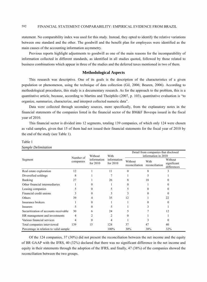
This financial sector is divided into 12 segments, totaling 139 companies, of which only 124 were chosen
as valid samples, given that 15 of them had not issued their financial statements for the fiscal year of 2010 by
the end of the study (see Table 1).
Table 1
Sample Delimitation
Segment Number of companies
Without information for 2010
With information for 2010
Detail from companies that disclosed information in 2010
Without reconciliation
With reconciliation
Without significant differences
Real estate exploration 12 1 11 0 8 3
Diversified soldings 8 1 7 1 5 1
Banking 27 1 26 8 18 0
Other financial intermediaries 1 0 1 0 1 0
Leasing companies 5 0 5 5 0 0
Financial credit unions 3 0 3 3 0 0
Others 39 4 35 12 1 22
Insurance brokers 1 0 1 1 0 0
Insurers 5 0 5 1 3 1
Securitization of accounts receivable 30 6 24 5 7 12
HR management and investments 4 2 2 0 1 1
Various financial services 4 0 4 1 3 0
Total companies interviewed 139 15 124 37 47 40
Percentage in relation to valid sample 100% 30% 38% 32%
Of the 124 companies, 37 (30%) did not present the reconciliation between the net income and the equity
of BR GAAP with the IFRS, 40 (32%) declared that there was no significant difference in the net income and
equity in their statements through the adoption of the IFRS, and finally, 47 (38%) of the companies showed the
reconciliation between the two groups.
FINANCIAL STATEMENT COMPARABILITY: EMPIRICAL EVIDENCE FROM BRAZIL
593
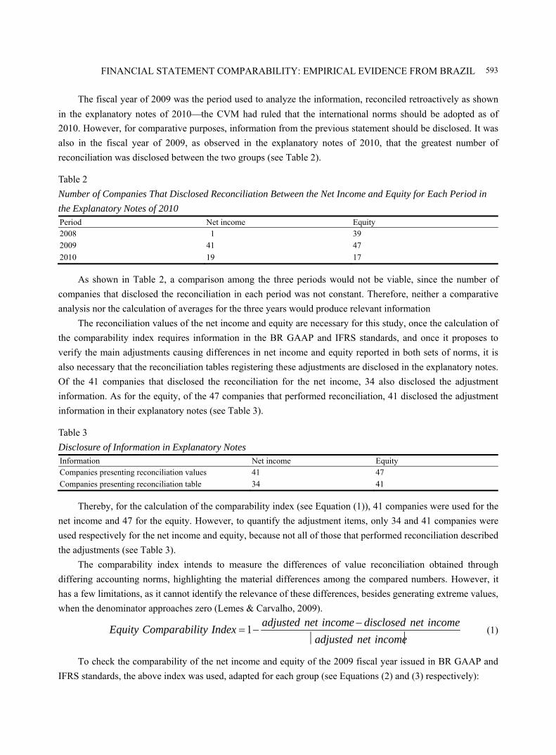
The fiscal year of 2009 was the period used to analyze the information, reconciled retroactively as shown
in the explanatory notes of 2010⎯the CVM had ruled that the international norms should be adopted as of
2010. However, for comparative purposes, information from the previous statement should be disclosed. It was
also in the fiscal year of 2009, as observed in the explanatory notes of 2010, that the greatest number of
reconciliation was disclosed between the two groups (see Table 2).
Table 2
Number of Companies That Disclosed Reconciliation Between the Net Income and Equity for Each Period in
the Explanatory Notes of 2010 Period Net income Equity 2008 1 39
2009 41 47
2010 19 17
As shown in Table 2, a comparison among the three periods would not be viable, since the number of
companies that disclosed the reconciliation in each period was not constant. Therefore, neither a comparative
analysis nor the calculation of averages for the three years would produce relevant information
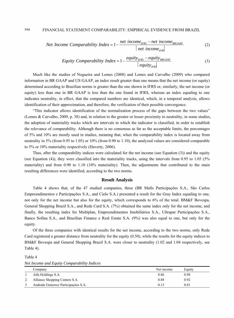
The reconciliation values of the net income and equity are necessary for this study, once the calculation of
the comparability index requires information in the BR GAAP and IFRS standards, and once it proposes to
verify the main adjustments causing differences in net income and equity reported in both sets of norms, it is
also necessary that the reconciliation tables registering these adjustments are disclosed in the explanatory notes.
Of the 41 companies that disclosed the reconciliation for the net income, 34 also disclosed the adjustment
information. As for the equity, of the 47 companies that performed reconciliation, 41 disclosed the adjustment
information in their explanatory notes (see Table 3).
Table 3
Disclosure of Information in Explanatory Notes Information Net income Equity Companies presenting reconciliation values 41 47
Companies presenting reconciliation table 34 41
Thereby, for the calculation of the comparability index (see Equation (1)), 41 companies were used for the
net income and 47 for the equity. However, to quantify the adjustment items, only 34 and 41 companies were
used respectively for the net income and equity, because not all of those that performed reconciliation described
the adjustments (see Table 3).
The comparability index intends to measure the differences of value reconciliation obtained through
differing accounting norms, highlighting the material differences among the compared numbers. However, it
has a few limitations, as it cannot identify the relevance of these differences, besides generating extreme values,
when the denominator approaches zero (Lemes & Carvalho, 2009).
1
adjusted net income disclosed net incomeEquity Comparability Index
adjusted net income
−= −
⏐ ⏐ (1)
To check the comparability of the net income and equity of the 2009 fiscal year issued in BR GAAP and
IFRS standards, the above index was used, adapted for each group (see Equations (2) and (3) respectively):
FINANCIAL STATEMENT COMPARABILITY: EMPIRICAL EVIDENCE FROM BRAZIL
594
1
IFRS BRGAAP
IFRS
net income net incomeNet Income Comparability Index
net income
−= −
⏐ ⏐ (2)
1 IFRS BRGAAP
IFRS
equity equityEquity Comparability Index
equity
−= −
⏐ ⏐ (3)
Much like the studies of Nogueira and Lemes (2008) and Lemes and Carvalho (2009) who compared
information in BR GAAP and US GAAP, an index result greater than one means that the net income (or equity)
determined according to Brazilian norms is greater than the one shown in IFRS or, similarly, the net income (or
equity) less than one in BR GAAP is less than the one found in IFRS, whereas an index equaling to one
indicates neutrality, in effect, that the compared numbers are identical, which, in a temporal analysis, allows
identification of their approximation, and therefore, the verification of their possible convergence.
“This indicator allows identification of the normalization process of the gaps between the two values”
(Lemes & Carvalho, 2009, p. 38) and, in relation to the greater or lesser proximity to neutrality, in some studies,
the adoption of materiality tracks which are intervals in which the indicator is classified, in order to establish
the relevance of comparability. Although there is no consensus as far as the acceptable limits, the percentages
of 5% and 10% are mostly used in studies, meaning that, when the comparability index is located away from
neutrality in 5% (from 0.95 to 1.05) or 10% (from 0.90 to 1.10), the analyzed values are considered comparable
to 5% or 10% materiality respectively (Haverty, 2006).
Thus, after the comparability indices were calculated for the net income (see Equation (3)) and the equity
(see Equation (4)), they were classified into the materiality tracks, using the intervals from 0.95 to 1.05 (5%
materiality) and from 0.90 to 1.10 (10% materiality). Then, the adjustments that contributed to the main
resulting differences were identified, according to the two norms.
Result Analysis
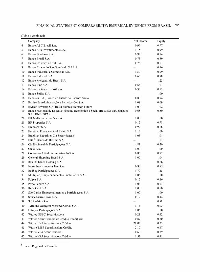
Table 4 shows that, of the 47 studied companies, three (BR Malls Participações S.A., São Carlos
Empreendimentos e Participações S.A., and Cielo S.A.) presented a result for the Gray Index equaling to one,
not only for the net income but also for the equity, which corresponds to 6% of the total. BM&F Bovespa,
General Shopping Brazil S.A., and Rede Card S.A. (7%) obtained the same index only for the net income, and
finally, the resulting index for Multiplan, Empreendimentos Imobiliários S.A., Ultrapar Participações S.A.,
Banco Sofina S.A., and Brazilian Finance e Real Estate S.A. (9%) was also equal to one, but only for the
equity.
Of the three companies with identical results for the net income, according to the two norms, only Rede
Card registered a greater distance from neutrality for the equity (0.50), while the results for the equity indices to
BM&F Bovespa and General Shopping Brazil S.A. were closer to neutrality (1.02 and 1.04 respectively, see
Table 4).
Table 4
Net Income and Equity Comparability Indices
Company Net income Equity
1 Alfa Holdings S.A. 0.86 0.98
2 Alliance Shopping Centers S.A. 0.88 0.92
3 Andrade Gutierrez Participações S.A. 0.13 0.81
FINANCIAL STATEMENT COMPARABILITY: EMPIRICAL EVIDENCE FROM BRAZIL
595
(Table 4 continued)
Company Net income Equity
4 Banco ABC Brasil S.A. 0.99 0.97
5 Banco Alfa Investimentos S.A. 1.15 0.99
6 Banco Bradesco S.A. 0.97 0.94
7 Banco Brasil S.A. 0.75 0.89
8 Banco Cruzeiro do Sul S.A. 0.75 0.57
9 Banco Estado do Rio Grande do Sul S.A. -- 0.96
10 Banco Industrial e Comercial S.A. 1.50 0.99
11 Banco Indusval S.A. 0.63 0.98
12 Banco Mercantil do Brasil S.A. -- 1.23
13 Banco Pine S.A. 0.64 1.07
14 Banco Santander Brasil S.A. 0.33 0.93
15 Banco Sofisa S.A. -- 1.00
16 Banestes S.A., Banco do Estado do Espírito Santo 0.88 0.94
17 Battistella Administração e Participações S.A. 1.08 0.09
18 BM&F Bovespa S.A. Bolsa Valores Mercado Futuro 1.00 1.02 19
Banco Nacional de Desenvolvimento Econômico e Social (BNDES) Participações S.A., BNDESPAR
0.68
0.50
20 BR Malls Participações S.A. 1.00 1.00
21 BR Properties S.A. 0.17 0.78
22 Bradespar S.A. 0.99 0.88
23 Brazilian Finance e Real Estate S.A. 1.17 1.00
24 Brazilian Securities Cia Securitização 1.05 1.01
25 BRB5 Banco de Brasília S.A. -- 1.01
26 Cia Habitasul de Participações S.A. 4.81 0.20
27 Cielo S.A. 1.00 1.00
28 Consórcio Alfa de Administração S.A. 0.85 0.97
29 General Shopping Brasil S.A. 1.00 1.04
30 Itaú Unibanco Holding S.A. -- 0.86
31 Itaúsa Investimentos Itaú S.A. 0.90 0.85
32 ItaúSeg Participações S.A. 1.70 1.15
33 Multiplan, Empreendimentos Imobiliários S.A. 1.05 1.00
34 Polpar S.A. 0.15 0.16
35 Porto Seguro S.A. 1.03 0.77
36 Rede Card S.A. 1.00 0.50
37 São Carlos Empreendimentos e Participações S.A. 1.00 1.00
38 Sonae Sierra Brasil S.A. 0.17 0.44
39 SulAmérica S.A. -- 0.88
40 Terminal Garagem Menezes Cortes S.A. 1.16 0.03
41 Ultrapar Participações S.A. 1.06 1.00
42 Wtoree NSBC Securitizadora 0.21 0.42
43 Wtoree Securitizadora de Crédito Imobiliário 0.87 0.50
44 Wtorre CRJ Securitizadora Crédito 28.07 0.33
45 Wtorre TSSP Securitizadora Crédito 2.10 0.67
46 Wtorre VPA Securitizadora 0.60 0.39
47 Wtorre VRJ Securitizadora Crédito 1.53 0.41
5 Banco Regional de Brasilia.
FINANCIAL STATEMENT COMPARABILITY: EMPIRICAL EVIDENCE FROM BRAZIL
596
For those companies where the equity was the same according to the two norms, the resulting index for the
net income was 1.05 and 1.06 for Multiplan, Empreendimentos Imobiliários S.A. and Ultrapar Participações
S.A. respectively, and 1.17 for Brazilian Finance e Real Estate S.A., which showed a greater distance
amongst the three companies. Banco Sofisa S.A. presented no net income reconciliation for the fiscal year of
2009.
Attention is called, yet, to Wtorre Mortgage Securitization S.A., Cia Habitatsul de Participações S.A., and
Wtorre TSSP Securitization S.A., as they showed the greatest distortions between the Gray Index and the
relative neutrality of the net income (see Table 4). In the first, an index of 28.07 (see Table 4) was found,
representing a reduction of 2.707%, because a net income of R$3,625,000 in BR GAAP became a loss of
R$139,000 in IFRS. In the same way, Cia Habitasul de Participações S.A. had an index result of 4.81 (see
Table 4) due to a net income in BR GAAP (R$17,009,000) and a loss in IFRS (R$6,047,000), which
corresponds to a reduction of 381%. Finally, the reduction of 110% verified for Wtorre TSSP Securitization
S.A. is due to the fact that in the local norms, a greater net income of R$308,000 was found, greater than the
R$147.000 in IFRS, which resulted in an index of 2.10 (see Table 4).
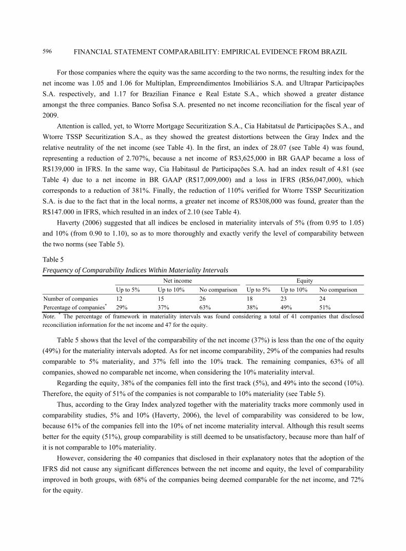
Haverty (2006) suggested that all indices be enclosed in materiality intervals of 5% (from 0.95 to 1.05)
and 10% (from 0.90 to 1.10), so as to more thoroughly and exactly verify the level of comparability between
the two norms (see Table 5).
Table 5
Frequency of Comparability Indices Within Materiality Intervals
Net income Equity
Up to 5% Up to 10% No comparison Up to 5% Up to 10% No comparison
Number of companies 12 15 26 18 23 24
Percentage of companies* 29% 37% 63% 38% 49% 51%
Note. * The percentage of framework in materiality intervals was found considering a total of 41 companies that disclosed reconciliation information for the net income and 47 for the equity.
Table 5 shows that the level of the comparability of the net income (37%) is less than the one of the equity
(49%) for the materiality intervals adopted. As for net income comparability, 29% of the companies had results
comparable to 5% materiality, and 37% fell into the 10% track. The remaining companies, 63% of all
companies, showed no comparable net income, when considering the 10% materiality interval.
Regarding the equity, 38% of the companies fell into the first track (5%), and 49% into the second (10%).
Therefore, the equity of 51% of the companies is not comparable to 10% materiality (see Table 5).
Thus, according to the Gray Index analyzed together with the materiality tracks more commonly used in
comparability studies, 5% and 10% (Haverty, 2006), the level of comparability was considered to be low,
because 61% of the companies fell into the 10% of net income materiality interval. Although this result seems
better for the equity (51%), group comparability is still deemed to be unsatisfactory, because more than half of
it is not comparable to 10% materiality.
However, considering the 40 companies that disclosed in their explanatory notes that the adoption of the
IFRS did not cause any significant differences between the net income and equity, the level of comparability
improved in both groups, with 68% of the companies being deemed comparable for the net income, and 72%
for the equity.
FINANCIAL STATEMENT COMPARABILITY: EMPIRICAL EVIDENCE FROM BRAZIL
597
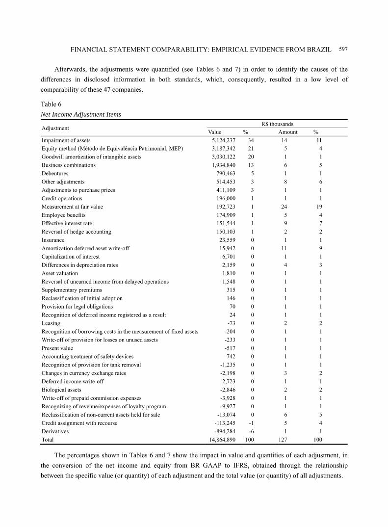
Afterwards, the adjustments were quantified (see Tables 6 and 7) in order to identify the causes of the
differences in disclosed information in both standards, which, consequently, resulted in a low level of
comparability of these 47 companies.
Table 6
Net Income Adjustment Items
Adjustment R$ thousands
Value % Amount %
Impairment of assets 5,124,237 34 14 11
Equity method (Método de Equivalência Patrimonial, MEP) 3,187,342 21 5 4
Goodwill amortization of intangible assets 3,030,122 20 1 1
Business combinations 1,934,840 13 6 5
Debentures 790,463 5 1 1
Other adjustments 514,453 3 8 6
Adjustments to purchase prices 411,109 3 1 1
Credit operations 196,000 1 1 1
Measurement at fair value 192,723 1 24 19
Employee benefits 174,909 1 5 4
Effective interest rate 151,544 1 9 7
Reversal of hedge accounting 150,103 1 2 2
Insurance 23,559 0 1 1
Amortization deferred asset write-off 15,942 0 11 9
Capitalization of interest 6,701 0 1 1
Differences in depreciation rates 2,159 0 4 3
Asset valuation 1,810 0 1 1
Reversal of unearned income from delayed operations 1,548 0 1 1
Supplementary premiums 315 0 1 1
Reclassification of initial adoption 146 0 1 1
Provision for legal obligations 70 0 1 1
Recognition of deferred income registered as a result 24 0 1 1
Leasing -73 0 2 2
Recognition of borrowing costs in the measurement of fixed assets -204 0 1 1
Write-off of provision for losses on unused assets -233 0 1 1
Present value -517 0 1 1
Accounting treatment of safety devices -742 0 1 1
Recognition of provision for tank removal -1,235 0 1 1
Changes in currency exchange rates -2,198 0 3 2
Deferred income write-off -2,723 0 1 1
Biological assets -2,846 0 2 2
Write-off of prepaid commission expenses -3,928 0 1 1
Recognizing of revenue/expenses of loyalty program -9,927 0 1 1
Reclassification of non-current assets held for sale -13,074 0 6 5
Credit assignment with recourse -113,245 -1 5 4
Derivatives -894,284 -6 1 1
Total 14,864,890 100 127 100
The percentages shown in Tables 6 and 7 show the impact in value and quantities of each adjustment, in
the conversion of the net income and equity from BR GAAP to IFRS, obtained through the relationship
between the specific value (or quantity) of each adjustment and the total value (or quantity) of all adjustments.
FINANCIAL STATEMENT COMPARABILITY: EMPIRICAL EVIDENCE FROM BRAZIL
598
The most evident adjustments in the conversion of the net income from BR GAAP into IFRS were those
of the impairment of assets, which contributes to an increase of 34% of the net income, with 14 adjustments
recorded in the 34 companies, followed by the MEP, accounting for 21% of the increase of the net income, with
five total adjustments. Thirdly, at 20%, only one adjustment referring to the amortization of the goodwill of
intangible assets registered for Santander Brazil S.A.. Six adjustments were made because of business
combinations which accounted for 13%.
Table 6 shows the measurement at fair value and the write-off of deferred assets respectively at the first
and third places, in relation to the number of occurrences. However, monetarily speaking, they are insignificant.
The adjustments related to derivatives and debentures are also highlighted, which, with an occurrence,
account respectively for 5% (net income increase) and 6% (net income decrease) of the total adjustments (see
Table 6) and are registered for BNDES Participations S.A..
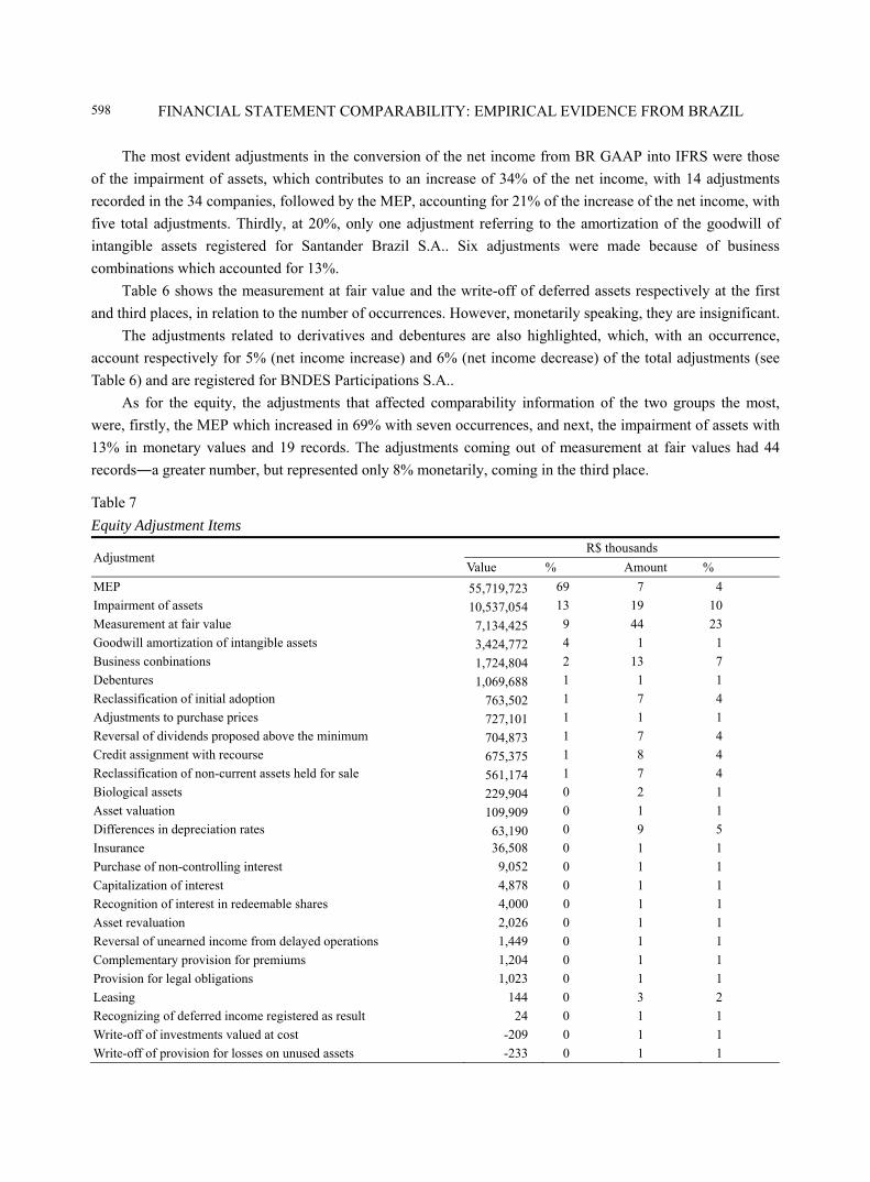
As for the equity, the adjustments that affected comparability information of the two groups the most,
were, firstly, the MEP which increased in 69% with seven occurrences, and next, the impairment of assets with
13% in monetary values and 19 records. The adjustments coming out of measurement at fair values had 44
records―a greater number, but represented only 8% monetarily, coming in the third place.
Table 7
Equity Adjustment Items
Adjustment R$ thousands
Value % Amount %
MEP 55,719,723 69 7 4
Impairment of assets 10,537,054 13 19 10
Measurement at fair value 7,134,425 9 44 23
Goodwill amortization of intangible assets 3,424,772 4 1 1
Business conbinations 1,724,804 2 13 7
Debentures 1,069,688 1 1 1
Reclassification of initial adoption 763,502 1 7 4
Adjustments to purchase prices 727,101 1 1 1
Reversal of dividends proposed above the minimum 704,873 1 7 4
Credit assignment with recourse 675,375 1 8 4
Reclassification of non-current assets held for sale 561,174 1 7 4
Biological assets 229,904 0 2 1
Asset valuation 109,909 0 1 1
Differences in depreciation rates 63,190 0 9 5
Insurance 36,508 0 1 1
Purchase of non-controlling interest 9,052 0 1 1
Capitalization of interest 4,878 0 1 1
Recognition of interest in redeemable shares 4,000 0 1 1
Asset revaluation 2,026 0 1 1
Reversal of unearned income from delayed operations 1,449 0 1 1
Complementary provision for premiums 1,204 0 1 1
Provision for legal obligations 1,023 0 1 1
Leasing 144 0 3 2
Recognizing of deferred income registered as result 24 0 1 1
Write-off of investments valued at cost -209 0 1 1
Write-off of provision for losses on unused assets -233 0 1 1
FINANCIAL STATEMENT COMPARABILITY: EMPIRICAL EVIDENCE FROM BRAZIL
599
(Table 7 continued)
Adjustment R$ thousands
Value % Amount %
Present value -452 0 1 1
Provision for asset retirement -2,000 0 1 1
Changes in currency exchange rates -2,775 0 2 1
Write-off of prepaid commission expenses -4,303 0 1 1
Deferred income write-off -8,427 0 1 1
Recognizing of revenue/expenses of loyalty program -9,927 0 1 1
Recognition of borrowing costs in the measurement of fixed assets -12,802 0 1 1 Contribution to business service management (BSM) establishment, treated as investment
-20,000 0
1
1
Recognition of provision for tank removal -38,008 0 1 1
Write-off of deferred assets -78,092 0 11 6
Financial assets available for sale -179,000 0 1 1
Effective interest rates -230,228 0 10 5
Other adjustments -261,707 0 8 4
Employee benefits -836,667 -1 9 5
Derivatives -894,284 -1 1 1
Total 80,926,688 100 191 100
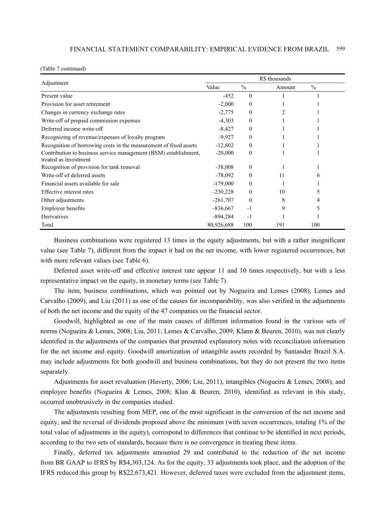
Business combinations were registered 13 times in the equity adjustments, but with a rather insignificant
value (see Table 7), different from the impact it had on the net income, with lower registered occurrences, but
with more relevant values (see Table 6).
Deferred asset write-off and effective interest rate appear 11 and 10 times respectively, but with a less
representative impact on the equity, in monetary terms (see Table 7).
The item, business combinations, which was pointed out by Nogueira and Lemes (2008), Lemes and
Carvalho (2009), and Liu (2011) as one of the causes for incomparability, was also verified in the adjustments
of both the net income and the equity of the 47 companies on the financial sector.
Goodwill, highlighted as one of the main causes of different information found in the various sets of
norms (Nogueira & Lemes, 2008; Liu, 2011; Lemes & Carvalho, 2009; Klann & Beuren, 2010), was not clearly
identified in the adjustments of the companies that presented explanatory notes with reconciliation information
for the net income and equity. Goodwill amortization of intangible assets recorded by Santander Brazil S.A.
may include adjustments for both goodwill and business combinations, but they do not present the two items
separately.
Adjustments for asset revaluation (Haverty, 2006; Liu, 2011), intangibles (Nogueira & Lemes, 2008), and
employee benefits (Nogueira & Lemes, 2008; Klan & Beuren, 2010), identified as relevant in this study,
occurred unobtrusively in the companies studied.
The adjustments resulting from MEP, one of the most significant in the conversion of the net income and
equity, and the reversal of dividends proposed above the minimum (with seven occurrences, totaling 1% of the
total value of adjustments in the equity), correspond to differences that continue to be identified in next periods,
according to the two sets of standards, because there is no convergence in treating these items.
Finally, deferred tax adjustments amounted 29 and contributed to the reduction of the net income
from BR GAAP to IFRS by R$4,303,124. As for the equity, 33 adjustments took place, and the adoption of the
IFRS reduced this group by R$22,673,421. However, deferred taxes were excluded from the adjustment items,
FINANCIAL STATEMENT COMPARABILITY: EMPIRICAL EVIDENCE FROM BRAZIL
600
so that the real magnitude of the impact of the other adjustments on the net income and the equity could be
verified, given that a few companies disclosed the net tax adjustments. Additionally, the item is often treated as
an adjustment, but practically, it only refers to the recalculation of taxes on the differences identified.
Closing Remarks
In the Brazilian scenario of convergence to IAS, the purpose of this study is to assess the level of
comparability of the net income and equity in companies listed in the financial sector of BM&F Bovespa,
commonly excluded from other studies because of its peculiarities.
The level of comparability was considered reasonable, because, analyzing the 40 companies that reported
not having found significant differences with the adoption of the IFRS, plus the 47 that presented reconciliation,
(41 of them for the net income), 68% of them had their information materially comparable to the net income
and 72% to the equity.
Although the percentage of companies that present comparable net income and equity is around 70%, it is
possible that decisions made based on the information disclosed by the two sets of norms are influenced by
information asymmetry. In effect, net income and equity comparability were not satisfactory for the companies
within the period studied.
The adjustments that most stood out in monetary terms were both for the net income and the equity,
monetarily speaking, the impairment of assets (34% for the net income and 13% for the equity), the MEP (21%
for the net income and 69% for the equity), business combinations followed with 13% for the net income, along
with measurement at fair value, with 9% for the equity. The measuring at fair value (24 records) appears in
greater numbers in the reconciliation of the net income, and the deferred income write-off (11 records) takes the
third place; however, both are irrelevant in terms of monetary value. In the case of the equity, business
combinations (13 records), write-off of deferred assets (11 records), and effective interest rates (10 records) are
significantly recorded, but are negligible in value.
Adjustments for the MEP and reversal of dividends proposed above the minimum are worth noting and
will continue to be identified in next periods, because both sets of norms are not convergent for the two items.
The main challenges in the course of this study were data collection and selection for developing the
research because of: (1) inconsistence in net income and equity reconciliation criteria in the companies
investigated; and (2) lack of uniformity in the designation of the adjustments that affect the net income and
equity in the conversion of the BR GAAP standard into the IFRS.
Regarding the lack of criteria consistency, there is the fact that some companies reported only the numbers
of the net income and equity according to the two standards, without detailing, in the explanatory notes or
reconciliation tables, the adjustments that caused the differences, as from the 47 companies that reconciled net
income and equity values, 34 presented adjustments for the net income and 41 for the equity.
Concerning the designation of the adjustments in the reconciliation disclosed in the explanatory notes, it
can be seen that various names were used for one single type of transaction, which damaged the uniformity of
information.
Because these research results are only applicable to the companies in the sector studied, it is suggested
that further work be carried out to study other sectors, aiming to analyze the comparability behaviors among
different sectors and that other aspects of the qualitative characteristics of the information be evaluated, because,
although this work proposes to study comparability, it detects deficiencies in other qualitative characteristics of
accounting information, such as in comprehensibility, adequate representation, and integrity.
FINANCIAL STATEMENT COMPARABILITY: EMPIRICAL EVIDENCE FROM BRAZIL
601
References
Accounting Pronouncement Committee [Comitê de Pronunciamentos Contábeis—CPC]. (2011). Basic conceptual pronouncement
(R1): Preparation and disclosure of accounting and financial reporting in correlation to international accounting standards—The conceptual framework for financial reporting. IASB-BV 2011 Blue Book, Brasília, Brazil, December 2, 2011. Retrieved from http://www.cpc.org.br/pdf/CPC00_R1.pdf
Beuren, I. M. (2006). Designing jobs in accounting monographics (3rd ed.). Sao Paulo: Atlas. BM&F Bovespa. (2011). A nova bolsa. Retrieved from http://www.bmfbovespa.com.br Callao, S., Jarne, J. I., & Lainez, J. A. (2007). Adoption of IFRS in Spain: Effect on the comparability. Journal of International
Accounting, Auditing, and Taxation, 16(2), 148-178.
Farah, P. L. S., Martins, E., Romani, S. R., & Lisboa, L. P. (2010). The international financial reporting standards⎯IFRS and key
similarities and differences in relation to Brazilian accounting standards and practices: introduction. In Ernest & Young and FIPECAFI, Handbook of international accounting standards: IFRS versus Brazilian standards (2nd ed.). Sao Paulo: Atlas.
Filho, J. F. R., Lopes, J., & Pederneiras, M. (2009). Studying theory of accounting. Sao Paulo: Atlas. Gil, A. C. (2206). Designing research projects (4th ed.). Sao Paulo: Atlas. Haverty, J. L. (2006). Are IFRS and US GAAP converging? Some evidence from People’s Republic of China companies listed on
the New York Stock Exchange. Journal of International Accounting, Auditing, and Taxation, 15(1), 48-71. Iudicibus, S. (2000). Accounting theory (6th ed.). Sao Paulo: Atlas. Klann, R. C., & Beuren, I. M. (2010). Reflections of differences between IFRS and US GAAP in accounting disclosure. Advances
in Scientific and Applied Accounting, 3(1), 2-240. Retrieved from http://www.asaaccount.org/ Lemes, S., & Carvalho, L. N. G. (2009). Comparability between the results in BR GAAP and US GAAP: Evidence from Brazilian
companies listed on US stock exchanges. Journal of Accounting and Finance, 20(5), 25-45. Liu, C. (2011). IFRS and US-GAAP comparability before release N. 33.8879: Some evidence from US-listed Chinese companies.
International Journal of Accounting and Information Management, 24(1), 24-33. Martins, G. A., & Theóphilo, C. R. (2007). Methodology of scientific research for applied social sciences. Sao Paulo: Atlas. Niyama, J. K. (2006). International accounting. Sao Paulo: Atlas. Niyama, J. K., & Silva, C. A. T. (2009). Theory of accounting. Sao Paulo: Atlas. Nogueira, L. M. M, & Lemes, S. (2008). Study level comparability of partial adjustments to US GAAP and GAAP. Journal of
Accounting and Organizations, 11, 19-36.
Journal of Modern Accounting and Auditing, ISSN 1548-6583 May 2013, Vol. 9, No. 5, 602-608
Can the Dominant Trait Indicator Predict Success in a Financial
Accounting Principles Course? A Preliminary Look
John Garlick South Carolina State University, South Carolina, USA
Susan Shurden Newberry College, South Carolina, USA
Mike Shurden Lander University, South Carolina, USA
The Myers Briggs Type Indicator (MBTI) test has been widely used in schools and career placement organizations
to counsel individuals into compatible career choices. The test has also been utilized in academia to enhance
instructor’s knowledge of the different learning styles and thus allows them to develop strategies to increase
students’ learning. The test is a forced-choice self-reporting exam comprised of 126 questions. Based on Jung’s
theory of personality type, the test seeks to categorize personality types into 16 discrete groups based on the four
preference poles (Myers, 1962). The poles are based on the preference for: (1) introversion (I) or extroversion (E);
(2) sensing (S) or intuition (N); (3) thinking (T) or feeling (F); and (4) judging (J) or perception (P). Laribee (1994)
studied American accounting students and found that certain personality traits were over represented in upper-level
accounting courses, while Macdaid, McCaulley, and Kainz (1986) found that the same personality trait groups
were over-represented in the profession. Oswick and Barber (1998), however, found no significant relationship
between the grade earned in an introductory accounting course and the personality traits as identified by the MBTI
with 344 UK-based accounting students. This study investigates the relationship between a student’s academic
success in a financial accounting principles course and the MBTI personality type indicators. The type distribution
of 59 historically black colleges and universities’ (HBCU) business administration majors was analyzed and
separated into two groups. The groups were then tested to determine if there was a significant difference in the
mean grade of the groups in accounting principles.
Keywords: accounting, personality, grades, introvert, extrovert
Introduction
For over 50 years, the Myers Briggs Type Indicator (MBTI) has been the most used method of measuring personality type. It is generally administered to about three million people a year. The four dimensions that are measured are:
John Garlick, Ph.D., adjunct, Department of Accounting, South Carolina State University. Susan Shurden, ABD, Department of Business, Behavioral and Social Science, Newberry College. Mike Shurden, DBA, School of Management, Lander University. Correspondence concerning this article should be addressed to Mike Shurden, DBA, School of Management, Lander University,
320 Stanley Avenue, Greenwood, SC 29649, USA. Email: [email protected].
DAVID PUBLISHING
D
SUCCESS IN A FINANCIAL ACCOUNTING PRINCIPLES COURSE
603
(1) Extroversion (E) vs. introversion (I): Indicates social relationships and whether the individual has more of an outward vs. inward orientation;
(2) Sensing (S) vs. intuition (N): Indicates whether an individual relies more on their senses or perceptions; (3) Thinking (T) vs. feeling (F): Indicates whether an individual relies more on impersonal characteristics
of cause and effect or values and beliefs to draw conclusions; (4) Judging (J) vs. perception (P): Indicates whether an individual is decisive with an inclination toward
organization or is more flexible and tolerant. After individuals take the 126-question test, they are rated as either one or the other in the above
dimensions. Their scores are then combined to categorize them as one of the 16 possible personality type combinations. For example, an individual would be of introversion, sensing, thinking, and judging (ISTJ) type, if he/she is “serious, quiet, and prefer to earn success through concentration and thoroughness” (Parkinson & Taggar, 2007, p. 55).
According to Parkman and Taggar (2007), approximately 20 studies have been published of accountants, and the revelation is that most accountants are either ISTJ or ESTJ. They went on to state that:
When faced with a decision, we (accountants) tend to be decisive and seek closure. In general, we have an aptitude for planning and organizing. When making decisions, we use the principles of cause and effect, and we tend to be impersonal. And, when we believe something, it is based on information received by our senses. The only surprise finding is that about half of us are introverts and about half are extroverts. (p. 55)
One study of Laribee (1994) gave useful knowledge about the psychological makeup of US accounting students. In his study, he indicated that in the lower-level accounting courses, students with a preference for E, N, F, and P personality types are predominant. However, in the upper-level accounting courses, students with these personality types become less numerous with S, T, and J type personalities being predominant in final-year accounting courses (Laribee, 1994). The conclusion that Oswick and Barber originally reached based on Laribee’s research was that the increase in the number of STJs to higher-level accounting courses could be attributed to more motivation and a higher ability than the NFPs. A note by this author is the fact that being extroverted or introverted in the higher-level classes is not noted. This could be explained by the finding of Parkinson and Taggar (2007) shown above which states that about half of accountants are introverts and half are extroverts.
Oswick and Barber (1998) conducted a study in which the MBTI was used to try to determine if psychology type is related to success and grade performance in introductory accounting courses. Their working hypothesis was that “The average performance of STJs on an introductory-level accounting course will be higher than the average performance for NFPs taking the same course”. The conclusion reached was that personality type had no relevance on success or grade performance in lower-level accounting courses. Additionally, the original hypothesis made by them that STJs were superior in performance was not even credible. There have been numerous studies which indicated that STJ was the most prevalent type among accountants (Shackleton, 1980; Jacoby, 1981; Otte, 1983; Kreiser, Mckeon, & Post, 1990; Scarborough, 1993). However, the overall conclusion is that it is an incorrect assumption that the STJs have outstanding ability in accounting, just because they tend to be attracted to that field (Oswick & Barber, 1998).
This study also seeks to determine if a student’s academic success in a financial accounting principles course is related to personality type as measured by the MBTI. According to Wheeler (2001), there are mixed
SUCCESS IN A FINANCIAL ACCOUNTING PRINCIPLES COURSE
604
reviews of the correlation between academic performance in accounting classes and the relationship to MBTI personality types. Another study of Nourayi and Cherry (1993) indicated a strong correlation between personality types in the SN scale and academic performance. This study differs from previous work in that the subjects are all students at a small historically black institution in the Southeastern United States.
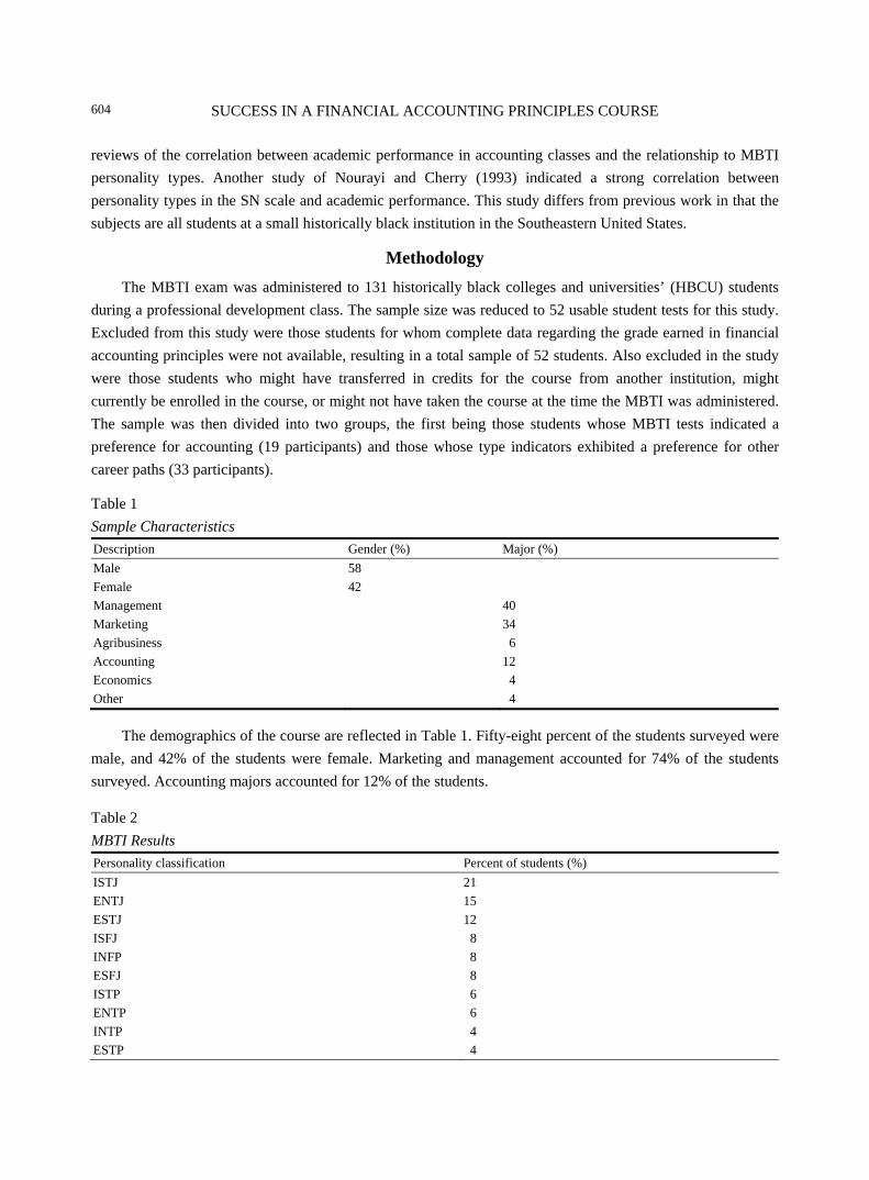
Methodology
The MBTI exam was administered to 131 historically black colleges and universities’ (HBCU) students during a professional development class. The sample size was reduced to 52 usable student tests for this study. Excluded from this study were those students for whom complete data regarding the grade earned in financial accounting principles were not available, resulting in a total sample of 52 students. Also excluded in the study were those students who might have transferred in credits for the course from another institution, might currently be enrolled in the course, or might not have taken the course at the time the MBTI was administered. The sample was then divided into two groups, the first being those students whose MBTI tests indicated a preference for accounting (19 participants) and those whose type indicators exhibited a preference for other career paths (33 participants).
Table 1 Sample Characteristics
Description Gender (%) Major (%) Male 58 Female 42 Management 40 Marketing 34 Agribusiness 6 Accounting 12 Economics 4 Other 4
The demographics of the course are reflected in Table 1. Fifty-eight percent of the students surveyed were male, and 42% of the students were female. Marketing and management accounted for 74% of the students surveyed. Accounting majors accounted for 12% of the students.
Table 2 MBTI Results
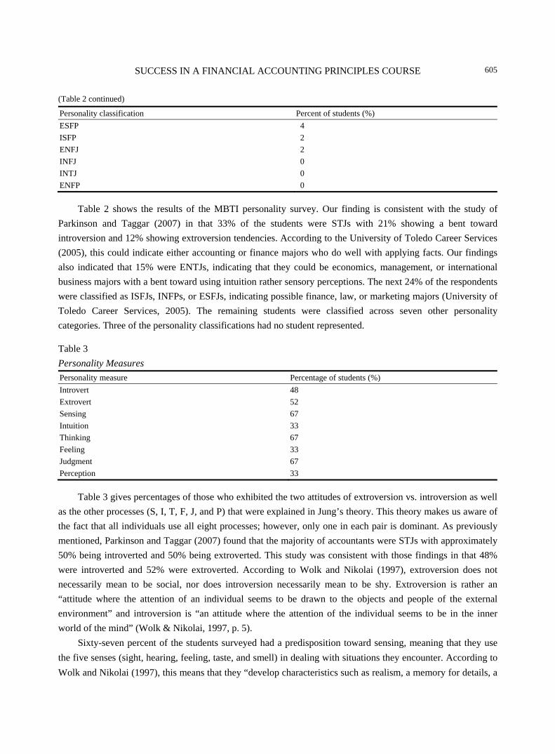
Personality classification Percent of students (%) ISTJ 21 ENTJ 15 ESTJ 12 ISFJ 8 INFP 8 ESFJ 8 ISTP 6 ENTP 6 INTP 4 ESTP 4
SUCCESS IN A FINANCIAL ACCOUNTING PRINCIPLES COURSE
605
(Table 2 continued)
Personality classification Percent of students (%) ESFP 4 ISFP 2 ENFJ 2 INFJ 0 INTJ 0 ENFP 0
Table 2 shows the results of the MBTI personality survey. Our finding is consistent with the study of Parkinson and Taggar (2007) in that 33% of the students were STJs with 21% showing a bent toward introversion and 12% showing extroversion tendencies. According to the University of Toledo Career Services (2005), this could indicate either accounting or finance majors who do well with applying facts. Our findings also indicated that 15% were ENTJs, indicating that they could be economics, management, or international business majors with a bent toward using intuition rather sensory perceptions. The next 24% of the respondents were classified as ISFJs, INFPs, or ESFJs, indicating possible finance, law, or marketing majors (University of Toledo Career Services, 2005). The remaining students were classified across seven other personality categories. Three of the personality classifications had no student represented.
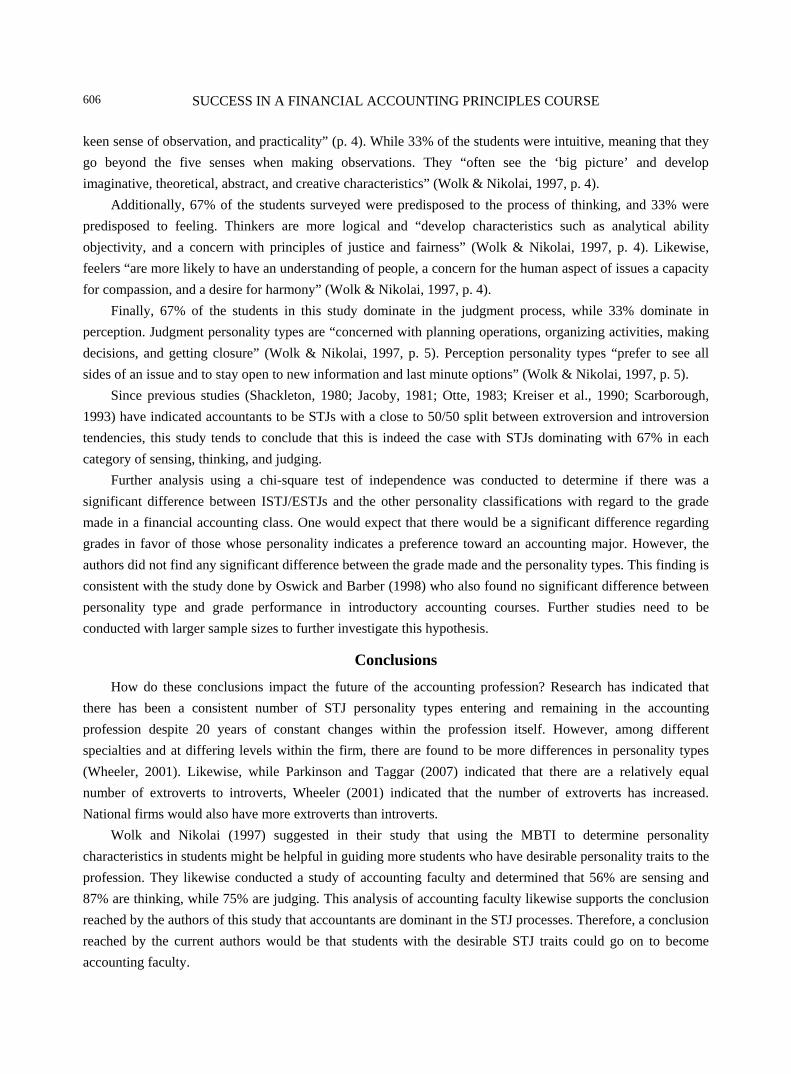
Table 3 Personality Measures
Personality measure Percentage of students (%) Introvert 48 Extrovert 52 Sensing 67 Intuition 33 Thinking 67 Feeling 33 Judgment 67 Perception 33
Table 3 gives percentages of those who exhibited the two attitudes of extroversion vs. introversion as well as the other processes (S, I, T, F, J, and P) that were explained in Jung’s theory. This theory makes us aware of the fact that all individuals use all eight processes; however, only one in each pair is dominant. As previously mentioned, Parkinson and Taggar (2007) found that the majority of accountants were STJs with approximately 50% being introverted and 50% being extroverted. This study was consistent with those findings in that 48% were introverted and 52% were extroverted. According to Wolk and Nikolai (1997), extroversion does not necessarily mean to be social, nor does introversion necessarily mean to be shy. Extroversion is rather an “attitude where the attention of an individual seems to be drawn to the objects and people of the external environment” and introversion is “an attitude where the attention of the individual seems to be in the inner world of the mind” (Wolk & Nikolai, 1997, p. 5).
Sixty-seven percent of the students surveyed had a predisposition toward sensing, meaning that they use the five senses (sight, hearing, feeling, taste, and smell) in dealing with situations they encounter. According to Wolk and Nikolai (1997), this means that they “develop characteristics such as realism, a memory for details, a
SUCCESS IN A FINANCIAL ACCOUNTING PRINCIPLES COURSE
606
keen sense of observation, and practicality” (p. 4). While 33% of the students were intuitive, meaning that they go beyond the five senses when making observations. They “often see the ‘big picture’ and develop imaginative, theoretical, abstract, and creative characteristics” (Wolk & Nikolai, 1997, p. 4).
Additionally, 67% of the students surveyed were predisposed to the process of thinking, and 33% were predisposed to feeling. Thinkers are more logical and “develop characteristics such as analytical ability objectivity, and a concern with principles of justice and fairness” (Wolk & Nikolai, 1997, p. 4). Likewise, feelers “are more likely to have an understanding of people, a concern for the human aspect of issues a capacity for compassion, and a desire for harmony” (Wolk & Nikolai, 1997, p. 4).
Finally, 67% of the students in this study dominate in the judgment process, while 33% dominate in perception. Judgment personality types are “concerned with planning operations, organizing activities, making decisions, and getting closure” (Wolk & Nikolai, 1997, p. 5). Perception personality types “prefer to see all sides of an issue and to stay open to new information and last minute options” (Wolk & Nikolai, 1997, p. 5).
Since previous studies (Shackleton, 1980; Jacoby, 1981; Otte, 1983; Kreiser et al., 1990; Scarborough, 1993) have indicated accountants to be STJs with a close to 50/50 split between extroversion and introversion tendencies, this study tends to conclude that this is indeed the case with STJs dominating with 67% in each category of sensing, thinking, and judging.
Further analysis using a chi-square test of independence was conducted to determine if there was a significant difference between ISTJ/ESTJs and the other personality classifications with regard to the grade made in a financial accounting class. One would expect that there would be a significant difference regarding grades in favor of those whose personality indicates a preference toward an accounting major. However, the authors did not find any significant difference between the grade made and the personality types. This finding is consistent with the study done by Oswick and Barber (1998) who also found no significant difference between personality type and grade performance in introductory accounting courses. Further studies need to be conducted with larger sample sizes to further investigate this hypothesis.
Conclusions
How do these conclusions impact the future of the accounting profession? Research has indicated that there has been a consistent number of STJ personality types entering and remaining in the accounting profession despite 20 years of constant changes within the profession itself. However, among different specialties and at differing levels within the firm, there are found to be more differences in personality types (Wheeler, 2001). Likewise, while Parkinson and Taggar (2007) indicated that there are a relatively equal number of extroverts to introverts, Wheeler (2001) indicated that the number of extroverts has increased. National firms would also have more extroverts than introverts.
Wolk and Nikolai (1997) suggested in their study that using the MBTI to determine personality characteristics in students might be helpful in guiding more students who have desirable personality traits to the profession. They likewise conducted a study of accounting faculty and determined that 56% are sensing and 87% are thinking, while 75% are judging. This analysis of accounting faculty likewise supports the conclusion reached by the authors of this study that accountants are dominant in the STJ processes. Therefore, a conclusion reached by the current authors would be that students with the desirable STJ traits could go on to become accounting faculty.
SUCCESS IN A FINANCIAL ACCOUNTING PRINCIPLES COURSE
607
Recommendations for Future Research
As with the recommendation by Wolk and Nikolai (1997) that accounting faculty personality should be measured with the teaching method used, this analysis would be helpful in determining if the teaching method used is effective in teaching the students. Additionally, this analysis would tie into a recommendation that students be measured on learning styles and see if one is more “suited” to certain “accounting” personality types than others. Likewise, the question arises as to whether the faculty teaching expressed a significant learning style. As Wolk and Nikolai (1997) suggested, the dynamics of classroom instruction can be measured. They went on to indicate that faculty with a predisposition toward intuition, feeling, and perceiving traits are more willing to accept innovation and changes in their teaching methods; whereas sensing, thinking, and judging traits prefer structures, rules, and situations that are not ambiguous. These accounting faculties would tend to resist changes, especially changes that lean toward solving problems from a creative stance. Likewise, this study shows that 60% of the accounting faculties are introverts and are consequently more private, tending to prefer communication that is written as opposed to having more oral communication (Wolk & Nikolai, 1997). This aspect of the nature of accounting faculty is compared with the impact that STJ accounting students have on academia. Booth and Winzar (1993, p. 114) indicated that accounting students “prefer structured learning experiences which present rules and concepts”. They additionally prefer repetition and step-by-step arguments, as well as being given appropriate feedback which includes an explanation for errors.
In summary, this paper examined the likelihood that students at a historical black college (HBC) taking a financial accounting principles course with a predisposition toward an accounting personality type based on the MBTI might have a higher grade than those who had other personality types. No significant difference was found in this case. Likewise, a conclusion was reached that the STJ personality type had a bent toward being an accounting major. Likewise, literature was examined in other cases where students and faculty had the STJ personality type, and a conclusion was reached that faculty tended to prefer the lecture method of teaching with written assignments rather than oral with little tendency toward a desire to change to more innovative teaching methods. These findings of accounting faculty create a challenge for the trend of more innovative teaching methods which have been advocated by the Accounting Education Change Commission (AECC) that in 1990 encouraged “changes in the basic accounting curriculum and explanation of teaching modalities to encourage students to ‘learn how to learn’ and to develop their critical thinking skills”. The present authors suggest further analysis as to the implementation of changes and the effect on the teaching of accounting courses and the learning of accounting students.
References Booth, P., & Winzar, H. (1993). Personality biases of accounting students: Some implications for learning style preferences.
Accounting and Finance, 33(2), 109-120. Jacoby, P. F. (1981). Psychological types and career success in the accounting profession. Research in Psychological Type, 4,
24-37. Kreiser, L., McKeon, J. M., & Post, A. (1990). A personality profile of CPAs in public practice. Ohio CPA Journal, 49(4), 29-34. Laribee, S. F. (1994). The psychological types of college accounting students. Journal of Psychological Type, 28, 37-42. Macdaid, G. P., McCaulley, M. H., & Kainz, R. (1986). Myers-Briggs type indicator: Atlas of type tables. Gainsville, FL: APT
Publications. Myers, I. B. (1962). Manual: The Myers-Briggs type indicator. Princeton, NJ: Educational Testing Service. Nourayi, M. M., & Cherry, A. C. (1993). Accounting students: Performance and personality types. Journal of Education for
Business, 69(2), 111-115.
SUCCESS IN A FINANCIAL ACCOUNTING PRINCIPLES COURSE
608
Oswick, C., & Barber, P. (1998). Personality type and performance in an introductory level accounting course: A research note. Accounting Education, 3(7), 249-254.
Otte, P. (1983). Do CPAs have a unique personality: Are certain personality types found more frequently in our profession? The Michigan CPA, 42(1), 29-36.
Parkinson, J., & Taggar, S. (2007). Earning and outgoing. Financial Management, pp. 55-56. Scarborough, D. P. (1993). Psychological types and job satisfaction of accountants. Journal of Psychological Type, 25, 3-10. Shackleton, V. (1980). The accountant stereotype: Myth or reality? Accountancy, 113(11), 122-123. University of Toledo Career Services. (2005). MBTI and major choice. Wheeler, P. (2001). The Myers-Briggs type indicator and applications to accounting education and research. Accounting
Education, 16(1), 125-150. Wolk, C., & Nikolai, L. (1997). Personality types of accounting students and faculty: Comparisons and implications. Journal of
Accounting Education, 1(15), 1-17.
Journal of Modern Accounting and Auditing, ISSN 1548-6583 May 2013, Vol. 9, No. 5, 609-615
Accounting of Foreign Currencies: Difference in Exchange
Transactions and Relation With Taxation of Indonesia (Case
Study in Fishery Company)
Ilham Hidayah Napitupulu Padjadjaran University, Bandung, Indonesia; Politeknik Negeri Medan, Medan, Indonesia
Abdul Rahman Dalimunthe Politeknik Negeri Medan, Medan, Indonesia
Future need of globalization in business is no longer focused on the local transaction; instead, it has involved many
countries so as to affect the exchange rate of rupiah against foreign currencies. As a result, differences in the
exchange rate will lead to foreign exchange, be it a foreign exchange gain or foreign exchange losses. Exchange
rate used at the beginning of the transaction is the exchange rate on the transaction, but in Indonesian currency
transactions, what is often used is the exchange rate issued by the Directorate General of Taxation (DGT). If at the
end of the period, a balance of foreign currency still exists, then it will be adjusted using a fixed rate or an
exchange rate of Central Bank of Indonesia. The results showed that the treatment of foreign exchange at the
fishery company was using both the exchange rate allowed in the accounting and taxation regulations in Indonesia.
The balance of transactions is related to export, be it a balance of accounts receivable on the sale of the outstanding
balance of exports and export freight carried at the exchange rate adjustment of Central Bank of Indonesia,
subsequent transactions relating to the purchase of imports were adjusted to a fixed exchange rate, which means
that the balance payable on imports will continue to use the exchange rate at the beginning of the transaction.
Keywords: accounting for foreign exchange, exchange rate, taxation
Introduction
The era of globalization and developments in information technology today can increase the mobility of goods, services, and capitals as the fulfillment of needs in the business. Activities of that need no longer to focus on local transactions, but have involved many countries so as to affect the exchange rate of rupiah against foreign currencies. In using foreign currency, there are two aspects made by business entities, namely: (1) translation of foreign exchange financial statement, the intention is as a translation of financial statements prepared in foreign currencies. This translation is used for a multinational company branch or subsidiary in another country; and (2) foreign exchange transaction, meant as an elaboration of that due to the company’s transactions relating to foreign exchange (Ariyanto, 2006; Waluyo, 2009).
Ilham Hidayah Napitupulu, student of Doctoral Program, Accounting Department, Padjadjaran University; lecturer, Accounting
Department, Politeknik Negeri Medan. Email: [email protected]. Abdul Rahman Dalimunthe, lecturer, Accounting Department, Politeknik Negeri Medan.
DAVID PUBLISHING
D
ACCOUNTING OF FOREIGN CURRENCIES
610
Companies in Indonesia, dominating foreign exchange transaction in foreign exchange. Exchange differences in question are the differences resulting from translation of a certain amount of one currency into another currency at different exchange rates (Ikatan Akuntan Indonesia (IAI1), Pernyataan Standar Akuntansi Keuangan (PSAK2) 10). The accounting treatment of foreign exchange can be done by imposing a direct impact on profit and loss account in the period (The Republic of Indonesia, 2008) and either partially or wholly capitalized (Ariyanto, 2006). This refers to the Decree of the Minister of Finance of Republic of Indonesia Number 597/KMK304/1997 about the income tax treatment of foreign currency on foreign exchange in 1997 which was reinforced by regulation BAPEPAM4 No. VIII G10 (Kep. 49/PM5/1998) issued when the economic crisis hit Indonesia.
Some types of foreign currency transactions that occur frequently can be seen by noting the sources of (IAI, PSAK 10): (1) buying or selling goods or services whose price is denominated in foreign currencies; (2) borrowing or lending funds denominated in foreign currencies; (3) acquiring or releasing assets, or conducting or completing a liability, denominated in foreign currencies; and (4) contract work, due to the implementation of labor contract agreements to use foreign currency in payment transactions work.
In the execution or recording of transactions that occur in business activities by using foreign currency, exchange rates used were two, namely, the exchange rate at the beginning of the transaction, which is usually adjusted with exchange rate issued by the Directorate General of Taxation (DGT), in order to facilitate businesses to pay taxes related to export transactions and import; the second is the exchange rate at the time of repayment, usually the exchange rate used by agreement of consumers and producers. In general, the settlement rate is the rate used to follow the bank where the transaction will be done. Thus, the study is limited to transactions that occur in business activities rather than to translations of financial statements of the companies as a whole as is done in multinational companies, and all foreign currency transactions routed into the functional currency used in Indonesia, the rupiah.
Bookkeeping-conducted business in Indonesia refers to the Financial Accounting Standards (PSAK), but not all are set forth in PSAK recognized by the taxation laws of Indonesia, so in tax reporting, there will be no further action that is known as fiscal reconciliation. The values that have been recognized in the accounting firm will be tailored according to PSAK applicable tax laws, for the treatment of foreign exchange but did not experience the difference between Generally Accepted Accounting Principles (GAAP) with tax regulations in Indonesia (IAI, PSAK 10; IAI, 2009b; The Republic of Indonesia, 2008) with the sense that what is recognized in accordance with International Accounting Standards (IAS) is also recognized by tax regulations.
Exchange rate is used for the benefit of the end of the period, the adjustment of balances that use foreign currency. There are two types of exchange rate used by the businesses in Indonesia (IAI, PSAK 10; DGT, 1997), i.e., fixed exchange rate and exchange rate of Central Bank of Indonesia. The use of foreign exchange rates in Indonesia is not much different from Romania. The use of foreign currency transactions follows rules based on tax laws and Central Bank of Romania (Ecobici, 2011). Of the different uses of the exchange rate impact on
1 The Indonesian Institute of Accountants. 2 Indonesian Financial Accounting Standards, also known as IFAS or PSAK. 3 Keputusan Menteri Keuangan (KMK), Decree of the Minister of Finance. 4 Badan Pengawas Pasar Modal, Capital Market Supervisory Agency. 5 Peraturan Menteri (PM), Regulation of the Minister.
ACCOUNTING OF FOREIGN CURRENCIES
611
accounting firms, especially firms that conduct foreign trade, the company is very sensitive to changes in exchange rates (Solano, 2000). Another impact of foreign exchange may also cause the stock market reaction (Chandarin & Tearney, 2000), foreign exchange which significantly influences the company’s stock price, as well as that done by Ariyanto (2006) that foreign exchange is also a significant effect on stock returns, which means that foreign exchange can also be used as an analytical tool to determine the choice of investors in investing.
Research Methods
Types of Research
This research is an applied research (Indriantoro & Supomo, 2002), i.e., research aimed at solving practical problems faced by the institution or organization which is generally done in a business environment. This research is an empirical research and archival research. The object of this research is a company in the fishing industry located in the city of Medan, Indonesia, which has several units working with the needs and supplies from domestic market or abroad.
Data Collection and Analysis Techniques
The data used are secondary data, obtained directly from the company that became the object of this research, i.e., several transaction data, such as data of export freight costs, debt export freight, product import for production processing, and data on the balance of foreign currency transactions in the period of December 2008 to January 2009. Analysis of the data is used to determine how the treatment of foreign currency in the fishing industry, particularly companies dealing with the taxation laws of Indonesia.
Results and Discussion
The results of this study describe the recognition of foreign exchange empirically related to taxation in Indonesia, while the data obtained are: (1) transactions related to export sales, such as data of export freight cost and data of debt of freight exports and repayment; and (2) transactions related to the purchase of imported goods, such as data of import purchases and debt of import and repayment of import.
Shipping Cost of Export Sales Transactions
Company’s export sales are made to countries of Europe, America, and Asia. Transactions are carried out by using the destination country’s currency, such as Europe’s use of the euro, USA’s use of the US dollar, and half of the Asian countries also use the US dollar. For Singaporeans, they use Singapore dollars, while for Japanese, they use the US dollar. All transactions carried out will be transferred to the functional currency in Indonesian Rupiah (IDR). Transactions that occur early will be transferred to the rupiah exchange rate following the DGT, fluctuations in the exchange rate against foreign currencies change every week. The use of the rupiah exchange rate makes it easier to adjust with obtaining a license for exports and imports.
Freight cost of export sales also used foreign currency, usually the US dollar. Many shipping companies are used in support of export sales, such as Hanjin, Hyundai, Maersk Sealand, APL, etc.. Considering the treatment of foreign exchange transactions in this case, there are two under different circumstances, namely, recognition of foreign exchange transactions settled during the month of transaction and recognition of foreign exchange transactions settled in the following month. For the first case, the transactions from December 2, 2008 to December 22, 2008 are delivered by Hanjin Shipping and Hyundai Shipping. For example, Hanjin invoice, December 2, 2008, the transaction with the invoice number BANA 01553003 and transaction
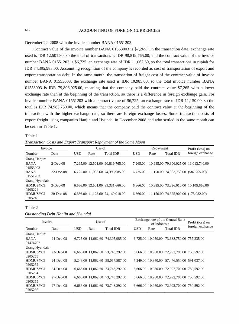
ACCOUNTING OF FOREIGN CURRENCIES
612
December 22, 2008 with the invoice number BANA 01551203. Contract value of the invoice number BANA 01553003 is $7,265. On the transaction date, exchange rate
used is IDR 12,501.80, so the total of transactions is IDR 90,819,765.00; and the contract value of the invoice number BANA 01551203 is $6,725, an exchange rate of IDR 11,062.60, so the total transactions in rupiah for IDR 74,395,985.00. Accounting recognition of the company is recorded as cost of transportation of export and export transportation debt. In the same month, the transaction of freight cost of the contract value of invoice number BANA 01553003, the exchange rate used is IDR 10,985.00, so the total invoice number BANA 01553003 is IDR 79,806,025.00, meaning that the company paid the contract value $7,265 with a lower exchange rate than at the beginning of the transaction, so there is a difference in foreign exchange gain. For invoice number BANA 01551203 with a contract value of $6,725, an exchange rate of IDR 11,150.00, so the total is IDR 74,983,750.00, which means that the company paid the contract value at the beginning of the transaction with the higher exchange rate, so there are foreign exchange losses. Some transaction costs of export freight using companies Hanjin and Hyundai in December 2008 and who settled in the same month can be seen in Table 1.
Table 1 Transaction Costs and Export Transport Repayment of the Same Moon
Invoice Use of Repayment Profit (loss) on foreign exchangeNumber Date USD Rate Total IDR USD Rate Total IDR
Utang Hanjin: BANA 01553003
2-Dec-08 7,265.00
12,501.00
90,819,765.00 7,265.00
10,985.00
79,806,025.00
11,013,740.00
BANA 01551203
22-Dec-08 6,725.00
11,062.60
74,395,985.00 6,725.00
11,150.00
74,983,750.00
(587,765.00)
Utang Hyundai: HDMUSYCI 0205224
2-Dec-08 6,666.00
12,501.00
83,331,666.00 6,666.00
10,985.00
73,226,010.00
10,105,656.00
HDMUSYCI 0205248
20-Dec-08 6,666.00
11,123.60
74,149,918.00 6,666.00
11,150.00
74,325,900.00
(175,982.00)
Table 2 Outstanding Debt Hanjin and Hyundai
Invoice Use of Exchange rate of the Central Bank of Indonesia Profit (loss) on
foreign exchangeNumber Date USD Rate Total IDR USD Rate Total IDR Utang Hanjin: BANA 01476707
24-Dec-08 6,725.00
11,062.60
74,395,985.00 6,725.00
10,950.00
73,638,750.00
757,235.00
Utang Hyundai: HDMUSYCI 0205253
23-Dec-08 6,666.00
11,062.60
73,743,292.00 6,666.00
10,950.00
72,992,700.00
750,592.00
HDMUSYCI 0205252
24-Dec-08 5,249.00
11,062.60
58,067,587.00 5,249.00
10,950.00
57,476,550.00
591,037.00
HDMUSYCI 0205254
24-Dec-08 6,666.00
11,062.60
73,743,292.00 6,666.00
10,950.00
72,992,700.00
750,592.00
HDMUSYCI 0205255
27-Dec-08 6,666.00
11,062.60
73,743,292.00 6,666.00
10,950.00
72,992,700.00
750,592.00
HDMUSYCI 0205256
27-Dec-08 6,666.00
11,062.60
73,743,292.00 6,666.00
10,950.00
72,992,700.00
750,592.00
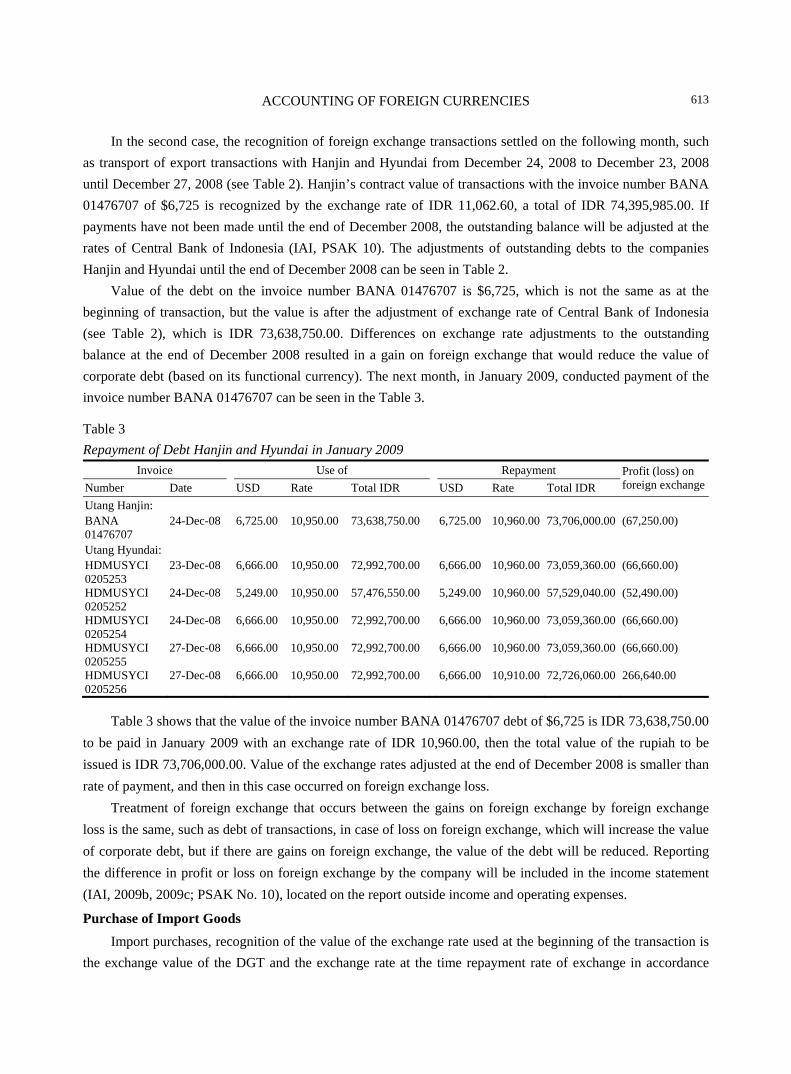
ACCOUNTING OF FOREIGN CURRENCIES
613
In the second case, the recognition of foreign exchange transactions settled on the following month, such as transport of export transactions with Hanjin and Hyundai from December 24, 2008 to December 23, 2008 until December 27, 2008 (see Table 2). Hanjin’s contract value of transactions with the invoice number BANA 01476707 of $6,725 is recognized by the exchange rate of IDR 11,062.60, a total of IDR 74,395,985.00. If payments have not been made until the end of December 2008, the outstanding balance will be adjusted at the rates of Central Bank of Indonesia (IAI, PSAK 10). The adjustments of outstanding debts to the companies Hanjin and Hyundai until the end of December 2008 can be seen in Table 2.
Value of the debt on the invoice number BANA 01476707 is $6,725, which is not the same as at the beginning of transaction, but the value is after the adjustment of exchange rate of Central Bank of Indonesia (see Table 2), which is IDR 73,638,750.00. Differences on exchange rate adjustments to the outstanding balance at the end of December 2008 resulted in a gain on foreign exchange that would reduce the value of corporate debt (based on its functional currency). The next month, in January 2009, conducted payment of the invoice number BANA 01476707 can be seen in the Table 3.
Table 3 Repayment of Debt Hanjin and Hyundai in January 2009
Invoice Use of Repayment Profit (loss) on foreign exchangeNumber Date USD Rate Total IDR USD Rate Total IDR
Utang Hanjin: BANA 01476707
24-Dec-08
6,725.00
10,950.00
73,638,750.00
6,725.00
10,960.00
73,706,000.00
(67,250.00)
Utang Hyundai: HDMUSYCI 0205253
23-Dec-08
6,666.00
10,950.00
72,992,700.00
6,666.00
10,960.00
73,059,360.00
(66,660.00)
HDMUSYCI 0205252
24-Dec-08
5,249.00
10,950.00
57,476,550.00
5,249.00
10,960.00
57,529,040.00
(52,490.00)
HDMUSYCI 0205254
24-Dec-08
6,666.00
10,950.00
72,992,700.00
6,666.00
10,960.00
73,059,360.00
(66,660.00)
HDMUSYCI 0205255
27-Dec-08
6,666.00
10,950.00
72,992,700.00
6,666.00
10,960.00
73,059,360.00
(66,660.00)
HDMUSYCI 0205256
27-Dec-08
6,666.00
10,950.00
72,992,700.00
6,666.00
10,910.00
72,726,060.00
266,640.00
Table 3 shows that the value of the invoice number BANA 01476707 debt of $6,725 is IDR 73,638,750.00 to be paid in January 2009 with an exchange rate of IDR 10,960.00, then the total value of the rupiah to be issued is IDR 73,706,000.00. Value of the exchange rates adjusted at the end of December 2008 is smaller than rate of payment, and then in this case occurred on foreign exchange loss.
Treatment of foreign exchange that occurs between the gains on foreign exchange by foreign exchange loss is the same, such as debt of transactions, in case of loss on foreign exchange, which will increase the value of corporate debt, but if there are gains on foreign exchange, the value of the debt will be reduced. Reporting the difference in profit or loss on foreign exchange by the company will be included in the income statement (IAI, 2009b, 2009c; PSAK No. 10), located on the report outside income and operating expenses.
Purchase of Import Goods
Import purchases, recognition of the value of the exchange rate used at the beginning of the transaction is the exchange value of the DGT and the exchange rate at the time repayment rate of exchange in accordance
ACCOUNTING OF FOREIGN CURRENCIES
614
with the agreement, usually based on the rate of bank where the payment is made. Outstanding debt of imported goods at the end of the period is not adjusted to the rate of Central Bank of Indonesia. Thus, in the case of import purchases, the balance of the debt using the fixed exchange rate (IAI, PSAK 10; DGT, 1997), such as transactions that occurred on December 3, 2008 from a supplier of plastic packaging products of Qingdou Ricai in Taiwan, can be seen in Table 4.
Table 4 Import Transaction
Name of goods Unity Qty Price per unit Total USD IDR rate Total IDR Plastik Vacum, China (Highliner 4-7) Lembar 453,600 $0.1839 $83,417.02 12,501.00 1,042,796,417 PE. Highliner 1 LB Lembar 245,300 $0.142 $34,832.60 12,501.00 435,442,333 Total 698,900 $118,249.62 1,478,238,750
Fixed exchange rate used by the end of the accounting period equals to the rate used at the beginning of the transaction (Waluyo, 2009). Thus, the total debt to Qingdou Ricai imports recognized companies in the rupiah value of IDR 1,478,238,750.00.
Conclusions
The study results showed that the treatment of foreign exchange at the fishery company use of taxation laws of Indonesia (The Republic of Indonesia, 2008), and the Financial Accounting Standards (IAI, 2009a, 2009b), recognition of foreign exchange which can be charged to the income statement in the current year and can be capitalized over the next five years (KMK RI Number 597/KMK04/1997).
The balance of accounts payable and accounts receivable on export sales at the end of the period, do adjustment to the exchange rate of Central Bank of Indonesia, companies refer to the Financial Accounting Standards (IAI, PSAK 10) and DGT (1997) about income tax treatment of exchange rate, the adjustment balance at the end of the period used a fixed exchange rate and the exchange rate of Central Bank of Indonesia. However, for the import purchase transactions, in the adjustment of the outstanding balance at the end of the period, a fixed exchange rate is used, meaning that at the end of the period, the company uses the same exchange rate at the time the beginning of a transaction, so the foreign exchange will occur only at transaction date of import purchases of debt repayment.
References Ariyanto, D. (2006). Capital market reaction reporting against foreign exchange (Empirical studies on the Indonesia Stock
Exchange). Bulletin of Economic Studies, 11(2), 191-201. Chandarin, G., & Tearney, M. G. (2000). The effect of reporting of exchange rate losses on the stock market reaction. Journal of
Accounting Research Indonesia, 3(1), 1-16. Directorate General of Taxation [DGT]. (1997). Number SE. 03/PJ.31/1997 on income tax treatment of foreign exchange. Ecobici, N. (2011). Ways of reflecting the foreign exchange transactions made by the currency exchange offices in Romania.
Annals of the University “Constantin Brancusi” in Targu Jiu, Economy Series, No. 3, 75-84. Ikatan Akuntan Indonesia [IAI]. (2009a). Indonesian financial accounting standard (Revision 2010). Salemba Empat Jakarta. Ikatan Akuntan Indonesia [IAI]. (2009b). Interpretation of financial accounting standard (ISAK). Salemba Empat, Jakartae. Ikatan Akuntan Indonesia [IAI]. (2009c). Indonesian financial accounting standard without public entities (PSAK ETAP)
(Revision May, 2009). Salemba Empat Jakarta.

ACCOUNTING OF FOREIGN CURRENCIES
615
Indriantoro, N., & Supomo, B. (2002). Research methods for accounting and management (2nd ed.). Yogyakarta: BPFE Yogyakarta.
Solano, P. M. (2000). Foreign exchange exposure on the Spanish stock market: Sources of risk and hedging (pp. 1-26). Social Science Research Network Electronic Paper Collection. Retrieved from http://papers.ssrn.com/ paper.id=110777
The Republic of Indonesia. (2008). Law of the Republic of Indonesia Number 36 of 2008. Waluyo. (2009). Tax accounting (4th ed., p. 370).
Journal of Modern Accounting and Auditing, ISSN 1548-6583 May 2013, Vol. 9, No. 5, 616-633
The Influence of Market and Company Characteristics on
Voluntary Disclosure
Eugenio D’Amico Rome Third University, Rome, Italy
Anna Maria Biscotti University of Foggia, Foggia, Italy
In this paper, the determinants of the voluntary disclosure level of firms have been investigated during a period of
deep financial crisis. Two disclosure indexes used as dependent variables are proposed: a global index based on
both quantitative and qualitative disclosure and a solely quantitative voluntary index. Firstly, the explanatory
variables have been selected taking into account the main contributions of international literature. In addition, some
specific variables have been introduced in order to take into account the peculiarities of Italian market system and
the ongoing financial crisis. A positive relationship has been found among the global voluntary disclosure (GVD)
and the number of employees, the dividend policy, and the presence of independent directors on the board. On the
contrary, a negative correlation with respect to the percentage of the firm’s outstanding shares held by directors (not
independent) exists. With reference to the quantitative voluntary disclosure (QVD) index, there is a positive
correlation with the number of employees, the dividend policy, the market floating, and the incidence of intangible
assets. Moreover, such (quantitative) a disclosure is different depending on the industrial membership sector.
Keywords: voluntary disclosure, market determinants, company characteristics
Introduction The purpose of this paper is to investigate the determinants of the voluntary disclosure reported in 2010
from Italian listed firms, in addition to the mandatory disclosure. In particular, it has been chosen to develop the analysis with reference to 2010 for the following reasons.
Firstly, it is interesting to examine the behavior of these firms looking at their attitudes toward disclosing more information (strategic, financial, and social) after the effects produced by the globalization process. In particular, this examination is developed over a difficult period characterized by a considerable financial and economical global crisis which has affected the credibility of our entire national economic system and its ability to avoid defaulting.
Moreover, it is interesting to verify the level of voluntary disclosure in the target year of 2010, because it has a reasonable distance from 2005 when the International Accounting Standards (IAS) and International Financial Reporting Standards (IFRS) were introduced in Italy as a forced system for listed companies. In fact,
Eugenio D’Amico, full professor of Accounting and Management, Department of Public Institutions, Economy, and Society, Rome Third University. Email: [email protected].
Anna Maria Biscotti, Ph.D. of Accounting and Management, tenured assistant professor of Accounting and Management, Department of Economics, University of Foggia.
DAVID PUBLISHING
D
THE INFLUENCE OF MARKET AND COMPANY CHARACTERISTICS
617
it could be supposed that after the sufficiently long span of five years (since 2005), the preparers of financial reporting also began to improve their voluntary disclosure (financial, strategic, and social).
This study aims to investigate the possible relationships between a set of variables identified in four specific categories by their nature and the level of voluntary disclosure of firms. The authors extend the existing literature by introducing both explanatory and dependent new variables.
The remainder of the paper is structured as follows. Section 2 provides a brief review of the relevant literature and introduces the development of hypotheses. In Section 3, a sample selection, disclosure index (dependent variable), and explanatory variables are presented. Section 4 discusses the results and Section 5 develops the conclusions.
Literature Review The studies on disclosure (either compulsory or above all voluntary) developed starting from the end of
the 1980s and underwent an exponential growth that still characterizes the international accounting. The pattern of the different contributions, not considering the statistical instrument employed, follows an
already consolidated path. Initially, a disclosure index is drawn up and then a regression function is estimated between the said index and a set of explicative variables.
Disclosure Index
In general, a disclosure index is built comparing the number of disclosure items applied by the individual companies with the number of applicable total items (Spero, 1979; Robbins & Austin, 1986; Wallace, 1987; Wallace, Naser, & Mora, 1994; Wallace & Naser, 1995; Meek, Roberts, & Gray, 1995; Cooke, 1996; Inchausti, 1997; Cammferman & Cooke, 2002). It is an index ranging from a minimum of zero when no item selected by the researcher is highlighted to a maximum of one when all items are highlighted. Usually, it is an index built to give the same importance to each considered item. Actually, some experts prefer to draw up a well-pondered index, giving more (less) importance to the items considered more (less) important (Singhvi & Desai, 1971; Buzby, 1974; Firth, 1979; McNally, Eng, & Hasseldine, 1982; Wallace, 1988; Malone, Fries, & Jones, 1993; Eng & Mak, 2003) mostly where the analysis is carried out with reference to one or more specific stakeholders (Wallace & Naser, 1995). It should be emphasized that some authors consider the use of well-pondered index wrong, because: (1) The element reckoned as the most important is not always revealed as such (Chow & Wong-Boren, 1987); (2) The expressed considerations do not always keep their validity over time (Dhalival, 1980); (3) Since the weights are not the same in all countries, it is quite difficult to carry out a comparative analysis (Firer & Meth, 1986); and (4) The empirical studies show the interchangeability of weights (Spero, 1979; Robbins & Austin, 1986).
Determinants of Voluntary Disclosure: Hypotheses
Though there is a broad typology of determinants of disclosure proposed by various authors, it is possible to pick up some elements that are common to the different analyses.
In particular, the variables will be identified and classified into four categories: market variables, financial variables, governance variables, and ownership structure variables.
The stock exchange belongs to the first category of variables (market). It is likely that companies listed in countries with more severe regulations will submit the requested information on a voluntary basis also in markets where such a disclosure is not requested (Singhvi & Desai, 1971; Gray, Meek, & Roberts, 1995). In
THE INFLUENCE OF MARKET AND COMPANY CHARACTERISTICS
618
this case, it could be assumed that a positive relationship exists between the listing in more than one stock market and voluntary disclosure. It can also be stated that a positive correlation may exist between the internationalization level and the level of the markets served by a company and disclosure (Meek et al., 1995; Owusu-Ansah, 1998). The empirical evidence does not always confirm these relationships (Chau & Gray, 2002; Glaum & Street, 2003). In this analysis, it is expected that:
Hypothesis 1: Voluntary disclosure is positively correlated to the internationalization of the firm. With reference to the market variables, attention should be paid to the industrial sector. It is possible that
the disclosure would not be the same in different industrial sectors (Cooke, 1992) in which it is possible that the same items are dealt with in a different way (Wallace, 1987). There is not any specific indication on which sector would prevail on others in terms of disclosure (Wallace & Naser, 1995; Meek et al., 1995; Inchausti, 1997; Tower, Hancock, & Taplin, 1999; Ferguson, Lam, & Lee, 2002; Akhtaruddin, 2005), even if there seems to be an imitation effect so that if a company does a lot of disclosure, other companies will tend to imitate it. The disclosure in a specific sector can be strongly influenced by the competition level characterizing it. In general, it can be stated that if the competition level increases, disclosure level will decrease (Verrecchia, 1983; Wagenhofer, 1990; Clinch & Verrecchia, 1997), since companies, mostly the smallest, do not want to disclose their own information to competitors (MohdGhazali & Weetman, 2006). Therefore, it is expected that:
Hypothesis 2: Voluntary disclosure is different among sectors. The market variables identified have been integrated from the previous literature with a new variable
which is a stock market segment where the company is listed. In particular, companies with medium-to-small capitalization are listed in a specific segment called “Star”, while companies with high capitalization are listed in a segment called “Blue Chip”. As regards this variable, a positive correlation between the disclosure level and the listed companies with higher capitalization appears to be likely. This relationship should exist to reduce the prevalence of information asymmetry among the different stakeholders of the largest companies (Jensen & Meckling, 1976). However, it is also possible that the smallest companies listed on the “Star” segment will disclose more information in the event of a planned increase of their own capitalization (through a planned increase of stock equity).
Hypothesis 3a: Voluntary disclosure is positively correlated to the Blue Chip firms. Hypothesis 3b: Voluntary disclosure is positively correlated to the Star firms. With reference to the second category of variables (financial), the company size expressed as assets
(logarithm) (Cooke, 1993; Imhoff, 1992; Malone et al., 1993; Hossain, Tan, & Adams, 1994), sales (Belkaoui & Kahl, 1978; Cooke, 1989a, 1989b; Walace et al., 1994), capitalization (Chow & Wong-Boren, 1987; Lang & Lundholm, 1993; Hossain et al., 1994), and number of employees (Wallace & Naser, 1995; Cooke, 1992) has been considered. Usually, a direct relationship between disclosure and size was theorized. This relationship can be motivated by various reasons. First of all, the costs for disclosure are considered to be heavy for small firms, while they can be easily afforded by the largest companies (Buzby, 1975; Lang & Lundholm, 1993; Cooke, 1989a). On the other hand, for the largest companies, information on disclosure is a part of the top management information system (Singhvi & Desai, 1971). Moreover, big companies want to assure reasonable stock prices in order to avoid takeover (Cooke, 1996). In general, it could be stated that big companies are more subjected to requests for information from various and important stakeholders (Wallace & Naser, 1995). In this sense, disclosure can be an important way to reduce agency costs and information
THE INFLUENCE OF MARKET AND COMPANY CHARACTERISTICS
619
asymmetry (Inchausti, 1997). The positive relationship between size and disclosure has been confirmed by several empirical evidence
carried out in different contexts and periods (Buzby, 1975; McNally et al., 1982; Malone et al., 1993; Wallace et al., 1994; Wallace & Naser, 1995; Meek et al., 1995; Raffournier, 1995; Inchausti, 1997; Owusu-Ansah, 1998; Haniffa & Cooke, 2002; Camfferman & Cooke, 2002; Ferguson et al., 2002; Chau & Gray, 2002; Ali, Ahmed, & Henry, 2004; Prencipe, 2004; Barako, 2007). It should be outlined that there is also evidence of low statistical significance on this relationship (Entwistle, 1999; Tower et al., 1999) or even a negative relationship (Naser, Alkhatib, & Karbhari, 2002).
The hypothesis to be checked is the following: Hypothesis 4: Voluntary disclosure is positively correlated to the size. A positive relationship is supposed to exist between disclosure and leverage ratio (Malone et al., 1993;
Naser et al., 2002; Wallace et al., 1994; Meek et al., 1995; Inchausti, 1997; Camfferman & Cooke, 2002; Raffournier, 1995; Depoers, 2000; Eng & Mak, 2003; Prencipe, 2004; Barako, 2007; Chow & Wang-Boren, 1987). In this regard, the companies with a higher leverage tend to disclose more information in order to assure creditors (Singhvi & Desai, 1971; Jensen & Meckling, 1976; Courtis, 1978).
The hypothesis to be verified, with the awareness that the empirical evidence has not always found a statistical significance of this relationship (Wallace et al., 1994; Raffournier, 1995; Inchausti, 1997; Tower et al., 1999; Depoers, 2000), is the following:
Hypothesis 5: Voluntary disclosure is positively correlated to the level of leverage. The positive correlation between disclosure and bad news is also theorized with reference to the dividend
payout. In particular, the lower the dividend payout, the higher the level of disclosure (Inchausti, 1997). This occurs, because the companies paying lower dividends have to provide more explanations to shareholders in order to assure them about the profitability and financial position of the firm. The following hypothesis is then formulated:
Hypothesis 6: Voluntary disclosure is negatively correlated to the dividend payout. On the contrary, disclosure is considered positively correlated to the company’s profitability (Singhvi &
Desai, 1971; Malone et al., 1993; Meek et al., 1995; Cammferman & Cooke, 2002; Ali et al., 2004; Barako, 2007). In particular, managers tend to disclose more detailed good news in order to maintain their own positions and to obtain higher remunerations (McKnight & Tomkins, 1999; Aboody & Kaznik, 2000). However, the empirical evidence has not always found a statistical significance on this relationship (Haniffa & Cooke, 2002; Naser et al., 2002; Ali et al., 2004; McNally et al., 1982; Malone et al., 1993; Wallace et al., 1994; Meek et al., 1995; Raffournier, 1995; Akhtaruddin, 2005). Therefore, it is expected that:
Hypothesis 7: Voluntary disclosure is positively correlated to profitability. Another positive relationship is theorized with reference to the company’s liquidity ratio (Belkaoui &
Kahl, 1978). In this sense, such a ratio indicates the solvency position of the company (Cammferman & Cooke, 2002; Wallace & Naser, 1995). Therefore, it is expected that:
Hypothesis 8: Voluntary disclosure is positively correlated to liquidity ratio. In respect of these financial variables, two new variables have been introduced which should characterize
the Italian Stock Market. The first of these variables measures the incidence of intangible assets, and it is used to calculate the ratio of intangible assets to total assets recognized in balance sheet statements. This type of
THE INFLUENCE OF MARKET AND COMPANY CHARACTERISTICS
620
variable has been considered because of its increasing prevalence in Italian listed companies’ balance sheets. On many occasions, the value relevance for these intangible assets was criticized. In this sense, a positive relationship between the disclosure level and the incidence of intangible assets will be expected, assuming that managers tend to justify their economical substance inherent in these values by disclosing more information. Therefore, it will be tested that:
Hypothesis 9: Voluntary disclosure is positively correlated to intangibles. The second “additional” variable is return on debts measured by the ratio between financial burdens and
financial debts. In the last years, banking systems, according to Basel II regulations, applied rating systems which penalize the companies identified as a higher risk. As a consequence, an increase in voluntary disclosure by higher risk companies is expected, in order to reassure the banking systems. The following hypothesis is then formulated:
Hypothesis 10: Voluntary disclosure is positively correlated to return on debts. There is a set of elements which influence disclosure level classified as governance variables (Klein, 2002;
Chiang, 2005). In particular, most of the literature on disclosure states that firms which are externally audited by major international independent audit companies tend to increase their disclosure. This increase occurs, because big audit firms have many clients, and any loss that they could incur from a possible decrease in their client portfolios as a consequence of their requests for greater disclosure would be economically sustainable. On the contrary, small audit firms typically depend on a few clients (Firth, 1979; Malone et al., 1993; Wallace & Naser, 1995; Wallace et al., 1994).
However, the relationship with the external auditors can also be considered under agency theory. More specifically, the companies audited by large audit firms (which request more information) can reduce the agency costs as a consequence of the greater disclosure levels (Watts & Zimmerman, 1983, 1986).
However, the empirical evidence demonstrates that there is no statistically significant correlation between the two variables (Malone et al., 1993; Depoers, 2000; Haniffa & Cooke, 2002; Chau & Gray, 2002; Ali et al., 2004), including even a negative relationship (Wallace & Naser, 1995; Naser et al., 2002).
The hypothesis to be verified is the following: Hypothesis 11: Voluntary disclosure is positively correlated to the major audit companies. According to agency theory (Jensen & Meckling, 1976; Fama & Jensen, 1983), the presence of more
independent directors on the board should imply greater disclosure (Chen & Jaggi, 2000; Cheng & Courtenay, 2006). Independent directors tend to decrease the conflict between management and ownership by fostering the dissemination of information (Al-Akra, Eddy, & Ali, 2010), thus limiting management opportunism (Eng & Mak, 2003). However, extending the concepts stated by Leftwich, Watts, and Zimmerman (1981) to this analysis, it can be asserted that if the presence of independent directors is considered by management to be a signal of minority protection, then managers might not disseminate more than the compulsory information. In this case, the relationship between the voluntary disclosure index and the presence of independent directors on the board would be negative. If independent directors are considered to be complementary to disclosure, then there could not be any relationship between the two variables. Finally, if independent directors are considered to be complementary to disclosure, but their actions are directed towards facilitating and protecting the minority shareholders through a better disclosure, then there should be a positive correlation between the two variables.
The controversial or even negative relationship between independent directors and disclosure can also
THE INFLUENCE OF MARKET AND COMPANY CHARACTERISTICS
621
exist when independents are appointed by blockholders (shareholders with a share greater than 5%). In this case, independent directors could serve the interests of these shareholders, communicating additional information directly to them (without public dissemination by external reporting) (Eng & Mak, 2003).
However, the mere presence of independent directors on the board could be not sufficient to ensure a better disclosure. Independent directors should be characterised by capabilities, experience, and authority (Gul & Leung, 2004). Afterwards, it will be tested if:
Hypothesis 12: Voluntary disclosure is positively/negatively correlated to the proportion of independent directors on the board.
Some authors found out that a negative correlation between duality and disclosure existed (Gul & Leung, 2004). In particular, a mutual monitoring is expected when the chair and the chief executive officer (CEO) are two different subjects. This role separation leads to a greater dissemination of information (Forker, 1992). The following hypothesis is then formulated:
Hypothesis 13: Voluntary disclosure is negatively correlated to duality. Theoretical and empirical analyses of the variables connected to the ownership structure (which is the
fourth variable category taken into account) are also interesting. Wallace and Naser (1995) stated that the greater the number of shares held by outsiders, the greater the level of disclosure. Outsiders, in fact, tend to request more information in order to reduce the information asymmetry with respect to insiders (MohdGhazali & Weetman, 2006). In the same way and for the same reason, it could be thought that a positive correlation exists between disclosure and market floating, even if the small shareholders’ level of expertise could be less advanced to be able to request specific information (Naser & Alkhatib, 2000; Naser et al., 2002). Therefore, the following hypothesis will be verified:
Hypothesis 14: Voluntary disclosure is positively correlated to market floating. Also with regard to the ownership structure, it is interesting to verify the correlation between the
disclosure level and the institutional investors’ shareholding. In this connection, it could be stated that, according to the agency theory, the companies held by large institutional investors tend to increase disclosure, because they require it and are able to impose that. Therefore, it is expected that:
Hypothesis 15: Voluntary disclosure is positively correlated to the shareholding of institutional investors. The same considerations can be applied to foreign investors (Boycko, Shleifer, & Vishny, 1996; Boubakri,
Cosset, & Guedhami, 2005; Al-Akra et al., 2010). They are usually large investors with international expertise which requires extending the best practice of disclosure already followed by the most advanced countries to the companies in which they invest (Naser et al., 2002). The empirical analysis has confirmed a positive correlation between disclosure and foreign investors (Craswell & Taylor, 1992; Haniffa & Cooke, 2002; Lakhal, 2005). The following hypothesis is then formulated:
Hypothesis 16: Voluntary disclosure is positively correlated to the shareholding of foreign investors. It can be stated that the companies with a shareholding of the government should be characterized by a
higher level of disclosure in comparison to the companies which do not have this type of shareholding. In fact, in such companies, there is a strong conflict among members with different interests. Politicians could be more interested in social matters, while the other shareholders and managers focus on profitability and economic value of their companies. In order to reduce this conflict, managers tend to disclose useful information to satisfy the request from the different investor categories. Therefore, it is expected that:
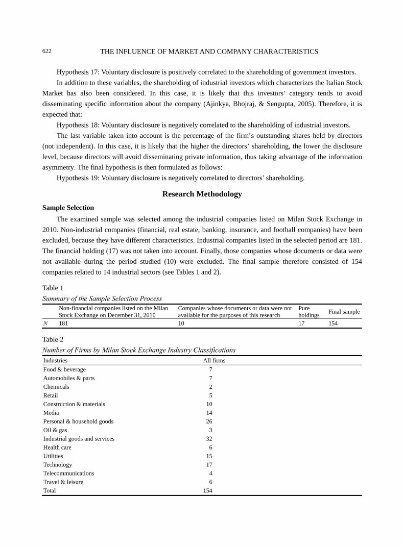
THE INFLUENCE OF MARKET AND COMPANY CHARACTERISTICS
622
Hypothesis 17: Voluntary disclosure is positively correlated to the shareholding of government investors. In addition to these variables, the shareholding of industrial investors which characterizes the Italian Stock
Market has also been considered. In this case, it is likely that this investors’ category tends to avoid disseminating specific information about the company (Ajinkya, Bhojraj, & Sengupta, 2005). Therefore, it is expected that:
Hypothesis 18: Voluntary disclosure is negatively correlated to the shareholding of industrial investors. The last variable taken into account is the percentage of the firm’s outstanding shares held by directors
(not independent). In this case, it is likely that the higher the directors’ shareholding, the lower the disclosure level, because directors will avoid disseminating private information, thus taking advantage of the information asymmetry. The final hypothesis is then formulated as follows:
Hypothesis 19: Voluntary disclosure is negatively correlated to directors’ shareholding.
Research Methodology Sample Selection
The examined sample was selected among the industrial companies listed on Milan Stock Exchange in 2010. Non-industrial companies (financial, real estate, banking, insurance, and football companies) have been excluded, because they have different characteristics. Industrial companies listed in the selected period are 181. The financial holding (17) was not taken into account. Finally, those companies whose documents or data were not available during the period studied (10) were excluded. The final sample therefore consisted of 154 companies related to 14 industrial sectors (see Tables 1 and 2).
Table 1 Summary of the Sample Selection Process
Non-financial companies listed on the Milan Stock Exchange on December 31, 2010
Companies whose documents or data were not available for the purposes of this research
Pure holdings Final sample
N 181 10 17 154
Table 2 Number of Firms by Milan Stock Exchange Industry Classifications Industries All firms Food & beverage 7 Automobiles & parts 7 Chemicals 2 Retail 5 Construction & materials 10 Media 14 Personal & household goods 26 Oil & gas 3 Industrial goods and services 32 Health care 6 Utilities 15 Technology 17 Telecommunications 4 Travel & leisure 6 Total 154
THE INFLUENCE OF MARKET AND COMPANY CHARACTERISTICS
623
Disclosure Index (Dependent Variable) For the purposes of this analysis, two disclosure indexes (dependent variable) have been calculated: a
quantitative index based only on quantitative type items (quantitative disclosure index) and an index that is both qualitative and quantitative (global disclosure index). The selected items were developed on the basis of the lists proposed by Gray et al. (1995), Hossain, Perera, and Rahman (1995), Meek et al. (1995), and Ferguson et al. (2002), relating to strategic, non-financial, and financial information. The list of items was then compared with the 2010 Associazione delle Società di Revisione Italiane (ASSIREVI, the Italian Association for External Audit Companies) checklist as benchmark in defining voluntary disclosure. As a consequence, six elements are excluded, because they are mandatory. Moreover, one item relating to employee information, which is not applicable to the Italian system, has been replaced with two items that are more suitable to the Italian employment system. Additionally, one further item has been added, thus obtaining a final list consisting of 90 items for the global disclosure index and 41 items for the quantitative disclosure index.
As suggested in the primary literature, the authors used an index that assigns the same importance to each item (Cooke, 1996; Inchausti, 1997; Cammferman & Cooke, 2002). As a consequence, the disclosure index for company “j” (j = 1 to 154) is:
10 1ni i
jj
xIn=∑
≤ = ≤ (1)
where “nj” is the number of items applicable to the company “j”; “n” is the maximum number of items (90 for the global and 41 for the quantitative index); and “x” is the x item of disclosure (the items ranging from one to n) whose value is “1” if it is disclosed and “0” if otherwise.
Table 3 reports the summaries relating to the two calculated indexes.
Table 3 Dependent Variables: Descriptive Statistics Index Min. 1st Qu. Median Mean 3rd Qu. Max. GVD 0.1379 0.2880 0.3750 0.3847 0.4586 0.7444 QVD 0.0250 0.1510 0.2179 0.2419 0.3250 0.6829
On the basis of the reported results in Table 3, it can be observed that the median and the third quartile of the first observed distribution from the global voluntary disclosure (GVD) index are higher than those from the quantitative voluntary disclosure (QVD) index (GVD median = 0.3750 vs. QVD median = 0.2179; GVD 3rd Qu. = 0.4586 vs. QVD 3rd Qu. = 0.3250). This result underlines that the values of the disclosure index are higher in the first distribution (GVD). For the examined companies, 75% are characterised by a global disclosure index which is not higher than 0.46. This value decreases to 0.32 when taking into account the quantitative disclosure index. Thus, it can be asserted that as regards the several selected voluntary disclosure items, most companies provide less than 50% of the possible disclosures. In particular, 75% of the companies only issue a maximum of 1/3 (30%) of the quantitative type disclosure items.
Explanatory Variables
Table 4 describes the specific selected independent variables used in this analysis and how they were measured.
The first selected variable is the incidence of foreign sales as a proxy measure of the company’s
THE INFLUENCE OF MARKET AND COMPANY CHARACTERISTICS
624
internationalization level. For this variable, it has been used a dummy having a value of one if the foreign sales are equal to or greater than 30% compared with total sales or zero if otherwise.
Table 4 Explanatory Variables Variable Description Measurement EX SEC SEG TA EM S L DIV ROE ROS CR INT ROD AUD IND DUAL MK II FI GI IP DIR
Incidence of foreign sales Industry Listing segment Total assets Employees Sales Leverage Cash dividend paid Return on equity Return on sales Current ratio Incidence of intangibles Return on debts Audit firm Independent directors Duality Market floating Institutional investors Foreign investors Government investors Industrial investors Director shareholding
Dummy Dummy Dummy Total assets scaled by 1,000 Number of employees Sales scaled by 1.000 Financial debts/equity Dummy Net income/equity Earnings before interest and taxes (EBIT)/sales Current assets/current liabilities Total intangibles/total assets Financial interests on debts/total financial debts Dummy No. of independent directors/total No. of directors Dummy Percentage of firm’s total shares held by irrelevant investors Dummy Dummy Dummy Dummy Percentage of firm’s outstanding shares held by directors
The second variable is the industry sector. The industry classification adopted by Milan Stock Exchange has been used. The third variable is the listing segment. Also for this variable, it has been used a dummy having a value of one if the company is listed on “Blue Chip” segment and zero if otherwise. The following three variables are dimensional variables: total assets, number of employees, and sales. For total assets and sales, the values have been divided by 1,000.
With reference to the “cash dividend paid” variable, it has been used a dummy, with the value of one if the dividend is paid, and zero if otherwise. As regards the profitability variables, two ratios have been used: the ROE was measured as net income/equity and the ROS as EBIT/sales, where EBIT is the earning before interests and taxes. As financial variables, the leverage and the current ratio have been considered. The first one was calculated as total financial debts/equity, while the second one as current assets/current liabilities. The variable relating to the incidence of intangibles was measured by dividing the recognized total intangibles by the total assets of the company. The ROD was computed as interest expenses on debt/total debts. As regards the variable “auditors”, it has been used a dummy, with the value of one if the audit firm is international, and zero if otherwise. The proportion of independent directors on the board was measured as total independent directors/total directors. For the duality variable, it has been used a dummy having the value of zero if the duality exists, and one if otherwise. The market floating variable was computed as the percentage of firm’s total shares held by irrelevant investors (i.e., shareholders with less than 2% of the share capital). For each of the three variables relating to the incidence of the institutional investors, foreign investors, and government investors on capital stock of the company, it has been used a dummy, with the value of one if their shareholding is relevant, and zero if otherwise. According to the specific regulation on the Italian Stock Market, a
THE INFLUENCE OF MARKET AND COMPANY CHARACTERISTICS
625
shareholding is considered relevant when it is equal to or higher than 2%. In these cases, the investor must communicate to the securities and exchange commission (CONSOB, Commissione Nazionale per le Società e la Borsa) that he/she holds a relevant shareholding. The last variable relating to the shareholding by directors (not independent) was measured as the percentage of firm’s outstanding shares held by directors.
Analysis and Results
The Multivariate Analysis
In order to test the hypotheses described in Section 2, an esteem has been carried out on two multivariate least squares regression models with respect to the two dependent variables “global voluntary disclosure index” and “quantitative voluntary disclosure index” (thereafter GVD and QVD respectively).
In particular, the following initial models were used:
1 2 3 4 5 6 7
8 9 10 11 12 13 14
15 16 17 18 19
GVD EX SEC SEG EM L PO ROSCR INT ROD AUD IND DUAL MK
II FI GI IP DIR
α β β β β β β ββ β β β β β β
β β β β β ε
= + + + + + + + ++ + + + + + +
+ + + + + (2)
1 2 3 4 5 6 7
8 9 10 11 12 13 14
15 16 17 18 19
QVD EX SEC SEG EM L PO ROSCR INT ROD AUD IND DUAL MK
II FI GI IP DIR
α β β β β β β ββ β β β β β β
β β β β β ε
= + + + + + + + ++ + + + + + +
+ + + + + (3)
For collinearity reasons, both TA and ROE have been excluded. The collinearity with the variance inflation factor (VIF) test has been verified, excluding the variables with a value greater than 10. For both the regression functions, heteroskedasticity and the normality of the error distribution were tested. As regards the regression function estimated with respect to the dependent variable QVD, a non-verification of the hypothesis of normality was discovered (normality test—null hypothesis: The errors are normally distributed. Test statistic: X-squared (2) = 9.59297; p-value = 0.00825871).
Therefore, the focus was only on the results of the estimated regression function relating to the dependent variable GVD.
Table 5 shows the results of this regression. The variable relating to the industrial sectors (SEC) does not show statistically significant results1.
Table 5 Multivariate Least Square Regression Results
1 2 3 4 5 6 7 8 9 10
11 12 13 14 15 16 17 18 19
GVD EX SEC SEG EM L PO ROS CR INT ROD
AUD IND DUAL MK II FI GI IP DIR
α β β β β β β β β β β
β β β β β β β β β ε
= + + + + + + + + + + +
+ + + + + + + + +
Estimate p-value Predicted sign VIF Const. 0.280371 0.00001*** L -0.00014442 0.30574 + 1.134 ROS -0.00412482 0.82807 + 2.420 ROD 0.018368 0.80925 + 1.263 INT 0.0502078 0.26687 + 1.224 CR -0.00488362 0.72258 + 2.614 1 For reasons of space, the authors avoided to include in Table 5 the list of the various industry sectors.
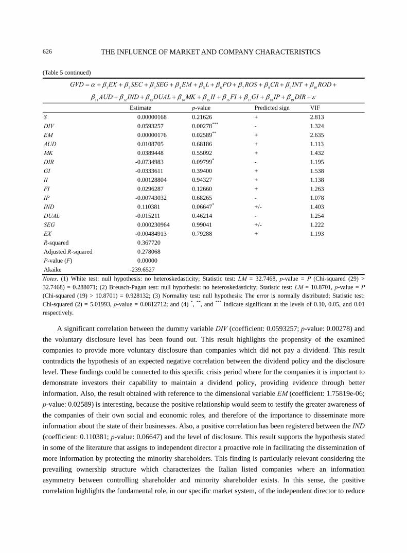
THE INFLUENCE OF MARKET AND COMPANY CHARACTERISTICS
626
(Table 5 continued)
1 2 3 4 5 6 7 8 9 10
11 12 13 14 15 16 17 18 19
GVD EX SEC SEG EM L PO ROS CR INT ROD
AUD IND DUAL MK II FI GI IP DIR
α β β β β β β β β β β
β β β β β β β β β ε
= + + + + + + + + + + +
+ + + + + + + + +
Estimate p-value Predicted sign VIF S 0.00000168 0.21626 + 2.813 DIV 0.0593257 0.00278*** - 1.324 EM 0.00000176 0.02589** + 2.635 AUD 0.0108705 0.68186 + 1.113 MK 0.0389448 0.55092 + 1.432 DIR -0.0734983 0.09799* - 1.195 GI -0.0333611 0.39400 + 1.538 II 0.00128804 0.94327 + 1.138 FI 0.0296287 0.12660 + 1.263 IP -0.00743032 0.68265 - 1.078 IND 0.110381 0.06647* +/- 1.403 DUAL -0.015211 0.46214 - 1.254 SEG 0.000230964 0.99041 +/- 1.222 EX -0.00484913 0.79288 + 1.193 R-squared 0.367720 Adjusted R-squared 0.278068 P-value (F) 0.00000 Akaike -239.6527 Notes. (1) White test: null hypothesis: no heteroskedasticity; Statistic test: LM = 32.7468, p-value = P (Chi-squared (29) > 32.7468) = 0.288071; (2) Breusch-Pagan test: null hypothesis: no heteroskedasticity; Statistic test: LM = 10.8701, p-value = P (Chi-squared (19) > 10.8701) = 0.928132; (3) Normality test: null hypothesis: The error is normally distributed; Statistic test: Chi-squared (2) = 5.01993, p-value = 0.0812712; and (4) *, **, and *** indicate significant at the levels of 0.10, 0.05, and 0.01 respectively.
A significant correlation between the dummy variable DIV (coefficient: 0.0593257; p-value: 0.00278) and the voluntary disclosure level has been found out. This result highlights the propensity of the examined companies to provide more voluntary disclosure than companies which did not pay a dividend. This result contradicts the hypothesis of an expected negative correlation between the dividend policy and the disclosure level. These findings could be connected to this specific crisis period where for the companies it is important to demonstrate investors their capability to maintain a dividend policy, providing evidence through better information. Also, the result obtained with reference to the dimensional variable EM (coefficient: 1.75819e-06; p-value: 0.02589) is interesting, because the positive relationship would seem to testify the greater awareness of the companies of their own social and economic roles, and therefore of the importance to disseminate more information about the state of their businesses. Also, a positive correlation has been registered between the IND (coefficient: 0.110381; p-value: 0.06647) and the level of disclosure. This result supports the hypothesis stated in some of the literature that assigns to independent director a proactive role in facilitating the dissemination of more information by protecting the minority shareholders. This finding is particularly relevant considering the prevailing ownership structure which characterizes the Italian listed companies where an information asymmetry between controlling shareholder and minority shareholder exists. In this sense, the positive correlation highlights the fundamental role, in our specific market system, of the independent director to reduce
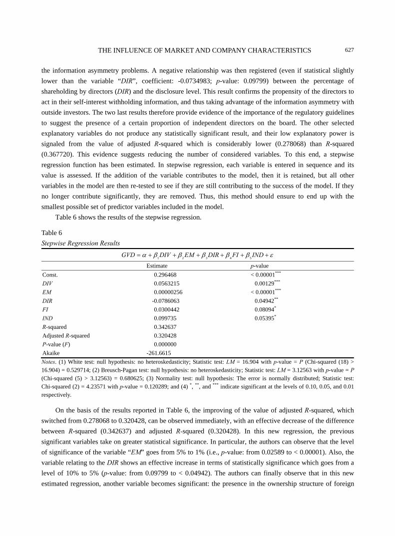
THE INFLUENCE OF MARKET AND COMPANY CHARACTERISTICS
627
the information asymmetry problems. A negative relationship was then registered (even if statistical slightly lower than the variable “DIR”, coefficient: -0.0734983; p-value: 0.09799) between the percentage of shareholding by directors (DIR) and the disclosure level. This result confirms the propensity of the directors to act in their self-interest withholding information, and thus taking advantage of the information asymmetry with outside investors. The two last results therefore provide evidence of the importance of the regulatory guidelines to suggest the presence of a certain proportion of independent directors on the board. The other selected explanatory variables do not produce any statistically significant result, and their low explanatory power is signaled from the value of adjusted R-squared which is considerably lower (0.278068) than R-squared (0.367720). This evidence suggests reducing the number of considered variables. To this end, a stepwise regression function has been estimated. In stepwise regression, each variable is entered in sequence and its value is assessed. If the addition of the variable contributes to the model, then it is retained, but all other variables in the model are then re-tested to see if they are still contributing to the success of the model. If they no longer contribute significantly, they are removed. Thus, this method should ensure to end up with the smallest possible set of predictor variables included in the model.
Table 6 shows the results of the stepwise regression.
Table 6 Stepwise Regression Results
1 2 3 4 5GVD DIV EM DIR FI INDα β β β β β ε= + + + + + +
Estimate p-value Const. 0.296468 < 0.00001*** DIV 0.0563215 0.00129*** EM 0.00000256 < 0.00001*** DIR -0.0786063 0.04942** FI 0.0300442 0.08094* IND 0.099735 0.05395* R-squared 0.342637 Adjusted R-squared 0.320428 P-value (F) 0.000000 Akaike -261.6615 Notes. (1) White test: null hypothesis: no heteroskedasticity; Statistic test: LM = 16.904 with p-value = P (Chi-squared (18) > 16.904) = 0.529714; (2) Breusch-Pagan test: null hypothesis: no heteroskedasticity; Statistic test: LM = 3.12563 with p-value = P (Chi-squared (5) > 3.12563) = 0.680625; (3) Normality test: null hypothesis: The error is normally distributed; Statistic test: Chi-squared (2) = 4.23571 with p-value = 0.120289; and (4) *, **, and *** indicate significant at the levels of 0.10, 0.05, and 0.01 respectively.
On the basis of the results reported in Table 6, the improving of the value of adjusted R-squared, which switched from 0.278068 to 0.320428, can be observed immediately, with an effective decrease of the difference between R-squared (0.342637) and adjusted R-squared (0.320428). In this new regression, the previous significant variables take on greater statistical significance. In particular, the authors can observe that the level of significance of the variable “EM” goes from 5% to 1% (i.e., p-value: from 0.02589 to < 0.00001). Also, the variable relating to the DIR shows an effective increase in terms of statistically significance which goes from a level of 10% to 5% (p-value: from 0.09799 to < 0.04942). The authors can finally observe that in this new estimated regression, another variable becomes significant: the presence in the ownership structure of foreign
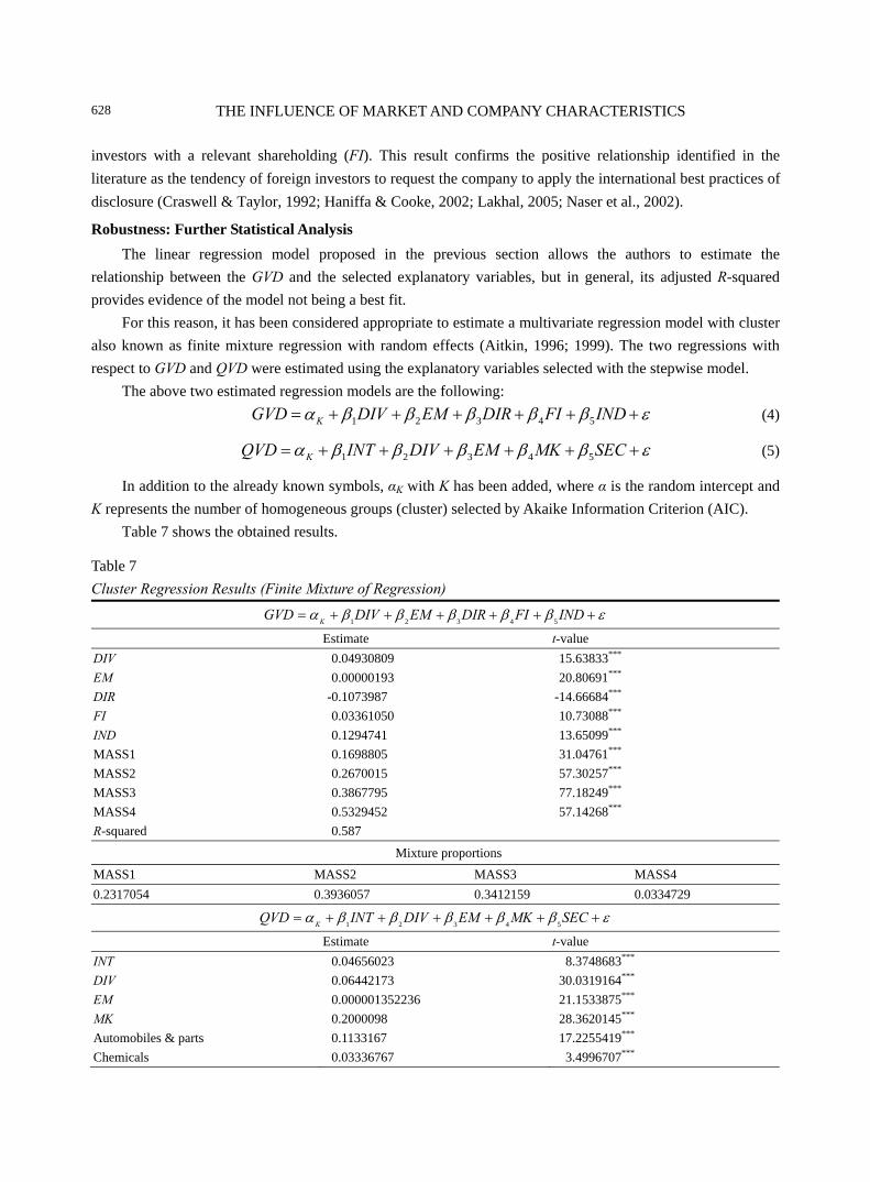
THE INFLUENCE OF MARKET AND COMPANY CHARACTERISTICS
628
investors with a relevant shareholding (FI). This result confirms the positive relationship identified in the literature as the tendency of foreign investors to request the company to apply the international best practices of disclosure (Craswell & Taylor, 1992; Haniffa & Cooke, 2002; Lakhal, 2005; Naser et al., 2002).
Robustness: Further Statistical Analysis
The linear regression model proposed in the previous section allows the authors to estimate the relationship between the GVD and the selected explanatory variables, but in general, its adjusted R-squared provides evidence of the model not being a best fit.
For this reason, it has been considered appropriate to estimate a multivariate regression model with cluster also known as finite mixture regression with random effects (Aitkin, 1996; 1999). The two regressions with respect to GVD and QVD were estimated using the explanatory variables selected with the stepwise model.
The above two estimated regression models are the following:
1 2 3 4 5KGVD DIV EM DIR FI INDα β β β β β ε= + + + + + + (4)
1 2 3 4 5KQVD INT DIV EM MK SECα β β β β β ε= + + + + + + (5)
In addition to the already known symbols, αK with K has been added, where α is the random intercept and K represents the number of homogeneous groups (cluster) selected by Akaike Information Criterion (AIC).
Table 7 shows the obtained results.
Table 7 Cluster Regression Results (Finite Mixture of Regression)
1 2 3 4 5KGVD DIV EM DIR FI INDα β β β β β ε= + + + + + +
Estimate t-value DIV 0.04930809 15.63833*** EM 0.00000193 20.80691*** DIR -0.1073987 -14.66684*** FI 0.03361050 10.73088*** IND 0.1294741 13.65099*** MASS1 0.1698805 31.04761*** MASS2 0.2670015 57.30257*** MASS3 0.3867795 77.18249*** MASS4 0.5329452 57.14268*** R-squared 0.587
Mixture proportions MASS1 MASS2 MASS3 MASS4 0.2317054 0.3936057 0.3412159 0.0334729
1 2 3 4 5KQVD INT DIV EM MK SECα β β β β β ε= + + + + + +
Estimate t-value INT 0.04656023 8.3748683*** DIV 0.06442173 30.0319164*** EM 0.000001352236 21.1533875*** MK 0.2000098 28.3620145*** Automobiles & parts 0.1133167 17.2255419*** Chemicals 0.03336767 3.4996707***
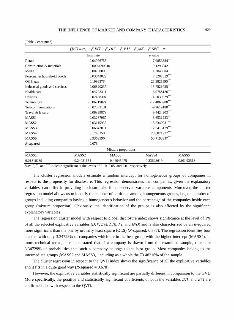
THE INFLUENCE OF MARKET AND COMPANY CHARACTERISTICS
629
(Table 7 continued)
1 2 3 4 5KQVD INT DIV EM MK SECα β β β β β ε= + + + + + +
Estimate t-value Retail 0.04976755 7.0853384*** Construction & materials 0.0007690010 0.1296642 Media 0.007300065 1.3045904 Personal & household goods 0.03843829 7.5207319*** Oil & gas 0.1993378 23.9821196*** Industrial goods and services 0.06820235 13.7521635*** Health care 0.04722311 6.9758126*** Utilities 0.02488304 4.5039329*** Technology -0.06719824 -12.4868288*** Telecommunications -0.07533131 -9.9619180*** Travel & leisure 0.06329873 9.4424203*** MASS1 -0.03287967 -3.6531223*** MASS2 -0.03115935 -5.2340031*** MASS3 0.06847011 12.6415179*** MASS4 0.1740350 29.6071277*** MASS5 0.3369596 50.7193937*** R-squared 0.678
Mixture proportions MASS1 MASS2 MASS3 MASS4 MASS5 0.01816239 0.24021154 0.44045475 0.23623619 0.06493513 Note. *, **, and *** indicate significant at the levels of 0.10, 0.05, and 0.01 respectively.
The cluster regression models estimate a random intercept for homogeneous groups of companies in respect to the propensity for disclosure. This regression demonstrates that companies, given the explanatory variables, can differ in providing disclosure also for unobserved variance components. Moreover, the cluster regression model allows us to identify the number of partitions among homogeneous groups, i.e., the number of groups including companies having a homogeneous behavior and the percentage of the companies inside each group (mixture proportion). Obviously, the identification of the groups is also affected by the significant explanatory variables.
The regression cluster model with respect to global disclosure index shows significance at the level of 1% of all the selected explicative variables (DIV, EM, DIR, FI, and IND) and is also characterized by an R-squared more significant than the one by ordinary least square (OLS) (R-squared: 0.587). The regression identifies four clusters with only 3.34729% of companies which are in the best group with the higher intercept (MASS4). In more technical terms, it can be stated that if a company is drawn from the examined sample, there are 3.34729% of probabilities that such a company belongs to the best group. Most companies belong to the intermediate groups (MASS2 and MASS3), including as a whole the 73.48216% of the sample.
The cluster regression in respect to the QVD index shows the significance of all the explicative variables and it fits in a quite good way (R-squared = 0.678).
However, the explicative variables statistically significant are partially different in comparison to the GVD. More specifically, the positive and statistically significant coefficients of both the variables DIV and EM are confirmed also with respect to the QVD.
THE INFLUENCE OF MARKET AND COMPANY CHARACTERISTICS
630
Moreover, the following variables have significant result: “incidence of the intangible assets” (INT); “market floating” (MK); almost of all the industrial membership sectors. Therefore, the findings relating to the quantitative index (QVD) seem to demonstrate that in a period of crisis, the companies tend to disclose more quantitative information in order to reassure the market, particularly when both the percentage of market floating and the incidence of intangible assets increase. The significance of the majority of sectors (not all), even with different signs and magnitudes of the coefficients, confirms the theoretical hypothesis developed by the accounting literature of the non-homogeneity of the said sectors with respect to the disclosure (Cooke, 1992).
In this last regression, the AIC has been applied, identifying five groups of homogeneous companies (cluster). Also in this case, the “best group” includes only 6.493513% of the companies (i.e., there are only 6.493513% of probabilities that a randomly chosen company belongs to the best group). Also the worst group includes a small number of companies (1.816239%). While the intermediate groups (MASS2, MASS3, and MASS4) contain almost the totality of the examined sample (91.690248%).
Conclusions
In this paper, voluntary disclosure determinants have been investigated, with reference to a sample of 154 Italian companies listed on Milan Stock Exchange in 2010. The development of an analysis about the industrial companies listed in Italy has been considered particularly interesting, because Italy is the second country in European Union (EU) for industrial production. It has also been considered significant to examine the year 2010, because it is characterized by a strong financial crisis.
Two types of disclosure index used as dependent variables have been calculated: a global index based on both quantitative and qualitative disclosure (GVD) and a quantitative-only voluntary index (QVD). An analysis has been carried out on the relationship between those indexes and some explanatory variables proposed by the existing international literature, adding some specific variables which have been identified in order to take into account the peculiarities of the Italian market system and the ongoing financial crisis.
At first, this analysis was based on pooled ordinary least square (OLS), as usually done in the studies relating to disclosure. Then, another regression model was estimated, with random intercept and cluster (also known as a finite mixture regression).
This study extends the prevailing empirical literature by adding an analysis of the determinants of voluntary disclosure also based on a solely quantitative disclosure index. Moreover, a further regression model is estimated.
A positive relationship has been found out among the GVD and the number of employees, the dividend policy, and the presence of independent directors on the board. On the contrary, there is a negative correlation with respect to the shareholding of directors. With reference to the QVD index, a positive correlation with the number of employees, the dividend policy, the market floating, and the incidence of intangible assets exists. Moreover, such (quantitative) a disclosure is different depending on the industrial membership sector.
The regression with cluster intercept has demonstrated the presence of groups of companies with a homogeneous behavior at disclosure level.
References Aboody, D., & Kaznik, R. (2000). CEO stock option awards and the timing of corporate voluntary disclosures. Journal of
Accounting and Economics, 29(1), 73-100.
THE INFLUENCE OF MARKET AND COMPANY CHARACTERISTICS
631
Aitkin, M. (1999). A general maximum likelihood analysis of variance components in generalized linear models. Biometrics, 55(1), 117-128.
Aitkin, M. (1996). A general maximum likelihood analysis of over dispersion in generalized linear models. Statistics and Computing, 6(3), 251-262.
Ajinkya, B., Bhojraj, S., & Sengupta, P. (2005). The association between outside directors, institutional investors, and the properties of management earnings forecasts. Journal of Accounting Research, 43(3), 343-376.
Akhtaruddin, M. (2005). Corporate mandatory disclosure practices in Bangladesh. International Journal of Accounting, 40(4), 399-422.
Al-Akra, M., Eddy, I. A., & Ali, M. J. (2010). The association between privatization and voluntary disclosure: Evidence from Jordan. Accounting and Business Research, 40(1), 55-74.
Ali, M. J., Ahmed, K., & Henry, D. (2004). Disclosure compliance with national accounting standards by listed companies in South Asia. Accounting and Business Research, 34(3), 183-199.
Barako, D. G. (2007). Determinants of voluntary disclosures in Kenyan companies annual reports. African Journal of Business Management, 1(5), 113-128.
Belkaoui, A., & Kahl, A. (1978). Corporate financial disclosure in Canada. Research Monograph No. 1 (Vancouver: Canadian Certified General Accountants Association).
Boubakri, N., Cosset, J. C., & Guedhami, O. (2005). Post privatization corporate governance: The role of ownership structure and investor protection. Journal of Financial Economics, 76(2), 369-399.
Boycko, M., Shleifer, A., & Vishny, R. W. (1996). A theory of privatization. The Economic Journal, 106(435), 309-319. Buzby, S. L. (1974). Selected items of information and their disclosure in annual reports. Accounting Review, 49(3), 423-435. Buzby, S. L. (1975). Company size, listed versus unlisted stocks, and the extent of financial disclosure. Journal of Accounting
Research, 13(1), 16-37. Cammferman, K., & Cooke, T. E. (2002). An analysis of disclosure in the annual reports of UK and Dutch companies. Journal of
International Accounting Research, 1(1), 3-30. Chau, G. K., & Gray, S. J. (2002). Ownership structure and corporate voluntary disclosure in Hong Kong and Singapore. The
International Journal of Accounting, 37(2), 247-265. Chen, C. J. P., & Jaggi, B. (2000). Association between independent non-executive directors, family control, and financial
disclosures in Hong Kong. Journal of Accounting and Public Policy, 19(4/5), 285-310. Cheng, E. C. M., & Courtenay, S. (2006). Board composition, regulatory regime, and voluntary disclosure. The International
Journal of Accounting, 41(3), 262-289. Chiang, H. (2005). An empirical study of corporate governance and corporate performance. The Journal of American Academy of
Business, 6(1), 95-101. Chow, C. W., & Wong-Boren, A. (1987). Voluntary financial disclosure by Mexican corporations. The Accounting Review, 62(3),
533-541. Clinch, G., & Verrecchia, R. E. (1997). Competitive disadvantage and discretionary disclosure in industries. Australian Journal of
Management, 22(2), 125-137. Cooke, T. E. (1989a). Disclosure in the corporate annual reports of Swedish companies. Accounting and Business Research,
19(74), 113-124. Cooke, T. E. (1989b). Voluntary corporate disclosure by Swedish companies. Journal of International Financial Management and
Accounting, 1(2), 171-195. Cooke, T. E. (1992). The impact of size, stock market listing, and industry type on disclosure in the annual reports of Japanese
listed corporations. Accounting and Business Research, 22(87), 229-237. Cooke, T. E. (1993). Disclosure in Japanese corporate annual report. Journal of Business Finance and Accounting, 20(4), 521-535. Cooke, T. E. (1996). The influence of Keiretsu on Japanese corporate disclosure. Journal of International Financial Management
and Accounting, 7(3), 191-214. Courtis, J. K. (1978). Annual report disclosure in New Zealand: Analysis of selected corporate attribute. New England Accounting
Research Study, Vol. 8. Craswell, A., & Taylor, S. (1992). Discretionary disclosure of reserves by oil and gas companies: An economic analysis. Journal
of Business Finance and Accounting, 19(2), 295-308. Depoers, F. (2000). A cost benefit study of voluntary disclosure: Some empirical evidence from French listed companies.
European Accounting Review, 9(2), 245-263.
THE INFLUENCE OF MARKET AND COMPANY CHARACTERISTICS
632
Dhalival, D. S. (1980). Improving the quality of corporate financial disclosure. Accounting and Business Research, 10(40), 385-391.
Eng, L. L., & Mak, Y. T. (2003). Corporate governance and voluntary disclosure. Journal of Accounting and Public Policy, 22(4), 325-345.
Entwistle, G. M. (1999). Exploring the R&D disclosure environment. Accounting Horizons, 13(4), 323-341. Fama, E. F., & Jensen, M. C. (1983). Separation of ownership and control. Journal of Law and Economics, 26(2), 301-325. Ferguson, M. J., Lam, K. C. K., & Lee, G. M. (2002). Voluntary disclosure by state owned enterprises listed on the stock exchange
of Hong Kong. Journal of International Financial Management and Accounting, 13(2), 125-152. Firer, C., & Meth, G. (1986). Information disclosure in annual reports in South Africa. Omega—The International Journal of
Management Science, 14(5), 373-382. Firth, M. (1979). The impact of size, stock market listing, and auditors on voluntary disclosure in corporate annual reports.
Accounting and Business Research, 9(36), 273-280. Forker, J. J. (1992). Corporate governance and disclosure quality. Accounting and Business Research, 22(80), 111-124. Glaum, M., & Street, D. (2003). Compliance with the disclosure requirement of German’s new market: IAS versus US GAAP.
Journal of International Financial Management and Accounting, 14(1), 64-100. Gray, S. J., Meek, G. K., & Roberts, C. B. (1995). International capital market pressures and voluntary annual report disclosures
by US and UK multinationals companies. Journal of International Financial Management and Accounting, 6(1), 43-69. Gul, F. A., & Leung, S. (2004). Board leadership, outside directors’ expertise, and voluntary corporate disclosures. Journal of
Accounting and Public Policy, 23(5), 351-379. Haniffa, R., & Cooke, T. E. (2002). Culture, corporate governance, and disclosure in Malaysian corporations. Abacus, 38(3),
317-349. Hossain, M., Perera, M. H. B., & Rahman, A. R. (1995). Voluntary disclosure in the annual reports of New Zealand companies.
Journal of International Financial Management and Accounting, 6(1), 69-87. Hossain, M., Tan, L. M., & Adams, M. (1994). Voluntary disclosure in an emerging capital market: Some empirical evidence from
companies listed on the Kuala Lumpur Stock Exchange. The International Journal of Accounting, 29, 334-351. Imhoff, E. A. (1992). The relation between perceived accounting quality and economic characteristics of the firm. Journal of
Accounting and Public Policy, 11(2), 97-118. Inchausti, B. G. (1997). The influence of company characteristics and accounting regulation on information disclosed by Spanish
firms. The European Accounting Review, 6(1), 45-68. Jensen, M. C., & Meckling, W. H. (1976). Theory of the firm: Managerial behavior, agency costs, and ownership structure.
Journal of Financial Economics, 3(4), 305-360. Klein, A. (2002). Audit committee, board of director characteristics, and earnings management. Journal of Accounting and
Economics, 33(3), 375-400. Lakhal, F. (2005). Voluntary earnings disclosures and corporate governance: Evidence from France. Review of Accounting and
Finance, 4(3), 64-85. Lang, M., & Lundholm, R. (1993). Cross-sectional determinants of analyst ratings of corporate disclosures. Journal of Accounting
Research, 31(2), 246-271. Leftwich, R., Watts, R., & Zimmerman, J. (1981). Voluntary corporate disclosure: The case of interim reporting. Journal of
Accounting Research, 19, 50-77. Malone, D., Fries, C., & Jones, T. (1993). An empirical investigation of the extent of corporate financial disclosure in the oil and
gas industry. Journal of Accounting, Auditing, and Finance, 8(3), 249-273. McKnight, P., & Tomkins, C. (1999). Top executive pay in the United Kingdom: A corporate governance dilemma. International
Journal of the Economics of Business, 6(2), 223-243. McNally, G. M., Eng, L. H., & Hasseldine, C. R. (1982). Corporate financial reporting in New Zealand: An analysis of user
preferences, corporate characteristics, and disclosure practices for discretionary information. Accounting and Business Research, 13(49), 11-20.
Meek, G. C., Roberts, B., & Gray, J. (1995). Factors influencing voluntary annual report disclosures by US, UK, and Continental European multinational corporations. Journal of International Business Studies, 26(3), 555-572.
MohdGhazali, N. A., & Weetman, P. (2006). Perpetuating traditional influence: Voluntary disclosure in Malaysia following the economic crisis. Journal of International Accounting, Auditing, and Taxation, 15(2), 226-248.
Naser, K., & Alkhatib, K. I. (2000). Determinants of the depth of information disclosure in the board of directors statements of a
THE INFLUENCE OF MARKET AND COMPANY CHARACTERISTICS
633
sample of Jordanian listed companies. Advances in International Accounting, 13, 99-118. Naser, K., Alkhatib, K. I., & Karbhari, Y. (2002). Empirical evidence on the depth of corporate information disclosure in
developing countries: The case of Jordan. International Journal of Commerce and Management, 12(3/4), 122-155. Owusu-Ansah, S. (1998). The impact of corporate attributes on the extent of mandatory disclosure and reporting by listed
companies in Zimbabwe. The International Journal of Accounting, 33(5), 605-631. Prencipe, A. (2004). Proprietary costs and determinants of voluntary segment disclosure: Evidence from Italian listed companies.
European Accounting Review, 13(2), 319-340. Raffournier, B. (1995). The determinants of voluntary financial disclosure by Swiss listed companies. European Accounting
Review, 4(2), 261-280. Robbins, W. A., & Austin, K. R. (1986). Disclosure quality in governmental financial reports: An assessment of the
appropriateness of a compound measure. Journal of Accounting Research, 24(2), 412-421. Singhvi, S. S., & Desai, H. B. (1971). An empirical analysis of the quality of corporate financial disclosure. The Accounting
Review, 46(1), 129-138. Spero, L. L. (1979). The extent and causes of voluntary disclosure of financial information in three European markets: An
exploratory study (Ph.D. dissertation, Harvard University Graduate School of Business). Tower, G., Hancock, P., & Taplin, R. H. (1999). A regional study of listed companies’ compliance with International Accounting
Standards. Accounting Forum, 23(3), 293-305. Verrecchia, R. (1983). Discretionary disclosure. Journal of Accounting and Economics, 5(1), 179-194. Wagenhofer, A. (1990). The demand for disclosure and actual disclosure by firms? Paper presented at the 13th Annual Congress of
the European Accounting Association, Budapest. Wallace, R. S. O. (1987). Disclosure of accounting information in developing countries: A case study of Nigeria (Ph.D. thesis,
University of Exeter, UK). Wallace, R. S. O. (1988). Corporate financial reporting in Nigeria. Accounting and Business Research, 18(72), 352-362. Wallace, R. S. O., & Naser, K. (1995), Firm specific determinants of the comprehensiveness of mandatory disclosure in the
corporate annual reports of firms listed on the stocks exchange of Hong Kong. Journal of Accounting and Public Policy, 14(4), 311-368.
Wallace, R. S. O., Naser, K., & Mora, A. (1994). The relationship between the comprehensiveness of corporate annual reports and firm characteristics in Spain. Accounting and Business Research, 25(97), 41-53.
Watts, R., & Zimmerman, J. (1983). Agency problems, auditing, and the theory of the firm: Some evidence. Journal of Law and Economics, 26(3), 613-633.
Watts, R., & Zimmerman, J. (1986). Positive accounting theory. Englewood Cliffs, NJ: Prentice-Hall.
Journal of Modern Accounting and Auditing, ISSN 1548-6583 May 2013, Vol. 9, No. 5, 634-640
Audit Reports of Financially Distressed Companies:
Emphasis of Matter (EOM) Versus Disclaimers
Hashanah Ismail, Mazlina Mustapha Universiti Putra Malaysia, Selangor, Malaysia
This paper examines audit reports issued to 39 Malaysian listed companies in financial distress categorized as
Practice Note 17 (PN17) companies by Bursa Malaysia. The study finds that for companies which experienced
financial distress, the audit reports are not similar, despite all companies are similarly troubled financially.
Companies receive either a disclaimer or an emphasis of matter (EOM) report. The study finds that which of the
two reports is given is associated with three variables: current-year operating loss, shareholders’ deficit, and
default status, implying that audit reports do convey information that financial distress is not of the same level and
severity among PN17 companies.
Keywords: financial distress, emphasis of matter (EOM) audit report, disclaimers, Practice Note 17 (PN17)
companies, International Standard on Auditing (ISA) 570
Introduction
Financial statements to be issued to shareholders each year are prepared based on a fundamental accounting assumption that the business is a going concern. Such an assumption shapes the contents and true and fair presentation of the statements. Hence, when there is a doubt as to whether the business is able to continue as a going concern or not, the doubt should be reflected by not applying such an assumption in the financial statements preparation, for to do so would result in materially misstated financial statements at a level deemed as pervasive and material. In Malaysia, external auditors are bound by the rules of the Malaysian Institute of Accountants (MIA) that audits must be performed in accordance with extant auditing standards approved by MIA. The auditors, as assurance providers on the quality of financial statements, are bound by International Standard on Auditing (ISA) 570 to exercise greater skepticism when auditing businesses exhibiting financial distress indicators, and the standard prescribes the issuance of the modified but unqualified report (emphasis of matter or EOM report) as the appropriate report for companies in financial distress.
Prior studies show that audit reports do signal increased reliability of financial statements (Coram, Mock, Turner, & Gray, 2011) and that the auditor’s going-concern modified report communicates valuable information about risk to investors (Blay, Geiger, & North, 2011). The market responds adversely to a going-concern report (Blay & Geiger, 2001; Menon & Williams, 2010). In Malaysia, listed companies are required by Bursa Malaysia via Practice Note 17 (PN17) regulation to declare themselves as financially
Hashanah Ismail, lecturer, Department of Accounting and Finance, Universiti Putra Malaysia. Email:
[email protected]. Mazlina Mustapha, lecturer, Department of Accounting and Finance, Universiti Putra Malaysia.
DAVID PUBLISHING
D
AUDIT REPORTS OF FINANCIALLY DISTRESSED COMPANIES
635
distressed companies, if they fulfill any one of the criteria listed in PN17. One of the criteria is the type of audit report issued, that is, when a listed company gets either a disclaimer or an EOM audit report, the company automatically becomes a PN17 company and must subsequently announce publicly that it is a financially distressed company officially termed by Bursa as an “affected issuer”. Given that PN17 recognizes two different audit reports as indicators that a company is facing going-concern problems and therefore deemed experiencing financial distress problems. Do the two types of audit reports distinguish different levels of financial distress? It is the objective of this paper to examine the type of audit reports issued to PN17 companies and to identify what financial indicators differ between disclaimer and EOM recipients. The results of the study will be useful to audit standard setters in reconsidering the appropriate reports to be issued for companies in financial distress.
The rest of the paper is organized as follows. The next section will highlight some literature on audit of going-concern companies followed by a description of the research method. The results are then discussed and the paper concludes.
Literature Review
Audited financial statements give users of the statements some level of assurance about the quality of financial statements issued. The type of audit report issued to companies in financial distress in particular has been of interest to regulators, the professionals, and scholars in many jurisdictions, such as Hasnah, Bambang, Mahfooz, and Ishak (2009) on Indonesian auditors, Lam and Mensah (2006) on Hong Kong, Carey, Geiger, and O’Connell (2008) on Australia, Ianniello (2012) on Italy, and Basioudis, Papakonstantinou, and Geiger (2008) on the United Kingdom (UK). Analysts in Australia indicated that the auditor’s report has communicative value. In the study by Coram et al. (2011), the analysts see the audit report as communicating enhanced reliability of the financial statements, thus rendering the financial statements useful for decision making. Auditing standards standardized how audit is to be conducted as a minimum, but within the domain of standardized procedures, auditors are still required to exercise judgments as to the extent and nature of work to be performed and the resultant opinion. ISA 705 on modified audit opinions prescribes that disclaimers are issued when auditors cannot get adequate evidence to support financial statement presentation, and the uncertainty is so serious that it forces the auditor to deny an opinion on the financial statements examined. However, nowhere in the standard does it say explicitly that auditors should disclaim an opinion under going-concern uncertainty. The auditors’ reports on the financial statements indicate whether the fundamental assumption of going concern is appropriate or not based on audit evidence accumulated during the audit process. To auditors, the entire audit process must be performed in compliance with the approved auditing standards to ensure a minimum level of the quality of work. However, the conclusions made are still based on auditors’ professional judgments as to how sufficient and reliable the collected evidence is. As audit is based largely on auditors’ professional judgments, the audit process creates risk to auditors that they may err in their conclusions and issue inappropriate reports. Audit managers have long recognized that the audit process is seen as more critical than difficult. However, within the audit process, one issue is perceived as both difficult and critical: the appropriateness of the going-concern assumption (Kelly, Yong, & Gibson, 1990). Auditors run the risk of issuing an inappropriate opinion in a going-concern situation, whereby a clean report is issued to going-concern firm and the firm subsequently becomes insolvent or the auditor gives a qualified report hastening the demise of an already distressed firm. Either way auditors may be sued for issuing an
AUDIT REPORTS OF FINANCIALLY DISTRESSED COMPANIES
636
inappropriate opinion. The audit profession has issued ISA 570 in relation to going-concern issues in audit. The standard emphasizes that auditors must be on the alert at all stages of the audits with respect to going-concern issues of the clients. The standard identifies three groups of warning signs to alert auditors to such problems: financial indicators, operating indicators, and others. In the event that an auditor encounters such indicators, the standard exhorts auditors to extend audit procedures in order to search for mitigating circumstances. The standard concludes by advising the use of the EOM report to be issued for going-concern uncertainty business, provided certain disclosures are made in the notes to the accounts. For listed companies in Malaysia, the regulators of the capital market have assisted the auditors by prescribing that ailing companies which receive a disclaimer or EOM report are officially recognized as being in financial difficulties. Thus, both regulators and the professionals have defined the parameters of “financial distress” using the auditors’ opinions, similar to the requirements in Italy (Ianniello, 2012). However, PN17 widens the net for financially distressed companies by decreeing that not just the EOM report identifies the going-concern problem but adverse as well as disclaimers too are recognized signals of financial distress. Therefore, the regulators are not as specific as the view of the professionals.
In an earlier study, Hashanah (1997) reported that over the period of 1975-1995, only 2.1% of 3,060 audit reports of Malaysian listed companies had going-concern qualifications of “subject to”, indicating a material uncertainty which was not pervasive. However, the standard on audit reports has been revised and in 2007, ISA 570 introduced the EOM report specific to going-concern uncertainties. In a more litigious environment like the United States (US), Kaplan and Williams (2012) found that auditors of financially distressed companies are more likely to issue an EOM audit report to avoid exposure to litigations. In a study on audit disclaimers, Hashanah (2011) reported that disclaimers are mostly for companies in financial distress, although ISA 705 on audit reports do not give this reason as the main cause of disclaimer reports. LaSalle and Anandarajan (1996) and A. Anandarajan, LaSalle, and M. Anandarajan (2001) studied disclaimer reports in a high litigation environment, whilst Lam and Mensah (2006) examined disclaimers in a low litigation environment. Despite different liability regimes, both papers conclude that disclaimers appear to be signals of greater financial distress even though audit takes place in different legal environments. In the Malaysian context, regulators of the capital market have mandated companies in financial distress to declare themselves as “affected issuers” under the PN17 ruling of Bursa Malaysia. Under PN17, there are seven criteria of financial distress, and two of the criteria are receipt of a disclaimer or adverse opinion or receipt of an EOM report. Hence, either type of audit report will automatically signal a company as facing financial difficulties to continue as a going concern. Thus, in practice, the listing regulation recognizes either disclaimers or EOM as indicators of financial distress, whilst the professional standard recognizes only one, ISA 570, as the appropriate report for such conditions, begging the question of which the appropriate audit report is.
Research Method
Companies in financial distress are identified by selecting all PN17 companies from January 1, 2006 to December 31, 2009, as PN17 ruling became effective only in 2005. Audit reports of all these companies were examined to identify the types of report issued, either disclaimers or EOM. Based on ISA 570, financial indicators, financial distress level, and other indicators were used as independent variables to measure nature and level of financial distress. Financial indicators tested in the study are substantial operating losses, accumulated losses, negative operating cash flows, negative working capital, and deficit in shareholders’ funds.
AUDIT REPORTS OF FINANCIALLY DISTRESSED COMPANIES
637
Financial distress level was measured by the number of good news and bad news characteristics (in receivership, prior-year going-concern report, loan default, ceased major business, and delay). Good news is measured by a viable plan and debt restructuring, whilst the other is litigation issue. Cross-tabulation and chi-squared tests were performed to test for association between these variables and type of audit report issued.
Results and Discussion
A total of 39 PN17 companies were identified over the period of study. Fourteen were still of PN17 category up to March 31, 2011, four were out of the PN17 category and uplifted the PN17 status (no longer in financial distress), whilst the balance of 21 companies was delisted from Bursa. One third of PN17 companies are in the industrial product category, whilst two thirds are spread out among construction, properties, trading and services, and plantation sectors. Although ISA 570 prescribes the use of the EOM report for companies in financial distress, not all audit reports are of the EOM category as prescribed by the said auditing standard. Slightly, more than half or 52% received disclaimers followed by 42% EOM, and 6% had a clean report. Under ISA 705 on modifications to the audit opinions, disclaimers are denials of opinions caused by lack of evidence assessed by auditors as creating uncertainty that is materially pervasive. Nothing in ISA 750 says that it is the appropriate form of audit report for companies in financial distress. If so, auditors are departing from the standardized audit conclusions, indicating perhaps auditors’ different interpretations of “substantial doubt” about going-concern ability of the clients, as the phrase is not defined in the standard. The resulting ambiguity and the absence of a decision-making model for auditors could result in different levels of professional skepticism being exercised (Kaplan & Williams, 2012). Different types of audit reports could also be due to auditors’ exercising different levels of prudent judgments (Krishnan, Raghunandan, & Yang, 2007). Lam and Mensah’s (2006) study of Hong Kong auditors in a less litigious environment is of the view that disclaimers are issued in severe going concern, whereby financial distress is ranked as less serious by EOM, more serious by an exception for qualification and highest by disclaimers. Carey et al.’s (2008) study of Australian companies in financial distress found that EOM is less severe than disclaimers even though it is difficult to identify truly failing companies, and therefore, the authors concluded that there is a need for auditors to have a more precise going-concern assessment aid. LaSalle (2006) argued that disclaimer is not required by professional standards in cases of severe financial distress. Instead, disclaimers are seen as audit failures or poor-quality audits to yield sufficient competent evidence, and giving disclaimers represents an abandonment of professional responsibility to report by the auditors. Results of statistical tests using the chi-squared test for differences between disclaimers and EOM are shown in Table 1.
Table 1 Financial Indicators and Type of Audit Reports Financial indicators EOM (%) Disclaimers (%) Significant* Net loss in current year 81 100 *
Accumulated losses 100 100 Not significant (NS) Negative cash flow from operations 44 65 NS Negative working capital 69 90 NS Deficit in shareholders’ fund 6 35 *
Note. * indicates significant results.
Table 1 indicates that all the five financial indicators are presented in both types of audit reports’
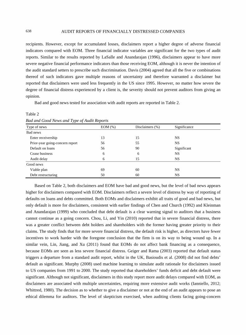
AUDIT REPORTS OF FINANCIALLY DISTRESSED COMPANIES
638
recipients. However, except for accumulated losses, disclaimers report a higher degree of adverse financial indicators compared with EOM. Three financial indicator variables are significant for the two types of audit reports. Similar to the results reported by LaSalle and Anandarajan (1996), disclaimers appear to have more severe negative financial performance indicators than those receiving EOM, although it is never the intention of the audit standard setters to prescribe such discrimination. Davis (2004) agreed that all the five or combinations thereof of such indicators gave multiple reasons of uncertainty and therefore warranted a disclaimer but reported that disclaimers were used less frequently in the US since 1995. However, no matter how severe the degree of financial distress experienced by a client is, the severity should not prevent auditors from giving an opinion.
Bad and good news tested for association with audit reports are reported in Table 2.
Table 2 Bad and Good News and Type of Audit Reports
Type of news EOM (%) Disclaimers (%) Significance Bad news
Enter receivership 13 15 NS Prior-year going-concern report 56 55 NS Default on loans 56 90 Significant Cease business 6 6 NS Audit delay 6 15 NS
Good news Viable plan 69 60 NS Debt restructuring 50 60 NS
Based on Table 2, both disclaimers and EOM have bad and good news, but the level of bad news appears higher for disclaimers compared with EOM. Disclaimers reflect a severe level of distress by way of reporting of defaults on loans and debts committed. Both EOMs and disclaimers exhibit all traits of good and bad news, but only default is more for disclaimers, consistent with earlier findings of Chen and Church (1992) and Kleinman and Anandarajan (1999) who concluded that debt default is a clear warning signal to auditors that a business cannot continue as a going concern. Chou, Li, and Yin (2010) reported that in severe financial distress, there was a greater conflict between debt holders and shareholders with the former having greater priority to their claims. The study finds that for more severe financial distress, the default risk is higher, as directors have fewer incentives to work harder with the foregone conclusion that the firm is on its way to being wound up. In a similar vein, Lin, Jiang, and Xu (2011) found that EOMs do not affect bank financing as a consequence, because EOMs are seen as less severe financial distress. Geiger and Rama (2003) reported that default status triggers a departure from a standard audit report, whilst in the UK, Basioudis et al. (2008) did not find debts’ default as significant. Murphy (2008) used machine learning to simulate audit rationale for disclaimers issued to US companies from 1991 to 2000. The study reported that shareholders’ funds deficit and debt default were significant. Although not significant, disclaimers in this study report more audit delays compared with EOM, as disclaimers are associated with multiple uncertainties, requiring more extensive audit works (Ianniello, 2012; Whittred, 1980). The decision as to whether to give a disclaimer or not at the end of an audit appears to pose an ethical dilemma for auditors. The level of skepticism exercised, when auditing clients facing going-concern
AUDIT REPORTS OF FINANCIALLY DISTRESSED COMPANIES
639
uncertainties, could indicate level of independence of the external auditors and willingness to bear the risk of dismissals by clients. This dilemma appears to be experienced in many jurisdictions with varying levels of litigation risks for auditors.
Conclusions
Auditors’ most fundamental judgment is to evaluate a client’s ability to continue as a going-concern. Despite standardized rules on auditing, auditors must exercise professional skepticism and therefore may arrive at different conclusions in a going-concern situation. The objective of this paper is to examine whether audit reports issued to PN17 companies, being companies designated by Bursa as financially distressed companies, convey auditors’ judgments that financial distress is different in nature and levels. The study finds that not all PN17 companies receive the same type of audit reports, even though all companies are financially distressed. Despite ISA 570 standardizing the EOM as the prescribed report for such companies, the highest number of reports given by auditors is disclaimers, thus rendering the audited financial statements as meaningless and therefore useless to users. Of the 12 variables tested for association with type of audit report, only three factors of current-year operating loss, shareholders’ deficit, and default status were found to be significantly associated with type of audit reports. Future studies may consider interviewing auditors on the factors judged as material in deciding between issuing a disclaimer or EOM report for firms in financial distress, when extant auditing standards do not give such a choice at all.
References Anandarajan, A., LaSalle, R. E., & Anandarajan, M. (2001). Policy issues concerning the choice of a disclaimer in the presence of
going concern uncertainties: An empirical analysis. Managerial Auditing Journal, 16(3), 165-175. Basioudis, I. G., Papakonstantinou, E., & Geiger, M. A. (2008). Audit fees, non-audit fees, and auditor going concern reporting
decision in the UK. ABACUS, 44(3), 284-311. Blay, A. D., & Geiger, M. A. (2001). Market expectations for first-timers of going concern recipients. Journal of Accounting,
Auditing, and Finance, 73-96. Blay, A. D., Geiger, M. A., & North, D. S. (2011). The auditor’s going-concern opinion as a communication of risk. Auditing: A
Journal of Practice and Theory, 30(2), 77-102. Carey, P. J., Geiger, M. A., & O’Connell, B. T. (2008). Costs associated with going-concern modified audit opinions: An analysis
of the Australian audit market. ABACUS, 44(1), 61-81. Chen, K. C., & Church, B. K. (1992). Default on debt obligations and the issuance of going concern opinions. Auditing: A Journal
of Practice and Theory, 11(2), 30-49. Chou, H. I., Li, H., & Yin, X. K. (2010). The effects of financial distress and capital structure on the outside work effort of outside
directors. Journal of Empirical Finance, 17(3), 300-312. Coram, P. J., Mock, T. J., Turner, J. L., & Gray, G. L. (2011). The communicative value of the auditor’s report. Australian
Accounting Review, 21(3), 235-252. Davis, R. R. (2004). Using disclaimers in audit reports: Discerning between shades of opinions. The CPA Journal, 74(4), 26-29. Geiger, M. A., & Rama, D. V. (2003). Audit fees, non-audit fees, and auditor reporting on stressed companies. Auditing: A
Journal of Practice and Theory, 22(2), 53-69. Hashanah, I. (1997). Audit going concern qualifications in Malaysia. The Malaysian Accountant, 2-5. Hashanah, I. (2011). Disclaimer reports among Malaysian listed companies (Paper presented at IIUM International Accounting
Conference V (INTAC V), Pan Pacific KLIA, July 12-13, 2011). Hasnah, H., Bambang, H., Mahfooz, A., & Ishak, I. (2009). Factors influencing auditors’ going concern opinion. Asian Academy
of Management Journal, 14(1), 1-19. Ianniello, G. (2012). Non-audit services and auditor independence in Italian regulatory environment. International Journal of
Auditing, 16(2), 147-164.
AUDIT REPORTS OF FINANCIALLY DISTRESSED COMPANIES
640
Kaplan, S. E., & Williams, D. D. (2012). The changing relationship between audit firm size and going concern reporting. Accounting, Organizations, and Society, 37(5), 322-341.
Kelly, C., Yong, E., & Gibson, R. (1990). Auditors’ perception of the audit process. Occasional Paper No. 109, Deakin University, February 1990, 1-28.
Kleinman, G., & Anandarajan, A. (1999). The usefulness of off-balance sheet variables as predictors of auditors’ going concern opinions: An empirical analysis. Managerial Auditing Journal, 14(6), 273-285.
Krishnan, J., Raghunandan, K., & Yang, J. S. (2007). Were former Andersen clients treated more leniently than other clients? Evidence from going-concern modified audit opinions. Accounting Horizons, 21(4), 423-435.
Lam, C. K., & Mensah, Y. M. (2006). Auditors’ decision making under going-concern uncertainties in low litigation risk environments: Evidence from Hong Kong. Journal of Accounting and Public Policy, 25(6), 706-739.
LaSalle, R. E. (2006). The civil justice system and going concern audit reports. Journal of Accounting and Public Policy, 25(6), 740-745.
LaSalle, R. E., & Anandarajan, A. (1996). Auditors’ views on the type of audit reports issued to entities with going concern uncertainties. Accounting Horizons, 10(2), 51-72.
Lin, Z., Jiang, Y., & Xu, Y. (2011). Do modified opinions have economic consequences? Empirical evidence based on financial constraints. China Journal of Accounting Research, 4(3), 135-154.
Menon, K., & Williams, D. (2010). Investor reaction to going concern audit reports. The Accounting Review, 85(6), 2075-2106. Murphy, C. K. (2008). Discovering auditing criteria for the going concern disclaimer. International Journal of Computer
Applications in Technology, 33(2/3), 138-145. Whittred, G. (1980). Audit qualification and the timeliness of corporate annual reports. The Accounting Review, 55(4), 563-577.
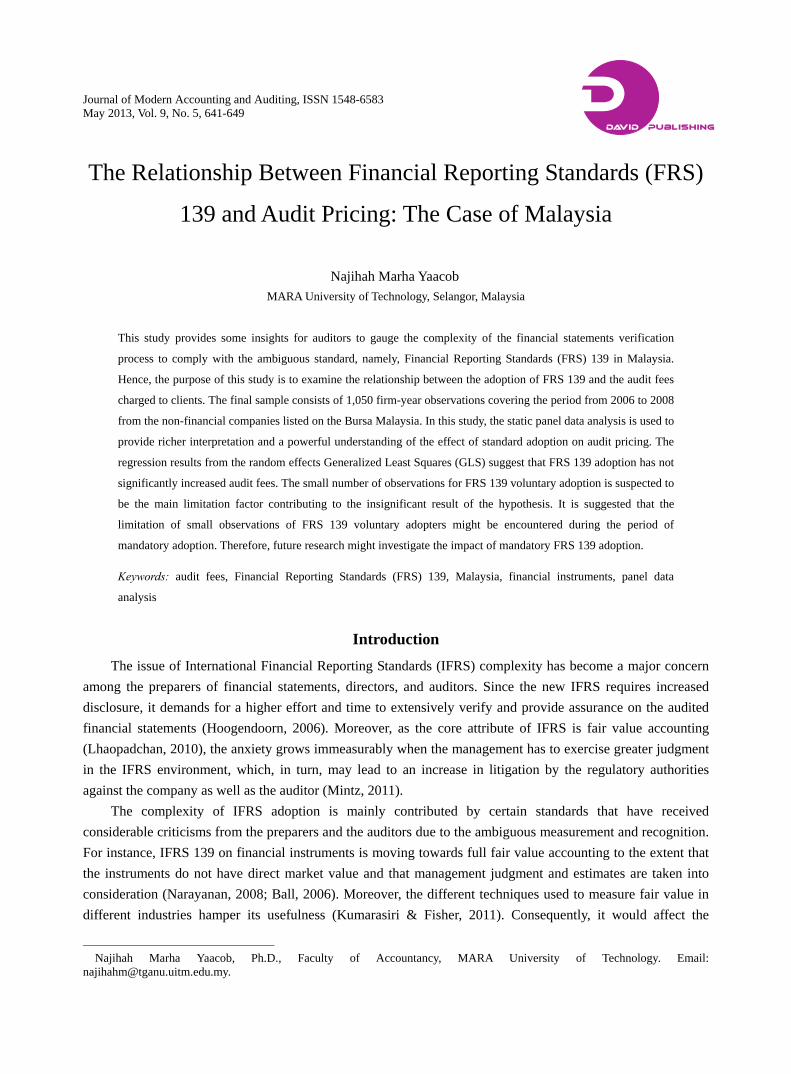
Journal of Modern Accounting and Auditing, ISSN 1548-6583 May 2013, Vol. 9, No. 5, 641-649
The Relationship Between Financial Reporting Standards (FRS)
139 and Audit Pricing: The Case of Malaysia
Najihah Marha Yaacob MARA University of Technology, Selangor, Malaysia
This study provides some insights for auditors to gauge the complexity of the financial statements verification
process to comply with the ambiguous standard, namely, Financial Reporting Standards (FRS) 139 in Malaysia.
Hence, the purpose of this study is to examine the relationship between the adoption of FRS 139 and the audit fees
charged to clients. The final sample consists of 1,050 firm-year observations covering the period from 2006 to 2008
from the non-financial companies listed on the Bursa Malaysia. In this study, the static panel data analysis is used to
provide richer interpretation and a powerful understanding of the effect of standard adoption on audit pricing. The
regression results from the random effects Generalized Least Squares (GLS) suggest that FRS 139 adoption has not
significantly increased audit fees. The small number of observations for FRS 139 voluntary adoption is suspected to
be the main limitation factor contributing to the insignificant result of the hypothesis. It is suggested that the
limitation of small observations of FRS 139 voluntary adopters might be encountered during the period of
mandatory adoption. Therefore, future research might investigate the impact of mandatory FRS 139 adoption.
Keywords: audit fees, Financial Reporting Standards (FRS) 139, Malaysia, financial instruments, panel data
analysis
Introduction
The issue of International Financial Reporting Standards (IFRS) complexity has become a major concern among the preparers of financial statements, directors, and auditors. Since the new IFRS requires increased disclosure, it demands for a higher effort and time to extensively verify and provide assurance on the audited financial statements (Hoogendoorn, 2006). Moreover, as the core attribute of IFRS is fair value accounting (Lhaopadchan, 2010), the anxiety grows immeasurably when the management has to exercise greater judgment in the IFRS environment, which, in turn, may lead to an increase in litigation by the regulatory authorities against the company as well as the auditor (Mintz, 2011).
The complexity of IFRS adoption is mainly contributed by certain standards that have received considerable criticisms from the preparers and the auditors due to the ambiguous measurement and recognition. For instance, IFRS 139 on financial instruments is moving towards full fair value accounting to the extent that the instruments do not have direct market value and that management judgment and estimates are taken into consideration (Narayanan, 2008; Ball, 2006). Moreover, the different techniques used to measure fair value in different industries hamper its usefulness (Kumarasiri & Fisher, 2011). Consequently, it would affect the
Najihah Marha Yaacob, Ph.D., Faculty of Accountancy, MARA University of Technology. Email:
DAVID PUBLISHING
D
THE RELATIONSHIP BETWEEN FRS 139 AND AUDIT PRICING
642
financial position of the companies that are dealing with financial instruments. In Malaysia, many parties have raised a similar concern. The accountants, the auditors, and the
management are in doubt as to whether all IFRSs1 could be applied due to the complexity and vagueness of several standards. As the Malaysian Institute of Accountants’ (MIA) by-laws propose that audit pricing is a function of audit partners and staff responsibilities—skills, risks, and the time needed on audit engagement (MIA, 2011), IFRS complexity is expected to heighten all the elements. Therefore, due to the additional audit effort and risk imposed on the auditors to audit the adherence to FRS 139 requirements, the question of whether FRS 139 voluntary2 adoption will increase audit pricing remains uncertain.
The remainder of the paper is set out as follows. Section 2 discusses the development of the hypothesis, and Section 3 describes the research methods and design. Section 4 presents the results, and the discussion of results is delineated in Section 5. Section 6 concludes the study.
Financial Instruments and Hypothesis Development
International Accounting Standards (IAS) 32 (IFRS 132) and IAS 39 (IFRS 139) are the standards that have been widely discussed concerning their practicality of implementation. The debates on the accounting treatment of financial instruments started in the 1990s among the financial institutions and banking industry. The most significant problem that has received considerable attentions concerns the recognition of fair value of the assets and liabilities in the balance sheet. The fair value measurement is claimed to have some degrees of volatility within the economic results’ structure and equity capital (Bonaci & Matis, 2008). Lhaopadchan (2010) revealed that the discretions involved in measuring fair value negatively encourage earnings management. In contrast, Ebling (2001) claimed that high volatility means that the financial statements reflect the reality of what the accounts are supposed to show.
The advocates of historical cost accounting and fair value accounting normally struggle to defend their principles. The former normally argues that historical is more reliable since no subjectivity is involved in the valuation of assets and liabilities, whereas the proponents of fair value state that the fair value of the financial assets and liabilities enhances the capacity of the investors, creditors, and other users of financial reporting to evaluate the impact of the enterprise’s investments and financing decisions (Bonaci & Matis, 2008). From the standard setters’ points of view, the root of the drawbacks in the recognition of financial instruments is due to the use of historical cost accounting (Ebling, 2001). Harvey and Keer (1983) noted that the inflation factor means that the historical cost basis is less meaningful in making decisions. Anagnostopoulos and Buckland (2005) investigated the usefulness, relevance, and reliability of two conflicting issues between historical costs and full fair value accounting on measurement, recognition, and disclosure of financial instruments in the banking books. The researchers revealed that the implementation of full fair value brings more benefits to the banking institutions (Stovall, 2010) as opposed to the practical difficulties in accomplishing such an accounting treatment.
The new reporting paradigm regards fair value as the most significant attribute for the financial instruments. Fair value accounting is an advanced alternative to the historical cost. Fair value reflects the 1 IFRS in Malaysia is branded as Financial Reporting Standards (FRS). The number assigned has been renumbered to match the IFRS. For instance, Malaysian Accounting Standards Board (MASB) 1 Presentation of Financial Statements is numbered as FRS 101, IFRS 1 is known as FRS 1, IFRS 139 is FRS 139 and so forth. 2 The standard on FRS 139 was released on January 1, 2006, however, due to its complexity, the effective date of the standard was deferred to January 1, 2010, with early adoption being highly encouraged.
THE RELATIONSHIP BETWEEN FRS 139 AND AUDIT PRICING
643
market’s assessment of current economic conditions where the value is determined in an open and competitive market. Barlev and Haddad (2003) regarded the transition to fair value measurement as a shift of paradigms. IFRS 139 defines fair value as the “amount for which an asset could be exchanged or liabilities settled, between knowledgeable, willing parties in the arm’s length transaction” (Lazar, Choo, & Arshad, 2006, p. 540). It is common as well to define fair value as the present value of estimated annual cash flows discounted with the current market rate of return. Alternatively, when the market value of the financial instruments cannot be identified for the respective instrument, the value can be derived from its components and other instruments if that value is readily available on the market (Bonaci & Matis, 2008). Even though the concept of fair value has been used since 1995 for some financial instruments (Anagnostopoulos & Buckland, 2005), the transition to full fair value accounting for all assets and liabilities is still at an early stage. According to Anagnostopoulos and Buckland (2005), the transition is a significant movement in the banking industry so that the weaknesses of historical cost accounting could be reverted. At the same time, the practitioners and scholars express their apprehension concerning the non-existence of active markets in determining the fair value of financial instruments, especially in less developed countries. In the case of the Czech and Romanian stock markets, the unavailability of market price is obvious, since their countries are regarded as a poorly transparent environment (Bonaci & Matis, 2008).
The complexity theory delineates that the future outcome becomes very difficult to predict when the system contains ambiguous or uncertain elements (Nunn, 2007). In the case of IFRS 139, it involves management judgments and estimates (Narayanan, 2008), thus, the auditors need to put in extra hours in order to verify and resolve certain unclear matters before the audit opinion can be issued. As Love and Eickemeyer (2009, p. 56) wrote, “The proposed transition period to IFRS will test an auditors’ ability to ascertain whether management accounting judgments are reasonable and supportable and communicate any identified deficiencies to management and the audit committee”. This statement provides a basis to judge the extent of auditors’ burden, especially when some IFRS treatments are also new to the auditors. Hence, it is admitted that accounting for fair value is a complex process where enterprises require investing their time and effort in order to understand the IFRS 139 requirements, impact on systems, processes, and documentation (Bonaci & Matis, 2008).
Therefore, the more audit efforts are devoted to completing the audit process due to the complexity of fair value measurements, the higher the audit price expected from the auditors. Similarly, using the monitoring hypothesis of the agency theory, the hypothesis postulates that the complexity of FRS 139 will increase the contract costs, that is, the monitoring cost of the agency relationship. Hence, the hypothesis is:
H: There is a positive association between FRS 139 voluntary adoption and audit fees.
Research Methodology
Sample Selection and Data Collection
The final sample for this study consists of 1,050 company-year observations from the companies listed on the main board (756 observations) and the second board (294 observations) of Bursa Malaysia for the period of three years from 2006 to 2008. The sample is limited to the companies with December 31, 2006 as the first year of adoption3. In order to be included as a final sample, the company must maintain the same accounting year 3 In Malaysia, since the new and revised IFRS would come into effect from the accounting period beginning on or after January 1, 2006, all companies with accounting year-end December 21, 2006 would be the first financial statements to comply with IFRS.
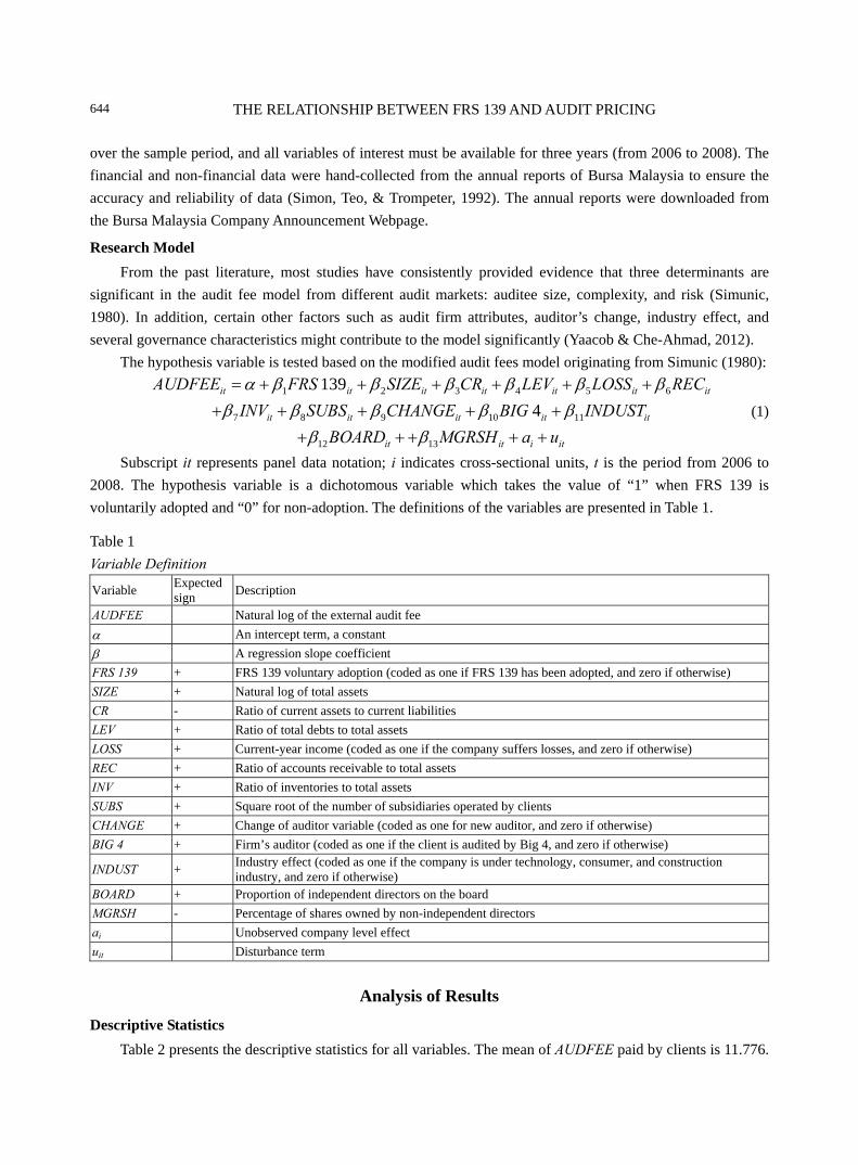
THE RELATIONSHIP BETWEEN FRS 139 AND AUDIT PRICING
644
over the sample period, and all variables of interest must be available for three years (from 2006 to 2008). The financial and non-financial data were hand-collected from the annual reports of Bursa Malaysia to ensure the accuracy and reliability of data (Simon, Teo, & Trompeter, 1992). The annual reports were downloaded from the Bursa Malaysia Company Announcement Webpage.
Research Model
From the past literature, most studies have consistently provided evidence that three determinants are significant in the audit fee model from different audit markets: auditee size, complexity, and risk (Simunic, 1980). In addition, certain other factors such as audit firm attributes, auditor’s change, industry effect, and several governance characteristics might contribute to the model significantly (Yaacob & Che-Ahmad, 2012).
The hypothesis variable is tested based on the modified audit fees model originating from Simunic (1980):
1 2 3 4 5 6
7 8 9 10 11
12 13
1394
it it it it it it it
it it it it it
it it i it
AUDFEE FRS SIZE CR LEV LOSS RECINV SUBS CHANGE BIG INDUST
BOARD MGRSH a u
α β β β β β ββ β β β β
β β
= + + + + + ++ + + + +
+ + + + + (1)
Subscript it represents panel data notation; i indicates cross-sectional units, t is the period from 2006 to 2008. The hypothesis variable is a dichotomous variable which takes the value of “1” when FRS 139 is voluntarily adopted and “0” for non-adoption. The definitions of the variables are presented in Table 1.
Table 1 Variable Definition
Variable Expected sign Description
AUDFEE Natural log of the external audit fee α An intercept term, a constant β A regression slope coefficient FRS 139 + FRS 139 voluntary adoption (coded as one if FRS 139 has been adopted, and zero if otherwise) SIZE + Natural log of total assets CR - Ratio of current assets to current liabilities LEV + Ratio of total debts to total assets LOSS + Current-year income (coded as one if the company suffers losses, and zero if otherwise) REC + Ratio of accounts receivable to total assets INV + Ratio of inventories to total assets SUBS + Square root of the number of subsidiaries operated by clients CHANGE + Change of auditor variable (coded as one for new auditor, and zero if otherwise) BIG 4 + Firm’s auditor (coded as one if the client is audited by Big 4, and zero if otherwise)
INDUST + Industry effect (coded as one if the company is under technology, consumer, and construction industry, and zero if otherwise)
BOARD + Proportion of independent directors on the board MGRSH - Percentage of shares owned by non-independent directors ai Unobserved company level effect uit Disturbance term
Analysis of Results
Descriptive Statistics
Table 2 presents the descriptive statistics for all variables. The mean of AUDFEE paid by clients is 11.776.
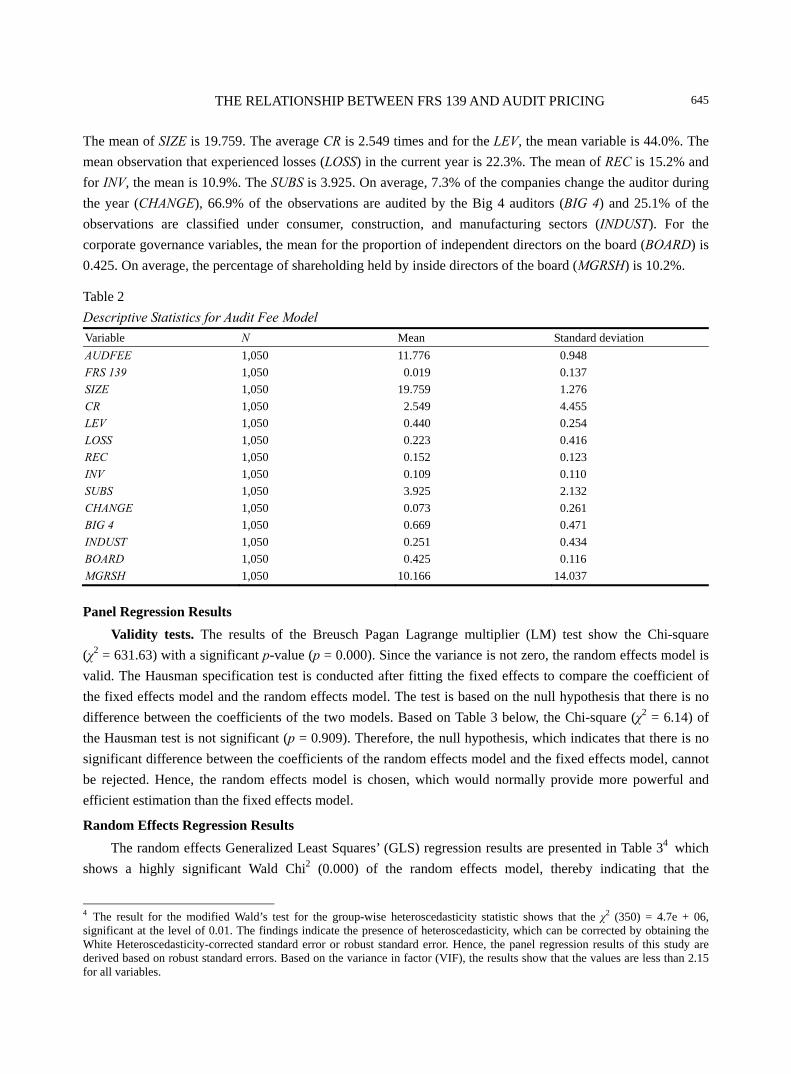
THE RELATIONSHIP BETWEEN FRS 139 AND AUDIT PRICING
645
The mean of SIZE is 19.759. The average CR is 2.549 times and for the LEV, the mean variable is 44.0%. The mean observation that experienced losses (LOSS) in the current year is 22.3%. The mean of REC is 15.2% and for INV, the mean is 10.9%. The SUBS is 3.925. On average, 7.3% of the companies change the auditor during the year (CHANGE), 66.9% of the observations are audited by the Big 4 auditors (BIG 4) and 25.1% of the observations are classified under consumer, construction, and manufacturing sectors (INDUST). For the corporate governance variables, the mean for the proportion of independent directors on the board (BOARD) is 0.425. On average, the percentage of shareholding held by inside directors of the board (MGRSH) is 10.2%.
Table 2 Descriptive Statistics for Audit Fee Model Variable N Mean Standard deviation AUDFEE 1,050 11.776 0.948 FRS 139 1,050 0.019 0.137 SIZE 1,050 19.759 1.276 CR 1,050 2.549 4.455 LEV 1,050 0.440 0.254 LOSS 1,050 0.223 0.416 REC 1,050 0.152 0.123 INV 1,050 0.109 0.110 SUBS 1,050 3.925 2.132 CHANGE 1,050 0.073 0.261 BIG 4 1,050 0.669 0.471 INDUST 1,050 0.251 0.434 BOARD 1,050 0.425 0.116 MGRSH 1,050 10.166 14.037
Panel Regression Results
Validity tests. The results of the Breusch Pagan Lagrange multiplier (LM) test show the Chi-square (χ2 = 631.63) with a significant p-value (p = 0.000). Since the variance is not zero, the random effects model is valid. The Hausman specification test is conducted after fitting the fixed effects to compare the coefficient of the fixed effects model and the random effects model. The test is based on the null hypothesis that there is no difference between the coefficients of the two models. Based on Table 3 below, the Chi-square (χ2 = 6.14) of the Hausman test is not significant (p = 0.909). Therefore, the null hypothesis, which indicates that there is no significant difference between the coefficients of the random effects model and the fixed effects model, cannot be rejected. Hence, the random effects model is chosen, which would normally provide more powerful and efficient estimation than the fixed effects model.
Random Effects Regression Results
The random effects Generalized Least Squares’ (GLS) regression results are presented in Table 34 which shows a highly significant Wald Chi2 (0.000) of the random effects model, thereby indicating that the
4 The result for the modified Wald’s test for the group-wise heteroscedasticity statistic shows that the χ2 (350) = 4.7e + 06, significant at the level of 0.01. The findings indicate the presence of heteroscedasticity, which can be corrected by obtaining the White Heteroscedasticity-corrected standard error or robust standard error. Hence, the panel regression results of this study are derived based on robust standard errors. Based on the variance in factor (VIF), the results show that the values are less than 2.15 for all variables.
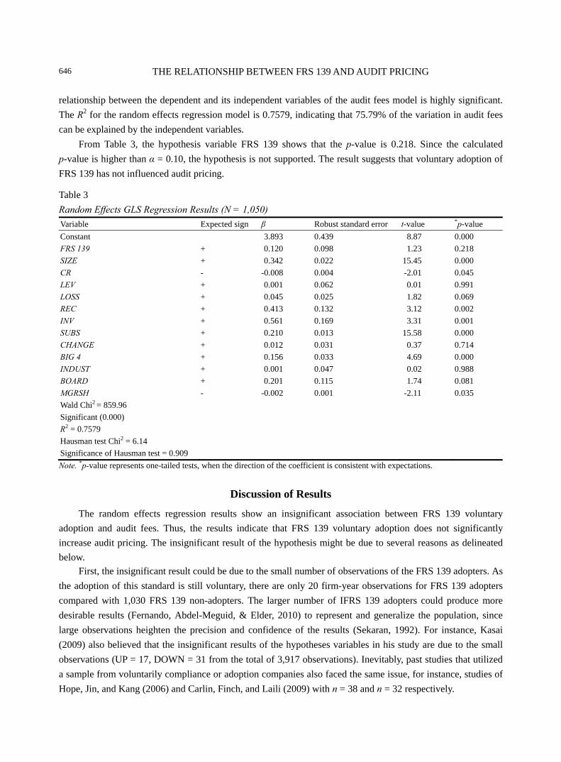
THE RELATIONSHIP BETWEEN FRS 139 AND AUDIT PRICING
646
relationship between the dependent and its independent variables of the audit fees model is highly significant. The R2 for the random effects regression model is 0.7579, indicating that 75.79% of the variation in audit fees can be explained by the independent variables.
From Table 3, the hypothesis variable FRS 139 shows that the p-value is 0.218. Since the calculated p-value is higher than α = 0.10, the hypothesis is not supported. The result suggests that voluntary adoption of FRS 139 has not influenced audit pricing.
Table 3 Random Effects GLS Regression Results (N = 1,050) Variable Expected sign β Robust standard error t-value *p-value Constant 3.893 0.439 8.87 0.000 FRS 139 + 0.120 0.098 1.23 0.218 SIZE + 0.342 0.022 15.45 0.000 CR - -0.008 0.004 -2.01 0.045 LEV + 0.001 0.062 0.01 0.991 LOSS + 0.045 0.025 1.82 0.069 REC + 0.413 0.132 3.12 0.002 INV + 0.561 0.169 3.31 0.001 SUBS + 0.210 0.013 15.58 0.000 CHANGE + 0.012 0.031 0.37 0.714 BIG 4 + 0.156 0.033 4.69 0.000 INDUST + 0.001 0.047 0.02 0.988 BOARD + 0.201 0.115 1.74 0.081 MGRSH - -0.002 0.001 -2.11 0.035 Wald Chi2 = 859.96 Significant (0.000) R2 = 0.7579 Hausman test Chi2 = 6.14 Significance of Hausman test = 0.909 Note. *p-value represents one-tailed tests, when the direction of the coefficient is consistent with expectations.
Discussion of Results
The random effects regression results show an insignificant association between FRS 139 voluntary adoption and audit fees. Thus, the results indicate that FRS 139 voluntary adoption does not significantly increase audit pricing. The insignificant result of the hypothesis might be due to several reasons as delineated below.
First, the insignificant result could be due to the small number of observations of the FRS 139 adopters. As the adoption of this standard is still voluntary, there are only 20 firm-year observations for FRS 139 adopters compared with 1,030 FRS 139 non-adopters. The larger number of IFRS 139 adopters could produce more desirable results (Fernando, Abdel-Meguid, & Elder, 2010) to represent and generalize the population, since large observations heighten the precision and confidence of the results (Sekaran, 1992). For instance, Kasai (2009) also believed that the insignificant results of the hypotheses variables in his study are due to the small observations (UP = 17, DOWN = 31 from the total of 3,917 observations). Inevitably, past studies that utilized a sample from voluntarily compliance or adoption companies also faced the same issue, for instance, studies of Hope, Jin, and Kang (2006) and Carlin, Finch, and Laili (2009) with n = 38 and n = 32 respectively.
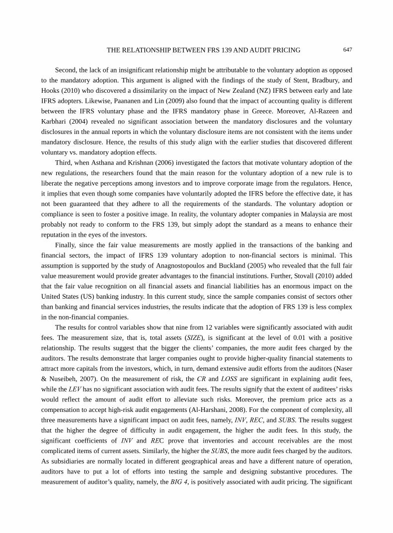
THE RELATIONSHIP BETWEEN FRS 139 AND AUDIT PRICING
647
Second, the lack of an insignificant relationship might be attributable to the voluntary adoption as opposed to the mandatory adoption. This argument is aligned with the findings of the study of Stent, Bradbury, and Hooks (2010) who discovered a dissimilarity on the impact of New Zealand (NZ) IFRS between early and late IFRS adopters. Likewise, Paananen and Lin (2009) also found that the impact of accounting quality is different between the IFRS voluntary phase and the IFRS mandatory phase in Greece. Moreover, Al-Razeen and Karbhari (2004) revealed no significant association between the mandatory disclosures and the voluntary disclosures in the annual reports in which the voluntary disclosure items are not consistent with the items under mandatory disclosure. Hence, the results of this study align with the earlier studies that discovered different voluntary vs. mandatory adoption effects.
Third, when Asthana and Krishnan (2006) investigated the factors that motivate voluntary adoption of the new regulations, the researchers found that the main reason for the voluntary adoption of a new rule is to liberate the negative perceptions among investors and to improve corporate image from the regulators. Hence, it implies that even though some companies have voluntarily adopted the IFRS before the effective date, it has not been guaranteed that they adhere to all the requirements of the standards. The voluntary adoption or compliance is seen to foster a positive image. In reality, the voluntary adopter companies in Malaysia are most probably not ready to conform to the FRS 139, but simply adopt the standard as a means to enhance their reputation in the eyes of the investors.
Finally, since the fair value measurements are mostly applied in the transactions of the banking and financial sectors, the impact of IFRS 139 voluntary adoption to non-financial sectors is minimal. This assumption is supported by the study of Anagnostopoulos and Buckland (2005) who revealed that the full fair value measurement would provide greater advantages to the financial institutions. Further, Stovall (2010) added that the fair value recognition on all financial assets and financial liabilities has an enormous impact on the United States (US) banking industry. In this current study, since the sample companies consist of sectors other than banking and financial services industries, the results indicate that the adoption of FRS 139 is less complex in the non-financial companies.
The results for control variables show that nine from 12 variables were significantly associated with audit fees. The measurement size, that is, total assets (SIZE), is significant at the level of 0.01 with a positive relationship. The results suggest that the bigger the clients’ companies, the more audit fees charged by the auditors. The results demonstrate that larger companies ought to provide higher-quality financial statements to attract more capitals from the investors, which, in turn, demand extensive audit efforts from the auditors (Naser & Nuseibeh, 2007). On the measurement of risk, the CR and LOSS are significant in explaining audit fees, while the LEV has no significant association with audit fees. The results signify that the extent of auditees’ risks would reflect the amount of audit effort to alleviate such risks. Moreover, the premium price acts as a compensation to accept high-risk audit engagements (Al-Harshani, 2008). For the component of complexity, all three measurements have a significant impact on audit fees, namely, INV, REC, and SUBS. The results suggest that the higher the degree of difficulty in audit engagement, the higher the audit fees. In this study, the significant coefficients of INV and REC prove that inventories and account receivables are the most complicated items of current assets. Similarly, the higher the SUBS, the more audit fees charged by the auditors. As subsidiaries are normally located in different geographical areas and have a different nature of operation, auditors have to put a lot of efforts into testing the sample and designing substantive procedures. The measurement of auditor’s quality, namely, the BIG 4, is positively associated with audit pricing. The significant
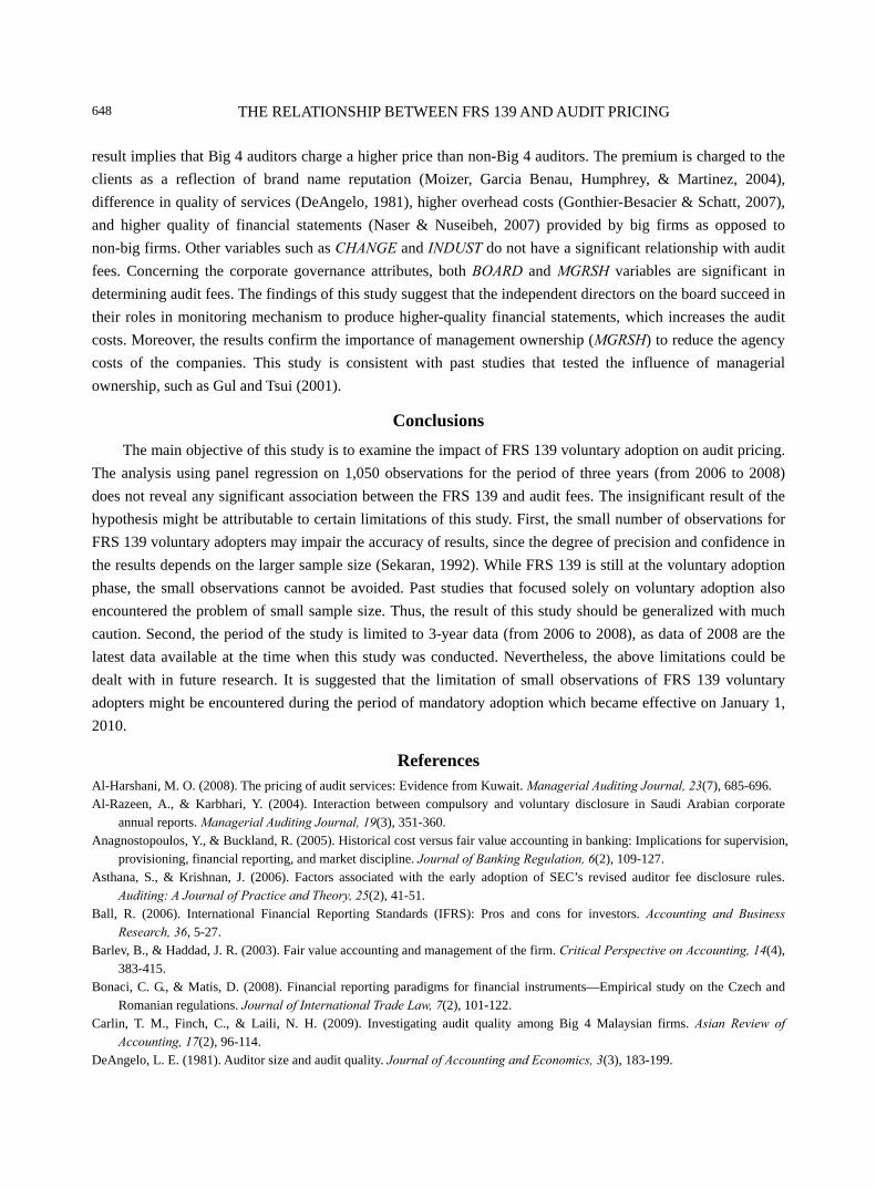
THE RELATIONSHIP BETWEEN FRS 139 AND AUDIT PRICING
648
result implies that Big 4 auditors charge a higher price than non-Big 4 auditors. The premium is charged to the clients as a reflection of brand name reputation (Moizer, Garcia Benau, Humphrey, & Martinez, 2004), difference in quality of services (DeAngelo, 1981), higher overhead costs (Gonthier-Besacier & Schatt, 2007), and higher quality of financial statements (Naser & Nuseibeh, 2007) provided by big firms as opposed to non-big firms. Other variables such as CHANGE and INDUST do not have a significant relationship with audit fees. Concerning the corporate governance attributes, both BOARD and MGRSH variables are significant in determining audit fees. The findings of this study suggest that the independent directors on the board succeed in their roles in monitoring mechanism to produce higher-quality financial statements, which increases the audit costs. Moreover, the results confirm the importance of management ownership (MGRSH) to reduce the agency costs of the companies. This study is consistent with past studies that tested the influence of managerial ownership, such as Gul and Tsui (2001).
Conclusions
The main objective of this study is to examine the impact of FRS 139 voluntary adoption on audit pricing. The analysis using panel regression on 1,050 observations for the period of three years (from 2006 to 2008) does not reveal any significant association between the FRS 139 and audit fees. The insignificant result of the hypothesis might be attributable to certain limitations of this study. First, the small number of observations for FRS 139 voluntary adopters may impair the accuracy of results, since the degree of precision and confidence in the results depends on the larger sample size (Sekaran, 1992). While FRS 139 is still at the voluntary adoption phase, the small observations cannot be avoided. Past studies that focused solely on voluntary adoption also encountered the problem of small sample size. Thus, the result of this study should be generalized with much caution. Second, the period of the study is limited to 3-year data (from 2006 to 2008), as data of 2008 are the latest data available at the time when this study was conducted. Nevertheless, the above limitations could be dealt with in future research. It is suggested that the limitation of small observations of FRS 139 voluntary adopters might be encountered during the period of mandatory adoption which became effective on January 1, 2010.
References Al-Harshani, M. O. (2008). The pricing of audit services: Evidence from Kuwait. Managerial Auditing Journal, 23(7), 685-696. Al-Razeen, A., & Karbhari, Y. (2004). Interaction between compulsory and voluntary disclosure in Saudi Arabian corporate
annual reports. Managerial Auditing Journal, 19(3), 351-360. Anagnostopoulos, Y., & Buckland, R. (2005). Historical cost versus fair value accounting in banking: Implications for supervision,
provisioning, financial reporting, and market discipline. Journal of Banking Regulation, 6(2), 109-127. Asthana, S., & Krishnan, J. (2006). Factors associated with the early adoption of SEC’s revised auditor fee disclosure rules.
Auditing: A Journal of Practice and Theory, 25(2), 41-51. Ball, R. (2006). International Financial Reporting Standards (IFRS): Pros and cons for investors. Accounting and Business
Research, 36, 5-27. Barlev, B., & Haddad, J. R. (2003). Fair value accounting and management of the firm. Critical Perspective on Accounting, 14(4),
383-415. Bonaci, C. G., & Matis, D. (2008). Financial reporting paradigms for financial instruments—Empirical study on the Czech and
Romanian regulations. Journal of International Trade Law, 7(2), 101-122. Carlin, T. M., Finch, C., & Laili, N. H. (2009). Investigating audit quality among Big 4 Malaysian firms. Asian Review of
Accounting, 17(2), 96-114. DeAngelo, L. E. (1981). Auditor size and audit quality. Journal of Accounting and Economics, 3(3), 183-199.
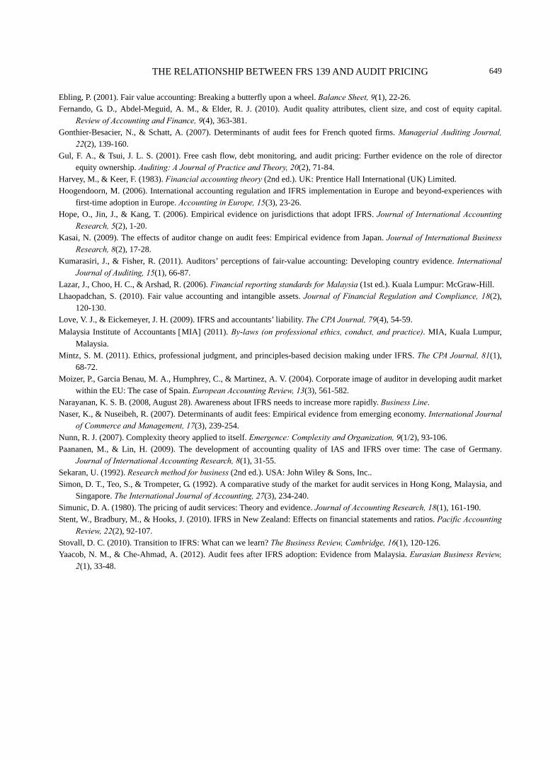
THE RELATIONSHIP BETWEEN FRS 139 AND AUDIT PRICING
649
Ebling, P. (2001). Fair value accounting: Breaking a butterfly upon a wheel. Balance Sheet, 9(1), 22-26. Fernando, G. D., Abdel-Meguid, A. M., & Elder, R. J. (2010). Audit quality attributes, client size, and cost of equity capital.
Review of Accounting and Finance, 9(4), 363-381. Gonthier-Besacier, N., & Schatt, A. (2007). Determinants of audit fees for French quoted firms. Managerial Auditing Journal,
22(2), 139-160. Gul, F. A., & Tsui, J. L. S. (2001). Free cash flow, debt monitoring, and audit pricing: Further evidence on the role of director
equity ownership. Auditing: A Journal of Practice and Theory, 20(2), 71-84. Harvey, M., & Keer, F. (1983). Financial accounting theory (2nd ed.). UK: Prentice Hall International (UK) Limited. Hoogendoorn, M. (2006). International accounting regulation and IFRS implementation in Europe and beyond-experiences with
first-time adoption in Europe. Accounting in Europe, 15(3), 23-26. Hope, O., Jin, J., & Kang, T. (2006). Empirical evidence on jurisdictions that adopt IFRS. Journal of International Accounting
Research, 5(2), 1-20. Kasai, N. (2009). The effects of auditor change on audit fees: Empirical evidence from Japan. Journal of International Business
Research, 8(2), 17-28. Kumarasiri, J., & Fisher, R. (2011). Auditors’ perceptions of fair-value accounting: Developing country evidence. International
Journal of Auditing, 15(1), 66-87. Lazar, J., Choo, H. C., & Arshad, R. (2006). Financial reporting standards for Malaysia (1st ed.). Kuala Lumpur: McGraw-Hill. Lhaopadchan, S. (2010). Fair value accounting and intangible assets. Journal of Financial Regulation and Compliance, 18(2),
120-130. Love, V. J., & Eickemeyer, J. H. (2009). IFRS and accountants’ liability. The CPA Journal, 79(4), 54-59. Malaysia Institute of Accountants [MIA] (2011). By-laws (on professional ethics, conduct, and practice). MIA, Kuala Lumpur,
Malaysia. Mintz, S. M. (2011). Ethics, professional judgment, and principles-based decision making under IFRS. The CPA Journal, 81(1),
68-72. Moizer, P., Garcia Benau, M. A., Humphrey, C., & Martinez, A. V. (2004). Corporate image of auditor in developing audit market
within the EU: The case of Spain. European Accounting Review, 13(3), 561-582. Narayanan, K. S. B. (2008, August 28). Awareness about IFRS needs to increase more rapidly. Business Line. Naser, K., & Nuseibeh, R. (2007). Determinants of audit fees: Empirical evidence from emerging economy. International Journal
of Commerce and Management, 17(3), 239-254. Nunn, R. J. (2007). Complexity theory applied to itself. Emergence: Complexity and Organization, 9(1/2), 93-106. Paananen, M., & Lin, H. (2009). The development of accounting quality of IAS and IFRS over time: The case of Germany.
Journal of International Accounting Research, 8(1), 31-55. Sekaran, U. (1992). Research method for business (2nd ed.). USA: John Wiley & Sons, Inc.. Simon, D. T., Teo, S., & Trompeter, G. (1992). A comparative study of the market for audit services in Hong Kong, Malaysia, and
Singapore. The International Journal of Accounting, 27(3), 234-240. Simunic, D. A. (1980). The pricing of audit services: Theory and evidence. Journal of Accounting Research, 18(1), 161-190. Stent, W., Bradbury, M., & Hooks, J. (2010). IFRS in New Zealand: Effects on financial statements and ratios. Pacific Accounting
Review, 22(2), 92-107. Stovall, D. C. (2010). Transition to IFRS: What can we learn? The Business Review, Cambridge, 16(1), 120-126. Yaacob, N. M., & Che-Ahmad, A. (2012). Audit fees after IFRS adoption: Evidence from Malaysia. Eurasian Business Review,
2(1), 33-48.
Journal of Modern Accounting and Auditing, ISSN 1548-6583 May 2013, Vol. 9, No. 5, 650-661
Executive Compensation and Corporate Financial Performance:
Empirical Evidences on Brazilian Industrial Companies∗
Elizabeth Krauter, Almir Ferreira de Sousa University of São Paulo (USP), São Paulo, Brazil
This survey investigated the relationship between executive compensation and the financial performance of
companies. It is hypothesized that a company can utilize its pay system to direct executives’ efforts toward its
strategic business objectives, thus contributing to higher levels of corporate financial performance. The survey data
consisted of a secondary and non-probabilistic sample of 44 Brazilian industrial companies. In order to
operationalize the independent remuneration variable, the authors used average monthly salary, average variable
salary, and three indices that were created for this survey: benefits, career, and development. These indices measure
the access to benefits, mechanisms for stimulating and supporting careers, and mechanisms to encourage education
and professional development that companies offer to their directors, vice presidents, and chief executive officers
(CEOs), who are referred to in this paper by the term “executive”. The remuneration data are from fiscal year 2006.
In order to operationalize the financial performance variable, two accounting indicators were used: sales growth
and return on equity (ROE) for fiscal years 2006 and 2007. The size of the companies was used as a control
variable. The results of a multiple regression analysis do not support the hypothesis that there is a positive and
significant relationship between executive compensation and corporate financial performance.
Keywords: compensation, executive compensation, financial performance, industrial companies, Brazil
Introduction
Corporations recorded high growth rates during the 20th century. This growth was accompanied by a share capital dispersion process that led to separation of corporate ownership and control. Due to this separation, conflicts of interest appeared within corporations. The approach most often used to explain conflicts of interest between shareholders and executives is the principal-agent theory or agency theory (Andrade & Rossetti, 2006). According to this theory, the principal (shareholder) hires an agent (executive) to carry out a particular task in the shareholder’s favor and then delegates decision-making authority to the agent. If the parties, shareholder and executive, both act so as to maximize their personal utility, the agent may not always act in the best interests of the shareholder (Jensen & Meckling, 1976).
∗ Acknowledgements: The authors are grateful to Programa de Estudos em Gestão de Pessoas (PROGEP) and Fundação Instituto de Pesquisas Contábeis, Atuariais e Financeiras (FIPECAFI) for having availabled their databases. Elizabeth Krauter acknowledges the financial support from the Conselho Nacional de Desenvolvimento Científico e Tecnológico (CNPq).
Elizabeth Krauter, professor, Faculty of Economics, Administration, and Accounting of Ribeirão Preto (FEA-RP), Department of Administration, University of São Paulo (USP). Email: [email protected].
Almir Ferreira de Sousa, professor, Faculty of Economics, Administration, and Accounting (FEA), Department of Administration, University of São Paulo (USP).
DAVID PUBLISHING
D
EXECUTIVE COMPENSATION AND CORPORATE FINANCIAL PERFORMANCE
651
Because shareholders have imperfect control over their executives, the corporate remuneration system is considered by many to be the most efficient mechanism to align interests and limit divergences (Aggarwal & Samwick, 1999; Devers, Cannella, Reilly, & Yoder, 2007; Shim & Lee, 2003).
Surveys of the relationship between executive compensation and corporate financial performance have focused on the American context and have only used data from US-based companies (Bálkin & Gómez-Mejia, 1987; Barkema & Gómez-Mejia, 1998). The results of these surveys are divergent and inconclusive (Bálkin & Gómez-Mejia, 1987; Barkema & Gómez-Mejia, 1998). Some of the surveys have found weak relationships among the variables (Barkema & Gómez-Mejia, 1998).
Despite the considerable number of surveys conducted over the past few years, there is little empirical evidence of a relationship between executive compensation and corporate financial performance. This survey, which was performed outside the American context, contributes to a better understanding of this topic.
The authors were motivated to conduct this study because of the importance and relevance of the topic, the discrepancies found in results of previous surveys of the same nature, and the absence of such studies in the context of the Brazilian marketplace. It aims to provide an answer to the following question: What is the relationship between executive compensation and the financial performance of companies in the Brazilian marketplace?
This survey investigated the relationship between executive compensation and corporate financial performance in the context of the Brazilian marketplace.
Literature Review
Compensation is a human resource management practice of vital importance both to companies, as it comprises a portion of their costs, and to people, as it symbolizes the relative value of their work (Schuster & Zingheim, 1992).
According to Gómez-Mejia and Welbourne (1988), a corporate pay system, if appropriately structured, can help a company to direct individual efforts toward strategic business objectives, and it can, thereby, enable the firm to reach higher levels of financial performance.
Surveys that have studied the relationship between executive compensation and corporate financial performance have produced divergent results (Bálkin & Gómez-Mejia, 1987; Barkema & Gómez-Mejia, 1998). Some surveys encountered weak relationships among variables, while others observed non-significant relationships (Barkema & Gómez-Mejia, 1998). The following paragraphs offer brief summaries of the empirical surveys that have been conducted on the relationship between pay and company performance.
Gerhart and Milkovich (1990) used the agency theory to examine the consequences of different pay strategies. They used data from a national survey conducted of approximately 14,000 middle and top management executives from 200 companies. The survey was conducted between 1981 and 1985 by a consulting firm specializing in remuneration. The results showed an association between variable pay and financial performance.
Attaway (2000) examined the relationship between company performance and chief executive officer (CEO) pay in a sample group of 42 large American firms in the computer and electronics sectors. The secondary data were gathered from 1992 to 1996. The study used the following control variables: age of the company’s CEO, time in current role, percentage of company shares held by the CEO, and education level of the CEO. The return on equity (ROE) was used to measure company performance. Correlation and regression
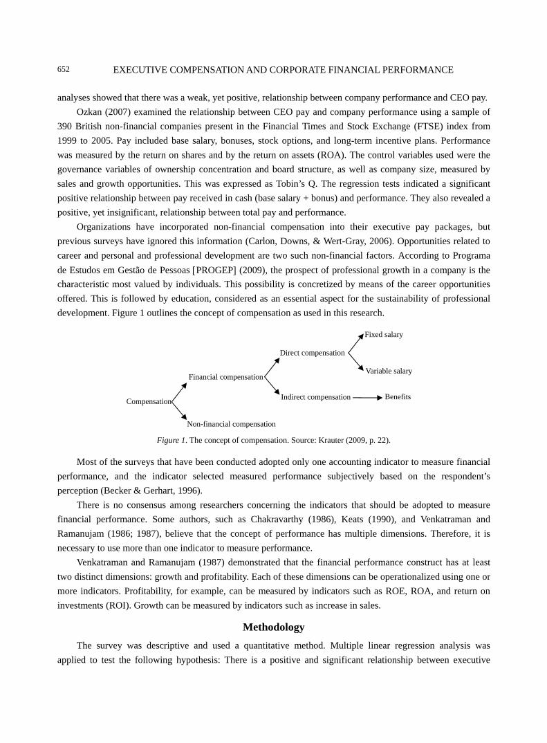
EXECUTIVE COMPENSATION AND CORPORATE FINANCIAL PERFORMANCE
652
analyses showed that there was a weak, yet positive, relationship between company performance and CEO pay. Ozkan (2007) examined the relationship between CEO pay and company performance using a sample of
390 British non-financial companies present in the Financial Times and Stock Exchange (FTSE) index from 1999 to 2005. Pay included base salary, bonuses, stock options, and long-term incentive plans. Performance was measured by the return on shares and by the return on assets (ROA). The control variables used were the governance variables of ownership concentration and board structure, as well as company size, measured by sales and growth opportunities. This was expressed as Tobin’s Q. The regression tests indicated a significant positive relationship between pay received in cash (base salary + bonus) and performance. They also revealed a positive, yet insignificant, relationship between total pay and performance.
Organizations have incorporated non-financial compensation into their executive pay packages, but previous surveys have ignored this information (Carlon, Downs, & Wert-Gray, 2006). Opportunities related to career and personal and professional development are two such non-financial factors. According to Programa de Estudos em Gestão de Pessoas [PROGEP] (2009), the prospect of professional growth in a company is the characteristic most valued by individuals. This possibility is concretized by means of the career opportunities offered. This is followed by education, considered as an essential aspect for the sustainability of professional development. Figure 1 outlines the concept of compensation as used in this research.
Figure 1. The concept of compensation. Source: Krauter (2009, p. 22).
Most of the surveys that have been conducted adopted only one accounting indicator to measure financial performance, and the indicator selected measured performance subjectively based on the respondent’s perception (Becker & Gerhart, 1996).
There is no consensus among researchers concerning the indicators that should be adopted to measure financial performance. Some authors, such as Chakravarthy (1986), Keats (1990), and Venkatraman and Ramanujam (1986; 1987), believe that the concept of performance has multiple dimensions. Therefore, it is necessary to use more than one indicator to measure performance.
Venkatraman and Ramanujam (1987) demonstrated that the financial performance construct has at least two distinct dimensions: growth and profitability. Each of these dimensions can be operationalized using one or more indicators. Profitability, for example, can be measured by indicators such as ROE, ROA, and return on investments (ROI). Growth can be measured by indicators such as increase in sales.
Methodology
The survey was descriptive and used a quantitative method. Multiple linear regression analysis was applied to test the following hypothesis: There is a positive and significant relationship between executive
Compensation
Financial compensation
Non-financial compensation
Direct compensation
Indirect compensation
Variable salary
Benefits
Fixed salary
EXECUTIVE COMPENSATION AND CORPORATE FINANCIAL PERFORMANCE
653
compensation and corporate financial performance in the context of the Brazilian marketplace. This technique was used in the majority of previous studies, such as those developed by Attaway (2000) and Ozkan (2007).
Secondary data were used in the survey. Information on the independent variables and the control variable was taken from the database of PROGEP of Fundação Instituto de Administração (FIA). The data on the dependent variables were taken from the database of Fundação Instituto de Pesquisas Contábeis, Atuariais e Financeiras (FIPECAFI).
The non-probability sampling method was employed. The sample consisted of 44 industrial companies with information available in the two abovementioned databases. The Statistical Package for Social Science (SPSS) program, version 16.0 for Windows, was used to tabulate the data.
The information on compensation is from fiscal year 2006 and refers to compensation received by directors, vice presidents, and presidents, herein referred to as “executives”. To operationalize the compensation variable, the following information from the PROGEP database was used:
(1) Value of the average monthly salary of the executive in December 2006 in Brazilian Real; (2) Average sum received by the executive in 2006 in Brazilian Real, as variable compensation and/or as
bonus (es); (3) Access of executives to the following 12 benefits: healthcare plan, medical clinic located within the
company facilities, dental plan, prescription drug subsidies, psychological support, group life insurance, education subsidies, professional specialization subsidies, language study subsidies, support for children’s education, home ownership subsidies as well as financing and loans;
(4) Executive access to 25 mechanisms for stimulating and supporting careers, including planning and tracking of professional development, encouragement and support for career planning, repositioning of dismissed executives, internal recruiting, information about career possibilities, and preparation for retirement;
(5) Executive access to the following eight mechanisms that encourage education and professional development: educational programs that incorporate the identification of critical corporate and human competencies, multiple learning methods, programs that reflect the company’s commitment to corporate citizenship, managers and leaders involved with the learning process, programs to disseminate the organizational culture, efficient systems for assessing investments in education and the results achieved, sharing knowledge and exchanging experiences, and partnerships with higher education institutions.
From the information about benefits, career, education, and professional development, the authors have created three indices: benefits, career, and development. In the database, such information is classified in the following way:
(1) No (the company does not offer the item to its executives); (2) Partial (the company offers the item to some of its executives); (3) All (the company offers the item to all its executives). To create such indices, each classification was given a point value from 0 to 2 as follows: (1) No = 0 point; (2) Partial = 1 point; (3) All = 2 points. To create the benefits index which measures the access of the executives to 12 benefits, two points were
given for each benefit offered by the company to all executives, one point was given for each benefit offered to some of its executives, and zero point was given for each benefit not offered to any of its executives.
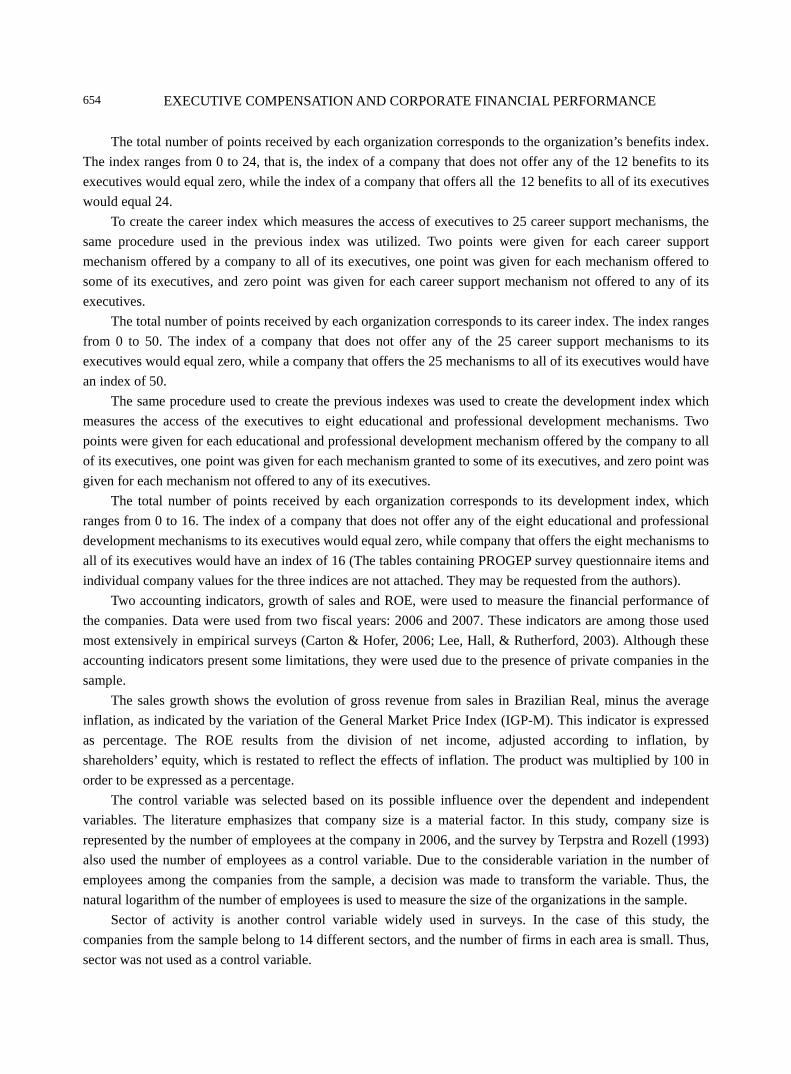
EXECUTIVE COMPENSATION AND CORPORATE FINANCIAL PERFORMANCE
654
The total number of points received by each organization corresponds to the organization’s benefits index. The index ranges from 0 to 24, that is, the index of a company that does not offer any of the 12 benefits to its executives would equal zero, while the index of a company that offers all the 12 benefits to all of its executives would equal 24.
To create the career index which measures the access of executives to 25 career support mechanisms, the same procedure used in the previous index was utilized. Two points were given for each career support mechanism offered by a company to all of its executives, one point was given for each mechanism offered to some of its executives, and zero point was given for each career support mechanism not offered to any of its executives.
The total number of points received by each organization corresponds to its career index. The index ranges from 0 to 50. The index of a company that does not offer any of the 25 career support mechanisms to its executives would equal zero, while a company that offers the 25 mechanisms to all of its executives would have an index of 50.
The same procedure used to create the previous indexes was used to create the development index which measures the access of the executives to eight educational and professional development mechanisms. Two points were given for each educational and professional development mechanism offered by the company to all of its executives, one point was given for each mechanism granted to some of its executives, and zero point was given for each mechanism not offered to any of its executives.
The total number of points received by each organization corresponds to its development index, which ranges from 0 to 16. The index of a company that does not offer any of the eight educational and professional development mechanisms to its executives would equal zero, while company that offers the eight mechanisms to all of its executives would have an index of 16 (The tables containing PROGEP survey questionnaire items and individual company values for the three indices are not attached. They may be requested from the authors).
Two accounting indicators, growth of sales and ROE, were used to measure the financial performance of the companies. Data were used from two fiscal years: 2006 and 2007. These indicators are among those used most extensively in empirical surveys (Carton & Hofer, 2006; Lee, Hall, & Rutherford, 2003). Although these accounting indicators present some limitations, they were used due to the presence of private companies in the sample.
The sales growth shows the evolution of gross revenue from sales in Brazilian Real, minus the average inflation, as indicated by the variation of the General Market Price Index (IGP-M). This indicator is expressed as percentage. The ROE results from the division of net income, adjusted according to inflation, by shareholders’ equity, which is restated to reflect the effects of inflation. The product was multiplied by 100 in order to be expressed as a percentage.
The control variable was selected based on its possible influence over the dependent and independent variables. The literature emphasizes that company size is a material factor. In this study, company size is represented by the number of employees at the company in 2006, and the survey by Terpstra and Rozell (1993) also used the number of employees as a control variable. Due to the considerable variation in the number of employees among the companies from the sample, a decision was made to transform the variable. Thus, the natural logarithm of the number of employees is used to measure the size of the organizations in the sample.
Sector of activity is another control variable widely used in surveys. In the case of this study, the companies from the sample belong to 14 different sectors, and the number of firms in each area is small. Thus, sector was not used as a control variable.
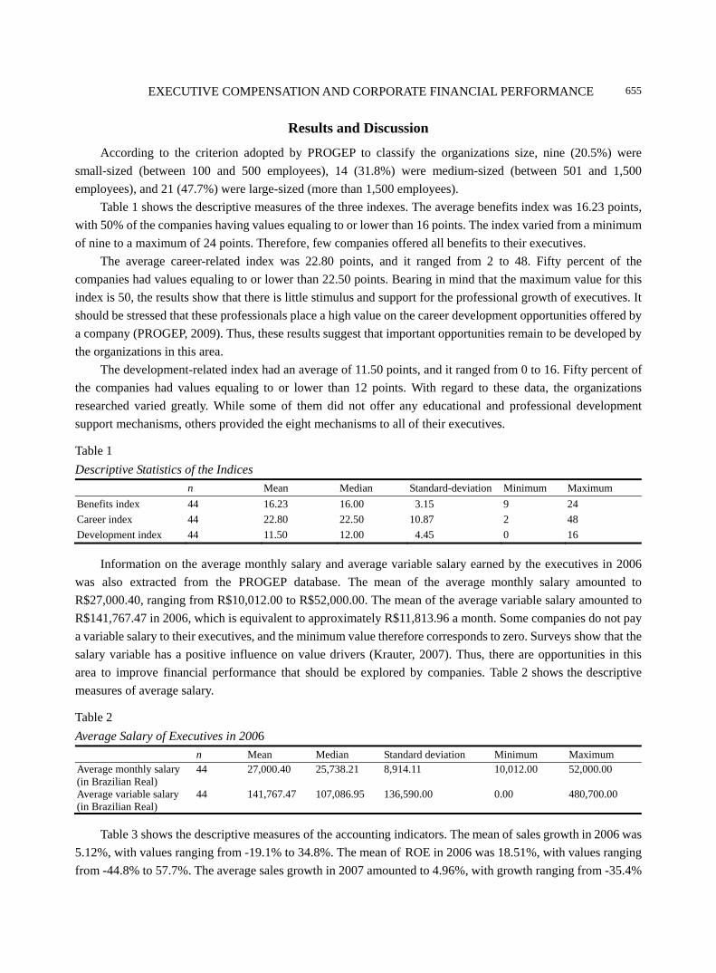
EXECUTIVE COMPENSATION AND CORPORATE FINANCIAL PERFORMANCE
655
Results and Discussion
According to the criterion adopted by PROGEP to classify the organizations size, nine (20.5%) were small-sized (between 100 and 500 employees), 14 (31.8%) were medium-sized (between 501 and 1,500 employees), and 21 (47.7%) were large-sized (more than 1,500 employees).
Table 1 shows the descriptive measures of the three indexes. The average benefits index was 16.23 points, with 50% of the companies having values equaling to or lower than 16 points. The index varied from a minimum of nine to a maximum of 24 points. Therefore, few companies offered all benefits to their executives.
The average career-related index was 22.80 points, and it ranged from 2 to 48. Fifty percent of the companies had values equaling to or lower than 22.50 points. Bearing in mind that the maximum value for this index is 50, the results show that there is little stimulus and support for the professional growth of executives. It should be stressed that these professionals place a high value on the career development opportunities offered by a company (PROGEP, 2009). Thus, these results suggest that important opportunities remain to be developed by the organizations in this area.
The development-related index had an average of 11.50 points, and it ranged from 0 to 16. Fifty percent of the companies had values equaling to or lower than 12 points. With regard to these data, the organizations researched varied greatly. While some of them did not offer any educational and professional development support mechanisms, others provided the eight mechanisms to all of their executives.
Table 1 Descriptive Statistics of the Indices
n Mean Median Standard-deviation Minimum Maximum Benefits index 44 16.23 16.00 3.15 9 24 Career index 44 22.80 22.50 10.87 2 48 Development index 44 11.50 12.00 4.45 0 16
Information on the average monthly salary and average variable salary earned by the executives in 2006 was also extracted from the PROGEP database. The mean of the average monthly salary amounted to R$27,000.40, ranging from R$10,012.00 to R$52,000.00. The mean of the average variable salary amounted to R$141,767.47 in 2006, which is equivalent to approximately R$11,813.96 a month. Some companies do not pay a variable salary to their executives, and the minimum value therefore corresponds to zero. Surveys show that the salary variable has a positive influence on value drivers (Krauter, 2007). Thus, there are opportunities in this area to improve financial performance that should be explored by companies. Table 2 shows the descriptive measures of average salary.
Table 2 Average Salary of Executives in 2006 n Mean Median Standard deviation Minimum Maximum Average monthly salary (in Brazilian Real)
44
27,000.40
25,738.21
8,914.11
10,012.00
52,000.00
Average variable salary (in Brazilian Real)
44
141,767.47
107,086.95
136,590.00
0.00
480,700.00
Table 3 shows the descriptive measures of the accounting indicators. The mean of sales growth in 2006 was 5.12%, with values ranging from -19.1% to 34.8%. The mean of ROE in 2006 was 18.51%, with values ranging from -44.8% to 57.7%. The average sales growth in 2007 amounted to 4.96%, with growth ranging from -35.4%
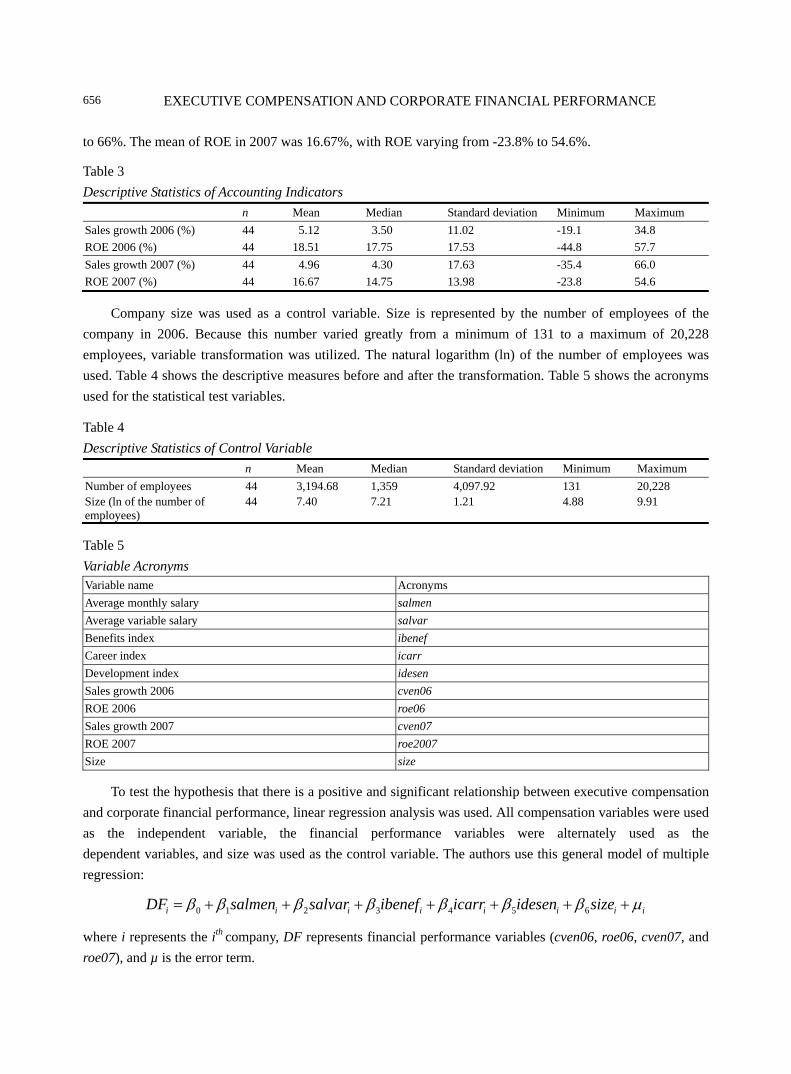
EXECUTIVE COMPENSATION AND CORPORATE FINANCIAL PERFORMANCE
656
to 66%. The mean of ROE in 2007 was 16.67%, with ROE varying from -23.8% to 54.6%.
Table 3 Descriptive Statistics of Accounting Indicators
n Mean Median Standard deviation Minimum Maximum Sales growth 2006 (%) 44 5.12 3.50 11.02 -19.1 34.8 ROE 2006 (%) 44 18.51 17.75 17.53 -44.8 57.7 Sales growth 2007 (%) 44 4.96 4.30 17.63 -35.4 66.0 ROE 2007 (%) 44 16.67 14.75 13.98 -23.8 54.6
Company size was used as a control variable. Size is represented by the number of employees of the company in 2006. Because this number varied greatly from a minimum of 131 to a maximum of 20,228 employees, variable transformation was utilized. The natural logarithm (ln) of the number of employees was used. Table 4 shows the descriptive measures before and after the transformation. Table 5 shows the acronyms used for the statistical test variables.
Table 4 Descriptive Statistics of Control Variable
n Mean Median Standard deviation Minimum Maximum Number of employees 44 3,194.68 1,359 4,097.92 131 20,228 Size (ln of the number of employees)
44
7.40
7.21
1.21
4.88
9.91
Table 5 Variable Acronyms Variable name Acronyms Average monthly salary salmen
Average variable salary salvar
Benefits index ibenef
Career index icarr
Development index idesen
Sales growth 2006 cven06
ROE 2006 roe06
Sales growth 2007 cven07
ROE 2007 roe2007
Size size
To test the hypothesis that there is a positive and significant relationship between executive compensation and corporate financial performance, linear regression analysis was used. All compensation variables were used as the independent variable, the financial performance variables were alternately used as the dependent variables, and size was used as the control variable. The authors use this general model of multiple regression:
0 1 2 3 4 5 6i i i i i i i iDF salmen salvar ibenef icarr idesen sizeβ β β β β β β μ= + + + + + + +
where i represents the ith company, DF represents financial performance variables (cven06, roe06, cven07, and roe07), and µ is the error term.
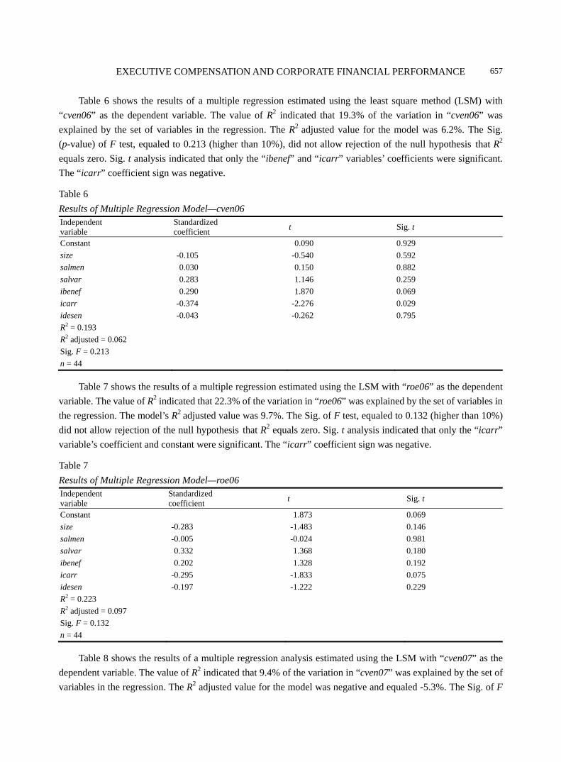
EXECUTIVE COMPENSATION AND CORPORATE FINANCIAL PERFORMANCE
657
Table 6 shows the results of a multiple regression estimated using the least square method (LSM) with “cven06” as the dependent variable. The value of R2 indicated that 19.3% of the variation in “cven06” was explained by the set of variables in the regression. The R2 adjusted value for the model was 6.2%. The Sig. (p-value) of F test, equaled to 0.213 (higher than 10%), did not allow rejection of the null hypothesis that R2 equals zero. Sig. t analysis indicated that only the “ibenef” and “icarr” variables’ coefficients were significant. The “icarr” coefficient sign was negative.
Table 6 Results of Multiple Regression Model—cven06 Independent variable
Standardized coefficient t Sig. t
Constant 0.090 0.929 size -0.105 -0.540 0.592 salmen 0.030 0.150 0.882 salvar 0.283 1.146 0.259 ibenef 0.290 1.870 0.069 icarr -0.374 -2.276 0.029 idesen -0.043 -0.262 0.795 R2 = 0.193 R2 adjusted = 0.062 Sig. F = 0.213 n = 44
Table 7 shows the results of a multiple regression estimated using the LSM with “roe06” as the dependent variable. The value of R2 indicated that 22.3% of the variation in “roe06” was explained by the set of variables in the regression. The model’s R2 adjusted value was 9.7%. The Sig. of F test, equaled to 0.132 (higher than 10%) did not allow rejection of the null hypothesis that R2 equals zero. Sig. t analysis indicated that only the “icarr” variable’s coefficient and constant were significant. The “icarr” coefficient sign was negative.
Table 7 Results of Multiple Regression Model—roe06 Independent variable
Standardized coefficient t Sig. t
Constant 1.873 0.069 size -0.283 -1.483 0.146 salmen -0.005 -0.024 0.981 salvar 0.332 1.368 0.180 ibenef 0.202 1.328 0.192 icarr -0.295 -1.833 0.075 idesen -0.197 -1.222 0.229 R2 = 0.223 R2 adjusted = 0.097 Sig. F = 0.132 n = 44
Table 8 shows the results of a multiple regression analysis estimated using the LSM with “cven07” as the dependent variable. The value of R2 indicated that 9.4% of the variation in “cven07” was explained by the set of variables in the regression. The R2 adjusted value for the model was negative and equaled -5.3%. The Sig. of F
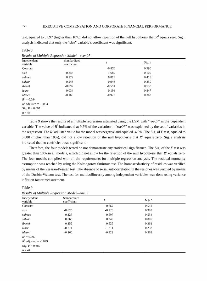
EXECUTIVE COMPENSATION AND CORPORATE FINANCIAL PERFORMANCE
658
test, equaled to 0.697 (higher than 10%), did not allow rejection of the null hypothesis that R2 equals zero. Sig. t analysis indicated that only the “size” variable’s coefficient was significant.
Table 8 Results of Multiple Regression Model—cven07 Independent variable
Standardized coefficient t Sig. t
Constant -0.870 0.390 size 0.348 1.689 0.100 salmen 0.172 0.819 0.418 salvar -0.248 -0.946 0.350 ibenef -0.097 -0.591 0.558 icarr 0.034 0.194 0.847 idesen -0.160 -0.922 0.363 R2 = 0.094 R2 adjusted = -0.053 Sig. F = 0.697 n = 44
Table 9 shows the results of a multiple regression estimated using the LSM with “roe07” as the dependent variable. The value of R2 indicated that 9.7% of the variation in “roe07” was explained by the set of variables in the regression. The R2 adjusted value for the model was negative and equaled -4.9%. The Sig. of F test, equaled to 0.680 (higher than 10%), did not allow rejection of the null hypothesis that R2 equals zero. Sig. t analysis indicated that no coefficient was significant.
Therefore, the four models tested do not demonstrate any statistical significance. The Sig. of the F test was greater than 10% in all models, which did not allow for the rejection of the null hypothesis that R2 equals zero. The four models complied with all the requirements for multiple regression analysis. The residual normality assumption was reached by using the Kolmogorov-Smirnov test. The homoscedasticity of residues was verified by means of the Pesarán-Pesarán test. The absence of serial autocorrelation in the residues was verified by means of the Durbin-Watson test. The test for multicollinearity among independent variables was done using variance inflation factor measurement.
Table 9 Results of Multiple Regression Model—roe07 Independent variable
Standardized coefficient t Sig. t
Constant 0.662 0.512 size -0.025 -0.123 0.903 salmen 0.126 0.597 0.554 salvar 0.065 0.249 0.805 ibenef 0.152 0.926 0.361 icarr -0.211 -1.214 0.232 idesen -0.160 -0.923 0.362 R2 = 0.097 R2 adjusted = -0.049 Sig. F = 0.680 n = 44
EXECUTIVE COMPENSATION AND CORPORATE FINANCIAL PERFORMANCE
659
The results of multiple linear regression analysis did not support the hypothesis that there is a positive and significant relationship between executive compensation and corporate financial performance. These results are compatible with the results of other researches, developed in other contexts, which also did not find a relationship among the variables.
Conclusions
Executive compensation is a complex and controversial subject that has attracted a lot of media attentions. In the recent past, “millionaire bonuses” have made the headlines in major media outlets worldwide. Executives, primarily Americans, have received huge sums of money despite having contributed to the ruin of the firms under their management.
Under the agency theory, the pay package is considered as one of the most efficient mechanisms to induce an executive who maximizes his or her own utility and is risk averse to act with the purpose of increasing the company’s financial performance. The assumption is that pay can help steer the efforts of executives toward strategic business objectives and thereby enable the company to reach higher levels of financial performance.
The objective of this survey was to investigate the relationship between executive compensation and corporate financial performance in the context of the Brazilian marketplace. It differs from previous surveys, because it adopts broader concepts to operationalize the variables. While previous surveys used only fixed salary and variable salary to operationalize the pay variable, this survey uses both salary measures and three indices created especially for the survey: benefits, career, and development. Moreover, previous surveys measured performance subjectively, based on the respondent’s perception; they also used only one accounting indicator from a single fiscal year. This survey uses two accounting indicators from two fiscal years, taken from the FIPECAFI database.
A descriptive analysis of the indices shows that companies have few mechanisms to encourage and support the careers and education of their executives. These are two aspects of the workplace valued by executives, according to PROGEP (2009). Hence, these areas offer opportunities that companies can explore to attract and retain qualified professionals.
The descriptive analysis of salaries indicates that some companies do not pay a variable salary to their executives. The survey shows that variable pay plans have a favorable influence on company performance, provided that they are developed appropriately and tie payment to the achievement of goals.
The results of multiple linear regression analysis did not confirm the survey’s hypothesis that there is a positive and significant relationship between executive compensation and corporate financial performance in the context of the Brazilian marketplace. These results are compatible with those of other surveys conducted in different contexts that are also unable to prove the existence of a relationship among these variables. It was expected that the use of an approach different from that used in previous studies, the creation of three indices and the use of two accounting indicators from two fiscal years would provide evidence to support the hypothesis. However, that expectation was not fulfilled.
This study of the relationship between executive compensation and financial performance in the context of the Brazilian marketplace contributes to the existing scholarship on corporate management practices by presenting incentives for companies to refine their pay systems, creating three indices, producing broader concepts to operationalize previously used variable, and providing new perspectives on which future studies can build.
EXECUTIVE COMPENSATION AND CORPORATE FINANCIAL PERFORMANCE
660
This survey had some limitations. The sampling method employed to select the companies from the sample was non-probabilistic. Consequently, it is not possible to generalize the results obtained for the population. Another limitation was the sample size. Most of the companies were private. The fact that these companies are not required to publish their financial statements made it difficult to obtain financial data. This lack of transparency creates obstacles to the performance of surveys that require these data, such as this one. In addition, the use of accounting information is a limiting factor, as it is subjected to distortions.
Further surveys and case studies could contribute to a better understanding of the relationship between executive compensation and corporate financial performance.
References Aggarwal, R. K., & Samwick, A. A. (1999). Executive compensation, strategic competition, and relative performance evaluation:
Theory and evidence. The Journal of Finance, 59(6), 1999-2043. Andrade, A., & Rossetti, J. P. (2006). Corporate governance: Fundamentals, developments, and trends. São Paulo: Atlas. Attaway, M. C. (2000). A study of the relationship between company performance and CEO compensation. American Business
Review, 18(1), 77-85. Bálkin, D. B., & Gómez-Mejia, L. R. (1987). Toward a contingency theory of compensation strategy. Strategic Management
Journal, 8(2), 169-182. Barkema, H. G., & Gómez-Mejia, L. R. (1998). Managerial compensation and firm performance: A general research framework.
Academy of Management Journal, 41(2), 135-145. Becker, B. E., & Gerhart, B. (1996). The impact of human resource management on organizational performance: Progress and
prospects. Academy of Management Journal, 39(4), 779-801. Carlon, D. M., Downs, A. A., & Wert-Gray, S. (2006). Statistics as fetishes: The case of financial performance and executive
compensation. Organizational Research Methods, 9(4), 475-490. Carton, R. B., & Hofer, C. W. (2006). Measuring organizational performance: Metrics for entrepreneurship and strategic
management research. Northampton: Edward Elgar. Chakravarthy, B. S. (1986). Measuring strategic performance. Strategic Management Journal, 7(5), 437-458. Devers, C. E., Cannella, A. A., Reilly, G. P., & Yoder, M. B. (2007). Executive compensation: A multidisciplinary review of recent
developments. Journal of Management, 33(6), 1016-1072. Gerhart, B., & Milkovich, G. T. (1990). Organizational differences in managerial compensation and financial performance.
Academy of Management Journal, 33(4), 663-691. Gómez-Mejia, L. R., & Welbourne, T. M. (1988). Compensation strategy: An overview and future steps. Human Resource Planning,
11(3), 173-189. Jensen, M. C., & Meckling, W. H. (1976). Theory of the firm: Managerial behavior, agency costs, and ownership structure. Journal
of Financial Economics, 3(4), 305-360. Keats, B. W. (1990). Diversification and business economic performance revisited: Issues of measurement and causality. Journal of
Management, 16(1), 61-72. Krauter, E. (2007). Profit sharing and results: Influence on value drivers. Sao Paulo: Saint Paul. Krauter, E. (2009). Contributions system of executive remuneration to financial performance: A study of Brazilian manufacturers
(Doctorate thesis in Business Administration, Graduate Program in Business Administration, Faculty of Economics, Administration and Accounting from the University of São Paulo).
Lee, J., Hall, E. H., & Rutherford, M. W. (2003). A comparative study of US and Korean firms: Changes in diversification and performance. International Journal of Commerce and Management, 13(1), 11-41.
Ozkan, N. (2007). CEO compensation and firm performance: An empirical investigation of UK panel data. SSRN Working Paper Series. Retrieved from http://ssrn.com/abstract=1102703
Programa de Estudos em Gestão de Pessoas [PROGEP]. (2009). Technical report: Research VOCÊ S/A—2009. Retrieved from http://www.fia.com.br/portalfia/Repositorio/13/Laudo_tecnico_2009.pdf
Schuster, J. R., & Zingheim, P. K. (1992). The new pay: Linking employee and organizational performance. New York, NY: Lexington Books.

EXECUTIVE COMPENSATION AND CORPORATE FINANCIAL PERFORMANCE
661
Shim, E., & Lee, J. A. (2003). A canonical analysis of CEO compensation and corporate performance in the service industry. Review of Accounting and Finance, 2(3), 72-90.
Terpstra, D. E., & Rozell, E. J. (1993). The relationship of staffing practices to organizational level measures of performance. Personnel Psychology, 46(1), 27-48.
Venkatraman, N., & Ramanujam, V. (1986). Measurement of business performance in strategy research: A comparison of approaches. Academy of Management Review, 11(4), 801-814.
Venkatraman, N., & Ramanujam, V. (1987). Measurement of business economic performance: An examination of method convergence. Journal of Management, 13(1), 109-122.
Journal of Modern Accounting and Auditing, ISSN 1548-6583 May 2013, Vol. 9, No. 5, 662-677
The Recent US Financial Crisis: Its Impact on Dividend Payout
Strategy and a Test of the Silver-Lining Hypothesis∗
Chuo-Hsuan Lee The State University of New York (SUNY), New York, USA
Edward J. Lusk The State University of New York (SUNY), New York, USA
University of Pennsylvania, Philadelphia, USA
Michael Halperin University of Pennsylvania, Philadelphia, USA
The authors investigate the impact of the recent financial crisis on dividend payout policies in the United States.
The results are as follows. The authors find that: (1) Firms must have good financial profiles to support a policy of
increasing dividend payouts during a financial crisis; (2) Overall firms increasing dividend payouts are also
engaged in stock repurchases; (3) Firms choosing to increase cash dividend payouts seem to have low opportunity
costs, that is, they do not have as many exercisable stock options that they may need in the face of possible future
redemptions; and (4) During a financial crisis, the aforementioned trade-off between exercisable stock options and
increased dividend payouts would peak, as the stock price slides to where it could be expected to V-bound and
then became moderate when stock price recovered. The abovementioned findings are consistent with the “silver-
lining” hypothesis which the authors proffer to suggest that the storm of economic bad times often creates
circumstances that influence dividend payout strategies for firms traded on exchanges in the United States, and
different dividend payout strategies may be strategically elected to reveal to the market participants a silver-lining
in the cloud of bad times.
Keywords: dividend payout, stock repurchases, financial crisis
Introduction
In this study, the authors investigate the impact of the financial crisis, starting after the Lehman Bros, limited liability partnership (LLP) sub-prime debacle and continuing to date, on dividend payout policies for
∗ Acknowledgements: The authors wish to thank the participants at the 2012 International Academy of Business Disciplines (IABD) 24th Annual Conference in Long Beach, CA, USA for their comments and helpful suggestions. Special thanks go to Dr. Matthew Wong of St. John’s University for his detailed observations.
Chuo-Hsuan Lee, CPA, CMA, CFM, CFE, Ph.D., professor of Accounting, School of Business and Economics, The State University of New York (SUNY).
Edward J. Lusk, CPA, Ph.D., professor of Accounting, School of Business and Economics, The State University of New York (SUNY); Department of Statistics, University of Pennsylvania.
Michael Halperin, Ph.D., director, Lippincott Library of the Wharton School, University of Pennsylvania. Correspondence concerning this article should be addressed to Chuo-Hsuan Lee, CPA, CMA, CFM, CFE, Ph.D., professor of
Accounting, School of Business and Economics, The State University of New York (SUNY), Plattsburgh, New York, USA. Email: [email protected]; Tel.: +01.518.564.4211; Fax: +01.518.564.3183.
DAVID PUBLISHING
D
THE RECENT US FINANCIAL CRISIS: ITS IMPACT ON DIVIDEND PAYOUT STRATEGY
663
firms traded on major exchanges in the United States. It is interesting to examine this topic, because it is a classic illustration of the silver-lining metaphor: “Every cloud has a silver lining”. The cloud: The recent financial crisis has compromised liquidity, effectively through falling values in marketable securities and reduced trading accounts receivable and increasing allowances for doubtful accounts as well as falling stock prices, but the silver lining: These economic difficulties are also positive opportunities for firms to strategically engage and rationalize in stock buy-back activities and/or change their dividend payout policies to the end of hedging (Ryan, 2012).
Different strategies can be rationalized by management as evidence of their excellent management skills to show that even in the financial crisis, they are able to reward the stockholders for making the wise decisions to hold their stocks. For example, on the one hand, the strained cash liquidity of firms may limit some companies’ ability to maintain their current dividend policies. Therefore, companies can argue that they need to reduce their dividend payouts to guarantee that they will be able to weather the economic bad times. On the other hand, for some other companies, they may decide to increase their dividend payouts in order to comfort their investors and restore their confidence, while the stock prices were depressed due to the overall economic situation (Ryan, 2012). For these companies, to increase dividend payouts across over time provides a really good value to the shareholders, and the ability to keep up with the increasing dividend payout during the financial crisis demonstrates the strategies and capabilities of the firms to offer sustained and long-term value to the stockholders (Ryan, 2012). Similarly, on the one hand, the depressed stock price may raise some concerns from the investors regarding the future prospect of companies; on the other hand, the low stock price offers great opportunities for companies which are still optimistic about the future development to repurchase their own stocks from the market in order to benefit from the expected price recovery and also reduce their prospective costs of giving stocks to their employees, as the employees redeem their stock options after the financial crisis. The “spins” are indeed endless.
In summary, the authors expect that during the financial crisis, firms, when facing conflicting forces which create limits—the cloud and seeing incentives and opportunities—the silver lining, will react differently based on the characteristics of their firms and industries, resulting in changes in the patterns of stock repurchase activities and dividend payout policies during this troubled period.
The results reveal some interesting findings. First, the results indicate a positive association between return on assets (ROA) and increased dividend payout, implying that firms must have good financial profiles in order to increase their dividend payouts before as well as after the financial crisis event starts. Second, the authors found a consistent and positive association between firms’ election to affect stock repurchases and increased dividend payout, indicating that firms that increased dividend payouts also elected to repurchase stocks, so these firms did not increase dividend payout by abandoning their stock repurchase plans.
Third, the authors offer the economic logic that at any point in time, if a firm decided to increase dividend payouts while engaging in stock buybacks, it would sacrifice opportunities to repurchase stocks with the same cash to cope with the future redemption of employees’ stock options. The above logic indicates that there should be a significant trade-off between increased dividend payout and exercisable stock options after controlling for other related variables and suggests that firms choosing to increase their cash dividend payouts have low opportunity costs, that is, they do not have as many exercisable stock options that they need to face the redemption in the future. The finding of this paper supports this logic.
THE RECENT US FINANCIAL CRISIS: ITS IMPACT ON DIVIDEND PAYOUT STRATEGY
664
Fourth, before the financial crisis, stock prices were biased on the high side. The higher stock price before crisis may trigger more current stock option exercises, adding pressure to stock repurchases1. Since the stock price was high and still increasing at this time, the pressure to repurchase stocks for current and incoming stock option exercises required more use of funding and left less funding available for increasing dividend payout2. This implies that before the financial crisis, more exercisable stock options would lead to a less likelihood of increasing dividend payout. Accordingly, the authors found a demonstrable tendency to engage in trade-off between exercisable stock options and increased dividend payout prior to the financial crisis, which provides support for the authors’ argument.
Fifth and lastly, when the financial crisis began and stock prices suddenly and dramatically dropped, it became easier and perhaps a wise strategy for a firm to repurchase its own stock. A firm with more exercisable stock options would be tempted to repurchase more stocks at a historically low price to pump up its reserve for future redemption of stock options. Given the tightened cash availability during the financial crisis period, to do so would further strain and possibly limit the resources available for increasing dividend payout. Therefore, the authors expect that during the financial crisis, the trade-off between exercisable stock options and increased dividend payout would reach the peak, as the stock price touched down for a “V-bound”—so named for the V-shaped trajectory sketched out by a fall followed by an equal slope rise in stock prices, and then became moderated when stock price recovered. The results confirmed this V-bounding argument.
This article is organized as follows. In the next section, the authors will discuss the previous literature related to stock repurchases and dividend payout policies. Then, they will develop the hypotheses for testing followed by a discussion for data collection and sample selection. Next, the empirical results will be presented and discussed. Lastly, the authors will present the concluding remarks and suggest future research directions in the interesting market context.
Literature Review
Stock Repurchases
There are many reasons behind the decisions of firms to buy back their own stocks. According to previous literatures, firms may repurchase stocks to distribute cash in excess of current investment opportunities (e.g., Jensen, 1986; Stephens & Weisbach, 1998; Barth & Kasznik, 1999; Dittmar, 2000). Also, firms may use stock buyback as a signal to the market, if the management feels that their stocks are undervalued (e.g., Vermaelen, 1981; Bartov, 1991; Ofer & Thakor, 1987; Jagannathan & Stephens, 2003). Stock repurchases were also often used by companies as a substitute for dividend payouts (Jagannathan, Stephens, & Weisbach, 2000; Brav, John, Campbell, & Michaely, 2005; Grullon & Michaely, 2002; Skinner, 2008). Stock repurchases may be used as a tool in a payout policy, which allows management to take advantage of financial flexibility between dividend payouts and stock repurchases (Jagannathan et al., 2000). Stock repurchases were often used as a substitute for dividends because of the personal tax rate advantage of capital gains (Scholes & Wolfson, 1992). Firms can also use stock repurchases to opportunistically manipulate earnings per share (EPS) (Bens, Nagar, & Wong, 2002; Brav et al., 2005).
1 At this time, a firm may consider to increase its stock reserve by repurchasing more stocks, given that the price is increasing and no one is aware of the looming financial crisis. 2 Before the financial crisis due to higher earnings in the denominator of dividend payout calculation, it would require more cash commitments to significantly increase dividend payouts.
THE RECENT US FINANCIAL CRISIS: ITS IMPACT ON DIVIDEND PAYOUT STRATEGY
665
In the 1990s, it was documented that there was a significant relationship between the stock option compensation and stock repurchases (e.g., Liang & Sharpe, 1999; Fenn & Liang, 2001; Young & Yang, 2011; Babenko, 2009). According to Liang and Sharpe (1999), it was observed that a significant increase in stock repurchases in the 1990s has been accompanied by a corresponding rise in employees’ stock option grants. Jolls (1998), Weisbenner (2000), and Fenn and Liang (2001) have looked into the relationship of stock repurchases and stock options through the lens of agency theory. They concluded that firms that rely on stock options to compensate their top management are more likely to repurchase stocks. Fenn and Liang (2001) have offered convincing evidence that top management’s stock option awards are positively related to stock repurchases and negatively related to dividend payments.
Agency theory is not the only factor explaining the relationship between stock repurchases and stock options, the “undo-dilution” hypothesis explains this relationship by referencing a different theoretical context. This hypothesis indicates that firms repurchase stocks to undo the dilution of EPS from the total outstanding stock options (Weisbenner, 2000; Klassen & Sivakumar, 2001; Kahle, 2002; Brav et al., 2005; Bens, Nagar, Skinner, & Wong, 2003). Weisbenner (2000) found a positive relationship between the number of stocks repurchased and stock options grants given in a current year and prior years. This very relationship was noted after the positive association of stock repurchases, with the number of stocks outstanding being found in the studies of Klassen and Sivakumar (2001) and Kahle (2002). Brav et al. (2005) surveyed 384 chief financial officers (CFOs) and treasurers. Their results showed that three-fourths of the CFOs and treasurers have indicated that an increase in EPS is an essential factor in their repurchase decisions, and two-thirds of the CFOs and treasurers feel that offsetting the dilutive effects of stock options is an important factor affecting stocks repurchase decisions.
Dividend Payout Policy
Dividend payouts must be authorized by the board of directors based upon the recommendation of the audit committee now in play due to Sarbanes-Oxley 2002. Many previous literatures investigated the dividend signaling effects and provided supports to the role of dividend payouts as signals to the market participants (e.g., H. DeAngelo, L. DeAngelo, & Skinner, 1992; Richardson, Sefcik, & Thompson, 1986; Gurgul, Mestel, & Schleicher, 2003; Bozos, Nikolopoulos, & Ramgandhi, 2011). For example, Ryan (2012, p. 18) indicated that, “Before jumping into paying a regular dividend, though, management has to determine whether it fits the company’s financial strategy”. Bozos et al. (2011) investigated dividend signaling under economic adversity using the recent data from London Stock Exchange from late 2007 to early 2008. They found that the information content of dividends varies with the economic situations and the information content of dividends is less than earnings in the period of strong and stable economy but more than earnings in the period of a bad economy, supporting the role of dividends as a signal from management in bad financial time. Therefore, the authors need to look at the senior management group as constituting the strategic montage. This is where the strategic aspect comes into play and spawns interest in the authors’ investigation of the silver-lining hypothesis.
Dividends can be paid in two ways: cash or stock dividends. By paying cash dividends, companies return a portion of the earnings to the shareholders in the form of cash. In contrast, stock dividends represent additional stocks given to existing shareholders to increase the number of shares held by the existing shareholders; however, there is usually a dilution of the market valuation at the day of declaration, but over time, the additional shares seem to have an incremental valuation over the market cap for the reduced number of shares. So, in discount valuation sense, stock dividends are real wealth adjustments (Healy & Palepu, 1993; Rankine &
THE RECENT US FINANCIAL CRISIS: ITS IMPACT ON DIVIDEND PAYOUT STRATEGY
666
Stice, 1997). This is critically important, as cash and stock dividends play a role in the strategy set of senior management. For example, some companies in high-tech industries (e.g., Google Inc. and Cisco Inc.) do not pay cash dividends. Many of them prefer to retain their cash and rationalize this policy option: need of cash for rapid expansion and growth in the future. Some other companies (e.g., McDonald’s and Exxon-Mobile) in different industries maintain a consistent cash dividend payout policy, because these companies are in a relatively stable industry with steady cash inflows (Russolillo, 2012).
The volatility of stock price in the recent years in the context of the recent financial crisis and Euro debt crisis has raised the concern for unpredictability of stock market and changed the tastes of the market participants in favor of cash dividend payout. For example, Russolillo (2012) indicated that:
Shares in these defensive categories are giving US equities an extra touch of resilience amid the tumult elsewhere. Stock markets in Europe and Latin America have seen significant selloffs this year amid the uncertainty surrounding Greece’s future in the euro zone and worries about weakening global demand which will likely negatively impact China. Defensive companies tend to get much of their revenue from the US, where the economy has remained relatively robust. And while most are in mature industries with limited growth prospects, investors are lured with higher dividend payouts. (C. 4)
Dividend Payout Policy and Stock Repurchases
Firms often use stock repurchases as a substitute for paying dividend (e.g., Jolls, 1998; Dittmar, 2000; Fenn & Liang, 2001). It is interesting to observe the trade-off between stock buybacks and dividend payouts. On the one hand, based on agency theory, a firm may decide not to pay dividends but use cash to buy back stocks from the market. In this case, the stock buy-back decision of this firm indicates the undervaluation of the stocks and signals to the market the private information concerning the unanticipated higher growth in the future, resulting in an increased stock price. On the other hand, a firm may decide to increase dividend payout without a simultaneous increase in stock buybacks. In this case, the increased dividend payout may send a signal to the market indicating that management has no pressing current need for cash to finance projects or retire debts and therefore may feel pressure to return the idle cash as dividends to placate the shareholders. This would likely to be considered by the market as a sign of managerial ineptness, leading to a negative stock price reaction on the stock market (Barth & Kasznik, 1999; Dittmar, 2000).
Also, a firm with an increasing longitudinal pattern of operating cash flows may choose to increase either dividend payouts or repurchases, or both simultaneously. Stock repurchases allow management to take advantage of financial flexibility between dividend payouts and stock repurchases (Jagannathan et al., 2000; Brav et al., 2005). For example, firms with increasing operating cash flows due to strong growth may decide to increase dividend payout to reflect the permanent portion of income growth but choose stock buybacks for the temporary increase of income, because they do not want to disappoint investors by increasing dividend payout excessively and then being forced to cut it back due to economic retrenchment (Jagannathan et al., 2000; Brav et al., 2005). According to Vascellaro (2012):
Apple on Monday bowed to mounting pressure to return some of its roughly $100 billion in cash reserves to shareholders by saying it would issue a dividend and buy back stock, marking the technology company’s biggest break yet from Mr. Jobs’ philosophy. (A. 1)
As one can see, the literature rationalizes many different underlying possible strategy sets that seem to be motivated by the internal and external economic climate facing the firm. In summary, dividends may be a sign of senior manager ineptitude, or a wise decision to reward loyal stockholders and garner support for future
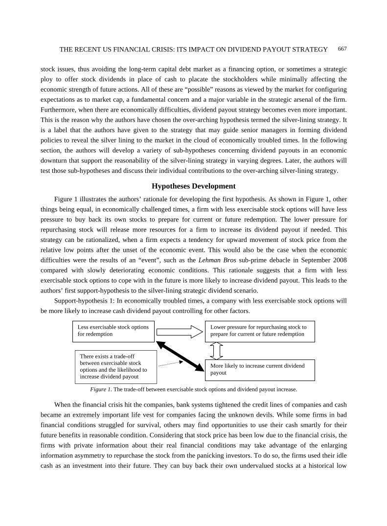
THE RECENT US FINANCIAL CRISIS: ITS IMPACT ON DIVIDEND PAYOUT STRATEGY
667
stock issues, thus avoiding the long-term capital debt market as a financing option, or sometimes a strategic ploy to offer stock dividends in place of cash to placate the stockholders while minimally affecting the economic strength of future actions. All of these are “possible” reasons as viewed by the market for configuring expectations as to market cap, a fundamental concern and a major variable in the strategic arsenal of the firm. Furthermore, when there are economically difficulties, dividend payout strategy becomes even more important. This is the reason why the authors have chosen the over-arching hypothesis termed the silver-lining strategy. It is a label that the authors have given to the strategy that may guide senior managers in forming dividend policies to reveal the silver lining to the market in the cloud of economically troubled times. In the following section, the authors will develop a variety of sub-hypotheses concerning dividend payouts in an economic downturn that support the reasonability of the silver-lining strategy in varying degrees. Later, the authors will test those sub-hypotheses and discuss their individual contributions to the over-arching silver-lining strategy.
Hypotheses Development
Figure 1 illustrates the authors’ rationale for developing the first hypothesis. As shown in Figure 1, other things being equal, in economically challenged times, a firm with less exercisable stock options will have less pressure to buy back its own stocks to prepare for current or future redemption. The lower pressure for repurchasing stock will release more resources for a firm to increase its dividend payout if needed. This strategy can be rationalized, when a firm expects a tendency for upward movement of stock price from the relative low points after the unset of the economic event. This would also be the case when the economic difficulties were the results of an “event”, such as the Lehman Bros sub-prime debacle in September 2008 compared with slowly deteriorating economic conditions. This rationale suggests that a firm with less exercisable stock options to cope with in the future is more likely to increase dividend payout. This leads to the authors’ first support-hypothesis to the silver-lining strategic dividend scenario.
Support-hypothesis 1: In economically troubled times, a company with less exercisable stock options will be more likely to increase cash dividend payout controlling for other factors.
Figure 1. The trade-off between exercisable stock options and dividend payout increase.
When the financial crisis hit the companies, bank systems tightened the credit lines of companies and cash became an extremely important life vest for companies facing the unknown devils. While some firms in bad financial conditions struggled for survival, others may find opportunities to use their cash smartly for their future benefits in reasonable condition. Considering that stock price has been low due to the financial crisis, the firms with private information about their real financial conditions may take advantage of the enlarging information asymmetry to repurchase the stock from the panicking investors. To do so, the firms used their idle cash as an investment into their future. They can buy back their own undervalued stocks at a historical low
Less exercisable stock options for redemption
Lower pressure for repurchasing stock to prepare for current or future redemption
There exists a trade-off between exercisable stock options and the likelihood to increase dividend payout
More likely to increase current dividend payout
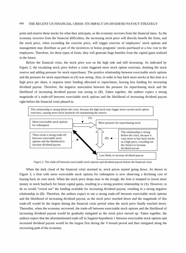
THE RECENT US FINANCIAL CRISIS: ITS IMPACT ON DIVIDEND PAYOUT STRATEGY
668
point and reserve these stocks for what they anticipate, as the economy recovers from the financial mess. As the economy recovers from the financial difficulties, the increasing stock price will directly benefit the firms, and the stock price, when exceeding the exercise price, will trigger exercise of employees’ stock options and management may distribute as part of the incentives or bonus programs’ stocks purchased at a low cost to the employees. Therefore, for these types of firms, they will generate huge benefits from the capital gains realized in the future.
Before the financial crisis, the stock price was on the high side and still increasing. As indicated by Figure 2, the escalating stock price before a crisis triggered more stock option exercises, draining the stock reserve and adding pressure for stock repurchases. The positive relationship between exercisable stock options and the pressure for stock repurchases in (A) was strong. Also, in order to buy back more stocks at this time at a high price per share, it requires more funding allocated to repurchases, leaving less funding for increasing dividend payout. Therefore, the negative association between the pressure for repurchasing stock and the likelihood of increasing dividend payout was strong in (B). Taken together, the authors expect a strong magnitude of a trade-off between exercisable stock options and the likelihood of increasing dividend payout right before the financial crisis phased in.
Figure 2. The trade-off between exercisable stock options and dividend payout before the financial crisis.
When the dark cloud of the financial crisis stormed in, stock prices started going down. As shown in Figure 3, a firm with more exercisable stock options for redemption is now observing a declining cost of buying back its own stock. When the stock price drops near to the trough, the firm is tempted to invest more money in stock buyback for future capital gains, resulting in a strong positive relationship in (A). However, to do so would “crowd out” the funding available for increasing dividend payout, resulting in a strong negative relationship in (B). Therefore, the authors expect to see a strong trade-off between exercisable stock options and the likelihood of increasing dividend payout, as the stock price touched down and the magnitude of this trade-off would be the largest during the financial crisis period when the stock price finally touched down. Thereafter, when the economy recovered, the trade-off between exercisable stock options and the likelihood of increasing dividend payout would be gradually mitigated as the stock price moved up. Taken together, the authors expect that the aforementioned trade-off in Support-hypothesis 1 between exercisable stock options and increased dividend payout would be the largest first during the V-bound period and then mitigated along the recovering path of the economy.
This relationship is strong before the crisis, because the high stock may trigger more current stock option exercises, causing more stock buybacks for maintaining the reserve
More exercisable stock options for redemption
More pressure for repurchasing stock
This relationship is strong before the crisis, because it costs more to buy back stocks at a high price, crowding out the chance to increase dividend payout
There exists a strong trade-off between exercisable stock options and the likelihood to increase dividend payout
Less likely to increase dividend payout
(A)
(B)
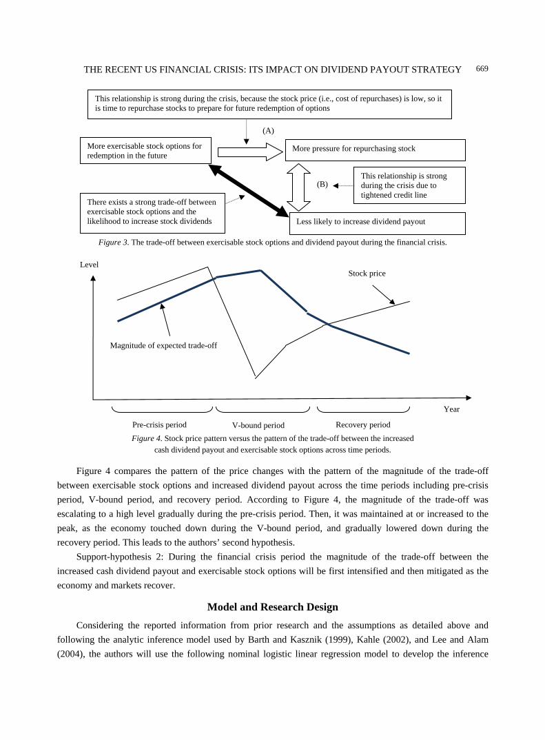
THE RECENT US FINANCIAL CRISIS: ITS IMPACT ON DIVIDEND PAYOUT STRATEGY
669
Figure 3. The trade-off between exercisable stock options and dividend payout during the financial crisis.
Figure 4. Stock price pattern versus the pattern of the trade-off between the increased
cash dividend payout and exercisable stock options across time periods.
Figure 4 compares the pattern of the price changes with the pattern of the magnitude of the trade-off between exercisable stock options and increased dividend payout across the time periods including pre-crisis period, V-bound period, and recovery period. According to Figure 4, the magnitude of the trade-off was escalating to a high level gradually during the pre-crisis period. Then, it was maintained at or increased to the peak, as the economy touched down during the V-bound period, and gradually lowered down during the recovery period. This leads to the authors’ second hypothesis.
Support-hypothesis 2: During the financial crisis period the magnitude of the trade-off between the increased cash dividend payout and exercisable stock options will be first intensified and then mitigated as the economy and markets recover.
Model and Research Design
Considering the reported information from prior research and the assumptions as detailed above and following the analytic inference model used by Barth and Kasznik (1999), Kahle (2002), and Lee and Alam (2004), the authors will use the following nominal logistic linear regression model to develop the inference
Year
Level
Pre-crisis period Recovery period V-bound period
Stock price
Magnitude of expected trade-off
More exercisable stock options for redemption in the future
More pressure for repurchasing stock
Less likely to increase dividend payout
There exists a strong trade-off between exercisable stock options and the likelihood to increase stock dividends
This relationship is strong during the crisis, because the stock price (i.e., cost of repurchases) is low, so it is time to repurchase stocks to prepare for future redemption of options
This relationship is strong during the crisis due to tightened credit line
(A)
(B)
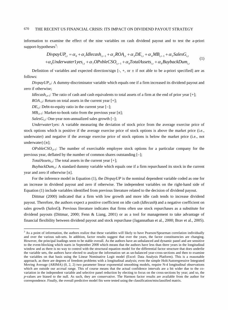
THE RECENT US FINANCIAL CRISIS: ITS IMPACT ON DIVIDEND PAYOUT STRATEGY
670
information to examine the effect of the nine variables on cash dividend payout and to test the a-priori support-hypotheses3:
, 0 1 , 1 2 , 3 , 4 , 1 5 ,
6 , 7 , 1 8 , 9 ,1i t i t i t i t i t i t
i t i t i t i t
DivpayUP Idlecash ROA DE MB SalesG
Underwater yes OPxbleCSO TotalAssets BuybackDum
α α α α α α
α α α α− −
−
= + + + + +
+ + + + (1)
Definition of variables and expected direction/sign [-, +, or ± if not able to be a-priori specified] are as follows:
DivpayUPi,t: A dummy-discriminator variable which equals one if a firm increased its dividend payout and zero if otherwise;
Idlecashi,t-1: The ratio of cash and cash equivalents to total assets of a firm at the end of prior year [+]; ROA i,t: Return on total assets in the current year [+]; DEi,t: Debt-to-equity ratio in the current year [−]; MBi,t-1: Market-to-book ratio from the previous year [±]; SalesGi,t: One-year non-annualized sales growth [−]; Underwater1yes: A variable measuring the deviation of stock price from the average exercise price of
stock options which is positive if the average exercise price of stock options is above the market price (i.e., underwater) and negative if the average exercise price of stock options is below the market price (i.e., not underwater) [±];
OPxbleCSOi,t-1: The number of exercisable employee stock options for a particular company for the previous year, deflated by the number of common shares outstanding [−];
TotalAssetsi,t: The total assets in the current year [+]; BuybackDumi,t: A standard dummy variable which equals one if a firm repurchased its stock in the current
year and zero if otherwise [±]. For the inference model in Equation (1), the DivpayUP is the nominal dependent variable coded as one for
an increase in dividend payout and zero if otherwise. The independent variables on the right-hand side of Equation (1) include variables identified from previous literature related to the decision of dividend payout.
Dittmar (2000) indicated that a firm with low growth and more idle cash tends to increase dividend payout. Therefore, the authors expect a positive coefficient on idle cash (Idlecash) and a negative coefficient on sales growth (SalesG). Previous literature indicates that firms often use stock repurchases as a substitute for dividend payouts (Dittmar, 2000; Fenn & Liang, 2001) or as a tool for management to take advantage of financial flexibility between dividend payout and stock repurchase (Jagannathan et al., 2000; Brav et al., 2005).
3 As a point of information, the authors realize that these variables will likely to have Pearson/Spearman correlation individually and over the various sub-sets. In addition, factor results suggest that over the years, the factor constituencies are changing. However, the principal loadings seem to be stable overall. As the authors have an unbalanced and dynamic panel and are sensitive to the event-blocking which starts in September 2008 which means that the authors have less than three years in the longitudinal window and as there is no way to control with the structural equation model for the differential factor structure that does underlie the variable sets, the authors have elected to analyze the information set as un-balanced year-cross-sections and then to examine the variables on that basis using the Linear Nominative Logit model (Excel: Data Analysis Platform). This is a reasonable approach, as there are degrees of freedom problems with a longitudinal analysis; even the simple Holt/Autoregressive Integrated Moving Average (ARIMA) (0, 2, 2) two parameter linear exponential smoothing models, require N-4 longitudinal observations which are outside our accrual range. This of course means that the actual confidence intervals are a bit wider due to the co-variation in the independent variable and selective panel reduction by electing to focus on the cross-sections by year; and so, the p-values are biased to the null. As such, they are conservative. The Harmon factor results are available from the author for correspondence. Finally, the overall predictive model fits were tested using the classification/misclassified matrix.
THE RECENT US FINANCIAL CRISIS: ITS IMPACT ON DIVIDEND PAYOUT STRATEGY
671
Accordingly, the authors expect that the coefficient on the dummy variable for stock repurchases (BuybackDum) could be either positive or negative.
During the financial crisis, a firm with a high debt-to-equity ratio will be less likely to increase dividend payout due to shrinking liquidity. Therefore, the authors proffer a negative coefficient on DE. The authors expect a positive coefficient on TotalAssets, because Fenn and Liang (2001) and Weisbenner (2000) found that logarithm of assets was positively associated with dividend payout and repurchase payout. Also, the authors believe that during the financial crisis, only a firm with a better financial profile will be more likely to increase dividend payout in order to restore shareholders’ confidence. Therefore, the authors expect a positive coefficient on ROA. The authors use the ratio of MB as a control variable for industry, and the direction of the coefficient on MB is unknown. The sign of the coefficient on the dummy variable coded as one for underwater stock options (Underwater1yes) is uncertain, because on the one hand, the underwater stock options resulting from the disappointing market performance could force management to increase dividend payout in order to please the frustrated investors; on the other hand, the underwater stock options could be linked to financially distressed firms with no cash available for increasing dividend payout.
Support-hypothesis 1 contends that a company with less exercisable stock options will be more likely to increase cash dividend payout after controlling for other factors. Therefore, the authors expect a significant negative coefficient on the OPxbleCSO in Equation (1). To test Support-hypothesis 2, the authors will observe the coefficient on OPxbleCSO in Equation (1) for the fiscal years from 2006 to 2010. The authors expect that the negative coefficient on OPxbleCSO representing the trade-off between the increased dividend payout and exercisable stock options will be intensified by the financial crisis and then moderated along the recovery of the economy.
Data and Sample Selection
All of the data used in this study are collected from the Standard & Poor (S&P) Compustat™ database as electronic data interchange (EDI) downloads from Wharton Research Data Services (WRDS™): The Wharton School. The period of investigation is from fiscal years from 2006 to 2010, which covers the event-period of financial crisis. All of the active US firms available on S&P Compustat as of February, 2011 are included in our sample except for the firms in the regulated or semi-regulated industries. No Industry: Standard Industrial Classification (SIC) or North American Industry Classification System (NAICS) dummies were used to control on SIC/NAICS groupings, because the abovementioned hypotheses and exploratory investigations are not conditioned upon industry coding, as the repurchase is motivated by general economic factors as opposed to industry specific considerations. This is confirmed in the literature, as there was no study that indicated that the economics or strategic repurchase had industry effects. The firms involved in stock repurchases are identified by examining the Compustat item concerning the market value of repurchases in common stocks and preferred stocks and then subtracting the market value of repurchases in preferred stocks. Therefore, the stock buybacks in this research include open-market stock repurchases and non-open market repurchases, such as tender offers and privately negotiated transactions.
The financial (SIC 6000-SIC 6999), regulated (utilities firms with SIC 4900-SIC 4999), and semi-regulated firms (SIC 8000-SIC 9999) are removed, because they are regulated, and thus their repurchase decisions are different from other firms. The firm-years are removed from the sample, if financial data are missing from Compustat. Finally, as a data preparation step, all of the data series that were used to develop the
THE RECENT US FINANCIAL CRISIS: ITS IMPACT ON DIVIDEND PAYOUT STRATEGY
672
inference information were screened for Mahalanobis outliers. These are correlation outlier-anomalies, over the non-dummy variable set, which interject non-model related possibly biasing noise (Sall, Lehman, & Creighton, 2005). The number of firms screened outside the 95% confidence level was in all cases less than 3% of the total number of firms in the full datasets (Sall et al., 2005).
Table 1 Testing Results of the Nominal Logistic Linear Regression
Variable Expected sign
Fiscal year 2006 Fiscal year 2007 Value Significance Value Significance
Idlecash + < 0.01 0.51 < 0.01 0.66 ROA + 0.63 0.012 1.88 < 0.0001 DE − < -0.01 0.67 0.000 0.75 MB ± < -0.01 0.02 0.000 0.31 SalesG − -1.1 < 0.0001 -0.87 < 0.0001 Underwater1yes ± 0.23 0.002 0.02 0.28 OPxbleCSO − -9.37 < 0.0001 -12.52 < 0.0001 TotalAssets + < 0.01 < 0.0003 < 0.01 < 0.0001 BuybackDum [0/1] ± 1.02 < 0.0001 0.96 < 0.0001 Constant ± -1.52 < 0.0001 -1.51 < 0.0001 Miss class % 15 16
N 3,201 3,352
Variable Expected sign
Fiscal year 2008 Fiscal year 2009 Fiscal year 2010
Value Significance Value Significance Value Significance Idlecash + < 0.01 0.67 < 0.01 0.15 < 0.01 0.76 ROA + 2.14 < 0.0001 0.87 < 0.0001 3.84 0.010 DE − < 0.01 0.67 < -0.01 0.64 0.14 0.20 MB ± < -0.01 0.93 -0.002 0.72 -0.03 0.56 SalesG − -0.63 0.0002 -0.61 0.0006 -0.88 0.14 Underwater1yes ± 0.0053 0.40 0.002 0.22 0.21 0.15 OPxbleCSO − -10.95 < 0.0001 -9.07 < 0.0001 -6.12 0.10 TotalAssets + < 0.01 < 0.0001 < 0.01 < 0.0001 < 0.01 0.009 BuybackDum ± 0.75 < 0.0001 0.67 < 0.0001 -0.073 0.795 Constant ± -1.49 < 0.0001 -1.55 < 0.0001 -1.34 < 0.0001 Miss class% 17 17 18 N 3,293 3,264 425a Notes. a For the data in the fiscal year 2010, the authors included the firms with data available on the Compustat as of February, 2011 (before the recent debt crisis in Europe). The fiscal year ends of these firms are prior to December 1, 2010. Therefore, the sample size was smaller. The longitudinal stability of the parameters of interest and the misclassification results are suggestive of panel with only slight random variations over the factor sets. Also as a point of model-fit information, the right-side values of the three 95% confidence intervals for the misclassifications are all less than 22%, indicating an effective model reclassification that is consistent with the fact that there are a number of significant variable classifiers.
Test Results
Our results indicate that during the financial crisis period in fiscal year 2008, around 16% of firms increased dividend payout and the remaining either did not increase or even decreased the dividend payout during the financial crisis. In contrast, prior to the financial crisis, only around 13% of firms increased dividend payout, a result for which the directional p-value is less than 0.01. This finding shows that during the financial
THE RECENT US FINANCIAL CRISIS: ITS IMPACT ON DIVIDEND PAYOUT STRATEGY
673
crisis, more firms took action to increase their dividend payouts to comfort and restore the confidence of the investors.
The results in Table 1 indicate that the lower the SalesG, the higher the DivpayUP, which is consistent with the previous literature (e.g., Dittmar, 2000). Also, the authors found a consistent positive relationship between the ROA and the DivpayUP. This finding was consistent across five years and supports the authors’ belief that only a firm with better financial profile will be more likely to increase dividend payout. It is interesting to note that the authors found a consistent and positive association between the incurrence of BuybackDum and increased DivpayUP from fiscal years 2006 to 2009, implying that the firms that engaged in increasing dividend payout are also involved in stock repurchases. These firms did not increase dividend payout by abandoning their stock repurchase plans. The result in Table 1 indicates that IdleCash is not a significant determining factor for the decision of increasing dividend payout. The authors also found that the variable underwater1yes (i.e., the exercise prices of stock options are on average above the market prices) is a significant factor in increasing dividend payout only in the pre-crisis fiscal year 2006. This finding is interesting and can be explained as follows. Before the financial crisis, a firm with underwater stock options was likely to be a firm with disappointing stock performance due to its own sluggish growth so that this firm with underwater stock options must allocate more funding to increase dividend payout in order to attract investors for holding the stocks. In contrast, during the financial crisis, many firms have underwater stock options due to the overall market crash so that underwater stock options are not the driving forces for the individual dividend payout decision.
Testing Support-Hypothesis 1
Support-hypothesis 1 contends that in a distressed market, a company with fewer exercisable stock options will be more likely to increase cash dividend payout, controlling for other factors. The results in Table 1 demonstrate that DivpayUP is inversely related to OPxbleCSO in all five years, supporting the first Support-hypothesis. Since a higher dividend payout would sacrifice the opportunities of using the same money to buy back more stocks at a historically low point, a firm that decides to offer higher dividend payout would face a higher opportunity cost, if this firm has a high volume of exercisable stock options to cope with in the future for redemption. This is consistent with the silver-lining scenario in that during the financial crisis, the extent of the trade-off between exercisable options and increased dividend payout for an individual firm reflected the perspectives of senior managers concerning the firm’s prospect, and this trade-off revealed different silver-lining strategies to the market during the storm. For example, given the same level of exercisable stock options during the financial storm, a firm that is more optimistic about its future may strategically buy back more stocks and decide not to increase the dividend payout, and other firms that are more pessimistic about their future may buy back less stocks and instead use the money as dividends to comfort the panicking stockholders. Either way, this could be argued by senior managers and would likely be viewed favorably as a wise decision in the distressed economic climate, thus supporting the relative retrenchment as warranted fiscal conservatism.
Testing Support-Hypothesis 2
The authors predict in Support-hypothesis 2 that during the financial crisis period, the magnitude of the trade-off between the increased cash dividend payout and exercisable stock options was first strong and then mitigated as the economy recovered. Comparison of the regression results from 2006 to 2010 provides further
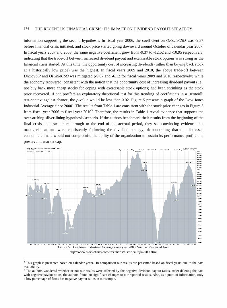
THE RECENT US FINANCIAL CRISIS: ITS IMPACT ON DIVIDEND PAYOUT STRATEGY
674
information supporting the second hypothesis. In fiscal year 2006, the coefficient on OPxbleCSO was -9.37 before financial crisis initiated, and stock price started going downward around October of calendar year 2007. In fiscal years 2007 and 2008, the same negative coefficient grew from -9.37 to -12.52 and -10.95 respectively, indicating that the trade-off between increased dividend payout and exercisable stock options was strong as the financial crisis started. At this time, the opportunity cost of increasing dividends (rather than buying back stock at a historically low price) was the highest. In fiscal years 2009 and 2010, the above trade-off between DivpayUP and OPxbleCSO was mitigated (-9.07 and -6.12 for fiscal years 2009 and 2010 respectively) while the economy recovered, consistent with the notion that the opportunity cost of increasing dividend payout (i.e., not buy back more cheap stocks for coping with exercisable stock options) had been shrinking as the stock price recovered. If one proffers an exploratory directional test for this trending of coefficients in a Bernoulli test-context against chance, the p-value would be less than 0.02. Figure 5 presents a graph of the Dow Jones Industrial Average since 20004. The results from Table 1 are consistent with the stock price changes in Figure 5 from fiscal year 2006 to fiscal year 20105. Therefore, the results in Table 1 reveal evidence that supports the over-arching silver-lining hypothesis/scenario. If the authors benchmark their results from the beginning of the final crisis and trace them through to the end of the accrual period, they see convincing evidence that managerial actions were consistently following the dividend strategy, demonstrating that the distressed economic climate would not compromise the ability of the organization to sustain its performance profile and preserve its market cap.
Figure 5. Dow Jones Industrial Average since year 2000. Source: Retrieved from
http://www.stockcharts.com/freecharts/historical/djia2000.html.
4 This graph is presented based on calendar years. In comparison our results are presented based on fiscal years due to the data availability. 5 The authors wondered whether or not our results were affected by the negative dividend payout ratios. After deleting the data with negative payout ratios, the authors found no significant changes to our reported results. Also, as a point of information, only a low percentage of firms has negative payout ratios in our sample.
THE RECENT US FINANCIAL CRISIS: ITS IMPACT ON DIVIDEND PAYOUT STRATEGY
675
Conclusions and Future Research
In this study, the authors investigated the impact of the recent financial crisis on dividend payout policies in the United States with an eye to better understand the silver-lining scenario guiding payout strategies of firms during the economic downturn. To this end, the authors created two Support-hypotheses that would provide “related” concurrent evidence. The first hypothesis is a static look at the dividend policy variable and the second is a more dynamic and benchmarked view of the same variable set. The authors test these two Support-hypotheses, and in both cases, they see consistent support for the silver-lining scenario. Specifically:
(1) The authors found that firms must have good financial profiles in order to increase their dividend payouts and the firms that engaged in increasing dividend payout are also involved in stock repurchases. Also, their evidence showed a higher percentage of firms that increased their dividend payouts possibly due to the effects of the financial crisis;
(2) The authors’ result suggests that a firm choosing to increase cash dividend payout did not have as many exercisable stock options that it needs for redemption in the future. Most importantly, the authors expect and confirm with their evidence that the aforementioned trade-off between increased cash dividend payout and exercisable stock options was intensified when stock price started falling due to the financial crisis and then moderated when stock price recovered. In conclusion, this study provides some insights into the dividend payout policies and stock buyback activities of US firms during the financial crisis;
(3) The context of the financial crisis in the USA offers an excellent opportunity to examine how companies reacted to the dramatic change in economic environment by adjusting their dividend payout policies and repurchase decisions;
(4) Future research may investigate, in a more direct way, the functioning of the silver-lining scenario as a “survival guide” in economic challenging times. This direct evidence will soon be available from firms that are involved in the Euro-zone. One may conjecture that the extent of dependence that a firm has in the global world is impacted by Euro-zone economic involvement compared with firms that are insulated from the Euro-zone current and coming difficulties. For example, the authors suggest a study using most of the same variables that they have offered in a blocked longitudinal panel and/or cross-sectional design on G-20 firms with heavy Euro-zone dependence compared with a matched set of firms with established China-connections, such as two-way partnering, venturing, and exclusive contracting. Here the authors anticipate differential effects for firms that are more committed to economic links in the Euro-zone compared with firms that are linked with the powerful Chinese economy. These differential effects should shed more light on the functioning of the silver-lining hypothesis as a way to strategize dividend payments in the face of differential economic difficulties. Another possible study is to identify firms that seem to have employed a silver-lining strategy and to select a match that does not exhibit a silver-lining profile and compare their market performance profiles over a short or intermediate run. This would identify possible market effects that reward management “strategic behavior”.
References Babenko, I. (2009). Share repurchases and pay-performance sensitivity of employee compensation contracts. Journal of Finance,
64(1), 117-150. Barth, M. E., & Kasznik, R. (1999). Share repurchases and intangible assets. Journal of Accounting and Economics, 28(5), 211-
241.
THE RECENT US FINANCIAL CRISIS: ITS IMPACT ON DIVIDEND PAYOUT STRATEGY
676
Bartov, E. (1991). Open-market stock repurchases as signals for earnings and risk changes. Journal of Accounting and Economics, 14(3), 275-294.
Bens, D. A., Nagar, V., & Wong, M. H. F. (2002). Real investment implications of employee stock option exercises. Journal of Accounting Research, 40(2), 359-393.
Bens, D. A., Nagar, V., Skinner, D. J., & Wong, M. H. F. (2003). Employee stock options, EPS dilution, and stock repurchases. Journal of Accounting and Economics, 36, 51-91.
Bozos, K., Nikolopoulos, K., & Ramgandhi, G. (2011). Dividend signaling under economic adversity: Evidence from the London Stock Exchange. International Review of Financial Analysis, 20(5), 364-374.
Brav, A., John, R. G., Campbell, R. H., & Michaely, R. (2005). Payout policy in the 21st century. Journal of Financial Economics, 77(3), 483-527.
DeAngelo, H., DeAngelo, L., & Skinner, D. J. (1992). Dividends and losses. The Journal of Finance, 47(5), 1837-1863. Dittmar, A. K. (2000). Why do firms repurchase stock? Journal of Business, 73(3), 331-355. Fenn, G. W., & Liang, N. (2001). Corporate payout policy and managerial stock incentives. Journal of Financial Economics,
60(1), 45-72. Grullon, G., & Michaely, R. (2002). Dividends, share repurchases, and the substitution hypothesis. The Journal of Finance, 57(4),
1649-1684. Gurgul, H., Mestel, R., & Schleicher, C. (2003). Stock market reactions to dividend announcements: Empirical evidence from the
Austrian stock market. Financial Markets and Portfolio Management, 17(3), 332-350. Healy, P. M., & Palepu, K. G. (1993). The effects of firms’ financial disclosure strategies on stock prices. Accounting Horizons,
7(1), 1-11. Jagannathan, M., & Stephens, C. (2003). Motives for multiple open-market repurchase programs. Financial Management, 32(2),
71-91. Jagannathan, M., Stephens, C. P., & Weisbach, M. S. (2000). Financial flexibility and the choice between dividends and stock
repurchases. Journal of Financial Economics, 57(3), 355-384. Jensen, M. (1986). Agency costs of free-cash-flow, corporate finance, and takeovers. American Economic Review, 76(2), 323-329. Jolls, C. (1998). Stock repurchases and incentive compensation. NBER Working Paper, No. 6467. Kahle, K. M. (2002). When a buyback isn’t a buyback: Open market repurchases and employee options. Journal of Financial
Economics, 63(2), 235-261. Klassen, K. J., & Sivakumar, R. (2001). Stock repurchases associated with stock options do represent dollars out of shareholders’
wallets (Unpublished Working Paper, University of Waterloo). Lee, C. H., & Alam, P. (2004). Stock option measures and the stock repurchase decision. Review of Quantitative Finance and
Accounting, 23(4), 329-352. Liang, J. N., & Sharpe, S. A. (1999). Shares repurchases and employee stock options and their implications for S&P 500 share
retirements and expected returns (Unpublished Working Paper, Division of Research and Statistics, Federal Reserve Board). Ofer, A., & Thakor, A. V. (1987). A theory of stock price responses to alternative corporate cash disbursement methods: Stock
repurchases and dividends. Journal of Finance, 42(2), 365-394. Rankine, G., & Stice, E. K. (1997). The market reaction to the choice of accounting method for stock splits and large stock
dividends. Journal of Financial and Quantitative Analysis, 32(2), 161-182. Richardson, G., Sefcik, S. E., & Thompson, R. (1986). A test of dividend irrelevance using volume reactions to a change in
dividend policy. Journal of Financial Economics, 17(2), 313-333. Russolillo, S. (2012, May 25). Some investors get defensive—Companies in certain US sectors are benefiting from a flight to
stability. Wall Street Journal, C. 4. Ryan, V. (2012). Dividends rising. CFO, pp. 17-18. Sall, J., Lehman, L., & Creighton, L. (2005). JMP start statistics: A guide to statistics and data analysis using JMP (2nd ed.).
California: Duxbury Press. Scholes, M. S., & Wolfson, M. A. (1992). Taxes and business strategy: A planning approach. Englewood Cliffs, NJ: Prentice-
Hall. Skinner, D. J. (2008). The evolving relation between earnings, dividends, and stock repurchases. Journal of Financial Economics,
87(3), 582-609. Stephens, C. P., & Weisbach, M. S. (1998). Actual share reacquisition’s in open-market repurchase programs. Journal of Finance,
53(1), 313-334.

THE RECENT US FINANCIAL CRISIS: ITS IMPACT ON DIVIDEND PAYOUT STRATEGY
677
Vascellaro, J. E. (2012, March 21). Apple pads investor wallets. In major shift, new CEO announces dividend, share buyback. Wall Street Journal.
Vermaelen, T. (1981). A common stock repurchases and market signaling: An empirical dissertation. Journal of Financial Economics, 9(2), 139-183.
Weisbenner, S. J. (2000). Corporate share repurchase in the 1990s: What role do stock options play? FEDS Working Paper, No. 2000-29.
Young, S., & Yang, J. (2011). Stock repurchases and executive compensation contract design: The role of earnings per share performance conditions. Accounting Review, 86(2), 703-733.
Journal of Modern Accounting and Auditing, ISSN 1548-6583 May 2013, Vol. 9, No. 5, 678-689
The Adoption and Maintenance of Executive Stock Option Plan
(ESOP): Company Characteristics Evaluation in Indonesia
Nur Fadjrih Asyik
Indonesia School of Economics, Surabaya, Indonesia
This paper investigates company characteristics associated with the adoption and maintenance of executive stock
option plan (ESOP) proxied with the proportion of stock options. In order to develop and inform public policies of
executive stock options, it is important to understand some of the factors that will drive a company’s decision in
order to adopt an ESOP. First, an analysis evaluates what kind of company’s characteristics is associated with these
plans. Second, an analysis examines the company characteristics that predict the adoption of such plans. This paper
contributes to that stream of accounting research by identifying several factors to the adoption of ESOP. The study
finds that intellectual capital (consisting of human capital efficiency (HCE), structural capital efficiency (SCE), and
capital employed efficiency (CEE)), risk, and financial constraints (FC) affect the adoption and maintenance of
stock option plans, these conditions will be increasingly supported in companies that experience relatively rapid
growth. HCE, risk, and FC are significant predictors of the adoption and maintenance of ESOP. The companies who
have some difficulties in observing human capital’s behavior are more likely to adopt executive stock options, and
based on our theoretical review, this is a rational course of action. Firms with higher levels of business risks are less
likely to shift some of the risks to employees through stock-based compensation, whereas firms with higher
variability in total shareholder returns are more likely to adopt executive stock options. Overall, our results suggest
that higher monitoring costs prompt firms to adopt and maintain ESOP.
Keywords: executive stock option plan (ESOP), adoption, maintenance, company characteristics
Introduction Executive stock option plan (ESOP) is a form of compensation which is given to employees, especially
executive employees, in order to reward the executives for their contributions to the company. The two parties
are performing a contract (in the agency theory, it is known as the principal and the agent) in a situation of
information asymmetry (asymmetrical information). That is, the agent has more information about the company
than the principal. In agency theory, it is assumed that individuals act to maximize their benefits. Each
individual is assumed to be motivated solely and to avoid the conflicts of interest between the principal and the
agent. ESOP is expected to be able to minimize conflict and improve the performance of agents that will be
reflected in the earnings information that is often called as the accounting profit. Theoretically, in the long term,
the company will have employees who are generally qualified and hold proprietary concepts in performing the
duties of the company. The incentives are given to corporate executives in the form of stock options in order to
increase the corporate value by improving its performance. Performance is achieved by a company related to
Nur Fadjrih Asyik, deputy chairman of Academic Affairs, Accounting, Indonesia School of Economics. Email: [email protected].
DAVID PUBLISHING
D
THE ADOPTION AND MAINTENANCE OF ESOP
679
the percentage of the capital owned by the company and also by the executives as well as the percentage of
equity-based compensation (Hribar & Collins, 2002).
The Financial Accounting Standards Board [FASB] (1995) issued a Statement of Financial Accounting
Standard (SFAS) No. 123 which recommended the company to recognize the fair value of stock compensation
as the number of dollars of compensation in the financial statements and to use option pricing model in
calculating the value of stock options. On September 4, 1998, Ikatan Akuntan Indonesia (IAI, Indonesian
Institute of Accountants) issued Financial Accounting Standards (Standar Akuntansi Keuangan, SAK) which
became officially effective on October 1, 1998, and through the SFAS No. 53, offered stock option plans to
executives as executive remuneration which was measured and recognized at fair value of stock options were
concerned (IAI, 2001).
By the developments in Indonesia, not many of the public companies adopt the ESOP in Indonesia Stock
Exchange (ISE). In 1999, only three companies implemented the ESOP, however, the number has increased to
90 in 2009. Company’s decision as to whether or not to adopt the ESOP is influenced by several characteristics,
including intellectual capital, risk, and financial constraints (FC) faced by the company (Kroumova & Sesil,
2004). In a situation where changes are very fast, a man must continue to expand and refine knowledge and to
develop creativity in order to innovate. Nahapiet and Ghosal (as cited in Agustina, 2007) stated that the
company that owns the intellectual capital will be more adaptive, innovative, and responsive to environmental
changes. This study is different from the study of Kroumova and Sesil (2004) relating to the intellectual capital
measurement methods that use the value-added intellectual coefficient (VAIC). VAIC is an analytical
procedure that is designed for management, shareholders, and relevant stakeholders in order to perform
effective monitoring and evaluation of the efficiency of value-added (VA) enterprises of the overall resources
of the company and each major component resource. Ownership of intellectual capital is one of the
determination factors of the adoption and maintenance of ESOP.
In connection with these conditions and in order to develop policy and inform the public of the executive
stock options, it is important to understand the factors that drive corporate decision for the adoption and
maintenance of ESOP, including the ownership of the intellectual capital, enterprise risk, and FC. The
condition increasingly supports the company that is currently in a state to grow and develop. Companies with
high potential growth rate have a tendency to generate high cash flows in the future and the high market
capitalization, thus enabling the company to have low capital costs.
Based on the background described above, the problems in this study can be formulated as follows: (1) Do
intellectual capital (consisting of human capital efficiency (HCE), structural capital efficiency (SCE), and
capital employed efficiency (CEE)), enterprise risk, and financial constrains influence simultaneously and
partially the adoption and maintenance of ESOP (the proportion of stock options) in companies listed in ISE?
and (2) Does the company’s growth rate have an impact on the intellectual capital (consisting of HCE, SCE,
and CEE), enterprise risk, and financial constrains that influence the adoption and maintenance of the ESOP
(the proportion of stock options) in companies listed in the ISE?
The purposes of the current study are as follows: (1) to examine simultaneously and partially the effect of
intellectual capital (consisting of HCE, SCE, and CEE), enterprise risk, and FC on the adoption and
maintenance of the ESOP (the proportion of stock options) in companies listed in the ISE; and (2) to examine
the impact of the company’s growth rate on the intellectual capital (consisting of HCE, SCE, and CEE),
THE ADOPTION AND MAINTENANCE OF ESOP
680
enterprise risk, and FC that influence the adoption and maintenance of the ESOP (the proportion of stock
options) in companies listed in ISE.
Theoretical Background
Agency Theory
The actual agency problem arises when the principal has a difficulty in ensuring that the agent acts to
maximize the welfare of the principal. According to the agency theory, one of the mechanisms that are widely
used and expected to align principal and agent goals is through the financial reporting. Because the trend for
managers is looking for their benefits (moral hazard) and the level of high information asymmetry, plus certain
motives, the likelihood of management to utilize accrual items to present the earnings in accordance with the
interests that may not fit with the interests of principals, such as owners, holders of shares, or lenders.
Problem that arises in agency relationships by Eisenhardt (1989) is the assumption of human nature
(self-interest, bounded rationality, and risk aversion), so that the pressure in the theory of agency is an
organization (the goal conflicts among members) and information (a commodity which can be purchased). With
this human nature, the principal needs to control the agent to do the work in accordance with the delegated
authority. Control of the agent can be done through monitoring, risk sharing, or both. Efforts to minimize or
control the agent-principal conflict can be classified into three main categories which are: (1) market disciplines;
(2) compensation structures; and (3) monitoring mechanisms (Traichal, Gallinger, & Johnson, 1999).
There are several alternatives in order to reduce the conflicts of interest and the agency costs. The first
alternative is the increase of the company’s stock ownership by management. This ownership will align
management interests with shareholder interests (Jensen & Meckling, 1976). The second alternative is the
increase of the ratio of dividends to net income (dividend payout ratio). Thus, there are not a lot of free cash
flows in circulation and the management was forced to seek external funding as sources for financing the
investment. The definition of free cash flow is the availability of funds in the amount that exceeds the need for
funding for profitable investments. If the profits are divided into dividends, it means that the investment needs
to be sought from the external funding sources. This will improve the oversight in external financing by
external parties, such as supervisors of capital markets, investment bankers, and investors.
ESOP
ESOP is an incentive to appreciate the long-term performance of the company, which is an effective step
to narrow and reduce the agency and agency cost problems through the alignment of interests of the executives
with the shareholders (Brenner, Sundaram, & Yermark, 2000). Ownership of shares by employees of the
company (insiders) is to give the impression as a financial investment. Ownership will provide a great feeling
of satisfaction and commitment to the company’s control (Iqbal & Abdul, 2000). ESOP is expected to improve
the performance of agents, which will be reflected in the earnings information that is often called as the
accounting earnings. Expectations are not excessive, because the theoretical equity-based compensation will
indirectly consider existence of labor, so that in the long run, companies will have employees who are generally
qualified and hold proprietary concepts in carrying out the duties of the company. Kaplan and Atkinson (1998)
stated that compensation contracts motivate corporate executives, so that the executive compensation program
should be competitive enough to attract and retain high-quality managers, linking bonuses to performance, and
able to develop performance-oriented climate within the company by giving rewards to performance assessed
well.
THE ADOPTION AND MAINTENANCE OF ESOP
681
Company Characteristics
Firm growth. Companies with high potential growth rate have a tendency to generate high cash flows in
the future and the high market capitalization, thus enabling the company to lower the cost of capital. Growth is
expected internally and externally by a company, because it can give a positive aspect to them. From the
standpoint of investors, the growth of a company is a sign that the company has a favorable aspect, and they
expect that the rate of return of their investments gives better results (Dzinkowski, 2000).
Intellectual capital. According to Stewart (as cited in Agustina, 2007), intellectual capital is a matter of
knowledge in intellectual, information, intellectual property rights, and experiences that can be used to create
wealth. Pulic (1998) proposed the measurement of intellectual capital by using the VAIC to provide
information about the efficiency of value creation of tangible and intangible assets within the company. The
VAIC method essentially measures the efficiency of companies’ three kinds of inputs, which is human capital,
structural capital, and physical and financial capital. HCE is an indicator of VA efficiency of human capital.
SCE is an indicator of VA efficiency of structural capital, while CEE is an indicator of VA efficiency of
venture capital (Bornemann & Leitner, 2002). The sum of these three indicators is VAIC value.
Risk. By comparing with a fixed salary contract, incentive pay shifts some of the risks associated with
owning a business to employees. Agency theorists suggest that it is efficient to transfer risk to employees
through incentive compensation when monitoring costs are high, and employees have control over performance
outcomes. However, a risk premium needs to be included to adjust the total compensation for the increase level
of risk. There is an extensive literature between chief executive officer (CEO) compensation and firm risk
(Aggarwal & Samwick, 1999; Beatty & Zajac, 1994; Bloom & Milkovich, 1998; Gray & Cannella, 1997;
Miller, Wiseman, & Gomez-Mejia, 2002). The literature suggests that there is an inverse relationship between
the level of firm risk and the degree to which incentive compensation for top managers is used, with some
studies finding a linear relationship between risk and CEO compensation (Miller et al., 2002). Whether such a
pattern holds for firm-wide incentive pay relatively that represents a small percentage of an individual’s total
pay is an open question that the author will address in this empirical analysis.
FC. In addition, in desiring to reduce and monitor costs, firms may be driven to adopt broad-based stock
option plans because of FC. Smaller and faster-growing firms may face higher costs of capital (Core & Guay,
2000; Ittner, Lambert, & Larcker, 2003) due to the high debt burdens already, low liquidity, or because
investors perceive the business prospects of such firms as risky. Under these circumstances, executive stock
options can help preserve the cash needed to sustain growth, assuming they are used as substitutes for other
forms of compensation, such as cash bonuses or above-average base compensation. Current accounting rules do
allow US companies to deduct the cost of stock options grants from the income reported to shareholders (as
they would be required to do if they used other forms of incentives such as bonuses or profit sharing), yet
companies can deduct the cost of options from their taxable income, calculated as the difference between the
grant price and the exercise price, if and when the options are exercised (McLean, 2000).
Related Research
There is, however, a more substantial body of literature associated with the adoption and maintenance of
equity compensation (Kruse, 1996; Sesil, Kroumova, Kruse, & Blasi, 2001). From the standpoint of investors,
the growth of a company is a sign that the company has a favorable aspect, and they expect that the rate of
return of their investments gives better results (Heath, Huddart, & Lang, 1998). Existing empirical research on
THE ADOPTION AND MAINTENANCE OF ESOP
682
employees’ stock option plans by Core and Guay (2000) found that firms use greater levels of stock option
compensation when facing capital requirements and financing constraints. Ittner et al. (2003) also examined
determinants of executive stock option compensation and found that growth opportunities, firm size, and cash
availability are associated with high levels of option compensation. Both of these studies use stock option grant
magnitude as a dependent variable and draw their data on employees’ stock option grant existence and
magnitude from 10-K financial statements. Also, both studies focus on financial factors as predictors of levels
of stock option grants and exclude from the analysis firms without broad-based employees’ stock options.
There are several reasons underlying the impacts of company characteristics on ESOP adoption and
maintenance like intellectual capital, enterprise risk, and FC. These conditions will be increasingly supported in
companies that experience relatively rapid growth. Therefore, operational hypotheses in alternative hypotheses
are advanced as follows:
H1: Intellectual capital (consisting of HCE, SCE, and CEE), risk, and financial constrains influence
simultaneously the adoption and maintenance of the ESOP (the proportion of stock options).
H2a : HCE has an influence on the adoption and maintenance of the ESOP (the proportion of stock
options).
H2b: SCE has an influence on the adoption and maintenance of the ESOP (the proportion of stock options).
H2c : CEE has an influence on the adoption and maintenance of the ESOP (the proportion of stock options).
H2d: Risk has an influence on the adoption and maintenance of the ESOP (the proportion of stock options).
H2e : FC has an influence on the adoption and maintenance of the ESOP (the proportion of stock options).
H3a : The growth rate has an impact on the HCE that influences the adoption and maintenance of the ESOP
(the proportion of stock options).
H3b: The growth rate has an impact on the SCE that influences the adoption and maintenance of the ESOP
(the proportion of stock options).
H3c : The growth rate has an impact on the CEE that influences the adoption and maintenance of the ESOP
(the proportion of stock options).
H3d: The growth rate has an impact on the risk that influences the adoption and maintenance of the ESOP
(the proportion of stock options).
H3e : The growth rate has an impact on the FC that influences the adoption and maintenance of the ESOP
(the proportion of stock options).
Methodology
Population and Sample
The study population includes companies listed in ISE (Bursa Efek Indonesia, BEI). Standards regarding
the stock-based compensation (executive stock options) became effective in 1998, and some companies had
implemented ESOP since 1999. The sample selection is determined by purposive sampling in order to obtain a
representative sample in accordance with the specified criteria. The criteria used for selecting the sample are as
follows: (1) companies that have listed in ISE before December 31, 2007 and offered stock options to executive;
(2) issuers that already include the financial statements in December 31, 2007, 2008, and 2009. Election periods
are based on the grounds that the statements at December 31 are the reports that have been audited, so that
those statements can be more reliable. In addition, most companies in the chosen period have offered stock
option programs; and (3) issuers that have adopted executive stock option program in 2007, 2008, and 2009
THE ADOPTION AND MAINTENANCE OF ESOP
683
continuously. The final sample of this study comprised as many as 21 samples of the company. The number of
observations was 63.
Variable and Operational Definition
Dependent variable (proportion of stock option). Dependent variable in this study is the adoption and
maintenance of ESOP. The variable measures the proportion of executive stock options. For Balsam, Chen, and
Sankaraguruswamy (2003), the proportion of employees’ stock options is the number of stock options granted
to executives during the event window deflated with managerial ownership.
Independent variables. Independent variables in this study include intellectual capital (consisting of HCE,
SCE, and CEE), risk, and FC.
Intellectual capital. Intellectual capital includes three components of the VAIC, namely, HCE, SCE, and
CEE. The data used in the calculation of VAIC are obtained from financial statements. VAIC calculation
procedure can be performed as follows:
, , , ,i t i t i t i tVAIC HCE SCE CEE= + + (1)
where:
VAICi,t = Value-added intellectual coefficient for firm i in period t;
HCEi,t = Human capital efficiency for firm i in period t;
SCEi,t = Structural capital efficiency for firm i in period t;
CEEi,t = Capital employee efficiency for firm i in period t.
The first step in determining VAIC is to determine the total VA. VA can be calculated by Equation (2):
, , , , , , , ,i t i t i t i t i t i t i t i tVA I DP D T M R WS= + + + + + + (2)
where:
VAi,t = Value added for firm i in period t;
Ii,t = Interest expense for firm i in period t;
DPi,t = Depreciation expense for firm i in period t;
Di,t = Dividend for firm i in period t;
Ti,t = Corporate taxes for firm i in period t;
Mi,t = Equity of minority shareholders in net income of subsidiaries for firm i in period t;
Ri,t = Profit retained for firm i in period t;
WSi,t = Wages and salaries for firm i in period t.
HCE. Total of salaries and wages is an indicator for human capital firms. HCE can be calculated with the
formula as below (see Equation (3)):
,,
,
i ti t
i t
VAHCE
HC= (3)
where HCi,t = Total of salary and wage cost for firm i in period t.
SCE. Structural capital can be calculated by Equation (4):
, , ,i t i t i tSC VA HC= − (4)
where SCi,t = Structural capital for firm i in period t.
To calculate the different calculations of HCE, SCE, and CEE, SC is a numerator, but HC and CE are
denominators. Specifically, SCE is the ratio of structural capital divided by total VA. Relationship is shown by
THE ADOPTION AND MAINTENANCE OF ESOP
684
Equation (5):
,,
,
i ti t
i t
SCSCE
VA= (5)
CEE. CEE is the ratio of VA divided by the total amount of capital employed, defined as book value of net
assets of the company. CEE can be calculated by Equation (6):
,,
,
i ti t
i t
VACEE
CE= (6)
where CEi,t = Book value of the net asset for firm i in period t.
Risk. The author used standard deviation of annual sales as a proxy.
Financial constraints. The author used the 3-year average ratio of long-term debt to invested capital (the
firm’s debt burden).
Moderating variable (Growth/Tobin’s q (G)). The growth of the company is a company’s ability to
improve size, proxied by Tobin’s q value (Ekawati, 2005). The company is said to grow if Tobin’s q value is
greater than or equal to one, and it is said to not grow if it has a value smaller than one. Tobin’s q is calculated
as follows:
( )' ( )
Total Debt Outstanding Share Closing PriceTobins q G
Book Valueof Asset
+ × =
(7)
Method of Analysis
This research utilizes primary analysis tool which is multiple linear regression to examine the impact
growth on influence of company characteristics to adoption and maintenance of ESOP as follows:
, 0 1 , 2 , 3 , 4 , 5 , 6 ,
7 , 8 , 9 , 10 , ,
- i t i t i t i t i t i t i t
i t i t i t i t i t
A M HCE SCE CEE R FC HCE G
SCE G CEE G R G FC G
β β β β β β β
β β β β ε
= + + + + + + ∗
+ ∗ + ∗ + ∗ + ∗ + (8)
where:
A-Mi,t = Adoption and maintenance of the ESOP;
HCEi,t = Human capital efficiency for firm i in period t;
SCEi,t = Structural capital efficiency for firm i in period t;
CEEi,t = Capital employee efficiency for firm i in period t;
Ri,t = Risk for firm i in period t;
FCi,t = Financial constraints for firm i in period t;
Gi,t = Growth for firm i in period t.
Normality Test
Normality test aims to test whether the regression model, the dependent variable and independent
variables have a normal distribution or not. A good regression model is to have a normal data distribution or
nearly normal.
Classic Assumption Test
Multicollinearity test. To determine the presence of multicollinearity, the rules can be seen are: (1) the
value of tolerance and its opponent variance inflation factor (VIF). Value commonly used to indicate the
presence of multicollinearity is the tolerance value less than 0.10 or equaling to the value of VIF > 10; and (2)
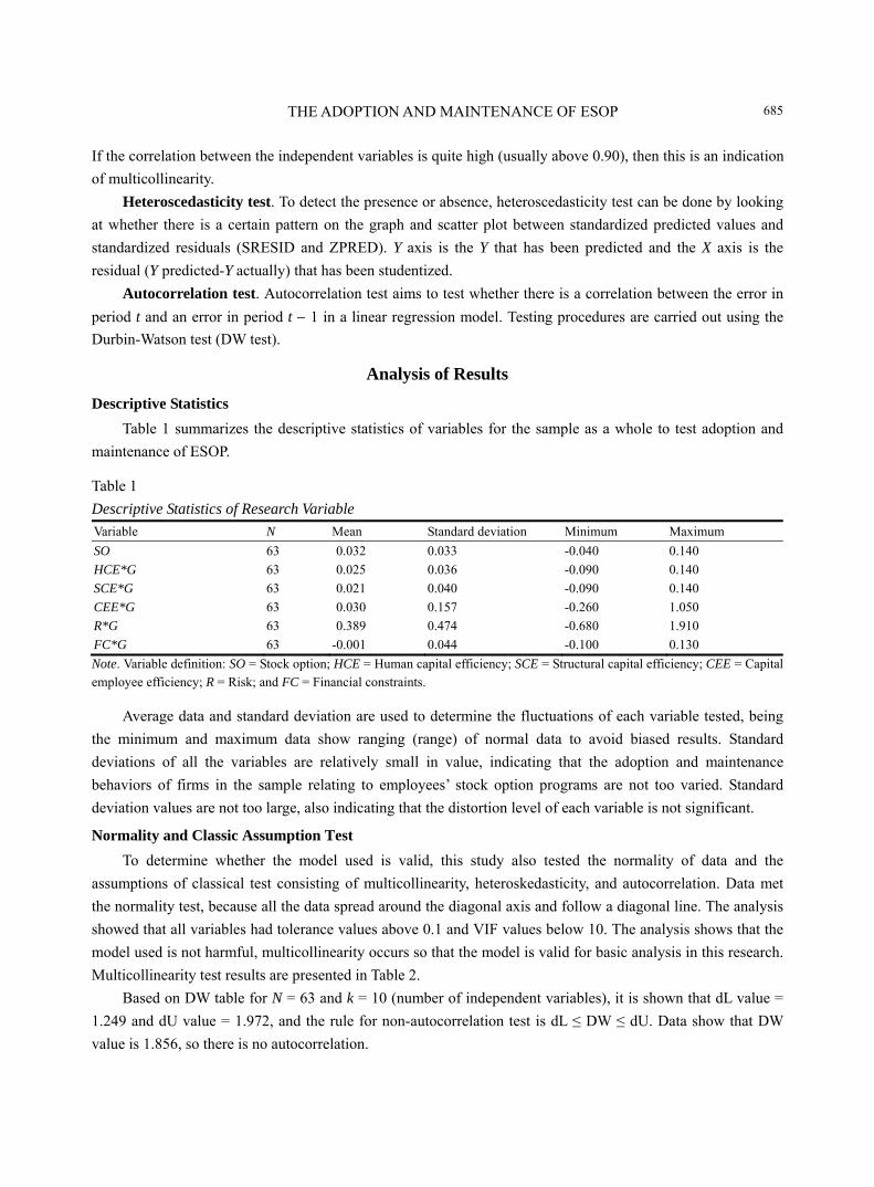
THE ADOPTION AND MAINTENANCE OF ESOP
685
If the correlation between the independent variables is quite high (usually above 0.90), then this is an indication
of multicollinearity.
Heteroscedasticity test. To detect the presence or absence, heteroscedasticity test can be done by looking
at whether there is a certain pattern on the graph and scatter plot between standardized predicted values and
standardized residuals (SRESID and ZPRED). Y axis is the Y that has been predicted and the X axis is the
residual (Y predicted-Y actually) that has been studentized.
Autocorrelation test. Autocorrelation test aims to test whether there is a correlation between the error in
period t and an error in period t − 1 in a linear regression model. Testing procedures are carried out using the
Durbin-Watson test (DW test).
Analysis of Results
Descriptive Statistics
Table 1 summarizes the descriptive statistics of variables for the sample as a whole to test adoption and
maintenance of ESOP.
Table 1
Descriptive Statistics of Research Variable
Variable N Mean Standard deviation Minimum Maximum
SO 63 0.032 0.033 -0.040 0.140
HCE*G 63 0.025 0.036 -0.090 0.140
SCE*G 63 0.021 0.040 -0.090 0.140
CEE*G 63 0.030 0.157 -0.260 1.050
R*G 63 0.389 0.474 -0.680 1.910
FC*G 63 -0.001 0.044 -0.100 0.130
Note. Variable definition: SO = Stock option; HCE = Human capital efficiency; SCE = Structural capital efficiency; CEE = Capital employee efficiency; R = Risk; and FC = Financial constraints.
Average data and standard deviation are used to determine the fluctuations of each variable tested, being
the minimum and maximum data show ranging (range) of normal data to avoid biased results. Standard
deviations of all the variables are relatively small in value, indicating that the adoption and maintenance
behaviors of firms in the sample relating to employees’ stock option programs are not too varied. Standard
deviation values are not too large, also indicating that the distortion level of each variable is not significant.
Normality and Classic Assumption Test
To determine whether the model used is valid, this study also tested the normality of data and the
assumptions of classical test consisting of multicollinearity, heteroskedasticity, and autocorrelation. Data met
the normality test, because all the data spread around the diagonal axis and follow a diagonal line. The analysis
showed that all variables had tolerance values above 0.1 and VIF values below 10. The analysis shows that the
model used is not harmful, multicollinearity occurs so that the model is valid for basic analysis in this research.
Multicollinearity test results are presented in Table 2.
Based on DW table for N = 63 and k = 10 (number of independent variables), it is shown that dL value =
1.249 and dU value = 1.972, and the rule for non-autocorrelation test is dL ≤ DW ≤ dU. Data show that DW
value is 1.856, so there is no autocorrelation.
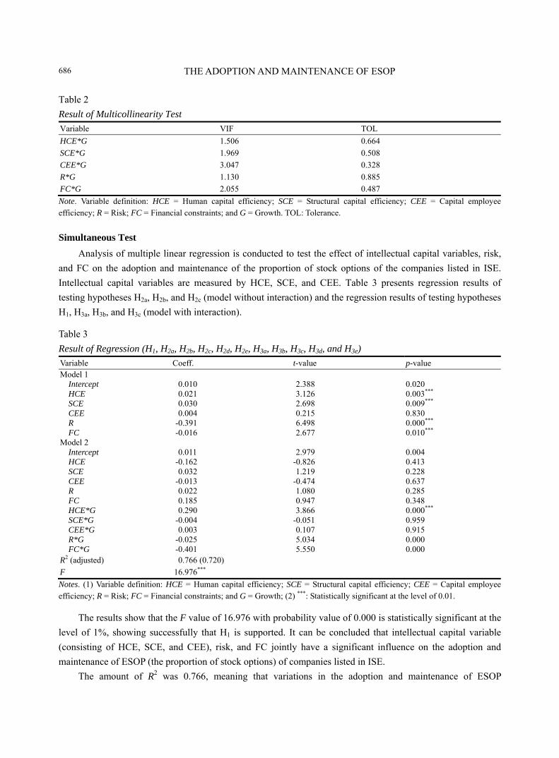
THE ADOPTION AND MAINTENANCE OF ESOP
686
Table 2
Result of Multicollinearity Test
Variable VIF TOL
HCE*G 1.506 0.664
SCE*G 1.969 0.508
CEE*G 3.047 0.328
R*G 1.130 0.885
FC*G 2.055 0.487
Note. Variable definition: HCE = Human capital efficiency; SCE = Structural capital efficiency; CEE = Capital employee efficiency; R = Risk; FC = Financial constraints; and G = Growth. TOL: Tolerance.
Simultaneous Test
Analysis of multiple linear regression is conducted to test the effect of intellectual capital variables, risk,
and FC on the adoption and maintenance of the proportion of stock options of the companies listed in ISE.
Intellectual capital variables are measured by HCE, SCE, and CEE. Table 3 presents regression results of
testing hypotheses H2a, H2b, and H2c (model without interaction) and the regression results of testing hypotheses
H1, H3a, H3b, and H3c (model with interaction).
Table 3
Result of Regression (H1, H2a, H2b, H2c, H2d, H2e, H3a, H3b, H3c, H3d, and H3e)
Variable Coeff. t-value p-value Model 1
Intercept HCE SCE CEE R FC
0.010 0.021 0.030 0.004
-0.391 -0.016
2.388 3.126 2.698 0.215 6.498 2.677
0.020 0.003*** 0.009*** 0.830 0.000*** 0.010***
Model 2 Intercept HCE SCE CEE R FC HCE*G SCE*G CEE*G R*G FC*G
0.011
-0.162 0.032
-0.013 0.022 0.185 0.290
-0.004 0.003
-0.025 -0.401
2.979
-0.826 1.219
-0.474 1.080 0.947 3.866
-0.051 0.107 5.034 5.550
0.004 0.413 0.228 0.637 0.285 0.348 0.000*** 0.959 0.915 0.000 0.000
R2 (adjusted) 0.766 (0.720)
F 16.976***
Notes. (1) Variable definition: HCE = Human capital efficiency; SCE = Structural capital efficiency; CEE = Capital employee efficiency; R = Risk; FC = Financial constraints; and G = Growth; (2) ***: Statistically significant at the level of 0.01.
The results show that the F value of 16.976 with probability value of 0.000 is statistically significant at the
level of 1%, showing successfully that H1 is supported. It can be concluded that intellectual capital variable
(consisting of HCE, SCE, and CEE), risk, and FC jointly have a significant influence on the adoption and
maintenance of ESOP (the proportion of stock options) of companies listed in ISE.
The amount of R2 was 0.766, meaning that variations in the adoption and maintenance of ESOP
THE ADOPTION AND MAINTENANCE OF ESOP
687
(proportion of stock options) of companies listed in ISE are influenced by the intellectual capital (comprised
HCE, SCE, and CEE), risk, financial constraints and growth of 76.6%, while the remaining balance of 23.4%
influenced by other factors is not examined. The results of this study support the research conducted by
Kroumova and Sesil (2004) who provided support to the claim that higher monitoring costs prompt firms to
adopt and maintain employees’ stock option plans. Firms with higher levels of business risks are less likely to
shift some of the risks to employees through stock-based compensation, whereas firms with higher variability
in total shareholder returns are more likely to adopt broad-based employees’ stock options or ESOP.
Partially Test
Test about influence of intellectual capital on the adoption and maintenance of ESOP (proportion of
stock options). The results of the analysis in Table 3 (model 1) show that the coefficients β1, β2, and β3 have
positive values of 0.021, 0.030, and 0.004 with p-values of 0.003, 0.009, and 0.830 which are statistically
significant at the level of 1% for HCE and SCE, while for the CEE, they are not significant. Thus, it is
concluded that the study successfully supports H2a and H2b, but not successfully supports H2c. Thus, HCE and
SCE partially have a significant influence on the adoption and maintenance of stock options of the companies
listed in ISE. This proves that the company needs employees’ skill in improving corporate performance,
because with many professional and expert employees who have extensive knowledge and experiences within
the company, the company will be able to compete (Kahneman & Tversky, 1973). Structural capital is always
associated with the company’s routines and structures that support employees’ efforts to produce an optimal
intellectual performance in order to improve the company’s overall business performance.
Test about influence of risk and FC on the adoption and maintenance of ESOP (proportion of stock
options). The results of the analysis in Table 3 (model 1) show that the coefficients β4 and β5 have negative
values of -0.391 and -0.016 with p-values of 0.000 and 0.010, thus, they are statistically significant at the level
of 5%. As such, it is concluded that this study successfully supports H2d and H2e, thus, risk and FC partially
have a significant effect on the adoption and maintenance of ESOP (proportion of stock options). The greater
the risk the company faces, the less likely the company will implement an executive stock option program. This
is equivalent to the condition of FC of the company.
Test about the impact of growth on the influence of intellectual capital (HCE, SCE, and CEE) on the
adoption and maintenance of ESOP (proportion of stock options). The results of the analysis in Table 3
(model 2) show that the coefficients β6, β7, and β8 have values of 0.290, -0.004, and 0.003 with p-values of
0.000, 0.959, and 0.915, thus, they are statistically significant at the level of 1%. Thus, it is concluded that the
study successfully supported H3a, but was unable to support the H3b and H3c. Thus, the higher the level of
corporate growth, the stronger the influence of HCE on the adoption of the ESOP of companies listed in ISE.
This will increase the profitability of the company that culminates in a performance improvement (Yermack,
1997).
Test about the impact of growth on the influence of risk on the adoption and maintenance of ESOP
(proportion of stock options). The results of the analysis in Table 3 (model 2) show that the coefficient β9 is
-0.025 with p-value of 0.000, thus, it is statistically significant at the level of 1%. Thus, it is concluded that the
research successfully supports H3d. Thus, the higher the growth of the company, the stronger the influence of
risk on the adoption and maintenance of ESOP (proportion of stock options) of companies listed in ISE. Every
investment involves risk, and the company will consider the risk level to decide the implementation of
THE ADOPTION AND MAINTENANCE OF ESOP
688
employees’ stock option programs. If the risk level is high, the company will be likely to delay the
implementation of the ESOP until the company’s condition is relatively stable.
Test about the impact of growth on the influence of FC on the adoption and maintenance of ESOP
(proportion of stock options). The results of the analysis in Table 3 (model 2) show that the coefficient β10 is
negative for -0.041 with p-value of 0.000, thus, it is statistically significant at the level of 1%. Thus, it is
concluded that the research successfully supports H3e. As such, the higher the growth of the company, the
stronger the influence of FC on the adoption and maintenance of ESOP (proportion of stock options) of
companies listed in ISE. Company’s financial condition will influence the decision for adoption and split shares
to the executive. If the company’s financial condition is good, then it shows the achievements of executives in
managing the company, so the company will tend to apply and divide the ESOP, but it will be the other way
around, if the company’s financial condition is not good.
Conclusions and Suggestions
Conclusions
Knowledge capabilities of employees in improving corporate performance are increasingly needed, as
with many professional employees and experts who have extensive knowledge and experiences within the
company will have an impact on the survival of an enterprise. This shows that intellectual capital is an
important factor for the company who offers executive stock options. The company’s risk and financial
constraints faced by the company have also been considered for implementation of executive stock options
program. In a growing company, employees’ increasing ability of bringing a brilliant idea of doing a new
innovation will encourage the creation of products that are more favorable in the eyes of consumers
(Abdolmohammadi, 2005).
Suggestions
The next research may use a longer period of time to get many research samples and perhaps find better
results. The next research can also test obtained research sample pursuant to the same period to know whether
there is a difference of behavior of earnings management related to stock option.
References Abdolmohammadi, M. J. (2005). Intellectual capital disclosure and market capitalization. Journal of Intellectual Capital, 6(3),
397-416. Aggarwal, R., & Samwick, A. (1999). The other side of the trade-off: The impact of risk on executive compensation. The Journal
of Political Economy, 107(1), 65-105. Agustina, W. (2007). Analysis of effect of intellectual capital performance against public accountant in Surabaya (Thesis, Faculty
of Economics, University of Airlangga, Surabaya). Balsam, S., Chen, H., & Sankaraguruswamy, S. (2003). Earnings management prior to stock option grants (Working Paper,
Temple University and Georgetown University). Beatty, R., & Zajac, E. (1994). Managerial incentives, monitoring, and risk bearing: A study of executive compensation,
ownership, and board structure in initial public offerings. Administrative Science Quarterly, 39(2), 313-335. Bloom, M., & Milkovich, G. T. (1998). Relationships among risk, incentive pay, and organizational performance. Academy of
Management Journal, 41(3), 283-297. Bornemann, M., & Leitner, K. H. (2002). Measuring and reporting intellectual capital: The case of a research technology
organization. Singapore Management Review, 24(3), 7-19. Brenner, M., Sundaram, R. K., & Yermark, D. (2000). Altering the term of executive stock option. Journal of Financial
Economics, 31(2), 103-128.
THE ADOPTION AND MAINTENANCE OF ESOP
689
Core, J., & Guay, W. (2000). Stock option plans for non-executive employees. Journal of Financial Economics, 61(2), 253-287. Dzinkowski, R. (2000). The measurement and management of intellectual capital: An introduction. Management Accounting,
78(2), 32-36. Eisenhardt, K. (1989). Agency theory: An assessment and review. Academy of Management Journal, 14(1), 57-74. Ekawati, E. (2005). Level of growth and accounting profitability in corporate value creation strategy. Journal of Accounting
Research Indonesia, 8(1), 50-64.
Financial Accounting Standards Board [FASB]. (1995). Accounting for stock-based compensation. Statement of Financial
Accounting Standard No. 123. Gray, S., & Cannella, A. (1997). The role of risk in executive compensation. Journal of Management, 23(4), 517-540. Heath, M., Huddart, S., & Lang, M. (1998). Psychological factors and stock option exercise. The Quarterly Journal of Economics,
114(2), 601-627. Hribar, P., & Collins, D. W. (2002). Errors in estimating accruals: Implication for empirical research. Journal of Accounting
Research, 40(1), 105-134. Ikatan Akuntan Indonesia [IAI]. (2001). Pernyataan Standar Akuntansi Keuangan No. 53. Standar Akuntansi Keuangan. Penerbit
Salemba, Jakarta. Iqbal, Z., & Abdul, H. S. (2000). Stock price and operating performance of ESOP firms: A time series analysis. Quarterly Journal
of Business and Economics, 39(3), 25-47. Ittner, C., Lambert, R., & Larcker, D. (2003). The structure and performance consequences of equity grants to employees of new
economy firms. Journal of Accounting and Economics, 34(1-3), 89-127. Jensen, M., & Meckling, W. H. (1976). Theory of the firm: Managerial behavior, agency costs, and ownership structure. Journal
of Financial Economics, 3(4), 305-360. Kahneman, D., & Tversky, A. (1973). On the psychology of prediction. Psychological Review, 80(4), 237-251. Kaplan, R., & Atkinson, A. A. (1998). Advanced management accounting (3rd ed.). Englewood Cliffs, New Jersey, NJ: Prentice
Hall. Kroumova, M. K., & Sesil, J. C. (2004). Intellectual capital, monitoring, and risk: What predicts the adoption of broad-based
employee stock options? Working Paper. Kruse, D. (1996). Why do firms adopt profit-sharing and employee ownership plans? British Journal of Industrial Relations,
34(4), 515-538. McLean, B. (2000). The bad news about options. Fortune Magazine, pp. 429-430. Miller, J., Wiseman, R., & Gomez-Mejia, L. (2002). The fit between CEO compensation design and firm risk. Academy of
Management Journal, 45(4), 745-756. Pulic, A. (1998). Measuring the performance of intellectual capital in knowledge economy. Retrieved from
http://www.measuring-ip.at/English/frame.html Sesil, J., Kroumova, M., Kruse, D., & Blasi, J. (2001). Broad-based employee stock options in US new economy firms. British
Journal of Industrial Relations, 40(2), 273-294. Traichal, P. A., Gallinger, G. W., & Johnson, S. A. (1999). The relationship between pay-for-performance contracting and external
monitoring. Managerial Finance, 25(9), 68-88. Yermack, D. (1997). Good timing: CEO stock option awards and company news announcements. Journal of Finance, 52(2),
449-476.
Journal of Modern Accounting and Auditing, ISSN 1548-6583 May 2013, Vol. 9, No. 5, 690-696
Pyramid Schemes and Multilevel Marketing (MLM):
Two Sides of the Same Coin
Olubusola H. Akinladejo, Marjorie Clarke, Felix O. Akinladejo University of Technology, Kingston, Jamaica
Since the recent crack down on pyramid and ponzi schemes, there have been attempts by unscrupulous persons to
devise alternative means of attracting unsuspecting persons willing to do legitimate businesses for financial gains.
The Caribbean Policy Research Institute [CaPRI1] (2008) in its report titled “Investigating Informal Investment
Schemes in Jamaica” stated in its analysis of the characteristics of multilevel, pyramid, and ponzi schemes that
despite the heterogeneity in the structure of these organizations, they all involve large numbers of small investors
who are often lured into participating in a wide range of investment activities or financial hedging through the
administration of a central unit. These schemes rely predominantly on new customers/clients to fund payments to
existing customers. The need for a consistent supply of new recruits for sustainability and perceived growth is
paramount. Based on the CaPRI report, pyramid schemes are unsustainable investment ploys that always fail to
meet the expectations of over 90% of its investors with very little emphasis on profit-making ventures or products.
This paper will examine the similarity between the recently foiled financial pyramid schemes and the current
multilevel marketing (MLM) strategies of consumables that are cunningly being proposed as legitimate business
and entrepreneurial options. This paper will present handy information for persons interested in participating in
MLM businesses and regulators in order to make informed decisions to avoid a repeat of unwise investment.
Keywords: pyramid scheme, multilevel marketing (MLM), market practices act, fraud
Introduction
At the beginning of the last decade, the Caribbean saw a fresh surge of the type of fraud popularly known as pyramid schemes. These schemes were presented to unsuspecting persons as alternative investment schemes and clubs. Initially, governments did very little to warn their citizens about these schemes not recognizing how enticing they were to people and perhaps relying on the efficacy of laws and mechanisms already put in place to deal with them. During the last decade, pyramid schemes rose and fell in countries such as Romania and Albania and by the middle of this decade, pyramid schemes were deeply rooted in countries such as Jamaica in the region with persons from all facets of society being involved in varying degrees. Even though some of these schemes originated in the Caribbean, a number of persons outside the Caribbean and especially in the United
Olubusola H. Akinladejo, senior lecturer/subject leader, College of Business and Management, University of Technology. Marjorie Clarke, lecturer, College of Business and Management, University of Technology. Felix O. Akinladejo, senior lecturer/graduate studies coordinator, Faculty of Engineering and Computing, University of
Technology. Correspondence concerning this article should be addressed to Olubusola H. Akinladejo, senior lecturer/subject leader, College
of Business and Management, University of Technology. Email: [email protected]. 1 CaPRI is a Caribbean think tank that promotes evidence-based policy making in the region.
DAVID PUBLISHING
D
PYRAMID SCHEMES AND MULTILEVEL MARKETING
691
States invested in these schemes as evidenced by the recent conviction of David Smith of Olint in the United States for wire fraud. It is believed that even persons in government within the Caribbean who should have known better were deceived by this nicely packaged fraud in wrappings of alternative investment schemes. Some believed that this was the road to financial freedom of underdeveloped countries and so disregarded public notices. According to Daily Gleaner (2009), the Financial Services Commission (FSC) issued a warning to the public not to invest in Worldwise scheme. The warning was not heeded by the public as persons continued to invest in the scheme. Originators of pyramid schemes supported laudable projects in society and were perceived to be the Moses leading many both poor and rich to their financial freedom. By the turn of the decade when government apparatus woke up from slumber, the warnings came too late. In February 2009, United States federal regulators charged Allen Stanford, head of the Antigua-based Stanford International Bank, and three of his firms with a massive fraud that centered on high interest rate certificates of deposit. By October 2009, according to the FSC Jamaica public notice (Sunday Observer, 2009), there had been about 58 unregistered alternative investment schemes in Jamaica. These unregulated investment schemes appeared to be a law onto themselves, with David Smith, head of the failed foreign exchange trading scheme, Olint, refusing to comply with the directives of the FSC in 2006, based on the statutory powers granted by the FSC under the Financial Services Act. David Smith challenged the FSC’s “cease and desist” order stating that the regulators had no statutory authority to regulate his operations (Olint Corporation Limited and David Smith v The Financial Services Commission, 2006). In 2010, David Smith, pleaded guilty to four of the 30 fraud-related charges and was sentenced in Turks and Caicos Islands. In November 2010, five weeks before he began serving his prison sentence, David Smith was slapped with additional 23 count indictments on fraud charges in Florida. It is now obvious that both Stanford and Smith gave what appeared to be face lifts to pyramid and ponzi schemes which they paraded as legitimate investments. This paper attempts to show similarities between pyramid schemes and some multilevel marketing (MLM) strategies for informed decisions by regulators and investors.
Pyramid Schemes
A pyramid literally is a triangular-shaped structure with the apex being the top tier, expanding as it gets closer to the base. As the name suggests pyramid, schemes are characterized by the same shape with one or few persons being at the apex and the majority of persons being at the base of the structure, hence the shape of a triangle. A pyramid scheme is often described as a “business opportunity”. The distinctive characteristic of this “business opportunity” is that the only way participants can make money is by recruiting other members to the scheme who quickly find out that their successes depend entirely on their ability to recruit other persons to the scheme. The scheme promises very high returns over relatively short periods, which is what makes it attractive, there is little or no product or service to generate income needed to justify the level of high returns promised and there is a high dependence on testimonials to prove credibility. The testimonials are however usually from a few persons at the top of the pyramid who are making the high profits. The persons at the bottom of the pyramid lose.
Types of Pyramid Schemes and How They Work
There are several types of pyramid schemes. This paper will focus on two basic types: naked pyramids and product-based pyramids.
PYRAMID SCHEMES AND MULTILEVEL MARKETING
692
Naked pyramid scheme. A naked pyramid starts with one person who is at the apex of the pyramid and recruits a number of persons, for example, 10 other persons to participate in an “investment opportunity”, each of whom is required to invest $100. Once they have invested in this scheme, they are required to recruit 10 other persons to participate in the same “business opportunity”. Assuming that each recruit is successful, they will all end up with $900 profit having only invested $100. Promotion within the scheme is based on how many recruits a participant brings in. An example of the naked pyramid scheme is a gifting scheme.
Product-based pyramid scheme. A product-based pyramid has all the features of a naked pyramid with the addition of a product which gives the impression of legitimate sales taking place. The initial recruiter as a distributor of the product recruits, for example, 10 sales persons who each pays an amount ($500) for a starter kit of products to sell, from which the distributor gets 10% of each starter kit sold. The distributor also gets 10% of each product sold by his recruits and any additional starter kits they sell. Typically, these products are not in high demand and the recruits quickly realize that the only way to make money is by recruiting other persons to buy starter kits knowing very well that selling the products is a difficult task.
Pyramid scheme is a category of fraud in that persons are deceived into believing that once they invest an amount, they will make significant profits in a very short period of time. In most instances, there is no product or service being offered, and even where there are, these products have little or no resale value, making the potential for earnings without recruiting very low or relatively insignificant compared with projections made. Irrespective of the type of pyramid scheme, mathematically, it is impossible for everyone to make money, as the wider the base of the pyramid becomes, the smaller the pool of potential recruits. The closer the recruits are to the bottom of the pyramid, the more likely they are to lose their investments due to market saturation and inability to get new recruits, and the scheme eventually collapses. The persons at the bottom of the pyramid who are not able to recruit would have invested and lost their money. The bottom line is that pyramid schemes are not sustainable.
A number of countries, such as USA, European Union countries, New Zealand, Australia, Canada, and Barbados, have legislation directly prohibiting pyramid selling schemes in their consumer protection laws in addition to general and specific fraud legislation. However, there are other countries, such as Jamaica, which have legislations dealing with fraud and unregulated investment schemes but where there is no specific prohibition of pyramid schemes. The Jamaica Consumer Protection Act (The Jamaica Parliament, 2005) provided for offences such as misleading advertising but has no specific provision prohibiting pyramid selling schemes. Pyramid schemes in these jurisdictions are unregulated and in the absence of robust scrutiny, there are more and more convoluting schemes being devised as the tricksters strategize new ways to avoid detections. Their target market is unsuspecting victims who are attracted by the promise of extremely high returns in relatively short periods for doing very little.
MLM
The marketing of products using individuals as sales persons is perhaps one of the earliest forms of marketing strategies. For hundreds of years, sales persons found creative ways of wooing buyers. However, this strategy of getting buyers sometimes called recruiters has been taken to another level in more recent time using a concept generally referred to as MLM or network marketing. MLM businesses draw income primarily from expansion of the hierarchical network of independent sellers conceived. The main purpose of the system is to recruit new distributors which in the hierarchy of the system can be climbed. Using a MLM strategy, a large
PYRAMID SCHEMES AND MULTILEVEL MARKETING
693
number of products such as cosmetics, cookware and health products, and more recently, coffee are sold through a large network of distributors. Sales persons who are sometimes called independent business owners (IBO) are recruited based on an attractive “sell” of the potential to earn significant amounts from an initial investment made to buy an instant business. Proponents of this strategy argue that it is a legitimate method of selling commercially viable products and services. The key element of a legitimate MLM is having commercially viable products and services to sell.
However, there are certain MLM strategies where the focus is not on the product but on the recruitment of IBOs. These MLM businesses are often referred to as motivational organizations focusing mainly on luring potential IBOs to recruitment/motivational meetings where they are told about extraordinary income opportunity in the business. Speakers claim that they have personally become wealthy. In addition, recruits are told that they need to purchase marketing materials which may include books, tapes, and sample kits and attend seminars offered by acclaimed distributors in order to become successful distributors. At these meetings, there is often a “big do” about how much profit is being made by specific distributors (team leaders) who are usually persons who joined the scheme early. Testimonials of these persons usually centre on how they use initial investment which is the cost of a starter kit/sample products to earn exponential profits. Some MLMs have taken the tactics of recruitment, a step further by enticing and appealing to ostentatious life styles through announcement of give-away expensive cars, diamonds, and other luxury items to top-performing recruiters/distributors. Selling products to end users is not the main criterion.
The disturbing aspect of these MLMs is that a high proportion of the subsequent IBOs when interviewed admit that they have not made any significant profit as envisioned and they usually have to fall back on testimonials of early IBOs to convince potential IBOs. The cost of the product is usually unrealistic and so the focus is on recruiting IBOs rather than on selling the product. Often, IBOs are encouraged to give away some of the products they purchased to potential IBOs in a bid to encourage them to join the scheme.
Inference and Implications
Whilst the originators of various MLM businesses have maintained that they do legitimate business, court judgments and settlements by these MLM businesses suggest otherwise. Amway, a USA-based MLM company involved in the production and distribution of household products, including cleaning agents, cookware, vitamins, food supplements, skin care products, make-up, hair, body, and oral care products is perhaps arguably, the largest, oldest, and best-known representative of MLM. Amway in 2010 announced that it agreed to pay restitution to consumers and reform costs estimated at over $150 million. A class action had been filed against Amway in 2007 by former distributors for Quixtar (former name used by Amway in the USA) alleging that the MLM business was a pyramid scheme which induced sales persons to buy thousands of dollars of overpriced products and useless “success tools” and recruit others to do the same in an endless chain scheme that doomed, by designing nearly all to losses (Pyramid Scheme Alert, 2010). According to West Michigan Business (2010), Chris Knape reported the same class action on November 3, 2010, stating that Amway announced a deal to pay $34 million in cash and to provide $22 million worth of products to settle the 2007 class action suit. The claimants alleged that the company and some of its top-level distributors operated an illegal pyramid scheme. One of the main aspects of the class action is the charge that Amway misleads consumers with false income claims and promises of business opportunity. Pyramid Scheme Alert analysis of Amway showed that 99% of all who signed up never earned a profit. Even though Amway in the settlement stated that it admitted no
PYRAMID SCHEMES AND MULTILEVEL MARKETING
694
wrongdoing, it has been suggested that the fact that it agreed to pay its accusers, incur other remedial costs up to $150 million, and choose not to allow the case to go to trial might be interpreted as compelling evidence of guilt. Prior to 2010, government regulators in England sought to close down Amway on allegation of defrauding consumers. Criminal charges have also been brought in India and the organization is also being sued for deception and fraud in Canada by consumers.
Another MLM organization, Global Online Systems Inc., a Canadian associate of Herbal Life (USA), according to Pyramid Scheme Alert (2004), pleaded guilty to deceptive marketing and paid a fine of $150,000. An investigation by the Canadian investigation bureau led to admission of guilt to two counts of violation of the deceptive marketing provisions of the Competition Act. It was revealed that participants were paid to recruit and were required to purchase specific amounts of products in order to participate in the MLM. Investigations revealed that the organization used exaggerated income claims in their recruiting. Also, in the same year, another associate company of Herbal Life, Newest Way to Wealth which is the recruiting organization of Herbal Life, settled an action with victims of their MLM in the USA in the tune of $6 million.
In Belgium, the commercial court in Brussels found Herbal Life International Belgium guilty of contravening the Market Practices Act and sentenced the organization to pay a fine of 5,000 euro per infringement with a maximum of 250,000 euro (Test-Aankoop vs. Herbal Life International, 2011). The action was brought by a non-profit organization, Test-Aankoop registered in Belgium. Test-Aankoop alleged that Herbal Life incorporated and promoted a pyramid scheme where persons upon payment of a fee had the opportunity to receive income either by recruiting new consumers/customers to the system or by selling or using the products. Herbal Life in its response to the action stated that it offered its products via a legal multilevel sales method. The Commercial Court in Brussels (A.R. 2004/7787) in its judgment ruled that Herbal Life International Belgium was in breach of Articles 4, 91, and 99 of the Market Practices Act regarding market practices and consumer protection, because it had established, managed, or promoted a pyramid scheme whereby the consumers or businesses stood to make money, which was more likely the result of introducing new consumers or businesses into the scheme than from the sale or use of its products (Test-Aankoop vs. Herbal Life International, 2011). The court found that in order to obtain goods at a fair price with a view to using them, the consumer had to become a distributor.
Recommendations and Conclusions
For thousands of years, unscrupulous people have devised and used incredible ways to persuade others into giving away their money, usually with the expectation of earning more (Delimpasis, 2001). This criminal act is what is generally known as fraud. Fraud has been described as occurring, when a person intends by deceit to induce a course of conduct in another, which puts other persons’ economic interest in jeopardy (Pinto & Evans, 2003). It is a generic category of conduct that involves the use of dishonest or deceitful means to obtain some unjust advantages over another person or entity. Fraud encompasses all types of actions aimed at obtaining financial gains through deception (Carvajal, Monroe, Patillo, & Wynter, 2009). A pyramid scheme will therefore fall into a category of fraud. The close semblance between pyramid schemes and MLMs should therefore raise regulatory alertness.
The existence of a free-market system does not mean that there should be no rules to protect the public; instead, all sectors should be regulated in order to protect the public from unscrupulous individuals and entities. Consumer protection laws are expected to protect consumers against fraud. Due to the close semblance between
PYRAMID SCHEMES AND MULTILEVEL MARKETING
695
pyramid schemes and MLMs, it is imperative that specific legislation is put in place to deal with all areas of pyramid schemes. Despite questions being asked whether the participation in pyramid schemes is that of “need, greed, or ignorance” on the part of the consumer (Eaton, 2008), a corollary question may also be asked whether the regulators charged with the responsibility of protecting consumers are doing all they can to protect. Pusey (2007) argued that regulators should encourage market participants to share the regulatory burden by exercising market discipline and self-regulation. According to Wynter (2007), a responsibility is placed on the investor to research and verify the legitimacy of the investment scheme. This duty is even more obvious in light of apparent disregard to public notices issued alerting the public to the illegitimacy of the investment schemes. Government has a responsibility to ensure that all aspects of consumer protection fall under the regulatory microscope. Jurisdictions such as Belgium, Canada, and Barbados have specific provisions in consumer protection legislation dealing with pyramid schemes. However, other countries such as Jamaica have no such provisions or legislation.
Section 55(1) of the Competition Act of Canada (Department of Justice, 1985) defined pyramid selling to include MLM plan whereby a participant in the plan gives consideration for the right to receive compensation by reason of the recruitment into the plan of another participant in the plan who gives consideration for the same right. Sub-section 2 of the provision prohibits the establishment, operation, advertisement, or promotion of a scheme or pyramid selling. Contravention of the provision may result in conviction on indictment to a fine in the discretion of the court or to imprisonment for a term not exceeding five years or both. Summary conviction for the same offence may result in a fine not exceeding $200,000 or imprisonment for a term not exceeding one year or both. The act also provides that no person who operates or participates in a MLM plan shall make any representations relating to compensation under the plan, unless the representations constitute or include fair, reasonable, and timely disclosure of information within the knowledge of the person, making the representation relating to compensation actually received or likely to be received by typical participants in the plan.
In Belgium, Article 91 of the Market Practices Act provides that setting up, managing, or promoting a pyramid system where consumers have upon payment a chance to receive income from either recruiting new consumers in the system or from sale or use of products is a misleading business practice and is considered to be dishonest and illegal.
In Barbados, section 23 of the Consumer Protection Act prohibits the promotion or operation of pyramid selling schemes. The Act defines pyramid selling scheme as a scheme that provides for the supply of goods or services or both for reward and which is considered by many participants as constituting primarily an opportunity to sell an investment opportunity rather than an opportunity to supply goods or services. The section further provides that this opportunity is unfair or likely to be unfair to many of the participants in that the financial rewards of many of the participants are dependent on the recruitment of additional participants, and the number of additional participants that must be recruited to produce reasonable rewards to participants is either not attainable or is not likely to be attained by many of the participants.
It is now imperative for jurisdictions such as Jamaica to amend its Consumer Protection Act 2005 following jurisdictions like Canada, Belgium, and Barbados to specifically deal with pyramid systems and MLM strategies decisively to avoid a repeat of a surge of investment scams and to make all jurisdictions unsafe havens for pyramid type frauds.
PYRAMID SCHEMES AND MULTILEVEL MARKETING
696
References
Caribbean Policy Research Institute [CaPRI]. (2008). Investigating informal investment schemes in Jamaica. Kingston: Caribbean Policy Research Institute Report.
Carvajal, A., Monroe, H., Patillo, C., & Wynter, B. (2009). Ponzi schemes in the Caribbean. International Monetary Fund Working Paper WP/09/95.
Daily Gleaner. (2009, April 1). Financial services commission public notice—World wise partners limited. p. D14. Delimpasis, K. (2001, June 22). The Nigerian advance fee fraud. E Telescope. Department of Justice. (1985). The competition act of Canada. Eaton, S. A. (2008, January 13). Unregulated investment schemes—Need, greed, or ignorance? Jamaica Daily Gleaner. Olint Corporation Limited and David Smith v The Financial Services Commission. (2006). Claim No. 2006 HCV O1365. Olint
Corporation Limited/David Smith and The Financial Services Commission. Pinto, A., & Evans, M. (2003). Corporate criminal liability. London: Butterworths. Pusey, I. (2007). The role of the regulator in combating financial crimes—A Caribbean perspective. Journal of Financial Crime,
14(3), 299-319. Pyramid Scheme Alert. (2004). Herbalife organization pleads guilty in Canada. Retrieved from
http://www.pyramidschemealert.org/PSAMain/news/herbalife_canad Pyramid Scheme Alert. (2010). Analysis: Amway accused of fraud; Pays $150 million; Where’s the FTC and DOJ? Retrieved
from http://pyramidschemealert.org/analysis-amway-accused-of-fraud-pay Sunday Observer. (2009, October 19). Financial services commission public notice—Unregistered investment entities. p. 16. Test-Aankoop vs. Herbal Life International. (2011). Commercial court in Brussels A.R. 2004/7787. The Non-profit Organization,
Belgium. The Jamaica Parliament. (2005). The Jamaica consumer protection act. West Michigan Business. (2010). Amway agrees to pay $56 million, settle case alleging it is a pyramid scheme. Retrieved from
www.mlive.com/business/west-michigan/index.ssf/2010/11/a Wynter, B. (2007). The role of the investor in investment schemes—Financial services commission public forum. Retrieved from
http://www.jis.gov.jm/finance_planning/html/2008103IT10000-0500
Journal of Modern Accounting and Auditing, ISSN 1548-6583 May 2013, Vol. 9, No. 5, 697-710
The Income Security System in Japanese Traditional Performing
Arts: A Strategy for Utilizing the Nation’s Traditional Arts
Resources∗
Tadashi Yagi
Doshisha University, Kyoto, Japan
Chisako Takashima
Kyoto University of Foreign Studies, Kyoto, Japan
Yoshinori Usui
Ikenobo College, Kyoto, Japan
The objective of this paper is to examine an effective strategy for maintaining and utilizing the traditional arts
resources of Japan. The authors explore two pillars of the strategy. One is to improve the quality of Japanese
traditional performing arts by securing incomes for artists. The other is to utilize the traditional arts as a medium to
expand Japanese cultural influence in foreign countries and to improve Japan’s branding as a nation. First, the
authors focus on the income security system practiced in traditional Japanese music and describe the discrepancy
between short- and long-run optimality. The authors prove that the reputation of this art form affects its popularity
and that it is optimal for the Iemoto (the head of the music school) to restrict the number of pupils in onstage
performances in order to maintain stage quality. Second, the authors provide evidence that effective methods for a
country to expand its cultural influence across the world differ among nations. The authors conduct
willingness-to-pay (WTP) experiments and find that while German audiences largely prefer traditional Japanese
music, those in the USA are slightly partial to its mixed fusion form. Therefore, the effective ways to expand
Japanese cultural influence in foreign countries differ from one country to another.
Keywords: traditional performing arts, the Iemoto system, income security system, stage quality, cultural influence,
national branding
Introduction
The objective of this paper is to examine a strategy for maintaining and utilizing the nation’s traditional arts
resources. The strategy comprises two pillars. One is to improve the quality of traditional arts by securing
∗ This paper was presented at Association for Cultural Economics International (ACEI) 2012, the 17th International Conference on Cultural Economics, Doshisha University, Kyoto (Japan), on July 23, 2012. Thereafter, this paper has undergone extensive revisions and enrichment.
Tadashi Yagi, professor, Faculty of Economics, Doshisha University. Email: [email protected]. Chisako Takashima, lecturer, Faculty of Foreign Studies, Kyoto University of Foreign Studies. Yoshinori Usui, professor, Department of Arts and Culture, Ikenobo College.
DAVID PUBLISHING
D
THE INCOME SECURITY SYSTEM IN JAPANESE TRADITIONAL PERFORMING ARTS
698
incomes for artists. The other is to utilize the traditional arts as a medium to expand Japanese cultural influence in
foreign countries and to improve Japan’s branding as a nation.
Traditional arts have garnered worldwide attention in recent years, largely on account of globalization. They
reflect the cultural diversity of the country they originated in. It is supposed that cultural differences act as an
important resource for the differentiation of goods and services. However, it is difficult for most traditional arts to
survive without government support. The active support of the United Nations Educational, Scientific, and
Cultural Organization (UNESCO) towards the preservation of the traditional arts is well known today, and
countries and regions across the world have initiated their own support programs aimed at conserving/reviving
their national and regional traditional arts. It is thought that preserving traditional arts is related primarily to
legislations and institutions. Indeed, some traditional arts are privately preserved and practiced by professional
artists in Japan which was the first country to pass a legislation protecting them (Cang, 2007; Kurin, 2004). While
cultural economics and cultural policies1 should also address income security for artists, few studies have
explored this topic. Past research on artists’ incomes (Alper & Wassall, 2006; Filer, 1986; Suo, 2003) clarified
that most artists settle for a low income and maintain side jobs to meet their day-to-day expenses. Moreover,
Japan’s cultural policy has primarily targeted not just the arts and related organizations, but tangible heritage as
well2. It is said that government support to individual artists falls short due to the arbitrariness of decision makers
(Frey & Pommerehne, 1989). Accordingly, it is necessary to build a system that helps artists secure adequate
incomes for themselves. In doing so, this paper describes the discrepancy between short- and long-run optimality
in which the reputation of a Japanese traditional art form affects its popularity. Additionally, the authors prove
that effective ways to expand Japanese cultural influence in foreign countries differ from one country to another.
This paper restricts itself to the discussion of Japanese traditional performing arts, especially a form of
traditional Japanese music, called Hogaku. The next section examines income security of performers of this
musical art form, followed by the description of successor training and performances of the chosen performing
art.
Traditional Japanese Music Hogaku and Income Security for Its Performers
An Outline of Hogaku3
There are numerous genres and schools engaged in traditional Japanese music. Hogaku is the generic term
used to refer to traditional Japanese music established in the 17th and 18th centuries (Tanaka, 2008). However,
Tanaka (2008) contended that Hogaku has a complex structure, making it difficult to clearly distinguish between
genres. The authors give due consideration to this complexity and roughly divide Hogaku into four genres (see
Figure 1). This paper concentrates on the most popular traditional Japanese music4, Ji-Uta Sokyoku5, which is
played with the Koto (Japanese harp) and Sangen (Japanese guitar).
1 Caves (2000), Rengers and Plug (2001), Snowball (2005), Throsby (2001), Towse (2006), and Watt and Towse (2006) discussed income security for artists from the viewpoint of copyright. 2 In 2010, direct support for artists amounted to a mere 6% of the Japanese government’s cultural budget (Agency for Cultural Affairs, 2010). 3 Sourced from Hirano, Kamisango, and Gamo (2005) and Horiuchi (1977a; 1977b). 4 Sokyoku is the general term employed for music played using the Koto (Tanaka, 2008). 5 According to the Foundation for Industrial Research (1992, p. 10, Table 3), which is the research institute of industrial studies, there are 8,358 musicians registered with the Nihon Sankyoku Kyokai (Association of Japanese Traditional Music). It is the largest number of registrations for artists among all associations of Japanese traditional music.
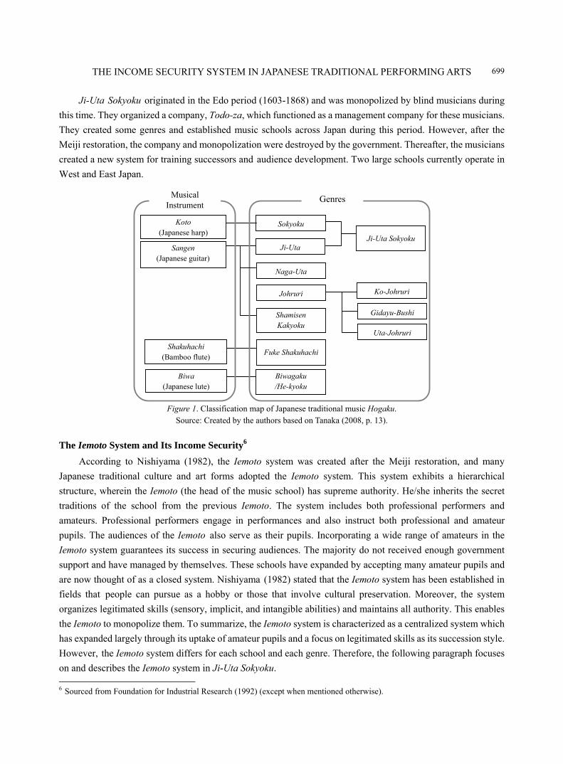
THE INCOME SECURITY SYSTEM IN JAPANESE TRADITIONAL PERFORMING ARTS
699
Ji-Uta Sokyoku originated in the Edo period (1603-1868) and was monopolized by blind musicians during
this time. They organized a company, Todo-za, which functioned as a management company for these musicians.
They created some genres and established music schools across Japan during this period. However, after the
Meiji restoration, the company and monopolization were destroyed by the government. Thereafter, the musicians
created a new system for training successors and audience development. Two large schools currently operate in
West and East Japan.
Figure 1. Classification map of Japanese traditional music Hogaku.
Source: Created by the authors based on Tanaka (2008, p. 13).
The Iemoto System and Its Income Security6
According to Nishiyama (1982), the Iemoto system was created after the Meiji restoration, and many
Japanese traditional culture and art forms adopted the Iemoto system. This system exhibits a hierarchical
structure, wherein the Iemoto (the head of the music school) has supreme authority. He/she inherits the secret
traditions of the school from the previous Iemoto. The system includes both professional performers and
amateurs. Professional performers engage in performances and also instruct both professional and amateur
pupils. The audiences of the Iemoto also serve as their pupils. Incorporating a wide range of amateurs in the
Iemoto system guarantees its success in securing audiences. The majority do not received enough government
support and have managed by themselves. These schools have expanded by accepting many amateur pupils and
are now thought of as a closed system. Nishiyama (1982) stated that the Iemoto system has been established in
fields that people can pursue as a hobby or those that involve cultural preservation. Moreover, the system
organizes legitimated skills (sensory, implicit, and intangible abilities) and maintains all authority. This enables
the Iemoto to monopolize them. To summarize, the Iemoto system is characterized as a centralized system which
has expanded largely through its uptake of amateur pupils and a focus on legitimated skills as its succession style.
However, the Iemoto system differs for each school and each genre. Therefore, the following paragraph focuses
on and describes the Iemoto system in Ji-Uta Sokyoku. 6 Sourced from Foundation for Industrial Research (1992) (except when mentioned otherwise).
Koto (Japanese harp)
Sangen (Japanese guitar)
Shakuhachi (Bamboo flute)
Biwa (Japanese lute)
Sokyoku
Ji-Uta
Naga-Uta
Johruri
Shamisen Kakyoku
Fuke Shakuhachi
Biwagaku /He-kyoku
Ji-Uta Sokyoku
Ko-Johruri
Gidayu-Bushi
Uta-Johruri
Musical Instrument
Genres
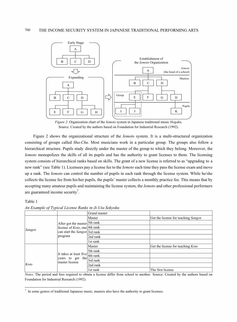
THE INCOME SECURITY SYSTEM IN JAPANESE TRADITIONAL PERFORMING ARTS
700
Figure 2. Organization chart of the Iemoto system in Japanese traditional music Hogaku.
Source: Created by the authors based on Foundation for Industrial Research (1992).
Figure 2 shows the organizational structure of the Iemoto system. It is a multi-structured organization
consisting of groups called Sha-Chu. Most musicians work in a particular group. The groups also follow a
hierarchical structure. Pupils study directly under the master of the group to which they belong. Moreover, the
Iemoto monopolizes the skills of all its pupils and has the authority to grant licenses to them. The licensing
system consists of hierarchical ranks based on skills. The grant of a new license is referred to as “upgrading to a
new rank” (see Table 1). Licensees pay a license fee to the Iemoto each time they pass the license exam and move
up a rank. The Iemoto can control the number of pupils in each rank through the license system. While he/she
collects the license fee from his/her pupils, the pupils’ master collects a monthly practice fee. This means that by
accepting many amateur pupils and maintaining the license system, the Iemoto and other professional performers
are guaranteed income security7.
Table 1
An Example of Typical License Ranks in Ji-Uta Sokyoku Grand master
Sangen
After got the master license of Koto, one can start the Sangen program
Master Get the license for teaching Sangen 5th rank 4th rank 3rd rank 2nd rank 1st rank
Koto
It takes at least five years to get the master license
Master Get the license for teaching Koto 5th rank 4th rank 3rd rank 2nd rank 1st rank The first license
Notes. The period and fees required to obtain a license differ from school to another. Source: Created by the authors based on Foundation for Industrial Research (1992).
7 In some genres of traditional Japanese music, masters also have the authority to grant licenses.
A
B C D
F E
J I
G H
K
Group
Iemoto (the head of a school)
Masters
Pupils
A
B C D
A
B C D
F E G H
Early Stage
Expanding
Establishment of the Iemoto Organization
THE INCOME SECURITY SYSTEM IN JAPANESE TRADITIONAL PERFORMING ARTS
701
In traditional Japanese music, while the Iemoto can control the number of pupils at each level, he/she does
not have the authority to control their performances. Masters can perform anywhere at will and can create new
plays without the Iemoto’s permission. Most masters offer their pupils opportunities to perform onstage to
motivate them. Pupils who engage in such performances must bear all costs and additional fees associated with
such performances, over and above the practice and license fees.
Successor Training and Performance
As mentioned in previous section, accepting many amateur pupils allows the school to expand8. Typically, a
pupil would need to attain 5-8 ranks to become a master, followed by another 5-7 ranks to become a grand
master9 (see Table 1). Pupils who pass the necessary exams to become masters can begin instructing newer
pupils. The master judges whether pupils possess the required qualifications to appear for an exam. When the
pupils earn their licenses, they must pay license fees to the Iemoto. The price of obtaining the lowest ranked
license is approximately 20,000 yen. The higher the pupil moves up the ranks, the more expensive the license fees.
It is said that it takes approximately five years at a total cost of 400,000-600,000 yen to obtain a master’s
license10.
As mentioned earlier, most masters offer pupils the opportunities to perform onstage in a recital to help
motivate them, promote a group, and prevent pupils from changing masters11. The quality of such recitals is
generally not controlled12. However, these performances go a long way in securing new pupils; the recital is
expected to attract impressionable audiences, especially new pupils and relative beginners.
The next section examines the relationship between income security and quality control of performances,
with a primary focus on recitals of the nature discussed above.
The Relationship Between Income Security System and Stage Quality
In previous section, the authors note that while the Iemoto system works as an income security system, it
does not always work towards improving stage/performance quality, especially for amateur pupils. In this
section, the authors focus on the mechanism of declining stage quality in the Iemoto system and discuss ways to
improve it whilst keeping the function of the income security system intact.
Model
The authors denote the number of pupils in the Iemoto organization by n and the earnings from the practice
fee by T which is given by:
T tn= (1) where t is the practice fee per pupil. The authors denote the stage quality by s which is considered to be a
function of the ratio of pupils who appear onstage to the total number of pupils in the Iemoto organization. The
smaller the ratio, the more competitive the Iemoto organization is. In other words, s is a decreasing function of
the ratio, given by:
( ), 0dss sd
αα
= ≤ (2)
8 The Nippon Hoso Kyokai (The Japan Broadcasting Corporation) provided a successor training program for a number of years. However, the program was terminated in 2009. Today, the Iemoto system alone runs a successor training program in Japan. 9 Grand master belongs to the Iemoto organization; he/she is also a pupil of the Iemoto. 10 Personal communication, on January 7, 2011, with a person well versed in traditional Japanese music. 11 In principle, pupils are not permitted to change masters. 12 Noting that this applies to amateur pupils only.
THE INCOME SECURITY SYSTEM IN JAPANESE TRADITIONAL PERFORMING ARTS
702
where α is the ratio.
In an Iemoto organization, it is usual for pupils to bear a part of the total stage cost. The authors denote
this cost by e. That is, the Iemoto receives payments from performing pupils, E, which is given by:
E e nα= (3) The authors denote the ticket price of the recital by p and the number of audience by q, which is a function
of p and s. Mathematically:
( , ( )), 0qq q p ss
α ∂= >
∂ (4)
where p is given exogenously in the market.
Profit from the recital π is given by:
( , ( ))pq p s e n Cπ α α= + − (5)
where C is the exogenously given total cost.
The authors consider the case where the number of pupils decreases as the possibility of appearing onstage
decreases, given a constant practice fee. This eventuality arises, when the motivation for learning comes from
the experience of appearing onstage, i.e.:
( , ), 0dnn n td
αα
= ≥ (6)
From Equation (1), the total profit of the Iemoto is given by:
( , ) ( , )tn t cn tπ α αΠ = + − (7)
where c is the marginal cost of instructing pupils. The first order condition (FOC) of profit maximization is given
by:
( , ) ( ) 0d q ds dnp en t e t cd s d d
αα α αΠ ∂
= + + + − =∂
(8)
Rewriting this, the authors get:
( ) ( )dn q dsen e t c pd s d
αα α
∂+ + − = −
∂ (9)
The left-hand side of the equation expresses the marginal revenue due to the increase in the number of
pupils who appear onstage. The right-hand side expresses the marginal cost of increasing the ratio via the
decline in the number of audience. The FOC implies that the optimal ratio is determined at the point where the
marginal revenue equals the marginal cost.
Differentiating the left-hand side by α, the authors get:
2
2( )
dn d ne e t cd dα α
+ + − (10)
The first term is positive and the second term is negative. It is reasonable to consider that the first-degree
derivative dominates its second-degree counterpart, and accordingly, Equation (10) could be considered to be
positive.
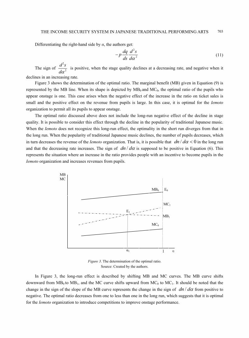
THE INCOME SECURITY SYSTEM IN JAPANESE TRADITIONAL PERFORMING ARTS
703
Differentiating the right-hand side by α, the authors get: 2
2
dq d spds dα
− (11)
The sign of 2
2
d sdα
is positive, when the stage quality declines at a decreasing rate, and negative when it
declines in an increasing rate. Figure 3 shows the determination of the optimal ratio. The marginal benefit (MB) given in Equation (9) is
represented by the MB line. When its shape is depicted by MB0 and MC0, the optimal ratio of the pupils who
appear onstage is one. This case arises when the negative effect of the increase in the ratio on ticket sales is
small and the positive effect on the revenue from pupils is large. In this case, it is optimal for the Iemoto
organization to permit all its pupils to appear onstage.
The optimal ratio discussed above does not include the long-run negative effect of the decline in stage
quality. It is possible to consider this effect through the decline in the popularity of traditional Japanese music.
When the Iemoto does not recognize this long-run effect, the optimality in the short run diverges from that in
the long run. When the popularity of traditional Japanese music declines, the number of pupils decreases, which
in turn decreases the revenue of the Iemoto organization. That is, it is possible that / 0dn dα < in the long run
and that the decreasing rate increases. The sign of /dn dα is supposed to be positive in Equation (6). This
represents the situation where an increase in the ratio provides people with an incentive to become pupils in the
Iemoto organization and increases revenues from pupils.
Figure 3. The determination of the optimal ratio.
Source: Created by the authors.
In Figure 3, the long-run effect is described by shifting MB and MC curves. The MB curve shifts
downward from MB0 to MB1, and the MC curve shifts upward from MC0 to MC1. It should be noted that the
change in the sign of the slope of the MB curve represents the change in the sign of /dn dα from positive to
negative. The optimal ratio decreases from one to less than one in the long run, which suggests that it is optimal
for the Iemoto organization to introduce competitions to improve onstage performance.
α
MB MC
1
MB0
MC0
MC1
MB1 E1
E0
α1
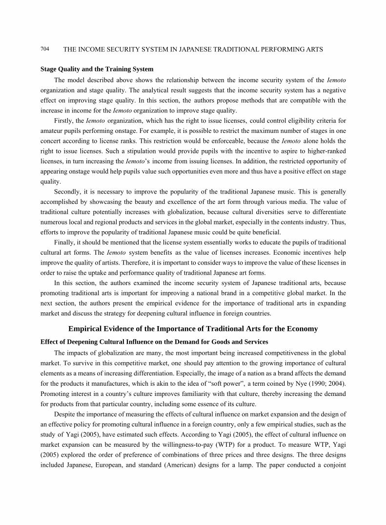
THE INCOME SECURITY SYSTEM IN JAPANESE TRADITIONAL PERFORMING ARTS
704
Stage Quality and the Training System
The model described above shows the relationship between the income security system of the Iemoto
organization and stage quality. The analytical result suggests that the income security system has a negative
effect on improving stage quality. In this section, the authors propose methods that are compatible with the
increase in income for the Iemoto organization to improve stage quality.
Firstly, the Iemoto organization, which has the right to issue licenses, could control eligibility criteria for
amateur pupils performing onstage. For example, it is possible to restrict the maximum number of stages in one
concert according to license ranks. This restriction would be enforceable, because the Iemoto alone holds the
right to issue licenses. Such a stipulation would provide pupils with the incentive to aspire to higher-ranked
licenses, in turn increasing the Iemoto’s income from issuing licenses. In addition, the restricted opportunity of
appearing onstage would help pupils value such opportunities even more and thus have a positive effect on stage
quality.
Secondly, it is necessary to improve the popularity of the traditional Japanese music. This is generally
accomplished by showcasing the beauty and excellence of the art form through various media. The value of
traditional culture potentially increases with globalization, because cultural diversities serve to differentiate
numerous local and regional products and services in the global market, especially in the contents industry. Thus,
efforts to improve the popularity of traditional Japanese music could be quite beneficial.
Finally, it should be mentioned that the license system essentially works to educate the pupils of traditional
cultural art forms. The Iemoto system benefits as the value of licenses increases. Economic incentives help
improve the quality of artists. Therefore, it is important to consider ways to improve the value of these licenses in
order to raise the uptake and performance quality of traditional Japanese art forms.
In this section, the authors examined the income security system of Japanese traditional arts, because
promoting traditional arts is important for improving a national brand in a competitive global market. In the
next section, the authors present the empirical evidence for the importance of traditional arts in expanding
market and discuss the strategy for deepening cultural influence in foreign countries.
Empirical Evidence of the Importance of Traditional Arts for the Economy
Effect of Deepening Cultural Influence on the Demand for Goods and Services
The impacts of globalization are many, the most important being increased competitiveness in the global
market. To survive in this competitive market, one should pay attention to the growing importance of cultural
elements as a means of increasing differentiation. Especially, the image of a nation as a brand affects the demand
for the products it manufactures, which is akin to the idea of “soft power”, a term coined by Nye (1990; 2004).
Promoting interest in a country’s culture improves familiarity with that culture, thereby increasing the demand
for products from that particular country, including some essence of its culture.
Despite the importance of measuring the effects of cultural influence on market expansion and the design of
an effective policy for promoting cultural influence in a foreign country, only a few empirical studies, such as the
study of Yagi (2005), have estimated such effects. According to Yagi (2005), the effect of cultural influence on
market expansion can be measured by the willingness-to-pay (WTP) for a product. To measure WTP, Yagi
(2005) explored the order of preference of combinations of three prices and three designs. The three designs
included Japanese, European, and standard (American) designs for a lamp. The paper conducted a conjoint
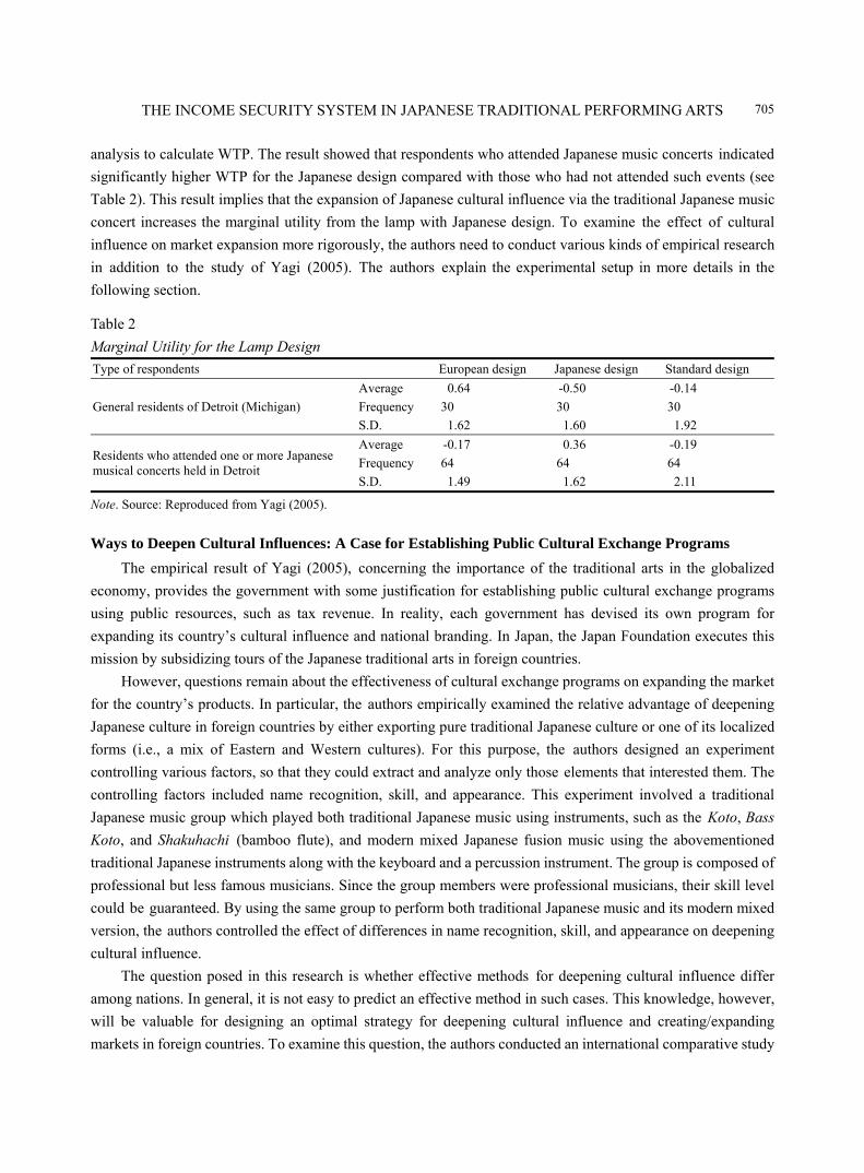
THE INCOME SECURITY SYSTEM IN JAPANESE TRADITIONAL PERFORMING ARTS
705
analysis to calculate WTP. The result showed that respondents who attended Japanese music concerts indicated
significantly higher WTP for the Japanese design compared with those who had not attended such events (see
Table 2). This result implies that the expansion of Japanese cultural influence via the traditional Japanese music
concert increases the marginal utility from the lamp with Japanese design. To examine the effect of cultural
influence on market expansion more rigorously, the authors need to conduct various kinds of empirical research
in addition to the study of Yagi (2005). The authors explain the experimental setup in more details in the
following section.
Table 2
Marginal Utility for the Lamp Design Type of respondents European design Japanese design Standard design
General residents of Detroit (Michigan)
Average 0.64 -0.50 -0.14
Frequency 30 30 30
S.D. 1.62 1.60 1.92
Residents who attended one or more Japanese musical concerts held in Detroit
Average -0.17 0.36 -0.19
Frequency 64 64 64
S.D. 1.49 1.62 2.11
Note. Source: Reproduced from Yagi (2005).
Ways to Deepen Cultural Influences: A Case for Establishing Public Cultural Exchange Programs
The empirical result of Yagi (2005), concerning the importance of the traditional arts in the globalized
economy, provides the government with some justification for establishing public cultural exchange programs
using public resources, such as tax revenue. In reality, each government has devised its own program for
expanding its country’s cultural influence and national branding. In Japan, the Japan Foundation executes this
mission by subsidizing tours of the Japanese traditional arts in foreign countries.
However, questions remain about the effectiveness of cultural exchange programs on expanding the market
for the country’s products. In particular, the authors empirically examined the relative advantage of deepening
Japanese culture in foreign countries by either exporting pure traditional Japanese culture or one of its localized
forms (i.e., a mix of Eastern and Western cultures). For this purpose, the authors designed an experiment
controlling various factors, so that they could extract and analyze only those elements that interested them. The
controlling factors included name recognition, skill, and appearance. This experiment involved a traditional
Japanese music group which played both traditional Japanese music using instruments, such as the Koto, Bass
Koto, and Shakuhachi (bamboo flute), and modern mixed Japanese fusion music using the abovementioned
traditional Japanese instruments along with the keyboard and a percussion instrument. The group is composed of
professional but less famous musicians. Since the group members were professional musicians, their skill level
could be guaranteed. By using the same group to perform both traditional Japanese music and its modern mixed
version, the authors controlled the effect of differences in name recognition, skill, and appearance on deepening
cultural influence.
The question posed in this research is whether effective methods for deepening cultural influence differ
among nations. In general, it is not easy to predict an effective method in such cases. This knowledge, however,
will be valuable for designing an optimal strategy for deepening cultural influence and creating/expanding
markets in foreign countries. To examine this question, the authors conducted an international comparative study
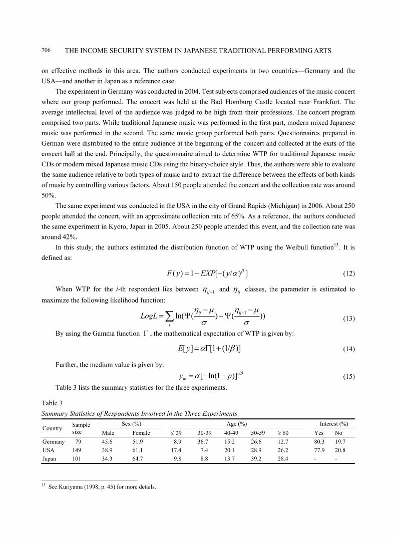
THE INCOME SECURITY SYSTEM IN JAPANESE TRADITIONAL PERFORMING ARTS
706
on effective methods in this area. The authors conducted experiments in two countries—Germany and the
USA—and another in Japan as a reference case.
The experiment in Germany was conducted in 2004. Test subjects comprised audiences of the music concert
where our group performed. The concert was held at the Bad Homburg Castle located near Frankfurt. The
average intellectual level of the audience was judged to be high from their professions. The concert program
comprised two parts. While traditional Japanese music was performed in the first part, modern mixed Japanese
music was performed in the second. The same music group performed both parts. Questionnaires prepared in
German were distributed to the entire audience at the beginning of the concert and collected at the exits of the
concert hall at the end. Principally, the questionnaire aimed to determine WTP for traditional Japanese music
CDs or modern mixed Japanese music CDs using the binary-choice style. Thus, the authors were able to evaluate
the same audience relative to both types of music and to extract the difference between the effects of both kinds
of music by controlling various factors. About 150 people attended the concert and the collection rate was around
50%.
The same experiment was conducted in the USA in the city of Grand Rapids (Michigan) in 2006. About 250
people attended the concert, with an approximate collection rate of 65%. As a reference, the authors conducted
the same experiment in Kyoto, Japan in 2005. About 250 people attended this event, and the collection rate was
around 42%.
In this study, the authors estimated the distribution function of WTP using the Weibull function13. It is
defined as:
( ) 1 [ ( ) ]F y EXP y βα= − − / (12)
When WTP for the i-th respondent lies between 1ijη − and ijη classes, the parameter is estimated to
maximize the following likelihood function:
1ln( ( ) ( ))ij ij
iLogL
η μ η μσ σ
−− −= Ψ − Ψ∑ (13)
By using the Gamma function Γ , the mathematical expectation of WTP is given by:
[ ] [1 (1 )]E y α β= Γ + / (14)
Further, the medium value is given by: 1[ ln(1 )]my p βα /= − − (15)
Table 3 lists the summary statistics for the three experiments.
Table 3
Summary Statistics of Respondents Involved in the Three Experiments
Country Sample size
Sex (%) Age (%) Interest (%)
Male Female ≤ 29 30-39 40-49 50-59 ≥ 60 Yes No
Germany 79 45.6 51.9 8.9 36.7 15.2 26.6 12.7 80.3 19.7
USA 149 38.9 61.1 17.4 7.4 20.1 28.9 26.2 77.9 20.8
Japan 101 34.3 64.7 9.8 8.8 13.7 39.2 28.4 - -
13 See Kuriyama (1998, p. 45) for more details.
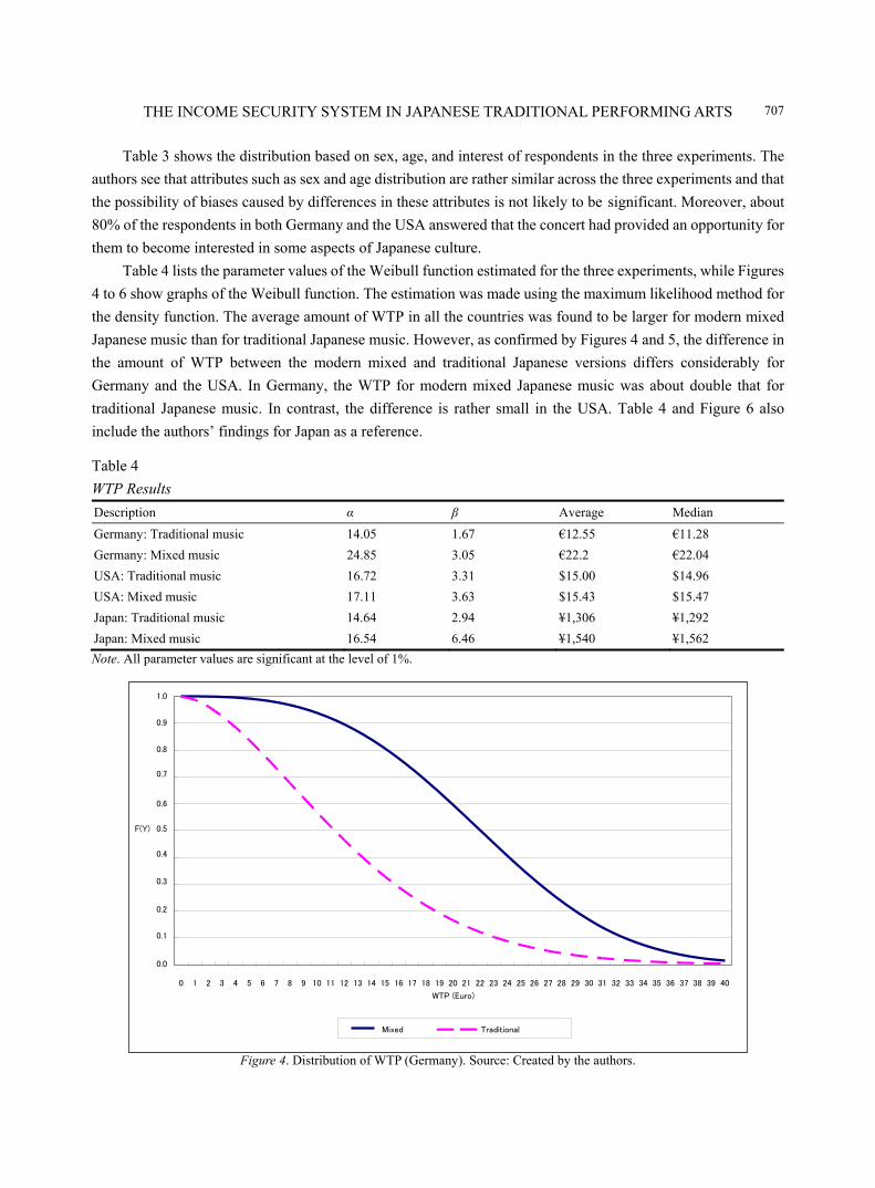
THE INCOME SECURITY SYSTEM IN JAPANESE TRADITIONAL PERFORMING ARTS
707
Table 3 shows the distribution based on sex, age, and interest of respondents in the three experiments. The
authors see that attributes such as sex and age distribution are rather similar across the three experiments and that
the possibility of biases caused by differences in these attributes is not likely to be significant. Moreover, about
80% of the respondents in both Germany and the USA answered that the concert had provided an opportunity for
them to become interested in some aspects of Japanese culture.
Table 4 lists the parameter values of the Weibull function estimated for the three experiments, while Figures
4 to 6 show graphs of the Weibull function. The estimation was made using the maximum likelihood method for
the density function. The average amount of WTP in all the countries was found to be larger for modern mixed
Japanese music than for traditional Japanese music. However, as confirmed by Figures 4 and 5, the difference in
the amount of WTP between the modern mixed and traditional Japanese versions differs considerably for
Germany and the USA. In Germany, the WTP for modern mixed Japanese music was about double that for
traditional Japanese music. In contrast, the difference is rather small in the USA. Table 4 and Figure 6 also
include the authors’ findings for Japan as a reference.
Table 4
WTP Results Description α β Average Median
Germany: Traditional music 14.05 1.67 €12.55 €11.28
Germany: Mixed music 24.85 3.05 €22.2 €22.04
USA: Traditional music 16.72 3.31 $15.00 $14.96
USA: Mixed music 17.11 3.63 $15.43 $15.47
Japan: Traditional music 14.64 2.94 ¥1,306 ¥1,292
Japan: Mixed music 16.54 6.46 ¥1,540 ¥1,562
Note. All parameter values are significant at the level of 1%.
Figure 4. Distribution of WTP (Germany). Source: Created by the authors.
0.0
0.1
0.2
0.3
0.4
0.5
0.6
0.7
0.8
0.9
1.0
0 1 2 3 4 5 6 7 8 9 10 11 12 13 14 15 16 17 18 19 20 21 22 23 24 25 26 27 28 29 30 31 32 33 34 35 36 37 38 39 40
WTP (Euro)
F(Y)
Mixed Traditional
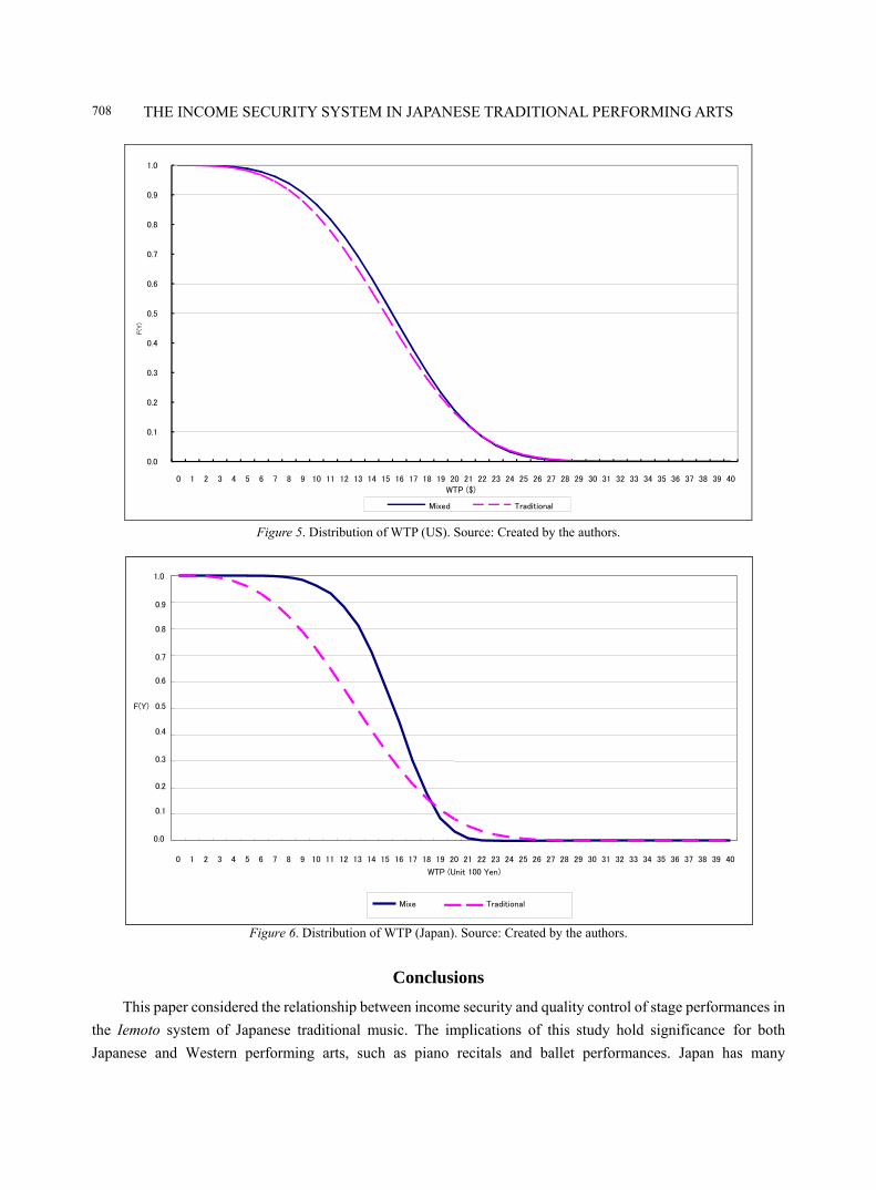
THE INCOME SECURITY SYSTEM IN JAPANESE TRADITIONAL PERFORMING ARTS
708
Figure 5. Distribution of WTP (US). Source: Created by the authors.
Figure 6. Distribution of WTP (Japan). Source: Created by the authors.
Conclusions
This paper considered the relationship between income security and quality control of stage performances in
the Iemoto system of Japanese traditional music. The implications of this study hold significance for both
Japanese and Western performing arts, such as piano recitals and ballet performances. Japan has many
0.0
0.1
0.2
0.3
0.4
0.5
0.6
0.7
0.8
0.9
1.0
0 1 2 3 4 5 6 7 8 9 10 11 12 13 14 15 16 17 18 19 20 21 22 23 24 25 26 27 28 29 30 31 32 33 34 35 36 37 38 39 40
F(Y
)
WTP ($)
Mixed Traditional
0.0
0.1
0.2
0.3
0.4
0.5
0.6
0.7
0.8
0.9
1.0
0 1 2 3 4 5 6 7 8 9 10 11 12 13 14 15 16 17 18 19 20 21 22 23 24 25 26 27 28 29 30 31 32 33 34 35 36 37 38 39 40
WTP (Unit 100 Yen)
F(Y)
Mixe
d
Traditional
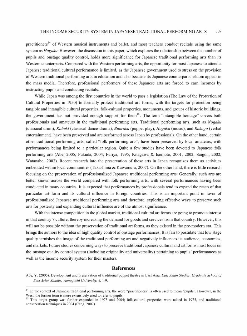
THE INCOME SECURITY SYSTEM IN JAPANESE TRADITIONAL PERFORMING ARTS
709
practitioners14 of Western musical instruments and ballet, and most teachers conduct recitals using the same
system as Hogaku. However, the discussion in this paper, which explores the relationship between the number of
pupils and onstage quality control, holds more significance for Japanese traditional performing arts than its
Western counterparts. Compared with the Western performing arts, the opportunity for most Japanese to attend a
Japanese traditional cultural performance is limited, as the Japanese government used to stress on the provision
of Western traditional performing arts in education and also because its Japanese counterparts seldom appear in
the mass media. Therefore, professional performers of these Japanese arts are forced to earn incomes by
instructing pupils and conducting recitals.
While Japan was among the first countries in the world to pass a legislation (The Law of the Protection of
Cultural Properties in 1950) to formally protect traditional art forms, with the targets for protection being
tangible and intangible cultural properties, folk-cultural properties, monuments, and groups of historic buildings,
the government has not provided enough support for them15. The term “intangible heritage” covers both
professionals and amateurs in the traditional performing arts. Traditional performing arts, such as Nogaku (classical drum), Kabuki (classical dance drama), Bunraku (puppet play), Hogaku (music), and Rakugo (verbal
entertainment), have been preserved and are performed across Japan by professionals. On the other hand, certain
other traditional performing arts, called “folk performing arts”, have been preserved by local amateurs, with
performances being limited to a particular region. Quite a few studies have been devoted to Japanese folk
performing arts (Abe, 2005; Fukuda, 2004; Furiya, 1995; Kitagawa & Isomoto, 2001, 2002; Saigoh, 2002;
Watanabe, 2002). Recent research into the preservation of these arts in Japan recognizes them as activities
embedded within local communities (Takashima & Kawamura, 2007). On the other hand, there is little research
focusing on the preservation of professionalized Japanese traditional performing arts. Generally, such arts are
better known across the world compared with folk performing arts, with several performances having been
conducted in many countries. It is expected that performances by professionals tend to expand the reach of that
particular art form and its cultural influence in foreign countries. This is an important point in favor of
professionalized Japanese traditional performing arts and therefore, exploring effective ways to preserve such
arts for posterity and expanding cultural influence are of the utmost significance.
With the intense competition in the global market, traditional cultural art forms are going to promote interest
in that country’s culture, thereby increasing the demand for goods and services from that country. However, this
will not be possible without the preservation of traditional art forms, as they existed in the pre-modern era. This
brings the authors to the idea of high quality control of onstage performances. It is fair to postulate that low stage
quality tarnishes the image of the traditional performing art and negatively influences its audience, economics,
and markets. Future studies concerning ways to preserve traditional Japanese cultural and art forms must focus on
the onstage quality control system (including originality and universality) pertaining to pupils’ performances as
well as the income security system for their masters.
References Abe, Y. (2005). Development and preservation of traditional puppet theatre in East Asia. East Asian Studies, Graduate School of
East Asian Studies, Yamaguchi University, 4, 1-9.
14 In the context of Japanese traditional performing arts, the word “practitioners” is often used to mean “pupils”. However, in the West, the former term is more extensively used to refer to pupils. 15 This target group was further expanded in 1975 and 2004; folk-cultural properties were added in 1975, and traditional conservation techniques in 2004 (Cang, 2007).
THE INCOME SECURITY SYSTEM IN JAPANESE TRADITIONAL PERFORMING ARTS
710
Agency for Cultural Affairs. (2010). The outline of budget in agency of cultural affairs. Resource Document. Retrieved from http://www.bunka.go.jp/bunka_gyousei/yosan/index.html
Alper, N., & Wassall, G. H. (2006). Artists’ careers and their labor markets. In V. Gisburg, & D. Throsby (Eds.), Handbook of the economics of arts and culture (Chapter 23, pp. 813-864). Amsterdam: Elsevier.
Cang, V. G. (2007). Defining intangible cultural heritage and its stakeholders: The case of Japan. International Journal of Intangible Heritage, 2, 45-56.
Caves, R. E. (2000). Creative industries. Cambridge: Harvard University Press.
Filer, R. K. (1986). “Starving artist”⎯Myth or reality? Earnings of artists in the United States. The Journal of Political Economy, 94(1), 56-75.
Foundation for Industrial Research. (1992). Studies on the development of industries related with traditional performing arts. Tokyo: Foundation for Industrial Research.
Frey, B. S., & Pommerehne, W. W. (1989). Muses and markets: Explorations in the economics of the arts. Boston: Basil Blackwell. Fukuda, H. (2004). Study on the issues relating the succession of folk performing arts in cultural properties protection policy:
Reviewing a case of Kowaka-mai of Ohe, Dengaku, and nohmai of Mizuumi and Noh and kyogen of Nogo. Cultural Economics, 4(1), 19-30.
Furiya, M. (1995). On the survival of folk culture and traditions: Fieldwork on Jangara-nenbutsu dance. The Bulletin: Miyazaki University of Education, 30, 97-120.
Hirano, K., Kamisango, U., & Gamo, S. (2005). Dictionary of Japanese music. Heibonsha. Horiuchi, K. (1977a). The 50-year history of music (Vol. 1). Tokyo: Kodansha. Horiuchi, K. (1977b). The 50-year history of music (Vol. 2). Tokyo: Kodansha. Kitagawa, H., & Isomoto, Y. (2001). Design and implementation of multimedia teaching material for preservation and succession
of traditional folk entertainment. Proceedings: Japanese Society for Information and Systems in Education, 1, 13-18. Kitagawa, H., & Isomoto, Y. (2002). Storage and usage of digital contents of movies for preservation and succession of traditional
performing arts. Proceedings: The Institute of Electronics, Information, and Communication Engineers. Denshi Joho Tsushin Gakkai, 102(139), 31-36.
Kurin, R. (2004). Safeguarding intangible cultural heritage in the 2003 UNESCO convention: A critical appraisal. Museum International, 56(1-2), 66-77.
Kuriyama, K. (1998). Assessment approach and value of environment. Hokkaido University. Nishiyama, M. (1982). Iemoto studies: A complete collection of Matsunosuke Nishiyam. Tokyo: Yoshikawa Kobun Kan. Nye, J. S. (1990). Soft power. Foreign Policy, 80, 153-171. Nye, J. S. (2004). Soft power: The means to success in world politics. Public Affairs. Rengers, M., & Plug, E. (2001). Private or public? How Dutch visual artists choose between working for the market and the
government. Journal of Cultural Economics, 25(1), 1-20. Saigoh, Y. (2002). How traditional art techniques are taught/learned? Community as school and traditional performance arts in
Japan. Bulletin: Japan Society for Theatre Research, Nihon Engeki Gakkai, 40, 127-141. Snowball, J. D. (2005). Art for the masses? Justification for the public support of the artisan developing countries. Two arts festivals
in South Africa. Journal of Cultural Economics, 29, 107-125. Suo, S. (2003). Research about development and systematization of statistical indicator for arts and cultural policy. In Ministry of
Education, Culture, Sports, Science and Technology (Ed.), The report of the research by scientific research fund of Ministry of Education, Culture, Sports, Science and Technology.
Takashima, C., & Kawamura, T. (2007). An activity-theoretical approach to the management study of traditional performing arts organizations: A case study of successor and audience development of Ningyo Johruri puppet play. Business Research, Osaka City University, 58(2), 81-104.
Tanaka, K. (2008). Illustration of Japanese music history. Tokyo: Tokyodo Shuppan. Throsby, D. (2001). Economics and culture. Cambridge: Cambridge University Press. Towse, R. (2006). Copyright and artists: A view from cultural economics. Journal of Economic Surveys, 20(4), 567-585. Watanabe, Y. (2002). Preservation and succession of folk traditional arts. Geino, Geino Gakkai, 8, 42-54. Watt, R., & Towse, R. (2006). Copyright protection standards and authors’ time allocation. Industrial and Corporate Change,
15(6), 995-1011. Yagi, T. (2005). Effect of cultural influence on expansion of market: Empirical evaluation of economic benefits of cultural social
infrastructure. Bulletin: Doshisha University, Faculty of Economics, 57(2), 1-28.
Journal of Modern Accounting and Auditing, ISSN 1548-6583 May 2013, Vol. 9, No. 5, 711-718
Analysis of Salaries and Some Non-traditional
Measures of Location∗
Milan Terek, Nguyen Dinh He
University of Economics in Bratislava, Bratislava, Slovakia
The paper deals with an analysis of how to use certain measures of location in analysis of salaries. One of the
traditional measures of location, the mean should offer typical value of variable, representing all its values by the
best way. Sometimes, the mean is located in the tail of the distribution and gives a very biased idea about the
location of the distribution. In these cases, using different measures of location could be useful. Trimmed mean is
described. The trimmed mean refers to a situation where a certain proportion of the largest and smallest
observations are removed and the remaining observations are averaged. The construction of some measures of
location is based on the analysis of outliers. Outliers are characterized. Then the possibilities of the detection of
outliers are analyzed. Computing of one-step M-estimator and modified one-step M-estimator of location is
described. A comparison of the trimmed means and M-estimators of location is presented. Finally, the paper focuses
on the application of the trimmed mean and M-estimators of location in analysis of salaries. The analysis of salaries
of employers of the big Slovak companies in second half of the year 2009 is realized. The data from the census are
used in the analysis. The median, 20% trimmed mean and the characteristics, based on the one-step M-estimator of
location and modified one step M-estimator, are calculated.
Keywords: trimmed mean, detecting outliers, one-step M-estimator, modified one-step M-estimator, analysis of
salaries
Introduction
One of the traditional indicators of the standard of living of population is average monthly salary
(Muchová, 2011). The distribution of salaries is obviously skewed and outliers are present. Then, the
interpretation power of this indicator is very small (Halley, 2004). It will be shown that the using of some
non-traditional measures of location could be interesting.
One of these measures of location is trimmed mean. Trimmed mean refers to a situation where a certain
proportion of the largest and smallest values are removed and from the rest, the average is calculated.
M-estimators provide another class of measures of location that have practical value. Their construction
requires the detection of outliers.
The paper focuses on the description of the trimmed mean and M-estimators and on their application in the
analysis of salaries.
∗ This paper was elaborated with the support of the grant agency VEGA in the framework of the project Number 1/0761/12.
Milan Terek, professor, Department of Statistics, University of Economics in Bratislava. Email: [email protected]. Nguyen Dinh He, assistant professor, Department of Statistics, University of Economics in Bratislava.
DAVID PUBLISHING
D
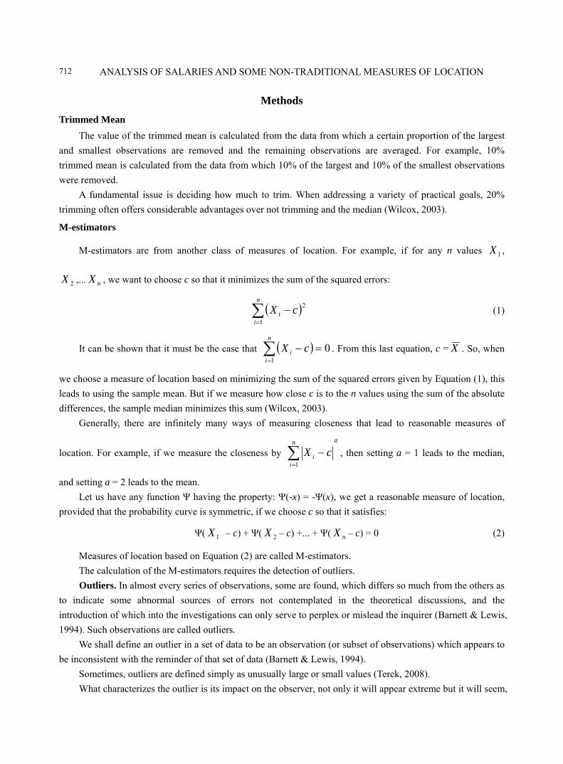
ANALYSIS OF SALARIES AND SOME NON-TRADITIONAL MEASURES OF LOCATION
712
Methods
Trimmed Mean
The value of the trimmed mean is calculated from the data from which a certain proportion of the largest
and smallest observations are removed and the remaining observations are averaged. For example, 10%
trimmed mean is calculated from the data from which 10% of the largest and 10% of the smallest observations
were removed.
A fundamental issue is deciding how much to trim. When addressing a variety of practical goals, 20%
trimming often offers considerable advantages over not trimming and the median (Wilcox, 2003).
M-estimators
M-estimators are from another class of measures of location. For example, if for any n values 1X ,
2X ,... nX , we want to choose c so that it minimizes the sum of the squared errors:
( )∑=
−n
ii cX
1
2 (1)
It can be shown that it must be the case that ( ) 01
=−∑=
n
ii cX . From this last equation, c = X . So, when
we choose a measure of location based on minimizing the sum of the squared errors given by Equation (1), this
leads to using the sample mean. But if we measure how close c is to the n values using the sum of the absolute
differences, the sample median minimizes this sum (Wilcox, 2003).
Generally, there are infinitely many ways of measuring closeness that lead to reasonable measures of
location. For example, if we measure the closeness by
an
ii cX∑
=
−1
, then setting a = 1 leads to the median,
and setting a = 2 leads to the mean.
Let us have any function Ψ having the property: Ψ(-x) = -Ψ(x), we get a reasonable measure of location,
provided that the probability curve is symmetric, if we choose c so that it satisfies:
Ψ( 1X – c) + Ψ( 2X – c) +... + Ψ( nX – c) = 0 (2)
Measures of location based on Equation (2) are called M-estimators.
The calculation of the M-estimators requires the detection of outliers.
Outliers. In almost every series of observations, some are found, which differs so much from the others as
to indicate some abnormal sources of errors not contemplated in the theoretical discussions, and the
introduction of which into the investigations can only serve to perplex or mislead the inquirer (Barnett & Lewis,
1994). Such observations are called outliers.
We shall define an outlier in a set of data to be an observation (or subset of observations) which appears to
be inconsistent with the reminder of that set of data (Barnett & Lewis, 1994).
Sometimes, outliers are defined simply as unusually large or small values (Terek, 2008).
What characterizes the outlier is its impact on the observer, not only it will appear extreme but it will seem,

ANALYSIS OF SALARIES AND SOME NON-TRADITIONAL MEASURES OF LOCATION
713
in some sense, surprisingly extreme.
Outlying observations are not necessarily bad or erroneous. There are situations in which an outlier can
indicate, for example, some unexpectedly useful industrial treatments. Frequently, outliers are very useful in the
fraud recognition. In the situations like these, it may not be necessary to adopt either of the extremes of
rejection (with a risk of losing genuine information) or inclusion (with the risk of contamination). Sometimes,
the using of the robust methods of inference which employ all the data but minimize the influence of any
outliers is useful.
We would like to note that the outlier problem is an unavoidable one. It is not enough to say that one
should not consider dealing with outlying observations. In fact, the persons who have to deal with data and take
decisions are forced to make judgments about outliers—whether or not to include them, whether to make
allowances for them on some compromise bases, and so on.
The detection of outliers requires assessing the integrity of a set of data. We need the techniques for
assessing the integrity of a set of data with respect to an assumed model. We require the methods for assessing,
rejecting, making allowances for, or minimizing the influence of outlying observations.
The outlier problem progresses in the following way. We examine the data set. Suppose, we decide that
outliers exist. Then we must ask: How should we react to the outliers, and what principles and methods can be
used to support rejecting them, adjusting their values, or leaving them unaltered, prior to processing the main
mass of data? The answers depend on the form of the population, the used techniques depend mainly on the
postulated model for the population.
Detecting outliers. The first strategy is based on the sample mean and sample standard deviation. If we
suppose normal distribution of the population, it is obvious to consider as outlier a value which is more than
2.24 standard deviation from the mean σ
μ−x> 2.24. If we suppose the normal distribution of the population
with the mean μ and standard deviation σ, the probability of declaring a value an outlier using this equation is
0.025.
Generally, μ and σ are unknown, but they can be estimated from the data using the value of the sample
mean x and of the sample standard deviation s. Then the following decision rule can be formulated:
The value x is declared to be an outlier if:
s
xx −> 2.24 (3)
where s = ( )∑ −− =
n
jj xx
n 1
2
1
1.
The described method can lead to the problem known as masking. Outliers inflate both the sample mean
and the sample standard deviation, which in turn can mask their presence when using Equation (3) (Wilcox,
2003).
A rule for detecting outliers that is not itself affected by outliers is needed. One robust method of outliers
detection will be described.
The method based on median absolute deviation (MAD). Firstly, a measure of dispersion called as MAD

ANALYSIS OF SALARIES AND SOME NON-TRADITIONAL MEASURES OF LOCATION
714
will be described. To compute it, we will first compute the value 2/1x of the sample median 2/1X , then we
will compute the absolute values of the differences: 2/1xxi − for i = 1, 2,... n.
Generally, MAD does not estimate σ, but it can be shown that when sampling from a normal distribution,
0.6745
MADMADN = estimates σ as well (Wilcox, 2003, p. 73).
The robust decision rule for the detection of outliers is as follows.
The value x is declared to be an outlier if:
MADN
xx 2/1−> 2.24 (4)
One-step M-estimator. Let 1n be the number of observations iX , for which ( )
MADN
XX i 2/1− < -K and
let 2n be the number of observations such that ( )
MADN
XX i 2/1− > K, where typically K = 1.28 is used. The
one-step M-estimator of location (based on Huber’ s Ψ) is:
( )( ) ( )
21
112
2
1ˆnnn
XnnMADNKnn
nii
os −−
+−=
∑−
+=μ (5)
where ( )iX is i-th order statistic1.
The calculation of the value of M-estimator requires the determination of outliers using the method based
on MAD, except that Equation (4) is replaced by:
MADN
xx 2/1−> K (6)
Next, remove the values flagged as outliers and average the values that remain. For technical reasons, the
one-step M-estimator makes an adjustment based on MADN, a measure of scale plus the number of outliers
above and below the median (Wilcox, 2003).
A modified one-step M-estimator. Sometimes, a simple modification of the one-step M-estimator is
used:
( )
21
1
2
1ˆnnn
Xnn
nii
mom −−=
∑−
+=μ (7)
where K = 2.24 is used to determine 1n and 2n .
1 Order statistic is determined by its ranking in a non-decreasing arrangement of random variables.
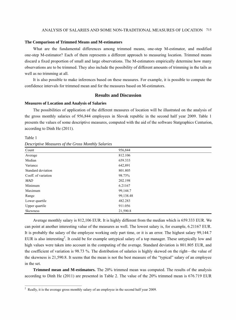
ANALYSIS OF SALARIES AND SOME NON-TRADITIONAL MEASURES OF LOCATION
715
The Comparison of Trimmed Means and M-estimators
What are the fundamental differences among trimmed means, one-step M-estimator, and modified
one-step M-estimator? Each of them represents a different approach to measuring location. Trimmed means
discard a fixed proportion of small and large observations. The M-estimators empirically determine how many
observations are to be trimmed. They also include the possibility of different amounts of trimming in the tails as
well as no trimming at all.
It is also possible to make inferences based on these measures. For example, it is possible to compute the
confidence intervals for trimmed mean and for the measures based on M-estimators.
Results and Discussion
Measures of Location and Analysis of Salaries
The possibilities of application of the different measures of location will be illustrated on the analysis of
the gross monthly salaries of 956,844 employees in Slovak republic in the second half year 2009. Table 1
presents the values of some descriptive measures, computed with the aid of the software Statgraphics Centurion,
according to Dinh He (2011).
Table 1
Descriptive Measures of the Gross Monthly Salaries
Count 956,844
Average 812.106
Median 659.333
Variance 642,891
Standard deviation 801.805
Coeff. of variation 98.73%
MAD 202.198
Minimum 6.21167
Maximum 99,144.7
Range 99,138.48
Lower quartile 482.283
Upper quartile 911.056
Skewness 21,590.8
Average monthly salary is 812,106 EUR. It is highly different from the median which is 659.333 EUR. We
can point at another interesting value of the measures as well. The lowest salary is, for example, 6.21167 EUR.
It is probably the salary of the employee working only part time, or it is an error. The highest salary 99,144.7
EUR is also interesting2. It could be for example untypical salary of a top manager. These untypically low and
high values were taken into account in the computing of the average. Standard deviation is 801.805 EUR, and
the coefficient of variation is 98.73 %. The distribution of salaries is highly skewed on the right—the value of
the skewness is 21,590.8. It seems that the mean is not the best measure of the “typical” salary of an employee
in the set.
Trimmed mean and M-estimators. The 20% trimmed mean was computed. The results of the analysis
according to Dinh He (2011) are presented in Table 2. The value of the 20% trimmed mean is 676.719 EUR
2 Really, it is the average gross monthly salary of an employee in the second half year 2009.
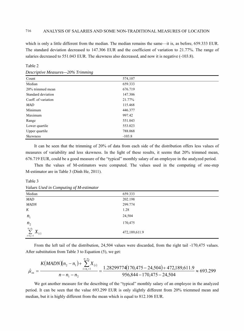
ANALYSIS OF SALARIES AND SOME NON-TRADITIONAL MEASURES OF LOCATION
716
which is only a little different from the median. The median remains the same—it is, as before, 659.333 EUR.
The standard deviation decreased to 147.306 EUR and the coefficient of variation to 21.77%. The range of
salaries decreased to 551.043 EUR. The skewness also decreased, and now it is negative (-103.8).
Table 2
Descriptive Measures—20% Trimming
Count 574,107
Median 659.333
20% trimmed mean 676.719
Standard deviation 147.306
Coeff. of variation 21.77%
MAD 115.468
Minimum 446.377
Maximum 997.42
Range 551.043
Lower quartile 553.023
Upper quartile 788.068
Skewness -103.8
It can be seen that the trimming of 20% of data from each side of the distribution offers less values of
measures of variability and less skewness. In the light of these results, it seems that 20% trimmed mean,
676.719 EUR, could be a good measure of the “typical” monthly salary of an employee in the analyzed period.
Then the values of M-estimators were computed. The values used in the computing of one-step
M-estimator are in Table 3 (Dinh He, 2011).
Table 3
Values Used in Computing of M-estimator
Median 659.333
MAD 202.198
MADN 299.774
K 1.28
1n 24,504
2n 170,475
( )∑−
+=
2
1 1
nn
niiX 472,189,611.9
From the left tail of the distribution, 24,504 values were discarded, from the right tail -170,475 values.
After substitution from Table 3 to Equation (5), we get:
( )( ) ( ) ( )299.693
504,24475,170844,956
9.611,189,472504,24475,17028299774.1ˆ
21
112
2
1 ≈−−
+−=
−−
+−=
∑−
+=
nnn
XnnMADNKnn
nii
osμ
We got another measure for the describing of the “typical” monthly salary of an employee in the analyzed
period. It can be seen that the value 693.299 EUR is only slightly different from 20% triemmed mean and
median, but it is highly different from the mean which is equal to 812.106 EUR.
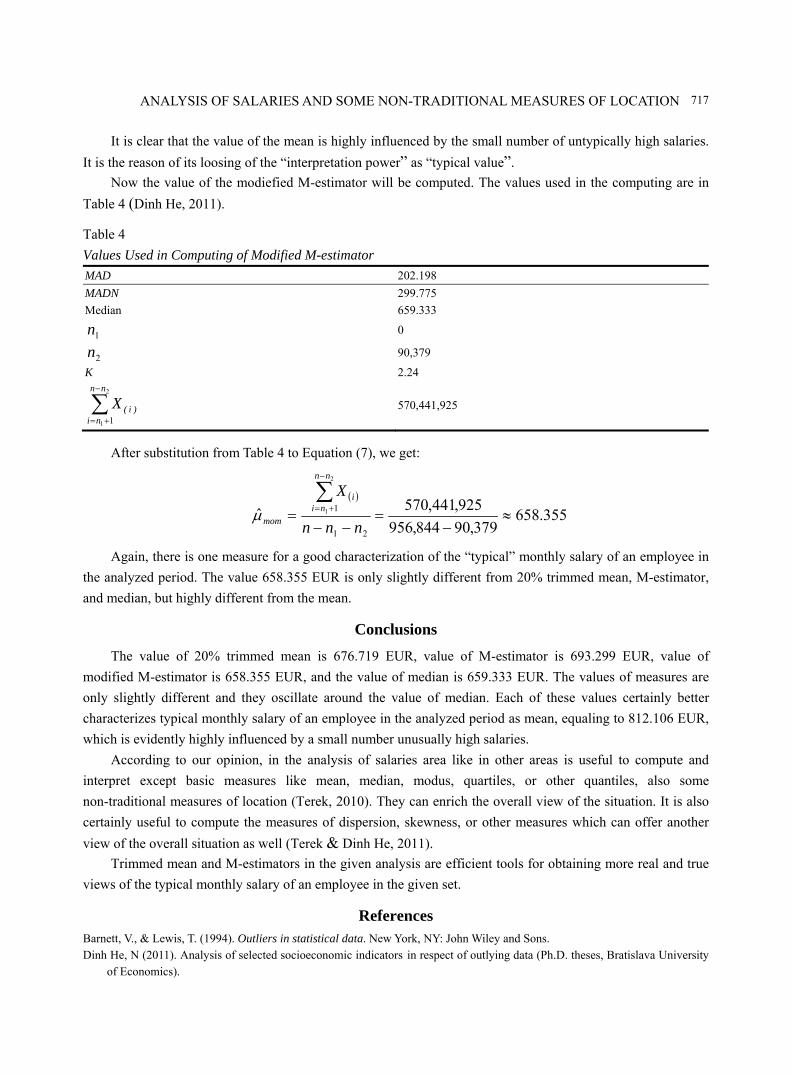
ANALYSIS OF SALARIES AND SOME NON-TRADITIONAL MEASURES OF LOCATION
717
It is clear that the value of the mean is highly influenced by the small number of untypically high salaries.
It is the reason of its loosing of the “interpretation power” as “typical value”.
Now the value of the modiefied M-estimator will be computed. The values used in the computing are in
Table 4 (Dinh He, 2011).
Table 4
Values Used in Computing of Modified M-estimator
MAD 202.198
MADN 299.775
Median 659.333
1n 0
2n 90,379
K 2.24
∑−
+=
2
1 1
nn
ni)i(X 570,441,925
After substitution from Table 4 to Equation (7), we get:
( )
355.658379,90844,956
925,441,570ˆ
21
1
2
1 ≈−
=−−
=∑−
+=
nnn
Xnn
nii
momμ
Again, there is one measure for a good characterization of the “typical” monthly salary of an employee in
the analyzed period. The value 658.355 EUR is only slightly different from 20% trimmed mean, M-estimator,
and median, but highly different from the mean.
Conclusions
The value of 20% trimmed mean is 676.719 EUR, value of M-estimator is 693.299 EUR, value of
modified M-estimator is 658.355 EUR, and the value of median is 659.333 EUR. The values of measures are
only slightly different and they oscillate around the value of median. Each of these values certainly better
characterizes typical monthly salary of an employee in the analyzed period as mean, equaling to 812.106 EUR,
which is evidently highly influenced by a small number unusually high salaries.
According to our opinion, in the analysis of salaries area like in other areas is useful to compute and
interpret except basic measures like mean, median, modus, quartiles, or other quantiles, also some
non-traditional measures of location (Terek, 2010). They can enrich the overall view of the situation. It is also
certainly useful to compute the measures of dispersion, skewness, or other measures which can offer another
view of the overall situation as well (Terek & Dinh He, 2011).
Trimmed mean and M-estimators in the given analysis are efficient tools for obtaining more real and true
views of the typical monthly salary of an employee in the given set.
References Barnett, V., & Lewis, T. (1994). Outliers in statistical data. New York, NY: John Wiley and Sons. Dinh He, N (2011). Analysis of selected socioeconomic indicators in respect of outlying data (Ph.D. theses, Bratislava University
of Economics).
ANALYSIS OF SALARIES AND SOME NON-TRADITIONAL MEASURES OF LOCATION
718
Halley, R. M. (2004). Measures of central tendency, location, and dispersion in salary survey research. Compensation and Benefits Review, 36(5), 39-52.
Muchová, E. (2011). The labor market and competitiveness in the European area. Proceedings of the contributions from the International Scientific Conference—Background and Challenges for Social Policy at the Impending Decades, Bratislava.
Terek, M. (2008). The analysis of outlying data. Forum Statisticum Slovacum, 6, 152-157. Terek, M. (2010). Analysis of outlying data and certain characteristics of location. Proceedings of the contributions from the
International Scientific Conference of the Knowledge Economy and its Reflection in Economic Theory and Economic Practice (pp. 371-384), Bratislava.
Terek, M., & Dinh He, N. (2011). The possibility of using some of the non-traditional characteristics in the analysis of wages. Economic Outlook, 1, 74-91.
Wilcox, R. R. (2003). Applying contemporary statistical techniques. USA: Academic Press.
Journal of Modern Accounting and Auditing, ISSN 1548-6583 May 2013, Vol. 9, No. 5, 719-727
A New Latent Class Stochastic Frontier Model for the Best
Practices of USA’s Corporate Governance
Wided Khiari, Yosra Mellouli University of Jendouba, Jendouba, Tunisia
In this paper, the authors study the association between firms’ specific characteristics and performances for a
sample of 320 American firms using a governance efficiency index, calculated by the stochastic frontier analysis.
The use of a latent class in the specification of the model, allowed detecting two groups of firms according to their
specific characteristics: the firm size, the leverage, the dividend yield, and the return on equity (ROE). The results
of affectation equation show that the probability to be in the second group (the most efficient) is more important
when the firm size, the dividend yield, and the ROE are high, while a high leverage level decreases the chance to be
in the first group (the less efficient).
Keywords: governance index, managerial efficiency, performance, corporate governance mechanisms, stochastic
frontier
Introduction
Promoted by corporate scandals such as Enron and WorldCom in the United States, France Telecom and Vivendi Universal (in France), the Credit Lyonnais or Air France in 1990, and the financial crises of 1998 occurred in Russia and Brazil, corporate governance has received a lot of attentions in the financial community. Institutional investors have started evaluating which role corporate governance should play in their investment policies. The important question as to whether good corporate governance leads to higher stock returns and consequently to higher firm valuations or not has received limited attentions in the academic literature.
A literature review allows taking a census of many works studying the relation between corporate governance and performance (Beiner, Drobetz, Schmid, & Zimmermann, 2004; Black, Jang, & Kim, 2004, 2006). Most of them examine the individual impact of every mechanism on performance, like the board of directors, its composition, the managers’ compensation, the ownership structure, the shareholders’ activism, and takeover mechanisms. Nevertheless, results seem to be mitigated, as the impact of certain mechanisms differs from one study to another. Besides, those studies do not provide an idea on the interaction among mechanisms. This can be attributed to the concentration on a particular governance aspect. Consequently, many authors resort to an indicial approach and especially efficiency indexes to study the relation between corporate governance and performance (El Mir & Khanchel, 2004; Zelenyuk & Zheka, 2006). Firms’ classification according to this index allows distinguishing firms according to their governance qualities.
This study contributes to the literature related to the corporate governance quality, as it takes into account
Wided Khiari, assistant professor, Faculty of Law, Economics and Management of Tunis, University of Jendouba. Email: [email protected].
Yosra Mellouli, assistant professor, Faculty of Law, Economics and Management of Tunis, University of Jendouba.
DAVID PUBLISHING
D
A NEW LATENT CLASS STOCHASTIC FRONTIER MODEL
720
the interaction among different governance mechanisms and integrates the performance as a concept which has an effect on the governance quality and so on the managerial efficiency. It takes into account criticisms addressed to the score computation using an approach based on the efficiency scores, the stochastic frontier analysis, in order to calculate governance indexes reflecting the efficiency of the latter. The idea that the authors try to exploit from the model adopted to compute the indexes is that firms’ specific characteristics can influence, with governance characteristics, firms’ performances.
Empirical Methodology
In this part, the authors are trying to appreciate, empirically, governance practices of a sample of American firms using an index which will be considered as a governance index. The latter is an efficiency score, calculated according to the stochastic frontier analysis which expresses, for every firm, the distance that separates it from a frontier reflecting corporate governance’s “best practices”. The idea that the authors try to exploit from the model adopted in the index computation is that firms’ specific characteristics can influence, with governance characteristics, firms’ performances.
Sample Characteristics
The study explores a sample of 320 large Americans firms (belonging to Fortune 500) for a period of eight years from 1994 to 2001. The accounting data and those related to governance variables were collected from EdgarScan database1. The stock data were extracted from Yahoo Finance2.
Firms belong to 11 different sectors. Indeed, 17.5% of them belong to service sector, 17.18% to the production sector, 15.62% to rough and detailed sales, 12.5% to consumption service, 10.625% to technology sector, 6.25% to energy sector, and the rest is constituted by firms belonging to financial sector, health, paper and publication, chemistry, and transport.
Variables Used in the Analysis
At this stage, the authors tried to list different variables to incorporate them in the model. These are relative to performance used as a dependent variable and to corporate governance. The latter is approached by a set of variables relative to ownership structure, board of director structure, and audit committee structure. The measures adopted for these variables and control variables are indicated in Appendix A.
A literature review shows that the majority of previous works concentrate on unique corporate governance aspects, like managerial ownership level, ownership structure, or board of director structure, while the authors concentrate on the interdependence among these mechanisms.
The non-linear factorial analysis (NLFA) appears, in this case, as an appropriate method. Indeed, it provides the authors with the description of the whole firms’ governance practices, according to the set of governance variables kept. From a statistic plan, the fact of keeping factorial axes rather than initial variables allows the authors to avoid problems of multi-colinearity.
Factorial axes construction rests on a significant association between initial variables modalities and factorial components. In the interpretation of every axe, the authors consider only associations among initial modalities which are highly correlated to it. From a practical plan, the authors keep in every axe variables where correlations between them are greater than 0.4.
1 Retrieved from http://www.edgarscan.com. 2 Retrieved from http://www.yahoofinance.com.
A NEW LATENT CLASS STOCHASTIC FRONTIER MODEL
721
The exam of correlation coefficient value between initial variables and factorial axes brings out six axes: inside control efficiency, managerial discretion, ownership concentration, dominance of the board by the chief executive officer (CEO), manager entrenchment, and inside financial control efficiency.
Model Presentation
The empirical work of Farrell (1957) was the first attempt to measure the efficiency empirically, and its principal contribution was that the technique efficiency could be analysed in terms of deviation from idealised frontier efficiency. After a decade, Leibenstein (1966) has introduced officially the concept of production efficiency. He particularly dealt with the fact that firms could deviate from the optimal efficiency frontier after information, a motivation, a control, or agency problems. Efficiency scores allow including many inputs and outputs, so they offer synthetic performance measures. Compared with all other performance measures, efficiency scores present the advantage of relative scores that take into account direct comparisons with the best firms.
This efficiency approach focuses the attention on internal management quality and strategic choices quality. The authors consider that it measures the managerial efficiency. It also forms a “benchmarking” tool, since the frontier allows identifying efficient firms that have the “best practices”, and so can serve as a reference to others. Also, it allows firms to identify the possible means to access to the “best practices”, which leads to a better performance.
The construction of the model used in this study is based essentially on works of Greene (1990) and Orea and Kumbhakar (2003).
The model proposed is presented as follows: ' ; 1,2,..., and 1,2,...,it t t it it iq I x i N t Tα ϑ β ε= + + + = = (1.1)
With:
{ }1
; 0, (0, ), ( , )
( ) - ; 0, 0, 0(
( )
it it i i it v i
i i i i
v u u v N u GAMMA
f u u exp u u
dF
λλ−
ε σ λ
λ >λ
ϑ ϑ
= − ≥ → → Θ
Θ= Θ ≥ Θ >
Γ )→
where: qit: Tobin Q level of the firm i during the year t; xit: Explicative variables vector associating governance characteristics of the firm i during the year t; It: Indicator variable of the year t; ϑ: Non-observable inter-firm heterogeneity capturing random effects specific to firms; αt and β: Vectors of parameters to estimate; vit: Symmetric error component; εit: Composite error; ui: Asymmetric error component which measures managerial inefficiency. It reflects the gap between the
Tobin Q observed (qit) and the maximum value which can be reached once the authors situate on the efficiency frontier ( ' v t t it itI xα ϑ β+ + + ). It follows a semi-normal distribution (the absolute value of a normal distribution (μi, σμ
2)). Following Greene (1990), the authors established the conditional density function εit knowing ϑ as
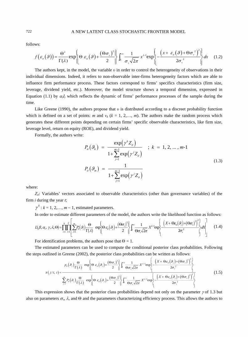
A NEW LATENT CLASS STOCHASTIC FRONTIER MODEL
722
follows:
( )( ) ( ) ( ) ( )( )222-1
20
1
( 2 22exp exp it vv
it itvv
xf x dx
λλ
ε ϑ σσε ϑ ε ϑ
λ σσ π
+∞ + + ΘΘΘ= Θ + −
Γ )
⎧ ⎫⎧ ⎫⎪ ⎪ ⎪ ⎪⎨ ⎬ ⎨ ⎬⎪ ⎪ ⎪ ⎪⎩ ⎭ ⎩ ⎭
∫ (1.2)
The authors kept, in the model, the variable υ in order to control the heterogeneity of observations in their individual dimensions. Indeed, it refers to non-observable inter-firms heterogeneity factors which are able to influence firm performance process. These factors correspond to firms’ specifics characteristics (firm size, leverage, dividend yield, etc.). Moreover, the model structure shows a temporal dimension, expressed in Equation (1.1) by αtIt which reflects the dynamic of firms’ performance processes of the sample during the time.
Like Greene (1990), the authors propose that υ is distributed according to a discreet probability function which is defined on a set of points: m and vk (k = 1, 2,…, m). The authors make the random process which generates these different points depending on certain firms’ specific observable characteristics, like firm size, leverage level, return on equity (ROE), and dividend yield.
Formally, the authors write:
( ) ( )( )
( )( )
1
1
1
1
exp ; 1, 2, ... , -1
1 exp
1 1 exp
kit
it k mj
itj
it m mj
itj
ZP k m
Z
PZ
γϑ
γ
ϑγ
−
=
−
=
= =+
=+
∑
∑
(1.3)
where: Zit: Variables’ vectors associated to observable characteristics (other than governance variables) of the
firm i during the year t; kγ : k = 1, 2,…, m − 1, estimated parameters.
In order to estimate different parameters of the model, the authors write the likelihood function as follows:
( ) ( ) ( ) ( ) ( ) ( ) ( )( )2221
2011 1
1, , , , exp exp2 22
iTN m it j vvt it j it j
ji t vv
XL P X dXλ
ε ϑ σσβ α γ λ ϑ ε ϑ
λ σσ π+∞ −
== =
⎡ ⎤⎧ ⎫+ Θ + Θ⎧ ⎫ΘΘ⎢ ⎥⎪ ⎪ ⎪ ⎪Θ = Θ + −⎨ ⎬ ⎨ ⎬⎢ ⎥Γ Θ⎪ ⎪ ⎪ ⎪⎩ ⎭⎢ ⎥⎩ ⎭⎣ ⎦
∑∏∏ ∫ (1.4)
For identification problems, the authors pose that Θ = 1. The estimated parameters can be used to compute the conditional posterior class probabilities. Following
the steps outlined in Greene (2002), the posterior class probabilities can be written as follows:
( )
( ) ( ) ( ) ( ) ( ) ( )( )
( ) ( ) ( ) ( ) ( ) ( )( )
2221
20
2221
201
1 exp exp2 22
/ , 1 exp exp
2 22
it j vvit j it j
vv
m it j vvit j it j
j vv
Xp X
j i tX
P X
λ
λ
ε ϑ σσϑ ε ϑ
λ σσ ππ
ε ϑ σσϑ ε ϑ
λ σσ π
+∞ −
+∞ −
=
⎧ ⎫+ Θ + Θ⎧ ⎫ΘΘ ⎪ ⎪ ⎪ ⎪Θ + −⎨ ⎬ ⎨ ⎬Γ Θ⎪ ⎪ ⎪ ⎪⎩ ⎭ ⎩ ⎭=⎧ ⎫+ Θ + Θ⎧ ⎫ΘΘ ⎪ ⎪ ⎪ ⎪Θ + −⎨ ⎬ ⎨ ⎬Γ Θ⎪ ⎪ ⎪ ⎪⎩ ⎭ ⎩ ⎭
∫
∑ ∫
(1.5)
This expression shows that the posterior class probabilities depend not only on the parameter γ of 1.3 but also on parameters σv, λ, and Θ and the parameters characterizing efficiency process. This allows the authors to
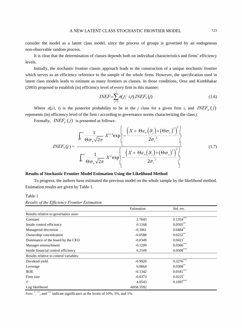
A NEW LATENT CLASS STOCHASTIC FRONTIER MODEL
723
consider the model as a latent class model, since the process of groups is governed by an endogenous non-observable random process.
It is clear that the determination of classes depends both on individual characteristics and firms’ efficiency levels.
Initially, the stochastic frontier classic approach leads to the construction of a unique stochastic frontier which serves as an efficiency reference to the sample of the whole firms. However, the specification used in latent class models leads to estimate as many frontiers as classes. In those conditions, Orea and Kumbhakar (2003) proposed to establish (in) efficiency level of every firm in this manner:
∑=
=J
jit jINEFtijINEF
1)().,(π (1.6)
Where π(j/i, t) is the posterior probability to be in the j class for a given firm i, and ( )itINEF j represents (in) efficiency level of the firm i according to governance norms characterizing the class j.
Formally, ( )itINEF j is presented as follows:
jINEFit ( ) =
( ) ( )( )
( ) ( )( )
22
-120
v
22
20v
1 exp22
1 exp22
it j v
v
it j v
v
XX
XX
λ
λ
ε ϑ σ
σσ π
ε ϑ σ
σσ π
+∞
+∞
⎧ ⎫+ Θ + Θ⎪ ⎪−⎨ ⎬Θ ⎪ ⎪
⎩ ⎭⎧ ⎫+ Θ + Θ⎪ ⎪−⎨ ⎬
Θ ⎪ ⎪⎩ ⎭
∫
∫
(1.7)
Results of Stochastic Frontier Model Estimation Using the Likelihood Method
To progress, the authors have estimated the previous model on the whole sample by the likelihood method. Estimation results are given by Table 1.
Table 1 Results of the Efficiency Frontier Estimation Estimation Std. err. Results relative to governance axes: Constant 2.7643 0.1354*** Inside control efficiency 0.1168 0.0505** Managerial discretion -0.1061 0.0484** Ownership concentration -0.0588 0.0232** Dominance of the board by the CEO -0.0349 0.0421* Manager entrenchment -0.1209 0.0366*** Inside financial control efficiency 0.2109 0.0508*** Results relative to control variables: Dividend yield -0.9920 0.3276*** Leverage 0.0664 0.0308** ROE -0.1342 0.0181*** Firm size -0.0373 0.0225* V 4.0543 0.1097*** Log likelihood -6058.3592
Note. *, **, and *** indicate significance at the levels of 10%, 5%, and 1%.
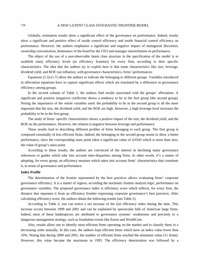
A NEW LATENT CLASS STOCHASTIC FRONTIER MODEL
724
Globally, estimation results show a significant effect of the governance on performance. Indeed, results show a significant and positive effect of inside control efficiency and inside financial control efficiency on performance. However, the authors emphasize a significant and negative impact of managerial discretion, ownership concentration, dominance of the board by the CEO and manager entrenchment on performance.
The object of the use of a non-observable latent class structure in the specification of the model is to establish many efficiency levels (or efficiency frontiers) for every firm, according to their specific characteristics. The idea that the authors try to exploit here is that some characteristics like size, leverage, dividend yield, and ROE can influence, with governance characteristics, firms’ performances.
Equations (1.5)-(1.7) allow the authors to indicate the belonging to different groups. Variables introduced in affectation equations have to capture significant effects which are translated by a difference in governance efficiency among groups.
In the second column of Table 1, the authors find results associated with the groups’ affectation. A significant and positive (negative) coefficient shows a tendency to be in the first group (the second group). Noting the importance of the whole variables used: the probability to be in the second group is all the more important that the size, the dividend yield, and the ROE are high. However, a high leverage level increases the probability to be in the first group.
The study of firms’ specific characteristics shows a positive impact of the size, the dividend yield, and the ROE on the performance. However, the relation is negative between leverage and performance.
These results lead to describing different profiles of firms belonging to each group. The first group is composed essentially of less efficient firms. Indeed, the belonging to the second group seems to show a better performance, since the corresponding mass point takes a significant value of 4.0543 which is more than zero, the value of group’s mass point.
According to these results, the authors are convinced of the interest in declining many governance references or guides which take into account inter-disparities among firms. In other words, it’s a matter of adopting, for every group, an efficiency measure which takes into account firms’ characteristics that constitute it, in terms of governance and performance.
Index Profile
The determination of the frontier represented by the best practices allows evaluating firms’ corporate governance efficiency. It is a matter of regress, according the stochastic frontier analysis logic, performance on governance variables. The proposed governance index is efficiency score which reflects, for every firm, the distance that separates it from an efficiency frontier expressing corporate governance’s best practices. After calculating efficiency score, the authors obtain the following results (see Table 2).
According to Table 2, one can notice a net increase of the (in) efficiency index during the time. This increase occurs between 1999 and 2001 and can be explained by spectacular falls of American large firms. Indeed, most of these bankruptcies are attributed to governance systems’ weaknesses and precisely to a dangerous management strategy, such as fraudulent events like Enron and WorldCom.
Also, results allow one to identify most efficient firms operating on the market and to classify them in a decreasing order annually. In this case, the authors kept efficient firms which have an index value lower than 10%. Noting that during 2000 and 2001, the number of efficient firms reached the minimum value (11 firms). However, this value became the maximum in 1995. The efficiency deterioration was followed by a
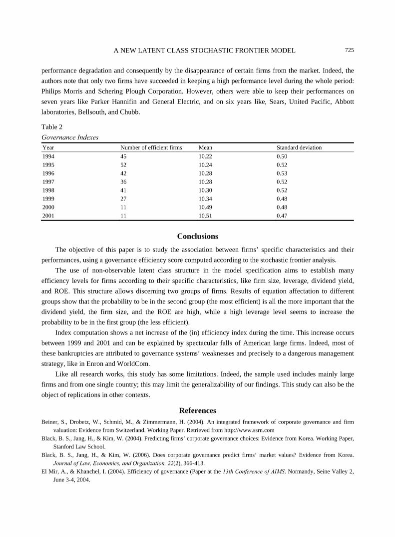
A NEW LATENT CLASS STOCHASTIC FRONTIER MODEL
725
performance degradation and consequently by the disappearance of certain firms from the market. Indeed, the authors note that only two firms have succeeded in keeping a high performance level during the whole period: Philips Morris and Schering Plough Corporation. However, others were able to keep their performances on seven years like Parker Hannifin and General Electric, and on six years like, Sears, United Pacific, Abbott laboratories, Bellsouth, and Chubb.
Table 2 Governance Indexes Year Number of efficient firms Mean Standard deviation 1994 45 10.22 0.50 1995 52 10.24 0.52 1996 42 10.28 0.53 1997 36 10.28 0.52 1998 41 10.30 0.52 1999 27 10.34 0.48 2000 11 10.49 0.48 2001 11 10.51 0.47
Conclusions
The objective of this paper is to study the association between firms’ specific characteristics and their performances, using a governance efficiency score computed according to the stochastic frontier analysis.
The use of non-observable latent class structure in the model specification aims to establish many efficiency levels for firms according to their specific characteristics, like firm size, leverage, dividend yield, and ROE. This structure allows discerning two groups of firms. Results of equation affectation to different groups show that the probability to be in the second group (the most efficient) is all the more important that the dividend yield, the firm size, and the ROE are high, while a high leverage level seems to increase the probability to be in the first group (the less efficient).
Index computation shows a net increase of the (in) efficiency index during the time. This increase occurs between 1999 and 2001 and can be explained by spectacular falls of American large firms. Indeed, most of these bankruptcies are attributed to governance systems’ weaknesses and precisely to a dangerous management strategy, like in Enron and WorldCom.
Like all research works, this study has some limitations. Indeed, the sample used includes mainly large firms and from one single country; this may limit the generalizability of our findings. This study can also be the object of replications in other contexts.
References Beiner, S., Drobetz, W., Schmid, M., & Zimmermann, H. (2004). An integrated framework of corporate governance and firm
valuation: Evidence from Switzerland. Working Paper. Retrieved from http://www.ssrn.com Black, B. S., Jang, H., & Kim, W. (2004). Predicting firms’ corporate governance choices: Evidence from Korea. Working Paper,
Stanford Law School. Black, B. S., Jang, H., & Kim, W. (2006). Does corporate governance predict firms’ market values? Evidence from Korea.
Journal of Law, Economics, and Organization, 22(2), 366-413. El Mir, A., & Khanchel, I. (2004). Efficiency of governance (Paper at the 13th Conference of AIMS. Normandy, Seine Valley 2,
June 3-4, 2004.
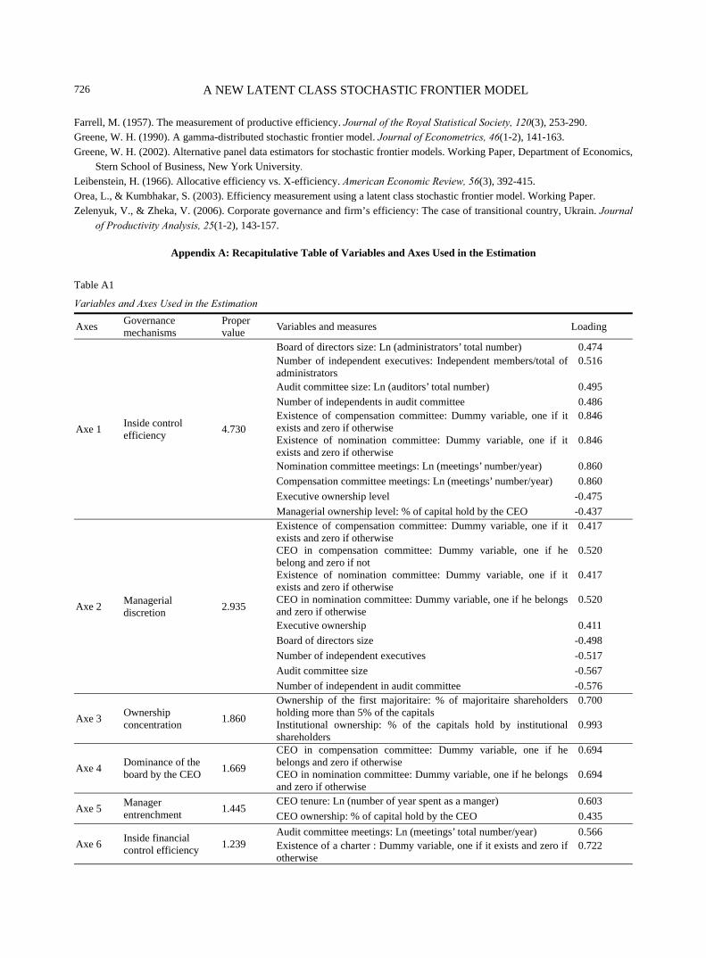
A NEW LATENT CLASS STOCHASTIC FRONTIER MODEL
726
Farrell, M. (1957). The measurement of productive efficiency. Journal of the Royal Statistical Society, 120(3), 253-290. Greene, W. H. (1990). A gamma-distributed stochastic frontier model. Journal of Econometrics, 46(1-2), 141-163. Greene, W. H. (2002). Alternative panel data estimators for stochastic frontier models. Working Paper, Department of Economics,
Stern School of Business, New York University. Leibenstein, H. (1966). Allocative efficiency vs. X-efficiency. American Economic Review, 56(3), 392-415. Orea, L., & Kumbhakar, S. (2003). Efficiency measurement using a latent class stochastic frontier model. Working Paper. Zelenyuk, V., & Zheka, V. (2006). Corporate governance and firm’s efficiency: The case of transitional country, Ukrain. Journal
of Productivity Analysis, 25(1-2), 143-157.
Appendix A: Recapitulative Table of Variables and Axes Used in the Estimation
Table A1
Variables and Axes Used in the Estimation
Axes Governance mechanisms
Proper value Variables and measures Loading
Axe 1 Inside control efficiency 4.730
Board of directors size: Ln (administrators’ total number) 0.474 Number of independent executives: Independent members/total of administrators
0.516
Audit committee size: Ln (auditors’ total number) 0.495 Number of independents in audit committee 0.486 Existence of compensation committee: Dummy variable, one if it exists and zero if otherwise
0.846
Existence of nomination committee: Dummy variable, one if it exists and zero if otherwise
0.846
Nomination committee meetings: Ln (meetings’ number/year) 0.860 Compensation committee meetings: Ln (meetings’ number/year) 0.860 Executive ownership level -0.475 Managerial ownership level: % of capital hold by the CEO -0.437
Axe 2 Managerial discretion 2.935
Existence of compensation committee: Dummy variable, one if it exists and zero if otherwise
0.417
CEO in compensation committee: Dummy variable, one if he belong and zero if not
0.520
Existence of nomination committee: Dummy variable, one if it exists and zero if otherwise
0.417
CEO in nomination committee: Dummy variable, one if he belongs and zero if otherwise
0.520
Executive ownership 0.411 Board of directors size -0.498 Number of independent executives -0.517 Audit committee size -0.567 Number of independent in audit committee -0.576
Axe 3 Ownership concentration 1.860
Ownership of the first majoritaire: % of majoritaire shareholders holding more than 5% of the capitals
0.700
Institutional ownership: % of the capitals hold by institutional shareholders
0.993
Axe 4 Dominance of the board by the CEO 1.669
CEO in compensation committee: Dummy variable, one if he belongs and zero if otherwise
0.694
CEO in nomination committee: Dummy variable, one if he belongs and zero if otherwise
0.694
Axe 5 Manager entrenchment 1.445
CEO tenure: Ln (number of year spent as a manger) 0.603 CEO ownership: % of capital hold by the CEO 0.435
Axe 6 Inside financial control efficiency 1.239
Audit committee meetings: Ln (meetings’ total number/year) 0.566 Existence of a charter : Dummy variable, one if it exists and zero if otherwise
0.722

A NEW LATENT CLASS STOCHASTIC FRONTIER MODEL
727
(Table A1 continued)
Control and performance variables Variable Measure Tobin Q Market value of liabilities on equity replacement value Firm size Log of the total equity Leverage Market value of long-term debts on total equity Dividend yield Market-adjusted return for the period of 12 months (Rt – Rm) ROE Net profit on total equity
Related Documents