Portland State University Portland State University PDXScholar PDXScholar Dissertations and Theses Dissertations and Theses 1996 Jitter and Wander Reduction for a SONET DS3 Jitter and Wander Reduction for a SONET DS3 Desynchronizer Using Predictive Fuzzy Control Desynchronizer Using Predictive Fuzzy Control Kevin Blythe Stanton Portland State University Follow this and additional works at: https://pdxscholar.library.pdx.edu/open_access_etds Part of the Electrical and Computer Engineering Commons Let us know how access to this document benefits you. Recommended Citation Recommended Citation Stanton, Kevin Blythe, "Jitter and Wander Reduction for a SONET DS3 Desynchronizer Using Predictive Fuzzy Control" (1996). Dissertations and Theses. Paper 1164. https://doi.org/10.15760/etd.1163 This Dissertation is brought to you for free and open access. It has been accepted for inclusion in Dissertations and Theses by an authorized administrator of PDXScholar. Please contact us if we can make this document more accessible: [email protected].

Welcome message from author
This document is posted to help you gain knowledge. Please leave a comment to let me know what you think about it! Share it to your friends and learn new things together.
Transcript
Portland State University Portland State University
PDXScholar PDXScholar
Dissertations and Theses Dissertations and Theses
1996
Jitter and Wander Reduction for a SONET DS3 Jitter and Wander Reduction for a SONET DS3
Desynchronizer Using Predictive Fuzzy Control Desynchronizer Using Predictive Fuzzy Control
Kevin Blythe Stanton Portland State University
Follow this and additional works at: https://pdxscholar.library.pdx.edu/open_access_etds
Part of the Electrical and Computer Engineering Commons
Let us know how access to this document benefits you.
Recommended Citation Recommended Citation Stanton, Kevin Blythe, "Jitter and Wander Reduction for a SONET DS3 Desynchronizer Using Predictive Fuzzy Control" (1996). Dissertations and Theses. Paper 1164. https://doi.org/10.15760/etd.1163
This Dissertation is brought to you for free and open access. It has been accepted for inclusion in Dissertations and Theses by an authorized administrator of PDXScholar. Please contact us if we can make this document more accessible: [email protected].
JITTER AND WANDER REDUCTION FOR A SONETIDS3 DESYNCHRONIZER
USING PREDICTIVE FUZZY CONTROL
by
KEVIN BLYTHE STANTON
A dissertation submitted in partial fulfillment of the requirements of the degree of
DOCTOR OF PHILOSOPHY in
ELECTRICAL AND COMPUTER ENGINEERING
Portland State University © 1996

UMI Number: 9635657
Copyright 1996 by Stanton, Kevin Blythe
All rights reserved.
UMI Microform 9635657 Copyright 1996, by UMI Company. All rights reserved.
This microform edition is protected against Uilauthorized copying under Title 17, United States Code.
UMI 300 North Zeeb Road Ann Arbor, MI 48103

DISSERTATION APPROVAL
The abstract and dissertation of Kevin Blythe Stanton for the Doctor of Philosophy in
Electrical and Computer Engineering were presented July 17, 1996, and accepted by the
dissertation committee and the doctoral program.
COMMITTEE APPROVALS:
David A. Turcic Representative of the Office of Graduate Studies
DOCTORAL PROGRAM APPROVA
f/• --~~~ Rolf Schaumann, Chair ) Department of Electrical Engineering
··························································································~·········
ACCEPTED FOR PORTLAND STATE UNIVERSITY BY THE LIBRARY
ABSTRACT
An abstract of the dissertation of Kevin Blythe Stanton for the Doctor of Philosophy in
Electrical and Computer Engineering presented July 17, 1996.
Title: Jitter and Wander Reduction for a SONETIDS3 Desynchronizer using Predictive
Fuzzy Control
Excessive high-frequency jitter or low-frequency wander can create problems
within synchronous transmission systems and must be kept within limits to ensure reli
able network operation. The emerging Synchronous Optical NETwork (SONET) intro
duces additional challenges for jitter and wander attenuation equipment (called desyn-
chronizers) when used to carry payloads from the existing Plesiochronous Digital Hier
archy (PDH), such as the DS3. The difficulty is primarily due to the large phase tran
sients resulting from the pointer-based justification technique employed by SONET
(called Pointer Justification Events or PJEs).
While some previous desynchronization techniques consider the buffer level in
their control actions, none has explicitly considered wander generation. Instead, com
pliance with jitter, wander, and buffer-size constraints have typically been met implicitly
- through testing and tuning of the Phase Locked Loop (PLL) controller.
We investigated a fuzzy/rule-based solution to this desynchronization/constraint
satisfaction problem. But rather than mapping the input state to an action, as is done in
standard fuzzy logic, our controller maps a state and a candidate action to a desired
result. In other words, this control paradigm employs prediction to evaluate which of a
set of candidate actions would result in the "best" predicted performance. Before the

2
controller could predict an action's affect on buffer and wander levels, appropriate mod
els were required. The model of the buffer is simply the integral of the frequency differ
ence between the input and output of the PLL, and a novel MTIE Constraint Envelope
technique was developed to evaluate future wander performance.
We show that a predictive knowledge-based controller is capable of achieving the
following three objectives:
• Reduce jitter implicitly by avoiding unnecessary frequency changes such that the
jitter limits specified in relevant standards are met
• Explicitly satisfy both buffer-level and wander (MTIE) constraints by trading off
performance in one to meet the hard limit of the other
• When both buffer-level and wander constraints are in danger of violation and can
not be satisfied simultaneously, maintain the preferred constraint by sacrificing
the other.
We also show that the computation required for this control algorithm is easily within
the reach of modem microprocessors.

ACKNOWLEDGEMENTS
First, I would like to thank Coreen. She has been a loving wife, a selfless mother, and a
faithful friend. She has never doubted that I could finish whatever I put my mind to. I
would also like to thank my mother and father for being a persistent source of encour
agement and support. I could not have asked for a better family. A big thanks to my
advisor Dr. Y.c. Jenq who was excellent to work with. He made sure that I always had
the tools necessary to complete each task and it is doubtful that 1 would have finished
when I did were it not for the guidance and insights he provided each week. I'd like to
acknowledge NEC America for funding this research. Specifically, Mr. Brian Reilly
and Mr. Steven Gorshe contributed by discussing ideas, offering assistance with T 1
standards and documents, and providing their industrial experience. It is doubtful that
these results would have been achieved without the freedom they gave me to explore
and create. The other members of my committee deserve acknowledgement as well: Dr.
Driscoll for his logical/sequential analysis of my research and for telling me early on
that to earn a Ph.D. I would "have to really, really want it" (I decided that I did); Dr.
Hall for sharing his many practical experiences and insights, time spent on numerous
occasions to train me as a teacher, and his convincing arguments for completing my
education sooner rather than later; Dr. Lendaris for his thorough and frank evaluation of
my ideas and writings, and for a genuinely friendly, personal interest in me and my fam
ily; Dr. Turcic for his encouragement and flexibility, and for bringing up the question of
simulation validity early on so that I had time to consider this critical component. I
would like to acknowledge the EE staff and several of my many supportive friends: Tim
Grant, Brian Heerwagen, Dan Marvin, Larry Trout, and Will Rogers; my sisters, sisters
in-law, brothers-in-law, and parents-in-law for their encouragement; and daughters
Tiffany and Chandelle for keeping my spirits up. Finally, I thank my God and Savior
for giving me the ability, the opportunity, and the endurance to finish what I started.
TABLE OF CONTENTS
PAGE
ACKNOWLEDGEMENTS ............................................................................................. ii
LIST OF TABLES ......................................................................................................... vii
LIST OF FIGURES ...................................................................................................... viii
ACRONYMS .................................................................................................................. xi
CHAPTER
I. INTRODUCTION ........................................................................................... .
II. SONETIDS3 DESYNCHRONIZATION ......................................................... 5
A. DIGITAL COMMUNICATIONS .............................................................. 5
1. Plesiochronous Digital Hierarchy (PDH) ......................................... 6
2. Synchronous Digital Hierarchy (SDH) ............................................. 6
3. Mixing the Hierarchies. .................................................................... 9
B. THE SONETIDS3 DESYNCHRONIZATION PROBLEM .................... II
1. Basic Architecture '" ...... ................ .......... ................................. ...... 11
2. Sources of Input Jitter ..................................................................... 11
3. Desynchronizer Requirements/Constraints .................................... 14
III. WANDER AND JITTER ................................................................................ 15
A. WANDER ................................................................................................ 15
1. MTIE Definition ....................... .................... ........ .......... ..... ........... 15
2. Wander Filter Design ........ .............................................................. 17
B. JITTER..................................................................................................... 18
1. Peak-to-Peak Jitter Measurement ................................................... 18
2. Jitter Filter Design .......................................................................... 18
3. Minimum TIE Sample Frequency .................................................. 19

iv
C. MTIE CONSTRAINT ENVELOPE ................................................... ..... 23
IV. PREVIOUS WORK........................................................................................ 28
A. PURELY ANALOG LOW PASS PLL .................................................... 28
B. PHASE SPREADING .............................................................................. 29
I. FIXED RATE.......................................................... ........................ 30
2. VARIABLE RATE ......................................................................... 30
E. STUFF THRESHOLD MODULATION (STM)...................................... 30
F. ADAPTIVE DITHER BIT LEAKING ..................................................... 31
G. FEED FORWARD POINTER SPREADING .......................................... 31
H. SUMMARY ............................................................................................. 32
V. THE KNOWLEDGE-BASED CONTROLLER. ............................................ 33
A. REASONS FOR CHOOSING AN HEURISTIC APPROACH .............. 34
I. Goal Equations are Nonlinear ......................................................... 34
2. Various Modes of Operation ...................................... ............. ... ..... 34
3. Opposing Constraints ...................................................................... 34
B. THE TRADITIONAL KNOWLEDGE-BASED CONTROLLER .......... 35
I. What is it? ....................................................................................... 35
2. When is a Fuzzy Knowledge-Based Controller appropriate? ......... 41
3. Disadvantages ................................................................................. 42
C. PREDICTIVE KNOWLEDGE BASED CONTROLLER ....................... 42
I. What is it? ....................................................................................... 42
2. When is a PKBC Appropriate ......................................................... 47
3. Disadvantages ................................................................................. 47
VI. PKBC FOR THE SONETIDS3 DESYNCHRONIZER ................................. 49
A. OVERVIEW ............................................................................................. 49
B. ARCHITECTURE ................................................................................... 50

v
1. Inputs .................. ............................ ............ .................................... 52
2. Rules ............................................................................................... 55
3. Fuzzy Sets ....................................................................................... 55
4. Models ............................................................................................ 57
5. Output ............................................................................................. 62
C. STRATEGIES FOR RULEIFUZZY SET DEVELOPMENT ................. 62
I. Partitioning the Space ..................................................................... 63
2. Delta Ruts ....................................................................................... 64
3. Full Domain Fuzzy Set Spanning Property .................................... 65
4. Output Fuzzy Sets ........................................................................... 67
5. Maintaining MTIE Compliance ...................................................... 67
6. Maintaining Buffer Compliance ..................................................... 68
7. Observations .................... ............ ........................... .................. ...... 69
D. FINAL CONTROLLER SPECIFICATION ............................................ 70
1. FUZZY SETS ................................................................................. 71
2. RULES ............................................................................................ 72
VII. SIMULATION ENVIRONMENT .................................................................. 75
A. SIMULATION FRAMEWORK .............................................................. 75
B. VALIDITY ............................................................................................... 75
C. SIMULATION MODULES ..................................................................... 77
1. Scheduler .................. ............. ................. ......... ........... ...... .............. 77
2. Input Signal ..................................................................................... 77
3. PJE Generator ................................................................................. 77
4. DDS Output .................................................................................... 78
5. Phase Comparator ........................................................................... 79
D. SIMULATION MEASUREMENTS ....................................................... 80
vi
I. TIE Reference Clock...... ...... .... ............ .... ... ............. ............. ..... .... 80
2. Jitter Measurement.............................................................. ............ 80
3. Wander ............................................................................................ 81
E. GRAPHICAL USER INTERFACE .................................................... ..... 81
F. COMPUTATIONAL COMPLEXITY ...................................................... 85
VIII. TESTING AND EVALUATION .................................................................... 88
A. STANDARD JITTER TESTS .................................................................. 88
I. Mapping Jitter ... ...................... .......... ........... ........... ................ ... ..... 89
2. Standard Mode ................................................................................ 93
3. Burst Mode ..................................................................................... 95
4. Phase-Transient Burst Mode ........................................................... 98
5. Degraded Mode ......... .............................. ....................... ..... ...... ... 101
6. Jitter Summary .............................................................................. III
C. CONSTRAINT-SATISFACTION TESTS .......................................... ... III
I. Wander Satisfied ............................................................................ 112
2. Buffer Satisfied ............................................................................. 115
IX. CONCLUSIONS/FUTURE WORK ............................................................ 117
A. CONCLUSION ...................................................................................... 117
B. FUTURE WORK ................................................................................... 119

LIST OF TABLES
TABLE PAGE
I. Dither Pattern ....................................................................................................... 31
II. Fuzzy Set Definitions .......................................................................................... 56
III. Computational Complexity Multipliers ............................................................... 87
IV. Mapping Jitter vs. Stuffing Ratio......................................................................... 90
V. Standard Mode Jitter............................................................................................ 95
VI. Burst Mode Jitter ................................................................................................. 96
VII. Phase Burst Jitter ............................................................................................... 101
VIII. Degraded Mode (Continuous Pattern) Jitter ...................................................... 104
IX. Degraded Mode (87-3 Pattern) Jitter ................................................................. 109
X. Jitter Summary ................................................................................................... III
XI. Proposed MTIE Mask................................... .................. ..... ....... ....................... 112
LIST OF FIGURES
FIGURE PAGE
1. STS-I Frame Structure ......................... ............................................................ ..... 7
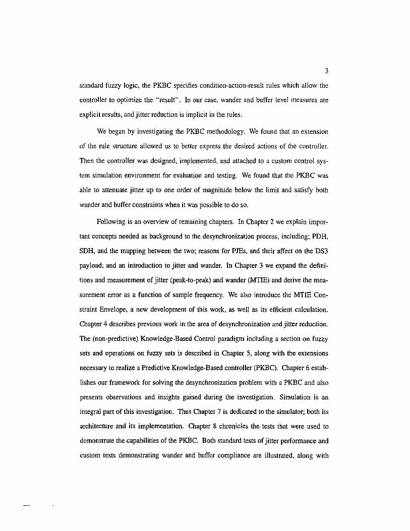
2. SPE Floating Within A Frame ............................................................................... 9
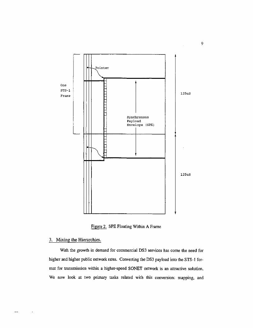
3. DS3/STS-I Mapping ........................................................................................... 10
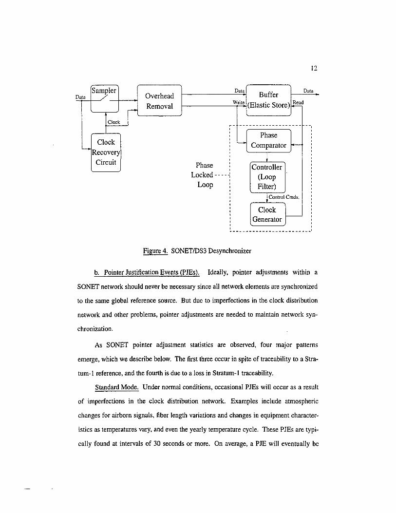
4. SONETIDS3 Desynchronizer .............................................................................. 12
5. Illustrated MTlE Definition ................................................................................. 16
6. Percent Error vs. Sample Frequency.. ............................................ ..................... 22
7. Example MTlE Mask ............. ........ .... .... ....................... ... .... .......... ............... ... ... 24
8. Example TIE Samples ......................................................................................... 24
9. Example MTIE Constraint Envelope ................................................................... 25
10. Actual MTIE Constraint Envelope with TIE Projection ..................................... 27
11. Architecture for the Phase Spreading technique ................................................. 29
12. Crisp and Fuzzy Definition of "tall" .................................................................. 36
13. Fuzzy Set Definitions for Sample KBC ............................................................... 38
14. Rule Matrix .......................................................................................................... 39
15. KBC Control Surface .......................................................................................... 40
16. PKBC Execution Diagram ........................................ .................... ............ .......... 45
17. New PKBC Rule Structure .................................................................................. 46
18. Basic Desynchronizer Diagram ........................................................................... 50
19. PKBC Desynchronizer Controller .............................. ............. .... ............ ............ 51
20. Fuzzy Set Definitions .......................................................................................... 56
21. DDS Block Diagram ............................................................................................ 61
22. Natural and Controlled Vector Fields .................................................................. 64
23. Original D_Buffer Fuzzy Set Definition ............................................................. 66

ix
24. Improved (for PKBC) D_Buffer Fuzzy Set Definition ........................................ 66
25. Output Singletons ................................................................................................ 67
26. Final Buffer Fuzzy Set Definitions ...................................................................... 71
27. Final ~uffer Fuzzy Set Definitions ................................................................... 71
28. Wander Fuzzy Set Definitions ............................................................................. 72
29. Simulator Object Interaction Diagram ................................................................ 76
30. Phase Measurement ............................................................................................. 79
31. Simulation Example Showing Predicted d_buffer movement............................. 83
32. Simulation Example Showing d_buffer movement............................................. 84
33. Rule and Term Execution Times ......................................................................... 87
34. Mapping Jitter Simulation Example ..................................................................... 91
35. Mapping Jitter vs. Stuffing Ratio......................................................................... 92
36. Standard Mode PJE Test Sequence ..................................................................... 93
37. Standard Mode Simulation Example ................................................................... 94
38. Standard Mode Jitter ............................................................................................ 95
39. Burst Mode PJE Test Sequence ........................................................................... 96
40. Burst Mode Simulation Example ........................................................................ 97
41. Burst Mode Jitter ................................................................................................. 98
42. Phase-Transient Burst Mode PJE Test Sequence ................................................ 99
43. Phase-Transient Burst Mode Simulation Example ............................................ 100
44. Phase-Transient Burst Mode Jitter ...................................................................... 99
45. Degraded Mode PJE Test Sequence (Continuous) ............................................ 102
46. Degraded Mode Simulation (Continuous) Example ......................................... 103
47. Degraded Continuous Pattern Jitter ................................................................... 106
48. Degraded Mode PJE Test Sequence (Continuous) ............................................ 107
49. Degraded Mode Simulation (87-3) Example ..................................................... 108
x
50. Degraded 87-3 Pattern Jitter .............................................................................. 109
51. Proposed DS3 Wander Specification ................................................................. 113
52. MTIE Satisfaction Plot...................................................................................... 114
53. MTIE Satisfaction Plot With Buffer .................................................................. 115
54. Buffer Satisfaction Plot ..................................................................................... 116

ATM dB DDS DS3 HPF KBC LPF MTIE Mbps MHz NE p-p PDH PJE PKBC PLL POH SOH SO NET SPE STS-1 SUT T3 TIE UI
ACRONYMS
Asynchronous Transfer Mode Decibels Direct Digital Synthesis Digital Signallevel-3 High-Pass Filter Knowledge-Based Controller Low-Pass Filter Maximum Time Interval Error Million (Mega)-Bits Per Second Mega-Hertz Network Element Peak-to-Peak Plesiochronous Digital Hierarchy Pointer Justification Event Predictive Knowledge-based Controller Phase Locked Loop Path OverHead Synchronous Digital Hierarchy Synchronous Optical NETwork Synchronous Payload Envelope Synchronous Transport Signal level- I Signal Under Test Transmission-level term for DS3 Time Interval Error Unit Interval
CHAPTER I
INTRODUCTION
The demand for high-speed digital communications is experiencing explosive
growth as more people expect more information in less time. The emerging ATM
(Asynchronous Transfer Mode) standard promises efficient transfer of diverse types of
payload over high-speed channels, and other network technologies are likely to follow.
Common to these existing and future services is the need for a physical layer communi
cations link - typically synchronous transmission - and common to all synchronous
data transmission systems, is synchronization.
Both the ubiquitous Tl and T3 physical layer services and the emerging SONET
(Synchronous Optical NETwork) hierarchy employ synchronous data transmission, and
thereby require synchronization. In addition, SONET employs global synchronization
[1], whereas the Plesiochronous (pronounced "pIe se a ' kro n ~ s") Digital Hierarchy
(PDH), of which the TI and T3 services are members, employs only local synchroniza
tion (point to point).
However, when the typically slower PDH services are carried by the faster
SONET, the difficult problem of desynchronizing the PDH signal from SONET is intro
duced. In particular, imperfections in the clock distribution network of any synchronous
network topology necessitate realignment of the data payload from time to time to pre
vent the network element buffers from underflowing or overflowing. SONET imple
ments these justification events by allowing the first byte of each frame of the payload
to be advanced or retarded by one byte as needed. However, these so-called justification

2
events appear as eight-bit phase transients in the data stream when the PDH payload is
reconstructed. Limits on both high-frequency phase transients Uitter) and low
frequency phase transients (wander) [2] are established by bodies such as ANSI and
Bellcore and must be met before equipment can be certified.
Our investigation focused on this - the SONETIDS3 Desynchronization prob
lem. A desynchronizer receives and buffers the "bursty" data to produce a smoother
outgoing data rate. Desynchronizers typically consist of an elastic store (buffer) and a
Phase Locked Loop (PLL). A PLL, in turn, contains a phase comparator, a loop filter,
and a programmable oscillator. If the buffer in the desynchronizer were infinitely large,
jitter and wander could be eliminated - at the cost of data latency. If jitter and wander
were not a concern, the buffer could be very small - reducing data latency. In practice,
however, the buffer has a limited size and jitter and wander must meet specifications.
An intelligent controller would use the buffer as much as possible to reduce jitter and
wander, yet would not allow it to overflow or underflow. In the event both buffer and
wander constraints reach their violation threshold, a decision would be made to main
tain one constraint by allowing the other to be violated.
Industry standards [3] specify jitter performance in terms of a set of PJE profiles,
applied during testing. Wander specifications [4], however, are universal and apply to
any and all possible scenarios. Although current desynchronizer designs exist which
satisfy the jitter performance requirements, none explicitly consider wander generation.
Our objective was to investigate the ability of a Predictive Knowledge-Based Controller
PKBC to excel in jitter reduction but also, and more importantly, satisfy wander and
buffer constraints dynamically.
The PKBC methodology operates on a rulebase ("Knowledge-Based") and uses
functional models to choose an action which will result in the highest performance
("Predictive"). Rather than simply specifying condition-action rules, as is the case with
3
standard fuzzy logic, the PKBC specifies condition-action-result rules which allow the
controller to optimize the "result". In our case, wander and buffer level measures are
explicit results, and jitter reduction is implicit in the rules.
We began by investigating the PKBC methodology. We found that an extension
of the rule structure allowed us to better express the desired actions of the controller.
Then the controller was designed, implemented, and attached to a custom control sys
tem simulation environment for evaluation and testing. We found that the PKBC was
able to attenuate jitter up to one order of magnitude below the limit and satisfy both
wander and buffer constraints when it was possible to do so.
Following is an overview of remaining chapters. In Chapter 2 we explain impor
tant concepts needed as background to the desynchronization process, including; PDH,
SDH, and the mapping between the two; reasons for PJEs, and their affect on the DS3
payload; and an introduction to jitter and wander. In Chapter 3 we expand the defini
tions and measurement of jitter (peak-to-peak) and wander (MTIE) and derive the mea
surement error as a function of sample frequency. We also introduce the MTIE Con
straint Envelope, a new development of this work, as well as its efficient calculation.
Chapter 4 describes previous work in the area of desynchronization and jitter reduction.
The (non-predictive) Knowledge-Based Control paradigm including a section on fuzzy
sets and operations on fuzzy sets is described in Chapter 5, along with the extensions
necessary to realize a Predictive Knowledge-Based controller (PKBC). Chapter 6 estab
lishes our framework for solving the desynchronization problem with a PKBC and also
presents observations and insights gained during the investigation. Simulation is an
integral part of this investigation. Thus Chapter 7 is dedicated to the simulator; both its
architecture and its implementation. Chapter 8 chronicles the tests that were used to
demonstrate the capabilities of the PKBC. Both standard tests of jitter performance and
custom tests demonstrating wander and buffer compliance are illustrated, along with

4
appropriate graphs and tables to illustrate the simulation results. Finally, Chapter 9
draws conclusions and suggests topics of future work which would build upon our con
tributions.

CHAPTER II
SONETIDS3 DESYNCHRONIZATION
Before discussing the details of the problem domain in which we frame our inves
tigation, we first provide a brief overview of the field of digital communications. Then,
in Section B. we define the specifics of the problem we set out to solve.
A. DIGITAL COMMUNICATIONS
Common to both digital hierarchies discussed below is the concept of syn
chronous data transmission. Synchronous transmission means that there is an a priori
agreed frequency of transmission between Network Elements (NEs), and thus there is
no handshaking between transmitter and receiver. The transmitter blindly sends data at
the predetermined data rate. The receiver locks on to the data rate and uses this "recov
ered" clock to sample the line.
A synchronous hierarchy is a multi-level network with many network elements
(NEs) which operate at multiples of the same fundamental frequency and are mutually
synchronized. Conversely, an plesiochronous hierarchy is a set of NEs which, while
they may communicate synchronously from point to point, are not synchronized to a
global frequency reference. The prefix plesio is derived from a greek word meaning
"close to", or "near". So, although the levels of the PDH are not strictly synchronous,
they are nearly synchronous.

6
1. Plesiochronous Digital Hierarchy (PDH)
In this hierarchy we have formats and rates commonly known as OS 1, OS2, OS3,
and so on (alternately TI, T2, T3). When signals which are lower in the hierarchy are
combined (multiplexed) to form higher level signals, the incoming bit streams are adap
tively padded with "stuff bits" in order to bring them up to a common (higher than nom
inal) rate before being bit-wise interleaved to form the higher level signal. When
demultiplexed, the stuff bits are removed and a desynchronizer is used to smooth the
resulting data rate. This is called asynchronous multiplexing, since higher rates are not
integer multiples of lower rates.
2. Synchronous Digital Hierarchy (SDH)
In contrast to the PDH, all NEs of the SDH (also called the Synchronous Optical
NETwork or SONET in North America) operate at a rate traceable to a Stratum-l global
frequency reference (accurate to one part in lxlO ll ), and higher levels operate at integer
multiples of the lower rates. Thus no rate adjustment (stuffing) is required under normal
circumstances when multiplexing lower-level signals into a higher-level signal, since the
higher rate is synchronized to a mUltiple of the lower-level signals and both are derived
from the same global reference clock. If this were implemented in a perfect environ
ment, our research in this area would be unnecessary. However, imperfections in the
clock distribution network occasionally require PJEs for timing justification. PJEs pro
duce jitter and wander as described below.
a. Frame Structure. For historical reasons, SONET is based on a frame-rate of
8KHz - the bit-rate for a single, digitized telephone line. The frame is organized as
nine rows and 3 + 87n columns, where n is the level in the hierarchy. The lowest signal
in the hierarchy, STS-l (Synchronous Transport Signal, level 1), operates at a rate of
Sl.84MHz. All other rates are derived from this rate. Figure 1 illustrates the STS-\

frame structure.
0\
Section and
Line Overhead
90 Bytes
STS-1 Envelope Capacity
Figure l. STS-l Frame Structure
7
Each row of the frame begins with three bytes of what is called Transport Over
Head (TOH). The remaining row capacity is termed the Synchronous Payload
Envelope, or SPE. The first byte of the SPE is Path OverHead (POH), leaving 86n
bytes for the payload.
b. Pointer Processing. Suppose an NE receives an STS-l, processes it, and
retransmits it. If, for reasons described later, the incoming STS-l data rate were to lag
behind the outgoing rate, the network element's transmitting circuit would eventually
run out of data, causing an underflow error. Conversely, if the incoming rate were
higher than the outgoing rate, the storage buffer would eventually overflow. For this
reason, the first byte of the Synchronous Payload Envelope (SPE) is allowed to float

8
with respect to the first byte of the frame.
The location of the first byte of the SPE within the frame is indicated by the value
of a pointer in the Transport Overhead. If the incoming data rate is higher than the out
going data rate, a pointer processing module responds by decrementing the "beginning
of-envelope" pointer as needed. The result is an advance of subsequent envelopes of
data by one byte. Since the first byte of the SPE where the pointer adjustment took
effect is the same location in the frame as the last byte of the previous SPE, a special
byte of storage is reserved in the overhead for such an occasion. Figure 2 illustrates the
f1oating-SPE concept.
An analogy is drawn in [5] between SONET pointer processing and a man walk
ing through a moving train: "If he moves toward the front, he is moving slightly faster
than the train. If he moves toward the rear, he moves slower than the train. A pointer
would be a person watching him and always knowing where he is on the train".
Each PJE produces an eight bit phase transient when a signal is extracted (desyn
chronized) from the SPE. These transients must be smoothed to meet jitter and wander
specifications.
This is a difficult problem. First, phase transients resulting from a PJE are eight
times larger than those in a PDH network. Also, PJEs may occur at an arbitrarily low
frequency and have a long-term nominal rate of zero. A nominal rate of zero has been
shown to produce worst-case waiting-time jitter [6].
c. Virtual Tributaries. As the lowest level of the SONET hierarchy, the STS-I
signal can not have other SONET signals as tributaries. Instead, virtual tributaries are
defined which allow other payload types to be mapped into the STS-I frame [7]. The
specific mapping is presented in Section 3.
One
STS-1
Frame
I• 1\nter
~~--------------~
Synchronous Payload Envelope (SPE)
Figure 2. SPE Floating Within A Frame
3. Mixing the Hierarchies.
9
125uS
125uS
With the growth in demand for commercial DS3 services has come the need for
higher and higher public network rates. Converting the DS3 payload into the STS-1 for-
mat for transmission within a higher-speed SONET network is an attractive solution.
We now look at two primary tasks related with this conversion: mapping, and

10
unmapping.
a. Mapping/Synchronization. DS3 operates at a rate of 44.736 Million Bits Per
Second (Mbps), and the STS-1 rate is 51.84Mbps. To account for the difference in
nominal rate, fixed locations within each SPE row are assigned fixed stuff bits. To
account for fluctuations of the DS3 signal with respect to the STS-1 rate, one special
stuff bit per row may be assigned payload data as necessary, depending on the relative
incoming and outgoing rates. Whether or not this "stuff opportunity" is taken is indi
cated by a majority vote of the previous Stuff Control (C) bits. It turns out that if
incoming and outgoing rates are exactly nominal, the stuff opportunity is taken two
thirds of the time. Figure 3 shows the precise location of the Path OverHead (POH),
the fixed stuff bits ("R"), the DS3 bits ("I"), the stuff bit ("S"), and the stuff Control
bits ("C") [7].
RRC 8R 8R \ I
CCRRRRRR 8R 8~ /
CCRROORS 8R 8~ /
I POH [Xc><J :51 I 25x81 25x81 lXIXI I 81 I 25x81
87 Bytes
Figure 3. DS3/STS-1 Mapping
b. UnMapping/Desynchronization. Upon arrival at a SONET/PDH mapping
node, it is necessary to remove the overhead and fixed stuff bits from the SPE and con
vert the SONET-mapped DS3 back to its original rate. As the payload data is received,
the elastic store write-clock is inhibited during the SONET overhead bytes, fixed stuff
bits, and untaken stuff opportunities, since they were not part of the original DS3 pay
load. The result is a write-clock whose instantaneous rate is that of the STS-1, but with
gaps which lower the average rate to the original DS3 level. Thus, after unmapping, the
DS3 must be desynchronized- brought back to the rate of the original DS3 signal. To

11
accomplish this, the data is stored in a buffer using the gapped clock and read out using
the clock generated by the desynchronizer, which is the topic of the next section.
B. THE SONETIDS3 DESYNCHRONIZATION PROBLEM
1. Basic Architecture
A SONETIDS3 desynchronizer is illustrated in Figure 4. The DS3 data is written
into the buffer using a gapped clock and the phase comparator measures the phase dif
ference betlveen the gapped write clock and the smooth read clock. The loop filter per
forms a low-pass operation on these measurements and sends an appropriate command
to the programmable oscillator such that future phase difference measurements tend
toward some desired value.
The loop filter has the responsibility of both smoothing jitter and wander and pre
venting buffer overflow - two opposing requirements as we have seen earlier. Past
attempts at addressing this challenge are presented in Chapter IV and our approach is
presented in Chapter VI. But first, we look more closely at the major causes of jitter in
the write (input) clock.
2. Sources of Input Jitter
Jitter is related to the variation in the bit arrival time of a data stream. When we
speak of jitter caused by the DS3/S0NET mapping, we can identify three major
sources: mapping jitter, pointer justification events, and bit-stuffing jitter.
a. Mapping Effects. The gaps in the DS3 datastream caused by the removal of
SONET overhead 'and fixed stuff bits are a source of high-frequency jitter which must
be suppressed by the desynchronizer. This jitter is constant, since the number of gaps
and their location is identical from row to row and frame to frame.
12
Sampler Data Buffer
Data Data Overhead
Removal Write (Elastic Store) 1 ~ead
Clock r- ------------------- -- I I I I
Phase I I I
Clock I I I c....-
Comparator - I
c....- I I
Recovery I I I
~ I
I '
Circuit I
' Phase Controller I I
Locked----I
(Loop I
' Loop
I
Filter) I I I
~Control Cmds. ' ' '
Clock I I I
Generator - I I I I
------------------------_I
Figure 4. SONET/DS3 Desynchronizer
b. Pointer Justification Events (PJEs). Ideally, pointer adjustments within a
SO NET network should never be necessary since all network elements are synchronized
to the same global reference source. But due to imperfections in the clock distribution
network and other problems, pointer adjustments are needed to maintain network syn-
chronization.
As SONET pointer adjustment statistics are observed, four major patterns
emerge, which we describe below. The first three occur in spite of traceability to aStra
tum- I reference, and the fourth is due to a loss in Stratum-! traceability.
Standard Mode. Under normal conditions, occasional PJEs will occur as a result
of imperfections in the clock distribution network. Examples include atmospheric
changes for airborn signals, fiber length variations and changes in equipment character-
istics as temperatures vary, and even the yearly temperature cycle. These PJEs are typi
cally found at intervals of 30 seconds or more. On average, a PJE will eventually be
13
canceled by a negative PJE since timing is derived from a common source.
Burst Mode. Under normal conditions, consecutive NEs may be near the thresh-
old for generating a PJE due to reasons described above. A PJE generated at the first
NE would then trigger an additional PJE at subsequent NEs, resulting in a sudden burst
of PJEs. Although the odds of this happening are not high, a desynchronizer must be
capable of attenuating these large, infrequent bursts.
Phase-Transient Burst Mode.
This mode is similar to Burst mode, except that the pointer adjustments are greater in
number and arrive at a lower rate.
Degraded Mode. If a NE looses its connection to the clock distribution network
due to equipment failure or a broken link, it temporarily switches to a local oscillator.
This is called "holdover" mode. Since the required accuracy of the holdover oscillator
is much lower than Stratum-I, a frequency offset results. The next NE which is still
synchronized to a Stratum-l would then need to rapidly generate pointer adjustments to
resolve the difference. According to tests specified in standards documents, these
pointer adjustments may be spaced as closely as 0.034 seconds or as far apart as 10 sec
onds. A desynchronizer must be capable of attenuating the high-frequency jitter result
ing from this mode of operation.
c. Bit Stuffing Jitter. To accommodate a range of input DS3 rates, the adaptive
bit stuffing mechanism determines on a row-by-row basis whether to include an extra
data bit in the stuffing location defined above. The stuffing rate can be derived as
DS3BitRate C = - DS3BitsPerRow
RowFrequency
DS3BitRate = 8K. 9 - 621
At the nominal DS3 rate of 44.736Mbs, C equals 113. Stuffing jitter is considered a

14
"mapping" effect.
3. Desynchronizer Requirements/Constraints
We now look at the desynchronizer and constraints it must satisfy.
a. Buffer. Typically, the PLL controller attempts to keep the buffer half-full. If
the fill-level is too low, underflow is threatened. If the fill-level is too high the danger is
overflow.
A half-full buffer is said to have a fill-level of zero. Similarly, a buffer which is
more than half full is said to have a positive fill-level and a buffer which is less than
half-full is said to have a negative fill-level. If an infinite buffer were used, any fixed
output frequency less than the input would yield optimal jitter performance. Of course
such a requirement cannot be met in practice. In addition, large data buffers increase
the data latency of the communications channel, slowing response times.
b. Phase Variation (Jitter and Wander). Both jitter and wander calculations begin
with a measure of phase variation, called Time Interval Error (TIE, pronounced "tI").
TIE is a measure of the difference in phase between a signal under test and a reference
signal,
I
TIE(t) = f fSUT(t) - fREFdt o
where fSUT(t) is the frequency of the signal under test, and fREF is the constant refer
ence frequency. TIE is typicaily specified in Unit Intervals, or VI (cycles of the nominal
frequency). Both low frequency and high frequency (jitter) phase variation measures
are derived from this signal.
The next chapter defines wander and jitter and derives criteria for accurately mea-
suring them in the discrete-time domain. Also, the method for predicting compliance
with wander constraints is developed.

CHAPTER III
WANDER AND JITTER
Bounded jitter and wander are necessary for error-free operation of synchronous
transmission networks. In this chapter we define "jitter" and "wander" in the context
of the PDH hierarchy and discuss established measurement procedures. For a broader
treatment of jitter in digital transmission systems the reader is referred to [8].
In Section C, after defining jitter and wander in Sections A and B, we present a
novel technique for transforming past measurements and wander specifications into a
constraint envelope which can be used to predict future wander compliance.
A. WANDER
1. MTIE Definition
Maximum Time Interval Error (MTIE, pronounced "em ti") is the primary wan
der measure. Rather than characterizing wander with a single quantity, MTIE is a func
tion of the width of an observation window in which a peak-to-peak measurement is
taken, and is expressed as a curve. Essentially, MTIE is a time-independent measure of
long-term drift. Thus it is logical to first pass the TIE measurements through a low-pass
filter. But before deriving the filter equation, we first illustrate the MTIE calculation
itself.
We define X(t) to be the filtered TIE samples, of which N samples have been
taken at an interval of to seconds. Figure 5 illustrates the MTIE calculation. First, a
peak-to-peak calculation is performed within a window (observation period) of size S.
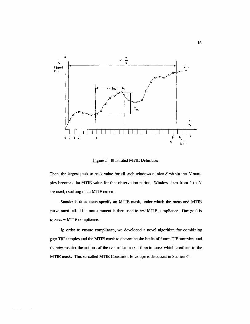
X; Fillered TIE
0 I 2 :1
N=!_ ru
j
Figure 5. Illustrated MTIE Definition
16
X(l)
~ \ N N+l
Then, the largest peak-to-peak value for all such windows of size S within the N sam
ples becomes the MTIE value for that observation period. Window sizes from 2 to N
are used, resulting in an MTIE curve.
Standards documents specify an MTIE mask, under which the measured MTIE
curve must fall. This measurement is then used to test MTIE compliance. Our goal is
to ensure MTIE compliance.
In order to ensure compliance, we developed a novel algorithm for combining
past TIE samples and the MTIE mask to determine the limits of future TIE samples, and
thereby restrict the actions of the controller in real-time to those which conform to the
MTIE mask. This so-called MTIE Constraint Envelope is discussed in Section C.

17
2. Wander Filter Design
ANSI specifications [2] require the TIE signal to be passed through a single-pole
low-pass filter with a 10Hz, 3dB cutoff before performing the MTIE calculation. Next
we briefly describe the design of a digital filter with these characteristics.
The expression for the discrete-time low-pass filter may be derived from a stan
dard continuous-time, single-pole low-pass filter,
a HLP(S) =--
s+a
with an appropriate substitution for s using the bilinear transformation,
a must be pre-warped because of the nonlinearity of the bilinear transformation [9],
based on the cutoff frequency Ie
("Ie) a=tan fr
To simplify calculations, we define a and bas,
and
I-a a=--
I+a
a b=-
l+a
The transfer function in the z-domain then becomes,
b +bz-1
HLP(z) = 1 1 -az-
This expression may be realized by an Infinite Impulse Response (IlR) filter with the
following difference equation,
18
YLp[n] = bx[n] + bx[n- I]+ a~'LP[n- I]
where x[] is the sequence of raw TIE samples andy LP [] is the filtered result.
B. JITTER
1. Peak-to-Peak Jitter Measurement
Jitter is a measurement of high-frequency TIE variations. Unlike wander. which
is expressed as a curve, jitter is represented by a single value.
Once TIE measurement is finished (the simulation is over), the peak-to-peak (p-p)
value of the filtered TIE samples is used to represent total jitter. This is analogous to a
single MTIE calculation with an observation period S equal to the entire measurement
period (N).
Although ANSI specifications places restrictions on p-p jitter, the limit is different
for each test scenario (see Chapter Vill), and therefore cannot be used as a global con-
straint in the same sense that MTIE is used as a constraint.
Nevertheless, p-p jitter is an important measure of a desynchronizer's perfor
mance and is often used by equipment manufactures to represent the performance of a
desynchronizer.
2. Jitter Filter Design
The jitter signal is generated by passing TIE samples through a single-pole, high
pass filter with a 10Hz, 3dB cutoff frequency [2].
In the discrete-time domain, the filter may be derived as
s s+a

19
Since the low-pass wander filter and high-pass jitter filter have the same cutoff fre-
quency, we can use an equivalence relation to derive the expression of one from the
other. Specifically,
(l-b)-(a+b)z-I = I-az-I
which yields the difference equation:
YHP[n] = (1- b)x[n] - (a + b)x[n- I] + aYHP[n- I]
where x[] is the sequence of raw TIE samples and Y HP [] is the filtered result.
3. Minimum TIE Sample Frequency
Since MTIE considers only low-frequency components of the TIE signal, a TIE
sample rate which is several multiples of the cutoff frequency is adequate. Jitter, on the
other hand, requires a filtered TIE signal with frequency components which extend to
infinity. Unfortunately, a discrete-time system such as ours is not able to take sample
fast enough to meet this requirement. Fortunately, however, we can calculate the error
which results from a non-infinite sample frequency. Once this expression is know,
choosing the sample rate is reduced to specifying an allowable error and finding the cor
responding sample frequency. In the following we assume that output jitter results only
from frequency steps, which is true for a controller employing a DDS (Direct Digital
Synthesis, described in Section 4.E of Chapter VI) for frequency generation.
First we derive an exact expression for jitter resulting from a frequency step, and
then for the jitter measured by a discrete-time system. Comparison of these two results
gives us the percent error as a function of sample period.
20
a. Continuous-Time Jitter Calculation. Jitter is a peak-to-peak measure of the
filtered integral of a frequency step. The integral of a step function is a ramp, with slope
equal to the magnitude of the step (mag in Hz). Thus the jitter signal J (s) is
s Hj(s) = mag ----
s(s + 2" j~.)
where J,. is the cutoff frequency of the high-pass filter in Hz. The inverse Laplace trans
form yields the time-domain jitter signal
j(t) = mag (I _ e-21rfcl) 2"1,
Since the expression is monotonically increasing, its peak-to-peak measurement is equal
to the difference between its initial and final values
and
j(t) = mag (I _ e-21rfcO) = 0 1-+0 2"1,
j(t) = mag (I _ e-2rrfcoo) = mag 1-+00 2" Ie 2" Ie
Thus the jitter resulting from a frequency step of magnitude mag is
.. mag Jltter(p - P)continuous = 2 J.
" e
This implies that with a cutoff frequency Ie of 10Hz, one UI of jitter is produced by a
frequency step of 2" Ie :::: 62. 8Hz
b. Discrete-Time Jitter Calculation. In the discrete-time domain, a ramp with
slope mag multiplied by the high-pass filter designed earlier yields
Z-I J(z) = mag Ts ----....,...----..,.
(1 + a) - 2z-1 + (1 - a)z-2
where the frequency variable a must now be pre-warped using the bilinear
21
transformation
(!rIc) a=tan T
As before, we derive the resulting peak-to-peak jitter measure by finding the initial and
final values of the jitter signal, this time by applying initial and final value theorems.
The initial value is
limj(t) = lim J(z) I-?() z-?oo
=0
and the final value is
lim j(t) = lim (1 -z- l l1 (z) I-?oo z-?I r
mag 1 =
-2- tan (Ie ;Jfs Peak-to-peakjitter is the difference between the two limits;
.. mag 1 Jltter(p - P)discfCle = -2- ( 7r 1+
tan Ie Is YS
For validation, we verified that the discrete-time jitter expression converged to the con-
tinuous-time jitter expression as the sample frequency approached infinity.
. mag 1 mag.. ( 1~-2- ( 7r 1+ = 27rle = Jitter p-P)conlinuous
tan It, i, ys

22
c. Jitter Measurement Error. Combining the results from the previous two sec-
tions we arrive at an expression for the jitter measurement error resulting from sampling
TIE at a rate less than infinity,
[ fc7r I error(%)= 100 I - tan ( f~~ y, (I)
Although a closed-form expression for the sample frequency as a function of error per-
centage does not exist, the above expression decreases monotonically above the singu-
larity at fc, so numerical solutions are easily found. This may be seen in Figure 6.
Jitter Error versus Sample Frequency
10 . .. ........... ... .. ................................. . ...........................
20 40 60 80 100 120 140 160 180 200 Sample Frequency (Hz)
Figure 6. Percent Error vs. Sample Frequency
Notice that the error, in percent, is independent of the magnitude of the frequency
step mag. This property increases the utility of this result since, although the controller
adjusts the frequency with steps of varying magnitudes, the measurement error remains
constant.
23
Suppose an error of I % were deemed acceptable. Equation (I) states that a TIE
sample frequency of 200Hz would suffice, yielding an error of only 0.82%.
C. MTIE CONSTRAINT ENVELOPE
One contribution of our research is the development of an MTIE Constraint
Envelope. The MTIE calculation is defined for a set of low-pass filtered TIE samples.
If the MTIE mask is to be used as feedback to the control algorithm, some method is
needed to determine the constraints on future TIE samples. Given a mask defining
MTIE oVt!r observation periods from So to S, .. a set of previous TIE samples TIE[i] and
a proposed frequency offset f'!lfset from the nominal frequency, the question may be
asked: At what time in the future will the mask be violated?
Following are expressions for the upper and lower bound on future TIE samples.
Any future TIE sample which lies above the upper boundary or below the lower bound-
ary will necessarily result in a violation of MTIE.
upper[p] = N;;;ik~P[nfin (TIE[j] + mask(j + P»] 1=0 ,=0
lower[p] = Nml&P[mhx (TIE[j] - mask(j + P»] ;=0 j=O
where p is the envelope index, with p = 1 as the first envelope point. TIE[i] refers to
previous TIE samples with i = 0 indicating the current sample and i = 1 the previous
TIE sample. N mask is the maximum observation period of the mask, in units of TIE
sample periods, and mask(j + p) is the MTIE mask value for an observation time of
(j + p)T TIE where T TIE is the TIE sample period.
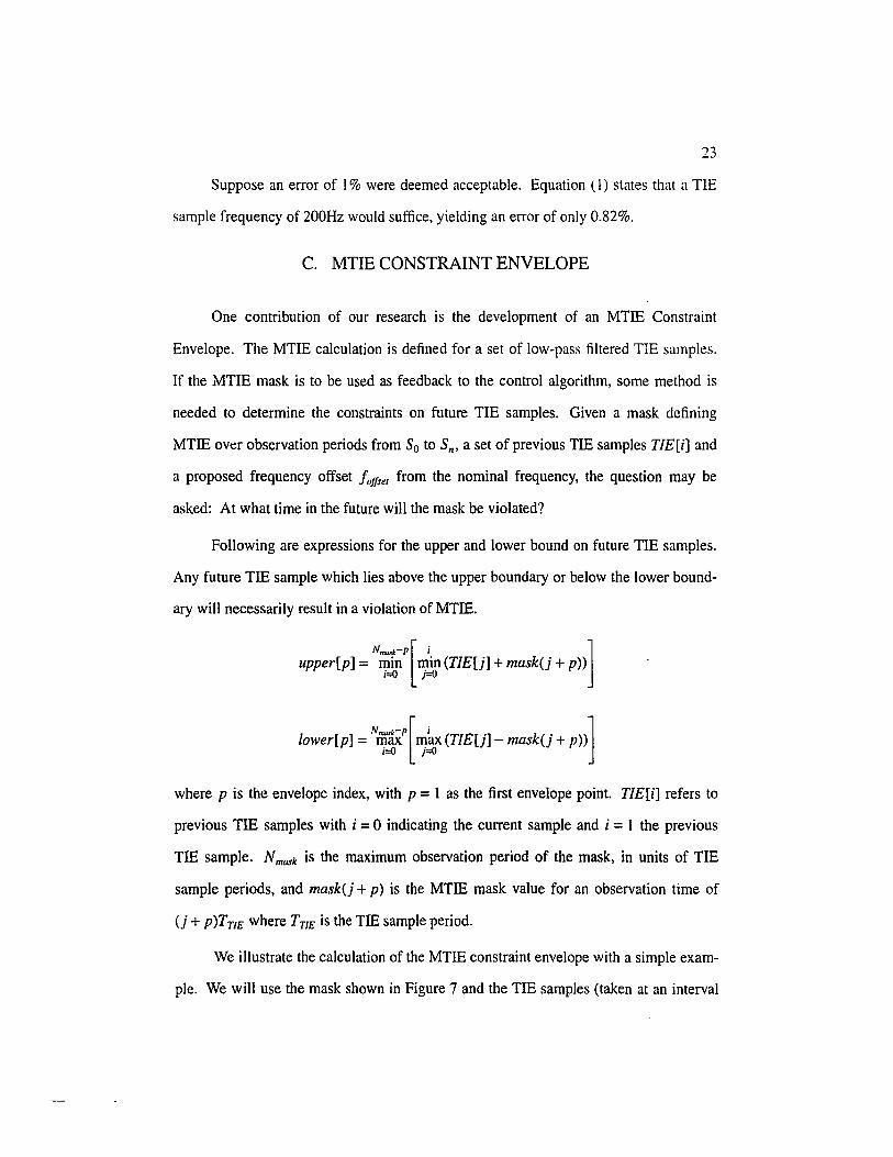
We illustrate the calculation of the MTIE constraint envelope with a simple exam
ple. We will use the mask shown in Figure 7 and the TIE samples (taken at an interval

MTIE (ns) 1000
100
10 0.1
MTIE vs. Observation Period
-..,......
10 Observation Period (sec)
Figure 7. Example MTIE Mask
of S0 = O.ls) shown in Figure 8.
"' s:: llJ • • • • • •••• E=: • • • • • •
t 1 time
Figure 8. Example TIE Samples
24
..
c
100
The question is: What values of TIE for the next sample period (t 1) will satisfy
the MTIE mask? To answer the question, one must look at the most recent sample, add
and subtract the MTIE value for an observation period of S0 , and plot the two points to
form an upper and lower bound. Next, the maximum and minimum of the two most
recent samples are calculated and the corresponding mask value for an observation
period of 2 · S0 is subtracted and added, respectively. This process continues until either

25
all TIE samples are exhausted or the upper limit of the observation period defined by the
mask is reached. The smallest upper bound and the largest lower bound values become
the first envelope pair.
Next, the above process is repeated, beginning with the current TIE, but this time
using an observation period of 2 · S0 • The result is the second envelope pair. The
envelope is generated in this way, and terminates when either the mask is exhausted or
the desired length of the envelope is reached. Figure 9 illustrates the envelope which
would result from this example.
"' c
Ul • E= • • • • • •• . .. . .
Figure 9. Example MTIE Constraint Envelope
After the envelope is generated, the projected TIE plot from a proposed offset
from the nominal frequency Uoffset) is plotted with the envelope
T/E[n · TTJE] = TIE[O] + foff.>ett(-n · TTIE) (2)
where the index n is negative, since it is indexing into the future.
Finally, a search is performed to find the point (if it exists) where the above TIE
projection crosses either the upper or lower boundaries of the envelope. The crossing,
nviol• indicates the time where the proposed frequency offset would result in an MTIE
violation. This quantity is used by the controller to evaluate the "goodness" of the pro
posed offset.
The computational complexity [10] of the envelope generation increases as
0(1Z 111a.>k · llem·) where llmask is the length of the mask and llenv is the desired length of the
26
envelope, both in units of TTIE' This complexity may be understood by realizing that it
is necessary to consider each observation period of the mask for each previous TIE sam
ple. If, for example, the mask extends to 5000s, T TIE is 0.1 s, and the maximum number
of envelope points is desired, the above calculation would require storage of 50,000 past
TIE samples, and more than 50,000 . 5000 total iterations of the loop. This calculation,
carried out repeatedly (one per TIE sample period) would soon dominate the total com
putationalload of the algorithm.
So instead of generating the envelope in linear time (p = nT), we modified the
increment of p to increase exponentially (p = b"T). The parameter b determines the
growth rate of the index, and the computational complexity of the algorithm is thus
reduced to o( nmask 10gb n env ) The resulting computational load is minimal c~mpared to
the rest of the simulator for b > 1.5.
The loss of resolution is not a concern, since the more important, close envelope
points are calculated with better resolution than envelope points which are far away. As
an added feature, when the crossing point Ilvilll falls between two envelope points (which
is nearly always the case), interpolation is used to estimate the violation time more pre
cisely.
Figure 10 shows a representative MTIE constraint envelope and the projected TIE
resulting from a proposed frequency offset in a real simulation. From the Figure we see
that the proposed frequency offset would violate MTIE in about 600 sample times.
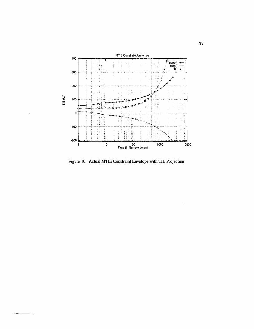
MTIE Constraint Envelope 400r-~--~~~~--~~~~~--~~~~"T--~~~~~
.~ 'upper' __. : 'lower' ·+---
/ 'tie' ·O···
300
200
100 ;:i
..... ,d. .o·
·······G·· .. :El .. ·O·:.~~CCJ··G··~·O··El·~·d·a·G·'El'G''O' o ·cc--b;•-..;_,,'-'"-'-~C.:;.:;:;:~.:;_~-•. , . .__~ •
··¢ ..
p .: .. i!i
-100 ........ .................... . ..... ;.~.~--:,;:·- .. .. :-~ .. .. . ,
..... ~ :"+ .. -200 ........... ,,.
10 100 1000 Time (in Sample times)
10000
Figure 10. Actual MTIE Constraint Envelope with TIE Projection
27

CHAPTER IV
PREVIOUS WORK
Published academic research in the area of Pointer Adjustment jitter and wander
reduction has begun to appear only recently. An online literature search turns up less
than 10 relevant journal papers and only one relevant masters thesis [11]. Quoting from
a recently published paper [12]:
With the exception of [J 3 J which focuses on oscillator design for digital
Phase Locked Loops (PLLs), the present authors are unaware of any pub
lished paper devoted to this subject [analysis of pointer adjustment jitter
and the search for efficient techniques to compensate for it] which is of
paramount importance to the operation of SDH networks.
However, Nunn [14] does give an analysis of the general requirements for jitter and
wander reduction when transmitting PDH payload over SONET.
In the following sections we outline some of the major desynchronization tech
niques which have been studied. While it has been shown that some have the ability to
attenuate jitter to levels set forth in the relevant standards, none specifically address the
MTIE wander constraint or algorithms for satisfying it.
A. PURELY ANALOG LOW PASS PLL
It has been said [12] that an analog implementation of a SONET PJE jitter attenu
ation filter would be "virtually impossible" due to the necessity of an extremely low
cutoff frequency. Instead, analog PLLs are augmented with pointer spreading

29
techniques which ease the accuracy requirements of the analog components. Examples
of such techniques are described below.
B. PHASE SPREADING
Figure 11 shows the basic architecture of the phase spreading technique [ 15].
Write Clock
Pointer Spreading
Pointer--+! L · Adjustment ogle
1---+--.;. Smoothed
I I I I I
PLL: I
~-------------------------!
Read Clock
Figure 11. Architecture for the Phase Spreading technique
The main problem addressed here is the large magnitude of the phase transient resulting
from a PJE. Rather than filtering the entire SUI phase hit, a digital circuit captures the
PJE and leaks it to the analog PLL one bit or fraction of a bit at a time. This strategy is
sometimes also called "Bit Leaking". The pointer spreading logic in the above diagram
is implemented in one of two ways: fixed rate and variable rate.
Kusyk [15] shows that with constant-rate pointer adjustments resulting from a
20ppm frequency offset, both fixed and variable rate pointer spreading techniques result
in acceptable jitter magnitudes when applied to the DSlNTl.S mapping. Note, how
ever, that SONET pointer processing allow sustained frequency offsets of up to 320ppm
[ 16].
30
1. FIXED RATE
For the fixed rate method, some leak rate must be chosen beforehand. Slow rates
result in superior jitter performance, but risk buffer overflow or underflow when exces
sive phase accumulates too rapidly in the Pointer Spreading Elastic Store. Larger leak
rates reduce the risk of a buffer spill but generate additional jitter.
Still, under restricted operating conditions, this technique is capable of meeting
the jitter constraints [15]. Unfortunately, fixed rate phase spreading is not guaranteed to
meet jitter performance objectives for some payload mappings [12].
2. VARIABLE RATE
An improvement to the fixed rate method adjusts the leak rate based o~ the statis
tics of incoming pointer adjustments [17]. If a single PJE is encountered, it is leaked at
a rate which generates negligible jitter. If a second pointer adjustment is encountered
before the first is leaked to the PLL, the leak rate is increased to reduce the risk of a
buffer spill. As might be expected, this modification allows variable-rate phase spread
ing to achieve better jitter performance than the fixed-rate method.
E. STUFF THRESHOLD MODULATION (STM)
Waiting time jitter poses a problem in desynchronizer design since its frequency
components have no lower bound [6]. An approach was put forth by Grover et al. [18]
wherein the threshold at which pointer adjustments occur is modulated at a relatively
high frequency. The result is a stream of positive and negative PJEs which act to shift
the jitter spectral components up in frequency to where they may be more readily atten
uated by the low-pass filter of the desynchronizer [19].
This method was been studied theoretically by [I5] and compared to pulse
spreading techniques by [20], where it was shown to significantly reduce the jitter

31
resulting from isolated PJEs. However, this strategy is implemented by the sY1lchronizer
and would require a change to the SONET standards. No move in this direction has
been observed.
F. ADAPTIVE DITHER BIT LEAKING
This method, proposed by Sari and Karam [12], combines concepts from the two
previous methods. Bit leaking is performed one bit at a time by a modulated, 128-bit
pattern shown in Table I
00000000 01000100 10101010 11011110
TABLE I
Dither Pattern
00010000 01001001 10101011 11111011
00100000 00101010 01101101 11110111
10000100 10101010 11011101 11111111
The modulated sequence is passed on to the low pass PLL where it resembles a ramp.
The above pattern generates a zero to one transition but it may also be scaled in magni-
tude and duration to achieve the desired transfer of PJEs to the PLL.
In addition, an extension was suggested whereby a sequence of PJEs could be
tracked by adjusting the slope of the the phase ramp such that the subsequent PJE would
be canceled out just as it arrived.
G. FEED FORWARD POINTER SPREADING
This method requires that the synchronizer and desynchronizer work together.
The synchronizer passes (in some manner) phase information to the desynchronizer so
that when a pointer adjustment occurs, the desynchronizer will have anti<::ipated the
event and leaked the appropriate amount of phase already - resulting in a zero phase
32
error upon arrival of the adjustment.
As will be seen in a later chapter, our controller is able to do precisely this -
when the PJEs occur in predictable cycles - without information from the synchro
nizer.
A system with this advanced information has the potential of jitter perrormance
which is superior to other methods. However, both the sending and the receiving equip
ment must support this (non-standard) mode of operation. This technique does not
operate with existing equipment and there is little evidence suggesting that the current
trend will change.
H. SUMMARY
While some of the above techniques have been shown to attenuate jitter resulting
from pointer adjustments, none is guaranteed to meet the constraints. Specifically, a
violation of the buffer constraint results in data errors, and a violation of the MTIE con
straint can lead to network instability and a loss of synchronization. This "self
evaluation" is the primary distinction between these techniques and the technique which
was the subject of our investigation. We set out to determine if a controller could evalu
ate how a particular frequency change would affect the wander and buffer constraints
before that frequency change was applied. We proposed that such a controller would be
capable of satisfying both wander and buffer constraints for as long as possible. Jitter
reduction was another goal, though not considered explicitly by the controller.
CHAPTER V
THE KNOWLEDGE-BASED CONTROLLER
We set out to investigate a control methodology which could meet our two pri
mary objectives. First, we wanted very small jitter compared with levels specified by
ANSI for the standard PJE tests. This would represent good performance under normal
conditions. Second, we wanted the controller to systematically satisfy the two primary
constraints. Specifically, if the wander of the output approached the maximum allowed
by MTIE specifications, we wanted the controller to adjust the output such that the wan
der constraint would not be violated until absolutely necessary - until the buffer was
also in danger of overflow or underflow. Likewise, if the buffer were about to overflow,
we wanted the controller to adjust the output in such a way that it wouldn't overflow
until absolutely necessary. Finally, when all other options are exhausted, the controller
would choose which constraint to violate, and maintain the other within specification.
Although we initially implemented a simple ProportionallDerivative-type con
troller, it soon became clear that more controller knowledge was necessary to accom
plish this task. The prospect of incorporating expert knowledge in rule form seemed
promising and we later found that a predictive knowledge-based controller was suitable
to the task.
In Section A of this chapter we list some of the virtues of the heuristic approach
to controller design and implementation. In Section B, the classical knowledge-based
(or fuzzy-logic) controller is described. Finally, Section C presents the foundations of
the PKBC applied to the desynchronization problem.

34
A. REASONS FOR CHOOSING AN HEURISTIC APPROACH
1. Goal Equations are Nonlinear
First, it was our expectation that common-sense rules facilitate the design of a
controller with acceptable performance in the usual case, thus satisfying condition one.
While this reason permits an heuristic approach, it doesn't mandate one since other
techniques can also meet jitter constraints.
MTIE and jitter calculations require peak-to-peak and other nonlinear operations
- removing many linear controllers from consideration. A heuristic approach would
specify appropriate actions as the wander and buffer values approached critical levels.
In addition, if prediction were used, the result of any control action could be evaluated
before that action is taken, adding confidence to its ability to operate within the con
straints.
2. Various Modes of Operation
The goals of the PLL are slightly different when experiencing different modes of
PJE generation. With rule-based approaches, such changes in operating regions are nat
ural. Since the current mode (or its estimate) may be incorporated into each rule,
smooth switching between operational strategies is possible.
3. Opposing Constraints
With no constraints on the buffer, ideal jitter may easily be realized. With no con
straints on jitter generation, no buffer would be needed. It is the coupling between these
opposing constraints which makes the problem such a challenge. A set of if-then rules
seemed to be a natural way of expressing the desired actions of the controller when
operating under varying conditions.
35
B. THE TRADITIONAL KNOWLEDGE-BASED CONTROLLER
1. What is it?
a. Philosophy. The KBC is a type of expert system. The "expert" is typically a
human who has the knowledge and experience necessary to control the system. The
expert expresses his knowledge of the control task in the form of If-Then rules which
use vague terms like "large" or "slow". The vague terms are defined by fuzzy sets [21]
and an inferencing method is used to transform plant measurements into control actions.
b. Architecture. The KBC is an input/output system with a many-to-one map
ping. The basic architecture consists of N inputs and a single output. If many indepen
dent outputs are desired, the basic architecture is replicated as needed. Each input vari
able is assigned some number of fuzzy sets, and each fuzzy set is assigned a label. Typ
ically, the output is also specified in terms of a fuzzy set. The rules associate condi
tional statements with an output, and the truth of the conditional determines the strength
of the association. The truth of a rule is sometimes called it's "firing strength" .
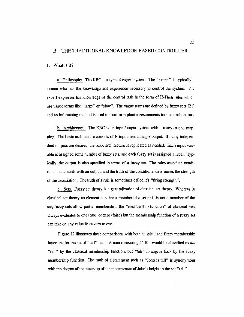
c. Sets. Fuzzy set theory is a generalization of classical set theory. Whereas in
classical set theory an element is either a member of a set or it is not a member of the
set, fuzzy sets allow partial membership; the "membership function" of classical sets
always evaluates to one (true) or zero (false) but the membership function of a fuzzy set
can take on any value from zero to one.
Figure 12 illustrates these comparisons with both classical and fuzzy membership
functions for the set of "tall" men. A man measuring 5' 10" would be classified as not
"tall" by the classical membership function, but "tall" to degree 0.67 by the fuzzy
membership function. The truth of a statement such as "John is tall" is synonymous
with the degree of membership of the meaurement of John's height in the set "tall".

36
Tall Tall
0.67
0~------------~--------- 0~----------+--++---------6'0" 5'6" 6'0"
5' 10"
Figure 12. Crisp and Fuzzy Definition of "tall"
d. Logical Operators. Although there are many logical operators defined for
fuzzy sets (see [22], for example), we present only conjunction (AND), disjunction
(OR), and complement (NOT).
• Conjunction/AND
The conjunction, or AND operator is typically defined by the the min() function.
For example,
0. 4 n 0. 5 = min(O. 4, 0. 5) = 0. 4.
An alternative definition is algebraic product. With this definition,
o. 4 n o. 5 = o. 4 . o. 5 = o. 2.
• Disjunction/OR
The disjunction, or OR operator is typically defined by the max() operator. For
example,
0.4 U 0.5 = ma.x(0.4, 0.5) = 0. 5.
An alternative definition is min(a + b, I). With this definition,
0.4 U 0.5 = min(0.4+0. 5, 1) = 0. 9.

37
• ComplementNOT
The complement, or NOT operator is almost universally defined as 1 - a. For
example,
""(0.3) = I - O. 3 = 0.7
Notice that if a and b are constrained to the crisp set {O, I}, each logical fuzzy
operator is reduced to the corresponding boolean definition.
e. Implication. Each input variable of a rule is fuzzified with the input fuzzy sets
to produce a truth value. Then these truth values are combined with the logical opera
tors to produce the aggregate truth of the conditional statement. This process is
repeated for each of the rules, yielding a set of truth values and an action associated
with each (the right hand side of each rule). Some method must be used to determine
how each desired action should be modified in the case of a conditional statement with a
truth value less than one.
The most common inferencing method was proposed first by Mamdani [23] and
states that the output fuzzy set of a rule r is
Y,(x) = min(K" C,(x))
where K, is the truth of the antecedent and C,(x) is the stated consequence of the rule
(the "then" part of the rule). If the output fuzzy sets are triangles, this inference
scheme produces trapezoids - triangles with flattened tops.
Another method is product inference. This method states that the output fuzzy set
of a rule r is equal to the product of the truth of the antecedent K, and the stated conse
quence C,
Y,(x) = Kr . C,(x)
With this method, the general shape of the output set is not changed but is simply scaled

38
proportionally.
f. Defuzzification. Once all the rules have been evaluated, the resulting output
fuzzy sets (modified according to inferencing method) must be combined to produce a
single output value. Typical methods include: the centroid, the maximum value, the
median value, the weighted sum of the maximums, height defuzzification, and others
[24]. The center of sums is the most common defuzzification method and consists of
computing the weighted average of each resulting output fuzzy set.
g. Controller Example. We demonstrate the above with a simple desynchronizer
controller. We begin by defining the controller's inputs and output. The inputs consist
of the buffer level, and its derivative. The output, or control effort, is a frequency
adjustment to the DDS, in Hz. The next step is to define fuzzy sets on the input and out
put domains. Figure 13 shows a possible configuration.
NL PL
Buffer
Steady
DecF XID< lncF
A Buffer
Frequency Effon
Figure 13. Fuzzy Set Definitions for Sample KBC
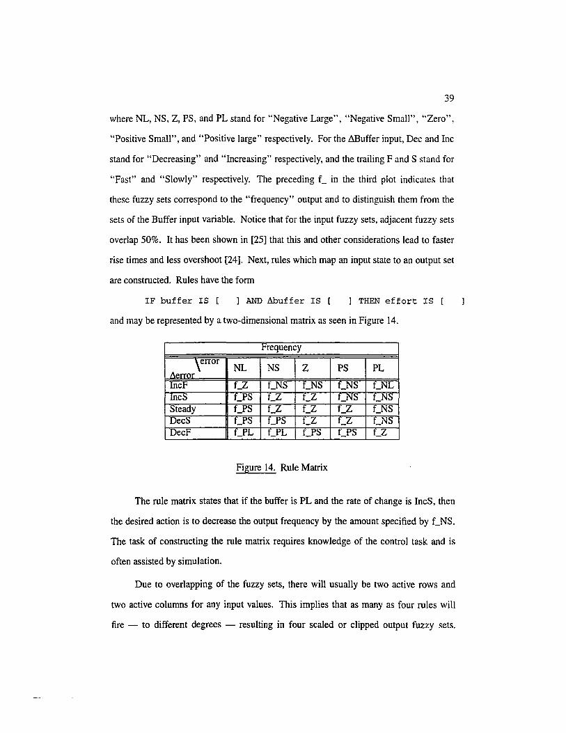
39
where NL, NS, Z, PS, and PL stand for "Negative Large", "Negative Small", "Zero",
"Positive Small", and "Positive large" respectively. For the .6Buffer input, Dec and Inc
stand for "Decreasing" and "Increasing" respectively, and the trailing F and S stand for
"Fast" and "Slowly" respectively. The preceding f_ in the third plot indicates that
these fuzzy sets correspond to the "frequency" output and to distinguish them from the
sets of the Buffer input variable. Notice that for the input fuzzy sets, adjacent fuzzy sets
overlap 50%. It has been shown in [25] that this and other considerations lead to faster
rise times and less overshoot [24]. Next, rules which map an input state to an output set
are constructed. Rules have the form
IF buffer IS [ ] AND Abuffer IS [ ] THEN effort IS [
and may be represented by a two-dimensional matrix as seen in Figure 14.
Frequency
_\error Aerror
NL NS z PS PL
lncF f_Z f_NS f_NS f_NS f_NL lncS t_PS t_Z t_Z t_NS t_NS Steady f_PS f_Z f_Z f_Z f_NS DecS f_PS f_PS f_Z f_Z f_NS DecF f_PL f_PL f_PS f_PS f_Z
Figure 14. Rule Matrix
The rule matrix states that if the buffer is PL and the rate of change is lncS, then
the desired action is to decrease the output frequency by the amount specified by f_NS.
The task of constructing the rule matrix requires knowledge of the control task and is
often assisted by simulation.
Due to overlapping of the fuzzy sets, there will usually be two active rows and
two active columns for any input values. This implies that as many as four rules will
fire - to different degrees - resulting in four scaled or clipped output fuzzy sets.
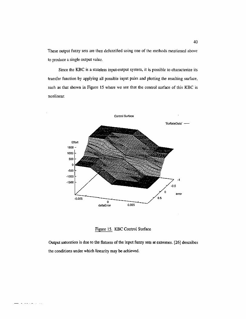
40
These output fuzzy sets are then defuzzified using one of the methods mentioned above
to produce a single output value.
Since the KBC is a stateless input-output system, it is possible to characterize its
transfer function by applying all possible input pairs and plotting the resulting surface,
such as that shown in Figure 15 where we see that the control surface of this KBC is
nonlinear.
Effort
1500-
1000
500
0
-500
-1000
-1500
Control Surface
'SurfaceData' -
-1
error
0 deltaError 0.005
Figure 15. KBC Control Surface
Output saturation is due to the flatness of the input fuzzy sets at extremes. [26] describes
the conditions under which linearity may be achieved.

41
2. When is a Fuzzy Knowledge-Based Controller appropriate?
a. Difficult or Intractable Mathematics. There are control applications where it
is very difficult to characterize the physics of a system due to its complexity, nonlinear
ity, or changing parameters. The design of a fuzzy controller doesn't require a mathe
matical plant model, but instead relies on an implicit understanding of the plant's opera
tion and knowledge of which actions are appropriate under which circumstances.
b. Accelerated Update Rates. Fuzzy sets may be represented discretely with
only a few points, and can be easily stored in a small memory [27]. Also, the common
operations on fuzzy sets are easily implemented in hardware, and often do not require
multiplication or division. Thus an entire controller may be easily implemented by an
inexpensive microcontroller. Tools exist which map a fuzzy controller ipto lookup
tables and inferencing routines. The parallel nature of the algorithm also makes it a
candidate for concurrent processing.
In addition, specialized stand-alone VLSI chips are capable of evaluating as many
as 30 million rules per second and are available for only a few dollars [28].
c. Non-Mathematical control objective. If the control objective is not readily
expressed mathematically, analytical design methods tend to break down. In other situ
ations, the control objectives may be expressed mathematically, but are more easily
expressed as if-then rules.
d. Universal stability proof not required. Many critics will claim that there exists
no mechanism for ensuring the stability of a fuzzy controller. While stability analysis
such as is available for linear controllers does not apply to fuzzy controllers, there are
nonlinear stability analysis techniques which may be used to demonstrate, for example,
asymptotic stability. Still, these techniques are rarely used in practice, and the stability
of most applications of fuzzy logic is verified by simulation or extensive tests. See [24]

42
for a survey of stability methods.
3. Disadvantages
a. No algorithm/mathematical algorithm for design/tuning. The rulebase of any
knowledge-based system will only be as good as the expert who constructed the rules.
Of course the expertise of both designer and controller increase as perfonnance is
observed and appropriate changes to the controller are made, but the process often fol
lows a path of trial-and-error.
b. Stability. As mentioned earlier, stability studies have not yet been conducted
for the PKBC paradigm. Applications where such guaranteed characteristics are
mandatory must look to other control strategies.
C. PREDICTIVE KNOWLEDGE BASED CONTROLLER
1. What is it?
a. Philosophy. Predictive Knowledge-Based Control (PKBC) is an extension of
standard KBC. Like KBC, it uses fuzzy sets and fuzzy set operators to evaluate the
truth of each rule statement. However, unlike standard PKC, the PKBC uses prediction
to evaluate the effect the stated action would have on the state of the system at a future
time. The predicted state is then evaluated in the same way as the current state was
evaluated by the KBC.
If the input and plant processes are well represented by the predictive models,
rules which would result in an undesired state are eliminated from consideration. This
can result in improved functionality and reliability.

43
b. History. PKBC was developed in Japan in the early 1980s by a group led by
Yasunobu [29], [30], and [29]. Their goal was to replace human subway operators with
automatic, computational controllers. After interviewing operators (the experts) they
identified several relevant performance parameters:
• Passenger safety
• Energy consumption
• Adherence to schedule
• Passenger comfort
• Speed limit constraints
• Accuracy of stopping at stations
A person driving a vehicle builds an internal model of the vehicle's mechanics
which is consulted to decide if, for example, the current deceleration rate will result in
the desired stopping position or if some adjustment is necessary. This concept was used
to extend the standard KBC to a Predictive KBC. The group found that the above per
formance parameters could be met through the application of a set of carefully crafted
rules of the form:
if (u is A -> X is J and y is K and z is L) then u is C sub i
For example,
If (when the power control is on coast, the safety is good and comfort is good and energy consumption is good) then coast
A model of the train's dynamics is used to predict the state that would result from
the action u=A and other models predict the value of the variables x, Y, and z. Finally,
the truth of the rule is evaluated using the fuzzy sets J, K, and L, and the candidate
action associated with the rule with the highest truth value is chosen and applied to the
output of the controller.
44
This control method makes concurrent use of three techniques: fuzzy set theory,
which evaluates multiple system objectives; artificial intelligence in the form of experi
ential Ifffhen rules; and real-time simulation and prediction of control results [31].
Simulations comparing PKBC to PID control were encouraging. Compared to a
PID controller, the standard deviation of stopping error was 10cm for PKBC, and 28cm
for the PID. For riding comfort, the PKBC made 6.6 command changes versus \6.0 by
the PID (which equates to a smoother ride). Field tests of PKBC on the subway in
Sendai Japan produced results similar to the simulations. The PKBC exhibited more
expert, human-like characteristics than other controllers, and conserved energy com
pared to other methods (including human control). The controller was still in active
operation in 1995.
As a side note; even under automatic control there is still a human operator near
the train's controls as a backup. Comparisons between human control and PKBC are
made with a human operator who - to retain his skills - operates the train during non
peak hours.
Other applications of PKBC include car parking [32] and the control of mobile
robots [33]. In both cases, the controller uses prediction to evaluate a set of candidate
actions and choose the one deemed most appropriate.
c. Architecture. The PKBC adds models and a predictor to the standard KBC
architecture as illustrated in Figure 16.
Each rule in the rulebase is evaluated in turn. The candidate action of the rule is
passed through the predictor which generates "virtual measurements" - measurements
which would be expected in the future if the proposed action were taken. The measure
ments are fuzzified and the inferencing rule determines the strength of the rule. The
optimal action is then chosen based on the firing strengths of the rules.
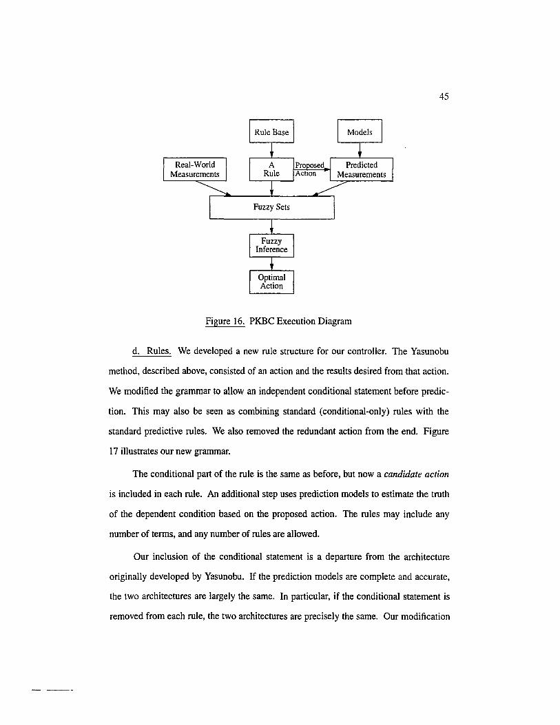
45
Real-World
Figure 16. PKBC Execution Diagram
d. Rules. We developed a new rule structure for our controller. The Yasunobu
method, described above, consisted of an action and the results desired from that action.
We modified the grammar to allow an independent conditional statement before predic
tion. This may also be seen as combining standard (conditional-only) rules with the
standard predictive rules. We also removed the redundant action from the end. Figure
17 illustrates our new grammar.
The conditional part of the rule is the same as before, but now a candidate action
is included in each rule. An additional step uses prediction models to estimate the truth
of the dependent condition based on the proposed action. The rules may include any
number of terms, and any number of rules are allowed.
Our inclusion of the conditional statement is a departure from the architecture
originally developed by Yasunobu. If the prediction models are complete and accurate,
the two architectures are largely the same. In particular, if the conditional statement is
removed from each rule, the two architectures are precisely the same. Our modification

46
Independent Conditional Proposed Action
~ IF [Input] IS [Fuzzy Set] {AND ••• } (AND [Output] = [Value) ->
[Input] IS [Fuzzy Set] (AND ••• }) THEN DOlT
Dependent (Predictive) Conditional
Figure 17. New PKBC Rule Structure
allows the use of actual physical measurements in the evaluation of rules, while the
standard architecture only evaluates predictions. The importance of this difference
increases as the accuracy of the predictive models decreases, since the controller may
use physical measurements in addition to predicted results to help it decide which action
is most appropriate.
e. Advantages. The use of prediction is like adding an additional feedback loop
in the control system. A candidate action is passed through a set of plant models and
the results evaluated to ascertain the goodness of that action. If sufficient candidates are
available, something close to the best action will be chosen and applied. This self-
evaluative approach yields several advantages over simpler feedback control methods.
One advantage is the ability of the controller to operate within hard constraints.
In a desynchronizer, for example, the buffer must not overflow. Each rule may reflect
this constraint by including a predictive term such as "and buffer is OK".
PKBC also has the potential of requiring less tuning than a standard KBC. The
knowledge of a KBC is completely contained in the content of the rules and the defini
tion of the fuzzy sets. Rules are defined in terms of existing conditions and desired
actions. Choosing a desired action requires that the designer have or obtain a good

47
understanding of the effects that action will have. With PKBC, the designer still must
have some knowledge of appropriate actions in different conditions, but if several candi
date actions are given in otherwise identical rules, the controller is able to choose the
one which results in the best performance. Using language of Kosko [27], the odds of a
"sabotage" rule firing are low, since the predicted results would be poor.
Also, when several constraints cannot be satisfied simultaneously, the designer
may specify which one to violate by adding rules which ignore the lesser constraint
when the more important one is near violation.
Finally, our addition of a conditional statement to the rule structure allows greater
flexibility and potentially greater tolerance to model inaccuracies, as described in Sec
tion Id above.
2. When is a PKBC Appropriate
If there is no model available for the system, classical control techniques are
severely disadvantaged and KBC or adaptive technique [34] may be able to provide a
solution. If there is a linear model available for the plant and the controller objectives
are expressed similarly, then one of many control techniques may be employed, with
proven results. However, if a model is available (which may be arbitrarily complex and
nonlinear) and the controller objectives are difficult to express symbolically, then PKBC
may be a viable option.
3. Disadvantages
The author is not aware of any study of the stability of the PKBC. This is an
important concern for some applications and, although our simulations have demon
strated stable behavior for many varied scenarios, conditions for global or asymptotic
stability have not yet been derived.
48
Also, offering many candidate actions can lead to a large number of rules, which
increases computation time. This is also true as the number of inputs increases since
there are many more combinations of the input state. However, although we specify
nearly 60 rules, the number could be reduced to below 15 if the grammar were changed
to allow a rule to specify a set of candidate actions rather than just one. (This change
would certainly affect the complexity of the rulebase, but would not be expected to
affect the time necessary to evaluate the rules).
Another disadvantage of PKBC over other methods is the need for simulation in
the design and evaluation of the controller. This disadvantage is not uniqu~ to PKBC.
however.
Despite these disadvantages, simulation has suggested that the control system is
stable, the computational load is within the reach of modern processors, and a reason
ably limited number of inputs leads to an acceptable number of rules.
CHAPTER VI
PKBC FOR THE SONETIDS3 DESYNCHRONIZER
A. OVERVIEW
A SONETIDS3 desynchronizer has one operational objective: Smooth the clock
signal without causing a buffer underflow or overflow. This objective may be decom
posed into three concrete goals:
• Keep the buffer half full to minimize the probability of either underflow or over
flow,
Keep the output frequency near enough to the nominal DS3 value that the wander
specification (MTIE) is not violated, and
• Exhibit low-pass behavior so that jitter generation is minimized.
The first two goals have explicit limits: the buffer has a fixed size, and MTIE is
bounded by the MTIE mask specified by Tl committee documents. This means that a
properly designed controller could conceivably evaluate itself in terms of these con
straints and take actions predicted to yield acceptable results.
It is not possible, however, to meet the third goal explicitly, because there is no
universally applicable jitter specification. Instead, jitter levels are specified in terms of
specific PJE profiles. Thus, assuming that the controller does not identify and adapt to
specific PJE tests, the desynchronizer must be designed, tested, and tuned using trial
and-error.
We determined that a PKBC-based approach is both possible and appropriate for
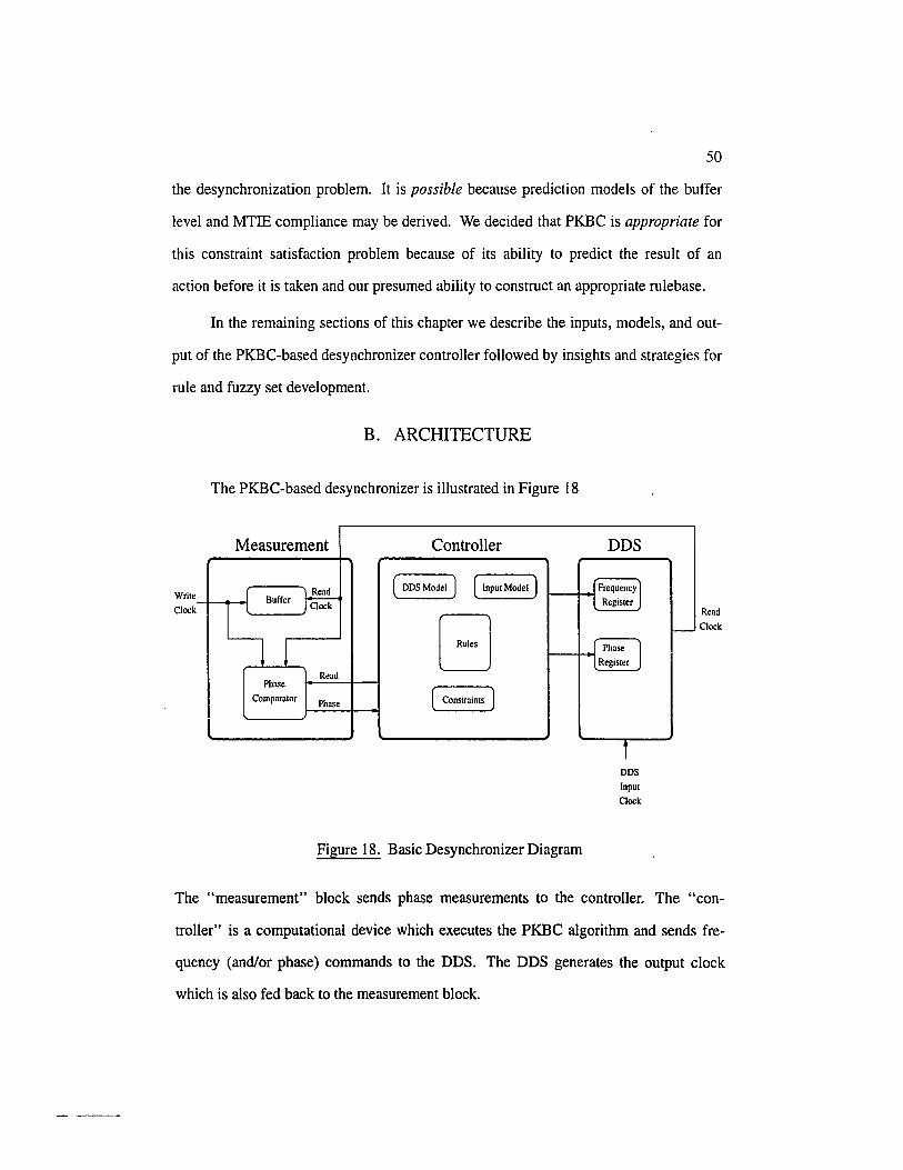
50
the desynchronization problem. It is possible because prediction models of the buffer
level and MTIE compliance may be derived. We decided that PKBC is appropriate for
this constraint satisfaction problem because of its ability to predict the result of an
action before it is taken and our presumed ability to construct an appropriate rulebase.
In the remaining sections of this chapter we describe the inputs, models, and out-
put of the PKBC-based desynchronizer controller followed by insights and strategies for
rule and fuzzy set development.
Writ<
Clock
B. ARCHITECTURE
The PKBC-based desynchronizer is illustrated in Figure 18
Measurement Controller
( DDS Model ) ( Input Model ) f ~ Buffer s k
G J Read
Phase
( Constraints ) Comparator Phase
Figure 18. Basic Desynchronizer Diagram
DDS
(Frequency) l Register
J Phase ) -l Register
f DDS Input
Clock
-Read
Clock
The "measurement" block sends phase measurements to the controller. The "con
troller" is a computational device which executes the PKBC algorithm and sends fre
quency (and/or phase) commands to the DDS. The DDS generates the output clock
which is also fed back to the measurement block.
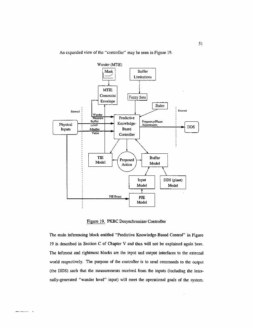
An expanded view of the "controller" may be seen in Figure 19.
I I
External 1 I I I I I
Physical I I
Inputs I
I I I I I I I I
I I I I
Wander (MTIE)
~ ~
MTIE Constraint
,--- Envelope
Wander Measure
Buffer Level ~Buffer
Value
TIE Model
Buffer Limitations
!Fuzzy Sets I I Rules I
: External I I I I Predictive
Knowledge
Based Controller
Frequency/Phase 1
~A~~~us~tm~e~n~~------~:~~J DDS l
._____ I \ ,....--'------
Input DDS (plant) Model Model
t PJEEvent PJE
Model
Figure 19. PKBC Desynchronizer Controller
51
The main inferencing block entitled "Predictive Knowledge-Based Control" in Figure
19 is described in Section C of Chapter V and thus will not be explained again here.
The leftmost and rightmost blocks are the input and output interfaces to the external
world respectively. The purpose of the controller is to send commands to the output
(the DDS) such that the measurements received from the inputs (including the inter
nally-generated "wander level" input) will meet the operational goals of the system.

52
The remaining blocks above and below the PKBC are supportive functions and models
which are described in more detail in the following sections.
1. Inputs
a. Buffer Level. The buffer, or phase measurement is synonymous with the fill
level of the elastic store, which may also be characterized by
I
buffer = f four - fill dt o
where fllul is the output frequency and fill is the incoming frequency. The buffer level is
measured at the end of each SPE row (explained in Section A.2 of Chapter II). and
accumulated until the sample time of the controller is reached.
The level of the buffer is measured at the end of each STS-I row, resulting in a
frames rows sample samples rate of 8000 -- . 9 -- . 1 --= 72,000 Measurements taken more
sec frame row second
often would be plagued by "jitter" caused by the fixed stuffing bits and overhead gaps.
Measurements taken more slowly would lack the resolution that may be achieved by
oversampling and averaging.
At the end of the row, either 621 or 622 bits of DS3 payload data - depending on
whether or not the stuff opportunity was taken - will have been written into the buffer.
Ideally, the same number of bits will have been read out of the buffer by the output
clock in order that the buffer doesn't fill or empty. We will call these SPE-row-based
phase samples sub-samples to avoid confusion with the overall control-system sample
period T,r.
The buffer measure may be thought of as a counter with its up-count input con
nected to the write clock and its down-count input connected to the read clock. If we
measured the buffer once per control algorithm sample time, a resolution of 1 VI would

53
be the limit (without more capable phase measurement equipment, such as [35]).
The sub-samples are averaged to produce the buffer measurement used by the
controller;
L (BufferLevel[i] - BufferSize/2) (3)
where BufferLevel[i] is the buffer sample after each row. Assuming a controller sample
period of 0.04 seconds, approximately 2880 row measurements are accumulated before
Equation (3) is evaluated.
Oversampling of the SPE-row results in a maximum resolution of
R. 1
esolutlOnbuffer = f T row requency· s
For a sample period of T.~ =O.04s,
=------8KHz· 9 . O. 04s
This theoretical limit on the phase resolution may not be realized if the stuffing ratio is
the quotient of small integers (like 1/3 or 6/10). This is evidenced in Section A.I of
Chapter 8 where mapping jitter is plotted as a function of the stuffing ratio. Fortunately,
sustained integer stuffing ratios would not be expected in a real network where random
processes are at work.
b. Lilluffer Value. The derivative of the buffer level is estimated by a first order
backward difference, normalized to the sample period;
Ab f~ .] buffer[i] - buffer[i - 1] u u ler[z = -------
Ts
Large or sudden changes in ~buffer - following a PJE, for example - limit the
54
usefulness of this measure. The predicted Llbuffer (described in a Section B.4.a) is more
representative, since the effect of periodic PJEs are considered over a long period of
time.
c. Wander Measure. Whereas the buffer measure is an absolute measure (the
number of bits from half full), wander is defined in terms of the amount of time before
the MTIE mask would be violated if the current frequency were maintained. This mea
sure is also called "time-till-violation". It is derived by first generating the MTIE Con
straint Envelope and superimposing it with the TIE samples which would result from
the proposed or current frequency action. Then a search is performed to determine
where TIE crosses the envelope. For example, a wander value of 30 means that the cur
rent or proposed frequency will violate MTIE in 30 sample times. If the tie line does
not cross the envelope, a very large number is returned.
If a candidate action is predicted to result in an MTIE time-till-violation of less
than one sample period, the action is obviously not acceptable, since MTIE would be
violated before a subsequent control action could be taken to avert it.
d. Comments. Both buffer and wander may be measured either in terms of time
till-violation or the distance from their current position to the constraint ceiling.
However, we chose to represent the buffer input by the absolute fill-level rather
than the predicted time-till-violation, due to the transient nature of the buffer measure.
If an unexpected PJE event occurs, for example, the previously predicted time-till
violation is meaningless. However, such sudden and unexpected changes are not seen
in the wander measure since wander is a function of only the output clock - over
which the algorithm has complete control. Thus, the time-till-violation measure is
more predictable and longer-term estimations are justified.

2. Rules
Our implementation of PKBC rules have the following fonn:
[Rule Number] : IF [ inputVariable IS iuzzySet
[ [ AND inputVariable IS iuzzySet ] ... ] ] ( AND outputVariable = action -> inputVariable IS iuzzySet
[ [ AND inputVariable IS iuzzySet ] ... ] ) THEN DOlT
55
Each rule begins with a rule number, used for easy reference, followed by the reserved
word IF and the conditional tenns. Then, in parenthesis, an output action is proposed
and the predicted result is evaluated in by the predictive tenns.
The rules are stored (one per line) in a text file and parsed by a custom parser
using lex [36] and yacc [37]. The parser enforces adherence to the grammar and
ensures that every referenced input (like buffer) and fuzzy set (like NL) is defined
elsewhere. The result is a doubly linked list of rules and tenns at runtime. The rule
base may contain an arbitrary number of rules, each with an arbitrary number of tenns.
Modifications or extensions to the grammar are easily accomplished by simply editing
the appropriate lex/yacc description files and rebuilding the executable.
3. Fuzzy Sets
Each fuzzy set used in the PKBC is read and parsed from an input file·at runtime.
The file is divided into sections, each identified with one of two keywords:
inputvar or outputvar followed by the variable name like buffer, d_buffer,
or wander. (We will refer to the derivative of buffer as .1buffer in textual discussions
and d_buffer in relation to the simulator). After the declaration of the variable name,
a terms statement declares the number of fuzzy sets defined for that variable. Then
the appropriate number of fuzzy sets are defined.
Each fuzzy set definition consists of a name and one or more real numbers

56
separated by spaces or tabs. Our representation of fuzzy sets allows four profiles. The
singleton is used to define candidate outputs and is defined by a single number. The tri-
angular membership function [38] is the most commonly used type and is defined by
three numbers (left corner, peak, and right corner). A trapezoid is defined by four num
bers (left corner, left peak, right peak, right corner), and if the first two or last two num-
hers are equal, a ramp is assumed. A ramp differs from a trapezoid in that one end of
the ramp never returns to zero, and thus its domain extends to infinity. Ramps are useful
for specifying default behavior outside standard input domains.
Figure 20 and Table IT illustrate our representation of fuzzy sets.
Singleton
-1 a
Ti ~l.z·~· ab c abc d a be a b c
Figure 20. Fuzzy Set Definitions
TABLE IT
Fuzzy Set Definitions
Fuzzy Set Numencal Type Definition
Smgleton a Tnangle a b c Trapezoid a b c d Left Ramp a a b c R1ght Ramp a b c c
The buffer constraint is embodied within the fuzzy sets, as described in Section C.l
below.

57
4. Models
Two types of models are used in the simulator: Simulation Models and Prediction
Models. To simulate the operation of the control algorithm, certain real-world pro
cesses must be emulated. The frequency of the original DS3, the frequency of the
SONET network, the mapping of the DS3 payload into an STS-I SPE, and the genera-
tion of PJEs must all be modeled by the simulator. Since the simulation models are not
part of the PKBC controller they are described in the next chapter on simulation.
A predictive controller must possess and maintain a model of each real~world pro
cess necessary for the evaluation of candidate actions. In a simulation environment, all
relevant information is contained in the simulation models mentioned above. But in a
real-world implementation, the future DS3 rate, for example, is not known exactly by
the controller and must be estimated. The Input Model, for example, characterizes the
observed DS3 signal and is used to estimate future DS3 rates such that the "truth" of
the predictive-term of each rule may be evaluated.
Prediction models are updated as new measurements are taken and only utilize
data which would be available to the controller in a real-world implementation. Follow
ing is a description of the prediction models used by the controller.
A. Buffer Model. As stated earlier, the theoretical buffer level is determined by
t+T,
buffer[i + 1] = buffer[i] + f fllul - hndt I
Assuming that the hn and fllUl remain constant between samples, this may be rewritten
as
buffer[i + I] = buffer[i] + (fllul - hn)Ts (4)
Both fllul' the output frequency of the DDS and T.p the sample period of the control sys-
tern are known quantities. The model for hn is described in the next section.

58
The predicted Llbuffer value is computed by calculating the difference between
the current buffer measurement and the predicted next buffer measurement.
B. Input Model. The goal of the Input Model is to estimate the frequency of the
original DS3 signal. To accomplish this, it assumes that notice of PJE events is avail-
able and also receives phase measurements. The assumed availability of PJE informa
tion is reasonable since other techniques, including the phase-spreading techniques [15],
utilize this information.
From Equation (4) we can derive an expression for fill
of _ buffer[i - 1] - buffer[i] );11- T +/0
s
While this might be an accurate model, the estimate of fill changes drastically
whenever a PJE occurs due to the sudden change of eight to 24UI. Thus we represent
fill with two separate models; one to estimate the input frequency without the effect of
PJEs, and another model to estimate the rate at which PJEs occur. Ultimately, the two
models are combined to form a more representative estimate of the input frequency. In
fact, the resulting estimate remains as constant as the instantaneous fin frequency and
the PJE rate.
Thus, when a PJE occurs, the PJE model is passed the polarity and timestamp of
the event, and its effect is removed from the instantaneous phase measurement. How
ever, this second action requires additional explanation.
Consider the example where a phase sample is taken at 25.0ms which yields a dif
ference of lOUI. Next, a negative PJE occurs at 25.75ms, and the next sample is taken
at 26ms. Although the correct buffer level at 26ms is I8UI, the measurement returns
something less - for the following reason. Since the first 75% of the sub-samples mea
sure IOUI and the last 25% measure I8UI, an average measure of I2UI is returned.
(The subsequent phase sample at 27ms correctly yields I8UI). This effect is modeled

59
by including the term P JEni], which indicates the amount of phase seen at time i from
a PJE during the previous sample time (0.75·8 in the example above) and PJE~d[i - 1]
which contains the remainder (0.25·8 in the example above).
Thus input frequency at sample i is estimated by the following expression:
p[i - I] - p[i] + fDDS[i - 2]Td + fDDS[i - I](Ts - Td) + P DDS[i - I] - PJE1,,[i] - PJE2nd[i] Ts
where p[i] is the PJE-removed measurement at sample i; fDDS[i] is the DDS frequency
applied Td seconds after sample i; and PDDS[i] is the change to the DDS phase register
(in VI). T d is used to simulate the time between the instant when the sample is taken
and the time when the algorithm finishes calculating the desired DDS action. When
asked for the average input frequency, the Input Model combines the estimate above
with the estimated PJE bit rate (described in the next section).
By decomposing a phase measurement into its two components - changes due to
a frequency offset and steps due to PJEs - this model can provide a very accurate esti
mate of past input frequency values. Our use of past estimates for future prediction is
validated by the fact that instantaneous input frequencies and PJE statistics change
slowly over time [3]. In fact, as will be seen in Chapter 8, the controller actually antici
pates the occurrence of regularly occurring PJEs and compensates for them before they
arrive.
The input model requires input parameters specifying the length of the averaging
filter and, if low-pass filtering of the average input measurement is desired, the filter's
cutoff frequency.
C. PJE Model. The PJE model predicts future PJE events. Since PJE statistics
are likely to change slowly [2], past events are a good indication of future events. Thus,
a list of recent PJEs are recorded, along with their polarity and the time at which they
occurred. From this list, an average PJE rate may be calculated.
60
If, in our implementation of the PJE model, a stream of PJEs occur at regular
intervals and suddenly an expected PJE doesn't arrive, the estimated PJE rate is ramped
down to zero such that a rate of zero is achieved at the time of the nIh expected PJE.
A more representative PJE model might have multiple levels of estimation. The
first level would acquire the instantaneous PJE rate. Missing PJEs from the first level
would be modeled by a second level and spurious or bursts of PJEs by a third.
Although this approach would yield a more accurate model of the PJE profiles used in
the tests (and greatly reduced jitter), we decided that a simpler, more general PJE model
which was not tailored to the standard tests would be more appropriate for real-world
operation.
The input parameters associated with this model include the number of past PJEs
to remember, and n.
D. TIE ModelIMTIE Constraint Envelope. The MTIE Constraint Envelope
module transforms an MTIE mask and past and future TIE samples into the constraint
envelope described in Chapter ill. This module is also able to calculate the time at
which the TIE - resulting from a proposed frequency - crosses the envelope, indicat
ing an MTIE violation.
The envelope is sent TIE samples at a fixed rate. Each of these samples is passed
through a 10Hz, low-pass filter, but they are only stored in the TIE collection at the rate
corresponding to the minimum observation time of the MTIE mask, since smaller obser
vation times are not constrained by MTIE.
The envelope is updated each time a TIE value is stored. Then, for each rule, a
candidate action is passed to the envelope, and a time-till-violation measurement is
requested. A predicted TIE plot is compared to the envelope, the time of the first cross
ing is determined, and interpolation is employed to increase the resolution of the
returned measurement.
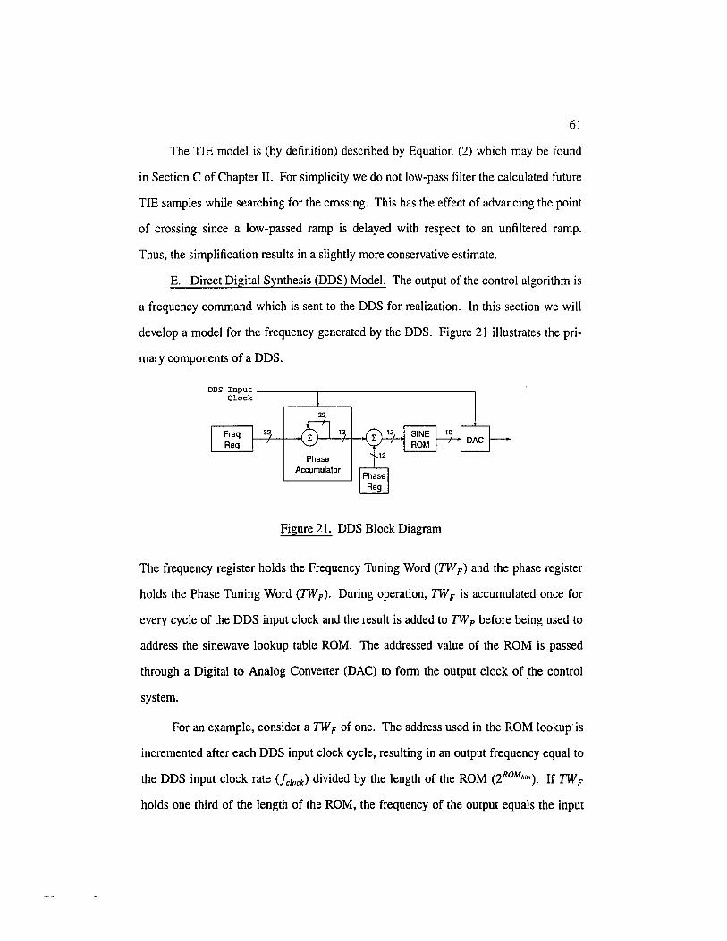
61
The TIE model is (by definition) described by Equation (2) which may be found
in Section C of Chapter II. For simplicity we do not low-pass filter the calculated future
TIE samples while searching for the crossing. This has the effect of advancing the point
of crossing since a low-passed ramp is delayed with respect to an unfiltered ramp.
Thus, the simplification results in a slightly more conservative estimate.
E. Direct Digital Synthesis (DDS) Model. The output of the control algorithm is
a frequency command which is sent to the DDS for realization. In this section we will
develop a model for the frequency generated by the DDS. Figure 21 illustrates the pri
mary components of a DDS.
DDS Input--------,---------------------, Clock
Accumulator
Figure 7.1. DDS Block Diagram
The frequency register holds the Frequency Tuning Word (TW F) and the phase register
holds the Phase Tuning Word (TW p ). During operation, TW F is accumulated once for
every cycle of the DDS input clock and the result is added to TW p before being used to
address the sinewave lookup table ROM. The addressed value of the ROM is passed
through a Digital to Analog Converter (DAC) to form the output clock of .the control
system.
For an example, consider a TW F of one. The address used in the ROM lookup· is
incremented after each DDS input clock cycle, resulting in an output frequency equal to
the DDS input clock rate (/clock) divided by the length of the ROM (2ROM,;"). If TW F
holds one third of the length of the ROM, the frequency of the output equals the input
62
clock rate divided by three.
The frequency of the DDS is modeled by the following equation
f DDS = C:; :m fclllCk
where ROM Brrs is the number of bits in the ROM address.
The input parameters to the DDS model include the frequency of the input clock,
the length of the tuning word, and the initial frequency and phase.
5. Output
The output of the PKBC is the candidate action which was predicted to result in
best performance. Although the DDS is capable of adjusting both the frequency and
phase of the output, our rules specify only frequency adjustments.
C. STRATEGIES FOR RULEIFUZZY SET DEVELOPMENT
In the process of designing rules and fuzzy sets, many different configurations
were discovered. Although not every attempted set of rules and fuzzy sets yielded a sat
isfactory controller, we were pleased with the overall robustness of the algorithm and its
tolerance of significant changes in operating point, input disturbances, and modifica
tions to the rules and fuzzy sets. Surprisingly, a rather small set of rules is sufficient to
provide acceptable performance.
The rules are divided into two primary classes. The first class of rules apply
under "normal" conditions - when neither MTlE nor buffer constraints are near viola
tion. A second set of rules define the constraint-satisfaction mode and are active when
one or more of the constraints approach their limit. The two classes of rules are struc
turally identical and are distinguished only by the regions over which their fuzzy sets
are defined. For example, the rule

IF buffer IS PM AND d_buffer IS SI AND wander IS OK AND ( freq = NS -> wander IS OK AND buffer IS PM ) THEN DOlT
63
belongs to the first class, since it applies only when the proposed action is predicted to
leave buffer and jitter within bounds.
By first ignoring the explicit MTIE and buffer constraints, we proceeded to
develop a controller which resulted in "good" jitter performance. Sections 1 through 3
below apply to this mode of operation. Section 4 describes the candidate actions and
Section 5 describes how the "normal" rules are augmented to ensure MTIE compliance
at the cost of spilling the buffer when necessary. Section 6 describes how the rules are
augmented to ensure buffer compliance. Finally, Section 7 provides miscellaneous
insights and observations for rule development.
1. Partitioning the Space
Large frequency steps generate jitter. Thus when small frequency offsets are pos
sible, jitter performance improves. If the buffer level is "OK", then no adjustment is
necessary. If the buffer level is moderately large, a moderately large frequency adjust
ment is warranted. When the buffer is about to overflow, a very large effort is allowed
- within the constraints of wander generation.
To accomplish this, we first partitioned the buffer space into regions: Zero Posi-
tive (ZP) and Zero Negative (ZN), Positive Small (PS), Positive_Large (PL), and Posi
tive_ Very_Large (PVL). Negative values were named similarly. These regions corre
spond to our goal of achieving good jitter performance in the usual case. A fifth region,
Positive Too Large (P2L) activates rules whose objective is constraint satisfaction, cor
responding to our goal of satisfying the constraints when necessary. We consider the
constraint-satisfaction regions in Sections five and six but for now we will assume that
the wander and the buffer values are well within limits.
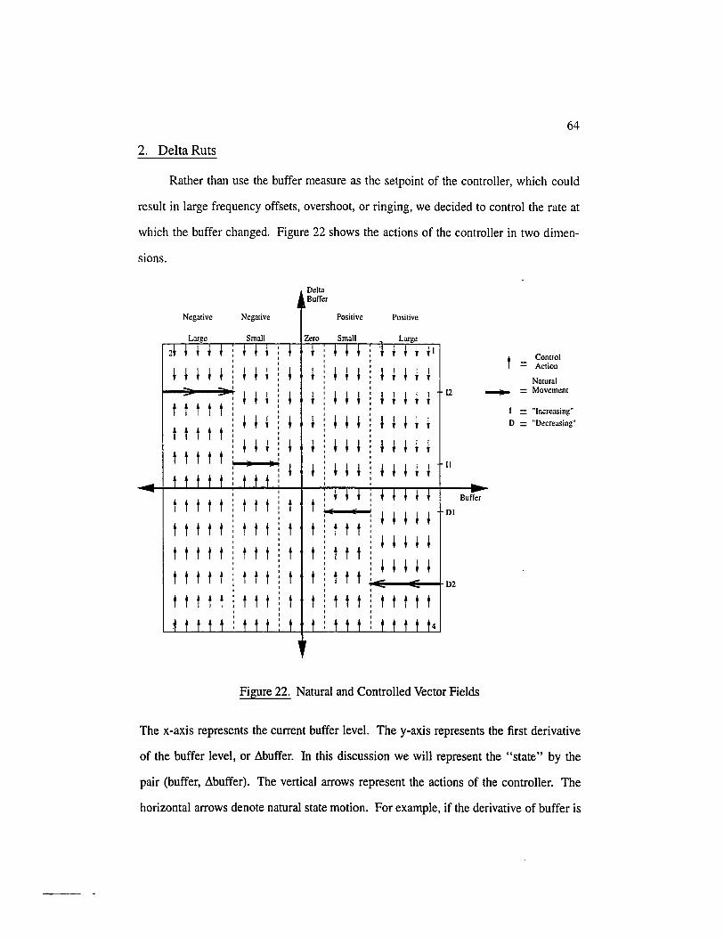
64
2. Delta Ruts
Rather than use the buffer measure as the setpoint of the controller, which could
result in large frequency offsets, overshoot, or ringing, we decided to control the rate at
which the buffer changed. Figure 22 shows the actions of the controller in two dimen-
sions.
t t t t t t t t t t t t t t t
t t t t t t t t t t t t t t t t t t t t t t t t t
~ ~ ~
~ ~ ~
~ ~ ~
t ~ ~
t t t t t t t t t t t t t t t t t
Delta Buffer
~
t
t t
~ ~ ~ ~ ~
~ ~ ~ ~ ~ ~ ~ ~ 12
t t t t t t t ~
t t t t t t t ~
t t t t t t t t II
t t t t t t t t t t t t ~
t t t t t ~ t t
t t t D2
t t t t t t t t
Figure 22. Natural and Controlled Vector Fields
Control = Action
Naturo~l
~ = Movement
I = "Increasing"
D = "Decreasing"
The x-axis represents the current buffer level. They-axis represents the first derivative
of the buffer level, or ~buffer. In this discussion we will represent the "state" by the
pair (buffer, ~buffer). The vertical arrows represent the actions of the controller. The
horizontal arrows denote natural state motion. For example, if the derivative of buffer is

65
negative, the state of the system will tend toward the left, indicated by the left-pointing
arrow.
If the state is in the first quadrant, the buffer is more than half full and is becom
ing more full. This is undesirable for obvious reasons and a negative ~buffer is desired.
If in the second quadrant, the buffer is less than half full but is filling. If the state is in
the third quadrant, the buffer is less than half full and is continuing to become less full.
The fourth quadrant represents the state where the buffer is more than half full, but is
emptying. Clearly quadrants two and four contain states which act to prevent buffer
overflow.
Next, we partition the x-axis. For simplicity, we define only five partitions: Zero,
Positive Small, Positive Large, Negative Small, and Negative Large as shown. We
decide that if the buffer is positive and Small we want it to Decrease at some rate D I ,
chosen by some means. D2,1I (rate of Increase), and 12 are chosen in the same way.
3. Full Domain Fuzzy Set Spanning Property
We chose to make predictions based on a time of one sample period. This implies
that the predictive terms of the rule must be achievable in a single sample period or a
low firing strength will result. We found that the best way to deal with this is to cause
all the ~buffer fuzzy sets to span the entire domain. Thus, since each predicted conse
quent is always true to some degree, the action which moves the state of the controller
closest to the peak of the fuzzy set (optimizes the function) is chosen.
Consider, for example, the situation where buffer is NS (Negative Small), and the
desired d_buffer value is SI (Slowly Increasing). If we define SI as shown in Fig
ure 23, the predictive part will evaluate to zero if none of the listed candidate actions is
predicted to place d_buffer precisely within the domain of IS. If the predictive part
evaluates to zero, the truth of the entire rule will be zero and the rule will not fire. The

66
probable result is a situation where no rules fire.
To solve this problem, we simply require all "target" fuzzy sets to span the entire
range, as shown in Figure 23. By "target" fuzzy sets we mean a fuzzy set which is part
of the predicted outcome of a rule.
current value
.. t. Buffer
Figure 23. Original D_Buffer Fuzzy Set Definition
~. I t. Buffer
current value
Figure 24. Improved (for PKBC) D_Buffer Fuzzy Set Definition
With this spanning definition, the statement d_buffer is SI is always true to some
degree. If a candidate action causes an increase in the degree of truth for this term its
overall truth value will increase. With everything else equal, the rule which maximizes
the predicted parameters will have the largest truth value and will be chosen. (Notice
that this assumes a definition of conjunction based on the product operator. See Section
7 for the justification of this choice.)
In short, if a fuzzy set is the goal of one or more rules (it occurs in a predictive
term), it should span the entire region over which it might be applied. If a fuzzy set is
not the goal of any rule (it occurs in only conditional terms), it may be defined over
whatever region is appropriate.
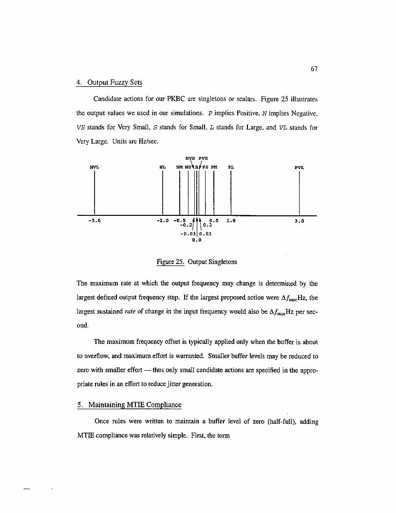
67
4. Output Fuzzy Sets
Candidate actions for our PKBC are singletons or scalars. Figure 25 illustrates
the output values we used in our simulations. P implies Positive, N implies Negative,
VS stands for Very Small, S stands for Small, L stands for Large, and VL stands for
Very Large. Units are Hz/sec.
NVL NL PL PVL
-3.0 -1.0 -o.s ,,~ o.s -o.2 I o.2 -0.03 0.03
1.0 3.0
o.o
Figure 25. Output Singletons
The maximum rate at which the output frequency may change is determined by the
largest defined output frequency step. If the largest proposed action were .6./maxHz, the
largest sustained rate of change in the input frequency would also be .6./maxHz per sec
ond.
The maximum frequency offset is typically applied only when the buffer is about
to overflow, and maximum effort is warranted. Smaller buffer levels may be reduced to
zero with smaller effort - thus only small candidate actions are specified in the appro
priate rules in an effort to reduce jitter generation.
5. Maintaining MTIE Compliance
Once rules were written to maintain a buffer level of zero (half-full), adding
MTIE compliance was relatively simple. First, the term
68
.... AND wander IS POK
was added to all the rules. This ensured that actions which would result in a violation or
near-violation of MTIE would evaluate to zero and be eliminated from consideration.
Remember that a wander value of 21, for example, means that the proposed action is
predicted to violate MTIE in 21 sample times.
Next, a set of rules was crafted which stated that if wander were not OK and a
candidate action would cause it to be more OK than it was, apply that candidate action.
Finally, if MTIE were viola ted, and a candidate action would result in moving TIE
closer to the envelope (closer to re-compliance), then apply that action. The net effect
of these rules is to cause the buffer to be kept at zero unless MTIE is in danger of viola-
tion. In that case, the action necessary to keep the violation from occurring is taken.
These results are illustrated in Chapter 8.
6. Maintaining Buffer Compliance
We also show, in Chapter 8, that it is possible to construct the rulebase such that
the buffer is given precedence over MTIE when both are near violation. Again, this was
a relatively simple task. First, the term
. . .. AND buffer IS OK
was appended to every rule in the ruleset which ensured MTIE compliance. Then, two
"ramp" fuzzy sets were defined on the buffer axis: Positive Too Large (P2L) and
Negative Too Large (N2L), and the two fuzzy sets POS and NEG were defined on the
d_buffer axis at +25 and -25 respectively. Finally, rules were added to the rulebase
which stated:
IF buffer IS P2L and ( freq = [action] -> d_buffer IS NEG ) THEN DOIT
A similar rule was added for N2L.

69
These rules ensure that if the buffer becomes too full or empty, appropriate
actions wiII be taken to ensure that they do not increase (or decrease) further without
regard for MTIE compliance. The location of P2L and N2L define the boundary at
which these buffer-constraints take effect.
Notice, however, that this action alone does not guarantee buffer compliance. If,
for example, the "too large" fuzzy sets were located 20 bits from the actual buffer lim
its, a single 3-pointer burst would cause the buffer to spill before the controller would
have time to react. Thus, buffer compliance may be guaranteed only if appropriate lim
its are placed on the rate and magnitude of PJE bursts, and the rate at which a continu
ous PIE stream changes.
7. Observations
Under most circumstances, a single term need not be in both the conditional and
predictive terms. The question to ask is: Is this term a prerequisite for this ~ction, or is
this term something that I want to come about due to this action. In addition, if a single
term is included twice, the product AND operator uses its truth value twice, decreasing
the overall truth of the rule. Conversely, this property might be useful in a situation
where a squared fuzzy set is desired.
Our implementation of the PKBC can employ either min or product definitions of
the AND and inference operators. We can also specify whether the centroid or
"winner-take-all" defuzzification method is employed. However, 'we have found that
the product definition is superior to min and that centroid defuzzification does not make
intuitive sense.
For example, suppose we have two rules as follows:
IF buffer IS NegativeLarge AND ( freq = PS -> d_buffer IS FastIncreasing ) THEN DOIT IF buffer IS NegativeLarge AND ( freq = PM -> d_buffer IS FastIncreasing ) THEN DOIT
70
Now suppose that the truth of the conditional term is 0.2 and the truth of the predictive
terms of the first and second rules are 0.6 and 0.9 respectively. With the min definition
of AND, both rules will have the same overall truth value
(nzin(O. 2, O. 6) = min(O. 2, O. 9)=0.2,) yet clearly the second rule proposes the most
appropriate action since it produces better compliance with the term Increasing-
Fas t. The product definition of AND is thus more appropriate for a predictive con
troller as we have defined it, yielding rule truths of 0.12 and 0.18 respectively.
In addition, we believe that centroid defuzzification is counter-intuitive. The per
formance of each rule is evaluated using measurements and prediction. If we then
weight each action based on the truth of the rule from which it came and combine them
all into a single action, it is not clear that the result will have a better predicted outcome
than the rule with the highest truth value. In fact, if a large action produces the most
benefits, combining it with other actions with smaller benefits will reduce the overall
effectiveness of the controller. Thus, we use a winner-take-all technique for rule selec
tion.
A possible extension would be to combine the most promising candidate actions
to form a new rule which would then be evaluated and compared to the rules from
which it was derived. As before, the rule with the largest truth value would be chosen.
D. FINAL CONTROLLER SPECIFICATION
We now describe the fuzzy sets and rules which were used in the simulations of
the next chapter to test jitter performance. Since neither constraint was threatened in
these tests, the controller employed the rules which act to keep the buffer half-full.
Although the constraint-satisfaction abilities were not demonstrated in the jitter tests,
the rules were written such that MTIE was the dominant constraint.
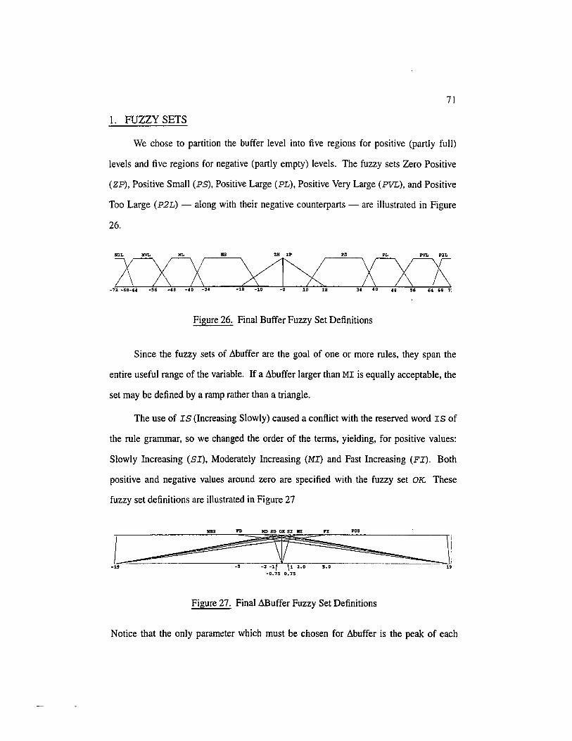
71
1. FUZZY SETS
We chose to partition the buffer level into five regions for positive (partly full)
levels and five regions for negative (partly empty) levels. The fuzzy sets Zero Positive
(ZP), Positive Small (PS), Positive Large (PL), Positive Very Large {PVL), and Positive
Too Large (P2L) -along with their negative counterparts- are illustrated in Figure
26.
NS ZN ZP
~ -72 -68-64 -56 -48 -40 -34 -18 -10 -o 10 1a
Figure 26. Final Buffer Fuzzy Set Definitions
Since the fuzzy sets of ~buffer are the goal of one or more rules, they span the
entire useful range of the variable. If a ~buffer larger than MI is equally acceptable, the
set may be defined by a ramp rather than a triangle.
The use of IS (Increasing Slowly) caused a conflict with the reserved word IS of
the rule grammar, so we changed the order of the terms, yielding, for positive values:
Slowly Increasing (SI), Moderately Increasing (MI) and Fast Increasing (FI). Both
positive and negative values around zero are specified with the fuzzy set OK. These
fuzzy set definitions are illustrated in Figure 27
Figure 27. Final M3uffer Fuzzy Set Definitions
Notice that the only parameter which must be chosen for ~buffer is the peak of each
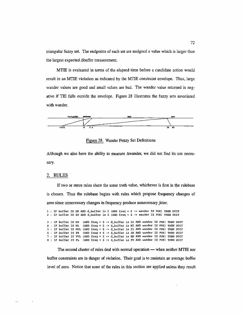
72
triangular fuzzy set. The endpoints of each set are assigned a value which is larger than
the largest expected Llbuffer measurement.
MTIE is evaluated in terms of the elapsed time before a candidate action would
result in an MTIE violation as indicated by the MTIE constraint envelope. Thus, large
wander values are good and small values are bad. The wander value returned is neg
ative if TIE falls outside the envelope. Figure 28 illustrates the fuzzy sets associated
with wander.
-1001 0 3 ' 38 '0
Figure 28. Wander Fuzzy Set Definitions
Although we also have the ability to measure Llwander, we did not find its use neces-
sary.
2. RULES
If two or more rules share the same truth value, whichever is first in the rulebase
is chosen. Thus the rulebase begins with rules which propose frequency changes of
zero since unnecessary changes in frequency produce unnecessary jitter.
1 : IF buffer IS ZN AND d_buffer is Z (AND freq = Z -> wander IS POK) THEN DOIT 2 : IF buffer IS ZP AND d_buffer is Z (AND freq = Z -> wander IS POK) THEN DOIT
3 : IF buffer IS NS (AND freq = z -> d_buffer is SI AND wander IS POK) THEN DOIT 4 IF buffer IS NL (AND freq = z -> d_buffer is MI AND wander IS POK) THEN DOIT 5 IF buffer IS NVL (AND freq = z -> d_buffer is FI AND wander IS POK) THEN DOIT 6 : IF buffer IS PS (AND freq = z -> d_buffer is SO AND wander IS POK) THEN DOIT 7 : IF buffer IS PVL (AND freq = z -> d_buffer is MD AND wander IS POK) THEN DOIT 8 IF buffer IS PL (AND freq = z -> d_buffer is FD AND wander IS POK) THEN DOIT
The second cluster of rules deal with normal operation - when neither MTIE nor
buffer constraints are in danger of violation. Their goal is to maintain an average buffer
level of zero. Notice that none of the rules in this section are applied unless they result
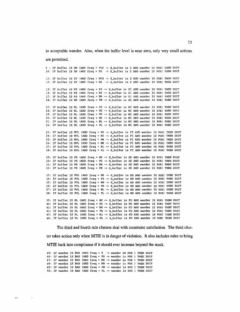
73
in acceptable wander. Also, when the buffer level is near zero, only very small actions
are permitted.
9 : IF buffer IS ZN (AND freq 10: IF buffer IS ZN (AND freq
11: IF buffer IS ZP (AND freq 12: IF buffer IS ZP (AND freq
13: IF buffer IS NS (AND freq 14: IF buffer IS NS (AND freq 15: IF buffer IS NS (AND freq 16: IF buffer IS NS (AND freq
PVS -> d_buffer is Z AND wander IS POK) THEN DOlT PS -> d_buffer is Z AND wander IS POK) THEN DOlT
NVS -> d_buffer is Z AND wander IS POK) THEN DOlT NS -> d_buffer is Z AND wander IS POK) THEN DOlT
PS -> d_buffer is SI AND wander IS POK) THEN DOlT NS -> d_buffer is SI AND wander IS POK) THEN DOlT NM -> d_buffer is SI AND wander IS POK) THEN DOlT PM -> d_buffer is SI AND wander IS POK) THEN DOlT
17: IF buffer IS NL (AND freq PS -> d_buffer is MI AND wander IS POK) THEN DOlT 18: IF buffer IS NL (AND freq = NS -> d_buffer is MI AND wander IS POK) THEN DOlT 19: IF buffer IS NL (AND freq = PM -> d_buffer is MI AND wander IS POK) THEN DOlT 20: IF buffer IS NL (AND freq = NM -> d_buffer is MI AND wander IS POK) THEN POIT 21: IF buffer IS NL (AND freq = NL -> d_buffer is MI AND wander IS POK) THEN DOlT 22: IF buffer IS NL (AND freq = PL -> d_buffer is MI AND wander IS POK) THEN DOlT
23: IF buffer IS NVL (AND freq PS -> d_buffer is FI AND wander IS POK) THEN DOlT 24: IF buffer IS NVL (AND freq NS -> d_buffer is FI AND wander IS POK) THEN DOlT 25: IF buffer IS NVL (AND freq PM -> d_buffer is FI AND wander IS POK) THEN DOlT 26: IF buffer IS NVL (AND freq NM -> d_buffer is FI AND wander IS POK) THEN DOlT 27: IF buffer IS NVL (AND freq NL -> d_buffer is FI AND wander IS POK) THEN DOlT 28: IF buffer IS NVL (AND freq = PL -> d_buffer is FI AND wander IS POK) THEN DOlT
29: IF buffer IS PS (AND freq = NS -> d_buffer is SO AND wander IS POK) THEN DOlT 30: IF buffer IS PS (AND freq = PS -> d_buffer is SO AND wander IS POK) THEN DOlT 31: IF buffer IS PS (AND freq = NM -> d_buffer is SO AND wander IS POK) THEN DOlT 32: IF buffer IS PS (AND freq = PM -> d_buffer is SD AND wander IS POK) THEN DOlT
33: IF buffer IS PVL (AND freq 34: IF buffer IS PVL (AND freq 35: IF buffer IS PVL (AND freq 36: IF buffer IS PVL (AND freq 37: IF buffer IS PVL (AND freq 38: IF buffer IS PVL (AND freq
NS -> d_buffer is MD AND wander IS POK) THEN DOlT PS -> d_buffer is MD AND wander IS POK) THEN DOlT NM -> d_buffer is MD AND wander IS POK) THEN DOlT PM -> d_buffer is MD AND wander IS POK) THEN DOlT NL -> d_buffer is MD AND wander IS POK) THEN DOlT PL -> d_buffer is MD AND wander IS POK) THEN DOlT
39: IF buffer IS PL (AND freq = NS -> d_buffer is FD AND wander IS POK) THEN DOlT 40: IF buffer IS PL (AND freq = PS -> d_buffer is FD AND wander IS POK) THEN DOlT 41: IF buffer IS PL (AND freq = NM -> d_buffer is FD AND wander IS POK) THEN DOlT 42: IF buffer IS PL (AND freq = PM -> d_buffer is FD AND wander IS POK) THEN DOlT 43: IF buffer IS PL (AND freq = NL -> d_buffer is FD AND wander IS POK) THEN POIT 44: IF buffer IS PL (AND freq = PL -> d_buffer is FD AND wander IS POK) THEN DOlT
The third and fourth rule clusters deal with constraint satisfaction. The third clus-
ter takes action only when MTIE is in danger of violation. It also includes rules to bring
MTIE back into compliance if it should ever increase beyond the mask.
45: IF wander IS BAD (AND freq Z -> wander IS POK THEN DOlT 46: IF wander IS BAD (AND freq PS -> wander is POK 47: IF wander IS BAD (AND freq NS -> wander is POK 48: IF wander IS BAD (AND freq NM -> wander is POK 49: IF wander IS BAD (AND freq PM -> wander is POK 50: IF wander IS BAD (AND freq = PL -> wander is POK
THEN DOlT THEN DOlT THEN DOlT THEN DOlT THEN DOlT
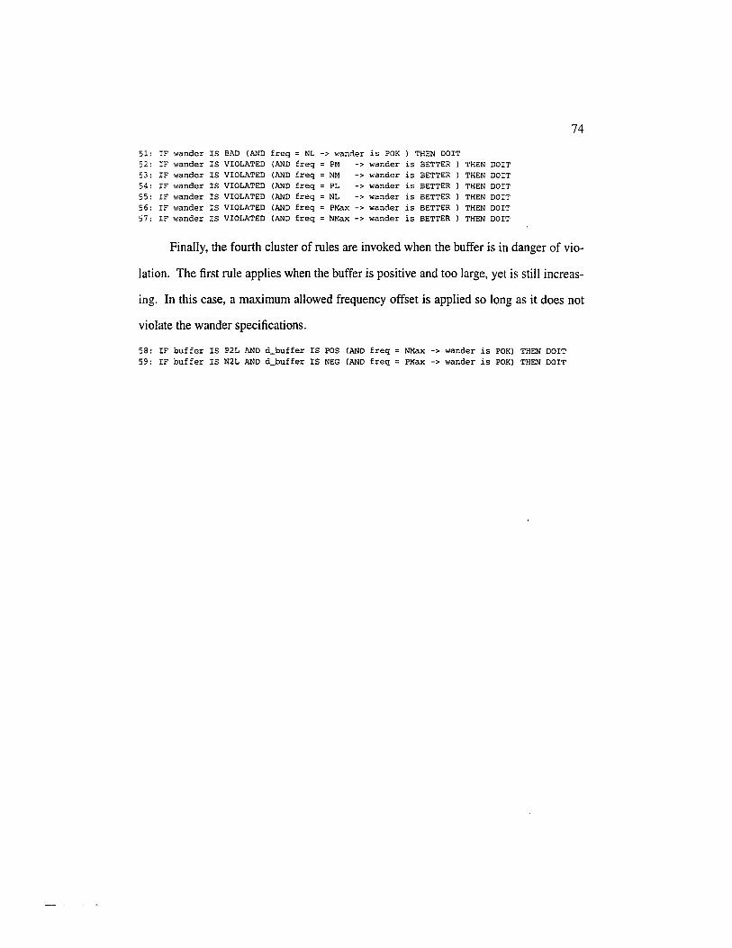
74
51: IF wander IS BAD (AND freq = NL -> wander is POK ) THEN DOlT 52: IF wander IS VIOLATED (AND freq = PM -> wander is BETTER ) THEN DOlT 53: IF wander IS VIOLATED (AND freq =NM -> wander is BETTER ) THEN DOlT 54: IF wander IS VIOLATED (AND freq = PL -> wander is BETTER ) THEN DOlT 55: IF wander IS VIOLATED (AND freq = NL -> wander is BETTER THEN DOlT 56: IF wander IS VIOLATED (AND freq = PMax -> wander is BETTER THEN DOlT 57: IF wander IS VIOLATED (AND freq = NMax -> wander is BETTER THEN DOlT
Finally, the fourth cluster of rules are invoked when the buffer is in danger of vio-
lation. The first rule applies when the buffer is positive and too large, yet is still increas-
ing. In this case, a maximum allowed frequency offset is applied so long as it does not
violate the wander specifications.
58: IF buffer IS P2L AND d_buffer IS POS (AND freq = NMax -> wander is POK) THEN DOlT 59: IF buffer IS N2L AND d_buffer IS NEG (AND freq = PMax -> wander is POK) THEN DOlT
CHAPTER VII
SIMULATION ENVIRONMENT
A. SIMULATION FRAMEWORK
The controller described in the previous chapter was implemented and incorpo
rated into the simulation environment illustrated in Figure 29.
The simulator consists of a set of C++ [39] objects which are coordinated by a
custom discrete-event simulation engine. Parameters are passed to the simulator
through a database object and various custom files. After the simulation is completed,
samples of pertinent quantities are written to files and illustrated by a motif-based
graphical display and browser.
B. VALIDITY
The validity of our results depend strongly on the validity of our simulation
engine and simulation models. Therefore great care was taken to ensure that each
model accurately reflected the system, signal, or format it was designed to represent.
Still, a physically realized implementation might exhibit slightly different waveforms,
just as no two physical systems of this complexity would be identical.
Fortuitously, our simulator has one significant advantage over simulators of other
types of systems: It is a digital program simulating a largely digital system. Specifi
cally, the input is a digital signal (albeit a continuous-time one), the PKBC algorithm
internal to the simulator is the very same program that would be recompiled for a real
world implementation, and the output frec:.uency generator is a purely digital system
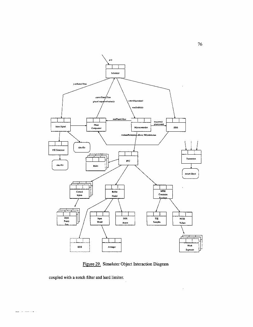
Cuntml lnJIU!S
Buner
Mudcl
Mii.TucuntmUer
rr~(wurd)
(lb'ICiwunn
Cunslr.l.int
TIE s ... ples
Figure 29. Simulator Object Interaction Diagram
coupled with a notch filter and hard limiter.
DDS
MTIE
Value!
Mask
Segmenl~
76

77
C. SIMULATION MODULES
Here we describe the components of the simulator which are not part of the
PKBC algorithm, but instead allow the algorithm to function in a virtual environment.
1. Scheduler
The scheduler schedules discrete-time events at the module level. Specifically,
the input and microcontroller modules (described below) are invoked by the scheduler at
the requested time. Then, when each module returns, it informs the scheduler of the
time at which the next caB is to occur. The scheduler exits when the terminal simulation
time is reached.
2. Input Signal
The input signal module emulates a DS3 signal after overhead and stuff-bytes
have been removed. To do this, the nominal (pre-PJE) DS3 rate, the STS-l synchro
nization frequency, and the structure of the DS3 to STS-l mapping are made available at
runtime. During early development, the input was modeled at the clock level (each ris
ing and falling edge), but it quickly became evident that such fine time resolution was
both unnecessary and extremely computation intensive. At nominal data rates, the
scheduler was required to caB the input module 2 . 44, 736, 000 times for each second of
simulation. Instead, we calculate the cumulative effect of an entire STS-I row, resulting
in an execution-time reduction of several orders of magnitude. After each row, the num
ber of DS3 data bits in the row (621 or 622, depending on the stuff bit) is·sent to the
phase comparator.
3. PJE Generator
All PJEs are generated by the PJE module. For maximum flexibility, a method of
specifying arbitrary PJE profiles was developed. PJEs may be specified at arbitrary
78
times and/or at arbitrary rates and with positive or negative polarities - within the con
straints of the SONET standard. The PIE input file may contain any number of entries
of the following form:
start Time TimeBetweenPJEs Polarity
where the startTirne supersedes the previous TirneToNextPJE.
If an indefinite sequence of positive PJEs is desired, beginning at a simulation
time of 3 seconds and with an interval of I second, the PJE file would contain the single
line:
3.0 1.0 1
If each PJE is to be placed at irregular times, the startTirne field may be assigned the
desired time of each PJE and TimeToNextPJE may be set to a number larger than the
length of the simulation. Most profiles use a combination of the above two techniques.
Although the PJE generator provides precise timing information during simula
tion, such precision would not be available in a real-world implementation. We antici
pate this lack of time resolution to have only negligible effect, however, since PJE sce
narios in Chapter VIII actually simulate missing or extra PIEs (as many as four missing
PJEs) while still meeting jitter specifications.
4. DDS Output
The DDS module models the operation of a DDS. It accepts frequency and phase
tuning words from the microcontroller object, and calculates the output frequency that
will result. When asked, it can give the number of output clock cycles since the last
time it was queried. The length of TW F is limited to the number of bits used in internal
integer calculations of the simulating microprocessor (32, in our case), since native
arithmetic operations are used to calculate the output of the DDS. This limitation could
be removed through the use of an arbitrary-precision library, but at a cost of increased
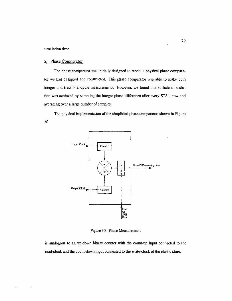
79
simulation time.
5. Phase Comparator
The phase comparator was initially designed to model a physical phase compara-
tor we had designed and constructed. This phase comparator was able to make both
integer and fractional-cycle measurements. However, we found that sufficient resolu-
tion was achieved by sampling the integer phase difference after every STS-1 row and
averaging over a large number of samples.
30
The physical implementation of the simplified phase comparator, shown in Figure
Input Clock
Out ut Clock
End Of SPE Row
Phase Difference (cycles)
Figure 30. Phase Measurement
is analogous to an up-down binary counter with the count-up input connected to the
read-clock and the count-down input connected to the write-clock of the elastic store.

80
D. SIMULATION MEASUREMENTS
1. TIE Reference Clock
The Time Interval Error measure, described previously, is necessary for the calcu
lation of both wander and jitter and requires a frequency reference fDS3' For jitter, long
term stability of the reference clock is not necessary since low frequencies are attenu
ated by the high-pass filter.
For the MTIE calculation, however, long-term stability of the reference clock is
important since it is against this clock that the long-term variation of the outgoing DS3
signal will be measured. The question that arises is: If the reference against which TIE
is measured is imperfect, would external equipment testing MTIE compliance reach the
same conclusion as the control algorithm? The answer to this question is found in the
definition of DS3 MTIE [4]. The specified mask assumes that TIE samples are taken
relative to a system clock readily available to the desynchronizer. Thus the same clock
that would be used by an external MTIE measurement device is available to our PKBC
algorithm. If this were not the case, a clock with sufficient accuracy would be required
such that the TIE samples used to generate the MTIE Constraint Envelope would yield
an acceptable margin of error.
2. Jitter Measurement
The rate at which TIE is sampled for calculating jitter is not bounded by the con
tra11er's update rate Ts (although our algorithm restricts it to an integer multiple of Ts).
In this way, the peak-to-peak jitter error resulting from the discrete-time measurement
(as derived in Chapter ill) may be reduced to whatever levels are deemed acceptable.
We operated at a TIE sample rate (T TIE) of 200Hz, which was shown to result in a jitter
measurement error of less than 1 %.
81
Jitter measurement is included in the simulator for testing purposes. It is not
specifically used by the controller and may be omitted in a hardware implementation.
3. Wander
Although we represent wander by the MTIE measure, we do not calculate MTIE
explicitly. Rather, the MTIE Constraint Envelope is generated as a function of both the
MTIE mask and all previous TIE measurements (to the limits of the mask) as described
in the previous Chapter. Since MTIE is undefined for observations times less than 0.1
second, the envelope is recomputed at a rate of 10Hz. When the simulation is com
plete, a single plot showing the generated TIE and the MTIE mask may be displayed for
the user.
E. GRAPHICAL USER INTERFACE
An important part of the simulation environment is our custom graphical user
interface. Any internal variable may be sampled and stored by a set of Signal
objects. These storage objects are given samples at regularly spaced intervals with the
member function:
[Object Name].dataln(Value, Time)
After the simulator reaches the terminal time, another object, called the GraphWindow
collects all the Signals and asks each to display itself within a PanedWindow Motif
widget which allows vertical scaling of any signal of choice. At the highest level, the
XIn terface object manages the PanedWindow, several push buttons for quitting or
writing the signals to their appropriate files, and the fuzzy sets illustration window
described below.
If the mouse button is pressed while the cursor is in the signals area, a vertical
bar cursor is displayed at the relevant time for each signal, and the value at the cursor
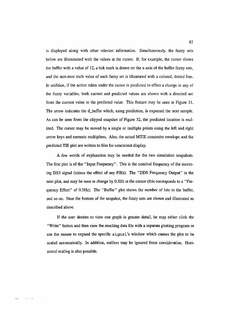
82
is displayed along with other relevant information. Simultaneously, the fuzzy sets
below are illuminated with the values at the cursor. If, for example, the cursor shows
the buffer with a value of 12, a tick mark is drawn on the x-axis of the buffer fuzzy sets,
and the non-zero truth value of each fuzzy set is illustrated with a colored, dotted line.
In addition, if the action taken under the cursor is predicted to effect a change in any of
the fuzzy variables, both current and predicted values are shown with a directed arc
from the current value to the predicted value. This feature may be seen in Figure 31.
The arrow indicates the d_buffer which, using prediction, is expected the next sample.
As can be seen from the clipped snapshot of Figure 32, the predicted location is real
ized. The cursor may be moved by a single or multiple points using the left and right
arrow keys and numeric multipliers. Also, the actual MTIE constraint envelope and the
predicted TIE plot are written to files for concurrent display.
A few words of explanation may be needed for the two simulation snapshots.
The first plot is of the "Input Frequency". This is the nominal frequency of the incom
ing DS3 signal (minus the effect of any PJEs). The "DDS Frequency Output" is the
next plot, and may be seen to change by O.5Hz at the cursor (this corresponds to a "Fre
quency Effort" of O.5Hz). The "Buffer" plot shows the number of bits in the buffer,
and so on. Near the bottom of the snapshot, the fuzzy sets are shown and illustrated as
described above.
If the user desires to view one graph in greater detail, he may either click the
"Write" button and then view the resulting data file with a separate plotting program or
use the mouse to expand the specific signal's window which causes the plot to be
scaled automatically. In addition, outliers may be ignored from consideration. Hori
zontal scaling is also possible.
.b DDSF~D.rt.put
Fr~ Effort
·F Buffer
·r cLbuff..-
Prodicted D_I>Uffor
r PJE Rate
I 1.653
1.653
~/34918.&36 3,307
83
• _J
~= 447349i9
44734918 0 500000-1 o:250000- I
0 QQ('!Q())o
-~:r -!.'!~;
0 117596· -32 -£S i
~! 0 OO<!QQ()o
.~~--~""'--'----------1.6s3-------~iS! .. -~----~----------~~:: · Predicted Wander
~O!!QQ QQQQ
TIE <UI>
Activo Rule
Truth of Activo Rule
Pts/Pixel= 0.1 Point ruober = 74 flltor Len: Error=!, c£rror=3 t= 3.0215
Figure 31. Simulation Example Showing Predicted d_buf fer movement
16 8,900000-e oo W·
0,$2346· 0,281173· 111!8!9>

84
~ slrn • ..J
Ie-ite Dote! '"-" Agoinl ~ "/tesWnec,deoo/sterdonL.Jttter~.OUG491_11onder:1,35295
I I!:f!!!: r.........,. ~~Z~9lB 3llB r.=.!
.b DDS Frequet'oC\1 lkltput ~413-19i9 I km.c9!'&.~ 1.653 44734919
I Freq.JenClj Eff~rt 0.500000-12000 0.250000-Q !Wili)O·
·r Buffer [9.oi~.~7 j.~ 1.653
·roo d,buff..-
I _L-~~7
2 Zlm;· 1.653 -32
-66
I Predicted DJ>Uffer
~~ -~ Z'?.il I
·F PJE Rate
I r-~3.~7 Q !Wili)O·
1.653
~thedlfi'Ut - 44734918 ---~------,_...------------r.473491!,•«61 ---~- -------• 1.653 ---- ,307 44734919
I Pr-edicted Wonder
~ ~QQQQ QQQQ
I TIE CUI>
~:!! ~-0000
I Active Rule 16 -1•,Q!l!!l a.oooooo-
~
I Truth of Active Rule 0,562346·
b 5623 0.291173· !!!!B!~·
Pts/Pixel= 0,1 Potnt ruber = 75 filter Len: Error=!, cEmr..,J t= 3.0601
~/~ owder
2:X2' !§ PS
~ -r~--1"-: I _,-' -~017.6 I ' -90'0 tbuffOI'
9,0 17,0 20.v <4,0 <t>,O ,.,, ..... Q!I :lo:' """'
--,-_.::;}~~- _sk·¥-_.:::.=-~ -- -- .f!__ -...-:ii-
,;>~iii iii ~~~s;; s~ ~}~~::~-::~:<~vrf-"t.:-z~~~;-~;~i£i~~~·;-\ / I~ -5.1>1.7 •4,0 -t.o -l.iiM o.o v.h.o to M .~ l ,0
Figure 32. Simulation Example Showing d_buffer movement
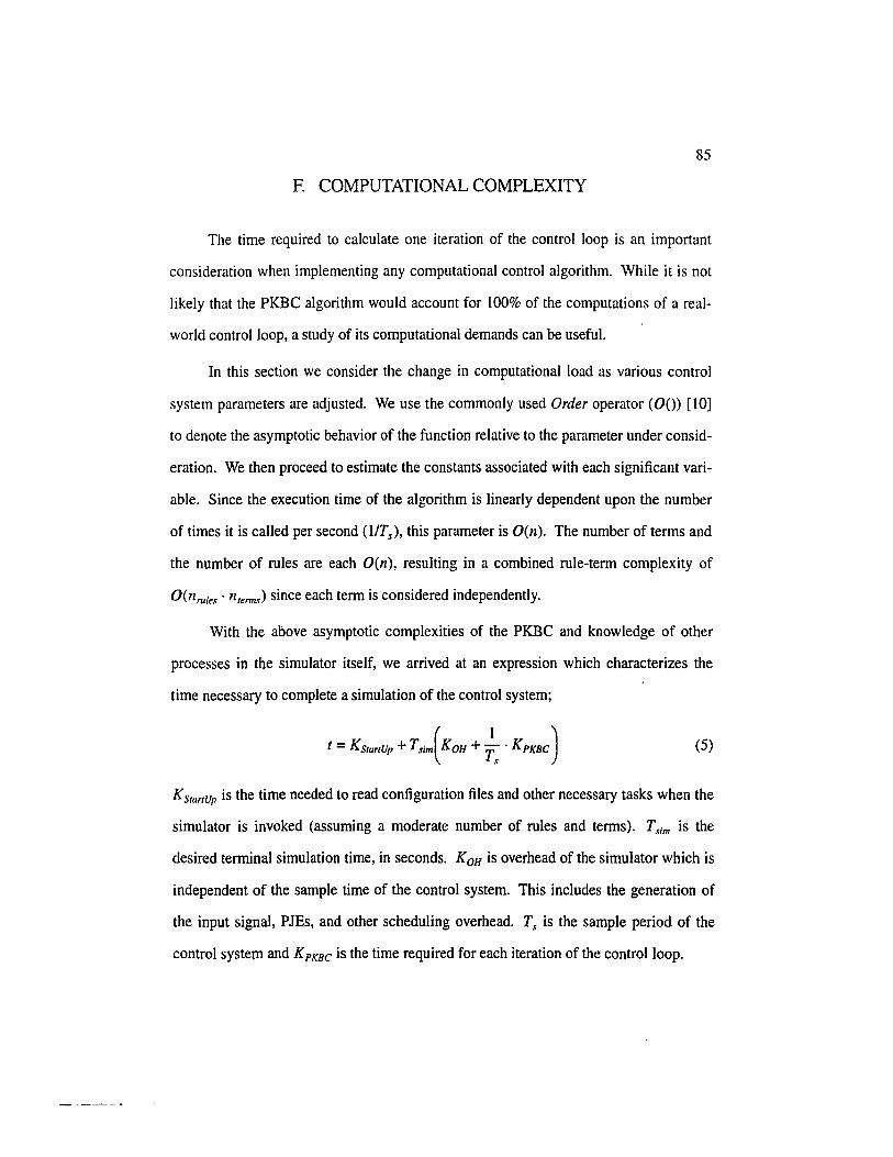
85
F. COMPUTATIONAL COMPLEXITY
The time required to calculate one iteration of the control loop is an important
consideration when implementing any computational control algorithm. While it is not
likely that the PKBC algorithm would account for 100% of the computations of a real
world control loop, a study of its computational demands can be useful.
In this section we consider the change in computational load as various control
system parameters are adjusted. We use the commonly used Order operator (00) [10]
to denote the asymptotic behavior of the function relative to the parameter under consid
eration. We then proceed to estimate the constants associated with each significant vari
able. Since the execution time of the algorithm is linearly dependent upon the number
of times it is called per second (lITs )' this parameter is O(n). The number of terms and
the number of rules are each O(n), resulting in a combined rule-term complexity of
O(nrules . llterms) since each term is considered independently.
With the above asymptotic complexities of the PKBC and knowledge of other
processes in the simulator itself, we arrived at an expression which characterizes the
time necessary to complete a simulation of the control system;
(5)
KSliIrtUp is the time needed to read configuration files and other necessary tasks when the
simulator is invoked (assuming a moderate number of rules and terms). T.rim is the
desired terminal simulation time, in seconds. KOH is overhead of the simulator which is
independent of the sample time of the control system. This includes the generation of
the input signal, PIEs, and other scheduling overhead. Ts is the sample period of the
control system and K pKBC is the time required for each iteration of the control loop.
86
K PKBC may be further expressed as
K pKBC = KRllle * N Rilles + KR&T(N Rules' NTerms) + K misc (6)
where K Ruie is the computation time associated with the evaluation of each rule, KR&T is
the time constant associated with each term of each rule, N Rules and NTerms are the num
ber of rules and terms per rule respectively, and K misc includes all other PKBC computa
tions.
Generation of the MTIE envelope has a theoretical computational complexity of
O(logbllse nenv ) where base is the exponential growth constant of the MTIE constraint
envelope (typically about 1.5) as described in Chapter 4 and nenv is the desired length of
the constraint envelope in units of Ts. This term is not included in the expression for
T PKBC since its effect on simulation time was too small to be measured with 'confidence
and is therefore included in K misc '
The first two terms of T PKBC and empirical measurements are plotted together in
Figure 33. Obviously, the model accurately reflects measurements of simulation time
for widely varying numbers of rules and terms.
The constants of Equations (5) and (6) are listed in Table III. They were derived
through timed simulations and in each case the linearity of the expression was verified
by multiple simulations.
The platform used for the simulations was a 90MHz Pentium-based mM compat
ible computer with 32 Megabytes of RAM and running Linux version 1.2.13. The com
piler was gcc/g++ version 2.6.3 with optimization level four. Assuming similar process
ing power, a single iteration of a 60-rule, 4-term controller would require 2.14ms, far
less than the Ts of 40ms used in our tests. It is also important to notice that K Rule , KR&T
and K Misc include the time necessary to collect data in Signal objects for later display,
execute debug statements and conditionals, and additional time due to algorithms which
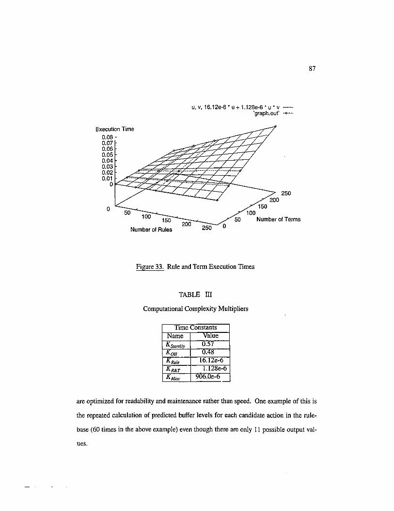
Execution Time 0.08-0.07 0.06 0.05 0.04 0.03 0.02 0.01
0
0
u, v, 16.12e-6 * u + 1.128e-6 * u • v -'graph.out' --o---·
150 100
250 200
Number of Terms
Number of Rules 250
Figure 33. Rule and Term Execution Times
TABLE III
Computational Complexity Multipliers
T1me Constants Name Value
KstarrUp 0.57 KoH 0.48 KRule lo.I2e-o KR&T l.l28e-6 KMisc 90o.Oe-o ·-
87
are optimized for readability and maintenance rather than speed. One example of this is
the repeated calculation of predicted buffer levels for each candidate action in the rule
base (60 times in the above example) even though there are only II possible output val-
ues.
CHAPTER VIII
TESTING AND EVALUATION
This chapter presents the tests used to verify that the PKBC meets our two pri
mary goals. Our first goal was to verify that the controller produced acceptable (or bet
ter) jitter in the normal case as a result of PJE profiles specified in [3]. The first set of
tests verify this claim. However, compliance with the standard tests is only part of the
capabilities of the controller (albeit a necessary part) since other desynchronization
techniques have also been shown to meet this requirement [15].
The second goal was to study the PKBC's ability to maintain MTIE compliance
and prevent buffer overflow or underflow for as iong as possible. With both constraints
facing the danger of violation, we suggested that the algorithm would be capable of sat
isfying one constraint at the expense of the other as determined beforehand by the
designer. This is the larger challenge. The performance of the PKBC is demonstrated
in a second set of tests.
A. STANDARD JITTER TESTS
To facilitate the testing of jitter performance, we created a directory structure
where the parameters file, rules, fuzzy sets, and MTIE mask could all be defined in one
place. Subdirectories for mapping, standard, burst, phase transient burst, and degraded
modes each included shell and Awk [40] scripts for automatically setting· up experi
ments and generating PJE files.
For example, a pair of files in the degraded/continuous subdirectory specify the

89
values of t (rate of continuous PJEs) and the values for T (the rate of spurious PJEs)
desired for the experiment. If T is defined by the set {3~, 35, 40, 60} and t is defined
by the set {0.034, 0.05, 0.1, 0.5, 1.0,5.0, lO.O}, directories with names derived from
each T value are created and in each of them, a directory is created for each of the t val
ues (for a total of 24 directories in this example). Finally, in each of these lowest direc
tories, a custom PJE generator writes the appropriate PJE profile file.
A simulation was run in each of the directories for 10 repetitions of the most
infrequent event and the resulting TIE samples were written to a file for future process
ing. We found that this number of repetitions was sufficient to reveal the amount of jit
ter that would result from the PJE input pattern. The jitter generated before the first few
spurious PJEs was ignored as specified in the standard by the Initialization and Cool
Down periods. If a change is made to a global file such as the rule or fuzzy set files, a
single command creates all the appropriate directories, generates the PJE profiles, runs
the simulations, calculates the resulting jitter, and automatically generates the represen
tative tables and graphs.
In the following sections we show the jitter generated by the various PJE profiles
defined in [3]. Desynchronization equipment must pass these standardized tests for cer
tification.
1. Mapping Jitter
In the absence of all other type of jitter, the desynchronizer must generate less
than 0.4U1 of jitter resulting from the mapping process and pulse stuffing. We found
that, in the absence of PJEs, the PKBC consistently generated less than 0.03UI of jitter
for various stuffing ratios.
Some jitter is unavoidable. Since the frequency range of the DDS is quantized,
the finite frequency mismatch between the input and the output requires that the output

90
be dithered to achieve the same average frequency as the input.
Figure 34 shows a representative simulation snapshot. The simulator's display is
described in Section E of Chapter VII. Table IV and Figure 35 show the jitter which
results from various stuffing ratios.
TABLE IV
Mapping Jitter vs. Stuffing Ratio
NoPJEs Stutting Jttter
Ratio (UI) .01019 0.00410 .05123 0.00315 .1 0.01089 .1010 0.00315 .2 0.02257 .2012 0.00378 .3 0.01183 .3013 0.00331 .4 0.02478 .4014 0.00363 .41 0.0037~
.5 0.02525
.5015 0.00331
.o 0.0247~
.6016 0.00315
.7 0.01041
.7017 0.00378
.8 0.02478
.8018 0.0037~
.9 0.00994
.9019 0.00378
.9901 0.00426

"/testslnothlns/0.3013_JI tw~.000473531.J4•nder~.9912
DDS F~ Out!>vt 1 - }C4733693.5923
29.98!_1___
F~Effcrt
I r OOO(j 29.987
1 to.m1 29.987 -
.p; PJE Rate 291.987 r·oooo
l'r<dlcted Wander
~0000 0000
TIE <Uil
Active ~olo
Truth or Active Rule
bsm Pts/Pixel= 1.8 Potnt rulber = 816 ftlter Len: Errcr=t~ c£rnr:3
t= 32.7199
buffer
slm
I 59.973
59.973
I 59.973
59.973
-~.o ~ _)<"--~.o ~ ~ d..burr..-
~-------------------------~-~~~~~~,v~~~i:=--~------------------------, I ...... .:::!:~~!!!---\- c.----==='!!~~11111........... I
I e• .. ~!!'!!.----- ------~!:~-.-~!5. ' I ---""'·-•••11• -- - r;t:lle.•-.. ..... ~ I
-!!iWII':o -5.o -2.o -tooro.o OlllO .o .o IO.«II!l
• _j
0.030000 0 OQOO()(). -0.030000
0.036111· -o.tf.GXI: -0.22812!
0.019958· -p Q036t: -o.02719:
0 O!)QQ()Q-
0 99J2(10. 0.435600-~
II 5.500000-? ?9"9Q()-
0.999752· 0.499876-
d. wonder
/~ o.o

c. c. 2. :;; = '?
0.1
0.01
Mapping Jitter (No PJEs)
'graph.out' -0.4 ......
0.001 l..----L--L--"------L---'--...1..-----''----'---'-----' 0 0.1 0.2 0.3 0.4 0.5 0.6 0.7 0.8 0.9
Stuffing Ratio
Figure 35. Mapping Jitter vs. Stuffing Ratio
Note that mapping jitter is far below the 0.4UI allowed.
92
We found that stuffing ratios composed with small integers produced higher lev
els of jitter than ratios composed with larger numbers. For example, a stuffing ratio of
1/10 = 0.1 results in more jitter than a ratio of 101/1000 = 0.101. This can be attributed
to the phase comparison method we employ. The additional digits in the stuffing ratio
act as dither to increase the effective resolution of the phase measurements.
Although the existence of a sustained stuffing ratio of precisely O.r where r is an
integer from one and nine is possible, such a state would be rare in a real network. Still,
mapping jitter performance even in this case would be greatly improved by using a bet
ter phase measurement scheme such as [35] or through additional filtering of the phase
measurements.
The following jitter tests allow for mapping jitter of 0.4UI. However, since simu
lations show that our mapping jitter is very small, we subtracted 0.4UI from each of
allowed jitter values below. It is expected that field tests of equipment employing this

93
controller would show even greater jitter attenuation than is stated here. Since stuffing
ratios are not specified in the standard, a ratio composed of large integers is used in the
following tests.
2. Standard Mode
In addition to mapping jitter, an occasional pointer adjustment will be seen even
in the standard mode. For this test, the time between spurious PJEs (T) may range from
30 seconds to infinity. Figure 36 shows the official test.
Poi mer Adjustment >= 30s
\) -- . 1+--1. -----0.-1--1. _.+--1. ---------f. 1 Time
Initialization Cool Down Measurement Period
Figure 36. Standard Mode PJE Test Sequence
As can be seen from the sample simulation in Figure 37, phase transients result
ing from the spurious PJE are eliminated within 30 seconds and thus an increase in T
does not significantly change the level of jitter generated. Jitter levels shown in Table V
and illustrated in Figure 38 show little dependence upon the PJE rate.
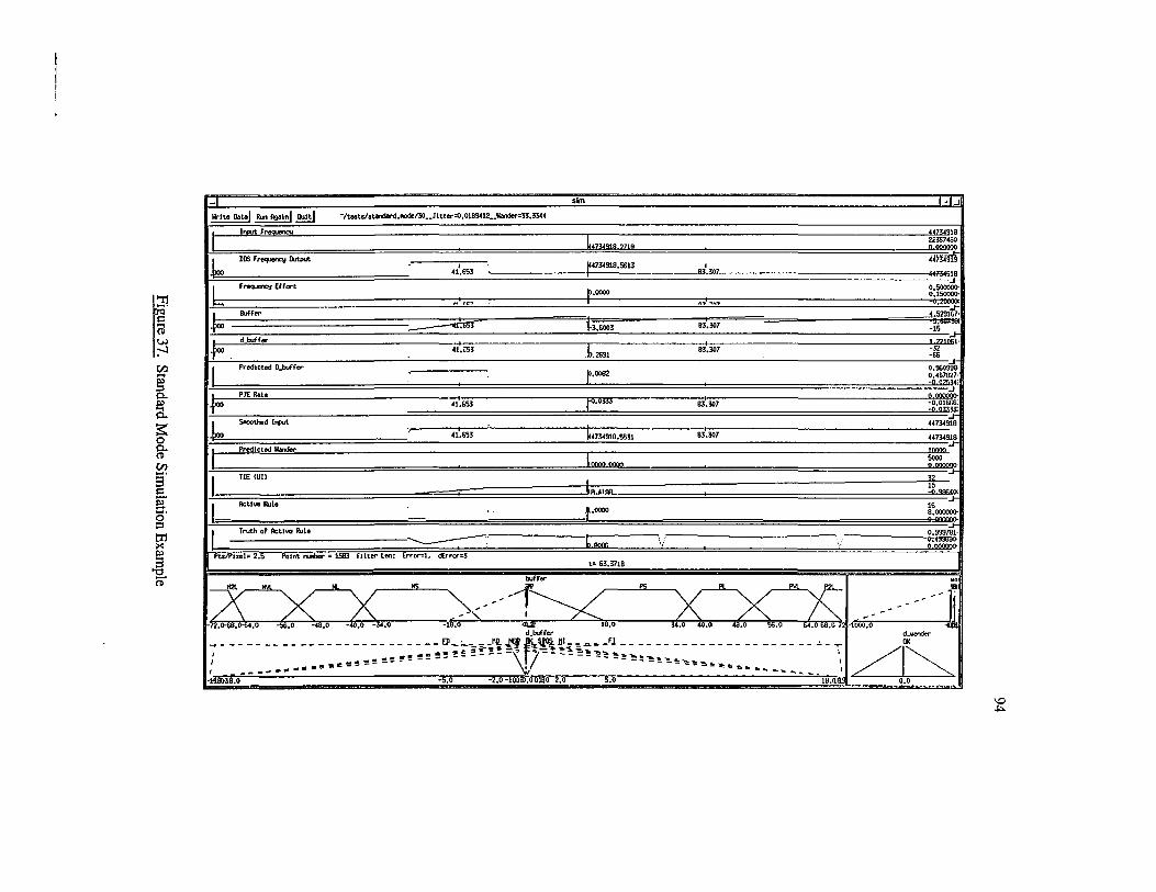
~ slm ' _J
lrlte Datal Ia> Agatnl ~ "/testslstendar<l,oodoi30_Jitt..-~,OI89412 •• 11onder=33,~4
I 1~Fre<U!I"'C'4
~~z~~B 2Z1B ~= k DDS Fr-eque.q Mf'Ut m:um
I ~73oi918.5613 I 41,653 83 302 44134918
L Fr-eque.q EHcrt
r·oooo 0,500000-0.150000-
.,.I rr.-. ,.,•., ...... =o.2WXK
~ lbffer
~#.~'lli ~ tuoo3 83.307 -15
r d_b.trFer I I l 221061· U,i:53
I26S1 83,307 -32
-66.
I Predicted D_buf'Fer t·0032
0,960939· 0,467827·
I I :il !:!2534:
·F PJE Rote I E. om I = 41,653 83,307
k Sooothed lrc>ut
~73oi919.5531 44734918
I 41.653 83.307 44734918
I Prodlcted llonder
'I:WII:WI ~ I TIE <UU _32_
hR,.A1M ~--01
L Act.lw ~le 16 -· ~-0000 8,00000()-2~
I TnM or Actlw Rule 0.999781· ............__- bllll!l!i '· ~·= ,, >
Pt.s/Phel= 2.5 Point I"UUber = 1583 ftlt.er Len: Err<r=1. c£rror=3 t= 63,3718
buffer
~ -~.6
!!S
'\~----~ Eli
~ ----Jl -------t[o ~a.o ·1000.0 d_buffer
d __
~ _______________________ --Ell-=.--~";., .L'f ,~ ~- =-=- _Fl ______________________ .:. _ ~ (J(
I .. ~ ,.., '!~ ~! :- :-\ll-- -~~~"!;!"'-..•-.. ; /I~ 1 e~~e~~~~~---- ----~~~'~'~•~• • I •••••·ll:t· ' !b~k-. ... .,~.._ I
-19an8.o- ~ - :S.o -2.o -tooili.60iBo 2.o s.o - - - IB.Q!J!; 0,0

95
TABLE V
Standard Mode Jitter
Standard Mode Time Between Jitter
Spurious PJEs (sec) (VI) 30 0.003 35 0.003 40 0.003 50 0.003 70 0.003
100 0.003
Standard Mode
'graph.out' -+-0.3 -----·
50 60 70 80 90 100 Time Between PJEs; T (s)
Figure 38. Standard Mode Jitter
Standard mode jitter is 12dB below the 0.30UI specified.
3. Burst Mode
A PJE burst is composed of three PJEs separated by 0.5ms. The time between
bursts (T) ranges from 30 seconds to infinity, as illustrated in Figure 39.
Figure 40 shows a representative simulation with several bursts. Table VI and

I I I I
~;--------------------,,
' ' I I
I I I I· ·I \
>= 30s ' / ','-------------------:;'
I ' I ' I '
Pointer Burst~\ _ _ _ _ _ ,'' \ ,; ' ,
I I /
'-: I I [/f I .
96
I t / t-1•----<•-+1-• ___ :t-t:--_-_-_' ------------------+1•1 Time Initialization Cool Down Measurement Period
Figure 39. Burst Mode PJE Test Sequence
Figure 41 show that jitter has little dependence upon the time between bursts since in
each case the buffer offset resulting from the burst is eliminated before the next burst.
TABLE VI
Burst Mode Jitter
Burst Mode Ttme Between Jttter
PJE Bursts (sec) (UI) 30 0.019 35 O.UlH 40 0.019 45 0.019 50 0.019 55 0.019 60 0.018
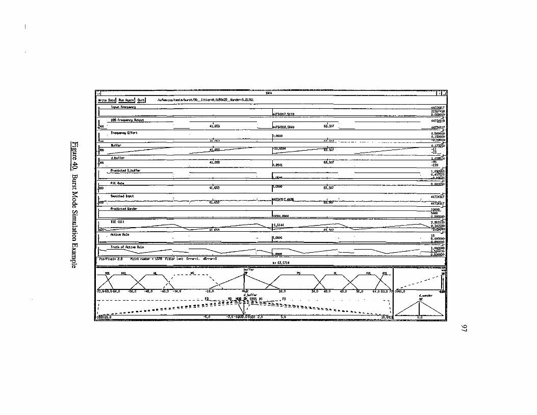
to .: .... "' .....
~
..,,,. Datal RLn Agatnl ~
I lrrutF~
.b DDSF~IMput
L F.-- Effort
}'? anr ...
-.jx;, d_b.rrrcr
I Predicted D_tMfer
.jx;, PJE Rate
~.-Sooothed .......
Predlctedllandefo
TIE <Uil
Active Rule
/ulkevtns/tesWbu-sti30_J 1 ttu-~.0159422_11andefo=5.21761
I ~1.653
... •r"': ...
I ~1.653
41.653
slm
I 83,307
85.307
I 83,307
83,307
• ...J
0,500000· 0,150000--0.2W»
0.1~· -II -23
1.01!!'524· -99 -199
0 {)QQQI)()·
~~~3~917
·----:'--,------.tm-·------''-fM·'~'z.~.----11wt1,l!l!Urr-r-'---.-----.------------«J34917 -
r·oooo
2,953199
........... ~~
16 8.0000<» 9 090900-
Pts/Pixel= 2.5 Point tulber = 1578 filter Len: Errcr=l, c£rror=3 t= 63.171~
; ~
-~ ~
1 ~ ---
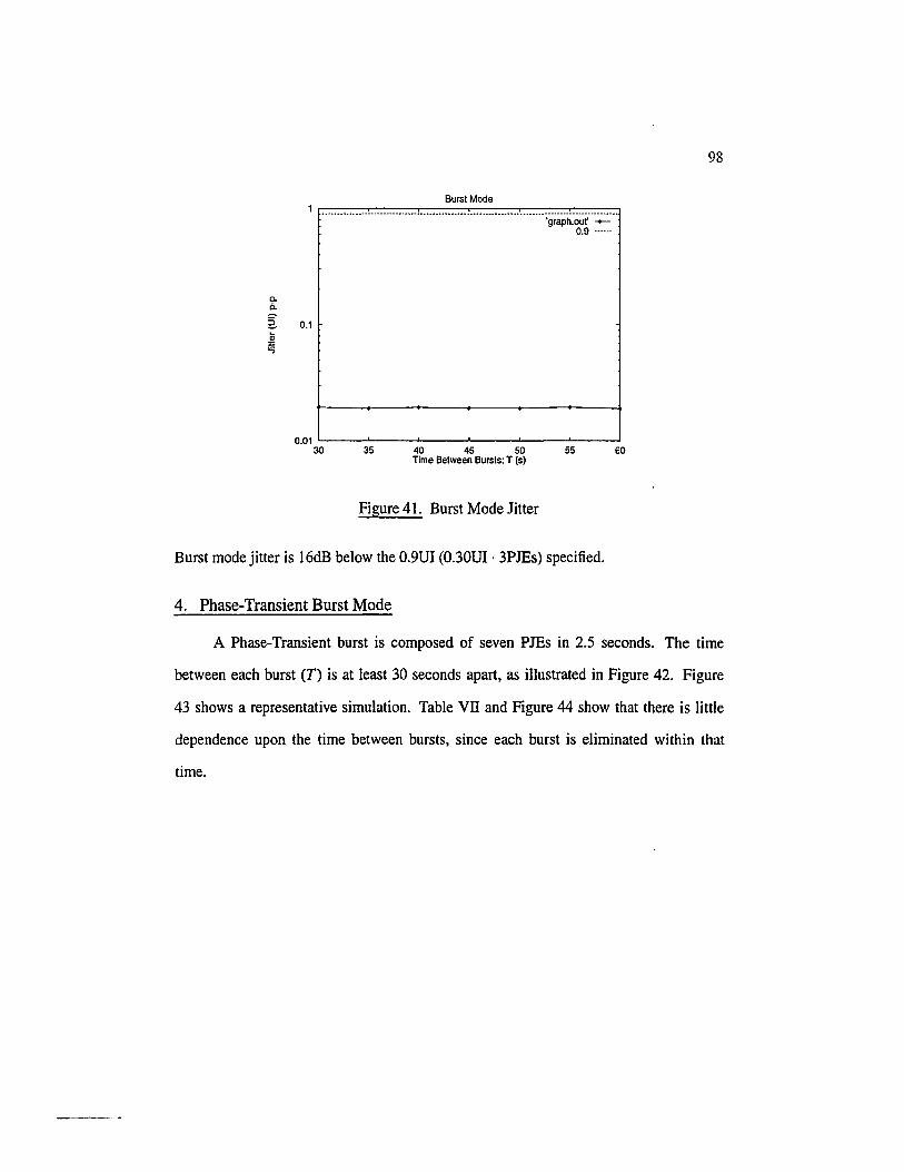
a. c. 2. 0.1 iii ::: "j
Burst Mode
'graph.out' -0.9 ..... .
O.o1 L_ _ __. __ _..._ __ _._ __ _._ __ _,___---l
30 35 40 45 50 Time Between Bursts; T (s)
Figure 41. Burst Mode Jitter
55
Burst mode jitter is 16dB below the 0.9UI (0.30UI · 3PJEs) specified.
4. Phase-Transient Burst Mode
60
98
A Phase-Transient burst is composed of seven PJEs in 2.5 seconds. The time
between each burst (T) is at least 30 seconds apart, as illustrated in Figure 42. Figure
43 shows a representative simulation. Table VII and Figure 44 show that there is little
dependence upon the time between bursts, since each burst is eliminated within that
time.
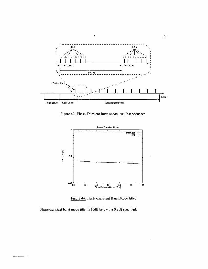
I
' I 0.5 s
~ I• •I• •I• •I• •I• •I
I Ill I I I : _., 1- 0.25 s
\
0.5 s ' \
~ I• •I• •I• •I• •I• •I Ill I I I I
_., 1- 0.25 s
'\, >= 30s ,/ ';---------------------------------------------:~-;
\ \
\
Pointer Bu~~~ ____ _ \ , '
\ ' \
\: I I l L-/r-
\ I
99
I \ ~ s-- •
1~·-----o•+•o------:t~.---_-_-_' ___________________ -1•1 Time
Initialization Cool Down Measurement Period
Figure 42. Phase-Transient Burst Mode PJE Test Sequence
0. 6.
2 0.1
~ ..,
Phase Transient Mode
'graph.out' -0.9 •..••.
0.01 .._ __ _._ __ ___,_ ___ ...._ __ _,_ __ ___. __ ---1
30 35 40 45 50 Time Between Bursts: T (s)
55
Figure 44. Phase-Transient Burst Mode Jitter
Phase-transient burst mode jitter is 16dB below the O.SUI specified.
60

slm
/uil<evtnsltesta/pioase, transtent130_J I tter=0,418286 __ 11onde.-:107 ,521
Jnput frNJ!nCY
~ F~Effa-t
. h.oooo 411.6S3
L Mrer
c.:..;;-~
fo clbJfFer 18ihii8El
·~'» Predict.l!d D_bof'f'er
_ .. ./ Lsw 41·6S3
·F PJE Rate
-
TIE <un ~
L Active Rule
•. r·oooo
Pt.s/Pixel= 2.5 Point fUIIber = 874 fllttt' Len: Error=l~ c£n-cr=3 t: 35,0128
I 83 7Dl
I 83.307
A~ Vl7
I 83,307
I 83.307
I 83.307
I 83.307
. _J
~= ~~734937 ~~73492~
1
1.oooooo-1.~
-3,()()(1()()1 -67 ~5~15·
21 ff.
-67 .·.
3.638712· -li -32
0 OMOCJO· -2,()()(1()()1 -~.000001
44734548 ~4734932 44734916
!! 98 ~~ 9 QJQCCM
58 29 0 QWK)O·
~_J_ix -72,<H;B,<rti4,o -56,0 -48,0 - o,o ..... o -IU,O .t"bufrer lo.o
PS
.~L.""'=,..,..,o----J~ ~- ________________ -- _:. ____ ~-=-~ li( S~ ~1__;...-.o--_FI .
.,..:=-.. ~~~ ... ~~':1.-:s.-... E • r ~ ~ .-- -·- --, ·r,·-- -- -_~"So-.:~....,
' -- - • - .. • • •" • ~ ~ ~ e ~ ~!!. !! - -- -- \ ,':~ - -- -!I:"!!!:~!:~!:.-~'!& ·e.~ • • ..... • .............
-~~~t:t.o .o - .o -100 .o 0180 2.o 5.0 1~.tl!i!l
d_...-.der
~ 0,0
0 0

101
TABLE VII
Phase Burst Jitter
Phase Transtent Mode Ttme Between Jitter
PJE Bursts (sec) (UI) 30 0.066 35 0.063 40 0.059 45 0.057 50 0.056 55 0.053 60 0.051
5. Degraded Mode
There are two separate PJE profiles for testing degraded mode jitter generation.
The two profiles correspond to differences in implementation of the algorithm used to
actually generate the PJEs. The first profile, shown in Figure 45 is called the "continu-
ous pattern" and consists of a constant stream of PJEs augmented with standard-mode
(spurious) PJEs every 30 seconds or more (T). The time between the stream of PJEs (t)
ranges from 34ms to lOs, and the distance between a continuous stream PJE and the
spurious, standard-mode PJE, is O.Sms. Again, separate tests are required for added and
canceled pointers. Figure 46 shows a representative simulation. Table VIII and Figure
47 illustrate how jitter depends upon T and whether the PJE is added or dropped.
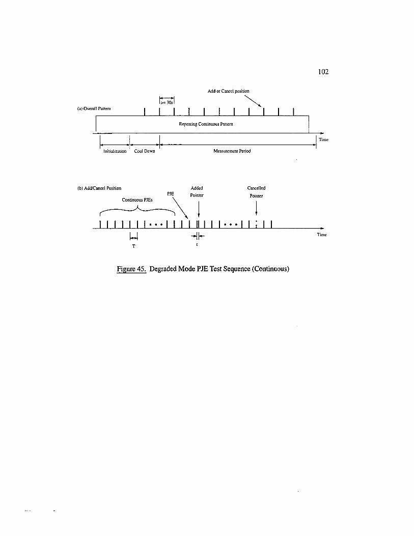
Add or Cancel position
~ I I (a) Overall Pattern
Repeating Continuous Pattern
Initialization Cool Down
(b) Add/Cancel Position Added
PJE Pointer
~\
Measurement Period
Cancelled
Pointer
! 1111111···111111111 · · · I I I I
T
Figure 45. Degraded Mode PJE Test Sequence (Continuous)
102
Time
Time

lulkevtnsltestsldeg-odecllcontt,..,.,.lliWO,I__Jttt.er=0,0145216 •• w.nder=7.12108
L
L
L
DDSF~Mput
Fr~ EFfort
IMfcr
dJ:uffr
Predicted D_buffer
PJE Rate
Sooothod l'l'Ut
Predicted~
TIE !U()
Acttve Rule
Truth of Active IWie
I 41.653
.. • .......
41.653
ao='.=:'L_==·--.-. --~~-""""-==--:=":"'-.--~-==-·::::::::::-"'----
Pt.s/Pixel= 2.5 Point rulber = 2533 filter Len: EfTOI"=l. c£rTOr=3
I 83.307
I .307
-----<==-t-· 83.307
---------1 83.307
83.307
' _j
r4734838.0451 44734918 4473411l0 .4473.4939
r-4734918.4754 44734918
44ztl918
f"'l.OlOO 0,500000-0.150000-
I -0.2WJOt
k~1 ~.S42708·
-·~"""""Ji(!!?;J~ -10 .. -
,3.ZRIR.
.--.lL_ .? EKUQ.( -20.
r-0037 0.592510 0.191341· &.2&!821
-s sg993; )10.0505 -10
-10
k4734918,4416
447~8
4Q3.(919
~QQQQ QQQQ e:: ro.5940
1.080000· ==:trmibOI
-6.043201
kw ·_ 16 8,000000· 9 QQOCOO·
t= 101.3807 l ~ . ~:: __ -z-_ " ~ ______ /~ (l) ~:U.o -~buffer ie,o -'<.o 40.o 4o,o ""·" 64,068,07:1000,0 -
---------------- '-- ------ --11.-=:;.i"~&\!l!i?!~ ,.tt;~~- .EI_ ---------- :.._ ---------- --~ ;!,.:"..-.lor : -~!!~~!!!!'!!~~~!!~'!!=--- ----:~~~~~~~~~~~~- 1 /1"'--, -- -- - .. 8" ., - - ~ .... ~ 1:11 ... , ............. - ... - • ~ / I ~
·MI!<l8,0 ->.0 -•.o •HJJiV.UU!llO •• 0 >.O 0,0
0 w

104
TABLE VITI
Degraded Mode (Continuous Pattern) Jitter
Degraded Mode (Contmuous) Time Between T1me Between . Jitter (Ul) Spurious PJEs Continuous PJEs Added Dropped
(sec) (sec) PJE PJE
30 0.034 0.0304 0.0254 30 0.05 0.0162 0.0164 30 0.1 0.0099 0.0101 30 0.2 0.0067 0.0140 30 0.4 0.0063 0.0073 30 0.8 0.0041 0.0108 30 I 0.0184 0.0053 30 2 0.0186 0.0052 30 4 0.0036 0.0047 30 8 0.0031 0.0093 30 10 0.0283 0.0047 35 0.034 0.0293 0.0263 35 0.05 0.0285 0.0284 35 0.1 0.0091 0.0094 35 0.2 0.0064 0.0155 35 0.4 0.0060 0.0193 35 0.8 0.0046 0.0086 35 1 0.0110 0.0066 35 2 0.0037 0.0080 35 4 0.0036 0.0052 35 8 0.0036 0.0047 35 10 0.0041 0.0052
40 0.034 0.02H5 O.OIH9 40 0.05 0.0290 0.0189 40 0.1 0.0091 0.0094 40 0.2 0.0064 0.0155 40 0.4 0.0052 0.0108 40 0.8 0.0045 0.0074 40 l 0.0047 0.0069 40 2 0.0113 0.0050 40 4 0.0399 0.0167 40 8 0.0334 0.0179 40 10 0.0294 0.0037
60 0.034 0.0280 0.0435 60 0.05 0.0288 0.0285

105
Degraded Mode (Continuous) Time Between Time Between Jitter (Ul) Spurious PJEs Continuous PJEs Added Dropped
(sec) (sec) PJE PJE 60 0.1 0.0145 0.0096 60 0.2 0.0069 0.0156 60 0.4 0.0066 0.0112 60 0.8 0.0052 0.0144 60 I 0.0041 0.0066 60 2 0.0082 0.0050 60 4 0.0479 0.0042 60 8 0.0036 0.0047 60 10 0.0336 0.0042
50000 0.034 0 0 50000 0.05 0.0004 0.0004 50000 0.1 0.0004 0.0004 50000 0.2 0.0004 0.0004 50000 0.4 0.0004 0.0004 50000 0.8 0.0009 0.0009 50000 1 0.0004 0.0004 50000 2 0.0004 0.0004 50000 4 0.0004 0.0004 50000 8 0.0004 0.0004 soooo 10 0.0004 0.0004
As may be seen from the table, this type of degraded-mode jitter is 8.5dB below the
0.9UI specified (0.3 for spurious PJEs, and 0.6 for degraded mode).
The standard also states that with T = oo, jitter must be below 0.6UI. This is
tested by setting T = 50, 000. As may be seen from Table vm, the resulting jitter is far
below the allowed value of 0.6UI.
The second degraded-mode profile, shown in Figure 48, is called the 87-3 pattern
due to the sequence of 87 regularly spaced PJEs followed by three missing PJEs.
Superimposed on each pattern of 90 PJE locations is an added or dropped standard
mode PJE at an interval of 30 or more seconds (T). The time between PJEs (t) is to
span a range from 34ms to 1 Os.
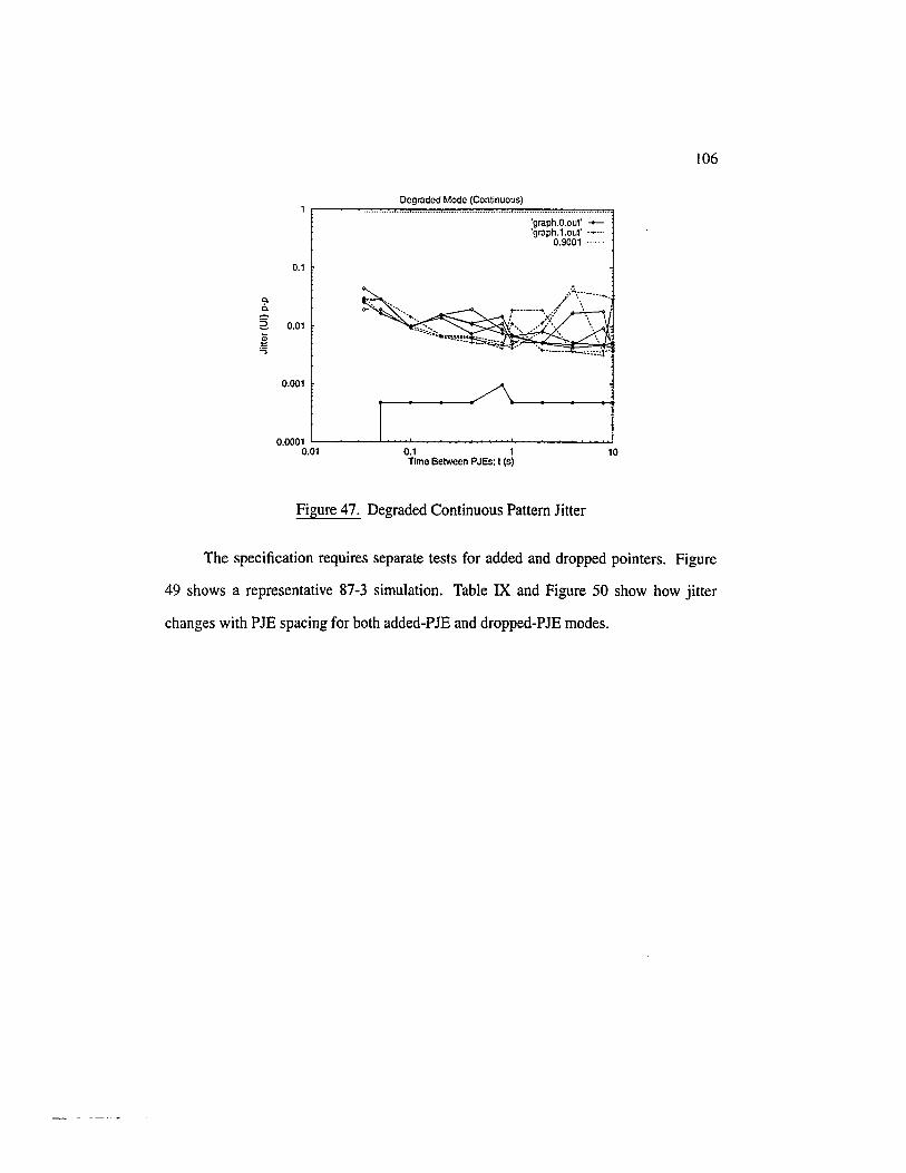
c. 6.
2. ;;; "' "5
0.1
O.D1
0.001
Degraded Mode (Continuous)
'graph.O.out' -'graph.1.out' ·+ ...
0.9001 .
0.0001 '--~~~....L.....~.L--~~~~...._-~~~~...J 0.01 0.1 1 10
Time Between PJEs; 1 (s)
Figure 47. Degraded Continuous Pattern Jitter
106
The specification requires separate tests for added and dropped pointers. Figure
49 shows a representative 87-3 simulation. Table IX and Figure 50 show how jitter
changes with PJE spacing for both added-PJE and dropped-PJE modes.
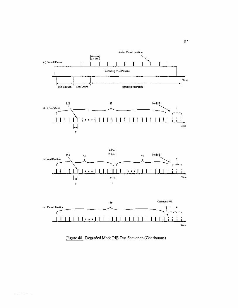
(a) Overall Pattern 1~=3~1 I I
107
Add or Cancel position
~ I I
Repeating 87-3 Patterns
Initialization Cool Down
PJE \
PJE
T
Added
Pointer
!
Time
Measurement Period
I' Time
44 No PJE
------------~~ 1111111···111111111···1 I I I I I I I ; ; I •
Time
T
(c) Cancel Positio::..n ---------
Cancelled PJE
\,-:_, 86
I I I I I I I · · · I I I I I I I I I I I I I I I I I ; ; ; 1 •
Time
Figure 48. Degraded Mode PJE Test Sequence (Continuous)
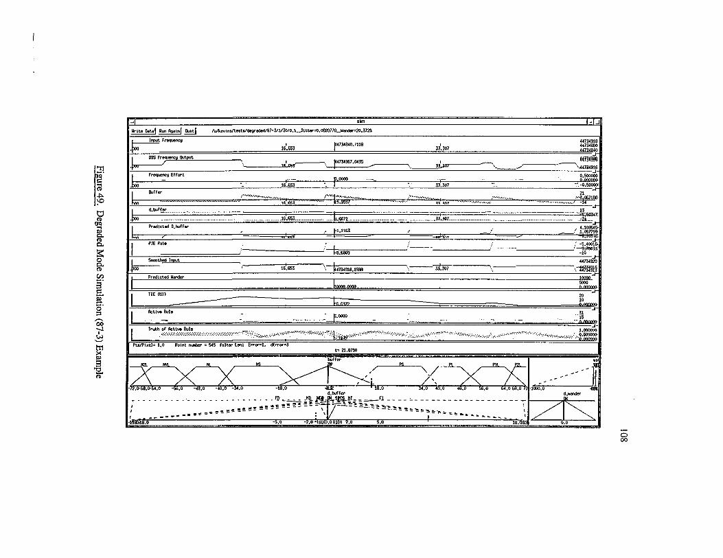
-~r,.._
~Jx.,--D-DS_F..Jr""' !Mput
.L r,.._Errcrt
L Buffer
.loo Predl"cted D_buffet" L 7 PJE Rote
~1::::::---Sooo-t.hed (!J'Ut
Predicted Wander
TIE <Ull
I 16.653
16.&53
/ ••. ~ .. ·,., .... ..,.,_ •• ,..,..,..._.-,.,><~ ... ,..,,.,
1j:;~~
slm
I 33.307
3-b>rr,-----·-----..
33.307
' .J
0,50(1()(10-0 ()()Q()QI)-
·:. -o.50000<
.................... J~~!i>L .............. ----~---------------= ................... ~J'."WL ............................................................. ~·-·_· ·.=Jr.~~4" • 4,108545-
; 1.osns~ 1.33!02:
' -9.4001&-·--------' ----, ______ __;• ~33:
44734920 .------,1::61-:.65:::3;----\-1Lf-,-rn-918-.-1590-----~ ---·"33,:."'30"'7----~ --~-------\'iffml~
~0000 0000
20 10 ? wrrr-
.. 31 15
·- 0 CXXP»
Pts/Pixel= 1.0 Point rutilxr = 5(5 fllter Len: Error=l~ c£rror=3 .. 21,9750
-~.o !IS ooffer ~ ~ ~'!; ~
-~~·-· >.·~. ~?< ....... .,, . ..;:;--------1 I
;Ht<t4B,O
~bofr..- ;i....-der _. _. _ ._ •••• _ ••••••••• .F.ll ~~;.'\~-4'!..s.t9i!l-:.~-_Fl ____ '-- ______ ---- -- ______ ~1-/--"71.,~~--.
...... !! ~ !! ! '! ~ ~ ~ ~! =- =--'~v,:-..:- ::~ =::==.~ ':!: "!!=:~ ~ ~ - ....... ~ _ .. _.,. •• •E~ !!e ~~ -- -- : " -- --~r:=·~!!r ~t. •• ...... ,.. ... , -
·5.0 -2,0 •100 .o 0190 .o 5.0 0,0
0 00
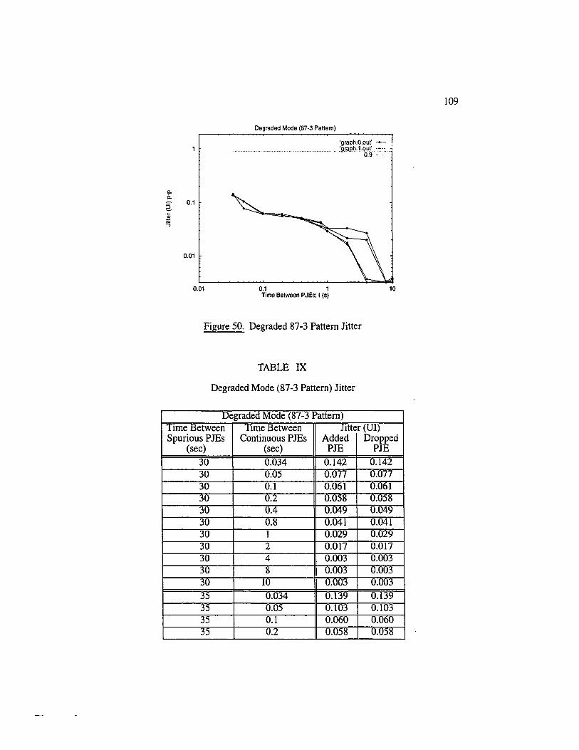
0.1
0.01
0.01
Degraded Mode (87-3 Pattern)
'graph.O.out' -+
....................................... .'9.raPh-.1-out'. -~·: ... 0.9 ....
0.1 1 Time Between PJEs; t (s)
10
Figure 50. Degraded 87-3 Pattern Jitter
TABLE IX
Degraded Mode (87-3 Pattern) Jitter
Degraded Mode (87-3 Pattern) Ttme Between Ttme Between Jttter (Ul) Spurious PJEs Continuous PJEs Added Dropped
(sec) (sec) PJE PJE
30 0.034 0.142 0.142 30 0.0) 0.077 0.077 30 0.1 0.061 0.061 30 0.2 0.0)8 0.058 30 0.4 0.049 0.049 30 0.8 0.041 0.041 30 1 0.029 0.029 30 2 0.017 0.017 30 4 0.003 0.003 30 8 0.003 0.003 30 10 0.003 0.003
35 0.034 0.139 0.139 35 0.0) 0.103 0.103 35 0.1 0.060 0.060 35 0.2 0.058 0.05~
109

110
Degraded Mode (87-3 Pattern) Time Between Time Between Jitter (Ul) Spurious PJEs Continuous PJEs Added Dropped
(sec) (sec) PJE PJE 35 0.4 0.050 0.050 35 0.8 0.041 0.041 35 1 0.029 0.029 35 2 0.017 0.017 35 4 0.003 0.003 35 8 0.003 0.003 35 10 0.003 0.003 40 0.034 0.135 0.135 40 0.05 0.103 0.103 40 0.1 0.061 0.061 40 0.2 0.055 0.055 40 0.4 0.051 0.051 40 0.8 0.036 0.036 40 I 0.033 0.033 40 2 0.021 0.021 40 4 0.019 0.019 40 8 0.003 0.003 40 10 0.003 0.003
60 0.034 0.138 0.138 60 0.05 0.104 0.104 60 0.1 0.063 0.063 60 0.2 0.061 0.061 60 0.4 0.051 0.051 60 0.8 0.042 0.042 60 1 0.033 0.033 60 2 0.033 0.033 60 4 0.026 0.026 60 8 0.003 0.003 60 10 0.003 0.003
50000 0.034 0.140 0.140 50000 0.05 0.077 0.077 50000 0.1 0.061 0.061 50000 0.2 0.058 0.058 50000 0.4 0.049 0.049 50000 0.8 0.035 0.035 50000 1 0.029 0.029 50000 2 0.016 0.016 50000 4 0.003 0.003 50000 8 0.003 0.003
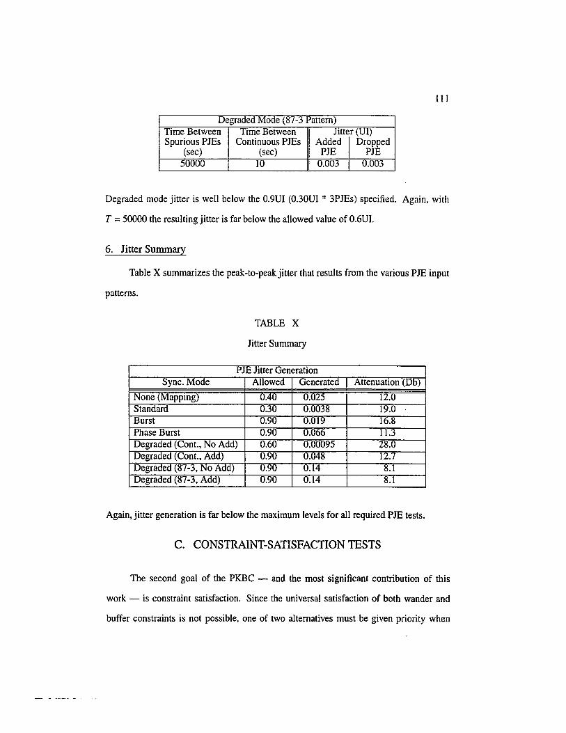
Ill
Degraded Mode (87-3 Pattern) Time Between Time Between Jitter (Ul) Spurious PJEs Continuous PJEs Added Dropped
(sec) (sec) PJE PJE 50000 10 0.003 0.003
Degraded mode jitter is well below the 0.9UI (0.30UI * 3PJEs) specified. Again, with
T = 50000 the resulting jitter is far below the allowed value of 0.6UI.
6. Jitter Summary
Table X summarizes the peak-to-peak jitter that results from the various PJE input
patterns.
TABLE X
Jitter Summary
PJE J1tter Uenerat10n Sync. Mode Allowed Generated AttenuatiOn (Db)
None (Mapping) 0.40 0.025 12.0 Standard 0.30 0.0038 19.0 Burst 0.90 0.019 16.8 Phase Burst 0.90 0.066 11.3 Degraded (Cont., No Add) 0.60 0.00095 28.0 Degraded (Cont., Add) 0.90 0.048 12.7 Degraded (87-3, No Add) 0.~0 0.14 H. I Degraded (87-3, Add) 0.90 0.14 8.1
Again, jitter generation is far below the maximum levels for all required PJE tests.
C. CONSTRAINT-SATISFACTION TESTS
The second goal of the PKBC - and the most significant contribution of this
work - is constraint satisfaction. Since the universal satisfaction of both wander and
buffer constraints is not possible, one of two alternatives must be given priority when

112
both are in danger of violation. Either the buffer is to be kept from overflowing even if
it means MTIE violation, or MTIE is to be kept from violating its specifications even if
it means that the buffer will overflow or underflow. These two strategies are investi-
gated in the following two sections.
1. Wander Satisfied
The most recent MTIE mask proposal from Bellcore [ 4] , is shown in Table XI
TABLE XI
Proposed MTIE Mask
Observation Time MTIE (s) (ns)
s <0.1 N/A (jitter region) 0.1 <S <0.22 4600 * s 0.22 < s < 5100 900 + 240 * S"'" 5100< s 18000
and illustrated in Figure 51. Thus we set out to prove that PKBC is capable of satisfy
ing the specified MTIE mask. This was accomplished by simply adding the term:
AND wander IS OK
to the predictive part of each rule as discussed in Section C.5 of Chapter VI. This addi
tion ensures that only those rules with candidate actions which do not violate MTIE are
considered. In particular, if a candidate action is predicted to produce an MTIE which
is not OK, the above term will evaluate to zero and the rule will not fire.
Since wander is measured in terms of time-to-violation in sample periods, there is
no mechanism to keep MTIE from moving arbitrarily close to the envelope. Thus, we
provided a simulation parameter which acts to narrow the neck of the envelope artifi
cially at some point in the envelope. This parameter acts as a safety mechanism by gen
erating a predicted MTIE fault when the TIE and envelope lines are about to converge.

113
DS3 MTIE Mask
100
10 ~~~~~~~~~~~~~ 0.1 1 10 100 1000 10000100000
Observation Time (s)
Figure 51. Proposed DS3 Wander Specification
An alternate solution would be to measure the distance to the envelope (a trivial task)
and either combine the two measurements into a composite wander-risk-of-violation
parameter, or create a new input variable which could be referenced separately by the
rules.
The reader will recall that TIE is the integral of the difference between the output
frequency and a reference signal at the nominal frequency. Thus, if an input is applied
which is different from the reference, the controller initially acts to maintain the appro
priate buffer level by adjusting the output away from the nominal frequency. The ensu
ing TIE ramp eventually approaches the MTIE constraint envelope and any actions
which would result in an MTIE violation are removed from consideration. The result-
ing MTIE plot, seen in Figure 52 shows the MTIE mask, the MTIE generated by the
controller, and their difference. The generated MTIE approaches the mask but does not
cross it - thus satisfying the wander specifications. This graph was precisely what
we had hoped to see, and verified our hypothesis regarding the constraint satisfac
tion capabilities of a PKBC.

114
MTIE Mask and Generated MTIE, with Difference
100
13" ••••• El··£3 •• ~y:~,.·· _,/ -~
10 il',' ...
........ -~
;. . .EJ·EJ -G]-13·EJ-ETI3·0·EJG-13·EJG G·El·O 13·0 "'"·EJ·EJ.oB-13
Time(s)
Figure 52. MTIE Satisfaction Plot
Figure 53 shows a similar simulation, this time with the buffer level shown also.
Notice that the buffer increases above its desired maximum of 25 when mandated by the
MTIE.
Although MTIE is specified in absolute terms, a slight violation is much better
than a large violation. So as an added precaution we crafted a set of rules which take
effect when the MTIE time-to-violation is negative (TIE is above the ceiling or below
the floor of the constraint envelope). These rules take whichever action is predicted to
result in the smallest positive wander value (the action which most rapidly moves TIE
back inside the envelope).
If the situation occurs where none of the listed candidate actions in the rulebase is
predicted to bring MTlE back into compliance, setting the frequency to its nominal
value would cause the predicted TIE to become flat. Since the envelope opens

100 ....................... .
80
40
20
MTIE Favored Over Buffer
Bufftlr Lavel .s·
-~, . .:~·. Generated MTIE .. >l·
p'
'mtie'-<>-. ........... .:0 . :~~s:;: ~;.::
..• r::;' 25 ... .. c·
.,• .
. .s
.............................. ~{: ......... ................................... B~ffer Limit
.. ~'~... / ........... :····-: .. ·::s··-·---........ :·:·:··.····:·:·:·:-···:·:·:· ........ ·:.:.::·.···-···
. .o· m·
.. s·
0 "8-·-13·-G--EI-·-9--G--&·-EI--9:' ...
·20~----~------~------~------~------~----~ 10 20 30 40 50 60
Time/ObservationTime (s)
Figure 53. MTIE Satisfaction Plot With Buffer
115
exponentially, this action would be guaranteed to eventually bring TIE back in compli-
ance. While a commercial application of our desynchronizer might want to include this
capability, we have not implemented it.
2. Buffer Satisfied
If, instead of maintaining MTIE compliance at all cost, the designer wishes to
maintain buffer compliance at all cost, the set of rules described in Section C.6 of Chap
ter VI is used.
A likely buffer-constraint-satisfaction scenario is now described. An input which
is offset from the nominal DS3 frequency is applied to the controller. The controller
reacts by tracking the input frequency to maintain the desired buffer level. The TIE that
results is a ramp with a slope of four- fDS3· Eventually, the MTIE constraint envelope
predicts an impending MTIE violation and the standard rules no longer apply - since
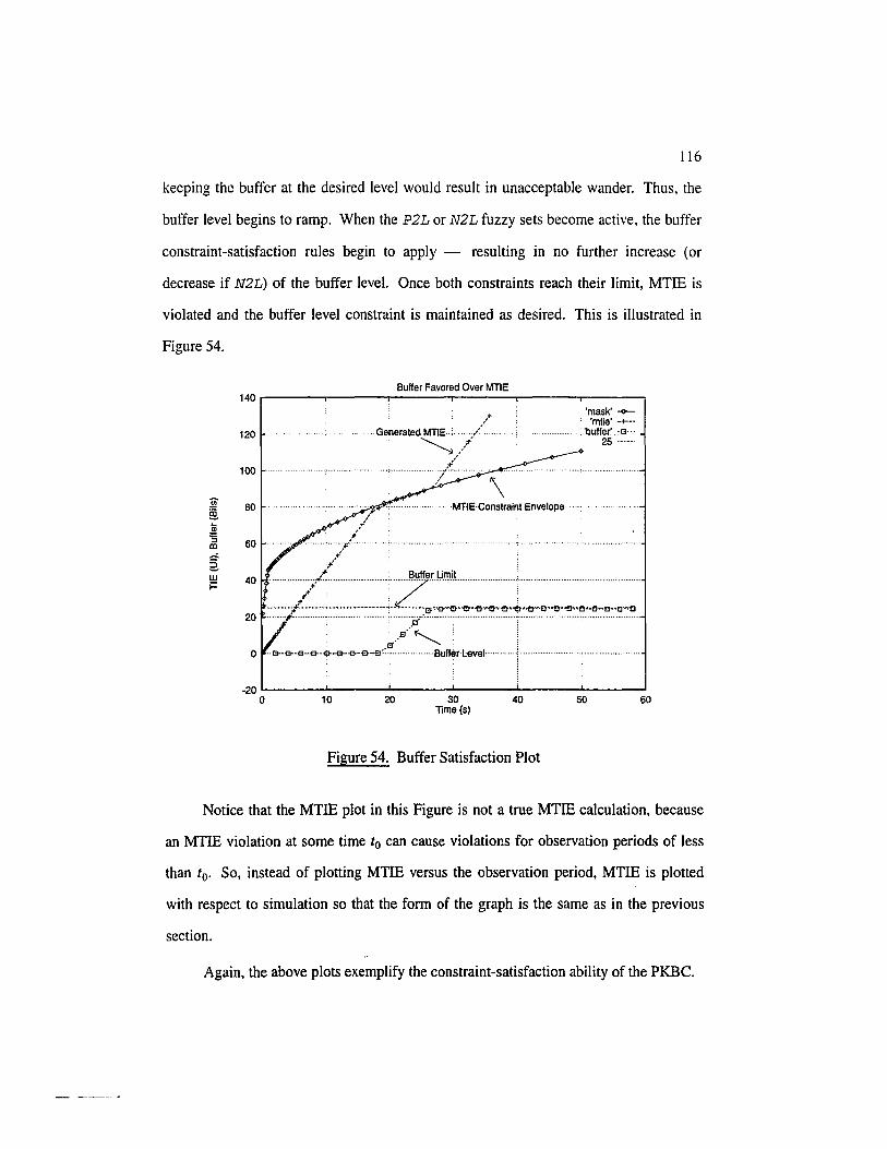
116
keeping the buffer at the desired level would result in unacceptable wander. Thus, the
buffer level begins to ramp. When the P2L or N2L fuzzy sets become active, the buffer
constraint-satisfaction rules begin to apply - resulting in no further increase (or
decrease if N2L) of the buffer level. Once both constraints reach their limit, MTIE is
violated and the buffer level constraint is maintained as desired. This is illustrated in
Figure 54.
140
120
100
.!!l 80 ~ ~ ::> 60 aJ
2 w 40 t=
20
0
-20 0
Buffer Favored Over MTIE
/ .. . ... Generated MTIE .......... /
~// •' .................... ~,7t: ....
'mask'-+-'mtie' -+--·
....... :buffet. .. :e··: .. 25
· ·MT!EConstrairit Envelope
10 20 30 Time(s)
40
Figure 54. Buffer Satisfaction Plot
50 60
Notice that the MTIE plot in this Figure is not a true MTIE calculation, because
an MTIE violation at some time t0 can cause violations for observation periods of less
than t0 • So, instead of plotting MTIE versus the observation period, MTIE is plotted
with respect to simulation so that the form of the graph is the same as in the previous
section.
Again, the above plots exemplify the constraint-satisfaction ability of the PKBC.
CHAPTER IX
CONCLUSIONSIFUTURE WORK
A. CONCLUSION
The need to carry PDH payloads such as the DS3 over a SONET network contin
ues to increase as PDH services gain popularity with corporate customers and SONET
gains popularity with public networks.
Our investigation targeted the configuration where a DS3 payload is mapped into
an STS-l envelope and then unmapped and desynchronized at the other end. PJEs
within the SONET network were shown to induce both high-frequency jitter and low
frequency wander in the desynchronized DS3. To ensure compatibility among different
equipment manufacturers, the ANSI-accredited T I committee and Bellcore have devel
oped standards defining acceptable operation. The standard specifies the maximum
allowed peak-to-peak jitter for each of several PJE profiles, and wander (MTIE) is spec
ified independently of any particular PJE input pattern. In addition, the desynchronizer
must ensure that its elastic store - used to absorb jitter and wander - does not over
flow or underflow.
Desynchronizers typically employ a low-pass filter and possibly some non-linear
transfer elements to attenuate high-frequency jitter. But the low frequency wander
passes below the cutoff frequency of the low-pass filter and can accumulate from net
work element to network element.
We set out to devise a technique with the following four capabilities:

118
• Exhibit the characteristics of a low-pass filter such that the jitter specifications are
met implicitly.
• Explicitly satisfy the size constraint of the buffer for as long as the MTlE con
straint allows.
• Explicitly satisfy the MTIE constraint for as long as the size constraint of the
buffer allows.
• When the above two constraints are in danger of violation, satisfy one at the
expense of the other as determined by the designer.
An MTIE violation may result in network instability and/or data errors. A buffer spill
results in data errors which would precipitate a retransmission.
As we have shown, a Predictive Knowledge-Based Controller (PKBC) with an
expanded rule grammar is a viable alternative to other desynchronizers in tenus of jitter
attenuation, but stands alone in its ability to dynamically satisfy MTIE and buffer con
straints. Our invention of the MTIE constraint envelope (and its efficient calculation)
allows the rule-based controller to evaluate the MTIE and buffer level which would
result from the application of a particular candidate action. Actions which would need
lessly cause constraint violation are removed from consideration automatically. We
showed that the computational complexity of the control algorithm is within the reach
of modern microprocessors.
To test the constraint satisfaction capabilities of the PKBC, a scenario was pre
sented where the output frequency was adjusted away from the TIE reference frequency
to prevent buffer overflow. As a result, TIE began to ramp, causing MTIE to approach
the mask. Eventually the controller was forced to slow the increase in TIE by adjusting
the output frequency back toward its nominal value. The resulting frequency mismatch
between the input and output caused the buffer level to increase. Ultimately, it was

119
impossible to simultaneously meet both constraints. For this case we demonstrated the
ability of PKBC to sustain either buffer or MTIE compliance. The priority of the con
straints was specified in the rules.
In addition to satisfying hard MTIE and buffer constraints, overall jitter genera
tion was very low - less than 0.02UI for a single PJE - compared to the limit of
0.3UI. The controller was shown to exceed the jitter performance for each pointer
adjustment test specified in [3].
Our hypothesis that a PKBC would be capable of good jitter performance in the
usual case and MTIElbuffer constraint satisfaction in the limit was thus confirmed.
The effect of our research is two-fold. First, desynchronization equipment which
implements a PKBC can be made to generate very small levels of jitter and satisfy the
hard constraints whenever possible - leading to better reliability and data integrity in
hybrid digital networks. Second, the PKBC has the potential to solve problems in other
areas of control. If a model of the process exists and expert knowledge is available for
rule generation, this control paradigm has the potential of good performance under nor
mal conditions and constraint satisfaction as a limiting condition.
B. FUTURE WORK
We have shown the dynamic constraint satisfaction capabilities of a Knowledge
Based Predictive Controller applied to the SONETIDS3 desynchronization problem. A
more general study of other applications would serve to broaden understanding of the
predictive controller, its rulebase, required model characteristics, and stability.
We extended the standard PKBC by allowing a conditional statement in each rule.
Other extensions to the grammar itself might yield other improvements in the designer's
ability to express the desired controller characteristics.
120
For example, it might be possible to specify a desired outcome in the rule without
specifying a candidate action. A single-variable gradient search could then be used to
find a suitable action to cause the specified outcome to be realized. This would require
an extension to both the grammar and the control algorithm and might also require addi
tional computational resources. Also, additional fuzzy set types would increase the
expressive power of the ruleset. In particular, a nonlinear or more general piecewise
linear construct could prove useful in specifying desired behavior more precisely.
With regard to the desynchronization problem, it might be beneficial to study the
latency effect of the buffer level compared to other latency effects. If the delay is pro
portionally significant, it might be possible to modify the rules such that the average
number of bits stored in the desynchronizer is reduced without significantly increasing
the risk of buffer underflow. While the latency could thereby be reduced, jitter would
likely be increased as the controller would need to act more quickly in some situations.
Although it is not likely to be reached, [41] defines an upper bound for data latency of
lOOms where the performance of echo suppression circuitry begins to degrade.
Our rulebase did not explicitly consider the current PJE mode (standard, burst,
degraded) when evaluating actions. Instead, we chose a simpler, unified approach.
There were two reasons for this. First, this choice simplified the controller, since a PJE
mode model would not necessary. Second, we believe that if a single mode-ignorant
method can be made to operate acceptably over the broad range of PJE profiles, new or
modified PJE profiles will be handled as well. Nonetheless, if PJE mode information
were available we expect that jitter performance could of the standard tests could be
improved further.
An additional measure of MTIE compliance is a topic worthy of further study. A
position measure of the projected TIE within the opening of the MTIE Constraint
Envelope would vary more smoothly than the current "time-till-violation" measure

121
currently used. A fuzzy region severa) VI from either envelope boundary would indi
cate an MTIE hazard to the controller, which could take appropriate action. This could
eliminate the need for our technique of artificially narrowing the envelope to maintain a
safe distance from the MTIE mask.
Finally, a hardware implementation of our algorithm would allow testing in a
real-world environment. Although we believe we have modeled the relevant real-world
processes in the simulator, there are always additional factors present when hardware
interfaces with a physical environment. We are confident, however, that the research
documented here will be shown to be valid and applicable were such a prototype con
structed.
We did not employ the phase adjustment capabilities of the DDS. A preliminary
investigation found that phase adjustments can be very useful when the buffer level is
not changing, and is non-zero. In this case, the phase may simply be adjusted such that
the buffer level returns to zero without necessitating a frequency change.
122
References 1. Scott Henderson and Randy Jones, "Synchronizing SONET," Telephony. pp.
27-31 (September 27, 1993). 2. American National Standards Institute (ANSI), "Synchronization Interface Stan
dard," T 1.1 0 1, American National Standard for Telecommunications (1994). 3. American National Standards Institute (ANSI), For Telecommunicatios - Syn-
chronous Optical Network (SONET) Jitter at Network Inteifaces. Tl.105.03-1994 (1994).
4. Ron Brown, "Proposal for DS3 Wander Specification at Customer-to-Carrier Interfaces," Tl X 1.3/96-006, Bellcore (January 1996).
5. George T. Hawley and Frank Nabavi, "Getting to the Pulse on Time," Telephony (February 1992).
6. D.L. Duttweiler, "Waiting time jitter," Bell System Technical Journal, 51, pp. 165-207 (January 1972).
7. American National Standards Institute (ANSI), "Synchronous Optical Network (SONET) - Basic Description including Multiplex Structure, Rates and Formats," tlxl.5/94-033R7, draft Tl.l05-199x (1994).
8. Patrick R. Trischitta and Eve L. Varma, Jitter in Digital Transmission Systems. Artech House (1989).
9. Alan V. Oppenheim and Ronald W. Schafer, Discrete-Time Signal Processing. Prentice Hall (1989).
10. Donald F. Stanat and David F. McAllister, Discrete Mathematics in Computer Science. Prentice Hall (1977).
11. R. G. Kusyk, "Techniques for the reduction of DS-l jitter caused by SONET VTI.5 pointer adjustments"," M.Sc. Thesis, Dept. of Electrical Engineering, Uni-versity of Alberta (Fall 1990).
12. Hikmet Sari and Georges Karam, "Cancellation of Pointer Adjustment Jitter in SDH Networks," IEEE Transactions on Communications, 42, 12, pp. 3200-3207 (1994).
13. R. F. Bridge and et aI., "Jitter Attenuation in Tl Networks," ICC '90 Conf Rec .. 2, pp. 685-689, Atlanta, GA (June 1990).
14. Robert O. Nunn, "SONET Requirements for Jitter Interworking with Existing Networks," IEEE Global Telecommunications Conference, 3, pp. 1501-1505 (1993).
15. R. G. Kusyk, "Analysis of Techniques for the Reduction of Jitter Caused by SONET Pointer Adjustments," IEEE Transactions on Communications, 42, 2/3/4, pp. 2036-2050 (Feb., Mar. 1994).
16. John C. Bellamy, "Digital Network Synchronization," IEEE Communications Magazine, pp. 70-83 (April 1995).
17. Andy Reid, "SONET desynchronizers," ECSA Contribution T1XI.6/89-012 (February 1989).
18. W. D. Grover, T. E. Moore, and J. A. McEachern, "Waiting time jitter reduction by synchronizer stuff threshold modulation," IEEE Globecom 87, 1, pp. 13.7.1-13.7.5 (1987).
19. R. G. Kusyk, T. E. Moore, and W. A. Krzymien, "Spectral analysis of waiting time jitter in the presence of stuff threshold modulation," Electronics Letters, 26,

123
8, pp. 526-528 (April 1990).
20. Gianfranco L. Pierobon and Romano P. Valussi, "Jitter Analysis of a Double Modulated Threshold Pulse Stuffing Synchronizer," IEEE Transactions on COlll-mll1zications, 39,4, pp. 594-602 (April 1991).
21. Lotfi A. Zadeh, "Fuzzy Sets," Infonnation and Control, 8, 3, pp. 338-353 (June 1965).
22. George 1. Klir and Tina A. Folger, Fuzzy sets, ullcertainty, and infomzation, Prentice-Hail (1988).
23. Ebrahim H. Mamdani, "Application of fuzzy algorithms for contol of simple dynamic plant," Proceedings of the lEE, 121, pp. 1585-1588 (1974).
24. Dimiter Driankov, Hans Hellendoom, and Michael Reinfrank, An Introduction to Fuzzy Control, Springer-Verlag (1993).
25. Boverie, S. et aI., "Fuzzy Logic Control Compared with other Automatic Control Approaches," Proceedings 30th IEEE-CDC Conference on Decision and Control, Brighton, UK (December 11-13, 1991).
26. c.-c. Wong, "Realization of linear outputs by using mixed fuzzy logics," Fuzzy Sets and Systems, 58,3, p. 329 (Sep. 24, 1993).
27. Bart Kosko, Neural Networks and Fuzzy Systems : A Dynamical Systems Approach to Machine Intelligence, Prentice-Hall (1992).
28. Adaptive Logic, "Single-Chip Fuzzy Logic NLX230 Information Sheet," 411 Central Park Drive, Sanford, FL 32771 (1995).
29. S. Yasunobu and S. Miyamoto, "Automatic Train Operation System by Predictive Fuzzy Control," Industrial Applications of Fuzzy Control (M. Sugeno ed.), pp. 1-18, North-Holland (1985).
30. S. Yasunobu, S. Miyamoto, T. Takaoka, and H. Oshima, "Application of Predictive Fuzzy Control to Automatic Train Operation Controller," Proceedings of the 1984 International Conference on Industrial Electronics, Contrl and Instrumenta-tion, 2, pp. 657-662 (1984).
31. Toshiro Terano, Kiyoji Asai, and Michio Sugeno, Applied Fuzzy Systems, Academic Press (AP) Professional (1994).
32. Seiji Yasunobu and Yasuhito Murai, "Predictive Fuzzy Control and Parking Control," Proceedings of the American Control Conference (1995).
33. M. Maeda, M. Shimakawa, and S. Murakami, "Predictive fuzzy control of an autonomous mobile robot with forecase learning function," Fuzzy Sets and Sys-tems, 72, 1, p. 51 (May 26, 1995).
34. Kumpati S. Narendra and Kannan Parthasarathy, "Identification and Control of Dynamical Systems Using Neural Networks," IEEE Transactions on Neural Net-works, 1, 1, pp. 5-27 (March 1990).
35. Yeo V. Zilbert and M. N. Koltonov, "Precision digital phase discriminator for a digital network synchronization system," Telecommunications and Radio Engi-neering,46, 10, pp. 37-43 (Oct 1991).
36. M. E. Lesk, "Lex - A Lexical Analyzer Generator," Computing Science Technical Report, 39, Bell Laboratories, Murray Hill, New Jersey (October 1975).
37. S. C. Johnson, "Yacc: Yet Another Compiler Compiler," Computing Science Technical Report, 32, Bell Laboratories, Murray Hill, NJ 07974 (1975).
124
38. Witold Pedrycz, "Why triangular membership functions?," Fuzzy sets and sys-tems. 64, pp. 21-30 (1994).
39. Margret A. Ellis and Bjarne Stroustrup, The Annotated c++ Reference Manual. Addison-Wesly (1990).
40. Alfred V. Aho, Brian W. Kernighan, and Peter J. Weinberger, The AWK Program-ming Language. Addison-Wesley (1988).
41. Peter Kartaschoff, "Synchronization in Digital Communications Networks:' Pro-ceedings of the IEEE. 79,7, pp. 1019-1028 (July 1991).
Related Documents


