TAMPERE UNIVERSITY OF TECHNOLOGY Department of Information Technology JARI MÄNTYNEVA AUTOMATED DESIGN SPACE EXPLORATION OF TRANS- PORT TRIGGERED ARCHITECTURES Master of Science Thesis Examiners: Prof. Tommi Mikkonen and Prof. Jarmo Takala Examiners and subject approved by Department Council 12th April 2006

Welcome message from author
This document is posted to help you gain knowledge. Please leave a comment to let me know what you think about it! Share it to your friends and learn new things together.
Transcript

TAMPERE UNIVERSITY OF TECHNOLOGY
Department of Information Technology
JARI MÄNTYNEVAAUTOMATED DESIGN SPACE EXPLORATION OF TRANS-PORT TRIGGERED ARCHITECTURESMaster of Science Thesis
Examiners: Prof. Tommi Mikkonen and
Prof. Jarmo Takala
Examiners and subject approved by
Department Council
12th April 2006

II
ABSTRACT
TAMPERE UNIVERSITY OF TECHNOLOGY
Master’s Degree Programme in Information Technology
MÄNTYNEVA, JARI RISTO : Automated Design Space Exploration ofTransport Triggered ArchitecturesMaster of Science Thesis: 47 pages
July 2009
Major: Software Engineering
Examiners: Prof. Tommi Mikkonen and Prof. Jarmo Takala
Keywords: transport triggered architecture, design space exploration, cost estimation
Application specific processors offer a great trade-off between cost and performance.
They are far more energy inexpensive compared to fixed processor designs. How-
ever, the design of these processors is still a challenging and time consuming task.
Selecting suitable configurations from a vast design space needs time, accuracy and
good practices. Thereby automated design space exploration tool has great inter-
est in designing application specific processors. It assists the designer to select the
most suitable resources for a given applications. Automated exploration tool must
give reliable results, so one corner stone of the design space exploration is fast but
accurate cost estimation of processor architectures.
TTA-Based Codesing Environment (TCE) framework is a set of non-commercial
software tools for designing application specific processors. Its purpose is to help
designers to find the most optimal processor architecture for the application at hand.
It uses transport triggered architectures (TTA) as a template. TTA is a modular
and flexible architecture and thereby suitable for customization.
In this thesis, an automated design space explorer tool of Transport Triggered Archi-
tectures was developed for TCE framework. The purpose of the automated design
space explorer is to find out the best architecture configuration for a given appli-
cation set. The automated design space explorer uses the toolset offered by the
framework to explore the design space and verify the functionality of the gener-
ated architectures. Results and cost statistics of the configurations are stored into
a database for further examination. In addition of the example algorithm that was
designed and implemented during this thesis new exploration algorithms can be de-
signed and implemented as plugins for the core application. This makes the further
implementation and adoption of new algorithms easy.

III
TIIVISTELMÄ
TAMPEREEN TEKNILLINEN YLIOPISTO
Tietotekniikan koulutusohjelma
MÄNTYNEVA, JARI RISTO: Automated Design Space Exploration ofTransport Triggered ArchitecturesDiplomityö: 47 sivua
Heinäkuu 2009
Pääaine: Ohjelmistotuotanto
Tarkastajat: prof. Tommi Mikkonen ja prof. Jarmo Takala
Avainsanat: transport triggered architectures, explorer, cost estimation
Sovelluskohtaisesti räätälöidyt suorittimet tarjoavat hyvän kompromissin hinnan ja
tehokkuuden väliltä. Ne ovat huomattavasti energiatehokkaampia verrattuna räätä-
löimättömiin yleiskäyttöisiin suorittimiin. Sovelluskohtaisten suorittimien suunnit-
telu on kuitenkin haastavaa ja aikaavievää. Sopivien konfiguraatioiden valitseminen
laajasta suunnitteluavaruudesta vaatii aikaa, tarkkuutta ja hyviä käytäntöjä. Sik-
si automaattinen sunnitteluavaruutta läpikäyvällä työkalulla on suurta kiinnostusta
sovelluskohtaisesti räätälöitävien suorittimien suunnittelussa. Se helpottaa suunnit-
telijaa valitsemaan sopivimmat resurssit tiettyä sovellusta varten. Automaattisen
työkalun täytyy antaa luotettavia tuloksia, joten yksi suunnitteluavaruuden läpi-
käynnin peruskivistä onkin nopea mutta tarkka suoritinarkkitehtuurin kustannus-
ten arviointi.
TTA-Based Codesing Environment (TCE) on kokoelma ei-kaupallisia ohjelmistotyö-
kaluja sovelluskohtaisten suorittimien suunnitteluun. Sen tarkoitus on auttaa suun-
nittelijoita löytämään juuri tietylle sovellukselle sopivin suoritinarkkitehtuuri. TCE
perustuu suoritinarkkitehtuuriin nimeltä "transport triggered architecture"(TTA).
TTA on modulaarinen ja joustava arkkitehtuurimalli, joka ominaisuuksien puolesta
soveltuu hyvin räätälöintiin.
Tässä diplomityössä on kehitetty automaattista TTA-suunnitteluavaruuden läpi-
käyntityökalua TCE-sovelluskehykseen. Automaattisen työkalun tarkoituksena on
löytää sopivin arkkitehtuurikonfiguraatio halutuille sovelluksille. Automaattinen
suunnitteluavaruuden läpikäyntitylkalu hyödyntää muita sovelluskehyksen työkalu-
ja tutkimaan suunnitteluavaruutta ja todentamaan luotujen arkkitehtuurien toimin-
nallisuuden. Tulokset ja kustannustiedot konfiguraatioista tallennetaan tietokantaan
myöhempää tutkiskelua varten. Esimerkkialgoritmin lisäksi, joka suunniteltiin ja to-
teutettiin osana tätä diplomityötä, uusia tutkimusalgoritmeja voidaan suunnitella ja
toteuttaa pääsovelluksen lisäosiksi. Tämä tekee tulevien toteutusten ja algoritmien
käyttöönoton helpoksi.

IV
PREFACE
This MSc thesis was completed in Department of Computer Systems of Tampere
University of Tecnology (TUT) in 2006-2009.
I would like to thank Professor Jarmo Takala for giving me an opportunity to be
a part of this interesting project and project team and giving me guides and im-
provement ideas to this thesis. I am also very pleased to Mr Pekka Jääskeläinen for
giving support and advices to this thesis. I would like to thank all of the people
in TCE project for making a great working team. Thanks goes also to Professor
Tommi Mikkonen for giving me improvement proposals for this thesis.
Finally very special thanks goes to my family and relatives for continuously support
among my studies and pushing me to finish this thesis. Most of all, I want to thank
my lovely Johanna for her love and support.
Tampere, July 14, 2009
Jari Mäntyneva

V
CONTENTS
1. Introduction . . . . . . . . . . . . . . . . . . . . . . . . . . . . . . . . . . . 1
2. Design Space Exploration of Application Specific Processors . . . . . . . . . 3
2.1 Application Specific Processors . . . . . . . . . . . . . . . . . . . . . . 3
2.2 TTA-Based Codesign Environment . . . . . . . . . . . . . . . . . . . . 7
2.2.1 Inputs for TCE . . . . . . . . . . . . . . . . . . . . . . . . . . . . 7
2.2.2 Processor Architecture Template of TCE . . . . . . . . . . . . . . 8
2.2.3 Design Flow . . . . . . . . . . . . . . . . . . . . . . . . . . . . . . 9
2.2.4 TCE Tools And File Formats Related to Exploration . . . . . . . 11
2.3 Design Space Exploration Process . . . . . . . . . . . . . . . . . . . . 16
2.3.1 Manual Design Space Exploration . . . . . . . . . . . . . . . . . . 18
2.3.2 Semi-Automated Design Space Exploration . . . . . . . . . . . . . 18
2.3.3 Automated Design Space Exploration . . . . . . . . . . . . . . . . 18
2.3.4 Exploration in TCE . . . . . . . . . . . . . . . . . . . . . . . . . . 19
3. TCE Design Space Exploration Framework . . . . . . . . . . . . . . . . . . 20
3.1 Cost Estimator . . . . . . . . . . . . . . . . . . . . . . . . . . . . . . . 21
3.1.1 Estimator Design . . . . . . . . . . . . . . . . . . . . . . . . . . . 22
3.1.2 Estimator Implementation . . . . . . . . . . . . . . . . . . . . . . 22
3.2 Explorer . . . . . . . . . . . . . . . . . . . . . . . . . . . . . . . . . . . 25
3.2.1 Design Space Explorer . . . . . . . . . . . . . . . . . . . . . . . . 25
3.2.2 Design Space Database . . . . . . . . . . . . . . . . . . . . . . . . 26
3.2.3 Design Space Explorer Algorithm Implementation . . . . . . . . . 27
3.2.4 Component Implementation Selector . . . . . . . . . . . . . . . . . 27
3.2.5 Cost Estimates . . . . . . . . . . . . . . . . . . . . . . . . . . . . 28
3.2.6 Test Application . . . . . . . . . . . . . . . . . . . . . . . . . . . . 28
4. Example Exploration Algorithm . . . . . . . . . . . . . . . . . . . . . . . . 30
4.1 Frequency Sweep Explorer Algorithm . . . . . . . . . . . . . . . . . . . 30
4.2 Cycle Count Optimization . . . . . . . . . . . . . . . . . . . . . . . . . 32
4.3 Execution Time Optimization . . . . . . . . . . . . . . . . . . . . . . . 32
4.3.1 Selecting Components . . . . . . . . . . . . . . . . . . . . . . . . . 33
4.3.2 Removing Unnecessary Components . . . . . . . . . . . . . . . . . 33
4.3.3 IC Optimization . . . . . . . . . . . . . . . . . . . . . . . . . . . . 34
4.4 Final Optimization . . . . . . . . . . . . . . . . . . . . . . . . . . . . . 34
5. Benhmarking and Verification . . . . . . . . . . . . . . . . . . . . . . . . . . 37
5.1 Algorithm Verification . . . . . . . . . . . . . . . . . . . . . . . . . . . 37
5.1.1 Verification of GrowMachine plugin . . . . . . . . . . . . . . . . . 37
5.1.2 Verification of MinimizeMachine Plugin . . . . . . . . . . . . . . . 38
5.1.3 Verification of SimpleICOptimizer Plugin . . . . . . . . . . . . . . 38
VI
5.2 Testing of Example Algorithm FrequencySweep . . . . . . . . . . . . . 38
6. Conclusions . . . . . . . . . . . . . . . . . . . . . . . . . . . . . . . . . . . . 43
Bibliography . . . . . . . . . . . . . . . . . . . . . . . . . . . . . . . . . . . . 45

VII
LIST OF ABBREVIATIONS
ADF Architecture Definition File
ASIC Application Specific Integrated Circuit
ASIP Application Specific Instruction Set Processor
CISC Complex Instruction Set Computer
CLI Command Line Interface
CU Control Unit
DCT Discrete Cosine Transform
DSDB Design Space Database
DSP Digital Signal Processor
FU Function Unit
GPP General Purpose Processor
GUI Graphical User Interface
HDB Hardware Database
HDL Hardware Description Language
IC Interconnection network
IDF Implementation Description File
ILP Instruction Level Parallelism
IU Immediate Unit
LLVM Low Level Virtual Machine
PIG Program Image Generator
ProDe Processor Designer
ProGe Processor Generator
RF Register File
RISC Reduced Instruction Set Computer

VIII
SQL Structured Query Language
TCE TTA-Based Codesign Environment
TTA Transport Triggered Architecture
VLIW Very Long Instruction Word
XML EXtensible Markup Language

1
1. INTRODUCTION
High performance and energy efficiency play the main roles in the current embed-
ded systems. Customizable processor architectures have taken an important role in
embedded system designs where increasing time-to-market requirements and more
demanding speed and other requirements are pushing designers to create more ad-
vanced designs in less time.
In a traditional off-the-shelf processor, resources are fixed. The processors are
designed to execute most applications efficiently and therefore are good for multi-
purpose uses. They are cheap and easy to get. But they also have their disadvan-
tages, i.e., they are not the most energy efficient solutions and therefore not the best
options for mobile devices or other devices that should run with small energy. These
general purpose processors (GPP) are not either the best choice to run specialized
tasks.
In embedded systems, microprocessors have often specific needs like low cost,
high performance or low power consumption. All of these requirements can not be
achieved with traditional multipurpose microprocessor architectures. A processor
architecture template, which can be tailored for certain application set, offers one
solution. Transport Triggered Architectures (TTA) represent a customizable proces-
sor architecture template. It is an efficient platform for a specific set of applications
at hand. TTA is a modular processor architecture which can be easily customized
and is, therefore, great in designing application specific processors. TTA processors
can be highly optimized to contain only needed resources that can efficiently execute
the specified applications. When designing a processor for a given set of applica-
tions it is possible to optimize the efficiency of TTA processor beyond the general
purpose processors. TTA combines flexibility, modularity and scalability and can
be tailored in use of wide variety of applications for mobile devices and other con-
sumer electronic applications to the needs of embedded systems designs i.e. image
processing.
When dealing with highly customizable processor architectures the design plays
an important role. Selecting resources for a processor is not a simple task. Each
component consume power so no extra components are preferred and some com-
ponents might be simply too expensive to use. Area-wise architecture design must
often have minimal area and energy consumption but still have high performance
1. Introduction 2
to execute the applications. When creating the optimal processor there are many
resource variations to be tested if one is better than the other. The functionality
of each variation must be tested and evaluated with an enough accurate estimate
of the energy consumption and speed. This design space exploration is very time
consuming and needs constant awareness from the designer. Automating this task
makes the whole design process faster.
In this thesis, a tool for the automated design space exploration of TTA the
Explorer was implemented as a part of TTA-based Codesign Environment (TCE)
toolset. The Explorer tries to create the optimal processor configuration which com-
bines the processor’s architectural components and implementations of each compo-
nent by testing a great number of component variations of TTA. Each variation is
simulated and cost estimated to ensure the functionality and comparability of the
configurations.
This thesis contains six chapters. Chapter 2 introduces the term design space
exploration of application specific processors. It covers how the task is carried
out for TTA in TCE. Chapter 3 tells more about the framework in TCE for TTA
exploration. In Chapter 4 an example exploration algorithm that was developed in
this thesis is introduced and in Chapter 5 there is a collection of results made with
this example algorithm. Finally Chapter 6 summarizes the thesis.

3
2. DESIGN SPACE EXPLORATION OF
APPLICATION SPECIFIC PROCESSORS
This chapter provides an introduction to application specific processors and what is
meant with their design space exploration. The latter part concentrates in introduc-
ing Transport Triggered Architectures (TTA) and how the design space exploration
is expected to work there.
2.1 Application Specific Processors
Application specific instruction set processors (ASIP) are processor designs which are
tailored for particular use. They are co-designed with the software that they should
run. This way the processor’s design can be most easily and efficiently tailored
for the specified software. The instruction set which tells all the different native
operations that the processor can operate can be optimized for the application set
at hand. With optimization the energy consumption and the silicon area costs of
the processor can be minimized and the processor can be used in such devices where
size or energy consumption would restrict the use of GPP. Instruction set tailoring
for specific application or a small set of applications sets the ASIP in between the
flexibility of GPP and an application specific integrated circuit (ASIC) which is
only capable of running the one program it is designed for. As an advantage against
the ASIC the software code of ASIP can be changed a little where ASIC needs a
whole new chip. This is handy when small fixes to the software or new features are
added after the device is already been produced. Also in this way the ASIP design
lies in between of the GPP and the ASIC designs. Every unnecessary instruction
wastes time and, more importantly, power. Also unnecessary bit transfers consume
energy. E.g. every 32x32-bit multiplication of quantities that would only require 20
bits of precision wastes time and more than 50% of the energy consumed in that
computation compared to computation made with adequate amount of bits [1]. This
gives the motivation to use ASIPs over the GPP, not spending resources.
Very long instruction word (VLIW) [2] processor architecture has been an attrac-
tive alternative, e.g., in the digital signal processor (DSP) applications. They are
scalable, so more logical units can be added to give performance, and flexible, i.e.,
operations can be almost anything [3]. The general organization of VLIW architec-
ture can be seen in Figure 2.1. The VLIW consists of instruction fetch, instruction

2. Design Space Exploration of Application Specific Processors 4
Figure 2.1: VLIW processor high-level organization.
decode units, parallel function units (FU) and a multi-ported register file (RF) which
is shared by the FUs. The RF consist of many registers and the number of ports
makes it complex and one of the bottlenecks of the design.
Instruction set parallelism (ILP), which is a measure of how many of the opera-
tions in a program code can be performed simultaneously, can be efficiently exploited
in these kinds of processors like VLIW. In Figure 2.2 there is a simple example how
ILP is generated. In the figure the operation on line 3 depends on the result of
operations in lines 1 and 2, so it cannot be calculated until the both of them are
completed. However, operations on lines 1 and 2 are not dependent of other oper-
ations, so they can be calculated simultaneously. If each of the operations can be
completed in one unit of time then these three instructions can be completed in total
of two time units. This gives an ILP of 3/2. A processor that executes all of the
instructions one after another might be very inefficient whereas the exploit of ILP
can give a huge burst in efficiency. The goal of compiler and processor designers is to
find this kind of structures and take advantage of ILP as much as possible. The per-
formance can be improved by executing different sub-steps of sequential instructions
simultaneously or by executing multiple instructions completely simultaneously. In
1: e := a + b2: f := c - d3: g := e * f
Figure 2.2: ILP example

2. Design Space Exploration of Application Specific Processors 5
Figure 2.3: Pipelining.
Figure 2.3 is a simple example of a unit that implements a three-stage pipelining.
In this kind of pipelining the execution of instruction is divided in three stages:
• Instruction fetch (A)
• Instruction decode and register fetch (B)
• Execute (C)
The idea of pipelining is to split the processing of an instruction into a series of
independent steps. This increases the number of instructions that can be executed
in a unit of time without the need of adding more processing units. One processing
unit can prepare the executing of following instructions in advance at the same time
it is processing the current instruction. A non-pipeline architecture is inefficient
since more processor components are idle when another component is active during
the instruction cycle. Pipelining decreases this idle time of components but does
not remove it completely.
In Figure 2.3 number of instructions i grows downwards and time t grows to
right. The different sub steps of operation execution can be utilized by using the
three-stage pipelining which consists of three stages. These stages could include:
instruction fetch, decode and execution. In instruction fetch phase, the instruction
fetch unit fetches the next instruction from the memory. In the decode stage the
instruction is decoded and data path is prepared for data transports and in the
execute stage the instruction is executed. This is just an example and these steps
may vary and there can also be more of these steps to give even more efficiency
depending on the used architecture.
In graphics and scientific computing applications there can be much of ILP. Also
applications from the field of digital communications and multimedia consumer elec-
tronics often spend most of their cycles executing a few time-critical code segments
with well-defined characteristics, making them amenable to processor specialization.

2. Design Space Exploration of Application Specific Processors 6
Figure 2.4: TTA processor high-level organization.
These computation-intensive components often exhibit a high degree of inherent par-
allelism, i.e., computations that can be executed concurrently. VLIW and similar
ASIPs are particularly effective in exploiting such fine-grained ILP. [4]
The basic idea of VLIW is to determine the schedule of the program execution at
the time of static scheduling. The scheduler needs to find out the interdependencies
of the instructions and determine which operations can be executed simultaneously
and by which part of the processor. In traditional processor architectures like CISC
(Complex Instruction Set Computer) or RISC (Reduced Instruction Set Computer)
the processed code is completely sequential and the processors themselves check
which instructions can be executed simultaneously without changing the result. This
needs logic and wastes power in these kind of processor architectures. Since in
VLIW the execution order of the operations is determined already by the compiler,
the processor itself does not need to contain the complex hardware to perform the
runtime scheduling. As a result, VLIWs potentially offer significant computational
power with less hardware complexity.
However, there are also drawbacks in the VLIW architecture. The length of
one instruction is longer than in traditional processor architectures so the compiled
code weights usually more. Longer instruction words lead to methods of instruction
packing which correspondingly adds the complexity of the instruction decoder.
Transport Triggered Architectures (TTA) reminds VLIW. Figure 2.4 illustrates
a high-level TTA architecture. In VLIW the FUs are always connected to a multi-
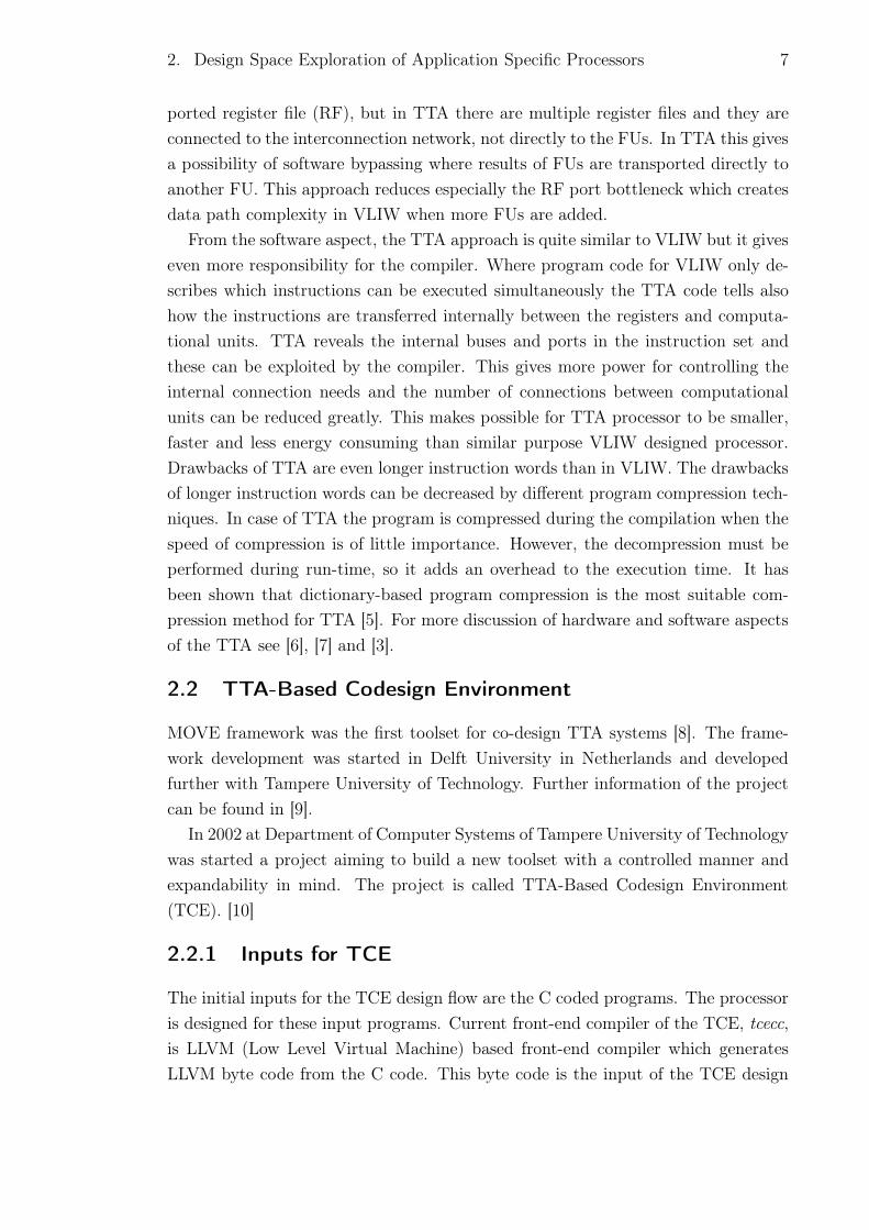
2. Design Space Exploration of Application Specific Processors 7
ported register file (RF), but in TTA there are multiple register files and they are
connected to the interconnection network, not directly to the FUs. In TTA this gives
a possibility of software bypassing where results of FUs are transported directly to
another FU. This approach reduces especially the RF port bottleneck which creates
data path complexity in VLIW when more FUs are added.
From the software aspect, the TTA approach is quite similar to VLIW but it gives
even more responsibility for the compiler. Where program code for VLIW only de-
scribes which instructions can be executed simultaneously the TTA code tells also
how the instructions are transferred internally between the registers and computa-
tional units. TTA reveals the internal buses and ports in the instruction set and
these can be exploited by the compiler. This gives more power for controlling the
internal connection needs and the number of connections between computational
units can be reduced greatly. This makes possible for TTA processor to be smaller,
faster and less energy consuming than similar purpose VLIW designed processor.
Drawbacks of TTA are even longer instruction words than in VLIW. The drawbacks
of longer instruction words can be decreased by different program compression tech-
niques. In case of TTA the program is compressed during the compilation when the
speed of compression is of little importance. However, the decompression must be
performed during run-time, so it adds an overhead to the execution time. It has
been shown that dictionary-based program compression is the most suitable com-
pression method for TTA [5]. For more discussion of hardware and software aspects
of the TTA see [6], [7] and [3].
2.2 TTA-Based Codesign Environment
MOVE framework was the first toolset for co-design TTA systems [8]. The frame-
work development was started in Delft University in Netherlands and developed
further with Tampere University of Technology. Further information of the project
can be found in [9].
In 2002 at Department of Computer Systems of Tampere University of Technology
was started a project aiming to build a new toolset with a controlled manner and
expandability in mind. The project is called TTA-Based Codesign Environment
(TCE). [10]
2.2.1 Inputs for TCE
The initial inputs for the TCE design flow are the C coded programs. The processor
is designed for these input programs. Current front-end compiler of the TCE, tcecc,
is LLVM (Low Level Virtual Machine) based front-end compiler which generates
LLVM byte code from the C code. This byte code is the input of the TCE design
2. Design Space Exploration of Application Specific Processors 8
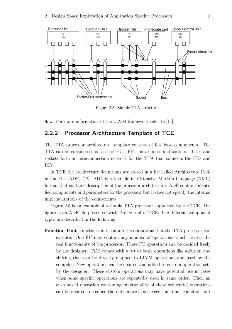
Figure 2.5: Simple TTA structure.
flow. For more information of the LLVM framework refer to [11].
2.2.2 Processor Architecture Template of TCE
The TTA processor architecture template consists of few base components. The
TTA can be considered as a set of FUs, RFs, move buses and sockets. Buses and
sockets form an interconnection network for the TTA that connects the FUs and
RFs.
In TCE the architecture definitions are stored in a file called Architecture Defi-
nition File (ADF) [12]. ADF is a text file in EXtensive Markup Language (XML)
format that contains description of the processor architecture. ADF contains identi-
fied components and parameters for the processor but it does not specify the internal
implementations of the components.
Figure 2.5 is an example of a simple TTA processor supported by the TCE. The
figure is an ADF file presented with ProDe tool of TCE. The different component
types are described in the following.
Function Unit Function units contain the operations that the TTA processor can
execute. One FU may contain any number of operations which creates the
real functionality of the processor. These FU operations can be decided freely
by the designer. TCE comes with a set of basic operations like addition and
shifting that can be directly mapped to LLVM operations and used by the
compiler. New operations can be created and added to custom operation sets
by the designer. These custom operations may have potential use in cases
when some specific operations are repeatedly used in same order. Then an
customized operation containing functionality of these sequential operations
can be created to reduce the data moves and execution time. Function unit

2. Design Space Exploration of Application Specific Processors 9
operations can also be pipelined to increase the potential clock frequency.
Data to and from a FU is transferred through ports. One of the FU ports is
used to select which operation of the FU is used. A triggering port is one of
the FU ports and it is used to start the executing of the selected operation.
Values are stored in internal registers of the FU where they are read in time
of execution and written as a result.
Some FUs in TTA processor have operations that can access memory, such as
loading and storing values into the data memory. These FUs must specify the
address space that is accessed by the FU. The address space defines a range
of memory addresses that the FU can access. [12]
Register File Registers are used to store temporal data during the program exe-
cution. A register file can contain any number of registers. All the registers
in a single RF have the same bit width which is not limited. Register files can
have any number of input and output ports to write and read the data of the
registers. RF having multiple input or output ports can be accessed multiple
times within one clock cycle. [12]
Immediate Unit Immediate units (IU) are optional components that are used to
transfer long immediates to the processor core. An IU is a special register file
where registers contain long immediate values that are written by the control
unit during instruction decoding. IU can contain only read ports since the
registers are written by the control unit directly. [12]
Control Unit Control unit (CU) is a specialized FU that creates control signals
for the interconnection network. It has functionality to fetch instructions from
the instruction memory and decode them to produce the control signals. The
CU usually have at least the operations call and jump which perform function
calls and jumps in the program code being executed. [12]
2.2.3 Design Flow
Designing a processor for TCE follows a particular design flow which includes fol-
lowing phases: sequential LLVM byte code generation, design space exploration
including configuration selection, parallel code generation and analysis and as a
final phase program image and processor generation. In this thesis the term con-
figuration holds two elements: architecture and implementation. The architecture
consist of components that tell how the processor is built and what kinds of resources
it holds. The implementation part combines the architectural components to the
hardware descriptions how the different components are implemented. There can

2. Design Space Exploration of Application Specific Processors 10
Sequential LLVM Byte Code Generation
Application (ANSI C)
Architecture Generation
Implementation Selection
Parallel Code Generation and Verification
Program Image and Processor Generation
- Processor described in HDL- Program images ready to be uploaded in the processor memory
Better configurationneeded.
Architecture meets the requirements.
Estimation and Analysis
Figure 2.6: Design Flow in TCE.
be many variations of the implementations for each architecture component so the
implementations must also be selected for each component. Figure 2.6 illustrates
the design flow in the TCE.
Sequential Code Generation In order to start the design space exploration it
is essential to have the target applications available. The processor is designed from
the basis of the resource utilization of the programs. The application code can be
written in high-level programming language such as C and it can be compiled as
LLVM byte code with the TCE front-end compiler.
Design Space Exploration and Implementation Selection After the initial
input code is generated, the target architecture is designed. This is done by exploring
the design space by adding and removing components of the target architecture.
Every component affects to costs of the processor so this phase is optimizing the
architecture until the design meets the set requirements. Implementations for the
architecture components are then selected from pre-created libraries. Complete

2. Design Space Exploration of Application Specific Processors 11
configurations are compiled and simulated for evaluating the configuration costs
such as speed, silicon area and energy consumption. This phase is repeated until no
better configuration is found. The simulator application of TCE toolset is described
in [7] and developed further as a compiling simulator in [13].
Parallel Code Generation and Analysis The initial sequential LLVM byte
code is scheduled and compiled as parallel code against the target processor config-
uration that is generated in the exploration process with tcecc compiler. The result
parallel TTA-program is then simulated with the processor configuration. With the
results of simulation the program and the processor configuration are analyzed and
evaluated for terms such as speed, silicon area and energy consumption. If the par-
allel code is not fast enough or the other processor requirements are not met, the
previous phase is repeated to fix the configuration. This can be done multiple times
when finding out the most affordable configuration before entering the final phase.
The costs of the configuration can be measured in terms of silicon area, clock speed,
execution time of energy consumption and some of them can be set as the criteria
of the most suitable configuration.
Program Image and Processor Generation Finally the processor is gener-
ated by writing the fixed processor configuration details in a hardware description
language. The hardware description language files are fetched for each building
block from a database. This database can be reused in processor generation of same
technology.
Also the final bit image of the program to be executed in the processor is generated
during this final phase of design flow. For more information of the program image
and processor generation process refer to [14].
2.2.4 TCE Tools And File Formats Related to Exploration
The current development version of TCE provides a complete set of tools that are
needed for designing a TTA processor from the scratch. Some of the tools contain
graphical user interface (GUI) but most provide only a command line interface
(CLI). The tools are, however, designed in such a manner that GUIs may be added
quite easily in the future, if needed. The file formats and tools of TCE that are used
or produced by the exploration process are the following:
LLVM Byte Code The front-end compiler generates code from high level code
to LLVM byte code. This byte code is not TTA-specified and can be com-
piled against any TTA architecture. This byte code is the initial input of the
explorer.

2. Design Space Exploration of Application Specific Processors 12
Architecture Definition File ADF is a file containing architecture description
of the processor. It is an input and output file of the design space explo-
ration. ADF is a file in XML format that contains description of the processor
architecture. ADF contains identified components and parameters for the pro-
cessor. ADF defines also constraints of the architecture template. The ADF
can be created and modified easily with a Processor Designer (ProDe) tool.
It is a tool with GUI for modifying all the components of the ADFs. ProDe
can be used for manual and partly manual design space exploration and also
to visualize the architectures. ProDe is not a necessary tool in TCE or in
automatic design space exploration but it is very useful tool because its good
presentation of the processor and it provides user a simple interface to modify
the ADF file.
Machine Implementation Description File Machine implementation descrip-
tion file (IDF) is a file that contains information of which component imple-
mentation is selected to implement an architecture component. It is an output
and optional input file of the design space exploration. Implementations for
architectures are stored in the IDF. IDF is an XML file which contains tags for
function units, register files and other necessary data to give the information
where the implementation details of each architectural component lies and
with which it is possible to synthesize the processor. IDF does not directly
tell the Hardware Description Language (HDL) file but it tells which entry of
the Hardware Database file is used to implement each architecture component
which finally tells the exact HDL description. Also IDFs for a ADF can be
created and modified easily with ProDe tool.
Hardware Database (HDB) HDB is a database that contains all the necessary
information of the building blocks needed by the tools of TCE. It consists of
provided and user defined processor building blocks, such as function units,
register files, sockets and buses.
The database contains architectural, cost and HDL implementation-specific
information of building blocks to make them usable in processor generation.
The data in HDB is stored in structured query language (SQL) relation tables.
The used SQL database engine is SQLite [15]. Tables and relations of the HDB
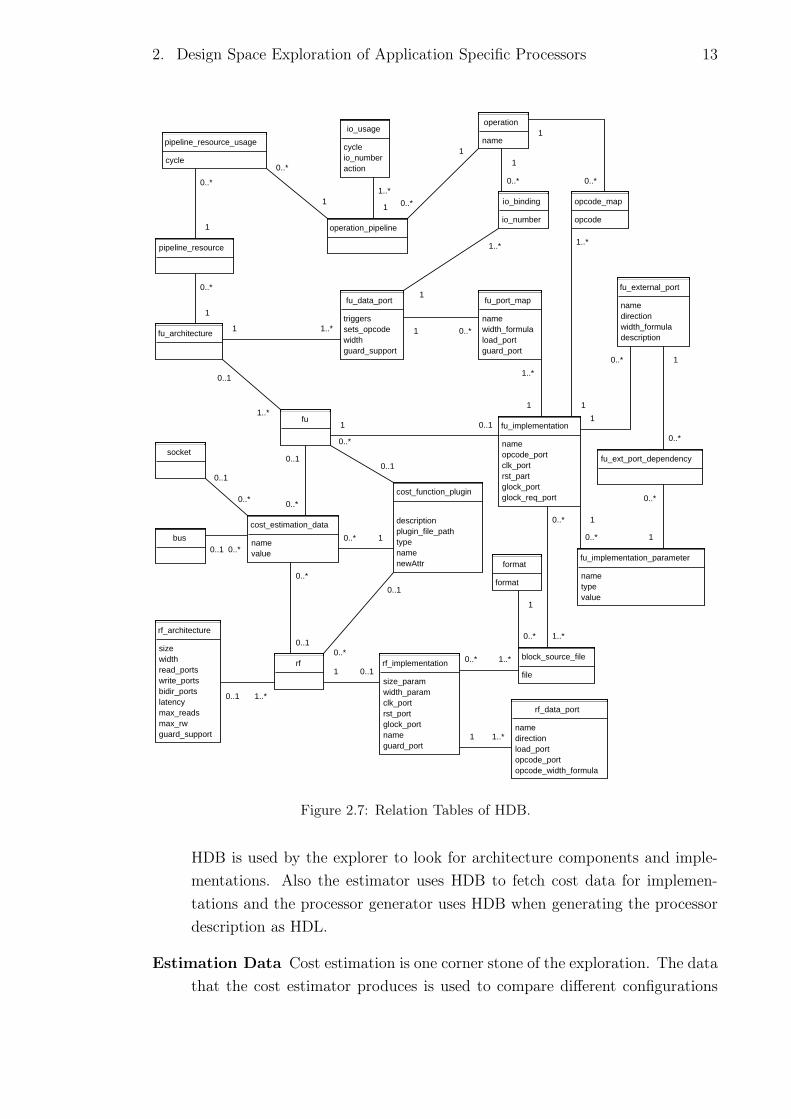
are sketched in Figure 2.7. Similar classes are implemented to represent the
data in objects. The tables include architecture details for both FUs and RFs
and implementation parameters. For each implementation there is a block
source file which contains the hardware block implementation information in
HDL. HDB can be viewed and edited with TCE tool HDBEditor.
2. Design Space Exploration of Application Specific Processors 13
cost_estimation_data
namevalue
cost_function_plugin
descriptionplugin_file_pathtypenamenewAttr
fu_architecture
fu_external_port
namedirectionwidth_formuladescription
fu_implementation
nameopcode_portclk_portrst_partglock_portglock_req_port
block_source_file
file
fu_implementation_parameter
nametypevalue
fu_ext_port_dependency
rf_architecture
sizewidthread_portswrite_portsbidir_portslatencymax_readsmax_rwguard_support
rf_implementation
size_paramwidth_paramclk_portrst_portglock_portnameguard_port
rf_data_port
namedirectionload_portopcode_portopcode_width_formula
format
format
1
0..*
socket
bus
fu
rf
pipeline_resource
pipeline_resource_usage
cycle
operation_pipeline
io_usage
cycleio_numberaction
operation
name
io_binding
io_number
fu_data_port
triggerssets_opcodewidthguard_support
fu_port_map
namewidth_formulaload_portguard_port
opcode_map
opcode
0..*
1
0..*
1
0..*
1
1..*
1 0..*
11
0..*
1..*
1
0..*1
0..*
1
1
1..*
1
0..*
1
0..*
1
0..*
1
0..*
1 1..*
1..*
11..*
0..1
1 0..1
0..*
0..10..1
0..*
0..*0..10..* 1
0..*
0..1
0..*
0..1
0..1
0..*
1..*0..1
1 0..1
0..* 1..*
1 1..*
0..*
1..*
Figure 2.7: Relation Tables of HDB.
HDB is used by the explorer to look for architecture components and imple-
mentations. Also the estimator uses HDB to fetch cost data for implemen-
tations and the processor generator uses HDB when generating the processor
description as HDL.
Estimation Data Cost estimation is one corner stone of the exploration. The data
that the cost estimator produces is used to compare different configurations

2. Design Space Exploration of Application Specific Processors 14
with each other. With the estimation data it is possible to see if the config-
uration fulfills the given requirements and which configuration is preferred to
another by terms of silicon area and energy consumption. The data must be
accurate enough and different data is needed numerous of times during the
design space exploration.
In TCE the cost estimation data is stored in HDB along the matching im-
plementations. The estimator fetches the data from HDB and builds a cost
database from it. This way the estimator is not dependent of the used technol-
ogy since each HDB contains data for the components in that specific HDB.
The estimation data can be obtained by analyzing the results of running logic
synthesis tools and hardware simulators [16]. This process, called the technol-
ogy characterization, can be automated and performed in advance and then
used through HDB by all exploration runs for the technology the data is gen-
erated against.
The estimation data consists of energy, delay and silicon area values. For
each clock cycle, an architecture component is assigned one of three energy
activities: Active, Stalled or Static, and Idle. During an active clock cycle the
component is performing its intended operation. For example, a register is
active when it is being read or written. Component is static when it is not
performing its intended operation but is holding information to be processed
later. A component is idle when it is not active or stalled. This method of
energy activities categorizing is referred to as the ASI method. [17] [18] [16]
The estimation data is used by the cost estimator that estimates if the pro-
cessor fulfills the given requirements. The hardware cost estimator is used to
evaluate the target processor area, energy consumption and execution time
of an application executed by the processor. The hardware cost estimator
uses HDB to look for the costs of the hardware components. In the easiest
case the HDB contains cost data for all of the processor components and the
estimator’s task is simply to add the costs together to get the result. The
target processor area and the execution time of the target application can be
calculated simply with the knowledge of the set of components in the target
processor. The energy estimate needs simulation data to get the execution
times of the components. If the HDB does not contain data that matches
the component details the cost estimator can use interpolation to find some
estimate for the components. The interpolation is done by finding the nearest
matching components and calculating the costs with linear interpolation. The
estimation of different components are detailed later in Section 3.1.
Program Image and Processor Image Program Image Generator (PIG) is an

2. Design Space Exploration of Application Specific Processors 15
application
@id : integerpath : varchar
architecture
@id : integeradf_xml : varchar
implementation
@id : integeridf_xml : varcharlongest_path_delay : doublearea : int
machine_configuration
@id : integer@architecture : id@implementation : id
cycle_count
@architecture : id@application : idcycles : bigint
energy_estimate
@implementation : id@application : idenergy_estimate : double
0..1 0..*
0..*
1
1
0..*
1 0..*
0..*
1
1
0..*
Figure 2.8: Tables and relations of DSDB.
application that generates a complete bit image of a TTA program in TCE
toolset. The program image is a bit-level representation of a TTA program
that is ready to be executed in a TTA processor where it is targeted to. [14]
Processor image is generated with Processor Generator (ProGe) tool that gen-
erates TCE designed processor as HDL for the hardware synthesis.
Design Space Database The Design Space Database (DSDB) is used as a storage
of explored configurations. DSDS is a database containing all the configura-
tions explored with the Design Space Explorer and cost estimations for them.
The explorer inserts new entry into the DSDB on each iteration it advances
the exploration process. Entry contains at least the architecture and in most
cases also the implementation and cost estimates for each application simu-
lated and estimated against the configuration. DSDB is internally an relational
database. Tables and relations of the DSDB are shown in the Figure 2.8. Each
full machine configuration has one architecture and implementation which are

2. Design Space Exploration of Application Specific Processors 16
stored into the database in XML strings. For an incomplete configuration the
implementation can also be omitted to store only the architecture information.
Each architecture contains any number of cycle counts that is bound to number
of applications in the application set. The cycle count tells how many cycles
is needed to run the application and it is used to determine the timing of the
configuration. The application table contains a directory path where the ap-
plication directory is located on the disk. The implementation table contains
the implementation information and the estimates of the longest path delay
of the configuration and the chip area estimation. Each implementation can
contain energy estimates that are bound to the applications of the application
set. DSDB is implemented by using SQLite which is a software library that
implements a Structured Query Language (SQL) database engine and it does
not need a separate server process [15].
2.3 Design Space Exploration Process
Design space exploration process is sketched in Figure 2.9. Design space exploration
is a process of finding out the best possible set of processor components and their
implementations, which together can be considered as configurations, to run specific
applications with some restrictive requirements. These requirements may set limits
for the processor area or energy consumption and may include a time frame when
the results of the application must be ready. This limits the number and type
of resources, that a processor can contain and sets the goals for the design space
exploration.
The configuration exploration process can be divided into two phases, resource
optimization and connectivity optimization. The resource optimization phase modi-
fies the architecture in component level by adding and removing units. In this phase
all the configurations are fully connected and have enough buses not to limit the
schedule. All resulting configurations have different cost/performance ratio. The
most interesting configurations are such that are the fastest or the cheapest within
a specific requirements. These interesting points are called the Pareto points
[19, 20]. The results of this phase are fully connected configurations. The most
interesting configurations of the resource optimization phase are taken into the sec-
ond phase where the connectivity is optimized. In this phase the connections can
be removed to reduce the area of the processor. [21]
The design space exploration process is started with some kind of minimal config-
uration that a program can be compiled for. The configuration contains architecture
information and how the architecture components are implemented. This starting
point configuration can then be used as a target machine by the compiler which
together with scheduler creates the parallel program code that can be executed with

2. Design Space Exploration of Application Specific Processors 17
Target application and requirements are given.The exploration is started with a configuration that can be compiled.
Compile and schedule the programagainst the configuration
Simulate the parallel program code and verify the program results
Estimate theconfiguration
Try to generate abetter configuration
No better configurationscan be found. Finish theexploration.
Modify the configuration
Figure 2.9: Exploration process.
the processor. This is where the iterative exploration process starts. Each iteration
may result in a better configuration or not. Results of all phases can be used as a
feedback for the next iteration and the process builds up as a loop where in each
cycle the architecture is modified and then the compilation and scheduling is done
followed by the compilation verification and analysis of the machine. These steps
may be needed to be repeated numerous of times before the final configuration is
found or there is always the possibility that the available components and compo-
nent implementations are insufficient to fulfill the given requirements and the task
is impossible no matter how good algorithms are processing the task.
Exploration is continued until the reasonable configurations are tested and no
better results can be found. All the configurations and results are gathered for
further inspection.

2. Design Space Exploration of Application Specific Processors 18
2.3.1 Manual Design Space Exploration
The tasks of the exploration process can be performed manually. By doing the
exploration manually the designer can easily consider limitations and tricks that
he can to achieve better results. Controlling the design is easy and good methods
and common sense and experience can be utilized to create simple and effective
processor models. Manual exploration is also a good approach to prove some new
implementation or architectural designs. Special operations and components can
easily be tested in machine configurations and find out the best practices. These
practices can then be implemented to be used in automated design space exploration.
Also utilizing different scheduling algorithms is easy in manual process.
Disadvantage of manual exploration is that it takes lots of time and high concen-
tration from the designer to find out the best possible configuration. Good configu-
rations might be created quite fast if the designer can see where the bottlenecks are
but great results are much harder to achieve.
2.3.2 Semi-Automated Design Space Exploration
Semi-automated exploration is exploiting the automated tools and manually modi-
fies the most potential results. The automated exploration algorithms have always
some weaknesses that a good designer can easily patch by selecting reasonable com-
ponents or even creating some special operations or units. Other possibility is to
continue automated exploration from some manually modified configuration where
some drawbacks of the algorithms are taken into account. Also the automated pro-
cess may be guided manually by selecting some interesting configurations for further
exploration.
2.3.3 Automated Design Space Exploration
Automated design space exploration is a process where the most suitable processor
configuration is searched completely automatically. The designer’s task is just to
give the applications and requirements to the automatic explorer. The explorer
generates multiple configurations and finds out the best possible configuration with
the written algorithms. Automatic exploration performs all the exploration steps
automatically and stores the gathered data as a result database that can be inspected
afterwards. The advantage of an automated process is that it can try hundreds or
even thousands of different combinations when finding out the best solution. Doing
this manually would be far too time consuming and inefficient.

2. Design Space Exploration of Application Specific Processors 19
2.3.4 Exploration in TCE
Since the TTA processor, like VLIW, itself does not contain the scheduling logic
the programs need to be scheduled in the time of compilation. The architecture of
the TCE scheduler is described in [22]. The compilation and scheduling depends
on the structure of the processor’s buses and components and the first step of ex-
ploration is to create a starting point TTA that contains the resources which are
needed to compile the programs. In TCE there is a simple base machine file called
minimal.adf that can be used as this initial architecture. TTA machine a is col-
lection of processor elements which in TCE are written in Architecture Definition
File the ADF. Processor elements of the ADF are detailed in Subsection 2.2.2. This
initial architecture is basically the minimal architecture the tcecc compiler can stull
compile any integer ANSI C programs for and so it contains all the needed opera-
tions for the first compilation. For a architecture component it is necessary to also
select an implementation that details the logic of the architecture component. With
the implementation information it is possible to fetch the correct HDL files from the
hardware block library. These HDL files are needed in cost estimation and processor
generation.

20
3. TCE DESIGN SPACE EXPLORATION
FRAMEWORK
The design space framework in TCE consists of set of tools that the explorer core
uses. The high level package description of the design space explorer in TCE is shown
in Figure 3.1. The explorer core is called from a user interface which currently is
command line based. GUI is also planned and might be implemented later. The
explorer core is a client of different entities of TCE. The cost estimator is needed to
estimate the costs of the architecture components while the simulation is also needed
for the estimation. DSDB is used by the explorer to store the created configurations
and result data of the configuration from the cost estimator. Explorer uses the
scheduler for creating the parallel TTA code.
In this chapter the estimator package and the core of the explorer is discussed.
The estimator classes are described in Section 3.1 and the explorer classes later in
Section 3.2.
ExplorerUI
Explorer
Scheduler Simulator Estimator
DSDB
Figure 3.1: High level module relations of the design space explorer.

3. TCE Design Space Exploration Framework 21
3.1 Cost Estimator
The hardware cost estimator is responsible for evaluating the costs of the target
processor. Costs include the used chip area, energy consumption and the timing for
a set of applications. The maximum clock frequency of the processor configuration
can be obtained from the timing evaluation. Results of the cost esimator are mainly
used by the explorer to select the best implementations and components for the
target processor. The best implementation is often the one that fulfills the given
requirements but is minimal in costs. Estimation is an important phase of processor
designing. In mobile processing where the processing power is not the only desired
feature but the long battery life of the device is essential together with the processing
performance there is a great interest for designing low energy consuming chips as
possible. For example in these situations with a good approximation of energy
consumption can the designer straight away decide which architecture models are
too energy consuming and are not considered as final products.
Accuracy is the key aspect in cost estimation. The more accurate the estimate is
the more useful it gets. The most accurate cost estimations would possibly be done
by performing logic synthesis together with gate-level simulation for the complete
processor. Synthesis is far too slow for automated design space exploration where
there can be hundreds or thousands of processor models to estimate. Because the
time requirements the accuracy of the estimation must be compromised. By gener-
ating the cost data in advance the cost estimator can obtain accurate enough data
quickly. Good results can be generated by getting the costs of each component by
performing logic synthesis with gate-level simulation to each component in advance.
This can mean a huge amount of data and simulations if all variable changes must
be simulated in advance. This is why the estimator is implemented to create an
interpolation of the estimates where feasible if no strict match is found.
There are three different costs that are estimated from the processor. The area is
simply the total area of silicon that is needed by the configuration. The total area
is a sum of all sub areas that include areas of register files, function units, intercon-
nection and control logic. Energy consumption is the total energy of the processor
that it uses during a program execution including idle and active energies of the
components. Delay is a time that is spent by the components and transfers during
the execution. With delay estimations it is possible to estimate the speed of the
processor configuration by resolving the longest path of the processor. The longest
path of the processor is the maximum of the delay of any unit and the longest path
found in the interconnection network through the processor logic. Interconnection
network paths include all “output socket -> bus -> input socket” chains as well as
“output socket -> bus -> input socket -> FU” chains.

3. TCE Design Space Exploration Framework 22
Estimator
CostEstimatorPluginRegistry
RFCostEstimatorPluginRegistry ICDecoderCostEstimatorPluginRegistry
FUCostEstimatorPlugin RFCostEstimatorPlugin ICDecoderEstimatorPlugin
StrictMatchFUEstimator InterpolatingFUEstimator StrictMatchRFEstimator InterpolatingRFEstimator
DefaultICDecoderPlugin
CostDatabase HDB
FUCostEstimatorPluginRegistry
0..*
1
0..*
1
0..*
1
<<realize>>
<<realize>>
<<realize>>
<<realize>><<realize>>
Figure 3.2: Estimator class diagram.
In the following section it is described how the cost estimator design and imple-
mentation is carried out in TCE and how the different costs are estimated.
3.1.1 Estimator Design
The cost estimator like other parts of TCE is designed with flexibility in mind. In
cost estimation it is possible to experiment different algorithms. This requirement
leads to such design of the Estimator that most of the actual algorithmic work is
allowed to be redefined easily.
3.1.2 Estimator Implementation
Cost estimation process can be carried out in various of ways. Since the estimation
methods can be researched and improved the TCE cost estimator is implemented
to support different algorithms for estimation. The algorithms can be imported to

3. TCE Design Space Exploration Framework 23
the estimator as estimation plugin. Estimator plugins are used to implement the
estimation process. Each estimation plugin implements the interface of the base cost
estimator plugin class that contains all necessary methods to estimate the processor
components in terms of area, energy consumption and timing. Plugins may use
different data or handle the data differently to find the best possible estimation
results. Currently there are two kinds of cost estimation plugins implemented for
the TCE: the strict match estimators which use exact matches of the components
and the interpolating estimators which try to interpolate the missing component
costs. Figure 3.2 represents the class structure of the cost estimator. The Estimator
class contains methods to estimate different costs of the processor. The actual
implementations of the different estimators are implemented in the plugins.
Different components are estimated a bit differently so there are their own im-
plementations to estimate the FUs and the RFs and the interconnection network.
RF Estimation
The area estimation of RF is simple for the estimator since the area is already known
during the data generation in gate level simulation and it is stored in HDB with all
the other cost data of the components. The energy of an RF cannot be obtained
directly from the cost database. For the energy estimation as described in [18] the
cost estimator needs simulation data to know the register files are utilized. With
the utilization statistics the RF energy can be obtained as follows
ERF = EidleUidle +
n∑
read=1
m∑
write=1
Eread,writeUread,write (3.1)
Eidle is the idle energy of the RF (obtained from the cost database)
Uidle is the number cycles that the RF is idle (obtained from the simulation trace
database)
n is the number of read ports that the RF contains
m is the number of write ports that the RF contains
Eread,write is the energy of the RF consumed when read ports are read and write
ports are written (obtained from the cost database)
Uread,write is the number of times read reads and write writes occurs simultaneously
into the RF (obtained from the simulation trace database).

3. TCE Design Space Exploration Framework 24
FU Estimation
The area estimation of FUs is similar to RF area estimation. The value is simply
fetched from the HDB. For the energy estimation of FUs the simulation data is
again needed. The number of operation execution times is counted from each unit
and the execution times are multiplied with the pre-estimated energy consumption
of each operation. These estimates are also a result of gate level simulation and are
stored as costs in HDB. Equation 3.2 shows how the energy of FU is summed up.
EFU = EidleNidle +∑
EkNk (3.2)
Eidle is the idle energy of the FU (obtained from the cost database)
Nidle is the number cycles that the FU is idle (obtained from the simulation trace
database)
Ek is the energy of the FU consumed for performing operation k once (obtained
from the cost database)
Nk is the number of times operation k was executed (obtained from the simulation
trace database).
Strict Match Estimators
Estimator can evaluate the costs using the exact costs of a component. In this
case all the cost data must be created earlier and added to the HDB. Strict match
estimation gives the best possible estimation values with the selected estimation
method. All the component costs are as near as possible to the real values. Strict
match estimator implementations are quite simple. They fetch cost data for each
component from the HDB. Result is gained by simply adding cost values of each
component to the result. Area estimation adds all of the component areas to the
result and there we have the area estimation. Energy estimation needs data from the
simulator to get the counts of operation usages, transfers to and from the registers
and idle times. These values are also fetched from the HDB and then added as result
when multiplied with the usage counts.
Interpolating Estimators
Making synthesis and gate-level simulations to all possible variations of components
would be very time consuming and the database would grow significantly. This is
why the amount of strict matches is reasonable to be compromised. With linear
interpolation it is possible and quite easy to obtain data with sufficient accurate for
such components which do not have strict match estimations. Having one similar

3. TCE Design Space Exploration Framework 25
Figure 3.3: Linear interpolation.
component estimated with greater and smaller variable the estimate can be counted
with a linear equation from the lower point to the higher. The interpolating esti-
mators in TCE use own data structure build as the CostDatabase where all cost
information from HDB is collected.
All parameter variations are not suitable for linear interpolation. In RFs the most
reasonable variable for interpolation is the number of registers. The costs grow quite
linearly when more registers are added so it is not necessary to synthesize cost data
for all possible register number combinations for a RF. However, more accurate
results can be interpolated if there are some estimates between the minimal number
and the maximum (reasonable) number of registers. Figure 3.3 shows how the
estimate is interpolated from the existing cost data. The nearest greater and smaller
value is selected for the interpolation and the cost is
y = y0 + (x− x0)y1 − y0
x1 − x0
. (3.3)
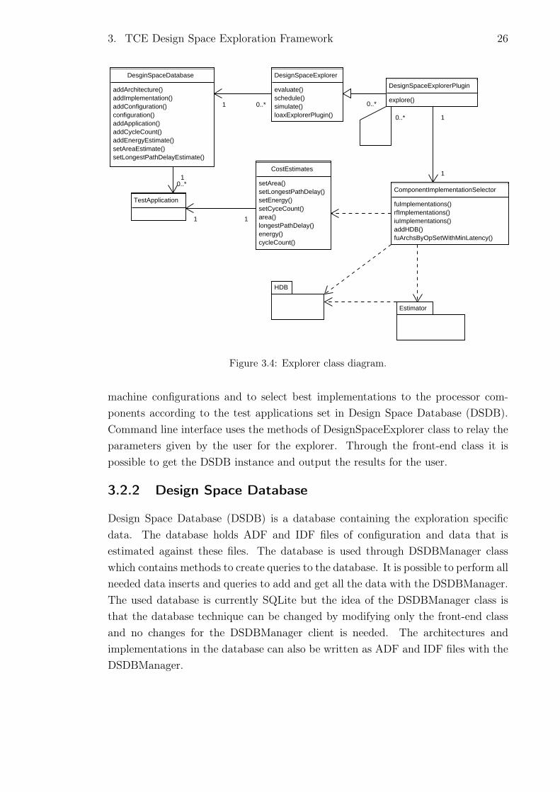
3.2 Explorer
Explorer in TCE consists of multiple classes. Figure 3.4 details the classes and
relations of the explorer. The classes shown in the class diagram are described in
the following sections.
3.2.1 Design Space Explorer
Design space explorer is the front-end of the explorer. It is a class that hides the com-
plex call hierarchies from the user, which is a realization of façade design pattern
[23]. Design space explorer interface provides methods to automatically evaluate
3. TCE Design Space Exploration Framework 26
DesignSpaceExplorerPlugin
explore()
DesginSpaceDatabase
addArchitecture()addImplementation()addConfiguration()configuration()addApplication()addCycleCount()addEnergyEstimate()setAreaEstimate()setLongestPathDelayEstimate()
TestApplication
10..*
0..*
0..*
ComponentImplementationSelector
fuImplementations()rfImplementations()iuImplementations()addHDB()fuArchsByOpSetWithMinLatency()
1
1CostEstimates
setArea()setLongestPathDelay()setEnergy()setCyceCount()area()longestPathDelay()energy()cycleCount()
11
Estimator
HDB
DesignSpaceExplorer
evaluate()schedule()simulate()loaxExplorerPlugin()
0..*1
Figure 3.4: Explorer class diagram.
machine configurations and to select best implementations to the processor com-
ponents according to the test applications set in Design Space Database (DSDB).
Command line interface uses the methods of DesignSpaceExplorer class to relay the
parameters given by the user for the explorer. Through the front-end class it is
possible to get the DSDB instance and output the results for the user.
3.2.2 Design Space Database
Design Space Database (DSDB) is a database containing the exploration specific
data. The database holds ADF and IDF files of configuration and data that is
estimated against these files. The database is used through DSDBManager class
which contains methods to create queries to the database. It is possible to perform all
needed data inserts and queries to add and get all the data with the DSDBManager.
The used database is currently SQLite but the idea of the DSDBManager class is
that the database technique can be changed by modifying only the front-end class
and no changes for the DSDBManager client is needed. The architectures and
implementations in the database can also be written as ADF and IDF files with the
DSDBManager.

3. TCE Design Space Exploration Framework 27
3.2.3 Design Space Explorer Algorithm Implementation
Design space explorer algorithms are implemented as design space explorer plugins.
Explorer plugins can be parts of the exploration chain or they can contain fully func-
tional explorers. The main idea of the plugin approach is the easy modularization
of the exploration process. With plugins the big complex exploration scheme can
be split to small blocks that can be tested and developed separately. One approach
could be that plugins are small explorers that can call other exploration plugins so
the final exploration output may be a result of many phases where the design space
is travelled to and forth in multiple steps. One advantage of the plugin approach
is also that new plugins are easy to create and import in future so that researches
can use their own exploration algorithms instead of the ones that are done into the
TCE distribution. Developing explorer in small sub explorers gives also researchers
and developers plenty of possibilities to do the small sub-tasks in order they find
the best.
Algorithms can be controlled with parameters. Parameters can be passed to
algorithms as pairs of name and value. Using parameters in the algorithms’ imple-
mentations is fully optional. Each algorithm may have operability guided with own
parameters if appropriate or algorithms can be so called pure algorithms.
There are a few required inputs for the algorithms. These are the name of the
algorithm and the DSDB where the results are stored. Also the ID of the configu-
ration where the algorithm begins to make progress is needed when the algorithm
is launched.
All the results of the implemented exploration plugins are added into the DSDB.
Results of the exploration plugins include the ADF and the IDF files and the calcu-
lated estimations of the configurations. From DSDB the results can be fetched for
later use, for observing or manual fine tuning.
3.2.4 Component Implementation Selector
The purpose of the component implementation selector is to provide methods for
selecting suitable implementations to the given architecture components. The com-
ponent implementation selector uses HDB to look for the implementations and re-
turns a set of suitable implementations that fulfill the given cost requirements such
as the clock frequency or the gate area of the component. ComponentImplemen-
tationSelector class uses the cost estimator to estimate the costs of the suitable
implementations and determines from the results if the implementation is good for
this purpose. The class has methods for searching suitable implementations for
function units, register files and immediate units. Implementations are searched for
matching the given architecture and meet the speed and area requirements if given.

3. TCE Design Space Exploration Framework 28
The component implementation selector can search suitable implementations from
multiple HDB files. The returned implementation location tells the HDB and the
entry of the HDB where the implementation lies.
3.2.5 Cost Estimates
Cost estimates are estimates for a machine configuration (ADF+IDF). The CostEs-
timates class stores the estimates of each configuration. These estimates include the
area of the processor configuration which is presented as number of gates. Longest
path delay is the delay of the processor’s critical path that is the speed bottleneck
of the configuration. The longest path delay value is presented in nano seconds.
The energy consumption of the configuration while processing the used application
is presented in milli joules. The fourth estimate value is the cycle count of the pro-
cessor with the current configuration and application which is presented in number
of clock cycles. The area and the longest path delay are constants to one machine
configuration while there can be multiple programs run with that configuration.
Therefore there can be multiple energy consumption estimations and cycle counts
as well out of one machine configuration. Each energy consumption and cycle count
is bound to one application that can be run with the machine configuration.
3.2.6 Test Application
Test application class is a helper class for the explorer to handle application specific
files. The applications that are run with the TTA processor being explored are
inserted into the test application directories. These directories contain files that are
needed by the explorer to ensure the correct functionality and speed requirements of
the processor configurations. Files include instructions to simulate the program and
verify the simulation. Methods include checkers for files and getters for simulation
execution and simulation output verification files:
• description(): A method that returns description file of the test application
directory.
• correctOutput(), A method that returns the correct program output string for
ensuring the architecture functioning.
• setupSimulation(): A method that sets up the simulation run by running the
setup script of the test application directory.
• simulateTTASim(): A method that returns an input stream to simulate.ttasim
file of the test application directory which can be given to the TTA simulator.

3. TCE Design Space Exploration Framework 29
• maxRuntime(): A getter method that returns the maximum runtime require-
ment of the test application.
• applicationPath(): A method that returns a directory path of the sequential
program file of the test application directory.
• verifySimulation(): A method that executes the verify script of the test appli-
cation directory. Return value is true if the verifying was a success.
• hasApplication(): Returns true if ’program.bc’ file is in the test application
directory.
• hasSetupSimulation(): Returns true if ’setup.sh’ file is in the test application
directory.
• hasSimulateTTASim(): Returns true if ’simulate.ttasim’ file is in the test ap-
plication directory.
• hasCorrectOutput(): Returns true if ’correct_simulation_output’ file is in the
test application directory.
• hasVerifySimulation(): Returns true if ’verify.sh’ file is in the test application
directory.
• hasCleanupSimulation(): Returns true if ’cleanup.sh’ file is in the test appli-
cation directory.
Test application directory must have at least the files for the sequential program
and a way to verify the output. Also the maximum runtime is needed for creating
reasonable TTAs.

30
4. EXAMPLE EXPLORATION ALGORITHM
The design space explorer’s brains are in the exploration algorithms. Explorer algo-
rithms are the guide for the explorer to do it’s job. These algorithms can always be
improved and new ideas invented. This is why the explorer algorithms can be added
as runtime libraries for the Design Space Explorer. Explorer algorithms can be im-
plemented as code sections that are derived from the DesignSpaceExplorerPlugin
class which can be seen in Figure 3.4. Plugins need to re-implement the explore()
method of the parent class where the plugin algorithm functionality and complexity
is hidden. Plugins can be used with explorer after compiling. Compiling can be
done with the aid of script named buildexplorerplugin.
Algorithms store all results to Design Space Database (DSDB). The starting
point configuration is given for the plugins and it can be any of the configurations
added to the DSDB. Configurations include initial architecture and architecture
implementation. Architecture implementation may also be empty as can be the
architecture when the plugin starts exploring from the scratch.
Plugins can be guided with parameters passed from the explorer application.
Parameters can be given as name-value pairs.
4.1 Frequency Sweep Explorer Algorithm
Frequency sweep is an exploration algorithm that travels through the design space by
setting one frequency at a time as a target frequency of the processor configuration.
The frequency limits and the interval are given by user. Frequency sweep is done by
using the lowest frequency first and then stepped towards the upper limit. Eg. if the
target limits are 100-200MHz and the interval is 50MHz would the algorithm try to
generate processor configurations with frequencies 100MHz, 150MHz and 200MHz.
The plugin parameters and their explanations are shown in Table 4.1.
Frequency sweep algorithm tries first to optimize the number of cycles needed to
run the programs. This part is described in Section 4.2. Minimizing the cycle count
in the first stage of exploration is done to achieve less energy consumpting results.
Smaller cycle count ends up to lower clock frequency needs and most possibly less
energy consuming processors.
Second phase of the algorithm is to optimize the execution time. In this phase
are the implementations to each component selected. The interconnection network

4. Example Exploration Algorithm 31
Parameter Name Purposestart_freq_mhz Frequency sweep starting frequency in MHz.end_freq_mhz Frequency sweep ending frequency in MHz.step_freq_mhz Interval of the frequency sweep in MHz.superiority This parameter is passed further to the cycle count minimiza-
tion plugin to indicate how many percents better must thenew cycle count be compared to the previous one to continuethe cycle count optimization.
Table 4.1: Parameters
(IC) is optimized after selecting the components. The second phase algorithm is
described in Section 4.3
Finally if the previous phases constructed configurations that fulfills the require-
ments then the algorithm is advances to the final optimization phase. These opti-
mizations are described in Section 4.4. The final optimization is not yet implemented
in the current version of the Frequency sweep algorithm but it can be added easiest
by creating the functionality in a separate explorer plugin.
1: minF ⊲ User given parameter for minimum frequency.2: maxF ⊲ User given parameter for maximum frequency.3: stepF ⊲ User given parameter for step frequency.4: superiority ⊲ User given parameter.5: C ⊲ Configuration6: currentF ← minF7: cycleOptArchs← OptimizeCycleCount(C, superiority)8: repeat9: for all cycleOptArch in cycleOptArchs do
10: if fastEnough(cycleOptArch, curMhz) then11: minArch← minimizeMachine(cycleOptArch)12: minConf ← selectImplementations(minArch)13: icOptimize(minConf) ⊲ Also stores the optimized configuration
into the DSDB.14: end if15: end for16: currentF ← currentF + stepF17: if currentF > maxF then18: currentF ← maxF19: end if20: until currentF 6= maxF
Figure 4.1: Frequency sweep algorithm.
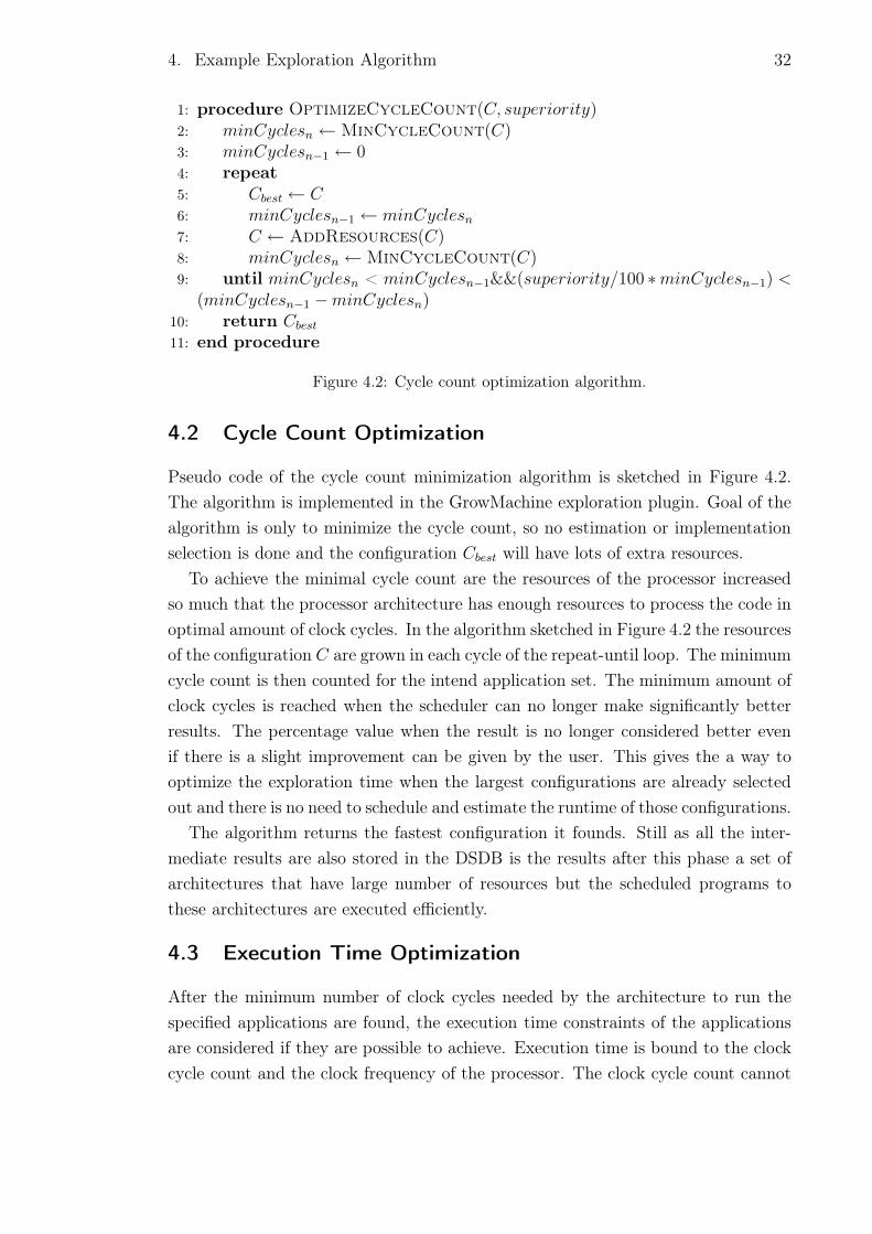
4. Example Exploration Algorithm 32
1: procedure OptimizeCycleCount(C, superiority)2: minCyclesn ←MinCycleCount(C)3: minCyclesn−1 ← 04: repeat5: Cbest ← C6: minCyclesn−1 ← minCyclesn
7: C ← AddResources(C)8: minCyclesn ←MinCycleCount(C)9: until minCyclesn < minCyclesn−1&&(superiority/100 ∗minCyclesn−1) <
(minCyclesn−1 −minCyclesn)10: return Cbest
11: end procedure
Figure 4.2: Cycle count optimization algorithm.
4.2 Cycle Count Optimization
Pseudo code of the cycle count minimization algorithm is sketched in Figure 4.2.
The algorithm is implemented in the GrowMachine exploration plugin. Goal of the
algorithm is only to minimize the cycle count, so no estimation or implementation
selection is done and the configuration Cbest will have lots of extra resources.
To achieve the minimal cycle count are the resources of the processor increased
so much that the processor architecture has enough resources to process the code in
optimal amount of clock cycles. In the algorithm sketched in Figure 4.2 the resources
of the configuration C are grown in each cycle of the repeat-until loop. The minimum
cycle count is then counted for the intend application set. The minimum amount of
clock cycles is reached when the scheduler can no longer make significantly better
results. The percentage value when the result is no longer considered better even
if there is a slight improvement can be given by the user. This gives the a way to
optimize the exploration time when the largest configurations are already selected
out and there is no need to schedule and estimate the runtime of those configurations.
The algorithm returns the fastest configuration it founds. Still as all the inter-
mediate results are also stored in the DSDB is the results after this phase a set of
architectures that have large number of resources but the scheduled programs to
these architectures are executed efficiently.
4.3 Execution Time Optimization
After the minimum number of clock cycles needed by the architecture to run the
specified applications are found, the execution time constraints of the applications
are considered if they are possible to achieve. Execution time is bound to the clock
cycle count and the clock frequency of the processor. The clock cycle count cannot

4. Example Exploration Algorithm 33
be improved at this point but the clock frequency can be tuned up with selecting
suitable components and making the connection network as fast as possible. These
actions will certainly weaken the cycle count performance and so it is first calculated
if it is possible to meet the runtime requirements with one target frequency. One
frequency is set as target at a time beginning the lowest frequency and stepped
towards the highest.
Execution time optimization removes extra components from the machine that
were generated in the cycle count optimization phase. The resource removal is im-
plemented in the MinimizeMachine explorer plugin. After the resource minimization
the implementations are selected for every component. The interconnection network
can be optimized after the implementation selection. This is done with another ex-
plorer plugin SimpleICOptimizer.
4.3.1 Selecting Components
Architecture component implementations are selected to meet the target processor
frequency. Too fast component implementations may contain more logic that takes
area and consumes energy. That is why the components are selected to be fast
enough but the costs of the components low as possible. If multiple candidate im-
plementations for the component are found is the smaller input and delays preferred.
If there still are multiple possibilities the least energy consuming implementation is
selected.
It is always possible that the given architecture is the speed bottleneck of the
processor and the time requirements are not met. In these cases there are no possible
implementations for given function unit architecture. The function architecture can
be changed by raising the latency of the FU. This way suitable implementations
may be found.
4.3.2 Removing Unnecessary Components
Unnecessary components are removed by minimizing the machine. Purpose of the
Minimize machine algorithm is to remove resources from the processor architecture
until the real time requirements of applications are not reached anymore. Minimizing
the machine thereby optimizes the resources of the machine by reducing the extra
ones.
At first the maximum running time of each application that the machine should
run is converted to cycle count. If no maximum run time is given, there is no
time limit and the maximum cycle count that the processor is allowed to run the
application is unlimited as long as the application can be executed. Figure 4.4 shows
the maximum cycle count computation.

4. Example Exploration Algorithm 34
After the maximum cycle counts have been computed the resources are reduced.
At first the not needed buses are removed. After that possible extra function units
and finally extra register files are removed. Minimizing the number of buses is
done by removing some number of buses from the original architecture. After the
removal the configuration is evaluated against each program. If any of the cycle
counts exceeds the calculated minimum cycle count is the number of removed buses
too high. Otherwise more buses can be tried to remove. Binary search algorithm is
used for solving out the number of buses that can be removed. With binary search
the number of iterations can be optimized. The minimizing of buses is shown in
Figure 4.3. The returned configuration is minimized in number of buses because if
more buses are removed the cycle counts get too high. The algorithm implements a
binary search algorithm and thereby it has an efficiency of O(log n).
After the buses have been minimized the FUs are minimized. At first the FUs in
the architecture are analyzed and the number of similar units is counted. Then each
type of FUs is tried to be reduced and after each removal the architecture is tested
to still reach the requirements. If the removal prevents the configuration to meet
the requirements the last working configuration is restored and next type of FU is
tried to remove. RFs are minimized after the FU minimization and it is carried out
similarly to FU minimization. After other minimizations the sockets that no longer
connect any units are removed from the machine.
4.3.3 IC Optimization
Removal of the unneeded connections and sockets reduces the energy consumption
and area needed by the configuration. The IC can be simply optimized by removing
the connections that are not used. This is an easy way of reducing the connectivity.
After this every connection removal means that the schedule has to be changed. The
SimpleICOptimizer plugin that currently implements the interconnection network
optimization first schedules optimized configuration to get the parallel program code.
Then it removes all the connections from the machine and adds those connections
back in place that are used in the scheduled program instructions. This way all the
extra connections that are not used can be removed. Those sockets and units that
no longer are connected to any buses can now also be dropped out. Finally the
functionality if the new optimized configuration is tested.
4.4 Final Optimization
The final optimization phase is not yet implemented in the current explorer but the
original plan is described as follows.
In the final phase the explorer has a set of configurations that are fast enough

4. Example Exploration Algorithm 35
1: high H ← Cb ⊲ Cb is the number of buses in configuration2: low L← 13: middle M ← (L + H)/24: for all a in set of applications A (that should be run with the configuration C)
do5: if cycles of application in current configuration aC > amax then return C6: end if7: end for8: while L < M do9: minimized configuration c← Cb −M
10: lowerM ← true11: for all a in set of applications A that should be run with the configuration
C do12: if cycles of application in minimized configuration ac > amax then13: L←M + 114: M ← (L + H)/215: lowerM ← false16: end if17: end for18: if lowerM = true then19: H ←M − 120: M ← (L + H)/221: end if22: end while23: return c
Figure 4.3: Minimizing buses.
1: for all max runtime r in set of applications A (that should be run with theconfiguration C) do
2: if ¬r then3: return ∞4: end if5: amax ← r ∗ fc ⊲ fc is the running frequency in MHz6: end for7: return amax
Figure 4.4: Maximum cycle count computation.
from the previous steps of exploration. The final optimization concentrates on three
things. Firstly can the FU’s be changed to ones with smaller latency implementa-
tions. If the configuration still fulfills the requirements after a FU change it can and
will be done. Secondly all the components are considered if some can be changed
to one with smaller energy consumption. Finally all the components are considered
if they can be changed to ones with smaller area. These three optimization checks
makes the result configuration to be fastest, least energy consuming and smallest in
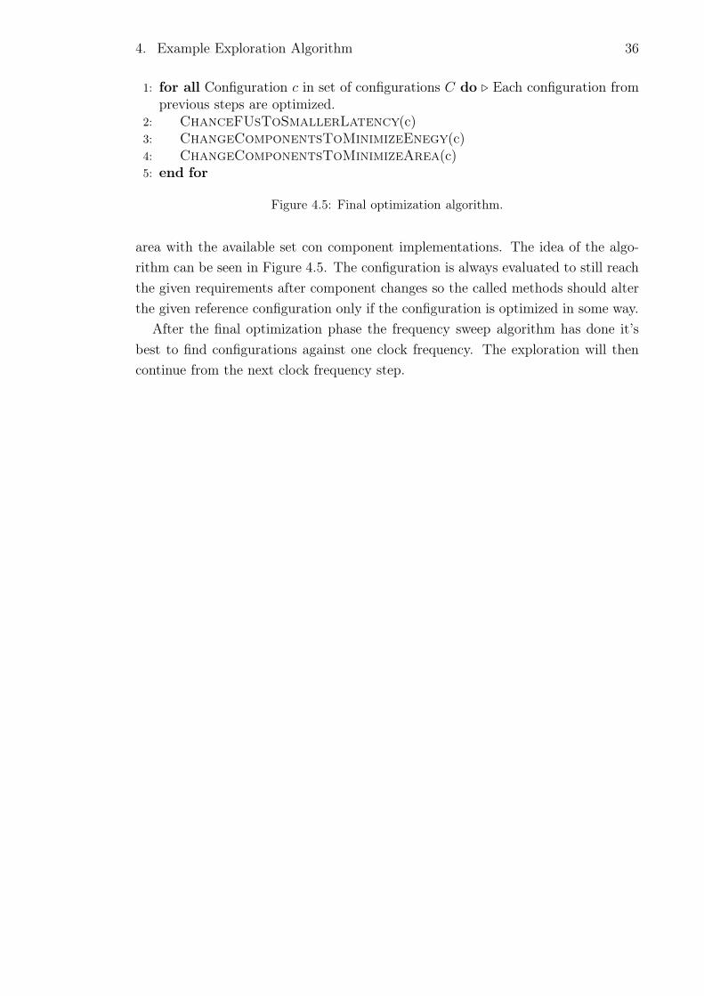
4. Example Exploration Algorithm 36
1: for all Configuration c in set of configurations C do ⊲ Each configuration fromprevious steps are optimized.
2: ChanceFUsToSmallerLatency(c)3: ChangeComponentsToMinimizeEnegy(c)4: ChangeComponentsToMinimizeArea(c)5: end for
Figure 4.5: Final optimization algorithm.
area with the available set con component implementations. The idea of the algo-
rithm can be seen in Figure 4.5. The configuration is always evaluated to still reach
the given requirements after component changes so the called methods should alter
the given reference configuration only if the configuration is optimized in some way.
After the final optimization phase the frequency sweep algorithm has done it’s
best to find configurations against one clock frequency. The exploration will then
continue from the next clock frequency step.

37
5. BENHMARKING AND VERIFICATION
The explorer plugins were tested against three different benchmark applications:
two different Discrete cosine transform (DCT) applications, one that computes the
transform to a 8 x 8 matrix and other that computes 32 bit transforms and one of
the benchmark applications implements the Viterbi algorithm introduced in [24].
5.1 Algorithm Verification
To verify the Frequency sweep algorithm the sub-algorithms were verified to function
as they were intent to. Then the Frequency sweep exploration algorithm was tested
in whole.
5.1.1 Verification of GrowMachine plugin
The GrowMachine exploration algorithm Section 4.2 is used first by the Frequency
sweep. In Table 5.1 is shown how the GrowMachine algorithm have optimized the
cycle counts of the Viterbi application. The superiority was set to one (1) percent
and the algorithm ended after the Row 10 when the cycle count improvement was no
longer better than one percent. Rows 2-9 were then selected to further investigation.
Table 5.1: Viterbi cycle count optimization.
Row Program Cycles Improvement %1 viterbi 31147383 -2 viterbi 6548954 78,9743%3 viterbi 3945912 39,7474%4 viterbi 2631193 33,3185%5 viterbi 2021880 23,1573%6 viterbi 1726200 14,624%7 viterbi 1621128 6,0869%8 viterbi 1565642 3,42268%9 viterbi 1549802 1,01173%10 viterbi 1548746 0,061377%
The total drop of the cycle count in this case was nearly 95% from the original
architecture.

5. Benhmarking and Verification 38
5.1.2 Verification of MinimizeMachine Plugin
The MinmizeMachine removes resources from the architecture until the speed re-
quirements are not met anymore. MinimizeMachine algorithm was tested by adding
components to a already minimized machine and running the algorithm against
this architecture. The algorithm successfully removed the extra components and
stopped when the cycle count and target frequency limited the removing of more
components.
5.1.3 Verification of SimpleICOptimizer Plugin
The SimpleICOptimizer algorithm removes the connections that are not used by the
scheduled program. When started the algorithm with a fully connected architecture
that was generated for the DCT8x8 program the architecture contained total of
374 bus to socket connections. After the SimpleICOptimizer algorithm was the
number of connections dropped to 345 giving total of 39 removed connections. This
connection removal changed also the area estimate to drop from 22632 gates to 21146
gates.
5.2 Testing of Example Algorithm FrequencySweep
Table 5.2 represents exploration results of program that counts the DCT 8 x 8 ma-
trix. The exploration was run by using the FrequencySweep algorithm and sweeping
frequencies from 50MHz to 200MHz with 50MHz steps. The maximum execution
time of the program was set to 0,01 seconds. In Figure 5.1 the graph contains the
chip area (gates) and energy estimate (mJ) of the generated configurations. The
figure presents those points of the exploration results where the speed requirements
were fulfilled and the functionality of the program was tested to work correctly. The
FrequencySweep algorithm takes care that the execution time limit is not theoreti-
cally exceeded when running the program with target frequency. Points in the result
table and graph are placed in the same order the configurations were generated by
the algorithm developed in this thesis. The peaks in the graph are the points from
the first configurations of each sweeping frequency optimized successfully in basis
of the cycle count minimization. Then the reducing of the components is shown in
decreasing chip area and energy. In Figure 5.2 the execution time of the DCT 8
x 8 program is drawn with the energy values. The execution time is calculated by
dividing the cycle count numbers with the target frequencies. All the configurations
fulfill the execution time constraint.
In Table 5.3 are the results given by the Frequency sweep algorithm when ex-
plored against the Viterbi program. The program was given a maximum execution
time of 0,1 seconds and the frequencies 50MHz to 200MHz with steps of 100MHz.

5. Benhmarking and Verification 39
Figure 5.1: DCT 8x8 energy and area of configurations.
Figure 5.3 shows the energy and area values of the configurations after the explo-
ration. The results are quite similar to the DCT8x8 program and the speed limits
Table 5.2: DCT8x8 Results
Row Target MHz ID Program Cycles Energy Path Area1 50 83 dct8x8 198791 0,01837610 14,01 23485,102 50 147 dct8x8 198791 0,00651983 13,51 21146,803 50 200 dct8x8 198791 0,00642959 13,15 17625,804 50 241 dct8x8 198791 0,00550757 13,04 14738,905 50 270 dct8x8 199047 0,00494168 12,79 11649,906 100 346 dct8x8 198791 0,01837610 14,01 23485,107 100 410 dct8x8 198791 0,00651983 13,51 21146,808 100 463 dct8x8 198791 0,00642959 13,15 17625,809 100 504 dct8x8 198791 0,00550757 13,04 14738,9010 100 533 dct8x8 199047 0,00494168 12,79 11649,9011 150 608 dct8x8 1025441 0,08510110 13,98 18199,8012 150 671 dct8x8 1025441 0,02898850 13,48 15987,8013 150 723 dct8x8 1025409 0,02866230 13,12 12654,0014 150 763 dct8x8 1028737 0,02385550 13,01 9901,5015 150 791 dct8x8 1096166 0,02101670 12,76 6900,2516 200 866 dct8x8 1025441 0,08510110 13,98 18199,8017 200 929 dct8x8 1025441 0,02898850 13,48 15987,8018 200 981 dct8x8 1025409 0,02866230 13,12 12654,0019 200 1021 dct8x8 1028737 0,02385550 13,01 9901,5020 200 1049 dct8x8 1096166 0,02101670 12,76 6900,25

5. Benhmarking and Verification 40
Figure 5.2: DCT 8x8 execution time and energy of configurations.
Table 5.3: Viterbi Results
Row Target Mhz ID Program Cycles Energy Path Area1 50 117 viterbi 5952840 0,690206 13,46 29688,602 50 213 viterbi 5952841 0,736374 13,25 26757,803 50 298 viterbi 5952840 0,669696 13,17 23083,804 50 372 viterbi 5970264 0,560587 14,01 20092,605 50 434 viterbi 5952840 0,226883 13,49 17489,606 50 485 viterbi 5953368 0,224529 13,13 13712,607 50 524 viterbi 5952840 0,193082 13,02 10569,608 150 632 viterbi 8645661 0,880884 13,45 27153,609 150 729 viterbi 8645662 0,972640 13,24 24078,6010 150 815 viterbi 8645661 0,885556 13,16 20714,3011 150 890 viterbi 8646189 0,777804 13,98 18070,3012 150 953 viterbi 8645661 0,305352 13,48 15858,4013 150 1005 viterbi 8645661 0,302699 13,12 12524,6014 150 1045 viterbi 8646189 0,261887 13,01 9772,1015 150 1073 viterbi 8649359 0,235679 12,76 6834,8516 200 1181 viterbi 15254700 1,354640 13,49 23935,6017 200 1278 viterbi 15254701 1,503230 13,28 21269,1018 200 1364 viterbi 15254701 1,367210 13,20 18341,8019 200 1439 viterbi 15254700 1,202170 14,02 16060,9020 200 1502 viterbi 15254700 0,459604 13,52 14238,1021 200 1554 viterbi 15254700 0,455299 13,16 11322,6022 200 1594 viterbi 15254700 0,392275 13,05 8935,6023 200 1622 viterbi 15254701 0,352727 12,80 6381,10

5. Benhmarking and Verification 41
Figure 5.3: Viterbi energy and area of configurations.
are not exceeded. Figure 5.4 shows the execution times and energies of the result
configurations. The figure shows that the execution time is not exceeded.
Table 5.4 shows the results from the DCT32 program when maximum time limit
was set to 0,005 and frequencies swept from 100MHz to 600MHz in steps of 250MHz.
In cases of 100MHz and 350MHz the resulting configurations were equal. In case of
600MHz target frequency the HDB did not contain any implementations that would
have been fast enough and no configurations could be found.
It was also tested though that when the time constraint was too tight there were
no results. The Frequency sweep algorithm was stated as deterministic by running
the same tests multiple times with same results.
Table 5.4: DCT32 Results
Row Target MHz ID Program Cycles Energy Path Area1 100 45 dct32 108314 0,00236824 13,05 9090,252 100 74 dct32 108314 0,00208706 12,80 6474,253 350 115 dct32 108314 0,00236824 13,05 9090,254 350 144 dct32 108314 0,00208706 12,80 6474,25- 600 - dct32 - - - -

5. Benhmarking and Verification 42
Figure 5.4: Viterbi execution time and energy of configurations.

43
6. CONCLUSIONS
The existence of a mathematical cost function is necessary to find an optimum.
Finding the minimum of the cost function is achieved by using advanced mathemat-
ical algorithms. This is understood by the term automation. Very often finding the
optimum requires human interaction. The automated design space exploration tool
created and described in this thesis is a tool that makes it possible to run and test
ideas and algorithms of a designer in the area of design space exploration of TTAs.
The implemented example algorithm of the exploration tool can guide the designer
to find and choose the optimal design. The optimum might need some fine tuning
from the designer but at least it gives the right direction and idea of which kind
of configuration works best. Also it is a good example if new algorithms are being
developed.
This thesis presented a design framework of TTA design space exploration and
an automated tool to exploit it. The thesis describes the exploration process in
TCE by using the available toolset. Furthermore the thesis describes the explorer
application and the example algorithm for the explorer.
The exploration algorithms are designed to be modular and such that it is easy to
attach and create new exploration and estimation algorithms as plugins. Estimation
is also designed to be technology independent. The exploration plugins can have
any number of parameters and may use other exploration plugins.
The results that were achieved by testing the example algorithm show that the
framework can give results in right direction. The algorithm is proved to produce
working configurations. Ideas for further development can be obtained from the
exploration results. The explorer also shows that the TCE framework is functional.
In conclusion, there are still many things to develop to create a better exploration
results more easily. One thing is to create such an interpolating estimator that can
handle more variations in the estimated components. This would ease the initial
work for creating cost estimation data for each technology which is currently a
very time consuming process and takes lots of megabytes which also slows down
the actual exploration. Of course this would decrease the accuracy of the estimate
but would give an easier and faster way to compare different technologies. Other
improvement places include the different optimization phases of the exploration.
The result given by the described algorithm is not final and can be optimized at

6. Conclusions 44
least in connectivity. Also the interaction between the compiler could be better by
giving parameters. Also a GUI for explorer would be a good way to visually see the
differences of the configurations and to manage the flow. Adding a GUI is possible
since the architecture is designed in such way that different interfaces can be built.
45
BIBLIOGRAPHY
[1] P. Ienne and R. Leupers, Customizable Embedded Processors: Design Technolo-
gies and Applications (Systems on Silicon). San Francisco, CA, USA: Morgan
Kaufmann Publishers Inc., 2006.
[2] J. A. Fisher, “Very long instruction word architectures and the ELI-512,” in
ISCA ’83: Proc. 10th Int. Symp. Comput. Arch. Los Alamitos, CA, USA:
IEEE Computer Society Press, 1983, pp. 140–150. [Online]. Available:
http://portal.acm.org/citation.cfm?id=801649
[3] H. Corporaal, Microprocessor Architectures: from VLIW to TTA. Chichester,
UK: John Wiley & Sons, 1997.
[4] M. F. Jacome and G. De Veciana, “Design challenges for new application
specific processors,” Design & Test of Computers, IEEE, vol. 17, no. 2, pp.
40–50, 2000. [Online]. Available: http://dx.doi.org/10.1109/54.844333
[5] J. Heikkinen, “Program compression in long instruction word application-
specific instruction-set processors,” Ph.D. dissertation, Tampere University of
Technology, 2007, See http://tce.cs.tut.fi/.
[6] ——, “DSP Applications on Transport Triggered Architectures,” Master’s the-
sis, Department of Electrical Engineering, Tampere University of Technology,
Tampere, Finland, May 2001, See http://tce.cs.tut.fi/.
[7] P. Jääskeläinen, “Instruction Set Simulator for Transport Triggered Ar-
chitectures,” Master’s thesis, Department of Information Technology,
Tampere University of Technology, Tampere, Finland, Sep 2005, See
http://tce.cs.tut.fi/.
[8] H. Corporaal and M. Arnold, “Using transport triggered architectures for em-
bedded processor design,” Integrated Computer-Aided Eng., vol. 5, no. 1, pp.
19–38, 1998.
[9] Move Project Home Page at Tampere Univ. of Tech.,
“http://www.cs.tut.fi/˜move,” Dec 2006. [Online]. Available:
www.cs.tut.fi/˜move
[10] Tampere Univ. of Tech., “TCE project at TUT,” http://tce.cs.tut.fi. [Online].
Available: tce.cs.tut.fi

BIBLIOGRAPHY 46
[11] C. Lattner and V. Adve, “LLVM: A compilation framework for lifelong pro-
gram analysis & transformation,” in Proc. Int. Symp. Code Generation and
Optimization, Palo Alto, CA, March 20–24 2004, p. 75.
[12] A. Cilio, H. J. M. Schot, and J. A. A. J. Janssen, “Architecture Definition
File: Processor Architecture Definition File Format for a New TTA Design
Framework,” Internal Project Document, Tampere Univ. of Tech., Tampere,
Finland, 2003-2006.
[13] T. V. Korhonen, “Tools for Fast Design of Applications-Specific Processors,”
Master’s thesis, Department of Information Technology, Tampere University of
Technology, Tampere, Finland, Jan 2009.
[14] L. Laasonen, “Program Image and Processor Generator for Transport Trig-
gered Architectures,” Master’s thesis, Department of Information Technol-
ogy, Tampere University of Technology, Tampere, Finland, Apr 2007, See
http://tce.cs.tut.fi/.
[15] The SQLite Development Team, “SQLite, SQLite is a in-process library
that implements a self-contained, serverless, zero-configuration, transac-
tional SQL database engine.” http://www.sqlite.org/. [Online]. Available:
http://www.sqlite.org/
[16] T. Pitkänen, R. Mäkinen, J. Heikkinen, T. Partanen, and J. Takala, “Low-
power, high-performance TTA processor for 1024-point fast Fourier transform.”
in Embedded Computer Systems: Architectures, Modelling, and Simulation, ser.
Lecture Notes in Computer Science, S. Vassiliadis, S. Wong, and T. Hämäläinen,
Eds. Heidelberg, Germany: Springer-Verlag, 2006, vol. 4017, pp. 227–236.
[17] T. S. Karkhanis and J. E. Smith, “Automated design of application specific
superscalar processors: an analytical approach,” in ISCA ’07: Proc. Int.
Comput. Arch. New York, NY, USA: ACM, 2007, pp. 402–411. [Online].
Available: http://portal.acm.org/citation.cfm?id=1250712
[18] T. Pitkänen, “Experiments of TTA on ASIC Technology,” Master’s thesis, De-
partment of Information Technology, Tampere University of Technology, Tam-
pere, Finland, Aug 2005, See http://tce.cs.tut.fi/.
[19] R. K. Brayton, Sensitivity and Optimization. New York, NY, USA: Elsevier
Science Inc., 1980.
[20] G. De Micheli, Synthesis and Optimization of Digital Circuits. New York:
McGraw-Hill International Editions, 1994.

BIBLIOGRAPHY 47
[21] J. Hoogerbrugge, “Code generation for transport triggered architectures,” Ph.D.
dissertation, Delft University of Technology, The Netherlands, 1996.
[22] A. Metsähalme, “Instruction Scheduler Framework for Transport Triggered Ar-
chitectures,” Master’s thesis, Department of Information Technology, Tampere
University of Technology, Tampere, Finland, Apr 2008.
[23] E. Gamma, R. Helm, R. Johnson, and J. Vlissides, Design Patterns. Addison-
Wesley, 1995.
[24] G. D. Forney, “The Viterbi algorithm,” Proceedings of the IEEE,
vol. 61, no. 3, pp. 268–278, 1973. [Online]. Available:
http://ieeexplore.ieee.org/xpls/abs_all.jsp?arnumber=1450960
Related Documents