David Bruce and Viara Bojkova Discussion Paper November 2014 International Financial Integration and Long Run Trends in Short Term Japanese Interest Rates Global Policy Institute, London Metropolitan University, Electra House, 84 Moorgate, London EC2M 6SQ

Japanese Short Term Interest Rates-2014
Aug 18, 2015
Welcome message from author
This document is posted to help you gain knowledge. Please leave a comment to let me know what you think about it! Share it to your friends and learn new things together.
Transcript

David Bruce and Viara Bojkova Discussion Paper November 2014
International Financial Integration and Long Run Trends in Short Term Japanese Interest Rates
G l o b a l P o l i c y I n s t i t u t e , L o n d o n M e t r o p o l i t a n U n i v e r s i t y , E l e c t r a H o u s e , 8 4 M o o r g a t e , L o n d o n E C 2 M 6 S Q

Discussion Paper November 2014
2
ABSTRACT1
This paper utilises long term data series on short-‐term Japanese interest rates to identify historical changes in interest rate behaviour. Japanese trajectories are then compared to those of key foreign
short-‐term rates and their relationship examined using cointegration analysis to assess the impact of international financial integration. The findings suggest that lasting changes began in the inter-‐war period when short-‐term volatility persistence fell. In the post-‐war period this was accompanied by
reduced range in fluctuation. An increased trend towards closer linkages between Japanese and foreign interest rates was also evident from the inter-‐war period, a process interrupted by wartime events. Possible reasons for this were closer international financial integration as Japanese financial
markets developed or a move to the interest rate as an adjustment mechanism to external imbalances.
The paper provides thorough explanation to the econometric results and all detailed test results can be seen in the addendum. It also gives information on how to access the original data used for the
purposes of replication and will be accessible at www.gpilondon.com.
1 We thank Neil Cantwell at the Japan Foundation, Junko Watanabe of Kyoto University and Chris Dixon of the Global Policy Institute, London, where the authors are senior research fellows.

Discussion Paper November 2014
3
INTRODUCTION
Although globalisation is often considered to be a very contemporary phenomenon, international economic integration has arguably proceeded in ebbs and flows. Historians have argued that the
world economy during the nineteenth century was highly integrated through trade, capital and labour flows (Williamson, 1996). However events starting around WWI led to a retreat in international economic integration as the hegemonic power, Britain, whose currency Sterling
underwrote the international trade system, was less able to maintain vital international trade, transport and communications links. The global economic and monetary system began to dissolve during the WWI and interwar periods with national economies raising barriers to outward and
inward trade and capital flows. Some of these barriers were created at the regional or other such non-‐national level, leading to trade blocs and other tendencies that reversed pre-‐WWI trends to towards multilateral integration on global scale. Financial markets did not fully begin to recover to
pre-‐World War I levels of international integration until well into the later stages of the post WWII Bretton Woods era (Maddison 1989, Obstfeld and Taylor 2002).
Closer international money market/financial market integration theoretically leads to a synchronisation and long run convergence in interest rates across countries as investors take
advantage of available arbitrage opportunities on substitutable assets. In the study below we employ long run data on Japanese short-‐term interest rates and key international rates to shed light on the historical trajectory of Japan’s integration into the international money markets. We also
wish to understand the effects of changes in domestic macroeconomic policy practice and regimes on interest rate behaviour. Under a fixed exchange rate regime with high capital mobility,2 a fair amount of variability in short term interest rates is likely as the prerogative of the central bank is to
maintain the exchange rate peg, and for this purpose it “must follow the interest rates of its trading partners” (Goodfriend, 1997, p. 7). However a country under a flexible exchange rate regime or a fixed exchange rate regime with minimal capital flows, offers more leverage for its central bank to
manipulate interest rate levels for the purposes of aggregate demand management or reduce interest rate volatility to assist the smooth workings of the economy’s flow of funds.
The study is organised in two parts. Part I explains the conceptual issues, evidence from past studies data sources and methodology. Within Part I, Section one reviews theoretical issues relating to
interest rate parity under international financial integration making use of the “Policy Trilemma” framework. We also review the concept of central bank “smoothing” of interest rates, a key factor likely to explain any change in the volatility of interest rate movements. Section 2 reviews the
evidence from past studies of international financial integration and historical changes in interest rate behaviour. Section 3 explains our methodology. In this study graphical presentation is supplemented with unit root tests for insights into the properties of long run series of short term
nominal interest rate data and co-‐integration analysis for insights into the relationships between short run nominal Japanese and foreign interest rates. Data sources are presented in Section 4.
2 Financial markets include money markets and capital markets, the former dealing with short run fund-‐ raising the latter, long-‐run investment flows. However, financial and capital markets are often used interchangeably. Capital flows refer to both short run (portfolio) flows and long run flows, such as foreign direct investment.
Discussion Paper November 2014
4
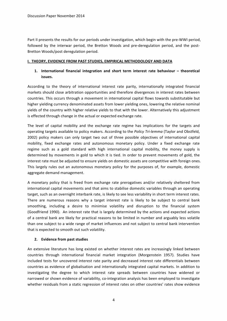
Part II presents the results for our periods under investigation, which begin with the pre-‐WWI period, followed by the interwar period, the Bretton Woods and pre-‐deregulation period, and the post-‐
Bretton Woods/post deregulation period.
I. THEORY, EVIDENCE FROM PAST STUDIES, EMPIRICAL METHODOLOGY AND DATA
1. International financial integration and short term interest rate behaviour – theoretical issues.
According to the theory of international interest rate parity, internationally integrated financial markets should close arbitration opportunities and therefore divergences in interest rates between
countries. This occurs through a movement in international capital flows towards substitutable but higher yielding currency denominated assets from lower yielding ones, lowering the relative nominal yields of the country with higher relative yields to that with the lower. Alternatively this adjustment
is effected through change in the actual or expected exchange rate.
The level of capital mobility and the exchange rate regime has implications for the targets and operating targets available to policy makers. According to the Policy Tri-‐lemma (Taylor and Obstfeld, 2002) policy makers can only target two out of three possible objectives of international capital
mobility, fixed exchange rates and autonomous monetary policy. Under a fixed exchange rate regime such as a gold standard with high international capital mobility, the money supply is determined by movements in gold to which it is tied. In order to prevent movements of gold, the
interest rate must be adjusted to ensure yields on domestic assets are competitive with foreign ones. This largely rules out an autonomous monetary policy for the purposes of, for example, domestic aggregate demand management.
A monetary policy that is freed from exchange rate prerogatives and/or relatively sheltered from international capital movements and that aims to stabilise domestic variables through an operating target, such as an overnight interbank rate, is likely to see less variability in short term interest rates.
There are numerous reasons why a target interest rate is likely to be subject to central bank smoothing, including a desire to minimise volatility and disruption to the financial system (Goodfriend 1990). An interest rate that is largely determined by the actions and expected actions
of a central bank are likely for practical reasons to be limited in number and arguably less volatile than one subject to a wide range of market influences and not subject to central bank intervention that is expected to smooth out such volatility.
2. Evidence from past studies
An extensive literature has long existed on whether interest rates are increasingly linked between
countries through international financial market integration (Morgenstein 1957). Studies have included tests for uncovered interest rate parity and decreased interest rate differentials between countries as evidence of globalisation and internationally integrated capital markets. In addition to
investigating the degree to which interest rate spreads between countries have widened or narrowed or shown evidence of variability, co-‐integration analysis has been employed to investigate whether residuals from a static regression of interest rates on other countries’ rates show evidence

Discussion Paper November 2014
5
of stationarity, that is a long run tendency not to drift apart but move together. In the short run, different dynamic processes affect the rates, but co-‐integration ties them together in the long-‐term.
Tests for uncovered interest rate parity (UIP) have shown a considerable divergence in results and
appear sensitive to the types of interest rates (short or long term, nominal or real) and the country and time samples used (for a review of see Devine 1997). A survey of post Bretton Woods interest rates by Meese and Rogoff (1988, p.941) found that short but not long term nominal and real
interest rates differentials between countries have remained non-‐stationary during the post WWII period. A study by Taylor and Obsfeld (2002) found that real long term interest rate differentials were at their widest and most volatile during the interwar period, and only relatively late into the
post Bretton Woods period did interest rates differentials begin to converge towards levels seen during the pre WWI era of globalisation and historically high levels of international capital market integration. In spite of these wide variations in variability in international interest rate differentials
between historical periods their co-‐integration tests rejected the null hypothesis of residuals’ non-‐stationarity for all periods investigated.
A number of studies have investigated the long-‐term trajectories of key interest rate series to determine whether there has been a change in their variability as an indicator of whether these
rates have been subject to central bank intervention. (Clark 1986, Barsky et al 1987, Goodfriend, 1990, Kugler 1988, Campbell and Hamao, 1992). If central banks remove seasonal and other predictable variation in interest rates, past variables are likely to be poor predictors of future
variables, that is, they are likely to follow a random walk. These studies found that short term interest rate variability showed a marked decrease during WWI, and from 1914 in particular. Stochastic tests also show that interest rates trajectories changed to random walk processes where
seasonal and other such predictable variation was almost entirely removed. Clark (1986) attributes this change to the end of the Gold Standard. Barsky et al (1987), however, attributes this change to
the establishment of the Federal Reserve. In addition, central banks that target the interest rate rather than a monetary aggregate are in particular less likely to tolerate interest rate variability. For example Kugler (1988) finds that US short term interest rates in the post war era are generally
unpredictable and follow a “random walk” process while Swiss and German rates show much more predictability and variability. His reasoning for this apparent difference is that in the former case the Federal Funds Rate is an operating target for US monetary policy, while the latter countries target
high powered money and its stabilisation and in so doing permit much more interest rate variability.
In this study we separate out time samples to roughly correspond phases of intensification and retreat in globalisation and international capital market integration that roughly comply with those demarcated by Schor (1992) and Obstfeld and Taylor (2002) with some adjustment to take into
account changes in Japanese macroeconomic regimes. Obstfeld and Taylor provide a useful tabular summary of their conclusions in terms of the Policy Tri-‐lemma over historical periods, which are reproduced here in Table 1. The following study examines the properties of short term nominal
Japanese interest rate data for periods 1883/1-‐1914/12 which roughly corresponds to the Gold Standard era and its preparation; the World War I (during which Japan was not a combatant) and interwar periods (1914/1-‐1931/12) under which Japan maintained a “suspended gold standard” with
a medium term objective of returning to a sterling peg until it abandoned attempts at Gold Standard restoration altogether and implemented a new macroeconomic regime in 1932; the post WWII pre-‐financial deregulation era during which we demarcate our samples as 1957/1-‐1964/12 and 1966/1
Discussion Paper November 2014
6
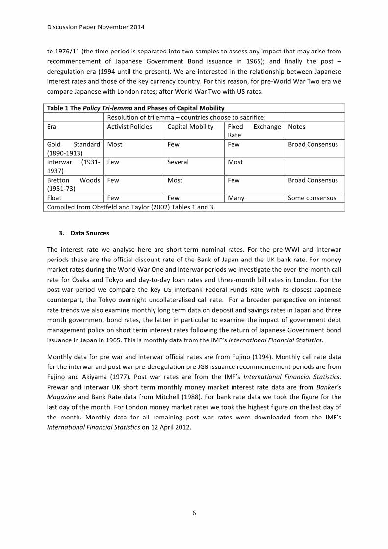
to 1976/11 (the time period is separated into two samples to assess any impact that may arise from recommencement of Japanese Government Bond issuance in 1965); and finally the post –
deregulation era (1994 until the present). We are interested in the relationship between Japanese interest rates and those of the key currency country. For this reason, for pre-‐World War Two era we compare Japanese with London rates; after World War Two with US rates.
Table 1 The Policy Tri-‐lemma and Phases of Capital Mobility Resolution of trilemma – countries choose to sacrifice: Era Activist Policies Capital Mobility Fixed Exchange
Rate Notes
Gold Standard (1890-‐1913)
Most Few Few Broad Consensus
Interwar (1931-‐1937)
Few Several Most
Bretton Woods (1951-‐73)
Few Most Few Broad Consensus
Float Few Few Many Some consensus Compiled from Obstfeld and Taylor (2002) Tables 1 and 3.
3. Data Sources
The interest rate we analyse here are short-‐term nominal rates. For the pre-‐WWI and interwar periods these are the official discount rate of the Bank of Japan and the UK bank rate. For money market rates during the World War One and Interwar periods we investigate the over-‐the-‐month call
rate for Osaka and Tokyo and day-‐to-‐day loan rates and three-‐month bill rates in London. For the post-‐war period we compare the key US interbank Federal Funds Rate with its closest Japanese counterpart, the Tokyo overnight uncollateralised call rate. For a broader perspective on interest
rate trends we also examine monthly long term data on deposit and savings rates in Japan and three month government bond rates, the latter in particular to examine the impact of government debt management policy on short term interest rates following the return of Japanese Government bond
issuance in Japan in 1965. This is monthly data from the IMF’s International Financial Statistics.
Monthly data for pre war and interwar official rates are from Fujino (1994). Monthly call rate data for the interwar and post war pre-‐deregulation pre JGB issuance recommencement periods are from Fujino and Akiyama (1977). Post war rates are from the IMF’s International Financial Statistics.
Prewar and interwar UK short term monthly money market interest rate data are from Banker’s Magazine and Bank Rate data from Mitchell (1988). For bank rate data we took the figure for the last day of the month. For London money market rates we took the highest figure on the last day of
the month. Monthly data for all remaining post war rates were downloaded from the IMF’s International Financial Statistics on 12 April 2012.

Discussion Paper November 2014
7
4. Methodology
In our study we graphically examine the long term trajectories of short term interest rates to determine whether there has been changes in variability in the phases of capital market integration
identified to elucidate whether monetary policy has been used to target interest rates or other domestic variables such as output and prices that would act to smooth out seasonal interest rate volatility and “spikes” in short term interest rates. We then graphically examine foreign and
domestic short term interest rate differentials to determine whether Japanese and foreign interest rates follow similar characteristics and move in parallel-‐wise processes or show significant deviation in their trajectories. The interest rate data is presented graphically in Figures 1 – 10.
1. Econometric models, variables and tests
We then investigate the random walk properties of the interest rate series. A random walk is an
example of a class of trending processes known as integrated processes. An I(0) process is a stationary process with positive and finite long-‐run variance. A process is integrated of order 1, I(1), if its first difference is I(0). Integrated processes involve variables that almost always produce
significant relationships. The following three models describe non-‐stationary processes:
A. Pure random walk
B. Random walk with drift3
C. Trend Stationary Process4
Each of these three series is characterised by a unit root, as such the data generating process can be written as: , where = , and 0, respectively. This equation has a single root
equal to one, hence the name. If we nest all three models in a single equation, then we have:
By subtracting from both sides and introducing the artificial parameter , the equation is:
, where by hypothesis, =1. This
theoretical equation provides the basis for a variety of tests for unit roots in data.
Those tests were developed by Dickey (1976) and Fuller (1976, 1981)5 and are referred to as Dickey-‐Fuller tests. Many alternatives to the DF-‐tests have been suggested, in some cases to improve on the simple finite properties and in others to accommodate more general modelling framework. Said and
Dickey (1984) augmented the basic autoregressive unit root test to accommodate ARMA models with unknown orders and their test is called the augmented Dickey-‐Fuller (ADF) test.
3 The constant term produces the deterministic trend in the random walk with drift. 4 This equation introduces the time trend . 5 Dickey and Fuller (1979), “Distribution of the estimators for autoregressive time series with a unit root”, Journal of the American Statistical Association, pp.427-‐31; Dickey and Fuller (1981), “Likelihood ratio statistics for autoregressive time series with a unit root”, Econometrica, pp.1057-‐72
Discussion Paper November 2014
8
Sargan and Bhargava (1983) developed an alternative test for a unit root based on the Durbin-‐Watson statistic. They show that, on the null hypothesis of a unit root, then DW – > 0 and construct
a test using this statistic. This test is a completely different test with a different null hypothesis than the Durbin-‐Watson test. It is designed for equations with a lagged dependent variable. Critical values
for the test are given in Table 1 of Sargan & Bhargava6.
On the other hand, stationarity tests are for the null that the series are I(0). The most commonly used test, the KPSS test, is due to Kwiatkowski, Phillips, Schmidt and Shin (1992)7. The process
€
zt = zt−1 +ε is a pure random walk and the null
€
H0 :σε2 = 0 , which implies that is a constant.
This stationary test is a one-‐sided right-‐tailed test so that one rejects the null of stationarity at the 100. level if the KPSS test statistic is greater than 100 .
€
(1−α)% quantile from the appropriate
asymptotic distribution.
Following standard practice, we apply a combination of tests to provide a better understanding of
the integrated processes in our analysis.8
2. Co-‐integrated series
In the regression model , the presumption is that are a stationary, white noise series.
This is unlikely to be true, if and are integrated series. If two series are integrated to different
orders, then their linear combinations will be integrated to the higher of the two orders. Intuitively, if two series are both I(1), then the partial difference between them might be stable around a fixed
mean. The implication would be that the series are drifting together at roughly the same rate. Two series that satisfy this requirement are said to be co-‐integrated. The econometric analysis distinguishes between a long-‐run relationship between and , and the short-‐run dynamics.
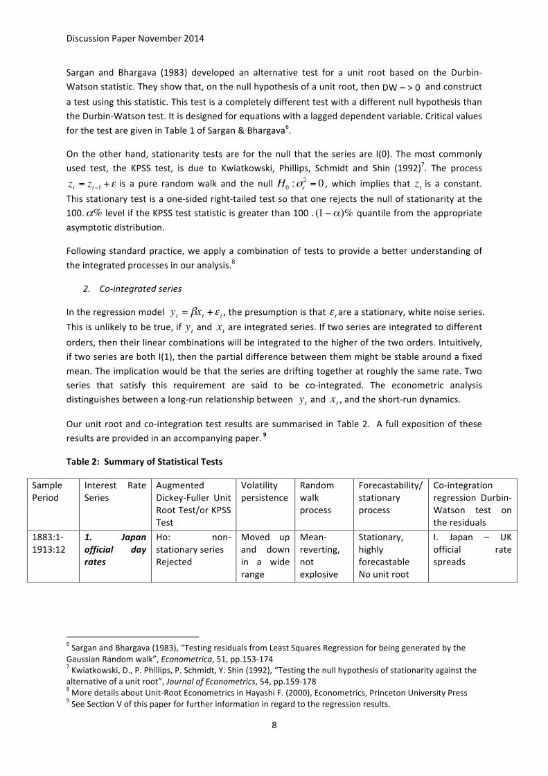
Our unit root and co-‐integration test results are summarised in Table 2. A full exposition of these results are provided in an accompanying paper. 9
Table 2: Summary of Statistical Tests
Sample Period
Interest Rate Series
Augmented Dickey-‐Fuller Unit Root Test/or KPSS Test
Volatility persistence
Random walk process
Forecastability/stationary process
Co-‐integration regression Durbin-‐Watson test on the residuals
1883:1-‐1913:12
1. Japan official day rates
Ho: non-‐stationary series Rejected
Moved up and down in a wide range
Mean-‐reverting, not explosive
Stationary, highly forecastable No unit root
I. Japan – UK official rate spreads
6 Sargan and Bhargava (1983), “Testing residuals from Least Squares Regression for being generated by the Gaussian Random walk”, Econometrica, 51, pp.153-‐174 7 Kwiatkowski, D., P. Phillips, P. Schmidt, Y. Shin (1992), “Testing the null hypothesis of stationarity against the alternative of a unit root”, Journal of Econometrics, 54, pp.159-‐178 8 More details about Unit-‐Root Econometrics in Hayashi F. (2000), Econometrics, Princeton University Press 9 See Section V of this paper for further information in regard to the regression results.

Discussion Paper November 2014
9
2. UK official day rates
Ho: non-‐stationary series Rejected
Moved up and down in a wide range
Mean-‐reverting, not explosive
Stationary, highly forecastable No unit root
Both series are stationary. No co-‐integration.
1. Osaka uncollateralized call rates;
Ho: stationary series – Rejected
Moved up and down in a wide range
A random walk, I(1)
Non-‐stationary; Less forecastable
2. London day-‐to-‐day loan rates;
Ho: stationary series – Cannot be rejected at a conventional significance level
Moved up and down in a narrow range
Mean-‐reverting, not explosive
Stationary, highly forecastable
1914:1-‐1931:12
3. London 3-‐month bank bill rates;
Ho: stationary series – Cannot be rejected at a conventional significance level
Moved up and down in a narrow range
Mean-‐reverting, not explosive
Stationary, highly forecastable
II. Osaka – London day-‐to-‐day yield spreads DW stat = 2.77 Ho: no co-‐integration -‐ Rejected III. Osaka – London 3-‐month bank bill yield spreads DW stat = 2.76 Ho: no co-‐integration -‐ Rejected
1. Japan official rates
Ho: non stationary series -‐ Cannot be rejected at a conventional significance level
Moved smoothly over a wide range
A random walk, I(1)
Non-‐stationary; Less forecastable
1914:1-‐1931:12
2. UK official rates
Ho: non stationary series -‐ Rejected
Moved smoothly over a wide range
Mean-‐reverting, not explosive
Stationary, highly forecastable
IV. Japan – UK official rate spreads DW stat = 1.17 Ho: no co-‐integration -‐ Rejected
1. Tokyo call rates
Ho: stationary series – Rejected
Moved up and down in a wide range
A random walk, I(1)
Non-‐stationary; Less forecastable
1914:1-‐1931:12
2. London 3-‐month bank bill rates;
Ho: stationary series – Not Rejected
Moved up and down in a wide range
Mean-‐reverting, not explosive
Stationary, highly forecastable
V. Tokyo-‐London 3-‐month bank bill yield spreads DW stat = 2.71 Ho: no co-‐integration -‐ Rejected
1957:1-‐1964:12
1. Tokyo call rates
Ho: non stationary series -‐ Cannot be rejected at a conventional significance level
Moved smoothly over a narrow range
A random walk, I(1)
Non-‐stationary; Less forecastable
VI. Tokyo – US Fed Fund yield spreads DW stat = 2.07 Ho: no co-‐

Discussion Paper November 2014
10
2. US Federal Fund Rates
Ho: non stationary series – Rejected at a 10% significance level
Moved smoothly over a narrow range
Mean-‐reverting, not explosive
Stationary, highly forecastable
integration -‐ Rejected
1. Tokyo call rates
Ho: non stationary series -‐ Cannot be rejected at a conventional significance level
Moved more smoothly over a wide range
Series I(2), Higher degree of integration
Non-‐stationary; Less forecastable
1966:10-‐1976:11
2. US Federal Fund Rates
Ho: non stationary series -‐ Cannot be rejected at a conventional significance level
Moved more smoothly over a wide range
A random walk, I(1)
Non-‐stationary; Less forecastable
VII. Tokyo – US Fed Fund yield spreads DW stat = 1.64 Ho: no co-‐integration -‐ Rejected
1. Japan Long-‐term Government Bond Rates
Ho: non stationary series -‐ Cannot be rejected at a conventional significance level
Moved smoothly over a wide range
Series I(2); Higher degree of integration
Non-‐stationary; Less forecastable
1966:10-‐1976:12
2. Tokyo Call Rates
Ho: non stationary series -‐ Cannot be rejected at a conventional significance level
Moved smoothly over a wide range
Series I(2); Higher degree of integration
Non-‐stationary; Less forecastable
VIII. Tokyo – Japan long-‐term bond yield spreads DW stat = 2.897 Ho: no co-‐integration – Rejected
1. Japan Call Rates
Ho: non stationary series -‐ Cannot be rejected at a conventional significance level
Moved smoothly over a narrow range
Series I(2); Higher degree of integration
Non-‐stationary; Less forecastable
1994:1-‐2011:7 (post deregulation)
2. US Federal Fund Rates
Ho: non stationary series -‐ Cannot be rejected at a conventional significance level
Moved smoothly over a wide range
Series I(2); Higher degree of integration
Non-‐stationary; Less forecastable
IX. Japan – US Fed Fund yield spreads DW stat = 2.16 Ho: no co-‐integration Rejected
1994:1-‐2011:7
1. Japan long-‐term Government Bond yields
Ho: non stationary series -‐ Cannot be rejected at a conventional significance level
Moved smoothly over a narrow range
A random walk, I(1)
Non-‐stationary; Less forecastable
X. Japan – US Government Bond yield spreads DW stat = 2.00

Discussion Paper November 2014
11
2. US long-‐term Government Bond yields
Ho: non stationary series -‐ Cannot be rejected at a conventional significance level
Moved more smoothly over a wide range
A random walk, I(1)
Non-‐stationary; Less forecastable
Ho: no co-‐integration -‐ Rejected
1. Japan Deposit Rates
Ho: non stationary series -‐ Cannot be rejected at a conventional significance level
Moved more smoothly over a wide range, and followed by ups & downs in a narrower range
A random walk, I(1)
Non-‐stationary; Less forecastable
1994:1-‐2011:6
2. Japan Lending Rates
Ho: non stationary series -‐ Cannot be rejected at a conventional significance level
Moved more smoothly over a wider range, and followed by ups & downs in a narrower range
A random walk, I(1)
Non-‐stationary; Less forecastable
XI. Deposit – Lending rate spreads DW stat = 1.74 Ho: no co-‐integration – Rejected
Note: 1. The lag-‐order selection criteria from the “vars” package of R, implies an appropriate lag-‐order, based on minimising the AIC and final prediction error.
2. Critical values for a co-‐integration regression Durbin-‐Watson test are given in Sargon J., A. Bhargava (1983), “Testing residuals from least squares regression for being generated by the Gaussian random
walk”, Econometrica Vol. 51, No 1.
II: DISCUSSION OF THE RESULTS: Japanese rates, US and UK rates, 1883 – 2011
1. Pre-‐World War One (1883-‐1913)
We would expect to see a close linkage in the movements of Japanese and UK rates in the pre World War I economy for two reasons. Firstly, the international economy and international financial markets were highly integrated and therefore international capital mobility was high. With high
capital mobility we would expect interest rate parity or movements towards interest rate parity to hold as investors would exploit and then run down available arbitrage opportunities on similar assets between countries. Secondly as Japan was preparing for, or under the Sterling based Gold Standard
for much of this time period (Shinjo 1962) the exchange rate against sterling for much of the period were fixed, ruling out exchange rate adjustment to changes in the balance of payments position. Central banks would also wish to avoid specie depletion from a trade deficit, but given that the

Discussion Paper November 2014
12
exchange rate is fixed, this adjustment would be effected through changes in the central bank’s discount rate.
As most countries were under this fixed exchange rate mechanism and Japan itself was either on the
gold standard or in the process of preparing for its own entry, we would expect that the maintenance of this rate would remove possibilities for the pursuit of an autonomous macro-‐economic policy for the purposes of domestic price and output stabilisation – that is macro
economic policy independent of that with the overriding objective of maintaining the fixed exchange rate. As a consequence considerable interest rate variability may have to be tolerated in the pursuit of this objective. Under the gold standard system, the volume of currency is tied to foreign exchange
reserves. Therefore there is an automatic adjustment mechanism whereby changes in the balance of the external accounts lead to changes in the volume of currency. A central bank can either adjust to these imbalances through specie shipment (generally a last resort), or alternatively raise the or
lower the discount rate to avoid such movement. If the latter approach is taken, we would expect such central bank intervention to be reflected in a reduction the frequency and volatility of interest rate changes in contrast to a situation whereby the interest rate was free to adjust to changes in the
market’s demand and supply for funds.
The trajectories official short term interest rates for the pre World War One era are shown in Figure 1. Both rates appear to fluctuate over a wide range, providing support for the view that interest rates were allowed a fair degree of variability. Seasonal variation is clearly evident in Bank Rate. The
unit root tests, reject the hypothesis of a non-‐stationary series. Both series were mean reverting, non explosive series which were highly forecastable. This again points to arguments that the central bank did not smooth out interest rates to avoid seasonal fluctuations. Rather it raised and lowered
the rates, even on a seasonal and predictable basis, or alternatively they were left to adjust according to market demand.
Fig. 1: Japan official day rates vs. UK official day rates, 1883/01 – 1913/12
International macro-‐economic theory would suggest that with high international capital mobility and a fixed exchange rate there would be a movement towards convergence of interest rates, as
arbitrage opportunities under high capital mobility would be run down and eliminated and under a
0.00 1.00 2.00 3.00 4.00 5.00 6.00 7.00 8.00 9.00 10.00
1883/1
1900/1
ODRJ
ODRUK

Discussion Paper November 2014
13
fixed exchange rate central banks would follow the interest rates of their major trading partners (Goodfriend, 2007, p. 17). Figure 1 shows that both rates converged a number of times during the
sample period, however there does not appear to be evidence of long term movement towards convergence or a stable equilibrating relationship (depicted for example in the two interest rate series moving in parallel). The statistical tests on the pre-‐WWI data do not confirm a long run
process in the differential towards a fixed mean; as both series are stationary, I(0), the residuals cannot be integrated. We may deduce from this that efforts may have been made at such points in time by the Japanese central bank to peg rates with Bank Rate, the key rate in the Sterling based
Gold Standard but there does not appear to be a stable and long run overall tendency towards the convergence of the Bank of Japan official discount rate with Bank Rate or a stable equilibrating relationship between them. Likewise, while interest rates may have responded to market demand
and supply and may have even been adjusted in response to changes in respective trade balances, this adjustment was also not part of a long run equilibrating relationship that tied them together. It is also possible that adjustment to balance of payments imbalances was not through the interest
rate but through specie or related flows (this is discussed in Bruce and Bojkova, forthcoming). In summary, international capital market integration and the integration of goods markets and the fixed exchange rate mechanism was not pulling interest behaviour in synchronised directions or
directions that implied a long term relationship associated with interest rate parity.
2. World War I and the Interwar Period (1914-‐1931)
The period from World War One is conventionally seen as one that witnessed the weakening of the cooperative gold standard system as increasingly more countries eschewed international capital mobility and the fixed exchange rate system in an effort to pursue domestic aggregate demand
stabilisation prerogatives. International financial market integration went into retreat in the context of increasing volatility and speculative movements in exchange rates.
The trajectories of a number of key short-‐term interest rates for the UK and Japan are made in
Figures 2, 3 and 4. Figure 2 compares the Bank of Japan official discount rate with Bank Rate. Key money market rates are compared for both countries in figures 3, 4 and 5. In Figure 2, although slightly reduced compared with WWI, fluctuations in the official Bank of Japan discount rate
continued over a relatively wide range but there was marked reduction in short run volatility compared with the pre-‐WWI period.
Discussion Paper November 2014
14
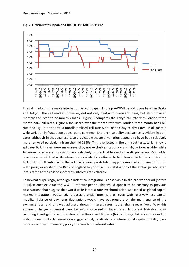
Fig. 2: Official rates Japan and the UK 1914/01-‐1931/12
The call market is the major interbank market in Japan. In the pre-‐WWII period it was based in Osaka and Tokyo. The call market, however, did not only deal with overnight loans, but also provided monthly and even three monthly loans. Figure 3 compares the Tokyo call rate with London three
month bank bill rates, Figure 4 the Osaka over the month rate with London three month bank bill rate and Figure 5 the Osaka uncollateralised call rate with London day to day rates. In all cases a wide variation in fluctuation appeared to continue. Short run volatility persistence is evident in both
cases, although in the Japanese case predictable seasonal variation appears to have been relatively more removed particularly from the mid 1920s. This is reflected in the unit root tests, which show a split result. UK rates were mean reverting, not explosive, stationary and highly forecastable, while
Japanese rates were non-‐stationary, relatively unpredictable random walk processes. Our initial conclusion here is that while interest rate variability continued to be tolerated in both countries, the fact that the UK rates were the relatively more predictable suggests more of continuation in the
willingness, or ability of the Bank of England to prioritise the stabilisation of the exchange rate, even if this came at the cost of short term interest rate volatility.
Somewhat surprisingly, although a lack of co-‐integration is observable in the pre-‐war period (before 1914), it does exist for the WWI – Interwar period. This would appear to be contrary to previous
observations that suggest that world-‐wide interest rate synchronisation weakened as global capital market integration weakened. A possible explanation is that, even with relatively less capital mobility, balance of payments fluctuations would have put pressure on the maintenance of the
exchange rate, and this was adjusted through interest rates, rather than specie flows. Why this apparent change in central bank behaviour occurred in Japan is an important historical point requiring investigation and is addressed in Bruce and Bojkova (forthcoming). Evidence of a random
walk process in the Japanese rate suggests that, relatively less international capital mobility gave more autonomy to monetary policy to smooth out interest rates.
0.00
1.00
2.00
3.00
4.00
5.00
6.00
7.00
8.00
9.00 1914/1
1914/10
1915/7
1916/4
1917/1
1917/10
1918/7
1919/4
1920/1
1920/10
1921/7
1922/4
1923/1
1923/10
1924/7
1925/4
1926/1
1926/10
1927/7
1928/4
1929/1
1929/10
1930/7
1931/4
ODRJ
Bank Rate

Discussion Paper November 2014
15
Fig. 3: Tokyo uncollateralised call rate and London three-‐month bank bill rates 1914/01-‐1931/12
Fig. 4: Osaka uncollateralized call-‐rates vs. London day-‐to-‐day loan rates, 1914/01 – 1931/12
In summary, at first what might seem a counterintuitive explanation emerges from these observations. Evidence of a random walk process in the Japanese rate suggests less low
international capital mobility gave more scope for monetary policy to smooth out predictable changes in interest rates while maintaining or working towards the restoration of a fixed exchange rate compared with the UK case. On the other hand, a movement towards interest rates as a form
of adjustment to payments imbalances led to more synchronisation in interest rate spreads between Japan and key overseas rates compared with the pre-‐WWI period.
0
2
4
6
8
10
12 1914
1925
Tokyo %
London three months bank bills

Discussion Paper November 2014
16
Fig. 5: Osaka uncollateralized call-‐rates vs. London 3-‐month bank bill rates, 1914/01 – 1931/12
3. Bretton Woods pre-‐deregulation (1957-‐1964)
The Post War Two Bretton Woods Era is conventionally seen as one where Keynesian policies were pursued that stabilised aggregate demand with little tolerance for exchange rate instability or
volatile international capital movements. Although monetary policy would be directed towards maintaining the fixed exchange rate, limited international capital mobility would have allowed more freedom to pursue macro-‐economic policy mixes that permitted anti-‐cyclical macroeconomic policy.
Some debate exists about whether Japanese monetary policy showed characteristics of moving towards a more orthodox form of monetary policy familiar in the United States in the post war period; that is moving away from direct liquidity provision by the central bank to one where money
supply was controlled through open market operations that targeted the interbank rate (Kosai, 1989, Bruce, forthcoming).
Figure 6 present the federal funds rate and Tokyo call rates for the periods 1957-‐1976. Notable was
the absence of volatility in the Federal Funds rate over the sample period and in the Japanese call rate after 1957. Although a fixed exchange rate was in place which would have meant the prioritisation of exchange rate rather than interest rate stabilisation, low capital mobility arguably
gave the central bank more scope to implement an interest rate smoothing policy. Although short run volatility was reduced, the range of interest rate fluctuation after a brief spike in the first few years settled into a narrower range. This suggests that the central bank until the mid 1960s, in
addition to engaging in smoothing policy to remove predictable fluctuation, did not permit excessive interest rate variation for the purposes of exchange rate and aggregate demand management.
We have separated the unit root tests for the pre-‐deregulation period to discern if there has been any impact from the recommencement of Japanese government bond issuance in 1966. In the
period from 1957 to 1964 although Figure 6 shows a clear reduction in volatility for the Japanese

Discussion Paper November 2014
17
interbank rate compared with the pre WWII period – suggesting central bank smoothing of the short term interest rate took place. The unit root tests also produced a split result for the US and Japanese
rates. The null hypothesis of a non-‐stationary series was not rejected for the Japanese short-‐term interest rate series but could be rejected for the US series at the 10 per cent significance level. The Federal Reserve is generally seen as targeting the Federal Funds Rate for most of its existence, so at
first sight this result is somewhat surprising.10
Although relative low capital mobility would have reduced tendencies towards interest rate convergence, maintenance of a fixed exchange rate in the absence of specie movements would have limited the degree of interest rate divergence between countries. Figure 6 suggests some degree of
parallel motion in the two series where they do not drift in opposite directions for extended periods between 1957 and 1965 and this is confirmed by the tests on the US-‐Japanese interest rate spreads which reject the null-‐hypothesis of no-‐cointegration.
Fig. 6: Tokyo call-‐rates vs. US Federal Fund rates, 1957/01 – 1976/11
4. Pre-‐deregulation, post Japanese Government Bond recommencement (1966-‐1976)
Until the recommencement of Japanese government bond issuance in 1966 Japan followed a balanced budget rule for fiscal policy. A debate has taken place in respect to this recommencement about whether this marked a further step towards a more conventional form of monetary policy that
used government bonds in open market operations (Kosai, 1989, Horiuchi 1988), or whether monetary policy became increasingly subject to government debt management requirements since the late 1960s. The relationship between the interbank rate and Japanese Government bond yields
following JGB reissuance is shown in Figure 7. It has been argued that the call rate was brought down in preparation for large government bond issuances in the middle 1970s to minimise capital
10 While this is the conventional view, the absence of a clear rejection of non-‐stationarity may be because the Federal Reserve did not use explicit federal funds rate targeting during the 1950s and 1960s, rather the discount rate was adjusted to merely provide a ceiling for other interest rates (Goodfriend and King 1986, fn 12).
0
5
10
15
20
25
1957m01
1957m12
1958m11
1959m10
1960m09
1961m08
1962m07
1963m06
1964m05
1965m04
1966m03
1967m02
1968m01
1968m12
1969m11
1970m10
1971m09
1972m08
1973m07
1974m06
1975m05
1976m04
FF TokyoUCR
Discussion Paper November 2014
18
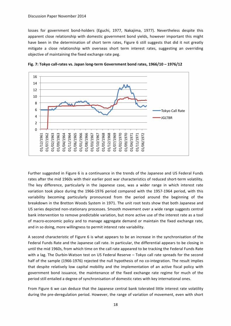
losses for government bond-‐holders (Eguchi, 1977, Nakajima, 1977). Nevertheless despite this apparent close relationship with domestic government bond yields, however important this might
have been in the determination of short term rates, Figure 6 still suggests that did it not greatly mitigate a close relationship with overseas short term interest rates, suggesting an overriding objective of maintaining the fixed exchange rate peg.
Fig. 7: Tokyo call-‐rates vs. Japan long-‐term Government bond rates, 1966/10 – 1976/12
Further suggested in Figure 6 is a continuance in the trends of the Japanese and US Federal Funds rates after the mid 1960s with their earlier post war characteristics of reduced short-‐term volatility. The key difference, particularly in the Japanese case, was a wider range in which interest rate
variation took place during the 1966-‐1976 period compared with the 1957-‐1964 period, with this variability becoming particularly pronounced from the period around the beginning of the breakdown in the Bretton Woods System in 1971. The unit root tests show that both Japanese and
US series depicted non-‐stationary processes. Smooth movement over a wide range suggests central bank intervention to remove predictable variation, but more active use of the interest rate as a tool of macro-‐economic policy and to manage aggregate demand or maintain the fixed exchange rate,
and in so doing, more willingness to permit interest rate variability.
A second characteristic of Figure 6 is what appears to be an increase in the synchronisation of the Federal Funds Rate and the Japanese call rate. In particular, the differential appears to be closing in until the mid 1960s, from which time on the call rate appeared to be tracking the Federal Funds Rate
with a lag. The Durbin-‐Watson test on US Federal Reserve – Tokyo call rate spreads for the second half of the sample (1966-‐1976) rejected the null hypothesis of no co-‐integration. The result implies that despite relatively low capital mobility and the implementation of an active fiscal policy with
government bond issuance, the maintenance of the fixed exchange rate regime for much of the period still entailed a degree of synchronisation of domestic rates with key international ones.
From Figure 6 we can deduce that the Japanese central bank tolerated little interest rate volatility during the pre-‐deregulation period. However, the range of variation of movement, even with short
0
2
4
6
8
10
12
14
16
01/12/1961
01/07/1962
01/02/1963
01/09/1963
01/04/1964
01/11/1964
01/06/1965
01/01/1966
01/08/1966
01/03/1967
01/10/1967
01/05/1968
01/12/1968
01/07/1969
01/02/1970
01/09/1970
01/04/1971
01/11/1971
01/06/1972
Tokyo Call Rate
JGLTBR
Discussion Paper November 2014
19
term predictable volatility removed, began to increase from the beginning of the closing years of the Bretton Woods period and the observation that the Japanese interbank rate began to more closely
follow movements in the Federal Funds rate suggesting a greater willingness to accept interest rate variability for the purposes of maintaining the exchange rate peg rather than aggregate demand related domestic inflation, output and employment goals. In the context of rising inflation, this
would imply that to keep the exchange rate at the fixed rate (which would mean a lower real effective exchange rate), prices would have had to be left to rise, raising nominal interest rates.
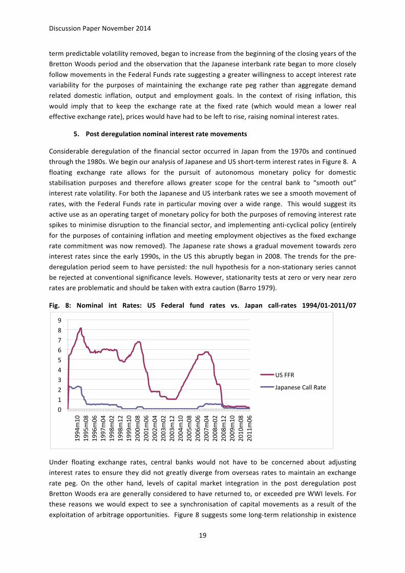
5. Post deregulation nominal interest rate movements
Considerable deregulation of the financial sector occurred in Japan from the 1970s and continued through the 1980s. We begin our analysis of Japanese and US short-‐term interest rates in Figure 8. A
floating exchange rate allows for the pursuit of autonomous monetary policy for domestic stabilisation purposes and therefore allows greater scope for the central bank to “smooth out” interest rate volatility. For both the Japanese and US interbank rates we see a smooth movement of
rates, with the Federal Funds rate in particular moving over a wide range. This would suggest its active use as an operating target of monetary policy for both the purposes of removing interest rate spikes to minimise disruption to the financial sector, and implementing anti-‐cyclical policy (entirely
for the purposes of containing inflation and meeting employment objectives as the fixed exchange rate commitment was now removed). The Japanese rate shows a gradual movement towards zero interest rates since the early 1990s, in the US this abruptly began in 2008. The trends for the pre-‐
deregulation period seem to have persisted: the null hypothesis for a non-‐stationary series cannot be rejected at conventional significance levels. However, stationarity tests at zero or very near zero rates are problematic and should be taken with extra caution (Barro 1979).
Fig. 8: Nominal int Rates: US Federal fund rates vs. Japan call-‐rates 1994/01-‐2011/07
Under floating exchange rates, central banks would not have to be concerned about adjusting interest rates to ensure they did not greatly diverge from overseas rates to maintain an exchange
rate peg. On the other hand, levels of capital market integration in the post deregulation post Bretton Woods era are generally considered to have returned to, or exceeded pre WWI levels. For these reasons we would expect to see a synchronisation of capital movements as a result of the
exploitation of arbitrage opportunities. Figure 8 suggests some long-‐term relationship in existence
0
1
2
3
4
5
6
7
8
9
1994m10
1995m08
1996m06
1997m04
1998m02
1998m12
1999m10
2000m08
2001m06
2002m04
2003m02
2003m12
2004m10
2005m08
2006m06
2007m04
2008m02
2008m12
2009m10
2010m08
2011m06
US FFR
Japanese Call Rate

Discussion Paper November 2014
20
between the two, although perhaps not as clearly evident as in earlier post WWII periods. Nevertheless, the Durbin – Watson test rejects the null hypothesis of no co-‐integration therefore
supporting proposition of internationally integrated financial markets producing a long run stationary relationship on the residuals of the Japanese and US interbank rates. However the caution regarding tests for stationarity at near zero or zero rates also applies here. While capital markets
arguably have returned to a high level of integration, both Japan and the US are large countries with large internal financial markets where domestic factors are still likely to play the dominant role. The fact that both rates converged to zero is arguably a result of the implementation of zero interest rate
policies in the case of Japan after 1999 or quantitative easing policies in the US that pushed the interest rates in their respective countries to their lower bounds. Particularly in view of the problems in drawing conclusions from unit root tests on interest rates at the zero lower bound we argue that,
rather than being a result of capital market integration, the convergence to zero rates in both counties is likely to be associated with more fundamental factors, such as the end of the Golden Age in the 1970s that followed the long post WWII recovery initiated boom (Maddison 1989) and the
subsequent encroachment of “secular stagnation”.
A summary of our conclusions on Japanese short-‐term interest rates are presented in Table 3. In so far as central bank smoothing can equate to monetary policy autonomy and the synchronisation of interest rate spreads with international capital mobility, comparisons can be made with Table 1.
Table 3: Long run tendencies in short term Japanese nominal interest rates – a summary.
Era Fixed Exchange Rate Central bank interest rate smoothing
Synchronisation with foreign interest rates
Pre World War One Gold Standard (1883-‐1913)
Yes No No
WWI and Interwar Period (1914-‐1932)
Yes Yes Yes
Post WWII pre –financial deregulation (1957-‐1964)
Yes Yes Yes
Post WWII pre –financial deregulation post JGB bond issuance (1966-‐1976)
Yes Yes Yes
Post deregulation (1994-‐2011)
No Yes Yes
Notes: “Fixed exchange rates” include the pre-‐WWI preparation period for Gold Standard entry and the interwar period “Suspended Gold Standard”. Japan finally abandoned fixed exchange rates in 1973 and adopted a managed exchange rate system.
An analysis of some other key interest rates may give us further insights into the overall pattern of
Japanese interest rate behaviour in the post-‐deregulation era. An investigation into Japanese and US long term government bond rates show similar profiles, with both moving smoothly over a wide range (Figure 9). Both series were low predictability random walks. A strong relationship appears to
exist between them with what appears to be relatively few occasions where the rates drifted in

Discussion Paper November 2014
21
opposite directions. This is confirmed with the tests on the interest rate differential, which rejected the null hypothesis of no co-‐integration.
Fig. 9: Bond markets – Japan/US 10-‐year yields, 1994/01 – 2011/07
During much of the earlier post war era up until deregulation in the late 1970s, Japan followed an “artificially low” deposit and savings interest rate policy. For much of the Post War High Speed
Growth Period (1955-‐1970) these rates were fixed at 5 per cent. Arguably this was to provide for long low interest loans, particularly for capital investment (Noguchi, 1980). In the post deregulation era we find that these rates essentially behave like the other short term and long term rates in that
they follow a smooth movement and a downward trend (Figure 9 and 10). Both lending and savings rates show a close relationship (Figure 10). The stochastic tests confirmed that these two interest rate series were random walks and co-‐integrated. The close relationship between the various types
of interest rates and the similarities in their profiles suggests that deregulation has closed arbitrage opportunities between different categories of interest rates. This is contrast to the earlier post war
period when great divergences in interest rate trajectories were evident and interest rates appeared to show little relationship to each other due to the segregated markets of the post war high-‐speed growth era (Teranishi, 1982).
Fig. 10: Japanese deposit savings and lending rates, 1994/01 – 2011/06 (Deposit R vs. Lending R)
0 2 4 6 8 10 12 14 16
1994m01
1995m01
1996m01
1997m01
1998m01
1999m01
2000m01
2001m01
2002m01
2003m01
2004m01
2005m01
2006m01
2007m01
2008m01
2009m01
2010m01
2011m01
US long term goverment bond yields
Japanese long term government bond rate
0
1
2
3
4
5
6
7
1994m01
1994m12
1995m11
1996m10
1997m09
1998m08
1999m07
2000m06
2001m05
2002m04
2003m03
2004m02
2005m01
2005m12
2006m11
2007m10
2008m09
2009m08
2010m07
2011m06
Japanese Lending Rates
Japanese Deposit rates

Discussion Paper November 2014
22
III: CONCLUSION
Previous studies that have examined the long term trajectory of interest rate movements in major countries have found that WWI stands out as a once and for all event that led to a permanent
change in interest rate behaviour. Our investigation into nominal Japanese short-‐term interest rates broadly replicates this pattern of behaviour but with the change seemingly to be particularly marked from the period of the mid 1920s. In the pre-‐WWI period, short-‐term interest rates were variable
with predictable short run volatility unremoved. From WWI until the early 1930s the range of interest rate variation remained wide with some continued element of short-‐term volatility; but seasonal and other predictable short-‐term volatility persistence was largely absent, particularly from
about 1925/27. In the post war period, the range of variation was brought down dramatically and short-‐term volatility, both of the regular and reoccurring seasonal form and otherwise, was virtually eliminated. However, while short term volatility was remained suppressed, the range of fluctuation
overall began to increase again in the latter stages of the Bretton Woods era. In the post-‐deregulation era, short-‐term interest rates steadily fell from already low levels towards zero or near zero levels where they settled.
The synchronisation of Japanese interest rates with foreign rates does not closely fit the “arc”
pattern described by major studies into international financial integration – that is a high level of financial integration before WWI followed by a retreat in such integration between WWI and the closing years of the Bretton Woods period in the 1970s, then followed by a return in its intensity
with the float and continued financial deregulation. Rather, Japanese interest rates show continuous long-‐term equilibrium relationships in interest rate spreads from the WWI/interwar period (apart from the years between 1932-‐1955 which was arguably a stand-‐alone period and not examined
here). We broadly attribute this difference in Japan’s profile to its position as a late industrialiser, whereby financial markets were gradually deregulated and internationalised in the process of its
evolution into a market economy integrated into the international system and an increased use of the interest rate by the central bank as a means of adjusting to payments imbalances. A retreat in the process of closer financial integration and assimilation towards overseas monetary policy
practice was repealed during the Bretton Woods and post-‐deregulation era. The narrowing disparity in interest rate spreads that developed in the latter stages of the Bretton Woods period is likely to reflect willingness to allow for price adjustment to maintain a fixed exchange and subsequent
managed exchange rate (rather than a move to revalue in the face of inflation). In the post deregulation era US rates converged towards Japanese ones at the zero or near-‐zero rate; however while the latter tracked a steady decline towards such levels, in the US they were met with more of
an abrupt fall. This latter convergence in spreads, however, is unlikely to be related to international integration, and more to do with fundamentals apparent in their respective domestic economies, of which “secular stagnation” arguments offer a possible explanation.
Nevertheless a more complete understanding of the critical changes we see in Japan’s interest rate
behaviour over time and its relationship with international capital markets call for an enquiry into historical events and institutional structures. This is addressed in Bruce and Bojkova (forthcoming).
Discussion Paper November 2014
23
IV: BIBLIOGRAPHY
Allen, G.C, “The recent currency and exchange policy of Japan”, Economic Journal, 35, March, 1925, pp 66-‐83.
Barro, R., Interest Rate Targetting, Journal of Monetary Economics, 23, 1989, pp 3-‐30.
Barsky, R., Mankiw, G., Miron J., and Weil, D., “The Worldwide change in the Behaviour of Interest
Rates”, NBER Working Paper, No. 2344, 1987.
Bruce, DS, Globalisation and the Japanese Economy (forthcoming).
Bruce, DS and Bojkova, V., “Japanese monetary policy and international financial integration – a long term perspective” (forthcoming).
Campbell, J, and Hamao, Y., “The Interest Rate Process and Term Structure of Interest Rates in Japan”, in Singleton (ed.) Japanese Monetary Policy, University of Chicago Press, Chicago, 1992.
Cargill, M., Political Economy of Japanese Monetary Policy, MIT Press, Cambridge MA, 1997.
Clark, T., “Interest rate seasonality and the Federal Reserve,” Journal of Political Economy, 94(1),
1986, pp 76-‐125.
Devine, M., “The co-‐integration of interest rates”, Technical Paper (Central Bank of Ireland), I/RT/97, 1997.
Dickey D., and Fuller W., “Distribution of the estimators for autoregressive time series with a unit root”, Journal of the American Statistical Association, pp.427-‐31, 1979. Dickey D., and Fuller W., “Likelihood ratio statistics for autoregressive time series with a unit root”, Econometrica, pp.1057-‐72, 1981. Dotsey, M., “Japanese Monetary Policy, A Comparative Analysis, ”, Federal Reserve Bank of Richmond Economic Review, November/December 1986, pp 12-‐24.
Eguchi, H. and Hamada, K., “Banking behavior under constraints”, Japanese Economic Studies, (VI/2), Winter 1978.
Eichengreen B. and Flandreau, M. (ed.) “Cuncliffe Committee on Currency and Foreign Exchanges
after the War,” in Eichengreen, B., and Flandreau, M. (ed.), The Gold Standard in Theory and History, Routledge, London, 1997, pp 213-‐245 .
Eichengreen, B., Golden Fetters, Oxford University Press, Oxford, 1995.
Flath, D., Japanese Economy, Oxford University Press, Oxford, 2005.
Fujino, S., and Akiyama, R., Shouken Kakaku to Rishiritsu [Security Prices and Rates of Interest in Japan 1874-‐1975], Institute of Economic Research, Hitotsubashi, Tokyo, 1977, In Japanese.
Fujino, S., Nihon no Manee Supurai [Japan’s Money Supply], Keisei Shoubou, 1994, Naitoh.

Discussion Paper November 2014
24
Gagnon, J., “Large scale Asset Purchases by the Federal Reserve; Did They Work?”, FRBNY Policy Review, May 2011, pp. 41-‐59.
Garner, A., and Wurtz, R., “Is the Business Cycle Disappearing”, Federal Reserve Bank of Kansas
Economic Review, May/June 1990, pp 25-‐39.
Goodfriend, M., “How the World Achieved Consensus on Monetary Policy”, Journal of Economic Perspectives, 21 (4), 2007, pp 47-‐68.
Goodfriend, M., “Interest on Reserves and Monetary Policy”, FRBNY Economic Policy Review, May 2002.
Goodfriend, M., and King, R., “Financial Deregulation, Monetary Policy and Central Banking”, Federal
Reserve Bank of Richmond Economic Review, May/June 1988, pp 3-‐22.
Goodfriend, M., Interest Rates and the Conduct of Monetary Policy, Federal Reserve Bank of Richmond Working Paper 90-‐6, 1990.
Goto, S., Nihon Tanki Kinyuu Shijou Hatatsu-‐shi (A History of the Development of Japan’s Short Term Financial Markets), Nihon Keizai Hyouronsha, 1986, In Japanese.
Greene, W., Econometric Analysis, Prentice Hall, New Jersey, 2003.
Hatase, M., Did the Structure of Trade and Foreign Debt Affect Reserve Currency Composition?
Evidence from Interwar Japan, IMES Discussion Paper, No. 2009–E–15, 2009.
Hawtrey, GC, A century of bank rate, Longman, London, 1938.
Hayashi, F., Econometrics, Princeton University Press, Princeton NJ, 2000.
Hilton, S., “Trends in Federal Funds Rate Volatility, Current Issues in Economics and Finance (FRBNY), 11(7), 2005, pp 1-‐7.
Hilton, S., “Trends in Federal Funds Rate Volatility”, Current Issues, 11(7), Federal Reserve Bank of
New York, July, 2005.
Hutchinson, M., Ito, T., and Westerman, F., The Great Japanese Stagflation: Lessons for Industrial Countries, MIT Press, Cambridge MA, 2006.
Itoh, K., “Senkanki Nihon Keizai no Makuro Keizai to Mikuro Keizai [The Interwar Japanese Micro and Macro economy”, in Nakamura, T. (Ed.), Senkanki no Nihon Keizai [The Interwar Japanese Economy],
Yamagawa, 1981. In Japanese
Kanamori, H., Kosai, Y., Katou, H., Nihon Keizai Dokuhon [Readings on the Japanese Economy], Touyou Keizai Shinhousha, Tokyo 2010. In Japanese.
Kosai, Y., “Nihon Seichouki Keizai Seisaku [Japanese High Speed Growth Period Macro-‐economic Policy], in Yasuba Y. and Inoki, (ed.) in Koudou Seichoki [High Speed Growth], Iwanami Shouten,
Tokyo, 1989. In Japanese.

Discussion Paper November 2014
25
Kwiatkowski, D., P. Phillips, P. Schmidt, Y. Shin, “Testing the null hypothesis of stationarity against the alternative of a unit root”, Journal of Econometrics, 54, pp.159-‐178, 1992
Maddison, A., Monitoring the World Economy, OECD, Paris, 1995.
Maddison, A., The world economy in the twentieth century, OECD, Paris, 1989.
Mankiw, G., “The Optimal Collection of Seignorage”, Journal of Monetary Economics, 20, September,
1987, pp 3-‐30.
Mankiw, G., and Mirron, J., “The Changing Pattern of the Term Structure of Interest Rates”, Quarterly Journal of Economics, CI (2), 1986, pp 211-‐228.
Masson P., and Mussa M., Long Run Tendencies in Budget Deficits and Debt, IMF Working Paper 95/128, 1995
Metzler M., Capital as Will and Imagination, Cornell University Press, Ithaca, 2013.
Metzler, M., Lever of Empire, the International Gold Standard and the Crisis of Liberalism in Prewar
Japan, UCA Press, Berkeley CA, 2006.
Mitchell, BR, British Historical Statistics, Cambridge University Press, Cambridge, 1988.
Mitsuhashi, T., Seminaru Nihon Keizai Nyuumon (An Introduction to the Japanese Economy), Nikkei, Tokyo, 2008. In Japanese.
Morgenstein, O., International Financial Transactions and Business Cycles, Princeton University Press, Princeton, 1959.
Nakamura T. and Odaka, T., “The Inter-‐war Period: an Overview”, in Nakamura, T. and Odaka T. (Ed.)
The Dual Economy, Oxford University Press, Oxford, 2003. Translated by Noah Brenner.
Noguchi, Y., Zaisei Kiki no Kouzou [The structure of a fiscal crisis], Touyou Keizai Shinposha, Tokyo, 1980. In Japanese.
Obstfeld, M. and Taylor, A., Globalisation and Capital Markets, NBER Working Paper Series, 2002.
Odate, G., Japan’s Financial Relations with the United States, Columbia University/Longman, New
York, 1922.
Okazaki, T. and Okuna F. “Japan’s Present Day Economic System and its Historical Origins”, in
Okazaki T. and Okuna F. (Ed.)、The Origins of the Modern Japanese Economy, Oxford University Press,
Oxford, 1999. Translated by Susan Herbert.
Said, S., and D. Dickey, “Testing for unit roots in Autoregressive moving-‐average models with
unknown order”, Biometrika, 71, 599-‐607, 1984
Sargan and Bhargava, “Testing residuals from Least Squares Regression for being generated by the Gaussian Random walk”, Econometrica, 51, pp.153-‐174, 1983
Discussion Paper November 2014
26
Schor, J, “Introduction”, in Banuri, T., and Schor, J. (ed.), Financial Openness and National Autonomy, Oxford University Press, New Delhi, 1992.
Shiratsuka, S., “Size and Composition of the Central Bank Balance Sheet: Revisiting Japan’s
Experience of the Quantitative Easing Policy”, Monetary and Economic Studies (Bank of Japan), November 2010, pp79-‐105.
Shizumi, M., Economic Developments and Monetary Policy Responses in Interwar Japan, IMES Discussion Paper Series 2002 –E-‐7, July, 2002.
Shizumi, M., “Economic Developments and Monetary Policy Responses in Interwar Japan: Evaluation
Based on the Taylor Rule”, Monetary and Economic Studies, 2002, pp 77-‐116,.
Srour, G., “Why do central banks smooth interest rates”, Bank of Japan Working Paper, 2001 -‐17, October, 2001.
Taylor, A., “A Century of Current Account Dynamics,” Journal of International Money and Finance, 21 ,November, 2002, pp 725–48.
Teranishi, J., Nihon Hatten to Kinyuu, [Japanese Development and Finance], Iwanami Shoten, Tokyo,
1982. In Japanese.
Teranishi, J, Nihon Keizai Shisutemu [The Japanese Economic System], Iwatami Shoten, Tokyo, 2003. In Japanese.
Teranishi, J., “The Development and Transformation of Japan’s Financial System and Monetary Policy”, in Nakamura, T., and Odaka, K. (ed.) The Economic History of Japan (Vol. 3), Oxford
University Press, Oxford, 1999. Translated by N. Brannen.
Throop, A., “International Financial Market Integration and Linkages of National Interest Rates, Federal Reserve Bank of San Francisco Quarterly Review, No. 3, 1994.
Ueda, K., “A Comparative Perspective on Japanese Monetary Policy: Short-‐run Monetary Control and
the Transmission Mechanism,” in Singleton (ed.) Japanese Monetary Policy, University of Chicago Press, Chicago, 1992.
Williamson, J.G., “Globalisation, Convergence and History”, Journal of Economic History, 5 (2), 1996 (6), pp 277-‐307.
Zevin, R., “Are Financial Markets More Open?”, in Banuri, T. and Schor, J. (ed.), Financial Openness
and National Autonomy, Oxford University Press, New Delhi, 1992.
RIIA (Royal Institute of International Affairs Group), Monetary Policy and the Great Depression, Chatham House, London, 1933.

Discussion Paper November 2014
27
V. DETAILED RESULTS
In the addendum to this paper we provide a full description of the unit root tests we have used for this paper. The addendum also provides information on how to access the data used for the
purposes of replication and is accessible at www.gpilondon.com
APPENDIX 1
RESULTS Japan official rates vs. UK official rates
1883/01-‐1913/12
SUMMARY: The ADF test results on the Japanese Official rates show that the series are stationary
during the period 1883-‐1913. They are mean-‐reverse and not integrated, I(0). The KPSS test results show the same fact of stationarity.
The ADF test results on the UK official rates show the same – the UK series for the period 1883-‐1913 are stationary. This means mean-‐reverse, weak, no unit root to drive them, and not integrated, I(0).
The KPSS test results do not reject the null, which proves the same that the UK series are stationary.
Thus, the Japan –UK official rates can’t be cointegrated. No unit root.
DETAILS:
1. Japanese Official Rates 1883-‐1913 ADF Unit Root Test (with 1 lag variable)
Null: of non-‐stationarity (there is a unit root) – ADF results reject the null
Test regression “trend” – with a trend
Call:
lm(formula = z.diff ~ z.lag.1 + 1 + tt + z.diff.lag)
Residuals:
Min 1Q Median 3Q Max
-‐0.98645 -‐0.03527 -‐0.01001 0.02249 2.88332
Coefficients:
Estimate Std. Error t value Pr(>|t|)
(Intercept) -‐0.0286753 0.0278226 -‐1.031 0.303
z.lag.1 -‐0.6703716 0.0723632 -‐9.264 <2e-‐16 ***
tt 0.0001766 0.0001297 1.362 0.174
z.diff.lag 0.0285639 0.0635318 0.450 0.653

Discussion Paper November 2014
28
-‐-‐-‐
Signif. codes: 0 ‘***’ 0.001 ‘**’ 0.01 ‘*’ 0.05 ‘.’ 0.1 ‘ ’ 1
Residual standard error: 0.265 on 365 degrees of freedom
Multiple R-‐squared: 0.2481, Adjusted R-‐squared: 0.2419
F-‐statistic: 40.14 on 3 and 365 DF, p-‐value: < 2.2e-‐16
Value of test-‐statistic is: -‐9.264 28.9917 43.27
Critical values for test statistics:
1pct 5pct 10pct
tau3 -‐3.98 -‐3.42 -‐3.13
phi2 6.15 4.71 4.05
phi3 8.34 6.30 5.36
Test regression “drift” – with an intercept
Call:
lm(formula = z.diff ~ z.lag.1 + 1 + z.diff.lag)
Residuals:
Min 1Q Median 3Q Max
-‐1.01422 -‐0.01384 -‐0.00422 0.00490 2.91578
Coefficients:
Estimate Std. Error t value Pr(>|t|)
(Intercept) 0.00422 0.01382 0.305 0.760
z.lag.1 -‐0.66489 0.07233 -‐9.192 <2e-‐16 ***
z.diff.lag 0.02533 0.06356 0.398 0.691
-‐-‐-‐
Signif. codes: 0 ‘***’ 0.001 ‘**’ 0.01 ‘*’ 0.05 ‘.’ 0.1 ‘ ’ 1
Residual standard error: 0.2653 on 366 degrees of freedom
Multiple R-‐squared: 0.2443, Adjusted R-‐squared: 0.2401
F-‐statistic: 59.15 on 2 and 366 DF, p-‐value: < 2.2e-‐16
Value of test-‐statistic is: -‐9.1918 42.4612
Critical values for test statistics:
1pct 5pct 10pct

Discussion Paper November 2014
29
tau2 -‐3.44 -‐2.87 -‐2.57
phi1 6.47 4.61 3.79
Test regression “none” – neither an intercept nor a trend
Call:
lm(formula = z.diff ~ z.lag.1 -‐ 1 + z.diff.lag)
Residuals:
Min 1Q Median 3Q Max
-‐1.01000 -‐0.00981 0.00000 0.00929 2.92000
Coefficients:
Estimate Std. Error t value Pr(>|t|)
z.lag.1 -‐0.66574 0.07219 -‐9.222 <2e-‐16 ***
z.diff.lag 0.02582 0.06346 0.407 0.684
-‐-‐-‐
Signif. codes: 0 ‘***’ 0.001 ‘**’ 0.01 ‘*’ 0.05 ‘.’ 0.1 ‘ ’ 1
Residual standard error: 0.265 on 367 degrees of freedom
Multiple R-‐squared: 0.2447, Adjusted R-‐squared: 0.2406
F-‐statistic: 59.45 on 2 and 367 DF, p-‐value: < 2.2e-‐16
Value of test-‐statistic is: -‐9.2217
Critical values for test statistics:
1pct 5pct 10pct
tau1 -‐2.58 -‐1.95 -‐1.62
2. KPSS on the Japanese official rates, 1883-‐1913
Null: of stationary series (the results do not reject the null)
TEST with a constant
Test is of type: mu with 5 lags.
Value of test-‐statistic is: 0.1742
Critical value for a significance level of:
10pct 5pct 2.5pct 1pct

Discussion Paper November 2014
30
Critical values 0.347 0.463 0.574 0.739
Test is of type: mu with 16 lags.
Value of test-‐statistic is: 0.1555
Critical value for a significance level of:
10pct 5pct 2.5pct 1pct
Critical values 0.347 0.463 0.574 0.739
TEST with a constant and linear trend
Test is of type: tau with 5 lags.
Value of test-‐statistic is: 0.0665
Critical value for a significance level of:
10pct 5pct 2.5pct 1pct
Critical values 0.119 0.146 0.176 0.216
Test is of type: tau with 16 lags.
Value of test-‐statistic is: 0.06
Critical value for a significance level of:
10pct 5pct 2.5pct 1pct
Critical values 0.119 0.146 0.176 0.216
3. ADF test on the first differenced series (Jap official rates)
Null: of non-‐stationary (the results reject the null)
Test regression “trend”
Call:
lm(formula = z.diff ~ z.lag.1 + 1 + tt + z.diff.lag)
Residuals:
Min 1Q Median 3Q Max
-‐1.0152 -‐0.0897 -‐0.0133 0.0815 2.8894
Coefficients:
Discussion Paper November 2014
31
Estimate Std. Error t value Pr(>|t|)
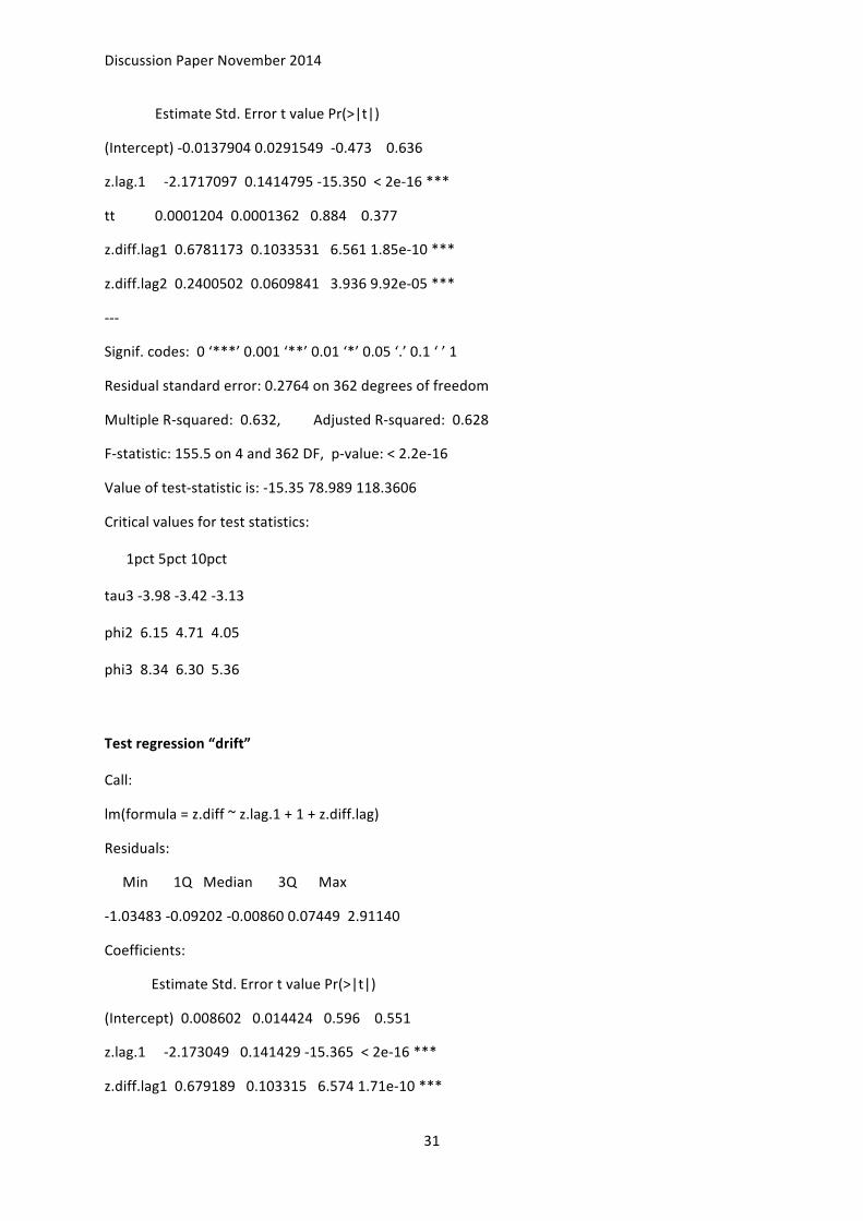
(Intercept) -‐0.0137904 0.0291549 -‐0.473 0.636
z.lag.1 -‐2.1717097 0.1414795 -‐15.350 < 2e-‐16 ***
tt 0.0001204 0.0001362 0.884 0.377
z.diff.lag1 0.6781173 0.1033531 6.561 1.85e-‐10 ***
z.diff.lag2 0.2400502 0.0609841 3.936 9.92e-‐05 ***
-‐-‐-‐
Signif. codes: 0 ‘***’ 0.001 ‘**’ 0.01 ‘*’ 0.05 ‘.’ 0.1 ‘ ’ 1
Residual standard error: 0.2764 on 362 degrees of freedom
Multiple R-‐squared: 0.632, Adjusted R-‐squared: 0.628
F-‐statistic: 155.5 on 4 and 362 DF, p-‐value: < 2.2e-‐16
Value of test-‐statistic is: -‐15.35 78.989 118.3606
Critical values for test statistics:
1pct 5pct 10pct
tau3 -‐3.98 -‐3.42 -‐3.13
phi2 6.15 4.71 4.05
phi3 8.34 6.30 5.36
Test regression “drift”
Call:
lm(formula = z.diff ~ z.lag.1 + 1 + z.diff.lag)
Residuals:
Min 1Q Median 3Q Max
-‐1.03483 -‐0.09202 -‐0.00860 0.07449 2.91140
Coefficients:
Estimate Std. Error t value Pr(>|t|)
(Intercept) 0.008602 0.014424 0.596 0.551
z.lag.1 -‐2.173049 0.141429 -‐15.365 < 2e-‐16 ***
z.diff.lag1 0.679189 0.103315 6.574 1.71e-‐10 ***
Discussion Paper November 2014
32
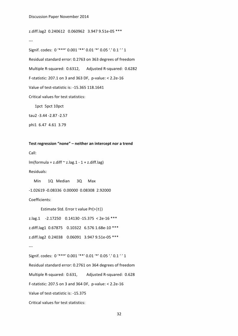
z.diff.lag2 0.240612 0.060962 3.947 9.51e-‐05 ***
-‐-‐-‐
Signif. codes: 0 ‘***’ 0.001 ‘**’ 0.01 ‘*’ 0.05 ‘.’ 0.1 ‘ ’ 1
Residual standard error: 0.2763 on 363 degrees of freedom
Multiple R-‐squared: 0.6312, Adjusted R-‐squared: 0.6282
F-‐statistic: 207.1 on 3 and 363 DF, p-‐value: < 2.2e-‐16
Value of test-‐statistic is: -‐15.365 118.1641
Critical values for test statistics:
1pct 5pct 10pct
tau2 -‐3.44 -‐2.87 -‐2.57
phi1 6.47 4.61 3.79
Test regression “none” – neither an intercept nor a trend
Call:
lm(formula = z.diff ~ z.lag.1 -‐ 1 + z.diff.lag)
Residuals:
Min 1Q Median 3Q Max
-‐1.02619 -‐0.08336 0.00000 0.08308 2.92000
Coefficients:
Estimate Std. Error t value Pr(>|t|)
z.lag.1 -‐2.17250 0.14130 -‐15.375 < 2e-‐16 ***
z.diff.lag1 0.67875 0.10322 6.576 1.68e-‐10 ***
z.diff.lag2 0.24038 0.06091 3.947 9.51e-‐05 ***
-‐-‐-‐
Signif. codes: 0 ‘***’ 0.001 ‘**’ 0.01 ‘*’ 0.05 ‘.’ 0.1 ‘ ’ 1
Residual standard error: 0.2761 on 364 degrees of freedom
Multiple R-‐squared: 0.631, Adjusted R-‐squared: 0.628
F-‐statistic: 207.5 on 3 and 364 DF, p-‐value: < 2.2e-‐16
Value of test-‐statistic is: -‐15.375
Critical values for test statistics:
Discussion Paper November 2014
33
1pct 5pct 10pct
tau1 -‐2.58 -‐1.95 -‐1.62
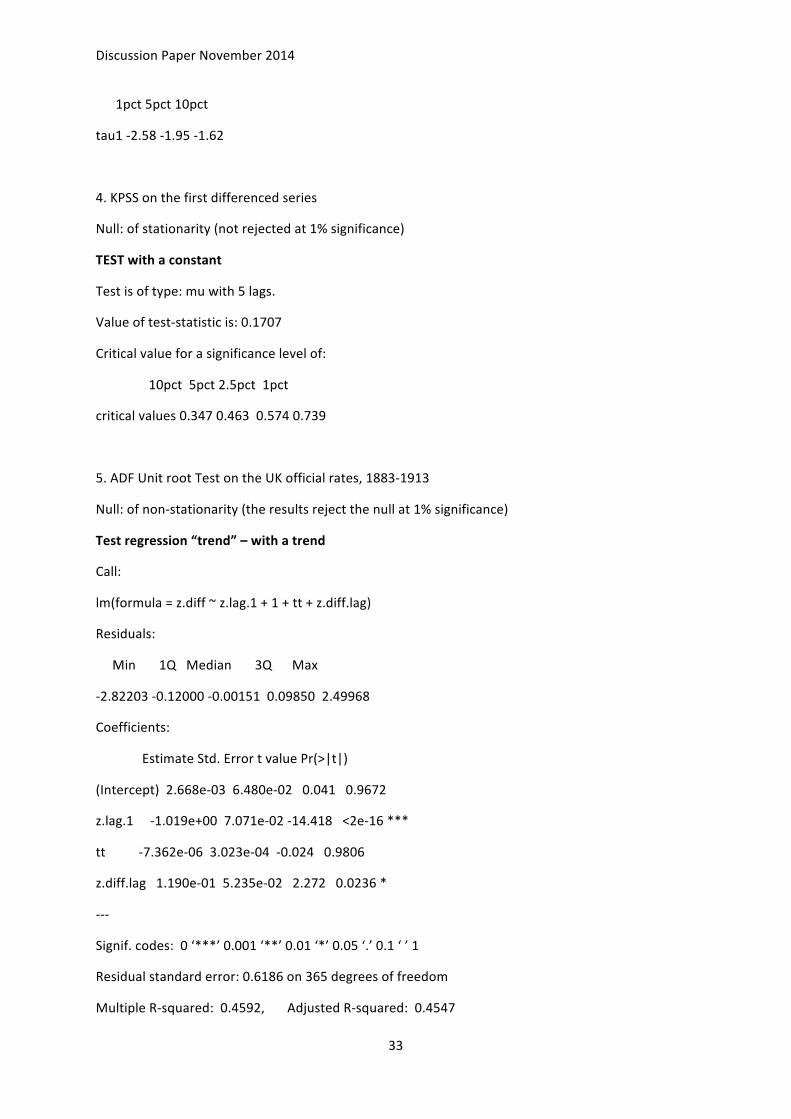
4. KPSS on the first differenced series
Null: of stationarity (not rejected at 1% significance)
TEST with a constant
Test is of type: mu with 5 lags.
Value of test-‐statistic is: 0.1707
Critical value for a significance level of:
10pct 5pct 2.5pct 1pct
critical values 0.347 0.463 0.574 0.739
5. ADF Unit root Test on the UK official rates, 1883-‐1913
Null: of non-‐stationarity (the results reject the null at 1% significance)
Test regression “trend” – with a trend
Call:
lm(formula = z.diff ~ z.lag.1 + 1 + tt + z.diff.lag)
Residuals:
Min 1Q Median 3Q Max
-‐2.82203 -‐0.12000 -‐0.00151 0.09850 2.49968
Coefficients:
Estimate Std. Error t value Pr(>|t|)
(Intercept) 2.668e-‐03 6.480e-‐02 0.041 0.9672
z.lag.1 -‐1.019e+00 7.071e-‐02 -‐14.418 <2e-‐16 ***
tt -‐7.362e-‐06 3.023e-‐04 -‐0.024 0.9806
z.diff.lag 1.190e-‐01 5.235e-‐02 2.272 0.0236 *
-‐-‐-‐
Signif. codes: 0 ‘***’ 0.001 ‘**’ 0.01 ‘*’ 0.05 ‘.’ 0.1 ‘ ’ 1
Residual standard error: 0.6186 on 365 degrees of freedom
Multiple R-‐squared: 0.4592, Adjusted R-‐squared: 0.4547

Discussion Paper November 2014
34
F-‐statistic: 103.3 on 3 and 365 DF, p-‐value: < 2.2e-‐16
Value of test-‐statistic is: -‐14.4176 69.3136 103.9643
Critical values for test statistics:
1pct 5pct 10pct
tau3 -‐3.98 -‐3.42 -‐3.13
phi2 6.15 4.71 4.05
phi3 8.34 6.30 5.36
Test regression “drift”
Call:
lm(formula = z.diff ~ z.lag.1 + 1 + z.diff.lag)
Residuals:
Min 1Q Median 3Q Max
-‐2.82283 -‐0.12028 -‐0.00130 0.09824 2.49870
Coefficients:
Estimate Std. Error t value Pr(>|t|)
(Intercept) 0.001299 0.032159 0.040 0.9678
z.lag.1 -‐1.019443 0.070601 -‐14.439 <2e-‐16 ***
z.diff.lag 0.118978 0.052276 2.276 0.0234 *
-‐-‐-‐
Signif. codes: 0 ‘***’ 0.001 ‘**’ 0.01 ‘*’ 0.05 ‘.’ 0.1 ‘ ’ 1
Residual standard error: 0.6177 on 366 degrees of freedom
Multiple R-‐squared: 0.4592, Adjusted R-‐squared: 0.4562
F-‐statistic: 155.4 on 2 and 366 DF, p-‐value: < 2.2e-‐16
Value of test-‐statistic is: -‐14.4394 104.2547
Critical values for test statistics:
1pct 5pct 10pct
tau2 -‐3.44 -‐2.87 -‐2.57
phi1 6.47 4.61 3.79
Test regression none – neither an intercept nor a trend
Call:

Discussion Paper November 2014
35
lm(formula = z.diff ~ z.lag.1 -‐ 1 + z.diff.lag)
Residuals:
Min 1Q Median 3Q Max
-‐2.82155 -‐0.11897 0.00000 0.09955 2.50000
Coefficients:
Estimate Std. Error t value Pr(>|t|)
z.lag.1 -‐1.0194 0.0705 -‐14.459 <2e-‐16 ***
z.diff.lag 0.1190 0.0522 2.279 0.0232 *
-‐-‐-‐
Signif. codes: 0 ‘***’ 0.001 ‘**’ 0.01 ‘*’ 0.05 ‘.’ 0.1 ‘ ’ 1
Residual standard error: 0.6169 on 367 degrees of freedom
Multiple R-‐squared: 0.4592, Adjusted R-‐squared: 0.4563
F-‐statistic: 155.8 on 2 and 367 DF, p-‐value: < 2.2e-‐16
Value of test-‐statistic is: -‐14.4595
Critical values for test statistics:
1pct 5pct 10pct
tau1 -‐2.58 -‐1.95 -‐1.62
6. KPSS Test on the UK official rates, 1883-‐1913
Null: of stationarity (not rejected, so no unit root)
TEST with a constant
Test is of type: mu with 5 lags.
Value of test-‐statistic is: 0.0097
Critical value for a significance level of:
10pct 5pct 2.5pct 1pct
Critical values 0.347 0.463 0.574 0.739
Test is of type: mu with 16 lags.
Value of test-‐statistic is: 0.0217
Critical value for a significance level of:
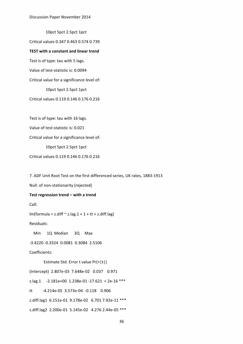
Discussion Paper November 2014
36
10pct 5pct 2.5pct 1pct
Critical values 0.347 0.463 0.574 0.739
TEST with a constant and linear trend
Test is of type: tau with 5 lags.
Value of test-‐statistic is: 0.0094
Critical value for a significance level of:
10pct 5pct 2.5pct 1pct
Critical values 0.119 0.146 0.176 0.216
Test is of type: tau with 16 lags.
Value of test-‐statistic is: 0.021
Critical value for a significance level of:
10pct 5pct 2.5pct 1pct
Critical values 0.119 0.146 0.176 0.216
7. ADF Unit Root Test on the first differenced series, UK rates, 1883-‐1913
Null: of non-‐stationarity (rejected)
Test regression trend – with a trend
Call:
lm(formula = z.diff ~ z.lag.1 + 1 + tt + z.diff.lag)
Residuals:
Min 1Q Median 3Q Max
-‐3.4220 -‐0.3324 0.0081 0.3084 2.5106
Coefficients:
Estimate Std. Error t value Pr(>|t|)
(Intercept) 2.807e-‐03 7.648e-‐02 0.037 0.971
z.lag.1 -‐2.181e+00 1.238e-‐01 -‐17.621 < 2e-‐16 ***
tt -‐4.214e-‐05 3.573e-‐04 -‐0.118 0.906
z.diff.lag1 6.151e-‐01 9.178e-‐02 6.701 7.92e-‐11 ***
z.diff.lag2 2.200e-‐01 5.145e-‐02 4.276 2.44e-‐05 ***
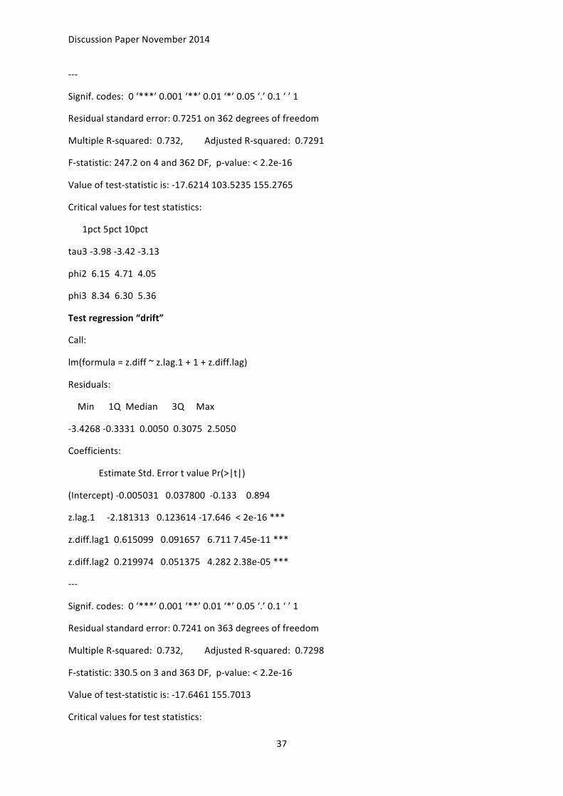
Discussion Paper November 2014
37
-‐-‐-‐
Signif. codes: 0 ‘***’ 0.001 ‘**’ 0.01 ‘*’ 0.05 ‘.’ 0.1 ‘ ’ 1
Residual standard error: 0.7251 on 362 degrees of freedom
Multiple R-‐squared: 0.732, Adjusted R-‐squared: 0.7291
F-‐statistic: 247.2 on 4 and 362 DF, p-‐value: < 2.2e-‐16
Value of test-‐statistic is: -‐17.6214 103.5235 155.2765
Critical values for test statistics:
1pct 5pct 10pct
tau3 -‐3.98 -‐3.42 -‐3.13
phi2 6.15 4.71 4.05
phi3 8.34 6.30 5.36
Test regression “drift”
Call:
lm(formula = z.diff ~ z.lag.1 + 1 + z.diff.lag)
Residuals:
Min 1Q Median 3Q Max
-‐3.4268 -‐0.3331 0.0050 0.3075 2.5050
Coefficients:
Estimate Std. Error t value Pr(>|t|)
(Intercept) -‐0.005031 0.037800 -‐0.133 0.894
z.lag.1 -‐2.181313 0.123614 -‐17.646 < 2e-‐16 ***
z.diff.lag1 0.615099 0.091657 6.711 7.45e-‐11 ***
z.diff.lag2 0.219974 0.051375 4.282 2.38e-‐05 ***
-‐-‐-‐
Signif. codes: 0 ‘***’ 0.001 ‘**’ 0.01 ‘*’ 0.05 ‘.’ 0.1 ‘ ’ 1
Residual standard error: 0.7241 on 363 degrees of freedom
Multiple R-‐squared: 0.732, Adjusted R-‐squared: 0.7298
F-‐statistic: 330.5 on 3 and 363 DF, p-‐value: < 2.2e-‐16
Value of test-‐statistic is: -‐17.6461 155.7013
Critical values for test statistics:
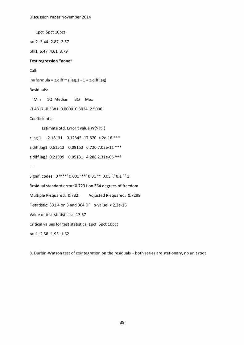
Discussion Paper November 2014
38
1pct 5pct 10pct
tau2 -‐3.44 -‐2.87 -‐2.57
phi1 6.47 4.61 3.79
Test regression “none”
Call:
lm(formula = z.diff ~ z.lag.1 -‐ 1 + z.diff.lag)
Residuals:
Min 1Q Median 3Q Max
-‐3.4317 -‐0.3381 0.0000 0.3024 2.5000
Coefficients:
Estimate Std. Error t value Pr(>|t|)
z.lag.1 -‐2.18131 0.12345 -‐17.670 < 2e-‐16 ***
z.diff.lag1 0.61512 0.09153 6.720 7.02e-‐11 ***
z.diff.lag2 0.21999 0.05131 4.288 2.31e-‐05 ***
-‐-‐-‐
Signif. codes: 0 ‘***’ 0.001 ‘**’ 0.01 ‘*’ 0.05 ‘.’ 0.1 ‘ ’ 1
Residual standard error: 0.7231 on 364 degrees of freedom
Multiple R-‐squared: 0.732, Adjusted R-‐squared: 0.7298
F-‐statistic: 331.4 on 3 and 364 DF, p-‐value: < 2.2e-‐16
Value of test-‐statistic is: -‐17.67
Critical values for test statistics: 1pct 5pct 10pct
tau1 -‐2.58 -‐1.95 -‐1.62
8. Durbin-‐Watson test of cointegration on the residuals – both series are stationary, no unit root

Discussion Paper November 2014
39
APPENDIX 2
RESULTS UK official rates vs. Japan official rates
1914/01-‐1931/12
SUMMARY:
The ADF test results on the Jap call rates show that the unit root exists, so the series follow the random walk hypothesis with one lag variable and I (1) during this period of 1914-‐1931. The KPSS test results show the same.
The ADF test results on the UK official rates are a little bit mixed but still they show that the series are stationary during the period 1914-‐1931. They are mean-‐reverse, weak and not integrated, I (0).
Technically, DW-‐value is 1.17: NULL rejected
DETAILS:
1. Japanese Call rates 1914-‐1931 ADF Unit Root Test (with 1 lag variable)
Null: of non-‐stationarity (there is a unit root)
Test regression “trend” – with a trend
Call:
lm(formula = z.diff ~ z.lag.1 + 1 + tt + z.diff.lag)
Residuals:
Min 1Q Median 3Q Max
-‐0.103691 -‐0.001930 0.000257 0.002842 0.110333
Coefficients:
Estimate Std. Error t value Pr(>|t|)
(Intercept) 3.005e-‐02 1.841e-‐02 1.632 0.104
z.lag.1 -‐1.511e-‐02 9.153e-‐03 -‐1.651 0.100
tt -‐1.400e-‐05 2.584e-‐05 -‐0.542 0.588
z.diff.lag 4.195e-‐01 6.293e-‐02 6.666 2.32e-‐10 ***
-‐-‐-‐
Signif. codes: 0 ‘***’ 0.001 ‘**’ 0.01 ‘*’ 0.05 ‘.’ 0.1 ‘ ’ 1
Residual standard error: 0.02189 on 208 degrees of freedom
Multiple R-‐squared: 0.1805, Adjusted R-‐squared: 0.1687
F-‐statistic: 15.28 on 3 and 208 DF, p-‐value: 5.092e-‐09
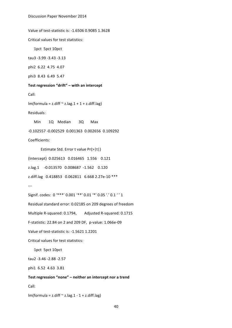
Discussion Paper November 2014
40
Value of test-‐statistic is: -‐1.6506 0.9085 1.3628
Critical values for test statistics:
1pct 5pct 10pct
tau3 -‐3.99 -‐3.43 -‐3.13
phi2 6.22 4.75 4.07
phi3 8.43 6.49 5.47
Test regression “drift” – with an intercept
Call:
lm(formula = z.diff ~ z.lag.1 + 1 + z.diff.lag)
Residuals:
Min 1Q Median 3Q Max
-‐0.102557 -‐0.002529 0.001363 0.002656 0.109292
Coefficients:
Estimate Std. Error t value Pr(>|t|)
(Intercept) 0.025613 0.016465 1.556 0.121
z.lag.1 -‐0.013570 0.008687 -‐1.562 0.120
z.diff.lag 0.418853 0.062811 6.668 2.27e-‐10 ***
-‐-‐-‐
Signif. codes: 0 ‘***’ 0.001 ‘**’ 0.01 ‘*’ 0.05 ‘.’ 0.1 ‘ ’ 1
Residual standard error: 0.02185 on 209 degrees of freedom
Multiple R-‐squared: 0.1794, Adjusted R-‐squared: 0.1715
F-‐statistic: 22.84 on 2 and 209 DF, p-‐value: 1.066e-‐09
Value of test-‐statistic is: -‐1.5621 1.2201
Critical values for test statistics:
1pct 5pct 10pct
tau2 -‐3.46 -‐2.88 -‐2.57
phi1 6.52 4.63 3.81
Test regression “none” – neither an intercept nor a trend
Call:
lm(formula = z.diff ~ z.lag.1 -‐ 1 + z.diff.lag)

Discussion Paper November 2014
41
Residuals:
Min 1Q Median 3Q Max
-‐0.102277 0.000192 0.000224 0.000235 0.112953
Coefficients:
Estimate Std. Error t value Pr(>|t|)
z.lag.1 -‐0.0001127 0.0007944 -‐0.142 0.887
z.diff.lag 0.4121244 0.0628738 6.555 4.24e-‐10 ***
-‐-‐-‐
Signif. codes: 0 ‘***’ 0.001 ‘**’ 0.01 ‘*’ 0.05 ‘.’ 0.1 ‘ ’ 1
Residual standard error: 0.02192 on 210 degrees of freedom
Multiple R-‐squared: 0.1699, Adjusted R-‐squared: 0.162
F-‐statistic: 21.49 on 2 and 210 DF, p-‐value: 3.235e-‐09
Value of test-‐statistic is: -‐0.1419
Critical values for test statistics: 1pct 5pct 10pct
tau1 -‐2.58 -‐1.95 -‐1.62
2. KPSS on the Jap call rates, 1914-‐1931
Null: of stationary series (the results reject the null)
TEST with a constant
Test is of type: mu with 4 lags.
Value of test-‐statistic is: 0.9598
Critical value for a significance level of:
10pct 5pct 2.5pct 1pct
critical values 0.347 0.463 0.574 0.739
Test is of type: mu with 14 lags.
Value of test-‐statistic is: 0.3476
Critical value for a significance level of: 10pct 5pct 2.5pct 1pct
critical values 0.347 0.463 0.574 0.739
TEST with a constant and linear trend

Discussion Paper November 2014
42
Test is of type: tau with 4 lags.
Value of test-‐statistic is: 0.6795
Critical value for a significance level of:
10pct 5pct 2.5pct 1pct
critical values 0.119 0.146 0.176 0.216
Test is of type: tau with 14 lags.
Value of test-‐statistic is: 0.2465
Critical value for a significance level of:
10pct 5pct 2.5pct 1pct
critical values 0.119 0.146 0.176 0.216
3. ADF test on the first differenced series (Jap call rates)
Null: of non-‐stationary is rejected. The series are integrated of degree 1.
Test regression “trend”
Call:
lm(formula = z.diff ~ z.lag.1 + 1 + tt + z.diff.lag)
Residuals:
Min 1Q Median 3Q Max
-‐0.102755 -‐0.000047 0.000001 0.000055 0.112851
Coefficients:
Estimate Std. Error t value Pr(>|t|)
(Intercept) 8.640e-‐05 3.116e-‐03 0.028 0.978
z.lag.1 -‐5.900e-‐01 7.540e-‐02 -‐7.825 2.57e-‐13 ***
tt -‐7.949e-‐07 2.496e-‐05 -‐0.032 0.975
z.diff.lag 3.483e-‐03 6.959e-‐02 0.050 0.960
-‐-‐-‐
Signif. codes: 0 ‘***’ 0.001 ‘**’ 0.01 ‘*’ 0.05 ‘.’ 0.1 ‘ ’ 1
Residual standard error: 0.02208 on 207 degrees of freedom
Multiple R-‐squared: 0.294, Adjusted R-‐squared: 0.2837

Discussion Paper November 2014
43
F-‐statistic: 28.73 on 3 and 207 DF, p-‐value: 1.423e-‐15
Value of test-‐statistic is: -‐7.8251 20.4112 30.6166
Critical values for test statistics:
1pct 5pct 10pct
tau3 -‐3.99 -‐3.43 -‐3.13
phi2 6.22 4.75 4.07
phi3 8.43 6.49 5.47
Test regression “drift”
Call:
lm(formula = z.diff ~ z.lag.1 + 1 + z.diff.lag)
Residuals:
Min 1Q Median 3Q Max
-‐0.1027 0.0000 0.0000 0.0000 0.1128
Coefficients:
Estimate Std. Error t value Pr(>|t|)
(Intercept) -‐2.519e-‐07 1.517e-‐03 0.000 1.00
z.lag.1 -‐5.900e-‐01 7.521e-‐02 -‐7.844 2.25e-‐13 ***
z.diff.lag 3.466e-‐03 6.942e-‐02 0.050 0.96
-‐-‐-‐
Signif. codes: 0 ‘***’ 0.001 ‘**’ 0.01 ‘*’ 0.05 ‘.’ 0.1 ‘ ’ 1
Residual standard error: 0.02203 on 208 degrees of freedom
Multiple R-‐squared: 0.294, Adjusted R-‐squared: 0.2872
F-‐statistic: 43.3 on 2 and 208 DF, p-‐value: < 2.2e-‐16
Value of test-‐statistic is: -‐7.844 30.764
Critical values for test statistics:
1pct 5pct 10pct
tau2 -‐3.46 -‐2.88 -‐2.57
phi1 6.52 4.63 3.81
Test regression “none”
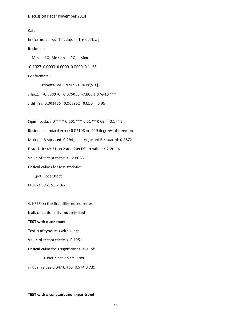
Discussion Paper November 2014
44
Call:
lm(formula = z.diff ~ z.lag.1 -‐ 1 + z.diff.lag)
Residuals:
Min 1Q Median 3Q Max
-‐0.1027 0.0000 0.0000 0.0000 0.1128
Coefficients:
Estimate Std. Error t value Pr(>|t|)
z.lag.1 -‐0.589970 0.075033 -‐7.863 1.97e-‐13 ***
z.diff.lag 0.003466 0.069252 0.050 0.96
-‐-‐-‐
Signif. codes: 0 ‘***’ 0.001 ‘**’ 0.01 ‘*’ 0.05 ‘.’ 0.1 ‘ ’ 1
Residual standard error: 0.02198 on 209 degrees of freedom
Multiple R-‐squared: 0.294, Adjusted R-‐squared: 0.2872
F-‐statistic: 43.51 on 2 and 209 DF, p-‐value: < 2.2e-‐16
Value of test-‐statistic is: -‐7.8628
Critical values for test statistics:
1pct 5pct 10pct
tau1 -‐2.58 -‐1.95 -‐1.62
4. KPSS on the first differenced series
Null: of stationarity (not rejected)
TEST with a constant
Test is of type: mu with 4 lags.
Value of test-‐statistic is: 0.1251
Critical value for a significance level of:
10pct 5pct 2.5pct 1pct
critical values 0.347 0.463 0.574 0.739
TEST with a constant and linear trend
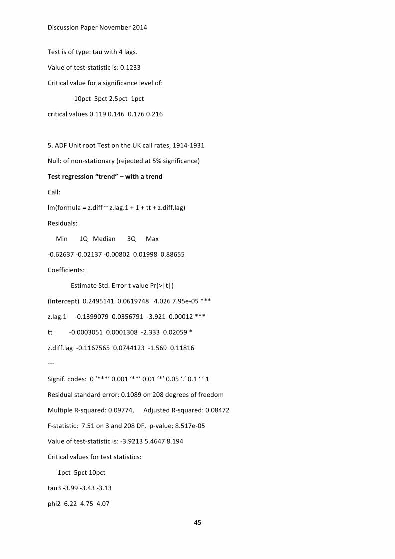
Discussion Paper November 2014
45
Test is of type: tau with 4 lags.
Value of test-‐statistic is: 0.1233
Critical value for a significance level of:
10pct 5pct 2.5pct 1pct
critical values 0.119 0.146 0.176 0.216
5. ADF Unit root Test on the UK call rates, 1914-‐1931
Null: of non-‐stationary (rejected at 5% significance)
Test regression “trend” – with a trend
Call:
lm(formula = z.diff ~ z.lag.1 + 1 + tt + z.diff.lag)
Residuals:
Min 1Q Median 3Q Max
-‐0.62637 -‐0.02137 -‐0.00802 0.01998 0.88655
Coefficients:
Estimate Std. Error t value Pr(>|t|)
(Intercept) 0.2495141 0.0619748 4.026 7.95e-‐05 ***
z.lag.1 -‐0.1399079 0.0356791 -‐3.921 0.00012 ***
tt -‐0.0003051 0.0001308 -‐2.333 0.02059 *
z.diff.lag -‐0.1167565 0.0744123 -‐1.569 0.11816
-‐-‐-‐
Signif. codes: 0 ‘***’ 0.001 ‘**’ 0.01 ‘*’ 0.05 ‘.’ 0.1 ‘ ’ 1
Residual standard error: 0.1089 on 208 degrees of freedom
Multiple R-‐squared: 0.09774, Adjusted R-‐squared: 0.08472
F-‐statistic: 7.51 on 3 and 208 DF, p-‐value: 8.517e-‐05
Value of test-‐statistic is: -‐3.9213 5.4647 8.194
Critical values for test statistics:
1pct 5pct 10pct
tau3 -‐3.99 -‐3.43 -‐3.13
phi2 6.22 4.75 4.07

Discussion Paper November 2014
46
phi3 8.43 6.49 5.47
Test regression “drift” – with an intercept
Call:
lm(formula = z.diff ~ z.lag.1 + 1 + z.diff.lag)
Residuals:
Min 1Q Median 3Q Max
-‐0.66600 -‐0.01770 0.00704 0.00704 0.93151
Coefficients:
Estimate Std. Error t value Pr(>|t|)
(Intercept) 0.17053 0.05246 3.251 0.00134 **
z.lag.1 -‐0.11033 0.03370 -‐3.273 0.00124 **
z.diff.lag -‐0.12795 0.07504 -‐1.705 0.08968 .
-‐-‐-‐
Signif. codes: 0 ‘***’ 0.001 ‘**’ 0.01 ‘*’ 0.05 ‘.’ 0.1 ‘ ’ 1
Residual standard error: 0.1101 on 209 degrees of freedom
Multiple R-‐squared: 0.07412, Adjusted R-‐squared: 0.06526
F-‐statistic: 8.365 on 2 and 209 DF, p-‐value: 0.0003199
Value of test-‐statistic is: -‐3.2735 5.3609
Critical values for test statistics:
1pct 5pct 10pct
tau2 -‐3.46 -‐2.88 -‐2.57
phi1 6.52 4.63 3.81
Test regression “none”
Call:
lm(formula = z.diff ~ z.lag.1 -‐ 1 + z.diff.lag)
Residuals:
Min 1Q Median 3Q Max
-‐0.68971 0.00211 0.00309 0.00309 0.98294
Coefficients:
Estimate Std. Error t value Pr(>|t|)
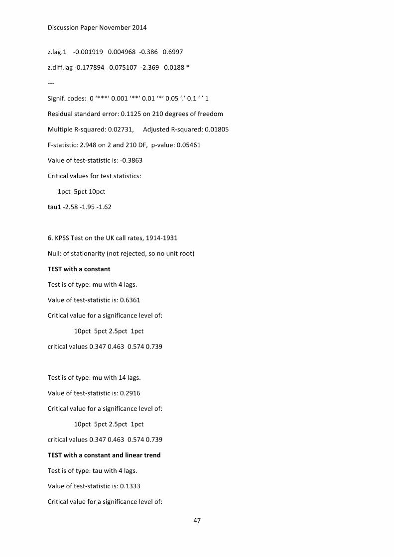
Discussion Paper November 2014
47
z.lag.1 -‐0.001919 0.004968 -‐0.386 0.6997
z.diff.lag -‐0.177894 0.075107 -‐2.369 0.0188 *
-‐-‐-‐
Signif. codes: 0 ‘***’ 0.001 ‘**’ 0.01 ‘*’ 0.05 ‘.’ 0.1 ‘ ’ 1
Residual standard error: 0.1125 on 210 degrees of freedom
Multiple R-‐squared: 0.02731, Adjusted R-‐squared: 0.01805
F-‐statistic: 2.948 on 2 and 210 DF, p-‐value: 0.05461
Value of test-‐statistic is: -‐0.3863
Critical values for test statistics:
1pct 5pct 10pct
tau1 -‐2.58 -‐1.95 -‐1.62
6. KPSS Test on the UK call rates, 1914-‐1931
Null: of stationarity (not rejected, so no unit root)
TEST with a constant
Test is of type: mu with 4 lags.
Value of test-‐statistic is: 0.6361
Critical value for a significance level of:
10pct 5pct 2.5pct 1pct
critical values 0.347 0.463 0.574 0.739
Test is of type: mu with 14 lags.
Value of test-‐statistic is: 0.2916
Critical value for a significance level of:
10pct 5pct 2.5pct 1pct
critical values 0.347 0.463 0.574 0.739
TEST with a constant and linear trend
Test is of type: tau with 4 lags.
Value of test-‐statistic is: 0.1333
Critical value for a significance level of:
Discussion Paper November 2014
48
10pct 5pct 2.5pct 1pct
critical values 0.119 0.146 0.176 0.216
Test is of type: tau with 14 lags.
Value of test-‐statistic is: 0.0656
Critical value for a significance level of:
10pct 5pct 2.5pct 1pct
critical values 0.119 0.146 0.176 0.216
7. Durbin-‐Watson test of cointegration
Null of no cointegration
> dwtest(creg)
DW = 1.1739, p-‐value = 5.934e-‐10
APPENDIX 3
RESULTS Tokyo rates vs. London 3-‐month bank rates
1914/01 – 1931/12
SUMMARY:
Tokyo rate series are non-‐stationary according to the KPSS results (the ADF test does not run due to the NA values). They are also integrated of degree 1. London rate series are stationary. Technically, DW-‐value is 2.7: NULL rejected
DETAILS:
I. KPSS Test on Tokyo rates, 1914-‐1931
Null: of stationary (it’s rejected) – the rates are non-‐stationary or explosive
TEST with a constant
Test is of type: mu with 14 lags.
Value of test-‐statistic is: 0.2779
Critical value for a significance level of:
10pct 5pct 2.5pct 1pct

Discussion Paper November 2014
49
critical values 0.347 0.463 0.574 0.739
Test is of type: mu with 4 lags.
Value of test-‐statistic is: 0.6941
Critical value for a significance level of:
10pct 5pct 2.5pct 1pct
critical values 0.347 0.463 0.574 0.739
TEST with a constant and linear trend
Test is of type: tau with 4 lags.
Value of test-‐statistic is: 0.6409
Critical value for a significance level of:
10pct 5pct 2.5pct 1pct
critical values 0.119 0.146 0.176 0.216
Test is of type: tau with 14 lags.
Value of test-‐statistic is: 0.2581
Critical value for a significance level of:
10pct 5pct 2.5pct 1pct
critical values 0.119 0.146 0.176 0.216
II. KPSS Test on the first-‐differentiated Tokyo rates
Null: of stationary (not rejected) – the series are of type I(1)
TEST with a constant
Test is of type: mu with 4 lags.
Value of test-‐statistic is: 0.0375
Critical value for a significance level of:
10pct 5pct 2.5pct 1pct
critical values 0.347 0.463 0.574 0.739
Test is of type: mu with 14 lags.

Discussion Paper November 2014
50
Value of test-‐statistic is: 0.0503
Critical value for a significance level of:
10pct 5pct 2.5pct 1pct
critical values 0.347 0.463 0.574 0.739
TEST with a constant and linear trend
Test is of type: tau with 4 lags.
Value of test-‐statistic is: 0.0379
Critical value for a significance level of:
10pct 5pct 2.5pct 1pct
critical values 0.119 0.146 0.176 0.216
Test is of type: tau with 14 lags.
Value of test-‐statistic is: 0.0508
Critical value for a significance level of:
10pct 5pct 2.5pct 1pct
critical values 0.119 0.146 0.176 0.216
III. KPSS Test results on London 3-‐month bank bill rates , 1914-‐1931
Null: of stationary (it is not rejected at 1% statistical significance)
TEST with a constant
Test is of type: mu with 14 lags.
Value of test-‐statistic is: 0.0701
Critical value for a significance level of:
10pct 5pct 2.5pct 1pct
critical values 0.347 0.463 0.574 0.739
Test is of type: mu with 4 lags.
Value of test-‐statistic is: 0.1429
Critical value for a significance level of:
10pct 5pct 2.5pct 1pct
Discussion Paper November 2014
51
critical values 0.347 0.463 0.574 0.739
TEST with a constant and linear trend
Test is of type: tau with 14 lags.
Value of test-‐statistic is: 0.0576
Critical value for a significance level of:
10pct 5pct 2.5pct 1pct
critical values 0.119 0.146 0.176 0.216
Test is of type: tau with 4 lags.
Value of test-‐statistic is: 0.1166
Critical value for a significance level of:
10pct 5pct 2.5pct 1pct
critical values 0.119 0.146 0.176 0.216
IV. KPSS Test on the first differentiated rates of London
Null: of stationary (not rejected) – the series are of type I(1)
TEST with a constant
Test is of type: mu with 4 lags.
Value of test-‐statistic is: 0.0651
Critical value for a significance level of:
10pct 5pct 2.5pct 1pct
critical values 0.347 0.463 0.574 0.739
Test is of type: mu with 14 lags.
Value of test-‐statistic is: 0.0996
Critical value for a significance level of:
10pct 5pct 2.5pct 1pct
critical values 0.347 0.463 0.574 0.739
TEST with a constant and linear trend

Discussion Paper November 2014
52
Test is of type: tau with 4 lags.
Value of test-‐statistic is: 0.0266
Critical value for a significance level of:
10pct 5pct 2.5pct 1pct
critical values 0.119 0.146 0.176 0.216
Test is of type: tau with 14 lags.
Value of test-‐statistic is: 0.0414
Critical value for a significance level of:
10pct 5pct 2.5pct 1pct
critical values 0.119 0.146 0.176 0.216
V. DW regression on the residuals, NULL: no co-‐integration
Durbin-‐Watson test
DW = 2.7147, p-‐value = 1
APPENDIX 4
RESULTS Osaka unconditional call rates vs London day-‐to-‐day loan rates
RESULTS Osaka unconditional call rates vs London 3-‐month bank bill rates
1914/01-‐1931/12
SUMMARY: The KPSS test results on the Osaka Uncollateralized Call rates demonstrate that the series are non-‐stationary and integrated I(1). Graphically, the series look non-‐stationary/explosive.
The test results on the London day-‐to-‐day loan rates demonstrate clearly that they are stationary, mean-‐reverting.
The test results on the London 3-‐month bank bill rates demonstrate clearly that they are stationary, mean-‐reverting.
DW stat is 2.77 for the Osaka call rates vs. London day-‐to-‐day loan rates. DW stat is 2.76 for the Osaka call rates vs. London 3-‐month bank bill rates.
DETAILS:

Discussion Paper November 2014
53
I. KPSS Test on the Osaka uncollateralized call rates, 1914-‐1931
Null: of stationary series (it is rejected) – the Osaka call rates are non-‐stationary or explosive.
TEST with a constant
Test is of type: mu with 14 lags.
Value of test-‐statistic is: 0.2938
Critical value for a significance level of:
10pct 5pct 2.5pct 1pct
critical values 0.347 0.463 0.574 0.739
Test is of type: mu with 4 lags.
Value of test-‐statistic is: 0.7455
Critical value for a significance level of:
10pct 5pct 2.5pct 1pct
critical values 0.347 0.463 0.574 0.739
TEST with a constant and linear trend
Test is of type: tau with 14 lags.
Value of test-‐statistic is: 0.2899
Critical value for a significance level of:
10pct 5pct 2.5pct 1pct
critical values 0.119 0.146 0.176 0.216
Test is of type: tau with 4 lags.
Value of test-‐statistic is: 0.7363
Critical value for a significance level of:
10pct 5pct 2.5pct 1pct
critical values 0.119 0.146 0.176 0.216
II. KPSS on the first differenced series of Osaka Uncollateralized call rates
Null: of stationary series (not rejected) – the series are integrated of degree 1.
TEST with a constant

Discussion Paper November 2014
54
Test is of type: mu with 14 lags.
Value of test-‐statistic is: 0.0732
Critical value for a significance level of:
10pct 5pct 2.5pct 1pct
critical values 0.347 0.463 0.574 0.739
Test is of type: mu with 4 lags.
Value of test-‐statistic is: 0.0515
Critical value for a significance level of:
10pct 5pct 2.5pct 1pct
critical values 0.347 0.463 0.574 0.739
TEST with a constant and linear trend
Test is of type: tau with 4 lags.
Value of test-‐statistic is: 0.0564
Critical value for a significance level of:
10pct 5pct 2.5pct 1pct
critical values 0.119 0.146 0.176 0.216
Test is of type: tau with 14 lags.
Value of test-‐statistic is: 0.0799
Critical value for a significance level of:
10pct 5pct 2.5pct 1pct
critical values 0.119 0.146 0.176 0.216
III. KPSS Test on the London day-‐to-‐day loan rates, 1914-‐1931
Null: of stationary series (it is not rejected at 1% statistical significance); series are mean-‐reverted.
1. TEST with a constant
Test is of type: mu with 14 lags.
Value of test-‐statistic is: 0.1152
Discussion Paper November 2014
55
Critical value for a significance level of:
10pct 5pct 2.5pct 1pct
critical values 0.347 0.463 0.574 0.739
Test is of type: mu with 4 lags.
Value of test-‐statistic is: 0.227
Critical value for a significance level of:
10pct 5pct 2.5pct 1pct
critical values 0.347 0.463 0.574 0.739
2. TEST with a constant and linear trend
Test is of type: tau with 14 lags.
Value of test-‐statistic is: 0.0552
Critical value for a significance level of:
10pct 5pct 2.5pct 1pct
critical values 0.119 0.146 0.176 0.216
Test is of type: tau with 4 lags.
Value of test-‐statistic is: 0.1077
Critical value for a significance level of:
10pct 5pct 2.5pct 1pct
critical values 0.119 0.146 0.176 0.216
IV. KPSS Test results on London 3-‐month bank bill rates
Null: of stationary (it is not rejected at 1% statistical significance)
TEST with a constant
Test is of type: mu with 14 lags.
Value of test-‐statistic is: 0.0701
Critical value for a significance level of:
Discussion Paper November 2014
56
10pct 5pct 2.5pct 1pct
critical values 0.347 0.463 0.574 0.739
Test is of type: mu with 4 lags.
Value of test-‐statistic is: 0.1429
Critical value for a significance level of:
10pct 5pct 2.5pct 1pct
critical values 0.347 0.463 0.574 0.739
TEST with a constant and linear trend
Test is of type: tau with 14 lags.
Value of test-‐statistic is: 0.0576
Critical value for a significance level of:
10pct 5pct 2.5pct 1pct
critical values 0.119 0.146 0.176 0.216
Test is of type: tau with 4 lags.
Value of test-‐statistic is: 0.1166
Critical value for a significance level of:
10pct 5pct 2.5pct 1pct
critical values 0.119 0.146 0.176 0.216
V. DW Test of cointegration
5.1 Co-‐integration between Osaka rates and London day-‐to-‐day loan rates
Durbin-‐Watson test
data: creg
DW = 2.7756, p-‐value = 1
5.2 Co-‐integration between Osaka rates and London 3-‐motn bank bills

Discussion Paper November 2014
57
Durbin-‐Watson test
data: creg1
DW = 2.7696, p-‐value = 1
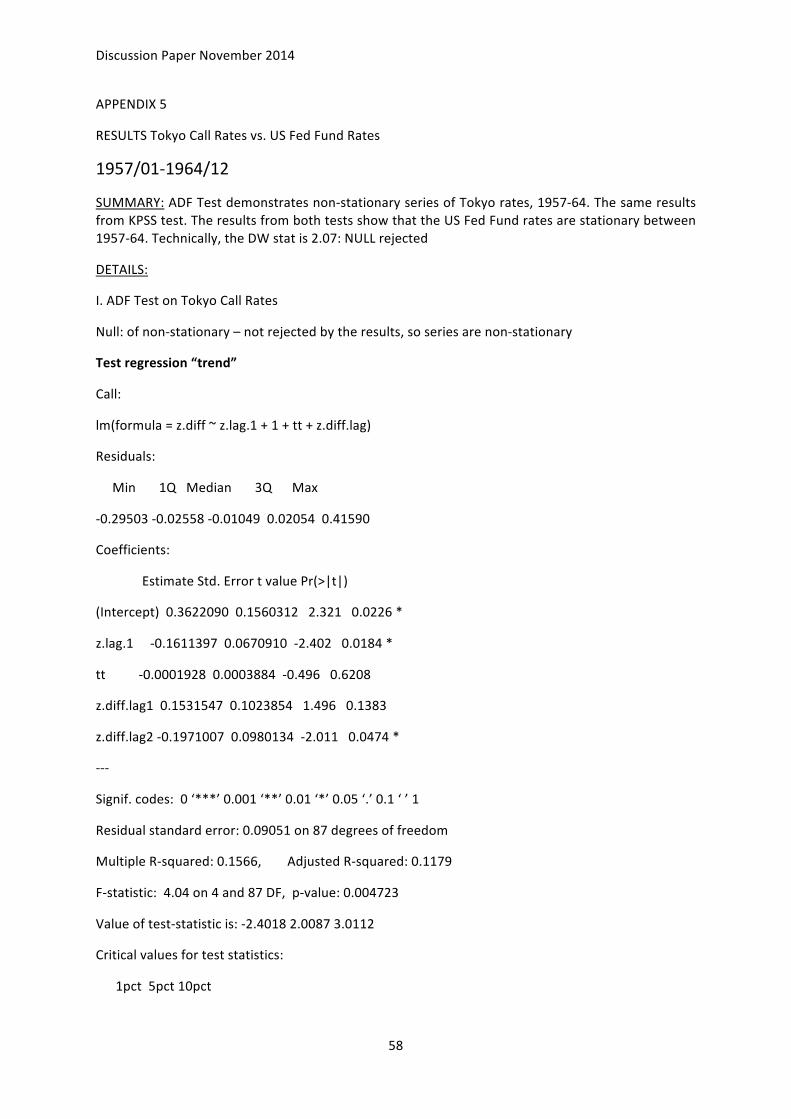
Discussion Paper November 2014
58
APPENDIX 5
RESULTS Tokyo Call Rates vs. US Fed Fund Rates
1957/01-‐1964/12
SUMMARY: ADF Test demonstrates non-‐stationary series of Tokyo rates, 1957-‐64. The same results from KPSS test. The results from both tests show that the US Fed Fund rates are stationary between 1957-‐64. Technically, the DW stat is 2.07: NULL rejected
DETAILS:
I. ADF Test on Tokyo Call Rates
Null: of non-‐stationary – not rejected by the results, so series are non-‐stationary
Test regression “trend”
Call:
lm(formula = z.diff ~ z.lag.1 + 1 + tt + z.diff.lag)
Residuals:
Min 1Q Median 3Q Max
-‐0.29503 -‐0.02558 -‐0.01049 0.02054 0.41590
Coefficients:
Estimate Std. Error t value Pr(>|t|)
(Intercept) 0.3622090 0.1560312 2.321 0.0226 *
z.lag.1 -‐0.1611397 0.0670910 -‐2.402 0.0184 *
tt -‐0.0001928 0.0003884 -‐0.496 0.6208
z.diff.lag1 0.1531547 0.1023854 1.496 0.1383
z.diff.lag2 -‐0.1971007 0.0980134 -‐2.011 0.0474 *
-‐-‐-‐
Signif. codes: 0 ‘***’ 0.001 ‘**’ 0.01 ‘*’ 0.05 ‘.’ 0.1 ‘ ’ 1
Residual standard error: 0.09051 on 87 degrees of freedom
Multiple R-‐squared: 0.1566, Adjusted R-‐squared: 0.1179
F-‐statistic: 4.04 on 4 and 87 DF, p-‐value: 0.004723
Value of test-‐statistic is: -‐2.4018 2.0087 3.0112
Critical values for test statistics:
1pct 5pct 10pct
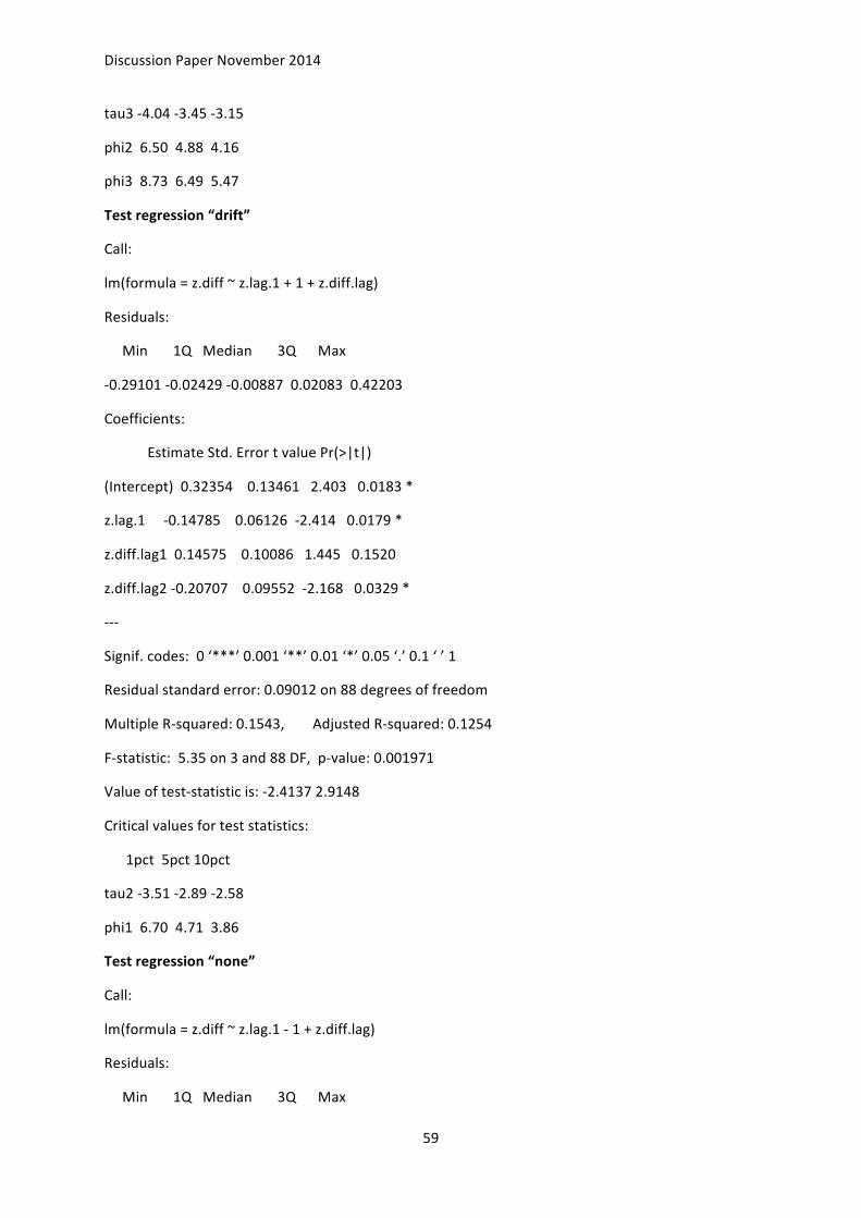
Discussion Paper November 2014
59
tau3 -‐4.04 -‐3.45 -‐3.15
phi2 6.50 4.88 4.16
phi3 8.73 6.49 5.47
Test regression “drift”
Call:
lm(formula = z.diff ~ z.lag.1 + 1 + z.diff.lag)
Residuals:
Min 1Q Median 3Q Max
-‐0.29101 -‐0.02429 -‐0.00887 0.02083 0.42203
Coefficients:
Estimate Std. Error t value Pr(>|t|)
(Intercept) 0.32354 0.13461 2.403 0.0183 *
z.lag.1 -‐0.14785 0.06126 -‐2.414 0.0179 *
z.diff.lag1 0.14575 0.10086 1.445 0.1520
z.diff.lag2 -‐0.20707 0.09552 -‐2.168 0.0329 *
-‐-‐-‐
Signif. codes: 0 ‘***’ 0.001 ‘**’ 0.01 ‘*’ 0.05 ‘.’ 0.1 ‘ ’ 1
Residual standard error: 0.09012 on 88 degrees of freedom
Multiple R-‐squared: 0.1543, Adjusted R-‐squared: 0.1254
F-‐statistic: 5.35 on 3 and 88 DF, p-‐value: 0.001971
Value of test-‐statistic is: -‐2.4137 2.9148
Critical values for test statistics:
1pct 5pct 10pct
tau2 -‐3.51 -‐2.89 -‐2.58
phi1 6.70 4.71 3.86
Test regression “none”
Call:
lm(formula = z.diff ~ z.lag.1 -‐ 1 + z.diff.lag)
Residuals:
Min 1Q Median 3Q Max

Discussion Paper November 2014
60
-‐0.35808 -‐0.01421 0.00210 0.01360 0.40481
Coefficients:
Estimate Std. Error t value Pr(>|t|)
z.lag.1 -‐0.0009853 0.0043922 -‐0.224 0.82301
z.diff.lag1 0.0703155 0.0983900 0.715 0.47669
z.diff.lag2 -‐0.2802458 0.0929389 -‐3.015 0.00334 **
-‐-‐-‐
Signif. codes: 0 ‘***’ 0.001 ‘**’ 0.01 ‘*’ 0.05 ‘.’ 0.1 ‘ ’ 1
Residual standard error: 0.09251 on 89 degrees of freedom
Multiple R-‐squared: 0.09876, Adjusted R-‐squared: 0.06838
F-‐statistic: 3.251 on 3 and 89 DF, p-‐value: 0.02549
Value of test-‐statistic is: -‐0.2243
Critical values for test statistics:
1pct 5pct 10pct
tau1 -‐2.6 -‐1.95 -‐1.61
II. ADF on the first differenced series of Tokyo Rates
Null: of non-‐stationary – the null is rejected by the results, the series are of type I(1)
Test regression “trend”
Call:
lm(formula = z.diff ~ z.lag.1 + 1 + tt + z.diff.lag)
Residuals:
Min 1Q Median 3Q Max
-‐0.313424 -‐0.016075 0.008181 0.025189 0.307497
Coefficients:
Estimate Std. Error t value Pr(>|t|)
(Intercept) -‐0.0333364 0.0172293 -‐1.935 0.05629 .
z.lag.1 -‐1.4544901 0.1583850 -‐9.183 2.08e-‐14 ***
tt 0.0005717 0.0003105 1.841 0.06900 .
z.diff.lag1 0.3141874 0.1158392 2.712 0.00807 **
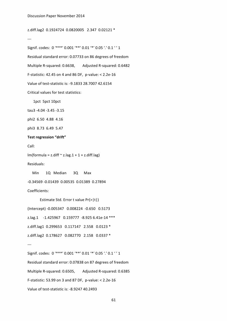
Discussion Paper November 2014
61
z.diff.lag2 0.1924724 0.0820005 2.347 0.02121 *
-‐-‐-‐
Signif. codes: 0 ‘***’ 0.001 ‘**’ 0.01 ‘*’ 0.05 ‘.’ 0.1 ‘ ’ 1
Residual standard error: 0.07733 on 86 degrees of freedom
Multiple R-‐squared: 0.6638, Adjusted R-‐squared: 0.6482
F-‐statistic: 42.45 on 4 and 86 DF, p-‐value: < 2.2e-‐16
Value of test-‐statistic is: -‐9.1833 28.7007 42.6154
Critical values for test statistics:
1pct 5pct 10pct
tau3 -‐4.04 -‐3.45 -‐3.15
phi2 6.50 4.88 4.16
phi3 8.73 6.49 5.47
Test regression “drift”
Call:
lm(formula = z.diff ~ z.lag.1 + 1 + z.diff.lag)
Residuals:
Min 1Q Median 3Q Max
-‐0.34569 -‐0.01439 0.00535 0.01389 0.27894
Coefficients:
Estimate Std. Error t value Pr(>|t|)
(Intercept) -‐0.005347 0.008224 -‐0.650 0.5173
z.lag.1 -‐1.425967 0.159777 -‐8.925 6.41e-‐14 ***
z.diff.lag1 0.299653 0.117147 2.558 0.0123 *
z.diff.lag2 0.178627 0.082770 2.158 0.0337 *
-‐-‐-‐
Signif. codes: 0 ‘***’ 0.001 ‘**’ 0.01 ‘*’ 0.05 ‘.’ 0.1 ‘ ’ 1
Residual standard error: 0.07838 on 87 degrees of freedom
Multiple R-‐squared: 0.6505, Adjusted R-‐squared: 0.6385
F-‐statistic: 53.99 on 3 and 87 DF, p-‐value: < 2.2e-‐16
Value of test-‐statistic is: -‐8.9247 40.2493

Discussion Paper November 2014
62
Critical values for test statistics:
1pct 5pct 10pct
tau2 -‐3.51 -‐2.89 -‐2.58
phi1 6.70 4.71 3.86
Test regression “none”
Call:
lm(formula = z.diff ~ z.lag.1 -‐ 1 + z.diff.lag)
Residuals:
Min 1Q Median 3Q Max
-‐0.34971 -‐0.01990 0.00000 0.00856 0.27433
Coefficients:
Estimate Std. Error t value Pr(>|t|)
z.lag.1 -‐1.4291 0.1592 -‐8.978 4.56e-‐14 ***
z.diff.lag1 0.3021 0.1167 2.589 0.0113 *
z.diff.lag2 0.1790 0.0825 2.170 0.0327 *
-‐-‐-‐
Signif. codes: 0 ‘***’ 0.001 ‘**’ 0.01 ‘*’ 0.05 ‘.’ 0.1 ‘ ’ 1
Residual standard error: 0.07813 on 88 degrees of freedom
Multiple R-‐squared: 0.6499, Adjusted R-‐squared: 0.638
F-‐statistic: 54.46 on 3 and 88 DF, p-‐value: < 2.2e-‐16
Value of test-‐statistic is: -‐8.978
Critical values for test statistics:
1pct 5pct 10pct
tau1 -‐2.6 -‐1.95 -‐1.61
III. KPSS Test
Null: of stationary series – is rejected by some of the results (with 3 lags), which reconfirms the results of the ADF Test that the Tokyo rate series are non-‐stationary.
TEST with a constant
Test is of type: mu with 3 lags.
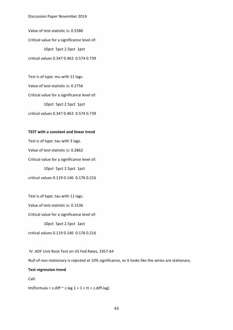
Discussion Paper November 2014
63
Value of test-‐statistic is: 0.5586
Critical value for a significance level of:
10pct 5pct 2.5pct 1pct
critical values 0.347 0.463 0.574 0.739
Test is of type: mu with 11 lags.
Value of test-‐statistic is: 0.2756
Critical value for a significance level of:
10pct 5pct 2.5pct 1pct
critical values 0.347 0.463 0.574 0.739
TEST with a constant and linear trend
Test is of type: tau with 3 lags.
Value of test-‐statistic is: 0.2862
Critical value for a significance level of:
10pct 5pct 2.5pct 1pct
critical values 0.119 0.146 0.176 0.216
Test is of type: tau with 11 lags.
Value of test-‐statistic is: 0.1536
Critical value for a significance level of:
10pct 5pct 2.5pct 1pct
critical values 0.119 0.146 0.176 0.216
IV. ADF Unit Root Test on US Fed Rates, 1957-‐64
Null of non-‐stationary is rejected at 10% significance, so it looks like the series are stationary.
Test regression trend
Call:
lm(formula = z.diff ~ z.lag.1 + 1 + tt + z.diff.lag)
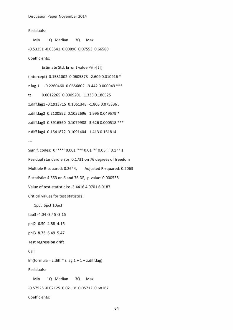
Discussion Paper November 2014
64
Residuals:
Min 1Q Median 3Q Max
-‐0.53351 -‐0.03541 0.00896 0.07553 0.66580
Coefficients:
Estimate Std. Error t value Pr(>|t|)
(Intercept) 0.1581002 0.0605873 2.609 0.010916 *
z.lag.1 -‐0.2260460 0.0656802 -‐3.442 0.000943 ***
tt 0.0012265 0.0009201 1.333 0.186525
z.diff.lag1 -‐0.1913715 0.1061348 -‐1.803 0.075336 .
z.diff.lag2 0.2100592 0.1052696 1.995 0.049579 *
z.diff.lag3 0.3916560 0.1079988 3.626 0.000518 ***
z.diff.lag4 0.1541872 0.1091404 1.413 0.161814
-‐-‐-‐
Signif. codes: 0 ‘***’ 0.001 ‘**’ 0.01 ‘*’ 0.05 ‘.’ 0.1 ‘ ’ 1
Residual standard error: 0.1731 on 76 degrees of freedom
Multiple R-‐squared: 0.2644, Adjusted R-‐squared: 0.2063
F-‐statistic: 4.553 on 6 and 76 DF, p-‐value: 0.000538
Value of test-‐statistic is: -‐3.4416 4.0701 6.0187
Critical values for test statistics:
1pct 5pct 10pct
tau3 -‐4.04 -‐3.45 -‐3.15
phi2 6.50 4.88 4.16
phi3 8.73 6.49 5.47
Test regression drift
Call:
lm(formula = z.diff ~ z.lag.1 + 1 + z.diff.lag)
Residuals:
Min 1Q Median 3Q Max
-‐0.57525 -‐0.02125 0.02118 0.05712 0.68167
Coefficients:

Discussion Paper November 2014
65
Estimate Std. Error t value Pr(>|t|)
(Intercept) 0.16043 0.05551 2.890 0.00498 **
z.lag.1 -‐0.15954 0.05447 -‐2.929 0.00446 **
z.diff.lag1 -‐0.17976 0.10488 -‐1.714 0.09049 .
z.diff.lag2 0.21145 0.10567 2.001 0.04888 *
z.diff.lag3 0.33376 0.10273 3.249 0.00171 **
-‐-‐-‐
Signif. codes: 0 ‘***’ 0.001 ‘**’ 0.01 ‘*’ 0.05 ‘.’ 0.1 ‘ ’ 1
Residual standard error: 0.1746 on 78 degrees of freedom
Multiple R-‐squared: 0.2317, Adjusted R-‐squared: 0.1923
F-‐statistic: 5.882 on 4 and 78 DF, p-‐value: 0.0003441
Value of test-‐statistic is: -‐2.9288 4.3731
Critical values for test statistics:
1pct 5pct 10pct
tau2 -‐3.51 -‐2.89 -‐2.58
phi1 6.70 4.71 3.86
Test regression none
Call:
lm(formula = z.diff ~ z.lag.1 -‐ 1 + z.diff.lag)
Residuals:
Min 1Q Median 3Q Max
-‐0.50184 -‐0.01431 0.01933 0.05858 0.85634
Coefficients:
Estimate Std. Error t value Pr(>|t|)
z.lag.1 -‐0.01179 0.01967 -‐0.599 0.5507
z.diff.lag1 -‐0.26336 0.10540 -‐2.499 0.0145 *
z.diff.lag2 0.13654 0.10711 1.275 0.2061
z.diff.lag3 0.26774 0.10471 2.557 0.0125 *
-‐-‐-‐
Signif. codes: 0 ‘***’ 0.001 ‘**’ 0.01 ‘*’ 0.05 ‘.’ 0.1 ‘ ’ 1

Discussion Paper November 2014
66
Residual standard error: 0.1825 on 79 degrees of freedom
Multiple R-‐squared: 0.1506, Adjusted R-‐squared: 0.1076
F-‐statistic: 3.501 on 4 and 79 DF, p-‐value: 0.01102
Value of test-‐statistic is: -‐0.5993
Critical values for test statistics:
1pct 5pct 10pct
tau1 -‐2.6 -‐1.95 -‐1.61
V. KPSS Unit Root Test on the US Fed rates, 1957-‐64
Null of stationary is not rejected, so these test results confirm that the US Fed rates are stationary.
TEST with a constant
Test is of type: mu with 3 lags.
Value of test-‐statistic is: 0.3418
Critical value for a significance level of:
10pct 5pct 2.5pct 1pct
critical values 0.347 0.463 0.574 0.739
Test is of type: mu with 11 lags.
Value of test-‐statistic is: 0.1823
Critical value for a significance level of:
10pct 5pct 2.5pct 1pct
critical values 0.347 0.463 0.574 0.739
TEST with a constant and linear trend
Test is of type: tau with 3 lags.
Value of test-‐statistic is: 0.0956
Critical value for a significance level of:
10pct 5pct 2.5pct 1pct
critical values 0.119 0.146 0.176 0.216

Discussion Paper November 2014
67
Test is of type: tau with 11 lags.
Value of test-‐statistic is: 0.0553
Critical value for a significance level of:
10pct 5pct 2.5pct 1pct
critical values 0.119 0.146 0.176 0.216
VI. DW Test of co-‐integration
Null: of no co-‐integration
Durbin-‐Watson test
DW = 2.0675, p-‐value = 0.6385
APPENDIX 6
RESULTS US Fed Fund Rates vs Tokyo Call Rates
1966/01 – 1976/11
SUMMARY: Tokyo Call rate series are non-‐stationary of type I(2), a higher degree of integration. The US Fed Fund rates are non-‐stationary of type I(1) with a unit root. Theoretically, they can be co-‐integrated of degree 2. Technically, DW stat is 1.64, NULL rejected
DETAILS:
I. ADF Test for Unit Root on Tokyo Call Rates, 1966-‐76
Null: of non-‐stationary – it is not rejected, the series are non-‐stationary.
Test regression “trend”
Call:
lm(formula = z.diff ~ z.lag.1 + 1 + tt + z.diff.lag)
Residuals:
Min 1Q Median 3Q Max
-‐0.190361 -‐0.031721 -‐0.001307 0.025927 0.119760
Coefficients:
Estimate Std. Error t value Pr(>|t|)

Discussion Paper November 2014
68
(Intercept) 0.061223 0.030725 1.993 0.048539 *
z.lag.1 -‐0.029954 0.016210 -‐1.848 0.067041 .
tt -‐0.000028 0.000121 -‐0.231 0.817320
z.diff.lag1 0.188240 0.091655 2.054 0.042134 *
z.diff.lag2 0.081557 0.094926 0.859 0.391933
z.diff.lag3 0.357279 0.093365 3.827 0.000206 ***
-‐-‐-‐
Signif. codes: 0 ‘***’ 0.001 ‘**’ 0.01 ‘*’ 0.05 ‘.’ 0.1 ‘ ’ 1
Residual standard error: 0.04662 on 122 degrees of freedom
Multiple R-‐squared: 0.2079, Adjusted R-‐squared: 0.1755
F-‐statistic: 6.405 on 5 and 122 DF, p-‐value: 2.56e-‐05
Value of test-‐statistic is: -‐1.8479 1.4733 2.1933
Critical values for test statistics:
1pct 5pct 10pct
tau3 -‐3.99 -‐3.43 -‐3.13
phi2 6.22 4.75 4.07
phi3 8.43 6.49 5.47
Test regression “drift”
Call:
lm(formula = z.diff ~ z.lag.1 + 1 + z.diff.lag)
Residuals:
Min 1Q Median 3Q Max
-‐0.192148 -‐0.031249 -‐0.001482 0.026104 0.120631
Coefficients:
Estimate Std. Error t value Pr(>|t|)
(Intercept) 0.06212 0.03037 2.046 0.04293 *
z.lag.1 -‐0.03134 0.01500 -‐2.090 0.03871 *
z.diff.lag1 0.18935 0.09118 2.077 0.03991 *
z.diff.lag2 0.08345 0.09421 0.886 0.37742
z.diff.lag3 0.35978 0.09238 3.895 0.00016 ***

Discussion Paper November 2014
69
-‐-‐-‐
Signif. codes: 0 ‘***’ 0.001 ‘**’ 0.01 ‘*’ 0.05 ‘.’ 0.1 ‘ ’ 1
Residual standard error: 0.04644 on 123 degrees of freedom
Multiple R-‐squared: 0.2076, Adjusted R-‐squared: 0.1818
F-‐statistic: 8.055 on 4 and 123 DF, p-‐value: 8.403e-‐06
Value of test-‐statistic is: -‐2.0896 2.2001
Critical values for test statistics:
1pct 5pct 10pct
tau2 -‐3.46 -‐2.88 -‐2.57
phi1 6.52 4.63 3.81
Test regression “none”
Call:
lm(formula = z.diff ~ z.lag.1 -‐ 1 + z.diff.lag)
Residuals:
Min 1Q Median 3Q Max
-‐0.190589 -‐0.027982 0.001663 0.031646 0.121960
Coefficients:
Estimate Std. Error t value Pr(>|t|)
z.lag.1 -‐0.0009425 0.0020548 -‐0.459 0.647275
z.diff.lag1 0.1878544 0.0923383 2.034 0.044043 *
z.diff.lag2 0.0699217 0.0951732 0.735 0.463922
z.diff.lag3 0.3354109 0.0927759 3.615 0.000435 ***
-‐-‐-‐
Signif. codes: 0 ‘***’ 0.001 ‘**’ 0.01 ‘*’ 0.05 ‘.’ 0.1 ‘ ’ 1
Residual standard error: 0.04703 on 124 degrees of freedom
Multiple R-‐squared: 0.1806, Adjusted R-‐squared: 0.1542
F-‐statistic: 6.834 on 4 and 124 DF, p-‐value: 5.275e-‐05
Value of test-‐statistic is: -‐0.4587
Critical values for test statistics: 1pct 5pct 10pct
tau1 -‐2.58 -‐1.95 -‐1.62

Discussion Paper November 2014
70
II. ADF Test on the first differenced series of Tokyo call rates
Null: of non-‐stationary – not rejected at 5% and 1% statistical significance, so the first differenced series are still non-‐stationary.
Test regression “trend”
Call:
lm(formula = z.diff ~ z.lag.1 + 1 + tt + z.diff.lag)
Residuals:
Min 1Q Median 3Q Max
-‐0.18460 -‐0.02906 -‐0.00124 0.03193 0.11719
Coefficients:
Estimate Std. Error t value Pr(>|t|)
(Intercept) 0.0068426 0.0088084 0.777 0.438766
z.lag.1 -‐0.4240913 0.1208898 -‐3.508 0.000633 ***
tt -‐0.0001132 0.0001153 -‐0.982 0.328207
z.diff.lag1 -‐0.3928206 0.1147683 -‐3.423 0.000844 ***
z.diff.lag2 -‐0.3287288 0.0933678 -‐3.521 0.000606 ***
-‐-‐-‐
Signif. codes: 0 ‘***’ 0.001 ‘**’ 0.01 ‘*’ 0.05 ‘.’ 0.1 ‘ ’ 1
Residual standard error: 0.04726 on 122 degrees of freedom
Multiple R-‐squared: 0.4078, Adjusted R-‐squared: 0.3884
F-‐statistic: 21.01 on 4 and 122 DF, p-‐value: 3.405e-‐13
Value of test-‐statistic is: -‐3.5081 4.2338 6.3034
Critical values for test statistics:
1pct 5pct 10pct
tau3 -‐3.99 -‐3.43 -‐3.13
phi2 6.22 4.75 4.07
phi3 8.43 6.49 5.47
Test regression “drift”
Call:
lm(formula = z.diff ~ z.lag.1 + 1 + z.diff.lag)

Discussion Paper November 2014
71
Residuals:
Min 1Q Median 3Q Max
-‐0.19169 -‐0.02969 0.00076 0.03097 0.12080
Coefficients:
Estimate Std. Error t value Pr(>|t|)
(Intercept) -‐0.0007599 0.0041960 -‐0.181 0.856594
z.lag.1 -‐0.4092700 0.1199256 -‐3.413 0.000871 ***
z.diff.lag1 -‐0.4035251 0.1142322 -‐3.532 0.000580 ***
z.diff.lag2 -‐0.3343015 0.0931813 -‐3.588 0.000480 ***
-‐-‐-‐
Signif. codes: 0 ‘***’ 0.001 ‘**’ 0.01 ‘*’ 0.05 ‘.’ 0.1 ‘ ’ 1
Residual standard error: 0.04725 on 123 degrees of freedom
Multiple R-‐squared: 0.4032, Adjusted R-‐squared: 0.3886
F-‐statistic: 27.69 on 3 and 123 DF, p-‐value: 9.394e-‐14
Value of test-‐statistic is: -‐3.4127 5.8706
Critical values for test statistics:
1pct 5pct 10pct
tau2 -‐3.46 -‐2.88 -‐2.57
phi1 6.52 4.63 3.81
Test regression “none”
Call:
lm(formula = z.diff ~ z.lag.1 -‐ 1 + z.diff.lag)
Residuals:
Min 1Q Median 3Q Max
-‐0.19244 -‐0.03047 0.00000 0.03020 0.12002
Coefficients:
Estimate Std. Error t value Pr(>|t|)
z.lag.1 -‐0.41008 0.11937 -‐3.435 0.000806 ***
z.diff.lag1 -‐0.40311 0.11376 -‐3.543 0.000558 ***
z.diff.lag2 -‐0.33407 0.09281 -‐3.600 0.000459 ***

Discussion Paper November 2014
72
-‐-‐-‐
Signif. codes: 0 ‘***’ 0.001 ‘**’ 0.01 ‘*’ 0.05 ‘.’ 0.1 ‘ ’ 1
Residual standard error: 0.04707 on 124 degrees of freedom
Multiple R-‐squared: 0.4034, Adjusted R-‐squared: 0.389
F-‐statistic: 27.95 on 3 and 124 DF, p-‐value: 7.111e-‐14
Value of test-‐statistic is: -‐3.4352
Critical values for test statistics:
1pct 5pct 10pct
tau1 -‐2.58 -‐1.95 -‐1.62
III. ADF on the US Federal Fund Rates
Null of non-‐stationary is not rejected. The Federal Fund rates are of type I(1), follow the random walk hypothesis.
Test regression trend (only one lag)
Call:
lm(formula = z.diff ~ z.lag.1 + 1 + tt + z.diff.lag)
Residuals:
Min 1Q Median 3Q Max
-‐0.097987 -‐0.007699 0.000472 0.007288 0.083816
Coefficients:
Estimate Std. Error t value Pr(>|t|)
(Intercept) 4.540e-‐02 2.277e-‐02 1.993 0.0486 *
z.lag.1 -‐2.713e-‐02 1.463e-‐02 -‐1.855 0.0662 .
tt 2.110e-‐05 8.059e-‐05 0.262 0.7940
z.diff.lag 6.190e-‐01 7.471e-‐02 8.285 2.58e-‐13 ***
-‐-‐-‐
Signif. codes: 0 ‘***’ 0.001 ‘**’ 0.01 ‘*’ 0.05 ‘.’ 0.1 ‘ ’ 1
Residual standard error: 0.02533 on 114 degrees of freedom
Multiple R-‐squared: 0.388, Adjusted R-‐squared: 0.3719
F-‐statistic: 24.09 on 3 and 114 DF, p-‐value: 3.802e-‐12

Discussion Paper November 2014
73
Value of test-‐statistic is: -‐1.8547 1.3785 2.0572
Critical values for test statistics:
1pct 5pct 10pct
tau3 -‐3.99 -‐3.43 -‐3.13
phi2 6.22 4.75 4.07
phi3 8.43 6.49 5.47
Test regression drift
Call:
lm(formula = z.diff ~ z.lag.1 + 1 + z.diff.lag)
Residuals:
Min 1Q Median 3Q Max
-‐0.098781 -‐0.007823 0.000403 0.007150 0.083315
Coefficients:
Estimate Std. Error t value Pr(>|t|)
(Intercept) 0.04350 0.02150 2.024 0.0453 *
z.lag.1 -‐0.02514 0.01245 -‐2.020 0.0457 *
z.diff.lag 0.61585 0.07346 8.384 1.46e-‐13 ***
-‐-‐-‐
Signif. codes: 0 ‘***’ 0.001 ‘**’ 0.01 ‘*’ 0.05 ‘.’ 0.1 ‘ ’ 1
Residual standard error: 0.02522 on 115 degrees of freedom
Multiple R-‐squared: 0.3876, Adjusted R-‐squared: 0.3769
F-‐statistic: 36.39 on 2 and 115 DF, p-‐value: 5.688e-‐13
Value of test-‐statistic is: -‐2.0196 2.0501
Critical values for test statistics:
1pct 5pct 10pct
tau2 -‐3.46 -‐2.88 -‐2.57
phi1 6.52 4.63 3.81
Test regression none
Call:

Discussion Paper November 2014
74
lm(formula = z.diff ~ z.lag.1 -‐ 1 + z.diff.lag)
Residuals:
Min 1Q Median 3Q Max
-‐0.092941 -‐0.002571 0.000174 0.000206 0.088524
Coefficients:
Estimate Std. Error t value Pr(>|t|)
z.lag.1 -‐9.927e-‐05 1.364e-‐03 -‐0.073 0.942
z.diff.lag 6.089e-‐01 7.435e-‐02 8.189 3.88e-‐13 ***
-‐-‐-‐
Signif. codes: 0 ‘***’ 0.001 ‘**’ 0.01 ‘*’ 0.05 ‘.’ 0.1 ‘ ’ 1
Residual standard error: 0.02556 on 116 degrees of freedom
Multiple R-‐squared: 0.3669, Adjusted R-‐squared: 0.3559
F-‐statistic: 33.61 on 2 and 116 DF, p-‐value: 3.072e-‐12
Value of test-‐statistic is: -‐0.0728
Critical values for test statistics:
1pct 5pct 10pct
tau1 -‐2.58 -‐1.95 -‐1.62
IV. ADF Test on the first-‐differenced series (US Fed Fund rates)
Null of non-‐stationary is rejected at 1% significance. So the series are already stationary
Test regression trend
Call:
lm(formula = z.diff ~ z.lag.1 + 1 + tt + z.diff.lag)
Residuals:
Min 1Q Median 3Q Max
-‐0.096885 -‐0.005443 -‐0.000193 0.002877 0.085056
Coefficients:
Estimate Std. Error t value Pr(>|t|)
(Intercept) 4.562e-‐03 5.605e-‐03 0.814 0.417
z.lag.1 -‐4.085e-‐01 8.447e-‐02 -‐4.836 4.21e-‐06 ***

Discussion Paper November 2014
75
tt -‐5.904e-‐05 7.117e-‐05 -‐0.830 0.409
z.diff.lag 2.388e-‐02 9.439e-‐02 0.253 0.801
-‐-‐-‐
Signif. codes: 0 ‘***’ 0.001 ‘**’ 0.01 ‘*’ 0.05 ‘.’ 0.1 ‘ ’ 1
Residual standard error: 0.02581 on 113 degrees of freedom
Multiple R-‐squared: 0.1986, Adjusted R-‐squared: 0.1773
F-‐statistic: 9.336 on 3 and 113 DF, p-‐value: 1.451e-‐05
Value of test-‐statistic is: -‐4.8361 7.8217 11.7242
Critical values for test statistics:
1pct 5pct 10pct
tau3 -‐3.99 -‐3.43 -‐3.13
phi2 6.22 4.75 4.07
phi3 8.43 6.49 5.47
Test regression drift
Call:
lm(formula = z.diff ~ z.lag.1 + 1 + z.diff.lag)
Residuals:
Min 1Q Median 3Q Max
-‐0.093421 -‐0.001147 -‐0.000331 0.000229 0.087642
Coefficients:
Estimate Std. Error t value Pr(>|t|)
(Intercept) 0.0003308 0.0022140 0.149 0.881
z.lag.1 -‐0.3999487 0.0805986 -‐4.962 2.27e-‐06 ***
z.diff.lag 0.0201944 0.0906432 0.223 0.824
-‐-‐-‐
Signif. codes: 0 ‘***’ 0.001 ‘**’ 0.01 ‘*’ 0.05 ‘.’ 0.1 ‘ ’ 1
Residual standard error: 0.02481 on 123 degrees of freedom
Multiple R-‐squared: 0.1937, Adjusted R-‐squared: 0.1806
F-‐statistic: 14.78 on 2 and 123 DF, p-‐value: 1.771e-‐06
Value of test-‐statistic is: -‐4.9622 12.3202

Discussion Paper November 2014
76
Critical values for test statistics: 1pct 5pct 10pct
tau2 -‐3.46 -‐2.88 -‐2.57
phi1 6.52 4.63 3.81
Test regression none
Call:
lm(formula = z.diff ~ z.lag.1 -‐ 1 + z.diff.lag)
Residuals:
Min 1Q Median 3Q Max
-‐0.093090 -‐0.000801 0.000000 0.000550 0.087963
Coefficients:
Estimate Std. Error t value Pr(>|t|)
z.lag.1 -‐0.39927 0.08015 -‐4.981 2.07e-‐06 ***
z.diff.lag 0.01981 0.09025 0.220 0.827
-‐-‐-‐
Signif. codes: 0 ‘***’ 0.001 ‘**’ 0.01 ‘*’ 0.05 ‘.’ 0.1 ‘ ’ 1
Residual standard error: 0.02471 on 124 degrees of freedom
Multiple R-‐squared: 0.1937, Adjusted R-‐squared: 0.1807
F-‐statistic: 14.89 on 2 and 124 DF, p-‐value: 1.599e-‐06
Value of test-‐statistic is: -‐4.9813
Critical values for test statistics:
1pct 5pct 10pct
tau1 -‐2.58 -‐1.95 -‐1.62
V. Durbin Watson Test of no co-‐integration (the residuals of Tokyo and FF rates)
Durbin-‐Watson test
DW = 1.6369, p-‐value = 0.01581
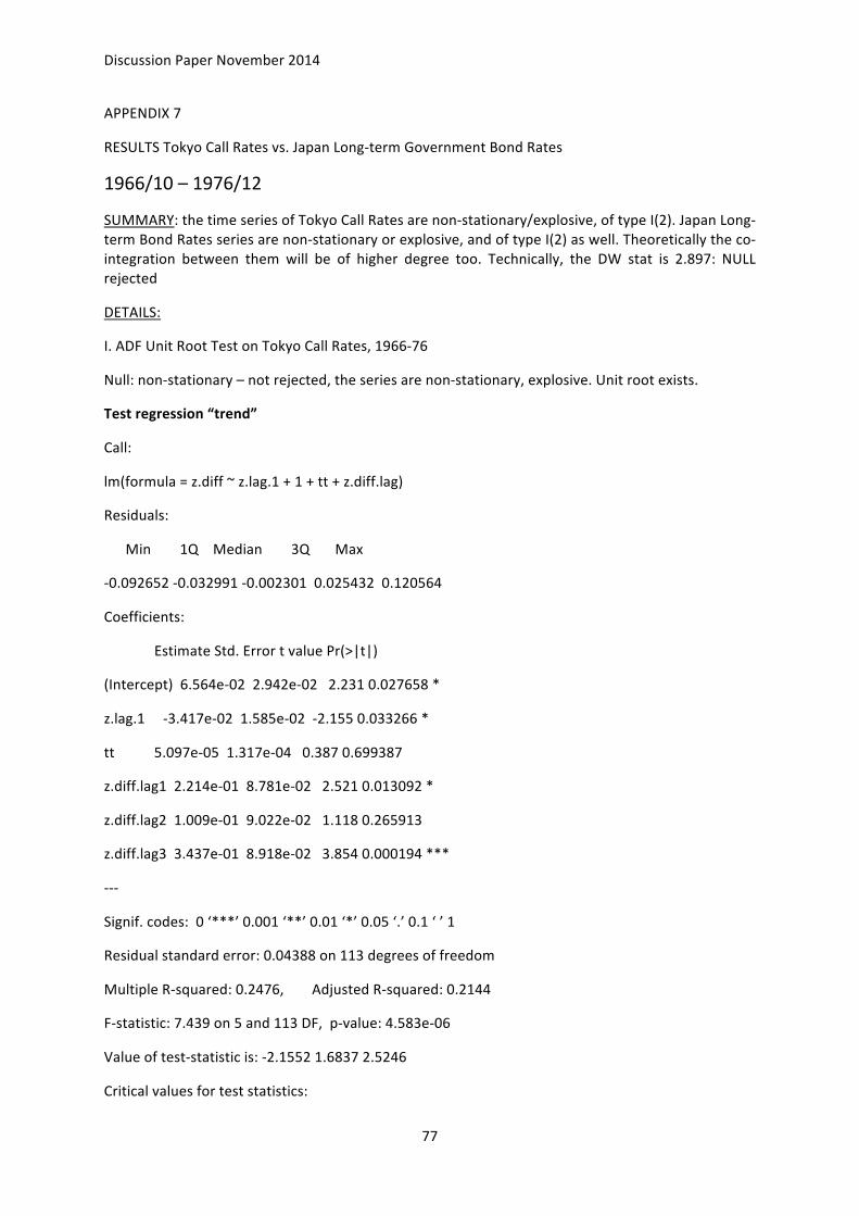
Discussion Paper November 2014
77
APPENDIX 7
RESULTS Tokyo Call Rates vs. Japan Long-‐term Government Bond Rates
1966/10 – 1976/12
SUMMARY: the time series of Tokyo Call Rates are non-‐stationary/explosive, of type I(2). Japan Long-‐term Bond Rates series are non-‐stationary or explosive, and of type I(2) as well. Theoretically the co-‐integration between them will be of higher degree too. Technically, the DW stat is 2.897: NULL rejected
DETAILS:
I. ADF Unit Root Test on Tokyo Call Rates, 1966-‐76
Null: non-‐stationary – not rejected, the series are non-‐stationary, explosive. Unit root exists.
Test regression “trend”
Call:
lm(formula = z.diff ~ z.lag.1 + 1 + tt + z.diff.lag)
Residuals:
Min 1Q Median 3Q Max
-‐0.092652 -‐0.032991 -‐0.002301 0.025432 0.120564
Coefficients:
Estimate Std. Error t value Pr(>|t|)
(Intercept) 6.564e-‐02 2.942e-‐02 2.231 0.027658 *
z.lag.1 -‐3.417e-‐02 1.585e-‐02 -‐2.155 0.033266 *
tt 5.097e-‐05 1.317e-‐04 0.387 0.699387
z.diff.lag1 2.214e-‐01 8.781e-‐02 2.521 0.013092 *
z.diff.lag2 1.009e-‐01 9.022e-‐02 1.118 0.265913
z.diff.lag3 3.437e-‐01 8.918e-‐02 3.854 0.000194 ***
-‐-‐-‐
Signif. codes: 0 ‘***’ 0.001 ‘**’ 0.01 ‘*’ 0.05 ‘.’ 0.1 ‘ ’ 1
Residual standard error: 0.04388 on 113 degrees of freedom
Multiple R-‐squared: 0.2476, Adjusted R-‐squared: 0.2144
F-‐statistic: 7.439 on 5 and 113 DF, p-‐value: 4.583e-‐06
Value of test-‐statistic is: -‐2.1552 1.6837 2.5246
Critical values for test statistics:

Discussion Paper November 2014
78
1pct 5pct 10pct
tau3 -‐3.99 -‐3.43 -‐3.13
phi2 6.22 4.75 4.07
phi3 8.43 6.49 5.47
Test regression “drift”
Call:
lm(formula = z.diff ~ z.lag.1 + 1 + z.diff.lag)
Residuals:
Min 1Q Median 3Q Max
-‐0.091014 -‐0.032359 -‐0.002637 0.025346 0.120203
Coefficients:
Estimate Std. Error t value Pr(>|t|)
(Intercept) 0.06339 0.02873 2.206 0.029384 *
z.lag.1 -‐0.03144 0.01415 -‐2.222 0.028277 *
z.diff.lag1 0.21898 0.08726 2.509 0.013496 *
z.diff.lag2 0.09763 0.08949 1.091 0.277602
z.diff.lag3 0.33983 0.08830 3.849 0.000196 ***
-‐-‐-‐
Signif. codes: 0 ‘***’ 0.001 ‘**’ 0.01 ‘*’ 0.05 ‘.’ 0.1 ‘ ’ 1
Residual standard error: 0.04372 on 114 degrees of freedom
Multiple R-‐squared: 0.2466, Adjusted R-‐squared: 0.2202
F-‐statistic: 9.331 on 4 and 114 DF, p-‐value: 1.468e-‐06
Value of test-‐statistic is: -‐2.2217 2.469
Critical values for test statistics:
1pct 5pct 10pct
tau2 -‐3.46 -‐2.88 -‐2.57
phi1 6.52 4.63 3.81
Test regression “none”
Call:
lm(formula = z.diff ~ z.lag.1 -‐ 1 + z.diff.lag)

Discussion Paper November 2014
79
Residuals:
Min 1Q Median 3Q Max
-‐0.096780 -‐0.028121 0.000931 0.031035 0.120891
Coefficients:
Estimate Std. Error t value Pr(>|t|)
z.lag.1 -‐0.0005273 0.0020089 -‐0.262 0.793426
z.diff.lag1 0.2177601 0.0887155 2.455 0.015603 *
z.diff.lag2 0.0842798 0.0907783 0.928 0.355138
z.diff.lag3 0.3153631 0.0890585 3.541 0.000576 ***
-‐-‐-‐
Signif. codes: 0 ‘***’ 0.001 ‘**’ 0.01 ‘*’ 0.05 ‘.’ 0.1 ‘ ’ 1
Residual standard error: 0.04445 on 115 degrees of freedom
Multiple R-‐squared: 0.215, Adjusted R-‐squared: 0.1877
F-‐statistic: 7.873 on 4 and 115 DF, p-‐value: 1.208e-‐05
Value of test-‐statistic is: -‐0.2625
Critical values for test statistics:
1pct 5pct 10pct
tau1 -‐2.58 -‐1.95 -‐1.62
II. ADF Test on the first differenced time series of Tokyo Call Rates
Null: of non-‐stationary – not rejected, even the first-‐differenced series are still non-‐stationary.
Test regression “trend”
Call:
lm(formula = z.diff ~ z.lag.1 + 1 + tt + z.diff.lag)
Residuals:
Min 1Q Median 3Q Max
-‐0.094866 -‐0.028787 -‐0.002625 0.031609 0.118520
Coefficients:
Estimate Std. Error t value Pr(>|t|)
(Intercept) 5.007e-‐03 8.686e-‐03 0.576 0.565504

Discussion Paper November 2014
80
z.lag.1 -‐3.938e-‐01 1.154e-‐01 -‐3.412 0.000897 ***
tt -‐7.704e-‐05 1.219e-‐04 -‐0.632 0.528787
z.diff.lag1 -‐3.923e-‐01 1.102e-‐01 -‐3.562 0.000541 ***
z.diff.lag2 -‐3.118e-‐01 8.974e-‐02 -‐3.474 0.000727 ***
-‐-‐-‐
Signif. codes: 0 ‘***’ 0.001 ‘**’ 0.01 ‘*’ 0.05 ‘.’ 0.1 ‘ ’ 1
Residual standard error: 0.04477 on 113 degrees of freedom
Multiple R-‐squared: 0.4211, Adjusted R-‐squared: 0.4006
F-‐statistic: 20.55 on 4 and 113 DF, p-‐value: 9.565e-‐13
Value of test-‐statistic is: -‐3.4117 3.8994 5.8428
Critical values for test statistics:
1pct 5pct 10pct
tau3 -‐3.99 -‐3.43 -‐3.13
phi2 6.22 4.75 4.07
phi3 8.43 6.49 5.47
Test regression “trend”
Call:
lm(formula = z.diff ~ z.lag.1 + 1 + tt + z.diff.lag)
Residuals:
Min 1Q Median 3Q Max
-‐0.094866 -‐0.028787 -‐0.002625 0.031609 0.118520
Coefficients:
Estimate Std. Error t value Pr(>|t|)
(Intercept) 5.007e-‐03 8.686e-‐03 0.576 0.565504
z.lag.1 -‐3.938e-‐01 1.154e-‐01 -‐3.412 0.000897 ***
tt -‐7.704e-‐05 1.219e-‐04 -‐0.632 0.528787
z.diff.lag1 -‐3.923e-‐01 1.102e-‐01 -‐3.562 0.000541 ***
z.diff.lag2 -‐3.118e-‐01 8.974e-‐02 -‐3.474 0.000727 ***
-‐-‐-‐

Discussion Paper November 2014
81
Signif. codes: 0 ‘***’ 0.001 ‘**’ 0.01 ‘*’ 0.05 ‘.’ 0.1 ‘ ’ 1
Residual standard error: 0.04477 on 113 degrees of freedom
Multiple R-‐squared: 0.4211, Adjusted R-‐squared: 0.4006
F-‐statistic: 20.55 on 4 and 113 DF, p-‐value: 9.565e-‐13
Value of test-‐statistic is: -‐3.4117 3.8994 5.8428
Critical values for test statistics:
1pct 5pct 10pct
tau3 -‐3.99 -‐3.43 -‐3.13
phi2 6.22 4.75 4.07
phi3 8.43 6.49 5.47
Test regression “drift”
Call:
lm(formula = z.diff ~ z.lag.1 + 1 + z.diff.lag)
Residuals:
Min 1Q Median 3Q Max
-‐0.098246 -‐0.029705 -‐0.000177 0.029983 0.119604
Coefficients:
Estimate Std. Error t value Pr(>|t|)
(Intercept) 0.0001772 0.0041151 0.043 0.965730
z.lag.1 -‐0.3848656 0.1142569 -‐3.368 0.001032 **
z.diff.lag1 -‐0.3978763 0.1095235 -‐3.633 0.000422 ***
z.diff.lag2 -‐0.3142284 0.0894176 -‐3.514 0.000634 ***
-‐-‐-‐
Signif. codes: 0 ‘***’ 0.001 ‘**’ 0.01 ‘*’ 0.05 ‘.’ 0.1 ‘ ’ 1
Residual standard error: 0.04465 on 114 degrees of freedom
Multiple R-‐squared: 0.4191, Adjusted R-‐squared: 0.4038
F-‐statistic: 27.41 on 3 and 114 DF, p-‐value: 2.016e-‐13
Value of test-‐statistic is: -‐3.3684 5.6794
Critical values for test statistics: 1pct 5pct 10pct
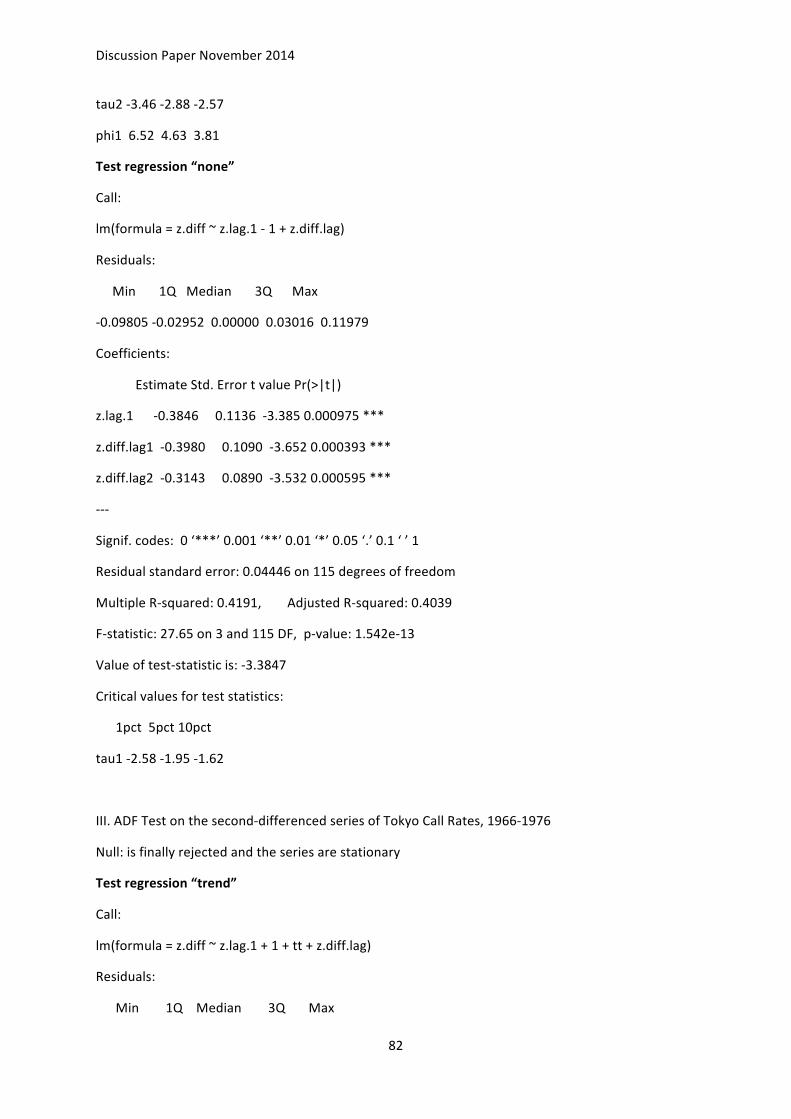
Discussion Paper November 2014
82
tau2 -‐3.46 -‐2.88 -‐2.57
phi1 6.52 4.63 3.81
Test regression “none”
Call:
lm(formula = z.diff ~ z.lag.1 -‐ 1 + z.diff.lag)
Residuals:
Min 1Q Median 3Q Max
-‐0.09805 -‐0.02952 0.00000 0.03016 0.11979
Coefficients:
Estimate Std. Error t value Pr(>|t|)
z.lag.1 -‐0.3846 0.1136 -‐3.385 0.000975 ***
z.diff.lag1 -‐0.3980 0.1090 -‐3.652 0.000393 ***
z.diff.lag2 -‐0.3143 0.0890 -‐3.532 0.000595 ***
-‐-‐-‐
Signif. codes: 0 ‘***’ 0.001 ‘**’ 0.01 ‘*’ 0.05 ‘.’ 0.1 ‘ ’ 1
Residual standard error: 0.04446 on 115 degrees of freedom
Multiple R-‐squared: 0.4191, Adjusted R-‐squared: 0.4039
F-‐statistic: 27.65 on 3 and 115 DF, p-‐value: 1.542e-‐13
Value of test-‐statistic is: -‐3.3847
Critical values for test statistics:
1pct 5pct 10pct
tau1 -‐2.58 -‐1.95 -‐1.62
III. ADF Test on the second-‐differenced series of Tokyo Call Rates, 1966-‐1976
Null: is finally rejected and the series are stationary
Test regression “trend”
Call:
lm(formula = z.diff ~ z.lag.1 + 1 + tt + z.diff.lag)
Residuals:
Min 1Q Median 3Q Max
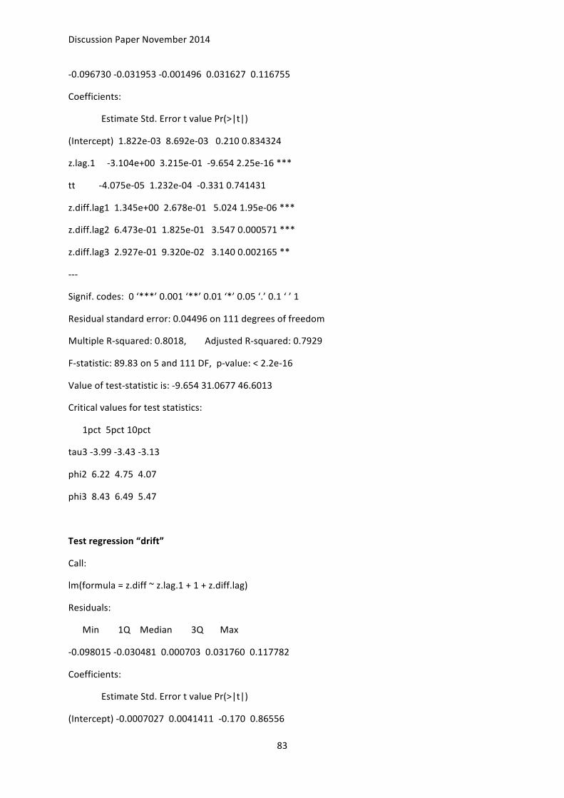
Discussion Paper November 2014
83
-‐0.096730 -‐0.031953 -‐0.001496 0.031627 0.116755
Coefficients:
Estimate Std. Error t value Pr(>|t|)
(Intercept) 1.822e-‐03 8.692e-‐03 0.210 0.834324
z.lag.1 -‐3.104e+00 3.215e-‐01 -‐9.654 2.25e-‐16 ***
tt -‐4.075e-‐05 1.232e-‐04 -‐0.331 0.741431
z.diff.lag1 1.345e+00 2.678e-‐01 5.024 1.95e-‐06 ***
z.diff.lag2 6.473e-‐01 1.825e-‐01 3.547 0.000571 ***
z.diff.lag3 2.927e-‐01 9.320e-‐02 3.140 0.002165 **
-‐-‐-‐
Signif. codes: 0 ‘***’ 0.001 ‘**’ 0.01 ‘*’ 0.05 ‘.’ 0.1 ‘ ’ 1
Residual standard error: 0.04496 on 111 degrees of freedom
Multiple R-‐squared: 0.8018, Adjusted R-‐squared: 0.7929
F-‐statistic: 89.83 on 5 and 111 DF, p-‐value: < 2.2e-‐16
Value of test-‐statistic is: -‐9.654 31.0677 46.6013
Critical values for test statistics:
1pct 5pct 10pct
tau3 -‐3.99 -‐3.43 -‐3.13
phi2 6.22 4.75 4.07
phi3 8.43 6.49 5.47
Test regression “drift”
Call:
lm(formula = z.diff ~ z.lag.1 + 1 + z.diff.lag)
Residuals:
Min 1Q Median 3Q Max
-‐0.098015 -‐0.030481 0.000703 0.031760 0.117782
Coefficients:
Estimate Std. Error t value Pr(>|t|)
(Intercept) -‐0.0007027 0.0041411 -‐0.170 0.86556
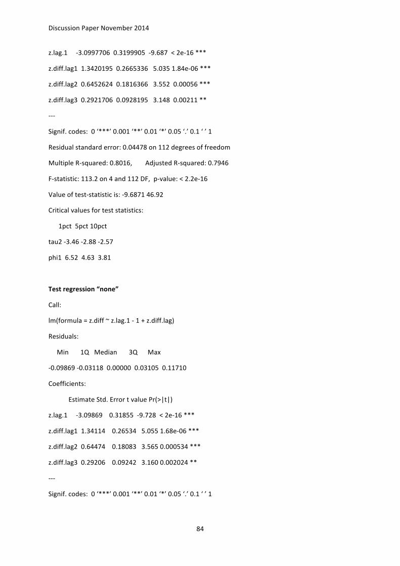
Discussion Paper November 2014
84
z.lag.1 -‐3.0997706 0.3199905 -‐9.687 < 2e-‐16 ***
z.diff.lag1 1.3420195 0.2665336 5.035 1.84e-‐06 ***
z.diff.lag2 0.6452624 0.1816366 3.552 0.00056 ***
z.diff.lag3 0.2921706 0.0928195 3.148 0.00211 **
-‐-‐-‐
Signif. codes: 0 ‘***’ 0.001 ‘**’ 0.01 ‘*’ 0.05 ‘.’ 0.1 ‘ ’ 1
Residual standard error: 0.04478 on 112 degrees of freedom
Multiple R-‐squared: 0.8016, Adjusted R-‐squared: 0.7946
F-‐statistic: 113.2 on 4 and 112 DF, p-‐value: < 2.2e-‐16
Value of test-‐statistic is: -‐9.6871 46.92
Critical values for test statistics:
1pct 5pct 10pct
tau2 -‐3.46 -‐2.88 -‐2.57
phi1 6.52 4.63 3.81
Test regression “none”
Call:
lm(formula = z.diff ~ z.lag.1 -‐ 1 + z.diff.lag)
Residuals:
Min 1Q Median 3Q Max
-‐0.09869 -‐0.03118 0.00000 0.03105 0.11710
Coefficients:
Estimate Std. Error t value Pr(>|t|)
z.lag.1 -‐3.09869 0.31855 -‐9.728 < 2e-‐16 ***
z.diff.lag1 1.34114 0.26534 5.055 1.68e-‐06 ***
z.diff.lag2 0.64474 0.18083 3.565 0.000534 ***
z.diff.lag3 0.29206 0.09242 3.160 0.002024 **
-‐-‐-‐
Signif. codes: 0 ‘***’ 0.001 ‘**’ 0.01 ‘*’ 0.05 ‘.’ 0.1 ‘ ’ 1
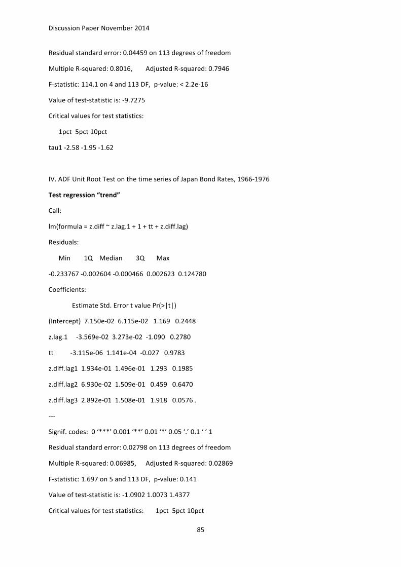
Discussion Paper November 2014
85
Residual standard error: 0.04459 on 113 degrees of freedom
Multiple R-‐squared: 0.8016, Adjusted R-‐squared: 0.7946
F-‐statistic: 114.1 on 4 and 113 DF, p-‐value: < 2.2e-‐16
Value of test-‐statistic is: -‐9.7275
Critical values for test statistics:
1pct 5pct 10pct
tau1 -‐2.58 -‐1.95 -‐1.62
IV. ADF Unit Root Test on the time series of Japan Bond Rates, 1966-‐1976
Test regression “trend”
Call:
lm(formula = z.diff ~ z.lag.1 + 1 + tt + z.diff.lag)
Residuals:
Min 1Q Median 3Q Max
-‐0.233767 -‐0.002604 -‐0.000466 0.002623 0.124780
Coefficients:
Estimate Std. Error t value Pr(>|t|)
(Intercept) 7.150e-‐02 6.115e-‐02 1.169 0.2448
z.lag.1 -‐3.569e-‐02 3.273e-‐02 -‐1.090 0.2780
tt -‐3.115e-‐06 1.141e-‐04 -‐0.027 0.9783
z.diff.lag1 1.934e-‐01 1.496e-‐01 1.293 0.1985
z.diff.lag2 6.930e-‐02 1.509e-‐01 0.459 0.6470
z.diff.lag3 2.892e-‐01 1.508e-‐01 1.918 0.0576 .
-‐-‐-‐
Signif. codes: 0 ‘***’ 0.001 ‘**’ 0.01 ‘*’ 0.05 ‘.’ 0.1 ‘ ’ 1
Residual standard error: 0.02798 on 113 degrees of freedom
Multiple R-‐squared: 0.06985, Adjusted R-‐squared: 0.02869
F-‐statistic: 1.697 on 5 and 113 DF, p-‐value: 0.141
Value of test-‐statistic is: -‐1.0902 1.0073 1.4377
Critical values for test statistics: 1pct 5pct 10pct

Discussion Paper November 2014
86
tau3 -‐3.99 -‐3.43 -‐3.13
phi2 6.22 4.75 4.07
phi3 8.43 6.49 5.47
Test regression “drift”
Call:
lm(formula = z.diff ~ z.lag.1 + 1 + z.diff.lag)
Residuals:
Min 1Q Median 3Q Max
-‐0.233856 -‐0.002505 -‐0.000390 0.002553 0.124712
Coefficients:
Estimate Std. Error t value Pr(>|t|)
(Intercept) 0.07267 0.04334 1.677 0.0963 .
z.lag.1 -‐0.03636 0.02135 -‐1.703 0.0913 .
z.diff.lag1 0.19361 0.14878 1.301 0.1958
z.diff.lag2 0.06953 0.15000 0.464 0.6439
z.diff.lag3 0.28958 0.14963 1.935 0.0554 .
-‐-‐-‐
Signif. codes: 0 ‘***’ 0.001 ‘**’ 0.01 ‘*’ 0.05 ‘.’ 0.1 ‘ ’ 1
Residual standard error: 0.02785 on 114 degrees of freedom
Multiple R-‐squared: 0.06984, Adjusted R-‐squared: 0.03721
F-‐statistic: 2.14 on 4 and 114 DF, p-‐value: 0.08036
Value of test-‐statistic is: -‐1.7029 1.5239
Critical values for test statistics:
1pct 5pct 10pct
tau2 -‐3.46 -‐2.88 -‐2.57
phi1 6.52 4.63 3.81
Test regression “none”
Call:
lm(formula = z.diff ~ z.lag.1 -‐ 1 + z.diff.lag)
Residuals:

Discussion Paper November 2014
87
Min 1Q Median 3Q Max
-‐0.238837 -‐0.001808 0.001723 0.003761 0.127746
Coefficients:
Estimate Std. Error t value Pr(>|t|)
z.lag.1 -‐0.0003274 0.0012824 -‐0.255 0.799
z.diff.lag 0.2206569 0.1479381 1.492 0.139
Residual standard error: 0.02824 on 117 degrees of freedom
Multiple R-‐squared: 0.01871, Adjusted R-‐squared: 0.001933
F-‐statistic: 1.115 on 2 and 117 DF, p-‐value: 0.3313
Value of test-‐statistic is: -‐0.2553
Critical values for test statistics:
1pct 5pct 10pct
tau1 -‐2.58 -‐1.95 -‐1.62
V. ADF Test on Japan Bond rates first-‐differenced series
Null: of non-‐stationary – still not rejected
Test regression “trend”
Call:
lm(formula = z.diff ~ z.lag.1 + 1 + tt + z.diff.lag)
Residuals:
Min 1Q Median 3Q Max
-‐0.233172 -‐0.003620 -‐0.000669 0.004692 0.126911
Coefficients:
Estimate Std. Error t value Pr(>|t|)
(Intercept) 5.114e-‐03 5.414e-‐03 0.944 0.3469
z.lag.1 -‐4.985e-‐01 2.243e-‐01 -‐2.223 0.0282 *
tt -‐9.859e-‐05 7.610e-‐05 -‐1.296 0.1978
z.diff.lag1 -‐3.191e-‐01 1.972e-‐01 -‐1.619 0.1083
z.diff.lag2 -‐2.668e-‐01 1.502e-‐01 -‐1.776 0.0784 .
-‐-‐-‐

Discussion Paper November 2014
88
Signif. codes: 0 ‘***’ 0.001 ‘**’ 0.01 ‘*’ 0.05 ‘.’ 0.1 ‘ ’ 1
Residual standard error: 0.02812 on 113 degrees of freedom
Multiple R-‐squared: 0.2269, Adjusted R-‐squared: 0.1995
F-‐statistic: 8.289 on 4 and 113 DF, p-‐value: 6.716e-‐06
Value of test-‐statistic is: -‐2.2225 2.5257 3.4649
Critical values for test statistics: 1pct 5pct 10pct
tau3 -‐3.99 -‐3.43 -‐3.13
phi2 6.22 4.75 4.07
phi3 8.43 6.49 5.47
Test regression “drift”
Call:
lm(formula = z.diff ~ z.lag.1 + 1 + z.diff.lag)
Residuals:
Min 1Q Median 3Q Max
-‐0.238978 -‐0.001144 0.001725 0.004525 0.124942
Coefficients:
Estimate Std. Error t value Pr(>|t|)
(Intercept) -‐0.001017 0.002638 -‐0.386 0.7005
z.lag.1 -‐0.513371 0.224689 -‐2.285 0.0242 *
z.diff.lag1 -‐0.307996 0.197569 -‐1.559 0.1218
z.diff.lag2 -‐0.260910 0.150551 -‐1.733 0.0858 .
-‐-‐-‐
Signif. codes: 0 ‘***’ 0.001 ‘**’ 0.01 ‘*’ 0.05 ‘.’ 0.1 ‘ ’ 1
Residual standard error: 0.0282 on 114 degrees of freedom
Multiple R-‐squared: 0.2154, Adjusted R-‐squared: 0.1947
F-‐statistic: 10.43 on 3 and 114 DF, p-‐value: 4.062e-‐06
Value of test-‐statistic is: -‐2.2848 2.9319
Critical values for test statistics: 1pct 5pct 10pct
tau2 -‐3.46 -‐2.88 -‐2.57
phi1 6.52 4.63 3.81
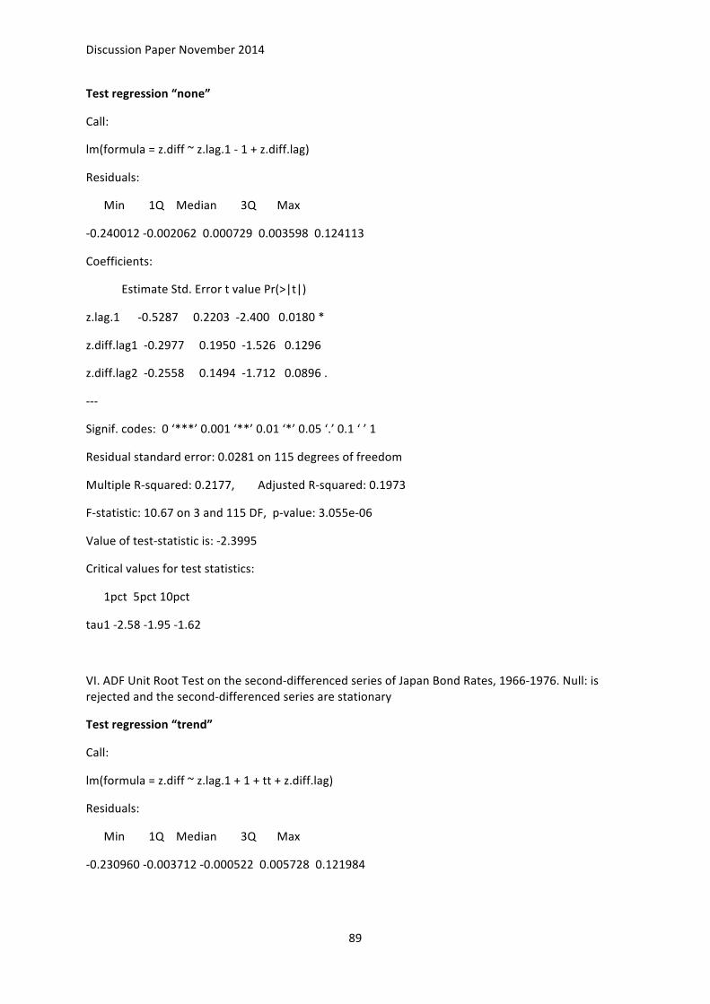
Discussion Paper November 2014
89
Test regression “none”
Call:
lm(formula = z.diff ~ z.lag.1 -‐ 1 + z.diff.lag)
Residuals:
Min 1Q Median 3Q Max
-‐0.240012 -‐0.002062 0.000729 0.003598 0.124113
Coefficients:
Estimate Std. Error t value Pr(>|t|)
z.lag.1 -‐0.5287 0.2203 -‐2.400 0.0180 *
z.diff.lag1 -‐0.2977 0.1950 -‐1.526 0.1296
z.diff.lag2 -‐0.2558 0.1494 -‐1.712 0.0896 .
-‐-‐-‐
Signif. codes: 0 ‘***’ 0.001 ‘**’ 0.01 ‘*’ 0.05 ‘.’ 0.1 ‘ ’ 1
Residual standard error: 0.0281 on 115 degrees of freedom
Multiple R-‐squared: 0.2177, Adjusted R-‐squared: 0.1973
F-‐statistic: 10.67 on 3 and 115 DF, p-‐value: 3.055e-‐06
Value of test-‐statistic is: -‐2.3995
Critical values for test statistics:
1pct 5pct 10pct
tau1 -‐2.58 -‐1.95 -‐1.62
VI. ADF Unit Root Test on the second-‐differenced series of Japan Bond Rates, 1966-‐1976. Null: is rejected and the second-‐differenced series are stationary
Test regression “trend”
Call:
lm(formula = z.diff ~ z.lag.1 + 1 + tt + z.diff.lag)
Residuals:
Min 1Q Median 3Q Max
-‐0.230960 -‐0.003712 -‐0.000522 0.005728 0.121984

Discussion Paper November 2014
90
Coefficients:
Estimate Std. Error t value Pr(>|t|)
(Intercept) 4.668e-‐03 5.552e-‐03 0.841 0.40218
z.lag.1 -‐2.085e+00 2.277e-‐01 -‐9.156 2.73e-‐15 ***
tt -‐1.091e-‐04 7.863e-‐05 -‐1.388 0.16783
z.diff.lag 4.351e-‐01 1.324e-‐01 3.286 0.00135 **
-‐-‐-‐
Signif. codes: 0 ‘***’ 0.001 ‘**’ 0.01 ‘*’ 0.05 ‘.’ 0.1 ‘ ’ 1
Residual standard error: 0.02873 on 113 degrees of freedom
Multiple R-‐squared: 0.5958, Adjusted R-‐squared: 0.5851
F-‐statistic: 55.52 on 3 and 113 DF, p-‐value: < 2.2e-‐16
Value of test-‐statistic is: -‐9.1563 28.7385 42.812
Critical values for test statistics:
1pct 5pct 10pct
tau3 -‐3.99 -‐3.43 -‐3.13
phi2 6.22 4.75 4.07
phi3 8.43 6.49 5.47
Test regression “drift”
Call:
lm(formula = z.diff ~ z.lag.1 + 1 + z.diff.lag)
Residuals:
Min 1Q Median 3Q Max
-‐0.237280 -‐0.002794 0.002095 0.005513 0.119691
Coefficients:
Estimate Std. Error t value Pr(>|t|)
(Intercept) -‐0.002099 0.002667 -‐0.787 0.43280
z.lag.1 -‐2.082752 0.228581 -‐9.112 3.25e-‐15 ***
z.diff.lag 0.434555 0.132942 3.269 0.00143 **
-‐-‐-‐

Discussion Paper November 2014
91
Signif. codes: 0 ‘***’ 0.001 ‘**’ 0.01 ‘*’ 0.05 ‘.’ 0.1 ‘ ’ 1
Residual standard error: 0.02884 on 114 degrees of freedom
Multiple R-‐squared: 0.5889, Adjusted R-‐squared: 0.5817
F-‐statistic: 81.65 on 2 and 114 DF, p-‐value: < 2.2e-‐16
Value of test-‐statistic is: -‐9.1116 41.8044
Critical values for test statistics:
1pct 5pct 10pct
tau2 -‐3.46 -‐2.88 -‐2.57
phi1 6.52 4.63 3.81
Test regression “none”
Call: lm(formula = z.diff ~ z.lag.1 -‐ 1 + z.diff.lag)
Residuals:
Min 1Q Median 3Q Max
-‐0.239376 -‐0.004892 -‐0.000004 0.003413 0.117591
Coefficients:
Estimate Std. Error t value Pr(>|t|)
z.lag.1 -‐2.0823 0.2282 -‐9.125 2.84e-‐15 ***
z.diff.lag 0.4345 0.1327 3.273 0.0014 **
-‐-‐-‐
Signif. codes: 0 ‘***’ 0.001 ‘**’ 0.01 ‘*’ 0.05 ‘.’ 0.1 ‘ ’ 1
Residual standard error: 0.02879 on 115 degrees of freedom
Multiple R-‐squared: 0.5875, Adjusted R-‐squared: 0.5803
F-‐statistic: 81.89 on 2 and 115 DF, p-‐value: < 2.2e-‐16
Value of test-‐statistic is: -‐9.1249
Critical values for test statistics:
1pct 5pct 10pct
tau1 -‐2.58 -‐1.95 -‐1.62
VII. DW Test of no co-‐integration
Durbin-‐Watson test -‐ > DW = 2.8977, p-‐value = 1

Discussion Paper November 2014
92
APPENDIX 8
RESULTS, Nominal Interest Rates, Japan-‐US,
1994/01-‐2011/07
Interest Rates usually follow the “random walk” hypothesis, I(1) and so the test regression should include a constant. Interest rates are considered to be non-‐trending financial series.
SUMMARY: The ADF results demonstrate that both the Japanese Call Rates and the Federal Money Rates are integrated of I(2). The ADF on the second differences rejects the null hypothesis, so the second-‐differenced series are already stationary.
DETAILS:
I. ADF Test Unit Root test on Japanese Call Rates
ADF Test: Null Hypothesis for non-‐stationarity or there is a unit-‐root (not rejected)
Test regression “trend” – with a trend
Call:
lm(formula = z.diff ~ z.lag.1 + 1 + tt + z.diff.lag)
Residuals:
Min 1Q Median 3Q Max
-‐0.61680 -‐0.03445 -‐0.00901 0.01525 2.11690
Coefficients:
Estimate Std. Error t value Pr(>|t|)
(Intercept) -‐0.0412570 0.0238152 -‐1.732 0.08472 .
z.lag.1 -‐0.6120017 0.2092375 -‐2.925 0.00384 **
tt 0.0004325 0.0001929 2.241 0.02607 *
z.diff.lag -‐0.1136080 0.1809351 -‐0.628 0.53078
-‐-‐-‐
Signif. codes: 0 ‘***’ 0.001 ‘**’ 0.01 ‘*’ 0.05 ‘.’ 0.1 ‘ ’ 1
Residual standard error: 0.1619 on 204 degrees of freedom
Multiple R-‐squared: 0.08534, Adjusted R-‐squared: 0.07189
F-‐statistic: 6.345 on 3 and 204 DF, p-‐value: 0.000392
Value of test-‐statistic is: -‐2.9249 3.9797 5.5097
Critical values for test statistics:
1pct 5pct 10pct

Discussion Paper November 2014
93
tau3 -‐3.99 -‐3.43 -‐3.13
phi2 6.22 4.75 4.07
phi3 8.43 6.49 5.47
Test regression “drift” – with an intercept
Call:
lm(formula = z.diff ~ z.lag.1 + 1 + z.diff.lag)
Residuals:
Min 1Q Median 3Q Max
-‐0.65449 -‐0.01044 -‐0.00551 0.00160 2.16022
Coefficients:
Estimate Std. Error t value Pr(>|t|)
(Intercept) 0.005577 0.011539 0.483 0.6294
z.lag.1 -‐0.496562 0.204781 -‐2.425 0.0162 *
z.diff.lag -‐0.170016 0.180927 -‐0.940 0.3485
-‐-‐-‐
Signif. codes: 0 ‘***’ 0.001 ‘**’ 0.01 ‘*’ 0.05 ‘.’ 0.1 ‘ ’ 1
Residual standard error: 0.1635 on 205 degrees of freedom
Multiple R-‐squared: 0.06282, Adjusted R-‐squared: 0.05367
F-‐statistic: 6.87 on 2 and 205 DF, p-‐value: 0.001294
Value of test-‐statistic is: -‐2.4248 3.3909
Critical values for test statistics:
1pct 5pct 10pct
tau2 -‐3.46 -‐2.88 -‐2.57
phi1 6.52 4.63 3.81
Test regression none (neither an intercept nor a trend; one lag)
Call: lm(formula = z.diff ~ z.lag.1 -‐ 1 + z.diff.lag)
Residuals:
Min 1Q Median 3Q Max
-‐0.64948 -‐0.00486 0.00006 0.00672 2.16583

Discussion Paper November 2014
94
Coefficients:
Estimate Std. Error t value Pr(>|t|)
z.lag.1 -‐0.5149 0.2009 -‐2.564 0.0111 *
z.diff.lag -‐0.1609 0.1796 -‐0.896 0.3715
-‐-‐-‐
Signif. codes: 0 ‘***’ 0.001 ‘**’ 0.01 ‘*’ 0.05 ‘.’ 0.1 ‘ ’ 1
Residual standard error: 0.1632 on 206 degrees of freedom
Multiple R-‐squared: 0.06561, Adjusted R-‐squared: 0.05654
F-‐statistic: 7.232 on 2 and 206 DF, p-‐value: 0.0009213
Value of test-‐statistic is: -‐2.5637
Critical values for test statistics:
1pct 5pct 10pct
tau1 -‐2.58 -‐1.95 -‐1.62
Test regression none (two lags)
Call: lm(formula = z.diff ~ z.lag.1 -‐ 1 + z.diff.lag)
Residuals:
Min 1Q Median 3Q Max
-‐0.64334 -‐0.00522 0.00005 0.00641 2.16446
Coefficients:
Estimate Std. Error t value Pr(>|t|)
z.lag.1 -‐0.4031 0.2225 -‐1.811 0.0716 .
z.diff.lag1 -‐0.3152 0.2193 -‐1.437 0.1521
z.diff.lag2 -‐0.2203 0.1823 -‐1.208 0.2283
-‐-‐-‐
Signif. codes: 0 ‘***’ 0.001 ‘**’ 0.01 ‘*’ 0.05 ‘.’ 0.1 ‘ ’ 1
Residual standard error: 0.1634 on 204 degrees of freedom
Multiple R-‐squared: 0.07289, Adjusted R-‐squared: 0.05925
F-‐statistic: 5.346 on 3 and 204 DF, p-‐value: 0.001452
Value of test-‐statistic is: -‐1.8113

Discussion Paper November 2014
95
Critical values for test statistics:
1pct 5pct 10pct
tau1 -‐2.58 -‐1.95 -‐1.62
II. KPSS Unit Root Test on Japanese Call Rates
In KPSS the Null Hypothesis is about stationarity (rejected)
TEST with a constant
Test is of type: mu with 4 lags (short)
Value of test-‐statistic is: 0.5668
Critical value for a significance level of:
10pct 5pct 2.5pct 1pct
critical values 0.347 0.463 0.574 0.739
Test is of type: mu with 14 lags (long)
Value of test-‐statistic is: 0.5055
Critical value for a significance level of:
10pct 5pct 2.5pct 1pct
critical values 0.347 0.463 0.574 0.739
TEST with a constant and linear trend
Short – sets lags to 4; Long-‐ sets lags to root 12
Test is of type: tau with 4 lags (short)
Value of test-‐statistic is: 0.0717
Critical value for a significance level of:
10pct 5pct 2.5pct 1pct
critical values 0.119 0.146 0.176 0.216
Test is of type: tau with 14 lags (long)
Value of test-‐statistic is: 0.0732
Critical value for a significance level of:

Discussion Paper November 2014
96
10pct 5pct 2.5pct 1pct
critical values 0.119 0.146 0.176 0.216
III. ADF Test Unit Root (Federal Money rates, US; on the first differences)
Test regression “trend” – with a trend
Call:
lm(formula = z.diff ~ z.lag.1 + 1 + tt + z.diff.lag)
Residuals:
Min 1Q Median 3Q Max
-‐0.61680 -‐0.03445 -‐0.00901 0.01525 2.11690
Coefficients:
Estimate Std. Error t value Pr(>|t|)
(Intercept) -‐0.0412570 0.0238152 -‐1.732 0.08472 .
z.lag.1 -‐0.6120017 0.2092375 -‐2.925 0.00384 **
tt 0.0004325 0.0001929 2.241 0.02607 *
z.diff.lag -‐0.1136080 0.1809351 -‐0.628 0.53078
-‐-‐-‐
Signif. codes: 0 ‘***’ 0.001 ‘**’ 0.01 ‘*’ 0.05 ‘.’ 0.1 ‘ ’ 1
Residual standard error: 0.1619 on 204 degrees of freedom
Multiple R-‐squared: 0.08534, Adjusted R-‐squared: 0.07189
F-‐statistic: 6.345 on 3 and 204 DF, p-‐value: 0.000392
Value of test-‐statistic is: -‐2.9249 3.9797 5.5097
Critical values for test statistics:
1pct 5pct 10pct
tau3 -‐3.99 -‐3.43 -‐3.13
phi2 6.22 4.75 4.07
phi3 8.43 6.49 5.47
Test regression “drift” – with an intercept
Call:
lm(formula = z.diff ~ z.lag.1 + 1 + z.diff.lag)
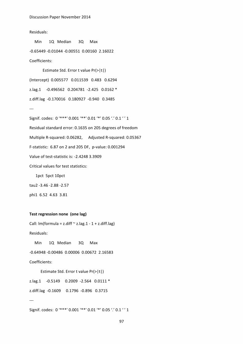
Discussion Paper November 2014
97
Residuals:
Min 1Q Median 3Q Max
-‐0.65449 -‐0.01044 -‐0.00551 0.00160 2.16022
Coefficients:
Estimate Std. Error t value Pr(>|t|)
(Intercept) 0.005577 0.011539 0.483 0.6294
z.lag.1 -‐0.496562 0.204781 -‐2.425 0.0162 *
z.diff.lag -‐0.170016 0.180927 -‐0.940 0.3485
-‐-‐-‐
Signif. codes: 0 ‘***’ 0.001 ‘**’ 0.01 ‘*’ 0.05 ‘.’ 0.1 ‘ ’ 1
Residual standard error: 0.1635 on 205 degrees of freedom
Multiple R-‐squared: 0.06282, Adjusted R-‐squared: 0.05367
F-‐statistic: 6.87 on 2 and 205 DF, p-‐value: 0.001294
Value of test-‐statistic is: -‐2.4248 3.3909
Critical values for test statistics:
1pct 5pct 10pct
tau2 -‐3.46 -‐2.88 -‐2.57
phi1 6.52 4.63 3.81
Test regression none (one lag)
Call: lm(formula = z.diff ~ z.lag.1 -‐ 1 + z.diff.lag)
Residuals:
Min 1Q Median 3Q Max
-‐0.64948 -‐0.00486 0.00006 0.00672 2.16583
Coefficients:
Estimate Std. Error t value Pr(>|t|)
z.lag.1 -‐0.5149 0.2009 -‐2.564 0.0111 *
z.diff.lag -‐0.1609 0.1796 -‐0.896 0.3715
-‐-‐-‐
Signif. codes: 0 ‘***’ 0.001 ‘**’ 0.01 ‘*’ 0.05 ‘.’ 0.1 ‘ ’ 1
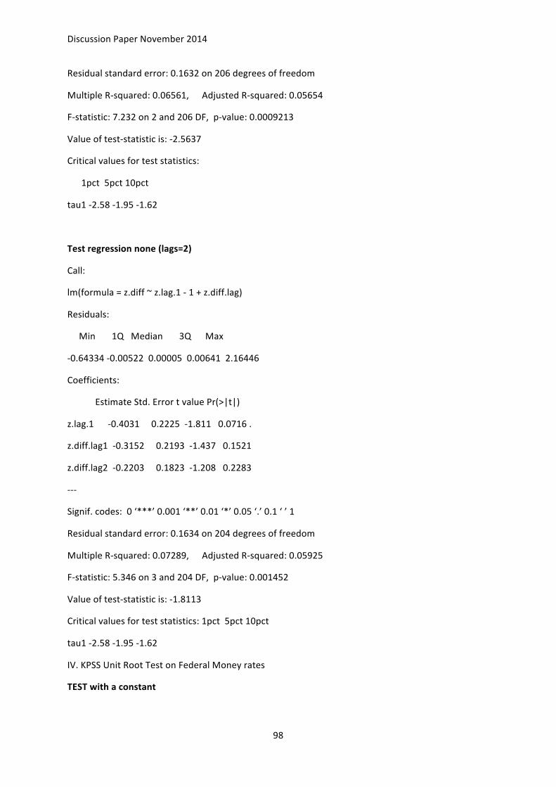
Discussion Paper November 2014
98
Residual standard error: 0.1632 on 206 degrees of freedom
Multiple R-‐squared: 0.06561, Adjusted R-‐squared: 0.05654
F-‐statistic: 7.232 on 2 and 206 DF, p-‐value: 0.0009213
Value of test-‐statistic is: -‐2.5637
Critical values for test statistics:
1pct 5pct 10pct
tau1 -‐2.58 -‐1.95 -‐1.62
Test regression none (lags=2)
Call:
lm(formula = z.diff ~ z.lag.1 -‐ 1 + z.diff.lag)
Residuals:
Min 1Q Median 3Q Max
-‐0.64334 -‐0.00522 0.00005 0.00641 2.16446
Coefficients:
Estimate Std. Error t value Pr(>|t|)
z.lag.1 -‐0.4031 0.2225 -‐1.811 0.0716 .
z.diff.lag1 -‐0.3152 0.2193 -‐1.437 0.1521
z.diff.lag2 -‐0.2203 0.1823 -‐1.208 0.2283
-‐-‐-‐
Signif. codes: 0 ‘***’ 0.001 ‘**’ 0.01 ‘*’ 0.05 ‘.’ 0.1 ‘ ’ 1
Residual standard error: 0.1634 on 204 degrees of freedom
Multiple R-‐squared: 0.07289, Adjusted R-‐squared: 0.05925
F-‐statistic: 5.346 on 3 and 204 DF, p-‐value: 0.001452
Value of test-‐statistic is: -‐1.8113
Critical values for test statistics: 1pct 5pct 10pct
tau1 -‐2.58 -‐1.95 -‐1.62
IV. KPSS Unit Root Test on Federal Money rates
TEST with a constant

Discussion Paper November 2014
99
Test is of type: mu with 4 lags (short)
Value of test-‐statistic is: 0.5668
Critical value for a significance level of:
10pct 5pct 2.5pct 1pct
critical values 0.347 0.463 0.574 0.739
Test is of type: mu with 14 lags (long)
Value of test-‐statistic is: 0.5055
Critical value for a significance level of:
10pct 5pct 2.5pct 1pct
critical values 0.347 0.463 0.574 0.739
TEST with a constant and linear trend
Test is of type: tau with 4 lags (short)
Value of test-‐statistic is: 0.0717
Critical value for a significance level of:
10pct 5pct 2.5pct 1pct
critical values 0.119 0.146 0.176 0.216
Test is of type: tau with 14 lags (long)
Value of test-‐statistic is: 0.0732
Critical value for a significance level of:
10pct 5pct 2.5pct 1pct
critical values 0.119 0.146 0.176 0.216
V. Durbin-‐Watson Test is run on a cointegrating regression with the null of no cointegration.
Durbin-‐Watson test
data: creg1
DW = 2.1596, p-‐value = 0.8702
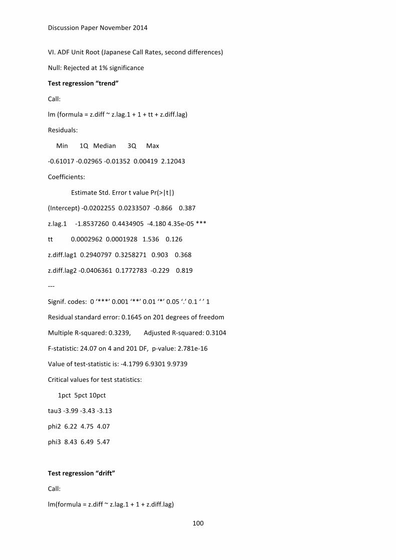
Discussion Paper November 2014
100
VI. ADF Unit Root (Japanese Call Rates, second differences)
Null: Rejected at 1% significance
Test regression “trend”
Call:
lm (formula = z.diff ~ z.lag.1 + 1 + tt + z.diff.lag)
Residuals:
Min 1Q Median 3Q Max
-‐0.61017 -‐0.02965 -‐0.01352 0.00419 2.12043
Coefficients:
Estimate Std. Error t value Pr(>|t|)
(Intercept) -‐0.0202255 0.0233507 -‐0.866 0.387
z.lag.1 -‐1.8537260 0.4434905 -‐4.180 4.35e-‐05 ***
tt 0.0002962 0.0001928 1.536 0.126
z.diff.lag1 0.2940797 0.3258271 0.903 0.368
z.diff.lag2 -‐0.0406361 0.1772783 -‐0.229 0.819
-‐-‐-‐
Signif. codes: 0 ‘***’ 0.001 ‘**’ 0.01 ‘*’ 0.05 ‘.’ 0.1 ‘ ’ 1
Residual standard error: 0.1645 on 201 degrees of freedom
Multiple R-‐squared: 0.3239, Adjusted R-‐squared: 0.3104
F-‐statistic: 24.07 on 4 and 201 DF, p-‐value: 2.781e-‐16
Value of test-‐statistic is: -‐4.1799 6.9301 9.9739
Critical values for test statistics:
1pct 5pct 10pct
tau3 -‐3.99 -‐3.43 -‐3.13
phi2 6.22 4.75 4.07
phi3 8.43 6.49 5.47
Test regression “drift”
Call:
lm(formula = z.diff ~ z.lag.1 + 1 + z.diff.lag)

Discussion Paper November 2014
101
Residuals:
Min 1Q Median 3Q Max
-‐0.63786 -‐0.01627 -‐0.01098 -‐0.00308 2.15079
Coefficients:
Estimate Std. Error t value Pr(>|t|)
(Intercept) 0.01102 0.01150 0.958 0.339
z.lag.1 -‐1.85986 0.44496 -‐4.180 4.34e-‐05 ***
z.diff.lag1 0.29741 0.32691 0.910 0.364
z.diff.lag2 -‐0.04012 0.17787 -‐0.226 0.822
-‐-‐-‐
Signif. codes: 0 ‘***’ 0.001 ‘**’ 0.01 ‘*’ 0.05 ‘.’ 0.1 ‘ ’ 1
Residual standard error: 0.1651 on 202 degrees of freedom
Multiple R-‐squared: 0.3159, Adjusted R-‐squared: 0.3058
F-‐statistic: 31.1 on 3 and 202 DF, p-‐value: < 2.2e-‐16
Value of test-‐statistic is: -‐4.1798 9.1539
Critical values for test statistics:
1pct 5pct 10pct
tau2 -‐3.46 -‐2.88 -‐2.57
phi1 6.52 4.63 3.81
Test regression “none” (with two lags)
Call:
lm(formula = z.diff ~ z.lag.1 -‐ 1 + z.diff.lag)
Residuals:
Min 1Q Median 3Q Max
-‐0.62680 -‐0.00529 0.00004 0.00792 2.16179
Coefficients:
Estimate Std. Error t value Pr(>|t|)
z.lag.1 -‐1.85545 0.44485 -‐4.171 4.49e-‐05 ***
z.diff.lag1 0.29468 0.32684 0.902 0.368
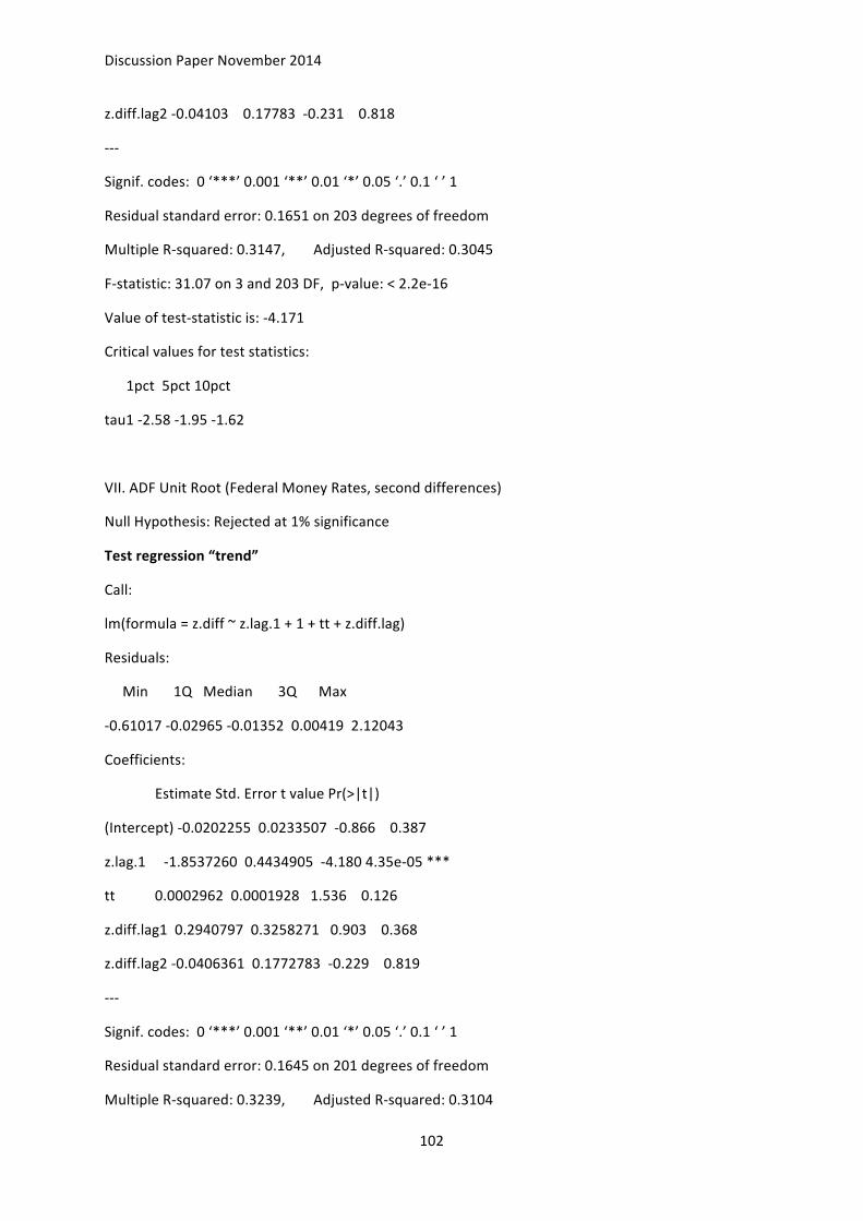
Discussion Paper November 2014
102
z.diff.lag2 -‐0.04103 0.17783 -‐0.231 0.818
-‐-‐-‐
Signif. codes: 0 ‘***’ 0.001 ‘**’ 0.01 ‘*’ 0.05 ‘.’ 0.1 ‘ ’ 1
Residual standard error: 0.1651 on 203 degrees of freedom
Multiple R-‐squared: 0.3147, Adjusted R-‐squared: 0.3045
F-‐statistic: 31.07 on 3 and 203 DF, p-‐value: < 2.2e-‐16
Value of test-‐statistic is: -‐4.171
Critical values for test statistics:
1pct 5pct 10pct
tau1 -‐2.58 -‐1.95 -‐1.62
VII. ADF Unit Root (Federal Money Rates, second differences)
Null Hypothesis: Rejected at 1% significance
Test regression “trend”
Call:
lm(formula = z.diff ~ z.lag.1 + 1 + tt + z.diff.lag)
Residuals:
Min 1Q Median 3Q Max
-‐0.61017 -‐0.02965 -‐0.01352 0.00419 2.12043
Coefficients:
Estimate Std. Error t value Pr(>|t|)
(Intercept) -‐0.0202255 0.0233507 -‐0.866 0.387
z.lag.1 -‐1.8537260 0.4434905 -‐4.180 4.35e-‐05 ***
tt 0.0002962 0.0001928 1.536 0.126
z.diff.lag1 0.2940797 0.3258271 0.903 0.368
z.diff.lag2 -‐0.0406361 0.1772783 -‐0.229 0.819
-‐-‐-‐
Signif. codes: 0 ‘***’ 0.001 ‘**’ 0.01 ‘*’ 0.05 ‘.’ 0.1 ‘ ’ 1
Residual standard error: 0.1645 on 201 degrees of freedom
Multiple R-‐squared: 0.3239, Adjusted R-‐squared: 0.3104

Discussion Paper November 2014
103
F-‐statistic: 24.07 on 4 and 201 DF, p-‐value: 2.781e-‐16
Value of test-‐statistic is: -‐4.1799 6.9301 9.9739
Critical values for test statistics:
1pct 5pct 10pct
tau3 -‐3.99 -‐3.43 -‐3.13
phi2 6.22 4.75 4.07
phi3 8.43 6.49 5.47
Test regression “drift”
Call: lm(formula = z.diff ~ z.lag.1 + 1 + z.diff.lag)
Residuals:
Min 1Q Median 3Q Max
-‐0.63786 -‐0.01627 -‐0.01098 -‐0.00308 2.15079
Coefficients:
Estimate Std. Error t value Pr(>|t|)
(Intercept) 0.01102 0.01150 0.958 0.339
z.lag.1 -‐1.85986 0.44496 -‐4.180 4.34e-‐05 ***
z.diff.lag1 0.29741 0.32691 0.910 0.364
z.diff.lag2 -‐0.04012 0.17787 -‐0.226 0.822
-‐-‐-‐
Signif. codes: 0 ‘***’ 0.001 ‘**’ 0.01 ‘*’ 0.05 ‘.’ 0.1 ‘ ’ 1
Residual standard error: 0.1651 on 202 degrees of freedom
Multiple R-‐squared: 0.3159, Adjusted R-‐squared: 0.3058
F-‐statistic: 31.1 on 3 and 202 DF, p-‐value: < 2.2e-‐16
Value of test-‐statistic is: -‐4.1798 9.1539
Critical values for test statistics:
1pct 5pct 10pct
tau2 -‐3.46 -‐2.88 -‐2.57
phi1 6.52 4.63 3.81
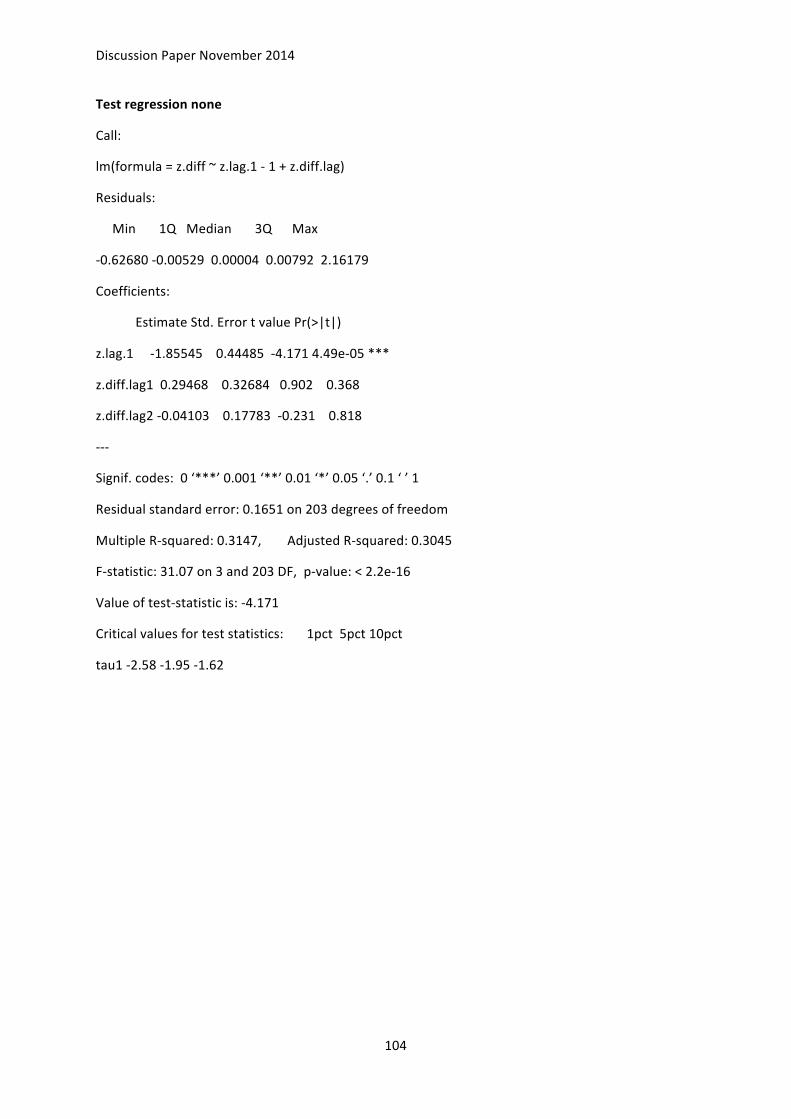
Discussion Paper November 2014
104
Test regression none
Call:
lm(formula = z.diff ~ z.lag.1 -‐ 1 + z.diff.lag)
Residuals:
Min 1Q Median 3Q Max
-‐0.62680 -‐0.00529 0.00004 0.00792 2.16179
Coefficients:
Estimate Std. Error t value Pr(>|t|)
z.lag.1 -‐1.85545 0.44485 -‐4.171 4.49e-‐05 ***
z.diff.lag1 0.29468 0.32684 0.902 0.368
z.diff.lag2 -‐0.04103 0.17783 -‐0.231 0.818
-‐-‐-‐
Signif. codes: 0 ‘***’ 0.001 ‘**’ 0.01 ‘*’ 0.05 ‘.’ 0.1 ‘ ’ 1
Residual standard error: 0.1651 on 203 degrees of freedom
Multiple R-‐squared: 0.3147, Adjusted R-‐squared: 0.3045
F-‐statistic: 31.07 on 3 and 203 DF, p-‐value: < 2.2e-‐16
Value of test-‐statistic is: -‐4.171
Critical values for test statistics: 1pct 5pct 10pct
tau1 -‐2.58 -‐1.95 -‐1.62

Discussion Paper November 2014
105
APPENDIX 9
RESULTS from the bond markets – Japan/US 10-‐year yields
1994/01 – 2011/07
SUMMARY: The Jap LT Gov rates are of type I(1). Both test ADF and KPSS show the same. The US Bond yields are of type I(1) as expected and both tests show the same. Technically DW-‐stat =2.00 (null is rejected). Series are cointegrated.
DETAILS:
I. ADF Unit root Test on the Japanese LT Government rates (the null not rejected)
Test regression trend
Call:
lm(formula = z.diff ~ z.lag.1 + 1 + tt + z.diff.lag)
Residuals:
Min 1Q Median 3Q Max
-‐0.35590 -‐0.07702 -‐0.00405 0.05749 1.53729
Coefficients:
Estimate Std. Error t value Pr(>|t|)
(Intercept) 3.639e-‐02 4.511e-‐02 0.807 0.4209
z.lag.1 -‐8.448e-‐02 3.938e-‐02 -‐2.145 0.0332 *
tt 2.764e-‐05 2.550e-‐04 0.108 0.9138
z.diff.lag1 7.822e-‐02 1.017e-‐01 0.769 0.4426
z.diff.lag2 8.662e-‐02 1.023e-‐01 0.846 0.3984
z.diff.lag3 -‐2.526e-‐01 1.026e-‐01 -‐2.463 0.0147 *
-‐-‐-‐
Signif. codes: 0 ‘***’ 0.001 ‘**’ 0.01 ‘*’ 0.05 ‘.’ 0.1 ‘ ’ 1
Residual standard error: 0.1511 on 192 degrees of freedom
Multiple R-‐squared: 0.08108, Adjusted R-‐squared: 0.05715
F-‐statistic: 3.388 on 5 and 192 DF, p-‐value: 0.005885
Value of test-‐statistic is: -‐2.1452 2.9869 4.4713
Critical values for test statistics:
1pct 5pct 10pct

Discussion Paper November 2014
106
tau3 -‐3.99 -‐3.43 -‐3.13
phi2 6.22 4.75 4.07
phi3 8.43 6.49 5.47
Test regression drift – with an intercept
Call:
lm(formula = z.diff ~ z.lag.1 + 1 + z.diff.lag)
Residuals:
Min 1Q Median 3Q Max
-‐0.35762 -‐0.07703 -‐0.00107 0.05735 1.54863
Coefficients:
Estimate Std. Error t value Pr(>|t|)
(Intercept) 0.02850 0.01647 1.731 0.0851 .
z.lag.1 -‐0.05393 0.02355 -‐2.290 0.0230 *
z.diff.lag1 0.07727 0.09902 0.780 0.4361
z.diff.lag2 0.08944 0.09931 0.901 0.3689
z.diff.lag3 -‐0.25565 0.09930 -‐2.574 0.0108 *
-‐-‐-‐
Signif. codes: 0 ‘***’ 0.001 ‘**’ 0.01 ‘*’ 0.05 ‘.’ 0.1 ‘ ’ 1
Residual standard error: 0.1492 on 202 degrees of freedom
Multiple R-‐squared: 0.06311, Adjusted R-‐squared: 0.04456
F-‐statistic: 3.402 on 4 and 202 DF, p-‐value: 0.01019
Value of test-‐statistic is: -‐2.2903 2.6249
Critical values for test statistics:
1pct 5pct 10pct
tau2 -‐3.46 -‐2.88 -‐2.57
phi1 6.52 4.63 3.81
Test regression “none”
Call: lm(formula = z.diff ~ z.lag.1 -‐ 1 + z.diff.lag)
Residuals:
Min 1Q Median 3Q Max

Discussion Paper November 2014
107
-‐0.34191 -‐0.05938 0.00480 0.06619 1.57309
Coefficients:
Estimate Std. Error t value Pr(>|t|)
z.lag.1 -‐0.02241 0.01499 -‐1.494 0.13664
z.diff.lag1 0.06324 0.09917 0.638 0.52439
z.diff.lag2 0.07324 0.09936 0.737 0.46186
z.diff.lag3 -‐0.27409 0.09921 -‐2.763 0.00626 **
-‐-‐-‐
Signif. codes: 0 ‘***’ 0.001 ‘**’ 0.01 ‘*’ 0.05 ‘.’ 0.1 ‘ ’ 1
Residual standard error: 0.1499 on 203 degrees of freedom
Multiple R-‐squared: 0.04922, Adjusted R-‐squared: 0.03049
F-‐statistic: 2.627 on 4 and 203 DF, p-‐value: 0.03572
Value of test-‐statistic is: -‐1.4943
Critical values for test statistics:
1pct 5pct 10pct
tau1 -‐2.58 -‐1.95 -‐1.62
II. KPSS Test on the Jap LT Gov rates
Null: of stationary – rejected by all results at 1% significance
TEST with a constant
Test is of type: mu with 4 lags.
Value of test-‐statistic is: 2.322
Critical value for a significance level of:
10pct 5pct 2.5pct 1pct
critical values 0.347 0.463 0.574 0.739
Test is of type: mu with 14 lags.
Value of test-‐statistic is: 0.9011
Critical value for a significance level of:
10pct 5pct 2.5pct 1pct

Discussion Paper November 2014
108
critical values 0.347 0.463 0.574 0.739
TEST with a constant and linear trend
Test is of type: tau with 4 lags.
Value of test-‐statistic is: 0.7106
Critical value for a significance level of:
10pct 5pct 2.5pct 1pct
critical values 0.119 0.146 0.176 0.216
Test is of type: tau with 14 lags.
Value of test-‐statistic is: 0.2942
Critical value for a significance level of:
10pct 5pct 2.5pct 1pct
critical values 0.119 0.146 0.176 0.216
III. ADF Test on the first differenced-‐series (the results reject the null of non-‐stationary). From the first differencing and the series are stationary already.
Test regression trend
Call:
lm(formula = z.diff ~ z.lag.1 + 1 + tt + z.diff.lag)
Residuals:
Min 1Q Median 3Q Max
-‐0.32966 -‐0.07714 -‐0.00236 0.05550 1.53476
Coefficients:
Estimate Std. Error t value Pr(>|t|)
(Intercept) -‐0.0413347 0.0241184 -‐1.714 0.08817 .
z.lag.1 -‐1.1797398 0.1643941 -‐7.176 1.52e-‐11 ***
tt 0.0003662 0.0001922 1.905 0.05822 .
z.diff.lag1 0.2312612 0.1386359 1.668 0.09692 .
z.diff.lag2 0.2894200 0.1019302 2.839 0.00501 **
-‐-‐-‐

Discussion Paper November 2014
109
Signif. codes: 0 ‘***’ 0.001 ‘**’ 0.01 ‘*’ 0.05 ‘.’ 0.1 ‘ ’ 1
Residual standard error: 0.1524 on 192 degrees of freedom
Multiple R-‐squared: 0.3396, Adjusted R-‐squared: 0.3258
F-‐statistic: 24.68 on 4 and 192 DF, p-‐value: < 2.2e-‐16
Value of test-‐statistic is: -‐7.1763 17.7834 26.3226
Critical values for test statistics:
1pct 5pct 10pct
tau3 -‐3.99 -‐3.43 -‐3.13
phi2 6.22 4.75 4.07
phi3 8.43 6.49 5.47
Test regression drift
Call: lm(formula = z.diff ~ z.lag.1 + 1 + z.diff.lag)
Residuals:
Min 1Q Median 3Q Max
-‐0.34983 -‐0.07536 -‐0.00763 0.05508 1.57168
Coefficients:
Estimate Std. Error t value Pr(>|t|)
(Intercept) -‐0.0003778 0.0110133 -‐0.034 0.97267
z.lag.1 -‐1.1429747 0.1643666 -‐6.954 5.36e-‐11 ***
z.diff.lag1 0.2059333 0.1389344 1.482 0.13991
z.diff.lag2 0.2766519 0.1024005 2.702 0.00751 **
-‐-‐-‐
Signif. codes: 0 ‘***’ 0.001 ‘**’ 0.01 ‘*’ 0.05 ‘.’ 0.1 ‘ ’ 1
Residual standard error: 0.1534 on 193 degrees of freedom
Multiple R-‐squared: 0.3271, Adjusted R-‐squared: 0.3166
F-‐statistic: 31.27 on 3 and 193 DF, p-‐value: < 2.2e-‐16
Value of test-‐statistic is: -‐6.9538 24.5255
Critical values for test statistics:
1pct 5pct 10pct
tau2 -‐3.46 -‐2.88 -‐2.57

Discussion Paper November 2014
110
phi1 6.52 4.63 3.81
Test regression none
Call:
lm(formula = z.diff ~ z.lag.1 -‐ 1 + z.diff.lag)
Residuals:
Min 1Q Median 3Q Max
-‐0.34943 -‐0.07244 -‐0.00555 0.05402 1.57166
Coefficients:
Estimate Std. Error t value Pr(>|t|)
z.lag.1 -‐1.13475 0.15932 -‐7.123 1.8e-‐11 ***
z.diff.lag1 0.20320 0.13516 1.503 0.13428
z.diff.lag2 0.27518 0.09963 2.762 0.00627 **
-‐-‐-‐
Signif. codes: 0 ‘***’ 0.001 ‘**’ 0.01 ‘*’ 0.05 ‘.’ 0.1 ‘ ’ 1
Residual standard error: 0.1506 on 203 degrees of freedom
Multiple R-‐squared: 0.3268, Adjusted R-‐squared: 0.3168
F-‐statistic: 32.85 on 3 and 203 DF, p-‐value: < 2.2e-‐16
Value of test-‐statistic is: -‐7.1225
Critical values for test statistics:
1pct 5pct 10pct
tau1 -‐2.58 -‐1.95 -‐1.62
IV. KPSS on the first differenced-‐series of Jap LT Gov Rates – the results do not reject the Null of stationary.
TEST with a constant
Test is of type: mu with 4 lags.
Value of test-‐statistic is: 0.3138
Critical value for a significance level of:
10pct 5pct 2.5pct 1pct
critical values 0.347 0.463 0.574 0.739

Discussion Paper November 2014
111
Test is of type: mu with 14 lags.
Value of test-‐statistic is: 0.3599
Critical value for a significance level of:
10pct 5pct 2.5pct 1pct
critical values 0.347 0.463 0.574 0.739
TEST with a constant and linear trend
Test is of type: tau with 4 lags.
Value of test-‐statistic is: 0.0536
Critical value for a significance level of:
10pct 5pct 2.5pct 1pct
critical values 0.119 0.146 0.176 0.216
Test is of type: tau with 14 lags.
Value of test-‐statistic is: 0.0666
Critical value for a significance level of:
10pct 5pct 2.5pct 1pct
critical values 0.119 0.146 0.176 0.216
V. ADF Unit Root Test on the US Bond Yields
Null of non-‐stationary is not rejected.
Test regression trend
Call: lm(formula = z.diff ~ z.lag.1 + 1 + tt + z.diff.lag)
Residuals:
Min 1Q Median 3Q Max
-‐0.34161 -‐0.02724 -‐0.00140 0.02624 0.57471
Coefficients:
Estimate Std. Error t value Pr(>|t|)
(Intercept) 0.3132129 0.1185635 2.642 0.00896 **
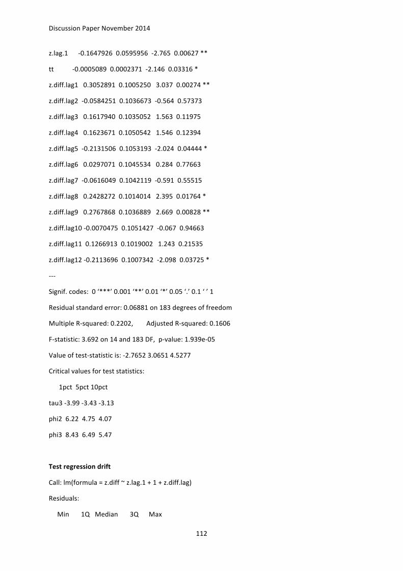
Discussion Paper November 2014
112
z.lag.1 -‐0.1647926 0.0595956 -‐2.765 0.00627 **
tt -‐0.0005089 0.0002371 -‐2.146 0.03316 *
z.diff.lag1 0.3052891 0.1005250 3.037 0.00274 **
z.diff.lag2 -‐0.0584251 0.1036673 -‐0.564 0.57373
z.diff.lag3 0.1617940 0.1035052 1.563 0.11975
z.diff.lag4 0.1623671 0.1050542 1.546 0.12394
z.diff.lag5 -‐0.2131506 0.1053193 -‐2.024 0.04444 *
z.diff.lag6 0.0297071 0.1045534 0.284 0.77663
z.diff.lag7 -‐0.0616049 0.1042119 -‐0.591 0.55515
z.diff.lag8 0.2428272 0.1014014 2.395 0.01764 *
z.diff.lag9 0.2767868 0.1036889 2.669 0.00828 **
z.diff.lag10 -‐0.0070475 0.1051427 -‐0.067 0.94663
z.diff.lag11 0.1266913 0.1019002 1.243 0.21535
z.diff.lag12 -‐0.2113696 0.1007342 -‐2.098 0.03725 *
-‐-‐-‐
Signif. codes: 0 ‘***’ 0.001 ‘**’ 0.01 ‘*’ 0.05 ‘.’ 0.1 ‘ ’ 1
Residual standard error: 0.06881 on 183 degrees of freedom
Multiple R-‐squared: 0.2202, Adjusted R-‐squared: 0.1606
F-‐statistic: 3.692 on 14 and 183 DF, p-‐value: 1.939e-‐05
Value of test-‐statistic is: -‐2.7652 3.0651 4.5277
Critical values for test statistics:
1pct 5pct 10pct
tau3 -‐3.99 -‐3.43 -‐3.13
phi2 6.22 4.75 4.07
phi3 8.43 6.49 5.47
Test regression drift
Call: lm(formula = z.diff ~ z.lag.1 + 1 + z.diff.lag)
Residuals:
Min 1Q Median 3Q Max

Discussion Paper November 2014
113
-‐0.34844 -‐0.02954 -‐0.00285 0.02845 0.57430
Coefficients:
Estimate Std. Error t value Pr(>|t|)
(Intercept) 0.06962 0.03464 2.010 0.04593 *
z.lag.1 -‐0.04559 0.02183 -‐2.089 0.03811 *
z.diff.lag1 0.23492 0.09596 2.448 0.01529 *
z.diff.lag2 -‐0.13757 0.09783 -‐1.406 0.16135
z.diff.lag3 0.09080 0.09904 0.917 0.36041
z.diff.lag4 0.08238 0.09918 0.831 0.40727
z.diff.lag5 -‐0.29184 0.09970 -‐2.927 0.00385 **
z.diff.lag6 -‐0.03476 0.10112 -‐0.344 0.73145
z.diff.lag7 -‐0.11365 0.10234 -‐1.110 0.26824
z.diff.lag8 0.20311 0.10067 2.018 0.04509 *
z.diff.lag9 0.23658 0.10298 2.297 0.02272 *
z.diff.lag10 -‐0.05846 0.10338 -‐0.566 0.57241
z.diff.lag11 0.08566 0.10107 0.848 0.39777
z.diff.lag12 -‐0.26088 0.09901 -‐2.635 0.00914 **
-‐-‐-‐
Signif. codes: 0 ‘***’ 0.001 ‘**’ 0.01 ‘*’ 0.05 ‘.’ 0.1 ‘ ’ 1
Residual standard error: 0.06948 on 184 degrees of freedom
Multiple R-‐squared: 0.2006, Adjusted R-‐squared: 0.1441
F-‐statistic: 3.552 on 13 and 184 DF, p-‐value: 5.633e-‐05
Value of test-‐statistic is: -‐2.0888 2.2501
Critical values for test statistics:
1pct 5pct 10pct
tau2 -‐3.46 -‐2.88 -‐2.57
phi1 6.52 4.63 3.81
Test regression none
Call:
lm(formula = z.diff ~ z.lag.1 -‐ 1 + z.diff.lag)

Discussion Paper November 2014
114
Residuals:
Min 1Q Median 3Q Max
-‐0.33812 -‐0.03268 -‐0.00402 0.03005 0.59242
Coefficients:
Estimate Std. Error t value Pr(>|t|)
z.lag.1 -‐0.002222 0.003297 -‐0.674 0.50123
z.diff.lag1 0.210999 0.095993 2.198 0.02919 *
z.diff.lag2 -‐0.166072 0.097591 -‐1.702 0.09049 .
z.diff.lag3 0.065583 0.099040 0.662 0.50868
z.diff.lag4 0.052766 0.098882 0.534 0.59424
z.diff.lag5 -‐0.324822 0.099139 -‐3.276 0.00126 **
z.diff.lag6 -‐0.059600 0.101186 -‐0.589 0.55657
z.diff.lag7 -‐0.135967 0.102568 -‐1.326 0.18660
z.diff.lag8 0.187739 0.101201 1.855 0.06517 .
z.diff.lag9 0.215566 0.103283 2.087 0.03825 *
z.diff.lag10 -‐0.089197 0.103075 -‐0.865 0.38796
z.diff.lag11 0.061063 0.101144 0.604 0.54677
z.diff.lag12 -‐0.294153 0.098418 -‐2.989 0.00318 **
-‐-‐-‐
Signif. codes: 0 ‘***’ 0.001 ‘**’ 0.01 ‘*’ 0.05 ‘.’ 0.1 ‘ ’ 1
Residual standard error: 0.07005 on 185 degrees of freedom
Multiple R-‐squared: 0.1833, Adjusted R-‐squared: 0.1259
F-‐statistic: 3.193 on 13 and 185 DF, p-‐value: 0.000237
Value of test-‐statistic is: -‐0.6739
Critical values for test statistics:
1pct 5pct 10pct
tau1 -‐2.58 -‐1.95 -‐1.62
VI. KPSS Test on the US Bond Yields

Discussion Paper November 2014
115
Null of stationary is rejected only by the TEST with a constant, but that is acceptable since the financial interest rate series follow the random walk hypothesis, I(1).
TEST with a constant
Test is of type: mu with 4 lags.
Value of test-‐statistic is: 3.4172
Critical value for a significance level of:
10pct 5pct 2.5pct 1pct
critical values 0.347 0.463 0.574 0.739
Test is of type: mu with 14 lags.
Value of test-‐statistic is: 1.2875
Critical value for a significance level of:
10pct 5pct 2.5pct 1pct
critical values 0.347 0.463 0.574 0.739
TEST with a constant and linear trend
Test is of type: tau with 4 lags.
Value of test-‐statistic is: 0.1009
Critical value for a significance level of:
10pct 5pct 2.5pct 1pct
critical values 0.119 0.146 0.176 0.216
Test is of type: tau with 14 lags.
Value of test-‐statistic is: 0.056
Critical value for a significance level of:
10pct 5pct 2.5pct 1pct
critical values 0.119 0.146 0.176 0.216
VII. ADF Test on the first differenced-‐series, US Bond yields
Null of non-‐stationary is rejected at 1% significance, so the series are already stationary.
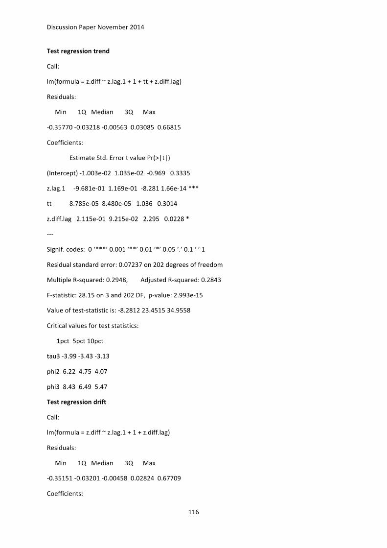
Discussion Paper November 2014
116
Test regression trend
Call:
lm(formula = z.diff ~ z.lag.1 + 1 + tt + z.diff.lag)
Residuals:
Min 1Q Median 3Q Max
-‐0.35770 -‐0.03218 -‐0.00563 0.03085 0.66815
Coefficients:
Estimate Std. Error t value Pr(>|t|)
(Intercept) -‐1.003e-‐02 1.035e-‐02 -‐0.969 0.3335
z.lag.1 -‐9.681e-‐01 1.169e-‐01 -‐8.281 1.66e-‐14 ***
tt 8.785e-‐05 8.480e-‐05 1.036 0.3014
z.diff.lag 2.115e-‐01 9.215e-‐02 2.295 0.0228 *
-‐-‐-‐
Signif. codes: 0 ‘***’ 0.001 ‘**’ 0.01 ‘*’ 0.05 ‘.’ 0.1 ‘ ’ 1
Residual standard error: 0.07237 on 202 degrees of freedom
Multiple R-‐squared: 0.2948, Adjusted R-‐squared: 0.2843
F-‐statistic: 28.15 on 3 and 202 DF, p-‐value: 2.993e-‐15
Value of test-‐statistic is: -‐8.2812 23.4515 34.9558
Critical values for test statistics:
1pct 5pct 10pct
tau3 -‐3.99 -‐3.43 -‐3.13
phi2 6.22 4.75 4.07
phi3 8.43 6.49 5.47
Test regression drift
Call:
lm(formula = z.diff ~ z.lag.1 + 1 + z.diff.lag)
Residuals:
Min 1Q Median 3Q Max
-‐0.35151 -‐0.03201 -‐0.00458 0.02824 0.67709
Coefficients:

Discussion Paper November 2014
117
Estimate Std. Error t value Pr(>|t|)
(Intercept) -‐0.0006832 0.0050664 -‐0.135 0.893
z.lag.1 -‐0.9698692 0.1169166 -‐8.295 1.49e-‐14 ***
z.diff.lag 0.2126930 0.0921588 2.308 0.022 *
-‐-‐-‐
Signif. codes: 0 ‘***’ 0.001 ‘**’ 0.01 ‘*’ 0.05 ‘.’ 0.1 ‘ ’ 1
Residual standard error: 0.07238 on 203 degrees of freedom
Multiple R-‐squared: 0.291, Adjusted R-‐squared: 0.2841
F-‐statistic: 41.67 on 2 and 203 DF, p-‐value: 6.884e-‐16
Value of test-‐statistic is: -‐8.2954 34.6282
Critical values for test statistics:
1pct 5pct 10pct
tau2 -‐3.46 -‐2.88 -‐2.57
phi1 6.52 4.63 3.81
Test regression none
Call: lm(formula = z.diff ~ z.lag.1 -‐ 1 + z.diff.lag)
Residuals:
Min 1Q Median 3Q Max
-‐0.35215 -‐0.03275 -‐0.00516 0.02754 0.67645
Coefficients:
Estimate Std. Error t value Pr(>|t|)
z.lag.1 -‐0.96835 0.11610 -‐8.341 1.09e-‐14 ***
z.diff.lag 0.21196 0.09177 2.310 0.0219 *
-‐-‐-‐
Signif. codes: 0 ‘***’ 0.001 ‘**’ 0.01 ‘*’ 0.05 ‘.’ 0.1 ‘ ’ 1
Residual standard error: 0.07221 on 204 degrees of freedom
Multiple R-‐squared: 0.2921, Adjusted R-‐squared: 0.2852
F-‐statistic: 42.09 on 2 and 204 DF, p-‐value: 4.978e-‐16
Value of test-‐statistic is: -‐8.341
Critical values for test statistics: 1pct 5pct 10pct

Discussion Paper November 2014
118
tau1 -‐2.58 -‐1.95 -‐1.62
VIII. KPSS on the first differenced-‐series, US bond yield rates
Null of stationary is not rejected, so the series are already stationary
TEST with a constant
Test is of type: mu with 4 lags.
Value of test-‐statistic is: 0.0968
Critical value for a significance level of:
10pct 5pct 2.5pct 1pct
critical values 0.347 0.463 0.574 0.739
Test is of type: mu with 14 lags.
Value of test-‐statistic is: 0.1231
Critical value for a significance level of:
10pct 5pct 2.5pct 1pct
critical values 0.347 0.463 0.574 0.739
TEST with a constant and linear trend
Test is of type: tau with 4 lags.
Value of test-‐statistic is: 0.0641
Critical value for a significance level of:
10pct 5pct 2.5pct 1pct
critical values 0.119 0.146 0.176 0.216
Test is of type: tau with 14 lags.
Value of test-‐statistic is: 0.0817
Critical value for a significance level of:
10pct 5pct 2.5pct 1pct
critical values 0.119 0.146 0.176 0.216
IX. DW regression on the residuals, NULL: no cointegration
Durbin-‐Watson test data: creg
DW = 2.0001, p-‐value = 0.4909

Discussion Paper November 2014
119
APPENDIX 10
RESULTS Japanese internal markets – Deposit rates vs Lending rates
1994/01 – 2011/06
SUMMARY: The ADF test results show that the lending rates follow the random walk hypothesis, only one lag variable and they are I(1). – the same from the KPSS test. Series of deposit rates are I(1). DW-‐value is 1.74 (Null rejected)
1. ADF Unit root Test Japanese Deposit Rates Null: of non-‐stationarity, or there is a unit root
Test regression “trend” – with a trend
Call:
lm(formula = z.diff ~ z.lag.1 + 1 + tt + z.diff.lag)
Residuals:
Min 1Q Median 3Q Max
-‐1.23530 -‐0.10717 0.02115 0.10621 1.10550
Coefficients:
Estimate Std. Error t value Pr(>|t|)
(Intercept) -‐0.1474020 0.0532913 -‐2.766 0.006261 **
z.lag.1 -‐0.0351586 0.0162239 -‐2.167 0.031528 *
tt 0.0008370 0.0003416 2.450 0.015236 *
z.diff.lag1 0.1493914 0.0758436 1.970 0.050387 .
z.diff.lag2 -‐0.2907312 0.0764205 -‐3.804 0.000194 ***
z.diff.lag3 -‐0.0548264 0.0790936 -‐0.693 0.489078
z.diff.lag4 0.1262645 0.0797110 1.584 0.114923
z.diff.lag5 -‐0.0906702 0.0799615 -‐1.134 0.258318
z.diff.lag6 0.1442845 0.0798398 1.807 0.072386 .
z.diff.lag7 -‐0.1010872 0.0800446 -‐1.263 0.208245
z.diff.lag8 -‐0.1313784 0.0800871 -‐1.640 0.102640
z.diff.lag9 0.0756268 0.0799982 0.945 0.345730
z.diff.lag10 -‐0.1027118 0.0799549 -‐1.285 0.200557
z.diff.lag11 0.1083614 0.0770391 1.407 0.161258
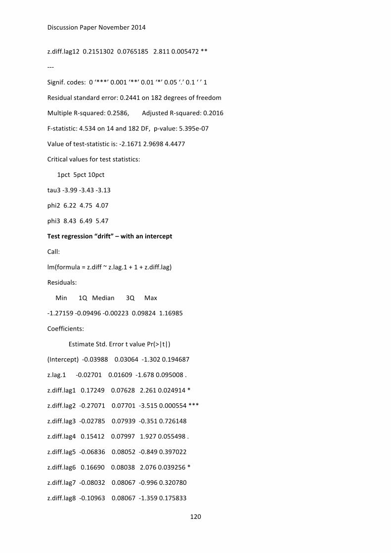
Discussion Paper November 2014
120
z.diff.lag12 0.2151302 0.0765185 2.811 0.005472 **
-‐-‐-‐
Signif. codes: 0 ‘***’ 0.001 ‘**’ 0.01 ‘*’ 0.05 ‘.’ 0.1 ‘ ’ 1
Residual standard error: 0.2441 on 182 degrees of freedom
Multiple R-‐squared: 0.2586, Adjusted R-‐squared: 0.2016
F-‐statistic: 4.534 on 14 and 182 DF, p-‐value: 5.395e-‐07
Value of test-‐statistic is: -‐2.1671 2.9698 4.4477
Critical values for test statistics:
1pct 5pct 10pct
tau3 -‐3.99 -‐3.43 -‐3.13
phi2 6.22 4.75 4.07
phi3 8.43 6.49 5.47
Test regression “drift” – with an intercept
Call:
lm(formula = z.diff ~ z.lag.1 + 1 + z.diff.lag)
Residuals:
Min 1Q Median 3Q Max
-‐1.27159 -‐0.09496 -‐0.00223 0.09824 1.16985
Coefficients:
Estimate Std. Error t value Pr(>|t|)
(Intercept) -‐0.03988 0.03064 -‐1.302 0.194687
z.lag.1 -‐0.02701 0.01609 -‐1.678 0.095008 .
z.diff.lag1 0.17249 0.07628 2.261 0.024914 *
z.diff.lag2 -‐0.27071 0.07701 -‐3.515 0.000554 ***
z.diff.lag3 -‐0.02785 0.07939 -‐0.351 0.726148
z.diff.lag4 0.15412 0.07997 1.927 0.055498 .
z.diff.lag5 -‐0.06836 0.08052 -‐0.849 0.397022
z.diff.lag6 0.16690 0.08038 2.076 0.039256 *
z.diff.lag7 -‐0.08032 0.08067 -‐0.996 0.320780
z.diff.lag8 -‐0.10963 0.08067 -‐1.359 0.175833

Discussion Paper November 2014
121
z.diff.lag9 0.10281 0.08030 1.280 0.202072
z.diff.lag10 -‐0.07939 0.08046 -‐0.987 0.325132
z.diff.lag11 0.13030 0.07756 1.680 0.094640 .
z.diff.lag12 0.23540 0.07710 3.053 0.002603 **
-‐-‐-‐
Signif. codes: 0 ‘***’ 0.001 ‘**’ 0.01 ‘*’ 0.05 ‘.’ 0.1 ‘ ’ 1
Residual standard error: 0.2474 on 183 degrees of freedom
Multiple R-‐squared: 0.2341, Adjusted R-‐squared: 0.1797
F-‐statistic: 4.304 on 13 and 183 DF, p-‐value: 2.71e-‐06
Value of test-‐statistic is: -‐1.6782 1.415
Critical values for test statistics:
1pct 5pct 10pct
tau2 -‐3.46 -‐2.88 -‐2.57
phi1 6.52 4.63 3.81
Test regression “none” -‐ neither an intercept nor a trend
Call: lm(formula = z.diff ~ z.lag.1 -‐ 1 + z.diff.lag)
Residuals:
Min 1Q Median 3Q Max
-‐1.26866 -‐0.12304 -‐0.01451 0.07371 1.14056
Coefficients:
Estimate Std. Error t value Pr(>|t|)
z.lag.1 -‐0.009921 0.009326 -‐1.064 0.288819
z.diff.lag1 0.167760 0.076334 2.198 0.029218 *
z.diff.lag2 -‐0.278240 0.076941 -‐3.616 0.000386 ***
z.diff.lag3 -‐0.031405 0.079489 -‐0.395 0.693239
z.diff.lag4 0.152388 0.080107 1.902 0.058693 .
z.diff.lag5 -‐0.071950 0.080624 -‐0.892 0.373338
z.diff.lag6 0.165428 0.080524 2.054 0.041352 *
z.diff.lag7 -‐0.085613 0.080724 -‐1.061 0.290280
z.diff.lag8 -‐0.112852 0.080788 -‐1.397 0.164130
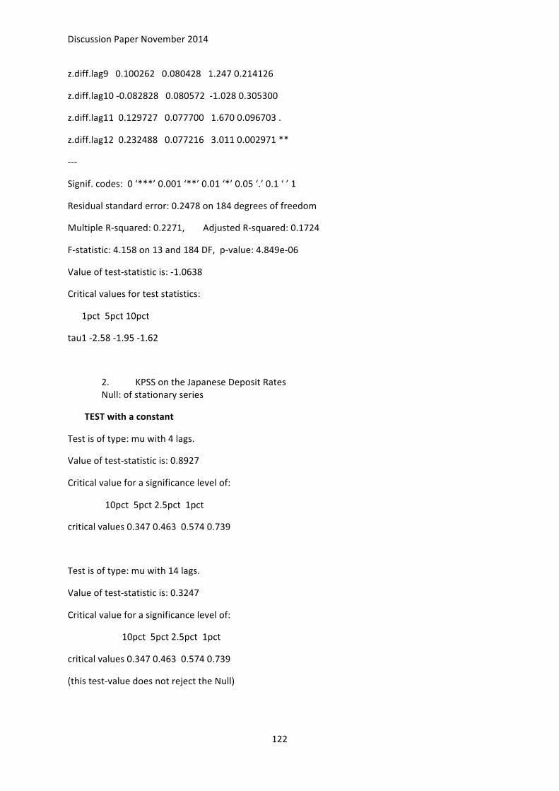
Discussion Paper November 2014
122
z.diff.lag9 0.100262 0.080428 1.247 0.214126
z.diff.lag10 -‐0.082828 0.080572 -‐1.028 0.305300
z.diff.lag11 0.129727 0.077700 1.670 0.096703 .
z.diff.lag12 0.232488 0.077216 3.011 0.002971 **
-‐-‐-‐
Signif. codes: 0 ‘***’ 0.001 ‘**’ 0.01 ‘*’ 0.05 ‘.’ 0.1 ‘ ’ 1
Residual standard error: 0.2478 on 184 degrees of freedom
Multiple R-‐squared: 0.2271, Adjusted R-‐squared: 0.1724
F-‐statistic: 4.158 on 13 and 184 DF, p-‐value: 4.849e-‐06
Value of test-‐statistic is: -‐1.0638
Critical values for test statistics:
1pct 5pct 10pct
tau1 -‐2.58 -‐1.95 -‐1.62
2. KPSS on the Japanese Deposit Rates Null: of stationary series
TEST with a constant
Test is of type: mu with 4 lags.
Value of test-‐statistic is: 0.8927
Critical value for a significance level of:
10pct 5pct 2.5pct 1pct
critical values 0.347 0.463 0.574 0.739
Test is of type: mu with 14 lags.
Value of test-‐statistic is: 0.3247
Critical value for a significance level of:
10pct 5pct 2.5pct 1pct
critical values 0.347 0.463 0.574 0.739
(this test-‐value does not reject the Null)

Discussion Paper November 2014
123
TEST with a constant and linear trend
Test is of type: tau with 4 lags.
Value of test-‐statistic is: 0.8527
Critical value for a significance level of:
10pct 5pct 2.5pct 1pct
critical values 0.119 0.146 0.176 0.216
Test is of type: tau with 14 lags.
Value of test-‐statistic is: 0.3111
Critical value for a significance level of:
10pct 5pct 2.5pct 1pct
critical values 0.119 0.146 0.176 0.216
3. ADF on the first differenced series, Deposit rates Test regression trend
Call:
lm(formula = z.diff ~ z.lag.1 + 1 + tt + z.diff.lag)
Residuals:
Min 1Q Median 3Q Max
-‐1.20528 -‐0.11706 0.01641 0.09894 1.08578
Coefficients:
Estimate Std. Error t value Pr(>|t|)
(Intercept) -‐0.0763598 0.0424760 -‐1.798 0.07388 .
z.lag.1 -‐1.0290517 0.3087717 -‐3.333 0.00104 **
tt 0.0006955 0.0003419 2.034 0.04336 *
z.diff.lag1 0.1701580 0.2937000 0.579 0.56306
z.diff.lag2 -‐0.1349899 0.2752937 -‐0.490 0.62448
z.diff.lag3 -‐0.1953334 0.2585812 -‐0.755 0.45098
z.diff.lag4 -‐0.0724257 0.2389542 -‐0.303 0.76216
z.diff.lag5 -‐0.1700294 0.2213095 -‐0.768 0.44331

Discussion Paper November 2014
124
z.diff.lag6 -‐0.0285883 0.2064577 -‐0.138 0.89002
z.diff.lag7 -‐0.1401998 0.1838680 -‐0.763 0.44675
z.diff.lag8 -‐0.2780197 0.1629004 -‐1.707 0.08959 .
z.diff.lag9 -‐0.2072023 0.1329471 -‐1.559 0.12084
z.diff.lag10 -‐0.3167615 0.0993256 -‐3.189 0.00168 **
z.diff.lag11 -‐0.2090240 0.0774562 -‐2.699 0.00762 **
-‐-‐-‐
Signif. codes: 0 ‘***’ 0.001 ‘**’ 0.01 ‘*’ 0.05 ‘.’ 0.1 ‘ ’ 1
Residual standard error: 0.2472 on 182 degrees of freedom
Multiple R-‐squared: 0.5486, Adjusted R-‐squared: 0.5164
F-‐statistic: 17.02 on 13 and 182 DF, p-‐value: < 2.2e-‐16
Value of test-‐statistic is: -‐3.3327 3.9386 5.826
Critical values for test statistics:
1pct 5pct 10pct
tau3 -‐3.99 -‐3.43 -‐3.13
phi2 6.22 4.75 4.07
phi3 8.43 6.49 5.47
Test regression drift
Call: lm(formula = z.diff ~ z.lag.1 + 1 + z.diff.lag)
Residuals:
Min 1Q Median 3Q Max
-‐1.24306 -‐0.11479 -‐0.00108 0.09360 1.14506
Coefficients:
Estimate Std. Error t value Pr(>|t|)
(Intercept) 0.002146 0.017901 0.120 0.904693
z.lag.1 -‐0.772635 0.284282 -‐2.718 0.007202 **
z.diff.lag1 -‐0.064600 0.272387 -‐0.237 0.812796
z.diff.lag2 -‐0.349554 0.256460 -‐1.363 0.174559
z.diff.lag3 -‐0.385366 0.243179 -‐1.585 0.114760

Discussion Paper November 2014
125
z.diff.lag4 -‐0.237652 0.226647 -‐1.049 0.295766
z.diff.lag5 -‐0.314513 0.211394 -‐1.488 0.138523
z.diff.lag6 -‐0.152876 0.198895 -‐0.769 0.443106
z.diff.lag7 -‐0.244386 0.178100 -‐1.372 0.171686
z.diff.lag8 -‐0.362015 0.158927 -‐2.278 0.023891 *
z.diff.lag9 -‐0.266733 0.130794 -‐2.039 0.042855 *
z.diff.lag10 -‐0.354674 0.098395 -‐3.605 0.000403 ***
z.diff.lag11 -‐0.227824 0.077560 -‐2.937 0.003735 **
-‐-‐-‐
Signif. codes: 0 ‘***’ 0.001 ‘**’ 0.01 ‘*’ 0.05 ‘.’ 0.1 ‘ ’ 1
Residual standard error: 0.2493 on 183 degrees of freedom
Multiple R-‐squared: 0.5384, Adjusted R-‐squared: 0.5081
F-‐statistic: 17.78 on 12 and 183 DF, p-‐value: < 2.2e-‐16
Value of test-‐statistic is: -‐2.7178 3.7738
Critical values for test statistics:
1pct 5pct 10pct
tau2 -‐3.46 -‐2.88 -‐2.57
phi1 6.52 4.63 3.81
Test regression none
Call: lm(formula = z.diff ~ z.lag.1 -‐ 1 + z.diff.lag)
Residuals:
Min 1Q Median 3Q Max
-‐1.24061 -‐0.11239 0.00079 0.09557 1.14725
Coefficients:
Estimate Std. Error t value Pr(>|t|)
z.lag.1 -‐0.77613 0.28202 -‐2.752 0.006515 **
z.diff.lag1 -‐0.06133 0.27029 -‐0.227 0.820753
z.diff.lag2 -‐0.34652 0.25452 -‐1.361 0.175039
z.diff.lag3 -‐0.38258 0.24141 -‐1.585 0.114744

Discussion Paper November 2014
126
z.diff.lag4 -‐0.23524 0.22514 -‐1.045 0.297475
z.diff.lag5 -‐0.31239 0.21008 -‐1.487 0.138736
z.diff.lag6 -‐0.15105 0.19778 -‐0.764 0.446006
z.diff.lag7 -‐0.24285 0.17716 -‐1.371 0.172115
z.diff.lag8 -‐0.36078 0.15817 -‐2.281 0.023694 *
z.diff.lag9 -‐0.26585 0.13024 -‐2.041 0.042650 *
z.diff.lag10 -‐0.35411 0.09802 -‐3.613 0.000391 ***
z.diff.lag11 -‐0.22752 0.07731 -‐2.943 0.003670 **
-‐-‐-‐
Signif. codes: 0 ‘***’ 0.001 ‘**’ 0.01 ‘*’ 0.05 ‘.’ 0.1 ‘ ’ 1
Residual standard error: 0.2486 on 184 degrees of freedom
Multiple R-‐squared: 0.5384, Adjusted R-‐squared: 0.5083
F-‐statistic: 17.89 on 12 and 184 DF, p-‐value: < 2.2e-‐16
Value of test-‐statistic is: -‐2.7521
Critical values for test statistics:
1pct 5pct 10pct
tau1 -‐2.58 -‐1.95 -‐1.62
4. KPSS Test on the first differenced series, Deposit rates (KPSS results do not reject the NULL, so the first differenced series are already stationary, as what could be expected from financial interest rate series of I(1))
TEST with a constant
Test is of type: mu with 4 lags.
Value of test-‐statistic is: 0.4653
Critical value for a significance level of:
10pct 5pct 2.5pct 1pct
critical values 0.347 0.463 0.574 0.739
Test is of type: mu with 14 lags.
Value of test-‐statistic is: 0.4417
Critical value for a significance level of:

Discussion Paper November 2014
127
10pct 5pct 2.5pct 1pct
critical values 0.347 0.463 0.574 0.739
TEST with a constant and linear trend
Test is of type: tau with 4 lags.
Value of test-‐statistic is: 0.0578
Critical value for a significance level of:
10pct 5pct 2.5pct 1pct
critical values 0.119 0.146 0.176 0.216
Test is of type: tau with 14 lags.
Value of test-‐statistic is: 0.0644
Critical value for a significance level of:
10pct 5pct 2.5pct 1pct
critical values 0.119 0.146 0.176 0.216
5. ADF on Japanese Lending rates (only with one lag, random walk hypothesis)
Test regression “trend” – with a trend (only one lag)
Call:
lm(formula = z.diff ~ z.lag.1 + 1 + tt + z.diff.lag)
Residuals:
Min 1Q Median 3Q Max
-‐0.03737 -‐0.01295 -‐0.00399 0.00323 1.01114
Coefficients:
Estimate Std. Error t value Pr(>|t|)
(Intercept) 0.0076153 0.0560509 0.136 0.892
z.lag.1 -‐0.0274903 0.0555709 -‐0.495 0.621
tt 0.0001201 0.0001829 0.657 0.512
z.diff.lag 0.3417747 0.5589088 0.612 0.542

Discussion Paper November 2014
128
Residual standard error: 0.07392 on 193 degrees of freedom
Multiple R-‐squared: 0.03431, Adjusted R-‐squared: 0.0193
F-‐statistic: 2.286 on 3 and 193 DF, p-‐value: 0.08011
Value of test-‐statistic is: -‐0.4947 1.578 2.1001
Critical values for test statistics:
1pct 5pct 10pct
tau3 -‐3.99 -‐3.43 -‐3.13
phi2 6.22 4.75 4.07
phi3 8.43 6.49 5.47
Test regression drift – with an intercept
Call: lm(formula = z.diff ~ z.lag.1 + 1 + z.diff.lag)
Residuals:
Min 1Q Median 3Q Max
-‐0.03274 -‐0.01249 -‐0.00505 0.00215 1.01442
Coefficients:
Estimate Std. Error t value Pr(>|t|)
(Intercept) 0.04193 0.02023 2.072 0.0395 *
z.lag.1 -‐0.05821 0.02994 -‐1.944 0.0533 .
z.diff.lag 0.29541 0.55362 0.534 0.5942
-‐-‐-‐
Signif. codes: 0 ‘***’ 0.001 ‘**’ 0.01 ‘*’ 0.05 ‘.’ 0.1 ‘ ’ 1
Residual standard error: 0.07381 on 194 degrees of freedom
Multiple R-‐squared: 0.03215, Adjusted R-‐squared: 0.02218
F-‐statistic: 3.223 on 2 and 194 DF, p-‐value: 0.042
Value of test-‐statistic is: -‐1.9443 2.1578
Critical values for test statistics:
1pct 5pct 10pct
tau2 -‐3.46 -‐2.88 -‐2.57
phi1 6.52 4.63 3.81
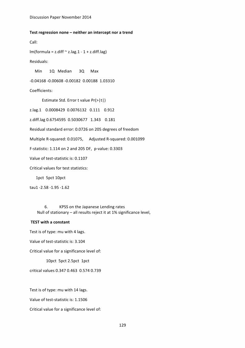
Discussion Paper November 2014
129
Test regression none – neither an intercept nor a trend
Call:
lm(formula = z.diff ~ z.lag.1 -‐ 1 + z.diff.lag)
Residuals:
Min 1Q Median 3Q Max
-‐0.04168 -‐0.00608 -‐0.00182 0.00188 1.03310
Coefficients:
Estimate Std. Error t value Pr(>|t|)
z.lag.1 0.0008429 0.0076132 0.111 0.912
z.diff.lag 0.6754595 0.5030677 1.343 0.181
Residual standard error: 0.0726 on 205 degrees of freedom
Multiple R-‐squared: 0.01075, Adjusted R-‐squared: 0.001099
F-‐statistic: 1.114 on 2 and 205 DF, p-‐value: 0.3303
Value of test-‐statistic is: 0.1107
Critical values for test statistics:
1pct 5pct 10pct
tau1 -‐2.58 -‐1.95 -‐1.62
6. KPSS on the Japanese Lending rates Null of stationary – all results reject it at 1% significance level,
TEST with a constant
Test is of type: mu with 4 lags.
Value of test-‐statistic is: 3.104
Critical value for a significance level of:
10pct 5pct 2.5pct 1pct
critical values 0.347 0.463 0.574 0.739
Test is of type: mu with 14 lags.
Value of test-‐statistic is: 1.1506
Critical value for a significance level of:
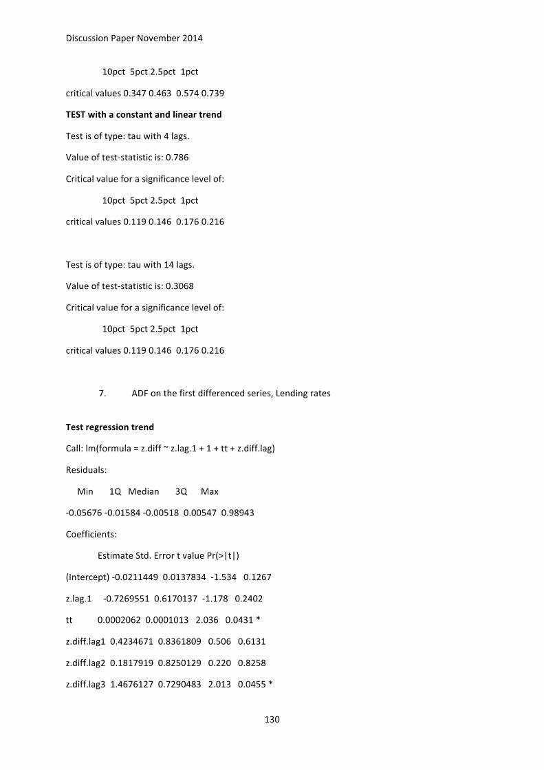
Discussion Paper November 2014
130
10pct 5pct 2.5pct 1pct
critical values 0.347 0.463 0.574 0.739
TEST with a constant and linear trend
Test is of type: tau with 4 lags.
Value of test-‐statistic is: 0.786
Critical value for a significance level of:
10pct 5pct 2.5pct 1pct
critical values 0.119 0.146 0.176 0.216
Test is of type: tau with 14 lags.
Value of test-‐statistic is: 0.3068
Critical value for a significance level of:
10pct 5pct 2.5pct 1pct
critical values 0.119 0.146 0.176 0.216
7. ADF on the first differenced series, Lending rates
Test regression trend
Call: lm(formula = z.diff ~ z.lag.1 + 1 + tt + z.diff.lag)
Residuals:
Min 1Q Median 3Q Max
-‐0.05676 -‐0.01584 -‐0.00518 0.00547 0.98943
Coefficients:
Estimate Std. Error t value Pr(>|t|)
(Intercept) -‐0.0211449 0.0137834 -‐1.534 0.1267
z.lag.1 -‐0.7269551 0.6170137 -‐1.178 0.2402
tt 0.0002062 0.0001013 2.036 0.0431 *
z.diff.lag1 0.4234671 0.8361809 0.506 0.6131
z.diff.lag2 0.1817919 0.8250129 0.220 0.8258
z.diff.lag3 1.4676127 0.7290483 2.013 0.0455 *
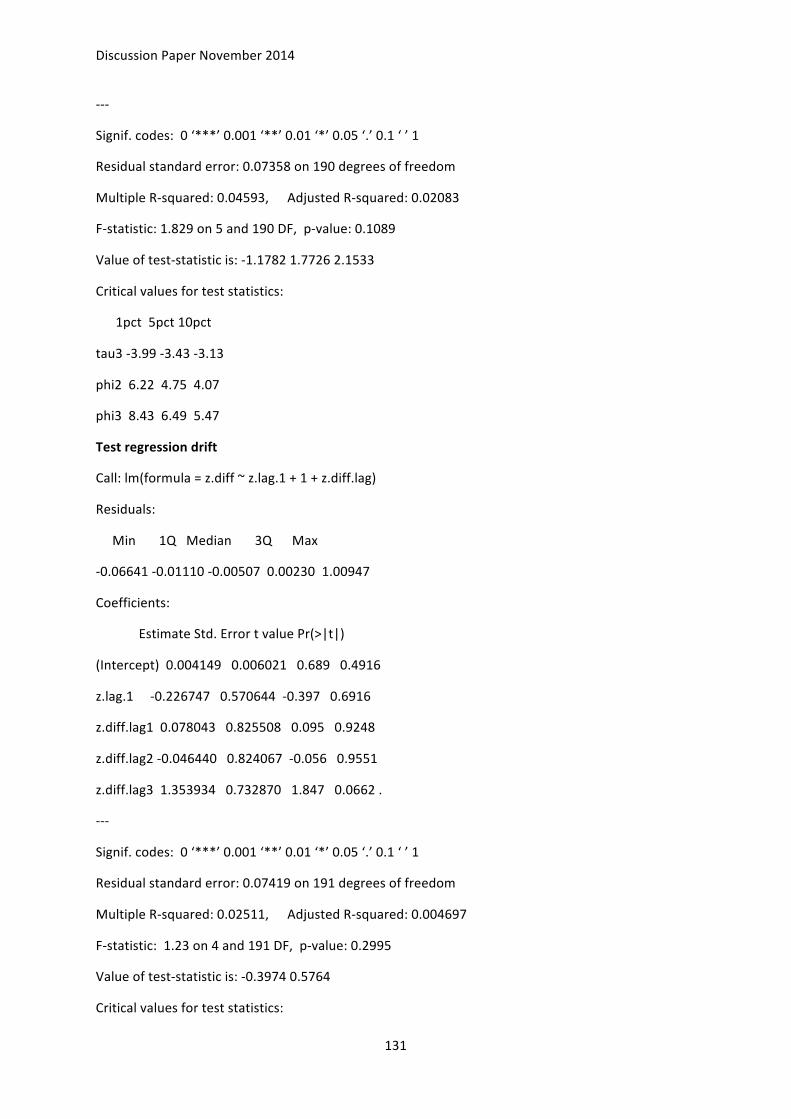
Discussion Paper November 2014
131
-‐-‐-‐
Signif. codes: 0 ‘***’ 0.001 ‘**’ 0.01 ‘*’ 0.05 ‘.’ 0.1 ‘ ’ 1
Residual standard error: 0.07358 on 190 degrees of freedom
Multiple R-‐squared: 0.04593, Adjusted R-‐squared: 0.02083
F-‐statistic: 1.829 on 5 and 190 DF, p-‐value: 0.1089
Value of test-‐statistic is: -‐1.1782 1.7726 2.1533
Critical values for test statistics:
1pct 5pct 10pct
tau3 -‐3.99 -‐3.43 -‐3.13
phi2 6.22 4.75 4.07
phi3 8.43 6.49 5.47
Test regression drift
Call: lm(formula = z.diff ~ z.lag.1 + 1 + z.diff.lag)
Residuals:
Min 1Q Median 3Q Max
-‐0.06641 -‐0.01110 -‐0.00507 0.00230 1.00947
Coefficients:
Estimate Std. Error t value Pr(>|t|)
(Intercept) 0.004149 0.006021 0.689 0.4916
z.lag.1 -‐0.226747 0.570644 -‐0.397 0.6916
z.diff.lag1 0.078043 0.825508 0.095 0.9248
z.diff.lag2 -‐0.046440 0.824067 -‐0.056 0.9551
z.diff.lag3 1.353934 0.732870 1.847 0.0662 .
-‐-‐-‐
Signif. codes: 0 ‘***’ 0.001 ‘**’ 0.01 ‘*’ 0.05 ‘.’ 0.1 ‘ ’ 1
Residual standard error: 0.07419 on 191 degrees of freedom
Multiple R-‐squared: 0.02511, Adjusted R-‐squared: 0.004697
F-‐statistic: 1.23 on 4 and 191 DF, p-‐value: 0.2995
Value of test-‐statistic is: -‐0.3974 0.5764
Critical values for test statistics:
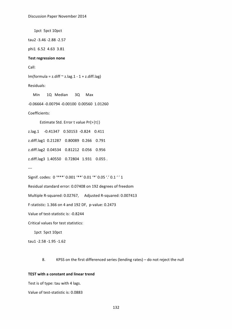
Discussion Paper November 2014
132
1pct 5pct 10pct
tau2 -‐3.46 -‐2.88 -‐2.57
phi1 6.52 4.63 3.81
Test regression none
Call:
lm(formula = z.diff ~ z.lag.1 -‐ 1 + z.diff.lag)
Residuals:
Min 1Q Median 3Q Max
-‐0.06664 -‐0.00794 -‐0.00100 0.00560 1.01260
Coefficients:
Estimate Std. Error t value Pr(>|t|)
z.lag.1 -‐0.41347 0.50153 -‐0.824 0.411
z.diff.lag1 0.21287 0.80089 0.266 0.791
z.diff.lag2 0.04534 0.81212 0.056 0.956
z.diff.lag3 1.40550 0.72804 1.931 0.055 .
-‐-‐-‐
Signif. codes: 0 ‘***’ 0.001 ‘**’ 0.01 ‘*’ 0.05 ‘.’ 0.1 ‘ ’ 1
Residual standard error: 0.07408 on 192 degrees of freedom
Multiple R-‐squared: 0.02767, Adjusted R-‐squared: 0.007413
F-‐statistic: 1.366 on 4 and 192 DF, p-‐value: 0.2473
Value of test-‐statistic is: -‐0.8244
Critical values for test statistics:
1pct 5pct 10pct
tau1 -‐2.58 -‐1.95 -‐1.62
8. KPSS on the first differenced series (lending rates) – do not reject the null
TEST with a constant and linear trend
Test is of type: tau with 4 lags.
Value of test-‐statistic is: 0.0883

Discussion Paper November 2014
133
Critical value for a significance level of:
10pct 5pct 2.5pct 1pct
critical values 0.119 0.146 0.176 0.216
Test is of type: tau with 14 lags.
Value of test-‐statistic is: 0.0908
Critical value for a significance level of:
10pct 5pct 2.5pct 1pct
critical values 0.119 0.146 0.176 0.216
TEST with a constant
Test is of type: mu with 4 lags.
Value of test-‐statistic is: 0.4938
Critical value for a significance level of:
10pct 5pct 2.5pct 1pct
critical values 0.347 0.463 0.574 0.739
Test is of type: mu with 14 lags.
Value of test-‐statistic is: 0.4686
Critical value for a significance level of:
10pct 5pct 2.5pct 1pct
critical values 0.347 0.463 0.574 0.739
9. DW test of cointegration (Null of no co-‐integration) data: creg
DW = 1.7452, p-‐value = 0.02979

Discussion Paper November 2014
134
Related Documents