J. Stat. Mech.

J.Stat.M

ech.(2010)

P01020

ournal of Statistical Mechanics:An IOP and SISSA journalJ Theory and Experiment

Optimized broad-histogram simulationsfor strong first-order phase transitions:droplet transitions in the large-Q Pottsmodel

Bela Bauer1, Emanuel Gull2, Simon Trebst3,Matthias Troyer1 and David A Huse4

1 Theoretische Physik, ETH Zurich, 8093 Zurich, Switzerland2 Department of Physics, Columbia University, New York, NY 10027, USA3 Microsoft Research, Station Q, University of California, Santa Barbara,CA 93106, USA4 Department of Physics, Princeton University, Princeton, NJ 08544, USAE-mail: [email protected], [email protected], [email protected],[email protected] and [email protected]

Received 10 December 2009Accepted 29 December 2009Published 29 January 2010

Online at stacks.iop.org/JSTAT/2010/P01020doi:10.1088/1742-5468/2010/01/P01020

Abstract. The numerical simulation of strongly first-order phase transitionshas remained a notoriously difficult problem even for classical systems due tothe exponentially suppressed (thermal) equilibration in the vicinity of such atransition. In the absence of efficient update techniques, a common approach forimproving equilibration in Monte Carlo simulations is broadening the sampledstatistical ensemble beyond the bimodal distribution of the canonical ensemble.Here we show how a recently developed feedback algorithm can systematicallyoptimize such broad-histogram ensembles and significantly speed up equilibrationin comparison with other extended ensemble techniques such as flat-histogram,multicanonical and Wang–Landau sampling. We simulate, as a prototypicalexample of a strong first-order transition, the two-dimensional Potts model withup to Q = 250 different states in large systems. The optimized histogram developsa distinct multi-peak structure, thereby resolving entropic barriers and theirassociated phase transitions in the phase coexistence region—such as dropletnucleation and annihilation, and droplet–strip transitions for systems withperiodic boundary conditions. We characterize the efficiency of the optimizedhistogram sampling by measuring round-trip times τ(N,Q) across the phase

c©2010 IOP Publishing Ltd and SISSA 1742-5468/10/P01020+22$30.00

J.Stat.M

ech.(2010)

P01020

Optimized broad-histogram simulations for strong first-order phase transitions

transition for samples comprised of N spins. While we find power-law scalingof τ versus N for small Q � 50 and N � 402, we observe a crossover toexponential scaling for larger Q. These results demonstrate that despite theensemble optimization, broad-histogram simulations cannot fully eliminate thesupercritical slowing down at strongly first-order transitions.

Keywords: classical Monte Carlo simulations, classical phase transitions(theory)

ArXiv ePrint: 0912.1192

Contents

1. Introduction 2

2. Optimized ensembles 32.1. Monte Carlo sampling and statistical ensembles . . . . . . . . . . . . . . . 42.2. Non-uniform diffusivity and optimized histograms . . . . . . . . . . . . . . 42.3. The feedback algorithm . . . . . . . . . . . . . . . . . . . . . . . . . . . . . 52.4. Improving the first feedback step . . . . . . . . . . . . . . . . . . . . . . . 6

3. The large-Q Potts model 73.1. Thermodynamic properties . . . . . . . . . . . . . . . . . . . . . . . . . . . 73.2. Phase coexistence and metastable states . . . . . . . . . . . . . . . . . . . 83.3. Droplet nucleation and droplet–strip transition . . . . . . . . . . . . . . . . 10

3.3.1. Multi-peak structure. . . . . . . . . . . . . . . . . . . . . . . . . . . 103.3.2. Location of droplet–strip transitions. . . . . . . . . . . . . . . . . . 113.3.3. Order parameter for the droplet–strip transition. . . . . . . . . . . . 143.3.4. Droplet anisotropy. . . . . . . . . . . . . . . . . . . . . . . . . . . . 14

3.4. Simulations on the cube surface . . . . . . . . . . . . . . . . . . . . . . . . 15

4. Sampling efficiency and round-trip times 16

5. Conclusions 20

Acknowledgments 20

References 20

1. Introduction

Competing phases or interactions in many-particle systems can give rise to complex freeenergy landscapes that exhibit multiple local minima and maxima, as sketched in figure 1.Thermal equilibration in these systems slows down exceedingly due to the (exponential)suppression of tunneling across free energy barriers. Examples of such slowly equilibratingsystems can be found in various settings ranging from spin glasses to folded proteins.

Numerical approaches to simulate these systems in thermal equilibrium suffer fromthe same slowing down when based on variational techniques or conventional Monte Carlosampling. To overcome this bottleneck various alternative sampling approaches have

doi:10.1088/1742-5468/2010/01/P01020 2

J.Stat.M

ech.(2010)

P01020

Optimized broad-histogram simulations for strong first-order phase transitions

been developed in recent years. Most of these approaches, which include multicanonicalsampling [1, 2], broad-histogram sampling [3], parallel tempering [4]–[6], multiple Gaussianmodified ensemble [7], and Wang–Landau sampling [8, 9], can be broadly grouped asextended ensemble techniques. Their common goal is to sample a statistical ensemble thatallows to significantly broaden the range of sampled energies beyond the comparativelynarrow distribution of the canonical ensemble.

The Wang–Landau algorithm tries to bring the idea of a broad sampling to anextreme by sampling a flat histogram in energy space. However, it was soon realizedthat sampling a uniform energy distribution is not necessarily the optimal way to improveequilibration and reduce autocorrelation times [10]–[12]. Instead it turns out that in orderto (considerably) speed up equilibration and minimize autocorrelation times one shouldsample a non-uniform energy distribution that allocates more statistical weight to thebottleneck(s) of the simulation which typically coincide with the free energy barriers [13].These so-called optimized ensembles are tailored to a given physical system and directlyreflect the underlying free energy landscape. One can systematically obtain the optimizedstatistical ensemble from an initial broad-histogram distribution by applying a feedbackalgorithm [13] that reallocates statistical weight based on measurements of the (local)diffusivity of the random walk which the system performs in energy space during thesimulation. This ensemble optimization has been applied in a broad variety of physicalsystems suffering from long thermal equilibration times in the absence of efficient non-local updates including folded proteins [14]–[17], frustrated magnetic systems [18, 19],and dense liquids [20]. The technique has further been generalized to optimize thegrid of temperature points used in parallel tempering simulations [21], has been usedin combination with cluster updates [22] and has been adopted for the simulation ofquantum systems [23, 24].

In this manuscript, we apply and analyze the ensemble optimization technique inthe context of a strong first-order phase transition where the characteristic double-well structure of the free energy provides a generic situation for entropically suppressedequilibration. In particular, we consider the thermal phase transition of the Q-state Pottsmodel in the limit of large Q, with our calculations being performed for up to Q = 250states. We find that the optimized ensemble aims to overcome the entropic barrier(s)of this transition by allocating most of the statistical weight in the energy range thatcorresponds to phase coexistence, e.g. the suppressed energy region of the characteristicbimodal distribution of the canonical ensemble. Remarkably, a multi-peak structureevolves in the optimized histogram that clearly resolves various intermediate transitionsbetween metastable states, such as droplet formation and droplet–strip transitions.

The remainder of the manuscript is structured as follows: we will first provide a briefreview of the ensemble optimization technique in section 2. In the subsequent section 3 weturn to the large-Q Potts model and discuss the multiple distinct features of the optimizedbroad-histogram distribution. We conclude our analysis by measuring the performance ofthe optimized ensemble technique in section 4.

2. Optimized ensembles

We start our discussion of the ensemble optimization technique by first offering a broaderview on Monte Carlo sampling and statistical ensembles. We then briefly review thederivation of the optimized ensembles and a related feedback algorithm.

doi:10.1088/1742-5468/2010/01/P01020 3

J.Stat.M

ech.(2010)

P01020

Optimized broad-histogram simulations for strong first-order phase transitions

2.1. Monte Carlo sampling and statistical ensembles

Speaking in broader terms one might take the perspective that the idea underlying MonteCarlo sampling is to map a random walk in some high-dimensional space of configurations{ci}

c1 → c2 → · · · → ci → ci+1 → · · ·onto a random walk in a lower-dimensional space, such as energy space (which is a one-dimensional space)

E(c1) → E(c2) → · · · → E(ci) → E(ci+1) → · · ·and to define a statistical ensemble in this latter low-dimensional space which thendetermines the transition probabilities between configurations in the original high-dimensional space. In particular, the statistical ensemble assigns a statistical weight w(c)to a configuration c solely on the basis of the respective energy E(c) of that configuration

w(c) ≡ w(E(c)).

The most commonly used statistical ensemble, of course, is the canonical ensemble, wherethe statistical weights are defined as

w(c) = exp (−βE(c)).

In order to simulate a reversible Markov process in configuration space one then definestransition probabilities from configuration c to c such that detailed balance is fulfilled.Common choices for these transition probabilities are Metropolis weights

pMetropolis(c → c) = min

(1,

w(c)

w(c)

)≡ min

(1,

w(E(c))

w(E(c))

),

or heat bath weights

pheat−bath(c → c) =w(c)

w(c) + w(c)≡ w(E(c))

w(E(c)) + w(E(c)).

While these choices of transition probabilities indeed ensure that the random walk inconfiguration space is Markovian, it should be noted that the projected random walkin energy space is not Markovian. This becomes clear when considering that multipleconfigurations may have the same energy E, whereas the distribution of energies that canbe reached by a single update may be completely different for each of these configurations.Thus, there is additional information encoded in configuration space which is not capturedby E, and it is this ‘memory’ which makes the projected random walk in energy spacenon-Markovian.

2.2. Non-uniform diffusivity and optimized histograms

The random walk in energy space has another distinct feature: the (local) diffusivity ofthis random walk, which for a given energy level measures the ability of the random walkerto move to other energy levels, is not uniform in energy space. In fact, it is exactly thismodulation of the local diffusivity which reflects the roughness of the underlying energylandscape. A suppressed diffusivity signals a ‘bottleneck’ of the simulation and is typicallyassociated with a phase transition or other entropic barrier.

doi:10.1088/1742-5468/2010/01/P01020 4

J.Stat.M

ech.(2010)

P01020

Optimized broad-histogram simulations for strong first-order phase transitions

This modulation of the local diffusivity thus differentiates the various energy regimesfor a given system, and in this light it becomes clear that one shortcoming of flat-histogram techniques is that they use a uniform distribution of statistical weight acrossthese inherently different energy regimes. In contrast the optimized ensemble methodallocates statistical weight based on measurements of the local diffusivity and shiftsadditional statistical weight towards the bottleneck(s) of the simulation, e.g. those energyregimes with a suppressed local diffusivity. As a result the so-optimized random walk inenergy space will sample a non-uniform histogram, spend more time in energy regimeswith low diffusivity, and thereby do its best to suppress the bottlenecks associated withthe underlying free energy landscape.

In more technical terms, we consider a random walk in some energy range [E−, E+]between two extremal energies E− and E+. In this paper we sample the entire energyrange, so E− and E+ are, respectively, the lowest and highest energies that our model has.The random walkers in energy space will drift between these two extremal energies andwe can think of the overall random walk as being composed of two opposite steady-state‘currents’ between these two extremal energies. These two currents exactly compensateone another, as the system remains in equilibrium, and are independent of energy. Wecan express these currents as

j = D(E)H(E)df

dE, (1)

where D(E) is the local diffusivity in energy space, H(E) is the sampled energy histogramand f(E) defines the orientation of the current by measuring for a given energy thefraction of random walkers which have last visited one of the two extremal energies, say,the lower extremal energy E−. This latter fraction can be measured by recording twohistograms, H+(E) and H−(E), where, for each Monte Carlo step, one increments thehistogram with label ‘+’ or ‘−’ depending on which extremal energy the random walkerhas visited last. The two histograms H+(E) and H−(E) thus sum up to the total histogramH(E) = H+(E) + H−(E). The fraction f(E) is then given by f(E) = H−(E)/H(E).

In order to speed up equilibration one wants to maximize the current (1) between thetwo extremal energies. Varying the histogram H(E) this can be achieved [13] by samplinga non-uniform distribution

Hopt(E) ∝ 1√D(E)

(2)

that is inversely proportional to the square root of the local diffusivity D(E) and thusreallocates statistical weight to those energy levels with suppressed diffusivity.

2.3. The feedback algorithm

In order to sample the optimized ensemble (2) we apply the feedback algorithm outlinedin [13]. We start from an initial broad-histogram ensemble with statistical weights w(E)which we obtain from a few iterations of the Wang–Landau algorithm or by extrapolatingresults from smaller system sizes. Running a (short) simulation for this initial ensemblewe record the two histograms H+(E) and H−(E) introduced above which in turn allow

doi:10.1088/1742-5468/2010/01/P01020 5

J.Stat.M

ech.(2010)

P01020

Optimized broad-histogram simulations for strong first-order phase transitions

us to calculate the local diffusivity as

D(E) ∝(

H(E)df

dE

)−1

. (3)

We then refine the statistical weights by feeding back this local diffusivity and define newoptimized weights as

wopt(E) = w(E)

√1

H(E)

df

dE. (4)

Subsequent simulations are performed for this new set of statistical weights. To furtherimprove and eventually converge the statistical weights for the optimized ensemble werepeat the feedback procedure several times. Note that in order to ensure convergencethe number of Monte Carlo steps between subsequent feedback iterations needs to beincreased; we typically double the number of Monte Carlo steps for consecutive runs.

2.4. Improving the first feedback step

There is a certain trade-off in performing the early feedback steps in the algorithm outlinedabove: on the one hand, an early feedback after only a small number of Monte Carlosweeps appears advantageous as it may quickly give dramatically improved statisticalweights and thereby speed up all subsequent simulations. On the other hand, the qualityof the feedback is rather sensitive to noisy input data, especially in calculating thenumerical derivative df/dE used in the feedback. To minimize this trade-off one thusneeds a way to quickly estimate this latter derivative in the presence of (substantial)noise. Conventional approaches such as finite-difference formulae, however, turn outto be exquisitely sensitive to the noise in the recorded histograms H+(E) and H−(E).In particular, the measured fraction f(E) = H−(E)/H(E) is a monotonically decayingfunction only when the simulation is in equilibrium in the simulated statistical ensemblewhich for a suboptimal choice, such as the flat-histogram ensemble, may require ratherlong Monte Carlo runs.

We have therefore developed a scheme that allows for the estimation of the derivativein the presence of significant noise. The idea is to analyze the measured fraction f(E) inFourier space, truncate the high-frequency terms which can be associated with noise, andthen determine the derivative using the low-frequency terms only. In doing so, we makeuse of the fact that for a continuous Fourier transformation

f(ω) =1√2π

∫ ∞

−∞e−iωEf(E) dE,

the derivative of the original function f(E)

∂Ef(E) =1√2π

∫ ∞

−∞iω · eiωE f(ω) dω (5)

can be easily calculated in Fourier space and then transformed back.In implementing this idea one needs to work around several obstacles. First, in

order to avoid irrelevant boundary terms, the function to be analyzed using the Fouriertransformation should be periodic. We therefore concatenate f(E) with its reflection.

doi:10.1088/1742-5468/2010/01/P01020 6

J.Stat.M

ech.(2010)

P01020

Optimized broad-histogram simulations for strong first-order phase transitions

Secondly, the above relation strictly holds only for the continuous Fourier transformation.As the energy levels of the Potts model and, in general, the energy bins of a broad-histogram simulation are discrete, we need to work with a discrete Fourier transformation.To overcome errors introduced by this, we make use of the following iterative scheme whichrefines the calculated derivative by iteratively reducing the deviation between the integralof the approximated derivative and the original function:

δf 1 = ∂Ef(E)

δf 2 = δf 1 + ∂E

(f(E) −

∫δf 1 dE

). . .

δf i+1 = δf i + ∂E

(f(E) −

∫δf i dE

)

Here, ∂E denotes the approximate derivative using the Fourier-based scheme above. Thescheme is iterated until the norm of the correction term falls below a certain threshold.

3. The large-Q Potts model

The two-dimensional Q-state Potts model is well known [25] to undergo a thermal phasetransition which turns from continuous for small Q ≤ 4 to weakly first order for Q > 4 andeventually becomes a strong first-order transition for Q � 5. We will turn to this lattercase of a strong first-order transition in systems with up to Q = 250 different Potts statesto explore the extent to which the optimized ensemble algorithm can achieve equilibrationat such a transition.

The Hamiltonian of the Q-state Potts model is given in terms of spins σi which takediscrete values σi ∈ {1, . . . , Q} as

H = −∑〈i,j〉

δ (σi, σj) . (6)

Here the sum runs over all pairs of nearest neighbors on a square lattice, and the Kroneckerδ-function tests whether two Potts spins have the same values. We have run simulations fortwo sample geometries: a ‘toroidal geometry’, i.e. a square lattice with periodic boundaryconditions, and a ‘cube geometry’ by forming a cube with square lattices on each of itssix faces.

We will start our discussion by briefly mentioning both exact and numerical resultsfor thermodynamic properties of the Potts model in this large, but finite Q limit. Wewill then turn to the energy regime associated with phase coexistence at this first-orderphase transition and examine the various intermediate, metastable states such as dropletsor strips which occur in this regime. In particular, we will discuss a distinct multi-peakstructure which emerges in the optimized histogram distribution and show how thesefeatures can be linked to transitions between the various metastable states.

3.1. Thermodynamic properties

The thermal phase transition in the Q-state Potts model from a disordered phase at hightemperatures to an ordered phase at low temperatures occurs at a transition temperature

doi:10.1088/1742-5468/2010/01/P01020 7

J.Stat.M

ech.(2010)

P01020

Optimized broad-histogram simulations for strong first-order phase transitions

Figure 1. Sketch of the free energy landscape in phase space for a slowlyequilibrating system.

T ∗ which for the infinite system is found [25] to be

T ∗ =1

ln(1 +√

Q). (7)

This phase transition is accompanied by sharp features in various thermodynamicproperties such as the energy, the specific heat, the free energy and the entropy. Since theoptimized ensemble algorithm allows to directly calculate the density of states g(E), wecan readily compute all of these thermodynamic variables. Our results are summarizedin figure 2 for simulations with Q = 10, 50, 250 states, where we have rescaled thetemperature axis by the transition temperature T ∗ in the thermodynamic limit. Asexpected, the features associated with the phase transition sharpen as we increase thenumber of Potts states Q for a system of fixed size L. For instance, the discontinuousjump in the energy grows with increasing Q and U(T ) approaches a step function in thelimit of Q → ∞. It is this broadening energy regime within the discontinuous jump ofthe energy that is associated with phase coexistence and the occurrence of intermediate,metastable states as we will discuss in detail below.

3.2. Phase coexistence and metastable states

The distinct characteristic of a first-order phase transition is a free energy profile thatpasses through a double-well shape as one drives the transition with some externalparameter such as temperature. At the transition temperature the two minima of thefree energy are exactly equal leading to coexistence of the two phases. For the high-QPotts model at hand there is a considerable amount of latent heat associated with thistransition, i.e. the internal energies of the two phases in proximity to this phase transitionvastly differ as shown in figure 2(a). As the system goes from one phase to the otherthis latent heat is not released (or absorbed) in a single step, but the system undergoesa sequence of phase transitions between various metastable states which are not minimaof the free energy in thermal equilibrium, but correspond to states with intermediateinternal energies. One such metastable state is a droplet of one phase inside the otherphase. Since the free energy density of the two phases becomes arbitrarily close in thevicinity of the transition, the free energy cost of forming a droplet is due to the surface of

doi:10.1088/1742-5468/2010/01/P01020 8

J.Stat.M

ech.(2010)

P01020

Optimized broad-histogram simulations for strong first-order phase transitions

Figure 2. Thermodynamic properties of the Q-state Potts model in the large,but finite Q limit: (a) internal energy, (b) specific heat, (c) free energy, and(d) entropy. The temperature axis is rescaled by the transition temperatureT ∗ = 1/ ln (1 +

√Q). Data shown is for system size L = 22 with periodic

boundary conditions.

the droplet, and not to its volume. It is thus entropically favorable to nucleate and grow asingle droplet of a shape that minimizes its surface free energy. This droplet condensationtransition has recently been studied in detail for a variety of physical systems using bothnumerical [10], [26]–[28] and analytical [29]–[33] approaches.

For a torus geometry, e.g. a system with periodic boundary conditions, this dropletwill subsequently expand as the total energy is changed until it percolates and it becomesentropically more favorable to form a strip wrapping around one of the boundaries. As thisstrip further grows the role of the two phases will eventually be reversed and the systemwill undergo a second sequence going from a strip to a droplet and eventually annihilatethe remaining droplet to complete the phase transition from one phase to the other. Thistransition was first discussed for the Ising model in an external magnetic field by Leungand Zia [34] and studied in detail by Neuhaus and Hager [10] using multicanonical MonteCarlo sampling. The droplet nucleation and droplet–strip transitions were also observedfor the Potts model with Q = 10 and system sizes of up to 1024 × 1024 spins using amicrocanonical approach [35].

We show representative snapshots of spin configurations reflecting these metastablestates in figure 3. All snapshots have been taken from our numerical simulations of the250-state Potts model.

doi:10.1088/1742-5468/2010/01/P01020 9

J.Stat.M

ech.(2010)

P01020

Optimized broad-histogram simulations for strong first-order phase transitions

Figure 3. Snapshots of spin configurations in the phase coexistence region of the250-state Potts model. (a) Formation of several small ordered droplets within thedisordered phase. (b) A dominant droplet is formed. (c) The droplet percolates toa strip wrapping around one boundary. (d) A single disordered droplet remains inthe ordered phase. All data shown is for system size L = 20. (a) E/2N = −0.20,(b) E/2N = −0.35, (c) E/2N = −0.54, (d) E/2N = −0.87.

3.3. Droplet nucleation and droplet–strip transition

For the toroidal system we can thus distinguish four intermediate transitions taking place‘within’ a first-order transition: the nucleation of a dominant droplet (which might occurvia the condensation of multiple small droplets), a droplet to strip transition and two moreprocesses where the roles of the two phases are reversed. These intermediate transitionsoccur at energies that are within the discontinuous jump of the internal energy U(T )plotted in figure 3(a) and are therefore not equilibrium energies at any temperature. Forthe canonical ensemble the states at these intermediate transitions are strongly suppressed,with its characteristic bimodal distribution of sampled energies as shown in the bottompanel of figure 4.

3.3.1. Multi-peak structure. In sharp contrast to the canonical ensemble the feedbackalgorithm of section 2 reallocates significant statistical weight to the energy rangelocated within the double-peak structure of the canonical distribution correspondingto the discontinuous jump of the internal energy. Strikingly, we find the emergenceof a distinct multi-peak structure in this energy range as shown in the top panel offigure 4. The emergent peaks resolve precisely the four intermediate transitions discussedabove. We come to this identification, as given in figure 4, by (i) comparing theenergies of typical configuration snapshots as shown in figure 3 with the locations ofthese peaks, (ii) estimating the transition energies of the droplet–strip transitions asdiscussed in section 3.3.2 and (iii) calculating order parameters for the droplet–striptransitions as detailed in section 3.3.3. The redistribution of statistical weight in thismulti-peak structure also reveals that these transitions between metastable states are ofdifferent severity. With the histogram peaks corresponding to the droplet–strip transitionsbeing much more pronounced than those corresponding to droplet nucleations we canconclude that the entropic barriers associated with the former transitions are significantlylarger than those associated with the latter transitions. Another observation regardingthis emerging multi-peak structure is that the histogram distribution is not perfectlysymmetric with respect to the ordered/disordered phases. For instance, the difference ofthe two smaller peaks reflects that droplet formation in the disordered phase is associatedwith a larger entropic barrier than droplet formation in the ordered phase.

doi:10.1088/1742-5468/2010/01/P01020 10

J.Stat.M

ech.(2010)

P01020

Optimized broad-histogram simulations for strong first-order phase transitions

Figure 4. Histograms of the optimized ensemble (top panel) and the canonicalensemble at the transition temperature T ∗ (bottom panel) for the 250-statePotts model with L = 22 and toroidal geometry. In contrast to the bimodaldistribution of the canonical ensemble the histogram of the optimized ensemblereveals a distinct four-peak structure reflecting the transitions between thevarious metastable states in the phase coexistence region.

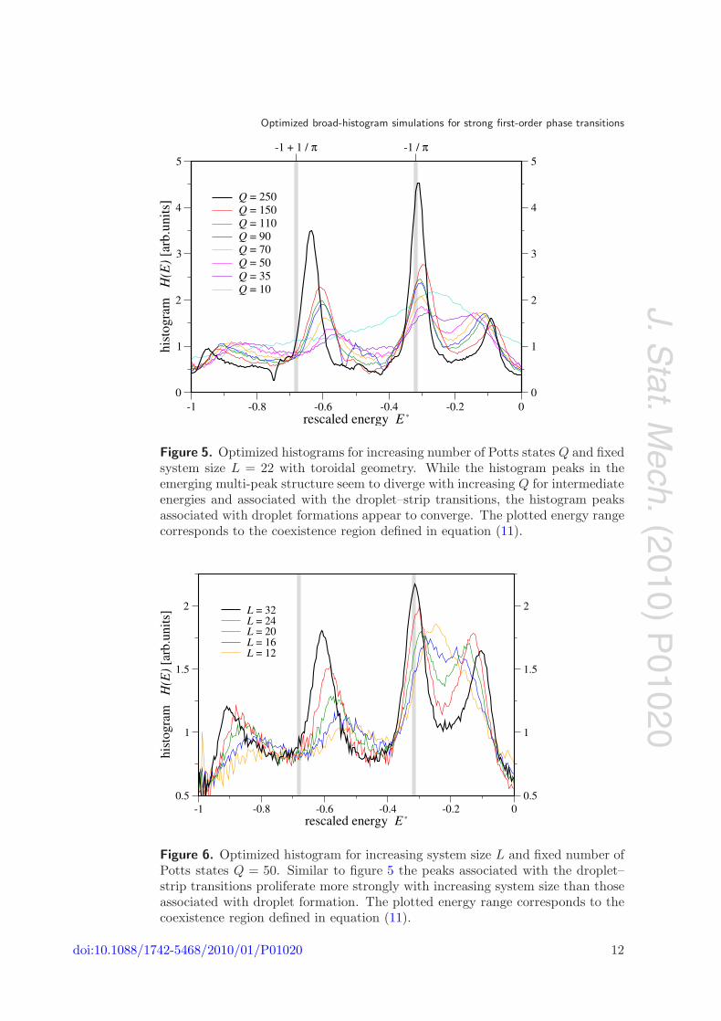
These characteristic features of the multi-peak structure further evolve as we varythe strength of the underlying first-order transition by increasing the number of Pottsstates Q or the system size L as shown in figures 5 and 6, respectively. With increasingthe number of Potts states Q we find the droplet–strip transitions to attract considerablymore statistical weight than the droplet formation transitions. In particular, the histogrampeaks associated with the droplet–strip transitions seem to diverge with increasing Q,while the histogram peaks associated with the droplet formation transitions appear toconverge to a finite height while sharpening with increasing Q, see figure 5. Similarly, wefind that increasing the system size L increases the peaks associated with the droplet–striptransitions more strongly than those associated with the formation of a droplet, as shownin figure 6.

3.3.2. Location of droplet–strip transitions. We can estimate the location of theintermediate droplet–strip transitions more quantitatively by estimating the interfacelength of the droplet/strip on either side of the transition. Making such an estimate forthe droplet, however, requires knowledge of its rough shape. The latter depends on theanisotropy of the surface tension and to some extent the geometry of the system. For the

doi:10.1088/1742-5468/2010/01/P01020 11

J.Stat.M

ech.(2010)

P01020

Optimized broad-histogram simulations for strong first-order phase transitions

Figure 5. Optimized histograms for increasing number of Potts states Q and fixedsystem size L = 22 with toroidal geometry. While the histogram peaks in theemerging multi-peak structure seem to diverge with increasing Q for intermediateenergies and associated with the droplet–strip transitions, the histogram peaksassociated with droplet formations appear to converge. The plotted energy rangecorresponds to the coexistence region defined in equation (11).

Figure 6. Optimized histogram for increasing system size L and fixed number ofPotts states Q = 50. Similar to figure 5 the peaks associated with the droplet–strip transitions proliferate more strongly with increasing system size than thoseassociated with droplet formation. The plotted energy range corresponds to thecoexistence region defined in equation (11).

doi:10.1088/1742-5468/2010/01/P01020 12

J.Stat.M

ech.(2010)

P01020

Optimized broad-histogram simulations for strong first-order phase transitions

Potts model, the surface tension and consequently the equilibrium droplet shape have beencalculated analytically for a droplet of fixed size embedded in an infinite volume [36, 37]; forfinite systems, Billoire et al [38] have estimated the surface tension based on multicanonicalsimulations of the canonical probability density for mixed-phase states. In the limit oflarge Q, which we consider here, the surface tension σ is found to become isotropic andthe droplet shape is expected to be roughly circular. The location of the droplet–striptransition can then be estimated by identifying the radius of the droplet R for which thesurface free energy of the droplet, Fdroplet = 2πσR, becomes equal to the surface freeenergy of the strip, Fstrip = 2σL. The transition is therefore expected to take place atR = L/π. At this transition point, the droplet occupies area πR2 = L2/π and thus afraction 1/π of the total area of the sample. We can estimate the total energy of a givendomain pattern as a sum of the contributions from the domains and the interfaces. Forthe example of an ordered droplet of radius R in a disordered background we have

E = (L2 − πR2)edis(T ) + πR2eord(T ) + 2πReσ. (8)

This configuration, by local stability of the curved interface, is at a temperature T thatis below the transition temperature T ∗ by an amount proportional to the curvature 1/Rof the interface. At that temperature, the energy densities of the two phases are eord(T )and edis(T ), while eσ is the excess energy per unit length in the interface.

Simplifying this expression by keeping only the contributions that are proportional tothe areas of the domains, we obtain that the transition energies of the two droplet–striptransitions can be approximated as

E∗droplet−strip,1 = −1

π, (9)

E∗droplet−strip,2 = −1 +

1

π, (10)

where these energies are given relative to the size of the coexistence region, e.g. the widthof the jump of the internal energy plotted in figure 3(a). In the following, we rescaleenergies such that the energy of the ordered phase Eord(T

∗) is mapped to −1 at thetransition temperature T ∗ and the energy of the disordered phase Edis(T

∗) becomes 0:

E∗ =E − Eord(T

∗)Edis(T ∗) − Eord(T ∗)

− 1. (11)

To rescale our numerical results we use the exactly known energy densities of the twophases at the transition temperature T ∗ in the thermodynamic limit.

We have indicated the so-estimated locations of the two droplet–strip transitions bythe vertical bars in figures 5 and 6. Indeed, the respective histogram peaks associatedwith these transitions seem to converge to these locations in the limit of large Q and L.In more quantitative terms, the energy of the interface moves E∗ at the transitions to ahigher energy by an amount proportional to 1/L. The small shift in T due to the curvatureof the interface of the droplet also moves E∗ at the transition by amount proportional(ignoring logs) to 1/(L

√Q) at large Q; this latter effect is of the same sign at the lower

energy droplet–strip transition, where the system is slightly ‘superheated’. The trendswith increasing Q and L at this lower transition can be clearly seen in figures 5 and 6,respectively. At the higher energy droplet–strip transition the two 1/L finite-size effectsare of opposite signs, so the peak in the histograms stays closer to E∗ = −1/π.

doi:10.1088/1742-5468/2010/01/P01020 13

J.Stat.M

ech.(2010)

P01020

Optimized broad-histogram simulations for strong first-order phase transitions

At the energies of these droplet–strip transitions, the two configurations (droplet andstrip) have the same entropy. However for the system to make a transition between thesetwo configurations, it must increase the amount of interface by an amount proportionalto L. The entropy deficit per unit length in the interface is proportional to log Q at largeQ, so the entropy barriers at these transitions are proportional to L log Q.

3.3.3. Order parameter for the droplet–strip transition. An alternative approach to locateand further describe the droplet–strip transition is to define an order parameter for thistransition. In doing so we follow an idea of Neuhaus and Hager [10] and measure theexistence of a strip by measuring the dimensions L1, L2 of the minimal bounding box forthe largest droplet in the system

Odis/ord = δ(L − max(Ldis/ord1 , L

dis/ord2 )), (12)

where the index ‘dis/ord’ distinguishes whether the phase in the droplet corresponds tothe disordered or ordered phase, respectively. When the droplet percolates and a strip isformed, one dimension of the bounding box becomes equal to the system size L and theorder parameter jumps from 0 to 1. Furthermore, we can associate a susceptibility withthis order parameter,

χO = 〈O2〉 − 〈O〉2 = 〈O〉 − 〈O〉2 ∈ [0, 1/4], (13)

which we expect to proliferate at the droplet–strip transition. Comparing the divergenceof this susceptibility with the respective intermediate peaks forming in the optimizedhistogram, we find that they coincide not only in location, but also their respective shapesas shown in figure 7. The latter illustrates that the entropic barriers at this intermediatetransition which the optimized ensemble overcomes by shifting statistical weight towardsthis transition arise solely from percolating a droplet into a strip.

3.3.4. Droplet anisotropy. Finally, we return to the droplet anisotropy and estimatecorrections to the circular shape induced by the finite size of our system. To this endwe monitor the anisotropy of the droplet by measuring the ratio of the dimensions L1, L2

of the minimal bounding box for the largest (ordered) droplet in the system

a =max(L1, L2)

min(L1, L2). (14)

In this notation a spherical droplet corresponds to a = 1.In figure 8 we plot this anisotropy for the largest ordered droplet measured for

energies in the phase coexistence region. At the droplet–strip transitions—indicated bythe vertical bars in the figure—the droplet anisotropy undergoes rapid changes as thedroplet percolates and deforms into a strip. For energies above the upper droplet–striptransition we find that the droplet anisotropy deviates from unity which indicates that theordered droplet in an otherwise disordered phase exhibits an non-spherical rather thana spherical shape. Since the analytical calculation for a droplet embedded in an infinitesystem predicts a roughly spherical shape [37], the observed anisotropy must be rooted inthe finite size of our system. Interestingly, we also seem to observe a signature indicatingthe droplet formation with the droplet anisotropy suddenly increasing from a ≈ 1.25 toa ≈ 1.5 in the respective energy region.

doi:10.1088/1742-5468/2010/01/P01020 14

J.Stat.M

ech.(2010)

P01020

Optimized broad-histogram simulations for strong first-order phase transitions

Figure 7. Optimized histogram and susceptibilities for the droplet percolationorder parameters. The lower susceptibility peak has been rescaled to match theheight of the peak in the optimized histogram. Data shown is for a 250-statePotts model and system size L = 24.

3.4. Simulations on the cube surface

Since the droplet–strip transition causes the main bottleneck for simulations in a toroidalgeometry, one could ask whether simulations on other surface topologies, in particularon simply connected surfaces, do not suffer from entropic barriers originating from suchshape transitions. In order to explore this idea we have simulated the Potts model in a‘sphere topology’ by considering the surface of a cube. We assemble such a cube surfacewith L sites on each edge and a total number of sites N = 6L2 − 12L + 8 such that thecorners have coordination number z = 3, while all other sites have coordination numberz = 4.

Figure 9 shows results for the optimized histograms for the Potts model on such acube surface. In panel (a), histograms for fixed Q = 250 and L in the range L = 6, . . . , 16are shown, while in panel (b), the system size is fixed at L = 10 and simulations areshown for various Q = 10, . . . , 250. As opposed to the simulations on the torus, the peakscorresponding to droplet nucleation/evaporation are now dominating the histogram forthese parameters.

However, for the largest systems with Q = 250 and L ≥ 14 (N ≥ 1016 spins) spins,four smaller peaks emerge. Examining snapshots of the system in the associated energyranges, we find that droplets nucleate around corners of the cube and the transitionsmark a change in the number of occupied corners. A similar observation has been madepreviously for multicanonical simulations of the Ising model in an external field [10].

There are multiple reasons why droplets nucleate at the corners of the cube. Naively,one might think that this is solely due to the lower coordination number of the cornersites, which provides a small energetic advantage (of order one in the system size) to placea droplet on a corner. Closer inspection of the surface free energy of a droplet enclosinga corner, however, reveals that similar to the droplet–strip transition there are entropic

doi:10.1088/1742-5468/2010/01/P01020 15

J.Stat.M

ech.(2010)

P01020

Optimized broad-histogram simulations for strong first-order phase transitions

Figure 8. Anisotropy of the largest droplet of ordered phase as defined inequation (14) in the phase coexistence region of a 250-state Potts model (L = 18).A spherical droplet corresponds to anisotropy 1 as indicated by the dashedline. At the droplet–strip transitions indicated by the vertical bars the dropletanisotropy quickly changes. The deviation from unity above the upper droplet–strip transition indicates an anisotropy due to finite-size effects.

barriers which scale with the system size L. To see this consider a droplet of area A. If Ais small enough (relative to L2), this droplet may sit on one of the faces of the cube so thatit encloses no corners of the cube. Then the surface it sits on is flat, so the surface freeenergy is minimized by a circular droplet with radius R so that A = πR2. Alternatively,the drop may enclose one corner. Putting the corner at the center of the droplet, thedroplet can be a quarter-circle on each of the three adjacent faces. These quarter-circleseach have radius R with A = (3πR2)/4. The net result is that the perimeter of the droplet(which sets the surface free energy) is smaller by a factor of

√3/2 when the droplet is

centered on a corner as compared to when it does not contain a corner. The difference isof order

√A, so for large enough cubes will dominate over the order one effect mentioned

above.While the simulation bottlenecks/entropic barriers associated with the corner

transitions are significantly suppressed in comparison with the droplet–strip transitions ofthe toroidal geometry, which is illustrated figure 10, we have not succeeded in suppressingall entropic barriers of order L by going from the torus to the cube surface. As aconsequence, we expect the same asymptotic performance of the optimized ensemblesimulations for both geometries.

4. Sampling efficiency and round-trip times

We finally address the numerical efficiency of sampling the optimized statistical ensemblefor the Q-state Potts model and, more generically, for a strong first-order phase transition.

doi:10.1088/1742-5468/2010/01/P01020 16

J.Stat.M

ech.(2010)

P01020

Optimized broad-histogram simulations for strong first-order phase transitions

Figure 9. Optimized histogram for the Potts model on the cube surface for(a) a fixed number of Potts states Q = 250 and various system sizes L, (b) afixed system size L = 10 and different choices of the number of Potts states Q.In contrast to the simulations on the torus (cf figure 6), the dominant peaks arerelated to droplet nucleation/annihilation transitions, while the emerging, smallerpeaks reveal transitions between states with droplets occupying an increasingnumber of corners of the cube. The plotted energy range corresponds to thecoexistence region defined in equation (11).

In order to quantify this performance we follow earlier work [11, 13, 12] and measure thecharacteristic timescale of the random walk in energy space, e.g. the round-trip time totraverse the full energy range [E−, E+], and its scaling with system size L and number ofPotts states Q. Our results are summarized in figures 11 and 12.

For systems undergoing continuous transitions it was shown [11] that the flat-histogram ensemble sampled in the Wang–Landau method generally suffers from a power-law slow down

τflat−histogram ∝ N2 · N z , (15)

which is reminiscent of the well-known critical slowing down in the canonical ensemble.The additional exponent z depends on the system at hand, and was measured to be

doi:10.1088/1742-5468/2010/01/P01020 17

J.Stat.M

ech.(2010)

P01020

Optimized broad-histogram simulations for strong first-order phase transitions

Figure 10. Comparison between optimized histograms for the cube surface andthe torus at Q = 50 for various system sizes L. The plotted energy rangecorresponds to the coexistence region defined in equation (11).

z ≈ 0.4 for the Ising model and z ≈ 0.9 for the fully frustrated Ising model [11]. Incontrast, the optimized ensemble method does not suffer from such a ‘critical slowingdown’ at continuous transitions and produces round-trip times that scale almost perfectlywith system size

τoptimized−ensemble ∝ N2 · (ln N)2, (16)

up to a logarithmic correction [13]. The improved scaling of the optimized ensemblecan thus considerably speed up the sampling efficiency of a broad-histogram simulation,with improvements of two orders of magnitude reported already for intermediate systemsizes [13].

Exploring the efficiency of simulations at a first-order phase transition, previous workhas found an exponential divergence of the round-trip time with L in the Ising model inan external magnetic field [10], which is referred to as supercritical slowing down. Thisdivergence occurs in the presence of shape transitions such as the droplet–strip transitiondiscussed above and the quantitative behavior of the scaling can indeed be related tothe surface tension of droplets. In a recent study Neuhaus et al [7] demonstrated thatthe multiple Gaussian modified ensemble (MGME) method suffers only from a residualsupercritical slowing down when applied to the Potts model (with Q = 20 and 256 statesin their simulations).

For the optimized ensembles the scaling of the round-trip times is shown in figures 11and 12 as a function of both system size L and number of Potts states Q, respectively.Similar to previous results for continuous transitions, we find a dramatic improvement of

doi:10.1088/1742-5468/2010/01/P01020 18

J.Stat.M

ech.(2010)

P01020

Optimized broad-histogram simulations for strong first-order phase transitions

Figure 11. Scaling of the round-trip time between the lowest and highest energystates with system size L for the optimized ensemble simulations using heat bathdynamics and the toroidal geometry. While the scaling can be fitted to polynomialbehavior for small Q � 35, the scaling crosses over to exponential behavior forlarger Q � 50.

the optimized ensemble when compared to the flat-histogram ensemble. However, evenfor the optimized ensemble we do not recover the almost perfect scaling (16) observed forcontinuous transitions when the severity of the first-order transition proliferates, e.g. byincreasing the system size L or the number of Potts states Q. In general, we find that thescaling is independent of the transition dynamics, e.g. whether we choose Metropolis orthe heat bath transition rates.

We first look at the scaling with system size L when fixing the number of Potts statesQ in the range 8 ≤ Q ≤ 150. As shown in figure 11 we find that, for the range of Lstudied, the round-trip times appear to scale polynomially τ ∼ N2+z in system size L forQ � 35. We estimate the effective exponents to be z ≈ 0.3 for Q = 8, z ≈ 0.31 for Q = 10,z ≈ 0.38 for Q = 20, and z ≈ 0.48 for Q = 35. We note that in this regime the first-ordertransition is still relatively weak and we do not (yet) observe the characteristic multi-peak structure in the optimized histogram. However, when further increasing number ofPotts states Q we find that the scaling crosses over to the expected exponential behaviorτ ∼ exp(αL) for Q � 50 due to the entropy barriers at the droplet–strip transitions,and this becomes apparent already on rather small system sizes. This, of course, bearswitness of the strong first-order nature of the phase transition in this regime, which alsobecomes evident in a noticeable multi-peak structure of the optimized histogram even forconsiderably small system sizes L ≥ 14. Our results however do not exclude a crossover tosupercritical scaling also for weaker transitions at some larger system size. Indeed, resultsin [35] indicate that also for Q = 10, an extended stripe phase emerges for system sizesL � 512, which may well lead to the same effect we observe for large Q at much smallerL.

doi:10.1088/1742-5468/2010/01/P01020 19

J.Stat.M

ech.(2010)P

01020

Optimized broad-histogram simulations for strong first-order phase transitions

Figure 12. Scaling of the round-trip time between the lowest and highest energystates with the number of Potts states Q for the optimized ensemble simulationsusing both Metropolis and heat bath dynamics in the toroidal geometry. Thedashed lines represent cubic regressions to the data.

5. Conclusions

We presented an application of the optimized ensemble method to improve equilibration ofbroad-histogram simulations of the first-order transition in the large-Q Potts model. Theoptimized histogram develops a characteristic multi-peak structure which indicates thatthe system releases latent heat in a sequence of phase transitions. The intermediatemetastable states exhibit droplets of the coexisting phases in varying shapes. For atoroidal system geometry the dominant bottleneck in the simulation is the entropic barrierassociated with a droplet–strip transition. We find that the ensemble optimization iscapable to only partially overcome this bottleneck by shuffling statistical weight towardsthe entropic barriers. It still exhibits the same asymptotic supercritical slowing down forstrongly first-order transitions previously reported for flat-histogram simulations [10]. Itthus remains an open question whether simulation schemes for strongly first-order phasetransitions can be further improved to overcome this asymptotic slowing down. Possibly,statistical ensembles defined in multiple system variables could further improve extendedensemble simulations, or one might turn to modified update technique, which, for instance,attempt to specifically update the boundaries of a droplet.

Acknowledgments

Our numerical calculations were performed on the Hreidar and Brutus clusters at ETHZurich. ST thanks the MPI-PKS Dresden for hospitality.

References

[1] Berg B A and Neuhaus T, Multicanonical algorithms for first order phase transitions, 1991 Phys. Lett. B267 249

doi:10.1088/1742-5468/2010/01/P01020 20

J.Stat.M

ech.(2010)P

01020

Optimized broad-histogram simulations for strong first-order phase transitions

[2] Berg B A and Neuhaus T, Multicanonical ensemble: a new approach to simulate first-order phasetransitions, 1992 Phys. Rev. Lett. 68 9

[3] de Oliveira P M C, Penna T J P and Herrmann H J, 1996 Braz. J. Phys. 26 677[4] Hukushima K and Nemoto K, Exchange Monte Carlo method and application to spin glass simulations,

1996 J. Phys. Soc. Japan 65 1604[5] Marinari E and Parisi G, Simulated tempering: a new Monte Carlo scheme, 1992 Europhys. Lett. 19 451[6] Lyubartsev A P, Martsinovski A A, Shevkunov S V and Vorontsov-Velyaminov P N, New approach to

Monte Carlo calculation of the free energy: method of expanded ensembles, 1992 J. Chem. Phys. 96 1776[7] Neuhaus T, Magiera M and Hansmann U, Efficient parallel tempering for first-order phase transitions, 2007

Phys. Rev. E 76 045701[8] Wang F and Landau D P, Efficient, multiple-range random walk algorithm to calculate the density of states,

2001 Phys. Rev. Lett. 86 2050[9] Wang F and Landau D P, Determining the density of states for classical statistical models: a random walk

algorithm to produce a flat histogram, 2001 Phys. Rev. E 64 56101[10] Neuhaus T and Hager J S, 2d crystal shapes, droplet condensation, and exponential slowing down in

simulations of first-order phase transitions, 2003 J. Stat. Phys. 113 47[11] Dayal P, Trebst S, Wessel S, Wurtz D, Troyer M, Sabhapandit S and Coppersmith S N, Performance

limitations of flat-histogram methods, 2004 Phys. Rev. Lett. 92 97201[12] Alder S, Trebst S, Hartmann A K and Troyer M, Dynamics of the Wang–Landau algorithm and complexity

of rare events for the three-dimensional bimodal Ising spin glass, 2004 J. Stat. Mech. P07008[13] Trebst Simon, Huse D A and Troyer M, Optimizing the ensemble for equilibration in broad-histogram Monte

Carlo simulations, 2004 Phys. Rev. E 70 046701[14] Trebst S, Troyer M and Hansmann U, Optimized parallel tempering simulations of proteins, 2006 J. Chem.

Phys. 124 174903[15] Escobedo F A and Martinez-Veracoechea F J, Optimization of expanded ensemble methods, 2008 J. Chem.

Phys. 129 154107[16] Binder K and Paul W, Recent developments in Monte Carlo simulations of lattice models for polymer

systems, 2008 Macromolecules 41 4537[17] Christen M and Van Gunsteren W F, On searching in, sampling of, and dynamically moving through

conformational space of biomolecular systems: a review , 2008 J. Comput. Chem. 29 157[18] Bergman D, Alicea J, Gull E, Trebst S and Balents L, Order by disorder and spiral spin liquid in frustrated

diamond lattice antiferromagnets, 2007 Nat. Phys. 3 487[19] Chern Gia-Wei, Moessner R and Tchernyshyov O, Partial order from disorder in a classical pyrochlore

antiferromagnet , 2008 Phys. Rev. B 78 144418[20] Trebst S, Gull E and Troyer M, Optimized ensemble Monte Carlo simulations of dense Lennard–Jones

fluids, 2005 J. Chem. Phys. 123 204501[21] Katzgraber H G, Trebst S, Huse D A and Troyer M, Feedback-optimized parallel tempering Monte Carlo,

2006 J. Stat. Mech. P03018[22] Wu Y, Korner M, Colonna-Romano L, Trebst S, Gould H, Machta J and Troyer M, Overcoming the slowing

down of flat-histogram Monte Carlo simulations: cluster updates and optimized broad-histogramensembles, 2005 Phys. Rev. E 72 046704

[23] Wessel S, Stoop N, Gull E, Trebst S and Troyer M, Optimized broad-histogram ensembles for the simulationof quantum systems, 2007 J. Stat. Mech. P12005

[24] Harada K and Kuge Y, Diffusion in the continuous-imaginary-time quantum world-line Monte Carlosimulations with extended ensembles, 2008 J. Phys. Soc. Japan 77 013001

[25] Wu F Y, The Potts model , 1982 Rev. Mod. Phys. 54 235[26] MacDowell L, Shen V and Errington J, Nucleation and cavitation of spherical, cylindrical, and slablike

droplets and bubbles in small systems, 2006 J. Chem. Phys. 125 034705[27] Nussbaumer A, Bittner E, Neuhaus T and Janke W, Monte Carlo study of the evaporation/condensation

transition of Ising droplets, 2006 Europhys. Lett. 75 716[28] Nussbaumer A, Bittner E and Janke W, Monte Carlo study of the droplet formation-dissolution transition

on different two-dimensional lattices, 2008 Phys. Rev. E 77 041109[29] Biskup M, Chayes L and Kotecky R, On the formation/dissolution of equilibrium droplets, 2002 Europhys.

Lett. 60 21[30] Biskup M, Chayes L and Kotecky R, Critical region for droplet formation in the two-dimensional Ising

model , 2003 Commun. Math. Phys. 242 137

doi:10.1088/1742-5468/2010/01/P01020 21

J.Stat.M

ech.(2010)

P01020

Optimized broad-histogram simulations for strong first-order phase transitions

[31] MacDowell L, Virnau P, Muller M and Binder K, The evaporation/condensation transition of liquiddroplets, 2004 J. Chem. Phys. 120 5293

[32] Binder K, Theory of the evaporation/condensation transition of equilibrium droplets in finite volumes, 2003Physica A 319 99

[33] Biskup M, Chayes L and Kotecky R, A proof of the Gibbs–Thomson formula in the droplet formationregime, 2004 J. Stat. Phys. 116 175

[34] Leung K and Zia R K P, Geometrically induced transitions between equilibrium crystal shapes, 1990 J.Phys. A: Math. Gen. 23 4593

[35] Martin-Mayor V, Microcanonical approach to the simulation of first-order phase transitions, 2007 Phys.Rev. Lett. 98 137207

[36] Borgs C and Janke W, An explicit formula for the interface tension of the 2d Potts model , 1992 J. PhysiqueI 2 2011

[37] Fujimoto M, Equilibrium crystal shape of the Potts model at the first-order transition point , 1997 J. Phys.A: Math. Gen. 30 3779

[38] Billoire A, Neuhaus T and Berg B A, A determination of interface free energies, 1994 Nucl. Phys. B413 795

doi:10.1088/1742-5468/2010/01/P01020 22