J. A. Jaramillo Aguado G. A. Muñoz Fernández A. Prieto Yerro J. B. Seoane Sepúlveda

Welcome message from author
This document is posted to help you gain knowledge. Please leave a comment to let me know what you think about it! Share it to your friends and learn new things together.
Transcript

J. A. Jaramillo AguadoG. A. Muñoz Fernández
A. Prieto YerroJ. B. Seoane Sepúlveda


Proceedings of
Function Theory on Innite Dimensional Spaces X
Editors:Jesus Angel Jaramillo AguadoGustavo Adolfo Munoz FernandezAngeles Prieto YerroJuan Benigno Seoane Sepulveda


Departamentode Análisis
Matemático
The conference programme includes a number of plenary talks and severalparallel sessions of 20-minute talkspreferably related to the following topics: Geometry of Banach spaces, nonlinear analysis, differentiability, polynomials and multilinear mappings in Banach spaces, holomorphy, lineability and spaceability, hypercyclicity and dynamical systems.
Organizing Committee:J.A. Jaramillo, G. A. Muñoz, A. Prieto and J. B. Seoane
http://www.mat.ucm.es/[email protected]
J. C. Álvarez-Paiva (Université des Sciences et Technologies de Lille, France)L. Ambrosio (Scuola Normale Superiore, Pisa, Italy)R. M. Aron (Kent State University, USA)R. Deville (Université de Bordeaux, France)A. Fathi (École Normale Supérieure de Lyon, France)P. Galindo (Universidad de Valencia, Spain)D. García (Universidad de Valencia, Spain)G. Godefroy (Université Paris 6, France)A. Ibort (Universidad Carlos III, Spain)J. Orihuela (Universidad de Murcia, Spain)A. Peris (Universidad Politécnica de Valencia, Spain) R. Ryan (National University of Ireland Galway, Ireland)J. B. Seoane Sepúlveda (Universidad Complutense de Madrid, Spain)I. Zalduendo (Universidad Torcuato di Tella, Buenos Aires, Argentina)


Preface
This volume contains the proceedings of the tenth edition of the Conference onFunction Theory on Infinite Dimensional Spaces, held at the Departamento de AnalisisMatematico of the Universidad Complutense de Madrid, between the 11th and 14thof December, 2007. This conference is a part of a series of meetings that began in1989 with the organization of the first edition by Jose Luis Gonzalez Llavona and JoseMarıa Martınez Ansemil, and since then it has been held on a biannual basis. Alongthese years, this Conference has gathered a large number of outstanding researchersin the field of Infinite-Dimensional Analysis, stressing the interaction with differentrelated topics, such as Differentiability, Convexity and Geometry of Banach Spaces,Non-linear Analysis, Polynomials and Multilinear Mappings, Holomorphy, FunctionAlgebras, Lineability and Spaceability and Hypercyclicity among others.
We would like to take the opportunity of this tenth edition to thank the partici-pants in all these meetings. Their active interest in this project and the high level oftheir contributions have been the key of the success and the very continuity of thisConference. They are also responsible for the warm and fruitful atmosphere that wehave enjoyed in all these editions.
This tenth conference was attended by more than 90 participants coming from 17different countries, including some of the most experienced specialists in the field, aswell as young mathematicians at earlier stages of their research programs.
The conference was sponsored by the Departamento de Analisis Matematico, theUniversidad Complutense de Madrid, the Instituto de Matematica Interdisciplinar(IMI), and the Ministerio de Educacion y Ciencia of Spain, to whom thanks are due.
We would like to thank all the people involved in the organization of this meeting.In particular, the graduate students of the Departamento de Analisis Matematico fortheir help with registration, and their assistance in running the talks. We also thankthe secretarial stuff for taking care of most of the required red tape. Thanks shouldbe also addressed to those who collaborated in chairing the main talks and parallelsessions.
The Organizing Committee,
Jesus Angel Jaramillo AguadoGustavo Adolfo Munoz FernandezAngeles Prieto YerroJuan Benigno Seoane Sepulveda.
i

Plenary lectures
During the meeting the following fourteen speakers delivered a plenary lecture:
1. Juan Carlos Alvarez Paiva. Universite des Sciences et Technologies de Lille,France. Dual normed spaces have the same girth.
2. Luigi Ambrosio. Scuola Normale Superiore, Pisa, Italy. Existence and sta-bility results of Fokker-Planck equations and Markov processes associated tolog-concave measures.
3. Richard M. Aron. Kent State University, USA. Norm divergent, weakly densesequences.
4. Robert Deville. Universite de Bordeaux, France. Almost classical solutions ofHamilton Jacobi equations.
5. Albert Fathi. Ecole Normale Superieure de Lyon, France. An Introduction toWeak KAM Theory.
6. Pablo Galindo. Universidad de Valencia, Spain. Interpolating sequences inspaces of bounded analytic functions.
7. Domingo Garcıa. Universidad de Valencia, Spain. The Bishop-Phelps-Bollobastheorem for operators.
8. Gilles Godefroy. Universite Paris 6, France. Isometrically universal Banachspaces.
9. Alberto Ibort. Universidad Carlos III, Spain. On the extensions of a class ofgeneralized -symmetric operators.
10. Jose Orihuela. Universidad de Murcia, Spain. James boundaries, selectors, andrisk measures applications.
11. Alfred Peris. Universidad Politecnica de Valencia, Spain. Hypercyclic opera-tors: When the linear dynamics becomes chaotic.
12. Raymond Ryan. National University of Ireland Galway, Ireland. Regular Holo-morphic Functions on Complex Banach Lattices.
13. Juan B. Seoane Sepulveda. Universidad Complutense de Madrid, Spain. Geom-etry of Polynomials in Banach spaces and its applications to Bernstein andMarkov inequalities.
14. Ignacio Zalduendo. Universidad Torcuato di Tella, Buenos Aires, Argentina.Linearization and Compactness.
ii

Short talks
Besides the main talks there also were three sessions of 20-minute talks with theparticipation of 35 more speakers listed below:
1. Jesus Araujo. Universidad de Cantabria. Spain. Stability and instability ofoperators between spaces of continuous functions.
2. Javier Cabello Sanchez. Universidad de Extremadura. Spain. Multiplicativebijections of Lipschitz and smooth functions.
3. Daniel Carando. Universidad de Buenos Aires. Argentina. Spectra of weightedalgebras of holomorphic functions.
4. Jose A. Conejero. Universidad Politecnica de Valencia. Spain. Hypercyclic andchaotic behaviour of C0-semigroups generated by Ornstein-Uhlenbeck operators.
5. Estibalitz Durand Cartagena. Universidad Complutense de Madrid. Spain. ABanach-Stone theorem for D∗ spaces.
6. Arsen R. Dzhanoev. Moscow State University, Moscow (Russia) and Universi-dad Rey Juan Carlos (Spain). Function of stabilization for dissipative dynamicalsystems.
7. Maite Fernandez Unzueta. CIMAT, Guanajuato. Mexico. Extension of poly-nomials as a local property.
8. Irene Ferrando. Instituto Universitario de Matematica Pura y Aplicada andUniversidad Politecnica de Valencia. Spain. Tensor product representation ofthe (pre)dual of order continuous p-convex Banach lattices.
9. Francisco Gallego Lupianez. Universidad Complutense de Madrid. Spain. OnM -spaces and Banach spaces.
10. Alma L. Gonzalez Correa. Universidad Politecnica de Valencia. Spain. Flatsets, `p-generating and fixing c0 in nonseparable setting.
11. Bogdan C. Grecu. Queen’s University Belfast. UK. The relationship betweenextreme homogeneous polynomials and multilinear forms on Hilbert spaces.
12. Olivia Gutu. Universidad Autonoma del Estado de Hidalgo. Mexico. GlobalInversion on Length Spaces.
13. Petr Hajek. Czech Academy of Sciences. Czech Republic. Zero sets of realpolynomials.
14. Beatriz Hernando. Universidad Nacional de Educacion a Distancia (UNED).Spain. Approximation numbers of nuclear and Hilbert-Schmidt multilinearforms defined on Hilbert spaces.
iii

15. Michal Johanis. Charles University Prague. Czech Republic. Functions locallydependent on finitely many coordinates.
16. Enrique Jorda. Universidad Politecnica de Valencia. Spain. On boundedvector-valued holomorphic functions.
17. Sebastian Lajara. Universidad de Castilla La Mancha. Spain. The geometry ofthe bidual of a separable Banach space.
18. Silvia Lassalle. Universidad de Buenos Aires. Argentina. Atomic decomposi-tions for tensor products and polynomial spaces.
19. Pablo Linares. Universidad Complutense de Madrid. Spain. Orthogonally ad-ditive polynomials in `p.
20. Mikael Lindstrom. Abo Akademi University. Finland. Essential norm of oper-ators on weighted Bergman spaces of infinite order.
21. Elena Martın Peinador. Universidad Complutense de Madrid. Spain. Frechet-Urysohn property for topological groups.
22. Alejandro Miralles. Universidad de Valencia, Spain. Hankel Operators on Al-gebras of Analytic Functions.
23. Vicente Montesinos. Universidad Politecnica de Valencia. Spain. Weak com-pactness and sigma-Asplund generated spaces.
24. Gustavo A. Munoz Fernandez. Universidad Complutense de Madrid. Spain.Unconditional constants in spaces of polynomials.
25. Santiago Muro. Universidad de Buenos Aires. Argentina. Hypercyclic convo-lution operators on Frechet spaces of analytic functions.
26. David Perez Garcıa. Universidad Complutense de Madrid. Spain. Bell inequal-ities: a long path from Einstein to Pisier.
27. Damian Pinasco. Universidad de Buenos Aires. Argentina. Lp representablefunctions on Banach spaces.
28. Antonın Prochazka.Charles University in Prague, Czech Republic and UniversiteBordeaux 1, France. Winning tactics in a geometrical game.
29. Pilar Rueda. Universidad de Valencia. Spain. Biduality in weighted Banachspaces of holomorphic functions.
30. Vıctor Manuel Sanchez de los Reyes. Universidad Complutense de Madrid.Spain. Strictly singular inclusions into L1 + L∞.
31. Yannis Sarantopoulos. National Technical University Athens. Greece. On thereal Plank problem and its applications.
32. Sorin Mirel Stoian. University of Petrosani. Romania. A functional Calculusfor Quotient Bounded Operators.
iv

33. Jesus Suarez. Universidad de Extremadura. Spain. Twisting Schatten classes.
34. Tino Ullrich. University of Jena. Germany. Tensor Products of Besov Spacesand Applications.
35. Andreas Weber. Universitat Karlsruhe (TH). Germany. A class of hypercyclicVolterra composition operators.
v


Index
Page
Weakly dense, norm divergent sequencesRichard M. Aron, Domingo Garcıa and Manuel Maestre 1
Monomial decompositions for homogeneous polynomials and tensor productsDaniel Carando and Silvia Lassalle 5
Spectral conditions for hypercyclic C0-semigroupsJose A. Conejero and Elisabetta M. Mangino 17
Flat sets and `p-generating in nonseparable Asplund Banach spacesMarian Fabian, Alma L. Gonzalez and Vaclav Zizler 27
A note on σ-finite dual dentability indicesMarian Fabian, Vicente Montesinos and Vaclav Zizler 31
Integral representation of operators defined on a p-convex Banach lattice with theσ-Fatou propertyIrene Ferrando and Enrique A. Sanchez Perez 37
Interpolating sequences for bounded analytic functionsPablo Galindo 45
Linearization and compactness
Jesus A. Jaramillo, Angeles Prieto and Ignacio Zalduendo 55
The unit ball of the Banach space of real trinomialsGustavo A. Munoz Fernandez and Juan B. Seoane Sepulveda 65
Hypercyclic operators: When the linear dynamics becomes chaoticAlfred Peris 77
Winning tactics in a geometrical gameAntonin Prochazka 83
Strictly singular inclusions into L1 + L∞
Vıctor M. Sanchez 87
Holomorphic Functional Calculus for Regular Operators on Locally Convex SpacesSorin Mirel Stoian 91
Volterra composition operators: supercyclicity and hypercyclicityAndreas Weber 111
vii


Proceedings ofFunction Theory on Infinite Dimensional Spaces XPages 1–4
Weakly dense, norm divergent sequences
R.M. ARON, D. GARCıA,
and M. MAESTRE
Department of Mathematical Sciences
Kent State University
Kent, Ohio 44242, USA
Departamento de Analisis
Matematico
Universidad de Valencia
Doctor Moliner 50
46100 Burjasot (Valencia), Spain
Departamento de Analisis
Matematico
Universidad de Valencia
Doctor Moliner 50
6100 Burjasot (Valencia), Spain
ABSTRACT
Let X be a separable Banach space. We provide an explicit construction of asequence in X that tends to ∞ in norm but which is weakly dense.
Key words: Banach space, weakly dense sequence, norm divergent sequence, weakhypercyclicity.
2000 Mathematics Subject Classification: Primary 46B20, 46B25; Secondary 46B45.
Our interest in the result stated in the Abstract originated with the following re-sults, of K. Chan and R. Sanders [3], and of V. Kadets [5] (see also [4]):
Theorem 1. (Chan and Sanders, [3]) For any p, 2 ≤ p < ∞, there is a boundedlinear operator T : `p(Z) → `p(Z) that is weakly hypercyclic but is not hypercyclic.
Theorem 2. (Kadets, [5]) For any Banach space X, for any sequence (cn) of positivereal numbers such that
∑∞n=1 c−2
n = ∞, there is a sequence (xn) ⊂ X, ‖xn‖ = cn forall n, such that 0 is in the weak closure of the sequence xn | n ∈ N.
The authors were supported in part by MEC and FEDER Project MTM2005-08210, and a grantfrom Prometeo/2008/101.
1

R.M. Aron/D. Garcıa/M. Maestre Weakly dense, norm divergent sequences
In fact, the proof in [3] shows the existence of a vector x0 such that ‖Tn(x0)‖ tendsto ∞ while Tn(x0) | n ∈ N is dense in `2(Z) with the weak topology. Chan andSanders remark ([3, page 49]) that for X = `p(Z), one can construct a weakly densesequence (xn) ⊂ X such that ‖xn‖ → ∞. Also, Kadets’ proof (and that of S. Shkarin[6], rediscovered independently several years later) makes use of Dvoretzky’s theorem.
Motivated by these results, we prove the following:
Theorem 3. For any separable Banach space X, there is a sequence (xn) ⊂ X suchthat ‖xn‖ → ∞ while xn | n ∈ N is weakly dense in X.
As opposed to the Kadets-Shkarin argument, the proof offered by the authors isan explicit construction. We outline the three steps of this argument below.
Proposition 4. Suppose that there is a sequence (yn) ∈ X with the following twoproperties:
(i) ‖yn‖ → ∞ as n →∞,
(ii) 0 is in the weak closure of yn | n ∈ N.Then there is a sequence (xn) ∈ X such that the following hold:
(i) ‖xn‖ → ∞ as n →∞,
(ii) xn | n ∈ N is weakly dense in X.
Together with the previous proposition, the next result proves Theorem 3 for thecase X = `1.
Proposition 5. There is a sequence (xn) ⊂ `1 such that ‖xn‖ → ∞ as n → ∞ and0 ∈ xn | n ∈ Nw
.
The final proposition, below, shows that Theorem 3 holds in general.
Proposition 6. If Theorem 3 is true for X = `1, then it holds for all separableBanach spaces X.
Crucial for the proof of Proposition 6 is the fact that each vector xn in the sequencein the proof of Proposition 5 has the form xn =
√k(ei − ej), 1 ≤ i < j ≤ (2k)k+1
where (em) is the usual basis for `1.
These results for real Banach spaces, with full details, are available in [1]. Herewe are going to present the proof for complex `1.
Theorem 7. Consider the sequence (xn) in `1(C) obtained by any ordering of the set∪∞k=1
√k(em1 − em2) : 1 ≤ m1 < m2 ≤ (4k2)k+1. We have that (‖xn‖) diverges to
∞ and 0 belongs to the weak closure of (xn).
——————————Function Theory on Infinite Dimensional Spaces X
2

R.M. Aron/D. Garcıa/M. Maestre Weakly dense, norm divergent sequences
Proof. Consider a natural number k and ϕ1, . . . , ϕk in S`∞ . We denote
K0 = 1, . . . , (4k2)k+1.
Ifϕj = (αj
m)∞m=1
we put
J1p,q = m ≤ (4k2)k+1 : α1
m ∈ [p
k,p + 1
k] + i[
q
k,q + 1
k]
for −k ≤ p, q ≤ k − 1, then
1, . . . , (4k2)k+1 =k−1⋃
p,q=−k
J1p,q.
Thus there exist p1, q1, −k ≤ p1, q1 ≤ k − 1, such that
Card(J1p1,q1
) ≥ (4k2)k.
Now we consider K1 ⊂ J1p1,q1
such that
Card(K1) = (4k2)k.
By induction we can find
Kk ⊂ Kk−1 ⊂ . . . ⊂ K2 ⊂ K1 ⊂ 1, . . . , (4k2)k+1,
Card(Kk) = 4k2,
and
|αjm − αj
r| ≤√
2k
for all j = 1, . . . , k and all m, r ∈ Kk. Since Card(Kk) = 4k2 > 2, we can takem1 < m2, such that
m1,m2 ⊂ Kk.
Considerx =
√k(em1 − em2).
|ϕj(x)| = |√
k(αjm1− αj
m2)| ≤
√2√k
, (1)
for all j = 1, . . . , k and‖x‖1 = 2
√k.
Now let
(xn)∞n=1 =∞⋃
k=1
√
k(em1 − em2) : 1 ≤ m1 < m2 ≤ (4k2)k+1
for any ordering. Clearly (‖xn‖) diverges to ∞ and, by (1), the origin belongs to theweak closure of (xn).
3
——————————Function Theory on Infinite Dimensional Spaces X

R.M. Aron/D. Garcıa/M. Maestre Weakly dense, norm divergent sequences
We conclude with several related comments.
Comments. There are at least two reasonable natural questions that arise.
(i) Theorem 3 is much weaker than Theorem 1. Indeed, the result of [3] producesan operator T : `p(Z) → `p(Z) which, in turn, produces the sequence (xn).Thus, we ask the following: Given an arbitrary separable Banach space X anda sequence (xn) that satisfies Theorem 3, is there a bounded linear operatorT : X → X that interpolates the sequence, in the sense that T (xn) = xn+1 forall n ∈ N?
(ii) What can be said about the speed with which the norm of the sequence (xn) inTheorem 3 tends to ∞?
First, as Shkarin notes, there is no bilateral shift on `p(Z) for 1 ≤ p < 2 that isweakly, but not norm, hypercyclic. Although this does not rule out a positive answerto the first question, it at least gives an indication of how difficult the solution wouldbe if the answer is affirmative.
Concerning the second question, Shkarin [6, Proposition 5.4] observes that if
∞∑n=1
‖xn‖−1 < ∞,
then 0 /∈ xn | n ∈ Nweak. As a consequence, no sequence (xn) having the properties
described in Theorem 3 can increase in norm very quickly.
Acknowledgements. We are grateful to Robert Deville and, in particular, toFrederic Bayart for bringing both his own work [2] and also that of S. Shkarin [6] toour attention.
References
[1] R. M. Aron, D. Garcıa, and M. Maestre, Construction of weakly dense, norm divergentsequences, J. Convex Analysis, to appear.
[2] F. Bayart, Weak-closure and polarization constant by Gaussian measure, to appear.
[3] K. Chan and R. Sanders, A weakly hypercyclic operator that is not norm hypercyclic,J. Operator Theory 52, no. 1, (2004), 39–59.
[4] G. Helmberg, Curiosities concerning weak topology in Hilbert space, Amer. Math.Monthly 113, no. 5, (2006), 447–452.
[5] V. M. Kadets, Weak cluster points of a sequence and coverings by cylinders, Mat. Fiz.Anal. Geom. 11, no. 2, (2004), 161–168.
[6] S. Shkarin, Non-sequential weak supercyclicity and hypercyclicity, J. Func. Anal. 242(2007), 37–77.
——————————Function Theory on Infinite Dimensional Spaces X
4
Proceedings ofFunction Theory on Infinite Dimensional Spaces XPages 5–16
Monomial decompositions for homogeneouspolynomials and tensor products
D. CARANDO and S. LASSALLE
Departamento de Matematica,
Pab I, Facultad de Cs. Exactas y Naturales,
Universidad de Buenos Aires,
(1428) Buenos Aires, Argentina.
[email protected], [email protected]
ABSTRACT
We review some results on the existence of atomic decomposition for tensorproducts of Banach spaces and spaces of homogeneous polynomials. First, weconsider duality properties of atomic decompositions, showing how the conceptof shrinking Schauder bases can be adapted to the context of atomic decompo-sitions. Then, we show that if the Banach space X admits an atomic decom-position of a certain kind, the symmetrized tensor product of the elements ofthe atomic decomposition is an atomic decomposition for the symmetric tensorproduct
Nns,µ X, for any symmetric tensor norm µ. Combined with our duality
results, this allows us to establish the existence of monomial atomic decompo-sitions for some usual ideals of polynomials on X. The reflexivity of spaces ofpolynomials is also studied.
Key words: Atomic decompositions, tensor products, symmetric tensor norms, homo-geneous polynomials, polynomial ideals.
2000 Mathematics Subject Classification: Primary: 46B28, 42C15, Secondary: 41A65,46G25, 46B15.
Introduction
A Schauder basis in a Banach space X and its bi-orthogonal dual sequence, in X ′,allow a reconstruction formula of the elements of X as a series expansion in terms ofboth sequences. The linear structure and properties of the spaces often reflects intothe structure and properties of the different type of functions defined on them. Forexample, for Banach spaces X and Y with shrinking bases, the space of bilinear formsB(X × Y ) has a monomial basis if and only if all the linear operators form X to Y ′
are compact, see [23].
This research was partially supported by PICT 05 17-33042, UBACyT X108, UBACyT X863and UBACyT 038.The authors wish to thank the Departamento de Analisis Matematico of the Universidad Com-plutense de Madrid and all our friends within it for their kind hospitality during December 2007.
5

D. Carando/S. Lassalle Monomial decompositions for homogeneous polynomials
Two basic results made us turn our attention to atomic decompositions which pro-vide a Banach space with a more flexible structure than bases do. In [21], Pelczynskishows that a separable Banach space admits an atomic decomposition if and only ifit has the bounded approximation property. On the other hand, any complementedsubspace of a Banach with basis has a natural atomic decomposition given by theprojection and the inclusion mappings.
Atomic decomposition were formally introduced by Grochening [17] as an exten-sion of the notion of frames for Hilbert spaces to the Banach space setting. Framesfor Hilbert spaces emerged in the context of nonharmonic Fourier series, and firstappeared in the work by Duffin and Schaeffer [13].
This note reviews the main results in [3, 4] related to the following question: if aBanach space X has an atomic decomposition and Q(X) is some space of polynomialson X, are the corresponding monomials an atomic decomposition for Q(X)? Moreprecisely, given an atomic decomposition ((x′i), (xi)) of X and any continuous n-homogeneous polynomial P on X, the series expansion
P (x) = P (x, · · · , x) =∑α1
· · ·∑αn
P (xα1 , . . . , xαn) x′α1(x) · · ·x′αn
(x)
is pointwise convergent (here, P denotes the symmetric n-linear form associatedto P ). The question is then to determine under which conditions the monomials(x′α1
· · ·x′αn), together with the n-tuples (xα1 , . . . , xαn), are atomic decomposition for
different spaces of polynomials. The particular case of X having a Schauder basis wasintensively studied by many authors [1, 2, 9, 10, 18, 22].
In order to study the existence of monomial atomic decompositions for spaces ofpolynomials, we develop two topics that have independent interest. First, we studyduality for atomic decompositions. Namely, if ((x′i), (xi)) is an atomic decompositionfor X, we investigate conditions ensuring that ((xi), (x′i)) is an atomic decomposi-tion for X ′. The second topic is the existence of atomic decomposition for full andsymmetric tensor products.
The article is organized as follows: The first section deals with the duality the-ory for atomic decompositions. We introduce the concept of shrinking and stronglyshrinking atomic decomposition, which extend the notion of shrinking Schauder ba-sis. We obtain that an atomic decomposition for X is shrinking if and only if thedual pair is an atomic decomposition for the dual space X ′. In the second section,we investigate the existence of atomic decompositions for full and symmetric ten-sor products endowed with different tensor norms. The third section is devoted toour main question: in which cases do monomials provide an atomic decompositionfor spaces of polynomials? As applications, we relate Asplund spaces with monomialatomic decompositions for integral polynomials and address the question of reflexivityof spaces of polynomials.
For further information on atomic decompositions and Banach frames see, forexample, [6, 7, 17] and the references therein. We refer to [19] for Banach spacetheory, [8, 14, 15, 22] for notation and properties of tensor products and [11, 20] forpolynomials on Banach spaces.
——————————Function Theory on Infinite Dimensional Spaces X
6

D. Carando/S. Lassalle Monomial decompositions for homogeneous polynomials
1. Duality for atomic decompositions
By a Banach sequence space we understand a Banach space of scalar sequences forwhich the coordinate functionals are continuous. We say that the space is a Schaudersequence space if, in addition, the unit vectors ei given by (ei)j = δi,j form a basisfor it. In this case, a sequence a = (ai) can be written as a =
∑i aiei.
Definition 1. Let X be a Banach space and Z be a Banach sequence space. Let (x′i)and (xi) be sequences in X ′ and X respectively. We say that ((x′i), (xi)) is an atomicdecomposition of X with respect to Z if for all x ∈ X:
(a) (〈x′i, x〉) ∈ Z,(b) A‖x‖ ≤ ‖(〈x′i, x〉)‖Z ≤ B‖x‖, with A and B positive constants,(c) x =
∑i〈x′i, x〉xi.
Property (c) in the above definition is usually referred to as the reconstructionformula associated to the atomic decomposition.
A Banach space admits an atomic decomposition if an only if it has the boundedapproximation property. Moreover, if ((x′i), (xi)) is an atomic decomposition of Xwith respect to some Banach sequence space Z, it is always possible to find a Schaudersequence space Xd and an operator S : Xd → X such that Sei = xi and ((x′i), (xi))is also an atomic decomposition of X with respect to Xd [21, 5]. From now on, weconsider atomic decompositions of the form ((x′i), (Sei)) associated to a Schaudersequence space Xd.
Now, if ((x′i), (Sei)) is an atomic decomposition of X with respect to Xd, we definethe natural inclusion J : X → Xd by
J(x) = (〈x′i, x〉) =∑
i
〈x′i, x〉ei. (1)
If (e′i) is the dual basic sequence of (ei) then, x′i = J ′e′i. Note that, SJ = IX andthen X is isomorphic to a complemented subspace of Xd. Conversely, if we haveJ : X → Xd and S : Xd → X continuous operators so that SJ = IX and (e′i) is thedual basic sequence of (ei), the pair ((J ′e′i), (Sei)) is an atomic decomposition for Xwith respect to Xd.
In order to achieve results for spaces of homogeneous polynomials we first investi-gate the existence of atomic decompositions for the space of 1-homogeneous polynomi-als (linear functionals), which is exactly X ′. A natural question arises: if ((x′i), (Sei))is an atomic decomposition for X, is ((Sei), (x′i)) an atomic decomposition for X ′?
The notion of shrinking basis allows an answer to the previous question concerningSchauder bases instead of atomic decompositions. Indeed, for a Schauder basis (xi)of X, its dual sequence (x′i) is a Schauder basis of X ′ if and only if (xi) is shrinking.Recall that (xi) is said to be shrinking if for all x′ ∈ X ′,
limN→∞
‖x′|[xi : i≥N ]‖ = 0.
The definition of a shrinking atomic decomposition requires the operator given asfollows. Let ((x′i), (Sei)) be an atomic decomposition of X with respect to Xd. For
7
——————————Function Theory on Infinite Dimensional Spaces X

D. Carando/S. Lassalle Monomial decompositions for homogeneous polynomials
each N ∈ N, consider the linear operator TN : X → X, by
TN (x) =∑
i≥N
〈x′i, x〉Sei. (2)
Each TN is a bounded linear operator as a consequence of the Banach-Steinhaustheorem. Also, a second application of this theorem shows that they are uniformlybounded. Now we define:
Definition 2. Let ((x′i), (Sei)) be an atomic decomposition of X with respect to Xd.We say that ((x′i), (Sei)) is shrinking if for all x′ ∈ X ′
‖x′ TN‖ −→ 0,
where TN is defined by (2).
Note that TN in not a projection on the closure of [Sei : i ≥ N ]. This establishesa main difference between atomic decompositions and bases. In fact, TN TM isgenerally different from Tmin(N,M) and the previous definition is not equivalent to‖x′|[Sei : i≥N ]‖ going to 0 for every x′ ∈ X ′. With the definition above, we are inconditions to establish the our first result.
Theorem 3. The pair ((Sei), (x′i)) is an atomic decomposition for X ′ with respectto (Xd)′ if and only if ((x′i), (Sei)) is shrinking.
Proof. Assume that ((x′i), (Sei)) is a shrinking atomic decomposition for X with re-spect to Xd. Since 〈x′, Sei〉 = 〈S′x′, ei〉 for all i, the sequence (〈x′, Sei〉) belongs to(Xd)′ considered as a Banach sequence space, and condition (a) is satisfied. Since Sis surjective, S′ is an isomorphism with its image and therefore the norms ‖x′‖ and‖(〈x′, Sei〉)‖ are equivalent.
Finally, we have to show the validity of the reconstruction formula, i.e., x′ =∑i〈x′, xi〉x′i, where xi = Sei. It is clear that 〈x′, x〉 =
∑i〈x′, xi〉〈x′i, x〉 for all x ∈ X,
so it only remains to show that the series∑
i〈x′, xi〉x′i converges. Let us see that itis a Cauchy series:
sup‖x‖≤1
∣∣∣M∑
i=N+1
〈x′, xi〉〈x′i, x〉∣∣∣ = sup
‖x‖≤1
∣∣〈x′, (TM − TN )x〉∣∣
≤ ‖x′ TM‖+ ‖x′ TN‖ −→N,M→∞
0.
Thus, we proved that ((Sei), (x′i)) is an atomic decomposition for X ′ with respectto (Xd)′.
The converse follows immediately from
‖x′ TN‖ = sup‖x‖≤1
∣∣∣⟨x′, TNx
⟩∣∣∣ =∥∥∥
∑
i≥N
〈x′, Sei〉x′i∥∥∥
and the fact that ((Sei), (x′i)) is an atomic decomposition for X ′ with respect to(Xd)′.
——————————Function Theory on Infinite Dimensional Spaces X
8

D. Carando/S. Lassalle Monomial decompositions for homogeneous polynomials
Corollary 4. Suppose that X admits a shrinking atomic decomposition, then X ′ isseparable and has the bounded approximation property.
Note that if ((x′i), (Sei)) is shrinking and the range of S′ is contained in the closedsubspace of (Xd)′ spanned by the dual sequence (e′i), then we can obtain an atomicdecomposition for X ′ with respect to a Schauder sequence space. This fact motivatesthe definition of strongly shrinking atomic decompositions.
The existence of the operator S provides us with a sequence of continuos operators(SN ) which is useful to avoid the obstacle that presents the fact that we work withnon unique representations. Namely, fixed N , SN : Xd → X is defined by SN (a) =∑
i≥N aiSei.
Definition 5. We say that the atomic decomposition ((x′i), (Sei)) is strongly shrink-ing if for all x′ ∈ X ′
‖x′ SN‖ −→ 0.
It is clear that any strongly shrinking atomic decomposition is shrinking, sinceTN = SN J . The converse is not true, an example of this fact can be found in [3].
It can be shown that whenever ((x′i), (Sei)) is strongly shrinking, S′(X ′) is con-tained in the closure of [e′i : i ≥ 1] in (Xd)′ and S′x′ =
∑i〈x′, Sei〉e′i for all x′ ∈ X ′.
In the sequel, we denote by X ′d the closed subspace spanned by (e′i) in (Xd)′, which
is a Schauder sequence space since (e′i) is a basic sequence.Now we are in conditions to establish the following:
Theorem 6. The pair ((Sei), (x′i)) is an atomic decomposition for X ′ with respectto X ′
d if and only if ((x′i), (Sei)) is strongly shrinking.
Proof. If ((x′i), (Sei)) is a strongly shrinking atomic decomposition for X with respectto Xd, it is shrinking. Then, by Theorem 3 and the fact that S′(X ′) is contained inX ′
d, we can see that ((Sei), (x′i)) is an atomic decomposition for X ′ with respect toX ′
d. The converse follows as in the proof of Theorem 3.
We end this section with some comments on the definition of a shrinking atomicdecomposition. The following two conditions seem more natural than the one givenabove:
(1) the basis (ei) of Xd is shrinking,
(2) limN→∞
‖x′|[Sei : i≥N ]‖ = 0 for all x′ ∈ X ′.
It can be seen that any of this conditions ensures that the atomic decomposition isshrinking, but there are examples showing that none of the converses hold [3]. Theduality result obtained in Theorem 3 shows that our definition is more appropriatethan these alternatives.
9
——————————Function Theory on Infinite Dimensional Spaces X

D. Carando/S. Lassalle Monomial decompositions for homogeneous polynomials
2. Atomic decomposition of symmetric tensor products
Given a Banach space X, we denote by⊗n
X the n-fold tensor product of X andby
⊗ns X the symmetric n-fold tensor product of X. A typical element in
⊗ns X has
the form∑k
i=1 λixi ⊗ · · · ⊗ xi, where xi ∈ X and λi = ±1. On the other hand, fixedx1, . . . , xn, the element x1 ⊗s · · · ⊗s xn denotes the symmetrization of x1 ⊗ · · · ⊗ xn
and the polarization formula shows that this type of vectors also belongs to⊗n
s X.We have the trace duality between
⊗nX ′ and
⊗nX given by
〈x′1 ⊗ · · · ⊗ x′n, x1 ⊗ · · · ⊗ xn〉 = 〈x′1, x1〉 · · · 〈x′n, xn〉.
for all x1, . . . , xn ∈ X, and x′1, . . . , x′n ∈ X ′. Analogously, the trace duality for the
symmetric tensor product is defined.Any operator T : X → Y , induces a linear operator
⊗ns T :
⊗ns X → ⊗n
s Y satis-fying ⊗n
s T (x⊗s · · · ⊗s x) = Tx⊗s · · · ⊗s Tx.
A symmetric n-tensor norm µ assigns to each normed space X a norm on⊗n
s Xsatisfying
(a) ⊗n1 ∈ (⊗n
s K, µ) has unit norm, where K denotes the real or complex field.
(b) The metric mapping property: every continuous linear mappings T : E → Fverifies,
‖⊗ns T : (
⊗ns X, µ) → (
⊗ns Y, µ)‖ = ‖T‖n.
We denote the completion of (⊗n
s X, µ) with respect to this norm by⊗n
µ,s X.Note that extending the definition of the n-tensor power of T from (
⊗ns X, µ) to⊗n
µ,s X by density we have⊗n
s T :⊗n
µ,s X → ⊗nµ,s Y a continuos linear operator.
For the symmetric n-tensor fold, there is a least symmetric n-tensor norm, calledthe symmetric injective norm, noted by ε and a greatest symmetric n-tensor norm,called the symmetric projective norm, noted by π. Both norms are defined as follows:given an n-fold symmetric tensor z ∈ ⊗n
s X, the symmetric injective norm is definedby
ε(z) = supx′∈BX′
∣∣∣∣∣k∑
i=1
λi〈x′, xi〉n∣∣∣∣∣ ,
where∑k
i=1 λixi ⊗ · · · ⊗ xi is a fixed representation of z.On the other hand
π(z) = inf
k∑
i=1
‖xi‖n
is the symmetric projective norm, where the infimum is taken over all the represen-tations of z of the form
∑ki=1 λixi ⊗ . . .⊗ xi, with λi = ±1.
In his PhD Thesis [22], Ryan states without a proof that the n-fold symmetrictensor product of a Banach space X has a Schauder basis whenever X does. An im-plicit proof is given by Dimant and Dineen for complex Banach spaces with shrinking
——————————Function Theory on Infinite Dimensional Spaces X
10

D. Carando/S. Lassalle Monomial decompositions for homogeneous polynomials
basis in [9]. Later, in [18], Grecu and Ryan provide a constructive proof for real orcomplex Banach spaces. To be more precise, if (en) is a Schauder basis for X andµ is a symmetric n-tensor norm, then the sequence (eα)α∈J is a Schauder basis for⊗n
µ,s X, where eα = eα1 ⊗s · · · ⊗s eαnand J = α ∈ Nn : α1 ≥ α2 ≥ · · · ≥ αn is the
set of decreasing n-multi-indices with the square ordering in which the role of rowsand columns is reversed. From now on we use this result without further mention.
Let Xd be a Schauder sequence space, then the sequence (eα)α∈J = (eα1 ⊗s · · ·⊗s
eαn)α∈J is a basis for the n-fold symmetric tensor product
⊗nµ,s Xd. In particular, it
means that⊗n
µ,s Xd can be considered as a sequence space, identifying the elementsin
⊗nµ,s Xd with their coefficients in the basis (eα)α∈J = (eα1 ⊗s · · · ⊗s eαn)α∈J . In
order to determine ((eα)′)α∈J the dual basic sequence of the basis (eα)α∈J we needto introduce the following notation.
Fix α any n-multi-index, we denote by Inv(α) the number of permutations in Sn
for which α is invariant, that is Inv(α) = ]σ ∈ Sn : ασ(i) = αi, ∀i = 1, . . . , n. Also,Perm(α) denotes the number different multi-indexes obtained by permutations of α.Then, the relation Perm(α)Inv(α) = n! holds.
Now, if ((eα)′)α∈J is the dual basic sequence of (eα)α∈J , then 〈e′α, eβ〉 = δα,β , forany pair of decreasing n-multi-indices α and β. Note that for full tensors, 〈e′ξ1
⊗· · ·⊗e′ξn
, eχ1 ⊗ · · · ⊗ eχn〉 = 〈e′ξ1, eχ1〉 . . . 〈e′ξn
, eχn〉. For decreasing α and β, we then have〈e′α1
⊗s · · · ⊗s e′αn, eβ1 ⊗s · · · ⊗s eβn〉 = 0 whenever β 6= α. Otherwise,
〈e′α1⊗s · · · ⊗s e′αn
, eα1 ⊗s · · · ⊗s eαn〉 =1n!
∑
σ∈Sn
〈e′ασ(1), eα1〉 . . . 〈e′ασ(n)
, eαn〉
=Inv(α)
n!.
Therefore, for any α ∈ J , we have
(eα)′ = Perm(α)e′α1⊗s · · · ⊗s e′αn
.
Let X be a Banach space, Xd be a Schauder sequence space and µ be a symmet-ric n-tensor norm. Suppose there exists a continuous linear operator S : Xd → Xand a sequence (x′i) ⊂ X ′ such that ((x′i), (Sei)) is an atomic decomposition for Xwith respect to Xd. If J : X → Xd is the natural inclusion defined in equation (1),both n-tensor power operators
⊗ns J :
⊗nµ,s X → ⊗n
µ,s Xd and⊗n
s S :⊗n
µ,s Xd →⊗nµ,s X are continuous with norms ‖J‖n and ‖S‖n respectively. Moreover, we have( ⊗n
s S)
( ⊗ns J
)=
⊗ns SJ =
⊗ns IX = INn
µ,s X . This identity and the fact
that⊗n
µ,s Xd can be thought of as a sequence space, allow us to conclude that(((⊗n
s J)′(eα)′)α∈J ,
((⊗n
s S)(eα))α∈J
)is an atomic decomposition for
⊗nµ,s X with
respect to⊗n
µ,s Xd. Furthermore, since (⊗n
s J)′ =⊗n
s J ′ and J ′(e′i) = x′i the atomicdecomposition has the form
(Perm(α)(x′α1
⊗s · · · ⊗s x′αn)α∈J , (Seα1 ⊗s · · · ⊗s Seαn)α∈J
).
We have shown the first part of the following theorem.
11
——————————Function Theory on Infinite Dimensional Spaces X

D. Carando/S. Lassalle Monomial decompositions for homogeneous polynomials
Theorem 7. Let X be a Banach space, Xd be a Schauder sequence space and let µbe a symmetric n-tensor norm. Take S : Xd → X a continuos operator and (x′i) ⊂ X ′
a sequence.If ((x′i), (Sei)) is an atomic decomposition for X with respect to Xd then
(Perm(α)(x′α1
⊗s · · · ⊗s x′αn)α∈J , (Seα1 ⊗s · · · ⊗s Seαn)α∈J
)(3)
is an atomic decomposition for⊗n
µ,s X with respect to⊗n
µ,s Xd.Conversely, if
⊗nµ,s X admits an atomic decomposition with respect to
⊗nµ,s Xd as
in (3) then, for some n-th root of the unit θ, ((θx′i), (Sei)) is an atomic decompositionfor X with respect to Xd.
We point out that the n-th root of the unit θ, in the previous theorem, is un-avoidable unless, of course, we deal with real Banach spaces and n is odd. Indeed,suppose ((x′i), (Sei)) is an atomic decomposition and θ 6= 1 is an n-th root of 1. Ify′i = θx′i, ((y′i), (Sei)) is not an atomic decomposition for X (the pair does not satisfythe reconstruction formula). However,
(Perm(α)(y′α1
⊗s · · · ⊗s y′αn)α∈J , (Seα1 ⊗s · · · ⊗s Seαn)α∈J
)
is an atomic decomposition for⊗n
µ,s X with respect to⊗n
µ,s Xd.
The existence of a basis for the full tensor product of a Banach space is previousto the result for symmetric tensor products and was proved by Gelbaum and Gil deLamadrid in [16]. Adapting the proof of Theorem 7, given in [3], the analogous resultfor atomic decompositions and full tensor products is obtained. Also, we are able tostate the converse of the result by Grecu and Ryan [18] and Dimant and Dineen [9]for symmetric tensor products. We have not found this converse in literature.
Theorem 8. Let X be a Banach space and (xi) be a sequence in X. Then, thefollowing statements are equivalent
(a) (xi) is a basis for X.
(b) (xα1 ⊗s · · · ⊗s xαn)α∈J is a basis for⊗n
µ,s X.
If the conditions hold and (x′i) is the dual basic sequence of the basis (xi), thendual basic sequence of (xα1 ⊗s · · · ⊗s xαn)α∈J is Perm(α)(x′α1
⊗s · · · ⊗s x′αn)α∈J .
Now we combine the previous results with those of Section 1 to investigate theexistence of atomic decompositions on tensor products of dual Banach spaces. Thiswill be used in the next section, in the setting of spaces of polynomials.
Theorem 9. Let X be a Banach space and Xd be a sequence space. Let S : Xd → Xbe a continuos operator and (x′i) ⊂ X ′ be a sequence such that ((x′i), (Sei)) is anatomic decomposition for X with respect to Xd. Then, for any symmetric n-tensornorm µ, the following are equivalent:
(a) the atomic decomposition ((x′i), (Sei)) is shrinking (strongly shrinking),
——————————Function Theory on Infinite Dimensional Spaces X
12

D. Carando/S. Lassalle Monomial decompositions for homogeneous polynomials
(b) the pair ((Sei), (x′i)) is an atomic decomposition for X ′ with respect to (Xd)′
(with respect to X ′d),
(c) the pair((
Seα1 ⊗s · · · ⊗s Seαn
)α∈J , Perm(α)(x′α1
⊗s · · · ⊗s x′αn)α∈J
)is an
atomic decomposition for⊗n
µ,s X ′ with respect to⊗n
µ,s(Xd)′, (with respect to⊗nµ,s X ′
d).
Proof. We only show the equivalences for strongly shrinking atomic decompositionssince they can be obtained as straightforward applications of the results already men-tioned. The proof of equivalences for shrinking atomic decompositions is substantiallymore technical and can be found in [4].
(a) ⇔ (b) is Theorem 6. (b) ⇒ (c) follows from Theorem 7. Now, if (c) holds, byTheorem 7 we know that ((θSei), (x′i)) is an atomic for X ′ with respect to X ′
d, withθ some n-th root of the unit. Since ((x′i), (Sei)) is an atomic decomposition, we musthave θ = 1.
3. Atomic decompositions and spaces of polynomials
In this section, we comment on some consequence of the previous results regardingmonomial expansion of homogeneous polynomials. First, we fix some notation:
For a Banach space X, a function P : X → K is said to be a (continuous) n-homogeneous scalar-valued polynomial if there exists a (continuous) n-linear mapA : X × · · · ×X︸ ︷︷ ︸
n−times
→ K such that P (x) = A(x, . . . , x) for all x ∈ X. In this way, each
polynomial P is associated to a unique symmetric linear form, which we denote P .By P(nX) we denote the Banach space of all continuous n-homogeneous polynomialson X endowed with the supremum norm ‖P‖ := sup‖x‖≤1 |P (x)|. From now on, allpolynomials will be assumed to be continuous and scalar-valued.
Definition 10. A pair (Q, ‖.‖Q) is a Banach ideal of n-homogeneous polynomials iffor any Banach spaces X and Y we have
(a) Q(X) = Q∩ P(nX) is a linear subspace of P(nX) and ‖ · ‖Q(X) is a norm onQ(X) that makes it a Banach space.
(b) If T ∈ L(X; Y ) and P ∈ Q(Y ); then P T ∈ Q(X) and ‖P T‖Q ≤ ‖P‖Q‖T‖n.(c) ⊗n1 = [K 3 z à zn ∈ K] ∈ Q and ‖ ⊗n 1: K→ K‖Q = 1.
We present some of the usual ideals of polynomials. An n-homogeneous polynomialP ∈ P(nX) is said to be of finite type if there are x′1, . . . , x
′k in X ′ and scalars
λ1, . . . , λk such that P (x) =∑k
j=1 λj〈x′j , x〉n for all x in X. Polynomials in theclosure of the finite type n-homogeneous polynomials are called approximable. Weuse Pf (nX) and PA(nX) to denote, respectively, the space of finite type and thespace of approximable n-homogeneous polynomials.
A polynomial P ∈ P(nX) is said to be nuclear if it can be written as P (x) =∑∞j=1 λj〈x′j , x〉n, where (λj) is a bounded sequence of scalars and (x′j) ⊂ X ′ verifies∑∞j=1 ‖x′j‖n < ∞. The space of nuclear n-homogeneous polynomials on X will be
13
——————————Function Theory on Infinite Dimensional Spaces X

D. Carando/S. Lassalle Monomial decompositions for homogeneous polynomials
denoted by PN (nX). It is a Banach space when considered with the norm
‖P‖N = inf
∞∑
j=1
|λj |‖x′j‖n
where the infimum is taken over all representations of P as above.A polynomial P on X is said to be integral if there is a regular Borel measure Γ
on (BX′ , σ(X ′, X)) such that
P (x) =∫
BX′〈x′, x〉n dΓ(x′) (4)
for every x in X. We write PI(nX) for the space of all n-homogeneous integralpolynomials on X. The integral norm of an integral polynomial P , ‖P‖I , is definedas the infimum of ‖Γ‖ taken over all regular Borel measures which satisfy (4). It isshown in [12] that the dual of
⊗nε,sX is isometrically isomorphic to (PI(nX), ‖ . ‖I).
Finally, we denote by Pwsc(nX) the space of polynomials which are weakly se-quentially continuous, and by Pw(nX) the space of those that are weakly continuouson bounded sets of X. Both spaces are endowed with the supremum norm.
Whenever ((x′i), (xi)) is an atomic decomposition of X, each x ∈ X can be writtenas x =
∑i〈x′i, x〉xi. Therefore, if P ∈ P(nX) we always have the pointwise series
expansion
P (x) = P (x, . . . , x)
=∑α1
· · ·∑αn
P (xα1 , . . . , xαn) 〈x′α1, x〉 · · · 〈x′αn
, x〉
=∑
α∈JPerm(α) P (xα1 , . . . , xαn) 〈x′α1
, x〉 · · · 〈x′αn, x〉.
Sometimes, for certain polynomial ideals Q and Banach spaces X, we have thatP can be written as:
P =∑
α∈JPerm(α) P (xα1 , . . . , xαn) x′α1
· · ·x′αn,
with this series expansion converging in ‖ ·‖Q. In this case, the atomic decompositionfor X induces monomial expansion for polynomials in Q. This motivates the followingdefinition:
Definition 11. Let ((x′i), (xi)) be any atomic decomposition of X with respect to Xd.We say that Q(X) has a monomial atomic decomposition with respect to ((x′i), (xi))if (
(xα1 ⊗s · · · ⊗s xαn)α∈J , (Perm(α) x′α1⊗s · · · ⊗s x′αn
)α∈J)
is an atomic decomposition for Q(X) with respect to the Banach sequence space⊗nµQ,s(Xd)′.Whenever the sequence space
⊗nµQ,s(Xd)′ can be replaced by
⊗nµQ,s X ′
d, we saythat the monomial atomic decomposition is sharp.
——————————Function Theory on Infinite Dimensional Spaces X
14

D. Carando/S. Lassalle Monomial decompositions for homogeneous polynomials
Using the concept of minimal hull of an ideal of polynomials and the representationtheorem for minimal ideals [15] we are able to show the following theorem, whichsummarizes some results in [4].
Theorem 12. Let ((x′i), (Sei)) be an atomic decomposition for X with respect to Xd.The following are equivalent:
(a) ((x′i), (Sei)) is (strongly) shrinking;
(b) Pw(nX) has a (sharp) monomial decomposition with respect to ((x′i), (Sei)).
(c) PA(nX) has a (sharp) monomial decomposition with respect to ((x′i), (Sei)).
(d) Pwsc(nX) has a (sharp) monomial decomposition with respect to ((x′i), (Sei)).
(e) PN (nX) has a (sharp) monomial decomposition with respect to ((x′i), (Sei)).
(f) PI(nX) has a (sharp) monomial decomposition with respect to ((x′i), (Sei)).
In addition, if the conditions hold, X is an Asplund space.
This results can also be applied to the study of the reflexivity of the space ofpolynomials. For a reflexive space X with the approximation property, the reflexivityof P(nX) is equivalent to every polynomial P ∈ P(nX) being approximable, that is, toP(nX) = PA(nX) (see [1, 22]). There is also a characterization of reflexivity in termsof monomial bases. We present a similar characterization for atomic decompositions.
Theorem 13. Let X be a reflexive Banach space with an atomic decomposition((x′i), (Sei)). The following statements are equivalent:
(a) P(nX) admits a (sharp) monomial decomposition with respect to ((x′i), (Sei)).
(b) P(nX) is reflexive and ((x′i), (Sei)) is (strongly) shrinking.
References
[1] Alencar, Raymundo. On reflexivity and basis for P (mE), Proc. Roy. Irish Acad. Sect.A 85 (1985), no. 2, 131–138.
[2] Boyd, Christopher; Ryan, Raymond. Geometric theory of spaces of integral polynomialsand symmetric tensor products, J. Funct. Anal. 179 (2001), no. 1, 18–42.
[3] Carando, Daniel; Lassalle, Silvia. Duality, Reflexivity and atomic decompositions inBanach spaces, Preprint.
[4] Carando, Daniel; Lassalle, Silvia. Atomic decompositions for tensor products and poly-nomial spaces, Preprint.
[5] Casazza, Pete; Christensen, Ole; Stoeva, Diana T. Frame expansions in separableBanach spaces. J. Math. Anal. Appl. 307 (2005), no. 2, 710–723.
[6] Casazza, Peter; Han, Deguang; Larson, David. Frames for Banach spaces, The func-tional and harmonic analysis of wavelets and frames (San Antonio, TX, 1999), Con-temp. Math., 247, 149–182, Amer. Math. Soc., Providence, RI, (1999).
15
——————————Function Theory on Infinite Dimensional Spaces X
D. Carando/S. Lassalle Monomial decompositions for homogeneous polynomials
[7] Christensen, Ole; Heil, Christopher. Perturbations of Banach frames and atomic de-compositions, Math. Nachr. 185 (1997), 33–47.
[8] Defant, Andreas; Floret, Klaus. Tensor norms and operator ideals. North Holland,Amsterdam, 1993.
[9] Dimant, Veronica; Dineen, Sean. Banach subspaces of spaces of holomorphic functionsand related topics, Math. Scand., 83 (1998), no. 1, 142–160.
[10] Dimant, Veronica; Zalduendo, Ignacio. Bases in spaces of multilinear forms over Ba-nach spaces. J. Math. Anal. Appl. 200 (1996), no. 3, 548–566.
[11] Dineen, Sean. Complex analysis on infinite dimensional spaces, Monographs in Math-ematics, Springer-Verlag, (1999).
[12] Dineen, Sean. Holomorphic types on Banach space, Studia Math. 39, (1971), 241–288.
[13] Duffin, Richard J. and Schaeffer, A. C. A class of nonharmonic Fourier series, Trans.Amer. Math. Soc., 72, (1952), 341–366.
[14] Floret, Klaus. Natural norms on symmetric tensor products of normed spaces. NoteMat. 17 (1999) 153–188.
[15] Floret, Klaus. Minimal ideals of n-homogeneous polynomials on Banach spaces, ResultsMath. 39 (2001), no. 3-4, 201–217.
[16] Gelbaum, Bernard R.; Gil de Lamadrid, Jesus. Bases of tensor products of Banachspaces, Pacific J. Math. 11 (1961), 1281–1286.
[17] Grochenig, Karlheinz. Describing functions: Atomic decompositions versus frames,Monatsh. Math., 112 (1) (1991), 1–42.
[18] Grecu, Bogdan; Ryan, Raymond. Schauder bases for symmetric tensor products, Publ.Res. Inst. Math. Sci. 41 (2005), no. 2, 459–469.
[19] Lindenstrauss, Joram; Tzafriri, Lior. Classical Banach spaces I and II, Springer,(1977).
[20] Mujica, Jorge. Complex Analysis in Banach Spaces, Math. Studies 120, North-Holland,Amsterdam (1986).
[21] Pelczynski, Aleksander. Any separable Banach space with the bounded approximationproperty is a complemented subspace of a Banach space with a basis. Studia Math. 40(1971), 239–243.
[22] Ryan, Raymond. Applications of topological tensor products to infinite dimensionalholomorphy, Ph.D. Thesis, University College, Dublin (1980).
[23] Ryan, Raymond The Dunford-Pettis property and projective tensor products, Bull.Polish Acad. Sci. Math. 35 (1987), no. 11-12, 785–792.
——————————Function Theory on Infinite Dimensional Spaces X
16

Proceedings ofFunction Theory on Infinite Dimensional Spaces XPages 17–26
Spectral conditions for hypercyclicC0-semigroups
J.A. CONEJERO and E.M. MANGINO
Instituto Universitario
de Matematica Pura y Aplicada
Universidad Politecnica de Valencia
Camino de Vera s/n
46022 Valencia, Spain
Dipartimento di Matematica
“Ennio di Giorgi”
Universita del Salento
Via per Arnesano, 73100 Lecce, Italy
ABSTRACT
In this note we make a review of some examples of hypercyclic C0-semigroupsthat arise as solutions of some partial differential equations. Sufficient conditionsfor hypercyclicity based on the spectral properties of the infinitesimal generatorof the semigroup are also discussed. Moreover, we present new results concerninghypercyclicity of semigroups generated by Ornstein-Uhlenbeck operators.
Key words: Chaotic C0-semigroups, hypercyclic C0-semigroups, spectral conditions,Ornstein-Uhlenbeck operators.
2000 Mathematics Subject Classification: 47A16, 47D06, 47D07.
1. Introduction
During the last years, different phenomena related with chaos have been studied fordynamical systems defined on infinite-dimensional linear spaces. Firstly, dynamicalsystems generated by the powers of some concrete linear operator were considered, see[6, 19, 20]. Later, Desch et al [13] developed the generalization to dynamical systemsgiven by one-parameter semigroups of linear and continuous operators.
Let X be a separable infinite-dimensional Banach space, and L(X) be the set oflinear and continuous operators from X to X. A one-parameter family of linear andcontinuous operators Ttt≥0 in L(X) is said to be a semigroup on X if the followingconditions are verified
1. T0 = I.
2. TtTs = Tt+s for all t, s ≥ 0.
17

J.A. Conejero/E.M. Mangino Spectral conditions for hypercyclic C0-semigroups
A semigroup in L(X) is strongly continuous (or a C0-semigroup) if in additionlimt→s Ttx = Tsx for all x ∈ X, s ≥ 0. Besides, if this limit holds uniformly on X thesemigroup is said to be uniformly continuous. It is known that Ttt≥0 is a uniformlycontinuous semigroup if and only if there is some operator A ∈ L(X) such that Tt =etA for all t ≥ 0. This notion can also be extended to C0-semigroups: given Ttt≥0
a C0-semigroup on X, we define its infinitesimal generator A : Dom(A) ⊆ X → X asthe operator
Ax := limh→0+
Thx− x
h
defined for every x where this limit exists. It is always closed and densely defined,and it can be seen that it determines the semigroup uniquely. For further detailsconcerning C0-semigroups we refer the reader to [18]. In the sequel we refer to C0-semigroups simply as semigroups.
A semigroup Ttt≥0 is said to be hypercyclic if there exists some x ∈ X such thatits orbit under the semigroup, Orb(Ttt≥0, x) := Ttx : t ≥ 0, is dense in X. Itis said that x is a periodic point for the semigroup Ttt≥0 if there exists some t > 0such that Ttx = x. A hypercyclic semigroup with a dense set of periodic points iscalled chaotic (in the sense of Devaney). Replacing the index set R+ by nt0n forsome t0 > 0, we can state the notion of hypercyclicity and chaos for a single operatorTt0 , just considering the dynamical system given by its powers. It has recently beenproved that every operator different from the identity in a hypercyclic semigroup ishypercyclic [9, Th. 2.3], and they share the set of hypercyclic vectors. However, thereexist chaotic semigroups whose single operators are not chaotic [1].
We end this section with some notation. Let A : D ⊆ X → X be a linear operator.We denote by σ(A) the spectrum of the operator A and by σp(A) the point spectrumof A.
2. First Examples of Hypercyclic Semigroups
The first example of a hypercyclic semigroup in linear spaces was the translationsemigroup. On a function space X it is defined as
Ttu(s) = u(s + t)
for every u ∈ X. In 1929 Birkhoff showed that it is hypercyclic in the space H(C)of entire functions endowed with the compact open topology [3]. In the Banachspace setting, the first example is due to Rolewicz in 1969 [28]. He proved that thetranslation operator is hypercyclic on the space
X = Lpρ(I) =
f : I → K measurable :
(∫
I
|f(t)|pρ(t)dt
)1/p
< ∞
for I = R+ or R, 1 ≤ p < ∞, and ρ(t) = a−|t| for some a > 1.This result was extended and characterized by Desch, Schappacher and Webb
for semigroups defined on Lpρ(I): If ρ : I → R is a measurable weight function
[13, Def. 4.1], that is ρ(τ > 0) for all τ > 0 and there exist M, w > 0 such thatρ(τ) ≤ Mewtρ(t + τ) for all τ ∈ I and t > 0, then the translation semigroup is
——————————Function Theory on Infinite Dimensional Spaces X
18

J.A. Conejero/E.M. Mangino Spectral conditions for hypercyclic C0-semigroups
hypercyclic in Lpρ(I) (for 1 ≤ p < ∞) if and only if lim inft→∞ ρ(t) = 0 [13, Th.
4.7]. In this case the translation semigroup has Du = u′ as infinitesimal generatorwith Dom(D) = u ∈ X : u absolutely continuous, and u′ ∈ X. So it has sense toconsider if other differential operators can generate a hypercyclic semigroup.
The ideas of the proof of each result are different: Birkhoff used a transitivityargument based on Runge Theorem, Rolewicz constructed the hypercyclic vector, andDesch et al. used an equivalence between transitivity and hypercyclicity. Nevertheless,all of them can be proved by applying the Hypercyclicity Criterion to any singleoperator Tt0 6= I. Several versions of this criterion have been stated, since the formerone of Kitai [24] and Gethner and Shapiro [21]. The following one can be found in[7].
Criterion 1. Hypercyclicity Criterion for OperatorsLet T ∈ L(X). If there is an increasing sequence nkk ⊂ N with limk→∞ nk = ∞,
two dense subsets Y,Z ⊂ X, and mappings Snk: Z → X defined for every k ∈ N,
such that
(i) limk→∞ Tnky = 0 for every y ∈ Y ,
(ii) limk→∞ Snkz = 0 for every z ∈ Z,
(iii) limk→∞ TnkSnkz = z for every z ∈ Z,
then T is hypercyclic.
For semigroups an analogous statement can be given. Further details concerningdifferent versions and their equivalences can be found in [10, 11].
Criterion 2. Hypercyclicity Criterion for SemigroupsLet Ttt≥0 be a semigroup in L(X). If there exists an increasing sequence tkk ⊂
R+ with limk→∞ tn = ∞, two dense subsets Y,Z ⊂ X, and mappings St : Z → Xdefined for every t ≥ 0, such that
(i) limk→∞ Ttky = 0 for every y ∈ Y ,
(ii) limk→∞ Stkz = 0 for every z ∈ Z,
(iii) limk→∞ TtkStk
z = z for every z ∈ Z,
then Ttt≥0 is hypercyclic.
In the semigroup version, if we consider tkk as a sequence nkt0k for somet0 > 0, then we get the operator version for the single operator Tt0 . In both cases,three ingredients will be needed to apply them: two dense sets Y, Z verifying thehypothesis and a family of mappings St which are nearly right inverses of the operatorsTt on Z (condition 3). As an example, for the case of the translation semigroup onLp
ρ(I), with ρ(t) = a−t, a > 1, this can be easily applied taking Y = Z as theset of smooth functions with compact support, and Stt≥0 as the right translationsStu(s) = u(s− t).
19
——————————Function Theory on Infinite Dimensional Spaces X

J.A. Conejero/E.M. Mangino Spectral conditions for hypercyclic C0-semigroups
3. Spectral conditions for hypercyclicity and chaos
In [22, Sec. 4] Godefroy and Shapiro analyzed chaos of multipliers in spaces of holo-morphic functions. Consider a non-empty open connected set Ω ⊂ C, and let H be theHilbert space of holomorphic functions on Ω. Assume that H is non trivial and thatpoint evaluations are bounded: for every z ∈ Ω the evaluation functional f → f(z) isbounded on H. Then they got the following result [22, Th. 4.5].
Theorem 3. Suppose that ϕ is a nonconstant multiplier of H, then M∗ϕ is hypercyclic
whenever ϕ(Ω) intersects the unit circle.
Its proof lays on the following fact [22, Prop. 4.4.b]: If ϕ is a multiplier, andz ∈ C, then M∗
ϕkz = ϕ(z)kz. As ϕ is non-constant, then ϕ(Ω) is open. Then thefollowing sets of eigenvalues are considered
V = z ∈ Ω : |ϕ(z)| < 1 and W = z ∈ Ω : |ϕ(z)| > 1,
and it is proved that HV := spankz : z ∈ V and HW := spankz : z ∈ W aredense. Now the Hypercyclicity Criterion can be used for M∗
ϕ taking Y, Z as HV ,Hw
resp., and the mappings S′s as the powers of the right inverse of M∗ϕ on Z.
On the other hand, Protopopescu and Azmy [27] used similar ideas when theystudied the hypercyclic behaviour of the following equation
(un)t = αun + βun+1, for n ∈ N(u0)t = −αu0
on the space `1 of summable sequences.These ideas led to state a criterion for operators with “enough” eigenvalues and
eigenvectors, see [22], [2, Th. 7], and [6].
Criterion 4. Eigenvalue Criterion for Hypercyclicity.Let T ∈ L(X). If
Y := spanx ∈ X : Tx = λx for some λ, |λ| < 1
andZ := spanx ∈ X : Tx = λx for some λ, |λ| > 1
are dense in X, then T satisties the Hypercyclicity Criterion, thus, is hypercyclic.
Clearly, Tnx tends to 0 for every x ∈ Y . Moreover, if we define S : Z → X asSx := x/λ if Tx = λx, then Snx := Snx tends to 0 for every x ∈ Z. On the otherhand, to get chaos we need a dense set of periodic points. It can be proved that ifT ∈ L(X) has a dense set of periodic points, then T has eigenvalues that are n-rootsof the identity, see for instance [6, Sec. 3]. So that, a hypercyclic operator with agood supply of eigenvalues of modulus 1 is expected to be chaotic.
Criterion 5. Eigenvalue Criterion for Chaos.Let T ∈ L(X). If the spaces
Y := spanx ∈ X : Tx = λx for some λ, |λ| < 1,
——————————Function Theory on Infinite Dimensional Spaces X
20

J.A. Conejero/E.M. Mangino Spectral conditions for hypercyclic C0-semigroups
Z := spanx ∈ X : Tx = λx for some λ, |λ| > 1,and
W := spanx ∈ X : Tx = λx for some λ, |λ| = 1, which is an n-root of 1
are dense in X, then T is chaotic.
In fact, using this result, the multipliers considered by Godefroy and Shapiro, werenot only hypercyclic but chaotic.
4. Spectral conditions on the generator of a semigroup
The idea of finding a good supply of eigenvectors to test hypercyclicity in the dis-crete case can be translated to the continuous case of semigroups. It would be moresuitable for applications to have conditions involving the spectrum of the generatorof the semigroup, but this should be done carefully since there is no one-to-one corre-spondence between the spectrum of the operators in the semigroup and the spectrumof its generator. Thus, the following result was stated by Desch et al [13]. We pointout that in the former version, there were two more assumptions that there are notneeded: U ⊂ σp(A) and f(λ) 6= 0 for all λ ∈ U , see [5, p. 961 and Rem. 3.9].
Theorem 6. Let Ttt≥0 be a C0-semigroup on X and let A be its infinitesimalgenerator. Assume that there exists an open connected subset U and an analyticfunction f such that
(i) U ∩ iR 6= ∅,(ii) f(λ) ∈ ker(A− λI) for every λ ∈ U ,
(iii) if for some φ ∈ X ′ the function f φ is identically zero on U , then φ = 0.
Then Ttt≥0 is chaotic.
In fact, it can be seen that every single operator of the semigroup different fromthe identity is chaotic [23]. This result can be improved, since the role of f need notbe done by just one mapping.
Theorem 7. Let Ttt≥0 be a C0-semigroup on X and let A be its infinitesimalgenerator. Assume that there exist an open connected subset U and analytic functionsf1, . . . , fk such that
(i) U ∩ iR 6= ∅,(ii) fi(λ) ∈ ker(A− λI) for every λ ∈ U, 1 ≤ i ≤ k,
(iii) if for some φ ∈ X ′ the function fiφ is identically zero on U for every 1 ≤ i ≤ k,then φ = 0.
Then Ttt≥0 is chaotic.
These conditions have been succesfully used to prove the hypercyclicity of solutionsemigroups to some partial differential equations.
21
——————————Function Theory on Infinite Dimensional Spaces X

J.A. Conejero/E.M. Mangino Spectral conditions for hypercyclic C0-semigroups
Example 8. [13, Ex. 4.12] Consider the following partial differential equation onX = L2(R+,C)
ut(x, t) = aux,x(x, t) + bux(x, t) + cu(x, t),u(0, t) = 0 for t ≥ 0,
u(x, 0) = f(x) for x ≥ 0 with some f ∈ X.
If a, b, c > 0 and c < b2/2a < 1, then the solution semigroup to this PDE is chaotic.
Example 9. [26, Th. 1] Let X = f ∈ C([0, 1],C) : f(0) = 0 and consider thefollowing partial differential equation
ut(x, t) = axux(x, t) + h(x)u(x, t),u(x, 0) = f(x) for x ≥ 0 with some f ∈ X.
for a < 0 and h ∈ C([0, 1],C), then the solution semigroup is chaotic on X.
Example 10. [4] Banasiak and Lachowicz studied the chaoticity of the solution semi-group for the birth (+) and death(-) process similar to the foregoing example ofProtopopescu and Azmy, when the coefficients α and β depend on n, that is:
(un)t = αnun ± βnun+1, for n ∈ N(u0)t = −α0u0
The utility of eigenvalues to prove the hypercyclicity was also noted by Dyson et aldealing with the transport equation with delays [14]. Further details concerning thehypercyclicity of the transport equation can be found in [17]. The chaotic behaviourof the solution semigroup of a model describing size structured cell populations for acertain range of parameters has been studied in [16].
The hypothesis on Theorem 6 have been carefully analyzed. Banasiak and Moszyn-ski proved that condition (3), the harder to be verified, can be reformulated withoutreferring to the analiticity of f [5, Crit. 3.8]:
(3) for some λ0 ∈ U dim(ker(A − λ0I)) = 1, f(λ0) 6= 0, and ker(A − λ0I)∞ =⋃n≥1 ker(A− λ0I)n is dense in X.
On the other hand, El Mourchid observed that the chaotic behaviour is essentiallydue to the imaginary eigenvalues. He reformulated Theorem 6 as follows:
Theorem 11. Let Ttt≥0 be a C0-semigroup on X and let A be its infinitesimalgenerator. Suppose that σp(A) ∩ iR ⊂ (iw1, iw2) for some −∞ ≤ w1 < w2 ≤ +∞,and ther is an integrable function f : (w1, w2) → X satisfying the following conditions:
(i) f(λ) ∈ ker(A− λI) for a.e. λ ∈ (w1, w2), and
(ii) spanf(s), s ∈ (w1, w2)\Ω is dense in X for every subset Ω with zero measure.
Then Ttt≥0 is hypercyclic.
This version has been applied in the following example.
——————————Function Theory on Infinite Dimensional Spaces X
22

J.A. Conejero/E.M. Mangino Spectral conditions for hypercyclic C0-semigroups
Example 12. [15, Ex. 2.5] The solution semigroup associated to the following partialdifferential quation on X = L1(R+) is hypercyclic.
ut(x, t) = ux(x, t) +2x
1 + x2u(x, t),
u(x, 0) = f(x) for x ≥ 0 with some f ∈ X,
Remark 13. These conditions are only sufficient, since there are hypercyclic semi-groups whose infinitesimal generators have empty point spectrum. The example isjust the translation semigroup in a suitable Lp
ρ(I), see [13, Ex. 4.11]. However, thepoint spectrum of the adjoint of the generator of a hypercyclic semigroup must beempty [13, Th. 3.3], see also [12].
5. Semigroups generated by Ornstein-Uhlenbeck Operators
We have studied the hypercyclic and chaotic behavior of the solution semigroupsassociated to the following partial differential operator
A =N∑
i,j=1
qi,jDi,j +N∑
i,j=1
bi,jxjDi = Tr(QD2) + 〈Bx,D〉, x ∈ RN ,
where Q = (qi,j) is a real, symmetric and positive definite matrix and B = (bi,j) is anon-zero real matrix. This operator generates in Lp(RN ) (1 ≤ p < ∞) the followingsemigroup, which was explicitly computed by Kolmogorov,
(Ttf)(x) =1
(4π)N2 (detQt)
12
∫
RN
e−〈Q−1t y,y〉/4f(etBx− y)dy, Qt =
∫ t
0
esBQesB∗ds.
Moreover, for every t ≥ 0
||Tt|| ≤ e−t Tr(B)/p.
Then, if Tr(B) ≥ 0, the semigroup is bounded and cannot be chaotic. Thus, westudy the hypercyclicity behaviour of the semigroup generated by a perturbation ofA obtained adding a multiple of the identity. In order to analyze the hypercyclicity ofthe semigroups generated by these operators, the work of Metafune computing theirspectrum on Lp(RN ), 1 ≤ p < ∞ has been crucial [25].
5.1. The 1-dimensional case
Let us begin with the 1-dimensional case in L2(R). Consider the operator Aα =u′′ + bxu′ + αu for α, b ∈ R. If b > 0, then
µ ∈ C : Re(µ) < − b
2+ α
⊂ σp(Aα)
Theorem 14. If b > 0 and α > b/2, then the semigroup generated by Aα is chaoticin L2(R).
23
——————————Function Theory on Infinite Dimensional Spaces X

J.A. Conejero/E.M. Mangino Spectral conditions for hypercyclic C0-semigroups
Proof. It lays on an application of Theorem 6: take U = σp(Aα), then for everyµ ∈ σp(Aα) we have that the functions u1
µ and u2µ, whose Fourier transforms are
u1µ(ξ) = e−ξ2/2bξ|ξ|−(2+(µ−α)/b), u2
µ(ξ) = e−ξ2/2b|ξ|−(1+(µ−α)/b),
are eigenfunctions of Aα. So that, the proof goes on taking the functions fi(µ) = uiµ
for i = 1, 2 and verifying condition (3) of Theorem 6, by taking inverse Fouriertransforms.
On the other hand, in some cases the semigroup is clearly not hypercyclic.
Theorem 15. Let b ∈ R and α < b/2. The semigroup generated by Aα is nothypercyclic.
Proof. Since the spectrum of each operator in the semigroup does not intersect theunit circle, then the operators in the semigroup cannot be hypercyclic, see for instance[24], and therefore the whole semigroup cannot be hypercyclic [9, Th. 2.3].
Theorem 16. Let b < 0 and α > b/2. The semigroup generated by Aα is nothypercyclic.
Proof. As A′α = u′′ − bxu′ + (α− b)u, we have that σp(A′α) 6= ∅, then the semigroupgenerated by Aα cannot be hypercyclic, see Remark 13.
5.2. N-dimensional case
For the N-dimensional case consider the following operator on L2(RN )
Aα =N∑
i=1
qiDii +N∑
i=1
bixiDi + αI
where qi > 0 and bi ∈ R, i = 1, . . . , N . If bi > 0, for every i = 1, . . . , N then
µ ∈ C : Re(µ) < −b1 + · · ·+ bN
2+ α
⊂ σp(Aα).
Theorem 17. If b1, . . . , bN > 0 and α > (b1+. . . bN )/2, then the semigroup generatedby Aα in L2(RN ) is chaotic.
Proof. We give a sketch of it for N = 2. Consider
U := µ ∈ C : Re(µ) < −(b1 + b2)/2 + α .
Every µ ∈ U is an eigenvalue of Aα so we can choose α1, α2, and µ1 = µ2 = µ/2with Re(µj) < −bj/2 + αj , j = 1, 2. If uµj is an eigenfunction associated to µj ofthe one-dimensional operator qjD
2 + bjxjD + αj , then uµ(x) = uµ1(x1)uµ2(x2) is aneigenfunction of Aα associated to µ. Now, fix s ∈ 1, 22, and consider the function fs
defined as fs(µ) = us1µ1
(x1)us2µ2
(x2). The proof goes on repeating the one-dimensionalargument for each coordinate with a pair of mappings fs.
——————————Function Theory on Infinite Dimensional Spaces X
24

J.A. Conejero/E.M. Mangino Spectral conditions for hypercyclic C0-semigroups
However, in a similar way to Theorem 16 we have
Theorem 18. If b1, . . . , bN < 0 and α > (b1 + · · · + bN )/2, then the semigroupgenerated by Aα in L2(RN ) is not hypercyclic nor chaotic.
For further details see the forthcoming paper [8].
6. Acknowledgements
The first author was supported in part by GVA, grant BEST/07, and by MEC andFEDER, Project MTM2006-64222.
References
[1] F. Bayart and T. Bermudez. Semigroups of chaotic operators. Preprint, 2007.
[2] L. Bernal-Gonzalez. Densely hereditarily hypercyclic sequences and large hyper-cyclic manifolds. Proc. Amer. Math. Soc., 127:3279–3285, 1999.
[3] G. D. Birkhoff. Demonstration d’un theoreme elementaire sur les fonctionsentieres. C. R. Math. Acad. Sci. Paris, 189(2):473–475, 1929.
[4] J. Banasiak and M. Lachowicz. Chaos for a class of linear kinetic models. C. R.Acad. Sci. Paris Ser. II b, 329:439–444, 2001.
[5] J. Banasiak and M. Moszynski. A generalization of Desch-Schappacher-Webbcriteria for chaos. Discrete Contin. Dyn. Syst., 12(5):959–972, 2005.
[6] J. Bonet, F. Martınez-Gimenez, and A. Peris. Linear chaos on Frechet spaces.Internat. J. Bifur. Chaos Appl. Sci. Engrg., 13(7):1649–1655, 2003. Dynamicalsystems and functional equations (Murcia, 2000).
[7] J. Bes and A. Peris. Hereditarily hypercyclic operators. J. Funct. Anal.,167(1):94–112, 1999.
[8] J. A. Conejero and E. M. Mangino. On the hypercyclicity of semigroups gener-ated by Ornstein-Uhlenbeck operators. Preprint.
[9] J. A. Conejero, V. Muller, and A. Peris. Hypercyclic behaviour of operators ina hypercyclic C0-semigroup. J. Funct. Anal., 244(1):342–348, 2007.
[10] J. A. Conejero and A. Peris. Linear transitivity criteria. Topology Appl., 153(5-6):767–773, 2005.
[11] J. A. Conejero and A. Peris. Hypercyclic translation semigroups on complexsectors. Preprint.
[12] G. Costakis and A. Peris. Hypercyclic semigroups and somewhere dense orbits.C. R. Math. Acad. Sci. Paris, 335(11):895–898, 2002.
[13] W. Desch, W. Schappacher, and G. F. Webb. Hypercyclic and chaotic semigroupsof linear operators. Ergodic Theory Dynam. Systems, 17(4):793–819, 1997.
[14] J. Dyson, R. Villella-Bressan, and G. Webb. Hypercyclicity of solutions of atransport equation with delays. Nonlinear Anal., 29(12):1343-1351, 1997.
[15] S. El Mourchid. The imaginary point spectrum and hypercyclicity. SemigroupForum, 73(2):313–316, 2006.
[16] S. El Mourchid, G. Metafune, A. Rhandi, and J. Voigt. On the chaotic behaviourof size structured cell populations. J. Math. Anal. Appl., 339(2): 918-924, 2008.
25
——————————Function Theory on Infinite Dimensional Spaces X

J.A. Conejero/E.M. Mangino Spectral conditions for hypercyclic C0-semigroups
[17] H. Emamirad. Hypercyclicity in the scattering theory for linear transport equa-tion. Trans. Amer. Math. Soc., 350(9):3707–3716, 1998.
[18] K.-J. Engel and R. Nagel. One-parameter semigroups for linear evolution equa-tions, volume 194 of Graduate Texts in Mathematics. Springer-Verlag, New York,2000. With contributions by S. Brendle, M. Campiti, T. Hahn, G. Metafune, G.Nickel, D. Pallara, C. Perazzoli, A. Rhandi, S. Romanelli and R. Schnaubelt.
[19] K.-G. Grosse-Erdmann. Universal families and hypercyclic operators. Bull.Amer. Math. Soc. (N.S.), 36(3):345–381, 1999.
[20] K.-G. Grosse-Erdmann. Recent developments in hypercyclicity. RACSAM Rev.R. Acad. Cienc. Exactas Fı s. Nat. Ser. A Mat., 97(2):273–286, 2003.
[21] R. M. Gethner and J. H. Shapiro. Universal vectors for operators on spaces ofholomorphic functions. Proc. Amer. Math. Soc., 100(2):281–288, 1987.
[22] G. Godefroy and J. H. Shapiro. Operators with dense, invariant, cyclic vectormanifolds. J. Funct. Anal., 98(2):229–269, 1991.
[23] T. Kalmes. On chaotic C0-semigroups and infinitely regular hypercyclic vectors.Proc. Amer. Math. Soc., 134(10):2997–3002 (electronic), 2006.
[24] C. Kitai. Invariant Closed Sets for Linear Operators. PhD thesis, University ofToronto, 1982.
[25] G. Metafune. Lp-spectrum of Ornstein-Uhlenbeck operators. Ann. Scuola Norm.Sup. Pisa Cl. Sci. (4), 30(1):97–124, 2001.
[26] M. Matsui and F. Takeo. Chaotic semigroups generated by certain differentialoperators of order 1. SUT J. Math., 37(1):51–67, 2001.
[27] V. Protopopescu and Y. Y. Azmy. Topological chaos for a class of linear models.Math. Models Methods Appl. Sci., 2(1):79–90, 1992.
[28] S. Rolewicz. On orbits of elements. Studia Math., 32:17–22, 1969.
——————————Function Theory on Infinite Dimensional Spaces X
26

Proceedings ofFunction Theory on Infinite Dimensional Spaces XPages 27–30
Flat sets and `p-generating in nonseparableAsplund Banach spaces
M. FABIAN, A. GONZALEZ,
and V. ZIZLER
Mathematical Institute of the
Czech Academy of Sciences
Zitna 25, 115 67, Prague 1
Czech Republic
Instituto de Matematica Pura y Aplicada,
Universidad Politecnica de Valencia
C/Vera, s/n. 46022 Valencia, Spain
Mathematical Institute of the
Czech Academy of Sciences
Zitna 25, 115 67, Prague 1
Czech Republic
ABSTRACT
This is a short note on the subject of `p-generating. We include here, as a pre-liminary version, some results to appear, together with applications and proofs,in [4]. We define asymptotically p-flat sets in Banach spaces and use theseconcept in characterizing WCG Asplund spaces that are c0(ω1)-generated or`p(ω1)-generated where p ∈ (1, +∞).
Key words: Lipschitz-weak∗-Kadets-Klee norm, c0(Γ)-generated space, `p(Γ)-generatedspace, asymptotically p-flat set.
2000 Mathematics Subject Classification: Primary: 46B03, 46B20, 46B26.
1. Introduction
In [5] it was proved that a separable Banach space (X, ‖ · ‖) is isomorphic to a sub-space of c0 if and only if its norm is C-Lipschitz weak∗-Kadec-Klee (in short, C-LKK∗) for some C ∈ (0, 1]. The norm ‖ · ‖ on X is C-LKK∗ if lim supn ‖x∗ + x∗n‖ ≥‖x∗‖ + C lim supn ‖x∗n‖ whenever x∗ ∈ X∗ and (x∗n) is a weak∗-null sequence in X∗.The norm is called LKK∗ if it is C-LKK∗ for some C ∈ (0, 1]. Clearly, the supremumnorm on c0 is 1-LKK∗.
The first author was supported by grants AVOZ 101 905 03 and IAA 100 190 610. The secondauthor was supported by a Grant CONACYT of the Mexican Government. The third author wassupported by grants AVOZ 101 905 03 and GACR 201/07/0394.
27

M. Fabian/A. Gonzalez/V. Zizler Flat sets and `p-generating
Recall that a Banach space X has the weak∗-Kadec-Klee property (KK∗, in short) ifthe dual norm has the property that, for every x∗ ∈ X∗ and every weak∗-null sequence(x∗n) in X∗ such that ‖x∗ + x∗n‖ → ‖x∗‖, we have ‖x∗n‖ → 0. Clearly, LKK∗ impliesKK∗.In this note, we deal with the c0(ω1)-generation and the `p(ω1)-generation of Banachspaces, where p ∈ (1, +∞). For simplicity we work in the context of nonseparableweakly compactly generated (WCG) Asplund Banach spaces. In a forthcoming paper[4] we shall provide proofs, consider the case of general (WCG) Banach space andinclude some applications. The restriction of the density to the first uncountablecardinal is done for the sake of simplicity.
For a Banach space (X, ‖ · ‖) we denote by BX its closed unit ball and by SX , itsunit sphere. If M is a bounded set in a Banach space X, we denote by ‖ · ‖M theseminorm in X∗ defined by
‖x∗‖M = sup|〈x, x∗〉|; x ∈ M, x∗ ∈ X∗.
The first infinite ordinal and the first uncountable ordinal are denoted by ω0 and ω1,respectively. Sometimes, we identify the interval [0, ω1) with ω1. Throughout thepaper, we assume that ∞
∞ = 1 and that 10 = ∞. Other concepts used in this paper
and not defined here can be found, e.g., in [1].
The following concept evolves from the definition of C-LKK∗ property consideredabove. It will be used in characterizing WCG Asplund spaces that are generated byc0(ω1) or by `p(ω1) for p ∈ (1, +∞).
Definition 1. Let (X, ‖ · ‖) be a Banach space X, let M ⊂ X be a bounded set, letp ∈ (1, +∞], and put q = p
p−1 . We say that M is ‖ · ‖-asymptotically p-flat if it isbounded and there exists C > 0 such that, for every f ∈ X∗ and every weak∗-nullsequence (fn) in X∗, we have
lim supn→∞
‖f + fn‖q ≥ ‖f‖q + C lim supn→∞
‖fn‖qM .
We say that M is asymptotically p-flat if there exists an equivalent norm |‖ · |‖ on Xsuch that M is |‖ · |‖-asymptotically p-flat.
Remark 2.
(i) A bounded set M ⊂ X is ‖ · ‖-asymptotically p-flat for some p ∈ (1, +∞] if andonly if there exists C > 0 such that whenever ε ∈ (0, C−q), f ∈ BX∗ , and (gn)is a sequence in SX∗ such that gn → f weak∗ and ‖f − gn‖M ≥ ε for all n ∈ N,then ‖f‖q ≤ 1− Cεq, where q = p
p−1 .
(ii) For a Banach space (X, ‖ · ‖), if BX is ‖ · ‖-asymptotically p-flat for some p ∈(1, +∞]. Then, (X, ‖ · ‖) has the KK∗ property.
(iii) It is easy to check that the unit ball in c0(Γ) is ‖ · ‖∞-asymptotically ∞-flat,and that the unit ball in `p(Γ) is ‖ · ‖p-asymptotically p-flat for all p ∈ (1,+∞),with constant C = 1.
——————————Function Theory on Infinite Dimensional Spaces X
28
M. Fabian/A. Gonzalez/V. Zizler Flat sets and `p-generating
(iv) More generally, if the usual modulus of smoothness of (X, ‖ · ‖) is of power typep ∈ (1, 2], then BX is ‖ · ‖-asymptotically p-flat.
(v) Any norm compact set in an arbitrary Banach space is ‖ · ‖-asymptotically ∞-flat. More generally, any limited set in any Banach space is asymptotically∞-flat. Recall that a set M in a Banach space X is limited if limn ‖fn‖M = 0whenever (fn) is a weak∗-null sequence in X∗.
(vi) Godefroy, Kalton, and Lancien in [5, Theorem 4.4] proved that the unit ball ofa WCG space X of density character ≤ ω1 is an asymptotically ∞-flat set ifand only if X is isomorphic to a subspace of c0(ω1).
We say that a Banach space X is generated by a set M ⊂ X if M is linearly densein it. X is said to be generated by a Banach space Y if there exists a bounded linearoperator from Y into X such that T (Y ) is dense in X.
In [2] and [3], we studied questions on generating Banach spaces by, typically, Hilbertor superreflexive spaces via the usual moduli of uniform smoothness. Here we con-tinue in this direction by using, in the Asplund setting, weak∗-uniform Kadec-Kleenorms instead. This allows to get a characterization also for p > 2, where the formerapproach cannot work as the usual moduli of smoothness are at most of power type 2.
2. The results
Theorem 3. Let X be an Asplund space of density ω1 and let p ∈ (1,+∞) be given.Then the following assertions are equivalent.(i) X is WCG and is generated by an asymptotically p-flat subset, resp. by an asymp-totically ∞-flat subset.(ii) X is generated by `p(ω1), resp. by c0(ω1).
Corollary 4. For p ∈ (1, +∞), every subspace of `p(ω1) is generated by `p(ω1).Every subspace of c0(ω1) is generated by c0(ω1).
Note that the fact that subspaces of c0(Γ) are WCG goes back to [6].Remark 5.
(i) Concerning the first statement in Corollary 4, we note that it is not true that“every subspace of an `p(ω1)-generated space is `p(ω1)-generated”. This is indi-cated by a Rosenthal’s counterexample [7]. He produced a non-WCG subspaceR of an L1(µ) space with “big” probability µ. Here L1(µ) is L2(µ)-generated,i.e. `2(Γ)-generated. Yet R is `p(Γ)-generated for no p ∈ (1, +∞), since it isnot WCG.
(ii) Given any p ∈ (1,+∞), then every subspace of an `p(Γ)-generated space is asubspace of a Hilbert generated space. Indeed, find a linear bounded operatorT : `p(Γ) → X, with dense range. Then T ∗ continuously injects (BX∗ , w∗)into a multiple of (the uniform Eberlein compact space )
(B`q , w
), and hence
(BX∗ , w∗) itself is a uniform Eberlein compact space. Thus C((BX∗ , w∗)
)is
Hilbert generated and hence every subspace of X is a subspace of the Hilbertgenerated space C
(BX∗ , w∗
).
29
——————————Function Theory on Infinite Dimensional Spaces X

M. Fabian/A. Gonzalez/V. Zizler Flat sets and `p-generating
References
[1] M. Fabian, P. Habala, P. Hajek, V. Montesinos, J. Pelant, and V. Zizler, FunctionalAnalysis and Infinite Dimensional Geometry, Canad. Math. Soc. Books in Mathematics8, Springer-Verlag, New York, 2001.
[2] M. Fabian, G. Godefroy, P. Hajek, and V. Zizler, Hilbert-generated spaces, J. FunctionalAnalysis 200 (2003), 301–323.
[3] M. Fabian, G. Godefroy, V. Montesinos, and V. Zizler, Inner characterization of weaklycompactly generated Banach spaces and their relatives, J. Math. Anal. and Appl., 297(2004), 419–455.
[4] M. Fabian. A. Gonzalez and V. Zizler, Flat sets, `p-generating and fixing c0 in nonsep-arable setting, to appear.
[5] G. Godefroy, N. Kalton, and G. Lancien, Subspaces of c0(N) an Lipschitz isomorphisms,Geometrical Funct. Anal. 10 (2000), 798–820.
[6] K. John and V. Zizler, Some notes on Markushevich bases in weakly compactly generatedBanach spaces, Compositio Math. 35 (1977), 113–123.
[7] H.P. Rosenthal, The heredity problem for weakly compactly generated Banach spaces,Compositio Math. 28(1974), 83–111.
——————————Function Theory on Infinite Dimensional Spaces X
30
Proceedings ofFunction Theory on Infinite Dimensional Spaces XPages 31–35
A note on σ-finite dual dentability indices
M. FABIAN, V. MONTESINOS,
and V. ZIZLER
Mathematical Institute of the
Czech Academy of Sciences
Zitna 25, 115 67, Prague 1
Czech Republic
Instituto de Matematica Pura y Aplicada,
Universidad Politecnica de Valencia
C/Vera, s/n. 46022 Valencia, Spain
Mathematical Institute of the
Czech Academy of Sciences
Zitna 25, 115 67, Prague 1
Czech Republic
ABSTRACT
This short note announces a forthcoming paper [9] on the subject of character-izing Banach spaces admitting uniformly Gateaux smooth equivalent norms interms of σ-finite dual dentability indices.
Key words: Dentability indices, uniformly Gateaux smooth norms, weak compactness,uniform Eberlein compacts.
2000 Mathematics Subject Classification: Primary: 46B03, 46B20, 46B26.
1. Introduction
Banach spaces admitting uniformly Gateaux smooth equivalent norms were charac-terized in [4] as those having a uniform Eberlein compact dual unit ball (equippedwith the weak∗-topology). In terms of Walsh-Paley martingales (a device used byEnflo, James and Pisier in renormings of superreflexive Banach spaces by equivalentuniformly Frechet smooth norms), it was done by Troyanski [16]. A different tech-nique to deal with the superreflexive case was used by Lancien [11]. Here we useLancien approach in the uniformly Gateaux smooth case.Our notation is standard. Let M be a bounded subset of X. Given f ∈ X∗, wedenote |f |M := supx∈M |f(x)| and, for a bounded set S ⊂ X∗, we let diamM (S) :=sup|f − g|M ; f, g ∈ S, the M -diameter of S. Let ε > 0 be given. We say that the
The first author was supported by grants AVOZ 101 905 03 and IAA 100 190 610, and by theUniversidad Politecnica de Valencia. The second author was supported in part by Project MTM2005-08210 and the Universidad Politecnica de Valencia. The third author was supported by grants AVOZ101 905 03 and IAA 100 190 502.
31

M. Fabian/V. Montesinos/V. Zizler A note on σ-finite dual dentability indices
dual norm ‖ · ‖ on X∗ is (M, ε)-LUR if lim supn |fn − f |M ≤ ε whenever f, fn ∈ SX∗
are such that limn ‖fn+f‖ = 2. The dual norm ‖·‖ on X∗ is called σ-LUR if for everyε > 0, there is a decomposition BX =
⋃∞k=1 Mε
k such that ‖ · ‖ is (Mεk , ε)-LUR for
every k ∈ N. We say that the dual norm ‖ · ‖ on X∗ is M -LUR if it is (M, ε)-LUR forevery ε > 0. The dual norm ‖ · ‖ on X∗ is called weak∗-LUR if it is M -LUR for everyfinite subset M of X. We say that the norm ‖·‖ on X is M -uniformly Gateaux smoothif limn |fn − gn|M = 0 whenever fn, gn ∈ SX∗ are such that limn ‖fn + gn‖ = 2. Wesay that the norm ‖·‖ on X is strongly uniformly Gateaux smooth if it is M -uniformlyGateaux smooth for some bounded linearly dense set M in X. Using the Smulyanduality (see, e.g., [2, Section I.1]), we can also define that ‖ · ‖ on X is uniformlyGateaux smooth [2, Definition II.6.5] if it is M -uniformly Gateaux smooth for everyfinite subset M of X [2, Lemma II.6.6].The notion of dual σ-LUR norms represents a sort of a common roof over uniformlyGateaux smooth and Frechet smooth norms (see Theorem 2 and Theorem 4 below).It is closely related to weak compactness (see [6] and [7]). In particular, the existenceof such a norm in a weakly Lindelof determined space implies that this space isnecessarily a subspace of a weakly compactly generated space [6]. We recall that aBanach space X is weakly Lindelof determined if (BX∗ , w∗) is a Corson compact space(for definitions see, e.g., [2, Chapter VI], [3], and [5, Chapter 12]). By a weak∗-sliceof a set D ⊂ X∗ we understand the intersection of D with a weak∗-open halfspacein X∗. Given a bounded set M ⊂ X, ε > 0, and D ⊂ BX∗ , we introduce the(M, ε)-dentability derivative of D by
D′(M,ε) = f ∈ D; diamM (S) ≥ ε for each weak∗-slice S of D containing f
Let α > 1 be an ordinal number and assume that we already defined a dentabilityderivatve D
(β)(M,ε) for every ordinal β < α. If α − 1 exists, we define the α-th (M, ε)-
dentability derivative of D as D(α)(M,ε) = (D(α−1)
(M,ε) )′(M,ε). Otherwise, we put D(α)(M,ε) =
⋂β<α D
(β)(M,ε). We observe a simple fact that, if D is convex and weak∗-closed, then
so is D′(M,ε).
Definition 1. Let (X, ‖ · ‖) be a Banach space. Let a bounded set M ⊂ X and ε > 0be given. We say that M has finite (resp. countable) ε-dual index if (BX∗)(α)
(M,ε) = ∅ forsome finite (resp. countable) ordinal number α. The first ordinal with this property,if it exists, is called the ε-dual index of M .We say that a Banach space (X, ‖ · ‖) has σ-finite (resp. σ-countable) dual index if,for every ε > 0, there is a decomposition BX =
⋃∞k=1 Mε
k such that each set Mεk has
finite (resp. countable) ε-dual index.
2. The results
Theorem 2. Let (X, ‖ · ‖) be a Banach space. Then the following assertions areequivalent.(i) X admits an equivalent uniformly Gateaux smooth norm.(ii) X has σ-finite dual index.
——————————Function Theory on Infinite Dimensional Spaces X
32

M. Fabian/V. Montesinos/V. Zizler A note on σ-finite dual dentability indices
Theorem 3. Let (X, ‖ · ‖) be a Banach space. Then the following assertions areequivalent.(i) X admits an equivalent strongly uniformly Gateaux smooth norm.(ii) There exists a bounded linearly dense set M ⊂ X that has finite ε-dual index forevery ε > 0.
Theorem 4. Assume that X has σ-countable dual index. Then X∗ admits an equiv-alent dual σ-LUR, and hence weak∗-LUR norm.
Theorem 5. Assume that a bounded set M in a Banach space X has countable ε-dualindex for every ε > 0. Then X∗ admits an equivalent dual M -LUR norm.
Examples and remarksAs it is usual, 〈P 〉 denotes that a Banach space has an equivalent norm with propertyP . If this concerns a dual space X∗, 〈P 〉∗ denotes that the equivalent norm on X∗
is, moreover, a dual norm. The following diagram (see Figure 1) summarizes some ofthe information given by the former results, and establish some connections amongthem. The thick-boxed examples justify that the broken-line implications do not hold(this is emphasized by a cross). The description of those examples is provided below.The meaning of the acronyms should be clear from the context. For example, SUGmeans strongly uniformly Gateaux, and so on.
(i) A Banach space X is said to be strongly generated by a Banach space Z ifthere exists a bounded linear operator T : Z → X such that, for every weaklycompact subset M of X and for every ε > 0, there exists n ∈ N such thatM ⊂ nT (BZ) + εBX (see [15]). Every Banach space strongly generated bya superreflexive Banach space admits an equivalent norm that is M -uniformlyGateaux smooth for every weakly compact set M ⊂ X (see, e.g., [8]); thus sucha norm is then uniformly Gateaux smooth. For a finite measure µ, the spaceL1(µ) is strongly generated by the Hilbert space L2(µ). Let X0 be the Rosenthalsubspace of L1(µ), for a certain finite measure µ, that is not weakly compactlygenerated ([14]). By Theorem 2, X0 has σ-finite dual index. The space X0 isweakly Lindelof determined as it is a subspace of the weakly compactly gener-ated space L1(µ) (see, e.g., [5, Chapters 11 and 12]). Assume that X0 containeda bounded linearly dense set M that had countable ε-dual index for every ε > 0.By Theorem 5, X0
∗ would then admit an equivalent dual M -locally uniformlyrotund norm. Thus X0 would be weakly compactly generated ([6, Theorem1]). Therefore, X0 is a space that has σ-finite dual index but for no ε > 0, X0
contains a bounded linearly dense set having countable ε-dual index.
(ii) Let X be the Ciesielski-Pol space C(K), where K is a scattered compact of finiteheight (see e.g., [2, Chapter VI]). Thus BX has countable ε-dual index for everyε > 0 ([12]). However, X does not admit any equivalent uniformly Gateauxsmooth norm. Indeed, otherwise X would be a subspace of a weakly compactlygenerated Banach space ([4], see, e.g., [5, Theorem 12.18]). However, this isnot the case as there is no bounded linear injection of X into any c0(Γ) ([2,Chapter VI]). Thus the Ciesielski-Pol space does not have σ-finite dual indexby Theorem 2. This space is somehow an optimal example. Indeed, for everyε > 0 the ε-dual index of BX is not only countable but it is also the smallest
33
——————————Function Theory on Infinite Dimensional Spaces X

M. Fabian/V. Montesinos/V. Zizler A note on σ-finite dual dentability indices
The following are equivalent(i) 〈SUG〉.(ii) There exists M ⊂ X, linearlydense, bounded, with ω0-dual in-dex.
There exists M ⊂ X, linearly dense,bounded, with countable dual index⇒ X∗ 〈M-LUR〉∗
(A-M)
X0 ⊂ L1(µ) (Rosenthal)
C(K) (Ciesielski-Pol)
The following are equivalent(i) 〈UG〉.(ii) X has σ-finite dual index.
X has σ-countable dual index⇒ X∗ 〈σLUR〉∗
⇒ X∗ 〈w∗-LUR〉∗
C[0, ω1]
Figure 1: Some connections and counterexamples
possible for a space that does not have a σ-finite dual index. Namely, we havethat
supα; α is the dual index of BX
< ω2.
This follows from the separable determination of this index and from a compu-tation made by P. Hajek and G. Lancien in [10].
(iii) The space X in [1, page 421] admits a dual weak∗-LUR norm ([13]) but does nothave σ-countable dual index. Indeed, otherwise, it would admit an equivalentdual σ-LUR norm by Theorem 4. Thus X would be a subspace of a weaklycompactly generated space as X is weakly Lindelof determined ([6]). However,as it is proved in [1], X is not a subspace of a weakly compactly generated space.
(iv) If M is the unit ball of the space C[0, ω1], then for every ε > 0 there is anordinal α such that (BX∗)(α)
(M,ε) = ∅. This is so as C[0, ω1] is an Asplund space(see, e.g., [2, Theorem 12.29]), and hence its dual is weak∗ dentable. However,C[0, ω1] does not have σ-countable dual index as otherwise C[0, ω1] would admitan equivalent dual strictly convex norm by Theorem 3, which is not the case bya classical Talagrand’s result (see, e.g., [2, page 313]).
——————————Function Theory on Infinite Dimensional Spaces X
34
M. Fabian/V. Montesinos/V. Zizler A note on σ-finite dual dentability indices
References
[1] S. Argyros and S. Mercourakis, On weakly Lindelof Banach spaces, Rocky Moun-tain J. Math. 23 (1993), 395–446.
[2] R. Deville, G. Godefroy and V. Zizler, “Smoothness and Renormings in Banachspaces,” Pitman Monographs, No. 64, Longman, 1993.
[3] M. Fabian, “Differentiability of Convex Functions and Topology -Weak AsplundSpaces,” John Wiley and Sons, New York, 1997.
[4] M. Fabian, G. Godefroy and V. Zizler, The structure of uniformly Gateaux smoothBanach spaces, Israel J. Math. 124 (2001), 243–252.
[5] M. Fabian, P. Habala, P. Hajek, V. Montesinos, J. Pelant, and V. Zizler, “Func-tional Analysis and Infinite Dimensional Geometry”, Canadian Math. Soc. Booksin Mathematics, No. 8, Springer-Verlag, New York, 2001.
[6] M. Fabian, G. Godefroy, V. Montesinos, and V. Zizler, Inner characterizationof weakly compactly generated Banach spaces and their relatives, J. Math. Anal.and Appl., 297 (2004), 419–455.
[7] M. Fabian, V. Montesinos, and V. Zizler, Weak compactness and σ-Asplundgenerated Banach spaces, Studia Math., 181 (2007), 125–152.
[8] M. Fabian, V. Montesinos, and V. Zizler, A note on weakly compact sets inL1-spaces, Rocky Mountain J. Math., to appear.
[9] M. Fabian, V. Montesinos, and V. Zizler, Sigma-finite dual dentability indices,Journal of Mathematical Analysis and Applications, to appear.
[10] P. Hajek and G. Lancien, Various slicing indices on Banach spaces, Mediter-ranean J. Math. 4 (2007), 179–190.
[11] G. Lancien, On uniformly convex and uniformly Kadets-Klee renormings, SerdicaMath. 21 (1995), 1–18.
[12] G. Lancien, A survey on the Szlenk index and some of its applications, Rev. RealAcad. Cienc. Exact. Fis. Natur. Madrid (RACSAM) 100 (2006), 209–235.
[13] M. Raja, Weak∗ locally uniformly rotund norms and descriptive compact spaces,J. Functional Analysis 197 (2003), 1–13.
[14] H. Rosenthal, The heredity problem for weakly compactly generated Banachspaces, Comp. Math. 28 (1974), 83–111.
[15] G. Schluchtermann and R. F. Wheeler, On strongly WCG Banach spaces, Math.Z. 199 (1988), 387–398.
[16] S. Troyanski, Construction of equivalent norms for certain local characteristicswith rotundity and smoothness by means of martingales, Proceedings of the 14thSpring Conference of the Union of Bulgarian Mathematicians (1985).
35
——————————Function Theory on Infinite Dimensional Spaces X


Proceedings ofFunction Theory on Infinite Dimensional Spaces XPages 37–43
Integral representation of operators definedon a p-convex Banach lattice with the
σ-Fatou property
I. FERRANDO and E.A. SANCHEZ PEREZ
Instituto Universitario de Matematica Pura y Aplicada
Universidad Politecnica de Valencia. Spain.
[email protected], [email protected]
ABSTRACT
Spaces Lpw(m) of weakly p-integrable functions with respect to a vector measure
m provide a general representation technique for p-convex Banach lattices withthe σ-Fatou property. In the framework of the Lp
w spaces, our aim is to obtaina characterization of the operators that can be described thought an integralwith respect to the vector measure m.
Key words: Vector measures, p-integrable functions, p-convexity, operators.
2000 Mathematics Subject Classification: Primary 46E30, Secondary 46G10.
1. Introduction
Abstract p-convex Banach lattices with the σ-Fatou property and having a weakunit belonging to the order continuous part of the lattice are precisely the spacesof (equivalent classes of a.e. equal) weakly p-integrable functions with respect tosome vector measure m (see for instance [10, Proposition 3.41] and [2]; see also [5,Proposition 2.4]). In this note our aim is to describe the subspace of operators fromsuch a Banach lattice on the Banach space where the vector measure is defined.
Such a representation has been obtained already in [11] for operators on Lp(m)of a vector measure m (and then, it can be extended for abstract order continuousp-convex Banach lattices). However the results obtained there give only a partialanswer to the general representation problem, since there are only valid under certainrestrictions for the measure m and the space Lp(m).
We will apply some recent results about the relation between the spaces Lpw(m)
and Lq(m), for 1 < p, q < ∞ conjugated exponents, and about the identificationof the space of multiplication operators from Lp
w(m) into L1(m) with the space ofp-integrable functions with respect to m (see [3]). Arguments based in those factsand a Radon-Nikodym type theorem proved in [9] will be the keystone to obtain ourcharacterization.
This research has been supported by the Spanish Ministerio de Educacion y Ciencia and FEDER,under project MTM2006-11690-C02-01. The first author also thanks the Universidad Politecnica deValencia for a grant FPI-UPV 2006-07
37

I. Ferrando/E.A. Sanchez Perez Integral representation of operators
2. Preliminaries and notation
We use standard Banach space and vector measure notation. If X is a Banach space,its unit ball is denoted by BX . We write X ′ for its dual space. The space of continuousoperators from the Banach space Y to the Banach space X is denoted by L(Y, X).
Let (Ω, Σ) be a measurable space and X a (real) Banach space. If m : Σ → X isa countably additive vector measure, we write ‖m‖ for its semivariation and |m| forits variation. A measurable function f : Ω → R is integrable with respect to m if
1) it is scalarly integrable, i.e. it is integrable with respect to each scalar measure〈m,x′〉(A) := 〈m(A), x′〉, A ∈ Σ, x′ ∈ X ′ and
2) for every A ∈ Σ there is an element∫
Afdm ∈ X such that
〈∫
A
fdm, x′〉 =∫
A
fd〈m,x′〉
(see [6]; the original definition of [1] is equivalent to the one given here).The space of all (classes of ‖m‖-almost everywhere equal) m-integrable functions
with the norm
‖f‖L1(m) := sup(∫
Ω
|f |d|〈m,x′〉|)
: x′ ∈ BX′
, f ∈ L1(m), (1)
is denoted by L1(m). If |〈m,x′〉|, x′ ∈ X ′, is a Rybakov measure for m —i.e. a scalarmeasure defined by an element of X ′ that is equivalent to m, see Ch.IX of [4]—, then(L1(m), ‖ · ‖L1(m)) is an order continuous Banach function space over (Ω, Σ, |〈m,x′〉|)with weak unit χΩ (see ”Kothe function space” in [7, p.28] for the definition). Theintegration operator I : L1(m) → X given by I(f) :=
∫fdm, f ∈ L1(m), is well
defined and continuous. We define L1w(m) as the space of (classes of ‖m‖-almost
everywhere equal) measurable functions that are scalarly integrable with respect tom; the norm is also given by the expression (1).
Now let 1 ≤ p < ∞. The space Lp(m) of p-integrable functions with respect tom, (i.e. classes of measurable functions f such that the set where they differ has nullm-semivariation and |f |p are m-integrable) is at the moment well-know. It have beenstudied in [5, 12, 11] for every 1 < p < ∞. In particular, Lp(m) is an order continuousBanach function space when endowed with the natural almost everywhere order andwith a norm given by
‖f‖Lp(m) := sup
(∫
Ω
|f |pd|〈m,x′〉|) 1
p
: x′ ∈ BX′
, f ∈ Lp(m), (2)
where |〈m,x′〉| denotes the variation of the scalar measure 〈m,x′〉. We denote byLp
w(m) the space of (classes of a.e. equal) functions f : Ω → R such that |f |p ∈ L1w(m);
it is a Banach lattice with the norm (2).Recall that a Banach lattice E has the σ-Fatou property if for each increasing
sequence xn ⊆ E+ which is norm bounded, x := sup xn ∈ E and ‖xn‖ ↑ ‖x‖. Thenorm in E is σ-order continuous if ‖xn‖ ↓ 0 whenever the sequence xn decreases to0 in E. Let
Ea := x ∈ E : |x| ≥ un ↓ 0 implies ‖un‖ ↓ 0
——————————Function Theory on Infinite Dimensional Spaces X
38

I. Ferrando/E.A. Sanchez Perez Integral representation of operators
denote the space of all elements of E which have σ-o.c. norm; it is the largest closedideal in E to which the restriction of the norm of E is σ-o.c. A Banach lattice isp-convex, for 1 ≤ p < ∞, if there exists a positive constant M such that for everychoice of elements x1, . . . , x2 ∈ E we have
∥∥∥∥∥∥
(n∑
i=1
|xi|p) 1
p
∥∥∥∥∥∥≤ M
(n∑
i=1
‖xn‖p
) 1p
.
We know that Lpw(m) is p-convex, has the σ-Fatou property and χΩ is a weak unit
which belongs to the σ-o.c. ideal of Lpw(m), (Lp
w(m))a; it is known that (Lpw(m))a =
Lp(m). All these definitions and the following result can be found in [10].
Theorem 1. [10, Proposition 3.41] Let 1 ≤ p < ∞ and E be any p-convex Banachlattice with the σ-Fatou property and possessing a weak unit that belongs to Ea. Thenthere exists a vector measure m such that E is lattice isomorphic to Lp
w(m).
We are interested in the characterization of those linear and continuous operatorsΦ : Lp
w(m) → X that can be represented as an integral operator, where m is avector measure with values in X. Thanks to the previous theorem, our results can beextended to a large class of Banach lattices. As a consequence of the representationwe will get a factorization of the operator Φ through the space L1(m).
For 1 < p, q < ∞ such that 1/p + 1/q = 1, the relation between the spaces Lpw(m)
and Lq(m) has been analyzed in [12, 5, 3]. We know in particular that Lpw(m)·Lq(m) =
L1(m). Actually, more is known; for every g ∈ Lq(m), the multiplication operatorMg : Lp
w(m) → L1(m) is well defined and continuous, and
‖g‖Lq(m) = ‖Mg‖,where ‖Mg‖ denotes the operator norm of the multiplication operator (see [5]).
Throughout the paper, m : Σ → X is a countably additive vector measure, 1 <p < ∞ and q is the real number given by 1/p+1/q = 1. Such a measure m is scalarlydominated by a measure m : Σ → X if there exists a positive constant K such that|〈m,x′〉| (A) ≤ K |〈m, x′〉| (A), for each A ∈ Σ and each x′ ∈ X ′.
3. Integral representations of operators
In this section we provide a complete characterization of the linear and continuousoperators G : Lp
w(m) → X that can be identified with (multiplication operatorsdefined by) functions of Lq(m) in terms of a domination property.
The following Radon-Nikodym theorem for scalarly dominated measures is givenin [9, Theorem 1] and provides a important tool for our work. We write an adaptedversion in the following lemma.
Lemma 2. Let m and m be vector measure with range in a Banach space X. Thefollowing assertions are equivalent:
(i) There exists a bounded measurable function θ such that
m(E) =∫
E
θdm, E ∈ Σ.
39
——————————Function Theory on Infinite Dimensional Spaces X

I. Ferrando/E.A. Sanchez Perez Integral representation of operators
(ii) m is scalarly dominated by m.
The following theorem provides a characterization of integration operators definedon the space Lp
w(m). The sufficient and necessary condition is related to the defin-ition of the class of uniformly scalarly integral operators given in [12, Definition 3],in which the integration operators are always contained. However, the class of oper-ators given in this reference is in general bigger than the class that is characterizedhere. Consequently, the representation obtained in the current paper provides a moreaccurate representation of the spaces Lp(m).
Theorem 3. The following assertions are equivalent for an operator G : Lpw(m) → X.
(i) There is a function g ∈ Lq(m) such that G(f) =∫
fgdm for every f ∈ Lpw(m).
(ii) There are g1, . . . , gn in Lq(m) such that for all x′ ∈ X ′:
|〈G(f), x′〉| ≤n∑
i=1
∣∣∣∣⟨∫
fgidm, x′⟩∣∣∣∣ , f ∈ Lp
w(m).
(iii) There is a function g0 in Lq(m) such that for all x′ ∈ X ′:
|〈G(f), x′〉| ≤∫|fg0|d|〈m, x′〉|, f ∈ Lp
w(m).
Moreover, the subspace of operators G ∈ L(Lpw(m), X) that satisfy (i), (ii) or (iii) is
isometrically isomorphic to Lq(m).
Proof. By the representation of the operator G of L(Lpw(m), X) as an integral, it is
obvious that (i) implies (ii). The proof of (ii) ⇒ (iii) is a direct consequence of thefollowing inequalities. Let G : Lp
w(m) → X be an operator satisfying (ii). For all x′
in X ′ and f in Lpw(m),
|〈G(f), x′〉| ≤n∑
i=1
|〈∫
fgidm, x′〉|
≤n∑
i=1
∫|fgi|d|〈m, x′〉| =
∫(
n∑
i=1
|gi|)|f |d|〈m,x′〉|.
Since∑n
i=1 |gi| ∈ Lqw(m), we obtain (iii). For the proof of (iii) ⇒ (i), first note
that the restriction of G to Lp(m) is well defined and continuous. We will prove theexistence of a function g ∈ Lq(m) such that (i) holds for every f ∈ Lp(m).
By (iii), there is a function g0 in Lq(m) that dominates G. Define the set functionmG : Σ → X by
mG(A) := G(χA), A ∈ Σ. (3)
It is easy to see that mG is a countably additive vector measure, since Lp(m) is ordercontinuous. Let us define the set function m1 : Σ → X by m1(A) :=
∫A
g0 dm, A ∈ Σ.Since g0 ∈ Lq(m), in particular g0 ∈ L1(m) and m1 is countably additive. It clearlysatisfies the inequality
|〈G(f), x′〉| ≤∫|f |d|〈m1, x
′〉|
——————————Function Theory on Infinite Dimensional Spaces X
40

I. Ferrando/E.A. Sanchez Perez Integral representation of operators
for all f in Lp(m). Now take a set A ∈ Σ; then
|〈mG(A), x′〉| = |〈G(χA), x′〉| ≤∫
χAd|〈m1, x′〉| = |〈m1, x
′〉|(A).
Hence, mG is scalarly dominated by m1. By Lemma 2, there is a bounded measurablefunction θ such that
mG(A) = G(χA) =∫
A
θdm1 =∫
A
θg0dm
for each A ∈ Σ. Note that the product θg0 is also in Lq(m). If Iθg0 is the integrationoperator from Lp(m) into X defined by Iθg0(f) =
∫fθg0dm, we have that Iθg0 and
G coincides in the set of simple functions. Since this set is dense in Lp(m) we obtain∣∣∣∣⟨∫
fgdm, x′⟩∣∣∣∣ ≤
∫|fg0|d|〈m,x′〉| (4)
for all f in Lp(m) which gives (i) for g = θg0. Note that we can extend the inequality(4); indeed for a bounded function h ∈ L∞(m), since we have fh ∈ Lp(m) for allf ∈ Lp(m) we get |〈∫ fhgdm, x′〉| ≤ ∫ |fhg0|d|〈m,x′〉|. Thus, taking supremum for hin the unit ball of L∞(m) we get
‖fg‖L1(|〈m,x′〉|) ≤ ‖fg0‖L1(|〈m,x′〉|) (5)
for all f ∈ Lp(m).Our aim is to show that we also have that Ig : Lp
w(m) → X —and not only itsrestriction to Lp(m)— is scalarly dominated by the integral of g0, as G in (iii). Thatmeans, to prove that (4) holds even for f ∈ Lp
w(m). Note that Ig is well defined, sinceLp
w(m) · Lq(m) ⊆ L1(m). We do it by contradiction; suppose that there is some f ∈Lp
w(m) such that, for a particular x′ ∈ X ′ we have∫ |fg| d|〈m,x′〉| > ∫ |fg0|d|〈m,x′〉|.
If g0 ∈ Lq(m), then for each x′ ∈ X ′, Lp(〈m,x′〉) ⊆ L1(g0d|〈m,x′〉|) as a consequenceof Holder inequality. Since the domination is satisfied for functions f ∈ Lp(m), simplefunctions belong to this space and are dense in L1(g0d|〈m,x′〉|), there is a sequenceof simple functions fnn such that fn ↑ f in L1(g0d|〈m,x′〉|). Thus we get
‖fg‖L1(|〈m,x′〉|) >∫ |fg0|d|〈m,x′〉| = ‖fg0‖L1(|〈m,x′〉|)
‖fng0‖L1(|〈m,x′〉|) ≥ ‖fng‖L1(|〈m,x′〉|) ↑ ‖fg‖L1(|〈m,x′〉|)
that is not possible (contradiction with (5).Therefore, Ig defines an operator from Lp
w(m) to X (we continue using the symbolIg to denote it) such that for every f ∈ Lp
w(m) and x′ ∈ X ′,
|〈(G− Ig)(f), x′〉| ≤ 2∫|f ||g0|d|〈m,x′〉|. (6)
Now we prove by contradiction that G = Ig. Suppose that this is not the case; thenthere is a function h ∈ Lp
w(m) and an element x′0 ∈ BX′ such that
0 < |〈G(h)−∫
hg dm, x′0〉| = |〈(G− Ig)(h), x′0〉|. (7)
41
——————————Function Theory on Infinite Dimensional Spaces X

I. Ferrando/E.A. Sanchez Perez Integral representation of operators
Since h ∈ L1(g0d|〈m,x′0〉|) and the simple functions are dense in this space, thereis a sequence of simple functions hnn converging to h in L1(g0d|〈m, x′0〉|). Thedomination of (6) and the fact that G = Ig in Lp(m) gives for each n
|〈(G− Ig)(h), x′0〉| ≤ |〈(G− Ig)(h− hn), x′0〉|+ |〈(G− Ig)(hn), x′0〉|
≤ 2∫|h− hn||g0| d|〈m,x′0〉|.
This gives a contradiction with (7) and proves the result.Finally, the isometry is given by the remarks involving the norms ‖Ig‖ and ‖g‖Lq
w(m)
that have been explained in the introduction.
Even for the finite dimensional case, the domination requirement given in (iii)Theorem 3 cannot be replaced by a domination in norm, i.e the condition given therefor G is not equivalent to the existence of a function g ∈ Lq(m) such that for everyf ∈ Lp
w(m),
‖G(f)‖ ≤ ‖∫
fg dm‖.Let us show this with a simple example of a vector measure with values in R2.
Define the vector measure m on the σ-algebra of Borel subset of [0, 1], B([0, 1])over R2 as
m(A) :=(
µ
(A ∩ [0,
12])
, µ
(A ∩ [
12, 1]
))
for A ∈ B([0, 1]). For 1 < p < ∞, the space Lpw(m) coincides with Lp(m), that is, the
direct sum of the spaces Lp(µ | [0, 12 ]) and Lp(µ | [ 12 , 1]), and the norm of a function
f ∈ Lp(m) is given by
‖f‖Lp(m) =
(∫ 12
0
|f |pdµ
)2
+
(∫ 1
12
|f |pdµ
)2
1/2p
.
Let Φ : Lp(m) → R2 be the operator defined by Φ(f) =(∫ 1
12
fdµ,∫ 1
20
fdµ). Note
that, for g0 = χΩ ∈ Lq(m) we have, for all f ∈ Lp(m)
‖Φ(f)‖ =∥∥∥∥∫
fgdm
∥∥∥∥ =∥∥∥∥∫
fdm
∥∥∥∥ .
But clearly Φ is not an integral operator: there is no function g such that Φ(f) =∫fgdm for all f ∈ Lp(m). Take for example f0 = χ[0,1/2], that gives Φ(f0) = (0, 1/2);
but for every g ∈ Lq(m) and f ∈ Lp(m),∫
fgdm = (k, 0) for some k ∈ R dependingon g and f .Remark 4. Note that as a consequence of the comments in Section 2, an operatorG : Lp
w(m) → X satisfying the requirements of Theorem 3 factorizes through thespace L1(m). Indeed, in this case there is a function g ∈ Lq(m) such that
Lpw(m) G //
Mg
²²
X
L1(m)I
<<yyyyyyyyy
——————————Function Theory on Infinite Dimensional Spaces X
42

I. Ferrando/E.A. Sanchez Perez Integral representation of operators
where Mg(f) = fg for all f ∈ Lpw(m) and I(h) =
∫hdm for all h ∈ L1(m).
This leads us to apply the results of [5] concerning some properties of the multipli-cation operator Mg from Lp
w(m) into L1(m). An operator T between a Banach latticeE and a Banach space F is said to be M–weakly compact whenever ‖T (fn)‖F → 0 forall disjoint sequences fnn in BE . This space of operators is denoted by M (E, F ).Note that the composition ST of an M–weakly compact operator T : E → G witha bounded operator S : G → F belongs to M (E, F ). We denote by W (E, F ) theideal of weakly compact operators. It is known (see [8, Proposition 3.6.12]) thatM (E, F ) ⊆ W (E,F ).
A. Fernandez et al. proved in [5, Theorem 7] that for g ∈ Lq(m), the multiplicationoperator Mg : Lp
w(m) → L1(m) is M–weakly compact (and then weakly compact).The following corollary is a direct consequence of this result and of the factorizationgiven in Remark 4.
Corollary 5. Let T : Lp(m) → X satisfy the requirements of Theorem 3. ThenT ∈ M (Lp
w(m), X). In particular T is weakly compact and its norm coincides withthe norm of the function g that is given by Theorem 3.
References
[1] R.G. Bartle, N. Dunford and J. Schwartz, Weak compactness and vector measures,Canad. J. Math., 7(1955), 289-305.
[2] G.P. Curbera and W.J. Ricker, Banach lattices with the Fatou property and optimaldomains of kernel operators, Indag. Mathem., N.S., 12(2006), 187-204.
[3] R. del Campo, A. Fernandez, I. Ferrando, F. Mayoral and F. Naranjo, Multiplicationoperators on spaces of integrable functions with respect to a vector measure, J. Math.Anal. Appl., 343, no.1 (2008), 514-524.
[4] J. Diestel and J.J. Uhl, Vector Measures, Math. Surveys, vol. 15, Amer. Math. Soc.,Providence, RI, 1977.
[5] A. Fernandez, F. Mayoral, F. Naranjo, C. Saez and E. A. Sanchez Perez, Spaces ofp-integrable functions with respect to a vector measure, Positivity, 10(2007), 1-16.
[6] D.R. Lewis, Integration with respect to vector measures, Pacific J. Math., 33(1970),157-165.
[7] J. Lindenstrauss and L. Tzafriri, Classical Banach Spaces II, Springer, Berlin, 1979.
[8] P. Meyer–Nieberg, Banach lattices, Springer–Verlag. Berlin, 1991.
[9] K. Musial, A Radon-Nikodym theorem for the Bartle-Dunford-Schwartz integral. AttiSem. Mat. Fis. Univ. Modena XLI(1993), 227-233.
[10] S. Okada, W. J. Ricker and E.A. Sanchez Perez , Optimal Domain and Integral Exten-sions of Operators acting in Function Spaces, Birkhauser, Operator Theory, to appear.
[11] E.A. Sanchez Perez, Vector Measure Duality and tensor Product Representation of Lp-Spaces of a Vector Maesure, Proc. Amer. Math. Soc. 132(2004), no.11, 3319-3326.
[12] E.A. Sanchez Perez, Compactness arguments for spaces of p-integrable functions withrespect to a vector measure and factorization of operators through Lebesgue-Bochnerspaces, Illinois J. Math. 45,3(2001), 907-923.
43
——————————Function Theory on Infinite Dimensional Spaces X

Proceedings ofFunction Theory on Infinite Dimensional Spaces XPages 45–54
Interpolating sequences for bounded analyticfunctions
P. GALINDO
Departamento de Analisis Matematico,
Universidad de Valencia,
46.100, Burjasot, Valencia, Spain.
ABSTRACT
A sufficient condition for a sequence in the open unit ball of a complex Banachspace E to be interpolating for H∞(BE) is presented: The sequence of theirnorms is interpolating for H∞. We survey some recent results on the spectra ofsome composition operators on H∞(BE) where such sufficient condition foundsan application.
Key words: Analytic function, composition operator, interpolation, spectrum.
2000 Mathematics Subject Classification: 46G20, 32A65, 47B38.
1. Introduction and preliminaries
We discuss sufficient conditions for a sequence (xn) in the open unit ball of a complexBanach space E to be interpolating for H∞(BE). Recall that H∞(BE) = f : BE →C : f is analytic and bounded . It is a uniform Banach algebra when endowed withthe sup-norm ‖f‖ = sup|f(x)| : x ∈ BE and it is, obviously, the analogue of theHardy space H∞. In particular we present a very recent result: If the sequence oftheir norms, (‖xn‖), is interpolating for H∞, then (xn) is interpolating for H∞(BE).In our way of surveying recent results on the spectra of some composition operatorson H∞(BE), we will apply such sufficient condition; this is in Section 3. In the finalsection we present an application of composition operator properties to interpolatingsequences.
Despite that we could have developed some parts the paper with no appeal to thefollowing abstract general approach, we think that it will make results easier to stateand it will allow us a pretty unified point of view.
Let A be a uniform algebra that is, a closed subalgebra of a complex C(K)-spacefor some compact Hausdorff space K which contains the constant functions and thatseparates the points in K.
I want to thank the Organizing Committee of the X Function Theory in Infinite DimensionalSpaces Conference held at Universidad Complutense (Madrid) for their kind invitation and thesupport received. Partially supported by MEC-FEDER Project MTM 2007 064521.
45

P. Galindo Interpolating sequences for bounded analytic functions
Let (xn) be a sequence in K and consider the restriction map
f ∈ AR−→ R(f) := (f(xn)) ∈ CN.
• If there is a map T : `∞ → A such that RT = id`∞ then (xn) is called interpo-lating for A.
• If such map T is a linear operator, then (xn) is called linear interpolating for A.
• The interpolation constant is defined by
K := infM > 0 : for any η ∈ `∞ ‖T (η)‖ ≤ M‖η‖.
There are other well-known ways of defining the concept of uniform algebra, butregardless the way, we can always find the largest K such that A embeds into C(K)as a subalgebra. We mean the spectrum MA of A, that is the collection of all scalarnon null homomorphisms on A. Actually, MA ⊂ A∗ and it is a compact space withthe pointwise (against the elements in A) convergence and A ⊂ C(MA), that is, theweak∗ topology w(A∗, A).
In studying interpolating sequences in H∞ the pseudohyperbolic metric plays anessential role. For z, w ∈ D, the open unit disc of C, it is defined by ρ(z, w) = | z−w
1−zw |.The notion can be carried over to any uniform algebra A. The pseudohyperbolic
metric ρA(·, ·) on MA is defined according to
ρA(µ, ν) = sup ρ(f(µ), f(ν)) : f ∈ A, ||f || < 1 µ, ν ∈ MA.
2. Interpolating sequences for H∞(BE).
We identify each point x ∈ BE with the evaluation homomorphism δx given byf ∈ H∞(BE) Ã f(x). Thus we can view BE as a subset of the spectrum of H∞(BE).Such type of identification can be extended to the unit ball of the bidual space thanksto A. Davie and T. Gamelin [7] who proved that each f ∈ H∞(BE) extends, bymeans of the Aron-Berner extension, to an element f ∈ H∞(BE∗∗) and that theextension mapping is a multiplicative linear isometry. Thus if x ∈ BE∗∗ , we are ledto the homomorphism δx given by f ∈ H∞(BE) Ã f(x). Accordingly, BE∗∗ can beseen as a subset of MH∞(BE) and so it makes sense to speak about the pseudohyper-bolic distance between two points in x, y ∈ BE∗∗ by understanding it as the pseudo-hyperbolic distance between the corresponding evaluation homomorphisms, that is,ρA(x, y) ≡ ρA(δx, δy).
Now we give a very brief account of existence conditions for interpolating sequencesfor H∞(BE), E being the most elementary Banach spaces. In the case of the complexplane, we have the famous L. Carleson theorem [4]:
Theorem 1. The sequence (zn) ⊂ D is interpolating for H∞, if, and only if, Car-leson’s condition holds, i. e.:
∃δ > 0 such that∏
k 6=j
∣∣∣∣zk − zj
1− zkzj
∣∣∣∣ ≥ δ ∀j ∈ N.
——————————Function Theory on Infinite Dimensional Spaces X
46

P. Galindo Interpolating sequences for bounded analytic functions
For the Euclidian space Cn, with unit ball Bn, B. Berndtson [2] modified a proofof P. Jones of Carleson’s result to obtain
Theorem 2. A sequence (xn) ⊂ Bn ⊂ Cn is interpolating for A = H∞(Bn) if
∃δ > 0 such that∏
k 6=j
ρA(xj , xk) ≥ δ ∀j ∈ N,
where ρA denotes the pseudohyperbolic distance for H∞(Bn).
Berndtson himself already noticed that this was not a necessary condition. Shortlyafter this, B. Berndtsson, S. Chang and K. Lin [3] addressed the case of the n-foldspace Cn :
Theorem 3. A sequence (xn) in the polydisc, Dn, is interpolating for A = H∞(Dn)if
∃δ > 0 such that∏
k 6=j
ρA(xj , xk) ≥ δ ∀j ∈ N,
where ρA denotes the pseudohyperbolic distance for A = H∞(Dn).
Motivated as well by the study of composition operators T. Gamelin, M. Lindstromand the author [10] extended Berndtson’s result to general Hilbert spaces:
Theorem 4. A sequence zk in BH ,H a Hilbert space, such that
∃δ > 0 such that∏
k 6=j
ρA(zj , zk) ≥ δ, 1 ≤ j < ∞,
is an interpolating sequence for H∞(BH). Here ρA denotes the pseudohyperbolic dis-tance for A = H∞(BH).
In all the above cases a formula for the pseudohyperbolic distance is known. Thisis key to prove the results. Moreover, the resulting interpolation constant dependsonly on δ.
The most general (in our present setting) existence result of which the author isaware is the following by R. Aron, B. Cole and T. Gamelin [1].
Theorem 5. Any sequence zk in BE (even in BE∗∗) such that limk ‖zk‖ = 1contains an interpolating subsequence for H∞(BE).
In spite of its generality this result turns not to be useful for our purposes ofstudying composition operators since one needs more than a mere existence condition:some more checkable condition is needed. This what A. Miralles and the author did[11]:
Theorem 6. A sequence (xn) in the open unit ball, BE, (even in BE∗∗) is interpo-lating for H∞(BE) if
∃δ > 0 such that∏
k 6=j
∣∣∣∣‖xj‖ − ‖xk‖1− ‖xj‖‖xk‖
∣∣∣∣ ≥ δ ∀j ∈ N.
The resulting interpolation constant depends only on δ.
47
——————————Function Theory on Infinite Dimensional Spaces X

P. Galindo Interpolating sequences for bounded analytic functions
It also happens that in each of the sufficient conditions described above the se-quences are actually linear interpolating. This is not at all accidental since already in1962 P. Beurling, for the unit disc, and later J. Mujica [14], in general, showed thatany interpolating sequence for H∞(BE) is linear interpolating.
The above Theorem combined with Carleson Theorem states that if the sequenceof the norms is an interpolating sequence for H∞, then the sequence is (linear) inter-polating. Recall the classical Hayman-Newman result:
Theorem 7. If a sequence (zk) ⊂ D approaches exponentially to the boundary, thatis, if there is a constant 0 < c < 1 such that
1− |zk+1|1− |zk| < c ∀k,
then (zk) is interpolating for H∞.
Now we combine it with the previous theorem to obtain a useful corollary.
Corollary 8. The sequence (xn) ⊂ BE∗∗ is interpolating for H∞(BE) if there is0 < c < 1 such that
1− ‖xk+1‖1− ‖xk‖ < c ∀k.
The interpolation constant depends only on c.
3. Application to Spectra of Composition Operators
This section’s aim is to collect some recent results on the spectra of compositionoperators on H∞(BE) whose proves rely on interpolating sequences. We present atheorem which covers the known cases and whose proof uses Corollary 2.8.
Each analytic map ϕ : BE → BE , gives rise to a composition operator Cϕ onH∞(BE) defined according to
f ∈ H∞(BE) Ã f ϕ ∈ H∞(BE).
When studying the spectrum of Cϕ we are led to consider the iterates of Cϕ,Cn
ϕ = Cϕn where ϕn = ϕ n. . . ϕ is the n-times self composition of ϕ. The behaviorof the sequence (ϕn) is described according to two possibilities: Either the image ofsome iterate ϕm lies strictly inside BE , that is ϕm(BE) ⊂ rBE for some 0 < r < 1,or for all n ∈ N the closure of ϕn(BE) in E meets the unit sphere; we shall refer tothis second possibility as to the approaching condition.
Observe that in case E is finite dimensional the first option leads to Cϕ beingpower compact. Something which fails in the infinite dimensional case: Just considerϕ(x) = x
2 for which ϕn(x) = x2n , and thus Cn
ϕ is not compact.The spectra of power compact composition operators Cϕ on any H∞(BE) has
been completely described in [10]:
Theorem 9. If Cϕ is power compact, then ϕ has a fixed point z0 ∈ BE such that‖ϕ′(z0)‖ < 1 and the spectrum of Cϕ consists of λ = 0 and λ = 1, together with allpossible products λ = λ1 · · ·λk, where k ≥ 1 and the λj’s are eigenvalues of ϕ′(z0).
——————————Function Theory on Infinite Dimensional Spaces X
48

P. Galindo Interpolating sequences for bounded analytic functions
Let us summarize the known results about the spectra of Cϕ under the approachingcondition:
Theorem 10. Let ϕ : BE → BE satisfy the approaching condition.
• If E = C and if ϕ has an attracting fixed point, then the spectrum of Cϕ coincideswith the closed unit disk D ([15]).
• If E is a Hilbert space, in particular the Euclidean space Cn, and ϕ satisfiesϕ(0) = 0 and ‖ϕ′(0)‖ < 1, and further ϕ(BE) is a relatively compact subset ofE, then σ(Cϕ) = D ([10]).
• The above statement also holds for any C(K)-space E. Thus, it is valid for thepolydisc and the unit ball of c0 ([13]).
The unit ball of any of the Banach spaces mentioned in the above theorem ishomogeneous, that is, there is an analytic automorphism of the ball which maps anygiven point to the origin. Therefore the fixed point required in each of the assumptionscan be any point in the unit ball.
It is in dealing with composition operators Cϕ whose symbol ϕ satisfies the ap-proaching condition where the use of interpolating sequences is crucial. Such usehas its root in a H. Kamowitz paper [12], where the idea of interpolating iterationsequences already appears.
Definition 11. A finite or infinite sequence zkk≥0 ⊂ BE is an iteration sequencefor ϕ if ϕ(zk) = zk+1 for k ≥ 0.
Let ϕ be an analytic self-map of BE such that ϕ(0) = 0 and ‖ϕ′(0)|| < 1. Considerthe analytic function h(λ) defined on the open unit disk D by h(λ) = L(ϕ(λw))/λ,where w ∈ E and L ∈ E∗ satisfy ‖w‖ = ||L|| = 1. Each such h satisfies |h| ≤ 1 and|h(0)| ≤ ‖ϕ′(0)||. A normal families argument shows that for each s < 1, there isa < 1 such that any such h satisfies |h(λ)| ≤ a for |λ| ≤ s. Taking the supremum overL and setting z = λw, we obtain
‖ϕ(z)‖ ≤ a‖z‖, z ∈ E, ‖z‖ ≤ s. (1)
Theorem 12. ([13]). Let ϕ be an analytic self-map of the unit ball BE satisfyingϕ(0) = 0 and ‖ϕ′(0)‖ < 1, such that ϕ(BE) is a relatively compact subset of E.Suppose that ϕ satisfies the approaching condition and that for some 0 < δ < 1 thereis 0 < c < 1 such that
(∗) 1− ‖z‖1− ‖ϕ(z)‖ ≤ c, if ‖z‖ > δ.
Then the spectrum of Cϕ coincides with the closed unit disk.
The proof of Theorem 3.4 is an evolution of the proof of Theorem 3.4 in [12], laterimproved by C. Cowen and B. MacCluer [5] 7.30 and then used by L. Zheng [15] toprove the first statement of Theorem 3.2. The actual presentation relies on a mixtureof joint results by T. Gamelin, M. Lindstrom and the, sincerely indebted to them,present author. A number of lemmas is needed to prove this theorem. The next onealthough deceptively innocent is key to the theorem’s proof.
49
——————————Function Theory on Infinite Dimensional Spaces X

P. Galindo Interpolating sequences for bounded analytic functions
Lemma 13. Let ϕ be an analytic self-map of BE . Let W ⊂ BE and 0 < c < 1 suchthat
1− ‖z‖1− ‖ϕ(z)‖ ≤ c, z ∈ W.
Then there is a constant M = M(W, c) such that any finite iteration sequence
z0, z1, . . . , zN ⊂ W
is an interpolating sequence for H∞(BE) with interpolation constant not greater thanM .
Proof. Since 1−‖z‖1−‖ϕ(z)‖ ≤ c, z ∈ W, the assumption in Corollary 2.8 is satisfied by
the finite sequence zN , zN−1, . . . , z1, z0 (note the reversal of the order). Thus thesequence is interpolating, with an interpolation constant M that depends only on Wand on c.
The following result is an improvement of Lemma 7.17 in [5] and is exactly whatwe need in the proof of the theorem.
Lemma 14. Let X be a Banach space such that X = E⊕F, where E, F are Banachspaces and let S : E ⊕ F → E ⊕ F be a bounded operator which leaves F invariantand for which S|E : E → X is a compact operator. If the operator S has the matrixrepresentation
S =(
S11 0S21 S22
)
with respect to this decomposition, then σ(S) = σ(S11) ∪ σ(S22).
Proof. Let λ /∈ σ(S) and suppose that
(S − λI)−1 =(
T RU V
).
Then (S11 − λI11 0
S21 S22 − λI22
)(T RU V
)=
(I11 00 I22
)
which implies that (S11− λI11)T = I11. If 0 6= λ, then since S11 : E → E is compact,the Fredholm alternative holds, that is: S11−λI11 is surjective if and only if S11−λI11
is injective; hence S11 − λI11 is invertible. If 0 = λ, then I11 is a compact operator,so E is finite dimensional, and again S11 − λI11 is invertible. Thus in any case weobtain that R = 0. This gives that (S22 − λI22)V = I22. Multiplying the oppositeorder gives that V (S22 − λI22) = I22, so S22 − λI22 is invertible.
The converse inclusion is proved as in [5], Lemma 7.17.
We denote
H∞m (BE) := f =
∑n
Pnf ∈ H∞(BE) with Pnf = 0 for n = 0, 1, . . . ,m− 1.
In other words, a function is in H∞m (BE) if the first m − 1 terms of its Taylor series
at 0 vanish. Clearly, H∞(BE) is isomorphic to the direct sum of the Banach spacesH∞
m (BE) and P (<mE), the subspace of polynomials of degree less than m.
——————————Function Theory on Infinite Dimensional Spaces X
50

P. Galindo Interpolating sequences for bounded analytic functions
Lemma 15. Let E be a Banach space. If ϕ : BE → BE is analytic, ϕ(0) = 0, thenCϕ leaves H∞
m (BE) invariant.
Proof. First, note that from the Taylor series expansion of ϕ at 0, we get that thereis no constant term in the Taylor series of λ ∈ D Ã ϕ(λz) = λϕ′(0)(z)+R(λz). Thenwe have (f ϕ)(λz)) =
∑n≥m Pnf(ϕ(λz)), and there is no non-null term of degree
less than m in this series expansion. Therefore, if ΣnQn is the Taylor series of f ϕ,there must be no non-null term of degree less than m in ΣnQn(λz) = ΣnλnQn(z).Thus Qn(z) = 0 for n = 0, . . . , m− 1.
Proof of Theorem 3.4. Since the spectrum σH∞(Cϕ) ⊂ D is closed, it suffices to dealwith λ such that 0 < |λ| < 1. For every m, each norm bounded subset of P (mH) isrelatively compact for the compact-open topology by Montel’s theorem. Since ϕ(BE)is a compact set in E, we conclude that the bounded operator Cϕ|P (<mE) : P (<mE) →H∞(BE) is compact. Let Cm denote the restriction of Cϕ to the invariant closedsubspace H∞
m (BE). By Lemmas 3.6 and 3.7 it is enough to show that λ ∈ σH∞m
(Cϕ)for some m. Since Cm−λI is not invertible if (Cm−λI)∗ is not bounded from below,we just need to find m with (Cm − λI)∗ not bounded from below.
We will consider iteration sequences zk∞k=0 such that z0 ∈ ϕ(BE) and ||z0|| > δ.In view of (3.1), the norms of the elements of any such iteration sequence decreaseto 0. We define N = N(z0) to be the largest integer such that ‖zN‖ > δ. Theapproaching condition guarantees that for all k ≥ 1, ϕk(BH) is not contained in theball z : ||z|| ≤ δ. Consequently we can find z0 for which N(z0) is arbitrarily large.
We can modify c if necessary so that
‖ϕ(z)‖ ≤ c‖z‖, z ∈ E, ‖z‖ ≤√
δ.
We can assume that c >√
δ. By considering separately the cases ‖zN‖ ≤√
δ and‖zN‖ >
√δ, we see then also that ‖zN+1‖ ≤ c‖zN‖. Since ‖zn+1‖ ≤ c‖zn‖ for
n > N + 1, we obtain by induction that
‖zN+k‖ ≤ ck‖zN‖, k ≥ 0.
Suppose now that zk∞k=0 is such an iteration sequence. We define the linearfunctional L on H∞
m (BE) by
L(f) =∞∑
k=0
f(zk)λk+1
, f ∈ H∞m (BE).
For f ∈ H∞m (BE), we have that |f(z)| ≤ ||f ||∞||z||m for all z ∈ BE . Hence
∞∑
k=N+1
|f(zk)||λ|k+1
≤∞∑
k=N+1
‖f‖ ‖zk‖m
|λ|k+1≤ ‖f‖‖zN‖m
|λ|N+1
∞∑
k=1
ckm
|λ|k .
Thus if we choose m so large that cm < |λ|, the series defining L converges, and weobtain an estimate for the tail of the series,
∣∣∣∣∞∑
k=N+1
f(zk)λk+1
∣∣∣∣ ≤ ‖f‖‖zN‖m
|λ|N+1
cm
|λ| − cm, f ∈ H∞
m (BE). (2)
51
——————————Function Theory on Infinite Dimensional Spaces X
P. Galindo Interpolating sequences for bounded analytic functions
Now choose an m-homogeneous polynomial P satisfying ‖P‖ = 1 and |P (zN )| =‖zN‖m. By Lemma 3.5 applied to W := ϕ(BE) ∩ z : ‖z‖ > δ, there is an interpo-lation constant M = M(W, c) and g ∈ H∞(BE) such that ||g|| ≤ M , g(zk) = 0 for0 ≤ k < N , and g(zN ) = 1. Then Pg ∈ H∞
m (BE) satisfies ‖Pg‖ ≤ M , and using theestimate in (3.2) for f = Pg, we obtain
|L(Pg)| ≥∣∣∣∣(Pg)(zN )
λN+1
∣∣∣∣−∣∣∣∣
∞∑
k=N+1
(Pg)(zk)λk+1
∣∣∣∣ ≥||zN ||m|λ|N+1
− ||zN ||m|λ|N+1
Mcm
|λ| − cm.
We choose m so that in addition to cm < |λ| we have
Mcm
|λ| − cm<
12,
and then
M‖L‖ ≥ |L(Pg)| ≥ ‖zN‖m
2|λ|N+1≥ 1
2 · 4m|λ|N+1. (3)
Next observe that for f ∈ H∞m (BE),
((λI − C∗m)L)(f) = λL(f)− L(f ϕ) = λ
∞∑
k=0
f(zk)λk+1
−∞∑
k=0
f(zk+1)λk+1
= f(z0).
Hence
‖(λI − C∗m)L‖ ≤ 1. (4)
We can form iteration sequences for which N is arbitrarily large, hence by (3.3) forwhich ‖L‖ is arbitrarily large. In view of (3.4), we see then that λI − C∗m is notbounded below. Consequently λI−C∗m is not invertible, and neither then is λI−Cm,so that λ ∈ σ(Cm).
As the reader will have already noticed Theorem 3.2 follows from Theorem 3.4once δ and c required are shown to exist. Assuming the remaining assumptions, inthe case of C, condition (∗) is typically obtained by using Julia’s lemma and angularderivatives (see [5] 7.33). A tailor-made argument for the Hilbert spaces was shownin [10] and for C(K)-spaces in [13]; such argument depends heavily on the explicitformula for the pseudohyperbolic distance available in each case. It is an open questionwhether (∗) follows from the rest of the assumptions for arbitrary Banach spaces E.
4. c0 interpolation
The notion of c0-(linear) interpolating sequence is defined by simply replacing `∞ byc0 in the definitions given in the introduction.
The algebra of all analytic and uniformly continuous functions on BE is denotedby Au(BE). We have Au(BE) ⊂ H∞(BE). We can look at it as the generalization ofthe disc algebra. It is not difficult to show that the spectrum of Au(BE) coincideswith the closed unit ball of E∗∗ if E∗ has the approximation property and the finitetype polynomials are dense (see [8]). This is, clearly, the case of c0.
——————————Function Theory on Infinite Dimensional Spaces X
52

P. Galindo Interpolating sequences for bounded analytic functions
Now we recall an example by Davie [6] of a c0-interpolating sequence without linearinterpolating subsequence. It shows the contrast between interpolating sequences inH∞(BE) and c0-interpolating sequences in Au(BE). We give a somehow differentproof to Davie’s original one as we use properties of composition operators to deriveinformation about interpolating sequences.
Example. Put A = Au(2Bc0). Choose a sequence (yj) of finitely supported pointsdense in Bc0 . Let xn = ((yj)n)j , the bounded sequence of the nth coordinates of (yj).Then (xn) ⊂ MA and it is a c0-interpolating sequence for A : Indeed, the image ofthe unit ball of Au(2Bc0) for the restriction map contains a dense subset of the c0
ball because R(πj) = (xn(πj)) = yj . It follows that R(Au(2Bc0)) ⊃ c0.For the natural embedding ι : Bc0 → 2Bc0 , the composition operator
Cι : H∞(2Bc0) → H∞(Bc0)
is completely continuous [9].If there is an extension operator T : c0 → A and Fi := T (ei), then (Fk)k is a
weakly null sequence in A. Thus, (Cι(Fi)) is null sequence in H∞(Bc0). However,
‖Cι(Fk)‖ = ‖Fk|Bc0‖ ≥ |Fk(xk)| = 1
since all xn ∈ MAu(Bc0 ).
References
[1] R. M. Aron, B.J. Cole, T.W. Gamelin. Spectra of algebras of analytic functions on aBanach space, J. reine angew. Math. 415 (1991), 51–93.
[2] B. Berndtsson, Interpolating sequences for H∞ in the ball, Indagationes Math. 88,1985, 1–10.
[3] B. Berndtsson, S. Chang, K. Lin, Interpolating sequences in the polydisc, Trans. Am.Math. Soc., (1987), 161–169.
[4] L. Carleson, An interpolation problem for bounded analytic functions, Amer. J. Math.80 (1958), 921-930.
[5] C. Cowen and B. MacCluer, Composition Operators on Spaces of Analytic Functions,CRC Press, Boca Raton, 1995.
[6] A. M. Davie, Linear extension operators for spaces and algebras of functions, Amer.J. Math. 94 (1972), 156-172.
[7] A. M. Davie, T. W. Gamelin, A theorem on polynomial-star approximation, Proc.Amer. Math. Soc. 106 (1989), 351–356.
[8] P. Galindo and M. Lindstrom, Weakly compact homomorphisms between small algebrasof analytic functions, Bull. London Math. Soc. 33 (2001), 715-726.
[9] P. Galindo, M. Lindstrom and R. Ryan, Weakly compact composition operators betweenalgebras of bounded analytic functions, Proc. Amer. Math. Soc. 128(2000), 149-155
[10] P. Galindo, T. Gamelin, M. Lindstrom, Spectra of Composition Operators of AnalyticFunctions on Banach Spaces, Proc. Roy. Soc. Edinburgh A (to appear).
[11] P. Galindo and A. Miralles Interpolating sequences for bounded analytic functions,Proc. Amer. Math. Soc. 135 (2007), 3225-3231.
53
——————————Function Theory on Infinite Dimensional Spaces X

P. Galindo Interpolating sequences for bounded analytic functions
[12] H. Kamowitz, The spectra of composition operators on Hp, J. Functional Analysis 18(1975), 132-150.
[13] A. Miralles, Ph. D. Thesis (in preparation). Universidad de Valencia (2008).
[14] J. Mujica, Linearization of holomorphic mappings on infinite dimensional spaces, Rev.Union Mat. Argentina 37,127-134 (1991)
[15] L. Zheng, The essential norm and spectra of composition operators on H∞, Pac. J.Math. 203(2) (2002), 503-510.
——————————Function Theory on Infinite Dimensional Spaces X
54

Proceedings ofFunction Theory on Infinite Dimensional Spaces XPages 55–63
Linearization and compactnessJ. A. JARAMILLO, A. PRIETO,
and I. ZALDUENDO
Departamento de Analisis Matematico,
Facultad de Ciencias Matematicas,
Universidad Complutense de Madrid,
28040 Madrid, Espana
Departamento de Analisis Matematico,
Facultad de Ciencias Matematicas,
Universidad Complutense de Madrid,
28040 Madrid, Espana
Departamento de Matematica,
Universidad Torcuato Di Tella,
Minones 2177 (C1428ATG), Buenos Aires, Argentina
ABSTRACTWe review the idea of linearizations of function spaces, and then study twoproblems related to compactness properties: First, the problem of characterizingwhen a Banach function space admits a Banach linearization in a natural way.Secondly, we study the relevance of compactness properties in linearizations,more precisely, the relation between compactness of a mapping, and compactnessof its associated linear operator.
Key words: Linearizations; Banach linearization; factorization of compact mappings.
2000 Mathematics Subject Classification: 46E10, 46E50, 47B07.
Introduction.
Let F(U) be a linear space of continuous complex-valued functions on a topologicalspace U . By a linearization of F(U) over U we understand a pair (Z, e), where Z isa locally convex vector space and e : U → Z is a continuous map satisfying
(i) For every continuous linear functional L ∈ Z ′ we have that L e ∈ F(U).
(ii) For each f ∈ F(U) there exists a unique continuous linear functional Lf ∈ Z ′
such that f = Lf e. That is, the following diagram commutes
U
e
²²
f // C
Z
Lf
??~~~~~~~
The first two authors have been partially supported by MEC grant MTM 2006-03531 and byCAM-910626. The third author by an ‘Estancia de Profesor Extranjero’ grant from Grupo San-tander/UCM, 2006.This contribution is an announcement of a paper to appear in Studia Mathematica
55

J.A. Jaramillo/A. Prieto/I. Zalduendo Linearization and compactness
In this way, F(U) is identified algebraically with the dual space of Z. Linearizationcan be a useful tool for the study of function spaces, since it enables the applicationof linear functional analysis to problems concerning non-linear functions.
Tensor products are a typical example of such an object, but many other lineariza-tions have been constructed for various kinds of function spaces. For example, whenF(U) is the space of Lipschitz functions on a metric space U , the classical Arens-Eellsconstruction provides a linearization of F(U) (see [1]). For the space of continuoushomogeneous polynomials on a Banach space, a linearization has been given by Ryanin [14]. In the holomorphic setting, linearizations have been constructed by Mazet[9] and by Mujica and Nachbin [12] for spaces of holomorphic functions on finite orinfinite dimensional domains. The case of bounded holomorphic functions was con-sidered by Mujica [10], and the space of holomorphic functions of bounded type wasstudied by Galindo, Garcıa and Maestre [6] and by Mujica [11] (see also [3]).
In [4] Carando and Zalduendo develop a general linearization procedure by con-structing a canonical linearization (F∗(U), e) for any linear space of continuous func-tions F(U), which encompasses the above mentioned examples. In their construction,F∗(U) is the completion of an appropriate topological vector space (X,α). This lin-earization also produces a factorization for vector-valued mappings in the followingway. If F is a locally convex space we denote by ωF(U,F ) the space of all continuousmappings f : U → F such that ϕ f ∈ F(U) for every continuous linear functionalϕ ∈ F ′. It is proved in ([4], Theorem 3) that for each f ∈ ωF(U,F ) there exists acontinuous linear operator Lf : F(U) → F such that the following diagram commutes
U
e
²²
f // F
F∗(U)Lf
<<yyyyyyyy
In this way, we can identify algebraically ωF(U,F ) with the space of continuous linearoperators L(F∗(U), F ).
One of the purposes in this paper is to explore the relationship between compact-ness and linearizations, in particular, the relationship between different compactnessproperties of a mapping f : U → F and compactness (or weak-compactness) of thecorresponding operator Lf : F(U) → F . This problem has been studied by PeÃlczynski[13], Ryan [15], Aron and Schottenholer [2], and Mujica [10] for spaces of polynomialsand holomorphic mappings in infinite dimensions. We provide here a general approachwhich extends and unifies some previous results.
The following uniqueness result will be useful:
([4], Corollary 2) If (Y, e) is a linearization of F(U) and Y is a Frechetspace, then there exists a topological isomorphism T : F∗(U) → Y suchthat the following diagram commutes
U
e
||yyyyyyyybe
ÂÂ???
????
?
F∗(U)T
// Y
——————————Function Theory on Infinite Dimensional Spaces X
56

J.A. Jaramillo/A. Prieto/I. Zalduendo Linearization and compactness
Now suppose that F(U) is endowed with a locally convex topology. A linearization(Z, e) of F(U) is said to be strong if F(U) is topologically isomorphic to the strongdual (Z ′, β).
1. Function spaces over different domains.
Many spaces can be viewed as spaces of continuous functions over several differentdomains, which can give rise to different linearizations.
Example 1. Consider the Banach space L1[0, 1]. Any Banach space E may be viewedas a space of continuous functions on (BE′ , ω
∗), by identifying each x ∈ E withx where x(γ) = γ(x), for every γ ∈ BE′ . Thus in particular we have that
L1[0, 1] = F(BL∞).
If E is any Banach space with Schauder basis (vk)k∈N, we denote by (v′k)k∈N thecorresponding coordinate functionals, and for each x ∈ E we have x =
∑∞k=1 v′k(x)vk.
We may then consider E as a space of (continuous) functions over N by identifyingeach element x ∈ E with the sequence of its coordinates (v′1(x), v′2(x), . . .). In thisway we have that
L1[0, 1] = F(N).
Finally, if A, B ∈ B (the Borel σ-algebra of [0,1]), put d(A,B) = m(A4B), andA ∼ B if d(A, B) = 0. Then d is a metric on B/∼, and each f ∈ L1[0, 1] may beidentified with the following map on B/∼, which is continuous:
A 7→∫
A
f dm.
In this way we obtain thatL1[0, 1] = F(B/∼).
The construction of the linearization F∗(U) corresponding to F(U) is heavilydependent on the domain U , and even on the topology of U , as the following simpleexample shows.
Example 2. Let E be a Banach space, and consider the two topological spaces U =(E, w) and V = (E, ‖ ‖). The dual E′ may then be viewed as
E′ = F(U) : the space of weakly continuous linear forms on E, orE′ = G(V ) : the space of norm continuous linear forms on E.
On linearizing, one obtains F∗(U) = U = (E,w) and G∗(V ) = V = (E, ‖ ‖).
We must, therefore, consider linearization of function spaces over different do-mains, and ask ourselves when such linearizations coincide. We have the followingresult.
57
——————————Function Theory on Infinite Dimensional Spaces X

J.A. Jaramillo/A. Prieto/I. Zalduendo Linearization and compactness
Proposition 3. Let U and V be topological spaces, F(U) and G(V ) linear spaces offunctions which are continuous over U and V respectively, and ϕ : V → U continuousand such that f ϕ ∈ G(V ) for each f ∈ F(U). Suppose that the transpose ϕt :F(U) → G(V ) given by ϕt(f) = f ϕ is an algebraic isomorphism, and F∗(U) is aFrechet space. Then there exists a topological isomorphism Tϕ : G∗(V ) → F∗(U) suchthat following diagram commutes
V
eV
²²
ϕ // U
eU
²²G∗(V )
Tϕ
// F∗(U)
A situation where Proposition 3 applies is the following. Let U be an open con-nected subset of a locally convex space and F(U) a linear space of holomorphic func-tions on U such that F∗(U) is a Frechet space. If now V ⊂ U is any non-empty opensubset, let us consider the inclusion map ι : V → U and the space
G(V ) = f |V : f ∈ F(U).
Since U is connected, the restriction map F(U) → G(V ) is an algebraic isomorphismand thus G∗(V ) is topologically isomorphic to F∗(U) through the associated Tι whichmakes commutative the corresponding diagram.
2. Banach Linearizations.
Suppose that (F(U), ‖ · ‖) is a Banach space of continuous functions on a topologicalspace U . In this section we consider the problem of studying when F(U) admitsa strong Banach linearization (Z, e). Recall that this means that Z is isomorphicto a Banach space and the Banach dual Z ′ is isomorphic to F(U). In particular,we study when F∗(U) is a strong Banach linearization. Note that the topology ofF(U) plays no role whatsoever in the construction of F∗(U), so in order to obtain ourresults relating the topologies of F∗(U) and F(U), we must necessarily impose sometopological conditions on F(U).
For the case in which U is a k-space, we obtain the following sufficient condition.Here, we denote τco the compact-open topology and τp the pointwise topology onF(U).
Theorem 4. Let U be a k-space and (F(U), ‖ · ‖) a Banach space of continuousfunctions on U . If the ball of F(U) is τco-compact, then F∗(U) is a strong Banachlinearization.
In the next Theorem, by an equivalent ball in F(U) we mean the unit ball of anorm in F(U) which is equivalent to the original norm. We have to consider equivalentballs since, in general, a dual Banach space may have equivalent norms which are notdual norms (see, e.g., [8]).
——————————Function Theory on Infinite Dimensional Spaces X
58

J.A. Jaramillo/A. Prieto/I. Zalduendo Linearization and compactness
Theorem 5. Let (F(U), ‖ · ‖) be a Banach space of continuous functions on U . Thefollowing conditions are equivalent.(i) F(U) admits a strong Banach linearization.(ii) F∗(U) is a strong Banach linearization.(iii) F(U) admits an equicontinuous and τp-compact equivalent ball.(iv) F(U) admits an equivalent ball which is τp-compact, and the evaluation mapδ : U → (F(U)′, ‖ · ‖) is continuous.
Furthermore, all of these conditions imply(v) F(U) admits a τco-compact equivalent ball.
Two direct consequences are the following.
Corollary 6. If U is a k-space, (i) through (v) in Theorem 5 above are all equivalent.
Corollary 7. Let K be an infinite compact set, and F(K) an infinite-dimensionalclosed subspace of (C(K), ‖ ·‖∞). Then F(K) does not admit a Banach linearization.
Note however, that when K is hyperstonean, C(K) is a dual Banach space by theDixmier-Grothendieck Theorem [7]. Thus, admitting a strong Banach linearizationis strictly stronger than admitting a Banach predual. A further example in this lineis the following. We can consider any Banach space E = F(BE′) as a space ofcontinuous functions on the dual unit ball BE′ with the w∗-topology, through thecanonical inclusion map E → C(BE′). Now, E = F(BE′) admits a Banach predualwhenever E is a dual space. Nevertheless, by Corollary above, F(BE′) admits aBanach linearization only when E is finite-dimensional.
If E is a Banach space with Schauder basis (vk)k∈N and we denote by (v′k)k∈Nthe coordinate functionals, we may consider E = F(N) as a space of (continuous)functions over N by identifying each element x ∈ E with the sequence of its coordinates(v′1(x), v′2(x), . . .). Note that, in this case, the evaluation map δ : N → (F(N)′, ‖ · ‖)is well-defined and continuous.
We ask ourselves when F∗(N) is a strong Banach linearization. This is not alwaysthe case as, for example, when F(N) = c0. Indeed, if B is a ball equivalent to the unitball of c0, B contains a sequence of the form xn = (a, ..(n).., a, 0, . . .) (where a 6= 0,and there are n a’s, then 0’s). This sequence converges pointwise to x = (a, a, a, . . .),which is not an element of c0, so B is not pointwise compact. More generally, we havethe following Corollary. Here, (iii)⇒(i) is essentially Alaoglu’s Theorem (Theorem6.10 in [8]).
Corollary 8. Let E be a Banach space with a Schauder basis (vk)k∈N , and considerE = F(N) as before. The following conditions are equivalent.
(i) F∗(N) is a strong Banach linearization.
(ii) Some equivalent ball of E is τp-compact.
(iii) (vk)k∈N is boundedly complete.
In the remainder of this Section we will consider a Banach space of continuousfunctions (F(U), ‖ · ‖) satisfying the following two conditions:
59
——————————Function Theory on Infinite Dimensional Spaces X

J.A. Jaramillo/A. Prieto/I. Zalduendo Linearization and compactness
(a) The norm ‖ · ‖ is finer than the pointwise topology τp on F(U), and
(b) The evaluation map δ : U → (F(U)′, ‖ · ‖) is continuous.
Note that, in this case, the unit ball B of (F(U), ‖ · ‖) is an equicontinuous τp-bounded set. Our purpose is to construct a Banach space containing F(U) whichadmits a strong Banach linearization and which is minimal in some sense. By analogywith [5], we define Fpb(U) as the space of functions on U which are approximablepointwise by bounded nets in F(U). Each f ∈ Fpb(U) is then the pointwise limit ofan equicontinuous net of functions on U and is therefore also continuous on U . Wetake ||| · ||| as its Minkowski functional, i.e., |||f ||| is the infimum of constants c > 0such that there is a net in cB converging pointwise to f on U . Note that conditions(a) and (b) above hold also for (Fpb(U), ||| · |||). We have
Proposition 9. (Fpb(U), ||| · |||) is a Banach space, and the inclusion mapping ι :(F(U), || · ||) → (Fpb(U), ||| · |||) is continuous.
Corollary 10. The space (Fpb(U), |||·|||) always admits a strong Banach linearization.Moreover, (F(U), || · ||) admits a strong Banach linearization if and only if F(U) =Fpb(U).
The minimality of Fpb(U) has to be understood in the following sense.
Proposition 11. Let G(U) be a Banach space of continuous functions on U con-taining F(U) with continuous inclusion ι : F(U) → G(U). If G(U) admits a strongBanach linearization, then G(U) also contains Fpb(U) with continuous inclusion.
In this sense, for Banach spaces of continuous functions satisfying conditions (a)and (b), to admit a strong Banach linearization is equivalent to be saturated withrespect to the pointwise limits of bounded nets. This is the case for the spaces ofk-homogeneous polynomials on a Banach space, the space of Lipschitz functions on ametric space, and the space of bounded holomorphic functions on the unit ball of aBanach space (endowed with their natural norms). Nevertheless, if we consider, as in[5], a dual Banach space Z and the uniform algebra A(B) generated by the weak-starcontinuous linear functionals on the closed unit ball B of Z, this is a non-saturatedsubalgebra of H∞(B). In this case, Apb(B) = H∞(B) only under certain assumptionson Z (for example, when Z has the metric approximation property; see [5], Theorem4.4.)
3. Compactness Properties.
We now focus our attention on compactness properties of mappings and of theirlinearizations. In this section, F(U) denotes a locally convex space of continuousfunctions on U , which need not be a Banach space.
Recall from [4] that the canonical linearization F∗(U) is defined to be the comple-tion of (X, α). A subset B ⊂ X is called F-bounded if it is bounded in the α-topology(or any compatible topology), while a subset A ⊂ U is called F-bounding if everyf ∈ F(U) is bounded on A.Definition. Let U be a topological space, and E and F locally convex spaces. Wesay that a mapping f : U → F is compact if for every x ∈ U there is a neighborhood
——————————Function Theory on Infinite Dimensional Spaces X
60

J.A. Jaramillo/A. Prieto/I. Zalduendo Linearization and compactness
Ux of x such that f(Ux) is precompact. Similarly, a linear operator L : E → F iscompact if there is a neighborhood V of 0 such that L(V ) is precompact.
We say that a mapping f : U → F is F-boundedly compact if for every F-boundingsubset A ⊂ U , f(A) is precompact. Similarly, a linear operator L : E → F will becalled boundedly compact if for all bounded subsets B ⊂ E, L(B) is precompact.
Clearly, compact linear operators are boundedly compact, and the two notionscoincide when E is a Banach space.
For a linear operator L : E → F we will denote its transpose by Lt : F ′ → E′.In a similar way, for f ∈ wF(U,F ), we will denote f t : F ′ → F(U) the transpose off defined by f t(ϕ) = ϕ f . The following result relates bounded compactness of amapping, of its linearization, and of its transpose. Here we denote by β and τco thestrong and the compact-open topologies, respectively.
Theorem 12. Suppose F(U) is barrelled and has the topology of uniform convergenceon F-bounding subsets of U . Consider F a locally convex space and f ∈ wF(U,F ).The following conditions are equivalent
(i) The mapping f : U → F is F-boundedly compact
(ii) The linearization Lf ∈ L(F∗(U), F ) is boundedly compact.If, in addition, F is a complete barrelled space, these conditions are also equivalent tothe following
(iii) The transpose operator (Lf )t : (F ′, β) → (F∗(U)′, β) is boundedly compact.
(iv) The transpose map f t : (F ′, β) → F(U) is boundedly compact.
(v) The transpose map f t : (F ′, τco) → F(U) is continuous.
The above result applies, for example, to the Frechet space F(U) = Hb(U), thespace of holomorphic functions of bounded type on a balanced open subset U ofa Banach space; also to F(U) = P(kE) the space of continuous k-homogeneouspolynomials on a Banach space E, and to F(U) = H∞(U), the space of boundedholomorphic functions on an open set of a Banach space. (See Examples 1, 3 and 4in [4]).
As an application, we have the following characterization of C∗(K).
Corollary 13. C∗(K) is the space of regular Borel measures on K with the topologyof uniform convergence over compact subsets of C(K).
A result for true compactness seems to require more of the functions in F(U), andcertainly does not hold for the space of all continuous functions:
Example 14. Consider F(K) = C(K), and F = C∗(K) as in the Corollary. It is clearthat e : K → C∗(K) is compact. Nevertheless, the linearization Le = id : C∗(K) →C∗(K) is compact only when dim C∗(K) < ∞ or, equivalently, when K is finite.
In the context of holomorphic functions, we have the following theorem.
Theorem 15. Suppose that E and F are locally convex spaces, U is a connectedopen subset of E and F(U) is a linear space of holomorphic functions on U . Forf ∈ wF(U,F ), the following are equivalent.
(i) The mapping f : U → F is compact.
61
——————————Function Theory on Infinite Dimensional Spaces X

J.A. Jaramillo/A. Prieto/I. Zalduendo Linearization and compactness
(ii) For every x ∈ U there is a neighborhood W of x such that the linearizationLf |W ∈ L(F∗(W ), F ) is compact, where F(W ) = g|W : g ∈ F(U).
For the space of continuous k-homogeneous polynomials between Banach spacesP(kE, F ), and for others with Banach linearizations, such as H∞(U), a bit more canbe said:
Corollary 16. Suppose U is a connected open subset of a Banach space, F(U) is alinear space of holomorphic functions on U , and F∗(U) is a Frechet space. ConsiderF a locally convex space and f ∈ wF(U,F ). The following are equivalent.
(i) The mapping f : U → F is compact.
(ii) The linearization Lf ∈ L(F∗(U), F ) is compact.
The above Corollary is false without the Frechet condition on F∗(U):
Example 17. Take as U any locally compact space and F(U) an infinite-dimensionalspace of holomorphic functions on U (for example, take F(U) = H(C), entire functionson the complex plane). Choose F to be F∗(U). Then e : U −→ F∗(U) is compact,but its linearization is the identity I : F∗(U) −→ F∗(U), which cannot be compact.
Remark. Note that the previous Corollary yields in other cases, such as the spaceLip(U) of Lipschitz functions on a metric space U , endowed with its natural norm.
We now combine our results with factorization theorems for linear operators toobtain the following result, which should be compared with [15]. Here, we say that amapping f : U → F is weakly compact if for every x ∈ U there is a neighborhood Ux
of x such that f(Ux) is weakly precompact. Similarly, a linear operator L : E → F isweakly compact if there is a neighborhood V of 0 such that L(V ) is weakly precompact.
Corollary 18. Suppose U is a connected open subset of a Banach space, F(U) is alinear space of holomorphic functions on U , and F∗(U) is a Frechet space. Considera Frechet space F and f ∈ wF(U,F ). The following are equivalent.
(i) The mapping f : U → F is weakly compact.
(ii) The linearization Lf ∈ L(F∗(U), F ) is weakly compact.
(iii) The mapping f : U → F factors through a reflexive Banach space. That is, thereexist a reflexive Banach space Z, a mapping g ∈ wF(U,Z), and a continuous linearoperator T : Z → F such that
f = T g.
References
[1] Arens, R. and Eells, J., On embedding uniform and topological spaces Pac. J. Math. 63 (1956), 397-403.
[2] R.M. Aron and M. Schottenloher, Compact holomorphic mappings on Banach spacesand the approximation property. J. Funct. Anal. 21 (1976), 7–30.
[3] C. Boyd, Montel and reflexive preduals of spaces of holomorphic functions on Frechetspaces. Studia Math. 107 (1993), 305–315.
——————————Function Theory on Infinite Dimensional Spaces X
62

J.A. Jaramillo/A. Prieto/I. Zalduendo Linearization and compactness
[4] D. Carando and I. Zalduendo, Linearization of functions, Math. Ann. 328 (2004), 683–700.
[5] T.K. Carne, R. Cole and T.W. Gamelin, A uniform algebra of analytic functions on aBanach space. Trans. Amer. Math. Soc. 314 (1989), 638–659.
[6] P. Galindo, D. Garcıa and M. Maestre, Holomorphic mappings of bounded type. J. Math.Anal. Appl. 166 1 (1992), 236–246.
[7] A. Grothendieck, Une caracterisation vectorielle-metrique des espaces L1. Canad. J.Math. 7 (1955), 552–561.
[8] M. Fabian, P. Habala, P. Hajek, V. Montesinos, J. Pelant, V. Zizler, Functionalanalysis and infinite-dimensional geometry. CMS Books in Mathematics/Ouvrages deMathematiques de la SMC, 8. Springer-Verlag, New York, 2001.
[9] P. Mazet, Analytic Sets in Locally Convex Spaces. North-Holland Mathematics Studies,vol. 89, North-Holland, Amsterdam, 1984.
[10] J. Mujica, Linearization of bounded holomorphic mappings on Banach spaces. Trans.Amer. Math. Soc. 324 (1991), 867–887.
[11] J. Mujica, Linearization of holomorphic mappings of bounded type. Progress in Func-tional Analysis. North-Holland, Amsterdam, 1992, 149–162.
[12] J. Mujica and L. Nachbin, Linearization of holomorphic mappings on locally convexspaces. J. Math. Pures Appl. 71 (1992), 543–560.
[13] A. PeÃlczynski, On weakly compact polynomial operators on B-spaces with Dunford-Pettisproperty. Bull. de l’Acad. Polon. des Sciences, Ser Sci. Math. 11 (1963), 371–378.
[14] R. Ryan, Applications of topological tensor products to infinite dimensional holomorphy.Ph.D.Thesis, University College, Dublin 1980.
[15] R. Ryan, Weakly compact holomorphic mappings on Banach spaces. Pacific J. Math.131 (1988), 179–190.
63
——————————Function Theory on Infinite Dimensional Spaces X


Proceedings ofFunction Theory on Infinite Dimensional Spaces XPages 65–76
The unit ball of the Banach space of realtrinomials
G.A. MUNOZ-FERNANDEZ and J.B. SEOANE-SEPULVEDA
Facultad de Ciencias Matematicas
Departamento de Analisis Matematico
Universidad Complutense de Madrid
Plaza de las Ciencias 3. 28040. Madrid. SPAIN
gustavo [email protected], [email protected]
ABSTRACT
In this paper the authors survey a number of already known results on thegeometry of spaces of real trinomials. In order to be more specific, for eachpair of numbers m, n ∈ N with m > n, if we consider the norm on R3 given by‖(a, b, c)‖m,n = sup|axm + bxn + c| : x ∈ [−1, 1] for every (a, b, c) ∈ R3, weprovide an explicit formula for ‖ · ‖m,n, a full description of the extreme pointsof the corresponding unit balls and a parametrization and a plot of their unitspheres.
Key words: Convexity, Extreme Points, Polynomial Norms, Trinomials.
2000 Mathematics Subject Classification: Primary 52A21; Secondary 46B04.
1. Introduction and notation
Let us recall that, given a convex body C in a Banach space, a point e ∈ C is said tobe extreme if x, y ∈ C and λx + (1− λ)y = e, for some 0 < λ < 1, entails x = y = e.Equivalently, e ∈ C is extreme if and only if C \ e is convex.
If Pm,n(R) denotes the 3−dimensional space of polynomials of the form axm +bxn +c with m,n ∈ N, m > n and a, b, c ∈ R, we give a full and detailed description ofthe geometry of Pm,n(R) endowed with the sup norm on the unit interval [−1, 1] forall m,n ∈ N. The mapping that assigns to each polynomial of the form axm + bxn + cits coordinates (a, b, c) in the basis xm, xn, 1 of Pm,n(R) is a linear isomorphismthat lets us identify Pm,n(R) with R3. In the following sections we will provide anexplicit formula for the norm ‖ · ‖m,n defined on R3 by
‖(a, b, c)‖m,n := maxx∈[−1,1]
|axm + bxn + c|,
in terms of a, b, c ∈ R, a parametrization and a sketch of the unit sphere of (R3, ‖ ·‖m,n) and a characterization of the extreme points of the unit ball of (R3, ‖ · ‖m,n).
Both authors were supported by MTM 2006 - 03531.
65

G.A. Munoz-Fernandez/J.B. Seoane-Sepulveda The space of real trinomials
Interestingly the geometry of (R3, ‖·‖m,n) strongly depends on the parity of m,n ∈ N,obtaining very different situations in each case. For this reason the study of thosespaces has been divided into four sections.
This work is a survey of the main results in [13]. The geometry of spaces of realpolynomials in one variable has been previously studied by Aron and Klimek [1] and byKonheim and Rivlin [12]. In a similar direction, Choi and Kim [2, 3, 4] considered thesame problem for scalar-valued 2−homogeneous polynomials on the real spaces `21, `22and `2∞ whereas Grecu [7] treated the same question for scalar-valued 2−homogeneouspolynomials on the real spaces `2p with 1 < p < ∞. See also [5, 6, 7, 8, 9, 10] forrelated questions concerning real or complex homogeneous polynomials of degree 2or 3. Trigonometric trinomials (real or complex) have also been studied by Aron andKlimek [1], Neuwirth [15] and Revesz [16].
From now on, Sm,n and Bm,n will denote, respectively, the unit sphere and unit ballof the space (R3, ‖·‖m,n). If C is a convex body, ext(C) will denote the set of extremepoints of C. Also, πab will denote the linear projection given by πab(a, b, c) = (a, b),for every (a, b, c) ∈ R3. The plots of the unit spheres appearing in this paper wereproduced using Maple (see, e.g. [11]). The rest of the graphs were performed usingMetaPost. All graphs appearing in this paper are scaled.
2. The geometry of the space (R3, ‖ · ‖m,n) for odd numbers m,n
Lemma 1. If m,n ∈ N are such that m > n then the equation
|n + mx| = (m− n)|x| mm−n
has only three roots, one at x = −1, another one at a point λ0 ∈ (− nm , 0) and a third
one at a point λ1 > 0. In addition to that we have
|n + mx| < (m− n)|x| mm−n , (1)
if and only if x < λ0 or x > λ1.
Remark 2. The reader can find below a table with 15 values for λ0 with an accuracyof 5 decimal digits.
λ0 m = 3 m = 5 m = 7 m = 9 m = 11n = 1 −0.25000 −0.13471 −0.09072 −0.06795 −0.05414n = 3 — −0.52145 −0.34142 −0.25000 −0.19558n = 5 — — −0.65076 −0.47306 −0.36750n = 7 — — — −0.72537 −0.56186n = 9 — — — — −0.77380
Theorem 3. If m,n ∈ N are odd numbers with m > n then
‖(a, b, c)‖m,n =
(m−n)|a|
n ·∣∣ nbma
∣∣ mm−n + |c| if a 6= 0 and −1 < nb
ma < λ0,
|a + b|+ |c| otherwise,(2)
where λ0 is the number in (− nm , 0) given by Lemma 1.
——————————Function Theory on Infinite Dimensional Spaces X
66

G.A. Munoz-Fernandez/J.B. Seoane-Sepulveda The space of real trinomials
a
b
W
W
V
V
b = Γ(a)
b = 1 − a
b = −Γ(a)
b = −1 − a
b = λ0
ma
n
b = −
ma
n
Figure 1: πab(B3,1). The general case πab(Bm,n) (m,n ∈ N odd with m > n) is ofsimilar shape. Here Γ(a) = m
(m−n)m−n
m nnm
|a| nm .
In order to sketch Sm,n and obtain the extreme points of Bm,n with m,n ∈ N(m > n) odd numbers, it is important to have a parametrization of Sm,n. Thisparametrization can be constructed by projecting Bm,n onto the ab-plane. To thisend let define Γ(a) = m
(m−n)m−n
m nnm
|a| nm and
V =
(a, b) ∈ R2 : a 6= 0, −1 ≤ nb
ma≤ λ0 and |b| ≤ Γ(a)
,
W1 =
(a, b) ∈ R2 : b ≥ −m
na, b ≥ λ0
ma
nand b ≤ 1− a
,
W2 =
(a, b) ∈ R2 : b ≤ −m
na, b ≤ λ0
ma
nand b ≥ −1− a
,
W = W1 ∪W2,
Figure 1 shows what V and W look like.
Theorem 4. For any m,n ∈ N odd numbers with m > n we have that πab(Bm,n) =V ∪W .
Theorem 5. Let m,n ∈ N be odd. If for every (a, b) ∈ R2 we define f+(a, b) =1− ‖(a, b, 0)‖m,n and f− = −f+, then
(a) Sm,n = graph (f+|V ) ∪ graph (f−|W ).
(b) ext(Bm,n) =±
(t,− m
(m−n)m−n
m nnm
tnm , 0
): n
m−n ≤ t ≤ nn+mλ0
∪ ±(0, 0, 1).
67
——————————Function Theory on Infinite Dimensional Spaces X

G.A. Munoz-Fernandez/J.B. Seoane-Sepulveda The space of real trinomials
−4
−2
0 a
2−1.0
−0.5
c 0.0
−3
0.5
1.0
−2−1
01 4
23b
Figure 2: Unit sphere of (R3, ‖·‖3,1). In the general case the unit sphere of (R3, ‖·‖m,n)with m, n ∈ N odd numbers has a similar shape.
Notice that f+ is given explicitly by
f+(a, b) =
1− (m−n)|a|
n ·∣∣ nbma
∣∣ mm−n if a 6= 0 and −1 < nb
ma < λ0,
1− |a + b| otherwise.
Figure 2 shows what S3,1 looks like. In the general case, Sm,n with m,n ∈ N oddnumbers and m > n has a similar shape.
3. The geometry of the space (R3, ‖·‖m,n) with m odd and n even
In this section we study the geometry of R3 endowed with the norm ‖ · ‖m,n, with modd and n even.
Theorem 6. Let m,n ∈ N with m odd, n even and m > n. Then for every (a, b, c) ∈R3 we have
‖(a, b, c)‖m,n = max |c|, |a|+ |b + c| .
Next, let
U = (a, b) ∈ R2 : |a|+ |b + 1| ≤ 1,V = (a, b) ∈ R2 : |b| ≤ |a| ≤ 1, andW = (a, b) ∈ R2 : |a|+ |b− 1| ≤ 1;
Figure 3 pictures what U , V and W look like.
Theorem 7. Let m,n ∈ N with m odd, n even and m > n. Then πab(Bm,n) =U ∪ V ∪W .
After the previous result we are now ready to give a parametrization of Sm,n theextreme points of Bm,n.
——————————Function Theory on Infinite Dimensional Spaces X
68

G.A. Munoz-Fernandez/J.B. Seoane-Sepulveda The space of real trinomials
a
b
W
U
VV
(0, 2)
(1, 1)
(1,−1)
(0,−2)
(−1,−1)
(−1, 1)
Figure 3: πab(Bm,n) with m, n ∈ N being m odd and n even.
Theorem 8. If for every m, n ∈ N (m > n) with m odd and n even and every(a, b) ∈ R2 we define
f+(a, b) = 1− |a| − b, f−(a, b) = −f+(a,−b) = −1 + |a| − b,g+(a, b) = 1, g−(a, b) = −g+(a, b) = −1,
then
(a) Sm,n = graph (g+|U ) ∪ graph (g−|W ) ∪ graph (f+|V ∪W ) ∪ graph (f−|U∪V ).
(b) ext(Bm,n) = ±(0, 2,−1),±(1, 1,−1),±(−1, 1,−1),±(0, 0,−1).
Figure 4 represents the unit sphere of (R3, ‖ · ‖m,n) with m,n ∈ N being m odd,n even and m > n.
4. The geometry of the space (R3, ‖ · ‖m,n) with m even and nodd
The results presented in this section extend to any pair of natural numbers m and nwith m even, n odd and m > n the results obtained by Aron and Klimek in [1] form = 2 and n = 1. Interestingly the proofs of Aron and Klimek can be adapted withlittle changes in order to describe Bm,n. We begin by obtaining a formula for ‖ · ‖m,n.
Theorem 9. If m,n ∈ N are such that m is even, n is odd and m > n, defining Im,n
as the set of triples (a, b, c) ∈ R3 such that
a 6= 0,
∣∣∣∣nb
ma
∣∣∣∣ < 1 and 1 +c
a<
12
[m− n
n
(nb
ma
) mm−n
−∣∣∣∣b
a
∣∣∣∣ + 1
],
69
——————————Function Theory on Infinite Dimensional Spaces X

G.A. Munoz-Fernandez/J.B. Seoane-Sepulveda The space of real trinomials
1.0−1.0
2.0
0.5
−0.8
−0.6
1.6
−0.4
c
−0.2
0.0
1.2
0.2
0.4
0.6
0.8
0.8
0.0
1.0
0.4
a
b
0.0−0.4
−0.5
−0.8−1.2
−1.6−2.0
−1.0
Figure 4: Unit sphere of (R3, ‖ · ‖m,n) with m,n ∈ N, odd and even respectively.
we have
‖(a, b, c)‖m,n =
∣∣∣ (m−n)an · ( nb
ma
) mm−n − c
∣∣∣ if (a, b, c) ∈ Im,n,
|a + c|+ |b| otherwise.(3)
Remark 10. Notice that if n ∈ N is odd and we set m = 2n in (3), then
‖(a, b, c)‖2n,n =
∣∣∣ b2
4a−c∣∣∣ if a 6=0,
∣∣ b2a
∣∣<1 and ca +1< 1
2
( ∣∣ b2a
∣∣−1)2,
|a + c|+ |b| otherwise.(4)
This formula was obtained by Aron and Klimek [1] when n = 1.
In order to sketch Sm,n and obtain the extreme points of Bm,n, it is important tohave a parametrization of Sm,n. This parametrization can be constructed by project-ing Bm,n onto the ab-plane. To this purpose we will require a technical lemma whoseproof, a direct application of the Implicit Function Theorem, is left to the reader.
Lemma 11. Let m,n ∈ N with m > n. Then the equation
(m− n)an
(∣∣∣∣nb
ma
∣∣∣∣) m
m−n
= 2− a− b, (5)
defines implicitly a unique differentiable curve b = Γm,n(a) defined on (0,∞) suchthat Γm,n(2) = 0 and Γm,n(n/m) = 1. Notice that whenever n is odd then
Γ2n,n(a) = 2(√
2a− a).
——————————Function Theory on Infinite Dimensional Spaces X
70

G.A. Munoz-Fernandez/J.B. Seoane-Sepulveda The space of real trinomials
a
b
U2n,n W2n,n
V2n,n
V2n,n
(1/2, 1)(−1/2, 1)
(1/2,−1)(−1/2,−1)
(2, 0)
(−2, 0)
b = Γ2n,n(a)b = Γ2n,n(|a|)
b = −Γ2n,n(a)b = −Γ2n,n(|a|)
el5.05
Figure 5: πab(B2n,n) with n ∈ N odd. In this situation we have Γ2n,n(a) = 2(√
2a−a),for a ∈ [ 12 , 2].
Now let
Um,n =
(a, b) ∈ R2 : a < 0 and |b| ≤ min
m|a|n
, Γm,n(|a|)
,
Vm,n =
(a, b) ∈[− n
m,
n
m
]× [−1, 1] : |b| ≥ m|a|
n
,
Wm,n =
(a, b) ∈ R2 : a > 0 and |b| ≤ min
m|a|n
, Γm,n(|a|)
.
Figure 5 shows what U2n,n, V2n,n and W2n,n look like whenever n ∈ N is odd. Itturns out that Um,n ∪ Vm,n ∪Wm,n is the projection of Bm,n onto the ab-plane.
Theorem 12. If m,n ∈ N are such that m is even, n is odd and m > n, thenπab(Bm,n) = Um,n ∪ Vm,n ∪Wm,n.
We are now in a position to give a parametrization of Sm,n and a characterizationof the extreme points of Bm,n.
Theorem 13. Let m,n ∈ N be such that m is even, n is odd and m > n. If for every(a, b) ∈ R2 we define
f+(a, b) = 1− a− |b|, f−(a, b) = −f+(−a, b),
and for every (a, b) ∈ R2 with a 6= 0 we define
g+(a, b) =(m− n)a
n·(
nb
ma
) mm−n
− 1, g−(a, b) = −g+(−a, b),
then
(a) Sm,n = graph(f+|Wm,n∪Vm,n
) ∪ graph(f−|Um,n∪Vm,n
) ∪ graph(g+|Wm,n
) ∪graph
(g−|Um,n
).
71
——————————Function Theory on Infinite Dimensional Spaces X
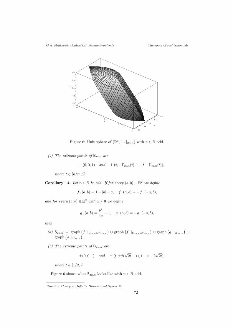
G.A. Munoz-Fernandez/J.B. Seoane-Sepulveda The space of real trinomials
−1.0
−2
−0.5
c
0.0
−1
0.5
1.0
a
1.0
00.5
10.0
b−0.5
2 −1.0
Figure 6: Unit sphere of (R3, ‖ · ‖2n,n) with n ∈ N odd.
(b) The extreme points of Bm,n are
±(0, 0, 1) and ± (t,±Γm,n(t), 1− t− Γm,n(t)),
where t ∈ [n/m, 2].
Corollary 14. Let n ∈ N be odd. If for every (a, b) ∈ R2 we define
f+(a, b) = 1− |b| − a, f−(a, b) = −f+(−a, b),
and for every (a, b) ∈ R2 with a 6= 0 we define
g+(a, b) =b2
4a− 1, g−(a, b) = −g+(−a, b),
then
(a) S2n,n = graph(f+|V2n,n∪W2n,n
) ∪ graph(f−|U2n,n∪V2n,n
) ∪ graph(g+|W2n,n
) ∪graph
(g−|U2n,n
).
(b) The extreme points of B2n,n are
±(0, 0, 1) and ± (t,±2(√
2t− t), 1 + t− 2√
2t),
where t ∈ [1/2, 2].
Figure 6 shows what S2n,n looks like with n ∈ N odd.
——————————Function Theory on Infinite Dimensional Spaces X
72

G.A. Munoz-Fernandez/J.B. Seoane-Sepulveda The space of real trinomials
5. The geometry of the space (R3, ‖ · ‖m,n) with m,n even
We begin by giving a formula for ‖ · ‖m,n.
Theorem 15. For every m,n ∈ N with m and n even and m > n, let us define Jm,n
as the set of triples (a, b, c) ∈ R3 such that
a 6= 0, 0 < − nb
ma< 1 and
12
[1 +
b
a+
∣∣∣∣1 +b
a
∣∣∣∣]
+2c
a<
m− n
n
(∣∣∣∣nb
ma
∣∣∣∣) m
m−n
.
Then we have
‖(a, b, c)‖m,n =
∣∣∣ (m−n)an
(∣∣ nbma
∣∣) mm−n − c
∣∣∣ if (a, b, c) ∈ Jm,n,∣∣a+b2 + c
∣∣ +∣∣a+b
2
∣∣ otherwise.(6)
Next, we need to define two curves in order to continue our description process.These curves will form part of the projection of our unit sphere on the ab-plane. Forevery a ∈ R\0 let define
Υm,n(a) =(
2m
m− n
)m−nm
·( |a|m
n
) nm
andΛm,n(a) = −Γm,n(|a|),
where b = Γm,n(a) for every a ∈ (0,∞) is the curve defined in Lemma 11. Notice thataccording to Lemma 11, b = Λm,n(a) for every a ∈ (−∞, 0) is the unique differentiablecurve passing through (−2, 0) (and hence Λm,n(−2) = 0), satisfying the equation
(m− n)an
(∣∣∣∣nb
ma
∣∣∣∣) m
m−n
= −2− a− b, (7)
Notice that whenever m = 2n with n ∈ N then
Υ2n,n(a) = 2√
2|a| and Λ2n,n(a) = 2(|a| −
√2|a|
).
Now, let
Um,n =n
(a, b)∈R2 :a∈ [γ0, 0), max0, Λm,n(a)≤b≤minn−m
na, Υm,n(a)
oo,
Wm,n =n
(a, b)∈R2 :a∈(0,−γ0],−max0, Λm,n(a)≤b≤−minn−m
na, Υm,n(a)
oo,
V 1m,n =
n(a, b) ∈ R2 : a ∈ [γ1, 2], max
n0,−m
nao≤ b ≤ 2− a
o,
V 2m,n =
n(a, b) ∈ R2 : a ∈ [γ1, 2],−2− a ≤ b ≤ min
n0,−m
naoo
,
Vm,n = V 1m,n ∪ V 2
m,n,
where
γ0 = − 2m− n
·(
mm
nn
) 1m−n
and γ1 =−2n
m− n.
Figure 7 shows what U2n,n, V2n,n and W2n,n with n ∈ N even look like.
73
——————————Function Theory on Infinite Dimensional Spaces X

G.A. Munoz-Fernandez/J.B. Seoane-Sepulveda The space of real trinomials
a
b
(−8, 8)
(−2, 4)
(2, 0)
(8,−8)
(2,−4)
(−2, 0)
b = 2 − a
b = −2 − a
b = Υ2n,n(a)
b = −Υ2n,n(a)
b = Λ2n,n(a)
b = −Λ2n,n(a)
U2n,n
V2n,n
V2n,n
W2n,n
5.04
Figure 7: πab(B2n,n) with n ∈ N even. In the picture we have Υ2n,n(a) = 2√
2|a| andΛ2n,n(a) = 2(|a| −
√2|a|).
Theorem 16. If m > n are even then πab(Bm,n) = Um,n ∪ Vm,n ∪Wm,n.
Theorem 17. Let m,n ∈ N be even with m > n. If for every (a, b) ∈ R2 we define
f+(a, b) = 1−∣∣∣∣a + b
2
∣∣∣∣−a + b
2, f−(a, b) = −f+(−a,−b),
and for every (a, b) ∈ R2 with a 6= 0 we define
g+(a, b) =(m− n)a
n
(∣∣∣∣nb
ma
∣∣∣∣) m
m−n
− 1, g−(a, b) = −g+(−a,−b),
then
(a) Sm,n = graph(f+|Wm,n∪Vm,n
) ∪ graph(f−|Um,n∪Vm,n
) ∪ graph(g+|Wm,n
) ∪graph
(g−|Um,n
).
(b) The extreme points of Bm,n are
±(0, 0, 1), ±(s,Λm,n(s),−1− s− Λm,n(s)) and ± (t,−Υm,n(t), 1)
where s ∈ [γ0,−2] and t ∈ [−γ1,−γ0].
Corollary 18. Let n ∈ N be even. If for every (a, b) ∈ R2 we define
f+(a, b) = 1−∣∣∣∣a + b
2
∣∣∣∣−a + b
2, f−(a, b) = −f+(−a,−b) = −1 +
∣∣∣∣a + b
2
∣∣∣∣−a + b
2,
——————————Function Theory on Infinite Dimensional Spaces X
74

G.A. Munoz-Fernandez/J.B. Seoane-Sepulveda The space of real trinomials
0
−1
c
b
0
1
−5
0
5
a
Figure 8: Unit sphere of (R3, ‖ · ‖2n,n) with n ∈ N even.
and for every (a, b) ∈ R2 with a 6= 0 we define
g+(a, b) =b2
4a− 1, g−(a, b) = −g+(−a,−b) =
b2
4a+ 1,
then
(a) S2n,n = graph (f+|W2n,n∪V2n,n) ∪ graph (f−|U2n,n∪V2n,n) ∪ graph (g+|W2n,n) ∪graph (g−|U2n,n).
(b) The extreme points of B2n,n are
±(0, 0, 1), ±(t, 2(√
2t− t), 1 + t− 2√
2t) and ± (t,−2√
2t, 1)
where t ∈ [2, 8].
With the aid of the previous parametrization we sketch S2n,n with n ∈ N even inFigure 8.
References
[1] R. M. Aron and M. Klimek. Supremum norms for quadratic polynomials. Arch. Math.(Basel) 76 (2001), 73–80.
[2] Y. S. Choi and S. G. Kim. The unit ball of P(2l22). Arch. Math. (Basel), 76 (1998),472–480.
[3] Y. S. Choi and S. G. Kim. Smooth points of the unit ball of the space P(2l1). ResultsMath., 36 (1999), 26–33.
[4] Y. S. Choi and S. G. Kim. Exposed points of the unit balls of the spaces P(2l2p) (p =1, 2,∞). Indian J. Pure Appl. Math., 35 (2004), 37–41.
75
——————————Function Theory on Infinite Dimensional Spaces X

G.A. Munoz-Fernandez/J.B. Seoane-Sepulveda The space of real trinomials
[5] B. C. Grecu, Geometry of homogeneous polynomials on two-dimensional real Hilbertspaces. J. Math. Anal. Appl. 293 (2004), no. 2, 578–588.
[6] B. C. Grecu, Extreme 2-homogeneous polynomials on Hilbert spaces, Quaest. Math. 25(2002), no. 4, 421–435.
[7] B. C. Grecu. Geometry of 2-homogeneous polynomials on lp spaces, 1 < p < ∞. J.Math. Anal. Appl. 273 (2002), no. 2, 262–282.
[8] B. C. Grecu. Smooth 2-homogeneous polynomials on Hilbert spaces. Arch. Math.(Basel) 76 (2001), no. 6, 445–454.
[9] B. C. Grecu, Geometry of three-homogeneous polynomials on real Hilbert spaces. J.Math. Anal. Appl. 246 (2000) 1, 217–229.
[10] B. C. Grecu, G. A. Munoz-Fernandez and J. B. Seoane-Sepulveda. The unit ball of thecomplex P(3H). Preprint.
[11] G. Klimek and M. Klimek. Discovering curves and surfaces with Maple. New York,1997.
[12] A. G. Konheim and T. J. Rivlin, Extreme points of the unit ball in a space of realpolynomials, Amer. Math. Monthly 73 (1966), 505–507.
[13] Gustavo A. Munoz-Fernandez and Juan B. Seoane-Sepulveda. Geometry of Banachspaces of trinomials. J. Math. Anal. Appl., 340(2):1069–1087, 2008.
[14] G. A. Munoz-Fernandez, Y. Sarantopoulos and J. B. Seoane-Sepulveda. An applicationof the Krein-Milman Theorem to Bernstein and Markov inequalities. J. Convex Anal.15 (2008), 299-312.
[15] S. Neuwirth. The maximum modulus of a trigonometric trinomial.arXiv:math/FA.0703236v1.
[16] S. Revesz. Minimization of maxima of nonnegative and positive definite cosine polyno-mials with prescribed first coefficients. Acta Sci. Math. (Szeged), 60 (1995), 589–608.
——————————Function Theory on Infinite Dimensional Spaces X
76

Proceedings ofFunction Theory on Infinite Dimensional Spaces XPages 77–82
Hypercyclic operators: When the lineardynamics becomes chaotic
A. PERIS
Departament de Matematica Aplicada and IUMPA, Edifici 7A,
Universitat Politecnica de Valencia, E-46022 Valencia, Spain
ABSTRACT
During the last two decades the study of hypercyclic operators, on Banach ormore general Frechet spaces, has developed into a very active research area. Hy-percyclicity is one of the main ingredients in the most widely know definitionsof chaos. Although chaos has long been thought of as being intrinsically linkedto non-linearity, the investigations into hypercyclicity show that many naturallinear dynamical systems exhibit chaos. In the past few years several open prob-lems, some of which long-standing, have been solved, and a number of landmarkresults have been obtained. From its very beginning, hypercyclicity has been atthe crossroads of several areas of mathematics, by taking its examples and itstechniques from various domains, and in turn its results have found applicationsand have motivated further research outside hypercyclicity. To mention a few,hypercyclicity is connected with the following areas of mathematics: OperatorTheory (e.g., through the invariant subspace problem), Semigroups of operatorsand applications to PDEs, Dynamical systems (complex dynamics, non-lineardynamics, topological dynamics, ergodic theory). Our purpose is to present asurvey on recent advances and connections of hypercyclicity with other areas.
Key words: Hypercyclic operators, Devaney chaos.
2000 Mathematics Subject Classification: 47A16, 37D45.
1. Introduction
Theorem 1 (G. D. Birkhoff, 1929). There is an entire function f : C→ C such that,for any entire function g : C→ C, there is a sequence (nk)k in N such that
limk
f(z + nk) = g(z) uniformly on compact sets of C.
The research was supported by MEC and FEDER, Project MTM2007-64222, and GeneralitatValenciana, Project PROMETEO/2008/101.
77

A. Peris Hypercyclic operators: When the linear dynamics becomes chaotic
Birkhoff’s result, in terms of dynamics
• H(C) := f : C→ C ; f is entire.
• Endow H(C) with the compact-open topology τ0 (topology of uniform conver-gence on compact sets of C).
• Consider the (continuous and linear!) map
T1 : H(C) → H(C), f(z) 7→ f(z + 1).
• Then there are f ∈ H(C) so that the orbit under T1:
Orb(T1, f) := f, T1f, T 21 f, . . .
is dense in H(C).
Framework and definitions
• From now on X will be a separable Frechet space and T : X → X anoperator.
• Given x ∈ X, its orbit under an operator T : X → X is:
Orb(T, x) := x, Tx, T 2x, . . . .
• An operator T : X → X on a Frechet space X is hypercyclic if there arex ∈ X such that Orb(T, x) = X.
2. Hypercyclic operators
Theorem 2 (Rolewicz, 1969). No finite dimensional space admits a hypercyclic op-erator
Theorem 3 (Birkhoff transitivity theorem, 1920). The following are equivalent:a) T is hypercyclic;b) T is topologically transitive:
∀U, V ⊂ X open and non-empty, ∃n ∈ N : Tn(U) ∩ V 6= ∅.
Joo, 1976, Kitai, 1982, Gethner, Shapiro, 1987, Godefroy, Shapiro, 1991, Bes,Peris, 1999, Grosse-Erdmann, 2003:
Theorem 4 (Hypercyclicity Criterion). If there are: (nk)k ⊂ N strictly increasing,and Y, Z ⊂ X dense subsets such that
(i) ∀y ∈ Y , limk Tnky = 0;(ii) ∀z ∈ Z, ∃(xk)k ⊂ X: limk xk = 0 and limk Tnkxk = z;
then T is hypercyclic.
——————————Function Theory on Infinite Dimensional Spaces X
78
A. Peris Hypercyclic operators: When the linear dynamics becomes chaotic
Proof. If U, V ⊂ X are open and non-empty, we find y ∈ Y ∩ U , z ∈ Z ∩ V , (xk)k
(depending on z), and k ∈ N such that
y + xk ∈ U, Tnk(y + xk) ∈ V.
Examples 5. (i) (MacLane, 1952) The derivative operator D : H(C) → H(C), f 7→f ′, is hypercyclic.
(ii) (Rolewicz, 1969) If |λ| > 1, the operator λB : `p → `p, 1 ≤ p < ∞, (x1, x2, . . . ) 7→(λx2, λx3, . . . ) is hypercyclic.
Proof. Set (nk)k = N in both cases.
(i) Y = Z := polynomials.(ii) Y := finite sequences, Z := `p.
Problem 6. Does every hypercyclic operator satisfy the Hypercyclicity Criterion?
Problem 7 (Herrero, 1992). If T is hypercyclic, is then T ⊕ T : X × X → X × Xhypercyclic?
Theorem 8 (Bes, Peris, 1999). T satisfies the Hypercyclicity Criterion if and onlyif T ⊕ T is hypercyclic.
Theorem 9 (De la Rosa, Read, 2006). There exist hypercyclic operators T such thatT ⊕ T is not hypercyclic.
3. Linear chaos
Definition 10 (Devaney, 1989). A continuous map f : M → M on a metric space(M, d) is chaotic if:
(i) f is topologically transitive;
(ii) Per(f) := periodic points of f = x ∈ M ; fnx = x for some n is dense inM ;
(iii) f has sensitive dependence on initial conditions, i.e., ∃ε > 0, ∀x ∈ M and δ > 0,∃y ∈ X and n ∈ N such that d(x, y) < δ, but d(fnx, fny) > ε.
Several authors showed that condition (3) is redundant in Devaney’s definition.Godefroy, Shapiro, 1991: Within our framework (1) implies (3).
Theorem 11 (Bes, Peris, 1999). Every chaotic operator satisfies the HypercyclicityCriterion.
Theorem 12 (Grivaux, 2005). If T is a hypercyclic operator and X admits a densesubset of vectors whose orbit under T is bounded, then T satisfies the HypercyclicityCriterion.
79
——————————Function Theory on Infinite Dimensional Spaces X

A. Peris Hypercyclic operators: When the linear dynamics becomes chaotic
Theorem 13 (Eigenvalue Criterion for chaos (Godefroy, Shapiro, 1991)). Supposethat T satisfies
• spanx ∈ X ; Tx = λx for some |λ| < 1 = X;
• spanx ∈ X ; Tx = λx for some |λ| > 1 = X;
• spanx ∈ X ; Tx = λx for some λ = eqπi, q ∈ Q = X;
then T is chaotic.
Proof. Y := spanx ∈ X ; Tx = λx for some |λ| < 1;Z := spanx ∈ X ; Tx = λx for some |λ| > 1; and observe that
Per(T ) = spanx ∈ X ; Tx = λx for some λ = eqπi, q ∈ Q.
Theorem 14 (Godefroy, Shapiro, 1991). If T : H(CN) → H(CN), T 6= λI, commuteswith the translations, then T is chaotic.
Hypercyclicity and the Invariant Subspace Problem
Theorem 15 (Read, 1988). There is an operator T on `1 so that every x 6= 0 has adense orbit under T . That is, T admits no (nontrivial) T -invariant closed subset.
Spaces of hypercyclic vectors
• (Bernal, Montes, 1995): Existence of infinite dimensional closed subspaces forcomposition operators so that every non-zero vector is hypercyclic (Hypercyclicsubspaces).
• (Montes, 1996): General conditions under which an operator admits hypercyclicsubspaces.
• (Chan, 1999): Abstract, but easier, proof of Montes’s result for Hilbert spaces.
• Several contributions: Bayart, Bes, Bonet, Chan, Gonzalez, Grosse-Erdmann,Leon, Matheron, Martınez-Gimenez, Peris, Petersson, Taylor.
• (Aron, Gurariy, Seoane, 2004): Spaceability (Existence of infinite dimensionalclosed subspaces so that every non-zero vector satisfies a special or “pathologi-cal” property).
Highlights on hypercyclicity
(i) (Ansari/Bernal, 1997, Bonet, Peris 1998) Every infinite dimensional separableFrechet space admits a hypercyclic operator.
(ii) (Bonet, Martınez-Gimenez, Peris, 2001) There are infinite dimensional separableBanach spaces which do not admit any chaotic operator.
——————————Function Theory on Infinite Dimensional Spaces X
80

A. Peris Hypercyclic operators: When the linear dynamics becomes chaotic
(iii) (Bourdon, 1993, Bes, 1999) If Orb(x, T ) = X, then X0 := Lin(Orb(x, T )) is adense subspace such that Orb(x0, T ) = X for all x0 ∈ X0 \ 0.
(iv) (Ansari, 1995) If T is hypercyclic then Tn is also hypercyclic for each n ∈ N.Moreover, they share the same hypercyclic vectors.
(v) (Costakis/Peris, 2000) If there is a finite family x1, . . . xk ⊂ X such that theunion of their orbits is dense in X, then there is an i such that the orbit of xi
is dense in X.
(vi) (Bourdon, Feldman, 2003) If the orbit of x ∈ X is somewhere dense in X, thenit is everywhere dense.
(vii) (Grivaux, 2003) For any dense and linearly independent sequence xn ; n ∈ Nin a separable Banach space X, there are, an operator T : X → X and x ∈ X,such that Orb(T, x) = xn ; n ∈ N.
(viii) (Feldman,2001) There is a (universal) chaotic operator T : H → H on a Hilbertspace H such that, for any continuous function f : K → K on a compactmetric space K, we find a T -invariant compact subset L ⊂ H such that thedynamical systems (f, K) and (T |L, L) are topologically conjugate, i.e., there isa homeomorphism I : K → L such that T I = I f .
4. Continuous (linear) dynamical systems
Definition 16 (Hypercyclic C0-semigroups). A C0-semigroup (or semiflow) of op-erators T := Tt : X → X ; t ≥ 0 is a one-parameter family of operators sothat T0 = I, Tt Ts = Tt+s, and limt→s Ttx = Tsx for each x ∈ X. The or-bit of x is Orb(T , x) := Ttx ; t ≥ 0. The semigroup is hypercyclic if itadmits a dense orbit, and it is chaotic if, moreover, the set of periodic pointsPer(T ) := x ∈ X ; Ttx = x for some t > 0 is dense in X.
• First results: Lasota, 1979. Desch, Schappacher, Webb, 1997.
• Several contributions: Badea, Banasiak, Bayart, Bermudez, Bonilla, Conejero,Costakis, De Laubenfels, El Mourchid, Emamirad, Grivaux, Grosse-Erdmann,Herzog, Kalmes, Muller, Peris, Rudnicki.
From the continuous to the discreteLet T := Tt : X → X ; t ≥ 0 be a C0-semigroup such that there is x ∈ X with
Orb(T , x) dense in X,
Theorem 17 (Oxtoby, Ulam, 1941). There is a dense Gδ-set A ⊂]0,∞[ such thatOrb(Tt, x) is dense in X for each t ∈ A.
Theorem 18 (Conejero, Muller, Peris, 2007). Orb(Tt, x) is dense in X for eacht > 0.
Theorem 19 (Bayart, Bermudez, 2007). There exist chaotic C0-semigroups T :=Tt : X → X ; t ≥ 0 such that no single operator Tt, t > 0, is chaotic.
81
——————————Function Theory on Infinite Dimensional Spaces X

A. Peris Hypercyclic operators: When the linear dynamics becomes chaotic
5. Hypercyclicity and complex dynamics
Here we will consider (complex) polynomials P on X.
Theorem 20 (Bernardes, 1998). No Banach space X admits a n-homogeneous (n ≥2) hypercyclic polynomial.
Theorem 21 (Peris, 1999). There are homogeneous chaotic polynomials of arbitrarydegree on ω := CN.
Theorem 22 (Martınez-Gimenez, 2000). There are homogeneous chaotic polynomialsof arbitrary degree on certain sequence spaces and on some spaces of holomorphicfunctions.
Theorem 23 (Aron, Miralles, 2008). There are homogeneous chaotic polynomials ofarbitrary degree on CC(R).
Problem 24 (Aron, 1998). Are there Banach spaces X and (non-homogeneous!)hypercyclic polynomials P on X of degree n ≥ 2?
Theorem 25 (Peris, 2003). There exist chaotic polynomials of arbitrary degree on`q (1 ≤ q < ∞). It is possible to characterize hypercyclicity of certain polynomials on`q in terms of Julia sets of their associated polynomials of one complex variable.
Theorem 26 (Martınez-Gimenez, Peris, 2007). Every infinite dimensional separableFrechet space admits a hypercyclic polynomial.
6. Ergodic theory and hypercyclicity
The motivation is the existence of T -invariant measures with full support such thatT is ergodic, i.e., T−1(A) = A for A measurable implies µ(A) = 0 or µ(A) = 1.
• First results: Flitzanis, 1994, 1995, Bayart, Grivaux, 2004, 2006.
• Frequent hypercyclic operators (Bayart, Grivaux, 2004): T is frequent hy-percyclic if there are x ∈ X such that, for any U ⊂ X open and nonempty,
lim infn
∣∣k ≤ n ; T kx ∈ U∣∣n
> 0.
• (Bayart, Grivaux, 2006): There are frequently hypercyclic operators which arenot chaotic.
• (Grosse-Erdmann, Peris, 2005): Every frequently hypercyclic operator satisfiesthe Hypercyclicity Criterion.
• Several contributions: Badea, Grivaux, 2006, Bonilla, Grosse-Erdmann, 2006,2007.
——————————Function Theory on Infinite Dimensional Spaces X
82

Proceedings ofFunction Theory on Infinite Dimensional Spaces XPages 83–85
Winning tactics in a geometrical game
A. PROCHAZKA
Universite Bordeaux 1
351 cours de la Liberation
33405 Talence cedex
France
or
Charles University in Prague
Sokolovska 83
18675 Prague
Czech Republic
ABSTRACT
A Banach space X has the RNP if and only if there exists a winning tactic forthe second player in the point-closed slice game played in the unit ball of X. Bycontrast, there is no winning tactic for the second player in the point-open slicegame in BX .
Key words: Point-slice game, Radon-Nikodym property characterization.
2000 Mathematics Subject Classification: Primary 91A05, 46B20.
1. Summary
Let BX be a closed unit ball in a real Banach space X. Let A be a class of subsetsof BX such as open slices (So), closed slices (Sc), hyperplane sections, etc.
A point-A game in BX (we denote it G(BX ,A)) is a two-player infinite gamewhere Player I plays points xn in BX and Player II plays subsets An ∈ A accordingto the simple rules:
• Player I starts by playing x1 ∈ BX arbitrarily;
• after xn has been played, Player II must choose An so that An ∈ A and xn ∈ An;
• after An has been played, Player I must play xn+1 so that xn+1 ∈ An.
Supported by the grant GA CR 201/07/0394.
83

A. Prochazka Winning tactics in a geometrical game
Formally G(BX ,A) = (x,A) ∈ BNX × AN : x = (xn), A = (An) and xn ∈ An 3xn+1 for all n ∈ N and each element of this set is called a run of the game. PlayerII wins the run (x, A) if the sequence (xn)∞n=1 is Cauchy. Otherwise Player I wins.
J. Maly and M. Zeleny [3], who were the first to mention the game, have establishedthat Player II has a winning strategy in the game G(BR2 , lines). Later R. Devilleand E. Matheron [2] fully characterized the spaces X where Player II has a winningstrategy in G(BX ,So) or, equivalently, in G(BX ,Sc) as the spaces with the Radon-Nikodym property (RNP). Recall that X has the RNP if every subset L of BX hasnonempty open slices of arbitrarily small diameter. This includes e.g. reflexive spacesor separable dual spaces (see [4]). Deville and Matheron also proved that in the caseX is a superreflexive space (i.e. it admits a uniformly convex norm), Player II haseven a winning tactic in G(BX ,Sc).
The difference between tactic and strategy may be informally described as follows.If Player II plays according to a tactic, he decides his next move An only taking intoaccount the last move xn of Player I. If Player II plays according to a strategy, heconsiders the whole history of Player’s I moves (xi)n
i=1 before playing An. Thus whilea strategy corresponds to a sequence of functions tn : Dn ⊂ Bn
X → A, a tactic isonly one function t : BX → A. By calling strategy (respectively a tactic) winningwe mean that every run of the game which satisfies xn ∈ tn(x1, . . . , xn) (respectivelyxn ∈ t(xn)) is won by Player II. It is obvious that winning tactics are a subset ofwinning strategies. Thus our main result is a strengthening of the result of Devilleand Matheron.
Theorem 1. If a real Banach space X has the Radon-Nikodym property, then PlayerII has a winning tactic in the game G(BX ,Sc).
In particular, the spaces where Player II has a winning tactic in G(BX ,Sc) areexactly spaces with the Radon-Nikodym property.
Since the very beginning, the assertions on the existence of winning strategy ortactics were used as a convenient sufficient condition for convergence of points readyfor applications (see [3, 2, 1]). It takes the following form.
Corollary 2. If a real Banach space X has the Radon-Nikodym property, then thereexists a mapping F : BX → X∗ such that a sequence (xn) ⊂ BX is convergentwhenever it satisfies 〈F (xn), xn+1〉 ≥ 〈F (xn), xn〉.
Finally, let us focus on the winning tactics in G(BX ,So). It may surprise thatwhile the winning tactics and winning strategies in G(BX ,Sc) either simultaneouslyexist or simultaneously don’t, the case of G(BX ,So) is different. Indeed, we knowthat Player II has a winning strategy in G(BX ,So) provided X has the RNP (thisis due to Deville and Matheron) but our next theorem shows that Player II cannothave a winning tactic.
Theorem 3. Let dim X ≥ 1. Then there is no winning tactic for Player II in thegame G(BX ,So).
For the theorems in full generality, the proofs and more results about games weinvite the reader to consult [5].
——————————Function Theory on Infinite Dimensional Spaces X
84

A. Prochazka Winning tactics in a geometrical game
Acknowledgements
I am grateful to Robert Deville for his valuable suggestions and encouragement.
References
[1] R. Deville J. Jaramillo, Almost classical solutions of Hamilton-Jacobi Equations, toappear in Revista Matematica Iberoamericana.
[2] R. Deville E. Matheron, Infinite games, Banach space geometry and the Eikonal equa-tion, Proc. London Math. Soc. 95 (2007) 49-68.
[3] J. Maly M. Zeleny, A note on Buczolich’s solution of the Weil gradient problem, ActaMath. Hungarica 113 (2006) 145-158.
[4] R. Phelps, Convex Functions, Monotone Operators and Differentiability, 2nd Edition,Lecture Notes in Mathematics 1364 (Springer, Berlin, 1993).
[5] A. Prochazka, Winning tactics in a geometrical game, Proc. Amer. Math. Soc., postedon September 26, 2008, PII S 0002-9939(08)09636-6 (to appear in print).
85
——————————Function Theory on Infinite Dimensional Spaces X


Proceedings ofFunction Theory on Infinite Dimensional Spaces XPages 87–89
Singular canonical inclusions forrearrangement invariant spaces on [0,∞)
V.M. SANCHEZ
Department of Mathematical Analysis
Faculty of Mathematics
Complutense University
28040 Madrid, Spain.
ABSTRACT
It is given a complete characterization of the strict singularity and the disjointstrict singularity of the inclusions E → L1 + L∞ for the class of rearrangementinvariant spaces E on [0,∞).
Key words: rearrangement invariant spaces, strict singularity, disjoint strict singularity
2000 Mathematics Subject Classification: 46E30
1. Introduction
An operator between two Banach spaces is said to be strictly singular (SS in short) ifit fails to be an isomorphism on any infinite-dimensional closed subspace. A weakernotion for Banach lattices is that of disjoint strict singularity: An operator T froma Banach lattice E to a Banach space is said to be disjointly strictly singular (DSSin short) if there is no sequence (xn)∞n=1 of disjointly supported non-null vectors inE such that the restriction of T to the closed subspace spanned by (xn)∞n=1 is anisomorphism.
The aim of this note is to study the strict singularity and the disjoint strict sin-gularity of the canonical embeddings E → L1 + L∞ for arbitrary rearrangementinvariant spaces E on [0,∞). It is well known that L1∩L∞ → E → L1 +L∞ for anyrearrangement invariant space E on [0,∞). The singularity of left extreme embed-dings has been studied in [2] finding a suitable characterization of strict singularity interms of the associated fundamental function φE . Thus for the operator L1∩L∞ → Ethe statements of strict singularity, disjoint strict singularity and weak compactnesscoincide and are equivalent to the conditions
limt→0
φE(t) = limt→∞
φE(t)t
= 0.
Partially supported by the Spanish Ministry of Education, grant MTM2005-00082 andComplutense-Santander grant PR27/05-14045.
87
V.M. Sanchez Singular canonical inclusions for r.i. spaces on [0,∞)
2. Preliminaries
We consider the Lebesgue measure λ on the interval [0,∞). The distribution functionλx associated to a measurable function x on [0,∞) is defined by
λx(s) = λt ≥ 0 : |x(t)| > sand the decreasing rearrangement x∗ of x is
x∗(t) = infs ≥ 0 : λx(s) ≤ t.A Banach space E of measurable functions defined on [0,∞) is said to be a re-
arrangement invariant space (briefly r.i. space) if the following conditions are satisfied:(a) if y ∈ E and |x(t)| ≤ |y(t)| λ-a.e. on [0,∞), then x ∈ E and ‖x‖E ≤ ‖y‖E ,(b) if y ∈ E and λx = λy, then x ∈ E and ‖x‖E = ‖y‖E .The fundamental function φE of an r.i space E is defined by φE(t) = ‖χ[0,t]‖E
with t ≥ 0.We shall denote by E0 the order continuous part of E.Important examples of r.i. spaces are the Orlicz, Lorentz and Marcinkiewicz
spaces.We refer to [1], [4] and [5] for general properties of r.i. spaces.
3. Disjoint strict singularity of E → L1 + L∞
Let us denote by W p, 1 ≤ p ≤ ∞, the scale of spaces:
W p =
Lp,∞0 if 1 < p < ∞,
L1 if p = 1,
L1 ∩ L∞L∞
if p = ∞.
Theorem 3.1. Let E be an r.i. space. The embedding E → L1 + L∞ is not DSS ifand only if there exists 1 ≤ p ≤ ∞ such that E contains a space W p.
Theorem 3.1 can be reformulated as the following criterion:
Theorem 3.2. Let E be an r.i. space. The embedding E → L1 + L∞ is DSS if andonly if
(i) limt→0
φE(t)t = lim
t→∞φE(t) = ∞.
(ii) supn
∥∥∥t−1p χ( 1
n ,n)
∥∥∥E
= ∞ for any 1 < p < ∞.
Remark 3.3. For the special class of r.i. spaces E with submultiplicative fundamen-tal functions, a stronger formulation of Theorem 3.1 can be given: If the canonicalembedding E → L1 + L∞ is not DSS, then E = W p for 1 ≤ p ≤ ∞, or E = Lp,∞ for1 < p < ∞, or E = L∞ (see [2, Theorem 4.5]).
Corollary 3.4. Let E be an r.i. space different from L∞ or W∞. Then the embeddingE → L1 + L∞ is DSS if and only if the embedding E0 → L1 + L∞ is DSS.
Corollary 3.5. If the embedding of an r.i. space E into L1 + L∞ is not DSS, thenthere exists a disjointly supported sequence (yn)∞n=1 in E which is equivalent in E andin L1 + L∞ to the canonical basis of `p for some 1 ≤ p < ∞ or to c0.
——————————Function Theory on Infinite Dimensional Spaces X
88

V.M. Sanchez Singular canonical inclusions for r.i. spaces on [0,∞)
4. Strict singularity of E → L1 + L∞
Theorem 4.1. Let E be an r.i. space. The embedding E → L1 + L∞ is SS if andonly if the embedding E → L1 +L∞ is DSS and E[0, 1] does not contain Lexp x2
0 [0, 1].
As a consequence of the above result and Theorem 3.2 we have the followingcriterion:
Proposition 4.2. Let E be a r.i. space. The embedding E → L1 + L∞ is SS if andonly if
(i) limt→0
φE(t)t = lim
t→∞φE(t) = ∞.
(ii) supn
∥∥∥t−1p χ( 1
n ,n)
∥∥∥E
= ∞ for all 1 < p < ∞.
(iii) E[0, 1] does not contain Lexp x2
0 [0, 1].
The results of this note have been already published and they are contained in [3].
References
[1] C. Bennett and R. Sharpley, Interpolation of operators, Academic Press (1988).
[2] F.L. Hernandez, V.M. Sanchez and E.M. Semenov, Disjoint strict singularity of inclu-sions between rearrangement invariant spaces, Studia Math. 144 (2001), 209-226.
[3] F.L. Hernandez, V.M. Sanchez and E.M. Semenov, Strictly singular inclusions into L1 +L∞, Math. Z. 258 (2008), 87-106.
[4] S.G. Kreın, Ju.I. Petunin and E.M. Semenov, Interpolation of linear operators, A.M.S.(1982).
[5] J. Lindenstrauss and L. Tzafriri, Classical Banach spaces II. Function spaces, Springer-Verlag (1979).
89
——————————Function Theory on Infinite Dimensional Spaces X


Proceedings ofFunction Theory on Infinite Dimensional Spaces XPages 91–110
Holomorphic Functional Calculus for RegularOperators on Locally Convex Spaces
S.M. STOIAN
Department of Mathematics,
University of Petrosani
Romania
ABSTRACT
In this paper we will study the regular operators on sequentially complete locallyconvex spaces.
Key words: Functional calculus, Spectrum, Spectral sets.
2000 Mathematics Subject Classification: Primary: 47A60, 47A10, 47A25.
1. Introduction
Through this paper all the locally convex spaces will be assumed sequentially completeHausdorff space, over the complex field C, and all the operators will be linear.
The collection of all families of seminorms P which generate the topology of alocally convex space X (in the sense that the topology of X is the coarsest withrespect to which all seminorms of P are continuous) will be denoted by C(X). Theset of all directed families P ∈ C(X) is denoted by C0(X). On a family of seminormson a linear space X we define the relation ,, ≤” by
p ≤ q ⇔ p (x) ≤ q (x), (∀)x ∈ X.
A family of seminorms is preordered by the relation ” ≺”, where
p ≺ q ⇔ there exists some r > 0 such that p (x) ≤ rq (x), for all x ∈ X.
If p ≺ q and q ≺ p, we write p ≈ q. Two families P1 and P2 of seminorms on alinear space are called Q-equivalent ( denoted P1 ≈ P2) if:
(i) for each p1 ∈ P1 there exists p2 ∈ P2 such that p1 ≈ p2;
This paper was written during the visit of the author to the Departamento de AnalisisMatematico, from the Facultad de Ciencias Matematicas, Universidad Complutense de Madrid(Spain), and was supported by the MEdC-ANCS CEEX grant ET65/2005 contract no.2987/11.10.2005 and the M.Ed.C. grant C.N.B.S.S. contract no. 5800/09.10.2006.
91

S.M. Stoian Holomorphic Functional Calculus for Regular Operators
(ii) for each p2 ∈ P2 there exists p1 ∈ P1 such that p2 ≈ p1.
Two Q-equivalent and separating families of seminorms on a linear space generatethe same locally convex topology.
An operator T ∈ L(X) is:
(i) a quotient bounded operator with respect to P ∈ C(X) if for every seminormp ∈ P there exists cp > 0 such that
p (Tx) ≤ cpp (x) , (∀)x ∈ X.
(ii) an universally bounded with respect to P ∈ C(X) if there exists c0 > 0 suchthat
p(Tx) ≤ c0p (x) , (∀)x ∈ X, (∀) p ∈ P.
The class of the quotient bounded operators (universally bounded operators) withrespect to P ∈ C(X) is denoted by QP(X) (respectively BP(X)). It is obvious thatBP(X) ⊂ QP(X). For every p ∈ P the application p : QP(X) → R defined by
p(T ) = inf r > 0 | p(Tx) ≤ rp (x) , (∀)x ∈ X,is a submultiplicative seminorm on QP(X), satisfying the relation p(I) = 1, and hasthe following properties
(i) p(T )= supp(x)=1
p (Tx) = supp(x)≤1
p (Tx), (∀) p ∈ P;
(ii) p (Tx) ≤ p (T ) p (x), (∀)x ∈ X.
For every P ∈ C(X), we denote by P the family p | p ∈ P. (QP(X), P) is asequentially complete locally multiplicatively convex algebra for all P ∈ C(X), andBP(X) is a unitary normed algebra with respect to the norm ‖·‖P defined by
‖T‖P = supp(T ) | p ∈ P, (∀)T ∈ BP(X).
and‖T‖P = infM > 0 | p (Tx) ≤ Mp (x) , (∀)x ∈ X, (∀) p ∈ P.
If T ∈ QP(X) we said that α ∈ C is in the resolvent set ρ(QP , T ) if there exists(αI−T )−1 ∈ QP(X). The spectral set σ(QP , T ) will be the complement of ρ(QP , T ).
An operator T ∈ QP(X) is a bounded element of the algebra QP(X) if it is abounded element in the sense of G.R. Allan [1], i.e some scalar multiple of it generatesa bounded semigroup. The class of the bounded elements of QP(X) is denoted by(QP(X))0. An operator T ∈ QP(X) is bounded in the algebra QP(X) if and only ifthere is P ′ ∈ C(X) such that P ≈ P ′ and T ∈ BP′(X) [9]. If rP(T ) is the P-spectralradius of the operator T , i.e. it is the radius of boundness of the operator T in QP(X)given by
rP(T ) = infα > 0 | α−1T generates a bounded semigroup in QP(X),then in [1] and [18] was proved that the following relations hold
rP(T ) = sup lim supn→∞
(p (Tn))1/n | p ∈ P =
——————————Function Theory on Infinite Dimensional Spaces X
92

S.M. Stoian Holomorphic Functional Calculus for Regular Operators
= sup limn→∞
(p (Tn))1/n | p ∈ P = sup infn≥1
(p (Tn))1/n | p ∈ P (1)
rP(T ) < +∞ if and only if T ∈ (QP(X))0; (2)
rP(T ) = inf
λ > 0 | limn→∞
Tn
λn= 0
; (3)
If (X,P) is a locally convex space and T ∈ (QP(X))0, then the Neumann series∞∑
n=0
T n
λn+1 converges to R (λ, T )(in QP(X)), for every |λ| > rP(T ), and R (λ, T ) ∈QP(X) [18]. Moreover,
|σ(QP , T )| = rP(T ). (4)
If T ∈ (QP , (X)) has the spectrum σ(QP , T ) bounded, then T ∈ (QP(X))0 [9].Hence, T ∈ (QP(X))0 if and only if the spectrum σ(QP , T ) is bounded. If (X,P) is alocally convex space and T ∈ (QP(X))0 we denote by r0
P(T ) the radius of boundnessof the operator T in (QP(X))0. We say that r0
P(T ) is the P-spectral radius of theoperator T in the algebra (QP(X))0. From definition it follows that r0
P(T ) = rP(T )and r0
P(T ) has all the properties of the spectral radius rP(T ) presented above. Wedenote by ρ(Q0
P , T ) the resolvent set of T in (QP(X))0. The spectral set σ(Q0P , T )
will be the complement of ρ(Q0P , T ).
Example 1. (i) Let X be the vectorial space of the complex function and F be theset of the finite parts from C. We consider on X the topology generated by thefamily of the seminorms P = pF | F ∈ F, where
pF (f) = max | f (x) | | x ∈ F, (∀)F ∈ F , (∀) f ∈ X.
Then, the operator T : X → X given by
(Tf) (x) = xf (x) , (∀)x ∈ C,
is a quotient bounded operator with respect to P, which is not a boundedelement of the algebra QP(X).
(ii) Let X be the space of all complex sequences x = ξnn∈N with the local convextopology determined by the family countable set of seminorms P
|x|p = max |ξk| |k ≤ p , p ∈ N.
If λnn∈N is a complex bounded sequences and en is the canonical basis ofX, then the operator T : X → X given by
(T (en)) (x) = λnen, (∀)n ∈ N,
is a bounded element of the algebra QP(X).
(iii) Every locally bounded operator on a locally convex space X (i.e. an operatorwhich maps some zero neighborhood into a bounded set) is universally boundedand quotient bounded with respect to some family of seminorms P ∈ C(X).
Definition 2. Let (X,P) be a locally convex space. The Waelbroeck resolvent setof an operator T ∈ QP(X), denoted by ρW (QP , T ), is the subset of elements λ0 ∈C∞ = C ∪ ∞, for which there exists a neighborhood V ∈ V(λ0) such that:
93
——————————Function Theory on Infinite Dimensional Spaces X

S.M. Stoian Holomorphic Functional Calculus for Regular Operators
(i) the operator λI − T is invertible in QP(X) for all λ ∈ V \∞
(ii) the set ( λI − T )−1 | λ ∈ V \∞ is bounded in QP(X).
The Waelbroeck spectrum of T , denoted by σW (QP , T ), is the complement of theset ρW (QP , T ) in C∞. It is obvious that σ(QP , T ) ⊂ σW (QP , T ).
An element x in a locally convex algebra (X,P) is regular if there is some t > 0such that:
(i) λI − T is invertible in X, for all | λ |> t;
(ii) the set(λI − x)−1 || λ |> t
is bounded in X.
so we can consider the following definition:
Definition 3. Let (X,P) be a locally convex space. An operator T ∈ QP(X) isP-regular (or a regular element of the algebra QP(X)) if ∞ /∈ σW (QP , T ) , i.e. thereexists some t > 0 such that:
(i) the operator λI − T is invertible in QP(X), for all | λ |> t;
(ii) the set R (λ, T ) || λ |> t is bounded in QP(X).
2. Regular Operators
Proposition 4. Let (X,P) be a locally convex space. An operator T ∈ QP(X) isP-regular if and only if T ∈ (QP(X))0.
Proof. Assume that T ∈ (QP(X))0. It follows that there is P ′ ∈ C(X) such thatP ≈ P ′ and T ∈ BP′(X). Moreover, QP(X) = QP′(X).
If | λ |> 2 ‖T‖P′ , then the Neumann series∞∑
n=0
T n
λn+1 converges in BP′(X) and its
sum is R (λ, T ). This means that the operator λI − T is invertible in QP(X) for all| λ |> 2 ‖T ‖P′ . Moreover, for each ε > 0 there exists an index nε ∈ N such that
∥∥∥∥∥R (λ, T )−n∑
k=0
T k
λk+1
∥∥∥∥∥P′
<ε, (∀)n ≥ nε,
which implies that for each n ≥ nε we have
‖R (λ, T )‖P′ ≤∥∥∥∥∥R (λ, T )−
nε∑
k=0
T k
λk+1
∥∥∥∥∥P′
+
∥∥∥∥∥nε∑
k=0
T k
λk+1
∥∥∥∥∥P′
<
<ε+ | λ |−1nε∑
k=0
∥∥∥∥∥T k
λk
∥∥∥∥∥P′
<ε + (2 ‖T‖P′)−1nε∑
k=0
2−k < ε + (‖T‖P′)−1.
Since ε > 0 was arbitrarily chosen, we have that
‖R (λ, T )‖P′ <(‖T‖P′)−1, (∀) | λ |> 2 ‖T‖P′——————————Function Theory on Infinite Dimensional Spaces X
94

S.M. Stoian Holomorphic Functional Calculus for Regular Operators
From the definition of the norm ‖ ‖P′ it follows that
p (R (λ, T ))<(‖T‖P′)−1,
for any p ∈ P ′ and for each | λ |> 2 ‖T‖P′ , which means that the set
R (λ, T ) | | λ |> 2 ‖T‖P′
is bounded in QP(X) = QP′(X). Hence T is P-regular.Now suppose that T ∈ QP(X) is P-regular, but it is not bounded in QP(X).
Since σ(QP , T ) ⊂ σW (QP , T ) from (2) it follows that
| σW (QP , T ) |=| σ(QP , T ) |= rP(T ) = ∞,
which contradicts the assumption we have made. Thus, T is a bounded element ofQP(X).
Remark 5. From previous proposition results that (QP(X))0 is the algebra of P-regular operators on X.
Lemma 6. Let (X,P) be a locally convex space and T ∈ (QP(X))0 such that rP(T ) <
1. Then the operator I − T is invertible and (I − T )−1 =∞∑
n=0Tn.
Proof. Assume that rP(T ) < t < 1. From relation (3) it follows that
lim supn→∞
(p (Tn))1/n< t, (∀) p ∈ P,
so for each p ∈ P there exists np ∈ N such that
(p (Tn))1/n ≤ supn≥np
(p (Tn))1/n< t, (∀) n ≥ np.
This relation implies that the series∞∑
n=0p (Tn) converges, so
limn→∞
p (Tn) = 0, (∀) p ∈ P,
therefore limn→∞
Tn = 0. Since the algebra QP(X) is sequentially complete it results
that the series∞∑
n=0Tn converges. Moreover,
(I − T )m∑
n=0
Tn =m∑
n=0
Tn(I − T ) = I − Tm+1,
so
(I − T )∞∑
n=0
Tn =∞∑
n=0
Tn(I − T ) = I,
which implies that I − T is invertible and (I − T )−1 =∞∑
n=0Tn.
95
——————————Function Theory on Infinite Dimensional Spaces X

S.M. Stoian Holomorphic Functional Calculus for Regular Operators
Lemma 7. Let (X,P) be a locally convex space. If T ∈ (QP(X))0 then
(i) the map λ → R(λ, T ) is holomorphic on ρW (QP , T );
(ii) dn
dλn R(λ, T ) = (−1)nn!R(λ, T )n+1, for every n ∈ N;
(iii) lim|λ|→∞
R(λ, T ) = 0 and lim|λ|→∞
R(1, λ−1T ) = lim|λ|→∞
λR(1, T ) = I;
(iv) σW (QP , T ) 6= ∅.
Proof. 1) If λ0 ∈ ρW (QP , T ) then there exists V ∈ V(λ0) with the properties (1) and(2) from definition (2). For every λ ∈ V \∞ we have
R(λ, T )−R(λ0, T ) = (λ0 − λ)R(λ, T )R(λ0, T )
and since the set R(λ, T )| λ ∈ V \∞ is bounded in QP(X) results that the mapλ → R(λ, T ) is continuous in λ0, so
limλ→λ0
R(λ, T )−R(λ0, T )λ− λ0
= −R2(λ0, T )
If λ0 = ∞ then, there exists some neighborhood V ∈ V(∞) such that the mapλ → R(λ, T ) is defined and bounded on V \∞. Moreover, this map is holomorphicand bounded on V \∞, which implies that it is holomorphic at ∞.
Therefore, the map λ → R(λ, T ) is holomorphic on ρW (QP , T ).2) Results from the proof of (1).3) For each λ ∈ ρW (QP , T ), λ 6= 0, we have
λ−1(I + TR(λ, T ))(λI − T ) = I,
soR(λ, T ) = λ−1(I + TR(λ, T )). (5)
If V ∈ V(λ0) satisfies the conditions of the definition 2, then the set
TR(λ, T )| λ ∈ V \∞
is bounded, so from relation (5) it results that lim|λ|→∞
R(λ, T ) = 0.
From the equalityR(λ, T ) = λ−1R(1, λ−1T ), λ 6= 0,
and relation (5) results that
R(1, λ−1T ) = I + TR(λ, T ),
solim
|λ|→∞R(1, λ−1T ) = lim
|λ|→∞(I + TR(λ, T )) = I.
4) Assume that σW (QP , T ) = ∅. Then the application λ → R(λ, T ) is holo-morphic on C and converges to 0 at infinity. From Liouville Theorem results thatR(λ, T ) = 0, for all λ ∈ C, hence I = (λI − T )R(λ, T ) = 0, which is not true.
——————————Function Theory on Infinite Dimensional Spaces X
96
S.M. Stoian Holomorphic Functional Calculus for Regular Operators
Proposition 8. Let (X,P) be a locally convex space. If T ∈ (QP(X))0, then
ρW (QP , T ) = ρ(Q0P , T ).
Proof. If λ0 ∈ ρ(Q0P , T ) then from the proposition 4 it follows that R(λ0, T ) is a P-
regular operator, so there is t > 0 for which the condition (1) and (2) of the definition3 are fulfilled. Those conditions are equivalent with
1’) (λ− λ0)−1I −R(λ0, T ) is invertible in QP(X) for all |λ− λ0| < t−1, λ 6= λ0;
2’) the setR((λ− λ0)−1, R(λ0, T ))| |λ− λ0| < t−1, λ 6= λ0
is bounded in QP(X).From the condition (2’) and lemma 7 it results that the set
(λ− λ0)−1R((λ− λ0)−1, R(λ0, T ))| |λ− λ0| < t−1, λ 6= λ0is bounded in QP(X). Moreover, each seminorm p, p ∈ P, is submultiplicative, sothe set
(λ− λ0)−1R(λ0, T )R((λ− λ0)−1, R(λ0, T ))| |λ− λ0| < t−1, λ 6= λ0is also bounded in QP(X). Since
(λI − T )(λ0 − λ)−1R(λ0, T )R((λ− λ0)−1, R(λ0, T )) =
= ((λ0I − T ) + (λ− λ0)I)(λ0 − λ)−1R(λ0, T )R((λ− λ0)−1, R(λ0, T )) =
= (λ0 − λ)−1R((λ− λ0)−1, R(λ0, T ))−R(λ0, T )R((λ− λ0)−1, R(λ0, T )) =
= ((λ0 − λ)−1I −R(λ0, T ))R((λ− λ0)−1, R(λ0, T )) = I,
results that
R(λ, T ) = (λ0 − λ)−1R(λ0, T )R((λ− λ0)−1, R(λ0, T )). (6)
Therefore, the conditions1) λI − T is invertible for all |λ− λ0| < t−1;2) R(λ, T )| |λ− λ0| < t−1 is bounded in QP(X),of definition (2) are fulfilled, so λ0 ∈ ρW (QP , T ) and ρ(Q0
P , T ) ⊂ ρW (QP , T ).Conversely, if λ0 ∈ ρW (QP , T ) there exists K > 0 such that
1”) λI − T is invertible for all |λ− λ0| < K;2”) R(λ, T )| |λ− λ0| < K is bounded in QP(X).
From the equality
(λ0 − λ)R(λ, T )(λ0I − T )((λ0 − λ)−1I −R(λ0, T )) = I
it follows that
R((λ0 − λ)−1, R(λ0, T )) = (λ0 − λ)R(λ, T )(λ0I − T )
Hence property (2”) implies that the set
(λ− λ0)−1R((λ− λ0)−1, R(λ0, T ))| |λ− λ0|−1 > K−1, λ 6= λ0is bounded in QP(X), so R(λ0, T ) is regular in QP(X). From the previous propositionresults that R(λ0, T ) ∈ (QP(X))0 and λ0 ∈ ρ(Q0
P , T ).
97
——————————Function Theory on Infinite Dimensional Spaces X

S.M. Stoian Holomorphic Functional Calculus for Regular Operators
Proposition 9. Let (X,P) be a locally convex space. If T ∈ (QP(X))0 and | λ0 |>rP(T ), then λ0 ∈ ρ(Q0
P , T ).
Proof. The series∞∑
n=0
T n
λn+1 converges to R (λ0, T ) ∈ QP(X), for all | λ |> rP(T ),
hence it results that there exists ε>0 such that
D (λ0, ε) = λ | |λ− λ0| < ε ⊂ µ | |µ| > rP(T ) ,
so the operator λI−T is invertible, for every λ ∈ D (λ0, ε), and (λI−T )−1 ∈ QP(X).Now we will prove that the set σ(QP , R(λ0, T )) is bounded. If | µ |> ε−1, then
| µ |−1< ε and λ0 − µ−1 ∈ D (λ0, ε). From the previous observations results that(λ0 − µ−1)I − T is invertible and ((λ0 − µ−1)I − T )−1 ∈ QP(X).
Sinceµ−1R
(λ0 − µ−1, T
)(λ0I − T ) (µI −R (λ0, T )) =
= R(λ0 − µ−1, T
)(λ0I − T )− µ−1R
(λ0 − µ−1, T
)=
= R(λ0 − µ−1, T
)(((λ0 − µ−1)I − T ) + µ−1I)− µ−1R
(λ0 − µ−1, T
)=
= I + µ−1R(λ0 − µ−1, T
)− µ−1R(λ0 − µ−1, T
)= I.
it results thatR(µ,R (λ0, T )) = µ−1R
(λ0 − µ−1, T
)(λ0I − T )
ButR
(λ0 − µ−1, T
), (λ0I − T ) ∈ QP(X),
so R(µ,R (λ0, T )) ∈ QP(X), for all | µ |> ε−1.This implies that σ(QP , R(λ0, T )) ⊂ D
(0, ε−1
), so the set σ(QP , R(λ0, T )) is
bounded. Thus R(λ0, T ) ∈ (QP(X))0.
Corollary 10. Let X be a locally convex space and P ∈ C(X). If T ∈ (QP(X))0 then
|σ(QP , T )| = |σW (QP , T )| = rP(T )
Proof. It is a direct consequence of propositions 8, 9 and relation (4).
Definition 11. Let (X,P) be a locally convex space. An operator T ∈ QP(X) issaid to be P-quasinilpotent if rP(T ) = 0.
Remark 12. (i) If T ∈ QP(X) is P-quasinilpotent, then T ∈ (QP(X))0 and
σW (QP , T ) = 0.
(ii) T ∈ QP(X) is P-quasinilpotent if and only if σ(QP , T ) = 0.
——————————Function Theory on Infinite Dimensional Spaces X
98

S.M. Stoian Holomorphic Functional Calculus for Regular Operators
3. Holomorphic Functional Calculus for Regular Operators
A functional calculus for regular elements of a quasi-complete locally convex algebrais presented by L.Waelbroeck in [20]. In this section using some ideas from I. Colo-joara [4] and L.Waelbroeck [20] it is presented a functional calculus for the P-regularoperators of the algebra QP(X), when X is a sequentially complete locally convexspace. For the theory of holomorphic functions on locally convex spaces see [2] or [5].
Let P ∈ C(X) be arbitrary chosen and D ⊂ C a relatively compact open set.Denote by O(D, QP(X)) the unitary algebra of the functions f : D → QP(X) whichare holomorphic on D and continuous on D.
Lemma 13. If p ∈ P, then the mapping | · |p,D: O(D, QP(X)) → R given by
| f |p,D= supz∈D
p(f (z)), (∀) f ∈ O(D,QP(X)),
is a submultiplicative seminorm on O(D, QP(X)).
If we denote by τP,D the topology defined by the family of seminorms
| · |p,D |p ∈ Pon O(D, QP(X)), then (O(D,QP(X)), τP,D) is a l.m.c.-algebra.
Let K ⊂ C be a compact set, arbitrarily chosen. We define the set
O(K, QP(X)) = ∪O(D, QP(X))| D is relatively compact open set and K ⊂ D.If D1, D2 ⊂ C are relatively compact open sets such that K ⊂ Di, i = 1, 2, and
fi ∈ O(Di, QP(X)), i = 1, 2, we say that f1 v f2 if and only if there exists an openset D such that K ⊂ D ⊂ D1 ∩ D2 and f1|D = f2|D. Denote by A(K,QP(X)) theset of the equivalence classes of O(K, QP(X)) respect to this equivalence relation. Itis easy to see that A(K, QP(X)) is a unitary algebra and the elements of this algebraare usually called germs of holomorphic functions from K to QP(X).
Remark 14. We consider the following notations:
(i) f is the germ of the holomorphic function f ∈ O(D, QP(X)).
(ii) ϕ is the canonical morphism O(K, QP(X)) → A(K, QP(X));
(iii) ϕD is the restriction of ϕ to O(D,QP(X)).
Remark 15. (i) Since we can identify C with CI = λI | λ ∈ C , the algebrasO(K,C) and A(K,C) can be considered subalgebras of O(K, QP(X)), respec-tively A(K, QP(X)). Therefore, we write O(K) and A(K) instead of O(K,C)and A(K,C).
(ii) If τP,ind = lim→D
τP,D (inductive limit), then (A(K,QP(X)), τP,ind) is a l.m.c.-
algebra.
We need the following lemma from complex analysis.
Lemma 16. For each compact set K ⊂ C and each relatively compact open set D ⊃ Kthere exists some open set G such that:
99
——————————Function Theory on Infinite Dimensional Spaces X

S.M. Stoian Holomorphic Functional Calculus for Regular Operators
(i) K ⊂ G ⊂ G ⊂ D;
(ii) G has a finite number of conex components (Gi)i=1,n, the closure of which arepairwise disjoint;
(iii) the boundary ∂Gi of Gi, i = 1, n, consists of a finite positive number of closedrectifiable Jordan curves (Γij)j=1,mi
, no two of which intersect;
(iv) K ∩ Γij = ∅, for each i = 1, n and every j = 1, mi.
Definition 17. If the sets K and D are like in the previous lemma, then an open setG is called Cauchy domain for the pair (K, D) if satisfies the properties (1)-(4). Theboundary
Γ = ∪i=1,n ∪j=1,miΓij
of G is called Cauchy boundary for the pair (K, D).
Theorem 18. If P ∈ C0(X) and T ∈ (QP(X))0, then for each relatively compactopen set D ⊃ σW (QP , T ) there exists a map
FT,D : O(D,QP(X)) → QP(X)
with the properties:
(i) FT,D is continuous and linear;
(ii) FT,D (kS) = S, where kS ≡ S;
(iii) FT,D (idI) = T , where idI(λ) = λI, for every λ ∈ C.
Proof. Let Γ be a Cauchy boundary for the pair (σW (QP , T ), D). Then the integral
12πi
∫
Γ
f (λ)R (λ, T ) dλ, (∀) f ∈ O(D, QP(X)),
exists like Stieltjes integral, since QP(X) is a sequentially complete locally multiplica-tively convex algebra and the maps t à f(ω(t))R(ω(t), T ) are continuous on [0, 1] fora continuous parametrization ω of Γ.
Moreover, if Γ1 and Γ2 are Cauchy boundaries for the pair (σW (QP , T ), D) then
12πi
∫
Γ1
f (z)R (λ, T ) dλ =1
2πi
∫
Γ2
f (λ)R (λ, T ) dλ, (∀) f ∈ O(D, QP(X)),
hence the map FT,D : O(K, QP(X)) → QP(X) given by formula
FT,D(f) =1
2πi
∫
Γ
f (λ)R (λ, T ) dz, (∀) f ∈ O(D,QP(X)),
is well defined. Now we prove that FT,D has the properties (1)-(3).The linearity is obvious. For every p ∈ P and every f ∈ O(D, QP(X)) we have
p(FT,D(f)) ≤ L(Γ)2π
supλ∈Γ
p(R (λ, T ))supλ∈Γ
p(f(λ)) ≤ L(Γ)2π
supλ∈Γ
p(R (λ, T )) | f |p,D,
——————————Function Theory on Infinite Dimensional Spaces X
100
S.M. Stoian Holomorphic Functional Calculus for Regular Operators
where L(Γ) is the length of Γ, which implies the continuity of the map FT,D.Let r > rP(T ) and Γr = z ∈ C| |z| = r. For each λ ∈ Γr we have rP(T
λ ) < 1, sofrom lemma 6 results that
R (λ, T ) = λ−1
(I − T
λ
)−1
= λ−1∑
n∈N
(T
λ
)n
=∑
n∈N
Tn
λn+1
This observation implies that
FT,D (kS) =1
2πi
∫
Γ
kS (λ)R (λ, T ) dλ =S
2πi
∑
n∈NTn
∫
Γ
dλ
λn+1= S
FT,D (idI) =1
2πi
∫
Γ
λR (λ, T ) dλ =1
2πi
∑
n∈NTn
∫
Γ
dλ
λn= T.
Corollary 19. If P ∈ C0(X) and T ∈ (QP(X))0, then there exists a map FT :A(σW (QP , T ), QP(X)) → QP(X) which satisfies the conditions:
(i) FT is continuous and linear;
(ii) FT
(kS
)= S, where kT is the germ of the function kS ≡ S;
(iii) FT
(idI
)= T , where idI is the germ of the function idI(λ) = λI, for all λ ∈ C
Proof. If f ∈ A(σW (QP , T )), then we consider
FT (f) = FT,D (f) , (∀) f ∈ A(σW (QP , T )),
where f ∈ O(D, QP , T )) is an element of the equivalence class f . It is obvious thatthe definition of FT
(f)
is independent of the function f and FT
(f)
is linear. SinceFT,D = FT ϕD and FT,D is continuous results that FT is continuous.
The properties (2) and (3) results directly from the previous theorem.
Corollary 20. If P ∈ C0(X) and T ∈ (QP(X))0, then there exists an unique unitarycontinuous morphism FT : A(σW (QP , T )) → QP(X) which satisfies the conditionFT
(id
)= T , where id is the identity function on C.
Proof. The application FT : A(σW (QP , T )) → QP(X) and FT,D : O(D) → QP(X)are defined in the same way like the applications FT and FT,D. It is easily to see that
FT and FT,D are linear and continuous. Moreover, FT is unitary and FT
(id
)= T.
Now, we prove that FT is multiplicative. Let f , g ∈ A(σW (QP , T )) and f ∈ f ,respectively g ∈ g. We consider that G and G′ are two Cauchy domains with theproperty G′ ⊂ G. If Γ and Γ′ are the boundaries of G and G′ then
FT (f)FT (g) = − 1(2πi)2
∫
Γ
∫
Γ′f(λ)g(ω)R(λ, T )R(ω, T )dλdω
101
——————————Function Theory on Infinite Dimensional Spaces X
S.M. Stoian Holomorphic Functional Calculus for Regular Operators
Since G′ ⊂ G, results that Γ ∩ Γ′ = ∅, so
ω − λ 6= 0, (∀)λ ∈ Γ, (∀)ω ∈ Γ′.
From the equality
R(λ, T )−R(ω, T ) = (ω − λ)R(λ, T )R(ω, T )
it follows
FT
(f)
FT (g) =1
(2πi)2
∫
Γ
f(λ)R(λ, T )(∫
Γ′
g(ω)ω − λ
dω
)dλ+
+1
(2πi)2
∫
Γ′g(ω)R(ω, T )
(∫
Γ
f(λ)λ− ω
dλ
)dω =
=1
2πi
∫
Γ
f(λ)g (λ) R(λ, T )dω = FT
(f g
)
Assume that F : A(σW (QP , T )) → QP(X) is an unitary continuous morphismwhich satisfies the condition F
(id
)= T . We prove that FT = F .
Let f ∈ A(σW (QP , T )), D ⊃ σW (QP , T ) a relatively compact open set, f ∈ O(D),such that f ∈ f , and G a Cauchy domain for (σW (QP , T ), D) with the boundary Γ.For every n ∈ N \ 0 and z1, ..., zn ∈ Γ we consider the function fn : G → C givenby the relation
fn (ω) =1
2πi
n∑
j=1
f (zj) (zj+1 − zj)zj − ω
, (∀) ω ∈ G. (7)
Then,
limn→∞
fn (ω) =1
2πi
∫
Γ
f(z)z − ω
dz = f (ω)
and since this convergence is uniformly on each compact set K ⊂ G, results thatlimτind
fn = f . Using the continuity of F it results that
limn→∞
F(fn
)= F
(f)
(8)
Since F is a unitary morphism with the property F(id
)= T , then from relation
(7) results that
F(fn
)=
12πi
n∑
j=1
f (zj) (zj+1 − zj)R(zj , T )
solim
n→∞F
(fn
)=
12πi
∫
Γ
f (z)R (z, T ) dz, (9)
From relations (8) and (9) results that
F(f)
=1
2πi
∫
Γ
f (z) R (z, T ) dz = FT,D(f) = FT
(f)
which implies that FT = F .
——————————Function Theory on Infinite Dimensional Spaces X
102

S.M. Stoian Holomorphic Functional Calculus for Regular Operators
Lemma 21. If K ⊂ C is a compact set, then each element of the algebra A(K) isregular.
Proof. Let f ∈ A(K), D ⊃ K a relatively compact open set, f ∈ O(D) (f ∈ f)and ω0 /∈ f (K). Then there are two relatively compact open set U and V such thatω0 ∈ U , f (K) ⊂ V and U ∩ V = Φ. For every ω ∈ U the function fω : f−1(V ) → Cgiven by relation
fω (λ) =1
ω − f (λ), (∀) λ ∈ f−1(V )
is holomorphic on f−1(V ), so fω ∈ A(K).Since for every compact set A ⊂ f−1(V ) we have
supω∈U
supλ∈A
|fω (λ) | < ∞
it results that the set fω|ω ∈ U is bounded in (A(K), τind). Moreover,
(ω1− f)fω =∼1
so ω ∈ σW (f). Therefore σW (f) ⊂ f (K). Since K is compact the set f (K) iscompact, hence σW (f) is compact and f is regular.
Lemma 22. If X and Y are unitary locally convex algebra and F : X → Y is anunitary continuous morphism, then F (Xr) ⊂ Yr, where Xr and Yr are the algebrasof the regular elements of X, respectively Y .
Proof. If x ∈ Xr, then there exists k > 0 such that λe − x is invertible for every|λ| > k and the set R (λ, x) ||λ| > k is bounded in X. Since F is unitary morphismit follows that
F (R (λ, x)) = R (λ, F (x)), (∀) |λ| > k,
so from continuity of F it results that the set
F (R (λ, x)) ||λ| > k = R (λ, F (x))||λ| > kis bounded. Hence, F (x) is regular.
Proposition 23. If P ∈ C0(X) and T ∈ (QP(X))0, then
FT (A(σW (QP , T ))) ⊂ (QP(X))0.
Proof. From lemmas 21 and 22 results that FT (f) is a P-regular operator, for everyf ∈ A(σW (QP , T )), so by proposition 4 we have that FT (f) ∈ (QP(X))0.
Remark 24. If P ∈ C0(X), T ∈ (QP(X))0 and P is a polynomial, then
FT (P ) = P (T ) and FT,D(P ) = P (T ).
for each relatively compact open set D ⊃ σW (QP , T ). Hence, for each T ∈ (QP(X))0we can use the following notation:
FT (f) = f(T ) and FT,D(f) = f(T ).
where f ∈ A(K), D ⊃ K open set and f ∈ O(D), such that f ∈ f .
103
——————————Function Theory on Infinite Dimensional Spaces X

S.M. Stoian Holomorphic Functional Calculus for Regular Operators
The following theorem represents the analogous of the spectral mapping theoremfor Banach spaces.
Theorem 25. If P ∈ C0(X), T ∈ (QP(X) )0 and f is a holomorphic function on anopen set D ⊃ σW (QP , T ), then
σW (QP , f(T )) = f(σW (QP , T )).
Proof. From lemma 22 it follows that the operator f(T ) is a regular element of thealgebra QP(X), so the spectrum σW (QP , f(T )) is compact.
Let ω0 /∈ f(σW (QP , T )). Then there are two relatively compact open set U andV such that ω0 ∈ U , σW (QP , f(T )) ⊂ V and U ∩ V = ∅. We proved in the proof oflemma 21 that if the functions fω : f−1(V ) → C, ω ∈ U , are given by
fω (λ) =1
ω − f (λ), (∀) λ ∈ f−1(V )
then the set fω|ω ∈ U is bounded in (A(σW (QP , f(T ))), τind). The morphism FT
is unitary, soFT (fω)(ωI − FT (f)) = FT (1) = I.
Now from the continuity of FT results that the set
FT (fω) | ω ∈ U = R(ω, FT (f)) | ω ∈ U = R(ω, f(T )) | ω ∈ U
is bounded in QP(X). Therefore, ω0 /∈ σW (QP , f(T )) and
σW (QP , f(T )) ⊂ f(σW (QP , T )).
If ω0 ∈ σW (QP , T ) and gω0 : D → C is defined by
gω0(λ) =
f(λ)−f(ω0)λ−ω0
, for λ 6= ω0,
f ′(ω0), for λ = ω0,
then gω0 ∈ O(D) and
f(ω0)− f(λ) = (ω0 − λ)gω0(λ), (∀)λ ∈ D.
Thereforef(ω0)I − f(T ) = (ω0I − T )gω0(T ).
and since ω0I − T is not invertible, it results that f(ω0) ∈ σW (QP , f(T )), so
f(σW (QP , T )) ⊂ σW (QP , f(T )).
Theorem 26. Let P ∈ C0(X) and T ∈ (QP(X))0. If f is holomorphic function onthe open set D ⊃ σW (QP , T ) and g ∈ O(Dg), such that Dg ⊃ f(D), then (g f) (T ) =g(f(T )).
——————————Function Theory on Infinite Dimensional Spaces X
104

S.M. Stoian Holomorphic Functional Calculus for Regular Operators
Proof. Let G be a Cauchy domain for the pair (σW (QP , T ), D) and Γ the boundaryof G. For each ω /∈ f(G), the function fω : G → C,
fω (λ) =1
ω − f (λ), (∀)λ ∈ G,
is holomorphic, hence we can define fω (T ), where
fω (T ) =1
2πi
∫
Γ
1ω − f (λ)
R(λ, T )dλ = R(ω, f(T )). (10)
If we chose a Cauchy domain G′ for the pair (σW (QP , f(T )), Dg) with boundaryΓ′ such that f(G) ⊂ G′, then f(Γ) ∩ Γ′ = ∅, so we can define the function given by(10) for all λ ∈ Γ and ω ∈ Γ′. Thus, from relation (10) and Cauchy formula it results
g(f (T )) =1
2πi
∫
Γ′g(ω)R(ω, f(T ))dω =
=1
2πi
∫
Γ′g(ω)
(1
2πi
∫
Γ
1ω − f (λ)
R(λ, T )dλ
)dω =
=1
2πi
∫
Γ
R(λ, T )(
12πi
∫
Γ′
g(ω)ω − f (λ)
dω
)dλ =
12πi
∫
Γ
g(f(λ))R(λ, T )dλ =
=1
2πi
∫
Γ
(g f) (λ)R(λ, T )dλ = (g f) (T )
Next, we develop the properties of the exponential function of a quotient boundedoperator.
Lemma 27. Assume that P ∈ C0(X) and T ∈ (QP(X))0. If f is a holomorphic
function on the open set D ⊃ σW (QP , T ) and f (λ) =∞∑
k=0
αkλk on D, then f (T ) =∞∑
k=0
αkT k.
Proof. For ε > 0, sufficiently small, the power series∞∑
k=0
αkλk converges uniformly on
the boundary Γ of the disc D = λ | |λ| = |σW (QP , T )|+ ε.From corollary 20 it results that
f(T ) =1
2πi
∫
Γ
f (λ)R (λ, T ) dλ =1
2πi
∫
Γ
( ∞∑
k=0
αkλk
)R (λ, T ) dλ =
=1
2πi
∞∑
k=0
αk
∫
Γ
λkR (λ, T ) dλ
For every |λ| > |σW (QP , T )| we have R (λ, T )=∞∑
k=0
T k
λk+1 , so from Cauchy formula
it follows
105
——————————Function Theory on Infinite Dimensional Spaces X
S.M. Stoian Holomorphic Functional Calculus for Regular Operators
f(T ) = 12πi
∞∑k=0
αk
∫Γ
λk
( ∞∑n=0
T n
λn+1
)dλ =
∞∑k=0
αkT k.
Corollary 28. If P ∈ C0(X) and T ∈ (QP(X))0, then exp T =∞∑
k=0
T k
k! .
Definition 29. If P ∈ C0(X) and T ∈ (QP(X))0, then a subset of σW (QP , T ) whichis both open and closed in σW (QP , T ) is called a spectral set of T .
Denote by δT the class of spectral sets of T .
Proposition 30. If P ∈ C0(X) and T ∈ (QP(X))0, then for each spectral set H ∈ δT
there exists a unique idempotent TH ∈ QP(X) with the following properties:
(i) THS = STH , whenever S ∈ QP(X) and ST = TS;
(ii) T∅ is the null element of QP(X);
(iii) TH∩K = THTK , (∀)H, K ∈ δT ;
(iv) TH∪K = TH + TK , for each H, K ∈ δT with the property H ∩K = ∅.
Proof. First we make the observation that for each set H ∈ δT there exists an uniquegerm fH ∈ A(σW (QP , T )) with the property (H), where
(H)
for every pair (D, D′) of relatively compact open sets of the complexplane which satisfies the conditions
H ⊂ D, σW (QP , T ) ⊂ D′ and D ∩D′ = ∅then there exists fH ∈ fH such that fH/D = 1 and fH /D′ = 0.
If Γ is the Cauchy boundary for the pair (H, D) (the closure of H is taken in thetopology of C) then we define
TH = FT (fH) =1
2πi
∫
Γ
R(λ, T )dλ.
1) If ST = TS, then SR(λ, T ) = R(λ, T )S, so THS = STH .2) Results from the definition of TH .3) Let H, K ∈ δT and fH , fK , fH∩K ∈ A(σW (QP , T )) which verifies the properties(H), (K), respectively (H ∩K).
Assume that the pairs (D,D′) and (G, G′) are like in (H) and (K) properties.Then there exists f ∈ fH , such that f/D = 1 and f/D′ = 0, and g ∈ fK , suchthat g/G = 1 and g/G′ = 0. It is obvious that fg/D∩G = 1 and fg/D′∩G′ = 0, sofg ∈ fH∩K and
TH∩M = FT (fH∩K) = FT,D∩G(fg) = FT,D∩G(f)FT,D∩G(g) =
= FT,D(f)FT,G(g) = F (fH)F (fK) = THTM .
——————————Function Theory on Infinite Dimensional Spaces X
106

S.M. Stoian Holomorphic Functional Calculus for Regular Operators
4) We consider the above notations and with the supplementary conditions D∩G = ∅and D ′ ∩G ′ = ∅ (since H ∩M = ∅). Then
f(λ) + g(λ) =
1, if λ ∈ D ∪G,0, for λ ∈ D ′ ∪G ′,
Therefore, if fH∪K ∈ A(σW (QP , T )) has the property (H∪K), then f+g ∈ fH∪K ,so
TH∪M = FT (fH∪K) = FT,D∪G(f + g) = FT,D∪G(f) + FT,D∪G(g) =
= FT,D(f) + FT,G(g) = FT (fH) + FT (fK) = TH + TM .
Corollary 31. If P ∈ C0(X) and T ∈ (QP(X))0, then for every pair of spectral setsspectral set H,K ∈ δT , which have the properties H∩K = ∅ and H∪K = σW (QP , T ), we have
TH + TK = I and THTK = O.
Remark 32. From proposition 23 results that TH ∈ (QP(X))0, for each H ∈ δT
Lemma 33. Assume that P ∈ C0(X) and T ∈ (QP(X))0. If F ⊂ C has the propertydist(σW (QP , T ), F ) > ε0 > 0, then for each p ∈ P there exists cp > 0 such that
p(R(λ, T )n) ≤ cp
εn0
, (∀)λ ∈ F, (∀)n ∈ N.
Proof. If D = C\F , then for the pair (σW (QP , T ), D) there exists a Cauchy domainG such that
|λ− ω| > ε0, (∀)λ ∈ F, (∀)ω ∈ G.
If Γ is boundary of G, then
p(R(λ, T )n) = p
(1
2πi
∫
Γ
R(ω, T )(ω − λ)n
dω
)≤ L(Γ)
2πsupω∈Γ
p(R(ω, T )n)|ω − λ|n
<L(Γ)2π supω∈Γ p(R(ω, T )n)
εn0
.
Hence the lemma is proved if we choose
rp =L(Γ)2π
supω∈Γ
p(R(ω, T )n).
The next theorem gives an extension for Taylor’s theorem to functions of an op-erator.
Theorem 34. Let P ∈ C0(X) and T ∈ (QP(X))0. If D is an relatively compactopen set which contains the set σW (QP , T ), f ∈ O(D) and S ∈ (Q P(X))0, such thatrP(S) < dist(σW (QP , T ),C\D) and TS = ST , then the following statements aretrue:
107
——————————Function Theory on Infinite Dimensional Spaces X

S.M. Stoian Holomorphic Functional Calculus for Regular Operators
(i) σW (QP , T + S) ⊂ D;
(ii) f(T + S) =∑n≥0
f(n)(T )n! Sn.
Proof. Let d, d1 > 0 such that
rP(S) < d1 < d < dist (σW (QP , T ),C\D) .
If Γ1 = λ ∈ C| |λ| = d1, then for each p ∈ P and every n ∈ N we have
p(Sn) = p
(1
2πi
∫
Γ
λnR(λ, S)dλ
)≤ L(Γ1)
2πsupω∈Γ1
(|λn| p(R(λ, S)) ≤
≤ L(Γ1)2π
supω∈Γ1
p(R(λ, S) supω∈Γ1
|λ|n ≤ kpdn1 (11)
where kp = L(Γ1)2π supω∈Γ1
p(R(λ, T ).Moreover, the previous lemma implies that for each p ∈ P there is cp > 0 such
thatp(R(λ, T )n+1) ≤ cp
dn+1, (∀)λ ∈ C\D, (∀) n ∈ N (12)
so from relations (11) and (12) it follows that
p(R(λ, T )n+1Sn) = p(R(λ, T )n+1)p(Sn) ≤ kpcp
d1
(d1
d
)n+1
(13)
for every p ∈ P, n ∈ N and λ ∈ C\D. Since d1d < 1 the relation (13) proves that the
series∑∞
n=1 R(λ, T )n+1Sn converge uniformly on C\D.From the equalities
(λI − T − S)∞∑
n=1
R(λ, T )n+1Sn =∞∑
n=1
R(λ, T )n+1Sn(λI − T − S) =
=∞∑
n=1
R(λ, T )nSn −∞∑
n=1
R(λ, T )n+1Sn+1 = I
it follows that λI − T − S is invertible in QP(X), for all λ ∈ C\D, and
R(λ, T + S) =∞∑
n=1
R(λ, T )n+1Sn. (14)
Therefore the relation (13) implies that the set R(λ, T +S)|λ ∈ C\D is boundedin QP(X), so σW (QP , T + S) ⊂ D.
If Γ is a Cauchy boundary for the pair (σW (QP , T + S), D), then from (14) andlemma 7 it results
f(λ, T + S) =1
2πi
∫
Γ
f(λ)R(λ, T + S)dλ =
——————————Function Theory on Infinite Dimensional Spaces X
108

S.M. Stoian Holomorphic Functional Calculus for Regular Operators
=∞∑
n=1
(1
2πi
∫
Γ
f(λ)R(λ, T )n+1dλ
)Sn =
=∞∑
n=1
(1
2πi
(−1)n
n!
∫
Γ
f(λ)dn
dλnR(λ, T )dλ
)Sn =
=∞∑
n=1
(1
2πi
1n!
∫
Γ
f (n)(λ)R(λ, T )dλ
)Sn =
∞∑n=1
f (n)(T )n!
Sn
Corollary 35. Let P ∈ C0(X) and T ∈ (QP(X))0. If S ∈ QP(X) is P-quasinilpotent,such that TS = ST , then
f(T + S) =∑
n≥0
f (n) (T )n!
Sn, (∀)f ∈ A(σW (QP , T ))
References
[1] Allan G.R., A spectral theory for locally convex algebras, Proc. London Math. Soc. 15(1965), 399-421.
[2] Barroso, J. A., Introduction To Holomorphy, North-Holland, Math. Stud., 106.
[3] Chilana, A., Invariant subspaces for linear operators on locally convex spaces, J. London.Math. Soc., 2 (1970) , 493-503.
[4] Colojoara, I., Elemente de teorie spectrala, Editura Academiei Republicii SocialisteRomania, Bucuresti 1968.
[5] Dineen, S., Complex analysis in Locally Convex Spaces, North-Holland, Math. Stud.,57.
[6] Dowson, H.R., Spectral theory of linear operators, Academic Press, 1978.
[7] Dunford, N and Schwartz, J., Spectral Theory, Part I, Interscience Publishers, Inc.,New-York, 1964.
[8] Edwards, R.E., Functional Analysis, Theory and Applications, Holt, Rinehart and Win-ston, Inc, 1965.
[9] Gilles, J.R., Joseph, G.A., Koehler, D.O. and Sims B., On numerical ranges of operatorson locally convex spaces, J. Austral. Math. Soc. 20 (Series A), (1975), 468-482.
[10] Joseph, G.A., Boundness and completeness in locally convex spaces and algebras, J.Austral. Math. Soc., 24 (Series A), (1977), 50-63.
[11] Kramar, E., On the numerical range of operators on locally and H-locally convex spaces,Comment. Math. Univ. Carolinae 34, 2 (1993), 229-237.
[12] Kramar, E., Invariant subspaces for some operators on locally convex spaces, Comment.Math. Univ. Carolinae 38, 3 (1997), 635-644.
[13] Maeda, F., Remarks on spectra of operators on locally convex space, Proc. N.A.S.,Vol.47, 1961.
[14] Michael, A., Locally multiplicatively convex topological algebras, Mem. Amer. Math.Soc., 11, 1952.
109
——————————Function Theory on Infinite Dimensional Spaces X

S.M. Stoian Holomorphic Functional Calculus for Regular Operators
[15] Moore, R.T., Banach algebras of operators on locally convex spaces, Bull. Am. Math.Soc., 75 (1969), 69-73.
[16] Moore, R.T., Adjoints, numerical ranges and spectra of operators on locally convexspaces, Bull. Am. Math. Soc., 75 (1969), 85-90.
[17] Robertson, A.P. and Robertson W.J., Topological vector spaces, Cambridge UniversityPress., New-York, 1964.
[18] Stoian, S.M., Spectral radius of a quotient bounded operator, Studia Univ. Babes-Bolyai,Mathematica, No.4, 2004, pg.115-126;
[19] Troitsky, V.G., Spectral Radii Of Bounded Operators On Topological Vector Spaces,Panamer. Math. J., 11(2001), no.3, 1-35.
[20] Waelbroeck, L., Etude des algebres completes, Acad.Roy.Belg.Cl.Sci.Mem. Coll. in-8,31(1960), no.7.
——————————Function Theory on Infinite Dimensional Spaces X
110

Proceedings ofFunction Theory on Infinite Dimensional Spaces XPages 111–114
Volterra composition operators:supercyclicity and hypercyclicity
A. WEBER
Institut fur Algebra und Geometrie,
Universitat Karlsruhe (TH),
Englerstr. 2, 76128 Karlsruhe, Germany.
ABSTRACT
We review several results concerning the cyclic behavior of Volterra and Volterracomposition operators on certain function spaces.
Key words: Volterra composition operator, hypercyclic operator, supercyclic operator.
2000 Mathematics Subject Classification: 47A16.
1. Introduction and preliminaries
The aim of this note is to review several results concerning the cyclic behavior ofVolterra and Volterra composition operators. To fix notation, we start with thefollowing definitions.
Definition 1. Let X denote one of the function spaces Lp[0, 1], p ∈ [1,∞) or theFrechet space defined in Section 2. The bounded operator
V : X → X, V f(x) =∫ x
0
f(t)dt
is called Volterra operator and (for some function ψ), the operator
Vψ : X → X, Vψf(x) =∫ ψ(x)
0
f(t)dt
is called Volterra composition opererator.
Definition 2. A continuous operator T on some Frechet space X over K (K = R orC), is called
(a) cyclic, if there is some x ∈ X such that spanTnx : n ∈ N is dense in X,
(b) supercyclic, if there is some x ∈ X whose projective orbit λTnx : λ ∈ K, n ∈ Nis dense in X,
111

A. Weber Volterra composition operators: supercyclicity and hypercyclicity
(c) hypercyclic, if there is some x ∈ X whose orbit Tnx : n ∈ N is dense in X.
It is easy to see, that for p ∈ [1,∞) the Volterra operator V : Lp[0, 1] → Lp[0, 1]is cyclic. Indeed, the linear span of the orbit V n1 = xn
n! : n ∈ N is dense in X. H.Salas raised in [7] the question wether V on Lp[0, 1] is even supercyclic. This questionwas answered in the negative by E. A. Gallardo-Gutierrez and A. Montes-Rodrıguez,see [3]. Their proof relied on the so-called angel criterion: Let T : X → X be abounded operator and let x ∈ X be a supercyclic vector for T . Then we have for anyx∗ ∈ X∗ with norm 1 the following:
lim supn→∞
|〈Tnx, x∗〉|||Tnx|| = 1.
S. Shkarin now proved in [8] that the Volterra operator on Lp[0, 1], p ∈ (1,∞), is ina certain sense even far away from being supercyclic. More precisely, he showed forV : Lp[0, 1] → Lp[0, 1], p ∈ (1,∞) that for any f 6= 0 the sequence V nf
||V nf || convergesweakly to 0 (if n →∞) and called operators satisfying this property anti-supercyclic.Note, that he also proved that the Volterra operator on L1[0, 1] is not anti-supercyclic.In [2] I. Domanov considered on Lp[0, 1], p ∈ [1,∞) the Volterra composition operatorVψ with ψ(x) = xβ for some β ∈ (0, 1). He showed that the point spectrum σ(V ∗
ψ )of the dual operator of Vψ is infinite and hence, Vψ can not be supercyclic as D.Herrero proved in [5] that the dual operator of a supercyclic operator has at most oneeigenvalue.
2. Main result
In this section we will consider the Frechet space
X = f ∈ C[0, 1) : f(0) = 0
of continuous functions on the half-open interval [0, 1) with f(0) = 0 endowed withthe following family of seminorms:
||f ||k = max|f(t)| : t ∈ [0, 1− 1
k + 1]
, k ∈ N.
Furthermore, let ψ ∈ X. Then the Volterra composition operator
Vψ : X → X
is continuous. Details for the results in this section can be found in [6].In contrast to the fact that for ψ(x) = xβ , β ∈ (0, 1) the Volterra composition
operator Vψ is far away from being hypercyclic on Lp[0, 1] (see Section 1), we have
Theorem 3. Let ψ(x) = xβ , β ∈ (0, 1). Then
Vψ : X → X
is hypercyclic.
——————————Function Theory on Infinite Dimensional Spaces X
112
A. Weber Volterra composition operators: supercyclicity and hypercyclicity
The proof of this theorem relies on the hypercyclicity criterion (see [1, 4]) that canbe stated in our case as follows:If there are dense subsets X0, X1 ⊂ X and a map S : X1 → X1, such that
(i) limn→∞ V nψ f = 0 if f ∈ X0,
(ii) limn→∞ Sng = 0 if g ∈ X1,
(iii) VψSg = g if g ∈ X1
then Vψ is hypercyclic.Here, we can choose X0 as the set of polynomials that vanish at 0,
X1 = span
xγ : γ ∈ R, γ >1 + β
1− β
,
andS : X1 → X1, Sf(x) =
d
dxf ψ−1(x) =
d
dxf(x1/β).
That the subsets X0 and X1 are dense in X follows from the Muntz-Szasz theorem.For the proofs of the properties (i)–(iii) we refer to [6].
To finish this note, we have a look at the Volterra operator on X:
Lemma 4. Let ψ : [0, 1) → [0, 1) be continuous with ψ(x) ≤ x on some interval[0, c], c ∈ (0, 1). Then
Vψ : X → X
is not hypercyclic. In particular, the Volterra operator on X is not hypercyclic.
Proof. Let f ∈ X and x ∈ [0, c]. By induction it follows
|V nψ f(x)| ≤ V n|f |(x) ≤ cn max
t∈[0,c]|f(t)| → 0
uniformly on [0, c].
Acknoledgement
I want to thank Juan B. Seoane-Sepulveda for his help before and during my stay inMadrid.
References
[1] Juan Bes and Alfredo Peris. Hereditarily hypercyclic operators. J. Funct. Anal.,167(1):94–112, 1999.
[2] I. Yu. Domanov. On the spectrum and eigenfunctions of the operator (V f)(x) =R xα
0f(t)dt. In Perspectives in operator theory, volume 75 of Banach Center Publ., pages
137–142. Polish Acad. Sci., Warsaw, 2007.
[3] Eva A. Gallardo-Gutierrez and Alfonso Montes-Rodrıguez. The Volterra operator is notsupercyclic. Integral Equations Operator Theory, 50(2):211–216, 2004.
113
——————————Function Theory on Infinite Dimensional Spaces X

A. Weber Volterra composition operators: supercyclicity and hypercyclicity
[4] Karl-Goswin Grosse-Erdmann. Universal families and hypercyclic operators. Bull. Amer.Math. Soc. (N.S.), 36(3):345–381, 1999.
[5] Domingo A. Herrero. Limits of hypercyclic and supercyclic operators. J. Funct. Anal.,99(1):179–190, 1991.
[6] Gerd Herzog and Andreas Weber. A class of hypercyclic Volterra composition operators.Demonstratio Math., 39(2):465–468, 2006.
[7] Hector N. Salas. Supercyclicity and weighted shifts. Studia Math., 135(1):55–74, 1999.
[8] Stanislav Shkarin. Antisupercyclic operators and orbits of the Volterra operator. J.London Math. Soc. (2), 73(2):506–528, 2006.
——————————Function Theory on Infinite Dimensional Spaces X
114


Related Documents