Spreadsheet Software ITQ Level 1 © CiA Training Ltd 2013 8 Excel 2013 Contents SKILL SET 1 FUNDAMENTALS ....................................................................................................... 11 1 - SPREADSHEET PRINCIPLES ........................................................................................................ 12 2 - STARTING EXCEL ...................................................................................................................... 13 3 - THE LAYOUT OF THE EXCEL SCREEN ........................................................................................ 14 4 - THE RIBBON.............................................................................................................................. 16 5 - THE WORKSHEET WINDOW ...................................................................................................... 18 6 - CLOSING EXCEL ........................................................................................................................ 19 7 - DEVELOP YOUR SKILLS............................................................................................................. 20 SUMMARY: FUNDAMENTALS ............................................................................................................... 21 SKILL SET 2 OPEN, SAVE AND CLOSE WORKBOOKS............................................................. 22 8 - OPENING A WORKBOOK ............................................................................................................ 23 9 - MOVING AROUND A WORKSHEET ............................................................................................. 25 10 - SHEET TABS ............................................................................................................................ 26 11 - CLOSING A WORKBOOK .......................................................................................................... 27 12 - SAVING A NAMED WORKBOOK ............................................................................................... 28 13 - DEVELOP YOUR SKILLS........................................................................................................... 29 SUMMARY: OPEN, SAVE AND CLOSE WORKBOOKS ............................................................................. 30 SKILL SET 3 CREATING A WORKSHEET .................................................................................... 31 14 - SPREADSHEET STRUCTURE ..................................................................................................... 32 15 - CREATING A SPREADSHEET ..................................................................................................... 33 16 - STARTING A NEW WORKBOOK................................................................................................ 34 17 - ENTERING LABELS .................................................................................................................. 35 18 - ENTERING NUMBERS............................................................................................................... 36 19 - INSERTING AN IMAGE .............................................................................................................. 37 20 - SAVING A NEW WORKBOOK.................................................................................................... 38 21 - DEVELOP YOUR SKILLS........................................................................................................... 39 SUMMARY: CREATING A WORKSHEET................................................................................................. 40 SKILL SET 4 EDITING CELLS ......................................................................................................... 41 22 - OVERTYPING........................................................................................................................... 42 23 - EDITING CELL CONTENTS........................................................................................................ 43 24 - COPYING CELLS ...................................................................................................................... 44 25 - FINDING TEXT ......................................................................................................................... 46 26 - REPLACING TEXT .................................................................................................................... 47 27 - DELETING CELL CONTENTS..................................................................................................... 48 28 - UNDO AND REDO .................................................................................................................... 49 29 - DEVELOP YOUR SKILLS........................................................................................................... 50 SUMMARY: EDITING CELLS ................................................................................................................. 51 SKILL SET 5 FORMULAS.................................................................................................................. 52 30 - INTRODUCING FORMULAS ....................................................................................................... 53 31 - MATHEMATICAL OPERATORS.................................................................................................. 54 32 - SELECTING CELLS WITH THE MOUSE....................................................................................... 55

Welcome message from author
This document is posted to help you gain knowledge. Please leave a comment to let me know what you think about it! Share it to your friends and learn new things together.
Transcript
Spreadsheet Software ITQ Level 1
© CiA Training Ltd 2013 8 Excel 2013
Contents
SKILL SET 1 FUNDAMENTALS....................................................................................................... 11 1 - SPREADSHEET PRINCIPLES ........................................................................................................ 12 2 - STARTING EXCEL ...................................................................................................................... 13 3 - THE LAYOUT OF THE EXCEL SCREEN ........................................................................................ 14 4 - THE RIBBON.............................................................................................................................. 16 5 - THE WORKSHEET WINDOW ...................................................................................................... 18 6 - CLOSING EXCEL ........................................................................................................................ 19 7 - DEVELOP YOUR SKILLS............................................................................................................. 20
SUMMARY: FUNDAMENTALS ............................................................................................................... 21
SKILL SET 2 OPEN, SAVE AND CLOSE WORKBOOKS............................................................. 22 8 - OPENING A WORKBOOK ............................................................................................................ 23 9 - MOVING AROUND A WORKSHEET ............................................................................................. 25 10 - SHEET TABS............................................................................................................................ 26 11 - CLOSING A WORKBOOK .......................................................................................................... 27 12 - SAVING A NAMED WORKBOOK ............................................................................................... 28 13 - DEVELOP YOUR SKILLS........................................................................................................... 29
SUMMARY: OPEN, SAVE AND CLOSE WORKBOOKS ............................................................................. 30
SKILL SET 3 CREATING A WORKSHEET.................................................................................... 31 14 - SPREADSHEET STRUCTURE ..................................................................................................... 32 15 - CREATING A SPREADSHEET ..................................................................................................... 33 16 - STARTING A NEW WORKBOOK................................................................................................ 34 17 - ENTERING LABELS .................................................................................................................. 35 18 - ENTERING NUMBERS............................................................................................................... 36 19 - INSERTING AN IMAGE .............................................................................................................. 37 20 - SAVING A NEW WORKBOOK.................................................................................................... 38 21 - DEVELOP YOUR SKILLS........................................................................................................... 39
SUMMARY: CREATING A WORKSHEET................................................................................................. 40
SKILL SET 4 EDITING CELLS ......................................................................................................... 41 22 - OVERTYPING........................................................................................................................... 42 23 - EDITING CELL CONTENTS........................................................................................................ 43 24 - COPYING CELLS ...................................................................................................................... 44 25 - FINDING TEXT ......................................................................................................................... 46 26 - REPLACING TEXT .................................................................................................................... 47 27 - DELETING CELL CONTENTS..................................................................................................... 48 28 - UNDO AND REDO .................................................................................................................... 49 29 - DEVELOP YOUR SKILLS........................................................................................................... 50
SUMMARY: EDITING CELLS ................................................................................................................. 51
SKILL SET 5 FORMULAS.................................................................................................................. 52 30 - INTRODUCING FORMULAS ....................................................................................................... 53 31 - MATHEMATICAL OPERATORS.................................................................................................. 54 32 - SELECTING CELLS WITH THE MOUSE....................................................................................... 55
ITQ Level 1 Spreadsheet Software
Excel 2013 9 © CiA Training Ltd 2013
33 - THE SUM FUNCTION .............................................................................................................. 56 34 - THE AVERAGE FUNCTION .................................................................................................... 57 35 - THE ROUND FUNCTION......................................................................................................... 58 36 - USING THE FILL HANDLE TO COPY.......................................................................................... 59 37 - COPYING FORMULAS............................................................................................................... 60 38 - BRACKETS .............................................................................................................................. 62 39 - CHECKING FORMULAS ............................................................................................................ 64 40 - DEVELOP YOUR SKILLS........................................................................................................... 66
SUMMARY: FORMULAS........................................................................................................................ 67
SKILL SET 6 PRINTING..................................................................................................................... 68 41 - INTRODUCTION TO PRINTING................................................................................................... 69 42 - PRINT PREVIEW....................................................................................................................... 70 43 - PRINT SETTINGS ...................................................................................................................... 71 44 - CHANGING PAGE MARGINS ..................................................................................................... 73 45 - PAGE ORIENTATION ................................................................................................................ 74 46 - HEADERS AND FOOTERS ......................................................................................................... 75 47 - SPELL CHECKING .................................................................................................................... 77 48 - PRINTING WORKSHEETS.......................................................................................................... 78 49 - DEVELOP YOUR SKILLS........................................................................................................... 79
SUMMARY: PRINTING .......................................................................................................................... 80
SKILL SET 7 FORMATTING WORKSHEETS ............................................................................... 81 50 - CHANGING COLUMN WIDTHS.................................................................................................. 82 51 - CHANGING ROW HEIGHT......................................................................................................... 83 52 - INSERTING ROWS AND COLUMNS ............................................................................................ 84 53 - DELETING ROWS AND COLUMNS............................................................................................. 86 54 - DEVELOP YOUR SKILLS........................................................................................................... 87
SUMMARY: FORMATTING WORKSHEETS ............................................................................................. 88
SKILL SET 8 FORMATTING CELLS............................................................................................... 89 55 - FORMAT CELLS ....................................................................................................................... 90 56 - FORMAT NUMBER ................................................................................................................... 91 57 - CURRENCY.............................................................................................................................. 93 58 - PERCENTAGES......................................................................................................................... 94 59 - FONTS AND FONT SIZE ............................................................................................................ 95 60 - DATE AND TIME ...................................................................................................................... 96 61 - ALIGNMENT ............................................................................................................................ 97 62 - BORDERS AND SHADING ......................................................................................................... 98 63 - DEVELOP YOUR SKILLS......................................................................................................... 101
SUMMARY: FORMATTING CELLS ....................................................................................................... 102
SKILL SET 9 SUMMARISING DATA............................................................................................. 103 64 - ORGANISING DATA................................................................................................................ 104 65 - SORTING DATA ..................................................................................................................... 105 66 - SUMMARISING DATA............................................................................................................. 106 67 - DEVELOP YOUR SKILLS......................................................................................................... 107
SUMMARY: SUMMARISING DATA ...................................................................................................... 108
Spreadsheet Software ITQ Level 1
© CiA Training Ltd 2013 10 Excel 2013
SKILL SET 10 INTRODUCTION TO CHARTS ............................................................................ 109 68 - INTRODUCTION TO CHARTS................................................................................................... 110 69 - CREATING A QUICK CHART................................................................................................... 111 70 - CREATING AN EMBEDDED CHART......................................................................................... 112 71 - MOVING AND RESIZING CHARTS ........................................................................................... 114 72 - DEVELOP YOUR SKILLS......................................................................................................... 115
SUMMARY: INTRODUCTION TO CHARTS ............................................................................................ 116
SKILL SET 11 CHART TYPES ........................................................................................................ 117 73 - TYPES OF CHART .................................................................................................................. 118 74 - PIE CHARTS........................................................................................................................... 119 75 - LINE CHARTS ........................................................................................................................ 120 76 - BAR CHARTS......................................................................................................................... 121 77 - DEVELOP YOUR SKILLS......................................................................................................... 122
SUMMARY: CHART TYPES ................................................................................................................. 123
SKILL SET 12 FORMATTING CHARTS ....................................................................................... 124 78 - PARTS OF A CHART ............................................................................................................... 125 79 - CHART TITLES....................................................................................................................... 126 80 - AXIS TITLES .......................................................................................................................... 127 81 - CHART LEGENDS................................................................................................................... 128 82 - ADDING DATA LABELS ......................................................................................................... 129 83 - EDITING CHART DATA .......................................................................................................... 130 84 - FORMATTING CHARTS........................................................................................................... 131 85 - PRINTING CHARTS................................................................................................................. 133 86 - DEVELOP YOUR SKILLS......................................................................................................... 134
SUMMARY: FORMATTING CHARTS..................................................................................................... 135
ANSWERS ............................................................................................................................................ 136
GLOSSARY.......................................................................................................................................... 141
INDEX................................................................................................................................................... 145
ITQ Level 1 Spreadsheet Software
Excel 2013 81 © CiA Training Ltd 2013
Skill Set 7
Formatting Worksheets
By the end of this Skill Set you should be able to:
Change Column Width and Row Height
Insert Rows and Columns
Delete Rows and Columns
Spreadsheet Software ITQ Level 1
© CiA Training Ltd 2013 82 Excel 2013
Exercise 50 - Changing Column Widths
Knowledge:
You may sometimes need to change column widths to display the contents of the cells within the columns. A column width is measured using the average number of digits in the standard font, the default is 8.43 or 64 pixels (the tiny dots which make up the screen). These figures are displayed as the Adjust Cursor, , is dragged to the required size.
Activity:
1. Open the workbook Theatre.
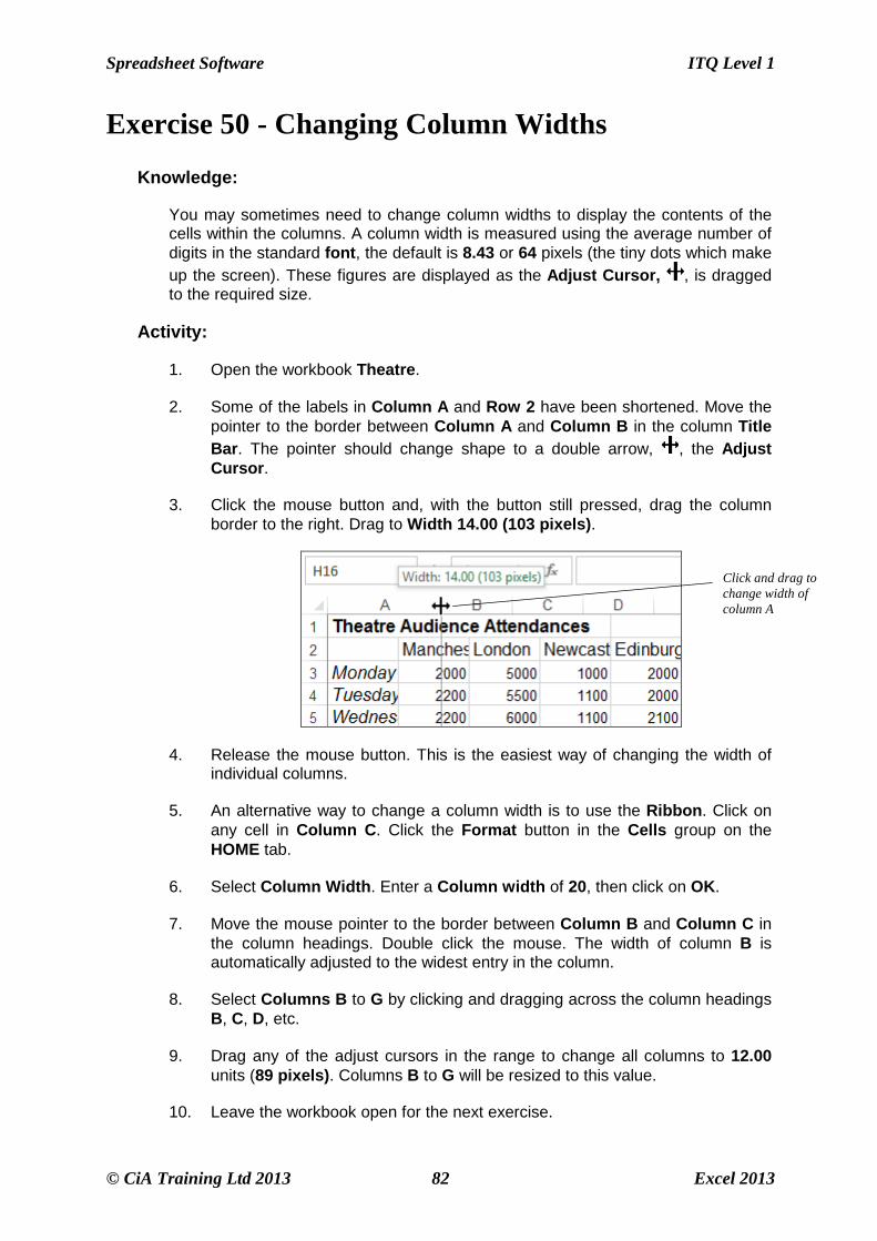
2. Some of the labels in Column A and Row 2 have been shortened. Move the pointer to the border between Column A and Column B in the column Title Bar. The pointer should change shape to a double arrow, , the Adjust Cursor.
3. Click the mouse button and, with the button still pressed, drag the column border to the right. Drag to Width 14.00 (103 pixels).
4. Release the mouse button. This is the easiest way of changing the width of individual columns.
5. An alternative way to change a column width is to use the Ribbon. Click on any cell in Column C. Click the Format button in the Cells group on the HOME tab.
6. Select Column Width. Enter a Column width of 20, then click on OK.
7. Move the mouse pointer to the border between Column B and Column C in the column headings. Double click the mouse. The width of column B is automatically adjusted to the widest entry in the column.
8. Select Columns B to G by clicking and dragging across the column headings B, C, D, etc.
9. Drag any of the adjust cursors in the range to change all columns to 12.00 units (89 pixels). Columns B to G will be resized to this value.
10. Leave the workbook open for the next exercise.
Click and drag to change width of column A
ITQ Level 1 Spreadsheet Software
Excel 2013 83 © CiA Training Ltd 2013
Exercise 51 - Changing Row Height
Knowledge:
Row Heights are increased to create more space between rows of data, making it easier to read the worksheet, or decreased to fit more data on a page.
Row heights are changed in exactly the same way as changing column widths, except the adjust cursor is between two rows and the adjustment changes the row above.
Activity:
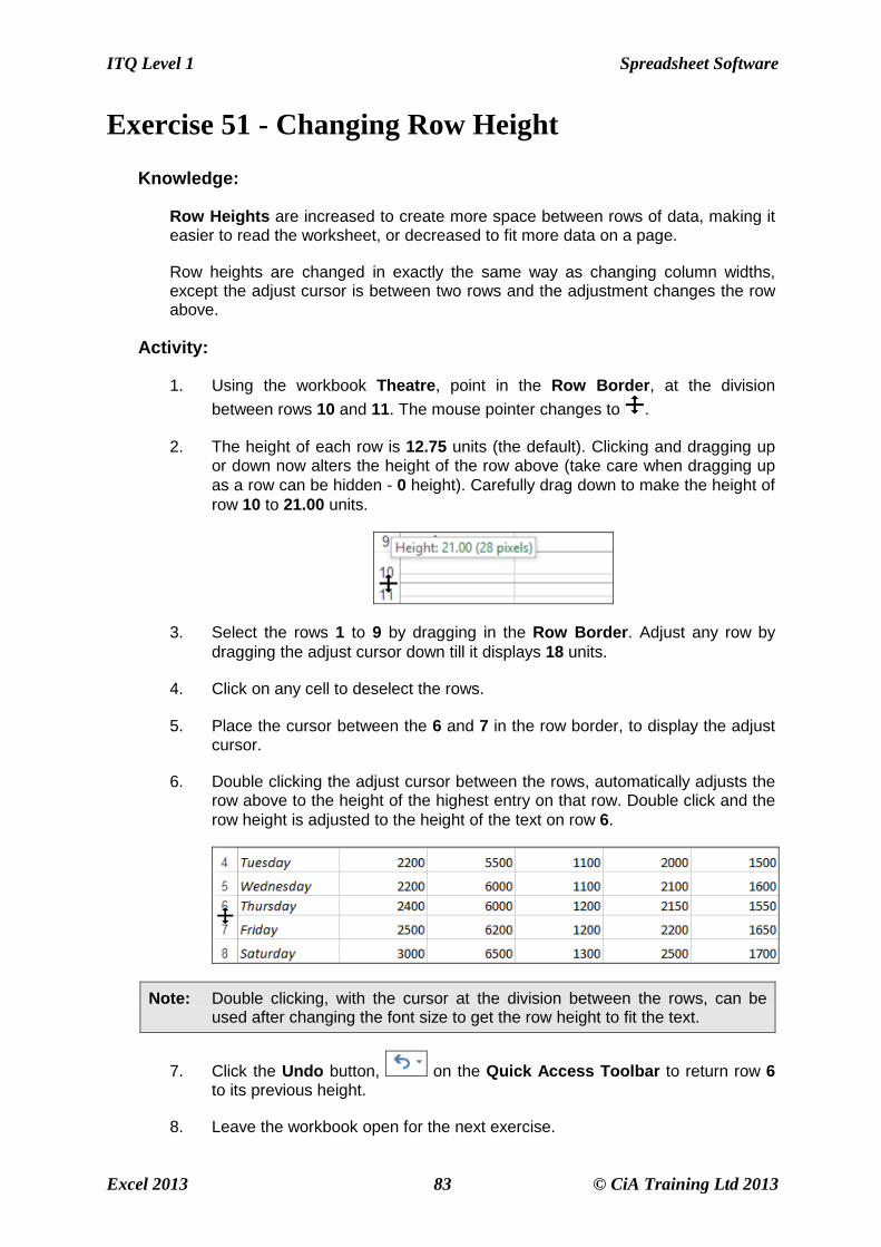
1. Using the workbook Theatre, point in the Row Border, at the division
between rows 10 and 11. The mouse pointer changes to .
2. The height of each row is 12.75 units (the default). Clicking and dragging up or down now alters the height of the row above (take care when dragging up as a row can be hidden - 0 height). Carefully drag down to make the height of row 10 to 21.00 units.
3. Select the rows 1 to 9 by dragging in the Row Border. Adjust any row by dragging the adjust cursor down till it displays 18 units.
4. Click on any cell to deselect the rows.
5. Place the cursor between the 6 and 7 in the row border, to display the adjust cursor.
6. Double clicking the adjust cursor between the rows, automatically adjusts the row above to the height of the highest entry on that row. Double click and the row height is adjusted to the height of the text on row 6.
Note: Double clicking, with the cursor at the division between the rows, can be used after changing the font size to get the row height to fit the text.
7. Click the Undo button, on the Quick Access Toolbar to return row 6 to its previous height.
8. Leave the workbook open for the next exercise.

Spreadsheet Software ITQ Level 1
© CiA Training Ltd 2013 84 Excel 2013
Exercise 52 - Inserting Rows and Columns
Knowledge:
When developing spreadsheets it is inevitable that at some point, room will not have been provided for particular data that is important. Instead of starting again, rows or columns can be inserted.
Columns are inserted to the left of the active cell. New rows are inserted above the active cell.
It is important to check that all formulas are correct after inserting rows and columns.
Activity:
1. The workbook Theatre should still be open. If not, open it.
2. Use AutoSum in cell G3 to total Row 3.
3. Use the Fill Handle to complete the row totals in cells G4 to G8.
4. Another city must be included in the statistics. Click on any cell in Column D. To insert a new column for Belfast, click the Insert button drop down in the Cells group on the HOME tab.
5. Select Insert Sheet Columns.
6. All the existing columns are moved to the right to make way for the new column.
Note: Columns are best inserted in the middle of a range, inserting at either end may require the formulas to be adjusted.
7. Enter the label Belfast in cell D2 and the attendance figures in column D, the same as for Newcastle.
8. The totals in column H are adjusted to include the new numbers. Click on cell H6. To check that Belfast is included in the range that is summed, look at the Formula Bar the formula is =SUM(B6:G6).
ITQ Level 1 Spreadsheet Software
Excel 2013 85 © CiA Training Ltd 2013
Exercise 52 - Continued
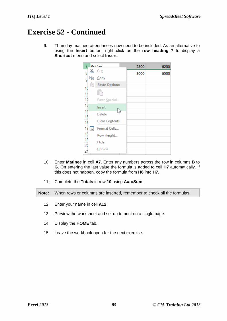
9. Thursday matinee attendances now need to be included. As an alternative to using the Insert button, right click on the row heading 7 to display a Shortcut menu and select Insert.
10. Enter Matinee in cell A7. Enter any numbers across the row in columns B to G. On entering the last value the formula is added to cell H7 automatically. If this does not happen, copy the formula from H6 into H7.
11. Complete the Totals in row 10 using AutoSum.
Note: When rows or columns are inserted, remember to check all the formulas.
12. Enter your name in cell A12.
13. Preview the worksheet and set up to print on a single page.
14. Display the HOME tab.
15. Leave the workbook open for the next exercise.
Spreadsheet Software ITQ Level 1
© CiA Training Ltd 2013 86 Excel 2013
Exercise 53 - Deleting Rows and Columns
Knowledge:
Unwanted rows or columns can be deleted. Deleting a whole row or column is not the same as deleting cell contents.
Activity:
1. The workbook Theatre should still be open. If not, open it.
2. Only cities in England are to be included. Columns D, F and G are to be deleted. Click on the column heading D. Click the Delete button in the Cells group.
Note: The column was deleted without using the drop down because the entire column was selected by clicking on the column heading.
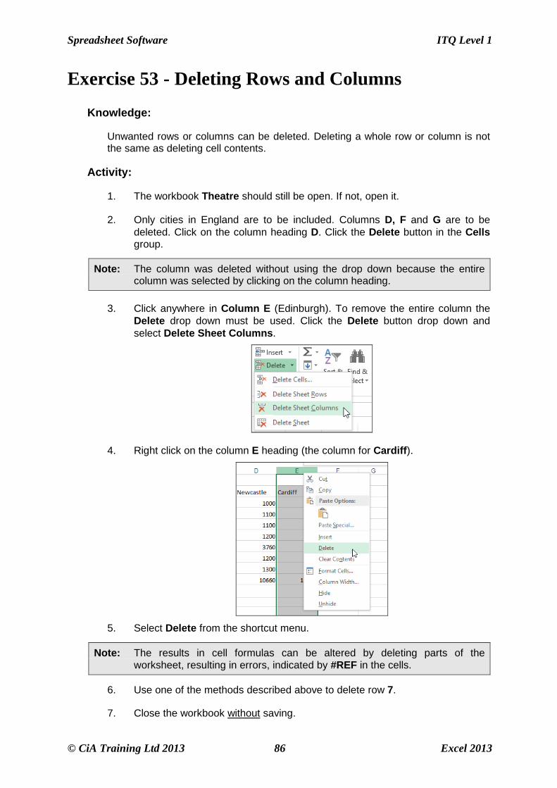
3. Click anywhere in Column E (Edinburgh). To remove the entire column the Delete drop down must be used. Click the Delete button drop down and select Delete Sheet Columns.
4. Right click on the column E heading (the column for Cardiff).
5. Select Delete from the shortcut menu.
Note: The results in cell formulas can be altered by deleting parts of the worksheet, resulting in errors, indicated by #REF in the cells.
6. Use one of the methods described above to delete row 7.
7. Close the workbook without saving.
ITQ Level 1 Spreadsheet Software
Excel 2013 87 © CiA Training Ltd 2013
Exercise 54 - Develop Your Skills
You will find a Develop Your Skills exercise at the end of each Skill Set. Work through it to ensure you’ve understood the previous exercises.
1. Open the workbook Home Accounts.
2. Insert 3 new columns between the March column and the Total column.
3. Enter labels in these new columns for April, May and June.
4. In Row 2, use the Fill Handle to complete cells E2, F2 and G2.
5. Click on cell H2 and notice the formula does not include the newly created columns. Edit the formula to correct this.
6. Copy the amended formula in H2 to the range H3 to H15.
7. Use the Cell Border drop-down button in the Font group on the HOME tab to add the cell borders to cells H4 and H14 to match other cells in their row.
8. Enter other income as follows: Apr-200, May-250 and June-100.
9. Click in E4 and use AutoSum to calculate the total income for April.
10. Complete the totals in cells F4 and G4 using any method.
11. The Rent has doubled to £200 from April onwards. Enter these amounts in the relevant cells.
12. Expenditure is to be cut severely. The car has been sold, therefore no petrol or car costs. There are to be no holidays and the telephone is disconnected. Remove the appropriate rows.
13. Remove the row for Leisure too.
14. Complete the column for April. Electricity: 40, Gas: 40, Food: 70 and Others: 150.
15. Copy the values for the above April values to May and June.
16. Complete Row 10, Total Expenses and Row 11, Savings.
17. Amend the formula in cell H11 to =G11 a copy of the previous cell.
18. Check all the other formulas in column H.
19. Insert two rows at the top of the worksheet and enter your name in cell A1.
20. Print a copy of the worksheet.
21. Save the workbook as home accounts2 and then close it.
Note: The solution is listed in the Answers section at the end of the guide.
Spreadsheet Software ITQ Level 1
© CiA Training Ltd 2013 88 Excel 2013
Summary: Formatting Worksheets
In this Skill Set you have manipulated worksheets by inserting, and deleting columns and rows, also by changing the column width and row height.
You should now be able to demonstrate your ability to:
• Format spreadsheet rows and columns by:
� Changing column widths to fully display the content
� Changing the row height to add more space and reduce clutter
• Change the worksheet structure:
� Insert column and rows
� Delete columns and rows
• Provide evidence of before and after formatting by printing worksheets
ITQ Level 1 Spreadsheet Software
Excel 2013 89 © CiA Training Ltd 2013
Skill Set 8
Formatting Cells
By the end of this Skill Set you should be able to:
Format Numbers
Format Currency
Format Percentages
Change Fonts and Font Size
Format Date and Time
Use Cell Alignment
Add Cell Borders and Shading
Spreadsheet Software ITQ Level 1
© CiA Training Ltd 2013 90 Excel 2013
Exercise 55 - Format Cells
Knowledge:
Cells can be formatted in a number of ways. Formatting cells in a worksheet improves its appearance and makes it easier to read and use.
Formatting can change the look of text, text alignment, text colour, number formats, font style, font size, border lines and cell colour. This Skill Set will concentrate on alignment, number and currency formatting.
Most of the basic formatting can be added to a worksheet in three ways: by clicking buttons on the Ribbon, selecting from dialog boxes and using key presses.
Activity:
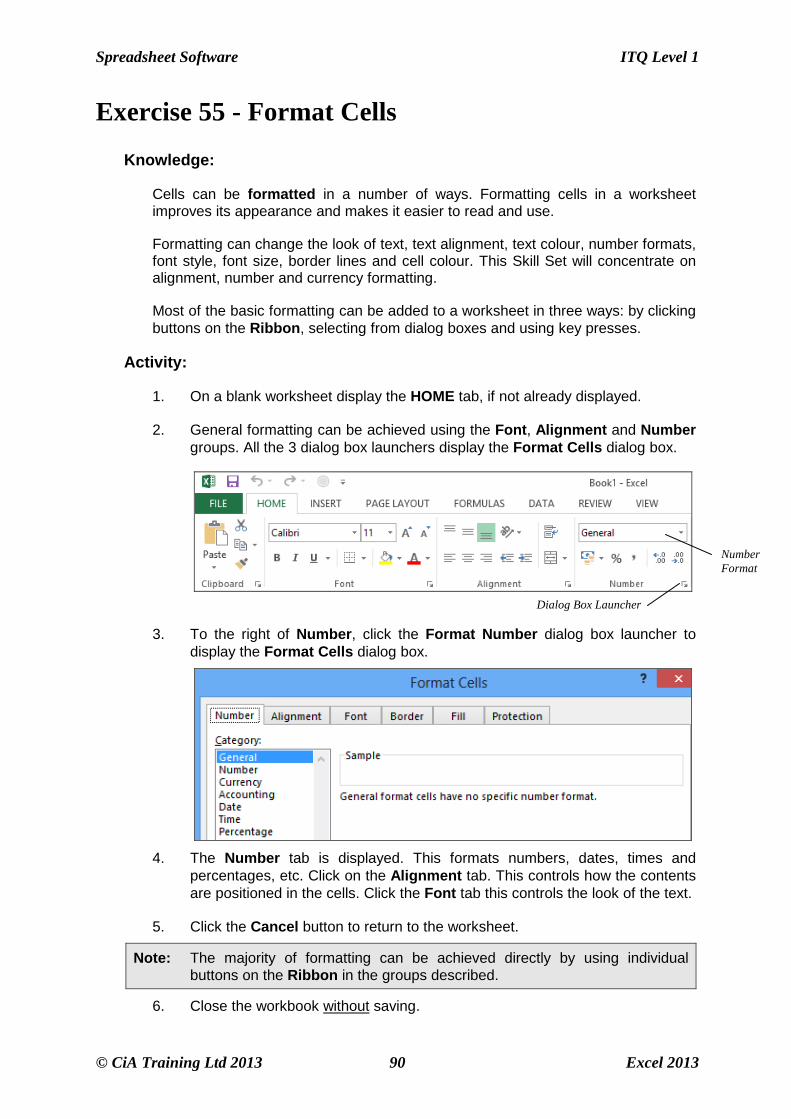
1. On a blank worksheet display the HOME tab, if not already displayed.
2. General formatting can be achieved using the Font, Alignment and Number groups. All the 3 dialog box launchers display the Format Cells dialog box.
3. To the right of Number, click the Format Number dialog box launcher to
display the Format Cells dialog box.
4. The Number tab is displayed. This formats numbers, dates, times and percentages, etc. Click on the Alignment tab. This controls how the contents are positioned in the cells. Click the Font tab this controls the look of the text.
5. Click the Cancel button to return to the worksheet.
Note: The majority of formatting can be achieved directly by using individual buttons on the Ribbon in the groups described.
6. Close the workbook without saving.
Dialog Box Launcher
Number Format
ITQ Level 1 Spreadsheet Software
Excel 2013 91 © CiA Training Ltd 2013
Exercise 56 - Format Number
Knowledge:
Numbers can be formatted to be displayed in a variety of ways, such as currency, percentages, etc.
The number formats are as follows:
Type Description
General No specific number format
Number Plain number formats
Currency Pound signs and decimal places
Accounting Specialised accounting formats
Date Various date formats
Time Various time formats
Percentage Multiplied by 100 (followed by %)
Fraction Decimals expressed as fractions
Scientific Exponent / Mantissa format
Text Displays formulas, not results
Special Telephone numbers, N.I. numbers or Postcode
Custom Allows custom formats to be designed
There are also six number formatting buttons on the HOME tab of the Ribbon.
Accounting Number format, , Percentage Style format, , Comma
Style format, , Increase Decimal, , Decrease Decimal, and a
Number Format box, .
Activity:
1. Open the workbook World Weather.
2. Click on cell B5 and drag the mouse to I16 to highlight all the cells that contain numbers.
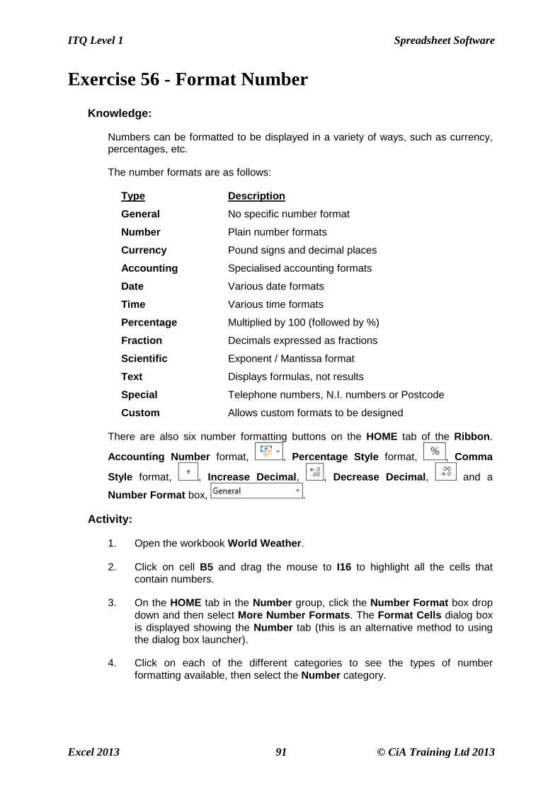
3. On the HOME tab in the Number group, click the Number Format box drop down and then select More Number Formats. The Format Cells dialog box is displayed showing the Number tab (this is an alternative method to using the dialog box launcher).
4. Click on each of the different categories to see the types of number formatting available, then select the Number category.
Spreadsheet Software ITQ Level 1
© CiA Training Ltd 2013 92 Excel 2013
Exercise 56 - Continued
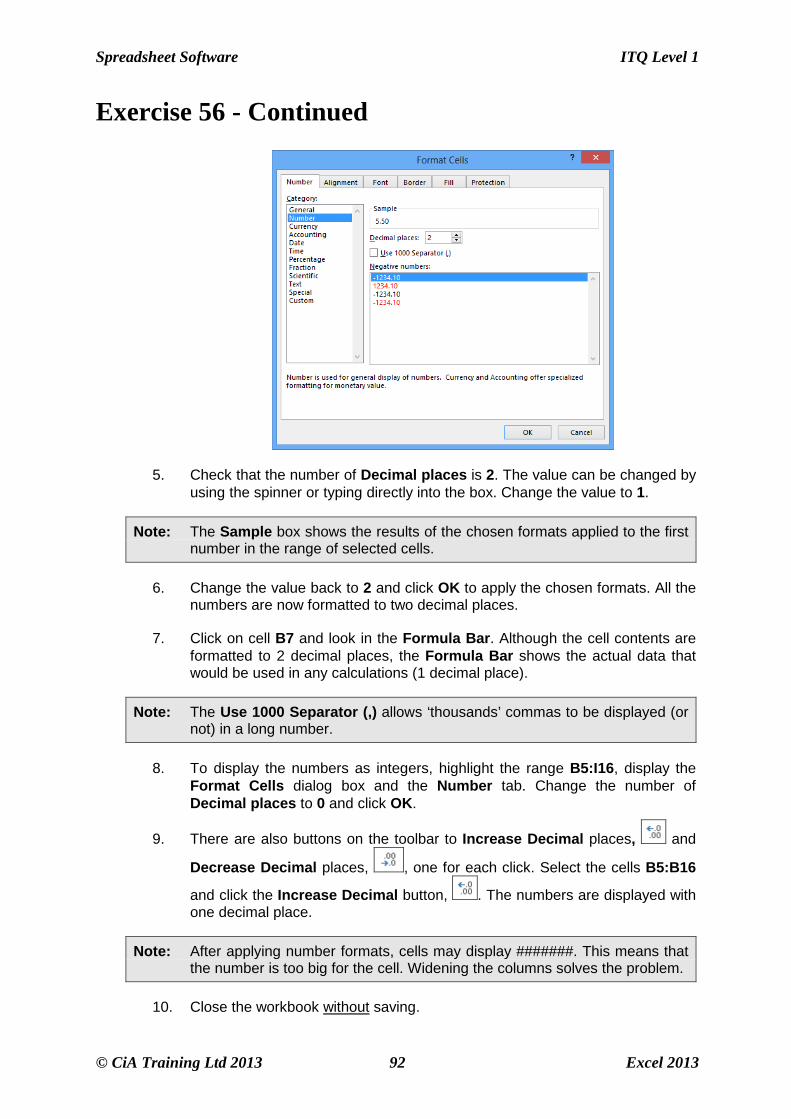
5. Check that the number of Decimal places is 2. The value can be changed by using the spinner or typing directly into the box. Change the value to 1.
Note: The Sample box shows the results of the chosen formats applied to the first number in the range of selected cells.
6. Change the value back to 2 and click OK to apply the chosen formats. All the numbers are now formatted to two decimal places.
7. Click on cell B7 and look in the Formula Bar. Although the cell contents are formatted to 2 decimal places, the Formula Bar shows the actual data that would be used in any calculations (1 decimal place).
Note: The Use 1000 Separator (,) allows ‘thousands’ commas to be displayed (or not) in a long number.
8. To display the numbers as integers, highlight the range B5:I16, display the Format Cells dialog box and the Number tab. Change the number of Decimal places to 0 and click OK.
9. There are also buttons on the toolbar to Increase Decimal places, and
Decrease Decimal places, , one for each click. Select the cells B5:B16
and click the Increase Decimal button, . The numbers are displayed with one decimal place.
Note: After applying number formats, cells may display #######. This means that the number is too big for the cell. Widening the columns solves the problem.
10. Close the workbook without saving.
ITQ Level 1 Spreadsheet Software
Excel 2013 93 © CiA Training Ltd 2013
Exercise 57 - Currency
Knowledge:
It is useful to be able to format numbers as currency. This does not always have to be to two decimal places, e.g. if you wanted to show rounded figures, such as £32 rather than £32.23.
Activity:
1. Open the workbook CD Sales.
2. Click on cell C7 and click the Number group dialog box launcher. Examine the selections in the dialog box. The figures in row 7 have been formatted as Currency with a currency symbol £ and 0 decimal places. Select Cancel to return to the worksheet.
3. Click on cell C8 and repeat the actions in step 2. The figures in row 8 have been formatted as Currency to 2 decimal places with negative numbers shown in red with a minus sign. Click Cancel again.
4. Click and drag the mouse to highlight cells C7 to F7. Display the Number tab of the Format Cells dialog box again. In the Decimal places area, increase the display to 2. Click OK.
5. Close the workbook without saving.
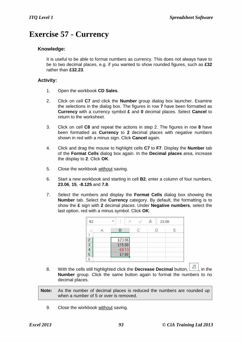
6. Start a new workbook and starting in cell B2, enter a column of four numbers, 23.06, 15, -8.125 and 7.8.
7. Select the numbers and display the Format Cells dialog box showing the Number tab. Select the Currency category. By default, the formatting is to show the £ sign with 2 decimal places. Under Negative numbers, select the last option, red with a minus symbol. Click OK.
8. With the cells still highlighted click the Decrease Decimal button, , in the Number group. Click the same button again to format the numbers to no decimal places.
Note: As the number of decimal places is reduced the numbers are rounded up when a number of 5 or over is removed.
9. Close the workbook without saving.

Spreadsheet Software ITQ Level 1
© CiA Training Ltd 2013 94 Excel 2013
Exercise 58 - Percentages
Knowledge:
Percentages are displayed with a percentage symbol, e.g. 25%. A percentage is a fraction or decimal displayed differently. Percent means per hundred. 20% is 20/100 as a fraction or 0.2 as a decimal.
There is a Percent Style button, , that changes a decimal to a percentage.
Activity:
1. Start a new workbook and create the following worksheet.
2. To display the first number as a percentage of the second in D3, enter the formula =B3/C3 using any method.
3. To format the answer as a percentage, click the Percent Style button, , found in the Number group on the HOME tab (this displays whole number percentage).
4. Change the second number from 25 to 27 and press <Enter>, notice that the percentage value changes automatically.
5. To display percentage with two decimal places, click cell D3 and click the Number Format box drop down, and select the Percentage option from the list. The cell displays 55.56%, a percentage to 2 decimal places.
6. Add the following data starting at cell B5.
Note: To enter 50% in cell C6 type 50 followed by <Shift 5>.
7. To find 50 percent of 20, in cell D6 enter the formula =B6*C6. The answer is 10 (half of 20 is 10).
8. Change the value in B6 to 86 and in C6 to 45%. Press <Enter> to display the new answer, 38.7.
9. Save the workbook as percentages and close it.
ITQ Level 1 Spreadsheet Software
Excel 2013 95 © CiA Training Ltd 2013
Exercise 59 - Fonts and Font Size
Knowledge:
A Font is a type or style of print. Examples of fonts are Arial, Times New Roman, Modern, Script, etc. The default font and font size in Excel is Calibri 11pt. Font Size is measured in points, more points means a larger size.
Activity:
1. Open the workbook Climate.
2. Select cell A2, the title. To change the font, a selection can be made using
the Font drop down (the down triangle) in the Font group, , on the HOME tab. As the mouse moves over each font the results are displayed on the worksheet.
3. Change the font to Algerian (if not available, any other font).
4. Change the formatting of the text in cell B2 to bold, using the Bold button,
in the Font group of the HOME tab.
5. Highlight the range B2:J2 and change the font to Times New Roman (scroll down the font list to find the required one).
6. To make the titles bigger you can change the Font Size. Select cell A2 and
change the size by clicking on the drop down Font Size box, , in the Font group.
7. Select 14 (clicking on the 11 and typing 14 also works. This is especially useful when a size is not displayed in the list).
Note: If the row height has not been manually changed then an increase in font size automatically increases row height to display the text correctly.
8. Select cells B2:J2 and change the font size to 12.
9. The formatting on any cell can be copied to other cell(s) using the Format
Painter. Click on cell B2, click the Format Painter button, in the Clipboard group, then click and drag the range B3:K4. On release of the mouse button the formats from cell B2 are painted to the range B3:K4.
10. Check that the cells in the range B3:K4 are Times New Roman font, size 12pt and bold.
Note: To use the Format Painter repeatedly, double click when selecting it and when finished painting the format, press <Esc> to turn it off.
11. Close the workbook without saving.
Note: These changes can also be made using the Format Cells dialog box.
Spreadsheet Software ITQ Level 1
© CiA Training Ltd 2013 96 Excel 2013
Exercise 60 - Date and Time
Date and Time are stored as numbers. The Date is stored as a number representing the number of days since 1 January 1900, but can be displayed in a variety of formats including both numbers and text. For those formats that represent the year with only two digits, years between 00 and 29 are treated as being after 2000, e.g. 18 is taken to be 2018.
The Time is stored as a decimal number representing a fraction of a day.
Activity:
1. Start a new workbook.
2. In cell B2 enter your date of birth (in the form 31/09/10). Press <Enter>.
3. Click back in cell B2. Display the Format Cells dialog box.
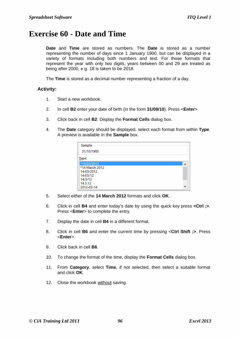
4. The Date category should be displayed, select each format from within Type. A preview is available in the Sample box.
5. Select either of the 14 March 2012 formats and click OK.
6. Click in cell B4 and enter today’s date by using the quick key press <Ctrl ;>. Press <Enter> to complete the entry.
7. Display the date in cell B4 in a different format.
8. Click in cell B6 and enter the current time by pressing <Ctrl Shift ;>. Press <Enter>.
9. Click back in cell B6.
10. To change the format of the time, display the Format Cells dialog box.
11. From Category, select Time, if not selected, then select a suitable format and click OK.
12. Close the workbook without saving.

ITQ Level 1 Spreadsheet Software
Excel 2013 97 © CiA Training Ltd 2013
Exercise 61 - Alignment
Knowledge:
Alignment is changing the position of cell contents within the cell relative to its edges. Contents can be aligned horizontally or vertically and the orientation may also be changed.
Activity:
1. Open the workbook Fruit Sales.
2. Select the range B3:E3. There are buttons in the Alignment group to align
these titles differently: Align Left , , Center, and Align Right, .
3. Click the Center button, . The labels are centred. Click the Align Right
button, and the labels are moved to the right, in line with the numbers beneath them. Click on a cell away from the range to see the effects.
4. There are also buttons to align text vertically. Top Align, , Middle Align,
and Bottom Align . Highlight the range A3:E3 and click the Top
Align button, .
5. The text moves to the top of the cell. With the range still highlighted, click the
Middle Align, . The labels are displayed in the vertical centre of the cells.
Note: Vertical alignment only applies when the row height is greater than the height of the cell contents.
6. Leave the workbook open for the next exercise.
Spreadsheet Software ITQ Level 1
© CiA Training Ltd 2013 98 Excel 2013
Exercise 62 - Borders and Shading
Knowledge:
Borders are lines around the edges of the cells. Options are available on the style of line used, including thin lines, thick lines, dotted lines, etc. The lines may be put around the outside or inside of the range, or on any cell edge. The colour of the lines may also be changed. The colour of the cells may be changed to improve the appearance of a worksheet. There is a Fill Color button (Yellow is the default) in the Font group on the HOME tab.
Activity:
1. The workbook Fruit Sales should still be open from the previous exercise. If not, open it.
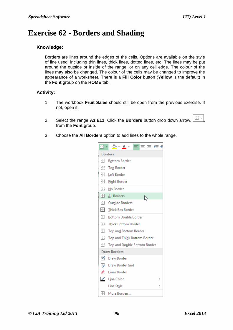
2. Select the range A3:E11. Click the Borders button drop down arrow, , from the Font group.
3. Choose the All Borders option to add lines to the whole range.
ITQ Level 1 Spreadsheet Software
Excel 2013 99 © CiA Training Ltd 2013
Exercise 62 - Continued
4. Click away to view the borders.
Note: Clicking on the button itself applies the last border chosen to the current cells.
5. Click the Undo button, on the Quick Access Toolbar to remove the lines.
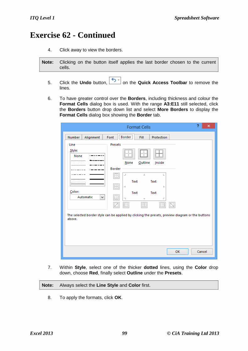
6. To have greater control over the Borders, including thickness and colour the Format Cells dialog box is used. With the range A3:E11 still selected, click the Borders button drop down list and select More Borders to display the Format Cells dialog box showing the Border tab.
7. Within Style, select one of the thicker dotted lines, using the Color drop down, choose Red, finally select Outline under the Presets.
Note: Always select the Line Style and Color first.
8. To apply the formats, click OK.
Spreadsheet Software ITQ Level 1
© CiA Training Ltd 2013 100 Excel 2013
Exercise 62 - Continued
9. Practise adding borders to ranges of cells, using the options in the Format Cells dialog box. Borders can be added by selecting line style and colour, and then either using the Presets buttons, the individual Border buttons, or by clicking the required positions on the Preview diagram in the centre of the dialog box.
10. Highlight the range A3:E11.
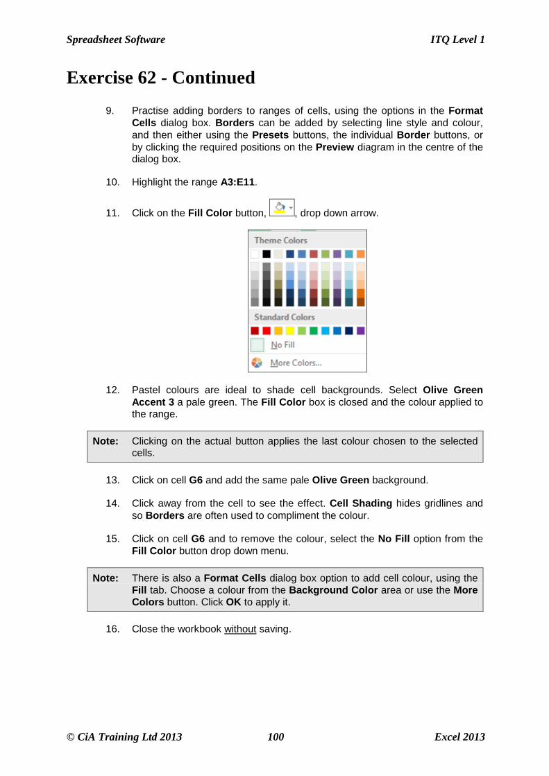
11. Click on the Fill Color button, , drop down arrow.
12. Pastel colours are ideal to shade cell backgrounds. Select Olive Green Accent 3 a pale green. The Fill Color box is closed and the colour applied to the range.
Note: Clicking on the actual button applies the last colour chosen to the selected cells.
13. Click on cell G6 and add the same pale Olive Green background.
14. Click away from the cell to see the effect. Cell Shading hides gridlines and so Borders are often used to compliment the colour.
15. Click on cell G6 and to remove the colour, select the No Fill option from the Fill Color button drop down menu.
Note: There is also a Format Cells dialog box option to add cell colour, using the Fill tab. Choose a colour from the Background Color area or use the More Colors button. Click OK to apply it.
16. Close the workbook without saving.
ITQ Level 1 Spreadsheet Software
Excel 2013 101 © CiA Training Ltd 2013
Exercise 63 - Develop Your Skills
You will find a Develop Your Skills exercise at the end of each Skill Set. Work through it to ensure you’ve understood the previous exercises.
1. Open the workbook Interest Rates. This is a table showing the interest received on varying amounts for different interest rates.
2. The amounts are right aligned, select the range A4:A11 and centre the range, horizontally.
3. Select the range B3:E3 and centre align the cell contents.
4. Select the range B4:E11 and format as Currency with 2 decimal places, with £ signs added.
5. Enter your name in cell A13.
6. Horizontally centre the worksheet and fit to a single page.
7. Preview the worksheet to check the results.
8. Save the workbook as interest rates2.
9. Close the workbook.
10. Open the workbook Home Accounts.
11. The range B1:E1 is currently centred. Select the range and right align it.
12. Select the range B2:E16 and format as currency but with no decimal places.
13. Change the paper orientation to Landscape.
14. Remove all the cell borders.
15. Use the Fill Color button to add pale blue cell shading to the ranges, A1:E1 and A2:A16.
16. Add pale green cell shading to the range B2:E16.
17. Add cell borders to the whole range A1:E16.
18. In cell A18 enter Printed on.
19. In cell A19 enter today’s date in the form dd/mm.
20. Format A19 to display the date in the format dd/mm/yyyy.
21. Preview the worksheet to check the results.
22. Close the workbook without saving.
Spreadsheet Software ITQ Level 1
© CiA Training Ltd 2013 102 Excel 2013
Summary: Formatting Cells
In this Skill Set you have formatted cells in a variety of ways, including: number (decimal places and currency), fonts, date and time, alignment, borders and shading.
You should now be able to demonstrate your ability to:
• Format cells by:
� Displaying numbers with decimal places and as currency
� Changing font and font size
� Changing cell alignment
� Adding borders and shading
• Add date and time
� Format dates and times
Related Documents