Itô calculus extended to systems driven by α -stable Lévy white noises (a novel clip on the tails of Lévy motion

www.elsevier.com/locate/nlm

Author’s Accepted Manuscript

Itô calculus extended to systems driven by alpha-stable lévy white noises (a novel clip on the tails oflévy motion)

M. Di Paola, A. Pirrotta, M. Zingales

PII: S0020-7462(07)00166-7DOI: doi:10.1016/j.ijnonlinmec.2007.07.001Reference: NLM 1389

To appear in: International Journal of Non-Linear Mechanics

Received date: 27 June 2006Revised date: 21 July 2007Accepted date: 24 July 2007

Cite this article as: M. Di Paola, A. Pirrotta and M. Zingales, Itô calculus extended to sys-tems driven by alpha-stable lévy white noises (a novel clip on the tails of lévy motion), Inter-national Journal of Non-Linear Mechanics (2007), doi:10.1016/j.ijnonlinmec.2007.07.001

This is a PDF file of an unedited manuscript that has been accepted for publication. Asa service to our customers we are providing this early version of the manuscript. Themanuscript will undergo copyediting, typesetting, and review of the resulting galley proofbefore it is published in its final citable form. Please note that during the production processerrors may be discovered which could affect the content, and all legal disclaimers that applyto the journal pertain.

peer

-005

0175

8, v

ersi

on 1

- 12

Jul

201

0Author manuscript, published in "International Journal of Non-Linear Mechanics 42, 8 (2007) 1046"

DOI : 10.1016/j.ijnonlinmec.2007.07.001

Accep

ted m

anusc

ript

1

ITÔ CALCULUS EXTENDED TO SYSTEMS DRIVEN BY

ALPHA-STABLE LÉVY WHITE NOISES

(A NOVEL CLIP ON THE TAILS OF LÉVY MOTION)

by

M. Di Paola, A. Pirrotta and M. Zingales*

Dipartimento di Ingegneria Strutturale e Geotecnica, Viale delle Scienze, I-90128, Palermo, Italy.

ABSTRACT

The paper deals with probabilistic characterization of the response of non-linear systems

under α-stable Lévy white noise input. It is shown that, by properly selecting a clip in the

probability density function of the input, the moments of the increments of Lévy motion process

remain all of the same order ( )dt , like the increments of the Compound Poisson process. It

follows that the Itô calculus extended to Poissonian input, may also be used for α-stable Lévy

white noise input processes. It is also shown that, when the clip on the tails of the probability of

the increments of the Lévy motion approaches to infinity, the Einstein-Smoluchowsky equation is

restored. Once these concepts are outlined extension to single oscillator is readily obtained. A

discussion on the proper way to perform Monte Carlo simulation is also exploited.

Keywords: α-Stable Processes, Einstein-Smoluchowsky Equation, Itô Calculus, Truncated

Lévy Motion.

1. INTRODUCTION

Normal white noises are very popular stochastic processes and they have been used to model

several types of physical phenomena. Such processes may be defined as formal time derivative of

Wiener processes. In this setting the powerful machinery of Itô stochastic differential calculus

may be used to yield the response probabilistic characterization of systems driven by normal

peer

-005

0175

8, v

ersi

on 1

- 12

Jul

201

0

Accep

ted m

anusc

ript

2

white noises, in terms of moments or of conditional probability density function (PDF), that is the

Fokker-Planck-Kolmogorov (FPK) equation. The Fourier transform, of the FPK equation, rules

the evolution of the characteristic function (CF) of the response, often termed as spectral FPK

equation.

However, several real phenomena observed in physics, seismology, electrical engineering,

economics and in some other research fields show evident non-Gaussianity either in heavy tails

distribution or in the impulsive nature of the recorded samples. According to this new need, the

Itô stochastic differential calculus has been extended to Poissonian white noises too, providing

the equation governing the evolution of the probability density, known as Kolmogorov-Feller

equation [1-4]. The need for non-Gaussian models, to describe the fluctuations exhibited by non-

Gaussian phenomena, has also raised the interest in the so-called α -stable Lévy processes [4-7].

This kind of stochastic process is characterized by the knowledge of four parameters, which are,

respectively, the stability index α , the scale factor σ , the skewness β and the shift μ [8]. The

choice for different values of the stability index α ( 0 2α< ≤ ) leads to formidable variety of

stochastic processes including the Gaussian white noise obtained for 2α = . Linear and non-linear

systems driven by external α -stable Lévy white noise processes (formal time derivative of the

Lévy motion processes labeled as ( )L tα ) have been treated, in the past, either in terms of PDF

Einstein-Smoluchowsky (ES) equation or in terms of CF (see e.g. [9]]). Moreover closed-form

expressions of the probability density function of dynamical systems driven by external α -stable

Lévy noises have been obtained for limited values of the stability index.

The main challenge in the analysis of dynamical systems in presence of α -stable Lévy

white noise is related to the divergence of statistical moments of the α -stable random variable

( )L tα , namely ( )pE L tα⎡ ⎤ = ∞⎣ ⎦ if p α≥ . Then unless the case of normal white noise ( 2)α = all

the moments starting from the variance would diverge because of the heavy tails of the

distribution of the random variable ( )L tα . In order to overcome this drawback some truncation of

the PDF of α -stable random variable ( )L tα have recently been performed [10] in which a

power law with exponent (5-α ) has been used to truncate the PDF of α -stable distribution. In

this context a modified fractional FPK equation has been obtained and the PDF of the response

converges towards a Gaussian density in the central part. Tails of solution of the response of non-

linear systems are discussed in [11].

peer

-005

0175

8, v

ersi

on 1

- 12

Jul

201

0

Accep

ted m

anusc

ript

3

In this paper, the Itô calculus will be extended to non-linear systems under α-stable Lévy

white noise. In order to aim at this, a new form of truncation is introduced, different from that

proposed in [10]. We, in fact, exclude the tails on the PDF for value greater than ( ) 1t n αα

−Δ ,

being tΔ the time step and nα a control clip parameter. It is shown that when a truncation is

performed, all the moments of ( )dL tα exist and are all of order dt like the increments of the

Compound Poisson process. It follows that the Itô rule extended to Poisson white noise process

may be used. It is also shown that when α → ∞n , the ES equation is fully recovered. In this

setting a correct way for Monte-Carlo simulation (MCS) for the response analysis of non-linear

systems under α-stable Lèvy white noise is given. Based on this solid ground, the extension to

single oscillator is readily found (see Appendix B). Some numerical examples have been reported

to assess the validity of the proposed formulation for linear and non-linear Langevin equation

under α -stable Lévy white noise.

2. INTRODUCTORY REMARKS ON ITÔ DIFFERENTIAL CALCULUS

In this section some well known concepts of Itô calculus are briefly summarized for sake of

clarity as well as for introducing appropriate symbology.

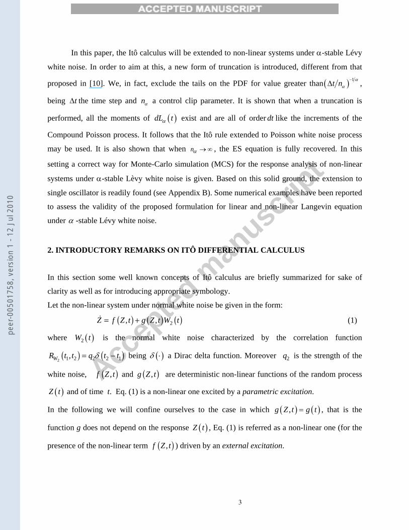
Let the non-linear system under normal white noise be given in the form:

( ) ( ) ( )2, ,Z f Z t g Z t W t= + (1)

where ( )2W t is the normal white noise characterized by the correlation function

( ) ( )2 1 2 2 2 1,WR t t q t tδ= - being ( )δ ⋅ a Dirac delta function. Moreover 2q is the strength of the

white noise, ( ),f Z t and ( ),g Z t are deterministic non-linear functions of the random process

( )Z t and of time t. Eq. (1) is a non-linear one excited by a parametric excitation.

In the following we will confine ourselves to the case in which ( ) ( ),g Z t g t= , that is the

function g does not depend on the response ( )Z t , Eq. (1) is referred as a non-linear one (for the

presence of the non-linear term ( ),f Z t ) driven by an external excitation.

peer

-005

0175

8, v

ersi

on 1

- 12

Jul

201

0

Accep

ted m

anusc

ript

4

From the definition of ( )2W t , as formal time derivative of Wiener process ( )B t having

independent increments, it follows that Eq.(1) may be rewritten in Itô form as follows:

( ) ( ) ( ),dZ f Z t dt g t dB t= + (2)

Once the original equation is transformed into an Itô type stochastic differential equation, the Itô

differential rule may be used for the probabilistic characterization of the response process ( )Z t :

( ) ( )2

22

1,2

d Z t dt dZ dZt Z Z

ψ ψ ψψ ∂ ∂ ∂= + +

∂ ∂ ∂ (3)

where ( ),Z tψ is any non-linear function of Z and t , continuous and differentiable on t and

twice differentiable on Z . The third term in the right-hand side of eq.(3) is essential since ( )dB t

is of order of magnitude ( )1 2dt and then term ( )2dZ is of the same order of the first term. In

order to derive the equation governing the evolution of the characteristic function

( ) ( )( ), expZ t E i Z tφ θ θ⎡ ⎤= ⎣ ⎦ we put ( ) ( ), expZ t i Zψ θ= in eq.(3), taking mathematical

expectation and accounting for the non-anticipative property of Itô calculus

( ) ( ) ( ) ( )( ), ,k kE Z t dB t E Z t E dB tψ ψ⎡ ⎤ ⎡ ⎤⎡ ⎤= ⎣ ⎦⎣ ⎦ ⎣ ⎦ the differential equation governing the evolution

of the CF is readily written as:

( ) ( ) ( ) ( ) ( )2

22,exp , ,

2Z

Zt qi E i Z f Z t t g t

tφ θ θθ θ φ θ∂

È ˘= -Î ˚∂ (4)

An inverse Fourier transform of eq.(4) yields the so-called Fokker-Planck-Kolmogorov (FPK)

equation governing the evolution of the PDF of the response:

( ) ( ) ( ) ( ) ( )222

2, ,

, ,2

Z ZZ

p z t p z tqp z t f z t g tt z z

∂ ∂∂ È ˘= - +Î ˚∂ ∂ ∂ (5)

Itô rule extended to the case of Poissonian white noise is reported in Appendix A.

3. THE CASE OF α-STABLE WHITE NOISE EXTERNAL EXCITATION

Let us now suppose that ( )2W t is substituted by ( )W tα , being ( )W tα the α -stable Lévy white

noise process. In analogy to the definition of the previous white noise, an α -stable Lévy white

noise may be defined as the formal derivative of a corresponding α -stable Lévy motion ( )L tα

(α is the stability index of the stableα - process) having the following properties:

peer

-005

0175

8, v

ersi

on 1

- 12

Jul

201

0

Accep

ted m

anusc

ript

5

i) It has independent, stationary increments following the stableα - distribution, that is

( ) ( ) ( )( )1 ,0,0L t L s S t s αα α α∼- - (6a)

ii) The CF of an increment of ( )αdL t , takes the form:

( ) expdL dtα

αφ θ θÈ ˘= -Î ˚ (6b)

where ( )dL tα represents the increment of α -stable Lévy motion ( )L tα and ( )kL tα , at a selected

time ( )kt , is a symmetric α-stable ( )S Sα random variable.

iii) For 2α = , ( )L tα reverts to ( )B t and then the non-normal stableα - process reverts to

normal white noise process, or in other words the Wiener process is a particular case of

the random process ( )L tα .

In the case of Lévy white noise the equation governing the evolution of the PDF, for

( ) ( ),g Z t g t= (external excitation), is the so-called Einstein-Smoluchowsky (ES) equation [9]

involving Riesz-Weil fractional derivative in the diffusion term, that is:

( ) ( ) ( )( ) ( ) ( ),, , ,Z

Z Zp z t

p z t f z t g t p z tt z z

ααα

∂ ∂ ∂= - +∂ ∂ ∂

(7)

in which z α∂ ∂ is the symmetric functional space derivative [12, 13] which is defined for a

“sufficiently well-behaved” function through its Fourier transform [ ]i¡ :

( ) ( ),,Z

Zp z t

tz

αα

α θ φ θÈ ˘∂

¡ = -Í ˙∂Í ˙Î ˚

(8)

or in terms of the Riemann-Liouville derivatives as:

( )( ) ( ) ( ), 1 , ,

2cos 2Z

Z Zp z t

D p z t D p z tz

αα α

α πα + -∂ È ˘= - +Î ˚∂

(9)

where 0α > and if 0 1α< < then Riemann-Liouville derivatives reads:

( ) ( )( )

( )

( ) ( )( )

( )

,1,1

,1,1

zZ

Z

ZZ

z

p tD p z t d

z z

p tD p z t d

z z

αα

αα

ξξ

α ξ

ξξ

α ξ

Γ

Γ

+-•

•

-

∂=- ∂ -

∂= -- ∂ -

Ú

Ú (10 a, b)

else for 1α > :

peer

-005

0175

8, v

ersi

on 1

- 12

Jul

201

0

Accep

ted m

anusc

ript

6

( ) ( )( ) ( )11

, ,n zn

nZ ZnD p z t p z t d

n zα αξ ξ ξ

αΓ∓- -

±-•

± ∂=- ∂ Ú (11)

with 1n nα- < £ Œ . In the specific case 1α = the Riemann-Liouville derivative coalesces

with the Hilbert transform of the function ( ),Zp tξ . The Dirichlet conditions about the existence

of the [ ]i¡ are guaranteed since the area under the PDF is one. The derivatives in eqs.(10, 11)

are characterized in the Fourier transform space as:

( ) ( ) ( ), ,Z ZD p z t i tαα θ φ θ∓±È ˘¡ =Î ˚ (12)

with:

( ) ( )exp sgn2

ii α α απθ θ θ∓È ˘- = Í ˙Î ˚ (13)

and ( )sgn i is the well-known signum function. Combining eqs.(9, 11) with eq.(12), eq.(8) is

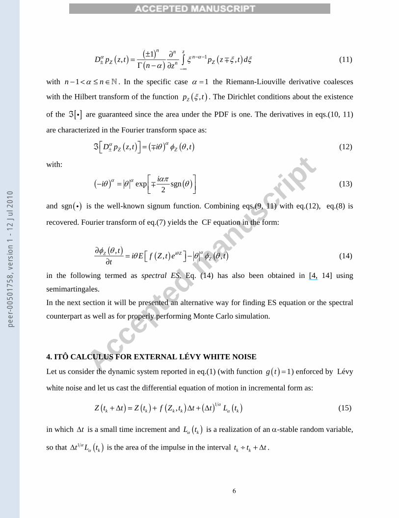
recovered. Fourier transform of eq.(7) yields the CF equation in the form:

( ) ( ) ( ),, ,i ZZ

Z

ti E f Z t e t

tαθφ θ

θ θ φ θ∂ È ˘= -Î ˚∂

(14)

in the following termed as spectral ES. Eq. (14) has also been obtained in [4, 14] using

semimartingales.

In the next section it will be presented an alternative way for finding ES equation or the spectral

counterpart as well as for properly performing Monte Carlo simulation.

4. ITÔ CALCULUS FOR EXTERNAL LÉVY WHITE NOISE

Let us consider the dynamic system reported in eq.(1) (with function ( ) 1g t = ) enforced by Lévy

white noise and let us cast the differential equation of motion in incremental form as:

( ) ( ) ( ) ( ) ( )1,k k k k kZ t t Z t f Z t t t L tααΔ Δ Δ+ = + + (15)

in which tΔ is a small time increment and ( )kL tα is a realization of an α-stable random variable,

so that ( )1kt L tα

αΔ is the area of the impulse in the interval k kt t tΔ∏ + .

peer

-005

0175

8, v

ersi

on 1

- 12

Jul

201

0

Accep

ted m

anusc

ript

7

Peculiarity of α-stable random variables is long tail PDF. This feature will be reflected on

experiencing eventual very high value ( )kL tα , when generating samples of ( )L tα . This leads to

numerical overflow in the response evaluation. To avoid the latter problem, it should be selected

the highest value of ( )kL tα , according to a negligible committed error in the evaluation of ( )L tα

PDF . Evaluating the probability that ( )kL tα is greater than a large real value ν of an α-stable

random variable ( ) ( ),0,0kL t Sα α σ∼ by:

( ){ }Pr ob kL t C αα αν ν −> = ; ν Æ• (16)

where ( )1

0

sinC x x dxαα

−∞−⎛ ⎞

= ⎜ ⎟⎝ ⎠∫ is a real number dependent on the stability index α , (for instance,

[ ]0 for 2, 2 for 1, 1 (2) =1 for 0 8C C Cα α αα π α Γ α= = = = = = ). It follows that the

probability of occurrence of values of ( )kL tα larger than ( ) 1t α−Δ is C tα Δ , that is

( ) ( ){ }1Pr ob ; 0kL t t C t tαα α

−> Δ Δ Δ → (17)

Based on this consideration in [15], realization of ( )kL tα greater than 1t α−Δ may be neglected.

Looking at eq.(17), we may say that, introducing a real value nα , ( 1nα ≥ ∈R ), in such a way:

( )1

Pr ob ; 0kt tL t C t

n n

α

α αα α

Δ ΔΔ

-Ï ¸Ê ˆÔ Ô> ÆÌ ˝Á ˜Ë ¯Ô ÔÓ ˛ (18)

the probability remains of order tΔ also for ( ) 1t n αα

−Δ . This means that neglecting outcomes of

( )kL tα larger than ( ) 1t n αα

−Δ , we introduce an approximation of order ( )t nαΔ . This

approximation corresponds “de facto” in a proper clip of the tails of PDF, through a right

choice of nα .

Increasing values of nα it results into smaller probability that ( )kL tα exceeds the value

( ) 1t n ααΔ − . For instance, if values of nα reach the order of magnitude of 1tΔ − , then the

probability that a realization of ( )kL tα is greater than ( ) 1t n ααΔ − is of order of magnitude

peer

-005

0175

8, v

ersi

on 1

- 12

Jul

201

0

Accep

ted m

anusc

ript

8

2tΔ and in the limit as 0tΔ → becomes an infinitesimal of higher order thus it may be really

neglected. It is worth stressing that, at the limit for α → ∞n the real PDF is restored.

Previous considerations lead us to represent α-stable increments of the Lévy process ( )dL tα in

the form:

( ) ( ) ( )1

1

0

limn

t

tdL t dt L t L tnα

αα

α α αα

→∞Δ →

⎛ ⎞Δ= = ⎜ ⎟

⎝ ⎠ (19)

It is worth noting, that if 2α = ( ) ( )( )L t B tα → , then Cα =0 and the area of each impulse that is

( )1 2kt B tΔ remains finite setting nα =1 in eq.(19).

In order to better clarify the role played by eq.(19) we may write

( ) ( ) ( )j j j j jk k LE dL t E L t dt dt x p x dx

α

α αα α

•

-•

È ˘ È ˘= =Î ˚ Î ˚ Ú (20)

Notice that in eq.(20) it is present the product of an infinitesimal quantity jdt α and a divergent

integral term. The question is: what is the order of magnitude of ( )jkdL tα ? In order to check out

the convergence of eq.(20) we introduce the representation of ( )dL tα as in eq.(19) yielding

( ) ( )( )

( )( )

1

10

limt n

j j jk L jt

t n

E dL t t x p x dx K n dt

αα

αα

α

αα α

Δ

ΔΔ

Δ

-

-Æ

-

È ˘ = =Î ˚ Ú (21)

where ( )jK nα are real finite numbers and then from eq.(21) we may state that the increments of

the Lèvy motion are of order dt . This remarkable result allows us to assess that in this

perspective, once nα has been selected, the increments of the Lèvy motion behave exactly as the

increments of the compound Poisson process [1-4] and then Itô rule for Poissonian white noise

may be used (see eq. (A5) in the Appendix A.).

As an example we may assume that ( )L tα is Cauchy distributed, then PDF reads:

( ) ( )21 1Lp x xα

π= + (22)

and terms ( ) 0jK nα = for j odd and ( ) ( )2 1jK n n jα α π= - for j even.

peer

-005

0175

8, v

ersi

on 1

- 12

Jul

201

0

Accep

ted m

anusc

ript

9

Moreover if 2α = , 1nα = and then

( )( )

( )1 2

1 2

2 2 2

0

1 1lim exp22

tj j j j

jtt

E dB t t x x dx t Kπ

−

−

Δ

Δ →− Δ

⎛ ⎞⎡ ⎤ = Δ − = Δ⎜ ⎟⎣ ⎦ ⎝ ⎠∫ (23)

where 2 1 0,jK + = and ( )22 2 2 1 !!j

jK q j= − , (being ( ) ( ) ( )2 1 !! 2 1 2 3 3 1j j j− = − ⋅ − ⋅ ; with (-

1)!!=1), that is dB(t) is of order 1 2dt . It follows that the Itô rules according eq.(3) contains terms

up to the order ( )2dZ since the latter remains of order dt . Conversely, when the system is driven

by Lèvy α -stable white noise, for fixed nα , all the increments ( )jdL tα are of order dt , as shown

in eq.(21). Then by selecting ( ) ( )( ), expZ t i Z tψ θ= in eq.(A5) of the Appendix A, we get

( ) ( ) ( ) ( ) ( ) ( )1

exp , exp exp!

jj

j

id i Z i f Z t i Z dt i Z dL t

j α

θθ θ θ θ

•

=

È ˘ = +Î ˚ Â (24)

By inserting eq.(21) into eq.(24), performing mathematical expectation, dividing by dt and using

the non-anticipative property of Itô calculus, we get:

( ) ( ) ( ) ( ) ( ) ( )1

, , exp ,!

j

Z Z jj

it i E f Z t i Z t K n

t j α

θφ θ θ θ φ θ

∞

=

∂⎡ ⎤= +⎣ ⎦∂ ∑ (25)

Summation in eq.(25) for 1α = leads to

( ) ( ) ( )( )

2 2 1

1 1

2! 2 ! 2 1

j j j

jj j

i i nK nj j j

αα

θ θπ

−∞ ∞

= =

=−∑ ∑ (26)

And in the limit when α → ∞n converges to θ− as shown in fig.(1a) in which the sum in the

series (26) has been reported for different values of nα .

Summation in eq.(25) for 1 2α = (Lèvy distribution) is given as

( ) ( ) ( )( )

2 1

1 1

2! ! 2 1

j j j

jj j

i i nK nj j j

αα

θ θπ

−∞ ∞

= =

=−∑ ∑ (27)

and in the limit when α → ∞n converges to 1 2θ− as shown in fig.(2a). Many other intermediate

values of ( )jK nα have been tested for different values of α and always they give that at the

peer

-005

0175

8, v

ersi

on 1

- 12

Jul

201

0

Accep

ted m

anusc

ript

10

limit for α → ∞n summation in eq.(25) converges to αθ− . Then we may conclude that eq.(25)

when α → ∞n coincides with eq.(14), and its Fourier transform fully restores the ES equation.

On the other hand once these results have been obtained we may also assert that for every value

of α the following relation

( ) ( ) ( ) ( )1

exp 1 1!

jj

dLj

iE dL t dt dt

j α

α αα

θθ φ θ θ

∞

=

⎡ ⎤ = − − = − −⎣ ⎦∑ (28)

holds true.

At this stage some further observations will be exploited about the validity of eq.(28) as claimed

in [4, 14]. It may be observed that formal analytical derivations led to eq.(28) but along way we

introduced two fundamental assumptions:

• Setting the value of nα , moments of increments jE dLα⎡ ⎤⎣ ⎦ exist for every value of j and

they are of order dt (eq.21).

• We consider that the series in eq.(28) converges to the CF of the increment ( )dL tα , that

coincides with eq.(25) for α → ∞n .

Summing up, the realization of the α - stable random variable may attain infinite values, if we

accept that for 0tΔ Æ the probability that the random variable ( ) ( ) 1kL t t n α

α αΔ-> is

negligible, then jE dLαÈ ˘Î ˚ is of order dt j" . This means, “de facto” a proper clip of the tails of

the PDF of the random variable ( )kL tα . If this operation is performed then Itô rule, (eq.A5) for

Poissonian white noise is still valid also for α - stable Lèvy white noise, and the ES equation is

recovered. The latter concept has to be accounted for the MCS, in which we have to neglect

realizations of values of ( )kL tα larger than ( ) 1t n ααΔ

- . In any cases, it suffices selecting at most

1n tα Δ= , for assessing that the error in clipping the tails of the PDF of ( )kL tα is of order 2tΔ .

Obviously if we select nα and we compute ( )jK nα and insert these values in eq.(24) we get

( ),E Z tψ⎡ ⎤⎣ ⎦ . The same result is obtained by performing MCS excluding realizations of ( )kL tα

larger than ( ) 1t n ααΔ

- . In this framework some numerical applications will be reported in the

following sections.

peer

-005

0175

8, v

ersi

on 1

- 12

Jul

201

0

Accep

ted m

anusc

ript

11

5. NUMERICAL APPLICATIONS

In this section applications to linear and cubic non-linear system under α − stable Lèvy white

noise ( )1α = will be presented. The problem involving cubic non-linear oscillator has been

selected since the solution in terms of spectral ES equation has been extensively studied (see i.e.

[4],[9],[14]) and the existent solutions may be used as benchmark to highlight the role played by

the truncation coefficient nα . The analyzed system is

( )3 Z a Z b Z W tα= + + (29)

5.1 Linear system under Cauchy white noise

The linear system, which is the hitherto studied case, is obtained setting 0b = in eq.(29). In this

case ( )Z t is also an α − stable process having the same stability index as the Lèvy white noise,

but with different scale (or amplitude). For this case the spectral ES may be written as:

( ) ( ) ( ), , , Z Z

Z

t ta t

tφ θ φ θ

θ θ φ θθ

∂ ∂= −

∂ ∂ (30 a)

( )0

1Z θφ θ

== (30 b)

With eq.(30 b) representing the attendant boundary condition. Steady-state solution of the

differential equation described in eqs.(30) reads:

( ) exp Z aφ θ θ⎡ ⎤= ⎣ ⎦ (31)

The Ornstein-Uhelembeck CF described in eq.(31) has been reported in fig.(2) with continuous

line. Such exact solution has been contrasted with results obtained by MCS for different values of

nα . The values of the time interval has been selected to value 310t −Δ = for the numerical

simulation reported. Characteristic function ( )Zφ θ in eq.(31) with the decaying factor 1a = − ,

has been depicted in fig.(2a) with continuous line. The CF obtained via MCS have been

contrasted in fig. (2a) for several values of the truncation parameter nα set equal to 1nα = (star),

50nα = (triangle) and for the limit value 1 1000n tα = Δ = (square).

The selected values of nα and tΔ led us to exclude values of

( ) ( ) ( )1000 (stars) ; 50000 (triangles); 1000000 (squares)k k kL t L t L tα α α> > > according to

peer

-005

0175

8, v

ersi

on 1

- 12

Jul

201

0

Accep

ted m

anusc

ript

12

sec.4. It may be observed that for small values of nα the Monte-Carlo estimate of the CF does not

coincide with CF in eq.(31). A different scenario is observed increasing the value of nα until its

upper bound 1 tΔ and it may be noticed that the CF obtained via numerical simulation coincides

with the exact reported in eq.(31). A more precise description of the trend of the CF, for different

nα , is furnished by observation of fig.(2b). In more detail, it may be observed that, a smooth CF

at the origin appears, assuming 1nα = . On the other hand for values of the coefficient nα

approaching the limit 1 tΔ the peak of the exact CF at the origin is captured. Several other

clipping values of 2 or 3n t n tα α= Δ = Δ have been considered for numerical analysis, but the

obtained results match the reported CF for the limit value 1 tΔ . This aspect is much more

important for numerical simulation of non-linear dynamical systems as it will be shown in the

following section.

5.2 Non-linear system under Cauchy white noise

Let us now consider that the non-linear coefficient 0b ≠ in eq.(29). The associated spectral ES

equation is [4],[9],[14].

( ) ( ) ( ) ( )

( ) ( ) ( )

3

3

0

, , , ,

,, 1; 0; lim , 0

Z Z ZZ

ZZ Z

t t ta b t

tt

t tθ θ

φ θ φ θ φ θθ θ θ φ θ

θ θφ θ

φ θ φ θθ= →∞

∂ ∂ ∂= + −

∂ ∂ ∂∂

= = =∂

(32)

The boundary conditions in eq. (32 c) has been used in [9] and it is valid only if ( )Zφ θ is

differentiable for 0θ = . For the steady-state case the boundary value problem described in eq.(32

a, b) may be solved for 0 and 0θ θ> < assuming that ( ) [ ]expZφ θ ρ λθ= with ρ a

normalization constant and λ obtained by the solution of the algebraic equation:

3 1 0b aλ λ- + = (33)

which for the selected values of parameters 1.0; 0.1a b= − = − as reported in [14], yields the real

roots 1 2 31.15347, 2.42362, 3.57709λ λ λ= − = − = . The latter positive real root must be

peer

-005

0175

8, v

ersi

on 1

- 12

Jul

201

0

Accep

ted m

anusc

ript

13

disregarded since it does not fulfill the boundary condition ( )lim , 0Z tθ

φ θ→∞

= and the stationary CF

reads:

( ) ( ) ( )

( ) ( ) ( )

1 22 1

1 2 1 2

1 22 1

1 2 1 2

exp exp ; 0

exp exp ; 0

Z

Z

λ λφ θ λ θ λ θ θλ λ λ λ

λ λφ θ λ θ λ θ θλ λ λ λ

⎛ ⎞= − ≥⎜ ⎟− −⎝ ⎠

⎛ ⎞= − − + − <⎜ ⎟− −⎝ ⎠

(34)

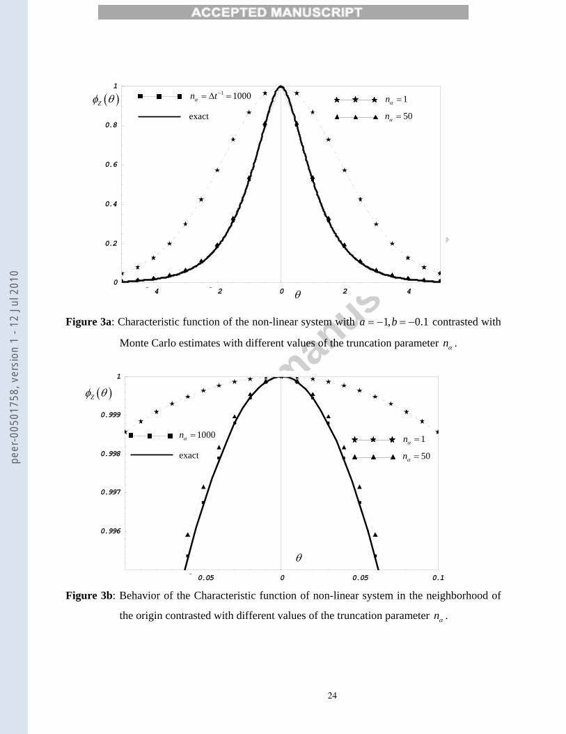
In order to assess the validity of eqs.(34 a,b) MCS has been performed estimating the CF with

747.000.000 deviates and for different values of nα . The time step of numerical integration has

been set to 310t −Δ = and the results of the estimation have been reported in fig.(3a) contrasted

with solution in eq.(34). Values of the truncation parameter nα has been set to 1nα = (star),

50nα = (triangle) and for the limit value 1 1000n tα = Δ = (square). The selected values of nα

and tΔ lead us to exclude values of

( ) ( ) ( )1000 (stars) ; 50000 (triangles) ; 1000000 (squares)k k kL t L t L tα α α> > > according to

sec.4. Close observation of fig.(3a) shows that in the limiting case 1n tα = Δ the estimated CF

totally overlaps the exact CF in eqs.(34 a,b) leading to conclude that the assumption reported in

[9] about the differentiability of the CF at 0θ = is correct. This consideration is still more

evident in fig. (3b) where the behavior of the CF in the close vicinity of the origin has been

investigated. In more detail we notice that for values of the truncation parameter too small, say

1nα = , the estimated CF does not coincide with the exact expression in eq.(34 a,b). However as

soon as the value of nα reaches 1 tΔ the estimated CF perfectly match the exact expression and

also for higher values of the truncation parameter, exceeding the limit value 1n tα = Δ , results do

not change. Moreover, it must be stressed that Monte Carlo simulation of non-linear systems fails

due to numerical overflows as soon as the truncation parameter exceeds the value 20n tα = Δ

and then a clipping control parameter 1n tα = Δ is the right choice, being the committed error of

order 2tΔ . Moreover at the limit when 0tΔ → and the nα → ∞ the ES equation is fully restored.

Question raised in [14] about the validity of the spectral ES equation remains clarified in sense

that the spectral ES and hence the ES equation are fully valid and the Itô calculus may still be

applied.

peer

-005

0175

8, v

ersi

on 1

- 12

Jul

201

0

Accep

ted m

anusc

ript

14

6. CONCLUSIONS

In this paper the Itô stochastic differential rule holding for normal and Poissonian white noise has

been extended to analysis of Lévy white noise in presence of external excitation. Extension of the

differential rule to analysis of Lévy white noise has led to the formulation of the Einstein-

Smoluchowsky fractional differential equation in terms of characteristic function. This

remarkable result relies on the assumption to neglect increments of the Lévy white noise larger

than ( ) 1/t n ααΔ

- and in this context the Einstein-Smoluchowsky equation is restored. This latter

consideration allows to perform Monte-Carlo simulation of dynamical systems under stableα -

external excitation with an opportune clip on the increments of the stableα - Lévy flights. Some

numerical analyses, contrasting the proposed formulation with a Monte-Carlo simulation

obtained neglecting values of the realization of the Lévy motion ( )L tα higher than ( ) 1/t n ααΔ

- ,

have been reported to assess the validity of the concepts here exploited. Analyses have been

conducted for linear and non-linear dynamical systems excited by a particular class of Lévy

flights with stability index 1α = , namely Cauchy white noises, which allows for an exact

solution in terms of spectral ES.

In this context a simple Langevin equation has been investigated to yield the stationary

characteristic function of the response contrasted with the proposed Monte-Carlo simulation

method. The numerical analyses conducted have shown that the proposed clip on tails of the

probability density function of the increments of the Lévy flights yields estimates which are in

good agreement with the estimate via the Monte-Carlo simulation, contrasted by solving the

spectral ES.

Remarkably it has been shown that the use of stochastic differential calculus yields the same

differential equation for the characteristic function obtained via Fourier transform of the

fractional Einstein-Smoluchowsky differential equation for the pdf of the dynamic response. This

latter consideration may raise some comments about the range of validity of the Einstein-

Smoluchowsky equation or of its spectral counterpart in the analysis of non-linear dynamical

systems under stableα - Lévy flights. As in fact we may conclude that the ES equation may be

considered as the limit case when the clip on the tails reaches infinity and the error made is of

peer

-005

0175

8, v

ersi

on 1

- 12

Jul

201

0

Accep

ted m

anusc

ript

15

order 2dt . In this perspective question raised in [14] about the validity of the spectral ES

equation remains fully clarified. That is ES equation and own spectral counterpart are valid as

soon as differentials of order greater than 2dt are neglected as usual done.

Acknoledgements: The author are very grateful to the Italian bureau of research and technology

trough grant: PRIN 2004 coordinated by Prof. A. Materazzi. This financial support has been

strongly appreciated.

REFERENCES 1. R. Iwanckievicz and R.S.K. Nielsen, Dynamic Response of non-linear systems to Poisson

distributed random pulses, J. Sou. Vibr., 156, 407 (1992).

2. A. Pirrotta, Non-linear systems under parametric white noise input: digital simulation and

response ” Int. J. Nlin. Mec., 40, 1088 (2005).

3. A. Pirrotta, Multiplicative cases from additive cases: Extension of Kolmogorov-Feller

equation to parametric Poisson white noise processes, Prob. Eng. Mech, 22, 2, 127(2207).

4. M. Grigoriu, Stochastic Calculus, Application in Science and Engineering, Birkauser,

(2002).

5. M. Grigoriu, Linear and NonLinear Systems with non-Gaussian White Noise Input, Prob.

Eng. Mech, 10, 171 (1995 b).

6. R. Metzler and J. Klafter, Boundary Value Problems for Fractional Diffusion Equations

Phys. Rep., 339, 1 (2000).

7. M. Grigoriu , Equivalent Linearization for Systems driven by Lévy White Noise, Prob.

Eng. Mech., 15, 285 (2000).

8. G. Samorodnitsky and M.S. Taqqu Stable non-Gaussian Random Processes: Stochastic

Models with Infinite Variance, Chapman and Hall, London (1994).

9. A. Chechkin, V. Gonchar, J. Klafter, R. Metzler and L. Tanatarov, Stationary States of

Non-linear Oscillators Driven by Lévy Noise, Chem. Phys., 284, 233 (2002).

10. I.M. Sokolov, A. Chechkin and J. Klafter, Fractional diffusion equation for a power-law-

truncated Lévy process, Phys. A, 336, 245 (2004).

peer

-005

0175

8, v

ersi

on 1

- 12

Jul

201

0

Accep

ted m

anusc

ript

16

11. G. Samorodnitsky and M. Grigoriu Tails of Solutions of Certain Nonlinear Stochastic

Differential Equations Driven by Heavy Tailed Lévy Motions, Stoch. Proc. Appl., 105, 69

(2003).

12. R. Hilfer (ed.) Fractional Calculus in Physics, World Scientific, Singapore (2000).

13. S.G., Samko, A.A. Kilbas and O.I. Marichev Fractional Integrals and Derivatives:

Theory and Applications, Gordon & Breach Science Publishers, Amsterdam, NL. (1993).

14. O. Ditlevsen, Invalidity of the Spectral Fokker-Planck Equation for Cauchy Noise Driven

Langevin Equation, Prob. Eng. Mech., 19, 385 (2004).

15. M. Di Paola and G. Failla, Stochastic response of linear and non-linear systems to α-

stable Lévy white noises, Prob. Eng. Mech., 20, 128 (2005).

peer

-005

0175

8, v

ersi

on 1

- 12

Jul

201

0

Accep

ted m

anusc

ript

17

Appendix A: Itô Rule for Poissonian White Noise

Let the equation of motion be given as:

( ) ( ) ( ), PZ t f Z t W t= + (A1)

where ( )PW t is a Poissonian white noise, that is a stochastic process constituted by random

impuleses randomly distributed in time in accordance to Poisson law. If R is the random variable

representing the intensities of the impulses and λ is the mean number of impulses per unit time,

then ( )PW t is characterized by the cumulants:

( ) [ ]( ) ( ) ( )

( ) ( ) ( ) ( ) ( )

1

22 1 2 2 1

1 2 2 1 1

...

... ...

p

p p

rr p p p r r

K W t E R

K W t W t E R t t

K W t W t W t E R t t t t

λ

λ δ

λ δ δ

⎡ ⎤ =⎣ ⎦⎡ ⎤⎡ ⎤ = −⎣ ⎦ ⎣ ⎦

⎡ ⎤⎡ ⎤ = − −⎣ ⎦ ⎣ ⎦

(A2)

White noise process may be considered as the formal derivative of the Compound Poisson

process ( )C t with increments characterized by the expressions:

( )r rE dC t E R dtλ⎡ ⎤ ⎡ ⎤= ⎣ ⎦⎣ ⎦ (A3)

Eq.(A1) may be reported in incremental form as:

( ) ( ) ( ),dZ t f Z t dt dC t= + (A4)

and since ( )rdC t is of order dt r∀ the Taylor expansion of ( ),Z tψ will be rewritten in its

complete form (omitting arguments) as:

( )

( ) ( )

1

1

,

jj

jj

jj

jj

d dt dZt Z

dt f Z t dt dCt Z Z

ψ ψψ

ψ ψ ψ

∞

=

∞

=

∂ ∂= + =

∂ ∂

∂ ∂ ∂= + +

∂ ∂ ∂

∑

∑ (A5)

Since ( )dC t has independend increments, the non-anticipative property of Itô calculus remains

still valid. By putting ( ) ( )( ), expZ t i Z tψ θ= in eq.(A5) taking into account eq.(A3) making

stochastic average and using the non-anticipative property of Itô calculus we get

( ) ( ) ( ) ( ) ( ) j

Z jZ

j 1

, t ii E f Z, t exp i Z , t E R

t j!φ ϑ ϑ

ϑ ϑ λφ ϑ∞

=

∂⎡ ⎤⎡ ⎤= +⎣ ⎦ ⎣ ⎦∂ ∑ (A6)

peer

-005

0175

8, v

ersi

on 1

- 12

Jul

201

0

Accep

ted m

anusc

ript

18

Since the Taylor expansion of CF of the random variable R is given as

( ) ( ) jj

Rj 1

i1 E R

j!ϑ

φ ϑ∞

=

⎡ ⎤= + ⎣ ⎦∑ (A7)

Then eq.(A6) may also be rewritten

( ) ( ) ( ) ( ) ( )( )ZZ R

, ti E f Z, t exp i Z , t 1

tφ ϑ

ϑ ϑ λ φ ϑ φ ϑ∂

⎡ ⎤= + −⎣ ⎦∂ (A8)

An inverse Fourier transform of eq. (A8) yields the Kolmogorov-Feller equation ruling the

evolution of the PDF

( ) ( ) ( )( ) ( ) ( ) ( )ZZ Z Z R

p z, tf z, t p z p z p z p d

t zλ λ ξ ξ ξ

∞

−∞

∂ ∂= − − + −

∂ ∂ ∫ (A9)

peer

-005

0175

8, v

ersi

on 1

- 12

Jul

201

0

Accep

ted m

anusc

ript

19

Appendix B: Extension to a Single Oscillator System

In this appendix the analysis of a non-linear system with two degrees of freedom has been

reported. Let the equation of motion of the system represented in the form:

( ) ( ),X f X X W tα+ = (B1)

Introducing the Lagrangian parameters ( ) ( ) ( ) ( )1 2;X t X t X t X t= = the second-order equation

of motion in eq.(B1) may be represented by a system of first-order differential equations in the

form:

( ) ( )( ) ( )

1 1 23

2 2 1

X t aX X W t

X t bX X W tα

αε⎧ = − + +⎪⎨ = − + +⎪⎩

(B2)

with system parameters 0, 0, 0a b ε> > < . System of differential equations in eqs.(B2 a,b) may

be cast in an alternative form by means of a linear transform which reads:

1 2 1

1 2 2

X X YX X Y

+ =− =

(B3)

which may be substituted into system in eqs.(B2 a,b) yielding the equivalent non-linear system:

( ) ( ) ( ) ( ) ( )( ) ( )

( ) ( ) ( ) ( )( )

31 1 2 1 2

32 1 2 1 2

1 1 22 2 2 2 8

1 12 2 2 2 8

a b a bY t Y t Y t Y t Y t W t

a b a bY Y t Y t Y t Y t

αε

ε

⎧ + −⎛ ⎞⎛ ⎞ ⎛ ⎞= − − + + + +⎜ ⎟ ⎜ ⎟⎪ ⎜ ⎟⎪ ⎝ ⎠ ⎝ ⎠⎝ ⎠⎨

+ +⎛ ⎞ ⎛ ⎞⎪ = − + − + + +⎜ ⎟ ⎜ ⎟⎪ ⎝ ⎠ ⎝ ⎠⎩

(B4)

Eqs.(B4 a,b) may be cast in an equivalent vector form as:

( ) ( ) ( ),d t t dt dL tα= +Z g Z v (B5)

where ( ) ( ) ( )1 2Tt Y t Y t= ⎡ ⎤⎣ ⎦Z , ( ) ( ) ( )1 2, , ,Tt g t g t= ⎡ ⎤⎣ ⎦g Z Z Z , [ ]1 0T =v with the non-linear

functions:

( ) ( )

( ) ( )

31 1 2 1 2

32 1 2 1 2

1 1,2 2 2 2 8

1 1,2 2 2 2 8

a b a bg t Y Y Y Y

a b a bg t Y Y Y Y

ε

ε

+ −⎛ ⎞⎛ ⎞ ⎛ ⎞= − − + + +⎜ ⎟ ⎜ ⎟⎜ ⎟⎝ ⎠ ⎝ ⎠⎝ ⎠+ +⎛ ⎞ ⎛ ⎞= − + − + + +⎜ ⎟ ⎜ ⎟

⎝ ⎠ ⎝ ⎠

Z

Z (B6)

peer

-005

0175

8, v

ersi

on 1

- 12

Jul

201

0

Accep

ted m

anusc

ript

20

The Itô rule for Poissonian white noise is written as:

( ) [ ] ( ) ( )[ ]

1

1, ,!

T jj

j

d t t dt j

ψψ ψ∞

=

∂= + ∇

∂ ∑ ZZ Z Z (B7)

where [ ]1 2T Y Y∇ = ∂ ∂ ∂ ∂Z is the gradient vector, the exponent into brackets is the Kronecker

power and ( ), tψ Z is any real-valued function continuosly differentiable in t and times∞ −

differentiable in Z . Particularization of eq.(B7) with ( ) ( ), exp Tt iψ =Z Zθ results in the

expression:

( )

( ) [ ] [ ] ( )1

exp , exp

exp !

T

T T T

jjj j T

j

d i i t i

idL i

j α

∞

=

⎡ ⎤ ⎡ ⎤=⎣ ⎦ ⎣ ⎦

⎡ ⎤+ ⎣ ⎦∑

Z g Z Z

v Z

θ θ θ

θ θ (B8)

The application of mathematical expectation operator to both sides of eq.(B8), taking into

account the non-anticipative property of the Itô calculus readss:

( ) ( )

( ) [ ] [ ] ( ) ( )1

, , exp

,!

T

T T

jjj j

j

d t i E t i dt

iE dL t

j α

φ

φ∞

=

⎡ ⎤⎡ ⎤= ⎣ ⎦⎣ ⎦⎡ ⎤

+ ⎢ ⎥⎢ ⎥⎣ ⎦∑

Z

Z

g Z Z

v

θ θ θ

θ θ (B9)

and resorting to eq.(21):

( ) [ ] [ ] ( ) ( ) ( )1 11 1! !

Tj j

jj j jjnj j

i iE dL lim K n dt dt

j jα

αα αθ θ

∞ ∞

→∞= =

⎡ ⎤= = −⎢ ⎥

⎢ ⎥⎣ ⎦∑ ∑vθ (B10)

yielding the spectral equation, ruling the evolution of the CF as:

( ) ( ) ( ), , exp ,T Tt

i E t i tt

αφθ φ

∂ ⎡ ⎤⎡ ⎤= −⎣ ⎦⎣ ⎦∂Z

Zg Z Zθ

θ θ θ (B11)

Fourier transform of eq.(B11) yields the Einstein-Smoluchowsky equation extended for the single

non-linear oscillator reported in eq.(B1) in the form:

( ) ( ) ( ) ( )1

,, , ,Tp tt p t p t

t Z

α

α

∂ ∂= −∇ +⎡ ⎤⎣ ⎦∂ ∂

ZZ Z Z

Zg Z Z Z (B12)

Eq.(B12) represents the extension of the ES equation for the single degree of freedom non-linear

system.

peer

-005

0175

8, v

ersi

on 1

- 12

Jul

201

0

Accep

ted m

anusc

ript

21

Figure Caption

Figure 1a: Asymptotic trend of the series ( ),f nαθ for various nα contrasted with θ− .

Figure 1b: Asymptotic trend of the series ( ),f nαθ for various nα contrasted with 1 2θ− .

Figure 2a: Characteristic function of the linear system with 1a = − contrasted with Monte Carlo

estimates with different values of the truncation parameter nα .

Figure 2b: Behavior of the Characteristic function of linear system in the neighborhood of the

origin contrasted with different values of the truncation parameter nα .

Figure 3a: Characteristic function of the non-linear system with 1, 0.1a b= − = − contrasted with

Monte Carlo estimates with different values of the truncation parameter nα .

Figure 3b: Behavior of the Characteristic function of non-linear system in the neighborhood of

the origin contrasted with different values of the truncation parameter nα .

peer

-005

0175

8, v

ersi

on 1

- 12

Jul

201

0

Accep

ted m

anusc

ript

22

Figure 1a: Asymptotic trend of the series ( ),f nαθ for various nα contrasted with θ− .

Figure 1b: Asymptotic trend of the series ( ),f nαθ for various nα contrasted with 1 2θ− .

0.1 0.05 0 0.05 0.1

0.3

0.25

0.2

0.15

0.1

0.05

0

0.1 0.05 0 0.05 0.1 0.1

0.08

0.06

0.04

0.02

0( ),f nαθ

θ

n 10α =

n 50α =

,nα θ→ ∞ −

0n 50α =

n 10α =

n 50α =

1 2,nα θ→ ∞ −

0n 50α =

( ),f nαθ

θ

peer

-005

0175

8, v

ersi

on 1

- 12

Jul

201

0

Accep

ted m

anusc

ript

23

Figure 2a: Characteristic function of the linear system with 1a = − contrasted with Monte Carlo

estimates with different values of the truncation parameter nα

Figure 2b: Behavior of the Characteristic function of linear system in the neighborhood of the

origin contrasted with different values of the truncation parameter nα

4 2 0 2 4

0.2

0.4

0.6

0.8

1

θ

( )Zφ θ1 1000n tα

−= Δ =

exact

1nα = 50nα =

0.1 0.05 0 0.05 0.10.95

0.96

0.97

0.98

0.99

1

1000nα =

exact

1nα = 50nα =

θ

( )Zφ θ

peer

-005

0175

8, v

ersi

on 1

- 12

Jul

201

0

Accep

ted m

anusc

ript

24

Figure 3a: Characteristic function of the non-linear system with 1, 0.1a b= − = − contrasted with

Monte Carlo estimates with different values of the truncation parameter nα .

Figure 3b: Behavior of the Characteristic function of non-linear system in the neighborhood of

the origin contrasted with different values of the truncation parameter nα .

4 2 0 2 40

0.2

0.4

0.6

0.8

1

1nα = 50nα =

1 1000n tα−= Δ =

exact

θ

( )Zφ θ

0.05 0 0.05 0.1

0.996

0.997

0.998

0.999

1

1000nα =

exact

1nα = 50nα =

θ

( )Zφ θ

peer

-005

0175

8, v

ersi

on 1

- 12

Jul

201

0