Iterative total-variation reconstruction versus weighted filtered-backprojection reconstruction with edge-preserving filtering

This content has been downloaded from IOPscience. Please scroll down to see the full text.

Download details:

IP Address: 155.98.164.39

This content was downloaded on 23/03/2015 at 15:06

Please note that terms and conditions apply.

Iterative total-variation reconstruction versus weighted filtered-backprojection reconstruction

with edge-preserving filtering

View the table of contents for this issue, or go to the journal homepage for more

2013 Phys. Med. Biol. 58 3413

(http://iopscience.iop.org/0031-9155/58/10/3413)

Home Search Collections Journals About Contact us My IOPscience

IOP PUBLISHING PHYSICS IN MEDICINE AND BIOLOGY

Phys. Med. Biol. 58 (2013) 3413–3431 doi:10.1088/0031-9155/58/10/3413

Iterative total-variation reconstruction versusweighted filtered-backprojection reconstructionwith edge-preserving filtering

Gengsheng L Zeng1, Ya Li2 and Alex Zamyatin3

1 Department of Radiology, Utah Center for Advanced Imaging Research (UCAIR),University of Utah, Salt Lake City, UT 84108, USA2 Department of Mathematics, Utah Valley University, Orem, UT 84058, USA3 Toshiba Medical Research Institute USA, Inc., 706 N. Deerpath Drive, Vernon Hills, IL 60061,USA

E-mail: [email protected]

Received 1 February 2013, in final form 28 March 2013Published 26 April 2013Online at stacks.iop.org/PMB/58/3413

AbstractIterative image reconstruction with the total-variation (TV) constraint hasbecome an active research area in recent years, especially in x-ray CT and MRI.Based on Green’s one-step-late algorithm, this paper develops a transmissionnoise weighted iterative algorithm with a TV prior. This paper compares thereconstructions from this iterative TV algorithm with reconstructions fromour previously developed non-iterative reconstruction method that consistsof a noise-weighted filtered backprojection (FBP) reconstruction algorithmand a nonlinear edge-preserving post filtering algorithm. This paper gives amathematical proof that the noise-weighted FBP provides an optimal solution.The results from both methods are compared using clinical data and computersimulation data. The two methods give comparable image quality, while thenon-iterative method has the advantage of requiring much shorter computationtimes.

1. Introduction

Total-variation (TV) minimization has been shown to be useful in constructing piecewiseconstant images with sharp edges, and has been widely used in x-ray CT and MRI applications(Sidky et al 2006, Candes et al 2006, Sidky and Pan 2008, Tang et al 2009, Bian et al 2010,Han et al 2011, Ritschl et al 2011, Han et al 2012). TV-based iterative image reconstructionalgorithms are effective in noise reduction especially when the measurements are under-sampled or noisy. Bruder et al (2010) suggested to use an edge image to control the smoothingfilter in an iterative algorithm, less filtering is performed at edges.

Fourteen years ago our group developed an iterative TV algorithm based on the emissionPoisson model, using Green’s one-step-late algorithm (Green 1990, Panin et al 1999). Inthis paper, we show that this one-step-late algorithm can be extended to any noise model.As an example, we present a version that uses the transmission noise model. We realize that

0031-9155/13/103413+19$33.00 © 2013 Institute of Physics and Engineering in Medicine Printed in the UK & the USA 3413

3414 G L Zeng and Y Li

iterative TV algorithms are computationally expensive. This paper also considers an alternativenon-iterative method to reach the same goal.

The filtered backprojection (FBP) algorithm has been in use for several decades (Radon1917, Bracewell 1956, Vainstein 1970, Shepp and Logan 1974, Zeng 2010). It is the workhorseof x-ray CT image reconstruction. A drawback of the FBP algorithm is that it produces verynoisy images. Algorithms based on optimization of an objective function are able to incorporatethe projection noise model and produce less noisy images than the FBP algorithm. Usuallythese algorithms are iterative algorithms (Dempster et al 1977, Shepp and Vardi 1982, Langerand Carson 1984, Geman and McClure 1987, Hudson and Larkin 1994). In order to shortenthe computation time of an iterative algorithm, effort has been made to transform a regulariterative algorithm into an iterative FBP algorithm (Delaney and Bresler 1996). Anotherapproach to noise control is to apply an adaptive filter or nonlinear filter to the projectionmeasurements (Hsieh 1998, Kachelrieß et al 2001). We recently developed a non-iterativeFBP-MAP (maximum a posteriori) algorithm that can model the projection noise on a view-by-view basis and in which an average or a maximum noise variance is used for all projectionrays in each view (Zeng 2012). It was an initial attempt to use the FBP algorithm to modeldata noise. In the view-by-view weighted FBP (vFBP) algorithm, a single weighting factor,w(view), is assigned to all projection rays in a view. This noise-weighting scheme is not asaccurate as ray-by-ray noise weighting which we recently proposed. The resulting algorithm isdenoted as the ray-by-ray noise-weighted FBP (rFBP) algorithm (Zeng and Zamyatin 2013).

One drawback of the vFBP and rFBP algorithms is that the Bayesian prior must be in theform of a quadratic function, which does not enforce sharp edges. However, the rFBP paperalso considered a special bilateral nonlinear filter to further smooth out the noise and preservethe edges (Aurich and Weule 1995, Zeng and Zamyatin 2013).

This paper has three goals: to develop an iterative one-step-late TV algorithm, to present amathematic proof of our previously suggested noise-weighted FBP algorithm, and to comparethe results with the above two algorithms.

The iterative TV algorithm will be presented in detail in section 2. In order to make thispaper self-contained, the non-iterative rFBP algorithm, and the edge-preserving bilateral filterare also presented in section 2. Computer implementation issues will be presented in section 3.Clinical and computer simulated data will be used to compare the proposed methods. Theresults will be reported in section 4. Some issues are discussed in section 5, and conclusionsare drawn in section 6. Due to the complex mathematical derivation, the proof of the noise-weighted FBP algorithm will be presented in the appendices.

2. Methods

2.1. Iterative Green-type TV algorithm with a general noise model

Green’s one-step-late ML-EM (maximum likelihood expectation maximization) MAP iterativealgorithm for emission measurements was extended to incorporate the TV norm 14 years ago(Panin et al 1999). The extended algorithm can be expressed as

xnewi = xi∑

jai j + γ ∂TV(X)

∂xi

∑j

ai j p j∑k

ak jxk(1)

where the image is presented by a one-index array xi, the projections pj also use one index j, aij

is the contribution from image pixel i to projection j, γ is a weighting parameter controllingthe influence of the TV prior on the image, and TV(X) is the TV norm of the current image

Iterative TV versus noise-weighed FBP with edge-preserving filtering 3415

X. The mathematical expressions for TV(X) and its partial derivative will be given in theimplementation section of this paper.

In order to extend algorithm (1) to a general noise model, an array of weighting factorsqj is introduced to the backprojection summations. In (1), the backprojection of a constant 1is given as

∑j ai j = ∑

j ai j1, which becomes∑

j ai jq j after weighting factors qj are inserted.In (1), the backprojection of the ratio pj/

∑k ak jxk is given as

∑j ai j p j/(

∑k ak jxk), which

becomes∑

j ai jq j p j/(∑

k ak jxk)after weighting factors qj are inserted. Therefore (1) becomes

xnewi = xi∑

jai jq j + γ ∂TV(X)

∂xi

∑j

ai jq j p j∑k

ak jxk. (2)

To understand how the weighting factors qj can be selected for noise modeling, themultiplicative update scheme (2) is re-written as an additive update scheme as follows:

xnewi = xi∑

j ai jq j + γ ∂TV(X)

∂xi

×⎛⎝∑

j

ai jq jp j − ∑

k ak jxk + ∑k ak jxk∑

k ak jxk− γ

∂TV(X)

∂xi+ γ

∂TV(X)

∂xi

⎞⎠

= xi∑j ai jq j + γ ∂TV(X)

∂xi

×⎛⎝∑

j

ai jq jp j − ∑

k ak jxk∑k ak jxk

+∑

jai jq j − γ

∂TV(X)

∂xi+ γ

∂TV(X)

∂xi

⎞⎠

= xi∑j ai jq j + γ ∂TV(X)

∂xi

×⎡⎣(∑

j

ai jq jp j − ∑

k ak jxk∑k ak jxk

− γ∂TV(X)

∂xi

)+(∑

jai jq j + γ

∂TV(X)

∂xi

)⎤⎦

= xi + xi∑j ai jq j + γ ∂TV(X)

∂xi

⎡⎣∑

j

ai jq j∑

k ak jxk(p j −

∑k

ak jxk) − γ∂TV(X)

∂xi

⎤⎦ . (3)

In the first line of (3), p j∑k ak jxk

is replaced by p j−∑

k ak jxk+∑

k ak jxk∑k ak jxk

, and −γ ∂TV(X)

∂xi+ γ ∂TV(X)

∂xi

is inserted without affecting anything. The second and third lines of (3) simply re-groupsome terms from the previous line. The last line of (3) is obtained by multiplying the factorxi/[

∑j ai jq j + γ ∂TV(X)

∂xi] to both terms in the brackets.

Let us consider an objective function:

Objective function = 1

2

∑j

w j

(∑k

ak jxk − p j

)2

+ γ TV(X), (4)

and a typical gradient-type iterative algorithm to minimize (4) can be expressed as

xnewi = xi + si

[∑j

ai jw j

(p j −

∑k

ak jxk

)− γ

∂TV(X)

∂xi

], (5)

where si is the iteration step size,[∑

j ai jw j(p j − ∑k ak jxk) − γ ∂TV(X)

∂xi

]is the negative

gradient of the objective function to be minimized, wj is the noise weighting factor for

3416 G L Zeng and Y Li

projection pj, and wj is usually chosen as the reciprocal of the variance of the noise in pj.Comparing (3) with (5), we have

Step size : si = xi∑j

ai jq j + γ ∂TV(X)

∂xi

, and (6)

Noise weighting factor: wi = q j∑k

ak jxk. (7)

Once the noise variance model is known, qj can be selected accordingly as

qi = w j

∑k

ak jxk =∑

kak jxk

noise variance of p j. (8)

For example, for emission projection, the Poisson noise model is assumed and the variance ofpj can be approximated by pj or

∑k ak jxk. Thus, wi ≈ 1/p j or w j ≈ 1/

∑k ak jxk. Therefore,

qj can be chosen as a constant 1.For transmission measurements, also using the Poisson noise model, the variance of line-

integral pj can be approximated by 1N0 exp(−p j )

or 1N0 exp(−∑

k ak jxk ). Thus, wi ≈ N0 exp(−p j) or

wi = N0 exp(−∑k ak jxk). Therefore, qj can be chosen as

qi = N0 exp(−p j)∑

k

ak jxk or qi = N0 exp

(−∑

k

ak jxk

)∑m

am jxm. (9)

Since weighting factors for measurements are relative, if the incoming flux N0 is stable, it doesnot need to be included in factors qj. In other words, qj can be chosen as

qi = exp(−p j)∑

k

ak jxk or qi = exp

(−∑

k

ak jxk

)∑m

am jxm. (10)

Therefore, two iterative transmission-data noise-weighted TV algorithms are obtained from(2) and (10) as

xnewi = xi∑

j

[ai j exp(−p j)

∑k

ak jxk

]+ γ ∂TV(X)

∂xi

∑j

[ai j p j exp(−p j)]; (11a)

xnewi = xi∑

j

[ai j exp

(− ∑

kak jxk

)∑m

am jxm

]+ γ ∂TV(X)

∂xi

∑j

[ai j p j exp

(−∑

k

ak jxk

)].

(11b)

In this section, a new iterative TV algorithm with a general noise-model is obtained as (2). Asa special case, for transmission measurements algorithm (2) has been further written as (11a)or (11b).

Algorithms (11a) and (11b) are not equivalent. The difference between (11a) and (11b) isdue to different selections of the weighting factors. Noise weighting is a double-edged sword.It can improve the image quality and it can also introduce artifacts. Our experience teaches usthat a smoother weighting function introduces fewer artifacts. The weighting function in (11b)is smoother than that in (11a). Another option is to use a lowpass filter to smooth ‘exp(–pj)’before it is used in (11a).

Iterative TV versus noise-weighed FBP with edge-preserving filtering 3417

2.2. Ray-by-ray noise-weighted FBP algorithm

A fundamental difference between an analytical FBP algorithm and an iterative algorithm isthat the iterative algorithm requires a discrete presentation of the image to perform forwardprojection at each iteration while the analytical algorithm can be formulated in the continuousfunction space. Solving for an optimal solution in the continuous function space requires thecalculus of variations (van Brunt 2004), which is more complicated than solving for an optimaldiscrete parameter or optimal discrete pixilated image. Due to the high level of complexity ofthe mathematical derivation, the weighted FBP algorithm is derived in appendices A and B atthe end of this paper.

Similar to a conventional FBP algorithm, the weighted FBP algorithm reconstructs animage in two steps: projection domain filtering and backprojection. The only differencebetween the weighted FBP algorithm and the conventional FBP algorithm is that theconventional ramp filter |ω| is replaced by a more general ramp-filter as given by (A.19)in appendix A:

H(ω) = |ω|1 + β · M1D(ω)·|ω|

w(θ )

where β is a control parameter for the contribution of the Bayesian prior, w(θ ) is the weightingfunction at view angle θ , and M1D(ω) is the Fourier domain transfer function associated witha spatial domain quadratic prior. If a minimal-norm solution is assumed to be the prior, thenM1D(ω) = 1. Thus, (A.19) becomes

H(ω) = |ω|1 + β · |ω|

w(θ )

. (12)

In (A.19) and (12), the weighting function w(θ ) is determined by the noise variance of theprojection at detector view angle θ (Zeng 2012).

This view-by-view noise-weighting scheme can be extended to a ray-by-ray noiseweighting scheme in an ad hoc manner (Zeng and Zamyatin 2013). For ray-based noiseweighting, w is a function of the ray: w = w(ray). At each view angle, we quantize theray-based weighting function into n + 1 values: w0, w1, . . . , wn, which in turn give n + 1different filters as defined in (12). That is,

Hk(ω) = |ω|/(1 + β · |ω|/wk), for k = 0, 1, ..., n. (13)

Using these n + 1 filters, n + 1 sets of filtered projections are obtained. Before backprojection,one of these n + 1 projections is selected for each ray according to its proper weightingfunction. Only one backprojection is performed using the selected filtered projections.

This noise weighted rFBP algorithm is the first stage of the proposed non-iterative imagereconstruction algorithm. Its purpose is to reconstruct the image while suppressing the noisetexture.

2.3. Nonlinear edge-preserving bilateral post filtering

One drawback of the rFBP algorithm is that its Bayesian prior must be quadratic, thus it isunable to incorporate edge-preserving filtering during image reconstruction. Our strategy is toapply a nonlinear, edge-preserving, bilateral filter to rFBP reconstructed images.

3418 G L Zeng and Y Li

Bilateral filters are a class of nonlinear filters that are specified by both domain (Gdomain)and range (Grange) functions (Aurich and Weule 1995). A general form of the input/outputrelationship of a bilateral filter can be given as

xoutputk =

∑j∈�(k)

xinputj Gdomain(k, j)Grange

(xinput

k − xinputj

)∑

j∈�(k)

Gdomain(k, j)Grange(xinput

k − xinputj

) , (14)

where xinputj represents the jth pixel of the input (unfiltered) image, xoutput

j represents the kthpixel of the output (filtered) image, �(k) is a neighborhood around pixel k, Gdomain is a ‘domain’function, and Grange is a ‘range’ function. In many applications, Gdomain and Grange are chosento be Gaussian functions.

In this paper, functions Gdomain and Grange are chosen as binary functions, with theirfunction values as 0 and 1. Our strategy is to use the average value to replace the originalimage value. Not every image pixel is allowed to participate in the ‘average’ operation. To bequalified, a pixel xj must satisfy two conditions: it must be in the close neighborhood of thepixel k, and its value xj is close enough to the value of xk. A larger neighborhood �(k) is moreeffective in noise reduction. However, a larger filtering neighborhood �(k) results in a highercomputation cost.

This image domain bilateral filtering is the second stage of the proposed non-iterativeimage reconstruction algorithm. Its purpose is to perform edge preserving smoothing to furthersuppress noise.

3. Implementation and data sets

3.1. Implementation of the iterative TV algorithm

Implementation of the iterative TV algorithm (11b) is almost the same as implementationof the conventional ML-EM algorithm, except for the evaluation of the partial derivative ofthe TV measure of the current image X. For 2D image reconstruction, it is easier to usedouble index to label the image pixels. Then the TV measure of the image is defined as(Panin et al 1999)

TV(X ) =∑k,l

√(xk,l − xk−1,l )2 + (xk,l − xk,l−1)2 + ε2 (15)

and its partial derivative can be calculated as∂TV(X )

∂xk,l= xk,l − xk−1,l√

(xk,l − xk−1,l )2 + (xk−1,l+1 − xk−1,l )2 + ε2

+ xk,l − xk,l−1√(xk+1,l−1 − xk,l−1)2 + (xk,l − xk,l−1)2 + ε2

− xk+1,l + xk,l+1 − 2xk,l√(xk+1,l − xk,l )2 + (xk,l+1 − xk,l )2 + ε2

, (16)

where a small non-zero value ε is to prevent the denominators from becoming zero.The iterative TV reconstruction is time consuming. In our clinical data study and computer

simulations, only the central axial slice of the image volume was reconstructed, using a 2Dfan-beam geometry. The image size was 840 × 840. The clinical data had 1200 views andthe computer simulation had 900 views, both over 360◦. Each view had 896 channels (i.e.,detector bins). Algorithm (11b) was implemented and γ = 10 and ε = 0.1 were chosen. Thenumber of iterations was 1000.

Iterative TV versus noise-weighed FBP with edge-preserving filtering 3419

3.2. Implementation of the new rFBP algorithm

The rFBP algorithm consists of a filtering procedure and backprojection. The backprojectionis the same as that in the conventional FBP algorithm. However, the filtering procedure isdifferent because the new modified ramp filter (13) depends on the ray-based noise-weightingfactor w(d,θ ), with w(d, θ ) ≈ wk, where θ is the detector view angle, d is the coordinate alongthe detector, and k is an index from {0, 1, . . . , n}.

Our strategy to implement (13) is to quantize the weighting function w(d, θ ) aswk = exp(−0.1 · k · pmax), where pmax is the maximum projection value, and k = 0, 1,2, . . . ,10. Then efficient Fourier domain filtering is used to perform the filtering and the fastFourier transform routine can be used. The detailed implementation steps are given below.

Before projection data are ready to process, form 11 Fourier domain filter transfer functionsHk(ω) as defined in (13) with wn = exp(−0.1 · k · pmax), k = 0, 1, 2, . . . ,10, respectively.Note: in implementation, ω is a discrete frequency index and takes discrete values of 0, 1/N,2/N, . . . , 0.5N/N, where N is twice the number of channels, this is a detector row.

Step 1: At each view angle θ , find the 1D Fourier transform of projection p(d, θ ) withrespect to d, obtaining P(ω, θ ).

Step 2: Form 11 versions of Qk(ω, θ ) = P(ω, θ ) Hk(ω) with k = 0, 1, . . . , 10.Step 3: Take the 1D inverse Fourier transform of Qk(ω, θ ) with respect to ω, obtaining

qk(d, θ ) with k = 0, 1, . . . , 10.Step 4: Construct the filtered projection q(d,θ ) by letting q(d,θ ) = qk(d,θ ) if p(d, θ ) ≈

0.1 · k · pmax.The Bayesian term was chosen as the minimal norm prior (i.e., M1D(ω) = 1), to encourage

a minimal norm solution, and the controlling parameter β was selected as 10−5. To be consistentwith the iterative reconstruction, only the central slice of the cone-beam data was used forimage reconstruction.

For the purposes of comparison, the central slice was also reconstructed with theconventional fan-beam FBP algorithm. The image size and the data were identical to those forthe iterative reconstruction.

The reconstruction times for the rFBP algorithm and the conventional FBP algorithm arealmost the same, which is about 1/3 of the computation time of one iteration of the iterativealgorithm (11b).

3.3. Implementation of the bilateral filter

Bilateral filters can be specially designed according to the application. The edge-preservingbilateral filter in this paper is suggested by (Zeng and Zamyatin 2013) and can be implementedas follows.

• Specify a neighborhood �(k) around pixel k in the image domain. For each image pixel,filtering is performed only in this region.

• Specify a threshold value t. This value t represents the smallest edge jump or smallestdetectable contrast. Image variation smaller than this value t is considered as noise.

• At each image pixel k, the filtered image value at xk is the average value of all pixels in theset {xj: j ∈ �(k) and |xk − x j| < t}.

Using the notation in (14), in our case,

�(k) = an r × r region, centered at pixel k; (17)

Gdomain(k, j) = 1 if j ∈ �(k), and Gdomain(k, j) = 0 if j /∈ �(k); (18)

Grange(xk − x j) = 1 if |xk − x j| < t, and Grange(xk − x j) = 0 if |xk − x j| � t. (19)

3420 G L Zeng and Y Li

A drawback of this bilateral filter is that if the noise influence is larger than the smallestcontrast t, the noise influence cannot be filtered out. The threshold t in our implementation wasselected as 0.001 for the clinical data, 0.0025 for the computer simulation phantom shown infigure 2, and 0.0005 for the computer simulation phantom shown in figure 3. Parameter r in(17) was chosen as 2 in the cadaver study, and as 19 in the computer simulations.

3.4. Low-dose cadaver CT data

To compare the results of the iterative TV algorithm and the non-iterative rFBP/bilateralalgorithm, a cadaver torso was scanned using an x-ray CT scanner with a low-dose setting,and the images were reconstructed with the conventional fan-beam FBP algorithm, therFBP/bilateral algorithm, as well as the proposed iterative TV algorithm. Data were collectedwith a diagnostic scanner (Aquilion ONETM, Toshiba America Medical Systems, Tustin, CA,USA; raw data courtesy of Leiden University Medical Center).

The imaging geometry was cone-beam, the x-ray source trajectory was a circle of radius600 mm. The detector had 320 rows, the row-height was 0.5 mm, each row had 896 channels,and the fan angle was 49.2◦. A low-dose noisy scan was carried out. The tube voltage was120 kV and current was 60 mA. There were 1200 views uniformly sampled over 360◦. Thereconstructed image array was 840 × 840. The noise weighting factor for this data set waschosen as w = exp(–p), where p is the line-integral measurement.

3.5. Computer simulation data

Two computer generated elliptical 2D torso phantoms were used to generate transmissionprojections. One of the phantoms (shown in figure 2) was elongated on purpose to illustratethe worst body shape, which generates severe streak artifacts. For both phantoms, the x-rayflux N0 was 105, the detector pixel size was 0.575 mm, the number of views was 900 over360◦, the number of detection channels (i.e., detector bins) was 896, and the focal length (i.e.,the distance from the x-ray source to the curved detector) was 600 mm. The reconstructedimage array was 840 × 840. The noise weighting factor for this data set was chosen as w =exp(–0.8p), where p is the line-integral measurement.

4. Results

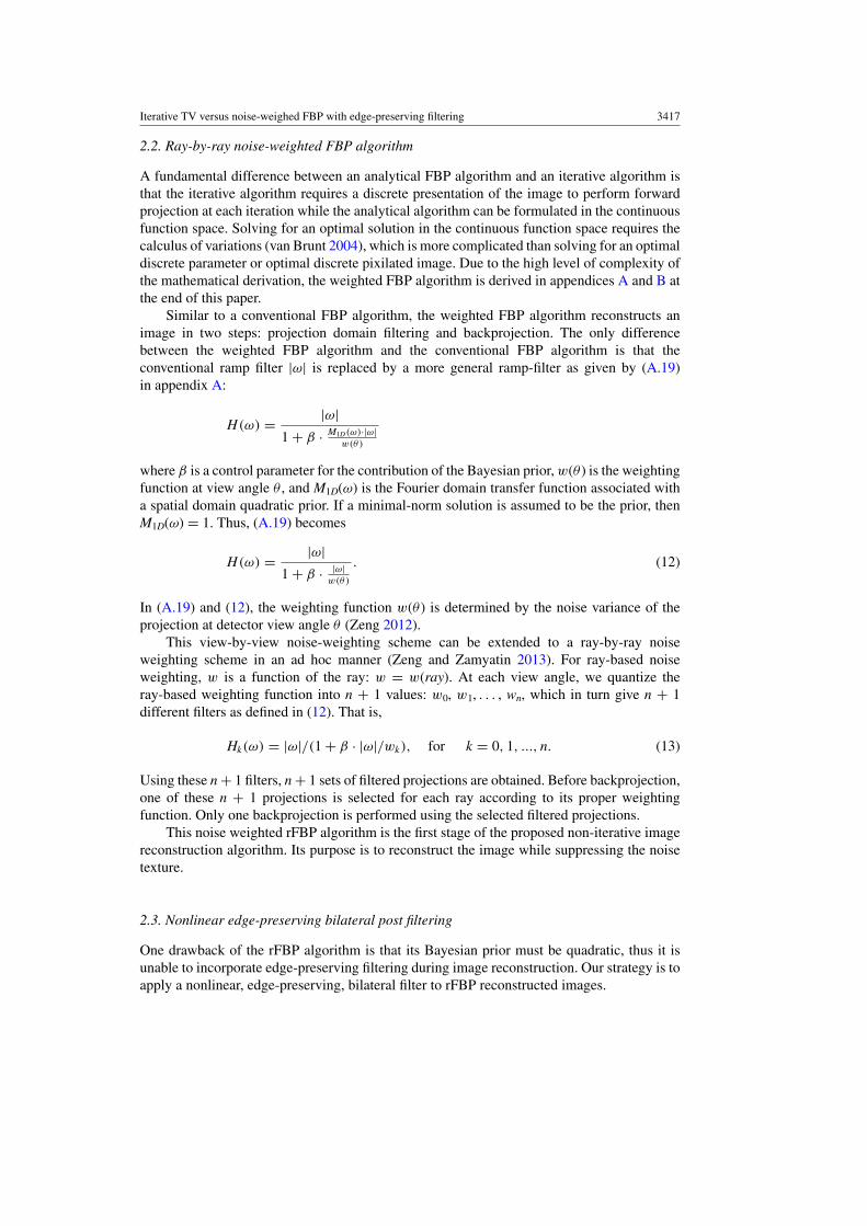
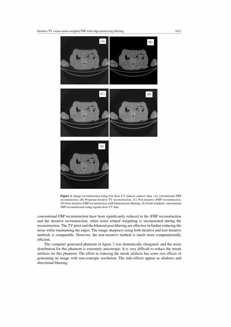
Figure 1(A) shows the conventional fan-beam FBP reconstruction of a transverse slice inthe abdominal region of the cadaver. The x-rays through the arms are attenuated more thanx-rays in other orientations, and create the left-to-right streak artifacts in the middle of theimage.

Figure 1(B) shows the cadaver data result from 1000 iterations of the proposed iterativeTV algorithm using a transmission noise model. The noise modeling effectively removes thestreak artifacts. The TV prior further reduces the noise fluctuation.

Figure 1(C) shows the rFBP reconstruction using the cadaver data. The streak artifactsare removed as well. The bilateral post filtering further reduces the noise fluctuation as shownin figure 1(D).

Figure 1(E) is the gold standard image, which is the conventional fan-beam FBPreconstruction using the standard dose CT data.

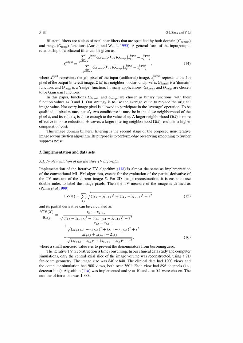
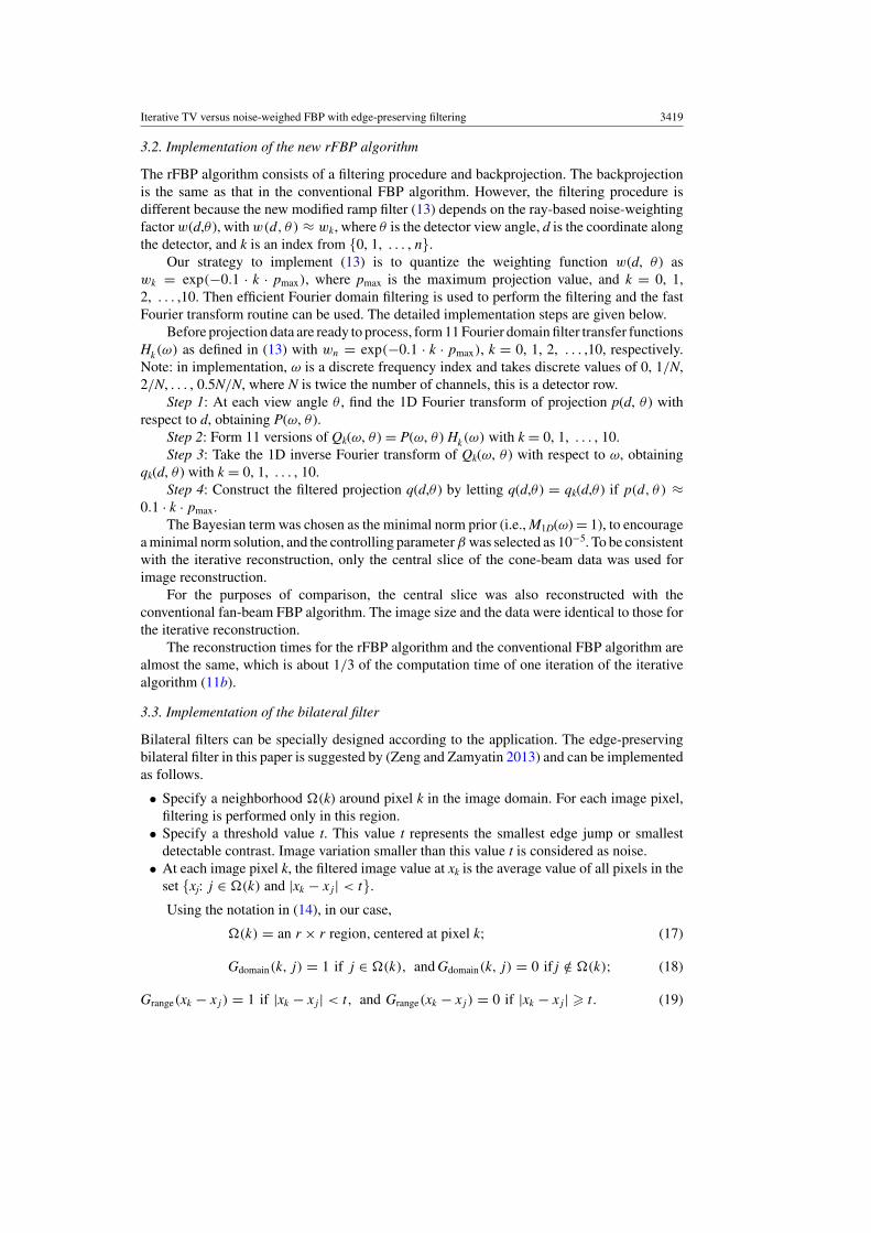
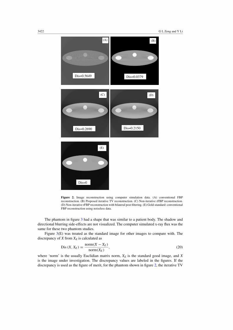
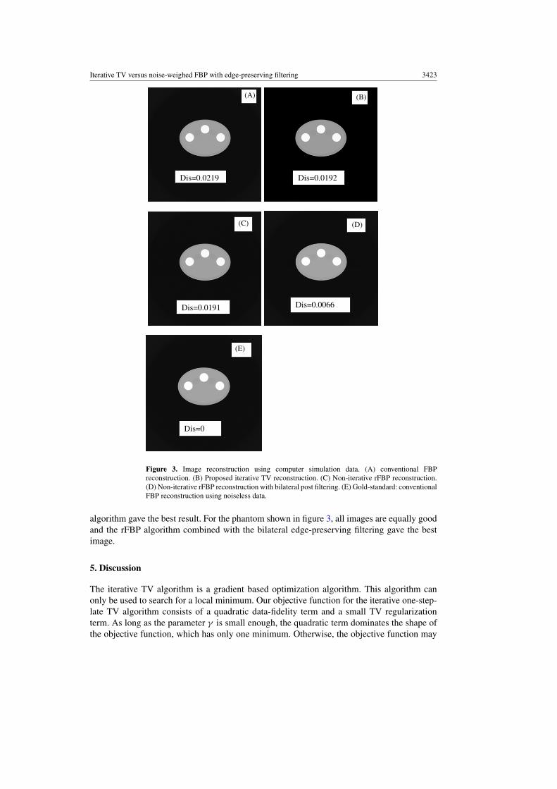
Figures 2 and 3 have the same arrangement as figure 1, except that the data were computersimulated. The gold standard images, figures 2(D) and 3(D), respectively, are the conventionalFBP reconstruction using noiseless simulation data. Streak artifacts that appeared in the

Iterative TV versus noise-weighed FBP with edge-preserving filtering 3421

(A) (B)

(C) (D)

(E)

Figure 1. Image reconstruction using low-dose CT clinical cadaver data. (A) conventional FBPreconstruction. (B) Proposed iterative TV reconstruction. (C) Non-iterative rFBP reconstruction.(D) Non-iterative rFBP reconstruction with bilateral post filtering. (E) Gold-standard: conventionalFBP reconstruction using regular dose CT data.

conventional FBP reconstruction have been significantly reduced in the rFBP reconstructionand the iterative reconstruction, when noise related weighting is incorporated during thereconstruction. The TV prior and the bilateral post filtering are effective in further reducing thenoise while maintaining the edges. The image sharpness using both iterative and non-iterativemethods is comparable. However, the non-iterative method is much more computationallyefficient.

The computer generated phantom in figure 2 was dramatically elongated, and the noisedistribution for this phantom is extremely anisotropic. It is very difficult to reduce the streakartifacts for this phantom. The effort in reducing the streak artifacts has some size effects ofgenerating an image with non-isotropic resolution. The side-effects appear as shadows anddirectional blurring.

3422 G L Zeng and Y Li

Dis=0.5649 Dis=0.0379

Dis=0.2690 Dis=0.2150

Dis=0

(A) (B)

(C) (D)

(E)

Figure 2. Image reconstruction using computer simulation data. (A) conventional FBPreconstruction. (B) Proposed iterative TV reconstruction. (C) Non-iterative rFBP reconstruction.(D) Non-iterative rFBP reconstruction with bilateral post filtering. (E) Gold-standard: conventionalFBP reconstruction using noiseless data.

The phantom in figure 3 had a shape that was similar to a patient body. The shadow anddirectional blurring side-effects are not visualized. The computer simulated x-ray flux was thesame for these two phantom studies.

Figure 3(E) was treated as the standard image for other images to compare with. Thediscrepancy of X from XE is calculated as

Dis (X, XE ) = norm(X − XE )

norm(XE ), (20)

where ‘norm’ is the usually Euclidian matrix norm, XE is the standard good image, and Xis the image under investigation. The discrepancy values are labeled in the figures. If thediscrepancy is used as the figure of merit, for the phantom shown in figure 2, the iterative TV

Iterative TV versus noise-weighed FBP with edge-preserving filtering 3423

Dis=0.0219 Dis=0.0192

Dis=0.0191 Dis=0.0066

Dis=0

(A) (B)

(C) (D)

(E)

Figure 3. Image reconstruction using computer simulation data. (A) conventional FBPreconstruction. (B) Proposed iterative TV reconstruction. (C) Non-iterative rFBP reconstruction.(D) Non-iterative rFBP reconstruction with bilateral post filtering. (E) Gold-standard: conventionalFBP reconstruction using noiseless data.

algorithm gave the best result. For the phantom shown in figure 3, all images are equally goodand the rFBP algorithm combined with the bilateral edge-preserving filtering gave the bestimage.

5. Discussion

The iterative TV algorithm is a gradient based optimization algorithm. This algorithm canonly be used to search for a local minimum. Our objective function for the iterative one-step-late TV algorithm consists of a quadratic data-fidelity term and a small TV regularizationterm. As long as the parameter γ is small enough, the quadratic term dominates the shape ofthe objective function, which has only one minimum. Otherwise, the objective function may

3424 G L Zeng and Y Li

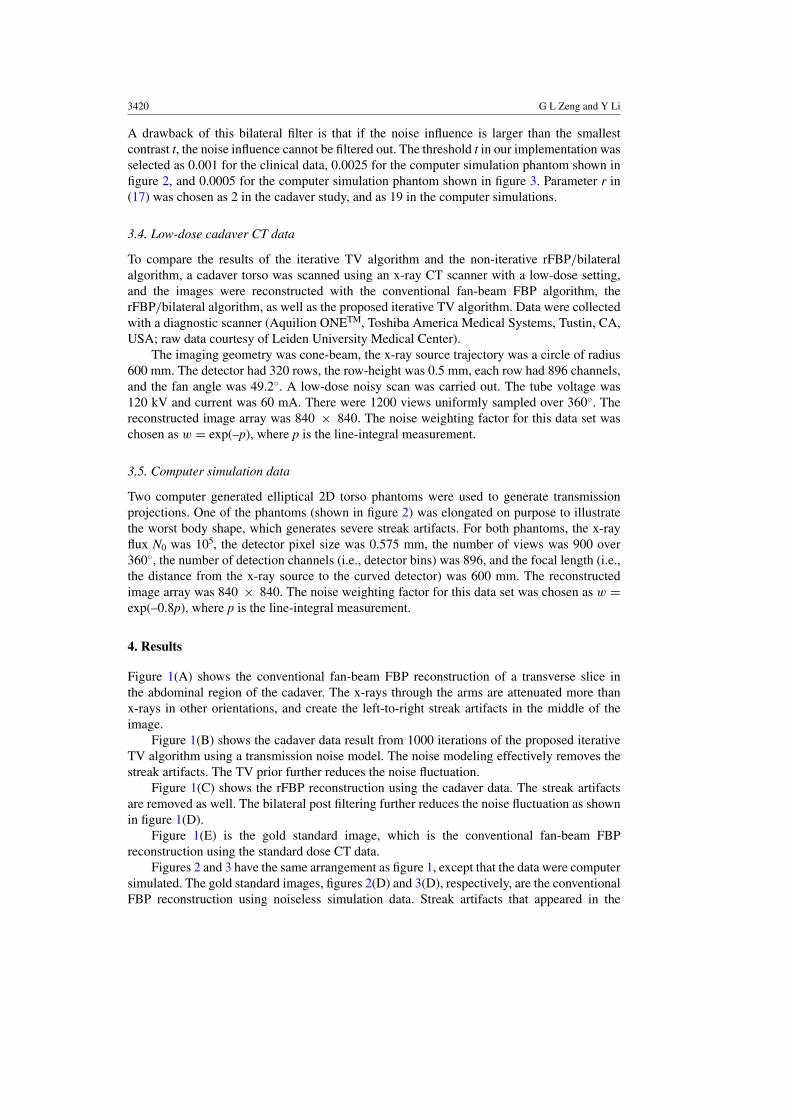
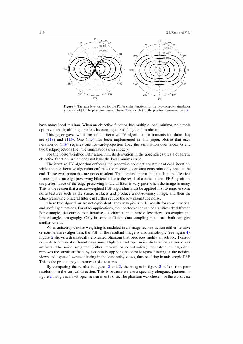
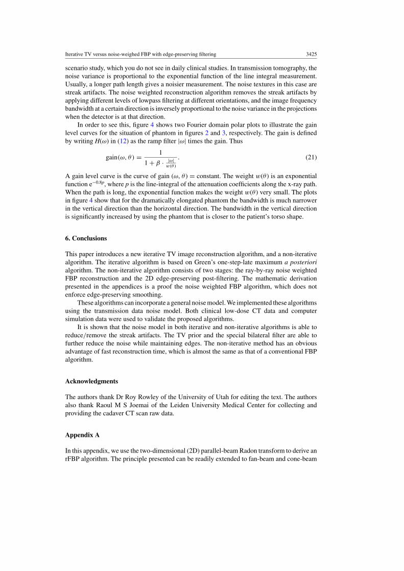
Figure 4. The gain level curves for the PSF transfer functions for the two computer simulationstudies: (Left) for the phantom shown in figure 2 and (Right) for the phantom shown in figure 3.

have many local minima. When an objective function has multiple local minima, no simpleoptimization algorithm guarantees its convergence to the global minimum.

This paper gave two forms of the iterative TV algorithm for transmission data; theyare (11a) and (11b). One (11b) has been implemented in this paper. Notice that eachiteration of (11b) requires one forward-projection (i.e., the summation over index k) andtwo backprojections (i.e., the summations over index j).

For the noise weighted FBP algorithm, its derivation in the appendices uses a quadraticobjective function, which does not have the local minima issue.

The iterative TV algorithm enforces the piecewise constant constraint at each iteration,while the non-iterative algorithm enforces the piecewise constant constraint only once at theend. These two approaches are not equivalent. The iterative approach is much more effective.If one applies an edge-preserving bilateral filter to the result of a conventional FBP algorithm,the performance of the edge-preserving bilateral filter is very poor when the image is noisy.This is the reason that a noise-weighted FBP algorithm must be applied first to remove somenoise textures such as the streak artifacts and produce a not-so-noisy image, and then theedge-preserving bilateral filter can further reduce the low magnitude noise.

These two algorithms are not equivalent. They may give similar results for some practicaland useful applications. For other applications, their performance can be significantly different.For example, the current non-iterative algorithm cannot handle few-view tomography andlimited angle tomography. Only in some sufficient data sampling situations, both can givesimilar results.

When anisotropic noise weighting is modeled in an image reconstruction (either iterativeor non-iterative) algorithm, the PSF of the resultant image is also anisotropic (see figure 4).Figure 2 shows a dramatically elongated phantom that produces highly anisotropic Poissonnoise distribution at different directions. Highly anisotropic noise distribution causes streakartifacts. The noise weighted (either iterative or non-iterative) reconstruction algorithmremoves the streak artifacts by essentially applying heaviest lowpass filtering in the noisiestviews and lightest lowpass filtering in the least noisy views, thus resulting in anisotropic PSF.This is the price to pay to remove noise textures.

By comparing the results in figures 2 and 3, the images in figure 2 suffer from poorresolution in the vertical direction. This is because we use a specially elongated phantom infigure 2 that gives anisotropic measurement noise. The phantom was chosen for the worst case

Iterative TV versus noise-weighed FBP with edge-preserving filtering 3425

scenario study, which you do not see in daily clinical studies. In transmission tomography, thenoise variance is proportional to the exponential function of the line integral measurement.Usually, a longer path length gives a noisier measurement. The noise textures in this case arestreak artifacts. The noise weighted reconstruction algorithm removes the streak artifacts byapplying different levels of lowpass filtering at different orientations, and the image frequencybandwidth at a certain direction is inversely proportional to the noise variance in the projectionswhen the detector is at that direction.

In order to see this, figure 4 shows two Fourier domain polar plots to illustrate the gainlevel curves for the situation of phantom in figures 2 and 3, respectively. The gain is definedby writing H(ω) in (12) as the ramp filter |ω| times the gain. Thus

gain(ω, θ ) = 1

1 + β · |ω|w(θ )

. (21)

A gain level curve is the curve of gain (ω, θ ) = constant. The weight w(θ ) is an exponentialfunction e−0.8p, where p is the line-integral of the attenuation coefficients along the x-ray path.When the path is long, the exponential function makes the weight w(θ ) very small. The plotsin figure 4 show that for the dramatically elongated phantom the bandwidth is much narrowerin the vertical direction than the horizontal direction. The bandwidth in the vertical directionis significantly increased by using the phantom that is closer to the patient’s torso shape.

6. Conclusions

This paper introduces a new iterative TV image reconstruction algorithm, and a non-iterativealgorithm. The iterative algorithm is based on Green’s one-step-late maximum a posteriorialgorithm. The non-iterative algorithm consists of two stages: the ray-by-ray noise weightedFBP reconstruction and the 2D edge-preserving post-filtering. The mathematic derivationpresented in the appendices is a proof the noise weighted FBP algorithm, which does notenforce edge-preserving smoothing.

These algorithms can incorporate a general noise model. We implemented these algorithmsusing the transmission data noise model. Both clinical low-dose CT data and computersimulation data were used to validate the proposed algorithms.

It is shown that the noise model in both iterative and non-iterative algorithms is able toreduce/remove the streak artifacts. The TV prior and the special bilateral filter are able tofurther reduce the noise while maintaining edges. The non-iterative method has an obviousadvantage of fast reconstruction time, which is almost the same as that of a conventional FBPalgorithm.

Acknowledgments

The authors thank Dr Roy Rowley of the University of Utah for editing the text. The authorsalso thank Raoul M S Joemai of the Leiden University Medical Center for collecting andproviding the cadaver CT scan raw data.

Appendix A

In this appendix, we use the two-dimensional (2D) parallel-beam Radon transform to derive anrFBP algorithm. The principle presented can be readily extended to fan-beam and cone-beam

3426 G L Zeng and Y Li

imaging geometries. Let the image to be reconstructed be f (x, y) and its Radon transform be[Rf](s, θ ), defined as

[R f ](s, θ ) =∫ ∞

−∞

∫ ∞

−∞f (x, y)δ(x cos θ + y sin θ − s) dx dy, (A.1)

where δ is the Dirac delta function, θ is the detector rotation angle, and s is the line-integrallocation on the detector. The Radon transform [Rf](s, θ ) is the line-integral of the object f (x, y).Image reconstruction is to solve for the object f (x, y) from its Radon transform [Rf](s, θ ).

A popular image reconstruction method is the FBP algorithm, which consists of twosteps. In the first step, [Rf](s, θ ) is convolved with a kernel function h(s) with respect tovariable s, obtaining q(s, θ ). The Fourier transform of the kernel h(s) is the ramp-filter |ω|. Thesecond step performs backprojection, which maps the filtered projection q(s, θ ) into the imagedomain as

f (x, y) =∫ π

0q(s, θ )|s=x cos θ+y sin θdθ. (A.2)

This appendix applies a noise-variance-derived weighting function on the projections andenforces a prior term in the objective function, and this approach is commonly used in iterativealgorithms.

Let the noisy line-integral measurements be p(s, θ ). The objective function is a functionalv depending on the function f (x, y) as follows.

v( f ) = ||[R f ](s, θ ) − p(s, θ )||2w + β|| f (x, y) ∗ ∗c(x, y)||2, (A.3)

where the first term enforces data fidelity, the second term imposes prior information aboutthe image f , the parameter β controls the level of influence of the prior information to theimage f, and w is a weighting function satisfying w(θ ) = w(θ ± π) in the fidelity norm. In(A.3), c(x,y) is a symmetric image domain convolution kernel and ‘∗∗’ represents the imagedomain 2D convolution. If c(x,y) is a Laplacian, the regularization term encourages a smoothimage. If c(x,y) is a constant 1, the regularization term encourages a minimum norm solution.Using integrals, v in (A.3) can be written as

v( f ) =∫ π

θ=0

∫ ∞

s=−∞

[∫ ∞

x=−∞

∫ ∞

y=−∞f (x, y)δ(x cos θ+y sin θ − s) dy dx−p(s, θ )

]2

dsw(θ ) dθ

+β

∫ ∞

x=−∞

∫ ∞

y=−∞

[∫ ∞

x=−∞

∫ ∞

y=−∞f (x, y)c(x − x, y − y) dy dx

]2

dy dx. (A.4)

In the following, calculus of variations (van Brunt 2004) will be used to find the optimalfunction f (x, y) that minimizes the functional v( f ) in (A.4). The initial step in the method isto replace the function f (x, y) in (A.4) by the sum of two functions: f (x, y) + εη(x, y). Thenext step is to evaluate the derivative dv

dε|ε=0 and set it to zero. That is,

0 = 2∫ π

θ=0

∫ ∞

s=−∞

{[∫ ∞

x=−∞

∫ ∞

y=−∞f (x, y)δ(x cos θ + y sin θ − s) dy dx − p(s, θ )

]

·[∫ ∞

x=−∞

∫ ∞

y=−∞η(x, y)δ(x cos θ + y sin θ − s)dy dx

]}dsw(θ ) dθ

+2β

∫ ∞

x=−∞

∫ ∞

y=−∞

{[∫ ∞

x=−∞

∫ ∞

y=−∞f (x, y)c(x − x, y − y) dy dx

]

·[∫ ∞

x=−∞

∫ ∞

y=−∞η(x, y)c(x − x, y − y) dy dx

]}dy dx. (A.5)

In practice, the function f (x, y) is compact, bounded, and continuous almost everywhere. Afterchanging the order of integrals, we have

Iterative TV versus noise-weighed FBP with edge-preserving filtering 3427

0 =∫ ∞

x=−∞

∫ ∞

y=−∞η(x, y)

{∫ π

θ=0

∫ ∞

s=−∞

[ ∫ ∞

x=−∞

∫ ∞

y=−∞f (x, y)δ(x cos θ

+ y sin θ − s) dy dx − p(s, θ )

]δ(x cos θ + y sin θ − s) dsw(θ ) dθ

+β

∫ ∞

x=−∞

∫ ∞

y=−∞f (x, y)

∫ ∞

�x=−∞

∫ ∞

�y=−∞

c(�x − x,

�y − y)c(

�x − x,

�y − y)d�

y d�x dy dx

}dy dx.

(A.6)

Equation (A.6) is in the form of∫ ∫

η(x, y)g(x, y) dy dx = 0. Since η(x, y) can be any arbitraryfunction, one must have g(x, y) = 0, which is the Euler–Lagrange equation (van Brunt 2004).The Euler–Lagrange equation in our case is∫ π

θ=0

∫ ∞

s=−∞

[ ∫ ∞

x=−∞

∫ ∞

y=−∞f (x, y)δ(x cos θ

+ y sin θ − s) dy dx − p(s, θ )

]δ(x cos θ + y sin θ − s) dsw(θ ) dθ

+β

∫ ∞

x=−∞

∫ ∞

y=−∞f (x, y)m(x − x, y − y) dy dx = 0 (A.7)

with

m(x − x, y − y) =∫ ∞

�x=−∞

∫ ∞

�y=−∞

c(�x − x,

�y − y)c(

�x − x,

�y − y) d�

y d�x

=∫ ∞

�x=−∞

∫ ∞

�y=−∞

c(�x,

�y)c((x − x) − �

x, (y − y) − �y) d�

y d�x. (A.8)

By moving the term containing p(s, θ ) to the right-hand-side, equation (A.7) can be furtherrewritten as∫ ∞

x=−∞

∫ ∞

y=−∞f (x, y)

[ ∫ π

θ=0

∫ ∞

s=−∞δ(x cos θ + y sin θ − s)δ(x cos θ

+ y sin θ − s) dsw(θ ) dθ

]dy dx

+β

∫ ∞

x=−∞

∫ ∞

y=−∞f (x, y)m(x − x, y − y) dy dx

=∫ π

θ=0

∫ ∞

s=−∞p(s, θ )δ(x cos θ − y sin θ − s) dsw(θ ) dθ. (A.9)

Notice that∫ π

θ=0

∫ ∞

s=−∞p(s, θ )δ(x cos θ + y sin θ − s) dsw(θ ) dθ

=∫ π

θ=0p(s, θ )|s=x cos θ+y sin θw(θ ) dθ = bw(x, y) (A.10)

is the weighted backprojection of the projection data p(s, θ ) with a view-angle dependentweighting function w(θ ), and the backprojection is denoted as bw(x, y). It must be pointed outthat bw(x, y) is not the same as f (x, y) even when p(s, θ ) is noiseless and w(θ ) = 1, because noramp filter has been applied to p(s, θ ).

Also notice that∫ π

θ=0

∫ ∞

s=−∞δ(x cos θ + y sin θ − s)δ(x cos θ + y sin θ − s) dsw(θ ) dθ

=∫ π

θ=0w(θ )δ((x − x) cos θ + (y − y) sin θ ) dθ

= PSFw(x − x, y − y) (A.11)

3428 G L Zeng and Y Li

is the point spread function (PSF) of the projection/weighted-backprojection operator at point(x, y) if the point source is at (x, y) and the view-based weighting function is w(θ ).

In appendix B, we show that

PSFw(x, y) = w(

tan−1 yx ± π

2

)√

x2 + y2. (A.12)

When w(θ ) is set to 1, the point spread function reduces to the familiar expression (Zeng2010):

PSFw=1(x, y) = 1√x2 + y2

. (A.13)

Using (A.10) and (A.11), (A.9) becomes∫ ∞

x=−∞

∫ ∞

y=−∞f (x, y)[PSFw(x − x, y − y) + β · m(x − x, y − y)] dy dx = bw(x, y). (A.14)

The left-hand-side of (A.14) is a 2D convolution. Taking the 2D Fourier transform of (A.14)yields

F(ωx, ωy) ×[

w(ϕ)√ω2

x + ω2y

+ β · M(ωx, ωy)

]= Bw(ωx, ωy), (A.15)

or

F(ωx, ωy) = Bw(ωx, ωy)

/⎡⎣ w(ϕ)√

ω2x + ω2

y

+ β · M(ωx, ωy)

⎤⎦. (A.16)

Here the capital letters are used to represent the Fourier transform of their spatial domaincounterparts, which are represented in lowercase letters; ωx and ωy are the frequency variables

for x and y, respectively, and tan−1(ωy /ωx) = ϕ. The expression w(ϕ)/√

ω2x + ω2

y is the 2DFourier transform of the point spread function PSFw(x, y) as derived in appendix B. Noticethat the Fourier transform Bw(ωx, ωy) of weighted backprojection can be related to the Fouriertransform B(ωx, ωy) of un-weighted backprojection as

Bw(ωx, ωy) = B(ωx, ωy)w(ϕ). (A.17)

Then (A.16) becomes

F(ωx, ωy) = w(ϕ)B(ωx, ωy)

/⎡⎣ w(ϕ)√

ω2x + ω2

y

+ β · M(ωx, ωy)

⎤⎦

= B(ωx, ωy)

√ω2

x + ω2y

/⎡⎣1 + β ·

M(ωx, ωy)√

ω2x + ω2

y

w(ϕ)

⎤⎦ . (A.18)

Equation (A.18) is in the form of ‘backprojection first, then 2D filter’ reconstruction approachand the Fourier domain 2D filter is

√ω2

x + ω2y/[1 + β · M(ωx, ωy)

√ω2

x + ω2y/w(ϕ)]. By

using the central slice theorem, an FBP algorithm, which performs 1D filtering first, thenbackprojects, can be obtained. The Fourier domain 1D filter for the FBP algorithm is thecentral slice of the 2D filter

√ω2

x + ω2y/[1 + β · M(ωx, ωy)

√ω2

x + ω2y/w(ϕ)], which gives

Fourier domain filter for the FBP - MAP algorithm = |ω|1 + β · M1D(ω)·|ω|

w(ϕ)

. (A.19)

When β = 0, (A.19) reduces to the ramp filter |ω| of the conventional FBP algorithm.

Iterative TV versus noise-weighed FBP with edge-preserving filtering 3429

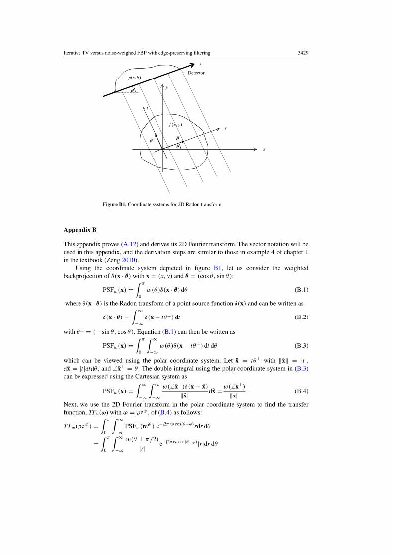
Figure B1. Coordinate systems for 2D Radon transform.

Appendix B

This appendix proves (A.12) and derives its 2D Fourier transform. The vector notation will beused in this appendix, and the derivation steps are similar to those in example 4 of chapter 1in the textbook (Zeng 2010).

Using the coordinate system depicted in figure B1, let us consider the weightedbackprojection of δ(x · θ) with x = (x, y) and θ = (cos θ, sin θ ):

PSFw(x) =∫ π

0w(θ )δ(x · θ) dθ (B.1)

where δ(x · θ) is the Radon transform of a point source function δ(x) and can be written as

δ(x · θ) =∫ ∞

−∞δ(x − tθ⊥) dt (B.2)

with θ⊥ = (− sin θ, cos θ ). Equation (B.1) can then be written as

PSFw(x) =∫ π

0

∫ ∞

−∞w(θ )δ(x − tθ⊥) dt dθ (B.3)

which can be viewed using the polar coordinate system. Let x = tθ⊥ with ‖x‖ = |t|,dx = |t|dtdθ , and ∠x⊥ = θ . The double integral using the polar coordinate system in (B.3)can be expressed using the Cartesian system as

PSFw(x) =∫ ∞

−∞

∫ ∞

−∞

w(∠x⊥)δ(x − x)

‖x‖ dx =w(∠x⊥)

‖x‖ . (B.4)

Next, we use the 2D Fourier transform in the polar coordinate system to find the transferfunction, TFw(ω) with ω = ρeiϕ , of (B.4) as follows:

T Fw(ρeiϕ ) =∫ π

0

∫ ∞

−∞PSFw(reiθ ) e−i2πrρ cos(θ−ϕ)rdr dθ

=∫ π

0

∫ ∞

−∞

w(θ ± π/2)

|r| e−i2πrρ cos(θ−ϕ)|r|dr dθ

3430 G L Zeng and Y Li

=∫ π

0w(θ ± π/2)

[∫ ∞

−∞e−i2πrρ cos(θ−ϕ)dr

]dθ

=∫ π

0w(θ ± π/2)δ(ρ cos(θ − ϕ)) dθ. (B.5)

To evaluate the integral with a δ-function in (B.5), we need to consider the zeros ofr cos(θ − ϕ). The zeros are θ = ϕ ± π/2 and only one of these zeros is between 0 andπ . The normalization factor at this zero is given by 1/|[ρ cos(θ − ϕ)]′|θ=ϕ±π/2| = 1/|ρ|.Recalling that w(ϕ) = w(ϕ ± π), (B.5) becomes

TFw(ρeiϕ ) =∫ π

0w(θ ± π

2

) 1

|ρ|δ(θ −

(ϕ ± π

2

))dθ = w(ϕ)

|ρ| . (B.6)

References

Aurich V and Weule J 1995 Non-linear Gaussian filters performing edge preserving diffusion Mustererkennung: Proc.17th DAGM Symp. (London: Springer) pp 538–45

Bian J, Siewerdsen J H, Han X, Sidky E Y, Prince J L, Pelizzari C A and Pan X 2010 Evaluation of sparse-viewreconstruction from flat-panel-detector cone-beam CT Phys. Med. Biol. 55 6575–99

Bracewell R N 1956 Strip integration in radio astronomy Aust. J. Phys. 9 198–217Brunder H, Raupach R, Sedlmair M, Wursching F, Schwarz K, Stierstorfer K and Flohr T 2010 Toward iterative

reconstruction in clinical CT: increased sharpness-to-noise and significant dose reduction owing to a new classof regularization priors Proc. SPIE 7622 102

Candes E, Romberg J and Tao T 2006 Robust uncertainty principles: exact signal reconstruction from highlyincomplete frequency information IEEE Trans. Inform. Theory 52 489–509

Delaney A H and Bresler Y 1996 A fast and accurate Fourier algorithm for iterative parallel-beam tomography IEEETrans. Image Process. 5 740–53

Dempster A, Laird N and Rubin D 1977 Maximum likelihood from incomplete data via the EM algorithm J. R. Stat.Soc. B 39 1–38

German S and McClure D E 1987 Statistical methods for tomographic image reconstruction Bull. Int. Stat. Inst.LII-4 5–21

Green P J 1990 Bayesian reconstruction from emission tomography data using a modified EM algorithm IEEE Trans.Med. Imaging 9 84–93

Han X, Bian J, Eaker D R, Kline T L, Sidky E Y, Ritman E L and Pan X 2011 Algorithm-enabled low-dose micro-CTimaging IEEE Trans. Med. Imaging 30 606–20

Han X, Bian J, Ritman E L, Sidky E Y and Pan X 2012 Optimization-based reconstruction of sparse images fromfew-view projections Phys. Med. Biol. 57 5245–73

Hsieh J 1998 Adaptive streak artifact reduction in computed tomography resulting from excessive x-ray photon noiseMed. Phys. 25 2139–47

Hudson H M and Larkin R S 1994 Accelerated image reconstruction using ordered subsets of projection data IEEETrans. Med. Imaging 13 601–9

Kachelrieβ M, Watzke O and Kalender W A 2001 Generalized multi-dimensional adaptive filtering for conventionaland spiral single-slice, multi-slice, and cone-beam CT Med. Phys. 28 475–90

Langer K and Carson R 1984 EM reconstruction algorithms for Emission and Transmission tomography J. Comput.Assist. Tomogr. 8 302–16

Panin V Y, Zeng G L and Gullberg G T 1999 Total variation regulated EM algorithm IEEE Trans. Nucl.Sci. 46 2202–10

Radon J 1917 Uber die Bestimmung von Funktionen durch ihre Integralwerte langs gewisser Mannigfaltigkeiten Ber.Verh. Sachs. Akad. Wiss. Leipzig, Math.-Nat. K1 69 262–7

Ritschl L, Bergner F, Fleischmann C and Kachelrieb M 2011 Improved total variation-based CT image reconstructionapplied to clinical data Phys. Med. Biol. 56 1545–61

Shepp L A and Logan B F 1974 The Fourier reconstruction of a head section IEEE Trans. Nucl. Sci. NS-21 21–43Shepp L A and Vardi Y 1982 Maximum likelihood reconstruction for emission tomography IEEE Trans. Med.

Imaging 1 113–22Sidky E Y, Kao C-M and Pan X 2006 Accurate image reconstruction from few-views and limited-angle data in

divergent-beam CT J. X-Ray Sci. Technol. 14 119–39Sidky E Y and Pan X 2008 Image reconstruction in circular cone-beam computed tomography by constrained,

total-variation minimization Phys. Med. Biol. 53 4777–807

Iterative TV versus noise-weighed FBP with edge-preserving filtering 3431

Tang J, Nett B E and Chen G-H 2009 Performance comparison between total variation (TV)-based compressedsensing and statistical iterative reconstruction algorithms Phys. Med. Biol. 54 5781–804

Vainstein B K 1970 Finding structure of objects from projections Kristallografiya 15 984–902van Brunt B 2004 The Calculus of Variations (New York: Springer)Zeng G L 2010 Medical Image Reconstruction: A Conceptual Tutorial (Beijing: Springer)Zeng G L 2012 A filtered backprojection MAP algorithm with non-uniform sampling and noise modeling Med.

Phys. 39 2170–8Zeng G L and Zamyatin A 2013 A filtered backprojection algorithm with ray-by-ray noise weighting Med.

Phys. 40 031113