Iterative Methods for LS 1 Iterative Methods for Solving Systems of Linear Equations NTNU Tsung-Min Hwang November 1, 2003 Department of Mathematics – NTNU Tsung-Min Hwang November 1, 2003

Welcome message from author
This document is posted to help you gain knowledge. Please leave a comment to let me know what you think about it! Share it to your friends and learn new things together.
Transcript

Iterative Methods for LS 1
Iterative Methods for Solving Systems of Linear Equations
NTNU
Tsung-Min Hwang
November 1, 2003
Department of Mathematics – NTNU Tsung-Min Hwang November 1, 2003

Iterative Methods for LS 2
1 – Classic Iterative Methods . . . . . . . . . . . . . . . . . . . . . . . . . . . 3
1.1 – Basic Concept . . . . . . . . . . . . . . . . . . . . . . . . . . . . . . . 3
1.2 – Richard’s Method . . . . . . . . . . . . . . . . . . . . . . . . . . . . . . 7
1.3 – Jacobi Method . . . . . . . . . . . . . . . . . . . . . . . . . . . . . . . 8
1.4 – Gauss-Seidel Method . . . . . . . . . . . . . . . . . . . . . . . . . . . 10
1.5 – Successive Over Relaxation (SOR) Method . . . . . . . . . . . . . . . . . 12
1.6 – Symmetric Successive Over Relaxation (SSOR) Method . . . . . . . . . . 13
2 – Convergence Analysis . . . . . . . . . . . . . . . . . . . . . . . . . . . . . 15
Department of Mathematics – NTNU Tsung-Min Hwang November 1, 2003
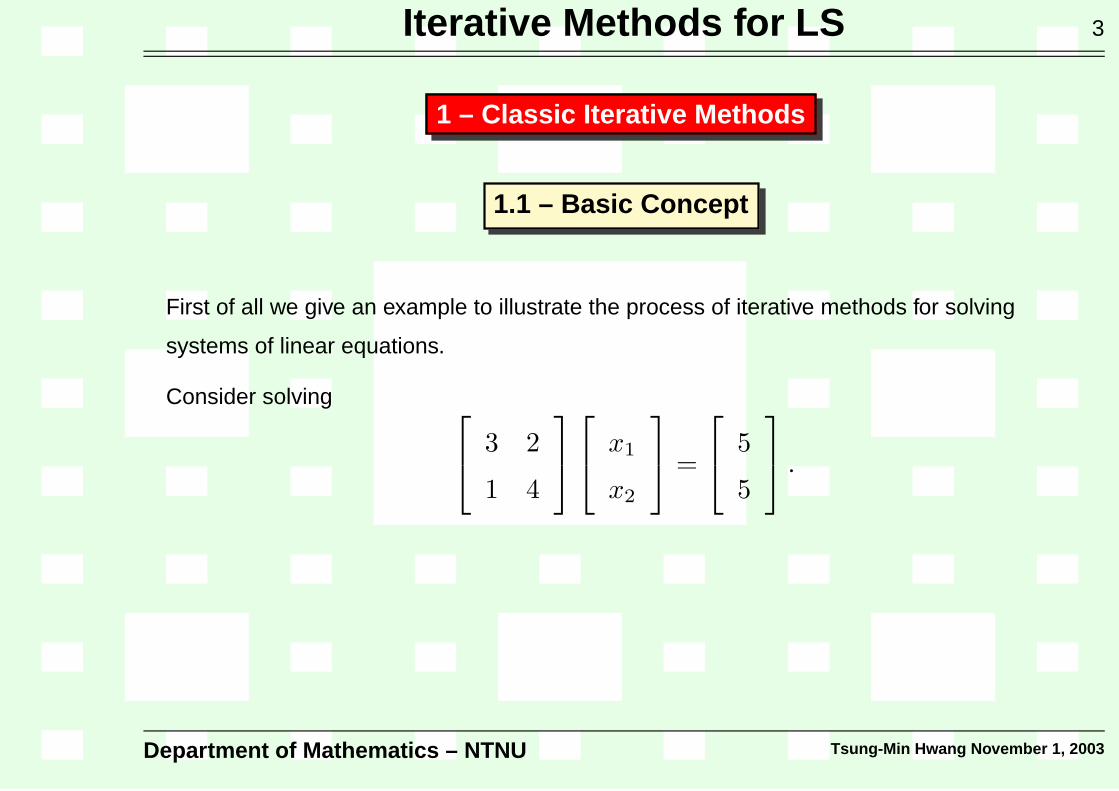
Iterative Methods for LS 3
1 – Classic Iterative Methods
1.1 – Basic Concept
First of all we give an example to illustrate the process of iterative methods for solving
systems of linear equations.
Consider solving
3 2
1 4
x1
x2
=
5
5
.
This system has the exact solution x1 = x2 = 1. Equivalently we can write the system as
3x1 + 2x2 = 5
x1 + 4x2 = 5
Department of Mathematics – NTNU Tsung-Min Hwang November 1, 2003

Iterative Methods for LS 3
1 – Classic Iterative Methods
1.1 – Basic Concept
First of all we give an example to illustrate the process of iterative methods for solving
systems of linear equations.
Consider solving
3 2
1 4
x1
x2
=
5
5
.
This system has the exact solution x1 = x2 = 1.
Equivalently we can write the system as
3x1 + 2x2 = 5
x1 + 4x2 = 5
Department of Mathematics – NTNU Tsung-Min Hwang November 1, 2003

Iterative Methods for LS 3
1 – Classic Iterative Methods
1.1 – Basic Concept
First of all we give an example to illustrate the process of iterative methods for solving
systems of linear equations.
Consider solving
3 2
1 4
x1
x2
=
5
5
.
This system has the exact solution x1 = x2 = 1. Equivalently we can write the system as
3x1 + 2x2 = 5
x1 + 4x2 = 5
Department of Mathematics – NTNU Tsung-Min Hwang November 1, 2003
Iterative Methods for LS 4
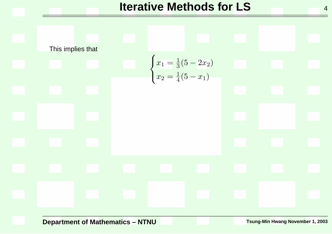
This implies that
x1 = 13 (5 − 2x2)
x2 = 14 (5 − x1)
A naive idea is to solve the system by
x(k)1 = 1
3 (5 − 2x(k−1)2 )
x(k)2 = 1
4 (5 − x(k−1)1 )
that is, to use the iterative formulation
x(k)1
x(k)2
=
13 0
0 14
5
5
−
0 2
1 0
x(k−1)1
x(k−1)2
Department of Mathematics – NTNU Tsung-Min Hwang November 1, 2003

Iterative Methods for LS 4
This implies that
x1 = 13 (5 − 2x2)
x2 = 14 (5 − x1)
A naive idea is to solve the system by
x(k)1 = 1
3 (5 − 2x(k−1)2 )
x(k)2 = 1
4 (5 − x(k−1)1 )
that is, to use the iterative formulation
x(k)1
x(k)2
=
13 0
0 14
5
5
−
0 2
1 0
x(k−1)1
x(k−1)2
Department of Mathematics – NTNU Tsung-Min Hwang November 1, 2003

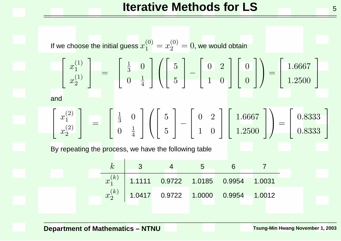
Iterative Methods for LS 5
If we choose the initial guess x(0)1 = x
(0)2 = 0, we would obtain
x(1)1
x(1)2
=
13 0
0 14
5
5
−
0 2
1 0
0
0
=
1.6667
1.2500
and
x(2)1
x(2)2
=
13 0
0 14
5
5
−
0 2
1 0
1.6667
1.2500
=
0.8333
0.8333
By repeating the process, we have the following table
k 3 4 5 6 7
x(k)1 1.1111 0.9722 1.0185 0.9954 1.0031
x(k)2 1.0417 0.9722 1.0000 0.9954 1.0012
Department of Mathematics – NTNU Tsung-Min Hwang November 1, 2003
Iterative Methods for LS 6
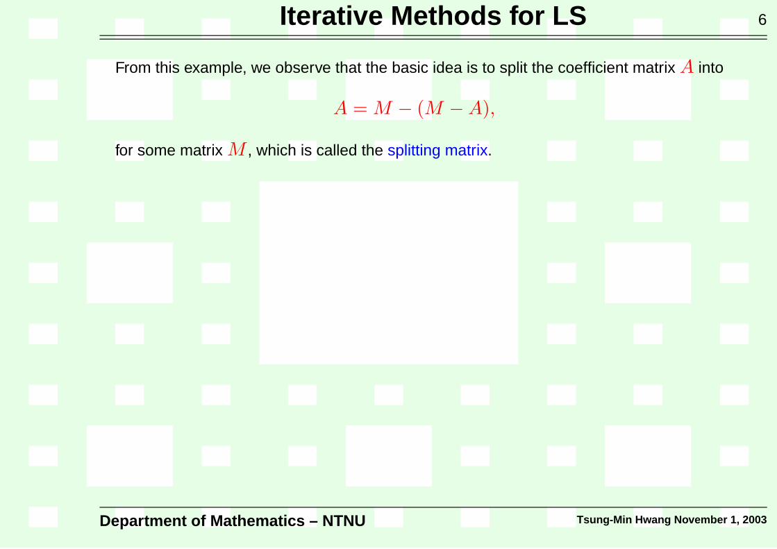
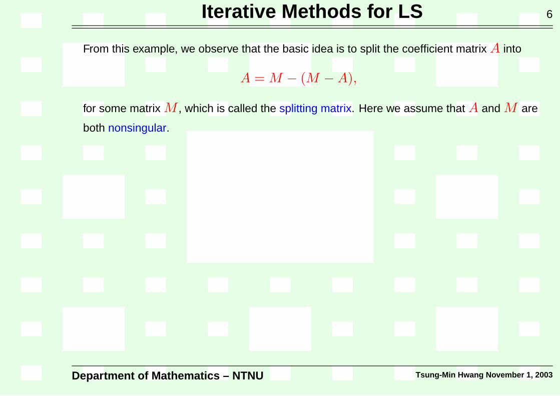
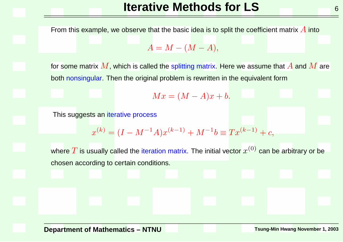
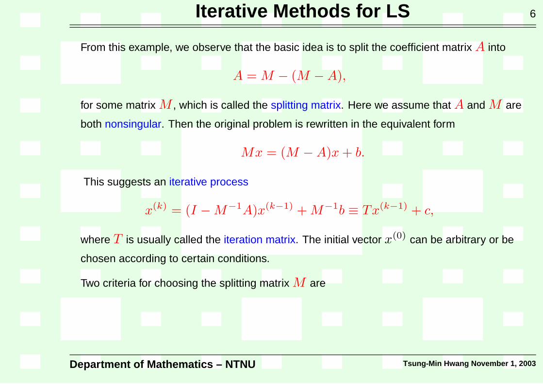
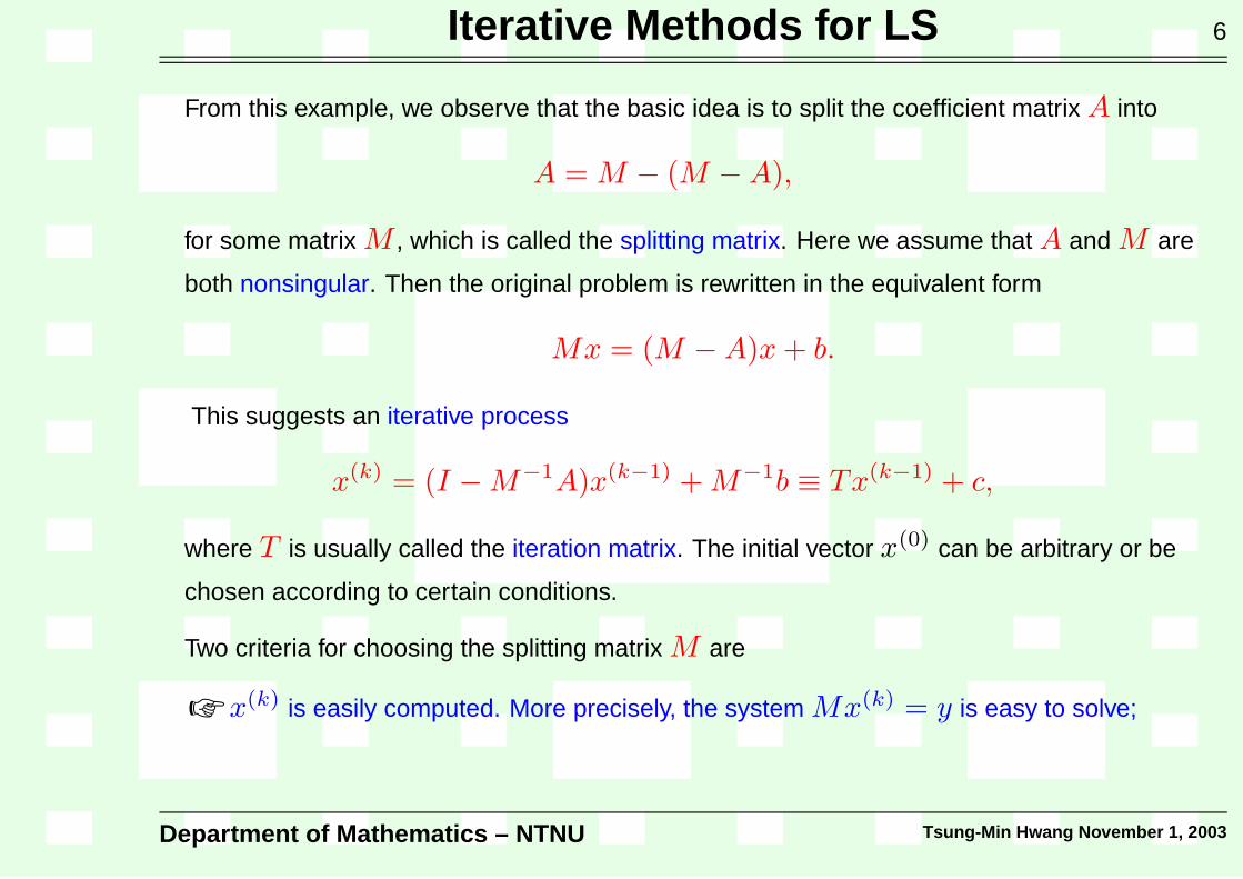
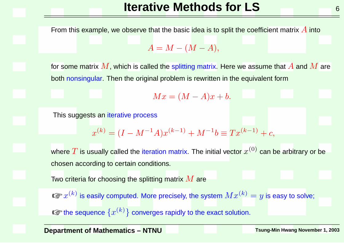
From this example, we observe that the basic idea is to split the coefficient matrix A into
A = M − (M − A),
for some matrix M , which is called the splitting matrix.
Here we assume that A and M are
both nonsingular. Then the original problem is rewritten in the equivalent form
Mx = (M − A)x + b.
This suggests an iterative process
x(k) = (I − M−1A)x(k−1) + M−1b ≡ Tx(k−1) + c,
where T is usually called the iteration matrix. The initial vector x(0) can be arbitrary or be
chosen according to certain conditions.
Two criteria for choosing the splitting matrix M are
☞ x(k) is easily computed. More precisely, the system Mx(k) = y is easy to solve;
☞ the sequence {x(k)} converges rapidly to the exact solution.
Department of Mathematics – NTNU Tsung-Min Hwang November 1, 2003
Iterative Methods for LS 6
From this example, we observe that the basic idea is to split the coefficient matrix A into
A = M − (M − A),
for some matrix M , which is called the splitting matrix. Here we assume that A and M are
both nonsingular.
Then the original problem is rewritten in the equivalent form
Mx = (M − A)x + b.
This suggests an iterative process
x(k) = (I − M−1A)x(k−1) + M−1b ≡ Tx(k−1) + c,
where T is usually called the iteration matrix. The initial vector x(0) can be arbitrary or be
chosen according to certain conditions.
Two criteria for choosing the splitting matrix M are
☞ x(k) is easily computed. More precisely, the system Mx(k) = y is easy to solve;
☞ the sequence {x(k)} converges rapidly to the exact solution.
Department of Mathematics – NTNU Tsung-Min Hwang November 1, 2003

Iterative Methods for LS 6
From this example, we observe that the basic idea is to split the coefficient matrix A into
A = M − (M − A),
for some matrix M , which is called the splitting matrix. Here we assume that A and M are
both nonsingular. Then the original problem is rewritten in the equivalent form
Mx = (M − A)x + b.
This suggests an iterative process
x(k) = (I − M−1A)x(k−1) + M−1b ≡ Tx(k−1) + c,
where T is usually called the iteration matrix. The initial vector x(0) can be arbitrary or be
chosen according to certain conditions.
Two criteria for choosing the splitting matrix M are
☞ x(k) is easily computed. More precisely, the system Mx(k) = y is easy to solve;
☞ the sequence {x(k)} converges rapidly to the exact solution.
Department of Mathematics – NTNU Tsung-Min Hwang November 1, 2003
Iterative Methods for LS 6
From this example, we observe that the basic idea is to split the coefficient matrix A into
A = M − (M − A),
for some matrix M , which is called the splitting matrix. Here we assume that A and M are
both nonsingular. Then the original problem is rewritten in the equivalent form
Mx = (M − A)x + b.
This suggests an iterative process
x(k) = (I − M−1A)x(k−1) + M−1b ≡ Tx(k−1) + c,
where T is usually called the iteration matrix. The initial vector x(0) can be arbitrary or be
chosen according to certain conditions.
Two criteria for choosing the splitting matrix M are
☞ x(k) is easily computed. More precisely, the system Mx(k) = y is easy to solve;
☞ the sequence {x(k)} converges rapidly to the exact solution.
Department of Mathematics – NTNU Tsung-Min Hwang November 1, 2003

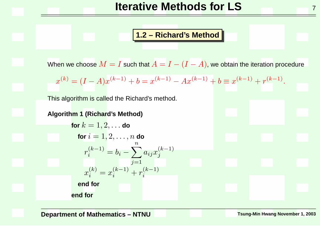
Iterative Methods for LS 7
1.2 – Richard’s Method
When we choose M = I such that A = I − (I − A), we obtain the iteration procedure
x(k) = (I − A)x(k−1) + b = x(k−1) − Ax(k−1) + b ≡ x(k−1) + r(k−1).
This algorithm is called the Richard’s method.
Algorithm 1 (Richard’s Method)
for k = 1, 2, . . . do
for i = 1, 2, . . . , n do
r(k−1)i = bi −
n∑
j=1
aijx(k−1)j
x(k)i = x
(k−1)i + r
(k−1)i
end for
end for
Department of Mathematics – NTNU Tsung-Min Hwang November 1, 2003
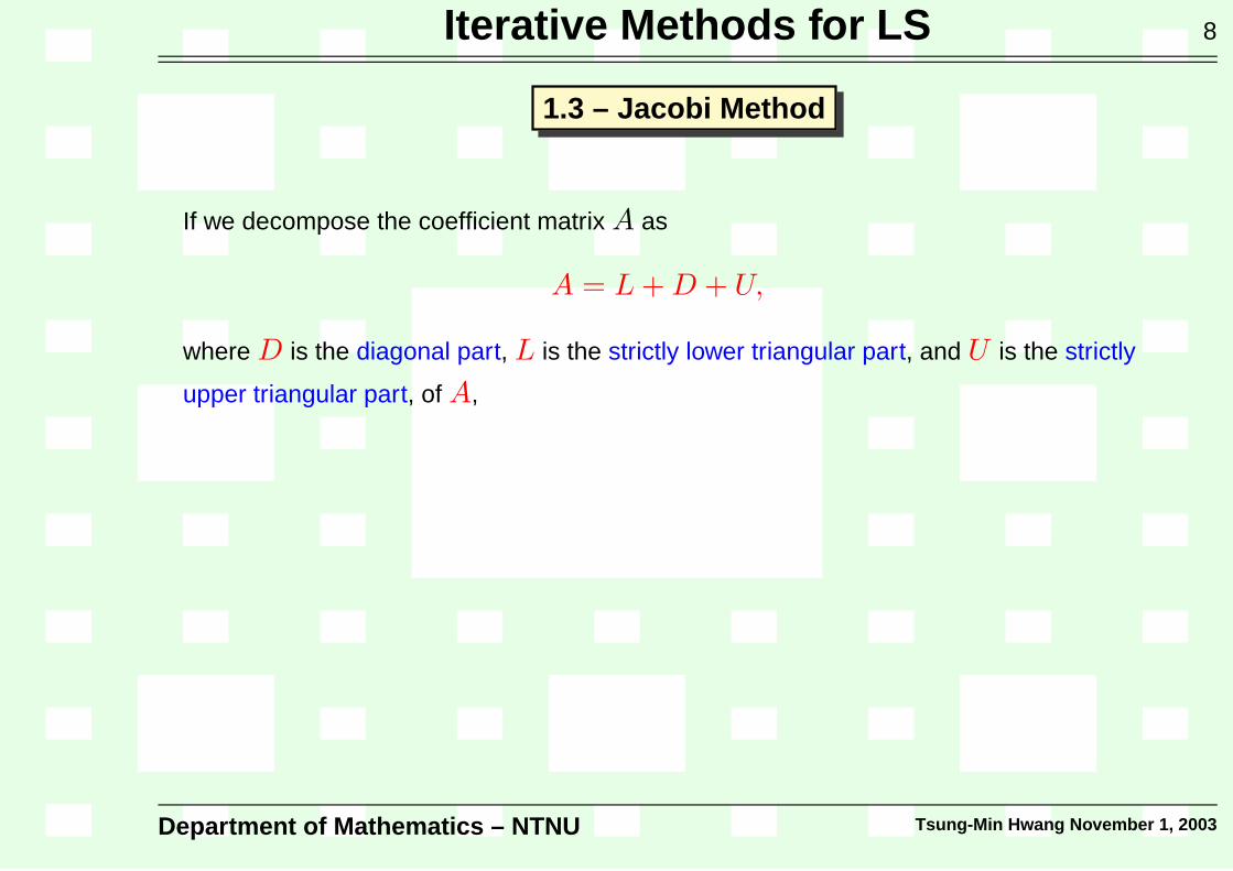
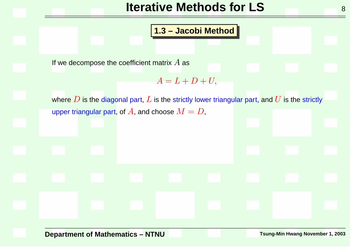
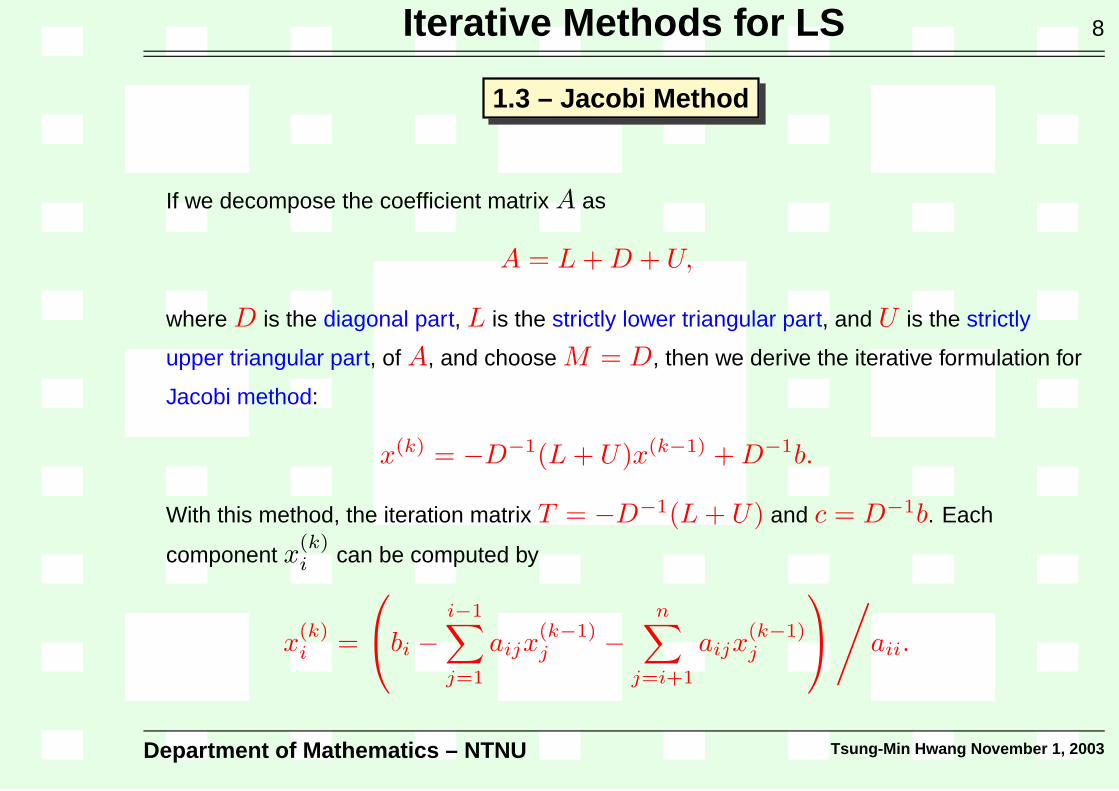
Iterative Methods for LS 8
1.3 – Jacobi Method
If we decompose the coefficient matrix A as
A = L + D + U,
where D is the diagonal part, L is the strictly lower triangular part, and U is the strictly
upper triangular part, of A,
and choose M = D, then we derive the iterative formulation for
Jacobi method:
x(k) = −D−1(L + U)x(k−1) + D−1b.
With this method, the iteration matrix T = −D−1(L + U) and c = D−1b. Each
component x(k)i can be computed by
x(k)i =
bi −
i−1∑
j=1
aijx(k−1)j −
n∑
j=i+1
aijx(k−1)j
/
aii.
Department of Mathematics – NTNU Tsung-Min Hwang November 1, 2003
Iterative Methods for LS 8
1.3 – Jacobi Method
If we decompose the coefficient matrix A as
A = L + D + U,
where D is the diagonal part, L is the strictly lower triangular part, and U is the strictly
upper triangular part, of A, and choose M = D,
then we derive the iterative formulation for
Jacobi method:
x(k) = −D−1(L + U)x(k−1) + D−1b.
With this method, the iteration matrix T = −D−1(L + U) and c = D−1b. Each
component x(k)i can be computed by
x(k)i =
bi −
i−1∑
j=1
aijx(k−1)j −
n∑
j=i+1
aijx(k−1)j
/
aii.
Department of Mathematics – NTNU Tsung-Min Hwang November 1, 2003

Iterative Methods for LS 8
1.3 – Jacobi Method
If we decompose the coefficient matrix A as
A = L + D + U,
where D is the diagonal part, L is the strictly lower triangular part, and U is the strictly
upper triangular part, of A, and choose M = D, then we derive the iterative formulation for
Jacobi method:
x(k) = −D−1(L + U)x(k−1) + D−1b.
With this method, the iteration matrix T = −D−1(L + U) and c = D−1b.
Each
component x(k)i can be computed by
x(k)i =
bi −
i−1∑
j=1
aijx(k−1)j −
n∑
j=i+1
aijx(k−1)j
/
aii.
Department of Mathematics – NTNU Tsung-Min Hwang November 1, 2003
Iterative Methods for LS 8
1.3 – Jacobi Method
If we decompose the coefficient matrix A as
A = L + D + U,
where D is the diagonal part, L is the strictly lower triangular part, and U is the strictly
upper triangular part, of A, and choose M = D, then we derive the iterative formulation for
Jacobi method:
x(k) = −D−1(L + U)x(k−1) + D−1b.
With this method, the iteration matrix T = −D−1(L + U) and c = D−1b. Each
component x(k)i can be computed by
x(k)i =
bi −
i−1∑
j=1
aijx(k−1)j −
n∑
j=i+1
aijx(k−1)j
/
aii.
Department of Mathematics – NTNU Tsung-Min Hwang November 1, 2003

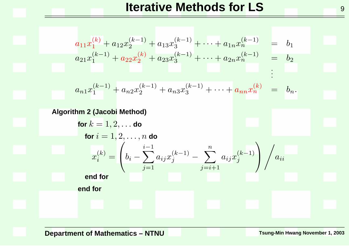
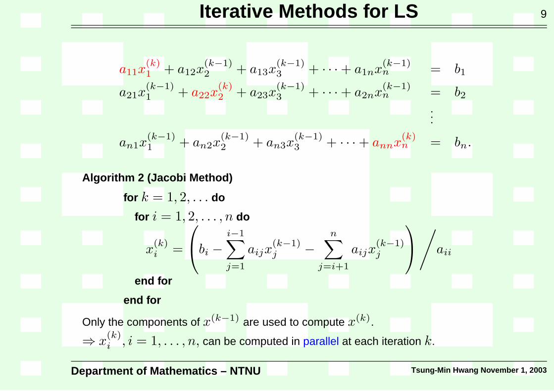
Iterative Methods for LS 9
a11x(k)1 + a12x
(k−1)2 + a13x
(k−1)3 + · · · + a1nx
(k−1)n = b1
a21x(k−1)1 + a22x
(k)2 + a23x
(k−1)3 + · · · + a2nx
(k−1)n = b2
...
an1x(k−1)1 + an2x
(k−1)2 + an3x
(k−1)3 + · · · + annx
(k)n = bn.
Algorithm 2 (Jacobi Method)
for k = 1, 2, . . . do
for i = 1, 2, . . . , n do
x(k)i =
bi −
i−1∑
j=1
aijx(k−1)j −
n∑
j=i+1
aijx(k−1)j
/
aii
end for
end for
Only the components of x(k−1) are used to compute x(k).
⇒ x(k)i , i = 1, . . . , n, can be computed in parallel at each iteration k.
Department of Mathematics – NTNU Tsung-Min Hwang November 1, 2003
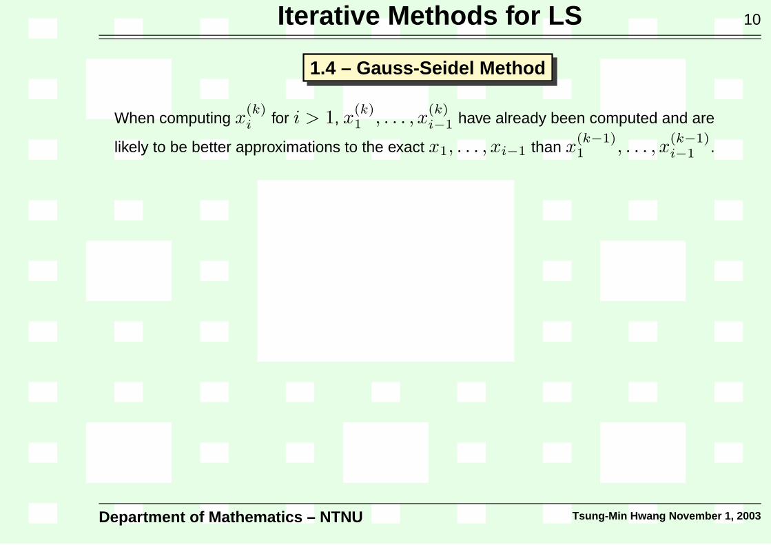
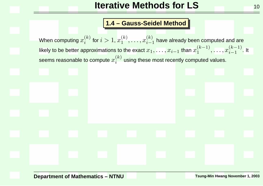
Iterative Methods for LS 10
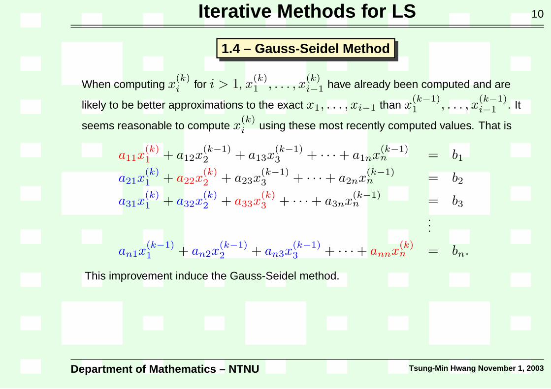
1.4 – Gauss-Seidel Method
When computing x(k)i for i > 1, x
(k)1 , . . . , x
(k)i−1 have already been computed and are
likely to be better approximations to the exact x1, . . . , xi−1 than x(k−1)1 , . . . , x
(k−1)i−1 .
It
seems reasonable to compute x(k)i using these most recently computed values. That is
a11x(k)1 + a12x
(k−1)2 + a13x
(k−1)3 + · · · + a1nx
(k−1)n = b1
a21x(k)1 + a22x
(k)2 + a23x
(k−1)3 + · · · + a2nx
(k−1)n = b2
a31x(k)1 + a32x
(k)2 + a33x
(k)3 + · · · + a3nx
(k−1)n = b3
...
an1x(k−1)1 + an2x
(k−1)2 + an3x
(k−1)3 + · · · + annx
(k)n = bn.
This improvement induce the Gauss-Seidel method.
The Gauss-Seidel method sets M = D + L and defines the iteration as
x(k) = −(D + L)−1Ux(k−1) + (D + L)−1b.
Department of Mathematics – NTNU Tsung-Min Hwang November 1, 2003
Iterative Methods for LS 10
1.4 – Gauss-Seidel Method
When computing x(k)i for i > 1, x
(k)1 , . . . , x
(k)i−1 have already been computed and are
likely to be better approximations to the exact x1, . . . , xi−1 than x(k−1)1 , . . . , x
(k−1)i−1 . It
seems reasonable to compute x(k)i using these most recently computed values.
That is
a11x(k)1 + a12x
(k−1)2 + a13x
(k−1)3 + · · · + a1nx
(k−1)n = b1
a21x(k)1 + a22x
(k)2 + a23x
(k−1)3 + · · · + a2nx
(k−1)n = b2
a31x(k)1 + a32x
(k)2 + a33x
(k)3 + · · · + a3nx
(k−1)n = b3
...
an1x(k−1)1 + an2x
(k−1)2 + an3x
(k−1)3 + · · · + annx
(k)n = bn.
This improvement induce the Gauss-Seidel method.
The Gauss-Seidel method sets M = D + L and defines the iteration as
x(k) = −(D + L)−1Ux(k−1) + (D + L)−1b.
Department of Mathematics – NTNU Tsung-Min Hwang November 1, 2003

Iterative Methods for LS 10
1.4 – Gauss-Seidel Method
When computing x(k)i for i > 1, x
(k)1 , . . . , x
(k)i−1 have already been computed and are
likely to be better approximations to the exact x1, . . . , xi−1 than x(k−1)1 , . . . , x
(k−1)i−1 . It
seems reasonable to compute x(k)i using these most recently computed values. That is
a11x(k)1 + a12x
(k−1)2 + a13x
(k−1)3 + · · · + a1nx
(k−1)n = b1
a21x(k)1 + a22x
(k)2 + a23x
(k−1)3 + · · · + a2nx
(k−1)n = b2
a31x(k)1 + a32x
(k)2 + a33x
(k)3 + · · · + a3nx
(k−1)n = b3
...
an1x(k−1)1 + an2x
(k−1)2 + an3x
(k−1)3 + · · · + annx
(k)n = bn.
This improvement induce the Gauss-Seidel method.
The Gauss-Seidel method sets M = D + L and defines the iteration as
x(k) = −(D + L)−1Ux(k−1) + (D + L)−1b.
Department of Mathematics – NTNU Tsung-Min Hwang November 1, 2003
Iterative Methods for LS 10
1.4 – Gauss-Seidel Method
When computing x(k)i for i > 1, x
(k)1 , . . . , x
(k)i−1 have already been computed and are
likely to be better approximations to the exact x1, . . . , xi−1 than x(k−1)1 , . . . , x
(k−1)i−1 . It
seems reasonable to compute x(k)i using these most recently computed values. That is
a11x(k)1 + a12x
(k−1)2 + a13x
(k−1)3 + · · · + a1nx
(k−1)n = b1
a21x(k)1 + a22x
(k)2 + a23x
(k−1)3 + · · · + a2nx
(k−1)n = b2
a31x(k)1 + a32x
(k)2 + a33x
(k)3 + · · · + a3nx
(k−1)n = b3
...
an1x(k−1)1 + an2x
(k−1)2 + an3x
(k−1)3 + · · · + annx
(k)n = bn.
This improvement induce the Gauss-Seidel method.
The Gauss-Seidel method sets M = D + L and defines the iteration as
x(k) = −(D + L)−1Ux(k−1) + (D + L)−1b.
Department of Mathematics – NTNU Tsung-Min Hwang November 1, 2003

Iterative Methods for LS 11
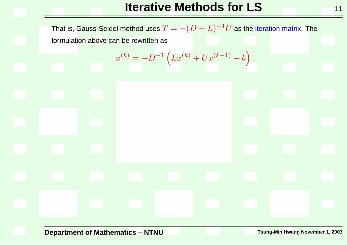
That is, Gauss-Seidel method uses T = −(D + L)−1U as the iteration matrix.
The
formulation above can be rewritten as
x(k) = −D−1(
Lx(k) + Ux(k−1) − b)
.
Hence each component x(k)i can be computed by
x(k)i =
bi −
i−1∑
j=1
aijx(k)j −
n∑
j=i+1
aijx(k−1)j
/
aii.
Algorithm 3 (Gauss-Seidel Method)
for k = 1, 2, . . . do
for i = 1, 2, . . . , n do
x(k)i =
bi −
i−1∑
j=1
aijx(k)j −
n∑
j=i+1
aijx(k−1)j
/
aii
end for
end for
Department of Mathematics – NTNU Tsung-Min Hwang November 1, 2003
Iterative Methods for LS 11
That is, Gauss-Seidel method uses T = −(D + L)−1U as the iteration matrix. The
formulation above can be rewritten as
x(k) = −D−1(
Lx(k) + Ux(k−1) − b)
.
Hence each component x(k)i can be computed by
x(k)i =
bi −
i−1∑
j=1
aijx(k)j −
n∑
j=i+1
aijx(k−1)j
/
aii.
Algorithm 3 (Gauss-Seidel Method)
for k = 1, 2, . . . do
for i = 1, 2, . . . , n do
x(k)i =
bi −
i−1∑
j=1
aijx(k)j −
n∑
j=i+1
aijx(k−1)j
/
aii
end for
end for
Department of Mathematics – NTNU Tsung-Min Hwang November 1, 2003

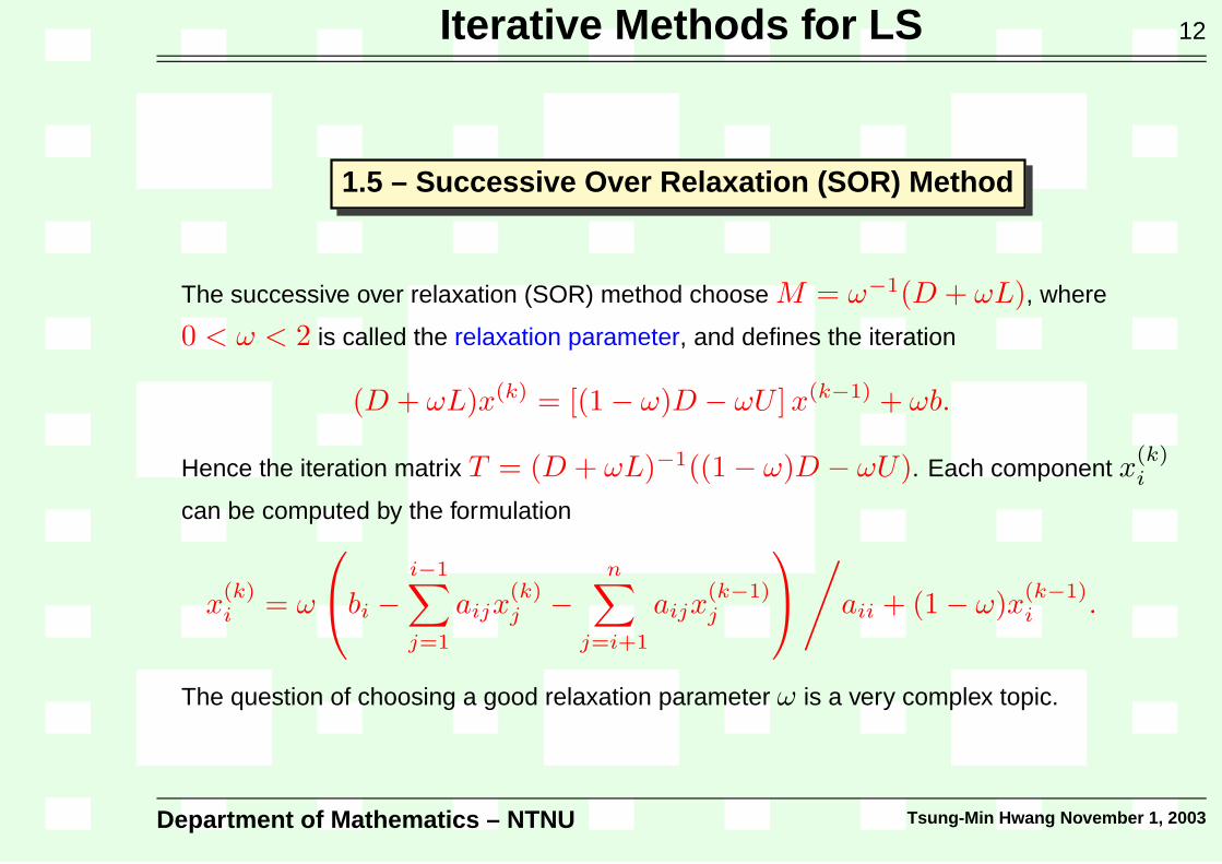
Iterative Methods for LS 12
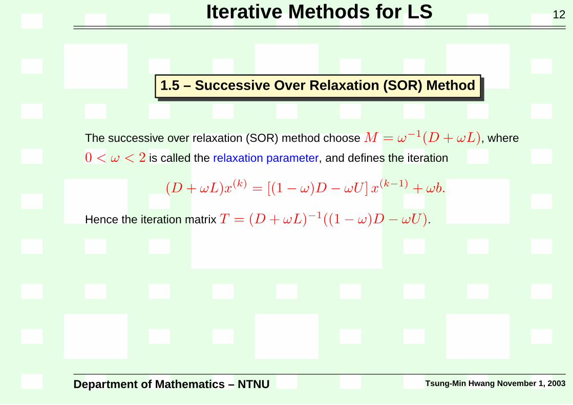
1.5 – Successive Over Relaxation (SOR) Method
The successive over relaxation (SOR) method choose M = ω−1(D + ωL),
where
0 < ω < 2 is called the relaxation parameter, and defines the iteration
(D + ωL)x(k) = [(1 − ω)D − ωU ] x(k−1) + ωb.
Hence the iteration matrix T = (D + ωL)−1((1 − ω)D − ωU). Each component x(k)i
can be computed by the formulation
x(k)i = ω
bi −
i−1∑
j=1
aijx(k)j −
n∑
j=i+1
aijx(k−1)j
/
aii + (1 − ω)x(k−1)i .
The question of choosing a good relaxation parameter ω is a very complex topic.
Department of Mathematics – NTNU Tsung-Min Hwang November 1, 2003

Iterative Methods for LS 12
1.5 – Successive Over Relaxation (SOR) Method
The successive over relaxation (SOR) method choose M = ω−1(D + ωL), where
0 < ω < 2 is called the relaxation parameter,
and defines the iteration
(D + ωL)x(k) = [(1 − ω)D − ωU ] x(k−1) + ωb.
Hence the iteration matrix T = (D + ωL)−1((1 − ω)D − ωU). Each component x(k)i
can be computed by the formulation
x(k)i = ω
bi −
i−1∑
j=1
aijx(k)j −
n∑
j=i+1
aijx(k−1)j
/
aii + (1 − ω)x(k−1)i .
The question of choosing a good relaxation parameter ω is a very complex topic.
Department of Mathematics – NTNU Tsung-Min Hwang November 1, 2003
Iterative Methods for LS 12
1.5 – Successive Over Relaxation (SOR) Method
The successive over relaxation (SOR) method choose M = ω−1(D + ωL), where
0 < ω < 2 is called the relaxation parameter, and defines the iteration
(D + ωL)x(k) = [(1 − ω)D − ωU ] x(k−1) + ωb.
Hence the iteration matrix T = (D + ωL)−1((1 − ω)D − ωU). Each component x(k)i
can be computed by the formulation
x(k)i = ω
bi −
i−1∑
j=1
aijx(k)j −
n∑
j=i+1
aijx(k−1)j
/
aii + (1 − ω)x(k−1)i .
The question of choosing a good relaxation parameter ω is a very complex topic.
Department of Mathematics – NTNU Tsung-Min Hwang November 1, 2003
Iterative Methods for LS 12
1.5 – Successive Over Relaxation (SOR) Method
The successive over relaxation (SOR) method choose M = ω−1(D + ωL), where
0 < ω < 2 is called the relaxation parameter, and defines the iteration
(D + ωL)x(k) = [(1 − ω)D − ωU ] x(k−1) + ωb.
Hence the iteration matrix T = (D + ωL)−1((1 − ω)D − ωU).
Each component x(k)i
can be computed by the formulation
x(k)i = ω
bi −
i−1∑
j=1
aijx(k)j −
n∑
j=i+1
aijx(k−1)j
/
aii + (1 − ω)x(k−1)i .
The question of choosing a good relaxation parameter ω is a very complex topic.
Department of Mathematics – NTNU Tsung-Min Hwang November 1, 2003

Iterative Methods for LS 12
1.5 – Successive Over Relaxation (SOR) Method
The successive over relaxation (SOR) method choose M = ω−1(D + ωL), where
0 < ω < 2 is called the relaxation parameter, and defines the iteration
(D + ωL)x(k) = [(1 − ω)D − ωU ] x(k−1) + ωb.
Hence the iteration matrix T = (D + ωL)−1((1 − ω)D − ωU). Each component x(k)i
can be computed by the formulation
x(k)i = ω
bi −
i−1∑
j=1
aijx(k)j −
n∑
j=i+1
aijx(k−1)j
/
aii + (1 − ω)x(k−1)i .
The question of choosing a good relaxation parameter ω is a very complex topic.
Department of Mathematics – NTNU Tsung-Min Hwang November 1, 2003
Iterative Methods for LS 12
1.5 – Successive Over Relaxation (SOR) Method
The successive over relaxation (SOR) method choose M = ω−1(D + ωL), where
0 < ω < 2 is called the relaxation parameter, and defines the iteration
(D + ωL)x(k) = [(1 − ω)D − ωU ] x(k−1) + ωb.
Hence the iteration matrix T = (D + ωL)−1((1 − ω)D − ωU). Each component x(k)i
can be computed by the formulation
x(k)i = ω
bi −
i−1∑
j=1
aijx(k)j −
n∑
j=i+1
aijx(k−1)j
/
aii + (1 − ω)x(k−1)i .
The question of choosing a good relaxation parameter ω is a very complex topic.
Department of Mathematics – NTNU Tsung-Min Hwang November 1, 2003

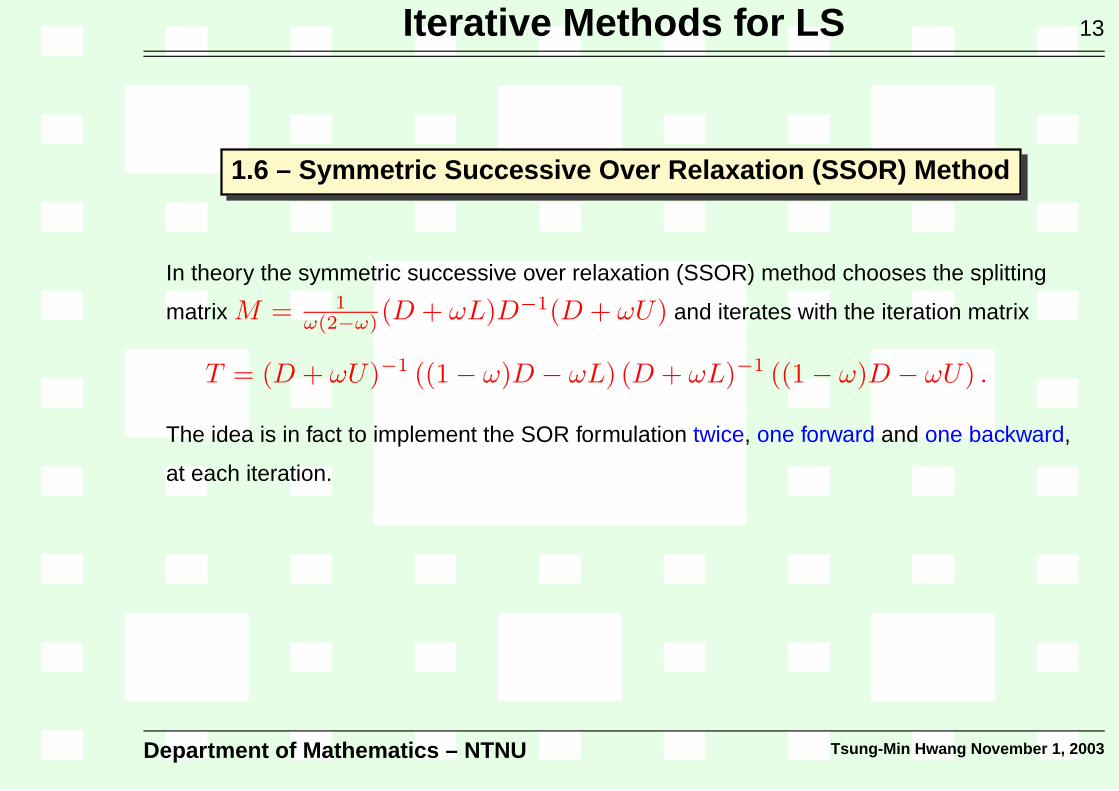
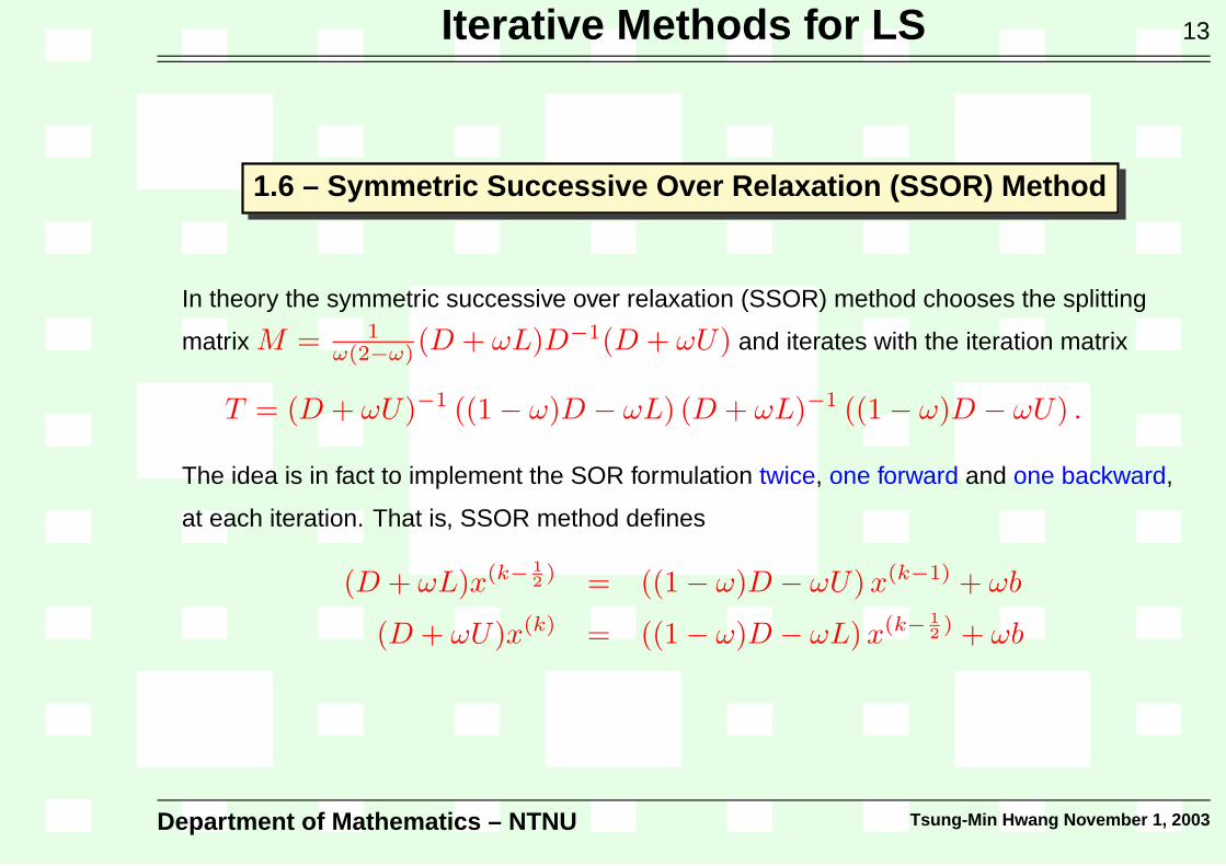
Iterative Methods for LS 13
1.6 – Symmetric Successive Over Relaxation (SSOR) Method
In theory the symmetric successive over relaxation (SSOR) method chooses the splitting
matrix M = 1ω(2−ω) (D + ωL)D−1(D + ωU) and iterates with the iteration matrix
T = (D + ωU)−1 ((1 − ω)D − ωL) (D + ωL)−1 ((1 − ω)D − ωU) .
The idea is in fact to implement the SOR formulation twice, one forward and one backward,
at each iteration. That is, SSOR method defines
(D + ωL)x(k− 1
2) = ((1 − ω)D − ωU)x(k−1) + ωb
(D + ωU)x(k) = ((1 − ω)D − ωL) x(k− 1
2) + ωb
Department of Mathematics – NTNU Tsung-Min Hwang November 1, 2003
Iterative Methods for LS 13
1.6 – Symmetric Successive Over Relaxation (SSOR) Method
In theory the symmetric successive over relaxation (SSOR) method chooses the splitting
matrix M = 1ω(2−ω) (D + ωL)D−1(D + ωU) and iterates with the iteration matrix
T = (D + ωU)−1 ((1 − ω)D − ωL) (D + ωL)−1 ((1 − ω)D − ωU) .
The idea is in fact to implement the SOR formulation twice, one forward and one backward,
at each iteration.
That is, SSOR method defines
(D + ωL)x(k− 1
2) = ((1 − ω)D − ωU)x(k−1) + ωb
(D + ωU)x(k) = ((1 − ω)D − ωL) x(k− 1
2) + ωb
Department of Mathematics – NTNU Tsung-Min Hwang November 1, 2003
Iterative Methods for LS 13
1.6 – Symmetric Successive Over Relaxation (SSOR) Method
In theory the symmetric successive over relaxation (SSOR) method chooses the splitting
matrix M = 1ω(2−ω) (D + ωL)D−1(D + ωU) and iterates with the iteration matrix
T = (D + ωU)−1 ((1 − ω)D − ωL) (D + ωL)−1 ((1 − ω)D − ωU) .
The idea is in fact to implement the SOR formulation twice, one forward and one backward,
at each iteration. That is, SSOR method defines
(D + ωL)x(k− 1
2) = ((1 − ω)D − ωU)x(k−1) + ωb
(D + ωU)x(k) = ((1 − ω)D − ωL) x(k− 1
2) + ωb
Department of Mathematics – NTNU Tsung-Min Hwang November 1, 2003
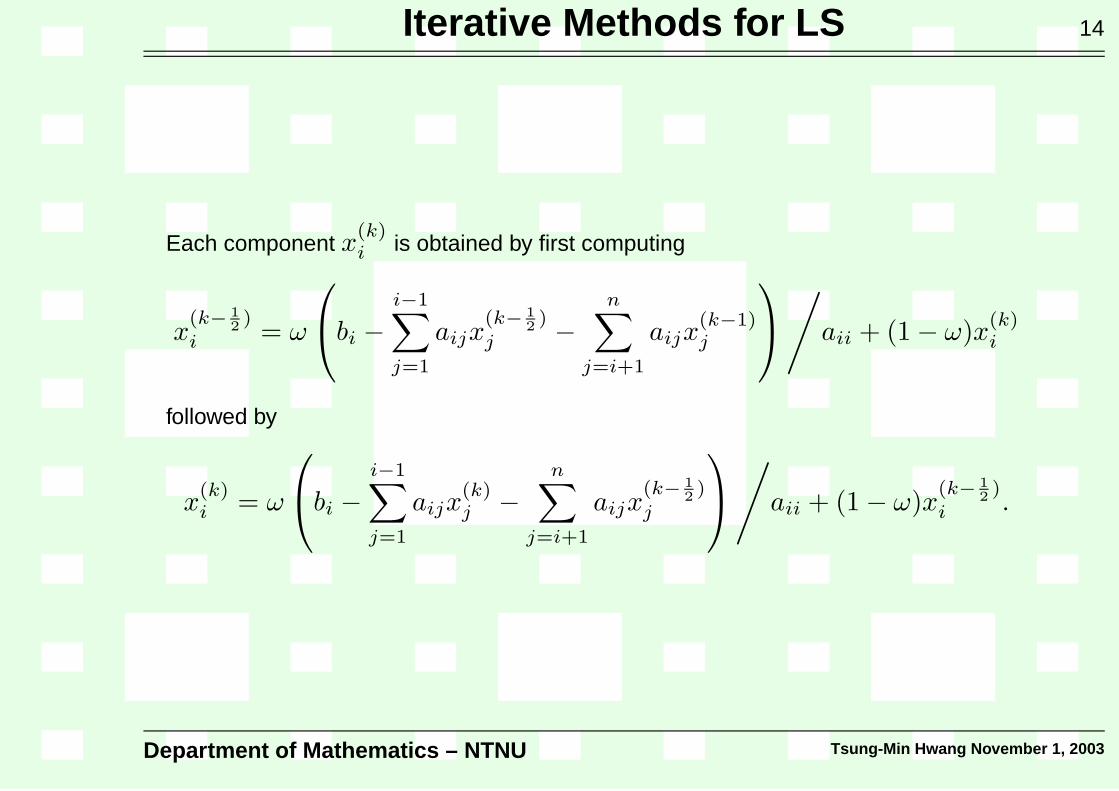
Iterative Methods for LS 14
Each component x(k)i is obtained by first computing
x(k− 1
2)
i = ω
bi −
i−1∑
j=1
aijx(k− 1
2)
j −
n∑
j=i+1
aijx(k−1)j
/
aii + (1 − ω)x(k)i
followed by
x(k)i = ω
bi −
i−1∑
j=1
aijx(k)j −
n∑
j=i+1
aijx(k− 1
2)
j
/
aii + (1 − ω)x(k− 1
2)
i .
Department of Mathematics – NTNU Tsung-Min Hwang November 1, 2003

Iterative Methods for LS 15
2 – Convergence Analysis
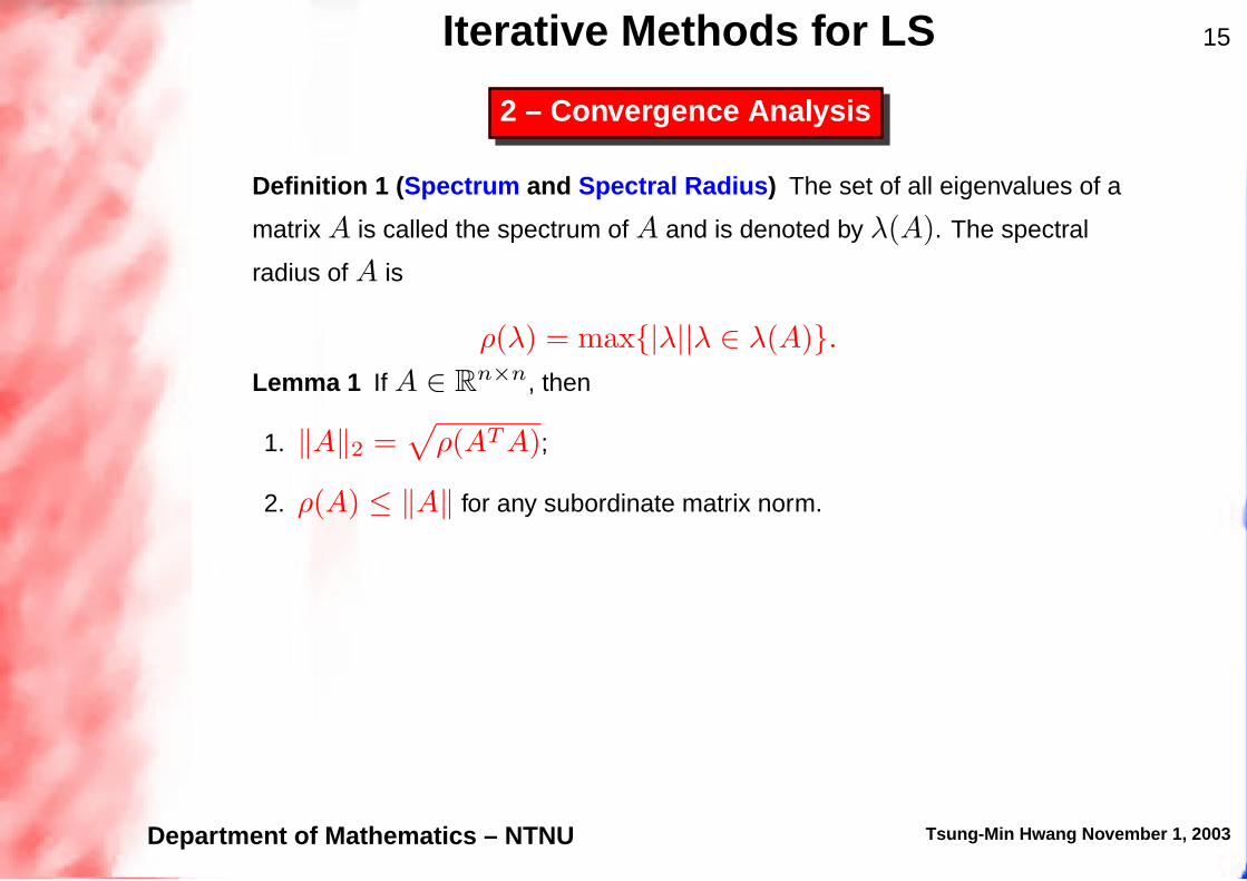
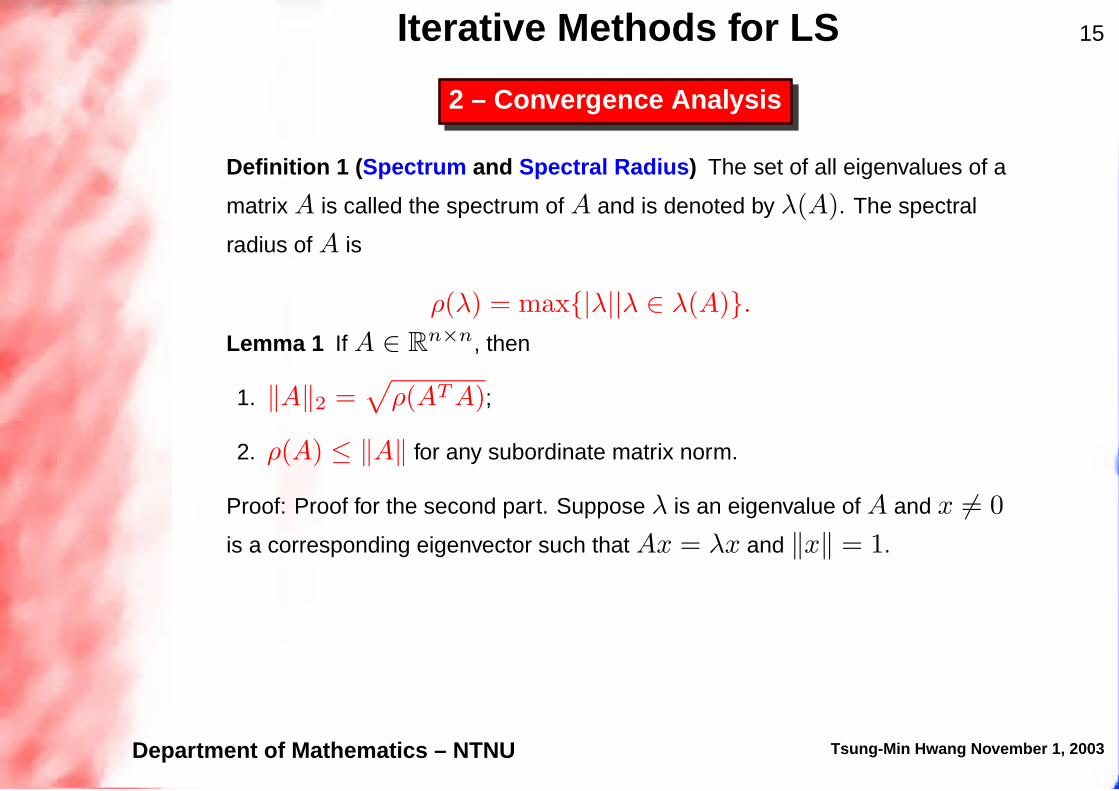
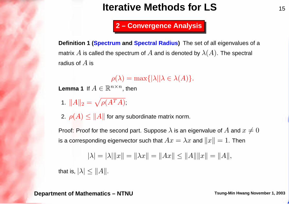
Definition 1 (Spectrum and Spectral Radius) The set of all eigenvalues of a
matrix A is called the spectrum of A and is denoted by λ(A).
The spectral
radius of A is
ρ(λ) = max{|λ||λ ∈ λ(A)}.
Lemma 1 If A ∈ Rn×n, then
1. ‖A‖2 =√
ρ(AT A);
2. ρ(A) ≤ ‖A‖ for any subordinate matrix norm.
Proof: Proof for the second part. Suppose λ is an eigenvalue of A and x 6= 0
is a corresponding eigenvector such that Ax = λx and ‖x‖ = 1. Then
|λ| = |λ|‖x‖ = ‖λx‖ = ‖Ax‖ ≤ ‖A‖‖x‖ = ‖A‖,
that is, |λ| ≤ ‖A‖. Since λ is arbitrary, this implies that
ρ(A) = max |λ| ≤ ‖A‖.
Department of Mathematics – NTNU Tsung-Min Hwang November 1, 2003

Iterative Methods for LS 15
2 – Convergence Analysis
Definition 1 (Spectrum and Spectral Radius) The set of all eigenvalues of a
matrix A is called the spectrum of A and is denoted by λ(A). The spectral
radius of A is
ρ(λ) = max{|λ||λ ∈ λ(A)}.
Lemma 1 If A ∈ Rn×n, then
1. ‖A‖2 =√
ρ(AT A);
2. ρ(A) ≤ ‖A‖ for any subordinate matrix norm.
Proof: Proof for the second part. Suppose λ is an eigenvalue of A and x 6= 0
is a corresponding eigenvector such that Ax = λx and ‖x‖ = 1. Then
|λ| = |λ|‖x‖ = ‖λx‖ = ‖Ax‖ ≤ ‖A‖‖x‖ = ‖A‖,
that is, |λ| ≤ ‖A‖. Since λ is arbitrary, this implies that
ρ(A) = max |λ| ≤ ‖A‖.
Department of Mathematics – NTNU Tsung-Min Hwang November 1, 2003

Iterative Methods for LS 15
2 – Convergence Analysis
Definition 1 (Spectrum and Spectral Radius) The set of all eigenvalues of a
matrix A is called the spectrum of A and is denoted by λ(A). The spectral
radius of A is
ρ(λ) = max{|λ||λ ∈ λ(A)}.
Lemma 1 If A ∈ Rn×n, then
1. ‖A‖2 =√
ρ(AT A);
2. ρ(A) ≤ ‖A‖ for any subordinate matrix norm.
Proof: Proof for the second part.
Suppose λ is an eigenvalue of A and x 6= 0
is a corresponding eigenvector such that Ax = λx and ‖x‖ = 1. Then
|λ| = |λ|‖x‖ = ‖λx‖ = ‖Ax‖ ≤ ‖A‖‖x‖ = ‖A‖,
that is, |λ| ≤ ‖A‖. Since λ is arbitrary, this implies that
ρ(A) = max |λ| ≤ ‖A‖.
Department of Mathematics – NTNU Tsung-Min Hwang November 1, 2003
Iterative Methods for LS 15
2 – Convergence Analysis
Definition 1 (Spectrum and Spectral Radius) The set of all eigenvalues of a
matrix A is called the spectrum of A and is denoted by λ(A). The spectral
radius of A is
ρ(λ) = max{|λ||λ ∈ λ(A)}.
Lemma 1 If A ∈ Rn×n, then
1. ‖A‖2 =√
ρ(AT A);
2. ρ(A) ≤ ‖A‖ for any subordinate matrix norm.
Proof: Proof for the second part. Suppose λ is an eigenvalue of A and x 6= 0
is a corresponding eigenvector such that Ax = λx and ‖x‖ = 1.
Then
|λ| = |λ|‖x‖ = ‖λx‖ = ‖Ax‖ ≤ ‖A‖‖x‖ = ‖A‖,
that is, |λ| ≤ ‖A‖. Since λ is arbitrary, this implies that
ρ(A) = max |λ| ≤ ‖A‖.
Department of Mathematics – NTNU Tsung-Min Hwang November 1, 2003

Iterative Methods for LS 15
2 – Convergence Analysis
Definition 1 (Spectrum and Spectral Radius) The set of all eigenvalues of a
matrix A is called the spectrum of A and is denoted by λ(A). The spectral
radius of A is
ρ(λ) = max{|λ||λ ∈ λ(A)}.
Lemma 1 If A ∈ Rn×n, then
1. ‖A‖2 =√
ρ(AT A);
2. ρ(A) ≤ ‖A‖ for any subordinate matrix norm.
Proof: Proof for the second part. Suppose λ is an eigenvalue of A and x 6= 0
is a corresponding eigenvector such that Ax = λx and ‖x‖ = 1. Then
|λ| = |λ|‖x‖ = ‖λx‖ = ‖Ax‖ ≤ ‖A‖‖x‖ = ‖A‖,
that is, |λ| ≤ ‖A‖. Since λ is arbitrary, this implies that
ρ(A) = max |λ| ≤ ‖A‖.
Department of Mathematics – NTNU Tsung-Min Hwang November 1, 2003
Iterative Methods for LS 15
2 – Convergence Analysis
Definition 1 (Spectrum and Spectral Radius) The set of all eigenvalues of a
matrix A is called the spectrum of A and is denoted by λ(A). The spectral
radius of A is
ρ(λ) = max{|λ||λ ∈ λ(A)}.
Lemma 1 If A ∈ Rn×n, then
1. ‖A‖2 =√
ρ(AT A);
2. ρ(A) ≤ ‖A‖ for any subordinate matrix norm.
Proof: Proof for the second part. Suppose λ is an eigenvalue of A and x 6= 0
is a corresponding eigenvector such that Ax = λx and ‖x‖ = 1. Then
|λ| = |λ|‖x‖ = ‖λx‖ = ‖Ax‖ ≤ ‖A‖‖x‖ = ‖A‖,
that is, |λ| ≤ ‖A‖.
Since λ is arbitrary, this implies that
ρ(A) = max |λ| ≤ ‖A‖.
Department of Mathematics – NTNU Tsung-Min Hwang November 1, 2003

Iterative Methods for LS 15
2 – Convergence Analysis
Definition 1 (Spectrum and Spectral Radius) The set of all eigenvalues of a
matrix A is called the spectrum of A and is denoted by λ(A). The spectral
radius of A is
ρ(λ) = max{|λ||λ ∈ λ(A)}.
Lemma 1 If A ∈ Rn×n, then
1. ‖A‖2 =√
ρ(AT A);
2. ρ(A) ≤ ‖A‖ for any subordinate matrix norm.
Proof: Proof for the second part. Suppose λ is an eigenvalue of A and x 6= 0
is a corresponding eigenvector such that Ax = λx and ‖x‖ = 1. Then
|λ| = |λ|‖x‖ = ‖λx‖ = ‖Ax‖ ≤ ‖A‖‖x‖ = ‖A‖,
that is, |λ| ≤ ‖A‖. Since λ is arbitrary, this implies that
ρ(A) = max |λ| ≤ ‖A‖.
Department of Mathematics – NTNU Tsung-Min Hwang November 1, 2003

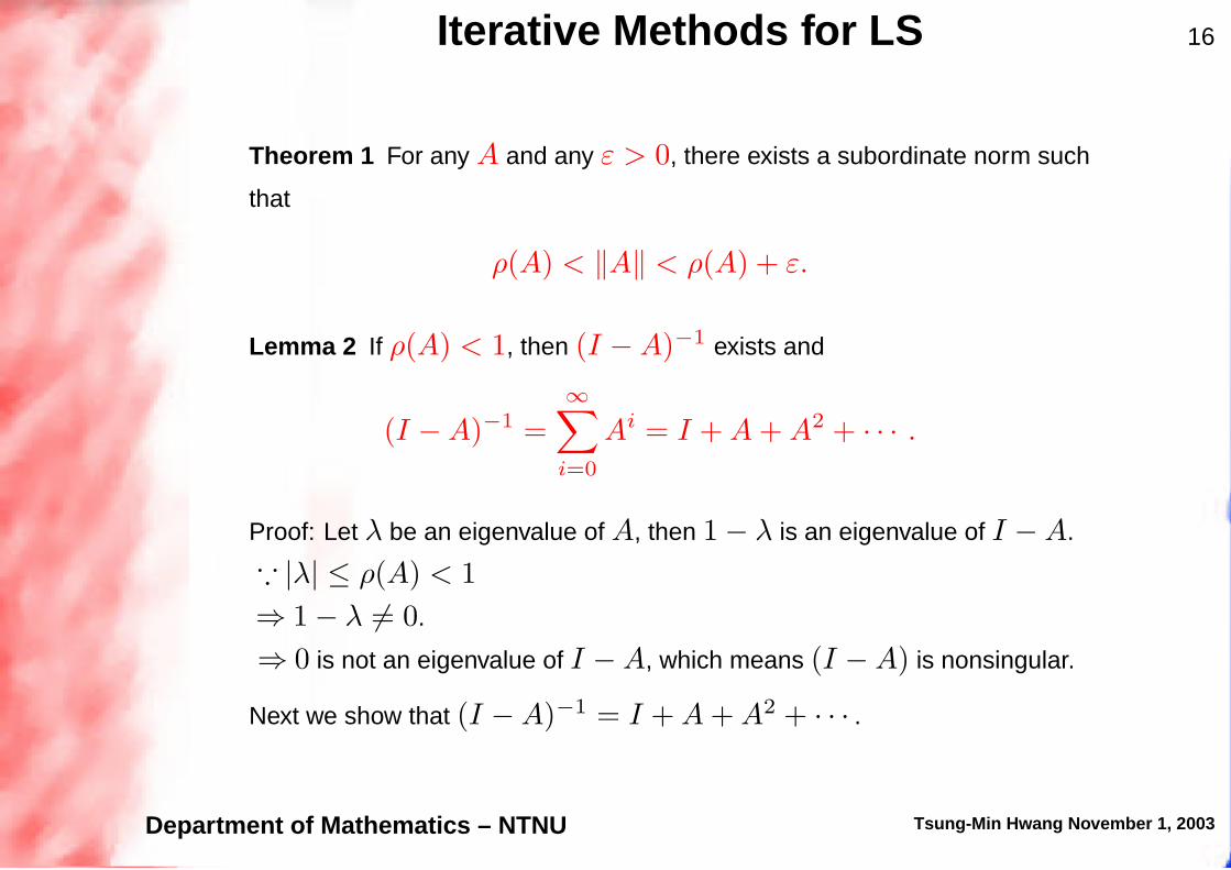
Iterative Methods for LS 16
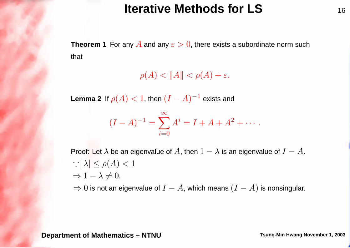
Theorem 1 For any A and any ε > 0, there exists a subordinate norm such
that
ρ(A) < ‖A‖ < ρ(A) + ε.
Lemma 2 If ρ(A) < 1, then (I − A)−1 exists and
(I − A)−1 =
∞∑
i=0
Ai = I + A + A2 + · · · .
Proof: Let λ be an eigenvalue of A, then 1 − λ is an eigenvalue of I − A.
∵ |λ| ≤ ρ(A) < 1
⇒ 1 − λ 6= 0.
⇒ 0 is not an eigenvalue of I − A, which means (I − A) is nonsingular.
Next we show that (I − A)−1 = I + A + A2 + · · · .
Department of Mathematics – NTNU Tsung-Min Hwang November 1, 2003

Iterative Methods for LS 16
Theorem 1 For any A and any ε > 0, there exists a subordinate norm such
that
ρ(A) < ‖A‖ < ρ(A) + ε.
Lemma 2 If ρ(A) < 1, then (I − A)−1 exists and
(I − A)−1 =
∞∑
i=0
Ai = I + A + A2 + · · · .
Proof: Let λ be an eigenvalue of A, then 1 − λ is an eigenvalue of I − A.
∵ |λ| ≤ ρ(A) < 1
⇒ 1 − λ 6= 0.
⇒ 0 is not an eigenvalue of I − A, which means (I − A) is nonsingular.
Next we show that (I − A)−1 = I + A + A2 + · · · .
Department of Mathematics – NTNU Tsung-Min Hwang November 1, 2003

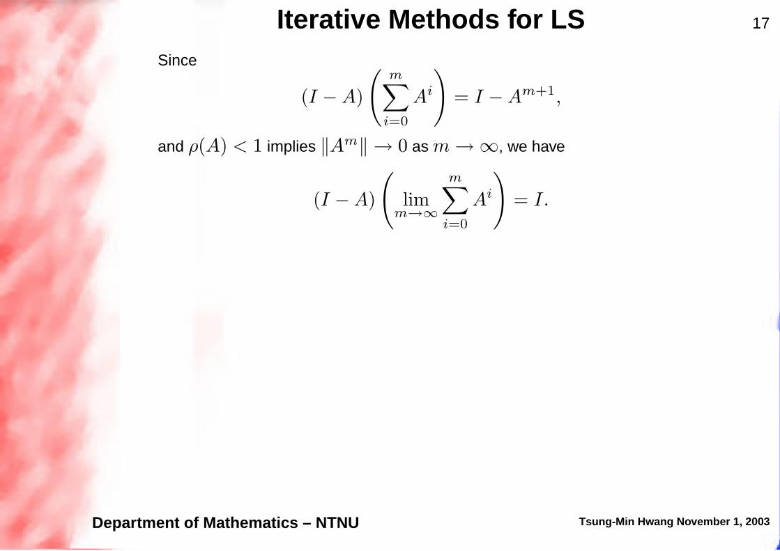
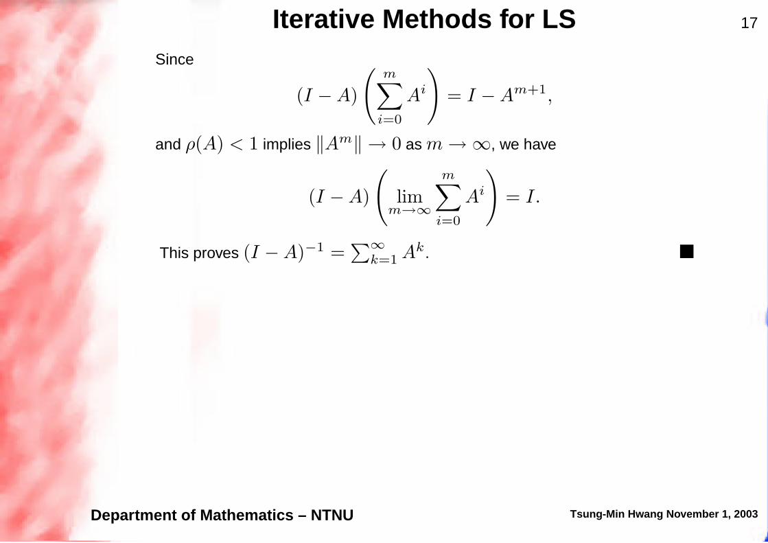
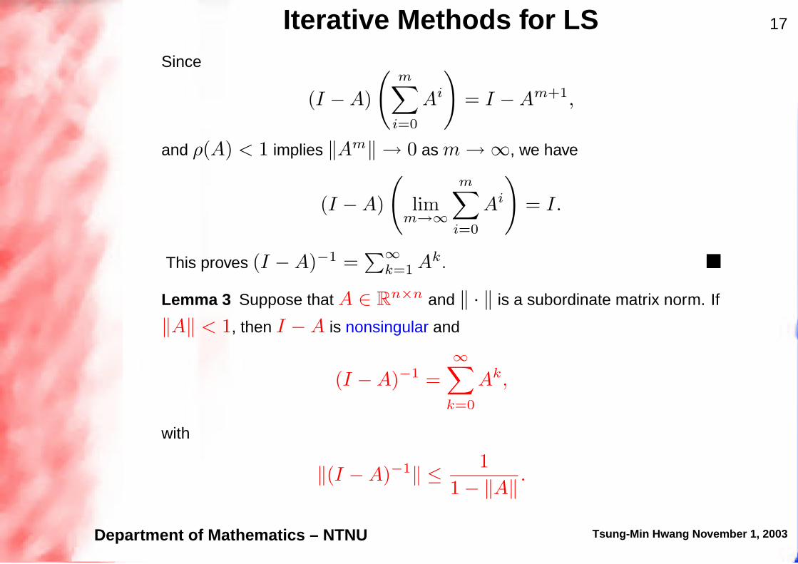
Iterative Methods for LS 17
Since
(I − A)
(
m∑
i=0
Ai
)
= I − Am+1,
and ρ(A) < 1
implies ‖Am‖ → 0 as m → ∞, we have
(I − A)
(
limm→∞
m∑
i=0
Ai
)
= I.
This proves (I − A)−1 =∑∞
k=1 Ak.
Lemma 3 Suppose that A ∈ Rn×n and ‖ · ‖ is a subordinate matrix norm. If
‖A‖ < 1, then I − A is nonsingular and
(I − A)−1 =
∞∑
k=0
Ak,
with
‖(I − A)−1‖ ≤1
1 − ‖A‖.
Department of Mathematics – NTNU Tsung-Min Hwang November 1, 2003

Iterative Methods for LS 17
Since
(I − A)
(
m∑
i=0
Ai
)
= I − Am+1,
and ρ(A) < 1 implies ‖Am‖ → 0 as m → ∞,
we have
(I − A)
(
limm→∞
m∑
i=0
Ai
)
= I.
This proves (I − A)−1 =∑∞
k=1 Ak.
Lemma 3 Suppose that A ∈ Rn×n and ‖ · ‖ is a subordinate matrix norm. If
‖A‖ < 1, then I − A is nonsingular and
(I − A)−1 =
∞∑
k=0
Ak,
with
‖(I − A)−1‖ ≤1
1 − ‖A‖.
Department of Mathematics – NTNU Tsung-Min Hwang November 1, 2003
Iterative Methods for LS 17
Since
(I − A)
(
m∑
i=0
Ai
)
= I − Am+1,
and ρ(A) < 1 implies ‖Am‖ → 0 as m → ∞, we have
(I − A)
(
limm→∞
m∑
i=0
Ai
)
= I.
This proves (I − A)−1 =∑∞
k=1 Ak.
Lemma 3 Suppose that A ∈ Rn×n and ‖ · ‖ is a subordinate matrix norm. If
‖A‖ < 1, then I − A is nonsingular and
(I − A)−1 =
∞∑
k=0
Ak,
with
‖(I − A)−1‖ ≤1
1 − ‖A‖.
Department of Mathematics – NTNU Tsung-Min Hwang November 1, 2003

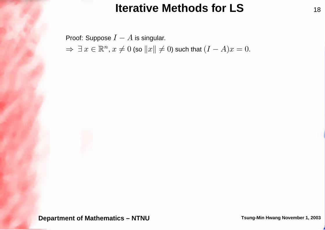
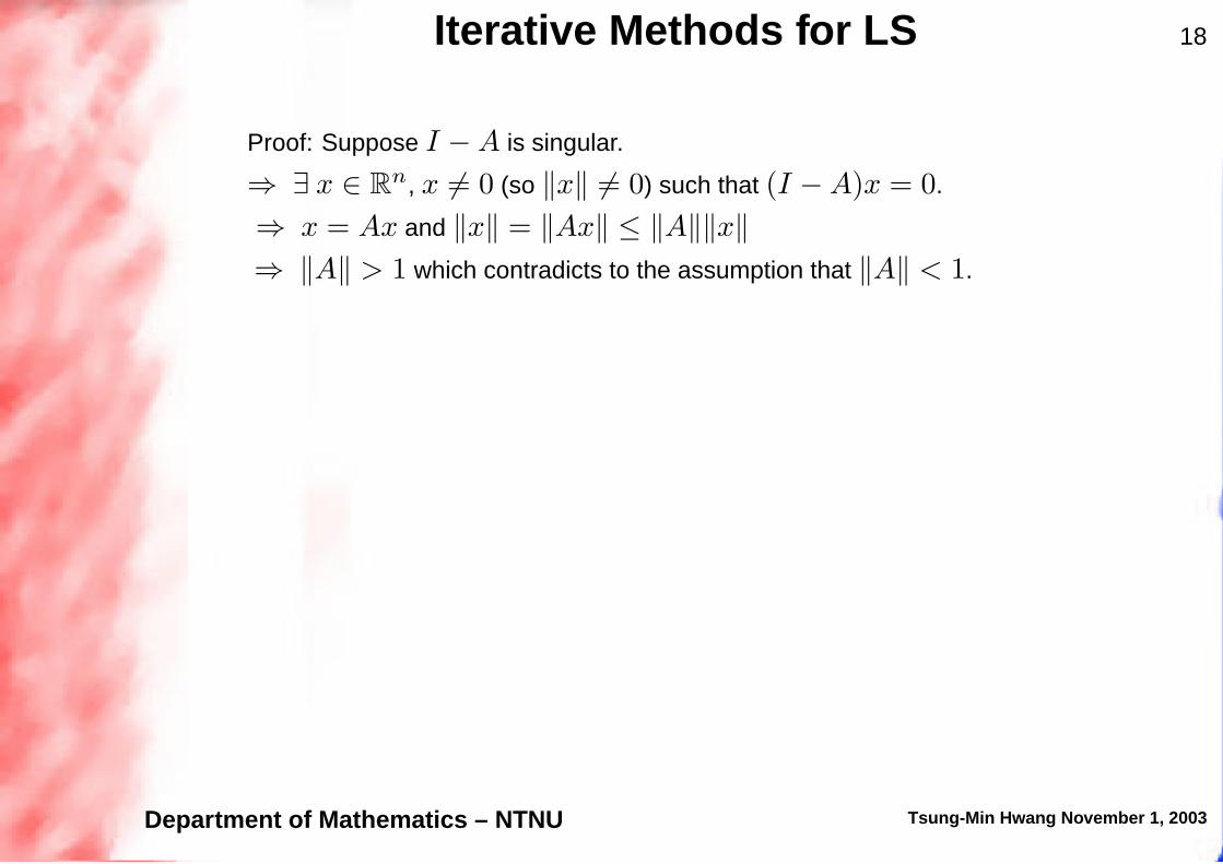
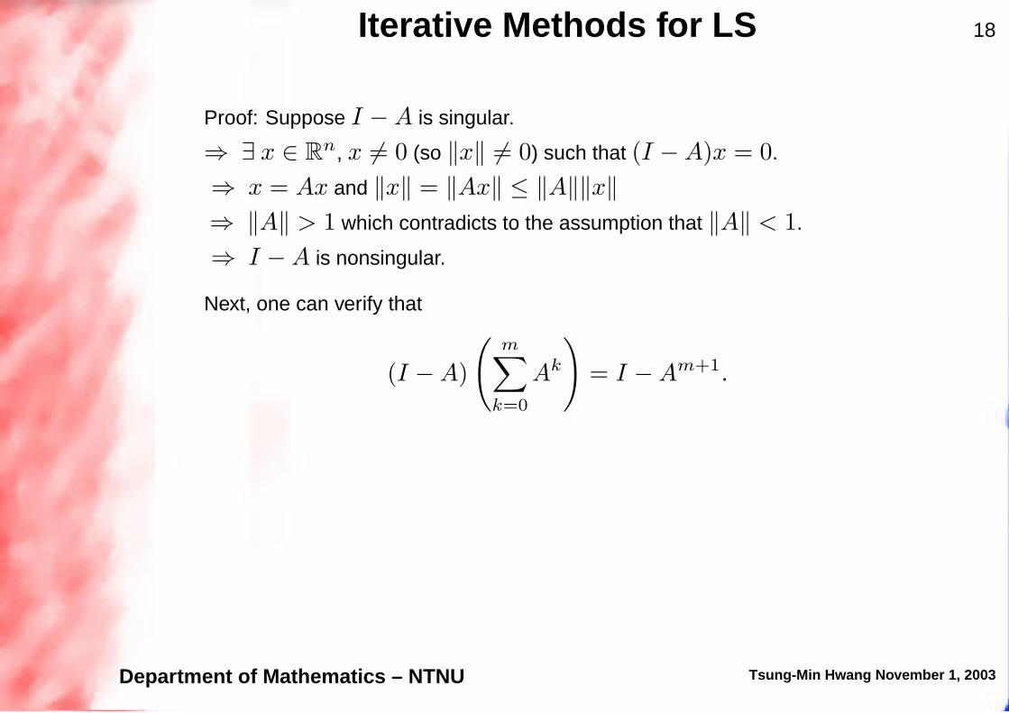
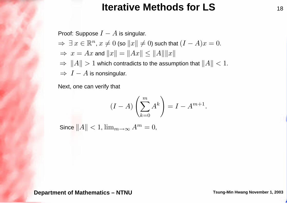
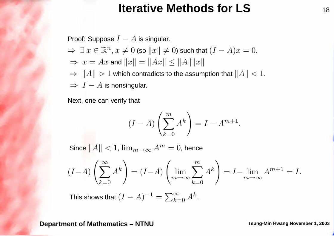
Iterative Methods for LS 18
Proof: Suppose I − A is singular.
⇒ ∃ x ∈ Rn, x 6= 0 (so ‖x‖ 6= 0) such that (I − A)x = 0.
⇒ x = Ax and ‖x‖ = ‖Ax‖ ≤ ‖A‖‖x‖
⇒ ‖A‖ > 1 which contradicts to the assumption that ‖A‖ < 1.
⇒ I − A is nonsingular.
Next, one can verify that
(I − A)
(
m∑
k=0
Ak
)
= I − Am+1.
Since ‖A‖ < 1, limm→∞ Am = 0, hence
(I−A)
(
∞∑
k=0
Ak
)
= (I−A)
(
limm→∞
m∑
k=0
Ak
)
= I− limm→∞
Am+1 = I.
This shows that (I − A)−1 =∑∞
k=0 Ak.
Department of Mathematics – NTNU Tsung-Min Hwang November 1, 2003
Iterative Methods for LS 18
Proof: Suppose I − A is singular.
⇒ ∃ x ∈ Rn, x 6= 0 (so ‖x‖ 6= 0) such that (I − A)x = 0.
⇒ x = Ax and ‖x‖ = ‖Ax‖ ≤ ‖A‖‖x‖
⇒ ‖A‖ > 1 which contradicts to the assumption that ‖A‖ < 1.
⇒ I − A is nonsingular.
Next, one can verify that
(I − A)
(
m∑
k=0
Ak
)
= I − Am+1.
Since ‖A‖ < 1, limm→∞ Am = 0,
hence
(I−A)
(
∞∑
k=0
Ak
)
= (I−A)
(
limm→∞
m∑
k=0
Ak
)
= I− limm→∞
Am+1 = I.
This shows that (I − A)−1 =∑∞
k=0 Ak.
Department of Mathematics – NTNU Tsung-Min Hwang November 1, 2003
Iterative Methods for LS 18
Proof: Suppose I − A is singular.
⇒ ∃ x ∈ Rn, x 6= 0 (so ‖x‖ 6= 0) such that (I − A)x = 0.
⇒ x = Ax and ‖x‖ = ‖Ax‖ ≤ ‖A‖‖x‖
⇒ ‖A‖ > 1 which contradicts to the assumption that ‖A‖ < 1.
⇒ I − A is nonsingular.
Next, one can verify that
(I − A)
(
m∑
k=0
Ak
)
= I − Am+1.
Since ‖A‖ < 1, limm→∞ Am = 0, hence
(I−A)
(
∞∑
k=0
Ak
)
= (I−A)
(
limm→∞
m∑
k=0
Ak
)
= I− limm→∞
Am+1 = I.
This shows that (I − A)−1 =∑∞
k=0 Ak.
Department of Mathematics – NTNU Tsung-Min Hwang November 1, 2003

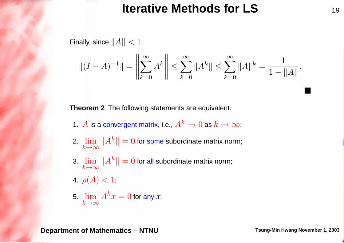
Iterative Methods for LS 19
Finally, since ‖A‖ < 1,
‖(I − A)−1‖ =
∥
∥
∥
∥
∥
∞∑
k=0
Ak
∥
∥
∥
∥
∥
≤
∞∑
k=0
‖Ak‖ ≤
∞∑
k=0
‖A‖k =1
1 − ‖A‖.
Theorem 2 The following statements are equivalent.
1. A is a convergent matrix, i.e., Ak → 0 as k → ∞;
2. limk→∞
‖Ak‖ = 0 for some subordinate matrix norm;
3. limk→∞
‖Ak‖ = 0 for all subordinate matrix norm;
4. ρ(A) < 1;
5. limk→∞
Akx = 0 for any x.
Department of Mathematics – NTNU Tsung-Min Hwang November 1, 2003

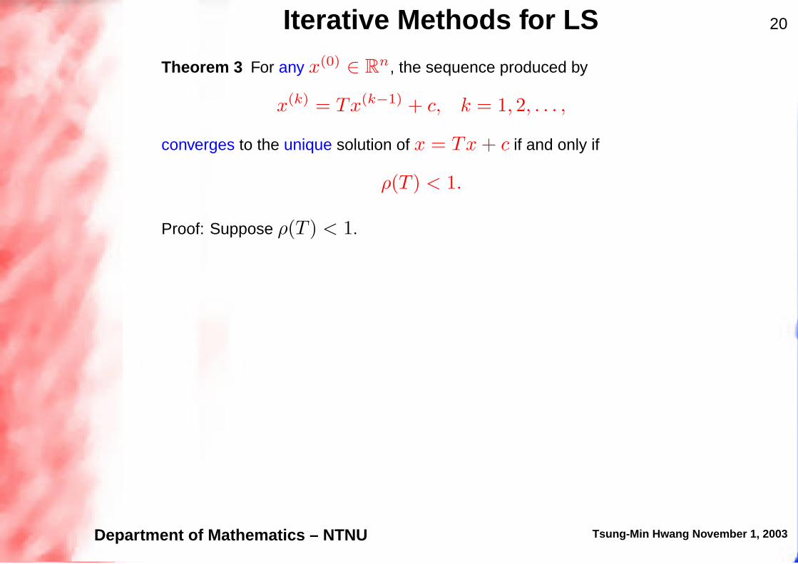
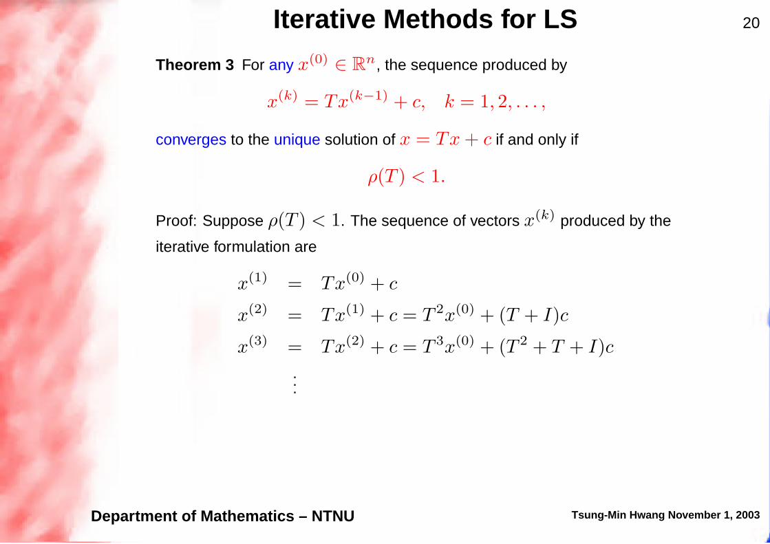
Iterative Methods for LS 20
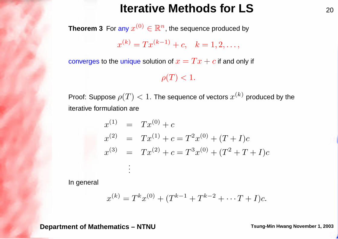
Theorem 3 For any x(0) ∈ Rn, the sequence produced by
x(k) = Tx(k−1) + c, k = 1, 2, . . . ,
converges to the unique solution of x = Tx + c if and only if
ρ(T ) < 1.
Proof: Suppose ρ(T ) < 1. The sequence of vectors x(k) produced by the
iterative formulation are
x(1) = Tx(0) + c
x(2) = Tx(1) + c = T 2x(0) + (T + I)c
x(3) = Tx(2) + c = T 3x(0) + (T 2 + T + I)c
...
In general
x(k) = T kx(0) + (T k−1 + T k−2 + · · ·T + I)c.
Department of Mathematics – NTNU Tsung-Min Hwang November 1, 2003
Iterative Methods for LS 20
Theorem 3 For any x(0) ∈ Rn, the sequence produced by
x(k) = Tx(k−1) + c, k = 1, 2, . . . ,
converges to the unique solution of x = Tx + c if and only if
ρ(T ) < 1.
Proof: Suppose ρ(T ) < 1.
The sequence of vectors x(k) produced by the
iterative formulation are
x(1) = Tx(0) + c
x(2) = Tx(1) + c = T 2x(0) + (T + I)c
x(3) = Tx(2) + c = T 3x(0) + (T 2 + T + I)c
...
In general
x(k) = T kx(0) + (T k−1 + T k−2 + · · ·T + I)c.
Department of Mathematics – NTNU Tsung-Min Hwang November 1, 2003
Iterative Methods for LS 20
Theorem 3 For any x(0) ∈ Rn, the sequence produced by
x(k) = Tx(k−1) + c, k = 1, 2, . . . ,
converges to the unique solution of x = Tx + c if and only if
ρ(T ) < 1.
Proof: Suppose ρ(T ) < 1. The sequence of vectors x(k) produced by the
iterative formulation are
x(1) = Tx(0) + c
x(2) = Tx(1) + c = T 2x(0) + (T + I)c
x(3) = Tx(2) + c = T 3x(0) + (T 2 + T + I)c
...
In general
x(k) = T kx(0) + (T k−1 + T k−2 + · · ·T + I)c.
Department of Mathematics – NTNU Tsung-Min Hwang November 1, 2003
Iterative Methods for LS 20
Theorem 3 For any x(0) ∈ Rn, the sequence produced by
x(k) = Tx(k−1) + c, k = 1, 2, . . . ,
converges to the unique solution of x = Tx + c if and only if
ρ(T ) < 1.
Proof: Suppose ρ(T ) < 1. The sequence of vectors x(k) produced by the
iterative formulation are
x(1) = Tx(0) + c
x(2) = Tx(1) + c = T 2x(0) + (T + I)c
x(3) = Tx(2) + c = T 3x(0) + (T 2 + T + I)c
...
In general
x(k) = T kx(0) + (T k−1 + T k−2 + · · ·T + I)c.
Department of Mathematics – NTNU Tsung-Min Hwang November 1, 2003

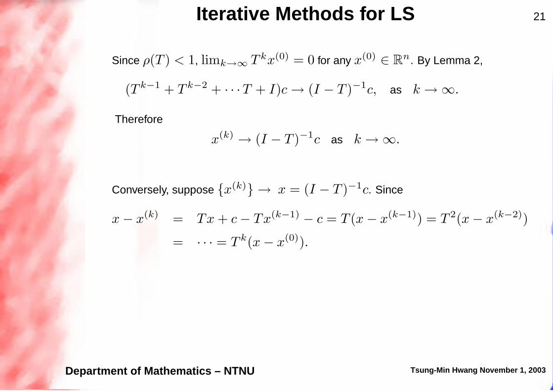
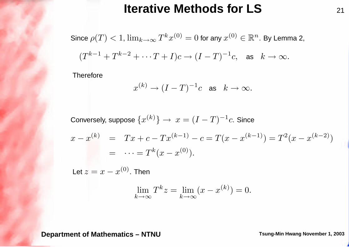
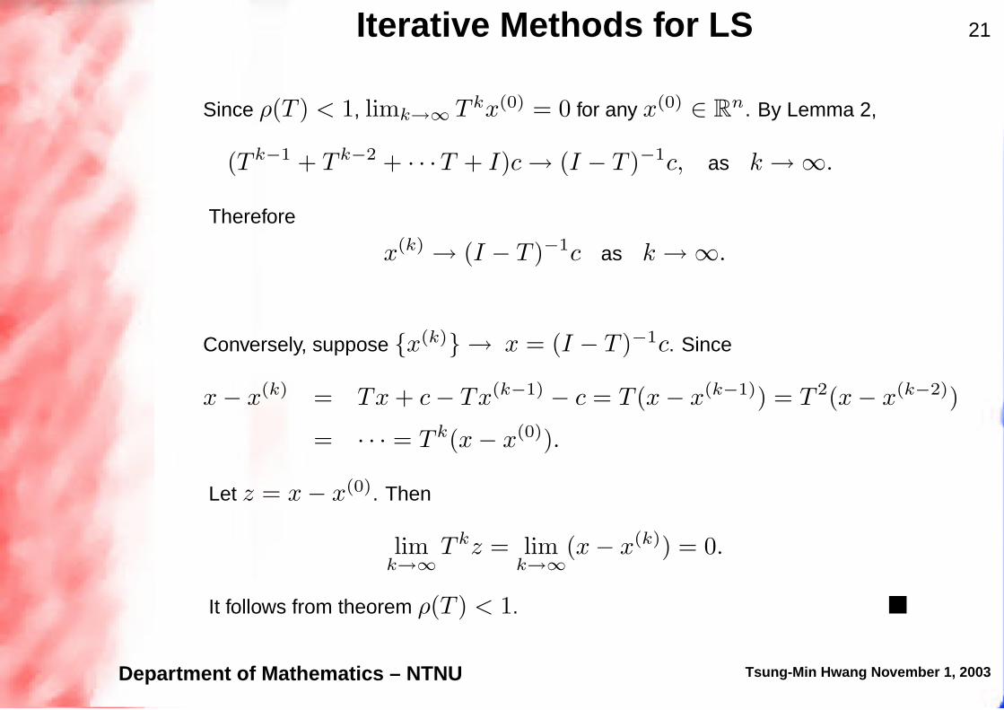
Iterative Methods for LS 21
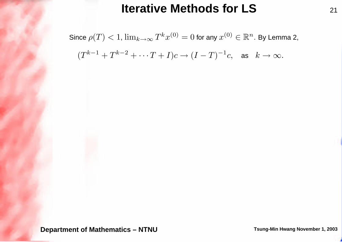
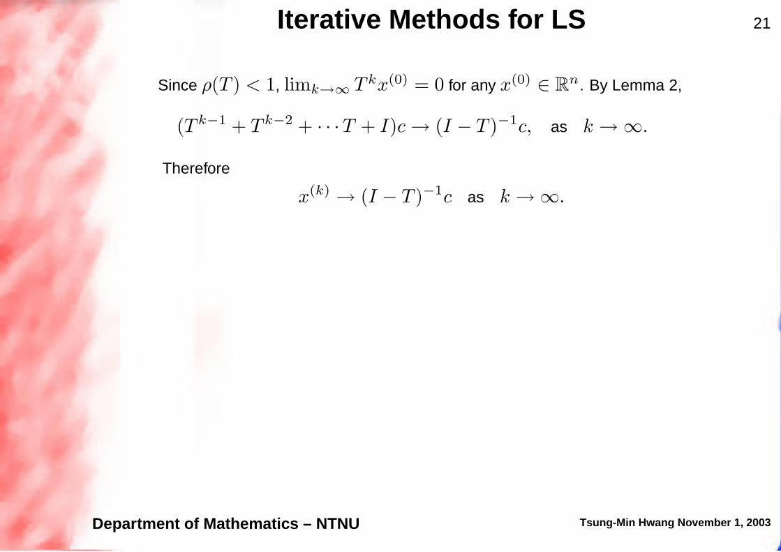
Since ρ(T ) < 1, limk→∞ T kx(0) = 0 for any x(0) ∈ Rn.
By Lemma 2,
(T k−1 + T k−2 + · · ·T + I)c → (I − T )−1c, as k → ∞.
Therefore
x(k) → (I − T )−1c as k → ∞.
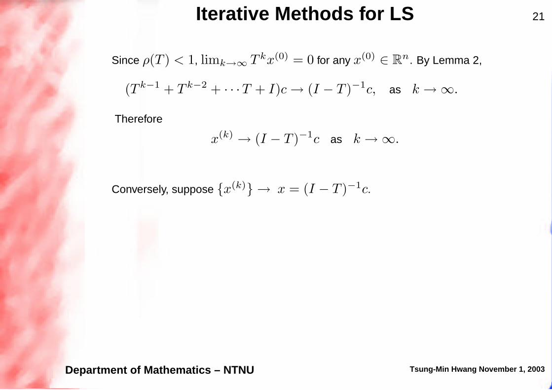
Conversely, suppose {x(k)} → x = (I − T )−1c. Since
x − x(k) = Tx + c − Tx(k−1) − c = T (x − x(k−1)) = T 2(x − x(k−2))
= · · · = T k(x − x(0)).
Let z = x − x(0). Then
limk→∞
T kz = limk→∞
(x − x(k)) = 0.
It follows from theorem ρ(T ) < 1.
Department of Mathematics – NTNU Tsung-Min Hwang November 1, 2003
Iterative Methods for LS 21
Since ρ(T ) < 1, limk→∞ T kx(0) = 0 for any x(0) ∈ Rn. By Lemma 2,
(T k−1 + T k−2 + · · ·T + I)c → (I − T )−1c, as k → ∞.
Therefore
x(k) → (I − T )−1c as k → ∞.
Conversely, suppose {x(k)} → x = (I − T )−1c.
Since
x − x(k) = Tx + c − Tx(k−1) − c = T (x − x(k−1)) = T 2(x − x(k−2))
= · · · = T k(x − x(0)).
Let z = x − x(0). Then
limk→∞
T kz = limk→∞
(x − x(k)) = 0.
It follows from theorem ρ(T ) < 1.
Department of Mathematics – NTNU Tsung-Min Hwang November 1, 2003
Iterative Methods for LS 21
Since ρ(T ) < 1, limk→∞ T kx(0) = 0 for any x(0) ∈ Rn. By Lemma 2,
(T k−1 + T k−2 + · · ·T + I)c → (I − T )−1c, as k → ∞.
Therefore
x(k) → (I − T )−1c as k → ∞.
Conversely, suppose {x(k)} → x = (I − T )−1c. Since
x − x(k) = Tx + c − Tx(k−1) − c = T (x − x(k−1)) = T 2(x − x(k−2))
= · · · = T k(x − x(0)).
Let z = x − x(0). Then
limk→∞
T kz = limk→∞
(x − x(k)) = 0.
It follows from theorem ρ(T ) < 1.
Department of Mathematics – NTNU Tsung-Min Hwang November 1, 2003

Iterative Methods for LS 21
Since ρ(T ) < 1, limk→∞ T kx(0) = 0 for any x(0) ∈ Rn. By Lemma 2,
(T k−1 + T k−2 + · · ·T + I)c → (I − T )−1c, as k → ∞.
Therefore
x(k) → (I − T )−1c as k → ∞.
Conversely, suppose {x(k)} → x = (I − T )−1c. Since
x − x(k) = Tx + c − Tx(k−1) − c = T (x − x(k−1)) = T 2(x − x(k−2))
= · · · = T k(x − x(0)).
Let z = x − x(0).
Then
limk→∞
T kz = limk→∞
(x − x(k)) = 0.
It follows from theorem ρ(T ) < 1.
Department of Mathematics – NTNU Tsung-Min Hwang November 1, 2003
Iterative Methods for LS 21
Since ρ(T ) < 1, limk→∞ T kx(0) = 0 for any x(0) ∈ Rn. By Lemma 2,
(T k−1 + T k−2 + · · ·T + I)c → (I − T )−1c, as k → ∞.
Therefore
x(k) → (I − T )−1c as k → ∞.
Conversely, suppose {x(k)} → x = (I − T )−1c. Since
x − x(k) = Tx + c − Tx(k−1) − c = T (x − x(k−1)) = T 2(x − x(k−2))
= · · · = T k(x − x(0)).
Let z = x − x(0). Then
limk→∞
T kz = limk→∞
(x − x(k)) = 0.
It follows from theorem ρ(T ) < 1.
Department of Mathematics – NTNU Tsung-Min Hwang November 1, 2003

Iterative Methods for LS 22
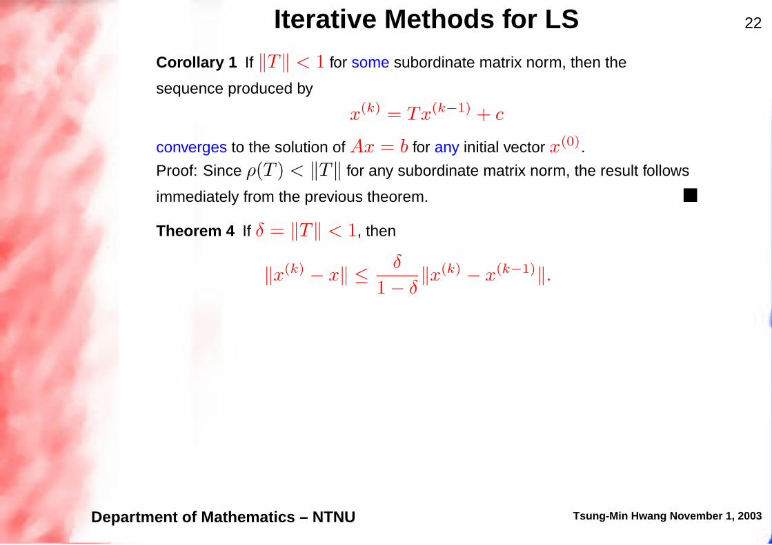
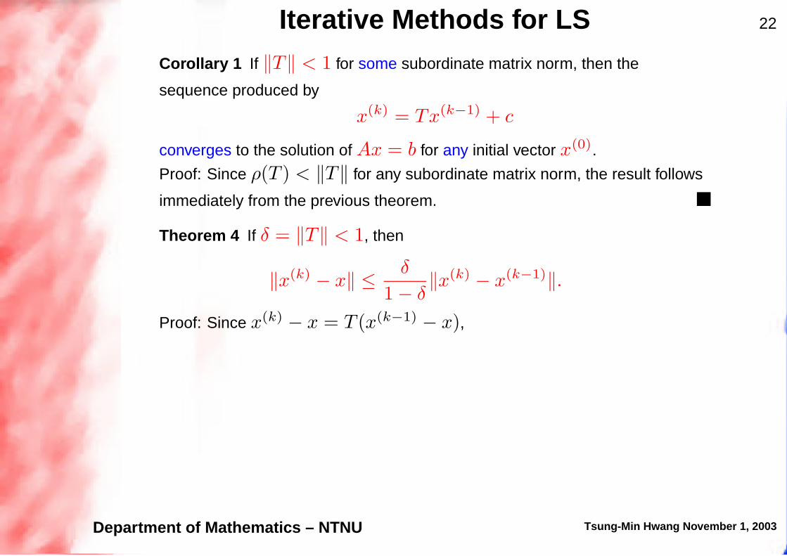
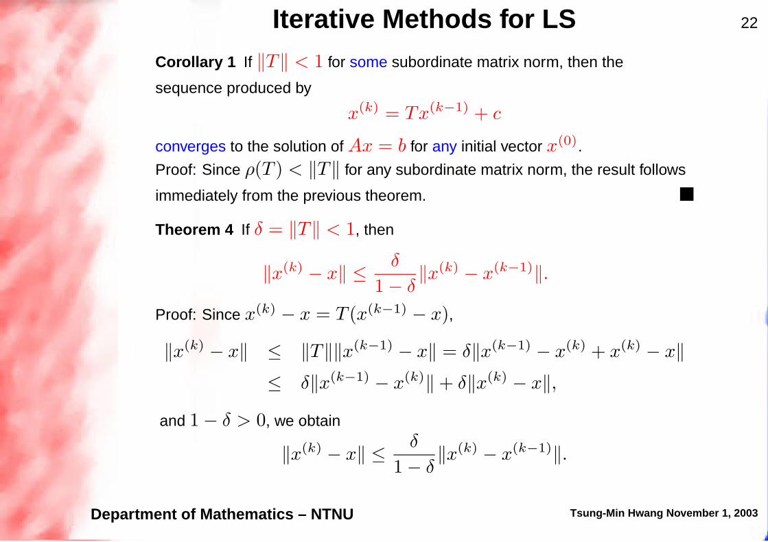
Corollary 1 If ‖T‖ < 1 for some subordinate matrix norm, then the
sequence produced by
x(k) = Tx(k−1) + c
converges to the solution of Ax = b for any initial vector x(0).
Proof: Since ρ(T ) < ‖T‖ for any subordinate matrix norm, the result follows
immediately from the previous theorem.
Theorem 4 If δ = ‖T‖ < 1, then
‖x(k) − x‖ ≤δ
1 − δ‖x(k) − x(k−1)‖.
Proof: Since x(k) − x = T (x(k−1) − x),
‖x(k) − x‖ ≤ ‖T‖‖x(k−1) − x‖ = δ‖x(k−1) − x(k) + x(k) − x‖
≤ δ‖x(k−1) − x(k)‖ + δ‖x(k) − x‖,
and 1 − δ > 0, we obtain
‖x(k) − x‖ ≤δ
1 − δ‖x(k) − x(k−1)‖.
Department of Mathematics – NTNU Tsung-Min Hwang November 1, 2003

Iterative Methods for LS 22
Corollary 1 If ‖T‖ < 1 for some subordinate matrix norm, then the
sequence produced by
x(k) = Tx(k−1) + c
converges to the solution of Ax = b for any initial vector x(0).
Proof: Since ρ(T ) < ‖T‖ for any subordinate matrix norm, the result follows
immediately from the previous theorem.
Theorem 4 If δ = ‖T‖ < 1, then
‖x(k) − x‖ ≤δ
1 − δ‖x(k) − x(k−1)‖.
Proof: Since x(k) − x = T (x(k−1) − x),
‖x(k) − x‖ ≤ ‖T‖‖x(k−1) − x‖ = δ‖x(k−1) − x(k) + x(k) − x‖
≤ δ‖x(k−1) − x(k)‖ + δ‖x(k) − x‖,
and 1 − δ > 0, we obtain
‖x(k) − x‖ ≤δ
1 − δ‖x(k) − x(k−1)‖.
Department of Mathematics – NTNU Tsung-Min Hwang November 1, 2003

Iterative Methods for LS 22
Corollary 1 If ‖T‖ < 1 for some subordinate matrix norm, then the
sequence produced by
x(k) = Tx(k−1) + c
converges to the solution of Ax = b for any initial vector x(0).
Proof: Since ρ(T ) < ‖T‖ for any subordinate matrix norm, the result follows
immediately from the previous theorem.
Theorem 4 If δ = ‖T‖ < 1, then
‖x(k) − x‖ ≤δ
1 − δ‖x(k) − x(k−1)‖.
Proof: Since x(k) − x = T (x(k−1) − x),
‖x(k) − x‖ ≤ ‖T‖‖x(k−1) − x‖ = δ‖x(k−1) − x(k) + x(k) − x‖
≤ δ‖x(k−1) − x(k)‖ + δ‖x(k) − x‖,
and 1 − δ > 0,
we obtain
‖x(k) − x‖ ≤δ
1 − δ‖x(k) − x(k−1)‖.
Department of Mathematics – NTNU Tsung-Min Hwang November 1, 2003
Iterative Methods for LS 22
Corollary 1 If ‖T‖ < 1 for some subordinate matrix norm, then the
sequence produced by
x(k) = Tx(k−1) + c
converges to the solution of Ax = b for any initial vector x(0).
Proof: Since ρ(T ) < ‖T‖ for any subordinate matrix norm, the result follows
immediately from the previous theorem.
Theorem 4 If δ = ‖T‖ < 1, then
‖x(k) − x‖ ≤δ
1 − δ‖x(k) − x(k−1)‖.
Proof: Since x(k) − x = T (x(k−1) − x),
‖x(k) − x‖ ≤ ‖T‖‖x(k−1) − x‖ = δ‖x(k−1) − x(k) + x(k) − x‖
≤ δ‖x(k−1) − x(k)‖ + δ‖x(k) − x‖,
and 1 − δ > 0, we obtain
‖x(k) − x‖ ≤δ
1 − δ‖x(k) − x(k−1)‖.
Department of Mathematics – NTNU Tsung-Min Hwang November 1, 2003
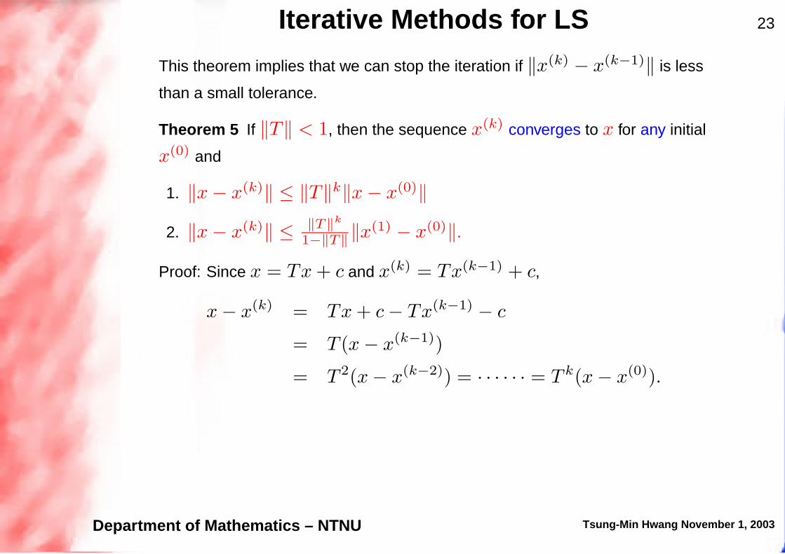
Iterative Methods for LS 23
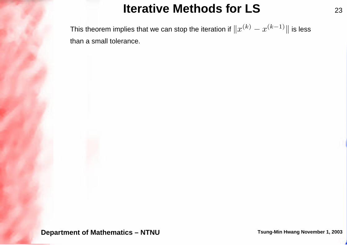
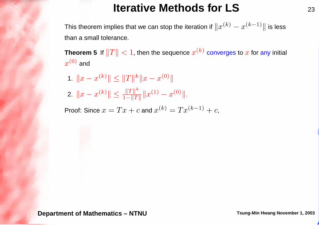
This theorem implies that we can stop the iteration if ‖x(k) − x(k−1)‖ is less
than a small tolerance.
Theorem 5 If ‖T‖ < 1, then the sequence x(k) converges to x for any initial
x(0) and
1. ‖x − x(k)‖ ≤ ‖T‖k‖x − x(0)‖
2. ‖x − x(k)‖ ≤ ‖T‖k
1−‖T‖‖x(1) − x(0)‖.
Proof: Since x = Tx + c and x(k) = Tx(k−1) + c,
x − x(k) = Tx + c − Tx(k−1) − c
= T (x − x(k−1))
= T 2(x − x(k−2)) = · · · · · · = T k(x − x(0)).
The first statement can then be derived
‖x − x(k)‖ = ‖T k(x − x(0))‖ ≤ ‖T‖k‖x − x(0)‖.
Department of Mathematics – NTNU Tsung-Min Hwang November 1, 2003

Iterative Methods for LS 23
This theorem implies that we can stop the iteration if ‖x(k) − x(k−1)‖ is less
than a small tolerance.
Theorem 5 If ‖T‖ < 1, then the sequence x(k) converges to x for any initial
x(0) and
1. ‖x − x(k)‖ ≤ ‖T‖k‖x − x(0)‖
2. ‖x − x(k)‖ ≤ ‖T‖k
1−‖T‖‖x(1) − x(0)‖.
Proof: Since x = Tx + c and x(k) = Tx(k−1) + c,
x − x(k) = Tx + c − Tx(k−1) − c
= T (x − x(k−1))
= T 2(x − x(k−2)) = · · · · · · = T k(x − x(0)).
The first statement can then be derived
‖x − x(k)‖ = ‖T k(x − x(0))‖ ≤ ‖T‖k‖x − x(0)‖.
Department of Mathematics – NTNU Tsung-Min Hwang November 1, 2003

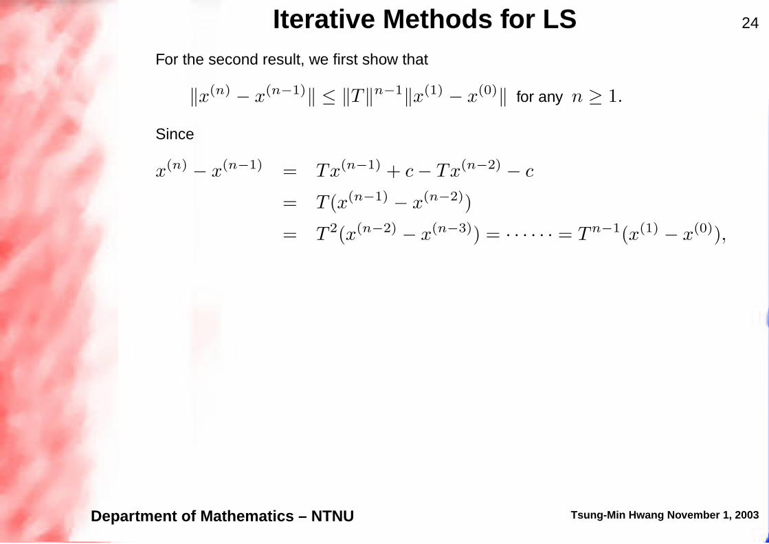
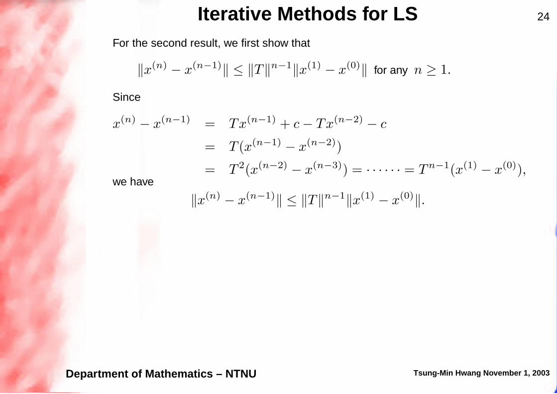
Iterative Methods for LS 24
For the second result, we first show that
‖x(n) − x(n−1)‖ ≤ ‖T‖n−1‖x(1) − x(0)‖ for any n ≥ 1.
Since
x(n) − x(n−1) = Tx(n−1) + c − Tx(n−2) − c
= T (x(n−1) − x(n−2))
= T 2(x(n−2) − x(n−3)) = · · · · · · = T n−1(x(1) − x(0)),we have
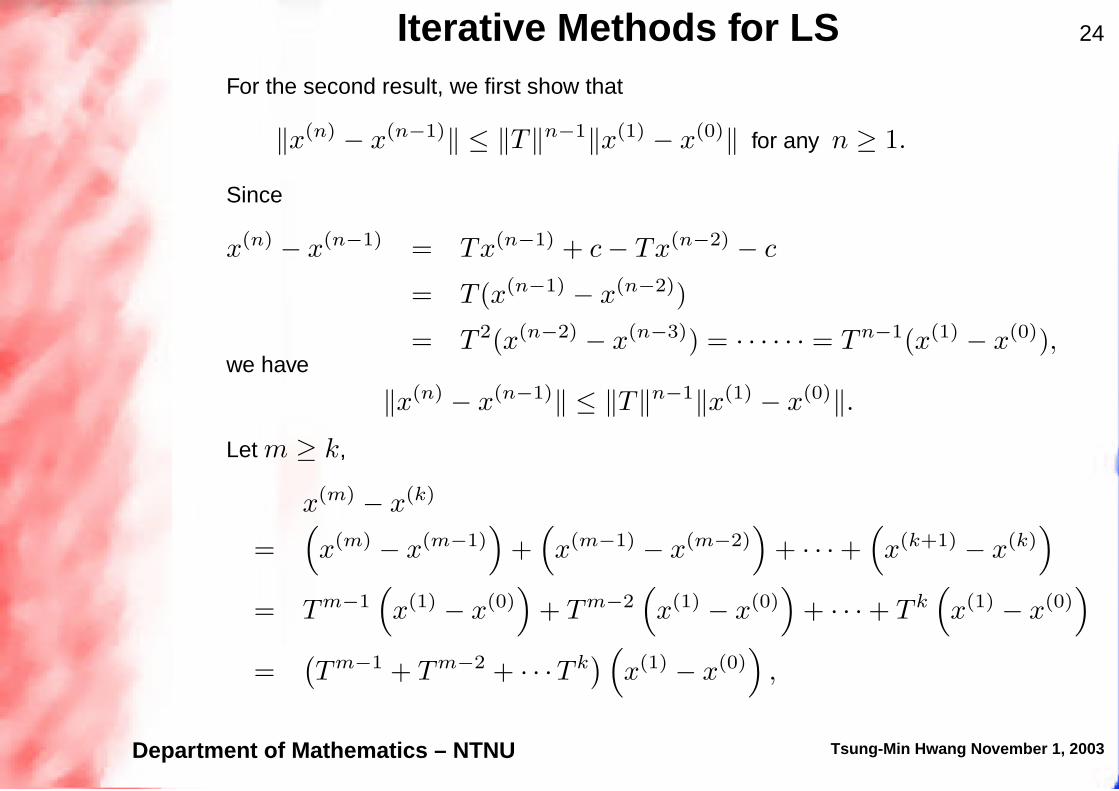
‖x(n) − x(n−1)‖ ≤ ‖T‖n−1‖x(1) − x(0)‖.
Let m ≥ k,
x(m) − x(k)
=(
x(m) − x(m−1))
+(
x(m−1) − x(m−2))
+ · · · +(
x(k+1) − x(k))
= Tm−1(
x(1) − x(0))
+ Tm−2(
x(1) − x(0))
+ · · · + T k(
x(1) − x(0))
=(
Tm−1 + Tm−2 + · · ·T k)
(
x(1) − x(0))
,
Department of Mathematics – NTNU Tsung-Min Hwang November 1, 2003
Iterative Methods for LS 24
For the second result, we first show that
‖x(n) − x(n−1)‖ ≤ ‖T‖n−1‖x(1) − x(0)‖ for any n ≥ 1.
Since
x(n) − x(n−1) = Tx(n−1) + c − Tx(n−2) − c
= T (x(n−1) − x(n−2))
= T 2(x(n−2) − x(n−3)) = · · · · · · = T n−1(x(1) − x(0)),
we have
‖x(n) − x(n−1)‖ ≤ ‖T‖n−1‖x(1) − x(0)‖.
Let m ≥ k,
x(m) − x(k)
=(
x(m) − x(m−1))
+(
x(m−1) − x(m−2))
+ · · · +(
x(k+1) − x(k))
= Tm−1(
x(1) − x(0))
+ Tm−2(
x(1) − x(0))
+ · · · + T k(
x(1) − x(0))
=(
Tm−1 + Tm−2 + · · ·T k)
(
x(1) − x(0))
,
Department of Mathematics – NTNU Tsung-Min Hwang November 1, 2003
Iterative Methods for LS 24
For the second result, we first show that
‖x(n) − x(n−1)‖ ≤ ‖T‖n−1‖x(1) − x(0)‖ for any n ≥ 1.
Since
x(n) − x(n−1) = Tx(n−1) + c − Tx(n−2) − c
= T (x(n−1) − x(n−2))
= T 2(x(n−2) − x(n−3)) = · · · · · · = T n−1(x(1) − x(0)),we have
‖x(n) − x(n−1)‖ ≤ ‖T‖n−1‖x(1) − x(0)‖.
Let m ≥ k,
x(m) − x(k)
=(
x(m) − x(m−1))
+(
x(m−1) − x(m−2))
+ · · · +(
x(k+1) − x(k))
= Tm−1(
x(1) − x(0))
+ Tm−2(
x(1) − x(0))
+ · · · + T k(
x(1) − x(0))
=(
Tm−1 + Tm−2 + · · ·T k)
(
x(1) − x(0))
,
Department of Mathematics – NTNU Tsung-Min Hwang November 1, 2003
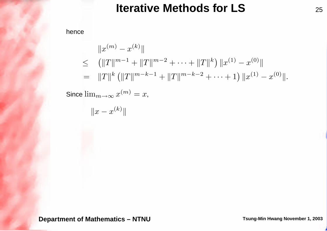
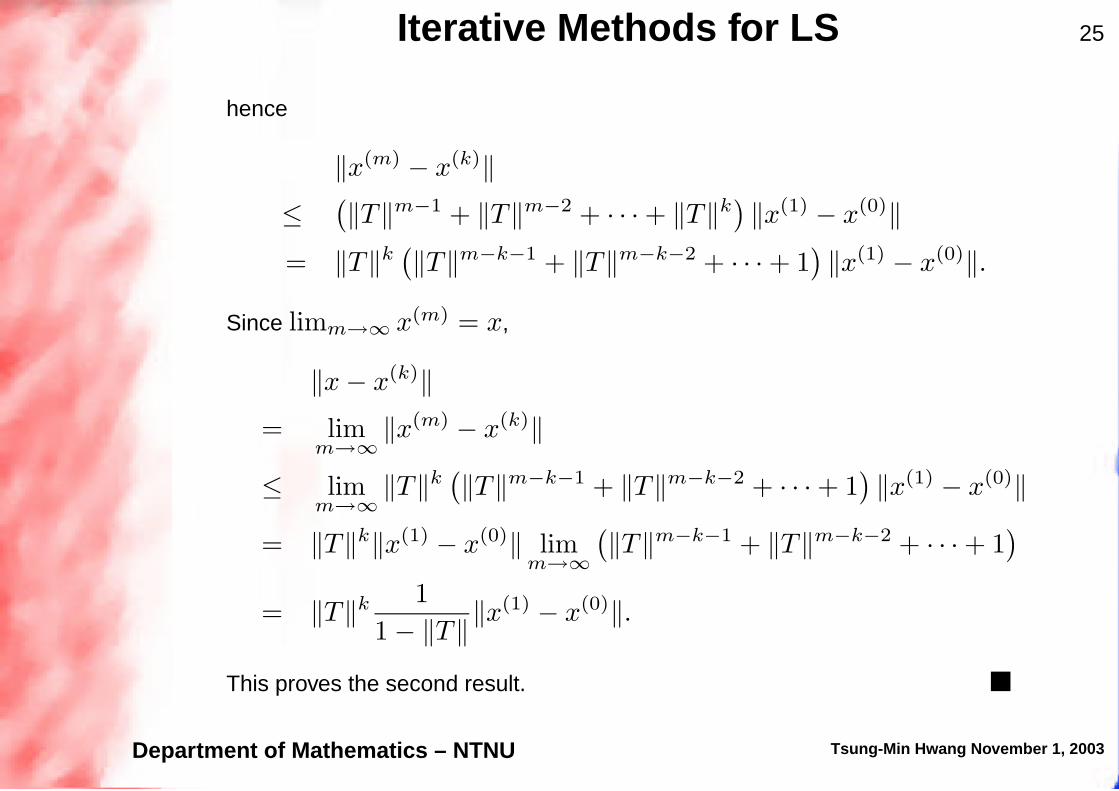
Iterative Methods for LS 25
hence
‖x(m) − x(k)‖
≤(
‖T‖m−1 + ‖T‖m−2 + · · · + ‖T‖k)
‖x(1) − x(0)‖
= ‖T‖k(
‖T‖m−k−1 + ‖T‖m−k−2 + · · · + 1)
‖x(1) − x(0)‖.
Since limm→∞ x(m) = x,
‖x − x(k)‖
= limm→∞
‖x(m) − x(k)‖
≤ limm→∞
‖T‖k(
‖T‖m−k−1 + ‖T‖m−k−2 + · · · + 1)
‖x(1) − x(0)‖
= ‖T‖k‖x(1) − x(0)‖ limm→∞
(
‖T‖m−k−1 + ‖T‖m−k−2 + · · · + 1)
= ‖T‖k 1
1 − ‖T‖‖x(1) − x(0)‖.
This proves the second result.
Department of Mathematics – NTNU Tsung-Min Hwang November 1, 2003

Iterative Methods for LS 26
Theorem 6 If A is strictly diagonal dominant, then both the Jacobi and
Gauss-Seidel methods converges for any initial vector x(0).
Proof: By assumption, A is strictly diagonal dominant, hence aii 6= 0
(otherwise A is singular) and
|aii| >
n∑
j=1,j 6=i
|aij |, i = 1, 2, . . . , n.
For Jacobi method, the iteration matrix TJ = −D−1(L + U) has entries
[TJ ]ij =
−aij
aiii 6= j
0 i = j
Hence
‖TJ‖∞ = max1≤i≤n
n∑
j=1,j 6=i
∣
∣
∣
∣
aij
aii
∣
∣
∣
∣
= max1≤i≤n
1
|aii|
n∑
j=1,j 6=i
|aij | < 1,
and this implies that the Jacobi method converges.
Department of Mathematics – NTNU Tsung-Min Hwang November 1, 2003
Iterative Methods for LS 26
Theorem 6 If A is strictly diagonal dominant, then both the Jacobi and
Gauss-Seidel methods converges for any initial vector x(0).
Proof: By assumption, A is strictly diagonal dominant,
hence aii 6= 0
(otherwise A is singular) and
|aii| >
n∑
j=1,j 6=i
|aij |, i = 1, 2, . . . , n.
For Jacobi method, the iteration matrix TJ = −D−1(L + U) has entries
[TJ ]ij =
−aij
aiii 6= j
0 i = j
Hence
‖TJ‖∞ = max1≤i≤n
n∑
j=1,j 6=i
∣
∣
∣
∣
aij
aii
∣
∣
∣
∣
= max1≤i≤n
1
|aii|
n∑
j=1,j 6=i
|aij | < 1,
and this implies that the Jacobi method converges.
Department of Mathematics – NTNU Tsung-Min Hwang November 1, 2003

Iterative Methods for LS 26
Theorem 6 If A is strictly diagonal dominant, then both the Jacobi and
Gauss-Seidel methods converges for any initial vector x(0).
Proof: By assumption, A is strictly diagonal dominant, hence aii 6= 0
(otherwise A is singular) and
|aii| >
n∑
j=1,j 6=i
|aij |, i = 1, 2, . . . , n.
For Jacobi method, the iteration matrix TJ = −D−1(L + U) has entries
[TJ ]ij =
−aij
aiii 6= j
0 i = j
Hence
‖TJ‖∞ = max1≤i≤n
n∑
j=1,j 6=i
∣
∣
∣
∣
aij
aii
∣
∣
∣
∣
= max1≤i≤n
1
|aii|
n∑
j=1,j 6=i
|aij | < 1,
and this implies that the Jacobi method converges.
Department of Mathematics – NTNU Tsung-Min Hwang November 1, 2003
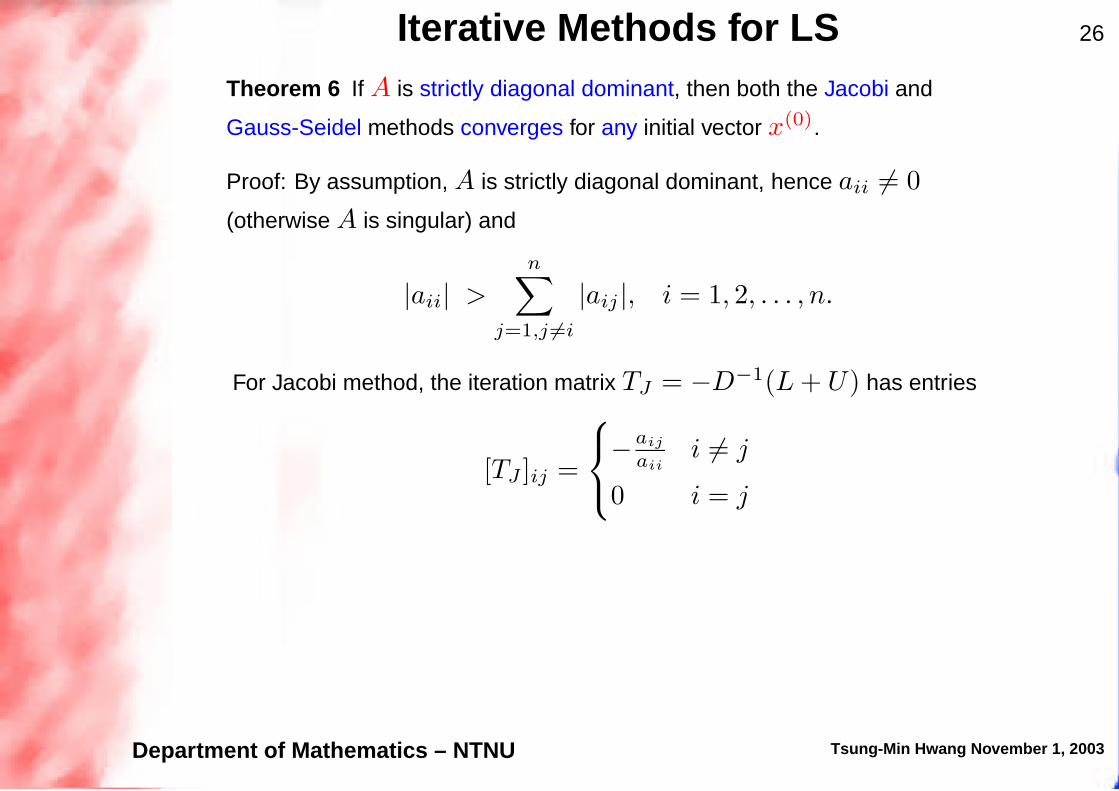
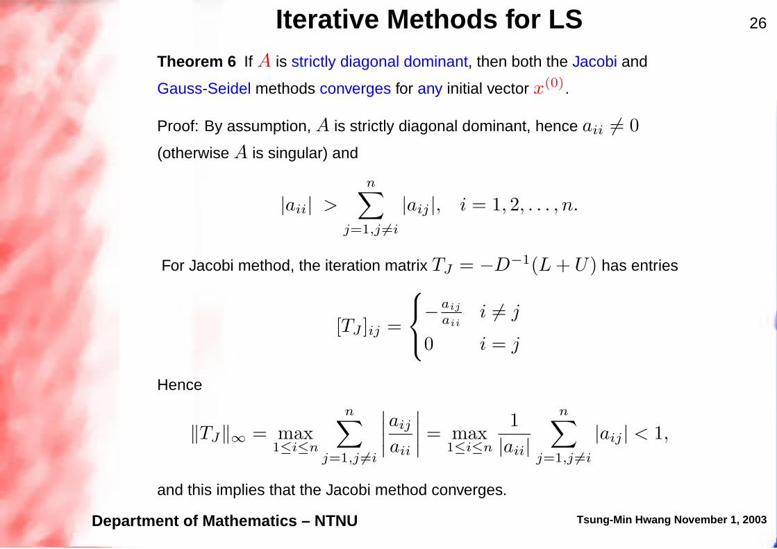

Iterative Methods for LS 27
For Gauss-Seidel method, the iteration matrix TGS = −(D + L)−1U .
Let λ
be any eigenvalue of TGS and y, ‖y‖∞ = 1, is a corresponding eigenvector.
Thus
TGSy = λy =⇒ −Uy = λ(D + L)y.
Hence for i = 1, . . . , n,
−
n∑
j=i+1
aijyj = λaiiyi + λ
i−1∑
j=1
aijyj .
This gives
λaiiyi = −λ
i−1∑
j=1
aijyj +n∑
j=i+1
aijyj
and
|λ||aii||yi| ≤ |λ|
i−1∑
j=1
|aij ||yj | +
n∑
j=i+1
|aij ||yj |.
Department of Mathematics – NTNU Tsung-Min Hwang November 1, 2003
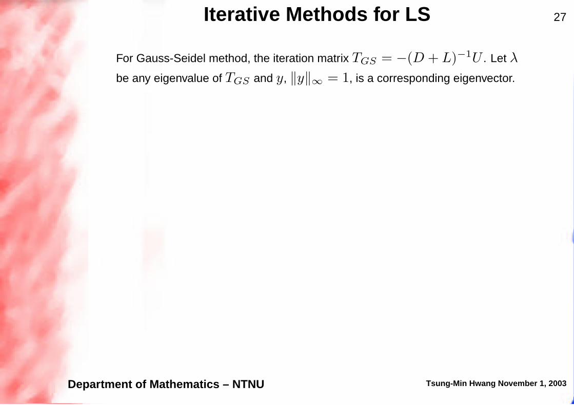
Iterative Methods for LS 27
For Gauss-Seidel method, the iteration matrix TGS = −(D + L)−1U . Let λ
be any eigenvalue of TGS and y, ‖y‖∞ = 1, is a corresponding eigenvector.
Thus
TGSy = λy =⇒ −Uy = λ(D + L)y.
Hence for i = 1, . . . , n,
−
n∑
j=i+1
aijyj = λaiiyi + λ
i−1∑
j=1
aijyj .
This gives
λaiiyi = −λ
i−1∑
j=1
aijyj +n∑
j=i+1
aijyj
and
|λ||aii||yi| ≤ |λ|
i−1∑
j=1
|aij ||yj | +
n∑
j=i+1
|aij ||yj |.
Department of Mathematics – NTNU Tsung-Min Hwang November 1, 2003
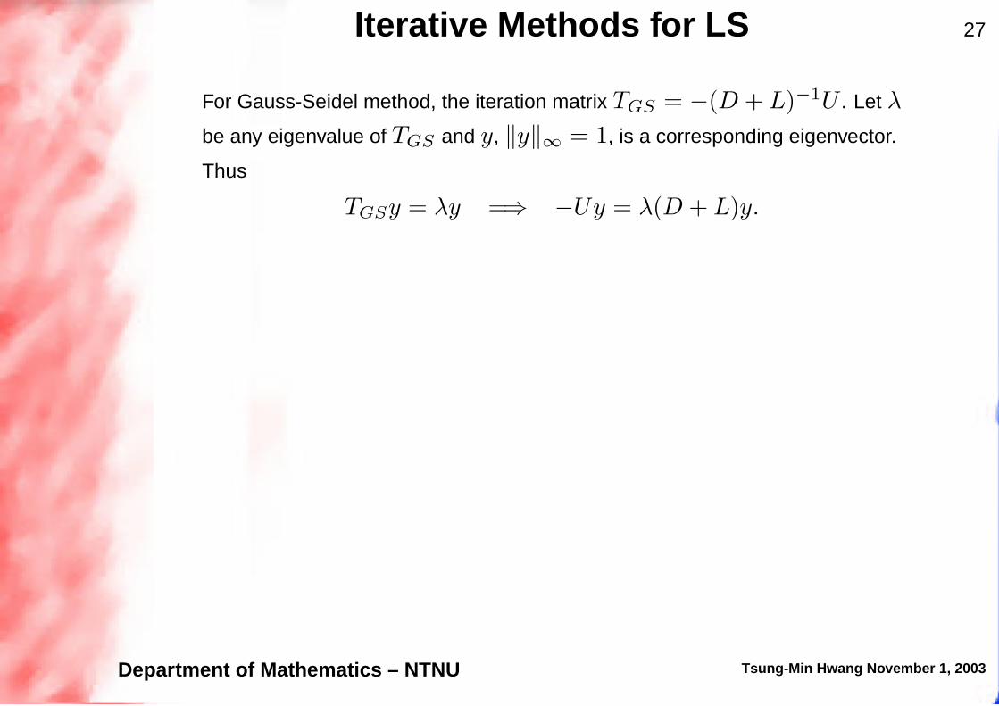
Iterative Methods for LS 27
For Gauss-Seidel method, the iteration matrix TGS = −(D + L)−1U . Let λ
be any eigenvalue of TGS and y, ‖y‖∞ = 1, is a corresponding eigenvector.
Thus
TGSy = λy =⇒ −Uy = λ(D + L)y.
Hence for i = 1, . . . , n,
−
n∑
j=i+1
aijyj = λaiiyi + λ
i−1∑
j=1
aijyj .
This gives
λaiiyi = −λ
i−1∑
j=1
aijyj +n∑
j=i+1
aijyj
and
|λ||aii||yi| ≤ |λ|
i−1∑
j=1
|aij ||yj | +
n∑
j=i+1
|aij ||yj |.
Department of Mathematics – NTNU Tsung-Min Hwang November 1, 2003
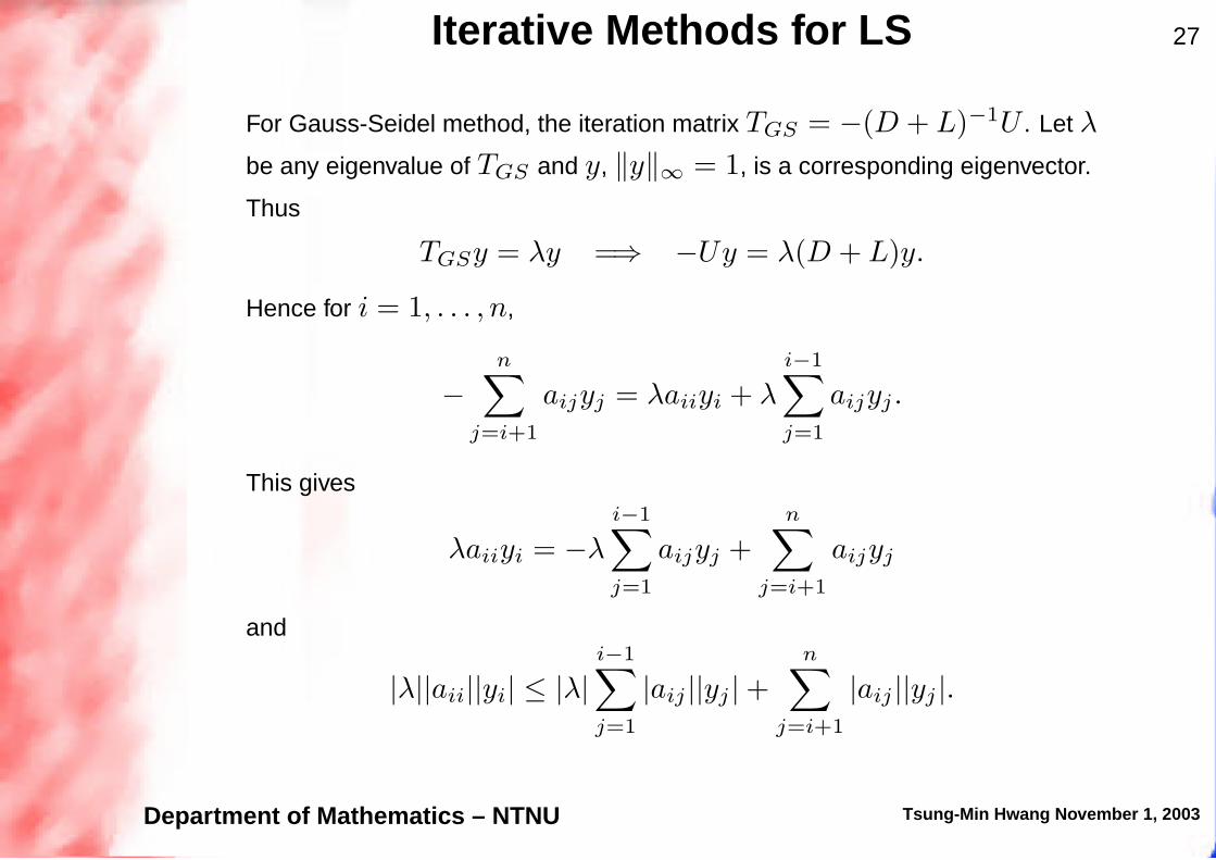
Iterative Methods for LS 27
For Gauss-Seidel method, the iteration matrix TGS = −(D + L)−1U . Let λ
be any eigenvalue of TGS and y, ‖y‖∞ = 1, is a corresponding eigenvector.
Thus
TGSy = λy =⇒ −Uy = λ(D + L)y.
Hence for i = 1, . . . , n,
−
n∑
j=i+1
aijyj = λaiiyi + λ
i−1∑
j=1
aijyj .
This gives
λaiiyi = −λ
i−1∑
j=1
aijyj +n∑
j=i+1
aijyj
and
|λ||aii||yi| ≤ |λ|
i−1∑
j=1
|aij ||yj | +
n∑
j=i+1
|aij ||yj |.
Department of Mathematics – NTNU Tsung-Min Hwang November 1, 2003
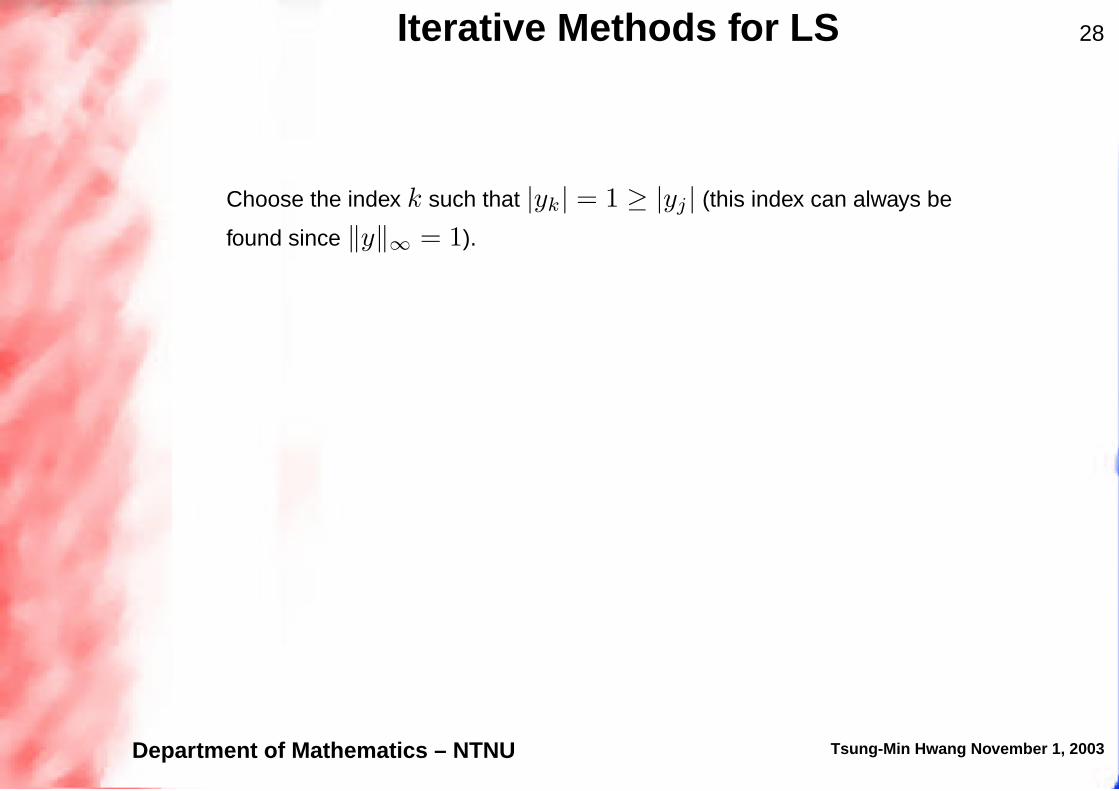
Iterative Methods for LS 28
Choose the index k such that |yk| = 1 ≥ |yj | (this index can always be
found since ‖y‖∞ = 1).
Then
|λ||akk| ≤ |λ|
k−1∑
j=1
|akj | +
n∑
j=k+1
|akj |
which gives
|λ| ≤
∑n
j=k+1 |akj |
|akk| −∑k−1
j=1 |akj |<
∑n
j=k+1 |akj |∑n
j=k+1 |akj |= 1
Since λ is arbitrary, ρ(TGS) < 1. This means the Gauss-Seidel method
converges.
Department of Mathematics – NTNU Tsung-Min Hwang November 1, 2003
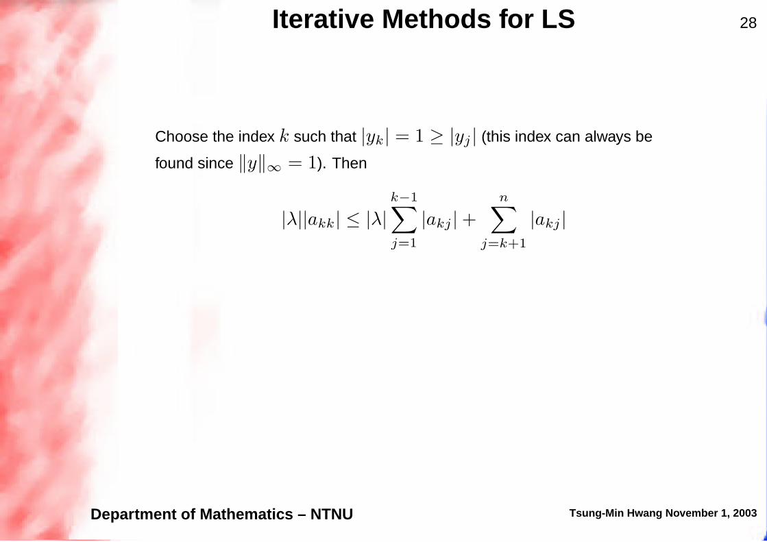
Iterative Methods for LS 28
Choose the index k such that |yk| = 1 ≥ |yj | (this index can always be
found since ‖y‖∞ = 1). Then
|λ||akk| ≤ |λ|
k−1∑
j=1
|akj | +
n∑
j=k+1
|akj |
which gives
|λ| ≤
∑n
j=k+1 |akj |
|akk| −∑k−1
j=1 |akj |<
∑n
j=k+1 |akj |∑n
j=k+1 |akj |= 1
Since λ is arbitrary, ρ(TGS) < 1. This means the Gauss-Seidel method
converges.
Department of Mathematics – NTNU Tsung-Min Hwang November 1, 2003
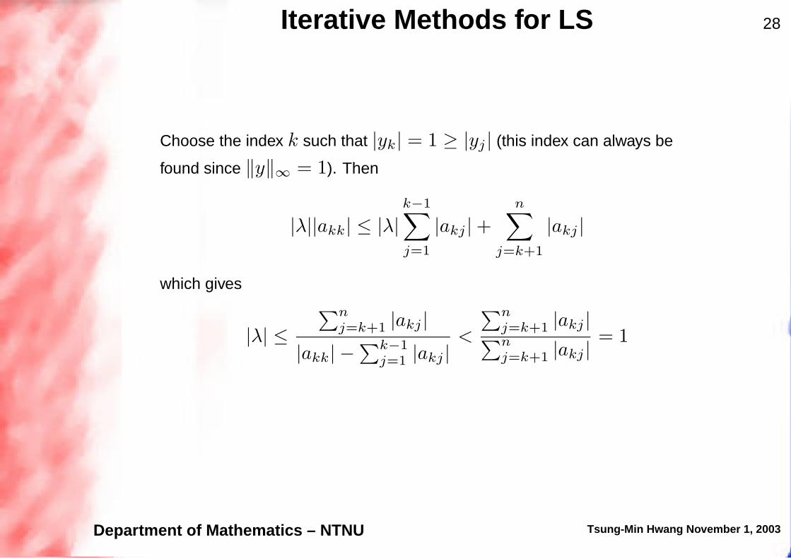
Iterative Methods for LS 28
Choose the index k such that |yk| = 1 ≥ |yj | (this index can always be
found since ‖y‖∞ = 1). Then
|λ||akk| ≤ |λ|
k−1∑
j=1
|akj | +
n∑
j=k+1
|akj |
which gives
|λ| ≤
∑n
j=k+1 |akj |
|akk| −∑k−1
j=1 |akj |<
∑n
j=k+1 |akj |∑n
j=k+1 |akj |= 1
Since λ is arbitrary, ρ(TGS) < 1.
This means the Gauss-Seidel method
converges.
Department of Mathematics – NTNU Tsung-Min Hwang November 1, 2003

Iterative Methods for LS 28
Choose the index k such that |yk| = 1 ≥ |yj | (this index can always be
found since ‖y‖∞ = 1). Then
|λ||akk| ≤ |λ|
k−1∑
j=1
|akj | +
n∑
j=k+1
|akj |
which gives
|λ| ≤
∑n
j=k+1 |akj |
|akk| −∑k−1
j=1 |akj |<
∑n
j=k+1 |akj |∑n
j=k+1 |akj |= 1
Since λ is arbitrary, ρ(TGS) < 1. This means the Gauss-Seidel method
converges.
Department of Mathematics – NTNU Tsung-Min Hwang November 1, 2003

Iterative Methods for LS 29
Theorem 7 If A is positive definite and the relaxation parameter ω satisfying
0 < ω < 2, then the SOR iteration converges for any initial vector x(0).
Theorem 8 If A is positive definite and tridiagonal, then
ρ(TGS) = [ρ(TJ)]2
< 1 and the optimal choice of ω for the SOR iteration is
ω =2
1 +
√
1 − [ρ(TJ)]2.
With this choice of ω, ρ(TSOR) = ω − 1.
Department of Mathematics – NTNU Tsung-Min Hwang November 1, 2003
Related Documents