ITERATIVE IMPROVEMENT TECHNIQUES FOR SOLVING ...

ITERATIVE IMPROVEMENT TECHNIQUES FOR SOLVING TIGHT CONSTRAINT

SATISFACTION PROBLEMS

by

Hui Zou

A THESIS

Presented to the Faculty of

The Graduate College at the University of Nebraska

In Partial Fulfilment of Requirements

For the Degree of Master of Science

Major: Computer Science

Under the Supervision of Professor Berthe Y. Choueiry

Lincoln, Nebraska

November, 2003

ITERATIVE IMPROVEMENT TECHNIQUES FOR SOLVING TIGHT CONSTRAINT

SATISFACTION PROBLEMS

Hui Zou, M.S.

University of Nebraska, 2003

Advisor: Berthe Y. Choueiry

In this thesis, we explore two iterative improvement techniques: a heuristic hill-climbing

strategy (denoted LS) and a multi-agent based search (denoted ERA). We focus our inves-

tigations on one small but challenging real-world application, which is the assignment of

Graduate Teaching Assistants (GTA) to academic tasks. We design and implement the

LS and ERA mechanisms to solve this application. We propose and test various heuristic

improvements. Finally, we compare the performance of thesemechanisms and that of the

heuristic backtrack search of[Glaubius and Choueiry, 2002a] for solving a set of real-world

data we have been collecting.

Our investigations demonstrate that although LS is able to find ‘good’ solutions quickly,

it suffers from known shortcomings such as monotonic improvement and quick stabiliza-

tion. We experimentally investigate the integration of noise strategies to enable LS to es-

cape from local optima. By introducing the framework of Generalized Local Search (GLS),

we summarize the various directions that can be pursued to performance of local search

techniques in general.

We demonstrate that, among the tested strategies, ERA is themost immune to local

optima because of its extreme decentralization. Indeed, itis the only strategy we imple-

mented that is capable of solving some tight problem instances that are thought to be over-

constrained. However, on unsolvable problem instances, ERA’s behavior becomes erratic

and unreliable in terms of stability and the quality of the solutions reached. We identify

the source of this shortcoming and characterize it as a deadlock phenomenon. Further, we

discuss possible approaches for handling and solving deadlocks.

ACKNOWLEDGEMENTS

First and foremost, I would like to thank my advisor, Dr. Berthe Y. Choueiry, for her

support, guidance and advice during my work on this thesis. By giving me the opportunity

to do this research, she has changed the course of my life so much for the better.

There are many people in the Department of Computer Science who have made my time

there enjoyable. In particular I would like to especially thank my committee members, Dr.

F. Fred Choobineh, Dr. Hong Jiang and Dr. Peter Revesz, for the many hours spent

reading and discussing my work.

I am very grateful that I had the opportunity to work as a member of the Constraint

Systems Laboratory for the past two years. I enjoyed pursuing my research interests and

obtaining a wealth of invaluable experience in many aspectsof my academic life. I also

thank the members in the lab, in particular Daniel Buettner,Amy Davis and Lin Xu, for

their support and for our many interesting discussions.

In addition, I would like to thank Deborah Derrick and Claudia Reinhardt for their

valuable editorial help.

Finally I am deeply grateful to my parents who sent me on my wayand provided a stable

and stimulating environment for my personal and intellectual development. I gratefully

acknowledge the constant support of Fenghong Liu for her wise advice and for all the love

we share.

This research is supported by NSF grant #EPS-0091900.

4

Contents

1 Introduction 11.1 Motivations . . . . . . . . . . . . . . . . . . . . . . . . . . . . . . . . . . 21.2 Related works . . . . . . . . . . . . . . . . . . . . . . . . . . . . . . . . . 31.3 Questions addressed . . . . . . . . . . . . . . . . . . . . . . . . . . . . . .51.4 Contributions . . . . . . . . . . . . . . . . . . . . . . . . . . . . . . . . . 61.5 Outline of the thesis . . . . . . . . . . . . . . . . . . . . . . . . . . . . . .8

2 Background 92.1 Constraint satisfaction problem (CSP) . . . . . . . . . . . . . .. . . . . . 9

2.1.1 Definition of a constraint satisfaction problem . . . . .. . . . . . . 102.1.2 CSP characteristics . . . . . . . . . . . . . . . . . . . . . . . . . . 102.1.3 Partial solutions . . . . . . . . . . . . . . . . . . . . . . . . . . . . 11

2.2 Graduate Teaching Assistants (GTA) problem . . . . . . . . . .. . . . . . 122.2.1 What is the GTA Assignment Problem? . . . . . . . . . . . . . . . 132.2.2 Characteristics of the GTA assignment problem . . . . . .. . . . . 13

2.3 Systematic Search (BT) . . . . . . . . . . . . . . . . . . . . . . . . . . . .162.4 Local search . . . . . . . . . . . . . . . . . . . . . . . . . . . . . . . . . . 16

2.4.1 Algorithms of local search (LS) . . . . . . . . . . . . . . . . . . .162.4.2 Guidance heuristics . . . . . . . . . . . . . . . . . . . . . . . . . . 17

2.5 Multi-agent based approaches . . . . . . . . . . . . . . . . . . . . . .. . 182.5.1 Multi-agent system . . . . . . . . . . . . . . . . . . . . . . . . . . 182.5.2 A Multi-agent-based search method . . . . . . . . . . . . . . . .. 18

2.6 Las Vegas algorithms . . . . . . . . . . . . . . . . . . . . . . . . . . . . . 20

3 A heuristic hill-climbing search 223.1 Hill-climbing search . . . . . . . . . . . . . . . . . . . . . . . . . . . . .233.2 Min-conflict heuristic . . . . . . . . . . . . . . . . . . . . . . . . . . . .. 25

3.2.1 Dealing with global constraints . . . . . . . . . . . . . . . . . .. 263.2.2 Improving min-conflict with random walk . . . . . . . . . . . .. . 273.2.3 Improving local search with random restart . . . . . . . . .. . . . 273.2.4 Algorithms tested . . . . . . . . . . . . . . . . . . . . . . . . . . . 28

3.3 Experimental study . . . . . . . . . . . . . . . . . . . . . . . . . . . . . . 283.3.1 Test cases . . . . . . . . . . . . . . . . . . . . . . . . . . . . . . . 29

3.3.2 Parameters setting . . . . . . . . . . . . . . . . . . . . . . . . . . 293.3.3 Conditions of experiments . . . . . . . . . . . . . . . . . . . . . . 29

3.4 Results and observations . . . . . . . . . . . . . . . . . . . . . . . . . .. 303.4.1 Non-binary constraints in local search . . . . . . . . . . . .. . . . 303.4.2 Local search versus systematic search . . . . . . . . . . . . .. . . 333.4.3 Solvable instances versus unsolvable instances . . . .. . . . . . . 343.4.4 Random-walk in the min-conflict heuristics . . . . . . . . .. . . . 353.4.5 Value of the noise probability in random walk . . . . . . . .. . . . 353.4.6 The number of restarts . . . . . . . . . . . . . . . . . . . . . . . . 38

3.5 Discussion . . . . . . . . . . . . . . . . . . . . . . . . . . . . . . . . . . . 393.5.1 Binary vs. non-binary representation . . . . . . . . . . . . .. . . . 403.5.2 Local search (LS) vs. systematic search (BT) . . . . . . . .. . . . 413.5.3 Solvable vs. unsolvable instances . . . . . . . . . . . . . . . .. . 423.5.4 One-time repair . . . . . . . . . . . . . . . . . . . . . . . . . . . . 423.5.5 Dealing with local optima . . . . . . . . . . . . . . . . . . . . . . 43

3.6 Conclusions . . . . . . . . . . . . . . . . . . . . . . . . . . . . . . . . . . 44

4 A multi-agent based search 464.1 Background . . . . . . . . . . . . . . . . . . . . . . . . . . . . . . . . . . 464.2 ERA model . . . . . . . . . . . . . . . . . . . . . . . . . . . . . . . . . . 47

4.2.1 Environment . . . . . . . . . . . . . . . . . . . . . . . . . . . . . 484.2.2 Reactive rules . . . . . . . . . . . . . . . . . . . . . . . . . . . . . 484.2.3 Agent . . . . . . . . . . . . . . . . . . . . . . . . . . . . . . . . . 494.2.4 ERA algorithm . . . . . . . . . . . . . . . . . . . . . . . . . . . . 50

4.3 Control strategies in ERA . . . . . . . . . . . . . . . . . . . . . . . . . .. 534.4 Empirical evaluation of ERA . . . . . . . . . . . . . . . . . . . . . . . .. 54

4.4.1 Testing the behavior of ERA . . . . . . . . . . . . . . . . . . . . . 554.4.2 Performance comparison: ERA, LS, and BT . . . . . . . . . . . .574.4.3 Observing behavior of individual agents . . . . . . . . . . .. . . . 624.4.4 Deadlock phenomenon . . . . . . . . . . . . . . . . . . . . . . . . 63

4.5 Discussion . . . . . . . . . . . . . . . . . . . . . . . . . . . . . . . . . . . 664.5.1 Control schema: Global vs. local. . . . . . . . . . . . . . . . . .. 674.5.2 Freedom to undo assignments. . . . . . . . . . . . . . . . . . . . . 684.5.3 Conflict resolution and deadlock prevention. . . . . . . .. . . . . 69

4.6 Dealing with the deadlock . . . . . . . . . . . . . . . . . . . . . . . . . .704.6.1 Direct communication and negotiation mechanism . . . .. . . . . 704.6.2 Hybridization algorithms . . . . . . . . . . . . . . . . . . . . . . .704.6.3 Mixing behaviored rules . . . . . . . . . . . . . . . . . . . . . . . 714.6.4 Adding global control . . . . . . . . . . . . . . . . . . . . . . . . 714.6.5 Conflict resolution . . . . . . . . . . . . . . . . . . . . . . . . . . 71

4.7 Conclusions . . . . . . . . . . . . . . . . . . . . . . . . . . . . . . . . . . 72

5

5 Further investigations in LS and ERA 755.1 Local search . . . . . . . . . . . . . . . . . . . . . . . . . . . . . . . . . . 75

5.1.1 Structure of local search . . . . . . . . . . . . . . . . . . . . . . . 765.1.2 Generalized local search . . . . . . . . . . . . . . . . . . . . . . . 77

5.2 Extensions of ERA . . . . . . . . . . . . . . . . . . . . . . . . . . . . . . 795.2.1 ERA with mixed-behavior rule . . . . . . . . . . . . . . . . . . . . 795.2.2 ERA with hybridization . . . . . . . . . . . . . . . . . . . . . . . 805.2.3 ERA with global control . . . . . . . . . . . . . . . . . . . . . . . 815.2.4 Conflict resolution . . . . . . . . . . . . . . . . . . . . . . . . . . 835.2.5 Improved communication protocols . . . . . . . . . . . . . . . .. 85

5.3 Conclusions . . . . . . . . . . . . . . . . . . . . . . . . . . . . . . . . . . 85

6 Conclusions and future work 876.1 Summary of the research conducted . . . . . . . . . . . . . . . . . . .. . 876.2 Conclusions of LS and ERA . . . . . . . . . . . . . . . . . . . . . . . . . 89

6.2.1 Local search strategy (LS) . . . . . . . . . . . . . . . . . . . . . . 896.2.2 Multi-agent strategy (ERA) . . . . . . . . . . . . . . . . . . . . . 90

6.3 Open questions and future research directions . . . . . . . .. . . . . . . . 916.3.1 Local search . . . . . . . . . . . . . . . . . . . . . . . . . . . . . 916.3.2 Multi-agent search . . . . . . . . . . . . . . . . . . . . . . . . . . 926.3.3 Backbone . . . . . . . . . . . . . . . . . . . . . . . . . . . . . . . 93

A Documentation for LS and ERA 95A.1 Introduction . . . . . . . . . . . . . . . . . . . . . . . . . . . . . . . . . . 95

A.1.1 File structure . . . . . . . . . . . . . . . . . . . . . . . . . . . . . 97A.1.2 Data structure . . . . . . . . . . . . . . . . . . . . . . . . . . . . . 98A.1.3 More details on data files . . . . . . . . . . . . . . . . . . . . . . . 101A.1.4 Function calls . . . . . . . . . . . . . . . . . . . . . . . . . . . . . 102

A.2 Usage of functions . . . . . . . . . . . . . . . . . . . . . . . . . . . . . . 104A.2.1 Manager script . . . . . . . . . . . . . . . . . . . . . . . . . . . . 105A.2.2 Global variables . . . . . . . . . . . . . . . . . . . . . . . . . . . 106A.2.3 Local search algorithm . . . . . . . . . . . . . . . . . . . . . . . . 109A.2.4 Multi-agent search: ERA algorithm . . . . . . . . . . . . . . . .. 127

A.3 GTA package Installation . . . . . . . . . . . . . . . . . . . . . . . . . .. 136

B Experimental Data 138B.1 Data Sets . . . . . . . . . . . . . . . . . . . . . . . . . . . . . . . . . . . 138

B.1.1 Original and Boosted . . . . . . . . . . . . . . . . . . . . . . . . . 138B.1.2 How to boost the resource . . . . . . . . . . . . . . . . . . . . . . 139

B.2 Data Files . . . . . . . . . . . . . . . . . . . . . . . . . . . . . . . . . . . 140B.3 Constraints . . . . . . . . . . . . . . . . . . . . . . . . . . . . . . . . . . 140B.4 Capacity and load . . . . . . . . . . . . . . . . . . . . . . . . . . . . . . . 141

6

Bibliography 142

8

List of Figures

1.1 Overview of using iterative search.. . . . . . . . . . . . . . . . . . . . . . . 3

2.1 Interaction with the environment.. . . . . . . . . . . . . . . . . . . . . . . . 18

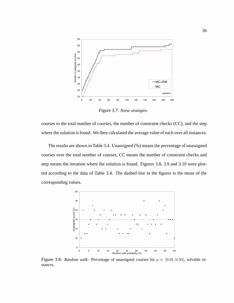
3.1 Local optimum and plateau with hill-climbing. . . . . . . . . . . . . . . . . . 243.2 Min-conflict heuristic.. . . . . . . . . . . . . . . . . . . . . . . . . . . . . . 253.3 Variables linked by a broken capacity constraint.. . . . . . . . . . . . . . . . . 273.4 Loop cycle in Local Search. . . . . . . . . . . . . . . . . . . . . . . . . . . 333.5 Local Search (LS) vs. Systematic Search (BT) on the GTA problem. . . . . . . . 343.6 Local Search on solvable and unsolvable instances.. . . . . . . . . . . . . . . 353.7 Noise strategies. . . . . . . . . . . . . . . . . . . . . . . . . . . . . . . . . 363.8 Random walk:Percentage of unassigned courses forp ∈ [0.01, 0.50], solvable

instances.. . . . . . . . . . . . . . . . . . . . . . . . . . . . . . . . . . . . 363.9 Random walk:CC forp ∈ [0.01, 0.50], on solvable instances.. . . . . . . . . . 383.10 Random walk:Number of iterations forp ∈ [0.01, 0.50], on solvable instances.. . 383.11 Random walk:Unassigned course (%) forp ∈ [0.01, 0.50], on unsolvable instances.403.12 Random walk:CC forp ∈ [0.01, 0.50], on unsolvable instances.. . . . . . . . . 403.13 Random walk:Number of iterations forp ∈ [0.01, 0.50], on unsolvable instances.. 41

4.1 Data structure of environmentE. . . . . . . . . . . . . . . . . . . . . . . . . 484.2 Agents in zero position for Fall2001b.. . . . . . . . . . . . . . . . . . . . . . 554.3 Random walk:Percentage of assigned courses forp ∈ [0.01, 0.50], solvable instances564.4 Random walk:CC forp ∈ [0.01, 0.50], on solvable instances.. . . . . . . . . . 564.5 Unassigned courses. . . . . . . . . . . . . . . . . . . . . . . . . . . . . . . 594.6 Constraint checks. . . . . . . . . . . . . . . . . . . . . . . . . . . . . . . . 614.7 ERA performance on solvable instances. . . . . . . . . . . . . . . . . . . . . 624.8 ERA performance on unsolvable instances. . . . . . . . . . . . . . . . . . . . 624.9 Three types of agent movement.. . . . . . . . . . . . . . . . . . . . . . . . . 634.10 Deadlock state . . . . . . . . . . . . . . . . . . . . . . . . . . . . . . . . . 64

5.1 Structure of local search.. . . . . . . . . . . . . . . . . . . . . . . . . . . . 765.2 Generalized local search.. . . . . . . . . . . . . . . . . . . . . . . . . . . . 785.3 ERA with hybridization.. . . . . . . . . . . . . . . . . . . . . . . . . . . . . 815.4 ERA with global control on Spring2001(0).. . . . . . . . . . . . . . . . . . . 825.5 ERA with global control on Fall2001 (O).. . . . . . . . . . . . . . . . . . . . 83

5.6 Two cases of a deadlock.. . . . . . . . . . . . . . . . . . . . . . . . . . . . 84

A.1 The subclasses of constraint.. . . . . . . . . . . . . . . . . . . . . . . . . . 100A.2 The subclasses of course.. . . . . . . . . . . . . . . . . . . . . . . . . . . . 101A.3 Function: load-data. . . . . . . . . . . . . . . . . . . . . . . . . . . . . . . 102A.4 Function: initialize-csp. . . . . . . . . . . . . . . . . . . . . . . . . . . . . 103A.5 Function: process-nc. . . . . . . . . . . . . . . . . . . . . . . . . . . . . . 103A.6 Function: fc-bound-search.. . . . . . . . . . . . . . . . . . . . . . . . . . . 104A.7 Function: solve. . . . . . . . . . . . . . . . . . . . . . . . . . . . . . . . . 104A.8 Function: mcrw. . . . . . . . . . . . . . . . . . . . . . . . . . . . . . . . . 105A.9 Function: era-screen. . . . . . . . . . . . . . . . . . . . . . . . . . . . . . 105A.10 Function: evaluate-moving-agent. . . . . . . . . . . . . . . . . . . . . . . . 105

List of Tables

2.1 Real-world data sets used in our experiments.. . . . . . . . . . . . . . . . . . 132.2 Constraints in the data sets.. . . . . . . . . . . . . . . . . . . . . . . . . . . 152.3 Las Vegas algorithms.. . . . . . . . . . . . . . . . . . . . . . . . . . . . . . 21

3.1 Experiments for local search.. . . . . . . . . . . . . . . . . . . . . . . . . . 303.2 Distribution of broken constraints.. . . . . . . . . . . . . . . . . . . . . . . . 313.3 Broken constraints for each variable.. . . . . . . . . . . . . . . . . . . . . . 323.4 Varying value ofp for random walk on solvable instances.. . . . . . . . . . . . 373.5 Varyingp for random walk on unsolvable instances.. . . . . . . . . . . . . . . 393.6 Average percentage of unassigned courses.. . . . . . . . . . . . . . . . . . . . 39

4.1 Comparing BT, LS, and ERA.(O/B indicates whether the instance is original orboosted.CCis # of constraint checks.). . . . . . . . . . . . . . . . . . . . . . 60

4.2 Comparing the behaviors of search strategies in our implementation. . . . . . . . 67

B.1 Data set. . . . . . . . . . . . . . . . . . . . . . . . . . . . . . . . . . . . . 139

1

Chapter 1

Introduction

Search techniques that operate byiterative improvementof the solutions have been found to

be particularly effective in solving large combinatorial decision or optimization problems.

Indeed, for many large problems,systematic searchtechniques, which operate by exhaus-

tively examining the solution space, may fail to return a solution in an acceptable amount

of time. In contrast, iterative improvement techniques start from a random set of decisions,

which may or may not be a consistent solution, and, by applying local changes, try to

reach better solutions, ideally the optimum. Our research is motivated by a small but chal-

lenging real-world application, which is the assignment ofGraduate Teaching Assistants

(GTA) to academic tasks. In practice, this application is large and tight, sometimes over-

constrained. Through solving the GTA assignment problem, we investigate two iterative

improvement techniques: a heuristic hill-climbing strategy (denoted LS) and a multi-agent

based search (denoted ERA). We also compare the performanceof these mechanisms and

that of the heuristic backtrack search[Glaubius and Choueiry, 2002a] in solving a set of

real-world data. This approach allows us to identify novel and insightful ways of charac-

terizing the behavior of these various mechanisms, which would not have been possible

if we had done our investigations in a more general context[Zou and Choueiry, 2003a;

2

2003b]. Our long-term goal is to provide a robust portfolio of search algorithms to solve

complex decision problems.

1.1 Motivations

A great deal of theoretical and empirical research has focused on developing and improving

the performance of general algorithms for solving CSPs. Search is the key to solve CSPs.

Search algorithms for solving CSPs are usually classified into two main categories: iterative

improvement and systematic search. The use of iterative search has become popular in

recent years for solving large, difficult real-world optimization problems where systematic

search algorithms are not powerful enough.

Unlike systematic search algorithms, which explore the entire search space, iterative

search algorithms start with a complete but preliminary assignment that is not necessar-

ily consistent, and improve this assignment in several iterative steps until some stopping

condition is reached. The iteration performs a search for a good solution; the process can

provide an approximate solutionanytime. This property is useful for practical applications

that require a solution within time limits without demanding an optimal solution. Addi-

tionally, such iterative improvement methods can be easilycombined with a heuristic to

improve performance, such as restart strategy, min-conflict ordering, and tabu search. This

kind of combination can enhance the ability of iterative search to cope with large, tight

CSPs.

The research on iterative search can be generalized into twofamilies: domain-specific

and general. The former usually encodes domain-specific knowledge into the problem

solver. Although this kind of approach increases efficiency, the highly sophisticated and

problem-tailored representations make the method more complex and limited to the prob-

lem for which the method is designed. Thus, general algorithms are worth studying. We

3

illustrate this in Figure 1.1. The algorithms at the left aremore independent of the problem

and use less knowledge; those on the right are more complex and dependent on the problem

but more efficient.

General algorithms Tailored algorithms

Complexity, efficiency, problem dependence, cost

Generality, less knowledge, problem independence

Figure 1.1:Overview of using iterative search.

Most real-world applications are over-constrained CSPs where no complete solution

exists. To date, much research has been carried out on searchtechniques for solvable

problems. However, the use of general methods to solve over-constrained CSPs seems to

have been overlooked. In recent years there has been a growing interest in ’soft’ CSPs,

in which some constraints are relaxed in order to obtain a solution where the maximum

number of constraints are satisfied. However, in some real-life applications, for example

the GTA problem, no constraint is allowed to be softened or relaxed. Partial, consistent

solutions are still useful for practical purposes. In thesecases, iterative search is worth

studying because of its efficiency and capability of finding apartial, consistent solution

anytime. However, it is impossible to decide if a given CSP issolvable or unsolvable

before hand. Therefore, an algorithm capable of dealing with both solvable and unsolvable

CSPs is worth studying.

1.2 Related works

While many real-world applications are over-constrained,most research efforts have fo-

cused on developing techniques suited to solvable problems. Only recently has there been

interest in over-constrained problems. We identify three main frameworks for modeling

4

over-constrained problems:

1. MAX-CSPs:Freuder and Wallace[Freuder and Wallace, 1992] proposed the MAX-

CSP framework to deal with over-constrained problems by finding (possibly incon-

sistent) solutions that minimize the number of violated constraints. In other words,

the approach seeks a solution that satisfies as many constraints as possible. This

simple approach does not work when none of the constraints isallowed to be broken.

2. Soft constraints:Another approach consists of recasting the satisfiability of over-

constrained problems as the optimization of problems with soft constraints[Bistarelli

et al., 1995] The problems are often represented as soft constraint satisfaction prob-

lems (SCSPs). SCSPs are just like classical CSPs except thateach assignment of

values to variables in the constraints is associated with anelement taken from a par-

tially ordered set. These elements can then be interpreted as levels of preference,

costs, levels of certainty, or some other criterion. The complex framework of SCSPs

makes it more difficult to express a real-world application and process and solve it.

3. Maximization of partial solutions:In many practical settings, yet another approach

seems to be more suitable. This approach consists of finding the partial, consistent

solution of maximal length. In other words, we maximize the number of decisions

that can be made without violating any constraint.

All iterative improvement methods must deal with the problem of local optima in some

way. Therefore, methods of moving from one current state to aneighborhood state, or

repairing the current state, are a very relevant topic. Different repair heuristics comprise

different techniques, such as simulated annealing[Kirkpatrick et al., 1983], random walk

[Papadimitriou and Yannakakis, 1991], tabu search[Glover, 1989; 1990], and min-conflict

[Minton et al., 1990]. Comprehensive studies of these heuristics can be found in[Hoos

and Stutzle, 1999; Wallace and Freuder, 1995; Wallace, 1996]. However, most of the

5

research is based on randomly-generated and binary CSPs. Inrecent years, autonomous

agents have become a vibrant research topic. Liu et al.[2002] introduced the multi-agent

system concept, combined with iterative improvement techniques, which gives us a new

perspective from which to understand how to avoid local optima.

1.3 Questions addressed

In this thesis, we address the following questions:

1. How should we deal with global constraints in LS?

Answer:To solve non-binary CSPs, the non-binary constraints can betranslated into

binary. Even so, the local search strategy might not performas well as it could. The

problem is caused by global constraints. We identify this asnugatory move, and we

show that constraint propagation can deal with this problemappropriately.

2. Does LS have the ability to solve both solvable and unsolvable CSPs?

Answer: In our experiments, we observe that LS has qualitatively similar behaviors

with both solvable and unsolvable problem instances.

3. What kind of strategies could help LS escape from local optima? Do these strategies

really work?

Answer:Noise strategies, e.g., restart, random walk, and tabu search, could be effec-

tive. In this thesis, we verify that random walk is particularly helpful to get out of

local optima.

4. How should the value of the noise probability be chosen?

Answer: We conduct empirical analysis on the settings of noise probability over

solvable and unsolvable instances to study the effect of thenoise probability on the

6

performance of LS. We find that the value of the noise probability might be problem-

dependent. It is difficult to suggest global values for all CSPs.

5. Is ERA the same as a local search strategy or just an extension of local search?

Answer:ERA can be viewed as an extension of local search, but they aredifferent.

In ERA each agent has its own cost value, whereas there is onlyone state cost in

local search; In ERA, the global goal is achieved by the individual local goal of each

agent, whereas there is only one goal in local search. These differences make ERA

more flexible and powerful than local search strategies.

6. Compared with local search and systematic search strategies, what is the main ad-

vantage of ERA?

Answer: In ERA, each agent has its own goal. Meanwhile, agents exchange their

information through communications. This means that each agent can explore more

search space, thus exhibiting the best ability to avoid local optima. As a result, ERA

can solve tight CSPs when local search and systematic searchapproaches fail.

7. How can the behavior of ERA be characterized

Answer: The evolution of ERA across iterations, although not necessarily mono-

tonic, is stable for solvable instances and gradually movestoward a full solution. For

unsolvable instances, ERA’s evolution is unpredictable and appears to oscillate sig-

nificantly, which is its main disadvantage. We identify the source of this shortcoming

and characterize it as a deadlock phenomenon.

1.4 Contributions

In this thesis, we focus on two different implementations ofiterative search, namely stan-

dard local search[Bartak, 1998] and multi-agent search[Liu et al., 2002]. We study their

7

performance in order to characterize and improve their behavior. We conduct our inves-

tigations in the context of a real-world application, whichis the assignment of Graduate

Teaching Assistants (GTAs) to academic tasks[Glaubius, 2001; Glaubius and Choueiry,

2002a]. Most instances of the GTA problem are tight, and some are over-constrained. This

particular application proves to be a good platform to investigate the behavior and perfor-

mance of iterative improvement techniques for solving tight CSPs. In particular, it allow

us to identify shortcomings of these techniques that were not apparent from testing them

on randomly generated problems.

Our main contributions can be summarized as follows:

Local search

• We implemented a greedy hill-climbing search[Bartak, 1998] based on the min-

conflict heuristic[Minton et al., 1992].

• We identified the nugatory-move phenomenon that degrades the performance of the

local search strategy and addressed how to deal with this problem.

• We demonstrated the performance of the local search approach on the GTA problem

and compared it with a systematic search approach in terms ofefficiency and solution

quality.

• We studied noise strategies to deal with local optima and found that the random-walk

strategy is more helpful than random restart strategy. Through detailed analysis we

demonstrated how the values of noise parameters affect the performance of these

strategies. Further, we found that the setting of noise parameters might be problem-

dependent.

Multi-agent search

8

• We implemented ERA, a multi-agent based search method on theGTA assignment

problem.

• We studied and characterized the behavior of ERA.

• We identified the deadlock phenomenon in ERA when solving over-constrained prob-

lems.

• We compared ERA with a standard local search approach and a systematic backtrack

approach to solve instances of the GTA problem. We learned that only ERA can find

a full solution when the instance is solvable.

• We proposed approaches to avoid deadlock and performed experiments to verify

those that can solve the deadlock problem.

Finally, we identified new directions for future research.

1.5 Outline of the thesis

This thesis is structured as follows. In Chapter 2 we give background information on CSPs,

the GTA problem, iterative improvement techniques and Las Vegas algorithms. In Chap-

ter 3, we demonstrate the performance of hill-climbing, conduct an experimental study

on strategies to deal with local optima, and draw comparisons with a systematic search

approach. Then we extend our observations in further discussions. In Chapter 4, we intro-

duce the ERA model. After presenting an empirical evaluation of ERA, we give detailed

discussions regarding the experimental observations. We then present approaches to deal

with the deadlock problem on unsolvable instances. We extend our study on these two

iterative improvement techniques in Chapter 5. Finally, Chapter 6 provides a review of our

conclusions and points out future research directions.

9

Chapter 2

Background

This chapter provides the background for our work. After a brief introduction to the Con-

straint Satisfaction Problem (CSP), we review ways to modeltight or over-constrained

problems, which are often challenging to solve. We then present a real-world application,

the Graduate Teaching Assistants (GTA) problem, which is atthe focus of our investiga-

tions. We briefly review how it was modeled by Glaubius and Choueiry as a CSP and

solved using systematic backtrack search[2001; 2002a; 2002b]. We then introduce the

general mechanism of local search and describe a particularly powerful variation of lo-

cal search based on a multi-agent formulation. Finally, we characterize these algorithms

according to their properties as Las Vegas algorithms.

2.1 Constraint satisfaction problem (CSP)

Constraints exist everywhere in everyday life. A constraint is simply a relation among

several variables that specifies the acceptable combinations these variables can have, and

thus restricts the possible values that variables can take.Examples of common constraints

are the requirements for college admission, the speed limitfor driving, and the time of

a meeting. Constraint Satisfaction Problems (CSPs) can be used to model decision or

10

optimization problems in many areas, such as scheduling, resource allocation, planning

and temporal reasoning,constraint databases[Revesz, 2002].

2.1.1 Definition of a constraint satisfaction problem

A CSP is defined byP = (V,D, C) whereV is a set of variables,D the set of their re-

spective domains, andC is a set of constraints that restricts the acceptable combinations

of values for variables. Solving a CSP requires assigning a value to each variable such

that all constraints are simultaneously satisfied, which isin generalNP-complete. CSPs

are used to model a wide range of decision problems, and thus are important in practical

settings. The CSP framework provides a common platform to researchers for developing

application-independent solvers and studying the behavior of different search techniques.

2.1.2 CSP characteristics

Although it is difficult to summarize concisely the characteristics of a given CSP instance,

there are a number of parameters that can be used to describe and compare problem in-

stances. We list these main features below:

Number of variables: This determines the number of individual decisions or assignments

that need to be made.

Domain size: Although the domain size of variables may differ, we usuallyuse the size of

the largest domain.

Problem size: The size of a problem can be measured by the number of variables, the

domain sizes, the number of constraints, or a combination ofall three. The most

commonly used measure is the size of the search space, which is given byΠv∈V |Dv|.

Note that a problem with a large size is not necessarily difficult to solve, and a small

11

size problem can easily be more challenging. However, it is clear that as the size of

the problem grows, it becomes exponentially difficult to examine all combinations if

needed.

Constraint arity: A number of CSP solving techniques have been developed for binary

CSPs. As the arity of a constraint increases, so does the complexity of checking the

consistency of the constraint, which increases the complexity of problem solving.

In systematic search, the type of constraint is a factor thataffects the efficiency of

constraint propagation.

Number of solutions: Some problems require finding all solutions, which means that the

entire search space should be explored. More often, a singlesolution is sought. In

our study, we focus on finding one solution.

Tightness of a problem: We define the tightness of a problem as the number of solutions

over the size of search space:Ptightness = Number of solutionsΠv∈V |Dv|

. For a problem, if

one solution is required, thenPtightness decides the hardness of the problem. Tighter

problems are harder to solve. In other words, the probability of finding a solution in

the search space is greatly reduced.

Quality of solutions: Domain specific criteria are usually used to compute and compare

the quality of solutions. Sometimes the quality of a solution is measured by the

number of satisfied constraints or the number of variables that can effectively be

instantiated.

2.1.3 Partial solutions

Over-constrained CSPs obviously have no solution. There are several possible ways

to deal with these problems:

12

1. Remove some constraints to relax the problem.

2. Express preferences between constraints or allocate weights to allowed tuples

with a constraint.

3. Maximize the number of satisfied constraints.

4. Accept solutions that do not cover all variables (i.e., partial solutions).

MAX-CSP is a framework proposed by Freuder and Wallace[1993; 1992] that aims

at finding the solutions that maximizes the number of satisfied constraints. Alterna-

tive approaches reported in the literature includefuzzy or weightedCSPs[Bistarelliet

al., 1995], partial constraint satisfaction[Freuder and Wallace, 1992], hierarchical

constraint satisfaction[Wilson and Borning, 1993] andconstrained heuristic search

[Fox et al., 1989]. All of these methods involve constraint comparisons and have

complex structures. They are particularly useful in the context of optimization. In

our study, all constraints must be satisfied even when some variables cannot be in-

stantiated (which happens in over-constrained instances). In this sense, our goal is

to find maximal partial solutionsthat are consistent with all constraints. We do not

allow any constraint violation. In the remainder of this document, a partial solution

is considered to necessarily be consistent.

2.2 Graduate Teaching Assistants (GTA) problem

As a real-world CSP, the GTA assignment problem is a good instance for us to test different

search techniques.

13

2.2.1 What is the GTA Assignment Problem?

The GTA assignment problem is a real-world application thatwe model as a CSP[Glaubius

and Choueiry, 2002a; 2002b; Glaubius, 2001]. It is a critical problem faced by our depart-

ment and likely other institutions across the world. It can be defined as follows. In a given

academic semester, the department hires a set of graduate teaching assistants that are as-

signed to a set of courses while respecting a number of constraints that specify allowable

assignments such as availability and proficiency of a graduate student for conducting a

given task. A solution to this problem is a consistent and satisfactory assignment of GTAs

to academic tasks. In the GTA assignment problem, the courses are modeled as variables

and the GTAs are the values of these variables. In practice, this problem is often over-

constrained[Glaubius and Choueiry, 2002a; 2002b; Glaubius, 2001].

2.2.2 Characteristics of the GTA assignment problem

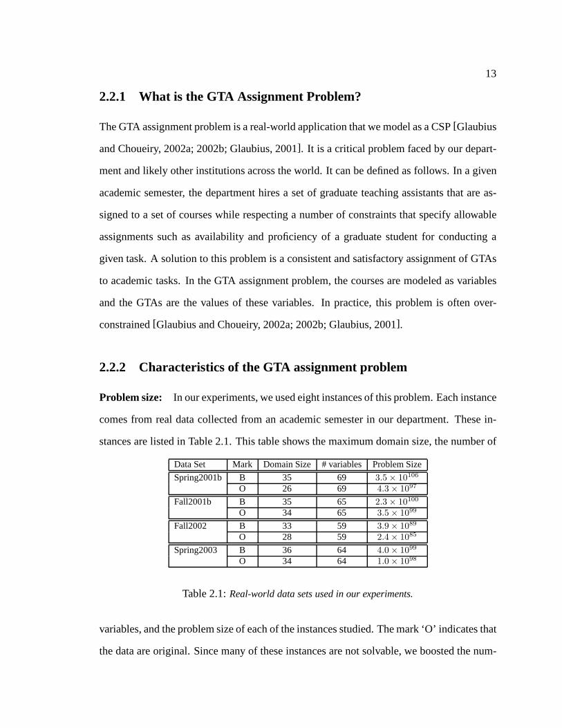
Problem size: In our experiments, we used eight instances of this problem.Each instance

comes from real data collected from an academic semester in our department. These in-

stances are listed in Table 2.1. This table shows the maximumdomain size, the number of

Data Set Mark Domain Size # variables Problem Size

Spring2001b B 35 69 3.5× 10106

O 26 69 4.3× 1097

Fall2001b B 35 65 2.3× 10100

O 34 65 3.5× 1099

Fall2002 B 33 59 3.9× 1089

O 28 59 2.4× 1085

Spring2003 B 36 64 4.0× 1099

O 34 64 1.0× 1098

Table 2.1:Real-world data sets used in our experiments.

variables, and the problem size of each of the instances studied. The mark ‘O’ indicates that

the data are original. Since many of these instances are not solvable, we boosted the num-

14

ber of available GTAs until they were solved by any one of our experimental techniques.

The mark ‘B’ indicates those boosted cases.1

Types of constraints: There are a number of unary, binary and non-binary constraints

that dictate the rules governing the assignments. In particular, each course has a load that

indicates the weight of the course. For example, the value of0.5 means this course needs

one-half of a GTA. Thetotal load of a semester is the maximum of the cumulative load

of the individual courses. In our setting, some courses are only offered during one-half of

the semester; thus the semester has two parts that do not always have equal loads. Further,

each GTA has a capacity factor which is constant throughout the semester and indicates the

maximum course weight he or she can be assigned at any point intime during the semester.

The sum of the capacities of all GTAs represents theresource capacity. We summarize the

constraints as follows:

• Unary constraints: English certification, enrollment, overlap and zero preference

constraints.

• Binary constraints: mutex and equality constraints.

• Non-binary constraints: capacity, equality and confinement constraints.

A detailed description of the problem and the constraints can be found in[Glaubius and

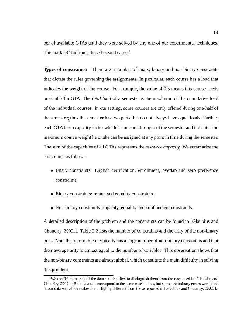
Choueiry, 2002a]. Table 2.2 lists the number of constraints and the arity of the non-binary

ones. Note that our problem typically has a large number of non-binary constraints and that

their average arity is almost equal to the number of variables. This observation shows that

the non-binary constraints are almost global, which constitute the main difficulty in solving

this problem.

1We use ‘b’ at the end of the data set identified to distinguish them from the ones used in[Glaubius andChoueiry, 2002a]. Both data sets correspond to the same case studies, but somepreliminary errors were fixedin our data set, which makes them slightly different from those reported in[Glaubius and Choueiry, 2002a].

15

Number of constraints Spring2001b Fall2001b Fall2002 Spring2003

Total 1526 2011 1413 940Unary 277 267 233 250Binary 1179 1676 1124 622

Non-binary 70 68 56 68Average arity 63 58 54 58

Number of variables 69 65 59 64

Table 2.2:Constraints in the data sets.

Difficulty of the problem: In general, the GTA problem is over-constrained. Typically

there are not enough GTAs to cover all tasks, and some coursesmay have no GTAs as-

signed. The goal of the GTA problem is to ensure GTA support toas many courses as

possible.

Quality of solutions: We measure the quality of a solution primarily by the number of

courses that get a consistent assignment. A secondary criterion is to maximize the arith-

metical or geometric average of the assignments with respect to the GTAs’ preference val-

ues (between 0 and 5) for each course.

Partial solution: Some instances of the GTA problem are over-constrained and do not

have a full solution. For these instances, only a partial solution can be obtained. Here

we need to note that GTA is not a MAX-CSP. In MAX-CSP, all constraints are soft and

the goal is to maximize the number of satisfied constraints. Thus, the solution of a MAX-

CSP problem is not consistent. In the GTA problem, however, it is not permissible for any

constraint to be broken. In other words, there is no soft constraint in this problem. Indeed,

the goal of the GTA problem is to get a consistent partial assignment where the number of

assigned courses is maximized.

16

2.3 Systematic Search (BT)

Glaubius and Choueiry[2002a] utilize systematic search techniques based on depth-first

backtrack search to solve the GTA problem. In their implementation (BT), forward check-

ing [Prosser, 1993] and branch-and-bound mechanisms are integrated into the search strat-

egy. A full look-ahead strategy would drastically increasethe number of constraint checks

while effectively yielding little filtering since the application has many mutex and global

constraints (it is a resource allocation problem). As depth-first search expands nodes in

a search path, the search checks if the expansion of the search path can improve on the

current best solution. Once the current best solution cannot be improved, backtrack oc-

curs. In addition, the dynamic variable and value ordering heuristics are applied in BT. The

implementation is described in detail in[Glaubius and Choueiry, 2002a].

2.4 Local search

Local search is a class of search methods that includes heuristics and nondeterminism in

traversing the search space. A local search algorithm movesfrom one state to another,

guided by heuristics in a nondeterministic manner. Local search algorithms strongly use

randomized decisions while searching for solutions to a given problem. They play an in-

creasingly important role in practically solving hard combinatorial problems from various

domains of artificial intelligence and operations research. For many problem domains, the

best-known algorithms are based on local search techniques.

2.4.1 Algorithms of local search (LS)

The use of local search has become popular in recent years forsolving complex real-world

optimization problems where systematic search methods arestill not powerful. In isolation,

17

LS is a simple iterative method for finding good approximate solutions. Generally speak-

ing, a local search algorithm operates as follows: startingfrom an initial, not-necessarily

consistent state in the solution space of the problem instance, the search iteratively moves

from one state to a neighboring state. The decision on each iteration is based on informa-

tion about the local neighborhood only. The local search methodology uses the following

terms:

• state: one possible assignment of all variables; All possible states form the search

space.

• evaluation value: the number of constraint violations of the state. Sometimes this is

also calledstate cost.

• neighbor: the state that is obtained from the current state by changing the value of

one variable.

• local optimum: a state that is not a solution, where the evaluation values of all its

neighbors are larger than or equal to its evaluation value.

Local optima are the main problem with local search. Although these solutions may be

of good quality, they are not necessary optimal. Furthermore, if the search gets stuck in a

local optimum, there is no obvious way to go to a state that holds a better solution.

2.4.2 Guidance heuristics

The means by which search moves from one state to another state is guided by heuristics.

Heuristics include greedy, min-conflict[Minton et al., 1992], simulated annealing[Kirk-

patricket al., 1983], tabu search[Glover and Laguna, 1993], constraint weighting. Modern

local search algorithms are often a combination of several strategies.

18

2.5 Multi-agent based approaches

Multi-agent based search techniques give us a new way to solve CSPs.

2.5.1 Multi-agent system

A multi-agent system (MAS) is a computational system in which several agents interact and

work together in order to achieve a set of goals. The basic agent concept incorporates pro-

active autonomous units with goal-directed behavior and communication capabilities. The

three basic components of MAS are: agents, interaction and environment. An agent is a

physical or virtual entity that acts, perceives its environment and communicates with others,

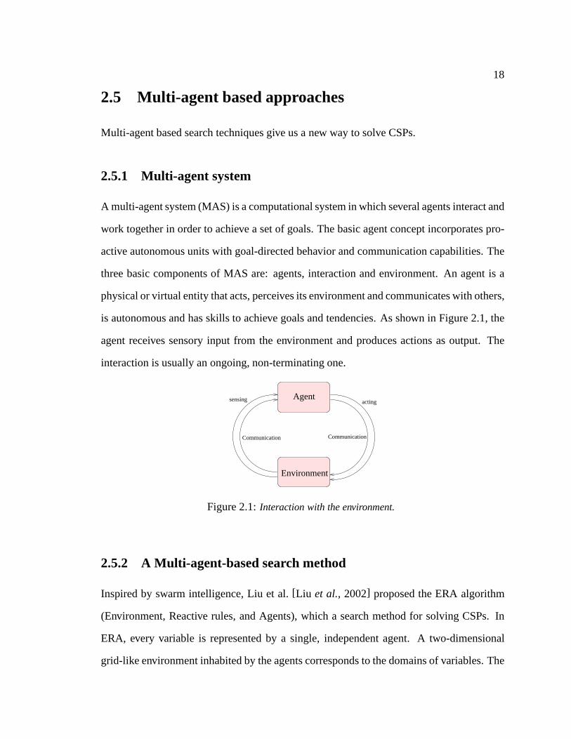
is autonomous and has skills to achieve goals and tendencies. As shown in Figure 2.1, the

agent receives sensory input from the environment and produces actions as output. The

interaction is usually an ongoing, non-terminating one.

Agent

Environment

acting

Communication Communication

sensing

Figure 2.1:Interaction with the environment.

2.5.2 A Multi-agent-based search method

Inspired by swarm intelligence, Liu et al.[Liu et al., 2002] proposed the ERA algorithm

(Environment, Reactive rules, and Agents), which a search method for solving CSPs. In

ERA, every variable is represented by a single, independentagent. A two-dimensional

grid-like environment inhabited by the agents correspondsto the domains of variables. The

19

final positions of the agents in this environment constitutethe solution to a CSP. Each agent

moves to the position that is most desirable given the constraints and the positions of the

other agents,regardless of whether this move improves or deteriorates the quality of the

global solution. The search stops when all agents are in positions that satisfy all applicable

constraints.

Liu et al.[2002] presented an algorithm, called ERA (i.e., Environment, Reactive rules,

and Agents), which is an alternative, multi-agent formulation for solving a general CSP.

Although ERA can be viewed as an extension to local search, itdiffers from local search

in some subtle ways as we try to explain below. In local search, moving from one state

to another typically involves changing the assignment of one (or two) variables, thus the

name local search[Dechter, 2003]. In ERA, any number of variables can change positions

at each step, each agent choosing its own most convenient position. Local search uses

an evaluation function to assess the quality of a given state, where a state is a global but

possibly inconsistent solution to the problem. This evaluation function is aglobal account

of the quality of the state, typically computed as thetotal number of broken constraints for

the whole assignment. In ERA, every agent applies the evaluation function individually,

typically computing the number of the broken constraints that apply to the particular agent.

The individual values of the evaluation function for the agents arenot combined to give a

global account of the quality of the state. Thus, ERA appearsto de-centralize the control for

selecting the new positions of the individual agents. Localsearch transitions from one state

to the next in an attempt to achieve aglobal goal. Thus, local search is directly applicable

to optimization problems. In ERA every agent strives to achieve its ownlocal goal. The

search succeeds and stops when every agent is in a legal position. ERA is therefore most

suited to model satisfaction problems. The original paper on this technique encompasses

an extensive comparison with other known distributed search techniques.

20

2.6 Las Vegas algorithms

A Las Vegas algorithm is a randomized algorithm that always produces correct results. The

only variation from one run to another is the run time. Formally, an algorithmA is aLas

Vegasalgorithm if it has the following properties:

• For a given problem ofπ, algorithmA guarantees to return a correct solution forπ.

• For each given instanceπ, the running time ofA is random, denoted astruntime(A, π).

Based on[Hoos, 1998], we can classify Las Vegas algorithms into the following three

categories:

• complete Las Vegas algorithm: for a solvable problemπ and each instance ofπ,

it always returns a solution withintmax, such thatP (truntime(A, π) ≤ tmax) = 1,

wheretmax is an instance-independent constant andP (truntime(A, π) ≤ t) denotes

the probability thatA finds a solution for an instance ofπ within time t.

• approximately complete Las Vegas algorithm: A always returns a solution such that

limt→∞P (truntime(A, π) ≤ t) = 1.

• essentially incomplete Las Vegas algorithm: A always returns a solution such that

limt→∞P (truntime(A, π) ≤ t) < 1.

For local search algorithms, essential incompleteness is usually caused by the search get-

ting stuck in local optima. Even if some techniques such as restart, random walk, or tabu

search are applied to escape from local optima, the local search algorithms still cannot

achieve completeness. Although these techniques are successfully used to solve the SAT

problem[Hoos, 1998] and to enforce completeness for local search algorithms, they are

only theoretical. The time limits for finding solutions are too large to be practical, and they

may be problem-dependent. From our experiments on the GTA problem, we observed only

21

ERA is always able to find a complete solution for a solvable instance while the other two

approaches, BT and LS, fail. Based on this observation, we might classify BT, LS and ERA

in Table 2.3.

Search method Las Vegas algorithmsBT (with heuristic) completeERA approximately completeLS essentially incomplete

Table 2.3:Las Vegas algorithms.

Summary

CSP provides a framework that allows researchers to study and solve problems by com-

puters. The GTA problem is a real-world application. In practice, this problem is tight,

even over-constrained. Through solving the GTA assignmentproblem, we investigate two

iterative improvement techniques: local search (LS) and multi-agent based search (ERA).

22

Chapter 3

A heuristic hill-climbing search

It is, in general, a challenge for local-search techniques to deal with a large number of

(almost) global constraints because these techniques relyon iterative improvement brought

by ‘local’ change. Our CSP model of the GTA assignment problem has a large number

of such constraints (see Table 2.2). In order to allow local search to handle these almost

global constraints, we integrate constraint propagation technique with local search. The

resulting mechanism can be characterized as greedy and is best classified as a hill-climbing

strategy, which is one type of local search known to be particularly effective in solving

large problems while requiring a modest amount of memory overhead and computation

time. However, it is also known to suffer from getting stuck in local optima when the

constraints are not convex.

In order toavoid local optima, we enhance the performance of our strategy with two

mechanisms: a heuristic (i.e., min-conflict heuristic) andstochastic noise (i.e., random

walk). In order torecover from local optima, we use random restarts, which consist of

repeating the search from different random states.

In this chapter, we describe our local search strategy, testits performance on the GTA

assignment problem, and compare it to the heuristic backtrack search of[Glaubius, 2001;

23

Glaubius and Choueiry, 2002a; 2002b]. We show that the former yields much better quality

solutions (in terms of the solution length) than the latter for a short response time (i.e., a

few minutes in our case). However, it loses this advantage when response time is allowed

to increase.

3.1 Hill-climbing search

A local search strategy navigates the set of possible statesof a problem moving from one

state to a neighboring one until it reaches an optimal or near-optimal state according to

some optimization criterion, or exceeds a threshold specified in terms of time or number of

iterations. In a CSP, a state is a global solution (i.e., an assignment of values to all variables)

that may be inconsistent with the constraints. Local searchproceeds as follows. Starting

from an initial state, usually chosen randomly, it exploresneighboring states. These are

states that can be reached by the application of some move operators such as changing the

assignment of a variable, thus the name local. A hill-climbing strategy allows only moves

to a state that improves the value of the evaluation criterion.

A heuristic is a simple and ‘cheap’ technique used to improvethe performance of a

search process by providing guidance to the search. Typically, it allows us to compare and

choose between two or more states by estimating their value,such as their proximity to

the goal. Most heuristics are not exact in the sense that theymay sacrifice completeness or

soundness. In general, they rely on domain knowledge.

The general hill-climbing algorithm (seeAlgorithm 1) usually start from a randomly

initialized stateSi, all neighbors which are adjacent toSi are evaluated by the evaluation

function eval. Among these neighboring states, aSj with a better evaluation value than

Si is randomly chosen as the new state. The algorithms continueuntil the value of current

state is better than the values of all the states adjacent to it. At this point, the current

24

Input: an initial stateSi

Output:current state

1: neighbor-list← neighbors(Si)2: while ∃ a stateSj ∈ neighbor-list, such thateval(Sj) better thaneval(Si) do3: Si ← Sj

4: neighbor-list← neighbors(Si)5: end while

Algorithm 1: Procedure: Hill-climbing

state is either an optimum or a local optimum. Note that the hill-climbing algorithms have

to explore all neighbors of the current state before choosing the move. A weakness of a

hill-climbing search it is that it may get stuck in some of thefollowing states:

• Local optimum:a state where all neighbors are worse than the current state,while

the current state is not the optimum. This is analogous to a climber that starts in the

foothills and spends his time climbing to the hill’s summit,only to be disappointed

that he is still far from the top of the neighboring mountain.

• Plateaux: a state where all neighbors have the same evaluation value.This is like

a climber who starts on a flat plain somewhere and wanders aimlessly because he

cannot determine the best direction.

global optimum

X

Y

Z

plateau

local optimum

Figure 3.1:Local optimum and plateau with hill-climbing.

There are several techniques to help hill-climbing avoid orescape from local optima

and plateaus. In the rest of this chapter we investigate combining two heuristics to avoid

local optima, and a restart strategy to escape from them.

25

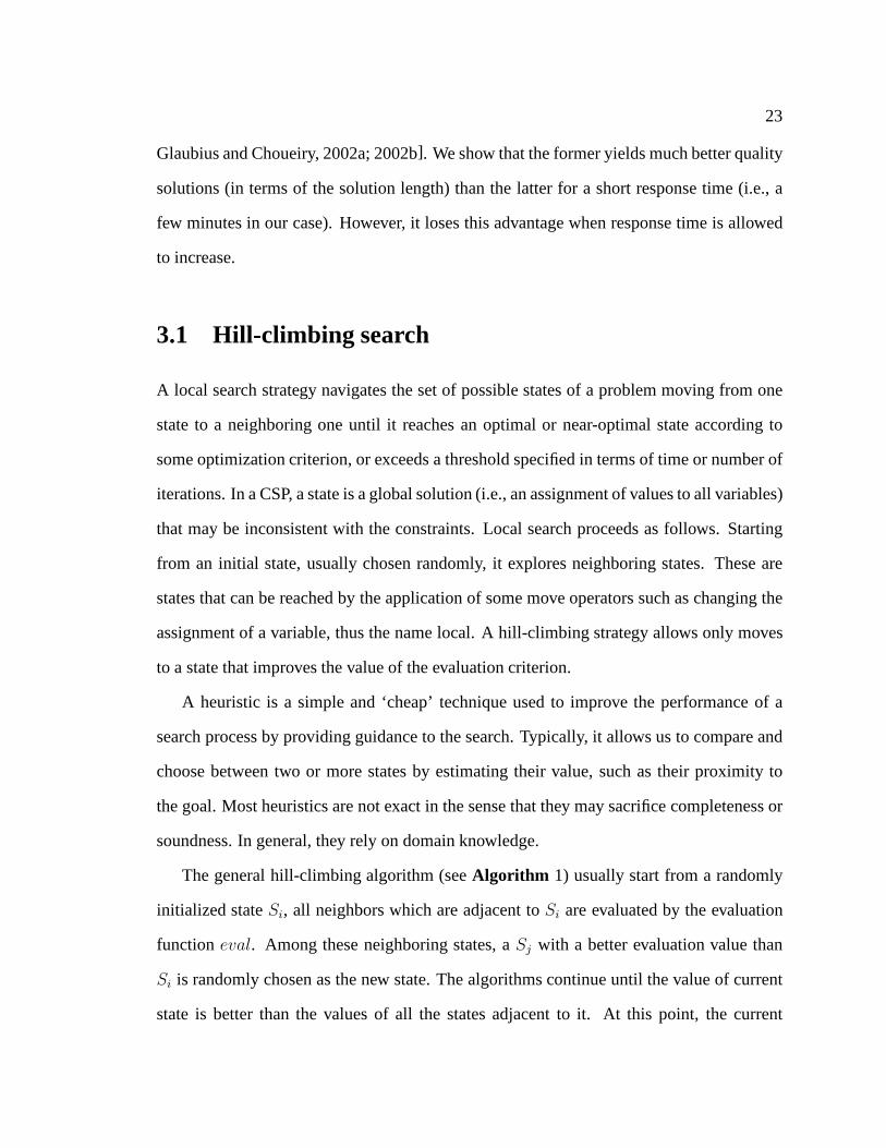
3.2 Min-conflict heuristic

It is common to use a value-ordering heuristic to guide search to choose the most promising

value for assignment to a variable. One such heuristic is called themin-conflict heuristic

[Minton et al., 1992], which basically orders the values according to constraintviolations

after each step. The heuristic can be used with a variety of different search strategies. The

formal definition presented in[Minton et al., 1992] is as follows:

Definition 1. Min-conflict heuristic:

Given: A set of variables, a set of binary constraints, and an assignment of a value to each

variable, two variables are said to be in conflict if their values violate a constraint.

Procedure:Select any variable that is in conflict and assign to it a valuethat minimizes the

number of conflicts, breaking ties randomly.

course−2 (GTA6, 2)




::

(GTA1, 10) (GTA2, 6) (GTA3, 2)......(GTA15, 9)

variables in conflict set

domain of course−6

Figure 3.2:Min-conflict heuristic.

At each iteration the search takes one variable in the conflict set and repairs it according

to the min-conflict heuristic. We illustrate it in Figure 3.2. In a conflict set each variable (a

course) is associated with a pair of values: the first one is the domain value (a gta), and the

second one is the conflict number. When a variable is repaired(e.g., course-6), a new value

will be assigned to it such that the conflict number is reduced. For example, after the local

reparation course-6 will be assigned the value of GTA3. Notethat the heuristic has essen-

26

tially been used on binary constraints and that experimental problems described in[Minton

et al., 1992] are all binary CSPs. However, for non-binary CSPs, a single constraint may

involve several variables, which are called the scope of theconstraint. The min-conflict

heuristic originally attempts to minimize the number of variables that need to be repaired.

This raises the following question: can the heuristic be used to solve non-binary constraint

CSPs or does it need to be modified? We answer this question in Section 3.2.1.

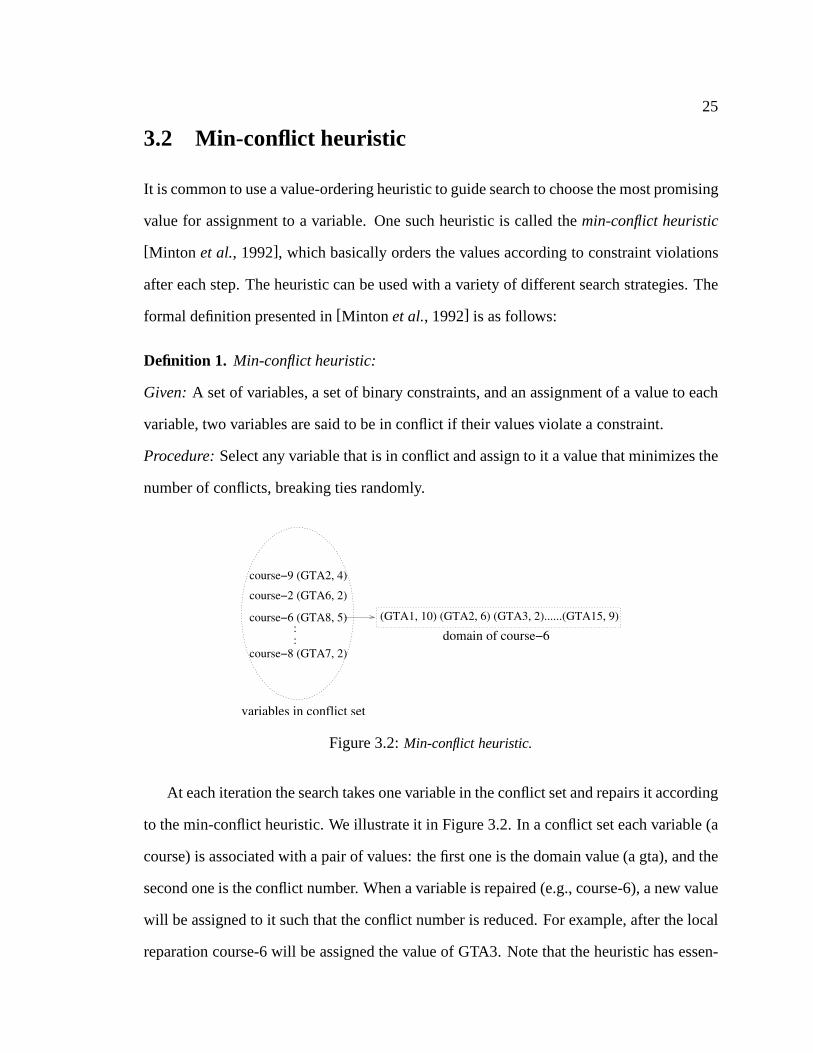
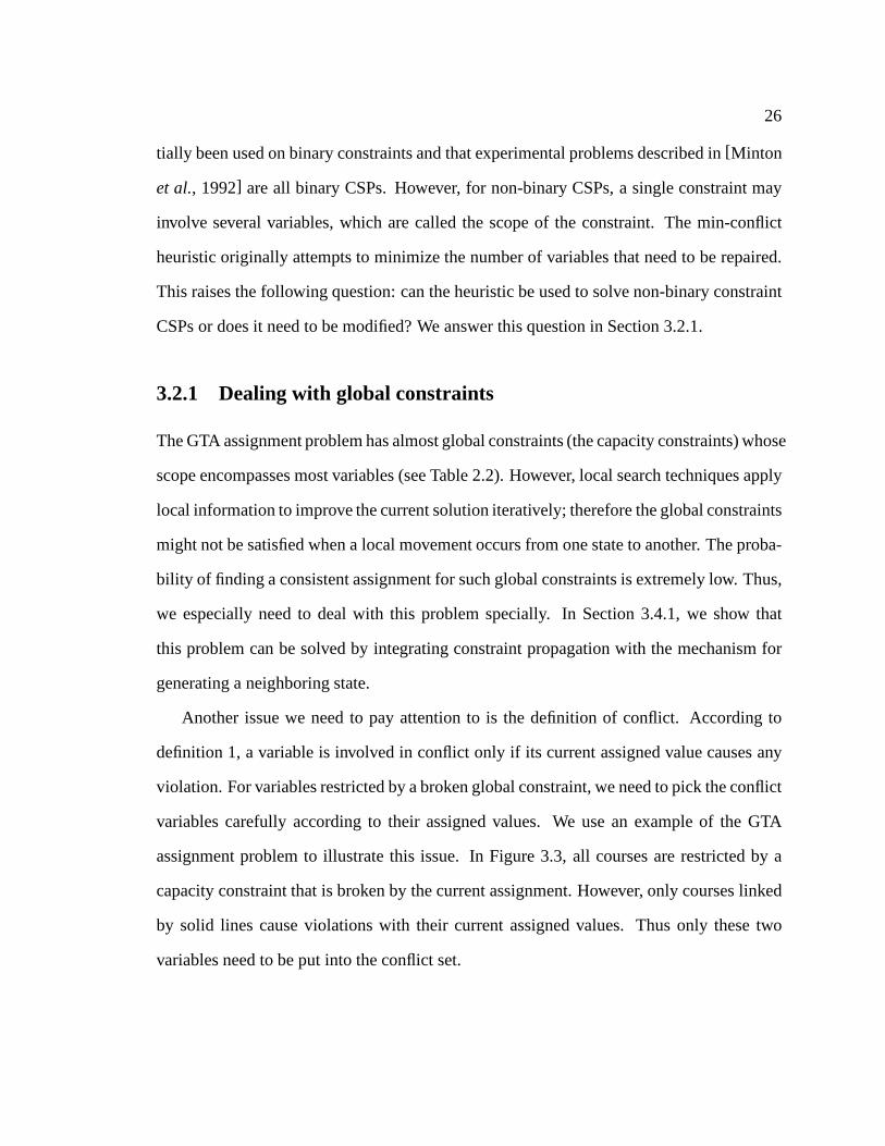
3.2.1 Dealing with global constraints

The GTA assignment problem has almost global constraints (the capacity constraints) whose

scope encompasses most variables (see Table 2.2). However,local search techniques apply

local information to improve the current solution iteratively; therefore the global constraints

might not be satisfied when a local movement occurs from one state to another. The proba-

bility of finding a consistent assignment for such global constraints is extremely low. Thus,

we especially need to deal with this problem specially. In Section 3.4.1, we show that

this problem can be solved by integrating constraint propagation with the mechanism for

generating a neighboring state.

Another issue we need to pay attention to is the definition of conflict. According to

definition 1, a variable is involved in conflict only if its current assigned value causes any

violation. For variables restricted by a broken global constraint, we need to pick the conflict

variables carefully according to their assigned values. Weuse an example of the GTA

assignment problem to illustrate this issue. In Figure 3.3,all courses are restricted by a

capacity constraint that is broken by the current assignment. However, only courses linked

by solid lines cause violations with their current assignedvalues. Thus only these two

variables need to be put into the conflict set.

27

course 1

course n

course 3

course 2

::

:: CAPACITY

course 4

course 5

Restricted by a constraint

Constraint

Variable

Figure 3.3:Variables linked by a broken capacity constraint.

3.2.2 Improving min-conflict with random walk

Noise strategies can be used to allow hill-climbing search to avoid local optima. Random

walk is one such strategy that we have implemented and tested. We show that is helpful

to avoid local optima; however, it does not allow us to recover from these deadlocks once

they occur.

The idea of random walk is to allow hill-climbing search, with a specified probabilityp,

to disobey the heuristic that selects the neighboring stateto move to. With probability 1-p,

search follows the decision made by the heuristic, which is min-conflict here. Clearly, the

value for the probabilityp has an influence on the performance of the algorithm resulting

from integrating random walk. Preliminary studies on this issue are presented in[Wallace

and Freuder, 1995; Wallace, 1996; Hoos and Stutzle, 1999]. The value ofp suggested in

[Selman and Kautz, 1993] is 0.35. In Section 3.4.5, we investigate the effect of varying the

value ofp on the behavior of our local search strategy.

3.2.3 Improving local search with random restart

In order to recover from local optima, it is advisable to use arandom restart strategy, which

consists of starting search from a new randomly selected state. This process can be repeated

a given number of times while keeping track of the best solution obtained so far, thus giving

the resulting algorithm an anytime flavor.

28

In Section 3.4.6, we study setting the value of restarts.

3.2.4 Algorithms tested

In summary, we tested the following variations of the hill-climbing search:

1. MC: This is hill-climbing using the min-conflict heuristic for value selection.

2. MC+RW: This strategy combines with random walk toMC in order to enhance its

ability to avoid local optima.

3. MC+RW+RR (LS): This strategy combines with random restart toMC+RW in or-

der to enhance all its recovery from local optima. The best solution found across

the experiment is kept to ensure an ‘anytime’ behavior. Thisis our most elaborate

variation on hill-climbing search, which we denote LS in therest of this document.

3.3 Experimental study

In this section, we study local search through LS and compareit with a systematic, back-

track search (BT) with dynamic variable ordering fully described in[Glaubius and Choueiry,

2002a]. There are two interesting topics for study:

• The characteristic behavior of local search: How does localsearch perform on solv-

able and unsolvable problem instances? How do the noise parameters work? Does it

perform differently with binary constraint and non-binaryconstraint CSPs?

• The performance comparisons between local search and systematic search.

As mentioned in Section 2.2.2, the GTA problem is hard to solve and some instances are

over-constrained. Even though a solution does exist for an instance, neither the systematic

search method nor a local search algorithm can find a completesolution. In this case, we

29

compare solutions according to the number of assigned variables. The more variables that

can be assigned, the better the solution.

3.3.1 Test cases

We test the eight instances of the GTA problem described in Section 2.2. These are

data for Spring2001b (B), Spring2001b (O), Fall2001b (B), Fall2001b (O), Fall2002 (B),

Fall2002 (O), Spring2003 (B) and Spring2003 (O). The numberof variables for each in-

stance, and the number of constraints are not necessarily equal. For these eight instances,

neither the local search algorithm nor the systematic search algorithm can find a full solu-

tion. However, some instances can be solved by a multi-agentsearch algorithm presented

in Chapter 4. Thus we divided all instances into two main classes: solvable and unsolvable

set. We conducted our experiments using these two categories of instances.

3.3.2 Parameters setting

The maximum number of iteration is set to 200. This value is based on our experiments,

because there is no improvement of the solution beyond this number of steps. In our initial

studies, we set the probabilityp of random walk to be0.02 according to[Bartak, 1998].

For systematic search, we allow it to run for about 8 minutes1.

3.3.3 Conditions of experiments

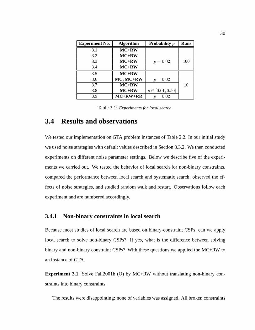
The experiment numbers and the corresponding conditions are shown in Table 3.1. The

number of runs defines how many times we run the procedure. We take the average value

over these runs for a certain evaluation criterion.1[Guddeti, 2004] shows that the quality of the solution found by the heuristicbacktrack search fails to

improve after the first few minutes.

30

Experiment No. Algorithm Probability p Runs

3.1 MC+RW3.2 MC+RW3.3 MC+RW p = 0.02 1003.4 MC+RW

3.5 MC+RW3.6 MC, MC+RW p = 0.023.7 MC+RW 103.8 MC+RW p ∈ [0.01, 0.50]3.9 MC+RW+RR p = 0.02

Table 3.1:Experiments for local search.

3.4 Results and observations

We tested our implementation on GTA problem instances of Table 2.2. In our initial study

we used noise strategies with default values described in Section 3.3.2. We then conducted

experiments on different noise parameter settings. Below we describe five of the experi-

ments we carried out. We tested the behavior of local search for non-binary constraints,

compared the performance between local search and systematic search, observed the ef-

fects of noise strategies, and studied random walk and restart. Observations follow each

experiment and are numbered accordingly.

3.4.1 Non-binary constraints in local search

Because most studies of local search are based on binary-constraint CSPs, can we apply

local search to solve non-binary CSPs? If yes, what is the difference between solving

binary and non-binary constraint CSPs? With these questions we applied the MC+RW to

an instance of GTA.

Experiment 3.1. Solve Fall2001b (O) by MC+RW without translating non-binary con-

straints into binary constraints.

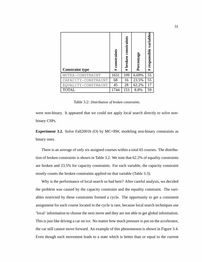
The results were disappointing: none of variables was assigned. All broken constraints

31

Constraint type #co

nstr

aint

s

#br

oken

cons

trai

nts

Per

cent

age

#re

spon

sibl

eva

riabl

es

MUTEX-CONSTRAINT 1631 109 6.69% 55CAPACITY-CONSTRAINT 68 16 23.5% 55EQUALITY-CONSTRAINT 45 28 62.2% 17TOTAL 1744 153 8.8% 59

Table 3.2:Distribution of broken constraints.

were non-binary. It appeared that we could not apply local search directly to solve non-

binary CSPs.

Experiment 3.2. Solve Fall2001b (O) by MC+RW, modeling non-binary constraints as

binary ones.

There is an average of only six assigned courses within a total 65 courses. The distribu-

tion of broken constraints is shown in Table 3.2. We note that62.2% of equality constraints

are broken and 23.5% for capacity constraints. For each variable, the capacity constraint

mostly counts the broken constraints applied on that variable (Table 3.3).

Why is the performance of local search so bad here? After careful analysis, we decided

the problem was caused by the capacity constraint and the equality constraint. The vari-

ables restricted by these constraints formed a cycle. The opportunity to get a consistent

assignment for each course located in the cycle is rare, because local search techniques use

’local’ information to choose the next move and they are not able to get global information.

This is just like driving a car on ice. No matter how much pressure is put on the accelerator,

the car still cannot move forward. An example of this phenomenon is shown in Figure 3.4.

Even though each movement leads to a state which is better than or equal to the current

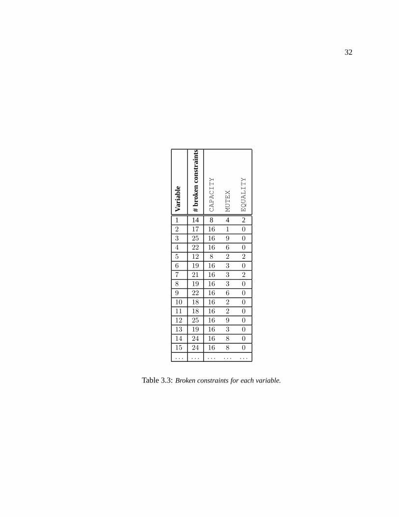
32

Var

iabl

e

#br

oken

cons

trai

nts

CA

PA

CIT

Y

MU

TE

X

EQ

UA

LIT

Y

1 14 8 4 22 17 16 1 0

3 25 16 9 0

4 22 16 6 0

5 12 8 2 2

6 19 16 3 0

7 21 16 3 2

8 19 16 3 0

9 22 16 6 0

10 18 16 2 0

11 18 16 2 0

12 25 16 9 0

13 19 16 3 0

14 24 16 8 0

15 24 16 8 0

. . . . . . . . . . . . . . .

Table 3.3:Broken constraints for each variable.

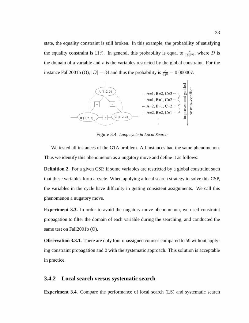
33

state, the equality constraint is still broken. In this example, the probability of satisfying

the equality constraint is11%. In general, this probability is equal to|v||D||v|

, whereD is

the domain of a variable andv is the variables restricted by the global constraint. For the

instance Fall2001b (O),|D| = 34 and thus the probability is3343 = 0.000007.

A=2, B=1, C=2

A=1, B=1, C=2

A=1, B=2, C=3

A=2, B=2, C=1

:

......

...

... ...

...

...

...

by

min

−co

nfl

ict

imp

rov

emen

t g

uid

ed

:

A {1, 2, 3}

C {1, 2, 3}B {1, 2, 3}

= =

=

Figure 3.4:Loop cycle in Local Search

We tested all instances of the GTA problem. All instances hadthe same phenomenon.

Thus we identify this phenomenon as a nugatory move and defineit as follows:

Definition 2. For a given CSP, if some variables are restricted by a global constraint such

that these variables form a cycle. When applying a local search strategy to solve this CSP,

the variables in the cycle have difficulty in getting consistent assignments. We call this

phenomenon a nugatory move.

Experiment 3.3. In order to avoid the nugatory-move phenomenon, we used constraint

propagation to filter the domain of each variable during the searching, and conducted the

same test on Fall2001b (O).

Observation 3.3.1.There are only four unassigned courses compared to59 without apply-

ing constraint propagation and2 with the systematic approach. This solution is acceptable

in practice.

3.4.2 Local search versus systematic search

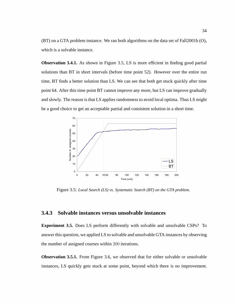
Experiment 3.4. Compare the performance of local search (LS) and systematicsearch

34

(BT) on a GTA problem instance. We ran both algorithms on the data set of Fall2001b (O),

which is a solvable instance.

Observation 3.4.1.As shown in Figure 3.5, LS is more efficient in finding good partial

solutions than BT in short intervals (before time point 52).However over the entire run

time, BT finds a better solution than LS. We can see that both get stuck quickly after time

point 64. After this time point BT cannot improve any more, but LS can improve gradually

and slowly. The reason is that LS applies randomness to avoidlocal optima. Thus LS might

be a good choice to get an acceptable partial and consistent solution in a short time.

0

10

20

30

40

50

60

70

0 20 40 60 80 100 120 140 160 180 200

Time (unit)

Num

ber

of a

ssig

ned c

ours

es

LS

BT

52

Figure 3.5:Local Search (LS) vs. Systematic Search (BT) on the GTA problem.

3.4.3 Solvable instances versus unsolvable instances

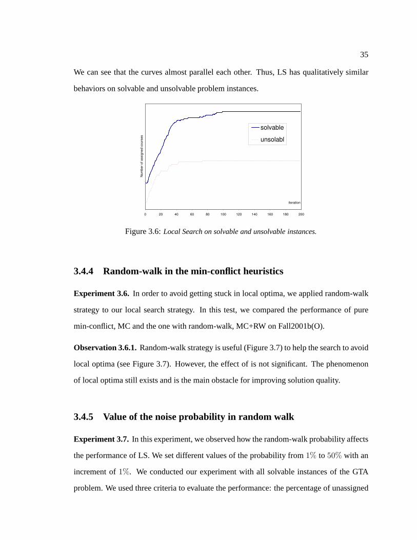
Experiment 3.5. Does LS perform differently with solvable and unsolvable CSPs? To

answer this question, we applied LS to solvable and unsolvable GTA instances by observing

the number of assigned courses within200 iterations.

Observation 3.5.1.From Figure 3.6, we observed that for either solvable or unsolvable

instances, LS quickly gets stuck at some point, beyond whichthere is no improvement.

35

We can see that the curves almost parallel each other. Thus, LS has qualitatively similar

behaviors on solvable and unsolvable problem instances.

0 20 40 60 80 100 120 140 160 180 200

iteration

Nu

mb

er

of

assig

ne

d c

ou

rse

s

solvable

unsolabl

Figure 3.6:Local Search on solvable and unsolvable instances.

3.4.4 Random-walk in the min-conflict heuristics

Experiment 3.6. In order to avoid getting stuck in local optima, we applied random-walk

strategy to our local search strategy. In this test, we compared the performance of pure

min-conflict, MC and the one with random-walk, MC+RW on Fall2001b(O).

Observation 3.6.1.Random-walk strategy is useful (Figure 3.7) to help the search to avoid

local optima (see Figure 3.7). However, the effect of is not significant. The phenomenon

of local optima still exists and is the main obstacle for improving solution quality.

3.4.5 Value of the noise probability in random walk

Experiment 3.7. In this experiment, we observed how the random-walk probability affects

the performance of LS. We set different values of the probability from 1% to 50% with an

increment of1%. We conducted our experiment with all solvable instances ofthe GTA

problem. We used three criteria to evaluate the performance: the percentage of unassigned

36

20

25

30

35

40

45

50

55

60

65

0 20 40 60 80 100 120 140 160 180 200

Iteration

Nu

mb

er

of a

ssig

ne

d c

ou

rse

s

MC+RW

MC

Figure 3.7:Noise strategies.

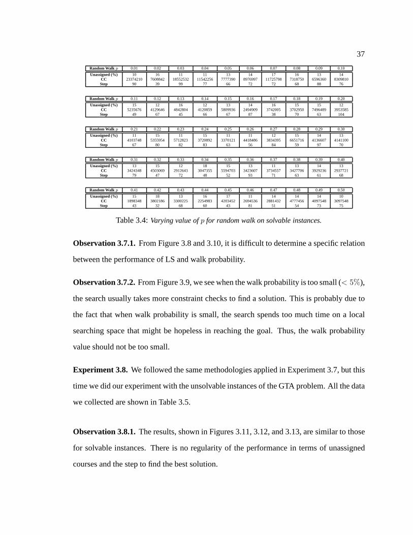
courses to the total number of courses, the number of constraint checks (CC), and the step

where the solution is found. We then calculated the average value of each over all instances.

The results are shown in Table 3.4. Unassigned (%) means the percentage of unassigned

courses over the total number of courses, CC means the numberof constraint checks and

step means the iteration where the solution is found. Figures 3.8, 3.9 and 3.10 were plot-

ted according to the data of Table 3.4. The dashed line in the figures is the mean of the

corresponding values.

8

10

12

14

16

18

20

0 5 10 15 20 25 30 35 40 45 50Random walk probability (%)

Unassig

ned c

ours

e (

%)

Figure 3.8: Random walk:Percentage of unassigned courses forp ∈ [0.01, 0.50], solvable in-stances.

37

Random Walk p 0.01 0.02 0.03 0.04 0.05 0.06 0.07 0.08 0.09 0.10

Unassigned (%) 10 16 11 11 13 14 17 16 13 14CC 23374210 7608842 18552532 11542256 7777390 8976997 11725798 7318750 6596360 8309810Step 90 39 99 77 66 72 72 68 88 76

Random Walk p 0.11 0.12 0.13 0.14 0.15 0.16 0.17 0.18 0.19 0.20


Random Walk p 0.21 0.22 0.23 0.24 0.25 0.26 0.27 0.28 0.29 0.30


Random Walk p 0.31 0.32 0.33 0.34 0.35 0.36 0.37 0.38 0.39 0.40


Random Walk p 0.41 0.42 0.43 0.44 0.45 0.46 0.47 0.48 0.49 0.50


Table 3.4:Varying value ofp for random walk on solvable instances.

Observation 3.7.1.From Figure 3.8 and 3.10, it is difficult to determine a specific relation

between the performance of LS and walk probability.

Observation 3.7.2.From Figure 3.9, we see when the walk probability is too small(< 5%),

the search usually takes more constraint checks to find a solution. This is probably due to

the fact that when walk probability is small, the search spends too much time on a local

searching space that might be hopeless in reaching the goal.Thus, the walk probability

value should not be too small.

Experiment 3.8. We followed the same methodologies applied in Experiment 3.7, but this

time we did our experiment with the unsolvable instances of the GTA problem. All the data

we collected are shown in Table 3.5.

Observation 3.8.1.The results, shown in Figures 3.11, 3.12, and 3.13, are similar to those

for solvable instances. There is no regularity of the performance in terms of unassigned

courses and the step to find the best solution.

38

0.00E+00

5.00E+06

1.00E+07

1.50E+07

2.00E+07

2.50E+07


# C

onstr

ain

t check

Figure 3.9:Random walk:CC forp ∈ [0.01, 0.50], on solvable instances.

30

40

50

60

70

80

90

100

110


No

. ste

p t

o f

ind

th

e b

est

so

lutio

n

Figure 3.10:Random walk:Number of iterations forp ∈ [0.01, 0.50], on solvable instances.

Observation 3.8.2.In Figure 3.11 and Figure 3.12, it is obvious that the performance of

LS behaves poorly with smaller walk probability values (≤ 5%). This confirms that the

value of walk probability should not be too conservative. Otherwise effort and time are

wasted searching a restricted portion of the search space. In other words, the searching is

too local to expand the space.

3.4.6 The number of restarts

Experiment 3.9. In this experiment, ten different values were tested for thenumber of

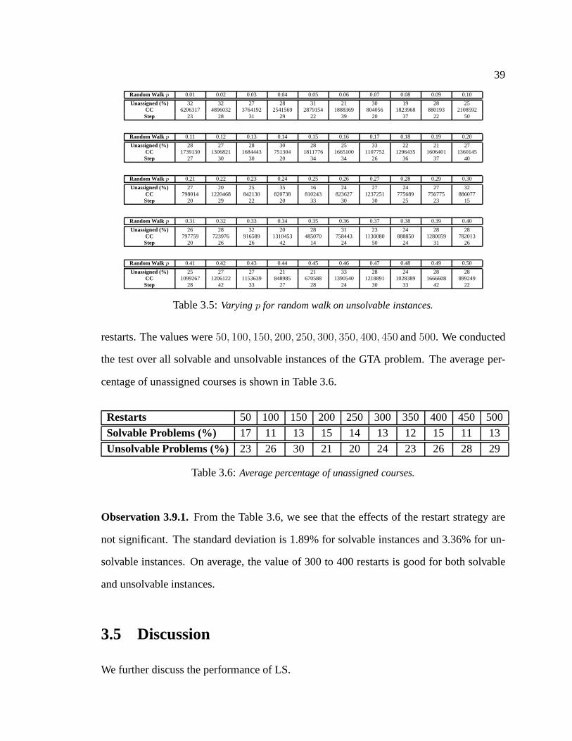
39

Random Walk p 0.01 0.02 0.03 0.04 0.05 0.06 0.07 0.08 0.09 0.10


Random Walk p 0.11 0.12 0.13 0.14 0.15 0.16 0.17 0.18 0.19 0.20


Random Walk p 0.21 0.22 0.23 0.24 0.25 0.26 0.27 0.28 0.29 0.30


Random Walk p 0.31 0.32 0.33 0.34 0.35 0.36 0.37 0.38 0.39 0.40


Random Walk p 0.41 0.42 0.43 0.44 0.45 0.46 0.47 0.48 0.49 0.50


Table 3.5:Varyingp for random walk on unsolvable instances.

restarts. The values were50, 100, 150, 200, 250, 300, 350, 400, 450 and500. We conducted

the test over all solvable and unsolvable instances of the GTA problem. The average per-

centage of unassigned courses is shown in Table 3.6.

Restarts 50 100 150 200 250 300 350 400 450 500

Solvable Problems (%) 17 11 13 15 14 13 12 15 11 13

Unsolvable Problems (%) 23 26 30 21 20 24 23 26 28 29

Table 3.6:Average percentage of unassigned courses.

Observation 3.9.1.From the Table 3.6, we see that the effects of the restart strategy are

not significant. The standard deviation is 1.89% for solvable instances and 3.36% for un-

solvable instances. On average, the value of 300 to 400 restarts is good for both solvable

and unsolvable instances.

3.5 Discussion

We further discuss the performance of LS.

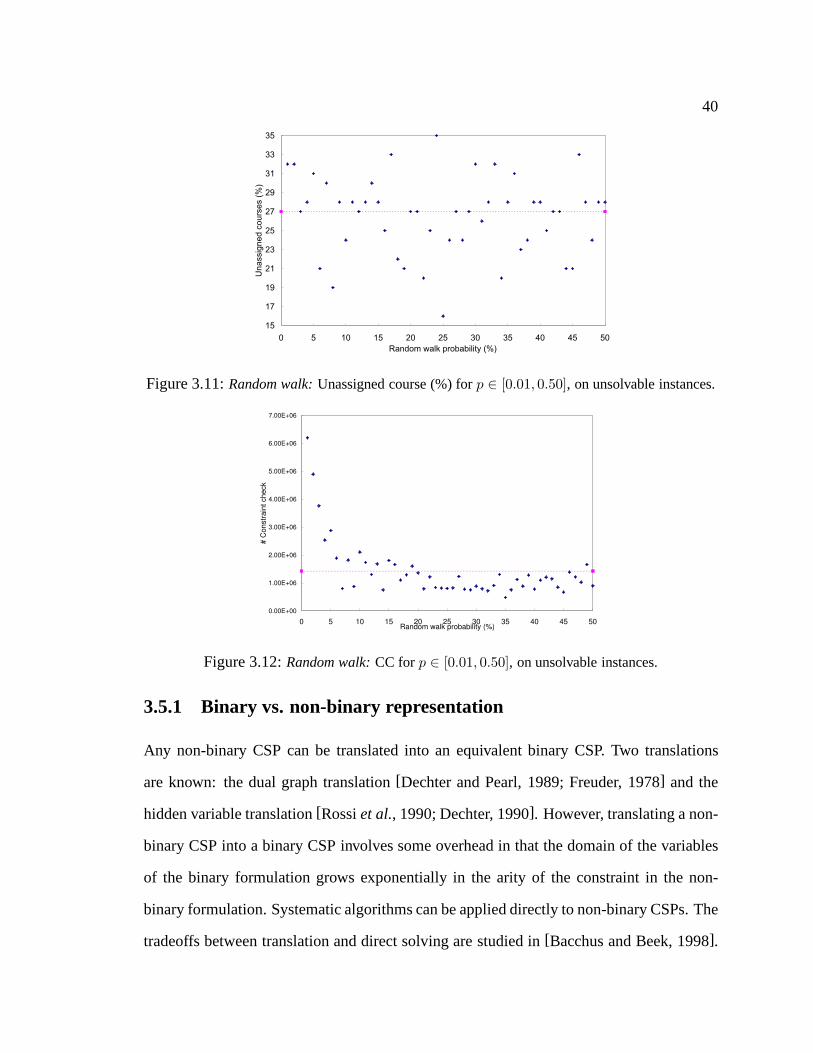
40

15

17

19

21

23

25

27

29

31

33

35

0 5 10 15 20 25 30 35 40 45 50

Random walk probability (%)

Un

assig

ne

d c

ou

rse

s (

%)

Figure 3.11:Random walk:Unassigned course (%) forp ∈ [0.01, 0.50], on unsolvable instances.

0.00E+00

1.00E+06

2.00E+06

3.00E+06

4.00E+06

5.00E+06

6.00E+06

7.00E+06


# C

onstr

ain

t check

Figure 3.12:Random walk:CC forp ∈ [0.01, 0.50], on unsolvable instances.

3.5.1 Binary vs. non-binary representation

Any non-binary CSP can be translated into an equivalent binary CSP. Two translations

are known: the dual graph translation[Dechter and Pearl, 1989; Freuder, 1978] and the

hidden variable translation[Rossiet al., 1990; Dechter, 1990]. However, translating a non-

binary CSP into a binary CSP involves some overhead in that the domain of the variables

of the binary formulation grows exponentially in the arity of the constraint in the non-

binary formulation. Systematic algorithms can be applied directly to non-binary CSPs. The

tradeoffs between translation and direct solving are studied in [Bacchus and Beek, 1998].

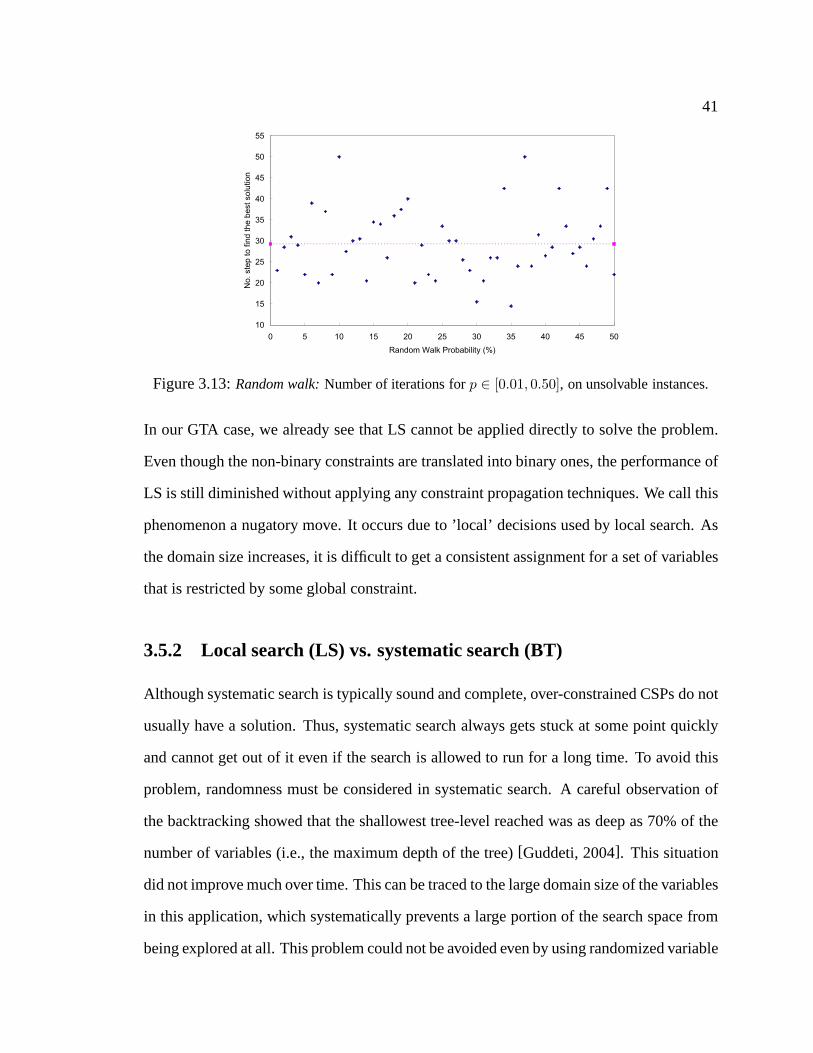
41

10

15

20

25

30

35

40

45

50

55

0 5 10 15 20 25 30 35 40 45 50

Random Walk Probability (%)

No.

ste

p t

o f

ind t

he b

est

solu

tion

Figure 3.13:Random walk:Number of iterations forp ∈ [0.01, 0.50], on unsolvable instances.

In our GTA case, we already see that LS cannot be applied directly to solve the problem.

Even though the non-binary constraints are translated intobinary ones, the performance of

LS is still diminished without applying any constraint propagation techniques. We call this

phenomenon a nugatory move. It occurs due to ’local’ decisions used by local search. As

the domain size increases, it is difficult to get a consistentassignment for a set of variables

that is restricted by some global constraint.

3.5.2 Local search (LS) vs. systematic search (BT)

Although systematic search is typically sound and complete, over-constrained CSPs do not

usually have a solution. Thus, systematic search always gets stuck at some point quickly

and cannot get out of it even if the search is allowed to run fora long time. To avoid this

problem, randomness must be considered in systematic search. A careful observation of

the backtracking showed that the shallowest tree-level reached was as deep as 70% of the

number of variables (i.e., the maximum depth of the tree)[Guddeti, 2004]. This situation

did not improve much over time. This can be traced to the largedomain size of the variables

in this application, which systematically prevents a largeportion of the search space from

being explored at all. This problem could not be avoided evenby using randomized variable

42

ordering[Gomeset al., 1998; Guddeti, 2004]. Later, we show that while some instances

are indeed solvable, they are hard to solve. For these hard ortight instances of the GTA

problem, systematic search without randomness still cannot find a full solution. Local

search can find a better partial solution than systematic search within a short time. That

means that LS explores a much larger search space than BT does, and thus it seems that LS

has more chance to find a solution than BT within a short time period. This property of LS

is useful when solving a large, difficult CSP and when there isa time limit. Hence, LS may

be a good choice to provide a starting point for other search methods to begin their search.

For example, in a hybrid method we could use LS to generate a starting point and then

use systematic search to solve the problem based on this point. It is also useful in a few

practical problems when, for example, a partial solution isneeded to evaluate the problem

instead of a full solution.

3.5.3 Solvable vs. unsolvable instances

It appears that the behavior of LS does not change qualitatively when applied to solvable

or unsolvable problems instances. (In Chapter 4, we show that this does not hold for multi-

agent search, which stabilizes on solvable instances and oscillates on over-constrained

ones.) LS quickly gets stuck on local optima with both types of instances. Thus we might

say that LS is a stable search approach because it does not depend on the CSP itself. No

matter whether the CSP is loose or tight, LS always behaves ina similar manner.

3.5.4 One-time repair

In our LS approach, we divide the variables into two sets: agood set and ano-good set.

The search keeps locally improving the solution based on incremental extensions of a fully-

consistent partial solution. The variables in thegood set increase monotonically, and the

43

variables in theno-good set decrease monotonically in terms of the cardinality of the set.

After a certain period, both thegood andno-good set do not change. That means the

current solution cannot be further improved. The problem isthat the algorithm attempts

to find a sequence of repairs such that no variables is repaired more than once. Once a

variable becomesgood , it is never taken out of thegood set. Thus it reduces the solution

space and quickly gets stuck. We summarize the phenomena as monotonic improvement,

quick stabilization and one-time reparation. These drawbacks degrade the performance of

local search so that the application of LS is limited. In order to avoid these phenomena, we

should develop a mechanism to undo the decision, i.e., to remove the variables in thegood

set and repair them again if needed, or to improve an initial assignment locally rather than

extend a fully consistent partial solution.

3.5.5 Dealing with local optima

To deal with the problem of local optima and plateaus, which undermine the performance

of local search, we apply noise strategies, namely random walk and random restart. Our

experiments demonstrate that these two strategies are helpful in improving performance of

LS. Local optima can be reduced but not totally overcome. Further, it is hard to identify

an appropriate value for the noise probabilityp for random walk, and this value depends

on the particular problem class or even problem instance. Previous studies of this issue

suggest different values (e.g., 0.35 in[Selman and Kautz, 1993] and 0.02∼0.05 in[Bartak,

1998]).

Our experiments suggest that the value ofp should not be too small or too large. A too

small value forp inhibits the effects of random walk. A too large value forp inhibits the

effects of the selected heuristic (i.e., min-conflict). ForLS, our experiments show thatp

should not be smaller than< 5% or larger than> 45%. We recommend settingp between

15% and 30%. In Section 4.4.1, where we apply the random walk principle to a multi-

44

agent search techniques for solving the GTA problem, our experiments show thatp should

be smaller than 25%.

3.6 Conclusions

In this chapter, we gave a brief introduction to the hill-climbing and min-conflict heuris-

tic, which is a typical technique of local search for solvingCSPs. The original min-

conflict heuristic was defined and tested only on binary CSPs.We adapted it to solve

non-binary CSPs. We conducted experiments to study local search focusing on two top-

ics: the performance of local search and noise strategies. Then we presented our ob-

servations and discussion for solving GTA problem with LS. We stress that our inves-

tigations are motivated by and focus on the GTA assignment problem, where we have

collected some real data samples. Consequently, our experiments are exploratory in na-

ture. More thorough experiments, using a methodology similar to that of[Hoos, 1998;

Hoos and Stutzle, 2004], still need to be carried out to validate our conclusions. Through

experiments conducted so far, we make the following conclusions:

• Unlike systematic search, local search techniques cannot be directly used to solve

non-binary CSPs. Even if the non-binary CSPs is translated into binary ones, local

search may still fail to work well because of global constraints. We identify the

reason for this drawback and characterize it as a nugatory-move phenomenon.

• Constraint propagation can be used to avoid the nugatory-move phenomenon. The

effect of applying constraint propagation is significant.

• Local search can find a better partial solution than systematic search within a short

time interval. We propose to exploit this feature of local search to generate good

quality ‘seed solutions’ for other search techniques. We will examine this approach

45

in a future study.

• For solvable or unsolvable CSPs, the local search presents the same behavior. In

other words, local search exhibits a uniform ‘stable’ behavior, regardless of whether

the instances being solved are solvable, tight, or over-constrained.

• In our approach to LS, the search improves the solution, based on incremental exten-

sions of a fully consistent partial solution. This approachdemonstrates some short-

comings: monotonic improvement, quick stabilization and one-time reparation. That

is, the assignment of a variable is only repaired by one time.Once a variable has a

consistent assignment, this assignment is never changed atall. As a result, the search

space is implicitly and greatly reduced.

• Noise strategies can be used to address the issue of local optima in local search.

Indeed, random walk can enhance the ability of the min-conflict heuristic to avoid

local optima. Random restart strategy allows search to recover from local optima.

However, neither strategy guarantees the search will move to a promising direction.

Summary

The local search approach shows that it is capable of finding apartial solution for a CSP

in a short interval. The main problem of hill-climbing is itstendency to get stuck in local

optima quickly; and the one-time repair heuristic eliminates the chance of a variable to

get a new consistent assignment. Thus hill-climbing exhibits monotonic improvement and

quick stabilization. Noise strategies such as random walk and restart are helpful to deal

with local optima. However it is hard to generalize how to setthe noise parameters which

greatly depend on a particular CSP.

46

Chapter 4

A multi-agent based search

In this chapter, we extend the empirical study of a multi-agent search method (ERA) for

solving CSPs[Liu et al., 2002]. We compare the performance of this method to that of

LS an BT for solving the GTA assignment problem. This real-world application, tight and

often over-constrained, allows us to discover strengths and shortcomings of this multi-agent

search which would not have been possible otherwise. We showthat for solvable, tight

CSPs, ERA clearly outperforms both LS and BT, as it finds a solution when the other two

techniques fail. However, for over-constrained problems,the multi-agent search method

degenerates in terms of stability and the quality of the solutions reached. We identify the

source of this shortcoming and characterize it as a deadlockphenomenon. Further, we

discuss possible approaches for handling and solving deadlocks. The chapter concludes

with a short summary of the main ideas and results.

4.1 Background

A multi-agent system is a computational system in which several agents interact and work

together to achieve a set of goals. Inspired by swarm intelligence, Liu et al.[2002] proposed

a search method for solving CSPs based on a multi-agent approach in which every variable

47

is represented by a single, independent agent. A two-dimensional grid-like environment,

inhabited by the agents, corresponds to the domains of variables. Thus, the positions of the

agents in such an environment constitute the solution to a CSP.

Liu et al.[2002] presented an algorithm, called ERA (i.e., Environment, Reactive rules,

and Agents), that is an alternative, multi-agent formulation for solving a general CSP. Al-

though ERA can be viewed as an extension to local search, it differs from local search

in some subtle ways. Moving from one state to another in localsearch typically involves

changing the assignment of one (or two) variables, thus the name local search. In multi-

agent search, any number of variables can change positions at each move; each agent

chooses its most convenient position (e.g., value). The evaluation function that assesses

the quality of a given state in local search is a global account of the quality of the state

(typically the total number of broken constraints). In ERA,the value of the state is a com-

bination of the value of the individual agents (typically the number of broken constraints of

an agent). ERA appears to de-centralize the global control of the selection of the next state

to the individual agents.

4.2 ERA model

In this section, we briefly introduce the ERA model includingthe components of ERA

and the algorithms. An ERA system has three components: an Environment (E), a set

of Reactive rules (R), and a set of Agents (A). The environment records the number of

constraint violations of the current state for each value inthe domains of all variables.

Each variable is an agent, and the position of the agent corresponds to the value assigned to

this variable. The agent moves according to its reactive rules. Two assumptions are made:

• All agents have the same reactive rules, and

• An agent can only move to positions in its own domain.

48

In our implementation, agents move in sequence, but the technique can also be asyn-

chronous.

4.2.1 Environment

The environmentE is represented as a two-dimensional array that hasn rows correspond-

ing to the number of courses, and|Dmax| columns whereDmax is the size of the largest

domain. Figure. 4.1 illustrates the environmentE of the GTA problem.

:

:

:

:

: :

:

::

:

:

:

:

:

:

(GTA1,3) (GTA2,12) (GTA7,52)(GTA4,12)

(GTA2,9) (GTA16, 80) (GTA21,18)

course-1

course-2

course-3

course-n

(GTA5, 15)

(GTA5,8)

Figure 4.1:Data structure of environmentE.

An entry e(i, j) in E refers to a position at rowi (representing Agenti) and column

j (representing the indexj in the domain of the variable). The entrye(i, j) stores a list

of two values, namelydomain valueand violation value. Domain value,e(i, j).value,

points to the data structure (i.e., object) of a GTA of position indexj. Violation value,

e(i, j).violation, is the number of broken constraints of the agent in the current assign-

ment. A zero position is a position for the agent that does not break any of the

constraints that apply to it. The current assignment of the agent is consistent with the other

agents’ assignments. Obviously, if agents are all inzero position , then we have a

full, consistent solution. The information inE is updated when an agent changes position.

The goal is to have each agent find itszero position .

4.2.2 Reactive rules

A set of reactive rules,R, governs the interaction between the agents and their environment.

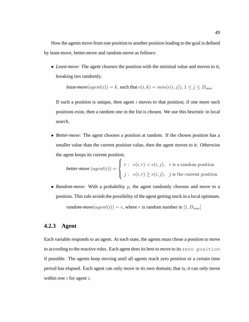
49

How the agents move from one position to another position leading to the goal is defined

by least-move, better-move and random-move as follows:

• Least-move: The agent chooses the position with the minimal value and moves to it,

breaking ties randomly.

least-move(agent(i)) = k, such thate(i, k) = min(e(i, j)), 1 ≤ j ≤ Dmax

If such a position is unique, then agenti moves to that position; if one more such

positions exist, then a random one in the list is chosen. We use this heuristic in local

search.

• Better-move: The agent chooses a position at random. If the chosen position has a

smaller value than the current position value, then the agent moves to it. Otherwise

the agent keeps its current position.

better-move(agent(i)) =

r : e(i, r) < e(i, j), r is a random position

j : e(i, r) ≥ e(i, j), j is the current position

• Random-move: With a probabilityp, the agent randomly chooses and move to a

position. This rule avoids the possibility of the agent getting stuck in a local optimum.

random-move(agent(i)) = r, wherer is random number in[1, Dmax]

4.2.3 Agent

Each variable responds to an agent. At each state, the agentsmust chose a position to move

to according to the reactive rules. Each agent does its best to move to itszero position

if possible. The agents keep moving until all agents reach zero position or a certain time

period has elapsed. Each agent can only move in its own domain; that is, it can only move

within row i for agenti.

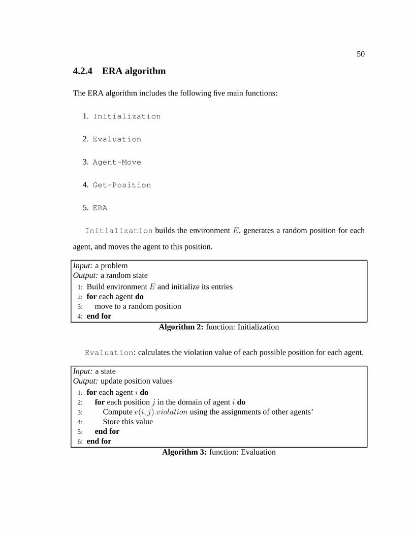
50

4.2.4 ERA algorithm

The ERA algorithm includes the following five main functions:

1. Initialization

2. Evaluation

3. Agent-Move

4. Get-Position

5. ERA

Initialization builds the environmentE, generates a random position for each

agent, and moves the agent to this position.

Input: a problemOutput:a random state

1: Build environmentE and initialize its entries2: for each agentdo3: move to a random position4: end for

Algorithm 2: function: Initialization

Evaluation : calculates the violation value of each possible position for each agent.

Input: a stateOutput:update position values

1: for each agenti do2: for each positionj in the domain of agenti do3: Computee(i, j).violation using the assignments of other agents’4: Store this value5: end for6: end for

Algorithm 3: function: Evaluation

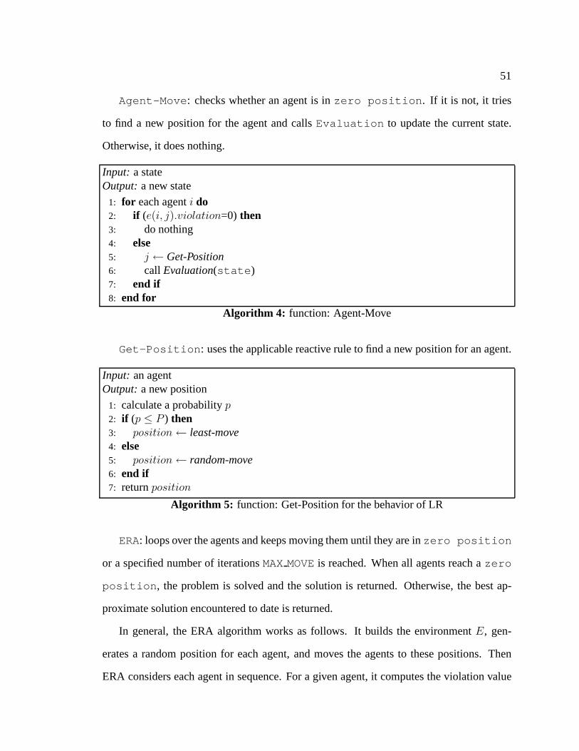
51

Agent-Move : checks whether an agent is inzero position . If it is not, it tries

to find a new position for the agent and callsEvaluation to update the current state.

Otherwise, it does nothing.

Input: a stateOutput:a new state

1: for each agenti do2: if (e(i, j).violation=0) then3: do nothing4: else5: j ← Get-Position6: call Evaluation(state )7: end if8: end for

Algorithm 4: function: Agent-Move

Get-Position : uses the applicable reactive rule to find a new position for an agent.

Input: an agentOutput:a new position

1: calculate a probabilityp2: if (p ≤ P ) then3: position← least-move4: else5: position← random-move6: end if7: returnposition

Algorithm 5: function: Get-Position for the behavior of LR

ERA: loops over the agents and keeps moving them until they are inzero position

or a specified number of iterationsMAXMOVEis reached. When all agents reach azero

position , the problem is solved and the solution is returned. Otherwise, the best ap-

proximate solution encountered to date is returned.

In general, the ERA algorithm works as follows. It builds theenvironmentE, gen-

erates a random position for each agent, and moves the agentsto these positions. Then

ERA considers each agent in sequence. For a given agent, it computes the violation value

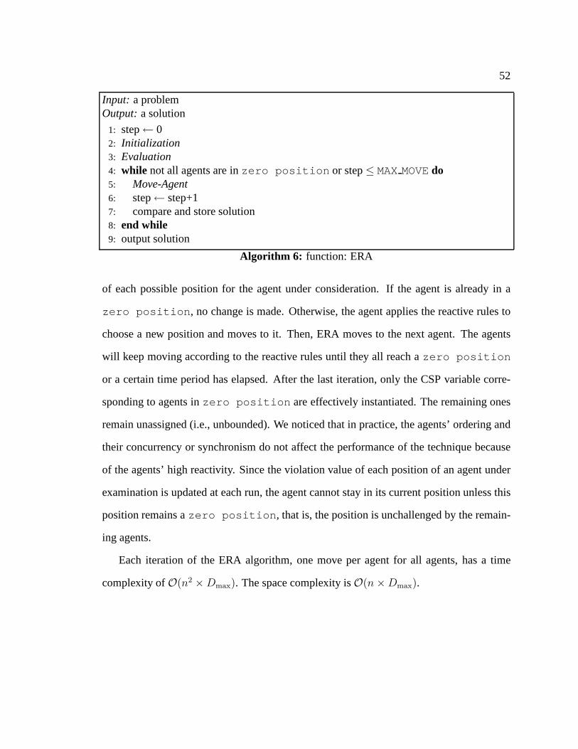
52

Input: a problemOutput:a solution

1: step← 02: Initialization3: Evaluation4: while not all agents are inzero position or step≤MAXMOVEdo5: Move-Agent6: step← step+17: compare and store solution8: end while9: output solution

Algorithm 6: function: ERA

of each possible position for the agent under consideration. If the agent is already in a

zero position , no change is made. Otherwise, the agent applies the reactive rules to

choose a new position and moves to it. Then, ERA moves to the next agent. The agents

will keep moving according to the reactive rules until they all reach azero position

or a certain time period has elapsed. After the last iteration, only the CSP variable corre-

sponding to agents inzero position are effectively instantiated. The remaining ones

remain unassigned (i.e., unbounded). We noticed that in practice, the agents’ ordering and

their concurrency or synchronism do not affect the performance of the technique because

of the agents’ high reactivity. Since the violation value ofeach position of an agent under

examination is updated at each run, the agent cannot stay in its current position unless this

position remains azero position , that is, the position is unchallenged by the remain-

ing agents.

Each iteration of the ERA algorithm, one move per agent for all agents, has a time

complexity ofO(n2 ×Dmax). The space complexity isO(n×Dmax).

53

4.3 Control strategies in ERA

Liu et al. [2002] demonstrated ERA with two benchmark CSPs: then-queen and coloring

problems. Both problems have only binary constraints and the instances tested were solv-

able. We examine the performance of the ERA in solving the more difficult, non-binary,

over-constrained GTA problem. Before we describe our experiment, we summarize some

possible behaviors of an agent and the rules that govern the behavior. We also review some

observations presented by[Liu et al., 2002].

Liu et al. [2002] experimented with the following behaviors:

• LR is the combination of the least-move and random-move rules.The agent typically

applies least-move and uses random-move with a probabilityp to get out of local

optimum.

• BR is the combination of the better-move and random-move rules. It is similar to

LRexcept that it replaces least-move with better-move.

• BLR is the combination of the better-move, least-move, and random-move rules. The

agent first applies better-move to find its next position. If it fails, it applies LR.

• rBLR : First, the agent appliesr times the rule better-move. If it fails to find one, it

applies theLR rule.

• FrBLR : The agent appliesrBLR for the firstr iterations and then appliesLR, typi-

cally r = 2.

Liu et al. [2002] further reported the following observations.

• The cost of better-move in CPU time is much smaller than that of least-move, which

requires evaluating all positions.

54

• The probability of better-move in successfully finding a position to move to is quite

high.

• Better-move allows most agents to find better positions at the first step.

• FrBLR outperformsrBLR , which in turn outperformsLR in terms of runtime.

4.4 Empirical evaluation of ERA

We tested our implementation on known problem instances. First, we solved the 100-queen

problem with different agent behaviors1. Then, usingFrBLR as the default behavior

of agents, we solved eight instances of the GTA problem, including solvable and over-

constrained cases. We conducted four main experiments:

1. In Section 4.4.1, we test the behavior of ERA on the GTA assignment problem to

confirm thatFrBLR is the best behavior of ERA . Then we examine the effect of the

value of probabilityp.

2. In Section 4.4.2, we compare the behavior of ERA to BT search of Glaubius[2002a]and

our LS strategy in Chapter 3.

3. In Section 4.4.3, we observed the behavior of individual agents (Section 4.4.3).

4. Finally, in Section 4.4.4, we identified a shortcoming of ERA that we characterize as

a deadlock phenomenon (section 4.4.4).

Our observations follow each experiment.

1Then-queen problem is not particularly well-suited for testingthe performance of search. However, weused it only to be on a common level with Liu et al.[2002]. Indeed, they conducted their tests on then-queenand the coloring problems, and drew their conclusions from then-queen problem.

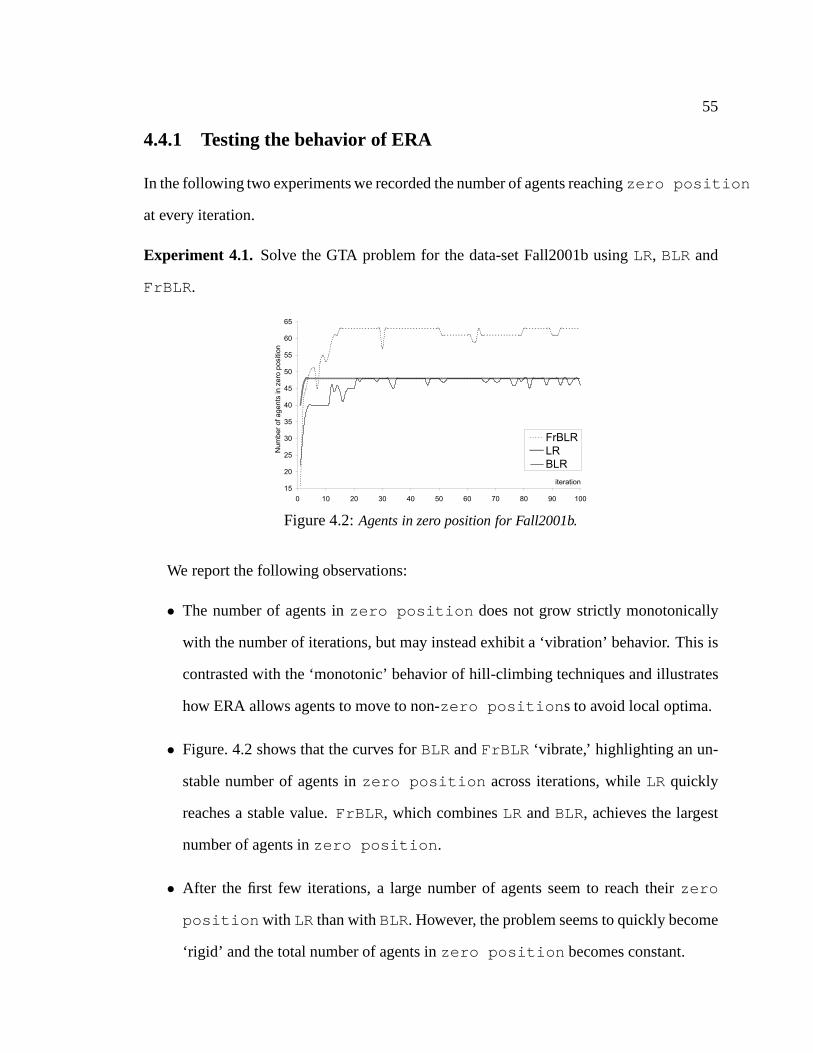
55

4.4.1 Testing the behavior of ERA

In the following two experiments we recorded the number of agents reachingzero position

at every iteration.

Experiment 4.1. Solve the GTA problem for the data-set Fall2001b usingLR, BLR and

FrBLR .

15

20

25

30

35

40

45

50

55

60

65

0 10 20 30 40 50 60 70 80 90 100

iteration

Nu

mb

er

of

ag

en

ts in

ze

ro p

ositio

n

FrBLR

LR

BLR

Figure 4.2:Agents in zero position for Fall2001b.

We report the following observations:

• The number of agents inzero position does not grow strictly monotonically

with the number of iterations, but may instead exhibit a ‘vibration’ behavior. This is

contrasted with the ‘monotonic’ behavior of hill-climbingtechniques and illustrates

how ERA allows agents to move to non-zero position s to avoid local optima.

• Figure. 4.2 shows that the curves forBLRandFrBLR ‘vibrate,’ highlighting an un-

stable number of agents inzero position across iterations, whileLR quickly

reaches a stable value.FrBLR , which combinesLR andBLR, achieves the largest

number of agents inzero position .

• After the first few iterations, a large number of agents seem to reach theirzero

position with LR than withBLR. However, the problem seems to quickly become

‘rigid’ and the total number of agents inzero position becomes constant.

56

In the GTA problem, as with the toy problems,FrBLR seems to yield the best results. We

adopt it as the default behavior for all agents.

Experiment 4.2. In ERA, we use the probabilityp to control random-move behavior. In

this experiment, we observed how the probabilityp affects the performance of ERA. We

set different values ofp from 1% to 50% with an increment of1%. We conducted our

experiment with all solvable instances of the GTA problem. We used two criteria to evaluate

the performance: the percentage of assigned courses to the total number of courses and the

number of constraint checks (CC). We then calculated the average value of each with all

instances.

20

30

40

50

60

70

80

90

100

110

0 5 10 15 20 25 30 35 40 45 50


Assig

ne

d c

ou

rse

s (

%)

Figure 4.3: Random walk:Percentage ofassigned courses forp ∈ [0.01, 0.50], solv-able instances

0.00E+00

1.00E+07

2.00E+07

3.00E+07

4.00E+07

5.00E+07

6.00E+07

0 5 10 15 20 25 30 35 40 45 50


# C

on

str

ain

t ch

eck

Figure 4.4: Random walk: CC for p ∈[0.01, 0.50], on solvable instances.

From Figures 4.3 and 4.4, we see that the percentage of assigned courses decreases

and the number of CC increases dramatically when the value ofp is larger than25%. The

reason can likely be explained as follows: with high probability, the search often jumps

from the current state (which might be promising in leading to the goal) and moves to a

random state. As a result, it wastes a lot of time on useless jumping. Thus the efficiency is

diminished. At this point, the value of probabilityp should be kept in a small range. In the

case of GTA, this value should be below25%. We had the same observation when solving

unsolvable instances.

57

4.4.2 Performance comparison: ERA, LS, and BT

In order to gather an understanding of the characteristics of ERA, we compared its perfor-

mance with that of two other search strategies. The first strategy is a systematic, backtrack

search (BT) with dynamic variable ordering fully describedin [Glaubius and Choueiry,

2002a]. The second strategy is the local search (LS) described in Chapter 3. LS is a com-

bination of constraint propagation to handle non-binary constraints and the min-conflict

random-walk algorithm as presented in[Bartak, 1998].

As stated in Section 2.2, the GTA problem is often over-constrained. We try to find the

assignment that covers the most tasks and, for an equal solution length, one that maximizes

the arithmetic or geometric average of the preference values of the assignments. In all three

searches (i.e., ERA, BT, and LS), we store the best solution found so far, so that the search

behaves as an anytime algorithm.

Experiment 4.3. Solve the GTA problem for the real-world data of Fall2001b, Fall2002

and Spring2003 using ERA, BT search[Glaubius and Choueiry, 2002a], and a hill-climbing,

local search technique (Chapter 3). Since all the problems were difficult to solve (and two

of them are unsolvable), we boosted the available resourcesto transform these problems

into solvable ones. To accomplish that, we added extra resources—dummy GTAs—into the

data set. The results are shown in Table 4.1 and Figures 4.5 and 4.6.

We adopted the following working conditions:

• The quality of the solution reached by BT search did not improve after the first 20

seconds, even when we let the search run for hours or days. A careful observation of

the backtracking showed that the shallowest tree-level reached was as deep as 70%

of the number of variables (i.e., the maximum depth of the tree). This situation did

not improve significantly over time and can be traced to the large domain size of

the variables in this application, which systematically prevents a large portion of the

58

search space from being explored. This problem cannot be avoided even by using

randomized variable ordering.

• The maximum iteration number for LS and ERA is 200. This corresponds to a few

minutes of run time for LS and a couple of minutes of ERA.

• We increased the number of dummy GTAs, one at time, until one of the search tech-

niques found a solution. This solvable instance thus obtained may have more GTAs

than it are actually needed.

• The ratio of total capacity and total load (shown in column 7 in Ta-

ble 4.1) is an indicator of the tightness of the problem. Whenthe ratio is less than

1, the instance is over-constrained and guaranteed not solvable. Otherwise, it may or

may not have a full solution.

We compared the search techniques according to five criteria:

1. Unassigned courses: the number of courses that are not assigned a GTA (col. 8, 13

and 18 in Table 4.1). Our goal is to minimize this value.

2. Solution quality: the geometric average of the preferences, with values∈ [1, 5]

(col. 9, 14, and 19 in Table 4.1). A larger value indicates a better solution.

3. Unused GTAs: the number of GTAs not assigned to any task (col. 10, 15, and 20 in

Table 4.1). This value is useful to analyze why certain resources are not used by the

search mechanism (useful feedback in the hiring process).

4. Available resources: the cumulative value of the remaining capacity of all GTAs after

assignment (col. 11, 16, and 21 in Table 4.1). This provides an estimate of whether a

search strategy is wasteful of resources.

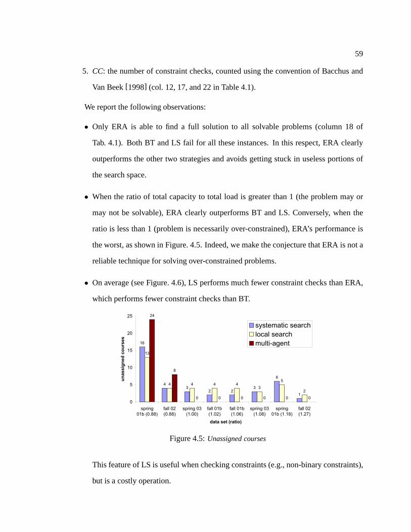
59

5. CC: the number of constraint checks, counted using the convention of Bacchus and

Van Beek[1998] (col. 12, 17, and 22 in Table 4.1).

We report the following observations:

• Only ERA is able to find a full solution to all solvable problems (column 18 of

Tab. 4.1). Both BT and LS fail for all these instances. In thisrespect, ERA clearly

outperforms the other two strategies and avoids getting stuck in useless portions of

the search space.

• When the ratio of total capacity to total load is greater than1 (the problem may or

may not be solvable), ERA clearly outperforms BT and LS. Conversely, when the

ratio is less than 1 (problem is necessarily over-constrained), ERA’s performance is

the worst, as shown in Figure. 4.5. Indeed, we make the conjecture that ERA is not a

reliable technique for solving over-constrained problems.

• On average (see Figure. 4.6), LS performs much fewer constraint checks than ERA,

which performs fewer constraint checks than BT.

16

43

2 23

6

1

13

4 4 4 43

5

2

24

8

0 0 0 0 0 00

5

10

15

20

25

spring

01b (0.88)

fall 02

(0.88)

spring 03

(1.00)

fall 01b

(1.02)

fall 01b

(1.06)

spring 03

(1.08)

spring

01b (1.18)

fall 02

(1.27)

data set (ratio)

un

as

sig

ne

d c

ou

rse

s

systematic search

local search

multi-agent

Figure 4.5:Unassigned courses

This feature of LS is useful when checking constraints (e.g., non-binary constraints),

but is a costly operation.

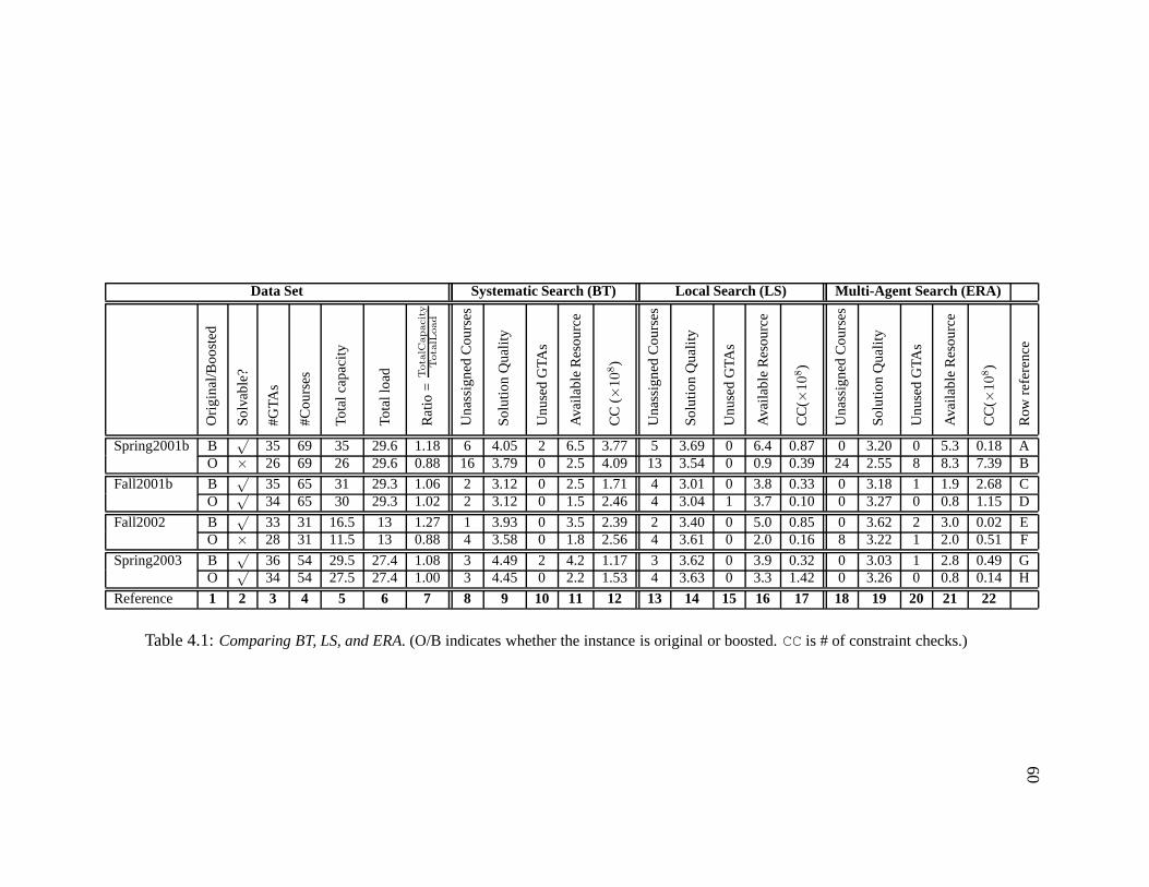
60

Data Set Systematic Search (BT) Local Search (LS) Multi-Agent Search (ERA)

Ori

gin

al/B

oo

sted

So

lvab

le?

#G

TAs

#C

ou

rses

Tota

lcap

acity

Tota

llo

ad

Rat

io=

Tota

lCapacity

Tota

lLoad

Un

assi

gn

edC

ou

rses

So

lutio

nQ

ual

ity

Un

use

dG

TAs

Ava

ilab

leR

eso

urc

e

CC

(×108)

Un

assi

gn

edC

ou

rses

So

lutio

nQ

ual

ity

Un

use

dG

TAs

Ava

ilab

leR

eso

urc

e

CC

(×108)

Un

assi

gn

edC

ou

rses

So

lutio

nQ

ual

ity

Un

use

dG

TAs

Ava

ilab

leR

eso

urc

e

CC

(×108)

Row

refe

ren

ce

Spring2001b B√

35 69 35 29.6 1.18 6 4.05 2 6.5 3.77 5 3.69 0 6.4 0.87 0 3.20 0 5.3 0.18 AO × 26 69 26 29.6 0.88 16 3.79 0 2.5 4.09 13 3.54 0 0.9 0.39 24 2.55 8 8.3 7.39 B

Fall2001b B√

35 65 31 29.3 1.06 2 3.12 0 2.5 1.71 4 3.01 0 3.8 0.33 0 3.18 1 1.9 2.68 CO

√34 65 30 29.3 1.02 2 3.12 0 1.5 2.46 4 3.04 1 3.7 0.10 0 3.27 0 0.8 1.15 D

Fall2002 B√

33 31 16.5 13 1.27 1 3.93 0 3.5 2.39 2 3.40 0 5.0 0.85 0 3.62 2 3.0 0.02 EO × 28 31 11.5 13 0.88 4 3.58 0 1.8 2.56 4 3.61 0 2.0 0.16 8 3.22 1 2.0 0.51 F

Spring2003 B√

36 54 29.5 27.4 1.08 3 4.49 2 4.2 1.17 3 3.62 0 3.9 0.32 0 3.03 1 2.8 0.49 GO

√34 54 27.5 27.4 1.00 3 4.45 0 2.2 1.53 4 3.63 0 3.3 1.42 0 3.26 0 0.8 0.14 H

Reference 1 2 3 4 5 6 7 8 9 10 11 12 13 14 15 16 17 18 19 20 21 22

Table 4.1:Comparing BT, LS, and ERA.(O/B indicates whether the instance is original or boosted.CCis # of constraint checks.)

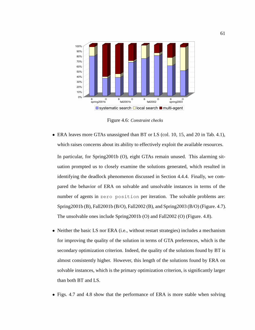
61

0%

10%

20%

30%

40%

50%

60%

70%

80%

90%

100%

systematic search local search multi-agent

spring2001b fall2001b fall2002 spring2003B O O O OB B B

Figure 4.6:Constraint checks

• ERA leaves more GTAs unassigned than BT or LS (col. 10, 15, and20 in Tab. 4.1),

which raises concerns about its ability to effectively exploit the available resources.

In particular, for Spring2001b (O), eight GTAs remain unused. This alarming sit-

uation prompted us to closely examine the solutions generated, which resulted in

identifying the deadlock phenomenon discussed in Section 4.4.4. Finally, we com-

pared the behavior of ERA on solvable and unsolvable instances in terms of the

number of agents inzero position per iteration. The solvable problems are:

Spring2001b (B), Fall2001b (B/O), Fall2002 (B), and Spring2003 (B/O) (Figure. 4.7).

The unsolvable ones include Spring2001b (O) and Fall2002 (O) (Figure. 4.8).

• Neither the basic LS nor ERA (i.e., without restart strategies) includes a mechanism

for improving the quality of the solution in terms of GTA preferences, which is the

secondary optimization criterion. Indeed, the quality of the solutions found by BT is

almost consistently higher. However, this length of the solutions found by ERA on

solvable instances, which is the primary optimization criterion, is significantly larger

than both BT and LS.

• Figs. 4.7 and 4.8 show that the performance of ERA is more stable when solving

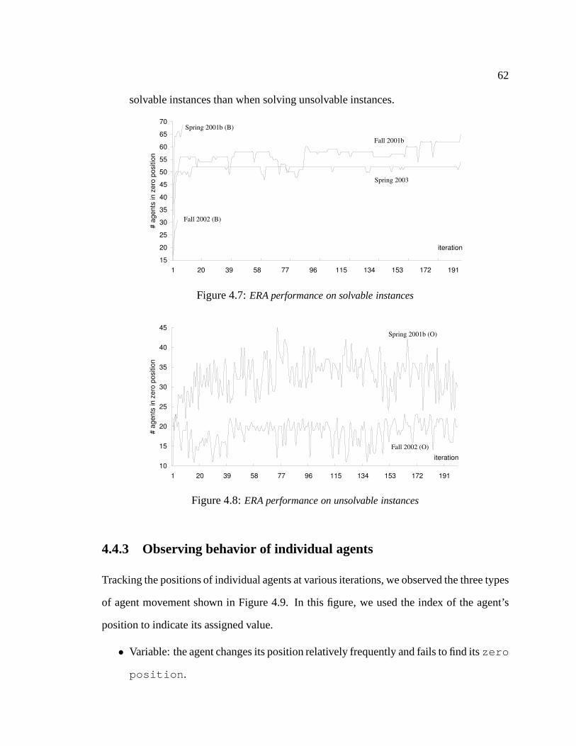
62

solvable instances than when solving unsolvable instances.

15

20

25

30

35

40

45

50

55

60

65

70

1 20 39 58 77 96 115 134 153 172 191

iteration

# a

gents

in z

ero

positio

n

Spring 2001b (B)

Fall 2002 (B)

Fall 2001b

Spring 2003

Figure 4.7:ERA performance on solvable instances

10

15

20

25

30

35

40

45

1 20 39 58 77 96 115 134 153 172 191

iteration

# a

gents

in z

ero

positio

n

Spring 2001b (O)

Fall 2002 (O)

Figure 4.8:ERA performance on unsolvable instances

4.4.3 Observing behavior of individual agents

Tracking the positions of individual agents at various iterations, we observed the three types

of agent movement shown in Figure 4.9. In this figure, we used the index of the agent’s

position to indicate its assigned value.

• Variable: the agent changes its position relatively frequently and fails to find itszero

position .

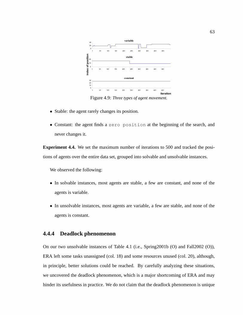
63

0

20

40

1 51 101 151 201 251 301 351 401 451

0

10

20

30

1 51 101 151 201 251 301 351 401 451

0

10

20

1 51 101 151 201 251 301 351 401 451

variable

stable

constant

ind

ex

of

po

sit

ion

iteration

Figure 4.9:Three types of agent movement.

• Stable: the agent rarely changes its position.

• Constant: the agent finds azero position at the beginning of the search, and

never changes it.

Experiment 4.4. We set the maximum number of iterations to 500 and tracked theposi-

tions of agents over the entire data set, grouped into solvable and unsolvable instances.

We observed the following:

• In solvable instances, most agents are stable, a few are constant, and none of the

agents is variable.

• In unsolvable instances, most agents are variable, a few arestable, and none of the

agents is constant.

4.4.4 Deadlock phenomenon

On our two unsolvable instances of Table 4.1 (i.e., Spring2001b (O) and Fall2002 (O)),

ERA left some tasks unassigned (col. 18) and some resources unused (col. 20), although,

in principle, better solutions could be reached. By carefully analyzing these situations,

we uncovered the deadlock phenomenon, which is a major shortcoming of ERA and may

hinder its usefulness in practice. We do not claim that the deadlock phenomenon is unique

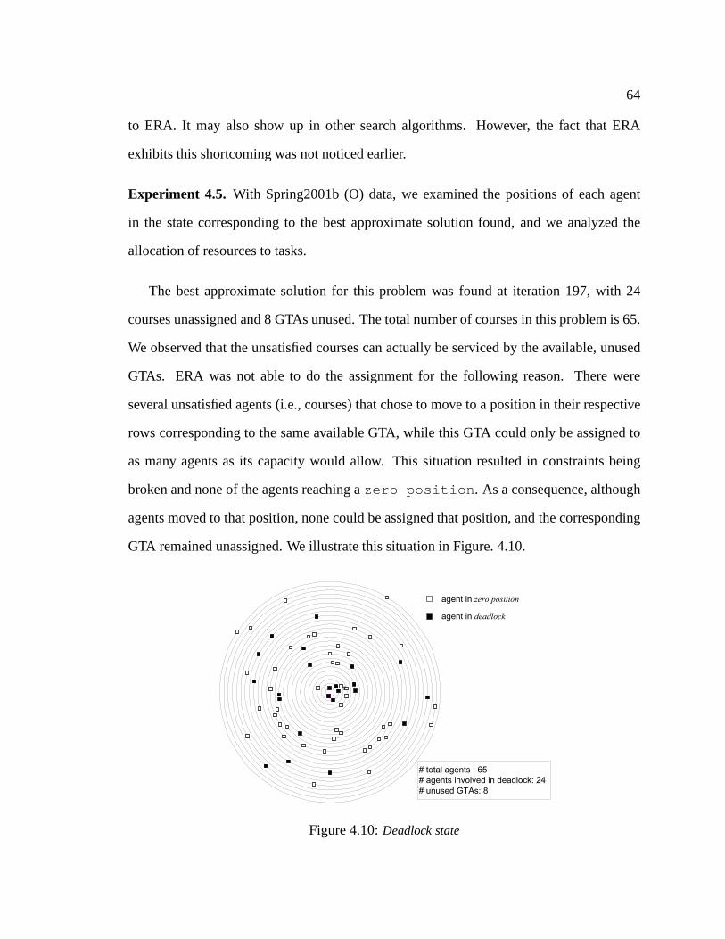
64

to ERA. It may also show up in other search algorithms. However, the fact that ERA

exhibits this shortcoming was not noticed earlier.

Experiment 4.5. With Spring2001b (O) data, we examined the positions of eachagent

in the state corresponding to the best approximate solutionfound, and we analyzed the

allocation of resources to tasks.

The best approximate solution for this problem was found at iteration 197, with 24

courses unassigned and 8 GTAs unused. The total number of courses in this problem is 65.

We observed that the unsatisfied courses can actually be serviced by the available, unused

GTAs. ERA was not able to do the assignment for the following reason. There were

several unsatisfied agents (i.e., courses) that chose to move to a position in their respective

rows corresponding to the same available GTA, while this GTAcould only be assigned to

as many agents as its capacity would allow. This situation resulted in constraints being

broken and none of the agents reaching azero position . As a consequence, although

agents moved to that position, none could be assigned that position, and the corresponding

GTA remained unassigned. We illustrate this situation in Figure. 4.10.

# total agents : 65

# agents involved in deadlock: 24

# unused GTAs: 8

ff

agent in zero position

agent in deadlock

Figure 4.10:Deadlock state

65

Each circle corresponds to a given GTA. Note that there is exactly one circle per GTA.

Each square represents an agent. The position of an square onthe circle is irrelevant and

only useful for visualization purposes. There may be zero ormore squares on a given

circle. Blank squares indicate that the position is azero position for the agent; these

will yield effective assignments. The filled squares indicate that although the position is

the best one for the agent, it results in some broken constraints. Thus it is not azero

position , and the actual assignment of the position to the agent cannot be made. The

circles populated by several filled squares are GTAs that remain unused.

Definition 3. Deadlock state:When the only positions acceptable to a subset for agents

are mutually exclusive, a deadlock occurs that prevents anyof the agents in the subset from

being allowed to move to the requested position.

None of the variables in a deadlock is instantiated, although some could be. Further,

a deadlock causes the behavior of ERA to degrade. When some agents are in a deadlock

state, one would hope that the independence of the agents would allow them to get out of

the deadlock (or remain in it) without affecting the status of agents inzero position .

Our observations show that this is not the case. Indeed, ERA is not able to avoid deadlocks

and yields a degradation of the solution in the sense that it does not maximize the number of

courses satisfied. Subsequent iterations of ERA, instead ofmoving agents out of deadlock

situations, move agents already inzero position out their positions and attempt to

find otherzero position s for them. The current best solution is totally destroyed, and

the behavior of the system degrades.

This problem was not reported in previous implementations of ERA, likely because they

were not tested on over-constrained cases. Further, it seriously hinders the applicability of

this technique to unsolvable problems.It is important that ERA be modified and enhanced

with a conflict resolution mechanism that allows it to identify and solve deadlocks. We

discuss this issue in Section 4.6.

66

4.5 Discussion

From observing the behavior of ERA on the GTA problem, we conclude the following:

• Better-move vs. least-move:A key point in iterative-improvement strategies is to

identify a good neighboring state. In ERA, this is achieved by the reactive rules. In

Minton et al.[Minton et al., 1992], this is the min-conflict heuristic. We noticed that

better-move provides more opportunities to explore the search space than least-move

does, and avoids getting stuck in local optima. With least-move, an agent moves to

its best position where it stays. This increases the difficulties of other agents and the

complexity of the problem, which quickly becomes harder to solve.

• Reactive behaviors:Different behaviors significantly affect the performance of ERA.

We found thatFrBLR results in the best behavior in terms of runtime and solution

quality. At the beginning of the search, better-move can quickly guide more agents

toward theirzero position . Then least-move prevents drastic changes in the

current state while allowing agents to improve their positions. Finally random-move

deals effectively with plateau situations and local optima.

• Stable vs. unstable evolution:As highlighted in Figure. 4.7 and 4.8, the evolution

of ERA across iterations, although not necessarily monotonic, is stable on solvable

problems and gradually moves toward a full solution. On unsolvable problems, its

evolution is unpredictable and appears to oscillate significantly. This complements

the results of Liu et al.[Liu et al., 2002] by characterizing the behavior of ERA on

over-constrained problems, which they had not studied.

From comparing systematic, local and multi-agent search onthe GTA problem, we

identify three parameters that seem to determine the behavior of search, namely

1. the control schema

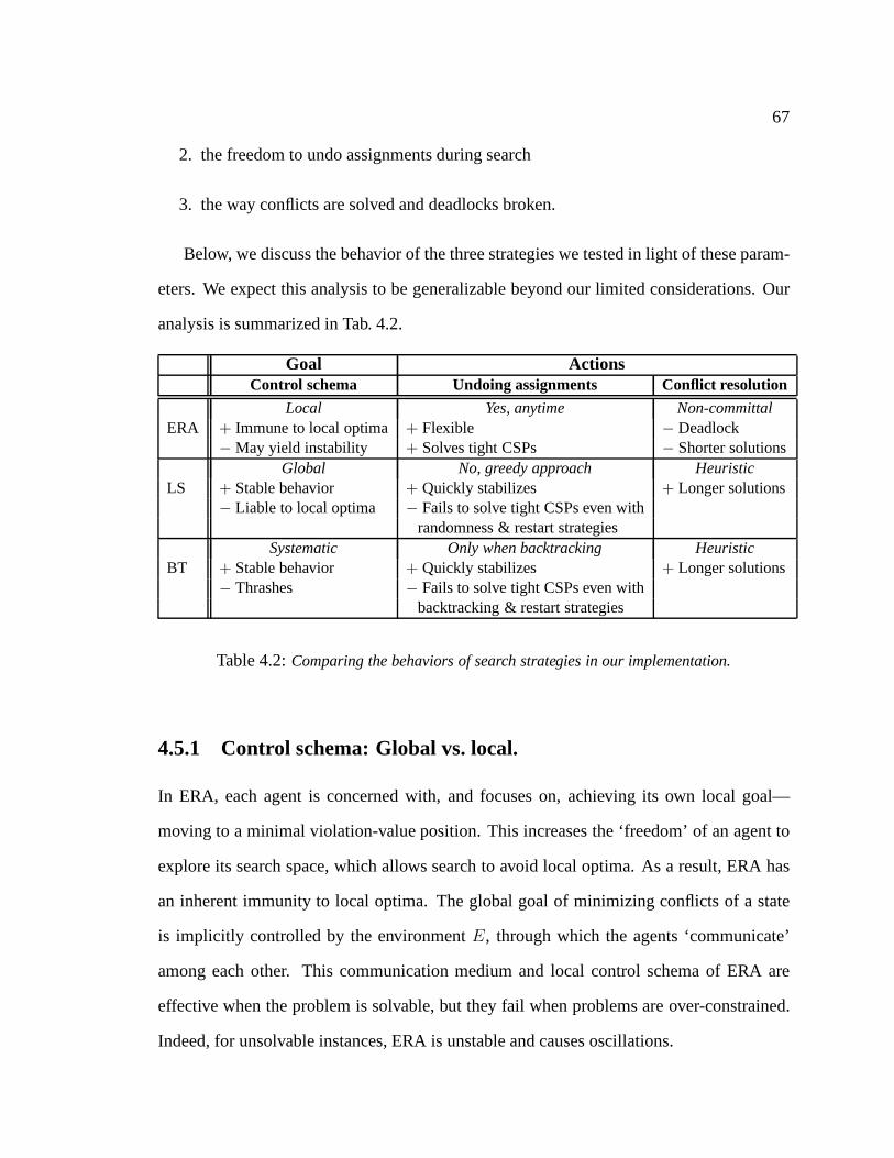
67

2. the freedom to undo assignments during search

3. the way conflicts are solved and deadlocks broken.

Below, we discuss the behavior of the three strategies we tested in light of these param-

eters. We expect this analysis to be generalizable beyond our limited considerations. Our

analysis is summarized in Tab. 4.2.

Goal ActionsControl schema Undoing assignments Conflict resolution

Local Yes, anytime Non-committalERA + Immune to local optima + Flexible − Deadlock

−May yield instability + Solves tight CSPs − Shorter solutionsGlobal No, greedy approach Heuristic

LS + Stable behavior + Quickly stabilizes + Longer solutions− Liable to local optima − Fails to solve tight CSPs even with

randomness & restart strategiesSystematic Only when backtracking Heuristic

BT + Stable behavior + Quickly stabilizes + Longer solutions− Thrashes − Fails to solve tight CSPs even with

backtracking & restart strategies

Table 4.2:Comparing the behaviors of search strategies in our implementation.

4.5.1 Control schema: Global vs. local.

In ERA, each agent is concerned with, and focuses on, achieving its own local goal—

moving to a minimal violation-value position. This increases the ‘freedom’ of an agent to

explore its search space, which allows search to avoid localoptima. As a result, ERA has

an inherent immunity to local optima. The global goal of minimizing conflicts of a state

is implicitly controlled by the environmentE, through which the agents ‘communicate’

among each other. This communication medium and local control schema of ERA are

effective when the problem is solvable, but they fail when problems are over-constrained.

Indeed, for unsolvable instances, ERA is unstable and causes oscillations.

68

This decentralized control is contrasted with the centralized control of local search,

where the neighboring states are evaluated globally by a centralized function. Global con-

trol used in LS leads to a stable performance: the movement toa successor state is, in

general, allowed only when the neighboring state reduces the global cost, such as the total

number of broken constraints in the state. However, this kind of control overly restricts the

movement of agents and the search easily gets trapped in local optima, which is unlikely to

be overcome even with random restarts[Hoos and Stutzle, 1999].

In backtrack search, alternative solutions are examined ina systematic way. Generally

speaking, we either expand a partial solution or we chronologically consider immediate

alternatives to the last decision. Usually, we record the best solution found so far as an

incumbent and update it only when a better solution is found.As a result, the quality of

solutions improves with time and the search is typically stable. However, thrashing is the

price we pay for the stability and completeness of search. Wetested both heuristic and

stochastic backtrack search[Gomeset al., 1998] and found that backtracking never goes

beyond the third of the depth of the tree on our problems. Random restart strategies and

credit-based search can be used to avoid this thrashing, butthey sacrifice completeness.

4.5.2 Freedom to undo assignments.

Among the three strategies we tested so far (we are testing others), only ERA was able to

solve our hard, solvable instances. This ability can be traced to its ability to undo assign-

ments.

In ERA, an agent can undo its assignment as needed, even if it is a consistent one. In

fact, no agent may remain in a given position unless this position is acceptable to all other

agents; that is, it remains azero position across iterations. This feature seems to be

the major reason why ERA was able to solve successfully large, tight problems that resisted

the other techniques we tested (i.e., the solvable instances of Tab. 4.1 were only solved by

69

ERA).

In contrast, in both systematic and hill-climbing search, avalue is assigned to the vari-

able that claims it first, on a first-come, first-served basis.Our implementation of local

search (a hill-climbing strategy with a combination of constraint propagation and a min-

conflict heuristic for value selection) does not undo consistent assignments. However, more

generally, in backtrack search and LS, assignments can be undone using backtracking and

random-restart strategies, respectively. In our experiments, both backtracking and random-

restarts failed to solve tight instances due to the sheer size of the search space.

4.5.3 Conflict resolution and deadlock prevention.

We identify two main approaches for search to deal with conflicts:

• heuristic, based on some priority such as a ‘first-come, first-served,’ least commit-

ment, fail-first principle, or using user-defined preferences

• non-committal, where conflict sets are merely identified andhanded either to the user

or to a conflict resolution procedure[Choueiry and Faltings, 1994].

When it is not able to solve a conflict (e.g., a resource contention in the case of a

resource allocation problem), ERAadopts a cautious approach and leaves the variables

unassigned. This yields the deadlock phenomenon encountered in over-constrained cases,

introduced in Section 4.4.4 and discussed in Section 4.6. Webelieve that the non-committal

strategy is more appropriate in practical settings becauseit clearly delimits the sources of

conflictand makes them the responsibility of a subsequent conflict resolution process. We

consider this feature of ERA to be particularly attractive.Indeed, conflict identification is

a difficult task (perhapsNP-hard) and ERA may constitute the first effective and general

strategy to approach this problem.

70

Both backtrack search and LS operate in a more resolute way: they heuristically assign

values to as many variables as possible. As a result, when maximizing the solution length,

as in the GTA problem, they end up finding solutions that are more competitive (i.e., longer)

than ERA.

4.6 Dealing with the deadlock

While ERA is notcompleteprocedure, we were puzzled by its ability to quickly solve tight

problems. However, in over-constrained problems, some agents may be always prevented

by other agents from reaching azero position . One can think of the deadlock phe-

nomenon as a powerful feature of ERA since it allows us to identify and isolate conflicts.

Conversely, one could think of it as a shortcoming of ERA since, in over-constrained cases,

it yields shorter solutions than LS or BT. We identify four possible avenues for dealing with

deadlocks.

4.6.1 Direct communication and negotiation mechanism

In ERA, agents exchange information indirectly, through the environmentE, and have no

explicit communication mechanism. The information that ispassed is a summary of the

state of the environment. Agents are not able to recognize each other’s individual needs

and thus are unable to establish coalition. One could investigate how to establish more

effective, informative communications among agents, as ina truly multi-agent approach.

4.6.2 Hybridization algorithms

When a deadlock occurs in ERA, we could use the solution foundas a seed for another

search technique such as LS or BT. One could even imagine a portfolio of algorithms

71

where various solvers, with various features and weaknesses, cooperate to solve a given

difficult problem. We are working in this direction.

4.6.3 Mixing behaviored rules

As mentioned in Section 4.2, two assumptions are made for theERA model: (1) all agents

have the same reactive rules, and (2) an agent can only move toposition in its own domain.

According to the first assumption, each agent must follow thesame reactive rules, such as

least-move, better-move and random-move. It seems this assumption restricts the behavior

of an agent. Thus, if we allow each agent to follow its own reactive rule so that each agent

is able to get more freedom to decide its behavior. This kind of mixed-behavior rule might

help ERA to improve its performance.

4.6.4 Adding global control

The decentralized control of ERA enables an agent to pursue the satisfaction of its own

local goal. However, it also undermines the ability of the system to cooperatively achieve

a common global goal (when such a goal exists but is not Paretooptimal). In Section 5.2.3

we investigate how to enhance ERA with global control and examine the advantages and

shortcomings of our proposed strategy.

4.6.5 Conflict resolution

An over-constrained problem by definition, has no solution.Conflict resolution is thus

necessarily heuristic and problem-dependent[Jampelet al., 1996]. There are two main

approaches to conflict resolution:

• Interactive:In an interactive setting, the identified conflicts are ano-good that can

be presented to the user and allow the user to integrate his orher own judgment in

72

the conflict resolution process. For the GTA problem, most conflict resolution is cur-

rently done interactively, which allows the integration of‘unquantifiable’ constraints

into the solutions.

• Automatic:Soft constraints, preferences, and rules to relax constraints could be in-

cluded in the model in order to solve conflicts automatically. Once a given conflict

is identified and solved, a new problem is generated based on the modification of the

initial one, and the problem solver is run on this new problem. This process repeats

until all conflicts are solved. In Section 5.2.4, we discuss two possible strategies for

deadlocks in the GTA problem.

4.7 Conclusions

In this chapter, we introduced a multi-agent search (ERA), in which each variable repre-

sents an agent that inhabits in the environment, a two-dimensional array structure to record

the information of the current state. Agents communicate implicitly each other through

this environment and take their movements according to reaction rules. Then we clearly

demonstrated the performance of ERA with a series of experiments on the GTA assign-

ment problem focusing on four topics: testing the behavior of ERA; comparing the per-

formance of ERA, LS and BT; observing behavior of individualagents and the deadlock

phenomenon. The experimental results show that for solvable, tight CSPs, multi-agent

search clearly outperforms both LS and BT, as it finds a solution when the other two tech-

niques fail. However, we found ERA degenerated in terms of stability and the quality of

the solutions when solving over-constrained problems. In amore detailed study, we iden-

tified the shortcoming and characterized it as deadlock phenomenon. We also proposed

possible approaches to solve deadlock problem when solvingover-constrained CSPs. Our

observations and conclusions are summarized below:

73

• The multi-agent approach exhibits an amazing ability to avoid local optima. We trace

this ability to its fine-grain and de-centralized control mechanism in which agents try

to selfishlyrealize their individual goals while communicating indirectly through the

environment. As a result, the multi-agent approach can solve tight CSPs when the

other two approaches fail.

• ERA shows two different behaviors: stable and unstable evolution. It is stable on

solvable problems and gradually moves towards a full solution. However its evolu-

tion is unpredictable and appears to oscillate greatly. This limits the application of

ERA on over-constrained CSPs.

• From the point of view of solving CSPs, ERA looks somewhat like local search. It

is easy but erroneous to conclude that ERA is just an extension of local search. The

main difference between ERA and local search is that ERA achieves the global goal

by satisfying the local goals of each individual agent, whereas in local search there is

only one global goal. In other words, the transitions between states happen in ERA

after an agent achieves its local goal. But in local search, the transitions happen only

after the global goal is achieved. Local search can be seen asa special case of ERA,

in which an agent’s local goal and the global goal are achieved at the same time.

• The communication mechanism of ERA is not enough for agents to exchange infor-

mation accurately. An agent interacts with other agents only through the environment

E; actually there is no direct communication among agents. The environmentE is

like a blackboard, every agent writes down its information after every movement.

Thus we call this kind of interaction protocol a blackboard system[Weiss, 2000]. In

this system, an agent or expert continues to add contributions to the blackboard until

the problem has been solved.

• ERA overcomes the drawback of LS. In LS the assignment is onlyrepaired once,

74

but in ERA an agent seeks its better position according to thesituation of the cur-

rent state. After the state changes, an agent can freely moveto a new position that

the agent thinks better. This kind of local reparation makesERA have an inherent

immunity to local optima.

• The main shortcoming of ERA is deadlock problem when solvingan over-constrained

CSP. Even though there are more resources that can be used to obtain a better solu-

tion, agents compete for some particular resources to lead the deadlock. As a result,

none of the agents involved in the dead lock can be granted an assignment. This

greatly degrades the quality of the solution.

• In ERA, assignments of agents to positions are made only whenthese positions

are zero-positions. Consequently, ERA produces only consistent solutions. ERA

is not the right framework for modeling MAX-CSPs because it does not allow to

ignore any constraint. Further, the identification of the deadlock phenomenon (in

over-constrained cases) proves that it is nota priori the right framework for finding

maximal consistent partial solutions.

Summary

The multi-agent approach exhibits the best ability to avoidlocal optima due to its goal-

directed behavior and communication capabilities. As a result, the multi-agent approach

can solve tight CSPs when the other two approaches fail. However, with unsolvable prob-

lems, its behavior becomes erratic and unreliable. We are able to trace this shortcoming to

the same feature that constitutes the strength of this approach, i.e. the inter-agent commu-

nication mechanism, which results in a deadlock state in over-constrained situations. We

identify the source of this shortcoming and characterize itas a deadlock phenomenon.

75

Chapter 5

Further investigations in LS and ERA

In this chapter, we extend our study of local search and ERA algorithms a little further,

and propose and test ideas to improve their performance. First we propose a generalized

local search based on the structure of local search. Then we discuss how it guides us

to analyze the algorithms of local search. We then present four approaches- ERA with

mixed behavior, ERA with hybridization, ERA with global control and ERA with conflict

resolution and demonstrate how to use them to avoid or resolve the deadlock problem in

ERA for unsolvable CSPs.

5.1 Local search

Learning the structure of local search can help us analyze and compare local search strate-

gies. Further, this kind of analysis and comparison of various strategies can guide us in the

design of design new algorithms for local search.

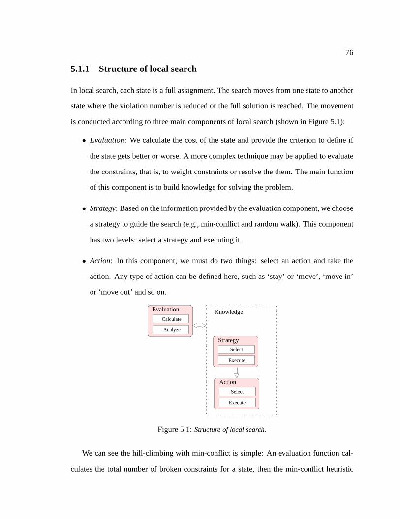
76

5.1.1 Structure of local search

In local search, each state is a full assignment. The search moves from one state to another

state where the violation number is reduced or the full solution is reached. The movement

is conducted according to three main components of local search (shown in Figure 5.1):

• Evaluation: We calculate the cost of the state and provide the criterionto define if

the state gets better or worse. A more complex technique may be applied to evaluate

the constraints, that is, to weight constraints or resolve the them. The main function

of this component is to build knowledge for solving the problem.

• Strategy: Based on the information provided by the evaluation component, we choose

a strategy to guide the search (e.g., min-conflict and randomwalk). This component

has two levels: select a strategy and executing it.

• Action: In this component, we must do two things: select an action and take the

action. Any type of action can be defined here, such as ‘stay’ or ‘move’, ‘move in’

or ‘move out’ and so on.

Calculate

Evaluation

Analyze

Knowledge

Select

Execute

Action

Strategy

Select

Execute

Figure 5.1:Structure of local search.

We can see the hill-climbing with min-conflict is simple: An evaluation function cal-

culates the total number of broken constraints for a state, then the min-conflict heuristic

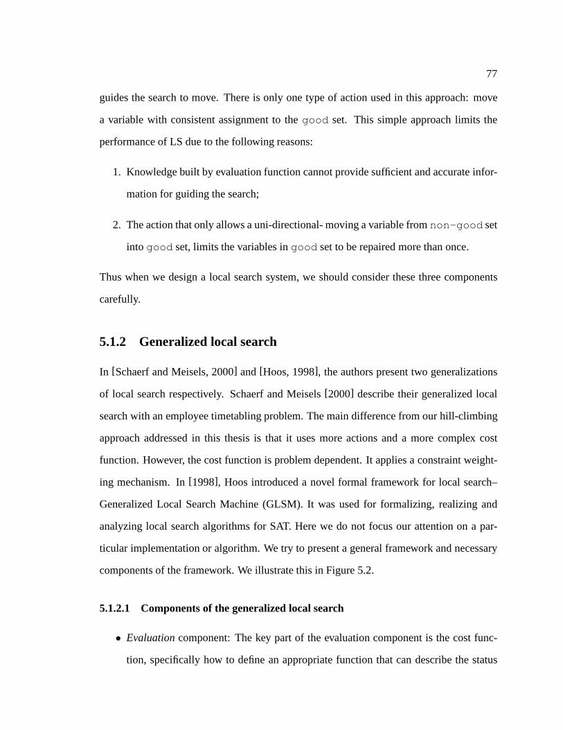
77

guides the search to move. There is only one type of action used in this approach: move

a variable with consistent assignment to thegood set. This simple approach limits the

performance of LS due to the following reasons:

1. Knowledge built by evaluation function cannot provide sufficient and accurate infor-

mation for guiding the search;

2. The action that only allows a uni-directional- moving a variable fromnon-good set

into good set, limits the variables ingood set to be repaired more than once.

Thus when we design a local search system, we should considerthese three components

carefully.

5.1.2 Generalized local search

In [Schaerf and Meisels, 2000] and[Hoos, 1998], the authors present two generalizations

of local search respectively. Schaerf and Meisels[2000] describe their generalized local

search with an employee timetabling problem. The main difference from our hill-climbing

approach addressed in this thesis is that it uses more actions and a more complex cost

function. However, the cost function is problem dependent.It applies a constraint weight-

ing mechanism. In[1998], Hoos introduced a novel formal framework for local search–

Generalized Local Search Machine (GLSM). It was used for formalizing, realizing and

analyzing local search algorithms for SAT. Here we do not focus our attention on a par-

ticular implementation or algorithm. We try to present a general framework and necessary

components of the framework. We illustrate this in Figure 5.2.

5.1.2.1 Components of the generalized local search

• Evaluationcomponent: The key part of the evaluation component is the cost func-

tion, specifically how to define an appropriate function thatcan describe the status

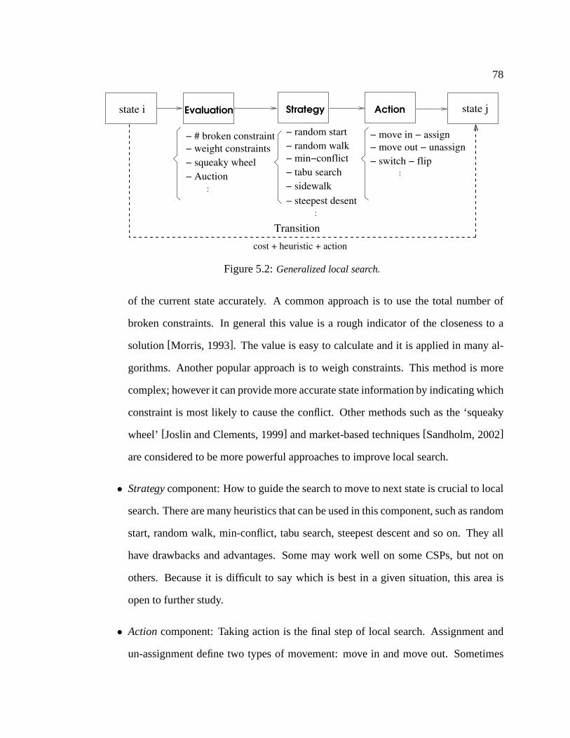
78

state jstate i Action

− move in − assign

− switch − flip

Evaluation

:

− move out − unassign

Transition

Strategy

cost + heuristic + action

− steepest desent

− random start

− min−conflict

− random walk

− tabu search

− sidewalk

:

− # broken constraint

− weight constraints

− squeaky wheel

− Auction

:

Figure 5.2:Generalized local search.

of the current state accurately. A common approach is to use the total number of

broken constraints. In general this value is a rough indicator of the closeness to a

solution[Morris, 1993]. The value is easy to calculate and it is applied in many al-

gorithms. Another popular approach is to weigh constraints. This method is more

complex; however it can provide more accurate state information by indicating which

constraint is most likely to cause the conflict. Other methods such as the ‘squeaky

wheel’ [Joslin and Clements, 1999] and market-based techniques[Sandholm, 2002]

are considered to be more powerful approaches to improve local search.

• Strategycomponent: How to guide the search to move to next state is crucial to local

search. There are many heuristics that can be used in this component, such as random

start, random walk, min-conflict, tabu search, steepest descent and so on. They all

have drawbacks and advantages. Some may work well on some CSPs, but not on

others. Because it is difficult to say which is best in a given situation, this area is

open to further study.

• Actioncomponent: Taking action is the final step of local search. Assignment and

un-assignment define two types of movement: move in and move out. Sometimes

79

‘move in’ is not enough for local search. ‘Move out’ could provide more solution

space to explore. Another possible action is to switch the assignments of two or

more variables. This kind of flipping may break the standoff caused by local optima

and lead the search to a promising state.

5.1.2.2 Transitions

Transitions happen when an action is taken. Determining thecharacteristics of transitions

could help us design algorithms. There are three basic typesof transitions: conditional,

probabilistic, and random. ‘Conditional transition’ means the action is taken according to

a certain set of conditions. For example, in min-conflict, the movement occurs only if a

better state is found. ‘Probabilistic transition’ means the action is taken with a probability

p. For example, we use a probabilityp to control the random walk strategy. ‘Random

transition’ means that the action is taken randomly, such asthe random restart strategy.

The combinations of these three types could comprise additional transition types.

5.2 Extensions of ERA

ERA has the best capability to solve solvable CSPs among our three experimental search

strategies, such as ERA, LS and BT. Among them, only ERA can find a full solution with

solvable problem instances. However, the deadlock phenomenon degrades the performance

of ERA on unsolvable instances. In this section, we continueour investigation on possible

solutions to handle deadlock.

5.2.1 ERA with mixed-behavior rule

The original ERA forces each agent to follow the same reactive rule. This approach might

limit the freedom of agents so that all agents have the same behavior. In our new approach,

80

we allow each agent to follow different reactive rules. In other words, the behavior of

agents is different. In this way we hope ERA can achieve a better performance in dealing

with the deadlock problem. We conducted our experiments in the following manner on all

unsolvable instances of the GTA problem.

Experiment 5.1. Each agent was set to take a random reactive rule at the beginning of the

search. Then an agent followed its assigned rule during the entire search processing. This

means that an agent never changes its reactive rule that was assigned at the beginning.

Experiment 5.2. Each agent was set to get a reactive rule randomly at each iteration during

the search, meaning that the reactive rule of an agent may vary during the search.

We observe in our results that the quality of solutions cannot be improved over the

original ERA without use of the mixed-behavior rule. In other words, the mixed-behavior

rule cannot solve the deadlock problem of ERA.

5.2.2 ERA with hybridization

Each search technique has its own advantages and shortcomings. Can we use the advan-

tages of one technique to improve the performance of another? The combination of differ-

ent search techniques would help to solve a problem when an individual technique cannot.

This hybrid approach is often applied in solving CSPs.

Experiment 5.3. we conducted our test on Spring2001b (O). We used a solution generated

by ERA as a seed, then fixed the consistent assignment in the seed and solved the problem

again by ERA. We repeated this process until the quality of the solution cannot be improved

further. Then we used BT or LS to solve the problem with the seed generated by the last

solution from ERA. The result is shown in Figure 5.3. The pairof numbers shown in the

parenthesis: the first one is the number of unassigned courses, the second one is the number

of unused GTAs.

81

ERA ERA ERA(16 , 4) (14 , 3)(25 , 8)

BT

ERA

LSno improvement

(8 , 0)

(10 , 0)

Figure 5.3:ERA with hybridization.

We see that the solution cannot be improved after applying ERA three times, because

ERA reaches the real deadlock situation. We also find that ERAcan improve the solutions

it generates by fixing the consistent assignment. But, why can the solutions be improved

the first three times when ERA is applied? At these points, theERA does not get stuck in

a real deadlock. In a state that is close to a deadlock, there is no guidance for agents on

which one should move or which one should keep its current position. Thus some agents

might ‘aimlessly’ move out from their promising positions.As a result, the performance of

ERA gets degraded. By forcing the consistent assignment to be fixed as a seed, it provides

a kind of guidance to agents so that some agents can keep theirpromising positions. When

a solution cannot be improved by ERA itself, a real deadlock occurs. At the point we apply

LS or BT, the deadlock is resolved and a better solution can beobtained.

5.2.3 ERA with global control

In the original ERA, each agent has one goal–its own local goal–to find a better position

to move to. The agents do not care about the global goal; theirmovements are driven only

by their local goals. In the case of solvable CSPs, where a solution must exist, each agent

can find itszero position , and the movements of agents are guaranteed to reach the

global goal. The proof is presented in[Liu et al., 2002]. However, in the case of unsolvable

CSPs, there is no full solution at all. Each agent reaches a better position but notzero

position ; the result of the movements might be far away from the globalgoal. Thus,

82

adding global control in the ERA system may help agents move toward the global goal.

Inspired by local search, we propose to enhance ERA with global control in order to

avoid deadlocks. To this end, we add the following reactive rule to the ERA system. After

selecting a position to move to (which is done according to the reactive rules of Section 4.2),

the agent also checks the effect of this move on the global goal, measured as the total

number of violations of the entire state. Only when the movement does not deteriorate the

global goal does the agent effectively execute the considered move.

Experiment 5.4. Solve the GTA problem for the data set of Spring2001 (O), an over-

constrained instance, and that of Fall2001 (O), a solvable instance, using the original and

the modified ERA algorithm. We chooseFrBLR as the default behavior and observe the

number of agents inzero position .

15

20

25

30

35

40

45

50

0 50 100 150 200 250 300 350 400 450 500

iteration

# a

ge

nts

in

ze

ro p

ositio

n

with global control

without global control

Figure 5.4:ERA with global control on Spring2001(0).

From the Figure 5.4, we see that the ERA with global control behaves in a much more

stable way than the ERA without global control. A better solution (the number of unas-

signed courses is reduced from 24 to 20) is obtained. In the solvable instance of the GTA

problem (Figure 5.5), the ERA with global control performs much like our local search

approach. It quickly gets stuck on local optima.

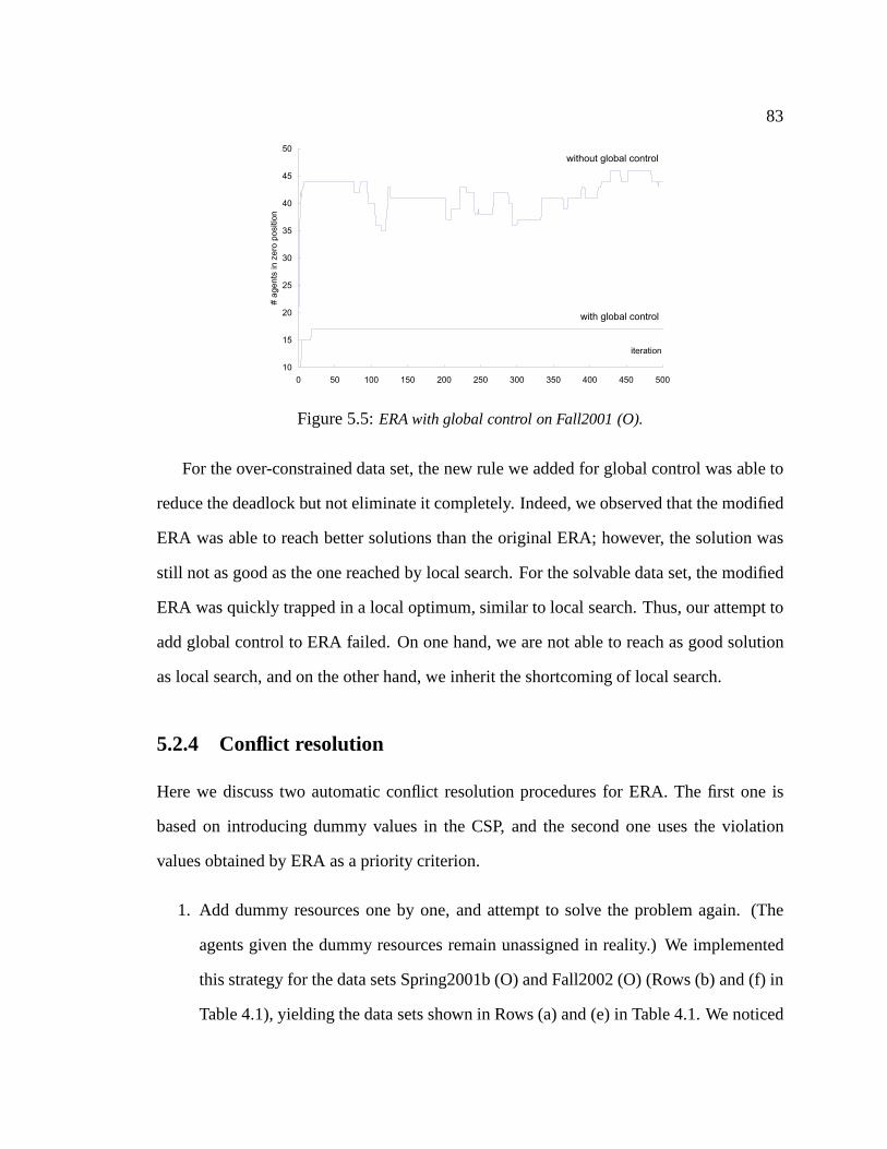
83

10

15

20

25

30

35

40

45

50

0 50 100 150 200 250 300 350 400 450 500

iteration

# a

gents

in z

ero

positio

n

with global control

without global control

Figure 5.5:ERA with global control on Fall2001 (O).

For the over-constrained data set, the new rule we added for global control was able to

reduce the deadlock but not eliminate it completely. Indeed, we observed that the modified

ERA was able to reach better solutions than the original ERA;however, the solution was

still not as good as the one reached by local search. For the solvable data set, the modified

ERA was quickly trapped in a local optimum, similar to local search. Thus, our attempt to

add global control to ERA failed. On one hand, we are not able to reach as good solution

as local search, and on the other hand, we inherit the shortcoming of local search.

5.2.4 Conflict resolution

Here we discuss two automatic conflict resolution procedures for ERA. The first one is

based on introducing dummy values in the CSP, and the second one uses the violation

values obtained by ERA as a priority criterion.

1. Add dummy resources one by one, and attempt to solve the problem again. (The

agents given the dummy resources remain unassigned in reality.) We implemented

this strategy for the data sets Spring2001b (O) and Fall2002(O) (Rows (b) and (f) in

Table 4.1), yielding the data sets shown in Rows (a) and (e) inTable 4.1. We noticed

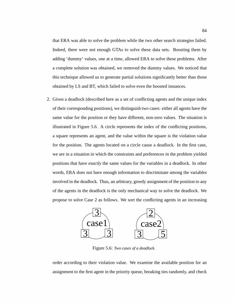
84

that ERA was able to solve the problem while the two other search strategies failed.

Indeed, there were not enough GTAs to solve these data sets. Boosting them by

adding ‘dummy’ values, one at a time, allowed ERA to solve these problems. After

a complete solution was obtained, we removed the dummy values. We noticed that

this technique allowed us to generate partial solutions significantly better than those

obtained by LS and BT, which failed to solve even the boosted instances.

2. Given a deadlock (described here as a set of conflicting agents and the unique index

of their corresponding positions), we distinguish two cases: either all agents have the

same value for the position or they have different, non-zerovalues. The situation is

illustrated in Figure 5.6. A circle represents the index of the conflicting positions,

a square represents an agent, and the value within the squareis the violation value

for the position. The agents located on a circle cause a deadlock. In the first case,

we are in a situation in which the constraints and preferences in the problem yielded

positions that haveexactlythe same values for the variables in a deadlock. In other

words, ERA does not have enough information to discriminateamong the variables

involved in the deadlock. Thus, an arbitrary, greedy assignment of the position to any

of the agents in the deadlock is the only mechanical way to solve the deadlock. We

propose to solve Case 2 as follows. We sort the conflicting agents in an increasing

3

33case1

3case2

2

5Figure 5.6:Two cases of a deadlock.

order according to their violation value. We examine the available position for an

assignment to the first agent in the priority queue, breakingties randomly, and check

85

whether this does not yield any inconsistency on the entire problem. If any inconsis-

tency is encountered, we remove the agent from the queue. If not, then we assign the

position to the agent, and we update the violation values forthe remaining agents.

The process is repeated until all agents in the deadlock havebeen examined. We did

not test this technique because it seemed more complex than the previous one.

5.2.5 Improved communication protocols

Another method to avoid deadlock on unsolvable problems forERA, is to improve the

communication protocol. However, the more complex the protocol, the more sophisticated

and problem-dependent the system becomes. It is difficult todefine a protocol such that

each agent has the same right to get a position. In other words, when a deadlock happens,

it is hard to decide which agent involved in the deadlock should have the position or should

give up the position. Thus we do not discuss this topic in depth in this thesis.

5.3 Conclusions

Generalized local search provides a platform for us to formalize, realize, and analyze local

search algorithms. To improve the performance of local search, we could concentrate our

attention on three components: evaluation, strategy, and action.

For the ERA approach, the problem is the deadlock phenomenonon unsolvable CSPs.

We address several approaches to deal with this problem. Through our experiments we

learned:

• The mixed-behavior rule cannot help ERA deal with the deadlock problem.

• The hybrid approach can help ERA resolve the deadlock problem.

86

• With global control, ERA can effectively avoid the deadlockproblem. However, it

sacrifices its de-centralized mechanism which helps ERA to be able to avoid local

optima.

• Constraint resolution techniques can help ERA solve the deadlock problem.

Summary

There are three basic components in a local search system: evaluation, strategy, and action.

The GLS establishes a platform to formalize, realize and analyze local search algorithms.

When solving over-constrained problems, ERA with hybrid method and ERA with conflict

resolution can help ERA overcome deadlock phenomenon.

87

Chapter 6

Conclusions and future work

In this thesis, we studied two iterative improvement techniques: a heuristic local search

and a multi-agent approach. In the local search approach, weimplemented min-conflict

heuristic hill-climbing with random walk and restart strategies (LS). We adapted the min-

conflict heuristic to non-binary CSPs, identified the nugatory-move phenomenon of LS, and

examined the performance of LS on the GTA assignment problem. Further, we investigated

how the noise strategies help LS deal with local optima. In the multi-agent approach, we

implemented the ERA algorithm and demonstrated its performance on the GTA assignment

problem. Through observing the behavior of individual agents, we identified the deadlock

phenomenon of ERA on over-constrained problems. We compared the performance of

ERA, LS and BT. Further, we discussed possible approaches for handling and solving

deadlocks. In this chapter, we summarize our research, discuss conclusions about LS and

ERA, and point out directions for future research.

6.1 Summary of the research conducted

Local search approach is a well-known example for applying iterative improvement. There

is a large body of research in this area, however most of the research was conducted using

88

puzzles or randomly-generated CSPs. In this study, we demonstrated the performance of

LS on the GTA assignment problem. The main shortcoming of LS is that it gets stuck in

local optima. Once the solution reaches some state in the solution space, the quality of

solution cannot be further improved. We examined noise strategies to help LS to handle

local optima. Further, we presented GLS as a framework in which to study and design local

search algorithms.

In this thesis, we also study a multi-agent search approach (ERA), which uses the same

iterative improvement mechanism as LS does. However, the improvement of ERA results

from a set of autonomous agents with local goal-directed behavior and communication ca-

pabilities. We demonstrated that ERA has the best ability toavoid local optima on the GTA

assignment problem. However, on unsolvable instances, itsbehavior becomes unstable.

We identified it as a deadlock phenomenon.

We conducted the following experiments on eight instances of the GTA assignment

problem in this thesis: For LS,

• Using constraint propagation to handle global constraints

• Comparing LS and BT

• Using random walk to avoid local optima

• Using random restart to recover from local optima

• Identifying behavior for solvable and unsolvable instances

For ERA,

• Testing the behavior of ERA

• Comparing the performance of ERA, LS and BT

• Observing behavior of individual agents

89

• Identifying the deadlock phenomenon

For improving ERA,

• Mixing behaviors of agents

• Using hybrid search techniques

• Adding global control

• Using conflict resolution strategies for ERA

6.2 Conclusions of LS and ERA

LS is able to find a consistent partial solution within a shorttime interval. This property

can be used when the computation time is limited. The multi-agent approach exhibits the

best ability to avoid local optima. A review of the main features of these two approaches is

given below:

6.2.1 Local search strategy (LS)

we summarize the features of LS as follows:

Nugatory-move phenomenon: For a CSP with global constraints, LS shows poor perfor-

mance. The problem is caused by the nugatory-move phenomenon. Our study shows

that constraint propagation is an effective approach to solve this problem.

Efficiency: LS can find a consistent partial solution within ashort time interval. This

property can be used for generating a seed solution for othersearch techniques in

hybrid approaches.

90

Monotonic improvement: LS improves the solution quality byrepairing variables in a

conflict set. Once a variable gets a consistent assignment, it is never repaired again.

This approach causes LS to stabilize and quickly get stuck inlocal optima.

Noise strategies: The effect of random restart and random walk in dealing with local

optima is insignificant. The value of noise probabilityp in random walk is difficult

to identify when solving the GTA assignment problem. We think the value ofp

depends on a particular CSP. A basic principle of how to choose this value should be

considered: the value ofp should not be too small (< 5%) or too big (> 45%).

6.2.2 Multi-agent strategy (ERA)

we summarize the features of LS as follows:

Ability to avoid local optima: ERA has an inherent immunity to avoiding local optima

due to its de-centralized control schema. As a result, the ERA can solve tight CSPs.

Local goal-directed behavior: ERA is different from local search, even though the cost

function looks like the one used in local search. In ERA, eachagent only cares about

its own cost of movement. Even though the movement of an agentcould cause the

quality of the entire state to worsen, the agent still insists on moving to that position

for its own purpose. This local goal-directed behavior allows ERA to explore more

search space so that the local optima may be overcome.

Simple and poor communication: All agents exchange their information through the en-

vironmentE. This simple communication is easy to implement. However, it is not

enough for over-constrained problems that may require additional information for

agents to choose their next move.

91

Deadlock phenomenon: ERA exhibits two different behaviors: stable and unstable evo-

lution. It is stable on solvable problems. However its evolution appears to oscillate

greatly on unsolvable problems. We identify this shortcoming and characterize it as a

deadlock phenomenon. This undermines the application of ERA on over-constrained

problems.

6.3 Open questions and future research directions

Our experiments were carried out on the real-world instances of the GTA assignment prob-

lem. Most contributions of this thesis, including observations and results of empirical and

theoretical investigations, as well as the discussions andconclusions, seem generalizable

beyond the GTA assignment problem. We still need to characterize the behavior of LS and

ERA on random and other real-world CSPs. In the following section, we briefly address

some of these issues.

6.3.1 Local search

To characterize the behavior of local search, we need to study more approaches besides

the hill-climbing method. Most studies on local search are based on empirical methods,

because the theoretical understanding of the behavior of local search is still limited. The

conclusions drawn from the experiments depend strongly on the empirical methodology

and problems applied. Thus,

• The empirical methodology in[Hoos, 1998; Hoos and Stutzle, 1999] needs to be

studied and followed as the guideline for future experiments.

• We need to study more local search approaches: simulated annealing[Metropoliset

al., 1953; S. Hirkpatrick and Vecchi, 1983], tabu search[Glover and Laguna, 1993]

92

and genetic algorithms[Davis, 1991; Holland, 1975].

• We should study noise strategies over random CSPs with different local search ap-

proaches.

• We should study and implement the breakout method[Morris, 1993] for escaping

from local optima.

6.3.2 Multi-agent search

We showed that ERA is particularly effective at handling tight, solvable problems that

resisted other search techniques. However, its shortcomings on over-constrained problems

(i.e., its instability and the degradation of the approximate solutions it finds) significantly

undermine its usefulness in practice. We plan to address this problem from the following

perspectives:

• Develop conflict resolution strategies to overcome deadlocks. Note that the ability of

ERA to isolate the deadlock is a significant advantage in thistask.

• Experiment with search hybridization techniques with LS, which can reach and main-

tain a good quality approximate solution within the first fewiterations.

• Further, we plan to expand our study to include techniques such as randomized sys-

tematic search[Gomeset al., 1998], the squeaky wheel method[Joslin and Clements,

1999], and market-based techniques[Sandholm, 2002], in a setting similar to the ‘al-

gorithm portfolios’ of[Gomes and Selman, 2001].

• GTA problem is a resource allocation problem. The deadlock is caused by limited

resources such as the capacity of an agent. Is deadlock specific for resource allocation

problems, and does deadlock occur in general CSPs? If not, isthere a general way

93

to characterize the behavior of ERA on general CSPs? As instability? As something

else? To explore these questions, we need:

1. to prove the deadlock on general resource allocation problems

2. to do experiments with over-constrained random CSPs

• Finally, we plan to conduct a more thorough empirical evaluation of the behavior of

the various algorithms on randomly generated problems following the methodology

of [Hoos, 1998; Hoos and Stutzle, 1999].

6.3.3 Backbone

The concept of backbone was introduced on the satisfiability(SAT) decision problem in

1999[Monassonet al., 1999]. Backbone stands for the set of variables that appear con-

strained to the same value in all solutions. In other words, the assignment of variables in

backbone is frozen in all solutions. As shown experimentally in [Parkes, 1997], the size of

backbone is a crucial index for the cost of local search approaches. For a problem with large

backbone size, all of its optimal assignments will be located in a particularly restricted area

of the search space. That means many erroneous assignments for the variables in backbone

may be made during the search. On the other hand, problems with small backbone size

have optimal assignments widely distributed in search space. Optimal and near optimal

assignments are expected to include at least a subset of the formula’s backbone constrained

to appropriate values[Telelis and Stamatopoulos, 2002]. According to[Slaney and Walsh,

2001], backbone should be studied because:

1. Backbone is an important indicator of hardness of CSPs.

2. Identification of backbone variables could reduce the difficulty of problems.

94

Regarding the GTA problem: Does it encounter backbone variables? If yes, what are the

reasons that cause backbone ? Is it possible that the backbone could improve LS or ERA?

Could we use the backbone to simplify the GTA assignment problem?

Building on previous studies of LS and ERA, the goal of this thesis was to enhance

the general understanding of LS and ERA algorithms and theirbehaviors. Through exper-

iments to evaluate their performance, we identified the shortcomings of LS and ERA and

proposed improvements. Finally, we pointed out future directions for research.

95

Appendix A

Documentation for LS and ERA

From 2001 to 2003, I worked on the study of two search techniques, local search and multi-

agent based search, in the context of a real-world application, the assignment of Graduate

Teaching Assistants (GTA) to academic tasks. I implementedtwo algorithms: hill-climbing

with min-conflict [Minton et al., 1992] heuristic (MC) and ERA[Liu et al., 2002]. The

detailed research on these two techniques can be found in this thesis.

This document gives a brief introduction of the model of the GTA assignment problem

and data structure of objects used in the model. Further, it describes how to install and use

the programs to solve the instances of the GTA assignment problem.

A.1 Introduction

The Graduate Teaching Assistants (GTA) problem is a real-world and hard constraint sat-

isfaction problem. Based on the model built by[Glaubius and Choueiry, 2002a], we devel-

oped a local search approach - hill climbing with min-conflict heuristic and a multi-agent

search algorithm - ERA. In a GTA assignment problem, we are given a set of graduate

teaching assistants, a set of courses, and a set of constraints that specify allowable assign-

ments of GTAs to courses. The goal is to find a consistent and satisfactory assignment.

In this problem, we model the courses as variables and the GTAs as values. Typically,

each semester a pool of 25 to 40 GTAs must be assigned as graders or instructors to the

96

majority of courses offered during that semester. In the past, this task has been performed

by hand by several members of the staff and faculty. Tentative schedules were iteratively

refined and updated based on feedback from other faculty members and the GTAs them-

selves, in a tedious and error-prone process dragging over athree-week period. It was

quite common to have the final hand-made assignments containa number of conflicts and

inconsistencies, which negatively affected the quality ofour academic program. For ex-

ample, when a course is assigned a GTA who has little knowledge of the subject matter,

the course’s instructor has to take over a large portion of the GTA’s job and the GTA has

to invest considerable effort in adjusting to the situation. Moreover, students in the course

may receive diminished feedback and unfair grading. Our efforts in modeling and solving

this problem using constraint processing techniques have resulted in a prototype system

under field testing in our department since August 2001[Glaubius and Choueiry, 2002a].

This system has effectively reduced the number of obvious conflicts, thus yielding a com-

mensurate increase in course quality. It has also decreasedthe amount of time and effort

spent on making assignments and has gained the acceptance and approval of our faculty

and students.

In this chapter, we give a brief review of the data structure of the GTA assignment

problem. That helps us to understand and use the functions described in next chapter.

97

A.1.1 File structure

The entire GTA package should be installed under gta directory. The following directory

tree illustrates the file structure:

-gta-+|-- BUG-LOG|-- DATA|-- ORIGINAL-DATA|-- LIST-FILE|-- PROBLEM-DEFINE---+| |-- basic-files| |-- consistency-checking| |-- csp-setup| |-- csp-utils| |-- read-data||-- SEARCH-ALGORITHM-+| |-- search-fc| |-- local-search| |-- era-search|-- make.lisp|-- my-extensions.lisp

The content of each directory is described as follows:

• BUG-LOG : records the log when a bug is reported and fixed

• DATA : stores all GTA data files collected

• ORIGINAL-DATA : all backup files from GTA data

• LIST-FILE : includes all list files used by make file

• PROBLEM-DEFINE : all files under this directory are used to build an instance of

the GTA assignment problem.

– basic-files: create the GTA package, declare global variables and create course

and gta objects

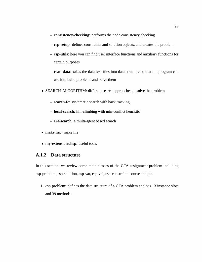
98

– consistency-checking: performs the node consistency checking

– csp-setup: defines constraints and solution objects, and creates the problem

– csp-utils: here you can find user interface functions and auxiliary functions for

certain purposes

– read-data: takes the data text-files into data structure so that the program can

use it to build problems and solve them

• SEARCH-ALGORITHM: different search approaches to solve the problem

– search-fc: systematic search with back tracking

– local-search: hill-climbing with min-conflict heuristic

– era-search: a multi-agent based search

• make.lisp: make file

• my-extensions.lisp: useful tools

A.1.2 Data structure

In this section, we review some main classes of the GTA assignment problem including

csp-problem, csp-solution, csp-var, csp-val, csp-constraint, course and gta.

1. csp-problem: defines the data structure of a GTA problem and has 13 instance slots

and 39 methods.

99

csp-problemID the identification numberclosed-variables closed or canceled coursesconflict-vars variables in no-good set for local searchconstraints all constraintsfuture-variables used for systematic searchgood-vars variables in good set for local searchnil-vars variables get nil assignment for local searchpast-variables used for systematic searchsolution a solution for the current problemstatic-variables pre-assigned variablestotal-broken-constraints number of broken constraints for local searchvals all valuesvariables all variables

2. csp-solution: defines the data structure of a solution andhas 10 instance slots and 45

methods.

csp-solutionID the identification numberproblem the problem objectassignment the final assignment in the form ((< var >< val >< pref >)...)conflict-vars variables involving conflict used by local searchnbr-broken-constraints number of broken constraints based on the current assignmentnob number of backtracksnull-assignment nil assignment used by local searchproduct-preference quality of the solutionsize non-nil assignmentssol-time CPU time to solve the problem

3. csp-var: defines the data structure of the CSP variable andhas 11 instance slots and

37 methods.

csp-varassigned-val the assigned valueconstraints all constraints on this variablecourse the corresponding course of the variablecurrent-domain current domainfuture-fc used by systematic searchinitial-domain the original domainneighbor-vars variables in the neighborproblem the problem objectreductions used by systematic searchtentative-val used by local searchconflict-num used by local search

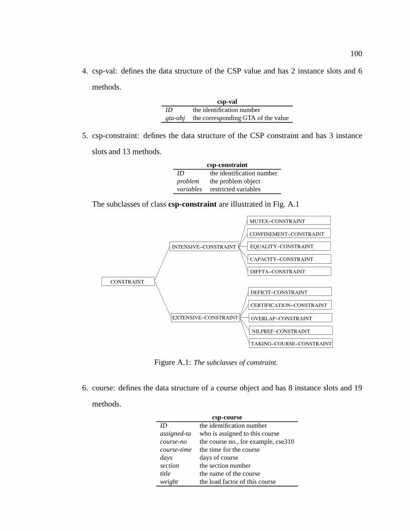
100

4. csp-val: defines the data structure of the CSP value and has2 instance slots and 6

methods.

csp-valID the identification numbergta-obj the corresponding GTA of the value

5. csp-constraint: defines the data structure of the CSP constraint and has 3 instance

slots and 13 methods.

csp-constraintID the identification numberproblem the problem objectvariables restricted variables

The subclasses of classcsp-constraintare illustrated in Fig. A.1

TAKING−COURSE−CONSTRAINT

NILPREF−CONSTRAINT

OVERLAP−CONSTRAINT

CERTIFICATION−CONSTRAINT

DEFICIT−CONSTRAINT

DIFFTA−CONSTRAINT

CAPACITY−CONSTRAINT

EQUALITY−CONSTRAINT

CONFINEMENT−CONSTRAINT

MUTEX−CONSTRAINT

EXTENSIVE−CONSTRAINT

INTENSIVE−CONSTRAINT

CONSTRAINT

Figure A.1:The subclasses of constraint.

6. course: defines the data structure of a course object and has 8 instance slots and 19

methods.

csp-courseID the identification numberassigned-ta who is assigned to this coursecourse-no the course no., for example, cse310course-time the time for the coursedays days of coursesection the section numbertitle the name of the courseweight the load factor of this course

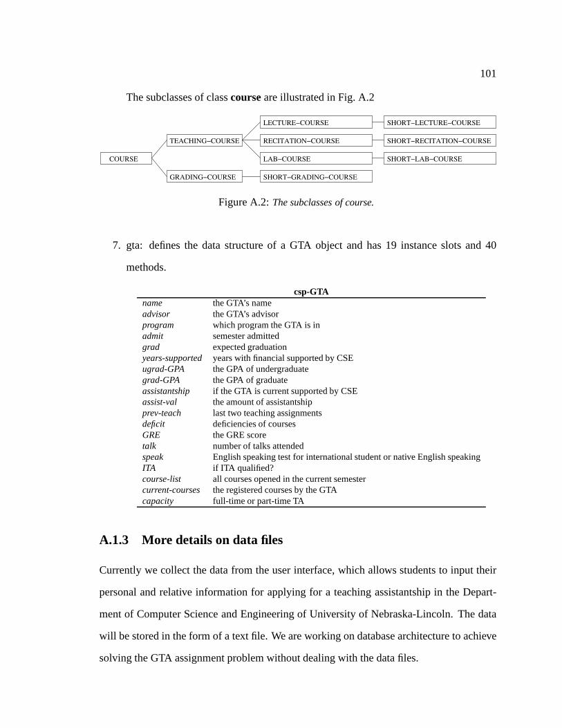
101

The subclasses of classcourseare illustrated in Fig. A.2

TEACHING−COURSE

GRADING−COURSE

LECTURE−COURSE

RECITATION−COURSE

LAB−COURSE

SHORT−GRADING−COURSE

SHORT−LECTURE−COURSE

SHORT−LAB−COURSE

SHORT−RECITATION−COURSE

COURSE

Figure A.2:The subclasses of course.

7. gta: defines the data structure of a GTA object and has 19 instance slots and 40

methods.

csp-GTAname the GTA’s nameadvisor the GTA’s advisorprogram which program the GTA is inadmit semester admittedgrad expected graduationyears-supported years with financial supported by CSEugrad-GPA the GPA of undergraduategrad-GPA the GPA of graduateassistantship if the GTA is current supported by CSEassist-val the amount of assistantshipprev-teach last two teaching assignmentsdeficit deficiencies of coursesGRE the GRE scoretalk number of talks attendedspeak English speaking test for international student or native English speakingITA if ITA qualified?course-list all courses opened in the current semestercurrent-courses the registered courses by the GTAcapacity full-time or part-time TA

A.1.3 More details on data files

Currently we collect the data from the user interface, whichallows students to input their

personal and relative information for applying for a teaching assistantship in the Depart-

ment of Computer Science and Engineering of University of Nebraska-Lincoln. The data

will be stored in the form of a text file. We are working on database architecture to achieve

solving the GTA assignment problem without dealing with thedata files.

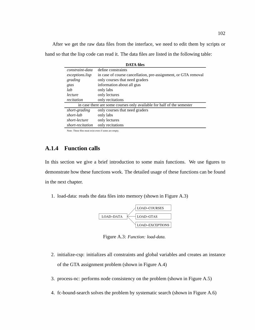
102

After we get the raw data files from the interface, we need to edit them by scripts or

hand so that the lisp code can read it. The data files are listedin the following table:

DATA filesconstraint-data define constraintsexceptions.lisp in case of course cancellation, pre-assignment, or GTA removalgrading only courses that need gradersgtas information about all gtaslab only labslecture only lecturesrecitation only recitations

in case there are some courses only available for half of the semestershort-grading only courses that need gradersshort-lab only labsshort-lecture only lecturesshort-recitation only recitationsNote: These files must exist even if some are empty.

A.1.4 Function calls

In this section we give a brief introduction to some main functions. We use figures to

demonstrate how these functions work. The detailed usage ofthese functions can be found

in the next chapter.

1. load-data: reads the data files into memory (shown in Figure A.3)

LOAD−EXCEPTIONS

LOAD−COURSES

LOAD−GTASLOAD−DATA

Figure A.3:Function: load-data.

2. initialize-csp: initializes all constraints and globalvariables and creates an instance

of the GTA assignment problem (shown in Figure A.4)

3. process-nc: performs node consistency on the problem (shown in Figure A.5)

4. fc-bound-search solves the problem by systematic search(shown in Figure A.6)

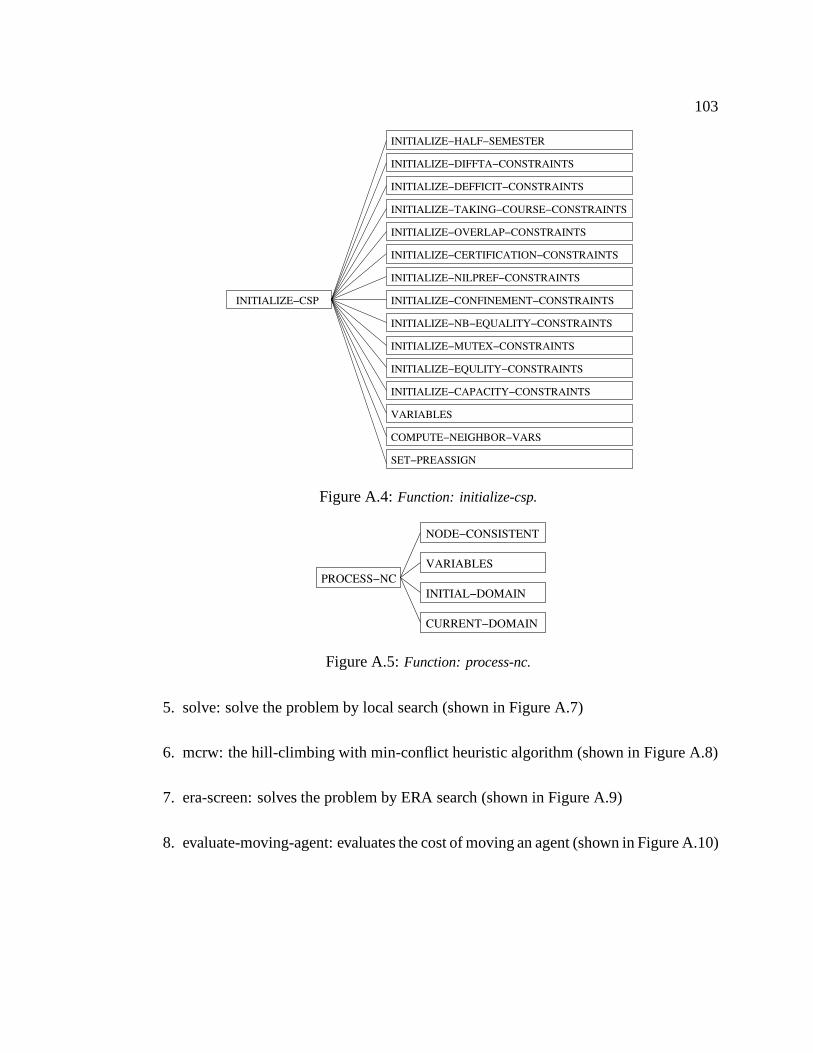
103

INITIALIZE−HALF−SEMESTER

INITIALIZE−DIFFTA−CONSTRAINTS

INITIALIZE−TAKING−COURSE−CONSTRAINTS

INITIALIZE−DEFFICIT−CONSTRAINTS

INITIALIZE−OVERLAP−CONSTRAINTS

INITIALIZE−CERTIFICATION−CONSTRAINTS

INITIALIZE−CONFINEMENT−CONSTRAINTS

INITIALIZE−NILPREF−CONSTRAINTS

INITIALIZE−NB−EQUALITY−CONSTRAINTS

INITIALIZE−MUTEX−CONSTRAINTS

INITIALIZE−EQULITY−CONSTRAINTS

INITIALIZE−CAPACITY−CONSTRAINTS

VARIABLES

COMPUTE−NEIGHBOR−VARS

SET−PREASSIGN

INITIALIZE−CSP

Figure A.4:Function: initialize-csp.

INITIAL−DOMAIN

VARIABLES

CURRENT−DOMAIN

NODE−CONSISTENT

PROCESS−NC

Figure A.5:Function: process-nc.

5. solve: solve the problem by local search (shown in Figure A.7)

6. mcrw: the hill-climbing with min-conflict heuristic algorithm (shown in Figure A.8)

7. era-screen: solves the problem by ERA search (shown in Figure A.9)

8. evaluate-moving-agent: evaluates the cost of moving an agent (shown in Figure A.10)

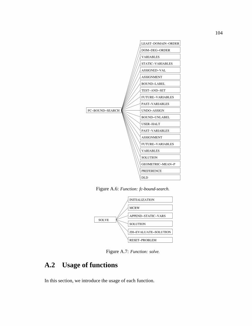
104

STATIC−VARIABLES

VARIABLES

DOM−DEG−ORDER

LEAST−DOMAIN−ORDER

ASSIGNED−VAL

VARIABLES

DLD

PREFERENCE

GEOMETRIC−MEAN−P

SOLUTION

FUTURE−VARIABLES

ASSIGNMENT

PAST−VARIABLES

USER−HALT

BOUND−UNLABEL

UNDO−ASSIGN

PAST−VARIABLES

FUTURE−VARIABLES

TEST−AND−SET

BOUND−LABEL

ASSIGNMENT

FC−BOUND−SEARCH

Figure A.6:Function: fc-bound-search.

RESET−PROBLEM

SOLUTION

ZH−EVALUATE−SOLUTION

APPEND−STATIC−VARS

MCRW

INITIALIZATION

SOLVE

Figure A.7:Function: solve.

A.2 Usage of functions

In this section, we introduce the usage of each function.

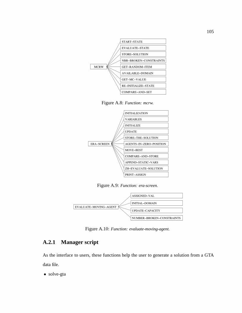
105

START−STATE

EVALUATE−STATE

STORE−SOLUTION

GET−RANDOM−ITEM

AVAILABLE−DOMAIN

GET−MC−VALUE

COMPARE−AND−SET

RE−INITIALIZE−STATE

NBR−BROKEN−CONSTRAINTS

MCRW

Figure A.8:Function: mcrw.

INITIALIZATION

VARIABLES

INITIALIZE

UPDATE

STORE−THE−SOLUTION

MOVE−BEST

COMPARE−AND−STORE

APPEND−STATIC−VARS

AGENTS−IN−ZERO−POSITION

ZH−EVALUATE−SOLUTION

PRINT−ASSIGN

ERA−SCREEN

Figure A.9:Function: era-screen.

UPDATE−CAPACITY

INITIAL−DOMAIN

ASSIGNED−VAL

NUMBER−BROKEN−CONSTRAINTS

EVALUATE−MOVING−AGENT

Figure A.10:Function: evaluate-moving-agent.

A.2.1 Manager script

As the interface to users, these functions help the user to generate a solution from a GTA

data file.

• solve-gta

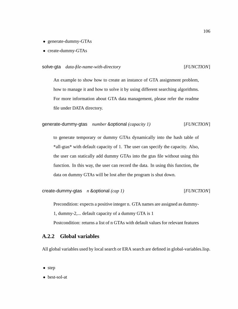
106

• generate-dummy-GTAs

• create-dummy-GTAs

solve-gta data-file-name-with-directory [FUNCTION]

An example to show how to create an instance of GTA assignmentproblem,

how to manage it and how to solve it by using different searching algorithms.

For more information about GTA data management, please refer the readme

file under DATA directory.

generate-dummy-gtas number&optional (capacity 1) [FUNCTION]

to generate temporary or dummy GTAs dynamically into the hash table of

*all-gtas* with default capacity of 1. The user can specify the capacity. Also,

the user can statically add dummy GTAs into the gtas file without using this

function. In this way, the user can record the data. In using this function, the

data on dummy GTAs will be lost after the program is shut down.

create-dummy-gtas n &optional (cap 1) [FUNCTION]

Precondition: expects a positive integer n. GTA names are assigned as dummy-

1, dummy-2,... default capacity of a dummy GTA is 1

Postcondition: returns a list of n GTAs with default values for relevant features

A.2.2 Global variables

All global variables used by local search or ERA search are defined in global-variables.lisp.

• step

• best-sol-at

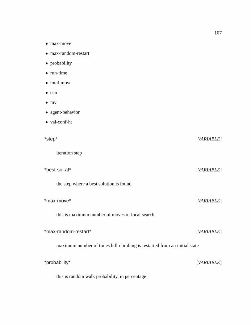
107

• max-move

• max-random-restart

• probability

• run-time

• total-move

• ccn

• mv

• agent-behavior

• val-conf-ht

*step* [VARIABLE]

iteration step

*best-sol-at* [VARIABLE]

the step where a best solution is found

*max-move* [VARIABLE]

this is maximum number of moves of local search

*max-random-restart* [VARIABLE]

maximum number of times hill-climbing is restarted from an initial state

*probability* [VARIABLE]

this is random walk probability, in percentage

108

*run-time* [VARIABLE]

cpu time

*total-move* [VARIABLE]

the number of movement for all agents for reaching zero position used by

multi-agent method.

*ccn* [VARIABLE]

the number of constraint checking

*mv* [VARIABLE]

a list of all values and each value marked by a number

*agent-behavior* [VARIABLE]

a list of all variables associated with its specified behavior

initialization [FUNCTION]

initialize the global parameters

renew-parameters [FUNCTION]

renew some global parameters

*val-conf-ht* [VARIABLE]

hash table for the state table of agents

109

A.2.3 Local search algorithm

We divide functions into four groups, for example:

1. search functions: used directly or indirectly by the search algorithm

2. analysis function: used to analyze the performance of thesearch or the quality of

solutions in order to provide some observation for improving the code or judging the

search

3. test functions: conduct different experiments for certain purposes

4. debug functions: used for debugging the code

A.2.3.1 Search functions

1. Hill-climbing with min-conflict heuristic algorithm

• start-state

• available-domain

• get-mc-value

• MCRW

• re-initialize-state

• non-empty-domain

• filter-domain

• is-a-ita

• course-need-ita

• gta-without-ita-first

• append-static-vars

• gta-without-ita-first

• start-solving

• start-and-store

110

• random-start

• solve

start-state problem [FUNCTION]

begin the local search from any a random state

Precondition : a given problem that is node-consistent.

Postcondition: each variable is assigned a random value anda random

solution for this problem is returned

available-domain var [FUNCTION]

for a given variable, check all values in its initial domain that return a list

of values allowed by the maximum capacity. should only be called after

evaluate-state [and store-solution]

get-mc-value variable [FUNCTION]

return a value to a variable. If this course needs an ITA, thenreturn an

ITA, otherwise first consider GTAs without ITA.

mcrw problem stream [FUNCTION]

the hill-climbing with min-conflict algorithm

re-initialize-state problem [FUNCTION]

release all assigned variables

111

non-empty-domain variables [FUNCTION]

check if the current domain of a variable is empty or not

filter-domain var [FUNCTION]

filter the value of each variable in the conflict-set so that the values that

are inconsistent with the variables in the good set will be filtered out.

is-a-ita x [FUNCTION]

check if a GTA is ITA qualified

course-need-ita x [FUNCTION]

check if a course requires an ITA

gta-without-ita-first vars [FUNCTION]

if a GTA is ITA qualified, it will not be considered in the assignment. First

consider GTAs without ITA

append-static-vars solution problem [FUNCTION]

if pre-assignment exists, just put them into the solution

start-solving stream [FUNCTION]

take a stream, then generate a problem and begin to solve the problem the

final solution will be put into the stream

112

start-and-store [FUNCTION]

a convenient driver to generate a problem and solve it with random-start

strategy ; Save the result into a specified destination

random-restart stream [FUNCTION]

called by start-and-store. It can also be used independently by just give a

stream.

solve problem stream [FUNCTION]

take a problem and a stream to solve the problem with random-start strat-

egy

2. Evaluation criteria

• num-broken-constraints

• broken-constraints

• nbr-broken-constraints

• evaluate-state

• null-assignment

• product-preferences

• zh-evaluate-solution

• broken-constraints

num-broken-constraints variable [FUNCTION]

for a given variable, check all constraints applied on it andreturn the num-

ber of broken constraints in which the variable is constrained. DOES NOT

check capacity constraints

113

broken-constraints (variable csp-var) [METHOD]

for a given variable, return a list of broken constraints applied on that

variable

nbr-broken-constraints (variable csp-var) [METHOD]

a method version of num-broken-constraints

evaluate-state (problem csp-problem) [METHOD]

partitions variables into 2 sets: good and bad; good variables do not break

*any* constraint and satisfy cap constraint; bad variablesbreak a con-

straint or do NOT satisfy cap constraint; ASSIGNMENTS ARE DONE

AS VARIABLES SATISFY CAP CONSTRAINTS and updates the num-

ber of broken constraints in the problem, which DOES NOT account for

capacity constraints

null-assignment (problem csp-problem) [METHOD]

count the number of variables that get a null assignment

product-preferences (problem csp-problem) [METHOD]

calculate the product of preferences for all GTAs

zh-evaluate-solution (sol csp-solution)&optional (stream t) [METHOD]

evaluate the quality of a solution based on:

1. number of unassigned courses

2. number of unused GTAs

114

broken-constraints (problem csp-problem) [METHOD]

return all broken constraints for a problem

3. Optimization functions

In local search, at each time when a solution is generated, wecompare it with the

previous one and store the better one in terms of the quality of solution. Thus when

the search ends, we have the best solution found so far.

• compare-and-set

• store-solution

• improvement-p

compare-and-set (sol csp-solution) (problem csp-problem) [METHOD]

if there is improvement, move to it; otherwise keep solution

1). the number of broken constraints

2). the number of nil assignments

3). the solution quality - max geometric mean

store-solution sol problem [FUNCTION]

in a solution, assignment = ’((var1 val1 pref1) (var2 nil)...) store the best

current solution

improvement-p (sol csp-solution) (problem csp-problem) [METHOD]

tests whether assignment in problem constitutes an improvement accord-

ing to 3 criteria:

1). the number of broken constraints

115

2). the number of nil assignments

3). the solution quality - max geometric mean

return true if the solution is improved.

4. Utilities

• available-capacity-p

• remaining-capacity

• assign-a-value

• deassign-a-value

• get-random-item

• vvps-of-c

• tentative-vvps-of-c

• sort-list

• release-curr-load

• undo-assignment

• deassign-vars-in-conflict

• messlist

• precise2

available-capacity-p var val [FUNCTION]

for a given variable and its value to check if the capacity constraint allows

granting the value to this variable

remaining-capacity capacity-constraint [FUNCTION]

for a given capacity constraint return the remaining capacity based on the

current assignment That is, remaining capacity=Max capacity - current

116

load called by function available-capacity-p

assign-a-value var val+pref [FUNCTION]

assign a value to a variable. The value has the format (val pref)

deassign-a-value var [FUNCTION]

remove the current assignment for a variable

get-random-item list [FUNCTION]

for a list of element, return a random element in the list

vvps-of-c constr [FUNCTION]

take a constraint, return a list of vvps from the scope of thisconstraint

tentative-vvps-of-c constr [FUNCTION]

take a constraint, return a list of vvps from the scope of thisconstraint

sort-list var-list &key (test #’¡) (key #’conflict-num) [FUNCTION]

sort a list of variables in decreasing order of conflict-num

release-curr-load problem [FUNCTION]

for a given problem, to release the load of the current assigned value

117

undo-assignment var [FUNCTION]

for a variable, undo the previous assignment and set the value to be nil

deassign-vars-in-conflict problem [FUNCTION]

unassign all variables in conflict set

mess list list [FUNCTION]

for a given list, mess up the order of elements in the list in random

precise2 f [FUNCTION]

for a given floating number, return the number by keeping two decimal

digit

A.2.3.2 Analysis functions

These function are divided, according to the different purposes, into three groups: global

analysis, search analysis and constraints analysis .

1. Global analysis

• total-capacity

• max-total-load

• courses-differ-in-half-semester

total-capacity problem [FUNCTION]

for a given problem, to calculate the sum of capacities over all GTAs.

118

max-total-load problem [FUNCTION]

for a given problem, to calculate the total load of all courses In some

cases, there are two parts of one semester. That is, some courses are only

available in the first half or second half of a semester. In this case, the

bigger one among the two loads will be returned.

courses-differ-in-half-semester problem [FUNCTION]

for a given problem, to check which courses are different between the first

half and second half of a semester.

2. Search analysis

• find-unassigned-gtas

• unassigned-gtas-info

• find-unassigned-gtas

• find-available-gta

• partial-assigned-gtas

• over-assigned-gtas-info

• get-capacity-constraints

• occurrence-of-vals

• in-domain-p

• where-val-appears

find-unassigned-gtas (problem csp-problem) [METHOD]

find out all unused resources given a problem for analysis, not for the

search

119

unassigned-gtas-info (solution csp-solution) [METHOD]

print out the information about each unused gta for analysis, not for the

search

find-unassigned-gtas (solution csp-solution) [METHOD]

find out all unused resources given a solution for analysis, not for the

search

find-available-gtas (solution csp-solution) [METHOD]

for a solution, find out all GTAs that still remain capacity for analysis, not

for the search

partial-assigned-gtas (solution csp-solution) [METHOD]

find out all resources that remain as unused capacity for analysis, not for

the search

partial-assigned-gtas-info (solution csp-solution) [METHOD]

print out the information about all resources that remain unused capacity

for analysis, not for the search

over-assigned-gtas-info (solution csp-solution) [METHOD]

For a given solution, find out all resources that are over-used.

120

get-capacity-constraints (problem csp-problem) [METHOD]

for a given problem, return all capacity constraints

get-capacity-constraints (var csp-var) [METHOD]

for variable, return all capacity constraints

occurrence-of-vals problem [FUNCTION]

to count the number of occurrence of a value in all variables

in-domain-p val var [FUNCTION]

test if val is in the domain of var

where-val-appears val problem [FUNCTION]

for a given value and problem, list all variables that contain the given value

in their domain; It is called by occurrence-of-vals.

3. Constraint analysis

• get-all-constraints

• all-non-unary-constraints

• get-conflict-constraints

• non-unary-broken-constraints

• ca-responsible

• all-ca-responsible

• value-responsible-for-ca

• all-values-responsible-ca

121

• all-mutex-responsible

• var-broken-constraint-pair

• all-var-broken-constraint-pairs

• types-constraint

• select-specify-constraint

• analysis-constraints

• analyses-broken-constraints

get-all-constraints problem [FUNCTION]

precondition : expect a problem

postcondition: return a list of all constraints in this problem

all-non-unary-constraints all-constraints [FUNCTION]

precondition : a list of constraints

postcondition: return all constraints except for unary constraints

get-conflict-constraints constraints [FUNCTION]

After the problem is solved, it takes all constraints and returns all broken

constraints

non-unary-broken-constraints problem [FUNCTION]

for given problem, return all non-unary and broken constraints

ca-responsible ca-const [FUNCTION]

122

Input: a broken capacity constraint

Output: return all variables that are responsible for the conflict. called by

function: all-ca-responsible

all-ca-responsible ca-consts [FUNCTION]

Input: a list of broken capacity constraints

Output: return all variables that are responsible for the conflict

value-responsible-for-ca constr [FUNCTION]

Input: a broken capacity constraint

Output: return the number of values that are responsible forthe conflict

Called by all-values-responsible-ca

all-values-responsible-ca ca-consts [FUNCTION]

Input: a list of broken capacity constraints

Output: return a list of numbers, each number correspondingto the num-

ber of a value that causes the conflict.

all-mutex-responsible mutex-consts [FUNCTION]

Input: a given list of mutex/equality broken constraints

Output: return all variables that are responsible for the conflict

var-broken-constraint-pair variable [FUNCTION]

Input: a given variable Output: return the pair of this variable and the

number of broken constraints on it.

123

C - Capacity constraint

M - Mutex constraint

E - Equality constraint

all-var-broken-constraint-pairs variables [FUNCTION]

Input: a list of variables

Output: return all pairs of a variable and the number of broken constraints

on this variable.

types-constraint consts [FUNCTION]

for a given list of constraints, return the types of these constraints.

select-specify-constraint type consts [FUNCTION]

pick up all constraints from consts with the specified type

analysis-constraints problem [FUNCTION]

for a given problem, analyze the broken non-unary constraints, to find out

the variables that are responsible for the broken.

analyses-broken-constraints pr [FUNCTION]

called by analysis-constraints

124

A.2.3.3 Test functions

1. Experiment: test the probability p for random walk

• walk-p-result

• walk-p-test

2. Experiment: restart strategy

• restart-test

3. Hybrid method (ERA + LS): After an acceptable solution is generated by ERA, take

this solution as a seed to solve the problem again by LS.

• hybrid-with-LS

• hybrid-with-ERA

• start-state1

• MCRW1

walk-p-result (sol csp-solution) pr&optional (stream t) [METHOD]

print out some information after a solution is obtained.

1. the percentage of unassigned courses over all courses

2. the number of CC

3. the best solution was found at which step

walk-p-test problem [FUNCTION]

take a GTA assignment problem, and solve it with different probability p

value from 0.01 to 0.50. The result will be stored in a specified destination.

restart-test problem [FUNCTION]

125

set the number of tries before restart from 50 to 500 by increment of 50

hybrid-with-ls pro sol [FUNCTION]

Start from a generated solution and solve the problem again with local

search method.

hybrid-with-era pro sol [FUNCTION]

Start from a generated solution and solve the problem again with ERA

method.

start-state1 problem [FUNCTION]

before use, make sure that the assignment is already done based on a gen-

erated solution

mcrw1 problem stream [FUNCTION]

an alternative version of MCRW. In MCRW the start state of thesearch

begins with random assignment. However, in MCRW1 it begins with a

solution point that was generated by other search approaches.

A.2.3.4 Debug functions

• ugly-set

• print-value-cap-cst

• improve-solution

• favorite-set

• sort-gta-by-highest-pref

126

ugly-set problem [FUNCTION]

for test purposes, this is not used in the search algorithm return a set of vari-

ables that are in nogood-set. There is no connection betweenthem and the

variables in good-set

print-value-cap-cst variables [FUNCTION]

for test purposes, not used in search; prints out the currentload for each vari-

able

favorite-set list [FUNCTION]

takes a sorted ((val pref) (val pref)...) in descending order of preference and

returns all GTAs with the highest preference. called by sort-gta-by-highest-

pref.

sort-gta-by-highest-pref list [FUNCTION]

for a given list of ((val pref) (val pref) ...), pick up all GTAs who like this course

with highest preference

favorite-set val-pref-ls highest-preference [FUNCTION]

for a list of ((val pref) (val pref) ...) and the value of a preference picks up all

GTAs who like this course with specified preference

ca-check problem [FUNCTION]

checks if all GTAs violate the CAPACITY constraint.

127

print-conflict-course conflict-vars [FUNCTION]

for a given set of course, print out the corresponding coursenumber

print-assign-all-vars variables [FUNCTION]

for a list of variables, print out the current assignments.

info pr [FUNCTION]

prints some information

verify-solution (solution csp-solution) [METHOD]

for verifying if all assignments of a solution are consistent. if the returned

result is zero , it is a consistent solution

A.2.4 Multi-agent search: ERA algorithm

This algorithm is implemented based on the paper[Liu et al., 2002]. But here we improved

it by changing the evaluation function. The original function evaluates the entire environ-

ment so that it costs a lot of CPU time. However, in our approach we only evaluate the

agent that is moving.

A.2.4.1 Basic functions

1. ERA basic functions

• build-VC-ht

• number-broken-constraints

• num-broken-constraints-problem

• initialize

• evaluate-Env

128

• evaluate-moving-agent

• update

• move-best

• move-best-with-filtering

• get-new-position

• LR

• rBLR

• better-move

• least-move

• random-move

build-vc-ht problem [FUNCTION]

To build the state table:

The hash table stores the position value for each agent in thestructure of

(key value) , where

1. each key is course object

2. each value is a list: (((gta-object preference) position-value),...,)

number-broken-constraints variable [FUNCTION]

calculate the number of broken constraints involved in a variable

num-broken-constraints-problem problem [FUNCTION]

for a given problem, return the number of broken constraintsbased on the

current assignment.

129

initialize problem [FUNCTION]

begin the search from any a random state

Precondition : a given problem that is node consistent.

Postcondition: each variable is assigned with a random value and a ran-

dom solution for this problem is returned

evaluate-env problem [FUNCTION]

calculate the position value for each agent and update the state table. In the

old version the function is called once an agent moves to a newposition.

But in our new version (this version), this function is only called after we

get the first initialized state.

evaluate-moving-agent agent [FUNCTION]

calculate the position value only for the current moving agent. We don’t

need to evaluate the entire state table.

update problem [FUNCTION]

after an agent moves to a new position, the position values ofother agents

may change. Thus after an agent changes its position, we needto update

the position information for all other agents.

move-best problem step [FUNCTION]

move agents with best effort to get a better solution, this version without

global control. (decentralized)

130

get-new-position variable step [FUNCTION]

FrBLR, the default behavior of ERA. Please refer to the paperor my thesis

for its meaning.

lr variable [FUNCTION]

LR behavior

rblr variable [FUNCTION]

rBLR behavior

better-move variable [FUNCTION]

better-move rule

least-move variable [FUNCTION]

least-move rule

random-move variable [FUNCTION]

random-move rule

2. Utilities for ERA

• compare-and-store

• store-the-solution

• improvement?

• hide-position

• filter-agent-domain

131

• put-solution-to-problem

• shared-constraint

• num-conflict-vals

• consistent?

• gents-in-zero-position

• num-zero-position

• sum-broken-constraints

• gent-in-zero-position?

• gent-violation-value

• vars-in-conflict

• print-state-matrix

• mark-values

• value-of-value

• gents-domain-value

compare-and-store (sol csp-solution) (problem csp-problem) [METHOD]

check if the current solution is better than previous one; ifyes then store

it. otherwise just ignore it.

store-the-solution sol problem [FUNCTION]

in a solution, assignment = ’((var1 val1 pref1) (var2 nil)...) to store the

best current solution

improvement? (sol csp-solution) (problem csp-problem) [METHOD]

132

tests whether assignment in problem constitutes an improvement accord-

ing to two criteria:

1. the number of unassigned courses

2. the preference

hide-position problem [FUNCTION]

when an agent is not in zero position, set its value as nil; we are only

concerned with the agents in zero position.

filter-agent-domain var [FUNCTION]

filter the domain of a variable according to the current assignment

put-solution-to-problem sol [FUNCTION]

put the current solution into the problem as an assignment

shared-constraint vals [FUNCTION]

take a list of variables, and return all constraints shared by these variables

num-conflict-vals variable problem [FUNCTION]

for a given variable and a problem, return the number of variables involved

in conflict with this variable

consistent? consts [FUNCTION]

check a list of constraints to see if they are all consistent

133

agents-in-zero-position [FUNCTION]

return all agents that are in zero position

num-zero-position [FUNCTION]

return the number of zero positions existing in current state.

sum-broken-constraints [FUNCTION]

return the sum of broken constraints on each variable for current state, if

the assignment of a variables is nil, set the number of brokenconstraints

on it as nil

agent-in-zero-position? variable [FUNCTION]

check if an agent is in zero position

agent-violation-value variable [FUNCTION]

return the violation value of an agent

vars-in-conflict problem [FUNCTION]

return the variables involving at least a conflict

print-state-matrix [FUNCTION]

print the hash table of the state

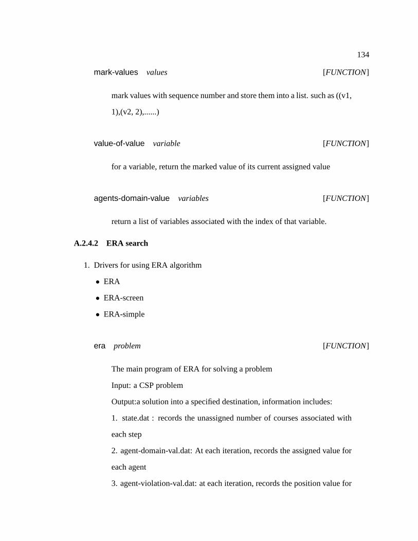
134

mark-values values [FUNCTION]

mark values with sequence number and store them into a list. such as ((v1,

1),(v2, 2),......)

value-of-value variable [FUNCTION]

for a variable, return the marked value of its current assigned value

agents-domain-value variables [FUNCTION]

return a list of variables associated with the index of that variable.

A.2.4.2 ERA search

1. Drivers for using ERA algorithm

• ERA

• ERA-screen

• ERA-simple

era problem [FUNCTION]

The main program of ERA for solving a problem

Input: a CSP problem

Output:a solution into a specified destination, information includes:

1. state.dat : records the unassigned number of courses associated with

each step

2. agent-domain-val.dat: At each iteration, records the assigned value for

each agent

3. agent-violation-val.dat: at each iteration, records the position value for

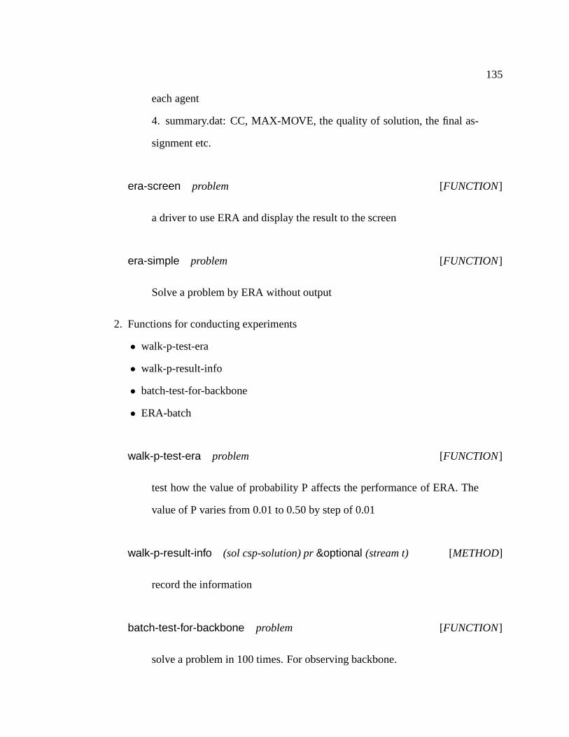
135

each agent

4. summary.dat: CC, MAX-MOVE, the quality of solution, the final as-

signment etc.

era-screen problem [FUNCTION]

a driver to use ERA and display the result to the screen

era-simple problem [FUNCTION]

Solve a problem by ERA without output

2. Functions for conducting experiments

• walk-p-test-era

• walk-p-result-info

• batch-test-for-backbone

• ERA-batch

walk-p-test-era problem [FUNCTION]

test how the value of probability P affects the performance of ERA. The

value of P varies from 0.01 to 0.50 by step of 0.01

walk-p-result-info (sol csp-solution) pr&optional (stream t) [METHOD]

record the information

batch-test-for-backbone problem [FUNCTION]

solve a problem in 100 times. For observing backbone.

136

era-batch problem sequence [FUNCTION]

the main program to perform a multi-agent search ; The batch problem

called by batch-test

A.3 GTA package Installation

This chapter describes how to install the GTA package. Allegro CL5.0 or above is needed

to run the lisp code. All files are stored in GTA.tar.gz; you need to extract this file under

your home directory by

gunzip GTA.tar.gztar xvf GTA.tar

After the file is decompressed, you will see the following directories created and some files

copied under your home directory.

/home/xxx/owninits.lisp/home/xxx/lisp/lisp-tools//home/xxx/lisp/lisp-tools-file-list.list/home/xxx/gta/

where xxx means your account name. All files and their destinations are listed below

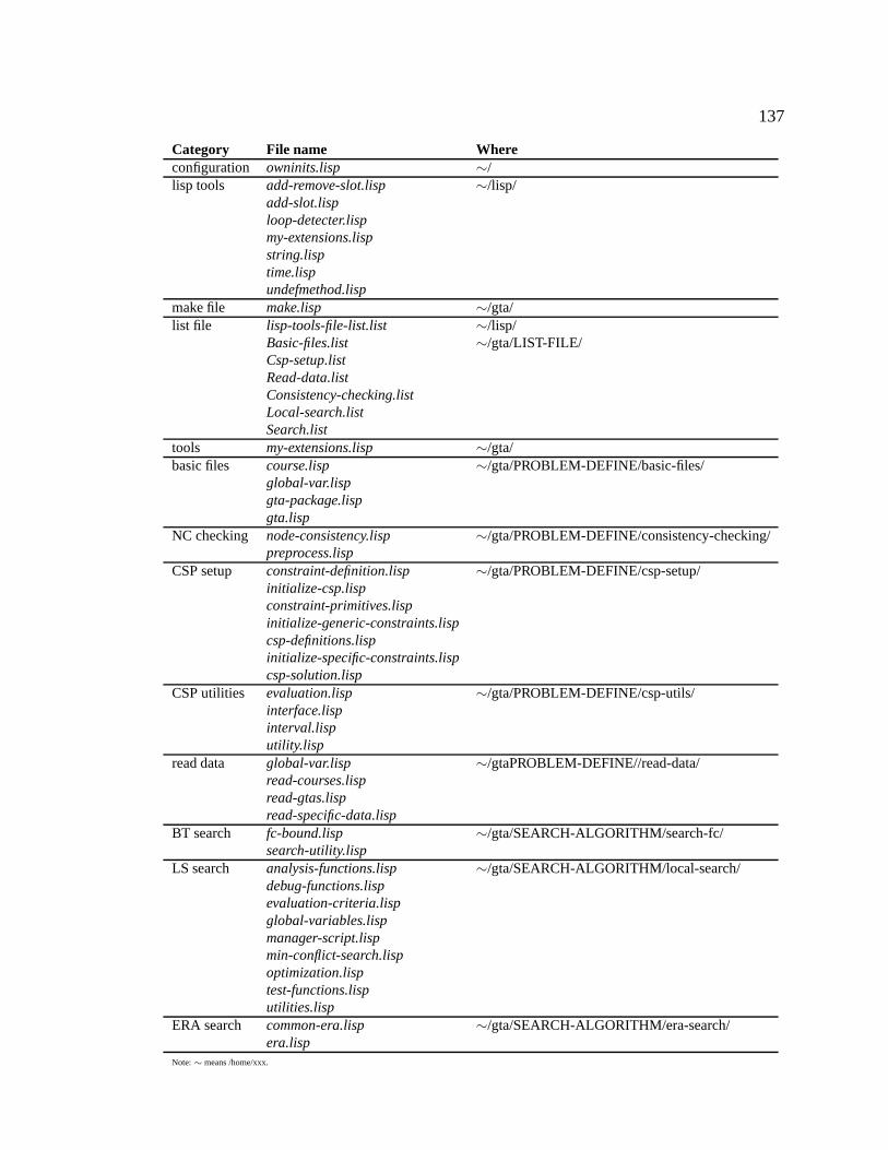
137

Category File name Whereconfiguration owninits.lisp ∼/lisp tools add-remove-slot.lisp ∼/lisp/

add-slot.lisploop-detecter.lispmy-extensions.lispstring.lisptime.lispundefmethod.lisp

make file make.lisp ∼/gta/list file lisp-tools-file-list.list ∼/lisp/

Basic-files.list ∼/gta/LIST-FILE/Csp-setup.listRead-data.listConsistency-checking.listLocal-search.listSearch.list

tools my-extensions.lisp ∼/gta/basic files course.lisp ∼/gta/PROBLEM-DEFINE/basic-files/

global-var.lispgta-package.lispgta.lisp

NC checking node-consistency.lisp ∼/gta/PROBLEM-DEFINE/consistency-checking/preprocess.lisp

CSP setup constraint-definition.lisp ∼/gta/PROBLEM-DEFINE/csp-setup/initialize-csp.lispconstraint-primitives.lispinitialize-generic-constraints.lispcsp-definitions.lispinitialize-specific-constraints.lispcsp-solution.lisp

CSP utilities evaluation.lisp ∼/gta/PROBLEM-DEFINE/csp-utils/interface.lispinterval.lisputility.lisp

read data global-var.lisp ∼/gtaPROBLEM-DEFINE//read-data/read-courses.lispread-gtas.lispread-specific-data.lisp

BT search fc-bound.lisp ∼/gta/SEARCH-ALGORITHM/search-fc/search-utility.lisp

LS search analysis-functions.lisp ∼/gta/SEARCH-ALGORITHM/local-search/debug-functions.lispevaluation-criteria.lispglobal-variables.lispmanager-script.lispmin-conflict-search.lispoptimization.lisptest-functions.lisputilities.lisp

ERA search common-era.lisp ∼/gta/SEARCH-ALGORITHM/era-search/era.lisp

Note:∼ means /home/xxx.

138

Appendix B

Experimental Data

As a real-world application, the GTA assignment problem is defined as follows. In a

semester, given a set of graduate teaching assistants, a setof courses, and a set of con-

straints that specify allowable assignments, find a consistent and satisfactory assignment

of GTAs to courses[Glaubius and Choueiry, 2002a; 2002b; Glaubius, 2001]. In the GTA

assignment problem, the courses are modeled as variables and the GTAs are the values. In

practice, this problem is over-constrained.

B.1 Data Sets

We collected four data sets from four academic semesters of the Department of Computer

Science and Engineering at the University of Nebraska-Lincoln: Spring 2001, Fall 2001,

Fall 2002 and Spring 2003. For conducting experiments, we also created four data sets

based on the real-world ones. Thus there are total of eight data sets used in our experiments.

B.1.1 Original and Boosted

As mentioned before, the GTA assignment problem may be over-constrained. That means

there is no solution. In order to make the problem solvable, we added extra GTAs into the

original data sets to boost the resource. Table B.1 lists alldata sets and their corresponding

instances.

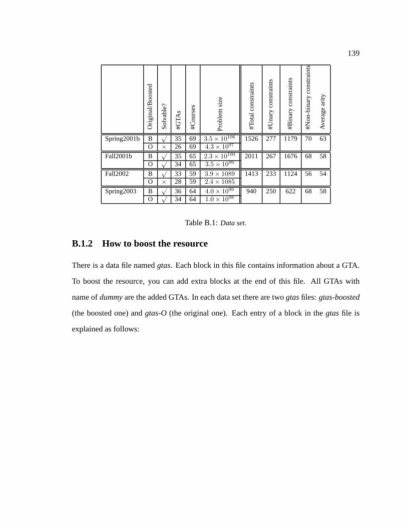
139

Ori

gin

al/B

oo

sted

So

lvab

le?

#G

TAs

#C

ou

rses

Pro

ble

msi

ze

#To

talc

on

stra

ints

#U

nar

yco

nst

rain

ts

#B

inar

yco

nst

rain

ts

#N

on

-bin

ary

con

stra

ints

Ave

rag

ear

ity

Spring2001b B√

35 69 3.5× 10106 1526 277 1179 70 63O × 26 69 4.3× 1097

Fall2001b B√

35 65 2.3× 10100 2011 267 1676 68 58O

√34 65 3.5× 1099

Fall2002 B√

33 59 3.9× 1089 1413 233 1124 56 54O × 28 59 2.4× 1085

Spring2003 B√

36 64 4.0× 1099 940 250 622 68 58O

√34 64 1.0× 1098

Table B.1:Data set.

B.1.2 How to boost the resource

There is a data file namedgtas. Each block in this file contains information about a GTA.

To boost the resource, you can add extra blocks at the end of this file. All GTAs with

name ofdummyare the added GTAs. In each data set there are twogtasfiles: gtas-boosted

(the boosted one) andgtas-O(the original one). Each entry of a block in thegtasfile is

explained as follows:

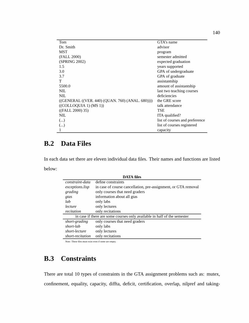
140

Tom GTA’s nameDr. Smith advisorMST program(FALL 2000) semester admitted(SPRING 2002) expected graduation1.5 years supported3.0 GPA of undergraduate3.7 GPA of graduateT assistantship5500.0 amount of assistantshipNIL last two teaching coursesNIL deficiencies((GENERAL ((VER. 440) (QUAN. 760) (ANAL. 680)))) the GRE score((COLLOQUIA 1) (MS 1)) talk attendance((FALL 2000) 35) TSENIL ITA qualified?(...) list of courses and preference(...) list of courses registered1 capacity

B.2 Data Files

In each data set there are eleven individual data files. Theirnames and functions are listed

below:

DATA filesconstraint-data define constraintsexceptions.lisp in case of course cancellation, pre-assignment, or GTA removalgrading only courses that need gradersgtas information about all gtaslab only labslecture only lecturesrecitation only recitations

in case if there are some courses only available in half of thesemestershort-grading only courses that need gradersshort-lab only labsshort-lecture only lecturesshort-recitation only recitationsNote: These files must exist even if some are empty.

B.3 Constraints

There are total 10 types of constraints in the GTA assignmentproblems such as: mutex,

confinement, equality, capacity, diffta, deficit, certification, overlap, nilpref and taking-

141

course constraints. Among them only equality and confinement constraints need to be

defined by hand. The others are defined automatically by the program.

Equality-constraint: isn-ary constraints between a set of courses, all of which should be

assigned the same GTA.

Confinement-constraint: allows us to specify that a GTA assigned to one or more courses

in given setS, called the confinement set, cannot be assigned to any courseoutsideS,

and vice versa. We use this constraint to prevent a GTA from being assigned outside

the set of labs or recitations associated with a specific section of a course.

B.4 Capacity and load

After a problem instance is loaded, we can use the following commands to check the total

capacity and the maximum load of an instance of the GTA assignment problem.

(total-load problem)(max-total-load problem)

142

Bibliography

[Bacchus and Beek, 1998] F. Bacchus and P.V. Beek. On the Conversion between Non-

Binary and Binary Constraint Satisfaction Problems. InProc. of AAAI-98, pages 310–

319, Madison, Wisconsin, 1998.

[Bartak, 1998] R. Bartak. On-Line Guide to Constraint Programming.

kti.ms.mff.cuni.cz/ bartak/constraints, 1998.

[Bistarelliet al., 1995] S. Bistarelli, U. Montanari, and F. Rossi. Constraint solving over

semirings. InProc. of the 14th IJCAI, pages 624–630, 1995.

[Choueiry and Faltings, 1994] B.Y. Choueiry and B. Faltings. A Decomposition Heuristic

for Resource Allocation. InProc. of the 11th ECAI, pages 585–589, Amsterdam, The

Netherlands, 1994.

[Davis, 1991] L. Davis. Handbook of Genetic Algorithms. Van Nostrand Reinhold, 1991.

[Dechter and Pearl, 1989] R. Dechter and J. Pearl. Tree Clustering for Constraint Net-

works. Artificial Intelligence, 38:353–366, 1989.

[Dechter, 1990] R. Dechter. On the Expressiveness of Networks with Hidden Variables.

In Proc. of AAAI-90, pages 556–562, Boston, MA, 1990.

[Dechter, 2003] R. Dechter.Constraint Programming. Morgan Kaufmann, 2003.

143

[Fox et al., 1989] M. S. Fox, N. Sadeh, and C. Baykan. Constraint Heuristic Search. In

IJCAI89, pages 309–315, Detroit, 1989.

[Freuder and Wallace, 1992] E.C. Freuder and R.J. Wallace. Partial Constraint Satisfac-

tion. Artificial Intelligence, 58:21–70, 1992.

[Freuder, 1978] E.C. Freuder. Synthesizing Constraint Expressions.Communications of

the ACM, 21 (11):958–966, 1978.

[Freuder, 1993] E. C. Freuder. Partial Constraint Satisfaction. InProc. of the 11th IJCAI,

pages 278–283, Detroit, MI, 1993.

[Glaubius and Choueiry, 2002a] R. Glaubius and B.Y. Choueiry. Constraint Modeling and

Reformulation in the Context of Academic Task Assignment. In Working Notes of

the Workshop on Modelling and Solving Problems with Constraints, ECAI 2002, Lyon,

France, 2002.

[Glaubius and Choueiry, 2002b] R. Glaubius and B.Y. Choueiry. Constraint Modeling in

the Context of Academic Task Assignment. In Pascal Van Hentenryck, editor,Proceed-

ings of8th International Conference on Principle and Practice of Constraint Program-

ming (CP’02), volume 2470 ofLecture Notes in Computer Science, page 789, Ithaca,

NY, 2002. Springer Verlag.

[Glaubius, 2001] R. Glaubius. A Constraint Processing Approach to AssigningGraduate

Teaching Assistants to Courses. Undergraduate Honors Thesis. Department of Com-

puter Science and Engineering, University of Nebraska-Lincoln, 2001.

[Glover and Laguna, 1993] F. Glover and M. Laguna. Tabu search. In C. Reeves, edi-

tor, Modern Heuristic Techniques for Combinatorial Problems, Oxford, England, 1993.

Blackwell Scientific Publishing.

144

[Glover, 1989] F. Glover. Tabu search: Part I. ORSA.Computing, 1 (3):190–206, 1989.

[Glover, 1990] F. Glover. Tabu search: Part II ORSA.Computing, 2 (1):4–32, 1990.

[Gomes and Selman, 2001] C.P. Gomes and B. Selman. Algorithm Portfolios.Artificial

Intelligence, 126 (1-2):43—62, 2001.

[Gomeset al., 1998] C.P. Gomes, B. Selman, and H. Kautz. Boosting Combinatorial

Search Through Randomization. InProc. of AAAI-98, pages 431–437, Madison, Wis-

consin, 1998.

[Guddeti, 2004] V. P. Guddeti. Empirical Evaluation of Heuristic and Randomized Back-

track Search. Master thesis, Department of Computer Science and Engineering, Univer-

sity of Nebraska-Lincoln, Lincoln, NE, 2004. Forthcoming.

[Holland, 1975] J.H. Holland. Adaption in natural and artificial systems. University of

Michigan Press, Ann Arbor, MI, 1975.

[Hoos and Stutzle, 1999] H.H. Hoos and T. Stutzle. Towards a Characterisation of theBe-

haviour of Stochastic Local Search Algorithms for SAT.Artificial Intelligence, 112 (1-

2):213—232, 1999.

[Hoos and Stutzle, 2004] H.H. Hoos and T. Stutzle.Stochastic Local Search Foundations

and Applications. Morgan Kaufmann, 2004. Forthcoming.

[Hoos, 1998] H.H. Hoos.Stochastic Local Search—Methods, Models, Applications. PhD

thesis, Technische Universitat Darmstadt, Germany, 1998.

[Jampelet al., 1996] M. Jampel, E.C. Freuder, and M.J. Maher, editors.Over-Constrained

Systems, volume 1106 ofLecture Notes in Computer Science. Springer, 1996.

[Joslin and Clements, 1999] D.E. Joslin and D.P. Clements. Squeaky Wheel Optimization.

Journal of Artificial Intelligence Research, 10:353–373, 1999.

145

[Kirkpatrick et al., 1983] S. Kirkpatrick, C.D. Gelatt, and M.P. Vecchi. Optimizationby

simulated annealing.Science, Number 4598, 13 May 1983, 220, 4598:671–680, 1983.

[Liu et al., 2002] J. Liu, H. Jing, and Y.Y. Tang. Multi-agent oriented constraint satisfac-

tion. Artificial Intelligence, 136:101–144, 2002.

[Metropoliset al., 1953] N. Metropolis, A.W. Rosenbluth, M.N. Rosenbluth, A.H. Teller,

and E. Teller. Equation of state calculation by fast computing machines.Journal of

chem. Phys., 21:1087–1091, 1953.

[Minton et al., 1990] S. Minton, M.D. Johnston, A.B. Philips, and P. Laird. Solving

Large-Scale Constraint Satisfaction and Scheduling Problems Using a Heuristic Repair

Method. InProc. of AAAI-90, pages 17–24, Boston, MA, 1990.

[Minton et al., 1992] S. Minton, M. D. Johnston, A. B. Philips, and P. Laird. Minimiz-

ing Conflicts: A Heuristic Repair Method for Constraint Satisfaction and Scheduling

Problems.Artificial Intelligence, 58:161–205, 1992.

[Monassonet al., 1999] R. Monasson, R. Zecchine, S. Kirpatrick, B. Selman, and L. Troy-

ansky. Determining Computational Complexity from Characteristic ‘Phase Transitions’.

Nature, 400 (8):133–137, 1999.

[Morris, 1993] P. Morris. The Breakout Method For Escaping From Local Minima. In

Proc. of AAAI-93, pages 40–45, Washington, DC, 1993.

[Papadimitriou and Yannakakis, 1991] C.H. Papadimitriou and M. Yannakakis. Optimiza-

tion, approximation, and complexity classes. InProceedings of the 20th ACM Sym-

posium on the Theory of Computing, pages 229–234, 1991. Also in the Journal of

Computer and System Sciences, Vol.43, pages 425-440, 1991.

146

[Parkes, 1997] A.J. Parkes. Clustering at the Phase Transition. InProc. of AAAI-97, pages

340–345, Providence, Rhode Island, 1997.

[Prosser, 1993] P. Prosser. Hybrid Algorithms for the Constraint Satisfaction Problem.

Computational Intelligence, 9 (3):268–299, 1993.

[Revesz, 2002] P. Revesz.Introduction to Constraint Databases. Springer-Verlag, New

York, 2002.

[Rossiet al., 1990] F. Rossi, C. Petrie, and V. Dhar. On the Equivalence of Constraint

Satisfaction Problems. InProc. of the 9th ECAI, pages 550–556, Stockholm, Sweden,

1990.

[S. Hirkpatrick and Vecchi, 1983] C.D. Gelatt S. Hirkpatrick and M.P. Vecchi. Optimisa-

tion by simulated annealing.Science, 220:671–680, 1983.

[Sandholm, 2002] T. Sandholm. Algorithms for Combinatorial Auctions and Exchanges.

Tutorial MA3, AAAI-02, Alberta, Edmonton, Canada, July 2002.

[Schaerf and Meisels, 2000] A. Schaerf and A. Meisels. Solving Employee Timetabling

Problems by Generalized Local Search. InAI*IA 99: Advances in Artificial Intelli-

gence, 6th Congress of the Italian Association for Artificial Intelligence, volume 1792

of Lecture Notes in Computer Science, pages 380–389, Bologna, Italy, 2000. Springer.

[Selman and Kautz, 1993] B. Selman and H.A. Kautz. An empirical study of greedy local

search for satisfiability testing. InProc. of AAAI-93, pages 46–51, Washington, DC,

1993.

[Slaney and Walsh, 2001] J. Slaney and T. Walsh. Backbones in Optimization and Ap-

proximation. InProc. of the 17th IJCAI, pages 254–259, Seattle, WA, 2001.

147

[Telelis and Stamatopoulos, 2002] O. Telelis and P. Stamatopoulos. Heuristic backbone

sampling for maximum satisfiablity. InSecond Hellenic Conference on Artificial Intel-

ligence SETN 2002, pages 129–139, 2002.

[Wallace and Freuder, 1995] R. Wallace and E. Freuder. Heuristic methods for over-

constrained constraint satisfaction problems. In M. Jampel, E. Freuder, and M. Maher,

editors,OCS’95: Workshop on Over-Constrained Systems at CP’95, Cassis, Marseilles,

1995.

[Wallace, 1996] R.J. Wallace. Analysis of heuristic methods for partial constraint satisfac-

tion problems. InPrinciples and Practice of Constraint Programming, pages 482–496,

1996.

[Weiss, 2000] G. Weiss. Multiagent Systems. The MIT Press, Cambridge, MA02142,

2000.

[Wilson and Borning, 1993] M. Wilson and A. Borning. Hierarchical constraint logic pro-

gramming.Logic Programming, 16(3):277—318, 1993.

[Zou and Choueiry, 2003a] H. Zou and B.Y. Choueiry. Characterizing the Behavior of a

Multi-Agent Search by Using it to Solve a Tight, Real-World Resource Allocation Prob-

lem. InWorkshop on Applications of Constraint Programming, pages 81–101, Kinsale,

County Cork, Ireland, 2003.

[Zou and Choueiry, 2003b] H. Zou and B.Y. Choueiry. Multi-agent Based Search versus

Local Search and Backtrack Search for Solving Tight CSPs: A Practical Case Study.

In Working Notes of the Workshop on Stochastic Search Algorithms (IJCAI 03), pages

17–24, Acapulco, Mexico, 2003.

ITERATIVE IMPROVEMENT TECHNIQUES FOR SOLVING ...

Documents