Iterative and Adaptive Processing for Multiuser Communication Systems Lance Linton B.Eng., M.Eng. College of Engineering and Science, Victoria University Submitted in fulfillment of the requirements of the degree of Doctor of Philosophy 15th April 2016

Welcome message from author
This document is posted to help you gain knowledge. Please leave a comment to let me know what you think about it! Share it to your friends and learn new things together.
Transcript
Iterative and Adaptive Processing forMultiuser Communication Systems
Lance Linton B.Eng., M.Eng.
College of Engineering and Science,Victoria University
Submitted in fulfillment of the requirements of the degree of
Doctor of Philosophy
15th April 2016
ii
Abstract
The huge demand of wireless communications has driven the require-
ment for highly-efficient multiple-access communications schemes that
can accommodate multiple simultaneous users, yet provide performance
similar to single-user systems. Recently, iterative multiuser detection
schemes have shown to provide this high level of performance at a
manageable level of complexity. This thesis is concerned with iterative
detection of two non-orthogonal asynchronous access schemes: code-
division multiple-access (CDMA); and interleave-division multiple-access
(IDMA).
A multi-rate IDMA system is developed where different users transmit
data at different rates. High-rate users support multiple sub-streams,
each coded as an IDMA layer. The iterative receiver treats each IDMA
layer as a virtual user. Variance transfer analysis is employed to analyse
the receiver performance, which is then optimised by developing a power
allocation strategy. Simulation results demonstrate that the performance
of this proposed system is close to the theoretical limit in a Rayleigh
flat-fading environment.
Next, receiver performance is optimised by forward error correction
code allocation. For multiuser systems with dynamic loads, new users are
allocated codes according to the existing system load in order to optimise
receiver convergence. Small multiuser systems have performances that
approach the theoretical single-user bound.
The Golden Code is a “perfect” space-time block-code for 2× 2
multiple-antenna (MIMO) systems. It can simultaneously achieve both
full-diversity and -rate. A MIMO-IDMA multiuser detector is developed
to extend the golden code scheme to the multiuser case. Decoding is
performed by an iterative receiver whose complexity is linear in the
iii
number of users. In a Rayleigh flat-fading environment, simulation
results show that the proposed scheme can outperform other common
MIMO schemes and approaches within 0.25dB of the single-user bound.
The application of iterative multiuser detection to underwater acous-
tic communications is considered next. Designing reliable communication
systems for the underwater acoustic channel has proven to be very chal-
lenging. A major channel impairment is the multipath interference
caused by multiple reflections of the acoustic signal from the water
surface and bottom. These reflections occur at small grazing angles and
with small reflection losses, causing both long delay spread and large
multipath amplitudes in the received signal.
The large delay-spread implies that single-carrier communication will
be plagued by inter-symbol interference (ISI) that spans many symbols.
As an alternative, multi-carrier modulation (MCM) has been proposed
to increase the symbol interval and thereby decrease the ISI span. We
combine Orthogonal Frequency-Division Multiplexing (OFDM), a low-
complexity spectrally-efficient MCM technique, with an IDMA overlay
to develop a multiple-access communications system that provides robust
performance in the presence of large time-delay spread and the other
impairments presented by the shallow water acoustic channel.
Finally, we consider multiuser communications in doubly-spread
underwater acoustic channels, where the relative motion between the
transmitter, receiver, and scattering objects imparts each path with a
unique Doppler shift. In this case, the orthogonality of OFDM is lost,
leading to subcarrier interference which greatly complicates optimal
data detection. Therefore, single-carrier system is considered with a
non-linear Kalman filter as equalizer. The doubly-selective channel is
modelled using basis expansion models (BEMs), a low-rank channel
model that exploits the inherent structure in the channel response. The
use of basis functions can turn a time-varying system identification
problem into a time-invariant one, thereby reducing the number of
parameters to estimate. The receiver uses a semi-blind iterative channel
estimation algorithm to estimate the channel parameters. Experimental
results demonstrate robust performance in underwater channels with
simultaneously large delay- and Doppler-spreads.
iv
Declaration
I, Lance Linton, declare that this PhD thesis entitled “Iterative and
Adaptive Processing for Multiuser Communication Systems” is no more than
100,000 words in length including quotes and exclusive of tables, figures,
appendices, bibliography, references and footnotes. This thesis contains no
material that has been submitted previously, in whole or in part, for the award
of any other academic degree or diploma. Except where otherwise indicated,
this thesis is my own work.
Lance Linton
15th April 2016
v
Acknowledgements
Of the many people who deserve thanks, some are particularly prominent, such as my
supervisors, Prof. Michael Faulker, Assoc. Prof. Patrick Leung, and Dr. Phillip Conder.
Their invaluable advice, guidance, and encouragement have made all of this possible.
Contents
Nomenclature 1
1 Introduction 2
1.1 Multiple-Access Schemes . . . . . . . . . . . . . . . . . . . . . . . . . . . 3
1.2 Error Correction Coding . . . . . . . . . . . . . . . . . . . . . . . . . . . 5
1.2.1 Block Codes . . . . . . . . . . . . . . . . . . . . . . . . . . . . . . 5
1.2.2 Convolutional Codes . . . . . . . . . . . . . . . . . . . . . . . . . 6
1.2.3 Concatenated Codes . . . . . . . . . . . . . . . . . . . . . . . . . 8
1.2.4 Turbo Codes . . . . . . . . . . . . . . . . . . . . . . . . . . . . . 9
1.3 Applications of Iterative Decoding . . . . . . . . . . . . . . . . . . . . . . 11
1.4 Summary of Thesis Work . . . . . . . . . . . . . . . . . . . . . . . . . . . 12
1.4.1 Iterative Methods for Equalization and Multiuser Detection . . . 13
1.4.2 IDMA Performance Optimisation using Variance Transfer Analysis 14
1.4.3 Optimal Space-Time Coding using the Golden Code . . . . . . . . 15
1.4.4 Multiuser Communications for Underwater Acoustic Channels . . 16
1.5 Original Contributions . . . . . . . . . . . . . . . . . . . . . . . . . . . . 18
1.6 Thesis Outline . . . . . . . . . . . . . . . . . . . . . . . . . . . . . . . . . 19
1.7 Related Publications . . . . . . . . . . . . . . . . . . . . . . . . . . . . . 20
2 Iterative Decoding for Equalization and Multiuser Detection 22
2.1 Convolutional Coding for the Gaussian Channel . . . . . . . . . . . . . . 24
2.1.1 Convolutional Encoding . . . . . . . . . . . . . . . . . . . . . . . 24
2.1.2 System Model . . . . . . . . . . . . . . . . . . . . . . . . . . . . . 27
2.1.3 Log Likelihood Ratios (LLRs) . . . . . . . . . . . . . . . . . . . . 29
2.1.4 MAP Decoding using the BCJR Algorithm . . . . . . . . . . . . . 29
2.2 Intersymbol Interference (ISI) Channels . . . . . . . . . . . . . . . . . . . 36
2.2.1 System Model . . . . . . . . . . . . . . . . . . . . . . . . . . . . . 38
2.2.2 Optimal Detection . . . . . . . . . . . . . . . . . . . . . . . . . . 41
vi

Contents vii
2.3 Separate Equalization and Decoding for ISI Channels . . . . . . . . . . . 42
2.3.1 Trellis-Based MAP Symbol Detection . . . . . . . . . . . . . . . . 44
2.3.2 Linear Equalization and Symbol Detection . . . . . . . . . . . . . 48
2.3.3 Trellis-Based MAP FEC Decoding . . . . . . . . . . . . . . . . . 52
2.3.4 System Performance . . . . . . . . . . . . . . . . . . . . . . . . . 55
2.4 Turbo Equalization for ISI Channels . . . . . . . . . . . . . . . . . . . . 57
2.5 Code Division Multiple Access (CDMA) and Multiuser Detection . . . . 63
2.5.1 Synchronous CDMA Signal Model . . . . . . . . . . . . . . . . . . 64
2.5.2 Asynchronous CDMA Signal Model . . . . . . . . . . . . . . . . . 65
2.5.3 Single-User Matched Filter Detector . . . . . . . . . . . . . . . . 68
2.6 The Optimum Multiuser Receiver . . . . . . . . . . . . . . . . . . . . . . 70
2.6.1 Synchronous Transmission . . . . . . . . . . . . . . . . . . . . . . 70
2.6.2 Asynchronous Transmission . . . . . . . . . . . . . . . . . . . . . 71
2.7 Linear Multiuser Detectors . . . . . . . . . . . . . . . . . . . . . . . . . . 74
2.7.1 Decorrelating Detector . . . . . . . . . . . . . . . . . . . . . . . . 74
2.7.2 Minimum Mean-Square-Error Detector . . . . . . . . . . . . . . . 76
2.8 Turbo Multiuser Detection for Synchronous CDMA . . . . . . . . . . . . 78
2.8.1 Optimal SISO Multiuser Detector . . . . . . . . . . . . . . . . . . 81
2.8.2 Low-Complexity SISO Multiuser Detector . . . . . . . . . . . . . 82
2.9 Turbo Multiuser Detection for CDMA with Multipath Fading . . . . . . 88
2.9.1 Signal Model and Sufficient Statistics . . . . . . . . . . . . . . . . 89
2.9.2 SISO Multiuser Detector in Multipath Fading Channels . . . . . . 93
2.10 Interleave-Division Multiple Access (IDMA) . . . . . . . . . . . . . . . . 98
2.10.1 Transmitter Structure . . . . . . . . . . . . . . . . . . . . . . . . 98
2.10.2 Iterative Receiver and Signal Model . . . . . . . . . . . . . . . . . 99
2.11 Conclusion . . . . . . . . . . . . . . . . . . . . . . . . . . . . . . . . . . . 103
3 IDMA Performance Optimisation using Variance Transfer Analysis 105
3.1 Variance Transfer Charts and Analysis . . . . . . . . . . . . . . . . . . . 107
3.1.1 ESE Variance Transfer Function . . . . . . . . . . . . . . . . . . . 107
3.1.2 FEC Decoder Variance Transfer Function . . . . . . . . . . . . . . 109
3.1.3 Example Variance Transfer Chart . . . . . . . . . . . . . . . . . . 109
3.2 Multi-Rate IDMA with Power Allocation . . . . . . . . . . . . . . . . . . 111
3.2.1 Transmit Power Allocation . . . . . . . . . . . . . . . . . . . . . . 113
3.2.2 Simulation Results . . . . . . . . . . . . . . . . . . . . . . . . . . 115
Contents viii
3.3 FEC Allocation for Dynamic System Loads . . . . . . . . . . . . . . . . . 116
3.3.1 Simulation Results . . . . . . . . . . . . . . . . . . . . . . . . . . 120
3.4 Conclusion . . . . . . . . . . . . . . . . . . . . . . . . . . . . . . . . . . . 120
4 Optimal Space-Time Coding using the Golden Code 123
4.1 Single-User MIMO System Model . . . . . . . . . . . . . . . . . . . . . . 125
4.2 Space-Time Coding and Linear Dispersion Codes . . . . . . . . . . . . . 126
4.3 Decoding of Linear Dispersion Codes . . . . . . . . . . . . . . . . . . . . 128
4.4 The Golden Code . . . . . . . . . . . . . . . . . . . . . . . . . . . . . . . 129
4.5 Single-User System Performance . . . . . . . . . . . . . . . . . . . . . . . 131
4.6 Multiuser MIMO System Model . . . . . . . . . . . . . . . . . . . . . . . 132
4.6.1 Multiuser Transmitter Structure . . . . . . . . . . . . . . . . . . . 132
4.6.2 Multiuser MIMO Signal Model . . . . . . . . . . . . . . . . . . . 134
4.6.3 Multiuser Iterative Receiver Structure . . . . . . . . . . . . . . . 136
4.7 Soft Multiuser Detector (MUD) . . . . . . . . . . . . . . . . . . . . . . . 137
4.8 Multiuser System Performance . . . . . . . . . . . . . . . . . . . . . . . . 140
4.9 Conclusion . . . . . . . . . . . . . . . . . . . . . . . . . . . . . . . . . . . 142
5 Multiuser Detection for Delay-Spread Underwater Acoustic Channels 144
5.1 Channel Model . . . . . . . . . . . . . . . . . . . . . . . . . . . . . . . . 145
5.1.1 Multipath Modeling . . . . . . . . . . . . . . . . . . . . . . . . . 146
5.1.2 Noise Modeling . . . . . . . . . . . . . . . . . . . . . . . . . . . . 150
5.2 Single-Carrier IDMA for Multipath-Fading . . . . . . . . . . . . . . . . . 152
5.2.1 Transmitter Structure and Signal Model . . . . . . . . . . . . . . 152
5.2.2 Iterative Receiver Structure . . . . . . . . . . . . . . . . . . . . . 153
5.3 Multi-Carrier IDMA (OFDM-IDMA) . . . . . . . . . . . . . . . . . . . . 156
5.4 MIMO-OFDM-IDMA . . . . . . . . . . . . . . . . . . . . . . . . . . . . . 159
5.5 System Performance . . . . . . . . . . . . . . . . . . . . . . . . . . . . . 161
5.6 Conclusion . . . . . . . . . . . . . . . . . . . . . . . . . . . . . . . . . . . 164
6 Multiuser Detection for Doubly-Spread Underwater Acoustic Channels 166
6.1 Introduction . . . . . . . . . . . . . . . . . . . . . . . . . . . . . . . . . . 167
6.2 Underwater Acoustic Channels and Channel Modelling . . . . . . . . . . 170
6.2.1 Models for Channel Simulation . . . . . . . . . . . . . . . . . . . 171
6.2.2 Models for Channel Estimation . . . . . . . . . . . . . . . . . . . 172
6.3 Single-User Channel Equalization using the Kalman Filter . . . . . . . . 179
6.3.1 State-Space System Model . . . . . . . . . . . . . . . . . . . . . . 179
Contents ix
6.3.2 Equalization of Channels with Known Coefficients . . . . . . . . . 181
6.3.3 Adaptive Equalization of Channels with Unknown Coefficients . . 184
6.4 Multiple Access IDMA . . . . . . . . . . . . . . . . . . . . . . . . . . . . 186
6.4.1 Transmitter Structure . . . . . . . . . . . . . . . . . . . . . . . . 186
6.4.2 Receiver Structure . . . . . . . . . . . . . . . . . . . . . . . . . . 188
6.5 Multiuser Adaptive Soft EKF-Based Equalizer for Doubly-Spread Channels190
6.5.1 Multiuser System Model . . . . . . . . . . . . . . . . . . . . . . . 190
6.5.2 State-Space Model Incorporating A Priori Information . . . . . . 192
6.5.3 Fixed-Lag Soft Input Extended Kalman Filtering . . . . . . . . . 195
6.5.4 Generating Extrinsic Information . . . . . . . . . . . . . . . . . . 196
6.6 Performance Evaluation . . . . . . . . . . . . . . . . . . . . . . . . . . . 197
6.7 Conclusion . . . . . . . . . . . . . . . . . . . . . . . . . . . . . . . . . . . 204
7 Conclusion 206
7.1 Summary and Thesis Contributions . . . . . . . . . . . . . . . . . . . . . 207
7.1.1 IDMA Performance Optimisation using Variance Transfer Analysis 207
7.1.2 Optimal Space-Time Coding using the Golden Code . . . . . . . . 208
7.1.3 Multiuser Communications for Underwater Acoustic Channels . . 209
7.2 Future Work . . . . . . . . . . . . . . . . . . . . . . . . . . . . . . . . . . 211
Bibliography 214
List of Figures 227
List of Tables 232
Nomenclature
Notation
R,Rn,Rn×m set of real numbers, vectors, and matrices
C,Cn,Cn×m set of complex numbers, vectors, and matrices
N∗ set of natural numbers 1, 2, 3 . . .
Q set of rational numbers
Z set of integers
? convolution
Hadamard product
⊗ Kronecker product
In n×n identity matrix
0n×m n×m zero matrix
Ai,j i, j-th element of matrix A
AT transpose of matrix A
AH conjugate transpose of matrix A
A−1 inverse of matrix A
diaga1, . . . , an diagonal matrix with elements a1, . . . , an on the main diagonal
tr(A) trace of matrix A
arg maxx f(x) denotes the value of x that maximises f(x)
arg minx f(x) denotes the value of x that minimises f(x)
Covx, y covariance of x and y
δ(t) Dirac delta function
Ex expected value of x
expx exponential function, exp(x) = ex
x

Contents xi
L(x) log likelihood ratio of x
log(x) natural logarithm of x
N (µ, σ2) normal (Gaussian) distribution with mean µ and variance σ2
N (µ,C) multivariate normal distribution with mean µ and covariance C
p(x) probability density function of x
p(x | y) conditional probability density function of x conditioned on y
P (x) probability mass function of x
P (x | y) conditional probability mass function of x conditioned on y
Rz, Iz real and imaginary parts of z
sgn(x) signum function, sgn(x) = −1 if x < 0; sgn(x) = 1 if x > 0
Varx variance of x
Commonly used symbols
Λ(x) a posteriori probability information in LLR form, Λ(x) = Lapp(x)
Λ1( · ) a posteriori probability information (in LLR form) output from the
soft equalizer or multiuser detector
Λ2( · ) a posteriori probability information (in LLR form) output from the
soft FEC channel decoder(s)
λ(x) extrinsic information in LLR form, λ(x) = Lext(x)
λ1( · ) extrinsic information (in LLR form) output from the soft equalizer
or soft multiuser detector, used as a priori information by the FEC
channel decoder(s)
λ2( · ) extrinsic information (in LLR form) output from the soft FEC channel
decoder(s), used as a priori information by the soft equalizer or soft
multiuser detector
b[i], bk[i] i-th bit (single-user case), i-th bit for the k-th user (multiuser case),
input to the symbol mapper or spreader (transmit side, coded or
uncoded systems). b[i], bk[i] is coded and interleaved in coded systems
b[i], bk[i] estimate of b[i], estimate of bk[i], output from the equalizer, detector,
or multiuser detector (receive side, coded or uncoded systems)
c[i], ck[i] i-th coded bit (single-user case), i-th coded bit for the k-th user (mul-
tiuser case), output from the FEC encoder(s) (transmit side, coded
systems)

Contents xii
c[i], ck[i] estimate of c[i], estimate of ck[i], input to the FEC decoder(s) (receive
side, coded systems)
d[i], dk[i] i-th input data bit (single-user case), i-th input data bit for the k-th
user (multiuser case), input to the FEC encoder(s) (transmit side,
coded systems)
d[i], dk[i] estimate of d[i], estimate of dk[i], output from the FEC decoder(s)
(receive side, coded systems)
K number of users in the multiuser system
n(t) continuous-time channel noise at time t
x[i], xk[i] i-th transmitted symbol (single-user case), i-th transmitted symbol or
chip from user-k (multiuser case), discrete-time channel input
x(t), xk(t) transmitted signal at time t (single-user case), transmitted signal from
user-k at time t (multiuser case), continuous-time channel input
y[i] i-th received symbol, discrete-time channel output
y(t) received signal at time t, continuous-time channel output
Abbreviations
APP a posteriori probability
AR autoregressive
AR(p) autoregressive process of order p
AWGN additive white Gaussian noise
BCJR Bahl, Cocke, Jelenik and Raviv (algorithm)
BEM basis expansion model
BER bit error rate
BI-AWGN binary-input additive white Gaussian noise
BPSK binary phase shift keying
CDMA code-division multiple-access
CE-BEM complex exponential BEM (discrete Fourier BEM)
DFE decision feedback equalizer
DFT discrete Fourier transform
DPSS discrete prolate spheroidal sequence (Slepian sequence)
EKF extended Kalman filter
Contents xiii
ESE elementary signal estimator
EXIT extrinsic information transfer
FEC forward error correction
FFT fast Fourier transform
FIR finite impulse response
ICI inter-carrier interference
i.i.d independent and identically distributed
IDMA interleave-division multiple-access
ISI intersymbol interference
KF Kalman filter
K-L Karhunen-Loeve expansion
LD linear dispersion
LDPC low-density parity check
LLR log-likelihood ratio
MAI multiple-access interference
MAP maximum a posteriori probability
MCM multi-carrier modulation
MF matched filter
MIMO multiple-input multiple-output
ML maximum likelihood
MMSE minimum mean square error
MSE mean square error
MUD multiuser detection/detector
NKF nonlinear Kalman filter
OFDM orthogonal frequency division multiplexing
p.d.f probability density function
QAM quadrature amplitude modulation
QPSK quadrature phase shift keying
SISO soft-input soft-output
SNR signal to noise ratio
Contents 1
ST space-time
STBC space-time block code/coding
UAC underwater acoustic channel
US uncorrelated scattering
V-BLAST vertical Bell Labs layered space-time
VT variance transfer
WSS wide sense stationary
WSSUS wide sense stationary uncorrelated scattering
Chapter 1
Introduction
The last two decades has witnessed a tremendous growth in wireless communications.
Cellar mobile telephony and data services, and wireless networking were once rare but
have become pervasive and an almost essential part of daily life. Future demand for
these wireless devices and services show no sign of abating. In addition to the traditional
network usage of wireless technology, the availability of low-cost wireless devices has
enabled many new wireless applications over recent years. One notable application is
distributed sensing, in which large numbers of inexpensive wireless nodes sense some
ongoing process and wirelessly communicate with each other and wired access points.
Environmental detection, surveillance, and health monitoring are just a few of the
numerous potential uses of distributed sensor networks.
A defining feature of wireless communications is that all devices must share the
electromagnetic spectrum in order to communicate with each other. Unlike in wired
communications, where each communication channel could conceivably have a physical
channel independent from all others, in wireless communication all channels come from a
common medium. The scarcity of radio spectrum resource requires wireless communica-
tion systems to reuse the frequency bands In order to achieve reliable communications,
some scheme must be developed for equitable sharing the usable frequencies. The issue
of a large number of users sharing a single allocated spectrum in order to communicate
is known as the multiple-access problem.
2
Introduction 3
1.1 Multiple-Access Schemes
In a multiuser communication system, a large number of users share a common multiple-
access channel to transmit information to a receiver. Multiple access systems generally
require that when different transmitting sources are sending messages simultaneously
through the same channel, the transmissions must be separated in some fashion so that
they do not interfere with one another. This is usually accomplished by making the
messages orthogonal to one another in the dimensions of frequency, time or code.
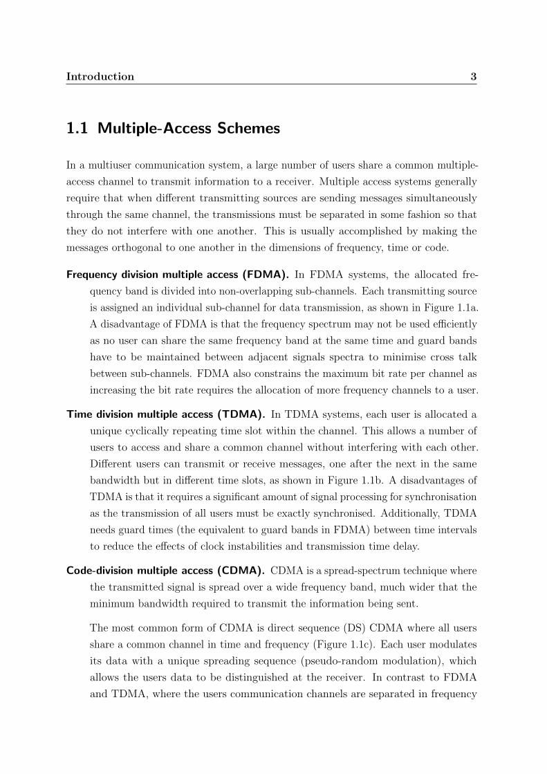
Frequency division multiple access (FDMA). In FDMA systems, the allocated fre-
quency band is divided into non-overlapping sub-channels. Each transmitting source
is assigned an individual sub-channel for data transmission, as shown in Figure 1.1a.
A disadvantage of FDMA is that the frequency spectrum may not be used efficiently
as no user can share the same frequency band at the same time and guard bands
have to be maintained between adjacent signals spectra to minimise cross talk
between sub-channels. FDMA also constrains the maximum bit rate per channel as
increasing the bit rate requires the allocation of more frequency channels to a user.
Time division multiple access (TDMA). In TDMA systems, each user is allocated a
unique cyclically repeating time slot within the channel. This allows a number of
users to access and share a common channel without interfering with each other.
Different users can transmit or receive messages, one after the next in the same
bandwidth but in different time slots, as shown in Figure 1.1b. A disadvantages of
TDMA is that it requires a significant amount of signal processing for synchronisation
as the transmission of all users must be exactly synchronised. Additionally, TDMA
needs guard times (the equivalent to guard bands in FDMA) between time intervals
to reduce the effects of clock instabilities and transmission time delay.
Code-division multiple access (CDMA). CDMA is a spread-spectrum technique where
the transmitted signal is spread over a wide frequency band, much wider that the
minimum bandwidth required to transmit the information being sent.
The most common form of CDMA is direct sequence (DS) CDMA where all users
share a common channel in time and frequency (Figure 1.1c). Each user modulates
its data with a unique spreading sequence (pseudo-random modulation), which
allows the users data to be distinguished at the receiver. In contrast to FDMA
and TDMA, where the users communication channels are separated in frequency

Introduction 4
or time, in a DS-CDMA system the users data are distinguished by the separation
(cross-correlation) between their spreading sequences.
Code
Freq. Time
Channel 1
Channel 2
Channel 3
FrequencyBands
(a) FDMA
TimeSlots
Code
Freq. TimeChannel 3
Channel 2
Channel 1
(b) TDMA
Freq. Time
Code
SpreadingCodes
3lenahC
n
1lenahC
n
2lenahC
n
(c) CDMA
Figure 1.1: Multiple-access techniques: (a) Frequency-division multiple access (FDMA); (b)Time-division multiple access (TDMA); and (c) Code-division multiple access(CDMA).
CDMA schemes have become a very popular method for multiple-access communica-
tions, and multiuser detection algorithms for CDMA receivers will be the focus of this
thesis. Since the users in a DS-CDMA system are distinguished by the separation (cross-
correlation) between their spreading sequences, we can categorise DS-CDMA schemes
according to the cross-correlation between users, i.e.,
• orthogonal signalling - where the cross-correlation between all users is zero; or
• non-orthogonal signalling - where the cross-correlation between users is non-zero.
Additionally, CDMA schemes can also be categorised according to the synchronism of
the users’ signals at the receiver, i.e.,
• synchronous schemes where the bit epochs of all the users are aligned at the receiver.
• asynchronous schemes where bit epochs of the users may be offset (not aligned) at
the receiver.
Asynchronous schemes are also non-orthogonal because there are no known sets of
spreading sequences that exhibit zero cross-correlation over a range of timing offsets.
In this thesis, we investigate asynchronous non-orthogonal CDMA schemes, and in
particular, Interleave Division Multiple Access (IDMA) which is a multiple-access scheme
Introduction 5
where users are separated by unique interleaver sequences (instead of unique spreading
sequences).
Iterative signal processing has proven to be an important technique in improving
the performance of receivers in communications systems. Iterative techniques can be
used to equalize inter-symbol interference channels (turbo equalization) and to resolve
multiple-access interference (MAI) in multiuser receivers (turbo multiuser-detection, or
turbo MUD). The origins of these techniques lie in error correction coding with the
concepts of concatenated coding [29] and turbo codes. A brief review of error correction
coding provides insight into the common building blocks of iterative processing.
1.2 Error Correction Coding
The approach to error correction coding taken by modern digital communication systems
started in the late 1940’s with the ground breaking work of Shannon [107], Hamming [38],
and Golay [34]. In his paper, Shannon developed the theoretical basis for coding which
has become known as information theory. By mathematically defining the entropy of
an information source and the capacity of a communications channel, he showed that it
was possible to achieve reliable communications over a noisy channel provided that the
source’s entropy is lower than the channel’s capacity. Shannon did not explicitly state
how channel capacity could be practically reached, only that it was attainable.
1.2.1 Block Codes
Hamming is generally credited with discovering the first error correcting code [68] when,
in 1946, he developed an algorithm that enabled early computers to correct isolated
errors detected in the input data. His method was to group the data into sets of four
information bits and then calculate three check bits which are a linearly combination of
the information bits, resulting in a seven bit code word. After reading in a code word,
the Hamming’s algorithm could detect errors and also determine the location of a single
error. Hence, the Hamming code was able to correct a single error in a block of seven
encoded bits.
While it was a major advancement, the Hamming code had a number of shortcomings.
Firstly, it was inefficient, requiring three check bits for every four data bits, and secondly, it

Introduction 6
only had the ability to correct a single error within the block. These issues were addressed
by Golay, who generalized Hamming’s construction, and in the process, discovered two
important codes: the binary Golay code; and ternary Golay code [137].
Reed-Muller (RM) codes [78] [99] were the next main class of linear block codes to be
discovered, and were an important development because they allowed more flexibility in
the size of the code word and the number of correctable errors per code word. They were
followed by the discovery of cyclic codes, first discovered by Prange [90]. Cyclic codes
are linear block codes that possess the additional property that any cyclic shift of a code
word is also a code word. The cyclic property adds considerable structure to the code,
which can be exploited by reduced complexity encoders and (more importantly) reduced
complexity decoders. Important cyclic codes include the binary BCH codes [14] [43], and
their non-binary extensions, the Reed and Solomon (RS) codes [100]. RS codes were a
major advancement because their non-binary nature allows for protection against bursts
of errors.
Although popular, block codes have two fundamental disadvantages: Firstly, their
frame-oriented nature means that the entire code word must be received before decoding
can be completed. This can introduce unacceptable latency into the system, particularly
when block lengths are large. Secondly, most algebraic-based decoders for block codes
work with hard-bit decisions, rather than with the unquantized, or “soft”, outputs of
the demodulator. With hard-decision decoding, the output of the channel is taken to be
binary, while with soft-decision decoding the channel output is continuous-valued [125].
In order to achieve the Shannon performance bound, a continuous-valued channel
output is required. Block codes can achieve good performance over relatively benign
channels, but they are generally power inefficient and have poor performance when the
signal-to-noise ratio (SNR) is low. This poor performance at low SNR is not a function of
the code itself, but is actually a function of the sub-optimality of hard-decision decoding.
It is possible to perform soft-decision decoding of block codes, although historically
soft-decision decoding has generally been regarded as too complex [125].
1.2.2 Convolutional Codes
Convolutional codes, introduced by Elias [26], avoid both main disadvantages of block
codes. Instead of segmenting data into distinct blocks, convolutional encoders add
redundancy to a continuous stream of input data by using linear shift registers. Each set

Introduction 7
of n output bits is a linear combination of the current set of m input bits and the bits
stored in the shift register. The total number of bits that each output depends on is called
the constraint length, L. The rate, Rc, of the convolutional encoder is the number of data
bits m taken in by the encoder in one coding interval, divided by the number of code
bits n output during the same interval, i.e., Rc = m/n. Just as the data is continuously
encoded, it can be continuously decoded with nominal latency. Additionally, the decoding
algorithms can make full use of soft-decision information from the demodulator.
The first practical decoding algorithm for convolutional codes was the sequential
decoder, introduced by Wozencraft and Reiffen [138]. However convolutional coding was
not widely used until the introduction of the Viterbi algorithm (VA) [129], which was the
first practical method for optimally (maximum likelihood) decoding convolutional codes.
de-interleaved data
1 2 3
7
4 5
8 9
6
interleaved data
1 2 3
7
4 5
8 9
6
Interleaver
De-Interleaver-1
read
write
read
input data
1 2 3 4 5 6 87 9
write
1 4 7 2 5 8 63 9
1 2 3 4 5 6 87 9
1 2 3
7
4 5
8 9
6
read
Step 1.Input (write) sequence
Step 2.Output (read) sequence
Interleaver Operation
De-Interleaver Operation
Step 1.Input (write) sequence
Step 2.Output (read) sequence
1 2 3
7
4 5
8 9
6
read
1 2 3
7
4 5
8 9
6
write
1 2 3
7
4 5
8 9
6
write
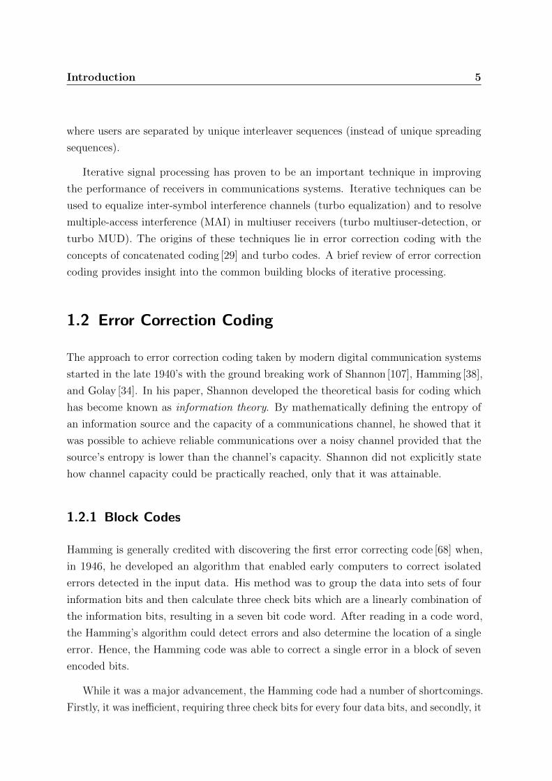
Figure 1.2: Block interleaver and de-interleaver operation
One of the main disadvantages of convolutional codes is their susceptibility to burst
errors. This susceptibility can be mitigated by using an interleaver, which scrambles the
order of the code bits prior to transmission. A deinterleaver at the receiver places the
Introduction 8
received code bits back in the proper order after demodulation and prior to decoding. By
scrambling the order of the code bits at the transmitter, and then reversing the process
at the receiver, burst errors can be spread out so that they appear independent to the
decoder. The most common type of interleaver is the block interleaver (Figure 1.2),
which is simply an Mb×Nb bit array. Data is placed into the array column-wise and
then read out row-wise. A burst error of length up to Nb bits can be spread out by a
block interleaver such that only one error occurs every Mb bits. There are also many
other interleaver types [130].
1.2.3 Concatenated Codes
Super Encoder
Outer CodeEncoder
inputdata
Super Decoder
BPSKModulator
Inner CodeEncoder
(generallyReed-Solomon
Code)
(generallyConvolutional
Code)
Outer CodeDecoder
BPSKDemodulator
Inner CodeDecoder
Channel
estimatesof input
data
Super Channel
Deinterleaver
p-1
Interleaver
p
(optional)
(optional)
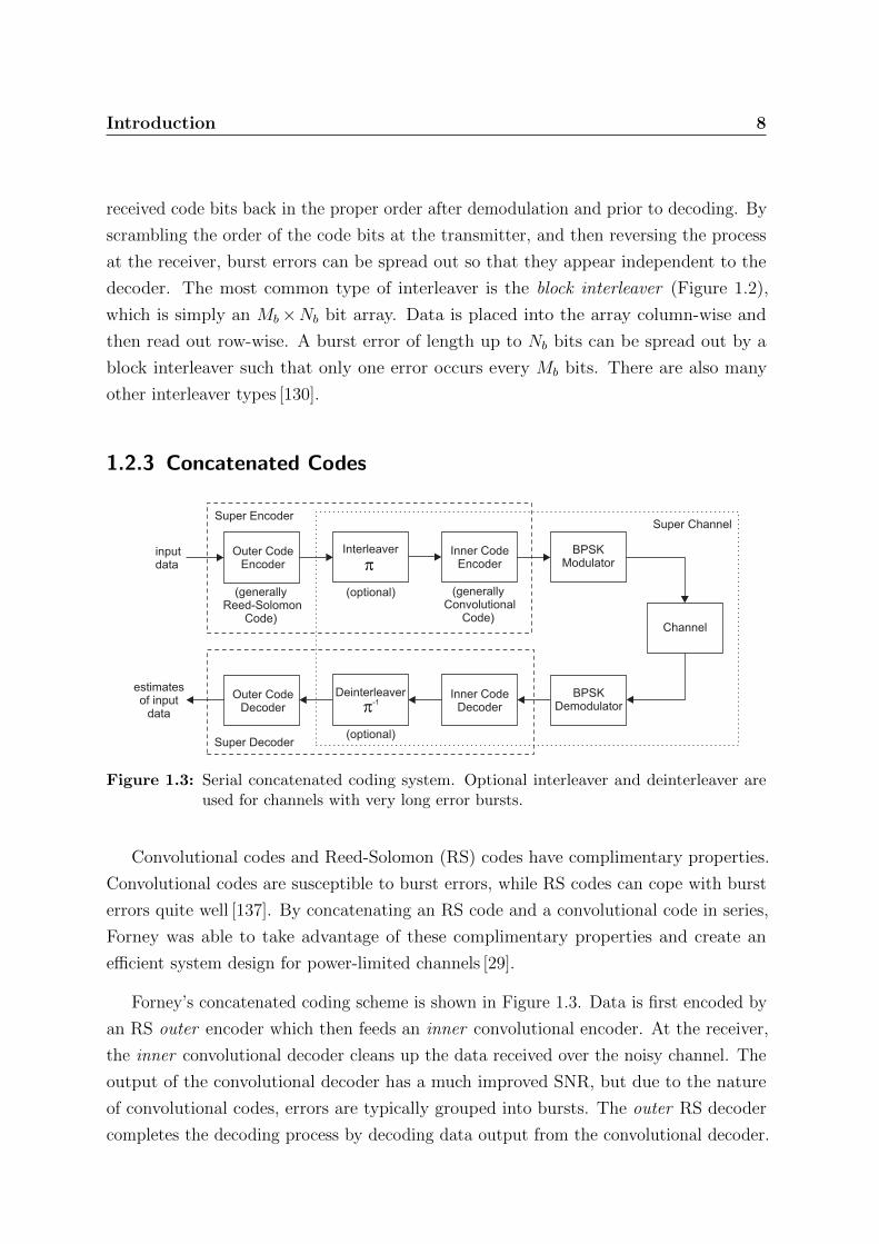
Figure 1.3: Serial concatenated coding system. Optional interleaver and deinterleaver areused for channels with very long error bursts.
Convolutional codes and Reed-Solomon (RS) codes have complimentary properties.
Convolutional codes are susceptible to burst errors, while RS codes can cope with burst
errors quite well [137]. By concatenating an RS code and a convolutional code in series,
Forney was able to take advantage of these complimentary properties and create an
efficient system design for power-limited channels [29].
Forney’s concatenated coding scheme is shown in Figure 1.3. Data is first encoded by
an RS outer encoder which then feeds an inner convolutional encoder. At the receiver,
the inner convolutional decoder cleans up the data received over the noisy channel. The
output of the convolutional decoder has a much improved SNR, but due to the nature
of convolutional codes, errors are typically grouped into bursts. The outer RS decoder
completes the decoding process by decoding data output from the convolutional decoder.
Introduction 9
Hence, each decoder works with the appropriate type of data—the convolutional decoder
works at low SNR with mostly independent errors, while the RS decoder works at high
SNR with mostly burst errors. For cases with very long error bursts, a block interleaver
can can be placed between the convolutional and RS encoders in order to spread long
error bursts across several RS code words [137].
1.2.4 Turbo Codes
Although considerable progress had been made in coding theory, there was still a
considerable gap between the performance of the best known codes and the theoretical
limit predicted by Shannon. This changed when Berrou, Glavieux, and Thitimajshima
[13] discovered turbo codes—a practical coding system that could approach Shannon’s
theoretical limit.
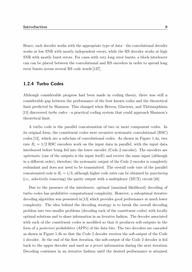
A turbo code is the parallel concatenation of two or more component codes. In
its original form, the constituent codes were recursive systematic convolutional (RSC)
codes [13], which are a subclass of convolutional codes. As shown in Figure 1.4a, two
rate Rc = 1/2 RSC encoders work on the input data in parallel, with the input data
interleaved before being fed into the lower encoder (Code 2 encoder). The encoders are
systematic (one of the outputs is the input itself) and receive the same input (although
in a different order), therefore, the systematic output of the Code 2 encoder is completely
redundant and does not need to be transmitted. The overall code rate of the parallel
concatenated code is Rc = 1/3, although higher code rates can be obtained by puncturing
(i.e., selectively removing) the parity output with a multiplexer (MUX) circuit [48].
Due to the presence of the interleaver, optimal (maximal likelihood) decoding of
turbo codes has prohibitive computational complexity. However, a suboptimal iterative
decoding algorithm was presented in [13] which provides good performance at much lower
complexity. The idea behind the decoding strategy is to break the overall decoding
problem into two smaller problems (decoding each of the constituent codes) with locally
optimal solutions and to share information in an iterative fashion. The decoder associated
with each of the constituent codes is modified so that it produces soft-outputs in the
form of a posteriori probabilities (APPs) of the data bits. The two decoders are cascaded
as shown in Figure 1.4b so that the Code 2 decoder receives the soft-output of the Code
1 decoder. At the end of the first iteration, the soft-output of the Code 2 decoder is fed
back to the upper decoder and used as a priori information during the next iteration.
Decoding continues in an iterative fashion until the desired performance is attained.

Introduction 10
systematic
MUX
Code 2RSC
Encoder
inputdata
d[i]
Code 1RSC
Encoder
d[i]
c [i](1)
c [i](2)
BPSKModulator
Channel
b [i],b [i],b [i](0) (1) (2)
x [i],x [i],x [i](0) (1) (2)
y [i],y [i],y [i](0) (1) (2)
Interleaver
p
AWGN
n[i]channeloutput
PC Turbo Encoder
where:b [i] = d[i],(0)
b [i] = c [i],b [i] = c [i]
(1) (1)
(2) (2)
d [i]p
code 1 parity
code 2parity
(a) Encoder
Code 1MAP
Decoder
systematic
Deinterleaver
Interleaver
y [i](1)
y [i](0)
y [i](2)
DEMUX
y [i],y [i],y [i](0) (1) (2)
-1
harddecision
Code 2MAP
Decoder
d[i]^
extrinsicinformationof code 1decoder
extrinsicinformationof code 2decoder
informationfor code 2decoder
a priori
informationfor code 1decoder
a priori
data bitestimates
code 2 parity
code 1 parity
channel output L1(d[i]) l1(d[i]) l1(d [i])p
l2(d [i])p
Deinterleaver
-1
Interleaver
l2(d[i]) L2(d [i])p
L2(d[i])
informationof code 2decoder
a posterior
(b) Decoder
Figure 1.4: Parallel concatenated (PC) turbo encoder and decoder (systematic form).
However, iterative decoding obeys a law of diminishing returns and hence the incremental
gain of each additional iteration is less than that of the previous iteration. It is the
decoding method that gives turbo codes their name, since the feedback action of the
decoder is similar to that of a turbo-charged engine [125].
Simulation results for the original turbo code of [13] showed that a bit error rate of
10−5 could be achieved at an Eb/N0 ratio of just 0.7dB after 18 iterations of decoding, i.e.,
turbo codes could come within a 0.7dB of the Shannon limit. Other researchers began to
look at using other concatenation configurations and other types of component codes.
It was found that serial concatenated codes offer performance that is comparable to, or
even exceeds, that of parallel concatenated codes [11]. Additionally, it was found that the

Introduction 11
performance with convolutional component codes could be matched or exceeded with
block component codes [19] [94] [1]. As a result, it became clear that the real breakthrough
from the introduction of turbo codes, was not the code construction, but the method of
iterative decoding.
SC Turbo Encoder
InnerCode
Encoderinputdata
OuterCode
Encoder
BPSKModulator
Channel
AWGN
d[i] Interleaver
p
n[i]
b[i] x[i] y[i]
channeloutput
c[i] c [i]p
(a) Encoder
channeloutput
(code bit) a posterioriinformation of the
outer code decoder
a posterioriinformation ofthe inner code
decoder
Deinterleaver
Interleaver
-1
L1(c [i])p
l1(c [i])p
l2(c [i])p
l1(c[i])
l2(c[i])
L2(d[i])
L2(c[i])
Inner CodeMAP
Decoder
Outer CodeMAP
Decoder
y[i]
harddecision
d[i]^
data bitestimates
informationfor the inner code
decoder
a priori
extrinsicinformation ofthe inner code
decoder
informationfor the outer code
decoder
a priori
extrinsic informationof the outer code
decoder
(data bit) a posterioriinformation of the
outer code decoder
(b) Decoder
Figure 1.5: Serial concatenated (SC) turbo encoder and decoder (non-systematic form).
1.3 Applications of Iterative Decoding
After the introduction of turbo codes, it was quickly recognized that the iterative
decoding method was suitable for many other applications, and could be used as a
general methodology for receiver design. Communication receivers typically consist of
a cascade of subsystems, each optimized to perform a single task. Examples of these
subsystems include equalizers, multiuser detectors, channel decoders, and source decoders.
Traditionally, the interface between subsystems involves the passing of hard-decisions
(e.g., bits) down the stages of the chain. Whenever hard-decisions are made, information is
lost and becomes unavailable to subsequent stages. Additionally, stages at the beginning

Introduction 12
of the processing chain do not benefit from information derived by stages further down the
chain. The interface between stages can be greatly improved by using the same strategy
devised to decode turbo codes. This general strategy of iterative feedback decoding or
detection is termed turbo processing [66].
Turbo processing frameworks are constructed using soft-input soft-output (SISO)
subsystems. A SISO subsystem receives soft-decision values as input and produces soft-
decision values as output. Soft-decision values are passed down the chain and refined by
subsequent stages. The soft-output of the final stage is then fed back to the first stage and
the next iteration of processing is initiated. Multiple iterations of turbo processing can be
performed, although, as with turbo codes, the incremental improvement in performance
diminishes with each additional iteration.
Turbo processing can be used to combine channel decoding with source decoding [36],
and channel decoding with symbol detection [66]. Other examples include:
Turbo equalization. This is a method of combining equalization with channel decoding
[23]. An equalizer is a subsystem that compensates for the intersymbol interference
(ISI) present in frequency selective channels. A frequency selective channel can be
described as a rate-one convolutional code defined over the field of real or complex
numbers. The combination of a convolutional channel code and ISI channel can
be viewed as a serial concatenation of two convolutional codes, which is a type of
serially concatenated turbo code, and can therefore can be decoded using the turbo
decoding algorithm.
Turbo multiuser detection. Here, the concept of turbo processing is applied to coded
multiple-access channels [44]. In a multiple-access channel, several users transmit at
the same time and frequency, producing multiple access interference (MAI), which
can be described as a form of time varying ISI. Thus, the multiple access channel
can be viewed as a rate-one convolutional code with time varying coefficients taken
over the field of real numbers. The combination of convolutional channel code and
MAI channel can also be viewed as a serial concatenation of two convolutional codes,
and is therefore suitable for turbo decoding.
1.4 Summary of Thesis Work
This thesis is concerned with two main topics related to iterative multiuser receivers.

Introduction 13
The first topic considers the optimisation of iteratively-decoded IDMA multiple-access
communications systems. Using variance-transfer charts to analyse the performance of
the iterative receiver, numerical methods are developed to maximise receiver performance
by optimally allocating transmit power, and also dynamically allocating FEC codes for
variable load systems. Optimal space-time coding (codes that provide both maximal
spatial-multiplexing and diversity) are also investigated, and an efficient iterative multiuser
receiver for the codes is developed.
The second topic considers the application of iteratively-decoded multiple-access
communications in underwater acoustic network. We develop novel iterative receiver
structures for underwater acoustic channels with delay-spread only, and with delay- and
Doppler-spread (doubly-spread). Adaptive channel estimation for the doubly-spread
channel is also developed.
1.4.1 Iterative Methods for Equalization and Multiuser Detection
An introduction and literature survey on applying the turbo principle to channel equal-
ization and multiuser detection is presented.
Turbo Equalization. Equalization is the process of compensating for the effects of
intersymbol interference (ISI) arising from the transmission of data over multipath
delay-spread channels. We discuss the application of the turbo decoding algorithm
to joint equalization and data detection.
Iterative Multiuser Detection. Multiuser detection (MUD) refers to the detection of
data from multiple sources transmitting in a non-orthogonal multiple-access channel.
For example, a CDMA system where users transmit using nonorthogonal spreading
codes. We discuss the application of the turbo decoding algorithm to multiuser
detection (MUD).
CDMA and IDMA. CDMA has become a widely used multiple-access technique. Re-
cently, a new multiple-access scheme, interleave division multiple access (IDMA)
has been proposed [85]. When used with low-complexity iterative receivers, IDMA
has been shown to outperform coded CDMA. In contrast to CDMA, which sepa-
rates users by specific spreading codes, IDMA separates users by unique interleaver
sequences. We provide detailed system models for the iterative decoding of CDMA
and IDMA systems.

Introduction 14
1.4.2 IDMA Performance Optimisation using Variance Transfer
Analysis
Variance Transfer (VT) charts [102] are used as a tool for analysing the iterative receiver
performance. VT charts track the variance of the estimation error in the soft estimates
that are exchanged between the multiuser detector (MUD) and the channel decoders,
providing a graphical representation of the receiver’s convergence process. Although
similar in concept to Extrinsic Information Transfer (EXIT) charts [115], VT charts
are better suited for analysing multiuser detectors. Using variance transfer analysis,
numerical methods are devised to optimise the receiver performance. Two multiuser
system scenarios are considered for optimisation:
Layered IDMA with Power Allocation. Firstly, the IDMA concept is extended to a
multi-rate system where different users transmit data at different rates and the
same low-complexity iterative receiver structure can still be used. High-rate users
are supported by breaking up the input data stream into multiple sub-streams.
An IDMA layer is created from each sub-stream, and the multiple layers are then
combined and the composite layered signal is transmitted from a single antenna.
The iterative receiver treats each IDMA layer as a virtual user.
Chayat et. al. [18] observed that the performance of an iterative receiver is improved
if different users transmit at different powers. This allows the iterative decoder to
operate in an “onion peeling” mode, where the higher-power layers converge first,
decreasing their contribution to the residual noise, and then the lower-power layers
converge. CDMA and IDMA systems utilising iterative receivers can exploit this
power allocation strategy to gain an improvement in performance.
To improve the performance of our layered IDMA scheme, we develop a simple power
allocation scheme, where the power levels for each IDMA layer are calculated using
Variance Transfer (VT) analysis and linear programming techniques. In a Rayleigh
flat-fading environment, simulation results demonstrate that the performance of
this proposed system is close to the theoretical limit.
FEC Code Allocation for Dynamic Loads. Secondly, we propose an alternative opti-
misation approach for inducing “onion peeling” operation in the iterative receiver.
Ten Brink [116] demonstrated that different FEC codes generate different variance
transfer characteristics within an iterative receiver. Therefore, as an alternative to

Introduction 15
manipulating transmit power, the judicious selection of FEC codes can also be used
to optimise receiver performance.
A simple FEC code allocation strategy for multiuser systems with dynamic loads is
devised. New users are allocated FEC codes according to the existing system load,
providing optimal system performance over a range of operating conditions. We
derive a numerical method for optimising performance based on FEC code allocation,
and present simulation results. For small multiuser systems, results demonstrate
that the performance of the proposed system approaches the theoretical single user
bound.
1.4.3 Optimal Space-Time Coding using the Golden Code
Multiple antenna systems (commonly referred MIMO systems) have proven to be an
effective method for realising high-rate reliable wireless communications. Generally
coding strategies for MIMO systems has focused on providing either higher-rate or
increased diversity over traditional single antenna systems. Layered space-time (BLAST)
coding schemes utilise spatial multiplexing to achieve high-throughput rates, but do not
provide any diversity gain. Orthogonal space time block coding (STBC) schemes provide
diversity gain, but generally have coding rates of 1/2 or less.
Linear dispersion (LD) codes are a generalised class of space-time codes that can
theoretically provide both diversity gain and high-rate [39]. Cyclic division algebra
techniques have provided the means for constructing LD codes that provide both full-
diversity and full-rate[105]. Space-time codes that achieve both full-diversity and -rate are
known as perfect codes. The golden code [7] is a perfect code for 2× 2 multiple-antenna
systems.
We extend the golden code (GC) system to the multiuser case, and develop a MIMO-
IDMA multiuser detector to decode LD codes. The performance of this GC-IDMA
scheme is compared against MIMO-IDMA schemes employing the Alamouti code and
V-BLAST, and also against the single-user bound. In a Rayleigh flat-fading environment,
simulation results show that GC-IDMA outperforms both Alamouti- and V-BLAST-
IDMA at moderate and high signal to noise ratios. For an Eb/N0 ratio of 8dB or greater,
the GC-IDMA scheme employing 16 users approaches within 0.25dB of the single-user
bound.
Introduction 16
1.4.4 Multiuser Communications for Underwater Acoustic Channels
We consider the application of multiuser communications to underwater sensor networks.
These networks enable a broad range of applications including environmental monitoring,
undersea exploration, assisted navigation, and distributed surveillance [2]. Reliable high-
performance sensor networks would need to be underpinned by a robust and efficient
multiple-access underwater communications scheme.
Transmission of acoustic waves is considered the most practical means of underwater
communications, as neither radio or optical systems have proved feasible. Radio systems
are not feasible because only radio waves in the extra-low frequency range (< 300Hz) are
capable of propagating any distance through conductive sea water. Optical systems are
also not suitable because optic waves, while not suffering as significantly from attenuation,
are severely affected by scattering and absorption [110]. However, designing reliable
underwater acoustic communications (UAC) systems has proven to be very challenging,
with the underwater acoustic channel being referred to as “quite possibly natures most
unforgiving wireless medium” [16].
Delay-spread underwater acoustic channels
One of the main channel impairments is multipath interference caused by multiple
reflections of the acoustic signal from the water surface and bottom. These reflections
occur at small grazing angles and with small reflection losses, causing both large delay-
spread and large multipath amplitudes to be present in the received signal [51].
Large delay-spread implies that single-carrier communication will be plagued by
inter-symbol interference (ISI) that spans many symbols. As an alternative, multi-
carrier modulation (MCM) has been proposed to increase the symbol interval and
thereby decrease the ISI span. In multi-carrier modulation, the data stream is split into
several substreams and transmitted, in parallel, on different subcarriers. This transforms
the inter-symbol interference (ISI)-inducing channel into a set of independent parallel
subchannels. The principle advantage of multi-carrier schemes, relative to single-carrier
schemes, is that they facilitate simple equalization of delay-spread channels. The is
significant as equalization of underwater acoustic channels is usually a complex task.
Orthogonal frequency division multiplexing (OFDM) [135], [20] is a practical MCM
scheme that uses the computationally-efficient fast Fourier transform (FFT) to transmit

Introduction 17
data in parallel over a large number of orthogonal subcarriers. Typically, the number of
subcarriers is chosen such that the symbol duration is large compared to the maximum
delay of the channel, reducing the effects of ISI. However, to completely avoid the effects
of ISI and thus, to maintain the orthogonality between the signals on the sub-carriers,
a cyclic prefix (called a guard interval) is inserted between adjacent OFDM symbols.
The guard time is chosen to be larger than the expected channel delay spread, such
that multipath components from one symbol cannot interfere with the next symbol
[28]. Maintaining subcarrier orthogonality eliminates intercarrier interference (ICI) and
therefore allow simple (low-complexity) data detection.
We combine Orthogonal Frequency Division Multiplexing (OFDM) with an IDMA
overlay to develop a multiple-access communications system that provides robust perfor-
mance in the presence of large time-delay spread and the other impairments presented
by the shallow water acoustic channel. The proposed OFDM-IDMA scheme utilises
a low-complexity iterative decoding algorithm based on the turbo-decoding concept.
The experimental results demonstrate that the OFDM-IDMA scheme provides robust
performance in delay-spread underwater acoustic environments.
Doubly-spread underwater acoustic channels
We extend the underwater acoustic channel to the doubly-spread case. The relative
motion between the transmitter, receiver, and scattering objects imparts each path
with a unique Doppler shift, so that multipath propagation also induces a frequency-
domain spreading effect on the information signal. Such channels are both delay- and
Doppler-spread (or equivalently, frequency- and time-selective), and are referred to as
“doubly-spread” or “doubly-selective”.
OFDM schemes have been successfully used for time-invariant and slowly time-varying
(TV) channels. But for doubly-spread (or rapidly TV) channels, using OFDM becomes
problematic. For time-invariant channels, the data stream can be split up and transmitted
in parallel on non-interfering subcarriers, with equalization being just a simple matter
of adjusting the gain and phase on each received subcarrier. This approach can be
easily extended to slowly TV channels, where a time-invariant channel is simulated by
choosing an OFDM symbol duration that is shorter than the coherence time of the
channel. However, this approach becomes impractical for rapidly TV channels. For
time-invariant or slowly TV channels, the loss in spectral efficiency due to the inclusion
of the guard intervals can be made small, since the channel delay spread (and hence the
Introduction 18
guard interval) is much smaller than the channel coherence time (and hence the OFDM
symbol length). But for rapidly TV channels, the OFDM symbol length would need
to be made extremely short, at which point the loss of spectral efficiency due to guard
insertion would be severe [104].
Therefore, we consider single-carrier system with adaptive channel-estimation for the
doubly-spread underwater channel. A single-carrier system with linear traversal equalizer
would face complexity issues due to the large number of equalizer taps required to
compensate for the long delay-spread. Instead, a Kalman filter (KF) is used as equalizer.
KF-based equalizers have been shown to perform significantly better than linear traversal
equalizers at a much lower complexity (fewer equalizer taps) [55], [101]. Moreover, the
state-space formulation of the Kalman equalizer is well suited for iterative receivers and
allows easy incorporation of soft (a-priori) information for channel-coded systems.
The doubly-selective channels are modeled using basis expansion models (BEMs). A
basis expansion model is a parsimonious (economical while accurate) low-rank channel
model that exploits the inherent structure in the channel response [32]. Modelling of
linear systems by basis functions can turn a time-varying system identification problem
into a time-invariant one, thereby reducing the number of channel parameters to estimate
and simplifying the equalization task.
The receiver uses a semi-blind iterative channel estimation algorithm to initially
estimate the channels using only the pilot sequences and then iteratively includes the
decoded data into the channel estimates to improve the estimation accuracy. Experimental
results show that the proposed system provides robust performance in doubly-spread
underwater acoustic environments.
1.5 Original Contributions
The original contributions of this research include:
• Simulation results illustrating the performance of the Golden Code over the wireless
channels with Doppler spread.
• A novel multiuser iterative receiver for linear dispersion codes developed specifically
for decoding the Golden Code.
Introduction 19
• A novel power allocation method for multirate IDMA systems, where the power
allocation is calculated using variance-transfer charts and linear programming.
• A novel FEC code allocation method to optimise multiuser system performance
over varying system loads.
• The novel application of OFDM-IDMA to underwater acoustic communications and
simulation results of the system performance.
• A novel iterative receiver for underwater acoustic communications for doubly-spread
underwater channels. The iterative receiver incorporates a non-linear Kalman filter
to perform joint decoding and channel equalization. Superimposed training is used
for channel estimation and the time-varying channels are modeled using low-rank
basis expansion models (BEMs).
These works were new when they were published or completed.
1.6 Thesis Outline
In this thesis, our goals are twofold. Firstly, we consider methods to multiuesr iterative
receiver performance using power allocation, FEC code allocation, and maximising
MIMO diversity through the use of perfect space-time codes. Secondly, we consider
the application of underwater acoustic communications and develop multiuser receiver
structures for channels with severe delay-spread and also doubly-spread. Therefore we
organise the rest of the thesis as follows
In Chapter 2, we provide an introduction and literature survey on turbo equalization
and turbo multiuser detection techniques. Detailed system models of iterative receivers
for CDMA and IDMA multiple-access systems are also presented.
In Chapter 3, we describe our method of selecting transmit power levels to optimise
the system performance. Next, we describe our method of assigning different FEC codes
to different users to optimise the multiuser receiver performance. Both methods use
variance transfer charts and linear programming.
In Chapter 4, we discuss MIMO systems and perfect space-time codes – codes that
maximise both diversity and coding-rate. We describe our new receiver structures for
decoding multiple perfect space-time codes.

Introduction 20
In Chapter 5, we describe propagation models and noise models to characterise the
underwater acoustic channel. Next, we describe a multiple-access system that combines
Orthogonal Frequency Division Multiplexing (OFDM) with an IDMA overlay to provide
robust performance in the presence of large time-delay spread and the other impairments
presented by the shallow water acoustic channel.
In Chapter 6, we extend our underwater channel model to include both delay- and
doppler-spread, so-called doubly-spread channel. Next, we describe our multiuser receiver
for doubly-spread channels. This is an iterative receiver that uses soft-input soft-output
Kalman filter as an adaptive MIMO equalizer. The time-varying characteristics of the
channel are modeled using low-rank basis expansion models.
In Chapter 7, we summarise the thesis work, state its major contributions, and finally
suggest some possible future directions
1.7 Related Publications
Part of the thesis work have been published in major conferences or journals related to
wireless communications or underwater acoustic oceanic communications. Below is an
incomplete list:
Related Publications of Chapter 3 include:
• L. Linton, P. Conder, and M. Faulkner, “Multi-Rate Communications Using Layered
Interleave-Division Multiple Access with Power Allocation,” 2009 IEEE Wireless
Communications and Networking Conference, WCNC 2009, 5-8 April 2009, Bu-
dapest, Hungary
• L. Linton, P. Conder, and M. Faulkner, “Improved Interleave-Division Multiple
Access (IDMA) Performance Using Dynamic FEC Code Allocation,” 2010 IEEE
Wireless Communications and Networking Conference, WCNC 2010, 18-21 April
2010, Sydney, Australia
Related Publications of Chapter 4 include:
• L. Linton, P. Conder, and M. Faulkner, “On the Performance of Golden Codes
in Rayleigh Fading Channels with Doppler Spread,” 1st International Conference

Introduction 21
on Signal Processing and Communication Systems, ICSPCS-2007 17-19 December
2007, Gold Coast, Australia
• L. Linton, P. Conder, and M. Faulkner, “Multiuser MIMO Communications using
Interleave-Division Multiple-Access and Golden Codes,” 2008 IEEE 67th Vehicular
Technology Conference: VTC2008-Spring 11-14 May 2008, Marina Bay, Singapore
Related Publications of Chapter 5 include:
• L. Linton, P. Conder, and M. Faulkner, “Multiuser Communications for Underwater
Acoustic Networks using MIMO-OFDM-IDMA,” 2nd International Conference on
Signal Processing and Communication Systems, ICSPCS-2008, 15-17 December
2008, Gold Coast, Australia
• L. Linton, P. Conder, and M. Faulkner, “Multiple-Access Communications for
Underwater Acoustic Sensor Networks using OFDM-IDMA,” MTS/IEEE Oceans
2009 Conference, 26-29 October 2009, Biloxi, Mississippi, USA
Related Publications of Chapter 6 include:
• L. Linton, P. Conder, and M. Faulkner, “Adaptive Multiuser Turbo Equaliza-
tion for Doubly-Spread Underwater Acoustic Channels” IEEE Journal of Oceanic
Engineering (submitted)
Chapter 2
Iterative Decoding for Equalization and
Multiuser Detection
In this chapter, the turbo decoding principle is applied to the communications problems
of channel equalization and multiuser detection. These fundamental techniques are the
basis for the research described in the the subsequent chapters of this thesis.
First, convolutional coding over an AWGN channel is introduced. Convolutional codes
are trellis-based (or state-machine based) codes that are commonly used for forward error
correction (FEC) and are also a fundamental building block of iterative communication
systems. An optimal decoding method for convolutional codes is the BCJR MAP
algorithm which decodes the transmitted data by estimating the most probable state
transitions of the encoder from the received (noisy) channel observations.
Next, the intersymbol interference (ISI) channel is presented. The traditional methods
of data protection used in FEC do not work well when the channel over which the data is
sent introduces additional distortions in the form of ISI. When the channel is bandlimited
of for other reasons is time-dispersive in nature, then the receiver will generally need to
compensate for the channel effects prior to employing a standard decoding algorithm for
the FEC. Such methods for channel compensation are typically referred to as channel
equalization .
One approach to the problem of coded transmission over an ISI channel is to consider
the channel as a rate-1 convolutional code and consequently the time dispersion of
the channel can be considered to be equivalent to the shift register elements of the
convolutional encoder. The FEC encoder of the transmitter and the ISI channel can then
22
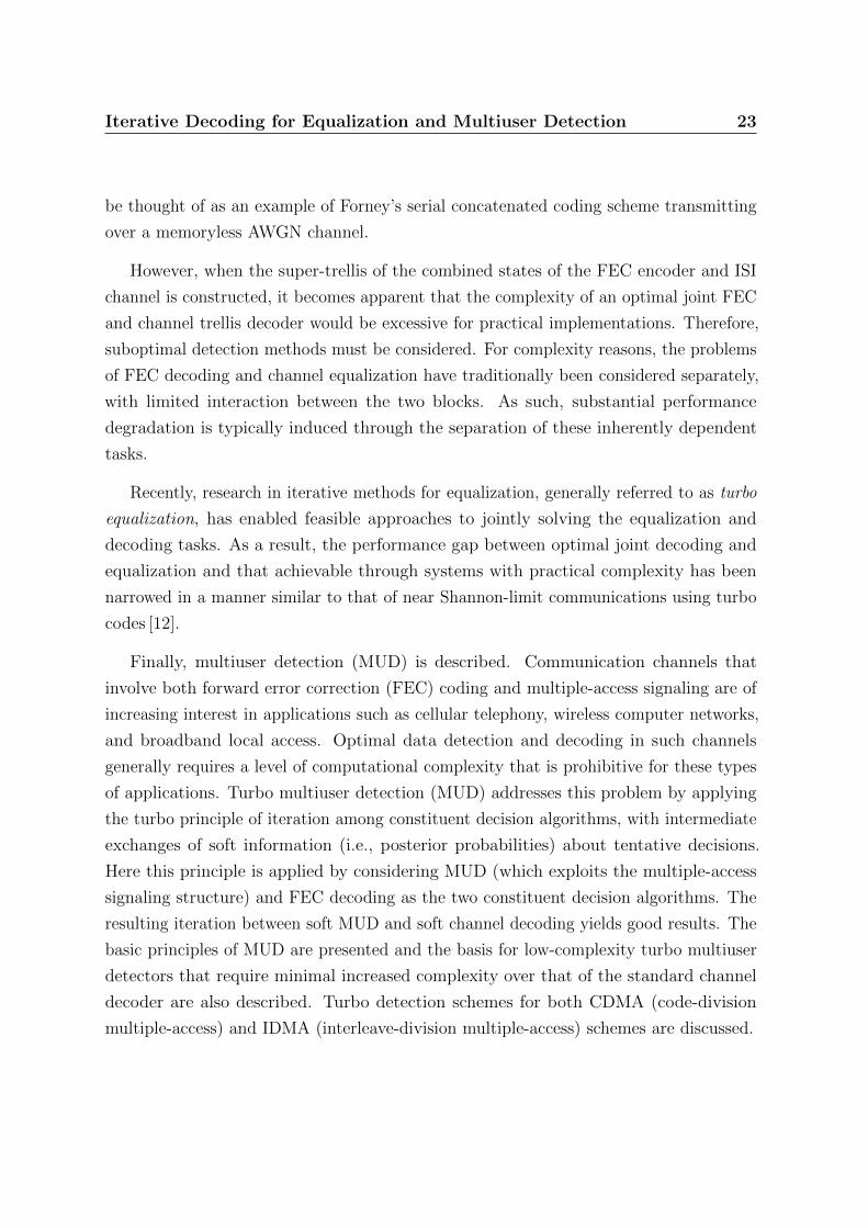
Iterative Decoding for Equalization and Multiuser Detection 23
be thought of as an example of Forney’s serial concatenated coding scheme transmitting
over a memoryless AWGN channel.
However, when the super-trellis of the combined states of the FEC encoder and ISI
channel is constructed, it becomes apparent that the complexity of an optimal joint FEC
and channel trellis decoder would be excessive for practical implementations. Therefore,
suboptimal detection methods must be considered. For complexity reasons, the problems
of FEC decoding and channel equalization have traditionally been considered separately,
with limited interaction between the two blocks. As such, substantial performance
degradation is typically induced through the separation of these inherently dependent
tasks.
Recently, research in iterative methods for equalization, generally referred to as turbo
equalization, has enabled feasible approaches to jointly solving the equalization and
decoding tasks. As a result, the performance gap between optimal joint decoding and
equalization and that achievable through systems with practical complexity has been
narrowed in a manner similar to that of near Shannon-limit communications using turbo
codes [12].
Finally, multiuser detection (MUD) is described. Communication channels that
involve both forward error correction (FEC) coding and multiple-access signaling are of
increasing interest in applications such as cellular telephony, wireless computer networks,
and broadband local access. Optimal data detection and decoding in such channels
generally requires a level of computational complexity that is prohibitive for these types
of applications. Turbo multiuser detection (MUD) addresses this problem by applying
the turbo principle of iteration among constituent decision algorithms, with intermediate
exchanges of soft information (i.e., posterior probabilities) about tentative decisions.
Here this principle is applied by considering MUD (which exploits the multiple-access
signaling structure) and FEC decoding as the two constituent decision algorithms. The
resulting iteration between soft MUD and soft channel decoding yields good results. The
basic principles of MUD are presented and the basis for low-complexity turbo multiuser
detectors that require minimal increased complexity over that of the standard channel
decoder are also described. Turbo detection schemes for both CDMA (code-division
multiple-access) and IDMA (interleave-division multiple-access) schemes are discussed.

Iterative Decoding for Equalization and Multiuser Detection 24
2.1 Convolutional Coding for the Gaussian Channel
Convolutional codes are stream-oriented linear codes and are a building block of turbo
code, turbo equalization, and turbo multiuser detection schemes. A convolutional encoder
assigns code bits to an incoming information bit stream continuously, in a stream-oriented
fashion. The convolutional code is named after its encoding method of using modulo-2
convolutions to generate the redundant bits.
2.1.1 Convolutional Encoding
The role of the encoder is to take the binary data sequence to be transmitted as input
and produce an output that contains not only this data but also additional redundant
information that can be used to protect the data from the possibility of errors that might
occur in the data stream as a result of additive noise in the transmission or detection
errors at the receiver.
A convolutional encoder can be represented by a finite-state machine, taking in a
continuous stream of message bits and producing a continuous stream of output bits.
The encoder has a memory of the past inputs, which is held in the encoder state. The
output depends on the value of this state, as well as on the present message bits at the
input, but is completely unaffected by any subsequent message bits.
The encoder memory is generally implemented using a linear finite-state shift register
circuit where each shift register element represents a time delay of one unit. The bit at
the output of the shift register element at time i is the bit that was present at the input
of the element at time i− 1. The set of all the shift registers elements together holds the
encoder state. An encoder can have one or more shift registers, one or more inputs and
one or more outputs.
Consider the convolutional encoder of Figure 2.1a. The serial-to-parallel converter
splits the input message into vectors of m-bits length, i.e., d[i] =[d(1)[i], . . . , d(m)[i]
]T.
At each state transition, i, the encoder receives a m-bit input vector and outputs a
n-bit coded vector, c[i] =[c(1)[i], . . . , c(n)[i]
]T. The parallel-to-serial converter generates
the output coded bit stream by concatenating the coded vectors c[i] from each state
transition. The convolutional code is said to have rate Rc = m/n if, at each time instant
i, the convolutional encoder receives m input bits and produces n output bits.

Iterative Decoding for Equalization and Multiuser Detection 25
ConvolutionalEncoder
S P
P S
(1)
d[i] c[i]
d [i]
(m)
d [i]
(1)c [i]
(n)c [i]
(a) Encoder schematic block
D D
s(1)
s(2)
(1)
d [i]
(1)c [i]
(2)c [i]
(b) Example rate-1/2 encoder circuit
Figure 2.1: Convolutional encoder schematic block code, and example rate-1/2 encoder forgenerator polynomial (1 +D2, 1 +D +D2).
Without loss of generality, we consider the case where the input to the convolutional
encoder is a single-bit vector, i.e., m = 1. For an input message of block length M ,
d[i]M−1i=0 , the output coded message will have a block length of N = nM , i.e., c[i]N−1
i=0 .
Figure 2.1b shows an example binary convolutional encoder, where D represents the
delay elements (shift register elements), and ⊕ represents modulo-2 addition. At time
i the input to the encoder is one message bit d(1)[i] and the output is a two-bit vector,
c[i] = [ c(1)[i], c(2)[i] ]T ; thus the code rate is 1/2. The state of this encoder is given by
S = (s(1), s(2)), where s(1) ∈ 1, 0 and s(2) ∈ 1, 0 are the contents of the left-hand
register element and the right-hand register element, respectively. Thus the encoder can
be in one of four possible states, S0 = (0, 0), S1 = (0, 1), S2 = (1, 0), and S3 = (1, 1). As
there is only one input, the message d is simply given by [ d(1)[0], . . . , d(1)[M − 1] ], and
therefore the superscript (1) can be dropped.
For the example encoder shown in Figure 2.1b, the output bits c(1)[i] and c(2)[i] (at
time i) are computed as:
c(1)[i] = d[i]⊕ s(2)[i] and c(2)[i] = d[i]⊕ s(1)[i]⊕ s(2)[i] (2.1)
where ⊕ represents modulo-2 addition. The equations in (2.1) can be more concisely
represented by the generator polynomial (1 +D2, 1 +D +D2), where D is equivalent to
the discrete-time delay operator z−1.
Generally, convolutional coding schemes are designed so that the encoder starts from
a known initial state, and ends at a known termination state. For the example encoder
of Figure 2.1b, we assume that the two delay elements in the circuit are zero at the
beginning of the encoding process (time i = 0) and at the end (time i = M − 1). To
achieve the latter assumption, the last two input data bits, d[M − 2] and d[M − 1],

Iterative Decoding for Equalization and Multiuser Detection 26
must be zero, which implies a small rate loss. This loss can be controlled by using long
sequences (i.e., large values of M), or can be avoided by using tail-biting encoding [136]
[48].
Since a convolutional encoder can be thought of as a finite-state machine, the encoder
behaviour can be described by a state diagram which portrays the temporal relationships
between inputs, states and outputs. This representation is often helpful for both encoding
and decoding purposes. For an encoder with L memory elements (i.e., L shift register
elements), there are 2L encoder states in the state diagram. The state diagram in
Figure 2.2a provides a graphical representation of the state transitions of the encoder
in Figure 2.1b. Each of the four states is represented by a node. The edges between
nodes represent the possible state transitions. Each edge is labeled with the input bit
that produced the transition and the output bits generated.
0/00 1/01
0/11
1/11 1/10
0/10
1/00
0/01
S
(0,0)0 S
(1,1)3
S
(1,0)1
S
(0,1)2
(a) State diagram
S3
S2
S1
S0
time = i-1
S3
S2
S1
S0
S3
S2
S1
S0
1/10
0/00
0/10
1/00
1/11
0/11
1/01
0/01
1/10
0/00
0/10
1/00
1/11
0/11
1/01
0/01
i i+1
(b) Trellis diagram
Figure 2.2: State diagram and trellis representations of the convolutional code of Figure 2.1b.The trellis states correspond to the content of the delay elements as S0 = (0, 0),S1 = (1, 0), S2 = (0, 1) and S3 = (1, 1).
Although the state diagram describes the convolutional encoder state and input-output
relationship completely, it does not provide a record of how the state has evolved with
time. For this we use a trellis diagram. Figure 2.2b shows the state diagram expanded in
time to produce a trellis segment. On the left each state is represented for time i and on
the right a copy of each state is represented for time i+ 1. The state transition edges
are joined from a state at time i to a state at time i+ 1 to show the changes with time.
Each path through the trellis is an evolution of the convolutional encoder for one of the
2M possible input streams. Consequently the set of codewords for a convolutional code
is the set of all possible paths through its trellis.
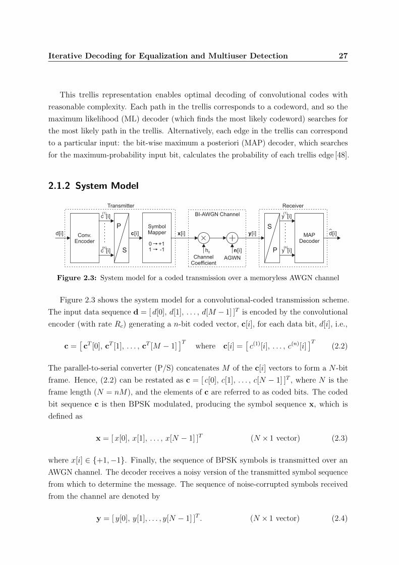
Iterative Decoding for Equalization and Multiuser Detection 27
This trellis representation enables optimal decoding of convolutional codes with
reasonable complexity. Each path in the trellis corresponds to a codeword, and so the
maximum likelihood (ML) decoder (which finds the most likely codeword) searches for
the most likely path in the trellis. Alternatively, each edge in the trellis can correspond
to a particular input: the bit-wise maximum a posteriori (MAP) decoder, which searches
for the maximum-probability input bit, calculates the probability of each trellis edge [48].
2.1.2 System Model
Conv.Encoder
SP
PS
MAPDecoder
SymbolMapperd[i] d[i]
Transmitter Receiver
AGWN
n[i]
BI-AWGN Channel
h0
ChannelCoefficient
(1)c [i]
(n)c [i]
y [i](1)
y [i](n)
x[i] y[i]c[i]
0-1+1
1
Figure 2.3: System model for a coded transmission over a memoryless AWGN channel
Figure 2.3 shows the system model for a convolutional-coded transmission scheme.
The input data sequence d = [ d[0], d[1], . . . , d[M − 1] ]T is encoded by the convolutional
encoder (with rate Rc) generating a n-bit coded vector, c[i], for each data bit, d[i], i.e.,
c =[cT [0], cT [1], . . . , cT [M − 1]
]Twhere c[i] =
[c(1)[i], . . . , c(n)[i]
]T(2.2)
The parallel-to-serial converter (P/S) concatenates M of the c[i] vectors to form a N -bit
frame. Hence, (2.2) can be restated as c = [ c[0], c[1], . . . , c[N − 1] ]T , where N is the
frame length (N = nM), and the elements of c are referred to as coded bits. The coded
bit sequence c is then BPSK modulated, producing the symbol sequence x, which is
defined as
x = [x[0], x[1], . . . , x[N − 1] ]T (N × 1 vector) (2.3)
where x[i] ∈ +1,−1. Finally, the sequence of BPSK symbols is transmitted over an
AWGN channel. The decoder receives a noisy version of the transmitted symbol sequence
from which to determine the message. The sequence of noise-corrupted symbols received
from the channel are denoted by
y = [ y[0], y[1], . . . , y[N − 1] ]T . (N × 1 vector) (2.4)

Iterative Decoding for Equalization and Multiuser Detection 28
The serial-to-parallel converter (S/P) divides the received symbol sequence into M vectors
of n-bits length, i.e.,
y =[yT [0], yT [1], . . . , yT [M − 1]
]Twhere y[i] =
[y(1)[i], . . . , y(n)[i]
]T(2.5)
At each state transition, i, the MAP decoder receives a n-bit input vector y[i], and
outputs the message bit estimate d[i]. After M state transitions of the MAP decoder,
the estimated message sequence can be formed as d = [ d[0], d[1], . . . , d[M − 1] ].
We consider the binary-input additive white Gaussian noise (BI-AWGN) channel,
which is both symmetric and memoryless. A binary-input channel is symmetric if both
input bits, +1,−1, are corrupted equally by the channel. A channel is considered
memoryless if the channel output at any time instant depends only on the input at that
time instant, and not on previously transmitted symbols. This property can be expressed
in terms of channel transition probabilities as
p(y | x) =N−1∏i=0
p(y[i] | x[i]) (2.6)
where x is the transmitted symbol sequence defined in (2.3), and y is the received symbol
sequence defined in (2.4). A memoryless channel is therefore completely described by its
input and output alphabets and the conditional probability distribution p(y | x) for each
input-output symbol pair.
The BI-AWGN channel of Figure 2.3 can be described by the equation
y[i] = h0x[i] + n[i] (2.7)
where x[i] ∈ −1,+1 is the i-th transmitted symbol, y[i] is the i-th received symbol
and n[i] is the additive noise sampled from a Gaussian random variable with zero mean
and σ2 variance, i.e., n[i]∼N (0, σ2). The probability density function for n is
p(n) =1√
2πσ2exp
(− n2
2σ2
), (2.8)
where exp( · ) is the exponential function. If the source is equiprobable then P (x[i] =
−1) = P (x[i] = +1), then we have for the BI-AWGN channel:
p(y[i] | x[i] = ± 1) =1√
2πσ2exp
(− 1
2σ2(y[i]∓h0)2
)(2.9)
Iterative Decoding for Equalization and Multiuser Detection 29
2.1.3 Log Likelihood Ratios (LLRs)
When using probabilistic decoding methods (such as the BCJR algorithm) on binary
codes, the probabilities input and output from the decoder are often expressed in log
likelihood ratio (LLR) form.
For a binary variable x, the probabilities P (x = 1) given P (x = 0) are related since
P (x = 1) = 1− P (x = 0). Therefore only a single value is needed in order to represent
the set of probabilities for x. The log likelihood ratio (LLR) is used to represent the
probability metrics for a binary variable by a single value, and is given by
L(x) = logP (x = 0)
P (x = 1)(2.10)
The sign of L(x) provides a hard decision on x and the magnitude |L(x)| gives the
reliability of this decision. In iterative decoding, a posteriori probability (APP) LLRs
are commonly denoted Λ( · ), i.e., Λ(x) = Lapp(x). Similarly, extrinsic information LLRs
are commonly denoted λ( · ), i.e., λ(x) = Lext(x). LLRs can be translated back to
probabilities as follows:
P (x = 1) =exp−L(x)
1 + exp−L(x)=
1
2
1− tanh
(L(x)
2
)(2.11)
and
P (x = 0) =expL(x)
1 + expL(x)=
1
2
1 + tanh
(L(x)
2
)(2.12)
A benefit of the logarithmic representation of probabilities is that when probabilities
need to be multiplied, log-likelihood ratios need only be added; which can reduce
implementation complexity.
2.1.4 MAP Decoding using the BCJR Algorithm
The binary symbol MAP decoder will output the probability p(d[i] | y) that the message
bit d[i] was 0 or 1 given all the information from the received vector y and the structure
of the code. An efficient algorithm for performing MAP decoding using a trellis was first
proposed Bahl et al. in [6] and is called the BCJR algorithm after its authors.

Iterative Decoding for Equalization and Multiuser Detection 30
Since the convolutional encoder has memory, the codeword bit output at time i is
influenced by the codeword bits sent before it and may itself influence the codeword bits
sent after it. Thus all the bits in y may tell us something about the message bit at time
i. To incorporate the information from both the bits transmitted before time i and the
bits transmitted after time i, the BCJR decoding uses two passes through the trellis:
• a forward pass that provides the current message bit on the basis of only the
codeword bits that were transmitted before it; and
• a backward pass that predicts the current message bit on the basis of only the
codeword bits that were transmitted after it.
Since the message bits are the input to a binary convolutional encoder we can
determine which message bit was sent by finding out which state transition occurred.
We denote:
• S as the set of possible states,
• T + as the set of state transitions (Sr, Ss) that correspond to a 1 input bit,
• T − as the set of state transitions (Sr, Ss) that correspond to a 0 input bit, and
• T as the set of all valid state transitions (Sr, Ss), i.e., T = T + ∪ T −.
For example, the convolutional encoder in Figure 2.1b has S = S0, S1, S2, S3,
T + = (S0, S1), (S1, S3), (S2, S1), (S3, S3), (2.13)
T − = (S0, S0), (S1, S2), (S2, S0), (S3, S2), and (2.14)
T = (S0, S0), (S0, S1), (S1, S2), (S1, S3), (S2, S0), (S2, S1), (S3, S3), (S3, S2). (2.15)
The probability that d[i] was 1 is the probability that a state transition in the set T +
occurred at time i:
P (d[i] = 1 | y) =∑
(Sr,Ss)∈T +
P (ψi = Sr, ψi+1 = Ss | y) (2.16)
where ψi is the variable for the state at time i, and S = S0, S1, . . . , S(2L−1) is the set
of possible values that the state can take. We represent by Sr and Ss the values of the
state at times i− 1 and time i respectively. Similarly, the probability that d[i] was 0 is
Iterative Decoding for Equalization and Multiuser Detection 31
the probability that a state transition in the set T − occurred at time i:
P (d[i] = 0 | y) =∑
(Sr,Ss)∈T −P (ψi = Sr, ψi+1 = Ss | y) (2.17)
For convenience, P (ψi = Sr) will be denoted as P (Sr), and P (ψi+1 = Ss) denoted as
P (Ss) when the context is clear.
Thus determining the message bit probabilities P (d[i] | y) requires that we determine
the probability of each state transition, P (Sr, Ss | y), given that we have only the received
vector y. Using Bayes’ rule we can rewrite P (Sr, Ss | y) as
P (Sr, Ss | y) =p(Sr, Ss,y)
p(y)(2.18)
Substituting (2.18) into equations (2.16) and (2.17), the log-likelihood ratio (LLR) for
bit d[i] can be defined as
Λ(d[i] | y) = log
∑(Sr,Ss)∈T + p(Sr, Ss,y)∑(Sr,Ss)∈T − p(Sr, Ss,y)
(2.19)
Note that the term p(y) in (2.18) cancels out when the ratio is taken, and therefore does
not need to be explicitly calculated.
To enable the efficient calculation of p(ψi, ψi+1,y), the received vector, y, is split into
three sets:
p(ψi, ψi+1,y) = p(ψi, ψi+1,y−[i],y[i],y+[i]) (2.20)
where
• y−[i] represents the values received for the set of bits sent before time i;
• y[i] represents the values received for the set of bits sent at time i; and
• y+[i] represents the values received for the set of bits sent after time i.
The values received for the set of bits sent at time i, y[i], are written as a vector since
the convolutional code may output more than one codeword bit at each time point (i.e.,
n may be greater than 1).
Iterative Decoding for Equalization and Multiuser Detection 32
Applying Bayes’ rule again,
p(ψi, ψi+1,y) = p(ψi, ψi+1,y−[i],y[i],y+[i])
= p(ψi,y−[i]) p(ψi+1,y[i] | ψi,y−[i]) p(y+[i] | ψi, ψi+1,y
−[i],y[i])
Since a convolutional encoder has been used to generate the codeword bits, we know that
the codeword bits output at time i are completely determined by the state transition,
ψi (at time i) to ψi+1 (at time i + 1). Also, since we are considering a memoryless
channel, the channel output y[i] depends only on the transmitted codeword bit c[i] and
the channel noise at time i, and is not affected by anything previously or subsequently
transmitted through the channel. Putting these together, if we know the probability of
the state transition ψi to ψi+1 then the probability of y[i] is completely independent of
y+[i] and y−[i], and so
p(ψi+1,y[i] | ψi,y−[i]) = p(ψi+1,y[i] | ψi).
Similarly, if we know the probability of the encoder state at time i then the probability
of y+[i] is independent of both the past states and past outputs and so
p(y+[i] | ψi, ψi+1,y−[i],y[i]) = p(y+[i] | ψi+1).
Thus finally
p(ψi, ψi+1,y) = p(ψi,y−[i]) p(ψi+1,y[i] | ψi) p(y+[i] | ψi+1). (2.21)
The BCJR algorithm assigns a label to each term in (2.21), therefore (2.21) can be
restated as [48]
mi(ψi, ψi+1) = αi(ψi) γi(ψi, ψi+1) βi+1(ψi+1) (2.22)
where
mi(ψi, ψi+1) = p(ψi, ψi+1,y), (2.23)
αi(ψi) = p(ψi,y−[i]), (2.24)
βi+1(ψi+1) = p(y+[i] | ψi+1), and (2.25)
γi(ψi, ψi+1) = p(ψi+1,y[i] | ψi). (2.26)
Iterative Decoding for Equalization and Multiuser Detection 33
Equation (2.22) shows that the probability of the state transition from state ψi at time i
to state ψi+1 at time i+ 1 is a function of three terms:
1. αi(ψi), which is the probability that the encoder is in state ψi at time i based on
what we know about y−[i],
2. βi+1(ψi+1), which is the probability that the encoder is in state ψi+1 at time i+ 1
based on what we know about y+[i], and
3. γi(ψi, ψi+1), which is the probability of a transition between the states ψi and ψi+1
based on what we know about y[i]
The calculation of the α values is called the forward recursion of the BCJR decoder,
while the β values are calculated in the backward recursion.
Applying Bayes’ rule to (2.26), γi(Sr, Ss) can be written as follows:
γi(Sr, Ss) = p(Ss,y[i] | Sr) = P (Ss | Sr) p(yi | Sr, Ss).
In this form it is easier to see that p(Ss,y[i] | Sr) has two parts.
• The first part, P (Sr | Ss), is the probability that the state of the encoder moves
to Ss at time i + 1 if it started in state Sr at time i. Since the encoder will have
moved from Sr to Ss for an input dr,s, we know that P (Ss | Sr) = P (d[i] = dr,s),
which is given by the probability distribution of the message source.
• The second part, p(y[i] | Sr, Ss), is the probability that y[i] was received given the
state transition Sr to Ss. Since this state transition produces the codeword bits
cr,s, the probability that y[i] is received is equal to the probability that the channel
turned cr,s into y[i], i.e., p(y[i] | Sr, Ss) = p(y[i] | c[i] = cr,s).
Thus γi(Sr, Ss) is a function of the source probability P (d[i] = dr,s) and the channel
transition probability p(y[i] | cr,s):
γi(Sr, Ss) = P (d[i] = dr,s) p(y[i] | cr,s) (2.27)
= P (d[i] = dr,s)n∏q=1
p(y(q)[i] | c(q)r,s) (2.28)
Note that the transition probability γi(Sr, Ss) is zero if the index pair is not in T . The
channel transition probability is a function of the modulation and channel model. For
Iterative Decoding for Equalization and Multiuser Detection 34
the system model shown in Figure 2.3, i.e., BI-AWGN channel with BPSK modulation,
p(y(q)[i] | c(q)r,s) =
1√2πσ2
exp
− 1
2σ2‖y(q)[i]− h0(2c(q)
r,s − 1)‖2
(2.29)
The key to the BCJR decoder is that the values of α and β can be calculated recursively.
Applying Bayes’ rule to (2.24), the following recursive form of α can be obtained:
αi(ψi) =∑
ψi−1∈S
αi−1(ψi−1) γi−1(ψi−1, ψi) (2.30)
Thus, for the forward recursion, the probability that the encoder is in state ψi at time i
is the sum, over all of the states ψi−1 at time i− 1, of the probability that it is in state
ψi−1 times the probability of its moving from ψi−1 to ψi. The encoder starts in the zero
state and so at initialisation α0(S0) = 1 .
Similarly, by applying Bayes’ rule to (2.25), the following recursive form of β can be
obtained:
βi(ψi) =∑
ψi+1∈S
βi+1(ψi+1) γi(ψi, ψi+1) (2.31)
For the backward recursion, the probability that the encoder is in state ψi at time i is the
sum, over all the states ψi+1 at time i+ 1, of the probability that it is in state ψi+1 times
the probability of its moving from ψi to ψi+1 If the encoder is terminated then it finishes
in the zero state and βM(S0) = 1. Alternatively, if the encoder has not been terminated,
β is initialised in such a way that every state is equally likely, i.e., βM(ψM) = 1/2L for
all ψM ∈ S.
The BCJR algorithm calculates the γ, α and β values and then puts them together
to find the state transition probabilities using (2.22). Therefore, the log-likelihood ratio
(LLR) for bit d[i], (2.19), becomes [48]
Λ(d[i] | y) = log
∑(Sr,Ss)∈T + αi(Sr)γi(Sr, Ss)βi+1(Ss)∑(Sr,Ss)∈T − αi(Sr)γi(Sr, Ss)βi+1(Ss)
(2.32)
The calculation of α and β involves multiplying together small numbers, and numerical
stability can become a problem. However, this can be avoided by normalizing α and β

Iterative Decoding for Equalization and Multiuser Detection 35
at each step so that they sum to unity, i.e.,
α′i(Sr) =αi(Sr)∑
ψi∈S αi(ψi)and β′i+1(Ss) =
βi+1(Ss)∑ψi+1∈S βi+1(ψi+1)
. (2.33)
In summary, the BCJR algorithm consists of an initialization in (2.27), a forward
pass to calculate α in (2.30), a backward pass to calculate β in (2.31), the calculation of
each state probability using (2.22), and lastly, the calculation of message bit probabilities
(in LLR form) using (2.32).
The source message bit probabilities P (d[i]) are called the a priori probabilities for
d because they are known in advance before the BCJR decoder is run. The message
bit probabilities P (d[i] |y) output by the BCJR decoder are called the a posteriori
probabilities for d.
Matrix Formulation of the BCJR Algorithm
For notational purposes it is often convenient to express the BCJR algorithm in matrix
form. Denote the vectors of the forward and backward probabilities as:
αi =[αi(S0), αi(S1), · · · , αi(S(2L−1))
]T, (|S|× 1 vector) (2.34)
βi =[βi(S0), βi(S1), · · · , βi(S(2L−1))
]T. (|S|× 1 vector) (2.35)
Let Pi be the probability matrix with dimensions |S|× |S| defined as
Pij,k = γi(Sj, Sk) (2.36)
where · j,k denotes the entry of a matrix in the j-th row and k-th column. Then the
forward recursion (2.30) can be expressed as
αi+1 = PTi αi, i = 1, 2, . . . , N − 1, (2.37)
and the backward recursion (2.31) can be expressed as
βi = Piβi+1, i = N − 1, N − 2, . . . , 1. (2.38)

Iterative Decoding for Equalization and Multiuser Detection 36
To compute (2.32), we need to define two matrices describing transitions in the trellis.
Let matrices T(0) and T(1) be defined as
T(0)j,k =
1, if (Sj, Sk) is a state transition with dj,k = 0,
0, otherwise
T(1)j,k =
1, if (Sj, Sk) is a state transition with dj,k = 1,
0, otherwise
respectively. For example, for the trellis shown in Figure 2.2b,
T(0) =
1 0 0 0
0 0 1 0
1 0 0 0
0 0 1 0
, and T(1) =
0 1 0 0
0 0 0 1
0 1 0 0
0 0 0 1
. (2.39)
Then the a posteriori probabilities for d[i] in LLR form, (2.32), can be expressed as [77]:
Λ(d[i] | y) = log
[αTi (T(1)Pi)βi+1
αTi (T(0)Pi)βi+1
], (2.40)
where denotes the element-by-element product of two matrices (Hadamard product).
2.2 Intersymbol Interference (ISI) Channels
Traditional forward error correction (FEC) methods do not work well when the data
is transmitted over a channel that introduces additional distortions in the form of ISI.
When the channel is bandlimited or for other reasons is time-dispersive in nature, then
the receiver will generally need to compensate for the channel effects prior to employing
a standard decoding algorithm for the FEC. Such methods for channel compensation are
commonly referred to as channel equalization.
Given observations of the received data, the receiver must estimate the data that was
transmitted, using knowledge of how the channel has corrupted the data together with
the available redundancy that has been introduced to protect the data, in the form of
the FEC. While the FEC alone would protect the data from additive noise, when the
channel introduces intersymbol interfernce, adjacent channel symbols become smeared
Iterative Decoding for Equalization and Multiuser Detection 37
together, introducing additional dependencies among the transmitted channel symbols
which degrades the decoder performance.
Three receiver structures for the reception of signals from an intersymbol interference
channel are considered.
Optimal Receiver (Joint Equalization and Detection). To optimally estimate the data
that was transmitted, in terms of minimizing the bit error rate (BER), the receiver
must find the set of transmitted bits that are most probable, given knowledge of the
complex statistical relationship between the observations and the transmitted bits.
An optimal receiver takes into account the FEC, the interleaver, the symbol map-
ping, and knowledge of the channel. With so many factors involved, the resulting
statistical relationship becomes difficult to manage efficiently. Therefore, in most
practical applications, the optimal receiver is infeasible, as it essentially tries to fit
all the possible sequences of transmitted bits to the received data, a task whose
complexity grows exponentially in the length of the data transmitted.
Separate Equalization and Decoding. Traditionally, most practical receivers have been
designed is to first process the received observations to account for the effects of
the channel and then to make estimates of the transmitted channel symbols that
best fit the observed data. Generally, the problem of mitigating the effects of an
ISI channel on the transmitted data is called equalization or detection, while the
subsequent problem of recovering the data bits from the equalized symbol stream,
making use of the FEC, is called decoding.
In the traditional implementation of this separate equalization and decoding process,
the equalizer makes hard decisions as to which sequence of channel symbols were
transmitted and then maps these hard decisions into their constituent binary code
bits. These code bits are then processed by the FEC decoder. However, the process
of making hard decisions on the channel symbols destroys information relating to
how likely each of the possible channel symbols might have been. This additional
“soft” information can be converted into probabilities that each of the received code
bits takes on the value of zero or one. This form of soft information can be readily
exploited by a BER optimal decoding algorithm. Many practical systems use this
type of soft-input FEC decoding by passing soft information between an equalizer
and decoding algorithm.
Turbo Equalization. The remarkable performance of turbo codes demonstrated the
benefits of passing soft information in both directions between constituent processing
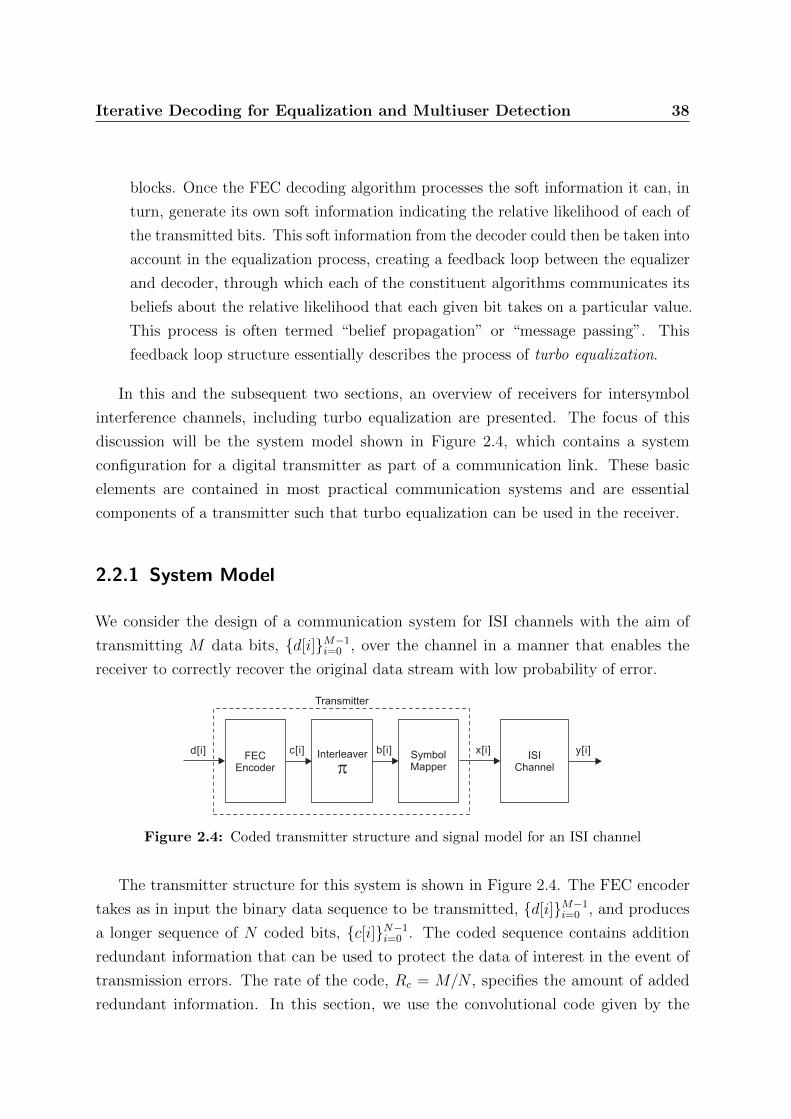
Iterative Decoding for Equalization and Multiuser Detection 38
blocks. Once the FEC decoding algorithm processes the soft information it can, in
turn, generate its own soft information indicating the relative likelihood of each of
the transmitted bits. This soft information from the decoder could then be taken into
account in the equalization process, creating a feedback loop between the equalizer
and decoder, through which each of the constituent algorithms communicates its
beliefs about the relative likelihood that each given bit takes on a particular value.
This process is often termed “belief propagation” or “message passing”. This
feedback loop structure essentially describes the process of turbo equalization.
In this and the subsequent two sections, an overview of receivers for intersymbol
interference channels, including turbo equalization are presented. The focus of this
discussion will be the system model shown in Figure 2.4, which contains a system
configuration for a digital transmitter as part of a communication link. These basic
elements are contained in most practical communication systems and are essential
components of a transmitter such that turbo equalization can be used in the receiver.
2.2.1 System Model
We consider the design of a communication system for ISI channels with the aim of
transmitting M data bits, d[i]M−1i=0 , over the channel in a manner that enables the
receiver to correctly recover the original data stream with low probability of error.
Interleaverd[i]FEC
EncoderISI
Channel
SymbolMapper
c[i] b[i] x[i] y[i]
Transmitter
Figure 2.4: Coded transmitter structure and signal model for an ISI channel
The transmitter structure for this system is shown in Figure 2.4. The FEC encoder
takes as in input the binary data sequence to be transmitted, d[i]M−1i=0 , and produces
a longer sequence of N coded bits, c[i]N−1i=0 . The coded sequence contains addition
redundant information that can be used to protect the data of interest in the event of
transmission errors. The rate of the code, Rc = M/N , specifies the amount of added
redundant information. In this section, we use the convolutional code given by the
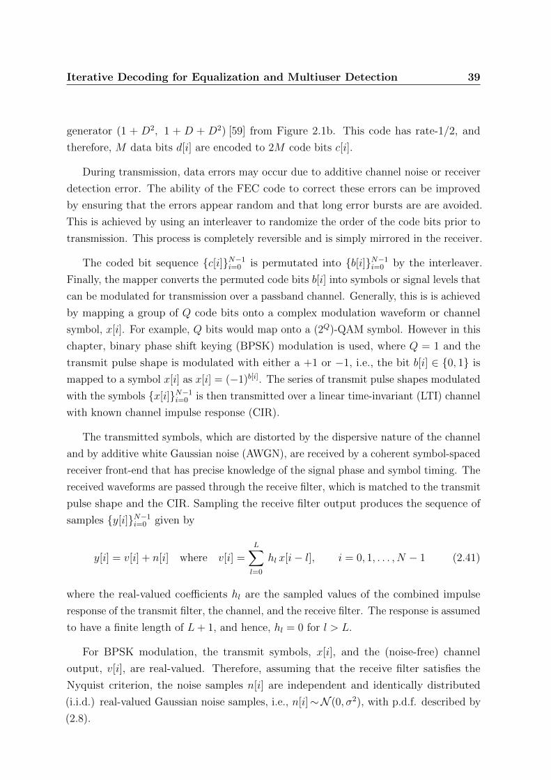
Iterative Decoding for Equalization and Multiuser Detection 39
generator (1 + D2, 1 + D + D2) [59] from Figure 2.1b. This code has rate-1/2, and
therefore, M data bits d[i] are encoded to 2M code bits c[i].
During transmission, data errors may occur due to additive channel noise or receiver
detection error. The ability of the FEC code to correct these errors can be improved
by ensuring that the errors appear random and that long error bursts are are avoided.
This is achieved by using an interleaver to randomize the order of the code bits prior to
transmission. This process is completely reversible and is simply mirrored in the receiver.
The coded bit sequence c[i]N−1i=0 is permutated into b[i]N−1
i=0 by the interleaver.
Finally, the mapper converts the permuted code bits b[i] into symbols or signal levels that
can be modulated for transmission over a passband channel. Generally, this is is achieved
by mapping a group of Q code bits onto a complex modulation waveform or channel
symbol, x[i]. For example, Q bits would map onto a (2Q)-QAM symbol. However in this
chapter, binary phase shift keying (BPSK) modulation is used, where Q = 1 and the
transmit pulse shape is modulated with either a +1 or −1, i.e., the bit b[i] ∈ 0, 1 is
mapped to a symbol x[i] as x[i] = (−1)b[i]. The series of transmit pulse shapes modulated
with the symbols x[i]N−1i=0 is then transmitted over a linear time-invariant (LTI) channel
with known channel impulse response (CIR).
The transmitted symbols, which are distorted by the dispersive nature of the channel
and by additive white Gaussian noise (AWGN), are received by a coherent symbol-spaced
receiver front-end that has precise knowledge of the signal phase and symbol timing. The
received waveforms are passed through the receive filter, which is matched to the transmit
pulse shape and the CIR. Sampling the receive filter output produces the sequence of
samples y[i]N−1i=0 given by
y[i] = v[i] + n[i] where v[i] =L∑l=0
hl x[i− l], i = 0, 1, . . . , N − 1 (2.41)
where the real-valued coefficients hl are the sampled values of the combined impulse
response of the transmit filter, the channel, and the receive filter. The response is assumed
to have a finite length of L+ 1, and hence, hl = 0 for l > L.
For BPSK modulation, the transmit symbols, x[i], and the (noise-free) channel
output, v[i], are real-valued. Therefore, assuming that the receive filter satisfies the
Nyquist criterion, the noise samples n[i] are independent and identically distributed
(i.i.d.) real-valued Gaussian noise samples, i.e., n[i]∼N (0, σ2), with p.d.f. described by
(2.8).
Iterative Decoding for Equalization and Multiuser Detection 40
h0
x[i]
y[i]
h1 h2
n[i]
v[i]
T Tx[i-1] x[i-2]
AWGN
Figure 2.5: Tapped delay line model of an ISI channel with memory L = 2 (and coefficientsh0 = 0.407, h1 = 0.815, and h2 = 0.407)
The discrete-time model of data transmission in a bandlimited additive noise channel
(2.41) can be represented by an equivalent tapped delay-line model. Figure 2.5 shows an
example tapped delay-line model for a three-tap ISI channel (L = 2) with coefficients
h0 = 0.407, h1 = 0.815, h2 = 0.407. These coefficients are assumed to be time-invariant
and known to the receiver. This example is from [92] and [53]. For channel shown in
Figure 2.5, the system model of (2.41) can be expressed in matrix form as
y = Hx + n, (2.42)
where channel matrix H is given by
H =
h0 0 0 0 0 · · · 0
h1 h0 0 0 0 · · · 0
h2 h1 h0 0 0 · · · 0
0 h2 h1 h0 0 · · · 0
. . . . . . . . .
0 0 . . . 0 h2 h1 h0
(N ×N matrix)
and vectors y, x, and n are given by
y = [ y[0], y[1], . . . , y[N − 1] ]T (N × 1 vector)
x = [x[0], x[1], . . . , x[N − 1] ]T (N × 1 vector)
n = [n[0], n[1], . . . , n[N − 1] ]T (N × 1 vector)
Iterative Decoding for Equalization and Multiuser Detection 41
2.2.2 Optimal Detection
An optimal receiver seeks to minimize the bit error rate (BER) by finding the set of
transmitted bits that are most probable, given knowledge of the complex statistical
relationship between the observations and the transmitted bits. Such a receiver takes into
account the FEC, the interleaver, the symbol mapping, and knowledge of the channel.
In the general case, the decision rule minimizing the bit error probability is based on the
maximization of the a posteriori probabilities (APP) of each data bit in the sequence, i.e.
d[i] = arg maxd∈0,1
P (d[i] = d | y), i = 0, 1, . . . ,M − 1 (2.43)
where d[i] is the data bit at time i, and y is the entire received symbol sequence [10].
Detection algorithms that implement the decision rule of (2.43) are commonly known as
maximum a posteriori probability (MAP) algorithms. By applying Bayes’ rule to (2.43),
the data bit estimates can be calculated as follows
P (d[i] = d | y) =∑
d:d[i]=d
P (d | y) =∑
d:d[i]=d
p(y | d)P (d)
p(y), d ∈ 0, 1 (2.44)
where P (d) is the a-priori probability of the sequence d, which can be used to include
knowledge about the source producing the bits d[i]. The data bits, d[i], are usually
assumed to be independent, and hence
P (d) =M−1∏i=0
P (d[i]). (2.45)
It then follow that (2.44) can be restated as
P (d[i] = d | y) =∑
d:d[i]=d
p(y | d)
p(y)
M−1∏j=0
P (d[j]), d ∈ 0, 1 (2.46)
In log-likelihood ratio (LLR) form, (2.46) can be written as
Λ(d[i] | y) = log
∑d:d[i]=0 p(y | d)
∏M−1j=0 P (d[j])∑
d:d[i]=1 p(y | d)∏M−1
j=0 P (d[j])
= λ(d[i] | y) + λ(d[i]) (2.47)
Iterative Decoding for Equalization and Multiuser Detection 42
where λ(d[i] | y) is the extrinsic information about d[i] contained in y, defined as
λ(d[i] | y) = log
∑d:d[i]=0 p(y | d)
∏M−1j=1:j 6=i P (d[j])∑
d:d[i]=1 p(y | d)∏M−1
j=1:j 6=i P (d[j]), (2.48)
and λ(d[i]) is the a priori information about d[i], defined as
λ(d[i]) = logP (d[i] = 0)
P (d[i] = 1). (2.49)
Extrinsic information plays an important role in the iterative detection schemes described
in later sections. Note that if the bits d[i] are assumed to be uniformly distributed (i.e.,
they take on the values 0 or 1 equally likely), then the a priori information (in LLR
form) is zero, i.e., λ(d[i]) = 0.
Using (2.47) to compute the a posteriori probabilities in LLR form, Λ(d[i] | y), the
MAP decision rule of (2.43) can be written in LLR form as
d[i] =
0, Λ(d[i] | y) ≥ 0
1, Λ(d[i] | y) < 0i = 0, 1, . . . ,M − 1 (2.50)
The main difficulty with optimal joint MAP detection is the computational complexity
of computing p(y | d) in (2.44) and (2.47), which involves 2M terms and becomes
impractical for large block lengths M .
2.3 Separate Equalization and Decoding for ISI
Channels
Optimal joint equalization and decoding using the MAP algorithm is rarely used in
practice because of the computational complexity. The traditional approach to minimising
receiver complexity is to split the detection task into a number of separate subtasks.
First, the equalizer estimates the transmitted channel symbols. Then, the symbols are
demapped into their associated code bits, deinterleaved, and finally, decoded using a
BER optimal decoder for the FEC. This approach is shown in Figure 2.6.
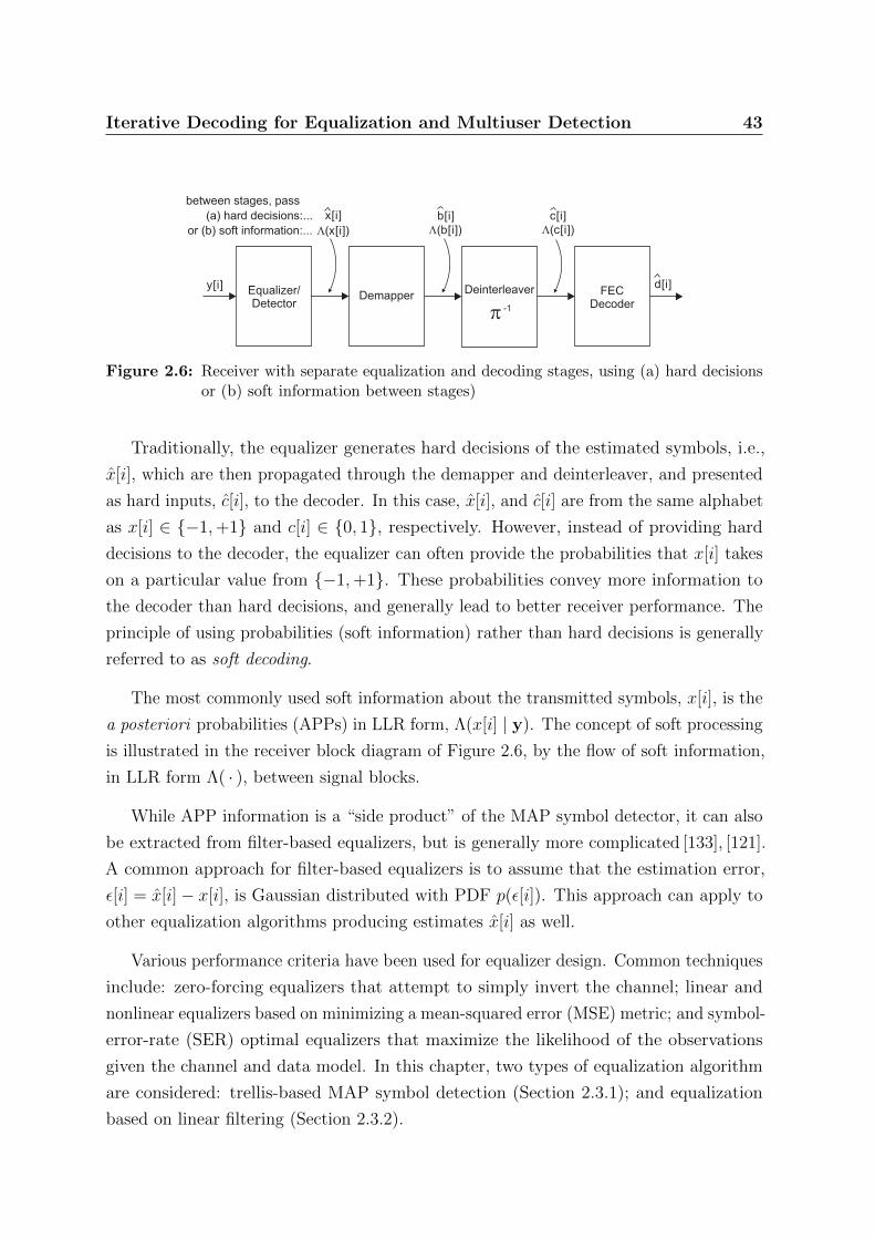
Iterative Decoding for Equalization and Multiuser Detection 43
Deinterleaver FECDecoder
Equalizer/Detector
Demapper-1
or (b) soft information:...
y[i] d[i]
x[i] b[i] c[i](a) hard decisions:...
between stages, pass
L(b[i])L(x[i]) L(c[i])
Figure 2.6: Receiver with separate equalization and decoding stages, using (a) hard decisionsor (b) soft information between stages)
Traditionally, the equalizer generates hard decisions of the estimated symbols, i.e.,
x[i], which are then propagated through the demapper and deinterleaver, and presented
as hard inputs, c[i], to the decoder. In this case, x[i], and c[i] are from the same alphabet
as x[i] ∈ −1,+1 and c[i] ∈ 0, 1, respectively. However, instead of providing hard
decisions to the decoder, the equalizer can often provide the probabilities that x[i] takes
on a particular value from −1,+1. These probabilities convey more information to
the decoder than hard decisions, and generally lead to better receiver performance. The
principle of using probabilities (soft information) rather than hard decisions is generally
referred to as soft decoding.
The most commonly used soft information about the transmitted symbols, x[i], is the
a posteriori probabilities (APPs) in LLR form, Λ(x[i] | y). The concept of soft processing
is illustrated in the receiver block diagram of Figure 2.6, by the flow of soft information,
in LLR form Λ( · ), between signal blocks.
While APP information is a “side product” of the MAP symbol detector, it can also
be extracted from filter-based equalizers, but is generally more complicated [133], [121].
A common approach for filter-based equalizers is to assume that the estimation error,
ε[i] = x[i]− x[i], is Gaussian distributed with PDF p(ε[i]). This approach can apply to
other equalization algorithms producing estimates x[i] as well.
Various performance criteria have been used for equalizer design. Common techniques
include: zero-forcing equalizers that attempt to simply invert the channel; linear and
nonlinear equalizers based on minimizing a mean-squared error (MSE) metric; and symbol-
error-rate (SER) optimal equalizers that maximize the likelihood of the observations
given the channel and data model. In this chapter, two types of equalization algorithm
are considered: trellis-based MAP symbol detection (Section 2.3.1); and equalization
based on linear filtering (Section 2.3.2).
Iterative Decoding for Equalization and Multiuser Detection 44
2.3.1 Trellis-Based MAP Symbol Detection
A MAP symbol detector computes symbol estimates, x[i], using a decision rule based on
the maximization of the a posteriori probabilities (APP) of each individual symbol in
the sequence, i.e., for BPSK transmission,
x[i] = arg maxx∈+1,−1
P (x[i] = x | y), i = 0, 1, . . . , N − 1 (2.51)
where x[i] is the transmitted symbol at time i and y is the entire received sequence [10].
Note that the decision rule ignores the effect of the FEC code. MAP detection may
appear intractably complex because of the large number of probabilities to be computed
(c.f. (2.43)-(2.44)), however it can be performed efficiently using trellis-based methods.
Consider the tapped delay line model of the transmitter, channel, and receive filter
shown in Figure 2.5. Given that the tapped delay line contains L delay elements and
that the input symbols are BPSK modulated, x[i] ∈ +1,−1, the channel can be in one
of 2L states Sl, l = 0, 1, . . . , 2L− 1, corresponding to the 2L different possible contents of
the delay elements. The set of possible states is denoted S = S0, S1, . . . , S(2L−1).
At each time instance i = 0, 1, . . . , N − 1 the state of the channel is a random variable
ψi ∈ S. If the channel is in state ψi at time i, then ψi+1 (the state at time i+ 1) can only
assume one of two values corresponding to a transmit symbol of x[i] = +1 or x[i] = −1
being input into the tapped delay line (channel model) at time i. This possible evolution
of states can be described using a trellis diagram. Figure 2.7a and Figure 2.7b show the
state and trellis diagrams, respectively, for the channel model of Figure 2.5. A branch of
the trellis is a four-tuple (Sr, Ss, xr,s, vr,s) such that state ψi+1 = Ss at time i+ 1 can be
reached from state ψi = Sr at time i with input x[i] = xr,s and output v[i] = vr,s, where
xr,s and vr,s are uniquely identified by the index pair (Sr, Ss). The output symbol v[i] at
time i is the noise-free output of the channel model, (2.41), given by
v[i] =L∑l=0
hl x[i− l].
The transitions from a state ψi = Sr at time i to a state ψi+1 = Ss at time i+1 are labeled
with the input/output pair xr,s/vr,s. The set of all index pairs (Sr, Ss) corresponding to
valid trellis branches (i.e. valid state transitions) is denoted T . The set T for the trellis

Iterative Decoding for Equalization and Multiuser Detection 45
in Figure 2.7b is
T = (S0, S0), (S0, S1), (S1, S2), (S1, S3), (S2, S0), (S2, S1), (S3, S3), (S3, S2) .
This trellis description can be used to efficiently compute the APPs, P (x[i] | y).
+1/+1.63 -1/-1.63
+1/+0.815
-1/+0.815 -1/-0.815
+1/-0.815
-1/0
+1/0
S0
S3
S1
S2
(+1,-1)
(+1,+1)
(-1,+1)
(-1,-1)
(a) State diagram
S3
S2
S1
S0
time = i-1
S3
S2
S1
S0
S3
S2
S1
S0
-1/-1.63
+1/+1.63
+1/0
-1/0
-1/+0.815
+1/+0.815
-1/-0
.815
+1/-0.815
-1/-1.63
+1/+1.63
+1/0
-1/0
-1/+0.815
+1/+0.815
-1/-0
.815
+1/-0.815
i i+1
(b) Trellis diagram
Figure 2.7: State diagram and trellis representations of the channel in Figure 2.5. The statesS0 = (+1,+1), S1 = (−1,+1), S2 = (+1,−1), S3 = (−1,−1) are the possiblecontents of the channel model delay elements.
The approach of separating the equalization and decoding tasks assumes that the
transmitted symbols, x[i], are i.d.d. random variables, ie
P (x) =N−1∏i=0
P (x[i]) (2.52)
and x[i] takes on values +1 and −1 equally for all i. With this assumption, the BCJR
algorithm (of Section 2.1.4) can be adapted to efficiently compute P (x[i] | y).
The probability that the transmitted sequence path in the trellis contained the branch
(Sr, Ss, xr,s, vr,s) at time i, i.e., P (ψi = Sr, ψi+1 = Ss | y) can be computed by the BCJR
algorithm[6], [97] based on the decomposition of the joint distribution p(ψi, ψi+1,y) given
by
p(ψi, ψi+1,y) = P (ψi, ψi+1 | y)p(y). (2.53)
The received signal sequence y in p(ψi, ψi+1,y) can be written as
p(ψi, ψi+1,y) = p(ψi, ψi+1, (y[0], . . . , y[i− 1]), y[i], (y[i+ 1], . . . , y[N − 1])), (2.54)

Iterative Decoding for Equalization and Multiuser Detection 46
and applying the chain rule for joint probabilities, i.e., P (a, b) = P (a)P (b|a), to (2.54)
produces the decomposition:
p(ψi, ψi+1,y) = p(ψi, y[0], . . . , y[i− 1])︸ ︷︷ ︸αi(ψi)
p(ψi+1, y[i] |ψi)︸ ︷︷ ︸γi(ψi,ψi+1)
p(y[i+ 1], . . . , y[N − 1] | ψi+1)︸ ︷︷ ︸βi+1(ψi+1)
.
The term αi(ψ) can be computed using the recursion of (2.30) with the initial value
α0(ψ) = P (ψ0 = ψ), the distribution of the state at time i = 0. The term βi(ψ) can be
computed using the recursion (2.30) with the initial value βN(ψ) = 1 for all ψ ∈ S. The
term γi(ψi, ψi+1) can be decomposed into two parts:
γi(ψi, ψi+1) = P (ψi+1 | ψi)p(y[i] | ψi, ψi+1), (2.55)
where P (ψi+1 | ψi) = P (x[i] = xr,s), which is given by the probability of the message
source; and p(y[i] | ψi, ψi+1) = p(y[i] | v[i] = vr,s) is the channel transition probability,
i.e., the probability that the channel turned vr,s into y[i].
The transition probability γi(Sr, Ss) is zero if the index pair (Sr, Ss) is not in T . For
pairs (Sr, Ss) from T , γi(Sr, Ss) is a function of the source probability and the channel
transition probability, i.e.,
γi(Sr, Ss) =
P (x[i] = xr,s)p(y[i] | v[i] = vr,s), (Sr, Ss) ∈ T
0, (Sr, Ss) /∈ T(2.56)
The symbols are assumed to be i.d.d. and hence P (x[i] = +1) = P (x[i]) = −1) = 1/2. For
the channel model of (2.41), i.e. y[i] = v[i]+n[i], and the assumption that n[i]∼N (0, σ2),
the channel transition probability is given by
p(y[i] | v[i]) =1√
2πσ2exp
− 1
2σ2(y[i]− v[i])2
.
The BCJR algorithm calculates the α(ψi), γi(ψi, ψi+1), and βi+1(ψi) probabilities and
puts them together to obtain the state transition probability p(ψi, ψi+1,y). Therefore
the conditional LLR Λ(b[i] | y) of the code bit b[i] can be written as
Λ(b[i] | y) = log
∑(Sr,Ss)∈T :xr,s=+1 αi(Sr)γi(Sr, Ss)βi+1(Ss)∑(Sr,Ss)∈T :xr,s=−1 αi(Sr)γi(Sr, Ss)βi+1(Ss)
(2.57)

Iterative Decoding for Equalization and Multiuser Detection 47
Note that (2.57) includes the demapping operation x[i]→ b[i], where
Λ(b[i] | y) = logP (b[i] = 0 | y)
P (b[i] = 1 | y)= log
P (x[i] = +1 | y)
P (x[i] = −1 | y)
Finally, the code bit estimates b[i] are computed from the sign of Λ(b[i] | y) as in (2.50).
The BCJR algorithm for MAP equalization can be concisely described in terms of
matrix operations. For a trellis with a set of states S, denote the following vectors and
matrices:
• αi as the set of |S|× 1 vectors of the forward probabilities (αi(ψ) values), as defined
in (2.34);
• βi as the set of |S|× 1 vectors of backward probabilities (βi(ψ) values), as defined
in (2.35);
• Pi as the set of |S|× |S| probability matrices as defined in (2.36); and
• T(x) for x ∈ +1,−1, as the two |S|× |S| trellis transition matrices, defined as
T(x)j,k =
1, (Sj, Sk) is a branch with xj,k = x,
0, otherwise(2.58)
For the trellis in Figure 2.7, the matrices T(+1) and T(−1) are defined as
T(+1) =
1 0 0 0
0 0 1 0
1 0 0 0
0 0 1 0
, and T(−1) =
0 1 0 0
0 0 0 1
0 1 0 0
0 0 0 1
.
Then the BCJR algorithm for MAP equalization can be expressed as shown in Table 2.1.
Note that the algorithm shown assumes that the channel is not in any predefined starting
or ending state, but can be readily modified to include defined starting and ending states.

Iterative Decoding for Equalization and Multiuser Detection 48
1. Initialization: calculate matrices Pi for i = 0, 1, . . . , N − 1, where
Pir,s = γi(Sr, Ss) and
γi(Sr, Ss) =
P (x[i] = xr,s)p(y[i] | v[i] = vr,s), (Sr, Ss) ∈ T
0, (Sr, Ss) /∈ T .
2. Forward recursion: calculate vectors αi for i = 0, 1, . . . , N − 1, where
α0 = [ 1, 1, . . . , 1 ]T and
αi = PTi−1αi−1, i = 1, 2, . . . , N − 1.
3. Backward recursion: calculate vectors βi for i = N,N − 1, . . . , 0, where
βN = [ 1, 1, . . . , 1 ]T and
βi = Piβi+1, i = N − 1, N − 2, . . . , 1.
4. Output: calculate code bit APPs in LLR form, Λ(b[i] | y), using
Λ(b[i] | y) = log
[αTi (T(+1)Pi)βi+1
αTi (T(−1)Pi)βi+1
], i = 0, 1, . . . , N − 1.
Table 2.1: MAP equalization using the BCJR algorithm
In a practical implementation of the algorithm, a frequent re-normalization of the
vectors is necessary to avoid numerical underflow. That is, after each step in the recursion
to compute αi and βi, both vectors are normalized using (2.33).
2.3.2 Linear Equalization and Symbol Detection
The computational complexity of the trellis-based approaches is determined by the
number of trellis states, equal to 2QL, where Q is the number of bits mapped onto each
symbol and L is the number of delay elements in the tapped delay line channel model
(Figure 2.5). Therefore, the computational complexity of trellis-based equalization can
become prohibitive for large signal constellations or long channel-delay spreads.

Iterative Decoding for Equalization and Multiuser Detection 49
In contrast to trellis-based equalization, linear-filter-based approaches perform only
simple operations on the received symbols, which are applied sequentially to a subset
of the observed symbols. Consider the transmitted symbols in the interval x[i −δ], . . . , x[i], . . . , x[i+ δ], where, for example, δ = 6. This subset of transmitted symbols,
denoted xi is given by
xi = [x[i− 6], x[i− 5], . . . , x[i], . . . , x[i+ 6] ]T ((∆ + L)× 1 vector)
where ∆ + L = 2δ + 1, and L is the number of delay elements in the channel model. For
the 3-tap ISI channel model of Figure 2.5, L = 2 and hence ∆ = 11. The signal model
can be expressed as
yi = Hxi + ni (2.59)
where channel matrix H is given by
H =
h2 h1 h0 0 0 · · · 0
0 h2 h1 h0 0 · · · 0...
. . . . . . . . ....
0 · · · 0 h2 h1 h0 0
0 · · · 0 0 h2 h1 h0
(∆× (∆ + L) matrix)
and received symbol vector, yi, and channel noise vector, ni, are given by
yi = [ y[i− 4], y[i− 3], . . . , y[i], . . . , y[i+ 6] ]T , (∆× 1 vector)
ni = [n[i− 4], n[i− 3], . . . , n[i], . . . , n[i+ 6] ]T , (∆× 1 vector)
respectively. Define vector wi as:
wi = [wδ, wδ−1, . . . , w0, . . . , w−δ+L ]T , (∆× 1 vector)
then the linear processing of yi to compute x[i] can be expressed with the linear (affine)
function
x[i] = wTi yi + ai, (2.60)

Iterative Decoding for Equalization and Multiuser Detection 50
where vector wi ∈ R∆ and scalar ai ∈ R are the parameters subject to optimization. The
general form on the linear equalizer is shown in Figure 2.8.
wd
y[i+ ]d
wd-1
T Ty[i+ -1]d
x[i]
ai
w- +Ld
Ty[i- +L]d
w0
Ty[i]
Figure 2.8: Linear-filter-based equalizer
The zero-forcing (ZF) equalizer optimizes wi so that x[i] is recovered perfectly from
yi in the absence of noise. However, with noise present, an estimate x[i] = x[i] + wTi ni
is obtained and the equalizer can suffer from severe “noise enhancement” if H is ill
conditioned [92]. This effect can be avoided using linear minimum mean square error
(MMSE) estimation [87].
A linear MMSE estimator computes x[i] such that the mean squared error (MSE)
E|x[i]− x[i] |2 is minimized, i.e., wi is computed such that
wi = arg minw∈R∆
E|x[i]−wTyi |2 (2.61)
where E · denotes expectation. This is achieved by the affine model
x[i] = wTi (yi − Eyi) + Ex[i], (2.62)
where
wi = Covyi,yi−1Covyi, x[i]. (2.63)
Note that (2.62) is not purely linear because of the bias terms Ex[i] and Eyi. From
(2.59), the following statistics can be defined:
Covyi,yi = σ2I∆ + H Covxi,xiHT, (2.64)
Covyi, x[i] = H Covxi, x[i], (2.65)
Eyi = H Exi, (2.66)
Iterative Decoding for Equalization and Multiuser Detection 51
where I∆ is the ∆×∆ identity matrix. Furthermore, assuming symbols x[i] are indepen-
dent, then
Covx[i], x[j] = 0 for i 6= j (2.67)
and hence, covariance matrix Covxi,xi is diagonal. Additionally,
Covxi, x[i] = e Covx[i], x[i] = e Varx[i] (2.68)
where
e = [ 01× δ, 1, 01× δ ]T ((∆ + L)× 1 vector)
Note that the element set to one in vector e corresponds to the x[i] element in vector xi.
Using these definitions, the MMSE linear equalizer of (2.62)-(2.63) can be restated as [53]
x[i] = wTi (yi − H Exi) + Ex[i], (2.69)
where
wi =(σ2I∆ + H Covxi,xiH
T)−1
He Varx[i], (2.70)
and the remaining statistics, Ex[i] and Covx[i], x[i], are obtained from the symbol a
priori probabilities, P (x[i]), using
Ex[i] =∑
x∈+1,−1
xP (x[i] = x), and (2.71)
Varx[i] =∑
x∈+1,−1
|x− E(x[i])|2 P (x[i] = x). (2.72)
In turbo equalization configurations (described in later sections), the a priori probabilities,
P (x[i]), would be provided by the soft FEC decoder.
When a priori information is not available (for example, in non-iterative configura-
tions), then symbols x[i] are assumed to be i.d.d. and it follows that
Ex[i] = 0, Varx[i] = 1, and Covxi,xi = I(∆+L). (2.73)
Iterative Decoding for Equalization and Multiuser Detection 52
Substituting (2.73) into (2.69) and (2.69), the MMSE linear equalizer (for the case where
there is no a priori information about the symbols available) is given by [112] [92]
x[i] = wTi yi, where wi =
(σ2I∆ + HH
T)−1
He. (2.74)
The estimates x[i] are usually not in the symbol alphabet +1, 1 and the decision
whether x[i] = +1 or x[i] = −1 is usually based on the estimation error ε[i] = x[i]− x[i].
Given the estimator (2.62)-(2.63), the p.d.f. of the estimation error, p(ε[i]), can be
assumed to be Gaussian and is given by [41]
p(ε[i]) =1√
2πVarε[i]exp
ε2[i]
2Varε[i]
,
where the mean and variance are given by
Eε[i] = 0, and Varε[i] = Varx[i] −wTi He,
respectively. The hard decision of x[i] is the symbol x ∈ +1,−1 that maximizes p(ε[i]),
which is the symbol x of closest distance to x[i], i.e.,
x[i] = arg minx∈+1,−1
|x− x[i] |.
2.3.3 Trellis-Based MAP FEC Decoding
The symbol a posteriori probabilities in LLR form, Λ(x[i] | y) ), output from the
equalizer/detector are demapped and deinterleaved to form the code bit probabilities,
Λ(c[i] | y), input to the FEC decoder. In LLR form, the code bit probabilities Λ(c[i] | y)
can be converted back to probability form using
P (c[i] = 1 | y) =1
2
1− tanh
(Λ(c[i] | y)
2
)(2.75)
and
P (c[i] = 0 | y) =1
2
1 + tanh
(Λ(c[i] | y)
2
). (2.76)
Iterative Decoding for Equalization and Multiuser Detection 53
The set of probabilities input to the FEC decoder is denoted p, where
p = [P (c[0] | y), P (c[1] | y), . . . , P (c[N − 2] | y), P (c[N − 1] | y) ]T (2.77)
Using these input probabilities, the decoder is tasked with decoding the FEC code,
which in this case, is a binary convolutional code. The BCJR algorithm operating on a
trellis description for the code can used here as an efficient MAP decoder for computing
estimates of the transmitted data bits, d[i]. In Section 2.1.4, the BCJR algorithm was
used as a MAP decoder for convolutional codes, but for case where channel observations
are used as input. In this section, the BCJR algorithm is modified for the case where
code bit probabilities are used as input.
Consider the convolutional encoder of Figure 2.1b and the corresponding trellis descrip-
tion of Figure 2.2b. The trellis branches are denoted by the tuple (Sr, Ss, dr,s, c(1)r,s , c
(2)r,s ),
where dr,s is the input bit d[i] and (c(1)r,s , c
(2)r,s ) are the two output bits (c(1)[i], c(2)[i])
belonging to the state transition (ψi = Sr, ψi+1 = Ss). The set T of valid transitions is
listed in (2.15).
The MAP decoder processes the N -bit block of coded bit probabilities in M state
transitions. Therefore, for notational convenience, the set of coded bit probabilities in
(2.77) can be restated as
p =[P (c(1)[0] | y), P (c(2)[0] | y), . . . , P (c(1)[M − 1] | y), P (c(2)[M − 1] | y)
]T(2.78)
where there are two coded bits per state transition since the FEC encoder uses a rate-1/2
code, i.e., N = 2M for Rc = 1/2. The change in notation from (2.77) to (2.78) represents
the serial-to-parallel conversion process at the input of the MAP decoder (as shown, for
example, in Figure 2.3).
To apply the BCJR MAP algorithm from Section 2.1.4, the computation of the
transition probabilities, γi(ψi, ψi+1), must be modified to use code bit probabilities as
input (instead of channel observations). For probabilistic input, γi(ψi, ψi+1) is computed
as
γi(Sr, Ss) =
P (d[i] = dr,s)P (c(1)[i] = c(1)r,s | y)P (c(2)[i] = c
(2)r,s | y), (Sr, Ss) ∈ T
0, (Sr, Ss) /∈ T(2.79)

Iterative Decoding for Equalization and Multiuser Detection 54
where P (d[i] = 0) = P (d[i] = 1) = 1/2 from the assumption that the data bits, d[i], are
i.i.d. The code bit probabilities are computed from (2.75) and (2.76).
The matrices T(x) for x ∈ 0, 1 are defined as
T(x)j,k =
1, (Sj, Sk) is a branch with dj,k = x,
0, otherwise.(2.80)
and the BCJR algorithm for MAP FEC decoding (with probabilistic input) can be
expressed as shown in Table 2.2. Note that the initialization of the αi and βi vectors
assumes that the encoder starts from state S0 at time i = 0 and terminates at state S0
at time i = M − 1.
When the soft FEC decoder is used in turbo equalization or turbo multiuser-detection
configurations (described in later sections), the decoder is required to compute the
code bit APPs, Λ(c[i] | p), in addition to the data bit APPs, Λ(d[i] | p). In turbo
configurations, the code bit APPs, Λ(c[i] | p), serve as a priori information for the
equalizer or multiuser detector algorithm. Code bit APPs can be computed using the
BCJR algorithm in Table 2.2 by changing the definitions of the T(x) matrices. For APPs
Λ(c(1)[i] | p), i = 0, 1, . . . ,M − 1 (in LLR from), matrices T(x) for x ∈ 0, 1 are defined
as
T(x)j,k =
1, (Sj, Sk) is a branch with c(1)j,k = x,
0, otherwise.(2.81)
Similarly, for APPs Λ(c(2)[i] | p), i = 0, 1, . . . ,M − 1 (in LLR form), matrices T(x) for
x ∈ 0, 1 are defined as
T(x)j,k =
1, (Sj, Sk) is a branch with c(2)j,k = x,
0, otherwise.(2.82)

Iterative Decoding for Equalization and Multiuser Detection 55
1. Initialization: calculate matrices Pi for i = 0, 1, . . . ,M − 1, where
Pir,s = γi(Sr, Ss) and
γi(Sr, Ss) =
P (d[i] = dr,s)P (c(1)[i] = c(1)r,s | y)P (c(2)[i] = c
(2)r,s | y), (Sr, Ss) ∈ T
0, (Sr, Ss) /∈ T
2. Forward recursion: calculate vectors αi for i = 0, 1, . . . ,M − 1, where
α0 = [ 1, 0, . . . , 0 ]T and
αi = PTi−1αi−1, i = 1, 2, . . . ,M − 1.
3. Backward recursion: calculate vectors βi for i = M,M − 1, . . . , 1, where
βM = [ 1, 0, . . . , 0 ]T and
βi = Piβi+1, i = M − 1,M − 2, . . . , 1.
4. Output: calculate data bit APPs in LLR form, Λ(d[i] | p), using
Λ(d[i] | p) = log
[αTi (T(0)Pi)βi+1
αTi (T(1)Pi)βi+1
], i = 0, 1, . . . ,M − 1.
where T(x) is defined in (2.80). Λ(c(1)[i] | p) and Λ(c(2)[i] | p) are
computed similarly, using T(x) defined in (2.81) and (2.82), respectively.
Table 2.2: MAP FEC decoding using the BCJR algorithm
2.3.4 System Performance
The performance of the separate equalization and decoding schemes is evaluated for the
ISI channel model of Figure 2.5. The schemes use an input data block length (M) of
512 bits with forward error correction performed by the rate-1/2 convolutional encoder
of Figure 2.1b, resulting in a coded block length (N) of 1024 bits. The coded bits are
scrambled using a random interleaver and mapped onto BPSK symbols. Figure 2.9
compares the receiver performance using the MAP symbol detector (‘MAP/APP Det.’)
of Section 2.3.1 and the MMSE linear equalizer (‘LMMSE Eq.’) of Section 2.3.2. In both
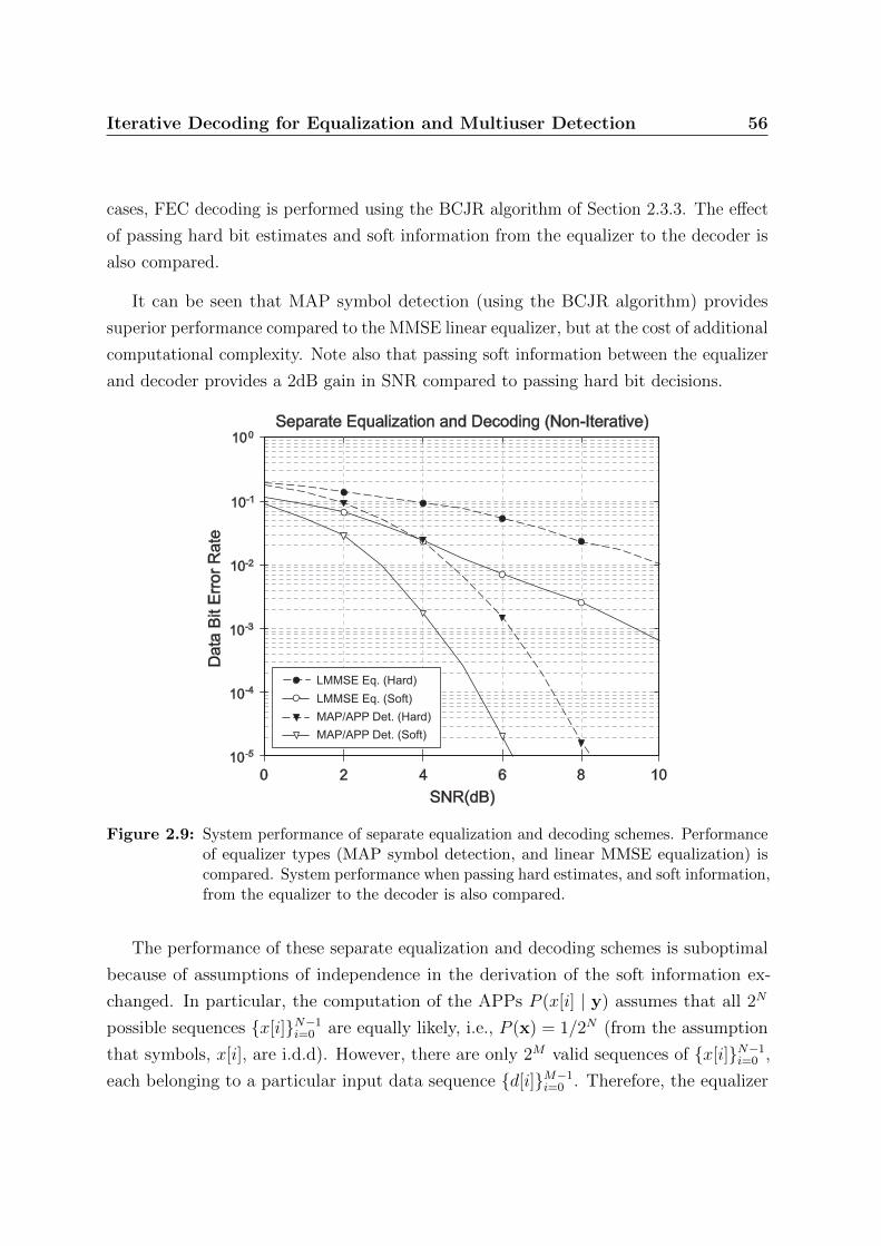
Iterative Decoding for Equalization and Multiuser Detection 56
cases, FEC decoding is performed using the BCJR algorithm of Section 2.3.3. The effect
of passing hard bit estimates and soft information from the equalizer to the decoder is
also compared.
It can be seen that MAP symbol detection (using the BCJR algorithm) provides
superior performance compared to the MMSE linear equalizer, but at the cost of additional
computational complexity. Note also that passing soft information between the equalizer
and decoder provides a 2dB gain in SNR compared to passing hard bit decisions.
SNR(dB)
Da
ta B
it E
rro
r R
ate
0 4 8 102 6
10-5
10-3
10-2
10-1
100
10-4
Separate Equalization and Decoding (Non-Iterative)
LMMSE Eq. (Hard)
LMMSE Eq. (Soft)
MAP/APP Det. (Hard)
MAP/APP Det. (Soft)
Figure 2.9: System performance of separate equalization and decoding schemes. Performanceof equalizer types (MAP symbol detection, and linear MMSE equalization) iscompared. System performance when passing hard estimates, and soft information,from the equalizer to the decoder is also compared.
The performance of these separate equalization and decoding schemes is suboptimal
because of assumptions of independence in the derivation of the soft information ex-
changed. In particular, the computation of the APPs P (x[i] | y) assumes that all 2N
possible sequences x[i]N−1i=0 are equally likely, i.e., P (x) = 1/2N (from the assumption
that symbols, x[i], are i.d.d). However, there are only 2M valid sequences of x[i]N−1i=0 ,
each belonging to a particular input data sequence d[i]M−1i=0 . Therefore, the equalizer

Iterative Decoding for Equalization and Multiuser Detection 57
performance would be significantly improved if the APPs were computed as
P (x[i] = x | y) =∑
all 2M valid x:x[i]=x
p(y | x)P (x)
p(y), (2.83)
where P (x) = 1/2M for valid x. However, this approach would require exhaustive search
methods, since trellis-based methods (such as the BCJR algorithm) could no longer be
used, and the resulting computational complexity would be prohibitive.
2.4 Turbo Equalization for ISI Channels
The MAP symbol detector computes symbol estimates using the MAP rule
x[i] = arg maxx∈+1,−1
P (x[i] = x | y), i = 0, 1, . . . , N − 1, (2.84)
where, using Bayes’ rule, the a posteriori probabilities can be computed from
P (x[i] = x | y) =∑
x:x[i]=x
p(y | x)P (x), x ∈ +1,−1. (2.85)
Here p(y | x) is the likelihood function and P (x) is the a priori probability. Note that
the marginal probability, p(y), does not have to be included in this form of the equation.
Hence, MAP detection can be thought of as a process that takes a series of observations,
y, and bit-wise a priori probabilities, P (x[i])i, and computes bit-wise a posteriori
probabilities, P (x[i] | y)i, as shown in the block diagram model in Figure 2.10.
MAP Detector
a posterioriprobabilities
a prioriprobabilities
observations
y
P( | )x y
P( )x
LikelihoodCalculation
PosteriorCalculation
P( | )y x
Figure 2.10: The MAP detection process in block diagram form, which takes a priori prob-abilities and observations as input and produces a posteriori probabilities asoutput

Iterative Decoding for Equalization and Multiuser Detection 58
In the BCJR equalization algorithm of Section 2.3.1, the a posteriori probabilities
are formed from the transition probabilities, γi(Sr, Ss), computed from (2.56), i.e.,
γi(Sr, Ss) = P (x[i] = xr,s)p(y[i] | v[i] = vr,s) (2.86)
where:
• p(y[i] | v[i] = vr,s) is the likelihood function, and can be interpreted as “local”
evidence about which branch in the trellis was traversed; and
• P (x[i] = xr,s) is the a priori information, which accounts for any prior knowledge
about the probability of trellis branch being traversed.
In the separate equalization and decoding strategy of Section 2.3, the equalizer does not
have any a priori information available, the symbols are assumed to be i.d.d (P (x[i] =
+1) = P (x[i]) = −1) = 1/2), and the transition probabilities, γi(Sr, Ss), are computed
solely from the observed data y[i]. However, the performance of the BCJR algorithm
can be greatly improved if good a priori information is available. In turbo equalization,
the a posteriori probabilities from the MAP FEC decoder are fed back and used as a
priori information by the MAP equalizer. This is performed in an iterative process where
the symbol and data bit estimates become more accurate as the quality of the a priori
information improves over a number of iterations.
MAPEqualizer
channeloutput
y[i]
MAPFEC
Decoder
extrinsicinformation
extrinsicinformation
a priori probabilities(intrinsic information)
a priori probabilities(intrinsic information)
(code bit)a posterioriprobabilities
a posterioriprobabilities
Deinterleaver
Interleaver
-1
L1(b[i]|y) l1(b[i]|y)
l2(b[i]|p)
l1(c[i]|y)
l2(c[i]|p)
L2(d[i]|p)
L2(c[i]|p)
harddecision
d[i]^
data bitestimates
(data bit)a posterioriprobabilities
Figure 2.11: Block diagram of a turbo equalization receiver.
When designing the feedback loop structure, it is important to consider the effect that
soft information generated from one bit in one of the constituent algorithms (equalizer
or decoder) will have on the other bits in the other constituent algorithm.
Iterative Decoding for Equalization and Multiuser Detection 59
When processing soft information input to the equalizer or the decoder, it is assumed
that the soft information about each bit (or channel symbol) is independent. This
assumption reduces the complexity of the equalizer and decoder algorithms. However, if
the decoder formulates its soft information about a given bit, based on soft information
provided to it from the equalizer about exactly the same bit, then the equalizer cannot
consider this information to be independent of its channel observations. In effect, this
would create a feedback loop in the overall process of length two: the equalizer informs
the decoder about a given bit; and then the decoder simply reiterates to the equalizer
what it already knows.
To avoid short cycles in the feedback, local minima, and limit cycle behavior in
the iterative process, when soft information is passed between constituent algorithms,
such information is never formed based on the information passed into the algorithm
concerning the same bit. Essentially, this amounts to the equalizer only telling the
decoder new information about a given bit based on information it gathered from distant
parts of the received signal. Similarly, the decoder only tells the equalizer information it
gathered from distant parts of the encoded bit stream. This consideration leads to the
concept of extrinsic and intrinsic information [53].
For the optimal receiver in Section 2.2.2, it was shown (from (2.47)-(2.49)) that the
a posteriori LLR, Λ(d[i] | y), can be separated into extrinsic LLR, λ(d[i] | y), and the
intrinsic (a priori) LLR, λ(d[i]). Also, that λ(d[i] | y) does not depend on λ(d[i]). In the
case of the (BCJR) MAP equalization algorithm, the same functional relation can be
applied to the output a posteriori LLRs in order to separate the two contributions. That
is, the a posteriori LLRs, Λ(b[i] | y), can be split into:
• extrinsic information, λ(b[i] | y) = Λ(b[i] | y)− λ(b[i]); and
• intrinsic information, λ(b[i]).
It is essential to the performance of turbo decoding algorithms that only extrinsic
information is passed between the constituent decoders.
The block diagram of a turbo equalization receiver is shown in Figure 2.11. The two
MAP algorithms form the core of the turbo equalizer. The MAP equalizer operates on
channel observations and a priori information about individual bits, while the MAP
FEC decoder operates on a priori information only. (In Figure 2.11, the observation
input of the MAP decoder is grounded to indicate that it is not used). Only the extrinsic
information is fed back in the iterative loop.

Iterative Decoding for Equalization and Multiuser Detection 60
1. Turbo equalizer inputs:
a) observation sequence, y = [ y[0], y[1], . . . , y[N − 1] ]T
b) channel coefficients, h0, h1, . . . , hL
2. Initialization: initialize the MAP equalizer a priori information to all
zeros, i.e., λ2(b | p) = [ 0N × 1 ]
3. Recursively compute (for a predetermined number of iterations):
Λ1(b | y) = MAP Equalizer( λ2(b | p) )
λ1(b | y) = Λ1(b | y)− λ2(b | p)
λ1(c | y) = Deinterleaver( λ1(b | y))
Λ2(c | p) = MAP FEC Decoder( λ1(c | y) )
λ2(c | p) = Λ2(c | p)− λ1(c | y)
λ2(b | p) = Interleaver( λ2(c | p) )
4. Turbo equalizer output: compute the data bit estimates, d[i], from the
probabilities, Λ2(d[i] | y), using:
d[i] = sgn (Λ2(d[i] | y)) , i = 0, 1, . . . ,M − 1
Table 2.3: Turbo equalization algorithm
The interleaver and deinterleaver are incorporated into the iterative loop to further
disperse the direct feedback effect. In particular, the BCJR algorithm creates output
that is locally highly-correlated, but the use of an interleaver can largely suppress the
correlations between neighboring symbols.
The operation of the turbo equalization receiver is shown in Table 2.3. The notation:
Λ1(b | y) = MAP Equalizer(λ2(b | p))
represents the generation of APP LLRs, Λ1(b | y), by the MAP Equalizer from observa-
tions, y, and a priori LLRs, λ2(b | p), using the BCJR algorithm described in Table 2.1.

Iterative Decoding for Equalization and Multiuser Detection 61
Similarly, the notation:
Λ2(c | p) = MAP FEC Decoder(λ1(c | y))
represents the generation of APP LLRs, Λ1(b | y), by the MAP FEC Decoder from the
a priori LLRs, λ2(c | y), using the BCJR algorithm described in Table 2.2.
While the turbo equalization algorithm presented is based on two MAP algorithms,
any pair of equalization and FEC decoding algorithms that make use of soft information
can be used as constituent algorithms in the turbo equalizer.
For example, the linear MMSE equalizer in Section 2.3.2 can use a priori information
about the transmitted symbol x[i] to compute symbol statistics Ex[i] and Varx[i](using (2.71)-(2.72)) which are then incorporated into the MMSE filter, (2.69)-(2.70),
to compute symbol estimate, x[i], and APP LLR, Λ1(x[i] | y). As with the MAP
equalization algorithm, the APP LLR is computed the constraint that Λ1(x[i] | y) is not
a function of the a priori LLR, λ2(b[i] | p), at the same index i. This helps to avoid short
feedback cycles, and is equivalent to extracting only the extrinsic part of the information
in the iterative scheme [53]. Note also that there are several low-complexity alternatives
for re-estimating x[i], e.g. [53], [121], [122], [33], [120], [98], [139].
Figure 2.12 shows the performance of the turbo equalization scheme (of Figure 2.11
and Table 2.3) for the ISI channel model of Figure 2.5. The scheme is evaluated for an
input data block length (M) of 512 bits with forward error correction performed by the
rate-1/2 convolutional encoder of Figure 2.1b, resulting in a coded block length (N) of
1024 bits. The coded bits are scrambled using a random interleaver and mapped onto
BPSK symbols.
Figure 2.12a shows the effect of receiver iterations for a turbo equalizer using the
MAP symbol detector of Section 2.3.1, while Figure 2.12b shows the effect of receiver
iterations for a turbo equalizer using the MMSE linear equalizer of Section 2.3.2. In both
cases, FEC decoding is performed using the BCJR algorithm of Section 2.3.3. Note that
zero-iterations represents the first pass when there is no a-priori information available
for APP equalizer–this is equivalent to the separate equalization and decoding scheme
(with soft information) evaluated in Section 2.3.4. The ISI-free bound represents the
lower BER performance bound of the underlying rate-1/2 code used over an ISI-free
channel, i.e., the performance bound for the evaluated system.

Iterative Decoding for Equalization and Multiuser Detection 62
Turbo Equalization using MAP Symbol Detection
SNR (dB)
-2 0 2 4 6
Bit E
rro
r R
ate
10-5
10-3
10-2
10-1
100
10-4
ISI-Free Bound
0 Iterations
1 Iteration
2 Iterations
10 Iterations
(a) Performance of turbo equalization using MAP symbol detection
SNR (dB)
-2 0 2 4 6
Bit E
rror
Rate
10-5
10-3
10-2
10-1
100
10-4
Turbo Equalization using Linear MSSE Equalizer
ISI-Free Bound
0 Iterations
1 Iteration
2 Iterations
10 Iterations
(b) Performance of turbo equalization using linear MMSE equalization
Figure 2.12: Performance of turbo equalization after 0, 1, 2, and 10 iterations using: (a)MAP symbol detection; and (b) linear MMSE equalization.
Iterative Decoding for Equalization and Multiuser Detection 63
Both schemes show significant BER performance gain over the iterations, with
performance approaching the ISI-free bound after 10 iterations. It is observed that turbo
equalization using MAP symbol detection provides superior performance compared to
the MMSE linear equalizer based scheme, but at the cost of additional computational
complexity. However, it is noted that for larger block lengths, M , the performance of
linear MMSE equalizer approaches that of the MAP detector [53], [121].
2.5 Code Division Multiple Access (CDMA) and
Multiuser Detection
For multiuser communications, CDMA is an attractive multiple-access technique that
has become widely used. Using the direct sequence spread-spectrum technique, each user
spreads its signal over the entire bandwith, such that when demodulating any particular
user’s data, the other users’ signals appear as pseudo white noise. A CDMA systems
are interference limited, meaning that multiple-access interference and intersymbol
interference (ISI) limit the system performance [127].
Multiuser detection (MUD) is the detection of data from multiple terminals in a
communication network when observed in a nonorthogonal multiplex, that is, when
derived from a nonorthogonal multiple-access channel. This situation may be the result
of system design, for example, in code-division multiple-access (CDMA) systems using
nonorthogonal spreading codes. It may also be the result of channel impairments in
orthogonally multiplexed systems, for example, in time-division multiple-access (TDMA)
wireless systems transmitting over multipath-fading delay-spread channels. Another
example is digital subscriber line (DSL) systems that are impaired by crosstalk and other
types of interference.
The fundamental concept of MUD is to make use of the known structure of all the
users’ transmitted signals, and the cross-correlations among these signals, in order to
improve the data detection process. Research has shown that the use of MUD can provide
significant performance advantages in interference-limited channels, and many advances
have been made in recent years [127], [134], [88], [102].
Optimal MUD techniques, based on maximum-likelihood (ML) or maximum a posteri-
ori probability (MAP) criteria, often achieve performance close to that of an interference-
free system. hat is free of interference. However, these methods have high computational
Iterative Decoding for Equalization and Multiuser Detection 64
complexity, particularly when compared with the processing resources available in most
communications receivers. As a result, considerably effort has been made to develop sub-
optimal low-complexity techniques that can achieve good performance. Linear multiuser
detection is a popular low-complexity technique that uses linear processing to suppress
interference, followed by simple quantization to perform data detection.
The computational complexity of optimal MUD techniques is further increased when
forward error correction (FEC) is considered in addition to nonorthogonal signaling.
In particular, the complexity of joint MUD and FEC decoding (based on ML or MAP
criteria) is prohibitively high. However, this combination can be considered as a serially
concatenated coding system, where the FEC code and multiple-access channel take the
roles of outer code and inner code, respectively [102]. This interpretation, provides the
basis for iterative MUD techniques to be developed using the turbo decoding concept
[12]. In these techniques, which are commonly known as turbo MUD [134], [88], the MUD
is used to provide tentative channel-symbol decisions to the FEC channel decoders, and
similarly, tentative channel-symbol decisions are produced by the channel decoders which
are fed back to the MUD. Several iterations between these two constituent processes
are made, with intermediate exchanges of soft channel symbol information. These turbo
MUD techniques have modest computational complexity, yet have been shown to provide
near-optimal performance.
2.5.1 Synchronous CDMA Signal Model
In CDMA systems, multiple users can share a common frequency band at the same time
by using different signature waveforms. Consider a CDMA channel that is shared by by
K simultaneous users. For simplicity, it is assumed that binary antipodal (BPSK) signals
are used to transmit the information from each user. The received signal, y(t), will
consist of the sum of antipodally modulated synchronous signature waveforms embedded
in additive white Gaussian noise:
y(t) =K∑k=1
Akbksk(t) + n(t), t ∈ [ 0, T ] (2.87)
where
• T is the symbol interval
• sk(t) is the deterministic signature waveform assigned to the k-th user.
Iterative Decoding for Equalization and Multiuser Detection 65
• Ak is the received amplitude of the k-th user’s signal. A2k is referred to as the energy
of the k-th user.
• bk is the bit transmitted by the k-th user, bk ∈ −1,+1
• n(t) is a zero-mean white Gaussian noise (AWGN) process with power spectral
density σ2. This models noise sources that are unrelated to the transmitted signal,
including thermal noise.
Each user is assigned a signature waveform sk(t) of duration T . A signature waveform
may be expressed as
sk(t) =L−1∑n=0
ak(n)pc(t− nTc), t ∈ [ 0, T ] (2.88)
where ak(n), 0 ≤ n ≤ L− 1 is a pseudo-noise (PN) code sequence consisting of L chips
that take values ± 1, pc(t) is a pulse of duration Tc, and Tc is the chip interval. Thus,
there are L chips per symbol and T = LTc. The signature waveforms are assumed to
be zero outside the interval [0, T ], and therefore, there is no intersymbol interference.
Additionally, it is also assumed that all K signature waveforms have unit energy, i.e.,
‖sk‖2 =
∫ T
0
s2k(t) dt = 1 (2.89)
The performance of various demodulation strategies depends on the signal-to-noise
ratios, Ak/σ, and on the similarity between the signature waveforms, quantified by their
cross-correlations, which for the synchronous case is defined as
ρij = ρij(0) =
∫ T
0
si(t)sj(t) dt. (2.90)
for the synchronous case.
2.5.2 Asynchronous CDMA Signal Model
In the synchronous model, bit epochs are aligned at the receiver. However, symbol-
synchronism is not necessary for CDMA to operate, and it is possible to let the users
transmit completely asynchronously. The asynchronous CDMA model is shown in
Figure 2.13 where time offsets are introduced to model the lack of alignment of the bit
epochs at the receiver: τk ∈ [0, T ), k = 1, . . . , K. The symbol epochs are defined with

Iterative Decoding for Equalization and Multiuser Detection 66
User 1
AWGN
s1(t)
y(t)S
b [i]1
s2(t)
b [i]2
s3(t)
b [i]3
n(t)
Delayt1
Delayt2
Delayt3
A1
A2
A3
User 2
User 3
x3(t)
x2(t)
x1(t)
Multiple Access Channel
(a) Asynchronous CDMA channel model for 3 users (K = 3)
T
User 2
User 1 ( =0)t1
User 3
b [0]1 b [1]1 b [2]1
b [0]2 b [1]2 b [2]2
b [0]3 b [1]3 b [2]3
2T 3T0 t2 t3 T+t2 T+t3time
(b) Asynchronism modelling using time offsets. Bit epochs for 3 users (K = 3)
Figure 2.13: Asynchronous CDMA channel model and asynchronism modelling using timeoffsets for 3 users (K = 3)
respect to an arbitrary origin (it is often advantageous to take τ1 = 0). Without loss of
generality, we assume that 0 ≤ τ1 ≤ τ2 ≤ · · · ≤ τK < T . Note that we still require the
symbol interval be identical for all users.
For the synchronous model it is sufficient to restrict attention to the received waveform
in an interval of length T , the bit duration. In the asynchronous case we must take into
account the fact that the users send a stream of bits. Without loss of generality, we
assume that all users transmit packets or frames of length N . Therefore the data block
for the k-th user is bk[i]N−1i=0 Generalising (2.87) to the asynchronous case, the CDMA

Iterative Decoding for Equalization and Multiuser Detection 67
channel model now becomes
y(t) =K∑k=1
Ak
N−1∑i=0
bk[i]sk(t− iT − τk) + σn(t), t ∈ [ 0, NT ], τk ∈ [ 0, T ) (2.91)
The synchronous channel corresponds to the special case of (2.91) where all the offsets
are identical, τk = 0 for 1 ≤ k ≤ K.
As with the synchronous channel, asynchronous channel performance depends on
the cross-correlation between the user signature waveforms. However for asynchronous
CDMA, the synchronous cross-correlation definition of (2.90) is not sufficient to determine
the performance, and two cross-correlations between every pair of signature waveforms
must be defined, as shown in Figure 2.14. Note that τ = |τk − τj|.
0 time
User j
User k
rjk( )t rjk( )t
t
sk(t-tk)sk(t+T-tk)
(0)
sj(t+T- )tj
tk T+tk
rjk( )t
sj(t-tj)
(1)
tj T T+tj
(0)
(a) τj < τk case
time
User k
User j
rjk( )t rjk( )t
t
sj(t-tj) sk(t-T-tj)
(0)
sk(t-T- )tk
tj T+tj
rjk( )t
sk(t-tk)
(-1)
tk T T+tk
(0)
2T+tk2T
(b) τj > τk case
Figure 2.14: Definition of asynchronous cross correlations (0 ≤ τj , τk < T )
For the case where τj < τk, the cross-correlations are defined as:
ρ(0)jk (τ) =
∫ T+τj
τk
sj(t− τj)sk(t− τk) dt (2.92)
ρ(+1)jk (τ) =
∫ τk
τj
sj(t− τj)sk(t+ T − τk) dt (2.93)
and ρ(−1)jk (τ) = 0. For the case where τj > τk, the cross-correlations are defined as:
ρ(−1)kj (τ) =
∫ T+τj
T+τk
sj(t− τj)sk(t− T − τk) dt (2.94)
ρ(0)jk (τ) =
∫ T+τk
τj
sj(t− τj)sk(t− τk) dt (2.95)
and ρ(+1)jk (τ) = 0. Note that the length of the integration interval is τ for ρ
(+1)jk (τ) or
ρ(−1)kj (τ) and T − τ for ρ
(0)jk (τ).

Iterative Decoding for Equalization and Multiuser Detection 68
2.5.3 Single-User Matched Filter Detector
The simplest approach to demodulate CDMA signals is the single-user matched filter
(MF). This is the demodulator that was first adopted in CDMA receivers, and is often
called the conventional detector. The matched filter is the optimal receiver for both
the single-user CDMA channel and the multiuser orthogonal CDMA channel. However
for the multiuser non-orthogonal CDMA channel, the performance of the matched
filter is degraded by multiple-access interference (interference from other users) and is
sub-optimal.
y [i]1
y [i]2
y [i]K
y(t)
Matched Filter
Sync 1
User 2
Sync 2
User K
Sync K
b [i]1
b [i]2
b [i]K
òy(t)s (t)dtK
òy(t)s (t)dt1
User 1
Matched Filter
òy(t)s (t)dt2
Matched Filter
Figure 2.15: Bank of single-user matched filters
In the conventional single-user detection, the receiver for each user consist of a
demodulator that correlates (or match filters) the received signal with the signature
sequence of the user and passes the correlator output to the detector, which makes a
decision based on the single correlator output. Thus, the conventional detector neglects
the presence of the other users of the channel or, equivalently, assumes that the aggregate
noise plus interference is white and Gaussian.
For the case of synchronous transmission, the output of the correlator for the k-th
user for the signal in i-th code bit interval, i.e., iT ≤ t ≤ (i+ 1)T is
yk ,∫ (i+1)T
iT
y(t)sk(t− iT ) dt (2.96)
= Akbk[i] +K∑j=1j 6=k
Ajρjk(0)bj[i] + nk[i] (2.97)

Iterative Decoding for Equalization and Multiuser Detection 69
where the noise component nk[i] is given as
nk[i] ,∫ (i+1)T
iT
n(t)sk(t) dt (2.98)
If the signature sequences are orthogonal, the interference from the other users given by
the middle term in (2.97) vanishes and the conventional single-user detector is optimum.
On the other hand, if one or more of the other signature sequences are not orthogonal
to the k-th user signature sequence, the interference from the other users can become
excessive if the power levels of one or more of the other users is sufficiently larger that
the power level of the k-th user. This situation is generally called the near-far problem in
multiuser communications, and necessitates some form of power control for conventional
detection.
For synchronous transmission, (2.97) can also be expressed in discrete-time matrix
form:
y[i] = RAb[i] + n[i] (2.99)
where
y[i] = [ y1[i], y2[i], . . . , yK [i] ]T (K × 1 vector) (2.100)
A = diagA1, A2, . . . , AK (K ×K matrix) (2.101)
b[i] = [ b1[i], b2[i], . . . , bK [i] ]T (K × 1 vector) (2.102)
n[i] = [n1[i], n2[i], . . . , nK [i] ]T (K × 1 vector) (2.103)
and R is the K ×K cross-correlation matrix, defined as
Rj,k = ρjk ,∫ T
0
sj(t)sk(t) dt (2.104)
The diagonal elements of R are the autocorrelation factors, ρjj, and are equal to 1. For
the synchronous case, R is symmetric and the cross-correlation factors have the feature:
ρjk = ρkj.
In asynchronous transmission, the conventional detector is more vulnerable to interfer-
ence from other users. This is because it is not possible to design signature sequences for
any pair of users that are orthogonal for all time offsets. Consequently, interference from
other users is unavoidable in asynchronous transmission with the conventional single-user
Iterative Decoding for Equalization and Multiuser Detection 70
detection. In such a case, the near-far problem resulting from unequal power in the
signals transmitted by the various users is particularly serious. The practical solution
generally requires a power adjustment method that is controlled by the receiver via a
separate communications channel that all users are continuously monitoring. Another
option is to employ one of the multiuser detectors described in the following sections.
2.6 The Optimum Multiuser Receiver
The optimum receiver is defined as the receiver that selects the most probable sequence
of bits bk[i], 0 ≤ i ≤ N − 1, 1 ≤ k ≤ K given the received signal y(t) observed over
the time interval 0 ≤ t ≤ NT for synchronous transmission, or 0 ≤ t ≤ NT + 2T for
asynchronous transmission.
2.6.1 Synchronous Transmission
In synchronous transmission, each (user) interferer produces exactly one symbol which
interferes with the desired symbol. In additive white Gaussian noise, it is sufficient to
consider the signal received in one signal interval, iT ≤ t ≤ (i+ 1)T , and determine the
optimum receiver. Hence y(t) may be expressed as
y(t) =K∑k=1
Akbk[i]sk(t) + n(t), t ∈ [ iT, (i+ 1)T ]. (2.105)
The optimum maximum-likelihood receiver computes the likelihood function, L(b[i]),
for all 2K possible combinations of information sequence b[i] = [b1[i], b2[i], . . . , bK [i]]T ,
and then selects the sequence of b[i] that maximises L(b[i]). For synchronous CDMA,
L(b[i]) = f(y(t) | b[i]), and [127]
f(y(t) | b[i]) = exp
− 1
2σ2
∫ (i+1)T
iT
[ y(t)− x(t; b[i]) ]2 dt
, t ∈ [ iT, (i+ 1)T ]
(2.106)

Iterative Decoding for Equalization and Multiuser Detection 71
where
x(t; b[i]) =K∑k=1
bk[i]Aksk(t), t ∈ [ iT, (i+ 1)T ] (2.107)
Equivalently, the most likely b[i] also maximises [127]
Ω(b[i]) = 2
∫ (i+1)T
iT
[K∑k=1
Akbk[i]sk(t)
]y(t) dt−
∫ (i+1)T
iT
[K∑k=1
Akbk[i]sk(t)
]2
dt
= 2bT [i]Ay[i]− bT [i]ARAb[i] (2.108)
The expression (2.108) shows that the dependence of the likelihood function of the
received signals is through the vector of matched filter outputs y[i], which is therefore a
sufficient statistic for demodulating the transmitted data.
There are 2K possible choices of the bits in the information sequences of the K users.
The optimum detector computes the correlation metrics for each sequence and selects
the sequence that yields the largest correlation metric. Therefore the optimum detector
has a complexity that grows exponentially with the number of users K.
2.6.2 Asynchronous Transmission
In this case, there are exactly two consecutive symbols from each interferer that overlap a
desired symbol. We assume that the receiver knows the received signal energies A2k for
the K users and the transmission delays τk. We view the K-user N -frame asynchronous
channel as a (K ×N)-user asynchronous channel. Let us define bn, a KN -vector, with
components
bn =[bT [0], bT [1], . . . , bT [N − 1]
]T(KN × 1 vector) (2.109)
and the KN -vector of matched-filter outputs yn,
yn =[yT [0], yT [1], . . . , yT [N − 1]
]T(KN × 1 vector) (2.110)
Iterative Decoding for Equalization and Multiuser Detection 72
where y[i] = [ y1[i], y2[i], . . . , yK [i] ]T with components
yk[i] ,∫ (i+1)T+τk
iT+τk
y(t)sk(t− iT − τk) dt 0 ≤ i ≤ N − 1 (2.111)
The integral (2.111) represents the outputs of the correlator or matched filter for the
k-th user in each of the signal intervals. This means that the yk[i] is the output of the
k-th matched filter applied to the signal in the interval [τk + iT, τk + (i+ 1)T ], that is,
the interval corresponding to bk[i].
Using vector notation, the K ×N correlator or matched filter outputs yk[i] can be
expressed in the form
yn = RnAnbn + nn (2.112)
with the following vector and matrix definitions: Rn is the asynchronous cross-correlation
matrix,
Rn =
R(0) R(−1) 0 0 · · · 0
R(1) R(0) R(−1) 0 · · · 0
0. . . . . .
......
. . . . . . 0
0 · · · 0 R(1) R(0) R(−1)
0 · · · 0 0 R(1) R(0)
(KN ×KN matrix) (2.113)
where R(−1), R(0), and R(1) are K ×K matrices with elements
R(−1)j,k = ρ(−1)jk (τ), R(0)j,k = ρ
(0)jk (τ), and R(1)j,k = ρ
(1)jk (τ).
Note that the asynchronous cross-correlations, ρ(−1)jk (τ), ρ
(0)jk (τ), and ρ
(1)jk (τ), are defined
in (2.92)-(2.95). An is the diagonal matrix,
An =
A 0 · · · 0
0 A 0...
.... . .
...
0 0 · · · A
(KN ×KN matrix) (2.114)
Iterative Decoding for Equalization and Multiuser Detection 73
where A is the K ×K diagonal matrix defined in (2.101), and nN is the vector,
nn =[nT [0], nT [1], · · · , nT [N − 1]
]T(KN × 1 vector) (2.115)
For the asynchronous case, the maximum-likelihood receiver computes the likelihood
function L(bn) for all 2KN possible combinations of bn, and then selects the sequence
bn that maximises L(bn). For this case, L(bn) = f(y(t) | bn), and [127]
f(y(t) | bn) = exp
− 1
2σ2
∫ NT+2T
0
[ y(t)− x(t; bn) ]2 dt
, t ∈ [0, NT + 2T ] (2.116)
where
x(t; bn) =K∑k=1
N−1∑i=0
bk[i]Aksk(t− iT − τk), t ∈ [0, NT + 2T ]. (2.117)
Equivalently, the most likely bn also maximises [127]
Ω(bn) = 2
∫ NT+2T
0
x(t; bn)y(t) dt−∫ NT+2T
0
(x(t; bn) )2 dt
= 2bTnAnyn − bTnAnRnAnbn. (2.118)
Once more, the observations enter in the function to be maximised by jointly optimum
decisions on through the matched filter outputs. Therefore, yn is a sufficient statistic for
bn. The vector yn given by (2.112) constitutes a set of sufficient statistics for estimating
the transmitted bits bk[i].
If we adopt a block processing approach, the optimum ML detector must compute
2KN likelihood functions and select the K sequences of length N that corresponds to the
greatest likelihood value. Clearly such an approach is much too complex computationally
to be implemented in practice, especially when K and N are large. An alterative approach
is ML sequence estimation employing the Viterbi algorithm. In order to construct a
sequential-type detector, we make use of the fact that each transmitted symbol overlaps
at most with 2K − 2 symbols. Thus, a significant reduction in computational complexity
is obtained with respect to the block-size parameter N , but the exponential dependence
on K cannot be reduced. It is apparent that the optimum ML receiver employing the
Viterbi algorithm also involves such a high computational complexity that its practical

Iterative Decoding for Equalization and Multiuser Detection 74
use is limited. In the following sections, a number of suboptimum detectors whose
complexity grows linearly with K are considered.
2.7 Linear Multiuser Detectors
The matched filter (conventional detector) has a complexity that grows linearly with the
number of users, K. But susceptibility to MAI from non-orthogonal users means that the
matched filter may make errors even in the absence of noise. In contrast, the optimum
receiver demodulates the data error-free in the absence of noise, but has a computational
complexity that grows exponentially with the number of users, K. In this section, we
consider linear multiuser detectors with computational complexities that grow linearly
with K, but do not exhibit vulnerability to interference from other users.
2.7.1 Decorrelating Detector
Firstly, the case of symbol-synchronous transmission is considered. In this case, the
output of the K matched filters in the i-th code bit interval is represented by the received
signal vector, y[i], given by
y[i] = RAb[i] + n[i] (2.119)
where R, A, b[i], and n[i] are defined in (2.104), (2.101), (2.102), and (2.103), respectively.
Noise vector n[i] has a covariance
En[i]nT [i] = σ2R. (2.120)
Since the noise is Gaussian, y[i] is described by a K-dimensional Gaussian PDF with
mean RAb[i] and covariance R. That is [93],
p(y[i] | b[i]) =1√
(2πσ2)K det Rexp
− 1
2σ2(y[i]−RAb[i])TR−1(y[i]−RAb[i])
(2.121)

Iterative Decoding for Equalization and Multiuser Detection 75
The best linear estimate of b[i], denoted by b0[i], is defined as the value of b[i] that
minimises the likelihood function
L(b[i]) = (y[i]−RAb[i])TR−1(y[i]−RAb[i]), (2.122)
and hence [69],
b0[i] = arg minb[i]
(y[i]−RAb[i])TR−1(y[i]−RAb[i]). (2.123)
The result of this minimisation yields
b0[i] = A−1R−1y[i], (2.124)
and the ML estimates of the detected symbols, bk[i], is given by
bk[i] = sgn
(1
Ak
R−1y[i]
k
)= sgn
( R−1y[i]
k
)for k = 1, . . . , K. (2.125)
Note that the estimate b0[i] is also the best linear estimate that maximises the likelihood
function given by (2.108). Since y[i] = RAb[i] + n[i], it follows from (2.124) that [69]
b0[i] = b[i] + A−1R−1n[i] (2.126)
Therefore, b0[i] is an unbiased estimate of b. The transformation R−1 has eliminated the
interference components between the users, and as a consequence, the near-far problem is
also eliminated. The decorrelating detector is so-called because the linear transformation
R−1 is used to tune out or decorrelate the multiuser interference. Figure 2.16 illustrates
the receiver structure. The symbol estimates bk[i] are obtained by performing the linear
transformation R−1 on the vector of matched filter outputs y[i], and therefore, the
computational complexity is linear in K.
In asynchronous transmission, the received signal at the output of the matched filters
is given by (2.112). The best linear estimate of bn, denoted by b0n, is the value of bn
that minimises the likelihood function [93]
L(bn) = (yn −RnAnbn)TR−1n (yn −RnAnbn) (2.127)
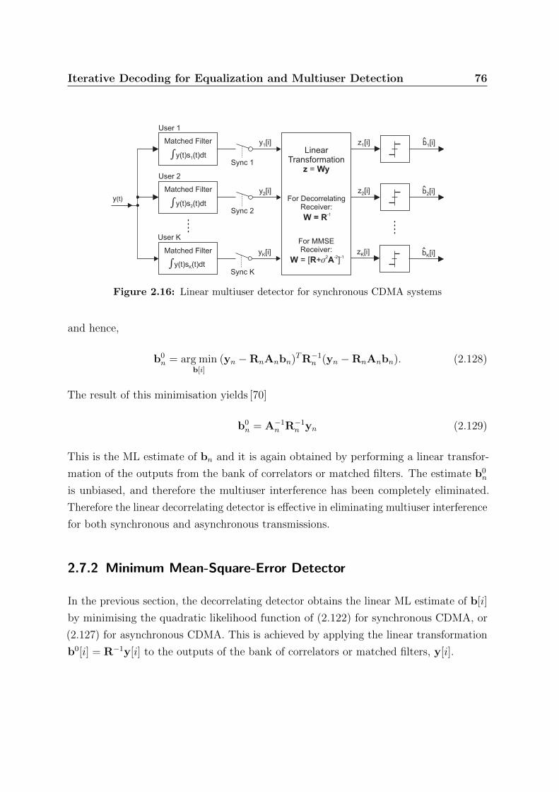
Iterative Decoding for Equalization and Multiuser Detection 76
W R A= [ + ]s2 -2 -1
W = R-1
LinearTransformation
=z Wy
For DecorrelatingReceiver:
For MMSEReceiver:
z [i]1
z [i]2
z [i]K
y [i]1
y [i]2
y [i]K
y(t)
Matched Filter
Sync 1
User 2
Sync 2
User K
Sync K
b [i]1
b [i]2
b [i]K
òy(t)s (t)dtK
òy(t)s (t)dt1
User 1
Matched Filter
òy(t)s (t)dt2
Matched Filter
Figure 2.16: Linear multiuser detector for synchronous CDMA systems
and hence,
b0n = arg min
b[i]
(yn −RnAnbn)TR−1n (yn −RnAnbn). (2.128)
The result of this minimisation yields [70]
b0n = A−1
n R−1n yn (2.129)
This is the ML estimate of bn and it is again obtained by performing a linear transfor-
mation of the outputs from the bank of correlators or matched filters. The estimate b0n
is unbiased, and therefore the multiuser interference has been completely eliminated.
Therefore the linear decorrelating detector is effective in eliminating multiuser interference
for both synchronous and asynchronous transmissions.
2.7.2 Minimum Mean-Square-Error Detector
In the previous section, the decorrelating detector obtains the linear ML estimate of b[i]
by minimising the quadratic likelihood function of (2.122) for synchronous CDMA, or
(2.127) for asynchronous CDMA. This is achieved by applying the linear transformation
b0[i] = R−1y[i] to the outputs of the bank of correlators or matched filters, y[i].
Iterative Decoding for Equalization and Multiuser Detection 77
Another approach is to seek the linear transformation b0[i] = Wy[i], where the
matrix W is to be determined so as to minimise the mean square error (MSE) [93]:
MSE(b[i]) = EA(b[i]− b0[i])TA(b[i]− b0[i])
= E
(Ab[i]−Wy[i])T (Ab[i]−Wy[i])
(2.130)
where the expectation is with respect to the data vector b[i] and the additive noise
n[i]. The optimum matrix W may be found by forcing the error (b[i]−Wy[i]) to be
orthogonal to the data vector y[i]. Thus
E
(Ab[i]−Wy[i])yT [i]
= 0
EAb[i]yT [i]
−WE
y[i]yT [i]
= 0 (2.131)
Consider the case of synchronous transmission. We have
EAb[i]yT [i] = EAb[i]AbT [i]RT = A2RT (2.132)
and
Ey[i]yT [i] = E
(RAb[i] + n[i])(RAb[i] + n[i])T
= RA2RT + σ2RT (2.133)
By substituting (2.132) and (2.133) into (2.131) and solving for W. We obtain
W =(R + σ2A−2
)−1(2.134)
Therefore, the minimum mean square error (MMSE) estimate of b[i] is [140] [73]
b0[i] = A−1(R + σ2A−2
)−1y[i] (2.135)
and the estimated symbols are obtained by
bk[i] = sgn
(1
Ak
(R + σ2A−2
)−1k
)= sgn
((R + σ2A−2
)−1k
)for k = 1, . . . , K (2.136)

Iterative Decoding for Equalization and Multiuser Detection 78
The MMSE criterion produces a biased estimate of b, hence there is some residual
multiuser interference. Note that in the high-SNR case when σ2 → 0, then
(R + σ2A−2
)−1 → R−1 (2.137)
and the MMSE solution approaches the ML solution in (2.129). In this case, the MMSE
detector becomes equivalent to the decorrelator detector. On the other hand, in the
low-SNR case when σ2A−2 R, then
(R + σ2A−2
)−1 → σ−2A2 (2.138)
and the detector essentially ignores the interference from other users because the additive
noise is the dominant term . In this case the MMSE detector becomes equivalent to
the matched filter detector with amplitude scaling to compensate for the received power
levels. Figure 2.16 illustrates the receiver structure for linear MMSE detector.
Similarly, for asynchronous transmission, the matrix W is chosen so as to minimise
the mean square error (MSE):
MSE(bn) = E
(Anbn −Wyn)T (Anbn −Wyn)
(2.139)
In this case, the optimum choice of W is
W =(Rn + σ2A−2
n
)−1(2.140)
and, hence the MMSE estimate of bn is [140] [73]
b0n = A−1
n
(Rn + σ2A−2
n
)−1yn (2.141)
The output of the MMSE detector is then bn = sgn(b0n).
2.8 Turbo Multiuser Detection for Synchronous CDMA
We consider a convolutionally coded synchronous real-valued CDMA system with K
users, employing normalised signature waveforms s1, s2, . . . , sK , and tranmitting through
an additive white Gaussian noise channel. The block diagram of the transmitter structure
for this system is shown in Figure 2.17. The binary data sequence dk[i]M−1i=0 for user
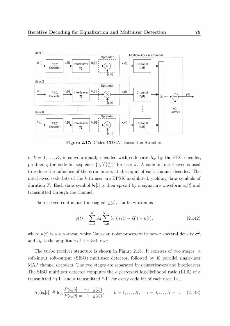
Iterative Decoding for Equalization and Multiuser Detection 79
AWGN
y(t)S
n(t)
Multiple Access Channel
FECEncoder
Interleaver
pChannel
h (t)1
Spreader
s1(t)
d [i]1 c [i]1 b [i]1
FECEncoder
Interleaver
pChannel
h (t)2
Spreader
s2(t)
d [i]2 c [i]2 b [i]2
FECEncoder
Interleaver
pChannel
h (t)K
Spreader
sK(t)
d [i]K c [i]K b [i]K
x (t)1
x (t)2
x (t)K
User 1
User 2
User K
Figure 2.17: Coded CDMA Transmitter Structure
k, k = 1, . . . , K, is convolutionally encoded with code rate Rc, by the FEC encoder,
producing the code-bit sequence ck[i]N−1i=0 for user k. A code-bit interleaver is used
to reduce the influence of the error bursts at the input of each channel decoder. The
interleaved code bits of the k-th user are BPSK modulated, yielding data symbols of
duration T . Each data symbol bk[i] is then spread by a signature waveform sk[t] and
transmitted through the channel.
The received continuous-time signal, y(t), can be written as
y(t) =K∑k=1
Ak
N−1∑i=0
bk[i]sk(t− iT ) + n(t), (2.142)
where n(t) is a zero-mean white Gaussian noise process with power spectral density σ2,
and Ak is the amplitude of the k-th user.
The turbo receiver structure is shown in Figure 2.18. It consists of two stages: a
soft-input soft-output (SISO) multiuser detector, followed by K parallel single-user
MAP channel decoders. The two stages are separated by deinterleavers and interleavers.
The SISO multiuser detector computes the a posteriori log-likelihood ratio (LLR) of a
transmitted “+1” and a transmitted “-1” for every code bit of each user, i.e.,
Λ1(bk[i]) , logP (bk[i] = +1 | y(t))
P (bk[i] = −1 | y(t)), k = 1, . . . , K, i = 0, . . . , N − 1. (2.143)

Iterative Decoding for Equalization and Multiuser Detection 80
Using Bayes’ rule, (2.143) can be rewritten as
Λ1(bk[i]) , logp(y(t) | bk[i] = +1)
p(y(t) | bk[i] = −1)︸ ︷︷ ︸λ1(bk[i])
+ logP (bk[i] = +1)
P (bk[i] = −1)︸ ︷︷ ︸λ2(bk[i])
, (2.144)
where the second term in (2.144), denoted by λ2(bk[i]), represents the a priori LLR of
the code bit bk[i], which is computed by the MAP channel decoder of the k-th user in
the previous iteration, interleaved and then fed back to the SISO multiuser detector. For
the first iteration, assuming equally likely code bits (i.e., no prior information available),
we then have λ2(bk[i]) = 0 for 1 ≤ k ≤ K and 0 ≤ i < N . The first term in (2.144),
denoted by λ1(bk[i]), represents the extrinsic information delivered by the SISO multiuser
detector based on the received signal y(t), the structure of the multiuser signal given by
(2.142), the prior information about the code bits of all the other users, λ2(bl[i])i; l 6=k,and the prior information about the code bits of the k-th user other than the i-th bit,
λ2(bk[j])j 6=i. The extrinsic information λ1(bk[i])i, of the k-th user, which is not
influenced by the a priori information λ2(bk[i])i provided by the MAP channel decoder,
is then reverse interleaved and fed into the k-th user’s channel decoder as the a priori
information in the next iteration.
SISOMultiuserDetector
Soft FECChannelDecoderInterleaver
Deinterleaver
user1
p-1
p
L1 1(b [i])
y(t)
l1 1(b [i])
l2 1(b [i])
Interleaver
Deinterleaver
p-1
p
L2 1(c [i])
L2 K(c [i])
l1 1(c [i])
l1 K(c [i])
l2 1(c [i])
l2 K(c [i])
Soft FECChannelDecoder
userK
L1 K(b [i]) l1 K(b [i])
l2 K(b [i])
d [i]1
d [i]K
Figure 2.18: Coded CDMA Turbo Multiuser Receiver Structure
Denote the code-bit sequence of the k-th user after deinterleaving as ck[i]i. Based
on the prior information λ1(ck[i])i and the trellis structure of the channel code (i.e.,
the constraints imposed by the code), the k-th user’s MAP channel decoder computes
Iterative Decoding for Equalization and Multiuser Detection 81
the a posteriori LLR of each code bit,
Λ2(ck[i]) , logP (ck[i] = +1 | λ1(ck[i])i ; code structure )
P (ck[i] = −1 | λ1(ck[i])i ; code structure )
= λ2(ck[i]) + λ1(ck[i]), (2.145)
for k = 1, . . . , K, and i = 0, . . . , N − 1. From (2.145), it can be seen that the output of
the MAP channel decoder is the sum of the prior information λ1(ck[i]) and the extrinsic
information λ2(ck[i]) delivered by the MAP channel decoder. This extrinsic information is
the information about the code bit ck[i] gathered from prior information about the other
code bits, λ1(ck[j])j 6=i, based on the trellis constraint of the code. The MAP channel
decoder also computes the a posteriori LLR of every information bit, which is used to
make a decision on the decoded bit at the last iteration. After interleaving, the extrinsic
information delivered by the K MAP channel decoders λ2(bk[i])i;k is then fed back to
the SISO multiuser detector, as the prior information about the code bits of all users, in
the next iteration. Note that at the first iteration, the extrinsic information quantities
λ1(bk[i])i;k and λ2(bk[i])i;k are statistically independent. But subsequently, since they
use the same information indirectly, they will become more and more correlated, which
will result in diminishing improvement through iteration.
2.8.1 Optimal SISO Multiuser Detector
For the synchronous CDMA system, a sufficient statistic for demodulating the i-th
code bits of the K users is given by the K-vector y[i] = [ y1[i], . . . , yK [i] ]T , whose k-th
component is the output of a filter matched to sk( · ) in the i-th code bit interval, i.e.,
(2.96). From Section 2.5.3, the sufficient statistic vector y[i] can be written as (2.99)
y[i] = RAb[i] + n[i], (2.146)
In what follows, the symbol index i is dropped whenever possible to simplify the
notation. Denote
B+k , (b1, . . . , bk−1,+1, bk+1, . . . , bK) : bj ∈ +1,−1 ,
B−k , (b1, . . . , bk−1,−1, bk+1, . . . , bK) : bj ∈ +1,−1 ,
Iterative Decoding for Equalization and Multiuser Detection 82
From (2.146), the extrinsic information λ1(bk) delivered by the SISO multiuser detector
is then given by [134]
λ1(bk) , logp(y | bk = +1)
p(y | bk = −1)
= log
∑b∈B+
k
exp
− 1
2σ2 (y −RAb)TR−1(y −RAb)∏
j 6=k P (bj)
∑b∈B−k
exp
− 1
2σ2 (y −RAb)TR−1(y −RAb)∏
j 6=k P (bj) (2.147)
where P (bj) , P (bj[i] = bj) for bj ∈ +1,−1. In (2.147), the summation in the
numerator is over all the 2K−1 possible vectors b in B+k . Similarly, the summation in the
denominator is over all the 2K−1 possible vectors b in B−k .
In (2.147), the a priori probabilities of the code bits, P (bj), can be expressed in terms
of their LLRs λ2(bj[i]), as follows.
P (bj) , P (bj[i] = bj) for bj ∈ +1,−1
=1
2
[1 + bj tanh
(λ2(bj[i])
2
)](2.148)
Substituting (2.148) into (2.147) and simplifying, we obtain [134]
λ1(bk[i]) =2Akyk[i]
σ2
+ log
∑b∈B+
k
exp
−12σ2 bTARAb
∏j 6=k
[1 + bj tanh
(Ajyj [i]
σ2
)] [1 + bj tanh
(λ2(bj [i])
2
)]∑
b∈B−k
exp
−12σ2 bTARAb
∏j 6=k
[1 + bj tanh
(Ajyj [i]
σ2
)] [1 + bj tanh
(λ2(bj [i])
2
)](2.149)
It can be seen from (2.149) that the extrinsic information λ1(bk[i]) at the output of the
SISO multiuser detector consists of two parts; the first term contains the channel value
of the desired user yk[i] and the second term is the information extracted from the other
users’ channel values yj[i]j 6=k as well as their prior information λ2(bj[i])j 6=k.
2.8.2 Low-Complexity SISO Multiuser Detector
From (2.149), it is clear that the computational complexity of the optimal SISO multiuser
detector is exponential in terms of the number of users K, which is prohibitive for
channels with moderate to large numbers of users. In this section, a low-complexity SISO

Iterative Decoding for Equalization and Multiuser Detection 83
multiuser detector based on a novel technique of combined soft interference cancelation
and linear MMSE filtering proposed by Wang and Poor [133] is presented. The structure
of this low-complexity multiuser detector is shown in Figure 2.19.
Extrin
sic
Info
rmatio
nC
om
puta
tion
Insta
nta
neous
MM
SE
Filte
ring
Soft In
terfe
rence
Cancella
tion
y (i)1 y1(i) z (i)1
y (i)K yK(i) z (i)K
l1 1(b (i))
l1 K(b (i))
y(t)
User 1
l2 1(b (i))
l2 K(b (i))
b (i)1
b (i)K
Com
puta
tion o
f Code
Bit S
oft E
stim
ate
s
òy(t)s (t)dtK
òy(t)s (t)dt1
matched filter
User K
matched filter
Figure 2.19: Low-complexity soft multiuser detector for synchronous CDMA
Soft Interference Cancellation and Instantaneous Linear MMSE Filtering
Based in the a priori LLR of the code bits of all users, λ2(bk[i])Kk=1, provided by the
MAP channel decoder from the previous iteration, we first form soft estimates of the
code bits of all the users (i.e., for k = 1, . . . , K) as
bk[i] , Ebk[i] =∑
b∈+1,−1
b P (bk[i] = b)
=∑
b∈+1,−1
b
2
[1 + b tanh
(λ2(bk[i])
2
)](2.150)
= tanh
(λ2(bk[i])
2
)(2.151)
where (2.150) follows from (2.148). Define
b[i] ,[b1[i], b2[i], . . . , bK [i]
]T(2.152)
bk[i] , b[i]− bk[i]ek
=[b1[i], . . . , bk−1[i], 0, bk+1[i], . . . , bK [i]
]T(2.153)
Iterative Decoding for Equalization and Multiuser Detection 84
where ek denotes a K-vector of all zeros, except for the k-th element, which is 1. Therefore,
bk[i] is obtained from b[i] by setting the the k-th element to zero. For each user, a soft
interference cancellation is performed on the matched filter output y[i] in (2.146), to
obtain
yk[i] , y[i]−RAbk[i]
= RA(b[i]− bk[i]
)+ n[i], k = 1, . . . , K (2.154)
Such a soft inference cancellation scheme was first proposed by Hagenauer [37]. Next,
in order to further suppress the residual interference in yk[i], an instantaneous linear
minimum mean-square error (MMSE) filter wk[i] is applied to yk[i] to obtain
zk[i] = wTk [i]yk[i] (2.155)
where the filter wk[i] ∈ RK is chosen to minimise the mean-square error between the
code bit and the filter output zk[i]:
wk[i] = arg minw∈RK
E(bk[i]−wTyk[i]
)2
= arg minw∈RK
wTEyk[i]y
Tk [i]
w − 2wTE bk[i]yk[i] (2.156)
where using (2.154), we have
Eyk[i]yTk [i] = RA Cov
b[i]− bk[i]
AR + σ2R (2.157)
and
Ebk[i]yk[i] = RA Ebk[i]
(b[i]− bk[i]
)= RAek (2.158)
Substituting (2.157) and (2.158) into (2.156), we have
wk[i] =(RVk[i]R + σ2R
)−1RAek
= AkR−1(Vk[i] + σ2R−1
)−1ek (2.159)
Iterative Decoding for Equalization and Multiuser Detection 85
where Vk[i] is defined as
Vk[i] , ACov
b[i]− bk[i]
A
=K∑j=1j 6=k
A2j
(1− b2
j [i])
ejeTj + A2
kekeTk . (2.160)
Substituting (2.154) and (2.159) into (2.155), we obtain [133]
zk[i] = AkeTk
(Vk[i] + σ2R−1
)−1(R−1y[i]−Abk[i]
). (2.161)
Note that the term R−1y[i] in (2.161) is the output of a linear decorrelating multiuser
detector (Section 2.7.1).
Gaussian Approximation of Linear MMSE Filter Output
The distribution of the residual interference plus noise at the output of a linear MMSE
multiuser detector is well approximated by a Gaussian distribution [89]. Therefore, the
output zk[i] of the instantaneous linear MMSE filter in (2.155) can be modelled as the
output of an equivalent additive white Gaussian noise channel having bk[i] as its input
symbol. This equivalent channel model can be represented as
zk[i] = µk[i]bk[i] + ηk[i], (2.162)
where µk[i] is the equivalent amplitude of the k-th user’s signal at the output and
ηk[i]∼N (0, ν2k [i]) is a Gaussian noise sample. Using (2.154) and (2.155), the parameters
µk[i] and ν2k [i] can be computed as follows,
µk[i] , Ezk[i]bk[i]
= AkeTk
(Vk[i] + σ2R−1
)−1Ebk[i]A
(b[i]− bk[i]
)+ bk[i]n[i]
= A2
k
[(Vk[i] + σ2R−1
)−1]k,k
(2.163)

Iterative Decoding for Equalization and Multiuser Detection 86
and
ν2k [i] , Varzk[i] = Ez2
k[i] − µ2k[i]
= wTk [i]Eyk[i]yTk [i]wk[i]− µ2
k[i]
= µk[i]− µ2k[i] (2.164)
where the expectation is taken with respect to the code bits of interfering users bj [i]j 6=kand the channel noise vector n[i]. Using (2.154) and (2.154), the extrinsic information
delivered by the instantaneous linear MMSE filter is then [133]
λ1(bk[i]) , logp(zk[i] | bk[i] = +1)
p(zk[i] | bk[i] = −1)
= −(zk[i]− µk[i])2
2ν2k [i]
+(zk[i] + µk[i])
2
2ν2k [i]
=2zk[i]
1− µk[i](2.165)
Recursive Procedure for Computing Soft Output
In order to form the extrinsic LLR λ1(bk[i]) at the instantaneous linear MMSE filter,
zk[i] and µk[i] must be computed first (2.165). From (2.161) and (2.163) the computation
of zk[i] and µk[i] involves inverting a K ×K matrix:
Φk[i] ,(Vk[i] + σ2R−1
)−1. (2.166)
This matrix inversion, Φk[i], can computed efficiently using the following recursive
procedure. Define Ψ(0) , (1/σ2)R, and
Ψ(k) ,
(σ2R−1 +
k∑j=1
A2j
(1− b2
j [i])
ejeTj
)−1
, k = 1, . . . , K. (2.167)
Using the matrix inversion lemma, Ψ(k) can be computed recursively as
Ψ(k) = Ψ(k−1) −
1
A−2k
(1− b2
k[i])−1
Ψ(k−1)k,k
(Ψ(k−1)ek) (
Ψ(k−1)ek)T,
k = 1, . . . , K. (2.168)

Iterative Decoding for Equalization and Multiuser Detection 87
Denote Ψ , Ψ(K). Using the definition of Vk[i] given by (2.160), we can then compute
Φk[i] from Ψ as follows [133]:
Φk[i] =(Ψ−1 + A2
kb2k[i]eke
Tk
)−1
= Ψ−
1(Akbk[i]
)−2
Ψk,k
(Ψek) (Ψek)T , k = 1, . . . , K. (2.169)
Finally, the low-complexity SISO multiuser detection algorithm for synchronous CDMA
systems is summarised in Table 2.4.
1. Given the extrinsic information (in LLR form), λ2(bk[i])k, from the FEC
decoders, calculate the soft bit estimates (for k = 1, . . . , K) using:
bk[i] = tanh
(1
2λ2(bk[i]
),
b[i] =[b1[i], · · · , bK [i]
]Tbk[i] = b[i]− bk[i]ek
2. Using the recursive procedure of (2.167), (2.168), and (2.169), calculate
the matrix inversion:
Φ(k) = (Vk[i] + σ2R−1)−1, for k = 1, . . . , K,
3. Perform soft interference cancellation and linear MMSE filtering (for
k = 1, . . . , K) using:
zk[i] = AkeTkΦk[i]
(R−1y[i]−Abk[i]
)4. Calculate the extrinsic information λ1(bk[i])k, for k = 1, . . . , K, using:
λ1(bk[i]) =2zk[i]
1− µk[i]where µk[i] = A2
k Φk[i]k,k
Table 2.4: Algorithm: Low-Complexity Soft MUD for Synchronous CDMA
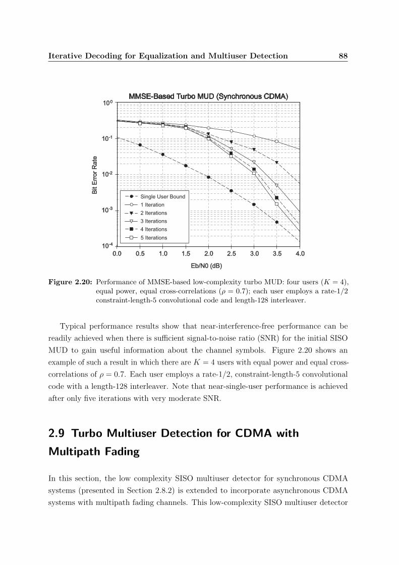
Iterative Decoding for Equalization and Multiuser Detection 88
Eb/N0 (dB)
Bit E
rror
Rate
10-4
10-3
10-2
10-1
100MMSE-Based Turbo MUD (Synchronous CDMA)
0.0 0.5 1.0 1.5 2.0 2.5 3.0 3.5 4.0
Single User Bound
1 Iteration
2 Iterations
3 Iterations
4 Iterations
5 Iterations
Figure 2.20: Performance of MMSE-based low-complexity turbo MUD: four users (K = 4),equal power, equal cross-correlations (ρ = 0.7); each user employs a rate-1/2constraint-length-5 convolutional code and length-128 interleaver.
Typical performance results show that near-interference-free performance can be
readily achieved when there is sufficient signal-to-noise ratio (SNR) for the initial SISO
MUD to gain useful information about the channel symbols. Figure 2.20 shows an
example of such a result in which there are K = 4 users with equal power and equal cross-
correlations of ρ = 0.7. Each user employs a rate-1/2, constraint-length-5 convolutional
code with a length-128 interleaver. Note that near-single-user performance is achieved
after only five iterations with very moderate SNR.
2.9 Turbo Multiuser Detection for CDMA with
Multipath Fading
In this section, the low complexity SISO multiuser detector for synchronous CDMA
systems (presented in Section 2.8.2) is extended to incorporate asynchronous CDMA
systems with multipath fading channels. This low-complexity SISO multiuser detector

Iterative Decoding for Equalization and Multiuser Detection 89
for asynchronous CDMA systems, which is also based on combined soft interference
cancelation and linear MMSE filtering, was proposed by Li, Wang, and Georghiades [57].
2.9.1 Signal Model and Sufficient Statistics
We consider a K-user asynchronous CDMA system transmitting over multipath fading
channels. The transmitted signal due to the k-th user is given by
xk(t) = Ak
N−1∑i=0
bk[i]sk(t− iT ) (2.170)
where N is the number of data symbols per user per frame; T is the symbol interval;
Ak is the amplitude of the k-th user; bk[i] is i-th transmitted bit of the k-th user; and
sk(t); 0 ≤ t ≤ T is the normalised signature waveform of the k-th user. It is assumed
that sk(t) is supported only on the interval [0, T ] and has unit energy.
The k-th user’s signal xk(t) propagates through a multipath channel with impulse
response
hk(t) =L∑l=1
g′k,l(t)δ(t− τk,l) (2.171)
where L is the number of paths in the k-th user’s channel, and where g′k,l(t) and τk,l
are the complex fading process and the delay of the l-th path of the k-th user’s signal,
respectively. It is assumed that the fading processes are known to the receiver and do
not vary during one coded symbol interval, but may vary from symbol to symbol, i.e.,
g′k,l(t) = g′k,l(iT ) , gk,l[i] for iT ≤ t < (i+ 1)T
The received signal, y(t), is the superposition of the K users’ signals plus the additive
white Gaussian noise, given by
y(t) =K∑k=1
xk(t) ? hk(t) + n(t) (2.172)
=K∑k=1
Ak
N−1∑i=0
bk[i]L∑l=1
gk,l[i]sk(t− iT − τk,l) + n(t) (2.173)
where n(t) is a zero-mean complex AWGN process with power spectral density σ2.
Iterative Decoding for Equalization and Multiuser Detection 90
From (2.102) and (2.109), denote
b[i] , [ b1[i], b2[i], . . . , bK [i] ]T and bn ,[bT [0], bT [1], . . . , bT [N − 1]
]T.
Using the Cameron-Martin formula [87], the likelihood function of the received waveform
y(t) in (2.173) conditioned on all the transmitted symbols bn of all users can be written
as
L(y(t) | bn) = C exp
Ω(bn)
σ2
, −∞ < t <∞ (2.174)
where C is some positive scalar constant, and
Ω(bn) , 2R
∫ ∞−∞
S(t; bn)∗y(t) dt
−∫ ∞−∞|S(t; bn)|2 dt (2.175)
and
S(t; bn) ,K∑k=1
Ak
N−1∑i=0
bk[i]L∑l=1
gk,l[i]sk(t− iT − τk,l) (2.176)
The first integral in (2.175) can be expressed as [57]
∫ ∞−∞
S(t; bn)∗y(t) dt ,K∑k=1
Ak
N−1∑i=0
bk[i]
yk[i]︷ ︸︸ ︷L∑l=1
g∗k,l[i]
∫ ∞−∞
y(t)sk(t− iT − τk,l) dt︸ ︷︷ ︸yk,l[i]
(2.177)
Since the second integral in (2.175) does not depend on the received signal y(t), from
(2.177) it can be seen that the sufficient statistic for detecting the multiuser symbols
bn is yk[i]K; N−1k=1;i=0 and that this sufficient statistic is obtained by passing the received
signal y(t) through a bank of K maximal-ratio multipath combiners, i.e., a Rake receiver
[91] (as shown in Figure 2.21).
Next, the expression for this sufficient statistic is restated in terms of the multiuser
channel parameters and transmitted symbols, which is fundamental to the development
of the SISO multiuser detector.
We assume that the multipath spread of any user’s channel is within one symbol
interval, that is, τk,l ∈ [0, T ) for k = 1, . . . , K and l = 1, . . . , L. Define the following

Iterative Decoding for Equalization and Multiuser Detection 91
y [i]k
g [i]*k,1
y [i]k,1
RAKE Detector - User k
conjugatepath gain
matched filter
òy(t)s (t- )dtk tk,1
y(t)
S
n(t)
Multipath Fading Channel - User k
x (t)k
path delay
tk,1 g’ (t)k,1
path delay
tk,2 g’ (t)k,2
path delay
tk,L g’ (t)k,L
path gain
path gain
path gain
g [i]*k,2
y [i]k,2
òy(t)s (t- )dtk tk,1
g [i]*k,L
y [i]k,L
òy(t)s (t- )dtk tk,L
matched filter
matched filter
conjugatepath gain
conjugatepath gain
Figure 2.21: CDMA Rake receiver for multipath fading channels
correlation of the delayed signalling waveforms:
ρ(j)(k,l)(k′,l′) ,
∫ ∞−∞
sk(t− τk,l)sk′(t+ jT − τk′,l′) dt,
j ∈ J , 1 ≤ k, k′ ≤ K, 1 ≤ l, l′ ≤ L (2.178)
where J , −1, 0,+1. Since τk,l ≤ T and si,k(t) is nonzero only t ∈ [0, T ], it then
follows that ρ(j)(k,l)(k′,l′) = 0 for j /∈ −1, 0,+1. Now substituting (2.173) into (2.177), we
have
yk,l[i] =N−1∑i′=0
K∑k′=1
Ak′bk′ [i′]
L∑l′=1
gk′,l′ [i′]
∫ ∞−∞
sk′(t− i′T − τk′,l′)sk(t− iT − τk,l) dt+ uk,l[i]
=∑j∈J
K∑k′=1
Ak′bk′ [i+ j]L∑l′=1
gk′,l′ [i]ρ(−j)(k,l)(k′,l′) + uk,l[i] (2.179)
where uk,l[i] are zero-mean complex Gaussian random sequences, defined as
uk,l[i] =
∫ ∞−∞
n(t)sk(t− iT − τk,l) dt (2.180)
with covariance
Cov uk,l[i], uk′,l′ [i′] = Euk,l[i]u
∗k′,l′ [i
′]
=
∫ ∞−∞
sk(t− iT − τk,l)sk′(t′ − i′T − τk′,l′) dt
= ρ(i−i′)(k,l)(k′,l′) (2.181)
Iterative Decoding for Equalization and Multiuser Detection 92
Define the following quantities:
R(j)(k,k′) ,
ρ
(j)(k,1)(k′,1) ρ
(j)(k,1)(k′,2) · · · ρ
(j)(k,1)(k′,L)
ρ(j)(k,2)(k′,1) ρ
(j)(k,2)(k′,2) · · · ρ
(j)(k,1)(k′,L)
......
...
ρ(j)(k,L)(k′,1) ρ
(j)(k,L)(k′,2) · · · ρ
(j)(k,L)(k′,L)
(L×L−matrix)
R(j) ,
R
(j)(1,1) R
(j)(1,2) · · · R
(j)(1,K)
R(j)(2,1) R
(j)(2,2) · · · R
(j)(2,K)
......
...
R(j)(K,1) R
(j)(K,2) · · · R
(j)(K,K)
(KL×KL−matrix)
Υ[i] , [ y1,1[i], . . . , y1,L[i], . . . , yK,1[i], . . . , yK,L[i] ]T (KL× 1− vector)
u[i] , [u1,1[i], . . . , u1,L[i], . . . , uK,1[i], . . . , uK,L[i] ]T (KL× 1− vector)
gk[i] , [ gk,1[i], gk,2[i], . . . , gk,L[i] ]T (L× 1− vector)
G[i] , diagg1[i],g2[i], . . . ,gK [i] (KL×K −matrix)
A , diag A1, A2, . . . , AK (K ×K −matrix)
y[i] , [ y1[i], y2[i], . . . , yK [i] ]T (K × 1− vector)
The sufficient statistic of (2.179) can be rewritten in vector form as follows:
Υ[i] =∑j∈J
R(−j)G[i]A b[i+ j] + u[i]. (2.182)
From (2.180), the complex Gaussian vector sequence u[i] has the covariance matrix of
Covu[i],u[i+ j] = Eu[i]uH [i+ j]
= σ2R(−j). (2.183)
Substituting (2.182) into (2.177), the expression for the sufficient statistic y[i] is given by
y[i] = GH [i]Υ[i] =∑j∈J
H(−j)[i]A b[i+ j] + v[i] (2.184)

Iterative Decoding for Equalization and Multiuser Detection 93
where H(−j)[i] is defined as
H(−j)[i] = GH [i]R(−j)G[i], (2.185)
and v[i] is a sequence of zero-mean complex Gaussian vectors, defined as
v[i] = GH [i]u[i] (2.186)
and has the covariance matrix of
Covv[i],v[i+ j] = Ev[i]vH [i+ j]
= σ2GH [i]R(−j)G[i] , σ2H(−j)[i]. (2.187)
Note that ρ(j)(k,l)(k′,l′) = ρ
(−j)(k′,l′)(k,l) by definition of (2.178). It then follows that R(−j) =
(R(j))T , and therefore, H(−j)[i] = (H(j)[i])H .
2.9.2 SISO Multiuser Detector in Multipath Fading Channels
The structure of the soft multiuser detector for multipath fading channels is shown in
Figure 2.22. First, the received signal y(t) is passed through a bank of K maximum-ratio
multipath combiners (i.e. Rake receivers) to obtain the sufficient statistic. Then, soft
interference cancellation is applied to the outputs of the combiners, followed by linear
MMSE filtering. Finally, the extrinsic information is computed from the MMSE filter
outputs.
Define the following quantities:
H[i] ,[H(1)[i], H(0)[i], H(−1)[i]
](K × 3K −matrix)
Aa , diag A, A, A (3K × 3K −matrix)
ba[i] ,[bT [i− 1], bT [i], bT [i+ 1]
]T(3K × 1− vector)
We can then write (2.184) in matrix form as
y[i] = H[i]Aaba[i] + v[i] (2.188)
where by (2.187), v[i]∼Nc(0, σ2H(0)[i]).
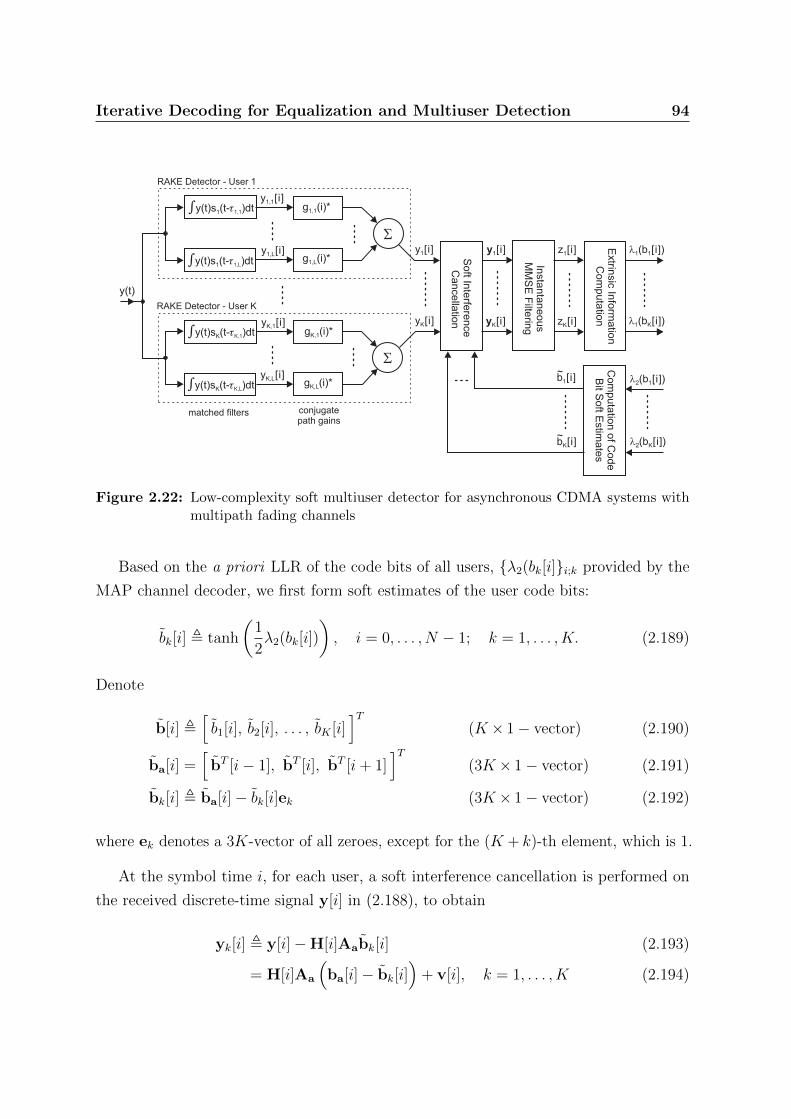
Iterative Decoding for Equalization and Multiuser Detection 94
g (i)*1,1
Extrin
sic
Info
rmatio
nC
om
puta
tion
Insta
nta
neous
MM
SE
Filte
ring
Soft In
terfe
rence
Cancella
tion
g (i)*1,L
y [i]1,1
y [i]1,Ly [i]1 y1[i] z [i]1
y [i]K yK[i] z [i]K
l1 1(b [i])
l1 K(b [i])g (i)*K,1
g (i)*K,L
y [i]K,1
y [i]K,L
y(t)
RAKE Detector - User 1
RAKE Detector - User K
l2 1(b [i])
l2 K(b [i])
b [i]1
b [i]K
Com
puta
tion o
f Code
Bit S
oft E
stim
ate
s
òy(t)s (t- )dtK tK,L
conjugatepath gains
matched filters
òy(t)s (t- )dtK tK,1
òy(t)s (t- )dt1 t1,1
òy(t)s (t- )dt1 t1,L
Figure 2.22: Low-complexity soft multiuser detector for asynchronous CDMA systems withmultipath fading channels
Based on the a priori LLR of the code bits of all users, λ2(bk[i]i;k provided by the
MAP channel decoder, we first form soft estimates of the user code bits:
bk[i] , tanh
(1
2λ2(bk[i])
), i = 0, . . . , N − 1; k = 1, . . . , K. (2.189)
Denote
b[i] ,[b1[i], b2[i], . . . , bK [i]
]T(K × 1− vector) (2.190)
ba[i] =[
bT [i− 1], bT [i], bT [i+ 1]]T
(3K × 1− vector) (2.191)
bk[i] , ba[i]− bk[i]ek (3K × 1− vector) (2.192)
where ek denotes a 3K-vector of all zeroes, except for the (K + k)-th element, which is 1.
At the symbol time i, for each user, a soft interference cancellation is performed on
the received discrete-time signal y[i] in (2.188), to obtain
yk[i] , y[i]−H[i]Aabk[i] (2.193)
= H[i]Aa
(ba[i]− bk[i]
)+ v[i], k = 1, . . . , K (2.194)
Iterative Decoding for Equalization and Multiuser Detection 95
An instantaneous linear MMSE filter is then applied to yk[i], to obtain
zk[i] = wHk [i]yk[i] (2.195)
where the filter wk[i] ∈ CK is chosen to minimize the mean-square error between the
code bit bk[i] and the filter output zk[i];
wk[i] = arg minw∈CK
E∣∣bk[i]−wHyk[i]
∣∣2= arg min
w∈CKwHE
yk[i]y
Hk [i]
w − 2R[wHE bk[i]yk[i]
](2.196)
where
Eyk[i]y
Hk [i]
= H[i]Aa∆k[i]AaHH [i] + σ2H(0)[i], and (2.197)
E bk[i]yk[i] = H[i]Aaek = AkH[i]ek (2.198)
with
∆k[i] , Cov
br[i]− bk[i]
= diag D[i− 1], Dk[i], D[i+ 1]
and
Dk[i] , diag
1− b21[i], . . . , 1− b2
k−1[i], 1, 1− b2k+1[i], . . . , 1− b2
K [i]
D[i+ j] , diag
1− b21[i+ j], 1− b2
2[i+ j], . . . , 1− b2K [i+ j]
,
for j = −1,+1. The solution to (2.196) is given by [57]
wk[i] = Ak(H[i]Aa∆k[i]AaH
H [i] + σ2H[0][i])−1
H[i]ek (2.199)
As before, in order to form the LLR of the code bit bk[i], we approximate the instantaneous
linear MMSE filter output zk[i] in (2.195) as being Gaussian, i.e., zk[i]∼Nc(µk[i]bk[i], ν2k [i]).
Conditioned on the code bit bk[i], the mean and variance of zk[i] are given, respectively
by
µk[i] , E zk[i]bk[i]
= eHk HH [i](H[i]∆k[i]H
H [i] + σ2H(0)[i])−1
H[i]ek (2.200)

Iterative Decoding for Equalization and Multiuser Detection 96
and
νk[i] , Var zk[i] = E|zk[i]|2
− µ2
k[i]
= wHk Eyk[i]y
Hk [i]
wk − µ2k[i]
= µk[i]− µ2k[i] (2.201)
Therefore, the extrinsic information λ1(bk[i]) delivered by the instantaneous linear MMSE
filter is given by [57]
λ1[bk(i)] = −|zk[i]− µk[i]|2
ν2k [i]
+|zk[i] + µk[i]|2
ν2k [i]
=4Rzk[i]1− µk[i]
(2.202)
Recursive Algorithm for Computing Soft Output
The extrinsic information can be computed efficiently by employing reduced-complexity
recursive techniques for performing matrix inversions. The K ×K matrix inversion,
Ψk[i] ,(H[i]∆k[i]H
H [i] + σ2H(0)[i])−1
, (2.203)
can be computed efficiently using the following procedure. Note that ∆k[i] can be written
as
∆k[i] = ∆[i] + b2k[i]eke
Tk (2.204)
where
∆[i] = diag D[i− 1], D[i], D[i+ 1] (2.205)
and
D[i+ j] , diag
1− b21[i+ j], 1− b2
2[i+ j], . . . , 1− b2K [i+ j]
,
for j = −1, 0,+1. Substituting (2.204) into (2.203), we have
Ψk[i] =(H[i]∆[i]HH [i] + σ2H(0)[i] + b2
k[i]H[i](:,K+k)HH [i](:,K+k)
)−1
(2.206)

Iterative Decoding for Equalization and Multiuser Detection 97
where H[i](:,K+k) denotes the (K + k)-th column of H[i]. Define
Ψ[i] ,(H[i]∆[i]HH [i] + σ2H(0)[i]
)−1(2.207)
1. Given the extrinsic information (in LLR form), λ2(bk[i])i,k, from the
FEC decoders, calculate the soft bit estimates (for i = 0, . . . , N − 1 and
k = 1, . . . , K) using:
bk[i] = tanh
(1
2λ2(bk[i])
)b[i] =
[b1[i], b2[i], . . . , bK [i]
]Tba[i] =
[bT [i− 1], bT [i], bT [i+ 1]
]T,
bk[i] = ba[i]− bk[i]ek
2. Using the recursive procedure of (2.207) and (2.208), calculate the matrix
inversions:
Ψk[i] ,(H[i]∆k[i]H
H [i] + σ2H(0)[i])−1
,
Φk[i] ,(H[i]Aa∆k[i]AaH
H [i] + σ2H(0)[i])−1
3. Perform soft interference cancellation and linear MMSE filtering (for
i = 0, . . . , N − 1 and k = 1, . . . , K) using:
yk[i] = y[i]−H[i]Aabk[i]
zk[i] = wHk [i]yk[i] where wk[i] = AkΦk[i]H[i]ek
4. Calculate the extrinsic information λ1(bk[i])i,k, for i = 0, . . . , N − 1 and
k = 1, . . . , K, using:
λ1(bk[i]) =4Rzk[i]1− µk[i]
where µk[i] = eHk HH [i]Ψk[i]H[i]ek
Table 2.5: Algorithm: Low-Complexity Soft MUD for Multipath Fading Channels
Iterative Decoding for Equalization and Multiuser Detection 98
Then by the matrix inversion lemma, (2.206) can be written as [57]
Ψk[i] = Ψ[i]−
(1
b−2k [i] + HH [i](:,K+k)Ψ[i]H[i](:,K+k)
)·(Ψ[i]H[i](:,K+k)
) (Ψ[i]H[i](:,K+k)
)H, k = 1, . . . , K (2.208)
Equations (2.207) and (2.208) form the recursive procedure for computing Ψk[i] in (2.203).
Similarly, the recursive procedure can be easily adapted to compute the K ×K matrix
inversion Φk[i] where
Φk[i] ,(H[i]Aa∆k[i]AaH
H [i] + σ2H(0)[i])−1
. (2.209)
Finally, the SISO multiuser detection algorithm for asynchronous CDMA systems with
multipath fading channels is summarised in Table 2.5.
2.10 Interleave-Division Multiple Access (IDMA)
Recently, a new multiple access system, interleave division multiple access (IDMA) has
been proposed by Ping, Liu, Wu, and Leung [86], [85]. IDMA when used with low-
complexity iterative receivers has been shown to outperform coded CDMA. In contrast
to CDMA, which separates users by specific spreading codes, IDMA separates users by
unique interleaver sequences. IDMA can be regarded as a special case of chip interleaved
CDMA, and therefore inherits many advantages of CDMA including diversity against
fading, and mitigation of the worst-case other-cell user interference problem [74].
2.10.1 Transmitter Structure
Figure 2.23 shows the transmitter structure of the multiuser IDMA scheme with K
simultaneous users [85]. The input data sequence dk[i]M−1i=0 of user-k is encoded by
the FEC encoder (with rate Rk) generating a coded sequence ck[i]N−1i=0 , where N is
the frame length. The elements ck[i] are referred to as coded bits. Then ck[i]N−1i=0
is permutated by the user-specific interleaver πk, producing bk[i]N−1i=0 . Finally, the
interleaved coded bit sequence is BPSK modulated, producing xk[i]N−1i=0 . The elements
xk[i] are referred to as chips in accordance with CDMA convention.
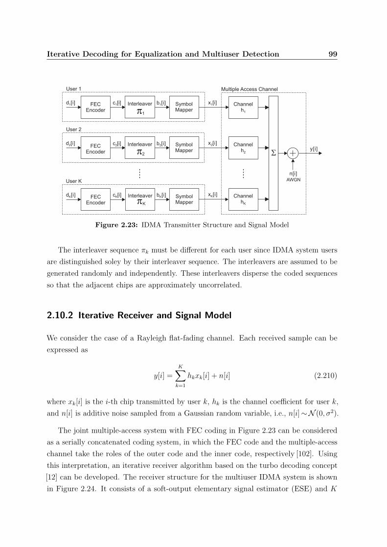
Iterative Decoding for Equalization and Multiuser Detection 99
Interleaver
x [i]KInterleaver
FECEncoder
FECEncoder
d [i]1
d [i]K
SymbolMapper
b [i]1 x [i]1
p1
pK
User 1
User K
c [i]1
SymbolMapper
InterleaverFECEncoder
d [i]2 SymbolMapper
x [i]2
p2
User 2
AWGN
y[i]S
n[i]
Multiple Access Channel
Channelh1
Channelh2
ChannelhK
b [i]2c [i]2
b [i]Kc [i]K
Figure 2.23: IDMA Transmitter Structure and Signal Model
The interleaver sequence πk must be different for each user since IDMA system users
are distinguished soley by their interleaver sequence. The interleavers are assumed to be
generated randomly and independently. These interleavers disperse the coded sequences
so that the adjacent chips are approximately uncorrelated.
2.10.2 Iterative Receiver and Signal Model
We consider the case of a Rayleigh flat-fading channel. Each received sample can be
expressed as
y[i] =K∑k=1
hkxk[i] + n[i] (2.210)
where xk[i] is the i-th chip transmitted by user k, hk is the channel coefficient for user k,
and n[i] is additive noise sampled from a Gaussian random variable, i.e., n[i]∼N (0, σ2).
The joint multiple-access system with FEC coding in Figure 2.23 can be considered
as a serially concatenated coding system, in which the FEC code and the multiple-access
channel take the roles of the outer code and the inner code, respectively [102]. Using
this interpretation, an iterative receiver algorithm based on the turbo decoding concept
[12] can be developed. The receiver structure for the multiuser IDMA system is shown
in Figure 2.24. It consists of a soft-output elementary signal estimator (ESE) and K
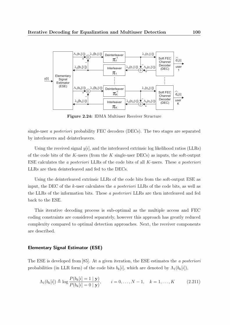
Iterative Decoding for Equalization and Multiuser Detection 100
y[i]
l1(b )1[ i ]
ElementarySignal
Estimator(ESE)
Soft FECChannelDecoder(DEC)Interleaver
Deinterleaver
user1
d1[i]
userK
dK[i]
p1-1
p1
Soft FECChannelDecoder(DEC)Interleaver
Deinterleaver
pK-1
pK
L2(c [ i ])1
l1(c )1[ i ]
l2(c )1[ i ]
L1(b [ i ])1
l2(b [ i ])1
L1(b [ i ])K
l2(b )K[ i ]
l1(b )K[ i ] l1(c )K[ i ]
L2(c [ i ])Kl2(c )K[ i ]
Figure 2.24: IDMA Multiuser Receiver Structure
single-user a posteriori probability FEC decoders (DECs). The two stages are separated
by interleavers and deinterleavers.
Using the received signal y[i], and the interleaved extrinsic log likelihood ratios (LLRs)
of the code bits of the K-users (from the K single-user DECs) as inputs, the soft-output
ESE calculates the a posteriori LLRs of the code bits of all K-users. These a posteriori
LLRs are then deinterleaved and fed to the DECs.
Using the deinterleaved extrinsic LLRs of the code bits from the soft-output ESE as
input, the DEC of the k-user calculates the a posteriori LLRs of the code bits, as well as
the LLRs of the information bits. These a posteriori LLRs are then interleaved and fed
back to the ESE.
This iterative decoding process is sub-optimal as the multiple access and FEC
coding constraints are considered separately, however this approach has greatly reduced
complexity compared to optimal detection approaches. Next, the receiver components
are described.
Elementary Signal Estimator (ESE)
The ESE is developed from [85]. At a given iteration, the ESE estimates the a posteriori
probabilities (in LLR form) of the code bits bk[i], which are denoted by Λ1(bk[i]),
Λ1(bk[i]) , logP (bk[i] = 1 | y)
P (bk[i] = 0 | y), i = 0, . . . , N − 1, k = 1, . . . , K (2.211)

Iterative Decoding for Equalization and Multiuser Detection 101
Where y denotes the received signal vector, given by y = [ y[0], . . . , y[N − 1] ]T . Using
Bayes’ rule, (2.211) can be rewritten as
Λ1(bk[i]) = logP (y | bk[i] = 1)
P (y | bk[i] = 0)︸ ︷︷ ︸λ1(bk[i])
+ logP (bk[i] = 1)
P (bk[i] = 0)︸ ︷︷ ︸λ2(bk[i])
. (2.212)
The first term in (2.212), denoted by λ1(bk[i]), is the extrinsic information calculated
by the ESE. The second term, denoted by λ2(bk[i]), is the a priori probability (in LLR
form) of bk[i]. An estimate of the a priori probability is calculated by the DEC of the
k -th user at the previous iteration. At the first iteration, no prior information about the
code bits is available, therefore all bit values are assumed equiprobable and the a priori
LLR values are set to zero. Finally, the sequence of extrinsic information, λ1(bk[i])i, is
deinterleaved by the deinterleaver of the k -th user (producing λ1(ck[i])i) and fed into
the corresponding DEC as a priori information for the next iteration.
The computation of the extrinsic information for each user is now described in detail.
For a particular user, k, we can rewrite (2.210) as
y[i] = hkxk[i] + ζk[i] (2.213)
where ζk[i] is the distortion (comprising of AWGN channel noise and interference from
other users) contained in sample y[i] with respect to xk[i], and is given by
ζk[i] , y[i]− hkxk[i] =K∑j=1
(j 6=k)
hjxj[i] + n[i] (2.214)
From the central limit theorem, ζk[i] can be approximated as a Gaussian variable, and
y[i] can be characterised by a conditional Gaussian probability density function
P (y[i] | bk[i] = ± 1) =1√
2πVarζk(i)exp
(−(y[i]− (±hk + Eζk[i]))2
2Varζk[i]
)(2.215)
where E · and Var · denote expectation and variance, respectively. Using (2.213)-
(2.215), the chip-by-chip ESE detection algorithm for IDMA systems can be developed
as shown in Table 2.6.

Iterative Decoding for Equalization and Multiuser Detection 102
1. Given the extrinsic information (in LLR form), λ2(bk[j])k, from the FEC
decoders, calculate the soft bit statistics for each user (k = 1, . . . , K):
Exk[i] = tanh
(1
2λ2(bk[i])
),
Varxk[i] = 1− (Exk[i])2 ,
2. Calculate the received signal statistics:
Ey[i] =K∑k=1
hkExk[i],
Vary[i] =K∑k=1
|hk|2Varxk[i]+ σ2.
3. Calculate the estimated interference mean and variance for each user
(k = 1, . . . , K):
Eζk[i] = Ey[i] − hkExk[i],
Varζk[i] = Vary[i] − |hk|2Varxk[i]
4. Perform soft interference cancellation for each user:
yk[i] = y[i]− Eζk[i]), k = 1, . . . , K
5. Calculate the extrinsic information, λ1(bk[i])k, using:
λ1(bk[i]) = 2hk ·(
yk[i]
Varζk[i]
), k = 1, . . . , K
Table 2.6: Algorithm: Soft Elementary Signal Estimator (ESE) MUD for IDMA
Iterative Decoding for Equalization and Multiuser Detection 103
Soft Channel Decoders (DEC)
The channel decoder for the k -th user estimates the a posteriori probabilities (APP) in
LLR form of the code bits, Λ2(ck[i]), which are given by
Λ2(ck[i]) , logP (ck[i] = 1 | λ1(ck[i])i ; code structure )
P (ck[i] = 0 | λ1(ck[i])i ; code structure ), (2.216)
= λ2(ck[i]) + λ1(ck[i]),
for i = 0, . . . , N − 1. These a posteriori probabilities are computed using the BCJR
algorithm [6] (from Section 2.3.3) based on the a priori information from the ESE,
λ1(ck[i])i, and knowledge of the code structure.
As in (2.212), Λ2(ck[i]) can be expressed as the sum of extrinsic information λ2(ck[i])
and a priori information λ1(ck[i]). The sequence of extrinsic information, λ2(ck[i])i, is
interleaved (producing λ2(bk[i])i) and fed back to the ESE as a priori information for
the next iteration.
Additionally, the DEC estimates the a posteriori LLRs of the information bits,
Λ2(dk[i])i, and at the final iteration, performs a hard decision on the information bits,
producing dk[i]i .
2.11 Conclusion
In this chapter, the iterative decoding principles from turbo coding were applied to
channel equalization and multiuser detection. The techniques presented will be the
basis for the work described in the following chapters. First, the BCJR MAP algorithm
was introduced for decoding convolutional codes over an AWGN channel. The BCJR
algorithm is a fundamental building block of turbo decoding schemes.
Next, the inter-symbol interference (ISI) channel was presented. For coded data
transmissions, the FEC encoder of the transmitter and the ISI channel can be modelled
as a serial concatenated coding scheme transmitting over a memoryless channel. This
model is similar to a standard serial encoder for turbo coding, and therefore, iterative
decoding techniques can be used at the receiver. Iterative decoding for ISI channels is
known as turbo equalization. Turbo equalization receiver structures were discussed and
performance results presented.

Iterative Decoding for Equalization and Multiuser Detection 104
Finally, the multiple-access channel and multiuser detection using iterative decoding
was presented. For coded data transmissions, the FEC encoder of the transmitter and the
MAI (multiple-access interference) channel can also be modelled as a serial concatenated
coding scheme, and therefore, iterative decoding techniques can be utilised. Iterative
decoding of multiple-access channels is commonly known as turbo MUD. Low-complexity
multiuser detectors for use in turbo MUD receivers were presented for synchronous
CDMA, asynchronous CDMA, and asynchronous IDMA systems.
Chapter 3
IDMA Performance Optimisation using
Variance Transfer Analysis
In this chapter, Variance Transfer (VT) charts are used to analyse and optimise iterative
receiver performance of a multiuser IDMA system. Introduced by Schlegel and Grant
[102], VT charts are similar in concept to Extrinsic Information Transfer (EXIT) charts
[115], but are better suited for analysing multiuser iterative receivers. VT Charts provide
a graphical interpretation of the reliability of information passed between the constituent
components of an iterative receiver. Once the VT characteristic curves have been
determined, receiver performance can be optimised by attempting to closely match the
VT characteristics of the multiuser detector (MUD) and the forward error correction
(FEC) channel decoders. The MUD VT characteristic can be manipulated by the selection
of multiuser detection algorithm and the number of simultaneous users (system load).
The FEC channel decoder VT characteristic can be manipulated by the selection of error
correction code.
Two multiuser system scenarios are considered for optimisation:
Layered IDMA with Power Allocation. Firstly, We extend the IDMA concept to a
multi-rate system where different users transmit data at different rates and the
same low-complexity iterative receiver structure can still be used. High-rate users
are supported by breaking up the input data stream into multiple sub-streams. An
IDMA layer is created from each sub-stream, and the multiple IDMA layers are then
combined and the composite layered signal is transmitted from a single antenna.
The iterative receiver treats each IDMA layer as a virtual user.
105

IDMA Performance Optimisation using Variance Transfer Analysis 106
Chayat et. al. [18] observed that the performance of an iterative receiver is improved
if different users transmit at different powers. This allows the iterative decoder
to operate in an “onion peeling” mode, where the higher-power layers converge
first, decreasing their contribution to the residual noise, and then the lower-power
layers converge. CDMA and IDMA systems utilising iterative receivers can exploit
this power allocation strategy to gain an improvement in performance. Caire
et. al. [17] have shown that this power optimisation problem can be solved by
optimising the partial loads, and developed simple optimisation methods based on
linear programming techniques. In [103], Schlegel et al. applied the work of [18] and
[17] to develop allocation schemes for iterative CDMA receivers that are based on
combined soft interference cancellation and MMSE filtering (i.e., CDMA multiuser
detector schemes of the type described in Section 2.8.2).
To improve the performance of our layered IDMA scheme, we develop a simple power
allocation scheme, where the power levels for each IDMA layer are calculated using
Variance Transfer (VT) analysis and linear programming techniques. In a Rayleigh
flat-fading environment, simulation results demonstrate that the performance of
this proposed system is close to the theoretical limit. This original contribution was
published in [63].
FEC Code Allocation for Dynamic Loads. Secondly, we propose an alternative opti-
misation approach for inducing “onion peeling” operation in the iterative receiver.
Ten Brink [116] demonstrated that different FEC codes generate different FEC
channel decoder VT characteristics. As an alternative to transmit power allocation,
the judicious selection of FEC codes can also be used to match the receiver VT
characteristics for optimal performance.
A simple FEC code allocation strategy for multiuser systems with dynamic loads
is devised. New users are allocated FEC codes according to the existing system
load, which allows the FEC decoder VT curve to dynamically match the MUD
VT curve as it changes with system load, providing optimal system performance
over a range of operating conditions. We derive a numerical method for optimising
performance based on FEC code allocation, and present simulation results. For
small multiuser systems, results demonstrate that the performance of the proposed
system approaches the theoretical single user bound. This original contribution was
published in [65].

IDMA Performance Optimisation using Variance Transfer Analysis 107
3.1 Variance Transfer Charts and Analysis
s2
n
ElementarySignal
Estimator userk
dk[ i ]Soft FECChannelDecoder
User k
ESE outputvariance
l1(b )k[ i ] l1(c )k[ i ]
l2(b )k[ i ] l2(c )k[ i ]Interleaver
Deinterleaver
pk-1
pkg( )
vardec
varese
vardec
x (t) hK K
S
n(t)
Multiple Access Channel
y(t)
x (t) h1 1
x (t) h2 2
ESE inputvariance
DEC outputvariance
f( )
varese
DEC inputvariancechannel
noisevariance
Figure 3.1: Variance transfer between constituent iterative receiver components
The Variance Transfer (VT) chart method [102] analyses the transfer functions of the
multiuser detector and the channel decoders in order to predict the behaviour of the
iterative receiver. Figure 3.1 shows the variance transfer paths for the IDMA iterative
receiver from Section 2.10.2. There are two VT functions:
• The ESE VT function is defined as the variance in the ESE output, varese, as a
function of the error variance in the soft-bit estimates from the FEC decoders,
vardec,k, and the channel noise variance, σ2n, i.e., varese = f(vardec,k , σ
2n)
• The FEC channel decoder (DEC) VT function is defined as the variance in the k-th
user DEC output, vardec,k, as a function of the estimation error variance from the
ESE, varese, i.e., vardec,k = g(varese)
3.1.1 ESE Variance Transfer Function
For our IDMA system, the multiuser interference is proportional to the system load,
β, and the variance of the estimation error, vardec,k. The system load is defined as the
ratio of users, K, to bandwidth expansion, R, (i.e. β = K/R), and the estimation error
variance is defined as
vardec,k = E
(ck[i]− ck[i])2 (3.1)
We first consider the case of equal power for all users, Pk = P . For this case, the
estimation error for all users will be equal, vardec,k = vardec. For the ESE, the expression

IDMA Performance Optimisation using Variance Transfer Analysis 108
for the residual multiple access interference plus channel noise at the input to the FEC
decoder is given by
varese( vardec ) =
(K − 1
R
)P vardec + σ2
n
= limK→∞
βP vardec + σ2n (3.2)
where σ2n is the channel noise, and the soft FEC decoder estimation error variance,
vardec , is the average power of the residual symbol interference. Therefore, given vardec ,
equation (3.2) describes the noise variance in the input signal to the FEC decoder for the
next iteration. Figure 3.2a shows the ESE VT function (3.2) for a typical IDMA system.
0.0 0.2 0.4 0.6 0.8 1.0
Cancelled Symbol Variance
Sin
gle
-User
Nois
e L
evel
ChannelNoiseLevel
Slope:System Load
0.0
0.5
1.0
1.5
2.0
2.5
3.0
3.5Variance Transfer: ESE Interference Canceller
DecreasingSystemLoad
IncreasingSystemLoad
(a) ESE interference canceller
Input N
ois
e V
ariance
0.0 0.2 0.4 0.6 0.8
3.5
3.0
2.5
2.0
1.5
0.5
1.0
0.0
1.0
Soft-Bit (FEC Decoder) Variance
Variance Transfer: FEC Decoder
Turbo Code
Conv. Code (v=2)
Repetition Code
Conv. Code (v=3)
Conv. Code (v=4)
(b) FEC decoder
Figure 3.2: Variance transfer functions for (a) ESE interference canceller, and (b) FECdecoder (for various 1/3-rate codes)
The more accurate the symbol estimates of the other interfering users, the smaller the
residual noise that the error control decoder has to overcome. But even if the interfering
symbols are known exactly, the FEC decoder still has to overcome the AWGN channel
noise.
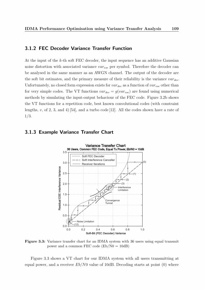
IDMA Performance Optimisation using Variance Transfer Analysis 109
3.1.2 FEC Decoder Variance Transfer Function
At the input of the k-th soft FEC decoder, the input sequence has an additive Gaussian
noise distortion with associated variance varese per symbol. Therefore the decoder can
be analysed in the same manner as an AWGN channel. The output of the decoder are
the soft bit estimates, and the primary measure of their reliability is the variance vardec.
Unfortunately, no closed form expression exists for vardec as a function of varese other than
for very simple codes. The VT functions vardec = g(varese) are found using numerical
methods by simulating the input-output behaviour of the FEC code. Figure 3.2b shows
the VT functions for a repetition code, best known convolutional codes (with constraint
lengths, v, of 2, 3, and 4) [54], and a turbo code [12]. All the codes shown have a rate of
1/3.
3.1.3 Example Variance Transfer Chart
0.0
0.5
1.0
1.5
2.0
2.5
3.0
0.0 0.2 0.4 0.6 0.8 1.0
Soft-Bit (FEC Decoder) Variance
Re
sid
ua
l E
SE
Inte
rfe
rence V
aria
nce
(0)
(1)
(2)
Noise Limitation
InterferenceLimitation
(12)
(3)
ConvergenceTunnel
3.5
Variance Transfer Chart36 Users, Common FEC Code, Equal Tx Power, Eb/N0 = 10dB
Soft FEC Decoder
Soft Interference Canceller
Receiver Iterations
Figure 3.3: Variance transfer chart for an IDMA system with 36 users using equal transmitpower and a common FEC code (Eb/N0 = 10dB)
Figure 3.3 shows a VT chart for our IDMA system with all users transmitting at
equal power, and a receiver Eb/N0 value of 10dB. Decoding starts at point (0) where
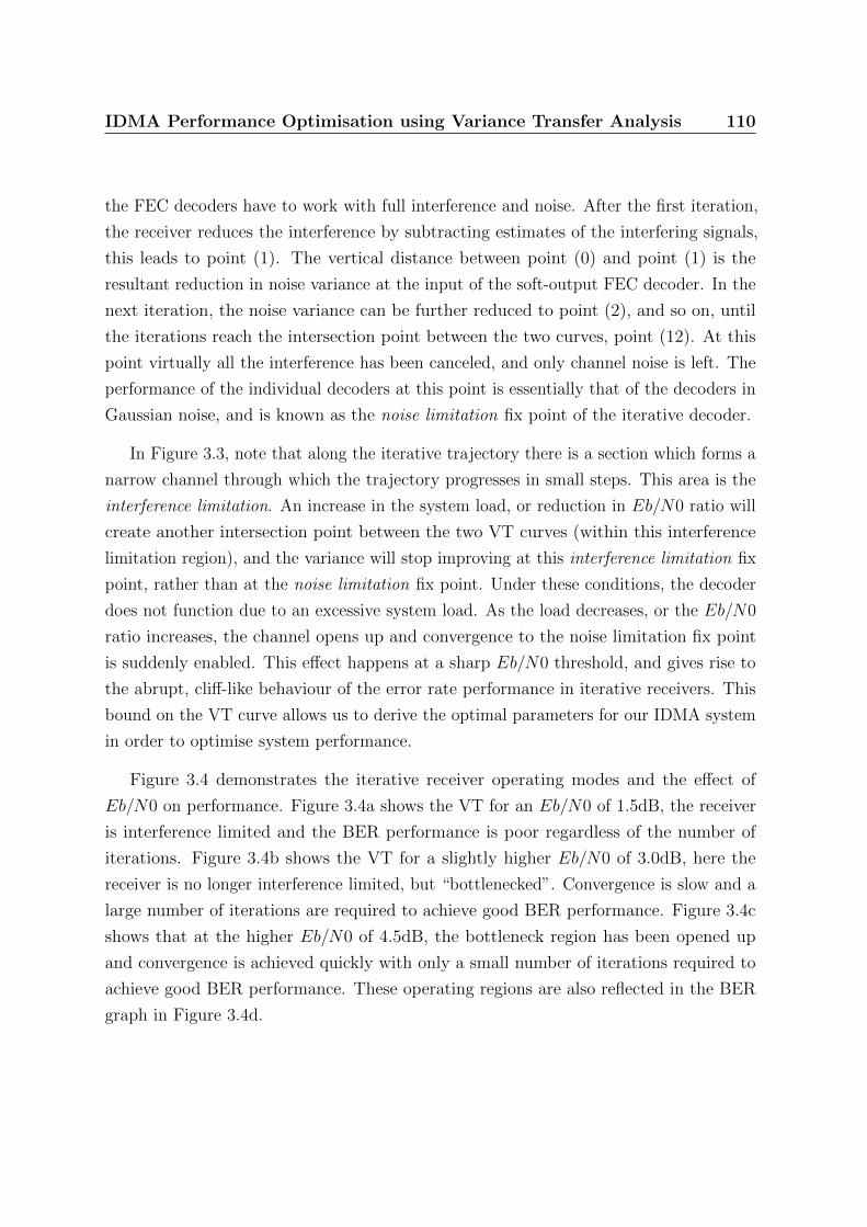
IDMA Performance Optimisation using Variance Transfer Analysis 110
the FEC decoders have to work with full interference and noise. After the first iteration,
the receiver reduces the interference by subtracting estimates of the interfering signals,
this leads to point (1). The vertical distance between point (0) and point (1) is the
resultant reduction in noise variance at the input of the soft-output FEC decoder. In the
next iteration, the noise variance can be further reduced to point (2), and so on, until
the iterations reach the intersection point between the two curves, point (12). At this
point virtually all the interference has been canceled, and only channel noise is left. The
performance of the individual decoders at this point is essentially that of the decoders in
Gaussian noise, and is known as the noise limitation fix point of the iterative decoder.
In Figure 3.3, note that along the iterative trajectory there is a section which forms a
narrow channel through which the trajectory progresses in small steps. This area is the
interference limitation. An increase in the system load, or reduction in Eb/N0 ratio will
create another intersection point between the two VT curves (within this interference
limitation region), and the variance will stop improving at this interference limitation fix
point, rather than at the noise limitation fix point. Under these conditions, the decoder
does not function due to an excessive system load. As the load decreases, or the Eb/N0
ratio increases, the channel opens up and convergence to the noise limitation fix point
is suddenly enabled. This effect happens at a sharp Eb/N0 threshold, and gives rise to
the abrupt, cliff-like behaviour of the error rate performance in iterative receivers. This
bound on the VT curve allows us to derive the optimal parameters for our IDMA system
in order to optimise system performance.
Figure 3.4 demonstrates the iterative receiver operating modes and the effect of
Eb/N0 on performance. Figure 3.4a shows the VT for an Eb/N0 of 1.5dB, the receiver
is interference limited and the BER performance is poor regardless of the number of
iterations. Figure 3.4b shows the VT for a slightly higher Eb/N0 of 3.0dB, here the
receiver is no longer interference limited, but “bottlenecked”. Convergence is slow and a
large number of iterations are required to achieve good BER performance. Figure 3.4c
shows that at the higher Eb/N0 of 4.5dB, the bottleneck region has been opened up
and convergence is achieved quickly with only a small number of iterations required to
achieve good BER performance. These operating regions are also reflected in the BER
graph in Figure 3.4d.
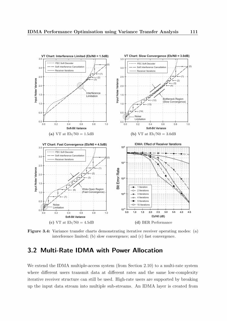
IDMA Performance Optimisation using Variance Transfer Analysis 111
0.0
0.5
1.0
1.5
2.0
2.5
3.0
3.5
0.0 0.2 0.4 0.6 0.8 1.0
Soft-Bit Variance
Input N
ois
e V
ariance
FEC Soft Decoder
Soft Interference Cancellation
Receiver Iterations
VT Chart: Interference Limited (Eb/N0 = 1.5dB)
InterferenceLimitation
(0)
(1)
(2)(3)
(a) VT at Eb/N0 = 1.5dB
0.0
0.5
1.0
1.5
2.0
2.5
3.0
0.0 0.2 0.4 0.6 0.8 1.0
Soft-Bit Variance
Input N
ois
e V
ariance
3.5
VT Chart: Slow Convergence (Eb/N0 = 3.0dB)
NoiseLimitation
Bottleneck Region(Slow Convergence)
(0)
(1)
(2)
(3)(4)
(12)
(13)
(14)
FEC Soft Decoder
Soft Interference Cancellation
Receiver Iterations
(b) VT at Eb/N0 = 3.0dB
0.0
0.5
1.0
1.5
2.0
2.5
3.0
3.5
0.0 0.2 0.4 0.6 0.8 1.0
Soft-Bit Variance
Input N
ois
e V
ariance
VT Chart: Fast Convergence (Eb/N0 = 4.5dB)
NoiseLimitation
Wide-Open Region(Fast Convergence)
(0)
(1)
(2)
(3)
(6)
(7)
FEC Soft Decoder
Soft Interference Cancellation
Receiver Iterations
(c) VT at Eb/N0 = 4.5dB
Eb/N0 (dB)
Bit E
rror
Rate
10-4
10-3
10-2
10-1
100
IDMA: Effect of Receiver Iterations
4.50.5 1.0 1.5 2.0 2.5 3.0 3.5 4.0
15 Iterations
1 Iteration
2 Iterations
3 Iterations
4 Iterations
5 Iterations
(d) BER Performance
Figure 3.4: Variance transfer charts demonstrating iterative receiver operating modes: (a)interference limited; (b) slow convergence; and (c) fast convergence.
3.2 Multi-Rate IDMA with Power Allocation
We extend the IDMA multiple-access system (from Section 2.10) to a multi-rate system
where different users transmit data at different rates and the same low-complexity
iterative receiver structure can still be used. High-rate users are supported by breaking
up the input data stream into multiple sub-streams. An IDMA layer is created from

IDMA Performance Optimisation using Variance Transfer Analysis 112
each sub-stream, and the multiple IDMA layers are then combined and the composite
layered signal is transmitted from a single antenna.
InterleaverFECEncoder
dk,1 SymbolMapper
bk,1xk,1
pk,1
High-Rate Tx - User k
ck,1pk,1
InterleaverFECEncoder
dk,J SymbolMapper
bk,Jxk,J
pk,J
ck,J
pk,J
dk
S
P
Tx
xk
Figure 3.5: Transmitter Structure for the Multi-Rate IDMA System
Figure 3.5 shows the transmitter structure for multi-rate users of the multiple-access
scheme. For the high-rate user, a serial-to-parallel converter breaks up the input data
stream is into J sub-streams. An IDMA layer is created from each sub-stream, and the
multiple layers are then combined and transmitted from a single antenna. Each layer
is of equal rate, but unequal power. In order to achieve optimal receiver performance,
transmit power is allocated to the various IDMA layers in accordance to the strategy
developed in Section 3.2.1.
ElementarySignal
Estimator(ESE)
Rx
l1(b )k,1
Soft FECChannelDecoderInterleaver
Deinterleaver
userk
dk,1
dk,J
pk,1-1
pk,1
Soft FECChannelDecoderInterleaver
Deinterleaver
pk,J-1
pk,J
L2(c )k,1
l1(c )k,1
l2(c )k,1
L1(b )k,1
l2(b )k,1
L1(b )k,J
l2(b )k,J
l1(b )k,J l1(c )k,J
L2(c )k,Jl2(c )k,J
S
P
dk
Decoder - User k
Figure 3.6: Receiver Structure for the Multi-Rate IDMA System
Figure 3.6 shows the receiver structure for the multi-rate IDMA system. The iterative
receiver operates as described in Section 2.10.2 and each IDMA layer is treated as a virtual
user. After the receiver has decoded the data for each virtual user, a parallel-to-serial
IDMA Performance Optimisation using Variance Transfer Analysis 113
converter recombines the IDMA layers into the appropriate high-rate streams for each
multi-rate user.
3.2.1 Transmit Power Allocation
Chayat et. al. [18], observed that differences in received power levels are beneficial to the
operation of the joint iterative decoder, and that in practice, only a few different power
levels are needed to achieve good performance.
We develop a power allocation scheme to improve the performance of our layered
IDMA system based on the methods from [102]. First, we extend the VT chart method
to the case of unequal received power levels. Denote σ2ι as the error variance in the ESE
output, varese, at iteration ι. The residual interference and noise variance of an arbitrary
user, at iteration ι, is given by
σ2ι =
1
R
K∑k=1
Pk g
(σ2ι−1
Pk
)+ σ2
n (3.3)
where g( · ) is VT function of the FEC decoder (Section 3.1.2). In the case where the
users are grouped into J power groups, we find
σ2ι =
J∑j=1
KjPjR
g
(σ2ι−1
Pk
)+ σ2
n (3.4)
where Kj, is the number of users in group j. Since different users now contribute with
different received power levels, we need to consider the average system load. The average
system load is defined as βav =∑J
j=1 βjPj. We now obtain
σ2ι = βav
∑ βjPjβav
g
(σ2ι−1
Kj
)+ σ2
n
= βav gav(σ2ι−1) + σ2
n (3.5)
where gav(σ2ι−1) is an average variance transfer function. It is obtained by weighing the
individual code VT functions by the weight factor βPj/βav (composed of their loads and
powers). Equation (3.5) can be visualised and charted in a similar manner as the equal
power case, where the FEC VT function of the code in the equal power case corresponds
to the composite FEC VT function gav( · ) in the unequal power levels case.

IDMA Performance Optimisation using Variance Transfer Analysis 114
If we assume that there are J different power levels, each with a partial load βj , then
the power levels can be optimised using numerical techniques. The number of levels J
is arbitrary and determines the complexity of the numerical method. Caire et. al. [17]
observed that the power optimisation problem can be solved by optimizing the partial
loads. This turns the optimisation into a well-known linear programming problem.
Using the residual recursive interference equation (3.4),
σ2ι =
J∑j=1
KjPjR
g
(σ2ι−1
Pj
)+ σ2
n = f(P, β, z = σ2ι−1) (3.6)
where P = (P1, . . . , PJ), and β = (β1, . . . , βJ). The condition that the VT curves of the
FEC decoders and the ESE do not intersect can be reformulated as
f(P, β, z) < z; z ∈ [σ2min,∞] (3.7)
where the lower limit σ2min is an arbitrary limit dictated by some minimal performance
criterion. In this case we use the error probability of the lowest power level group as
the performance criterion. Given the power Pj and the error control codes used, we
can calculate the maximum tolerable error variance σ2min and (3.7) ensures that no
intersection point exist for larger residual interference variances, therefore enforcing this
minimal performance criterion. This results in the following optimization problem:
minimiseJ∑j=1
βjPj subject to:
f(P,β, z) ≤ z − ε∑J
j−1 βj = β
βj ≥ 0
(3.8)
where z ∈ [σ2min,∞]. The optimisation criterion in (3.8) minimises the average Eb/N0,
which is equivalent to optimising the system load of a given average Eb/N0. The parameter
ε controls the width of the convergence tunnel and ensures that there is a sufficient
opening for the iterations to proceed through. A wider convergence tunnel allows for
faster convergence, but at the cost of a decreased system load. Equation (3.8) becomes a
linear optimisation problem which can be solved by numerical techniques.
We consider the optimisation problem for a high-rate transmitter with 3 IDMA layers.
Figures 3.7a & 3.7b both show the VT charts for 3 equal-sized power groups. Figure 3.7a
uses a FEC code consisting of a 1/3-rate convolutional code serially concatenated with

IDMA Performance Optimisation using Variance Transfer Analysis 115
0.0
1.0
2.0
3.0
4.0
5.0
6.0
7.0
8.0
9.0
0.0 0.2 0.4 0.6 0.8 1.0
Soft-Bit (FEC Decoder) Variance
Re
sid
ua
lE
SE
Va
ria
nce
(Effe
ctive
)
Variance Transfer:Different Tx Power Levels, Conv. Code (CC) FEC
10.0
Interference Cancellation
FEC CC: P (= 1.00 x P)1
FEC CC: P (= 0.50 x P)2
FEC CC: P (= 0.25 x P)3
Combined FEC Code
(a) Convolutional code
Variance Transfer:Different Tx Power Levels, Turbo Code (TC) FEC
0.0
1.0
2.0
3.0
4.0
5.0
6.0
7.0
8.0
9.0
10.0
0.0 0.2 0.4 0.6 0.8 1.0
Soft-Bit (FEC Decoder) Variance
Re
sid
ua
lE
SE
Va
ria
nce
(Effe
ctive
)
Interference Cancellation
FEC TC: P (= 1.00 x P)1
FEC TC: P (= 0.50 x P)2
FEC TC: P (= 0.25 x P)3
Combined FEC Code
(b) Turbo code
Figure 3.7: VT charts for layered-IDMA with power allocation using (a) convolutional codeFEC, and (b) turbo code FEC
a 1/6-rate repetition code. Figure 3.7b uses 1/3-rate turbo code concatenated with
a 1/6-rate repetition code. In both cases, the optimal power levels are found to be
P1 = 0.25×P, P2 = 0.50×P , and P3 = 1.00×P .
Note that the optimisation strategy does not take into account the physical constraints
of the transmitter power amplifier (e.g., power budget and dynamic range). However,
the optimisation results are pleasing in that the optimal power levels do not make any
untoward demands on the underlying physical hardware and the scheme could be readily
implemented using standard transmitter components.
3.2.2 Simulation Results
The simulations assume the receiver has perfect channel knowledge. The system is
evaluated for fast time-varying Rayleigh flat-fading channels where the individual user
channels are independent and uncorrelated.
Figure 3.8a compares the average bit error rate (BER) for 3 high-rate users after
12 receiver iterations versus the signal to noise ratio (SNR) Eb/N0 for layered-IDMA
with and without power allocation, and with 2 types of FEC code (convolutional code,

IDMA Performance Optimisation using Variance Transfer Analysis 116
and turbo code). For Eb/N0 values of 4 dB and greater we observe a performance
improvement of 0.5dB to 1.0dB for layered IDMA with power allocation when compared
to the equal power case. We also observe a modest improvement (of 0.25dB to 0.5dB)
when comparing IDMA with Turbo code FEC against IDMA with convolutional code
FEC.
Figure 3.8b compares the average bit error rate (BER) for 9 high-rate users after
12 receiver iterations versus the signal to noise ratio (SNR) Eb/N0 for layered-IDMA
with and without power allocation, and with 2 types of FEC code (convolutional code,
and turbo code). For Eb/N0 values of 4 dB and greater we observe a performance
improvement of 0.5dB to 1.0dB for layered IDMA with power allocation when compared
to the equal power case. We also observe minimal difference between IDMA with Turbo
code FEC against IDMA with convolutional code FEC.
3.3 FEC Allocation for Dynamic System Loads
From Figure 3.3 we observe that for good system performance, we need to match the
FEC decoder VT curve to ESE VT curve, such that the FEC decoder VT curve is always
above the ESE VT curve (maintaining an acceptable convergence tunnel width), and
only crossing the ESE VT curve at the noise limitation fix point. From Figure 3.2b we
observe that strong FEC codes are a good match for light system loads, and that weaker
FEC codes are a better match for heavier system loads.
We consider a system consisting of a number of persistent users (primary users) and a
number of intermittent users (secondary and tertiary users, where the tertiary users are
more sporadic that the secondary users). From our observations, we hypothesise that the
optimal FEC code allocation strategy is for assign strong FEC codes to primary users,
and increasingly weaker FEC codes to the secondary and tertiary users. The composite
FEC decoder VT function would be dominated by the strong codes at light loads, and
dominated by the weaker codes at heavy loads. We now develop optimisation techniques
to test our hypothesis
Caire et. al. [17] observed that the power optimisation problem can be solved by
optimising the partial loads, and developed simple optimisation methods based on well-
known linear programming techniques. This optimisation method splits the system
load into a number of sub-groups (or partial loads), where each sub-groups represents

IDMA Performance Optimisation using Variance Transfer Analysis 117
Bit E
rror
Rate
10-3
10-2
10-1
100
Layered IDMA: Effect of Power Allocation (9 Virtual Users)
Eb/N0 (dB)
10-4
0 2 4 6 8 10
Single User Bound
Power Allocation, Turbo Code
Powe Allocation, Conv. Code
Equal Power, Turbo Code
Equal Power, Conv. Code
(a) 3 Users with 3-Layers/User
Bit E
rror
Rate
10-3
10-2
10-1
100
Layered IDMA: Effect of Power Allocation (36 Virtual Users)
Eb/N0 (dB)
10-4
0 2 4 6 8 10
Single User Bound
Power Allocation, Turbo Code
Power Allocation, Conv. Code
Equal Power, Turbo Code
Equal Power, Conv. Code
(b) 12 Users with 3-Layers/User
Figure 3.8: Effect of power allocation on layered IDMA Performance for (a) 3 Users with3-Layers/User; and (b) 12 Users with 3-Layers/User.
IDMA Performance Optimisation using Variance Transfer Analysis 118
a different power level. These sub-groups can be optimised using numerical techniques.
The number of sub-groups (power levels) is arbitrary and determines the complexity of
the numerical method.
Adapting the optimisation techniques from [17], we develop a simple method for FEC
code allocation that optimises the overall system performance.
Denote σ2ι as the error variance in the ESE output, varese, at iteration ι. The residual
interference and noise variance of an arbitrary user, at iteration ι, is given by
σ2ι =
1
R
K∑k=1
P gk
(σ2ι−1
Pk
)+ σ2
n (3.9)
where gk( · ) is the VT function of the FEC decoder for user k (Section 3.1.2). In the
case where the users are grouped into J FEC code groups (each group uses a different
FEC code), we find
σ2ι =
J∑j=1
KjP
Rgj
(σ2ι−1
P
)+ σ2
n (3.10)
where Kj, is the number of users in group j. Since different users now contribute with
different FEC code VT functions, we consider the average system load. The average
system load is defined as βav =∑J
j=1 βjgj( · ). We now obtain
σ2ι = βav
∑ βjP
βavgj
(σ2ι−1
Kj
)+ σ2
n
= βav gav(σ2ι−1) + σ2
n (3.11)
where gav(σ2ι−1) is the average VT function, which is obtained by weighing the individual
code VT functions by the weight factor βj/βav (composed of their loads). Equation (3.11)
can be graphed in a similar manner as the common FEC code case, where the FEC VT
function of the code in the common code case corresponds to the composite FEC VT
function gav( · ) in the multiple code groups case.
The residual recursive interference equation, (3.10), can be restated as
σ2ι = f
(g(σ2ι−1
P), β, z = σ2
ι−1
)(3.12)

IDMA Performance Optimisation using Variance Transfer Analysis 119
where g( · ) = (g1( · ), . . . , gJ( · )), and β = (β1, . . . , βJ). By choosing the maximum error
probability as the minimum performance criterion, the condition that the VT curves of
the FEC decoders and the ESE do not intersect can be reformulated as the following
linear optimisation problem:
minimiseJ∑j=1
βjPgj( · ) subject to:
f(g(
σ2ι−1
P), β, z) ≤ z − ε∑J
j=1 βj = β
βj ≥ 0
(3.13)
where z ∈ [σ2min,∞], and σ2
min is the arbitrary lower limit dictated by the minimal
performance criterion. The optimisation criterion in (3.13) minimises the average Eb/N0,
which is equivalent to optimising the system load of a given average Eb/N0. The parameter
ε controls the width of the convergence tunnel and ensures that there is a sufficient
opening for the iterations to proceed through. A wider convergence tunnel allows for
faster convergence, but at the cost of a decreased system load. Equation (3.13) can be
solved by numerical techniques.
We consider the optimisation problem for an IDMA system with 8 primary users
(always present), 8 secondary users and 16 tertiary users (where the secondary and tertiary
users are intermittent users, the tertiary users are more sporadic than the secondary
users). To minimise the complexity of the optimisation problem, we consider an allocation
of 3 FEC codes (one code for each user group). Each of the following candidate codes are
considered for optimisation: convolutional codes with constraint lengths,v, of 2, 3, 4, 5,
and 6; and turbo codes with RSC encoders of constraint lengths 2 and 3. All candidate
codes are rate 1/3.
The optimal FEC code allocation for the three user groups are found to be turbo code
(with RSC encoders of constraint length 2) for the primary user group; convolutional
code with constraint length of 3 for the secondary user group; and convolutional code
code with constraint length of 2 for the tertiary user group.
We also consider the optimisation problem for an IDMA system where FEC code
allocation is not used, and all 32 users (8 primary, 8 secondary, and 16 tertiary) employ
the same FEC code. Using the same candidate group of codes, the optimal FEC code is
found to be the convolutional code with constraint length of 3.

IDMA Performance Optimisation using Variance Transfer Analysis 120
3.3.1 Simulation Results
The simulations assume the receiver has perfect channel knowledge. The system is
evaluated for fast time-varying Rayleigh flat-fading channels where the individual user
channels are independent and uncorrelated.
We consider the scenario of an IDMA system with up to 32 simultaneous users
(consisting of 8 primary users, which are always present; 8 secondary users; and 16
tertiary users, where the secondary and tertiary users are intermittent users, and the
tertiary users are more sporadic than the secondary users). We compare the performance
of a system employing FEC code allocation against a system using a common FEC code
for all users (in this latter case, the FEC code is a convolutional code with constraint
length of 3, which was found to be the optimal code for a 32-user system without code
allocation).
Figure 3.9a compares the average bit error rate (BER) for 9 users after 12 receiver
iterations versus the signal to noise ratio (SNR) Eb/N0 for an IDMA system with and
without FEC code allocation. For Eb/N0 values of 4 dB and greater we observe a
performance improvement of up 0.5dB to 0.8dB for IDMA with FEC code allocation
when compared to the standard FEC code case. We also observe that performance of
the IDMA system with FEC code allocation is generally within 0.5dB of the single user
bound.
Figure 3.9b compares the average BER for 16 and 32 users after 12 receiver iterations
versus the SNR Eb/N0 for an IDMA system with and without FEC code allocation. For
Eb/N0 values of 4 dB and greater, with 16 users, we observe a performance improvement
of approximately 0.5dB to 1.0dB for IDMA with FEC code allocation when compared to
the standard FEC code case. For 32 users, we observe a modest performance improvement
of approximately 0.3dB when comparing FEC code allocation against standard FEC
code case.
3.4 Conclusion
The analysis of iterative multiuser receiver performance using Variance Transfer (VT)
analysis has been presented. It was shown that receiver performance is optimal when
the VT characteristics of the constituent components are “matched”. Using linear
programming techniques, allocation schemes for transmitter power and FEC codes were
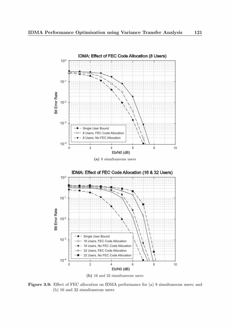
IDMA Performance Optimisation using Variance Transfer Analysis 121
Bit E
rror
Rate
10-3
10-2
10-1
100
IDMA: Effect of FEC Code Allocation (8 Users)
Eb/N0 (dB)
10-4
0 2 4 6 8 10
Single User Bound
8 Users, FEC Code Allocation
8 Users, No FEC Allocation
(a) 8 simultaneous users
Bit E
rror
Rate
10-3
10-2
10-1
100
IDMA: Effect of FEC Code Allocation (16 & 32 Users)
Eb/N0 (dB)
10-4
0 2 4 6 8 10
Single User Bound
16 Users, FEC Code Allocation
16 Users, No FEC Code Allocation
32 Users, FEC Code Allocation
32 Users, No FEC Code Allocation
(b) 16 and 32 simultaneous users
Figure 3.9: Effect of FEC allocation on IDMA performance for (a) 8 simultaneous users; and(b) 16 and 32 simultaneous users

IDMA Performance Optimisation using Variance Transfer Analysis 122
developed to achieve optimal system performance. Two multiuser system scenarios were
considered for optimisation.
First, a multi-rate multiuser scheme using the layered-IDMA with power allocation
was presented and compared with a layered scheme without power allocation (equal
power). The layered IDMA scheme with power allocation was shown to provide superior
performance at moderate and high SNR levels while using the same low-complexity
iterative decoding receiver structure as the other IDMA schemes. In a Rayleigh flat-
fading environment, simulation results show that for Eb/N0 values of 6dB and greater,
the performance of layered IDMA system with power allocation is within 0.5dB of the
single user bound.
Second, an IDMA multiuser scheme employing FEC code allocation for dynamic
loads was presented and compared with a IDMA scheme without FEC code allocation
(all users employ the same FEC code). The IDMA scheme with FEC code allocation was
shown to provide superior performance at moderate and high SNR levels while using the
same low complexity iterative decoding receiver structure as the other IDMA schemes.
In a Rayleigh flat-fading environment, simulation results show that for Eb/N0 values of
6.5dB and greater, the performance of the IDMA system with FEC code allocation and
32 simultaneous users is within 0.7dB of the single user bound.

Chapter 4
Optimal Space-Time Coding using the
Golden Code
In recent years, multiple antenna systems (commonly referred to as multi-input multi-
output or MIMO systems) have proven to be an effective method for realising high-rate
reliable wireless communications. Research in MIMO systems has generally focused on
providing either higher-rate or increased diversity over traditional single antenna (SISO)
systems.
Foschini [30] introduced the layered space-time (BLAST) architecture where a high
throughput rate is achieved by using multiple transmit antennas to transmit multiple
independent data sub-streams in parallel. Multiple receive antennas and multi-user
detection algorithms are used at the receiver end to separate and decode the individual
sub-streams. Although providing high-rate, BLAST has the shortcoming that it does not
provide diversity gain as each data symbol is only transmitted once from one antenna.
Alamouti [3] introduced a simple orthogonal space time block code (STBC) that
provided diversity gain for 2× 1 and 2× 2 multi-antenna systems. This scheme was
generalised and extended by Tarokh et. al. [113] to include higher-dimension MIMO
systems, using real and complex orthogonal STBCs. Although providing diversity gain,
orthogonal STBCs have the shortcoming that (with the exception of a few sporadic
codes) the coding rate does not exceed 1/2.
A generalised class of space-time codes that encompassed both orthogonal STBCs and
BLAST architectures was proposed by Hassibi and Hochwald [39]. This generalised class
of codes, which are known as linear dispersion (LD) codes, are defined as codes that break
up the input data stream into sub-streams that are dispersed in linear combinations over
123

Optimal Space-Time Coding using the Golden Code 124
space and time. Theoretically, LD codes can provide both diversity gain and high-rate.
In general, LD codes can outperform their orthogonal STBC and BLAST sub-classes.
Sethuraman et. al. [105] proposed a methodology for designing full-diversity high-rate
LD codes using cyclic division algebras. A division algebra is used to provide a structured
set of invertible matrices to construct LD space-time codes. Using this technique, Belfiore
et. al. [7] developed the Golden Code, a 2× 2 LD code that provides both diversity gain
and full-rate.
In the first part of this chapter, we investigate the effect of Doppler spread on the
performance of the 2× 2 Golden Code single-user system. Doppler spread is a measure of
spectral broadening caused by the relative motion between the transmitter and receiver
antennas or by the movement of reflecting objects in the channel. Doppler spread is an
important consideration in the design of mobile communication systems.
The decoding methodology for the Golden code is presented, followed by performance
comparisons with the Alamouti code and V-BLAST in Rayleigh fading environments
with Doppler spread. Simulation results show that the Golden Code outperforms both
the Alamouti code and V-BLAST at high SNR levels. For a symbol error rate of 10−4
the Eb/N0 requirement for the Golden code is 5dB less than the Alamouti code and
V-BLAST. This original contribution was published in [60].
The second part of this chapter considers the multiuser case, and we develop a MIMO
framework for IDMA that can provide both diversity gain and high-rate.
Recently multiuser MIMO-IDMA has been proposed [81], where IDMA has been
generalised to multiple antenna systems where users employ V-BLAST (vertical-encoded
layered space time) spatial multiplexing to achieve higher data rates. Decoding is still
performed by an iterative receiver whose complexity is linear in the number of users. We
further extend the MIMO-IDMA concept from IDMA with V-BLAST spatial multiplexing
to IDMA with linear dispersion (LD) codes.
In particular, we investigate the performance of the MIMO-IDMA using the Golden
Code. The Golden Code (GC), is 2× 2 LD code derived from cyclic division algebra
that provides both diversity gain and full-rate [7]. We compare the performance of this
GC-IDMA scheme against MIMO-IDMA schemes employing the Alamouti code and
V-BLAST, and also against the single-user bound. In a Rayleigh flat-fading environment,
simulation results show that GC-IDMA outperforms both Alamouti- and V-BLAST-
IDMA at moderate and high SNR levels. For signal to noise ratios of 8dB and greater,
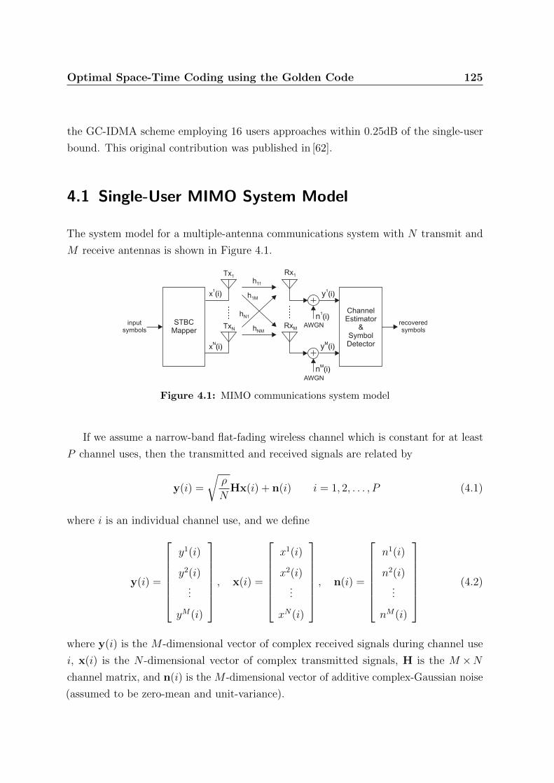
Optimal Space-Time Coding using the Golden Code 125
the GC-IDMA scheme employing 16 users approaches within 0.25dB of the single-user
bound. This original contribution was published in [62].
4.1 Single-User MIMO System Model
The system model for a multiple-antenna communications system with N transmit and
M receive antennas is shown in Figure 4.1.
Tx1
STBCMapper
TxN
inputsymbols
h11
hNM
Rx1
RxM
hN1
h1M
recoveredsymbols
ChannelEstimator
&SymbolDetectorx
N(i)
y1(i)
nM(i)
AWGN
AWGN
x1(i)
yM(i)
n1(i)
Figure 4.1: MIMO communications system model
If we assume a narrow-band flat-fading wireless channel which is constant for at least
P channel uses, then the transmitted and received signals are related by
y(i) =
√ρ
NHx(i) + n(i) i = 1, 2, . . . , P (4.1)
where i is an individual channel use, and we define
y(i) =
y1(i)
y2(i)...
yM(i)
, x(i) =
x1(i)
x2(i)...
xN(i)
, n(i) =
n1(i)
n2(i)...
nM(i)
(4.2)
where y(i) is the M -dimensional vector of complex received signals during channel use
i, x(i) is the N -dimensional vector of complex transmitted signals, H is the M ×Nchannel matrix, and n(i) is the M -dimensional vector of additive complex-Gaussian noise
(assumed to be zero-mean and unit-variance).
Optimal Space-Time Coding using the Golden Code 126
If we assume that H, x(τ) and n(τ) are random and independent quantities, the
signal power normalisation√ρ/N ensures that ρ is the signal-to-noise ratio (SNR) at
each receive antenna, independently of N . It is assumed that the channel matrix is
known by the receiver.
We define the matrices Y, X, and V as:
Y =
yT (1)
yT (2)...
yT (P )
, X =
xT (1)
xT (2)...
xT (P )
, V =
nT (1)
nT (2)...
nT (P )
where the superscript T denotes transpose. Equation (4.1) is usually more convenient in
its transposed form, i.e.,
Y =
√ρ
NXH + V (4.3)
where the transpose notation is omitted from H, and the channel matrix is simply
redefined to have dimension N ×M . Y is the P ×M received signal matrix, X is the
P ×N transmitted signal matrix, and n is the P ×M additive noise matrix. In matrices
Y, X, and V, time runs vertically and space runs horizontally.
4.2 Space-Time Coding and Linear Dispersion Codes
A space-time block code (STBC) is defined by a (P ×N) code matrix X, where N
denotes the number of transmit antennas or the spatial transmitter diversity order, and P
denotes the number of channel usages for transmitting a STBC codeword or the temporal
transmitter diversity order [113].
The STBC encoder takes as input a code vector, x, and transmits each row of symbols
as specified in X at P consecutive channel usages. At each channel usage, the symbols
contained in the N -dimensional row vector of X are transmitted through N transmitter
antennas simultaneously.
Optimal Space-Time Coding using the Golden Code 127
As an example, consider the 2× 2 Alamouti STBC (ie., P = 2, N = 2). The Alamouti
STBC matrix X is defined by
X =
x(1) x(2)
−x∗(2) x∗(1)
(4.4)
where ( · )∗ denotes the complex conjugate operation. The input to this STBC is the
code vector x = [x(1), x(2) ]T . During the first channel use, the two symbols of the top
row of X, [x(1), x(2) ], are transmitted simultaneously from the two transmit antennas;
and during the second channel use, the symbols in the second row of X, [−x∗(2), x∗(1) ],
are transmitted.
A Linear Dispersion (LD) code is a general class of space time block code (STBC)
that breaks up the input data stream into sub-streams that are dispersed in linear
combinations over space and time. Specifically, a linear dispersion code is defined as:
X =
Q∑q=1
(xqCq + x∗qD
q) (4.5)
where the data sequence is broken up into Q sub-streams, x1, . . . , xQ are complex symbols
from an arbitrary constellation (typically r-PSK or r-QAM), and Cq and Dq are fixed
P ×N complex matrices. The code is completely determined by the set of dispersion
matrices Cq, Dq.
It is generally more convenient to decompose the complex scalar xq into its real and
imaginary components
xq = αq + jβq, q = 1, . . . , Q (4.6)
The LD code can then be redefined in terms of real and imaginary components as follows:
X =
Q∑q=1
(αqAq + jβqB
q) (4.7)
where Aq = Cq + Dq and Bq = Cq − Dq. The dispersion matrices Aq, Bq also
completely specify the code. LD codes include many commonly used ST codes including
the Alamouti Scheme and V-BLAST (Vertical-encoding spatial multiplexing).
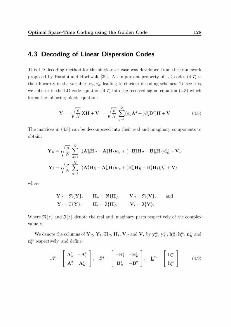
Optimal Space-Time Coding using the Golden Code 128
4.3 Decoding of Linear Dispersion Codes
This LD decoding method for the single-user case was developed from the framework
proposed by Hassibi and Hochwald [39]. An important property of LD codes (4.7) is
their linearity in the variables αq, βq, leading to efficient decoding schemes. To see this,
we substitute the LD code equation (4.7) into the received signal equation (4.3) which
forms the following block equation:
Y =
√ρ
NXH + V =
√ρ
N
Q∑q=1
(αqAq + jβqB
q)H + V (4.8)
The matrices in (4.8) can be decomposed into their real and imaginary components to
obtain:
YR =
√ρ
N
Q∑q=1
[(AqRHR −Aq
IHI)αq + (−BqIHR −Bq
RHI)βq] + VR
YI =
√ρ
N
Q∑q=1
[(AqIHR −Aq
RHI)αq + (BqRHR −Bq
IHI)βq] + VI
where
YR = RY, HR = RH, VR = RV, and
YI = IY, HI = IH, VI = IV.
Where Rz and Iz denote the real and imaginary parts respectively of the complex
value z.
We denote the columns of YR, YI , HR, HI , VR and VI by ymR , ymI , hmR , hmI , nmR and
nmI respectively, and define:
Aq =
AqR −Aq
I
AqI Aq
R
, Bq =
−BqI −Bq
R
BqR −Bq
I
, hm =
hmR
hmI
(4.9)
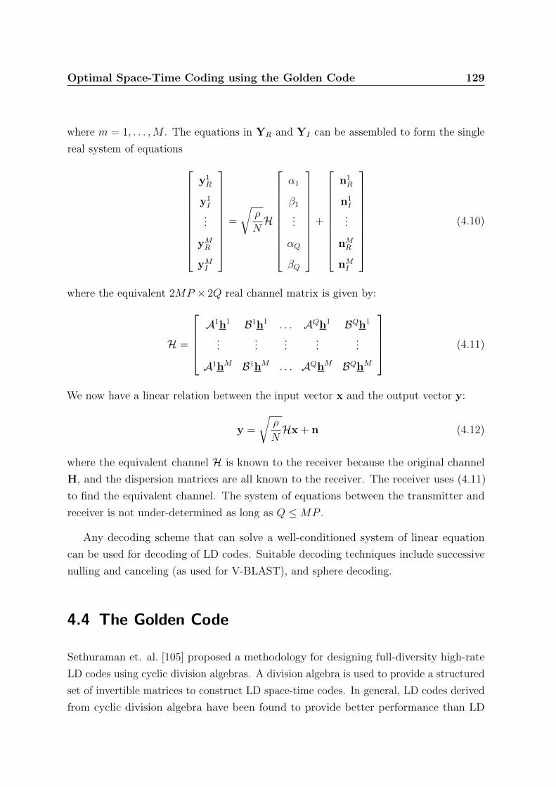
Optimal Space-Time Coding using the Golden Code 129
where m = 1, . . . ,M . The equations in YR and YI can be assembled to form the single
real system of equations
y1R
y1I
...
yMR
yMI
=
√ρ
NH
α1
β1
...
αQ
βQ
+
n1R
n1I
...
nMR
nMI
(4.10)
where the equivalent 2MP × 2Q real channel matrix is given by:
H =
A1h1 B1h1 . . . AQh1 BQh1
......
......
...
A1hM B1hM . . . AQhM BQhM
(4.11)
We now have a linear relation between the input vector x and the output vector y:
y =
√ρ
NHx + n (4.12)
where the equivalent channel H is known to the receiver because the original channel
H, and the dispersion matrices are all known to the receiver. The receiver uses (4.11)
to find the equivalent channel. The system of equations between the transmitter and
receiver is not under-determined as long as Q ≤MP .
Any decoding scheme that can solve a well-conditioned system of linear equation
can be used for decoding of LD codes. Suitable decoding techniques include successive
nulling and canceling (as used for V-BLAST), and sphere decoding.
4.4 The Golden Code
Sethuraman et. al. [105] proposed a methodology for designing full-diversity high-rate
LD codes using cyclic division algebras. A division algebra is used to provide a structured
set of invertible matrices to construct LD space-time codes. In general, LD codes derived
from cyclic division algebra have been found to provide better performance than LD

Optimal Space-Time Coding using the Golden Code 130
0.5 1.0 1.5 2.0
Diversity-Multiplexing Gain Tradeoff (M=2, N=2)
Spatial Multiplexing Gain, r = R / log(SNR)
0.0
2.0
1.0
3.0
0.0
4.0
Alamouti Code
V-BLAST (OSIC Decoding)
Golden Code (= Optimal)
Div
ers
ity G
ain
, d(r
)
Figure 4.2: Diversity-Multiplexing Gain Tradeoff (M=2, N=2) [142] [83]
codes derived using the original information theoretic approach proposed by Hassibi and
Hochwald [39].
The Golden Code is a full-rate 2× 2 LD code and is defined as subset of the cyclic
division algebra (Q(i,√
5), i) with centre Q(i) [7]. The 2× 2 Golden Code has the
structure:
X =1√5
αx(1) + x(2)θ αx(3) + x(4)θ
jαx(3) + x(4)θ αx(1) + x(2)θ
(4.13)
where
θ =1 +√
5
2, θ =
1−√
5
2= (1− θ), α = j(1− θ), α = 1 + j(1− θ)
and j =√−1. In[114], Tarokh et. al. defined the rank criterion and determinant criterion
for designing ST codes. Oggier et. al. [82] extended this design criteria to include: (a) full
rate; (b) full diversity; (c) non-vanishing determinant for increasing spectral efficiency;
(d) good shaping of the constellation; and (e) uniform average transmitted energy per
antenna. ST Codes that meet all of these criteria are termed perfect space-time block
Optimal Space-Time Coding using the Golden Code 131
codes. The Golden Code has been found to be the best perfect code for MIMO systems
with 2 transmit and 2 or more receive antennas.
Elia et. al. [25] have shown that the Golden code achieves the optimal diversity-
multiplexing tradeoff for a 2× 2 MIMO system. Zheng and Tse [142] developed a
simple characterisation of the optimal tradeoff between diversity and degrees of freedom
(multiplexing gain), and then used it to evaluate the performance of existing multiple
antenna schemes. The concept is that for a given MIMO channel, both diversity and
multiplexing gain can be simultaneously obtained, but there is a fundamental tradeoff
between how much of each type of gain any coding scheme achieve. For example, for a
particular coding scheme, increased spatial multiplexing gain comes at the cost of reduced
diversity gain. Figure 4.2 uses Zheng’s and Tse’s method to compare the Alamouti
STBC, V-BLAST and the Golden Code STBC.
From Figure 4.2 we see that neither the Alamouti STBC nor V-BLAST are optimal.
The Alamouti STBC does not provide full spatial-multiplexing gain, while V-BLAST
does not provide full diversity gain. The Golden Code however provides both the full
spatial-muliplexing gain and the full diversity gain available for a 2× 2 system.
4.5 Single-User System Performance
The simulations assume the receiver has perfect channel knowledge. The individual
channels in the channel matrix are uncorrelated, and the system does not use error
correction coding. The constellations of each of the coding schemes has been chosen to
ensure a common spectral efficiency of 8-bits per channel use. The V-BLAST and Golden
code simulations both use 16-QAM constellations, while the Alamouti code simulations
use 256-QAM (the higher-order constellation is required to compensate for the absence
of spatial multiplexing gain).
In Figure 4.3 we compare the performance of the Golden Code STBC against the
Alamouti code and V-BLAST in a Rayleigh flat-fading environment. The figure shows
the superior performance of the Golden code, particularly at higher SNR values. For a
symbol error rate of 10−4 the Eb/N0 requirement for the Golden code is 5dB less than
the Alamouti code and V-BLAST.
Figure 4.4a compares the performance of the Golden code over a range of Doppler
frequencies that would be typical in mobile communications scenarios. We observe

Optimal Space-Time Coding using the Golden Code 132
Eb/N0 (dB)
Bit E
rror
Rate
10-4
10-3
10-2
10-1
100
STBC Performance in Rayleigh Flat-Fading Channel
0 5 10 15 20 25 30
Alamouti Code
V-BLAST
Golden Code
Figure 4.3: Alamouti, V-BLAST and Golden Code Performance (M=2, N=2)
a performance degradation of approximately 2dB for every 5Hz increase in Doppler
frequency.
Figure 4.4b compares the Golden code performance against the Alamouti code at
selected Doppler frequencies. The performance degradation of approximately 2dB for
every 5Hz increase in Doppler frequency previously observed with the Golden code is also
observe with the Alamouti code. The 5dB performance advantage at high SNR levels of
the Golden code compared to the Alamouti code is maintained over the range of Doppler
frequencies investigated.
4.6 Multiuser MIMO System Model
4.6.1 Multiuser Transmitter Structure
Figure 4.5 shows the transmitter structure of the multiple-access IDMA scheme with
K simultaneous users. The input data sequence dk[i]i of user-k is encoded by the
FEC encoder generating a coded sequence ck[i]J−1i=0 , where J is the frame length. Then
ck[i]J−1i=0 is permutated by the interleaver πk, producing bk[i]J−1
i=0 . IDMA users are
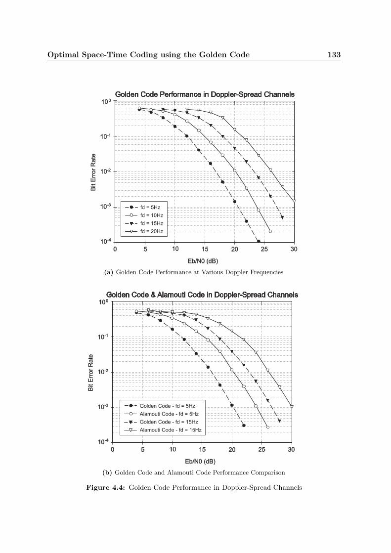
Optimal Space-Time Coding using the Golden Code 133
Eb/N0 (dB)
Bit E
rror
Rate
10-4
10-3
10-2
10-1
100
Golden Code Performance in Doppler-Spread Channels
0 5 10 15 20 25 30
fd = 5Hz
fd = 10Hz
fd = 15Hz
fd = 20Hz
(a) Golden Code Performance at Various Doppler Frequencies
Bit E
rror
Rate
10-3
10-2
10-1
100
Golden Code & Alamouti Code in Doppler-Spread Channels
Eb/N0 (dB)
10-4
0 5 10 15 20 25 30
Golden Code - fd = 5Hz
Alamouti Code - fd = 5Hz
Golden Code - fd = 15Hz
Alamouti Code - fd = 15Hz
(b) Golden Code and Alamouti Code Performance Comparison
Figure 4.4: Golden Code Performance in Doppler-Spread Channels
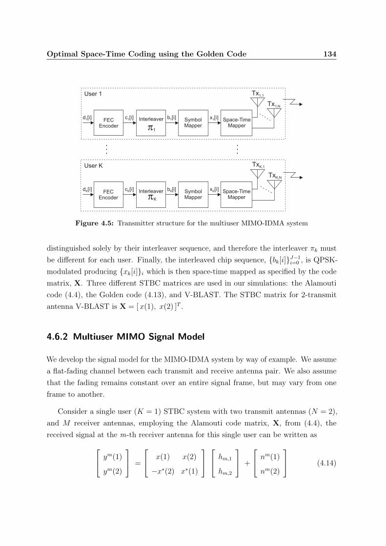
Optimal Space-Time Coding using the Golden Code 134
Interleaver
b [i]KInterleaver
FECEncoder
FECEncoder
d [i]1
d [i]K
TxK,1
TxK,N
Space-TimeMapper
Space-TimeMapper
Tx1,1
Tx1,N
b [i]1
p1
pK
User 1
User K
c [i]1
c [i]K
x [i]1SymbolMapper
x [i]KSymbolMapper
Figure 4.5: Transmitter structure for the multiuser MIMO-IDMA system
distinguished solely by their interleaver sequence, and therefore the interleaver πk must
be different for each user. Finally, the interleaved chip sequence, bk[i]J−1i=0 , is QPSK-
modulated producing xk[i]i which is then space-time mapped as specified by the code
matrix, X. Three different STBC matrices are used in our simulations: the Alamouti
code (4.4), the Golden code (4.13), and V-BLAST. The STBC matrix for 2-transmit
antenna V-BLAST is X = [x(1), x(2) ]T .
4.6.2 Multiuser MIMO Signal Model
We develop the signal model for the MIMO-IDMA system by way of example. We assume
a flat-fading channel between each transmit and receive antenna pair. We also assume
that the fading remains constant over an entire signal frame, but may vary from one
frame to another.
Consider a single user (K = 1) STBC system with two transmit antennas (N = 2),
and M receiver antennas, employing the Alamouti code matrix, X, from (4.4), the
received signal at the m-th receiver antenna for this single user can be written as ym(1)
ym(2)
=
x(1) x(2)
−x∗(2) x∗(1)
hm,1
hm,2
+
nm(1)
nm(2)
(4.14)
Optimal Space-Time Coding using the Golden Code 135
where ym(p) is the received signal vector from channel usage p, hm,n is the complex
fading gain from the n-th transmitter antenna to the m-th receiver antenna, nm(p) is
the additive Gaussian noise samples from channel usage p, and m = 1, 2, . . . ,M .
Combining the channel matrix with the STBC code matrix X, (and conjugating ym[2]
to simplify notation), (4.14) can be written in the following alternative form
ym = Hm1 x1 + nm (4.15)
where m = 1, 2, . . . ,M and we define
ym =
ym(1)
ym(2)∗
, Hm1 =
hm,1 hm,2
hm,2 hm,1
, x1 =
x(1)
x(2)
, and nm =
nm(1)
nm(2)∗
We see that Hm
1 combines information of the channel response related to the m-th receiver
antenna and the code constraint of the STBC, X.
By stacking the ym vectors from (4.15) for all M receiver antennas, the following
signal model is obtained
y =
y1
y2
...
yM
=
H1
1
H21
...
HM1
x(1)
x(2)
+
n1
n2
...
nM
(4.16)
We now consider the multiuser case of a STBC system with K users, each employing
N transmitter antennas. At the receiver, M receiver antennas are employed. In this case,
the received signal can be written asy1
y2
...
yM
=[
H1, H2, . . . , HK
]
x1
x2
...
xK
+
n1
n2
...
nM
(4.17)
where ym , [ ym(1), ym(2), . . . , ym(P ) ]T , m = 1, 2, . . . ,M , and contains the received
signal vectors from channel usages 1 to P , at the m-th antenna; Hk, k = 1, 2, . . . , K is

Optimal Space-Time Coding using the Golden Code 136
the channel response matrix for the kth user; xk , [xk(1), xk(2), . . . , xk(N) ]T is the code
vector for the k -th user; and nm , [nm(1), nm(2), . . . , nm(P ) ]T contains the additive
Gaussian noise samples from channel usages 1 to P at the m-th receiver antenna.
In addition to the Alamouti code, we use this same methodology to develop signal
models for the Golden code and V-BLAST. For the Golden code case, signal vectors are
separated into their real and imaginary components. This method was first developed in
[79] and [67].
4.6.3 Multiuser Iterative Receiver Structure
l1(b )1[i]
SoftMIMO
MultiuserDetector(MUD)
Soft FECChannelDecoder(DEC)Interleaver
De-Interleaver
user1
d [i]1
userK
d [i]K
p1-1
p1
Soft FECChannelDecoder(DEC)Interleaver
De-Interleaver
pK-1
pK
L2(c [i])1
l1(c )1[i]
l2(c )1[i]
L1(b [i])1
l2(b )1[i]
L1(b [i])K
l2(b )K[i]
l1(b )K[i]
l2(c )K[i] L2(c [i])K
l1(c )K[i]
Rx1
RxM
Figure 4.6: Receiver structure for the multiuser MIMO-IDMA system
The iterative receiver structure for the MIMO IDMA system is shown in Figure 4.6.
It consists of a soft-output multiuser detector (MUD) and K single users a posteriori
probability decoders (DECs). The two stages are separated by interleavers and deinter-
leavers. The soft-output MUD takes as input the received signals from the M receiver
antennas and the interleaved extrinsic log likelihood ratios (LLRs) of the code bits of all
users (which are fed back by the K single-user DECs), and computes as the output the a
posteriori LLRs of the code bits of all users. The DEC of kth users takes as input the
deinterleaved extrinsic LLRs of the code bits from the soft-output MUD and computes
as output the a posteriori LLRs of the code bits, as well as the LLRs of the information
bits.
At a given iteration, the MUD estimates the a posteriori LLRs of the code bits, i.e.,
Λ1(bk[i]) , logP (bk[i] = 1 | y)
P (bk[i] = 0 | y), i = 0, . . . , J − 1, k = 1, . . . , K (4.18)

Optimal Space-Time Coding using the Golden Code 137
where y denotes the received vectors from all M antennas. With Bayes’ rule, (4.18) can
be rewritten as
Λ1(bk[i]) = logP (y | bk[i] = 1)
P (y | bk[i] = 0)︸ ︷︷ ︸λ1(bk[i])
+ logP (bk[i] = 1)
P (bk[i] = 0)︸ ︷︷ ︸λ2(bk[i])
(4.19)
The first term in (4.19), denoted by λ1(bk[i]), is the extrinsic information calculated by
the MUD. The second term, denoted by λ2(bk[i]), is the a priori information (in LLR
form) of bk(i). An estimate of the a priori LLR is calculated by the DEC of the k -th
user at the previous iteration. At the first iteration, no prior information about the
code bits is available, therefore all bit values are assumed equiprobable and the a priori
LLR values are set to zero. Finally, the sequence of extrinsic information, λ1(bk(i))i, is
deinterleaved by the deinterleaver of the k -th user (producing λ1(ck(i))i) and fed into
the corresponding DEC as a priori information for the next iteration.
The channel decoder for the k -th user estimates the a posteriori probabilities (in LLR
form) of the code bits, i.e.,
Λ2(ck[i]) , logP (ck[i] = 1 | λ1(ck[i])i ; code structure )
P (ck[i] = 0 | λ1(ck[i])i ; code structure ), (4.20)
= λ2(ck[i]) + λ1(ck[i]).
These a posteriori probabilities are computed using the BCJR algorithm [6] based on the
a priori information from the MUD, λ1(ck[i]), and knowledge of the code structure.
Additionally, the DEC estimates the a posteriori LLRs of the information bits, Λ2(dk[i]),and at the final iteration, performs a hard decision on the information bits, producing
dk[i]).
4.7 Soft Multiuser Detector (MUD)
The MUD operation is now described in more detail. The MUD is developed largely
from the concepts described in [67].
First, the soft estimate xk(i) of the k -th users i -th code symbol xk(i) is calculated by
xk(i) , Exk(i) =∑x∈X
xP (xk(i) = x) (4.21)

Optimal Space-Time Coding using the Golden Code 138
where X is the set of possible code symbols. At first iteration, all code symbols are
assumed to be equiprobable. In subsequent iterations, the probability P (xk(i) = x) is
computed from the extrinsic information provided by the DEC.
For our multi-user system, where each user employs multiple transmit antennas, we
use the concept of treating each transmit antenna as a virtual user. Therefore, for a
system with K -users, where each user employs N transmit antennas, there are (NK)
virtual users in the system. We define an (NK)-dimensional soft code vector
x , [ xT1 , xT2 , . . . , xTK ]T
= [ x1(1), . . . , x1(N), x2(1), . . . , x2(N), . . . , xK(1), . . . , xK(n) ]T (4.22)
where every element in x as a virtual user. We use the notation k(i) to index a virtual
user, and define
xk(i) , x− xk(i)ek(i) (4.23)
where ek(i) is an (NK)-vector of all zeros, except for the “1” value in the vector element
corresponding to the k(i)-th virtual user. That is, xk(i) is obtained from x by setting
the k(i)−th element to zero.
Subtracting the soft estimate of the interfering signals of the other virtual users from
the received signal y, we get
yk(i) , y −Hxk(i) = H[x− xk(i)] + n (4.24)
In order to further suppress the residual interference in yk(i), we apply an instantaneous
linear minimum mean square error (MMSE) filter to yk(i). The linear MMSE weight
vector wk(i) is chosen to minimise the mean square error between the transmitted symbol
xk(i) and the filter output xk(i) , wHk (i)xk(i), (where ( · )H denotes the Hermitian
transpose operation), hence
wk(i) = arg minw∈CMP
E‖xk(i)−wHyk(i)‖2
= E
yk(i)y
Hk (i)
−1E x∗k(i)yk(i) (4.25)
Optimal Space-Time Coding using the Golden Code 139
Using (4.24) and assuming that the symbol xk(i) is of unit energy, ie., ‖xk(i)‖2 = 1 and
EnnH = σ2I, where I is the identity matrix, we have
Ex∗k(i)yk(i) = HE x∗k(i)[x− xk(i)] = Hek(i) (4.26)
Eyk(i)yHk (i) = HVk(i)HH + σ2I (4.27)
with
Vk(i) , Covx− xk(j)
= diag 1− ‖x1(1)‖2, . . . , 1− ‖x1(N)‖2, . . . ,
1− ‖xk(i− 1)‖2, 1, 1− ‖xk(i+ 1)‖2,
. . . , 1− ‖xK(1)‖2, . . . , 1− ‖xK(N)‖2
(4.28)
Using equations (4.25) to (4.28), the instantaneous MMSE estimate for xk(i) is given by
xk(i) , wHk (i)yk(i)
= eTk (i)HH[HVk(i)H
H + σ2I]−1
yk(i) (4.29)
The instantaneous MMSE filter can be modeled by an equivalent additive white Gaussian
noise channel (with µk(i) mean and v2k(i) variance) having xk(i) as its input symbol. The
output of this filter can then be written as
xk(i) = µk(i)xk(i) + ηk(i) (4.30)
with
µk(i) , Exk(i)x∗k(i)
=
HH[HVk(i)H
H + σ2I]−1
Hk,k
(4.31)
and
v2k(i) , Varxk(i) = µk(j)xk(i)− µ2
k(i) (4.32)
where · j,k denotes the matrix element at the j -th row and k -th column. Equations
(4.30) to (4.32) give the probability distribution of the code symbol xk(i), which is used
to calculate the a posteriori probability of the code bits.
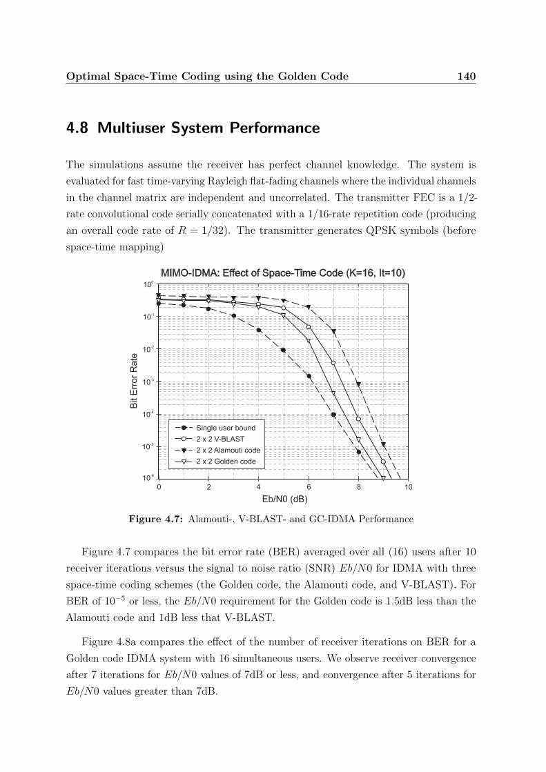
Optimal Space-Time Coding using the Golden Code 140
4.8 Multiuser System Performance
The simulations assume the receiver has perfect channel knowledge. The system is
evaluated for fast time-varying Rayleigh flat-fading channels where the individual channels
in the channel matrix are independent and uncorrelated. The transmitter FEC is a 1/2-
rate convolutional code serially concatenated with a 1/16-rate repetition code (producing
an overall code rate of R = 1/32). The transmitter generates QPSK symbols (before
space-time mapping)
0 2 4 6 8 10
Eb/N0 (dB)
MIMO-IDMA: Effect of Space-Time Code (K=16, It=10)
Bit E
rror
Rate
10-1
10-2
10-3
10-5
10-6
100
10-4
Single user bound
2 x 2 V-BLAST
2 x 2 Alamouti code
2 x 2 Golden code
Figure 4.7: Alamouti-, V-BLAST- and GC-IDMA Performance
Figure 4.7 compares the bit error rate (BER) averaged over all (16) users after 10
receiver iterations versus the signal to noise ratio (SNR) Eb/N0 for IDMA with three
space-time coding schemes (the Golden code, the Alamouti code, and V-BLAST). For
BER of 10−5 or less, the Eb/N0 requirement for the Golden code is 1.5dB less than the
Alamouti code and 1dB less that V-BLAST.
Figure 4.8a compares the effect of the number of receiver iterations on BER for a
Golden code IDMA system with 16 simultaneous users. We observe receiver convergence
after 7 iterations for Eb/N0 values of 7dB or less, and convergence after 5 iterations for
Eb/N0 values greater than 7dB.

Optimal Space-Time Coding using the Golden Code 141
0 2 4 6 8 10
Eb/N0 (dB)
GC-IDMA: Effect of No. of Receiver Iterations (K=16)B
it E
rror
Rate
10-1
10-2
10-3
10-5
10-6
100
10-4
3 Iterations
4 Iterations
5 Iterations
7 Iterations
10 Iterations
(a) Effect of Number of Receiver Iterations
0 2 4 6 8 10
Eb/N0 (dB)
GC-IDMA: Effect of No. of Simultaneous Users (It=10)
Bit E
rror
Rate
10-1
10-2
10-3
10-5
10-6
100
10-4
4 Users
8 Users
16 Users
24 Users
32 Users
(b) Effect of Number of Simultaneous Users
Figure 4.8: GC-IDMA Performance for a) Various Number of Receiver Iterations; and b)Various Numbers of Users
Optimal Space-Time Coding using the Golden Code 142
Figure 4.8b compares the effect of the number of simultaneous users on the BER for
Golden Code IDMA. The performance is shown for 10 receiver iterations. We observe
almost identical performance for 1, 8 and 16 user systems over the simulated Eb/N0
range of 0dB to 10dB. For 24 and 32 user systems, we observe a slight degradation in
performance (compared to 16-users) of up to 1dB and 0.5dB for 24 and 32 user systems
respectively for Eb/N0 values of 5 to 7dB. For Eb/N0 values of 7dB and greater, the
performance of 24 and 32 user systems is almost identical to the 1, 8 and 16 user systems.
4.9 Conclusion
In this chapter, the Golden Code—an optimal linear-dispersion (LD) code providing
both diversity gain and full-rate—was presented.
First, the single-user case was considered and the performance of the Golden Code
was been presented and compared with common multiple-antenna systems, namely the
Alamouti code and V-BLAST (spatial multiplexing). The Golden Code was shown to
provide superior performance at high-SNR levels while using the same low-complexity
linear dispersion code decoding schemes typically used to decode Alamouti and V-BLAST
schemes.
Simulation results of a single-user MIMO system using the Golden Code at various
Doppler frequencies were presented. These results showed that the Golden Code maintains
its superior performance when compared to the Alamouti scheme over the range of Doppler
frequencies that would typically be encountered in a mobile communications system. For
a symbol error rate of 10−4 the Eb/N0 requirement for the Golden code is 5dB less than
the Alamouti code and V-BLAST.
Next, the multiuser case was considered and a MIMO framework for incorporating
LD codes into an IDMA multiple-access scheme was developed. The performance of
the 2× 2 MIMO-IDMA multiuser scheme using the Golden Code (GC-IDMA) was then
presented and compared with other 2× 2 MIMO-IDMA schemes using the Alamouti code
and V-BLAST space-time codes. GC-IDMA was shown to provide superior performance
at moderate and high SNR levels while using the same low-complexity iterative decoding
receiver structure as the other MIMO-IDMA schemes.
In a Rayleigh flat-fading environment, simulation results show that GC-IDMA out-
performs Alamouti and V-BLAST IDMA at moderate and high SNR levels. For bit

Optimal Space-Time Coding using the Golden Code 143
error rate of 10−5 or less, the Eb/N0 requirement for the GC-IDMA is 1dB less than
the Alamouti-IDMA and V-BLAST-IDMA. Simulation results showing the effect of the
number of simultaneous users and the effect of the number of receiver iterations on
GC-IDMA performance were also presented.
Chapter 5
Multiuser Detection for Delay-Spread
Underwater Acoustic Channels
Underwater sensor networks enable a broad range of applications including environmental
monitoring, undersea exploration, assisted navigation, and distributed surveillance [2]. A
robust and efficient communications scheme between the underwater network nodes is
an essential foundation for reliable high-performance sensor networks.
The shallow water acoustic channel is an exceptionally difficult medium for data
transmission, and developing reliable communications systems for this environment has
proved to be very challenging. One of the main channel impairments is multipath
interference caused by multiple reflections of the acoustic signal from the water surface
and bottom. These reflections occur at small grazing angles and with small reflection
losses. This effect causes both long time-delay spread and large multipath amplitudes to
be present in the received signal [51].
Over the past decade, CDMA has been successfully employed as the modulation
scheme for shallow water networks [15] [119] [111]. Spread-spectrum schemes, such
as CDMA, employ a transmission bandwidth that is considerably greater than the
information rate. Utilization of the bandwidth in this manner introduces a number
of benefits, including multiple-access interference suppression capability and improved
immunity against multipath effects.
Unfortunately, the long time-delay spreads that are typical for shallow water acoustic
channels cause severe inter-symbol interference (ISI). This ISI degrades the performance
of many CDMA receiver detection schemes. Multi-carrier modulation (MCM) is an
attractive alternative because it is particularly resilient to long time-delay spreads.
144

Multiuser Detection for Delay-Spread Underwater Acoustic Channels 145
The basic principle of MCM is to split a high-rate data stream into a number of
lower-rate streams that are transmitted simultaneously over a number of sub-carriers.
This significantly reduces the ISI span because the lower-rate parallel sub-carriers have
increased symbol duration [126].
In [75], Orthogonal Frequency Division Multiplexing (OFDM), a low-complexity
spectrally-efficient MCM technique, was combined with an IDMA overlay to develop
a multiple-access scheme for multi-path fading channels. In this chapter we develop
an OFDM-IDMA scheme that provides robust performance in the presence of large
time-delay spread and the other impairments presented by the shallow water acoustic
channel. The proposed scheme utilises a low-complexity iterative decoding algorithm
based on the turbo-decoding concept [12].
The performance of the proposed OFMD-IDMA scheme is compared against other
shallow water communication schemes, including single-carrier CDMA, single-carrier
IDMA. Using ray-trace underwater channel models combined with noise models of
commonly occurring oceanic noise phenomena, simulations of multiple-access sensor
network systems are performed to assess the overall performance of the different schemes.
A Multiple-Input Multiple-Output (MIMO) extension to the OFDM-IDMA scheme
is also investigated, where each transmitter and receiver use multiple transmitting and
receiving elements respectively. This MIMO concept is used to exploit the multi-path
nature of the underwater channel to provide improved performance in the form of either
increased data robustness or increased data throughput.
Simulations of various underwater acoustic sensor network scenarios show that the
OFDM-IDMA scheme consistently outperforms other common multiple-access schemes
in the shallow water environment. The work in this chapter was published in [61] and
[64].
5.1 Channel Model
Acoustic signals transmitted in shallow water are corrupted by interference from reflection
and scattering at the water surface and bottom. For this reason, the shallow water
channel is a difficult medium in which to achieve the high data rates needed for many
applications. An especially difficult problem is that the acoustic signal transmitted over
a shallow water channel has associated with it inherently small grazing angles and small

Multiuser Detection for Delay-Spread Underwater Acoustic Channels 146
reflection losses. This results in significant corruption due to large amplitude multi-path
signals.
n(t)Noise
Models
y(t)
x(t)
Ray TracingMethod
h(t,0)dt
Channel Model h(t)
dt
h(t,d )dt t
dt dt
h(t,2d )dt t
ChannelInput
ChannelOutput
h(t, d¥) t
Inputs: Ocean Acoustic Parameters
Outputs: Model Parameters(Delay structure, Attenuation coefficients)
S
Figure 5.1: Channel Model Simulator Description
Ray tracing methods have been shown to provide realistic modeling of these effects
for high frequency acoustic signals propagating in shallow water environments [27]. For
our system simulations, we develop a ray-trace underwater channel model combined with
noise models of commonly occurring oceanic ambient and intermittent noise sources. The
channel model is shown in Figure 5.1.
5.1.1 Multipath Modeling
The shallow water propagation is modeled using the multipath channel model proposed
by Zielinski, et al. [145]. This model is characterised by Ray theory and simplified with
assumptions of constant sound velocity profile and constant bottom depth. Boundaries
at the channel surface and bottom reflect an acoustic signal, resulting in multiple travel
paths between transmitter and receiver. Therefore, the receiver can acquire signals
arriving on different paths, each signal delayed according to the channel geometry.
We assume a channel geometry as shown in Figure 5.2 where the channel has uniform
depth, h, and constant sound speed, c. The transmitter and receiver height are denoted
by a, and b respectively. We only consider the case where the channel has a large range
to channel depth ratio (L/h), such that it supports coherent, specular reflection.

Multiuser Detection for Delay-Spread Underwater Acoustic Channels 147
j
j
Bottom
Tx
Rx
a
b
h
L
SB1
SS1
BS1 BB
1
y
D
Water Surface
Figure 5.2: Multipath structure of a shallow water channel
The transmitted signal path can be classified as either the direct path D or multipath.
Multipath signals are grouped into four types according to their first and last boundary
reflection before arriving at the receiver. We use the following notation:
• SSn denotes a multipath signal which has a first and last boundary reflection from
the sea-surface;
• SBn denotes a multipath signal which has first and last boundary reflections from
the sea surface and bottom respectively;
• BSn denotes a multipath signal which has first and last boundary reflections from
the sea bottom and surface respectively; and
• BBn to denote multipath signals which make a first and last boundary reflection
from the sea bottom.
The subscript n denotes the multipath “order”. Multipath signals with an order, n,
of 2 or more have an additional (n− 1) intermediatory boundary reflections. Figure 5.2
shows these four types of multipath signals for the primary (n = 1) path.
Multiuser Detection for Delay-Spread Underwater Acoustic Channels 148
Multipath Signal Amplitude Calculation
The normalised amplitudes of each of the four types of multipath signals can be calculated
from the following:
αSSn =
[LDLSSn
]RSSn , αSBn =
[LDLSBn
]RSBn ,
αBSn =
[LDLBSn
]RBSn , αBBn =
[LDLBBn
]RBBn (5.1)
where LD is length of the direct signal path; LSSn , LSBn , LBSn , LBBn are the lengths of
the multipath signal paths; and RSSn , RSBn , RBSn , RBBn are the combined reflection
attenuation coefficients for each of the multipath types.
The path lengths can be calculated using the channel geometry. Using the binomial
expansion to simplify the equations, the path lengths for the direct signal and each of
the multipath types is given by:
LD '[L+
1
2L(b− a)2
]
LSSn '[L+
1
2L(2nh− a− b)2
]LSBn '
[L+
1
2L(2nh− a+ b)2
]LBSn '
[L+
1
2L(2nh+ a− b)2
]LBBn '
[L+
1
2L(2(n− 1)h+ a+ b)2
](5.2)
The combined reflection attenuation coefficients represent the total attenuation due
to repeated surface and/or bottom reflections for each multipath type. The coefficient
values are calculated as follows:
RSSn = rns r(n−1)b ' −|rs|n, RSBn = rns r
nb ' |rs|n,
RBSn = rns rnb ' |rs|n, RBBn = r(n−1)
s rnb ' −|rs|n−1 (5.3)
where rs is the surface reflection coefficient, and rb is the bottom reflection coefficient.
The surface reflection coefficient, rs can be evaluated using the Bechmann-Spezzichino
model, and the bottom reflection coefficient, rb can be evaluated using either the Rayleigh
model (Brekhovskikh) or the NUSC model (Yarger)[145]. In general, reflection coefficients
depend on grazing angle and therefore on the order of the multipath.

Multiuser Detection for Delay-Spread Underwater Acoustic Channels 149
Multipath Signal Arrival Time Calculation
The signal arrival times can be calculated from the signal path lengths and the sound
speed. The difference in arrival times between the direct path and each of the four types
of multipath signals can be calculated from the following:
τSSn = tSSn − tD '2
cL
[n2h2 − nh(a+ b) + ab
]τSBn = tSBn − tD '
2
cL
[n2h2 − nh(b− a)
]τBSn = tBSn − tD '
2
cL
[n2h2 − nh(a− b)
]τBBn = tBBn − tD '
2
cL
[(n− 1)2h2 + (n− 1)h(a+ b) + ab
](5.4)
Combined Multipath Channel Response
The impulse response of a multi-path channel can be modeled by the weighted sum of
delayed delta functions [93], therefore the received signal y(t) can be represented by a
weighted sum of the delayed transmitted signal x(t), i.e.:
y(t) =∞∑`=1
α`x(t− τ`) (5.5)
where α` is the amplitude of the signal received from the `-th path normalised by the
amplitude of the direct path signal (` = 1), and τ` designates the difference in time of
arrivals between the direct path signal (` = 1) and reflected signals (` > 1).
Elaborating (5.5) for the channel geometry shown in Figure 5.2, the received signal
y(t) constructed from the summation of image signals is given by:
y(t) =expjω(t− tD)
LD
1 +
∞∑n=1
(αSSn exp−τSSn+ αSBn exp−τSBn
+ αBSn exp−τBSn+ αBBn exp−τBBn )
(5.6)
where j =√−1. In the computation of (5.6), the number of terms is usually limited
to include only those with significant amplitudes. In our simulations, we neglect terms
smaller than 2% of the amplitude of the direct path signal. An example multipath
channel response for frequencies between 10kHz and 100kHz, and channel lengths (L)

Multiuser Detection for Delay-Spread Underwater Acoustic Channels 150
Figure 5.3: Shallow water multipath channel response example
from 100m to 1100m, is shown in Figure 5.3. In this example, the channel depth (h) is
20m, the transmitter height (a) and receiver height (b) is 10m. The surface reflection
coefficient (rs) is 0.33, bottom reflection coefficient (rb) is 1.00, and sound speed (c) of
1500m/s.
5.1.2 Noise Modeling
The channel model includes models for ambient and significant intermittent noise sources.
Ambient noise sources include surface agitation noise, and thermal nose. Intermittent
noise sources include noise due to snapping shrimp and rain noise. Figure 5.4 shows the
typical noise levels of the following common ambient and intermittent sources.
Shipping Noise. The noise level (in dB re 1µPa) due to shipping is given by [71][124]
NLshipping =
NL100 f ≤ 100Hz
NL100 − 20 log(10f) f > 100Hz(5.7)
where NL100 is typically between 60 and 80 dB re 1µPa (depending on shipping
density), and f is the frequency in kHz.
Surface Agitation Noise. The noise caused by the bursting of bubbles of dissolved air
at the air-water interface, gives rise to noise which is mainly dependant on wind

Multiuser Detection for Delay-Spread Underwater Acoustic Channels 151
101
101
102
102
103
103
104
104
105
105
106
106
Frequency (Hz) Frequency (Hz)
0 0
20 20
40 40
60 60
80 80
100 100
Nois
e L
evel (d
B/
Pa/ H
z)
m
Nois
e L
evel (d
B/
Pa/ H
z)
m
Typical Underwater Ambient Noise Levels (1/2) Typical Underwater Ambient Noise Levels (2/2)
Surface, U=30m/s
Surface, U=20m/s
Surface, U=10m/s
Surface, U=1m/s
Thermal
Rain, 2.5mm/h
Rain, 0.25mm/h
Shipping, High
Shipping, Med.
Shipping, Low
Rain, 100mm/h
Rain, 25mm/h
Figure 5.4: Typical noise levels of ambient and intermittent sources
speed [35].
Nwind = 20.5 + 22.4 logU (5.8)
where U is the wind speed in m/s at a reference height of 10m above the surface of
the water. The frequency dependent ambient noise level due to surface agitation
can be given by [5]
Nsurface agitation = Nwind + 20.7− 15.9 log f (5.9)
where f is the frequency in kHz.
Thermal Noise. The noise due to the thermal excitation of the water can be modeled
by [124]
Nthermal = −15 + 20 log f (5.10)
where f is the frequency in kHz.
Rain Noise. The noise level for rain is a function of the size and velocity of the water
droplets when they hit the water surface. Both of these factors are dependent on
the rainfall rate [124]. In addition, rain noise is also effected by wind speed [5]. The
noise level (in dB re 1µPa) due to rain is given by
NLrain = b+ a logRR (5.11)

Multiuser Detection for Delay-Spread Underwater Acoustic Channels 152
where
a =
25.0 U ≤ 1.5
5.0 + 5.7(5.0− U) 1.5 < U < 5.0
5.0 U ≥ 5.0
(5.12)
and
b =
41.6 U ≤ 1.5
50.0 + 2.4(5.0− U) 1.5 < U < 5.0
50.0 U ≥ 5.0
(5.13)
RR is the rainfall rate in mm/h, and U is the wind speed in m/s.
Noise due to Snapping Shrimp. There are currently no theoretical models for modeling
the noise due to snapping shrimp [35]. The empirical formula developed by Urick
[124] for modeling snapping shrimp noise (in dB re 1µPa) is
Nshrimp = −15 + 20 log f (5.14)
where f is the frequency in kHz.
5.2 Single-Carrier IDMA for Multipath-Fading
5.2.1 Transmitter Structure and Signal Model
The single-carrier IDMA transmitter structure and multipath-channel signal model is
shown in Figure 5.5. The transmitter operates as described in Section 2.10.1.
We consider the case of underwater acoustic channels with memory due to multipath
delay dispersion. Each received sample can be expressed using an L-tap model as
y[i] =K∑k=1
L−1∑l=0
hk,l xk[i− l] + n[i] (5.15)
where xk(i) is the i-th chip transmitted by user k, hk,l is the channel coefficient for user k
(corresponding to a delay of l chip durations), and n[i] is a noise sample. For a particular
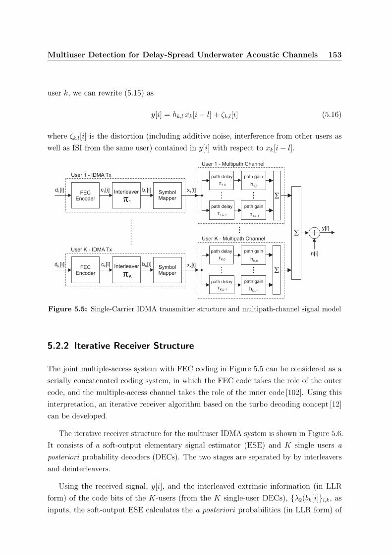
Multiuser Detection for Delay-Spread Underwater Acoustic Channels 153
user k, we can rewrite (5.15) as
y[i] = hk,l xk[i− l] + ζk,l[i] (5.16)
where ζk,l[i] is the distortion (including additive noise, interference from other users as
well as ISI from the same user) contained in y[i] with respect to xk[i− l].
Interleaver
b [i]KInterleaver
FECEncoder
FECEncoder
d [i]1
dK[i]
SymbolMapper
b [i]1
p1
pK
User 1 - IDMA Tx
User K - IDMA Tx
c [i]1
c [i]K SymbolMapper
x [i]K
x [i]1
User K - Multipath Channel
y[i]S
n[i]
path delay
t1,0 h1,0
path delay
t1,L-1
path gain
path gain
path delay
tK,0 hK,0
path delay
path gain
path gain
S
S
User 1 - Multipath Channel
h1,L-1
tK,L-1 hK,L-1
Figure 5.5: Single-Carrier IDMA transmitter structure and multipath-channel signal model
5.2.2 Iterative Receiver Structure
The joint multiple-access system with FEC coding in Figure 5.5 can be considered as a
serially concatenated coding system, in which the FEC code takes the role of the outer
code, and the multiple-access channel takes the role of the inner code [102]. Using this
interpretation, an iterative receiver algorithm based on the turbo decoding concept [12]
can be developed.
The iterative receiver structure for the multiuser IDMA system is shown in Figure 5.6.
It consists of a soft-output elementary signal estimator (ESE) and K single users a
posteriori probability decoders (DECs). The two stages are separated by by interleavers
and deinterleavers.
Using the received signal, y[i], and the interleaved extrinsic information (in LLR
form) of the code bits of the K-users (from the K single-user DECs), λ2(bk[i]i,k, as
inputs, the soft-output ESE calculates the a posteriori probabilities (in LLR form) of
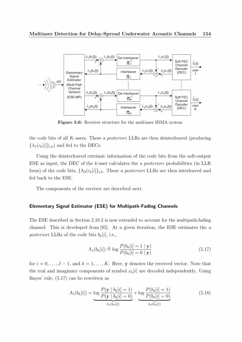
Multiuser Detection for Delay-Spread Underwater Acoustic Channels 154
l1(b [i])1
ElementarySignal
Estimator
Soft FECChannelDecoder(DEC)Interleaver
De-Interleaver
user1
d [i]1
userK
p1-1
p1
Soft FECChannelDecoder(DEC)Interleaver
De-Interleaver
pK-1
pK
L2(c [i])1
l1(c [i])1
l2(c [i])1
L1(b [i])1
l2(b [i])1
L1(b [i])K
l2(b [i])K
l1(b [i])K
l2(c [i])K L2(c [i])K
l1(c [i])K
y[i](Multi-PathChannelVersion)
(ESE-MP)d [i]K
Figure 5.6: Receiver structure for the multiuser IDMA system
the code bits of all K-users. These a posteriori LLRs are then deinterleaved (producing
λ1(ck[i]i,k) and fed to the DECs.
Using the deinterleaved extrinsic information of the code bits from the soft-output
ESE as input, the DEC of the k-user calculates the a posteriori probabilities (in LLR
form) of the code bits, Λ2(ck[i]i,k. These a posteriori LLRs are then interleaved and
fed back to the ESE.
The components of the receiver are described next.
Elementary Signal Estimator (ESE) for Multipath-Fading Channels
The ESE described in Section 2.10.2 is now extended to account for the multipath-fading
channel. This is developed from [85]. At a given iteration, the ESE estimates the a
posteriori LLRs of the code bits bk[i], i.e.,
Λ1(bk[i]) , logP (bk[i] = 1 | y)
P (bk[i] = 0 | y)(5.17)
for i = 0, . . . , J − 1, and k = 1, . . . , K. Here, y denotes the received vector. Note that
the real and imaginary components of symbol xk[i] are decoded independently. Using
Bayes’ rule, (5.17) can be rewritten as
Λ1(bk[i]) = logP (y | bk[i] = 1)
P (y | bk[i] = 0)︸ ︷︷ ︸λ1(bk[i])
+ logP (bk[i] = 1)
P (bk[i] = 0)︸ ︷︷ ︸λ2(bk[i])
(5.18)
Multiuser Detection for Delay-Spread Underwater Acoustic Channels 155
The first term in (5.18), denoted as λ1(bk[i]), is the extrinsic information calculated by
the ESE. The second term, denoted as λ2(bk[i]) is the a priori probability (in LLR form)
of bk[i]. An estimate of the a priori probability is calculated by the DEC of the k -th
user at the previous iteration. At the first iteration, no prior information about the code
bits is available, therefore all bit values are assumed equiprobable and the a priori LLR
values are set to zero.
The calculation of the extrinsic information for each user is now described in detail.
By rewriting (5.16), the received signal from user-k via path-l can be described as
y[i+ l] = hk,l xk[i] + ζk,l[i]. (5.19)
Let h∗k,l denote the conjugate of hk,l, and define
y[i+ l] , h∗k,l y[i+ l]
= |hk,l|2xk[i] + ζk,l[i] (5.20)
where
ζk,l[i] = h∗k,l ζk,l[i]. (5.21)
By the central limit theorem, ζk,l[i] can be approximated as a Gaussian variable. The
phase shift due hk,l is canceled out in (5.20), which means that the real and imaginary
parts of xk[i] can be decoded independently. This reduces the complexity of decoding
the QPSK mapping.
The extrinsic information for user-k and path-l can be written as
λ1(bk[i])l , logP (y[i+ l] | bk[i] = 1)
P (y[i+ l] | bk[i] = 0)
= 2|hk,l|2 y[i+ l]− E
ζk,l[i]
Var
ζk,l[i]
(5.22)
where E · and Var · denote expectation and variance, respectively. Finally, the
extrinsic information for user-k, considering all l-paths of the channel can be written as
λ1(bk[i]) =L−1∑l=0
λ1(bk[i])l. (5.23)

Multiuser Detection for Delay-Spread Underwater Acoustic Channels 156
Soft Channel Decoding (DEC)
The channel decoder for the k -th user estimates the a posteriori probabilities (in LLR
form) of the code bits, Λ2(ck(i)), which are given by
Λ2(ck[i]) , logP (ck[i] = 1 | λ1(ck[i])i ; code structure )
P (ck[i] = 0 | λ1(ck[i])i ; code structure ), (5.24)
= λ2(ck[i]) + λ1(ck[i]).
These a posteriori probabilities are computed using the BCJR algorithm [6] based on
the a priori information from the ESE, λ1(ck[i]), and knowledge of the code structure.
Additionally, the DEC estimates the a posteriori LLRs of the information bits, Λ2(dk[i]),and at the final iteration, performs a hard decision on the information bits, producing
dk[i]).
5.3 Multi-Carrier IDMA (OFDM-IDMA)
The concept of multicarrier modulation is to split a high-rate data stream into a number
of lower-rate streams that are transmitted simultaneously over a number of subcarriers.
These lower-rate parallel streams have increased symbol duration, and therefore the
relative amount of time dispersion caused by multipath delay spread is decreased. The
bandwidth of each subcarrier is made sufficiently narrow so that the frequency response
characteristics of the individual sub-channels are nearly flat [126].
OFDM is an efficient realization of multicarrier modulation communication in which
the subcarriers are made mutually orthogonal. The orthogonality attribute allows the
subcarrier spectra to overlap, while still allowing the subcarrier signals to be received
and decoded without interference from the adjacent carriers.
Consider an OFDM system with Nc subcarriers. The frequency spacing of the Nc
subcarriers is 4f . The total system bandwdith B is divided into Nc equidistant sub-
channels. All subcarriers will be mutually orthogonal within a time interval of length
Ts = 1/4f . The n-th subcarrier signal, denoted by s(n)(t), can be given by
s(n)(t) = expj2πn4ft, n = 0, 1, . . . Nc − 1; 0 ≤ t ≤ TS, (5.25)
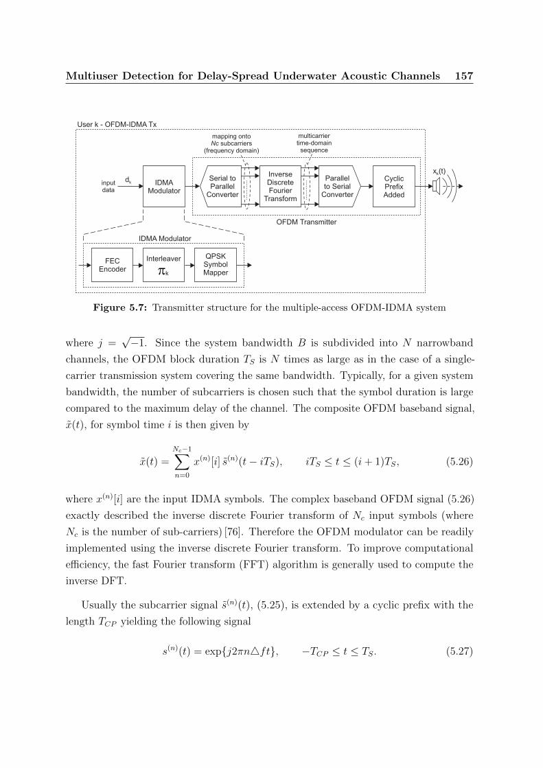
Multiuser Detection for Delay-Spread Underwater Acoustic Channels 157
OFDM Transmitter
Serial toParallel
Converter
InverseDiscreteFourier
Transform
Parallelto Serial
Converter
CyclicPrefixAdded
User k - OFDM-IDMA Tx
FECEncoder
Interleaver
pk
QPSKSymbolMapper
IDMAModulator
dk
mapping ontosubcarriers
(frequency domain)Nc
multicarriertime-domain
sequence
inputdata
IDMA Modulator
x (t)k
Figure 5.7: Transmitter structure for the multiple-access OFDM-IDMA system
where j =√−1. Since the system bandwidth B is subdivided into N narrowband
channels, the OFDM block duration TS is N times as large as in the case of a single-
carrier transmission system covering the same bandwidth. Typically, for a given system
bandwidth, the number of subcarriers is chosen such that the symbol duration is large
compared to the maximum delay of the channel. The composite OFDM baseband signal,
x(t), for symbol time i is then given by
x(t) =Nc−1∑n=0
x(n)[i] s(n)(t− iTS), iTS ≤ t ≤ (i+ 1)TS, (5.26)
where x(n)[i] are the input IDMA symbols. The complex baseband OFDM signal (5.26)
exactly described the inverse discrete Fourier transform of Nc input symbols (where
Nc is the number of sub-carriers) [76]. Therefore the OFDM modulator can be readily
implemented using the inverse discrete Fourier transform. To improve computational
efficiency, the fast Fourier transform (FFT) algorithm is generally used to compute the
inverse DFT.
Usually the subcarrier signal s(n)(t), (5.25), is extended by a cyclic prefix with the
length TCP yielding the following signal
s(n)(t) = expj2πn4ft, −TCP ≤ t ≤ TS. (5.27)

Multiuser Detection for Delay-Spread Underwater Acoustic Channels 158
The cyclic prefix is added to the subcarrier signal in order to reduce or eliminate ISI
from a multipath channel. At the receiver, the cyclic prefix is removed and only the time
interval 0 ≤ t ≤ TS is evaluated. The total OFDM block duration is T = TS + TCP .
Figure 5.7 shows the transmitter structure of the OFDM-IDMA scheme. After
IDMA processing (FEC encoding, interleaving and symbol mapping), a serial to parallel
(S/P) buffer sub-divides the chip sequence into Nc substreams. Then each substream is
modulated onto a sub-carrier by IFFT operation. Finally, the cyclic prefix is added.
OFDM Receiver
Serial toParallel
Converter
DiscreteFourier
Transform
Parallelto Serial
Converter
RemoveCyclicPrefix
IDMAIterativeReceiver
re-mapped ontosubcarriers
(frequency domain)Nc
receivedtime-domain
sequence
ElementarySignal
Estimator(ESE)
Soft FECChannelDecoder(DEC)Interleaver
De-Interleaver
user1
d1
userK
p1-1
p1
Soft FECChannelDecoder(DEC)Interleaver
De-Interleaver
pK-1
pK
y(t)
d1
d2
dK
K usersoutputdata
dK
IDMA Iterative Receiver
Figure 5.8: Receiver structure for the multiple-access OFDM-IDMA system
Figure 5.8 shows the receiver structure of the OFDM-IDMA scheme. OFDM demod-
ulation is performed before iterative multiuser detection. OFDM demodulation can be
readily performed by a discrete Fourier transform, which for computational efficiency,
is usually implemented using the FFT algorithm. In this scheme, ISI and MAI are
independently processed by the OFDM demodulator and the ESE, respectively. Note
that the multipath-fading version of the ESE (from Section 5.2.2) is not required here,
and the lower-complexity version of the ESE (for flat-fading) from Section 2.10.2 is used.
Multiuser Detection for Delay-Spread Underwater Acoustic Channels 159
5.4 MIMO-OFDM-IDMA
MIMO (Multiple-Input and Multiple-Output) is a general term that refers to communica-
tion systems where each transmitter and receiver use multiple transmitting and receiving
elements respectively. These systems exploit the spatial diversity of the multipath trans-
mission channel underwater channel to provide improved performance in the form of
either increased data robustness or increased data throughput.
At the transmitter side of a MIMO system, Space-Time Block Codes (STBCs) are
used to map the input data stream into multiple sub-streams that are dispersed in linear
combinations over space (i.e., transmit elements) and time. A STBC is defined by a
(P ×N) code matrix X, where N denotes the number of transmit antennas or the spatial
transmitter diversity order, and P denotes the number of channel usages for transmitting
a STBC codeword or the temporal transmitter diversity order.
The STBC encoder takes as input a code vector, x, and transmits each row of symbols
as specified in X at P consecutive channel usages. At each channel usage, the symbols
contained in the N -dimensional row vector of X are transmitted through N transmitter
antennas simultaneously [114].
As an example, consider the 2× 2 Alamouti STBC (ie., P = 2, N = 2) [3]. The
Alamouti STBC matrix X is defined by
X =
x(1) x(2)
−x∗(2) x∗(1)
(5.28)
where ( · )∗ denotes the complex conjugate operation. The input to this STBC is the code
vector x = [x(1), x(2) ]T . During the first channel use, the two symbols of the top row
of X, [x(1), x(2) ], are transmitted simultaneously from the two transmit elements; and
during the second channel use, the symbols in the second row of X, [−x∗(2), x∗(1) ], are
transmitted. The Alamouti STBC provides diversity gain (compared to a single-input
single-output systems), but not multiplexing gain.
In this chapter, we restrict our investigation to 2× 2 MIMO systems (transmitters and
receivers with 2 transmitting and 2 receiving elements respectively), using the Alamouti
STBC (5.28).
Figure 5.9 shows the transmitter structure of the MIMO-OFDM-IDMA scheme. The
input data sequence is encoded and interleaved by the FEC encoder and interleaver
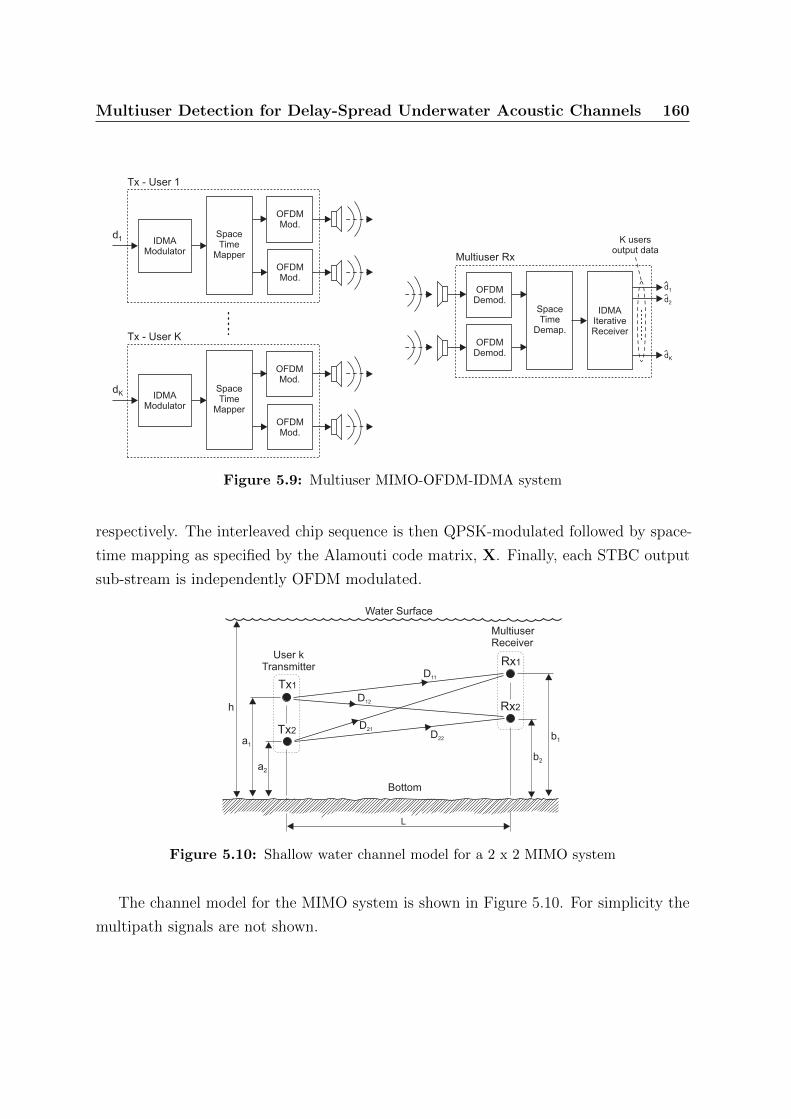
Multiuser Detection for Delay-Spread Underwater Acoustic Channels 160
OFDMDemod.
OFDMDemod.
d1
OFDMMod.
Tx - User 1
SpaceTime
Mapper
OFDMMod.
IDMAModulator
SpaceTime
Demap.
IDMAIterativeReceiver
d1
d2
dK
K usersoutput data
dK
OFDMMod.
Tx - User K
SpaceTime
Mapper
OFDMMod.
IDMAModulator
Multiuser Rx
Figure 5.9: Multiuser MIMO-OFDM-IDMA system
respectively. The interleaved chip sequence is then QPSK-modulated followed by space-
time mapping as specified by the Alamouti code matrix, X. Finally, each STBC output
sub-stream is independently OFDM modulated.
h
Water Surface
Bottom
L
D11
a1
a2
Tx2
Tx1
User k
Transmitter
Rx2
Rx1
b2
b1
D22
D12
D21
Multiuser
Receiver
Figure 5.10: Shallow water channel model for a 2 x 2 MIMO system
The channel model for the MIMO system is shown in Figure 5.10. For simplicity the
multipath signals are not shown.
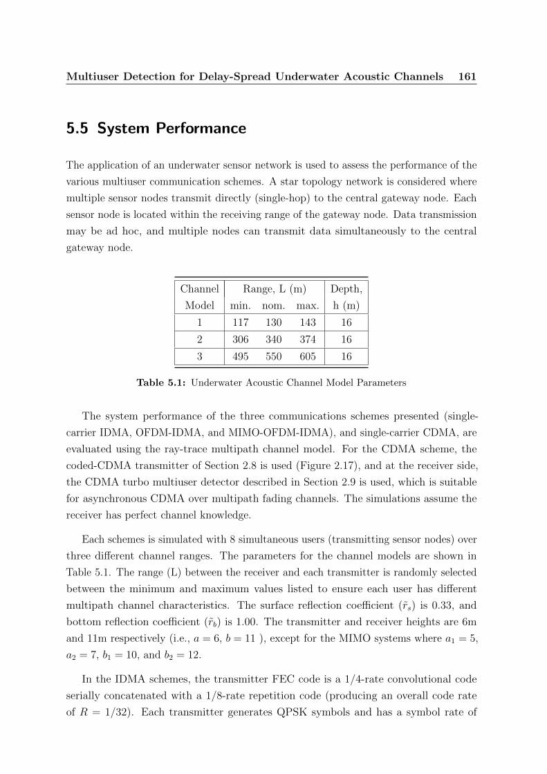
Multiuser Detection for Delay-Spread Underwater Acoustic Channels 161
5.5 System Performance
The application of an underwater sensor network is used to assess the performance of the
various multiuser communication schemes. A star topology network is considered where
multiple sensor nodes transmit directly (single-hop) to the central gateway node. Each
sensor node is located within the receiving range of the gateway node. Data transmission
may be ad hoc, and multiple nodes can transmit data simultaneously to the central
gateway node.
Channel Range, L (m) Depth,
Model min. nom. max. h (m)
1 117 130 143 16
2 306 340 374 16
3 495 550 605 16
Table 5.1: Underwater Acoustic Channel Model Parameters
The system performance of the three communications schemes presented (single-
carrier IDMA, OFDM-IDMA, and MIMO-OFDM-IDMA), and single-carrier CDMA, are
evaluated using the ray-trace multipath channel model. For the CDMA scheme, the
coded-CDMA transmitter of Section 2.8 is used (Figure 2.17), and at the receiver side,
the CDMA turbo multiuser detector described in Section 2.9 is used, which is suitable
for asynchronous CDMA over multipath fading channels. The simulations assume the
receiver has perfect channel knowledge.
Each schemes is simulated with 8 simultaneous users (transmitting sensor nodes) over
three different channel ranges. The parameters for the channel models are shown in
Table 5.1. The range (L) between the receiver and each transmitter is randomly selected
between the minimum and maximum values listed to ensure each user has different
multipath channel characteristics. The surface reflection coefficient (rs) is 0.33, and
bottom reflection coefficient (rb) is 1.00. The transmitter and receiver heights are 6m
and 11m respectively (i.e., a = 6, b = 11 ), except for the MIMO systems where a1 = 5,
a2 = 7, b1 = 10, and b2 = 12.
In the IDMA schemes, the transmitter FEC code is a 1/4-rate convolutional code
serially concatenated with a 1/8-rate repetition code (producing an overall code rate
of R = 1/32). Each transmitter generates QPSK symbols and has a symbol rate of

Multiuser Detection for Delay-Spread Underwater Acoustic Channels 162
Eb/N0 (dB)
Bit E
rror
Rate
10-4
10-3
10-2
10-1
100UAC Sys. Performance: Delay-Spread Chan., Model No. 1
0 2 4 8 106 12 14 16 18 20
Single-Carrier CDMA
Single-Carrier IDMA
OFDM-IDMA
MIMO-OFDM-IDMA
(a) Channel Model No. 1
Eb/N0 (dB)
Bit E
rror
Rate
10-4
10-3
10-2
10-1
100UAC Sys. Performance: Delay-Spread Chan., Model No. 2
0 2 4 8 106 12 14 16 18 20
Single-Carrier CDMA
Single-Carrier IDMA
OFDM-IDMA
MIMO-OFDM-IDMA
(b) Channel Model No. 2
Figure 5.11: UAC System Performance in Delay-Spread Channels (Model Nos. 1 & 2)
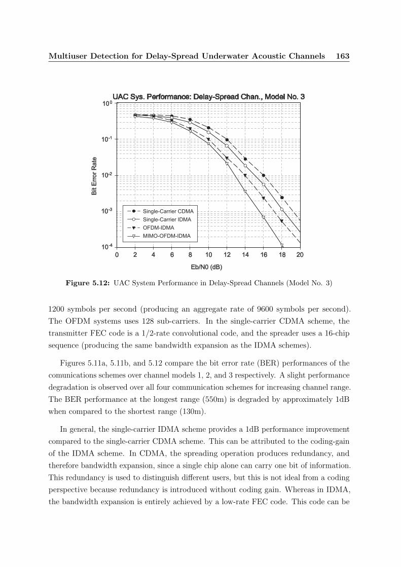
Multiuser Detection for Delay-Spread Underwater Acoustic Channels 163
Eb/N0 (dB)
Bit E
rror
Rate
10-4
10-3
10-2
10-1
100UAC Sys. Performance: Delay-Spread Chan., Model No. 3
0 2 4 8 106 12 14 16 18 20
Single-Carrier CDMA
Single-Carrier IDMA
OFDM-IDMA
MIMO-OFDM-IDMA
Figure 5.12: UAC System Performance in Delay-Spread Channels (Model No. 3)
1200 symbols per second (producing an aggregate rate of 9600 symbols per second).
The OFDM systems uses 128 sub-carriers. In the single-carrier CDMA scheme, the
transmitter FEC code is a 1/2-rate convolutional code, and the spreader uses a 16-chip
sequence (producing the same bandwidth expansion as the IDMA schemes).
Figures 5.11a, 5.11b, and 5.12 compare the bit error rate (BER) performances of the
comunications schemes over channel models 1, 2, and 3 respectively. A slight performance
degradation is observed over all four communication schemes for increasing channel range.
The BER performance at the longest range (550m) is degraded by approximately 1dB
when compared to the shortest range (130m).
In general, the single-carrier IDMA scheme provides a 1dB performance improvement
compared to the single-carrier CDMA scheme. This can be attributed to the coding-gain
of the IDMA scheme. In CDMA, the spreading operation produces redundancy, and
therefore bandwidth expansion, since a single chip alone can carry one bit of information.
This redundancy is used to distinguish different users, but this is not ideal from a coding
perspective because redundancy is introduced without coding gain. Whereas in IDMA,
the bandwidth expansion is entirely achieved by a low-rate FEC code. This code can be

Multiuser Detection for Delay-Spread Underwater Acoustic Channels 164
a combination of a repetition code (for bandwidth expansion) and a stronger code (for
coding gain), which provides a trade-off between performance and complexity.
The OFDM-IDMA scheme provides a performance improvement of approximately
1dB compared to single-carrier IDMA. This improvement in BER comes with the cost of
reduced bandwidth efficiency because of the addition of cyclic-prefix to each transmitted
OFDM block. Finally, the MIMO-OFDM-IDMA provides an improvement in BER
performance of approximately 2dB, which can be attributed to the diversity-gain of the
Alamouti STBC. The rich multipath nature of the underwater acoustic channel makes it
an ideal candidate for MIMO systems.
5.6 Conclusion
In this chapter, multiuser communications schemes for shallow water acoustic channels
were presented. The underwater acoustic channel is characterised by strong multipath
signals and long delay spreads, and is considered to be an exceptionally difficult medium
for data transmission.
Three IDMA schemes were developed for the underwater channel:
• single-carrier IDMA with a modified multiuser detector for multipath channels;
• OFMD-IDMA, combining multicarrier-modulation with an IDMA overlay; and
• MIMO-OFDM-IDMA, a multiple-input multiple-output extension added to the
OFDM-IDMA scheme employing space-time coding to provide diversity gain.
The performance of the three schemes was presented and also compared to single-carrier
CDMA.
The single-carrier IDMA scheme was shown to consistently outperform CDMA over
the range of conditions tested. The use of low-rate FEC codes to generate bandwidth
expansion in IDMA provides additional coding gain compared to CDMA, which uses
spreading sequences for bandwidth expansion (producing redundancy without coding
gain). The OFDM-IDMA and MIMO-OFDM-IDMA provided further performance
improvement, outperforming CDMA by approximately 2dB and 4dB respectively.
The efficient use of bandwidth makes IDMA an attractive spread-spectrum modulation
scheme for underwater channels that are severely limited in bandwidth. MIMO systems

Multiuser Detection for Delay-Spread Underwater Acoustic Channels 165
with space-time coding are able to exploit the rich multipath nature of the underwater
channel and are also attractive for underwater communications schemes. The results
demonstrate that both OFDM-IDMA and MIMO-OFDM-IDMA schemes are strong
candidates for shallow water sensor communication schemes, and are worthy of further
research.

Chapter 6
Multiuser Detection for Doubly-Spread
Underwater Acoustic Channels
Designing reliable multiple-access communication systems to underpin underwater acous-
tic sensor networks has proved challenging. For single-carrier modulation schemes with
time-domain equalization, the long delay-spread inherent in shallow water channels
dictates that a large number of equalizer taps must be used. The resulting computational
complexity means that these schemes are often considered unattractive. Multicarrier
modulation schemes, such as orthogonal frequency division multiplexing (OFDM), are
commonly used for delay-spread channels. However, shallow water channels are often
both delay- and Doppler-spread. In Doppler-spread channels, the orthogonality of OFDM
is lost, leading to subcarrier interference which complicates data detection and degrades
performance. In this chapter, we develop an adaptive multiuser single-carrier system
where time-domain equalization is performed using a Kalman filter (KF). KF-based
equalization has been shown to outperform traditional linear transversal equalizers, and
have much lower complexity. Low-level pilot sequences are superimposed on each users’
transmitted data to enable semi-blind channel estimation at the receiver. An adaptive
receiver is created by embedding an extended Kalman filter (EKF) into a turbo mul-
tiuser detector. The EKF-based equalizer jointly optimizes the estimates of the channel
coefficients and data symbols in each iteration of the detection process. EKF state-space
modelling is performed using low-rank basis expansion models which provide accurate
tracking of time-varying channels at minimal computational complexity. Experimen-
tal results demonstrate that the proposed multiple-access scheme with adaptive turbo
receiver provides robust performance in doubly-spread underwater acoustic channels.
166

Multiuser Detection for Doubly-Spread Underwater Acoustic Channels 167
6.1 Introduction
Underwater sensor networks facilitate a wide range of applications including environmental
monitoring, undersea exploration, distributed surveillance, and assisted navigation [2].
A robust and efficient multiple-access communications scheme between the underwater
network nodes is an essential foundation for reliable high-performance sensor network
operation. However, the shallow water acoustic channel has proved to be a difficult
medium for data transmission, and developing reliable communications systems for this
environment has been challenging [51].
Code-division multiple-access (CDMA) has been successfully employed as the modu-
lation scheme for shallow water networks [15] [119] [111]. CDMA is a spread-spectrum
technique that can provide simultaneous access for multiple users. By employing a
transmission bandwidth that is considerably greater than the information rate, spread-
spectrum schemes provide a number of benefits, including multiple-access interference
(MAI) suppression capability and improved immunity against multipath effects.
The underwater channel is generally impaired by significant multipath interference
which produces both long time-delay spread and large multipath amplitudes in the
received signal [51]. These long time-delay spreads cause severe inter-symbol interference
(ISI) which degrades the performance of many CDMA receiver detection schemes. To
alleviate the effects of long time-delay spreads, Multi-carrier modulation (MCM) schemes,
such as the spectrally-efficient orthogonal frequency division multiplexing (OFDM), are
often used. The basic principle of MCM is to split a high-rate data stream into a number
of lower-rate streams that are transmitted simultaneously over a number of sub-carriers.
This significantly reduces the ISI span because the lower-rate parallel sub-carriers have
increased symbol duration [126].
In [64], a multiple-access communications system that provides robust performance
over delay-spread shallow water acoustic channels was developed by combining OFDM
with an interleave-division multiple-access (IDMA) overlay. IDMA [85] is a new multiple-
access spread-spectrum scheme that uses a low-complexity iterative receiver structure to
perform multiuser detection, and has been shown to outperform coded CDMA. However,
many practical shallow water acoustic channels are not only delay-spread but are also
significantly Doppler-spread. Channels that are both delay- and Doppler-spread are said
to be doubly-spread. In the case of doubly-spread channels, the orthogonality of OFDM
is lost, leading to subcarrier interference which greatly complicates data-detection and
Multiuser Detection for Doubly-Spread Underwater Acoustic Channels 168
degrades performance. For Doppler-spread (time-varying) channels, guard bands can be
used in OFDM systems to maintain sub-carrier orthogonality, but this is at the expense of
spectral efficiency. For channels with large Doppler-spread, this loss of spectral efficiency
would be severe.
In this chapter, we develop a multiple-access IDMA system that would be suitable
for underwater acoustic sensor networks. The receiver using a turbo multiuser detection
(MUD) algorithm with time-domain equalization. The application of the turbo processing
principle to data detection of coded transmission systems with ISI is commonly referred
to as turbo equalization [23]. For underwater acoustic channels, time-domain equalization
using traditional linear traversal equalizers would require a large number of equalizer
taps, and may be considered impractical due to the computational complexity. However,
we consider equalization based on the Kalman filter (KF). KF-based equalizers have
been shown to perform significantly better than linear transversal equalizers, and at
much lower complexity (fewer equalizer taps) [101], [55]. Additionally, the state-space
formulation of the Kalman equalizer is well suited for iterative receivers and can easily
incorporate the soft a-priori information from forward error correction (FEC) channel
decoders.
For practical systems, it is necessary to perform channel estimation at the receiver
because the channel coefficients will be unknown. Channel estimation schemes are
generally categorized into one of two methodologies: pilot-aided methods that use
information induced from known pilot symbols or training sequences that are interspersed
with the data symbols; and blind methods that only use information contained in the
receive data symbols. However, with turbo processing, the receiver’s the channel estimator
can begin with a coarse channel estimate deduced from the pilot symbols, and then
utilize the a posteriori decision on data symbols obtained from previous iterations to
further improve the channel estimate. This type of scheme that combines both pilot
symbols and blind information is called a semi-blind method and is more powerful than
the two methods separately [22].
In[109], an iterative linear channel estimator employing Kalman filtering was developed
for turbo processing, where channel estimation and equalization are performed separately
in each iteration. However this type of scheme generally only works well for slow fading
channels. Also, there can be significant correlation between the estimates of the channel
and data symbols because the estimator and equalizer use the estimates obtained from
each other.

Multiuser Detection for Doubly-Spread Underwater Acoustic Channels 169
In [58], an adaptive turbo equalizer was developed using nonlinear Kalman filtering
to incorporate channel estimation into the equalization process. The resulting adaptive
soft nonlinear Kalman filter (NKF) takes the soft decisions of data symbols from the soft
decoder as its a priori information, and performs equalization iteratively. With such an
approach, the proposed scheme jointly optimizes the estimates of the channel and data
symbols in each iteration. This avoids the convergence to a local minima problem that
can occur when channel estimation and equalization are performed separately.
Linear channel estimation schemes using pilot-symbols has been shown to provide
good performance in delay-spread (multipath) channels and in Doppler-spread (fast-
fading) channels. However, in doubly-spread channels, the number of unknown channel
parameters often exceeds the number of known data variables (pilot symbols) and the
underlying linear system used by the estimation algorithm becomes underdetermined. To
alleviate this problem, the number of unknown channels parameters must be reduced so
that the linear system becomes tractable. This can be achieved by using low-dimensional
models to approximate the time-varying nature of the channel. The accuracy of the
channel model employed by the estimation scheme will largely determine the system
performance.
Low-order autoregressive (AR) processes are popular low-complexity models of
discrete-time random processes. The first-order AR model, AR(1), has been shown
to be effective for modelling Rayleigh channels with slow- and moderate-fading on
a symbol-by-symbol basis [132] [131], and was employed as state-space model in the
NKF-based turbo equalizer of [58].
The basis expansion model (BEM) is low-dimensional low-rank model that can
accurately capture the fast time-variations of a doubly-spread channel over a period
of time. A BEM consists of superpositions of time-varying basis functions weighted
by time-invariant coefficients. Modelling of linear systems by basis functions can turn
a time-varying identification problem into a time-invariant one, thereby reducing the
number of channel parameters to estimate. The usefulness of using BEMs to model
underwater acoustic channels was first recognised in [95] and [96].
In [52], an adaptive NKF-based turbo equalizer was developed using a Fourier BEM
channel model. The NKF is used to track the changes in the BEM coefficients instead
of tracking the actual channel changes, since the time-variations of BEM coefficients
generally evolve much slower that the time-variations of the channel itself. For fast-fading
channels, the NKF with Fourier BEM model [52] achieves better performance than the

Multiuser Detection for Doubly-Spread Underwater Acoustic Channels 170
NKF scheme in [58] where the channel is modelled as an AR process. The Fourier BEM
is the time-domain equivalent of the (frequency-domain) Doppler-line filters used in [24]
to equalize underwater Doppler-spread channels.
For the multiple-access IDMA system developed in this chapter, the receiver embeds
a NKF-based channel estimator/equalizer into the turbo multiuser detection framework.
This approach will be shown to be considerably more effective at tracking and equalizing
doubly-spread channels than the traditional linear systems-based schemes for IDMAS
multiuser channel estimation [86]. The channel estimation and equalization scheme are
based on the nonlinear Kalman filtering approach of [58] and [52], but are extended to the
multiuser case, adapted to IDMA with superimposed training sequences, and generalised
to accommodate different BEM and AR models. The performance of the proposed
scheme is evaluated using shallow-water acoustic channel simulation models that been
verified by sea trial data. A number of BEM and AR channel estimation models are
evaluated to assess the channel estimation/tracking ability and also the system bit error
rate performance.
6.2 Underwater Acoustic Channels and Channel
Modelling
In a shallow water environment, transmitted acoustic signals undergo multiple reflections
at the water surface and sea floor. These reflections occur at small grazing angles and
with small reflection losses creating large multipath amplitudes and long time-delay
spread in the received signal [51].
Relative movements between the transmitters and the receiver, and the movements
of the propagation medium induce Doppler effects, which can be significant even for slow
changes. Additional amplitude and phase fluctuations may also result from scattering
which is caused by the roughness of the channel surface and bottom. When the sea surface
is rough, the vertical motion of the surface modulates the amplitude of the incident
wave and superposes its own spectrum as upper and lower sidebands on the spectrum of
the incident sound. Moreover, when there is a surface current, the horizontal motion
will appear in the scattered sound and cause a Doppler-shifted and Doppler-smeared
spectrum [123], [27]. The frequency of the signal received might differ significantly from
the frequency of the signal transmitted (by up to 1% typically) [71].
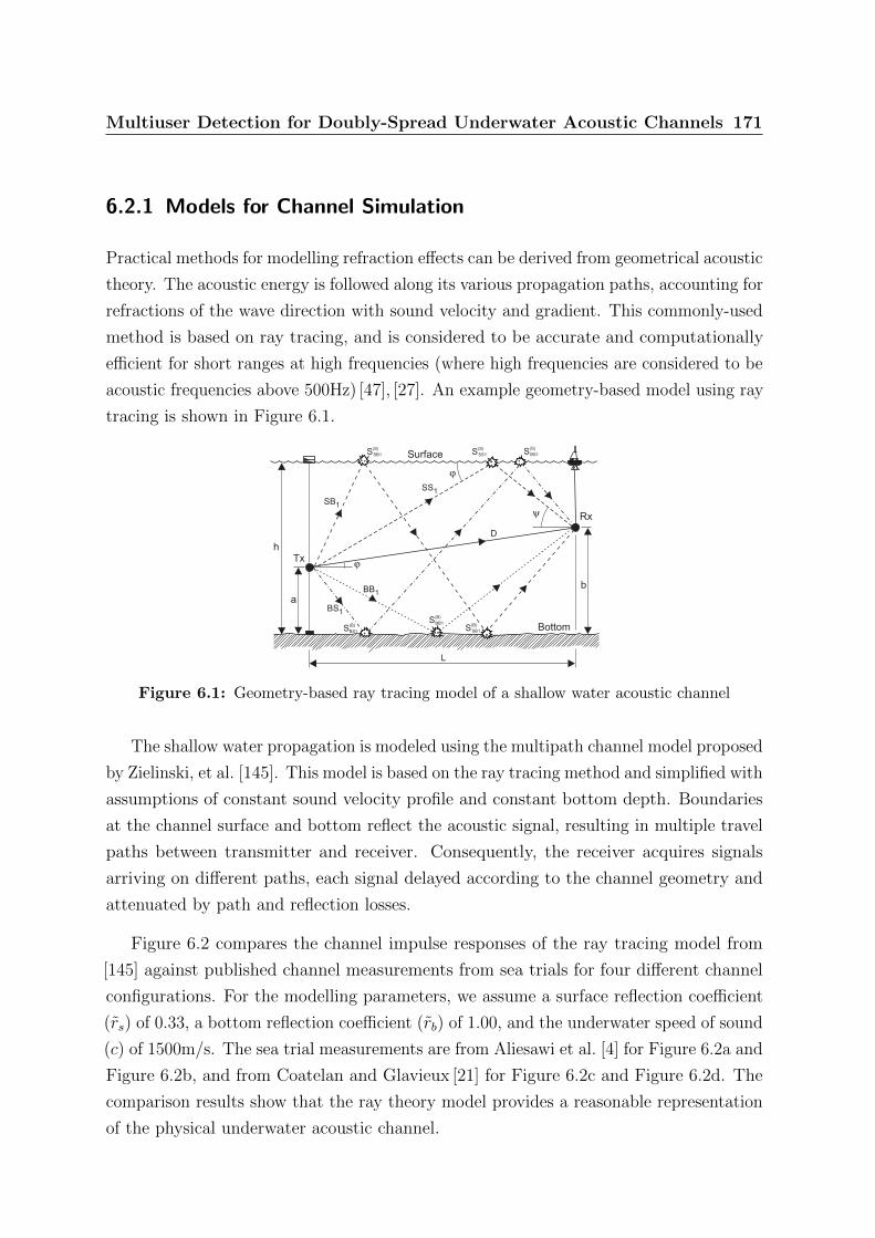
Multiuser Detection for Doubly-Spread Underwater Acoustic Channels 171
6.2.1 Models for Channel Simulation
Practical methods for modelling refraction effects can be derived from geometrical acoustic
theory. The acoustic energy is followed along its various propagation paths, accounting for
refractions of the wave direction with sound velocity and gradient. This commonly-used
method is based on ray tracing, and is considered to be accurate and computationally
efficient for short ranges at high frequencies (where high frequencies are considered to be
acoustic frequencies above 500Hz) [47], [27]. An example geometry-based model using ray
tracing is shown in Figure 6.1.
j
j
Surface
Bottom
Tx
Rx
a
b
h
L
SB1
SS1
BS1
BB1
y
D
S(S)
SB1 S(S)
SS1 S(S)
BS1
S(B)
SB1
S(B)
BB1
S(B)
BS1
Figure 6.1: Geometry-based ray tracing model of a shallow water acoustic channel
The shallow water propagation is modeled using the multipath channel model proposed
by Zielinski, et al. [145]. This model is based on the ray tracing method and simplified with
assumptions of constant sound velocity profile and constant bottom depth. Boundaries
at the channel surface and bottom reflect the acoustic signal, resulting in multiple travel
paths between transmitter and receiver. Consequently, the receiver acquires signals
arriving on different paths, each signal delayed according to the channel geometry and
attenuated by path and reflection losses.
Figure 6.2 compares the channel impulse responses of the ray tracing model from
[145] against published channel measurements from sea trials for four different channel
configurations. For the modelling parameters, we assume a surface reflection coefficient
(rs) of 0.33, a bottom reflection coefficient (rb) of 1.00, and the underwater speed of sound
(c) of 1500m/s. The sea trial measurements are from Aliesawi et al. [4] for Figure 6.2a and
Figure 6.2b, and from Coatelan and Glavieux [21] for Figure 6.2c and Figure 6.2d. The
comparison results show that the ray theory model provides a reasonable representation
of the physical underwater acoustic channel.

Multiuser Detection for Doubly-Spread Underwater Acoustic Channels 172
0.20
0.15
0.10
0.05
0.00Norm
alis
ed
Am
plit
ude
0 5 10 15 20
Delay (ms)
L = 200m, h = 25~30m
sea trial data
chan. model
(a) Channel A: L=200m, h=25-30m
0.20
0.15
0.10
0.05
0.00No
rma
lise
dA
mp
litu
de
0 5 10 15 20
Delay (ms)
sea trial data
chan. model
L = 500m, h = 25~30m
(b) Channel B: L=500m, h=25-30m
0.20
0.15
0.10
0.05
0.00Norm
alis
ed
Am
plit
ude
0 5 10 15 20
Delay (ms)
sea trial data
chan. model
L=370m, h=29m, rocky seafloor
(c) Channel C: L=370m, h=29m
0.20
0.15
0.10
0.05
0.00Norm
alis
ed
Am
plit
ude
0 5 10 15 20
Delay (ms)
sea trial data
chan. model
L=470m, h=29m, sandy seafloor
(d) Channel D: L=470m, h=35m
Figure 6.2: Normalised channel impulse responses from sea trial data and channel models
Additionally, the Doppler effects and micropath scattering can be modelled using
Rayleigh random processes. Independent and uncorrelated Rayleigh random processes
are applied to each path within the ray-theory multipath model. Each Rayleigh process
is generated by the method in [143] and satisfies Jakes’ model [46].
6.2.2 Models for Channel Estimation
The shallow water acoustic channel can be modelled as a stochastic linear time-variant
(LTV) system, with Bello system functions [8] employed to characterize the system in
terms of time (t); frequency (f); delay (τ); and Doppler shift (ν).
The input-output relation of the channel is defined by
y(t) =
∫ ∞−∞
h(t, τ)x(t− τ) dτ (6.1)
where y(t) is the channel output at time t, x(t) is the channel input at time t, and h(t, τ)
is the input delay-spread function and is interpreted as the response of the channel at
time t to a unit impulse input that stimulated the channel at the time t− τ .

Multiuser Detection for Doubly-Spread Underwater Acoustic Channels 173
The delay-Doppler-spread function S(τ, ν) of the channel is defined by the Fourier
transform of h(t, τ) with respect to time t, i.e.,
S(τ, ν) =
∫ ∞−∞
h(t, τ) exp−j2πfτ dt (6.2)
Expressing the time-variant impulse response h(t, τ) by the inverse Fourier transform of
S(τ, ν), allows the representation of (6.1) in the form
y(t) =
∫ 0
−∞
∫ ∞−∞
S(τ, ν)x(t− τ) exp−j2πνt dν dτ (6.3)
This relation shows that the output signal y(t) can be represented by an infinite sum of
delayed, weighted, and Doppler shifted replicas of the input signal x(t). Signals delayed
during transmission in the range of [τ, τ + dτ) and affected by a Doppler shift within
[ν, ν+dν) are weighted by the differential part S(τ, ν)dν dτ . Therefore, S(τ, ν) explicitly
describes the dispersive behaviour of the channel as a function of both the propagation
delays τ and the Doppler frequencies ν.
In the discrete-time setting, the channel’s input-output relation becomes
y(i) =L−1∑l=0
h(i, l)x(i− l) (6.4)
and the delay-Doppler-spread function in discrete-time form becomes
S(l, d) =N−1∑i=0
h(i, l) exp
−j2diN
(6.5)
Here, x(i), y(i), h(i, l) and S(l, d) are sampled versions of x(t), y(t), h(t, τ) and S(τ, ν),
respectively, from (6.1) and (6.2). The sampling frequency fs = 1/Ts is assumed to be
larger than B + νmax, where B is the transmit bandwidth, and νmax is the maximum
Doppler frequency. Furthermore, L = dτmax/Tse is the number of discrete channel taps,
i.e., the maximum discrete-time delay.
Estimating the complete mathematical description of a doubly-spread LTV channel
is a complex task. For every N received samples, we need NL channel coefficients to
accurately characterize the channel. Even with superimposed training, where a pilot-
symbol is superimposed onto each of the N data symbols, we cannot solve for NL
coefficients as the number of unknown variables exceeds the known data variables (i.e.
Multiuser Detection for Doubly-Spread Underwater Acoustic Channels 174
N pilot symbols). Fortunately, most practical channels exhibit some additional structure
which simplifies the description so that a smaller number of parameters are sufficient
to model the channels behavior. Such low-dimensional low-rank representations of LTV
channels are often referred to as parsimonious models.
A popular class of low-rank channel model is the basis expansion model (BEM) [118],
[32] which employs a basis expansion gq(l)ψq(i)Q−1q=0 , with respect to time i, for each
tap of the channel impulse response h(i, l), i.e.,
h(i, l) =
Q−1∑q=0
gq(l)ψq(i). (6.6)
The BEM is motivated by the observation that the temporal (i) variation of h(i, l) is
generally smooth due to the channels limited Doppler spread, and hence ψq(i)Q−1q=0 can
be chosen as a small set of smooth functions. In most cases, the BEM (6.6) is considered
only within a finite interval, which we assume to be i ∈ [0, N − 1]. The q-th coefficient
for the l-th tap in (6.6) is given by
gq(l) = 〈h( · , l), ψq〉 =N−1∑n=0
h(i, l)ψq(i), (6.7)
where ψq(i)Q−1q=0 is the bi-orthogonal basis for the span of ψq(i)Q−1
q=0 (i.e., 〈ψq, ψq′〉 = δqq′
for all q, q′) [42].
The BEM of (6.6) is useful because the complexity of characterizing h(i, l) for the
interval i ∈ [0, N − 1] is reduced from NL to QL parameters, where Q N . Although,
in general, an extension of the time interval will require a proportional increase in the
BEM model order (i.e., Q ∝ N). Using the basis expansion of (6.6) in the channel
input-output relation of (6.4) results in
y(i) =L−1∑l=0
Q−1∑q=0
gq(l)ψq(i)x(i− l)
=
Q−1∑q=0
ψq(i)L−1∑l=0
gq(l)x(i− l)
=
Q−1∑q=0
ψq(i)yq(i) where yq(i) =L−1∑l=0
gq(l)x(i− l) (6.8)
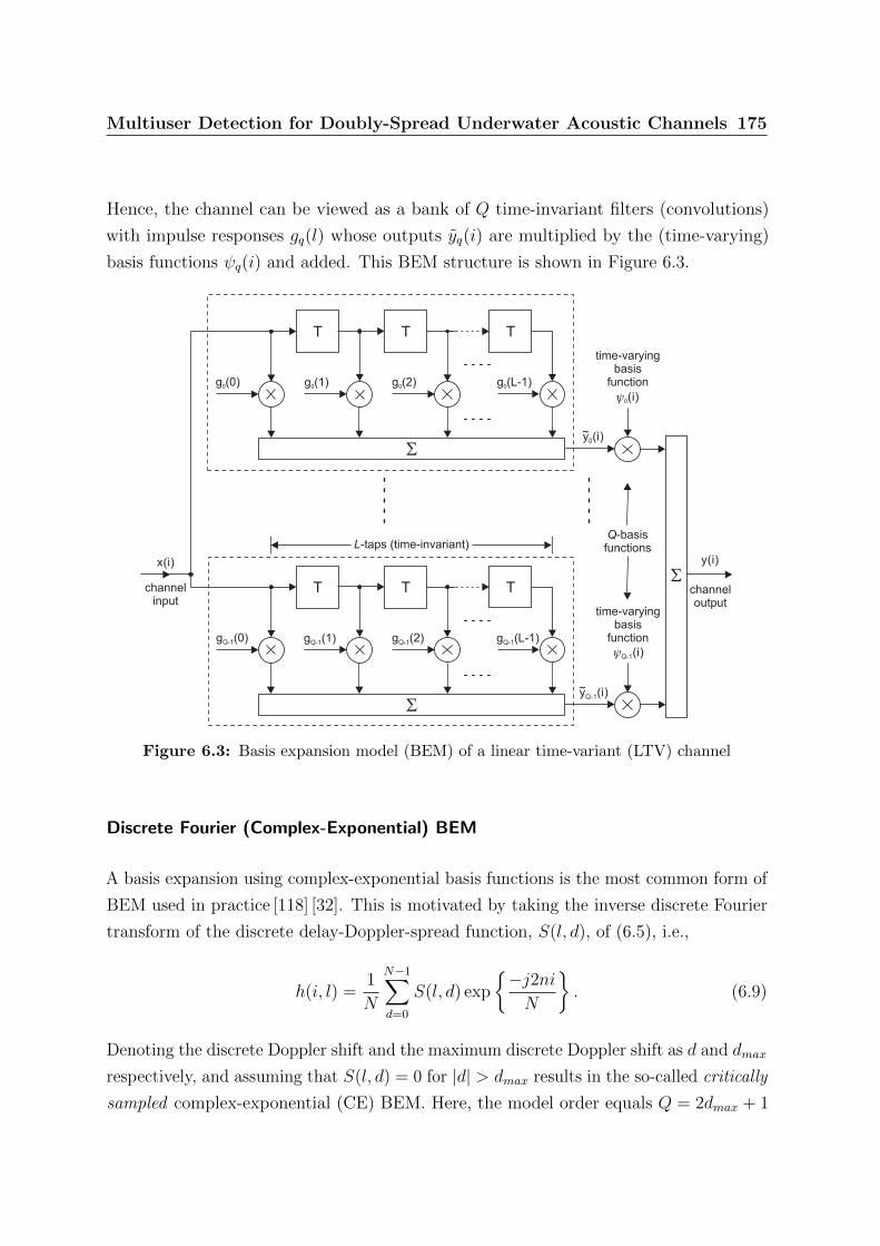
Multiuser Detection for Doubly-Spread Underwater Acoustic Channels 175
Hence, the channel can be viewed as a bank of Q time-invariant filters (convolutions)
with impulse responses gq(l) whose outputs yq(i) are multiplied by the (time-varying)
basis functions ψq(i) and added. This BEM structure is shown in Figure 6.3.
g (0)Q-1
x(i)
g (1)Q-1 g (2)Q-1 g (L-1)Q-1
g (0)0 g (1)0 g (2)0 g (L-1)0
y(i)
time-varyingbasis
function
T T T
y0(i)
T T T
time-varyingbasis
function
yQ-1(i)
channeloutput
channelinput
S
y (i)Q-1
y (i)0
L-taps (time-invariant)Q-basis
functions
S
S
Figure 6.3: Basis expansion model (BEM) of a linear time-variant (LTV) channel
Discrete Fourier (Complex-Exponential) BEM
A basis expansion using complex-exponential basis functions is the most common form of
BEM used in practice [118] [32]. This is motivated by taking the inverse discrete Fourier
transform of the discrete delay-Doppler-spread function, S(l, d), of (6.5), i.e.,
h(i, l) =1
N
N−1∑d=0
S(l, d) exp
−j2niN
. (6.9)
Denoting the discrete Doppler shift and the maximum discrete Doppler shift as d and dmax
respectively, and assuming that S(l, d) = 0 for |d| > dmax results in the so-called critically
sampled complex-exponential (CE) BEM. Here, the model order equals Q = 2dmax + 1
Multiuser Detection for Doubly-Spread Underwater Acoustic Channels 176
with the basis functions given by
ψq(i) = exp
−j2π(q − dmax)i
N
, 0 ≤ i ≤ N − 1; 0 ≤ q ≤ Q− 1 (6.10)
and the corresponding BEM coefficients given by
gq(l) =1
NS(l, q − dmax), 0 ≤ q ≤ Q− 1. (6.11)
The BEM coefficients, gq(l)q, remain invariant during the block of N symbols, but
may change from block to block. The Fourier basis functions ψq(i)q are common for
every block. the basis functions of the CE-BEM can be inferred if the delay spread and
the Doppler spread (or at least their upper bounds) are known [72]. Treating the basis
functions as known, estimation of a time-varying process is reduced to estimating the
invariant coefficients over a block of N symbols.
Oversampled Complex-Exponential (CE) BEM
The critically-sampled CE BEM often suffers from spectral leakage introduced by the
the (time-limited) rectangular window of the truncated discrete Fourier transform. This
Doppler leakage often requires a rather large value of dmax to achieve satisfactory modeling
accuracy. An alternative interpretation of this problem is that the uniformly-spaced
discrete Doppler frequencies d/N (i.e., Doppler resolution 1/N) usually do not coincide
with the actual Doppler frequencies of the continuous channel. In the time domain,
this manifests as a Gibbs (or ringing) phenomenon, which degrades the quality of the
CE-BEM particulary near the interval boundaries.
These issues of Doppler leakage and Gibbs phenomenon can be alleviated by over-
sampling [117]. The basis functions for the oversampled CE-BEM are given by
ψq(i) = exp
−j2π(q − ξdmax)i
ξN
, 0 ≤ i ≤ N − 1; 0 ≤ q ≤ Q− 1 (6.12)
where ξ is the oversampling factor (ξ ∈ N∗), and Q = 2ξdmax + 1. The oversampling
reduces the frequency spacing of complex exponentials and gives a better representation
of the channel impulse response [56]. Although in the oversampled model, the basis
functions are no longer orthogonal. Example critically-sampled and oversampled CE
BEMs are shown in Figure 6.4.

Multiuser Detection for Doubly-Spread Underwater Acoustic Channels 177
0 10-10 5-5
Normalised Doppler Frequency (f .T) x 10d-3
-f .Td,max +f .Td,max
15-15
(a) Example Doppler spectrum
0 10-10 5-5
Normalised Doppler Frequency (f .T) x 10d-3
15-15
(b) Critically-sampled model (ξ=1, dmax=2, Q=5)
0 10-10 5-5
Normalised Doppler Frequency (f .T) x 10d-3
15-15
(c) Oversampled model (ξ=2, dmax=2, Q=9)
0 10-10 5-5
Normalised Doppler Frequency (f .T) x 10d-3
15-15
(d) Oversampled model (ξ=3, dmax=2, Q=13)
Figure 6.4: Example Doppler spectrum and CE-BEM frequencies
Discrete Prolate Spheroidal Sequences (DPSS) BEM
The Doppler leakage that afflicts the CE-BEM can be significantly reduced by replacing
the complex-exponential basis functions with truncated versions of discrete prolate
spheroidal sequences (DPSSs) [141]. DPSSs are functions that are band-limited as well as
maximally time-concentrated in the sense of having minimum energy outside a prescribed
time interval [0, N − 1]. For a given time sequence of length N and a given maximum
normalized Doppler frequency νmax, the DPSSs are the solutions ψq(i) to the eigenvalue
problem [108]:
N−1∑i′=0
sin(2πνmax(i− i′))π(i− i′)
ψq(i′) = λqψq(i), i ∈ Z. (6.13)

Multiuser Detection for Doubly-Spread Underwater Acoustic Channels 178
Equivalently, the eigenvalues λqq are the eigenvalues of the N ×N matrix C where
Cψq = λqψq and Ci,i′ =sin[2π(i− i′)νmax]
π(i− i′)0 ≤ i, i′ ≤ N − 1
where Ci,i′ denotes the (i, i′)-th element of C. The N -elements of the corresponding
eigenvectors for this matrix, ψq , [ψq(0), ψq(1), . . . , ψq(N − 1)]T , are the length-N sub-
sequences of the DPSSs [84]. The DPS sequences, ψq(i), form an orthogonal basis on
[0, N − 1] and also an orthonormal basis on Z. Assuming that the maximum Doppler
frequency can be established with reasonable accuracy, DPS sequences usually provide
better modelling accuracy than complex-exponential (Fourier) sequences with the same
number of basis functions.
Karhunen-Loeve Expansion (K-L) BEM
The normalised mean square (MS) error E|h(t) − h(t)|2 between h(t) and its series
representation h(t) depends on the number of terms in the series and the basis functions
used in the series expansion. A series expansion is considered optimum in a MS sense if
it yields the smallest MS error for a given number of terms. The Karhunen-Loeve (K-L)
expansion is optimum in a MS sense for expanding a stationary random process over a
finite time interval [−T/2, T/2]. The orthonormal set of basis functions, ψq(t)q, used
in the K-L expansion of h(t) are obtained from the solutions of the integral equation
[106]: ∫ T/2
−T/2Rhh(t− τ)ψ(τ)dτ = λψ(t) − T/2 < t < T/2, (6.14)
where Rhh(t− τ) denotes the autocorrelation of h(t) and is defined as Eh(t)h∗(t+ τ).The solution yields a set of eigenvalues λ1 > λ2 > . . . > λQ, and eigenfunctions ψq(t)Qq=1,
and the K-L expansion is written in terms of the eigenfunctions as
h(t) =
Q∑q=1
gqψq(t) − T/2 < t < T/2 (6.15)
where
gq =
∫ T/2
−T/2h(t)ψ∗n(t) dt q = 1, 2, . . . , Q (6.16)
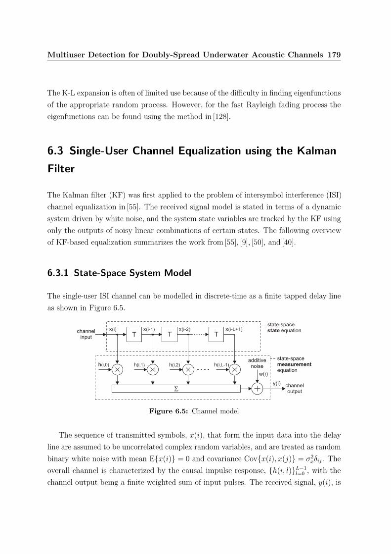
Multiuser Detection for Doubly-Spread Underwater Acoustic Channels 179
The K-L expansion is often of limited use because of the difficulty in finding eigenfunctions
of the appropriate random process. However, for the fast Rayleigh fading process the
eigenfunctions can be found using the method in [128].
6.3 Single-User Channel Equalization using the Kalman
Filter
The Kalman filter (KF) was first applied to the problem of intersymbol interference (ISI)
channel equalization in [55]. The received signal model is stated in terms of a dynamic
system driven by white noise, and the system state variables are tracked by the KF using
only the outputs of noisy linear combinations of certain states. The following overview
of KF-based equalization summarizes the work from [55], [9], [50], and [40].
6.3.1 State-Space System Model
The single-user ISI channel can be modelled in discrete-time as a finite tapped delay line
as shown in Figure 6.5.
h(i,0)
TT T
y(i)
h(i,1) h(i,2) h(i,L-1)
channeloutput
channelinput
S
w(i)
additivenoise
state-spaceequationstate
state-space
equationmeasurement
x(i-1) x(i-2) x(i-L+1)x(i)
Figure 6.5: Channel model
The sequence of transmitted symbols, x(i), that form the input data into the delay
line are assumed to be uncorrelated complex random variables, and are treated as random
binary white noise with mean Ex(i) = 0 and covariance Covx(i), x(j) = σ2xδij. The
overall channel is characterized by the causal impulse response, h(i, l)L−1l=0 , with the
channel output being a finite weighted sum of input pulses. The received signal, y(i), is

Multiuser Detection for Doubly-Spread Underwater Acoustic Channels 180
given by
y(i) =L−1∑l=0
h(i, l)x(i− l) + w(i) (6.17)
where w(i) is the so-called additive measurement noise. This is a discrete-time complex
white noise process with mean Ew(i) = 0 and covariance Cov(w(i), w(j) = σ2wδij.
The measurement noise, w(i), is statistically independent of the channel input, x(i).
In state-space form, the L-tap delay line and transmit data sequence are modelled
using two equations: the state equation; and the measurement equation. The state
equation is defined as:
s(i+ 1) = Φs(i) + Γu(i+ 1) (6.18)
where Φ is a L×L matrix (termed the state transition matrix ), Γ is a L× 1 vector, and
u(i) is the so-called process noise, with definitions:
Φ =
01× (L−1) 0
IL−1 0(L−1)× 1
, Γ =
1
0(L−1)× 1
, u(i+ 1) = x(i+ 1). (6.19)
The L× 1 state vector, s(i), represents the state of the system at time i. The components
of the state vector, s1(i), s2(i), . . . , sL(i), are thus, respectively, the channel input x(i)
at time i, and the L− 1 successive outputs of the delay elements in the channel model
(Figure 6.5), i.e.,
s(i) =
s1(i)
s2(i)...
sL(i)
,
x(i)
x(i− 1)...
x(i− L+ 1)
(6.20)
The measurement equation describes the channel output at time i, i.e.,
y(i) = H(i)s(i) + w(i) (6.21)
where y is the (scalar) measured output; H(i) is the 1×L row vector of channel coefficients
defined as H(i) , [h(i, 0), h(i, 1), . . . , h(i, L− 1)], and w(i) is the so-called observation

Multiuser Detection for Doubly-Spread Underwater Acoustic Channels 181
noise. The observation noise is assumed to be scalar Gaussian white noise with mean
Ew(i) = 0 and covariance Covw(i), w(j) = σ2wδij. From inspection, it can be seen
that the state space model of (6.18) and (6.21) has the same expression as the signal
model of (6.17).
6.3.2 Equalization of Channels with Known Coefficients
The Kalman filtering algorithm calculates the minimum error-variance estimate of the
state vector s(i) of the state space model ((6.18) and (6.21)), in the sense that it minimizes
the mean square of the norm of the estimation error
E||s(i | i)||2 , E||s(i)− s(i | i)||2 (6.22)
where s(i | i) is the estimate of state vector s(i) based on the set of sequential observations
y(1), y(2), . . . , y(i). The L×L error covariance matrix P(i | i) is defined as
P(i | i) , E
[s(i | i)− s(i)][s(i | i)− s(i)]H
(6.23)
and (6.22) becomes E||s(i | i)||2 = tr ( P(i | i) ). The KF minimizes the trace of the
error covariance matrix, or any linear combination of the main diagonal elements of the
matrix. For the state vector defined in (6.20), the KF minimizes E|x(i)− x(i)|2 [9].
The KF for the discrete state-space system of (6.18) and (6.21) is described by the
following recursive equations for the state estimate vector and error covariance matrix
[55], [9]:
1. Time update:
s(i | i− 1) = Φs(i− 1 | i− 1) (6.24)
P(i | i− 1) = ΦP(i− 1 | i− 1)ΦT + ΓQΓT (6.25)
2. Kalman gain:
K(i) = P(i | i− 1)HT (i)[σ2w + H(i)P(i | i− 1)HT (i)
]−1(6.26)
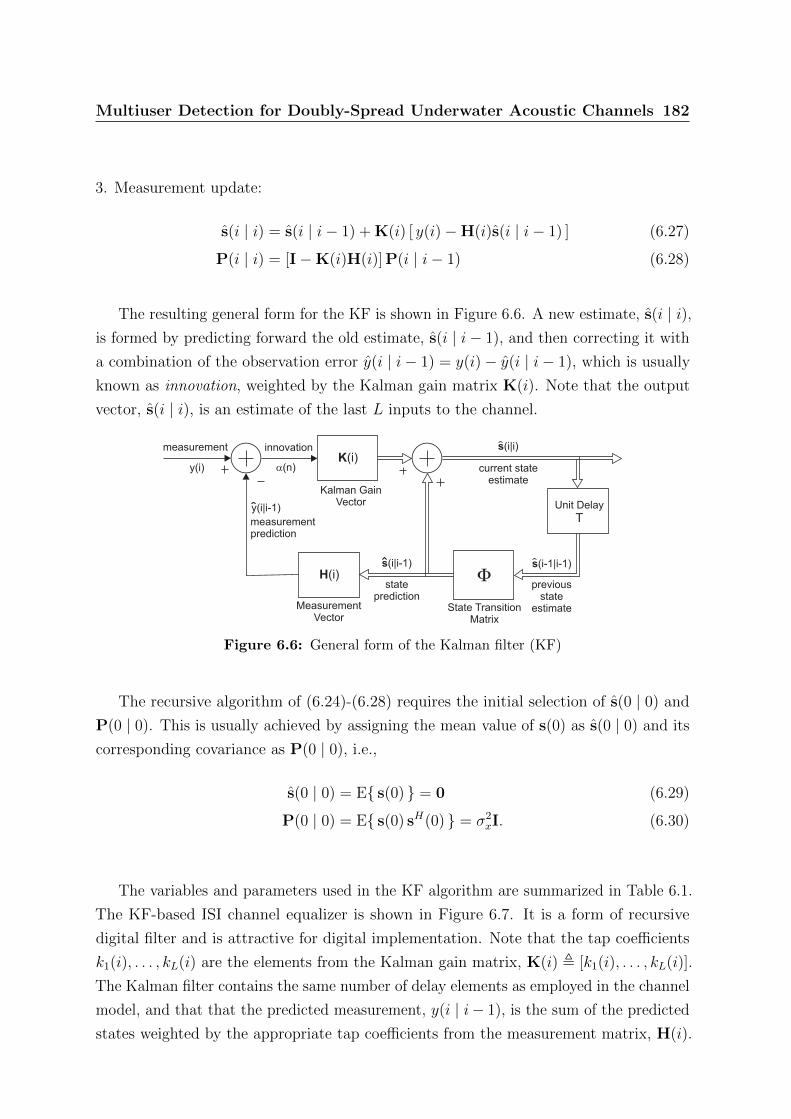
Multiuser Detection for Doubly-Spread Underwater Acoustic Channels 182
3. Measurement update:
s(i | i) = s(i | i− 1) + K(i) [ y(i)−H(i)s(i | i− 1) ] (6.27)
P(i | i) = [I−K(i)H(i)] P(i | i− 1) (6.28)
The resulting general form for the KF is shown in Figure 6.6. A new estimate, s(i | i),is formed by predicting forward the old estimate, s(i | i− 1), and then correcting it with
a combination of the observation error y(i | i− 1) = y(i)− y(i | i− 1), which is usually
known as innovation, weighted by the Kalman gain matrix K(i). Note that the output
vector, s(i | i), is an estimate of the last L inputs to the channel.
Kalman GainVector
K(i)
MeasurementVector
H(i)
innovation
y(i)
State TransitionMatrix
Unit Delay
T
stateprediction
measurement
previousstate
estimate
current stateestimate
s(i|i)
s(i-1|i-1)s(i|i-1)
y(i|i-1)
measurementprediction
F
a(n)
Figure 6.6: General form of the Kalman filter (KF)
The recursive algorithm of (6.24)-(6.28) requires the initial selection of s(0 | 0) and
P(0 | 0). This is usually achieved by assigning the mean value of s(0) as s(0 | 0) and its
corresponding covariance as P(0 | 0), i.e.,
s(0 | 0) = E s(0) = 0 (6.29)
P(0 | 0) = E s(0) sH(0) = σ2xI. (6.30)
The variables and parameters used in the KF algorithm are summarized in Table 6.1.
The KF-based ISI channel equalizer is shown in Figure 6.7. It is a form of recursive
digital filter and is attractive for digital implementation. Note that the tap coefficients
k1(i), . . . , kL(i) are the elements from the Kalman gain matrix, K(i) , [k1(i), . . . , kL(i)].
The Kalman filter contains the same number of delay elements as employed in the channel
model, and that that the predicted measurement, y(i | i− 1), is the sum of the predicted
states weighted by the appropriate tap coefficients from the measurement matrix, H(i).
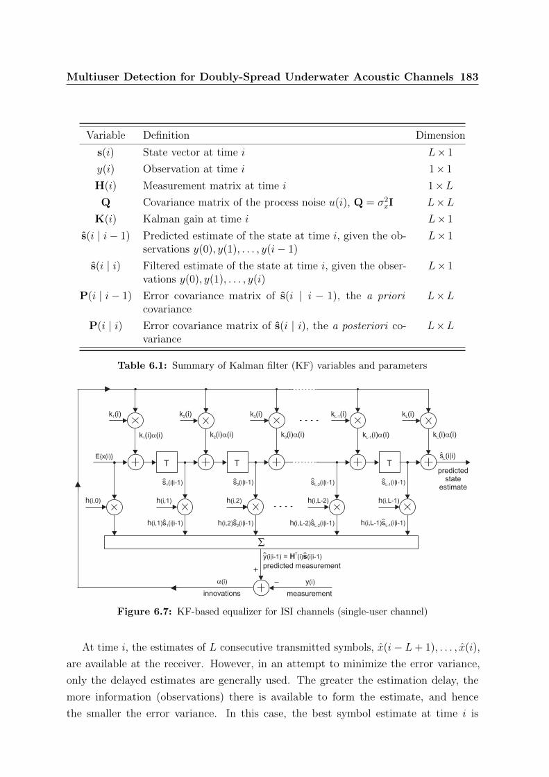
Multiuser Detection for Doubly-Spread Underwater Acoustic Channels 183
Variable Definition Dimension
s(i) State vector at time i L× 1
y(i) Observation at time i 1× 1
H(i) Measurement matrix at time i 1×LQ Covariance matrix of the process noise u(i), Q = σ2
xI L×LK(i) Kalman gain at time i L× 1
s(i | i− 1) Predicted estimate of the state at time i, given the ob-servations y(0), y(1), . . . , y(i− 1)
L× 1
s(i | i) Filtered estimate of the state at time i, given the obser-vations y(0), y(1), . . . , y(i)
L× 1
P(i | i− 1) Error covariance matrix of s(i | i − 1), the a prioricovariance
L×L
P(i | i) Error covariance matrix of s(i | i), the a posteriori co-variance
L×L
Table 6.1: Summary of Kalman filter (KF) variables and parameters
h(i,0)
T T T
h(i,1) h(i,2) h(i,L-2) h(i,L-1)
k (i)1 k (i)2 k (i)3 k (i)L-1 k (i)L
y(i)
measurement
predictedstate
estimate
a(i)
innovations
Ex(i) s (i|i)L
sL-1(i|i-1)sL-2(i|i-1)s2(i|i-1)s1(i|i-1)
y =(i|i-1) (i) (i|i-1)H sT
k (i) (i)1 a
h s(i,1) (i|i-1)1 h s(i,2) (i|i-1)2 h s(i,L-2) (i|i-1)L-2 h s(i,L-1) (i|i-1)L-1
k (i) (i)2 a k (i) (i)3 a k (i) (i)L-1 a k (i) (i)L a
S
predicted measurement
Figure 6.7: KF-based equalizer for ISI channels (single-user channel)
At time i, the estimates of L consecutive transmitted symbols, x(i− L+ 1), . . . , x(i),
are available at the receiver. However, in an attempt to minimize the error variance,
only the delayed estimates are generally used. The greater the estimation delay, the
more information (observations) there is available to form the estimate, and hence
the smaller the error variance. In this case, the best symbol estimate at time i is

Multiuser Detection for Doubly-Spread Underwater Acoustic Channels 184
x(i − L + 1) = s(i | i)L. This is a so-called fixed-lag estimate with delay-δ, where
δ = L− 1
6.3.3 Adaptive Equalization of Channels with Unknown Coefficients
To account for unknown coefficients, the equalizer must estimate the channel coefficients
and use these values to estimate the signal. This is accomplished by extending the state
vector to include the channel parameters as states, i.e.
s(i) =[
sT1 (i) sT2 (i)]T
(2L× 1 vector) (6.31)
where
s1(i) = [ x(i), x(i− 1), . . . x(i− L+ 1) ]T (L× 1 vector) (6.32)
s2(i) = [h(i, 0), h(i, 1), . . . h(i, L− 1) ]T (L× 1 vector) (6.33)
and hence the state equation is appended with L additional difference equations:
h(i+ 1, l) = h(i, l), 0 ≤ l ≤ L− 1 (6.34)
assuming a time-invariant channel. (The case of a time-varying channel is considered in
Section 6.5.) The state equation then assumes the form
s(i+ 1) = Fs(i) + Gu(i+ 1) (6.35)
where F is a 2L× 2L matrix, and G is a 2L× 1 vector, with definitions:
F =
Φ 0L×L
0L×L IL
, G =
Γ
0L× 1
, u(i+ 1) = x(i+ 1) (6.36)
The 2L× 1 state vector s(i) represents the state of the system at time i, the first L
components of the vector are the last L transmitted signals, and the last L components
are the channel coefficients. Matrices Φ and Γ are as defined in (6.19).
Multiuser Detection for Doubly-Spread Underwater Acoustic Channels 185
The adaptive equalizer formulaton of the KF includes a non-linearity in the measure-
ment equation:
y(i) = h (s(i)) + w(i), (6.37)
where the function h (s(i)) represents the transformation from the state variables to the
ideal observations (without noise), and is defined as
h (s(i)) = s1(i)sL+1(i) + · · · + sL(i)s2L(i) =L∑n=1
sn(i)sL+n(i) (6.38)
and sL+n(i) is the channel coefficient corresponding to the n-th input sn(i)
The KF is a linear filter and is unable to process non-linear equations intrinsically.
However, an approximate solution can be achieved by linearizing h. The result of this
linearization and the subsequent application of the linear KF of (6.24)-(6.28) results in
the extended Kalman filter (EKF). We linearize h (s(i)) about the estimate of s(i) based
on the previous data or predicted estimate s(i | i − 1), since a linearized observation
equation is needed to determine s(i | i) in (6.27). Using a first-order Taylor expansion to
linearize h (s(i)) yields
h (s(i)) ≈ h (s(i | i− 1)) +∂h
∂s(i)
∣∣∣∣s(i)=s(i|i−1)
(s(i)− s(i | i− 1)) (6.39)
Denoting the Jacobian matrix by
H(i) =∂h
∂s(i)
∣∣∣∣s(i)=s(i|i−1)
(6.40)
the linearized version of the observation equation from (6.37) becomes
y(i) = H(i)s(i) + (h(s(i | i− 1))−H(i)s(i | i− 1)) + w(i) (6.41)
For the function h (s(i)) defined in (6.38), the Jacobian matrix, H(i), is a 1× 2L vector
defined as
H(i) = [sL+1(i | i− 1), . . . , s2L(i | i− 1), s1(i | i− 1), . . . , sL(i | i− 1)] (6.42)
The linear KF for this model is the EKF which is defined by the following equations [50]:

Multiuser Detection for Doubly-Spread Underwater Acoustic Channels 186
1. Time update:
s(i | i− 1) = Fs(i− 1 | i− 1) (6.43)
P(i | i− 1) = FP(i− 1 | i− 1)FT + GQGT (6.44)
2. Kalman gain:
K(i) = P(i | i− 1)HT (i)[σ2w + H(i)P(i | i− 1)HT (i)
]−1(6.45)
3. Measurement update:
s(i | i) = s(i | i− 1) + K(i) [ y(i)− h (s(i | i− 1)) ] (6.46)
P(i | i) = [I−K(i)H(i)] P(i | i− 1) (6.47)
6.4 Multiple Access IDMA
Interleave division multiple-access (IDMA) [85] is a new spread-spectrum multiple-access
scheme, that when used with low-complexity iterative receivers has been shown to
outperform coded CDMA. In contrast to CDMA, which separates users by specific
spreading codes, IDMA separates users by unique interleaver sequences. IDMA can
be regarded as a special case of chip interleaved CDMA, and therefore inherits many
advantages of CDMA including dynamic channel sharing, asynchronous transmission,
and robustness against fading [74].
In an IDMA system, bandwidth expansion is entirely achieved by low-rate forward
error correction (FEC) code. A compromise between complexity and performance can be
achieved by constructing the FEC code as a combination of simple repetition code (for
bandwidth expansion) and strong code (for coding gain).
6.4.1 Transmitter Structure
Fig 6.8 shows the transmitter structure of the multiple-access IDMA scheme with K
simultaneous users [85]. The input data sequence dk of user-k is encoded by the FEC
encoder generating a coded sequence ck , [ck(1), . . . , ck(i), . . . ck(N)]T , where N is the
frame length. The elements in ck are referred to as coded bits. Then ck is passed through

Multiuser Detection for Doubly-Spread Underwater Acoustic Channels 187
Interleaver
b (i)K x (i)KInterleaver
FECEncoder
FECEncoder
d (i)K
QPSKSymbolMapper
b1(i) x (i)1
p1
pK
User 1 - Tx
User K - Tx
c (i)KQPSKSymbolMapper
Ep
Ed
PilotGenerator
PilotGenerator
Ep
Ed
y(t)
S
n(t)
Channel
h (t, )1 t
Channel
h (t, )K t
Doubly-SpreadMultiple Access Channel
d (i)1 c (i)1
x (i)K
p
px (i)1
Figure 6.8: Transmitter structure for a multiple-access IDMA system
a random interleaver πk, generating the interleaved coded bit sequence bk(i) = πk[ck(i)].
Finally, the interleaved chip sequence is QPSK modulated, producing xk. The QPSK
symbols are assumed to have unity average energy, with mean Exk(i) = 0 and variance
E|xk(i)|2 = 1. The elements of xk are referred to as chips in accordance with CDMA
convention.
The interleaver sequence for each user, πk, must be unique since IDMA system users
are distinguished solely by their interleaver sequence. These interleavers disperse the
coded sequences so that the adjacent chips are approximately uncorrelated.
Our proposed scheme employs a pilot-embedding method, where low-level pilots are
transmitted concurrently with the data, is used to obtain an initial coarse estimate of the
channel such that the iterative detection process at the receiver can be started. The soft
information obtained from the turbo decoder is subsequently used to improve channel
estimates.
For each user, the pilot sequences are superimposed over the entire transmission block.
For each chip, xk(i), there is one pilot chip, xpk(i). Therefore, the channel memory length
does not need to be smaller than the spreading length. Additionally, as the training is
performed in parallel to the data transmission, it is possible to track rapidly time-varying
channels. Compared with the more conventional approach of time-multiplexing pilot

Multiuser Detection for Doubly-Spread Underwater Acoustic Channels 188
symbols with data, superimposing the pilot-sequences has the advantage of not increasing
the transmission bandwidth [45].
In this chapter, the pilot symbols are transmitted at 10dB below the signal level of
the data symbols, and the pilot sequence design is from [80].
6.4.2 Receiver Structure
The joint multiple-access system with FEC coding in Figure 6.8 can be considered as
a serially concatenated coding system, where the FEC code and the multiple-access
channel assume the roles of outer code and inner code, respectively [102]. Using this
interpretation, an iterative receiver algorithm based on the turbo decoding concept [13]
can be developed.
SoftMultiuser
EKFEqualizer
extrinsicoutput
a prioriinformation
userK
d [i]K
x (i), (i)K Ks2
x (i),v (i)K K
y(t)
Soft FECChannelDecoder(DEC)
Interleaver
Deinterleaver
pK-1
pK
LLR -to-Symbol
SoftDemod.
l2(c [i])K
L2(c [i])K
l1(c [i])K
l2(b [i])K
L2(b [i])K
l1(b [i])K
Interleaver
pK
extrinsicoutput
a prioriinformation
userK
d [i]1
x (i), (i)1 1s2
x (i),v (i)1 1
Soft FECChannelDecoder(DEC)
Interleaver
Deinterleaver
p1-1
p1
LLR -to-Symbol
SoftDemod.
l2(c [i])1
L2(c [i])1
l1(c [i])1
l2(b [i])1
L2(b [i])1
l1(b [i])1
Interleaver
p1
receivedsignal
a posteriori
extrinsic
a posteriori
extrinsic
Figure 6.9: Receiver structure for a multiple-access IDMA system
The iterative receiver structure for the multiuser IDMA system is shown in Fig. 6.9.
This structure is based on the IDMA iterative receiver structure for joint channel
estimation and multiuser detection from [86] and [144], except here an adaptive soft
extended Kalman filter (EKF) is embedded into the iterative decoding process (in place
of the elementary signal estimator (ESE) of [86]). The adaptive EKF combined with
appropriate state-space channel models enables the receiver to effectively track and
Multiuser Detection for Doubly-Spread Underwater Acoustic Channels 189
equalize time-varying frequency-selective fading channels. The EKF is developed from
[58], [101], and [52].
The receiver structure consists of a soft-input soft-output (SISO) Kalman filter-based
multiuser equalizer and K single-user a posteriori probability FEC decoders (DECs).
The two stages are separated by interleavers and deinterleavers.
In each decoding iteration, the equalizer uses its a priori information to perform
joint adaptive channel estimation and equalization. The a priori information consists of
the the received signal y(t), soft information about the data symbols (supplied by the
K single-user FEC decoders from the previous iteration), and knowledge of the pilot
symbols. The equalizer produces soft-valued extrinsic information consisting of updated
sequences of soft symbol estimates xk(i), and the associated error variance σ2k(i), for
the K users. The estimates xk(i) are assumed to be complex Gaussian distributed with
mean xk(i) and variance σ2k(i).
The K single-user demodulators then perform symbol-by-symbol MAP demodulation
using the extrinsic information from the equalizer, and the a priori information, λ2(bk(i)),
for the coded bits, bk(i), from the soft FEC decoders (produced in the previous iteration).
The demodulators produce extrinsic information, λ1(bk(i)), (in log-likelihood ratio (LLR)
form) for the coded bits bk(i). The demodulator output LLRs, λ1(bk(i)), are then
deinterleaved according to λ1(ck(i)) = π−1k λ1(bk(i)), where each user (k) has a unique
interleaver sequence (πk). The deinterleavers reorder the extrinsic information sequences
into the correct order for the FEC decoding. The deinterleaver outputs, λ1(ck(i)), (which
are now the extrinsic LLRs for the coded sequence ck(i)) are then passed to the K
single-user soft FEC decoders which then use the BCJR algorithm [6] to perform MAP
decoding.
The K FEC decoders generate both the extrinsic information λ2(ck(i)) and the a
posteriori probabilities Λ2(ck(i)) for each user’s coded sequence ck(i)i. The interleaved
extrinsic LLRs λ2(bk(i)) = πλ2(ck(i)) are then used as a priori information for the
demodulator, while the a posteriori LLRs Λ2(bk(i)) = λ1(bk(i)) + λ2(bk(i)) are used to
compute the mean xk(i) and variance vk(i) for data symbols xk(i) as
xk(i) = Exk(i) =∑x∈X
xP (xk(i) = x), (6.48)
Multiuser Detection for Doubly-Spread Underwater Acoustic Channels 190
and
vk(i) = Varxk(i) =∑x∈X
|x− xk(i)|2 P (xk(i) = x),
= 1− |xk(i)|2 (6.49)
where X denotes the set of possible symbol constellations, and the probability P (xk(i) = x)
is calculated based on the assumption of independent bit sequence bk(i)i. Finally, xk(i)
and vk(i) are fed back into the equalizer as a priori information for the next iteration.
6.5 Multiuser Adaptive Soft EKF-Based Equalizer for
Doubly-Spread Channels
In this section, we describe the multiuser adaptive EKF-based equalizer that is embedded
in the turbo multiuser detector (MUD). The doubly-spread channels are modelled using
basis expansion models, and the EKF performs joint channel estimation and equalization
where their correlation is implicity considered. The multiuser EKF design is based on
the single-user channel EKF designs of [58] and [52], except here it is extended to the
multiuser case, adapted for IDMA systems with superimposed training, and incorporates
different channel models.
6.5.1 Multiuser System Model
The single-user channel of (6.17) is now extended to the doubly-spread multiuser case
with K users. The sequence of transmitted symbols from the k-th user is denoted xk(i),and the channel response for the k-th user at time i to a unit impulse at time i− l is
denoted hk(i, l)Ll=0. The received signal, y(i), is given by
y(i) =K∑k=1
L∑l=0
hk(i, l)xk(i− l) + w(i) (6.50)
where w(i) is the additive measurement noise, described previously. The channels
hk(i, l) are modelled using the wide-sense stationary uncorrelated scattering (WSSUS)
assumption [8], and are independent for different users, k. The transmitted symbols,

Multiuser Detection for Doubly-Spread Underwater Acoustic Channels 191
xk(i), are assumed mutually independent and identically distributed (i.i.d.) with mean
Exk(i) = 0 and variance Exk(i)x∗k(i) = σ2xk
= σ2x ∀ k.
For a block of NB consecutive received symbols, the BEM representation of the
channel for user-k is
hk(i, l) =
Q∑q=1
gk,q(l)ψq(i), 0 ≤ i ≤ NB − 1; 0 ≤ l ≤ L− 1 (6.51)
where gk,q(l)Qq=1 are the BEM coefficients for k-th user, and ψq(i)Qq=1 are the basis
functions. The BEM coefficients are time-invariant during the block i ∈ [0, N − 1],
but may change from block to block. The basis functions vary with time i, but are
common for every block (and all users). For a given set of basis functions, estimation of
the time-varying channel hk(i, l)i,l is reduced to estimating the invariant coefficients
gk,q(l)q,l over a block of NB symbols.
The basis functions in (6.51) are stacked into the following vector:
Ψ(i) , [ψ1(i), ψ2(i), . . . , ψQ(i) ]T (Q× 1 vector) (6.52)
and the BEM coefficients (for all K users) are stacked into the following vectors:
g(l)q , [ g1,q(l), g2,q(l), . . . , gK,q(l) ]T (K × 1 vector) (6.53)
g(l) , [ g(l)T1 , g
(l)T2 , . . . , g
(l)TQ ]T (KQ× 1 vector) (6.54)
g , [ g(0)T , g(1)T , . . . , g(L)T ]T (J1× 1 vector) (6.55)
where dimension J1 , KQ(L+ 1). Define the following transmit symbol vectors:
x(i) , [x1(i), x2(i), . . . , xK(i) ]T (K × 1 vector) (6.56)
X(i) , [ xT (i), xT (i− 1), . . . , xT (i− L) ]T (K(L+ 1)× 1 vector) (6.57)
Then, with the time restriction of i ∈ [0, NB − 1], the multiuser system model of (6.56)
using the BEM channel representation of (6.51), can be restated in vector form as
y(i) = XT (i)[ I(L+1) ⊗ (Ψ(i)⊗ IK) ]Hg + w(i), 0 ≤ i ≤ NB − 1 (6.58)
where ⊗ denotes the Kronecker product.
Multiuser Detection for Doubly-Spread Underwater Acoustic Channels 192
6.5.2 State-Space Model Incorporating A Priori Information
Using the approach of [52], the time-varying channels are modelled using BEMs, with
the BEM coefficients tracked by the EKF employing a low-order vector autoregressive
(VAR) process as state-space model. A VAR process of dimension KQ(L+ 1) is used to
track the corresponding number of BEM coefficients.
Although the BEM coefficients in (6.58) are invariant over the block of NB symbols,
they can change from block to block, therefore, in the broader sense, the BEM coefficient
vectors can be considered to be varying with time i. Consequently, the coefficient vector
of (6.55) can be denoted as g(i). With the assumption that the channel BEM coefficients
follow an AR(1) model [52], a first-order VAR model is used to track the time-variations
of the BEM coefficient vector, g(i), as follows:
g(i) = A1g(i− 1) + z(i) (6.59)
where A1 = αIJ1 is the VAR coefficient matrix, and the driving noise vector z(i) is zero-
mean complex Gaussian with variance σ2zIJ1 and statistically independent of g(i−1). The
Yule-Walker method (autocorrelation method) [49] can be used to calculate α. Typically
α ≈ 1 but α < 1. Assuming the multiuser channel is wide-sense stationary (WSS) and
the BEM coefficients gk,q(l) are independent, we have
σ2z = σ2
h(1− |α|2)/Q (6.60)
where σ2h , E|hk(i; l)|2, based on the assumption that all users (k) and all taps (l)
have the same Doppler spectrum.
The KF-equalization is performed with a fixed-lag of δ symbols (δ > 0) in order to
minimize the symbol estimate error variance. Generally, the equalization delay (δ) should
be greater than the maximum discrete delay-spread (L) to capture all the available
information. Define D , maxδ + 1, L+ 1.
The state vector must include estimates of both the transmitted symbols and the
BEM channel coefficients to enable the EKF to adaptively equalize the multiuser channel
with unknown coefficients. The state vector, s(i), is defined as follows:
s(i) =[
sT1 (i) sT2 (i)]T
(J × 1 vector) (6.61)

Multiuser Detection for Doubly-Spread Underwater Acoustic Channels 193
where
s1(i) , [xT (i), xT (i− 1), . . . , xT (i−D + 1)]T , (KD× 1 vector) (6.62)
s2(i) , g(i). (J1× 1 vector) (6.63)
and J , KD + KQ(L + 1) = KD + J1. Transmit symbol vector, x(i), is the K × 1
vector defined in (6.56).
For the EKF to be used within a turbo processing framework, the standard EKF
formulation (of Section 6.3.3) must be modified to incorporate soft a priori information
from the FEC channel decoders. This is achieved by considering each user’s transmit
symbol sequence, xk(i)i, to be a WSS stochastic process [109]. Then, using Wold’s
theorem [49], the symbol sequence of the k-th user, xk(i), can be expressed as
xk(i) = xk(i) + xk(i), (6.64)
where xk(i) = Exk(i) is a deterministic sequence, and xk(i) is approximated as an
uncorrelated stochastic process with mean Exk(i) = 0 and autocorrelation Exk(i)x∗k(i+j) = vk(i)δ(j) (assuming an ideal interleaver).
The statistical characteristics of xk(i), namely xk(i) and vk(i), are calculated from
the a priori information. For data symbols, xk(i) and vk(i) are calculated from (6.48)
and (6.49), respectively. While for pilot symbols, xk(i) = xpk(i) and vk(i) = 0, since the
pilot symbols are known to the equalizer.
Collecting the K users together, the following vectors are defined:
x(i) = [ x1(i), x2(i), . . . , xK(i) ]T (K × 1 vector) (6.65)
x(i) = [ x1(i), x2(i), . . . , xK(i) ]T (K × 1 vector) (6.66)
Using the state vector, s(i) in (6.61), the state equation (incorporating a priori informa-
tion) can be written as
s(i) = Fs(i− 1) + Gx(i) + u(i), (6.67)

Multiuser Detection for Doubly-Spread Underwater Acoustic Channels 194
with the following definitions:
F =
Φ 0KD× J1
0J1×KD A
(J × J matrix) (6.68)
A = αIJ1 (J1× J1 matrix) (6.69)
Φ =
01× (D−1) 01× 1
I(D−1) 0(D−1)× 1
⊗ IK (KD×KD matrix) (6.70)
G =[IK 0K× (J−K)
]T(J ×K matrix) (6.71)
(6.72)
The vector u(i) is zero-mean uncorrelated process noise, defined as
u(i) =[ΓT x(i) zT (i)
]T, (J × 1 vector) (6.73)
where
Γ = [ 1 01× (D−1) ]T ⊗ IK (KD×K matrix) (6.74)
and z(i) is the J1× 1 vector defined in (6.59). The covariance matrix of u(i) is given by
Q(i) = Eu(i) uH(i) = Q + GVGT , (J × J matrix) (6.75)
where
V = diag v1(i), v2(i), . . . , vK(i) (K ×K matrix) (6.76)
Q =
0KD×KD 0KD× J1
0J1×KD σ2zIJ1
(J × J matrix) (6.77)
The measurement equation is given by
y(i) = h[s(i)] + w(i), (6.78)
and the nonlinear function for h[s(i)] is defined as
h[s(i)] , XT (i)[I(L+1) ⊗ (Ψ(i)⊗ IK)
]Hg(i), (6.79)

Multiuser Detection for Doubly-Spread Underwater Acoustic Channels 195
where both X(i) and g(i) can be obtained from the the state vector, s(i).
6.5.3 Fixed-Lag Soft Input Extended Kalman Filtering
The EKF is applied to the state and measurement equations of (6.67) and (6.78),
respectively, to jointly decode the data symbols and track the channel BEM coefficients.
The EKF is initialized with
s(−1 | −1) = 0J × 1 and P(−1 | −1) = Q,
The EKF is described by the following recursive equations:
1. Time update:
s(i | i− 1) = Fs(i− 1 | i− 1) + Gx(i), (6.80)
P(i | i− 1) = FP(i− 1 | i− 1)FT + Q + GVGT . (6.81)
2. Kalman gain:
H(i) =∂f [s]
∂s
∣∣∣∣∣s=s(i|i−1)
(Jacobian matrix), (6.82)
K(i) = P(i | i− 1)HH(i)[σ2w + H(i)P(i | i− 1)HH(i)
]−1. (6.83)
3. Measurement update:
s(i | i) = s(i | i− 1) + K(i)y(i)− h[s(i | i− 1)], (6.84)
P(i | i) = [IJ −K(i)H(i)]P(i | i− 1). (6.85)
The EKF recursions are shown diagrammatically in Figure 6.10. The a priori
information xk(i), vk(i)Kk=1 is the soft information (at time i) obtained from the K
single-user FEC channel decoders, via the LLR-to-symbol blocks (as shown in Figure 6.9).
The output xk(i) = s(i + δ | i + δ)(Kδ+k) is the delayed a posteriori estimate of the
data symbol xk(i) for the k-th user, k ∈ [1, K].

Multiuser Detection for Doubly-Spread Underwater Acoustic Channels 196
EKFRecursion
x (i) ,
v (i) ,
y(i)
k k
k k
x (i+1) ,
v (i+1) ,
y(i+1)
k k
k k
s
P
(i-1|i-1),(i-1|i-1)
s
P
(i|i),(i|i)
s
P
(i+1|i+1),(i+1|i+1)
time = i time = i + 1
EKFRecursion
to nextrecursion
frompreviousrecursion
inputs at time i inputs at time i+1
Figure 6.10: Extended Kalman filter (EKF) recursions
6.5.4 Generating Extrinsic Information
The fixed-lag EKF generates delayed a posteriori estimates for xk(i)Kk=1. However,
if the EKF equalizer is to be used within a turbo framework, it must produce delayed
extrinsic estimates. To generate extrinsic estimates, xk(i)Kk=1, that are independent
of the a priori information xk(i), vk(i)Kk=1, the comb structure shown in Figure 6.11
(adapted from [58]) is used in conjunction with the EKF.
EKF EKF EKF EKF
x (i-1) ,
v (i-1) ,
y(i-1)
k
k
k
k
x (i) ,
v (i) ,
y(i)
k k
k k
EKF EKF EKF
x (i+1) ,
v (i+1) ,
y(i+1)
k k
k k
x (i+ ) ,
v (i+ ) ,
y(i+ )
k k
k k
d
d
d
s
P
(i-2|i-2),(i-2|i-2)
s
P
e
e
(i+n|i+n),
(i+n|i+n)
s
P
(i-1|i-1),(i-1|i-1)
( +1) timesd
x (i+2) ,
v (i+2) ,
y(i+2)
k k
k k
x (i+ +1) ,
v (i+ +1) ,
y(i+ +1)
k k
k k
d
d
d
s
P
e
e
(i+n+1|i+n+1),
(i+n+1|i+n+1)
x (i+1) ,
v (i+1) ,
y(i+1)
k k
k k
x (i+3) ,
v (i+3) ,
y(i+3)
k k
k k
x (i+ +2) ,
v (i+ +2) ,
y(i+ +2)
k k
k k
d
d
d
s
P
e
e
(i+n+2|i+n+2),
(i+n+2|i+n+2)
s
P
(i|i),(i|i)
s
P
(i+1|i+1),(i+1|i+1)
s
P
(i+2|i+2),(i+2|i+2)
EKF EKF EKF
EKF EKF EKF
x (i+2) ,
v (i+2) ,
y(i+2)
k k
k k
x (i)=0 ,
v (i)=1 ,
y(i)
k k
k k
x (i+1)=0 ,
v (i+1)=1 ,
y(i+1)
k k
k k
x (i+2)=0 ,
v (i+2)=1 ,
y(i+2)
k k
k k
x (i), (i)k k ks2
x (i+1), (i+1)k k ks2
x (i+2), (i+2)k k ks2
extrinsicestimates
a posterioriestimates
Figure 6.11: Adaptive SISO equalizer using fixed-lag extended Kalman filters (EKFs).
At each time i, the vertical branch composed of (δ + 1) EKFs produce the extrinsic
estimates for each user, xk(i)Kk=1, while the horizontal branch keeps updating the

Multiuser Detection for Doubly-Spread Underwater Acoustic Channels 197
a posteriori estimate s(i | i) and its error covariance P(i | i). In order to exclude
the effect of the a priori information, the first EKF in the vertical branch assigns
xk(i) = 0, vk(i) = 1Kk=1 to the a priori inputs, in place of the information generated by
the FEC decoders, Let se(i+ n | i+ n) and Pe(i+ n | i+ n) denote the state estimate
and its error covariance matrix, respectively, generated by the (n+ 1)-th vertical filtering
branch. Then the δ-delayed estimate xk(i) and its error covariance σ2k(i), which form the
extrinsic information for xk(i), are given by
xk(i) = se(i+ δ | i+ δ) (Kδ+k) , and (6.86)
σ2k(i) = Pe(i+ δ | i+ δ) (Kδ+k),(Kδ+k) , (6.87)
respectively (for user k).
6.6 Performance Evaluation
We consider an underwater sensor network multiuser system where multiple sensor
nodes can directly transmit (single-hop) to the central gateway node. Sensor node data
transmission may be ad hoc, and multiple nodes may transmit data simultaneously to the
central gateway node. Each sensor node must be located within the receiving range of
the gateway node. The adaptive equalization schemes are evaluated with 8 simultaneous
users (transmitting sensor nodes). The transmitter FEC code (which is common to all
users) is a 1/4-rate convolutional code serially concatenated with a 1/8-rate repetition
code (producing an overall code rate of R = 1/32). Each transmitter generates QPSK
symbols and has a symbol rate of 1200 symbols per second (producing an aggregate rate
of 9600 symbols/second).
A multiple-access random doubly-spread underwater acoustic channel is simulated by
a tapped delay line (multipath) structure derived from the ray-tracing methods of [145],
with independent and uncorrelated Rayleigh processes applied to each tap. Within the
multiuser channel, the channel coefficients hk(i, l)k,l are mutually independent for each
user k and for each tap l. Each tap is generated via the method in [143] and satisfies
Jakes’ model [46]. Channel ranges of 200 to 500m, and water depth of 25 to 30m are
considered, using the models described in Section 6.2.1. From the channel fading rate
definitions in Table 6.2, we consider fast- and very-fast-fading rates with normalised
Doppler frequency range of 2.5× 10⁻³ to 15× 10−3.
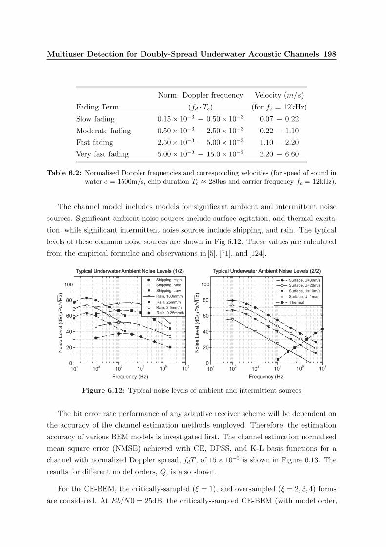
Multiuser Detection for Doubly-Spread Underwater Acoustic Channels 198
Norm. Doppler frequency Velocity (m/s)
Fading Term (fd ·Tc) (for fc = 12kHz)
Slow fading 0.15× 10⁻³ − 0.50× 10⁻³ 0.07 − 0.22
Moderate fading 0.50× 10⁻³ − 2.50× 10⁻³ 0.22 − 1.10
Fast fading 2.50× 10⁻³ − 5.00× 10⁻³ 1.10 − 2.20
Very fast fading 5.00× 10⁻³ − 15.0× 10⁻³ 2.20 − 6.60
Table 6.2: Normalised Doppler frequencies and corresponding velocities (for speed of sound inwater c = 1500m/s, chip duration Tc ≈ 280us and carrier frequency fc = 12kHz).
The channel model includes models for significant ambient and intermittent noise
sources. Significant ambient noise sources include surface agitation, and thermal excita-
tion, while significant intermittent noise sources include shipping, and rain. The typical
levels of these common noise sources are shown in Fig 6.12. These values are calculated
from the empirical formulae and observations in [5], [71], and [124].
101
101
102
102
103
103
104
104
105
105
106
106
Frequency (Hz) Frequency (Hz)
0 0
20 20
40 40
60 60
80 80
100 100
Nois
e L
evel (d
B/
Pa/ H
z)
m
Nois
e L
evel (d
B/
Pa/ H
z)
m
Typical Underwater Ambient Noise Levels (1/2) Typical Underwater Ambient Noise Levels (2/2)
Surface, U=30m/s
Surface, U=20m/s
Surface, U=10m/s
Surface, U=1m/s
Thermal
Rain, 2.5mm/h
Rain, 0.25mm/h
Shipping, High
Shipping, Med.
Shipping, Low
Rain, 100mm/h
Rain, 25mm/h
Figure 6.12: Typical noise levels of ambient and intermittent sources
The bit error rate performance of any adaptive receiver scheme will be dependent on
the accuracy of the channel estimation methods employed. Therefore, the estimation
accuracy of various BEM models is investigated first. The channel estimation normalised
mean square error (NMSE) achieved with CE, DPSS, and K-L basis functions for a
channel with normalized Doppler spread, fdT , of 15× 10−3 is shown in Figure 6.13. The
results for different model orders, Q, is also shown.
For the CE-BEM, the critically-sampled (ξ = 1), and oversampled (ξ = 2, 3, 4) forms
are considered. At Eb/N0 = 25dB, the critically-sampled CE-BEM (with model order,
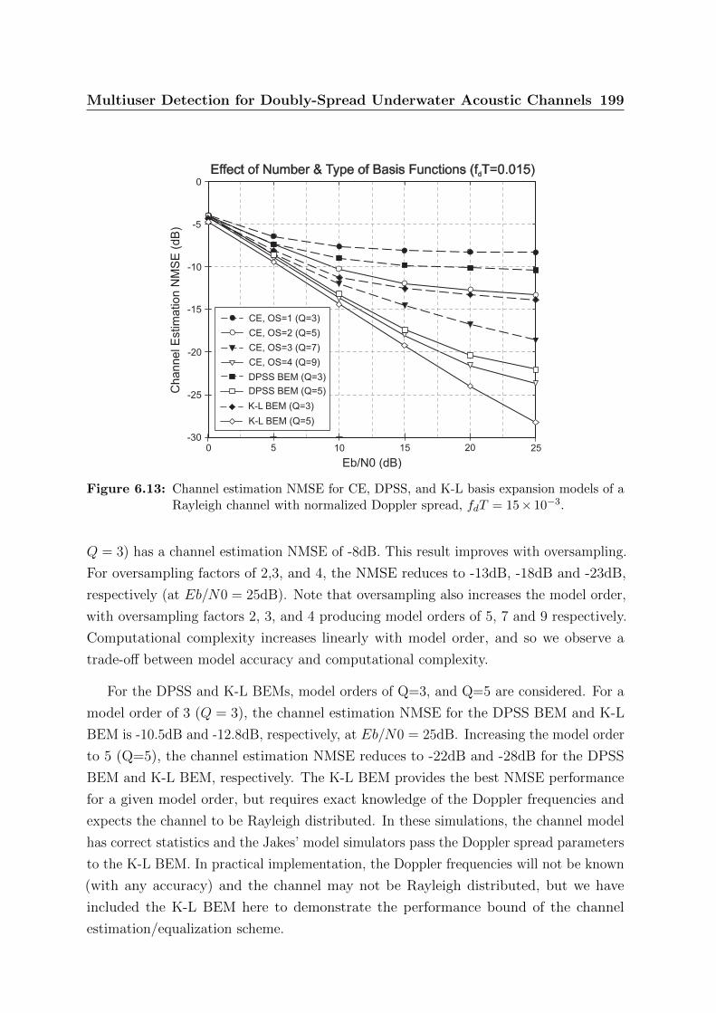
Multiuser Detection for Doubly-Spread Underwater Acoustic Channels 199
Ch
an
ne
l E
stim
atio
n N
MS
E (
dB
) -5
-10
-20
-25
-30
-15
Eb/N0 (dB)
0
0
5 10 15 20 25
Effect of Number & Type of Basis Functions (f T=0.015)d
DPSS BEM (Q=3)
K-L BEM (Q=3)
DPSS BEM (Q=5)
K-L BEM (Q=5)
CE, OS=1 (Q=3)
CE, OS=2 (Q=5)
CE, OS=3 (Q=7)
CE, OS=4 (Q=9)
Figure 6.13: Channel estimation NMSE for CE, DPSS, and K-L basis expansion models of aRayleigh channel with normalized Doppler spread, fdT = 15× 10−3.
Q = 3) has a channel estimation NMSE of -8dB. This result improves with oversampling.
For oversampling factors of 2,3, and 4, the NMSE reduces to -13dB, -18dB and -23dB,
respectively (at Eb/N0 = 25dB). Note that oversampling also increases the model order,
with oversampling factors 2, 3, and 4 producing model orders of 5, 7 and 9 respectively.
Computational complexity increases linearly with model order, and so we observe a
trade-off between model accuracy and computational complexity.
For the DPSS and K-L BEMs, model orders of Q=3, and Q=5 are considered. For a
model order of 3 (Q = 3), the channel estimation NMSE for the DPSS BEM and K-L
BEM is -10.5dB and -12.8dB, respectively, at Eb/N0 = 25dB. Increasing the model order
to 5 (Q=5), the channel estimation NMSE reduces to -22dB and -28dB for the DPSS
BEM and K-L BEM, respectively. The K-L BEM provides the best NMSE performance
for a given model order, but requires exact knowledge of the Doppler frequencies and
expects the channel to be Rayleigh distributed. In these simulations, the channel model
has correct statistics and the Jakes’ model simulators pass the Doppler spread parameters
to the K-L BEM. In practical implementation, the Doppler frequencies will not be known
(with any accuracy) and the channel may not be Rayleigh distributed, but we have
included the K-L BEM here to demonstrate the performance bound of the channel
estimation/equalization scheme.

Multiuser Detection for Doubly-Spread Underwater Acoustic Channels 200
Both the CE BEM and DPSS BEM only require an upper bound on the Doppler
spread (not knowledge of the exact Doppler frequencies), so the performance of these
two models should be more representative of what is achievable in practice.
As a general rule, for a coded system to achieve an acceptable receiver bit error rate
performance (e.g., a BER in the order of 10−4 or better), the channel estimation scheme
should have a NMSE performance of approximately -12dB or better. From the results of
Figure 6.13, this suggests that a minimum BEM order of 5 (Q=5) is required for channels
with normalised Doppler spread up to 15× 10−3. Therefore the following results all use
BEM models of order 5 or greater.
Figure 6.14 compares the performance of channel estimation models employed by
the iterative multiuser detector over a range of normalised Doppler spread. The linear
equalizer is the standard IDMA channel estimation scheme of [86] and [144]. The auto-
regressive (AR) model and basis expansion models (CE, DPSS, K-L) are the state-space
models employed by the extended Kalman filter (EKF) embedded in the IDMA turbo
multiuser detector. Figure 6.14a shows the channel estimation normalised mean square
error (NMSE), while Figure 6.14b shows the bit error rate performance.
The linear equalizer scheme performs well at lower Doppler spreads (with NMSE of
18.8dB and BER of 1.7× 10⁻⁵ at fdT = 1× 10⁻³ and Eb/N0 = 10dB) but at higher
Doppler spreads the performance rapidly deteriorates, with a BER greater than 1× 10⁻¹
for fdT ≥ 5× 10⁻³.
The EKF using the 10th-order AR model, AR(10), also performs well for slow and
moderate fading channels, with a BER of 4× 10⁻⁵ at fdT = 1× 10⁻³ and Eb/N0 = 10dB,
but performance also deteriorates significantly with increasing Doppler spread, with a
BER of greater than 1× 10⁻² for fdT ≥ 6.25× 10⁻³.
The EKF using the BEM state-space models provides better performance. The
critically-sampled CE-BEM (OS=1) has a channel NMSE of -14.6dB or better for fdT ≤8.75× 10⁻³, deteriorating to -9.6dB for fdT = 15× 10−3. Similarly the BER performance
is 2.6× 10⁻⁵ at fdT = 1× 10⁻³ and slowly rises to 7× 10⁻⁴ for fdT = 15× 10−3.
The oversampled CE (OS=2), DPSS, and K-L BEMs provide the best performances,
all providing BER of 2× 10⁻⁵ or better and channel NMSE values of -18dB or better for
fdT ≤ 10× 10−3. At fdT = 15× 10−3, the channel NMSE is -12.5dB or better and the
BER is 2× 10⁻⁴ or better.

Multiuser Detection for Doubly-Spread Underwater Acoustic Channels 201
Channel E
stim
ation
NM
SE
(dB
)
-25
0Effect of Chan. Model on Chan. Est. MSE (E /N =10dB)b 0
Normalised Doppler spread (f T) x10d
-3
0.0 5.02.5 7.5 10.0 12.5 15.0
-5
-10
-15
-20
Linear
AR(10)
CE, OS=1, Q=5
CE, OS=2, Q=9
DPSS, Q=5
K-L, Q=5
(a) Channel estimation normalised mean square error (NMSE)
Bit E
rror
Rate
10-1
10-2
10-3
10-5
10-6
100
10-4
Effect of Chan. Model on Bit Error Rate (E /N =10dB)b 0
Normalised Doppler spread (f T) x10d
-3
0.0 5.02.5 7.5 10.0 12.5 15.0
Linear
AR(10)
CE, OS=1, Q=5
CE, OS=2, Q=9
DPSS, Q=5
K-L, Q=5
(b) Bit error rate performance
Figure 6.14: Effect of channel estimation scheme and Doppler spread on system performance:a) channel estimation NMSE; and b) bit error rate. (Eb/N0 = 10dB)

Multiuser Detection for Doubly-Spread Underwater Acoustic Channels 202
As the maximum normalised Doppler frequency increases, the number of significant
eigenvalues in the BEM representation increases and thus a larger number of basis
functions, Q, need to be used for an accurate approximation. As a general case, the BEM
accuracy deteriorates with increasing fdT . The accuracy can be improved by increasing
the number of basis functions used (Q), but this comes with the cost of increasing
computational complexity.
Figure 6.15 compares the performance of the channel estimation schemes over a range
of signal-to-noise ratios at maximum Doppler spread (fdT = 15× 10−3). Figure 6.15a
shows the channel estimation normalised mean square error (NMSE), while Figure 6.14b
shows the bit error rate performance.
As discovered previously, the linear equalization scheme performs poorly at theis
high Doppler spread, with channel NMSE and BER values of approximately -3dB and
3× 10⁻¹ respectively, over the range of Eb/N0 values. The EKF with autoregressive
model achieves better performance than the linear scheme, but still only attains a BER
of 1.2× 10⁻³ and channel NMSE of -8dB at Eb/N0 = 20dB.
The four basis expansion models all achieve good performance at high Doppler spread.
The K-L BEM achieves a channel NMSE and BER of -16.5dB and 4.8× 10⁻⁶ respectively
at Eb/N0 = 12.5dB. The K-L BEM is exactly matched to the Jakes’ model Rayleigh
spectrum, so this represents the best case performance of the multiuser EKF scheme
(for 5 basis functions, Q = 5). The DPSS BEM achieves a channel NMSE and BER of
-15dB and 1.3× 10⁻⁵, respectively, at Eb/N0 = 12.5dB. This is within 2dB of the K-L
BEM performance and the DPSS BEM doesn’t require detailed knowledge of he channel
spectrum, only the maximum Doppler frequency.
The critically-sampled CE-BEM achieves a channel NMSE and BER of -10.5dB and
9× 10⁻⁵, respectively, at Eb/N0 = 12.5dB. While the over-sampled CE-BEM achieves a
channel NMSE of -15.5dB and 6.5× 10⁻⁶, respectively, for the same Eb/N0 ratio. The
over-sampled CE-BEM performance is within 1.5dB of the K-L BEM, but this comes
at the expense of computational complexity with the oversampled CE-BEM requiring 9
basis functions compared to 5 for the K-L BEM (and other BEM types evaluated).

Multiuser Detection for Doubly-Spread Underwater Acoustic Channels 203
Effect of Chan. Model on Chan. Est. MSE (f T=0.015)dC
hannel E
stim
ation
NM
SE
(dB
)
-5
-10
-15
-20
-25
0
2.5 5.0 7.5 10.0 12.5 17.5 20.0
Eb/N0 (dB)
15.0
Linear
AR(10)
CE, OS=1, Q=5
CE, OS=2, Q=9
DPSS, Q=5
K-L, Q=5
(a) Channel estimation normalised mean square error (NMSE)
Eb/N0 (dB)
Effect of Chan. Model on Bit Error Rate (f T=0.015)d
Bit E
rror
Rate
10-1
10-2
10-3
10-5
10-6
100
10-4
2.5 5.0 7.5 10.0 12.5 17.5 20.015.0
Linear
AR(10)
CE, OS=1, Q=5
CE, OS=2, Q=9
DPSS, Q=5
K-L, Q=5
(b) Bit error rate performance
Figure 6.15: Effect of channel estimation scheme and Eb/N0 ratio on system performance: a)channel estimation NMSE; and b) bit error rate. (fdT = 15× 10−3)
Multiuser Detection for Doubly-Spread Underwater Acoustic Channels 204
6.7 Conclusion
In this chapter, a multiple-access communications scheme for doubly-selective underwater
acoustic channels was developed. It is envisaged that the schmee could be used to support
an underwater sensor network.
The communications scheme uses interleave-division multiple access (IDMA), a
scheme where users are separated by unique interleaver sequences. When used with
low-complexity iterative receivers, IDMA has been shown to outperform coded CDMA.
To enable joint channel estimation and data detection, low-level pilot symbols are
superimposed onto the transmitted data. These pilots, which are at a level much lower
that the signal level, are used by the receiver to obtain the initial coarse estimates of
the channel. Improved estimates of the channel are then obtained by integrating the
estimation of the channel into the decoding loop. Soft information from the iterative
decoder is used to improve channel estimation after every iteration of the decoder.
Such schemes have been shown to provide good performance in multipath (delay-
spread) channels, and in fast-fading (Doppler-spread) channels. However in doubly-spread
channels, the number of unknown channel variables exceeds the number of known data
variables (pilot symbols). The underlying system of equations used by the channel
estimation algorithm becomes underdetermined, and accurate channel estimation becomes
intractable.
To alleviate this problem, we model the doubly-selective channel using basis expansion
models (BEMs). A BEM is an economical or parsimonious model that can provide a
good approximation of a time-varying channel using a a reduced number of parameters.
Modelling of linear systems by basis expansion models can turn a time-varying system
identification problem into a time-invariant one. Using BEM representations of the
channel, estimation of doubly-spread channels from using pilot symbols becomes tractable.
An adaptive turbo multiuser receiver was developed where time-domain equalization
is performed using a Kalman filter (KF). KF-based equalization has been shown to
outperform traditional linear transversal equalizers, and have much lower complexity. An
extended Kalman filter (EKF) is embedded into the turbo multiuser detector to create a
multiuser equalizer that jointly optimizes the estimates of the channel coefficients and
data symbols in each iteration of the detection process. EKF state-space modelling
Multiuser Detection for Doubly-Spread Underwater Acoustic Channels 205
is performed using basis expansion models to provide a tractable means of estimating
doubly-spread channels at minimal computational complexity.
Experimental results demonstrate that the proposed multiple-access scheme with
adaptive turbo receiver provides robust performance in doubly-spread underwater acoustic
channels.
Chapter 7
Conclusion
This thesis explores and applies iterative and adaptive processing techniques to multiple-
access IDMA systems. The research consists of two parts. The first is concerned
with the optimisation of the iterative detection process, this is achieved through power
allocation, FEC code allocation and perfect space-time coding. The second part is
concerned with the application of IDMA systems with iterative receivers to underwater
acoustic communications. The underwater acoustic channel is a challenging environment
characterised by long delay-spreads and limited bandwidth. An OFDM-IDMA system
was presented as a solution for underwater channels with delay spread, and an iterative
receiver for IDMA using a non-linear Kalman filter to perform joint decoding and
channel equalization was presented for doubly-spread underwater acoustic channels. The
non-linear Kalman filter utilised low-rank basis expansion models (BEMs) to track the
temporal variation of the channels.
In this final chapter, the main conclusions from the novel findings and future research
directions on this work are presented. The following section summarises the work that
has been conducted in this thesis which highlights the contributions of this research work.
Thereafter, directions for further research are discussed.
206
Conclusion 207
7.1 Summary and Thesis Contributions
7.1.1 IDMA Performance Optimisation using Variance Transfer
Analysis
Variance Transfer (VT) charts were used as a tool for analysing the iterative receiver
performance. VT charts track the variance in the log-likelihood ratio (LLR) values
that are exchanged between the multiuser detector (MUD) and the channel decoders,
providing a graphical representation of the receiver’s convergence process. The variance
transfer (input/output) characteristic curves of the constituent receiver components, the
multiuser detector (MUD) and the forward error correction (FEC) channel decoders,
were calculated and then the iterative receiver performance was optimised by matching
the VT characteristic curves. Two optimisation schemes were developed:
Power Allocation. Chayat et. al. [18] have shown that the performance of an iterative
receiver is optimised if different users transmit at different powers, allowing the
iterative decoder to operate in an “onion peeling” mode, where the higher-power
layers converge first, decreasing their contribution to the residual noise, and then
the lower-power layers converge.
The IDMA concept was extended to a multi-rate system where different users
transmit data at different rates, but the same low-complexity iterative receiver
structure could still be used. High-rate users were supported by breaking up the
input data stream into multiple sub-streams. An IDMA layer was created from each
sub-stream, and the multiple IDMA layers are then combined and transmitted from
a single antenna. The iterative receiver treats each IDMA layer as a virtual user.
VT charts where then used to analyse the iterative receiver performance, and to
develop an optimal power allocation strategy for assigning transmit power levels to
IDMA layers. In a Rayleigh flat-fading environment, simulation results demonstrated
that the performance of the proposed scheme is close to the theoretical limit.
FEC Code Allocation. Ten Brink [116] demonstrated that different FEC codes generate
different FEC channel decoder VT characteristics. The allocation of FEC codes can
also be used to manipulate the reciever VT characteristics and thereby optimise
system performance.
Conclusion 208
Using numerical methods and VT Charts, a simple FEC code allocation strategy is
devised so that new users are allocated FEC codes according to the existing system
load, this allows the FEC decoder VT curve to dynamically match the MUD VT
curve as it changes with system load, providing optimal system performance over a
range of operating conditions. For small multiuser systems, results demonstrated
that the performance of the proposed system approaches the theoretical single user
bound.
7.1.2 Optimal Space-Time Coding using the Golden Code
Multiple antenna systems (commonly referred to as multi-input multi-output or MIMO
systems) have proven to be an effective method for realising high-rate reliable wireless
communications. While coding strategies for MIMO systems have generally focused on
providing either higher-rate or increased diversity over traditional single antenna (SISO)
systems, linear dispersion (LD) codes are a generalised class of space-time codes that
can theoretically provide both diversity gain and high-rate.
LD codes are defined as codes that break up the input data stream into sub-streams
that are dispersed in linear combinations over space and time. Recently, cyclic division
algebra techniques have provided the means for constructing LD codes that provide both
full-diversity and full-rate. Codes that achieve both full-diversity and -rate (and meet a
few energy efficiency criteria) are known as perfect STBCs or perfect codes. The golden
code is a perfect STBC for 2× 2 multiple-antenna systems.
The Golden Code system was extended to the multiuser case, and a MIMO-IDMA
multiuser detector to decode LD codes was developed. The complexity of the receiver
was linear in the number of users. The performance of this GC-IDMA scheme was
compared with MIMO-IDMA schemes employing the Alamouti STBC and V-BLAST,
and also against the single-user bound. In a Rayleigh flat-fading environment, simulation
results demonstrated that GC-IDMA outperforms both Alamouti- and V-BLAST-IDMA
at moderate and high SNR levels. For signal to noise ratios of 8dB and greater, the
GC-IDMA scheme employing 16 users approaches within 0.25dB of the single-user bound.

Conclusion 209
7.1.3 Multiuser Communications for Underwater Acoustic Channels
Underwater sensor networks enable a broad range of applications including environmental
monitoring, undersea exploration, assisted navigation, and distributed surveillance [2].
Reliable high-performance sensor networks would need to be underpinned by a robust
and efficient multiple-access underwater communications scheme.
Transmission of acoustic waves is considered the most practical means of underwater
communications. Radio systems are not feasible because the only radio waves in the
extra-low frequency range (< 300Hz) are capable of propagating any distance through
conductive sea water. Optical systems are also not suitable because optic waves, while
not suffering as significantly from attenuation, are severely affected by scattering and
absorption [110].
However, designing reliable underwater acoustic communications (UAC) systems
has proven to be very challenging. One of the main channel impairments is multipath
interference caused by multiple reflections of the acoustic signal from the water surface
and bottom. These reflections occur at small grazing angles and with small reflection
losses. This effect causes both long time-delay spread and large multipath amplitudes to
be present in the received signal [51].
Delay-spread underwater acoustic channels
Large delay-spread implies that single-carrier communication will be plagued by inter-
symbol interference (ISI) that, for practical signal bandwidths, spans many symbols.
As an alternative, multi-carrier modulation (MCM) has been proposed to increase the
symbol interval and thereby decrease the ISI span. Multicarrier modulation (MCM) is a
popular transmission scheme in which the data stream is split into several substreams
and transmitted, in parallel, on different subcarriers. MCM transforms the inter-symbol
interference (ISI)-inducing frequency selective channel into a set of independent parallel
subchannels.
Orthogonal frequency division multiplexing (OFDM) [135], [20] has emerged as one
of the most practical MCM techniques for data communication over frequency-selective
fading channels. In OFDM, the computationally-efficient fast Fourier transform (FFT)
is used to transmit data in parallel over a large number of orthogonal subcarriers.
The principle advantage of multi-carrier schemes like OFDM, relative to single-carrier
Conclusion 210
schemes, is that they facilitate simple equalization of delay-spread (i.e., frequency-
selective) channels. When an adequate number of subcarriers are used in conjunction
with a cyclic prefix of adequate length, subcarrier orthogonality is maintained, even in
the presence of frequency-selective fading. Orthogonality implies a lack of subcarrier
interference and permits simple, high-performance data detection.
Orthogonal Frequency Division Multiplexing (OFDM) was combined with an IDMA
overlay to develop a multiple-access communications system that provides robust perfor-
mance in the presence of large time-delay spread and the other impairments presented by
the shallow water acoustic channel. A low-complexity iterative decoding algorithm based
on the turbo-decoding concept was developed for the OFDM-IDMA system receiver, and
experimental results demonstrate good performance.
Doubly-spread underwater acoustic channels
The underwater acoustic channel was extended to the doubly-spread case. The relative
motion between the transmitter, receiver, and scattering objects imparts each path
with a unique Doppler shift, so that multipath propagation also induces a frequency-
domain spreading effect on the information signal. Such channels are both delay- and
Doppler-spread (or equivalently, frequency- and time-selective), and are referred to as
“doubly-spread” or “doubly-selective”.
OFDM schemes can been used successfully for time-invariant and slowly time-varying
(TV) channels, but they become problematic for doubly-spread (or rapidly TV) channels.
For time-invariant channels, the data stream can be split up and transmitted in parallel
on non-interfering subcarriers, with equalization being just a simple matter of adjusting
the gain and phase on each received subcarrier. This approach can be easily extended
to slowly TV channels, where a time-invariant channel is simulated by choosing an
OFDM symbol duration that is shorter than the coherence time of the channel. For
time-invariant or slowly TV channels, the loss in spectral efficiency due to the inclusion
of the guard intervals can be made small, since the channel delay spread (and hence the
guard interval) is much smaller than the channel coherence time (and hence the OFDM
symbol length). But for rapidly TV channels, the OFDM symbol length would need
to be made extremely short, at which point the loss of spectral efficiency due to guard
insertion would be severe [104]. Hence, OFDM schemes become impractical for rapidly
TV channels.

Conclusion 211
As a result, a single-carrier system with adaptive channel-estimation is considered
for the doubly-spread underwater channel. A single-carrier system with linear traversal
equalizer would face complexity issues due to the large number of equalizer taps required
to compensate for the long delay-spread. Instead, a Kalman filter (KF) is used as
equalizer. KF-based equalizers have been shown to perform significantly better than
linear traversal equalizers at a much lower complexity. Additionally, the state-space
formulation of the Kalman equalizer is well suited for iterative receivers and allows easy
incorporation of soft (a-priori) information for channel-coded systems.
The Kalman filter utilises basis expansion models (BEMs) to model the doubly-
selective underwater channels. A basis expansion model is a parsimonious low-rank
channel model that exploits the inherent structure in the channel response [32]. Modelling
of linear systems by basis functions turns a time-varying system identification problem
into a time-invariant one, thereby reducing the number of channel parameters to estimate
and simplifying the equalization task.
The receiver uses a semi-blind iterative channel estimation algorithm to initially
estimate the channels using only the pilot sequences and then iteratively includes the
decoded data into the channel estimates to improve the estimation accuracy. Experimental
results showed that the proposed system provides robust performance in doubly-spread
underwater acoustic environments.
7.2 Future Work
For future work, we would like to examine multiple directions, including:
• Further investigation into iterative receiver optimisation. For example, as an
alternative to the power and code allocation methods presented, allocation of Low-
Density Parity-Check (LDPC) codes [31] with different degree sequences could be
considered.
• The MIMO-IDMA scheme for the 2× 2 Golden code could be extended to accom-
modate optimal space-time codes of higher dimensions, for example, the 3× 3, 4× 4,
and 6× 6 perfect space-time codes proposed by Oggier, et al. [82].
• Further investigation of the nonlinear Kalman filter equalizer. Potentially improved
accuracy may be achieved by using other forms of non-linear Kalman filter instead
Conclusion 212
of the extended Kalman filter, for example, the particle filter. Complexity reduction
could also be addressed be considering lower-complexity variants of the Kalman
filter, for example, the reduced-complexity Kalman filter proposed by Roy and
Duman [101].
• Sea trials of the underwater acoustic communications schemes would provide insight
into the performance of the both the OFDM-IDMA scheme and the non-linear
Kalman Filter based single-carrier IDMA scheme. Sea trial data would also help
improve the accuracy of the simulation channel models.
• Channel tracking using Basis Expansion Models. Additional types of basis expansion
model could be considered for the channel tracking function. The Wavelet BEM is
a potential candidate. Also, sea trial data could allow the KL BEM to be better
customised to the underwater environment, instead of just matching the KL BEM
to the Jakes-model spectrum.
• To maximise the performance of the underwater communications schemes, the
optimisation methods proposed in the first part of the thesis could be applied to
the underwater schemes. Namely power allocation, FEC code allocation and perfect
space-time codes.

Conclusion 213
Bibliography
[1] O. Aitsab and R. Pyndiah, “Performance of reed-solomon block turbo code,” in
IEEE GLOBECOM, London, UK, 1996, pp. 121–125.
[2] I. F. Akyildiz, D. Pompili, and T. Melodia, “Underwater Acoustic Sensor Networks:
Research Challenges,” Ad Hoc Networks (Elsevier), no. 3, pp. 257–279, 2005.
[3] S. M. Alamouti, “A simple transmit diversity technique for wireless communications,”
IEEE Journal on Selected Areas in Communications, vol. 16, no. 8, pp. 1451–1458,
Oct. 1998.
[4] S. A. Aliesawi, C. C. Tsimenidis, B. S. Sharif, and M. Johnston, “Iterative Mul-
tiuser Detection for Underwater Acoustic Channels,” IEEE Journal of Oceanic
Engineering, vol. 36, no. 4, pp. 728–744, Oct. 2011.
[5] APL-UW High-Frequency Ocean Environmental Acoustic Models Handbook, Techni-
cal Report APL-UW TR9407, Applied Physic Laboratory, Univeristy of Washington,
Seattle WA, USA, 1994.
[6] L. R. Bahl, J. Cocke, F. Jelinek, and J. Raviv, “Optimal decoding of linear codes
for minimizing symbol error rate,” IEEE Transactions on Information Theory,
vol. 20, pp. 284–287, Mar. 1974.
[7] J.-C. Belfiore, G. Rekaya, and E. Viterbo, “The golden code: a 2 x 2 full-rate space-
time code with nonvanishing determinants,” IEEE Transactions on Information
Theory, vol. 51, no. 4, pp. 1342–1436, Apr. 2005.
[8] P. A. Bello, “Characterization of randomly time-variant linear channels,” IEEE
Trans. Comm. Syst., vol. 11, no. 4, pp. 360–393, 1963.
[9] S. Benedetto and E. Biglieri, “On linear receivers for digital transmission systems,”
IEEE Transactions on Communications, vol. 22, no. 9, pp. 1205–1215, Sep. 1974.
[10] ——, Principles of Digital Transmission with Wireless Applications. New York:
214

BIBLIOGRAPHY 215
Kluwer Academic / Pelnum Publishers, 1999.
[11] S. Benedetto and G. Montorsi, “Unveiling turbo codes: Some results on parallel
concatenated coding schemes,” IEEE Transactions on Information Theory, vol. 42,
pp. 409–428, Mar. 1996.
[12] C. Berrou and A. Glavieux, “Near optimum error correcting coding and decoding:
Turbo codes,” IEEE Transactions on Communications, vol. 44, no. 10, pp. 1261–
1271, Oct. 1996.
[13] C. Berrou, A. Glavieux, and P. Thitimasjshima, “Near Shannon limit error-
correcting coding and decoding: Turbo-codes(1),” in IEEE International Con-
ference on Communications, 1993 (ICC ’93), Geneva, Switzerland, May 1993, pp.
1064–1070.
[14] R. C. Bose and D. K. Ray-Chaudhuri, “On a class of error correcting binary group
codes,” Information and Control, vol. 3, pp. 68–79, Mar. 1960.
[15] C. Boulanger, G. Loubet, and J. R. Lequepeys, “Spreading sequences for underwater
multiple-access communications,” in MTS/IEEE OCEANS ’98, Sep.-Oct. 1998, pp.
1038–1042.
[16] D. Brady and J. C. Preisig, “Underwater acoustic commmunications,” in Wireless
Communications: A Signal Processing Perspective, H. V. Poor and G. W. Wornell,
Eds. Prentice Hall, Mar. 1998, ch. 8, pp. 330–379.
[17] G. Caire, R. R. Muller, and T. Tanaka, “Iterative multiuser joint decoding: optimal
power allocation and low-complexity implementation,” IEEE Transactions on
Information Theory, vol. 50, no. 9, pp. 1950 – 1973, Sep. 2004.
[18] N. Chayat and S. Shamai, “Iterative soft onion peeling for multi-access and broad-
cast channels,” in The Ninth IEEE International Symposium on Personal, Indoor
and Mobile Radio Communications, 1998,, vol. 3, Sep. 1998, pp. 1385–1390.
[19] J. F. Cheng and R. J. McEliece, “Unit-memory hamming turbo codes,” in IEEE
International Symposium on Information Theory, 1995, p. 33.
[20] L. J. Cimini Jr., “Analysis and simulation of a digital mobile radio channel using or-
thogonal frequency division multiplexing,” IEEE Transactions on Communications,
vol. COM-33, pp. 665–765, Jul. 1985.
[21] S. Coatelan and A. Glavieux, “Design and test of a coding OFDM system on the
BIBLIOGRAPHY 216
shallow water acoustic channel,” in MTS/IEEE OCEANS ’95, vol. 3, Oct 1995, pp.
2065–2070.
[22] E. de Carvalho and D. Slock, “Blind and semi-blind FIR multichannel estimation:
(global) identifiability conditions,” IEEE Transactions on Signal Processing, vol. 52,
no. 4, pp. 1053–1064, Apr. 2004.
[23] C. Douillard, M. Jezequel, C. Berrou, A. Picart, P. Didier, and A. Glavieux,
“Iterative correction of intersymbol interference: Turbo equalization,” European
Transactions on Telecommunications, vol. 6, pp. 507–511, Sep.-Oct. 1995.
[24] T. H. Eggen, A. B. Baggeroer, and J. C. Preisig, “Communication over Doppler
spread channels. Part I: Channel and receiver presentation,” IEEE Journal of
Oceanic Engineering, vol. 25, no. 1, pp. 62–71, Jan. 2000.
[25] P. Elia, K. R. Kumar, S. A. Pawar, P. V. Kumar, and H. F. Lu, “Explicit,
Minimum-Delay Space-Time Codes Achieving the Diversity Multiplexing Gain
Tradeoff,” IEEE Transactions on Information Theory, vol. 52, no. 9, pp. 3869–3884,
Sep. 2006.
[26] P. Elias, “Coding for noisy channels,” in IRE Convention Record, vol. 4, 1955, pp.
37–47.
[27] P. C. Etter, Underwater Acoustic Modeling and Simulation, 3rd ed. London, UK:
Spon Press, 2003.
[28] K. Fazel and S. Kaiser, Multi-carrier and Spread Spectrum Systems: From OFDM
and MC-CDMA to LTE and WiMAX, 2nd ed. Chichester, U.K.: John Wiley &
Sons, 2008.
[29] G. D. Forney, Concatenated Codes. Cambridge, MA: MIT Press, 1966.
[30] G. J. Foschini, “Layered Space-Time Architecture for Wireless Communication
in a Fading Environment When Using Multiple Antennas,” Bell Labs Technical
Journal, vol. 1, no. 2, pp. 41–56, Autumn 1996.
[31] R. Gallager, “Low density parity check codes,” IRE Trans. Inform. Theory, vol. 8,
pp. 21–28, Jan. 1962.
[32] G. B. Giannakis and C. Tepedelenlioglu, “Basis expansion models and diversity
techniques for blind identification and equalization of time-varying channels,” Pro-
ceedings of the IEEE, vol. 86, no. 10, pp. 1969–1986, Oct. 1998.

BIBLIOGRAPHY 217
[33] A. Glavieux, C. Laot, and J. Labat, “Turbo equalization over a frequency selective
channel,” in Proc. Intern. Symp. Turbo Codes, Brest, France, Sep. 1997, pp. 96–102.
[34] M. J. E. Golay, “Notes on digital coding,” Proceedings of the IEEE, vol. 37, p. 657,
1949.
[35] S. R. Govilkar, “A simulator for the microcontroller-based underwater ultrasonic
communications,” Master’s thesis, North Carolina State University, Raleigh, North
Carolina, USA, 2006.
[36] J. Hagenauer, “Source-controlled channel decoding,” IEEE Transactions on Com-
munications, vol. 43, pp. 2449–2457, Sep. 1995.
[37] ——, “Forward error correcting for CDMA systems,” in 1996 International Sym-
posium on Spread Spectrum Techniques and Applications (ISSSTA ’96), Mainz,
Germany, Sep. 1996, pp. 566–569.
[38] R. W. Hamming, “Error detecting and correcting codes,” Bell System Technical
Journal, vol. 29, pp. 147–160, 1950.
[39] B. Hassibi and B. M. Hochwald, “High-rate codes that are linear in space and
time,” IEEE Transactions on Information Theory, vol. 48, no. 7, pp. 1804–1824,
Jul. 2002.
[40] S. Haykin, Adaptive Filter Theory, 4th ed. New Jersey, USA: Prentice Hall, 2002.
[41] W. Hirt and J. Massey, “Capacity of the discrete-time gaussian channel with
intersymbol interference,” IEEE Transactions on Information Theory, vol. 34, pp.
380–388, May 1988.
[42] F. Hlawatsch and G. Matz, Wireless Communications over Rapidly Time-Varying
Channels. Amsterdam, The Netherlands: Academic Press, 2011.
[43] A. Hocquenghem, “Codes correcteurs d’erreurs,” Chiffres, vol. 2, pp. 147–156, 1959.
[44] P. Hoeher, “On channel coding and multi-user detection for DS-CDMA,” in IEEE
International Conference on Universal Personal Communications, Ottawa, Canada,
Oct. 1993, pp. 641–646.
[45] P. Hoeher and F. Tufvesson, “Channel estimation with superimposed pilot sequence,”
in IEEE Global Telecommunications Conference, 1999 (GLOBECOM ’99), Rio de
Janeiro, Brazil, Dec. 1999, pp. 2162–2166.
BIBLIOGRAPHY 218
[46] W. C. Jakes, Microwave Mobile Communications, 1st ed. New York: Wiley, 1974.
[47] F. B. Jensen, “Numerical models of sound propagation in real oceans,” in
MTS/IEEE OCEANS ’82, 1982, pp. 147–154.
[48] S. J. Johnson, Iterative Error Correction: Turbo, Low-Denisty Parity-Check and
Repeat-Accumulate Codes. Cambridge, UK: Cambridge University Press, 2010.
[49] S. M. Kay, Modern Spectral Estimation: Theory and Application. New Jersey,
USA: Prentice Hall, 1988.
[50] ——, Fundamentals of Statistical Signal Processing, Volume 1: Estimation Theory.
New Jersey, USA: Prentice Hall, 1993.
[51] D. B. Kilfoyle and A. B. Baggeroer, “The state of the art in underwater acoustic
telemetry,” IEEE Journal of Oceanic Engineering, vol. 25, no. 1, pp. 4–27, Jan.
2000.
[52] H. Kim and J. K. Tugnait, “Turbo equalization for doubly-selective fading channels
using nonlinear Kalman filtering and basis expansion models,” IEEE Transactions
on Wireless Communications, vol. 9, no. 6, pp. 2076–2087, Jun. 2010.
[53] R. Koetter, A. C. Singer, and M. Tuchler, “Turbo equalization,” IEEE Signal
Processing Magazine, vol. 21, no. 1, pp. 67–80, Jan. 2004.
[54] K. Larsen, “Short convolutional codes with maximmal free distance for rates 1/2,
1/3, and 1/4,” IEEE Transactions on Information Theory, vol. 19, no. 5, pp. 371 –
372, May 1973.
[55] R. Lawrence and H. Kaufman, “The Kalman filter for equalization of a digital
communications channel,” IEEE Transactions on Communication Technology, vol.
COM-19, no. 6, pp. 1137–1141, Dec. 1971.
[56] G. Leus, “On the estimation of rapidly time-varying channels,” in 12th European
Signal Processing Conference, EURASIP 2004, Vienna, Austria, Sep. 2004, pp.
2227–2230.
[57] Q. Li, X. Wang, and C. Georghiades, “Turbo mulituser detection for turbo coded
CDMA in multipath fading channels,” IEEE Transactions on Vehicular Technology,
vol. 51, no. 5, pp. 1096–1108, Sep. 2002.
[58] X. Li and T. F. Wong, “Turbo equalization with nonlinear Kalman filtering for

BIBLIOGRAPHY 219
time-varying frequency-selective fading channels,” IEEE Transactions on Wireless
Communications, vol. 6, pp. 691–700, Feb. 2007.
[59] S. Lin and J. J. Costello, Error Control Coding, 2nd ed. Englewood Cliffs, NJ:
Prentice-Hall, 2004.
[60] L. Linton, P. Conder, and M. Faulkner, “On the Performance of Golden Codes in
Rayleigh Fading Channels with Doppler Spread,” in 1st International Conference
on Signal Processing and Communication Systems, ICSPCS 2007, Gold Coast,
Australia, Dec. 2007.
[61] ——, “Multiuser Communications for Underwater Acoustic Networks using MIMO-
OFDM-IDMA,” in 2nd International Conference on Signal Processing and Com-
munication Systems, ICSPCS-2008, Gold Coast, Australia, Dec. 2008.
[62] ——, “Multiuser MIMO Communications using Interleave-Division Multiple-Access
and Golden Codes,” in 2008 IEEE 67th Vehicular Technology Conference, VTC2008-
Spring, Marina Bay, Singapore, May 2008.
[63] ——, “Multi-Rate Communications Using Layered Interleave-Division Multiple
Access with Power Allocation,” in IEEE Wireless Communications and Networking
Conference, WCNC 2009, Budapest, Hungary, Apr. 2009.
[64] ——, “Multiple-Access Communications for Underwater Acoustic Sensor Networks
using OFDM-IDMA,” in MTS/IEEE Oceanic Engineering Conference, OCEANS
2009. Biloxi, Mississippi, USA: MTS/IEEE, Oct. 2009, pp. 1–8.
[65] ——, “Improved Interleave-Division Multiple Access (IDMA) Performance Using
Dynamic FEC Code Allocation,” in IEEE Wireless Communications and Network-
ing Conference, WCNC 2010, Sydney, Australia, Apr. 2010.
[66] J. Lodge and M. Gertsman, “Joint detection and decoding by turbo processing for
fading channel communications,” in International Symposium on Turbo Codes and
Related Topics, Brest, France, Sep. 1997, pp. 88–95.
[67] B. Lu and X. Wang, “Iterative receivers for multiuser space-time coding systems,”
IEEE Journal on Selected Areas in Communications, vol. 18, no. 11, pp. 2322 –
2335, Nov. 2000.
[68] R. W. Lucky, Silicon Dreams: Information, Man, and Machine. New York, NY:
St. Martin’s Press, 1989.

BIBLIOGRAPHY 220
[69] R. Lupas and S. Verdu, “Linear multiuser detectors for synchronous code-division
multiple-access channels,” IEEE Transactions on Information Theory, vol. 35, no. 1,
pp. 123–136, Jan. 1989.
[70] ——, “Near-far resistance of multiuser detectors in asynchronous channels,” IEEE
Transactions on Communications, vol. 38, no. 4, pp. 496–508, Apr. 1990.
[71] X. Lurton, An Introduction to Underwater Acoustics: Principles and Applications.
Chichester, UK: Praxis Publishing Ltd, 2002.
[72] X. Ma, G. B. Giannakis, and S. Ohno, “Optimal training for block transmissions
over doubly selective channels,” IEEE Transactions on Signal Processing, vol. 51,
no. 5, pp. 1351–1366, May 2003.
[73] U. Madhow and M. L. Honig, “MMSE interference suppression for direct-sequence
spread-spectrum CDMA,” IEEE Transactions on Communications, vol. 42, no. 12,
pp. 3178–3188, Dec. 1994.
[74] R. H. Mahadevappa and J. G. Proakis, “Mitigating multiple access interfence and
intersymbol interference in uncoded CDMA systems with chip-level interleaving,”
IEEE Transactions on Wireless Communications, vol. 1, no. 10, pp. 781–792, Oct.
2002.
[75] I. M. Mahafeno, C. Langlais, and C. Jego, “OFDM-IDMA versus IDMA with ISI
cancellation for quasistatic rayleigh fading multipath channels,” in 4th International
Symposium on Turbo Codes and Related Topics, Apr. 2006, pp. 1–6.
[76] T. May and H. Rohling, “Orthogonal frequency division multiplexing,” in Wideband
Wireless Digital Communications, A. F. Molisch, Ed. New Jersey, USA: Prentice
Hall PTR, 2001.
[77] T. K. Moon, Error Correction Coding: Mathematical Methods and Algorithms.
Hoboken, NJ, USA: John Wiley and Sons, 2005.
[78] D. E. Muller, “Application of boolean algebra to switching circuit design,” IEEE
Transactions on Computers, vol. 3, pp. 6–12, Sep. 1954.
[79] A. F. Naguib, N. Seshadri, and A. R. Calderbank, “Applications of space-time
block codes and interference for high capcaity and high data rate wireless systems,”
in 32nd Asilomar Conference on Signals, Systems, and Computers, Nov. 1998, pp.
1803 – 1810.

BIBLIOGRAPHY 221
[80] J. C. L. Ng, K. B. Letaief, and R. D. Murch, “Complex optimal sequences with
constant magnitude for fast channel estimation initialization,” IEEE Transactions
on Communications, vol. 46, no. 3, pp. 305–308, Mar. 1998.
[81] C. Novak, F. Hlawatsch, and G. Matz, “MIMO-IDMA: Uplink multiuser com-
munications using interleave-divison multiple access and low-complexity iterative
receivers,” in IEEE International Conference on Acoustics, Speech and Signal
Processing, 2007 (ICASSP ’07), vol. 3, Apr. 2007, pp. 225 – 228.
[82] F. Oggier, G. Rekaya, J.-C. Belfiore, and E. Viterbo, “Perfect Space-Time Block
Codes,” IEEE Transactions on Information Theory, vol. 52, no. 9, pp. 3885–3902,
Sep. 2006.
[83] R. Ouertani, A. Saadani, G. R.-B. Othman, and J.-C. Belfiore, “On the Golden
Code Performance for MIMO-HSDPA System,” 64th IEEE Vehicular Technology
Conference, 2006 (VTC-2006 Fall), pp. 1–5, 2006.
[84] D. P. Percival and A. T. Walden, Spectral Analysis for Physical Applications:
Multitaper and Conventional Univariate Techniques. Cambridge, UK: Cambridge
University Press, 1993.
[85] L. Ping, L. Liu, K. Wu, and W. K. Leung, “Interleave-divison multiple-access,”
IEEE Transactions on Wireless Communications, vol. 5, no. 4, pp. 938–947, Apr.
2006.
[86] L. Ping, L. Liu, K. Y. Wu, and W. K. Leung, “Interleave-Division Multiple-Access
(IDMA) Communications,” in International Symposium on Turbo Codes and Related
Topics, 2003. (ISTC 2003), Brest, France, Sep. 2003, pp. 173–180.
[87] H. V. Poor, An Introduction to Signal Detection and Estimation, 2nd ed. New
York: Springer-Verlag, 1994.
[88] ——, “Iterative multiuser detection,” IEEE Signal Processing Magazine, vol. 21,
no. 1, pp. 81–88, Jan. 2004.
[89] H. V. Poor and S. Verdu, “Probability of error in MMSE multiuser detection,”
IEEE Transactions on Information Theory, vol. 43, pp. 858–871, 1997.
[90] E. Prange, “Cyclic error-correcting codes in two symbols,” Air Force Cambridge
Research Center, Cambridge, MA, Tech. Rep. Tech. Rep. TN-57-103, Sep. 1957.
[91] R. Price and P. E. Green, “A communication technique for multipath channels,”

BIBLIOGRAPHY 222
Proceedings of the IRE, vol. 46, no. 3, pp. 555–570, Mar. 1958.
[92] J. G. Proakis and M. Salehi, Communication Systems Engineering, 2nd ed. Upper
Saddle River, NJ: Prentice-Hall, 2002.
[93] J. Proakis, Digital Communications, 4th ed. New York, USA: McGraw-Hill, 2001.
[94] R. Pyndiah, A. Glavieux, A. Picart, and S. Jacq, “Near optimum decoding of
product codes,” in IEEE GLOBECOM, 1994, pp. 393–343.
[95] F. Qu and L. Yang, “Orthogonal space-time block-differential modulation over un-
derwater acoustic channels,” in MTS/IEEE OCEANS 2007 Conference, Vancouver,
BC, Canada, Sep. 2007, pp. 1–5.
[96] ——, “Basis expansion model for underwater acoustic channels?” in MTS/IEEE
OCEANS 2008 Conference, Quebec City, QC, Canada, Sep 2008, pp. 1–7.
[97] L. Rabiner, “A tutorial on hidden Markov models and selected applications in
speech recognition,” Proceedings of the IEEE, vol. 77, pp. 257–286, Feb. 1989.
[98] D. Raphaeli and A. Saguy, “Linear equalizers for turbo equalization: A new
optimization criterion for determining the equalizer taps,” in 2nd Intern. Symp.
Turbo Codes, Brest, France, Sep. 2000, pp. 371–374.
[99] I. S. Reed, “A class of multiple-error-correcting codes and a decoding structure,”
IEEE Transactions on Information Theory, vol. 4, pp. 38–49, Sep. 1954.
[100] I. S. Reed and G. Solomon, “Polynomial codes over cerain finite fields,” SIAM
Journal on Applied Mathematics, vol. 8, pp. 300–304, 1960.
[101] S. Roy and T. M. Duman, “Soft input soft output Kalman equalizer for MIMO fre-
quency selective fading channels,” IEEE Transactions on Wireless Communications,
vol. 6, no. 2, pp. 506–514, Feb. 2007.
[102] C. Schlegel and A. Grant, Coordinated Multiuser Communications. Dordrecht,
The Netherlands: Springer, 2006.
[103] C. Schlegel, Z. Shi, and M. Burnashev, “Optimal power-rate allocation and code
selection for iterative joint detection of coded random cdma,” IEEE Transactions
on Information Theory, vol. 52, no. 9, pp. 4286–4294, Sep. 2006.
[104] P. Schniter, S.-J. Hwang, S. Das, and A. P. Kannu, “Equalization of time-varying
channels,” in Wireless Communications over Rapidly Time-Varying Channels,

BIBLIOGRAPHY 223
F. Hlawatsch and G. Matz, Eds. Oxford, U.K.: Academic Press, 2011, ch. 6, pp.
237–284.
[105] B. A. Sethuraman, B. S. Rajan, and V. Shashidhar, “Full-diversity, high-rate
space-time block codes from division algebras,” IEEE Transactions on Information
Theory, vol. 49, no. 10, pp. 2596–2616, Oct. 2003.
[106] K. S. Shanmugan and A. M. Breipohl, Random Signals: Detection, Estimation and
Data Analysis. New York, USA: John Wiley and Sons., 1988.
[107] C. E. Shannon, “A mathematical theory of communication,” Bell System Technical
Journal, vol. 27, pp. 379–423, 623–656, 1948.
[108] D. Slepian, “Prolate spheroidal wave functions, Fourier analysis, and uncertainty-V:
The discrete case,” Bell Labs Technical Journal, vol. 57, no. 5, pp. 1371–1430,
May-Jun. 1978.
[109] S. Song, A. C. Singer, and K. Sung, “Soft input channel estimation for turbo
equalization,” IEEE Transactions on Signal Processing, vol. 52, no. 10, pp. 2885–
2894, Oct. 2004.
[110] M. Stojanovic., “Underwater acoustic communication,” in Wiley Encyclopedia of
Electrical and Electronics Engineering. New York, USA: John Wiley & Sons, 1999.
[111] M. Stojanovic and L. Freitag, “Multiple Detection for Wideband Underwater
Acoustic CDMA Communications,” IEEE Journal of Oceanic Engineering, vol. 31,
no. 3, pp. 685–695, Jul. 2006.
[112] G. L. Stuber, Principles of Mobile Communication. New York: Springer, 2012.
[113] V. Tarokh, H. Jafarkhani, and A. Calderbank, “Space-time block codes from
orthogonal designs,” IEEE Transactions on Information Theory, vol. 45, no. 5, pp.
1456–1467, Jul. 1999.
[114] V. Tarokh, N. Seshadri, and A. Calderbank, “Space-time codes for high data
rate wireless communication: performance criterion and code construction,” IEEE
Transactions on Information Theory, vol. 44, no. 2, pp. 744–765, Mar. 1998.
[115] S. ten Brink, “Convergence of iterative decoding,” Electronics Letters, vol. 35,
no. 10, pp. 806–808, May 1999.
[116] ——, “Design of conatenated coding schemes based on iterative decoding conver-
BIBLIOGRAPHY 224
gence,” Ph.D. dissertation, Institite of Telecommunications, University of Stuttgart,
Germany, Apr. 2001.
[117] T. A. Thomas and F. W. Vook, “Multi-user frequency-domain channel identification,
interference suppression, and equalization for time-varying broadband wireless
communications,” in IEEE Workshop Sensor Array & Multichannel Signal Process.,
Boston, MA, USA, Mar. 2000, pp. 444–448.
[118] M. K. Tsatsanis and G. B. Giannakis, “Modeling and equalization of rapidly fading
channels,” Int. J. Adapt. Control Signal Process., vol. 10, pp. 159–176, Mar. 1996.
[119] C. C. Tsimenidis, O. R. Hinton, A. E. Adams, and B. S. Sharif, “Underwater
acoustic receiver employing direct-sequence spread spectrum and spatial diversity
combining for shallow-water multiaccess networking,” IEEE Journal of Oceanic
Engineering, vol. 26, no. 4, pp. 594–603, Oct. 2001.
[120] M. Tuchler and J. Hagenauer, “Turbo equalization using frequency domain equal-
izers,” in Proc. Allerton Conf., Monticello, IL, Oct. 2000.
[121] M. Tuchler, R. Koetter, and A. C. Singer, “Turbo equalization: Principles and new
results,” IEEE Transactions on Communications, vol. 50, no. 5, pp. 754–767, May
2002.
[122] M. Tuchler, A. Singer, and R. Kotter, “Minimum mean squared error (MMSE)
equalization using a priori information,” IEEE Transactions on Signal Processing,
vol. 50, no. 3, pp. 673–683, Mar. 2002.
[123] R. J. Urick, Principles of underwater sound, 3rd ed. Los Altos Hills, CA, USA:
Peninsula Publishing, 1983.
[124] ——, “Ambient noise in the sea,” Naval Sea Systems Command, Department of
the Navy, Washington DC, USA, Tech. Rep., 1984.
[125] M. Valenti, “Iterative detection and decoding for wireless communications,” Ph.D.
dissertation, Virginia Polytechnic Institute and State University, Blacksburg, Vir-
ginia, USA, Jul. 1999.
[126] R. van Nee and R. Prasad, OFDM for wireless multimedia communications. Boston,
USA,: Artech House, 2000.
[127] S. Verdu, Multiuser Detection. Cambridge, UK: Cambridge Univ. Press, 1998.
BIBLIOGRAPHY 225
[128] M. Vistintin, “Karhunen-Loeve expansion of a fast Rayleigh fading process,” IEE
Electronic Letters, vol. 32, no. 18, pp. 1712–1713, Aug. 1996.
[129] A. J. Viterbi, “Error bounds for convolutional codes and an asymptotically optimum
decoding algorithm,” IEEE Transactions on Information Theory, vol. 13, pp. 260–
269, Apr. 1967.
[130] B. Vucetic and J. Yuan, Turbo Codes: Principles and Applications. Boston, USA:
Kluwer Academic Publishers, 2000.
[131] H. S. Wang and P.-C. Chang, “On verifying the first-order Markovian assumption
for a Rayleigh fading channel model,” IEEE Transactions on Vehicular Technology,
vol. 45, no. 2, pp. 353–357, May 1996.
[132] H. S. Wang and N. Moayeri, “Finite-state Markov channel-a useful model for radio
communication channels,” IEEE Transactions on Vehicular Technology, vol. 44,
no. 1, pp. 163–171, Feb. 1995.
[133] X. Wang and H. V. Poor, “Iterative (turbo) soft interference cancellation and
decoding for coded CDMA,” IEEE Transactions on Communications, vol. 47, no. 7,
pp. 1046–1061, 1999.
[134] ——, Wireless Communication Systems: Advanced Techniques for Signal Reception.
Upper Saddle River, NJ: Prentice-Hall, 2004.
[135] S. B. Weinstein and P. M. Ebert, “Data transmission by frequency division multiplex-
ing using the discrete Fourier transform,” IEEE Transactions on Communications,
vol. COM-19, pp. 628–634, Oct. 1971.
[136] C. Weiss, C. Bettstetter, and S. Riedel, “Code construction and decoding of parallel
concatenated tail-biting codes,” IEEE Transactions on Information Theory, vol. 47,
no. 1, pp. 366–386, Jan. 2001.
[137] S. Wicker, Error Control Systems for Digital Communications and Storage. En-
glewood Cliffs, NJ: Prentice Hall,, 1995.
[138] J. M. Wozencraft and B. Reiffen, Sequential Decoding. Cambridge, MA: MIT
Press, 1961.
[139] Z. Wu and J. Cioffi, “Turbo decision aided equalization for magnetic recording
channels,” in IEEE Global Telecommunications Conference, 1999 (GLOBECOM
’99), Dec. 1999, pp. 733–738.
BIBLIOGRAPHY 226
[140] Z. Xie, R. T. Short, and C. K. Rushforth, “A family of suboptimum detectors for
coherent multiuser communications,” IEEE Journal on Selected Areas in Commu-
nications, vol. 8, no. 4, pp. 683–690, May 1990.
[141] T. Zemen and C. F. Mecklenbrauker, “Time-variant channel estimation using
discrete prolate spheroidal sequences,” IEEE Transactions on Signal Processing,
vol. 53, no. 9, pp. 3597–3607, Sep. 2005.
[142] L. Zheng and D. N. C. Tse, “Diversity and Multiplexing: A Fundamental Tradeoff
in Multiple Antenna Channels,” IEEE Transactions on Information Theory, vol. 49,
no. 5, pp. 1073–1096, May 2003.
[143] Y. R. Zheng and C. Xiao, “Simulation models with correct statistical properties
for Rayleigh fading channels,” IEEE Transactions on Communications, vol. 51,
no. 6, pp. 920–928, Jun. 2003.
[144] H. Zhu, B. Farhang-Boroujeny, and C. Schlegel, “Pilot embedding for joint channel
estimation and data detection in MIMO communication systems,” IEEE Commu-
nications Letters, vol. 7, no. 1, pp. 30–32, Jan. 2003.
[145] A. Zielinski, Y.-H. Yoon, and L. Wu, “Performance analysis of digital acoustic
communication in a shallow water channel,” IEEE Journal of Oceanic Engineering,
vol. 20, no. 4, pp. 293–299, Oct. 1995.
List of Figures
1.1 Multiple-access techniques: (a) Frequency-division multiple access (FDMA);
(b) Time-division multiple access (TDMA); and (c) Code-division multiple
access (CDMA). . . . . . . . . . . . . . . . . . . . . . . . . . . . . . . . . 4
1.2 Block interleaver and de-interleaver operation . . . . . . . . . . . . . . . 7
1.3 Serial concatenated coding system. Optional interleaver and deinterleaver
are used for channels with very long error bursts. . . . . . . . . . . . . . 8
1.4 Parallel concatenated (PC) turbo encoder and decoder (systematic form). 10
1.5 Serial concatenated (SC) turbo encoder and decoder (non-systematic form). 11
2.1 Convolutional encoder schematic block code, and example rate-1/2 encoder
for generator polynomial (1 +D2, 1 +D +D2). . . . . . . . . . . . . . . 25
2.2 State diagram and trellis representations of the convolutional code of
Figure 2.1b. The trellis states correspond to the content of the delay
elements as S0 = (0, 0), S1 = (1, 0), S2 = (0, 1) and S3 = (1, 1). . . . . . . 26
2.3 System model for a coded transmission over a memoryless AWGN channel 27
2.4 Coded transmitter structure and signal model for an ISI channel . . . . . 38
2.5 Tapped delay line model of an ISI channel with memory L = 2 (and
coefficients h0 = 0.407, h1 = 0.815, and h2 = 0.407) . . . . . . . . . . . . 40
2.6 Receiver with separate equalization and decoding stages, using (a) hard
decisions or (b) soft information between stages) . . . . . . . . . . . . . . 43
2.7 State diagram and trellis representations of the channel in Figure 2.5. The
states S0 = (+1,+1), S1 = (−1,+1), S2 = (+1,−1), S3 = (−1,−1) are
the possible contents of the channel model delay elements. . . . . . . . . 45
227
LIST OF FIGURES 228
2.8 Linear-filter-based equalizer . . . . . . . . . . . . . . . . . . . . . . . . . 50
2.9 System performance of separate equalization and decoding schemes. Per-
formance of equalizer types (MAP symbol detection, and linear MMSE
equalization) is compared. System performance when passing hard es-
timates, and soft information, from the equalizer to the decoder is also
compared. . . . . . . . . . . . . . . . . . . . . . . . . . . . . . . . . . . . 56
2.10 The MAP detection process in block diagram form, which takes a pri-
ori probabilities and observations as input and produces a posteriori
probabilities as output . . . . . . . . . . . . . . . . . . . . . . . . . . . . 57
2.11 Block diagram of a turbo equalization receiver. . . . . . . . . . . . . . . . 58
2.12 Performance of turbo equalization after 0, 1, 2, and 10 iterations using:
(a) MAP symbol detection; and (b) linear MMSE equalization. . . . . . . 62
2.13 Asynchronous CDMA channel model and asynchronism modelling using
time offsets for 3 users (K = 3) . . . . . . . . . . . . . . . . . . . . . . . 66
2.14 Definition of asynchronous cross correlations (0 ≤ τj, τk < T ) . . . . . . . 67
2.15 Bank of single-user matched filters . . . . . . . . . . . . . . . . . . . . . 68
2.16 Linear multiuser detector for synchronous CDMA systems . . . . . . . . 76
2.17 Coded CDMA Transmitter Structure . . . . . . . . . . . . . . . . . . . . 79
2.18 Coded CDMA Turbo Multiuser Receiver Structure . . . . . . . . . . . . 80
2.19 Low-complexity soft multiuser detector for synchronous CDMA . . . . . 83
2.20 Performance of MMSE-based low-complexity turbo MUD: four users (K =
4), equal power, equal cross-correlations (ρ = 0.7); each user employs a
rate-1/2 constraint-length-5 convolutional code and length-128 interleaver. 88
2.21 CDMA Rake receiver for multipath fading channels . . . . . . . . . . . . 91
2.22 Low-complexity soft multiuser detector for asynchronous CDMA systems
with multipath fading channels . . . . . . . . . . . . . . . . . . . . . . . 94
2.23 IDMA Transmitter Structure and Signal Model . . . . . . . . . . . . . . 99
2.24 IDMA Multiuser Receiver Structure . . . . . . . . . . . . . . . . . . . . . 100

LIST OF FIGURES 229
3.1 Variance transfer between constituent iterative receiver components . . . 107
3.2 Variance transfer functions for (a) ESE interference canceller, and (b)
FEC decoder (for various 1/3-rate codes) . . . . . . . . . . . . . . . . . . 108
3.3 Variance transfer chart for an IDMA system with 36 users using equal
transmit power and a common FEC code (Eb/N0 = 10dB) . . . . . . . . 109
3.4 Variance transfer charts demonstrating iterative receiver operating modes:
(a) interference limited; (b) slow convergence; and (c) fast convergence. . 111
3.5 Transmitter Structure for the Multi-Rate IDMA System . . . . . . . . . 112
3.6 Receiver Structure for the Multi-Rate IDMA System . . . . . . . . . . . 112
3.7 VT charts for layered-IDMA with power allocation using (a) convolutional
code FEC, and (b) turbo code FEC . . . . . . . . . . . . . . . . . . . . . 115
3.8 Effect of power allocation on layered IDMA Performance for (a) 3 Users
with 3-Layers/User; and (b) 12 Users with 3-Layers/User. . . . . . . . . . 117
3.9 Effect of FEC allocation on IDMA performance for (a) 8 simultaneous
users; and (b) 16 and 32 simultaneous users . . . . . . . . . . . . . . . . 121
4.1 MIMO communications system model . . . . . . . . . . . . . . . . . . . . 125
4.2 Diversity-Multiplexing Gain Tradeoff (M=2, N=2)[142][83] . . . . . . . . . 130
4.3 Alamouti, V-BLAST and Golden Code Performance (M=2, N=2) . . . . 132
4.4 Golden Code Performance in Doppler-Spread Channels . . . . . . . . . . 133
4.5 Transmitter structure for the multiuser MIMO-IDMA system . . . . . . . 134
4.6 Receiver structure for the multiuser MIMO-IDMA system . . . . . . . . 136
4.7 Alamouti-, V-BLAST- and GC-IDMA Performance . . . . . . . . . . . . 140
4.8 GC-IDMA Performance for a) Various Number of Receiver Iterations; and
b) Various Numbers of Users . . . . . . . . . . . . . . . . . . . . . . . . . 141
5.1 Channel Model Simulator Description . . . . . . . . . . . . . . . . . . . . 146
5.2 Multipath structure of a shallow water channel . . . . . . . . . . . . . . . 147
LIST OF FIGURES 230
5.3 Shallow water multipath channel response example . . . . . . . . . . . . 150
5.4 Typical noise levels of ambient and intermittent sources . . . . . . . . . . 151
5.5 Single-Carrier IDMA transmitter structure and multipath-channel signal
model . . . . . . . . . . . . . . . . . . . . . . . . . . . . . . . . . . . . . 153
5.6 Receiver structure for the multiuser IDMA system . . . . . . . . . . . . . 154
5.7 Transmitter structure for the multiple-access OFDM-IDMA system . . . 157
5.8 Receiver structure for the multiple-access OFDM-IDMA system . . . . . 158
5.9 Multiuser MIMO-OFDM-IDMA system . . . . . . . . . . . . . . . . . . . 160
5.10 Shallow water channel model for a 2 x 2 MIMO system . . . . . . . . . . 160
5.11 UAC System Performance in Delay-Spread Channels (Model Nos. 1 & 2) 162
5.12 UAC System Performance in Delay-Spread Channels (Model No. 3) . . . 163
6.1 Geometry-based ray tracing model of a shallow water acoustic channel . 171
6.2 Normalised channel impulse responses from sea trial data and channel
models . . . . . . . . . . . . . . . . . . . . . . . . . . . . . . . . . . . . . 172
6.3 Basis expansion model (BEM) of a linear time-variant (LTV) channel . . 175
6.4 Example Doppler spectrum and CE-BEM frequencies . . . . . . . . . . . 177
6.5 Channel model . . . . . . . . . . . . . . . . . . . . . . . . . . . . . . . . 179
6.6 General form of the Kalman filter (KF) . . . . . . . . . . . . . . . . . . . 182
6.7 KF-based equalizer for ISI channels (single-user channel) . . . . . . . . . 183
6.8 Transmitter structure for a multiple-access IDMA system . . . . . . . . . 187
6.9 Receiver structure for a multiple-access IDMA system . . . . . . . . . . . 188
6.10 Extended Kalman filter (EKF) recursions . . . . . . . . . . . . . . . . . . 196
6.11 Adaptive SISO equalizer using fixed-lag extended Kalman filters (EKFs). 196
6.12 Typical noise levels of ambient and intermittent sources . . . . . . . . . . 198
LIST OF FIGURES 231
6.13 Channel estimation NMSE for CE, DPSS, and K-L basis expansion models
of a Rayleigh channel with normalized Doppler spread, fdT = 15× 10−3. 199
6.14 Effect of channel estimation scheme and Doppler spread on system perfor-
mance: a) channel estimation NMSE; and b) bit error rate. (Eb/N0 = 10dB)201
6.15 Effect of channel estimation scheme and Eb/N0 ratio on system perfor-
mance: a) channel estimation NMSE; and b) bit error rate. (fdT = 15× 10−3)203

List of Tables
2.1 MAP equalization using the BCJR algorithm . . . . . . . . . . . . . . . . 48
2.2 MAP FEC decoding using the BCJR algorithm . . . . . . . . . . . . . . 55
2.3 Turbo equalization algorithm . . . . . . . . . . . . . . . . . . . . . . . . 60
2.4 Algorithm: Low-Complexity Soft MUD for Synchronous CDMA . . . . . 87
2.5 Algorithm: Low-Complexity Soft MUD for Multipath Fading Channels . 97
2.6 Algorithm: Soft Elementary Signal Estimator (ESE) MUD for IDMA . . 102
5.1 Underwater Acoustic Channel Model Parameters . . . . . . . . . . . . . 161
6.1 Summary of Kalman filter (KF) variables and parameters . . . . . . . . . 183
6.2 Normalised Doppler frequencies and corresponding velocities (for speed
of sound in water c = 1500m/s, chip duration Tc ≈ 280us and carrier
frequency fc = 12kHz). . . . . . . . . . . . . . . . . . . . . . . . . . . . . 198
232
Related Documents


![[IEEE]Blind Adaptive DSCDMA Receivers for Multipath and Multiuser Environments](https://static.cupdf.com/doc/110x72/58a283b71a28ab891a8b6715/ieeeblind-adaptive-dscdma-receivers-for-multipath-and-multiuser-environments.jpg)

