IT Training Handbook - San Diego Unified School District

IT Training

Handbook

Advanced

Microsoft Excel 2013

Version 1.0

October 2017

October 2017

IT Training

Copyright 2017, San Diego Unified School District. All rights reserved.

This Handbook may be reproduced internally by San Diego Unified School District. Except as noted, all rights are reserved. No part of this

publication may be reproduced, transcribed, stored in retrieval systems, or translated into any language in any form by any means without

written permission of San Diego Unified School District, Integrated Technology Support Services (ITSS), 4100 Normal St, San Diego, CA 92103

October 2017

IT Training Advanced Microsoft Excel 2013 Page 1

Table of Contents Part 1: Introduction ....................................................................................................................................... 3

The Advanced Excel 2013 Class & Handbook ......................................................................................... 4

Part 2: Conditional Formatting ..................................................................................................................... 5

Using Conditional Formatting ................................................................................................................. 6

Exercise 2.0 Emphasize Certain Data........................................................................................ 6

Part 3: Custom Sorting .................................................................................................................................. 9

Using Custom Sorting ........................................................................................................................... 10

Exercise 3.0 Multiple Custom Sorting Choices ....................................................................... 10

Part 4: Grouping .......................................................................................................................................... 13

Using the Grouping Feature ................................................................................................................. 14

Exercise 4.0 How to Group Columns or Rows ........................................................................ 14

Part 5: Locking Cells & Protecting Worksheets ......................................................................................... 17

Locking Cells & Protecting Worksheets ................................................................................................ 18

Exercise 5.0 How to Lock Cells & Protect Worksheets ........................................................... 18

Exercise 5.1 Lock Some Cells, Skip & Unlock Others .............................................................. 20

Part 6: Consolidate & Sparklines ................................................................................................................. 21

Using the Consolidation Tool ............................................................................................................... 22

Exercise 6.0 Consolidate Data to a Single Master Worksheet ............................................... 22

Using the Sparkline Feature ................................................................................................................. 26

Exercise 6.1 How to Insert Sparklines to Demonstrate Trends .............................................. 26

Part 7: V-Lookup ......................................................................................................................................... 31

Using the V-Lookup Function ............................................................................................................... 32

Exercise 7.0 How to Find Specific Data in a Large Worksheet ............................................... 32

Exercise 7.1 V-LOOKUP Across Multiple Worksheets ............................................................ 34

Part 8: The Watch Window ......................................................................................................................... 37

Using the Watch Window Feature ....................................................................................................... 38

Exercise 8.0 How to Use the Watch Window Feature ........................................................... 38

Part 9: Trace Precedents & Trace Dependents ........................................................................................... 43

October 2017


How to use the Trace Precedents &Trace Dependents Feature… ....................................................... 44

Exercise 9.0 How to Trace Where Data Comes From & Goes ............................................... 44

Part 10: Pivot Tables ................................................................................................................................... 47

PivotTables ........................................................................................................................................... 48

Exercise 10.0 A “Recommended” PivotTable ......................................................................... 49

Exercise 10.1 Creating a Pivot Table ....................................................................................... 53

PivotCharts ........................................................................................................................................... 62

Exercise 10.2 How to Create a PivotChart .............................................................................. 62

Part 11: Tips and Tricks ............................................................................................................................... 65

Customizing the Quick Access Toolbar ................................................................................................. 66

Adding or Removing Features of the Quick Access Toolbar .......................................................... 66

Customizing the Ribbon ....................................................................................................................... 67

Adding or Removing Features of the Ribbon ................................................................................. 67

Creating a New Tab and Renaming it............................................................................................. 68

Adding Commands and Features to the New Ribbon Tab ............................................................. 69

How to Create a Hyperlink to a Specific Website ................................................................................. 70

Exercise 11.0: How to Insert a Hyperlink ............................................................................... 70

How to Shade Every Other Row in Excel 2013 ..................................................................................... 72

Exercise 11.1: How to Shade Every Other Row in Excel ........................................................ 72

How to Print the Worksheet Header .................................................................................................... 74

Exercise 11.2: How to Print the Worksheet Header on each page ....................................... 74

Using Paste Special Values to Remove Formulas ................................................................................. 76

How to Freeze the Top Row of a Worksheet ....................................................................................... 77

Exercise 11.3: How to Freeze the Top Row ............................................................................ 77

How to Split a Screen to Display two Programs ................................................................................... 78

Exercise 11.4: How to display Two Programs at the same time ............................................ 78

Proofreading: The Excel Spell Check Command ................................................................................... 79

Limitations of the Excel Spelling Check Feature ............................................................................ 79

The New Flash Fill Feature (in Excel 2013) ........................................................................................... 81

Exercise 11.5 How to Reorder Text Data Using Flash Fill ....................................................... 81

Exercise 11.6 How to Combine Multiple Columns Using Flash Fill ......................................... 83

Help ...................................................................................................................................................... 85

October 2017


Part 1:

Introduction

October 2017


The Advanced Excel 2013 Class & Handbook

This IT Training handbook contains advanced Microsoft Excel 2013 topics selected for use by the employees of the San Diego Unified School District. It is not intended to be a comprehensive review of Excel 2013.

San Diego Unified staff should be comfortable using the basic tools and features of Excel 2013. These basic topics are covered in the Introduction to Excel 2013 class and handbook provided by the IT Training Department. It is recommended that staff take the Introduction to Excel 2013 class before taking Advanced Excel 2013.

The following topics are covered in the Introduction to Excel 2013 class and handbook. Staff taking the Advanced Excel 2013 course should already be familiar with these tools and features.

Create, Save, and Open an Excel Workbook

Format Painter

Copy-and-Paste and Move Cell Contents

Insert and Delete Columns and Rows

Build a Formula by Typing it, using Insert Function, and Function Library

Hide and Unhide Columns and Rows

Copy and Insert Formulas

Basic Data Sorting and Filtering

Find and Replace Text

Create Headers and Footers

Create a Bookmark Link

Create Charts

Preview & Print a Whole or Partial Worksheet

The following topics are covered in the Advanced Word 2013 class and handbook:

Conditional Formatting

Custom Sorting & Grouping

Lock Cells, Protect Sheet

Consolidate & Sparklines

V-Lookup

Watch Window

Trace Precedents & Trace Dependents

PivotTables & Pivot Charts

The new to Excel 2013 feature; Flash Fill

This handbook was written by the IT Training Department expressly for use by the employees of the San Diego Unified School District. The illustrations and step-by-step instructions were created using Word 2013 software on a PC computer running the Windows 7 operating system.

October 2017


Part 2:

Conditional

Formatting

October 2017


Using Conditional Formatting

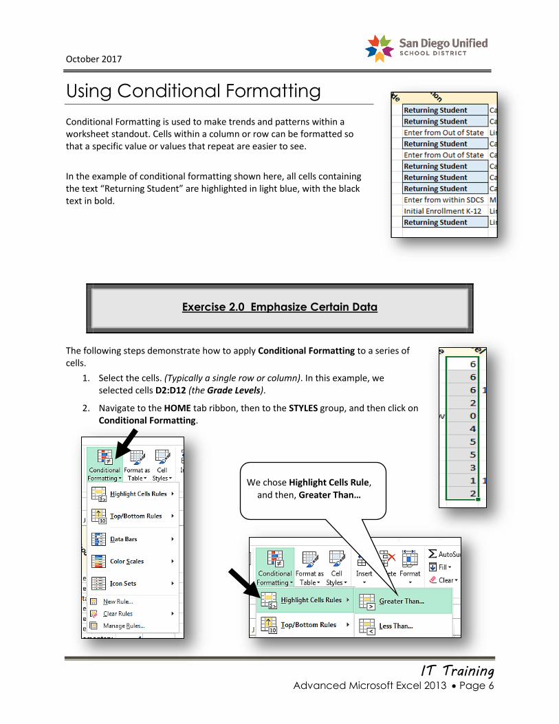
Conditional Formatting is used to make trends and patterns within a worksheet standout. Cells within a column or row can be formatted so that a specific value or values that repeat are easier to see.

In the example of conditional formatting shown here, all cells containing the text “Returning Student” are highlighted in light blue, with the black text in bold.

Exercise 2.0 Emphasize Certain Data

The following steps demonstrate how to apply Conditional Formatting to a series of cells.

1. Select the cells. (Typically a single row or column). In this example, we selected cells D2:D12 (the Grade Levels).

2. Navigate to the HOME tab ribbon, then to the STYLES group, and then click on Conditional Formatting.

We chose Highlight Cells Rule, and then, Greater Than…

October 2017


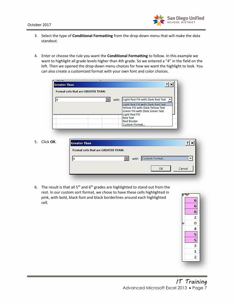
3. Select the type of Conditional Formatting from the drop-down menu that will make the data standout.

4. Enter or choose the rule you want the Conditional Formatting to follow. In this example we want to highlight all grade levels higher than 4th grade. So we entered a “4” in the field on the left. Then we opened the drop-down menu choices for how we want the highlight to look. You can also create a customized format with your own font and color choices.

5. Click OK.

6. The result is that all 5th and 6th grades are highlighted to stand out from the rest. In our custom sort format, we chose to have these cells highlighted in pink, with bold, black font and black borderlines around each highlighted cell.

October 2017


October 2017


Part 3:

Custom Sorting

October 2017


Using Custom Sorting

If regular ascending/descending sorting doesn’t meet your needs, you can create a Custom Sort.

A Custom Sort can be set to focus on values (any numeric value typed in a cell), or cell colors, font colors, or cell icons. There are many ways to arrange the sort using the different options.

In the example shown below, a Custom Sort was done in which cell colors (that were applied using

Conditional Formatting) were the primary criterion.

Exercise 3.0 Multiple Custom Sorting Choices

1. Select the cells. In this example we selected the same cells we used in the last Exercise: cells D2:D12. Click this navigation: HOME EDITING SORT & FILTER CUSTOM SORT…

2. IMPORTANT! Click to select Expand the selection. Then click Sort…

October 2017


3. Select the criteria for how you want the Sorting to happen. Here we chose to sort by the Grade Level column, by the cell color, and we chose the Order we wanted (the pink color). Lastly, we chose to have all the pink cells (the 5th and 6th grades) move to the top of the list. Then, click OK.

Note: All of the 5th & 6th grade level students have been moved to the top of the list.

October 2017


.

October 2017


Part 4:

Grouping

October 2017


Using the Grouping Feature

You can “group” together designated rows and/or columns using the Grouping feature in Excel 2013. This makes it easier to view the data in larger worksheets, without having to freeze anything.

Exercise 4.0 How to Group Columns or Rows

1. Click the Enrollment by Date worksheet.

2. We want to group (hide) Column B.

Click Cell B1 (“Last Name”).

3. On the DATA tab, in the Outline group on the far right, click Group.

4. In the Group dialog box, select Columns and click OK.

5. Note that above the B column a horizontal line with a minus button on the right appears. This means that Column B has been grouped, and is currently open/displayed.

Click the minus button to “close” Column B.

October 2017


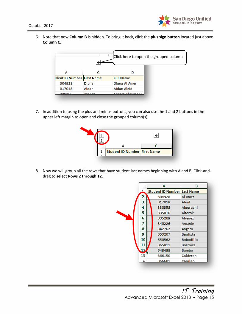
6. Note that now Column B is hidden. To bring it back, click the plus sign button located just above Column C.

7. In addition to using the plus and minus buttons, you can also use the 1 and 2 buttons in the upper left margin to open and close the grouped column(s).

8. Now we will group all the rows that have student last names beginning with A and B. Click-and-drag to select Rows 2 through 12.

Click here to open the grouped column

October 2017


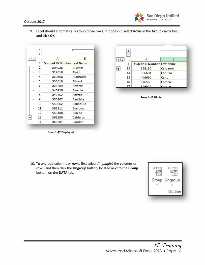
9. Excel should automatically group those rows. If it doesn’t, select Rows in the Group dialog box, and click OK.

10. To ungroup columns or rows, first select (highlight) the columns or rows; and then click the Ungroup button, located next to the Group button, on the DATA tab.

Rows 1-12 Displayed

Rows 1-12 Hidden

October 2017


Part 5:

Locking Cells

&

Protecting

Worksheets

October 2017


Locking Cells & Protecting Worksheets

You can prevent other people from making changes to your worksheet. To do this, you must lock the cells, and then protect the worksheet.

Exercise 5.0 How to Lock Cells & Protect Worksheets

FIRST: Select the entire worksheet and make sure it is completely unlocked: HOME CELLS FORMAT LOCK CELL

NOTE: The cells are unlocked if there is not a green square around the padlock icon:

1. Select all the cells you want to lock.

2. Follow this navigation path: HOME CELLS FORMAT LOCK CELL

NOTE: You know the cells are locked if you see the square around the padlock icon:

Click Format…

… and then click Lock Cell

October 2017


3. The Worksheet must now be protected. On the Format drop down menu, Click on Protect Sheets.

Note: DO NOT ENTER A PASSWORD! If you forget the password, there is NO WAY TO RETRIEVE IT.

4. Checkmark each action you do want others to be able to do. For example, click a checkmark for “Select unlocked cells”. This will only allow the user to select the locked cells, but not make any changes to.

5. Click OK.

Click Protect Sheet…

October 2017


To try it out, deselect the cells and try to edit one of the locked cells. The following message may or may not display. If it does, Click OK. Then go ahead and release the sheet from protection.

Exercise 5.1 Lock Some Cells, Skip & Unlock Others

FIRST: Select the entire worksheet and make sure it is completely unlocked: HOME CELLS FORMAT LOCK CELL

NOTE: The cells are unlocked if there is not a green square around the padlock icon:

1. Select Columns A, B, and C.

2. Press and hold down the CTRL key on your keyboard. (This allows the selection of cells, columns,

or rows in non-sequential order). While holding down the CTRL key, pass over column D and then select any other column or columns.

3. Release the CTRL key.

4. Navigate: HOME CELLS FORMAT LOCK CELLS to lock the columns you selected (skipping column D).

5. Navigate: HOME CELLS FORMAT Protect Sheet. Place checkmarks only for “Select unlocked cells” and “Format cells”.

6. Click, OK.

7. Try it out. We set it up so that only unlocked cells can be clicked on, and can be formatted (change color,

change font, etc.). The locked cells can only be selected, but not formatted.

When done, be sure to Un-protect the sheet.

October 2017


Part 6:

Consolidate

&

Sparklines

October 2017


Using the Consolidation Tool

In Excel, the Consolidate tool summarizes data from separate ranges, consolidating the results in a single output range. For example, if you have a separate worksheet for each fiscal year of spending in certain given accounts, the Consolidate tool can create a “Master” worksheet that brings all those individual years of spending data together into one place for easy review.

Open the Consolidate and Sparklines Excel file.

Exercise 6.0 Consolidate Data to a Single Master Worksheet

1. There are several worksheets, one for each year dating from 2012 to 2016. To the right of the 2016 worksheet, open a new blank worksheet. This will be the Master worksheet. Rename the worksheet tab: MASTER

2. Click any blank cell on the Master worksheet. This is where the consolidation summary will appear.

3. On the DATA tab in the Data Tools group, click the Consolidate button.

4. In the Consolidate dialog box, make sure the Function is SUM, and place a checkmark into both check boxes in the bottom left corner for Top row and Left column.

5. Click to place the flashing cursor into the Reference field of the dialog box.

October 2017


6. Click the 2012 worksheet tab.

7. On the 2012 worksheet, click-and-drag to select cells A1:B5.

Note: The Reference field should now look like this:

8. Click the Add button to add this reference to the All references field list.

Click 2012

October 2017


9. Your screen should now look like this:

10. Click the 2013 worksheet tab, and then click the Add button on the dialog box again. Your screen should now look like this:

October 2017


11. Repeat Step 10 for each of the annual worksheets (2014, 2015, and 2016). When done, your screen should look like this:

12. Click OK on the Consolidate dialog box.

13. Your screen should now display the Master worksheet.

October 2017


14. Adjust the formatting as desired, and leave this file open for the next exercise:

Using the Sparkline Feature

A Sparkline is a miniature chart placed into a single cell, graphically representing a single row of data. Sparklines are often used to demonstrate trends over time.

Exercise 6.1 How to Insert Sparklines to Demonstrate Trends

1. On the Master worksheet, click the cell indicated by the instructor. The Sparkline for the data in row 2 will go here.

2. There are three different formats of Sparklines: Line, Column, and Win/Loss. On the INSERT tab in the Sparklines group, click Line.

Click a cell where the Sparkline will go

October 2017


3. In the Create Sparklines dialog box, make sure the flashing cursor is inside the Data Range field. Then:

a. Click-and-drag to select the first row of percentage cells.

b. Click OK on the dialog box.

4. The Sparkline is inserted into the designated cell and the SPARKLINE TOOLS contextual tab is displayed.

Sparkline

Click OK

Select Cells B2:F2

October 2017


5. Use the SPARKLINE TOOLS features to format the Sparkline as desired. In the example shown below, we did the following:

a. We chose a dark blue color for the Sparkline Color.

b. We clicked Marker Color Markers and chose purple.

c. We clicked Marker Color High Point and chose red.

6. Use the AutoFill tool (the black, plus-sign, mouse cursor) to copy the Sparkline into cells just below the first Sparkline.

Note: The worksheet may look different from the one pictured here.

AutoFill cursor

October 2017


7. To see what the Column Sparklines look like, click into another column, and insert a column style Sparkline there for the appropriate data range.

8. Copy the column Sparkline down into the cells below it.

Use the SPARKLINE TOOLS to format the column Sparklines as desired. It’s usually helpful to color the High Point Markers with a bright, different color, such as red.

9. NOTE the following:

a. Sparklines can be static or live linked. If linked, they can update automatically if you change the data on any worksheet within the Sparkline’s Data Range.

b. You can use the Clear tool to delete one or all selected Sparklines.

October 2017


October 2017


Part 7:

V-Lookup

October 2017


Using the V-Lookup Function

Use the V-lookup function (vertical searching in a single column) when you want a faster way to find specific information, instead of having to read through long columns of data, searching for it.

Click to the Enrollment by Date worksheet. In this example, we want to be able to type any given student ID number, and have it instantly display the name of the student it belongs to.

Exercise 7.0 How to Find Specific Data in a Large Worksheet

1. In any blank column to the far right, type: ID# and in the cell just beneath that, type: Name

2. Click into the blank cell just to the right of where you typed Name. This is where the V-LOOKUP formula will go.

3. Click the Insert Function (fx) button to the left of the Formula Bar.

4. Type V-LOOKUP in the Search for a Function field at the top of the dialog box and click OK.

October 2017


5. Enter the 4 Function Arguments like this:

a. Lookup_Value: Choose the cell just to the right of where you typed ID#. This is where you will enter a given student’s ID number, not knowing the student’s name yet.

b. Table_array: Enter the cell range A2:D473. This needs to include the very first column on the left, through the column containing the students’ full names (Column D). Include all rows containing all student data.

c. Col_index_num: Enter the number for the column containing the information you are searching for to display… the student names. This would be the number 4, for Column D, since it’s the fourth column from the left.

d. Range_lookup: Enter the word FALSE. This will display the exact name for that one student, matching up with whatever student ID# you use to look it up with.

6. Click OK.

a

b

c

d

October 2017


7. In the cell with the V-LOOKUP formula you just created, you will see an error displayed (#N/A), because it’s looking for an ID# to be entered into the cell just above it. We haven’t done that yet.

8. In the cell just to the right of ID#, enter one of the student ID’s from Column A, and press ENTER. The cell just beneath that (that has the

VLOOKUP formula) will then display the student’s name that matches that ID#.

The V-LOOKUP formula can be created on a blank worksheet that points the arguments to an entirely separate worksheet with columns of data.

Exercise 7.1 V-LOOKUP Across Multiple Worksheets

1. Click into the worksheet labeled “V-LOOKUP”.

2. There is already an example formula set up in the upper left corner of this worksheet. But to build your own, follow these steps. In any other two blank cells, type ID# and Name, just as you see them here.

3. As in the last exercise, use the Insert Function wizard tool to input the arguments. The only difference now is that in the Table array field you have to point to the correct worksheet that has all the student data. That means you enter the name of the worksheet and an exclamation point in front of the cell range.

Enter a student ID# and press ENTER

The matching student’s name will appear

NOTE: The tab label (name) of the worksheet cannot have any spaces.

October 2017


4. Click OK on the Insert Function dialog box, and test out your new VLOOKUP formula by entering one of the Student ID numbers from the Enrollment_by_Date worksheet. Press ENTER and watch the student’s name appear.

October 2017


October 2017


Part 8:

The Watch

Window

October 2017


Using the Watch Window Feature

When you want to monitor the value of a cell, the Watch Window feature lets you keep an eye on it even if you’re working in a different area, or on a different worksheet… or even a different file entirely. You just have to make sure that the Excel file with the cell you’re watching is open on your computer.

In the next example exercise we’ll set up a Watch Window to keep monitoring how many students are enrolling into or transferring out of a given school.

Exercise 8.0 How to Use the Watch Window Feature

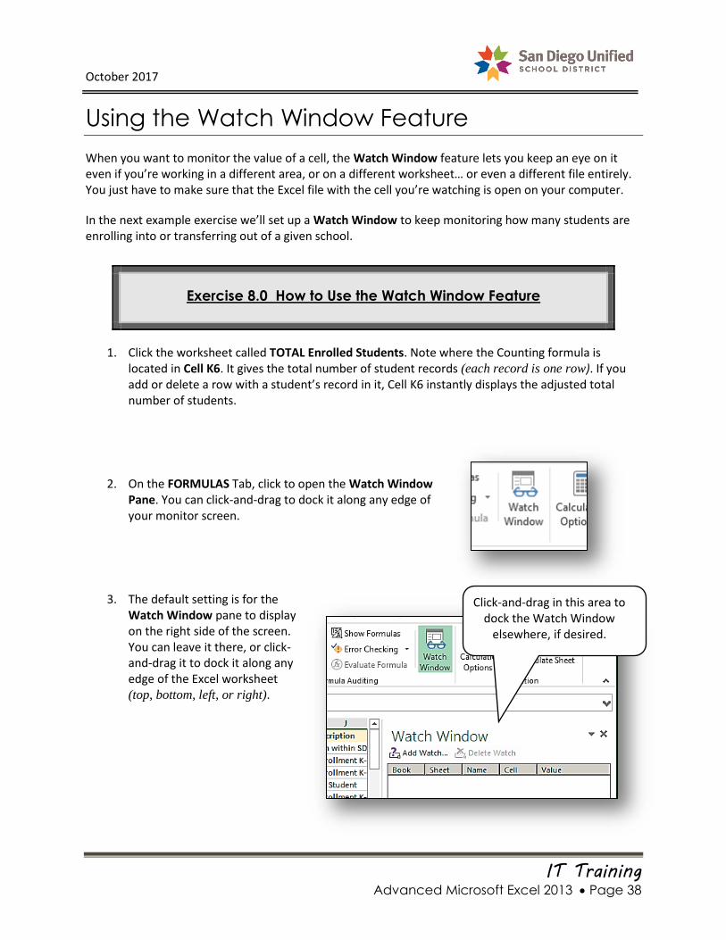
1. Click the worksheet called TOTAL Enrolled Students. Note where the Counting formula is located in Cell K6. It gives the total number of student records (each record is one row). If you add or delete a row with a student’s record in it, Cell K6 instantly displays the adjusted total number of students.

2. On the FORMULAS Tab, click to open the Watch Window Pane. You can click-and-drag to dock it along any edge of your monitor screen.

3. The default setting is for the Watch Window pane to display on the right side of the screen. You can leave it there, or click-and-drag it to dock it along any edge of the Excel worksheet (top, bottom, left, or right).

Click-and-drag in this area to dock the Watch Window

elsewhere, if desired.

October 2017


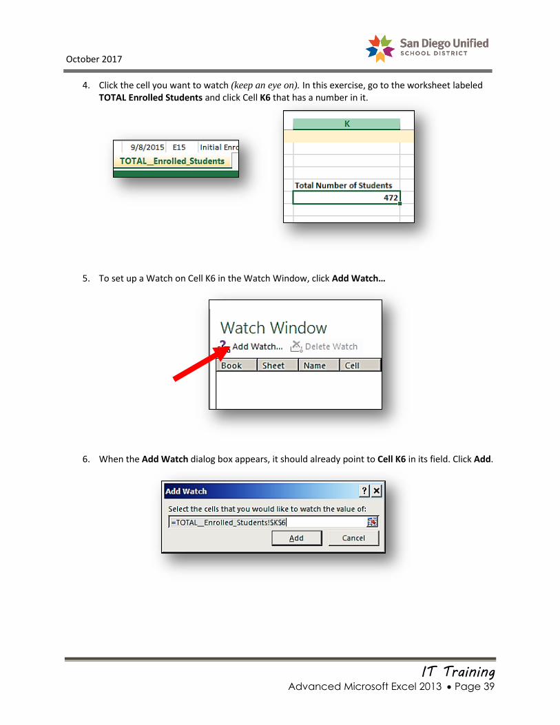
4. Click the cell you want to watch (keep an eye on). In this exercise, go to the worksheet labeled TOTAL Enrolled Students and click Cell K6 that has a number in it.

5. To set up a Watch on Cell K6 in the Watch Window, click Add Watch…

6. When the Add Watch dialog box appears, it should already point to Cell K6 in its field. Click Add.

October 2017


7. Check to see that the cell information appears in the Watch Window pane.

8. If the Watch Window pane is too big and you want to resize it, click the Task Pane Options arrow icon in the upper right corner of the pane.

9. Select Size in the menu.

10. Click-and-drag the double-headed black arrow cursor to the size you want.

Name of Excel file (Workbook)

Name of Worksheet

Name of Cell The watched cell’s Formula

Current value in watched cell.

Any changes to value will show here instantly.

October 2017


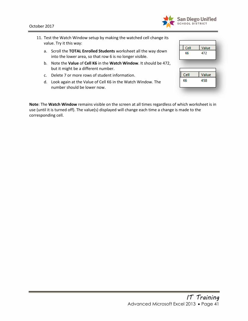
11. Test the Watch Window setup by making the watched cell change its value. Try it this way:

a. Scroll the TOTAL Enrolled Students worksheet all the way down into the lower area, so that row 6 is no longer visible.

b. Note the Value of Cell K6 in the Watch Window. It should be 472, but it might be a different number.

c. Delete 7 or more rows of student information.

d. Look again at the Value of Cell K6 in the Watch Window. The number should be lower now.

Note: The Watch Window remains visible on the screen at all times regardless of which worksheet is in use (until it is turned off). The value(s) displayed will change each time a change is made to the corresponding cell.

October 2017


October 2017


Part 9:

Trace

Precedents

&

Trace

Dependents

October 2017


How to use the Trace Precedents &Trace

Dependents Feature…

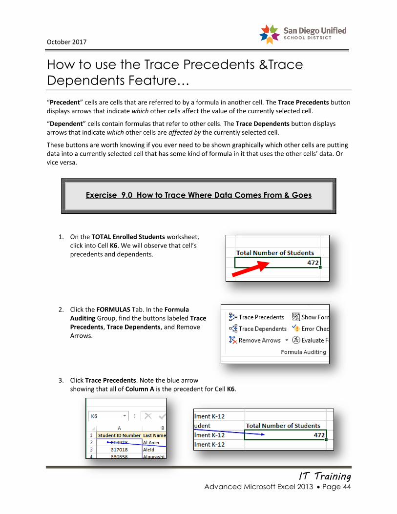
“Precedent” cells are cells that are referred to by a formula in another cell. The Trace Precedents button displays arrows that indicate which other cells affect the value of the currently selected cell.

“Dependent” cells contain formulas that refer to other cells. The Trace Dependents button displays arrows that indicate which other cells are affected by the currently selected cell.

These buttons are worth knowing if you ever need to be shown graphically which other cells are putting data into a currently selected cell that has some kind of formula in it that uses the other cells’ data. Or vice versa.

Exercise 9.0 How to Trace Where Data Comes From & Goes

1. On the TOTAL Enrolled Students worksheet, click into Cell K6. We will observe that cell’s precedents and dependents.

2. Click the FORMULAS Tab. In the Formula Auditing Group, find the buttons labeled Trace Precedents, Trace Dependents, and Remove Arrows.

3. Click Trace Precedents. Note the blue arrow showing that all of Column A is the precedent for Cell K6.

October 2017


4. With Cell K6 still selected, click the Trace Dependents button. Two more blue arrows appear, showing which other cells are affected by Cell K6. In other words, the value in K6 helps determine the values for the formulas in these other two cells.

5. To turn off the blue arrows, click the Remove Arrows button. You can also use this button to remove only the Precedents arrows, or, only the Dependents arrows.

October 2017


October 2017


Part 10:

Pivot Tables

October 2017


PivotTables

A PivotTable is a way Excel can organize and summarize complex data to make it easier to interpret. Excel’s definition of a PivotTable is: A PivotTable is a program tool that allows you to reorganize and summarize selected columns and rows and data in a spreadsheet or database table to obtain a desired report.

You can use a PivotTable report to summarize, analyze, explore, and present summary data. PivotCharts complement PivotTables by adding visualizations to the summary data in a PivotTable, and allow you to easily see comparisons, patterns, and trends. Both PivotTables and PivotCharts enable you to make informed decisions about critical data in your Excel worksheets.

A PivotTable is an interactive way to quickly summarize large amounts of data. You can use a PivotTable to analyze numerical data in detail, and answer unanticipated questions about your data. Note that a PivotTable does not actually change the spreadsheet or database itself.

A PivotTable is especially designed for:

Querying large amounts of data in many user-friendly ways.

Subtotaling and aggregating numeric data, summarizing data by categories and subcategories, and creating custom calculations and formulas.

Expanding and collapsing levels of data to focus your results, and drilling down to details from the summary data for areas of interest to you.

Moving rows to columns or columns to rows (or "pivoting") to see different summaries of the source data.

Filtering, sorting, grouping, and conditionally formatting the most useful and interesting subset of data enabling you to focus on just the information you want.

Presenting concise, attractive, and annotated online or printed reports.

For example, here's a simple list of household expenses on the left, and a PivotTable based on the list to the right:

Household Expense Data Corresponding PivotTable

October 2017


Before you get started…

You data should be organized in a tabular format, and not have any blank rows or columns. Ideally, you can use an Excel table like in the example above.

Tables are a great PivotTable data source, because rows added to a table are automatically included in the PivotTable when you refresh the data, and any new columns will be included in the PivotTable Fields List. Otherwise, you need to either manually update the data source range, or use a dynamic named range formula.

Data types in columns should be the same. For example, you shouldn't mix dates and text in the same column.

PivotTables work on a snapshot of your data, called the cache, so your actual data doesn't get altered in any way.

Using the Recommended PivotTables feature in Excel is a good place to start, if you have limited experience with them. Excel can recommend the best types of PivotTables to suit the data in your worksheet.

Exercise 10.0 A “Recommended” PivotTable

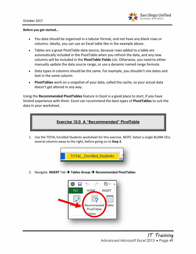
1. Use the TOTAL Enrolled Students worksheet for this exercise. NOTE: Select a single BLANK CELL several columns away to the right, before going on to Step 2.

2. Navigate: INSERT Tab Tables Group Recommended PivotTables

October 2017


3. Click the Recommended PivotTable button. When the Choose Data Source dialog box appears, you need to tell it which cells in your Table you want to include in the PivotTable. You could type it in, but it’s usually best to click-and-drag over the cell range you want (see the next step).

4. Select Cells A1:G473. Click OK on the dialog box.

October 2017


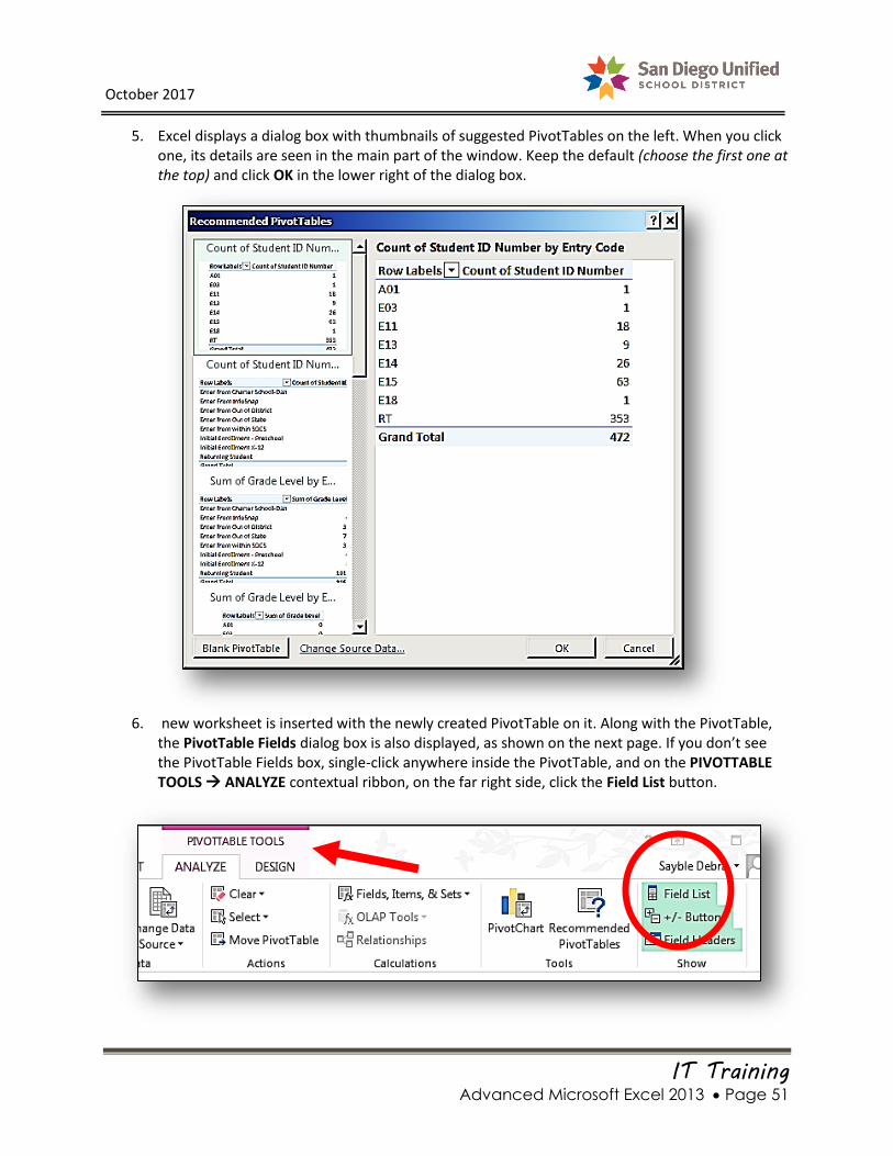
5. Excel displays a dialog box with thumbnails of suggested PivotTables on the left. When you click one, its details are seen in the main part of the window. Keep the default (choose the first one at the top) and click OK in the lower right of the dialog box.

6. new worksheet is inserted with the newly created PivotTable on it. Along with the PivotTable, the PivotTable Fields dialog box is also displayed, as shown on the next page. If you don’t see the PivotTable Fields box, single-click anywhere inside the PivotTable, and on the PIVOTTABLE TOOLS ANALYZE contextual ribbon, on the far right side, click the Field List button.

October 2017


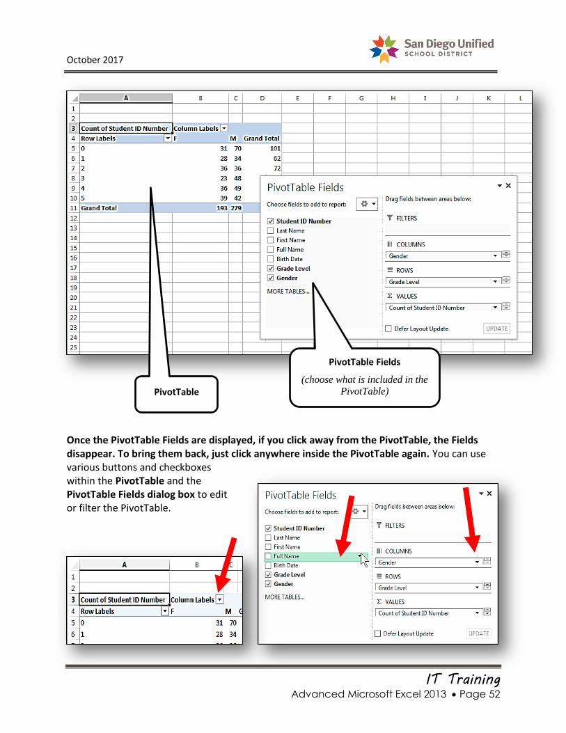
Once the PivotTable Fields are displayed, if you click away from the PivotTable, the Fields disappear. To bring them back, just click anywhere inside the PivotTable again. You can use various buttons and checkboxes within the PivotTable and the PivotTable Fields dialog box to edit or filter the PivotTable.

PivotTable

PivotTable Fields

(choose what is included in the

PivotTable)

October 2017


Exercise 10.1 Creating a Pivot Table

Observe this example of a PivotTable with its Fields displayed. In the next exercise, you will build it from scratch:

1. Click Cell A1 on the TOTAL Enrolled Students worksheet.

PivotTable

(based on choices made in

PivotTable Fields)

Fields (Data) Chosen to Display in PivotTable

Placement of Fields in PivotTable (click-and-

drag to move them)

October 2017


2. On the INSERT Tab, on the far left-side, click the PivotTable button.

3. On the Create PivotTable dialog box, leave the default settings as they are and click OK.

NOTE: Before you click OK, verify that the Table/Range shows:

TOTAL_Enrolled_Students!$A$1!:$J$473, and that the PivotTable will be placed on a New Worksheet.

Verify

Verify

October 2017


4. A new worksheet is inserted with a blank PivotTable displayed, along with the PivotTable Fields dialog box with nothing chosen yet.

5. In the PivotTable Fields dialog box, click the drop-down menu for Settings, and select Fields Section and Area Section Side-by-Side.

Settings

Select this one

October 2017


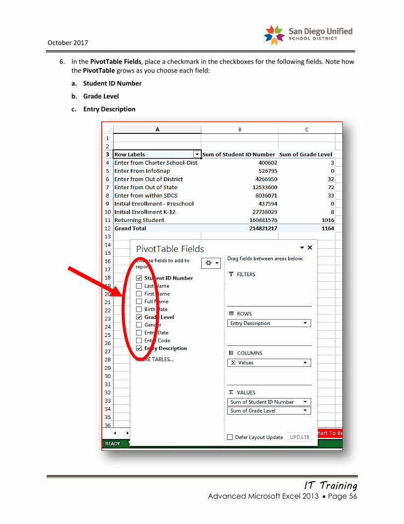
6. In the PivotTable Fields, place a checkmark in the checkboxes for the following fields. Note how the PivotTable grows as you choose each field:

a. Student ID Number

b. Grade Level

c. Entry Description

October 2017


7. Excel tends to assume things sometimes. It displayed the fields into the areas it thinks we wanted. We still need to rearrange the fields, so they display the way we want. As the PivotTable stands now, it doesn’t make much sense. For instance, we don’t want it to show a sum of student ID numbers. In the PivotTable Fields dialog box, in the lower right area, click the drop-down menu for Sum of Student ID Number, and then click Value Field Settings…

8. On the Value Field Settings dialog box, change it from Sum to Count; then, change the Custom Name to: Number of Students and click OK.

Change to read:

Number of Students

Select Count

October 2017


9. Click-and-drag to move Sum of Grade Level up to the Filter area

10. Your worksheet should look like this, now:

Drag this into the Filter area at the top

October 2017


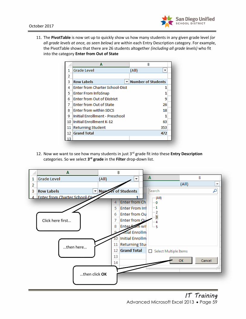
11. The PivotTable is now set up to quickly show us how many students in any given grade level (or all grade levels at once, as seen below) are within each Entry Description category. For example, the PivotTable shows that there are 26 students altogether (including all grade levels) who fit into the category Enter from Out of State

12. Now we want to see how many students in just 3rd grade fit into these Entry Description categories. So we select 3rd grade in the Filter drop-down list.

Click here first…

…then here…

…then click OK

October 2017


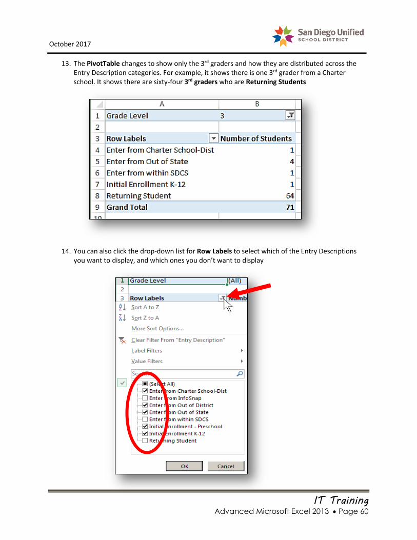
13. The PivotTable changes to show only the 3rd graders and how they are distributed across the Entry Description categories. For example, it shows there is one 3rd grader from a Charter school. It shows there are sixty-four 3rd graders who are Returning Students

14. You can also click the drop-down list for Row Labels to select which of the Entry Descriptions you want to display, and which ones you don’t want to display

October 2017


15. This illustration shows the PivotTable after making the selections in Step 14, and including all grade levels

NOTE: Double-click any numeral below “Number of Students” to open a list of those

individual student records in a new worksheet:

16. Add a Style to your PivotTable. Click anywhere inside the PivotTable to open the PIVOTTABLE TOOLS contextual ribbon at the top of your screen. Click on the DESIGN tab. Select any PivotTable Style you like.

October 2017


PivotCharts

PivotCharts complement PivotTables by adding visualizations that allow you to easily see comparisons, patterns, and trends. A PivotChart illustrates a PivotTable in a graphic format. PivotCharts are also interactive. When you create a PivotChart, the PivotChart Filter Pane is displayed. You can use this filter pane to sort and filter the PivotChart’s underlying data. Changes you make to the layout and data in a PivotTable are immediately reflected in the PivotTable’s associated PivotChart, and vice versa.

Before starting the next exercise, be sure that you are on the TOTAL Enrolled Students worksheet.

Exercise 10.2 How to Create a PivotChart

1. With your flashing insertion cursor anywhere inside the PivotTable, look at the top of the screen at the PIVOTTABLE TOOLS contextual ribbon, and click to the ANALYZE Tab. Click the PivotChart button.

2. Select the type of chart you want, and set it on the worksheet next to the PivotTable. NOTE that you can use the Grade Level and Entry Description filters here just as you can on the PivotTable.

October 2017


3. With the PivotChart selected, use the PIVOTCHART TOOLS contextual ribbon Tabs – ANALYZE, DESIGN, and FORMAT – to format the chart in a way that clearly represents the data.

October 2017


October 2017


Part 11:

Tips and Tricks

October 2017


Customizing the Quick Access Toolbar

It is easy to customize the Quick Access Toolbar. As in most cases in Microsoft Office, there are several ways to accomplish this task. This section will cover the easiest way.

Adding or Removing Features of the Quick Access Toolbar

The Quick Access Toolbar can be customized with any number of shortcuts and commands. In the example below, more than 30 icons representing various commands and shortcuts have been added to the Quick Access Toolbar for convenience in editing and formatting.

Follow the instructions below to modify or add features to the Quick Access Toolbar:

Add a Command to the Quick Access Toolbar:

1. On the Ribbon of your choice, right-click the command or button you want to add.

2. Left-click Add to Quick Access Toolbar on the Shortcut Menu that appears.

Remove a Command from the Quick Access Toolbar:

1. On the Quick Access Toolbar, right-click the command or button you want to remove.

2. Left-click Remove from Quick Access Toolbar on the Shortcut Menu that appears.

October 2017


Customizing the Ribbon

In Word 2013 the Ribbon can be customized. As in most cases in Microsoft Office, there are several ways to accomplish this task. This section will cover the easiest method.

Adding or Removing Features of the Ribbon

The Ribbon can be customized with any number of shortcuts and commands located on existing or newly created tabs. In the example below, a new tab has been created for the purpose of demonstrating this ability within Word.

To create a new Ribbon tab with custom commands, simply right click on any existing tab and select Customize the Ribbon from the pop-up window.

This will open up a Word Options pane which will allow the user to customize the Ribbon.

(See the Word Options screenshot on the next page.)

October 2017


Creating a New Tab and Renaming it

At the bottom of the column on the right, select New Tab. A new tab will then appear within the column of existing Ribbon tab names. Next, with the new tab selected, click on Rename. A dialog box will appear allowing you to rename the new Ribbon tab.

In our example, we have named the new Ribbon tab, Sample Ribbon Tab (see next page).

October 2017


Adding Commands and Features to the New Ribbon Tab

At this point, it is as simple as selecting a command or feature from the column on the left, then clicking the Add button to move it to the newly created tab. Repeat this process as many times as needed to create the fully customized tab with as many groups and features as needed. Use the up or down arrows on the right to reposition newly acquired commands, groups, or tabs. When finished, click OK.

The newly created tab with its custom features will appear on the ribbon of the Word user-interface.

This process can be repeated as many times as needed to create a truly customized Word user-interface.

Note: These changes will remain until the user removes or modifies them, regardless of which document is in use.

October 2017


How to Create a Hyperlink to a Specific Website

A Hyperlink can be created anywhere within a Word document—associated with both text or graphics. It can automatically link to any website or webpage you choose. This process can be repeated as many times as needed. All that is required is the URL address of the website or web page that the Hyperlink will link to.

Exercise 11.0: How to Insert a Hyperlink

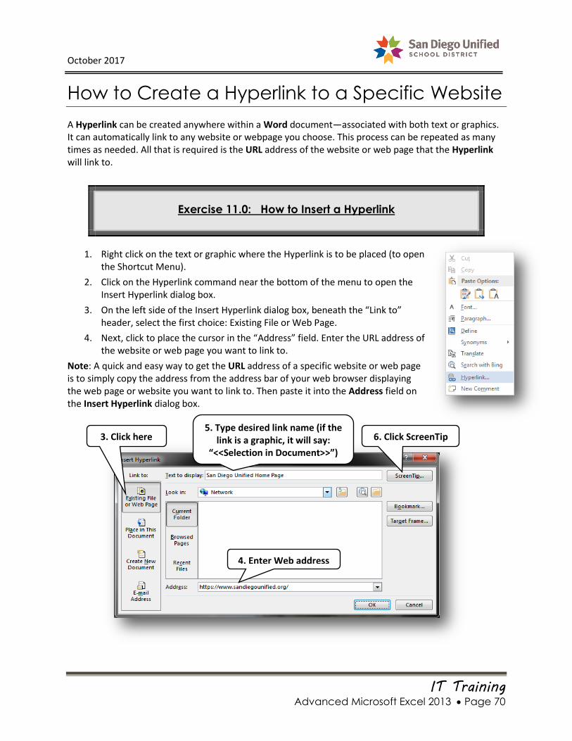
1. Right click on the text or graphic where the Hyperlink is to be placed (to open the Shortcut Menu).

2. Click on the Hyperlink command near the bottom of the menu to open the Insert Hyperlink dialog box.

3. On the left side of the Insert Hyperlink dialog box, beneath the “Link to” header, select the first choice: Existing File or Web Page.

4. Next, click to place the cursor in the “Address” field. Enter the URL address of the website or web page you want to link to.

Note: A quick and easy way to get the URL address of a specific website or web page is to simply copy the address from the address bar of your web browser displaying the web page or website you want to link to. Then paste it into the Address field on the Insert Hyperlink dialog box.

6. Click ScreenTip 5. Type desired link name (if the

link is a graphic, it will say: “<<Selection in Document>>”)

3. Click here first

4. Enter Web address here.

October 2017


5. At the top of the Insert Hyperlink dialog box (to the right of the “Text to display” header), type in the words you want to display on your hyperlink. In our example we have written, “San Diego Unified Home Page.”

Note: If the Hyperlink is set on a graphic, then this space will be grayed-out and read, “<<Selection in Document>>”.

6. You can add a Screen Tip to the new Hyperlink that will display when you mouse over it. Click on the Screen Tip button in the upper-right corner of the Insert Hyperlink dialog box.

7. Type the screen tip message you want to display. Then, click the OK button to return to the Insert Hyperlink dialog box.

8. With all the steps above complete, click on the OK button to set the hyperlink. The new Hyperlink will appear where you first inserted your cursor to begin this process.

Note: The new Hyperlink is active when the text appears in blue and is underlined. The Hyperlink can be modified or removed by right clicking and selecting the appropriate choice from the Shortcut Menu.

October 2017


How to Shade Every Other Row in Excel 2013

The best way to shade every other row on a worksheet is to use the Conditional Formatting option. Formatting your worksheet to display this way will make it much easier to track data across large worksheets.

Exercise 11.1: How to Shade Every Other Row in Excel

1. Open the worksheet.

2. Select the cell range that you want to shade, or press Ctrl+A to select the whole worksheet.

3. On the HOME tab, navigate to the Styles group, select Conditional Formatting, and then click Manage Rules.

4. Select New rule.

5. Select Use a formula to determine which cells to format.

6. In the Format values where this formula is true box, type =MOD(ROW(),2)=1, and then select Format.

October 2017


7. On the Fill tab, click the color that you want to use to shade every other row, and then click OK.

8. Click OK to close the New Formatting Rule dialog box.

9. Select Apply, then click OK to close the Conditional Formatting Rules Manager dialog box.

October 2017


10. Your Worksheet should now look similar to the example below. Every other line will have the shading color that you chose in step 8 above. This makes it easier to tract data across long rows.

How to Print the Worksheet Header

When printing large Worksheets it is helpful to have the Header row (usually Row 1) print out on each page so that you do not have to constantly flip the pages back to page one to see the Header information. This can be easily set up so that the Headers of the Worksheet will repeat on each printed page. Follow the steps below to include the header on each printed page.

Exercise 11.2: How to Print the Worksheet Header on each page

1. On the PAGE LAYOUT tab, in the Page Setup group, select the Print Titles command.

2. The Sheet tab of the Page Setup dialog box will display. Click into the Rows to repeat at top: field and type $1:$1 to lock the row 1 header for the purpose of printing. At this point you can preview the printing or simply select Print.

October 2017


Note: Instead of typing the formula for which rows to repeat, you can simply click on the Row 1 name on the far left side of the Worksheet and the formula will auto populate in the Rows to repeat at top field.

October 2017


Using Paste Special Values to Remove Formulas

Copying a column with a formula (such as column G, below) and then pasting it back into the same column using the Paste Special Values (V), is a clever way to remove the formula in that column replacing it with just the Value (the names). In the example below, cell G1 has the Concatenate formula operating to combine the contents of columns E and F.

Columns E and F (in the example above) cannot be erased because the formula in column G is dependent on their content. As such, any column that has a formula that references other columns must be reconfigured such that it is no longer dependent on those columns. This can easily be done with the Paste Special Values (V) command. To remove the Formula from column G, simply Copy the entire column and Paste it back into the same column using the Paste Special Value (V) option. This will keep the names in the column (the Value), but will eliminate the formula that created the original content. When the formula has been removed, then columns E and F can safely be deleted.

October 2017


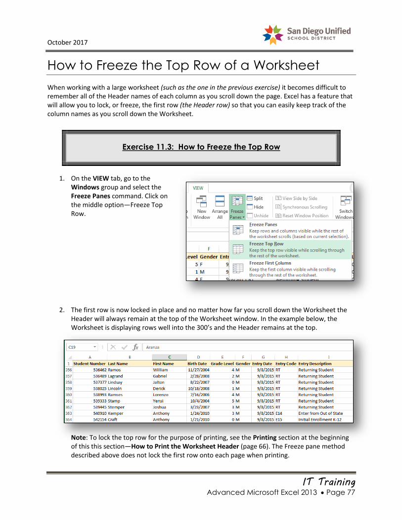
How to Freeze the Top Row of a Worksheet

When working with a large worksheet (such as the one in the previous exercise) it becomes difficult to remember all of the Header names of each column as you scroll down the page. Excel has a feature that will allow you to lock, or freeze, the first row (the Header row) so that you can easily keep track of the column names as you scroll down the Worksheet.

Exercise 11.3: How to Freeze the Top Row

1. On the VIEW tab, go to the Windows group and select the Freeze Panes command. Click on the middle option—Freeze Top Row.

2. The first row is now locked in place and no matter how far you scroll down the Worksheet the Header will always remain at the top of the Worksheet window. In the example below, the Worksheet is displaying rows well into the 300’s and the Header remains at the top.

Note: To lock the top row for the purpose of printing, see the Printing section at the beginning of this this section—How to Print the Worksheet Header (page 66). The Freeze pane method described above does not lock the first row onto each page when printing.

October 2017


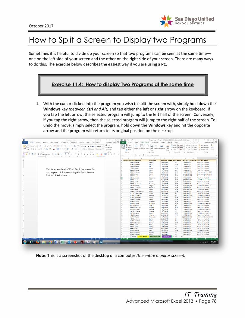
How to Split a Screen to Display two Programs

Sometimes it is helpful to divide up your screen so that two programs can be seen at the same time—one on the left side of your screen and the other on the right side of your screen. There are many ways to do this. The exercise below describes the easiest way if you are using a PC.

Exercise 11.4: How to display Two Programs at the same time

1. With the cursor clicked into the program you wish to split the screen with, simply hold down the Windows key (between Ctrl and Alt) and tap either the left or right arrow on the keyboard. If you tap the left arrow, the selected program will jump to the left half of the screen. Conversely, if you tap the right arrow, then the selected program will jump to the right half of the screen. To undo the move, simply select the program, hold down the Windows key and hit the opposite arrow and the program will return to its original position on the desktop.

Note: This is a screenshot of the desktop of a computer (the entire monitor screen).

October 2017


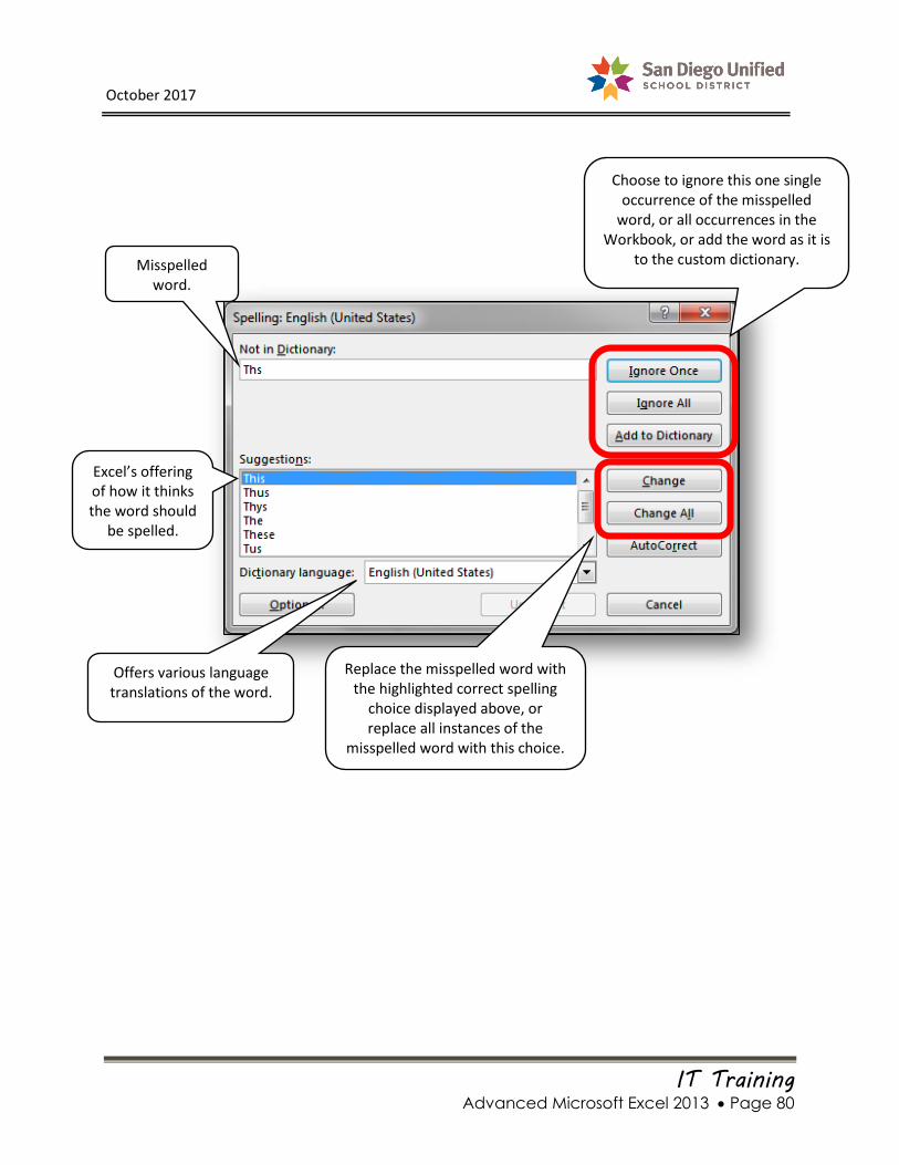
Proofreading: The Excel Spell Check Command

Limitations of the Excel Spelling Check Feature

It is always a good idea to proofread the sections of your Workbook that have text yourself, because Excel’s Spell Check tool is less than perfect. It doesn’t always catch certain nuances of the English language, or make it very easy to see the words that are misspelled. That said, Excel does have a Spelling Check tool that checks your Workbook for any spelling errors.

The Spelling Check command is located on the REVIEW tab, in the Proofing group on the far left side of the Ribbon.

To check your Worksheet for spelling errors, use one of the following methods:

1. Click the Spelling check command on the REVIEW tab. A Spelling check dialog box will open on your screen. Excel will begin checking your entire Worksheet (beginning with the last cell selected) and display its findings in the Spelling check dialog box. It will offer you choices regarding each instance of an incorrectly spelled word.

2. Press the F7 key on your keyboard to open the same Spelling Check dialog box described above.

Note: If you have multiple cells within your Workbook containing substantial amounts of text, it is highly recommended (because of the awkwardness or obvious limitations of Excel’s Spelling check feature) that you create the textual content of each cell in Word, Spell Check it there, then Copy and Paste that text into the corresponding cell within the Excel Worksheet. This will assure you that your Workbook will display correctly spelled textual content.

(Please see illustration of the Spelling check dialog box on the next page)

Spell Check REVIEW Tab

October 2017


Misspelled word.

Excel’s offering of how it thinks the word should

be spelled.

Choose to ignore this one single occurrence of the misspelled

word, or all occurrences in the Workbook, or add the word as it is

to the custom dictionary.

Replace the misspelled word with the highlighted correct spelling

choice displayed above, or replace all instances of the

misspelled word with this choice.

Offers various language translations of the word.

October 2017


The New Flash Fill Feature (in Excel 2013)

The 2013 version of Excel came with a new feature that is by far the best new feature in years. Simply put, this new feature has the potential to eliminate the need for many, basic formulas and functions. In Part 8 of this handbook (Formulas & Functions), many pages are dedicated to several, detailed formulas that manipulate text and text strings within an Excel Worksheet. Specifically, Part 8 describes how to use the Concatenate function to build a formula that rearranges text data from two, existing columns into a new, third column. Then, that section demonstrates how to change that new text data into the proper case using the Proper function. Although these formulas are not difficult to use, they are very detailed and require absolute accuracy to set them up correctly. The new Flash Fill feature bypasses the need for these cumbersome functions and formulas by recognizing repeating data-entry patterns in columns adjacent to existing data.

Exercise 11.5 How to Reorder Text Data Using Flash Fill

The following exercise can be completed using the “Last Name, First” worksheet within the Excel practice workbook provided by the instructor.

1. Insert the cursor into cell “G1” and enter “Gable, Clark.” (In this example, the text of columns E and F have been rearranged into column G in the “last name, first” order.) After typing in “Gable, Clark” in the new column (G), press the Enter key to activate the cell directly below it. The Flash Fill feature will attempt to recognize a pattern to repeat.

2. By entering a “G” in this new cell (the first letter in the name, Gardner), Flash Fill will incorrectly guess that you are attempting to repeat the name “Gable, Clark.” (If that is what was wanted, then by pressing the Enter key it would be inserted.) Continue to enter each letter of the next name on the list (Gardner, Eva).

October 2017


3. As soon as the letter “r” is entered (see below), the Flash Fill feature recognizes the “list” pattern based on the text data in the preceding columns and auto-populates the remaining cells within column G.

Note: When the name, “Gable, Clark” was entered into cell G1, care was taken to put the proper name Gable in the Proper case. The Flash Fill feature picked up that pattern and applied it to all of the last names in the new column (even though the source column F has several of the names listed in lowercase).

4. Select the first letter of the name “cary” (that auto-populated in cell G3) and replace it with an uppercase letter “C.” Then press the Enter key. The remaining lowercase names will automatically become uppercase because of the Flash Fill feature (see screenshot below).

Note: The Flash Fill feature required only a few easy steps to reorder the text data in columns E & F. Prior to the 2013 release, this same reordering would require the use of multiple formulas involving numerous, detailed steps.

October 2017


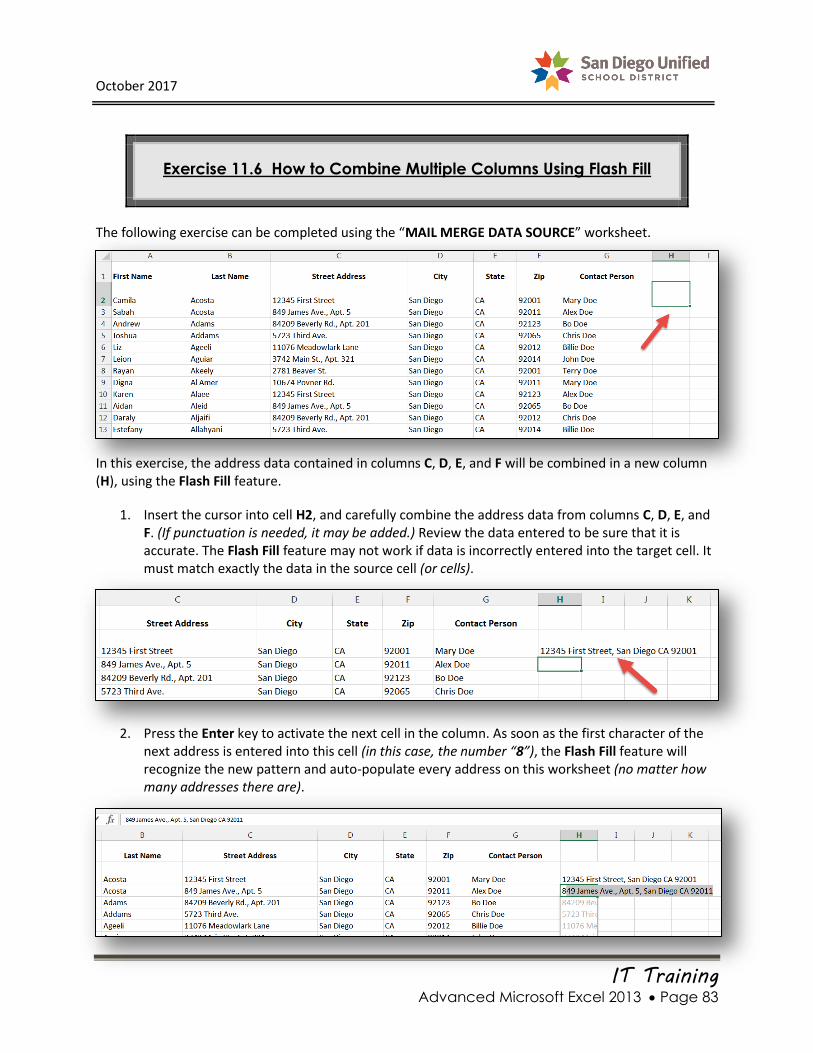
Exercise 11.6 How to Combine Multiple Columns Using Flash Fill

The following exercise can be completed using the “MAIL MERGE DATA SOURCE” worksheet.

In this exercise, the address data contained in columns C, D, E, and F will be combined in a new column (H), using the Flash Fill feature.

1. Insert the cursor into cell H2, and carefully combine the address data from columns C, D, E, and F. (If punctuation is needed, it may be added.) Review the data entered to be sure that it is accurate. The Flash Fill feature may not work if data is incorrectly entered into the target cell. It must match exactly the data in the source cell (or cells).

2. Press the Enter key to activate the next cell in the column. As soon as the first character of the next address is entered into this cell (in this case, the number “8”), the Flash Fill feature will recognize the new pattern and auto-populate every address on this worksheet (no matter how many addresses there are).

October 2017


3. Pressing the Enter key again, locks the Flash Fill suggestions (the remaining addresses) in place.

Note: There is a Flash Fill Options drop-down menu that will appear next to data that was auto-populated using the Flash Fill feature. Clicking on the down-arrow will reveal additional options related to this feature.

October 2017


Help

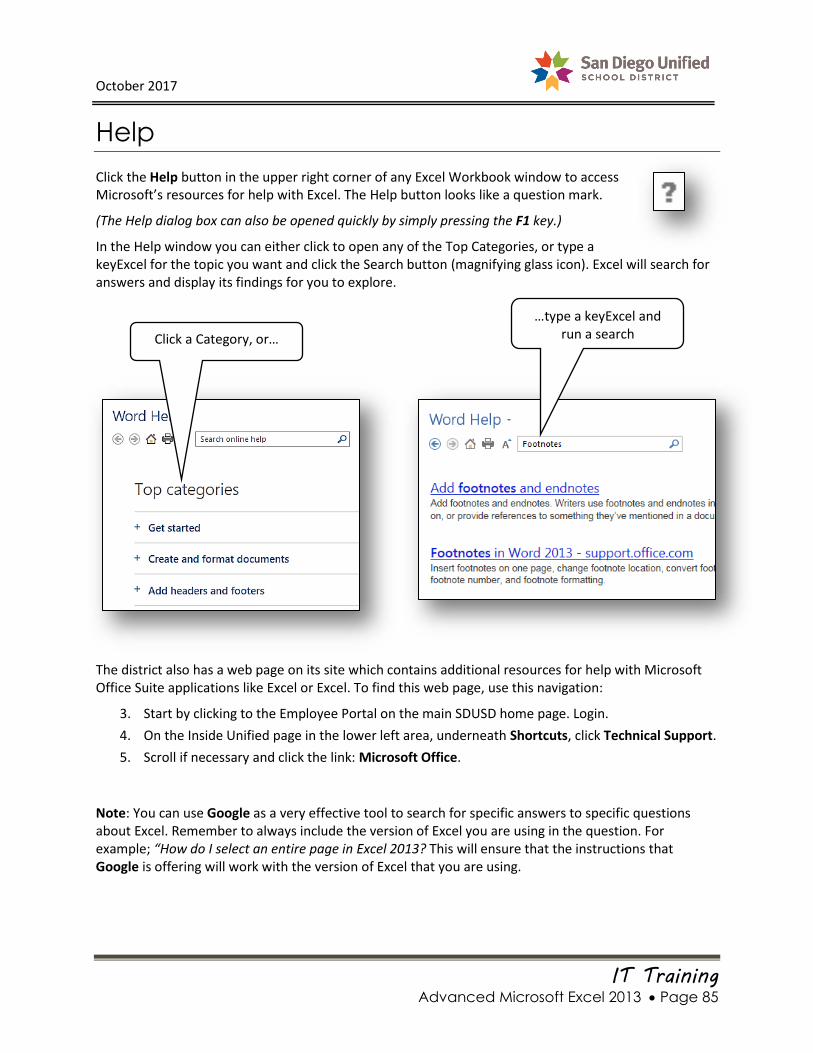
Click the Help button in the upper right corner of any Excel Workbook window to access Microsoft’s resources for help with Excel. The Help button looks like a question mark.

(The Help dialog box can also be opened quickly by simply pressing the F1 key.)

In the Help window you can either click to open any of the Top Categories, or type a keyExcel for the topic you want and click the Search button (magnifying glass icon). Excel will search for answers and display its findings for you to explore.

The district also has a web page on its site which contains additional resources for help with Microsoft Office Suite applications like Excel or Excel. To find this web page, use this navigation:

3. Start by clicking to the Employee Portal on the main SDUSD home page. Login.

4. On the Inside Unified page in the lower left area, underneath Shortcuts, click Technical Support.

5. Scroll if necessary and click the link: Microsoft Office.

Note: You can use Google as a very effective tool to search for specific answers to specific questions about Excel. Remember to always include the version of Excel you are using in the question. For example; “How do I select an entire page in Excel 2013? This will ensure that the instructions that Google is offering will work with the version of Excel that you are using.

Click a Category, or…

…type a keyExcel and run a search

IT Training Handbook - San Diego Unified School District

Documents