Istv¶an CSORG˜ O} February 2016 - ELTE

Analysis-1 Lecture Schemes

(with Homeworks)1

Istvan CSORGO

February 2016

1Supported by the Higher Education Restructuring Fund allocated to ELTE by the Hunga-rian Government

Written byassist. prof. Dr. Istvan CSORGO

Vetted byassist prof. Dr. Istvan MEZEIandassoc. prof. Dr. Gabor GERCSAK

Contents

Preface 5

1. Lesson 1 61.1. Real Numbers . . . . . . . . . . . . . . . . . . . . . . . . . . . . . . . . . 61.2. Boundedness . . . . . . . . . . . . . . . . . . . . . . . . . . . . . . . . . 111.3. Other Operations in R . . . . . . . . . . . . . . . . . . . . . . . . . . . . 131.4. Archimedean Ordering . . . . . . . . . . . . . . . . . . . . . . . . . . . . 141.5. Homework . . . . . . . . . . . . . . . . . . . . . . . . . . . . . . . . . . . 16

2. Lesson 2 172.1. Some Important Inequalities . . . . . . . . . . . . . . . . . . . . . . . . . 172.2. Complex Numbers . . . . . . . . . . . . . . . . . . . . . . . . . . . . . . 202.3. Functions . . . . . . . . . . . . . . . . . . . . . . . . . . . . . . . . . . . 222.4. Polynomials . . . . . . . . . . . . . . . . . . . . . . . . . . . . . . . . . . 232.5. Homework . . . . . . . . . . . . . . . . . . . . . . . . . . . . . . . . . . . 27

3. Lesson 3 283.1. Sequences . . . . . . . . . . . . . . . . . . . . . . . . . . . . . . . . . . . 283.2. Convergent Number Sequences . . . . . . . . . . . . . . . . . . . . . . . 293.3. Convergency and Ordering . . . . . . . . . . . . . . . . . . . . . . . . . . 323.4. Convergency and Boundedness . . . . . . . . . . . . . . . . . . . . . . . 343.5. Zero Sequences . . . . . . . . . . . . . . . . . . . . . . . . . . . . . . . . 353.6. Homework . . . . . . . . . . . . . . . . . . . . . . . . . . . . . . . . . . . 36

4. Lesson 4 374.1. Operations with Convergent Sequences . . . . . . . . . . . . . . . . . . . 374.2. Some Important Convergent Sequences . . . . . . . . . . . . . . . . . . . 414.3. Complex Number Sequences . . . . . . . . . . . . . . . . . . . . . . . . . 454.4. Homework . . . . . . . . . . . . . . . . . . . . . . . . . . . . . . . . . . . 47

5. Lesson 5 485.1. Monotone Sequences . . . . . . . . . . . . . . . . . . . . . . . . . . . . . 485.2. Euler’s Number e . . . . . . . . . . . . . . . . . . . . . . . . . . . . . . . 505.3. Cauchy’s Convergence Test . . . . . . . . . . . . . . . . . . . . . . . . . 515.4. Infinite Limits of Real Number Sequences . . . . . . . . . . . . . . . . . 535.5. Homework . . . . . . . . . . . . . . . . . . . . . . . . . . . . . . . . . . . 59

6. Lesson 6 606.1. Numerical Series . . . . . . . . . . . . . . . . . . . . . . . . . . . . . . . 606.2. Geometric Series . . . . . . . . . . . . . . . . . . . . . . . . . . . . . . . 626.3. The Zero Sequence Test and the Cauchy Criterion . . . . . . . . . . . . 63

4 CONTENTS

6.4. Positive Term Series . . . . . . . . . . . . . . . . . . . . . . . . . . . . . 656.5. The Hyperharmonic Series . . . . . . . . . . . . . . . . . . . . . . . . . . 666.6. Alternating Series . . . . . . . . . . . . . . . . . . . . . . . . . . . . . . 686.7. Homework . . . . . . . . . . . . . . . . . . . . . . . . . . . . . . . . . . . 69

7. Lesson 7 717.1. Absolute and Conditional Convergence . . . . . . . . . . . . . . . . . . . 717.2. The Root Test and the Ratio Test . . . . . . . . . . . . . . . . . . . . . 747.3. Product of Series . . . . . . . . . . . . . . . . . . . . . . . . . . . . . . . 797.4. Homework . . . . . . . . . . . . . . . . . . . . . . . . . . . . . . . . . . . 84

8. Lesson 8 858.1. Function Series . . . . . . . . . . . . . . . . . . . . . . . . . . . . . . . . 858.2. Power Series . . . . . . . . . . . . . . . . . . . . . . . . . . . . . . . . . . 878.3. Analytical Functions . . . . . . . . . . . . . . . . . . . . . . . . . . . . . 908.4. Homework . . . . . . . . . . . . . . . . . . . . . . . . . . . . . . . . . . . 93

9. Lesson 9 949.1. Five Important Analytical Functions . . . . . . . . . . . . . . . . . . . . 949.2. The Exponential Function and the Powers of e . . . . . . . . . . . . . . 999.3. The Irrational e . . . . . . . . . . . . . . . . . . . . . . . . . . . . . . . . 1019.4. Homework . . . . . . . . . . . . . . . . . . . . . . . . . . . . . . . . . . . 103

10.Lesson 10 10510.1. Limits of Functions . . . . . . . . . . . . . . . . . . . . . . . . . . . . . . 10510.2. The Transference Principle . . . . . . . . . . . . . . . . . . . . . . . . . 10710.3. Operations with Limits . . . . . . . . . . . . . . . . . . . . . . . . . . . 10810.4. Homework . . . . . . . . . . . . . . . . . . . . . . . . . . . . . . . . . . . 111

11.Lesson 11 11211.1. One-sided Limits . . . . . . . . . . . . . . . . . . . . . . . . . . . . . . . 11211.2. Limits of Monotone Functions . . . . . . . . . . . . . . . . . . . . . . . . 11611.3. Homework . . . . . . . . . . . . . . . . . . . . . . . . . . . . . . . . . . . 119

12.Lesson 12 12012.1. Limits of Rational Functions at Infinity . . . . . . . . . . . . . . . . . . 12012.2. Limits of Rational Functions at Finite Places . . . . . . . . . . . . . . . 12112.3. Homework . . . . . . . . . . . . . . . . . . . . . . . . . . . . . . . . . . . 122

13.Lesson 13 12313.1. Limits of Analytical Functions at Finite Places . . . . . . . . . . . . . . 12313.2. Homework . . . . . . . . . . . . . . . . . . . . . . . . . . . . . . . . . . . 126

Preface

This work is the first member of the author’s series of lecture schemes published in theDigital Library of the Faculty of Informatics. These lecture schemes are addressed tothe Computer Science BSc students of Linear Algebra and of Analysis. All these worksare based on the lectures and practices of the above subjects given by the author fordecades in the English Course Education.

The recent work contains the topics of the first semester course Analysis-1 of thesubject Analysis. It starts from the axiomatic definition of real numbers, and containsthe following topics: the most important properties of real numbers, sequences, series,power series, limits of functions. It builds intensively on the following preliminary sub-jects:

– Mathematics in secondary school– Discrete Mathematics– Linear Algebra– Precalculus Practices

This work uses the usual mathematical notations. The set of natural numbers (N)will begin with 1. For the notation of the subset relation we will use the usual ⊆ and⊂. The symbol K will denote one of the sets of real numbers (R) or of the complexnumbers (C). Most of theorems will be supported with proof, but some of them aregiven without proof.

The topics are explained on a weekly basis. Every chapter contains the material ofan educational week. The homework related to the topic can be found at the end ofthe chapter.

Thanks to my teachers and colleagues, from whom I learned a lot. I thank the lectorsof this textbook – assist. prof. Dr. Istvan Mezei and assoc. prof. Dr. Gabor Gercsak –for their thorough work and valuable advice.

Budapest, February 2016

Istvan CSORGO

1. Lesson 1

1.1. Real Numbers

In our Analysis studies we will use the natural numbers and the method of proof ofmathematical induction (see: secondary school and the subject Discrete Mathematics).We will start the natural numbers from 1, that is:

N = {1, 2, 3, . . .} .

The real numbers and their basic properties were taught in secondary school and inDiscrete Mathematics. To built up a precise analysis we need to give exactly the basicproperties of real numbers in the following definition. In this connection the propertiesare called axioms.

1.1. Definition Let R 6= ∅, and let

R× R 3 (x, y) 7→ x + y (addition), and

R× R 3 (x, y) 7→ x · y = xy (multiplication)

be two mappings (operations), and

≤⊂ R× R

be a relation (called: less or equal). Suppose that

I. 1. ∀ (x, y) ∈ R× R : x + y ∈ R (closure under addition)

2. ∀x, y ∈ R : x + y = y + x (commutative law).

3. ∀x, y, z ∈ R : (x + y) + z = x + (y + z) (associative law)

4. ∃ 0 ∈ R ∀x ∈ R : x + 0 = x (existence of the zero)It can be proved that 0 is unique. Its name is: zero.

5. ∀x ∈ R ∃ (−x) ∈ R : x + (−x) = 0. (existence of the opposite number oradditive inverse)It can be proved that (−x) is unique. Its name is: the opposite of x.

II. 1. ∀ (x, y) ∈ R× R : xy ∈ R (closure under addition)

2. ∀x, y ∈ R : xy = yx (commutative law).

3. ∀x, y, z ∈ R : (xy)z = x(yz) (associative law)

4. ∃ 1 ∈ R \ {0} ∀x ∈ R : x · 1 = x (existence of the unit element)It can be proved that 0 is unique. Its name is: unit element or simply: one.

1.1. Real Numbers 7

5. ∀x ∈ R \ {0} ∃x−1 ∈ R : x · x−1 = 1. (existence of the reciprocal numberor multiplicative inverse)It can be proved that x−1 is unique. Its name is: the reciprocal of x.

III. ∀x, y, z ∈ R : x(y + z) = xy + xz (distributive law)

Using the commutativity of multiplication we obtain the other distributive law:∀x, y, z ∈ R : (x + y)z = xz + yz .

IV. 1. The relation ≤ is a total ordering relation (reflexive, antisymmetric, transi-tive, trichotomy)

2. ∀x, y, z ∈ R, x ≤ y : x + z ≤ y + z

3. ∀x, y, z ∈ R, x ≤ y, 0 ≤ z : xz ≤ yz

V. (the axiom of Dedekind about the completeness)

Let A,B ⊂ R, A 6= ∅, B 6= ∅ and suppose that

∀ a ∈ A ∀ b ∈ B : a ≤ b .

Then there exists an element s ∈ R such that:

∀ a ∈ A ∀ b ∈ B : a ≤ s ≤ b .

s is called a separator element between A and B. Thus this axiom guarantees aseparator element between any two nonempty sets one of them is left from theother.

In this case we say that R is the structure of real numbers with the two given operations(addition and multiplication) and relation. The elements of R are called real numbers.The above written requirements are the axioms of real numbers.

1.2. Remarks.

1. The axioms in I., II., III. express that (R, +, ·) is a field. This is the reason thatthe real number set R is often called real number field.

2. The axioms in I., II., III., IV. express that (R, +, ·, ≤) is an ordered field.

3. There exists a (essentially unique) model for R. This model can be constructedstarting from the set theory.

4. Applying several times the associative laws of addition and multiplication we candefine the sums or products of several numbers:

x1 + x2 + · · ·+ xn =n∑

i=1

xi (n ∈ N, xi ∈ R) ,

x1 · x2 · · · · · xn =n∏

i=1

xi (n ∈ N, xi ∈ R) .

8 1. Lesson 1

Moreover – using also the commutative laws – we can define the sums and pro-ducts of type ∑

i∈Γ

xi and∏

i∈Γ

xi ,

where Γ is a nonempty finite index set, and xi ∈ R (i ∈ Γ).

5. We can define the subtraction as

x− y := x + (−y) (x, y ∈ R)

and the division as

x

y:= x · y−1 (x, y ∈ R, y 6= 0).

In this connection the reciprocal of x can be written as1x

.

6. We can define the raising to natural powers as

xn := x · x · . . . · x︸︷︷︸n times

(x ∈ R, n ∈ N) ,

and the raising to negative integer powers as

x−n :=1xn

(x ∈ R \ {0}, n ∈ N) ,

and the raising to zero power as

x0 := 1 (x ∈ R \ {0}) .

7. We will often use the well-known identity

an − bn = (a− b) · (an−1 + an−2b + an−3b2 . . . , +bn−1) =

= (a− b) ·n−1∑

i=0

an−1−i · bi (a, b ∈ R; n ∈ N) .(1.1)

8. We can define the factorial and the binomial coefficients as we have learnt insecondary school and in Discrete Mathematics:

n! := 1 · 2 · 3 · . . . · n =n∏

i=1

i (n ∈ N), 0! := 1

(n

k

):=

n!k! · (n− k)!

=n(n− 1) . . . (n− k + 1)

k!(n ∈ N, k = 0, 1, . . . n) .

We will use the well-known

1.1. Real Numbers 9

1.3. Theorem [Binomial Theorem]

For any a, b ∈ R and n ∈ N holds

(a + b)n =(

n

0

)an +

(n

1

)an−1b + . . .

(n

n− 1

)abn−1 +

(n

n

)bn =

=n∑

k=0

(n

k

)an−kbk =

n∑

k=0

(n

k

)akbn−k

The natural numbers (see: Discrete Mathematics) can be identified with the follo-wing elements of R:

The natural number 1 is identified with the unit element of the multiplicationguaranteed in axiom II./4.

The natural number 2 is identified with 1 + 1, the natural number 3 is identifiedwith 2 + 1, the natural number 4 is identified with 3 + 1, etc.

Thus the set of natural numbers is identified with the following subset of R:

{n · 1 := 1 + 1 + . . . + 1︸︷︷︸n times

| n ∈ N} .

In this sense: N ⊂ R. It can be proved that each natural number is positive.Starting out from the natural numbers we can define the well-known special number

sets as follows:The set of integers: Z := {m− n ∈ R | m,n ∈ N} = N ∪ (−N) ∪ {0},where−N denotes the set of the opposites of natural numbers:−N := {−n | n ∈ N}.

The elements of −N are called negative integers.The set of rational numbers: Q := {p

q∈ R | p, q ∈ Z, q 6= 0},

The set of irrational numbers: R \Q.

1.4. Remark. The set of rational numbers (with the usual operations and orderingrelation) satisfies all the axioms of real numbers except V. Namely, it can be shown that,for example, the following rational number sets have no rational separator element:

A = {r ∈ Q | r > 0, r2 < 2} B = {r ∈ Q | r > 0, r2 > 2} .

Starting out from the ≤ relation we can define the <, ≥, > relations too. The numberx ∈ R is called

• positive if x > 0. The set of positive real numbers is denoted by R+;

• negative if x < 0. The set of negative real numbers is denoted by R−;

• nonnegative if x ≥ 0 The set of nonnegative real numbers is denoted by R+0 ;

• non positive if x ≤ 0. The set of non positive real numbers is denoted by R−0 .

10 1. Lesson 1

Regarding the above operations and the relations ≤, <, ≥, >, all the propertiesand identities can be proved that we have learnt in secondary school and in the subjectDiscrete Mathematics.

1.5. Definition The absolute value of a real number x ∈ R is denoted by |x| and it isdefined as follows:

|x| :={

x if x ≥ 0,−x if x ≤ 0.

If you consider the real number line, then the absolute value means the distance betweenthe numbers x and 0. From here we obtain intuitively that the distance between thenumbers x and y is |x − y|. Really, denote by d(x, y) the distance between x and y.Since the shifting does not affect the distance, then

d(x, y) = d(x− y, y − y) = d(x− y, 0) = |x− y| .

Sometimes it is useful to expand the set of real numbers with the ideal elements−∞ and +∞:

1.6. Definition The set R := R∪{−∞, +∞} is called the extended real number field.We require from the ideal elements −∞ and +∞ the following axiom:

∀x ∈ R : −∞ < x < +∞ .

Thus the ordering relation is extended from R into R. Later, at the limit of sequenceswe will extend the algebraic operations too.

At the end of this section we define the intervals of different types:

1.7. Definition Let a, b ∈ R, a < b.

• Suppose that a, b ∈ R. Then [a, b] := {x ∈ R | a ≤ x ≤ b}: closed interval;

• Suppose that a ∈ R. Then [a, b) := [a, b[:= {x ∈ R | a ≤ x < b}: interval closedfrom the left, open from the right;

• Suppose that b ∈ R. Then (a, b] :=]a, b] := {x ∈ R | a < x ≤ b}: interval openfrom the left, closed from the right;

• (a, b) :=]a, b[:= {x ∈ R | a < x < b}: open interval.

a is called the beginning point (or: left endpoint), b is called the terminal point (or:right endpoint) of the interval.

1.8. Remark. Obviously:

[a,+∞) = {x ∈ R | a ≤ x}, (a,+∞) = {x ∈ R | a < x}, (−∞, +∞) = R, etc.

1.2. Boundedness 11

1.2. Boundedness

1.9. Definition Let ∅ 6= H ⊆ R and K, L ∈ R. We say that

a) K is an upper bound of H if ∀x ∈ H : x ≤ K ,

b) L is a lower bound of H if ∀x ∈ H : x ≥ L .

1.10. Definition Let ∅ 6= H ⊆ R. We say that

a) H is bounded above if it has an upper bound, that is ∃K ∈ R∀x ∈ H : x ≤ K ,

b) H is bounded below if it has a lower bound, that is ∃L ∈ R ∀x ∈ H : x ≥ L ,

c) H is bounded if it is bounded above and it is bounded below.

1.11. Remark. It can be proved easily that H is bounded if and only if

∃M > 0 ∀x ∈ H : |x| ≤ M .

1.12. Definition Let ∅ 6= H ⊆ R and a ∈ R. We say that

• a is the minimal element (or: least element) of H if a ∈ H and ∀x ∈ H : x ≥ a.Notation: a = minH .

• a is the maximal element (or: greatest element) of H if a ∈ H and ∀x ∈ H :x ≤ a. Notation: a = max H .

It can be proved that the minimal element (if it exists) is unique and that themaximal element (if it exists) is unique.

It follows from the definition that minH is the lower bound of H contained in H.Similarly, maxH is the upper bound of H contained in H.

1.13. Theorem [the Existence of the Least Upper Bound]Let ∅ 6= H ⊆ R and suppose that H is bounded above. Then the set of its upper

boundsB := {K ∈ R | K is upper bound of H}

has minimal element. This minimal element is called the least upper bound of H andis denoted by supH or lubH. So

supH = lubH := minB .

The term sup is from Latin supremum.

12 1. Lesson 1

Proof. Let A := H and B as defined in the theorem. Then A and B satisfy theassumptions of the Dedekind axiom. Thus there exists a separator element between Aand B:

∃ s ∈ R ∀ a ∈ A ∀ b ∈ B : a ≤ s ≤ b .

We will show that s = minB. Using the definitions of A and B we have for this s that

∀x ∈ H ∀K ∈ B : x ≤ s ≤ K .

The inequality x ≤ s (x ∈ H) shows us that s is an upper bound of H, thus s ∈ B.This shows together with the other inequality s ≤ K (K ∈ B) that s = minB. ¤

1.14. Remarks.

1. If α ∈ R and we want to prove that supH = α, then we make the following steps:

Step 1: Show that α is an upper bound of H, that is: ∀x ∈ H : x ≤ α;

Step 2: Show that for any ε > 0 the number α− ε is not upper bound of H, that is:

∀ ε > 0 ∃x ∈ H : x > α− ε .

2. ∃maxH ⇔ supH ∈ H. In this case supH = max H.

A similar theorem can be proved about the greatest lower bound.

1.15. Theorem [the Existence of the Greatest Lower Bound]Let ∅ 6= H ⊆ R and suppose that H is bounded below. Then the set of its lower

boundsA := {K ∈ R | K is lower bound of H}

has maximal element. This maximal element is called the greatest lower bound of Hand is denoted by inf H or glbH. So

inf H = glbH := maxA .

The term inf is from Latin infimum.

1.16. Remarks.

1. If α ∈ R and we want to prove that inf H = α, then we make the following steps:

Step 1: Show that α is a lower bound of H, that is: ∀x ∈ H : x ≥ α;

Step 2: Show that for any ε > 0 the number α + ε is not lower bound of H, that is:

∀ ε > 0 ∃x ∈ H : x < α + ε .

2. ∃ minH ⇔ inf H ∈ H. In this case inf H = minH.

The concepts of the least upper bound and the greatest lower bound can be extendedfor unbounded sets as follows:

1.3. Other Operations in R 13

1.17. Definition Let ∅ 6= H ⊆ R and suppose that H is unbounded above. ThensupH := +∞.

Let ∅ 6= H ⊆ R and suppose that H is unbounded below. Then inf H := −∞.

Using the concepts of the least upper bound and the greatest lower bound we cangive the following characterization for intervals:

1.18. Theorem Let ∅ 6= H ⊆ R. Then the following three statements are equivalent:

1. H is an interval

2. ∀ a, b ∈ H, a < b : [a, b] ⊆ H

3. (inf H, supH) ⊆ H

1.3. Other Operations in R

In secondary school we have learnt about the powers, roots and logarithms. In thissection we will give the precise definitions of these operations. We will tell the theoremson which these definitions are based, without proof.

The definition of the powers with integer exponents was given sooner. Now let usdefine the roots.

1.19. Theorem Let a ∈ R, a ≥ 0, n ∈ N. Then there exists uniquely the numberx ∈ R, x ≥ 0 for which xn = a holds. The number x can be given as:

x = sup{t ∈ R | t ≥ 0, tn ≤ a} .

1.20. Definition The number x in the above theorem is called the n-th root of thenumber a and it is denoted by n

√a. In the case n = 2 it is called square root and it is

denoted by√

a. Furthermore we define the odd roots of negative numbers as

2n+1√−a := − 2n+1

√a (a > 0, n ∈ N ∪ {0}) .

The usual identities of roots were proved in secondary school.Using roots we can define the powers of a positive number into rational exponent,

and we can prove the usual identities in connection with them.

1.21. Definition Let a ∈ R, a > 0 and r =p

q∈ Q with p, q ∈ Z, q ≥ 1. Then

ar = apq := q

√ap

Now we can define the powers of a positive number into real exponent.

14 1. Lesson 1

1.22. Definition Let a ∈ R, a > 0 and x ∈ R.

• If a > 1, then letax := sup{ar | r ∈ Q, r < x},

• If 0 < a < 1, then letax := inf{ar | r ∈ Q, r < x},

• If a = 1, then let ax := 1.

It can be proved that in the case x ∈ Q we obtain back the powers into rationalexponent. Furthermore, the usual identities are valid for the powers with real exponent.

The definition of the logarithm is based on the concept of the least upper boundtoo.

1.23. Theorem Let a, b ∈ R, a 6= 1, b > 0. Then there exists uniquely the numberx ∈ R such that ax = b. A possible formula for x can be given as follows: If a > 1, then

x := sup{t ∈ R | at < b} .

If 0 < a < 1, thenx := sup{t ∈ R | at > b} .

1.24. Definition The number x in the above theorem is called the logarithm of b withbase a, and it is denoted by loga b.

The usual identities of the logarithm were proved in secondary school.

1.25. Remark. Later, in Analysis-2 we will give other equivalent definitions for ax

and for loga b.

Finally, we speak some words about the number π and about the trigonometricfunctions. They were defined in secondary school in geometric way, and we will usethem temporarily in this level. Their precise definition will be given later.

1.4. Archimedean Ordering

A well-known intuitive property of the real numbers is that you can count with themas far as you like. For example, if you count one by one:

0, 1, 1 + 1, 1 + 1 + 1, . . . , that is 0 · 1, 1 · 1, 2 · 1, 3 · 1, . . . ,

then you will get over any number. In other words the set

{n · 1 | n ∈ N}

is not bounded above. This property is called the Archimedean property of the orderingof real numbers. Since this property is not in the list of axioms, we have to prove it.

1.4. Archimedean Ordering 15

1.26. Theorem The set N = {n · 1 | n ∈ N} ⊂ R is not bounded above.

Proof. Suppose indirectly that N is bounded above. Then ∃α := supN.Since α− 1 < α, then α− 1 is not an upper bound of N. Therefore

∃n0 ∈ N : n0 > α− 1 .

However, this implies n0 + 1 > α and since n0 + 1 ∈ N, we have a contradiction withthe fact α is an upper bound of N. ¤

1.27. Corollary. 1. Instead of counting one by one we can count by any fixed unit.More precisely: let x, y ∈ R be two positive numbers. Then

y

xis not upper bound

of N, thus∃n ∈ N : n >

y

x.

From here follows that nx > y. This means that the set {n · x | n ∈ N} ⊂ R isalso not bounded above. This fact is ”sharp” when x is near to 0 and y is great.

2. If ε ∈ R, ε > 0, then

∃n ∈ N :1n

< ε .

Really, since1ε

is not upper bound of N thus

∃n ∈ N : n >1ε

.

After rearrangement follows that1n

< ε.

3. The set of rational numbers is everywhere dense in R. This fact is expressed inthe following theorem:

1.28. Theorem If a, b ∈ R, a < b, then (a, b) ∩ Q 6= ∅. In other words: everyopen interval contains rational number.

Proof.

We will prove only the case when 0 ≤ a < b. The other cases can be reduced tothis case. So let us suppose that 0 ≤ a < b.

Using the previous corollary

∃ q ∈ N :1q

< b− a .

Then using the first corollary:

∃n ∈ N : n · 1q

> a .

16 1. Lesson 1

Let us denote by p the least of these numbers n. We will show that a a. On the other hand:

p

q=

p− 1 + 1q

=p− 1

q+

1q≤ a +

1q

< a + (b− a) = b .

¤

1.5. Homework

1. Using the axioms of real numbers prove the followings:

a) xy = 0 ⇔ x = 0 or y = 0b) ∀x ∈ R, x 6= 0 : x2 > 0c) 1 > 0

2. Prove the statement in Remark 1.11.

3. Determine (without using the concept of the limit) supH, inf H, max H, minHif

a) H ={

7n− 22n + 5

| n ∈ N}

b) H ={

2n+2 + 93 · 2n + 2

| n ∈ N}

4. The diameter of a nonempty subset H ⊆ R is defined as the distance of its

”farthest” points:diamH := sup{|x− y| | x, y ∈ H} .

Prove that if H is bounded, then

diamH = supH − inf H .

How can this formula be generalized for unbounded sets?

5. Define the homogeneous relation ∼ on R as follows:

∀x, y ∈ R : x ∼ y ⇔ x− y ∈ Q .

a) Prove that ∼ is an equivalence relation.b) Denote by [x] the equivalence class of x ∈ R, and by R/∼ the set of the

equivalence classes:

[x] = {y ∈ R | x ∼ y} and R/∼ = { [x] | x ∈ R} .

Prove that for any open interval I has at least one common element withany equivalence class, that is:

∀ I open interval and ∀x ∈ R : I ∩ [x] 6= ∅ .

2. Lesson 2

2.1. Some Important Inequalities

2.1. Theorem [Triangle Inequalities]For any real numbers x, y ∈ R hold

a) |x + y| ≤ |x|+ |y| (first triangle inequality)

b) |x− y| ≥∣∣∣ |x| − |y|

∣∣∣ (second triangle inequality)

Proof. From the definition of the absolute value follows that

−|x| ≤ x ≤ |x| and − |y| ≤ y ≤ |y| .

Adding these inequalities we obtain that

−(|x|+ |y|) ≤ x + y ≤ |x|+ |y| .

From here follows |x + y| ≤ |x|+ |y|.To prove part b) apply part a) with x− y and y:

|x| = |(x− y) + y| ≤ |x− y|+ |y| . From here follows: |x| − |y| ≤ |x− y| .

Similarly (change x with y) we can deduce that:

|y| − |x| ≤ |y − x| = |x− y| .

The last two inequalities imply that∣∣∣ |x| − |y|

∣∣∣ ≤ |x− y| .

¤Remark that – applying the first triangle inequality several times – we obtain that

|x1 + x2 + . . . + xn| ≤ |x1|+ |x2|+ . . . + |xn| (x1, x2, . . . xn ∈ R) .

2.2. Theorem [Bernoulli’s Inequality]Let n ∈ N, h ∈ R, h > −1. Then

(1 + h)n ≥ 1 + nh .

18 2. Lesson 2

Proof. We prove with mathematical induction. If n = 1, then the statement is (1 +h)1 ≥ 1 + 1h, which is obviously true. Let n ∈ N be a natural number for which(1 + h)n ≥ 1 + nh holds. Then

(1+h)n+1 = (1 + h︸︷︷︸>0

)·(1+h)n ≥ (1+h)·(1+nh) = 1+nh+h+nh2︸︷︷︸≥0

≥ 1+nh+h = 1+(n+1)h .

¤

2.3. Remark. In the case h > 0, n ≥ 2 the Bernoulli inequality is a simple corollaryof the Binomial Theorem, namely:

(1 + h)n =(

n

0

)1nh0 +

(n

1

)1n−1h1 +

(n

2

)1n−2h2 + . . . +

(n

n

)10hn

︸︷︷︸>0, we leave them

>

>

(n

0

)+

(n

1

)h = 1 + nh (n ≥ 2).

Using this idea we can construct ”Bernoulli inequalities of higher degree”. Let k ∈ Nbe fixed and write the Binomial Theorem for n ≥ k + 1:

(1 + h)n =

=(

n

0

)1nh0 + . . . +

(n

k − 1

)1n−k+1hk−1


+(

n

k

)1n−khk+

+(

n

k + 1

)1n−k−1hk+1 + . . . +

(n

n

)10hn


>

>

(n

k

)hk =

n(n− 1) . . . (n− k + 1)k!

hk =hk

k!· P (n),

whereP (n) = n(n− 1) . . . (n− k + 1)

is a k-th degree polynomial of the variable n. For k = 1 we obtain that (1 + h)n > nh,that is almost the ”classical” Bernoulli-inequality.

In the following part we will state and prove the inequality between the arithmeticand geometric means.

2.4. Definition Let n ∈ N and x1, . . . , xn ∈ R. Then the number

An :=x1 + . . . + xn

n

is called the arithmetic mean of the numbers x1, . . . , xn.

2.1. Some Important Inequalities 19

2.5. Remark. It can be easily proved that min{x1, . . . , xn} ≤ An ≤ max{x1, . . . , xn}.Moreover, if the numbers x1, . . . , xn are not all the same (in this case necessarily n ≥ 2),then min{x1, . . . , xn} < An < max{x1, . . . , xn}.

2.6. Definition Let n ∈ N and x1, . . . , xn ∈ R+0 . Then the number

Gn := n√

x1 · . . . · xn

is called the geometric mean of the nonnegative numbers x1, . . . , xn.

2.7. Remark. It can be easily proved that min{x1, . . . , xn} ≤ Gn ≤ max{x1, . . . , xn}.Moreover, if the numbers x1, . . . , xn are positive and are not all the same (in this casenecessarily n ≥ 2), then min{x1, . . . , xn} < Gn < max{x1, . . . , xn}.

2.8. Theorem [Inequality between the Arithmetic and Geometric Means]Let n ∈ N, n ≥ 2 and x1, . . . , xn ∈ R+. Then Gn ≤ An, that is

n√

x1 · . . . · xn ≤ x1 + . . . + xn

n,

or equivalently Gnn ≤ An

n, that is:

x1 · . . . · xn ≤(

x1 + . . . + xn

n

)n

.

The equality holds if and only if x1 = . . . = xn.

Proof. It is obvious that the equality holds if x1 = . . . = xn. We have to prove thatif the numbers x1, . . . , xn are not all the same, then the strict inequality holds. Thiswill be proved by mathematical induction. If n = 2, then the equality to be proved

√x1x2 <

x1 + x2

2

is equivalent to (x1 − x2)2 > 0. However, this is true, because of x1 6= x2.To deduce the statement from n to n + 1 let us take the non-all-equal positive

numbers x1, . . . , xn, xn+1. We can assume – by the symmetry of the statement – thatwe have denoted them in nondecreasing order

x1 ≤ . . . ≤ xn ≤ xn+1 ,

and at least in one position stands the strict inequality < instead of ≤. Denote by An+1

and Gn+1 the arithmetic and the geometric mean of the above numbers respectively.Furthermore denote by An and Gn the arithmetic and the geometric mean of thenumbers x1, . . . , xn respectively. We will prove that Gn < An implies Gn+1 < An+1.

Using Remark 2.5 we obtain

• in the case xn < xn+1:

An ≤ xn < xn+1, that is xn+1 −An > 0 ,

20 2. Lesson 2

• in the case xn = xn+1:

An < xn = xn+1, that is xn+1 −An > 0 .

Thus xn+1 −An > 0. Using this fact we can continue as follows:

Gn+1n+1 = x1 · . . . · xn+1 =

= (x1 · . . . · xn) · xn+1 ≤ Ann · xn+1 = An+1

n + Ann · xn+1 −An+1

n =

= An+1n + (n + 1) ·An

n ·xn+1 −An

n + 1=

(n + 1

0

)An+1

n +(

n + 11

)An

n

xn+1 −An

n + 1<

<n+1∑

k=0

(n + 1

k

)An+1−k

n ·(

xn+1 −An

n + 1

)k

=

=(

An +xn+1 −An

n + 1

)n+1

=(

nAn + An + xn+1 −An

n + 1

)n+1

=

=(

nAn + xn+1

n + 1

)n+1

=(

x1 + . . . + xn + xn+1

n + 1

)n+1

= An+1n+1 .

Taking n + 1-th root from this inequality we have Gn+1 < An+1.Remark that the first ≤ in this chain is the consequence of the inductional assump-

tion. More precisely:

• If x1 = . . . = xn, then x1 · . . . ·xn = Gnn = An

n, thus x1 · . . . ·xn ·xn+1 = Ann ·xn+1,

• If x1, . . . , xn are not all the same, then by the inductional assumption

x1 · . . . · xn = Gnn < An

n, thus x1 · . . . · xn · xn+1 < Ann · xn+1 .

¤

2.2. Complex Numbers

A quick discussion of complex numbers was given in Linear Algebra. The precise defini-tion of the complex numbers and their operations was made in Discrete Mathematics.The set of complex numbers will be denoted by C. The symbol K will denote one ofthe number sets R or C. This notation makes the discussion possible parallel with Rand C.

Because of its importance we will prove the triangle inequalities in C.

2.9. Theorem [Triangle Inequalities in C]For any complex numbers z, w ∈ C hold

|z + w| ≤ |z|+ |w| and |z − w| ≥∣∣∣ |z| − |w|

∣∣∣ .

2.2. Complex Numbers 21

Proof. It is enough to prove the first inequality, because the second one can be deducedfrom the first like in the real case.

To prove the first triangle inequality, let z = a + bi, w = c + di be the algebraicforms of z and w respectively. Then we have to prove

|a + bi + c + di| ≤ |a + bi|+ |c + di| .

After squaring both sides we obtain the equivalent inequality

(a + c)2 + (b + d)2 ≤ a2 + b2 + 2√

a2 + b2√

c2 + d2 + c2 + d2 .

After ordering we have the equivalent

ac + bd ≤√

a2 + b2√

c2 + d2 . (2.1)

If ac + bd ≤ 0, then the above inequality is trivially true. If ac + bd > 0, then thesquaring is an equivalent step:

a2c2 + 2abcd + b2d2 ≤ a2c2 + b2c2 + a2d2 + b2d2 .

Ordering this inequality we obtain the equivalent

0 ≤ (bc− ad)2 ,

which is obviously true. ¤

2.10. Remarks.

1. The inequality (2.1) follows immediately if we apply the Cauchy inequality (see:Linear Algebra) for the vectors (a, b) and (c, d) in the Euclidean space R2.

2. Applying the first triangle inequality several times, we obtain that

|z1 + z2 + . . . + zn| ≤ |z1|+ |z2|+ . . . + |zn| (z1, z2, . . . zn ∈ C) .

The following theorem is a simple consequence of the first triangle inequality. It willbe important at the proofs of Theorem 7.8 and of Theorem 7.18.

2.11. Theorem Let Γ and ∆ be finite nonempty index sets, and suppose that Γ ⊆ ∆.Let

xi ∈ K (i ∈ ∆) .

Then ∣∣∣∣∣∑

i∈∆

xi −∑

i∈Γ

xi

∣∣∣∣∣ ≤∑

i∈∆

|xi| −∑

i∈Γ

|xi| .

22 2. Lesson 2

Proof. The left-hand side of the above inequality is equal to∣∣∣∣∣∣

∑

i∈∆\Γxi

∣∣∣∣∣∣,

furthermore the right-hand side of it is equal to∑

i∈∆\Γ|xi| .

It follows immediately from here – by the first triangle inequality –, that the left-handside is less or equal than the right-hand side. ¤

2.3. Functions

The concept of the function (which is a special relation) was defined in Discrete Mathe-matics. In this subject the students learned about some concepts and theorems aboutfunctions. In this section we review shortly this topic.

Let A and B be nonempty sets. The set of functions ordering elements from B toelements of A is denoted by A → B. The domain of a function f ∈ A → B is denotedby Df , the range of f is denoted by Rf . Obviously

Df ⊂ A and Rf ⊂ B .

For an x ∈ Df f(x) denotes the element of B that is ordered to x. f(x) is called thefunction value at x.

Thus

Rf = {f(x) ∈ B | x ∈ Df} = {y ∈ B | ∃x ∈ Df : f(x) = y} .

The notation f : A → B means that f ∈ A → B and Df = A.

2.12. Definition Let f ∈ A → B. The set

{(x, f(x)) ∈ A×B | x ∈ Df} ⊆ A×B

is called the graph of the function f .

2.13. Remark. If f ∈ R→ R, then its graph is a subset of R2, that is a set of pointsin the plane (often a plane curve). If we put this point set into the Cartesian coordinatesystem, then the equation of the graph of f will be y = f(x).

If we want to give a function, then we have to give:

• the type of the function, that is the sets A and B,

• the domain of the function,

2.4. Polynomials 23

• the law of correspondence associating f(x) to x.

We agree that if the domain is not given, then the domain will be the maximalsubset of A for which f(x) is defined if x is in this subset. For example, if we give afunction in this way:

f ∈ R→ R, f(x) :=1x

,

then – by the above agreement – Df = R \ {0}.

2.14. Definition Let f ∈ A → B and H ⊆ Df . The function

g : H → B, g(x) := f(x) (x ∈ H)

is called the restriction of f onto H, and it is denoted by f|H .

2.15. Definition Let f ∈ A → B. We say that f is one-to-one (injective) if

∀u, v ∈ Df , u 6= v : f(u) 6= f(v) .

2.16. Definition Let f ∈ A → B be a one-to-one function. Then its inverse is thefollowing function, denoted by f−1:

f−1 ∈ B → A, Df−1 = Rf ,

f−1(y) := the unique x ∈ Df for which f(x) = y holds .

2.17. Definition Let g ∈ A → B and f ∈ C → D. Suppose that the set

Df◦g := {x ∈ Dg | g(x) ∈ Df} ⊆ Dg

is nonempty. Then the function

f ◦ g : Df◦g → D, (f ◦ g)(x) := f(g(x))

is called the composition of the functions f and g. The function g is called inner function,f is called outer function.

2.4. Polynomials

2.18. Definition A function P : K → K is called polynomial over K (or simply:polynomial) if either P = 0 or

∃n ∈ N ∪ {0} and ∃ a0, . . . , an ∈ K, an 6= 0 :

P (x) = a0 + a1x + a2x2 + . . . + anxn =

n∑

j=0

ajxj (x ∈ K) .

24 2. Lesson 2

It can be proved that for each f 6= 0 the numbers

n, a0, . . . , an

are unique. The number n is called the degree of the polynomial P , and is denoted bydeg P . The numbers a0, . . . , an are the coefficients of P , an is the main coefficient. Thedegree of the 0 polynomial is undefined. The set of polynomials is denoted by K[x] orby P.

In the following part we give an algorithm – the Horner scheme – for the divisionof a polynomial by a linear polynomial.

Let

P (x) = anxn + an−1xn−1 + · · ·+ a1x + a0 =

n∑

j=0

ajxj (2.2)

with coefficients aj ∈ K and let α ∈ K. Divide P by x− α:

P (x) = (x− α) · (bnxn−1 + bn−1xn−2 + · · ·+ b2x + b1) + b0 (2.3)

We want to determine the coefficients bj ∈ K. The numbers bn, . . . b1 will be thecoefficients of the quotient polynomial, and b0 will be the remainder.

Substituting x = α, it is obvious that b0 = P (α), which means that b0 is the valueof the polynomial at place α.

2.19. Theorem [Horner’s Scheme]The coefficients bj (j = n, n − 1, . . . , 1, 0) can be computed with the following

recursion:

bn = an; bj = α · bj+1 + aj (j = n− 1, n− 2, . . . 1, 0).

Proof.By the equations (2.2) and (2.3) we have:

n∑

j=0

ajxj = (x− α) ·

n∑

j=1

bjxj−1 + b0 . (2.4)

Let us transform the right-hand side:

(x− α) ·n∑

j=1

bjxj−1 + b0 =

n∑

j=1

bjxj −

n∑

j=1

α · bjxj−1 + b0 =

=n∑

j=1

bjxj −

n−1∑

j=0

α · bj+1xj + b0 = bnxn +

n−1∑

j=1

bjxj −

n−1∑

j=1

αbj+1xj − αb1 + b0 =

= bnxn +n−1∑

j=1

(bj − αbj+1)xj + b0 − αb1 =

= bnxn +n−1∑

j=0

(bj − αbj+1)xj .

2.4. Polynomials 25

Then we make equal the coefficients of the same degree terms on the sides of (2.4):

an = bn and aj = bj − α · bj+1 (j = n− 1, . . . , 1, 0) .

Hence we obtain by rearrangement the recursion formulas of the theorem:

bn = an and bj = α · bj+1 + aj (j = n− 1, . . . , 1, 0) .

¤

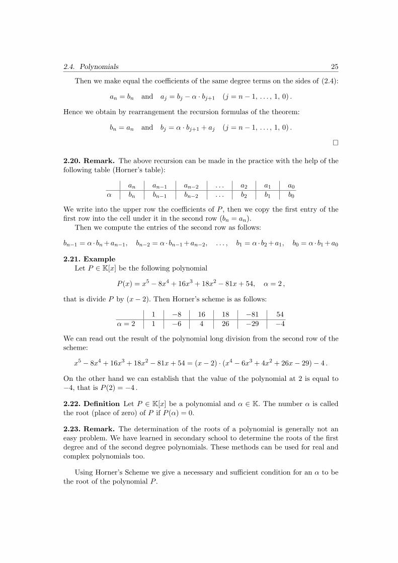
2.20. Remark. The above recursion can be made in the practice with the help of thefollowing table (Horner’s table):

an an−1 an−2 . . . a2 a1 a0

α bn bn−1 bn−2 . . . b2 b1 b0

We write into the upper row the coefficients of P , then we copy the first entry of thefirst row into the cell under it in the second row (bn = an).

Then we compute the entries of the second row as follows:

bn−1 = α · bn +an−1, bn−2 = α · bn−1 +an−2, . . . , b1 = α · b2 +a1, b0 = α · b1 +a0

2.21. ExampleLet P ∈ K[x] be the following polynomial

P (x) = x5 − 8x4 + 16x3 + 18x2 − 81x + 54, α = 2 ,

that is divide P by (x− 2). Then Horner’s scheme is as follows:

1 −8 16 18 −81 54α = 2 1 −6 4 26 −29 −4

We can read out the result of the polynomial long division from the second row of thescheme:

x5 − 8x4 + 16x3 + 18x2 − 81x + 54 = (x− 2) · (x4 − 6x3 + 4x2 + 26x− 29)− 4 .

On the other hand we can establish that the value of the polynomial at 2 is equal to−4, that is P (2) = −4 .

2.22. Definition Let P ∈ K[x] be a polynomial and α ∈ K. The number α is calledthe root (place of zero) of P if P (α) = 0.

2.23. Remark. The determination of the roots of a polynomial is generally not aneasy problem. We have learned in secondary school to determine the roots of the firstdegree and of the second degree polynomials. These methods can be used for real andcomplex polynomials too.

Using Horner’s Scheme we give a necessary and sufficient condition for an α to bethe root of the polynomial P .

26 2. Lesson 2

2.24. Theorem Let P ∈ R[x] \ {0} and α ∈ R. Then α is the root of P if and only ifthere exists a polynomial S ∈ R[x] such that

P (x) = (x− α) · S(x) (x ∈ R) . (2.5)

In words: P (x) can be divided by x− α.

Proof. Suppose that α is the root of P , that is P (α) = 0. Using Horner’s scheme wecan determine the polynomial S ∈ R[x] and the number r ∈ R such that

P (x) = (x− α) · S(x) + r (x ∈ R) .

Substituting x = α, we obtain

0 = P (α) = (α− α) · S(α) + r = r .

Thus r = 0, whence

P (x) = (x− α) · S(x) + 0 = (x− α) · S(x) (x ∈ R) .

Conversely, suppose (2.5), and substitute x = α. Thus we have

P (α) = (α− α) · S(x) = 0 .

¤

2.25. Corollary. Suppose that α is the root of P . Then it can be determined (e.g.with the help of Horner’s scheme) a polynomial S such that

P (x) = (x− α) · S(x) (x ∈ R) .

If α is the root of S, then it can be determined a polynomial T such that

S(x) = (x− α) · T (x) ,

therefore

P (x) = (x− α) · (x− α) · T (x) = (x− α)2 · T (x) (x ∈ R) .

This process can be continued. Suppose that we can factor out the polynomial x − αm times. Then in the last step we have a polynomial P1 such that

P (x) = (x− α)m · P1(x) (x ∈ R) and P1(α) 6= 0 .

The number m is called the multiplicity of the root α.

2.5. Homework 27

2.5. Homework

1. Prove the statement in Remark 2.5

2. Determine whether the following functions are invertible or not. If a function isinvertible, determine its inverse (domain and formula).

a) f(x) =5x + 32x− 4

b) f(x) =5x + 32x− 4

Df = (2, +∞)

c) f(x) = x2 − 6x d) f(x) = x2 − 6x Df = [4, +∞]

3. Determine the compositions f ◦ g and g ◦ f if it exists (domain and formula).

f(x) =√

3− x, g(x) =√

x2 − 16 .

4. Using Horner’s scheme factor out x + 1 from the following polynomials:

a) 2x4 − x3 − 5x2 + x + 3

b) x5 + 6x4 + 2x3 − 4x2 + 5x + 6

3. Lesson 3

3.1. Sequences

3.1. Definition Let H be a nonempty set.The functions

a : N→ H

are called sequences in H. For an n ∈ N the element a(n) ∈ H is called the n-th termof the sequence. Its usual notation is an.

Some notations for the sequence a:

a ; (an) ; (an, n ∈ N) ; an ∈ H (n ∈ N)

3.2. Remarks.

1. Sometimes the terms are indexed starting from a fixed p ∈ Z. In this case thesequence is a function defined on the set {n ∈ Z | n ≥ p}.

2. A sequence can be given by a formula, e.g. an :=1n

(n ∈ N) or by a recursion,e.g.

a1 := 1 , a2 := 1 , an+1 := an + an−1 (n ∈ N, n ≥ 2) .

3.3. Definition The sequence nk ∈ N (k ∈ N) is called index sequence if it is strictlymonotone increasing, that is

∀n ∈ N : nk < nk+1 .

3.4. Definition Let a : N → H be a sequence and let (nk) be an index sequence.Then the sequence

ank∈ H (k ∈ N)

is called the subsequence of (an) (composed with the index sequence (nk)).

3.5. Example

If an =1n

(n ∈ N) and nk = 2k (k ∈ N), then

ank= a2k =

12k

=(

12

)k

(k ∈ N) .

The type of a sequence is depending on H. Some types of sequences:

3.2. Convergent Number Sequences 29

• Real number sequence if H = R (more generally: H ⊆ R)

• Complex number sequence if H = C (more generally: H ⊆ C)

• Vector sequence if H is a vector space (more generally: H is a subset of a vectorspace), for example H = Rn.

• Function sequence if H is a set consisting of functions.

• Set sequence if H is a system of sets.

The real or complex sequences are called number sequences. We will use the commonnotation a : N→ K for them.

3.6. Remark. The set of number sequences (sequences of type N → K) is an infinitedimensional vector space over K with respect to the usual pointwise addition and scalarmultiplication.

3.2. Convergent Number Sequences

Let us discuss the real number sequence an =1n

(n ∈ N). We feel intuitively thatthe terms of this sequence are arbitrarily near to the number 0 if the index n is great

enough. We say that the numbers1n

approach 0 or converge to 0. This impression isthe base of the concept of the convergency and of the limit.

To define exactly what ”near to a number” means, we need the concept of neigh-bourhood (or ball or environment).

3.7. Definition Let a ∈ K and r > 0. The neighbourhood (or ball or environment) ofa with radius r is the set

B(a, r) := {x ∈ K | |x− a| < r } ⊂ K .

3.8. Remarks.

1. If K = R, then the neighbourhood B(a, r) = {x ∈ R | |x − a| < r } is equal tothe open interval (a− r, a + r).

2. If K = C, then the neighbourhood B(a, r) = {z ∈ C | |z−a| < r } is equal to theopen circular disk with centre a and with radius r on the complex number plane.Really, let

a = u + vi and z = x + yi .

Then|z − a| = |(x− u) + (y − v)i| =

√(x− u)2 + (y − v)2 ,

thus the inequality |z − a| < r is equivalent to

(x− u)2 + (y − v)2 < r2 ,

which describes the above mentioned circular disk.

30 3. Lesson 3

3. Sometimes we use the closed neighbourhoods (closed balls) defined as

B(a, r) := {x ∈ K | |x− a| ≤ r } ⊂ K .

Similarly, we can consider that

• If K = R, then the closed neighbourhood B(a, r) is equal to the closedinterval [a− r, a + r].

• If K = C, then the closed neighbourhood B(a, r) is equal to the closedcircular disk with centre a and with radius r.

4. Sometimes we use the neighbourhood of a ∈ K with radius +∞ as

B(a,+∞) := K .

An important topological property of K (what is called T2-property) is that any twopoints can be separated by disjoint neighbourhoods. This is expressed in the followingtheorem.

3.9. Theorem Let a, b ∈ K, a 6= b. Then

∃ r1, r2 > 0 : B(a, r1) ∩B(b, r2) = ∅ .

Proof. Let r1 :=|a− b|

2> 0. Then for every x ∈ B(a, r1) holds (using the second

triangle inequality):

|x−b| = |x−a+a−b| = |(a−b)−(a−x)| ≥ |a−b|−|a−x| > |a−b|−r1 = |a−b|−|a− b|2

=|a− b|

2.

thus if r2 :=|a− b|

2> 0, then |x− b| > r2, therefore x /∈ B(b, r2). ¤

After these preliminaries we can formulate the definition of the convergency and ofthe limit.

3.10. Definition The number sequence an ∈ K (n ∈ N) is named convergent if

∃A ∈ K ∀ε > 0 ∃N ∈ N ∀n ≥ N : an ∈ B(A, ε) .

The definition can be written using inequalities as follows:

∃A ∈ K ∀ε > 0 ∃N ∈ N ∀n ≥ N : |an −A| < ε .

A number sequence is named divergent if it is not convergent.

3.11. Theorem The number A in the above definition is unique.

3.2. Convergent Number Sequences 31

Proof. Suppose that A1, A2 ∈ K match the above definition in the role of A, and thatA1 6= A2. Then using the T2-property of K (see Theorem 3.9):

∃ε1, ε2 > 0 : B(A1, ε1) ∩B(A2, ε2) = ∅ .

By the definition to ε1:

∃N1 ∈ N ∀n ≥ N1 : an ∈ B(A1, ε1) .

Similarly, to the number ε2

∃N2 ∈ N ∀n ≥ N2 : an ∈ B(A2, ε2) .

Let us take e.g. the index N := max{N1 ; N2}. Then we obtain

aN ∈ B(A1, ε1) ∩B(A2, ε2) ,

which is a contradiction. Thus A1 = A2. ¤

3.12. Definition Let an ∈ K (n ∈ N) be a convergent number sequence. The uniquenumber A in the definition 3.10 is called the limit of the sequence (an), and is denotedin one of the following ways:

lim a = A , lim an = A , limn→∞ an = A , an → A (n →∞) ,

lim(an) = A , (an) → A (n →∞) .

We often say that an tends to A, or an tends to A if n tends to infinity.

3.13. Remarks.

1. If a : N→ K is a number sequence and A ∈ K, then limn→∞ an = A is equivalent to

∀ε > 0 ∃N ∈ N ∀n ≥ N : an ∈ B(A, ε) ,

or – using inequalities – to

∀ε > 0 ∃N ∈ N ∀n ≥ N : |an −A| < ε .

The number N is called a threshold index to ε.

2. It can be easily proved that a number sequence is convergent if and only if itsevery subsequence is convergent. In this case the limit of the sequence is equal tothe limit of its any subsequence. This fact is useful at proving the divergency of asequence: if you find two convergent subsequences with different limits, then thesequence is divergent.

32 3. Lesson 3

3.14. Examples

1. Let (an) be the constant sequence, that is

an := c (n ∈ N), where c ∈ K is fixed .

Then (an) is convergent and lim an = c. Really, let ε > 0. Then any N ∈ N is agood threshold index, because if n ≥ N , then

|an − c| = |c− c| = 0 < ε .

2. Let an :=1n

(n ∈ N) be the harmonic sequence.

Then (an) is convergent and lim an = 0. Really, let ε > 0. Then – by the Archi-

medean property of real numbers – there exists an N ∈ N such that N >1ε. This

N will be a good threshold index, because for all n ≥ N :

|an − 0| = | 1n− 0| = 1

n≤ 1

N<

11ε

= ε .

3. Let an := (−1)n (n ∈ N).

Then (an) is divergent, because the subsequences (a2k) and (a2k+1) have differentlimits:

limk→∞

a2k = (−1)2k = limk→∞

1 = 1

limk→∞

a2k+1 = (−1)2k+1 = limk→∞

−1 = −1

3.3. Convergency and Ordering

We can prove – using a similar idea as at the proof of the uniqueness of the limit – thefollowing theorem for real number sequences:

3.15. Theorem Let an, bn ∈ R (n ∈ N) be convergent sequences and suppose that

limn→∞ an < lim

n→∞ bn .

Then∃N ∈ N ∀n ≥ N : an < bn .

Proof. Let A := limn→∞ an and B := lim

n→∞ bn. It is assumed that A < B. Let ε :=B −A

2> 0. Then – by the definition of the limits – we have

∃N1 ∈ N ∀n ≥ N1 : |an −A| < B −A

2,

3.3. Convergency and Ordering 33

and∃N2 ∈ N ∀n ≥ N2 : |bn −B| < B −A

2.

Using the definition of the absolute value we obtain for any n ≥ N := max{N1 ; N2}that

A− B −A

2< an < A +

B −A

2and B − B −A

2< bn < B +

B −A

2.

Since A +B −A

2= B − B −A

2=

A + B

2, then we deduce from here that

an <A + B

2< bn (n ∈ N, n ≥ N) .

¤A simple corollary of the previous theorem is the following theorem.

3.16. Theorem Let an, bn ∈ R (n ∈ N) be convergent sequences and suppose that

∃N0 ∈ N ∀n ≥ N0 : an ≤ bn . (3.1)

Thenlim

n→∞ an ≤ limn→∞ bn .

Proof. Suppose indirectly that limn→∞ an > lim

n→∞ bn, that is limn→∞ bn < lim

n→∞ an. Then bythe previous theorem

∃N ∈ N ∀n ≥ N : bn < an .

Let n ∈ N be a number greater than max{N0, N}. For this n holds an > bn, incontradiction with (3.1). ¤

3.17. Remarks.

1. If we assume a stronger condition instead of (3.1), namely

∃N0 ∈ N ∀n ≥ N0 : an < bn ,

then we cannot state the strong inequality between the limits, as the followingcounterexample shows:

an := 0 <1n

=: bn (n ∈ N)

but limn→∞ an = lim

n→∞ bn = 0.

2. Applying the theorem in the case when one of the sequences is the constant 0sequence we obtain that

• If (an) is convergent and an ≥ 0 (n ≥ N0), then limn→∞ an ≥ 0,

• If (an) is convergent and an ≤ 0 (n ≥ N0), then limn→∞ an ≤ 0.

34 3. Lesson 3

3.4. Convergency and Boundedness

The boundedness of a sequence is defined as the boundedness of its range.

3.18. Definition The sequence an ∈ K (n ∈ N) is called bounded if

∃M > 0 ∀n ∈ N : |an| ≤ M .

The number M is called a bound of the sequence.A number sequence is called unbounded if it is not bounded.

3.19. Remark. The set of bounded sequences is an infinite dimensional vector spaceover K, which is a subspace in the vector space of all N→ K type sequences.

3.20. Definition The sequence an ∈ R (n ∈ N) is called

• bounded above if ∃M ∈ R ∀n ∈ N : an ≤ M . The name of M is: upperbound

• bounded below if ∃M ∈ R ∀n ∈ N : an ≥ M . The name of M is: lower bound

It can be easily proved that a real number sequence is bounded if and only if it isbounded above and it is bounded below.

3.21. Theorem Every convergent number sequence is bounded.

Proof. Let an ∈ K (n ∈ N) be a convergent sequence and A = limn→∞ an ∈ K. Apply

the definition of convergency with ε = 1:

∃N ∈ N ∀n ≥ N : |an −A| < 1 .

Use the second triangle inequality:

|an| − |A| ≤ | |an | − |A | | ≤ |an −A| < 1 ,

from where we have after rearranging

|an| < 1 + |A| (n ≥ N) .

Thus obviously

|an| ≤ M (n ∈ N) where M := max{|a1|, |a2|, . . . , |aN−1|, 1 + |A|} .

¤We remark that the reverse statement is not true. The sequence ((−1)n) is bounded

but divergent (see example 3.14). Later we will prove that any bounded sequence hasa convergent subsequence (Bolzano-Weierstrass theorem).

3.22. ExampleIt follows immediately from the previous theorem that an unbounded sequence is

divergent. By this reason e.g. the sequences

an := n2 (n ∈ N) and bn := (−1)n · n2 (n ∈ N)

are divergent.

3.5. Zero Sequences 35

3.5. Zero Sequences

3.23. Definition The number sequence an ∈ K (n ∈ N) is called zero sequence if it isconvergent and lim

n→∞ an = 0.

We will prove five short theorems about the zero sequences. They will be useful atthe discussion of operations with convergent sequences.

3.24. Theorem [T1] Let an ∈ K (n ∈ N) and A ∈ K. Then

limn→∞ an = A ⇔ lim

n→∞(an −A) = 0 .

Proof. The statement is a simple consequence of the definition of the limit and of theobvious identity

|an −A| = |(an −A)− 0| .¤

3.25. Theorem [T2] Let an ∈ K (n ∈ N). Then

limn→∞ an = 0 ⇔ lim

n→∞ |an| = 0 .

Proof. The statement is a simple consequence of the definition of the limit and of theobvious identity

|an − 0| = ||an| − 0| .¤

3.26. Theorem [T3, Majorant Principle] Let an ∈ K (n ∈ N) and bn ∈ R (n ∈ N).Suppose that (bn) is a zero sequence and that

∃N0 ∈ N ∀n ≥ N0 : |an| ≤ bn ,

Then (an) is also a zero sequence.

Proof. Let ε > 0. Since limn→∞ bn = 0, then

∃N1 ∈ N ∀n ≥ N1 : bn = |bn − 0| < ε .

Thus for the threshold index N := max{N0, N1} holds:

|an − 0| = |an| ≤ bn < ε .

This means that limn→∞ an = 0. ¤

3.27. Theorem [T4, Sum] Let an, bn ∈ K (n ∈ N) be zero sequences. Then their sum(an + bn) is also a zero sequence.

36 3. Lesson 3

Proof. Let ε > 0. Since limn→∞ an = 0, then

∃N1 ∈ N ∀n ≥ N1 : |an| = |an − 0| < ε

2,

and since limn→∞ bn = 0, then

∃N2 ∈ N ∀n ≥ N2 : |bn| = |bn − 0| < ε

2.

Let N := max{N1, N2}. It will be a good threshold index, because – using the firsttriangle inequality – for any n ≥ N holds:

|(an + bn)− 0| = |an + bn| ≤ |an|+ |bn| < ε

2+

ε

2= ε .

This means that limn→∞(an + bn) = 0. ¤

3.28. Theorem [T5, Product] Let an ∈ K (n ∈ N) be a zero sequence and bn ∈ K (n ∈N) be a bounded sequence. Then their product (anbn) is a zero sequence.

Proof. Let ε > 0. Since (bn) is bounded, then

∃M > 0 ∀n ∈ N : |bn| ≤ M .

Since limn→∞ an = 0, then

∃N ∈ N ∀n ≥ N : |an| < ε

M.

This N will be a good threshold index, because for any n ≥ N holds:

|(anbn)− 0| = |an| · |bn| ≤ |an| ·M <ε

M·M = ε .

This means that limn→∞(anbn) = 0. ¤

3.29. Remark. The set of zero sequences is an infinite dimensional vector space overK, which is a subspace in the vector space of all N→ K type sequences.

3.6. Homework

1. Prove by definition of the limit that

a) limn→∞

3n− 27n + 5

=37

b) limn→∞

n3 − 2n2 + 5n + 34n3 − 23n2 + 11n + 8

=14

c) limn→∞

n3 − 3n2 + n− 11− 2n3 + n

= −12

d) limn→∞

n2 + 3n− 1n3 − 7n2 + 6n− 10

= 0

e) limn→∞

n− 1n3 + 17n− 30

= 0

In each question determine a threshold index to ε = 0, 001.

4. Lesson 4

4.1. Operations with Convergent Sequences

Using Theorems T1, . . . , T5 about the zero sequences we can easily discuss the opera-tions with convergent sequences.

4.1. Theorem [Absolute Value]Let an ∈ K (n ∈ N) be a convergent sequence. Then its absolute value sequence

(|an|) is also convergent and

limn→∞ |an| = | lim

n→∞ an | .

Proof. Let A := limn→∞ an. We have to prove that lim

n→∞ |an| = |A|.Using the second triangle inequality we have:

∣∣∣ |an| − |A|∣∣∣ ≤ |an −A| .

Since – by T1 – (an −A) is a zero sequence, then by T3 we have that (|an| − |A|) is azero sequence. Thus – once more by T1 – lim

n→∞ |an| = |A|. ¤

4.2. Remark. The reverse statement is not true. For example, if an = (−1)n (n ∈ N),then (|an|) is convergent, but (an) is divergent.

4.3. Theorem [Addition]Let an, bn ∈ K (n ∈ N) be convergent sequences. Then their sum (an + bn) is also

convergent andlim

n→∞(an + bn) = limn→∞ an + lim

n→∞ bn .


n→∞ bn. We have to prove that limn→∞(an + bn) =

A + B.Since – by T1 – (an−A) and (bn−B) are zero sequences, then by T4 the sequence

(an + bn)− (A + B) = (an −A) + (bn −B)

is also a zero sequence. Thus ((an + bn)− (A+B)) is a zero sequence. Using once moreT1 it follows that

limn→∞(an + bn) = A + B .

¤

38 4. Lesson 4

4.4. Theorem [Multiplication]Let an, bn ∈ K (n ∈ N) be convergent sequences. Then their product (anbn) is also

convergent andlim

n→∞(anbn) = ( limn→∞ an) · ( lim

n→∞ bn) .


n→∞ bn. We have to prove that limn→∞(anbn) = AB.

Let us see the following transformations:

anbn −AB = anbn −Abn + Abn −AB = (an −A)bn + A(bn −B) .

(an −A) and (bn −B) are zero sequences by T1.The sequences (bn) and (A) are convergent, consequently, they are bounded. Thus

– using T5 – the sequences ((an −A)bn) and (A(bn −B)) are zero sequences.Using T4 we obtain that their sum (anbn −AB) is a zero sequence.Finally, using T1 we have lim

n→∞(anbn) = AB. ¤

4.5. Corollary. If bn = c, (n ∈ N) is a constant sequence, then we have

limn→∞(can) = c · lim

n→∞ an (c ∈ K) .

Combining this result with the theorem about addition we have that if the sequencesan, bn ∈ K (n ∈ N) are convergent, then their difference (an − bn) is also convergentand

limn→∞(an − bn) = lim

n→∞ an − limn→∞ bn .

4.6. Corollary. If p ∈ N is a fixed positive integer exponent, then

limn→∞ ap

n = ( limn→∞ an)p .

4.7. Remark. The theorems about the addition and the scalar multiplication of con-vergent sequences imply that the set of convergent sequences is a vector space. This isan infinite dimensional subspace in the vector space of all N→ K type sequences.

4.8. Theorem [Reciprocal]Let bn ∈ K \ {0} (n ∈ N) be a convergent sequence. Suppose that B := lim

n→∞ bn 6= 0.Then

a) The sequence(

1bn

)is bounded

b) The sequence(

1bn

)is convergent and

limn→∞

1bn

=1B

.

4.1. Operations with Convergent Sequences 39

Proof.

a) Using Theorem 4.1 we have that limn→∞ |bn| = |B| > 0. Applying the definition of

the limit for ε :=|B|2

> 0 we obtain:

∃N ∈ N ∀n ≥ N :|B|2

= |B| − |B|2

< |bn| < |B|+ |B|2

=3|B|

2. (4.1)

Thus ∣∣∣∣1bn

∣∣∣∣ =1|bn| ≤ max

{1|b1| , . . . ,

1|bN−1| ,

2|B|

}.

b)1bn− 1

B=

B − bn

bnB=

1bn·(− 1

B

)· (bn −B) .

(bn −B) is a zero sequence by T1.

The sequences(

1bn

)and

(− 1

B

)are bounded. Thus – using T5 – the sequence

on the right side of the above equality is a zero sequence.

Finally, using T1 we have limn→∞

1bn

=1B

.

¤

4.9. Corollary. If p ∈ Z, p < 0 is a fixed negative integer exponent, then

limn→∞ bp

n = ( limn→∞ bn)p .

Combining the theorems about the reciprocal and about the multiplication we ob-tain the theorem about the quotient of two sequences:

4.10. Theorem [Division]Let an ∈ K (n ∈ N) bn ∈ K \ {0} (n ∈ N) be convergent sequences. Suppose that

limn→∞ bn 6= 0. Then their quotient

(an

bn

)is also convergent and

limn→∞

an

bn=

limn→∞ an

limn→∞ bn

.

Proof.

limn→∞

an

bn= lim

n→∞

(an · 1

bn

)= ( lim

n→∞ an) · limn→∞

1bn

= ( limn→∞ an) · 1

limn→∞ bn

=lim

n→∞ an

limn→∞ bn

.

¤

40 4. Lesson 4

4.11. Remark. The theorems about the reciprocal and about the quotient and theircorollaries can be extended to the case when the assumption bn 6= 0 (n ∈ N) is notrequired, only the assumption lim

n→∞ bn 6= 0 is required. In this case – using the estimation

in (4.1) – we have:

∃N ∈ N ∀n ≥ N : |bn| > |B|2

> 0 ,

that isbn 6= 0 for n = N, N + 1, . . .

So we can take the sequence (bn, n ∈ N, n ≥ N) instead of (bn, n ∈ N).

4.12. Theorem [q-th root]Let q ∈ N, q ≥ 2 and an ∈ R (n ∈ N) be a convergent sequence. Suppose that

an ≥ 0 (n ∈ N). Then its q-th root sequence ( q√

an) is also convergent, and

limn→∞

q√

an = q

√lim

n→∞ an .

Remark that by Theorem 3.16 and its corollary limn→∞ an ≥ 0.

Proof. Let A := limn→∞ an ≥ 0. We have to prove that lim

n→∞q√

an = q√

A.

First suppose A > 0. We will use the well-known elementary identity (see: (1.1))

an − bn = (a− b) · (an−1 + an−2b + . . . + abn−2 + bn−1)

with n = q, a = q√

an ≥ 0, b = q√

A > 0. Thus

|an −A| = |( q√

an)q − ( q√

A)q| == | q√

an − q√

A| ·(( q√

an)q−1 + ( q√

an)q−2 q√

A + . . . + q√

an( q√

A)q−2 + ( q√

A)q−1)

.

Here we have used that each term of the second factor on the right side is nonnegativeand the last term is positive. This is the reason that the absolute value is not writtenaround the second factor.

After leaving the first q−1 nonnegative terms from the second factor we obtain thefollowing inequality:

|an −A| ≥ | q√

an − q√

A| · ( q√

A)q−1 .

Consequently

| q√

an − q√

A| ≤ |an −A|( q√

A)q−1

Since – by T1 and T2 – (|an−A|) is a zero sequence, then by T3 we have that ( q√

an− q√

A)is a zero sequence. Thus – once more by T1 – lim

n→∞q√

an = q√

A.In the remainder case A = 0 we will use the definition of the limit. Let ε > 0. Then

εq > 0, therefore

∃N ∈ N ∀n ≥ N : 0 ≤ an = |an − 0| < εq .

4.2. Some Important Convergent Sequences 41

Taking q-th root we obtain

∃N ∈ N ∀n ≥ N : 0 ≤ | q√

an − q√

0| = q√

an < q√

εq = ε .

This implies the statement of the theorem in the case A = 0. ¤

4.13. Corollary. If an ∈ R an > 0 (n ∈ N) and r ∈ Q is a fixed rational exponent,then

limn→∞ ar

n = ( limn→∞ an)r .

4.14. Theorem [Sandwich Theorem]Let an, bn, cn ∈ R (n ∈ N) be real number sequences and suppose that

a) ∃N0 ∈ N ∀n ≥ N0 : an ≤ bn ≤ cn and that

b) (an) and (cn) are convergent and limn→∞ an = lim

n→∞ cn =: A.

Then (bn) is also convergent and limn→∞ bn = A.

Proof. Let us start from the inequalities

an ≤ bn ≤ cn (n ∈ N, n ≥ N0) .

After subtracting an we have

0 ≤ bn − an ≤ cn − an (n ∈ N, n ≥ N0) .

Sincelim

n→∞(cn − an) = limn→∞ cn − lim

n→∞ an = A−A = 0 ,

then (cn − an) is a zero sequence. Using T3 we obtain that (bn − an) is also a zerosequence. Finally

limn→∞ bn = lim

n→∞ ((bn − an) + an) = limn→∞(bn − an) + lim

n→∞ an = 0 + A = A .

¤

4.2. Some Important Convergent Sequences

In the Examples 3.14 we have seen that

limn→∞ an = c (c ∈ K) and lim

n→∞1n

= 0 .

Now let us discuss the geometric sequence.

4.15. Definition Let q ∈ K be a fixed number. Then the sequence

an := qn (n ∈ N)

is called a geometric sequence (with base q or with quotient q).

42 4. Lesson 4

4.16. Theorem The geometric sequence is convergent if and only if |q| < 1 or q = 1.In this case

limn→∞ qn =

0 if |q| < 1

1 if q = 1

Proof. The statement of the theorem is trivial if q = 0 or if q = 1. Suppose that

0 < |q| < 1. Then1|q| > 1 and – using the Bernoulli inequality (see Theorem 2.2) –

1|q|n =

(1|q|

)n

=(

1 +1|q| − 1

)n

≥ 1 + n ·(

1|q| − 1

)> n ·

(1|q| − 1

).

After rearranging we have

0 ≤ |qn| = |q|n ≤ 11|q| − 1

· 1n

(n ∈ N) .

The right side sequence tends to 0. Using the Sandwich Theorem we obtainlim

n→∞ |qn| = 0. Using Theorem 3.25 we have lim

n→∞ qn = 0.

Suppose that |q| > 1. Once more using the Bernoulli inequality:

|qn| = |q|n = (1 + |q| − 1)n ≥ 1 + n · |q| > n · |q| ,which implies that the sequence (qn) is unbounded. Consequently it is divergent.

Finally, suppose that |q| = 1 but q 6= 1. Suppose indirectly that (an = qn) isconvergent and denote by A its limit. Then by Theorem 4.1 we have

|A| = | limn→∞ qn | = lim

n→∞ |qn| = lim

n→∞ |q|n = lim

n→∞ 1n = 1 ,

which implies A 6= 0.On the other hand lim

n→∞ an+1 = limn→∞ an = A, therefore

0 = A−A = limn→∞ an+1 − lim

n→∞ an = limn→∞(an+1 − an) = lim

n→∞(qn+1 − qn) =

= limn→∞ qn(q − 1) = (q − 1) · lim

n→∞ qn = (q − 1) ·A .

We obtained that0 = (q − 1) ·A ,

which is a contradiction, because on the right side stands the product of two nonzeronumbers. ¤

We have finished the discussion of the geometric sequence. In the following theoremswe will discuss some other interesting convergent sequences.

4.17. Theorem Let a ∈ R, a > 0 be fixed. Then

limn→∞

n√

a = 1 .

4.2. Some Important Convergent Sequences 43

Proof. Suppose first that a > 1.Let n ≥ 2 and apply the inequality between the arithmetic and the geometric means

(see Theorem 2.8) for the n pieces of non-all-equal positive numbers

a, 1, 1, . . . , 1 :

1 < n√

a = n√

a · 1 · . . . · 1 <a + n− 1

n= 1 +

a− 1n

.

The sequence on the right side obviously tends to 1. Applying the Sandwich Theoremwe obtain the statement of the theorem.

The case 0 < a < 1 can be reduced to the first case. Really, since1a

> 1, then

n√

a =11

n√a

=1

n

√1a

−→ 11

= 1 .

Finally, the case a = 1 is trivial. ¤

4.18. Theoremlim

n→∞n√

n = 1 .

Proof. Suppose that n ≥ 2 and apply the inequality between the arithmetic and thegeometric means (see Theorem 2.8) for the n pieces of non-all-equal positive numbers

√n,√

n, 1, 1, . . . , 1 :

1 < n√

n = n

√√n · √n · 1 · . . . · 1 <

2√

n + n− 2n

=2√n

+ 1− 2n

The sequence on the right side obviously tends to 1. Applying the Sandwich Theoremwe obtain the statement of the theorem. ¤

4.19. Corollary. For any fixed r ∈ Q:

limn→∞

n√

nr = limn→∞

(n√

n)r = 1r = 1 .

4.20. Theorem Let q ∈ K and k ∈ N be fixed. Then

limn→∞nk · qn = 0 .

Proof. For any n ∈ N we have

|nkqn| = nk · |q|n =((

n√

n)n)k · |q|n =

(n√

nk · |q|)n

. (4.2)

Let s ∈ R, |q| < s < 1 be fixed. Since limn→∞( n

√nk) · |q| = 1 · |q| = |q|, then by the

definition of the limit:

∃N ∈ N ∀n ≥ N : (n√

nk) · |q| < s .

44 4. Lesson 4

Thus we can continue (4.2) for n ≥ N as follows:

|nkqn| =(

n√

nk · |q|)n

< sn .

However, limn→∞ sn = 0, because (sn) is a geometric sequence with 0 < s < 1. Using the

majorant principle for zero sequences (see: Theorem 3.26) we obtain that (nkqn) is azero sequence. ¤

4.21. Corollary. Let a ∈ R, a > 1. Applying the previous theorem with q :=1a

weobtain for any k ∈ N that

limn→∞

nk

an= 0 .

We can express this fact in this way: the exponential function (with base greater than1) increases faster than a power function of any degree.

In the following theorem we will show that the factorial increases faster than anyexponential function.

4.22. Theorem Let x ∈ K be fixed. Then

limn→∞

xn

n!= 0 .

Proof. Let n ∈ N, n > |x|. (There exists such n by the Archimedean property ofordering.) Then we have for any n ≥ N + 2:

∣∣∣∣xn

n!

∣∣∣∣ =|x|nn!

=

N factors︷︸︸︷|x| · . . . · |x| ·|x| · . . . · |x|

1 · . . . ·N︸︷︷︸N factors

·(N + 1) · . . . · n =|x|NN !

· |x|N + 1

· . . .|x|

n− 1· |x|

n≤

≤ |x|NN !

· |x|n−→ 0 (n →∞) .

In the above estimation we have used that

|x|N + 1

< 1, . . . ,|x|

n− 1< 1 ,

and that the other factors of the product are nonnegative.Finally, applying the majorant principle for zero sequences (see: Theorem 3.26) we

obtain that (xn

n!) is a zero sequence. ¤

4.3. Complex Number Sequences 45

4.3. Complex Number Sequences

4.23. Definition Let zn ∈ C (n ∈ N) be a complex number sequence. Let us write itseach term in canonical form:

zn = an + bni (n ∈ N) ,

where i denotes the imaginary unit in C: i =√−1. Thus we have defined the real

number sequences (an) and (bn). Obviously an = Re zn and bn = Im zn.The sequence (an) is called the real part sequence of (zn). The sequence (bn) is

called the imaginary part sequence of (zn).

4.24. ExampleIf zn = (n + i)2 (n ∈ N), then

zn = (n + i)2 = n2 + 2ni + i2 = n2 − 1 + 2ni ,

thusan = Re zn = n2 − 1, bn = Im zn = 2n (n ∈ N) .

The following auxiliary theorem will be useful at the discussion of boundedness andconvergency of complex sequences.

4.25. Theorem If z ∈ C, then

|Re z| ≤ |z| ≤ |Re z|+ |Im z| and |Im z| ≤ |z| ≤ |Re z|+ |Im z| .

Proof. Denote by x the real part of z and by y the imaginary part of z respectively.Then

|x| =√

x2 ≤√

x2 + y2 = |z| and |y| =√

y2 ≤√

x2 + y2 = |z|imply the left-hand inequalities immediately. The common right-hand inequality canbe proved as follows:

|z| =√

x2 + y2 =√|x|2 + |y|2 ≤

√|x|2 + 2|x||y|+ |y|2 =

√(|x|+ |y|)2 =

= |x|+ |y| = |Re z|+ |Im z| .¤

4.26. Theorem The complex number sequence zn ∈ C (n ∈ N) is bounded if and onlyif its real and imaginary part sequences are bounded.

Proof. Suppose that (zn) is bounded.Then

∃M > 0 ∀n ∈ N : |zn| ≤ M .

Using the auxiliary theorem we have

|Re zn| ≤ M and |Im zn| ≤ M (n ∈ N) ,

46 4. Lesson 4

which means that (Re zn) and (Im zn) are bounded.Conversely, suppose that (Re zn) and (Im zn) are bounded sequences. Then

∃M1 > 0 ∀n ∈ N : |Re zn| ≤ M1, and ∃M2 > 0 ∀n ∈ N : |Im zn| ≤ M2 .

Once more by the auxiliary theorem we have:

|zn| ≤ |Re zn|+ |Im zn| ≤ M1 + M2 ,

which implies the boundedness of (zn). ¤

4.27. Theorem The complex number sequence zn = an+bni ∈ C (n ∈ N) is convergentif and only if its real part sequence (an = Re zn) and its imaginary part sequence(bn = Im zn) both are convergent. In this case:

limn→∞ zn = lim

n→∞Re zn + ( limn→∞ Im zn) · i .

Proof. Suppose that (zn) is convergent and denote its limit by Z = A+Bi ∈ C. Thenthe sequence

zn − Z = an + bni−A−Bi = (an −A) + (bn −B)i (n ∈ N)

is a zero sequence. Using the auxiliary theorem we have

|an −A| ≤ |zn − Z| −→ 0 and |bn −B| ≤ |zn − Z| −→ 0 (n →∞) .

From here it follows – by the majorant principle for zero sequences (see: Theorem 3.26)– that (an −A) and (bn −B) both are zero sequences. This implies that (an) and (bn)are convergent, moreover lim

n→∞ an = A and limn→∞ bn = B.

Conversely, suppose that (an) and (bn) are convergent. Then (see: operations withconvergent sequences) the linear combination

zn = 1 · an + i · bn (n ∈ N)

is also convergent and

limn→∞ zn = lim

n→∞(an + ibn) = limn→∞ an + i · lim

n→∞ bn .

¤

4.28. Example Let

zn :=n + 1

n+

2n + 1n + 1

i (n ∈ N) .

Then

Re zn =n + 1

n−→ 1 (n →∞) and Im zn =

2n + 1n + 1

−→ 2 (n →∞) ,

thus by the theoremlim

n→∞ zn = 1 + 2i.

4.4. Homework 47

4.4. Homework

1. Determine the following limits if they exist.

a) limn→∞

3n4 − 5n3 + n2 − 17(n + 1)4 + n3 − 7n2 + 6n− 10

b) limn→∞

(n + 2)6 − (n + 3)6

(n2 − 2n− 5)(2n3 + n2 + 3)

c) limn→∞(

√n2 + n− n) d) lim

n→∞(√

2n− 1−√n + 3)

e) limn→∞(

√2n− 1−√2n + 3) f) lim

n→∞

√n + 1−√n√n−√n− 1

g) limn→∞(

√n + 4 · √n−

√n− 10 · √n) h) lim

n→∞n

√n + 12n + 3

i) limn→∞

6n+2 − 3n+1

2 · 6n + 5n+1j) lim

n→∞n3 · 2n + 5n+1

5n−1 − n · 3n

5. Lesson 5

5.1. Monotone Sequences

5.1. Definition Let an ∈ R (n ∈ N) be a real number sequence. We say that thissequence is

• monotonically increasing if ∀n ∈ N : an ≤ an+1

• strictly monotonically increasing if ∀n ∈ N : an < an+1

• monotonically decreasing if ∀n ∈ N : an ≥ an+1

• strictly monotonically decreasing if ∀n ∈ N : an > an+1

• monotone if it is either monotonically increasing or monotonically decreasing

• strictly monotone if it is either strictly monotonically increasing or strictly mo-notonically decreasing

5.2. Remarks.

1. The strictly monotonically increasing sequences are often called increasing se-quences or strictly increasing sequences.

2. The strictly monotonically decreasing sequences are often called decreasing se-quences or strictly decreasing sequences.

3. The monotonically increasing sequences are sometimes called nondecreasing se-quences.

4. The monotonically decreasing sequences are sometimes called nonincreasing se-quences.

5.3. Theorem Every real number sequence has a monotone subsequence.

Proof. Let an ∈ R (n ∈ N) be a real number sequence. Let us call a natural numberk ∈ N a vertex of (an) if

∀n > k : ak > an .

Case 1: Suppose that the number of vertices is infinite. In this case the vertices forman index sequence:

n1 < n2 < n3 < . . .

Since n1 is a vertex and n2 > n1, then an1 > an2 ,since n2 is a vertex and n3 > n2, then an2 > an3 ,

5.1. Monotone Sequences 49

and so on. We have obtained a strictly monotonically decreasing subsequence

an1 > an2 > an3 > . . .

Case 2: Suppose that the number of vertices is finite (may be no vertex). Let n0 bethe last vertex of (an) and n1 := n0 +1. Then n1 is no vertex, consequently ∃n2 > n1 :an1 ≤ an2 ,

n2 is no vertex, consequently ∃n3 > n2 : an2 ≤ an3 ,and so on. We have obtained a monotonically increasing subsequence

an1 ≤ an2 ≤ an3 ≤ . . .

¤

5.4. Theorem Let an ∈ R (n ∈ N) be a monotone real number sequence. Then it isconvergent if and only if it is bounded. Moreover

limn→∞ an =

sup{an | n ∈ N} if (an) is monotonically increasing

inf{an | n ∈ N} if (an) is monotonically decreasing

Proof. Suppose that (an) is convergent. Then it is bounded (see Theorem 3.21).Conversely, suppose that (an) is bounded and let us see the case when (an) is

monotonically increasing. Because of its boundedness (an) is bounded above. Thereforeit has finite least upper bound

A := sup{an | n ∈ N} ∈ R .

Let ε > 0. Then A− ε < A, thus A− ε is not upper bound. Therefore

∃N ∈ N : aN > A− ε .

Since (an) is monotonically increasing, then we obtain that ∀n ≥ N : an ≥ aN . Hence

A− ε < aN ≤ an ≤ A < A + ε (∀n ≥ N) ,

which implies |an −A| < ε.This means – by the definition of the limit – that lim

n→∞ an = A.The monotone decreasing case can be proved similarly. ¤

5.5. Remark. Since every monotone increasing sequence is bounded below, then fora monotone increasing sequence the property ”bounded” is equivalent to ”boundedabove”. Similarly, for a monotone decreasing sequence the property ”bounded” is equi-valent to ”bounded below”.

5.6. Theorem [Bolzano-Weierstrass]Every bounded number sequence contains a convergent subsequence.

50 5. Lesson 5

Proof. In the first step we will prove the statement for real number sequences. Letan ∈ R (n ∈ N) be a bounded real number sequence. By Theorem 5.3 it contains amonotone subsequence (ank

). The subsequence (ank) is obviously bounded (with the

same bound as (an), therefore it is a monotone and bounded sequence. Consequently– by the previous theorem – (ank

) is convergent.

In the second step we will prove the statement for complex number sequences.Let zn = an + bni ∈ C (n ∈ N) be a bounded complex number sequence. Then byTheorem 4.26 the real sequences (an) and (bn) are bounded. Applying the provedpart of the theorem for the real part sequence (an), it has a convergent subsequence(ank

, k ∈ N). However, the subsequence (bnk, k ∈ N) of the imaginary part sequence

(bn) is also bounded, so – applying once more the proved part of the theorem – (bnk)

has a convergent subsequence (bnks, s ∈ N). Hence – using Theorem 4.27 – the complex

number sequenceznks

= anks+ bnks

i (s ∈ N)

is convergent, and obviously it is a subsequence of (zn). ¤

5.2. Euler’s Number e

5.7. Theorem The sequence

an :=(

1 +1n

)n

(n ∈ N)

is convergent.

Proof. We want to apply Theorem 5.4, therefore we will prove that (an) is increasingand bounded above.

To prove that (an) is increasing, let us apply the inequality between the arithmeticand the geometric means (see Theorem 2.8) for the n+1 pieces of non-all-equal positivenumbers

1 +1n

, 1 +1n

, . . . , 1 +1n

, 1 .

We obtain that

an =(

1 +1n

)n

=(

1 +1n

)· . . . ·

(1 +

1n

)

︸︷︷︸n times

· 1 <

n ·(

1 +1n

)+ 1

n + 1

n+1

=

=(

n + 2n + 1

)n+1

=(

1 +1

n + 1

)n+1

= an+1.

This means that (an) is increasing

5.3. Cauchy’s Convergence Test 51

To prove that (an) is bounded above, let us apply the inequality between the arith-metic and the geometric means for the n + 2 pieces of non-all-equal positive numbers

1 +1n

, 1 +1n

, . . . , 1 +1n

,12,

12

.

We obtain that

14an =

14·(

1 +1n

)n

=(

1 +1n

)· . . . ·

(1 +

1n

)

︸︷︷︸n times

· 12· 12

<

<

n ·(

1 +1n

)+

12

+12

n + 2

n+2

=(

n + 2n + 2

)n+2

= 1,

Hence we have an < 4 (n ∈ N). Thus (an) is bounded above. ¤

5.8. Definition On the base of the previous theorem we can define Euler’s number eas

e := limn→∞

(1 +

1n

)n

.

5.9. Remark. Later (see Theorem 9.15) we will prove that the number e is irrational.Its approximating value for three decimal digits is 2.718. This means that

| e− 2.718 | < 12· 10−3, that is 2.7175 < e < 2.7185 .

5.3. Cauchy’s Convergence Test

5.10. Definition The number sequence an ∈ K (n ∈ N) is called a Cauchy sequenceif

∀ε > 0 ∃N ∈ N ∀m, n ≥ N : |an − am| < ε .

5.11. Theorem Every Cauchy sequence is bounded. Consequently – by the Bolzano-Weierstrass theorem – it has convergent subsequence.

Proof. Let an ∈ K (n ∈ N) be a Cauchy sequence and let us apply the above definitionwith ε = 1. Then

∃N ∈ N ∀m, n ≥ N : | an − am| < 1 .

Let m := N and apply the second triangle inequality. Thus we have

1 > | an − aN | ≥∣∣∣ |an| − |aN |

∣∣∣ ≥ |an| − |aN | (n ≥ N) .

Consequently|an| < 1 + |aN | (n ≥ N) .

52 5. Lesson 5

Hence we have

|an| ≤ max{|a1|, . . . , |aN−1|, 1 + |aN |} (n ∈ N) .

This means that (an) is bounded. ¤

5.12. Theorem [Cauchy’s Convergence Test]The number sequence an ∈ K (n ∈ N) is convergent if and only if it is a Cauchy

sequence.

Proof. Suppose that (an) is convergent and denote by A ∈ K its limit. Furthermorelet ε > 0. Then

∃N ∈ N ∀n ≥ N : |an −A| < ε

2.

This N will be a good threshold index to prove that (an) is a Cauchy sequence. Really,using the first triangle inequality, we have for any m,n ≥ N :

| an−am| = | an−A+A−am| ≤ | an−A|+ |A−am| = | an−A|+ | am−A| < ε

2+

ε

2= ε .

Conversely, suppose that (an) is a Cauchy sequence. By the previous theorem (an)has a convergent subsequence (ank

). Denote by A the limit of (ank). We will show that

limn→∞ an = A. Let ε > 0.

By the definition of the Cauchy sequence we have

∃N ∈ N ∀m,n ≥ N : |an − am| < ε

2.

This number N will be a good threshold index to prove that (an) tends to A.Since lim

k→∞ank

= A, then

∃K ∈ N ∀k ≥ K : |ank−A| < ε

2.

The index sequence (nk) is unbounded above, therefore

∃ k ∈ N : k ≥ K and nk ≥ N.

Fix such a k. Then we have for any n ≥ N – since in this case n, nk ≥ N – the followinginequalities:

| an − ank| < ε

2and | ank

−A| < ε

2.

Finally, using the first triangle inequality we have

| an −A| = | an − ank+ ank

−A| ≤ | an − ank|+ | ank

−A| < ε

2+

ε

2= ε .

This means that limn→∞ an = A. ¤

5.13. Remark. The fact that every Cauchy sequence is convergent is a typical pro-perty of the real numbers. This property is known as R is a complete metric space.

5.4. Infinite Limits of Real Number Sequences 53

5.4. Infinite Limits of Real Number Sequences

5.14. Definition Let an ∈ R (n ∈ N) be a real number sequence. We say that (an)tends to +∞ if

∀P > 0 ∃N ∈ N ∀n ≥ N : an > P .

This fact is denoted in one of the following ways:

lim a = +∞ , lim an = +∞ , limn→∞ an = +∞ , an → +∞ (n →∞) ,

lim(an) = +∞ , (an) → +∞ (n →∞) .

5.15. Definition Let an ∈ R (n ∈ N) be a real number sequence. We say that (an)tends to −∞ if

∀P < 0 ∃N ∈ N ∀n ≥ N : an < P .

This fact is denoted in one of the following ways:

lim a = −∞ , lim an = −∞ , limn→∞ an = −∞ , an → −∞ (n →∞) ,

lim(an) = −∞ , (an) → −∞ (n →∞) .

5.16. Definition Let an ∈ R (n ∈ N) be a real number sequence. We say that (an)has a limit if

(an) is convergent or limn→∞ an = +∞ or lim

n→∞ an = −∞ .

In other words:∃A ∈ R : lim

n→∞ an = A .

5.17. Remark. Define the neighbourhoods of +∞ and of −∞ with radius r > 0 asfollows:

B(+∞, r) := {x ∈ R | x >1r} = (

1r, +∞) ⊂ R ,

andB(−∞, r) := {x ∈ R | x < −1

r} = (−∞, −1

r) ⊂ R .

Using these definitions we can express uniformly that limn→∞ an = A.

Let an ∈ R (n ∈ N) be a real sequence and A ∈ R. Then limn→∞ an = A is equivalent

to∀ε > 0 ∃N ∈ N ∀n ≥ N : an ∈ B(A, ε) .

5.18. Remark. It is obvious that if a sequence tends to +∞, then it is unboundedabove. If a sequence tends to −∞, then it is unbounded below. The converse statementis not true as we can see from the example an := (−1)n · n, (n ∈ N).

54 5. Lesson 5

5.19. Theorem a) Let an ∈ R (n ∈ N) be a monotonically increasing sequence.Suppose that it is not bounded above. Then

limn→∞ an = +∞ .

b) Let an ∈ R (n ∈ N) be a monotonically decreasing sequence. Suppose that it isnot bounded below. Then

limn→∞ an = −∞ .

Proof. We will prove part a). Let P > 0. Since (an) is not bounded above, then

∃N ∈ N : aN > P.

However, (an) is monotone increasing, therefore

∀n ≥ N : an ≥ aN > P .

This means that limn→∞ an = +∞.

Part b) can be proved similarly. ¤

5.20. Corollary. Combining this theorem with Theorem 5.4 we obtain that everymonotone sequence has a limit. If the sequence is bounded, then this limit is finite, ifit is unbounded, then the limit is infinite.

Now we will discuss the algebraic operations with infinite limits.

5.21. Theorem [Addition]Let an, bn ∈ R (n ∈ N). Suppose that lim

n→∞ an = A where −∞ < A ≤ +∞ andlim

n→∞ bn = +∞. Then

limn→∞(an + bn) = +∞ .

Proof. Let us fix a real number P1 < A. Then by definition of the limit

∃N1 ∈ N ∀n ≥ N1 : an > P1 .

Let P > 0. Since limn→∞ bn = +∞, then to the real number P − P1

∃N2 ∈ N ∀n ≥ N2 : bn > P − P1 .

Let N := max{N1, N2}. Then for every n ≥ N holds

an + bn > P1 + P − P1 = P .

This means that limn→∞(an + bn) = +∞. ¤


5.22. Remarks.

1. The theorem does not state anything about the case when A = −∞. It is notby chance, in this case the sequence (an + bn) can behave itself variously, as thefollowing table shows:

an A = lim an bn B = lim bn an + bn lim(an + bn)

−n + c(c ∈ R −∞ n +∞ c c

arbitrarilyfixed)

−2n −∞ n +∞ −n −∞

−n −∞ 2n +∞ n +∞

does not exist−n −∞ n + (−1)n +∞ (−1)n (and bounded)

does not exist−n2 −∞ n2 + (−1)n · n +∞ (−1)n · n (and

unbounded)

2. Our theorem makes it possible for us to extend the addition from R into Rpreserving the identity

limn→∞(an + bn) = lim

n→∞ an + limn→∞ bn .

The table of addition in R is the following:

56 5. Lesson 5

x + y y = −∞ y ∈ R y = +∞

notx = −∞ −∞ −∞ defined

x ∈ R −∞ x + y +∞

notx = +∞ defined +∞ +∞

You can see that the sum of the elements −∞ and +∞ is undefined. In all othercases the sum is defined.

3. After these definitions the theorem about the limit of the sum of two real sequen-ces having limits can be stated shortly as

5.23. Theorem If the real number sequences (an) and (bn) have limits, further-more the sum of lim

n→∞ an and limn→∞ bn exists, then

limn→∞(an + bn) = lim

n→∞ an + limn→∞ bn .

4. The sums (−∞)+ (+∞) and (+∞)+ (−∞) are called indeterminate sums. Theyare a kind of indeterminate expressions.

5. Using the connection between the addition and subtraction we can reduce thesubtraction of sequences having infinite limits to addition. Accordingly the diffe-rences (+∞)− (+∞) and (−∞)− (−∞) are also indeterminate expressions.

5.24. Theorem [Multiplication]Let an, bn ∈ R (n ∈ N). Suppose that lim

n→∞ an = A where A ∈ R\{0} and limn→∞ bn =

+∞. Then

limn→∞(anbn) =

+∞ if A > 0

−∞ if A < 0

Proof. We will prove the case 0 < A ≤ +∞. The proof of the other case is similar.Let us fix a real number P1 such that 0 < P1 < A. Then by definition of the limit

∃N1 ∈ N ∀n ≥ N1 : an > P1 .


Let P > 0. Since limn→∞ bn = +∞, then to the real number

P

P1

∃N2 ∈ N ∀n ≥ N2 : bn >P

P1.

Let N := max{N1, N2}. Then for every n ≥ N holds

anbn > an · P

P1> P1 · P

P1= P .

This means that limn→∞(anbn) = +∞. ¤

5.25. Remark. From our theorem we can deduce that if we define the multiplicationin R as follows

x · y y = −∞ −∞ < y < 0 y = 0 0 < y < +∞ y = +∞

notx = −∞ +∞ +∞ defined −∞ −∞

−∞ < x < 0 +∞ xy 0 xy −∞

not notx = 0 defined 0 0 0 defined

0 < x < +∞ −∞ xy 0 xy +∞

notx = +∞ −∞ −∞ defined +∞ +∞

then we have the following theorem

5.26. Theorem If the real number sequences (an) and (bn) have limits, furthermorethe product of lim

n→∞ an and limn→∞ bn exists, then

limn→∞(anbn) = ( lim

n→∞ an) · ( limn→∞ bn) .

Accordingly the products 0·(+∞), 0·(−∞), (+∞)·0 and (−∞)·0 are indeterminateexpressions.

58 5. Lesson 5

5.27. Theorem [Reciprocal] Let bn ∈ R \ {0}, (n ∈ N) be a real number sequence.Suppose that it has a limit and lim

n→∞ bn = B ∈ R. Then

limn→∞

(1bn

)=

1B

if B 6∈ {−∞ , 0 , +∞}

0 if B ∈ {−∞ , +∞}

+∞ if B = 0 and ∃N0 ∈ N ∀n ≥ N0 : bn > 0

−∞ if B = 0 and ∃N0 ∈ N ∀n ≥ N0 : bn < 0

does not exist if B = 0 and there are infinitely many positiveand infinitely many negative terms in the sequence

Proof. The case B 6∈ {−∞ , 0 , +∞} was proved at the convergence sequences (seeTheorem 4.8).

Suppose that B = +∞. Let ε > 0. Then

∃N ∈ N ∀n ≥ N : bn >1ε

.

After rearranging we have −ε < 0 <1bn

< ε, that is∣∣∣∣

1bn− 0

∣∣∣∣ < ε.

The case B = −∞ can be proved similarly.Suppose that

B = 0 and ∃N0 ∈ N ∀n ≥ N0 : bn > 0 .

Let P > 0. Then

∃N1 ∈ N ∀n ≥ N1 : bn <1P

,

thus for any n ≥ N := max{N0, N1} holds 0 < bn <1P

. After rearranging we have1bn

> P (n ≥ N).

The case when B = 0 and ∃N0 ∈ N ∀n ≥ N0 : bn < 0 can be proved similarly.

Finally, suppose that the sequence (bn) contains infinitely many positive and in-finitely many negative terms and lim

n→∞ bn = 0. In this case the subsequence of thereciprocals of the positive terms tends to +∞, the subsequence of the reciprocals of the

negative terms tends to −∞. Thus (1bn

) has no limit. ¤

5.5. Homework 59

5.28. ExampleIf q ∈ R, q > 1, then the geometric sequence (qn) tends to +∞. Really, in this case

qn =1

(1q )n

and 0 <1q

< 1

Thus limn→∞

(1q

)n

= 0 and(

1q

)n

> 0 (n ∈ N). Using the previous theorem we obtain

limn→∞ qn = +∞ .

The quotients having infinite limits can be discussed by combining the results aboutthe reciprocal and the product.

Finally let us collect the undefined (indeterminate) expressions:Sums: (−∞) + (+∞), (+∞) + (−∞)Differences: (+∞)− (+∞), (−∞)− (−∞)Products: 0 · (±∞), (±∞) · 0Quotients:

00,±∞±∞

If a limit problem results in an indeterminate form, then we need to transform theformula of the sequence into a non-indeterminate form.

5.5. Homework

1. Determine the limits of the following recursive sequences if they exist.

a) a1 = 0, an+1 =√

4 + 3an b) a1 = 1, an+1 = 1 +a2

n

4


a) limn→∞

(1− 3

n

)2n+5

b) limn→∞

(1 +

1n

)2n+3

c) limn→∞

(3n− 43n + 5

)4n+2

d) limn→∞

(2n + 12n− 3

)3n−2

3. Prove by definition of the limit that

a) limn→∞

n3 − 3n2 + n− 15n2 + n− 3

= +∞ b) limn→∞

n4 − 4n3 + 3n + 21− 7n− 4n2

= −∞

In question a) determine a threshold index to P = 1000. In question b) determinea threshold index to P = −2000.

6. Lesson 6

6.1. Numerical Series

In this chapter we will discuss the problem that the terms of a numerical sequence canbe added in some sense.

6.1. Definition Let an ∈ K (n ∈ N) be a number sequence. The expression

a1 + a2 + a3 + . . . =∞∑

n=1

an

is called an infinite numerical sum or an infinite numerical series. The numbers an arethe terms of the series. The sequence

Sn := a1 + a2 + . . . + an =n∑

k=1

ak (n ∈ N)

is called the partial sum sequence of the series. Sn is the n-th partial sum.

6.2. Remark. As mentioned at the sequences, the starting index is not necessarily 1.If the starting index is the integer p ∈ Z, then the series is

ap + ap+1 + ap+2 . . . =∞∑

n=p

an ,

and the partial sum sequence is

Sn := ap + ap+1 + . . . + an =n∑

k=p

ak (n ∈ Z, n ≥ p) .

If p 6= 1, then it is better to say for Sn ”the partial sum according to the index n”instead of ”the n-th partial sum”.

6.3. Definition The series∞∑

n=1an is called convergent if its partial sum sequence (Sn)

is convergent. In this case the limit of the partial sum sequence is called the sum of theseries. For the sum of the series we will use the same symbol as for the series itself:

∞∑

n=1

an := limn→∞Sn = lim

n→∞

n∑

k=1

ak .

A series is called divergent if it is not convergent. In this case the sum of the infinitelymany terms an is undefined.

6.1. Numerical Series 61

6.4. Theorem Let an, bn ∈ K (n ∈ N) and suppose that the series∞∑

n=1an and

∞∑n=1

bn

are convergent. Then

a) The series∞∑

n=1(an + bn) is also convergent and

∞∑

n=1

(an + bn) =∞∑

n=1

an +∞∑

n=1

bn .

b) For any c ∈ K the series∞∑

n=1(c · an) is also convergent and

∞∑

n=1

(c · an) = c ·∞∑

n=1

an .

Proof.

a) We have for any n ∈ N that

n∑

k=1

(ak + bk) =n∑

k=1

ak +n∑

k=1

bk .

Therefore (taking n →∞)

∞∑

n=1

(an + bn) = limn→∞

n∑

k=1

(ak + bk) = limn→∞

(n∑

k=1

ak +n∑

k=1

bk

)=

= limn→∞

n∑

k=1

ak + limn→∞

n∑

k=1

bk =∞∑

n=1

an +∞∑

n=1

bn .

b) Using a similar idea we have for any n ∈ N that

n∑

k=1

(c · ak) = c ·n∑

k=1

ak .

Therefore (taking n →∞)

∞∑

n=1

(c · an) = limn→∞

n∑

k=1

(c · ak) = limn→∞

(c ·

n∑

k=1

ak

)= c · lim

n→∞

n∑

k=1

ak = c ·∞∑

n=1

an .

¤

62 6. Lesson 6

6.2. Geometric Series

An important type of convergent series is the geometric series. This is the series whoseterms form a geometric sequence.

6.5. Definition Let q ∈ K be a fixed number. Then the series

q + q2 + q3 + . . . =∞∑

n=1

qn

is called a geometric series (with base q or with quotient q).

6.6. Theorem The geometric series is convergent if and only if |q| < 1. In this case∞∑

n=1

qn =q

1− q.

Proof. Suppose that q = 1. Then

Sn =n∑

k=1

1k = n (n ∈ N) ,

which is an obviously divergent sequence.Suppose that q 6= 1. Using the formula for the sum of the first n terms of a geometric

sequence (the formula was proved in secondary school), we have

Sn =n∑

k=1

qk = q · qn − 1q − 1

(n ∈ N) .

It follows from the theorem about the convergency of a geometric sequence (see Theorem4.16) that if |q| ≥ 1, then (Sn) is divergent. Furthermore if |q| < 1, then we have

∞∑

n=1

qn = limn→∞Sn = lim

n→∞ q · qn − 1q − 1

= q · 0− 1q − 1

=q

1− q.

¤

6.7. Remark. In many cases the indices of the geometric series start with 0. Then –using a proof similar to the previous one – we have the following

6.8. Theorem The geometric series

1 + q + q2 + q3 + . . . =∞∑

n=0

qn

is convergent if and only if |q| < 1. In this case∞∑

n=0

qn =1

1− q.

Remark that this formula is valid for q = 0 too, if we agree that the first term q0 of theseries denotes the number 1 for any q ∈ K, independently of the fact that the power 00

is undefined.

6.3. The Zero Sequence Test and the Cauchy Criterion 63

6.3. The Zero Sequence Test and the Cauchy Criterion

6.9. Theorem [Zero Sequence Test]

Let an ∈ K (n ∈ N) and suppose that the series∞∑

n=1an is convergent. Then

limn→∞ an = 0 .

Proof. Let A :=∞∑

n=1an and (Sn) be the partial sum sequence. Obviously

Sn = Sn−1 + an (n ∈ N, n ≥ 2) .

Moreover we havelim

n→∞Sn = A and limn→∞Sn−1 = A ,

therefore

limn→∞ an = lim

n→∞(Sn − Sn−1) = limn→∞Sn − lim

n→∞Sn−1 = A−A = 0 .

¤

6.10. Remark. The converse statement is not true. As a counterexample let us studythe harmonic series ∞∑

n=1

1n

.

The terms of this series obviously tend to 0. We will show that the harmonic series isdivergent.

Denote by Sn its partial sums:

Sn :=n∑

k=1

1k

=11

+12

+13

+ . . . +1n

(n ∈ N) .

We will prove that the sequence (Sn) is not bounded above. To see this, it is enough toshow that the subsequence (S2n , n ∈ N) is not bounded above. Let us see the followingestimation:

S2n =11

+12

+13

+ . . . +12n

=

=11

+12

+(

13

+14

)+

(15

+16

+17

+18

)+ . . . +

(1

2n−1+

12n−1 + 1

+ . . . +12n

)≥

≥ 11

+12

+(

14

+14

)+

(18

+18

+18

+18

)+ . . . +

(12n

+12n

+ . . . +12n

)=

= 1 + 20 · 12

+ 21 · 14

+ 22 · 18

+ . . . + 2n−1 · 12n

= 1 + n · 12

>n

2(n ∈ N) .

The sequence (n

2) is obviously not bounded above, consequently so does (S2n).

64 6. Lesson 6

6.11. Theorem [Cauchy Criterion]

Let an ∈ K (n ∈ N). Then the series∞∑

n=1an is convergent if and only if

∀ ε > 0 ∃N ∈ N ∀m ≥ n ≥ N : |an + an+1 + . . . + am| < ε . (6.1)

The number N is called threshold index.

Proof. Denote by (Sn) the sequence of the partial sums: Sn = a1 + a2 + . . . + an.Since for m ≥ n ≥ 2

an + an+1 + . . . + am = Sm − Sn−1 ,

then the statement is a simple consequence of the application of Cauchy’s convergencetest (see Theorem 5.12) for the sequence (Sn). ¤

The following theorem is a simple corollary of the Cauchy criterion.

6.12. Theorem Let an ∈ K (n ∈ N).Let nk ∈ N (k ∈ N) and mk ∈ N (k ∈ N) be two index sequences

(see Definition 3.3). Suppose that

nk ≤ mk (k ∈ N) .

If the series∞∑

n=1an is convergent, then

limk→∞

mk∑

i=nk

ai = 0 .

Proof. Let ε > 0. Since the series is convergent, then by (6.1)

∃N ∈ N ∀m ≥ n ≥ N :

∣∣∣∣∣m∑

i=n

ai

∣∣∣∣∣ < ε .

However, limk→∞

nk = +∞, therefore

∃K ∈ N ∀ k ≥ K : mk ≥ nk ≥ N .

Thus we have proved that

∀ ε > 0 ∃K ∈ N ∀ k ≥ K :

∣∣∣∣∣∣

mk∑

i=nk

ai

∣∣∣∣∣∣< ε ,

which implies the statement of the theorem. ¤

6.13. Corollary. If we apply the above result for the index sequencesnk = mk = k (k ∈ N), then we obtain once more the zero sequence test.

6.4. Positive Term Series 65

6.4. Positive Term Series

6.14. Definition Let an ∈ R (n ∈ N). The series∞∑

n=1an is called a positive term series

if an ≥ 0 (n ∈ N).

6.15. Theorem A positive term series is convergent if and only if its partial sumsequence is bounded above.

Proof. Denote by∞∑

n=1an a positive term series and by (Sn) its partial sum sequence.

Since by an+1 ≥ 0Sn+1 = Sn + an+1 ≥ Sn ,

then (Sn) is monotone increasing. Thus by Theorem 5.4 it is convergent if and only ifit is bounded above. ¤

6.16. Remark. By the previous theorem the only possibility for divergency of a po-sitive term series is that lim

n→∞Sn = +∞. By this reason we use the following notationsfor positive term series:

•∞∑

n=1an < ∞ if

∞∑n=1

an is convergent

•∞∑

n=1an = ∞ if

∞∑n=1

an is divergent

6.17. Theorem [Direct Comparison Tests]Let an, bn ∈ R (n ∈ N) and suppose that 0 ≤ an ≤ bn (n ∈ N). Then

a) If∞∑

n=1bn < ∞, then

∞∑n=1

an < ∞ (Majorant Criterion)

b) If∞∑

n=1an = ∞, then

∞∑n=1

bn = ∞ (Minorant Criterion)

Proof. Denote by Sn and by Tn the partial sums of the series∞∑

n=1an and

∞∑n=1

bn

respectively. By the assumptions of the theorem (Sn) and (Tn) are monotone increasing,furthermore

Sn ≤ Tn (n ∈ N) . (6.2)

a) If∞∑

n=1bn < ∞, then (Tn) is bounded above. Therefore by (6.2) (Sn) is also bounded

above. Consequently∞∑

n=1an < ∞.

b) If∞∑

n=1an = ∞, then (Sn) is not bounded above. Therefore by (6.2) (Tn) is also

not bounded above. Consequently∞∑

n=1bn = ∞.

66 6. Lesson 6

¤

6.18. Remarks.

1. The statement of the theorem will be obviously true if the condition 0 ≤ an ≤ bn

holds except for a finite number of indices n.

2. If a real number series does not contain infinitely many positive and infinitelymany negative terms, then it can be investigated as a positive term series. Namely,if every term is negative, then we factor out (−1) from the series. If the seriescontains a finite number of positive or a finite number of negative terms, then weleave these terms.

6.5. The Hyperharmonic Series

6.19. Definition Let p > 0 be a fixed real number. The positive term series∞∑

n=1

1np

is called a hyperharmonic series or a p-series.

To investigate the convergence of the hyperharmonic series, first we prove an inte-resting auxiliary theorem.

6.20. Theorem [Cauchy’s Condensation Principle]Let an ≥ 0 (n ∈ N) be a monotone decreasing sequence of nonnegative numbers.

Then ∞∑

n=1

an < ∞ ⇐⇒∞∑

k=0

2k · a2k < ∞ .

Proof. Both series are positive term series, therefore we will apply Theorem 6.15.Let us denote by Sn and by Tk the partial sums:

Sn := a1 + . . . + an and Tk := 20 · a20 + 21 · a21 + . . . + 2k · a2k .

First suppose that∞∑

k=0

2k · a2k < ∞. Then (Tk) is bounded above. Denote by M one of

its upper bounds. Then for any k ∈ N holds

S2k−1 = a1 + . . . + a2k−1 == a1 + (a2 + a3) + (a4 + a5 + a6 + a7) + . . . + (a2k−1 + a2k−1+1 + . . . + a2k−1) ≤≤ a1 + (a2 + a2) + (a4 + a4 + a4 + a4) + . . . + (a2k−1 + a2k−1 + . . . + a2k−1) =

= 1a1 + 2a2 + 4a4 + . . . + 2k−1 · a2k−1 = Tk−1 ≤ M .

Therefore the subsequence (S2k−1) of (Sn) is bounded above. However, (Sn) is monotone

increasing, which implies that (Sn) is bounded above, consequently∞∑

n=1an < ∞.

6.5. The Hyperharmonic Series 67

Conversely, suppose that∞∑

n=1an < ∞. Then (Sn) is bounded above. Denote by M

one of its upper bounds. Then for any k ∈ N holds

S2k = a1 + . . . + a2k == a1 + a2 + (a3 + a4) + (a5 + a6 + a7 + a8) + . . . + (a2k−1+1 + a2k−1+2 + . . . + a2k) ≥≥ a1 + a2 + (a4 + a4) + (a8 + a8 + a8 + a8) + . . . + (a2k + a2k + . . . + a2k) =

= a1 + a2 + 2a4 + 4a8 + . . . + 2k−1 · a2k =

= a1 +2a2 + 4a4 + 8a8 + . . . + 2k · a2k

2= a1 +

Tk − a1

2=

a1 + Tk

2≥ Tk

2.

After rearranging we obtain that

Tk ≤ 2S2k ≤ 2M .

Therefore (Tk) is bounded above, consequently∞∑

k=0

2k · a2k < ∞. ¤

Using this auxiliary theorem we can prove the convergence theorem of hyperhar-monic series.

6.21. Theorem Let p > 0. The hyperharmonic series∞∑

n=1

1np

is convergent if and only if p > 1.

Proof. We can apply Cauchy’s condensation principle, consequently∞∑

n=1

1np

< ∞ ⇐⇒∞∑

k=0

2k · 1(2k)p < ∞ .

However, the series on the right side can be transformed as∞∑

k=0

2k · 1(2k)p =

∞∑

k=0

2k

(2p)k=

∞∑

k=0

(22p

)k

=∞∑

k=0

(21−p)k .

This geometric series is convergent if and only if 21−p < 1, that is if p > 1. ¤

6.22. Remark. Using Theorem 6.12, we can present a simple proof for divergence ofthe hyperharmonic series in the case 0 < p ≤ 1.

Let 0 < p ≤ 1. Then 1− p ≥ 0, and we have for any n ∈ N:

2n∑

i=n+1

1ip

=1

(n + 1)p+

1(n + 2)p

+ . . . +1

(n + n)p≥

≥ 1(n + n)p

+1

(n + n)p+ . . . +

1(n + n)p

︸︷︷︸n times

= n · 1(2n)p

=n1−p

2p≥ 1

2p.

68 6. Lesson 6

Thus the sequence2n∑

i=n+1

1ip

(n ∈ N)

is not a zero sequence. Consequently – using Theorem 6.12 – the series∞∑

n=1

1np

is diver-

gent.

6.6. Alternating Series

A real number series is called an alternating series if it contains alternately positiveand negative terms.

6.23. Definition Let a1 ≥ a2 ≥ a3 ≥ . . . > 0 be a monotonically decreasing sequenceof positive numbers. Then the series

a1 − a2 + a3 − a4 + a5 − . . . =∞∑

n=1

(−1)n−1 · an

is called a series of Leibniz type.

6.24. Theorem [Leibniz Criterion]The series of Leibniz type

∞∑

n=1

(−1)n−1 · an

is convergent if and only if limn→∞ an = 0.

Proof. Suppose that∞∑

n=1(−1)n−1 · an is convergent. Then by Theorems 6.9 and 3.25

limn→∞ an = 0 holds.

Conversely, suppose that limn→∞ an = 0.

Denote by Sn the partial sums

Sn =∞∑

k=1

(−1)k−1 · ak (n ∈ N) ,

and let us discuss the subsequences (S2n) and (S2n−1).Since

S2n+2 = S2n + (a2n+1 − a2n+2) ≥ S2n and

S2n+1 = S2n−1 − (a2n − a2n+1) ≤ S2n−1 (n ∈ N) ,

then the subsequence (S2n) is monotone increasing and the subsequence (S2n−1) ismonotone decreasing. Moreover by

S2 ≤ S2n ≤ S2n + a2n+1 = S2n+1 ≤ S1 (n ∈ N)

6.7. Homework 69

the sequence (S2n) is bounded above and the sequence (S2n+1) is bounded below. Thusboth are convergent. Let

A := limn→∞S2n and B := lim

n→∞S2n−1 .

Taking n →∞ in the inequality

S2n+1 = S2n + a2n+1

(using limn→∞ a2n+1 = 0) we have A = B.

Since (S2n) and (S2n+1) are complement subsequences, then limn→∞ an = A = B. ¤

6.25. ExampleIf we add the terms of the hyperharmonic series with alternating signs, we obtain a

convergent series of Leibniz type. More precisely, if p > 0 is fixed, then the alternatinghyperharmonic series

∞∑

n=1

(−1)n−1

np=

11p− 1

2p+

13p− 1

4p+ . . .

is convergent. Especially (for p = 1) the alternating harmonic series

∞∑

n=1

(−1)n−1

n=

11− 1

2+

13− 1

4+ . . .

is convergent.

6.7. Homework

1. Determine the partial sums and the sums of the following series.

a)∞∑

n=0

(−1)n · 2n+1 − 4n+2

6n+3b)

∞∑

n=1

22n+1 − 3 · 2n+3

6 · 5n

c)∞∑

n=1

1n · (n + 3)

d)∞∑

n=1

1(3n− 2) · (3n + 1)

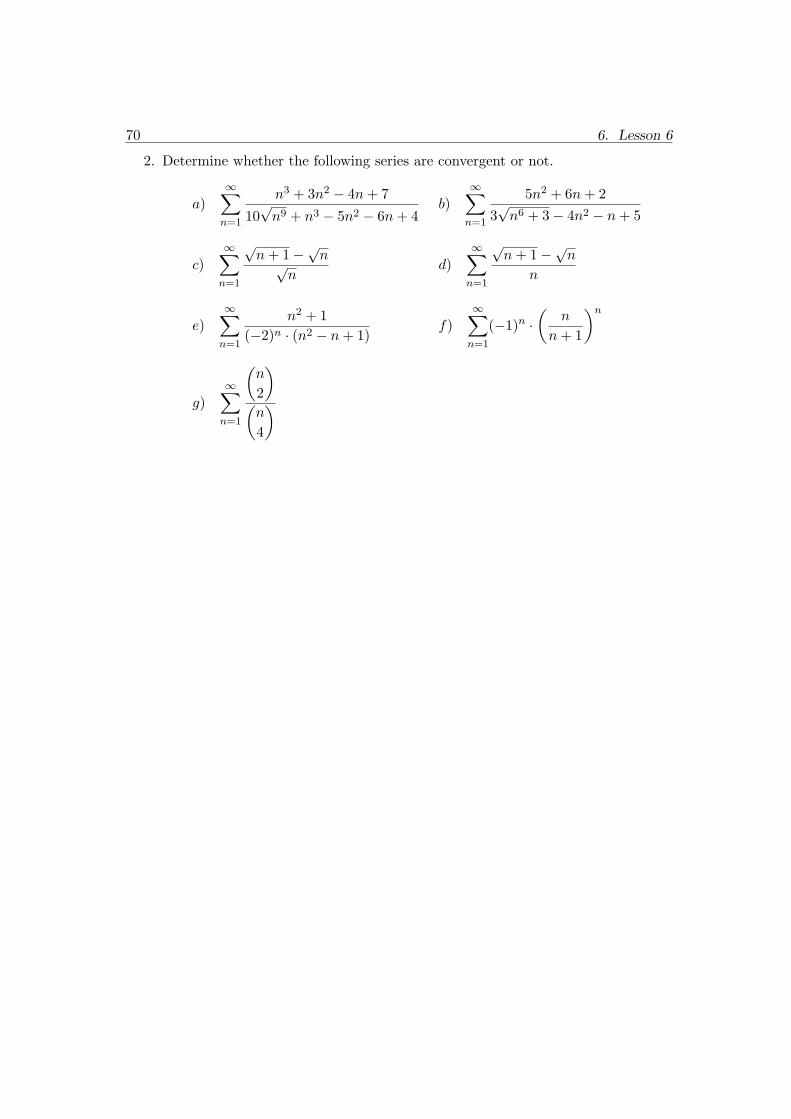
70 6. Lesson 6

2. Determine whether the following series are convergent or not.

a)∞∑

n=1

n3 + 3n2 − 4n + 7

10√

n9 + n3 − 5n2 − 6n + 4b)

∞∑

n=1

5n2 + 6n + 23√

n6 + 3− 4n2 − n + 5

c)∞∑

n=1

√n + 1−√n√

nd)

∞∑

n=1

√n + 1−√n

n

e)∞∑

n=1

n2 + 1(−2)n · (n2 − n + 1)

f)∞∑

n=1

(−1)n ·(

n

n + 1

)n

g)∞∑

n=1

(n

2

)

(n

4

)

7. Lesson 7

7.1. Absolute and Conditional Convergence

At the end of the previous section (see: Example 6.25) we have seen that the alterna-

ting harmonic series∞∑

n=1

(−1)n−1

nis convergent. However, (see Remark 6.10) the series

consisting of the absolute values of its terms

∞∑

n=1

∣∣∣∣(−1)n−1

n

∣∣∣∣ =∞∑

n=1

1n

is divergent. Thus the convergence of the series consisting of the absolute values seemsto be a stronger requirement than the common convergence of a series.

7.1. Definition Let an ∈ K (n ∈ N). The series∞∑

n=1an is called absolutely convergent,

if the series of absolute values ∞∑

n=1

|an|

is convergent.

7.2. Theorem Let an ∈ K (n ∈ N). If the series∞∑

n=1an is absolutely convergent, then

it is convergent.

Proof. Since∞∑

n=1|an| is convergent, then by the Cauchy criterion (see Theorem 6.11)

we have

∀ ε > 0 ∃N ∈ N ∀m ≥ n ≥ N : |an|+|an+1|+ . . .+|am| =∣∣∣ |an|+|an+1|+ . . .+|am|

∣∣∣ < ε .

Using the first triangle inequality,

|an + an+1 + . . . + am| ≤ |an|+ |an+1|+ . . . + |am| ,

thus we obtain that

∀ ε > 0 ∃N ∈ N ∀m ≥ n ≥ N : |an + an+1 + . . . + am| < ε .

Consequently – once more using the Cauchy criterion – the series∞∑

n=1an is convergent.

¤

72 7. Lesson 7

7.3. Remark. The converse statement is not true as we have seen at the beginning of

the section via the counterexample∞∑

n=1

(−1)n−1

n.

7.4. Definition A numerical series is called conditionally convergent if it is convergent,but not absolutely convergent.

7.5. Example

The alternating hyperharmonic series∞∑

n=1

(−1)n−1

npis absolutely convergent if p > 1,

and it is conditionally convergent if 0 < p ≤ 1.

7.6. Remark. If a real number series does not contain infinitely many positive andinfinitely many negative terms, then it is convergent if and only if it is absolutelyconvergent. In this case the convergence and the absolute convergence are equivalent.

It is natural that a finite sum can be rearranged arbitrarily without changing theresult of the addition. Now we present two theorems about the rearrangement of theinfinite sums.

7.7. Theorem Let an ∈ K (n ∈ N), and p : N→ N be a bijection. If the series∞∑

n=1an

is absolutely convergent, then the series

∞∑

i=1

ap(i)

is absolutely convergent.

The series∞∑i=1

ap(i) is called a rearrangement of∞∑

n=1an.

Proof. Since the absolutely convergence the quantity K :=∞∑

n=1|an| is finite. Further-

more, for any n ∈ N let

M = M(n) := max{p(1), p(2), . . . , p(n)} .

Then{p(1), p(2), . . . , p(n)} ⊆ {1, 2, . . . , M} ,

thereforen∑

i=1

|ap(i)| ≤M∑

k=1

|ak| ≤ K (n ∈ N) .

Thus the partial sum sequence(

n∑i=1

|ap(i)|)

is bounded above, the proof is complete. ¤

7.1. Absolute and Conditional Convergence 73

7.8. Theorem Let an ∈ K (n ∈ N), and p : N→ N be a bijection. If the series∞∑

n=1an

is absolutely convergent, then∞∑

i=1

ap(i) =∞∑

n=1

an .

(The absolute convergence of the rearranged series was proved in the previous theo-rem.)

Proof. Let A :=∞∑i=1

ap(i). Furthermore, for any n ∈ N let

N = N(n) := max{p−1(1), p−1(2), . . . , p−1(n)} ,

M = M(n) := max{p(1), p(2), . . . , p(N)} ,

Rn :=N∑

i=1

ap(i) −n∑

k=1

ak .

Then n ≤ N ≤ M , and

{1, 2, . . . , n} ⊆ {p(1), p(2), . . . , p(N)} ⊆ {1, 2, . . . , M} ,

therefore – using Theorem 2.11 – we have

|Rn| =∣∣∣∣∣

N∑

i=1

ap(i) −n∑

k=1

ak

∣∣∣∣∣ ≤N∑

i=1

|ap(i)| −n∑

k=1

|ak| ≤

≤M∑

k=1

|ak| −n∑

k=1

|ak| =M∑

k=n+1

|ak| .

Since the series∞∑

n=1an is absolutely convergent, then – using Theorem 6.12 – we have

limn→∞

M∑

k=n+1

|ak| = limn→∞

M(n)∑

k=n+1

|ak| = 0 .

Consequently limn→∞Rn = 0.

Therefore

n∑

k=1

ak =N∑

i=1

ap(i) −Rn −→ A− 0 = A (n →∞) .

¤

74 7. Lesson 7

7.2. The Root Test and the Ratio Test

7.9. Theorem [Root Test]Let an ∈ K (n ∈ N) and suppose that the limit

L := limn→∞

n√|an| ∈ [0 , +∞]

exists. Then

a) If L < 1, then the series∞∑

n=1an is absolutely convergent

b) If L > 1, then the series∞∑

n=1an is divergent. Moreover, lim

n→∞ |an| = +∞.

Proof.

a) Suppose that L < 1. Let q ∈ R, 0 ≤ L < q < 1. Then q − L > 0, therefore

∃N ∈ N ∀n ≥ N : L− (q − L) < n√|an| < L + (q − L) .

The right side inequality implies that

0 ≤ n√|an| < q (n ≥ N) .

Taking the n-th power we obtain

|an| < qn (n ≥ N) .

By 0 < q < 1 the geometric series∞∑

n=N

qn is convergent, then by the majorant

criterion the series∞∑

n=1|an| is also convergent.

b) Suppose that L > 1. Let q ∈ R, 1 < q < L. Then L− q > 0, therefore

∃N ∈ N ∀n ≥ N : L− (L− q) < n√|an| < L + (L− q) .

The left side inequality implies that

n√|an| > q (n ≥ N) .

Taking the n-th power we obtain

0 ≤ |an| > qn (n ≥ N) .

This inequality shows us that (an) cannot be a zero sequence, consequently – by

the zero sequence test – the series∞∑


n→∞ |an| = +∞.

7.2. The Root Test and the Ratio Test 75

¤

7.10. Remarks.

1. The theorem does not say anything about the case L = 1. This is the indetermi-nate case. In this case anything can happen. For example, at each of the followingsequences L = 1, but

a)∞∑

n=1

1n2

is absolutely convergent

b)∞∑

n=1

(−1)n−1

nis conditionally convergent

c)∞∑

n=1

1n

is divergent, the terms tend to 0.

d)∞∑

n=11 is divergent, the terms do not tend to 0, the terms form a bounded

sequence

e)∞∑

n=1n is divergent, the terms do not tend to 0, the terms form an unbounded

sequence

2. The essentiality of the proof of the theorem was the application of the DirectComparison Test with a geometric series. Thus it turns out from the proof ofthe root test that it works (i.e. L 6= 1) in those cases when the sequence of theabsolute values of the terms (|an|)• either tends to 0 faster than a geometric sequence with some 0 ≤ q < 1,

• or tends to ∞ faster than a geometric sequence with some q > 1.

In all other cases the root test is inactive, that is it finishes in the indeterminatecase L = 1.

3. If the statement in part b) is only the divergency of the series, then the proof issimpler if you start with L− 1 > 0 instead of L− q > 0.

We remark that the root test can be extended to the case when limn→∞

n√|an| does

not exist.

7.11. Theorem [Ratio Test]Let an ∈ K \ {0} (n ∈ N) and suppose that the limit

L := limn→∞

∣∣∣∣an+1

an

∣∣∣∣ ∈ [0 , +∞]

exists. Then

76 7. Lesson 7

a) If L < 1, then the series∞∑

n=1an is absolutely convergent

b) If L > 1, then the series∞∑


n→∞ |an| = +∞.

Proof.

a) Suppose that L < 1. Let q ∈ R, 0 ≤ L < q < 1. Then q − L > 0, therefore

∃N ∈ N ∀n ≥ N : L− (q − L) <

∣∣∣∣an+1

an

∣∣∣∣ < L + (q − L) .

The right side inequality implies that

0 ≤∣∣∣∣an+1

an

∣∣∣∣ < q (n = N, N + 1, N + 2, . . .) .

Let us fix a natural number k ≥ N + 1, and write the above inequalities forn = N , N +1 . . . , k−1. Then multiply these k−N inequalities with each other.We obtain that

∣∣∣∣aN+1

aN

∣∣∣∣ ·∣∣∣∣aN+2

aN+1

∣∣∣∣ ·∣∣∣∣aN+3

aN+2

∣∣∣∣ · . . . ·∣∣∣∣

ak

ak−1

∣∣∣∣ < q · q · . . . · q︸︷︷︸k−N

,

that is ∣∣∣∣aN+1 · aN+2 · aN+3 · . . . · ak

aN · aN+1 · aN+2 · . . . · ak−1

∣∣∣∣ < qk−N .

Hence – after simplifications – we have∣∣∣∣ak

aN

∣∣∣∣ <qk

qN,

that is|ak| < |aN |

qN· qk (k ≥ N + 1) .

By 0 < q < 1 the series

∞∑

k=1

|aN |qN

· qk =|aN |qN

·∞∑

k=1

qk

is convergent, then by the majorant criterion the series∞∑

n=1|an| is also convergent.

b) Suppose that L > 1. Let q ∈ R, 1 < q < L. Then L− q > 0, therefore

∃N ∈ N ∀n ≥ N : L− (L− q) <

∣∣∣∣an+1

an

∣∣∣∣ < L + (L− q) .

7.2. The Root Test and the Ratio Test 77

The left side inequality implies that∣∣∣∣an+1

an

∣∣∣∣ > q (n = N, N + 1, N + 2, . . .) .

As in part a), let us fix a natural number k ≥ N + 1, and write the aboveinequalities for n = N , N + 1 . . . , k − 1. Then multiply these k −N inequalitieswith each other. We obtain that

∣∣∣∣aN+1

aN

∣∣∣∣ ·∣∣∣∣aN+2

aN+1

∣∣∣∣ ·∣∣∣∣aN+3

aN+2

∣∣∣∣ · . . . ·∣∣∣∣

ak

ak−1

∣∣∣∣ > q · q · . . . · q︸︷︷︸k−N

,

that is ∣∣∣∣aN+1 · aN+2 · aN+3 · . . . · ak

aN · aN+1 · aN+2 · . . . · ak−1

∣∣∣∣ > qk−N .

Hence – after simplifications – we have∣∣∣∣ak

aN

∣∣∣∣ >qk

qN,

that is

|ak| > |aN |qN

· qk (k ≥ N) .

This inequality shows us that (an) cannot be a zero sequence, consequently – by

the zero sequence test – the series∞∑


n→∞ |an| = +∞.

¤

7.12. Remark.

Writing ”ratio test” instead of ”root test”, then all the statements in Remarks 7.10 aretrue.

The ratio test can be extended to the case when limn→∞

∣∣∣∣an+1

an

∣∣∣∣ does not exist.

7.13. Remarks.

1. It was no coincidence that in the Root Test and in the Ratio Test we have usedthe same L. Later we will prove (see Corollary 8.12) that if both the limits

L1 := limn→∞

n√|an| and L2 := lim

n→∞

∣∣∣∣an+1

an

∣∣∣∣

exist, then L1 = L2.

78 7. Lesson 7

2. We can give simple examples for that case when L1 exists but L2 does not exist.Let (an) be the following sequence:

a2n−1 := 1, a2n := 2 (n ∈ N) .

Then2n−1

√|a2n−1| = 2n−1

√1 = 1 −→ 1 (n →∞) ,

2n

√|a2n| =

2n√

2 =n

√√2 −→ 1 (n →∞) .

Consequently limn→∞

n√|an| = 1. The root test is inactive.

On the other hand,∣∣∣∣

a2n

a2n−1

∣∣∣∣ =21

= 2 −→ 2 (n →∞) ,

∣∣∣∣a2n+1

a2n

∣∣∣∣ =12

= 1 −→ 1 (n →∞) .

Consequently limn→∞

∣∣∣∣an+1

an

∣∣∣∣ does not exist.

Using the previous sequence (an) let

bn :=an

2nand cn := 2n · an (n ∈ N) .

Then

limn→∞

n√|bn| = lim

n→∞n√

an

2=

12

< 1 ,

thus the root test is active, it shows that the series∞∑

n=1bn is convergent.

On the other hand

limn→∞

n√|cn| = lim

n→∞ 2 · n√

an = 2 > 1 ,

thus the root test is active, it shows that the series∞∑

n=1cn is divergent.

However, the limits limn→∞

∣∣∣∣bn+1

bn

∣∣∣∣ and limn→∞

∣∣∣∣cn+1

cn

∣∣∣∣ do not exist.

3. It can be proved that if limn→∞

∣∣∣∣an+1

an

∣∣∣∣ exists, then limn→∞

n√|an| also exists.

7.3. Product of Series 79

7.3. Product of Series

If we want to multiply two finite sumsn∑

i=1ai and

m∑j=1

bj , then – using the distributive

law of numbers several times – we multiply every term by every term and then we addthese partial products, whose number is mn. In formula:

(n∑

i=1

ai

)·

m∑

j=1

bj

=

n∑

i=1

m∑

j=1

aibj .

The result is independent of the order and grouping of the partial products at theaddition on the right-hand side.

If we want to multiply two infinite sums∞∑i=0

ai and∞∑

j=0bj , then the first step – in

which we multiply every term by every term – results in the following ”infinite by infi-nite” matrix

a0b0 a0b1 a0b2 a0b3 · · ·

a1b0 a1b1 a1b2 a1b3 · · ·

a2b0 a2b1 a2b2 a2b3 · · ·

a3b0 a3b1 a3b2 a3b3 · · ·...

......

...

(7.1)

The ij-th entry of this matrix is equal to aibj where i, j ∈ N ∪ {0}.The problem is that the entries of this matrix form a double sequence (or: two-fold

sequence), and we did not learn about the addition of the terms of such sequences. Theresult may depend on the order and grouping of the entries at the addition.

Unless investigating the theory of double sequences and series and their consequen-ces for the product of series, we will discuss only a special but important way of additionof partial products in the above matrix.

7.14. Definition Let an, bn ∈ K (n ∈ N ∪ {0}). Then the series∞∑

n=0

∑

i,j∈N∪{0}i+j=n

aibj

is called the Cauchy product of the series∞∑i=0

ai and∞∑

j=0bj .

The above formula often is written shortly as∞∑

n=0

∑

i+j=n

aibj .

80 7. Lesson 7

7.15. Remarks.

1. The n-th term of the Cauchy product is

cn :=∑

i+j=n

aibj = a0bn + a1bn−1 + a2bn−2 + . . . + an−1b1 + anb0 ,

which is the sum of the ”n-th diagonal” of the infinite matrix (7.1).

The sequence (cn) is called the convolution of the sequences (an) and (bn).

2. Another usual form of the n-th term of the Cauchy product is as follows:

cn =n∑

k=0

akbn−k .

3. The n-th partial sum Sn of the Cauchy product

Sn =n∑

k=0

ck =n∑

k=0

∑

i+j=k

aibj

can be rewritten in the following useful form:

Sn =n∑

i=0

n−i∑

j=0

aibj .

The equality of the two forms follows immediately from the equality of the sum-mation index sets. Both the index sets sum up the elements of the left uppertriangle with vertices a0b0, a0bn, anb0 in the infinite matrix (7.1). The left-handside index set sums by diagonals, the right-hand one sums by rows.

About the convergence of the Cauchy product we present the following two theo-rems. Their proofs use similar idea as Theorem 7.7 and Theorem 7.8.

7.16. Theorem Let an, bn ∈ K (n ∈ N ∪ {0}). If the series∞∑

n=0an and

∞∑n=0

bn are

absolutely convergent, then their Cauchy product is absolutely convergent.

Proof. By the absolutely convergence, the quantities

P :=∞∑

n=0

|an| and Q :=∞∑

n=0

|bn|

are finite. If cn denotes the n-th term of the Cauchy product, then for any n ∈ N holds

n∑

k=0

|ck| =n∑

k=0

∣∣∣∣∣∣∑

i+j=k

aibj

∣∣∣∣∣∣≤

n∑

k=0

∑

i+j=k

|aibj | =n∑

i=0

n−i∑

j=0

|aibj | ≤

≤n∑

i=0

n∑

j=0

|aibj | =(

n∑

i=0

|ai|)·

n∑

j=0

|bj | ≤ P ·Q .


This result means that the partial sum sequence

n∑

k=0

|ck| (n ∈ N)

is bounded above, consequently∞∑

n=0|cn| < ∞. ¤

7.17. Remark. It turns out from the proof, that the absolute convergence of theCauchy product is true in the following stronger sense:

∞∑

n=0

∑

i+j=n

|aibj | < ∞ .

7.18. Theorem Let an, bn ∈ K (n ∈ N ∪ {0}), and suppose that the series∞∑

n=0an and

∞∑n=0

bn are absolutely convergent. Denote by A and by B their sum:

A :=∞∑

n=0

an and B :=∞∑

n=0

bn .

Then the sum of their Cauchy product equals A ·B.(The absolute convergence of the Cauchy product was proved in the previous theo-

rem.)

Proof. As in the previous part, Sn denotes the n-th partial sum of the Cauchy product:

Sn =n∑

i=0

n−i∑

j=0

aibj (n ∈ N ∪ {0}) .

We have to prove that limn→∞Sn = AB.

Let Un and Vn be the following partial sums

Un :=n∑

k=0

ak and Vn :=n∑

k=0

bk ,

and letRn := UnVn − Sn (n ∈ N ∪ {0}) .

If we prove that limn→∞Rn = 0, then the proof is complete, because

Sn = UnVn −Rn −→ AB − 0 = AB (n →∞) .

To prove limn→∞Rn = 0 we will show that the complement subsequences (R2n) and

(R2n+1) are zero sequences.

82 7. Lesson 7

The proof of limn→∞R2n = 0:

|R2n| = |U2nV2n − S2n| =∣∣∣∣∣∣

(2n∑

i=0

ai

)·

2n∑

j=0

bj

−

2n∑

i=0

2n−i∑

j=0

aibj

∣∣∣∣∣∣=

=

∣∣∣∣∣∣

2n∑

i=0

2n∑

j=0

aibj −2n∑

i=0

2n−i∑

j=0

aibj

∣∣∣∣∣∣≤

2n∑

i=0

2n∑

j=0

|aibj | −2n∑

i=0

2n−i∑

j=0

|aibj | .

In the last step we applied Theorem 2.11.Now we decrement the subtrahend in the following way:

2n∑

i=0

2n−i∑

j=0

|aibj | ≥n∑

i=0

2n−i∑

j=0

|aibj | ≥n∑

i=0

n∑

j=0

|aibj | .

In the last step we used that i ≤ n, consequently 2n− i ≥ 2n− n = n.Consequently:

|R2n| ≤2n∑

i=0

2n∑

j=0

|aibj | −n∑

i=0

n∑

j=0

|aibj | =

=2n∑

i=n+1

2n∑

j=0

|aibj |+n∑

i=0

2n∑

j=0

|aibj | −n∑

i=0

n∑

j=0

|aibj | =

=2n∑

i=n+1

2n∑

j=0

|aibj |+n∑

i=0

2n∑

j=n+1

|aibj | =

=

(2n∑

i=n+1

|ai|)·

2n∑

j=0

|bj | +

(n∑

i=0

|ai|)·

2n∑

j=n+1

|bj | ≤

≤ Q ·2n∑

i=n+1

|ai|+ P ·2n∑

j=n+1

|bj | .

The quantities P and Q are defined in the proof of the previous theorem.

Since the series∞∑

n=0|an| and

∞∑n=0

|bn| are convergent, then by Theorem 6.12

limn→∞

2n∑

i=n+1

|ai| = 0 and limn→∞

2n∑

j=n+1

|bj | = 0 ,

therefore (R2n) is really a zero sequence.


The proof of limn→∞R2n+1 = 0:

This proof is almost the same as in the previous case, only a few modification willbe required.

|R2n+1| = |U2n+1V2n+1 − S2n+1| =∣∣∣∣∣∣

(2n+1∑

i=0

ai

)·

2n+1∑

j=0

bj

−

2n+1∑

i=0

2n+1−i∑

j=0

aibj

∣∣∣∣∣∣=

=

∣∣∣∣∣∣

2n+1∑

i=0

2n+1∑

j=0

aibj −2n+1∑

i=0

2n+1−i∑

j=0

aibj

∣∣∣∣∣∣≤

2n+1∑

i=0

2n+1∑

j=0

|aibj | −2n+1∑

i=0

2n+1−i∑

j=0

|aibj | .

In the last step we applied Theorem 2.11.Now we decrement the subtrahend in the following way:

2n+1∑

i=0

2n+1−i∑

j=0

|aibj | ≥n∑

i=0

2n+1−i∑

j=0

|aibj | ≥n∑

i=0

n∑

j=0

|aibj | .

In the last step we used that i ≤ n, consequently 2n + 1− i ≥ 2n + 1− n = n + 1 > n.Consequently:

|R2n+1| ≤2n+1∑

i=0

2n+1∑

j=0

|aibj | −n∑

i=0

n∑

j=0

|aibj | =

=2n+1∑

i=n+1

2n+1∑

j=0

|aibj |+n∑

i=0

2n+1∑

j=0

|aibj | −n∑

i=0

n∑

j=0

|aibj | =

=2n+1∑

i=n+1

2n+1∑

j=0

|aibj |+n∑

i=0

2n+1∑

j=n+1

|aibj | =

=

(2n+1∑

i=n+1

|ai|)·

2n+1∑

j=0

|bj | +

(n∑

i=0

|ai|)·

2n+1∑

j=n+1

|bj | ≤

≤ Q ·2n+1∑

i=n+1

|ai|+ P ·2n+1∑

j=n+1

|bj | .

From here follows – using Theorem 6.12 and similar argument as in the previouscase – that (R2n+1) is a zero sequence. ¤

84 7. Lesson 7

7.4. Homework

1. Determine whether the following series are convergent or not.

a)∞∑

n=1

(n + 22n

)n

b)∞∑

n=1

2n · n!nn

c)∞∑

n=1

n!7n + 45

d)∞∑

n=1

(√

2016)n

(2n + 1)!

2. Determine the Cauchy product of the series∞∑

n=0

12n

by itself. Using this result

compute the sum of the series∞∑

n=0

n

2n.

8. Lesson 8

8.1. Function Series

8.1. Definition Let D 6= ∅ and fn : D → K (n ∈ N) be a sequence of functions. Theexpression (designated sum)

f1 + f2 + f3 + · · · =∞∑

n=1

fn

is called a function series. The functions fn are the terms of the series. The functionsequence

Sn := f1 + f2 + . . . + fn =n∑

k=1

fk (n ∈ N)

is called the partial sum sequence of the function series. Sn is the n-th partial sum.

8.2. Remarks.

1. If the common domain D is not given, then – by definition – D is the intersectionof the domains of the functions fn.

2. The addition of the functions in (Sn) is defined in the usual pointwise way:

Sn(x) := f1(x) + . . . + fn(x) =n∑

k=1

fk(x) (x ∈ D; n ∈ N) .

3. The function series∞∑

n=1fn is often written using the symbol of its variable:

f1(x) + f2(x) + f3(x) + · · · =∞∑

n=1

fn(x) (x ∈ D) .

In this sense we can speak about the function series∞∑

n=1fn(x) and say that x

denotes its variable.

4. The starting index is not necessarily 1, it can be any integer. The starting indexis frequently 0.

The convergency of a function series can be defined in a lot of senses. In our subjectwe will use what is called pointwise convergence.

86 8. Lesson 8

8.3. Definition Let∞∑

n=1fn be a function series and x ∈ D. We say that this function

series is convergent at the point x if the numerical series

∞∑

n=1

fn(x)

is convergent. Otherwise we say that the function series is divergent at x.

8.4. Remark. Using the definition of convergence of a numerical series we obtain thatthe function series is convergent at x if and only if the numerical sequence (Sn(x) n ∈ N)is convergent.


n=1fn be a function series. The set S of all x ∈ D at which the

function series is convergent is called its convergence set. In formula:

S :=

{x ∈ D |

∞∑

n=1

fn is convergent at x

}=

=

{x ∈ D |

∞∑

n=1

fn(x) is convergent

}⊆ D .

The function

f : S → K, f(x) :=∞∑

n=1

fn(x) (x ∈ S)

is called the sum function (or simply the sum) of the function series.If ∅ 6= T ⊆ S, then we say that the function series is pointwise convergent on T . In

this case the function f|T is called the sum function of the function series on T .

8.6. ExampleLet

fn : R→ R, f0(x) := 1, fn(x) := xn (x ∈ R; n ∈ N) .

Then for any fixed x ∈ R the number sequence

∞∑

n=0

fn(x) =∞∑

n=0

xn

is a geometric series. Consequently, the convergence set of the function series∞∑

n=0xn is

S = {x ∈ K | |x| < 1} = B(0, 1) .

The sum function is

f(x) =∞∑

n=0

xn =1

1− x(x ∈ S = B(0, 1)) .

8.2. Power Series 87

8.2. Power Series

8.7. Definition Let an ∈ K (n ∈ N ∪ {0}) be a number sequence and let x0 ∈ K. Theseries ∞∑

n=0

an · (x− x0)n = a0 + a1 · (x− x0) + a2 · (x− x0)2 + . . .

is called a power series. The numbers an are the coefficients, the number x0 is the centreof the power series. The symbol x is the variable of the power series.

8.8. Examples

1.∞∑

n=0xn. Here x0 = 0, an = 1.

2.∞∑

n=0

xn

n!. Here x0 = 0, an =

1n!

.

3.∞∑

n=0

(x− 5)n

n · 2n. Here x0 = 5, an =

1n · 2n

.

Now we will investigate the convergence set of a power series. Obviously, the powerseries is absolutely convergent at x = x0 and its sum is equal to a0, because in this casethe sum contains only one term: a0.

8.9. Theorem Let∞∑

n=0an · (x−x0)n be a power series and denote by S its convergence

set. Suppose that the following limit exists:

L := limn→∞

n√|an| ∈ [0, +∞] .

Then

a) If L = 0, then the power series is absolutely convergent for any x ∈ K. ThusS = K.

b) If L = +∞, then the power series is

– absolutely convergent at x = x0,

– divergent at any x 6= x0.

Thus S = {x0}.c) If 0 < L < +∞, then the power series is

– absolutely convergent at any x ∈ K for which holds |x− x0| < 1L

,

– divergent at any x ∈ K for which holds |x− x0| > 1L

.

Thus B(x0,1L) ⊆ S ⊆ B(x0,

1L).

88 8. Lesson 8

Proof. We have remarked that the power series is absolutely convergent at x = x0,thus x0 ∈ S. Suppose that x ∈ K \ {x0} and apply the Root Test for the numericalseries ∞∑

n=0

an · (x− x0)n .

First we compute the limit of the n-th roots:

limn→∞

n√|an(x− x0)n| = lim

n→∞n√|an| · |x− x0|n = lim

n→∞ |x− x0| · n√|an| =

= |x− x0| · limn→∞

n√|an| = |x− x0| · L .

Then we can discuss the cases of the theorem:

a) Suppose that L = 0. Then

|x− x0| · L = |x− x0| · 0 = 0 < 1 ,

therefore by the Root Test the power series is absolutely convergent at x. Thisimplies the statement of part a).

b) Suppose that L = +∞. Then (here it is important that x 6= x0)

|x− x0| · L = |x− x0| · (+∞) = +∞ > 1 ,

therefore by the Root Test the power series is divergent at x. This implies thestatement of part b).

c) Suppose that 0 < L < +∞. Then

|x− x0| · L < 1 ⇐⇒ |x− x0| < 1L

.

This implies the statement of part c).

¤The convergence set of the power series can be investigated with the ratio test too.

The following theorem can be proved – using the ratio test – as in the case of Theorem8.9, therefore the proof will be omitted.

8.10. Theorem Let∞∑

n=0an · (x− x0)n be a power series with coefficients

an 6= 0 (n ∈ N ∪ {0}), and denote by S its convergence set. Suppose that the followinglimit exists:

L := limn→∞

∣∣∣∣an+1

an

∣∣∣∣ ∈ [0, +∞] .

Then

a) If L = 0, then the power series is absolutely convergent for any x ∈ K. ThusS = K.

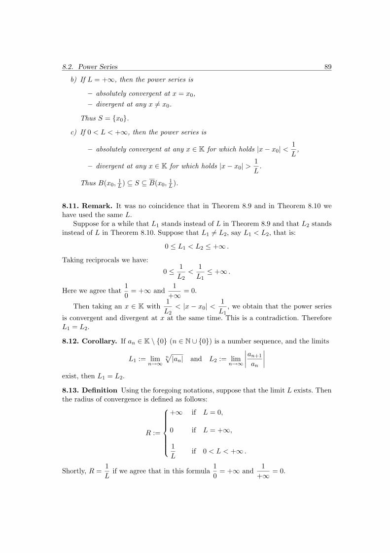
8.2. Power Series 89

b) If L = +∞, then the power series is

– absolutely convergent at x = x0,– divergent at any x 6= x0.

Thus S = {x0}.c) If 0 < L < +∞, then the power series is

– absolutely convergent at any x ∈ K for which holds |x− x0| < 1L

,

– divergent at any x ∈ K for which holds |x− x0| > 1L

.

Thus B(x0,1L) ⊆ S ⊆ B(x0,

1L).

8.11. Remark. It was no coincidence that in Theorem 8.9 and in Theorem 8.10 wehave used the same L.

Suppose for a while that L1 stands instead of L in Theorem 8.9 and that L2 standsinstead of L in Theorem 8.10. Suppose that L1 6= L2, say L1 < L2, that is:

0 ≤ L1 < L2 ≤ +∞ .

Taking reciprocals we have:

0 ≤ 1L2

<1L1

≤ +∞ .

Here we agree that10

= +∞ and1

+∞ = 0.

Then taking an x ∈ K with1L2

< |x − x0| <1L1

, we obtain that the power series

is convergent and divergent at x at the same time. This is a contradiction. ThereforeL1 = L2.

8.12. Corollary. If an ∈ K \ {0} (n ∈ N ∪ {0}) is a number sequence, and the limits

L1 := limn→∞

n√|an| and L2 := lim

n→∞

∣∣∣∣an+1

an

∣∣∣∣exist, then L1 = L2.

8.13. Definition Using the foregoing notations, suppose that the limit L exists. Thenthe radius of convergence is defined as follows:

R :=

+∞ if L = 0,

0 if L = +∞,

1L

if 0 < L < +∞ .

Shortly, R =1L

if we agree that in this formula10

= +∞ and1

+∞ = 0.

90 8. Lesson 8

8.14. Remarks.

1. Using the radius of convergence, we can shortly say that that the power series isabsolutely convergent if x ∈ B(x0, R) and is divergent if x /∈ B(x0, R).

2. Theorem 8.9, Theorem 8.10 and the concept of radius of convergence can begeneralized for the case when the limit L does not exist.

3. Suppose that for the radius of convergence R holds 0 < R < +∞.

If x ∈ K and |x − x0| = R, then nothing can be stated generally about theconvergence at x (indeterminate case). For example, in the case K = R, at eachof the following power series R = 1, but

a)∞∑

n=1xn is divergent at x = 1 and at x = −1.

b)∞∑

n=1

xn

nis divergent at x = 1 and is conditionally convergent at x = −1.

c)∞∑

n=1

xn

n2is absolutely convergent at x = 1 and at x = −1.

In the practice the most important power series are which have positive radius ofconvergence.


n=0an · (x− x0)n be a power series. Suppose that the radius of

convergence is positive, that is R > 0. Then the function

f : B(x0, R) → K, f(x) :=∞∑

n=0

an · (x− x0)n

is called the sum function of the power series.

8.16. Remark. The sum function of a power series is not exactly the same as the sumfunction of a function series, because the power series can converge at some points thatare not in B(x0, R). For power series we will use the concept of sum function as writtenin the above definition.

8.3. Analytical Functions

8.17. Definition Suppose that the radius of convergence of a power series is positive.Then its sum function is called an analytical function.

8.18. Examples

1. The constant function f(x) = c (x ∈ K) (where c ∈ K is fixed) is analytical onK, since

f(x) = c + 0x + 0x2 + 0x3 + . . . (x ∈ K), R = +∞ .

8.3. Analytical Functions 91

2. Every polynomial

f(x) = a0 + a1x + . . . + anxn (x ∈ K)

is analytical on K, since

f(x) = a0+a1x+ . . . +anxn+0xn+1+0xn+2+ . . . (x ∈ K), R = +∞ .

3. The function f(x) :=1

1− x(x ∈ B(0, 1)) is analytical on B(0, 1), because it is

the sum function of the power series∞∑

n=0xn, and the radius of convergence of this

power series is R = 1 > 0.

In what follows, we will prove an important inequality about the analytical functi-ons. It will be basically important at the limits of analytical functions(see: Theorem 13.3). We begin with an auxiliary theorem.

8.19. Theorem [Auxiliary Theorem]Let an ∈ K (n ∈ N ∪ {0}) be a number sequence and let x0 ∈ K. Then the radii of

convergence of the power series

∞∑

n=0

an · (x− x0)n and∞∑

n=1

n · an · (x− x0)n

are equal.

Proof. For simplicity we will prove the theorem only in the case when limn→∞

n√|an|

exists or when limn→∞

∣∣∣∣an+1

an

∣∣∣∣ exists.

Denote by R the radius of convergence of the power series

∞∑

n=0

an · (x− x0)n

and by R′ the radius of convergence of the power series

∞∑

n=0

n · an · (x− x0)n .

In the case when limn→∞

n√|an| exists, we have

R′ =1

limn→∞

n√

n · |an|=

1lim

n→∞n√

n· 1

limn→∞

n√|an|

=11·R = R .

92 8. Lesson 8

Similarly, in the case when limn→∞

∣∣∣∣an+1

an

∣∣∣∣ exists, we have

R′ =1

limn→∞

∣∣∣ (n+1)an+1

nan

∣∣∣=

1lim

n→∞n+1

n

· 1

limn→∞

∣∣∣an+1

an

∣∣∣=

11·R = R .

¤After this preliminary we can state and prove the promised important inequality.

8.20. Theorem Let f ∈ K→ K be an analytical function defined by the power series

f(x) :=∞∑

n=0

an · (x− x0)n (x ∈ B(x0, R)) ,

where the centre x0 and the coefficients an lie in K. Let R > 0 denote its radius ofconvergence. Then

∀ r ∈ R, 0 < r < R ∃M > 0 ∀x, y ∈ B(x0, r) : | f(x)− f(y)| ≤ M · |x− y| .Proof. For the sake of brevity let h := x− x0 and k := y − x0. Then h− k = x− y,and we have

f(x)− f(y) =∞∑

n=0

an · (x− x0)n −∞∑

n=0

an · (y − x0)n =

=

(a0 +

∞∑

n=1

an · hn

)−

(a0 +

∞∑

n=1

an · kn

)=

=∞∑

n=1

an · (hn − kn) =∞∑

n=1

an · (h− k)(hn−1 + hn−2k + . . . , +kn−1) =

= (x− y) ·∞∑

n=1

an ·n−1∑

i=0

hn−1−i · ki .

Since|h| = |x− x0| < r and |k| = |y − x0| < r,

then

|hn−1−iki| = |h|n−1−i|k|i < rn−1−i · ri = rn−1 (i = 0, . . . , n− 1) .

Therefore

| f(x)− f(y)| = |x− y| ·∣∣∣∣∣∞∑

n=1

an ·n−1∑

i=0

hn−1−iki

∣∣∣∣∣ ≤ |x− y| ·∞∑

n=1

|an| ·n−1∑

i=0

|hn−1−ik|i <

< |x− y| ·∞∑

n=1

|an| ·n−1∑

i=0

rn−1 = |x− y| ·∞∑

n=1

|an| · n · rn−1 =

= |x− y| · 1r·∞∑

n=1

|an| · n · rn = |x− y| · 1r·∞∑

n=1

|nanrn| .

8.4. Homework 93

If we prove that the number series∞∑

n=1

nanrn (8.1)

is absolutely convergent, then we are ready, because the searched constant M in thestatement will be:

M :=1r·∞∑

n=1

|nanrn| .

To prove that (8.1) is absolutely convergent let us take the number x0 + r ∈ K. Since

|(x0 + r)− x0| = |r| = r < R ,

and using the Auxiliary Theorem, we obtain that the power series∞∑

n=0

n · an · (x− x0)n

is absolutely convergent at x = x0 + r. Thus the series∞∑

n=0

n · an · ((x0 + r)− x0)n =∞∑

n=0

n · an · rn

is absolutely convergent. The proof is complete. ¤

8.4. Homework

1. Determine the radius of convergence of the following power series. If it is positive,then give the domain of the corresponding analytical function.

a)∞∑

n=1

n!n2· xn b)

∞∑

n=1

1n2 · 3n

· (x− 2)n

c)∞∑

n=1

(1 +

1n

)n

· (x + 3)n d)∞∑

n=0

3n + (−2)n

n + 1· (x + 1)n

2. Expand the following functions into power series around the centre x0 = 0, thenaround the centre x0 = 2

a) f(x) =1

1− xb) f(x) =

3x

1 + x

c) f(x) =2x

3− xd) f(x) =

13− 2x

e) f(x) =x

2 + x

9. Lesson 9

9.1. Five Important Analytical Functions

In this section we will define five important analytical functions as the sum functionsof everywhere absolutely convergent power series. First we give the definitions, after itwe will state and partially prove the everywhere absolute convergence.

9.1. Definition Let us define the following functions.

a) The function exp : K→ K,

exp(x) := 1 +x

1!+

x2

2!+

x3

3!+ . . . =

∞∑

n=0

xn

n!(x ∈ K)

is called the exponential function.

b) The function sin : K→ K,

sin(x) := x− x3

3!+

x5

5!− x7

7!+ . . . =

∞∑

n=0

(−1)n · x2n+1

(2n + 1)!(x ∈ K)

is called the sine (or: sinus) function.

c) The function cos : K→ K,

cos(x) := 1− x2

2!+

x4

4!− x6

6!+ . . . =

∞∑

n=0

(−1)n · x2n

(2n)!(x ∈ K)

is called the cosine (or: cosinus) function.

d) The function sinh : K→ K,

sinh(x) := x +x3

3!+

x5

5!+

x7

7!+ . . . =

∞∑

n=0

x2n+1

(2n + 1)!(x ∈ K)

is called the hyperbolic sine (or: sinus hiperbolicus) function.

e) The function cosh : K→ K,

cosh(x) := 1 +x2

2!+

x4

4!+

x6

6!+ . . . =

∞∑

n=0

x2n

(2n)!(x ∈ K)

is called the hyperbolic cosine (or: cosinus hiperbolicus) function.

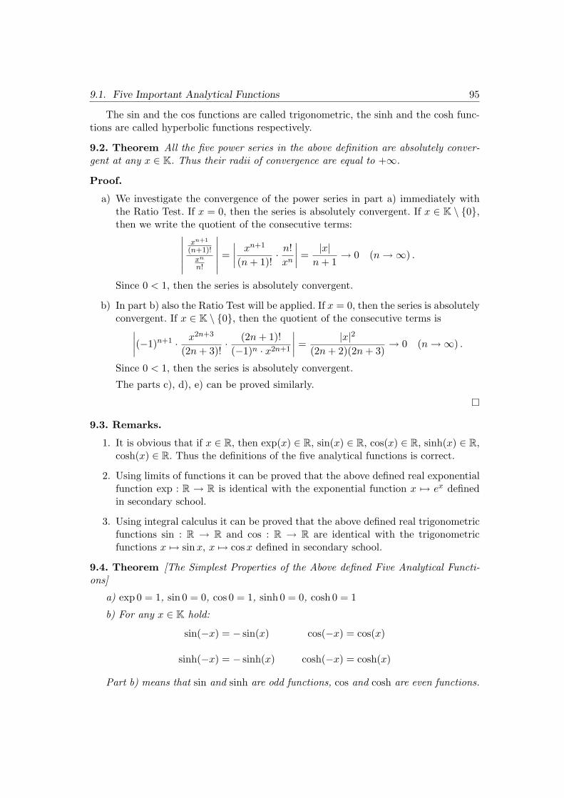
9.1. Five Important Analytical Functions 95

The sin and the cos functions are called trigonometric, the sinh and the cosh func-tions are called hyperbolic functions respectively.

9.2. Theorem All the five power series in the above definition are absolutely conver-gent at any x ∈ K. Thus their radii of convergence are equal to +∞.

Proof.

a) We investigate the convergence of the power series in part a) immediately withthe Ratio Test. If x = 0, then the series is absolutely convergent. If x ∈ K \ {0},then we write the quotient of the consecutive terms:

∣∣∣∣∣∣

xn+1

(n+1)!xn

n!

∣∣∣∣∣∣=

∣∣∣∣xn+1

(n + 1)!· n!xn

∣∣∣∣ =|x|

n + 1→ 0 (n →∞) .

Since 0 < 1, then the series is absolutely convergent.

b) In part b) also the Ratio Test will be applied. If x = 0, then the series is absolutelyconvergent. If x ∈ K \ {0}, then the quotient of the consecutive terms is

∣∣∣∣(−1)n+1 · x2n+3

(2n + 3)!· (2n + 1)!(−1)n · x2n+1

∣∣∣∣ =|x|2

(2n + 2)(2n + 3)→ 0 (n →∞) .

Since 0 < 1, then the series is absolutely convergent.

The parts c), d), e) can be proved similarly.

¤

9.3. Remarks.

1. It is obvious that if x ∈ R, then exp(x) ∈ R, sin(x) ∈ R, cos(x) ∈ R, sinh(x) ∈ R,cosh(x) ∈ R. Thus the definitions of the five analytical functions is correct.

2. Using limits of functions it can be proved that the above defined real exponentialfunction exp : R → R is identical with the exponential function x 7→ ex definedin secondary school.

3. Using integral calculus it can be proved that the above defined real trigonometricfunctions sin : R → R and cos : R → R are identical with the trigonometricfunctions x 7→ sinx, x 7→ cosx defined in secondary school.

9.4. Theorem [The Simplest Properties of the Above defined Five Analytical Functi-ons]

a) exp 0 = 1, sin 0 = 0, cos 0 = 1, sinh 0 = 0, cosh 0 = 1

b) For any x ∈ K hold:

sin(−x) = − sin(x) cos(−x) = cos(x)

sinh(−x) = − sinh(x) cosh(−x) = cosh(x)

Part b) means that sin and sinh are odd functions, cos and cosh are even functions.

96 9. Lesson 9

Proof. a) In all the five cases we have computed the function values at the centre.In this case the power series is a one-term-sum, the single term is the first term of theseries.

b)

sin(−x) =∞∑

n=0

(−1)n · (−x)2n+1

(2n + 1)!=

∞∑

n=0

(−1)n · (−1)2n+1x2n+1

(2n + 1)!=

=∞∑

n=0

(−1)n · (−1) · x2n+1

(2n + 1)!= −

∞∑

n=0

(−1)n · x2n+1

(2n + 1)!= − sin(x) .

The remainder equalities can be proved similarly. ¤

9.5. Theorem Let i denote the imaginary unit in C. Then for any x ∈ K holds

a)exp(x) = cosh(x) + sinh(x) (9.1)

b)exp(ix) = cos(x) + i · sin(x) (Euler’s identity) (9.2)

Proof.

a)

expx =∞∑

n=0

xn

n!=

∞∑

n=0

x2n

(2n)!+

∞∑

n=0

x2n+1

(2n + 1)!= cosh(x) + sinh(x).

b)

exp (ix) =∞∑

n=0

(ix)n

n!=

∞∑

n=0

(ix)2n

(2n)!+

∞∑

n=0

(ix)2n+1

(2n + 1)!=

=∞∑

n=0

i2nx2n

(2n)!+

∞∑

n=0

i2n+1x2n+1

(2n + 1)!=

∞∑

n=0

(i2)nx2n

(2n)!+

∞∑

n=0

i(i2)nx2n+1

(2n + 1)!=

=∞∑

n=0

(−1)n · x2n

(2n)!+ i ·

∞∑

n=0

(−1)n · x2n+1

(2n + 1)!= cosx + i · sinx (x ∈ K).

¤

9.6. Corollary. a) Apply (9.1) for x:

exp(x) = cosh(x) + sinh(x) ,

and for −x:

exp(−x) = cosh(−x) + sinh(−x) = cosh(x)− sinh(x) .

9.1. Five Important Analytical Functions 97

After addition and subtraction of these equalities we obtain:

exp(x) + exp(−x) = 2 · cosh(x) and exp(x)− exp(−x) = 2 · sinh(x) .

Thus we have proved

coshx =expx + exp (−x)

2and sinhx =

expx− exp (−x)2

(x ∈ K) .

b) Apply (9.2) for x:exp(ix) = cos(x) + i · sin(x) ,

and for −x:

exp(−ix) = cos(−x) + i · sin(−x) = cos(x)− i · sin(x) .

After addition and subtraction of these equalities we obtain:

exp(ix) + exp(−ix) = 2 · cos(x) and exp(ix)− exp(−ix) = 2i · sin(x) .

Thus we have proved

cosx =exp (ix) + exp (−ix)

2and sinx =

exp (ix)− exp (−ix)2i

(x ∈ K) .

9.7. Theorem [Addition Formula of the Exponential Function]For any x, y ∈ K holds

exp (x + y) = (expx) · (exp y) .

Proof. Apply the Cauchy product for the absolutely convergent power series of expxand exp y, then use the Binomial Theorem:

expx · exp y =

( ∞∑

n=0

xn

n!

)·( ∞∑

n=0

yn

n!

)=

∞∑

n=0

n∑

k=0

xk

k!· yn−k

(n− k)!=

=∞∑

n=0

1n!·

n∑

k=0

n!k! · (n− k)!

· xk · yn−k =∞∑

n=0

1n!·

n∑

k=0

(n

k

)· xk · yn−k =

=∞∑

n=0

1n!· (x + y)n =

∞∑

n=0

(x + y)n

n!= exp (x + y) .

¤

9.8. Corollary. Apply the Addition Formula for y = −x where x ∈ K. Then we obtaina formula for exp(−x):

1 = exp 0 = exp (x + (−x)) = (expx) · (exp (−x)) ,

whenceexp (−x) =

1expx

(x ∈ K) .

The above equations imply that ∀x ∈ K : expx 6= 0, that is 0 /∈ Rexp.

98 9. Lesson 9

9.9. Theorem [Addition Formulas of cos sin cosh sinh]For any x, y ∈ K holds

a) cos (x + y) = (cosx)(cos y)− (sinx)(sin y)

b) sin (x + y) = (sinx)(cos y) + (cosx)(sin y)

c) cosh (x + y) = (coshx)(cosh y) + (sinhx)(sinh y)

d) sinh (x + y) = (sinhx)(cosh y) + (coshx)(sinh y)

Proof. We will prove part a). First we express cos with exp (Euler’s Formula), thenwe apply the Addition Formula of exp. Finally, with the help of Euler’s Formula we getback to sin and cos.

cos(x + y) =exp(i(x + y)) + exp(−i(x + y))

2=

exp(ix + iy) + exp((−ix) + (−iy))2

=

=(exp(ix)) · (exp(iy)) + (exp(−ix)) · (exp(−iy))

2=

=(cosx + i sinx)(cos y + i sin y) + (cosx− i sinx)(cos y − i sin y)

2.

Hence – completing the operations in the numerator – we obtain that the above fractionis equal to

2(cosx)(cos y)− 2(sinx)(sin y)2

= (cosx)(cos y)− (sinx)(sin y) .

The proof of the other parts of the theorem is similar. ¤

9.10. Corollary. 1. If we apply the Addition Formulas in the previous theorem fory = x, then we obtain:

cos(2x) = cos2 x− sin2 x

sin(2x) = 2 sinx cosx

cosh(2x) = cosh2 x + sinh2 x

sinh(2x) = 2 sinhx coshx

2. If we apply the Addition Formulas of cos and cosh in the previous theorem fory = −x, then we obtain:

1 = cos2 x + sin2 x

1 = cosh2 x− sinh2 x

9.2. The Exponential Function and the Powers of e 99

9.2. The Exponential Function and the Powers of e

We recall that the definition of e is

e := limn→∞

(1 +

1n

)n

.

9.11. Theoremexp 1 = e .

Proof. By the definition of the exponential function

exp 1 =∞∑

n=0

1n!

.

Denote by Sn the partial sums of this series:

Sn :=n∑

k=0

1k!

(n ∈ N) .

Using the Binomial Theorem, let us see the following transformations for n ∈ N, n ≥ 2:

(1 +

1n

)n

=n∑

k=0

(n

k

)·(

1n

)k

· 1n−k = 1 + 1 +n∑

k=2

(n

k

)· 1nk

=

= 1 + 1 +n∑

k=2

n · (n− 1) · . . . · (n− (k − 1))k!

· 1nk

=

= 1 + 1 +n∑

k=2

1k!· n · (n− 1) · . . . · (n− (k − 1))

n · n · . . . · n =

= 1 + 1 +n∑

k=2

1k!·(

1− 1n

)· . . . ·

(1− k − 1

n

)

︸︷︷︸k−1 times

.

(9.3)

Since the factors in the parentheses are less than 1, we obtain the following estima-tion: (

1 +1n

)n

< 1 + 1 +n∑

k=2

1k!· 1 · 1 · . . . · 1︸︷︷︸

k−1 times

=n∑

k=0

1k!

= Sn (n ≥ 2)

Taking n →∞ we have:

e = limn→∞

(1 +

1n

)n

≤ limn→∞Sn = exp 1 .

100 9. Lesson 9

Thus we have proved that e ≤ exp 1.

To prove the reverse inequality, let us fix a natural number m ∈ N, m ≥ 2 andwrite the identity (9.3) for n > m:

(1 +

1n

)n

= 1 + 1 +n∑

k=2

1k!·(

1− 1n

)· . . . ·

(1− k − 1

n

).

Then let us omit the terms with indices k = m+1, . . . , n from the right-hand sum.Thus the sum will be decreased.

(1 +

1n

)n

> 1 + 1 +m∑

k=2

1k!·(

1− 1n

)· . . . ·

(1− k − 1

n

)(n > m ≥ 2) .

Since the number of terms in the sum is independent of n, then we can take thelimit n →∞ by terms:

e = limn→∞

(1 +

1n

)n

≥

≥ 1 + 1 +m∑

k=2

1k!·(

limn→∞

(1− 1

n

))· . . . ·

(lim

n→∞

(1− k − 1

n

))≥

≥ 1 + 1 +m∑

k=2

1k!· 1 · 1 · . . . · 1︸︷︷︸

k−1 times

=m∑

k=0

1k!

= Sm .

Thus we have for arbitrary m ∈ N m ≥ 2 that

e ≥ Sm .

Taking the limit m →∞ we obtain

e ≥ exp 1 .

¤

9.12. Theorem For any rational number r ∈ Q holds

exp r = er .

9.3. The Irrational e 101

Proof. First let p, q ∈ N be positive integers. Applying two times the Addition Formulaof exp we have

(exp

(p

q

))q

=(

expp

q

)· . . . ·

(exp

p

q

)

︸︷︷︸q times

= exp(

p

q+ . . . +

p

q

)=

= exp(

q · p

q

)= exp p = exp(1 + 1 + . . . , +1︸︷︷︸

p times

) =

= (exp 1) · . . . · (exp 1)︸︷︷︸p times

= e · e · . . . e︸︷︷︸p times

= ep ,

whence after extraction of a q-th root we obtain

exp(

p

q

)= e

pq .

Thus the theorem is proved for r ∈ Q, r > 0. The case of negative rational numberscan be easily traced back to the proved case. Indeed, for any r < 0 holds:

exp r = exp(−(−r)) =1

exp(−r)=

1e−r

= er .

We have used here that −r > 0 if r < 0.Finally, the statement is trivial for r = 0, because

exp 0 = 1 = e0 .

¤

9.13. Remark. It can be shown – using the limits of functions – that the equalityexpx = ex is valid for any x ∈ R too.

9.3. The Irrational e

In the previous section (see Theorem 9.11) we have proved that∞∑

n=0

1n!

= e .

First we prove an estimation for the speed of convergence of the above expansion.

9.14. Theorem Denote by Sn the partial sums of the above series, that is

Sn :=n∑

k=0

1k!

(n ∈ N) .

Then for any n ∈ N holds

0 < e− Sn <1

n · n!.

102 9. Lesson 9

Proof. Sn can be regarded as an infinite series for any fixed n :

Sn =n∑

k=0

1k!

=∞∑

k=0

ak , where ak =

1k!

if k ≤ n

0 if k > n

Hence we have

e− Sn =∞∑

k=0

1k!−

∞∑

k=0

ak =∞∑

k=0

(1k!− ak

)=

∞∑

k=n+1

1k!

.

Thus e− Sn > 0. On the other hand, we can write that:

0 < e− Sn =∞∑

k=n+1

1k!

=1

(n + 1)!+

1(n + 2)!

+1

(n + 3)!+ . . . =

=1n!·(

1n + 1

+1

(n + 1)(n + 2)+

1(n + 1)(n + 2)(n + 3)

+ . . .

)<

<1n!·(

1n + 1

+1

(n + 1)2+

1(n + 1)3

+ . . .

)

︸︷︷︸geometric series

=

=1n!·

1n+1

1− 1n+1

=1n!· 1n + 1− 1

=1

n · n!.

¤

9.15. Theorem Euler’s number e is irrational.

Proof. Suppose indirectly that e is rational. Then (using e > 0) there exist the positiveintegers p, q ∈ N such that e =

p

q.

Apply the previous theorem for n = q:

0 <p

q− Sq <

1q · q! .

Multiply these inequalities by q ! :

0 <p

q· q!− Sq · q! <

1q

< 1 . (9.4)

Sincep

q· q! = p · (q − 1)! ∈ Z ,

9.4. Homework 103

andSq · q! = q! +

q!1!

+q!2!

+q!3!

+ . . .q!q!∈ Z .

Thusp

q· q!−Sq · q! ∈ Z. However, this is a contradiction with (9.4), because an integer

never can lie in the open interval (0, 1). ¤

9.16. Remark. It can be proved that the number e is no root of any nonzero polyno-mial with rational coefficients, that is:

∀ f ∈ Q[x] \ {0} : f(e) 6= 0 .

We say about this property of e that e is a transcendental number.This fact has a very interesting linear algebraic consequence. We have seen in Linear

Algebra that R is a vector space over the number field Q. Let n ∈ N and let us see thevector system

1, e, e2, . . . en ∈ R .

If we take a nontrivial linear combination with rational coefficients

λ0 · 1 + λ1 · e + λ2 · e2 + . . . λn · en ,

then it can be regarded f(e) where f is the following polynomial in Q[x]:

f(x) =n∑

k=0

λkxk .

Since e is transcendental, then f(e) 6= 0. This means that the vector system

1, e, e2, . . . en ∈ R .

is linearly independent.However, n is arbitrary, consequently R is an infinite dimensional vector space over

Q.

9.4. Homework

1. Prove the addition formulas for the functions sin, cosh, sinh:

a) sin (x + y) = (sinx)(cos y) + (cos x)(sin y)

b) cosh (x + y) = (coshx)(cosh y) + (sinhx)(sinh y)

c) sinh (x + y) = (sinhx)(cosh y) + (coshx)(sinh y)

for any x, y ∈ K.

104 9. Lesson 9

2. Prove for any x, y ∈ R that

exp (x + iy) = (expx) · (cos y + i sin y)

where i =√−1. Using this result prove that

∀ z ∈ C : exp z 6= 0 .

3. Prove for any x, y ∈ R that

a) cos (x + iy) = (cosx)(cosh y)− i(sinx)(sinh y)

b) sin (x + iy) = (sinx)(cosh y) + i(cosx)(sinh y)

where i =√−1.

10. Lesson 10

10.1. Limits of Functions

The limit is the central concept of Mathematical Analysis. It expresses where the func-tion value tends to if its variable tends to somewhere. In Analysis-1 we will investigatethe limits of functions of type R→ R (one variable functions).

Remember the different types of neighbourhoods:

a) The neighbourhoods of a finite number:

B(a, r) := {x ∈ R | |x− a| < r } = (a− r, a + r) ⊂ R .

b) The neighbourhoods of +∞:

B(+∞, r) := {x ∈ R | x >1r} = (

1r, +∞) ⊂ R .

c) The neighbourhoods of −∞:

B(−∞, r) := {x ∈ R | x < −1r} = (−∞, −1

r) ⊂ R .

10.1. Definition (Accumulation Point and Isolated Point) Let ∅ 6= H ⊆ R anda ∈ R. The point a is called an accumulation point of H if

∀ r > 0 : (B(a, r) \ {a}) ∩H 6= ∅ .

The set of all accumulation points of H is denoted by H ′, that is

H ′ := {a ∈ R | a is an accumulation point of H} .

The points of H \H ′ are called isolated points.

10.2. Remark. An accumulation point of H can be approximated from H with arbit-rary accuracy, without using the accumulation point itself. The isolated point cannotbe approximated in such way.

After these preliminaries it follows the definition of the limit:

10.3. Definition Let f ∈ R→ R, a ∈ D′f . We say that f has a limit at the point a if

∃A ∈ R ∀ ε > 0 ∃ δ > 0 ∀x ∈ (B(a, δ) \ {a}) ∩Df : f(x) ∈ B(A, ε) .

As in the case of Theorem 3.11 it can be proved that A in this definition is unique. Thisunique A is called the limit of the function f at the point a. The following notationsare used to express this fact:

A = lima

f, A = limx→a

f(x), f(x) → A (x → a) .

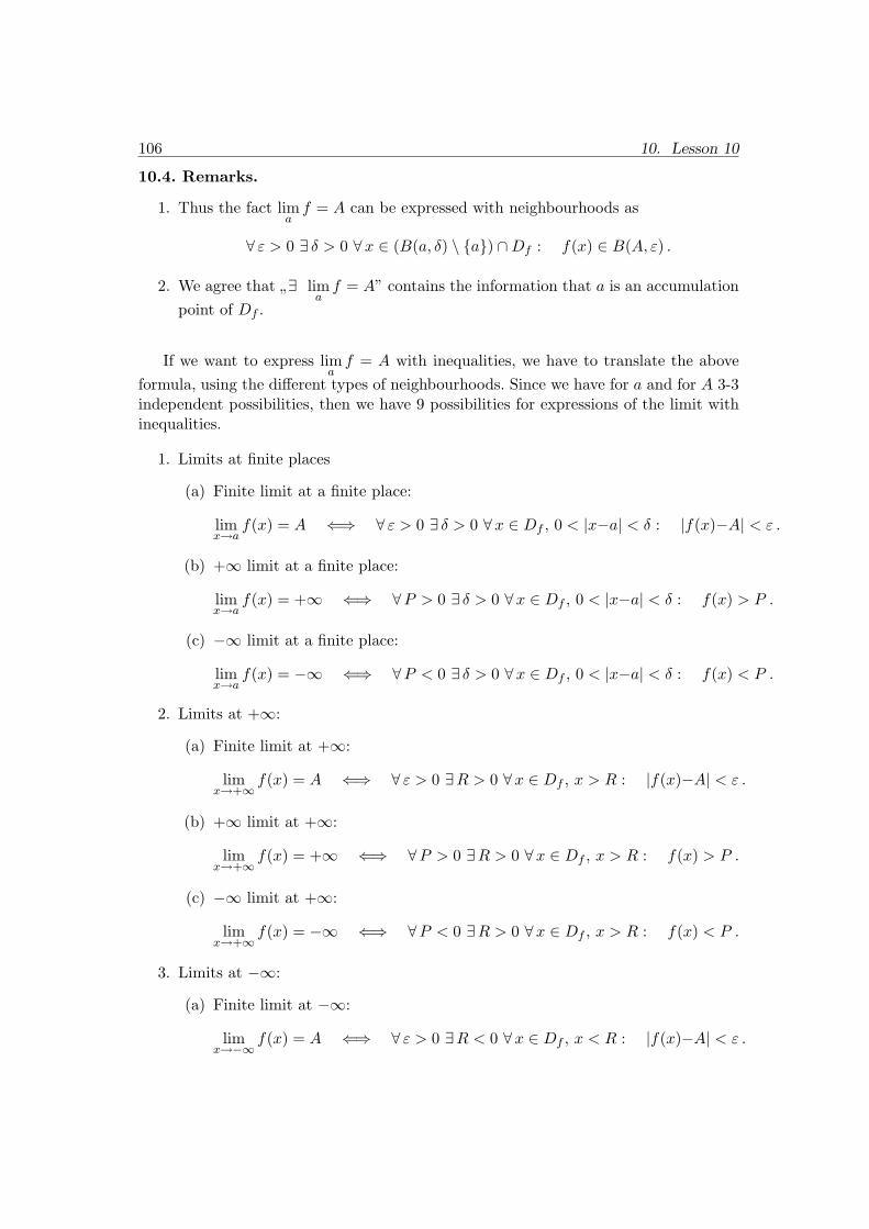
106 10. Lesson 10

10.4. Remarks.

1. Thus the fact lima

f = A can be expressed with neighbourhoods as

∀ ε > 0 ∃ δ > 0 ∀x ∈ (B(a, δ) \ {a}) ∩Df : f(x) ∈ B(A, ε) .

2. We agree that ”∃ lima

f = A” contains the information that a is an accumulationpoint of Df .

If we want to express lima

f = A with inequalities, we have to translate the aboveformula, using the different types of neighbourhoods. Since we have for a and for A 3-3independent possibilities, then we have 9 possibilities for expressions of the limit withinequalities.

1. Limits at finite places

(a) Finite limit at a finite place:

limx→a

f(x) = A ⇐⇒ ∀ ε > 0 ∃ δ > 0 ∀x ∈ Df , 0 < |x−a| < δ : |f(x)−A| < ε .

(b) +∞ limit at a finite place:

limx→a

f(x) = +∞ ⇐⇒ ∀P > 0 ∃ δ > 0 ∀x ∈ Df , 0 < |x−a| < δ : f(x) > P .

(c) −∞ limit at a finite place:

limx→a

f(x) = −∞ ⇐⇒ ∀P < 0 ∃ δ > 0 ∀x ∈ Df , 0 < |x−a| < δ : f(x) 0 ∃R > 0 ∀x ∈ Df , x > R : |f(x)−A| < ε .

(b) +∞ limit at +∞:

limx→+∞ f(x) = +∞ ⇐⇒ ∀P > 0 ∃R > 0 ∀x ∈ Df , x > R : f(x) > P .

(c) −∞ limit at +∞:

limx→+∞ f(x) = −∞ ⇐⇒ ∀P < 0 ∃R > 0 ∀x ∈ Df , x > R : f(x) 0 ∃R < 0 ∀x ∈ Df , x < R : |f(x)−A| < ε .

10.2. The Transference Principle 107

(b) +∞ limit at −∞:

limx→−∞ f(x) = +∞ ⇐⇒ ∀P > 0 ∃R < 0 ∀x ∈ Df , x < R : f(x) > P .

(c) −∞ limit at −∞:

limx→−∞ f(x) = −∞ ⇐⇒ ∀P < 0 ∃R < 0 ∀x ∈ Df , x < R : f(x) 0 be arbitrary. The any δ > 0 will be good, because

∀x ∈ (B(a, δ) \ {a}) ∩Df : f(x) = c ∈ B(c, ε) .

2. The identity of R. Let f : R→ R, f(x) := x. Then for any a ∈ R holds:

limx→a

f(x) = limx→a

x = a .

Indeed, let ε > 0 be arbitrary. The δ := ε will be good, because

∀x ∈ (B(a, δ) \ {a}) ∩Df : f(x) = x ∈ B(a, δ) = B(a, ε) .

10.2. The Transference Principle

The Transference Principle makes a contact between the limit of functions and the limitof sequences.

10.6. Theorem [Transference Principle]Let f ∈ R→ R, a ∈ D′

f and A ∈ R. Then

limx→a

f(x) = A ⇔ ∀xn ∈ Df \ {a} (n ∈ N), lim xn = a : lim f(xn) = A .

A sequence (xn) with the properties

xn ∈ Df \ {a} (n ∈ N), limn→∞xn = a

is called: allowed sequence (more precisely: allowed sequence of f with respect to a).

Proof. Assume first limx→a

f(x) = A.

Let (xn) be an allowed sequence and let ε > 0. Then by limx→a

f(x) = A we have

∃ δ > 0 ∀x ∈ (B(a, δ) \ {a}) ∩Df : f(x) ∈ B(A, ε) .

108 10. Lesson 10

Since limxn = a, then to δ > 0

∃N ∈ N ∀n ≥ N : xn ∈ (B(a, δ) \ {a}) ∩Df .

Combining the two observations we have

∃N ∈ N, ∀n ≥ N : f(xn) ∈ B(A, ε) .

Hence follows that limn→∞ f(xn) = A.

To prove the opposite direction suppose indirectly that limx→a

f(x) = A is not true.Then

∃ ε > 0, ∀ δ > 0 ∃x ∈ (B(a, δ) \ {a}) ∩Df : f(x) /∈ B(A, ε) . (10.1)

Apply this statement with choosing δ :=1n

(n ∈ N). The x according to n will be

denoted by xn. Then (xn) is an allowed sequence, because

xn ∈ Df \ {a}, (n ∈ N), and by |xn − a| < 1n→ 0 (n →∞)

holds limn→∞xn = a.

Using the assumption of this direction of the theorem follows that limn→∞ f(xn) = A.

This is a contradiction, because by (10.1):

f(xn) /∈ B(A, ε) (n ∈ N) .

¤

10.3. Operations with Limits

Using the Transference Principle we can easily trace back the problem of operationswith limits of functions into the problem of operations with limits of sequences.

Let us review the algebraic operations with real-valued functions.

10.7. Definition Let f ∈ R→ R, g ∈ R→ R, and suppose that Df ∩Dg 6= ∅. Then

f+g ∈ R→ R, Df+g = Df∩Dg, (f+g)(x) = f(x)+g(x) the sum of f and g

f−g ∈ R→ R, Df−g = Df∩Dg, (f−g)(x) = f(x)−g(x) the difference of f and g

fg ∈ R→ R, Dfg = Df ∩Dg, (fg)(x) = f(x) ·g(x) the product of f and g

Suppose that D := {x ∈ Df ∩Dg | g(x) 6= 0} 6= ∅. Then

f

g∈ R→ R, D f

g= D

f

g(x) =

f(x)g(x)

the quotient of f and g

10.3. Operations with Limits 109

10.8. Theorem Let us use the notations of the previous definition, and let a ∈ R.Then

a) if a ∈ D′f+g then lim

a(f + g) = lim

af + lim

ag;

b) if a ∈ D′f−g then lim

a(f − g) = lim

af − lim

ag;

c) if a ∈ D′fg then lim

a(fg) = (lim

af) · (lim

ag);

d) if a ∈ D′fg

then lima

(f

g

)=

lima

f

lima

g;

in the following sense:If the limits on the right-hand sides of the above equations exist, and the operations

between them are defined, then the limits on the left-hand sides exist and they are equalto the expressions on the right-hand sides.

Proof. We will prove only the statement for the addition. The other rules can beproved similarly.

Let A = lima

f and B = lima

g. We have to prove that lima

(f + g) = A + B, providedA + B is defined.

Let (xn) be an allowed sequence of f + g with respect to a. Then

xn ∈ Df+g \ {a} (n ∈ N), limn→∞xn = a .

By Df+g = Df ∩Dg we deduce that (xn) is an allowed sequence of f and of g respec-tively. Using the Transference Principle for f and for g we have:

limn→∞ f(xn) = A and lim

n→∞ f(xn) = B .

Using Theorem 5.23 about the limits of the sum of sequences we have:

limn→∞(f + g)(xn) = lim

n→∞(f(xn) + g(xn)) = A + B .

Hence – using once more the Transference Theorem – follows that limx→a

(f+g)(x) = A+B.¤

10.9. Corollary. Applying the limit of the product in that case when one of the factorsis constant, we obtain that

limx→a

(c · f(x)) = c · limx→a

f(x) .

110 10. Lesson 10

10.10. Examples

1. Using the limits of the identity function x → x and part c) of the previous theorem(limit of product) we have for any n ∈ N:

limx→+∞xn = ( lim

x→+∞x)n = (+∞)n = +∞ ,

limx→−∞xn = ( lim

x→−∞x)n = (−∞)n = (−1)n · (+∞) ,

∀ a ∈ R : limx→a

xn = (limx→a

x)n = an .

2. Using the previous result and applying part d) of the previous theorem (limit ofquotient) we have

limx→+∞

1xn

=1

limx→+∞xn

=1

+∞ = 0 ,

limx→−∞

1xn

=1

limx→−∞xn

=1

(−1)n · (+∞)= 0 .

3. Let n ∈ N, a0, a1, . . . , an ∈ R, an 6= 0. Then the limits of the polynomial

P : R→ R, P (x) = anxn + an−1xn−1 + . . . + a1x + a0 =

∞∑

k=0

akxk

are as follows:

• If a ∈ R, then

limx→a

P (x) = limx→a

(anxn + an−1xn−1 + . . . + a1x + a0) =

= (anan + an−1an−1 + . . . + a1a + a0) = P (a) .

• If a = +∞ or a = −∞, then let us see the following transformation:

P (x) = anxn+an−1xn−1+ . . . +a1x+a0 = xn·

(an +

an−1

x+ . . . +

a1

xn−1+

a0

xn

).

Hence

limx→+∞P (x) = ( lim

x→+∞xn) · (an + 0 + . . . + 0) = an · (+∞) ,

and

limx→−∞P (x) = ( lim

x→−∞xn) · (an + 0 + . . . + 0) = an · (−1)n · (+∞) .

10.4. Homework 111

10.4. Homework

1. Prove by the definition of the limit that

a) limx→1

x2 − 9x2 − 3x

= 4 b) limx→3

x2 − 9x2 − 3x

= 2

c) limx→2

x2 + 4x− 5x3 − 1

= 1 d) limx→1

x2 + 4x− 5x3 − 1

= 2

e) limx→2

x + 1x3 − 4x2 + 4x

= +∞ f) limx→1

2− 3x

x3 − 2x2 + x= −∞

11. Lesson 11

11.1. One-sided Limits

In many cases the variable x approaches the number a ∈ R only from one direction,namely

• x → a, but x < a: x approaches a from the left-hand side. This case can beextended for a = +∞, but it does not give any newness with respect to thecommon limit, because +∞ can be approached only from the left.

• x → a, but x > a: x approaches a from the right-hand side. This case can beextended for a = −∞, but it does not give any newness with respect to thecommon limit, because −∞ can be approached only from the right.

In these cases we speak about left-hand limits and right-hand limits respectively.Their common names are: one-sided limits.

11.1. Definition Let f ∈ R → R, a ∈ R, −∞ ≤ a < +∞. Suppose that a is anaccumulation point of the set (a, +∞)∩Df (we say that a is a right-hand accumulationpoint of Df ). Then the right-hand limit of f at a is denoted by lim

a+f and it is defined

as follows:lima+

f := lima

f|(a,+∞)∩Df.

11.2. Remarks.

1. In the case a = −∞ the right-hand limit is equivalent to the common limit.Really, since

(−∞, +∞) ∩Df = Df ,

then the point −∞ is or both right-hand accumulation point and accumulationpoint at the same time, or none of them. Furthermore, if it is, then:

lim(−∞)+

f = lim−∞ f .

2. Some other notations for the right-hand limit:

limx→a+

f(x), limx→ax>a

f(x), f(x) → A (x → a+), f(x) → A (x → a, x > a) .

lima+0

f, limx→a+0

f(x), f(x) → A (x → a + 0), f(a + 0) .

3. We agree that ”∃ lima+

f = A” contains the information that a is a right-hand

accumulation point of Df .

11.1. One-sided Limits 113

4. Since the right-hand limit is a usual limit of the restricted function, then – withapplicable modifications – the Transference Principle is valid for right-hand limitstoo.

5. Using the Transference Principle for right-hand limits, we can prove easily theconnections between the algebraic operations and the right-hand limits.

At a finite place a ∈ R the right-hand limit can be expressed by inequalities asfollows:

1. Finite right-hand limit:

limx→a+

f(x) = A ⇐⇒ ∀ ε > 0 ∃ δ > 0 ∀x ∈ Df , a < x < a+δ : |f(x)−A| < ε .

2. +∞ right-hand limit:

limx→a+

f(x) = +∞ ⇐⇒ ∀P > 0 ∃ δ > 0 ∀x ∈ Df , a < x < a+δ : f(x) > P .

3. −∞ right-hand limit:

limx→a+

f(x) = −∞ ⇐⇒ ∀P < 0 ∃ δ > 0 ∀x ∈ Df , a < x < a+δ : f(x) 0, then δ :=1P

> 0 will be good in the definition, because

a < x < a + δ ⇒ 0 < x− a < δ =1P

⇒ 1x− a

> P .

2. Let a ∈ R and n ∈ N. Then – applying the previous result and the limit of product– we have

limx→a+

1(x− a)n

= limx→a+

(1

x− a

)n

=(

limx→a+

1x− a

)n

= (+∞)n = +∞ .

11.4. Definition Let f ∈ R→ R, Suppose thatLet f ∈ R → R, a ∈ R, −∞ < a ≤ +∞. Suppose that a is an accumulation point

of the set (−∞, a)∩Df (we say that a is a left-hand accumulation point of Df ). Thenthe left-hand limit of f at a is denoted by lim

a− f and it is defined as follows:

lima− f := lim

af|(−∞, a)∩Df

.

114 11. Lesson 11

11.5. Remarks.

1. In the case a = +∞ the left-hand limit is equivalent to the common limit. Really,since

(−∞, +∞) ∩Df = Df ,

then the point +∞ is or both left-hand accumulation point and accumulationpoint at the same time, or none of them. Furthermore, if it is, then:

lim(+∞)−

f = lim+∞ f .

2. Some other notations for the left-hand limit:

limx→a− f(x), , lim

x→ax<a

f(x) f(x) → A (x → a−), f(x) → A (x → a, x < a) .

lima−0

f, limx→a−0

f(x), f(x) → A (x → a− 0), f(a− 0) .

3. We agree that ”∃ lima− f = A” contains the information that a is a left-hand

accumulation point of Df .

4. Since the left-hand limit is a usual limit of the restricted function, then – withapplicable modifications – the Transference Principle is valid for left-hand limitstoo.

5. Using the Transference Principle for left-hand limits, we can prove easily theconnections between the algebraic operations and the left-hand limits.

At a finite place a ∈ R the left-hand limit can be expressed by inequalities as follows:

1. Finite left-hand limit:

limx→a− f(x) = A ⇐⇒ ∀ ε > 0 ∃ δ > 0 ∀x ∈ Df , a−δ < x < a : |f(x)−A| < ε .

2. +∞ left-hand limit:

limx→a− f(x) = +∞ ⇐⇒ ∀P > 0 ∃ δ > 0 ∀x ∈ Df , a−δ < x < a : f(x) > P .

3. −∞ left-hand limit:

limx→a− f(x) = −∞ ⇐⇒ ∀P < 0 ∃ δ > 0 ∀x ∈ Df , a−δ < x < a : f(x) 0 will be good in the definition, because

a− δ < x < a ⇒ 1P

= −δ < x− a < 0 ⇒ 1x− a

< P .

2. Let a ∈ R and n ∈ N. Then – applying the previous result and the limit of product– we have

limx→a−

1(x− a)n

= limx→a−

(1

x− a

)n

=(

limx→a−

1x− a

)n

= (−∞)n = (−1)n · (+∞) .

3. Especially if n is an even number, then the right-hand and the left-hand limitsof the previous function are equal (see the previous example and Examples 11.3).Thus we have:

limx→a

1(x− a)n

= +∞ if n is even .

Using the notations in the definitions of one-sided limits we can state the followingtheorems about the connection between the limits and the one-sided limits.

11.7. Theorem If limx→a− f(x) = lim

x→a+f(x) = A, then lim

x→af(x) = A.

Proof. Since ∃ limx→a− f(x), then a is a left-hand accumulation point of Df . This implies

that a is an accumulation point of Df .Let ε > 0. Then by the definition of the left-hand limit we have:

∃ δ1 > 0 ∀x ∈ B(a, δ1) ∩ (−∞, a) ∩Df : f(x) ∈ B(A, ε) .

Similarly, by the definition of the right-hand limit we have:

∃ δ2 > 0 ∀x ∈ B(a, δ2) ∩ (a, +∞) ∩Df : f(x) ∈ B(A, ε) .

Let δ := min{δ1, δ2} > 0, and let us observe that

B(a, δ) ∩ (−∞, a) ∩Df ⊆ B(a, δ1) ∩ (−∞, a) ∩Df

B(a, δ) ∩ (a, +∞) ∩Df ⊆ B(a, δ2) ∩ (a, +∞) ∩Df

(B(a, δ) ∩ (−∞, a) ∩Df ) ∪ (B(a, δ) ∩ (a, +∞) ∩Df ) = (B(a, δ) \ {a}) ∩Df .

This implies that:

∀x ∈ B(a, δ) \ {a}) ∩Df : f(x) ∈ B(A, ε) ,

which means limx→a

f(x) = A. ¤The reverse statement is stated in the following theorem, and it can be proved easily.

116 11. Lesson 11

11.8. Theorem Using the previous notations, suppose that limx→a

f(x) = A. Then

a) a is a left-hand accumulation point or a right-hand accumulation point of Df ;

b) If a is a left-hand accumulation point of Df , then limx→a− f(x) = A;

c) If a is a right-hand accumulation point of Df , then limx→a+

f(x) = A.

11.2. Limits of Monotone Functions

11.9. Definition Let f ∈ R→ R. We say that f is

• monotonically increasing if ∀x1, x2 ∈ Df , x1 < x2 : f(x1) ≤ f(x2)

• strictly monotonically increasing if ∀x1, x2 ∈ Df , x1 < x2 : f(x1) < f(x2)

• monotonically decreasing if ∀x1, x2 ∈ Df , x1 < x2 : f(x1) ≥ f(x2)

• strictly monotonically decreasing if ∀x1, x2 ∈ Df , x1 < x2 : f(x1) > f(x2)

• monotone if it is monotonically increasing or monotonically decreasing

• strictly monotone if it is strictly monotonically increasing or strictly monotoni-cally decreasing

11.10. Remarks.

1. The strictly monotonically increasing functions are often called increasing func-tions or strictly increasing functions.

2. The strictly monotonically decreasing functions are often called decreasing func-tions or strictly decreasing functions.

3. The monotonically increasing functions are sometimes called nondecreasing func-tions.

4. The monotonically decreasing functions are sometimes called nonincreasing func-tions.

11.11. Theorem Let f ∈ R→ R a monotonically increasing function and let a ∈ R.

a) If a < +∞ and a ∈ ((a, +∞) ∩Df )′, then

lima+

f = inf f [(a, +∞) ∩Df ] = inf{f(x) ∈ R | x ∈ Df , x > a} .

b) If a > −∞ and a ∈ ((−∞, a) ∩Df )′, then

lima− f = sup f [(−∞, a) ∩Df ] = sup{f(x) ∈ R | x ∈ Df , x < a} .

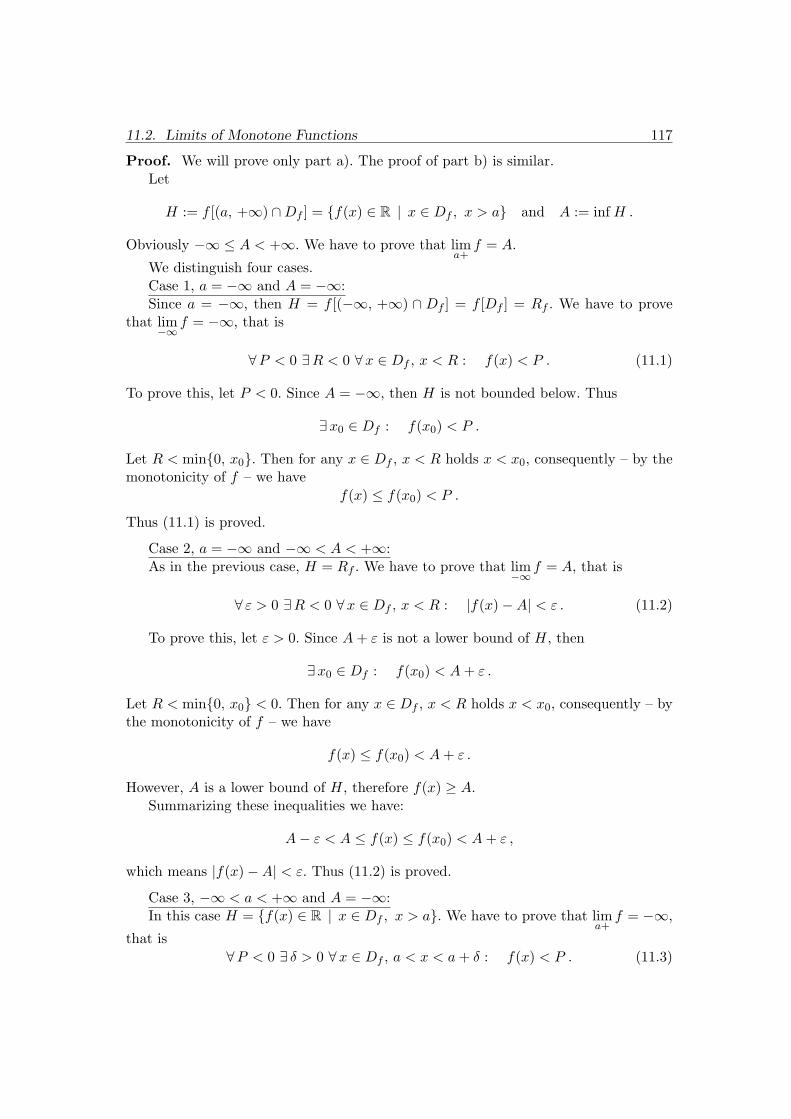
11.2. Limits of Monotone Functions 117

Proof. We will prove only part a). The proof of part b) is similar.Let

H := f [(a, +∞) ∩Df ] = {f(x) ∈ R | x ∈ Df , x > a} and A := inf H .

Obviously −∞ ≤ A < +∞. We have to prove that lima+

f = A.

We distinguish four cases.Case 1, a = −∞ and A = −∞:Since a = −∞, then H = f [(−∞, +∞) ∩ Df ] = f [Df ] = Rf . We have to prove

that lim−∞ f = −∞, that is

∀P < 0 ∃R < 0 ∀x ∈ Df , x < R : f(x) < P . (11.1)

To prove this, let P < 0. Since A = −∞, then H is not bounded below. Thus

∃x0 ∈ Df : f(x0) < P .

Let R < min{0, x0}. Then for any x ∈ Df , x < R holds x < x0, consequently – by themonotonicity of f – we have

f(x) ≤ f(x0) 0 ∃R < 0 ∀x ∈ Df , x < R : |f(x)−A| < ε . (11.2)

To prove this, let ε > 0. Since A + ε is not a lower bound of H, then

∃x0 ∈ Df : f(x0) < A + ε .

Let R < min{0, x0} < 0. Then for any x ∈ Df , x < R holds x < x0, consequently – bythe monotonicity of f – we have

f(x) ≤ f(x0) < A + ε .

However, A is a lower bound of H, therefore f(x) ≥ A.Summarizing these inequalities we have:

A− ε < A ≤ f(x) ≤ f(x0) < A + ε ,

which means |f(x)−A| < ε. Thus (11.2) is proved.

Case 3, −∞ < a < +∞ and A = −∞:In this case H = {f(x) ∈ R | x ∈ Df , x > a}. We have to prove that lim

a+f = −∞,

that is∀P < 0 ∃ δ > 0 ∀x ∈ Df , a < x < a + δ : f(x) a : f(x0) 0. Then for any x ∈ Df , a < x < a + δ = x0 holds x < x0,consequently – by the monotonicity of f – we have

f(x) ≤ f(x0) a}. We have to prove that lim

a+f = A,

that is∀ ε > 0 ∃ δ > 0 ∀x ∈ Df , a < x < a + δ : |f(x)−A| < ε . (11.4)

To prove this, let ε > 0. Since A + ε is not a lower bound of H, then

∃x0 ∈ Df , x0 > a : f(x0) < A + ε .

Let δ := x0 − a > 0. Then for any x ∈ Df , a < x < a + δ = x0 holds x < x0,consequently – by the monotonicity of f – we have

f(x) ≤ f(x0) < A + ε .

However, A is a lower bound of H, therefore f(x) ≥ A.Summarizing these inequalities we have:

A− ε < A ≤ f(x) ≤ f(x0) < A + ε ,

which means |f(x)−A| < ε. Thus (11.4) is proved. ¤A similar theorem can be stated for monotonically decreasing functions. We tell it

without proof.

11.12. Theorem Let f ∈ R→ R a monotonically decreasing function and let a ∈ R.

a) If a < +∞ and a ∈ ((a, +∞) ∩Df )′, then

lima+

f = sup f [(a, +∞) ∩Df ] = sup{f(x) ∈ R | x ∈ Df , x > a} .

b) If a > −∞ and a ∈ ((−∞, a) ∩Df )′, then

lima− f = inf f [(−∞, a) ∩Df ] = inf{f(x) ∈ R | x ∈ Df , x < a} .

11.13. Remark. Since the monotone sequences can be regarded as f : N→ R mono-tone functions, and N′ = {+∞}, then we obtain that the theorems about the limits ofmonotone sequences (see Theorem 5.4 and Theorem 5.19) are the special cases of theabove theorems (Theorem 11.11 and Theorem 11.12).

11.3. Homework 119

11.3. Homework

1. Prove by the definitions of the one-sided limits that

a) limx→2−

x2 − 4|x− 2| = −4 b) lim

x→2+

x2 − 4|x− 2| = 4

c) limx→3−

x− 5x2 − 2x− 3

= +∞ d) limx→3+

x− 5x2 − 2x− 3

= −∞

12. Lesson 12

12.1. Limits of Rational Functions at Infinity

LetP (x) = anxn + an−1x

n−1 + . . . + a1x + a0 (x ∈ R) and

Q(x) = bmxn + bm−1xm−1 + . . . + b1x + b0 (x ∈ R)

be two nonzero polynomials, where the coefficients are

a0, a1, . . . , an ∈ R, an 6= 0 and b0, b1, . . . , bm ∈ R, bm 6= 0 .

In this section we investigate the limits of the rational function

P (x)Q(x)

at +∞ and at −∞.Let us see the following transformation:

P (x)Q(x)

=anxn + an−1x

n−1 + . . . + a1x + a0

bmxn + bm−1xm−1 + . . . + b1x + b0=

xm ·( an

xm−n+ . . . +

a1

xm−1+

a0

xm

)

xm ·(

bm +bm−1

x+ . . . +

b1

xm−1+

b0

xm

) .

Let us simplify by xm and make up the limits. Then we have

limx→+∞

P (x)Q(x)

=lim

x→+∞

( an

xm−n+ . . . +

a0

xm

)

bm=

an

bnif m = n

an

bm· (+∞) if m < n

0 if m > n

and

limx→−∞

P (x)Q(x)

=lim

x→−∞

( an

xm−n+ . . . +

a0

xm

)

bm=

an

bnif m = n

an

bm· (−1)n−m · (+∞) if m < n

0 if m > n

12.2. Limits of Rational Functions at Finite Places 121

12.2. Limits of Rational Functions at Finite Places

Let P, Q ∈ R[x] \ {0} and a ∈ R. In this section we will investigate the limit

limx→a

P (x)Q(x)

.

If Q(a) 6= 0, then the result is obvious:

limx→a

P (x)Q(x)

=limx→a

P (x)

limx→a

Q(x)=

P (a)Q(a)

.

The interesting case is when a is a root of the denominator, that is Q(a) = 0. ByCorollary 2.25 we can factor out from Q the root factor x− a on the maximal degree.This means that we determine the number m and the polynomial Q1 such that

Q(x) = (x− a)m ·Q1(x) where m ∈ N and Q1(a) 6= 0 .

Then factor out from P the root factor x − a on the maximal degree, but maximallym times. More precisely, we determine the number n and the polynomial P1 such that

or n = m or (0 ≤ n < m and P1(a) 6= 0) .

12.1. Remarks.

1. If a is no root of P , then we are in the second case with n = 0, P1 = P .

2. In the case n = m it may be possible that the root factor can be factored outfrom P1 several times, but this factoring out is unnecessary.

After these factorizations we will continue with two cases:

Case 1.: n = m.In this case we have

P (x)Q(x)

=(x− a)nP1(x)(x− a)nQ1(x)

=P1(x)Q1(x)

−→ P1(a)Q1(a)

(x → a) .

Case 2.: 0 ≤ n < m and P1(a) 6= 0.In this case we have

P (x)Q(x)

=(x− a)nP1(x)(x− a)mQ1(x)

=1

(x− a)m−n·P1(x)Q1(x)

−→ P1(a)Q1(a)

· limx→a

1(x− a)m−n

(x → a) .

The limits of the function x → 1(x− a)m−n

can be determined using the Examples

11.3 and 11.6. Thus the result is

limx→a+

P (x)Q(x)

=P1(a)Q1(a)

· (+∞) ,

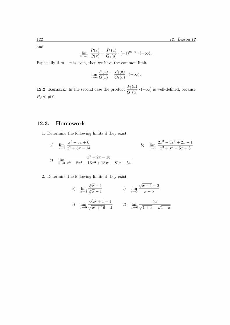
122 12. Lesson 12

andlim

x→a−P (x)Q(x)

=P1(a)Q1(a)

· (−1)m−n · (+∞) .

Especially if m− n is even, then we have the common limit

limx→a

P (x)Q(x)

=P1(a)Q1(a)

· (+∞) .

12.2. Remark. In the second case the productP1(a)Q1(a)

· (+∞) is well-defined, because

P1(a) 6= 0.

12.3. Homework


a) limx→2

x2 − 5x + 6x2 + 5x− 14

b) limx→1

2x3 − 3x2 + 2x− 1x3 + x2 − 5x + 3

c) limx→3

x2 + 2x− 15x5 − 8x4 + 16x3 + 18x2 − 81x + 54


a) limx→1

3√

x− 15√

x− 1b) lim

x→5

√x− 1− 2x− 5

c) limx→0

√x2 + 1− 1√x2 + 16− 4

d) limx→0

5x√1 + x−√1− x

13. Lesson 13

13.1. Limits of Analytical Functions at Finite Places

In Theorem 8.20 we have proved an important inequality for analytical functions. Theessentiality of this statement was that for any analytical function

f(x) =∞∑

n=0

an · (x− x0)n (x ∈ B(x0, R))

holds|f(x)− f(y)| ≤ M · |x− y| (x, y ∈ B(x0, r)) .

Here r is an arbitrary radius for which 0 < r < R holds, and the constant M maybe depending at most on r. The statement is valid for real and for complex analyticalfunctions too.

On the base of this inequality we can investigate the limits of analytical functionsat finite places. Although we discuss the limits for functions of type R → R, in thefollowing theorem we will make an exception: we will state and prove the theorem forfunctions of type K→ K. For K = R it will contain the R→ R case.

Before the theorem the concept of finite limits at finite places will be extended forfunctions of type K→ K:

13.1. Definition Let f ∈ K→ K, a ∈ K and A ∈ K. Suppose that a is an accumula-tion point of Df , that is

∀ r > 0 : (B(a, r) \ {a}) ∩Df 6= ∅ .

In this case we say that limx→a

f(x) = A if

∀ ε > 0 ∃ δ > 0 ∀x ∈ (B(a, δ) \ {a}) ∩Df : f(x) ∈ B(A, ε) ,

or equivalently (using inequalities):

∀ ε > 0 ∃ δ > 0 ∀x ∈ Df , 0 < |x− a| < δ : |f(x)−A| < ε .

13.2. Remark. In the case K = R we have once more the definition of the finite limitat finite place for functions of type R→ R.

13.3. Theorem Let f ∈ K→ K be an analytical function:

f(x) =∞∑

n=0

an · (x− x0)n (x ∈ B(x0, R)) ,

where R denotes the positive radius of convergence of its power series. Then for anya ∈ B(x0, R) holds

limx→a

f(x) = f(a) .

124 13. Lesson 13

Proof. Let us fix an arbitrary a ∈ B(x0, R). It is obvious that a is an accumulationpoint of Df = B(x0, R). Furthermore

∃ r > 0 : 0 ≤ |a− x0| < r < R (for example r =R + |a− x0|

2) .

Apply Theorem 8.20 with this r and with y = a. We obtain that

∃M > 0 ∀x ∈ B(x0, r) : |f(x)− f(a)| ≤ M · |x− a| . (13.1)

Let ε > 0. To this ε the following δ will be good:

δ := min{ ε

M, r − |a− x0|

}.

Really, if 0 < |x− a| < δ, then by

|x−x0| = |x− a+a−x0| ≤ |x−a|+ |a−x0| < δ + |a−x0| ≤ r−|a−x0|+ |a−x0| = r

holds x ∈ B(x0, r). Consequently by (13.1) we have:

|f(x)− f(a)| ≤ M · |x− a| < M · δ ≤ M · ε

M= ε .

Thus by the definition limx→a

f(x) = f(a). ¤

13.4. Examples

1. Using the above theorem it is obvious that for any a ∈ K hold

limx→a

expx = exp a, limx→a

sinx = sin a, limx→a

cosx = cos a ,

especiallylimx→0

expx = 1, limx→0

sinx = 0, limx→0

cosx = 1 .

2. Let us discuss the basic00

type limit

limx→0

sinx

x.

Applying the power series expansion of sinx we have for any x 6= 0:

sinx

x=

x− x3

3! + x5

5! − x7

7! + . . .

x= 1− x2

3!+

x4

5!− x6

7!+ . . . .

This power series is absolutely convergent for any x ∈ K. Denote by g : K→ K its

sum function. The functions x 7→ sinx

xand x 7→ g(x) differ only at 0, but it does

not affect their limits at 0. Applying Theorem 13.3 for the analytical function gwe have

limx→0

sinx

x= lim

x→0g(x) = g(0) = 1− 02

3!+

04

5!− 06

7!+ . . . = 1 .


limx→0

sinx

x= 1 .

13.1. Limits of Analytical Functions at Finite Places 125

3. The following basic00

type limit will be

limx→0

1− cosx

x2.

Applying the power series expansion of cosx we have for any x 6= 0:

1− cosx

x2=

1− (1− x2

2! + x4

4! − x6

6! + . . .)x2

=

=x2

2! − x4

4! + x6

6! − . . .

x2=

12!− x2

4!+

x4

6!− . . . .

This power series is absolutely convergent for any x ∈ K. Denote by g : K → Kits sum function. The functions x 7→ 1− cosx

x2and x 7→ g(x) differ only at 0,

but it does not affect their limits at 0. Applying Theorem 13.3 for the analyticalfunction g we have

limx→0

1− cosx

x2= lim

x→0g(x) = g(0) =

12!− 02

4!+

04

6!− . . . =

12

.


limx→0

1− cosx

x2=

12

.

4. Finally, let us determine the basic00

type limit

limx→0

expx− 1x

.

Applying the power series expansion of expx we have for any x 6= 0:

expx− 1x

=1 + x

1! + x2

2! + x3

3! + . . .− 1x

=

=x1! + x2

2! + x3

3! + . . .

x=

11!

+x

2!+

x2

3!+ . . .

This power series is absolutely convergent for any x ∈ K. Denote by g : K → Kits sum function. The functions x 7→ expx− 1

xand x 7→ g(x) differ only at 0,

but it does not affect their limits at 0. Applying Theorem 13.3 for the analyticalfunction g we have

limx→0

expx− 1x

= limx→0

g(x) = g(0) =11!

+02!

+02

3!+ . . . = 1 .


limx→0

expx− 1x

= 1 .

126 13. Lesson 13

13.2. Homework


a) limx→0

1− cos 3x

5x2b) lim

x→0

sin 6x− sin 7x

sin 3x

c) limx→0

1 + sinx− cosx

1− sinx− cosxd) lim

x→0

1−√

cos3 x

1− cosx

e) limx→π

6

sin(x− π

6

)√

3− 2 cosxf) lim

x→π

sinx

π2 − x2

Istv¶an CSORG˜ O} February 2016 - ELTE

Documents