IST 203 Statistics for Social Sciences (Section 5231, 5232) Review for Final Examination Bangkok University International College May 7, 2011 [ Lectures 1, 2, 3 (A, B), 4A, 5A, 6, 7 ]

IST 203 Statistics for Social Sciences (Section 5231, 5232) Review for Final Examination Bangkok University International College May 7, 2011 [ Lectures.
Dec 25, 2015
Welcome message from author
This document is posted to help you gain knowledge. Please leave a comment to let me know what you think about it! Share it to your friends and learn new things together.
Transcript
IST 203 Statistics for Social Sciences (Section 5231, 5232)
IST 203 Statistics for Social Sciences (Section 5231, 5232)
Review for Final Examination
Bangkok University International College
May 7, 2011
[ Lectures 1, 2, 3 (A, B), 4A, 5A, 6, 7 ]

1-2
IST 203: Statistics for Social Sciences
IST 203: Statistics for Social Sciences
Lecture 1
1-3
What is Statistics?What is Statistics?
• StatisticsStatistics is the science of collecting, organizing, is the science of collecting, organizing,analyzing, interpreting, and presenting data.analyzing, interpreting, and presenting data.
• A A statisticstatistic is a single measure (number) used to is a single measure (number) used to summarize a sample data set. For example, the summarize a sample data set. For example, the average height of students in this class.average height of students in this class.
• AA statisticianstatistician is an expert with at least a master’s is an expert with at least a master’s degree in mathematics or statistics or a trained degree in mathematics or statistics or a trained professional in a related field.professional in a related field.
McGraw-Hill/Irwin © 2008 The McGraw-Hill Companies, Inc. All rights reserved.
1-4
Uses of StatisticsUses of Statistics
Two primary uses for statistics:Two primary uses for statistics:• Descriptive statisticsDescriptive statistics – the collection, organization, – the collection, organization,
presentation and summary of data.presentation and summary of data.
• Inferential statisticsInferential statistics – generalizing from a sample – generalizing from a sample to a population, estimating unknown parameters, to a population, estimating unknown parameters, drawing conclusions, making decisions.drawing conclusions, making decisions.
1-5
Statistical ChallengesStatistical Challenges
Working with Imperfect DataWorking with Imperfect Data
Dealing with Practical ConstraintsDealing with Practical Constraints
• State any assumptions and limitations and use generally State any assumptions and limitations and use generally accepted statistical tests to detect unusual data points or to accepted statistical tests to detect unusual data points or to deal with missing data.deal with missing data.
• You will face constraints on the type and quantity You will face constraints on the type and quantity of data you can collect.of data you can collect.

1-6
Statistical ChallengesStatistical Challenges
Upholding Ethical StandardsUpholding Ethical Standards
Using ConsultantsUsing Consultants
• Know and follow accepted procedures, maintain Know and follow accepted procedures, maintain data integrity, carry out accurate calculations, data integrity, carry out accurate calculations, report procedures, protect confidentiality, cite report procedures, protect confidentiality, cite sources and financial support.sources and financial support.
• Hire consultants at the Hire consultants at the beginningbeginning of the project, of the project, when your team lacks certain skills or when an when your team lacks certain skills or when an unbiased or informed view is needed.unbiased or informed view is needed.

1-7
Statistical PitfallsStatistical Pitfalls
Pitfall 1: Making Conclusions about a LargePitfall 1: Making Conclusions about a Large Population from a Small Sample Population from a Small Sample
Pitfall 2: Making Conclusions fromPitfall 2: Making Conclusions from Nonrandom Samples Nonrandom Samples
• Be careful about making generalizations from Be careful about making generalizations from small samples (e.g., a group of 10 patients).small samples (e.g., a group of 10 patients).
• Be careful about making generalizations from Be careful about making generalizations from retrospective studies of special groups (e.g., retrospective studies of special groups (e.g., heart attack patients).heart attack patients).
1-8
Statistical PitfallsStatistical Pitfalls
Pitfall 3: Attaching Importance to RarePitfall 3: Attaching Importance to Rare Observations from Large Samples Observations from Large Samples
Pitfall 4: Using Poor Survey MethodsPitfall 4: Using Poor Survey Methods
• Be careful about drawing strong inferences from events that Be careful about drawing strong inferences from events that are not surprising when looking at the entire population (e.g., are not surprising when looking at the entire population (e.g., winning the lottery).winning the lottery).
• Be careful about using poor sampling methods or Be careful about using poor sampling methods or vaguely worded questions (e.g., anonymous vaguely worded questions (e.g., anonymous survey or quiz).survey or quiz).

1-9
Statistical PitfallsStatistical Pitfalls
Pitfall 5: Assuming a Causal Link Based onPitfall 5: Assuming a Causal Link Based on Observations Observations
Pitfall 6: Making Generalizations about Pitfall 6: Making Generalizations about Individuals from Observations about Groups Individuals from Observations about Groups
• Be careful about drawing conclusions when no cause-and-Be careful about drawing conclusions when no cause-and-effect link exists (e.g., most shark attacks occur between effect link exists (e.g., most shark attacks occur between 12p.m. and 2p.m.).12p.m. and 2p.m.).
• Avoid reading too much into Avoid reading too much into statistical statistical generalizationsgeneralizations (e.g., men are taller than women). (e.g., men are taller than women).
1-10
Statistical PitfallsStatistical Pitfalls
Pitfall 7: Unconscious BiasPitfall 7: Unconscious Bias
Pitfall 8: Attaching Practical Importance to Pitfall 8: Attaching Practical Importance to Every Statistically Significant Study Result Every Statistically Significant Study Result
• Be careful about unconsciously or subtly allowing bias to Be careful about unconsciously or subtly allowing bias to color handling of data (e.g., heart disease in men vs. color handling of data (e.g., heart disease in men vs. women).women).
• Statistically significant effects may lack practical Statistically significant effects may lack practical importance (e.g., Austrian military recruits born in the importance (e.g., Austrian military recruits born in the spring average 0.6 cm taller than those born in the fall).spring average 0.6 cm taller than those born in the fall).

1-11
IST 203: Statistics for Social Sciences
IST 203: Statistics for Social Sciences
Lecture 2
1-12
Data VocabularyData VocabularyData VocabularyData Vocabulary
• DataData is the plural form of the Latin is the plural form of the Latin datumdatum (a “given” (a “given” fact).fact).
• In scientific research, In scientific research, datadata arise arise from experiments whose results from experiments whose results are recorded systematically.are recorded systematically.
• Important decisions may depend on Important decisions may depend on data.data.
• In business, In business, datadata usually arise from usually arise from accounting transactions or accounting transactions or management processes.management processes.
1-13
Data VocabularyData VocabularyData VocabularyData Vocabulary
Subjects, Variables, Data SetsSubjects, Variables, Data Sets• We will refer to We will refer to DataData as plural and as plural and data setdata set as a as a
particular collection of data as a whole.particular collection of data as a whole.
• ObservationObservation – each data value. – each data value.
• SubjectSubject (or (or individualindividual) – an item for study (e.g., an ) – an item for study (e.g., an employee in your company).employee in your company).
• VariableVariable – a characteristic about the subject or – a characteristic about the subject or individual (e.g., employee’s income).individual (e.g., employee’s income).
1-14
Data VocabularyData VocabularyData VocabularyData Vocabulary
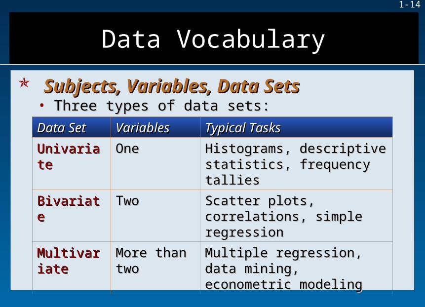
Subjects, Variables, Data SetsSubjects, Variables, Data Sets• Three types of data sets:Three types of data sets:
Data SetData Set VariablesVariables Typical TasksTypical Tasks
UnivariateUnivariate OneOne Histograms, descriptive Histograms, descriptive statistics, frequency talliesstatistics, frequency tallies
BivariateBivariate TwoTwo Scatter plots, correlations, Scatter plots, correlations, simple regressionsimple regression
MultivariateMultivariate More than More than twotwo
Multiple regression, data Multiple regression, data mining, econometric modelingmining, econometric modeling

1-15
Data VocabularyData VocabularyData VocabularyData Vocabulary
Subjects, Variables, Data SetsSubjects, Variables, Data SetsConsider the multivariate data set with Consider the multivariate data set with
5 variables5 variables 8 subjects8 subjects 5 x 8 = 40 observations5 x 8 = 40 observations

1-16
Data Data VocabularyData Data Vocabulary
Attribute DataAttribute Data• Also called Also called categoricalcategorical, , nominalnominal or or qualitativequalitative data. data.
• Values are described by words rather than numbers.Values are described by words rather than numbers.
• For example, For example, - Automobile style (e.g., - Automobile style (e.g., XX = full, midsize, = full, midsize, compact, subcompact). compact, subcompact).- Mutual fund (e.g., - Mutual fund (e.g., XX = load, no-load). = load, no-load).

1-17
Data VocabularyData VocabularyData VocabularyData Vocabulary
Data CodingData Coding• CodingCoding refers to using numbers to represent categories to facilitate statistical analysis. refers to using numbers to represent categories to facilitate statistical analysis.
• Coding an attribute as a number does Coding an attribute as a number does notnot make the data numerical. make the data numerical.
• For example, For example, 1 = Bachelor’s, 2 = Master’s, 3 = Doctorate 1 = Bachelor’s, 2 = Master’s, 3 = Doctorate
• Rankings may exist, for example, Rankings may exist, for example, 1 = Liberal, 2 = Moderate, 3 = Conservative 1 = Liberal, 2 = Moderate, 3 = Conservative

1-18
Data VocabularyData VocabularyData VocabularyData Vocabulary
Binary DataBinary Data• A A binary variablebinary variable has only two values, has only two values,
1 = presence, 0 = absence of a characteristic of interest (codes themselves are arbitrary).1 = presence, 0 = absence of a characteristic of interest (codes themselves are arbitrary).
• For example, For example, 1 = employed, 0 = not employed 1 = employed, 0 = not employed 1 = married, 0 = not married 1 = married, 0 = not married 1 = male, 0 = female 1 = male, 0 = female 1 = female, 0 = male 1 = female, 0 = male
• The coding itself has no numerical value so binary variables are The coding itself has no numerical value so binary variables are attribute dataattribute data..

1-19
Data VocabularyData VocabularyData VocabularyData Vocabulary
Numerical DataNumerical Data• NumericalNumerical or or quantitativequantitative data arise from counting or some kind of mathematical operation. data arise from counting or some kind of mathematical operation.
• For example, For example, - Number of auto insurance claims filed in - Number of auto insurance claims filed in March (e.g., March (e.g., XX = 114 claims). = 114 claims).- Ratio of profit to sales for last quarter - Ratio of profit to sales for last quarter (e.g., (e.g., XX = 0.0447). = 0.0447).
• Can be broken down into two types – Can be broken down into two types – discretediscrete or or continuouscontinuous data. data.
1-20
Data VocabularyData VocabularyData VocabularyData Vocabulary
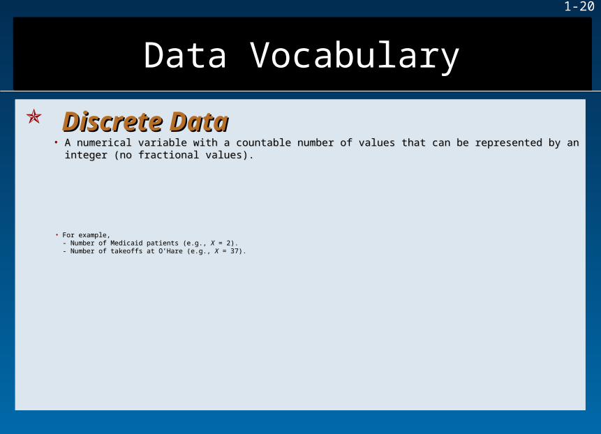
Discrete DataDiscrete Data• A numerical variable with a countable number of values that can be represented by an integer (no fractional A numerical variable with a countable number of values that can be represented by an integer (no fractional
values).values).
• For example, For example, - Number of Medicaid patients (e.g., - Number of Medicaid patients (e.g., XX = 2). = 2).- Number of takeoffs at O’Hare (e.g., - Number of takeoffs at O’Hare (e.g., XX = 37). = 37).
1-21
Data VocabularyData VocabularyData VocabularyData Vocabulary
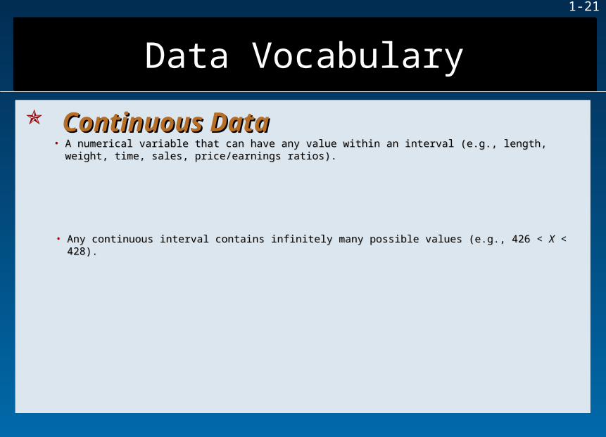
Continuous DataContinuous Data• A numerical variable that can have any value within an interval (e.g., length, weight, time, sales, A numerical variable that can have any value within an interval (e.g., length, weight, time, sales,
price/earnings ratios).price/earnings ratios).
• Any continuous interval contains infinitely many possible values (e.g., 426 < Any continuous interval contains infinitely many possible values (e.g., 426 < XX < 428). < 428).

1-22
Level of MeasurementLevel of MeasurementLevel of MeasurementLevel of Measurement
Four levels of measurement for data:Four levels of measurement for data:
Level of Level of MeasurementMeasurement CharacteristicsCharacteristics ExampleExample
NominalNominal Categories onlyCategories only Eye color (Eye color (blueblue, , brownbrown, , greengreen, , hazelhazel))
OrdinalOrdinal Rank has meaningRank has meaning Bond ratings (Aaa, Aab, Bond ratings (Aaa, Aab, C, D, F, etc.)C, D, F, etc.)
IntervalInterval Distance has Distance has meaningmeaning
Temperature (57Temperature (57oo Celsius)Celsius)
RatioRatio Meaningful zero Meaningful zero existsexists
Accounts payable ($21.7 Accounts payable ($21.7 million)million)

1-23
Level of MeasurementLevel of MeasurementLevel of MeasurementLevel of Measurement
Nominal MeasurementNominal Measurement• Nominal data merely identify a category.• Nominal data are qualitative, attribute, categorical or classification data (e.g., Apple, Compaq, Dell, HP).
• Nominal data are usually coded numerically, codes are arbitrary (e.g., 1 = Apple, 2 = Compaq, 3 = Dell, 4 = HP).
• Only mathematical operations are counting (e.g., frequencies) and simple statistics.

1-24
Level of MeasurementLevel of MeasurementLevel of MeasurementLevel of Measurement
Ordinal MeasurementOrdinal Measurement• Ordinal data codes can be Ordinal data codes can be rankedranked
(e.g., 1 = Frequently, 2 = Sometimes, 3 = Rarely, (e.g., 1 = Frequently, 2 = Sometimes, 3 = Rarely, 4 = Never).4 = Never).
• DistanceDistance between codes is not meaningful between codes is not meaningful (e.g., distance between 1 and 2, or between 2 and 3, or between 3 and 4 lacks meaning).(e.g., distance between 1 and 2, or between 2 and 3, or between 3 and 4 lacks meaning).
• Many useful statistical tests exist for ordinal data. Especially useful in social science, marketing and human Many useful statistical tests exist for ordinal data. Especially useful in social science, marketing and human resource research.resource research.
1-25
Level of MeasurementLevel of MeasurementLevel of MeasurementLevel of Measurement
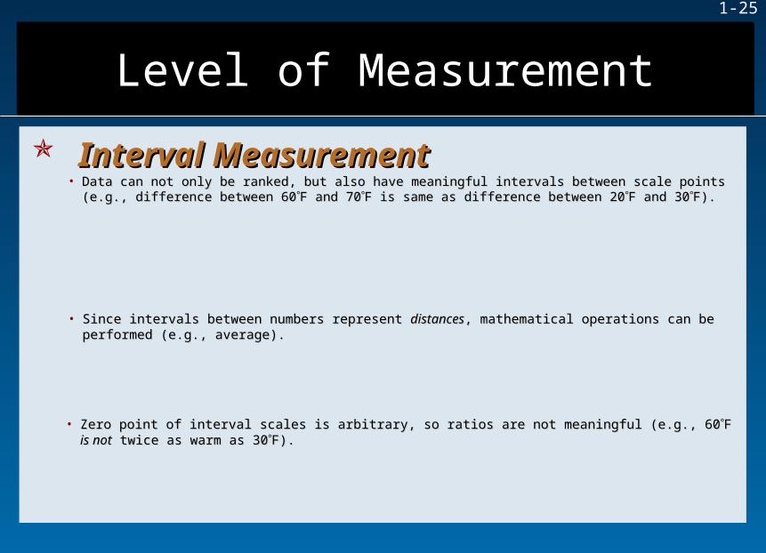
Interval MeasurementInterval Measurement• Data can not only be ranked, but also have meaningful intervals between scale points Data can not only be ranked, but also have meaningful intervals between scale points
(e.g., difference between 60(e.g., difference between 60F and 70F and 70F is same as difference between 20F is same as difference between 20F and 30F and 30F).F).
• Since intervals between numbers represent Since intervals between numbers represent distancesdistances, mathematical operations can be performed (e.g., , mathematical operations can be performed (e.g., average).average).
• Zero point of interval scales is arbitrary, so ratios are not meaningful (e.g., 60Zero point of interval scales is arbitrary, so ratios are not meaningful (e.g., 60 F F is notis not twice as warm as 30 twice as warm as 30F).F).
1-26
Level of MeasurementLevel of MeasurementLevel of MeasurementLevel of Measurement
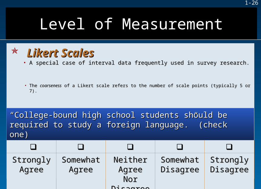
Likert ScalesLikert Scales• A special case of interval data frequently used in survey research.A special case of interval data frequently used in survey research.
• The The coarsenesscoarseness of a Likert scale refers to the number of scale points (typically 5 or 7). of a Likert scale refers to the number of scale points (typically 5 or 7).
““College-bound high school students should be required to study a College-bound high school students should be required to study a foreign language.” (check one)foreign language.” (check one)
StronglyStronglyAgreeAgree
SomewhatSomewhatAgreeAgree
Neither Neither AgreeAgreeNor Nor
DisagreeDisagree
SomewhatSomewhatDisagreeDisagree
StronglyStronglyDisagreeDisagree
1-27
Level of MeasurementLevel of MeasurementLevel of MeasurementLevel of Measurement
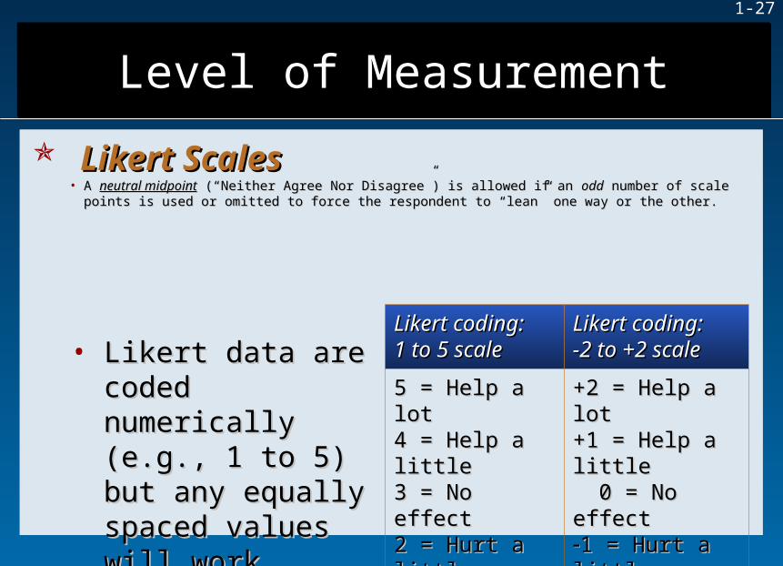
Likert ScalesLikert Scales• A A neutral midpointneutral midpoint (“Neither Agree Nor Disagree”) is allowed if an (“Neither Agree Nor Disagree”) is allowed if an oddodd number of scale points is used or number of scale points is used or
omitted to force the respondent to “lean” one way or the other.omitted to force the respondent to “lean” one way or the other.
• Likert data are Likert data are coded numerically coded numerically (e.g., 1 to 5) but any (e.g., 1 to 5) but any equally spaced equally spaced values will work.values will work.
Likert coding: Likert coding: 1 to 5 scale1 to 5 scale
Likert coding: Likert coding: -2 to +2 scale-2 to +2 scale
5 = Help a lot5 = Help a lot4 = Help a little4 = Help a little3 = No effect 3 = No effect 2 = Hurt a little2 = Hurt a little1 = Hurt a lot1 = Hurt a lot
+2 = Help a lot+2 = Help a lot+1 = Help a little+1 = Help a little 0 = No effect0 = No effect1 = Hurt a little1 = Hurt a little2 = Hurt a lot2 = Hurt a lot
1-28
Sampling ConceptsSampling ConceptsSampling ConceptsSampling Concepts
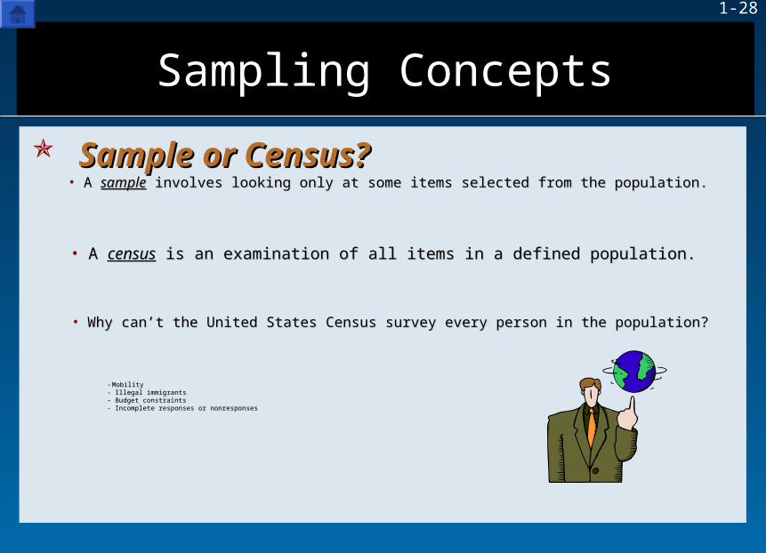
Sample or Census?Sample or Census?• A A samplesample involves looking only at some items selected from the population. involves looking only at some items selected from the population.
• A A censuscensus is an examination of all items in a defined population. is an examination of all items in a defined population.
- MobilityMobility- Illegal immigrants- Illegal immigrants- Budget constraints- Budget constraints- Incomplete responses or nonresponses- Incomplete responses or nonresponses
• Why can’t the United States Census survey every person in the population?Why can’t the United States Census survey every person in the population?
1-29
Sampling ConceptsSampling ConceptsSampling ConceptsSampling Concepts
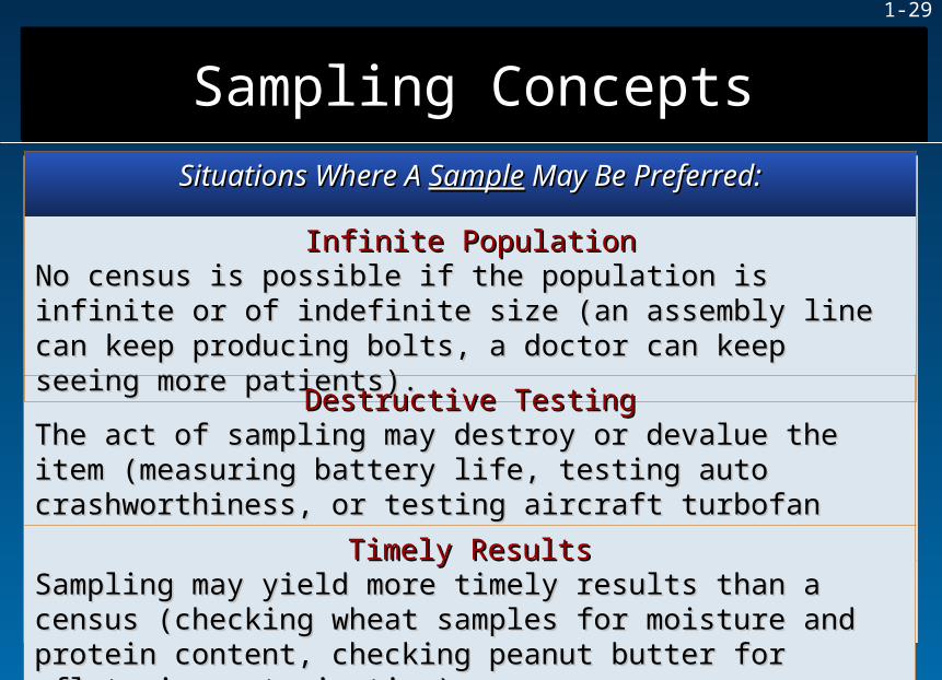
Situations Where A Situations Where A SampleSample May Be Preferred: May Be Preferred:
Infinite PopulationInfinite PopulationNo census is possible if the population is infinite or of indefinite size No census is possible if the population is infinite or of indefinite size (an assembly line can keep producing bolts, a doctor can keep (an assembly line can keep producing bolts, a doctor can keep seeing more patients).seeing more patients).
Destructive TestingDestructive TestingThe act of sampling may destroy or devalue the item (measuring The act of sampling may destroy or devalue the item (measuring battery life, testing auto crashworthiness, or testing aircraft turbofan battery life, testing auto crashworthiness, or testing aircraft turbofan engine life). engine life).
Timely ResultsTimely ResultsSampling may yield more timely results than a census (checking Sampling may yield more timely results than a census (checking wheat samples for moisture and protein content, checking peanut wheat samples for moisture and protein content, checking peanut butter for aflatoxin contamination). butter for aflatoxin contamination).
1-30
Sampling ConceptsSampling ConceptsSampling ConceptsSampling Concepts
Situations Where A Situations Where A SampleSample May Be Preferred: May Be Preferred:
AccuracyAccuracySample estimates can be more accurate than a census. Instead of Sample estimates can be more accurate than a census. Instead of spreading limited resources thinly to attempt a census, our budget spreading limited resources thinly to attempt a census, our budget of time and money might be better spent to hire experienced staff, of time and money might be better spent to hire experienced staff, improve training of field interviewers, and improve data safeguards.improve training of field interviewers, and improve data safeguards.
CostCostEven if it is feasible to take a census, the cost, either in time or Even if it is feasible to take a census, the cost, either in time or money, may exceed our budget.money, may exceed our budget.
Sensitive InformationSensitive InformationSome kinds of information are better captured by a well-designed Some kinds of information are better captured by a well-designed sample, rather than attempting a census. Confidentiality may also sample, rather than attempting a census. Confidentiality may also be improved in a carefully-done sample.be improved in a carefully-done sample.

1-31
Sampling ConceptsSampling ConceptsSampling ConceptsSampling Concepts
Situations Where A Situations Where A CensusCensus May Be Preferred May Be Preferred
Small PopulationSmall PopulationIf the population is small, there is little reason to sample, for the effort of If the population is small, there is little reason to sample, for the effort of data collection may be only a small part of the total cost.data collection may be only a small part of the total cost.
Large Sample SizeLarge Sample SizeIf the required sample size approaches the population size, we might as If the required sample size approaches the population size, we might as well go ahead and take a census.well go ahead and take a census.
Legal RequirementsLegal RequirementsBanks must count Banks must count allall the cash in bank teller drawers at the end of each the cash in bank teller drawers at the end of each business day. The U.S. Congress forbade sampling in the 2000 decennial business day. The U.S. Congress forbade sampling in the 2000 decennial population census.population census.
Database ExistsDatabase ExistsIf the data are on disk we can examine 100% of the cases. But auditing or If the data are on disk we can examine 100% of the cases. But auditing or validating data against physical records may raise the cost.validating data against physical records may raise the cost.
1-32
Sampling ConceptsSampling ConceptsSampling ConceptsSampling Concepts
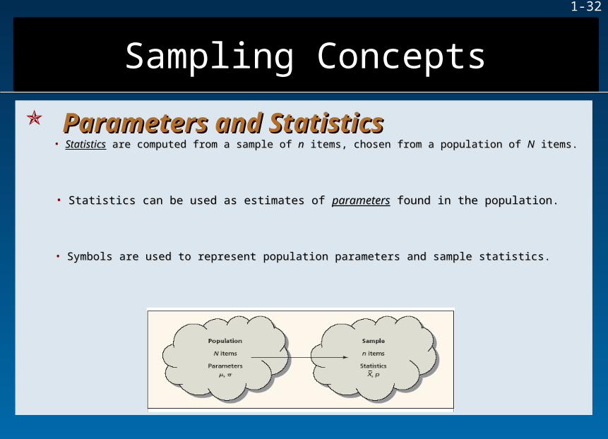
Parameters and StatisticsParameters and Statistics• StatisticsStatistics are computed from a sample of are computed from a sample of nn items, chosen from a population of items, chosen from a population of NN items. items.
• Statistics can be used as estimates of Statistics can be used as estimates of parametersparameters found in the population. found in the population.
• Symbols are used to represent population parameters and sample statistics.Symbols are used to represent population parameters and sample statistics.

1-33
Sampling ConceptsSampling ConceptsSampling ConceptsSampling Concepts
Parameters and StatisticsParameters and Statistics
StatisticStatistic Any measurement computed from a Any measurement computed from a samplesample. Usually, . Usually, the statistic is regarded as an estimate of a population the statistic is regarded as an estimate of a population parameter. Sample statistics are often (but not parameter. Sample statistics are often (but not always) represented by Roman letters.always) represented by Roman letters.
Parameter or Statistic?Parameter or Statistic?
ParameterParameter Any measurement that describes an entire Any measurement that describes an entire populationpopulation. . Usually, the parameter value is unknown since we Usually, the parameter value is unknown since we rarely can observe the entire population. Parameters rarely can observe the entire population. Parameters are often (but not always) represented by Greek are often (but not always) represented by Greek letters.letters.

1-34
Sampling ConceptsSampling ConceptsSampling ConceptsSampling Concepts
Parameters and StatisticsParameters and Statistics• The population must be carefully specified and the sample must be drawn scientifically so that the sample is The population must be carefully specified and the sample must be drawn scientifically so that the sample is
representative.representative.
• The The target populationtarget population is the population we are interested in (e.g., U.S. gasoline prices). is the population we are interested in (e.g., U.S. gasoline prices).
Target PopulationTarget Population
• The The sampling framesampling frame is the group from which we take the sample (e.g., 115,000 stations). is the group from which we take the sample (e.g., 115,000 stations).
• The frame should not differ from the target population.The frame should not differ from the target population.
1-35
NN nn
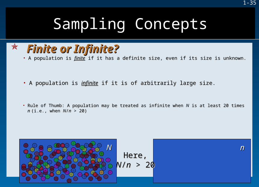
Finite or Infinite?Finite or Infinite?• A population is A population is finitefinite if it has a definite size, even if its size is unknown. if it has a definite size, even if its size is unknown.
• A population is A population is infiniteinfinite if it is of arbitrarily large size. if it is of arbitrarily large size.
• Rule of Thumb: A population may be treated as infinite when Rule of Thumb: A population may be treated as infinite when NN is at least 20 times is at least 20 times n n (i.e., when (i.e., when NN//nn > 20) > 20)
Sampling ConceptsSampling ConceptsSampling ConceptsSampling Concepts
Here,Here,NN//nn > 20 > 20

1-36
Sampling MethodsSampling MethodsSampling MethodsSampling Methods
Probability SamplesProbability Samples
Simple Random Simple Random SampleSample
Use random numbers to select items Use random numbers to select items from a list (e.g., VISA cardholders).from a list (e.g., VISA cardholders).
Systematic SampleSystematic Sample Select every Select every kkth item from a list or th item from a list or sequence (e.g., restaurant customers).sequence (e.g., restaurant customers).
Stratified SampleStratified Sample Select randomly within defined strata Select randomly within defined strata (e.g., by age, occupation, gender).(e.g., by age, occupation, gender).
Cluster SampleCluster Sample Like stratified sampling except strata Like stratified sampling except strata are geographical areas (e.g., zip are geographical areas (e.g., zip codes).codes).
1-37
Sampling MethodsSampling MethodsSampling MethodsSampling Methods
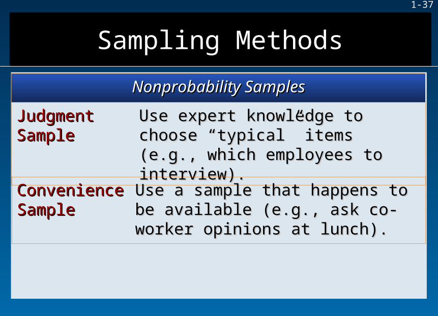
Nonprobability SamplesNonprobability Samples
Judgment Judgment SampleSample
Use expert knowledge to choose Use expert knowledge to choose “typical” items (e.g., which employees “typical” items (e.g., which employees to interview).to interview).
Convenience Convenience SampleSample
Use a sample that happens to be Use a sample that happens to be available (e.g., ask co-worker opinions available (e.g., ask co-worker opinions at lunch).at lunch).

1-38
Sampling MethodsSampling MethodsSampling MethodsSampling Methods
With or Without ReplacementWith or Without Replacement• If we allow duplicates when sampling, then we are sampling If we allow duplicates when sampling, then we are sampling with replacementwith replacement..
• Duplicates are unlikely when Duplicates are unlikely when nn is much smaller than is much smaller than NN..
• If we If we do notdo not allow duplicates when sampling, then we are sampling allow duplicates when sampling, then we are sampling without replacementwithout replacement..
1-39
Sampling MethodsSampling MethodsSampling MethodsSampling Methods
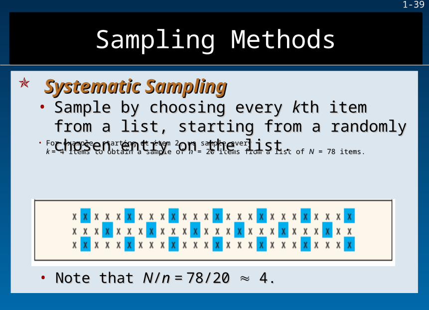
Systematic SamplingSystematic Sampling
• For example, starting at item 2, we sample every For example, starting at item 2, we sample every k k = 4 items to obtain a sample of = 4 items to obtain a sample of nn = 20 items from a list of = 20 items from a list of NN = 78 items. = 78 items.
• Note that Note that NN//n = n = 78/20 78/20 4. 4.
• Sample by choosing every Sample by choosing every kkth item from a list, th item from a list, starting from a randomly chosen entry on the list.starting from a randomly chosen entry on the list.

1-40
Sampling MethodsSampling MethodsSampling MethodsSampling Methods
Systematic SamplingSystematic Sampling• A systematic sample of A systematic sample of nn items from a population of items from a population of NN items requires that periodicity items requires that periodicity kk be approximately be approximately N/nN/n..
• Systematic sampling should yield acceptable results unless patterns in the population happen to recur at Systematic sampling should yield acceptable results unless patterns in the population happen to recur at periodicity periodicity kk..
• Can be used with unlistable or infinite populations.Can be used with unlistable or infinite populations.
• Systematic samples are well-suited to linearly organized physical populations.

1-41
Sampling MethodsSampling MethodsSampling MethodsSampling Methods
Systematic SamplingSystematic Sampling• For example, out of 501 companies, we want to obtain a sample of 25. What should the periodicity For example, out of 501 companies, we want to obtain a sample of 25. What should the periodicity kk be? be?
k = Nk = N//n n = 501/25= 501/25 20. 20.
• So, we should choose every 20So, we should choose every 20 thth company from a random starting point. company from a random starting point.

1-42
Sampling MethodsSampling MethodsSampling MethodsSampling Methods
Stratified SamplingStratified Sampling• Utilizes prior information about the population.• Applicable when the population can be divided into relatively homogeneous subgroups of known size (strata).
• A simple random sample of the desired size is taken within each stratum.
• For example, from a population containing 55% males and 45% females, randomly sample 120 males and 80 females (n = 200).

1-43
Sampling MethodsSampling MethodsSampling MethodsSampling Methods
Stratified SamplingStratified Sampling• Or, take a random sample of the entire population and then combine individual strata estimates using Or, take a random sample of the entire population and then combine individual strata estimates using
appropriate weights.appropriate weights.
• For a population with For a population with LL strata, the population size strata, the population size NN is the sum of the stratum sizes: is the sum of the stratum sizes: NN = = NN11 + + NN22 + ... + + ... + NNLL
• The weight assigned to stratum The weight assigned to stratum jj is is wwjj = = NNjj / / nn
• For example, take a random sample of For example, take a random sample of nn = 200 = 200 and then weight the responses for males by and then weight the responses for males by wwMM = = .55 and for females by .55 and for females by wwFF = .45. = .45.
1-44
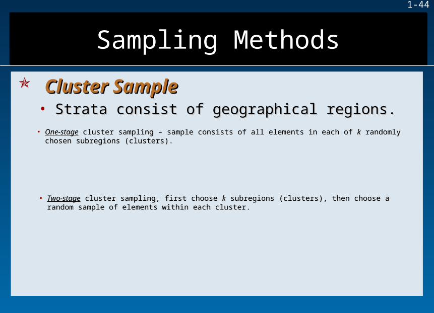
Sampling MethodsSampling MethodsSampling MethodsSampling Methods
Cluster SampleCluster Sample• Strata consist of geographical regions.Strata consist of geographical regions.• One-stageOne-stage cluster sampling – sample consists of all elements in each of cluster sampling – sample consists of all elements in each of kk randomly chosen subregions randomly chosen subregions
(clusters).(clusters).
• Two-stageTwo-stage cluster sampling, first choose cluster sampling, first choose kk subregions (clusters), then choose a random sample of elements subregions (clusters), then choose a random sample of elements within each cluster.within each cluster.

1-45
Sampling MethodsSampling MethodsSampling MethodsSampling Methods
Judgment SampleJudgment Sample• A nonprobability sampling method that relies on the expertise of the sampler to choose items that are A nonprobability sampling method that relies on the expertise of the sampler to choose items that are
representative of the population.representative of the population.
• Can be affected by subconscious bias (i.e., Can be affected by subconscious bias (i.e., nonrandomnessnonrandomness in the choice). in the choice).
• Quota samplingQuota sampling is a special kind of judgment sampling, in which the interviewer chooses a certain number of is a special kind of judgment sampling, in which the interviewer chooses a certain number of people in each category.people in each category.

1-46
Sampling MethodsSampling MethodsSampling MethodsSampling Methods
Convenience SampleConvenience Sample• Take advantage of whatever sample is available at that moment. A quick way to sample.Take advantage of whatever sample is available at that moment. A quick way to sample.
• Sample size depends on the inherent variability of the quantity being measured and on the desired precision Sample size depends on the inherent variability of the quantity being measured and on the desired precision of the estimate.of the estimate.
Sample SizeSample Size
1-47
IST 203: Statistics for Social Sciences
IST 203: Statistics for Social Sciences
Lecture 3 (A, B)

1-48
Visual DescriptionVisual DescriptionVisual DescriptionVisual Description
• Methods of organizing, exploring and summarizing Methods of organizing, exploring and summarizing data include:data include:
- - VisualVisual (charts and graphs) (charts and graphs) provides insight into characteristics of a data set provides insight into characteristics of a data set withoutwithout using using mathematics.mathematics.
- - NumericalNumerical (statistics or tables) (statistics or tables) provides insight into characteristics of a data set provides insight into characteristics of a data set usingusing mathematics. mathematics.

1-49
• Begin with univariate data (a set of Begin with univariate data (a set of nn observations observations on one variable) and consider the following:on one variable) and consider the following:
CharacteristicCharacteristic InterpretationInterpretation
MeasurementMeasurement What are the units of measurement? What are the units of measurement? Are the data integer or continuous? Are the data integer or continuous? Any missing observations? Any concerns with Any missing observations? Any concerns with accuracy or sampling methods? accuracy or sampling methods?
Visual DescriptionVisual DescriptionVisual DescriptionVisual Description
Central TendencyCentral Tendency Where are the data values concentrated? What Where are the data values concentrated? What seem to be typical or middle data values?seem to be typical or middle data values?

1-50
CharacteristicCharacteristic InterpretationInterpretation
DispersionDispersion How much variation is there in the data? How much variation is there in the data? How spread out are the data values? How spread out are the data values? Are there unusual values?Are there unusual values?
Visual DescriptionVisual DescriptionVisual DescriptionVisual Description
ShapeShape Are the data values distributed symmetrically? Are the data values distributed symmetrically? Skewed? Sharply peaked? Flat? Bimodal?Skewed? Sharply peaked? Flat? Bimodal?
1-51
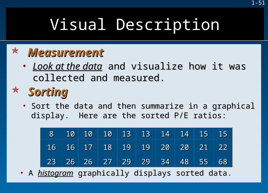
• Look at the dataLook at the data and visualize how it was collected and visualize how it was collected and measured.and measured.
• Sort the data and then summarize in a graphical Sort the data and then summarize in a graphical display. Here are the sorted P/E ratios:display. Here are the sorted P/E ratios:
88 1010 1010 1010 1313 1313 1414 1414 1515 1515
1616 1616 1717 1818 1919 1919 2020 2020 2121 2222
2323 2626 2626 2727 2929 2929 3434 4848 5555 6868
• A A histogramhistogram graphically displays sorted data. graphically displays sorted data.
MeasurementMeasurement
Visual DescriptionVisual DescriptionVisual DescriptionVisual Description
SortingSorting

1-52
• Sorting allows you to observe central tendency, dispersion and shape as well Sorting allows you to observe central tendency, dispersion and shape as well as minimum, maximum and range. as minimum, maximum and range.
SortingSorting
Visual DescriptionVisual DescriptionVisual DescriptionVisual Description
• What else do What else do you observe?you observe?
1-53
• A dot plot is the simplest graphical display of A dot plot is the simplest graphical display of nn individual values of numerical data. individual values of numerical data. - Easy to understand - Easy to understand - Not good for large samples (e.g., > 5,000).- Not good for large samples (e.g., > 5,000).
1.1. Make a scale that covers the data range Make a scale that covers the data range
2.2. Mark the axes and label them Mark the axes and label them3.3. Plot each data value as a dot above the scale at its approximate location Plot each data value as a dot above the scale at its approximate location
If more than one data value lies at about the same If more than one data value lies at about the same axis location, the dots are piled up vertically.axis location, the dots are piled up vertically.
Steps in Making a Dot PlotSteps in Making a Dot Plot
Dot PlotsDot PlotsDot PlotsDot Plots

1-54
• Range of data shows Range of data shows dispersiondispersion. .
• Can add Can add annotationsannotations (text boxes) to call attention (text boxes) to call attention to specific features.to specific features.
• Clustering shows Clustering shows central tendencycentral tendency. . • Dot plots do not tell much of Dot plots do not tell much of shapeshape of distribution. of distribution.
Dot PlotsDot PlotsDot PlotsDot Plots

1-55
• Consider the following Consider the following median home prices median home prices for nine U.S. Cities.for nine U.S. Cities.
Metropolitan AreaMetropolitan AreaMedian Home Price Median Home Price
(000)(000)
Akron OHAkron OH 119.6119.6
Bergen-Passaic NJBergen-Passaic NJ 363.0363.0
Bradenton FLBradenton FL 170.4170.4
Colorado Springs COColorado Springs CO 181.7181.7
Hartford CTHartford CT 198.5198.5
Milwaukee WIMilwaukee WI 186.2186.2
Raleigh-Durham NCRaleigh-Durham NC 173.8173.8
San Francisco CASan Francisco CA 560.2560.2
Topeka KSTopeka KS 100.7100.7
Dot PlotsDot PlotsDot PlotsDot Plots
Small Sample: Home PricesSmall Sample: Home Prices

1-56
• A dot plot is useful to realtors as they discuss A dot plot is useful to realtors as they discuss patterns in home selling prices within their patterns in home selling prices within their community.community.
Dot PlotsDot PlotsDot PlotsDot Plots
Small Sample: Home PricesSmall Sample: Home Prices
1-57
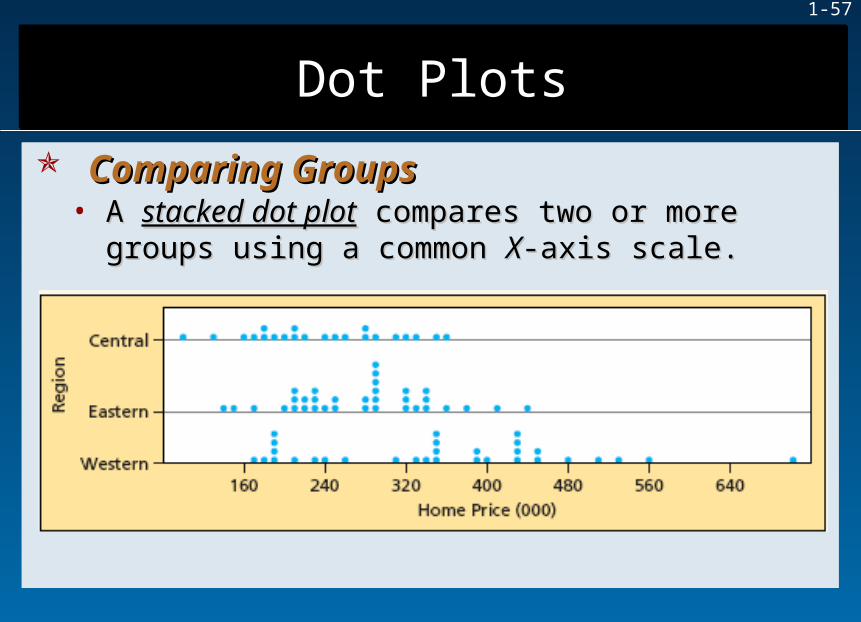
• A A stacked dot plotstacked dot plot compares two or more groups compares two or more groups using a common using a common XX-axis scale.-axis scale.
Dot PlotsDot PlotsDot PlotsDot Plots
Comparing GroupsComparing Groups

1-58
• A A frequency distributionfrequency distribution is a table formed by is a table formed by classifying classifying nn data values into data values into kk classes (bins). classes (bins).
• Bin limitsBin limits define the values to be included in each define the values to be included in each bin. Widths must all be the same.bin. Widths must all be the same.
• FrequenciesFrequencies are the number of observations within are the number of observations within each bin.each bin.
• ExpressExpress as as relative frequenciesrelative frequencies (frequency divided by (frequency divided by the total) or the total) or percentagespercentages (relative frequency times 100). (relative frequency times 100).
Frequency Distributions Frequency Distributions and Histogramsand Histograms
Frequency Distributions Frequency Distributions and Histogramsand Histograms
Bins and Bin LimitsBins and Bin Limits
3A-58
1-59
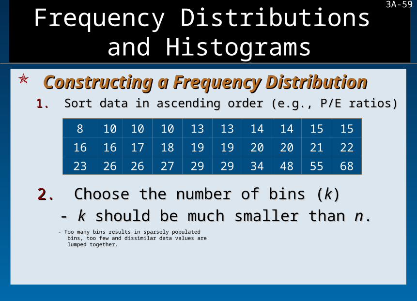
1.1. Sort data in ascending order (e.g., P/E ratios) Sort data in ascending order (e.g., P/E ratios)
8 10 10 10 13 13 14 14 15 15
16 16 17 18 19 19 20 20 21 22
23 26 26 27 29 29 34 48 55 68
Frequency Distributions Frequency Distributions and Histogramsand Histograms
Frequency Distributions Frequency Distributions and Histogramsand Histograms
Constructing a Frequency DistributionConstructing a Frequency Distribution
2.2. Choose the number of bins ( Choose the number of bins (kk))
- - kk should be much smaller than should be much smaller than nn..- Too many bins results in sparsely populated- Too many bins results in sparsely populated bins, too few and dissimilar data values are bins, too few and dissimilar data values are lumped together. lumped together.
3A-59

1-60
- Herbert Sturges proposes the following rule:- Herbert Sturges proposes the following rule:
Sample Size Sample Size (n)(n)
Number of Bins Number of Bins (k)(k)
1616 55
3232 66
6464 77
128128 88
Sample Size Sample Size (n)(n)
Number of Bins Number of Bins (k)(k)
256256 99
512512 1010
10241024 1111
Frequency Distributions Frequency Distributions and Histogramsand Histograms
Frequency Distributions Frequency Distributions and Histogramsand Histograms
Constructing a Frequency DistributionConstructing a Frequency Distribution
3A-60

1-61
3.3. Set the bin limits: Set the bin limits: Bin width Bin width max minX X
k
For example, for For example, for kk = 7 bins, the approximate bin width is: = 7 bins, the approximate bin width is:
68 8 608.57
7 7
Bin width Bin width
To obtain “nice” limits, we round the width to 10 and start the first bin at 0 to get bin limits:To obtain “nice” limits, we round the width to 10 and start the first bin at 0 to get bin limits:
0, 10, 20, 30, 40, 50, 60, 700, 10, 20, 30, 40, 50, 60, 70
Frequency Distributions Frequency Distributions and Histogramsand Histograms
Frequency Distributions Frequency Distributions and Histogramsand Histograms
Constructing a Frequency DistributionConstructing a Frequency Distribution
3A-61

1-62
4.4. Put the data values in the appropriate bin Put the data values in the appropriate binIn general, the lower limit is In general, the lower limit is includedincluded in the bin while the upper limit is in the bin while the upper limit is excluded.excluded.
5.5. Create the table, you can include Create the table, you can includeFrequenciesFrequencies – counts for each bin – counts for each binRelative frequenciesRelative frequencies – absolute frequency divided by total number of data values. – absolute frequency divided by total number of data values.
Cumulative frequenciesCumulative frequencies – accumulated relative frequency values as bin limits increase. – accumulated relative frequency values as bin limits increase.
Frequency Distributions Frequency Distributions and Histogramsand Histograms
Frequency Distributions Frequency Distributions and Histogramsand Histograms
Constructing a Frequency DistributionConstructing a Frequency Distribution
3A-62

1-63
Bin Range FrequencyRelative
Frequency
Cumulative Relative
Frequency
0<P/E Ratio<10 1 0.0333 0.0333
10<P/E Ratio<20 15 0.5000 0.5333
20<P/E Ratio<30 10 0.3333 0.8666
30<P/E Ratio<40 1 0.0333 0.8999
40<P/E Ratio<50 1 0.0333 0.9332
50<P/E Ratio<60 1 0.0333 0.9665
60<P/E Ratio<70 1 0.0333 0.9998
What are the bin limits for the P/E ratio data?What are the bin limits for the P/E ratio data?
Frequency Distributions Frequency Distributions and Histogramsand Histograms
Frequency Distributions Frequency Distributions and Histogramsand Histograms
3A-63
1-64
• A histogram is a graphical representation of a frequency distribution.
• A histogram is a bar chart.
Y-axis shows frequency within each bin.
X-axis ticks shows end points of each bin.
Frequency Distributions Frequency Distributions and Histogramsand Histograms
Frequency Distributions Frequency Distributions and Histogramsand Histograms
HistogramsHistograms
3A-64

1-65
• Consider 3 histograms for the P/E ratio data with different bin widths. What do they tell you?
Frequency Distributions Frequency Distributions and Histogramsand Histograms
Frequency Distributions Frequency Distributions and Histogramsand Histograms
HistogramsHistograms
3A-65
1-66
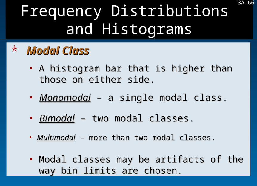
• A histogram bar that is higher than those on either A histogram bar that is higher than those on either side. side.
• MonomodalMonomodal – a single modal class. – a single modal class.
• BimodalBimodal – two modal classes. – two modal classes.
• MultimodalMultimodal – more than two modal classes. – more than two modal classes.
• Modal classes may be artifacts of the way bin Modal classes may be artifacts of the way bin limits are chosen.limits are chosen.
Frequency Distributions Frequency Distributions and Histogramsand Histograms
Frequency Distributions Frequency Distributions and Histogramsand Histograms
Modal ClassModal Class
3A-66

1-67
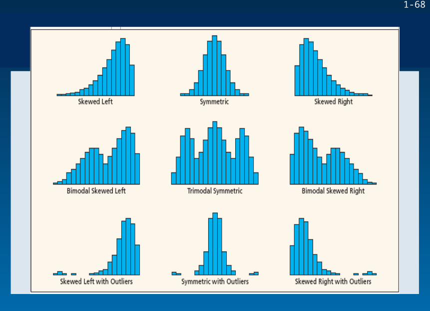
• A histogram suggests the A histogram suggests the shapeshape of the population. of the population.
• SkewnessSkewness – indicated by the direction of the longer – indicated by the direction of the longer tail of the histogram.tail of the histogram.
• It is influenced by number of bins and bin limits.It is influenced by number of bins and bin limits.
Left-skewedLeft-skewed – (negatively skewed) a longer left – (negatively skewed) a longer left tail. tail.Right-skewedRight-skewed – (positively skewed) a longer right – (positively skewed) a longer right tail. tail.SymmetricSymmetric – both tail areas approximately the – both tail areas approximately the same. same.
Frequency Distributions Frequency Distributions and Histogramsand Histograms
Frequency Distributions Frequency Distributions and Histogramsand Histograms
ShapeShape
3A-67
1-68
1-69
• Arithmetic scaleArithmetic scale – distances on the – distances on the YY-axis are -axis are proportional to the magnitude of the variable being proportional to the magnitude of the variable being displayed.displayed.
• Logarithmic scaleLogarithmic scale – ( – (ratio scaleratio scale) equal distances represent equal ratios.) equal distances represent equal ratios.
• Use a Use a log scalelog scale for the vertical axis when data vary over a wide range, say, by for the vertical axis when data vary over a wide range, say, by more than an order of magnitude.more than an order of magnitude.
• This will reveal more detail for small data values.This will reveal more detail for small data values.
Line ChartsLine ChartsLine ChartsLine Charts
Log ScalesLog Scales
3A-69

1-70
• A A scatter plotscatter plot shows shows nn pairs of observations as dots (or some other symbol) on an pairs of observations as dots (or some other symbol) on an XYXY graph. graph.
• A starting point for bivariate data analysis.A starting point for bivariate data analysis.
• Allows observations about the relationship between two variables.Allows observations about the relationship between two variables.
• Answers the question: Is there an association between the two variables and if so, Answers the question: Is there an association between the two variables and if so, what kind of association?what kind of association?
Scatter PlotsScatter PlotsScatter PlotsScatter Plots
1-71
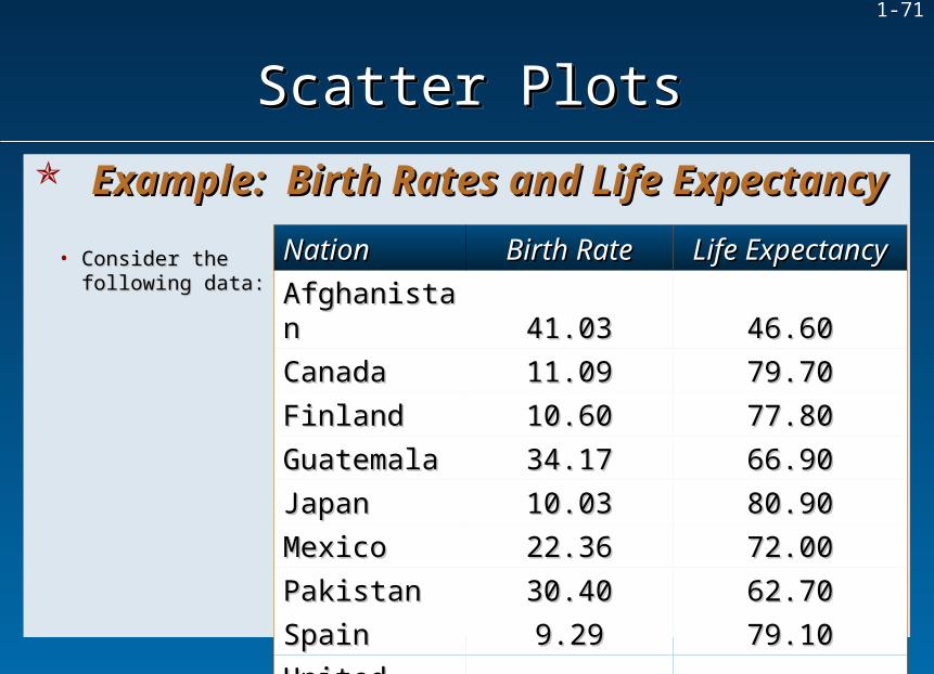
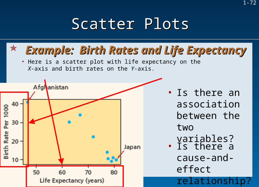
• Consider the Consider the following data:following data:
NationNation Birth RateBirth Rate Life ExpectancyLife Expectancy
AfghanistanAfghanistan 41.0341.03 46.6046.60
CanadaCanada 11.0911.09 79.7079.70
FinlandFinland 10.6010.60 77.8077.80
GuatemalaGuatemala 34.1734.17 66.9066.90
JapanJapan 10.0310.03 80.9080.90
MexicoMexico 22.3622.36 72.0072.00
PakistanPakistan 30.4030.40 62.7062.70
SpainSpain 9.299.29 79.1079.10
United United StatesStates 14.1014.10 77.4077.40
Example: Birth Rates and Life ExpectancyExample: Birth Rates and Life Expectancy
Scatter PlotsScatter PlotsScatter PlotsScatter Plots
1-72
• Here is a scatter plot with life expectancy on the X-axis and birth rates on the Y-axis.
• Is there an association between the two variables?
• Is there a cause-and-effect relationship?
Example: Birth Rates and Life ExpectancyExample: Birth Rates and Life Expectancy
Scatter PlotsScatter PlotsScatter PlotsScatter Plots
1-73
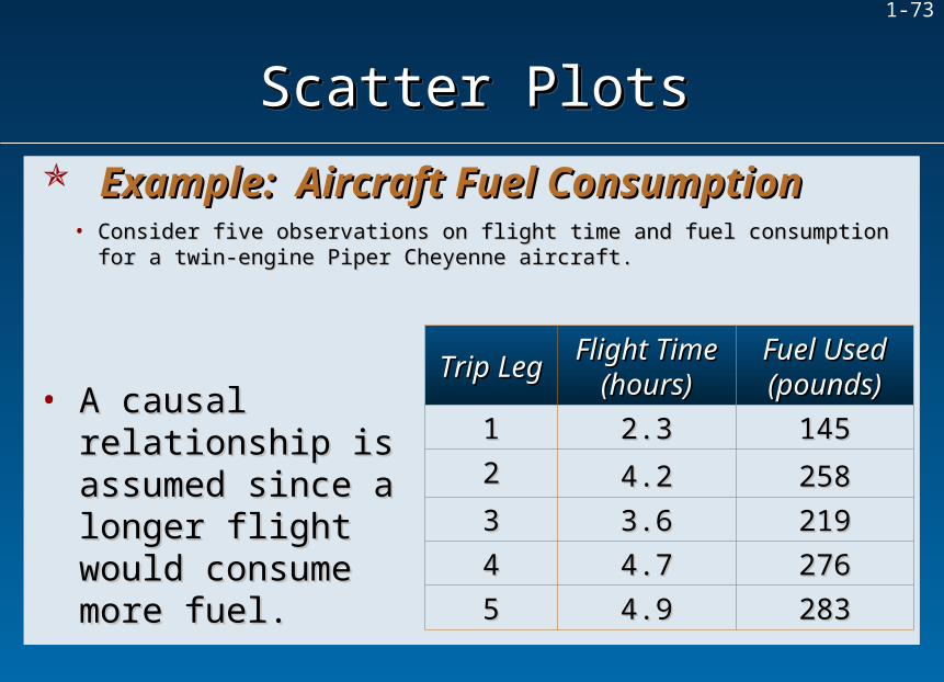
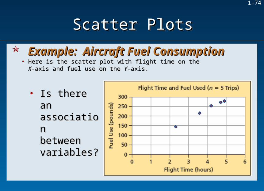
• Consider five observations on flight time and fuel consumption for a twin-engine Consider five observations on flight time and fuel consumption for a twin-engine Piper Cheyenne aircraft. Piper Cheyenne aircraft.
Trip LegTrip Leg Flight Time Flight Time (hours)(hours)
Fuel Used Fuel Used (pounds)(pounds)
11 2.32.3 145145
22 4.24.2 258258
33 3.63.6 219219
44 4.74.7 276276
55 4.94.9 283283
• A causal relationship A causal relationship is assumed since a is assumed since a longer flight would longer flight would consume more fuel.consume more fuel.
Example: Aircraft Fuel ConsumptionExample: Aircraft Fuel Consumption
Scatter PlotsScatter PlotsScatter PlotsScatter Plots
1-74
• Here is the scatter plot with flight time on the Here is the scatter plot with flight time on the XX-axis and fuel use on the -axis and fuel use on the YY-axis. -axis.
• Is there an Is there an association association between between variables?variables?
Example: Aircraft Fuel ConsumptionExample: Aircraft Fuel Consumption
Scatter PlotsScatter PlotsScatter PlotsScatter Plots
1-75
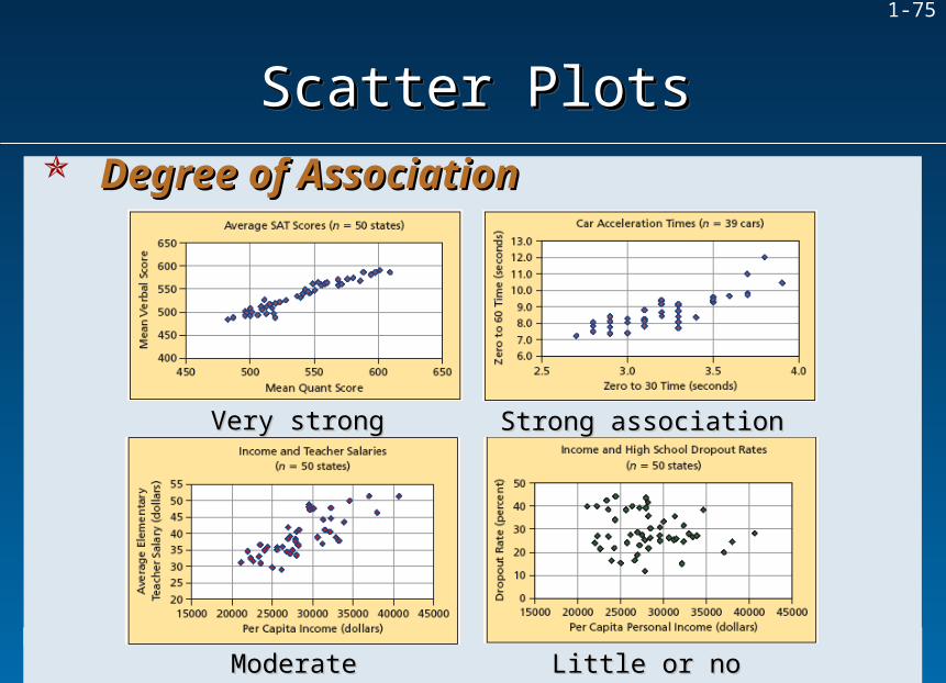
Degree of AssociationDegree of Association
Scatter PlotsScatter PlotsScatter PlotsScatter Plots
Very strong associationVery strong association Strong associationStrong association
Moderate associationModerate association Little or no associationLittle or no association
1-76
• TablesTables are the simplest form of data display. are the simplest form of data display.
• Arrangement of data is in rows and columns to enhance meaning.Arrangement of data is in rows and columns to enhance meaning.
• A A compound tablecompound table is a table that contains time series data down the columns and is a table that contains time series data down the columns and variables across the rows.variables across the rows.
• The data can be viewed by focusing on the time pattern (down the columns) or by The data can be viewed by focusing on the time pattern (down the columns) or by comparing the variables (across the rows).comparing the variables (across the rows).
Example: School ExpendituresExample: School Expenditures
TablesTablesTablesTables
1-77
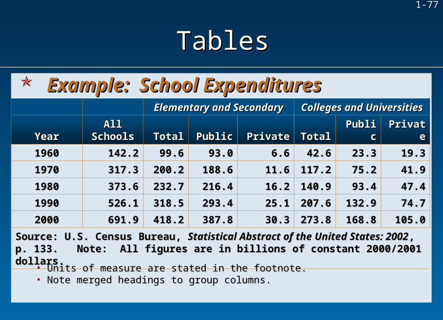
Elementary and SecondaryElementary and Secondary Colleges and UniversitiesColleges and Universities
YearYearAll All
SchoolsSchools TotalTotal PublicPublic PrivatePrivate TotalTotal PublicPublic PrivatePrivate
19601960 142.2142.2 99.699.6 93.093.0 6.66.6 42.642.6 23.323.3 19.319.3
19701970 317.3317.3 200.2200.2 188.6188.6 11.611.6 117.2117.2 75.275.2 41.941.9
19801980 373.6373.6 232.7232.7 216.4216.4 16.216.2 140.9140.9 93.493.4 47.447.4
19901990 526.1526.1 318.5318.5 293.4293.4 25.125.1 207.6207.6 132.9132.9 74.774.7
20002000 691.9691.9 418.2418.2 387.8387.8 30.330.3 273.8273.8 168.8168.8 105.0105.0
Source: U.S. Census Bureau, Source: U.S. Census Bureau, Statistical Abstract of the United States: 2002Statistical Abstract of the United States: 2002 , p. 133. , p. 133. Note: All figures are in billions of constant 2000/2001 dollars. Note: All figures are in billions of constant 2000/2001 dollars.
• Units of measure are stated in the footnote.Units of measure are stated in the footnote.• Note merged headings to group columns.Note merged headings to group columns.
Example: School ExpendituresExample: School Expenditures
TablesTablesTablesTables

1-78
• A A pie chartpie chart can only convey a general idea of the data. can only convey a general idea of the data.
• Pie charts should be used to portray data which sum to a total (e.g., percent Pie charts should be used to portray data which sum to a total (e.g., percent market shares).market shares).
• A pie chart should only have a few (i.e., 2 or 3) slices.A pie chart should only have a few (i.e., 2 or 3) slices.
• Each slice should be labeled with data values or percents.Each slice should be labeled with data values or percents.
An Oft-Abused ChartAn Oft-Abused Chart
Pie ChartsPie ChartsPie ChartsPie Charts
1-79
• Pie charts can only convey a general idea of the data values.Pie charts can only convey a general idea of the data values.
• Pie charts are ineffective when they have too many slices.Pie charts are ineffective when they have too many slices.
• Pie chart data must represent Pie chart data must represent parts of a wholeparts of a whole (e.g., percent market share). (e.g., percent market share).
Common Errors in Pie Chart UsageCommon Errors in Pie Chart Usage
Pie ChartsPie ChartsPie ChartsPie Charts

1-80
• A visual display in which data values are replaced by pictures.A visual display in which data values are replaced by pictures.
Maps and PictogramsMaps and PictogramsMaps and PictogramsMaps and Pictograms
PictogramsPictograms
1-81
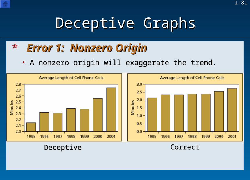
• A nonzero origin will exaggerate the trend.A nonzero origin will exaggerate the trend.
DeceptiveDeceptive CorrectCorrect
Deceptive GraphsDeceptive GraphsDeceptive GraphsDeceptive Graphs
Error 1: Nonzero OriginError 1: Nonzero Origin
1-82
IST 203: Statistics for Social Sciences
IST 203: Statistics for Social Sciences
Lecture 4A

1-83
• StatisticsStatistics are descriptive measures derived from a are descriptive measures derived from a sample (sample (nn items). items).
• ParametersParameters are descriptive measures derived from are descriptive measures derived from a population (a population (NN items). items).
Numerical DescriptionNumerical DescriptionNumerical DescriptionNumerical Description
1-84
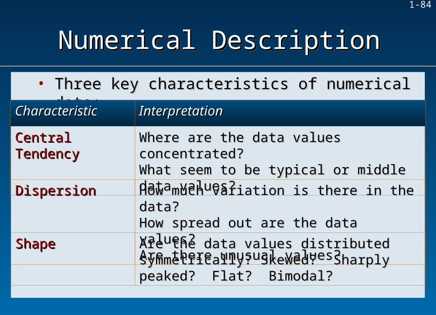
• Three key characteristics of numerical data:Three key characteristics of numerical data:
CharacteristicCharacteristic InterpretationInterpretation
Central TendencyCentral Tendency Where are the data values concentrated? Where are the data values concentrated? What seem to be typical or middle data What seem to be typical or middle data values?values?
Numerical DescriptionNumerical DescriptionNumerical DescriptionNumerical Description
DispersionDispersion How much variation is there in the data? How much variation is there in the data? How spread out are the data values? How spread out are the data values? Are there unusual values?Are there unusual values?
ShapeShape Are the data values distributed symmetrically? Are the data values distributed symmetrically? Skewed? Sharply peaked? Flat? Bimodal?Skewed? Sharply peaked? Flat? Bimodal?
1-85
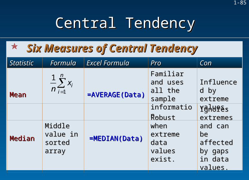
StatisticStatistic FormulaFormula Excel FormulaExcel Formula ProPro ConCon
MeanMean =AVERAGE(Data)=AVERAGE(Data)
Familiar and Familiar and uses all the uses all the sample sample information. information.
Influenced Influenced by extreme by extreme values.values.1
1 n
ii
xn
Central TendencyCentral TendencyCentral TendencyCentral Tendency
Six Measures of Central TendencySix Measures of Central Tendency
MedianMedian
Middle Middle value in value in sorted sorted arrayarray
=MEDIAN(Data)=MEDIAN(Data)Robust when Robust when extreme data extreme data values exist. values exist.
Ignores Ignores extremes extremes and can be and can be affected by affected by gaps in data gaps in data values.values.

1-86
StatisticStatistic FormulaFormula Excel FormulaExcel Formula ProPro ConCon
ModeMode
Most Most frequently frequently occurring occurring data valuedata value
=MODE(Data)=MODE(Data)
Useful for Useful for attribute attribute data or data or discrete data discrete data with a small with a small range.range.
May not be May not be unique, unique, and is not and is not helpful for helpful for continuous continuous data.data.
Central TendencyCentral TendencyCentral TendencyCentral Tendency Six Measures of Central TendencySix Measures of Central Tendency
MidrangeMidrange =0.5*(MIN(Data)=0.5*(MIN(Data)+MAX(Data))+MAX(Data))
Easy to Easy to understand understand and and calculate.calculate.
Influenced Influenced by extreme by extreme values and values and ignores ignores most data most data values.values.
min max
2
x x
1-87
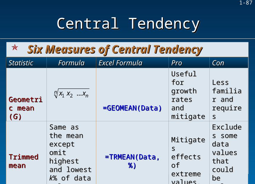
StatisticStatistic FormulaFormula Excel FormulaExcel Formula ProPro ConCon
Geometric Geometric mean (mean (GG))
=GEOMEAN(Data)=GEOMEAN(Data)
Useful for Useful for growth growth rates and rates and mitigates mitigates high high extremes.extremes.
Less Less familiar familiar and and requires requires positive positive data.data.
Trimmed Trimmed meanmean
Same as the Same as the mean except mean except omit highest omit highest and lowest and lowest kk% of data % of data values (e.g., values (e.g., 5%)5%)
=TRMEAN(Data, %)=TRMEAN(Data, %)
Mitigates Mitigates effects of effects of extreme extreme values.values.
Excludes Excludes some data some data values values that could that could be be relevant.relevant.
Central TendencyCentral TendencyCentral TendencyCentral Tendency
Six Measures of Central TendencySix Measures of Central Tendency
1 2 ... nnx x x

1-88
• A familiar measure of central tendency.A familiar measure of central tendency.
• In Excel, use function =AVERAGE(Data) where In Excel, use function =AVERAGE(Data) where Data is an array of data values.Data is an array of data values.
Population Formula Sample Formula
1
N
ii
x
N
1
n
ii
xx
n
Central TendencyCentral TendencyCentral TendencyCentral Tendency
MeanMean

1-89
• For the sample of For the sample of nn = 37 car brands: = 37 car brands:
1 87 93 98 ... 159 164 173 4639125.38
37 37
n
ii
xx
n
Central TendencyCentral TendencyCentral TendencyCentral Tendency
MeanMean
1-90
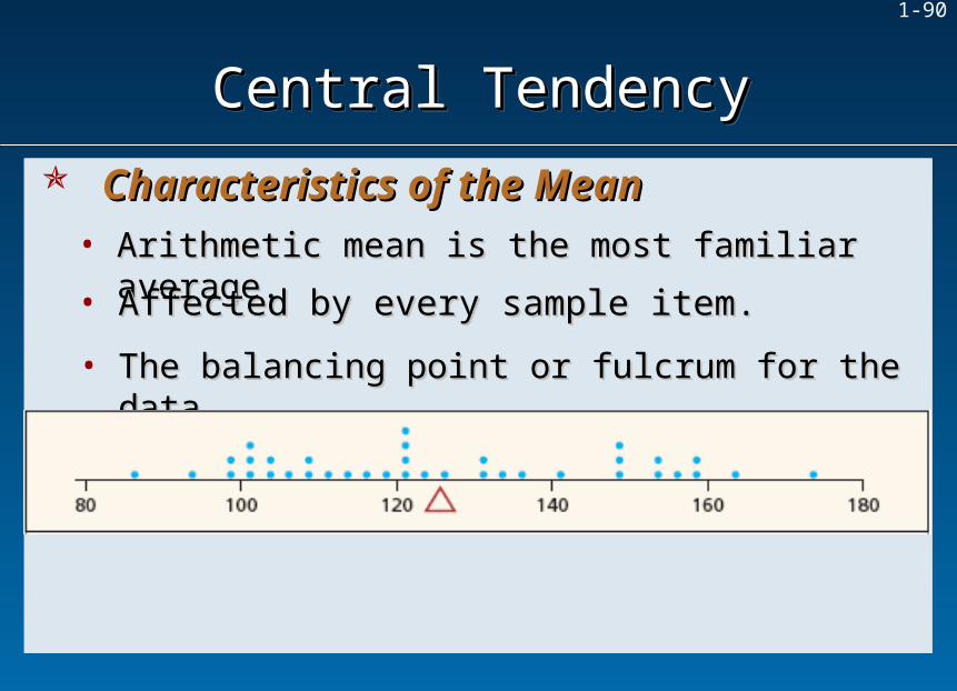
• Arithmetic mean is the most familiar average.Arithmetic mean is the most familiar average.
• Affected by every sample item.Affected by every sample item.
• The balancing point or fulcrum for the data.The balancing point or fulcrum for the data.
Central TendencyCentral TendencyCentral TendencyCentral Tendency
Characteristics of the MeanCharacteristics of the Mean

1-91
• Regardless of the shape of the distribution, absolute distances Regardless of the shape of the distribution, absolute distances from the mean to the data points always sum to zero.from the mean to the data points always sum to zero.
1
( ) 0n
ii
x x
Central TendencyCentral TendencyCentral TendencyCentral Tendency
Characteristics of the MeanCharacteristics of the Mean
• Consider the following asymmetric Consider the following asymmetric distribution of quiz scores whose mean = 65.distribution of quiz scores whose mean = 65.
1
( )n
ii
x x
= (42 – 65) + (60 – 65) + (70 – 65) + (75 – 65) + (78 – 65)= (42 – 65) + (60 – 65) + (70 – 65) + (75 – 65) + (78 – 65)= (-23) + (-5) + (5) + (10) + (13) = -28 + 28 = 0= (-23) + (-5) + (5) + (10) + (13) = -28 + 28 = 0

1-92
• The The medianmedian ( (MM) is the 50) is the 50thth percentile or midpoint of percentile or midpoint of the the sortedsorted sample data. sample data.
• MM separates the upper and lower half of the sorted separates the upper and lower half of the sorted observations.observations.
• If If nn is odd, the median is the middle observation in is odd, the median is the middle observation in the data array.the data array.
• If If nn is even, the median is the average of the is even, the median is the average of the middle two observations in the data array.middle two observations in the data array.
Central TendencyCentral TendencyCentral TendencyCentral Tendency
MedianMedian
1-93
Central TendencyCentral TendencyCentral TendencyCentral Tendency
MedianMedian
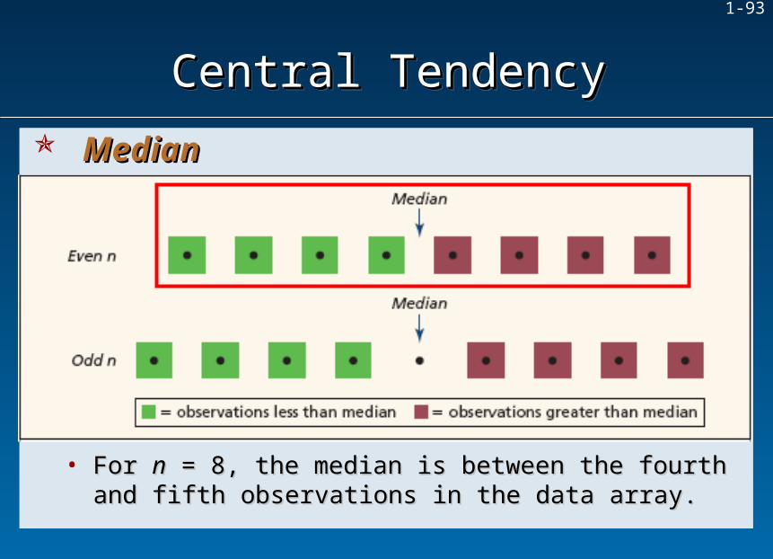
• For For nn = 8, the median is between the fourth and = 8, the median is between the fourth and fifth observations in the data array.fifth observations in the data array.
1-94
Central TendencyCentral TendencyCentral TendencyCentral Tendency
MedianMedian
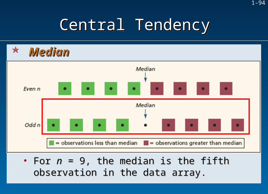
• For For nn = 9, the median is the fifth observation in the = 9, the median is the fifth observation in the data array.data array.
1-95
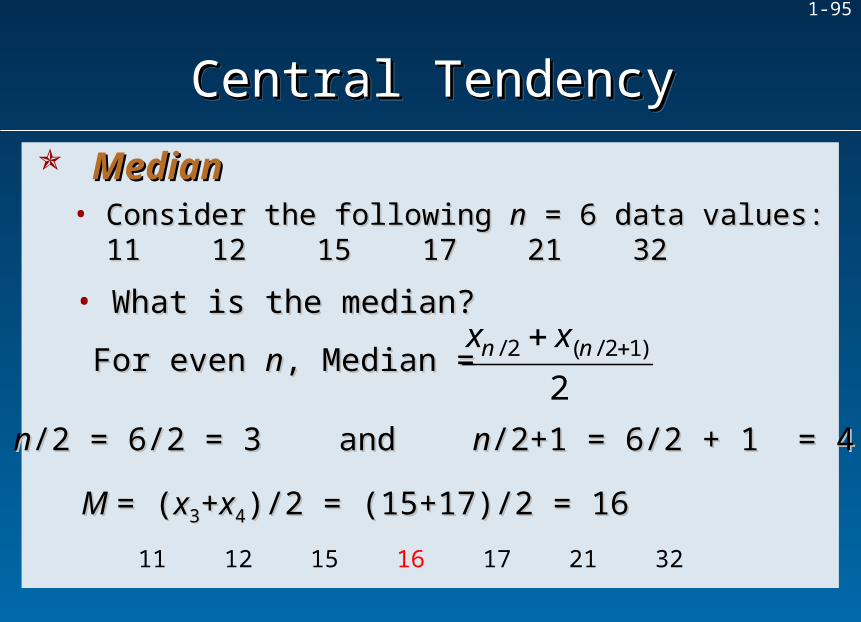
• Consider the following Consider the following nn = 6 data values: = 6 data values:11 12 15 17 21 3211 12 15 17 21 32
• What is the median?What is the median?
M M = (= (xx33++xx44)/2 = (15+17)/2 = 16 )/2 = (15+17)/2 = 16
11 12 15 16 17 21 32
For even For even nn, Median = , Median = / 2 ( / 2 1)
2n nx x
nn/2 = 6/2 = 3 and /2 = 6/2 = 3 and nn/2+1 = 6/2 + 1 = 4/2+1 = 6/2 + 1 = 4
Central TendencyCentral TendencyCentral TendencyCentral Tendency
MedianMedian

1-96
• Consider the following Consider the following nn = 7 data values: = 7 data values:12 23 23 25 27 34 4112 23 23 25 27 34 41
• What is the median?What is the median?
M M = = xx44 = 25 = 25
12 23 23 25 27 34 41
For odd For odd nn, Median = , Median = ( 1) / 2nx
((nn+1)/2 = (7+1)/2 = 8/2 = 4+1)/2 = (7+1)/2 = 8/2 = 4
Central TendencyCentral TendencyCentral TendencyCentral Tendency
MedianMedian

1-97
• Use Excel’s function =MEDIAN(Data) where Data Use Excel’s function =MEDIAN(Data) where Data is an array of data values.is an array of data values.
• For the 37 vehicle quality ratings (odd For the 37 vehicle quality ratings (odd nn) the position of the median is ) the position of the median is ((nn+1)/2 = (37+1)/2 = 19.+1)/2 = (37+1)/2 = 19.
• So, the median is So, the median is xx1919 = 121. = 121.
• When there are several duplicate data values, the median When there are several duplicate data values, the median does not provide a clean “50-50” split in the data.does not provide a clean “50-50” split in the data.
Central TendencyCentral TendencyCentral TendencyCentral Tendency
MedianMedian

1-98
• The median is insensitive to extreme data values.The median is insensitive to extreme data values.• For example, consider the following quiz scores for For example, consider the following quiz scores for
3 students:3 students:
Tom’s scores:Tom’s scores: 20, 40, 70, 75, 80 20, 40, 70, 75, 80 Mean =57, Mean =57, Median = 70Median = 70, Total = 285, Total = 285Jake’s scores:Jake’s scores: 60, 65, 70, 90, 95 60, 65, 70, 90, 95 Mean = 76, Mean = 76, Median = 70Median = 70, Total = 380, Total = 380Mary’s scores:Mary’s scores: 50, 65, 70, 75, 90 50, 65, 70, 75, 90 Mean = 70, Mean = 70, Median = 70Median = 70, Total = 350, Total = 350
• What does the median for each student tell you?What does the median for each student tell you?
Central TendencyCentral TendencyCentral TendencyCentral Tendency
Characteristics of the MedianCharacteristics of the Median
1-99
• The most frequently occurring data value.The most frequently occurring data value.
• Similar to mean and median if data values occur Similar to mean and median if data values occur often near the center of sorted data.often near the center of sorted data.
• May have multiple modes or no mode. May have multiple modes or no mode.
Central TendencyCentral TendencyCentral TendencyCentral Tendency
ModeMode

1-100
Lee’s scoresLee’s scores:: 60, 70, 70, 70, 80 60, 70, 70, 70, 80 Mean =70, Median = 70, Mean =70, Median = 70, Mode = 70Mode = 70Pat’s scoresPat’s scores:: 45, 45, 70, 90, 100 45, 45, 70, 90, 100 Mean = 70, Median = 70, Mean = 70, Median = 70, Mode = 45Mode = 45Sam’s scoresSam’s scores:: 50, 60, 70, 80, 90 50, 60, 70, 80, 90 Mean = 70, Median = 70, Mean = 70, Median = 70, Mode = noneMode = noneXiao’s scoresXiao’s scores:: 50, 50, 70, 90, 90 50, 50, 70, 90, 90 Mean = 70, Median = 70, Mean = 70, Median = 70, Modes = 50,90Modes = 50,90
Central TendencyCentral TendencyCentral TendencyCentral Tendency
ModeMode• For example, consider the following quiz scores for For example, consider the following quiz scores for
3 students:3 students:
• What does the mode for each student tell you?What does the mode for each student tell you?
1-101
• Easy to define, not easy to calculate in large Easy to define, not easy to calculate in large samples.samples.
• Use Excel’s function =MODE(Array)Use Excel’s function =MODE(Array)- will return #N/A if there is no mode.- will return #N/A if there is no mode.- will return first mode found if multimodal.- will return first mode found if multimodal.
• May be far from the middle of the distribution and May be far from the middle of the distribution and not at all typical.not at all typical.
Central TendencyCentral TendencyCentral TendencyCentral Tendency
ModeMode

1-102
• Generally isn’t useful for continuous data since Generally isn’t useful for continuous data since data values rarely repeat.data values rarely repeat.
• Best for attribute data or a discrete variable with a Best for attribute data or a discrete variable with a small range (e.g., Likert scale).small range (e.g., Likert scale).
Central TendencyCentral TendencyCentral TendencyCentral Tendency
ModeMode
1-103
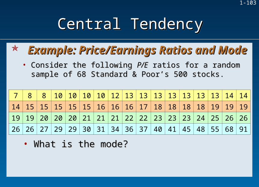
• Consider the following Consider the following P/EP/E ratios for a random ratios for a random sample of 68 Standard & Poor’s 500 stocks.sample of 68 Standard & Poor’s 500 stocks.
• What is the mode?What is the mode?
Central TendencyCentral TendencyCentral TendencyCentral Tendency
Example: Price/Earnings Ratios and ModeExample: Price/Earnings Ratios and Mode
7 8 8 10 10 10 10 12 13 13 13 13 13 13 13 14 14
14 15 15 15 15 15 16 16 16 17 18 18 18 18 19 19 19
19 19 20 20 20 21 21 21 22 22 23 23 23 24 25 26 26
26 26 27 29 29 30 31 34 36 37 40 41 45 48 55 68 91

1-104
• Excel’s descriptive Excel’s descriptive statistics results are:statistics results are:
• The mode 13 occurs 7 times, The mode 13 occurs 7 times, but what does the dot plot but what does the dot plot show?show?
Mean 22.7206
Median 19
Mode 13
Range 84
Minimum 7
Maximum 91
Sum 1545
Count 68
Central TendencyCentral TendencyCentral TendencyCentral Tendency
Example: Price/Earnings Ratios and ModeExample: Price/Earnings Ratios and Mode

1-105
• The dot plot shows local modes (a peak with The dot plot shows local modes (a peak with valleys on either side) at 10, 13, 15, 19, 23, 26, 29.valleys on either side) at 10, 13, 15, 19, 23, 26, 29.
• These multiple modes suggest that the mode is These multiple modes suggest that the mode is not a stable measure of central tendency.not a stable measure of central tendency.
Central TendencyCentral TendencyCentral TendencyCentral Tendency
Example: Price/Earnings Ratios and ModeExample: Price/Earnings Ratios and Mode
1-106
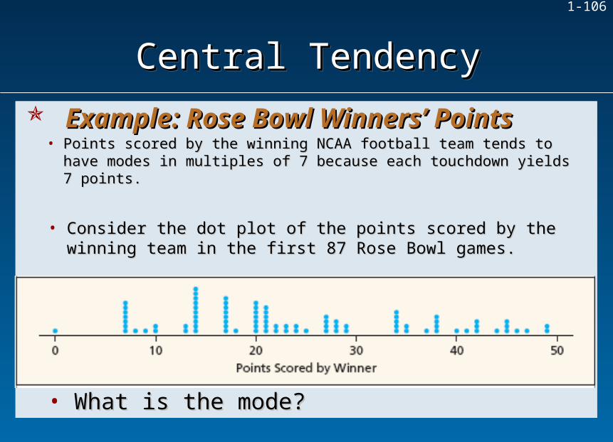
• Points scored by the winning NCAA football team tends to have Points scored by the winning NCAA football team tends to have modes in multiples of 7 because each touchdown yields 7 points.modes in multiples of 7 because each touchdown yields 7 points.
Central TendencyCentral TendencyCentral TendencyCentral Tendency
Example: Rose Bowl Winners’ PointsExample: Rose Bowl Winners’ Points
• Consider the dot plot of the points scored by the Consider the dot plot of the points scored by the winning team in the first 87 Rose Bowl games.winning team in the first 87 Rose Bowl games.
• What is the mode?What is the mode?
1-107
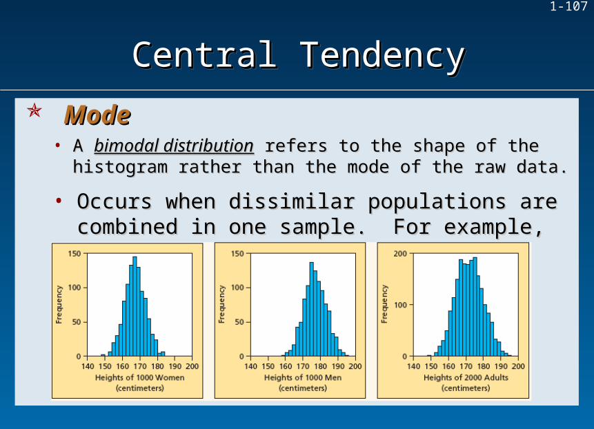
• A A bimodal distributionbimodal distribution refers to the shape of the refers to the shape of the histogram rather than the mode of the raw data.histogram rather than the mode of the raw data.
• Occurs when dissimilar populations are combined Occurs when dissimilar populations are combined in one sample. For example,in one sample. For example,
Central TendencyCentral TendencyCentral TendencyCentral Tendency
ModeMode

1-108
Distribution’s Distribution’s ShapeShape
Histogram AppearanceHistogram Appearance StatisticsStatistics
Skewed leftSkewed left(negative (negative skewness)skewness)
Long tail of histogram points leftLong tail of histogram points left(a few low values but most data (a few low values but most data on right)on right)
Mean < MedianMean < Median
Central TendencyCentral TendencyCentral TendencyCentral Tendency
Symptoms of SkewnessSymptoms of Skewness
SymmetricSymmetric Tails of histogram are balancedTails of histogram are balanced (low/high values offset)(low/high values offset) Mean Mean Median Median
Skewed rightSkewed right(positive (positive skewness)skewness)
Long tail of histogram points rightLong tail of histogram points right(most data on left but a few high (most data on left but a few high values)values)
Mean > MedianMean > Median
1-109
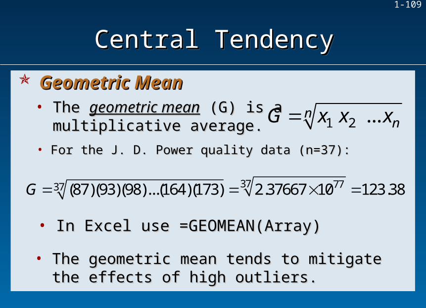
• The The geometric meangeometric mean (G) is a (G) is a multiplicative average.multiplicative average.
• For the J. D. Power quality data (n=37):For the J. D. Power quality data (n=37):
1 2 ... nnG x x x
37 7737 (87)(93)(98)...(164)(173) 2.37667 10 123.38G
• In Excel use =GEOMEAN(Array)In Excel use =GEOMEAN(Array)
• The geometric mean tends to mitigate the effects The geometric mean tends to mitigate the effects of high outliers.of high outliers.
Central TendencyCentral TendencyCentral TendencyCentral Tendency
Geometric MeanGeometric Mean
1-110
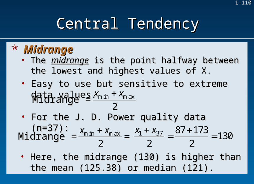
• The The midrangemidrange is the point halfway between the is the point halfway between the lowest and highest values of X.lowest and highest values of X.
• Easy to use but sensitive to extreme data values.Easy to use but sensitive to extreme data values.min max
2
x xMidrange = Midrange =
• For the J. D. Power quality data (n=37):For the J. D. Power quality data (n=37):
min max
2
x xMidrange = Midrange = 1 37 87 173
1302 2
x x =
• Here, the midrange (130) is higher than the mean Here, the midrange (130) is higher than the mean (125.38) or median (121).(125.38) or median (121).
Central TendencyCentral TendencyCentral TendencyCentral Tendency
MidrangeMidrange
1-111
• To calculate the To calculate the trimmed meantrimmed mean, first remove the , first remove the highest and lowest highest and lowest kk percent of the observations. percent of the observations.
• For example, for the For example, for the nn = 68 P/E ratios, we want a 5 = 68 P/E ratios, we want a 5 percent trimmed mean (i.e., percent trimmed mean (i.e., kk = .05). = .05).
• To determine how many observations to trim, To determine how many observations to trim, multiply multiply kk x x nn = 0.05 x 68 = 3.4 or 3 observations. = 0.05 x 68 = 3.4 or 3 observations.
• So, we would remove the three smallest and three largest So, we would remove the three smallest and three largest observations before averaging the remaining values.observations before averaging the remaining values.
Central TendencyCentral TendencyCentral TendencyCentral Tendency
Trimmed MeanTrimmed Mean
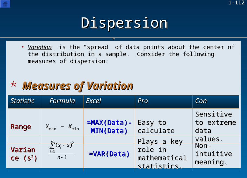
1-112
• VariationVariation is the “spread” of data points about the center of the distribution is the “spread” of data points about the center of the distribution in a sample. Consider the following measures of dispersion:in a sample. Consider the following measures of dispersion:
StatisticStatistic FormulaFormula ExcelExcel ProPro ConCon
RangeRange xxmaxmax – – xxminmin=MAX(Data)-=MAX(Data)-
MIN(Data)MIN(Data) Easy to calculateEasy to calculateSensitive to Sensitive to extreme data extreme data values.values.
DispersionDispersionDispersionDispersion
VarianceVariance (s(s22))
=VAR(Data)=VAR(Data)Plays a key role Plays a key role in mathematical in mathematical statistics.statistics.
Non-intuitive Non-intuitive meaning.meaning.
2
1
1
n
ii
x x
n
Measures of VariationMeasures of Variation

1-113
StatisticStatistic FormulaFormula ExcelExcel ProPro ConCon
Standard Standard deviationdeviation ((ss))
=STDEV(Data)=STDEV(Data)
Most common Most common measure. Uses measure. Uses same units as the same units as the raw data ($ , £, ¥, raw data ($ , £, ¥, etc.).etc.).
Non-intuitive Non-intuitive meaning.meaning.
2
1
1
n
ii
x x
n
DispersionDispersionDispersionDispersion
Measures of VariationMeasures of Variation
Coef-Coef-ficient. officient. ofvariationvariation ((CVCV))
NoneNone
Measures relative Measures relative variation in variation in percentpercent so can so can compare data compare data sets.sets.
Requires Requires non-non-negative negative data.data.
100s
x
1-114
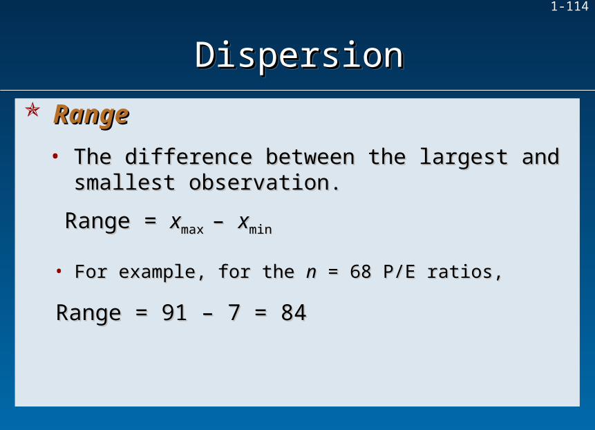
• The difference between the largest and smallest The difference between the largest and smallest observation.observation.
Range = Range = xxmax max – – xxminmin
• For example, for the For example, for the nn = 68 P/E ratios, = 68 P/E ratios,
Range = 91 – 7 = 84 Range = 91 – 7 = 84
DispersionDispersionDispersionDispersion
RangeRange

1-115
• The The population variancepopulation variance ( (22) is defined as the sum ) is defined as the sum of squared deviations around the mean of squared deviations around the mean divided by divided by the population size.the population size.
• For the For the sample variancesample variance (s (s22), we divide by ), we divide by nn – 1 instead of – 1 instead of nn, otherwise , otherwise ss22 would tend to underestimate the unknown population variance would tend to underestimate the unknown population variance 22..
2
2 1
N
ii
x
N
2
2 1
1
n
ii
x xs
n
DispersionDispersionDispersionDispersion
VarianceVariance

1-116
• The square root of the variance.The square root of the variance.
• Units of measure are the same as Units of measure are the same as XX..
Population Population standard deviationstandard deviation 2
1
N
ii
x
N
Sample standard Sample standard
deviationdeviation 2
1
1
n
ii
x xs
n
• Explains how individual values in a data set vary Explains how individual values in a data set vary from the mean.from the mean.
DispersionDispersionDispersionDispersion
Standard DeviationStandard Deviation
1-117
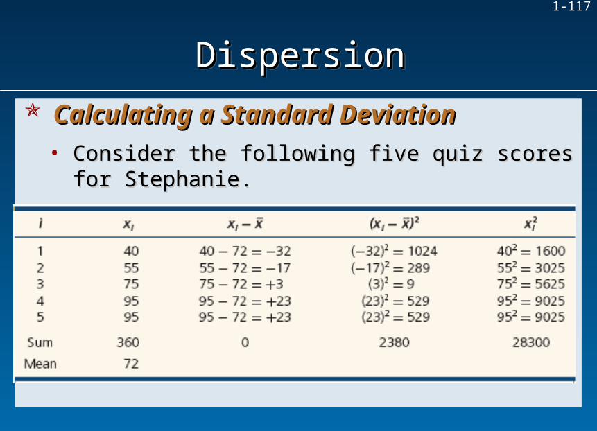
• Consider the following five quiz scores for Consider the following five quiz scores for Stephanie.Stephanie.
DispersionDispersionDispersionDispersion
Calculating a Standard DeviationCalculating a Standard Deviation
1-118
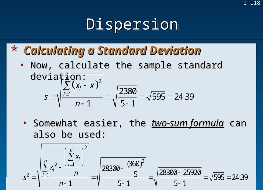
• Now, calculate the sample standard deviation:Now, calculate the sample standard deviation:
2
1 2380595 24.39
1 5 1
n
ii
x xs
n
• Somewhat easier, the Somewhat easier, the two-sum formulatwo-sum formula can also can also be used:be used:
2
212
2 1
(360)28300 28300 259205 595 24.39
1 5 1 5 1
n
ini
ii
x
xns
n
DispersionDispersionDispersionDispersion
Calculating a Standard DeviationCalculating a Standard Deviation

1-119
IST 203: Statistics for Social Sciences
IST 203: Statistics for Social Sciences
Lecture 5A
1-120
• A A random experimentrandom experiment is an observational process whose results cannot be known is an observational process whose results cannot be known in advance.in advance.
• The set of all The set of all outcomesoutcomes ( (SS) is the ) is the sample spacesample space for the experiment. for the experiment.
• A sample space with a countable number of outcomes is A sample space with a countable number of outcomes is discretediscrete..
Sample SpaceSample Space
Random ExperimentsRandom ExperimentsRandom ExperimentsRandom Experiments

1-121
• For a single roll of a die, the sample space is:For a single roll of a die, the sample space is:
S = {1, 2, 3, 4, 5, 6}• When two dice are rolled, the sample space is the following pairs:When two dice are rolled, the sample space is the following pairs:
Sample SpaceSample Space
Random ExperimentsRandom ExperimentsRandom ExperimentsRandom Experiments
{(1,1), (1,2), (1,3), (1,4), (1,5), (1,6),
(2,1), (2,2), (2,3), (2,4), (2,5), (2,6),
(3,1), (3,2), (3,3), (3,4), (3,5), (3,6),
(4,1), (4,2), (4,3), (4,4), (4,5), (4,6),
(5,1), (5,2), (5,3), (5,4), (5,5), (5,6),
(6,1), (6,2), (6,3), (6,4), (6,5), (6,6)}
SS = =
1-122
• Consider the sample space to describe a randomly chosen United Airlines employee by Consider the sample space to describe a randomly chosen United Airlines employee by 2 genders, 2 genders, 21 job classifications, 21 job classifications, 6 home bases (major hubs) and 6 home bases (major hubs) and 4 education levels4 education levels
• It would be impractical to enumerate this sample space.It would be impractical to enumerate this sample space.
There are: 2 x 21 x 6 x 4 = 1008 possible outcomesThere are: 2 x 21 x 6 x 4 = 1008 possible outcomes
Sample SpaceSample Space
Random ExperimentsRandom ExperimentsRandom ExperimentsRandom Experiments

1-123
• If the outcome is a If the outcome is a continuouscontinuous measurement, the sample space can be described measurement, the sample space can be described by a rule. by a rule.
• For example, the sample space for the length of a randomly chosen cell phone call For example, the sample space for the length of a randomly chosen cell phone call would bewould be
SS = {all = {all XX such that such that X X >> 0} 0}
• The sample space to describe a randomly chosen student’s GPA would beThe sample space to describe a randomly chosen student’s GPA would be
SS = { = {XX | 0.00 | 0.00 << X X << 4.00} 4.00}
or written as or written as SS = { = {XX | | X X >> 0} 0}
Sample SpaceSample Space
Random ExperimentsRandom ExperimentsRandom ExperimentsRandom Experiments

1-124
• An An eventevent is any subset of outcomes in the sample space. is any subset of outcomes in the sample space.
• A A simple eventsimple event or or elementary eventelementary event, is a single outcome., is a single outcome.
• A discrete sample space A discrete sample space SS consists of all the simple events ( consists of all the simple events (EEii):):
SS = { = {EE11, , EE22, …, , …, EEnn}}
EventsEvents
Random ExperimentsRandom ExperimentsRandom ExperimentsRandom Experiments
1-125
• What are the chances of observing a H or T?What are the chances of observing a H or T?
• These two elementary events are These two elementary events are equally likelyequally likely..
SS = {H, T} = {H, T}
• Consider the random experiment of tossing a Consider the random experiment of tossing a balanced coin. balanced coin. What is the sample space?What is the sample space?
• When you buy a lottery ticket, the sample space When you buy a lottery ticket, the sample space SS = {win, lose} has only two events. = {win, lose} has only two events.
EventsEvents
Random ExperimentsRandom ExperimentsRandom ExperimentsRandom Experiments
• Are these two events equally likely to occur?Are these two events equally likely to occur?
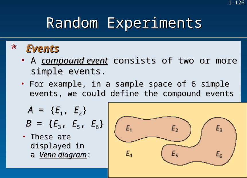
1-126
• For example, in a sample space of 6 simple For example, in a sample space of 6 simple events, we could define the compound eventsevents, we could define the compound events
• A A compound eventcompound event consists of two or more simple consists of two or more simple events. events.
• These are These are displayed in a displayed in a Venn diagramVenn diagram::
AA = { = {EE11, , EE22}}
BB = { = {EE33, , EE55, , EE66}}
EventsEvents
Random ExperimentsRandom ExperimentsRandom ExperimentsRandom Experiments

1-127
• Many different compound events could be defined.
• Compound events can be described by a rule.
S = {(1,6), (2,5), (3,4), (4,3), (5,2), (6,1)}
• For example, the compound event A = “rolling a seven” on a roll of two dice consists of 6 simple events:
EventsEvents
Random ExperimentsRandom ExperimentsRandom ExperimentsRandom Experiments

1-128
• The The probabilityprobability of an event is a number that measures the relative likelihood that of an event is a number that measures the relative likelihood that the event will occur.the event will occur.
• The probability of event The probability of event A A [denoted [denoted PP((AA)], must lie within the interval from 0 to 1:)], must lie within the interval from 0 to 1:
0 0 << PP((AA) ) << 1 1
If P(A) = 0, then the event cannot occur.
If P(A) = 1, then the event is certain to occur.
DefinitionsDefinitions
ProbabilityProbabilityProbabilityProbability
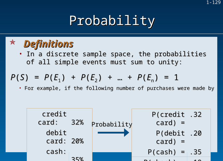
1-129
• In a discrete sample space, the probabilities of all In a discrete sample space, the probabilities of all simple events must sum to unity:simple events must sum to unity:
• For example, if the following number of purchases were made byFor example, if the following number of purchases were made by
PP((SS) = ) = PP((EE11) + ) + PP((EE22) + … + ) + … + PP((EEnn) = 1 ) = 1
credit card: credit card: 32%32%
debit card:debit card: 20%20%
cash:cash: 35%35%
check:check: 18%18%
Sum = Sum = 100%100%
DefinitionsDefinitions
ProbabilityProbabilityProbabilityProbability
P(credit card) =P(credit card) = .32.32
P(debit card) =P(debit card) = .20.20
P(cash) =P(cash) = .35.35
P(check) =P(check) = .18.18
Sum =Sum = 1.01.0
ProbabilityProbability
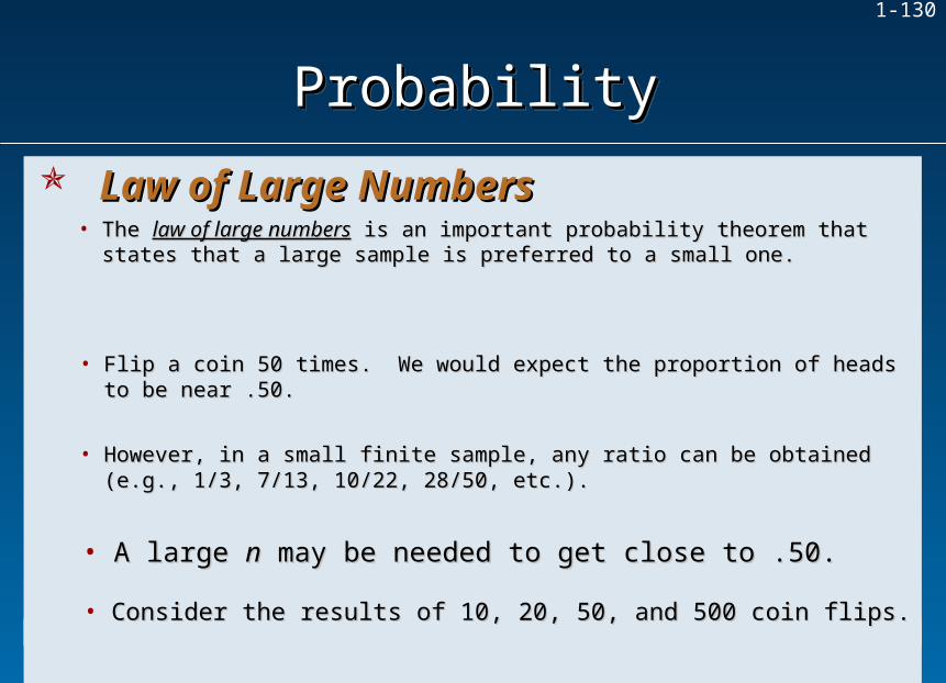
1-130
• The The law of large numberslaw of large numbers is an important probability theorem that states that a is an important probability theorem that states that a large sample is preferred to a small one.large sample is preferred to a small one.
• Flip a coin 50 times. We would expect the proportion of heads to be near .50. Flip a coin 50 times. We would expect the proportion of heads to be near .50.
• A large A large nn may be needed to get close to .50. may be needed to get close to .50.
• However, in a small finite sample, any ratio can be obtained (e.g., 1/3, 7/13, 10/22, However, in a small finite sample, any ratio can be obtained (e.g., 1/3, 7/13, 10/22, 28/50, etc.).28/50, etc.).
Law of Large NumbersLaw of Large Numbers
ProbabilityProbabilityProbabilityProbability
• Consider the results of 10, 20, 50, and 500 coin flips.Consider the results of 10, 20, 50, and 500 coin flips.

1-131
ProbabilityProbabilityProbabilityProbability

1-132
• Actuarial scienceActuarial science is a high-paying career that involves estimating empirical is a high-paying career that involves estimating empirical probabilities.probabilities.
• For example, actuaries For example, actuaries - calculate payout rates on life insurance,- calculate payout rates on life insurance, pension plans, and health care plans pension plans, and health care plans- create tables that guide IRA withdrawal- create tables that guide IRA withdrawal rates for individuals from age 70 to 99 rates for individuals from age 70 to 99
Practical Issues for ActuariesPractical Issues for Actuaries
ProbabilityProbabilityProbabilityProbability

1-133
• The The complementcomplement of an event of an event AA is denoted by is denoted by AA′′ and consists of everything in the sample space and consists of everything in the sample space SS except event except event AA..
Complement of an EventComplement of an Event
Rules of ProbabilityRules of ProbabilityRules of ProbabilityRules of Probability
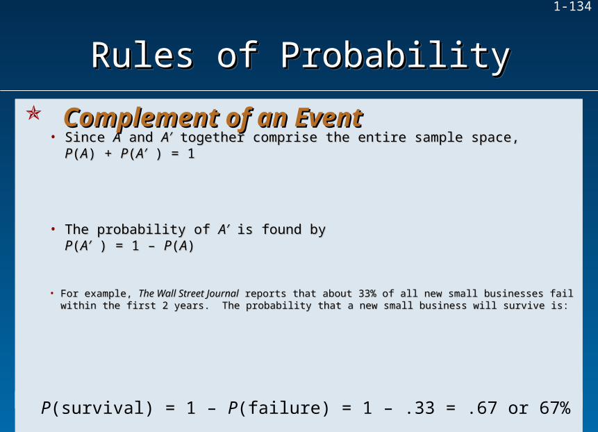
1-134
• Since Since AA and and AA′′ together comprise the entire sample space, together comprise the entire sample space, PP((AA) + ) + PP((AA′′ ) = 1 ) = 1
• The probability of The probability of AA′′ is found by is found by PP((AA′′ ) = 1 – ) = 1 – PP((AA) )
• For example, For example, The Wall Street JournalThe Wall Street Journal reports that about 33% of all new small businesses reports that about 33% of all new small businesses fail within the first 2 years. The probability that a new small business will survive is:fail within the first 2 years. The probability that a new small business will survive is:
P(survival) = 1 – P(failure) = 1 – .33 = .67 or 67%
Complement of an EventComplement of an Event
Rules of ProbabilityRules of ProbabilityRules of ProbabilityRules of Probability
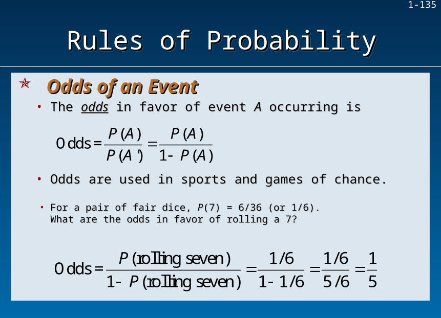
1-135
• The The oddsodds in favor of event in favor of event AA occurring is occurring is
• Odds are used in sports and games of chance.Odds are used in sports and games of chance.
• For a pair of fair dice, For a pair of fair dice, PP(7) = 6/36 (or 1/6). (7) = 6/36 (or 1/6). What are the odds in favor of rolling a 7?What are the odds in favor of rolling a 7?
( ) ( )Odds =
( ') 1 ( )
P A P A
P A P A
(rolling seven) 1/ 6 1/ 6 1Odds =
1 (rolling seven) 1 1/ 6 5/ 6 5
P
P
Odds of an EventOdds of an Event
Rules of ProbabilityRules of ProbabilityRules of ProbabilityRules of Probability
1-136
• On the average, for every time a 7 is rolled, there will be 5 times that it is not On the average, for every time a 7 is rolled, there will be 5 times that it is not rolled.rolled.
• In other words, the odds are 1 to 5 In other words, the odds are 1 to 5 in favorin favor of rolling a 7. of rolling a 7.
• The odds are 5 to 1 The odds are 5 to 1 againstagainst rolling a 7. rolling a 7.
Odds of an EventOdds of an Event
Rules of ProbabilityRules of ProbabilityRules of ProbabilityRules of Probability
• In horse racing and other sports, odds are usually quoted In horse racing and other sports, odds are usually quoted againstagainst winning. winning.

1-137
• If the odds against event If the odds against event AA are quoted as are quoted as bb to to aa, then the implied probability of , then the implied probability of event event AA is: is:
• For example, if a race horse has a 4 to 1 odds For example, if a race horse has a 4 to 1 odds againstagainst winning, the winning, the PP(win) is (win) is
PP((AA) =) =a
a b
Odds of an EventOdds of an Event
Rules of ProbabilityRules of ProbabilityRules of ProbabilityRules of Probability
1 10.20
4 1 5
a
a b
PP(win) = (win) = or 20%or 20%

1-138
• The union of two events consists of all outcomes in the sample space S that are contained either in event A or in event B or both (denoted A B or “A or B”).
may be read as “or” since one or the other or both events may occur.
Union of Two EventsUnion of Two Events
Rules of ProbabilityRules of ProbabilityRules of ProbabilityRules of Probability
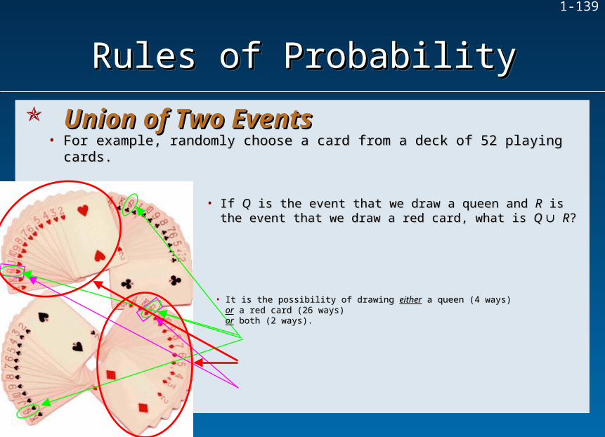
1-139
• For example, randomly choose a card from a deck of 52 playing cards. For example, randomly choose a card from a deck of 52 playing cards.
• It is the possibility of drawing It is the possibility of drawing eithereither a queen (4 ways) a queen (4 ways) oror a red card (26 ways) a red card (26 ways) oror both (2 ways). both (2 ways).
• If If QQ is the event that we draw a queen and is the event that we draw a queen and RR is the event is the event that we draw a red card, what is that we draw a red card, what is Q Q RR??
Union of Two EventsUnion of Two Events
Rules of ProbabilityRules of ProbabilityRules of ProbabilityRules of Probability
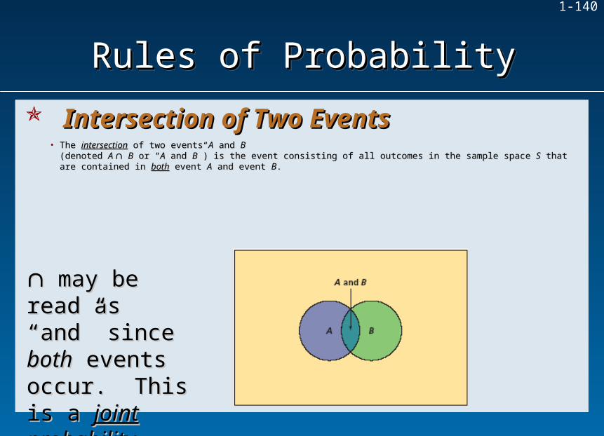
1-140
• The The intersectionintersection of two events of two events AA and and BB (denoted (denoted A A BB or “ or “AA and and BB”) is the event consisting of all outcomes in the sample space ”) is the event consisting of all outcomes in the sample space SS that are contained in that are contained in bothboth event event AA and event and event BB. .
may be read may be read as “and” since as “and” since bothboth events events occur. This is a occur. This is a joint probabilityjoint probability..
Intersection of Two EventsIntersection of Two Events
Rules of ProbabilityRules of ProbabilityRules of ProbabilityRules of Probability

1-141
• It is the possibility of getting It is the possibility of getting bothboth a queen a queen andand a red card a red card (2 ways).(2 ways).
• If If QQ is the event that we draw a queen and is the event that we draw a queen and RR is the event that we draw a red card, is the event that we draw a red card, what is what is Q Q RR??
• For example, randomly choose a card from a deck of 52 playing cards. For example, randomly choose a card from a deck of 52 playing cards. Intersection of Two EventsIntersection of Two Events
Rules of ProbabilityRules of ProbabilityRules of ProbabilityRules of Probability

1-142
• The The general law of additiongeneral law of addition states that the probability of the union of two events states that the probability of the union of two events AA and and B B is:is:
PP((A A BB) = ) = PP((AA) + ) + PP((BB) – ) – PP((A A BB))
When you add When you add the the PP((AA) and ) and PP((BB) together, ) together, you count the you count the P(A and B) P(A and B) twice.twice.
So, you have So, you have to subtract to subtract PP((A A BB) to ) to avoid over-avoid over-stating the stating the probability.probability.
A B
A and B
General Law of AdditionGeneral Law of Addition
Rules of ProbabilityRules of ProbabilityRules of ProbabilityRules of Probability

1-143
• For the card example:For the card example:
PP((QQ) = 4/52) = 4/52 (4 queens in a deck) (4 queens in a deck)
= 4/52 + 26/52 – 2/52= 4/52 + 26/52 – 2/52
PP((Q Q RR) = ) = PP((QQ) + ) + PP((RR) – ) – PP((Q Q QQ))
Q4/52
R26/52
Q and R = 2/52
General Law of AdditionGeneral Law of Addition
Rules of ProbabilityRules of ProbabilityRules of ProbabilityRules of Probability
= 28/52 = .5385 or 53.85%= 28/52 = .5385 or 53.85%
PP((RR) = 26/52 (26 red cards in a deck)) = 26/52 (26 red cards in a deck)PP((Q Q RR) = 2/52 (2 red queens in a deck)) = 2/52 (2 red queens in a deck)
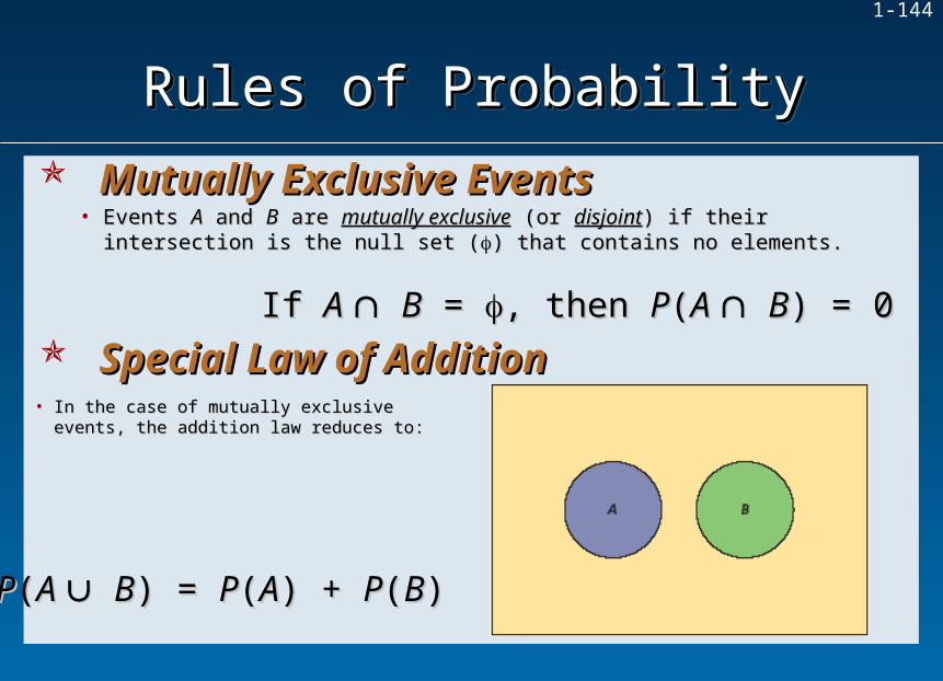
1-144
• Events Events AA and and BB are are mutually exclusivemutually exclusive (or (or disjointdisjoint) if their intersection is the null ) if their intersection is the null set (set () that contains no elements.) that contains no elements.
If If A A BB = = , then , then PP((A A BB) = 0) = 0
• In the case of mutually exclusive In the case of mutually exclusive events, the addition law reduces to:events, the addition law reduces to:
PP((A A BB) = ) = PP((AA) + ) + PP((BB))
Mutually Exclusive EventsMutually Exclusive Events
Rules of ProbabilityRules of ProbabilityRules of ProbabilityRules of Probability
Special Law of AdditionSpecial Law of Addition
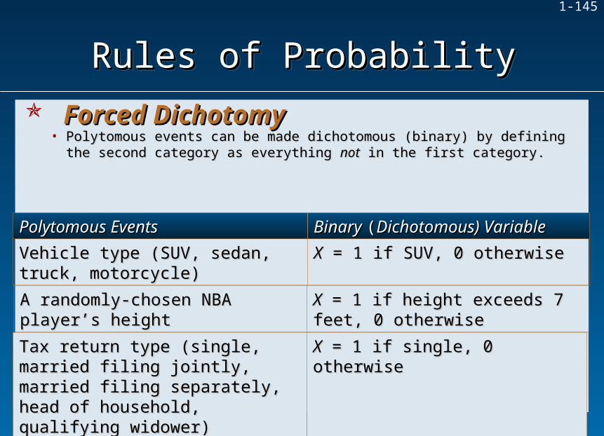
1-145
• Polytomous events can be made dichotomous (binary) by defining the second Polytomous events can be made dichotomous (binary) by defining the second category as everything category as everything notnot in the first category. in the first category.
Polytomous Events Polytomous Events Binary Binary ((Dichotomous) VariableDichotomous) Variable
Vehicle type (SUV, sedan, truck, Vehicle type (SUV, sedan, truck, motorcycle)motorcycle)
XX = 1 if SUV, 0 otherwise = 1 if SUV, 0 otherwise
Forced DichotomyForced Dichotomy
Rules of ProbabilityRules of ProbabilityRules of ProbabilityRules of Probability
A randomly-chosen NBA player’s A randomly-chosen NBA player’s heightheight
XX = 1 if height exceeds 7 feet, 0 = 1 if height exceeds 7 feet, 0 otherwiseotherwise
Tax return type (single, married filing Tax return type (single, married filing jointly, married filing separately, head jointly, married filing separately, head of household, qualifying widower) of household, qualifying widower)
XX = 1 if single, 0 otherwise = 1 if single, 0 otherwise

1-146
• The probability of event The probability of event AA givengiven that event that event BB has occurred. has occurred.
• Denoted Denoted PP((A A | | BB). ). The vertical line “ | ” is read as “given.”The vertical line “ | ” is read as “given.”
( )( | )
( )
P A BP A B
P B
for for PP((BB) > 0 and ) > 0 and
undefined otherwise undefined otherwise
Conditional ProbabilityConditional Probability
Rules of ProbabilityRules of ProbabilityRules of ProbabilityRules of Probability
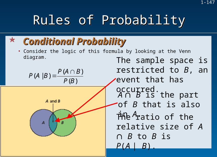
1-147
• Consider the logic of this formula by looking at the Venn diagram.
( )( | )
( )
P A BP A B
P B
The sample space is restricted to B, an event that has occurred.
A B is the part of B that is also in A.
The ratio of the relative size of A B to B is P(A | B).
Conditional ProbabilityConditional Probability
Rules of ProbabilityRules of ProbabilityRules of ProbabilityRules of Probability
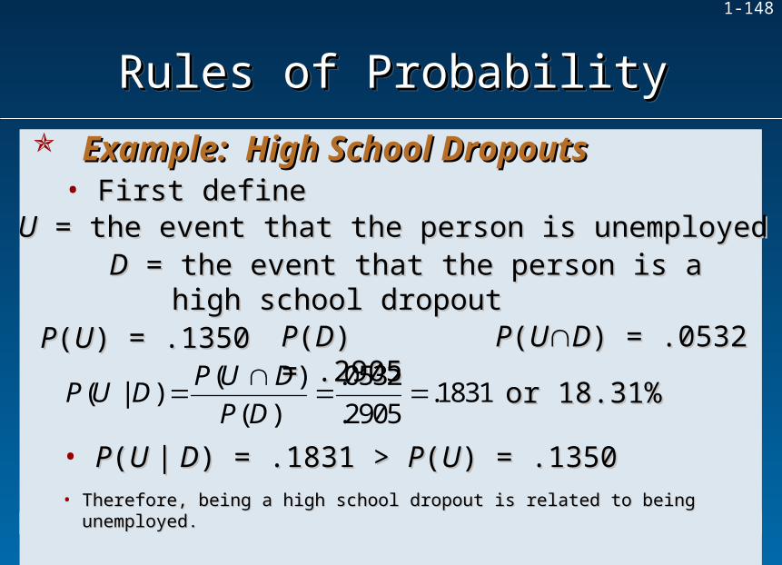
1-148
• First defineFirst defineUU = the event that the person is unemployed = the event that the person is unemployedDD = the event that the person is a high school = the event that the person is a high school
dropoutdropoutPP((UU) = .1350) = .1350 PP((DD) = .2905) = .2905 PP((UUDD) = .0532) = .0532
( ) .0532( | ) .1831
( ) .2905
P U DP U D
P D
or 18.31%or 18.31%
• PP((U | DU | D) = .1831 > ) = .1831 > PP((UU) = .1350) = .1350• Therefore, being a high school dropout is related to being unemployed.Therefore, being a high school dropout is related to being unemployed.
Example: High School DropoutsExample: High School Dropouts
Rules of ProbabilityRules of ProbabilityRules of ProbabilityRules of Probability

1-149
IST 203: Statistics for Social Sciences
IST 203: Statistics for Social Sciences
Lecture 6

1-150
Probability ModelsProbability ModelsProbability ModelsProbability Models
• A A randomrandom (or stochastic) (or stochastic) processprocess is a repeatable is a repeatable random experiment.random experiment.
• Probability can be used to analyze random (or stochastic) Probability can be used to analyze random (or stochastic) processes and to understand business processes.processes and to understand business processes.
• For example, each call arriving at the L.L. Bean For example, each call arriving at the L.L. Bean order center is a random experiment in which the order center is a random experiment in which the variable of interest is the amount of the order.variable of interest is the amount of the order.
Probability ModelsProbability Models

1-151
Discrete DistributionsDiscrete Distributions
• A A random variablerandom variable is a function or rule that assigns a numerical value to is a function or rule that assigns a numerical value to each outcome in the sample space of a random experiment.each outcome in the sample space of a random experiment.
Random VariablesRandom Variables
• Nomenclature:Nomenclature:- Capital letters are used to represent- Capital letters are used to represent random variablesrandom variables (e.g., (e.g., XX, , YY).).- Lower case letters are used to represent - Lower case letters are used to represent valuesvalues of the random variable (e.g., of the random variable (e.g., xx, , yy).).
• A A discrete random variablediscrete random variable has a countable has a countable number of distinct values.number of distinct values.

1-152
Probability DistributionsProbability Distributions• A A discrete probability distributiondiscrete probability distribution assigns a probability assigns a probability
to each value of a discrete random variable to each value of a discrete random variable XX..
• To be a valid probability, each probability must be To be a valid probability, each probability must be betweenbetween 0 0 P P((xxii)) 1 1
• and the sum of all the probabilities for the values of and the sum of all the probabilities for the values of XX must be equal to unity. must be equal to unity.
1
( ) 1n
ii
P x
Discrete DistributionsDiscrete Distributions

1-153
When you flip a coin When you flip a coin three times, the three times, the sample space has sample space has eight equally likely eight equally likely simple events. simple events. They are:They are:
Example: Coin FlipsExample: Coin Flips
11stst Toss Toss 22ndnd Toss 3 Toss 3rdrd Toss TossHH HH HHHH HH TTHH TT HHHH TT TTTT HH HHTT HH TTTT TT HHTT TT TT
Discrete DistributionsDiscrete Distributions

1-154
If If XX is the number of heads, then is the number of heads, then XX is a random is a random variable whose probability distribution is as follows:variable whose probability distribution is as follows:
Possible EventsPossible Events xx PP((xx))
TTTTTT 00 1/81/8
HTT, THT, TTHHTT, THT, TTH 11 3/83/8
HHT, HTH, THHHHT, HTH, THH 22 3/83/8
HHHHHH 33 1/81/8
TotalTotal 11
Discrete DistributionsDiscrete Distributions
Example: Coin FlipsExample: Coin Flips

1-155
• The The expected valueexpected value E E((XX) of a discrete random variable is the ) of a discrete random variable is the sum of all sum of all XX-values -values weightedweighted by their respective probabilities. by their respective probabilities.
• The The EE((XX) is a measure of ) is a measure of central tendencycentral tendency..
• If there are If there are nn distinct values of distinct values of XX, ,
1
( ) ( )n
i ii
E X x P x
Discrete DistributionsDiscrete Distributions
Expected ValueExpected Value

1-156
The probability distribution of emergency service calls The probability distribution of emergency service calls on Sunday by Ace Appliance Repair is:on Sunday by Ace Appliance Repair is:
What is the average or What is the average or expectedexpected number of service number of service calls?calls?
xx PP((xx))
00 0.050.05
11 0.100.10
22 0.300.30
33 0.250.25
44 0.200.20
55 0.100.10
TotalTotal 1.001.00
Discrete DistributionsDiscrete Distributions
Example: Service CallsExample: Service Calls

1-157
The sum of the The sum of the xPxP((xx) column is the expected ) column is the expected value or mean of the discrete distribution.value or mean of the discrete distribution.
x P(x) xP(x)
0 0.05 0.00
1 0.10 0.10
2 0.30 0.60
3 0.25 0.75
4 0.20 0.80
5 0.10 0.50
Total 1.00 2.75
5
1
( ) ( )i ii
E X x P x
First calculate First calculate xxiiPP((xxii):):
Discrete DistributionsDiscrete Distributions
Example: Service CallsExample: Service Calls

1-158
0.00
0.05
0.10
0.15
0.20
0.25
0.30
0 1 2 3 4 5
Number of Service Calls
Pro
bab
ilit
y
This particular This particular probability distribution probability distribution is not symmetric is not symmetric around the mean around the mean = 2.75. = 2.75.
However, the mean However, the mean is still the balancing is still the balancing point, or fulcrum.point, or fulcrum. = 2.75= 2.75
Because Because EE((XX) is an ) is an averageaverage, it does not have to be an , it does not have to be an observable point.observable point.
Discrete DistributionsDiscrete Distributions
Example: Service CallsExample: Service Calls

1-159
• Expected value is the basis of life insurance.Expected value is the basis of life insurance.• For example, what is the probability that a 30-year-old white female will For example, what is the probability that a 30-year-old white female will
die within the next year?die within the next year?
• Based on mortality statistics, the probability is .00059 and the probability Based on mortality statistics, the probability is .00059 and the probability of living another year is 1 - .00059 = .99941.of living another year is 1 - .00059 = .99941.
• What premium should a life insurance company charge to break even on What premium should a life insurance company charge to break even on a $500,000 1-year term policy?a $500,000 1-year term policy?
Discrete DistributionsDiscrete Distributions
Application: Life InsuranceApplication: Life Insurance
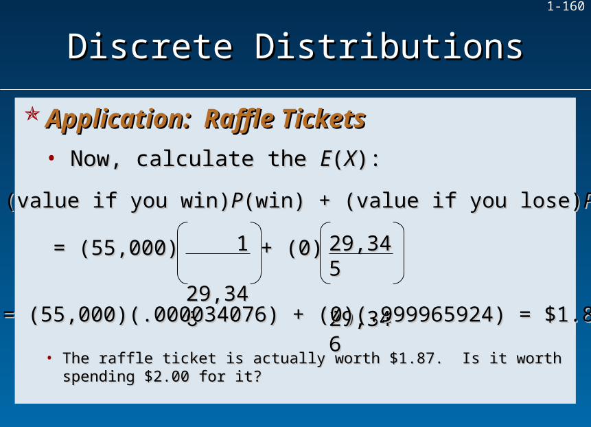
1-160
• Now, calculate the Now, calculate the EE((XX):):
EE((XX)) = (value if you win)= (value if you win)PP(win) + (value if you lose)(win) + (value if you lose)PP(lose)(lose)
= (55,000)= (55,000) 1 1 29,34629,346
+ (0)+ (0) 29,345 29,345 29,34629,346
= (55,000)(.000034076) + (0)(.999965924) = $1.87= (55,000)(.000034076) + (0)(.999965924) = $1.87
• The raffle ticket is actually worth $1.87. Is it worth spending $2.00 for The raffle ticket is actually worth $1.87. Is it worth spending $2.00 for it?it?
Discrete DistributionsDiscrete Distributions
Application: Raffle TicketsApplication: Raffle Tickets

1-161
• If there are If there are nn distinct values of distinct values of XX, then the , then the variancevariance of a discrete of a discrete random variable is:random variable is:
• The variance is a The variance is a weightedweighted average of the average of the dispersiondispersion about the mean and about the mean and is denoted either as is denoted either as 22 or or VV((XX).).
2 2
1
( ) [ ] ( )n
i ii
V X x P x
• The The standard deviationstandard deviation is the square root of the variance and is denoted is the square root of the variance and is denoted ..
2 ( )V X
Discrete DistributionsDiscrete Distributions
Variance and Standard DeviationVariance and Standard Deviation
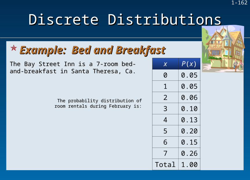
1-162
The probability distribution of The probability distribution of room rentals during February is:room rentals during February is:
The Bay Street Inn is a 7-room bed-and-The Bay Street Inn is a 7-room bed-and-breakfast in Santa Theresa, Ca.breakfast in Santa Theresa, Ca.
x P(x)
0 0.05
1 0.05
2 0.06
3 0.10
4 0.13
5 0.20
6 0.15
7 0.26
Total 1.00
Discrete DistributionsDiscrete Distributions
Example: Bed and BreakfastExample: Bed and Breakfast

1-163
First find the expected valueFirst find the expected value x P(x)
0 0.05
1 0.05
2 0.06
3 0.10
4 0.13
5 0.20
6 0.15
7 0.26
Total 1.00
7
1
( ) ( )i ii
E X x P x
= 4.71 rooms= 4.71 rooms
x P(x)
0.00
0.05
0.12
0.30
0.52
1.00
0.90
1.82
= 4.71
Discrete DistributionsDiscrete Distributions
Example: Bed and BreakfastExample: Bed and Breakfast

1-164
The The EE((XX) is then used to find ) is then used to find the variance:the variance:
xx PP((xx)) x Px P((xx))
00 0.050.05 0.000.00
11 0.050.05 0.050.05
22 0.060.06 0.120.12
33 0.100.10 0.300.30
44 0.130.13 0.520.52
55 0.200.20 1.001.00
66 0.150.15 0.900.90
77 0.260.26 1.821.82
TotalTotal 1.001.00 = 4.71= 4.71
72 2
1
( ) [ ] ( )i ii
V X x P x
= 4.2259 rooms2
The standard deviation is:The standard deviation is:
= 4.2259= 4.2259 = 2.0577 rooms= 2.0577 rooms
[[xx]]22 P P((xx))
1.1092051.109205
0.6882050.688205
0.4406460.440646
0.2924100.292410
0.0655330.065533
0.0168200.016820
0.2496150.249615
1.3634661.363466
22 = 4.225900 = 4.225900
[[xx]]22
22.184122.1841
13.764113.7641
7.34417.3441
2.92412.9241
0.50410.5041
0.08410.0841
1.66411.6641
5.24415.2441
Discrete DistributionsDiscrete Distributions
Example: Bed and BreakfastExample: Bed and Breakfast
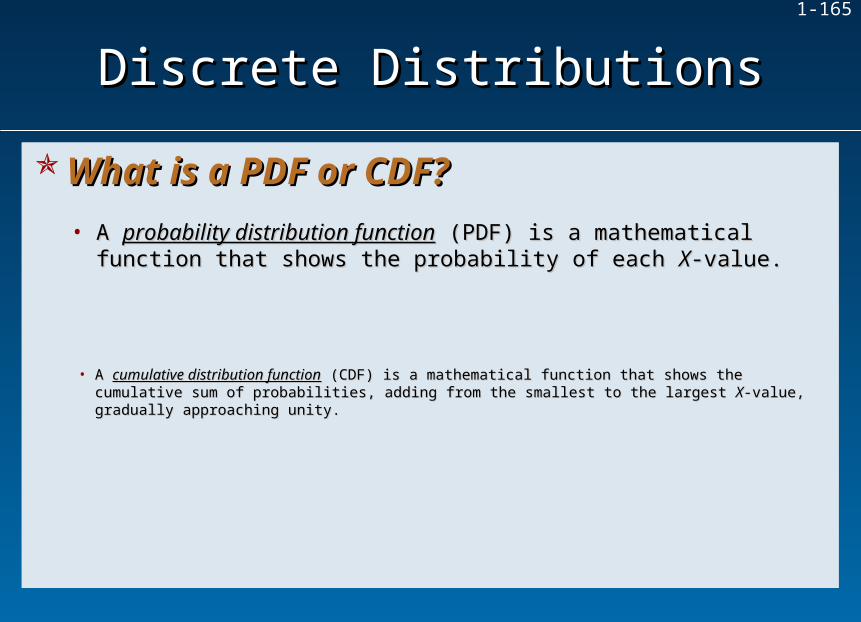
1-165
• A A probability distribution functionprobability distribution function (PDF) is a mathematical function that (PDF) is a mathematical function that shows the probability of each shows the probability of each XX-value.-value.
• A A cumulative distribution functioncumulative distribution function (CDF) is a mathematical function that shows the cumulative (CDF) is a mathematical function that shows the cumulative sum of probabilities, adding from the smallest to the largest sum of probabilities, adding from the smallest to the largest XX-value, gradually approaching unity.-value, gradually approaching unity.
Discrete DistributionsDiscrete Distributions
What is a PDF or CDF?What is a PDF or CDF?

1-166
0.00
0.05
0.10
0.15
0.20
0.25
0 1 2 3 4 5 6 7 8 9 10 11 12 13 14
Value of X
Pro
bab
ility
0.00
0.10
0.20
0.30
0.40
0.50
0.60
0.70
0.80
0.90
1.00
0 1 2 3 4 5 6 7 8 9 10 11 12 13 14
Value of X
Pro
bab
ility
Illustrative PDFIllustrative PDF(Probability Density Function)(Probability Density Function)
Cumulative CDFCumulative CDF(Cumulative Density Function)(Cumulative Density Function)
Consider the following illustrative histograms:Consider the following illustrative histograms:
The equations for these functions depend on the The equations for these functions depend on the parameter(s)parameter(s) of the distribution. of the distribution.
Discrete DistributionsDiscrete Distributions
What is a PDF or CDF?What is a PDF or CDF?

1-167
Characteristics of the Uniform DistributionCharacteristics of the Uniform Distribution• The The uniform distributionuniform distribution describes a random variable with a finite number describes a random variable with a finite number
of integer values from of integer values from aa to to bb (the only two parameters). (the only two parameters).
• Each value of the random variable is equally likely to occur.Each value of the random variable is equally likely to occur.
• Consider the following summary of the uniform distribution:Consider the following summary of the uniform distribution:
Uniform DistributionUniform Distribution

1-168
ParametersParameters aa = lower limit = lower limitbb = upper limit = upper limit
PDFPDF
RangeRange aa xx bb
MeanMean
Std. Dev.Std. Dev.
Random data generation Random data generation in Excelin Excel =a+INT((b-a+1)*RAND())=a+INT((b-a+1)*RAND())
CommentsComments Used as a benchmark, to generate random Used as a benchmark, to generate random integers, or to create other distributions.integers, or to create other distributions.
2( ) 1 1
12
b a
1( )
1P x
b a
2
a b
Uniform DistributionUniform Distribution

1-169
• The number of dots on the roll of a die form a uniform random variable The number of dots on the roll of a die form a uniform random variable with six equally likely integer values: 1, 2, 3, 4, 5, 6with six equally likely integer values: 1, 2, 3, 4, 5, 6
0.00
0.02
0.04
0.06
0.08
0.10
0.12
0.14
0.16
0.18
1 2 3 4 5 6
Number of Dots Showing on the Die
Pro
bab
ility
0.00
0.10
0.20
0.30
0.40
0.50
0.60
0.70
0.80
0.90
1.00
1 2 3 4 5 6
Number of Dots Showing on the Die
Pro
bab
ility
PDF for one diePDF for one die CDF for one dieCDF for one die
• What is the probability of rolling any of these?What is the probability of rolling any of these?
Uniform DistributionUniform Distribution
Example: Rolling a DieExample: Rolling a Die

1-170
• The PDF for all The PDF for all xx is: is:
• Calculate the standard deviation as:Calculate the standard deviation as:
• Calculate the mean as:Calculate the mean as:
1 1 1( )
1 6 1 1 6P x
b a
1 63.5
2 2
a b
2 2( ) 1 1 (6 1) 1 1
1.70812 12
b a
Uniform DistributionUniform Distribution
Example: Rolling a DieExample: Rolling a Die
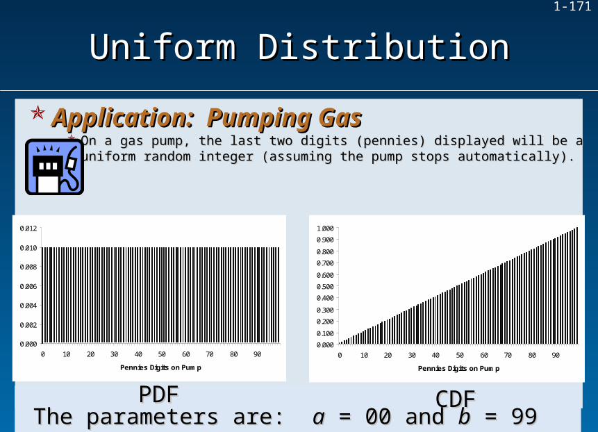
1-171
On a gas pump, the last two digits (pennies) displayed will be a uniform On a gas pump, the last two digits (pennies) displayed will be a uniform random integer (assuming the pump stops automatically).random integer (assuming the pump stops automatically).
0.000
0.002
0.004
0.006
0.008
0.010
0.012
0 10 20 30 40 50 60 70 80 90
Pennies Digits on Pump
0.000
0.100
0.200
0.300
0.400
0.500
0.600
0.700
0.800
0.900
1.000
0 10 20 30 40 50 60 70 80 90
Pennies Digits on Pump
PDFPDF CDFCDFThe parameters are: The parameters are: aa = 00 and = 00 and bb = 99 = 99
Uniform DistributionUniform Distribution
Application: Pumping GasApplication: Pumping Gas
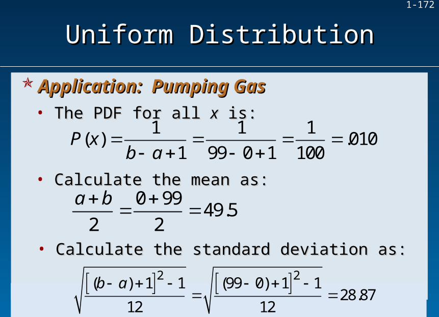
1-172
• The PDF for all The PDF for all xx is: is:
• Calculate the standard deviation as:Calculate the standard deviation as:
• Calculate the mean as:Calculate the mean as:
1 1 1( ) .010
1 99 0 1 100P x
b a
0 9949.5
2 2
a b
2 2( ) 1 1 (99 0) 1 1
28.8712 12
b a
Uniform DistributionUniform Distribution
Application: Pumping GasApplication: Pumping Gas

1-173
• A random experiment with only 2 outcomes is a A random experiment with only 2 outcomes is a Bernoulli experimentBernoulli experiment..
• One outcome is arbitrarily labeled a One outcome is arbitrarily labeled a “success” (denoted “success” (denoted XX = 1) and the other a “failure” (denoted = 1) and the other a “failure” (denoted XX = 0). = 0).
is the is the PP(success), 1 – (success), 1 – is the is the PP(failure).(failure).
• Note that Note that PP(0) + (0) + PP(1) = (1 – (1) = (1 – ) + ) + = 1 and = 1 and0 0 << << 1. 1.
• ““Success” is usually defined as the less likely outcome so that Success” is usually defined as the less likely outcome so that < .5 < .5 for convenience.for convenience.
Bernoulli ExperimentsBernoulli Experiments
Bernoulli DistributionBernoulli Distribution

1-174
Bernoulli Experiment Possible Outcomes Probability of “Success”
Flip a coin 1 = heads0 = tails
= .50
Consider the following Bernoulli experiments:Consider the following Bernoulli experiments:
Inspect a jet turbine blade 1 = crack found0 = no crack found
= .001
Purchase a tank of gas 1 = pay by credit card0 = do not pay by credit card
= .78
Do a mammogram test 1 = positive test0 = negative test
= .0004
Bernoulli ExperimentsBernoulli Experiments
Bernoulli DistributionBernoulli Distribution
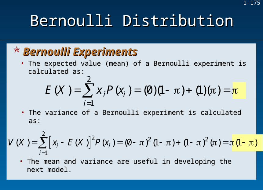
1-175
2
2 2 2
1
( ) ( ) ( ) (0 ) (1 ) (1 ) ( ) (1 )i ii
V X x E X P x
• The expected value (mean) of a Bernoulli experiment is calculated as:The expected value (mean) of a Bernoulli experiment is calculated as:
2
1
( ) ( ) (0)(1 ) (1)( )i ii
E X x P x
• The variance of a Bernoulli experiment is calculated as:The variance of a Bernoulli experiment is calculated as:
• The mean and variance are useful in developing the next model.The mean and variance are useful in developing the next model.
Bernoulli DistributionBernoulli Distribution
Bernoulli ExperimentsBernoulli Experiments

1-176
• The The binomial distributionbinomial distribution arises when a Bernoulli experiment is arises when a Bernoulli experiment is repeated repeated nn times. times.
• Each Bernoulli trial is independent so the probability of success Each Bernoulli trial is independent so the probability of success remains remains constant on each trial.constant on each trial.
• In a binomial experiment, we are interested in In a binomial experiment, we are interested in XX = number of successes = number of successes in in nn trials. So, trials. So,
XX = = xx11 + + xx22 + ... + + ... + xxnn • The probability of a particular number of successes The probability of a particular number of successes PP((XX) is determined ) is determined
by parameters by parameters nn and and ..
Binomial DistributionBinomial Distribution
Characteristics of the Binomial DistributionCharacteristics of the Binomial Distribution
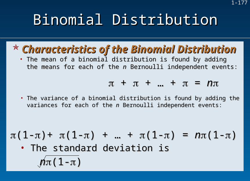
1-177
• The mean of a binomial distribution is found by adding the means for The mean of a binomial distribution is found by adding the means for each of the each of the nn Bernoulli independent events: Bernoulli independent events:
+ + + … + + … + = = nn• The variance of a binomial distribution is found by adding the variances The variance of a binomial distribution is found by adding the variances
for each of the for each of the nn Bernoulli independent events: Bernoulli independent events:
(1-(1-)+ )+ (1-(1-) + … + ) + … + (1-(1-) = ) = nn(1-(1-))• The standard deviation isThe standard deviation is
nn(1-(1-))
Binomial DistributionBinomial Distribution
Characteristics of the Binomial DistributionCharacteristics of the Binomial Distribution

1-178
Parameters n = number of trials = probability of success
Excel function =BINOMDIST(k,n,,0)
Range X = 0, 1, 2, . . ., n
Mean n
Std. Dev.
Random data generation in Excel
Sum n values of =1+INT(2*RAND()) or use Excel’s Tools | Data Analysis
Comments Skewed right if < .50, skewed left if > .50, and symmetric if = .50.
!( ) (1 )
!( )!x n xn
P xx n x
(1 )n
Binomial DistributionBinomial Distribution
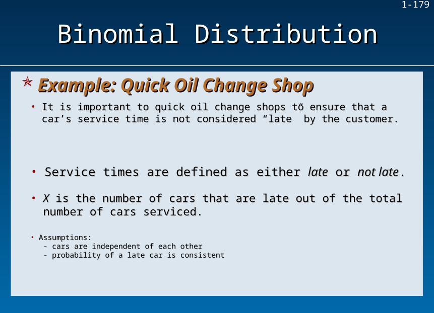
1-179
• It is important to quick oil change shops to ensure that a car’s service It is important to quick oil change shops to ensure that a car’s service time is not considered “late” by the customer.time is not considered “late” by the customer.
• Service times are defined as either Service times are defined as either latelate or or not latenot late..• XX is the number of cars that are late out of the total number of cars is the number of cars that are late out of the total number of cars
serviced.serviced.
• Assumptions:Assumptions: - cars are independent of each other - cars are independent of each other - probability of a late car is consistent - probability of a late car is consistent
Binomial DistributionBinomial Distribution
Example: Quick Oil Change ShopExample: Quick Oil Change Shop

1-180
• What is the probability that exactly 2 of the next What is the probability that exactly 2 of the next nn = 10 cars serviced = 10 cars serviced are late (are late (PP((X X = 2))?= 2))?
• PP(car is late) = (car is late) = = .10 = .10
• PP(car not late) = 1 - (car not late) = 1 - = .90 = .90
!( ) (1 )
!( )!x n xn
P xx n x
PP((X X = 2) = = 2) = 10!10!
2!(10-2)!2!(10-2)!(.1)(.1)22(1-.10)(1-.10)10-210-2 = .1937= .1937
Binomial DistributionBinomial Distribution
Example: Quick Oil Change ShopExample: Quick Oil Change Shop

1-181
• On average, 20% of the emergency room patients at Greenwood General Hospital lack health insurance.
• In a random sample of 4 patients, what is the probability that at least 2 will be uninsured?
• X = number of uninsured patients (“success”)• P(uninsured) = = 20% or .2020% or .20
• P(insured) = 1 – = 1 – .20 = .801 – .20 = .80
• n =
• The range is X = 0, 1, 2, 3, 4 patients.4 patients4 patients
Binomial DistributionBinomial Distribution
Application: Uninsured PatientsApplication: Uninsured Patients

1-182
• What is the mean and standard deviation of this binomial distribution?What is the mean and standard deviation of this binomial distribution?
Mean = Mean = = = nn = = (4)(.20) = (4)(.20) = 0.8 patients0.8 patients
Standard deviation = Standard deviation = = = (1 )n
= 4(.20(1-.20)= 4(.20(1-.20)
= 0.8 patients= 0.8 patients
Binomial DistributionBinomial Distribution
Application: Uninsured PatientsApplication: Uninsured Patients
1-183
IST 203: Statistics for Social Sciences
IST 203: Statistics for Social Sciences
Lecture 7

1-184
Continuous VariablesContinuous VariablesContinuous VariablesContinuous Variables
• Discrete VariableDiscrete Variable – each value of – each value of XX has its own has its own probability probability PP((XX).).
• Continuous VariableContinuous Variable – events are – events are intervalsintervals and and probabilities are areas underneath smooth probabilities are areas underneath smooth curves. A single point has no probability.curves. A single point has no probability.
Events as IntervalsEvents as Intervals
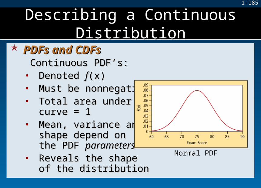
1-185
Describing a Continuous Describing a Continuous DistributionDistribution
Describing a Continuous Describing a Continuous DistributionDistribution
Continuous PDF’s:Continuous PDF’s:• Denoted Denoted ff(x)(x)• Must be nonnegativeMust be nonnegative• Total area under Total area under
curve = 1curve = 1• Mean, variance and Mean, variance and
shape depend onshape depend onthe PDF the PDF parametersparameters
• Reveals the shape Reveals the shape of the distributionof the distribution
PDFs and CDFsPDFs and CDFs
Normal PDF
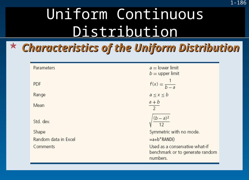
1-186
Uniform Continuous Uniform Continuous DistributionDistribution
Uniform Continuous Uniform Continuous DistributionDistribution
Characteristics of the Uniform DistributionCharacteristics of the Uniform Distribution

1-187
Uniform Continuous Uniform Continuous DistributionDistribution
Uniform Continuous Uniform Continuous DistributionDistribution
Example: Anesthesia EffectivenessExample: Anesthesia Effectiveness• An oral surgeon injects a painkiller prior to An oral surgeon injects a painkiller prior to
extracting a tooth. Given the varying extracting a tooth. Given the varying characteristics of patients, the dentist views the characteristics of patients, the dentist views the time for anesthesia effectiveness as a uniform time for anesthesia effectiveness as a uniform random variable that takes between 15 minutes random variable that takes between 15 minutes and 30 minutes.and 30 minutes.
• XX is is UU(15, 30)(15, 30)• aa = 15, = 15, bb = 30, find the mean and standard = 30, find the mean and standard
deviation.deviation.

1-188
Uniform Continuous Uniform Continuous DistributionDistribution
Uniform Continuous Uniform Continuous DistributionDistribution
Example: Anesthesia EffectivenessExample: Anesthesia Effectiveness
= = aa + + bb 2 2 = =
15 + 3015 + 30 2 2 = = 22.5 minutes 22.5 minutes
= = ((bb – – aa))22 12 12 = = 4.33 minutes 4.33 minutes
(30 – 15)(30 – 15)22 12 12==
Find the probability that the anesthetic takes between Find the probability that the anesthetic takes between 20 and 25 minutes.20 and 25 minutes.
PP((cc < < XX < < dd) = () = (dd – – cc)/()/(bb – – aa))
(25 – 20)/(30 – 15)(25 – 20)/(30 – 15)PP(20 < (20 < XX < 25) = < 25) = = 5/15 = 0.3333 or 33.33%= 5/15 = 0.3333 or 33.33%

1-189
Normal DistributionNormal DistributionNormal DistributionNormal Distribution
What is Normal?What is Normal?A normal random variable should:A normal random variable should:• Be measured on a continuous scale.Be measured on a continuous scale.• Possess clear central tendency.Possess clear central tendency.• Have only one peak (unimodal).Have only one peak (unimodal).• Exhibit tapering tails.Exhibit tapering tails.• Be symmetric about the mean (equal tails).Be symmetric about the mean (equal tails).
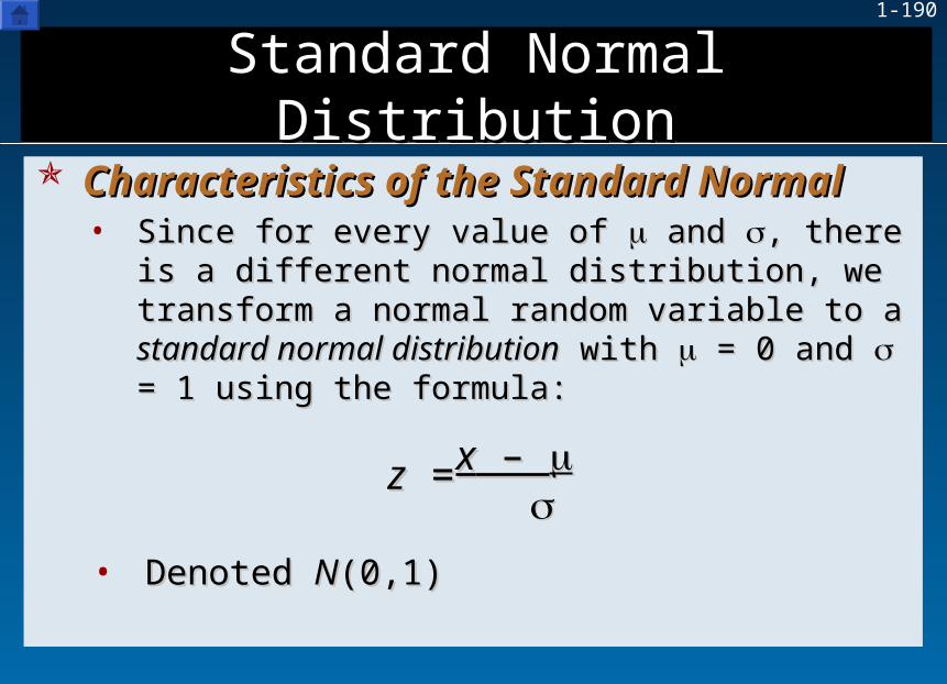
1-190
Standard Normal DistributionStandard Normal DistributionStandard Normal DistributionStandard Normal Distribution
Characteristics of the Standard NormalCharacteristics of the Standard Normal• Since for every value of Since for every value of and and , there is a , there is a
different normal distribution, we transform a different normal distribution, we transform a normal random variable to a normal random variable to a standard normal standard normal distributiondistribution with with = 0 and = 0 and = 1 using the = 1 using the formula:formula:
zz = = xx – –
• Denoted Denoted NN(0,1)(0,1)
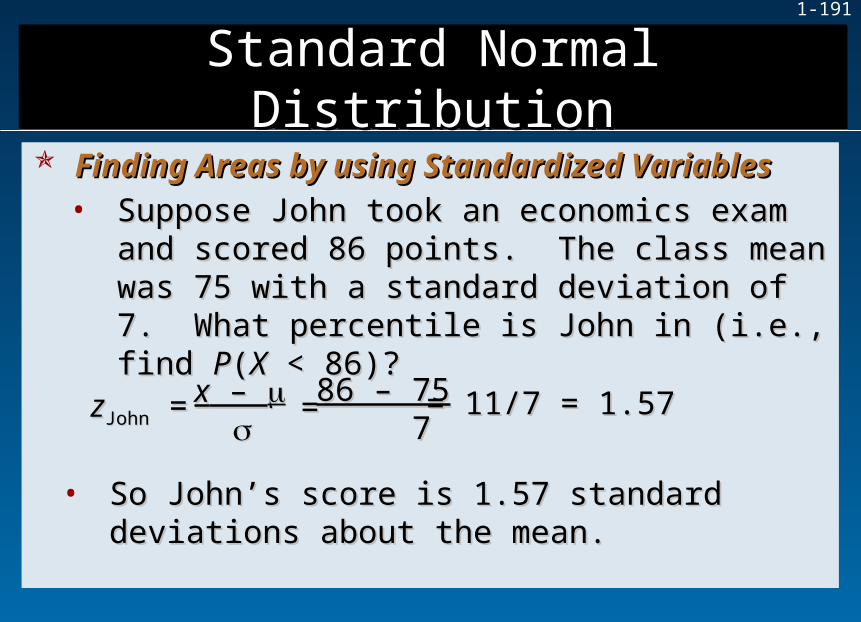
1-191
Standard Normal DistributionStandard Normal DistributionStandard Normal DistributionStandard Normal Distribution
Finding Areas by using Standardized VariablesFinding Areas by using Standardized Variables• Suppose John took an economics exam and Suppose John took an economics exam and
scored 86 points. The class mean was 75 with a scored 86 points. The class mean was 75 with a standard deviation of 7. What percentile is John standard deviation of 7. What percentile is John in (i.e., find in (i.e., find PP((XX < 86)? < 86)?
zzJohnJohn = = xx – –
== 86 – 7586 – 75 7 7
= 11/7 = 1.57= 11/7 = 1.57
• So John’s score is 1.57 standard deviations about So John’s score is 1.57 standard deviations about the mean. the mean.
Related Documents