Isotropic-to-nematic transition in liquid-crystalline heteropolymers: I. Formalism and main-chain liquid-crystalline polymers

INSTITUTE OF PHYSICS PUBLISHING JOURNAL OF PHYSICS: CONDENSED MATTER

J. Phys.: Condens. Matter 18 (2006) 9359–9374 doi:10.1088/0953-8984/18/41/004

Isotropic-to-nematic transition in liquid-crystallineheteropolymers: II. Side-chain liquid-crystallinepolymers

Paul P F Wessels1 and Bela M Mulder

FOM Institute for Atomic and Molecular Physics (AMOLF), Kruislaan 407, 1098 SJ Amsterdam,The Netherlands

E-mail: [email protected]

Received 19 January 2006, in final form 28 June 2006Published 29 September 2006Online at stacks.iop.org/JPhysCM/18/9359

AbstractWe apply a density functional approach for arbitrary branched liquid-crystalline(LC) heteropolymers consisting of elongated rigid rods coupled throughelastic joints developed in a companion paper (Wessels and Mulder 2006J. Phys. Condens. Matter. 18 9335) to a model for side-chain liquid-crystallinepolymers. In this model mesogenic units are coupled through finite-lengthspacers to a linear backbone polymer. The stereochemical constraints imposedat the connection between spacer and backbone are explicitly modelled. Usinga bifurcation analysis, analytical results are obtained for the spinodal density ofthe I–N transition and the variation of the degree of ordering over the variousmolecular parts at the instability as a function of the model parameters. We alsodetermine the location of the crossover between oblate and prolate backboneconformations in the nematic phase.

1. Introduction

Liquid-crystalline (LC) polymers combine the the optical properties of liquid crystals withthe mechanical and processing characteristics of polymers. To create such LC polymerslow-molecular-weight liquid-crystal forming moieties, called mesogens, are either directlyincorporated into a linear polymer backbone (main-chain LC polymers) or laterally attachedto them (side-chain LC polymers). To achieve an optimal balance of properties, it is essentialthat, on the one hand, the mesogens can freely interact to drive orientational ordering, whileon the other hand the polymer backbone retains a sufficient amount of conformational entropy.Apart from the technological interest in the combination of properties mentioned above, theseconflicting tendencies give rise to a rich phase behaviour and these systems are thereforealso interesting from a fundamental perspective [1–6]. The practical solution for achieving

1 Present address: ABN-AMRO Corporate Research, Amsterdam, The Netherlands.

0953-8984/06/419359+16$30.00 © 2006 IOP Publishing Ltd Printed in the UK 9359

9360 P P F Wessels and B M Mulder

the necessary balance of tendencies has turned out to be the insertion of more flexiblemoieties within the polymers in the form of aliphatic spacer chains [7–9]. These spacerseffectively spatially decouple the mesogens, minimizing any stereo-chemical frustration to theLC ordering process, while the polymer chain as a whole can still have an approximately coil-like conformation.

In the companion paper [10], hereafter referred to as I, we have set up a general formalismfor describing the phase behaviour of arbitrary branched liquid-crystalline (LC) heteropolymersconsisting of elongated rigid rods coupled through elastic joints. Here we will apply thisformalism to model side-chain polymers.

The history of understanding of the molecular origin of LC order has a few definitemilestones. The seminal paper of Onsager on the explanation of nematic LC order incolloidal suspensions of rigid hard rodlike particles [11], which introduced the concept ofexcluded volume, focused on entropic effects. The mean field theory of Maier and Saupe [12]successfully made contact with the large number of data on thermotropic liquid crystals. Therole of molecular flexibility was first discussed by Khokhlov and Semenov (KS) [13, 14] byextending Onsager’s theory to hard wormlike chains, and later by Warner and co-workers [15],who similarly extended the Maier–Saupe theory. We refer the reader to I for a review of howthese elements can be combined to make models of main-chain LC polymers.

Given the additional complexity, due to their heterogeneous composition and branchedgeometry, it is not surprising that much less work has been done on LC ordering in side-chainLC polymers. Khokhlov and co-workers first used a Flory type lattice approach [16, 17]. Lateron a more realistic off-lattice model for side-chain LC polymers was considered by Warner et al(WWR) [18, 19]. In their model rigid mesogenic side-groups are directly laterally connectedto a semi-flexible backbone. Except for the bending interactions of the wormlike backbone,all interactions between the various molecular components are treated in a Maier–Saupe typemean-field manner. They have explored the full (nematic) phase diagram, finding three nematicphases, first-order phase transition between them and a critical point. Later on, they includedbiaxial phases as well [20]. However, their model does not take into account that in realityadditional spacers are used as lateral connectors between the mesogens and the backbone.Moreover, the stereo-chemical constraints on the relative orientation of the side-groups withrespect to the backbone are also treated as a mean-field cross-interaction, and therefore not onthe same footing as the bending interactions of the backbone, this in spite of the fact that allthese interactions, which are related to the way the various molecular components are linkedtogether to form the whole polymer, are similar in origin and as short-range intra-molecularinteractions distinct from the inter-molecular orientational interactions. One aim of the presentwork is to specifically address these two shortcomings.

The generic model for side-chain LC polymers we consider in this paper consist of threedifferent components: a polymer backbone, mesogens and spacer chains, that laterally connectthese mesogens to the backbone. All these components are modelled as consisting of hard,slender, cylindrically symmetric rods connected through appropriate bending potentials. Theformalism we have developed in I allows us to deal with the intra-molecular interactions ofsuch a branched, but simply connected, molecule exactly. The inter-molecular interactionsare treated within the Onsager approximation. Both for the backbone polymer and the lateralspacer chains we take the wormlike chain limit. Moreover, we let the number of polymer repeatunits go to infinity, disregarding any end effects. The remaining theory is fully described by sixparameters: the length, the persistence length and the diameters of both the backbone, within asingle repeat unit, and the lateral spacers, all measured in units relative to the mesogen lengthand diameter respectively. A brief report, containing a number of numerical results on thismodel, has been presented elsewhere [21].

I–N transition in LC heteropolymers: II 9361

1

B

B

1

S

Backbone

Spacer

Mesogen

Unit

Figure 1. The model of a side-chain LC polymer we employ, with the inset showing the labellingof the segments in the different components.

The outline of the paper is as follows. In section 2.1 we briefly recall the formalismpresented in more detail in I, setting up the free-energy functional, discussing the appropriatestationarity equations, discussing the isotropic–nematic phase equilibrium and formulating thewormlike-chain limit, which is applied to both the backbone and the spacer chains. In section 3we turn to the results, first performing a bifurcation analysis of the isotropic phase. This yieldsan analytical determination of the isotropic–nematic spinodal. We explicitly determine thevalues of the model parameters for which the backbone conformation crosses over from prolateto oblate with respect to the preferred orientation of the mesogens. Finally, we present therelative degree of order along a polymer repeat unit and compare with some numerical resultspresented earlier for the same model [21].

2. Formalism

2.1. Model

We consider a fluid N LC polymers in a volume V , where we denote the polymernumber density as ρ = N/V . The polymers consist of a backbone (denoted by B)with side-chains attached laterally at regular distances. Each side-chain consists of a rigidmesogen (M) connected to the backbone via a flexible spacer (S). A repeating section ofthe backbone with a single side-chain attached we refer to as a unit, and there are Nof these units in the polymer (see figure 1). The polymer is modelled as a segmentedchain, with the segments being slender cylindrical rods. Within a unit, each of the threedifferent components τ , where τ ∈ {B, S, M}, consists of Mτ segments characterizedby a length lτ and a width dτ with lτ � dτ . Consequently, there are NMτ segmentsof each component in the whole chain and by definition there is only one mesogen perunit, hence MM = 1. Every segment has a label m which specifies its location in thechain but is also assumed to (implicitly) contain its type-specification, i.e. by the notationm ∈ τ we mean that segment m is a type-τ segment. Additionally, each segment has anorientation ωm , which is a unit vector pointing along the long axis of the segment. Theconformation of the whole polymer is then given by the orientations of all segments Ω ={ω1, ω2, . . . , ωN (MB+MS+1)}.

We assume a bending potential um,m′ = uτ,τ ′ between any two segments m ∈ τ andm ′ ∈ τ ′ which are nearest neighbours in the polymer,

9362 P P F Wessels and B M Mulder

uB,B(ωm, ω′m′ ) = −JBωm · ω′

m′

uB,S(ωm, ω′m′) =

{0 if ωm · ω′

m′ = 0

∞ if ωm · ω′m′ �= 0

uS,S(ωm, ω′m′ ) = −JSω · ω′

m′

uS,M(ωm, ω′m′ ) = −JSω · ω′

m′

(1)

which is obviously symmetric, uτ,τ ′ = uτ ′,τ . The BB, SS and SM potentials favour mutualalignment and oppose bending in a generic fashion via the orientational coupling constantsJB and JS for the backbone and the spacer respectively. The BS potential uniquely selects aperpendicular arrangement, in order to force (at least locally) the spacers to be at right angleswith the backbone, which mimics the stereo-chemical constraints inherent in this attachment.Concerning the interaction between different polymers, we assume only hard-body repulsionbetween the segments, meaning that the potential is infinity when two segments overlap andzero when they do not [11].

2.2. Stationarity equations

Within density functional theory the free energy is a functional of the single-moleculeconfiguration distribution function [22]. In the present case, we only consider homogeneousfluid phases, so this function has no spatial dependence and it reduces to ρ f (Ω). We call thefunction f (Ω) the conformational distribution function (CDF), which is normalized as follows∫

dΩ f (Ω) = 1 where∫

dΩ = ∫ ∏k dωk . The density functional (in terms of f (Ω)) for our

system in the second virial (or Onsager) approximation is given by

βF[ f ]N

= log (ρVT) +∫

dΩ f (Ω)[log f (Ω) − 1

]+ β

∫dΩ f (Ω)U(Ω) + 1

2ρ

∫dΩ dΩ′ f (Ω) f (Ω′)E(Ω,Ω′). (2)

Here, β = 1/kBT , kB the Boltzmann constant, T the temperature and VT is a product of therelevant de Broglie thermal wavelengths. The quantity U(Ω) is the total internal energy of thepolymer and is given by

U(Ω) =(m,m′)∑m,m′

um,m′(ωm, ωm′ ), (3)

where the sum runs over all m and m ′ which are nearest neighbours in the chain (notation:(m, m ′), note that m and m ′ do not need to be of the same type). In fluid phases of hard-bodymolecules a central role is played by the so-called excluded volume E(Ω,Ω′) between twomolecules. It is approximated as the sum over all segment–segment excluded volumes,

E(Ω,Ω′) =∑m,m′

em,m′ (ωm, ω′m′ ). (4)

which are em,m′ = eτ,τ ′ for m ∈ τ and m ′ ∈ τ ′. For very slender rods (lτ � dτ ) these are givenby

eτ,τ ′(ωm, ω′m′ ) = lτ lτ ′(dτ + dτ ′)| sin γ (ωm, ω′

m′)|, (5)

where γ (ω, ω′) is the planar angle between ω and ω′.At this point, we note that three approximations have been made; we neglect

(i) interactions between three or more chains simultaneously (Onsager approximation),

I–N transition in LC heteropolymers: II 9363

(ii) simultaneous interactions between two chains involving more than one pair of segments(equation (4)) and

(iii) overlaps of segments on the same chain (equation (3)).

For homogeneous bulk phases these approximations are commonly assumed to be reasonableand to retain the essential physics [23, 24]. Furthermore, we stress that for sufficiently slendersegments (lτ � dτ ) the Onsager description becomes exact [11, 25].

In equilibrium, the free energy reaches a minimum and the functional is stationary,i.e. δF/δ f (Ω) = Nμ, where μ is the chemical potential acting as a Lagrange multiplierenforcing the normalization of f (Ω). This yields the following Euler–Lagrange equation:

log f (Ω) + βU(Ω) + ρ

∫dΩ′ f (Ω′)E(Ω,Ω′) = βμ, (6)

where μ can be eliminated using∫

dΩ f (Ω) = 1.Via the following projection, we define the single-segment orientational distribution

function (ODF),

fm(ωm) =∫ ∏

k �=m

dωk f (Ω), (7)

where the integration is over all ωk except the mth. Inserting the detailed forms(equations (1), (3), (4) and (5)) in equation (6) and using equation (7), we obtain the followingset of coupled equations in terms of the ODFs:

fm(ωm) = Q−1∫ ∏

k �=m

dωk

(k,k′ )∏k,k′

wk,k′ (ωk, ωk′ )∏

k

exp

[−ρ

∑k′

∫dω′ek,k′ (ωk, ω

′) fk′ (ω′)

].

(8)

In order to ease notation we have introduced wk,k′ (ωk, ωk′ ) = exp[−βBuk,k′ (ωk, ωk′ )]. A moredetailed version of the derivation of equation (8) is given in [25] for linear homopolymersand [10] for general heteropolymers.

2.3. Isotropic and nematic phases

The isotropic phase, in which fm(ωm) = 1/4π , is always a solution to equations (8), and atlow densities also (globally) stable. At higher densities the mesogen–mesogen interactions willdrive the system towards an orientationally ordered phase: the nematic. Here we only consideruniaxial nematics and consequently it suffices to use the standard Maier–Saupe order parameteras a measure of the orientational order of a segment m,

Sm = 2π

∫ π

0dθ sin θ P2(cos θ) fm(θ), (9)

with the factor 2π in front due to the azimuthal integration (∫

dω = ∫ π

0 dθ sin θ∫ 2π

0 dφ).The average degree of order per component can be defined straightforwardly: Sτ =1/Mτ

∑m∈τ Sm . In the isotropic phase, Sτ = 0 for all three components τ ∈ {B, S, M}.

In the nematic phase, the mesogens order with respect to a certain preferred direction, givenby the director n, and, because of their direct connection to the mesogens, the same willhappen to the spacers, 0 < SM, SS < 1. However, the backbone experiences two mutuallyopposing contributions: (i) via the spacers a tendency to orient perpendicular to the mesogensis transferred whereas (ii) due to the external (nematic) field a parallel arrangement is favoured.If the first effect dominates the net nematic order is negative SB < 0 and the backbone willbe in an oblate conformation, whereas if the second effect wins the backbone will have a

9364 P P F Wessels and B M Mulder

positive order SB > 0 and be in prolate conformation2. If the spacers are relatively short andtherefore stiff, the result will be an ‘oblate nematic’ (ON), and if they are longer and floppier a‘prolate nematic’ (PN) results. The excluded volume term in the free energy scales with density,whereas intrachain bending (elastic) energy does not depend on density. Therefore, for higherdensities the system will eventually always favour a PN phase. Upon compression we thusexpect to find a phase sequence I–ON–PN or directly I–PN. In [10], we have studied numericalsolutions to equations (8) for this system, locating the I–N coexistence and computing thedependence of the order parameters of the various components in the nematic phase. It canbe shown that the transition from ON to PN is continuous and is in fact not a thermodynamicphase transition [21, 10]. In this paper, we restrict ourselves to the I–N transition and studythe properties of the I–N bifurcation point. Furthermore, we compare some of the bifurcationresults on the I–N transition to the numerical results of [21].

2.4. Wormlike chains and infinite backbones

Since Khokhlov and Semenov [13, 14], the wormlike chain concept is widely used to modelnematic ordering in partially flexible molecules. Wormlike chains are continuously flexibleobjects characterized by a persistence length [26]. In order to reduce the number of modelparameters we transform our segmented backbone and lateral spacers in wormlike chains byapplying the so-called wormlike chain limit (WCL). Going from our system of segmentedchains to continuously flexible chains, the WCL can be formulated as [25]

lB → 0, β JB → ∞, MB → ∞lS → 0, β JS → ∞, MS → ∞ (10)

where the following products and ratios stay finite:

PB = β JBlB MB = MB/β JB

PS = β JSlS MS = MS/β JS,(11)

where the quantities PB and PS turn out to be the persistence lengths and MB and MS thenumber of persistence lengths in one repeat unit [25]. Throughout this paper, an overbar denotesquantities obtained after taking the WCL. By applying the WCL to the backbone and the spacerswe can drop two model parameters: lB, JB,MB → PB,MB and lS, JS,MS → PS,MS.

We can proceed simplifying the system and drop another model parameter by assumingthat the backbone is infinitely long. In this way, every unit is effectively located in the ‘middle’of the polymer, since the influence of the free ends of the backbone is zero. We call this theinfinite backbone limit (IBL),

N → ∞ ρ → 0 with η = ρN finite, (12)

where the polymer density ρ has to go to zero in order to obtain a finite unit density η (=mesogen density, which is driving the LC phase transitions). This limit allows us to consider(effectively) only a single unit, as every unit in the chain is exactly the same as its neighbour,and as a consequence there are no ‘free end effects’.

Finally, as our system is scale invariant we can use dimensionless length scales. Themesogens are the largest segments (they are the liquid-crystal formers) and are not subjectto the WCL, and therefore we choose to measure all other lengths in units of lM and dM,i.e. Pτ = Pτ / lM and dτ = dτ /dM with τ ∈ {B, S}, with the tilde denoting dimensionless

2 Strictly speaking the connection between the positive sign of the nematic order of the backbone SB > 0 (SB < 0)

and prolate (oblate) conformations (which are determined by the radii of gyration of the backbone parallel andperpendicular to the nematic field) is not trivial. There is, however, a rough correspondence and we will proceedbearing this in mind.

I–N transition in LC heteropolymers: II 9365

quantities. As a result this reduces the set of effective model parameters to six, i.e. PB, dB

and MB for the backbone, and PS, dS and MS for the spacers (the mesogens now have unitdimensions for both the length and the width). The only thermodynamic intensive variable isthe unit density, η, which can be made dimensionless with the prefactor of the MM excludedvolume: η = 2ρN l2

MdM. A special case we find instructive, and frequently use, is obtainedby setting dB = dS = 0 and PB = PS, leaving only three model parameters. In this case, thebackbone and spacers have zero thickness, and the BB, BS and SS excluded volumes are zero,but the BM, SM and of course the MM interactions are not. In spite of the above limits andsimplifications, we believe the essential physics is still retained.

3. Bifurcation analysis

3.1. Bifurcation density

The stationarity equations can be studied by means of an I–N bifurcation analysis to locate thedensity where the nematic solution branches off the isotropic. Thereto, we substitute isotropicdistributions with infinitesimal (ε) nematic perturbations, fm(ωm) = 1/4π + εcm P2(ωm · n)

in the stationarity equations, equations (8). Subsequent linearization with respect to ε,performance of the integrals and averaging over all segments belonging to the same type yieldsthe following three-dimensional matrix eigenvalue equation:

c = − ρ

4πW(2)E(2)c. (13)

The details of this derivation are given in I. In this equation the lowest (positive) solution forthe density ρ is identified as the ‘physical’ bifurcation density ρ∗. The corresponding solutionfor the components of c represents the average relative degree of ordering of each of the typesof components at the bifurcation, cτ,∗ = 1

Mτ

∑k∈τ ck,∗ (which we will normalize by setting

the mesogen order to one, cM,∗ = 1). The matrices W(2) and E(2) depend on molecularparameters and correspond to intramolecular (due to flexibility) and intermolecular (due toexcluded volume) interaction contributions respectively. The definitions of W(2) and E(2), interms of segmented chains, are given below, after which they are evaluated in the WCL and theIBL.

We consider first the excluded volume matrix, which is defined as [10]

E (2)τ,τ ′ = N 2MτMτ ′e(2)

τ,τ ′ = s2N 2Mτ lτMτ ′lτ ′(dτ + dτ ′), (14)

where e(2)τ,τ ′ and s2 = −π2/8 are the second order Legendre coefficients of eτ,τ ′(ω · ω′)

(from equation (5)) and | sin γ (ω · ω′)| respectively. We choose to order the types in thesequence B, S, M. We normalize E(2) with respect to its lower right element (MM), and defineκ = (s2N 22l2

MdM)−1E(2). In the WCL, κ → κ , we then get

κ =⎡⎣ M2

B P2B dB MB PBMS PS

12 (dB + dS) MB PB

12 (1 + dB)

MB PBMS PS12 (dB + dS) M2

S P2S dS MS PS

12 (1 + dS)

MB PB12 (1 + dB) MS PS

12 (1 + dS) 1

⎤⎦ . (15)

Note that there is no N -dependence in κ .Next we consider the matrix elements of W (2)

τ,τ ′ , which are defined as [10]

W (2)

τ,τ ′ = 1

MτMτ ′N 2

∑m∈τ

∑k∈τ ′

W (2)

m,k = 1

MτMτ ′N 2

∑m∈τ

∑k∈τ ′

( ∏( j, j ′)∈Pk,m

w(2)j, j ′

w(0)

j, j ′

). (16)

Here the product is over all pairs of nearest neighbour segments ( j, j ′) between segments kand m, i.e. the path Pk,m along the chain. The coefficients w

(n)j, j ′ = w

(n)τ,τ ′ are nth Legendre

9366 P P F Wessels and B M Mulder

coefficients of wτ,τ ′(ω · ω′) with j ∈ τ and j ′ ∈ τ ′. However, the matrix elements W (2)

τ,τ ′ vanishin the case of infinitely long polymers, so therefore we define α = NW(2). Furthermore, fornotational purposes we also define

στ,τ ′ = w(2)τ,τ ′/w

(0)τ,τ ′ . (17)

Here we only show the calculation of the SM element of α; the procedure is similar for theremaining elements. From equation (16) we obtain

αS,M = NMSN 2

⎛⎜⎜⎝N

MS∑k=1

σMS−kS,S σS,M +

N∑n,n′=1n �=n′

MS∑k=1

σ k−1S,S σB,Sσ

|n−n′|MBB,B σB,Sσ

MS−1S,S σS,M

⎞⎟⎟⎠ . (18)

The contributions to αS,M come from two distinct sources: the first are contributions fromspacer segments k and the mesogen within the same side-chain, σ

MS−kS,S σS,M. The second

contributions are due to mesogens on other side-chains, and consequently are passed on viapart of the backbone, σ k−1

S,S σB,Sσ|n−n′|MBB,B σB,Sσ

MS−1S,S σS,M. The indices n, n′ are used to sum

over units, and the indices k, k ′ are used to sum over segments within a unit. At this point, wenote that the sums above can be performed analytically. However, we are interested in the WCLand IBL, so we proceed to these limits directly. The στp ,τp′ s we need become in the WCL (tofirst order in β Jτ )

σB,B =∫ 1−1 dx P2(x) exp[β JBx]∫ 1

−1 dx exp[β JBx] → 1 − 3 (β JB)−1,

σS,S → 1 − 3 (β JS)−1 ,

σB,S =∫ 1

−1dx P2(x)δ(x) = − 1

2 ,

σS,M = σS,S.

(19)

We note that σB,S is the single element with a negative value and it is this element which forcesthe oblate backbone conformations. Next, a power of στ,τ (τ ∈ {B, S}) becomes in the WCL

σMτ

τ,τ = (1 − 3 (β Jτ )

−1)β JτMτ → exp

[−3Mτ

], (20)

where we have used limn→∞(1 + xn )n = exp[x]. Furthermore, as the backbone and the spacers

are continuous, the summations over k and k ′ (N.B. not the summations over n and n′) have tobe replaced by integrations. For example, the following sum becomes, using kS = k/β JS,

1

MS

MS∑k=1

σ kS,S → 1

MS

∫ MS

0dkSe−3kS = 1 − e−3MS

3MS. (21)

The summation over n and n′ becomes

limN→∞

1

NN∑

n,n′=1n �=n′

σMB|n−n′|B,B → lim

N→∞1

NN∑

n,n′=1n �=n′

e−3MB|n−n′| = 2e−3MB

1 − e−3MB. (22)

Combining these results, we obtain a fairly simple expression for αS,M (in the IBL as well asthe WCL, α → α),

αS,M = 1 − e−3MS

3MS

(1 + 1

2e−3MS

e−3MB

1 − e−3MB

). (23)

I–N transition in LC heteropolymers: II 9367

The other elements are similarly calculated,

αB,B = 2

3MB, (24)

αB,S = − 1

3MB

(1 − e−3MS

3MS

), (25)

αB,M = −e−3MS

3MB, (26)

αS,S = 2

3MS

(1 − 1 − e−3MS

3MS

)+ 1

2

(1 − e−3MS

3MS

)2e−3MB

1 − e−3MB, (27)

αM,M = 1 + 1

2e−6MS

e−3MB

1 − e−3MB, (28)

with α symmetrical. We note that the components which are perpendicularly coupled, i.e. BMand SM, have a minus sign in the corresponding element of α. This is due to the minus sign inσB,S in equation (19).

In terms of the new matrices α and κ and in the WCL and IBL, the eigenvalue equationbecomes

c = −ηs2

4πακc. (29)

This is a 3 × 3-matrix eigenvalue problem and therefore soluble. The eigenvalues λ of thecombined matrix ακ each correspond to a density. The lowest density we identify as thebifurcation density η∗ where the nematic solution appears, so

η∗ = − 4π

s2 max λ= 32

π max λ. (30)

In fact, it is easy to check that det(κ) = 0, so there are only two nonzero eigenvalues. Thecorresponding eigenvector c∗ yields the relative degree of order at the bifurcation. Normalizingc∗ such that its third element (M) equals one, cM,∗ = 1, the first two elements are at bifurcationequal to the average order of the backbone and the spacers in units of that of the mesogens.

In I, we showed that we can also calculate the order profile along a polymer, i.e. c′B,∗(mB)

is the relative order along the backbone and c′S,∗(mS) along the spacer. In the present case of

LC polymers in the WCL and the IBL we obtain

c′∗(mB, mS) =

⎛⎝ c′

B,∗(mB)

c′S,∗(mS)

1

⎞⎠ = −η∗s2

4πα′(mB, mS)κc∗. (31)

So after having solved the bifurcation equation (29) one can obtain the order profile viaequation (31) by using the bifurcation density η∗ and the order vector c∗ as an input. The onlyadditional ingredient we need is the new matrix α′(mB, mS), whose elements are calculated inthe same way as α and are given in the appendix (for more details, we again refer to I). Thematrices α and α′ are related through

α = 1

MBMS

∫ MB

0dmB

∫ MS

0dmS α′(mB, mS). (32)

9368 P P F Wessels and B M Mulder

(a) (b)

(c) (d)

Figure 2. The I–N bifurcation density and the relative order of the components (inset) as a functionof spacer length, MS, for various values of the spacer separation, MB. The parameters aredB = dS = 0, PB = PS = 0.3 and (a) MB = 0.1, (b) MB = 0.4, (c) MB = 1 and (d) MB = 5.The order of the backbone (cB,∗, dotted line) and the spacers (cS,∗ , dashed line) is measured in termsof that of the mesogens (cM,∗, solid line), which is set equal to unity everywhere. For comparison,the bifurcation density of a gas of free mesogens is 32/π ≈ 10.186.

3.2. Results

In figures 2(a)–(d), we have plotted the I–N bifurcation density, η∗, and the components of thebifurcating eigenvector, c∗, (inset) as a function of the spacer length MS. The four figurescorrespond to an increasing spacer separation, MB = {0.1, 0.4, 1.0, 5}. The parameter valuesare not representative of real systems but chosen to exhibit the amount of variation possible.

In figure 2(a), the length of the backbone between side-chains is very small. When inaddition the effective spacer length MS is also small, each mesogen is strongly coupled tothe neighbouring mesogens (which are ‘closely connected’ through spacer and backbone).The I–N transition will therefore be at low densities, due to the relatively rigid nature ofthe molecule. Upon increasing the spacer length, the mesogens become more decoupled andthe transition is postponed to higher densities. Above a certain spacer length, the mesogensare effectively decoupled, and increasing the spacer length further just increases the overalllength of the molecule. This results in a decrease of the I–N bifurcation density after passingthrough a maximum (this effect is better visible in figure 2(b)). For larger backbone lengths,MB, the mesogens are already disconnected for MS = 0 and the MS-dependence of η∗ ismonotonically decreasing (figures 2 (c) and (d)).

The MS-dependences of the components of c∗ is roughly the same for all four cases,figures 2(a)–(d). The normalization is such that cM,∗ = 1 for all parameters. For small MS, the

I–N transition in LC heteropolymers: II 9369

Figure 3. Phase diagram. Combinations of MB and MS for which the system has zero backboneorder at bifurcation. Parameters are dB = dS = 0, PB = 0.3 and PS = 0.3 (upper curve), PS = 0.15(middle curve) and PS = 0 (lower curve). (Inset: parameters are PB = PS = 0.3, dB = dS = 0(upper curve), dB = dS = 0.25 (middle curve) and dB = dS = 0.5 (lower curve).) The lowercurve in the main figure is the analytical result, equation (34), MB PB = e−3MS , and the others areobtained by numerically finding the root of equation (33). For each curve, the system has negativebackbone order at bifurcation when its model parameters are below it, and positive when above. IfMB PB > 1 the nematic is always PN.

degree of order of the spacers is close to that of the mesogens, because of their tight coupling.The degree of order of the backbone, however, is very low (often negative even, correspondingto a ON arrangement), because the coupling with the mesogen is strong and perpendicularin orientation. Increasing the spacer length decouples the backbone from the mesogens, andits segments are able to align themselves more with respect to the (infinitesimal) effectivemolecular field. This means that cB,∗ increases and it passes through zero at some MS, ifit was negative. For the spacers, on average the coupling to the mesogens decreases, causingthe average spacer order to go down.

The combination of model parameters, for which the backbone has zero average order atthe bifurcation, can be found from

cB,∗ = 0. (33)

To analytically solve this equation (containing all six parameters) is impossible as it has a fairlycomplex transcendental structure, i.e. it is a combination of e−3MS , MS and powers of them(the same for MB). The cause for this complexity is the dual role that the backbone as well asthe spacers play; on the one hand, through the stiffness, they couple orientations on differentparts of the chain (yielding factors like e−3MS and e−3MB ), but on the other hand they alsocontribute to the effective field through their excluded volume interactions (giving factors MS

and MB). It is rather straightforward, however, to construct a numerical scheme to find theroots of equation (33) and the results are presented in figure 3.

We can solve equation (33), analytically, when we put PS = 0. In this way, the spacer hasno dimensions (it does not matter what value dS has) and does not enter into the external field.As MS �= 0, this means that the mesogens are directly hinged on the backbone with e−3MS

acting as an orientational coupling parameter (large MS, small coupling, and vice versa). Ifwe also set the backbone diameter to zero, dB = 0, we get a very simple relation between theremaining parameters,

MB PB = e−3MS . (34)

So basically, when the mesogen–backbone coupling, e−3MS , equals the backbone distancebetween two spacers, the average backbone order at bifurcation is zero (for these polymerswithout spacers). Moreover, if MB PB > 1, even for zero spacer length, MS = 0, the nematicis PN (see figure 3).

9370 P P F Wessels and B M Mulder

Figure 4. Relative order within the spacers and backbone (inset) at bifurcation. The positionsalong the backbone are labelled by a continuous parameter running from zero to MB, with theattachment point of the side-chain located at 1

2MB. The label of the side-chains runs from zero atthe attachment point to the backbone to MS at the attachment point to the mesogen. The parametersare dB = dS = 0 and PB = PS = 0.3. In order to obtain variation in the plots we have varied MB

and MS simultaneously in each graph; i.e., (top left) MB = MS = 0.1, (top right) MB = MS = 1and MB = MS = 10 (bottom). The mesogen order is again used as the unit, cM,∗ = 1.

In figure 4, we have plotted the relative degree of order at the bifurcation along thebackbone (inset) and spacer for three cases, molecules with very short backbones and spacers,with intermediate lengths and with very long backbones and spacers. Again, the parametervalues are chosen to illustrate the possible degree of variation, and do not correspond to realisticcases. The unit of order is again the bifurcating mesogen order, cM,∗ = 1. We first focus on thebackbones (inset). If the backbone were completely decoupled from the spacers and mesogens,it would only experience the effective molecular field, and would respond by ordering withrespect to it. The case which comes closest to this is when the backbone component is relativelylong (figure 4, lower left). In this case, the parts of the backbone in between the spacer hingeshardly experience the effects of the spacers, and therefore order as if they were decoupled. Theparts where the spacers are connected are affected and one can see an (exponential) relaxationof the spacer influence on the backbone on moving away from the hinge. For shorter backbones,this relaxation is already less pronounced (figure 4, upper right), and for very short values ofMB (figure 4, upper left) there is basically no relaxation (although the slope is zero halfwaybetween two hinges, but this is due to symmetry). The claim that there is almost no relaxationin the upper left figure of figure 4 is strengthened by the fact that the vertical scale is muchsmaller than those of the other two figures. From the upper right figure, it is now clear as wellthat an average zero backbone order does not mean that the whole backbone has zero order, but

I–N transition in LC heteropolymers: II 9371

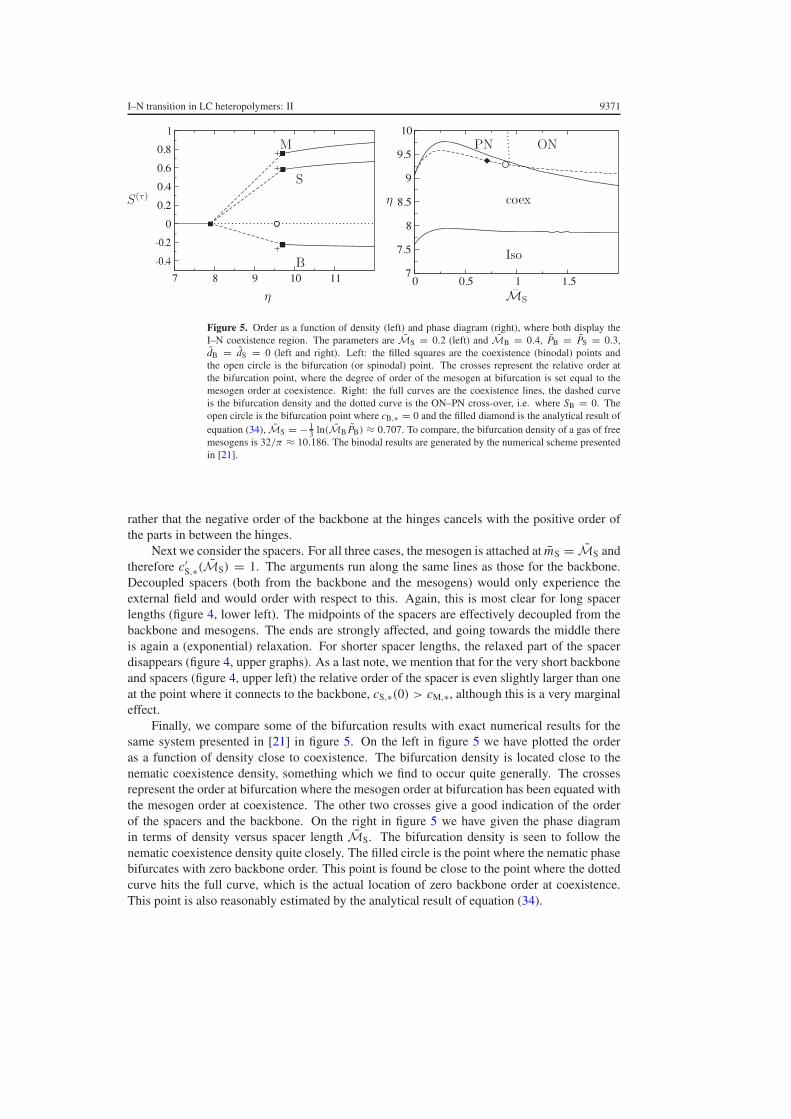
Figure 5. Order as a function of density (left) and phase diagram (right), where both display theI–N coexistence region. The parameters are MS = 0.2 (left) and MB = 0.4, PB = PS = 0.3,dB = dS = 0 (left and right). Left: the filled squares are the coexistence (binodal) points andthe open circle is the bifurcation (or spinodal) point. The crosses represent the relative order atthe bifurcation point, where the degree of order of the mesogen at bifurcation is set equal to themesogen order at coexistence. Right: the full curves are the coexistence lines, the dashed curveis the bifurcation density and the dotted curve is the ON–PN cross-over, i.e. where SB = 0. Theopen circle is the bifurcation point where cB,∗ = 0 and the filled diamond is the analytical result ofequation (34), MS = − 1

3 ln(MB PB) ≈ 0.707. To compare, the bifurcation density of a gas of freemesogens is 32/π ≈ 10.186. The binodal results are generated by the numerical scheme presentedin [21].

rather that the negative order of the backbone at the hinges cancels with the positive order ofthe parts in between the hinges.

Next we consider the spacers. For all three cases, the mesogen is attached at mS = MS andtherefore c′

S,∗(MS) = 1. The arguments run along the same lines as those for the backbone.Decoupled spacers (both from the backbone and the mesogens) would only experience theexternal field and would order with respect to this. Again, this is most clear for long spacerlengths (figure 4, lower left). The midpoints of the spacers are effectively decoupled from thebackbone and mesogens. The ends are strongly affected, and going towards the middle thereis again a (exponential) relaxation. For shorter spacer lengths, the relaxed part of the spacerdisappears (figure 4, upper graphs). As a last note, we mention that for the very short backboneand spacers (figure 4, upper left) the relative order of the spacer is even slightly larger than oneat the point where it connects to the backbone, cS,∗(0) > cM,∗, although this is a very marginaleffect.

Finally, we compare some of the bifurcation results with exact numerical results for thesame system presented in [21] in figure 5. On the left in figure 5 we have plotted the orderas a function of density close to coexistence. The bifurcation density is located close to thenematic coexistence density, something which we find to occur quite generally. The crossesrepresent the order at bifurcation where the mesogen order at bifurcation has been equated withthe mesogen order at coexistence. The other two crosses give a good indication of the orderof the spacers and the backbone. On the right in figure 5 we have given the phase diagramin terms of density versus spacer length MS. The bifurcation density is seen to follow thenematic coexistence density quite closely. The filled circle is the point where the nematic phasebifurcates with zero backbone order. This point is found be close to the point where the dottedcurve hits the full curve, which is the actual location of zero backbone order at coexistence.This point is also reasonably estimated by the analytical result of equation (34).

9372 P P F Wessels and B M Mulder

4. Conclusion and discussion

We have studied the isotropic-to-nematic transition in a fluid of side-chain LC polymers. Theside-chain LC polymers are explicitly modelled to consist of a (more or less) flexible backboneand lateral spacers and rigid mesogens, thus incorporating the relevant molecular details as wellas their branched geometry. Using the segmented chain approach, which we developed in I forvery general heteropolymeric systems, we are able to locate the so-called bifurcation densitywhere the nematic solution branches off the isotropic solution. For conceptual simplicity, butalso to reduce the number of model parameters, we have applied the wormlike chain limitto the segmented backbone and spacers and we assumed the backbone to be infinitely long.The I–N bifurcation density has been obtained in closed analytical form as a function of thesix model parameters. The average backbone order at bifurcation can be negative or positivewith respect to that of the mesogens, corresponding respectively to oblate or prolate backboneconformations. We have determined the phase diagram of for which combinations of modelparameters an oblate or prolate nematic is formed. Other results include order profiles alongthe backbone and the spacers. Finally, we have compared some of the bifurcation results withthe exact numerical results obtained in [21] for the same system.

In [18, 19], Warner and co-workers (WWR) considered a similar system of polymersconsisting of wormlike backbones and laterally hinged rigid mesogen side-groups, but notincluding spacers as a separate component. Using Maier–Saupe type interactions betweenthe components and the temperature as the thermodynamic variable, they identified threedifferent nematic phases, two of which are the oblate and prolate nematic also consideredhere, and the third corresponds to a backbone-induced nematic. However, in the WWR-approach, no distinction is made between mesogen–backbone interactions acting through theeffective mean field (interchain) or mediated by the connecting hinges (intrachain). As aresult, the orientational fields of the mesogens act in a delocalized fashion on the backbonesand vice versa. In our approach we explicitly distinguish between these two different sourcesof interaction between the mesogens and the backbone, and include the intrachain (bending)contributions exactly. Consequently, we are able to study the non-uniform order profiles alongspacers and backbone due to the connectivity between all the components. Furthermore, thedistinction between these two interaction contributions also results in a different scaling: i.e.interchain interactions, which are due to the interaction with other polymers, scale with thedensity, whereas the intrachain interactions, which are single-polymer effects, are densityindependent. The fact that we use a lyotropic (Onsager type) theory where WWR use athermotropic (Maier–Saupe type) approach is not expected to yield great differences, as thetwo approaches have an almost identical formal structure. Identifying density with inversetemperature gives a rough correspondence in (phase) behaviour. An additional advantage ofthe Onsager type interactions over Maier–Saupe interactions is that in this case the dimensionsof the molecule totally fix the relative magnitude of the various interactions, whereas theseinteractions in the WWR approach can be tuned to arbitrary relative magnitudes, which doesnot necessarily reflect realistic physical behaviour. Our theory does need six model parameters,in contrast to WWR, who use four. This difference is due to the fact that we explicitly takeinto account the lateral spacer chains, whose dimensions yield two extra model parameters: PS

and dS. In [21] we have already compared the full nematic phase behaviour for the presentsystem to WRR. The most striking difference is that nematic–nematic phase transitions of thetype found by WRR are ruled out by a convexity argument on the free energy. This differencecan be directly traced to the difference in the way the intrachain degrees of freedom are treated.

Experimental systems of side-chain LC polymers commonly show smectic phases[3, 6, 2, 27, 28]. Indeed, the system we consider, for which we here have calculated the stability

I–N transition in LC heteropolymers: II 9373

with respect to nematic perturbations, may in principle become unstable with respect to thesmectic phase even before becoming a nematic. It would thus be very interesting to includethis type of ordering in the present approach and study the competition between smectics andnematics. However, this poses a major theoretical challenge. The bifurcation analysis certainlywill become a lot more complicated, as the smectic density would cause non-trivial position–orientation couplings along the polymer. The resulting eigenfunctions of the interaction kernelwould no longer follow from a symmetry related argument, as the Legendre polynomials do inthe nematic case, but would have to be computed numerically. A first attempt in this direction,which considers the formation lamellar phases in liquid-crystalline heteropolymers, is foundin [29]. Polydispersity in the degree of polymerization is also inevitable in experimentalsystems, but its effect on the I–N phase behaviour is expected to be marginal, justifying ouruse of infinitely long backbones. In inhomogeneous phases, however, correlations travel muchfurther along the polymers and polydispersity is seen to affect the phase behaviour [2, 28].Finally, odd–even effects of the transition temperatures are often reported, where e.g. theclearing temperature shows oscillations as a function of spacer length. These could in principlebe studied with the present model, but more sophisticated interactions along the chain wouldbe necessary, i.e. between next-nearest-neighbouring segments, modelling e.g. the differentrotation-isomeric states that occur in –(CH2)– chains.

Acknowledgments

This work is part of the research programme of the Stichting voor Fundamenteel Onderzoekder Materie (FOM), which is financially supported by the Nederlandse organisatie voorWetenschappelijk Onderzoek (NWO).

Appendix. The elements of α′

In this appendix we give the elements of the matrix α′(mB, mS), which is needed to calculateorder profiles along the spacers and backbone (equation (31)):

α′B,B = αB,B, (A.1)

α′B,S(mB) = −1

2

(1 − e−3MS

3MS

){e−3|mB− 1

2 MB|

+(

e3(mB− 12 MB) + e−3(mB− 1

2 MB)) e−3MB

1 − e−3MB

}, (A.2)

α′B,M(mB) = −1

2e−3MB

{e−3|mB− 1

2 MB| +(

e3(mB− 12 MB) + e−3(mB− 1

2 MB)) e−3MB

1 − e−3MB

}, (A.3)

α′S,B(mS) = − 1

3MBe−3mS , (A.4)

α′S,S(mS) = 1

3MS

(2 − e−3mS − e−3(MS−mS) + 1

2e−3mS

(1 − e−3MS

) e−3MB

1 − e−3MB

), (A.5)

α′S,M(mS) = e−3(MS−mS) + 1

2e−3MS−3mS

e−3MB

1 − e−3MB, (A.6)

α′M,B = αM,B, (A.7)

α′M,S = αM,S, (A.8)

α′M,M = αM,M. (A.9)

9374 P P F Wessels and B M Mulder

Here, mB ∈ [0,MB] where mB = 0 and mB = MB are the same (because the backbone isinfinitely periodic) in between the spacers and mB = 1

2MB is where the spacer is attached tothe backbone. Further, mS ∈ [0,MS] where mS = 0 is on the backbone side of the spacerand mS = MS is on the mesogen side of the spacer. In contrast with α, α′ is not symmetric.Obviously, the elements α′

M,τ = αM,τ have no mM-dependence as there is only one mesogen ina unit. Also α′

B,B = αB,B has no mB-dependence due to the complete translational symmetryalong the infinite backbone.

References

[1] Donald A and Windle A 1992 Liquid Crystalline Polymers (Cambridge: Cambridge University Press)[2] Shibaev V and Lam L (ed) 1994 Liquid Crystalline and Mesomorphic Polymers (Berlin: Springer)[3] McArdle C B (ed) 1989 Side Chain Liquid Crystalline Polymers (Glasgow: Blackie)[4] Ciferri A, Krigbaum W R and Meyer R B (ed) 1982 Polymer Liquid Crystals (New York: Academic)[5] Plate N A and Shibaev V P 1987 Comb-Shaped Polymers and Liquid Crystals (New York: Plenum)[6] Demus D, Goodby J, Gray G W, Spiess H-W and Hill V (ed) 1998 Handbook of Liquid Crystals vol 3 High

Molecular Weight Liquid Crystals (New York: Wiley–VCH)[7] Finkelmann H, Ringsdorf H and Wendorff J H 1978 Makromol. Chem. 179 273[8] Finkelmann H, Ringsdorf H, Siol W and Wendorff J H 1978 Makromol. Chem. 179 829[9] Finkelmann H, Happ M, Portugal M and Ringsdorf H 1978 Makromol. Chem. 179 2541

[10] Wessels P P F and Mulder B M 2006 Isotropic-to-nematic transition in LC heteropolymers: I. Formalism andmain chain LC polymers J. Phys.: Condens. Matter 18 9335

[11] Onsager L 1949 Ann. New York Acad. Sci. 51 627[12] Maier W and Saupe A 1959 Z. Naturf. 14 882[13] Khokhlov A R and Semenov A N 1981 Physica A 108 546[14] Khokhlov A R and Semenov A N 1982 Physica A 112 605[15] Warner M, Gunn J M F and Baumgartner A B 1985 J. Phys. A: Math. Gen. 18 3007[16] Semenov A N and Khokhlov A R 1988 Sov. Phys.—Usp. 31 988[17] Vasilenko S, Shibaev V and Khokhlov A 1985 Makromol. Chem. 186 1951[18] Wang X and Warner M 1987 J. Phys. A: Math. Gen. 20 713[19] Renz W and Warner M 1988 Proc. R. Soc. A 417 213[20] Bladon P, Warner M and Liu H 1992 Macromolecules 25 4329[21] Wessels P P F and Mulder B M 2003 Europhys. Lett. 64 337[22] Evans R 1979 Adv. Phys. 28 143–200[23] Vroege G J and Lekkerkerker H N W 1992 Rep. Prog. Phys. 55 1241[24] Holyst R and Oswald P 2001 Macromol. Theory Simul. 10 1[25] Wessels P P F and Mulder B M 2003 Soft Mater. 1 313[26] Flory P J 1989 Statistical Mechanics of Chain Molecules (Munich: Hanser)[27] Noirez L, Boeffel C and Daoud-Aladine A 1998 Phys. Rev. Lett. 80 1453[28] Ostrovskii B, Sulyanov S N, Boiko N I, Shibaev V P and de Jeu W H 2001 Eur. Phys. J. E 6 277[29] Wessels P P F and Mulder B M 2004 Phys. Rev. E 70 031503