The Manifold Setting Constructing Isospectral Manifolds Isospectral Orbifolds Summary & Outlook Isospectral Orbifolds An Introduction To Spectral Geometry on Orbifolds Martin Weilandt [email protected] Humboldt-Universität zu Berlin Berlin Mathematical School 2009-04-03 / UFCG

Welcome message from author
This document is posted to help you gain knowledge. Please leave a comment to let me know what you think about it! Share it to your friends and learn new things together.
Transcript
The Manifold Setting Constructing Isospectral Manifolds Isospectral Orbifolds Summary & Outlook
Isospectral OrbifoldsAn Introduction To Spectral Geometry on Orbifolds
Martin [email protected]
Humboldt-Universität zu BerlinBerlin Mathematical School
2009-04-03 / UFCG

The Manifold Setting Constructing Isospectral Manifolds Isospectral Orbifolds Summary & Outlook
Outline
1 The Manifold SettingThe Notion of a ManifoldThe Laplace operator
2 Constructing Isospectral ManifoldsIsospectral ToriSunada’s Theorem
3 Isospectral OrbifoldsOrbifoldsExamples of Isospectral Orbifolds
The Manifold Setting Constructing Isospectral Manifolds Isospectral Orbifolds Summary & Outlook
Manifolds as Basic Objects of Differential Geometry
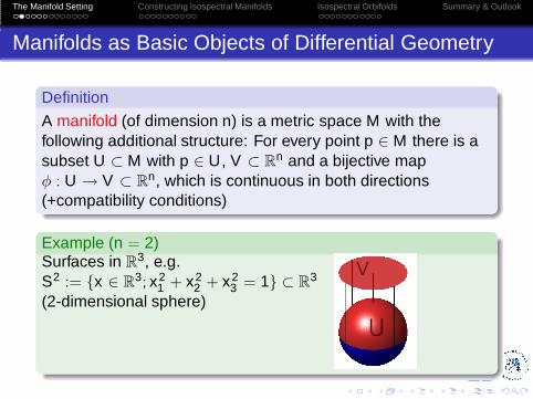
Definition
A manifold (of dimension n) is a metric space M with thefollowing additional structure: For every point p ∈ M there is asubset U ⊂ M with p ∈ U, V ⊂ R
n and a bijective mapφ : U → V ⊂ R
n, which is continuous in both directions(+compatibility conditions)
The Manifold Setting Constructing Isospectral Manifolds Isospectral Orbifolds Summary & Outlook
Manifolds as Basic Objects of Differential Geometry
Definition
A manifold (of dimension n) is a metric space M with thefollowing additional structure: For every point p ∈ M there is asubset U ⊂ M with p ∈ U, V ⊂ R
n and a bijective mapφ : U → V ⊂ R
n, which is continuous in both directions(+compatibility conditions)
Example (n = 2)Surfaces in R
3, e.g.S2 := {x ∈ R
3; x21 + x2
2 + x23 = 1} ⊂ R
3
(2-dimensional sphere)
The Manifold Setting Constructing Isospectral Manifolds Isospectral Orbifolds Summary & Outlook
More Examples of Manifolds
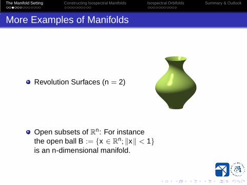
Revolution Surfaces (n = 2)
Open subsets of Rn: For instance
the open ball B := {x ∈ Rn; ‖x‖ < 1}
is an n-dimensional manifold.
The Manifold Setting Constructing Isospectral Manifolds Isospectral Orbifolds Summary & Outlook
One More Structure on a Manifold
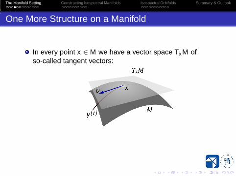
In every point x ∈ M we have a vector space TxM ofso-called tangent vectors:

The Manifold Setting Constructing Isospectral Manifolds Isospectral Orbifolds Summary & Outlook
One More Structure on a Manifold
In every point x ∈ M we have a vector space TxM ofso-called tangent vectors:
Every vector v ∈ TxM has a certain length ‖v‖(e.g. the usual length in R
3 if M is just a surface in R3).

The Manifold Setting Constructing Isospectral Manifolds Isospectral Orbifolds Summary & Outlook
Why This Lengthy Definition?
On manifolds we have a distance function (= metric).
The Manifold Setting Constructing Isospectral Manifolds Isospectral Orbifolds Summary & Outlook
Why This Lengthy Definition?
On manifolds we have a distance function (= metric).The additional structures allow us to define:
the notion of differentiable functions, denoted by C∞,the integral
∫
U f of a function f : M → R over a subset U ofM,
The volume of a compact manifold M is given by∫
M 1.
The Manifold Setting Constructing Isospectral Manifolds Isospectral Orbifolds Summary & Outlook
A Word of Warning
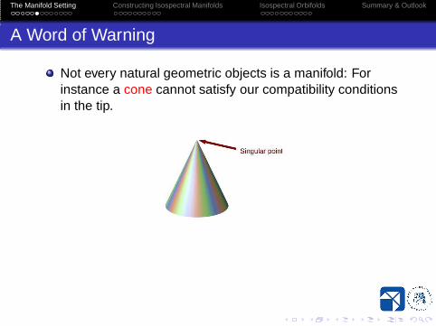
Not every natural geometric objects is a manifold: Forinstance a cone cannot satisfy our compatibility conditionsin the tip.
The Manifold Setting Constructing Isospectral Manifolds Isospectral Orbifolds Summary & Outlook
A Word of Warning
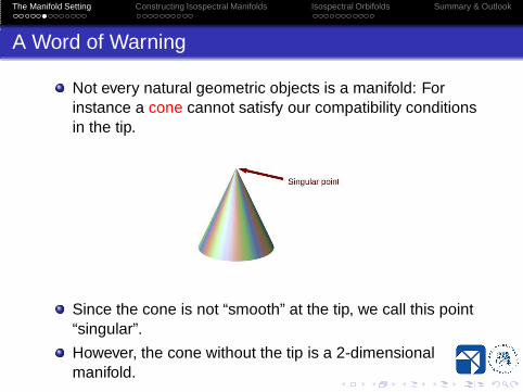
Not every natural geometric objects is a manifold: Forinstance a cone cannot satisfy our compatibility conditionsin the tip.
Since the cone is not “smooth” at the tip, we call this point“singular”.
However, the cone without the tip is a 2-dimensionalmanifold.
The Manifold Setting Constructing Isospectral Manifolds Isospectral Orbifolds Summary & Outlook
Outline
1 The Manifold SettingThe Notion of a ManifoldThe Laplace operator
2 Constructing Isospectral ManifoldsIsospectral ToriSunada’s Theorem
3 Isospectral OrbifoldsOrbifoldsExamples of Isospectral Orbifolds
The Manifold Setting Constructing Isospectral Manifolds Isospectral Orbifolds Summary & Outlook
The Laplace operator on Rn
Let {ei}ni=1 denote the standard basis of R
n. On Rn we have the
following differential operators:
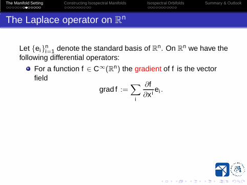
For a function f ∈ C∞(Rn) the gradient of f is the vectorfield
grad f :=∑
i
∂f∂x i ei .
The Manifold Setting Constructing Isospectral Manifolds Isospectral Orbifolds Summary & Outlook
The Laplace operator on Rn
Let {ei}ni=1 denote the standard basis of R
n. On Rn we have the
following differential operators:
For a function f ∈ C∞(Rn) the gradient of f is the vectorfield
grad f :=∑
i
∂f∂x i ei .
For a vector field X =∑
i X iei (with X i ∈ C∞(Rn)) thedivergence of X is the function
div X :=∑
i
∂X i
∂x i .
The Manifold Setting Constructing Isospectral Manifolds Isospectral Orbifolds Summary & Outlook
The Laplace operator on Rn
The Laplacian of a function f ∈ C∞(Rn) is the function
∆f := − div ◦grad f = −
(
∂2
∂x21
+ . . . +∂2
∂x2n
)
f .
Note that we can use the same definition for complex-valuedfunctions (see the second example below).
Example
(n = 2) For f (x) = x31 − 3x1x2
2 we have
∆f (x) = −(3 · 2x1 − 3 · 2x1), i.e. ∆f = 0.
(n = 1) For f (x) = eix we have
∆f (x) = −(i2eix) = eix , i.e. ∆f = f .
The Manifold Setting Constructing Isospectral Manifolds Isospectral Orbifolds Summary & Outlook
The Laplace Operator on a Riemanian manifold
Definition
Now let M be a manifold. The operators grad and divgeneralize to operators on M. Just like on R
n, the equation∆ = −div ◦ grad defines an endomorphism
∆ : C∞(M, R)−→C∞(M, R),
the Laplace Operator on M.
Since ∆ is linear, we can consider the eigenspaces (assubspaces of C∞(M)) and eigenvalues of ∆.The preceding example gave eigenfunctions to theeigenvalues 0 and 1, respectively.
Note that C∞(M) is an infinite-dimensional vectorspace. We need to study functional analysis.
The Manifold Setting Constructing Isospectral Manifolds Isospectral Orbifolds Summary & Outlook
Properties of ∆
Theorem
Let M be a compact manifold. Then
∫
Mf1∆f2 =
∫
M‖grad f‖2 =
∫
Mf2∆f1.
This implies that the eigenvalues of ∆ are non-negative.
The eigenspace of ∆ are finite-dimensional.
The Manifold Setting Constructing Isospectral Manifolds Isospectral Orbifolds Summary & Outlook
Properties of ∆
Theorem
Let M be a compact manifold. Then
∫
Mf1∆f2 =
∫
M‖grad f‖2 =
∫
Mf2∆f1.
This implies that the eigenvalues of ∆ are non-negative.
The eigenspace of ∆ are finite-dimensional.
Definition
Two manifolds M1, M2 are called isospectral, if the eigenvaluesand the corresponding dimensions of the eigenspaces of thetwo Laplace operators ∆1, ∆2 coincide.

The Manifold Setting Constructing Isospectral Manifolds Isospectral Orbifolds Summary & Outlook
Classical Questions/Results
Question
“Can one hear the shape of a drum” (Kac, 1966)In other words: Is the geometry of a manifold determined by theeigenvalues of ∆?
The Manifold Setting Constructing Isospectral Manifolds Isospectral Orbifolds Summary & Outlook
Classical Questions/Results
Question
“Can one hear the shape of a drum” (Kac, 1966)In other words: Is the geometry of a manifold determined by theeigenvalues of ∆?
Theorem
Let M1, M2 be two isospectral manifolds. Then the followingcoincide for M1 und M2:
The dimension: dim(M1) = dim(M2)
The volume: vol(M1) = vol(M2)
Certain other (more complicated) geometric properties.

The Manifold Setting Constructing Isospectral Manifolds Isospectral Orbifolds Summary & Outlook
Main Goal
Task
In order to find geometric properties which are not determinedby the eigenvalues of ∆, we need to construct pairs ofisospectral manifolds.
The Manifold Setting Constructing Isospectral Manifolds Isospectral Orbifolds Summary & Outlook
Main Goal
Task
In order to find geometric properties which are not determinedby the eigenvalues of ∆, we need to construct pairs ofisospectral manifolds.
Note that isometric manifolds are not interesting in this contextbecause:
they are identical from the point of view of a geometer andtherefore
the Laplacians have the same eigenvalues, i.e., they aretrivially isospectral.

The Manifold Setting Constructing Isospectral Manifolds Isospectral Orbifolds Summary & Outlook
Outline
1 The Manifold SettingThe Notion of a ManifoldThe Laplace operator
2 Constructing Isospectral ManifoldsIsospectral ToriSunada’s Theorem
3 Isospectral OrbifoldsOrbifoldsExamples of Isospectral Orbifolds
The Manifold Setting Constructing Isospectral Manifolds Isospectral Orbifolds Summary & Outlook
Quotient Manifolds
Let M be a manifold and let G be a discrete (e.g. finite) group ofisometries acting on M. Two points p1, p2 ∈ M are regarded asequivalent, if there is g ∈ G such that gp1 = p2.
The Manifold Setting Constructing Isospectral Manifolds Isospectral Orbifolds Summary & Outlook
Quotient Manifolds
Let M be a manifold and let G be a discrete (e.g. finite) group ofisometries acting on M. Two points p1, p2 ∈ M are regarded asequivalent, if there is g ∈ G such that gp1 = p2. Denote the setof equivalence classes by M/G. If
Gp := {g ∈ G; gp = p} = {Id}
for all p ∈ M, then M/G carries a natural manifold structuresuch that the differentiable functions on M/G are given by
C∞(M/G) = C∞(M)G := {f ∈ C∞(M, R); f ◦ g = f ∀g ∈ G}.
Restricting ∆ on M to this subspace of C∞(M) gives theLaplace operator
∆ : C∞(M/G) → C∞(M/G)
on M/G.
The Manifold Setting Constructing Isospectral Manifolds Isospectral Orbifolds Summary & Outlook
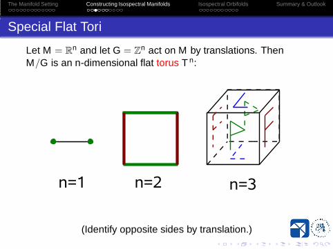
Special Flat Tori
Let M = Rn and let G = Z
n act on M by translations. ThenM/G is an n-dimensional flat torus T n:
(Identify opposite sides by translation.)
The Manifold Setting Constructing Isospectral Manifolds Isospectral Orbifolds Summary & Outlook
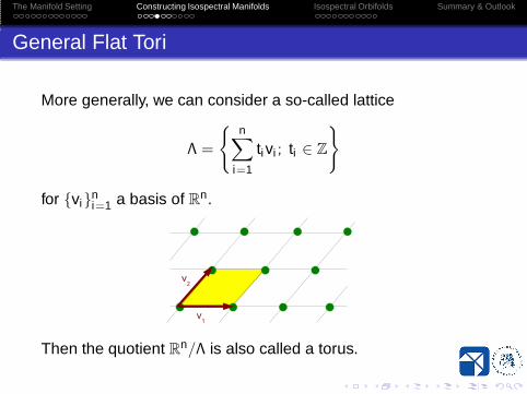
General Flat Tori
More generally, we can consider a so-called lattice
Λ =
{
n∑
i=1
tivi ; ti ∈ Z
}
for {vi}ni=1 a basis of R
n.
Then the quotient Rn/Λ is also called a torus.

The Manifold Setting Constructing Isospectral Manifolds Isospectral Orbifolds Summary & Outlook
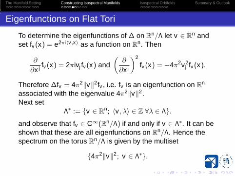
Eigenfunctions on Flat Tori
To determine the eigenfunctions of ∆ on Rn/Λ let v ∈ R
n andset fv (x) = e2πi〈v ,x〉 as a function on R
n. Then
∂
∂x j fv (x) = 2πivj fv (x) and(
∂
∂x j
)2
fv (x) = −4π2v2j fv (x).
Therefore ∆fv = 4π2‖v‖2fv , i.e. fv is an eigenfunction on Rn
associated with the eigenvalue 4π2‖v‖2.
The Manifold Setting Constructing Isospectral Manifolds Isospectral Orbifolds Summary & Outlook
Eigenfunctions on Flat Tori
To determine the eigenfunctions of ∆ on Rn/Λ let v ∈ R
n andset fv (x) = e2πi〈v ,x〉 as a function on R
n. Then
∂
∂x j fv (x) = 2πivj fv (x) and(
∂
∂x j
)2
fv (x) = −4π2v2j fv (x).
Therefore ∆fv = 4π2‖v‖2fv , i.e. fv is an eigenfunction on Rn
associated with the eigenvalue 4π2‖v‖2.Next set
Λ∗ := {v ∈ Rn; 〈v , λ〉 ∈ Z ∀λ ∈ Λ}.
and observe that fv ∈ C∞(Rn/Λ) if and only if v ∈ Λ∗. It can beshown that these are all eigenfunctions on R
n/Λ. Hence thespectrum on the torus R
n/Λ is given by the multiset
{4π2‖v‖2; v ∈ Λ∗}.
The Manifold Setting Constructing Isospectral Manifolds Isospectral Orbifolds Summary & Outlook
The First Example of Isospectral Manifolds
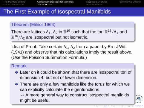
Theorem (Milnor 1964)
There are lattices Λ1, Λ2 in R16 such that the tori R
16/Λ1 andR
16/Λ2 are isospectral but not isometric.
Idea of Proof: Take certain Λ1, Λ2 from a paper by Ernst Witt(1941) and observe that his calculations imply the result above.(Use the Poisson Summation Formula.)
The Manifold Setting Constructing Isospectral Manifolds Isospectral Orbifolds Summary & Outlook
The First Example of Isospectral Manifolds
Theorem (Milnor 1964)
There are lattices Λ1, Λ2 in R16 such that the tori R
16/Λ1 andR
16/Λ2 are isospectral but not isometric.
Idea of Proof: Take certain Λ1, Λ2 from a paper by Ernst Witt(1941) and observe that his calculations imply the result above.(Use the Poisson Summation Formula.)
Remark
Later on it could be shown that there are isospectral tori ofdimension 4, but not of lower dimension.
There are only a few manifolds like the torus for which wecan explicitly calculate the eigenfunctions A more general way to construct isospectral manifoldsmight be useful.
The Manifold Setting Constructing Isospectral Manifolds Isospectral Orbifolds Summary & Outlook
Outline
1 The Manifold SettingThe Notion of a ManifoldThe Laplace operator
2 Constructing Isospectral ManifoldsIsospectral ToriSunada’s Theorem
3 Isospectral OrbifoldsOrbifoldsExamples of Isospectral Orbifolds
The Manifold Setting Constructing Isospectral Manifolds Isospectral Orbifolds Summary & Outlook
Sunada’s Theorem
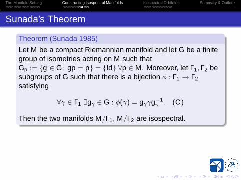
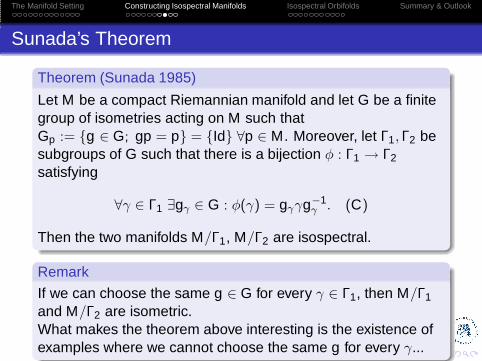
Theorem (Sunada 1985)
Let M be a compact Riemannian manifold and let G be a finitegroup of isometries acting on M such thatGp := {g ∈ G; gp = p} = {Id} ∀p ∈ M. Moreover, let Γ1,Γ2 besubgroups of G such that there is a bijection φ : Γ1 → Γ2
satisfying
∀γ ∈ Γ1 ∃gγ ∈ G : φ(γ) = gγγg−1γ
. (C)
Then the two manifolds M/Γ1, M/Γ2 are isospectral.
The Manifold Setting Constructing Isospectral Manifolds Isospectral Orbifolds Summary & Outlook
Sunada’s Theorem
Theorem (Sunada 1985)
Let M be a compact Riemannian manifold and let G be a finitegroup of isometries acting on M such thatGp := {g ∈ G; gp = p} = {Id} ∀p ∈ M. Moreover, let Γ1,Γ2 besubgroups of G such that there is a bijection φ : Γ1 → Γ2
satisfying
∀γ ∈ Γ1 ∃gγ ∈ G : φ(γ) = gγγg−1γ
. (C)
Then the two manifolds M/Γ1, M/Γ2 are isospectral.
Remark
If we can choose the same g ∈ G for every γ ∈ Γ1, then M/Γ1
and M/Γ2 are isometric.What makes the theorem above interesting is the existence ofexamples where we cannot choose the same g for every γ...
The Manifold Setting Constructing Isospectral Manifolds Isospectral Orbifolds Summary & Outlook
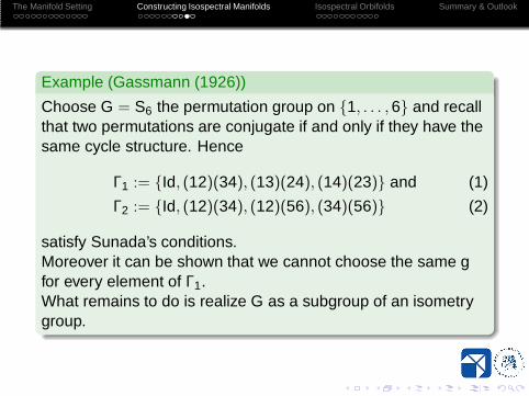
Example (Gassmann (1926))
Choose G = S6 the permutation group on {1, . . . , 6} and recallthat two permutations are conjugate if and only if they have thesame cycle structure. Hence
Γ1 := {Id, (12)(34), (13)(24), (14)(23)} and (1)
Γ2 := {Id, (12)(34), (12)(56), (34)(56)} (2)
satisfy Sunada’s conditions.Moreover it can be shown that we cannot choose the same gfor every element of Γ1.What remains to do is realize G as a subgroup of an isometrygroup.
The Manifold Setting Constructing Isospectral Manifolds Isospectral Orbifolds Summary & Outlook
Sunada’s Theorem
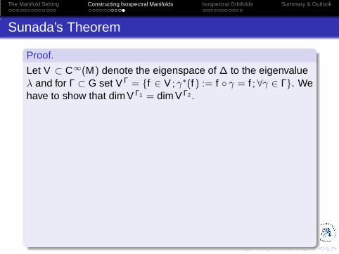
Proof.
Let V ⊂ C∞(M) denote the eigenspace of ∆ to the eigenvalueλ and for Γ ⊂ G set V Γ = {f ∈ V ; γ∗(f ) := f ◦ γ = f ;∀γ ∈ Γ}. Wehave to show that dim V Γ1 = dim V Γ2 .
The Manifold Setting Constructing Isospectral Manifolds Isospectral Orbifolds Summary & Outlook
Sunada’s Theorem
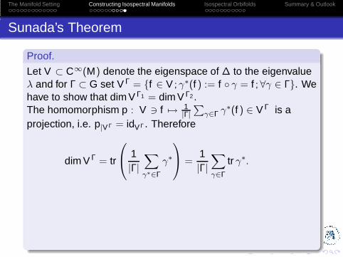
Proof.
Let V ⊂ C∞(M) denote the eigenspace of ∆ to the eigenvalueλ and for Γ ⊂ G set V Γ = {f ∈ V ; γ∗(f ) := f ◦ γ = f ;∀γ ∈ Γ}. Wehave to show that dim V Γ1 = dim V Γ2 .The homomorphism p : V ∋ f 7→ 1
|Γ|
∑
γ∈Γ γ∗(f ) ∈ V Γ is aprojection, i.e. p|V Γ = idV Γ . Therefore
dim V Γ = tr
1|Γ|
∑
γ∗∈Γ
γ∗
=1|Γ|
∑
γ∈Γ
tr γ∗.
The Manifold Setting Constructing Isospectral Manifolds Isospectral Orbifolds Summary & Outlook
Sunada’s Theorem
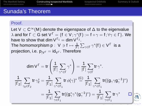
Proof.
Let V ⊂ C∞(M) denote the eigenspace of ∆ to the eigenvalueλ and for Γ ⊂ G set V Γ = {f ∈ V ; γ∗(f ) := f ◦ γ = f ;∀γ ∈ Γ}. Wehave to show that dim V Γ1 = dim V Γ2 .The homomorphism p : V ∋ f 7→ 1
|Γ|
∑
γ∈Γ γ∗(f ) ∈ V Γ is aprojection, i.e. p|V Γ = idV Γ . Therefore
dim V Γ = tr
1|Γ|
∑
γ∗∈Γ
γ∗
=1|Γ|
∑
γ∈Γ
tr γ∗.
1|Γ2|
∑
γ2∈Γ2
tr γ∗2 =
1|Γ1|
∑
γ∗∈Γ1
tr φ(γ)∗(C)=
1|Γ1|
∑
γ∗∈Γ1
tr((gγγg−1γ
)∗)
=1
|Γ1|
∑
γ∈Γ1
tr((g∗γγ∗(g−1
γ)∗) =
1|Γ1|
∑
γ∈Γ1
tr γ∗

The Manifold Setting Constructing Isospectral Manifolds Isospectral Orbifolds Summary & Outlook
Outline
1 The Manifold SettingThe Notion of a ManifoldThe Laplace operator
2 Constructing Isospectral ManifoldsIsospectral ToriSunada’s Theorem
3 Isospectral OrbifoldsOrbifoldsExamples of Isospectral Orbifolds
The Manifold Setting Constructing Isospectral Manifolds Isospectral Orbifolds Summary & Outlook
A Short Repetition
Recall the definition of a quotient manifold: G a group ofisometries on a manifold M with Gp = {g ∈ G; gp = p} = {Id}.Then
M/G is a manifold withC∞(M/G) = {f ∈ C∞(M); f ◦ g = f ∀g ∈ G}
∆ on M induces the Laplacian ∆ : C∞(M/G) → C∞(M/G)on M/G.
Observation
The condition Gp = {Id} was not necessary for the definition of∆ on M/G.
So maybe omitting the condition Gp = {Id} might give aninteresting geometric object...

The Manifold Setting Constructing Isospectral Manifolds Isospectral Orbifolds Summary & Outlook
Good Orbifolds
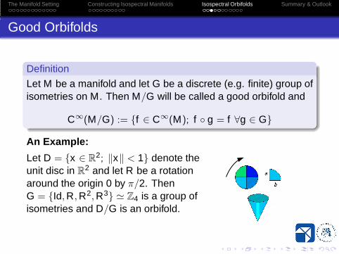
Definition
Let M be a manifold and let G be a discrete (e.g. finite) group ofisometries on M. Then M/G will be called a good orbifold and
C∞(M/G) := {f ∈ C∞(M); f ◦ g = f ∀g ∈ G}
The Manifold Setting Constructing Isospectral Manifolds Isospectral Orbifolds Summary & Outlook
Good Orbifolds
Definition
Let M be a manifold and let G be a discrete (e.g. finite) group ofisometries on M. Then M/G will be called a good orbifold and
C∞(M/G) := {f ∈ C∞(M); f ◦ g = f ∀g ∈ G}
An Example:
Let D = {x ∈ R2; ‖x‖ < 1} denote the
unit disc in R2 and let R be a rotation
around the origin 0 by π/2. ThenG = {Id, R, R2, R3} ≃ Z4 is a group ofisometries and D/G is an orbifold.
The Manifold Setting Constructing Isospectral Manifolds Isospectral Orbifolds Summary & Outlook
∆ on Orbifolds
∆ : C∞(M/G) → C∞(M/G) is defined as in the setting ofquotient manifolds.
The eigenspaces are again finite-dimensional.
The definition of isospectrality is also analogous to themanifold case.
However, orbifolds have one additional structure in comparisonto manifolds...
The Manifold Setting Constructing Isospectral Manifolds Isospectral Orbifolds Summary & Outlook
Isotropy
Definition
Let M/G be an orbifold and p ∈ M. The isotropy (or thestabilizer) of M/G in p is given by the group
Gp := {g ∈ G; gp = p} ⊂ G.
In our example of the quotient D/G of the unit disc we have
G0 = {Id, R, R2, R3} ≃ Z4
Gp = {Id} for p ∈ D \ {0}
Question
Do the eigenvalues of ∆ determine the (isomomorphismclasses of) isotropy groups on an orbifold?
The Manifold Setting Constructing Isospectral Manifolds Isospectral Orbifolds Summary & Outlook
Outline
1 The Manifold SettingThe Notion of a ManifoldThe Laplace operator
2 Constructing Isospectral ManifoldsIsospectral ToriSunada’s Theorem
3 Isospectral OrbifoldsOrbifoldsExamples of Isospectral Orbifolds
The Manifold Setting Constructing Isospectral Manifolds Isospectral Orbifolds Summary & Outlook
Observation (Bérard)
The proof of Sunada’s Theorem did not use Gp = {Id}, hence italso applies to orbifols.
This observation has been used to prove the followingtheorems:
The Manifold Setting Constructing Isospectral Manifolds Isospectral Orbifolds Summary & Outlook
Observation (Bérard)
The proof of Sunada’s Theorem did not use Gp = {Id}, hence italso applies to orbifols.
This observation has been used to prove the followingtheorems:
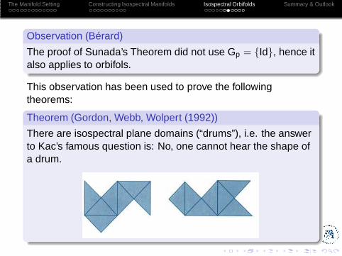
Theorem (Gordon, Webb, Wolpert (1992))
There are isospectral plane domains (“drums”), i.e. the answerto Kac’s famous question is: No, one cannot hear the shape ofa drum.
The Manifold Setting Constructing Isospectral Manifolds Isospectral Orbifolds Summary & Outlook
Another Application of Sunada
A little less historic but more relevant to our question is:
Theorem (Shams, Stanhope, Webb (2006))
There are isospectral 27-dimensional orbifolds where themaximal isotropy groups are not isomorphic.
To find examples of smaller dimension, one can use thefollowing generalization of tori...
The Manifold Setting Constructing Isospectral Manifolds Isospectral Orbifolds Summary & Outlook
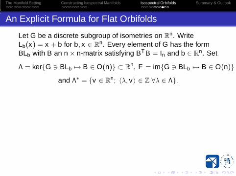
An Explicit Formula for Flat Orbifolds
Let G be a discrete subgroup of isometries on Rn. Write
Lb(x) = x + b for b, x ∈ Rn. Every element of G has the form
BLb with B an n × n-matrix satisfying BT B = In and b ∈ Rn. Set
Λ = ker{G ∋ BLb 7→ B ∈ O(n)} ⊂ Rn, F = im{G ∋ BLb 7→ B ∈ O(n)} ⊂
and Λ∗ = {v ∈ Rn; 〈λ, v〉 ∈ Z ∀λ ∈ Λ}.
The Manifold Setting Constructing Isospectral Manifolds Isospectral Orbifolds Summary & Outlook
An Explicit Formula for Flat Orbifolds
Let G be a discrete subgroup of isometries on Rn. Write
Lb(x) = x + b for b, x ∈ Rn. Every element of G has the form
BLb with B an n × n-matrix satisfying BT B = In and b ∈ Rn. Set
Λ = ker{G ∋ BLb 7→ B ∈ O(n)} ⊂ Rn, F = im{G ∋ BLb 7→ B ∈ O(n)} ⊂
and Λ∗ = {v ∈ Rn; 〈λ, v〉 ∈ Z ∀λ ∈ Λ}.
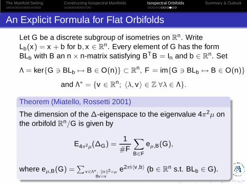
Theorem (Miatello, Rossetti 2001)
The dimension of the ∆-eigenspace to the eigenvalue 4π2µ onthe orbifold R
n/G is given by
E4π2µ(∆G) =1
#F
∑
B∈F
eµ,B(G),
where eµ,B(G) =∑
v∈Λ∗, ‖v‖2=µ
Bv=v
e2πi〈v ,b〉 (b ∈ Rn s.t. BLb ∈ G).
The Manifold Setting Constructing Isospectral Manifolds Isospectral Orbifolds Summary & Outlook
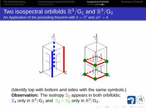
Two isospectral orbifolds R3/G1 and R
3/G2An Application of the preceding theorem with Λ = Z
3 and #F = 4
(Identify top with bottom and sides with the same symbols.)Observation: The isotropy Z2 appears in both orbifolds;Z4 only in R
3/G1 and Z2 × Z2 only in R3/G2.
The Manifold Setting Constructing Isospectral Manifolds Isospectral Orbifolds Summary & Outlook
Maximal Isotropy Order
Observation
The isotropy groups of maximal order in the example abovehad the same order 4.
This leads us to the following
Question
Do the eigenvalues of ∆ determine the maximal isotropy order(=: mio)?
Using the same methods as above, one can actually constructa pair of isospectral orbifolds R
3/Λ1, R3/Λ2 with mio1 = 2 and
mio2 = 4 (see the references on the last slide).
The Manifold Setting Constructing Isospectral Manifolds Isospectral Orbifolds Summary & Outlook
Summary & Outlook
The eigenvalues of ∆ do not determine the maximalisotropy order mio.
The Manifold Setting Constructing Isospectral Manifolds Isospectral Orbifolds Summary & Outlook
Summary & Outlook
The eigenvalues of ∆ do not determine the maximalisotropy order mio.
Open question (and motivation for this research): Can amanifold (mio = 1) be isospectral to an orbifold withnon-trivial isotropies (mio > 2)?
One possible approach: Study so-called bad orbifolds.
Appendix
Further Reading I
M. Weilandt.Isospectral Orbifolds with different Isotropy OrdersDiplom Thesis, 2007.(Available on www.math.hu-berlin.de/~weilandt)
D. Schüth, J.P. Rossetti, M. Weilandt.Isospectral orbifolds with different maximal isotropy ordersAnnals of Global Analysis and Geometry 34 (4), 2008
Related Documents